/


Author: Hinkelmann Klaus Kempthorne Oscar
Tags: математика информатика эксперимент
ISBN: 978-0-471-72756-9
Year: 2008


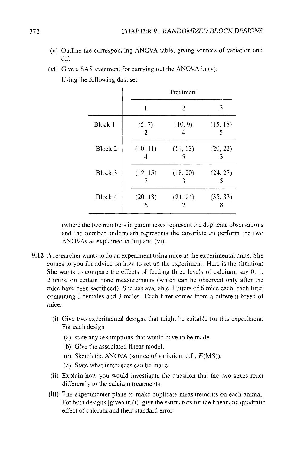
Text
Design and Analysis
of Experiments
BICENTENNIAL
BICENTINNI
The Wiley Bicentennial-Knowledge for Generations
/?~)ach generation has its unique needs and aspirations. When Charles Wiley first
opened his small printing shop in lower Manhattan in 1807, it was a generation
of boundless potential searching for an identity. And we were there, helping to
define a new American literary tradition. Over half a century later, in the midst
of the Second Industrial Revolution, it was a generation focused on building the
future. Once again, we were there, supplying the critical scientific, technical, and
engineering knowledge that helped frame the world. Throughout the 20th
Century, and into the new millennium, nations began to reach out beyond their
own borders and a new international community was born. Wiley was there,
expanding its operations around the world to enable a global exchange of ideas,
opinions, and know-how.
For 200 years, Wiley has been an integral part of each generation's journey,
enabling the flow of information and understanding necessary to meet their needs
and fulfill their aspirations. Today, bold new technologies are changing the way
we live and learn. Wiley will be there, providing you the must-have knowledge
you need to imagine new worlds, new possibilities, and new opportunities.
Generations come and go, but you can always count on Wiley to provide you the
knowledge you need, when and where you need it!
William J. Pesce
President and Chief Executive Officer
Peter Booth Wiley
Chairman df the Board
Design and Analysis
of Experiments
Volume 1
Introduction to Experimental Design
Second Edition
Klaus Hinkelmann
Virginia Polytechnic Institute and State University
Department of Statistics
Blacksburg, VA
Oscar Kempthorne
Iowa State University
Department of Statistics
Ames, IA
BICENTENNIAL.
BICENTENNIAL
WILEY-INTERSCIENCE
A John Wiley & Sons, Inc., Publication
Copyright © 2008 by John Wiley & Sons, Inc. All rights reserved.
Published by John Wiley & Sons, Inc., Hoboken, New Jersey.
Published simultaneously in Canada.
No part of this publication may be reproduced, stored in a retrieval system, or transmitted in any form
or by any means, electronic, mechanical, photocopying, recording, scanning, or otherwise, except as
permitted under Section 107 or 108 of the 1976 United States Copyright Act, without either the prior
written permission of the Publisher, or authorization through payment of the appropriate per-copy fee to
the Copyright Clearance Center, Inc., 222 Rosewood Drive, Danvers, MA 01923, (978) 750-8400, fax
(978) 750-4470, or on the web at www.copyright.com. Requests to the Publisher for permission should
be addressed to the Permissions Department, John Wiley & Sons, Inc., 111 River Street, Hoboken, NJ
07030, (201) 748-6011, fax (201) 748-6008. or online at http://www.wiley.com/go/permission.
Limit of Liability/Disclaimer of Warranty: While the publisher and author have used their best efforts in
preparing this book, they make no representations or warranties with respect to the accuracy or
completeness of the contents of this book and specifically disclaim any implied warranties of
merchantability or fitness for a particular purpose. No warranty may be created or extended by sales
representatives or written sales materials. The advice and strategies contained herein may not be
suitable for your situation. You should consult with a professional where appropriate. Neither the
publisher nor author shall be liable for any loss of profit or any other commercial damages, including
but not limited to special, incidental, consequential, or other damages.
For general information on our other products and services or for technical support, please contact our
Customer Care Department within the United States at (800) 762-2974, outside the United States at
(317) 572-3993 or fax (317) 572-4002.
Wiley also publishes its books in a variety of electronic formats. Some content that appears in print may
not be available in electronic format. For information about Wiley products, visit our web site at
www.wiley.com.
Wiley Bicentennial Logo: Richard J. Pacifico
Library of Congress Cataloging-in-Publication Data:
Hinkelmann, Klaus, 1932-
Design and analysis of experiments / Klaus Hinkelmann, Oscar
Kempthorne. — 2nd ed.
v. cm. — (Wiley series in probability and statistics)
Includes index.
Contents: v. 1. Introduction to experimental design
ISBN 978-0-471-72756-9 (cloth)
1. Experimental design. I. Kempthorne, Oscar. II. Title.
QA279.K45 2008
519.57—dc22 2007017347
Printed in the United States of America.
10 987654321
Contents
Preface to the Second Edition xvii
Preface to the First Edition xxi
1 The Processes of Science 1
1.1 INTRODUCTION 1
1.1.1 Observations in Science 1
1.1.2 Two Types of Observations 2
1.1.3 From Observation to Law 3
1.2 DEVELOPMENT OF THEORY 5
1.2.1 The Basic Syllogism 5
1.2.2 Induction, Deduction, and Hypothesis 6
1.3 THE NATURE AND ROLE OF THEORY IN SCIENCE 8
1.3.1 What Is Science? 8
1.3.2 Two Types of Science 9
1.4 VARIETIES OF THEORY 11
1.4.1 Two Types of Theory 11
1.4.2 What Is a Theory? 12
1.5 THE PROBLEM OF GENERAL SCIENCE 14
1.5.1 Two Problems 15
1.5.2 The Role of Data Analysis 15
1.5.3 The Problem of Inference 16
1.6 CAUSALITY 16
1.6.1 Defining Cause, Causation, and Causality 17
1.6.2 The Role of Comparative Experiments 19
1.7 THE UPSHOT 21
1.8 WHAT IS AN EXPERIMENT? 21
1.8.1 Absolute and Comparative Experiments 22
1.8.2 Three Types of Experiments 23
1.9 STATISTICAL INFERENCE 24
1.9.1 Drawing Inference 24
1.9.2 Notions of Probability 25
1.9.3 Variability and Randomization 26
VI
CONTENTS
Principles of Experimental Design 29
2.1 CONFIRMATORY AND EXPLORATORY EXPERIMENTS .... 29
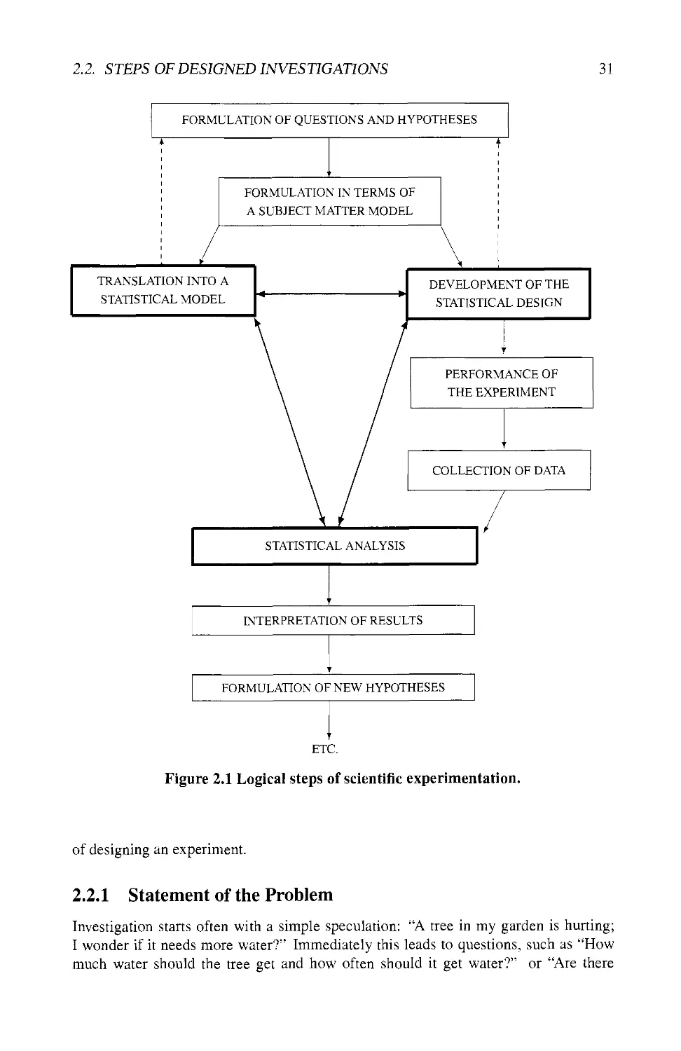
2.2 STEPS OF DESIGNED INVESTIGATIONS 30
2.2.1 Statement of the Problem 31
2.2.2 Subject Matter Model 32
2.2.3 Three Aspects of Design 33
2.2.4 Modeling the Response 35
2.2.5 Choosing the Response 36
2.2.6 Principles of Analysis 36
2.3 THE LINEAR MODEL 37
2.3.1 Three Types of Effects 37
2.3.2 Experimental and Observational Units 38
2.3.3 Outline of a Model 40
2.4 ILLUSTRATING INDIVIDUAL STEPS: STUDY 1 41
2.4.1 The Questions and Hypotheses 41
2.4.2 The Experiment and a Model 41
2.4.3 Analysis 42
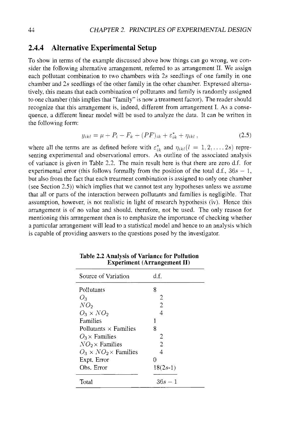
2.4.4 Alternative Experimental Setup 44
2.5 THREE PRINCIPLES OF EXPERIMENTAL DESIGN 45
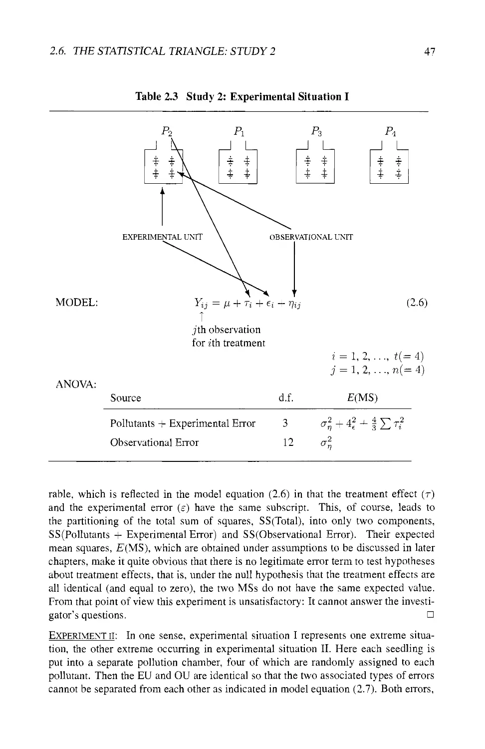
2.6 THE STATISTICAL TRIANGLE: STUDY 2 46
2.6.1 Statement of the Problem 46
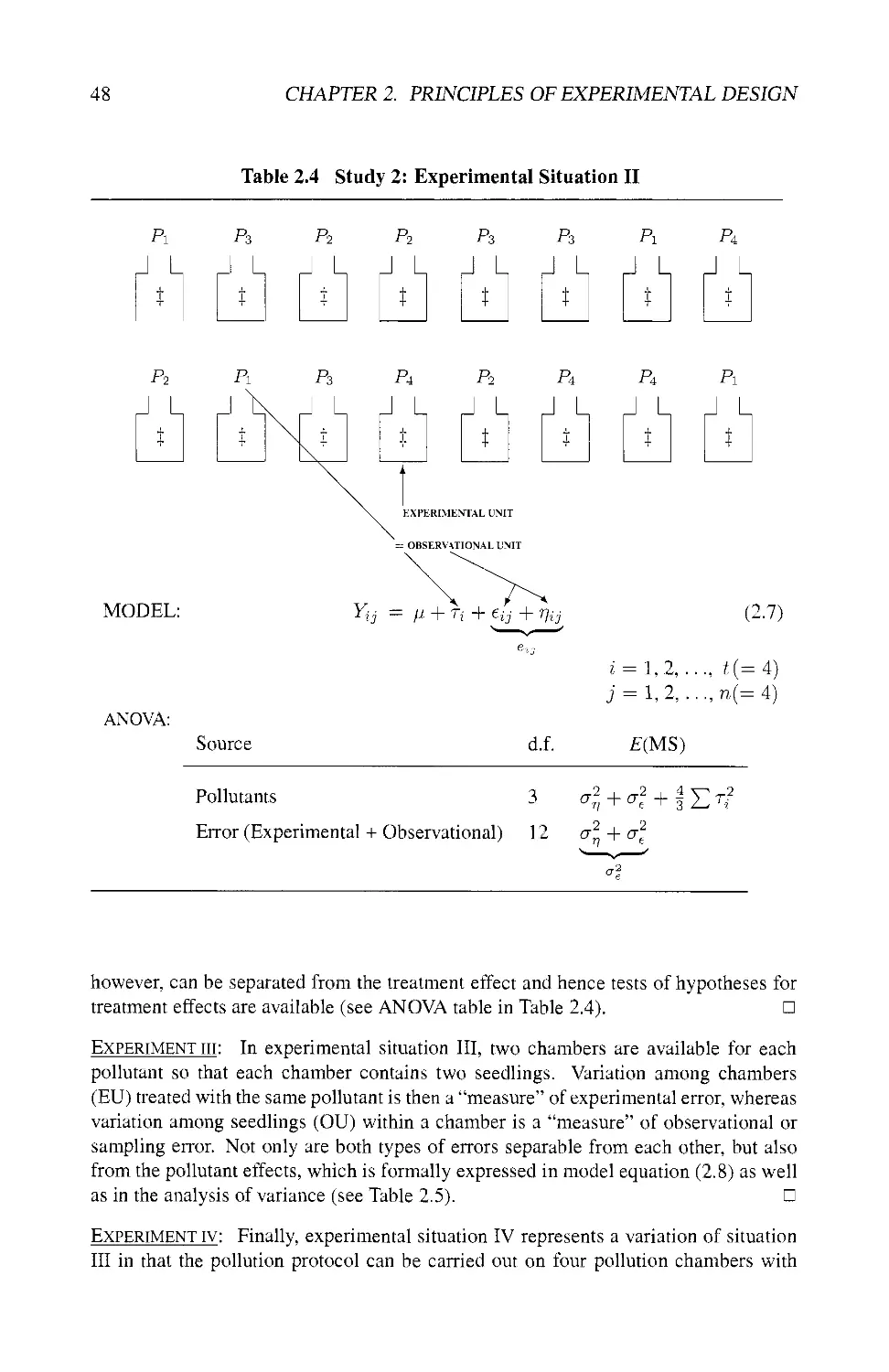
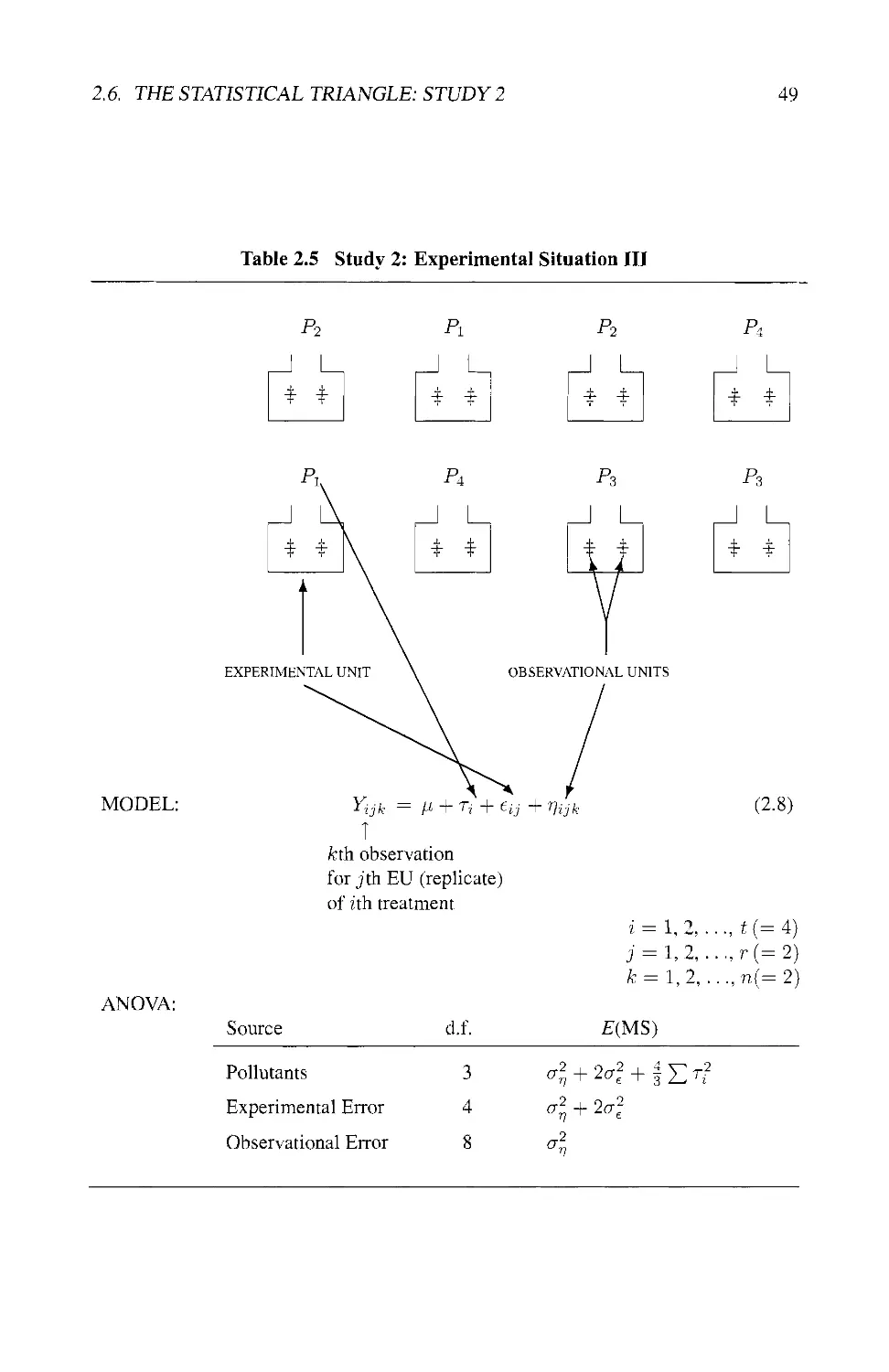
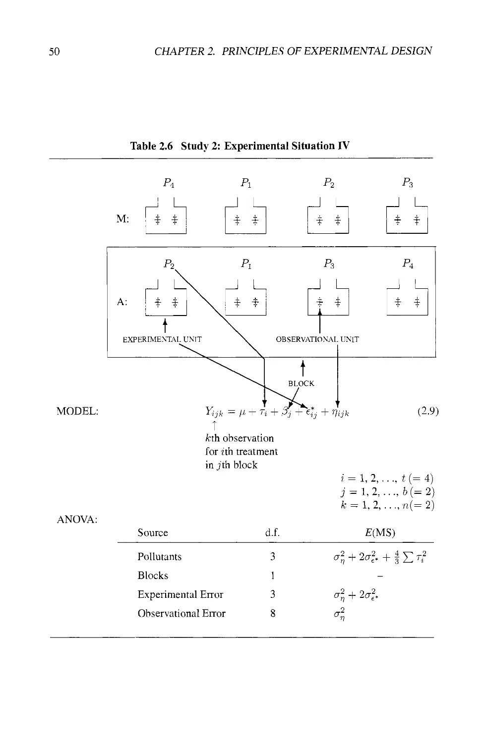
2.6.2 Four Experimental Situations 46
2.7 PLANNING THE EXPERIMENT: THINGS TO THINK ABOUT . . 51
2.8 COOPERATION BETWEEN SCIENTIST AND STATISTICIAN . . 53
2.9 GENERAL PRINCIPLE OF INFERENCE AND TYPES OF
STATISTICAL ANALYSES 56
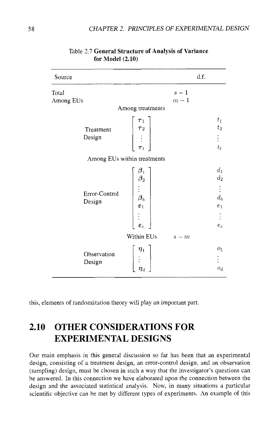
2.9.1 General Model 56
2.9.2 Outline of the ANOVA 56
2.10 OTHER CONSIDERATIONS FOR EXPERIMENTAL DESIGNS . . 58
Survey of Designs And Analyses 61
3.1 INTRODUCTION 61
3.2 ERROR-CONTROL DESIGNS 62
3.3 TREATMENT DESIGNS 64
3.4 COMBINING IDEAS FROM ERROR-CONTROL AND
TREATMENT DESIGNS 65
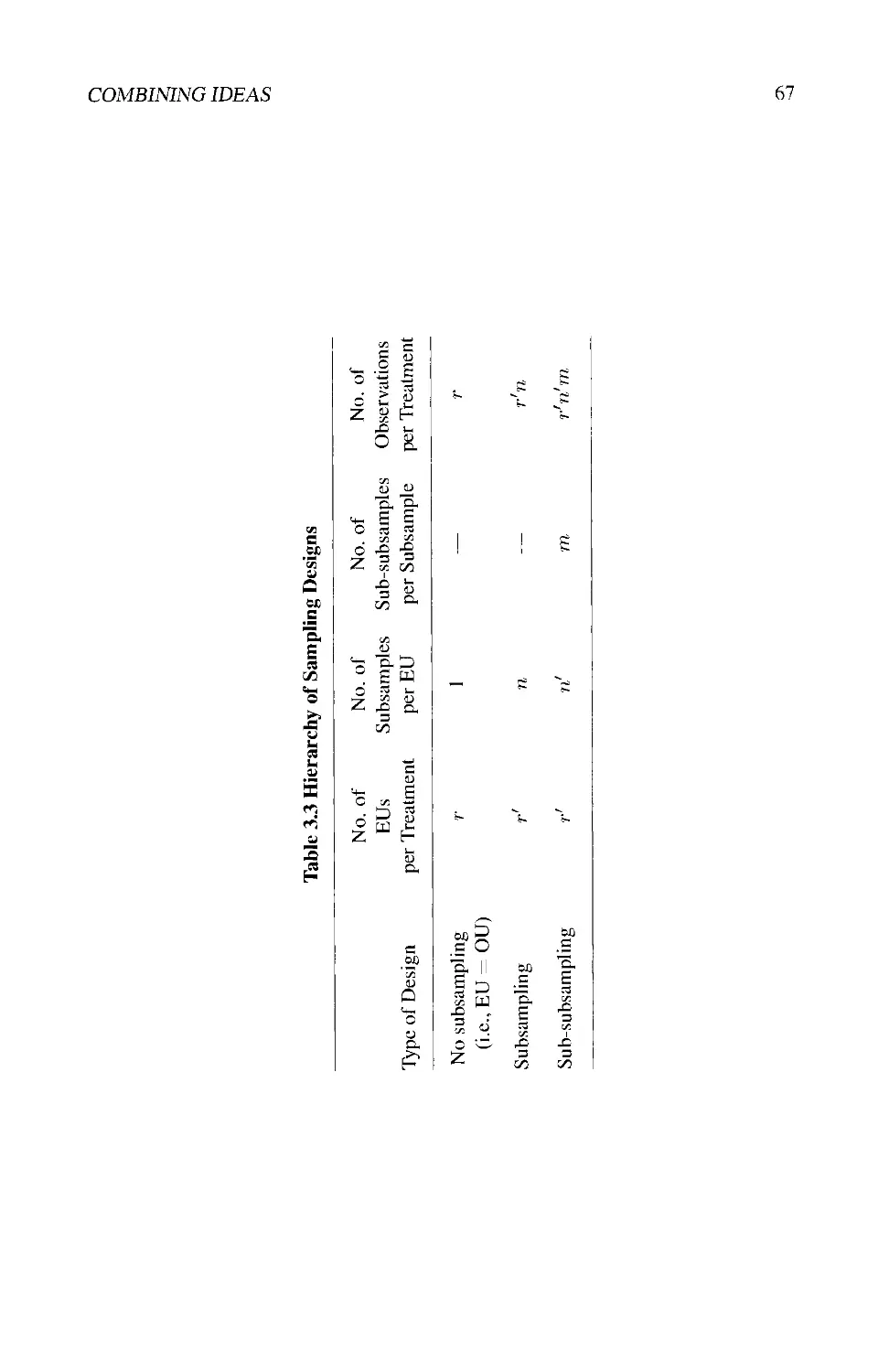
3.5 SAMPLING DESIGNS 68
3.6 ANALYSIS AND STATISTICAL SOFTWARE 68
3.7 SUMMARY 69
Linear Model Theory 71
4.1 INTRODUCTION 71
4.1.1 The Concept of a Model 71
4.1.2 Comparative and Absolute Experiments 73
4.2 REPRESENTATION OF LINEAR MODELS 73
4.3 FUNCTIONAL AND CLASSIFICATORY LINEAR MODELS ... 74
CONTENTS vii
4.3.1 Functional Models 74
4.3.2 Classificatory Models 74
4.3.3 Models with Classificatory and Functional
Components 75
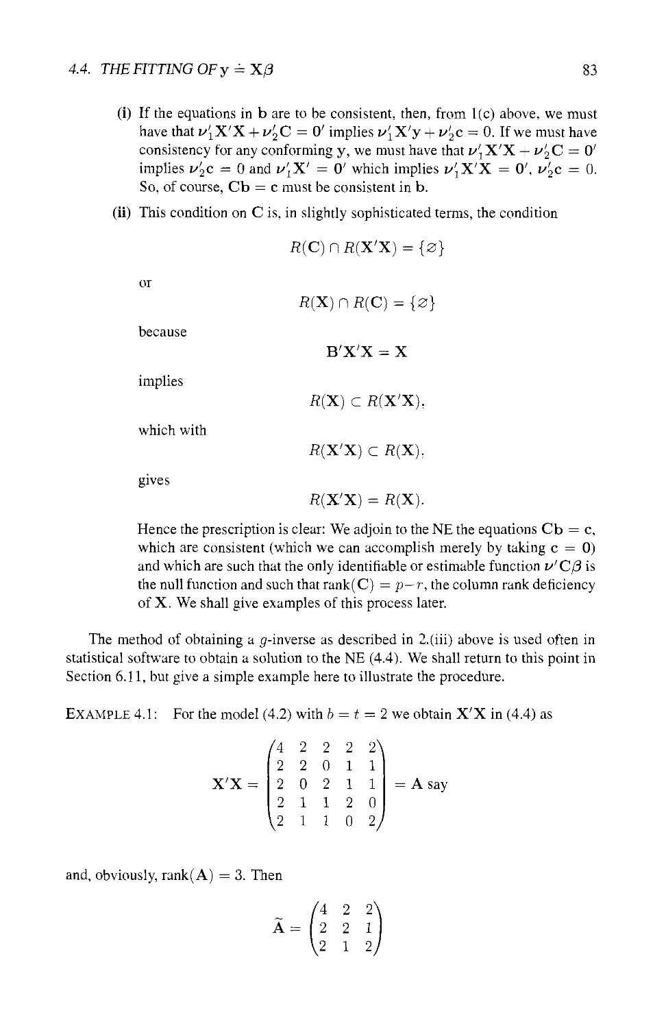
4.4 THE FITTING OF y = X/3 76
4.4.1 The Notion of Identifiability 76
4.4.2 The Notion of Estimability 77
4.4.3 The Method of Least Squares 77
4.4.4 Theory of Linear Equations 81
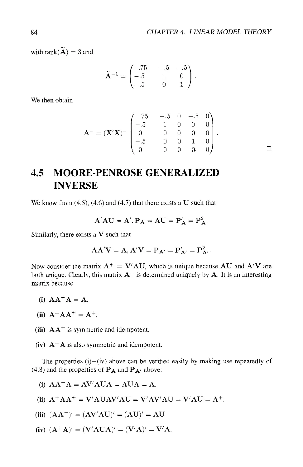
4.5 MOORE-PENROSE GENERALIZED INVERSE 84
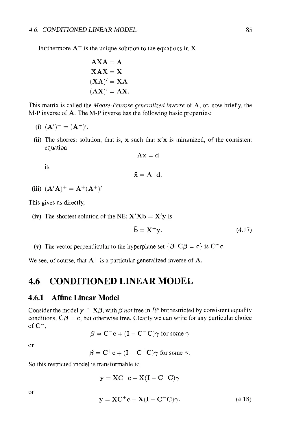
4.6 CONDITIONED LINEAR MODEL 85
4.6.1 Affine Linear Model 85
4.6.2 Normal Equations for the Conditioned Model 87
4.6.3 Different Types of Conditions 88
4.6.4 General Case 89
4.7 TWO-PART LINEAR MODEL 90
4.7.1 Ordered Linear Models 90
4.7.2 Using Orthogonal Projections 91
4.7.3 Orthogonal ANOVA 93
4.8 SPECIAL CASE OF A PARTITIONED MODEL 94
4.9 THREE-PART MODELS 94
4.10 TWO-WAY CLASSIFICATION WITHOUT INTERACTION .... 95
4.11 K-PART LINEAR MODEL 97
4.11.1 The General Model and Its Sums of Squares 97
4.11.2 The Means Model 99
4.12 BALANCED CLASSIFICATORY STRUCTURES 100
4.12.1 Factors, Levels, and Partitions 101
4.12.2 Nested, Crossed, and Confounded Factors 101
4.12.3 The Notion of Balance 102
4.12.4 Balanced One-Way Classification 102
4.12.5 Two-Way Classification with Equal Numbers 103
4.12.6 Experimental versus Observational Studies 104
4.12.7 General Classificatory Structure 106
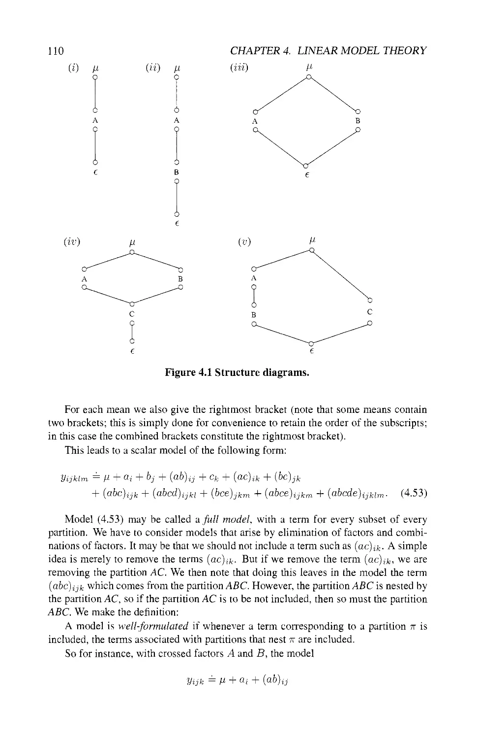
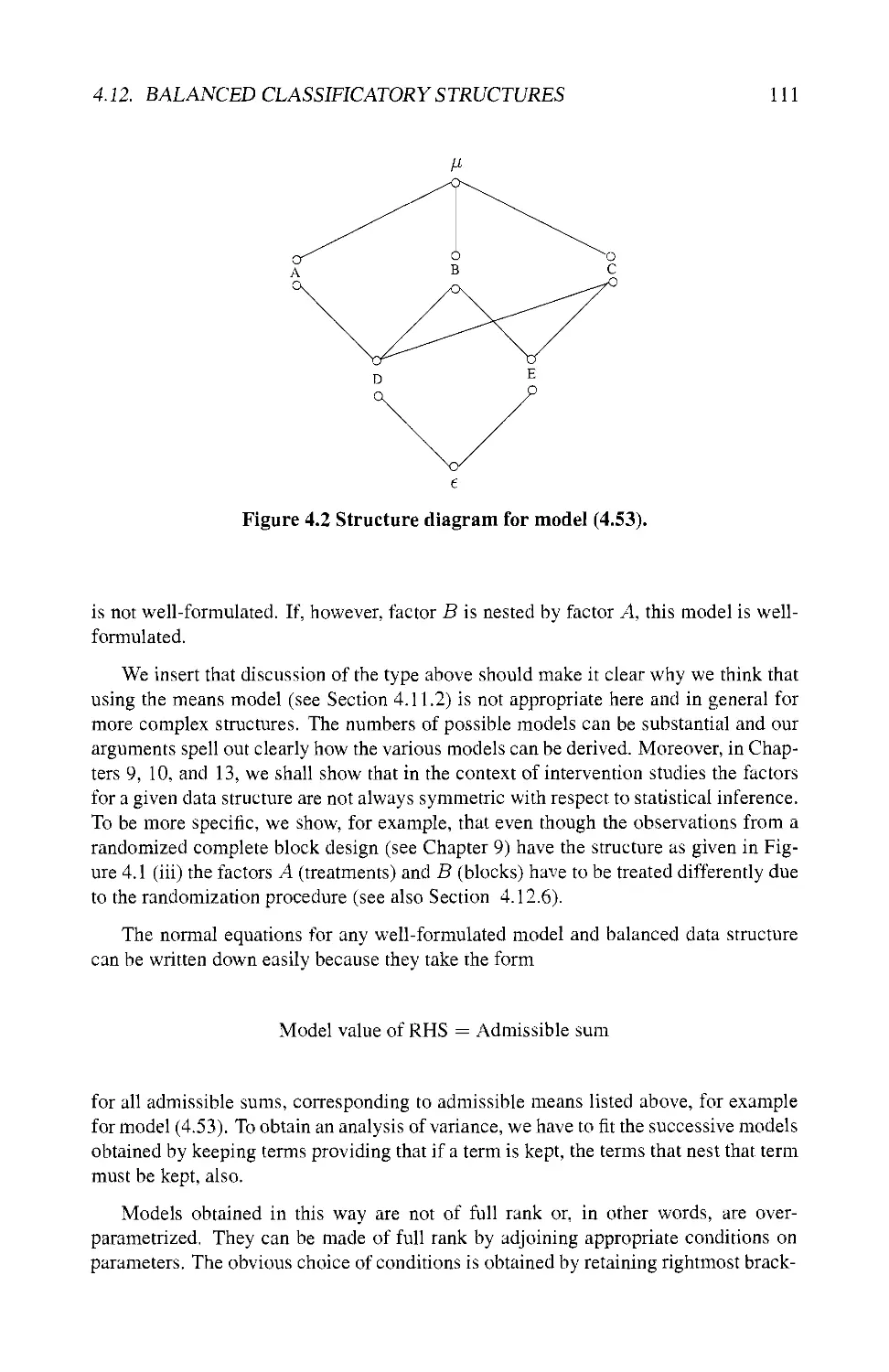
4.12.8 The Well-Formulated Model 109
4.13 UNBALANCED DATA STRUCTURES 112
4.13.1 Two-Fold Nested Classification 112
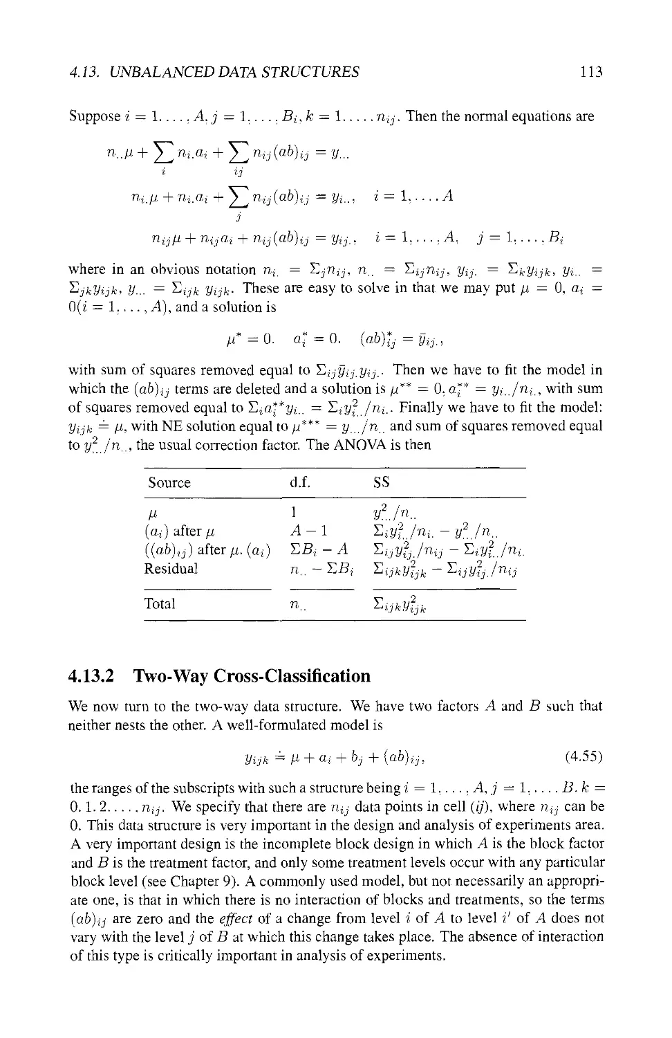
4.13.2 Two-Way Cross-Classification 113
4.13.3 Two-Way Classification without Interaction 116
4.14 ANALYSIS OF COVARIANCE MODEL 118
4.14.1 The Question of Explaining Data 118
4.14.2 Obtaining the ANOVA Table 120
4.14.3 The Case of One Covariate 121
4.14.4 The Case of Several Covariates 121
4.15 FROM DATA ANALYSIS TO STATISTICAL INFERENCE 122
4.16 SIMPLE NORMAL STOCHASTIC LINEAR MODEL 123
4.16.1 The Notion of Estimability 123
viii CONTENTS
4.16.2 Gauss-Markov Linear Model 124
4.16.3 Ordinary Least Squares and Best Linear Unbiased Estimators 126
4.16.4 Expectation of Quadratic Forms 128
4.17 DISTRIBUTION THEORY WITH CjMNLM 128
4.17.1 Distributional Properties of X'f3 128
4.17.2 Distribution of Sums of Squares 130
4.17.3 Testing of Hypotheses 131
4.18 MIXED MODELS 132
4.18.1 The Notion of Fixed, Mixed and Random Models 132
4.18.2 Aitken-like Model 133
4.18.3 Mixed Models in Experimental Design 134
5 Randomization 137
5.1 INTRODUCTION 137
5.1.1 Observational versus Intervention Studies 137
5.1.2 Historical Controls versus Repetitions 139
5.2 THE TEA TASTING LADY 139
5.3 TRIANGULAR EXPERIMENT 140
5.3.1 Medical Example 141
5.3.2 Randomization, Probabilities, and Beliefs 141
5.4 SIMPLE ARITHMETICAL EXPERIMENT . 142
5.4.1 Noisy Experiments 142
5.4.2 Investigative Experiments and Beliefs 144
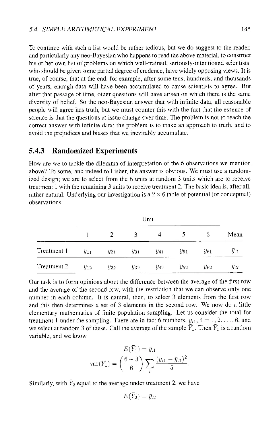
5.4.3 Randomized Experiments 145
5.5 RANDOMIZATION IDEAS 148
5.6 EXPERIMENT RANDOMIZATION TEST 150
5.7 INTRODUCTION TO SUBSEQUENT CHAPTERS 151
6 Completely Randomized Design 153
6.1 INTRODUCTION AND DEFINITION . 153
6.2 RANDOMIZATION PROCESS 154
6.2.1 Use of Random Numbers 154
6.2.2 Design Random Variables 154
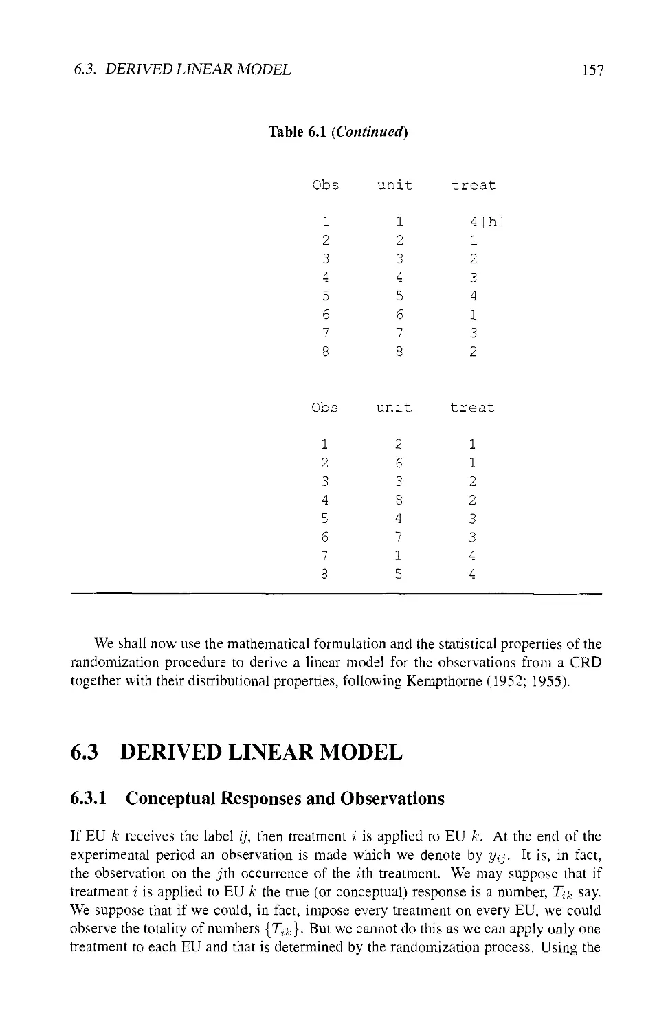
6.3 DERIVED LINEAR MODEL 157
6.3.1 Conceptual Responses and Observations 157
6.3.2 Distributional Properties 159
6.3.3 Additivity in the Broad Sense 161
6.3.4 Error Structure 162
6.3.5 Summary of Results 164
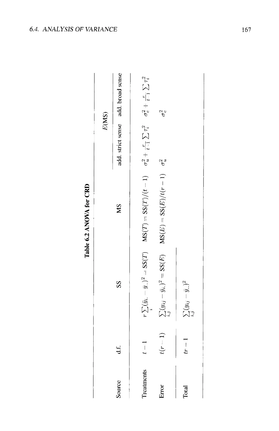
6.4 ANALYSIS OF VARIANCE 165
6.4.1 Deriving the ANOVA Table 165
6.4.2 Obtaining Expected Mean Squares 168
6.5 STATISTICAL TESTS 171
6.5.1 Enumerating Randomizations 171
6.5.2 Randomization Test 172
6.6 APPROXIMATING THE RANDOMIZATION TEST 174
CONTENTS ix
6.6.1 Moments of the Test Statistic 174
6.6.2 Approximation by the F-Test 177
6.6.3 Simulation Study 177
6.7 CRD WITH UNEQUAL NUMBERS OF REPLICATIONS 179
6.7.1 Randomization 180
6.7.2 The Model and ANOVA 180
6.7.3 Comparing Randomization Test and F-Test 180
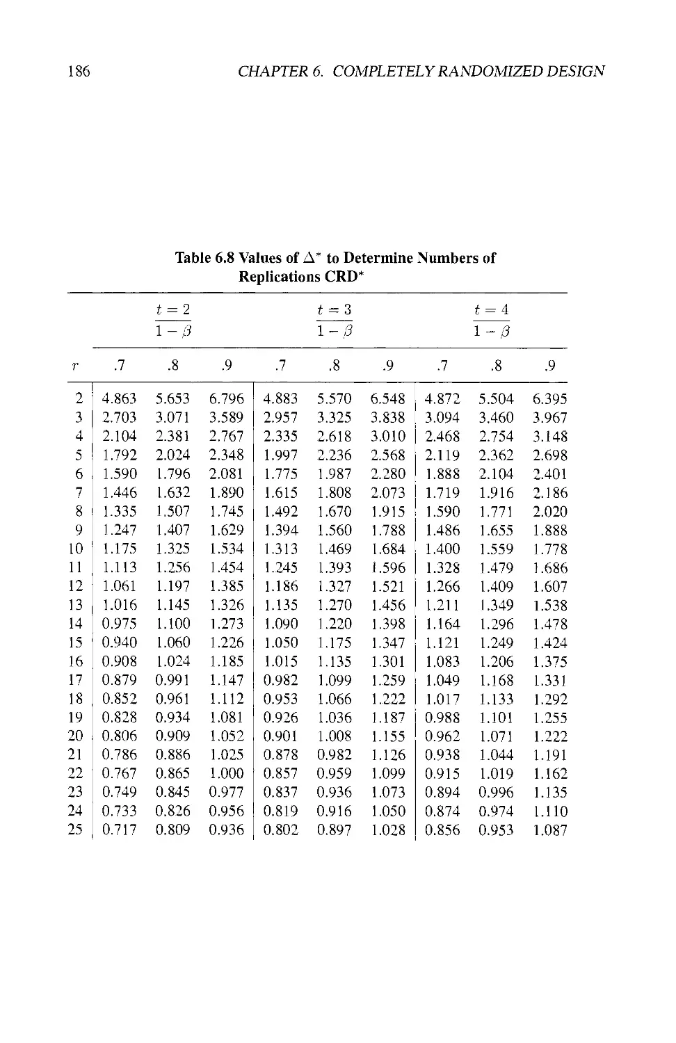
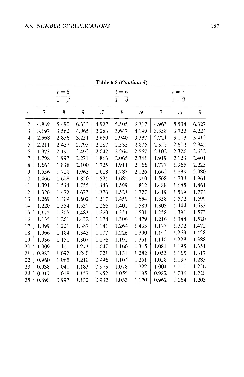
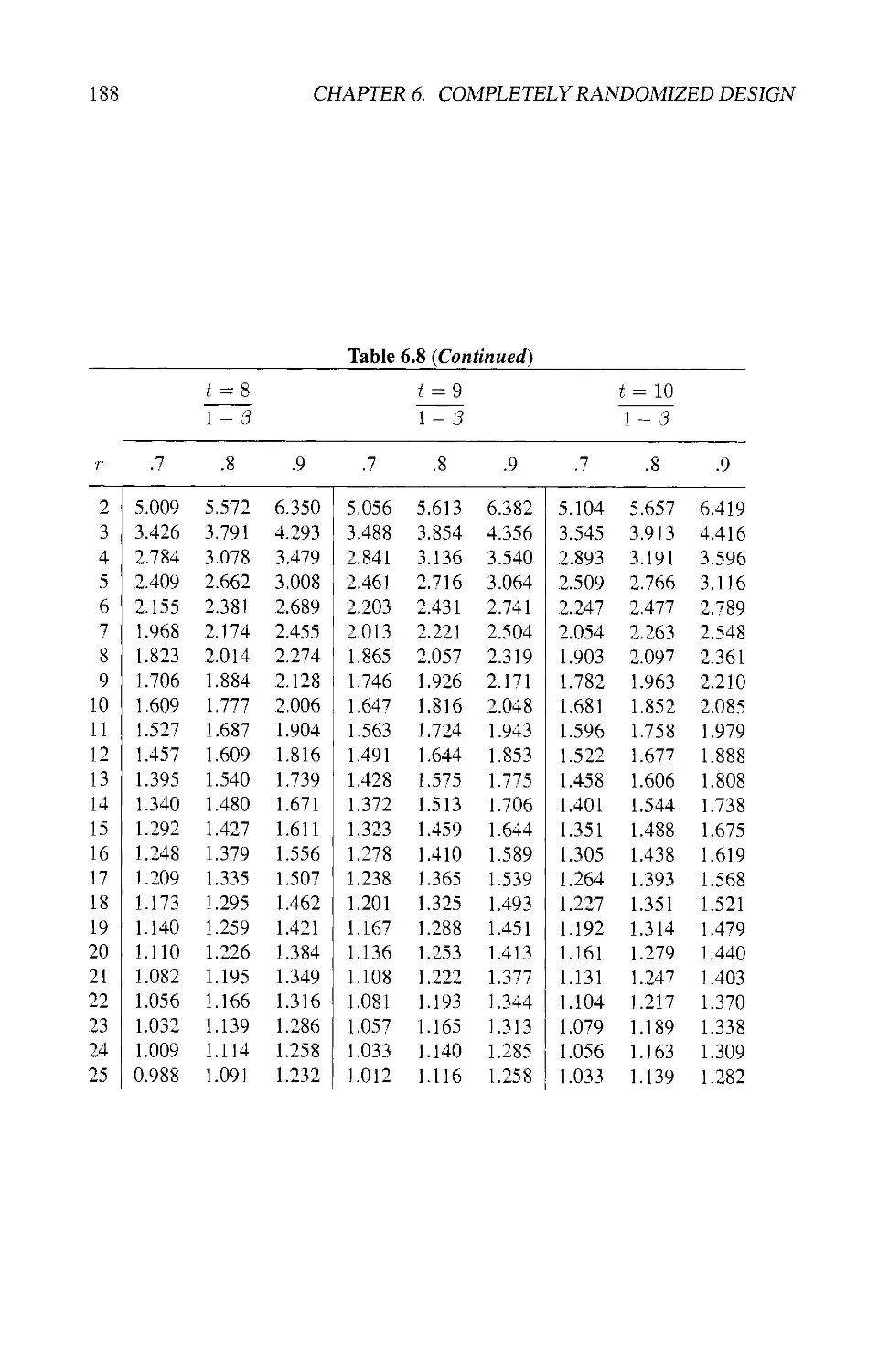
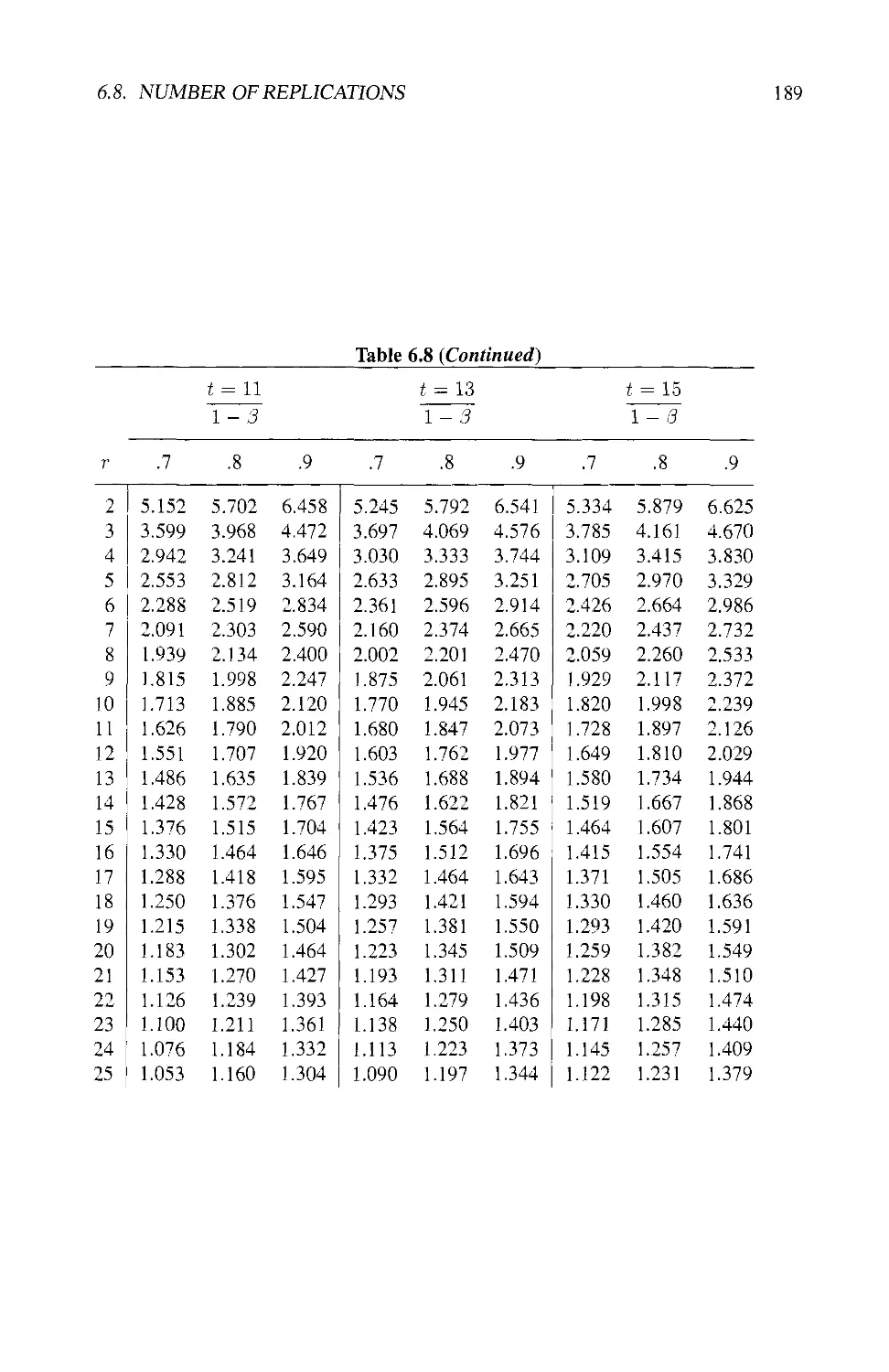
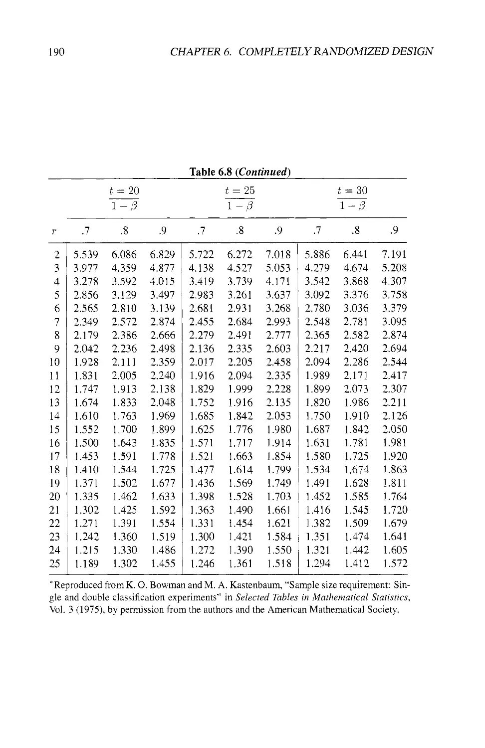
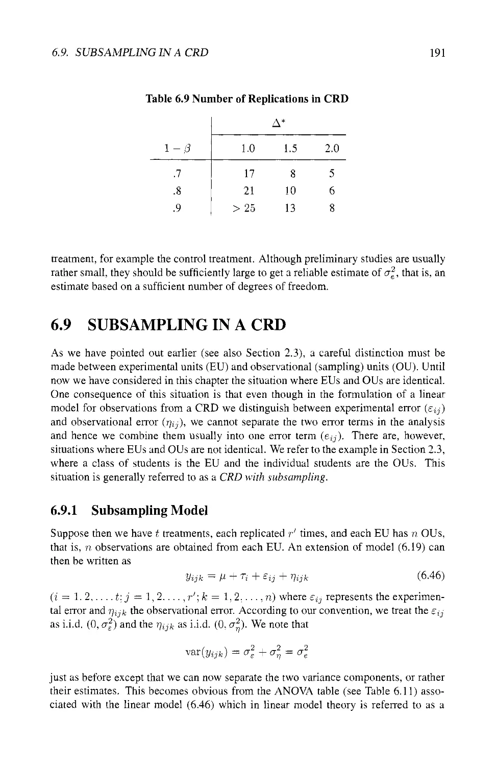
6.8 NUMBER OF REPLICATIONS 180
6.8.1 Power of the F-Test 182
6.8.2 Smallest Detectable Difference 184
6.8.3 Practical Considerations 185
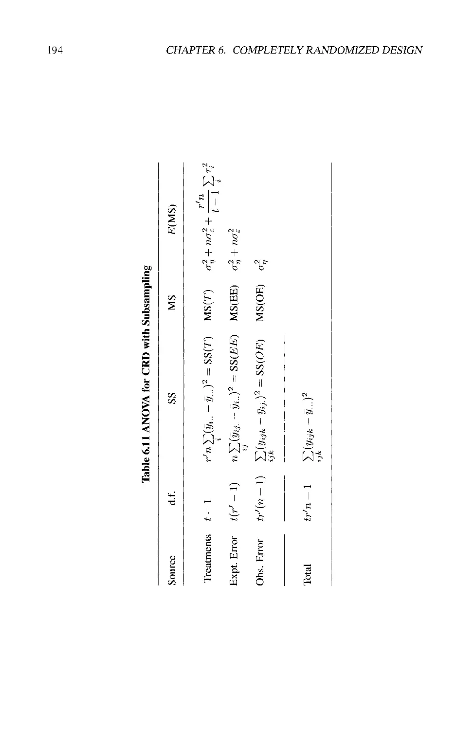
6.9 SUBSAMPLING IN A CRD 191
6.9.1 Subsampling Model 191
6.9.2 Inferences with Subsampling 193
6.9.3 Comparison of CRDs without and with Subsampling 193
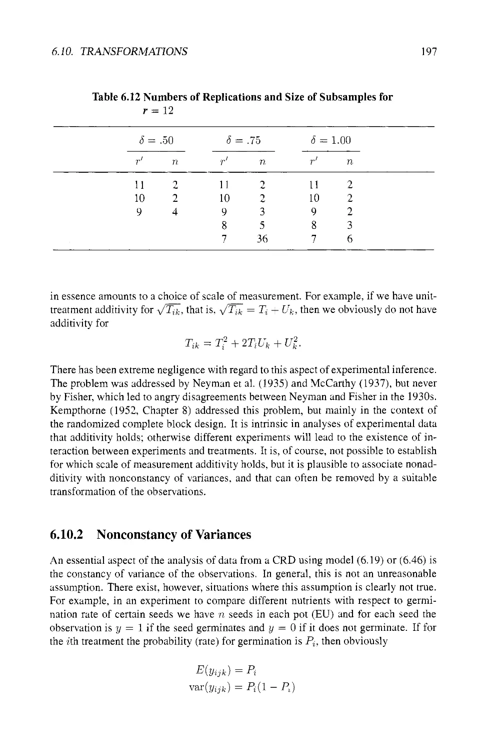
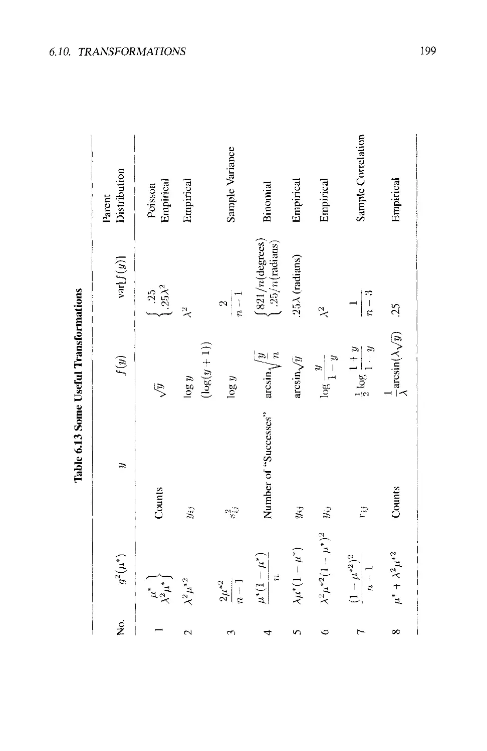
6.10 TRANSFORMATIONS 196
6.10.1 Nonadditivity in the General Sense 196
6.10.2 Nonconstancy of Variances 197
6.10.3 Choice of Transformation 198
6.10.4 Power Transformations 200
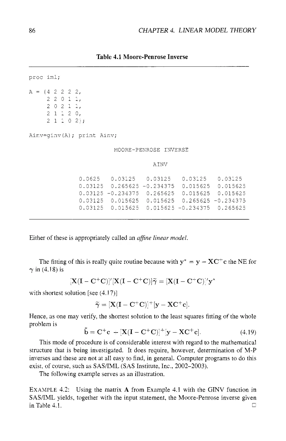
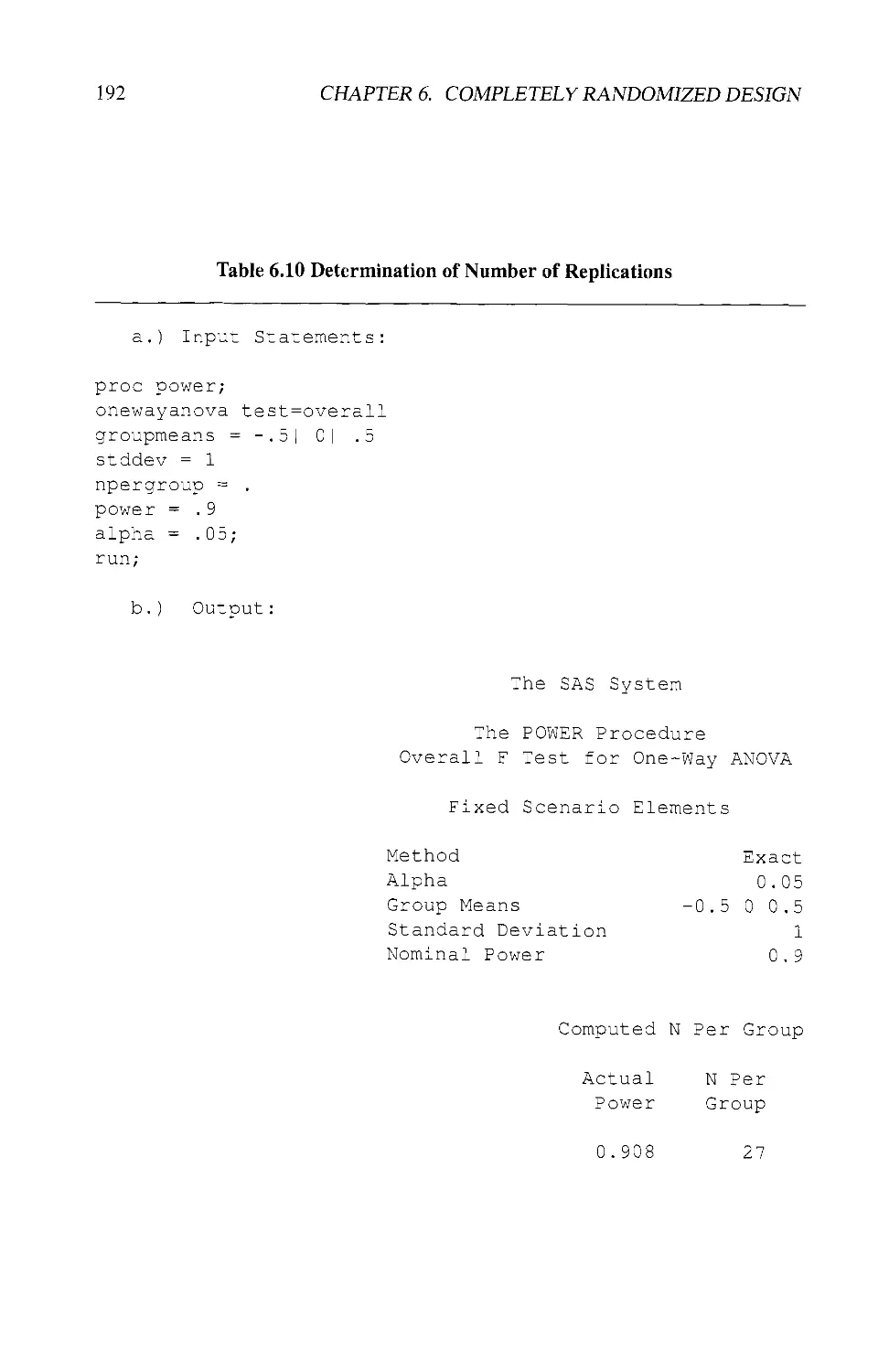
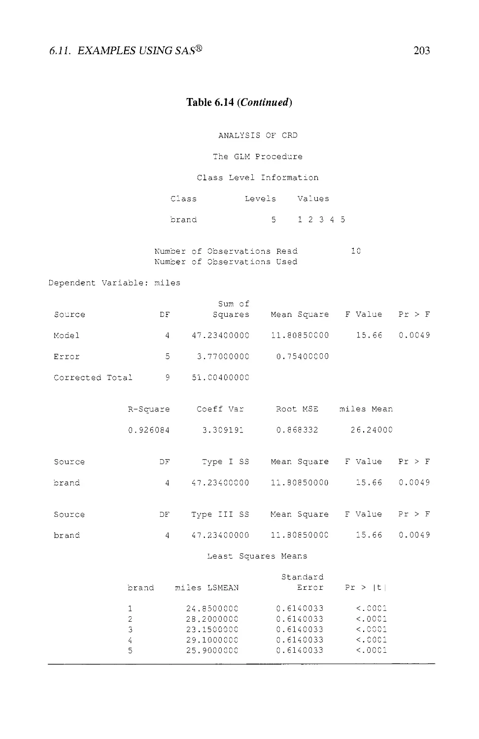
6.11 EXAMPLES USING SAS® 201
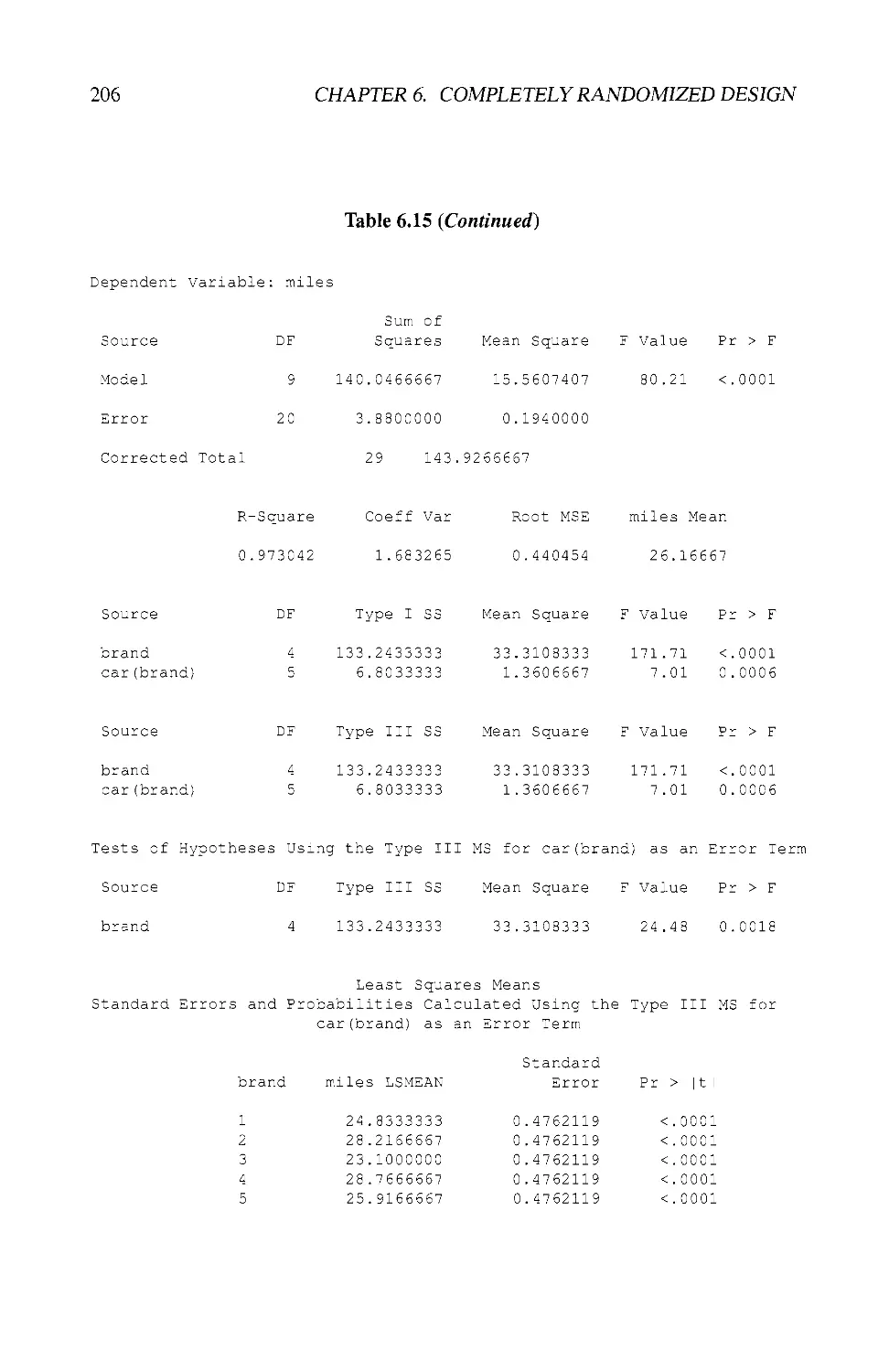
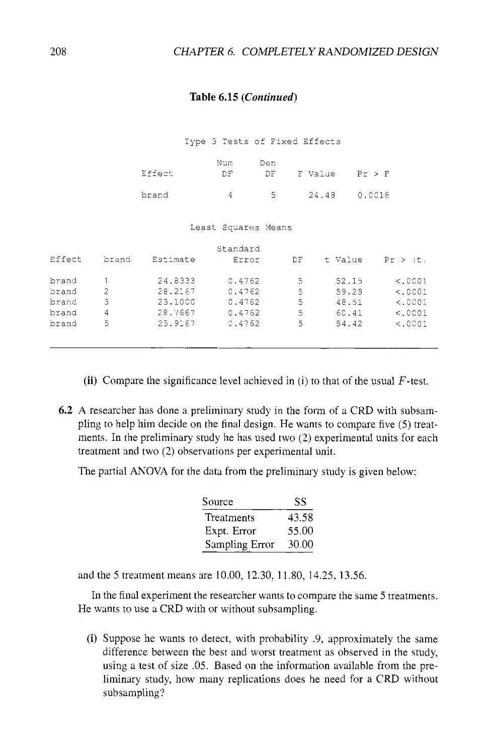
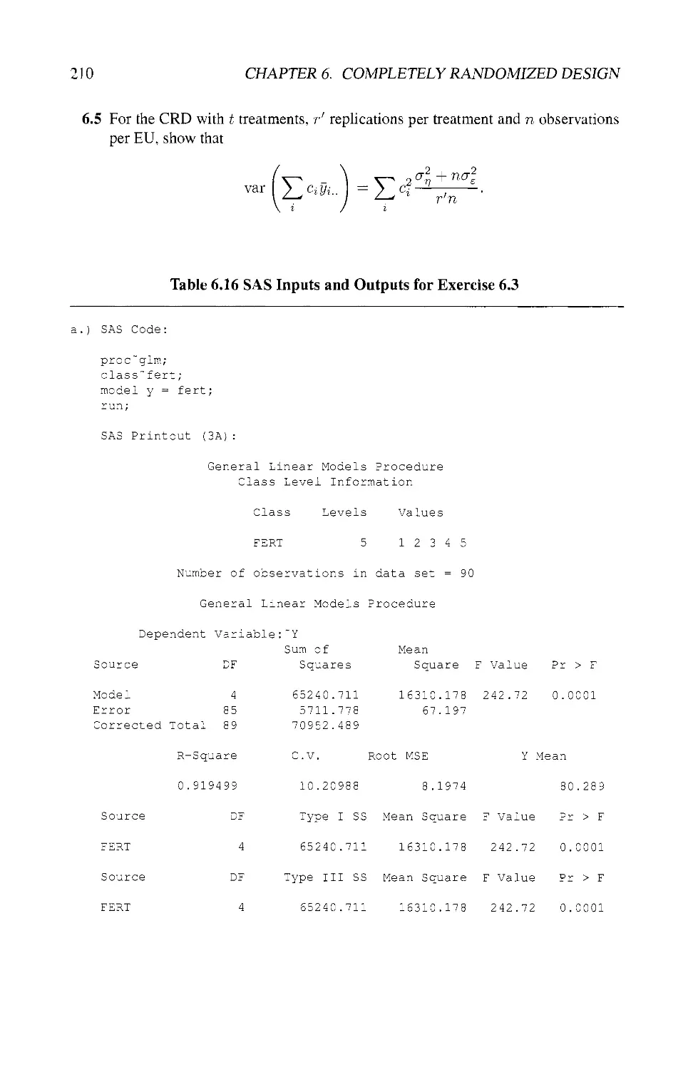
6.12 EXERCISES 204
7 Comparisons of Treatments 213
7.1 INTRODUCTION 213
7.2 COMPARISONS FOR QUALITATIVE TREATMENTS 213
7.2.1 Treatment Contrasts 214
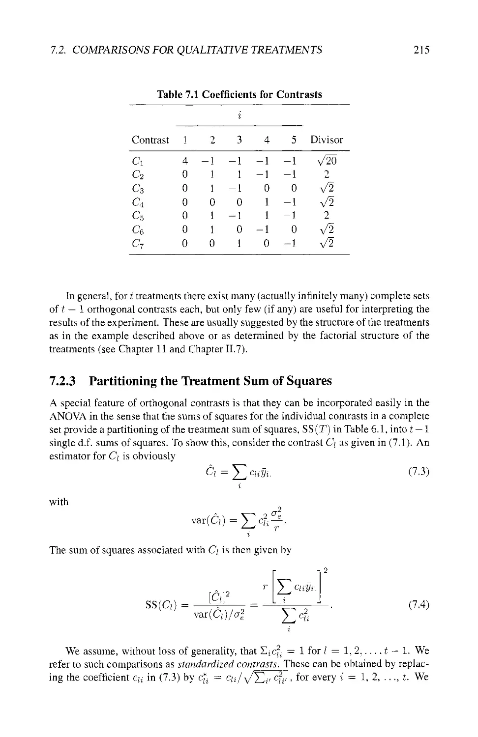
7.2.2 Orthogonal Contrasts 214
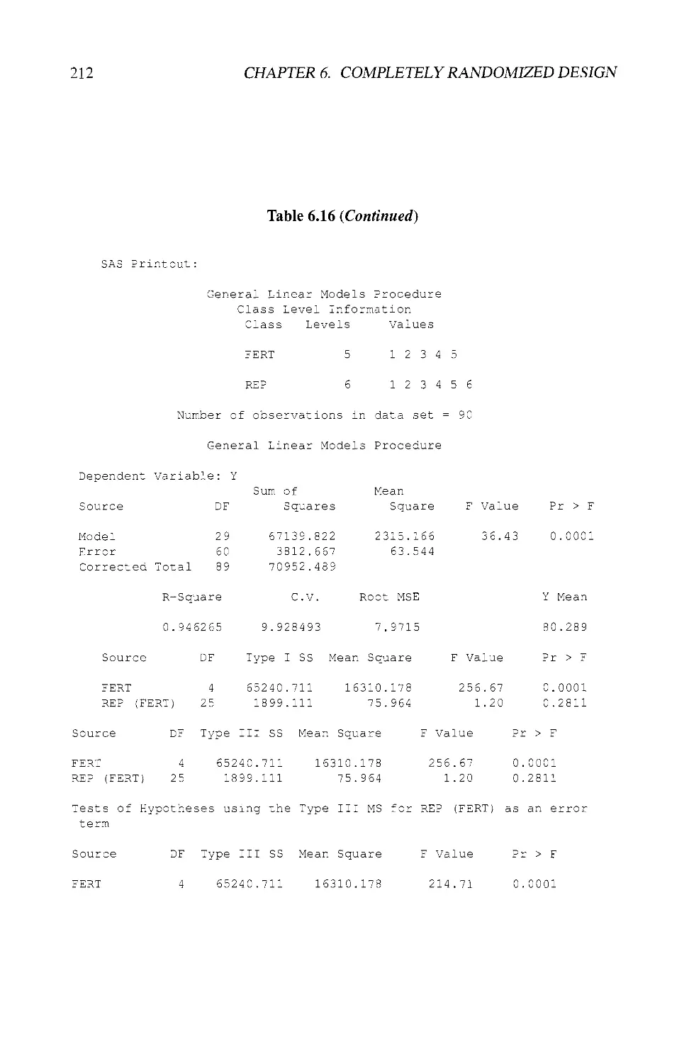
7.2.3 Partitioning the Treatment Sum of Squares 215
7.3 ORTHOGONALITY AND ORTHOGONAL COMPARISONS .... 218
7.4 COMPARISONS FOR QUANTITATIVE TREATMENTS 219
7.4.1 Comparisons for Treatments with Equidistant Levels 219
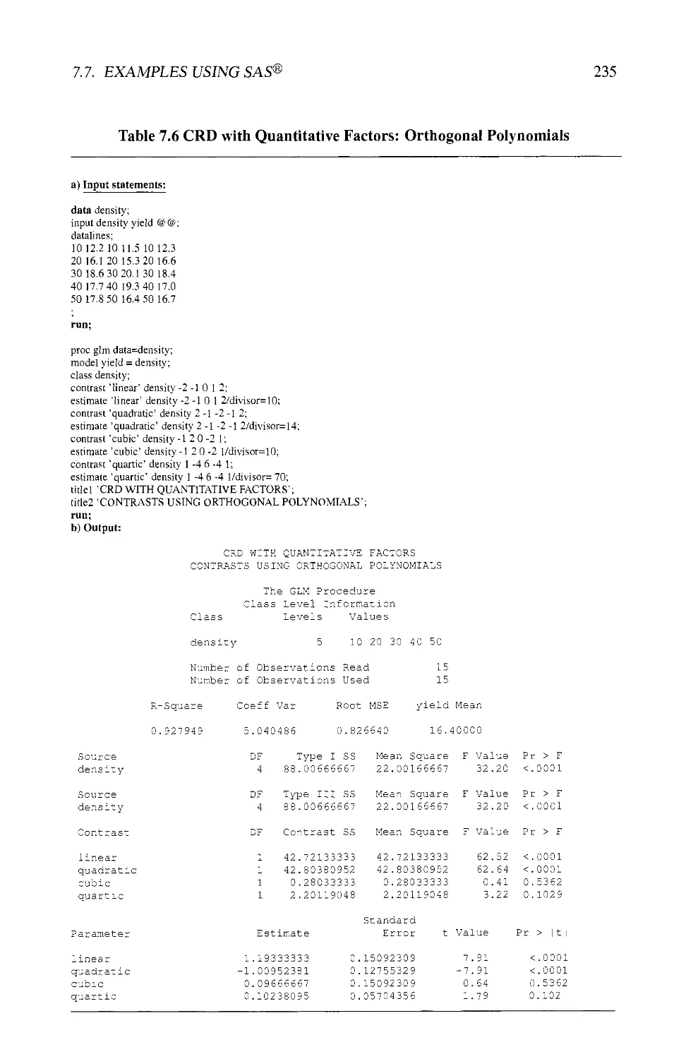
7.4.2 Use of Orthogonal Polynomials 220
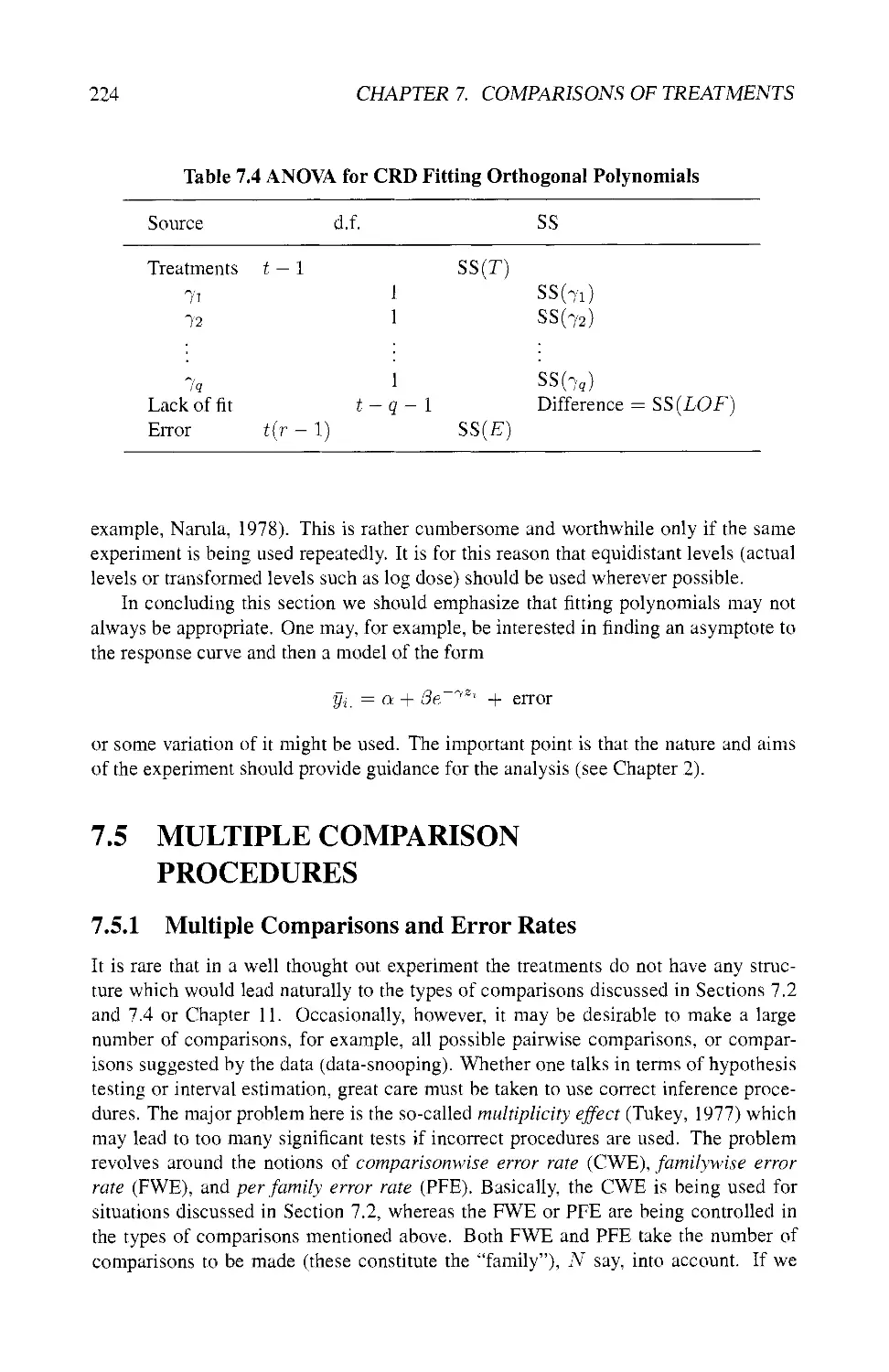
7.4.3 Contrast Sums of Squares and the ANOVA 223
7.5 MULTIPLE COMPARISON PROCEDURES 224
7.5.1 Multiple Comparisons and Error Rates 224
7.5.2 Least Significant Difference Test 225
7.5.3 Bonferroni i-Statistics 225
7.5.4 Studentized Range Procedure 226
7.5.5 Duncan's Multiple Range Test 226
7.5.6 Scheffe's Procedure 227
7.5.7 Comparisons with a Control 227
7.5.8 Alternatives to Tests Based on Normality 228
7.6 GROUPING TREATMENTS 229
7.7 EXAMPLES USING SAS® 230
7.8 EXERCISES 236
CONTENTS
Use of Supplementary Information 239
8.1 INTRODUCTION 239
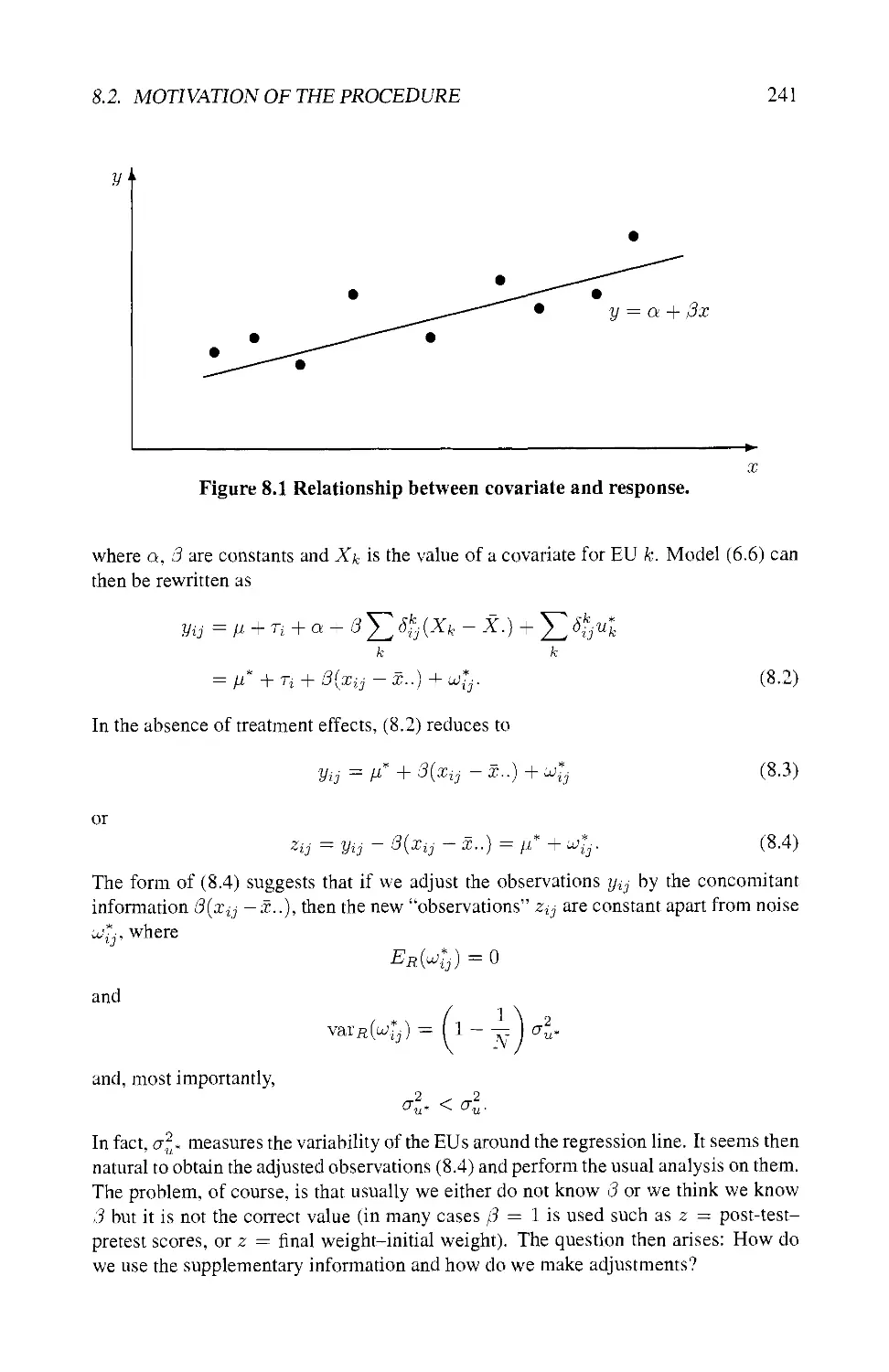
8.2 MOTIVATION OF THE PROCEDURE 240
8.3 ANALYSIS OF COVARIANCE PROCEDURE 242
8.3.1 Basic Model 242
8.3.2 Least Squares Analysis 242
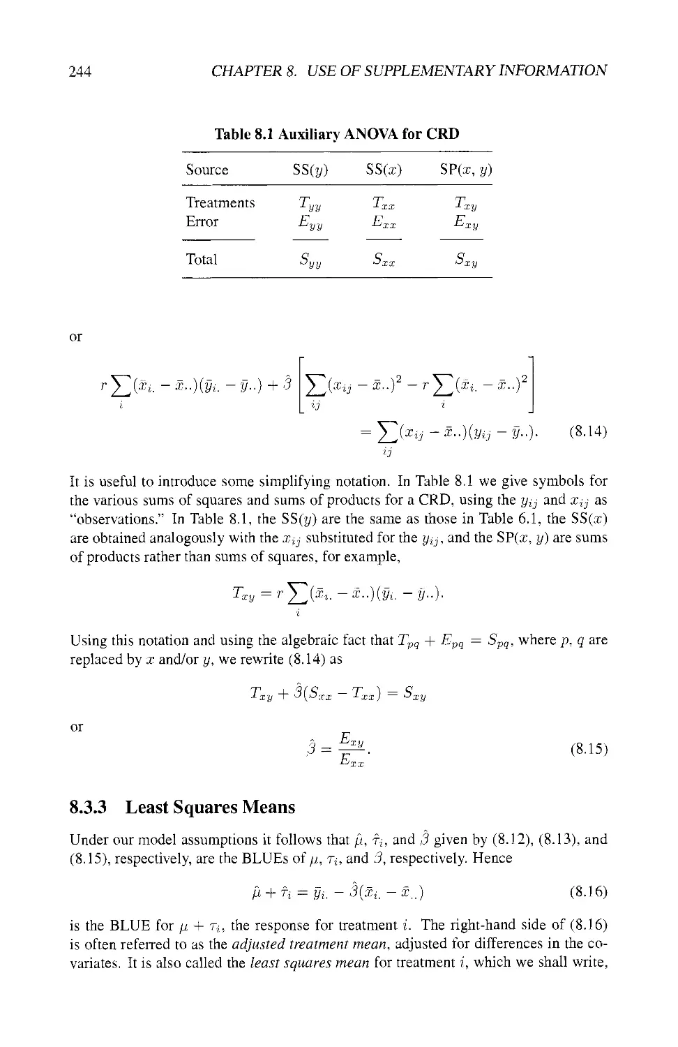
8.3.3 Least Squares Means 244
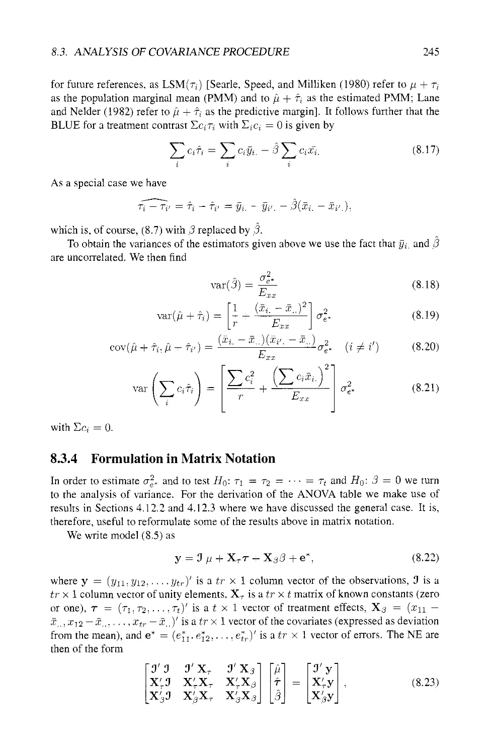
8.3.4 Formulation in Matrix Notation 245
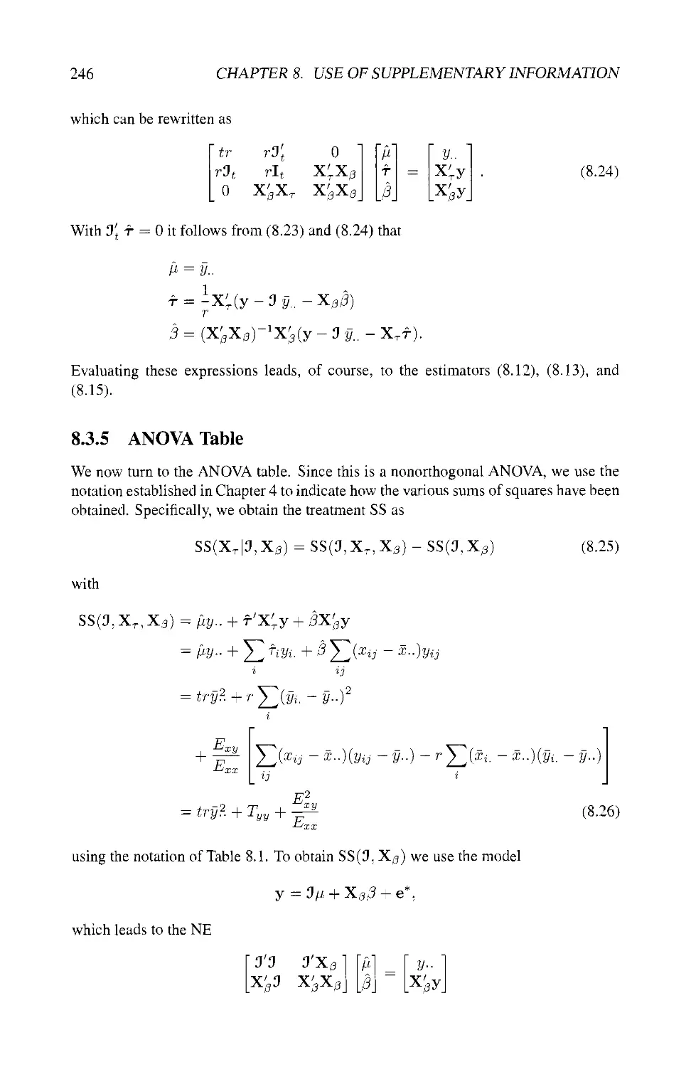
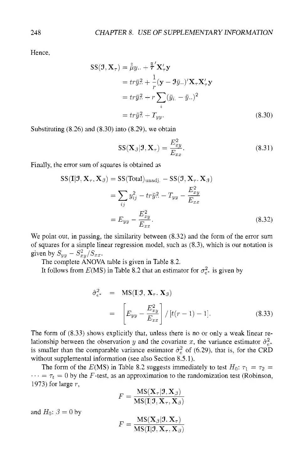
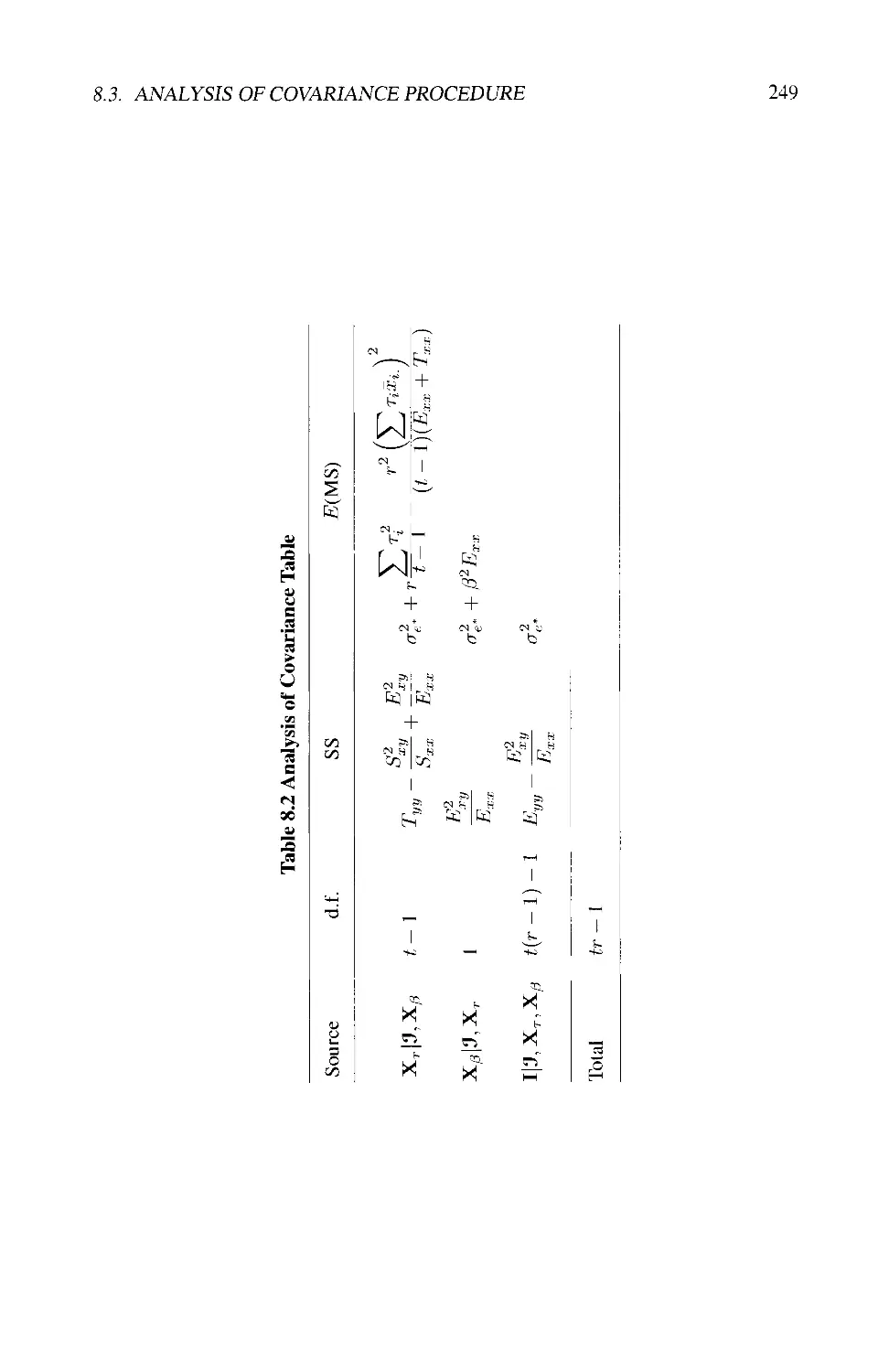
8.3.5 ANOVA Table 246
8.4 TREATMENT COMPARISONS 250
8.4.1 Preplanned Comparisons 250
8.4.2 Multiple Comparison Procedures 251
8.5 VIOLATION OF ASSUMPTIONS 252
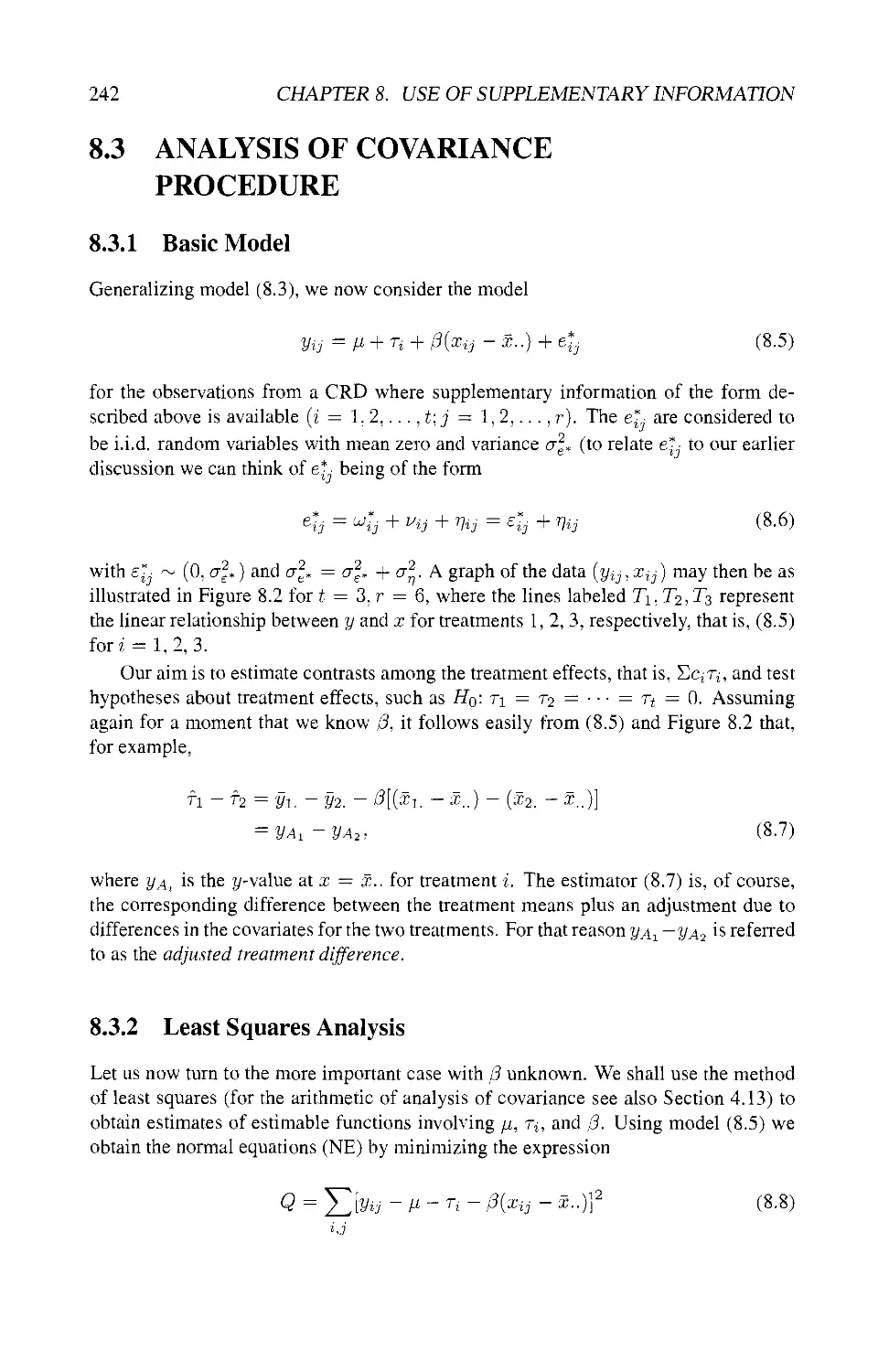
8.5.1 Linear Relationship between* andy 252
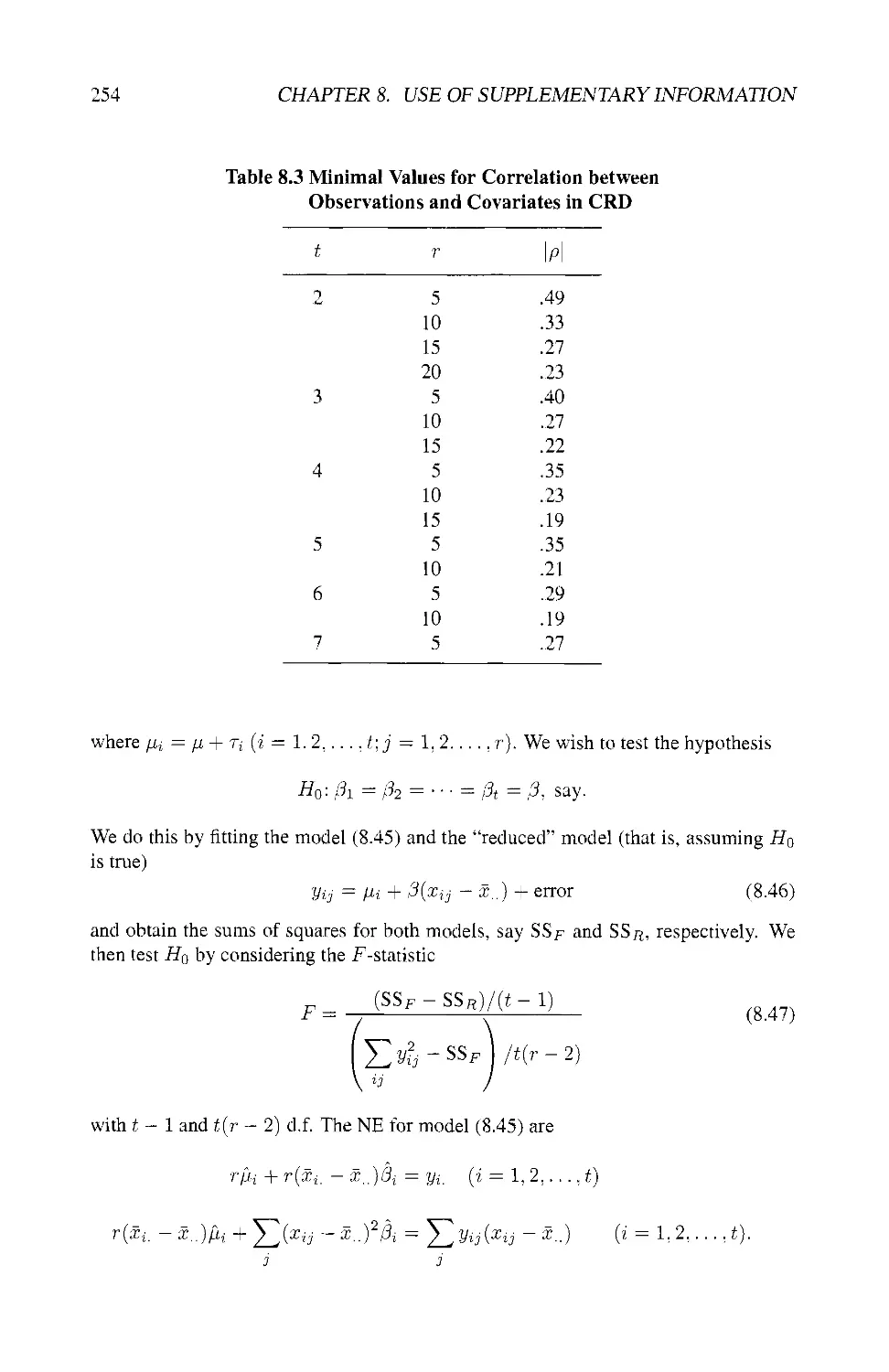
8.5.2 Common Slope 253
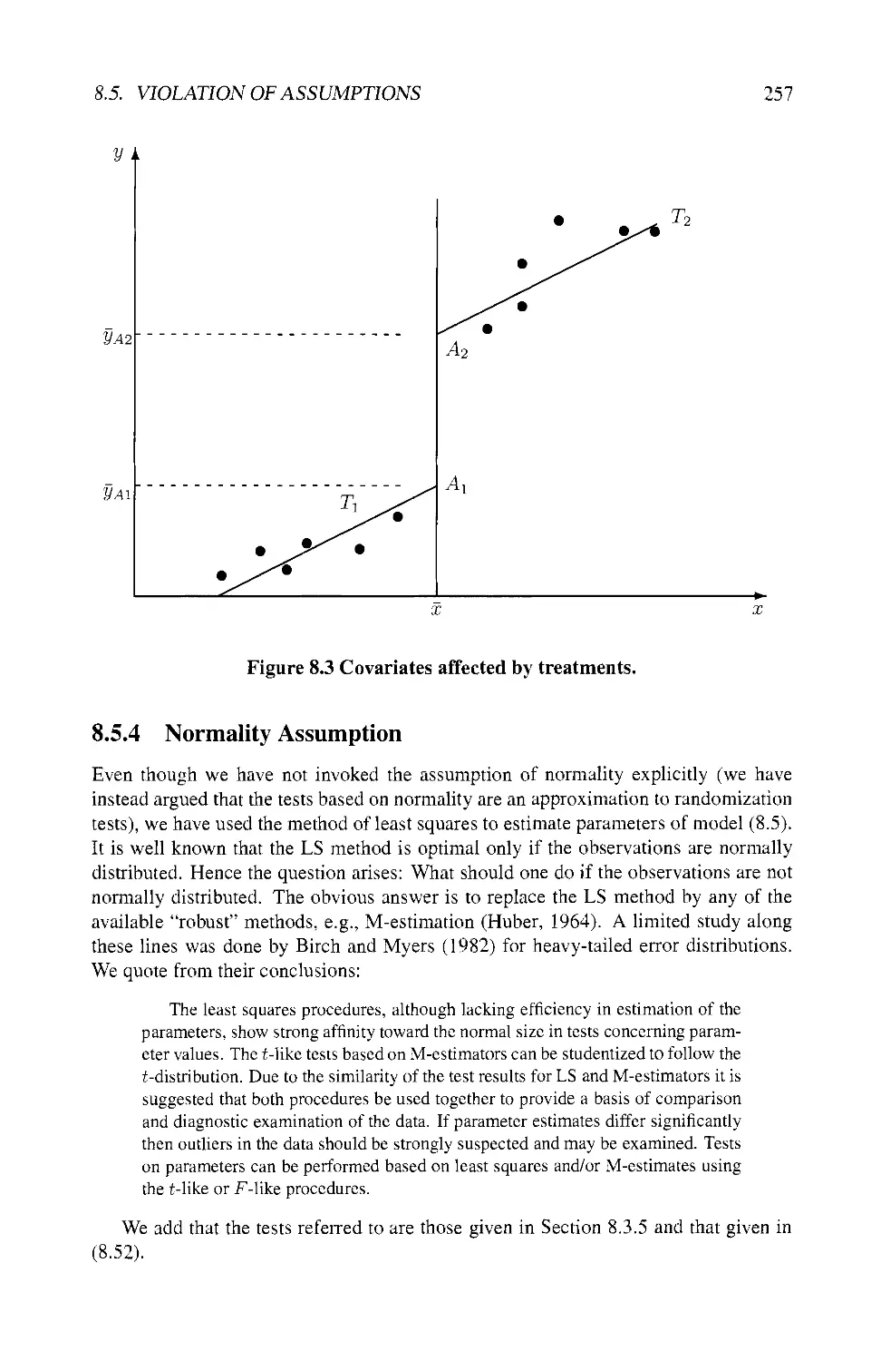
8.5.3 Covariates Affected by Treatments 256
8.5.4 Normality Assumption 257
8.6 ANALYSIS OF COVARIANCE WITH
SUBSAMPLING 258
8.7 CASE OF SEVERAL COVARIATES 259
8.7.1 General Case 260
8.7.2 Two Covariates 262
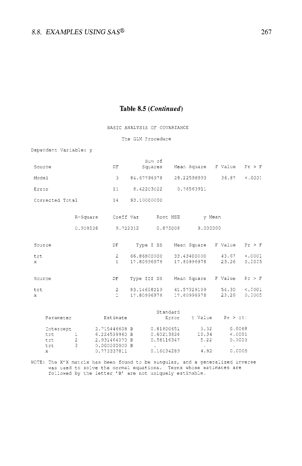
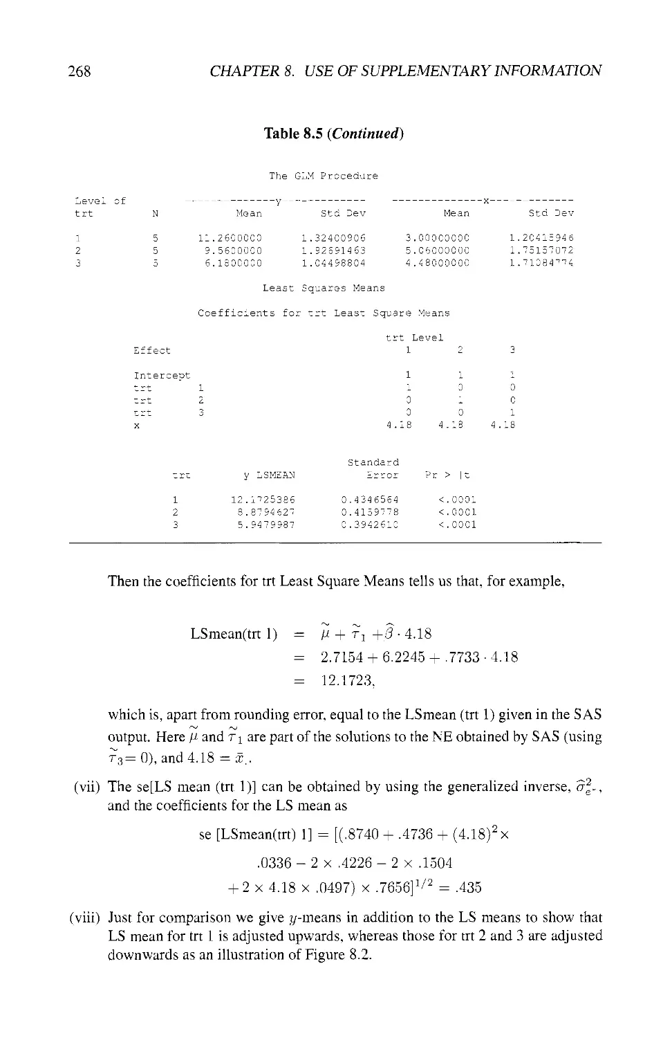
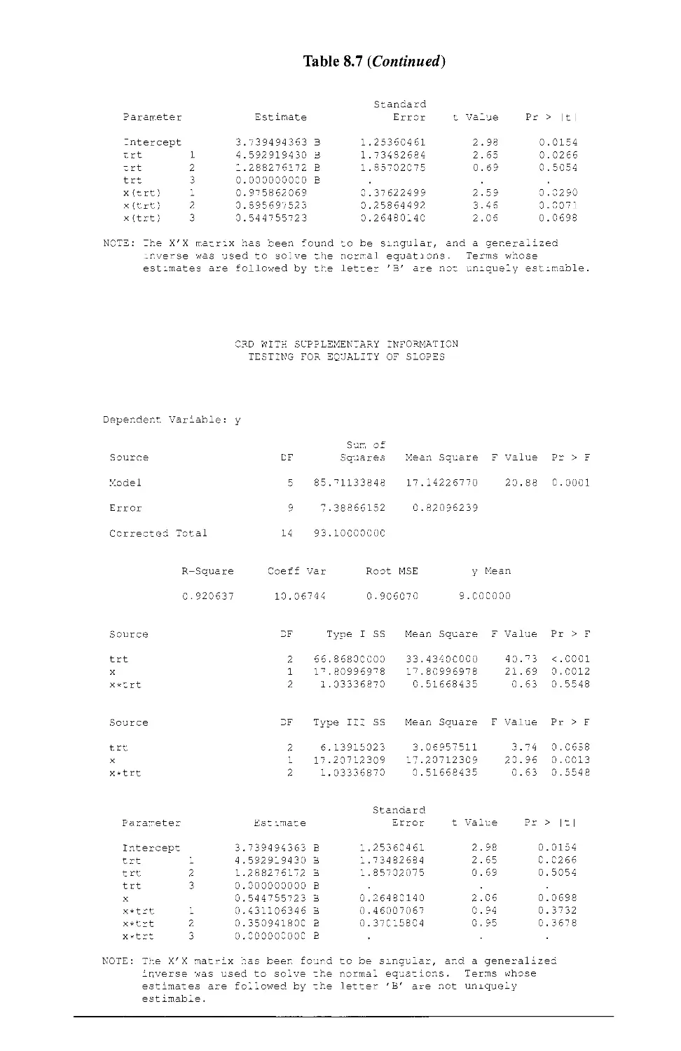
8.8 EXAMPLES USING SAS® 264
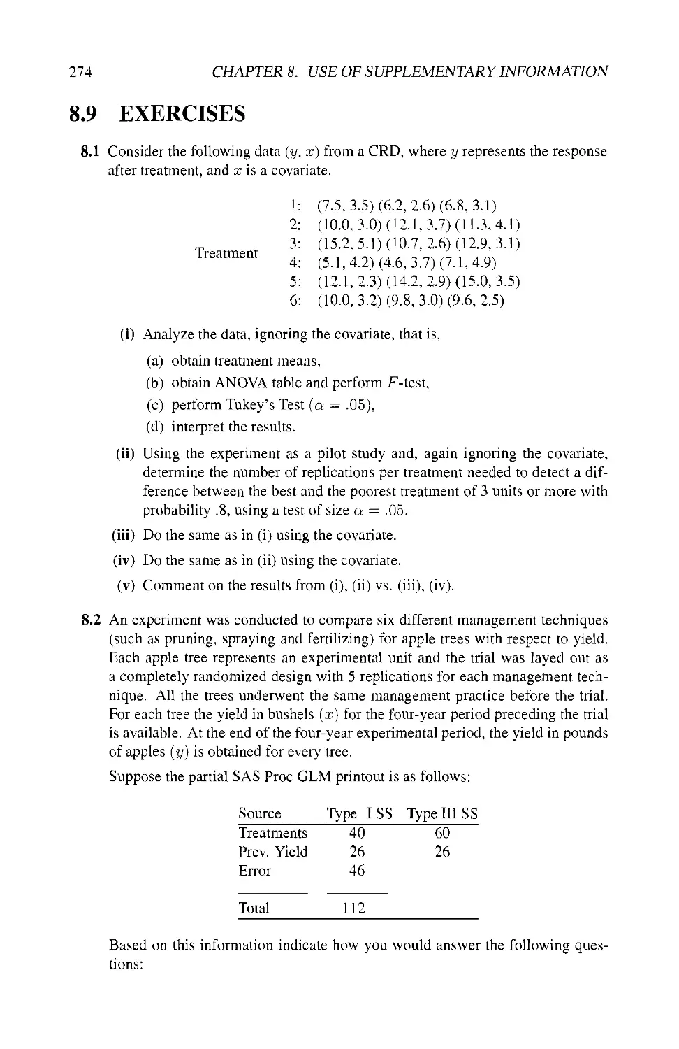
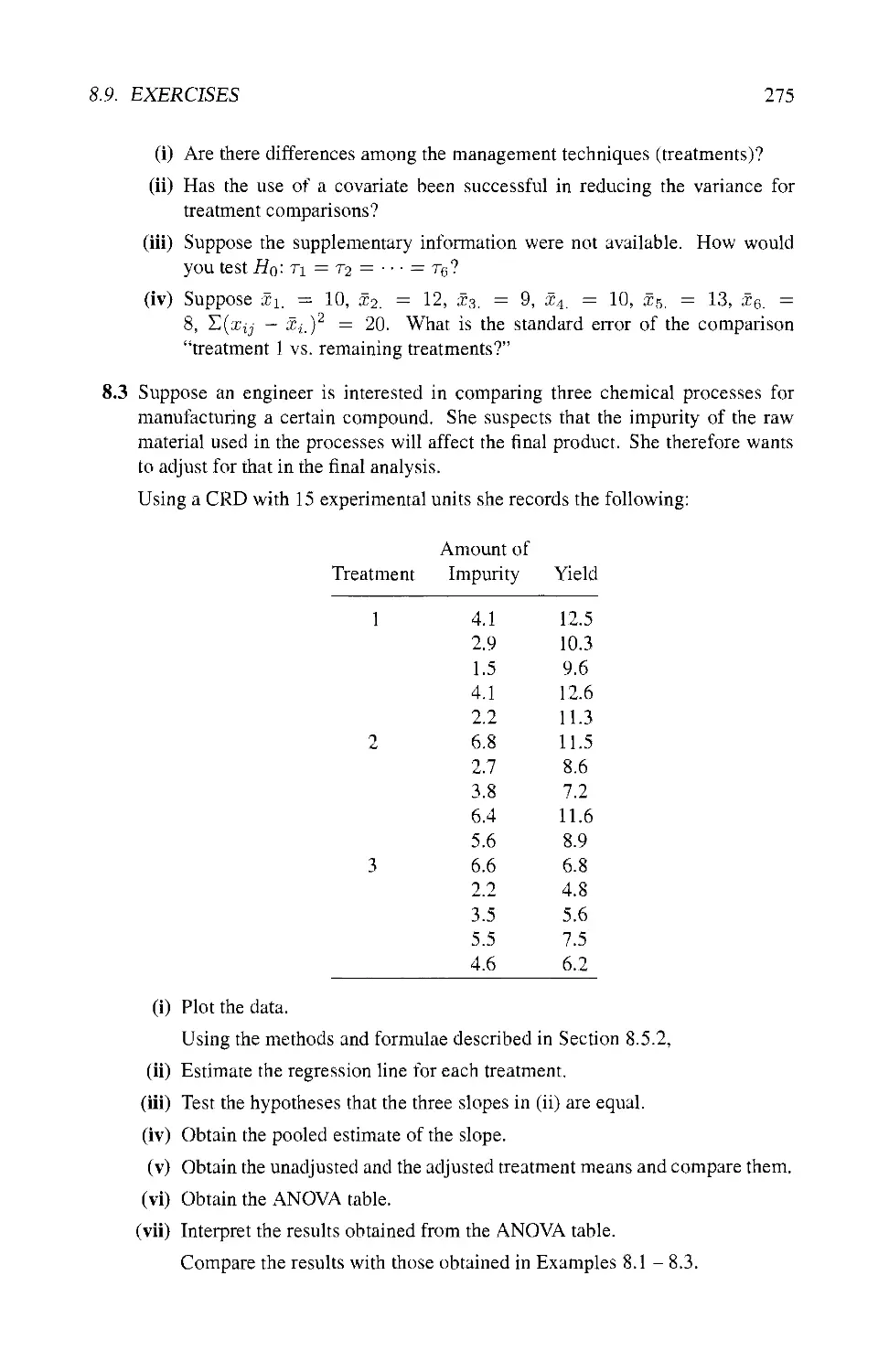
8.9 EXERCISES 274
Randomized Block Designs 277
9.1 INTRODUCTION 277
9.2 RANDOMIZED COMPLETE BLOCK DESIGN 278
9.2.1 Definition 278
9.2.2 Derived Linear Model 278
9.2.3 Estimation of Treatment Contrasts 282
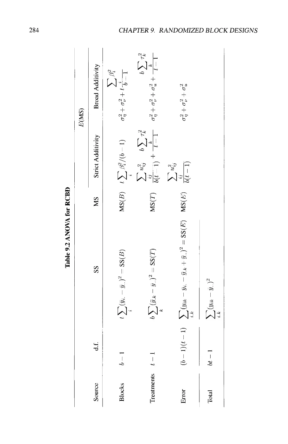
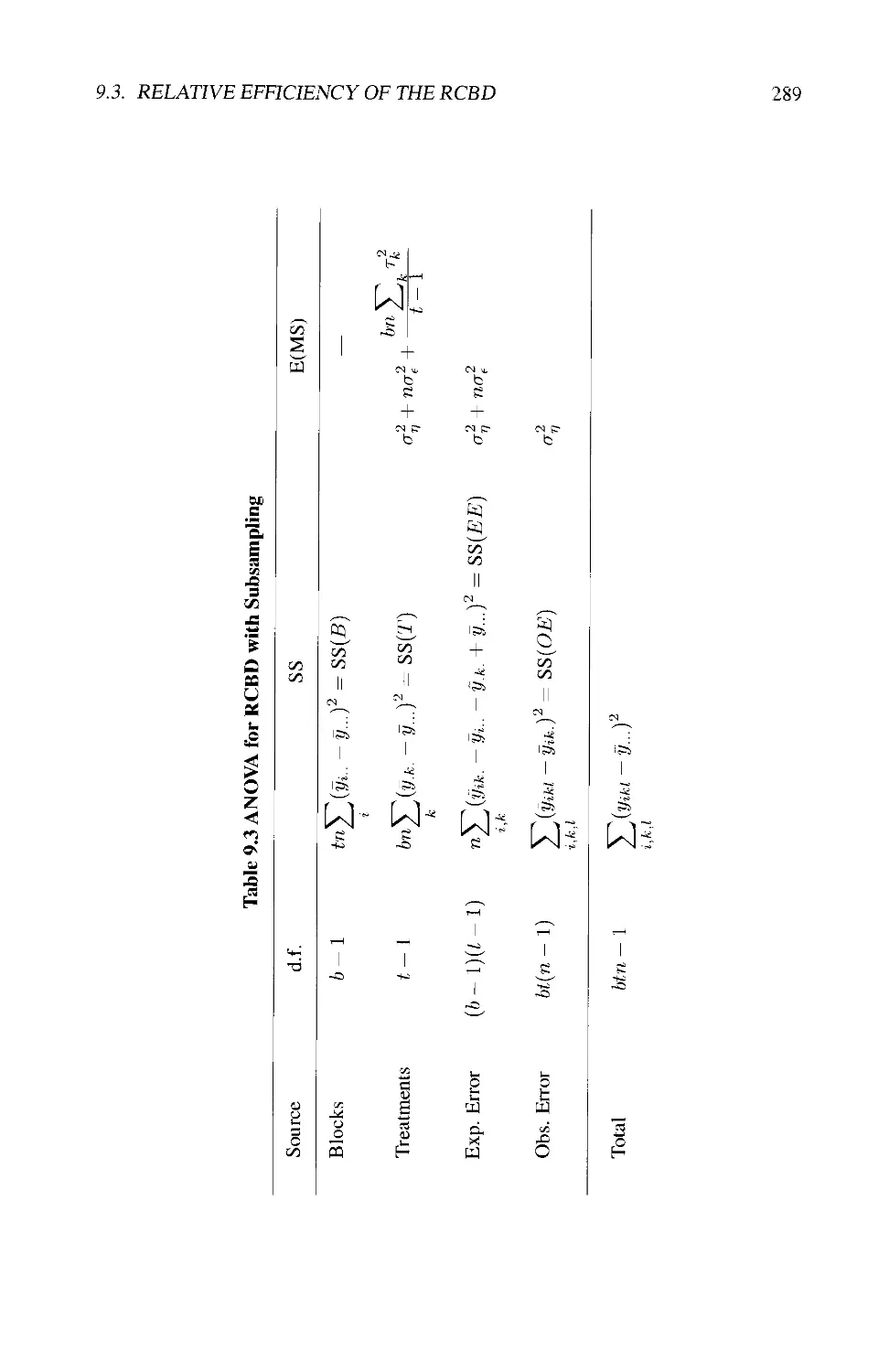
9.2.4 Analysis of Variance 282
9.2.5 Randomization Test and F-Test 285
9.2.6 Additivity in the Broad Sense 286
9.2.7 Subsampling in an RCBD 288
9.3 RELATIVE EFFICIENCY OF THE RCBD 288
9.3.1 Question of Effectiveness of Blocking 288
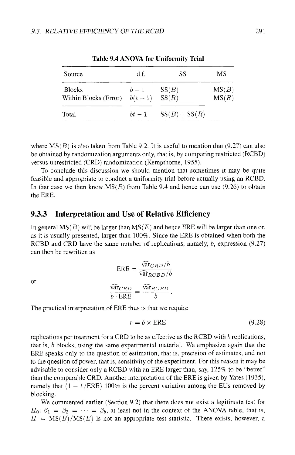
9.3.2 Use of Uniformity Trials 290
9.3.3 Interpretation and Use of Relative Efficiency 291
9.4 ANALYSIS OF COVARIANCE 292
9.4.1 The Model 292
9.4.2 Least Squares Analysis 293
9.4.3 The ANOVA Table 294
9.5 MISSING OBSERVATIONS 295
9.5.1 Estimating a Missing Observation 295
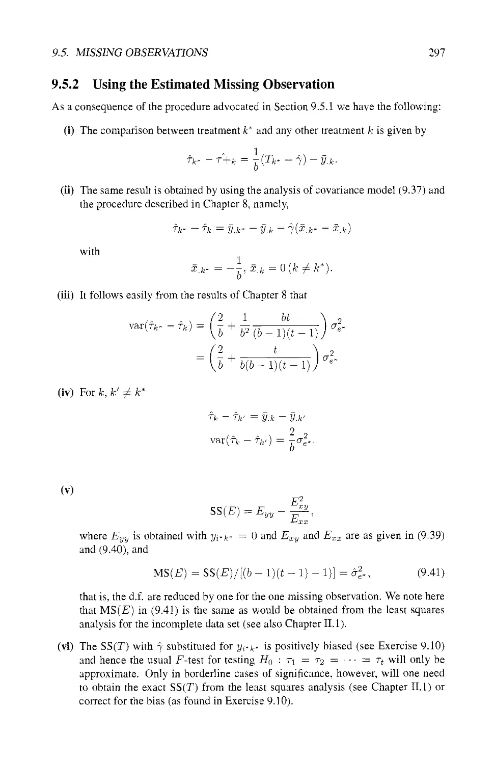
9.5.2 Using the Estimated Missing Observation 297
CONTENTS xi
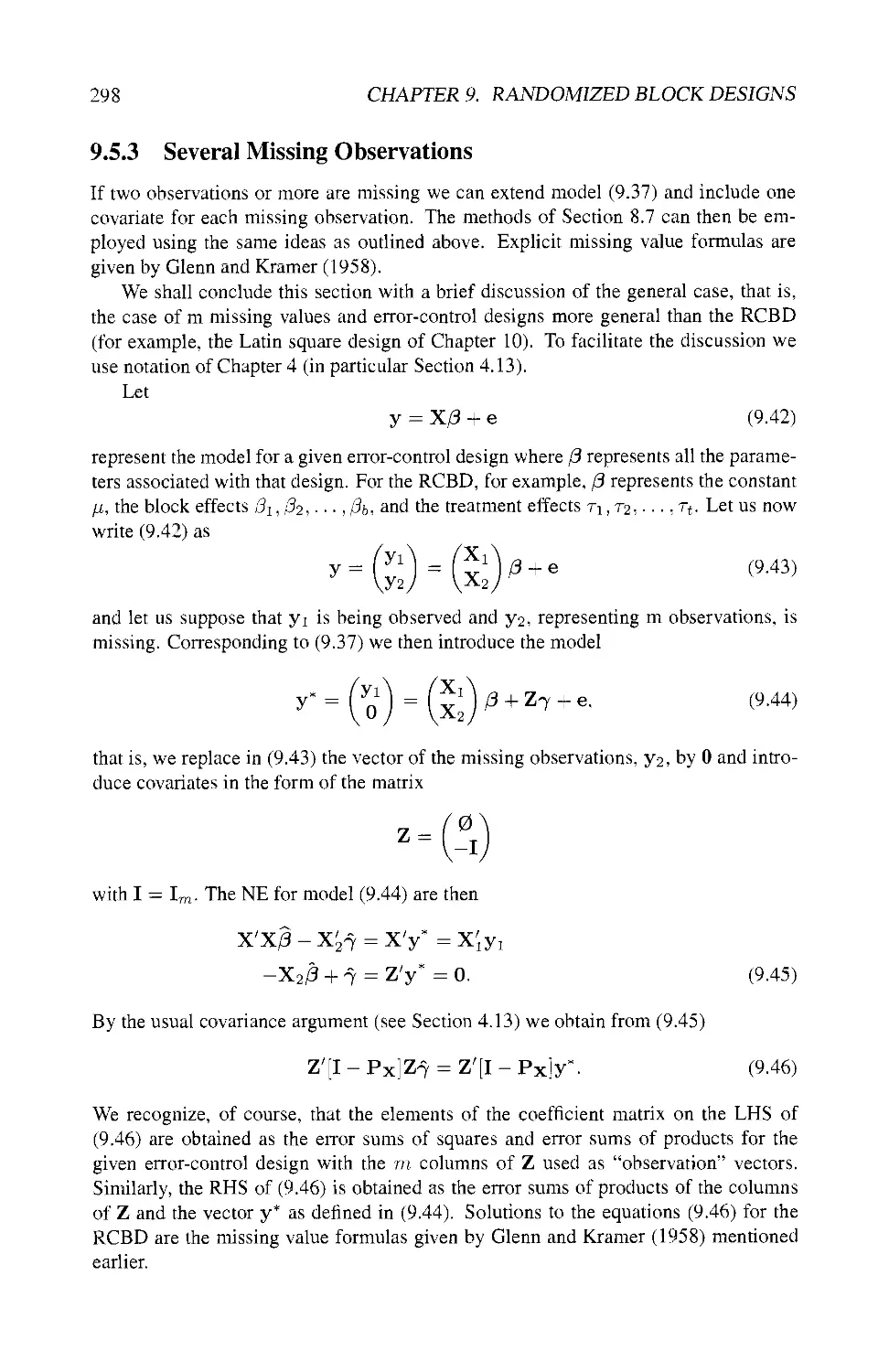
9,5,3 Several Missing Observations 298
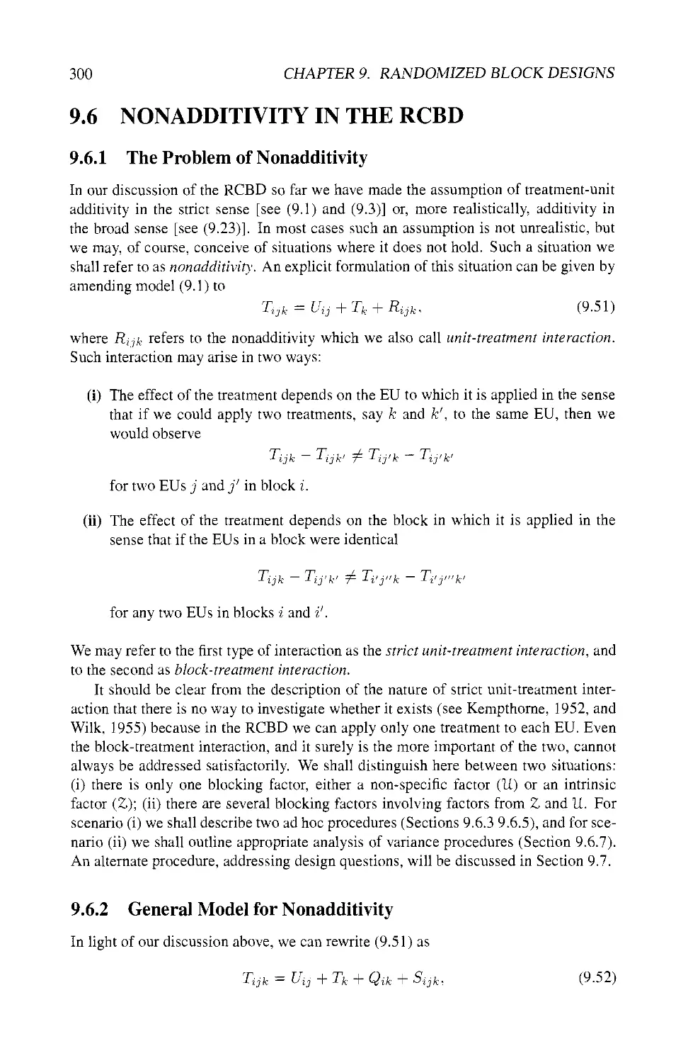
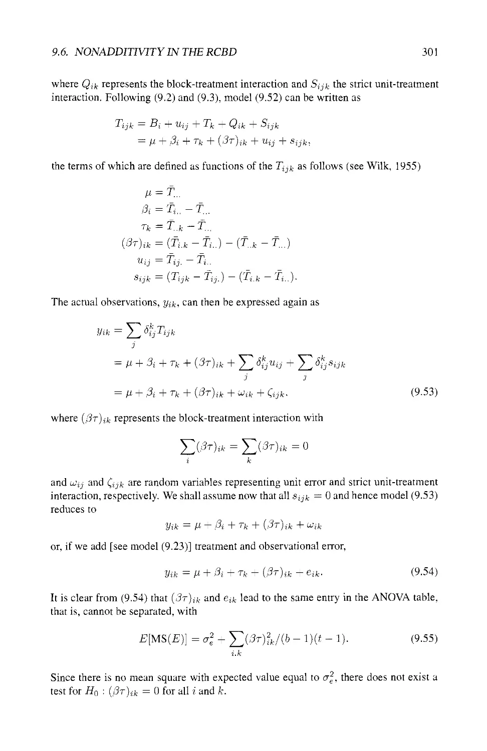
9.6 NONADDITIVITY IN THE RCBD 300
9.6.1 The Problem of Nonadditivity 300
9.6.2 General Model for Nonadditivity 300
9.6.3 One Blocking Factor: A Specific Model for
Nonadditivity 302
9.6.4 Testing for Nonadditivity 303
9.6.5 Tukey's Test for Nonadditivity 303
9.6.6 Generalizations 305
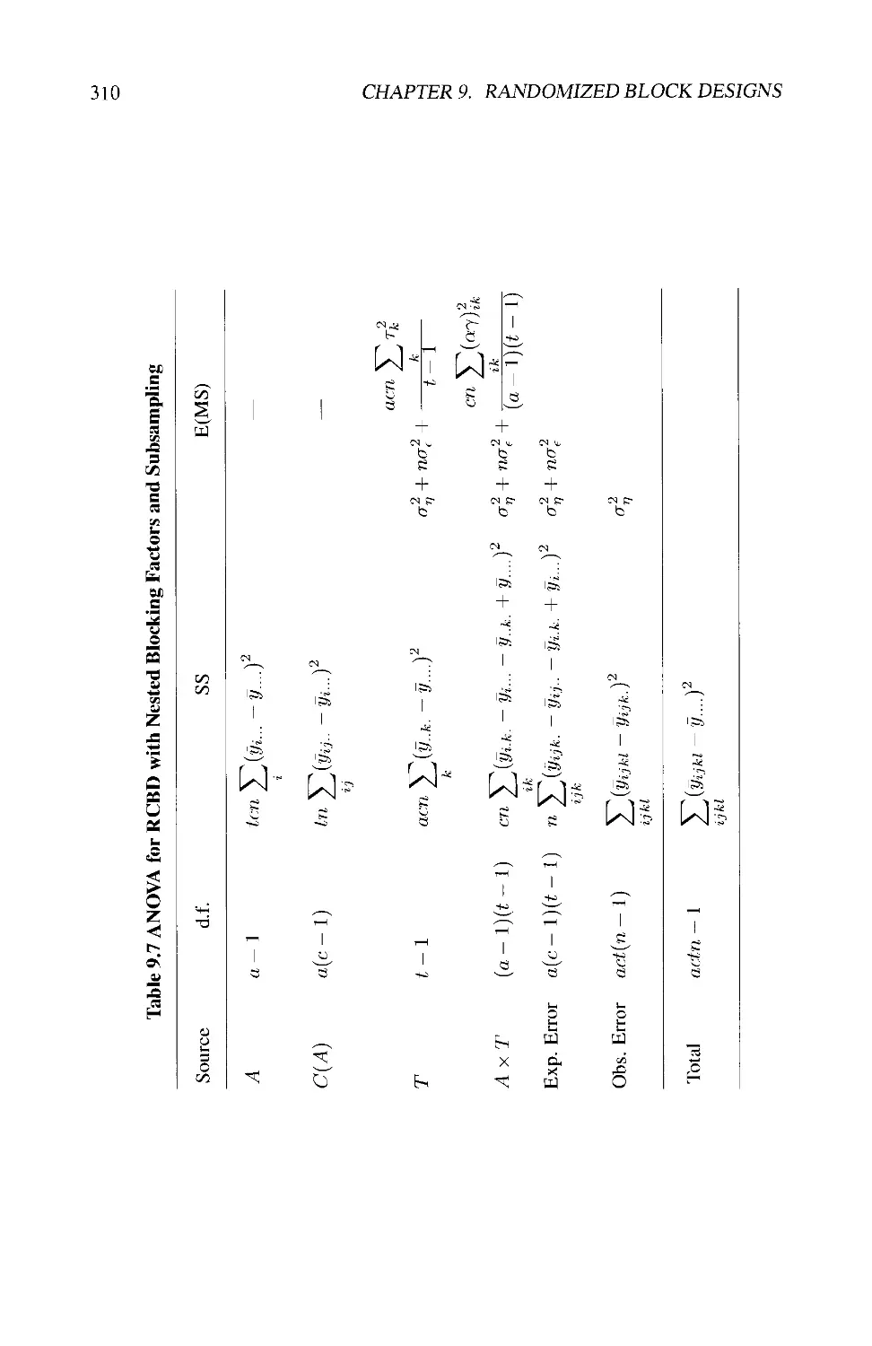
9.6.7 Several Blocking Factors 306
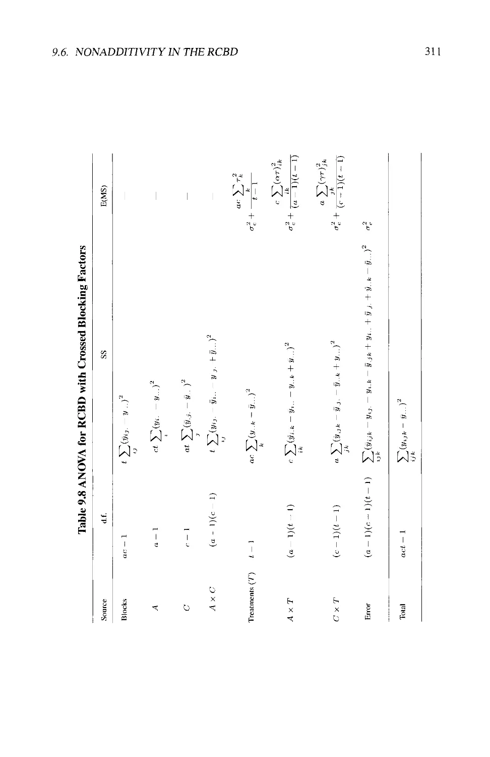
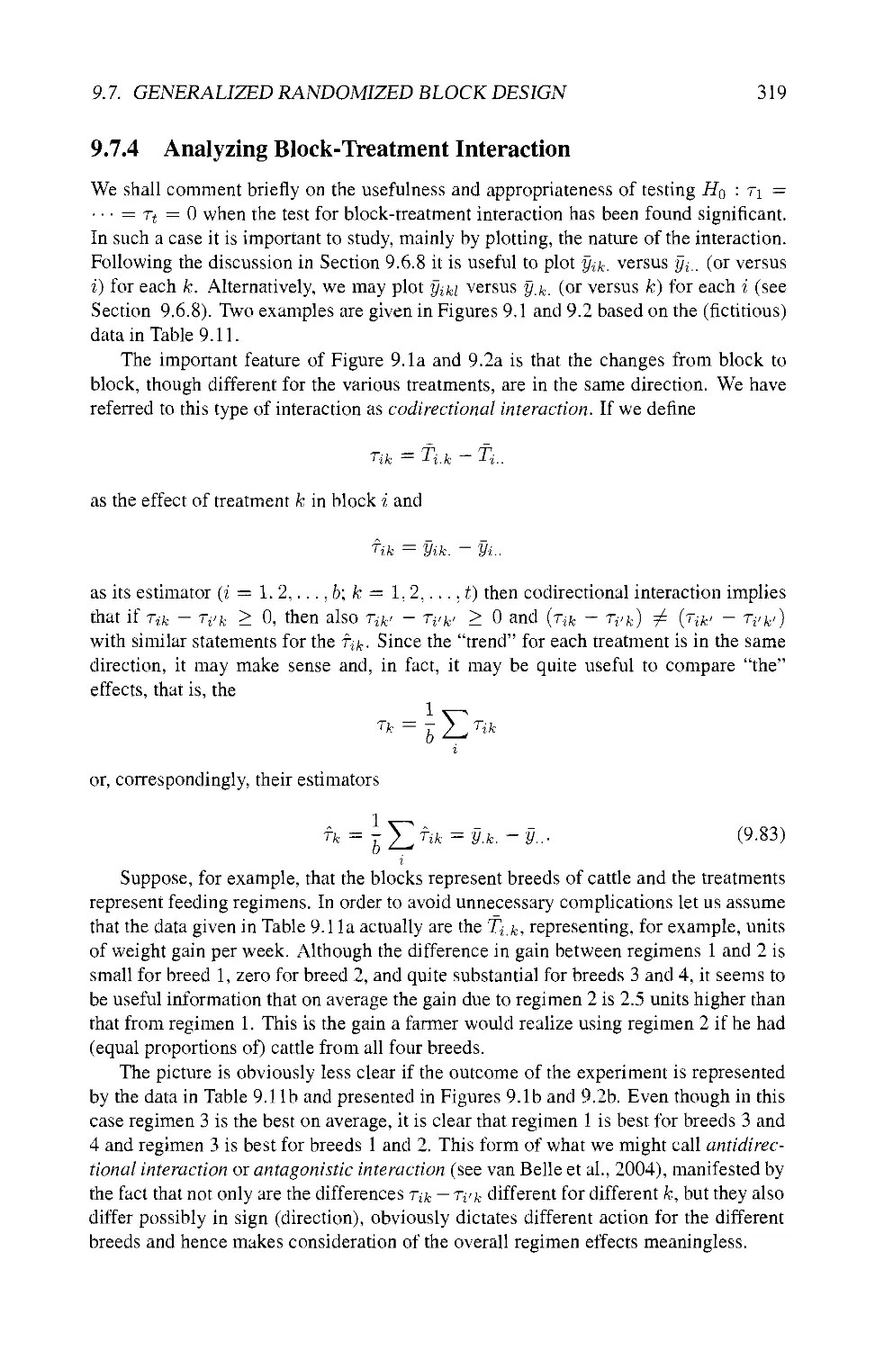
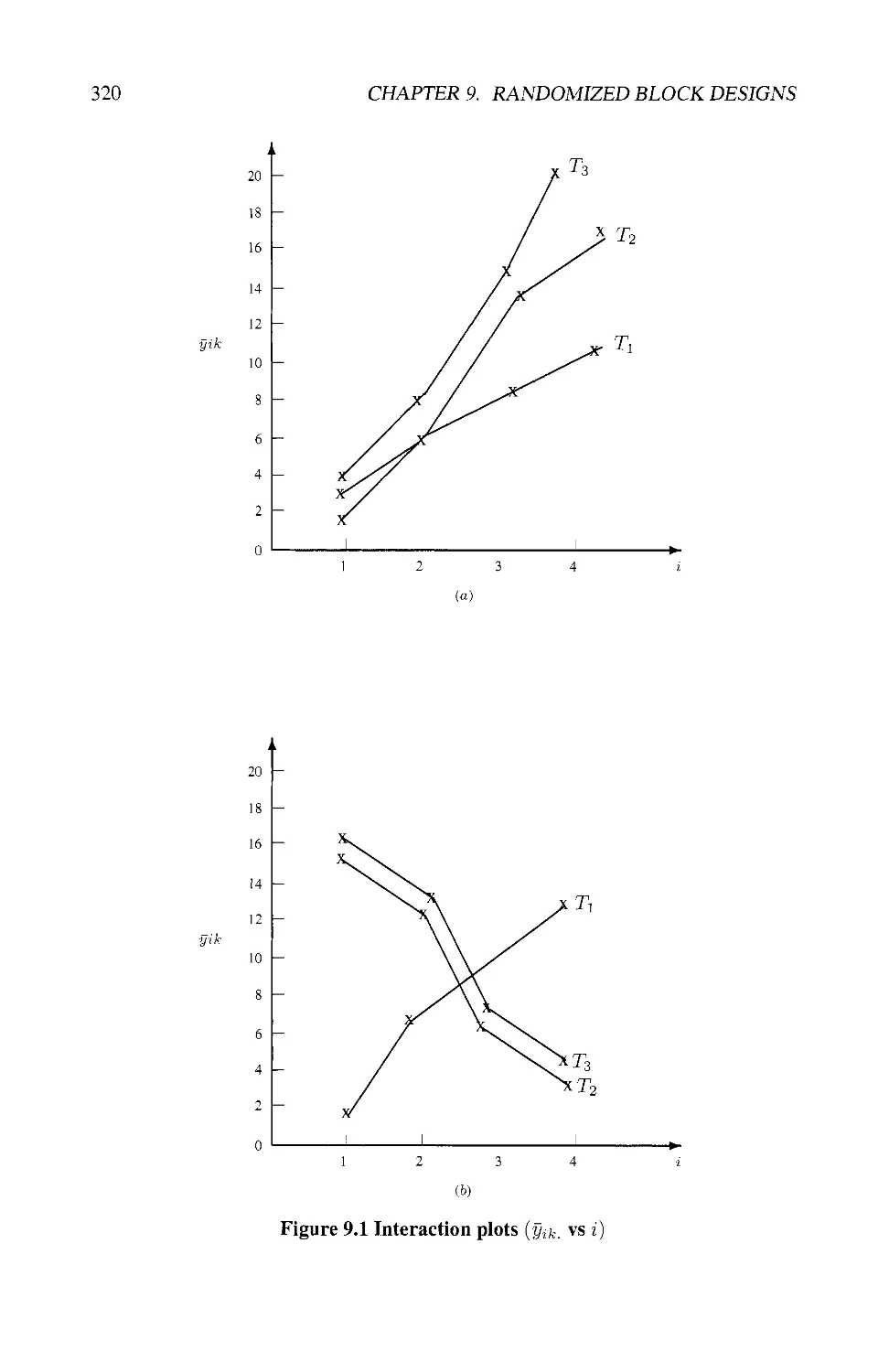
9.6.8 Dealing with Block-Treatment Interaction 312
9.7 GENERALIZED RANDOMIZED BLOCK DESIGN 314
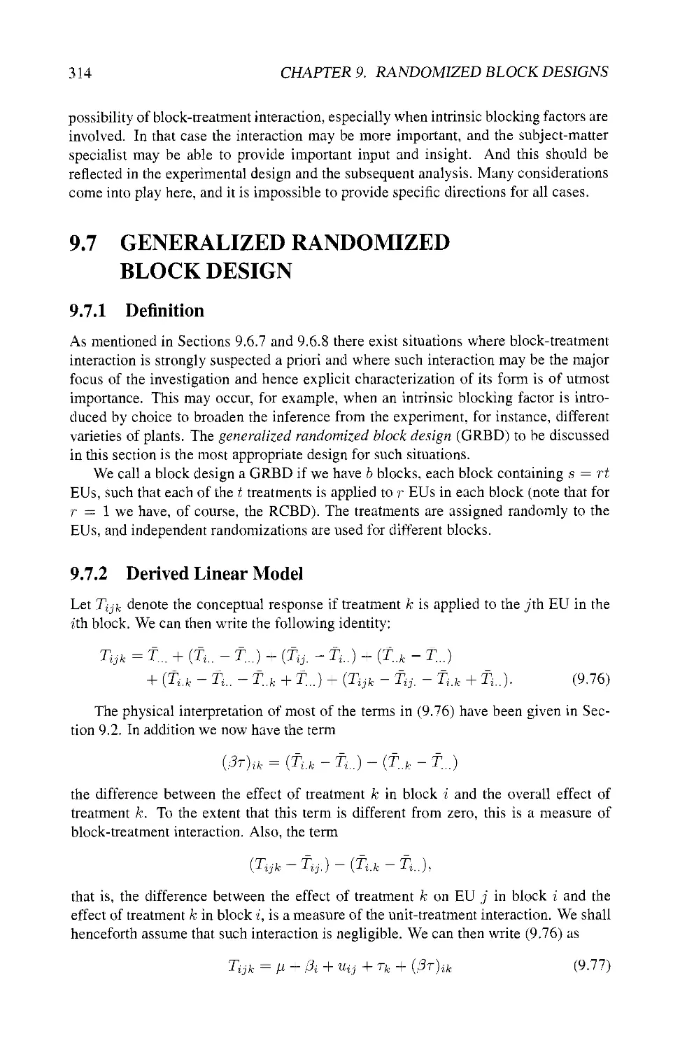
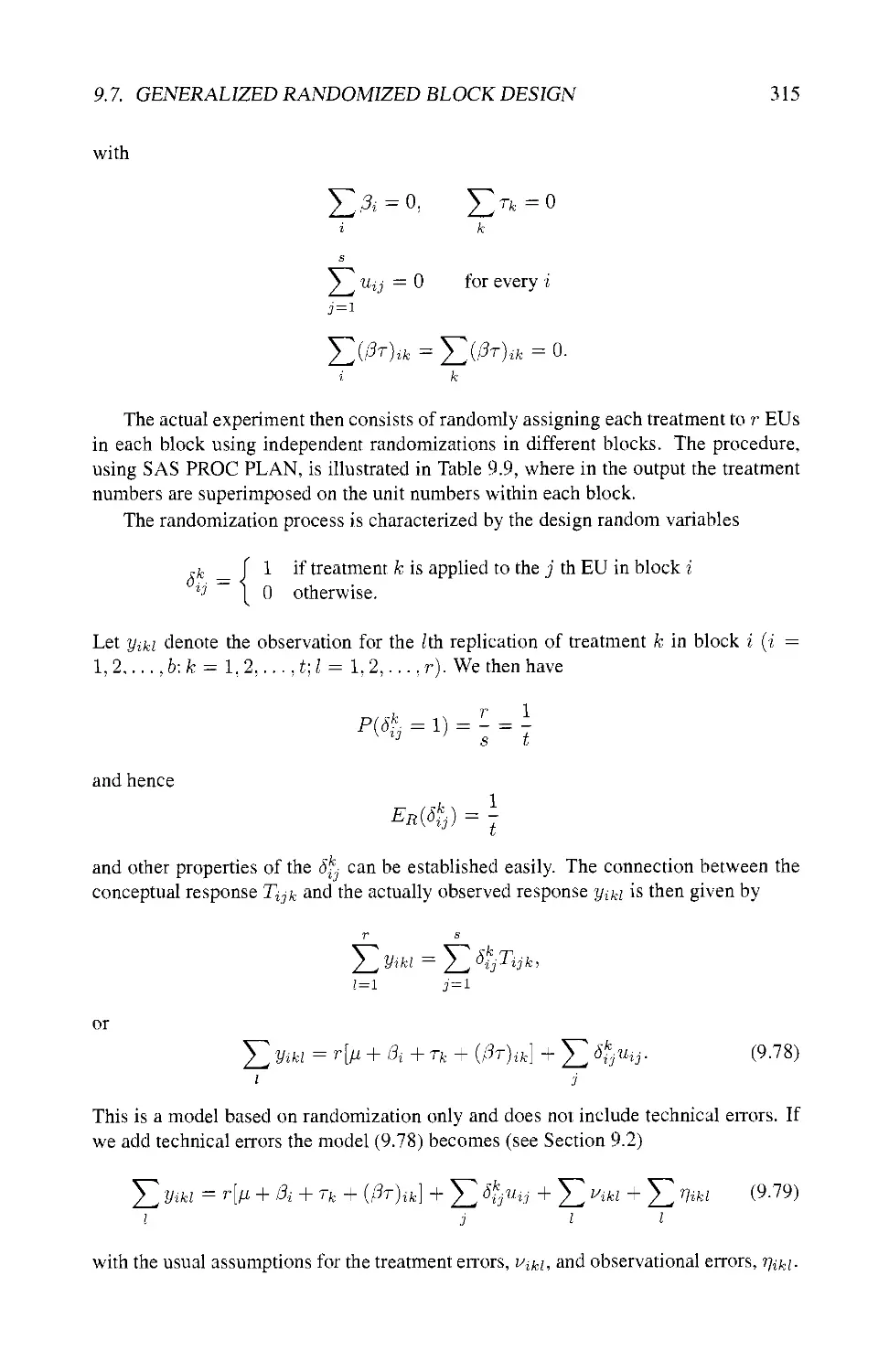
9.7.1 Definition 314
9.7.2 Derived Linear Model 314
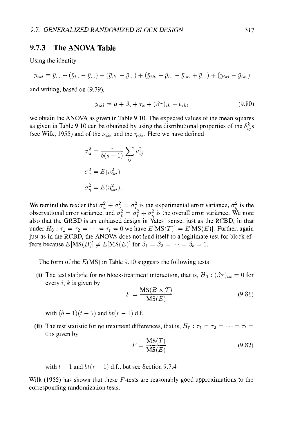
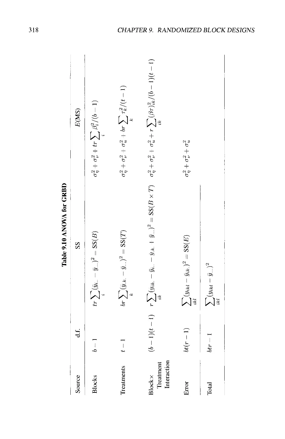
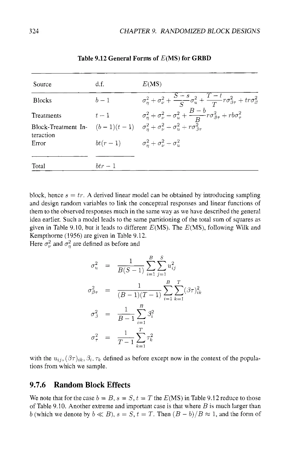
9.7.3 The ANOVA Table 317
9.7.4 Analyzing Block-Treatment Interaction 319
9.7.5 A More General Formulation 323
9.7.6 Random Block Effects 324
9.7.7 Using Satterthwaite's Procedure 326
9.8 INCOMPLETE BLOCK DESIGNS 328
9.8.1 General Notion of Designs with Incomplete
Blocks 328
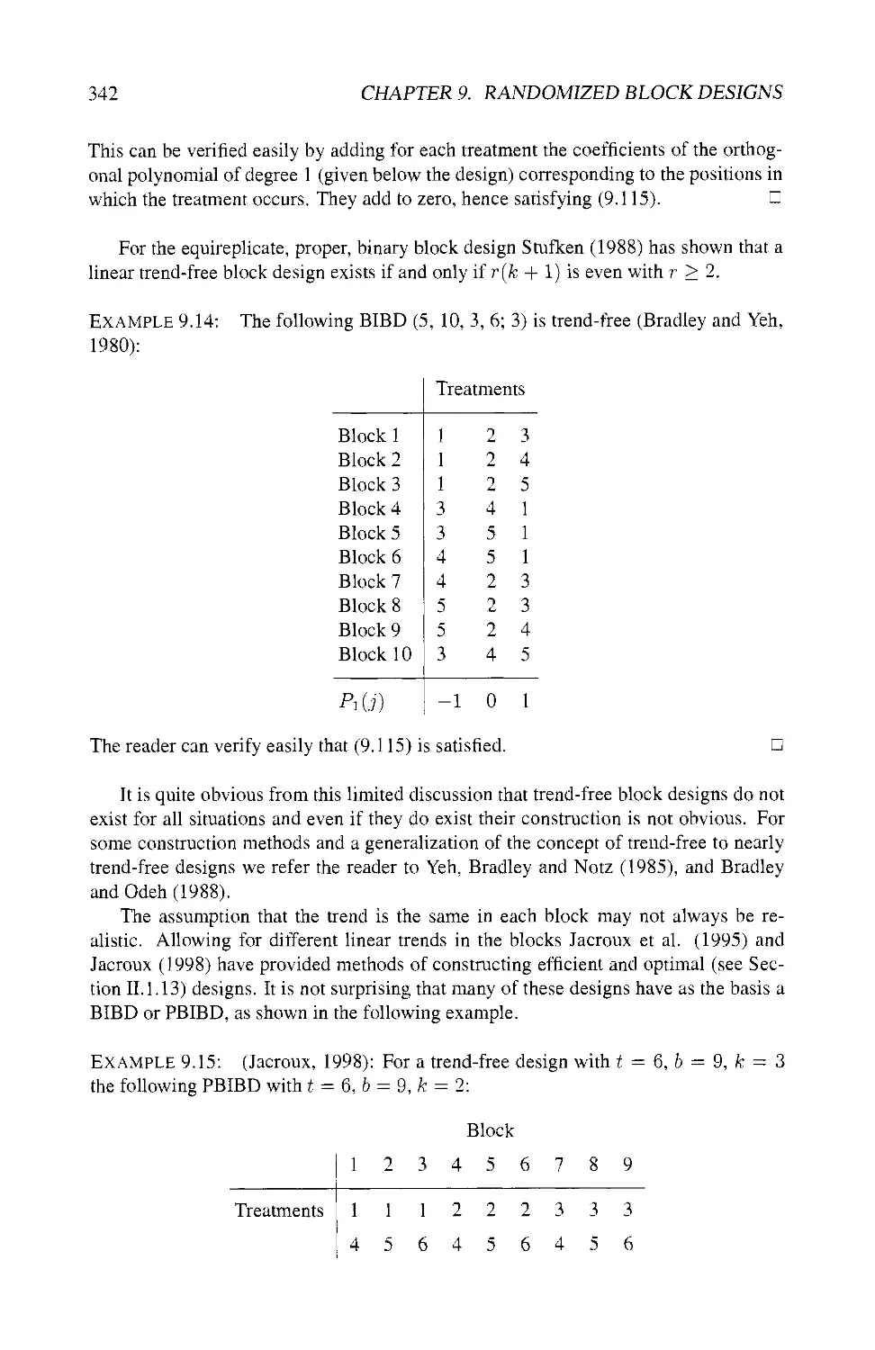
9.8.2 Balanced Incomplete Block Designs 330
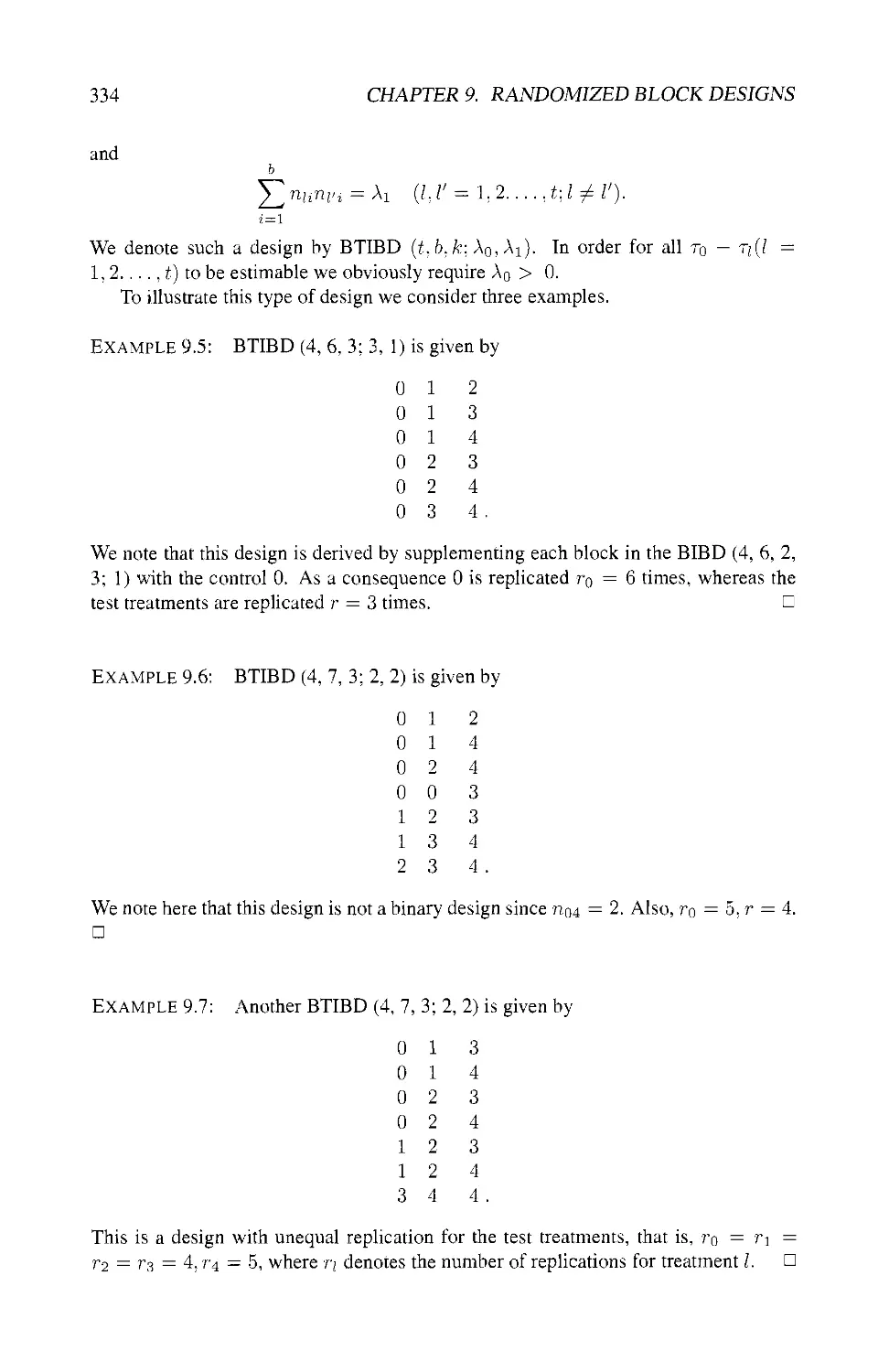
9.8.3 Balanced Treatment Incomplete Block Designs 333
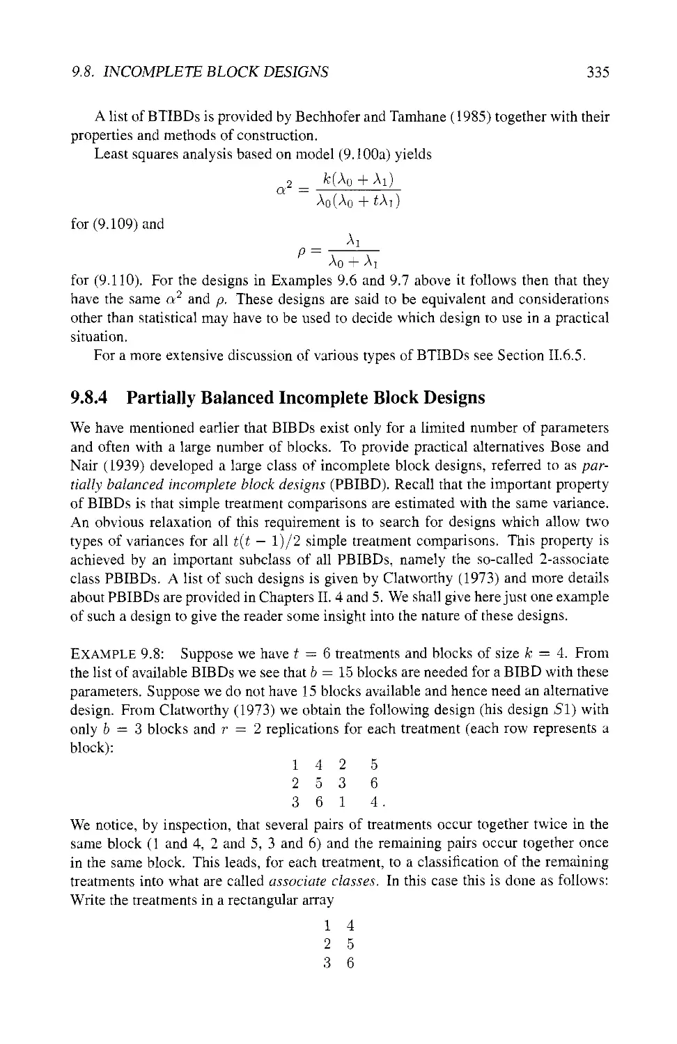
9.8.4 Partially Balanced Incomplete Block Designs 335
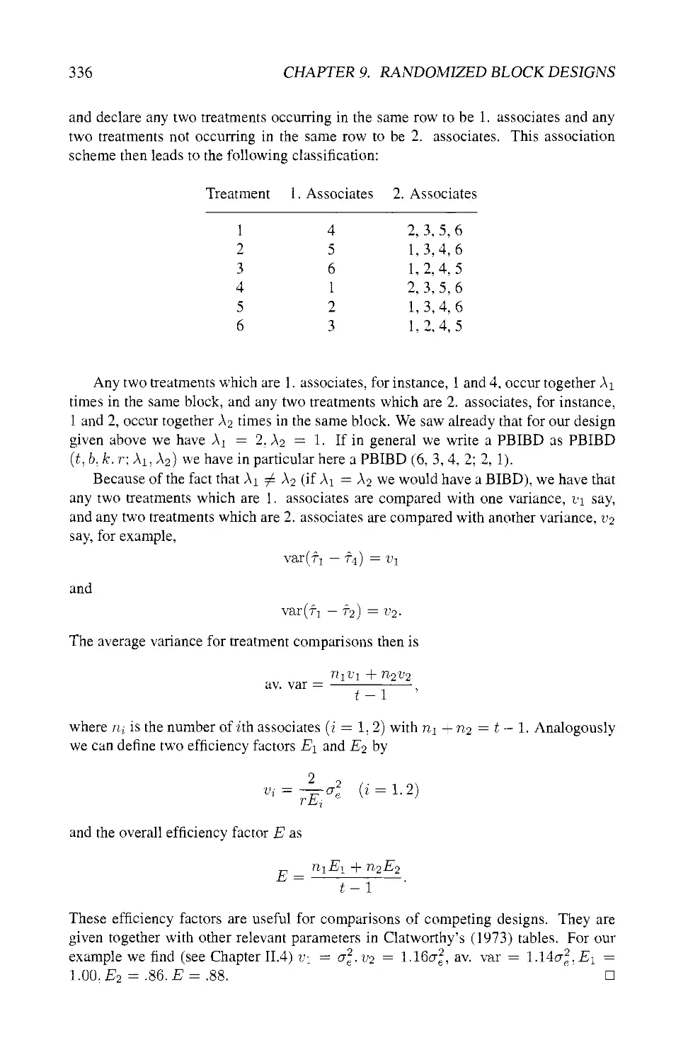
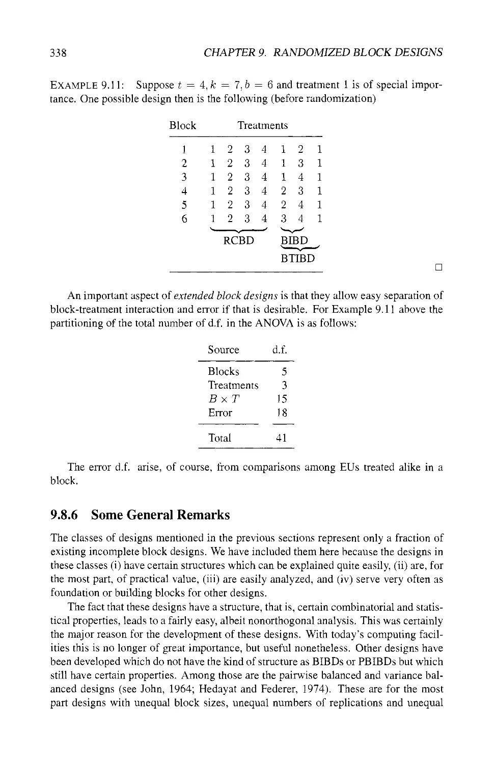
9.8.5 Extended Block Designs 337
9.8.6 Some General Remarks 338
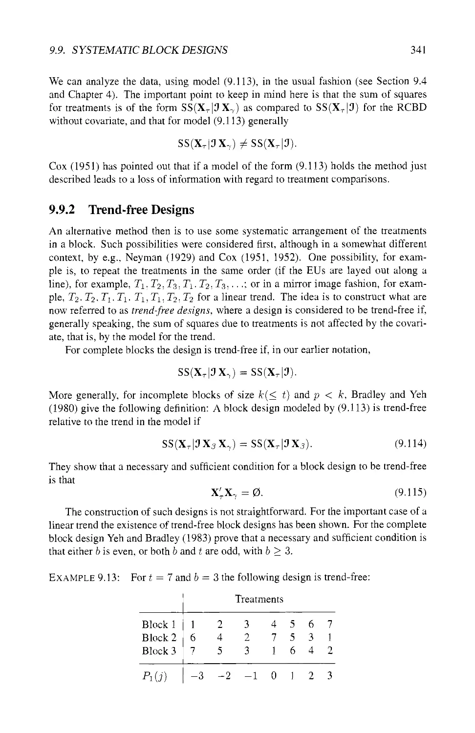
9.9 SYSTEMATIC BLOCK DESIGNS 340
9.9.1 Dealing with Trends 340
9.9.2 Trend-free Designs 341
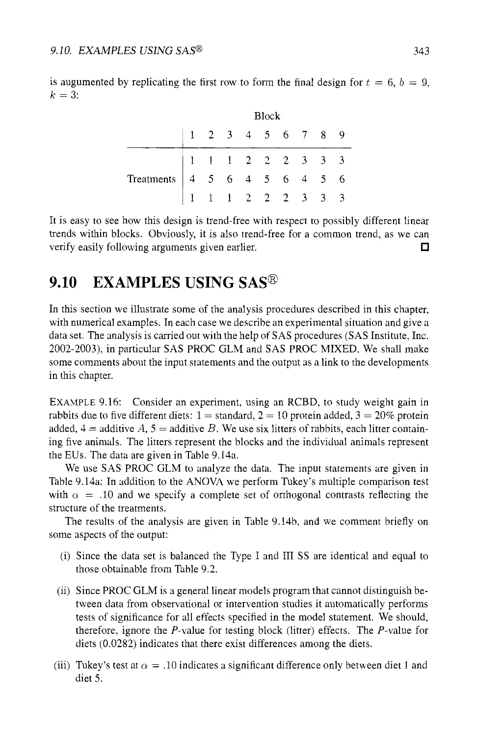
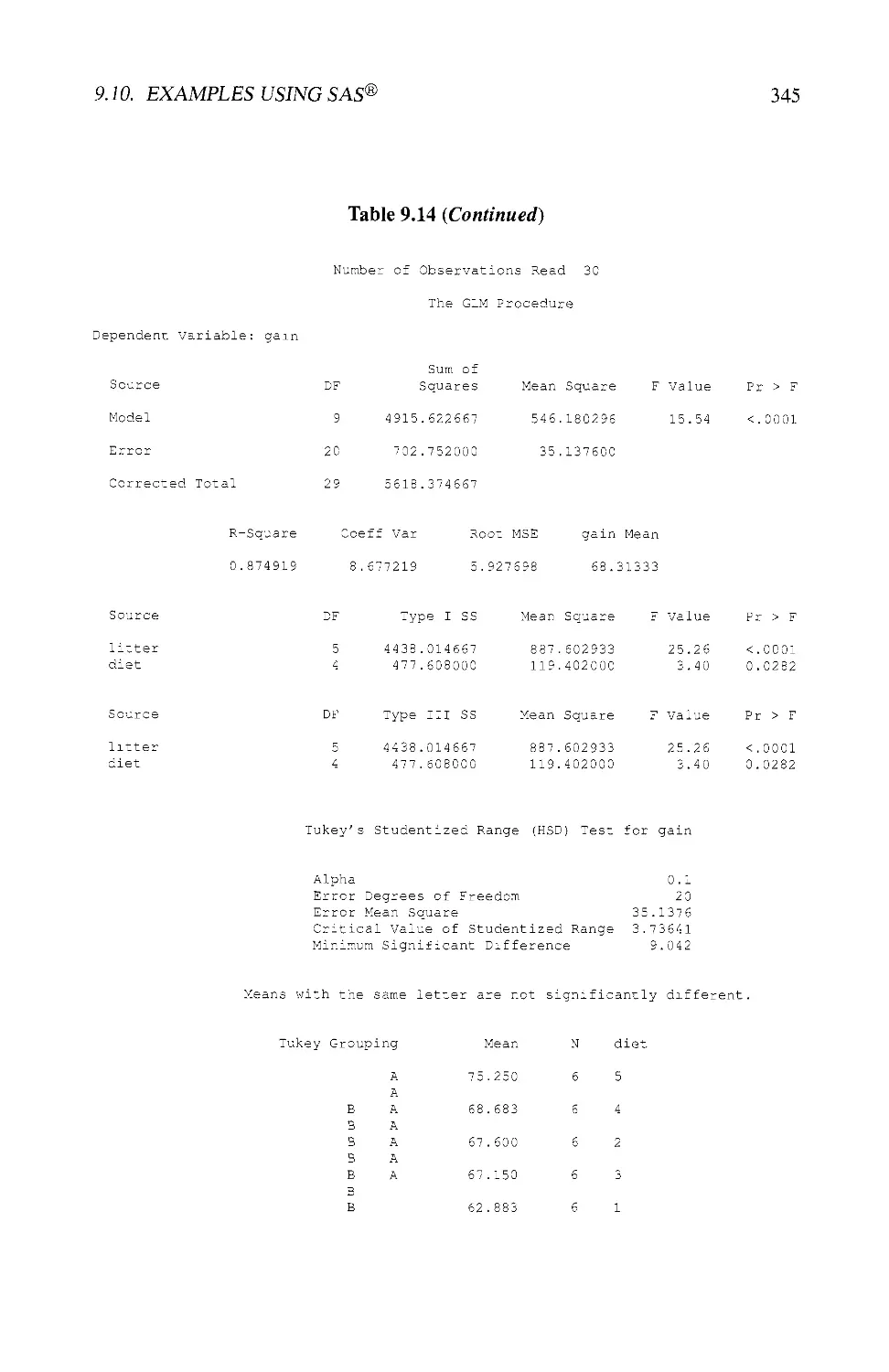
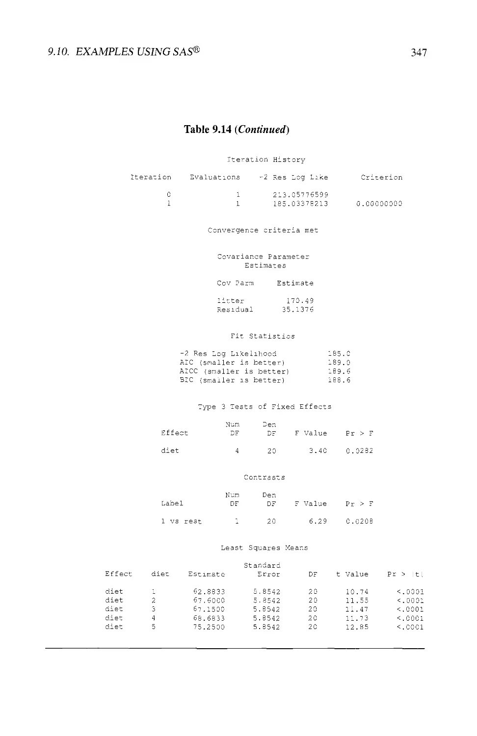
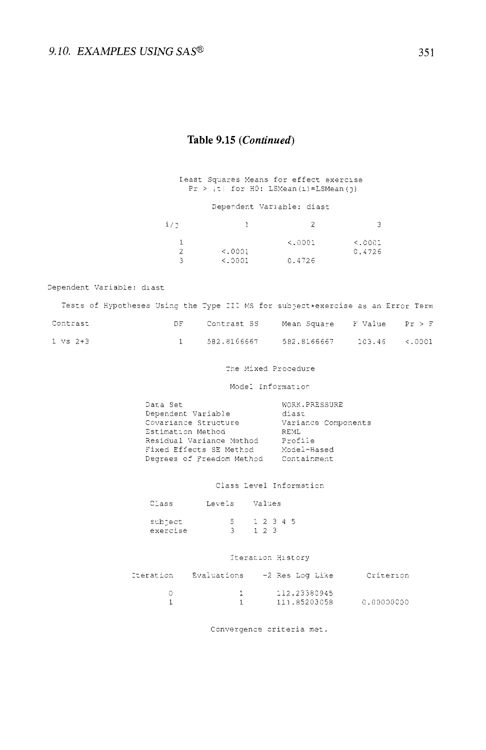
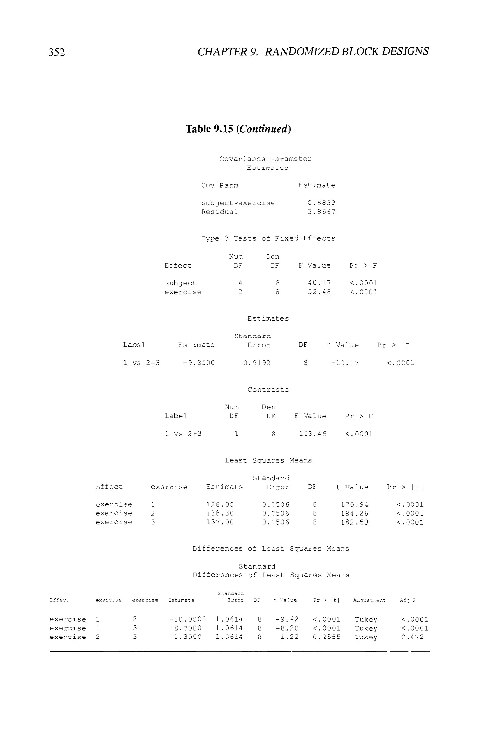
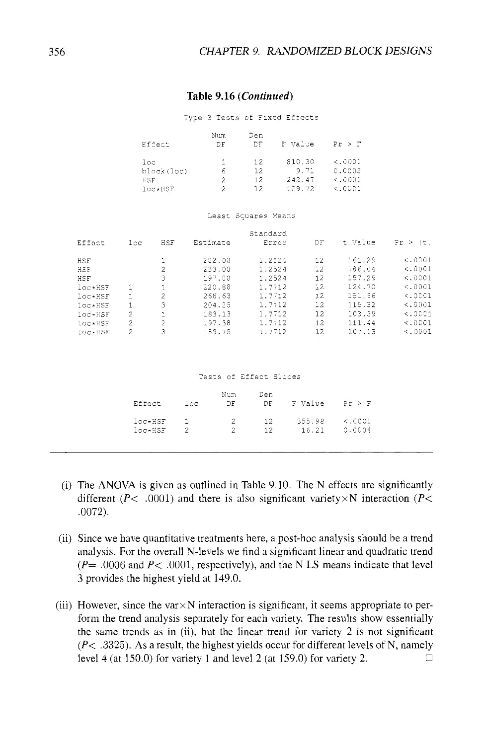
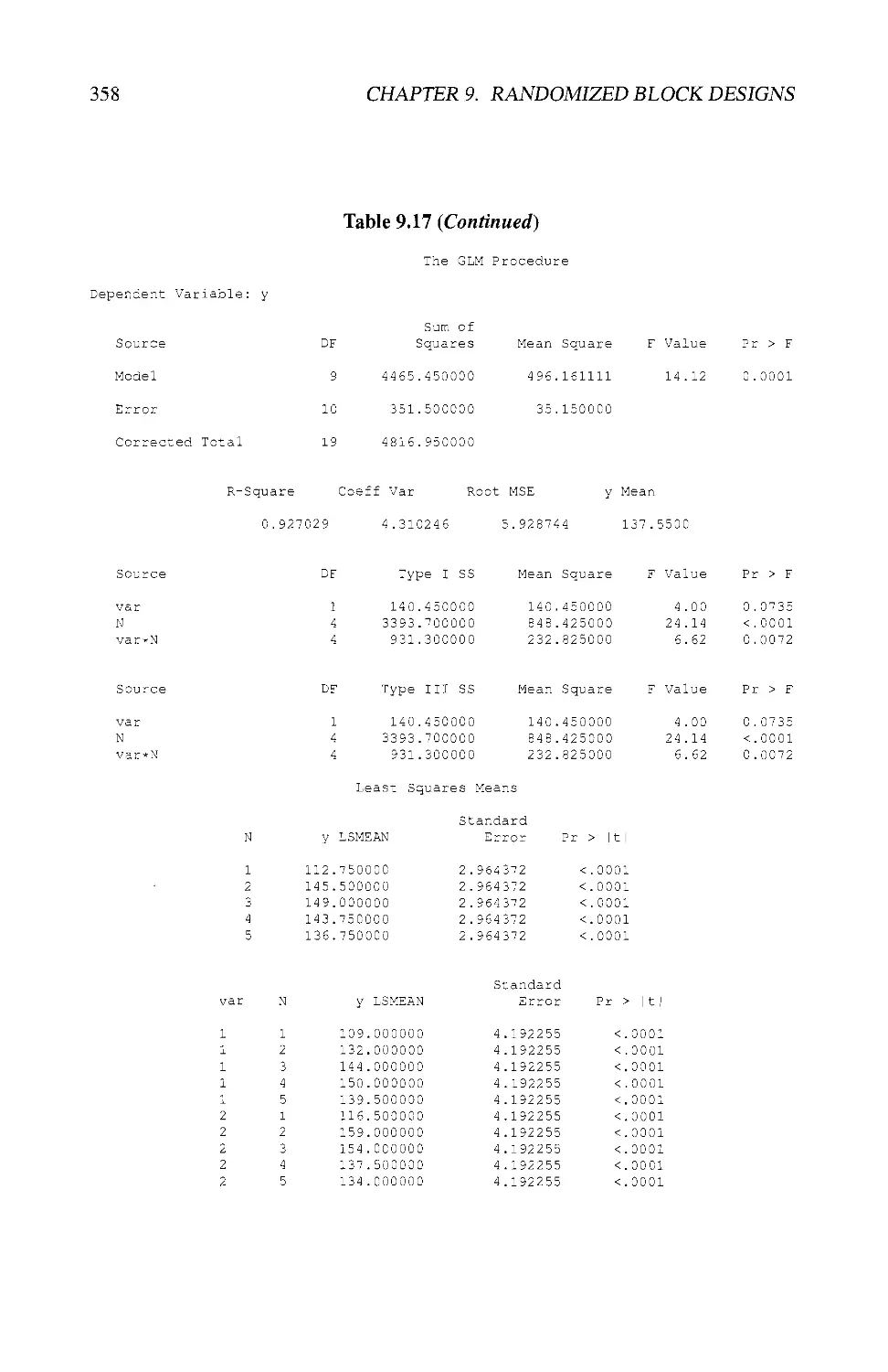
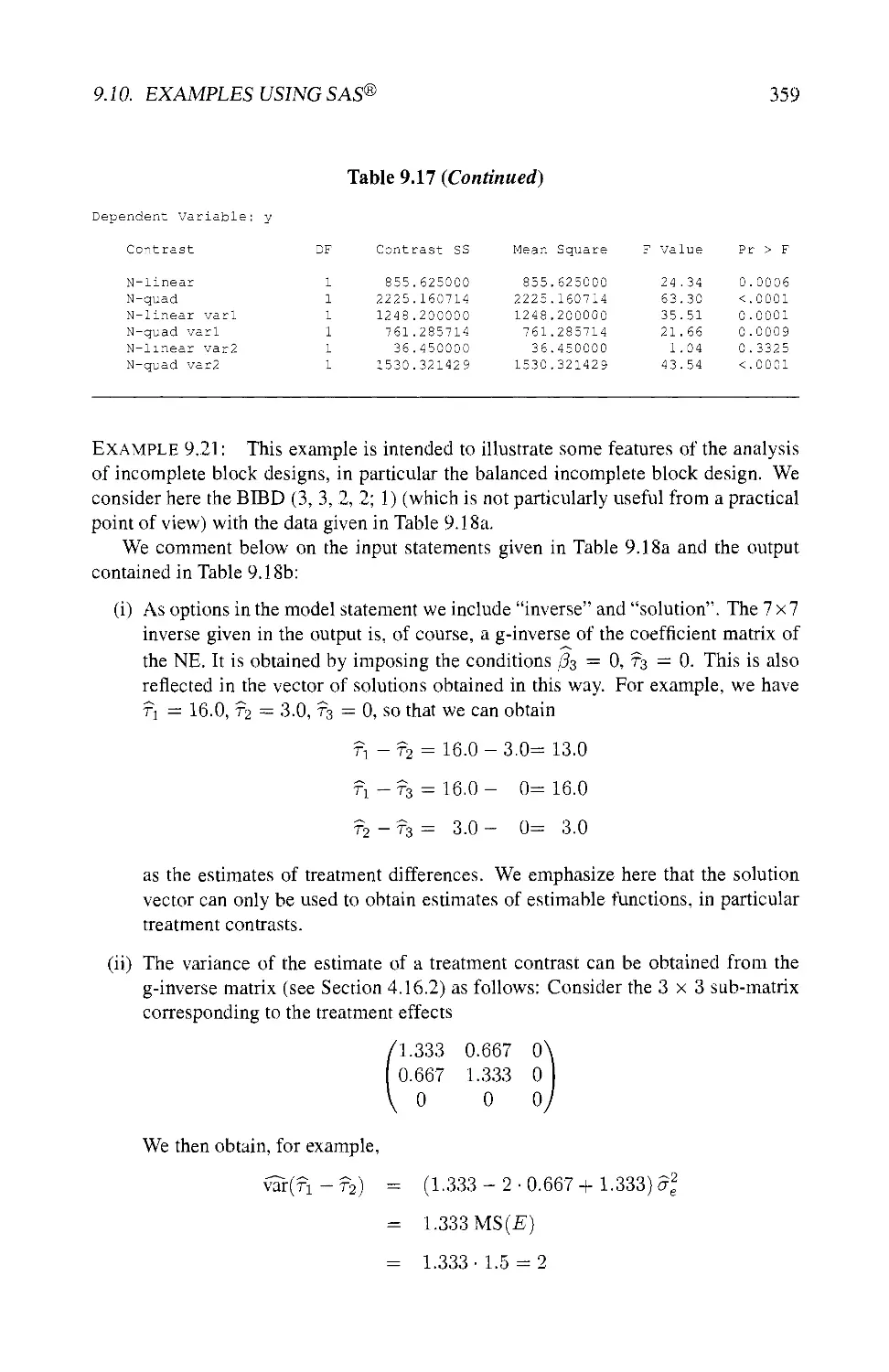
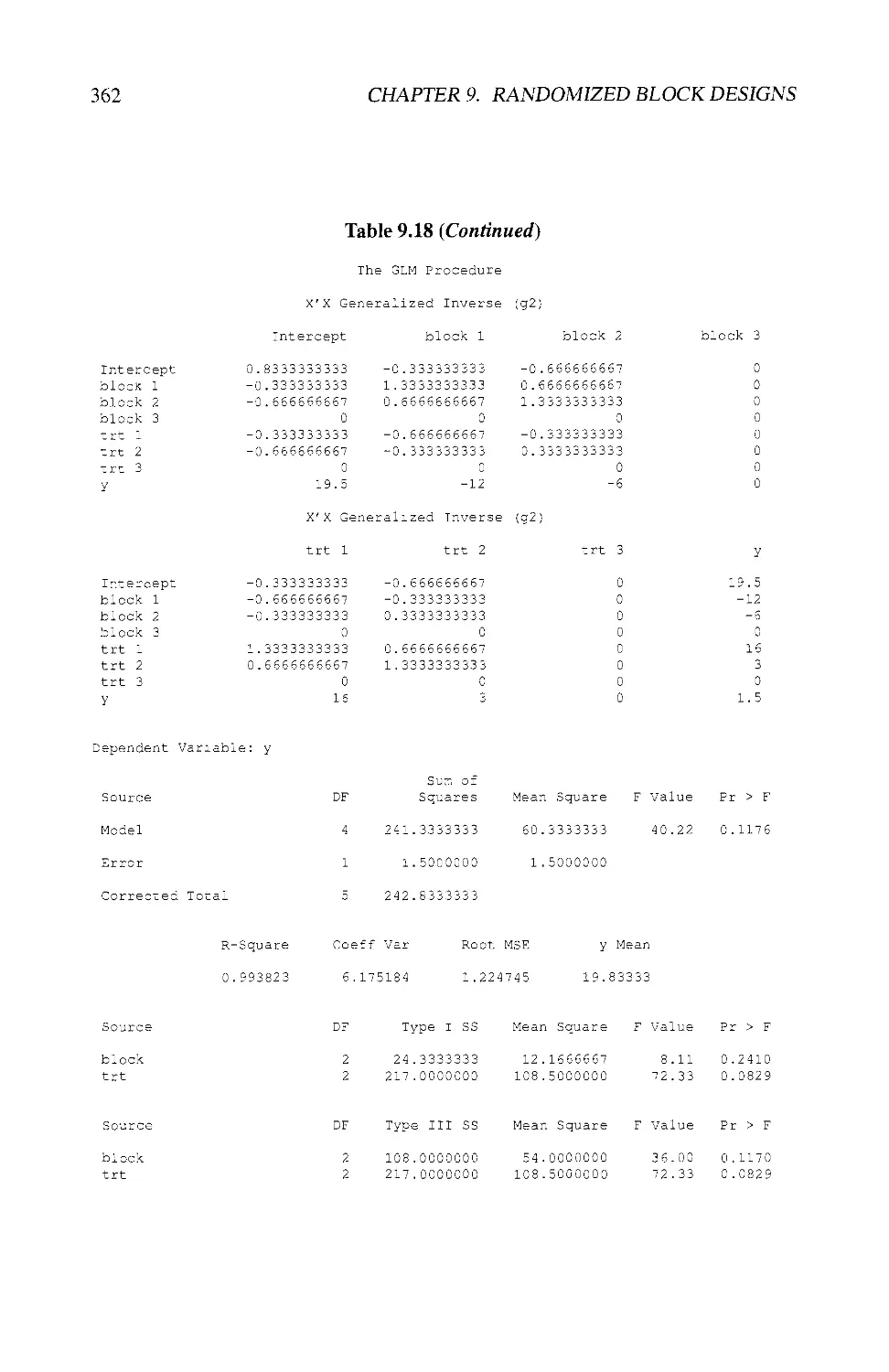
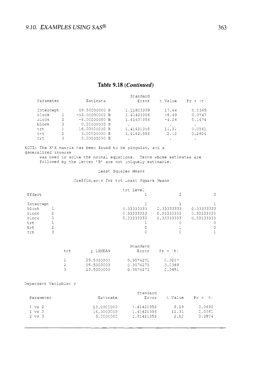
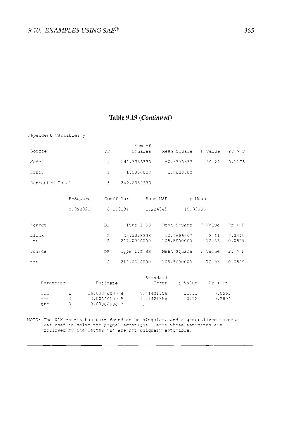
9.10 EXAMPLES USING SAS® 343
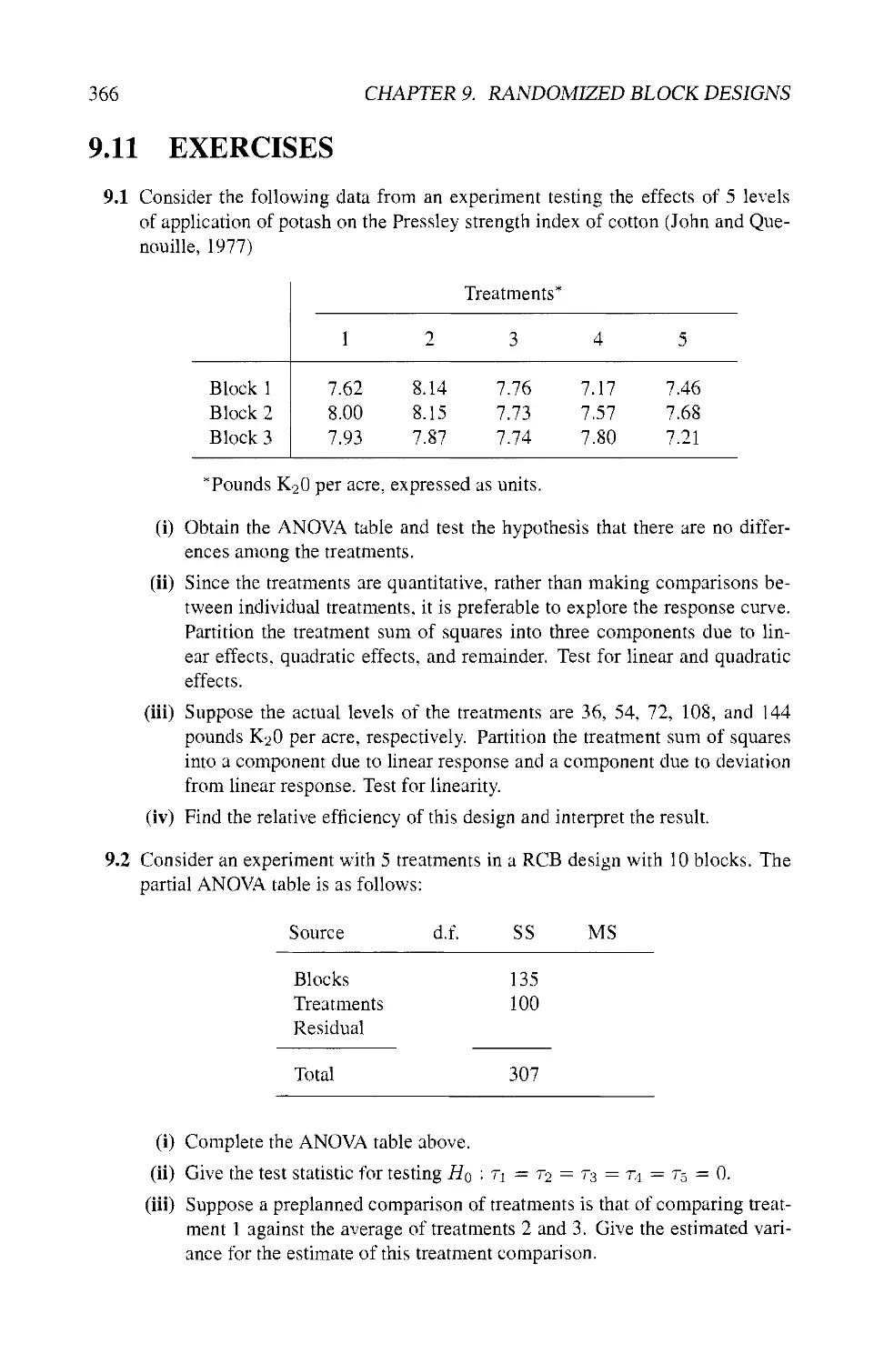
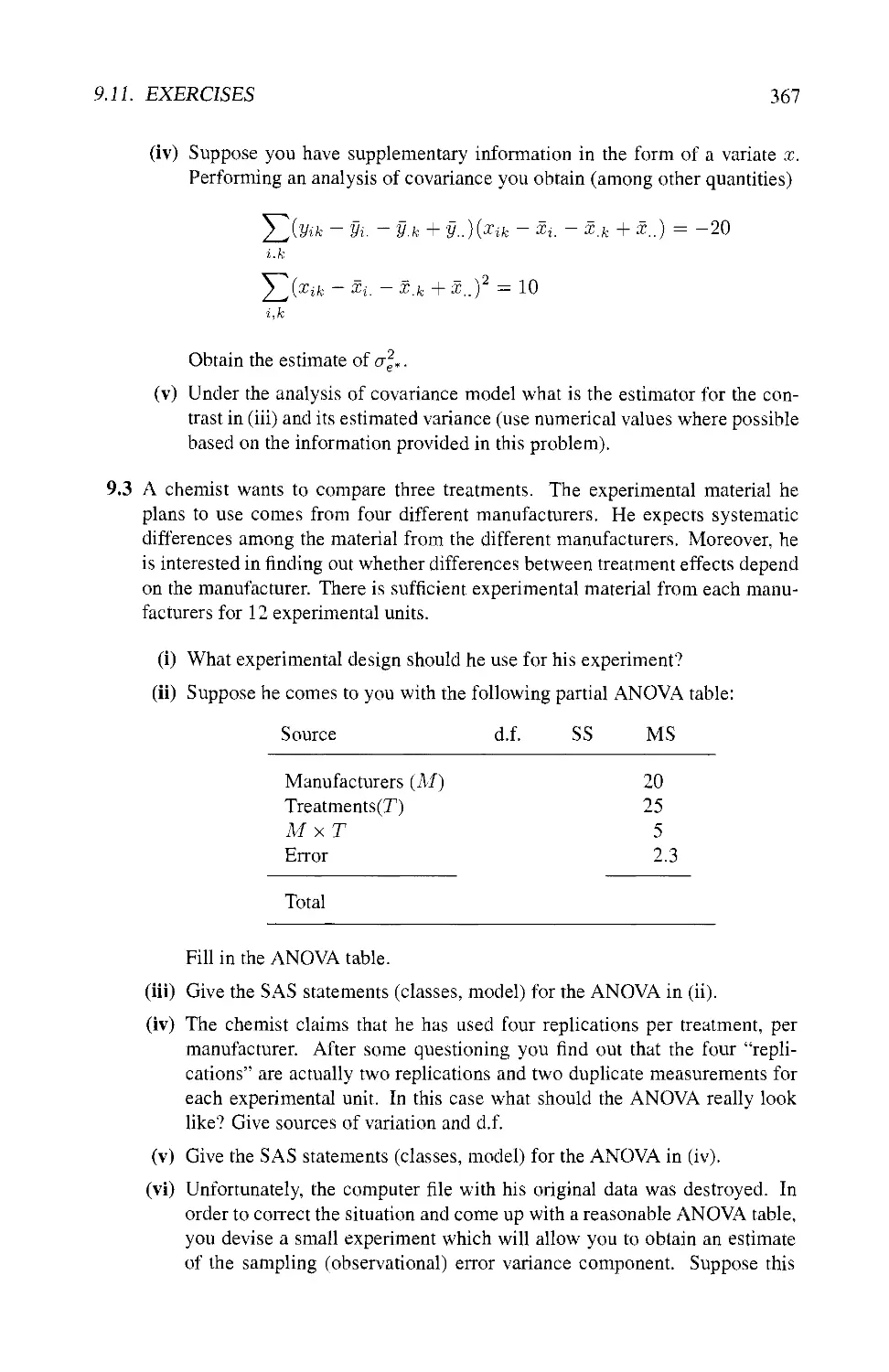
9.11 EXERCISES 366
10 Latin Square T^pe Designs 373
10.1 INTRODUCTION AND MOTIVATION 373
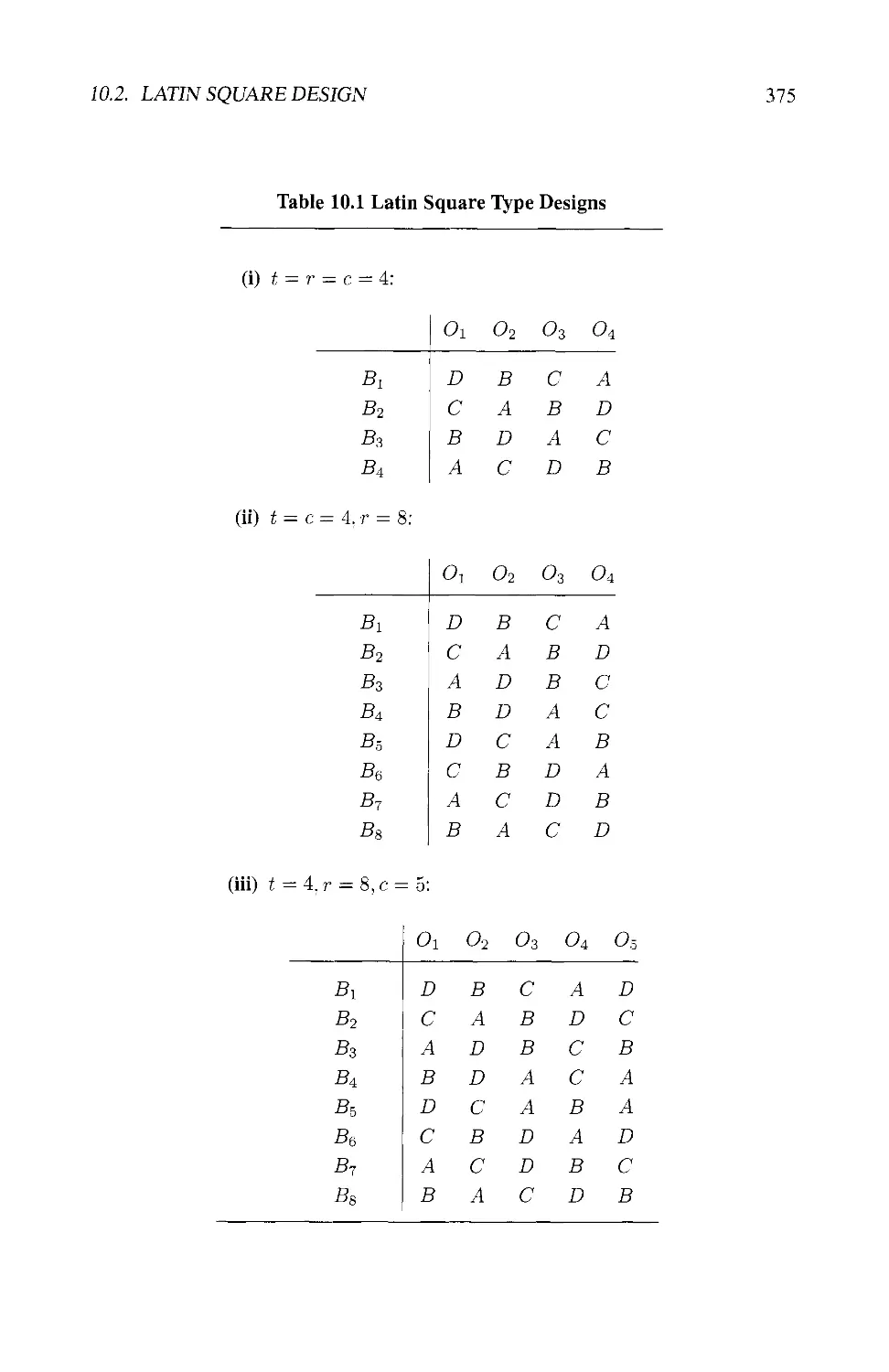
10.2 LATIN SQUARE DESIGN 374
10.2.1 Definition 374
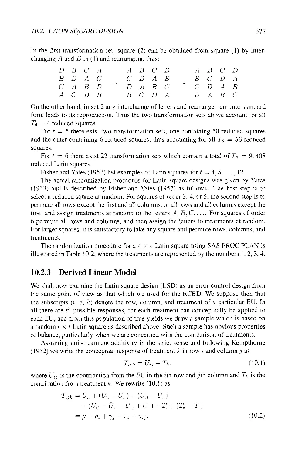
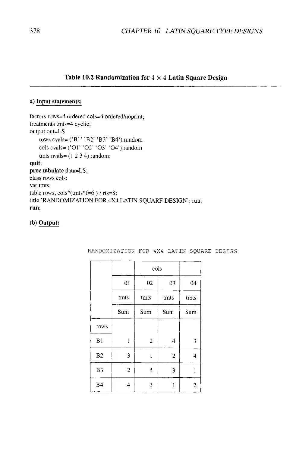
10.2.2 Transformation Sets and Randomization 376
10.2.3 Derived Linear Model 377
10.2.4 Estimation of Treatment Contrasts 380
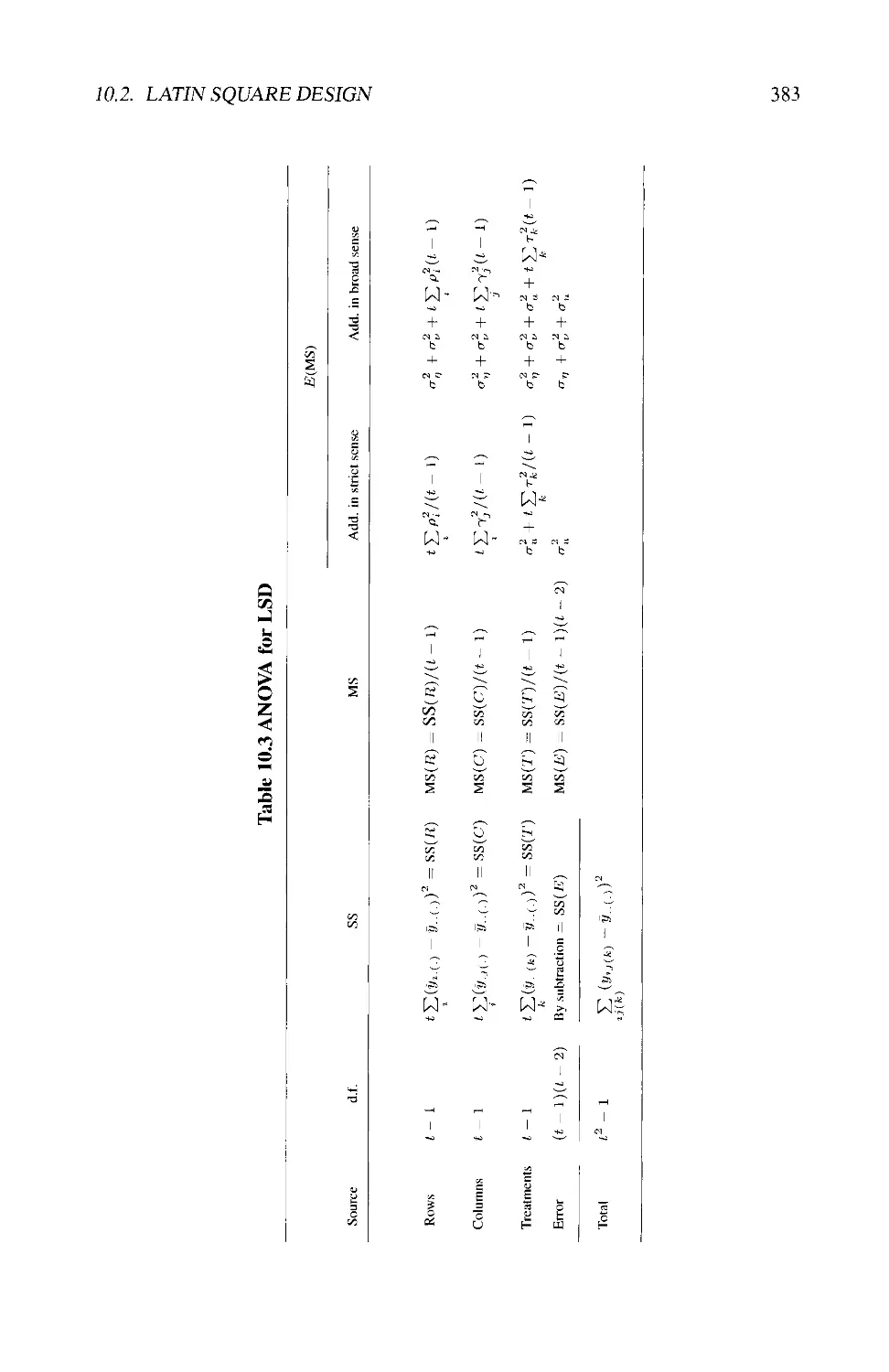
10.2.5 Analysis of Variance 382
10.2.6 The Model under Additivity in the Broad Sense 385
10.2.7 Consequences of Nonadditivity 386
10.2.8 Investigating Nonadditivity 387
10.2.9 Miscellaneous Remarks 389
10.3 REPLICATED LATIN SQUARES 390
xii CONTENTS
10.3.1 Different Scenarios for Replication 390
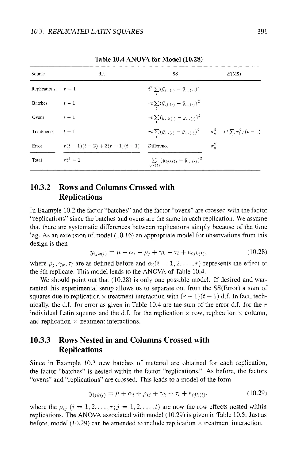
10.3.2 Rows and Columns Crossed with
Replications 391
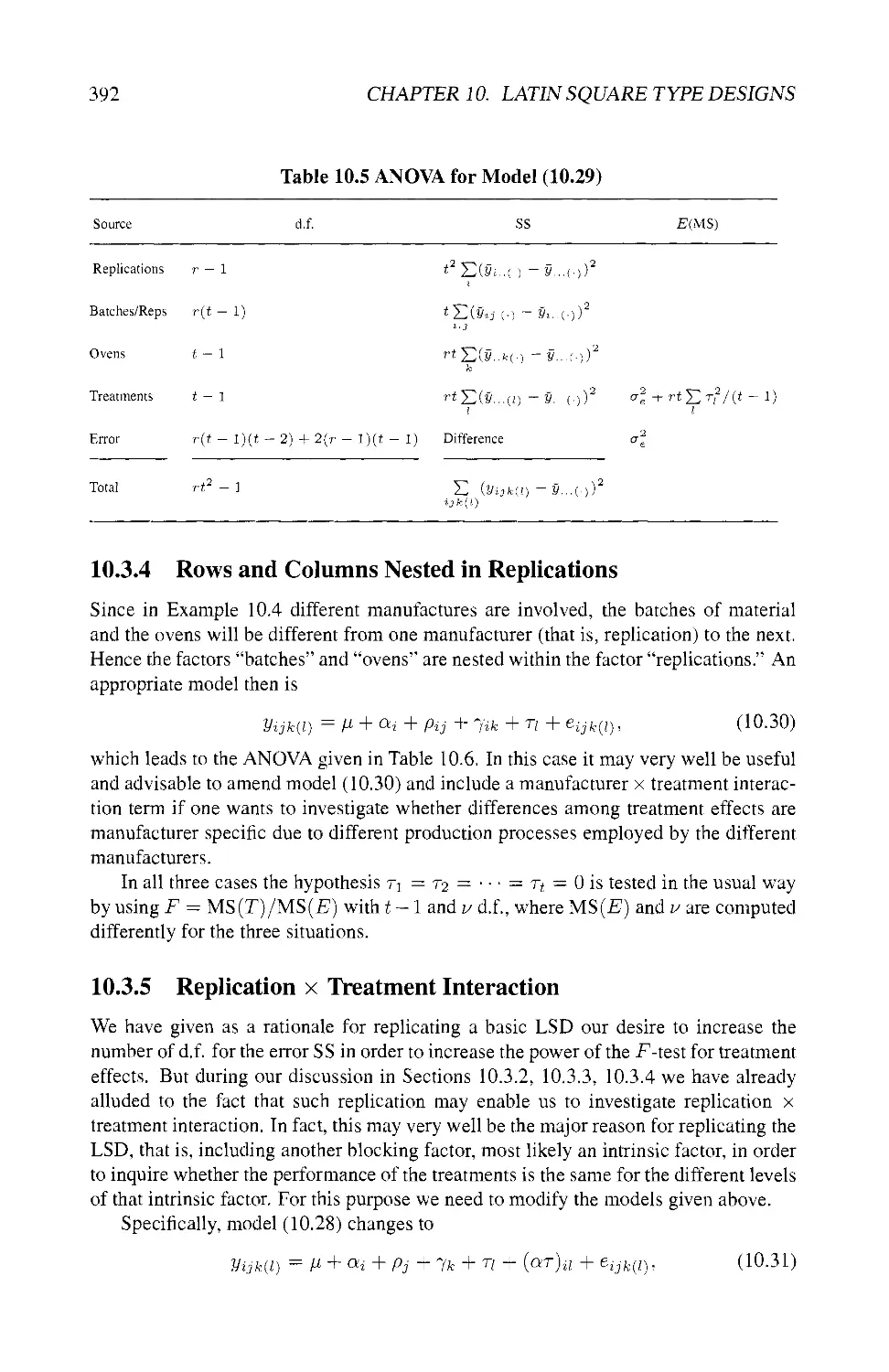
10.3.3 Rows Nested in and Columns Crossed with
Replications 391
10.3.4 Rows and Columns Nested in Replications 392
10.3.5 Replication x Treatment Interaction 392
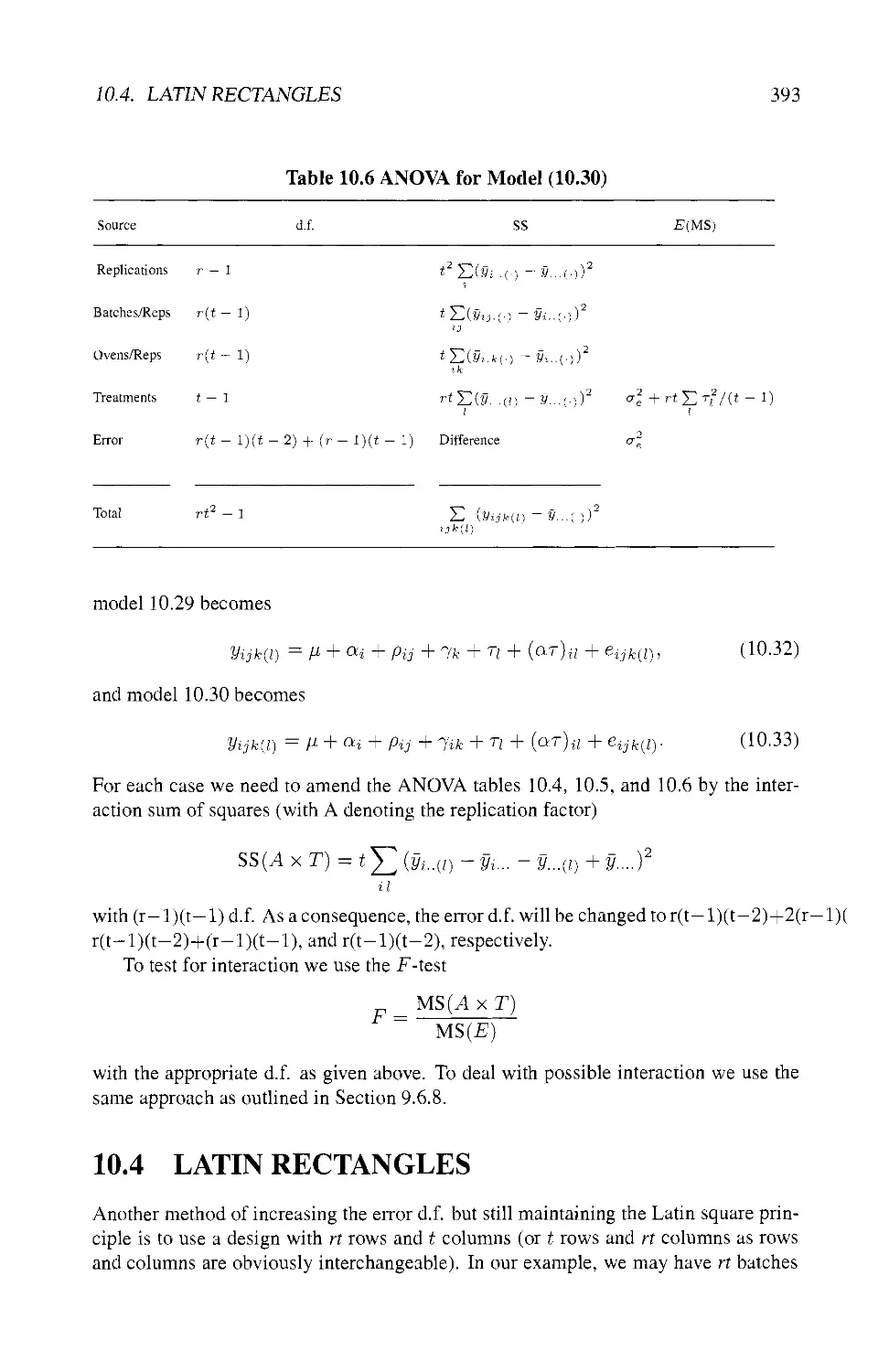
10.4 LATIN RECTANGLES 393
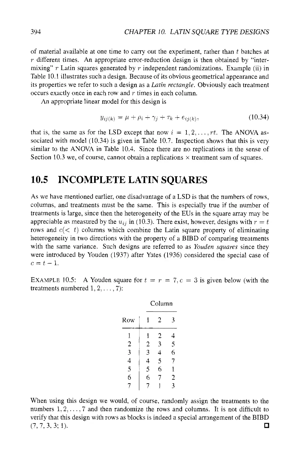
10.5 INCOMPLETE LATIN SQUARES 394
10.6 ORTHOGONAL LATIN SQUARES 395
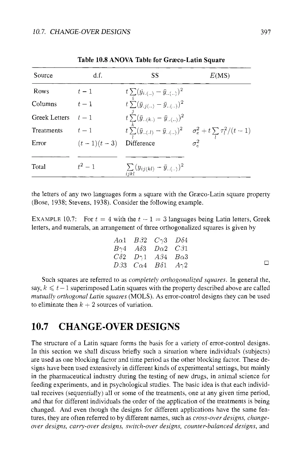
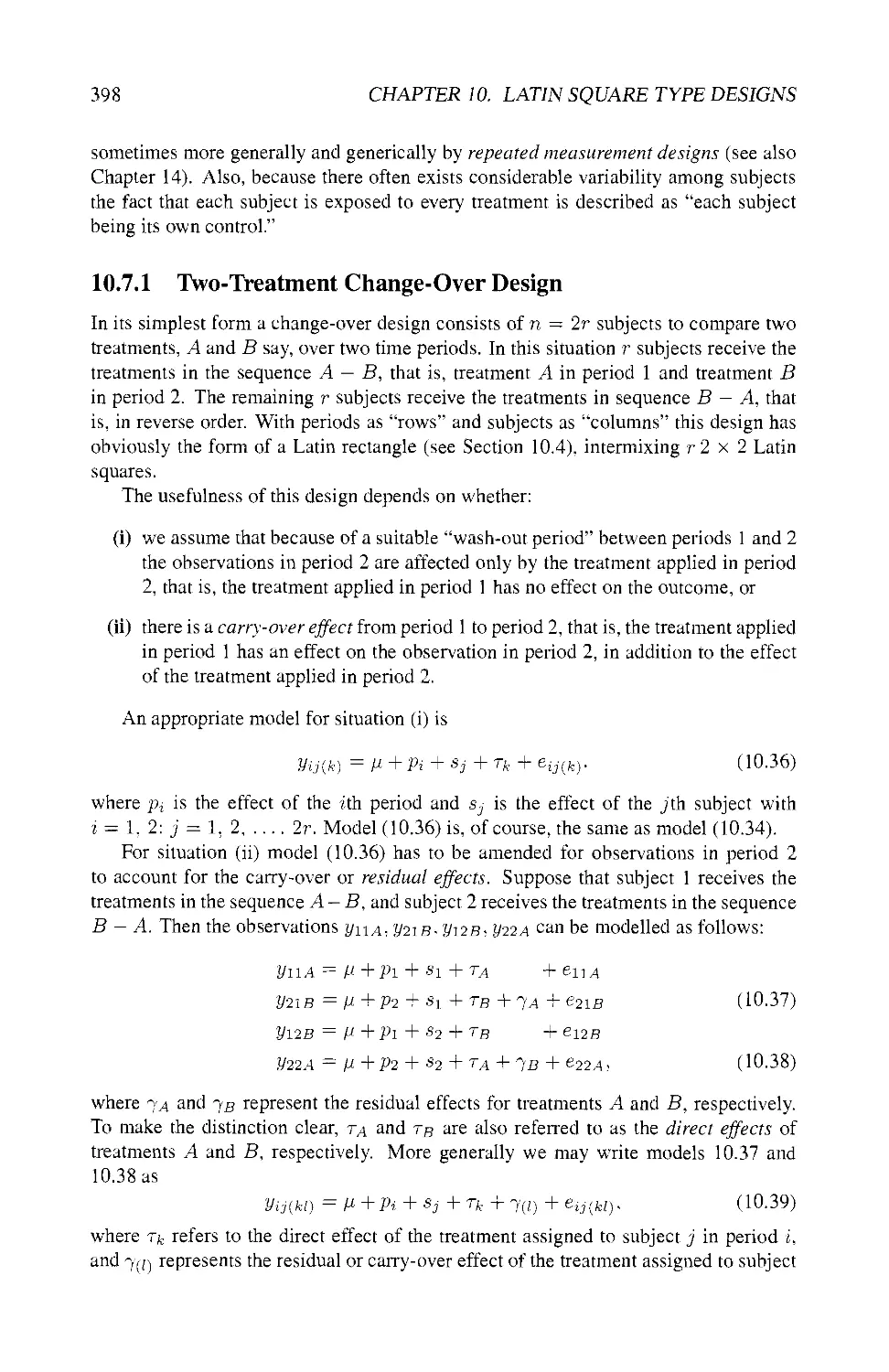
10.6.1 Grsco-Latin Squares 395
10.6.2 Mutually Orthogonal Latin Squares 396
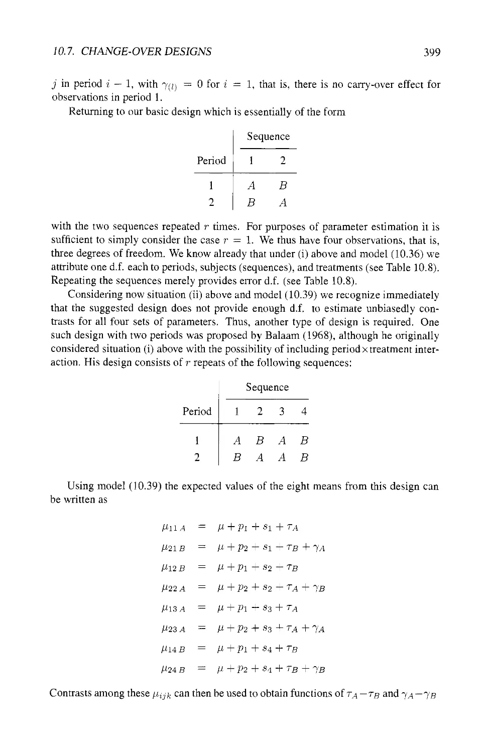
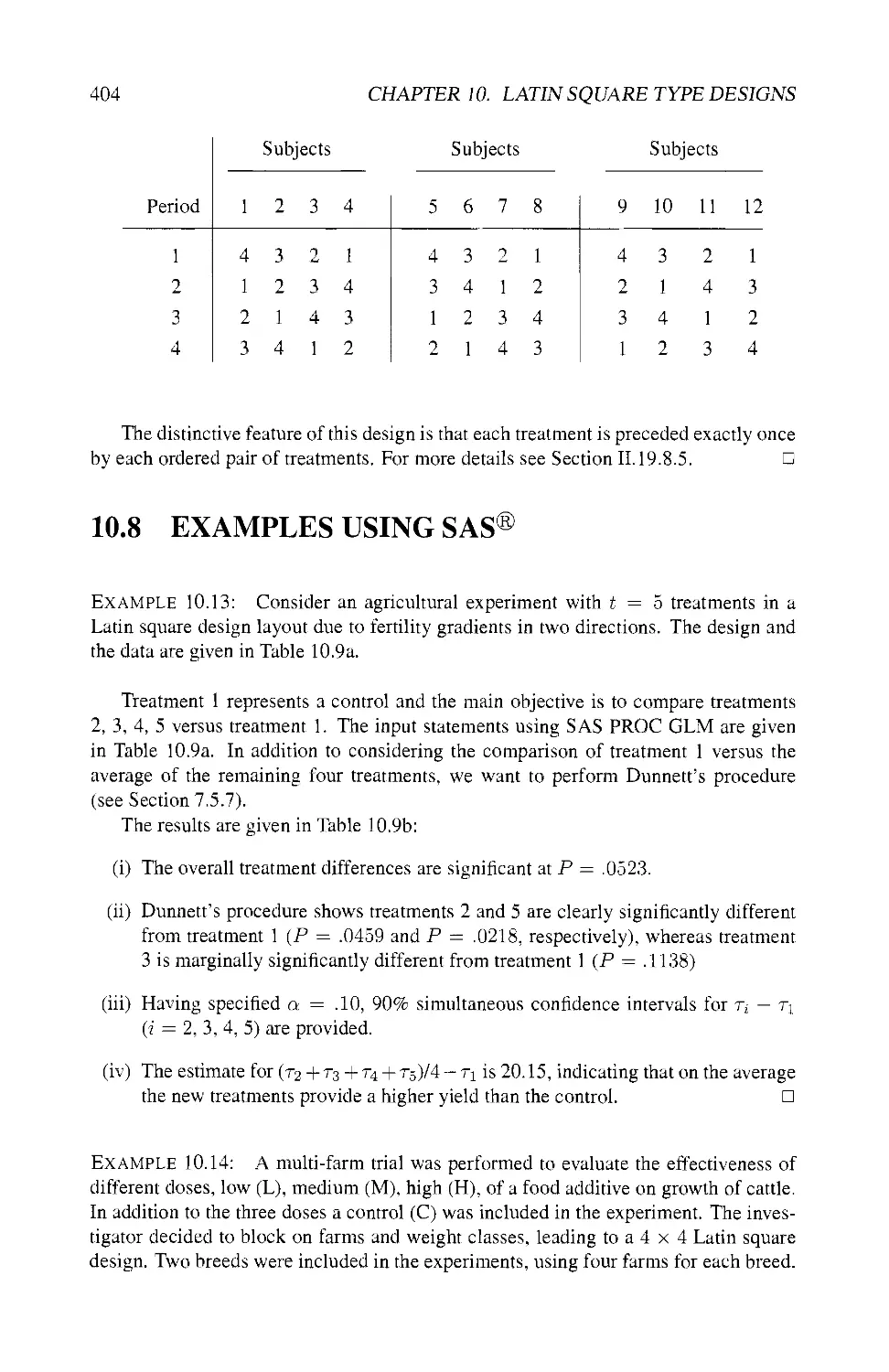
10.7 CHANGE-OVER DESIGNS 397
10.7.1 Two-Treatment Change-Over Design 398
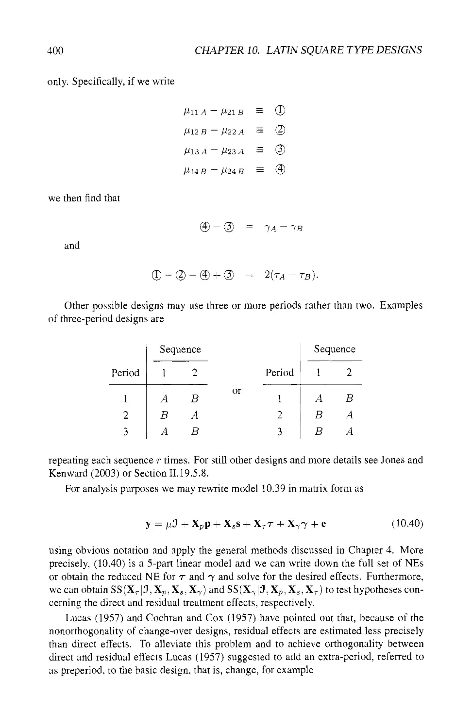
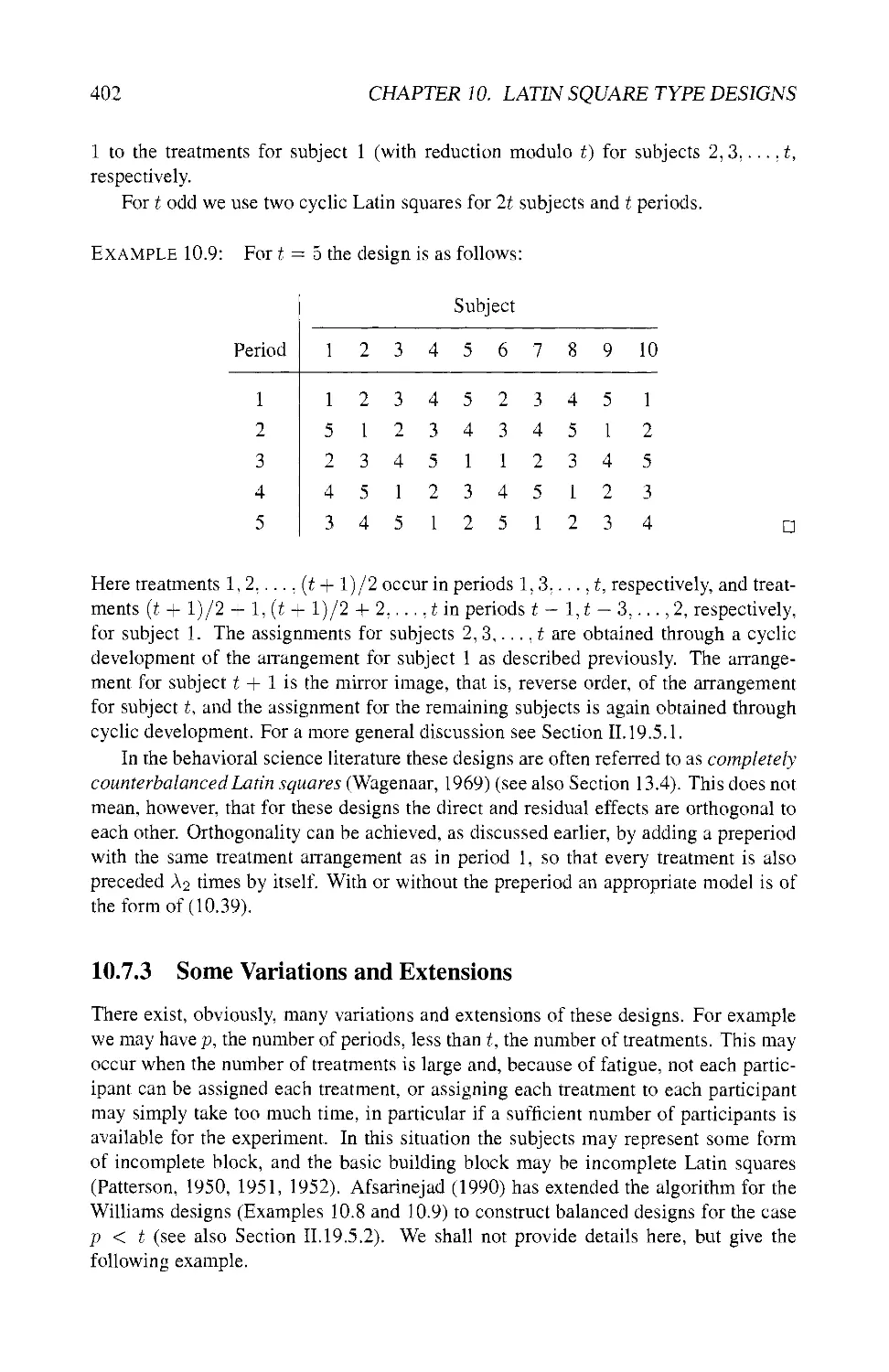
10.7.2 Change-Over Designs for More than Two Treatments 401
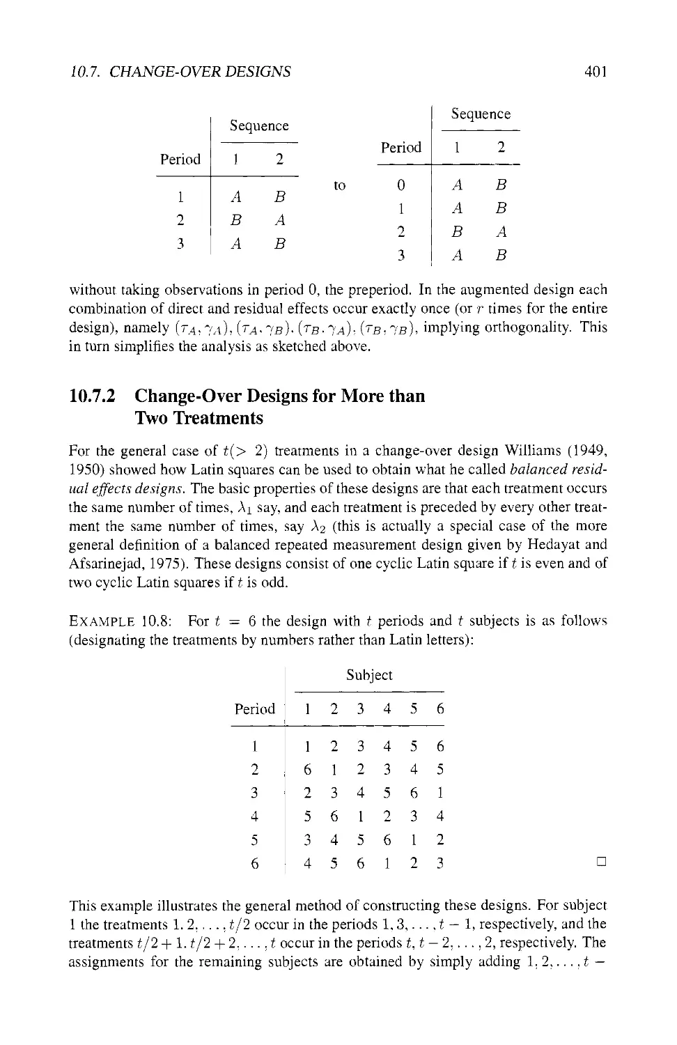
10.7.3 Some Variations and Extensions 402
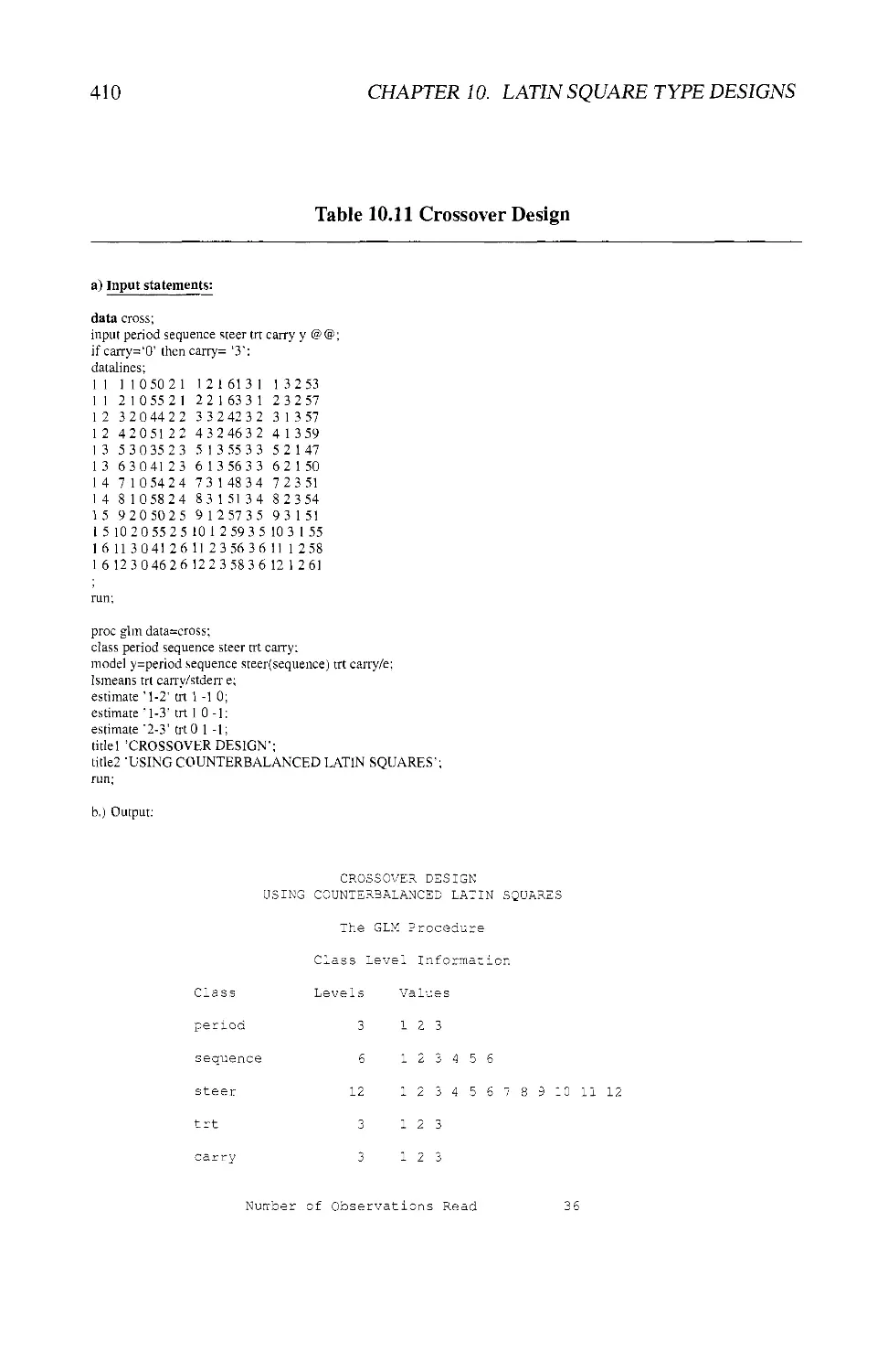
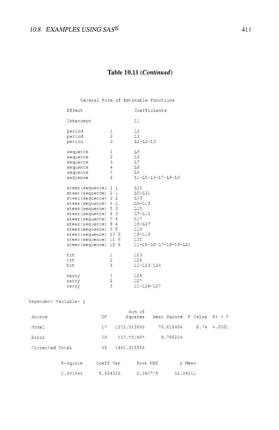
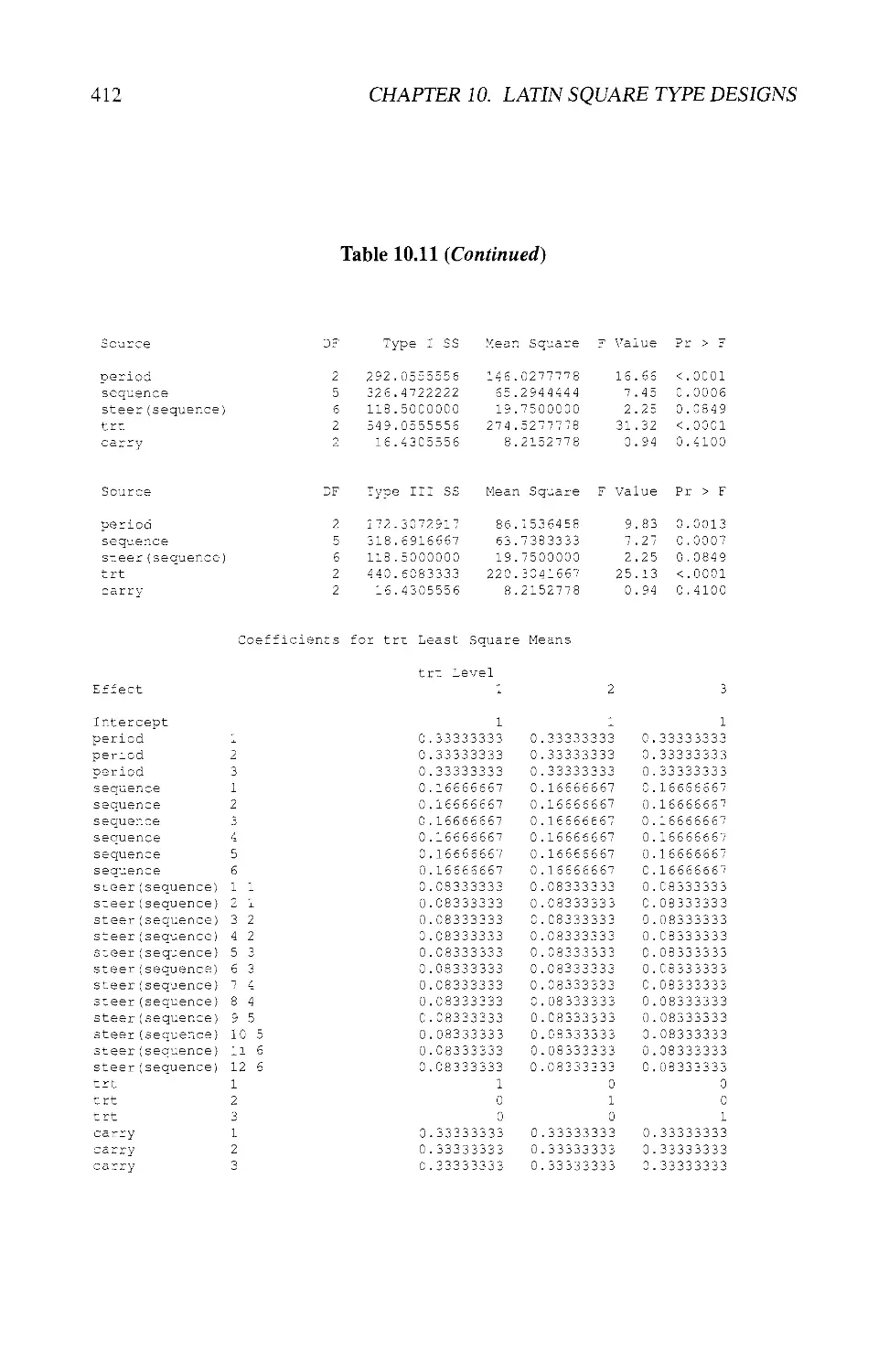
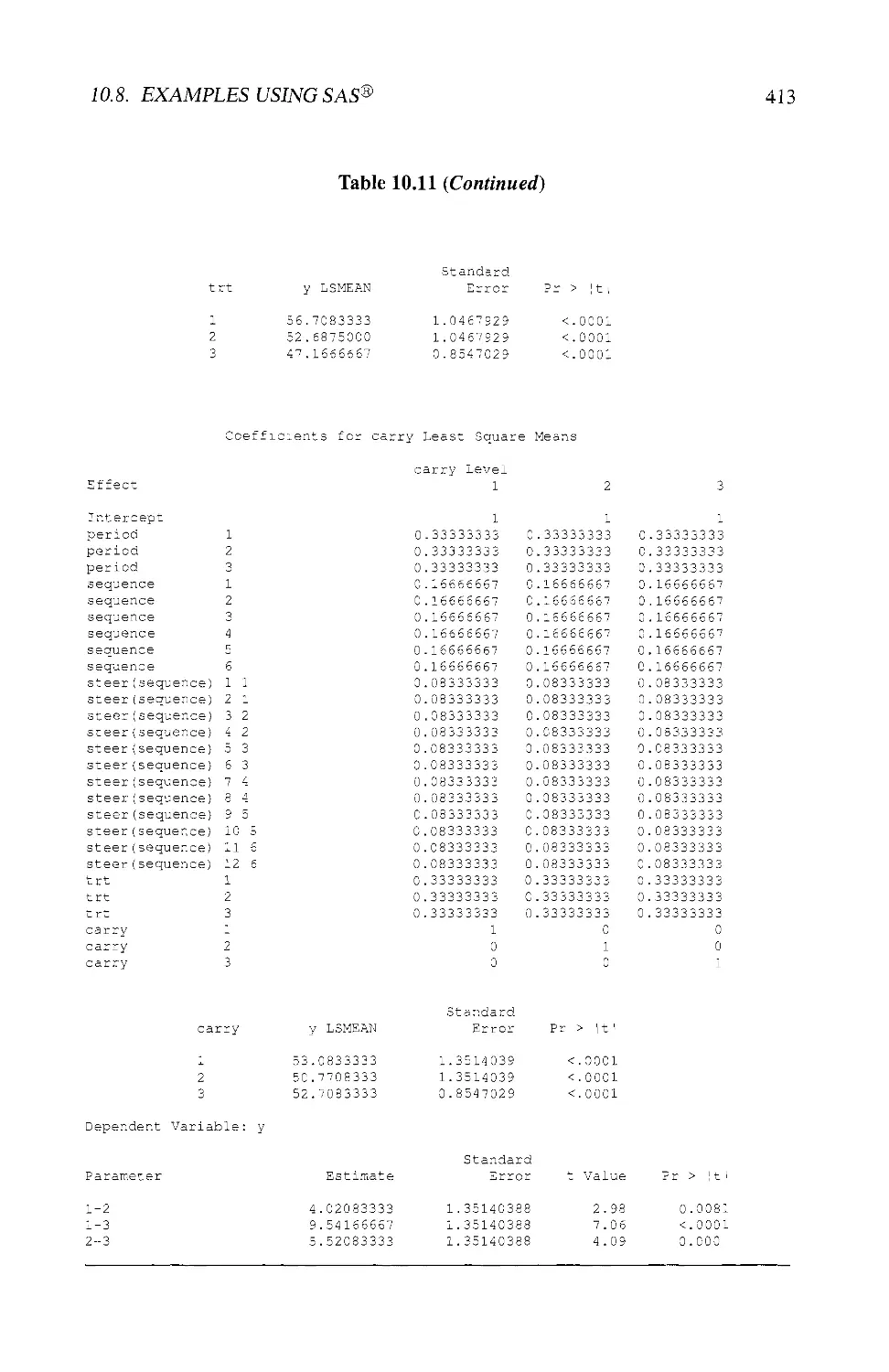
10.8 EXAMPLES USING SAS® 404
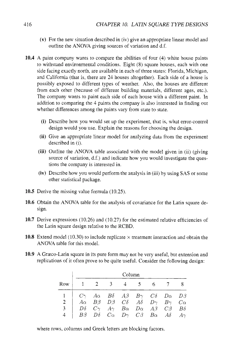
10.9 EXERCISES 414
11 Factorial Experiments: Basic Ideas 419
11.1 INTRODUCTION 419
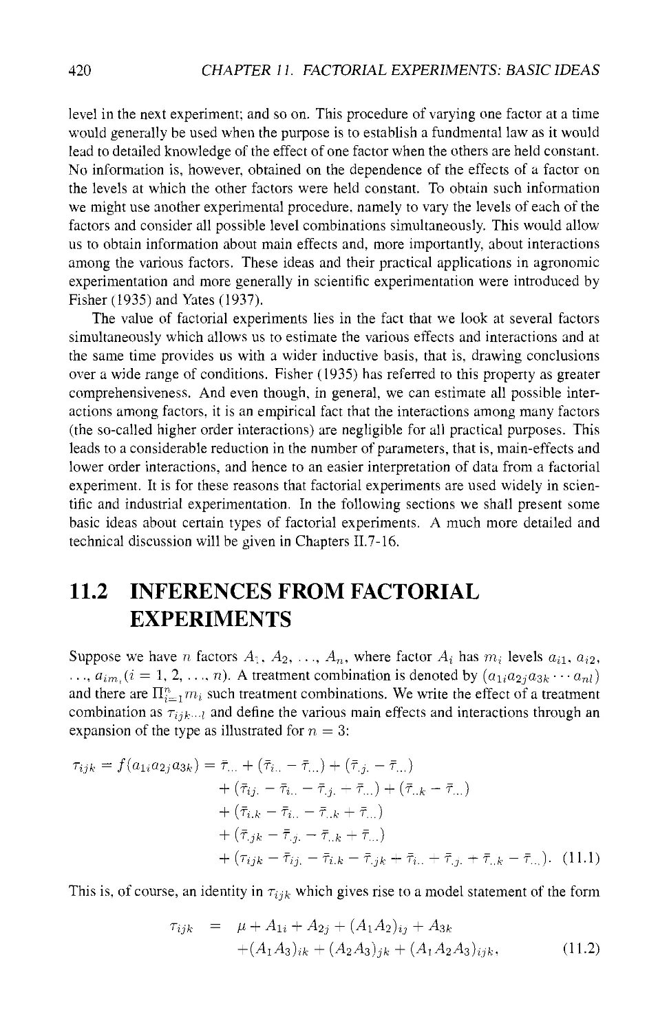
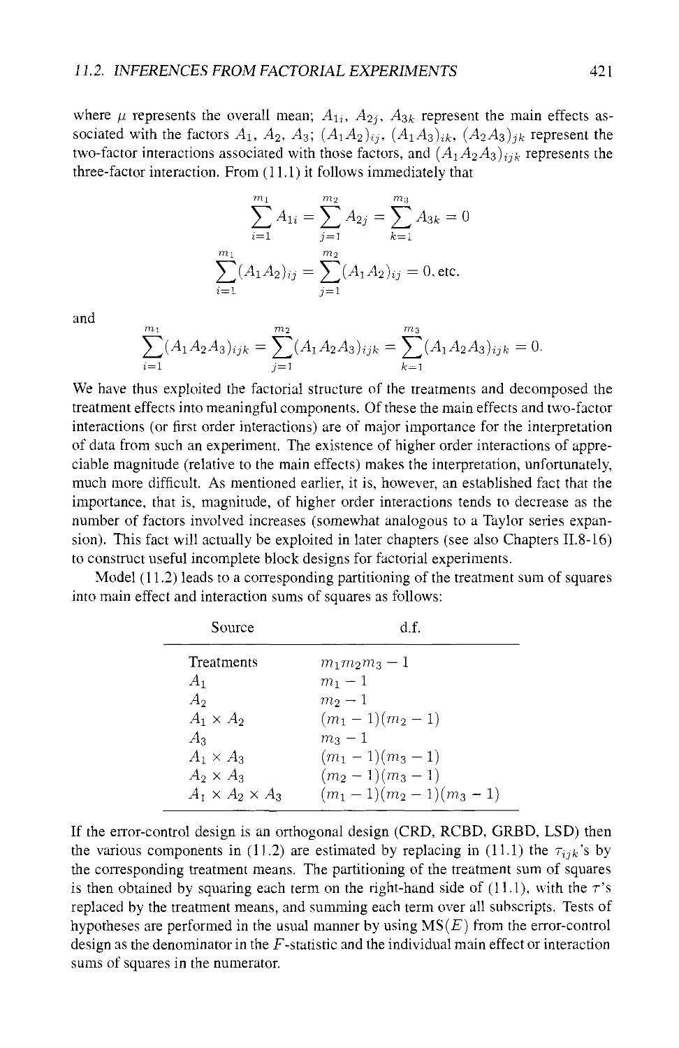
11.2 INFERENCES FROM FACTORIAL EXPERIMENTS 420
11.3 EXPERIMENTS WITH FACTORS AT TWO LEVELS 422
11.3.1 Definition of Main Effects and Interactions 422
11.3.2 Estimation of Main Effects and Interactions 425
11.3.3 Sums of Squares for Main Effects and Interactions 426
11.4 INTERPRETATION OF EFFECTS AND INTERACTIONS 426
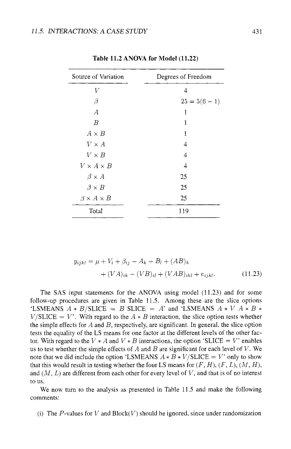
11.5 INTERACTIONS: A CASE STUDY 428
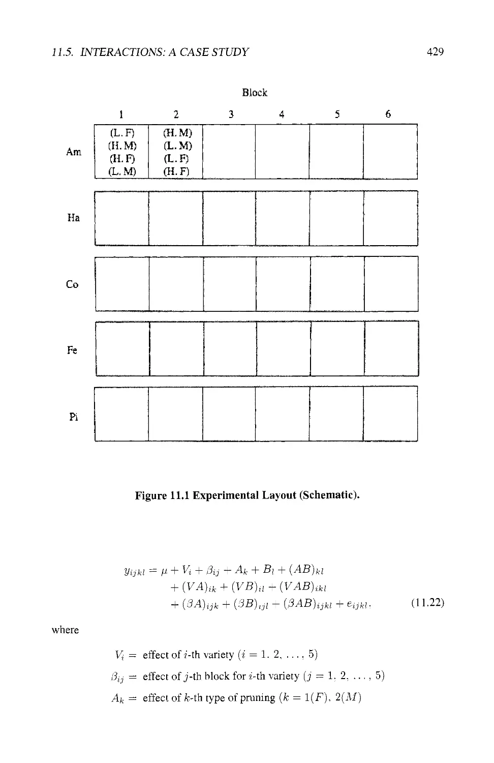
11.5.1 The Experiment 428
11.5.2 The Model 428
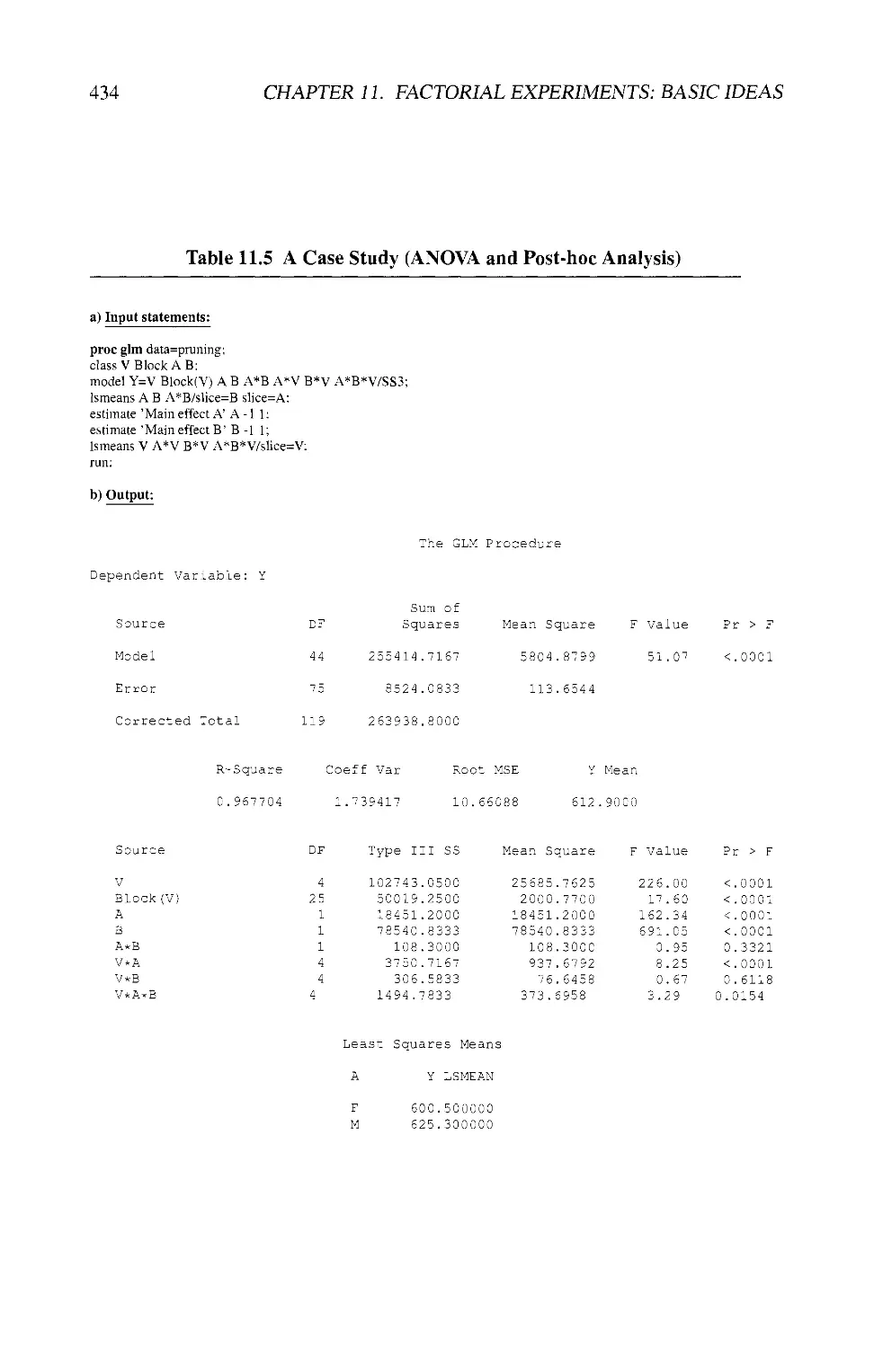
11.5.3 The Analysis 430
11.5.4 Separate Analyses 439
11.5.5 Blocking by Intrinsic Factor Only 440
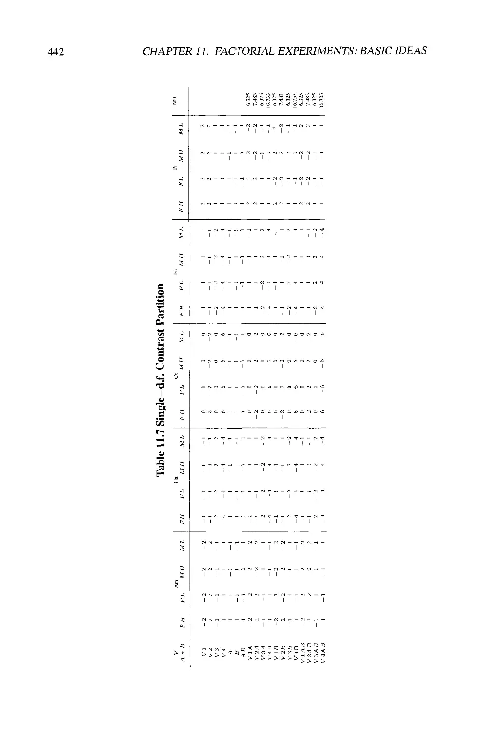
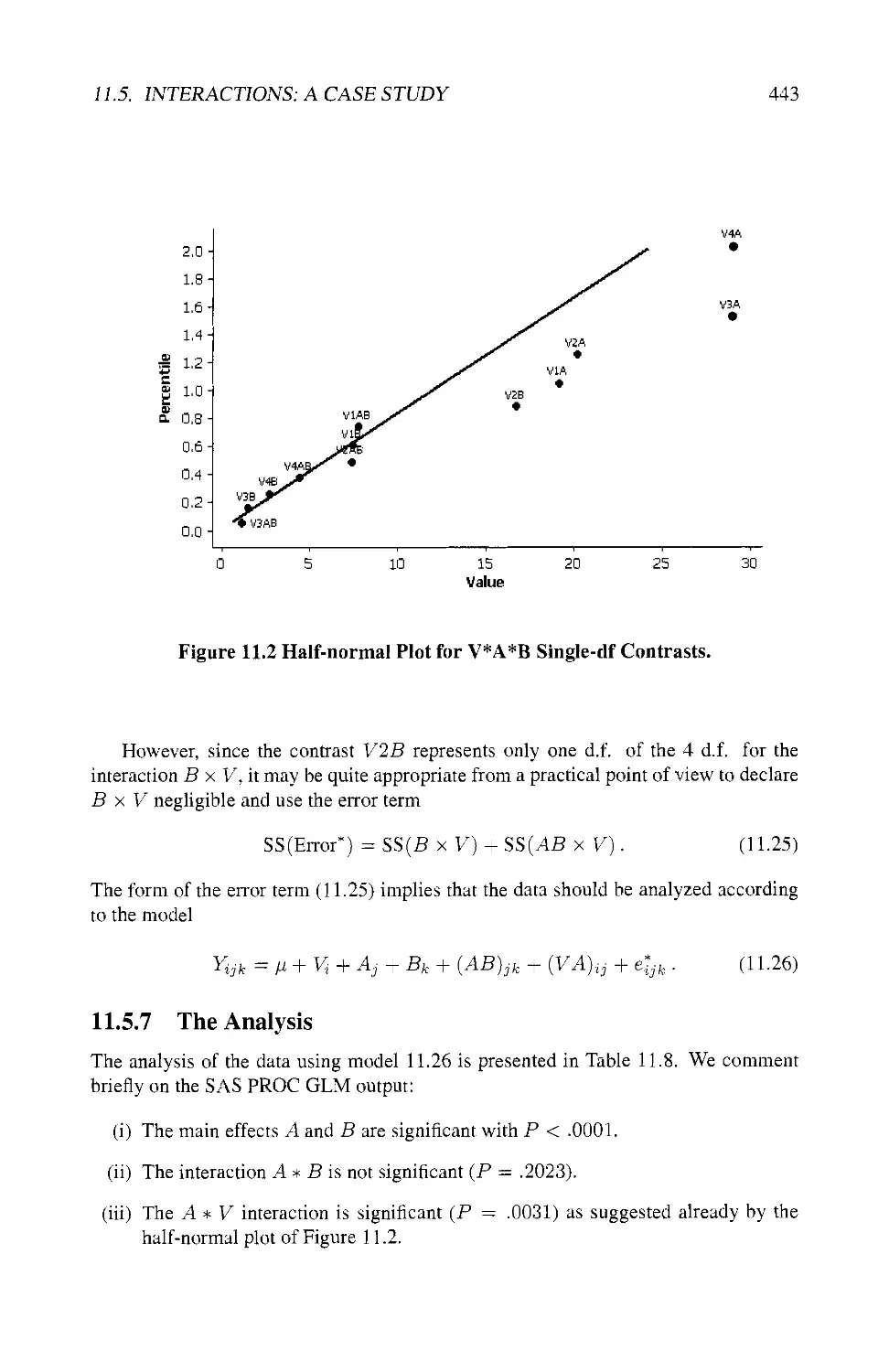
11.5.6 Using the Half-normal Plot Technique 441
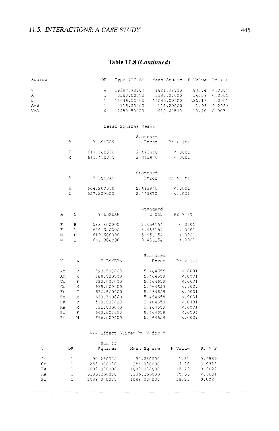
11.5.7 The Analysis 443
11.5.8 Summary 446
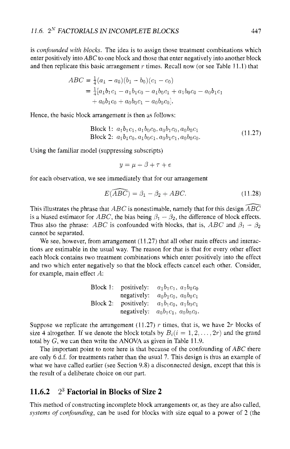
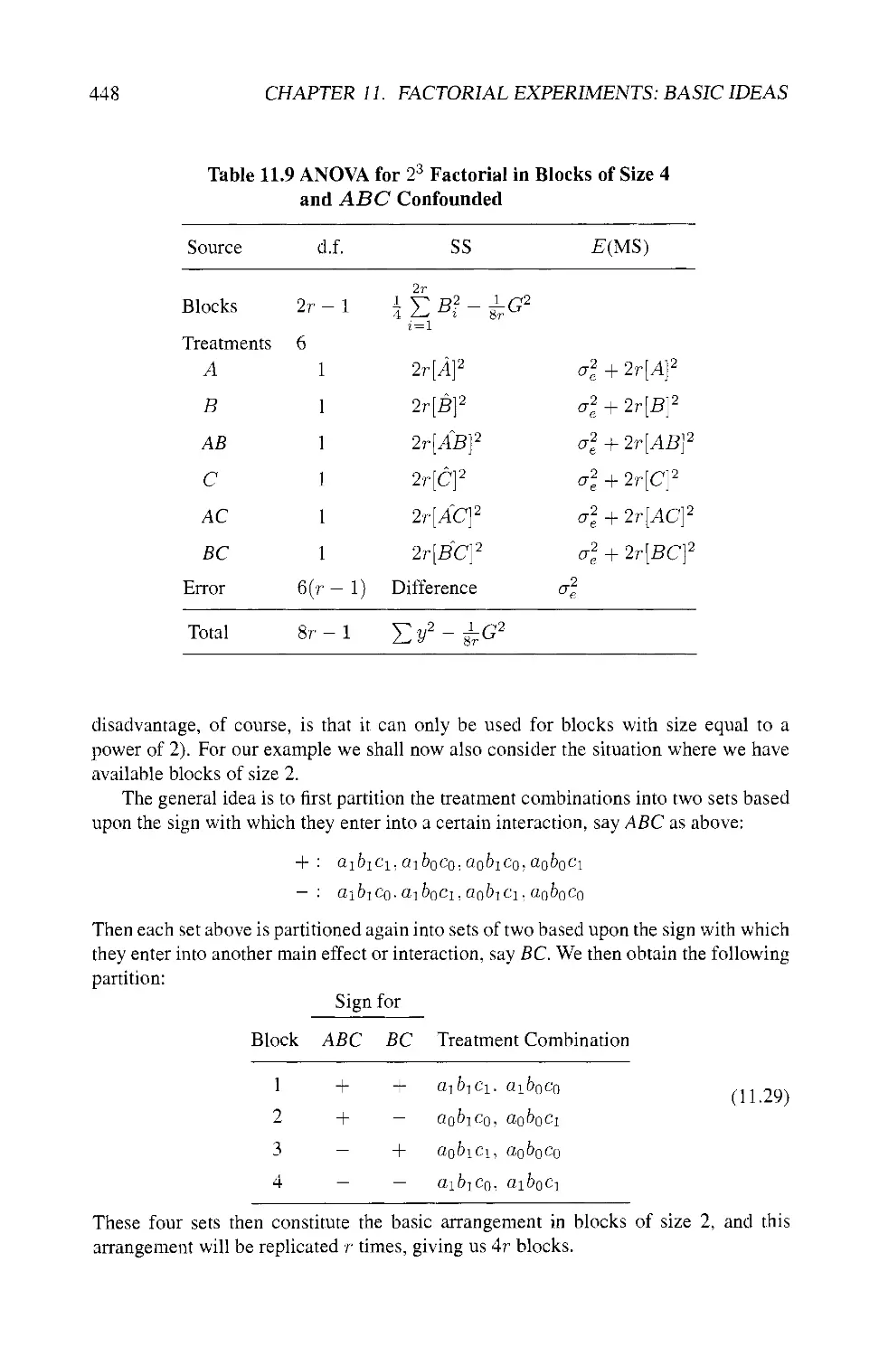
11.6 2n FACTORIALS IN INCOMPLETE BLOCKS 446
11.6.1 23 Factorial in Blocks of Size 4 446
11.6.2 23 Factorial in Blocks of Size 2 447
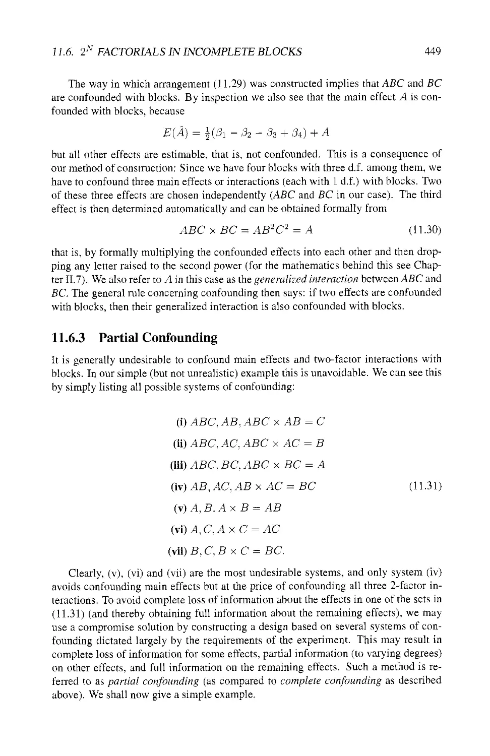
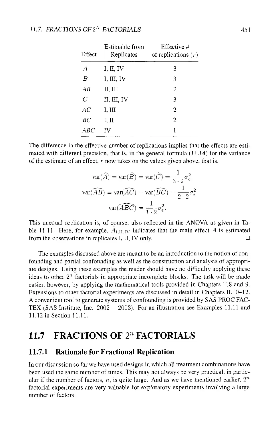
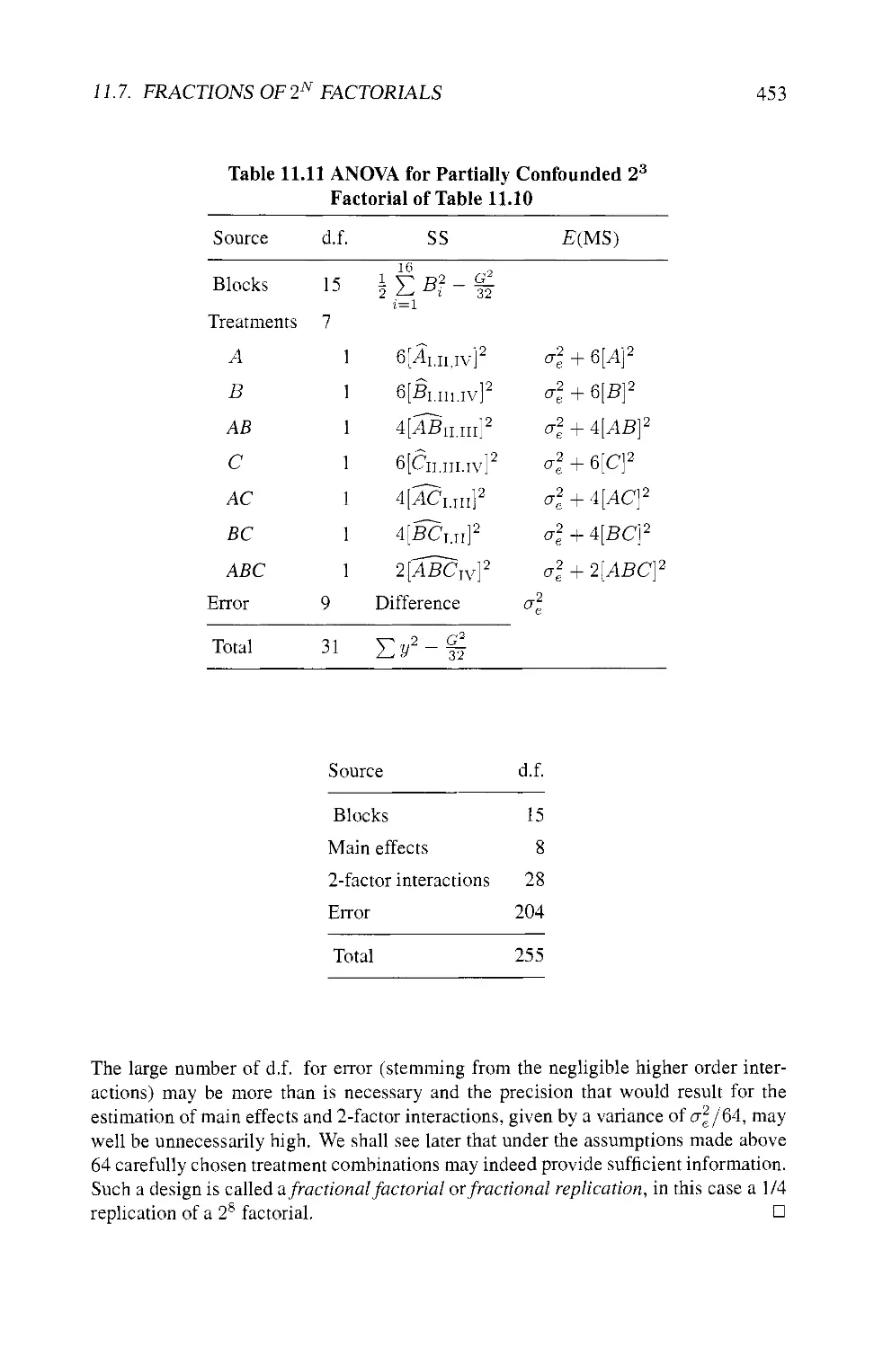
11.6.3 Partial Confounding 449
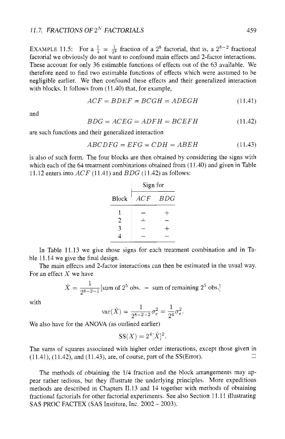
11.7 FRACTIONS OF 2" FACTORIALS 451
11.7.1 Rationale for Fractional Replication 451
11.7.2 1/2 Fraction of the 23 Factorial 454
11.7.3 The Alias Structure 454
11.7.4 1/4 Fraction of the 28 Factorial 456
11.7.5 Systems of Confounding for Fractional Factorials 457
CONTENTS xiii
11.8 ORTHOGONAL MAIN EFFECT PLANS FOR 2" FACTORIALS . . 462
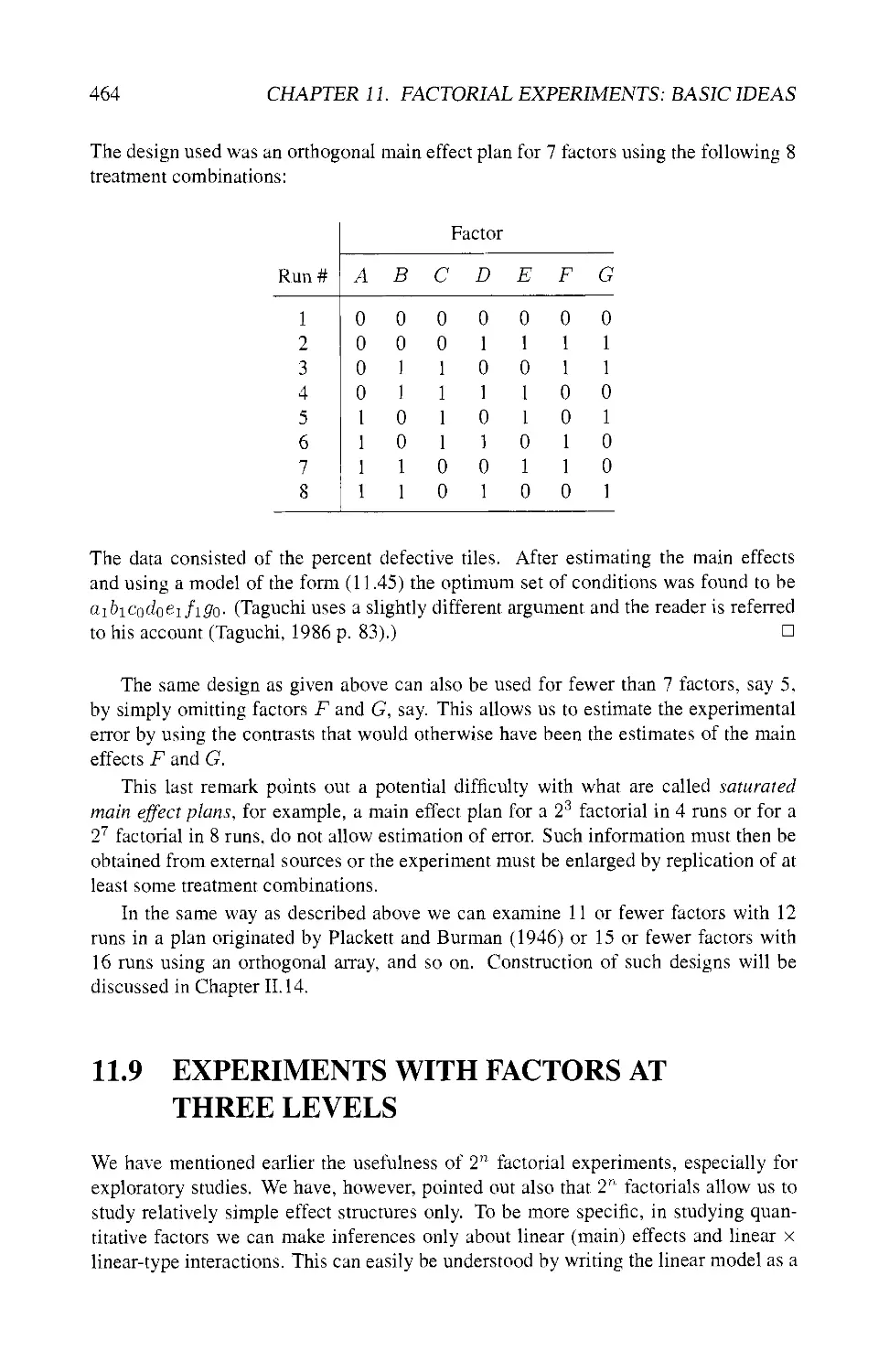
11.9 EXPERIMENTS WITH FACTORS AT THREE LEVELS 464
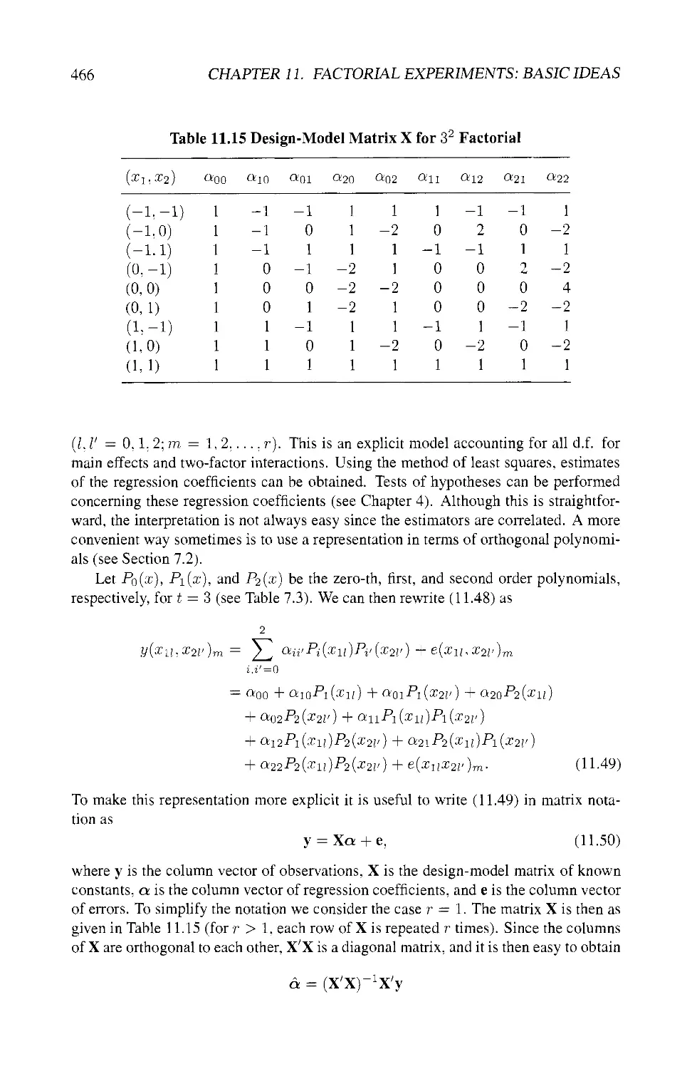
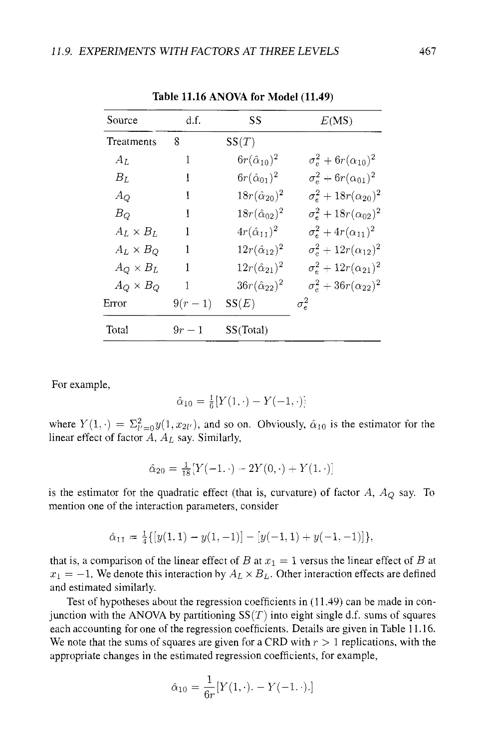
11.9.1 The 32 Factorial 465
11.9.2 Extensions 468
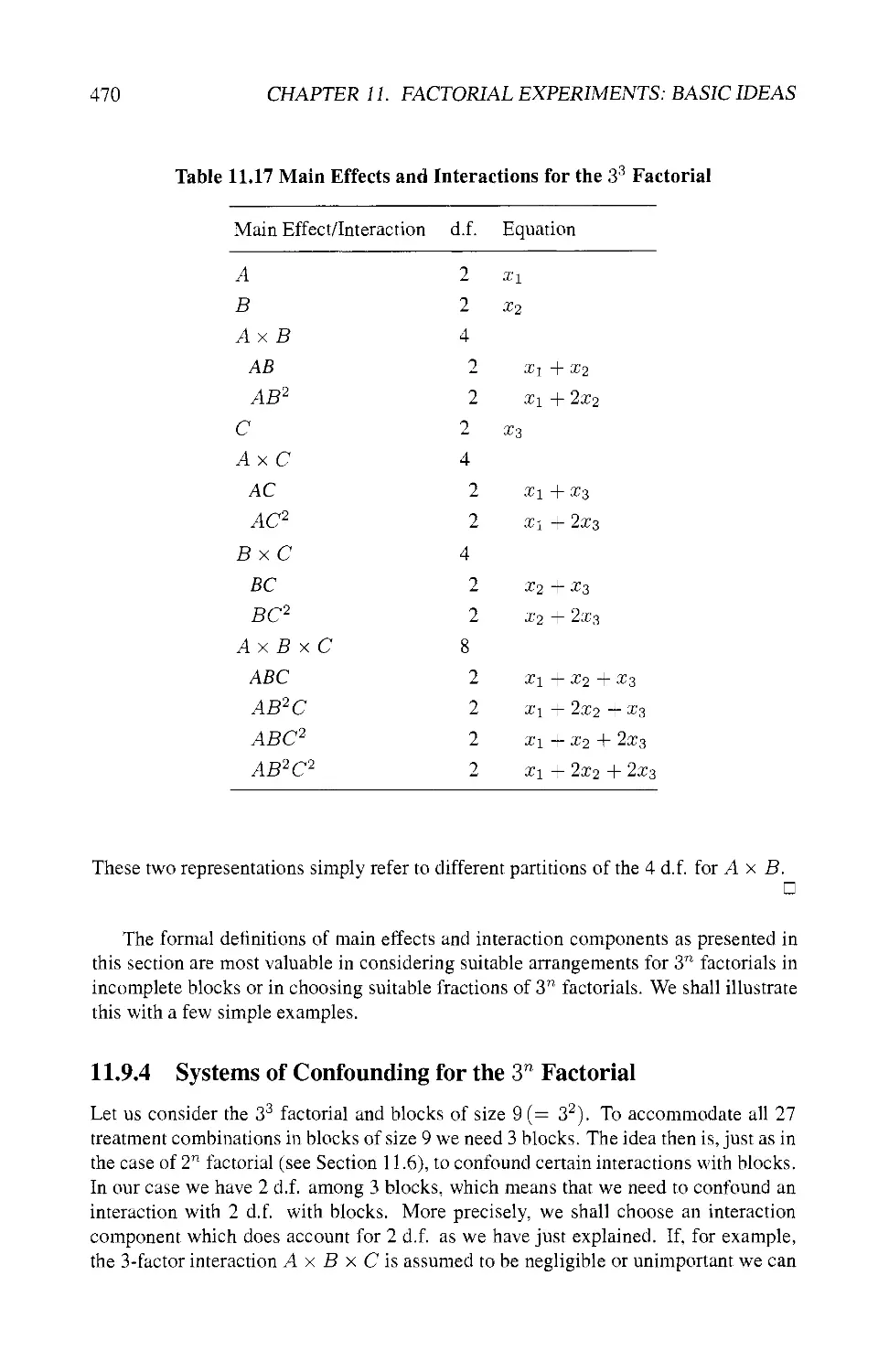
11.9.3 Formal Definition of Main Effects and Interactions 468
11.9.4 Systems of Confounding for the 3" Factorial 470
11.9.5 Fractions of 3" Factorials 472
11.9.6 Highly Fractionated 3" Factorials 475
11.9.7 Systems of Confounding for Fractions of 3n
Factorials 475
11.10 FACTORS AT TWO AND THREE LEVELS 476
11.10.1 Asymmetrical Factorial Experiments 476
11.10.2 Confounding in 2m x 3n Factorials 477
Blocks of Size 18: 478
Blocks of Size 12; 478
Blocks of Size 9; 478
Blocks of Size 6: 478
Blocks of Size 4; 478
11.10.3 Fractions of 2m X 3n Factorials 479
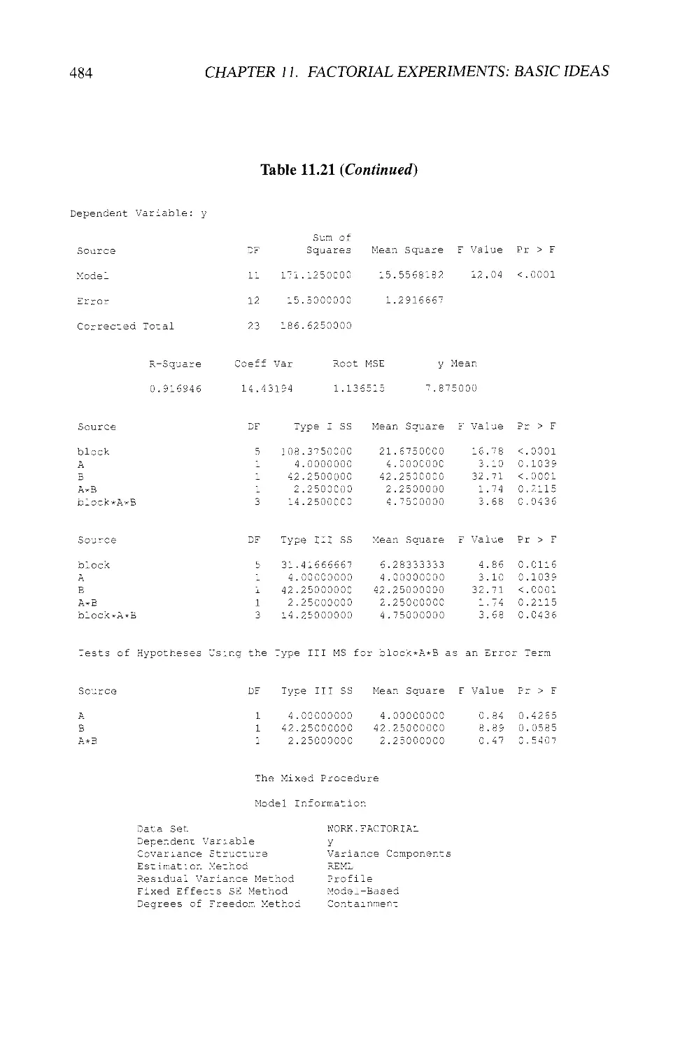
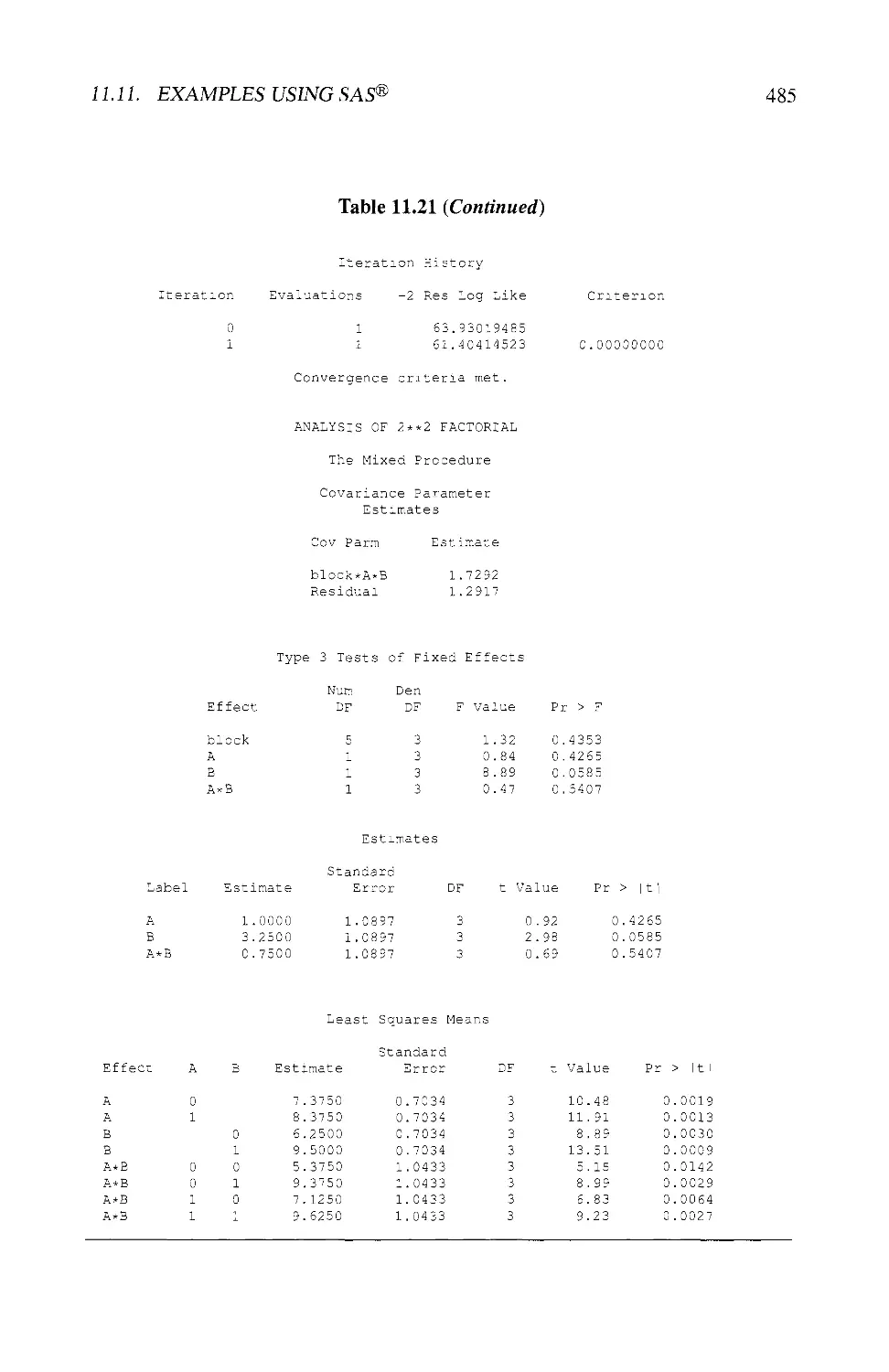
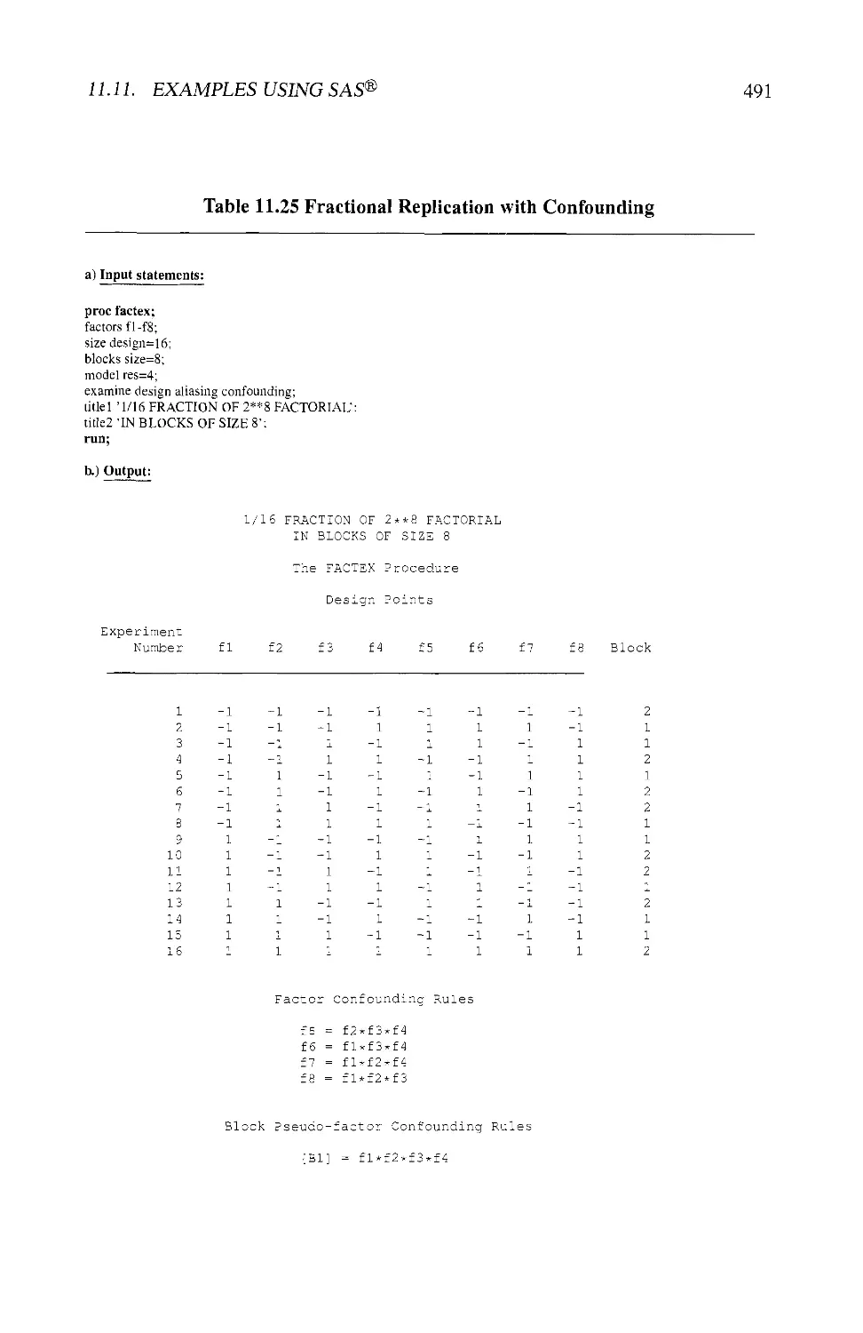
11.11 EXAMPLES USING SAS® 481
11.12 EXERCISES 492
12 Response Surface Designs 497
12.1 INTRODUCTION 497
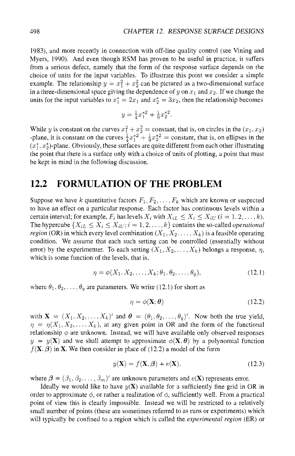
12.2 FORMULATION OF THE PROBLEM 498
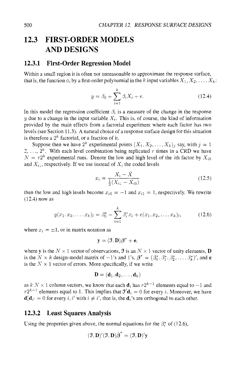
12.3 FIRST-ORDER MODELS AND DESIGNS 500
12.3.1 First-Order Regression Model 500
12.3.2 Least Squares Analysis 500
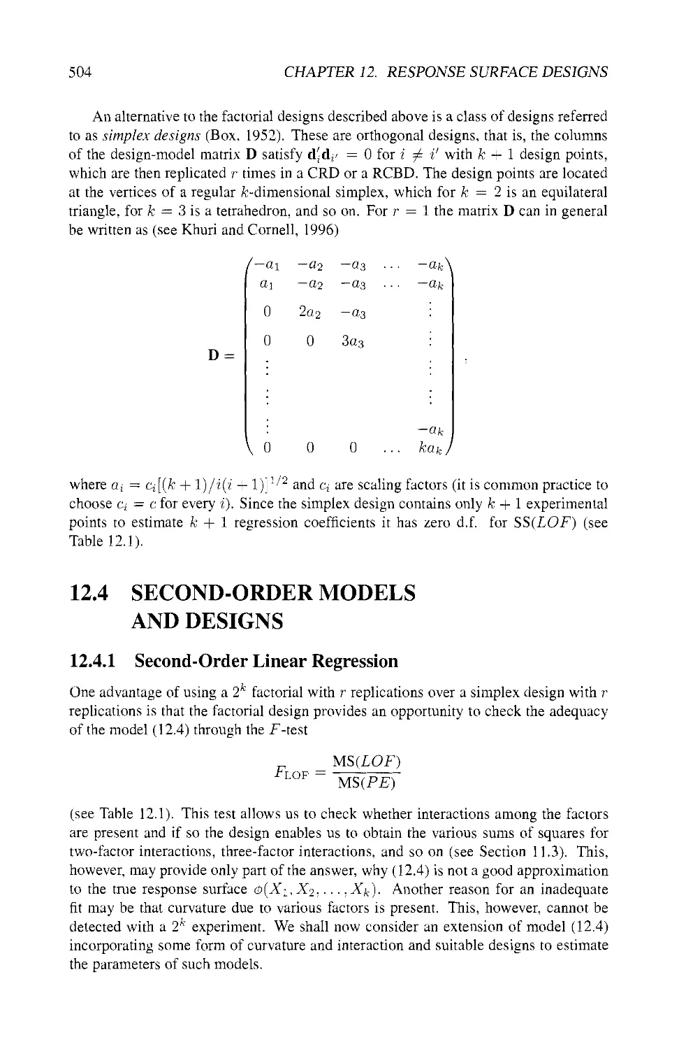
12.3.3 Alternative Designs 503
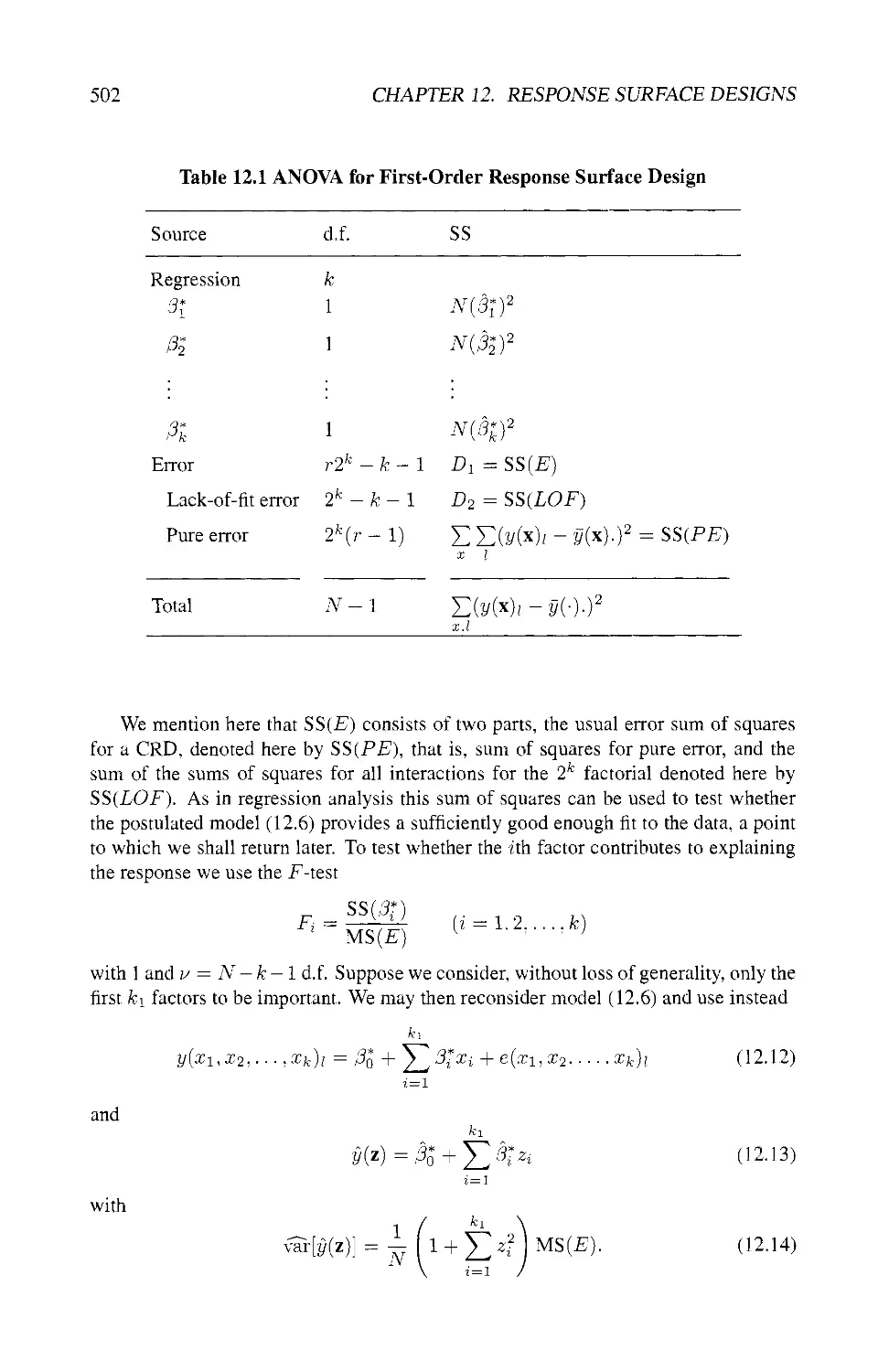
12.4 SECOND-ORDER MODELS AND DESIGNS 504
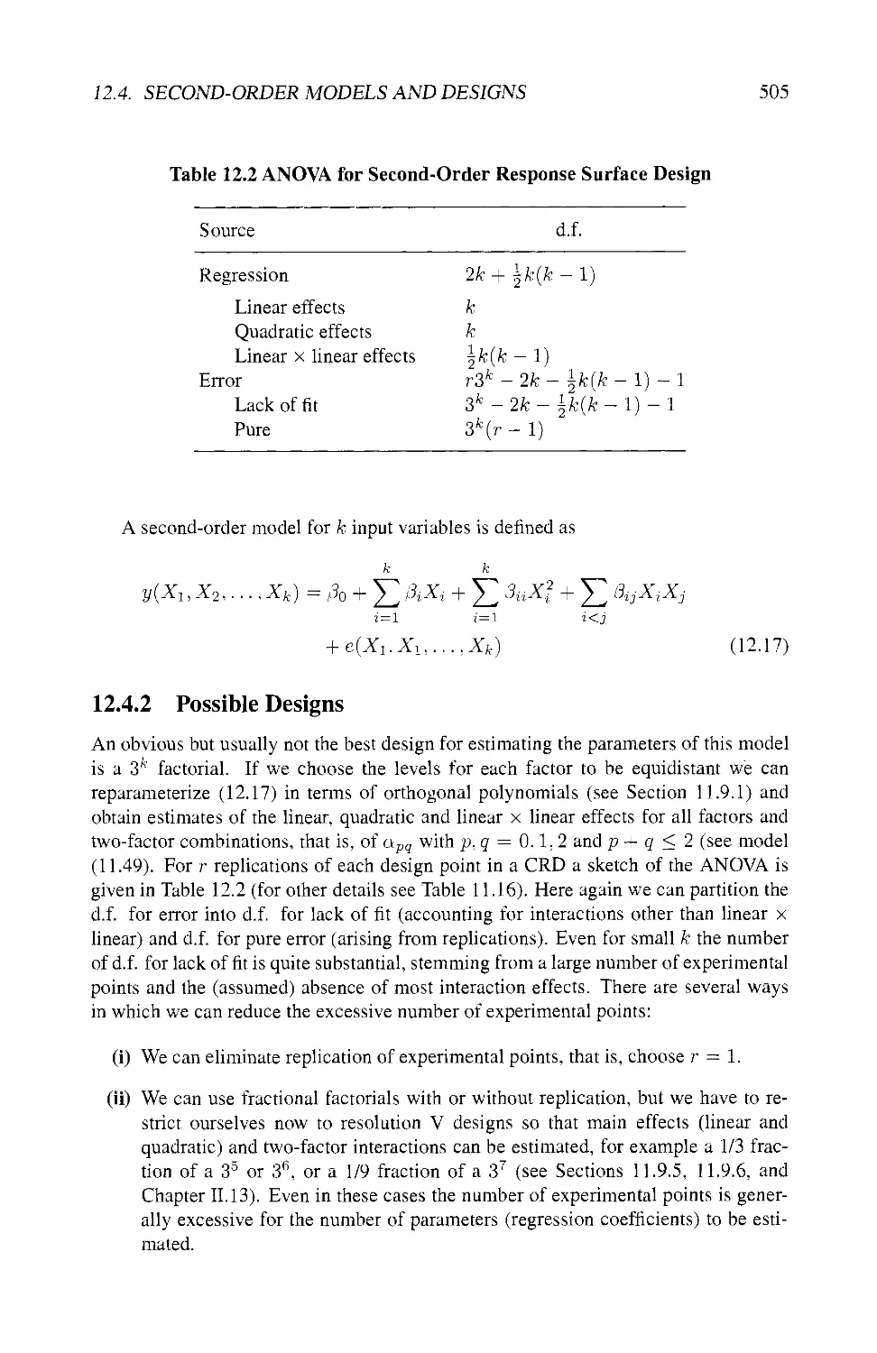
12.4.1 Second-Order Linear Regression 504
12.4.2 Possible Designs 505
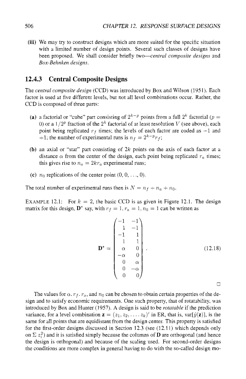
12.4.3 Central Composite Designs 506
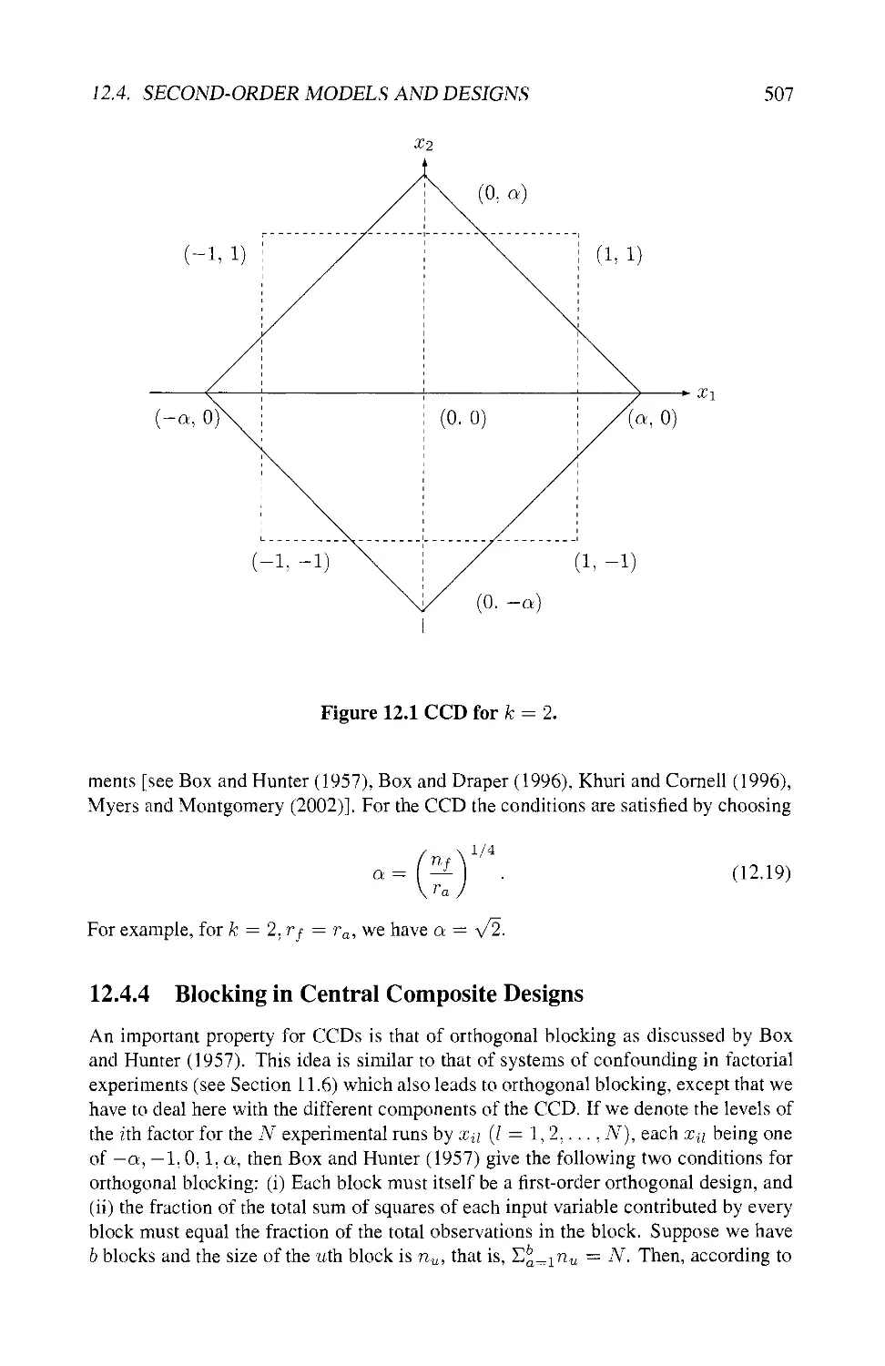
12.4.4 Blocking in Central Composite Designs 507
12.4.5 Box-Behnken Designs 509
12.4.6 Hard-to-Change versus Easy-to-Change Factors 511
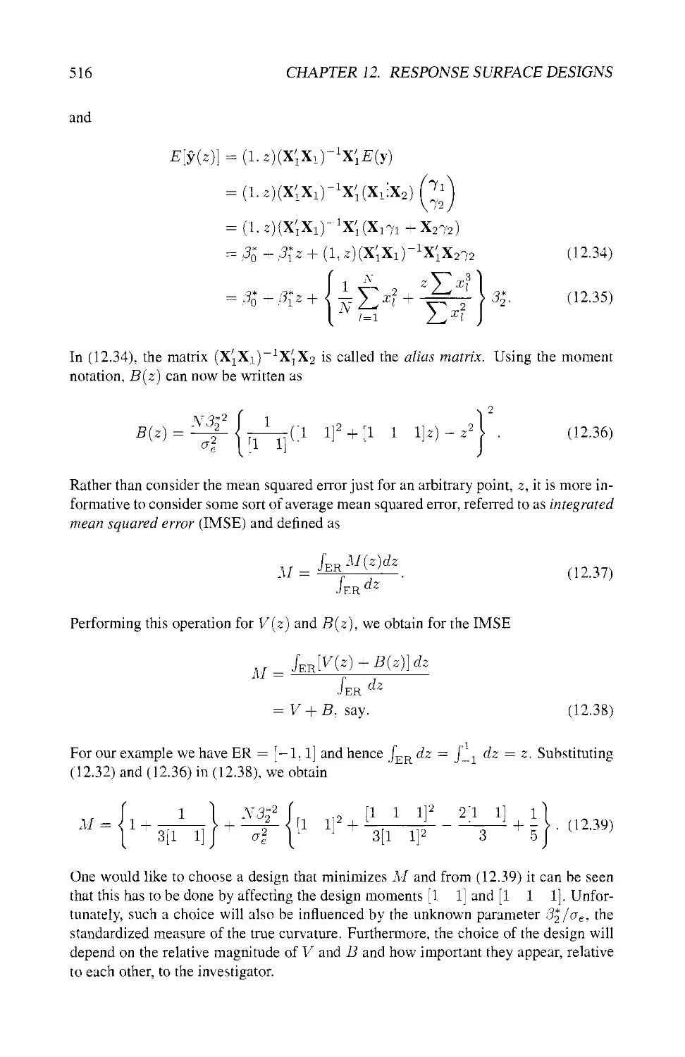
12.5 INTEGRATED MEAN SQUARED"ERROR DESIGNS 513
12.5.1 Variance and Bias for the One-Factor Case 514
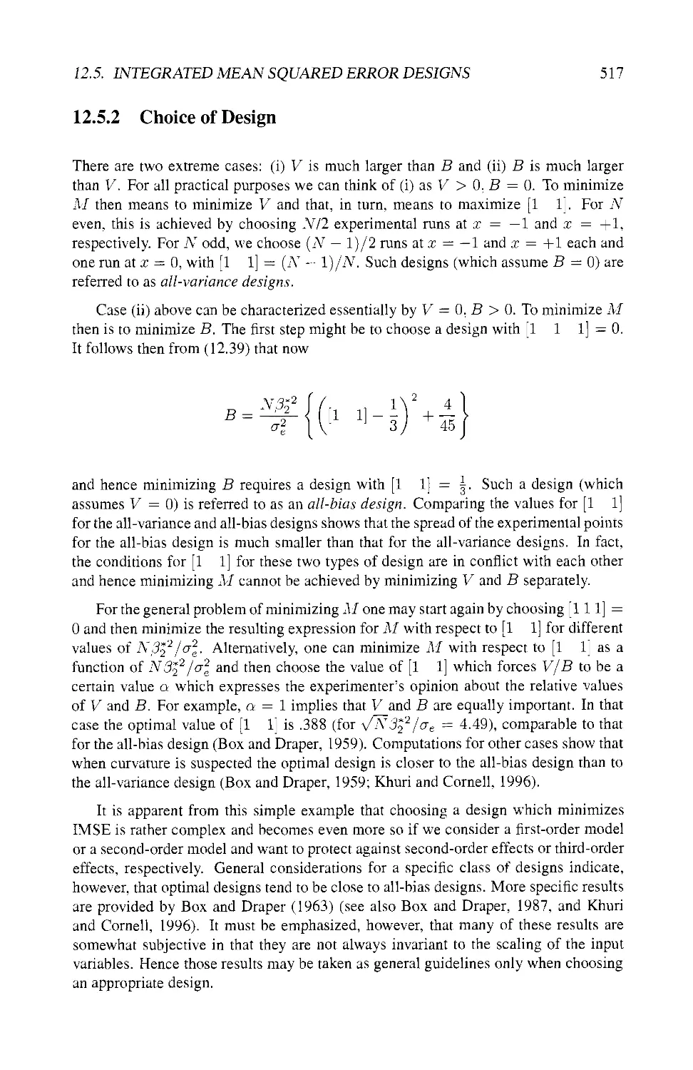
12.5.2 Choice of Design 517
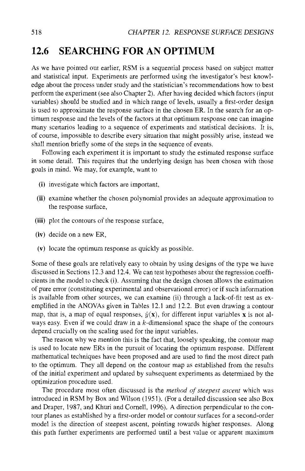
12.6 SEARCHING FOR AN OPTIMUM 518
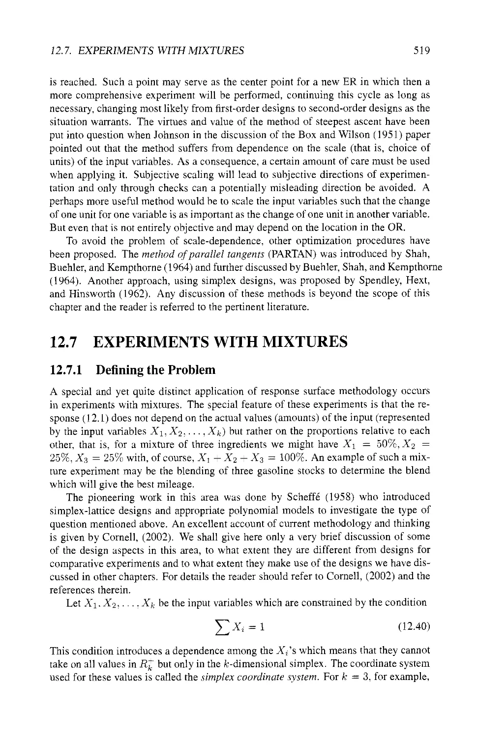
12.7 EXPERIMENTS WITH MIXTURES 519
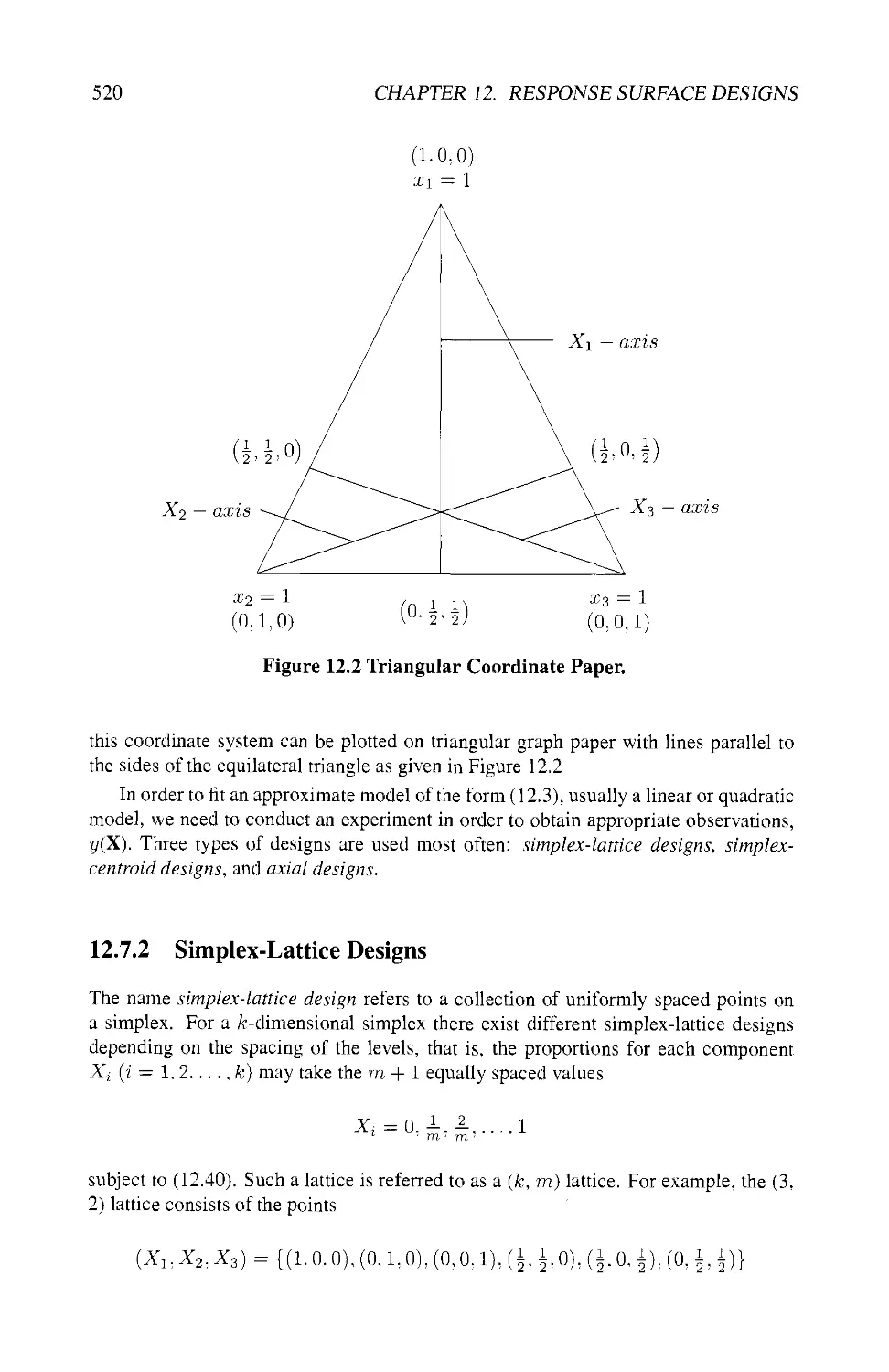
12.7.1 Defining the Problem 519
12.7.2 Simplex-Lattice Designs 520
12.7.3 Simplex-Centroid Designs 521
12.7.4 Axial Designs 521
12.7.5 Canonical Polynomials 521
xiv CONTENTS
12.7.6 Including Process Variables 523
12.8 EXAMPLES USING SAS® 523
12.9 EXERCISES 531
13 Split-Plot Type Designs 533
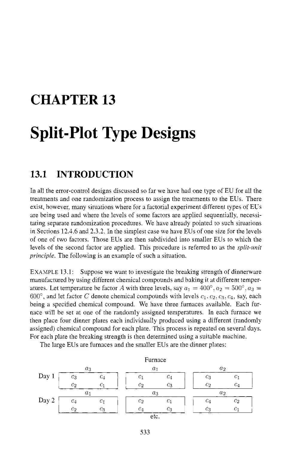
13.1 INTRODUCTION 533
13.2 SIMPLE SPLIT-PLOT DESIGN 534
13.2.1 Superimposing Two Randomized Complete Block Designs . . 534
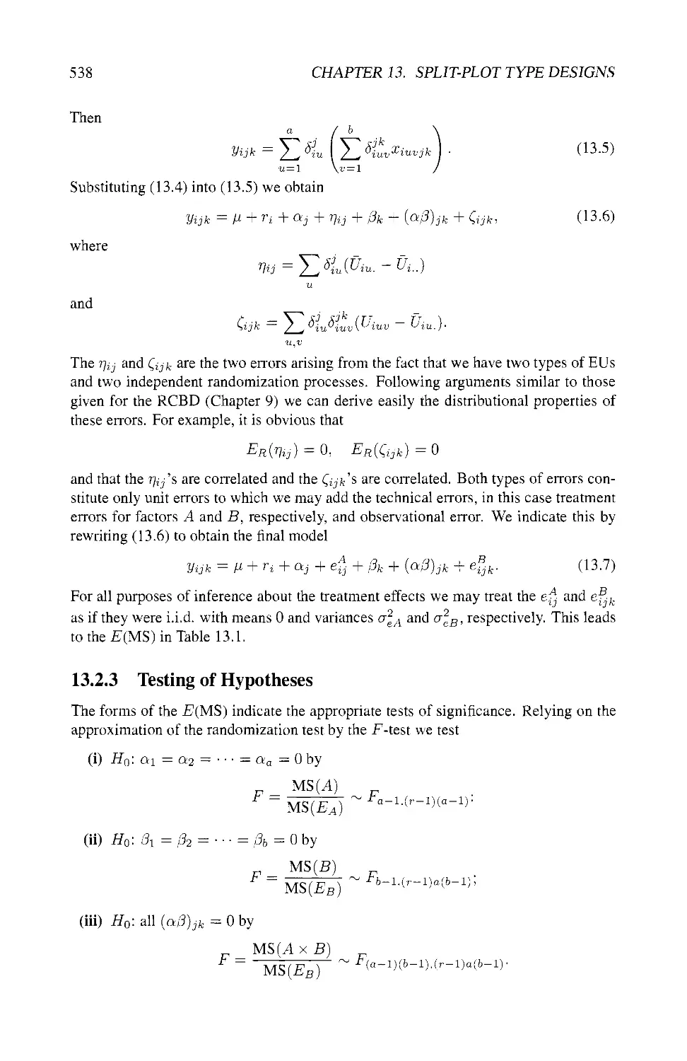
13.2.2 Derived Linear Model 537
13.2.3 Testing of Hypotheses 538
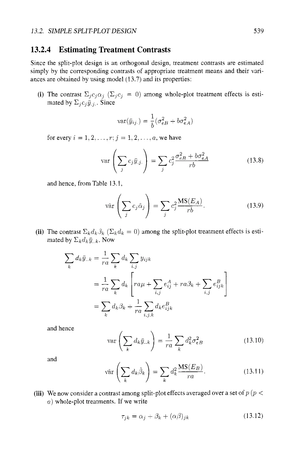
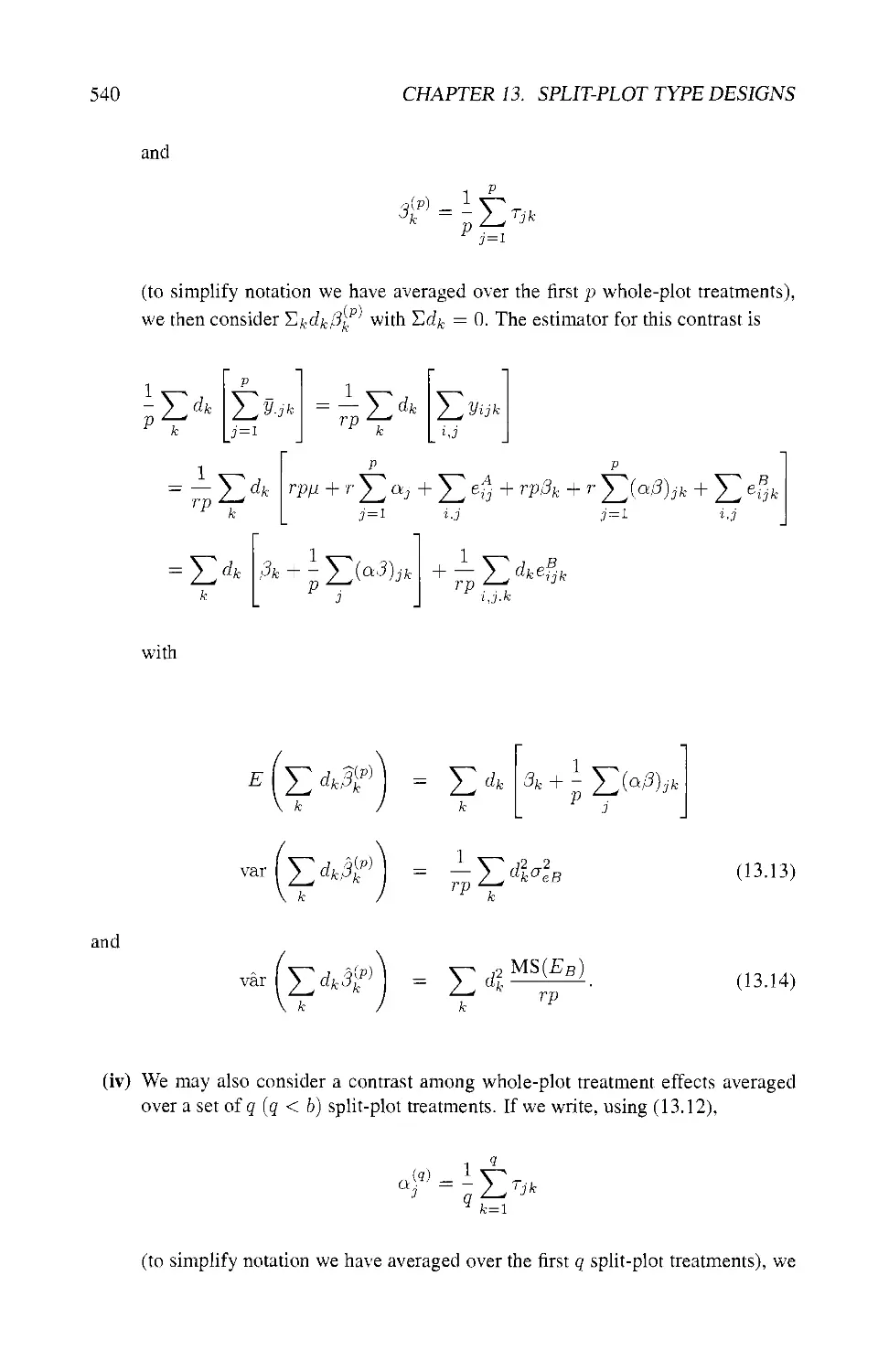
13.2.4 Estimating Treatment Contrasts 539
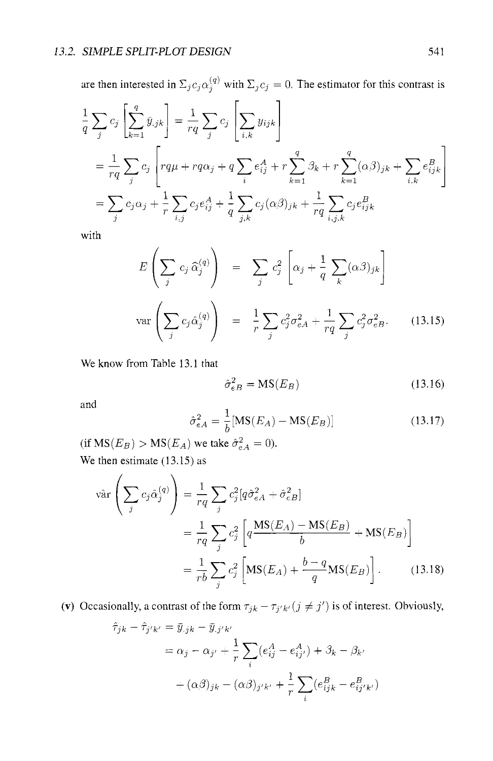
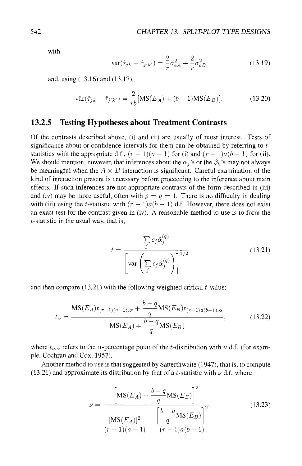
13.2.5 Testing Hypotheses about Treatment Contrasts 542
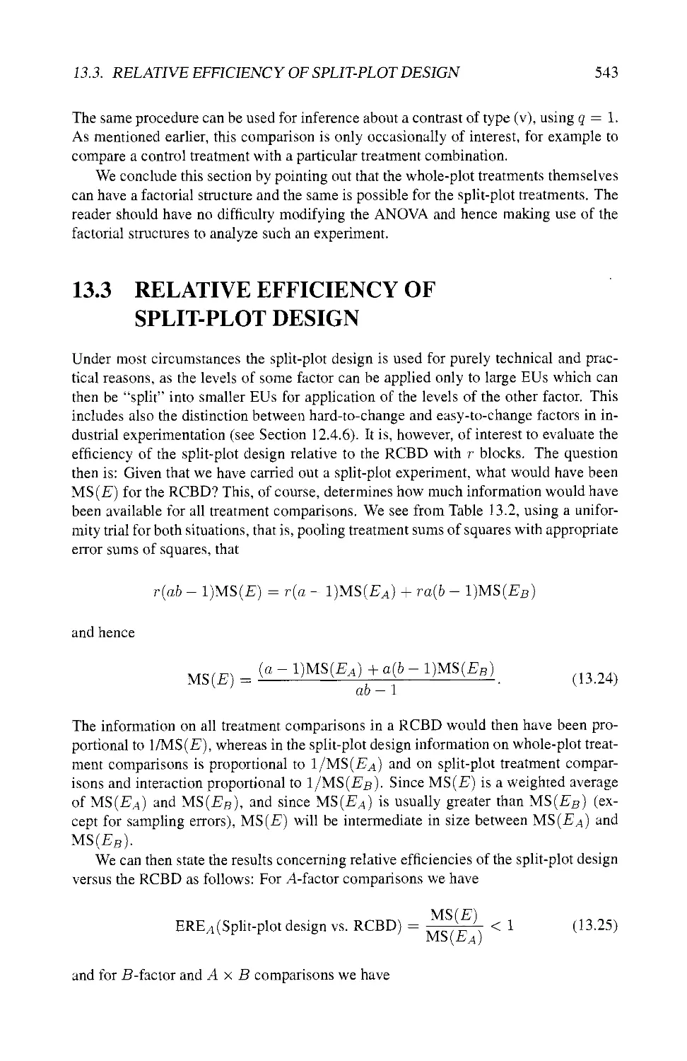
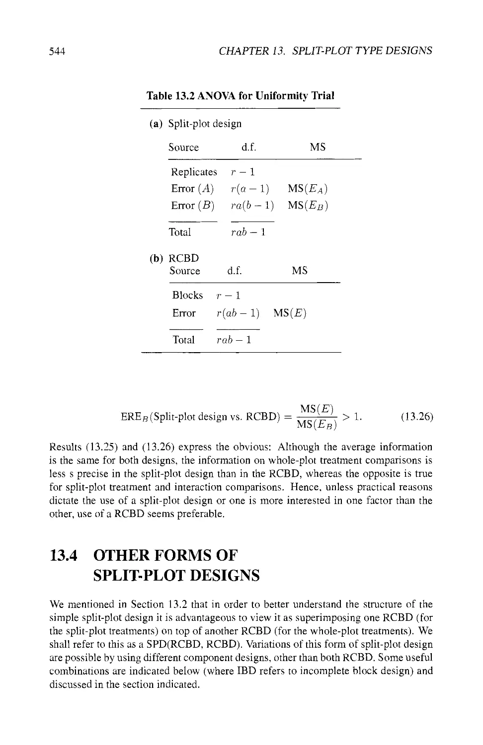
13.3 RELATIVE EFFICIENCY OF SPLIT-PLOT DESIGN 543
13.4 OTHER FORMS OF SPLIT-PLOT DESIGNS 544
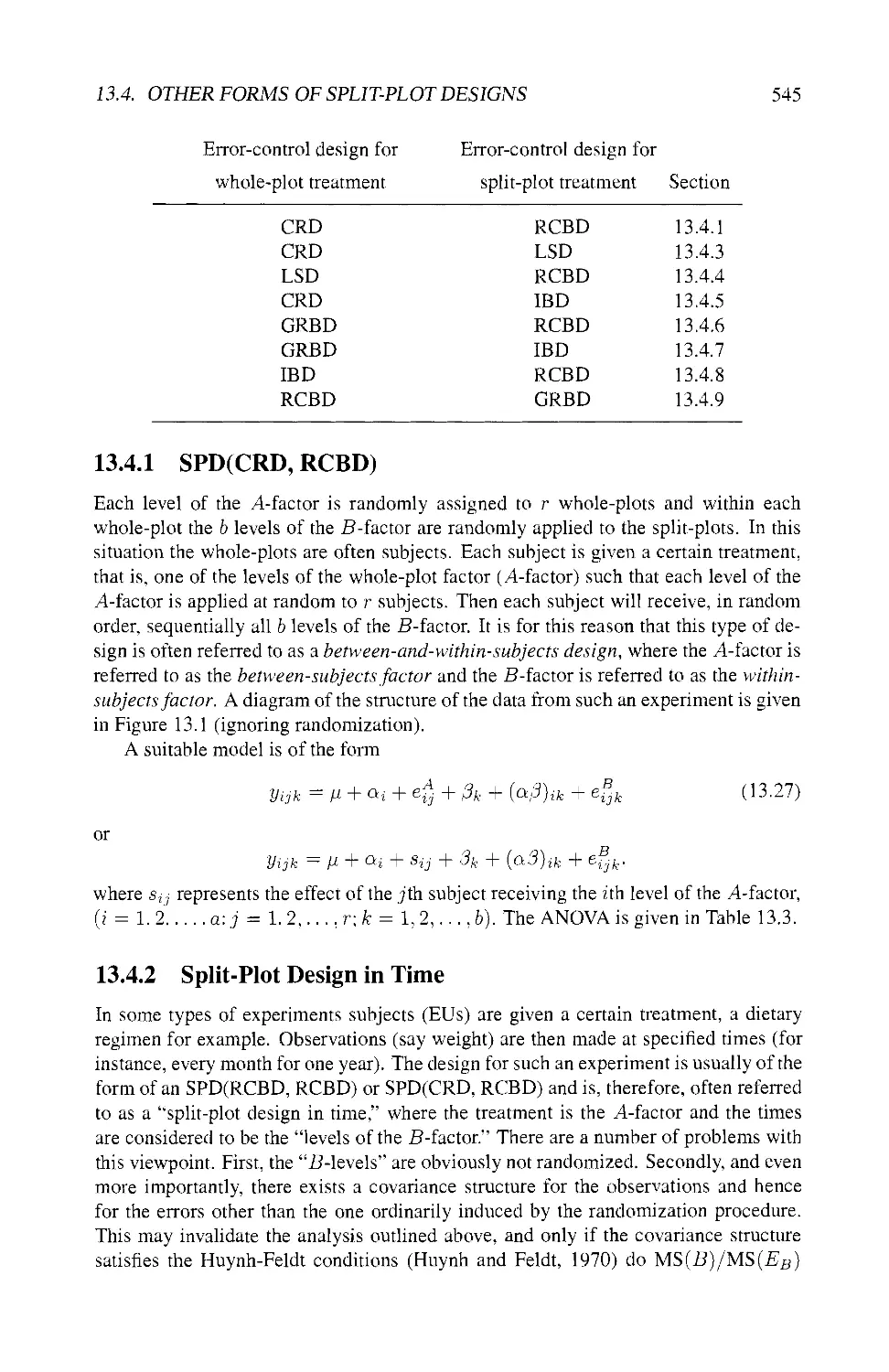
13.4.1 SPD(CRD, RCBD) 545
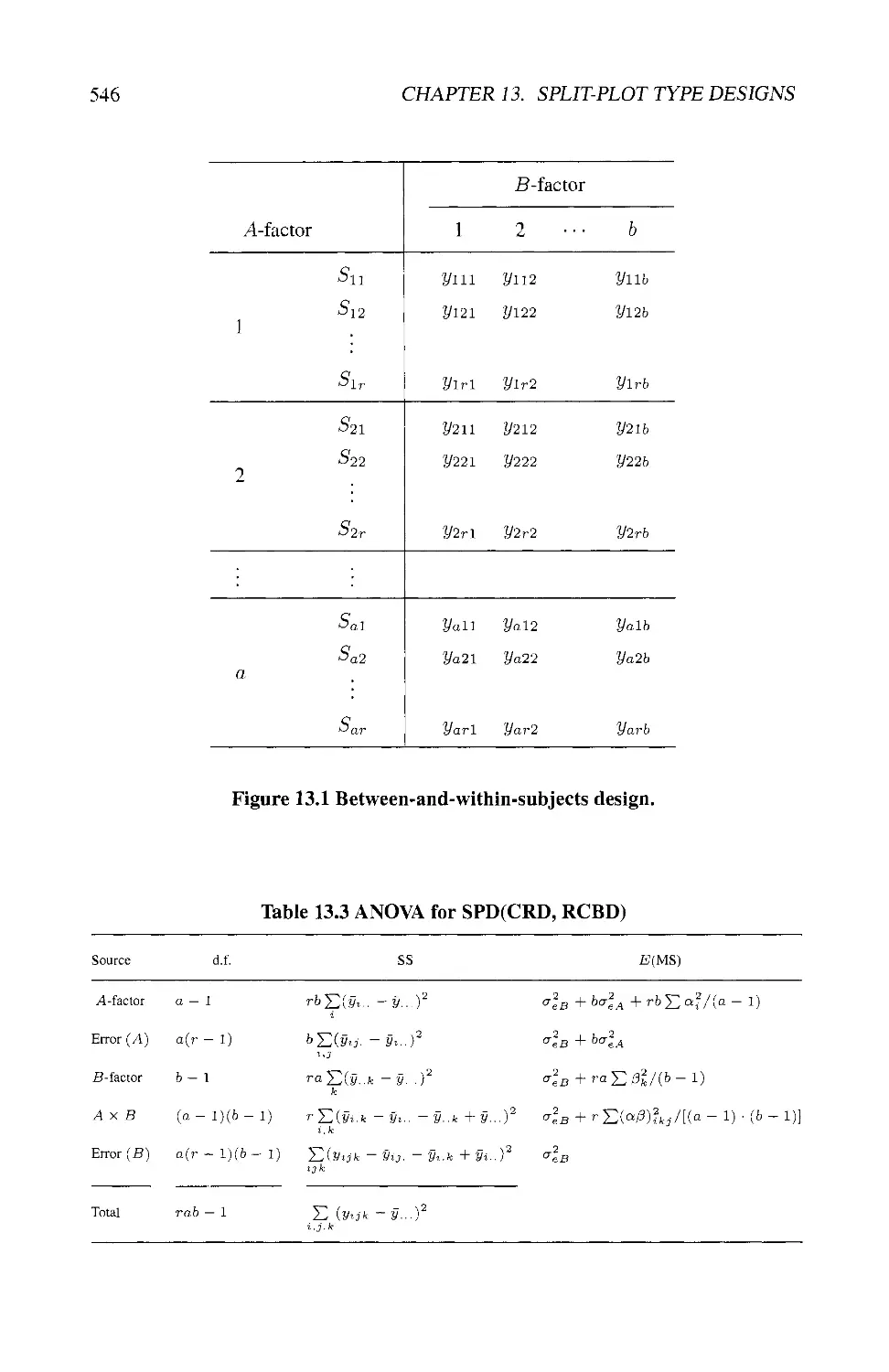
13.4.2 Split-Plot Design in Time 545
13.4.3 SPD(CRD, LSD) 547
13.4.4 SPD(LSD, RCBD) 548
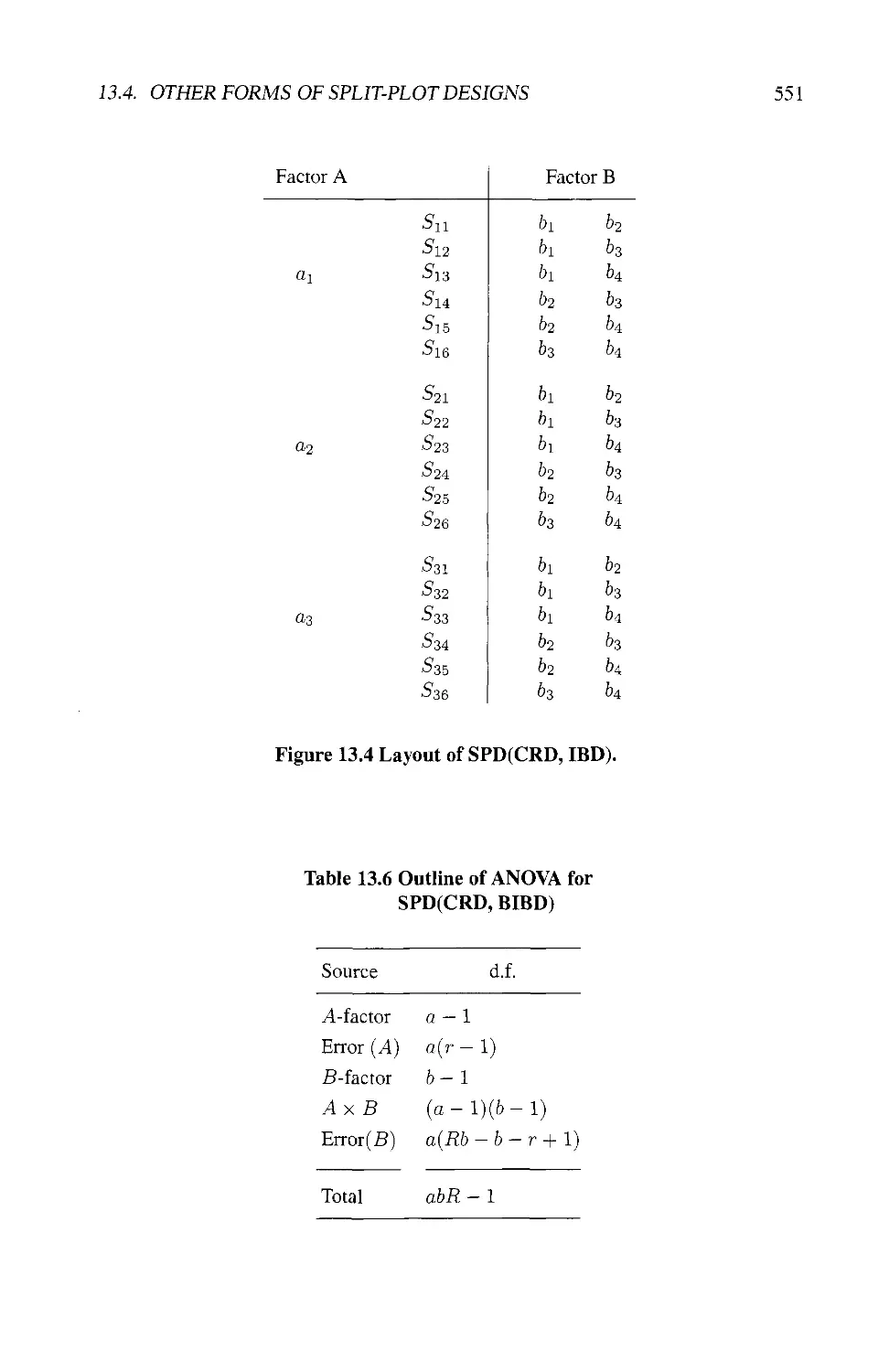
13.4.5 SPD(CRD, IBD) 549
13.4.6 SPD(GRBD, RCBD) 550
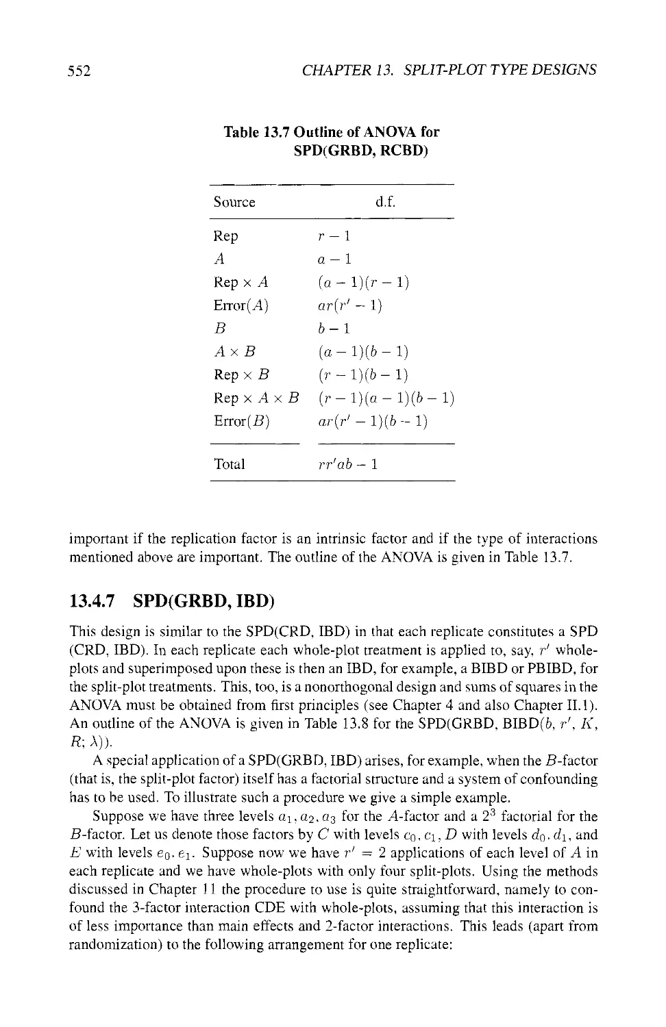
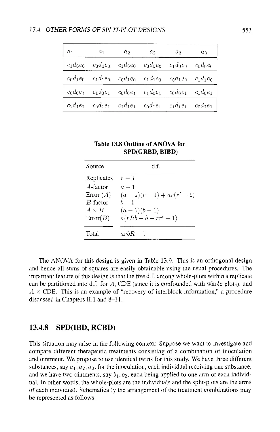
13.4.7 SPD(GRBD, IBD) 552
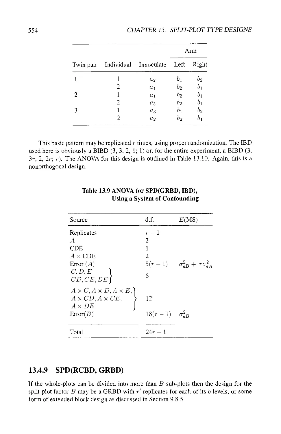
13.4.8 SPD(IBD, RCBD) 553
13.4.9 SPD(RCBD, GRBD) 554
13.4.10 Summary 555
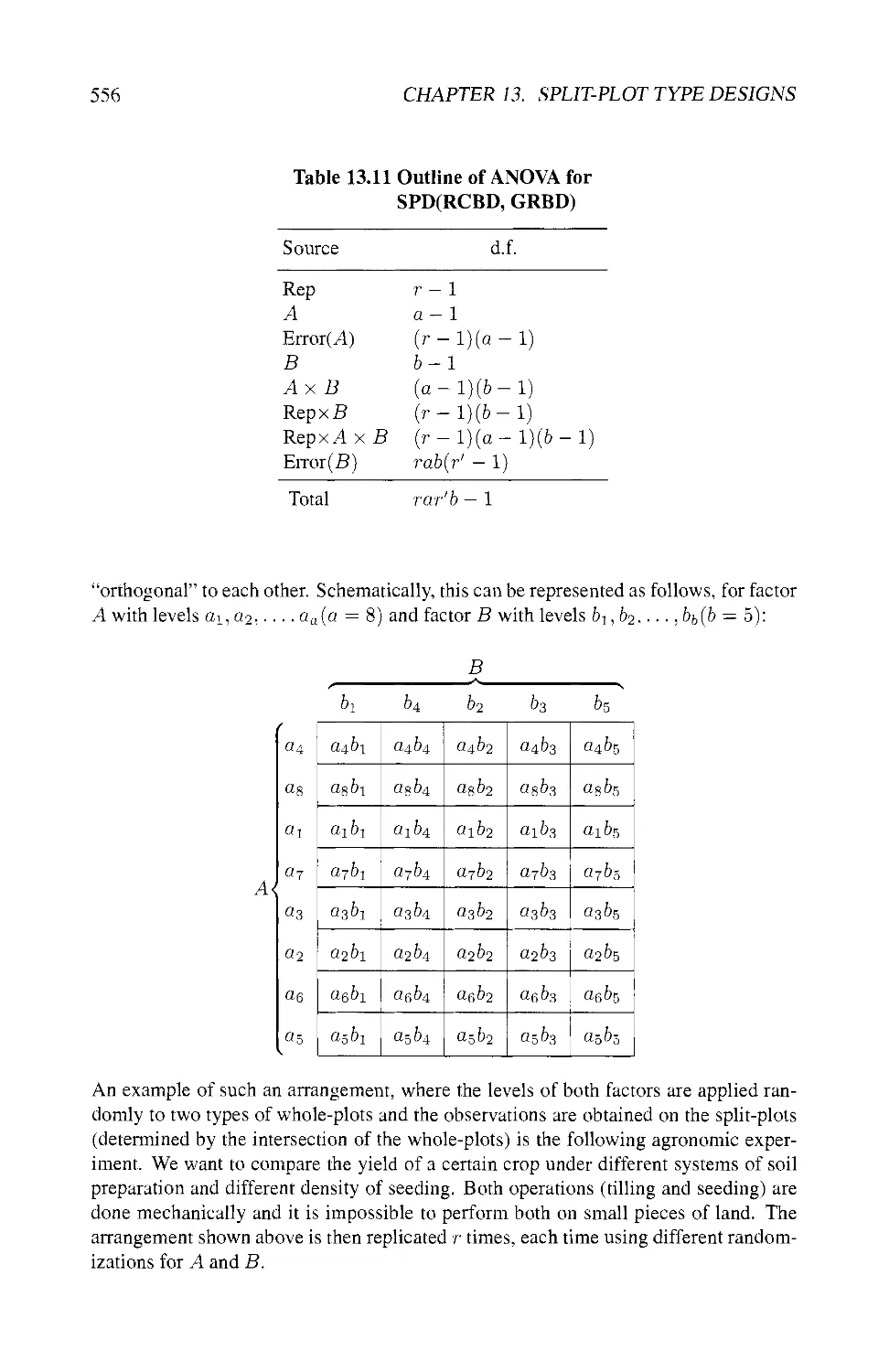
13.5 SPLIT-BLOCK DESIGN 555
13.5.1 The Layout 555
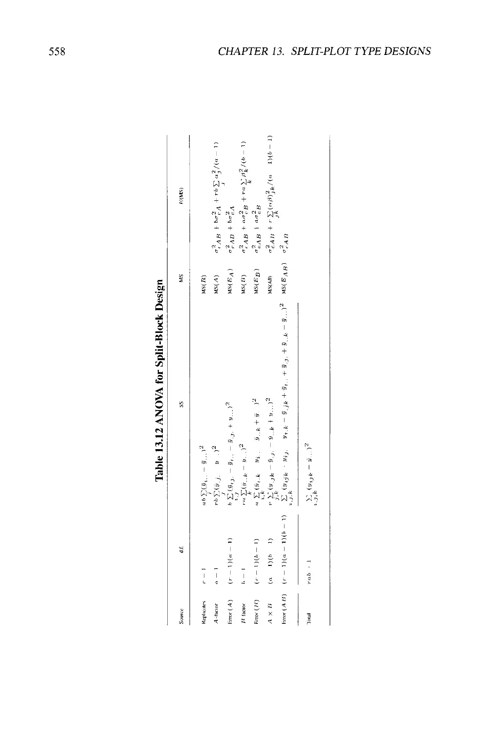
13.5.2 Linear Model and ANOVA 557
13.5.3 Estimating Treatment Contrasts 557
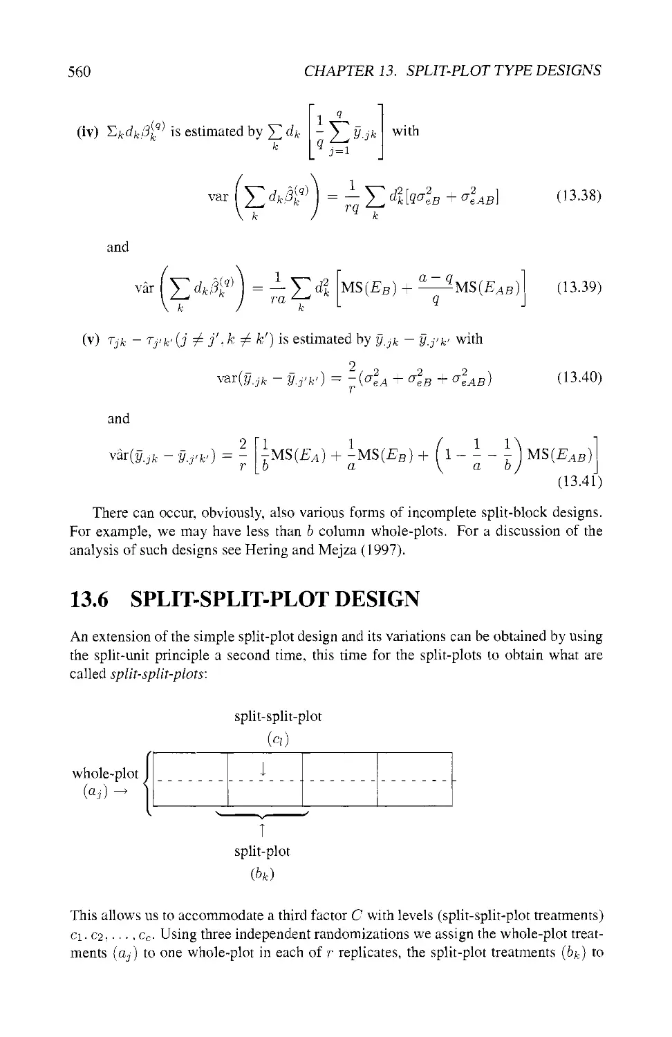
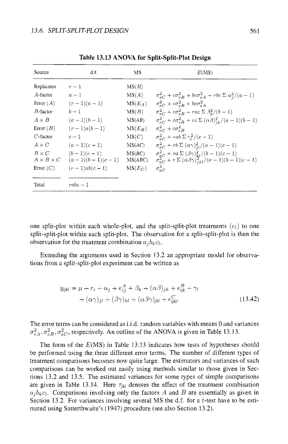
13.6 SPLIT-SPLIT-PLOT DESIGN 560
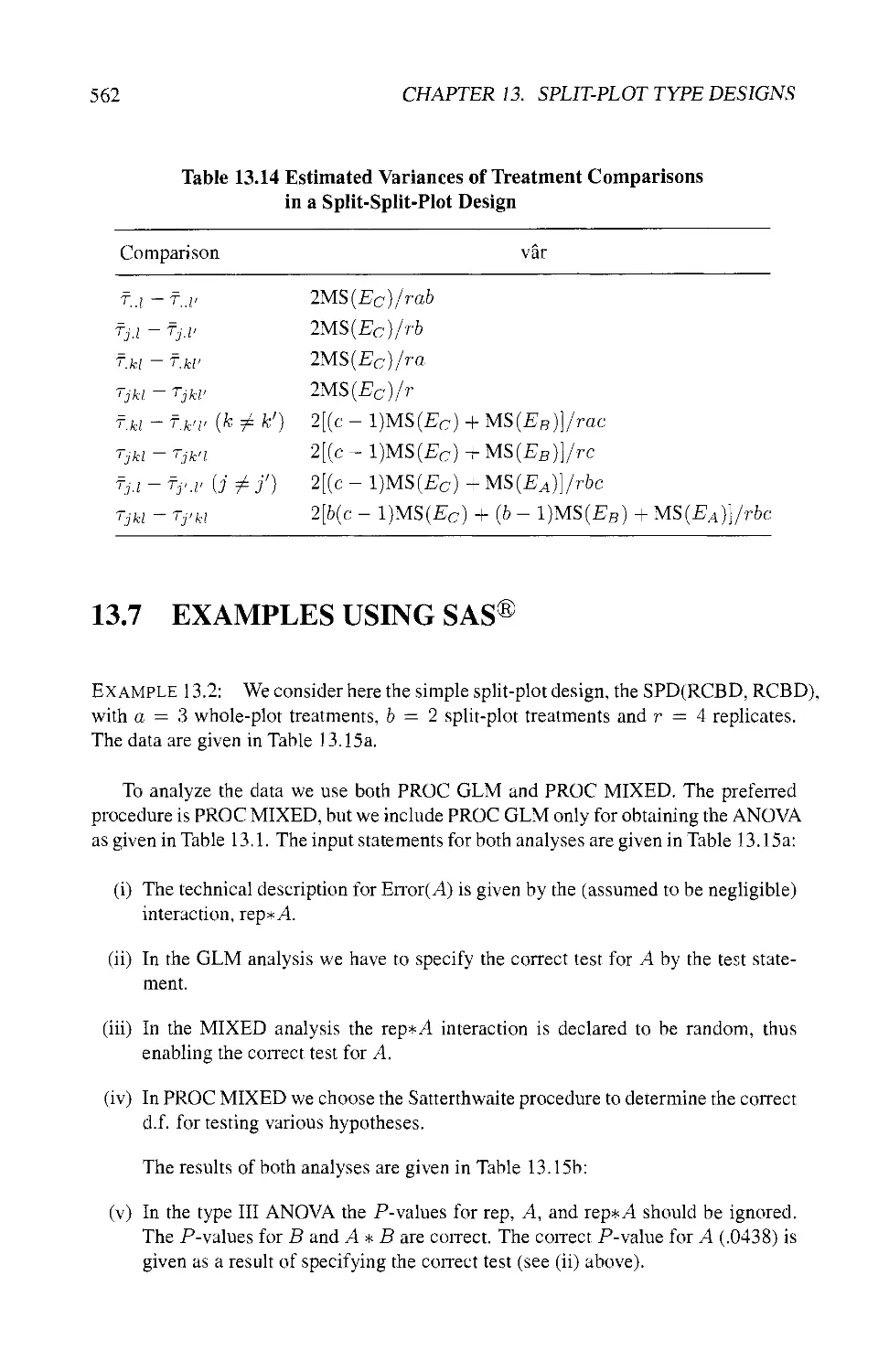
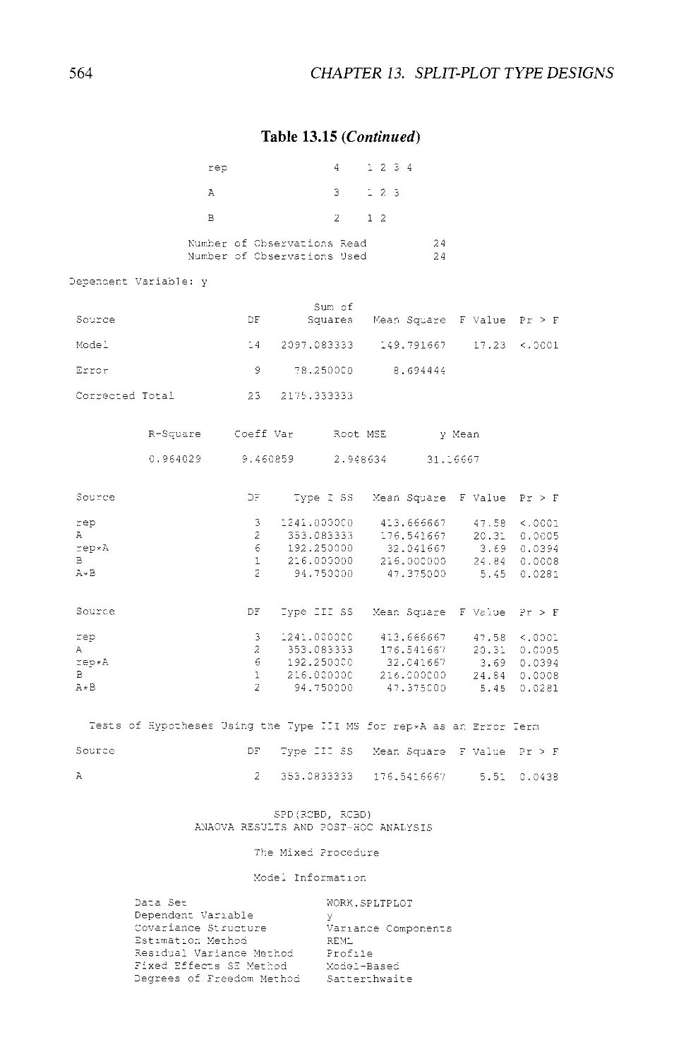
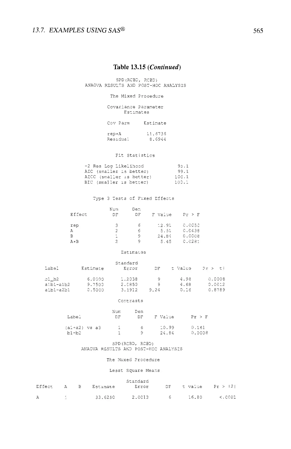
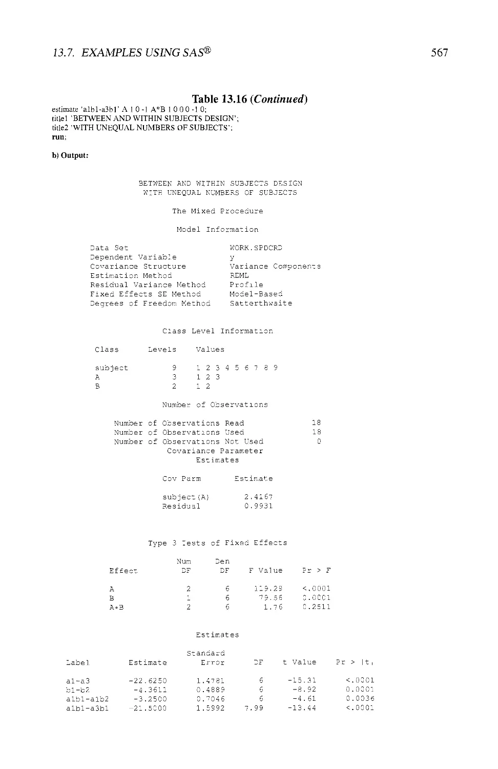
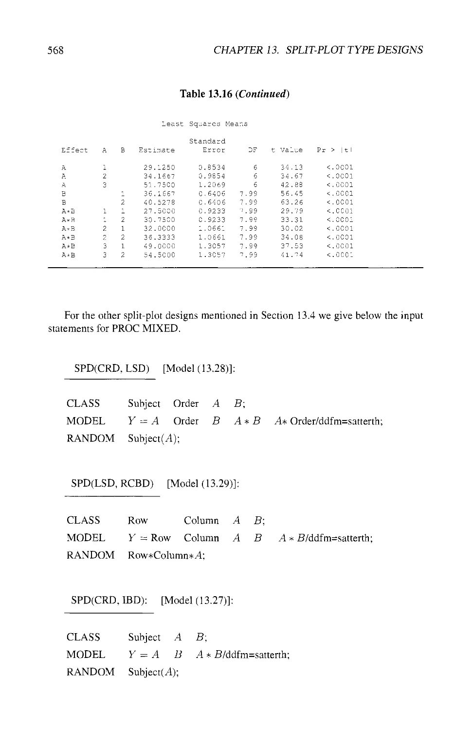
13.7 EXAMPLES USING SAS® 562
13.8 EXERCISES 569
14 Designs with Repeated Measures 573
14.1 INTRODUCTION 573
14.2 METHODS FOR ANALYZING REPEATED MEASURES DATA . . 574
14.2.1 Comparisons at Separate Time Points 574
14.2.2 Use of Summary Measures 575
14.2.3 Trend Analysis 575
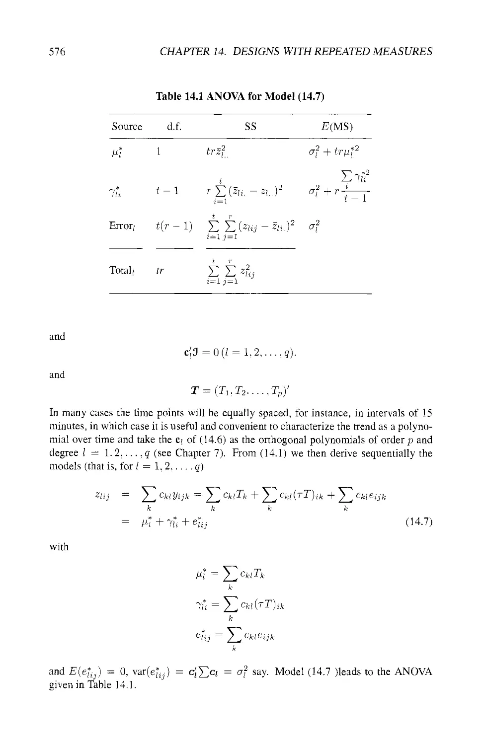
14.2.4 The ANOVA Method 577
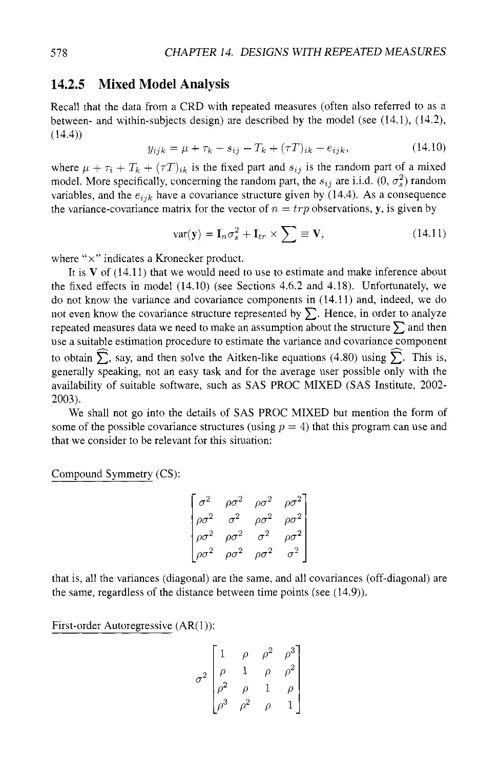
14.2.5 Mixed Model Analysis 578
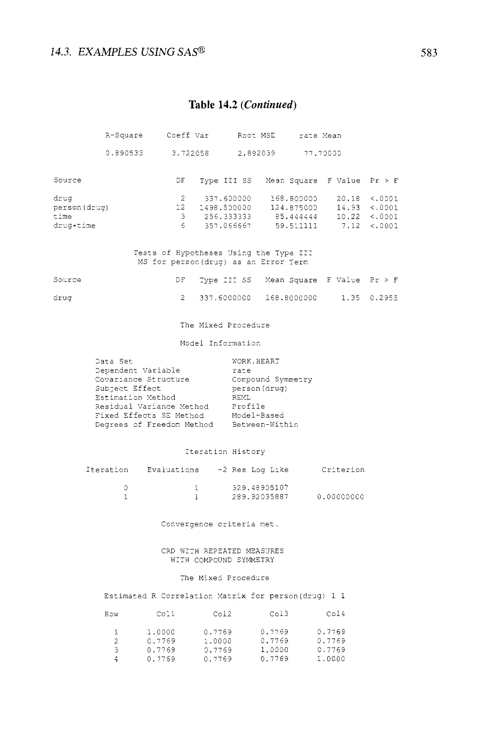
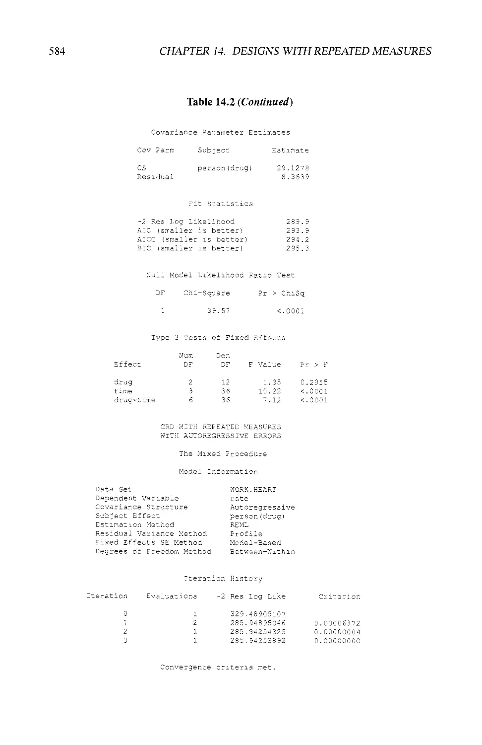
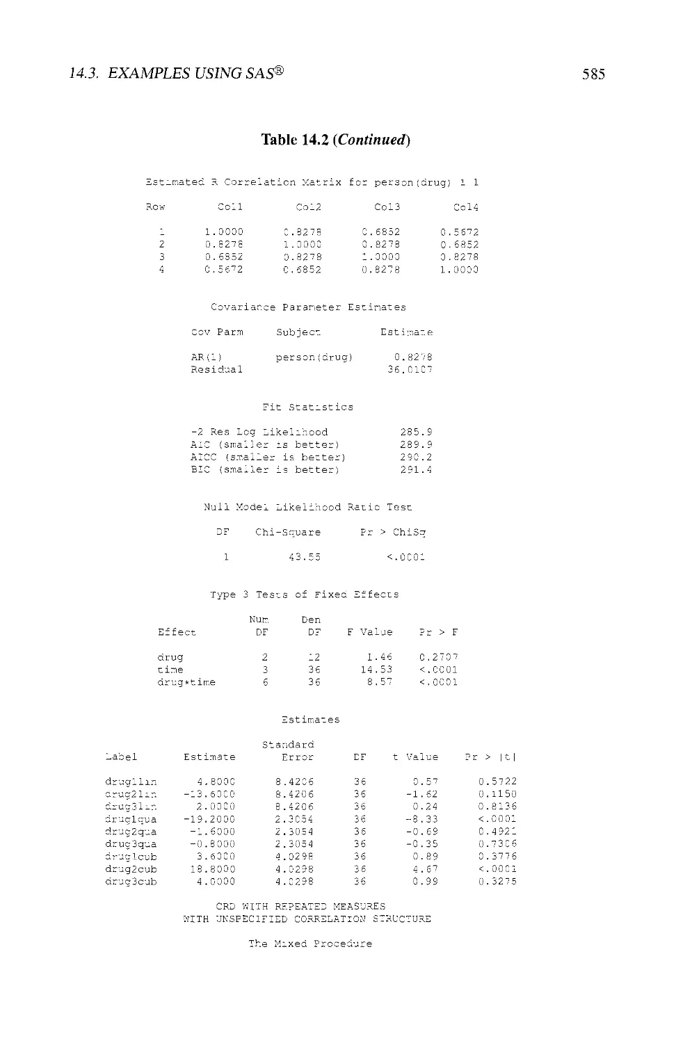
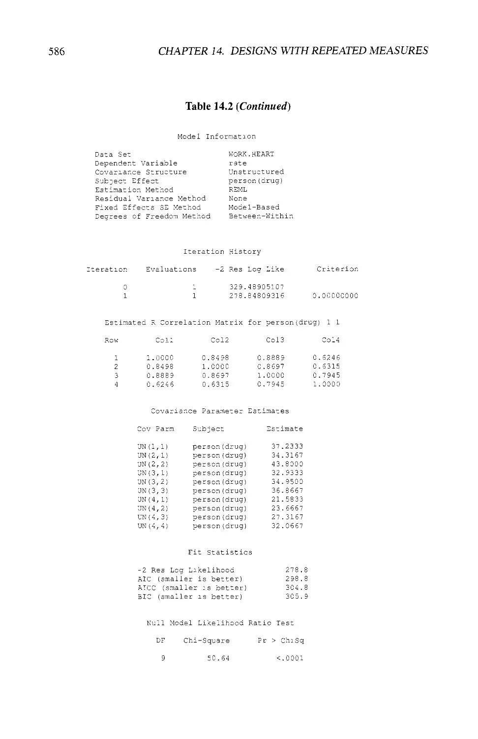
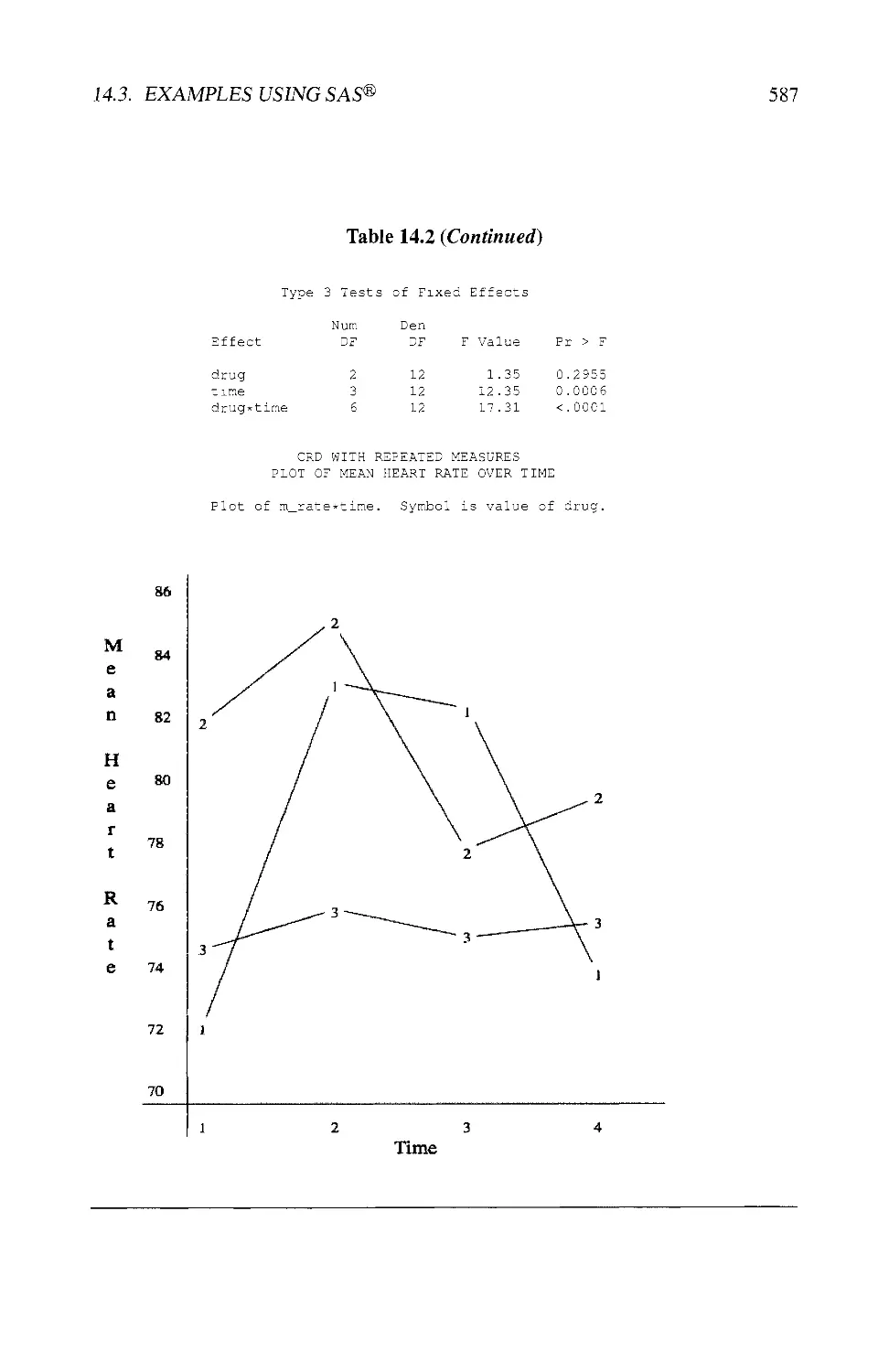
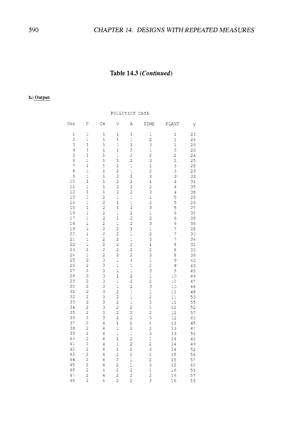
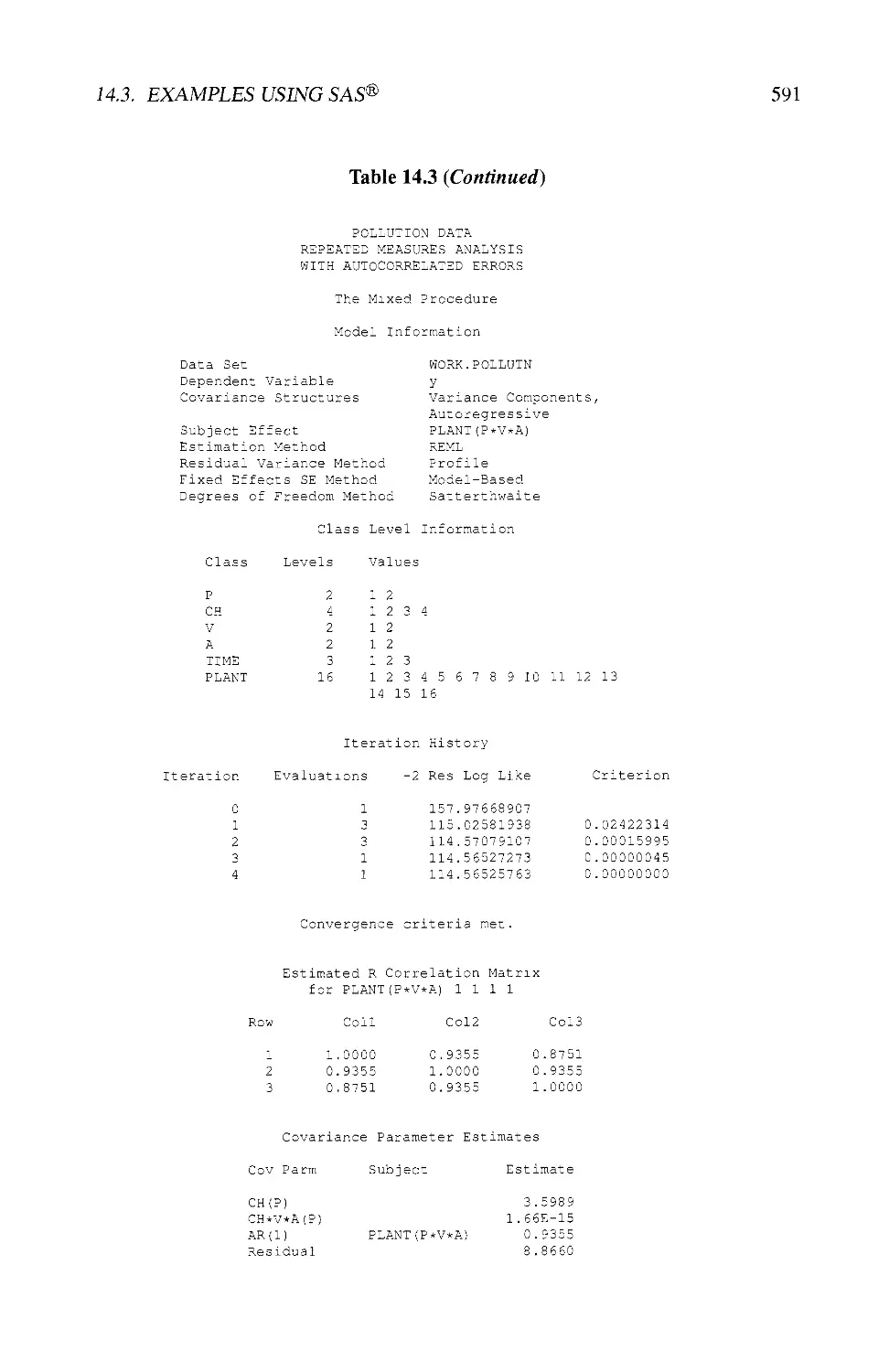
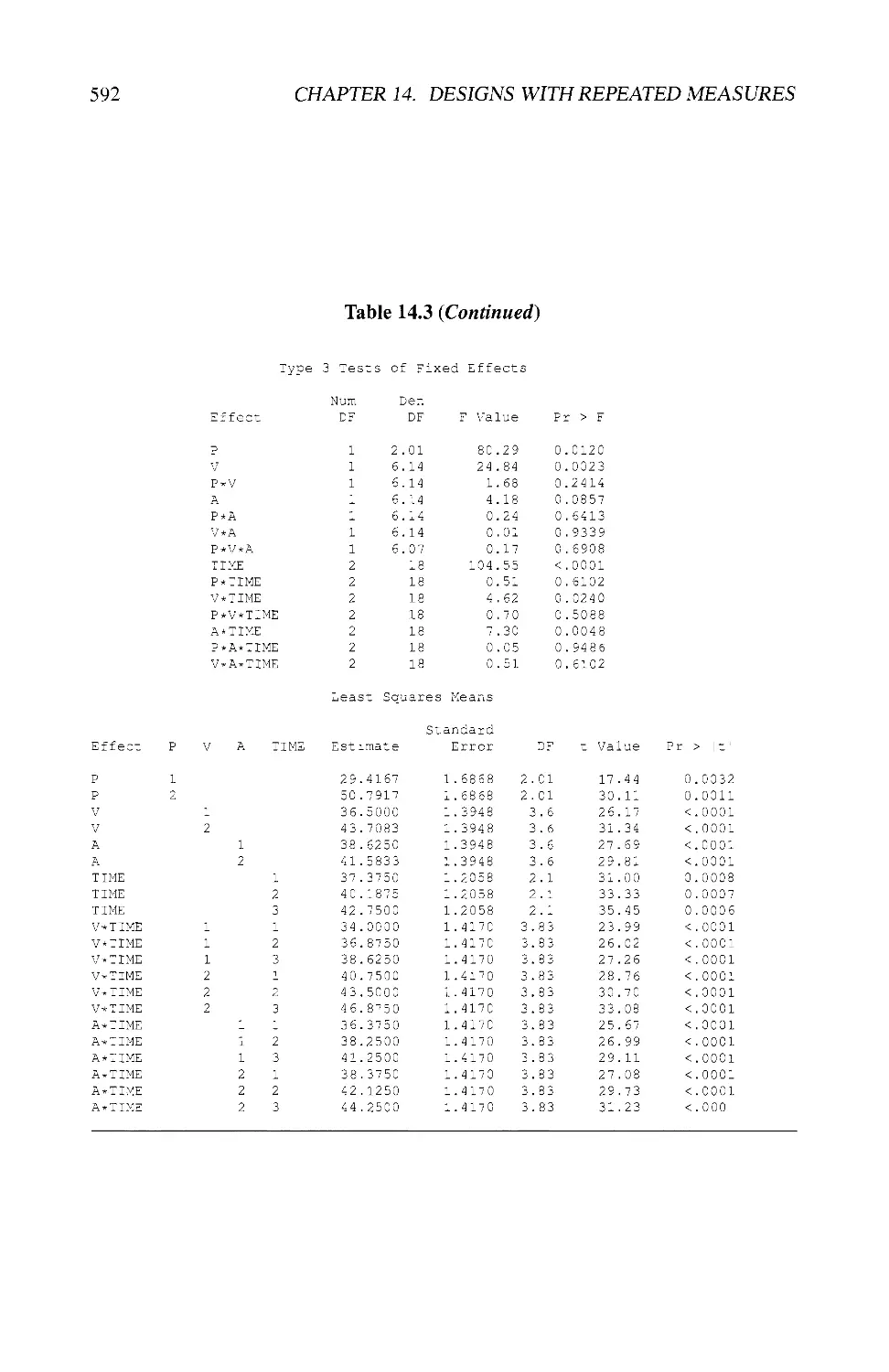
14.3 EXAMPLES USING SAS® 580
14.4 EXERCISES 593
Epilogue 595
CONTENTS xv
Bibliography 597
Abbreviations O1J
Author Index 615
Subject Index 619
This Page Intentionally Left Blank
Preface to the Second Edition
Imagine the following telephone conversation between a statistician (S) and a research
scientist (R). R: "Hello, Mr. Stat, I wonder whether you have just a minute for a quick
statistical question." S: "Usually I do not do statistical consulting over the phone, but
let me see if I can help you. What is the problem?" R: "We are developing new
growth media for industrial producers for growing flower plants. We have three such
media and we use them with four flower varieties. We have five replications for each
combination of medium and flower. We have analyzed the data as a 3 x 4 two-way
classification with five observations per cell. But my graduate assistant has talked to
one of your students and he is now confused about the validity of this analysis. I just
want you to confirm that we have done the right thing." S: "Well, I do not know." R:
"What do you mean, you do not know? You are the expert!" S: "I really need to know
more about how you performed the experiment. For example, how did you prepare the
media that you used in the individual pots? I assume that you grow the flowers in pots
in the greenhouse." R: "Yes, that is right. My graduate assistant simply mixed each
medium in a big container, which we then put in the individual pots." S: "That may be
a problem, because now you may not have any replication." R: "What do you mean,
we have no replication? I just told you that we have five replications." S: "Yes, but...
I think it would be best if you would come to my office for me to explain this to you
and to take a closer look at your experiment." R: "But we have already submitted the
paper for publication." S: "Then why don't you come when you get the reviews back."
Silence. R: "Yes, thank you. I'll do that."
This is, of course, just a fictitious conversation. But many consulting statisticians
have had similar conversations. The aim of this book is to help statisticians as well as
research scientists not only to better understand each other but also to obtain a better
understanding of the intricacies of designing and analyzing experiments It is our hope
that this can be achieved by using the book as a textbook as well as a reference book.
Having used the first edition for several years as a textbook in an MS level class for
statistics students and well-qualified graduate students from other fields relying heavily
on experimental research, I have gained valuable insight into the needs of both types of
students. This has led to some changes and enhancements in the second edition without
giving up the general flavor and philosophy of the book.
Although some readers may feel the book is too theoretical, we strongly believe
that these developments are necessary to understand the basic ideas and principles of
experimental design, to enable students and researchers to pursue ideas of designing
experiments not covered in this book, and to lay the foundation for even more theo-
xvii
xviii PREFACE
retical work as covered, for example, in Volume 2: Advanced Experimental Design.
For the non-statistics student it is not always necessary to understand all the details
leading to important results as long as they develop a certain feel for these results and
appreciate their role and importance in the overall picture. A skillful teacher will be
able to accomplish these aims without compromising the rigor of the development of
the material.
Having said this, I have tried to make the second edition more user-friendly by also
emphasizing the practical aspects of designing and analyzing experiments. I have
considerably expanded Chapter 2 with further discussion of the planning aspects of setting
up an experiment and giving heuristic arguments why the various steps are so
important for a successful experiment. This should appeal to both consulting statisticians and
research scientists.
Other major changes involve the development in Chapter 9, which I consider to be
one of the most important chapters in the book because of the introduction of the notion
of blocking. I spend a great deal of time discussing the different types of blocking
factors and their importance in the overall scheme of setting up, analyzing, and drawing
inference using various forms of block designs. These ideas are then carried over to
Chapter 11, which introduces the basic concepts of factorial treatment structure and
design. I have included a case study, based on an invited presentation at a meeting
of the American Society for Horticultural Science, which discusses in some detail the
role, analysis, and interpretation of various forms of interactions.
The discussion about repeated measures has been moved to a separate chapter
(Chapter 14) to give it more emphasis, as this type of experimentation occurs quite
often. I explain how repeated measures can be paired with any error-control design,
how this leads to a split-plot type structure of the experiment, and how and why the
analysis differs from that of a split-plot experiment.
Finally, I have added to most chapters numerical examples using the statistical
software package SAS® (SAS Institute, Inc. 2002-2003)as a tool to analyze the data.
This should not considered to be a tutorial in SAS, but it should provide some help
to readers of this book about how to analyze similar data from their experiments and
to relate such analyses to the developments, in particular ANOVA tables, given in the
book. In order to preserve space I have omitted some information provided in the usual
SAS output. Also, I should mention that the data are not real, even though some of the
experiments described are, as research scientists are generally not willing to share their
original raw data. The results presented should, therefore, not be interpreted as findings
in a given subject matter area, but rather as illustrations of statistical procedures useful
for analyzing such data. For readers who do not have access to SAS or who prefer to
use other statistical software, the examples should provide some help in setting up the
analyses in their environment. In addition to using SAS as a tool for the analysis from
designed experiments I also show how SAS can be used for randomization procedures
and for constructing certain types of factorial designs.
I hope that the changes and enhancements in the second edition will prove useful
to students, teachers, and researchers. For those who seek a deeper understanding and
further developments of the material presented here I provide references to chapters
and sections in Volume 2 indicated, for short, by II.xx or II.xx.yy, respectively.
An FTP (ftp://ftp.wiley.com/public/sci_tech.med/design_experiments/) for this book
PREFACE xix
will be maintained by wiley.com, which will also contain additional exercises and
solutions to selected exercises.
During the process of thinking about and completing this revision I have received
help from several people. I would like to thank my students and colleagues for pointing
out errors in the first edition and for making suggestions for changes. I am grateful to
Yoon Kim and Ayca Ozol-Godfrey for their help with some computational and
graphical aspects in Chapters 6 and 11. It is difficult to find the right words to express my
profound gratitude to Linda Breeding for her tireless and skillful efforts in producing
the camera-ready manuscript. This has been a monumental and difficult job, and even
during times of despair she found a way to carry on until the work was completed.
Nobody could have done it better. Thank you, Linda. I also would like to thank Jonathan
Duggins, Amy Hendrickson, and Scotland Leman for their expert advice and help with
LaTeX.
Finally, I would like to dedicate this edition to the memory of my co-author and
mentor, Oscar Kempthorne, for his many important contributions to the philosophy,
theory, practice, and teaching of experimental design (for a bibliography, see Hinkel-
mann, 2001).
Klaus Hinkelmann
This Page Intentionally Left Blank
Preface to the First Edition
The subject of the design of experiments has been built up largely by two men, R. A.
Fisher and F Yates. The contributions of R. A. Fisher to mathematical statistics form
a major portion of the subject as we now know it. His contributions to the logic of
the scientific method and of experimentation are no less outstanding, and his book The
Design of Experiments will be a classic of statistical literature. The contributions of
F. Yates to the field of the design of experiments are such that nearly all the complex
designs of value were first put forward by him in a series of papers since 1932. Both
Fisher and Yates have also made indirect contributions through the staff of the statistical
department of Rothamsted Experimental Station, since its founding in 1920. It is not
surprising that the contributions originated from Rothamsted, because Rothamsted was
probably the first place in the world to incorporate a statistical department as a regular
part of its research staff, and the design of experiments is a subject that must grow
through stimulation by the needs of the experimental sciences.
This quotation from the preface of Design and Analysis of Experiments by Kemp-
thorne (1952) affirms our recognition of the enormous and path-breaking contributions
made by these two men to the field of experimental design and experimentation in
general. Even though most of their ideas originated in connection with agricultural or
genetic experiments, the resulting principles and designs have found wide applicability
in all areas of scientific investigations as well as in many areas of industrial production
and development.
Because of the widespread use and increasing importance of experimental design,
it is essential that students and users obtain a firm understanding of the philosophical
basis and of the principles of experimental design as well as a broad knowledge of
available designs together with their assumptions, their construction, their applicability,
and their analysis. These topics then are the subject of this book which will appear in
two volumes.
Volume I is a general introduction to the subject laying the foundation for the
development of various aspects of experimental design. In it we describe and discuss many
of the commonly used designs and their analyses. We return to some of these designs
and introduce other designs in Volume II at a more technical and mathematically more
advanced level.
With respect to the present volume, Chapters 1 through 5 describe in some detail
the philosophical foundation and the mathematical-statistical framework for our
approach to the discussion of experimental design. We put the notion of and the necessity
for intervention studies, the main topic of this book, squarely into the context of the
xxi
xxii PREFACE
scientific method. We develop and draw a sharp distinction between observational and
intervention studies, a theme to which we return at various places throughout the book,
in particular in connection with the analysis of data. Much of the analysis is based on
the theory of linear models. A thorough discussion of linear models theory is given in
Chapter 4. Our major aim here is to provide the reader with the basic tools to
understand and develop the analysis of data from intervention studies of the sort discussed
in this book.
Although linear models play a fundamental role we stress the fact that they do
not exist in and of themselves but that they evolve from very basic principles and in
the context of the experimental situation at hand. Indeed, in Chapter 2 we argue that
many facets are involved in advancing from a research idea or question to a designed
experiment which permits the investigator to draw valid conclusions. Some of these
facets are of a statistical nature such as developing an appropriate experimental design,
developing an appropriate model, and carrying out an appropriate analysis, and they
are the subject of this book. But it is important, we assert, to always keep in mind that
statisticians and subject-matter scientists have to combine their knowledge to develop
an experimental protocol according to sound principles of both fields.
We have alluded earlier to the impact that R. A. Fisher had on the development
of the field of experimental design. One of his contributions concerning the design of
experiments is the use of randomization. In Chapter 5, as well as in following chapters,
we discuss the general idea and then apply it to specific designs. It forms the basis of
the analysis for all intervention studies.
Beginning with Chapter 6 we develop from first principles various error-control
designs. We start with the completely randomized design (Chapter 6) as the simplest form
of error-control design and then move on to more complex error-control designs such
as randomized block designs (Chapter 9), Latin square type designs (Chapter 10) and
split-plot type designs (Chapter 13). For each design we derive linear models and the
associated analyses, mainly in the form of analyses of variance. Other forms of
analysis such as estimating and testing treatment contrasts are dealt with in Chapter 7. And
further reduction of experimental error through the use of supplementary information
is described in Chapter 8.
The notion of treatment design is introduced in Chapter 11 when we discuss
factorial experiments. Particular attention is paid to experiments involving factors with two
and three levels. This serves as an introduction to the vast opportunities and techniques
that are available for such type of experimentation. We emphasize in particular how
treatment designs can be combined with or embedded in error-control designs in the
form of systems of confounding.
In Chapter 12 we touch briefly on a different form of experiment designs: response
surface and mixture designs. It serves mainly to point out the difference between
comparative and absolute experiments, but it also serves to show how error-control designs
and treatment designs can be applied towards the construction of response surface
designs.
Although many experiments can be conducted using the designs discussed here and
in Volume II, there are many others for which special designs need to be constructed.
It is our aim here to lay the foundation for such work by discussing in detail the major
principles of experimental design, such as randomization, blocking (in particular in-
PREFACE xxiii
complete blocks), the Latin square principle, the split-unit principle, and the notion of
factorial treatment structure.
The relationship of the present two volumes to the book Design and Analysis of
Experiments by O. Kempthorne published in 1952 merits some discussion. Very much
is common. We have felt it absolutely necessary to add a long chapter on the
process of science, discussing our perception of observation theory in science, the role of
experiments, the role of data analysis, and the introduction of ideas of probability as
related to relative frequency in a defined population of repetitions. The presentation
of least squares and the general linear hypothesis needed large improvement. We have
based most of the data analysis and inference on randomization analysis, expanding
and formalizing the presentation. The remainder of the presentation in the present two
volumes is a considerable expansion and rearrangement of standard material of the
1952 book taking many of the developments during the last 40 years into account.
The organization and presentation of the material has evolved over a number of
years of teaching the subject to graduate students in statistics. Volume I is intended
as a textbook for a one-semester course for first year graduate students. To make the
course effective, the students should have been exposed to a fairly rigorous course
in statistical methods. They should be familiar with the basic principles of statistical
inference and with the rudimentary ideas of analysis of variance and regression, i.e.,
they should have some understanding of and appreciation for linear models and their
role in statistical inference.
The book contains more material than can be taught reasonably in one semester, and
hence a selection of topics will have to be made. This will depend to some extent on the
students' background and preparation. One suggestion is to skip some details and omit
certain parts in individual chapters, Another is to omit much of Chapter 4 and Chapter 7
and omit all of Chapter 12 (at Virginia Tech, for example, there exists a concurrent
course in the theory of linear models covering the material in Chapter 4, most of the
material in Chapter 7 will have been covered in a course on applied statistics, and
there exists a separate course for response surface designs). At any rate, Chapters 6
through 13 are fairly self-contained except that frequent reference is made to results in
Chapter 4 for a better understanding of the underlying principles.
The reader will notice that no numerical examples are given throughout the text.
It is assumed that the reader is familiar with mathematical notation and does not have
any difficulty with reading and handling formulas. There is no emphasis at all on
calculations. Instead, we provide some guidance on how to use available statistical
software. This attempt is, however, rather limited in that we refer only to SAS as an
example of available software packages, and even that is by necessity not complete.
A thorough knowledge of the material in Volume I is a prerequisite for
understanding Volume II. As mentioned before, the presentation of the material in Volume II is
more technical and hence suited for a more advanced course in experimental design.
It contains more than enough material for another one-semester course. In addition,
Volume II is intended to serve as a reference book on many topics in experimental
design.
Many people have contributed to this book in different ways. Foremost among them
are our students who have been exposed to this material over the years. We thank them
for their questions and comments. K. H. would like to thank Virginia Tech for granting
xxiv PREFACE
him study-research leaves and the Departments of Statistics at the University of New
South Wales and Iowa State University for providing him with support, facilities, and a
congenial atmosphere in which to work. O. K. is grateful to Iowa State University for
providing more than 40 years of stimulating environment and association with many
graduate students of high ability. We thank Yoon Kim and Sungsue Rheem for help
with the simulations for the randomization analyses, and Markus Hiittmann and Sandra
Schlafke for extensive help with the preparation of the index. And finally, we express
our deep appreciation and gratitude to Linda Breeding and Ginger Wenzlik for their
expert typing and word-processing.
Klaus Hinkelmann
Oscar Kempthorne
CHAPTER 1
The Processes of Science
1.1 INTRODUCTION
In order to understand the role of statistics, generally, and the role of design of
experiments in particular, it is useful to attempt to characterize the processes of science and
technology. All science and technology starts with questions or problems. The grand
aim is to develop a model which will describe adequately, that is, accurately, the past,
present, and future of the universe. Obviously, if we are to describe the future, we must
have a model that incorporates development over time—that is, a dynamic model, and
a model that predicts what alterations will be brought about by interventional acts, such
as drug therapy, reducing money supply, or supplying a nation with armaments, to give
widely disparate examples.
1.1.1 Observations in Science
The foundation of all science is, obviously, observation. This, which we all do every
waking minute of our lives, would seem to be a very simple matter, with a logic that
is entirely clear. It is not clear from several points of view. Curiously enough, it
is not discussed, it seems by philosophers of knowledge. It is obvious that animals
make observations—all one has to do is to try to catch a rabbit. It observes that it
is being chased and takes evasive action. This is, presumably, an instinct bred into
rabbits by the evolutionary process. In science, a reaction to a portion of the world is
an observation only if that reaction can be recorded, perhaps only in memory, or better,
of course, by actual physical recording. To do this requires a language and descriptive
terms. It is necessary that an observation can be described in terms that have some
meaning to others. The development of a language for this purpose, a language that is
effective, is a process of science that continues. We need only look at the development
of the language of biology. This field is full of names of things, and indeed, one of
the great difficulties of the field is to learn the naming that has been developed in the
past, a task that becomes more and more difficult as processes of observation are being
developed, one can almost say, day by day. Many parts of the journal Science of today
are unreadable except by experts and would be unreadable for the experts of decades
1
2 CHAPTER I. THE PROCESSES OF SCIENCE
ago. The development of this type of descriptive language proceeds with care, and
with the discipline of the area of study. A descriptive term does not receive validation
until it is agreed on and can be confirmed by any observer who follows the prescribed
protocol of observation and has been educated in the use of the descriptive terms. This
is no more than a cliche in physical and biological science and one might be led to the
view that it is not worth stating. But when we turn to any aspect of human mental status
or mental behavior, the "obvious" cliche becomes critical. One merely has to look at
the nosology that occurs in psychiatry to see the problem. This is not to imply that
workers in that area are dolts—the area is remarkably difficult because of the problem
of validation of observation.
A second point about observation is that it is by its very nature incomplete. One
observes, one says, a robin outside one's window. Humanity uses this mode of
expression and it has served it well. But one does not observe the whole of the phenomenon.
Just recall the commonplace interchange. Person A says "I see a robin." Person B says,
"Yes, I see it too. Did you notice that it has a gray bar on its wing tips?" Person A says,
"No, I did not notice that, but now that you mention it, I do see it." Person A's
observation was incomplete relative to B's observation. Obviously, there can be person C, who
sees more. Also, obviously, observation is not an innate ability; it is one which may
require high "professional" training—even in areas that use no more than the ordinary
unaided human eye. For the naturalist of the sixteenth century, for the ordinary citizen
naturalist, and for the person who has received two years of training, observation is not
at all the same. If we adjoin the obvious massive development of observational
processes, with physical devices, for instance, observing in infrared light, observing with
an electron microscope, and so on, there is not an elemental activity which we can call
"making observation."
Another aspect, which is much more subtle, is that the process of observation may
or may not have an effect on what is being observed, with the elementary consequence
that one simply cannot observe the status of an object of observation. There are, of
course, elementary techniques for combating this, as in the use of blinds to observe
birds, or of walls that have one-way vision. But when one considers observing, or
trying to observe, the mental state of a human and leaving aside the possibility of
observing what one thinks to be physical correlates of mental status, one has to talk to
the human and ask questions and then it is not at all clear what the status of ensuing
conversation by the human being observed is. Turning aside from an obviously
fantastically difficult area, we saw a revolution in physics at the beginning of the twentieth
century with the realization that one could not look at a particle except by shooting
another particle at it and getting a collision. This type of situation led to the famous
Heisenberg uncertainty principle in an area for which it was thought previously that
one could observe without interfering with the object observed. This phenomenon has
huge consequences as any modern physicist knows. It has, also, huge consequences
with respect to epistemology.
1.1.2 Two Types of Observations
We leave this discussion. For the purposes of our discussion here, we assume that there
is a validated process of observation that has no effect on the object being observed. We
1.1. INTRODUCTION 3
must, however, discuss a major point. There are fundamentally, it seems, two types of
observation. The first consists of placing an observation of an object of observation in a
class: for instance, the flower being observed is pink or has pinnate leaves. In most
circumstances, there is no doubt of the recorded observation (though one can be doubtful,
e.g., on a color designation). In other cases, the result of the observation is uncertain;
we merely have to imagine being given sequentially with repetition unknown to the
observer of a set of colored blocks that do not have strongly distinguishable colors. One
will find that one's observation of a block will give different results in repetitions, over
which one is fairly sure that color has not changed. In such cases, one has no recourse
but to use a probability model to the effect that, in repetitions that are unconnected in a
known way, there will be a frequency distribution of observational outcomes. We shall
not be concerned with this at present. The second type of observation, which
permeates quantitative science, is the measurement of a numerical magnitude, for example,
the weight of a piece of rock, which one is confident does not change. In this case,
there is always an error and an imprecision of measurement. The nature of the error
and of the imprecision is again representable by some frequency distribution of results.
This type of problem permeates, of course, the physical sciences, and increasingly so,
as the sought after observation, such as weight, becomes smaller and smaller.
We hope that we have given a useful discussion of observation, though elementary
and potentially highly obscure at a philosophical level. We take comfort in the fact that
even if the process of observation is quite unclear (as it is at a fundamental level), the
world of science is permeated with interpersonally validated observation.
1.1.3 From Observation to Law
Our writing here is aimed at constructing a useful model of what happens in science. It
seems clear that the beginning of science is observation and description. It also seems
clear that this is still a critical feature of science. This observation process requires no
theory. It is interesting in this connection, to look at what Darwin (1809-1882) did in
the voyage of the Beagle. He was, for his age, a very remarkable observer. The point
of expressing the above views is that it is sometimes said that the mere collection of
observations has to be based on a theory, a concept to which we shall turn. If one wishes
to state that even the simplest observation is based on the informal theory that one's
observation process obtained an attribute of what is observed and not of the observer,
one cannot object. Apart from this, much observation has been generated not by any
theory but by curiosity, an attribute that one observes in animals. It is true, of course,
that, very often, observation is initiated by a question or by a problem situation. One
could say that curiosity is the result of a question, but this seems to be mere playing of a
verbal game. Obviously, our presentation is Baconian and we quote his first Aphorism
(Spedding et al, Vol. I, 1861, p. 241):
Homo, Naturae minister et interpres, tantum facit et intelligit quantum de Naturae
ordine re vel mente observaverit, nee amplius scit aut potest.
for in its translation (Spedding et al., Vol. VIII, 1863, p. 67):
Man, being the servant and interpreter of Nature, can do and understand so much
and so much only as he has observed in fact or thought of the course of nature:
4 CHAPTER 1. THE PROCESSES OF SCIENCE
beyond this he neither knows anything nor can do anything.
However, we cannot accept the full Baconian prescription as given by his
successive aphorisms.
It is obvious that science does not consist merely of a collection of, shall we say,
interpersonally validated observations. What comes next? Rather clearly, it is the
organization of such observations—let us call them facts, into sets of related facts. Let
us suppose that our observations are categorical. We observe trees. This consists of
noting, with our developed language, that there are trees that keep their leaves through
the winter and those that do not. We deliberately take simple examples that even the
proverbial man-in-the-street can appreciate. So this part of our observation places the
objects of observation into one of an exhaustible polytomy. Let us call the classes
of one polytomy ai, a2. ■ ■ ■ ■ ar and of the second, 3i,02, • • •, 0S. We look at our
observations and we see that in our observations every object which was 0-3 is 02-
Obviously, a generalization is suggested: every object that is Q3 is 02- We have a
suggestion of a "law." The word "law" is used in our language in many senses and
even in science it is used in at least two senses. A "law" states that something must
occur. The Creator has decreed so. This is one sense. Another sense, which is really
quite different, is that a law is an empirical generalization. A hoary and false example
is: I have seen 10 swans and they were all white. So I infer (falsely) the "law" that
all swans are white. This example leads, of course, into the problem of induction, on
which libraries of books have been written, without resolution.
We then see a very curious thing happening, the development of a theory. From the
"law" obtained as a suggested empirical generalization, we convert our generalization
into a "law" of Nature, something that must necessarily be the case. When we do this,
we are beginning to make a theory. This is, however, just one part of the construction
of a theory. It is the absence of a role for theory that has been the main criticism of the
prescription of Bacon (1560-1626).
It is informative, here, to bring in the work of Kepler (1571-1630). The
observations were the positions of planets at different times of the year. The contribution of
Kepler was to analyze the data and to show that the path of each planet was an ellipse,
with the sun as focus, and other aspects that are given in his famous three laws. It is
also informative to recall the work of Mendel (1822-1884) in biology. The crossing of
types X and Y gave offspring of type Z, say, and then the crossing of these offspring
gave an array of offspring which had the appearance that j were X, \ were Z, and
I were Y. Interestingly, this appears to be the first case of occurrence of a validated
probability model in science (apart from mere gambling).
In the one case, we have Kepler's laws and, in the other case, Mendel's laws. Now,
we have to raise the hard question. Are these laws as empirical generalizations or are
these laws that tell us what must happen? Are they built into Nature by the Creators?
Our answer is obvious, we think: they are merely empirical generalizations.
How then do we get to a theory? The process is rather simple, though rarely ex-
posited in our experience. At first, we have what may be called "naive" laws, merely
empirical generalizations. But we want an explanation. We are in a morass and we
shall have to discuss the idea of "explanation."
1.2. DEVELOPMENT OF THEORY 5
1.2 DEVELOPMENT OF THEORY
The suggestion of Bacon that all we need to do is make observations has been rather
uniformly criticized in the ensuing four centuries or so. We suggest that the criticism
has not been entirely justified. One question is: what observations should one make?
Obviously, we could suggest that the way to understand the universe is to have millions
of humans observing—observing, only observing. It is obvious, indeed, that such a
program would lead to an incredible mass of observational facts. The first missing
ingredient in the Baconian prescription is given by the question: "What are we to
do with all the facts that are obtained?" This question is interesting to the field of
statistics, and eventually, to the whole of science, because it tells us that we have to
do "data analysis." It is interesting and curious that this is a term used to denote an
activity that has been pursued by humans from the beginning of time, but which has
been popularized since the 1960s in all discussions of statistics.
It is surely pretentious to think that one can encapsulate the efforts of humanity to
understand the universe in a few printed pages. But it is useful, we think, to attempt to
present a broad picture that captures essential features of the human efforts that have
been made. Interestingly, this is, of course, a problem of data analysis of its own. We
can look over the history of science. None of us can do this completely, but perhaps
we can see a general pattern which is not misleading.
1.2.1 The Basic Syllogism
The beginning is surely observation of entities that have some degree of permanence
in time, usually entities that one can, so to speak "hold in one's hand," literally or
metaphorically. These are looked at and classified. This is just Aristotelian
classification. From this came laws as empirical generalizations such as "All A are B," or "All
entities which have attributes a and d have attribute 7." It is interesting that this led to
the basic syllogism: (i) All entities with a have 0; (ii) entity E has q; therefore, (iii)
entity E has j3. We find this presented as a mode of deduction, and this matter needs
discussion. This syllogism is used widely and essentially in mathematical reasoning,
and without it, the possibility of the sort of mathematics we do would be impossible.
For instance, every triangle has the property that the sum of its interior angles is 180°:
here is a triangle; therefore, the sum of its interior angles is 180°. From where do
we get the first part of the syllogism? The answer is simple. We prove it! But then
we have to ask: "What do you mean by that?" What does it mean to say: "We prove
it"? The answer is given in simple and not misleading form. We have defined
"triangle." We have developed modes of deduction that we accept as constituting proof.
This whole process is very subtle. Just how subtle it is can be seen from the
developments of mathematics of the past two centuries or so. We see students in high school
trying to write proofs in geometry. We see ourselves writing proofs that we judge to
be complete. But we later see that our proofs are incorrect or incomplete. We see in
the history of mathematics incorrect proofs by great mathematicians. We see proofs in
which a questionable syllogism has been used with total unawareness that it has been
used. The curious outcome of this phenomenon is that a proof of a mathematical
theorem is a sequence of statements, in mathematical form, developed from axioms that
6 CHAPTER 1. THE PROCESSES OF SCIENCE
are unquestionable, that the world of mathematics accepts as constituting proof. The
purported proofs have been examined by thousands of mathematicians and found to be
convincing. This should not be taken to be derogative and pejorative. The world of
non-mathematicians should know that there is considerable controversy at the
foundations of mathematics, a controversy that has arisen only in the past century or so. What
are the axioms that we are to accept as indubitable?
Our interest in the basic syllogism is not with respect to its use in mathematics,
but its use in describing and explaining the real world—the world we can observe. It
seems entirely clear that the use of the syllogism in this context is totally questionable.
It is questionable from the point that it is empty. If we know that all A's are B, and
we know that X is an A, we are allowed to deduce "Therefore X is B." But this is an
empty deduction, because with respect to the real observable world, we cannot use as
a premise that all A's are B without having assured ourselves that X, which is an A, is
B. We read texts on logic and we find the standard example:
All men are mortal.
Socrates is a man.
Therefore, Socrates is mortal.
Can we use this in deduction about the real world? The problem is, of course, the
validity of the first statement—the premise. As we have said, by accepting that all men
are mortal, that Socrates is a man, we have accepted the so-called conclusion. From
one point of view, we are just playing a word game, and are hoping to impress our
reader by using the very heavy word "therefore." A curious example was given in the
popular press recently. Consider the sequence of statements:
All babies are nurtured in a uterus before birth.
Individual X is a baby.
Therefore X was nurtured in a uterus.
The point of the example is that the uterus of a mother had been removed some years
before.
Surely one cannot say that the basic syllogism is nonsense. Without it, no science
would be possible. What then is going on? The answer to this question is very simple
in form. If the premise is to be useful, it must be established independently of the
individual use of it; in other words, we must have the knowledge that all men are
mortal, without having observed that Socrates is mortal. The upshot is then obvious;
to establish the premise in such a way as to be useful in the syllogism, we must use
induction. We can do no more than say: We have examined many humans and found
that everyone of them was mortal. So we induce that mortality is a universal property
of the class "humans." Then if we see that Socrates is in the class "humans," it must be
the case that Socrates is mortal.
1.2.2 Induction, Deduction, and Hypothesis
The punch line of this stream of thinking is that the use of the basic syllogism as a tool
of science is based on induction. Or, with perhaps a harsh mode of statement, deduction
as applied to the real world is totally ineffective without the establishing of the premise
1.2. DEVELOPMENT OF THEORY 7
by induction. Bacon in his Aphorism XIV stated (Spedding et al., Vol. VIII, 1863,
p. 70): "Our only hope therefore lies in a true induction." So we have to try to say
something reasonable about induction. This is a very difficult task; we merely have to
read the many volumes on the topic. To exemplify the difficulties, we quote Bertrand
Russell (1959):
But there is a much more general problem involved here, which has continued
to bedevil logicians to the present day. The difficulty is, roughly, that somehow
people feel induction is not after all as respectable as it ought to be. Therefore it
must be justified. But this would seem to lead to an insidious dilemma that is not
always recognized. For justification is a matter of deductive logic. It cannot itself
be inductive if induction is what must be justified. As for deduction itself, this
no one feels compelled to justify, it has been respectable from time immemorial.
Perhaps the only way is to let induction be different without seeking to tie it to
deductive apologies.
This statement deserves comment. It tells us, clearly, that Russell (1872-1970), surely
one of the ten or so finest minds of the twentieth century, does not help us. It tells us
that Russell cannot help us with the problem of understanding and carrying on science,
because it is obvious, we assert, that one of the primary bases of science is induction.
The foremost philosopher of science, perhaps, was C. S. Peirce (1839-1914) (see
Gallie, 1966). We cannot, here, give our detailed understanding (which may be
fallacious) of his ideas. Peirce distinguished three types of inference: deduction, induction,
and hypothesis. The third he preferred to call "abduction", which, it seems, is a method
of testing rather than of developing knowledge. Workers in statistics will have no
difficulty in appreciating this third type: a considerable portion of statistical theory and
practice is the testing of statistical models. This, of course, entertains the possibility
that a model or a theory can be shown to be false. The essential feature of science is
that its theories can be "falsified." This view is supported strongly, it appears, by the
philosopher of science, Karl Popper (1902-1994). The only problem we see with his
writings is an absence of an approach to methods of falsifying hypotheses or models.
If we have a universal, "All A's are B," how are we to falsify it? Rather obviously, the
only thing we can do is to continue to examine the A's that we meet and see if they are
B. A single occurrence of A and not B falsifies the universal. Suppose, however, that
we have observed 100 A's and find that they are all B. Does this justify the universal?
Obviously not. It does, of course, suggest it. Can we quantify strength of support for
the universal? Obviously, we should feel more confident if we found the occurrence
with 100 A's rather than 10 A's. We shall not pursue this discussion except to state our
view that this problem can be addressed only by making an assumption of randomness,
which must be questioned, followed by tests of significance and tests of hypotheses.
These are hypothesis "falsification" procedures. If our hypothesis is that an unknown,
which is a constant in a theory takes a certain value or lies in a certain range we shall
again use statistical tests, and associated statistical intervals.
No theory put forward so far, even in physics, the so-called "Queen of Science",
has withstood the test of falsification. We do not bother to substantiate this; we merely
advise the reader of this exposition to look over the sequence of theories. A facet of
this must be discussed. Even though a theory, for example, the theory of gravitation
or the theory of electricity and magnetism of some past period, has been shown to be
8 CHAPTER 1. THE PROCESSES OF SCIENCE
false, that theory may be excellent for predicting a wide variety of outcomes of
circumstances. Our ordinary living is based, with the use of electricity, on what may be called
the classical theory of electricity and magnetism, and in such application this theory
is excellent, and obviously so. This tells us something that is highly significant. We
cannot talk about a theory being absolutely true. We can only talk about a theory being
true in a given context of application. Obviously, we have many such theories which
we use every day, in devising, for instance, the "gadgets," heating systems, cooling
systems, transportation systems, sending man to the moon, etc., and in the nutritional
"theories" that we use for plant, animal and human nutrition, etc., and the medical
theories we use, such as those to cure deadly diseases, such as syphilis or gonorrhea, etc.,
or to palliate chronic diseases, such as diabetes.
We do not have the time or the ability to pursue this line of thought. However, it
leaves us with the view, that we hold rather firmly that the question of whether a theory
is true, unconditionally, is not a well-formed question. We have to ask if the application
of a given theory to a specified set of circumstances gives a prediction that is verified
to be correct.
1.3 THE NATURE AND ROLE OF THEORY
IN SCIENCE
We read writings, which we shall not cite, which take the position that there cannot be
science without scientific theory. We may mention, however, the writings of Poincare
(1854-1912) and the writings of Popper as indicating at least a strong tendency toward
this view. We shall first exposit our opinion that this view is wrong. It is wrong for the
very simple reason that there are varieties of science.
It is absurd for any writer to claim that he or she can classify science into well-
defined disjoint activities. However, any writer who pretends, that is, claims, to write
about science in the broad sense must make an attempt and must recognize that there
are, indeed, partially disjoint activities.
1.3.1 What Is Science?
A century ago, with some exceptions, some of which we shall mention, science was
thought to consist of physics. Perhaps chemistry could be admitted to the domain of
science, if only because much of it is based on physics. This view, we believe, persisted
and still persists in the writings of philosophers of science. We shall not attempt to
give our basis for this perception. What were the exceptions? Rather obviously, one
had to admit that biology is a branch of science. As regards agriculture, it is obvious,
being ironical, that is a problem for farmers, not for science. But should one admit
psychology, sociology, economics (the so-called "dismal science"), political science,
demography (and all related problems, such as nature and amount of employment, cost
of living, etc.), education, child development, ecology, traffic, and so on to the august
realm of science? Our view is that we should do so. Furthermore, any exposition
of philosophy of science that does not give this status to the areas of investigation
1.3. THE NATURE AND ROLE OF THEORY IN SCIENCE 9
mentioned and to others that could be listed, should be regarded as being so defective
as not to merit deep acceptance.
It is useful, perhaps, to give some perceptions on the origin and history of the
limitation of science in the way indicated. One has to go back to the Greeks, for whom
science is what one knows, or science is what is true. This leads, of course, to the
question of "What is truth?" This question has, obviously plagued humanity "since
time began," and it is clearly impossible to address this question in all its depths, for
many reasons, including that of competence of the writers.
To cut a long story short, and, hopefully, not to do rank injustice to the thinkers of
the past, the basic idea of proving something, that is, proving a proposition to be true,
is to take as true certain axioms and then deduce the proposition from those axioms by
Aristotelian logic. An early formulation of this was the process of Descartes (1596—
1650), whose prescription was to subject every proposition to extreme doubt. As a
result of this process, one would reach certain propositions that cannot be doubted.
One would, then, have a basis for a deductive argument. The problem with this
prescription is, obviously, that a process of extreme doubting will lead to nothing certain.
For Descartes, the first unquestionable proposition was "Cogito ergo sum"—"I think,
therefore I am." Whether we can accept this translation with the present-day meanings
of words is not at all clear. However, it is surely the case that this, as a basic proposition,
has been questioned severely over the centuries, most recently by Sartre (1905-1980).
The whole history of philosophy since Descartes has been very tangled. Certainly,
highly significant thinkers were the so-called British empiricists: Locke (1632-1704),
and, especially, Hume (1711-1776), who, it seems, was the first to pose the problem
of induction. If we continue the development, we come to Kant (1724-1804), who
had two highly significant ideas. One is that behind the world of phenomena there is
a world of noumena, about which we can know nothing. If this is a correct, even if
brutally short, characterization, the idea is remarkably modem. A second Kantian idea
is that there are two types of truth: a priori analytic truth, which is true by virtue of
language, e.g., "I am the father of my son," and a priori synthetic truth. There can be
no doubt about the first within a language, it would seem. The word "synthetic" means
"about the real world." The question then is simply: Are there any a priori synthetic
truths? One may suggest that there are indeed none. The one such that Kant accepted
is "Every event has a cause." This leads us into the meaning of cause and causality,
which we shall take up later.
1.3.2 Two Types of Science
The point toward which we are directing the previous discussion is absurdly simple.
There are two types of science. The first type is descriptive science, in which man looks
at the universe and describes what he sees. This surely characterizes the biology work
of Aristotle (384-322 B.C.), the naturalist work of Charles Darwin (1809-1882), all the
description of the biological world that we see in a good basic college text on biology,
and so on. It is essential to realize that all description is incomplete. We may quote the
Existential aphorism: "Essence is the totality of appearances" which we translate to
mean: the real nature of an entity that is being observed is given only by "all possible
ways of looking at it." Obviously, we never reach this end and will never do so, because,
10 CHAPTER 1. THE PROCESSES OF SCIENCE
even with today's observational techniques and apparatuses, the task is impossible, and
also, critically, a highly significant part of science is the development of new ways of
looking at things, e.g., via the electron microscope, by the quite remarkable techniques
of "chopping up" chromosomes and determining DNA sequences, to give just two, now
common, but very new (in the history of science) observation techniques.
The second part of science is the development of theory. This forces us to give
a picture (our picture, of course) of the nature of theory in science. Our perception
of this, as a concept of theory that was used before modern physics and quantum
mechanics, is as follows. One observed the world by certain observational procedures.
These procedures possessed two critical properties. The first is that the observations
made by one trained observer were essentially the same as those made by any other
trained observer. If, in fact, two observers do not obtain essentially the same resultant
observations, then the actual process of observation used by each has to be examined.
If two observers appear to be following the same protocol of measurement and they get
different results, then we conclude that the specification of protocol of measurement is
incomplete and is susceptible to different implementation by different observers. This
is, of course, a frequently traveled path of investigation. If a protocol of measurement
cannot be specified so that two trained observers cannot obtain essentially the same
observation by following the written protocol of measurement, then the measurement
process is not well-defined and needs further specification. We have used the phrase
"essentially the same." We have to include this because much observation consists of
placing an observed unit into a category or of attaching a numerical magnitude to the
unit being observed. In the former case, it may be that the placing in a category is not
entirely reproducible between observers, or even between repeated observations of a
unit that is judged on other evidence not to have changed. A simple example of this is
observation, say, of a mouse recorded on a film as being normally active, hyperactive
or hypoactive; another is classification of individuals who are "mentally ill" as being
"organic, psychotic or characterological." Clearly, we are unable to describe all the
problems in this area, or even indicate, even superficially what they are, except to give
our perception of reports in this area, which is that psychiatric diagnoses are unreliable
in terms of agreement of independently acting observers. In giving this, we do not
intend to be pejorative: the problems are incredibly difficult, much more so than
observing growth of a plant, the endocrinology of an ant, or the behavior of an atom that
has been hit by a particular type of particle. In the latter case mentioned, that of
attaching a numerical magnitude to an object of observation, it is always the case that there
is error of measurement, either of inexplicable variability of result of measuring an
object that does not vary (according to all we know), or of measuring to a prespecified
degree of "tolerance," as when we say that the height of a human is 69 inches,
meaning that our judgment is that the height is somewhere between 68.5 and 69.5 inches.
Such grouping error of measurement is obviously inevitable; the extent of such error
can be diminished by using an improved measurement process but it cannot be
eliminated totally. We suggest that this is entirely obvious. If the point is accepted then the
implications with respect to the use of continuous probability (or relative frequency)
models are clear. Our use of a mathematical distribution such as the Gaussian
distribution to represent real observations of a numerical magnitude is an approximation that is
convenient for many purposes but misleading for some purposes. Without discussion,
1.4. VARIETIES OF THEORY 11
we give our view that one never observes exactly a random variable that is Gaussian,
and furthermore, that we, finite individuals with finite observational abilities, do not
observe events of probability zero, as a naive reading of some statistical theory would
suggest. The point here is discussed by Kempthorne and Folks (1971, pp. 258-263) in
connection with likelihood ideas.
A second property is that the measurement process itself does not affect the
properties being measured, so that the achieved measurement can be regarded solely as a
property of the object being measured. In all the common cases of physical
measurement this is a property that is assumed, rationally, to be met. In the case of measurement
of a mental attribute, it is a property that may be questioned. Certainly, in a
psychological or psychiatric interview it cannot be assumed. At the level of measuring properties
of elementary particles in physics, there is a fundamental indeterminacy in measuring
two attributes; position and momentum, that is formalized in the Heisenberg (1901-
1976) uncertainty principle.
1.4 VARIETIES OF THEORY
It is essential to distinguish several types or varieties of theory. Rather than attempt to
characterize these by terms, such as weak or strong, which always carry pejorative and
derogatory connotations, we shall try to give an idea of what we have in mind.
1.4.1 Two Types of Theory
There are, it seems, two basic types of theory. One type is exemplified by the
theories of classical physics. These are dominated by modeling a system of one or more
particles through time. One observes attributes, say, a,b,..., at times £i, £2, • ■ • • One
looks at the resultant data and one surmises that the variables a.b...., are functions
of time a(t),b(t),.... One can then conceptualize that their observations are
realizations of functions of time, which we can denote by A(T), B(T),..., such that these
are general relations holding over time, T, which are subject to various mathematical
relations, usually involving derivatives and partial derivatives. One then has a formal
mathematical problem in the conceptual mathematical variables, which one can solve.
Having then obtained an understanding of the mathematical functions A(T), B(T),
and so on, one then translates this into functions ait), b(t), and so on, that are to give
predictions of what one will observe with the observable variables. Proof of the validity
or rather justification, because there can be no proof, of the process is given by
observation, obtaining empirical relationships by data analysis, "translating" these into
relationships among the conceptual mathematical variables, deducing the consequences
in the mathematical formulation, and checking that these consequences are verified as
predictions in the observable world. A general problem underlies the whole of this
process, the problem of epistemic correlations; on the one hand, we have the observable
real world, with observations given by observation protocols; on the other hand, one
has a mathematical theory with mathematical variables; one wishes to use deduction in
the mathematical system with formulae for and relationships among the mathematical
variables to infer formulae for and relationships among the real-world variables. One
12 CHAPTER 1. THE PROCESSES OF SCIENCE
is using what are called epistemic correlations between observable variables of the real
world with mathematical variables of the mathematical formalization. This process is
so widely used in basic mathematical physics that one uses the same symbols for the
real-world variables and the mathematical variables. In other areas of science, one finds
mathematical variables used in a mathematical formalization that do not correspond to
any real-world variables that can be observed. Under such circumstances, the nature,
role, and utility of theory must, surely, be questioned severely.
There is no disagreement that the so-called theories of physics are really and truly
theories. We see what may be termed the full mix: observation, data analysis,
conceptualization to a mathematically exact theory, developing this theory to mathematical
consequences of the elements of the theory, and finally verification by reference to the
real observable world.
To exhibit the contrast that we wish to emphasize, we ask the reader to consider
some examples: the Aristotelian theory of tragedy, sociological theory, psychological
theory, and the theory of plant and animal nutrition. In all these cases, we hold the
view that the designation as "theory" is valid. It would seem that it should be quite
unnecessary to make this statement, and we would not feel called on to make it if
we do not see clear evidence that some individuals educated in the so-called "exact
sciences" dismiss what some groups, e.g., sociologists or psychologists, describe as
their theories, as being not theories at all but strings of highly imprecise verbal, that is,
nonmathematical, "literary" expositions that cannot be given the status of theory.
1.4.2 What Is a Theory?
To form judgment of the question of whether an account of an area of human interest
should be accorded the status of theory, it is helpful, we think, to first look at physics.
Obviously, we cannot review the progression of theory in any direction, but it is useful,
indeed critical, to glance over physical theory. We are told by Russell (1959), that
philosophy and science began with Thales of Miletus (624-547 B.C.)), who is reported to
have said, "All things are made of water," a theory, even though entirely verbal. Anaxi-
mander (610- ca. 546 B.C.)) questioned this, "Why choose water?" He said, it appears,
that man derives from the fish of the sea—again a theory. For Anaximenes (ca. 570-ca.
500 B.C.)), the basic matter was air. Later for Pythagoras (ca. 569-ca. 475 B.C.)), the
whole of reality could be captured by numbers and mathematics. For Heraclitus (ca.
600 B.C.)) the real world consisted of a balanced adjustment of opposing tendencies,
then he chose Fire as the primary ingredient. These are mere examples from the
succession of theories that were held at one time or another. Somewhat later Leucippus
(480-420 B.C.)) put forward the theory that the world is made up of "rigid, solid, and
indivisible" atoms. This theory was developed by Democritus (460-370 B.C.)).
Necessarily, we do not enumerate the Socrates—Plato story, which used the theory of ideas,
except to give our impression that this was both sterile and highly captivating to the
point that it has influenced science strongly over the millennia. Also, rather clearly,
its main thrust was towards ethics and the nature of man. Books on the nature of the
thoughts of Socrates (469-399 B.C.)) and Plato (427-347 B.C.)) would easily fill a small
library. The scientific ideation of Plato was that everything could be reduced to
geometry, which much later was reduced to algebra by Descartes. Next came Aristotle who,
1.4. VARIETIES OF THEORY 13
we suggest, was perhaps the first real scientist. He worked on classification of animals
and did research in marine biology. The assessment of Aristotle, by the later world,
and particularly in comparison to Plato is very mixed—on the one hand, just a pale
imitation of Plato and on the other hand the first scientist and philosopher of science,
as well as having made vast original contributions to human knowledge. After a
dormancy of centuries, apart from some Moslem thinkers, such as Avicenna (980-1037),
in opposition to the writings of Aquinas (1225-1274), Roger Bacon (1214-1294) can
reasonably be regarded as initiating modern science with the thesis that we must
resort to experiment. Bacon was condemned by the Pope and spent 12 years in prison.
Again summarizing a huge history, and perhaps rather unreasonably, we see the
heliocentric theory of Copernicus (1473-1543), the works of observation of Tycho Brahe
(1546-1601), and the data analysis of Kepler (1571-1630), events which must surely
be regarded as early and critical in the development of physical science. During the
same period Francis Bacon (1560-1626) produced his "Novum Organum." According
to Russell (1959) "to replace the evidently bankrupt theory of the syllogism," Bacon
put forward the method of induction. Again "cutting through" a long and fascinating
history and talking only about science, which was physical science, we see the
theories of Boyle (1627-1691), Lavoisier (1743-1794), Faraday (1791-1867), Maxwell
(1831-1879), and so on, just to mention a few of the significant names. The point
of the present discussion is to indicate the succession of theories—theories that are
mathematically based. A curiosity of the present time is that the Einstein (1879-1955)
axiom that nothing can exceed in velocity the speed of light is now being questioned,
and it seems seriously. So, we see, no axiom of a theory of the real world, no basic
proposition about the real world, survives the so-called extreme doubting of Descartes.
There is, at base, no single generalization about the real world that should be taken as
undoubtable. The life of undoubted generalizations of the past has decreased over the
centuries, and much more rapidly so in the twentieth century with relatively huge and
growing scientific efforts of mankind.
It is our view, then, that there are varieties of theory. There are systems of the real
world that can be idealized into very simple ones, with the aid of ideas such as mass
and force. Furthermore, these systems can be isolated from the rest of the world, as
in the physics laboratory at the elementary college level and even at a more advanced
level such as the now easy experiment of weighting an electron. The same happens
in chemistry as is too obvious to need discussion. But the actual world is so much
more complicated that to try to place biology, medicine, psychology, and so on in the
so-called exact physical science mold is little short of ludicrous.
This rather forthright statement needs, perhaps, substantiation. So we give some
obvious examples. Consider plant growth, for instance. We have no problem in being
reductionist, that is reducing, in our minds, a plant or a tree, say, to a physical system.
A standard college text on plants tells us about the system, roots, stems, leaves,
flowers, and so on; we can see, to some extent, the vascular system; we can, in some cases,
feed the plant radioactively tagged chemicals, via the soil in which it grows, and we
can follow this material as it progresses through the plant. We know a huge amount
about plants, but, also, there is a huge amount we do not know; for instance we may
ask what "really" goes on in mitochondria, what do the Golgi bodies do? These are
merely two examples. Then we know that the growth of plants depends on many types
14 CHAPTER 1. THE PROCESSES OF SCIENCE
of nutrients, nitrogen, phosphate, potash, and so-called minor elements; on the amount,
nature, and timing of water supply to the plant; on the climate the plant experiences,
and so on. Then we have to adjoin the demonstrated experiential fact that genetics is
important. Perhaps, in the not too distant future, we shall have a technique by which we
can determine the whole DNA sequence in the chromosomes of a plant. This will be
represented by a string of well-defined symbols, doublets from C, G, A, T. The
reductionist hypothesis is, essentially, the hypothesis that if we know everything described
above and a huge variety of other aspects not mentioned, then we could explain why
one ash tree sheds its leaves three weeks earlier than another ash tree which grows
some 70 feet apart. This is plainly silly. We shall never have enough data to establish
the types of law that we see in physical science. Even if we had all the data on plants
that a group of well-trained biologists regard as relevant, we shall be in the position of
trying to model, for simplicity, one attribute such as plant height at maturity in terms
of thousands, even millions, of potential explanatory factors.
Now let us take another example—humans. The complexity of the bio-physical
system in humans is really quite fantastic. Surely, there is no need to exposit why a pure
reductionist attitude and approach cannot be generally followed. We can be reductionist
about certain phenomena, such as certain genetic diseases, and many other medical
workers could enumerate. But it is plainly silly or ludicrous to attempt to formulate
a system of differential equations, say, to explain human growth, these equations, of
course, involving all or even a small fraction of the factors that we know to be involved.
Obviously, the same sort of discussion can be applied to psychology, sociology,
and wildlife studies, to mention just three areas of science.
A consequence of this argument is that in many areas of science the modeling
can only be simple, and, often, not even mathematical. As we have said, to use this
experiential fact to dismiss many areas of science as not being "real science" is stupid
and myopic as well as arrogant. An example is given by Linus Pauling (1901-1994),
winner of two Nobel Prizes, one in science and one in peace. The one in science was
surely one for reductionist science in an area that could be reduced. In his later years,
Pauling exposited over the nation his theory that massive dosing of vitamin C will
prevent the common cold (Pauling, 1970). Additionally, Pauling has a theory, a verbal
one, as to why this should happen, this theory relating to the ascent of man in tropical
environments (Pauling, 1970). Our point is that Pauling has a theory. One may not like
it. One may question it. It is a falsifiable theory, obviously, by means of comparative
experimentation.
1.5 THE PROBLEM OF GENERAL SCIENCE
In the pure physical sciences, one can isolate "small" systems from the rest of the
world (perhaps at the cost of vast concrete enclosures). Any such small system can be
manufactured independently by many scientists. The proof of validity is that different
scientists following the same protocol of investigation obtain equivalent results (apart,
perhaps, from measurement error).
1.5. THE PROBLEM OF GENERAL SCIENCE 15
1.5.1 Two Problems
When we turn to general science, in contrast, a first problem is that we cannot
manufacture essentially or nearly identical small systems. In human biology, we cannot find
two humans who are essentially identical. Even in the case of so-called identical twins,
it is the case that the two members will not have experienced the same environment
at the same moment of life. What then are we to do to attempt to falsify Pauling's
theory, for example. In agriculture, we cannot find two plots of land that are identical.
Two plots may look identical to the man in the street, but one can make many
physical, biological, and microbiological measurements, to show that the two plots are not
identical. Consider, again, a rather advanced and frequently used, surgical procedure,
the coronary bypass operation. Can one find two identical humans so that we can have
a simple comparative experiment, with one being a control and the other receiving the
operation? Obviously, we cannot. Can we model, mathematically, the heart system so
that we have a theory to which we can apply the tight deductive approaches of
mathematics? Again, obviously not. What then are we to do? Chapters that follow on
randomization give one suggested process.
A second problem is that we wish to draw conclusions about a population of
units, for instance, humans who at present or in the future will have the problems for
which coronary bypass surgery is a possible treatment. The standard way (except to
Bayesians) to approach examination of a large defined population of units, for instance,
humans, is to use the ideas of random sampling—that is, draw a sample at random from
the population, examine the sample and attempt to make some sort of inference about
the population. But this prescription cannot be applied to the populations of the future
for which we wish to "make an inference." We do not know the set of humans who
will be candidates for bypass surgery in the future. How then are we to attempt to form
judgments?
1.5.2 The Role of Data Analysis
This problem is, obviously, of vast importance. Unfortunately, it does not seem to be
generally recognized to be one in common statistical circles. So we give a little
discussion. Given a set of human subjects in 2005, we can perform a comparative experiment.
Having performed the comparative experiment, we have to attempt to determine if the
response to treatment is in the same direction for all groupings of subjects that we can
envisage; i.e., is this so for males and females, for nonsmokers and smokers, for
blondes and brunettes, for thin and fat people, and so on. This is obviously an impossible
prescription to fill. All we can do is to do data analysis in which we look to see if
such factors of classification (categorical, ordered categorical, or arithmetically based)
give evidence of having explanatory power with respect to outcome of the experiment.
We shall discuss this in the later text under the names of "additivity" and concomitant
variable analysis. However, we inform the reader that there are no simple answers. The
discipline of statistics suggests data analysis procedures.
16 CHAPTER 1. THE PROCESSES OF SCIENCE
1.5.3 The Problem of Inference
The outcome of such analysis may be, for instance, that thin people do not respond well
and that fat people do respond well. Or that individuals of blood group O respond well
and individuals of other groups do not. We are merely giving examples. Obviously, in
this type of activity "one swallow does not make a spring," or, more explicitly, one such
study is mere evidence, perhaps strongly suggestive. So studies have to be repeated
under different naturally occurring circumstances, with different groups of people, for
example, South European, North European, African, Oriental, and so on. The outcome,
one hopes, is very much the same in all these groups. The wider the groups of people
experimented with, the more confidence one will have, in an unquantifiable way, to
"extending" a resultant inference to groups not represented in the studies and the more
confidence one will have in extending the inference to John Smith in August, 2010, who
is 57, white, blood group O,.... It is clear that the extension of an inference from data to
this John Smith is not one that can be made tight. The inference is subjective. It will be
made by the controlling physician, and you, the patient, can do nothing except to hope
that the physician makes good judgments. One will be able, perhaps, to see data that
enables one to quantify formally the judgment ability of the physician; as, for instance,
it can be found that he had met 25 cases "like" the one under consideration, made a
decision, and then found that he was correct, in some sense, in 24 of the cases. One
could formalize this problem somewhat. One could say to the physician, "You, surely,
understand coin tossing, so that you understand what a probability of j^ is; simply
the probability of getting four heads on four successive tosses of a (tested) penny. So,
now please give me your judgment of your probability that this proposed operation
will benefit me." We can be quite sure that practicing physicians follow some route of
this sort. Presumably and hopefully, this judgment will be based on literature search
and on actual experiential facts. Also, however, it is necessarily based on incomplete
analogy, expressed by the physician somewhat as follows. "You, John Smith, are a
unique individual. No one else has your genetic structure: no one has had your life
experiences; no one is in exactly the same configuration as you; but my judgment is
that you are sufficiently like the humans in such and such studies, that I feel justified in
applying, say, the 95% chance of success observed therein to you."
1.6 CAUSALITY
It is obviously critical that a general discussion, even if brief and even potentially
partially misleading, be given of the idea of causality. This is a topic with history going
back to the pre-Socratics; also, we are confident, that it occurs in early non-Greek
writings; and it surely occurs in ancient philosophy of the East. We, not only in science,
but in nearly all human mental activities, use some concept of causation. As the
ensuing discussion indicates the word "cause" has been used for millennia and at present
in several senses that are not at all consonant with each other. Because the design of
experiments is directly aimed at one type of causality, it is essential to try to achieve
a coherent and useful understanding. Underlying every use of the word "cause" is a
primeval concept that everything that happens had a cause (cf. the Kantian a priori
1.6. CAUSALITY 17
synthetic truth).
To begin, let us list some examples, "higgledy-piggledy" of statements using the
words "cause, caused, and because of." Our reason for writing these in haphazard order
is a simple one, namely, to exhibit the fact that the concept of cause is used with a
recklessness that is really quite appalling. We shall not always complete the statements
and shall give ... to indicate that a proverbial intelligent and educated person, could
complete the sentence in various ways.
The sky is blue because ...
A rainbow is caused by ...
Such and such happens because of the second law of thermodynamics.
The apple fell because of gravitation.
Genes cause IQ.
Radiation causes cancer.
Socioeconomic status is one of the causal variables of crimes.
The tight money supply causes stagflation.
Bill Jones caused the automobile accident.
The hooter in the factory at Birmingham caused the workers to stop for lunch.
We have day and night because the earth is rotating.
1.6.1 Defining Cause, Causation, and Causality
We now attempt to encapsulate the ideas of Aristotle on cause and causation. We use
Runes (1962) as part of our information sources. First on the nature of cause, Aristotle
distinguished four interpretations: (1) the material cause out of which something arises;
(2) the formal cause, the essence determining the creation of a thing; (3) the efficient
cause, a force or agent producing an effect; and (4) the final cause or purpose. This
language is surely perplexing. Why should one equate cause and purpose? Obviously,
one becomes enmeshed in teleology, that everything is in the world for some end,
some "telos." Not unsurprisingly, both the idea that there must be a prime, necessarily
single, cause and the idea that life has a "telos," led Aquinas to one of his proofs for the
existence of God, a proof rejected by many outstanding philosophers since, especially
Kant. Newton (1643-1727) was a great believer in a concept of causation, that to every
effect we must assign a cause, though just what Newton really meant by this obviously
innocuous proposition should, we suggest, be considered moot and uncertain.
When we turn to causality, we find ourselves drawn into an even deeper quagmire
of words and statements. Causality is the relationship between cause and effect. Given
the obvious obscurity about cause and also of effect, it is hard to make progress. We
have no doubt, in these days, about accepting the idea that radiation, a "cause,"
produces cancer, an effect. M. T. Keeton in the aforementioned Dictionary of Philosophy
(Runes, 1962) lists nine definitions for causality; they are so important that we have no
alternative but to attempt to encapsulate these in very few words:
1. a relation between events, processes or entities in the same time series subject to
several conditions;
2. a relationship between events, processes or entities in a time series such that
when one occurs the other follows invariably;
18 CHAPTER 1. THE PROCESSES OF SCIENCE
3. a relationship, etc., such that one has the efficacy to produce or alter another;
4. a relationship, etc., such that without one, the other could not occur;
5. a relationship between experienced events, processes or entities and extra-experiential
events, processes or entities;
6. a relation between a thing and itself (self-causality);
7. a relation between an event, process or entity, and the reason or explanation for it;
8. a relation between an idea and an experience;
9. a principle or category incorporating into experience one of the previous.
If the reader is perplexed with all this, we have great sympathy.
A shorter classification is given by Nowell-Smith (1960). He distinguishes three
senses which we attempt to summarize:
I. Human agency—to cause an event is to perform an action which produces a
prechosen outcome;
II. Causes in Nature—to characterize a natural event that produces a certain
prechosen outcome;
III. Cause as explanation.
This third sense begs the question: "What is explanation?" of course, on which
many are curiously silent. This seems to be a conceptualization like I and II without an
active agent or a natural agent. It can always be used in answering the question "Why?'
It may be a state of affairs, as in the proposition "Height at age 6 causes height at age
12." The reader may find it useful to place the usages given earlier into categories (1)
to (9), or in categories I, II, and III. In spite of the huge use of sense III, the usage is
murky. Mill (1806-1873) thought selection of one factor as cause from the whole set
of antecedents was arbitrary. Nowell—Smith says: "... alternative explanations do not
exclude one another; any number of them can be true, and the cause will be relative to
the interests and abilities of the investigator." This, we suggest, "lets the cat out of the
bag." The use of cause in sense III is remarkably vague, fuzzy, and indeterminate.
It is useful, we think, to recall a famous example of Bertrand Russell, the hooters.
One is an observer looking at a factory in Birmingham, England; one notices that when
a hooter is sounded, the workers stop work for lunch. The event A—"workers stop
for lunch" invariably follows the event B—"the hooter sounds at the factory around
midday." We have invariable succession. Therefore, event B causes event A. Who
can question this? It is surely obvious. But there is, we suggest, a hole. Suppose
you are an observer in Glasgow, some 200 miles away. Factory hooters are used there
also. Also, you have a screen which you have excellent reason to trust as conveying
what is happening at the factory in Birmingham. However, you do not hear sounds
at Birmingham. What will you see? The event A*, "the hooter sounds in Glasgow"
is invariably followed by the event B, the workers stop for lunch in Birmingham—the
1.6. CAUSALITY 19
same B as before. Hence it is obvious to you that A* causes B. Surely! But this is
plainly ludicrous. Suppose we really wished to check the proposition that A* causes
B. To do so is easy; most children would, we surmise, tell one what to do: Simply,
just arrange for the hooter in Glasgow not to work, e.g., cut off its power or, whatever.
Then see if B occurs. What will happen, of course, is that the observer will note that
B does occur. The point of this rather silly example is merely to indicate that the idea
of inferring causation from invariable succession is a rather hopelessly inadequate and
improper act. This problem is, of course, rather simple to look at. Merely stop the
hooter in Birmingham and see what happens.
1.6.2 The Role of Comparative Experiments
We do not wish to be derogatory of the various uses of cause and causation. Obviously,
humanity has found the various usages useful. The use of cause as explanation as in
explaining what happens in a physical process by means of a law—even a conceptual
theoretical one rather than a purely inductive generalization—has been fantastically
useful. The absence of role of theory has been the perennial and valid criticism of
Bacon's "Novum Organum."
This having been said, however, we take the view that cause in sense I, that of
human agency, is the critical one for very many, perhaps most, of the concerns of
humanity. If we were to radiate humans, would we later find cancer in them? "How can
I make the grass on my lawn grow?" is a perennial question of suburban America (and
elsewhere, perhaps even in Russia). Our horticulturists have a partial answer: Put on
nitrogen. We have experimented, we have done comparative experiments and we found
an invariable succession. Event or action, A: "Put nitrogen on a lawn" is followed
invariably by event B: "The grass grows." Outside the sphere of purely theoretical
science, the idea underlying this "inference" permeates real world science. The big
philosophical movement that underlies this approach is "Pragmatism," formulated by
the leading United States epistemologist of all time, C. S. Peirce. It is summarized in
the oft-quoted statement of Peirce (1963, p.6):
In order to ascertain the meaning of an intellectual conception one should consider
what practical consequences might conceivably result by necessity from the truth
of that conception, and the sum of these consequences will constitute the entire
meaning of the conception.
We do not claim, really, to understand exactly what Peirce was saying—we merely
have glimmerings. (What is the meaning of "by necessity," a phrase so often used in
epistemological writings.) We do, however, interpret this and other writings, especially
those of John Dewey (1859-1952), to conclude that a necessary and even critical
process in all science, whether "pure" or "applied" (an unfortunate but commonly used
dichotomy) is the process of comparative experiments. Does vitamin C prevent colds
or cause absence of colds? The only way to form a good judgment on this is the
controlled experiment in which some individuals receive massive doses of vitamin C and
others do not. Then compare the outcomes. It would be plain silly and page-filling
to make a list of questions and problems that are attacked by the comparative
experiment method. It is hard, even, to think of a human problem of the biophysical nature
20 CHAPTER 1. THE PROCESSES OF SCIENCE
and even psychologic, which cannot be attacked by the comparative experiment. We
close with just one example. We are all concerned about disease; we all want
alleviation of some pain or discomfort at one time or another time. So we have investigators
studying methods of intervention—take this pill, have that operation and so on. The
last requirement for a submission of a request for licensing a drug use is the clinical
trial—a comparative experiment. Without such an experiment that is judged adequate,
an application is simply not even considered. The immediate foregoing constitute the
case for the importance of comparative experiments.
We must now cover a general point. The simple comparative experiment uses
experimental units, mice, humans, pieces of steel, etc., and with a proposed treatment, T,
includes also a control, C, say, which is nothing but absence of T. One then compares
the two groups of outcomes, those following T and those following C. In most so-called
inexact sciences it is critical that a study possess "adequate controls," to use a
hackneyed but useful expression. It appears necessary to state an "obviosity," something
that is obvious. The behavior under the control may have been established with
indefinitely strong validation by previous investigation. If we want to investigate the effect
of applied heat to, say, a beaker of sulfuric acid, to take an absurdly simple example,
one does not have to do the full comparative experiment of having, say, 6 beakers of
acid which merely sit on the bench and 6 beakers to which heat is applied. One knows
what will happen to the controls. If we are studying cancer of the colon and
contemplate a surgical procedure we do not have to obtain, say, 12 patients and then merely
maintain 6, while treating 6 by the surgical procedure. We know, empirically what will
happen to the controls. In the case of coronary bypass surgery, on the other hand, we do
not know how the controls will react, so that we have a huge comparative experiment
known as the Coronary Artery Surgery Study (CASS) sponsored by the National Heart,
Lung and Blood Institute (see e.g. CASS Principal Investigators, 1983a, b; Rogers et
al., 1990; van Belle et al., 2004 (Chapter 20)). We could trace down perhaps 100 such
large comparative trials in human medicine, and we could track down thousands in
health research organizations, including so-called "drug houses." We could track down
many thousands of comparative experiments in agriculture and biology over the world.
And so, on and on. The subject of "Design and Analysis of Experiments" needs no
justification by philosophers of science or mathematical statisticians.
Finally, there is a critical point that must be discussed, at least, in a preliminary way.
A comparative experiment consists of treating experimental units according to various
protocols of experimentation, with necessarily one unit receiving only one protocol.
Having done the experiment, what can one conclude? Clearly, nothing more at best
than that protocol A led, say, to recovery from such and such a disease; or that the total
act of putting 40 pounds of nitrogen per acre on the lawn led to a fine lawn. Having
found such a conclusion, it is both necessary and inevitable that one should ask: What
in the protocol produced the effect? Recall the hoary, but informative, example that
goes as follows: When I drink vodka and tonic, I get drunk; when I drink a scotch and
water, I get drunk; when I drink gin and tonic water, I get drunk. What then is the cause
of my getting drunk? I ponder the question and come to the conclusion: the only thing
common to those interventions that make me drunk is that each intervention includes
my drinking water. The example is laughable—but we must interpose—to us with our
knowledge. It is, of course, easily questioned by asking: Does drinking water make me
1.7. THE UPSHOT 21
drunk? Obviously, here, we have a historical control with respect to the hypothesis and
then, obviously, the causal inference is merely silly.
The example illustrates, however, a remarkably critical aspect. The isolation from
a protocol of one particular component as being the "real" causative agent is in some
cases a very simple matter, as in our hoary example above. But in general this can be
very difficult. The health research field is interesting, and perhaps, exemplar. It is not
enough to know that drug X cures an ulcer (supposing that it does). It is regarded as
essential to have evidence and hypotheses that are consonant with accepted scientific
knowledge of the mode of action of the drug; in what way, does it produce its effect?
This brings in, of course, the whole field of pharmacology. This type of epistemolog-
ical problem pervades science. It is an attempt to justify the efficacy by reference to
established scientific laws.
This final point has a rather curious aspect that arises in psychological and
sociological experiments. The mere fact of intervention, independently of the nature of
the intervention, may produce an effect. This is strongly reminiscent of the possibility
that the act of observation alone may produce an effect. The only way of attacking
or falsifying such an explanation is, again, by comparative experiment appropriately
designed.
1.7 THE UPSHOT
We have given a very long discussion of basic ideas. We do not apologize for the
length. We have tried, foolishly perhaps, to capture or encapsulate in a few short pages
the whole of the intellectual efforts of Mankind to "come to peace with" the unending
anxiety of Mankind to understand and control the processes, haphazard though they
may seem to be and must have seemed to be to, say, the educated Greek of 1500
B.C. The outcome of this effort is, we suggest, to convince the reader that the role of
experiments and in particular that of comparative experiments and of interventional
studies are critical in the grand effort. If this is accepted, then there is a clear need for
a book on "Design and Analysis of Experiments."
1.8 WHAT IS AN EXPERIMENT?
To focus briefly, and on a less philosophical basis, on the nature of this book, it is
appropriate to ask and discuss this question.
An experiment is "deliberate observation under conditions deliberately arranged by
the observer" (Stebbing, 1961, p. 302). This statement is acceptable as a beginning, but
it is surely not adequate for general use, because there are many sorts of experiment,
just as, for instance, there are many sorts of mammal. It is important to make some sort
of classification. If, for instance, John Doe goes to New York to look at Rockefeller
Center, this action could be called an experiment, according to the quasi-definition
above.
22 CHAPTER 1. THE PROCESSES OF SCIENCE
1.8.1 Absolute and Comparative Experiments
One, by now fairly ancient, partition was that into absolute experiments and
comparative experiments. Unfortunately, the ideation behind this dichotomy is not at all clear.
The determination of the weight of an object, for example, a human, or a sack of sugar
is based on the idea that the object has a definite fixed attribute, the weight, which is the
result of applying a measuring apparatus to it. The determination of the speed of light,
assumed to be a constant attribute of light is obtained by a particular process of
measurement. The process of measurement may well be based on theory, which consists
of a mathematical structure incorporating mathematical variables that are considered
to represent actual real world properties. In any of the examples of this paragraph, the
hope is that if the whole process is repeated, one will obtain the same result. If the result
is a categorical one such as a color, this may happen. If, however, the result is an
arithmetic number, like weight in kg, grams, milligrams,..., it is entirely unusual for this
to happen. One need only experience the taking of one's weight on a well-graduated
balance, e.g., with gradation of \ or \ of an ounce. Repetitions of the measurement
process will not yield the same number. The assumption that is made, rather uniformly,
is that the numbers that are obtained are independent "realizations" of a random
variable, which, furthermore, is in fact a standard Gaussian random variable, that is, with
zero mean. We place the word realizations in quotes because an actual realization of
such a random variable will be an infinite decimal. We say that this assumption has
been made by essentially everyone in this area. A few workers have suggested that the
appropriate distribution is the double exponential with zero mean.
The idea of repetitions, along with the idea of replication which permeates this area
of design and analysis of experiments, is very difficult to characterize. Suppose John
Doe makes a measurement at 9:00 a.m. Then has a cup of coffee, and then repeats the
measurement at 10:00 a.m. Is this repetition a replication? John Doe at 10: a.m. is
different from John Doe at 9:00 a.m. Also, of course, what is being measured may be
different over the two times. Curiously, there is very little discussion of the semantic
problem that underlies the ideas. Repetition of an observation requires constancy of
what is being observed. If what is being observed is not constant, then repetition does
not have constant significance. It is clear that a basic component of education in the
physical sciences is training in observation so that different observers will obtain "the
same result." This does not happen, of course, with any measurement problem of
an (assumed) underlying continuous variable. If we assume, for instance, as seems
reasonable, that x equals the weight of John Doe at 10:00 a.m. can be any real number,
then x cannot be observed. The simplest model of actual observation is that the real
line is partitioned by a grid, and actual observation consists of deciding that the value
sought lies in a particular cell of the grid. This will not be totally satisfying because
the observer will meet cases such as the grid being in intervals of . 1 and the observer
will meet observations which appear to him to be at a good point. If this happens at
all frequently and if, say, the difference between an observation being in [5, 5.01] and
being in [5.01, 5.02] is important, then a finer grid must be used.
It is necessary, obviously, that measurements made by scientists agree—that
measurements have interpersonal validity. It is not at all obvious that this will happen with
a measurement process. So it is necessary that a study be made of the process, by
1.8. WHAT IS AN EXPERIMENT? 23
repeated measurements by the same and different measures. This involves the
construction of a design and protocol of such a study.
1.8.2 Three Types of Experiments
We distinguish basically among the following three types of experiments.
Type I: The observation of an assumed constant. Examples are the measurement of
(i) the velocity of light;
(ii) the mass of an electron;
(iii) the gravitational constant;
(iv) the conductivity of a sample of water.
Any book on chemistry describes a multitude of fixed properties of chemical
substances. If a measurement gives variable results in which the variability is greater than
that explainable by pure measurement variability, the natural assumption is that the
material being measured is not constant.
Type II: The measurement of a property of a population the numbers of which have
variability. Obvious examples are
(i) the average income of the population of families in the USA;
(ii) the average age of automobiles that can use the roads of the USA;
(iii) the average of the number of years of education of the adults of the USA;
(iv) the area in the USA that has been planted to corn in the year 2000. Any book on
economics and sociology mentions many such properties.
In Type I, there is strong evidence that there is an underlying constant and the only
problem is that there may be, or more generally, will be measurement errors. In Type
II, there is the assumption, usually somewhat well based, that there is an underlying
constant for each member of the population.
The present book is concerned with a very different situation, which we call Type
III. It is best exemplified by biological examples, but the same considerations arise
throughout all technology, including engineering, and agriculture. Suppose we wish to
develop a diet to promote growth in children of, say, age two years. We know from
utterly casual observation that children grow at various rates. Suppose we quantify
growth by measuring height at two years and at three years of age. We know that
we can measure height easily within j inch. We know that growth is a very variable
process. Some children grow very little from age two to three. Others grow a lot. The
variable we are trying to understand and modify is height gain from age two to three.
We do not know what diet to use but we have ideas. The only thing we can do is to run
an experiment comparing the diets that we judge to merit consideration.
This situation is entirely different from those of Type I and II above. In both of these
types there is a true value with the possibility, or, in fact, certainty of measurement or
24 CHAPTER 1. THE PROCESSES OF SCIENCE
observation error. In Type III it is impossible to have total replication of any diet.
To obtain this, we would have to possess two or more children of age two, who are
totally alike and who will be exposed to the same environment from age two to age
three. The only thing we can do is to apply each diet to several two year old children
and observe them from age two to age three. In doing this, we have replication over
children variability. We can obtain measurement variability by repeated measurement
using a measurement process that is under statistical control. This Type III experiment
is commonly called a comparative experiment because the experimenter is comparing
what are naturally called treatments. It is obvious that comparative experiments have
been used and, indeed, should be used in all endeavors of critical inquiry, be this in
science, and in this we include all sciences, in industry, especially in the manufacturing
process, or in government, for developing certain types of social policies (see Northrop,
1948; Scheffler, 1967).
1.9 STATISTICAL INFERENCE
As discussed above and as will become clearer in subsequent chapters, we are
concerned about the effects of interventions. The sole purpose of the performance and
analysis of experiments is therefore the drawing of inferences about the effects of
treatments.
1.9.1 Drawing Inference
We have to present our opinions on what meanings we attach to the term "inference"
and to the phrase "drawing of inference." In Webster's Dictionary (1948, p. 1273)
inferences are classified as mediate (= drawn from more than one proposition or premise)
or immediate (= drawn from a single premise). The making of an inference is the act
of passing from one judgment to another, or from a belief or cognition to a judgment.
The field of statistics has been concerned with drawing judgments from
observations.
Let us give a few examples. You, an ordinarily educated citizen, were exposed
to various plays, allegedly written by William Shakespeare. This exposure we call
the observation. Then you hear that a question has been raised on whether the plays
were written by said Shakespeare or by someone else. Your task is to pass from the
observation to your judgment.
A second example is that you are to form a judgment on whether the sun will "rise"
tomorrow.
A third example is that an observation consists of the result of n tosses of a two-
headed coin, which is r heads and (n - r) tails. You are to make a judgment of the
result of a (n + l)th toss.
These three examples have plagued philosophers of science for centuries. They
exhibit differences in content. In the first case, the simple judgment is yes or no, though
clearly a judgment could be that the author was Bacon, or perhaps others of large extent.
In the second and third cases, a classical answer was to assume that the event was
a realization of a binomial trial, p. Then we were to assume that p is a random variable
1.9. STATISTICAL INFERENCE 25
uniformly distributed over the interval [0,1]. And then to assume that we have observed
r successes (heads) in n outcomes. By writing down the joint probability, one can
obtain the conditional probability of p, given the observation of r successes from n
trials, the posterior distribution of p, as
fPost{p)dp oc pr(l - p)n~r dp.
The posterior expectation of pis then (r + l)/(n + 2). This result, that the "probability"
of a success after r successes in n trials is (r + l)/(ra + 2) was known as the law of
succession. This "result" received wide support from philosophers and observational
scientists for decades, even centuries. The whole story is absurd. What was
probability? Why should the "true" probability be "distributed" uniformly over the interval [0,
1]? Where did the representation of the result r successes from a trial as a realization
of the result of n independent Bernoulli trials come from?
1.9.2 Notions of Probability
Quite a different use of an idea of probability arose in connection with games of chance:
for example, with dice tossing and the question of what is the probability that a toss
of three coins will yield three heads. This question is, of course, totally unanswerable
without assuming a probability structure, that is, a class of elementary events with
associated probabilities (which were equal). These elementary probabilities were assumed
to be frequencies of outcomes. The outcomes were then frequency probabilities in an
indefinitely large number of repetitions. The probabilities will not be realized unless
the elementary assumed probabilities will be realized in an indefinitely large number
of repetitions. This mode of development became a very significant portion of
mathematics, particularly in the development of asymptotics. This theory has little bearing
on inference except to make a judgment of where the probability model is reasonable.
A very different formulation of probability was developed by J. M. Keynes (1883—
1946). He considers our premises to be a set of propositions h, and our conclusion to be
a set of propositions a. "If knowledge of h justifies a rational belief in a of degree a, we
say that there is a probability-relation of degree a between a and h" (Keynes, 1921, p.
4). So for Keynes, probability is a degree of rational belief. However, Keynes does not
explain what he intends belief to be and not at all what is rational belief. He claims that
probable beliefs are objective and logical. Keynes then (Chapter IV) discusses a rule
by which equiprobability could be established, due to Bernoulli (1654-1705), which
he names the Principle of Indifference, according to which if there were several
alternatives with no reason for predicating one rather than another, each of the alternatives
should have an equal probability. This was discussed by very powerful
mathematicians: Borel (1871-1956), Poincare (1854-1912), and Bertrand (1822-1900). After
an unsuccessful attempt to give a forceful presentation of his Principle of Indifference,
Keynes (1921, p. 92) says: "The theory of probability, outlined in previous chapters,
has serious difficulties to overcome. There is.. .difficulty in measuring or comparing
degrees of probability " He turns to the frequency theory of probability and bases
his ideas on those of Venn's Logic of Chance (1962).
Venn (1834-1923) uses as a fundamental concept a series. The variable attributes
of a series occur in a certain definite proportion of the whole number of cases in the
26 CHAPTER 1. THE PROCESSES OF SCIENCE
series. The probability of an event is the proportion of the event in the series. The
origin of the phrase "the frequency theory of probability" is obvious. However, Venn
did not discuss how a series should be envisaged. In fact, a series appropriate to a
situation can be obtained only by assumption or from a history judged to be relevant
and from data analysis.
It is clear that philosophy has not been able to give a well-founded logic of the use
of ideas of probability. There have been three developers of ideas of belief calculus
of the twentieth century. Harold Jeffreys (1891-1989) gave a set of axioms which
included the idea of a prior distribution: let y = (y\, y^..... yn) be the data; assume that
this is a realization of a random variable whose probability distribution p(y\6) depends
on a vector of parameters 9; then suppose 0 is a random variable with probability
distribution p(6); then the joint distribution of y and 9 is p(y, 9) = p(9)p(y\9) which
is also equal to p(9\y)p(y). Hence p(6\y) = p(y\0)p(9)/p(y). This is the posterior
distribution of 0 given y. There are two problems: (1) how do we get p(y\9)l and (2)
how do we get p{9)1 Jeffreys did not address the first. He attempted to obtain a p{9)
by a logical argument, but failed (naturally). The Jeffreys development is an attempted
completion of the Keynes development.
A second development was by F. P. Ramsey (1903-1930), who held the view that
probability had to be based on knowledge and could be scaled by reference to frequency
obtained by independent tosses of a perfect coin.
A third development was made by L. J. Savage (1917-1971), who used the ideation
of Ramsey, in his book, The Foundations of Statistics (1954), where he advocated
that the prior should be obtained by "introspection." This work has received great
support and has led to the resurgence of "Bayesian inference," which, incidentally,
is a misnaming, because Bayes (1701-1761) obtained his prior by a supplementary
experiment.
There have been attempts to justify what are called noninformative prior
distributions. Also there have been attempts to relate the choice of prior to the nature of the
likelihood functions, p{y\6). This function must be obtained from data analysis, so we
are back to "square one."
1.9.3 Variability and Randomization
The need for use of probability ideas arises from the fact that variability of outcome is
omnipresent. Furthermore, this variability must be discovered by actual observation of
the variability and cannot be discovered by "pure thought." So, in the beginning must
come the obtaining of data and data analysis.
Because we are concerned with design and analysis of experiments we have to
consider how we can "live with" variability. We cannot assume that our data are a
realization of some convenient stochastic process, e.g., a Gaussian linear model. We
shall use randomization and rely on randomization tests of significance and inversions
thereof to obtain intervals of uncertainty about effects of treatments. Doing one full test
and inversion requires massive computation. However, we find that the randomization
distribution of the usual test statistics is closely approximated by the Gaussian linear
model distribution of the same statistics. This will be discussed in Chapter 6. The
inversions of randomization tests of significance gives then statistical intervals of uncer-
1.9. STATISTICAL INFERENCE 27
tainty, commonly called (but erroneously) confidence intervals (see, e.g., Kempthorne
and Folks, 1971). The point is simply that the probability is ensured essentially by the
randomization procedure.
This Page Intentionally Left Blank
CHAPTER 2
Principles of Experimental
Design
In subsequent chapters we shall describe in detail various experimental designs, their
properties, construction, and analysis. We shall start with very simple designs and then
proceed to more complex designs. Each design is based on a certain rationale (and
we shall explain the basis for this) and is applicable in certain experimental situations.
There are, however, some basic, common principles of experimentation and
experimental designs that need to be clearly understood. These principles have to do with the
formulation of the problem under investigation, the choice of the experimental design,
the execution of the experiment, the analysis of the data, and the interpretation of the
results. We shall discuss these principles in general terms in this chapter, leaving the
more specific details for later chapters dealing with specific designs.
2.1 CONFIRMATORY AND EXPLORATORY
EXPERIMENTS
Most experiments are of an exploratory nature in the following sense. The investigator
is interested in finding out what factors have an influence on the outcome of a certain
process. For example, one might be interested whether or to what extent the factors
concentration of a chemical compound, time of baking, temperature of oven, degree of
cooling, and amount of pressure have an effect, either individually and/or jointly, on
the breakability of a certain type of cookware. The obvious procedure to follow here is
to vary the "levels" of these factors and compare the performance of the various level
combinations. How exactly this is to be done is, however, not so obvious. To perform
the experiment many decisions have to be made, such as: the choice and number of
levels of the various factors, possibly selecting only a subset of all feasible combinations;
the choice of the experimental layout as determined partly by the physical conditions,
partly by statistical considerations; the choice of measurement of the performance; and
the choice of the statistical analysis which is most appropriate for drawing conclusions
29
30 CHAPTER 2. PRINCIPLES OF EXPERIMENTAL DESIGN
for the intended purpose. We shall address these types of questions in later chapters
in great detail and discuss the underlying principles so that an investigator can make
appropriate decisions for a particular problem at hand.
Experimentation is essentially a sequential process. One experiment leads to
another as some insight is gained from a process and new questions are being asked. An
exploratory experiment, as described above, may be followed by what we may call a
confirmatory experiment. We may, for example, want to compare the "best" procedure
found from the exploratory experiment with an established procedure or product and
"establish" that the procedure or product is "better" than the old. This in itself is already
a well-defined and narrower problem than the one described earlier. As such, it calls
for different design considerations. For example, the number of experimental runs may
be very important so that the resulting statistical analysis, that is, the statistical test,
may achieve a certain desirable power.
To pursue the idea of a confirmatory experiment in a different direction, we may
have found the "best" procedure and may want to establish, for process control
purposes for example, its statistical properties. We know that process conditions may
change and it is important, therefore, to establish the mean performance and the
variability associated with the process. For unsatisfactory values this may lead to
refinements in the actual production process.
The discussion up to this point has been deliberately vague. It is merely intended
to give the reader some idea about kinds of experiments. We urge the reader to think
about similar experiments in other fields of investigation and then carry them through
the individual steps (to the extent possible) of experimentation which we shall outline
in the following sections.
2.2 STEPS OF DESIGNED INVESTIGATIONS
In practical situations many scientific or industrial investigations are doomed to fail.
There are many and varied reasons for this, but the most often encountered reason
is simply that the investigation was not properly planned. Many investigators fail to
understand that careful pre-planning is essential for a successful experiment. This
involves going through a number of steps and making decisions at each point before the
actual investigation begins.
A schematic presentation depicting the logical steps of scientific and industrial
experimentation is given in Figure 2.1.
In the following sections we shall comment on the individual steps and explain their
importance in the overall process (for an alternative description of such an approach
for industrial experiments see Coleman and Montgomery, 1993). These steps can be
divided into two categories: statistical (that is, development of the statistical design,
translation into a statistical model, and statistical analysis, which we shall refer to as
the "statistical triangle," indicated by solid lines in Figure 2.1) and nonstatistical in
nature. Even though we shall concentrate in this book on the purely statistical aspects
of experimentation, it is important to realize that the nonstatistical steps are intimately
connected with the statistical steps and require interaction between the subject matter
scientist/investigator and the statistician and should not be ignored in any discussion
2.2. STEPS OF DESIGNED INVESTIGATIONS
31
FORMULATION OF QUESTIONS AND HYPOTHESES
FORMULATION IN TERMS OF
A SUBJECT MATTER MODEL
TRANSLATION INTO A
STATISTICAL MODEL
DEVELOPMENT OF THE
STATISTICAL DESIGN
PERFORMANCE OF
THE EXPERIMENT
COLLECTION OF DATA
STATISTICAL ANALYSIS
INTERPRETATION OF RESULTS
FORMULATION OF NEW HYPOTHESES
ETC.
Figure 2.1 Logical steps of scientific experimentation.
of designing an experiment.
2.2.1 Statement of the Problem
Investigation starts often with a simple speculation: "A tree in my garden is hurting;
I wonder if it needs more water?" Immediately this leads to questions, such as "How
much water should the tree get and how often should it get water?" or "Are there
32 CHAPTER 2. PRINCIPLES OF EXPERIMENTAL DESIGN
other deficiencies that need to be corrected and if so, how?" On a more scientific level,
speculations and questions of this kind lead to the formulation of a problem: "I wish
to determine the best cure for the tree in its present state" or, more in keeping with the
topic of this book, "I wish to compare the effectiveness of alternative procedures for
curing the tree."
Although this may sound obvious, each scientific investigation must begin with the
development and a statement of a problem. This is important not only with respect to
subsequent statistical considerations, but also with respect to delimiting the problem to
one that can be addressed realistically. All too often experiments are started without
a clearly formulated question, purpose or goal in mind, and all too often it is realized
too late that such an experiment has been conceived and laid out on too broad a basis
leading often to practical difficulties in actually carrying out the experiment. This may
lead to a curtailment of the experiment in midstream which may in turn result in an
unsatisfactory experiment, that is, one that cannot answer the most important question
or questions that the researcher may have. Obviously, other considerations come into
play also. These will be outlined in general terms below as a guide to determining
reasonable strategies for experimental investigations.
2.2.2 Subject Matter Model
The first step, statement of the problem, is equivalent to the formulation of questions
or research and working hypotheses. As mentioned above, such hypotheses must be
stated as clearly as possible even though the formulation may not be as precise as that
of a statistical hypothesis. Statements such as "I want to compare treatment
(procedure) X with treatment (procedure) Y" or "I want to compare several treatments" or
"I want to find out which factors have an effect on a certain outcome of a process" are
usually quite appropriate. This, in turn, will lead in an obvious way, to the formulation
of what we might call a subject matter model. By this we simply mean a listing of all
the factors that might influence the outcome of the experiment. Such factors will
include the treatment factors which are the main objective of the investigation as well as
classification (or blocking) factors which are determined by the conditions under which
the experiment is performed (see also Section 2.2.4). It cannot be emphasized enough
that such a listing is crucial to the whole investigation for the following reasons: (i)
It determines, if not completely then to a large extent, the choice of the experimental
designs, and (ii) it defines the target population with respect to which inferences can be
drawn.
We shall illustrate these ideas with the following examples.
Example 2.1: Suppose we are planning a chronic heart failure randomized clinical
trial to investigate the effect of carvedilol and metoprolol on the regional vascular
responses to adrenergic stimuli (Hryniewicz et al., 2003). In addition to the treatment
factor the following factors may need to be considered in deciding on the final trial
protocol: gender of subjects; type of subjects, e.g. normal subjects, New York Heart
Association class II, III, IV patients; prior or concurrent type of treatment; age of
subjects. □
2.2. STEPS OF DESIGNED INVESTIGATIONS 33
Example 2.2: In a study to assess the effect of cognitive behavioral therapy for
nocturnal panic (Craske et al., 2005) additional factors to include may be gender, race,
marital status, level of education, employment status. □
Example 2.3: The importance of mycorrhizal colonization in the establishment and
growth of forest trees has long been recognized, and mycorrhizal inoculum is used
regularly in replanting (Amaranthus et al., 2005). To further study this effect the
following treatment factor may be considered: Type of ectomycorrhizal fungus inoculum,
amount of inoculum, type of application. Other classification factors may include:
Species of trees, age of seedlings at time of inoculation, environmental conditions in
the greenhouse, type and amount of pesticide application. □
Example 2.4: A study was conducted to investigate the effects of drinking saline
water on farmed deer (Kii and Dryden, 2005). In addition to the treatment factor
salinity, the following factors may have to be considered: Deer species, gender of deer, age
of deer, location of deer population, other environmental conditions. □
Based upon these factors and possibly others imposed by physical or biological
limitations and/or statistical considerations (which will be explained in detail in this book),
a suitable experimental design has to be chosen together with an appropriate statistical
model. These two steps go hand in hand and once they are established the course of the
investigation is pretty well determined and so is the basic statistical analysis. Thus, at
this point any reconsideration of the experiment, if needed, should take place (indicated
by the broken lines in Figure 2.1). One can think of a number of reasons why such a
reevaluation and reformulation of the experiment might become necessary: (i) The
experiment, as conceived, has become too big and too complex to be carried out under
existing conditions, (ii) the physical limitations imposed by the available experimental
material may make it impossible to obtain any or part of the information sought, and
(iii) not enough experimental units are available to yield "good" information.
2.2.3 Three Aspects of Design
The point we are trying to make here is that this is the appropriate time to think the
experiment through to its logical conclusion before embarking on it. Of crucial
importance in this respect is the choice of the experimental design which consists of three
components: (i) treatment design, (ii) error-control design, and (iii) sampling and
observation design. The treatment design determines the treatments to be included in the
study: which treatments should we choose and how many? The treatments may be
determined by various treatment factors and level combinations of such factors. Then the
questions arise how many factors should be used, how many levels should be included
for each factor, what is a reasonable range for these levels or what are possible choices
for these levels. Not only will this depend on whether the factors are qualitative or
quantitative, but also what kind of information is being sought and how that will be
reflected in the analysis. It is impossible to give specific guidelines as to how to answer
these questions. Each experiment has its own characteristics and demands. General
guidelines will, however, become obvious as we discuss in later chapters more specific
34 CHAPTER 2. PRINCIPLES OF EXPERIMENTAL DESIGN
designs, both treatment designs and error-control designs.
Aspects of treatment design are closely connected to aspects of error-control
design. By error-control design we mean the actual arrangement of the treatments in an
experimental plan using a rule of assigning the treatments to experimental units, that
is, to pieces of experimental material. Examples of such designs are the completely
randomized design, randomized (complete or incomplete) block design, Latin square
design, etc. (see Chapter 3). The choice of an error-control design depends on the
availability of experimental units, the structure of those units, and the precision of
estimation desired by the investigator. For example, if the experimental units have a block
structure, that is, can be grouped into sets (blocks) of homogeneous units, then some
form of randomized block design may be called for. Or if the experimental units exhibit
heterogeneity in two directions (as perhaps in a field trial), some form of row-column
design (e.g., Latin square, Youden square) may be the most appropriate design. The
principle of blocking (see Section 2.5) and the way in which the resulting designs
control the error will be explained in later chapters together with reasons for choosing one
design over another.
The third component of the experimental design is the sampling and observation
design. It determines at which level observations are being taken and what kinds of
observations are being taken. More precisely it tells us whether the observational units
are the same as the experimental units or whether subsampling from the experimental
units is to be done. Also, it specifies whether univariate or multivariate observations
are to be taken.
As mentioned before and as indicated in Figure 2.1, the development of the
experimental design and the formulation of an appropriate statistical model are intimately
connected in that the structures of the treatment design, the error-control design, and
the sampling and observation design determine essentially the complexity of the
statistical model. In the context of this book, the statistical models will be linear models
or linearized forms of nonlinear models, more specifically classification and regression
models (see Chapter 4). Since this book is concerned mainly with comparative rather
than absolute experiments, the linear models used will be classification models
incorporating the effects associated with the three component designs discussed above. This
will be made clearer as we discuss the various designs.
Having chosen a suitable experimental design, the experiment itself can now be
performed. It is worth noting here that although this part of the whole experimental
process appears to be nonstatistical in nature, it is crucial that it be carried out in con-
formance with the statistical requirements for the design chosen. This includes, for
example, proper randomization of the treatments to the experimental units and proper
replication of the application of the treatments. For this reason it is important for the
statistician and the investigator to at least work out and write up a protocol spelling out
all the details of the experiment as far as possible. Included in this should also be
details about the actual data collection and the measurement process, for example, when
data should be collected and what the scales of measurement are.
2.2. STEPS OF DESIGNED INVESTIGATIONS 35
2.2.4 Modeling the Response
In the actual experiment each treatment factor is represented by different "levels", that
is, different forms or different amounts, such as different types of inoculum, different
amounts of inoculum. With regard to the other factors in the subject matter model, the
investigator may decide to restrict a factor to just one level, for example, only russa
deer, or include several levels, such as patients from different illness severity groups.
In the latter case these factors will have to be also included in the ensuing analysis of
the data. For this purpose it is important to provide a suitable model of the response
data.
To formalize this idea in general terms (which will be made more specific in later
chapters) we write
Response = /(Explanatory variables) + Error. (2.1)
where / represents an unknown function and the explanatory variables refer to
treatment and blocking factors as employed in the treatment and error-control designs,
respectively.
Among the blocking factors are factors identified by the subject matter model
(Section 2.2.2) as essential for defining the target population for purposes of statistical
inference. Cox (1984) referred to these factors as intrinsic factors. We shall adopt his
terminology and divide the blocking factors into intrinsic and nonspecific factors, the
latter being determined by the necessities of the error-control design, that is,
considerations of further reducing heterogeneity of the experimental material. If we denote
the set of treatment factors by X = {xi.x2- ■ ■ ■, xt}, the set of intrinsic factors by
2. = {zi, z2, . . . . zq}, and the set of nonspecific factors by U — {ui.u2-, ■ • ■, us}, we
can rewrite (2.1) more explicitly as
y = f(xux2....,xt-, zx.z2,... ,zq\ ui,u2,.,, ,us) + e. (2.2)
We illustrate the above terminology with the following examples.
Example 2.5: We consider an experiment reported by Pearce (1953, 1983) (see also
Hinkelmann, 2004) comparing different pruning managements of pear trees.
Combinations of different types and amounts of pruning are assigned to individual trees in
each of several selected rows of trees. The trees in each row are quite uniform, but
there exist row-to-row differences due to environmental conditions. For purposes of
inference several varieties of pear trees were included in the experiment. In this setting
there are two treatment factors: x\ = type of pruning and x2 = amount of pruning,
one intrinsic factor: z\ = variety of pears, and one nonspecific factor: u\ = rows of
trees. The final experimental design is a factorial treatment design (see Section 11.1)
in a randomized complete block design (see Sections 9.1 and 9.2). □
Example 2.6: The following description of a clinical trial serves as another
illustration. Suppose we want to investigate the effectiveness of different treatments with
regard to the elimination of a certain type of skin rash on the human body. The treatment
factors are x\ = concentration of lotion, x2 = frequency of application. A
combination of different levels of each factor defines the medical treatment, and each arm of
36 CHAPTER 2. PRINCIPLES OF EXPERIMENTAL DESIGN
each patient included in the trial receives a different treatment. The trial includes male
and female patients classified according to disease severity. Thus gender and severity
classes represent the intrinsic factors z\ and z2, respectively. The patients represent a
nonspecific factor, u\. The resulting experimental design consists of a factorial
treatment design (see Section 11.1) and some form of incomplete block design (see Section
9.8) as the error-control design. □
2.2.5 Choosing the Response
In the preceding discussion we have used the term "response" in a generic sense. In
many situations it is actually clear what the response or response variable should be.
If, for example, we want to determine the effect of different manufacturing processes
on the strength of a certain type of plastic tube, then the obvious response is measured
in psi, pounds per square inch, needed to destroy the tube. As another example, if we
want to assess the effects of different pollutants on a certain crop, it may not be so clear
what should be measured. We could measure the growth of the plants at the end of
the trial or at the end of the growth period, or the yield of the plants at the end of the
growing season, or the amount of damage on the leaves of the plants at the end of the
trial.
Our intention here is to point out that the researcher must give careful
consideration to the choice of response variable, one that is most meaningful in the context of
and most clearly associated with the expected outcome of the experiment. In other
words, the response variable should be chosen so that the inferences and results from
the experiment can be clearly stated and communicated. In this context, a continuous
response variable is preferable to a binary or ordinal variable because it contains more
information. On the same grounds, an objective, that is, measurable variable is
preferable to a subjective variable. All this depends, of course, on whether we have a choice
at all.
There are still other considerations. For example, should we measure the yield of
an individual plant or of a bunch of plants? Or, should we measure the pulse rate of an
individual at a certain point in time or at several time points within a specified period?
Again, this may be determined by the type of inference we want to make concerning
the treatments used in the experiment.
2.2.6 Principles of Analysis
Once data have been collected they will be subjected to a statistical analysis in
concordance with the experimental design and its associated model. Such analyses will be
dealt with in great detail in later chapters. We shall mention at this point only the basic
principles involved.
A major aim of analyzing data from designed experiments is to quantify and
evaluate the importance of possible sources of variation. This can be achieved through the
analysis of variance (ANOVA) associated with the underlying linear model, either in
its univariate or multivariate form. The topic of ANOVA will be taken up in great detail
in Chapter 4. For purposes of the discussion in this chapter we shall give just a brief
outline.
2.3. THE LINEAR MODEL 37
Given observations, y say, from an experiment, the general idea of ANOVA is to
partition the "total variability" (or total sum of squares), SS(Total) = S(y - y)2, into
component parts as specified by an underlying linear model. Such a model reflects the
structure of the observations as determined by the treatment design, the error-control
design, and the sampling design [see also (2.3)]. Each design is represented by several
sets of effects (parameters). These effects provide a more explicit expression of model
(2.2) in the form of so-called main effects of and various interactions among the
explanatory variables in (2.2), in addition to one or more error terms (see Section 2.3.2).
Suppose there are q such sets altogether. Then, using the method of least squares (see
Chapter 4), SS(Total) is partitioned (not necessarily uniquely) as follows
SS(Total) = SS(1) + SS(2) + • • • + SS(q).
where SS(i) represents the sum of squares associated with the ith set of effects (i =
1, 2,.... q) accounting in some sense for the variation that can be attributed to these
effects [see also Section 2.9 for a brief discussion of the partition of the total number
of degrees of freedom (d.f.) into the d.f. associated with the individual SS(z)]. Of
particular interest and importance in our subsequent discussion will be the sums of
squares associated with the treatments, and with experimental error.
The ANOVA provides the basic information necessary for making statistical
inference either in terms of tests of hypotheses (or tests of significance) or confidence
interval estimation. Associated with a sum of squares, SS(z'), are the d.f. z/j, and the mean
squares, MS(i) = SS(i)/V,. It is the form of the expected mean squares, E[MS(i)],
which determines, for example, how tests of hypotheses are performed and how error
variances are estimated.
All tests of hypotheses (or significance) and estimation of parametric functions are
done in accordance with the aims of the experiment. Thus the statistical results will
have to be interpreted in terms of the investigator's originally formulated hypotheses.
2.3 THE LINEAR MODEL
2.3.1 Three Types of Effects
In our discussion we have pointed out repeatedly the importance of the linear model
as it relates to the subject matter model and the experimental design. Such models
will be given or derived for all designs presented in later chapters, but it seems useful
to give some heuristic arguments here about the form of these models. The general
idea is to express the observations, generally denoted by y, in terms of "effects" which
contribute to y. These effects or components fall basically into three categories: (i)
treatment effects, (ii) design effects, and (iii) error effects.
The treatment effects are a reflection of the intervention procedure or treatment
design. The treatment factors listed in X (see Section 2.2.4) indicate whether a single
treatment or combinations of several treatment factors are used. Together with subject
matter considerations this will determine which effects, that is main and interaction
effects, will be included in the linear model.
38 CHAPTER 2. PRINCIPLES OF EXPERIMENTAL DESIGN
The design effects are determined by the explanatory variables included in Z and
U (see Section 2.2.4). We refer to these effects also as block effects as part of the
error-control design.
In addition to pure treatment and design effects we may need to include
occasionally treatment x design interaction effects into the model. These arise from possible
interactions between treatment factors in X and intrinsic factors in 2, (see Section 9.6.8,
also Hinkelmann, 2004).
Finally, the error effects, or errors for short, represent different kinds of random
variation. Such variation arises in connection with the experimental and observational
units (see Section 2.3.2) as well as some aspects of the actual experimentation and
data collection. Again, these aspects will be discussed in more specific details in the
following chapters (see, in particular, Section 6.3).
We illustrate some of the notions discussed above in the following example.
Example 2.7: The objective of a study by Rosen et al. (2005) was to determine
whether nitrogen and sulfur fertility affects glucosinolate concentrations in cabbage.
The treatment factors were x\ = nitrogen = N (at two rates), x2 = sulfur = 5 (at two
rates), x3 = cultivars (two types: green cabbage and red cabbage). The experiment
was set up as a so-called split-plot design (see Chapter 13) with four replications in
two years. Thus z\ = year as an intrinsic factor and «i = replicate as a nonspecific
factor.
The treatment effects included in the model then are: TV rate, S rate, TV rate x 5
rate interaction, cultivar, cultivar x TV rate interaction, cultivar x S rate interaction,
cultivar x TV rate x S rate interaction. The design effects are year effects and replicate
within year effects. In addition, the treatment x design interaction effects include TV
rate x year interaction, S rate x year interaction, cultivar x year interaction. □
2.3.2 Experimental and Observational Units
In order to understand the nature and use of the error effects or error components it is
essential to understand the distinction between the (possibly different) units to which
treatments are applied and on which observations or measurements are being made.
These units are called experimental units and observational or sampling units,
respectively. The experimental unit (EU) is the piece of experimental material, to which a
treatment is assigned and applied. For example, in a clinical trial where different
patients are given different drugs, each patient is an EU. If, on the other hand, each patient
is given a different ointment on each arm, then each arm constitutes an EU. Associated
with an EU is experimental error. Such error is a reflection of the fact that EUs are not
alike, that is, cannot be replicated exactly. Contributing to experimental error is also
our failure to replicate a treatment exactly, that is, instead of administering 15 ppm of a
certain substance, as called for in the protocol, we administer to some units 14 ppm or
16 ppm and so on. We refer to this component of the experimental error as treatment
error.
We emphasize here already that it is very important to always clearly identify the
experimental units for a given experimental situation. In the case of several treatment
2.3. THE LINEAR MODEL
39
(ni,
si)
si)
S2)
S2)
O
•
•
O
•
O
O
•
O
•
•
O
•
O
O
•
0
•
•
O
•
O
O
•
O
•
•
O
•
O
O
•
large EU
small EU
Figure 2.2 Schematic representation of experimental layout.
factors it may happen that different treatment factors are applied independently and
separately to different types of experimental units. As a consequence there will then be
also different experimental errors, and that becomes important for tests of significance.
This is the special characteristic of split-plot type designs (see Chapter 13).
We shall use the experimental setup of the study in Example 2.7 to illustrate the
point mentioned above.
Example 2.7 (continued): Here we have two types of experimental units. More
specifically we have "large" EUs to which combinations of the two rates of N and S are
applied, and two "small" EUs within each large EU in each of which one type of
cabbage is grown. If we denote the two rates of N by ni,ri2, the two rates of 5 by s\, S2,
and a combination of them by (rij, Sj) (i, j = 1, 2), then the essence of the
experimental layout for one replicate in one year is illustrated in the schematic representation of
Figure 2.2, where the open circles O represent green cabbage and the full circles •
represent red cabbage. □
It is important to distinguish between the EU and the observational unit (OU). The
observational (or sampling) unit is the unit on which observations, that is,
measurements, are made. In many situations EU and OU are identical, but in other situations
they are not. For example, in an educational study a class, that is, a collection of
students, is the EU as the class as a whole is subjected to a particular teaching method
which is the treatment. Observations are made, however, on the individual students in
the form of test scores. Then the students are the OUs. Associated with the OU is an
observational (or sampling) error, which reflects, among other things, measurement
error and also sampling error in that if the experiment were repeated, most likely other
students would be part of the study.
40 CHAPTER 2. PRINCIPLES OF EXPERIMENTAL DESIGN
To elaborate on this point further we consider again the experiment described in
Example 2.7.
Example 2.7 (continued): One can think of different scenarios of obtaining data in this
setting:
(0 In each row (small EU) we may randomly select one cabbage head and perform
the appropriate chemical analysis on it. In this case, at least from a statistical
point of view, there is then no distinction between EU and OU. It illustrates,
however, the point that there will be sampling error as part of the observational
error.
(ii) We may randomly harvest two cabbage heads per row, chop them and then
combine them in a forced air dryer for further analysis. For purposes of statistical
analysis the situation is the same as in (i).
(Hi) Two (or more) cabbage heads are randomly harvested from each row and glu-
cosinate extraction is performed on each head. In this case then the EUs and
OUs are different: The rows are the EUs and the individual cabbage heads are
the OUs. This is an example of what is referred to as subsampling (see Sections
3.5 and 6.9). □
2.3.3 Outline of a Model
In equations (2.1) and (2.2) we have given a very general form of a model for the
observations from an experiment. The discussion above suggests that the function /
in (2.1) and (2.2) is a linear function. A formal derivation, based on the notion of
unit-treatment additivity (see Section 6.3), will be given in later chapters. The idea
we want to convey here is that the response after the intervention, which, following
an agronomic practice, is often called yield, is made up additively of a unit effect plus
a treatment effect plus error effects, e.g., unit or experimental error, observational or
measurement and sampling error. The unit effects and experimental error effects are
used to model the systematic and random influences, respectively, of the error-control
design. Hence we shall refer to the unit effects also as the design effects. They contain
the effects of the intrinsic and nonspecific factors of (2.2).
Schematically we write all this as
Observation = Design effect + Treatment effect
[+ Design x Treatment interaction effect]
+ Experimental error
+ Observational error.
In (2.3) we have added the design x treatment interaction effect which may arise in
certain experimental situation as a component of interest. We shall elaborate on this
model in more detail as we discuss specific examples and different designs — error
control designs as well as treatment designs — in later chapters.
2.4. ILLUSTRATING INDIVIDUAL STEPS: STUDY 1 41
2.4 ILLUSTRATING INDIVIDUAL STEPS:
STUDY 1
2.4.1 The Questions and Hypotheses
We shall now illustrate the various steps we have described in Section 2.2 and the
formulation of a linear model as outlined in Section 2.3 in terms of an example. Suppose
an investigator wants to study the effects of air pollutants on seedlings of loblolly pine.
The pollutants to be used, singly and in combinations, are O3, ozone, and NO2,
nitrogen dioxide, at levels .00, .05, .10 ppm for 6 hours/day for 28 consecutive days, applied
to seedlings at uniform age. The investigator is interested in: (i) comparing the
damaging effects of the pollutants and (ii) assessing potential synergistic effects of O3 and
NO2. These effects are possibly influenced also by the genetic make-up of the trees,
that is, whether they are relatively susceptible or relatively resistant to air pollutants
(Kress, Skelly and Hinkelmann, 1982b). More formally, the research hypotheses can
then be stated as follows:
(i) Long-term exposure to O3 and NO2 has damaging effects on pine seedlings with
respect to growth, mottling, and chlorotic spot symptoms (see e.g., Kress, Skelly
and Hinkelmann, 1982a).
(ii) The amount of damage increases with the level of pollution.
(iii) A combination of pollutants will exhibit synergistic effects.
(iv) The amount of damage will also depend on the degree of sensitivity (as
determined genetically) of the family from which the seedlings come, one type of
family being relatively resistant and one being relatively susceptible.
The observations and measurements will then be determined and influenced by the
treatments, that is, the type (combination) of pollutants, the level of pollution, by the
genetic background, and for growth by initial height. Other factors such as temperature,
amount of light, and humidity, may have to be taken into account depending on the
experimental design to be adopted. The seedlings will be exposed to the pollutants in
pollution chambers.
2.4.2 The Experiment and a Model
In what follows we shall use language and terminology which is not very precise and
intended only to give the reader some feeling for and appreciation of the various
concepts we have mentioned so far. More precise formulations will be given in subsequent
chapters.
The error-control design depends on the availability and arrangement of the
pollution chambers. Suppose the researcher has 18 chambers available to him distributed
in a laboratory under uniform environmental conditions, such as heat, light, and
humidity. One possible arrangement then would be to randomly assign each treatment,
that is, each of the nine possible pollution combinations, to two pollution chambers. In
42 CHAPTER 2. PRINCIPLES OF EXPERIMENTAL DESIGN
each chamber a specified number of seedlings, 2s say, equally divided between the two
families will be exposed in the prescribed way to the assigned pollutant. We shall refer
to this as arrangement I.
A linear model associated with this experimental setup might be as follows:
yiiki =n + Pt+ dj +Fk + (PF)ik + eljk + Vijki, (2-4)
where yijki denotes an observation for the Zth seedling of the fcth type of family in the
jth chamber assigned to the ith pollutant, and ji is an overall mean, Pi is the effect of the
ith pollutant (i = 1,2,..., 9), dj is the effect of the jth chamber (j = 1,2) assigned
to the ith pollutant, Fk is the effect associated with the fcth type of family (k = 1,2),
(PF)ik is an effect due to the interaction (nonadditivity) between the zth pollutant and
the fcth type of family, and e^ represents an experimental error component and rjijki
represents the observational (or sampling) error (7 = 1, 2,.... s). We note that the
experimental error here consists of two components: one component (Cy) arises from
the application of the pollutants to different chambers (= EU); the other component
(Sijk) arises in connection with each chamber-family combination as the families, even
though they are labeled resistant, say, are not identical, that is, not exactly reproducible
as they may be full-sib families produced from different trees. Model (2.4) can be
expanded further by making use of the fact that the treatments, that is, pollutants, are
actually level combinations of two factors, O3 and NO2, as shown below:
03
.00
.05
.10
.00
Pi
Pi
Pi
NO2
.05
P2
P5
Ps
.10
P3
Pv
P9
This structure, which is also referred to as a factorial structure, enables one to partition
each effect Pt into O3 and NO2 main effects and O3 x NO2 interaction. This leads to
particular comparisons among the nine pollutants which will enable us to answer, for
example, the question posed originally whether O3 and NO2 if applied jointly exhibit
synergism.
Relating model (2.4) to the terms of our discussion in Section 2.2.4 we note that
O3 and NO2 represent treatment factors, type of family represents an intrinsic factor,
and pollution chamber represents a non-specific factor.
2.4.3 Analysis
An outline of the statistical analysis can be exhibited in an analysis of variance table
as given in Table 2.1 (see Chapter 13). This table indicates, again not in very precise
terms, which hypotheses can be tested and that these are in agreement with the
investigator's aims. More specific hypotheses can be tested using follow-up procedures as
described in Chapter 7. Our main point in all of this is that the experiment is designed
in such a way that it can provide answers to the questions posed at the outset of the
2.4. ILLUSTRATING INDIVIDUAL STEPS: STUDY 1
43
Table 2.1 Analysis of Variance for pollution
Arrangement 1
Source of Variation
Pollutants
o3
NO2
O3 x NO2
Chambers (Error 1)
Families
Pollutants x Families
Error 2
Obs. Error
Total
d.f.
36(s-
36s-
8
2
2
4
9
1
8
9
1)
1
Research Hypothesis That
Can Be Tested
Differences among pollutants [see (i)]
Differences among levels of O3,
averaged over NO2 [see (ii)]
Differences among levels of NO2,
averaged over O3 [see (ii)]
Synergism between O3 and NO2
[see (iii)]
Interaction between pollutants and
families [see (iv)]
experiment. This, of course, does not imply that this is the only way to achieve these
objectives. Physical conditions and fiscal considerations may, indeed, dictate another
course of action as long as it is consistent with the aims of the experiment.
Concerning the performance of the experiment, care must be taken that the treatments, that
is, pollutants, are assigned at random to the pollution chambers, and that the seedlings
within a chamber are arranged at random or in some rotating fashion for the duration of
the experiment. An established protocol controlling other "environmental" conditions
will have to be followed. Attention must be given to the evaluation procedures. For
example, should foliar symptoms be measured or evaluated on each needle and how,
or should each seedling as a whole be rated. How should height growth be measured,
from where to where and during which time period?
After the appropriate data have been collected they will be analyzed according
to the model outlined above. It is difficult to draw conclusions in the abstract here
without any real data, but in light of what has been said before it should be clear how
the results from this experiment can be interpreted. The question of synergism can be
answered directly. As a result, it is not difficult to imagine that new questions might be
raised which then will lead to a new investigation as part of sequential experimentation.
The crucial point in designing an experiment is to make sure that the investigator's
questions can be answered in the context of the statistical analysis. This means that we
must be able to test, in the analysis of variance table, the statistical hypotheses which
correspond to the research hypotheses.
44 CHAPTER 2. PRINCIPLES OF EXPERIMENTAL DESIGN
2.4.4 Alternative Experimental Setup
To show in terms of the example discussed above how things can go wrong, we
consider the following alternative arrangement, referred to as arrangement II. We assign
each pollutant combination to two chambers with 2s seedlings of one family in one
chamber and 2s seedlings of the other family in the other chamber. Expressed
alternatively, this means that each combination of pollutants and family is randomly assigned
to one chamber (this implies that "family" is now a treatment factor). The reader should
recognize that this arrangement is, indeed, different from arrangement I. As a
consequence, a different linear model will be used to analyze the data. It can be written in
the following form:
yiki = n + Pl + Fk + {PF)lk + e*k + rjiki, (2.5)
where all the terms are as defined before with e*k and rjiki{l = 1,2...., 2s)
representing experimental and observational errors. An outline of the associated analysis
of variance is given in Table 2.2. The main result here is that there are zero d.f. for
experimental error (this follows formally from the position of the total d.f., 36s — 1,
but also from the fact that each treatment combination is assigned to only one chamber
(see Section 2.5)) which implies that we cannot test any hypotheses unless we assume
that all or parts of the interaction between pollutants and families is negligible. That
assumption, however, is not realistic in light of research hypothesis (iv). Hence this
arrangement is of no value and should, therefore, not be used. The only reason for
mentioning this arrangement then is to emphasize the importance of checking whether
a particular arrangement will lead to a statistical model and hence to an analysis which
is capable of providing answers to the questions posed by the investigator.
Table 2.2 Analysis of Variance for Pollution
Experiment (Arrangement II)
Source of Variation
Pollutants
o3
NO2
O3 x NO2
Families
Pollutants x Families
O3X Families
NO2 x Families
O3 x NO2 x Families
Expt. Error
Obs. Error
Total
d.f.
8
2
2
4
1
8
2
2
4
0
18(2s-l)
36s-1
2.5. THREE PRINCIPLES OF EXPERIMENTAL DESIGN 45
2.5 THREE PRINCIPLES OF
EXPERIMENTAL DESIGN
In describing the steps of an experiment we have emphasized the statistical aspects, in
particular what we have called with reference to Figure 2.1, the "statistical triangle,"
namely choice of an experimental design, that is, treatment and error-control design,
formulation of an appropriate linear model, and outline of the statistical analysis based
on the chosen experimental design and its associated model. To assure validity of the
analysis and to increase its sensitivity we have to observe three basic principles which
are crucial to any experiment.
The first principle is that of replication. By this we mean that each treatment (or
some of the treatments) must be applied to several experimental units. In the absence
of systematic differences among experimental units treated alike, such replications will
enable us to estimate the experimental (random) error against which differences among
treatments are judged. (Unreplicated experiments are useful only in certain situations
under certain assumptions.)
To ensure validity of the estimate of experimental error we rely on the second
principle which is that of randomization. It leads to an unbiased estimate of variance as well
as an unbiased estimate of treatment differences, that is, estimates that are free from
systematic differences due to otherwise uncontrolled variation. We shall comment on
the principle of randomization in more detail in Chapter 5 as well as in connection
with the individual types of designs. We shall point out then how randomization is
to be performed and how that enables one to formulate appropriate linear models and
what effect it has on the statistical analysis.
One of the main objectives in choosing an appropriate error-control design is, in
fact the reduction of experimental error. In many cases this is achieved by means of the
third principle, that of local control or blocking. The basic idea is to partition the total
set of experimental units into subsets (blocks) that are as homogeneous as possible.
In this way the effects of nuisance factors which contribute systematic variation to
the differences among experimental units can be eliminated. This in turn will lead
to a more sensitive analysis since, loosely speaking, the experimental error will be
evaluated in each block so generated and then pooled over the whole experiment. Such
blocking (by intrinsic and/or nonspecific factors) can occur in various ways and at
various stages of the experiment and is dictated by the experimental conditions and the
requirements on the desired sensitivity of the experiment. The Latin square design and
the split-plot design are examples of more complicated blocking structures which will
be discussed in greater detail later in this book. The obvious implication of the present
discussion is that the more blocking is being done, the more sensitive the experiment
becomes. This is true, however, only up to a certain point and depends on the amount of
systematic variability associated with blocking factors, that is to say that it is a function
of the given experimental situation and the amount of knowledge one has about it. Also,
it should come as no surprise that increased amounts of blocking will invariably lead
to more complex experiments, complex from the point of view of execution as well as
analysis. All this will become clearer later on.
46 CHAPTER 2. PRINCIPLES OF EXPERIMENTAL DESIGN
2.6 THE STATISTICAL TRIANGLE: STUDY 2
In Section 2.2 we have outlined in great detail the various steps essential to designed
investigations. These were outlined schematically in Figure 2.1. We have drawn special
attention to the intimate relationship between the choice of the experimental design,
the associated statistical model, and the resulting statistical analysis. With reference to
Figure 2.1, we have called this the "statistical triangle." Because of its central role in the
whole endeavor of scientific experimentation as described in this book, it is important
that we give some further discussion along these lines so that the reader can develop an
understanding and appreciation of it. We shall do this in terms of a very simple example
(Study 2). The idea behind this is to show how, using only heuristic arguments, models
for the observations (yields) can be formulated which reflect different experimental
situations. The major point we would like to impress upon the reader is that, although
all models for the situations described below contain the same components in the form
of treatment effect, experimental error and observational error, the roles of the two
error components and their associated mean squares in the ANOVA depend heavily
and crucially on the underlying experimental plan.
2.6.1 Statement of the Problem
Suppose an investigator wants to study and compare the effects of pollutants on pine
seedlings. In addition to charcoal filtered air (Pi) as the control, he includes the
following pollutants: ozone (P2), sulfur dioxide (P3), and nitrogen dioxide (P4). This is
an exploratory experiment for which he has available four seedlings for each pollutant,
that is, 16 seedlings altogether. We shall assume that the seedlings are of the same age
and of uniform height, and that a reasonable fumigation protocol has been established
and is being carried out properly. The questions we are addressing here are: What are
some of the alternative designs for this experiment; what are the corresponding linear
models; how can these experiments be analyzed; and most importantly, to what extent
can these experiments provide answers to the investigator's questions?
2.6.2 Four Experimental Situations
In Tables 2.3-2.6 we outline schematically four possible (not necessarily good)
experimental plans together with appropriate linear models and an outline of the associated
analysis of variance table. There are, obviously, other ways of conducting this
experiment, but we shall use the four situations given here to point out differences among
them and their associated models and subsequent analyses.
Experiment I: In experimental situation I (Table 2.3), four pollution chambers are
used, each chamber containing four seedlings. The pollutants are randomly assigned
to the chambers with four seedlings placed in each chamber. Since a particular
pollutant is administered to a chamber, the chamber or, alternatively, the collection of
four seedlings constitutes the experimental unit (EU) whereas each individual seedling
constitutes the observational (or sampling) unit (OU). As a consequence, the
treatment effect and the experimental error are "confounded" with each other, or insepa-
2.6. THE STATISTICAL TRIANGLE: STUDY2
47
Table 2.3 Study 2: Experimental Situation I
f
-1+1-
p2
Pi
P3
P4
-i+i-
\
-i+i-
4 4
* $
4 4
-1+1-
-i+i-
EXPERIMENTAL UNIT
OBSERVATIONAL UNIT
MODEL:
ANOVA:
Source
Yij = /I + Ti + €i + Tjij
T
jth observation
for ith treatment
d.f.
Pollutants + Experimental Error 3
Observational Error 12
(2.6)
i = 1,2, ..., t(=4)
£(MS)
+ 4?
rable, which is reflected in the model equation (2.6) in that the treatment effect (r)
and the experimental error (c) have the same subscript. This, of course, leads to
the partitioning of the total sum of squares, SS(Total), into only two components,
SS(Pollutants + Experimental Error) and SS(Observational Error). Their expected
mean squares, £(MS), which are obtained under assumptions to be discussed in later
chapters, make it quite obvious that there is no legitimate error term to test hypotheses
about treatment effects, that is, under the null hypothesis that the treatment effects are
all identical (and equal to zero), the two MSs do not have the same expected value.
From that point of view this experiment is unsatisfactory: It cannot answer the
investigator's questions. □
Experiment II: In one sense, experimental situation I represents one extreme
situation, the other extreme occurring in experimental situation II. Here each seedling is
put into a separate pollution chamber, four of which are randomly assigned to each
pollutant. Then the EU and OU are identical so that the two associated types of errors
cannot be separated from each other as indicated in model equation (2.7). Both errors,
48
CHAPTER 2. PRINCIPLES OF EXPERIMENTAL DESIGN
Table 2.4 Study 2: Experimental Situation II
Pi p3 p2 p2 p3 p3 Pi p4
J L JL JL JL JL JL JU
$
i
t
i
t
t
p2
J I
i
Pi
J \
4-4-
Pa
J
V
L
p4
J I
-i-i-
P:
J
4-4-
L
p4
J I
4-4-
P4
J I
t
J
ft
4-4-
L
MODEL:
ANOVA:
Source
EXPERIMENTAL UNIT
= OBSERVATIONAL UNIT
d.f.
Pollutants 3
Error (Experimental + Observational) 12
i = 1,2,
£(MS)
(2.7)
.., i(=4)
however, can be separated from the treatment effect and hence tests of hypotheses for
treatment effects are available (see ANOVA table in Table 2.4). □
Experiment hi: In experimental situation III, two chambers are available for each
pollutant so that each chamber contains two seedlings. Variation among chambers
(EU) treated with the same pollutant is then a "measure" of experimental error, whereas
variation among seedlings (OU) within a chamber is a "measure" of observational or
sampling error. Not only are both types of errors separable from each other, but also
from the pollutant effects, which is formally expressed in model equation (2.8) as well
as in the analysis of variance (see Table 2.5). □
Experiment iv: Finally, experimental situation IV represents a variation of situation
III in that the pollution protocol can be carried out on four pollution chambers with
2.6. THE STATISTICAL TRIANGLE: STUDY 2
49
Table 2.5 Study 2: Experimental Situation III
MODEL:
ANOVA:
Pi Pi p2 Pi
i f
f *
* *
EXPERIMENTAL UNIT
OBSERVATIONAL UNITS
kth observation
for jth EU (replicate)
of ith treatment
* *
* *
(2.8)
i = 1,2, .
j = 1,2,.
fc = 1,2,
Source
d.f.
£(MS)
Pollutants
Experimental
Observational
Error
Error
3
4
8
2(7?
50
CHAPTER 2. PRINCIPLES OF EXPERIMENTAL DESIGN
Table 2.6 Study 2: Experimental Situation IV
Pa
Pi
MODEL:
ANOVA:
M:
t t
- r-
EXPERIMENTAL UNIT
OBSERVATIONAL UNIT
fcth observation
for ith treatment
in jth block
(2.9)
Source
d.f.
i = 1, 2,..., t (= 4)
i = 1. 2 6 (= 2)
fc = 1, 2, ...,n(= 2)
£(MS)
Pollutants
Blocks
Experimental Error
Observational Error
3
1
3
8
2.7. PLANNING THE EXPERIMENT: THINGS TO THINK ABOUT 51
each pollutant once in the morning (M) and again in the afternoon (A). It is expected
that because of the diurnal rhythm of plants, there are systematic differences among
the seedlings in the morning and in the afternoon, that is, time of day represents an
intrinsic factor. Those systematic differences can be "eliminated" by considering the
two sets of four chambers each as blocks. Moreover, this arrangement may lead to a
reduction in experimental error (as indicated by a2£ * instead of al in Table 2.6). All
effects are separable [see model equation (2.9)] and hence this is a suitable experimental
procedure. □
Experimental situations I, II, and III are different versions of a completely
randomized design (see Chapter 6) and experimental situation IV represents a randomized
complete block design (see Chapter 9). The reader should notice how these different
arrangements lead to different models and hence to different analyses. This discussion
should also help to bring out the point we have made earlier that it is important to
consider the analysis along with the experimental design to ensure that valid statistical
inferences can be made. We shall not discuss here which arrangement is best, except to
say that arrangement I should not be used, but the use of the other arrangements may
be determined entirely by practical considerations and conditions about which we have
said nothing here.
2.7 PLANNING THE EXPERIMENT:
THINGS TO THINK ABOUT
In the preceding sections we have discussed various aspects of the design process. We
have shown how these aspects are interconnected and why it is therefore important
to approach the planning of an experiment in a careful and systematic fashion. To
emphasize this point we shall summarize below the important features of the individual
steps.
1. Statement of the objective (or objectives):
At least a general formulation of the problem to be investigated is essential before
proceeding to the next steps. This is even more important if there are multiple
objectives which are not to be investigated at the same time.
2. Formulation of the subject-matter model:
The important point here is to prepare a list of all factors that potentially affect the
measured response. This involves choosing the treatment factors and identifying
possible intrinsic factors. In the interest of keeping the size of the experiment at a
reasonable level it may be necessary to restrain some intrinsic factors to just one
level, for example female subjects at one age group rather than male and female
subjects at different age groups. This will, of course, curtail the applicability of
the results concerning the treatment effects, that is, narrow the inference space of
the experiment. Another important - and possibly negative - aspect of narrowing
the scope of the experiment is the inability of investigating possible interactions
between treatment and intrinsic factors.
52 CHAPTER 2. PRINCIPLES OF EXPERIMENTAL DESIGN
3. Choosing factor levels:
We are concerned here with both, treatment factors and intrinsic factors. And
when we refer to factor "levels" we mean different expressions of that factor,
for example, different settings, for instance, 200°C and 300°C, for the factor
"temperature", or different therapies, for instance, radiation and chemotherapy,
for the factor "cancer treatment". For both, treatment and intrinsic factors, it is
important to consider carefully how many and which levels we should choose.
The choice will affect the type and amount of inferential information as well as
the size of the experiment.
For a quantitative treatment factor, for example, it may be important to use more
than two levels to assess any possible curvature in the response function (see
Section 7.4). Moreover, the levels should be chosen within the practical range
for the treatment, including lower and upper limits of the range. Furthermore, the
levels should be chosen far enough apart so that a possible difference in response
becomes detectable, but not too far apart so that a possible change in response
at an intermediate level goes undetected. For example, there may not be any
difference between the temperature factor levels 200°C and 225°C, but 200°C
and 250°C may be far enough apart for detecting a possible change in response.
On the other hand, the levels 200°C and 400°C, may be too far apart because
important changes may occur between 250°C and 300°C.
Similar considerations hold also for qualitative factors. For the treatment factors
it is usually quite clear which levels to choose, but for the choice of intrinsic
factor levels the size of the experiment may become important. For example, in
order to investigate the effects of different types of pollutants on plants it may
be appropriate to confine oneself to trees or tree seedlings initially. And rather
than including in the experiment different species of conifers it may be useful to
choose one species from coniferous and one from deciduous trees. A subsequent
experiment may then include other plants, such as different types of vegetables.
4. Measuring the response:
The statement of the problem as in 1. above usually not only defines the
observational unit (OU) and the response variable but also the way in which the latter
should be measured. Such measurements are either continuous or discrete. In
some situations different types of measurement are possible, and a decision has
to be made which one should be used. For example, to assess the damage due to
pollution we may actually measure for each plant the damaged leaf area and the
total leaf area and then obtain the percentage of damaged leaf area. This may be
rather cumbersome. Alternatively, we may set up a scoring system, say a 5-point
score, and then visually assign each plant a score, that is, put it in one of the
five categories, that best reflects the amount of damage. Clearly, a continuous
measurement is most informative. To approach such a measurement and keep it
relatively simple at the same time, we may choose instead of the 5-point system a
10-point system, say, realizing that such a more differentiated subjective scoring
2.8. COOPERATION BETWEEN SCIENTIST AND STATISTICIAN 53
system becomes less repeatable. The other extreme, of course, is a binary
system - damaged versus non-damaged - which may be too crude to establish any
differences among the pollutants under investigations. In summary, the choice
of measurement may be important from a practical as well as from a statistical
point of view.
5. Specification of the error-control design:
Identifying intrinsic factors and including several levels of one or more intrinsic
factors will already determine to a great extent the type of error-control design
that needs to be used, for example, some form of block design (see Chapter 9). To
specify the design more explicitly, we need to identify the EUs and OUs and how
the treatments are applied to the EUs. This is particularly important if there are
several treatment factors. There may be different types of EUs (see Example 2.7)
and hence different error-control designs, for example, block design (Chapter 9)
versus split-plot design (Chapter 13).
6. Formulating a model and aspects of the analysis:
Although we shall discuss these topics extensively in later chapters, it is
important to point out again that mapping out a model and at least parts of the ensuing
analysis is a crucial aspect of planning an experiment. These considerations will
tell us if and how the research hypothesis can be evaluated within a statistical
framework. Among other things we can identify appropriate error terms to test
statistical hypotheses or obtain confidence intervals for informative parametric
functions. We then can assess whether the error terms are based on a sufficient
number of degrees of freedom (d.f.) (see, for example, Sections 6.8 and 6.9.3).
In the end these considerations may lead us to conclude that either the
experiment as planned is satisfactory or that changes may have to be made to provide
for a successful experiment. We cannot emphasize enough that the last point
above represents really the culmination of the planning process.
2.8 COOPERATION BETWEEN
SCIENTIST AND STATISTICIAN
We have just discussed in detail the various steps of a scientific investigation, with
special emphasis on the planning of an experiment. This process requires a close
cooperation between the subject-matter, scientist/investigator and the statistician. Below
we shall outline some features of such cooperation, paralleling the points discussed in
Section 2.7.
l'. Statement of the objective:
Research objectives and hypotheses originate in the context of research activities
within a certain subject-matter field. Thus, formulation of such objectives is
clearly the primary responsibility of the investigator. It is, however, never too
early to contact a statistician if experimental work will be involved. The main
54 CHAPTER 2. PRINCIPLES OF EXPERIMENTAL DESIGN
reason for this is to draw attention to the various steps of planning and executing
an experiment.
2 . Formulation of the subject-matter model:
This aspect, too, is the primary responsibility of the investigator. This is,
however, already a good time for the statistician to raise questions about the desired
and possible inference space of the results from the contemplated experiment.
Sometimes "dumb" questions by the statistician will help the researcher to
clarify and perhaps modify the aims of the experiment. In particular, considerations
of potential intrinsic factors will draw attention to the size of the experiment.
3'. Choosing factor levels:
We have argued earlier that in order to make an experiment meaningful it is
important to choose the levels of the treatment and intrinsic factors with great care.
Here again the statistician has to rely on the subject-matter knowledge of the
investigator. It may be desirable from a statistical perspective, for example, to have
certain level combinations of the treatment factors present in the experiment, but
such combinations may be undesirable or even impossible for biological,
physical or chemical reasons, or they may be difficult to achieve for purely practical
reasons. In the end, compromises may have to be made to satisfy both
statistical and subject-matter considerations without sacrificing the objectives of the
experiment.
4 . Measuring the response:
Not many experiments are conducted in a complete vacuum, that is similar
experiments have been performed previously. As a consequence, procedures have
been agreed upon now to measure the response to treatments. It is generally
desirable to conform to such procedures in order to make it possible to make
comparisons among the outcomes of different experiments. Precedent and new
ways to look upon the results of an experiment may, in fact, lead to using
different response measures. This may have to be decided on practical and economical
grounds.
5 . Specification of the error-control design:
This aspect of the experiment requires a close collaboration between the
investigator and the statistician. Here, questions have to be settled as to how the
experiment should actually be performed. At this point a number of questions
have to be answered: What are the experimental units (EU)? What are the
observational units (OU)? How homogeneous are the EUs? Can and should they be
divided into more homogeneous groups (blocks)? Will the experiment be
performed at different stages, that is at different times or different places? How will
the treatments be assigned to the EUs? Will there be different such assignments?
Answers to these and perhaps additional questions will help in selecting one of
the error-control designs discussed in later chapters, or help in modifying one of
those error-control designs in accordance with the needs of the experiment. An
2.8. COOPERATION BETWEEN SCIENTIST AND STATISTICIAN 55
important aspect of these considerations here is the identification of non-specific
factors (see Section 2.2.4) in addition to the already chosen intrinsic factors.
Representing one vertex of the statistical triangle of Figure 2.1, developing the
error-control design sets the stage for actually performing the experiment.
Therefore, there must be complete agreement between the investigator and the
statistician on all points of the design. In order to facilitate communication between
both sides and avoid misunderstandings, we strongly recommend to draw a
diagram which represents a schematic picture of the physical layout of the
experiment, similar to those in Tables 2.3 - 2.6.
6 . Formulating a model and aspects of the analysis:
The model for analyzing the data to be obtained from the experiment is
determined in large measure by the treatment and error-control designs, aspects of
which we have discussed above. In fact, for each error-control design we shall
show in later chapters how a linear model can be derived, and what assumptions
have to be made. Such assumptions may involve the nature of certain
interactions. Subject-matter knowledge can be of great help in deciding, in particular,
which treatment-intrinsic factor interactions may be negligible.
We cannot overemphasize enough how important it is to give careful thought to
the basic elements of the statistical analysis and how the various elements relate
to the various aspects of the research hypotheses. Hinkelmann (1963) describes
an example where from what appeared to be a perfectly logical experimental
setup (albeit different from the designs discussed in this book), not all of the
researcher's questions could be answered and how the situation could have been
rescued if the analysis had been anticipated.
7 . Performing the experiment:
Although the investigator is responsible for performing the experiment, ideally
the assisting statistician should be involved, too. Both should make sure that the
agreed upon experimental protocol is being followed. For example, it is
important to carry out the appropriate treatment randomization in order to avoid bias
or confounding. Also, if it turns out that, in spite of careful planning, the
experiment cannot be performed in its original form, ways will have to be found to
modify or curtail the experiment such that most, if not all, of the original
questions can still be answered. An arbitrary curtailment without close consultation
between investigator and statistician can lead to undesirable consequences and,
indeed, failure of the experiment.
8 . Collecting and recording data:
This is the final step prior to the formal analysis of the data. Not only is it
important to collect the data as carefully and completely as possible, following the
established protocol, but also to label and organize them in close cooperation in
order to facilitate the analysis, typically using some statistical software program.
Although so-called missing observations can be handled in many situations by
56 CHAPTER 2. PRINCIPLES OF EXPERIMENTAL DESIGN
statistical software packages, this does not provide a license for carelessness,
since this may lead to needless complications in the analysis and its
interpretation.
2.9 GENERAL PRINCIPLE OF INFERENCE
AND TYPES OF STATISTICAL ANALYSES
Our discussion in previous sections has made it clear that the analysis of data obtained
from a designed experiment depends very heavily on a linear model which should
reflect the structure of the experiment itself. In fact, formulation of such a linear model
is a very important aspect in this whole endeavor and we shall return to this problem
throughout the book. Once an appropriate linear model has been formulated, the next
step will be to obtain the associated analysis of variance or, as the case may be, several
analyses of variance. These then provide the basis for making statistical inferences as
deemed appropriate for the particular situation at hand.
2.9.1 General Model
As mentioned earlier, a linear model for an experimental design contains generally
three types of components: treatment components, design components, and error
components. A linear model can be written more formally than (2.2) and 2.3) as follows:
t b c d
Y = 3fi + J2 XiTi + J2 VjPj + ^ Zfc£fc + ^ Wm (2.10)
1 = 1 j = l k=l 1 = 1
where Y represents an s x 1 vector of observations, /z is an overall mean, and
Ti = (tu, Ti2,..., TjaJ' is an a, x 1 vector of "treatment effects" (i — 1,2,..., t),
j3j = {flji, 0j2, ■ ■ ■ ■ PjbjY is a bj x 1 vector of "blocking effects" (j = 1,2,.... 6),
£k = (ski- £fc2: • • • -£fccfe)' is a Cfc x 1 vector of experimental errors (fc=1.2,...,c),
Vi — (Vii;rli2: ■ ■ ■ •Vidl)' is a di x 1 vector of observational errors (I — 1,2.... ,d),
3 is an s x 1 vector of unity elements, Xj, Uj, Z^, W; are known matrices of
order s x a{(i = 1,2,.... i), s x bj(j = 1, 2,... ,b), s x ck(k = 1,2. ...,c),
sxdi(/ = l,2,...,d), respectively. The matrices X, represent the treatment structure,
e.g., treatment factors and their interactions (and possibly treatment-intrinsic factor
interactions), whereas the matrices Uj reflect the error-control design aspects, that is, the
various blocking devices as suggested by the intrinsic and non-specific factors, and the
matrices Z^ and W; reflect the error structure which is partly induced by the
blocking devices and various stages of randomization as well as the nature of EUs and OUs
and the various types of errors associated with them and with the measurement and
observation process.
2.9.2 Outline of the ANOVA
Based upon a model of the form (2.8) we can outline, albeit in not very precise terms,
the general structure of the analysis of variance as given in Table 2.7. The basic parti-
GENERAL PRINCIPLE OF INFERENCE 57
tion of SS(Total) is into SS(Among EUs) and SS(Within EUs) with m - lands-m
d.f., respectively, assuming that there are m EUs. The SS(Among EUs) can then be
partitioned further into SS(Among Treatments) with t. = Y, U d.f- and SS(Among
EUs Within Treatments) with m - t. d.f. Further partitioning of SS(Among
Treatments) is possible and sometimes desirable, for example, when one is interested in
testing hypotheses about certain treatment contrasts or when the treatments have a
factorial structure. Thus, such partitioning is determined largely by the treatment design.
The partitioning of the SS(Among EUs Within Treatments) is determined by the error-
control design, which leads to various sums of squares associated with blocking factors
and associated experimental errors as a function of the different randomizations. The
different SS(Experimental Error) will, of course, be used to make statistical inferences
about the treatment effects (examples of this will be provided later in the book). Finally,
the partitioning of the SS(Within EUs) is determined by the various types of sampling
and sub-sampling, that is, by the observational structure.
We shall illustrate this general discussion with Study 1 (Arrangement I) given in
Section 2.4.2. Model equation (2.4) can be expressed in the form (2.10) by way of the
following correspondences: The fact that with respect to the pollutants the chambers
Model (2.2)
Pi
(PF)lk
Model (2.8)
Tl
£2
Vijki 1 Vi
are the EUs implies that SS(ei) provides the appropriate error term (denoted as Error 1
in Table 2.1) for testing hypotheses about pollutant effects. SS(£2)> on the other hand,
provides the error term (denoted by Error 2 in Table 2.1) for testing hypotheses about
pollutant x family interaction effects. A sampling error is provided by SS^).
As illustrated above, one important feature of the analysis of variance is the
separation of systematic effects such as treatment and block effects from random or error
effects. This is not only important in the context of hypothesis testing but also for
establishing confidence intervals and obtaining standard errors for treatment comparisons.
Together with model equations of the form (2.10) and properties of (or assumptions
about) the error components, the analysis of variance of a properly designed experiment
enables us to estimate the variance components oi1, o\2...., o\c and u^, cr^2,..., <r^d
(or linear functions of them) which can then be used as mentioned above. Knowledge
about these variance components is quite often useful also to establish further
experimental strategies such as determining the appropriate numbers of replications for each
treatment and the amount of sampling within EUs. To summarize, statistical inference
from experimental data, whether it is in the form of testing or estimation, is based on
an underlying linear model. The method of least squares (Chapter 4) is then used to
obtain estimates of pertinent parameters as well as the analysis of variance table. In all
58
CHAPTER 2. PRINCIPLES OF EXPERIMENTAL DESIGN
Table 2.7 General Structure of Analysis of Variance
for Model (2.10)
Source
d.f.
Total
Among EUs
s- 1
m — 1
Treatment
Design
Among treatments
r-2.
Tt
h
Among EUs within treatments
Error-Control
Design
02
Within EUs s - m
Observation
Design
this, elements of randomization theory will play an important part.
2.10 OTHER CONSIDERATIONS FOR
EXPERIMENTAL DESIGNS
Our main emphasis in this general discussion so far has been that an experimental
design, consisting of a treatment design, an error-control design, and an observation
(sampling) design, must be chosen in such a way that the investigator's questions can
be answered. In this connection we have elaborated upon the connection between the
design and the associated statistical analysis. Now, in many situations a particular
scientific objective can be met by different types of experiments. An example of this
2.10. OTHER CONSIDERATIONS FOR EXPERIMENTAL DESIGNS 59
was given in Section 2.6. In such a case an obvious question is: Which experiment
setup should we choose? Or what is the "best" experimental design for this situation?
Although the question is straightforward, the answer may not always be easy as
different criteria have been developed to compare competing designs. We shall mention
briefly some of these criteria. Some of them will be discussed in more detail later.
One of the most important criteria is that of optimality or better, variance-optimality.
By this we mean maximum precision (in some sense) in estimating linear combinations
of treatment effects. Usually a functional of all such variances is minimized which has
led to various optimality criteria, such as A-optimality, D-optimality, or J5-optimality,
(for example, Kiefer, 1959) and it is not always clear which is the best criterion to use
(see II. 1.13).
A useful property for a design is that of orthogonality. It allows one to look simply
at treatment means for purposes of comparisons. It also leads to a unique analysis of
variance the sums of squares of which can be computed easily. All this may not seem
very important in these days of high speed electronic computers. It does, however,
make the interpretation of results easier and more transparent.
Many of the existing and most commonly used designs are orthogonal, but if
orthogonality cannot be achieved, the property of balancedness is often sought. Here
we are referring to variance-balanced designs in the sense that normalized treatment
comparisons are estimated with the same precision. Other notions of balance exist,
particularly in the context of factorial experiments, which are important in the whole
discussion of experimental design (for example, Yates, 1935,1937; Shah, 1958; Preece,
1982; and II.12.5).
There are many other criteria and properties that we could mention here such as
connectedness, efficiency, and unbiasedness (see, for example, Federer, 1984), but we
shall defer these to later chapters when the need for them will become more apparent.
As pointed out earlier, one of the major objectives in designing an experiment is
to estimate comparisons among treatment effects as precisely as possible. This can
be achieved in a number of ways such as replication and blocking or refinement of
experimental and measurement techniques. One other important device is to use
supplementary information in the form of measurements on the OUs which are correlated
with the final responses and not affected by the treatments applied to the units. This
has the effect of "making the EUs more uniform" and hence of reducing the
variability. The statistical technique to be used for this situation is the so-called analysis of
covariance (see Chapter 8). It can be used in connection with all types of experimental
designs.
Supplementary information may not always be available and if available it may not
always be advantageous or it may be too expensive to obtain. It is quite clear that in
many instances of designed experiments cost considerations come into the picture.
Unfortunately, there is very little of concrete advice that we can offer the reader. Related
to this problem we only make one point here: to keep the design as simple as possible
as long as it is consonant with the investigator's objectives. Simplicity is a requirement
that affects the execution of the experiment as well as the analysis and the
interpretation of results. But simplicity is not an absolute term. The simplest experiment for a
given situation may be rather complex indeed.
The notion of simplicity is also tied to another concept which is perhaps the most
60 CHAPTER 2. PRINCIPLES OF EXPERIMENTAL DESIGN
important among the ones that we have mentioned: range of validity or target
population. If the range of validity is very narrow the experimental design can be rather
simple. To give an example, if we want to investigate the effect of ozone at 5 ppm over
a period of 30 days at 6 hours/day exposure on loblolly pine seedlings at age 20 days,
the target population is rather small and a completely randomized design (similar to the
one described in Section 2.6) would be an appropriate design. If, however, we would
like to extend the range of validity to natural forests and various forms of pollution,
both the treatment design and the error-control design would have to be much more
complicated, if indeed it can be done at all without making simplifying assumptions or
limiting the target population.
The reader will realize that the preceding discussion has not been exhaustive but
rather sketchy. The purpose has been to point out the many facets, statistical and non-
statistical, that one must be aware of when designing an experiment. Furthermore, it
shows that it is not always possible to meet all the requirements and criteria and that, in
fact, some are in conflict with each other so that compromises have to be made. Even
though the basic ideas and principles of experimental design are well understood and
appreciated, new criteria are being constantly developed (see, for example, Srivastava,
1984) and need be incorporated in this field.
CHAPTER 3
Survey of Experimental Designs
and Analyses:
A Preview
3.1 INTRODUCTION
In the preceding chapter we have discussed, in general terms, the basic ideas and steps
of scientific experimentation, how simple questions and speculations together with
knowledge of the subject matter should eventually guide the investigator to a designed
experiment which is based on sound statistical principles. We have touched on the
major principles of randomization, replication, and blocking and their functions with
respect to designing and analyzing an experiment. We shall pursue these ideas in much
more detail, of course, as we discuss various forms of statistical designs in subsequent
chapters. Our major aim in Volume I is to acquaint the reader, first of all, with a broad
variety of error-control designs, treatment designs, and sampling designs so that, given
a certain experimental situation, he or she can make a choice among various options,
and make that choice intelligently. This means the reader must understand the
properties of the various designs, how they can be used to answer the researcher's questions
and how a choice of a design from among the possible ones will affect the answer.
The following overview of statistical designs is intended to provide a catalog of
designs to be discussed in Volumes I and II and also to describe, albeit somewhat
superficially at this point, the hierarchy of error-control designs in terms of their complexity,
the nature of treatment designs, the connection between certain types of error-control
and treatment designs, and finally, the sublety of sampling designs. We shall do this
in a somewhat schematic way showing the progression from simple to more complex
designs. It is useful to keep this in mind as one chooses an appropriate design, be it
an error-control or a treatment design, because the choice of a design is often made
difficult by conflicting ideas and principles. On the one hand one would like the design
to be as simple as possible, mainly for practical reasons, but on the other hand one
61
62 CHAPTER 3. SURVEY OF DESIGNS AND ANALYSES
would like to account for as many sources of systematic variation as possible, that is,
use a more complex design, mainly for reasons of statistical inference. A compromise
is often the final result.
We shall conclude this chapter with some remarks about analyzing experimental
data.
3.2 ERROR-CONTROL DESIGNS
Table 3.1 gives a list of classes of error-control designs in increasing order of
complexity, where complexity is defined by the number of blocking factors for each class.
The blocking factors correspond to different sources of systematic variation. The sense
then in which the designs "control" the error is through the amount of blocking.
Eliminating, that is, blocking for, additional sources of systematic variation (using some
intrinsic and/or non-specific factors) will lead to a reduction of the experimental error.
The simplest design is the completely randomized design (see Chapter 6) with no
blocking factors, that is, assuming essentially homogeneous experimental material
(experimental units). Next, a rather large class of designs is that of randomized block
designs (see Chapter 9). As the name indicates for these designs we have one type of
blocking, such as different litters, different breeds, different species, different sources
of raw material, different manufacturers, and so on. The specific designs in this class
are the complete block design, the generalized block design, and various forms of
incomplete block designs which are characterized by the fact that each treatment occurs
exactly once in each block, several times in each block, or not in every block,
respectively. The complete and generalized block designs have a very simple structure and
are easy to analyze and interpret. The incomplete block designs have a more intricate
structure. Because of the fact that not every treatment occurs in every block these
designs constitute what we shall refer to as nonorthogonal designs. Historically that has
meant a more complicated analysis (for instance, various forms of analysis of variance)
but in today's computing environment that is no longer true. Nevertheless, these
designs which are very versatile and flexible deserve special attention and although they
are introduced briefly in Chapter 9, a much more detailed technical discussion of the
properties, analysis, and construction is given in Volume II.
The use of intrinsic factors will introduce additional blocking, leading to designs
that we shall refer to as replicated randomized block designs. As we have already
alluded to earlier an important feature of these designs is that they allow the investigation
of possible interaction between treatments and some or all intrinsic factors.
An important principle in the design of experiments is that of a Latin square. In its
simplest form this is a t x t row-column array such that every one of t symbols appears
exactly once in each row and in each column. In the context of experimental design,
the rows and columns refer to two different blocking factors and the t symbols refer
to the treatments (see Chapter 10). Thus, compared to the randomized block designs,
we have one additional blocking factor. Furthermore, the structure obtained through
the Latin square principle is such that the blocking (in two directions) is orthogonal,
resulting again in a very simple analysis. The general class of Latin square type designs
contains several specific designs, such as the Latin square design and the Latin rectan-
3.2. ERROR-CONTROL DESIGNS
63
Table 3.1 Hierarchy of Error-Control Designs
Number of
Blocking
Factors Class of Designs
Specific Designs
0 Completely Randomized
Designs
1 Randomized Block Designs
Randomized Complete Block Design
Generalized Randomized Block
Design
Incomplete Block Designs:
Balanced Incomplete Block
Design
Balanced Treatment Incomplete
Block Design
Partially Balanced Incomplete
Block Design
Lattice Design
Extended Block Design
Trend-free Block Design
>2
2
>3
3
>3
Replicated Randomized
Block Designs
Latin Square Type Designs
Replicated Latin Square
Designs
Grseco-Latin Square Designs
Mutually Orthogonal Latin
Squares
Latin Square Design
Latin Rectangle
Incomplete Latin Square Design
(Youden Square)
Cross-over Design
64 CHAPTER 3. SURVEY OF DESIGNS AND ANALYSES
gle design, which are, except for the degree of blocking, comparable to the complete
and generalized block designs, respectively. Corresponding to the incomplete block
designs, we now have incomplete Latin square designs where, as the name implies, the
Latin square principle is not completely satisfied because, for example, the number of
columns is less than the number of rows and treatments. This makes the requirement
for the design less rigid, but it makes the analysis slightly more complicated. This is a
reoccurring theme: We "gain" something on the one hand, but "lose" something on the
other hand.
The usefulness of Latin square designs can be enhanced through replications of the
basic design. This enables us to take one more blocking factor into account which, of
course, widens the inferential basis for the experimental results. Other extensions of the
Latin square design using more than two blocking factors lead to designs in the form
of mutually orthogonal Latin squares. An example of this is the Grceco Latin square
design with three orthogonal blocking factors. Just as for the Latin square design,
replications of the basic design will make them more useful.
3.3 TREATMENT DESIGNS
Each of the error-control designs mentioned in the previous section is used to compare
t treatments with each other. So far we have not said anything about the nature of the
treatments, and it is indeed not necessary to do so. Very often, however, the treatments
are chosen to have some structure, in particular & factorial structure. This is what we
have referred to as the treatment design. Just as the error-control design, the treatment
design has to be chosen by the experimenter based upon the goals of the investigation
and the experimental material and resources available. The chosen treatment design
will then be embedded into an appropriate error-control design.
For factorial treatment structures, we distinguish between symmetrical (pure)
factorial structures (also referred to as symmetrical (pure) factorial experiments) and
asymmetrical (mixed) factorial structures or experiments (see Chapter 11). For the
symmetrical structure, we have n factors each at s levels, say, where s is an integer. This is also
referred to as an sn factorial. The most useful and practical values for s are 2, 3, and 4.
For the asymmetrical factorial structure we have n\ factors at s\ levels, ni factors at S2
levels,.... nm factors at sm levels, where the Si(i = 1,2,... ,m) are different integers
and rii > 1 (i = 1.2..... to). We refer to this as an s™1 x s%2 x • • • x s^m factorial.
An important property of any factorial experiment is that it allows one to study not
only the effects of the individual treatment factors, but also the interactions between
treatment factors. The usefulness of factorial experiments rests, however, upon the fact
that, typically, interactions involving several factors are nonexistent or negligible from
a practical point of view.
This observation is of great value in that it allows us often to reduce the size of
the experiment by considering only a fraction of all possible treatment (level)
combinations. Such an experiment is referred to as a fractional factorial. For 2™, 3", and
2™ x 3n factorials we discuss the basic ideas of a fraction briefly in Chapter 11, but
general methods of constructing various types of fractional factorials are discussed
extensively in Volume II (see II. 13 - 16). The difficulty in choosing appropriate fractions
COMBINING IDEAS 65
is to ensure that essential information about interactions is not being lost.
A schematic overview of these treatment designs and their hierarchy is given in
Table 3.2.
3.4 COMBINING IDEAS FROM ERROR-
CONTROL AND TREATMENT DESIGNS
It is important to be aware of and understand the properties and purpose of existing
error-control and treatment designs in order to make appropriate choices for a particular
experiment. But just as these two design aspects are important in and by themselves, it
is imperative to understand how error-control designs and treatment designs have
influenced each other in generating special error-control designs in particular for factorial
experiments. Especially noteworthy here are incomplete block designs for complete
factorial or fractional factorial experiments. A brief introduction for 2" factorial
experiments is given in Chapter 11, but the more technical and detailed discussion is deferred
to Volume II (see II. 8-12, 13.8). Suffice it to say here only that these designs are
constructed by making use of the notion, mentioned above, that certain interactions among
treatment factors are negligible and hence information on them can be sacrificed.
Other examples of the interplay between error-control and treatment design are the
various forms of split-plot type designs (see Chapter 13). This is a large class of designs
in which the treatments have a factorial structure, typically with two or three factors.
The essential feature of these designs is that the levels of the various factors are applied
independently (using independent randomizations) to different types of experimental
units by superimposing different error-control designs upon each other. For example,
in a simple split-plot design the levels of one factor are applied to "large" experimental
units in a randomized complete block design, and the levels of another factor are
applied to "smaller" experimental units in a randomized complete block design with the
large units representing the blocks, that is, the experimental units for the first factor are
split into experimental units for the second factor (hence the name split-plot). Many
variations and extensions of this principle exist and are discussed in Chapter 13. As a
special case, this contains also so-called repeated measures designs (see Chapter 14).
In Chapter 12, we give a brief introduction to response surface designs. And even
though these designs are not intended for comparative experiments but rather for
absolute experiments, the notions of treatment design, that is, factorial experiment, and
error-control design, that is, blocking, play a prominent role. As one interesting
example of the simultaneous use of error-control and treatment design we mention the
so-called Box-Behnken designs, the construction of which is based on essentially
superimposing a factorial structure over an incomplete block design.
And finally, we mention a class of designs which are constructed by using the
notion of pseudo-factors, that is, by pretending that a factorial structure exists for the
treatments when in fact it does not, to construct certain types of incomplete block
designs for a large number t of treatments, where t is of the form; t = k2 or t = k3 or
t = k(k — 1), etc., for some integer k. These are referred to as Lattice designs and are
of practical value for agronomic experiments (see II. 18).
66
CHAPTER 3. S URVEY OF DESIGNS AND ANALYSES
CO
s
o
t
2
x
C
3
z
u o
II
3 Oh
Z
O
u
o.
O
u
U 3
a tt
s o
o
C
S E
g j-
— t3
.SI
i!
.2 >»
COMBINING IDEAS
67
II
u
X u
o g.
eg to
^ J3
"§■§
x in
x
3
in
per
v:
C3 u
£ W
ent
I "
per
.5?
P
.§>§
"o. II
3 o
so
c
£
C3
a.
S
3
X
3
X
3
68 CHAPTER 3. SURVEY OF DESIGNS AND ANALYSES
3.5 SAMPLING DESIGNS
In Section 2.3.2, we have discussed the importance of the notions of experimental units,
EU, and observational (or sampling) units, OU. In many experimental situations, the
EU and OU are identical. However, if they are not the same, then this needs to be
recognized and reflected in the analysis (an example of this is given in Section 2.6.2).
Such a situation is referred to as subsampling and it can occur in connection with any
error-control design. We shall discuss the consequences of subsampling in detail for
the completely randomized design (see Section 6.9). The same arguments apply then
to all other error-control designs discussed in this book.
The most important feature of an error-control design with subsampling is that it
allows the separation of experimental error and observational (or sampling) error, or
more precisely, the separation, that is, separate estimation of the experimental error
variance and the observational error variance. We shall discuss the statistical
implications of this fact in connection with making inference about treatment effects and
comparisons among treatment effects. The possibility of being able to estimate the two
types of variances may prove to be useful to the investigator in assessing the "quality"
of the experimental and observational (measurement) procedures. Large variances may
lead to a closer look at and, hence, to possible refinements of one or the other or both
procedures.
The notion of subsampling can obviously be extended to more than one level, for
example, for each experimental unit we may have several sampling units and then for
each sampling unit we may have several observational units. We refer to this
situation as sub-subsampling for obvious reasons. As an example, consider an individual
as the experimental unit receiving a particular treatment; several blood samples,
constituting the sampling units, are taken at one time from this individual, and duplicate
determinations of, say, the blood sugar level are made, each determination
representing an observational unit. Such a scheme would enable the investigator to assess the
variability due to three sources: experimental, sampling, and observational.
Theoretically this can be extended even further, but this does not provide any new
insight from the point of view of experimental design as discussed in this book.
A schematic representation of the sampling designs described above is given in
Table 3.3.
3.6 ANALYSIS AND STATISTICAL
SOFTWARE
Following chapters will show that the notion of randomization is not only fundamental
to physically performing the experiment but also to analyzing the data from such an
experiment. This is accomplished by introducing the notion of design random variables
which are then used to obtain a derived linear model which reflects the
randomization procedure used for a particular error-control design. Such a model and the ensuing
analysis of variance will then be used to formulate the randomization analysis due to R.
A. Fisher (1926, 1935). This is a nonparametric analysis and, hence, does not depend
on the often quoted normality assumption for experimental data.
3.7. SUMMARY 69
Although we advocate the randomization analysis as the proper analysis, it is
often met with practical difficulties, because for most situations the number of possible
randomizations becomes extremely large. We shall show how the randomization
analysis, that is, randomization tests, can be approximated by appropriate F-tests. At this
point we shall then make use of existing statistical software for purposes of analysis,
always keeping in mind, however, that this represents an approximation only, albeit
a "good" approximation. Among the available statistical software packages we have
chosen SAS®, a Statistical Analysis System (SAS Institute, Inc., 2002-2003), the use
of which will be illustrated through numerous examples.
3.7 SUMMARY
The preceding discussion and enumeration of classes of error-control and treatment
designs and combinations thereof by no means exhaust the list of available designs. Many
speciality designs have been constructed and it would be impossible to list and discuss
them all. We have, however, mentioned and we shall discuss in subsequent chapters
the major classes of designs and their properties, how they are constructed, how they
are analyzed, and how they are applied. The major point here is that for many
experimental situations special designs may have to be constructed and that this can be done
easily by having a firm understanding of the notions of blocking, incomplete blocks,
the Latin square principle, the split-unit (split-plot) principle, and factorial treatment
structure. They are the building blocks of almost all designs, and it is the aim of this
book to elucidate them in a rigorous way, emphasizing the mathematical and statistical
aspects.
This Page Intentionally Left Blank
CHAPTER 4
Linear Model Theory
4.1 INTRODUCTION
4.1.1 The Concept of a Model
The greatest intellectual achievement, perhaps, of the twentieth century has been the
development of the concept of model and the use of that concept. A model is an
explanation of observables in terms of observables. Explanations are of various types.
The most simple is, surely, the notion of descriptive explanation; so, for instance, to use
an ancient statistical example, height and weight of human adults of one or the other sex
follow approximately a bivariate normal distribution. Or at an even more elementary
level, with s denoting distance and t being time then with certain units of measurement,
s = \gt2, where g is a constant of gravitivity. Models can be static in the sense that
they describe a situation. They can be dynamic in the sense that they tell us, given the
truth of the model, what will happen in, say, the future, the prime example being those
arising from differential equations, such as dy/dt = at + b, where t indicates time.
The whole area of differential equations and partial differential equations is concerned
with what may be reasonably called dynamic models so that from a starting point, the
differential equation, one can, hopefully, obtain the solution which tells us the outcome
over the relevant space, for instance, physical space and time. Models can be classified
in another way as being merely explanatory or causal. If we envisage a variable y
as being affected by a variable x, and we can, furthermore, envisage a comparative
experiment in which the variable x is controllable and is observed at various prechosen
levels, then we can reasonably regard a resulting explanation, y = f(x), where /(#), as
a special case of (2.2), is some function such as ax, In x, sin x, or whatever, as being
a causal explanation or a causal model. Clearly, the imputation of the explanation
or model having a causal basis must in the last resort have an experimental, that is,
interventional, basis.
An approximate model is one in which a variable (of arbitrarily general form) is
approximated by a function of variables deemed appropriate, or merely being available.
So, for instance, we may have the variable y denoting the weight of a child, and we
71
72 CHAPTER 4. LINEAR MODEL THEORY
have a mathematical formula
y = do
in which we approximately describe y in terms of two variables, x = sex, and z = age.
As we shall see later, a very common situation is that we have a vector variable y, say
n x 1, which we wish, for one reason or another to describe approximately in terms of
other vector variables, xi. x2,..., xp, and we seek a description
y = fliXi + /32x2 H h /3pxp.
In contrast to the notion of the previous paragraph which is solely in the realm of
approximation and approximation theory, we have the notion of a stochastic model.
In this case we have, for example, a random variable, Y, which has a probability
distribution, and we wish to describe the distribution of Y; for instance, that Y follows
N(fi. a2), the normal distribution with mean \x and variance a2. There is, of course, no
limit to the nature and complexity of such stochastic models. One that is surely easy
to imagine and think about is that we have a sequence of random variables Y\, Y?,. ■ ■
and we wish to characterize in some way the joint distribution of the random variables.
In such problems, we may have some variables that are considered, in our proposed
explanation, to be predetermined, or exogenous, the variables for which we need an
explanation being called endogenous. In the case of stochastic models general
development involves two entirely different directions, with different mathematical techniques.
It may be that we have a basic probability model that is specified mathematically, and
we then have to derive by mathematical reasoning the probability distribution of
variables that result from numerical processes from the variables in the basic and given
probability model. All this leads, of course, and as many readers will realize, to the
whole realm of probability theory, stochastic processes, and so on. This is one of the
two directions and it requires certain easy and many not-so-easy types of mathematical
analysis and technique. The other direction is that we have to envisage, by one route or
another (perhaps rather naive and perhaps very sophisticated mathematically) a
probability distribution, perhaps specified only to a partial extent, or perhaps completely.
Then our task is to do one or both of the following: (a) Obtain observations
according to some investigative plan (or even with no plan at all, except that we accept what
our observation process gives) and then (b) follow procedures of statistical analysis to
estimate, that is, form judgments, preferably, in objective ways, of aspects of the
probability distributions, with the assumptions that our given data comprise realizations of
random variables.
What we have described above, characterizes, in a sense, all that goes on in all
branches of science, though what we have given is a short picture that would require
huge amount of writing to exposit in reasonable detail.
What is really happening in this whole broadly specified process is a two-branched
operation. In one branch, one abstracts what one envisages as being relevant variables
into mathematical entities, variables of one sort or another, one abstracts properties of
these real-world variables, and one develops consequences of this mathematical
structure that one has abstracted. Then one examines the real world, and one has
measurement processes: one decides, or merely hopes, that the result of a measurement
4.2. REPRESENTATION OF LINEAR MODELS 73
process on the real world, say X, can be regarded as a correlate of an element x in
the associated mathematical abstracted structure. In other words, one makes epistemic
correlations of real world observables to entities in the associated mathematical
structure. In general, the whole process is very complicated. Just to take a very simple case,
consider temperature, as a measurable attribute of a specimen, and temperature as it
appears in some mathematically formulated theory. The process of developing modes
of observation and drawing on measurement protocols is itself a result, nearly always,
of some interplay of formal (or perhaps, very informal) theory and observation.
4.1.2 Comparative and Absolute Experiments
We are concerned with the area of design and analysis of experiments, and more
specifically, with comparative experiments. The use of the restricting adjective "comparative"
is very natural in that we are concerned with entities called treatments which can be
applied to experimental units, for example, children, cows, plots of lawn, and pieces of
steel, and we are concerned with determining differences between treatments with
respect to outcome or response variables, which we shall, often, call yields; for example,
with children under different treatments beginning at the age of 6, we are interested in
height and weight at age 8, the latter being yields or outcomes or response variables.
In contrast to the comparative experiment we have the absolute experiment. In this
case we have observations on a presumed constant (or set of constants) and our task is
to determine it; for example, the charge on an electron, or the life curve of a species or
race of mice.
The most widely used approach to the comparative experiment, and to a large
extent, to the absolute experiment, is the use of linear models to which we now turn.
4.2 REPRESENTATION OF LINEAR
MODELS
We suppose that we have a variable y to be explained in terms of variables xi, x2. ■ ■ ■ ,xp.
We have units or entities, such as, human subjects, plots of land, and pieces of steel,
on which we have observed each of the variables y, xi, x2, ■ ■ ■, xp. Suppose we have
observed n units. We may then represent our data set as an n x 1 vector y, y' =
(yi, 2/2) • • •; Un) which is to be explained by means of the columns of what we call the
model matrix
X =
x2i ■■• x2p
= (x1,x2.....xp),
where xi, x2,.. ., xp are vectors. A linear model is given by the equation
y = X/3 = /3ixi + 32x2 H h 3pxp, (4.1)
in which the coefficients 3i, 32, ■ ■ ■ ■ 3V are either given or are to be determined, and
there are no relationships among the coefficients 3i, 32, ■ ■ ■ ■ Pp- We use = to be a
74 CHAPTER 4. LINEAR MODEL THEORY
shorthand for "approximately described by." In contrast to a linear model, we might
have occasion, for instance, to consider the model
y = /?iXi +/312X2+/33x3,
which is nonlinear in the parameters (3i and fa. Equation 4.1 will be used to encompass
two types of model:
(a) An approximative model in which we wish to represent a given vector y by a
linear form in xi, x2,.... xp, so that the problem is then strictly one of defining
a distance between two n x 1 vectors, say y and z and then obtaining that z
which is a linear combination of xi, x2,.... xp which is nearest to y, a problem
that clearly lies in approximation theory, perhaps elementary.
(b) A stochastic linear model in which y is a random vector and
y = X/3 + e,
where X/3 is some fixed vector, to be estimated in one way or another and e is a
random vector following some distribution.
4.3 FUNCTIONAL AND CLASSIFICATORY
LINEAR MODELS
4.3.1 Functional Models
If we measure, say humans of age 21, with y being weight, x\ height, xi being adult
height of the male parent and if we wish to explain or fit y by means of a model on x\
and X2, the values of the explanatory variables can take a continuum of values. It is
useful to give such models the name functional models.
A general problem that arises in observational studies in which one merely observes
the explanatory variables and these are continuous variables is when the explanatory
vectors xi. x2,.... xp are nearly linearly related by one or more relations of the sort
7i*i + 72X2 H h 7pXp = 0,
where 71,72, • • ■, 7P are constants and 0 is the n x 1 vector of zeros. This is called the
problem of multicollinearity. It leads to considerable difficulties (for example, Myers,
1990). This problem is of great concern when the explanatory variables are numerous
and related in some way not necessarily known or even partially understood as in many
economic studies, for example.
4.3.2 Classificatory Models
In contrast to the previous case, the individuals with y-values which we wish to fit by
the model may be classified according to factors of classification: for example, with
an experiment in blocks and treatments (see Chapter 9) the observational units may be
4.3. FUNCTIONAL AND CLASSIFICATORY LINEAR MODELS 75
classified by the block classificatory factor and the treatment classificatory factor. In
such cases a classificatory linear model is considered of the type
y = block effect + treatment effect
or more conveniently for many purposes
y = n + block effect + treatment effect.
where /x is some (appropriately defined) constant.
Formal representation of this as a linear model is achieved by the following type of
language. Let the units be indexed by u = 1,2.... ,n. Let x(u, i) = 1 if unit u is in
block i and let z(u,j) = 1 if unit u has treatment j, these variables being otherwise
equal to zero. Then a linear classificatory model in simple scalar form is
yu = x(u, l)/3i + x(u, 2)/?2 + • • • + x(u, b)0b
+ z(u. 1)ti + z(u, 2)r2 H h z(u, t)rt
b t
= Y^ x(u, i)6i + ^ ztu-, J)Tj ■.
i=l j=l
where /3, (i = 1,2,... b) represents the effect of the zth block and Tj (j = 1. 2,..., t)
the effect of the jth treatment. In matrix form this can be written as
y = Xg(3 + XTr,
where X3 and Xr are n x b and n x t matrices, respectively, of known constants and
j3 — (0i,02, ■■■ ,0b)', t = (t~i,T2, ... ,Tt)' are vectors of unknown parameters. One
may wish to include a constant term and would then have
y = 3nii + XpP + XTr, (4.2)
where 3n is the nxl vector of unities.
The significant aspect of models of the form (4.2) is that every element of X, the
model matrix, is equal to 0 or 1. Then, additionally, because every unit is in one and
only one of the blocks and receives one and only one treatment, we have
relationships like
X/jUj, = 3n, XrJj = 0n.
From one point of view we have in the model multicollinearity of a very simple type
resulting from the fact that the model contains contributions, combining additively, from
subsets of the data resulting from imposition of classifications into disjoint subsets.
4.3.3 Models with Classificatory and Functional
Components
A more general class of linear models has both functional and classificatory portions.
A very simple example occurs with a block-treatment classification if an additional
"continuous" variable has been obtained: so, for instance, we might have
76 CHAPTER 4. LINEAR MODEL THEORY
where observations are indexed by ij, {pi} are block effects, {tj} are treatment effects,
and Xij is an observation on the i/th individual, such as initial weight in a growth
feeding experiment. Continuous variables that are adjoined to a classificatory linear
model as potential explanatory variables are given, for some quite obscure reason, the
name concomitant variables, or covariates (see Section 4.13 and Chapter 8).
4.4 THE FITTING OF y = X/3
In formal terms the problem of fitting a model of the form (4.1) may be represented
as follows: determine /3 and X/3 such that the badness of fit of y by X/3, denoted
by BF(y, X/3), is minimized. We shall not give a general discussion of this general
problem. Instead we shall take, for our purposes,
BF(y,Xj9) = (y-XJa)'(y-X/3), (4.3)
and we refer to this as least squares fitting. We shall suppose at this point that j3 may
be any vector in Rp, that is, the components of (31 = (Pi. p2- ■ ■ ■. Pv) may be any real
numbers.
4.4.1 The Notion of Identifiability
Before proceeding with this, we ask a simple question: Suppose one is actually given
the vector X/3 with knowledge of X but not of j3. Can one determine a linear function
A'/3 = XiPi + X2p2 + ■■■ + Xppp
for given values Ai, A2, •. ■. Ap? As background for the question, suppose we are given
that, with Pi = (i, P2 = Q'i, P3 = Oc2,
/i + a 2 = 7
can we determine qi? This question can be thought about in very simple terms or in
nonelementary but nonadvanced terms. Here is a geometric way of doing so.
We suppose X/3 = X/30, that is, there is a vector /30 which gives the vector X/3. Is
then A'/3 necessarily determined to be A'/30? A slightly sophisticated way of thinking
about this is to note the following: The equation X(/3 — /30) = 0 is equivalent to the
vector (3 — /30 being perpendicular to every vector that is the transpose of a row of the
matrix X. With
X = (xi,x2,...,Xp) =
we say: The row space of X is the set of all vectors {£f=1aj7^:a,'s arbitrary real
numbers, and we denote this by R = R(X). Also A'(/3 - /30) = 0 says that /3 - /30 is
4.4. THE FITTING OF y = X/3 77
perpendicular to the vector
A2
\XpJ
which we write as (/3 - f30) _L X. Then we can see that
(/3 - /30) J_ R(X)
must imply
(/3-/30)lA.
This happens if and only if A £ R(X) or A' = a'X for some vector a, or A = X'a.
In the case of an approximative linear model, y = X/3, we say A'/3 is identifiable
if A' = a'X for some vector a.
4.4.2 The Notion of Estimability
In the case of a stochastic linear model
y = X/3 + e
with E(e) = 0, where E(-) denotes the expectation or expected value, we say that A'/3
is linearly estimable if there exists a vector a such that
E(a'y) = A'/3
or because
= E[&'Xf3 + a'e]
= a'X/3 + £(a'e)
= a'X/3
we say, given that (3 is a completely free vector, that A'/3 is estimable if there exists a
vector a such that
a'X = A'
or, again, A e R(X).
4.4.3 The Method of Least Squares
Now we proceed to the least squares fitting and give a sequence of results.
1. By differentiation of (4.3) with respect to the unknowns, d\. 02, ■ ■ ■, ftp, we get
the normal equations (NE)
X'Xb = X'y, (4-4)
where we use b to denote the variable in the equations.
78 CHAPTER 4. LINEAR MODEL THEORY
2. These equations are consistent for all y € Rn; that is, all vectors y' = (yi, j/2, ■ ■ ■ ■ Vn)
where each yi can be any real number. Hence solution vectors b exist for any
such vector y.
3. Whatever solution we take, the vector Xb is unique given a particular vector y.
This is so because for two solutions to (4.4), say bi and b2, we have X'Xbi =
X'Xb2 which implies X'X(bi - b2) — 0 and hence
(bi-b2)'X'X(b1 -b2) = 0
or
(Xbi - Xb2)'(Xbi - Xb2) = 0,
from which it follows that Xbi - Xb2 = 0.
4. No matter what solution vector b we take, BF(y, Xb) is the minimum value of
(y-X/3)'(y-X/3).
5. Because Xb is unique, the NE necessarily give a unique answer for a given y
for any identifiable or estimable function A'/3. In fact, A then is such that there
exists a solution to the conjugate normal equation: X'Xp = A, and the fit for
X'P is p'X'y.
6. There is, from (2) above, a vector b, such that
-A.Di — -A. e^.
where
T
ith position
So there is a matrix B = (bi. b2..... hn) such that
X'XB = X'(ei e2---en)=X'In = X', (4.5)
and XB is unique.
7. From (4.5) we have
B'X'XB = B'X'
and transposing yields
B'X'XB = XB.
So BX is symmetric and idempotent (s.i.p.). This matrix XB is determined
solely by the matrix X and we write
Px = XB (4.6)
with
Px = Px = Px, (4.7)
these encompassing the symmetric idempotent properties. Furthermore
PXX = XBX = B'X'X = X. (4.8)
4.4. THE FITTING OF y = X/3 79
8. Premultiplying
X'Xb = Xyy
by B' we get
B'X'Xb = B'X'y
or, using (4.6), (4.7), and (4.8),
Xb = Pxy.
9. We write
(i-Px)y
= ax + a0, (4.9)
where ax represents the fit of y by Xb and ao represents the residual. Then
ajax = y'(I - Px)'PXy - 0.
So Pxy and (I — Px)y are n x 1 vectors that are perpendicular and
y'y = (Pxy)'(Pxy) + [(I - Px)y]'[(i - Px)y]
y'(i-Px)y- (4.10)
10. This gives the very simple analysis of variance:
Explanatory Source Degrees of Freedom Sum of Squares
X rank(X) y'Pxy
Residual n - rank(X) y'(I - Px)y
Total n y'y
11. We attach a number, the degrees of freedom (d.f.) associated with the explanatory
source, X, equal to rank(X), the rank of X, which is equal to the row rank of X
or the column rank of X or the determinant rank of X. Also
rank(X) = rank(Px)
because
Px = XB, so rank(Px) < rank(X)
and
X = PXX, so rank(X) < rank(Px)-
A rationale for the number of d.f. is as follows: The fit for y is Xb for some
b. Writing Xb = b\X\ + 62X2 + • ■ • + 6pxp, we say that Xb is in the column
space of X, denoted by C(X). Now C(X) is a space of dimension r = rank(X).
Similarly, the residual is (I - Px)y which is restricted to C(I — Px) which is
a space of dimension rank(I - Px) which is equal to n — r, because X'[(I -
Px)y] = 0 for every y. So the elements of (I — Px)y are n linear forms which
are restricted to be null in r ways.
80 CHAPTER 4. LINEAR MODEL THEORY
12. We must emphasize that the matrix Px which is utterly intrinsic in the
mathematics of the least squares approximation is not at all essential to the actual
numerics of least squares fitting. We are given the NE: X'Xb = X'y and we
have to find a solution, it does not matter which because Xb is invariant. We
shall describe below how one may adjoin conditions on solutions in the form of
Cb = c (which we may take to be 0), so as to get a definite solution to the NE.
13. If b is a solution vector, we have
y'Pxy = (y'XPxy) = y'xb = b'x'y- (4.11)
The well-established phrase associated with this is:
The sum of squares removed by the fitting of y by X/3 is equal to the sum of
products of a solution of the NE and the right-hand sides of the NE, that is, the
inner product of a solution vector and the right-hand side of the NE.
14. It is worth noting that rank(X) is equal to the dimensionality of C(X), that is with
X = (xi. X2,..., xp) so that Xj is the ith column of X, the set of all vectors
f P )
< VJ ciiXi : a, a real number > = C(X).
U=i J
Given the vectors xi, x2,.... xp, we can find a maximal set of linearly
independent vectors
{£l,*2. •••.*,•}
such that
r
] ai£i = 0 implies a» = 0 (i = 1, 2,.... r)
and every vector x, is given by
The number of vectors in such a maximal set is the column rank of X.
We have seen that Px = XB, Pxy = X(By); so Px takes a vector y into a
vector that is in C(X). Further,
(y - Pxy)'Pxz = y'(l - Px)Pxz = o
so Px projects y orthogonally onto C(X).
15. It is also clear that there exist maximal sets of independent row vectors in X.
One merely "works down" the row vectors keeping in a list those that are linearly
independent of previous ones on that list. Necessarily, any such maximal set has
4.4. THE FITTING OF y = X/3
81
r members, where r = rank(X). This tells us that there exists a set of linear
functions of f3, Aj/3. \'2f3,.... \'rf3, such that with
6 =
\er)
a;
\Kj
= A'/3
it is the case that
X/3 = ZA'/3 = Z6.
where Z is n x r of rank r. Also, if A'/3 is identifiable or estimable then
A'/3 = u'6
for some za In other words: a linear model y = X/3 of rank r on a parameter
that is a p-vector (p ^ r, of course) can be written as a model y = Zd where Z is
n x r of rank r, and 0 is a set of r linearly independent identifiable or estimable
functions. This process is called reparametrization to full rank. Clearly, it can
be done in many ways. We shall see that some ways are more natural or more
convenient than others.
4.4.4 Theory of Linear Equations
We have seen that to obtain the fit for any identifiable or estimable function we merely
have to obtain any solution of the NE: X'Xb = X'y and then if b* is any such
solution, the solution for Xb is Xb* and the solution for any identifiable function A'/3
is A'b*. The question is, therefore, to exhibit ways of getting one solution.
1. We now give a few basic ideas on the theory of equations. A necessary and
sufficient condition for the equations Ax = d with unknown vector x to be
consistent can be expressed equivalently as
(a) d e C(A) or
(b) rank(A|d) = rank(A) or
(c) i/A = 0' implies v'd = 0.
2. Notions of generalized inverses of matrices are useful. Consider the equation
with a given real matrix A in an unknown matrix X,
AXA = A.
It is solvable because of the following:
(i) From basic matrix theory, there exist invertible P and Q such that
PAQ =
(4.12)
82 CHAPTER 4. LINEAR MODEL THEORY
or
where r = rank(A); and 0 are null-matrices of appropriate dimensions,
(ii) Take such P and Q. Then, take
where J, K, L are arbitrary but of appropriate dimensions. It is easy to
verify that AXA = A and hence X of (4.14) is a solution and any solution
is necessarily representable in this way.
(iii) Suppose A is of rank r and the submatrix consisting of rows ai, a2, ...,
ar and columns (31. (32, ■ ■ ■, (3r is A and is invertible. Then we can obtain
an X satisfying AXA = A by making up X from A"1 by inserting this
in rows /31; /32,... ,j3r and columns ai, ot2, ■ ■ ■, otr and inserting zeros
everywhere else (see Example 4.1).
Any solution X of AXA = A is called a generalized inverse (or g-inverse
for short) of A and is usually denoted by A~, even though it is not unique.
3. Let A~ be a particular generalized inverse of A. Then
(i) the equation Ax = d is consistent if AA~d = d,
(ii) any solution to a consistent equation is of the form
x = A"d + (I-A"A)z (4.15)
for some z.
4. Hence, if we have to solve the NE, X'Xb = X'y. we can find an (X'X)" by
the procedure in (2) above and then take as solution
b = (X'X)-X'y (4-16)
It is the case necessarily that
X(X'X)"X' = Px
because with X'XB = X' and Px = XB = Px = P^ we have
X(X'X)-X' = B'X'X(X/X)-X'XB = B'X'XB = PXPX = Px.
5. Another process for obtaining a solution to the consistent equation Ax = d is
merely to adjoin consistent equations Cx = c so that the augmented equations
have a unique solution. In our case, then, given the NE, X'Xb = X'y we adjoin
conditions on solutions: Cb = c. It is the case that
4.4. THE FITTING OFy = X/3
83
(i) If the equations in b are to be consistent, then, from l(c) above, we must
have that i^X'X + i^C = 0' implies v'xX'y + v'2c = 0. If we must have
consistency for any conforming y, we must have that i^X'X + v'2C = 0'
implies u'2c = 0 and i/[X' = 0' which implies i^X'X = 0', v'2c = 0.
So, of course, Cb = c must be consistent in b.
(ii) This condition on C is, in slightly sophisticated terms, the condition
R{C) n R{X'x) = {0}
or
because
implies
which with
gives
R(X) n R(C) = {0}
B'X'X = X
R(X) c R(X'X),
R{X'X) C R(X),
R{X'X) = R{X).
Hence the prescription is clear: We adjoin to the NE the equations Cb = c,
which are consistent (which we can accomplish merely by taking c = 0)
and which are such that the only identifiable or estimable function i/C/3 is
the null function and such that rank(C) = p—r, the column rank deficiency
of X. We shall give examples of this process later.
The method of obtaining a ^-inverse as described in 2.(iii) above is used often in
statistical software to obtain a solution to the NE (4.4). We shall return to this point in
Section 6.11, but give a simple example here to illustrate the procedure.
Example 4.1: For the model (4.2) with b = t = 2 we obtain X'X in (4.4) as
X'X =
/4 2 2 2 2\
2 2 0 11
2 0 2 11
2 112 0
\2 1 1 0 2}
= A say
and, obviously, rank(A) = 3. Then
84
CHAPTER 4. LINEAR MODEL THEORY
with rank(A) = 3 and
We then obtain
A" = (X'X)
.75
-.5
0
-.5
\ °
-.5 0 -.5 0
10 0 0
0 0 0 0
0 0 10
0 0 0-0
□
4.5 MOORE-PENROSE GENERALIZED
INVERSE
We know from (4.5), (4.6) and (4.7) that there exists a U such that
A'AU = A', PA = AU = PA = PA.
Similarly, there exists a V such that
AAV = A, A'V = PA = PA = PA
Now consider the matrix A+ = V'AU, which is unique because AU and A'V are
both unique. Clearly, this matrix A+ is determined uniquely by A. It is an interesting
matrix because
(i) AA+A = A.
(ii) A+AA+ = A+.
(iii) AA+ is symmetric and idempotent.
(iv) A+A is also symmetric and idempotent.
The properties (i)—(iv) above can be verified easily by making use repeatedly of
(4.8) and the properties of Pa and Pa' above:
(i) AA+A = AV'AUA = AUA = A.
(ii) A+AA+ = V'AUAV'AU = V'AV'AU = V'AU = A+.
(iii) (AA+)' = (AV'AU)' = (AU)' = AU
(iv) (A+A)' = (V'AUA)' = (V'A)' = V'A.
4.6. CONDITIONED LINEAR MODEL 85
Furthermore A~ is the unique solution to the equations in X
AXA = A
XAX = X
(XA)' = XA
(AX)' = AX.
This matrix is called the Moore-Penrose generalized inverse of A, or, now briefly, the
M-P inverse of A. The M-P inverse has the following basic properties:
(D (A')+ = (A+y.
(ii) The shortest solution, that is, x such that x'x is minimized, of the consistent
equation
Ax = d
is
x = A+d.
(iii) (A'A)+
This gives us directly,
(iv) The shortest solution of the NE: X'Xb = X'y is
b = X+y. (4.17)
(v) The vector perpendicular to the hyperplane set {/3: C/3 = c} is C^c.
We see, of course, that A+ is a particular generalized inverse of A.
4.6 CONDITIONED LINEAR MODEL
4.6.1 Affine Linear Model
Consider the model y = X/3, with f3 not free in Rp but restricted by consistent equality
conditions, C/3 = c, but otherwise free. Clearly we can write for any particular choice
ofC-,
/3 = C"c + (I- C"C)7forsome7
or
(3 = C+c + (I - C+C)7 for some 7.
So this restricted model is transformable to
or
+
c + X(I-C-C)7
y = XC+c + X(I-C+C)7. (4.18)
86 CHAPTER 4. LINEAR MODEL THEORY
Table 4.1 Moore-Penrose Inverse
proc iml;
A = {4 2 2 2 2,
2 2 0 11,
2 0 2 11,
2 112 0,
2 110 2};
Ainv=ginv(A); print Ainv;
MOORE-PENROSE INVERSE
AINV
0.0625 0.03125 0.03125 0.03125 0.03125
0.03125 0.265625 -0.234375 0.015625 0.015625
0.03125 -0.234375 0.265625 0.015625 0.015625
0.03125 0.015625 0.015625 0.265625 -0.234375
0.03125 0.015625 0.015625 -0.234375 0.265625
Either of these is appropriately called an affine linear model.
The fitting of this is really quite routine because with y* = y - XC+c the NE for
7 in (4.18) is
[X(I - C+C)]'[X(I - C+C)]7 = [X(I - C+C)]'y*
with shortest solution [see (4.17)]
7=[X(I-C+C)]+[y-XC+c].
Hence, as one may verify, the shortest solution to the least squares fitting of the whole
problem is
b = C+c + [X(I - C+C)] + [y - XC+c]. (4.19)
This mode of procedure is of considerable interest with regard to the mathematical
structure that is being investigated. It does require, however, determination of M-P
inverses and these are not at all easy to find, in general. Computer programs to do this
exist, of course, such as SAS/IML (SAS Institute, Inc., 2002-2003).
The following example serves as an illustration.
Example 4.2: Using the matrix A from Example 4.1 with the GINV function in
SAS/IML yields, together with the input statement, the Moore-Penrose inverse given
in Table 4.1. □
4.6. CONDITIONED LINEAR MODEL 87
4.6.2 Normal Equations for the Conditioned Model
A quite different method of tackling the problem is to use Lagrange multipliers and
differentiation. This gives the following equations, which we define to be the NE
associated with y = X/3, C/3 = c,
in which the vector m is a vector of undetermined multipliers. We now state basic
properties of this NE (4.20):
(i) It is consistent for all y and all c such that C/3 = c is consistent.
(ii) The vector X/3 is invariant over all solutions.
(iii) Any part solution b gives a minimum of (y — X/3)' (y — X/3) subject to C/3 — c.
(iv) The minimum sum of squares is
y'y - b'X'y - b'C'm.
Interesting and relevant properties of matrices involved are
(i) rank I = rank „ + rank(C).
(ii) Suppose a generalized inverse of the coefficient matrix is given by
X'X C'\+ /D E
C 0 ) \F G) '
then a solution of (4.20) is
b = DX'y + Ec
m = FX'y + Gc
and
Xb = XDX'y + XEc.
Furthermore XDX' is symmetric idempotent and is, in fact, equal to
[see (4.19)].
88 CHAPTER 4. LINEAR MODEL THEORY
4.6.3 Different Types of Conditions
An interesting point arises if C/3 is not identifiable or estimable. In that case u[X. +
v'2C = 0' implies u[X = 0'. v'2C = 0'. It follows then from (4.20), which can be
written in part as (Xb - y)'X + m'C = 0', that m'C = 0' and the minimum sum of
squares is the same as that which would be obtained with just y = X/3, that is, without
the restriction, C/3 = c. Also, we may note that if R(C) fl R(X) = {0}, that is, no
nontrivial v'Cj3 is identifiable or estimable, and rank C = p — r, the rank deficiency
of X, then
X'X C'N
is invertible and implies
(X'X + C'C)b = X/y + C'c (4.21)
with solution
b = (X'X + C'C)-1(X'y + C'c). (4.22)
A particularly important special case of the preceding occurs when C = A'X so
that for every i>, it is the case that v'Cfi is identifiable or estimable. In that case, in
(4.20),
X'Xb + C'm = X'y
gives
X'Xb + X'Am = X'y
or
Xb = Px(y-Am). (4.23)
Then
c = Cb = A'Xb = A'Px(y - Am)
so that
A'PxAm = A'Pxy - c = A'Px(y - X/30) (4.24)
for /30 such that C/30 = c. Then (4.24) gives a unique solution for Px Am, which can
be written as
PxAm = PxA(A'PxA)-A'Px(y - X/30) = Q(y - X/30),
which, substituted into (4.23), gives
Xb = Pxy-Q(y-X/30).
The minimum sum of squares is
(y - Xb)'(y - Xb) = y'(I - Px)y + (y - X/30)'Q(y - X/30). (4.25)
This is the sum of squares of residuals plus
(y - X/30)'PxA(A'PxA)-A'Px(y - X/30).
4.6. CONDITIONED LINEAR MODEL 89
But
A'Pxy = A'Xb = Cb. A'PXX/3O = A'X/30 = c,
where A'b is the fit for A'/3 in the model y = X/3, that is, the one without the
restriction, and the additional sum of squares of deviation is then
(Cb-c)'(A'PxA)-(Cb-c).
Here, we may, of course, also use (A'PXA)+ and if, as would normally be the case,
C = A'X is of full row rank, then A'PX A is of full rank. Note that we can also write
A'PXA = A'X(X'X)-X'A = C(X'X)-C.
It is clear from the above that if we have the model: y = X/3, Ci/3 = ci, C2/3 =
c2, with .R(Ci) c R(X), and R{C2) n i?(X) = {0}, then the space of possible fit
vectors {Xb: b e Rp} is not restricted by the conditions C2b = c2. In other words,
given bj such that Cibi = ci, C2bi = c2, we can find b2 such that Cib2 = ci,
but C2b2 — c2 7^ c2. Obviously, then the restriction C2b = c2 has no impact
on the goodness of the representation of y by a vector Xb. More formally, with the
model specified in the preceding, we have, with Ci = A'XX, that the LS fit for X/3 is,
according to (4.23),
Xb = Px[y-Aim]
with m satisfying (4.24), and it will be the case that
{Xb: Cib = d, C2b = c2} = {Xb: Cib = ci, C2b = c2, c2 / c2}.
4.6.4 General Case
We can now describe very succinctly the situation with general conditions on
parameters, C/3 = c. Necessarily, there exists with C of dimensions q x p, a partitioned
matrix
of order q x q and invertible, such that
C R(X)
R{T2C)DR(X) = {0}
and the conditions C/3 = c have impact on the fitting (whatever "reasonable" criterion
of badness of fit is used) only with respect to the "portion": TiC/3 = Tic.
Furthermore, the conditions T2C/3 = T2c have no impact on the resulting fit of X/3 by Xb
for some vector b.
A small final point merits a little consideration. How do we find Ti and T2? A
possible procedure, not necessarily optimal with regard to computing, is as follows:
Obtain first a basis for R(X). Let the matrix of this be X. Then consider
X
c
90 CHAPTER 4. LINEAR MODEL THEORY
Reduce this to row echelon form. Then we shall obtain a matrix C as the lower nonnull
part of the row echelon form. Then C/3 = c, C/3 = c, and C/3 is not identifiable or
estimable and the conditions C/3 = c are not restrictive at all. The conditions C/3 = c
are equivalent then to C/3 = c and TiC/3 = Tic. We are not giving here any attention
to the question of how best to perform the operations that are involved.
4.7 TWO-PART LINEAR MODEL
4.7.1 Ordered Linear Models
Suppose we wish to consider explaining or approximating a variable vector y by means
of a linear model on explanatory variables x\. ;r2, ■ ■ ■, xp, and z\, Z2, ■ ■ ■. zq. Then we
will wish to ask:
Do the variables z\. Z2, ■ ■ ■, zq help in explaining y after we have used x\, X2, ■ ■.,
t ■>
or
Do the variables x \, X2- ■ ■ ■ ■ xp help in explaining y after we have used z\, Z2, ■ ■ ■ ■ zql
We may address these questions with matrix language by considering two ordered two-
part linear models:
y = Xx/3! + X2/32 (4.26)
and
y = X2/32+X1/31. (4.27)
Here the order of writing is strongly relevant. To address this, taking the model (4.26)
we can contemplate fitting y by Xi/31; for which we are then looking at the residual
(I- Pxjy [see (4.9)]. Then, multiplying (4.26) by (I —PxJ, our model would give
(I-PXl)y = (I-PXl)X2/32. (4.28)
If now we fit (4.28) by the method of least squares we get the NE
X2(I-PXl)X2b2 = X2(I-PXl)y. (4.29)
Rather naturally, we call (4.29) the reduced normal equation, RNE, associated with
X2/32 after Xi/3X. Since (4.29) is a normal equation [that is, of the type Z'Z0 =
Z'y], it follows that (I - PXl)X2b2 is uniquely determined. We achieve then the
representation, based on (4.28),
y^PxxY + CI-PxJXaba. (4.30)
In the same way, we have the RNE for Xi/3X, after X2/32> using model (4.27), which is
Xi(I - PxjXibi = Xi(I - PX2)y. (4.31)
The overall minimum sum of squares is then obtained from (4.30) as
[(I - PXl)y - (I - PXl)X2b2]'[(I - PXl)y - (I - PXl)X2b2]
- y'(I - PXl)y - 2y'(I - PXl)(I - PXl)X2b2 + b2X^(I - PXl)X2b2
= y'(I - PXl)y - b'2X'2(I - PXl)y. (4.32)
4.7. TWO-PART LINEAR MODEL 91
We note that in (4.32) y'(I — Pxjy is the minimum sum of squares for fitting the
model y = Xif31. Hence (4.32) says that the additional sum of squares removed is
the inner product of a solution vector of the RNE (4.29) and the right-hand vector of
the RNE.
4.7.2 Using Orthogonal Projections
We shall now develop the situation by the use of P-matrices, projection matrices. We
use s.i.p. as an abbreviation for symmetric idempotent matrix.
We have the following:
(i) There exists Bx such that X^XiBi = X': and Pxj = XiBj is s.i.p. with
PxxXi = Xi and Px[ is the orthogonal projector onto C(Xi), the column
space of Xi.
(ii) There exists B2 such that X'2X2B2 = X2 and Px2 = X2B2 is s.i.p. with
Px2X2 = X2 and Px2 is the orthogonal projector onto C(X2).
(iii) There exist Bi, B2 such that
/■V" '.~V WV 'Y "l I 1 1 /Y >Y V
^Ai.A2j (.A1.A2J ^ I = (iAi.A2J
or
1 Y' Y Y/ Y
\A2A1 A2A2/
and
i^XiX2 = (A1.A2J ^ I = AiiSi + A2±32
is s.i.p. with PXlx2(Xi:X2) — (Xi:X2) and PxiX2 is the orthogonal
projector onto C(Xi:X2).
For brevity of writing, we now use
PXl=Pl, PX2=P2, PXlX2=Pl2
Then
and
y = Pxy + (Pi2 - Pi)y + (I - Pi2)y
= ai + a2.i + ao.12 (by definition). (4.34)
92 CHAPTER 4. LINEAR MODEL THEORY
Table 4.2 (X2 |Xi)—ANOVA for the Ordered
Model y = X1(31 + X2/32
Explanatory Source d.f. Sum of Squares
n y'Piy
X2/32 after X1j3l r12 - n y'(P12 - P^
Residual n - r12 y'(I - Pi2)y
Total n y'y
Then we have decomposed the vector y additively into three orthogonal vectors ai, a2. i
and ao.i2- We believe the reader will recognize immediately the rationale for the
naming of these that we use. A little thought gives
Pi2Pi=Pi: so P1P12 = Pi by transposition.
(I-P12)2 = (I-
So Pi, P12 — Pi and I — Pi are each s.i.p. and we then have from (4.34)
y'y = aiai + a2.ia2.i + a
= y'Piy + y'(Pi2 - Pi)y + y'(I - Pi2)y.
This is nothing but the ANOVA corresponding to the ordered linear model: y =
Xi/3X + X2/32 which is normally presented as in Table 4.2 where r\ = rankXi,
ri2 = rank(Xi:X2).
We see that the degrees of freedom associated with y'(Pi2 - Pi)y are the degrees
of freedom associated with (Pi2 — Pi)y, which is rank(Pi2 — Pi) = trace(Pi2 —Pi)
(because P12 - Px is s.i.p.) = trace P12 - trace Px = rank(Pi2) - rank(Pi) =
rank(Xx:X2) -rank(Xi).
We can abbreviate our naming of sources, clearly, to the following:
I|XiX2
a usage we shall find very handy.
Clearly, rather than fitting 'X.if31 first and then X2/32 to the residuals, we can fit
X2/32 first and then Xi/32 to the residuals. This corresponds to the identity
I = P2 + (Pl2-P2) + (I-Pl2)
4.7. TWO-PART LINEAR MODEL 93
Table 4.3 (Xx |X2)—ANOVA for the
Ordered Model y = X2/32 +
Explanatory Source
x2
Xi|X2
I|X2Xi
Total
d.f.
n — rij
n
Sum of Squares
y'P2y
2 y'(Pi2-P2)y
: y'(l-Pi2)y
y'y
and
y - a2 +ai.2 +ao.i2.
We then get from this decomposition the ANOVA of Table 4.3.
We note that the residual sum of squares of Table 4.2 and 4.3, y'(I - Pi2)y, is the
same as (4.32).
How do we use these ANOVAs? We suggest that this is rather obvious. If we need
X2/32 after 'Ki/3l, then it is the case that
S5(X2|Xi)
5S(I|XiX2)
is "large." Just what we mean here by "large" will be clarified later (see Section 4.17).
4.7.3 Orthogonal ANOVA
A small question is "When are the two ANOVAs the same apart from naming?" This
happens only if
y'(Pi2-Pi)y = y'P2y, for ally
and
y'(P12-P2)y = y'Piy, for ally
or
P12 = PX +P2
or
XiPi2X2 = XiPiXa + X;P2X2
or, using the properties of Pi2, Pi, P2,
or
x;x2 = 0.
94 CHAPTER 4. LINEAR MODEL THEORY
Conversely, if X[X2 = 0, it is clear from (4.33) that
Pl2 = Pl+P2
and we have just one ANOVA (see also Section 4.11). This is referred to as orthogonal
ANOVA.
Little addenda to the above are as follows:
(a) P12 — Pi is the orthogonal projector onto C[(I — P1JX2], and
(b) P12 — P2 is the orthogonal projector onto C[(I — P2)Xi]
4.8 SPECIAL CASE OF A PARTITIONED
MODEL
Consider the model: y = 3[i + X/3, where 3' = (1,1,..., 1) with n components.
Then we see that
P3 = -33'. (4.35)
n
The RNE for X/3 is
X' (I - -33') Xb = X' ( I - -33') y. (4.36)
V n ) \ n )
We obtain (4.36) merely by performing least squares fitting on y with the mean y
subtracted from each y and with the mean of each column of X subtracted from the
elements of that column.
The sum of squares for the explanatory source 3fi is y'Pgy, which is nothing but
^y'33'y, or ^[square of total of y], a quantity commonly called the correction factor
in ANOVAs "around the mean."
4.9 THREE-PART MODELS
Here we consider
y = Xi/3! + X2/32 + X3/33
with six ordered three-part linear models, one for each of the six orderings of Xi, X2,
and X3. We have thus six ANOVAs, which we represent in Table 4.4. To explain
what the associated sums of squares are we use Pi, P2, P3, P12, P13, P23 and P123,
extending in an obvious way the results of Section 4.7, and merely give an example:
It is rather easy to see that the matrix of any sum of squares is s.i.p. The third ANOVA
of Table 4.4 corresponds to the identity
I = P2 + (P12 - P2) + (P123 - P12) + (I -
123;
4.10. TWO-WAY CLASSIFICATION WITHOUT INTERACTION
95
x2j
X3|
Table 4.4 The 6 ANOVAs with an Unordered Three-Part Model
^iX2
Explanatory Sources
X2 X2
X1X3
Xi|X2
X3|XX]
x3
x2
X0X3
2X3 I[XiX2X3 IX1X2X3 IX1X2X
x3
x2
x3
X1X3
x3
X2|X3
Xi X2X3
1X2X3 IjXiX2X3
giving
y = a2
a3.12 + ao-123,
that is, the vector y has been decomposed additively into four vectors that are
orthogonal.
4.10 TWO-WAY CLASSIFICATION
WITHOUT INTERACTION
We have given earlier [see (4.2)] the data model structure
y = 3ji + Xrr + Xcc,
(4.37)
where Xr and Xc are incidence matrices with Xr3 — 3, XC3 = 3, the 3-vectors
having appropriate dimensions. This represents a special case of a three-part model, but a
very important one in the context of comparative experiments (see Chapters 9 and II. 1).
In this case we are interested, as we shall see, only in two ANOVAs. We are interested
in the extent to which incorporation of Xrr and/or Xcc improve approximation of y
by 3\x. We then have only two relevant ANOVAs:
3
Xr 3
3
XC|J
Xc\3Xr and Xr|JXc
I|3XrXc I|JXrXc.
A very natural question is whether we shall have
SS(Xc|3Xr) = SS(Xc|3),
which then induces and is equivalent to
SS(Xr|3Xc) = SS(Xr|3).
It is clear from Section 4.7 that if this is to happen we must have
y'(Prc-Pr)y=y'(Pc-P3)y,
96 CHAPTER 4. LINEAR MODEL THEORY
where P3 is the orthogonal projector onto C(3), Pr is the orthogonal projector onto
C(Xr) = C(3:Xr), Pc is the orthogonal projector onto C(Xr:Xc) = C(3:Xr:Xc).
The equality must hold for all y so we need
This gives
x;(prc - pr)xc = x;(pc - p3)xc
or
0 -V' Y _ V' p Y
or, using (4.35),
' ic). (4.38)
Since the elements of X^,XC are the numbers of observations for each row-column
combination, (4.38) tells us that we have one ANOVA if the frequencies are
proportional. Contrariwise, if X'rXc = X'rP3Xc, then with Prc = XrBr + XCBC, where
X'rXr X>rXc\ (Br
X'cXr X'CX) [
cXr XCXC) [bJ {XJ (4'39)
with X;XrBr = X'r, X^XCBC = X'c, Pr - XrBr, Pc = XCBC, we obtain from
(4.39), premultiplying by B'r and BJ., respectively,
XrBr + PrPaXcBc = Pr (4.40)
PcPDXrBr + XcBc = Pc- (4.41)
But
PrP3= Pg, PcPg = Pj
so, adding (4.40) and (4.41),
Prc + PDPrc = Pr + Pc.
Since PrcPg = Pj, this implies
or
Prc — Pc = Pr — P3
so that we have just one ANOVA. Hence, proportional frequencies are a necessary and
sufficient condition for both ANOVAs to be identical.
4.11. K-PART LINEAR MODEL 97
4.11 K-PART LINEAR MODEL
4.11.1 The General Model and Its Sums of Squares
Consider the linear model
y = Xi/31 + X2/32 + --- + Xfc/3fc.
Clearly, there are k\ associated ordered /c-part linear models. Taking the original order,
we have
Pi; Pl2r Pl23; • • ■ ; Pl2...fc
and
I = Px + (P12 -PJ + ... + (P12...fc _ Pia.-J=T) + (I - P12...fe),
giving
y = a! + a2.i + • • ■ + afc.12 ^—j + ao-i2...fc
and
y'y = aiai + a2.1a2.i + h a'fe.12...fc=Tafc-i2...fc3i + ao-i2...fcao-i2...fc-
This may be presented as an ANOVA:
Explanatory Source
X2
...xfc
in which degrees of freedom and sums of squares may be written down at sight. Every
sum of squares is obtainable by considering for some Zi, Z2
y = Zi7: + Z272
with respective sums of squares
7i'ziy, (4.42)
where ZiZi7| = Z'xy, and
& z (4.43)
where
(Zi:Z2)'(Zi:Z2) U1 ) =(Z1:Z2)'y
98 CHAPTER 4. LINEAR MODEL THEORY
and then taking (4.43) minus (4.42). For example, to obtain SS(X3|XiX2) we take
Zx = (XiiX,), 7i = (1X
and
Z2 — X3. 72 ~ @3 ■
The difference (4.43) minus (4.42) can then be expressed as
SS(Z2|Z1) = SS(Z1Z2)-SS(Zi)
or, alternatively, as
SS(X3|X!X2) = SS(X!X2X3) - SS(XiX2).
This shows that the sums of squares are obtained by fitting sequentially "larger"
models, that is,
then
y = Xi/3! + X2/32
and then
y = Xi^ + X2/32 + X3/33
etc., and obtain SS(Xi), SS(XiX2), SS(XiX2X3) etc., respectively, and then
SS(X2|XX) = SS(X!X2) - SS(Xi)
and
SS(X3|X!X2) = SS(XiX2X3) - SS(XiX2)
etc. It is for this reason that the sums of squares in the table above are often referred to
as sequential sums of squares in the context of the fc-part linear model. We emphasize
again, that the use of P-matrices is particularly valuable for mathematical purposes.
Among the fc! orderings for the fc-part linear model we can identify fc orderings
such that for the ith ordering Xif3i occurs in the last position (i = 1,2,.... fc). Then
the last sum of squares of the sequential sums of squares is
SS(Xi|all other X.,-) = SS(X1X2... Xfe) - SS(all Xj except X,)
for i = 1. 2...., fc. These fc sums of squares are referred to as partial sums of squares.
These play an important role for nonorthogonal models, that is, models for which
conditions corresponding to those given in Section 4.7.3 do not hold, for testing hypotheses
involving Xif3t (see, for instance, Sections 8.3.5, 8.8, 9.8, 9.10, and 13.4).
For later reference we mention here that for the Statistical Analysis System (SAS)
package (SAS Institute, Inc. 2002-2003) the sequential sums of squares correspond to
the Type I sums of squares and the partial sums of squares correspond to the Type III
sums of squares.
4.11. K-PART LINEAR MODEL 99
4.11.2 TheMeansModel
It is relevant to give a little detail of alternative modes of specification of models.
The simple case which we have denoted by y = 3/j, + Xi/3 (see Section 4.8) where
Xi is a n x p binary (0, 1) matrix, can be written as y = Xj7, because 3 = 3n =
Xi3p, so 7 = /3 + 3p/i. When written in the latter mode, the rank of the model equals
rank (Xi), and there are no dependences that the model y = 3/2 + Xi/3 contains. This
model without dependences is called a cell means model (e.g., Hocking 1985, 2003) or
means model for short, which we shall write as y = X/x.
In the case of the two-way classification without interaction, we have written the
model as y = 3\i + Xi/3X + X2/32. We use this because it leads, automatically and
directly, to the two relevant and interesting ANOVAs. Alternatively, we may write this
in the form of a means model as
Vijk = fJ-ij (4.44)
with conditions on the model as
Hij - Pi. - P.j +P>.. - 0 (4.45)
for all i, j, or, as
Hij - Hij> - fii'j + Hi'j' = 0 (4.46)
for all i, i',j,f.
We have given earlier, modes of presentation of a conditional linear model. To
write either of the alternative models in matrix form and then to construct the
normal equations is an unpleasant chore. Additionally, to go from the conditional means
model, say
with C of the form appropriate to (4.45) or (4.46) to consideration of what linear forms
in (31 and in /32 are identifiable is awkward.
We want, of course, to write models for higher classification data structures.
Consider a three-way structure with observations indicated by i = level of factor 1, j =
level of factor 2, k = level of factor 3, and I = level of observation within levels i, j, k
of factors 1, 2, and 3. We prefer the model written as
y = 3fi + Xi/3j + X2/32 + X3/33 + X12/312 + X13/313 + X23/323 + X123/3123,
in which we include the possibility of interactions between factors 1, 2, and 3. How are
we to represent the case of no triple interaction? The only alternative way is to write
the means model as
Vijki = Hijk (4-47)
and then adjoin conditions, such as
fJ-ijk - Hijk' - Hij'k - (J-i'jk + /J-i'j'k + fJ'ij'k' + Vi'jk> - fJ-i'j'k> = 0 (4.48)
100 CHAPTER 4. LINEAR MODEL THEORY
for all i, i', j, j', k, k!. To write the model with no interactions we have to write (4.47)
and (4.48) with, also,
■ = 0,
■ = o,
. =0.
for
all
for all
for
all
i,3:
i.i'
f,
,j;
k,
k,
f,
k'
k'
k.
and
To write this as
y = X*/x
with conditions on fi, given by Cfi = 0 is exceedingly awkward and space filling.
We suggest, by way of this brief discussion, that using means models is, in general,
not good data analysis procedure. Such models do not, without additional notation and
commentary, reflect the structure of the data and hence are not suggestive concerning
tests of hypothess or estimation of linear functions of interest to the researcher. For
example, model (4.44) can just as well represent a data structure where factor 2 is nested
within factor 1. Similarly, model (4.47) could represent, among several possibilities, a
data structure where factor 3 is nested in factor 2, and factors 1 and 2 are crossed. Such
ambiguity can lead easily to inappropriate inference and hence to erroneous
conclusions and explanations of the data (see also Section 4.12.7), although the proponents of
the means model argue contrariwise (Hocking and Speed, 1975).
Models of the form we prefer are said to be overparameterized models. We discuss
such models in more detail in Section 4.12.7. We shall show that for balanced classifi-
catory data structures the perceived disadvantage of overparameterized models can be
dealt with very easily. It is only for certain types of unbalanced data structures that the
means model seems preferable (see Section 4.13.2).
4.12 BALANCED CLASSIFICATORY
STRUCTURES AND ANALYSIS OF
VARIANCE
In the previous sections we have considered linear models from a rather general point of
view without distinguishing between what are usually referred to as regression models
and classificatory or classification models. The reason, of course, is that the
mathematics associated with these different models is really the same. In the context of
comparative experiments, however, classificatory models play a major role. It is useful
then to digress briefly from the general discussion and introduce and illustrate some
important concepts for classificatory models. More specifically we want to discuss
certain data structures, how such structures lead to classificatory linear models, and
associated analyses of variance.
4.12. BALANCED CLASSIFICATORY STRUCTURES 101
4.12.1 Factors, Levels, and Partitions
The analysis of variance (ANOVA) was first developed for what we call balanced clas-
sificatory structures. We have a set of individuals which can be partitioned or classified
by one or more factors of classification. So human individuals can be classified by
country of birth, by sex, by religion of ancestors, and so on. A. factor of classification
thus gives a partition of the set of individuals into disjoint subclasses. We denote a
factor of classification by a capital letter, say, A, and we call the subsets produced by
the factor the levels of the factor. So with any one factor every individual in the set
possesses a level of each factor. Obviously, the set can be partitioned into subclasses
by whatever number of factors is given by the data. So with two factors, which we
denote by A and B, every individual in the whole set possesses a level of each of the two
factors. There is a critically important attribute of the relationship between two factors
or two subsets of the totality of factors. Clearly, a combination of factors is itself a
factor because, for example, we can partition the set of individuals by two factors, A
and B, and every individual is at a particular level of factor A and a particular level
of factor B, so every individual is at a particular level of the joint factor AB. So then
with four factors A, B, C, and D, we have four single factors, A, B, C, and D and we
have six factors involving two factors, AB, AC, AD, BC, BD, and CD, and we have four
factors involving three factors, BCD, ACD, ABD, and ABC, with one factor involving
all four simple factors which we denote, naturally, by ABCD. We call the constituent
factors in any joint factor by the name of the single factors.
4.12.2 Nested, Crossed, and Confounded Factors
Now consider two factors. Let these be sex, S, and continent of birth, C. Then there
are individuals in every subclass formed by the joint factor, SC. In contrast, let the two
factors be county of residence and state of residence which we denote by C and 5
respectively. For exposition we assume that the states and counties of the USA have
different names, which is not "quite true." Then there is only one county called Story
County and one state called Iowa, and Story County is in the State of Iowa. It is
obvious then that all individuals in Story County, having the same level of the factor
county, have the same level of state, namely Iowa. In this case we say that the factor C
is nested by the factor 5, or, equivalently, that the factor S nests the factor C. Clearly,
in this situation, we cannot have county Story in the state of Virginia so the combination
(Story, Virginia) is not a possible combination.
It is clear that in this case, the joint factor CS gives the same partition as the factor
C. The same type of relationship can be considered with joint factors, say AS and CD.
So we can say, for example, that the joint factor AB nests the factor C, or that the joint
factor AS nests the joint factor CD. And so on.
If two factors A and B or two joint factors, say, AB and CD are such that one does
not nest the other, they are said to be crossed.
There is a third type of relationship between two factors. Suppose we have t EUs
and t treatments, and that we assign each of the treatments to one unit. Then it is
clear that the factors, units and treatments, are not crossed and that one is not nested
by the other. We say that units and treatments are completely confounded. We say this
102 CHAPTER 4. LINEAR MODEL THEORY
because whatever difference we observe between the units receiving, say, treatment 1
and treatment 2 can be explained by the difference caused by the difference between the
treatments, or by the difference between the units on which treatment 1 and treatment
2 fell.
4.12.3 The Notion of Balance
We now turn to the matter of balance. We have a data set consisting of a set of
individuals which may be humans, mice, pieces of engineering equipment, for example,
which can be classified by a factor A. If the number of individuals at each level of A is
the same for all levels, we say that the data set is balanced with respect to factor A. If
we have two factors A and B, we say that the data set is balanced with respect to (joint)
factor AB if the number of individuals at each level of AB is the same for all possible
levels of A and B.
With data in a classificatory factorial structure, it is natural to index individuals by
the levels of the several factors which the individual possesses. So with only one factor,
A, we may index individuals by i(j), or simply by ij without causing any confusion,
in which i denotes the level of the factor A of the individual and j indexes individuals
within the subclass of individuals having level i of A. We may note that i(j) indexes
subclasses which each consists of one individual.
4.12.4 Balanced One-Way Classification
We have just one factor of classification, A, and we index the levels of this factor
by i = 1,2..... A. Our use of the letter A for two purposes should not cause any
confusion. To use different letters is easy but very tedious. We suppose that there are r
individuals in each subclass, we denote the totality of observations by
Now we note that we can form an average within each i class, which we denote by yi.
and an overall average which we denote by y... Then, obviously, we have the identity
y^j = y -\- (y^ — y ) -\- (yij — y~i).
Then we can form
2_,y2j ~ z2 y2 ^"Z-!^*1 ~y^2 + 7_>(^j ~y»-)2 plus sums of cross products.
ij ij ij ij
But the sums of cross products give zero:
j i
4.12. BALANCED CLASSIFICATORY STRUCTURES 103
Table 4.5 ANOVA for One-Way Classification
with Equal Numbers
Source
CF
A
Residual
Total
d.f.
1
A-l
A(r - 1)
rA
SS
rAy2
-y..)2
-y,)2
We have further
y2 = r Ay2 =CF,
where CF is referred to as the correction factor, and
ij ~ y~i.)2 = SS (Units within A)
ij
thus giving the ANOVA of Table 4.5. The d.f. can be obtained as follows:
(i) CF is the square of one linear function so CF has 1 degree of freedom,
(ii) rSj(yj. - y.)2 is the sum of squares of A linear functions \fr{y~i. - y..),i =
1,.... A, which are connected by one linear relation Ej-v/^Cj/i. ~ V--) — 0- So
this sum of squares is said to have (A - 1) degrees of freedom.
(iii) Finally, T,ij(yij — ;t/i.)2 is the sum of squares of Ar linear functions that are
connected by A linear relations, T,j(yij — yt.) = 0, i = 1,..., A and hence is
said to have Ar - A = A(r - 1) degrees of freedom.
Usually the term CF is subtracted from Total without renaming so that
new Total = VJ yfj — rAy2 with d.f. = rA — 1.
4.12.5 Two-Way Classification with Equal Numbers
We have a data set classified by rows (ii) and columns (C) with n(^l) observations
within each row-column cell. The observations are indexed by i = 1,..., R; j =
1,..., C; and k = 1,..., n, that is, ytjk- We can now have the identity:
= y... + (Vi.. - V...) + (y.j. - y...)
+ (Vij. - Vi.. - y.j. + y...) + (yijk - yy.), (4.49)
104 CHAPTER 4. LINEAR MODEL THEORY
in which
ijk jk
and so on.
Then just as in the simple case in Section 4.12.4 we obtain by squaring both sides
of (4.49) and summing over all indices
ijk ijk ijk ijk
+ ^{m. - Vi.. - v.j. + y-)2 + ^2(vijk - Vij.)2- (4.50)
ij k ij k
The cross product terms in the square of the sum yield zero; for example,
m.. - y...){vij. - m.. - y.j. + y...)
ijk
because by the "equal numbers" T,j(yij. — y,.. — y.j, + y...) = 0.
The constituent terms on the RHS of (4.50) are in order: CF, SS(Rows), SS(Cols),
SS(Rows x Cols), and SS(within cells). We thus have the ANOVA as given in Table 4.6.
4.12.6 Experimental versus Observational Studies
We shall digress here briefly from our general development of classificatory structures
and elucidate how these structures can occur in different contexts. We shall
demonstrate later (Chapter 9) that this has certain consequences regarding inference obtained
from the models of such structures. To keep the discussion focused on the essential
idea we confine ourselves here to the two-way classification and use the following
examples.
Example 4.3: An experiment was conducted to determine the effects of three
different fungicides (Ai, A2, A3) on the yield of fruit from four different cultivars of apple
trees (Si, B2, B3, B4). In an orchard six trees from each cultivar were available for
the experiment. Each fungicide was applied, by random assignment, to two trees from
each cultivar. Yields of fruit were obtained at the end of the growing season. □
Example 4.4: An experiment was conducted to determine the effect of ozonization
at three reaction times (A\, A2, A3) and four pH levels (B\, B2, S3, S4) on effluent
decline. Each combination (Ai, Bj)(i =1, 2, 3; j =1, 2, 3, 4) was applied to two
samples of effluent. □
4.12. BALANCED CLASSIFICATORY STRUCTURES 105
Table 4.6 ANOVA for Two-Way Classification with
Equal Numbers
Source d.f. SS
CF 1 RCny2,
Rows R-l CriLidji.. - y...)2
)
Columns C - 1 RnY.j{y.i. -y...)2
Rows x Columns (R - 1)(C - 1) nS^^y. - y*.. - y.j. + y...)2
Within Cells RC(n-l) Eijk (yijk - yl3)2
Total RCn ^ijkyfj
Example 4.5: A study was conducted to investigate possible differences in milk
butter fat for cows in three age groups {A\, A2, A3) from four breeds {B\, B2, B$,
B4). For each combination (A,, Bj)(i =1,2, 3; j =1, 2, 3,4) two cows were randomly
selected and their butterfat percentages determined. □
The common feature of these three examples is that the observations y^k (? = 1, 2,
3,; j = 1, 2, 3, 4; k = 1, 2) are typically displayed in a two-way table as given below:
Ax
A2
A3
B
X,
X,
X,
1
X
X
X
B2
X, X
X, X
X, X
B
X,
x,
x,
3
X
X
X
E
X,
X,
X,
h
X
X
X
where the x's represent the two observations for each cell, that is, each combination
(Ai, Bj). Furthermore, each y^k can be expressed in terms of a two-way classification
model as
or, mimicking (4.49),
yijk = H + ^ + bj + (ab)ij + eijk (4.51)
or in terms of a cell means model as
or
where at represents the effect of Ai(i = 1, 2, 3), bj represents the effect of Bj(j = 1, 2,
3,4), and (ab)ij represents the interaction between A, and Bj (expressing, for example,
differences among the effects of factor A depending on the levels of factor B).
106 CHAPTER 4. LINEAR MODEL THEORY
The reader will have noticed that although there appears to be only one linear
model, the situations leading to this model are quite different. More specifically,
Example 4.3 represents a generalized randomized block design (Section 9.7), where the
fungicides represent the levels of the treatment factor, and the cultivars represent the
levels of the blocking (or intrinsic) factor. Example 4.4 describes a completely
randomized design (Chapter 6) with a factorial treatment structure (Section 11.2), where
reaction time and pH level represent the treatment factors. Thus Examples 4.3 and 4.4
describe intervention or experimental studies. On the other hand, Example 4.5
represents an observational study, and only data from such a study should be referred to,
strictly speaking, as a "two-way classification".
One may ask why we draw this distinction. The reason will become clear when
we discuss the individual experimental designs and how statistical inferences can be
drawn from such experiments (for Example 4.5 we do this in Section 4.17). We shall
show that the distinction arises because of different properties for the error term e^, in
model (4.51) as a consequence of the randomization of the treatments to experimental
units. For Example 4.3 this will lead to an asymmetry for the treatment effects, ai,
and the block effects, bj, a crucial distinction arising only in experimental but not
in observational studies. This is another reason why we discourage the use of the cell
means model like (4.52) for experimental studies since such a model implies symmetry
of the various factors.
4.12.7 General Classificatory Structure
To develop a complete picture of the nesting and hence of the crossing relationship, the
following is useful. Let the units or a set of individuals be indexed by a variable u. Let
A be a factor. Then individual u lies in some level of A. Denote that level by xa(u).
Take a subset 5 consisting of k factors. Then the joint level of u with respect to 5 will
be a k-vector, S(u). Individuals u and u' will be at the same level of S if S(u) = S(u').
Let T be another subset of m factors. Then the level of u with respect to T will be an
m-vector, T(u). If whenever S(u) = S(u'), it is the case that T{u) = T(u'), we say
that factor subset S is nested by factor subset T or equivalently that T nests S. It is
useful also to define what will be meant by the product of two sets of factors S and
T. We define ST to be the set of factors that contains the factors in S and/or in T.
So that if S = ADE and T = ABF, ST = ABDEF. Let S and T be two sets of
factors with associated partitions. Then 5 and T have the same associated partitions if
S{u) = S(u') implies T(u) = T(it') and T(u) = T(v!) implies S(u) = S(u').
Suppose there are factors A, B and C. Then the totality of formal possible product
factors are A, B, AB, C, AC, BC, and ABC. These will be different generalized factors
only if there are no nestings. Suppose B is nested by A. Then B gives the same
partition as does AB, and BC gives the same partitioning as ABC. The totality of distinct
partitionings or factors is then
A, AB, C, AC, and ABC.
It is useful to name a partition by that name with the most letters.
This leads to a useful indexing of levels of factors. If A nests B and if we index
the levels of A by i, then we index the levels of B by ij. Then we index units in AB
4.12. BALANCED CLASSIFICATORY STRUCTURES 107
subclasses by ij, the first index giving the level of A and the second index j indexing
levels of B within A levels. And similarly for generalized factors.
These ideas lead to the concept of admissible means. A mean is admissible if it
is a mean of a subclass resulting from a particular partition. If, for instance, A nests
B and B nests C with observations indexed by i = level of A, ij = level of B and
ijk = level of C, then the admissible means are y...,y~i.., ijij. and y^- If we have two
factors A and B that are crossed, with factor C nested by AB combinations, and levels
indexed by i, j, k, respectively, the admissible means are y..., tji.., y.j., tjij. and yi3k-
We can transfer the idea of nesting of factors to the idea of nesting of subscripts.
So, for example, if A nests B and B nests C and we index by ijk, we say that i nests j,
and j nests k.
A useful idea given by Zyskind (1962) is that of the rightmost bracket of a set
or a subset of subscripts. Suppose the full set of subscripts is i1, i2,..., im. Then
an admissible mean is defined as one in which whenever a nested index occurs, then
all the subscripts that nest it must also appear. Let j1, j2,... ,jr be a subset of the
subscripts. Then the group of subscripts (in that subset) that nest no other subscripts is
said to be the rightmost bracket of the subset. It is convenient to enclose the rightmost
bracket of a subset of subscripts in parentheses. If, for example, we have a structure in
which A nests B and C is crossed with A and B, with subscripts i, j, k, respectively,
the admissible means are denoted by y...,y~i.., Vi(j).- y..k-,yi.k> and yajk)- Alternatively,
we say that a subscript belongs to the rightmost bracket of a group of subscripts if no
subscript of the group is nested in it.
We can now give the ANOVA of a balanced data structure, which is one such that
when cross labeling is used for every factor, whether crossed or nested, the range of any
subscript is the same for all possible combinations of values of all the other subscripts.
Then with ij(uv), for example, we define the component associated with this group of
subscripts to be
Uij(uv) - Vij(u-) - Viji-r) + Vij..
The sum of such components with fixed ij, and summing over u and/or v is zero because
of the balance in the balanced data structure. The idea is that a component starts with
an admissible mean and contains admissible means given by averaging over subscripts
in the rightmost bracket with sign equal to -1 if averaging is over an odd number of
subscripts and +1 if averaging is over an even number of subscripts.
For a balanced data structure, we can write an identity such as (see Section 4.12.4)
Via) = v.. + {y~i. - v.) + iviU) - tit.)
and clearly Ej(j/;. - y..) = 0, E^y^j) - y~i.) = 0 for each i. Also we have a sort of
orthogonality in that we see that Y,ij(y~i. - y..){yi(j) - y~i.) is zero by summing first
on j.
Hence
108 CHAPTER 4. LINEAR MODEL THEORY
This expresses the total sum of squares of the data in the data structure as
Total sum of squares = correction factor
+ sum of squares between classes
+ sum of squares within classes.
We have a further property exemplified by the following:
53(y».-i/..)2 = X^ ~^y2
ij ij ij
Identities for balanced data structures contain components associated with each
admissible mean, each component being given by averaging over subscripts in the rightmost
bracket with the sign chosen as explained above. Each component gives rise to a sum
of squares by squaring the component and summing over all subscripts for a single
observation. The totality of those sums of squares then constitutes the ANOVA. As an
example, consider the structure in which A nests B and C is crossed with A and B.
Following Zyskind (1962) we express this data structure symbolically as (A : B){C),
where : denotes the nesting relationship and (•)(•) indicates that factors in different
parentheses are crossed. Six admissible means, the associated components and sums
of squares are given in Table 4.7.
Table 4.7 Admissible Means, Components, and Sums of
Squares for Model (A : B)(C)
Means
V...
Vi..
yl{j).
v..k
Vi.k
Vi(jk)
Components
y...
Vi.. - V...
ViU). - Vi..
y..k -y...
Vi.k - Vi.. - y..k + y...
Vi(jk) ~ Vi(j). ~ Vi.k +
ViUk)
yi..
Sums of Squares
^ijkV2.
^ijkyVi.. V...)
V ■ ■ i (Ti , n Ti- \^
ZjijKVyi(j). yi..)
YJi ,k<y k — y )2
^ijkiVi.k - Vi.. - V..k + y....
Xijk{yiUk)-Vi(j).-Vi.k +
Vi.y
We note that the sum of the components is equal to the individual observation.
Hence
Vi(jk) = sum of components
represents an identity which gives rise to an appropriate linear model for the given data
structure. As a consequence of this representation and the assumed balancedness of the
4.12. BALANCED CLASSIFICATORY STRUCTURES 109
data structure we also have that
y,2(jfc)
ijk
y,2(jfc) = sum of sums of squares
as exhibited in Table 4.7.
To help understand data structures such as the one discussed above and others it
is useful to use a diagrammatic representation as developed by Throckmorton (1961)
(see also Kempthorne et al., 1961). To illustrate this we show the following examples
in Figure 4.1:
(i) A (one-way classification),
(ii) A : B (two-fold nested classification, that is, B nested in A),
(Hi) (A)(B) (two-way crossed classification),
(iv) [(A)(B)]: C (A and B crossed, C nested within AS),
(v) {A : B)(C) (B nested in A and C crossed with A and B).
In these structure diagrams fj, indicates the overall population to be partitioned
according to the structure and e indicates the fully indexed individual observation.
4.12.8 The Well-Formulated Model
In order to fully understand the concepts of crossed and nested factors (see Section 4.12.6)
and to understand the impact of these notions on the formulation of appropriate linear
models it is useful and important to present the idea of a well-formulated model. To do
this in complete generality would be rather cumbersome, so we shall illustrate this idea
in terms of examples.
Suppose we have factors A, B, C, D, E where factors A, B, C are crossed. D
is nested in ABC combinations, and E is nested in BC combinations. The structure
diagram is given in Figure 4.2. Then the list of generalized factors is
A, B, AB, C, AC, BC, ABC, ABCD. BCE. ABCE, ABCDE.
We index combinations by i, j, k, I, m, for levels of A, B, C, D, E and n for the
individual in ABCDE subclasses. The admissible means are then
110
(i)
(ii) II
CHAPTER 4. LINEAR MODEL THEORY
(in)
Figure 4.1 Structure diagrams.
For each mean we also give the rightmost bracket (note that some means contain
two brackets; this is simply done for convenience to retain the order of the subscripts;
in this case the combined brackets constitute the rightmost bracket).
This leads to a scalar model of the following form:
M + on + bj + {ab)tj + ck + (ac)ik + {bc)jk
(abc)ijk + {abcd)ijki + (bce)jkm + (abce)ijk
(abcde)ijkim- (4.53)
Model (4.53) may be called a full model, with a term for every subset of every
partition. We have to consider models that arise by elimination of factors and
combinations of factors. It may be that we should not include a term such as (ac)jfc. A simple
idea is merely to remove the terms {ac)ik. But if we remove the term (ac)ik, we are
removing the partition AC. We then note that doing this leaves in the model the term
(abc)ijk which comes from the partition ABC. However, the partition ABC is nested by
the partition AC, so if the partition AC is to be not included, then so must the partition
ABC. We make the definition:
A model is well-formulated if whenever a term corresponding to a partition it is
included, the terms associated with partitions that nest n are included.
So for instance, with crossed factors A and B, the model
Vijk = M + di + {ab)l3
4.12. BALANCED CLASSIFICATORY STRUCTURES
111
Figure 4.2 Structure diagram for model (4.53).
is not well-formulated. If, however, factor B is nested by factor A, this model is well-
formulated.
We insert that discussion of the type above should make it clear why we think that
using the means model (see Section 4.11.2) is not appropriate here and in general for
more complex structures. The numbers of possible models can be substantial and our
arguments spell out clearly how the various models can be derived. Moreover, in
Chapters 9, 10, and 13, we shall show that in the context of intervention studies the factors
for a given data structure are not always symmetric with respect to statistical inference.
To be more specific, we show, for example, that even though the observations from a
randomized complete block design (see Chapter 9) have the structure as given in
Figure 4.1 (iii) the factors A (treatments) and B (blocks) have to be treated differently due
to the randomization procedure (see also Section 4.12.6).
The normal equations for any well-formulated model and balanced data structure
can be written down easily because they take the form
Model value of RHS = Admissible sum
for all admissible sums, corresponding to admissible means listed above, for example
for model (4.53). To obtain an analysis of variance, we have to fit the successive models
obtained by keeping terms providing that if a term is kept, the terms that nest that term
must be kept, also.
Models obtained in this way are not of full rank or, in other words, are over-
parametrized. They can be made of full rank by adjoining appropriate conditions on
parameters. The obvious choice of conditions is obtained by retaining rightmost brack-
112 CHAPTER 4. LINEAR MODEL THEORY
ets. In the above somewhat complicated data structure (4.53), they are as follows:
j k
j i k
= 0, 2_j(bc)jk = 0,
k
t = 0. \\{abc)ijk = 0, 2_,(abc)ijk = 0,
i j k
X—^ / \ \—^
I rn
y j(abce)jjkm — 0, y ^(abce)jjkm — 0, f ^(abcde)jjkim = 0. y ^(abcde)jjkirn = 0.
i rn I m
Note that, as indicated above, the conditions on any parameter involve single
summations over all indices in the rightmost bracket for that term (as given for the
corresponding admissible mean). Therefore, it is easy to write out these conditions. We shall not
pursue this example because to do so would involve a mass of equations which can be
solved in reasonable form only if the whole data structure is factor balanced and data
balanced.
4.13 UNBALANCED DATA STRUCTURES
We have seen in Section 4.12 that for balanced data structures we can easily derive
a well-formulated model, obtain the normal equations and the ANOVA table. Much
of the ease of doing this is a consequence of balancedness, in particular solving the
NE and then writing out the ANOVA table. In practical situations, in particular for
observational studies and to a lesser degree for intervention studies, we do encounter,
however, unbalanced data structures. Such structures can lead to certain problems and,
in fact, to different approaches for solving the NE and obtaining the ANOVA table. We
shall not give a general discussion here, but rather consider some simple structures to
illustrate the basic ideas.
4.13.1 Two-Fold Nested Classification
For the two-fold structure, a well-formulated model with natural indexing is
yijk= fJ, + ai + (ab)ij. (4.54)
4.13. UNBALANCED DATA STRUCTURES 113
Suppose i — 1..... A. j — 1..... Bi, k — 1...., Uij. Then the normal equations are
ij(ab)ij = y...
mj(ab)ij = yt., i=l,...,A
where in an obvious notation n,. = HjUij, n.. = E^n^, j/^. = E^y^, j/^.. =
^jkVijk, y... = ^ijk Vijk- These are easy to solve in that we may put /z = 0, a, =
0(i = 1...., A), and a solution is
li* =0, a*=0, {ab)*i:j = yij.,
with sum of squares removed equal to Tiijyij.yij.. Then we have to fit the model in
which the (ab)ij terms are deleted and a solution is //** = 0, a** = yi.Jrii,, with sum
of squares removed equal to Ei<2**y,.. = X^y,2,Jrn.. Finally we have to fit the model:
Vijk = /A with NE solution equal to /x*** = y..Jn.. and sum of squares removed equal
to y2jn.., the usual correction factor. The ANOVA is then
Source
A*
(a,) after /i
((ab)ij) after/x, (a.
Residual
Total
d.f.
1
A-l
) ZBt-A
n.. — SB
n..
SS
vl.ln..
i ^i]kV2ijk
Y,iky2.
>. -y2..ln-
4.13.2 Two-Way Cross-Classification
We now turn to the two-way data structure. We have two factors A and B such that
neither nests the other. A well-formulated model is
yijk = » + ai + bj + {ab)ij, (4.55)
the ranges of the subscripts with such a structure being i = 1,..., A, j = 1,.... B, k =
0.1, 2...., riij. We specify that there are iiy data points in cell (ij), where n^ can be
0. This data structure is very important in the design and analysis of experiments area.
A very important design is the incomplete block design in which A is the block factor
and B is the treatment factor, and only some treatment levels occur with any particular
block level (see Chapter 9). A commonly used model, but not necessarily an
appropriate one, is that in which there is no interaction of blocks and treatments, so the terms
(ab)ij are zero and the effect of a change from level i of A to level i' of A does not
vary with the level j of B at which this change takes place. The absence of interaction
of this type is critically important in analysis of experiments.
114 CHAPTER 4. LINEAR MODEL THEORY
It is important for the reader to understand the difference between models (4.54)
and (4.55) as they are associated with different data structures. For example, both
models contain the term (ab)ij, but they have different meanings. In (4.54) (ab)ij
denotes the effect of the jlh level of factor B nested in the zth level of factor A, whereas
in (4.55) (afytj denotes the interaction between the ith level of factor A and the jth
level of factor B.
The first important feature of the two-way classification is the matter of identifi-
ability. It is useful here to invoke the cell means model, that is, to define fiij to be
the model value for ytjk- The question then arises with a data structure that has some
arbitrary set of cell occupancies, (riij), what aspects of the model values are
identified. As in all cases of linear models, the question is that of linear identifiability. We
may ask then if any particular linear function of fi, {ai}, {bj}, {(ab)ij} is identified.
The answer to this question is easily seen by representing a linear function of {jiij}
as "SijCijfiij where necessarily summation is over cells (ij) which contain at least one
observation. Consider then a linear function of the parameters in model (4.55):
fjbj + Y hiJ
Here the summations extend over all i, all j, and all ij, respectively. This linear function
of the parameters is identifiable if there exists a set {ctj, ij occupied} such that
iai + Yhbi~
ij i j ij
where E* denotes summation over occupied cells, and the equation holds identically
when fiij is replaced by fi + a, + bj + (ab)ij. Comparing the left-hand side and right-
hand side of (4.56) we must have
Y cv = do, Y Cii =di (« = !>•••> ^)
ij j
z{j = fj {j = l,...,B), Cij = hij for all cells.
Further, from these conditions it follows that we must have
i = d0, ]T fj = d0, Yj hii = di~'
Now, in order for fi to be identifiable it follows from (4.56) that we must have d0 = 1,
all di = 0, all fj = 0, and all hl} = 0. But because T,d{ = d0, with d0 = 1, these
conditions cannot be satisfied. Hence // is not identifiable. Also, no linear function
of {ai} is identifiable, no linear function of {bj} is identifiable, and a linear function
^ijhij (ab)ij is identifiable if and only if hij is zero for unoccupied cells and S*/i,j =
0. T,*hij = 0, and S^/iij = 0. In fact, the only identifiable functions are E^c^/iy =
J2*j Cijifi + ai + bj + (ab)ij), for any {c{j}.
4.13. UNBALANCED DATA STRUCTURES 115
For model (4.55) the admissible means are y..., y~i... y.j.. y~ij.. According to the rule
given earlier, the NE for this model can be written out easily as follows:
= V...
riij/i + riijUi + riijbj + riij(ab)ij = Vij. (i = 1,..., A: j — 1,..., B)
Just as for model (4.54) it is easy to solve the NE by putting /i = 0, a, = 0 (i =
1,..., A), bj = 0 (j = 1,.... B). A solution then is
M*=0, a*i=0, b*j=0, (ab)*ij=yij.
To obtain the ANOVA table we need to fit successively smaller, that is, reduced models.
In the context of Section 4.10 model (4.55) is a four-part model. Ordinarily a four-part
model would have associated with it 4! = 24 ordered four-part models and hence 24
associated ANOVAs. This, however, is not the case for the type of classificatory model
we are considering here. This is a consequence of the fact that not all such models are
well-formulated models. For example, the model
Uijk = /" + at + {ab)ij
is not a well-formulated model for this case or, for that matter, the ordered four-part
model
Vijk = M + ai + {ab)ij + bj
is not a well-formulated model. In fact, the only two well-formulated models are
and
Vijk = H + bj +a{ + (ab)ij.
The issues of a well-formulated and overparametrized model point to some
difficulties with the derivation of the ANOVA table, or better tables, for the model (4.55)
with riij > 0 and riij = 0 for some (i, j). This would require a huge amount of writing.
We shall point out, however, that it is in this context that the means model mentioned
in Section 4.11.13 is useful. Indeed, it is for situations like this that the means model
has received more attention. It allows us to spell out sets of identifiable or estimable
functions of the /j,^ which may be of interest in explaining data. Since fijj = yij, and
var(/ijj) = a2/riij for riij > 0, it is easy to test hypotheses about T,*jCijfXij. We
emphasize, however, that it is the fact we are dealing here or in other more complex
situations of this sort with the full model, that is, the model that includes all interactions
and hence does not require any side conditions, that leads to this ease. Furthermore, we
need to distinguish carefully between comparisons (of cell means) for experimental or
observation studies (see Section 4.12.6).
116
CHAPTER 4. LINEAR MODEL THEORY
4.13.3 Two-Way Classification without Interaction
A special case of model (4.55) occurs when there is no interaction. For such a no-
interaction model we can write
b3.
(4.57)
Just as with model (4.55) a linear function of the parameters in (4.57) is identifiable if
there exists a set {cij.ij occupied} such that
i
From (4.58) we infer immediately that
j = d0,
(4.58)
and furthermore
= d0
It is then obvious that, just as for model (4.55), /i in model (4.57) is not identifiable. It
is, however, possible now to choose the c^ such that E* jCij = 0, not all di = 0 but,
of course, Sid; = 0, and all fj = 0. Thus linear combinations of the aj,£id,ai, are
identifiable for different choices of the dj. These choices depend on the structures of
the occupied cells. We shall illustrate this with some examples.
Example 4.6: We consider the following 4x4 two-way structure where occupied
cells, that is, identifiable /i^, are marked by x:
B
A
Then, with C21 = 1, C31 = — 1, all other c^ = 0, a<i — 0,3 is identified. It is then easy to
see, by simply looking at each column in this fashion, that a\ - a3, a\ - 0,4, a3 - a4,
ai -a2, and a2-a4 are also identified. Obviously, any 0,-0^(1 ^ i':i,i' = 1.2,3.4)
is identifiable. We say that this data set is row-connected. Looking at the rows in the
same way we see that 61 - b^.b-y - 63, and 61 - fe4, are identified, and hence all
bj ~~ bj' (j 7^ j'',j-j' — 1)2,3,4) are identifiable, a property we refer to as column-
connected. This exemplifies a rather obvious result: if a two-way data set is row-
connected, it is column-connected and vice versa. □
1
2
3
4
1
X
X
2
X
X
X
3
X
X
4
X
X
Example 4.7: The simplest example of a connected array is in the diagram:
4.13. UNBALANCED DATA STRUCTURES
117
B
A
1
2
3
4
1
X
X
X
X
2
X
3
X
4
X
a
The point is, simply, that in general, with y = X/3, if a.[/3 and a'2f3 are identified,
then so are cia^/3 + c2a'2/3 for any scalars ci and c2. This is provable in that if a[ =
i^X, a'2 = ^'2X, then cia'j + c2a2 = (cii^ + c2i>2)X. Obviously, the result holds
only with respect to rows and columns that are represented in the data set.
Example 4.8: It is useful to give a small, nontrivial example of a two-way data set
that is not row-connected and equivalently not column-connected:
1
2
A 3
4
5
1
X
X
1
2
X
i
3
X
X
X
4
X
5
X
X
We see that columns 1, 2, and 3 are row-connected as are columns 4 and 5, while rows
1, 2, and 5 are column-connected as are rows 3 and 4. This data set consists of two
disconnected subsets: rows (1, 2, 5) by columns (1, 2, 3), and rows (3, 4) by columns
(4,5). □
The NE for model (4.57) are easy to write out following the recipe given earlier:
rii.di + 2_^n.j°j = V..
—V.j U =
We recognize that for this set of 1 + A + B equations, summing equations 2 to (^4 + 1)
yields equation 1 and so does summing equations {A + 2) \o (I + A + B). Hence
the rank of the coefficient matrix is equal to A + B — 1. One way to solve the NE
then is to use the method described in Section 4.4.4 [see 2(iii)]: Using the fact that
individual a^'s and bj's are not identifiable, we set a a = 0 and bs — 0 and solve
the remaining A + B — 1 equations in fi, a.i(i = 1,.... A — 1), bj(j = 1..... B — 1).
Following arguments described earlier it is then clear how to proceed further and obtain
the ANOVA table or tables for model (4.57) (see also Section 4.7).
118 CHAPTER 4. LINEAR MODEL THEORY
4.14 ANALYSIS OF COVARIANCE MODEL
In previous sections we have discussed the linear model y = X/3 in general terms. We
then focused attention on classificatory models since they play a major role in modeling
observations arising from comparative experiments. We now turn to models which
incorporate elements from both classificatory and regression models. These models,
too, play an important role in the design and analysis of comparative experiments (see
Chapter 8). The analysis using such models is generally referred to as analysis of
covariance.
4.14.1 The Question of Explaining Data
We place this in the context of approximative or explanatory or descriptive linear
models. We suppose that we have observations which arise from classificatory data
structure with what are called concomitant variables. We are interested in the value of
classificatory variables and/or concomitant variables, towards explaining or describing
the variation in the observation variable.
We can define the questions that are of interest by first writing the linear model
y = X/3 + Z7, (4.59)
where X represents the values of classificatory variables and Z represents the
concomitant variables. We then partition X into Xi and X2, and Z into Zi and Z2 so that the
linear model is
y = X1f31 + X2/92 + Zl7l + Z272.
Because we are interested in describing or explaining the variation in y, we would
normally include a term 3po so that a model with useful degree of generality is
y = 30O + X1/31 + X2f32 + Z1j1 + Z272-
Here is one example (see Chapter 9):
Xi is a block incidence matrix,
X2 is a treatment incidence matrix,
Zi represents the observations on one concomitant scalar variable,
Z2 represents the observations on another concomitant variable.
We are interested, then, in the questions:
(i) Do Zi, Z2 help explaining the data?
(ii) Does Z1 help?
(iii) Does Z2 help?
(iv) DoXi,X2help?
4.14. ANALYSIS OF COVARIANCE MODEL 119
(v) Does Xi help?
(vi) Does X2 help?
(vii) Do X2, Z2 help?
plus other questions given by altering subscripts of Xs and Zs.
To answer these questions, we have to ask what they mean. What should we mean
by "HELP"? It is obvious that if we wish to describe or explain the variation in y, we
can insert whatever explanatory variables that come to mind. If, for instance, we are
trying to describe the variation in a test score over, say, 30 individuals, we might insert
the variable SN, the social security number of each individual, and then consider a
polynomial in SNt (SN)2..... (SN")29. We would describe the variation in test score
perfectly because the residual sum of squares would be zero.
We use least squares fitting to address these questions. As we have seen with y =
Xj/3-l + X2/32 (Section 4.7), we form a quantification of what X2 does by considering
SS(X2|Xi) and SS(I|XiX2). The former measures how much X2 helps after Xi
is used, and the latter measures the residual variation after using Xi and X2. So we
address the questions by computing the following:
(i) SS(Z1Z2|3XiX2)
(ii) SS(Z1j3X1X2Z2)
(iii) SS(Z2[3X1X2Z1)
(iv) SS(XiX2|3Z1Z2)
(v) SS(X1\0 X2ZXZ2)
(vi) SS(X2i3X1Z1Z2)
(vii) SS(X2Z2|ax1Z1)
We may note in passing that there are 14 possible interesting sums of squares with the
formulation we are presenting, given by 5(a|rest) where a is one of
Xi, X2, Zx, Z2, X^X2. X} Zi, Xi Li2y X2^i; X2zi2. £i\ci2;
XiX2Zi, XjX2Z2, XiZiZ2, X2ZxZ2
We compare each of these sum of squares with SS(I|3 X!X2ZiZ2). Just how we can
compare these will be discussed in Section 4.17, in which we give an exposition of
tests of significance. There is, in fact, simple arithmetic if the factors represented by
Xi and X2 are orthogonal partitions. In that case we have a simple ANOVA that we
shall describe now.
120 CHAPTER 4. LINEAR MODEL THEORY
4.14.2 Obtaining the ANOVA Table
The general situation is given by the model (4.59):
y = X/3 + Z7.
We suppose that fitting X/3 and the ANOVA associated with X/3 can be specified
easily. We then know that the NE for (4.59) are
X'Xb + X'Zg = X'y
with solution given by
Px(y-Zg)
Z'[I-Px]Zg = Z'[I-Px]y. (4.60)
For purposes of identifiability we must have that Z'[I — Px]Z is of full rank. The sum
of squares of y resulting from fitting y = X/3 + Z7 is equal to
y'Pxy + g'Z'[I-Px]y. (4.61)
Suppose now that in (4.59) we have X = (X!:X2) and, conformably, 0 = (/3'1,(3'2).
And we wish to compare the models
y = X/3 + Z7
and
y = XnOj + Z7. (4.62)
To return to our introductory comments, we wish to assess how much X2 helps
explaining the variability of y. In typical applications X2 represents a treatment incidence
matrix and f32 represents the vector of treatment effects, r (see Chapters 8 and 9). What
is needed then is SS(X2|Xi, Z) which can be obtained by using the method explained
in Section 4.7. To this end we need to determine the sum of squares from fitting model
(4.62), and to determine the sum of squares we have the ANOVA of y, a sum of squares
y'PxiY, and the RNE for 7:
Z'[I-PXl]Zg = Z/[I-Px1]y. (4.63)
The result then is
y'Pxxy + g'z'p-PxJy. (4.64)
To obtain SS(X2|Xi, Z) we simply take the difference between (4.61) and (4.64).
4.14. ANALYSIS OF COVARIANCE MODEL
121
4.14.3 The Case of One Covariate
In order to illustrate the simple general structure of the arithmetic or algebra of the
analysis of covariance we consider first the usual structure where Z is an n x 1 vector
z and 7 is a scalar, 7. Using the solutions to the RNE for 7, that is, (4.60) and (4.63),
given by
z'[l-Px]y
and
respectively, we obtain
9
9 =
z'[I-Px]z
SS(X2|X1,z)=y'(Px-Px1)y
[z'(I-Px)y]2 [z'(l-PXl)y]s
z'[I-Px]z z'[I-PXl]z
(4.65)
By inspection we see that (4.65) contains different types of sums of squares and sums
of products in y and z. These can be represented as in Table 4.8(a). For brevity, the
SS and SP of Table 4.8(a) are renamed in Table 4.8(b). The SS and SP for the model
y = Xi/3X + Z7 are obtained by simply amalgamating the X2IX1 and IIX1X2 lines
in Table 4.8(b) as given in Table 4.8(c). Then (4.65) can be written as
IV »> T
|Xl,Z) =T
yy
hyy
It 4- w \
^ yz Vz>
--^■}. (4.66)
To form an opinion on whether X2/32 is useful after including X.i/31 + Z7 we have to
compare (4.66) with
E2
E ZM1
which is the remainder sum of squares for the model y = X/3 + Z7. We shall discuss
how this comparison may be made in Section 4.17 and give more details on this whole
procedure in connection with specific experimental designs (see Chapters 8 and 9).
4.14.4 The Case of Several Covariates
To conclude this section we comment briefly on the case of more than one covariate, say
m covariates. For this purpose we write Z = (zi, z2,.... zm),~f' = (71,72, • ■ • ,7m),
and g' = (51,52: • • •, 9m) in (4.59). Then the RNE for 7 as given in (4.60) consists of
m scalar equations
[I-Px](zi,z2....,zm)
(9i\
92
\9m/
/z[\
\Zm/
[i-Px]y.
122 CHAPTER 4. LINEAR MODEL THEORY
Table 4.8 Auxiliary ANOVAs
(a) Sums of Squares and Sums of Products for y = Xi/3X + X2/32 + z~f
Source SS(y) SP(y, z) SS(z)
Xi y'PXly y'PXlz z'PXlz
X2|X! y'[Px-PXl]y y'[Px-PXl]z z'[Px-PXl]z
IlXiXa y'[I-Px]y y'[I-Px]z z'[I-Px]z
(b) Symbolic Expressions for SS(y), SP(y, z), and SS(z)
XA A A
i ~^yy ~^y % -^-zz
X2|Xl Tyy TyZ TZZ
I |XlX2 Eyy EyZ EZZ
(c) Symbolic Expressions for SS(y), SP(y, z), and SS(z) for y = Xi/3X + Z7
1 ji-l lyy + Eyy 1 y Z + £/yj; 1 Z Z + ^ZZ
The ?th equation (i = 1,2...., m) is given by
We note that all the arithmetic that is involved here can be represented by the ANOVA
of y, z 1, Z2..... zm and partition of the sum of products of y and each Zj. Furthermore,
the partition of the sum of products of y and a particular z, say Zj, is given by the
ANOVA of y + z, with for any source in the ANOVA
SS(y + Zj) = SS(y) + SS(Zj) + 2SP(y; Zj),
where SP(y, z3) is denned by, or given by, this equation. For m = 2, this is illustrated
in Section 8.7.
4.15 FROM DATA ANALYSIS TO
STATISTICAL INFERENCE
So far we have described some procedures for analyzing data, that is, looking at data.
In that presentation, we start with the data and we adjoin no assumptions. A standard
problem is that we wish to make inferences. In the area of the present book, our aim is
to establish laws of uncertainty with regard to treatment effects. We shall discuss this
in the chapter on randomization (see Chapter 5). This outlook and procedure stands
outside the standard ideas of mathematical statistics. It is based, however, on ideas
4.16. SIMPLE NORMAL STOCHASTIC LINEAR MODEL 123
coming out of general mathematical statistics. It is necessary therefore, to describe the
general approach of that area.
The approach uses the assumption exemplified in the standardly exposited case,
that our data xi, x%, ■ ■., xn is a realization of n random variables X\. X2,.... Xn
that are distributed independently according to N(n, a2) (or whatever). One must ask
where this assumption comes from. It permeates statistical theory and practice. It is the
basis of all theory whether frequentist or Bayesian. The frequentist approach in general
says the data set D, say, is a realization of some random entity that has a distribution
Fd which depends on a parameter, scalar or vector, 0. The Bayesian approach adjoins
the assumption that 0 is a realization of some random entity that has a distribution, say
Gq, which is fixed or depends on a parameter scalar or vector, ip. And so on, leading
to what is called hierarchical Bayes process.
What are the problems? The obvious one is the assumption that observations are
a realization of independent random variables. This is the initial assumption and it is
surely of very doubtful status. To exemplify this we consider as a simple example the
agronomic field experiment.
Suppose one wishes to compare the yields of two varieties of, say, corn. One finds,
by some process that can be described, a piece of agricultural land. One partitions this
land into plots. We need not mention blocking because that idea is irrelevant to the
point under discussion. We put variety one on some plots and variety two on other
plots. We get observations {Oy} and {O2j}. It is easy, absurdly easy, to say that an
appropriate model is
Oij = in + etj
with {eij} being independent realizations of the mathematical random variable X
which is distributed as N(0.a2). With this assumption one can apply the statistical
tests, etc., the so-called inference procedures of a first course in statistics. But what is
the justification for this assumption? The field plots are not a random sample of any
population.
It may be intuitively reasonable to take the view that the field plots chosen are the
outcome of some stochastic process. In recent years, ideas of spatial statistics and
spatial random-processes are being put forward for this experimental situation. The
problem that immediately arises is that there is a huge number (indeed, an uncountable
infinity) of such processes, each being described by a sentence. To use these ideas one
has to make a choice of what assumptions to make.
The approach followed by essentially every writer is to make use of the simple
normal stochastic linear model.
4.16 SIMPLE NORMAL STOCHASTIC
LINEAR MODEL
4.16.1 The Notion of Estimability
We now turn to the basic case of a stochastic linear model: y = X/3 + e, in which X/3
is a fixed unknown vector in C(X), e and hence y are random vectors in Rn. Rather
124 CHAPTER 4. LINEAR MODEL THEORY
naturally we assume that the expectation of e, E(e), is null, because with E(e) = fi, a
nonnull vector, we would have
y = ix + X/3 + [e - E(e)}
or
y = fi + X/3 + e,
with £"(e) = 0 and then E(y) = /j, + X/3 is an unknown vector in the linear variate
{/j, + X/3}. So we consider the stochastic model: y = X/3 + e, with E(e) = 0. We
then have E(y) = X/3. We suppose that /3 is some unknown fixed vector in Rp which
is not restricted a priori in any way. As discussed briefly in Section 14.4, we say that
a parametric function, A'/3, is estimable if there exists a vector a, such that E(a'y) =
A'/3. Obviously, this tells us that A'/3 is estimable if and only if there exists an a such
that A' = a'X, or A e R{X), recalling that R(X) = {£. £' = v'X for some u}. This
tells us also that A'/3 is estimable if and only if X'(X')~ A = A.
The general idea of estimability is useful in many contexts. Consider, for instance,
the 2-part model: y = Xi/3j + X2/32 + e- We may ask if a parametric function, X[/31
is estimable. For this to happen we must have that there exists an ai such that
ajXi = A1: a^^2 = 0.
We can write this in various ways, of which the following is informative. Using M-P
inverses we need
which implies
a1 = (X+)'A1 + [I-(X+)X'1]7,
for some 7. So we must have
X'2(Xt)'Xi +X'2[I- (Xjh)'X'1]7 = 0
or
X2 = X2(X^ ) Xj. X2(X^ ) Ai = 0,
a potentially useful statement of what must hold for X[l3i to be estimable.
Rather clearly, we have gone as far as we can go without additional assumptions.
The next natural step is to assume that the random vector e possesses a variance matrix,
that is, -E(ee'), annxn matrix, the variance matrix of y, exists.
4.16.2 Gauss-Markov Linear Model
The natural initial assumption to consider is E(ee') = a2l. We give the following
definition:
Definition 4.1. The Gauss-Markov Linear Model (GMLM) is
y = X/3 + e, E(e) = 0. E(ee') = <r2l,
where X is the known and fixed model matrix and /3 is an unknown p x 1 vector
parameter that may take any value in Rp. □
4.16. SIMPLE NORMAL STOCHASTIC LINEAR MODEL 125
The following basic theorem is one of the most important results in linear model
theory.
Theorem 4.1 (The Gauss-Markov Theorem). With the GMLM, the best (minimum
variance) linear unbiased estimator (BLUE) A'/3 of an estimable A'/3 is given by A'b where
b is any solution of the NE: X'Xb = X'y.
Proof. We know A' = a'X, A'/3 = a'X/3, Xb = Pxy, A'b = a'Pxy. Consider
the linear estimator (a'Px + S')y for arbitrary 6. For unbiasedness we must have
(a'Px + S')X(3 = A'/3 = a'X/3. With (3 free this tells us that S'X = 0 or <5'Xb = 0
or 6'PX = 0. Hence
var[(a'Px + S')y] = a2(a'Px + <5')(PXa + 6)
This is minimized with respect to d, obviously, by taking 6 = 0. So the result is
proved.
The result of Theorem 4.1 implies, of course, that
= E{\'b) = \'p.
For later purposes it is useful to obtain also an expression for var I A'/3 j. Using results
from Sections 4.4.2 and 4.4.4 we find
var (Xp) = var(A'b)
= var(a'Xb)
= var[o'X(X'X)-X'y]
= a/X(X'X)-X'X(X'X)-1X'ac72
= a'PxP^ocr2
= a'Pxocr2
= a'X(X'X)-X'acr2
= A'(X'X)"Acr2.
In words: the ^-inverse (X'X)~ acts as the variance-covariance matrix (apart from a2)
for estimable functions, independent of which g-inverse is used.
We next give a very important generalization of the Gauss-Markov Theorem.
Theorem 4.2 (The Aitken Theorem). Suppose y = Xj3 + e. E(e) = O.E(ee') =
Vcr2 with V invertible, then the BLUE \'j3 of an estimable A'/3 is A'b where b
satisfies the Aitken equation
X'V-xXb = X'V^y- (4.67)
126 CHAPTER 4. LINEAR MODEL THEORY
Proof. Since Visa real symmetric matrix, there exists an orthogonal matrix O such that
i 0\
O'VO = D
d2
= diag(di,d2,... ,dn).
\0 dnj
Then because V is an invertible variance matrix, the elements di(i — 1,.... n) are
positive and hence have square roots, so we can form D1/2 where we take the positive
root always. Then
V = ODO' - OD12O'OD1/2O' = V^V1/2 where (V1/2)' = V1'2.
Consider then
which is a linear model, and can be written (using obvious notation) as
with
E(e*) = 0, £(e*e*') =
Hence the derived model is a GMLM. In this case X'f3 is estimable if and only if there
exists an a* such that a*'X* = A' or (a*'V~~1/2)X = A' which is equivalent to
a'X = A' with a' = a*'V~1//2. We then apply the Gauss-Markov Theorem and we
know that the BLUE of an estimable function A'/3 is A'b, where
X*'X*b = X*'y
or
X'V^Xb = X'VV
4.16.3 Ordinary Least Squares and Best Linear
Unbiased Estimators
An interesting question is: When is the so-called ordinary least squares (OLS)
estimator for an estimable A'/3, obtained from (4.4), also BLUE, as obtained from (4.67),
which is referred to as generalized least squares (GLS) estimator.
We can address this very easily. If Xb = Pxy satisfies the Aitken equation (4.67)
for all y, then the following equations result:
p y-ip _ pxv-1
= V i-x
VPX = PxV.
4.16. SIMPLE NORMAL STOCHASTIC LINEAR MODEL 127
Hence
VX = XQ
for some Q for the least squares estimator to be BLUE. Contrariwise, if VX = XQ
for some Q, then
VX = XQ
implies
VXB = XQB
or
VPX = XQB
(where X'XB = X') and
PxVPx = VPX
so
VPX = PxV
and by transposition
X'V"1X(By) = X'V-y
So b = By satisfies the Aitken equation and Xb = XBy = Pxy satisfies the Aitken
equation. Estimable X'/3 is a'X/3 with OLS estimator a'Pxy which is the same as
what the Aitken equation gives.
The result given above is particularly important in the context of linear models
for data from intervention studies. We shall show, starting with Chapter 6, that the
derived linear models associated with the various error-control designs have a variance-
covariance structure of the form Va2 with V^I, but with V such that OLS estimators
are, indeed, BLUE.
In discussing the Aitken Theorem we have assumed that V is nonsingular. Without
going into any detail we shall mention briefly the case where V is singular. Obviously,
we cannot form the Aitken equation. It can be shown, however, that the BLUE of X/3
is given by A'y, where
VA + XM = 0
X'A = X
for some matrix M. There is a considerable literature on this [Zyskind (1967), Rao
(1967, 1971, 1973), Kempthorne (1971, 1972, 1973a,b, 1976), Watson (1967), and
Kempthorne and Doerfler (1969)].
We shall merely state, without proof,
(i) The OLS estimator and the BLUE are identical if and only if VX = XQ, and
(ii) the class of matrices V such that the BLUE of an estimable A'/3 as given by OLS
is
V = col + PxAPx + (I - Px)B(I - Px),
where A and B are arbitrary matrices such that V is a variance matrix.
128 CHAPTER 4. LINEAR MODEL THEORY
4.16.4 Expectation of Quadratic Forms
We can adjoin a few very useful ideas from our present basis. With the model: y =
X/3 + e, with E(e) = 0 and E(ee') = V, we have for a fixed vector a, -E(a'y) =
a'X/3. Also, we can obtain higher moments of the elements of y. The simple one is
E(y'Ay), the expectation of a fixed quadratic form. We have
y'Ay = (X/3 + e)'A(X/3 + e)
and with E(e) = 0,
E(y'Ay) = £(X/3)'A(X/3) + £(e'Ae)
= P'X'AXP + £[trace(e'Ae)]
= P'X'AXP + £[trace(Aee')]
= P'X'AXp + trace[A£(ee')]
+ trace[(AV)] (4.68)
If now V = cr2l, (4.68) becomes
P'X'AX/3 + a1 trace A (4.69)
and if A is symmetric idempotent, (4.69) equals
P'X'AXP + a2 rank A.
This provides useful simple results on the vector of residuals, defined to be y —
Fit(X/3). With least squares fitting this is y - PxY- This residual vector has variance-
covariance matrix equal to
E{\ - Px)ee'(I - Px) = (I - Px)V(I - Px). (4.70)
If V = a2l, (4.70) is a2 (I - Px). The residual sum of squares is
[(I - Px)y]'(I - Px)y = [(I - Px)e]'(I - Px)e
with expectation equal to
E trace[(I - Px)2(ee')] = cr2 trace(I - Px) = a2{n - rank X).
4.17 DISTRIBUTION THEORY WITH
GMNLM
4.17.1 Distributional Properties of X'(3
By Gauss-Markov Normal Linear Model (GMNLM), we mean the stochastic model:
y = X/3 + e, E(e) = 0, E(ee') = a2l
4.17. DISTRIBUTION THEORY WITH GMNLM 129
and e ~ Arn(0. cr2l), that is e and hence y follows the multivariate (n-variable) normal
distribution (MVN). We shall throughout use the notation y ~ Nn(fj,, E) to mean that
y is an n x 1 random vector that has a multivariate normal distribution with mean vector
equal to /j, and with variance matrix equal to S.
The distribution theory associated with GMNLM is rather straightforward:
(i) The estimator V/3 of an estimable X'f3 = a'X/3 is a'Pxy = A'(X'X)"X'y =
p'X'y, where p satisfies X'Xp = A, and follows Ar(A'/3, a2p'X). Also p'A =
A'(X/X)~A. The equations X'Xp = A are called the conjugate NE.
(ii) Suppose we have k linearly independent estimable functions A'/3. i = 1, 2...., k. Th
cov(A'/3, X'jfi) = cr2p'tXj — ^X^pp
where X'Xp, = A,, X'Xp^ = Xj. If we write
then with 6' = {X[(3,..., X'kj3) and corresponding 6, we have that
7\ AT (£\
U r*-; l\k{".(
Additionally,
{e-eyw-1{9-e) 2
a2
where x| is a random variable having the chi-squared distribution with k degrees
of freedom.
(iii) The estimator of any estimable function is p'X'y for some p. The residual vector
is (I — Px)y. Then any set of linear functions {p'^X'y} and any set of linear
functions {^(1 — Px)y} being linear functions of multivariate normal random
variables, have a joint multivariate normal distribution which is specified entirely
by a mean vector and a variance matrix. But
cov(p'X'y, v'(I - Px)y) = E[p'X'ei/(I - Px)e]
= £[p'X'ee/(I-Px)i']
because PxX = X, X' = X'Px- So any linear function p'X'y and any linear
function i/(I — Px)y are uncorrelated and hence independent.
It is then natural to use the following terminology:
The estimation space is the set of linear functions {p'X'y : p e Rp}, and
the error space is the set of linear functions {f'(I — Px)y ; v £ Rn}.
Then any function defined on the estimation space is independent of any function
defined on the error space. So the estimators of any set of estimable functions is
independent of (I - Px)y = (I - Px)e and hence independent of y'(I - Px)y which is the
residual sum of squares.
130 CHAPTER 4. LINEAR MODEL THEORY
4.17.2 Distribution of Sums of Squares
We still have to think about the distribution of the residual sum of squares and of
any sum of squares in an ANOVA and the joint distribution of linear and quadratic
functions. We can accomplish this task rather easily. Every sum of squares in our
ANOVA is of the form y'S^y, where S^ = Sj = S? is s.i.p. with roots that are 1
or 0. More specifically, with s = k + 1 sources, we have, using the notation for the
projection matrices in Section 4.11.1,
Si=P!, Si = P12.,-t, (i = 2, .... k),Ss=I-P12...k,
with
and
Hence by the standard theorem that with {S,:SjSj = SjS^} there exists a single
orthogonal matrix that diagonalizes every S,, with s sources in the ANOVA there exists
a single n x n orthogonal matrix
where Oj is nxrjTj= rank(S;), such that
OfrOi = Irt, O^O, = 0. i^ j. (4.71)
(see e.g. Harville, 1997, Section 21.13). The ANOVA comes from
y = Siy + S2y + .-- + Ssy (4.72)
and then, using the fact that OO' = In,
O'y = (O'S1O)O'y + (O'S2O)O'y + ■ • • + (O'SsO)O'y- (4.73)
Because of 4.71 we have
s
2(O'SiO)=diag[O'1Oi, O'2O2, ..., O'SO8],
where diag[ • ] is a block diagonal matrix. Together with (4.73) this implies that O^Oj =
In. Hence with z = O'y,Zi = O^y, we have, using (4.72) and (4.73), y'S^y =
(OJy)'(O^y) = z^Zj. Furthermore, zi, z2,..., zs are vectors that are distributed
according to the multivariate normal distribution. Each will have a certain mean
vector; the variance of each vector is cr2l of appropriate dimensions and the covariance
matrix of different vectors is null. Hence the {zj} are independent. Clearly, then,
{y'S^y = z^Zi} are independent. Finally, we know that if a vector z is N(v. V), that
is, is multivariate normal with mean vector u and variance matrix V, then
4.17. DISTRIBUTION THEORY WITH GMNLM 131
(i) (z - v)'\~1(z - v) is distributed as x2 with degrees of freedom equal to the
dimensionality of z,
(ii) z'V^z is distributed as the noncentral chi-squared distribution with the same
number of degrees of freedom and noncentrality parameter v'N~xv [or \ of this
with an alternative definition].
From this, we know the distribution under GMNLM of every sum of squares. In our
case V = o2\ of appropriate dimension. Hence, under GMNLM with sums of squares,
5Si, SS2,..., SSS it is the case that SSi/a2 is distributed with its associated degrees
of freedom, ri; according to the noncentral \2 distribution. Also the separate such
variables are independent. A particular sum of squares has notable behavior, namely,
the residual sum of squares with y — X/3 + e: This is equal to [(I —Px)y]'[(I —Px)y]
but(I —Px)y = (I —Px)(X/3 + e) = (I — Px)e which has zero expectation. Hence
we have, under GMNLM,
SS (residuals) ,
where r = rank(X).
4.17.3 Testing of Hypotheses
From the discussion above, we have the following as simple consequences:
(i) The estimator of any set of estimable functions is distributed independently of
the residual sum of squares.
(ii) The estimator, X'f3, of an estimable function X'/3 is such that
V/3-A73
— ~ tn-r,
where, as usual, p satisfies X'Xp = X, s2 is [sum of squares of residuals/(rt—r)]
and t is a random variable that follows the ^-distribution with (n — r) degrees of
freedom.
t'_ where t' is a random variable that follows the noncentral
^-distribution with noncentrality equal to
X'(3
(iv) With 9' = (Ai/3, A2/3,.... X'mf3), a vector of m linearly independent estimable
functions, with associated estimator 9 where 9 = (A'i/3, A'2/3,..., X'mf3), and
132 CHAPTER 4. LINEAR MODEL THEORY
where X'Xpf = Xi and with
V = (d\i)
It IS
and
the
case that
(0
6
-ey
-6
ms2
~AT
L(6-
(0,Vcr2
-0) ,
p
1 m,n — r:
where jFm,n_r follows the F distribution with numerator degrees of freedom
equal to m and denominator degrees of freedom equal to (n — r).
(v) Furthermore,
is distributed according to the noncentral F distribution with the same degrees
of freedom and with numerator noncentrality equal to {6'Y~ld)/a2, or half of
this with an alternative definition.
(vi) For any sum of squares SSj(i = 1,2,... ,k) in the ANOVA table and SS(residuals)
we have
SS(residuals)/(n - r) r"""r'
where F'n n_r denotes the non-central -F-distribution with r, and n — r d.f.
The random variables defined in (ii) and (iv) can be used to test hypotheses about a
single estimable function and about a set of m estimable functions, respectively. And,
finally, the statistic defined in (vi) can be used to test Ho: Ui'vi/a2 = 0, that is, the
noncentrality parameter for SSi equals zero (i = 1.2.... ,k). If H0 is true, then
Frt.n-r = ^rl,n-r, the central F-distribution.
4.18 MIXED MODELS
4.18.1 The Notion of Fixed, Mixed and Random Models
The general linear models that we have discussed so far are referred to, following
terminology introduced by Eisenhart (1947), as fixed effects models or, for short, fixed
models. This means that, rewriting model (4.1) as model (4.74), the individual terms
in (3* in the model
y = ^3+X*/3*+e (4.74)
are (unknown) constants or fixed effects. This is the type of model most often used in
explaining observations from experimental studies, as we shall describe in the
following chapters.
4.18. MIXED MODELS 133
There are, however, situations where we may want to partition j3* and, conformably,
X* and rewrite (4.74) as
y = fiD + XJ/3J + X*2(3*2 + e (4.75)
where the elements of (3\ represent fixed effects and the elements of (3*2 are random
variables having certain distributional properties. Model (4.75) is then referred to as
a mixed effects model or, for short, mixed model. As an extreme case, model (4.75)
with /32 = (3* is referred to as a random effects model since all the terms, except \i,
in (4.75) are random variables. The other extreme, of course, is (3\ = (3*, the fixed
effects model.
4.18.2 Aitken-like Model
For ease of notation we now rewrite (4.75) as
y = /i3 + X/3 + Z7 + e, (4.76)
where Z7 represents the random part of the model. Since 7 and e represent vectors of
random variables with £(7) = E(e) = 0 and
var(7) = £(77') = V7
and (4.77)
var(e) = E(ee') = Ve
we can rewrite (4.76) as
y = fi3 + X/3 + e* (4.78)
with E(e*) = 0 and, using (4.77) and, assuming that 7 and e are uncorrelated,
var(e*) = ZV7Z' + Ve = V*. (4.79)
Obviously, V* of (4.79) is a real symmetric matrix and assuming that it is invertible
it appears that we find ourselves in the situation of Theorem 4.2 (see Section 4.16.2).
The difficulty, however, is that V* in (4.79) depends, generally, on more than one
unknown parameter, namely in particular the variance and covariance components of
7 in (4.76).
Under these circumstances we cannot, obviously, obtain the equations (4.67). An
easy way out of this dilemma is to estimate the unknown variance and covariance
components and substitute these estimates in(4.67). In other words, we estimate V* in
(4.79) by V , say, and then solve the Aitken-like equation
X' (\*) Xb = X' (v*) y. (4.80)
The solution of (4.80) depends, of course, on the type of estimation used to obtain V ,
for instance, ANOVA-type estimation. Thus, the solution to (4.80) is no longer BLUE.
134 CHAPTER 4. LINEAR MODEL THEORY
4.18.3 Mixed Models in Experimental Design
We conclude this section by giving a brief discussion of the occurrence of mixed
models in the context of intervention studies. Generally speaking, they do not occur very
often. Referring to (2.3), we recall that the essential parts of the linear model with
respect to this question are the treatment effects, the design effects, and possibly
treatment x design interaction effects. The design effects refer mainly to blocking effects
as related to intrinsic or nonspecific factors (see Section 2.2.4). To the extent that the
levels of a particular blocking factor can be considered to constitute a random sample
from a larger population of such levels, the effects of that blocking factor may
constitute random effects. As the treatment effects are always fixed effects, the above
situation may thus lead to a mixed model, but never to a random effects model. We
should emphasize here that if blocking effects are considered to be random effects,
then also possible treatment x blocking interaction effects are also random effects.
In its simplest form a mixed linear model can occur to describe data from a block
design. In the model (see (9.5))
Vik - /" + Pi +Tk + eik
the block effects, pi, may in certain situations be considered to represent random
effects. This is of particular importance for the so-called recovery of inter-block
information in incomplete block designs, as described in detail in Section II. 1.7. The pi
are considered to be i.i.d. random variables with mean 0 and variance a\. Different
methods for estimating V* in (4.79) are described in Sections II. 1.10 and II.l.ll.
A somewhat more complicated situation arises when in a block design the block
effects are considered to be random effects and block x treatment interaction is included
in the model (see (9.75)), that is, we have
Hike = M + Pi + rfc + (pT)ik + eiM
The problem arises with defining the distributional properties of the interaction effects,
{pT)ik. A commonly used approach is to consider them to be i.i.d. with mean 0
and variance <r|r. A different approach based on finite population and randomization
theory is presented in Section 9.7.5. Both approaches lead to the same result
concerning inferences about the treatment effects, rk, but lead to different results concerning
inferences about a2g. For a general discussion of the controversy in the context of
observational studies we refer the reader to, for example, Hocking (2003), Lencina et al.
(2005), Nelder (1994, 1995) and Voss (1999).
4.18. MIXED MODELS 135
EXERCISES
4.1 Prove that the NE X'Xb = X'y is consistent in b for all y.
4.2 Prove that there exists a p such that X'Xp = A implies A' = a'X and vice
versa.
4.3 Prove that the shortest solution of a consistent set of equations Ax = b is x =
A+b.
4.4 Verify that A~ of Example 4.1 satisfies the properties of a generalized inverse.
4.5 Verify that A+ of Example 4.2 satisfies the properties of a Moore-Penrose
inverse.
4.6 Prove that the NE for
C/3 = c
is given by (4.20).
4.7 Prove the basic properties (i), (ii), (iii) and (iv) of the NE (4.20).
4.8 Refer to Section 4.6.2 and prove that X'DX is s.i.p. and equals X[X(I -
4.9 Prove that
rank _ = rank _ + rank(C).
V c 0J \W
4.10 Prove that (4.22), with appropriate conditions on C, is a solution of (4.20).
4.11 Consider the following balanced data structure: We have four factors A, B, C,
D, where A and B are crossed, C is nested in AB and D is nested in C.
(i) Draw a structure diagram.
(ii) Give all admissible means.
(iii) Write out an identity for the individual observation in terms of components
obtained from the admissible means.
(iv) Write a model in standard notation.
(v) Impose side conditions on the parameters to remove overparameterization.
(vi) Write out the ANOVA table.
4.12 For the three-way cross-classification write out all possible well-defined models.
4.13 (i) Give a definition for connectedness in a three-way cross-classification
assuming that all interactions are zero.
136 CHAPTER 4. LINEAR MODEL THEORY
(ii) Consider the three-way classification with factors A, B, C, where each
factor has four levels. Denote a design point by (i,j, k) where i.j, k =
1,2,3.4 indicate the levels of the factors A, B, C, respectively. Suppose
we have the following design points:
(1,1,1). (1,2,2), (1,3,3), (1,4,4)
(2,1,4), (2,2,1), (2,3.2), (2,4,3)
(3,1,3). (3,2,4), (3,3,1), (3,4,2)
(4,1,2). (4,2,3), (4,3,4), (4,4,1)
Show that the design is connected,
(iii) Write out and solve the NE for the design in (ii).
(iv) Write out the model for the design in (ii) in matrix notation and show that
the sum of squares for any factor is independent of the order of the factors
in the model.
4.14 A complete set of linearly independent functions for the linear model y = X/3 +
e is a set of rx linearly independent functions X!k(3(k = 1,2,..., rx), where rx
is the rank of X, such that all estimable functions can be generated from this set.
(i) For the linear model
%/ij = n + cii+bj + eij
(i = 1,2,... .A: j = 1.2,...,B) obtain a complete set of linearly
independent estimable functions.
(ii) Obtain a complete set of linearly independent estimable functions involving
only the a* (i = 1,2,..., A) and show that the sum of squares associated
with this set is identical to SS(A) = b~£(yi.-y..)2, the usual sum of squares
for factor A.
CHAPTER 5
Randomization
5.1 INTRODUCTION
We have seen (see Chapter 4) that if we use the GMNLM
y = X/3 + e e ~ MVN(0, ct2I),
then we can go through the panorama of conventional statistical ideas, that is,
estimation of parametric functions, estimation of error, statistical tests, and statistical
intervals.
Insofar as we are merely studying mathematical statistics per se, we have completed
the basic ideas. But our interest must surely be directed, in part, at least, to the use of
the ideas in the "improvement of natural knowledge."
What are the problems in applying the mathematical material? First, we have to
envisage a population of repetitions. Ordinarily, in substantive experimental science,
the population of repetitions over which certain statistical or stochastic properties are
to hold is defined by the experimental protocol. This will say something like the
following: If you do such and such, then such and such will happen. This is, of course,
merely an assertion. In order to make the assertion one will have done "such and such"
a number of times, one will have obtained results, and one will demonstrate that the
data follow the model or class of models one asserts. Whether this will hold up for a
new trial is, of course, mere speculation, hope or faith. The status is no better than our
faith that the sun will rise tomorrow morning. This is the classical Humean problem of
induction.
5.1.1 Observational versus Intervention Studies
Suppose now that we have observational data. To be specific, suppose we have
observed two groups of humans. One group has been taking large doses of vitamin C
for five years, and the other group has been taking no vitamin C over and above what
is obtained in an "ordinary" diet. Suppose further, that we have a measure of the
frequency, duration, and intensity of the common cold for each member of each group.
137
138 CHAPTER 5. RANDOMIZATION
Our problem is then to set up a model for the data. What population of repetitions
are we to assume? What are we to assume about the behavior of deviations from true
values in this population of repetitions? The answers to these questions are not at all
obvious. We shall surely be involved in model search, and the outcome of our study
can have no tighter outcome than the assertions, for which we give, of course, our
basis, that the data are "like" a realization of a stochastic model, say y = X/3 + e,
with e ~ MVN(0, <r2l), and that given this basis our estimates are such and such, our
statistical intervals are such and such, and so on.
The purpose of the remarks is not to denigrate observational studies. There are
huge areas of human interest, for instance, astronomy and cosmology, in which we can
clearly do no experimentation, though we can experiment on many of the scientific
bases for our theories. At a more human and "down to earth" level, we cannot set up an
experiment to determine the effects of cigarette smoking in humans. We cannot do an
experiment to show that thalidomide produced in humans the awful effects we believe
it to produce. We do have, in this case, very strong evidence that it does so. And,
we can do actual experiments with other organisms, which we have strong reason to
believe mimic essentially perfectly what happens in humans.
We now turn from observational studies to experimental (or intervention) studies.
We take, for discussion, a "simple" experiment in which the material to be
experimented on is humans and the treatments to be compared are interventions to overcome
the problems of heart disease. These interventions will be taken to consist of no
intervention, cardizem, procardia angioplasty, and bypass surgery. The point of the
experiment is that there is a subset of our human population which suffers from heart disease,
and the problem is to obtain information on what the effects of the four named
interventions will be. We prefer the name intervention experiment rather than the vague
general term, experiment. The point of the study is that the experimental units alter
over time, and we wish to intervene in the dynamical process of each unit to produce a
good outcome.
In attempting to assess the different interventions, we shall call on all the available
opinions, especially scientific experience that is available. However, the dynamical
situation is so complex that we shall be forced to do an experiment, or, indeed, many
experiments.
Obviously, we shall need a number of experimental units. We shall set up a protocol
for selecting candidates for experimentation. Obviously, each treatment must be a
somewhat appropriate treatment for each candidate.
We suppose that 20 candidates are available. We then have the problem of
deciding how to allocate treatments to candidates—with the obvious requirement that each
candidate can receive one and only one treatment. Suppose we have decided on a
treatment allocation and we have imposed that allocation and conducted our experiment.
We suppose that a treatment period has been chosen before the experiment. Then at the
end of the experiment we have 20 doublets of, say, (i,t), where i is the name (or
number) of the unit (person) and t is the name (or number) of the treatment, and for each
doublet the outcome, y(i, t) say, which we take to be a scalar. Our problem is easy to
state: What conclusions can we draw about differences of treatments? It is obvious that
treatment effects are confounded with unit effects. The problem is obvious in the case
of two doublets (1, 1) and (2, 2) with observations y(l, 1) and y(2, 2). We do not know
5.2. THE TEA TASTING LADY 139
what y(l, 2) or y(2, 1) could be. So, if our data triples are (1, 1, 20) and (2, 2, 10), we
can conclude only that we cannot determine whether the difference between the yields
of 10 and 20 occurs because there is no treatment effect and that unit 1 gives a response
greater by 10 than unit 2, or that treatment 2 gives a yield 10 less than treatment 1, or
that unit-treatment combination (1,1) gives a yield of 20 and (2, 2) a yield of 10. How
is one to get around this basic indeterminacy?
5.1.2 Historical Controls versus Repetitions
We can, perhaps, call on our past experience and say that a difference of 10 ( = 20 -10)
has occurred very frequently in observations on the same treatment. Or, we can say,
from past experience, that a difference of 10 has never occurred under the same
treatment. Perhaps we can condense our historical experience into a probability distribution,
an empirical Bayes experience, that the difference between two individuals on the same
treatment is distributed with mean \i and variance, 4, say. We would then have to say
that we have observed a random variable, O say, with mean /i, the unknown treatment
difference, and standard deviation equal to 2. We can then say that (O - /i) is an
approximate pivotal so that, according to Tchebycheff's inequality, Prob{|O - /i\ > k2]
is less than or equal to 1/fc2 for any k > 1.
The procedures of the previous paragraphs are in a general category called "use of
historical controls." Undoubtedly, this procedure has been used very widely
throughout the development of science, certainly in physics and chemistry. In the absence of
appropriate controls, there is no alternative to requiring that a study contain its own
controls.
So we now ask if there is an experimental protocol that contains within itself a
population of repetitions, and such that we may apply our probabilistic models to the
resulting data and obtain conclusions, as regards statistical tests and statistical intervals
which we may have faith in because of the experimental protocol we have followed.
The suggestion of R. A. Fisher (1935) in this respect is the use of randomization.
We shall follow to some extent the sequence of ideas that Fisher used.
5.2 THE TEA TASTING LADY
R. A. Fisher wrote his classic, The Design of Experiments, in 1935. He opened his
exposition with the most famous experiment in statistical thinking, the lady-tasting-tea
experiment. The lady of the Rothamsted Experiment Station staff claimed that she
could discriminate between a cup of tea made with milk and one with tea added first.
Fisher's experiment design consisted of making 8 cups of tea with 4 made in one way
and 4 in the other. The lady was told of this structure. The 8 cups are presented to
the lady in random order and she has to partition the 8 cups into two sets of 4. The
interpretation will be made on the basis that there are 70 [= 8!/(4!4!)] partitions. So, if
the assignment was random, the probability of the lady obtaining the correct partition
is 1/70, if she can not discriminate. Because 1/70 is a small probability, it is rational to
conclude that if she obtains the correct partition she has given evidence in favor of her
claim.
140 CHAPTER 5. RANDOMIZATION
Fisher then discusses the experimental technique that must be followed if the
probability of 1/70, under the null hypothesis, can be justified. He mentions temperature of
infusion and the nature of the cups, as two possible differences, which would
invalidate the probability. He says these are only two possibilities from an indefinitely large
number of such. If the 8 cups are prepared and laid out for presentation to the lady in
positions 1 to 8, in 8! ways, indexed by i and we number the possible partitions by 1 to
70, indexed by j, then there will be probability pij with Ej^jj — 1 of the lady choosing
partition j. If the correct partition is chosen with probability of 1/70, the probability
of the lady choosing the correct partition is ^[ = |Ejjp,j^]. This probability will
hold regardless of the nature of the cups, the method of preparation, and the method of
presentation of the cups to the lady. The relevant part of the whole prescription is that
the partition used has a probability of 1/70 regardless of the conduct of the experiment.
So, if this partition is obtained after everything else has been done, the probability
under the hypothesis of no discrimination ability is 1/70. This is true even if 4 cups are
paper or bone china, or 4 cups inadvertently receive sugar, or whatever.
The tea tasting experiment discussed above has a special structure in that the
outcome of the experiment comes about because the taster has to make a comparison of
the 8 cups of tea. The taster does not make a quantitative assessment of the properties
of each cup. Fisher gives a discussion of the sensitivity of his design which is
unsatisfactory, as pointed out by Neyman (1950). Fisher uses a definition: One experiment,
Ei, is more sensitive than another, £2, if E\ "will allow the detection of a lower degree
of sensory discrimination, or, in other words, a quantitatively smaller departure from
the null hypothesis" (Fisher, 1937, p. 25). For this idea to be implemented, we must
be able to compare E\ and Ei with respect to the deviations from the null hypothesis
that they will express. In an attempt to convince us on Fisher's ideas, he says that an
experiment with 12 cups, 6 of each kind, is more sensitive than the one with 8 cups, 4
of each kind. However, Fisher assumes that a difference from the null hypothesis will
be the same in the two experiments. This is obviously not the case, because the task
involves comparisons, and making a partition of 12 cups into two groups of 6, is more
difficult than making a partition of 8 cups into two groups of 4, when there is the same
difference between the two types of tea. In the tea tasting example, the only way to
increase sensitivity is to repeat the study with the same design. So, for instance, with
two repetitions, the probability of two successes is 1/4900 and of one success is .028,
under the null hypothesis.
5.3 TRIANGULAR EXPERIMENT
It is also useful to mention a much smaller type of discriminatory test, the triangular
test. The question is whether a "taster" can discriminate between two versions of a
drink. The taster is presented with two specimens of drink A and one of drink B,
and is asked to pick out the odd one. In this case, with the proper randomization and
experimental technique, the probability of being correct in the absence of detection of
a real difference is 1/3. This test has been used widely in the beer industry, for instance.
5.3. TRIANGULAR EXPERIMENT 141
5.3.1 Medical Example
Let us now adapt the ideas of the triangular test experiment to a more serious matter.
The experiment we shall consider is a very small one, and if considered useful, it should
be repeated many times. Suppose we are considering a disease in humans. The disease
could be a minor one such as "the common cold" or a very serious one such as cancer.
Suppose, furthermore, that we have two possible treatments. In the case of the common
cold, these could be
1. Go to bed for three days.
2. Take drug X according to a prescribed regimen for three days.
In the case of cancer the two treatments could be
1. Undergo a regimen of radiation plus a potential anticancer chemical.
2. Do the same as 1 with a different potential anticancer chemical.
The protocol will be that we decide to give one of the two treatments to one of three
patients, and the other treatment to the other two patients. We will then have the patients
examined by a doctor with a prechosen observation protocol and whatever additional
observations he may choose, and this examining doctor is to specify which of the three
patients received the odd treatment. The examining doctor will be given, of course, no
information on which patients received which treatment. This example is interesting
because of several features which contrast with the beer tasting situation. In that case,
we can easily envisage obtaining three glasses which are so nearly identical that one
glass would not be sufficiently different from the other two to cause it to be chosen
as the odd one. In contrast, our three patients will be not "nearly identical" by any
stretch of the imagination. They will surely differ in age, in their whole backgrounds,
their weights, their dietary intakes, their personalities, and so on. We, the applier of the
treatments, may have unconscious biases. The doctor who examines the patients at the
end of the experimental period may have unconscious biases. He may think that the
appearance of a particular symptom or reaction to treatment is significant. The situation
is, formally, analogous to the beer-tasting situation, with the presence of a high amount
of data which may be entirely irrelevant, but that may influence the judgment of the
evaluator. It is obvious, we suggest, that the randomized triangular test is a candidate
design for the study. The end result is, of course very simple. Did the evaluator pick
out the odd treatment correctly? To assert the force of the whole experimental design,
we adduce the simple probabilistic fact: the probability—and a frequency probability
at that—that the evaluator makes the correct choice of the "odd" patient, under the
hypothesis that he cannot really discriminate is 1/3.
5.3.2 Randomization, Probabilities, and Beliefs
Some will attempt to argue, perhaps, that with such a small experiment, randomization
is unnecessary. To do so is to fail to see the nature of the logical argument that is being
followed. It could be that the evaluator will pick one patient out of the three to be the
142 CHAPTERS. RANDOMIZATION
odd one for reasons related only to the patients. What then is the probability that he will
pick out the odd one? There can be a probability only if there is a probability that any
particular individual is in fact the odd one vis-a-vis treatment. One cannot determine
probabilities without injecting probabilities. One can calculate a probability only on
the basis of probabilities of elementary sets.
The argumentation above has been criticized particularly by some representatives
of the neo-Bayesian school of statistics. Their idea is, it seems, that without the
slightest use of randomization in the protocol, the rational person may have the belief
probability of 1/3 that the evaluator will pick out the odd one correctly in the absence of
there being a treatment-induced basis for discrimination. An assertion of this sort is
absurd. Who can formulate such a belief probability of 1/3 without an understanding
of the psychophysical processes of the evaluator? It would seem that what is being
called on is an assumption of ignorance, namely that with three possible decisions the
evaluator will make any one of these with a probability of 1/3. One may mention a
variety of problems. The medical evaluator knows, of course, the disease; he may have
the idea that fair-haired people are different in their reactions to the disease from dark-
haired people, and he may choose the odd one on this basis. In fact, the study of how
the evaluator picks out the odd one could be a huge investigation per se. One would
have to do the following sort of investigation of the evaluator. One would convince him
that we have done a real experiment, when, indeed, we have not. The evaluator would
then pick out the odd one, and we could collect a set of data, consisting of attributes of
each triple of patients and of the patient he chooses as the odd one. One could then
attempt to determine how he does, in fact, pick out the odd one. We close the discussion
of this view with the remark that the force of randomization is accepted throughout
experimental sciences in which there is unavoidable variability between experimental
units.
5.4 SIMPLE ARITHMETICAL
EXPERIMENT
5.4.1 Noisy Experiments
We now consider a class of experiments of the following nature. We have N
experimental units, which may be mice, men, plots of land, pieces of steel, 8-hour time
segments of a functioning chemical reactor, "pieces" of the lower atmosphere, such as
clouds, or whatever. We have t treatments, one of which can be imposed on any one
experimental unit. A treatment will then be imposed on each experimental unit and
after a chosen period an attribute of the experimental unit will be observed, and we
suppose this attribute to be an arithmetical or interval measurement, such as height,
weight, percent conversion, tensile strength, or whatever. Let us label our units by
i (i = 1,2,..., N) and our treatments by j (j = 1. 2..... t) and our final observation
by yij. Clearly for given i, we shall have only one j represented. We may represent
our possible data by a two-way table:
5.4. SIMPLE ARITHMETICAL EXPERIMENT
143
Unit
1
2
N
1
Treatment
2
t
Now it is obvious that within any row of this table, we shall have only one cell occupied.
Suppose that we have an observation y^, that is, unit 1 received treatment 3. Our task
is to try to understand the observation 3/13. Suppose j/13 = 21. Then we know that
this is a function of the unit and of the treatment. Consider, for example, the following
additive model (see Chapter 6):
21 = 5 + 16,
by which we mean that the unit value is 5 and the treatment contributed 16. Or, for
instance
21 = 26-5,
by which we mean that the unit contributed 26 and the treatment contributed minus 5.
Obviously, we cannot distinguish among these possibilities, and indeed we can write
21 =Ul+t3,
and we can see that there is an infinity of values for u\, each with an associated value
for £3 which satisfy this equation.
If, of course, one could assert that without treatment, unit 1 would have given an
observation of 24, say, one could then assert that the observation y13 = 21 tells us
that £3 equals minus 3. In non-noisy sciences one may well be able to be confident
in taking such a view. But, suppose our observation is weight at age 6 of a child
entering the experiment at age 5. Obviously, one cannot be assertive about what a
child of age 5 will weigh at age 6. Or to take a harder example, suppose we have a
strain of mice or men, such that say, 20% develop a certain disease by a certain age.
Then our task, in order to use this sort of argument, is to state what the status of each
particular individual will be with respect to the disease at the age of post-experiment
observation. In the case of mice or men to consider doing this effectively is simply
ludicrous. Contrariwise, if the experimental unit is a carefully prepared test tube with
well-defined and well-determined contents, and the question of what the status of that
test tube will be in, say, 30 minutes, presents no problems. This latter example is a case
from a nonnoisy science. Though we have to realize that the deeper the investigation
of any scientific field the more noisy it becomes. So the distinction is not between
different fields of science in their basic natures, but between different fields of science
at particular levels of noise. The noise level in basic physics and chemistry which is
144 CHAPTER 5. RANDOMIZATION
now at high school or beginning college level, is very low. In the determination of the
weight of an electron it is higher but controllable. In radioactive decay, it may be high
and completely uncontrollable.
5.4.2 Investigative Experiments and Beliefs
Let us broaden our consideration of the data we might get. Suppose we have 6 units
and 2 treatments and observe
y12 = 22, 2/2i = 14, V32 = 30. y41 = 18, y-ol = 24. y62 = 42.
We see that the average for treatment 1 is 181 and for treatment 2 is 311. Are we then
to infer, surmise or guess, that treatment 2 gives a result greater than treatment 1 by
121? How indeed, may we make such a surmise? We may make the following sort of
statement: We have looked at the set of 3 units which received treatment 1 and the set
of 3 units which received treatment 2, and we believe that these two sets would give
nearly the same means if, in fact, there were no treatment effect. Or one might surmise
the following: We believe that the difference between the two means in the absence of
a treatment difference would have been no more than 4; so we believe the effect of the
treatment is somewhere between 8| and 161.
We suggest that while our beliefs should be given some weight, one simply does
not know how much weight to give them. We have well-trained and well-intentioned
investigators who exhibit a wide panorama of beliefs. The task of investigative
experimental science is to remove the role of personal belief that cannot be validated in some
way. And the fact that an individual has had a good record of his prior beliefs being
sustained by investigation is a weak straw (but in many cases, let it be said, the only
straw) on which to base our own outlook. Perhaps some examples, without possible
citation, should be given:
(a) Some years ago, a highly trained and successful medical worker had the very
strong belief that stomach ulcers in humans could be cured by freezing the
stomach for a period.
(b) For several years, some high experts had the strong belief that birth control pills
were entirely without risk.
(c) For many years, some scientists with excellent records have had the strong belief
that cloud seeding does, in fact, produce rain.
(d) Some well-trained scientists have the strong belief that the eating of high-cholesterol
foods does not increase the risk of heart disease. Other well-trained scientists are
convinced of the opposite.
(e) Some well-trained scientists believe strongly that present-day uses of weed killers
and insecticides are not producing a poisonous environment for all organic life.
Other very well-trained scientists believe totally the opposite.
5.4. SIMPLE ARITHMETICAL EXPERIMENT 145
To continue with such a list would be rather tedious, but we do suggest to the reader,
and particularly any neo-Bayesian who happens to read the above material, to construct
his or her own list of problems on which well-trained, seriously-intentioned scientists,
who should be given some partial degree of credence, have widely opposing views. It is
true, of course, that at the end, for example, after some tens, hundreds, and thousands
of years, enough data will have been accumulated to cause scientists to agree. But
after that passage of time, other questions will have arisen on which there is the same
diversity of belief. So the neo-Bayesian answer that with infinite data, all reasonable
people will agree has truth, but we must counter this with the fact that the essence of
science is that the questions at issue change over time. The problem is not to reach the
correct answer with infinite data; the problem is to make an approach to truth, and to
avoid the prejudices and biases that we inevitably accumulate.
5.4.3 Randomized Experiments
How are we to tackle the dilemma of interpretation of the 6 observations we mention
above? To some, and indeed to Fisher, the answer is obvious. We must use a
randomized design; we are to select from the 6 units at random 3 units which are to receive
treatment 1 with the remaining 3 units to receive treatment 2. The basic idea is, after all,
rather natural. Underlying our investigation is a 2 x 6 table of potential (or conceptual)
observations:
Unit
Treatment 1
Treatment 2
1
2/ii
2/12
2
2/21
2/22
3
2/31
2/32
4
2/41
2/42
5
2/51
2/52
6
2/61
2/62
Mean
27.1
27.2
Our task is to form opinions about the difference between the average of the first row
and the average of the second row, with the restriction that we can observe only one
number in each column. It is natural, then, to select 3 elements from the first row
and this then determines a set of 3 elements in the second row. We now do a little
elementary mathematics of finite population sampling. Let us consider the total for
treatment 1 under the sampling. There are in fact 6 numbers, yn, i = 1, 2..... 6, and
we select at random 3 of these. Call the average of the sample Y\. Then Y\ is a random
variable, and we know
E(Y1)=y.l
-y.i)2
6 J ^ 5
Similarly, with Y2 equal to the average under treatment 2, we have
E(Y2) = y.2
146 CHAPTER 5. RANDOMIZATION
and
Here we use the basic formulae for the expectation which is obvious, and variance
of a sample mean with sampling from a population of N finite numbers {xi,i =
1,2, ...,JV} which is
'N -n 2
N )^ N-1 '
We are not through, however. We cannot use
var(Yi - Y2) = var(Yi) + var(?2),
because the samples under treatment 1 and under treatment 2 are not independent.
This gives us a reason to exposit a little more elementary theory of finite sampling.
Let Si = 1 if unit i receives treatments 1; = 0 otherwise (i = 1. 2..... 6). Then our
estimator of the difference 3(y.i — y.2) is equal to
T = Siyn + #22/21 H H ^62/61
- [(1 - <&i)l/i2 + (1 - S2)y22 + • ■ ■ + (1 - 5e)y62}
= ^biivn +Vi2) -6y.2. (5.1)
i
Under random sampling we have the following properties:
E(6i) = l E{5}) = \, vax(<Ji) = i; i = 1,2 6 (5.2)
E{6t6v) = (1 x |) = \
cov(<MV) = i-i = -i (i^i')- (5.3)
We see this because 8i5i>, is 1 or 0 and is 1 only if treatment 1 falls on i, which has
probability \, and then given that treatment 1 falls on i, treatment 1 falls on i' the
probability of which is 2/5. So we have, using (5.1), (5.2), (5.3),
E(T) - 3(|7.i - y.2)
var(T) = var l^ 6i(ya + yi2)
lYl J2 ^o (5-4)
i i.i'
Let
Yi.=ya+yi2 (i = 1,2, ...,6).
5.4. SIMPLE ARITHMETICAL EXPERIMENT 147
Then (5.4) can be written as
_6_ V^ y2 1_V2
20 Z^ «■ 20 ■■
Now suppose that treatments have additive effects, that is, the number with unit i and
treatment j, which we have denoted by yij, is made up additively of a unit effect, Ui
and a treatment effect Tj (see also Section 6.3.1); that is,
Then
t2 (5.6)
+ 6r2 (5.7)
and we see that by substituting (5.6) and (5.7) into (5.5)
var(T) = (— i ^^<"- <■- ^
if we define
Finally, since Yi - F2 = \T, it follows that the variance of the difference of the
treatment means is
var(y! - y2) = ^6ct2 = 2(a2/3).
This result is formally the same as we get with the model
Vij = fi + Tj + ei:j
with the eij having the Gauss-Markov properties.
Also, elementary computation shows that the expectation under randomization of
the mean square within treatments is equal to the quantity (or parameter) a2.
A single such small experiment cannot, of course, tell us a lot. We can certainly
imagine repeating this experiment a number of times. For each repetition we will have
148 CHAPTERS. RANDOMIZATION
an estimated mean difference and a standard error, an estimated standard deviation of
this estimated difference. Then we will look at the collection of these results.
Obviously, we may apply the Central Limit Theorem to infer that the average of a number of
such experiments will be normally distributed, and we may apply ordinary tests (using
normality) on the average, with a standard error based on the variability between the
mean differences for the separate experiments.
As regards the assessment of the significance of an observed mean difference in
a single such experiment we will use a procedure called the randomization test
procedure. Before we give a general description of the randomization test we shall trace
briefly the ideas of randomization and the resulting test procedure as developed by
R. A. Fisher.
5.5 RANDOMIZATION IDEAS FOR
INTERVENTION EXPERIMENTS
The test procedure is an outgrowth by Fisher of his discussion entitled "The
Arrangement of Field Experiments," which was published in the Journal of the Ministry of
Agriculture in 1926. The ideas are expressed in terms of agricultural experiments,
naturally, because Fisher was then statistician of Rothamsted Experiment Station. This
paper should be read by all students of experimental design. In the field experiment,
treatments are applied to plots of land, and the questions considered are how this
assignment should be made and how results with different treatments should be evaluated.
The reader should realize that the arguments apply to any interventional comparative
experiment: for example, on humans, on animals, on engineering material, and so on.
Fisher bases his whole argument on the use of tests of significance. He asks (Fisher,
1926, p. 503): "When is a result significant?" and then "What is meant by a valid
estimate of error?" He discusses what may be called the use of historical controls,
dismissing them in the context of agricultural experiments (erroneously, to some extent,
we judge). He states (p. 504): "A scientific fact should be regarded as
experimentally established only if a properly designed experiment rarely fails to give this level of
significance." To obtain a valid estimate of error, he advocates the use of replication,
that is, the occurrence of the same treatment on different plots. He says that we wish
to quantify the differences between plots with different treatments. We do this by
obtaining the estimate of error from differences between plots that are treated alike. This
estimate "will only be valid if we make sure that in the plot arrangement, pairs of plots
treated alike are not distinguishable from pairs of plots treated differently" (p.506).
This prescription is, however, not realizable. In the case of the field experiment, in
addition to the positions of the plots, each plot will have many attributes, e.g., nature
of soil, pH, amount of N, P, and K, and so on. Each plot thus will be representable as a
point in a space with a large number of dimensions. The Fisher prescription described
above requires "pairs of plots treated alike be not distinguishable from pairs of plots
treated differently." Fisher says: "An experiment either admits a valid estimate of error
or it does not: whether it does so or not, depends not on the actual arrangement of plots,
but only on the way that arrangement was arrived at" (p. 508). So "If the arrangement
5.5. RANDOMIZATION IDEAS 149
ABBAABBA was arrived at by writing down a succession of sandwiches ABBA, it
does not admit of any estimate of certain validity" (p. 508). Furthermore, according to
Fisher: "If the same arrangement happened to occur subject to the condition that each
pair of strips shall contain an A and a B, but that which came first shall be decided
by the toss of a coin, then a valid estimate may be obtained from the four differences
in yield in the four pairs of strips." He continues: "Thus validity of estimation can be
guaranteed by appropriate methods of arrangement..." (p. 508). Later, he says:
"experiments capable of genuine tests of significance can" easily be designed to be very
much more accurate than any experiments ordinarily conducted" (p. 508).
We have found the early writings of Fisher discussed above at best obscure and not
entirely coherent.
The beginning of Fisher's arguments lies with the use of significance tests.
Unfortunately, Fisher never made clear his ideas on this: the obscurity on this has plagued
statistics for the past 80 or more years. Fisher was fond of (obscure) classical theory of
errors. He did not make a clear distinction between what we call observational studies
and interventional (comparative experimental) studies. We are concerned in this book
only with the latter.
Fisher made his ideas of 1926 more clear in his book The Design of Experiments. In
this book, he pursued his ideas on randomization and made the statement: "The purpose
of randomization in this, as in the previous experiments exemplified, is to guarantee the
validity of the test of significance, this test being based on an estimate of error model
possible by replication" (Fisher, 1937, p. 71). Singularly, in connection with the Latin
Square design (see Chapter 10) he says: "The purpose of randomization, necessary
to ensure the validity of the test of significance applied to the experiment, consists in
choosing one at random of the set of squares which can be generated from any chosen
arrangement" (Fisher, 1937, p. 80).
Fisher discusses estimation of error and tests of significance by means of
analysis of variance. He continues his treatment by use of tests of significance based on
the comparison of certain mean squares in the analysis of variance he considers to be
appropriate. He continues his discussion with a treatment of "systematic squares" of
which the prime example is the Knut Vik square:
ABODE
D E A B C
B C D E A
E A B C D
C D E A B
The point of this square and of the name is that the positions occupied by any treatment
are given (nearly) by the knight mode in chess. Actually, this is not achieved: consider
A which is in the sequence of cells, (1,1), (2, 3), (3, 5), (4, 2), (5,4). The move from (3,
5) to (4, 2) is not a knight move. "In this arrangement, the areas bearing each treatment
are nicely distributed over the experimental area,..." (Fisher, 1937, p. 87). He says:
"The total ... ascribed to treatments and to error" is "independent of the experimental
arrangement." He continues his discussion with the remark, "The failure of systematic
arrangements came from not recognizing that the function of the experiment was not
150 CHAPTER 5. RANDOMIZATION
only to make an unbiased comparison, but to supply at the same time a valid statement
of its significance" (Fisher, 1937, p. 89).
In fact, the Knut Vik square given above is one of two possible, apart from treatment
names, so it will be seen that the only test by analysis of variance combined with
randomization can give levels of significance of 50% or 100% only.
The way out of the dilemmas was given by Fisher (1937, Section 21) without real
understanding. He says: "In these discussions it seems to have escaped recognition that
the physical act of randomization, ..., affords the means ... of examining the wider
hypothesis in which no normality is implied" (Fisher, 1937, p. 51). His procedure
is the use of the randomization test, which is totally related to the randomization that
was used.
We now turn to this, which in Fisher's words shows the possibility of an
independent check on the more expeditious methods in common use.
5.6 GENERAL IDEA OF THE
EXPERIMENT RANDOMIZATION TEST
We first describe the particular example of Fisher. He has 15 pairs of cross-fertilized
and self-fertilized plants and the differences in yield between the former and the latter.
On the assumption that the members of each pair have been applied to pairs of sites at
random, the 15 differences would have occurred with equal frequency with a positive
or with a negative sign. The observed total difference was 314 and in the total of
215 possible (=32,768) arrangements this difference was equaled or exceeded in 863
cases. The difference in absolute magnitude would be exceeded in 1,726 cases, so the
significance level by this procedure is 1,726/32,768 = 5.267 percent. This may be
compared with 5 percent given by the normal theory based t test.
Turning now to comparative experiments, we suppose that we have t treatments that
are to be compared using N experimental units. We decide that we shall have Ni units
for the ith treatment with EjiV; = Ar. We wish to determine the acceptability of the
hypothesis that the treatment differences {tj — tj = Oij}. We can, obviously, adjust the
observations according to the hypothesis so that all observations arise under treatment
1. For example, if the hypotheses are t\—ti = 3. T\ - r3 = 5, n - r4 = -4, etc. (with
Tj being the treatment effects) then the original data yui (u denoting the experimental
unit and i the treatments) are adjusted as follows:
y*ull=Vull, 2/«22 = 2/^22 - 3
Vu33 = Vu33 - 5, y*44 = Vu44 + 4
etc. We then evaluate the resultant data y*ui with respect to the null hypothesis that the
treatment differences are null.
The logical basis for the test is that if the hypothesis {tj — tj = 9ij} is true, then
after the adjustment the data should be a realization of the data we would observe if
there were no differences in treatment effects. Hence, we can apply the test of this null
hypothesis to the adjusted data.
5.7. INTRODUCTION TO SUBSEQUENT CHAPTERS 151
What test criterion should we use? We suggest that a good criterion is given by least
squares. We shall by randomization choose one of a set of experimental plans. We shall
compute the test criterion for the actual plan, equal to Ca, then we shall compute the
criterion for each of the plans of the set and shall compute the significance level with
respect to the hypothesis, {tj - Tj = %}, as
- [numbers of C > Ca], (5.8)
s
where s is the logical number of possible plans.
A simple and instructive example of the randomization test for a design discussed
above with t = 2, Ni = N2 = 4 is described by Kempthorne (1952, p. 130). Using
(5.8) with s = 70, the significance level for the randomization was found to be .71
which compares favorably with the significance level of .63 using the usual F-test for
the one-way analysis of variance. This is an important point to which we shall return
later (see Chapter 6).
5.7 INTRODUCTION TO SUBSEQUENT
CHAPTERS
We have given above the basic ideas and philosophy of randomization in a comparative
experiment illustrating some basic aspects with the completely randomized design. For
further discussion of intervention experiments, randomization, and inference we refer
the reader to Kempthorne (1992).
We shall in Chapter 6 give more detailed theory of randomization for the
completely randomized design. We shall discuss estimation of differences of treatment
effects, estimation of error, and tests of significance. This is in strong agreement with
the views of Cox (2006, p. 192) who states:
"Randomization has three roles in applications: as a device for eliminating
biases, for example from unobserved explanatory variables and selection
effects; as a basis for estimating standard errors; and as a foundation for
formally exact significance tests."
We shall then give some mathematical and simulation results about the
approximation of the randomization test by the corresponding F-test in the analysis of variance.
Then we shall repeat the same line of development for increasingly more
complicated structures such as the randomized complete block design (Chapter 9), Latin
square design (Chapter 10), and designs that are of split-plot nature (Chapter 13). One
important feature of this approach will be to show how the physical act of
randomization influences the statistical analysis of data from various experimental designs and
how, as a consequence, randomization determines what statistical inferences can be
drawn from such data and how it should be done.
This Page Intentionally Left Blank
CHAPTER 6
Completely Randomized Design
6.1 INTRODUCTION AND DEFINITION
The simplest error-control design for comparative experiments is the completely
randomized design. Its use and usefulness is predicated by the availability of a set of
homogeneous experimental units (EU) (for the description of an EU see Section 2.3).
The word "homogeneous" in this context should not be interpreted too narrowly. As
explained earlier, there do not exist in nature identical EUs and hence homogeneous
here means "alike to the extent possible." Even that phrase is quite relative. The
variability among EUs that arise naturally, for instance, humans of a given gender, within
a certain age range, with a certain disease, will be much higher than the variability
among EUs that have been manufactured, for example, test tubes under controlled
conditions. And yet, in both situations the use of a completely randomized design may be
quite appropriate. The implications, however, will become evident as we discuss the
nature of this design in more detail.
We shall now give the formal definition of the completely randomized design and
discuss in subsequent sections the randomization procedure, the derived linear model,
tests of hypotheses, and "sample size" considerations.
Suppose we have t treatments and Ar = tr homogeneous EUs. Let the tr EUs be
partitioned randomly with equal probability into t sets of r EUs. Let the t treatments
be assigned to the t sets such that the ith treatment is applied to each of the r EUs
in the i\h set (i = 1, 2.... ,£). This procedure defines the completely randomized
equal replication design for t treatments. A realization from this protocol is called a
completely randomized equal replication experiment. In what follows we shall discuss
mainly the equal replication situation and hence we shall refer to such a design simply
as a completely randomized design (CRD).
It is clear from this definition that one has a randomized design if and only if one
has randomized the assignment of the treatments to the EUs. We shall now describe
the randomization process more formally and show how such a mathematical
characterization leads to the formulation of a linear model and to the analysis of data from
such an experiment.
153
154 CHAPTER 6. COMPLETELY RANDOMIZED DESIGN
6.2 RANDOMIZATION PROCESS
6.2.1 Use of Random Numbers
The randomization process for the CRD can be described in various ways which are
equivalent to the following:
Label the EUs 1,2,.... Ar. Make up chips labeled by A; = 1, 2,..., N. Draw
a chip after shaking and label it (11). Discard the chip. Draw a chip after shaking
and label it (12). Discard the chip. Draw another chip after shaking and label it (13).
Continue this process and thereby establish a random correspondence of 1,2,... ,N
with the tr labels 11,12,..., lr, 21,..., 2r,..., tl, 12,..., tr. If chip k, and hence EU
k, is associated with the label ((/), apply treatment i to this EU. More precisely, this
will be the jth application of treatment i.
This is, of course, equivalent to establishing a random association of the numbers
1,2,..., Ar = tr to the set of tr labels 11,12,.... tr by using a table of so-called
random numbers. As an example, suppose N = 24 and t = 6, r = 4. Then with
two-digit random numbers we may discard all the numbers except 01,02,..., 24. This
will prove very tedious. Instead, we may discard 00, 97, 98, 99. We then associate the
random numbers 1, 2, 3, 4 with the EU number 1, the random numbers 5, 6, 7, 8 with
the EU number 2, and so on. If we get a repetition of the associated EU number, we
ignore it. So if our random numbers are
07, 21, 34, 65, 43, 22, 05, 83, 77,...
our associated EU numbers are (ignoring repetitions)
2, 6, 9, 17, 11, 6, 2, 21, 20,...
and the associated labels are then
11, 12, 13, 14, 21, 22, 23. 24, 31,...
Consequently, EUs 2, 6, 9, 17 receive treatment 1, EUs 11, 21, 20 receive treatment
2, and so on. Even this process will become tedious, and one may have to alter the
algorithm at one stage to pick a random member of the unselected subset.
An alternative procedure is to use a computer program such as given, for example,
by SAS PROC PLAN (SAS Institute, Inc., 2002-2003), as illustrated in the following
example.
Example 6.1: For t = 4, r = 2 the SAS input statements are given in Table 6.1a.
and the actual design (presented in two different forms) is given in Table 6.1b. We note
here that the seed number used in Table 6.1a. can be chosen freely. □
6.2.2 Design Random Variables
The whole randomization process can be expressed mathematically as follows. Let
6.2. RANDOMIZATION PROCESS 155
.k I 1 if EU k is associated with label ij
lj JO otherwise,
such that the following probability statements, denoted by P(.), hold:
£ #, k± k', (ij) ? (i'j')
P(5% = 1, **;., = 1,4',;,, = 1) = l/iV(Ar - l)(jV - 2),
k, k', fc"unequal. {ij), (i'j1), {i"j") unequal,
and so on.
The variables 5^(k = 1,2.... ,N = rt;i = 1,2,... ,t;j = 1,2,... ,r) are called
design random variables. There are (rt)2 such random variables. Obviously, these
have many dependencies among them as illustrated in the following example.
Example 6.2: Consider t = 2, r = 2, N = 4. Then we have
<Jlli ^12' ^21) "22:
a2 x2 r2 x2
"Hi "12' "21' "22;
"lli "12' "21:
A4 A4 A4 A4
"11; "12' "21' "22
If, for instance, 5^2 = 1> that is, EU 2 receives label 12 and hence treatment 1, then
A^ = a^ — a|2 = 0 and also 5\2 = Sf2 = 5\2 = 0. This is so because if EU
2 receives label 12, then EU 2 cannot receive any other label and label 12 cannot be
associated with any other EU. □
Hence, we have, in general,
expressing the fact that one EU receives label ij and EU k receives only one such label.
This implies, for example,
= 1,^ = 1) =0 {tj)^(i'j')
% = lj^., = 1) = 0 (ij) ± (i'j')
Probabilities involving three random variables S^.S^'^jS^'j,, can also be derived
easily, and so on. All one needs to recognize is that the {6^} are simple Bernoulli (0, 1)
random variables and that they are identically but not independently distributed. We
have a peculiar, but highly structured dependence.
156
CHAPTER 6. COMPLETELY RANDOMIZED DESIGN
Table 6.1 Randomization Procedure for CRD
a.) Input Statements:
proc plan seed= 17683;
factors unit=8;
treatments treat=8 cyclic (1 12 2 3 3 4 4);
output out=CRD;
title 1 'COMPLETELY RANDOMIZED DESIGN (t=4, r=2, N=
run;
proc sort out=CRD;
by unit;
run;
proc print;
run;
proc sort out=CRD;
by treat;
run;
proc print;
run;
b.) Output:
COMPLETELY RANDOMIZED DESIGN (t=4, r=2, N=8)
The PLAN Procedure
Plot Factors
Factor Select Levels Order
unit 8 8 Random
Treatment Factors
Factor
treat
Select
8
6 2
Le
--unit
3 8 7
vels
8
4 15
Order
Cyclic
1 1
Initial Block
/ Increment
(112 2 3 3
--treat
2 2 3 3 4 4
6.3. DERIVED LINEAR MODEL
157
Table 6.1 (Continued)
Obs
unit
treat
1
2
3
4
5
6
7
8
1
2
3
4
5
6
7
8
4[h]
1
2
3
4
1
3
2
Obs
unit
treat
1
2
3
4
5
6
7
8
2
6
3
8
4
7
1
5
1
1
2
2
3
3
4
4
We shall now use the mathematical formulation and the statistical properties of the
randomization procedure to derive a linear model for the observations from a CRD
together with their distributional properties, following Kempthorne (1952; 1955).
6.3 DERIVED LINEAR MODEL
6.3.1 Conceptual Responses and Observations
If EU k receives the label ij, then treatment i is applied to EU k. At the end of the
experimental period an observation is made which we denote by yij. It is, in fact,
the observation on the jth occurrence of the ith treatment. We may suppose that if
treatment i is applied to EU k the true (or conceptual) response is a number, T^ say.
We suppose that if we could, in fact, impose every treatment on every EU, we could
observe the totality of numbers {Tn~\. But we cannot do this as we can apply only one
treatment to each EU and that is determined by the randomization process. Using the
158 CHAPTER 6. COMPLETELY RANDOMIZED DESIGN
design random variables, 5^, we can then link the y^ and the T{k as
N
i/y = E^fc. (6.D
fc=i
This states that if EU k receives the label ij, then we observe X^. The {X^} are fixed
numbers under repetitions of the randomization. This is just at x N array of numbers,
and we may write the identity
Tlk = X.. + (X, - f..) + (Tfc - X..) + {Tlk - %. - Tfc + X..), (6.2)
where T.. is the overall average of the T^; Xj, is the average of all conceptual responses
for the ith treatment; Xfc is the average of all conceptual responses for EU k.
We shall now assume that
Tlk=Tl + Uk, (6.3)
that is, the response of treatment i applied to EU k is made up additively from a
contribution due to the ith treatment, T,, and a contribution due to the fcth EU, Uk. We refer
to this as additivity in the strict sense. It follows then from (6.3) that
Tik-%. -fk+f.. = 0
and hence (6.2) reduces to
which, using (6.3), we rewrite as
Tlk = (X. + U.) + (X, - X.) + (Uk - U.) (6.4)
with X. being the average of all treatment contributions X;, and U. being the average
of all EU contributions Uk. Letting
Ti T T T~i T1 T T T~T
. + [/., Ti = T{-T., uk = Uk-U.
we rewrite (6.4) as
Tlk = fi + n + uk. (6.5)
It follows immediately from the definitions that
t N
\—^ \—^
i=\ k=\
Substituting (6.5) into (6.1) we obtain
^■Wfc, (6.6)
6.3. DERIVED LINEAR MODEL 159
where we have used the property that £fc<5^ = 1. Let
Uij = 2_^^ijuk- (6.7)
k
Then, finally, yij can be written as
Uij = V + Ti +LOij. (6.8)
We refer to (6.8) as the derived linear model associated with the CRD.
6.3.2 Distributional Properties
In (6.8) the only random variable on the right-hand side is uiij. Its distributional
properties are determined entirely by those of the d*j. Denoting the expectation operator E
and the variance and covariance operator var and cov under the randomization model
as Er, v&vr, and cov_r, respectively, we obtain first
I
13 Ar
varfl(4) = ER((d^)2) - (Er(S^))2
2
covR(5%, $;.,) = -± k = k', (ij) + d'j')
= -^2 k^k',(ij) = (i'j')
1 k^k', (ij) + (i'j').
N2(N -1)
Using these results we obtain further
N^~" (6-9)
k
160 CHAPTER 6. COMPLETELY RANDOMIZED DESIGN
since Y,k^ukuk' = -Sfcu|. Defining
^ EW-1) (6-10)
k
we then write (6.9) as
;J)=(1--]^. (6.11)
Similarly, we find for ij ^ i'j'
Recall that uk = Uk- U. denotes the deviation of the contribution of the fcth EU from
the average contribution of all EUs. Then a\ can be interpreted as a measure of the
variability among the EUs, that is, the heterogeneity of the EUs. Also, u>%j may then be
referred to as unit error.
We note here parenthetically that the above covariance structure is interesting as
an example for which the simple least squares estimators are best unbiased estimators
(see Section 4.16.3).
From the results above and the model (6.8) we can easily derive
varii(j/ij) = v&miuJij) = ( 1 - — J (T2U
.) = l^r(l-^yi- r(r - 1)1^
oovR{yi.,yv) = ~al {i^i'). (6.14)
If we consider a contrast among the treatment effects tj, say T,iCiTi with T,iCi = 0, we
find immediately that EjC^i. is an unbiased estimator for that contrast, that is,
with
V&TR VCi^i =zlCi— (6-15)
using (6.13) and (6.14).
6.3. DERIVED LINEAR MODEL 161
6.3.3 Additivity in the Broad Sense
Our discussion up to this point has been based entirely on the model (6.8) under the
assumption of additivity in the strict sense. We have mentioned earlier (see Chapter 2)
that associated with each observation are two error components: experimental error
and observational error. The only error we have encountered so far is the unit error ujij
associated with the observation ytj. The unit error is part of the experimental error,
but in order to incorporate other error components we must broaden our model and our
assumptions. Let
(6.16)
denote the conceptual observation from EU k to which treatment i has been applied.
We shall refer to (6.16) as the model under additivity in the broad sense. The
component Mik expresses what we might call technical error (Wilk and Kempthorne, 1956).
This includes:
(i) treatment error; that is, error due to our inability to replicate a treatment from
one application to the next;
(ii) state error; that is, error due to random changes in the physical state of an EU;
(iii) selection error; that is, error due to the random selection of EUs for the
experiment;
(iv) measurement error; that is, error due to imprecision in our measurement or
scoring procedure;
(v) sampling error; that is, error due to the random selection of observational units
(OUs) for the investigation.
We may consider the errors (i), (ii) and (iii) as part of experimental error, and errors
(iv) and (v) as observational error. Accordingly, it is convenient to partition Mik as
Mik=Eik+Oik (6.17)
to reflect these two components. Using (6.17) and (6.5) we then rewrite (6.16) as
Yik= v + n + Uk+Eik + Oik. (6.18)
This is now the conceptual response of applying treatment i to EU k. The actual
observation yij can then be modelled, following (6.1), as
Y^ %uk + J2 8%E^ + E tip*
k k k
Uij + Vij + 7]ij. (6.19)
162 CHAPTER 6. COMPLETELY RANDOMIZED DESIGN
say, where
As an illustration of the error structure as described above we consider the
following example.
Example 6.3: Suppose we want to compare different spraying regimens for peach
trees in an effort to increase the yield and improve the quality of the fruit. We have
available an orchard consisting of trees of the same variety and same age. For each of
the t regimens we randomly select r trees. The trees are then sprayed at a specified rate
on several specified occasions throughout the growing season. We can then identify the
various error components as follows:
(i) treatment error: even though the rate is specified for each tree and occasion
the rate may not be achieved exactly and/or the spray may not cover the tree
uniformly;
(ii) state error: the trees may grow differently during the growing season due to
different micro climates such as wind, moisture, sun exposure;
(iii) selection error: different trees could have been included in the experiment;
(iv) measurement error: the judgement in assessing the quality of the individual
peaches may not be quite uniform;
(v) sampling error: typically only a few peaches per tree are judged for quality, they
are picked at random and hence different peaches could have been selected. □
6.3.4 Error Structure
The quantities E^ and Olk are random variables with mean zero. Furthermore, the
5!?j, Eik, and Oik are statistically independent. Hence
and
var(i^) = a2u
var(7?ij) = o\,
say. It then follows that
6.3. DERIVED LINEAR MODEL 163
and
vaxiVij) = U -—) <r2u + a2, + a2.
Furthermore, as an extension of (6.13) and (6.14) we have
,_ s 1 r/. r
cov(&.,&/.) = - —ct£ (i^i')
so that, corresponding to (6.15), we find, for ^ Cj = 0,
var {V^ayi. J = £ c2(a2u + a2v + <7*)/r. (6.20)
Expressions (6.15) and (6.20) for var(Ecjyi.) are the same as would have been
obtained if the LOij were uncorrelated with variance a\. We shall, therefore, from now
on, mainly to facilitate the computation of variances and other functions of the
observations yij, treat the u>ij as if they were independently, identically distributed (i.i.d.)
random variables with mean zero and variance cr2. Since cuij and v^ are components
of experimental error it is then also convenient to combine them into one term and
define the random variable
Eij = U>ij + Vij
to be the experimental error with
E(et:) = 0
and
(f ) — 2— 2 4- 2
V 1J J £ XL V '
that is, we may consider the e^, for purely practical reasons, also as i.i.d. random
variables. It follows then from (6.19) that
and from our earlier discussion that
where a2 is referred to as the experimental error variance component, and a2 as the
observational (sampling) error variance component. To condense the notation even
further we shall find it usually convenient to use a single error term
eij = £ij + Vij
with
var(ey) = a2 = a2 + a2 (6.21)
164 CHAPTERS. COMPLETELY RANDOMIZED DESIGN
6.3.5 Summary of Results
We can summarize our discussion up to this point as follows:
(i) Under the assumption of additivity in the strict sense, the randomization process
leads to the derived linear model
k
= M + n
(ii) The ujjj have mean zero and a simple covariance structure
(iii) A treatment contrast EciT, is estimated unbiasedly by the same contrast in the
treatment means, that is, Sc^. with
(iv) Under the assumption of additivity in the broad sense, the model in (i) is amended
by technical error components to a partly derived, partly assumed model
k
= 11 + n +
with
(v) As an extension of (iii), for J2i ci = 0,
var (JT ctyA = E <%{?l +°l+ a%)ir
6.4. ANALYSIS OF VARIANCE 165
(vi) Because of the result in (iii) and (v) we treat, in the appropriate context, u>ij as if
they were i.i.d. (0. a%) and write the experimental error as
with
E(£ij) = 0
COv(cjj, £j',') = 0 (jj) 7^ (l j
(vii) The overall error, experimental and observational, is
with
E{ei3) = 0
and, as explained above, we can treat the e^ such that
cov(eij.ei'J') = 0 (ij) ^ (i'j
(viii) Useful expressions for var(£cjj^.) are
var > avi. -
To make further inferences about treatment comparisons beyond point estimation
we need to consider questions of interval estimation or tests of significance (see
Sections 6.5-6.7).
6.4 ANALYSIS OF VARIANCE
6.4.1 Deriving the ANOVA Table
As indicated earlier, one of the most important tools for analyzing data from designed
experiments is the analysis of variance. For data from a CRD, the analysis of variance
(ANOVA) is based on the model
Uij = fi + n + eij (6.22)
166 CHAPTER 6. COMPLETELY RANDOMIZED DESIGN
as developed in Sections 6.3.3 and 6.3.4. In linear models terminology this is a
oneway classification model and the analysis of variance table is as given in Table 6.2 (see
also Section 4.12).
We shall comment in some detail, mainly to lay the groundwork for future chapters,
on the ANOVA Table 6.2 and its various parts.
The number of entries (sources) is determined by the number of components, apart
from /i, in the model. In this case the model is given by (6.22) and contains two terms,
due to treatments (r,) and error (etj). We note here that even if we had written (6.22)
in its more explicit form (6.19), the number of entries in the ANOVA table would have
been two, since for an actual data set the various error terms cannot be separated (see
also Section 2.6). The corresponding partition of the (corrected) total sum of squares,
SS(Total) can be obtained by writing the following identity:
yij = y.. + (Vi. - y.) + (yij - Vi)
or
(y^ - V.) = (y~i. -V.) + (y^ - Vi)- (6-23)
Squaring both sides of (6.23) and summing over both subscripts, we obtain, using the
fact that Hij(yi. - V.)(Vij - Vi) - 0,
Yl(yij ~y-)2 = Z^- -v.)2 -
ij ij
or
Yj(ya - v.)2 =r X](&- - y~-)2 + Yl^y^ ~ y{^2- (6-24^
ij i ij
which is indeed
where SS(7") and SS(E) refer to the treatment and error sum of squares, respectively.
The partition (6.24) exhibits two things:
(i) If we substitute in each term on the right-hand side of (6.24) for y^ the model
(6.22), we recognize that T.ij(yij — yi,)2 is a quadratic function in the e^ only
and Hi(Vi. — y.)2 is a quadratic function in the tj and the e,j, hence the names
SS(Error) and SS(Treatments), respectively.
(ii) Since Ej(j/j. - y.) = 0, this sum contains only t - 1 (mathematically)
independent terms which accounts for the t -1 degrees of freedom (d.f.) associated with
SS(T). Similarly, in Sj[Ej(y,j - y^)] we have for every i, Ej(y~ij - Vi) = 0.
Hence each such sum contains r — 1 independent terms and hence the number
of d.f. associated with SS(E) is t(r - 1).
6.4. ANALYSIS OF VARIANCE
167
I
1/
2
c
0)
3
CS
O
"8
00
2
o
00
w
b b
N 3 cs 3
b b
oo
s
w
s
in
" S
15s :s
168 CHAPTER 6. COMPLETELY RANDOMIZED DESIGN
Turning to the expected mean squares, E'(MS), the reader will notice that we have
given two forms: one based on the assumption of additivity in the strict sense [model
(6.8)], and the other based on the assumption of additivity in the broad sense [models
(6.19) and (6.22)]. From a practical point of view, that is, for real data sets from a
CRD, only the latter is important, but by exhibiting both forms we want to demonstrate
their similarity and show that whether we use the covariance structure (6.11) and (6.12)
of the u!ij or treat the w,j together with the ^ and rjij as i.i.d. random variables, we
obtain equivalent results, that is, a\ in the first form is simply substituted by a\ —
at + a1 + G% = CT? + u\- This may be a subtle and philosophical point, but it is
an important one in the transition from purely derived models to partly derived, partly
assumed models.
6.4.2 Obtaining Expected Mean Squares
There are different methods of obtaining U(MS). One is to substitute for the y% in the
expression for the mean square the linear model and then evaluate the expected value
of that expression. We shall illustrate this for £'[MS(T)] under model (6.8). We have
ss(T) = rJ2(yi. - y-f = rY.(Ti + Q*- ~f- ^-)2- (6-25)
Now,
and
Then, (6.25) apart from the multiplier r can be expanded as follows:
6.4. ANALYSIS OF VARIANCE 169
( x
i y j k J ij k
ij k
—z > > > OjjdjiUkUk' H—o > > > d,-.-o;
SiiUk- (6.26)
ij k
Taking the expected value of the right-hand side of (6.26) and using the properties of
the Sfj, we obtain
k
i k
where we have used the fact that N = tr, T,Uk = 0, and Eu|/(Ar — 1) = <j\. It then
follows that
as given in Table 6.2.
Another method to find E(MS) is to use the fact that for any random variable X,
E{X2) = var(X) + [E{X)f.
170 CHAPTER 6. COMPLETELY RANDOMIZED DESIGN
We shall illustrate this method also for £[MS(T)] but this time under model (6.19). To
this end, we consider
E{(m. - y..)2} = vax(ft. - y.) + [E(yL - y..)]2.
Now
var(£i. - y.) = var { [ 1 - - ) yL - - ^ yv.
^ (6.27)
t r
and
E(Vi.-y..) = Ti, (6.28)
where we have used the fact that the e^- can be treated as i.i.d. with mean zero and
variance a\. It follows then immediately from (6.27) and (6.28) that
as given in Table 6.2.
The expected value of MS(.E) can be obtained similarly. It follows then from
Table 6.2 that an estimator for <r2 is
(6.29)
And hence the standard error for the estimator of the treatment contrast EcjTj is given by
s.e. (JTciTi) = s.e. (Jiy
()
(630)
As has been shown in Chapter 4, the ANOVA table can be used to test
hypotheses about parametric functions in the context of the underlying linear model (see also
Chapter 7). We shall examine the ideas of testing hypotheses about treatment effects
using observations from the CRD in the next section.
6.5. STATISTICAL TESTS 171
6.5 STATISTICAL TESTS
The mathematical description of the randomization process together with the
assumption of treatment-unit additivity in the strict sense, has allowed us to derive a linear
model the properties of which are determined by the very process. It also determines
the properties of functions of the observation as we have seen, for example, in the
analysis of variance. We shall now go one step further and show how the randomization
process, together with the analysis of variance, leads to a simple procedure for
testing hypotheses about treatment effects. We shall give this development in some detail
so that the reader can see immediately the application and extension to more complex
designs to be discussed in later chapters.
6.5.1 Enumerating Randomizations
The outcome of our completely randomized assignment is that we have a plan
associating treatments to EUs. We then perform the experiment and obtain a data table which
may look like this, for example,
EU#
Treatment
Response
1
3
2/32
2
1
2/13
3 ■•■
4
2/4i ■■■
N
7
2/74
where yij refers to the response for the jth application of treatment i. We wish to
consider the hypothesis that the treatments have no differential effects, that is, we would
observe the same response on an EU regardless of which treatment has been used. The
experimental plan we have used is a random one of
possible plans (assignments). Let us name and index these plans by Il7 (7 = 1, 2,... ,s).
Then if treatments were without differential effects, we would have obtained exactly
the same result, that is, the same responses, for each Il7. We can thus visualize data
sets for the s plans as given in Table 6.3. In sketching this table we have inserted
treatment plans that could have been used (the numbering is arbitrary). One of these
plans is, of course, the plan we have actually used, say IIi. The observations from the
experiment using 111 are labeled z\, Z2,- ■., zn. Under the null hypothesis that there are
no differences among the treatment effects the same observations would have been
obtained from any of the other plans. For purposes of the analysis the observations would
then have to be relabeled indicating for each Z( (£ = 1, 2,..., N) which treatment had
been applied to the ^-th EU. For example for II1 we would have z\ = j/21. Z2 — 2/51>
zz = 2/31, • •., zN = t/lr (assuming that the treatments are applied sequentially to the
EU, starting with EU 1 and ending with EU A").
172 CHAPTER 6. COMPLETELY RANDOMIZED DESIGN
Table 6.3 Possible Outcomes for CRD
EU#
Response
Planl
2
3
s
1
Zl
2
1
3
1
2
22
5
2
1
5
3
.3
3
2
4
1
... n
ZN
1
4
2
4
6.5.2 Randomization Test
We now construct a criterion that is determined by the treatment plan whether actual or
potential. A criterion depends on the treatment plan if and only if when the observations
are indexed by (ij) with i denoting the treatment and j the replication (application)
within the treatment, it is invariant under permutations of j within i. The variety of
such criteria is, of course, essentially unlimited. In order to exposit the idea we give
some examples:
(i) the sum of squares for treatments, SS(T), in the ANOVA table,
(ii) MS(T)/MS(£),
(iii) the range of treatment totals,
(iv) the range of medians of the treatment groups (supposing there are no ties and an
odd number of applications of each treatment),
(v) the sum of squares (or range) of trimmed treatment means,
(vi) the sum of squares (or range) of Winzorized treatment means,
(vii) the sum of squares of robust estimates of treatment means.
Having chosen a criterion C, say, we are able to evaluate C for all possible plans
II7, giving us a set of numbers {C7,7 = 1. 2,.... s}. Actually, there are only s* =
s/(t\) different values C7 since each permutation of the treatment labels yields the
same value for C. We denote the s* different values by C7*. Amongst these is the
number associated with our actual plan, which we denote by Ca. Then we declare
that the significance level (SL) against the null hypothesis of no differential treatment
effects, with the chosen criterion, is
SL = -[number of C7(7 = 1, 2,..., s) > Ca] (6.32a)
SL = \[number of Cr (7* = 1.2...., s*) > Ca] (6.32b)
s
6.5. STATISTICAL TESTS 173
(Note that the number of C1 on the right-hand side of (6.32a) and (6.32b) includes Ca,
so that always SL > 1/s*).
We then assert: Under the null hypothesis of no differential treatment effects if a is
an achievable level, which will be a multiple of 1/s*, the probability of obtaining a
significance level less than or equal to a is a. This assertion is obvious since under the
null hypothesis we are observing with probability 1/s* one of the numbers of the set
{C7.,7* = l,2,...,s*}.
The procedure just described is called the randomization test (see Chapter 5). We
illustrate it with the following example.
Example 6.4: Suppose we have t = 3 treatments and r = 3 replications for each
treatment. Let our plan, III say, and the observed responses be as follows:
EU
Trt
y
l
l
7
.58
2
3
11
.61
3
2
9
.97
4
1
8.
56
5
2
11
.03
6
1
8.
82
7
3
10.
32
8
3
11
.73
9
2
10
.06
This plan is one out of s = 9!/(3!)3 = 1680. Using C = SS(T) as our test
criterion we obtain Ca = SS{T)X = 13.2956. This is one of s* = 1680/6 = 280
different values for all possible values. It is not difficult to write a computer program
to enumerate all possible 1680 plans and their associated 280 different SS(T)-values.
As a result we obtain for the significance level using (6.32a) or (6.32b)
SL = -^- = — = .00714
1680 280
Inspection of the plan III above suggests that in this case it is not necessary to spell out
all different plans in order to obtain SL: it is clear that the largest SS(T)-value, using
the ^-values above, is obtained from the plan
EU 123456789
Trt 1 3 2 1 3 1 2 3 2
which has Treatment 1 associated with the 3 lowest observations and Treatment 3 with
the 3 highest observations, providing thus the largest mean separation among the
treatments and hence the highest SS(T), namely 14.8623. The plan above is obtained
from the plan IIi by simply interchanging the treatments assigned to EUs 5 and 7 and
thereby interchanging the third and fourth highest observations. As a consequence IIi
then leads to the second largest mean separation and hence to the second largest SS(T).
Since each plan has five additional permutations with the same SS(T) the result for SL
as given above follows immediately. □
Unfortunately, such simple arguments are not always possible. This means that
usually all plans have to be enumerated and each C-value computed in order to obtain
the significance level.
174 CHAPTER 6. COMPLETELY RANDOMIZED DESIGN
6.6 APPROXIMATING THE
RANDOMIZATION TEST
We saw in the previous section that even for small t and r the number of possible plans
s under randomization is quite large. Further evidence of the rapid increase in s for
moderate values of t and r is given in Table 6.4.
These numbers indicate that even though it is possible today, in the computer age,
to spin out all possible plans and proceed with the randomization analysis as described
in Section 6.5, the procedure becomes rather cumbersome. It is in this context that
we shall discuss an approximation to the randomization test by the F-test (see also
Kempthorne, 1955) as suggested by the GMNLM theory (see Chapter 4).
6.6.1 Moments of the Test Statistic
We note first that under the null hypothesis, Ho : T\ = t<i = ... r< = 0 (remember
from Section 6.3.1 that J2 Ti = 0)> using the results of Sections 6.2.2, 6.3.1, and 6.4.2
Table 6.4 Number of Experimental Plans
Treatments
(«)
2
3
4
5
Number of
Replications
(r)
4
5
6
7
3
4
5
2
3
4
2
3
Plans
(s)
70
210
924
3,432
1,680
34,650
252,252
2,520
369,600
63,063,000
113,400
168,168,000
Different C- Values
35
105
462
1,716
280
5,775
42,042
105
15,400
2,627,625
945
1,401,400
6.6. APPROXIMATING THE RANDOMIZATION TEST 175
SS(T) 4- SS(E) = SS(Total)
ij \ k
E E
ij fc^fc'
is a constant and, by definition, equal to (N — l)cr^. Instead of using SS(T) as our test
criterion we could, therefore, just as well consider
7_ ss(r)
SS(T) + SS(£)' *■ '
We know that under GMNLM theory the quantity
F = MS(r)
MS(£)
is distributed as i7t_i,t(,— i) (see Chapter 4). It is then a fact that
(t-l)F _ SS(T)
follows a beta distribution with density
for 0 < 2 < 1, that is, a beta (a, ,/3) with a = (t - l)/2, ,5 = i(r - l)/2 (see Johnson,
Kotz and Balakrishnan, 1995, p.327). From the properties of the beta distribution we
know that if a random variable X is beta (a, (3), then
B(a,/3) (a + /3 + fc-l)! ' (a - 1)! "
In particular, we have
176 CHAPTER 6. COMPLETELY RANDOMIZED DESIGN
E(X) = -?— (6.34)
a + jj
and
We now consider the first two moments of Z, our test criterion, under GMNLM theory
and randomization theory. Since Z, as defined in (6.33), is beta [(t —1)/2. i(r —1)/2)],
it follows from (6.34) that
E(Z) = ^- (6.36)
tr — 1
and from (6.35) that
We now consider Er(Z) and Er{Z2). We have already shown (see Section 6.4) that,
under the null hypothesis
ER[SS(T)} = (t- l)a2u.
It follows then that
ER(Z) - i^l. (6.38)
To work out i?fl[SS(T)]2 and hence ER(Z2) is rather tedious and lengthy. We shall
not give a derivation but use a result from Richards (1980) which yields
(t-l)(r-l)(N2-3N + 3) (N - r)2 fX
+
r(N _ i)(jv - 2){N - 3) Y *'
For large r, in the sense that 1/r and hence 1/Ar are small compared to 1, (6.39) can be
approximated by
,2l2
— (N-l)2aAu.
It follows then that
(6.40)
6.6. APPROXIMATING THE RANDOMIZATION TEST 111
6.6.2 Approximation by the F-Test
Comparing (6.38) with (6.36) and (6.40) with (6.37) we can say that the distributions
of Z under normal theory and under randomization theory are in good agreement with
respect to the first two moments. We take this to mean that the randomization
distribution of Z is "fairly accurately" represented by the beta distribution. This implies
that the randomization distribution of MS(T)/MS(F) is fairly accurately represented
by the F-distribution with t - 1 and t(r - 1) d.f. It is in this sense that we consider
the ordinary F-test for testing the hypothesis of no differences among the treatment
effects as a good approximation to the randomization test discussed in Section 6.5. We
mention here that these ideas and results go back to Fisher (1935), Pitman (1937), and
Welch (1937).
It should be pointed out that the preceding discussion was based entirely on the
derived linear model based on the assumption of additivity in the strict sense. As
discussed earlier (see Section 6.3) for practical applications the model obtained under
the assumption of additivity in the broad sense is more realistic. The question then
arises: How should we test the hypothesis of no treatment differences under this model?
There does not seem to be an easy way, if any at all, to derive a result for model (6.22)
analogous to the one just derived for model (6.8). Nevertheless, we take the results of
this section as a strong indication that the usual F-test as suggested by the ANOVA is
an appropriate test procedure.
6.6.3 Simulation Study
The arguments given above for suggesting that the randomization test can be
approximated by the usual F-test is of course, not entirely satisfactory. The following
questions remain: (i) What happens for small r, and (ii) to what extent does agreement
of the first two moments imply agreement of both distributions? Although we cannot
provide an analytical solution, we can give some indication that, indeed, the agreement
between both distributions is quite good in general.
We shall illustrate the argument in terms of a simple example. Suppose we have
t — 4, r = 8. The total number of randomizations is s = 2.39 x 1024. Except
for very powerful computers it is a nearly impossible task to enumerate all possible
randomizations as described in Section 6.5, hence approximation of the randomization
test by the F-test appears to be the only practical solution. To demonstrate that this is,
indeed, a reasonable approach we conduct the following simulation experiment. Out
of all possible randomizations we select at random s' = 500 randomizations of the
4 treatments to the 32 EUs. Assigning the (arbitrarily chosen) responses 0, 1, 2, 3,
to 8 EUs each we then compute for each of the s' arrangements the quantity F =
MS(T)/MS(F), denoted by f'1),^2),..., F^oo\ For each F(i\i = 1,2,..., 500)
we then obtain the significance level in two ways:
(i) based on the F-distribution with 3 and 28 d.f.,
(ii) based on the rank among all 500 F-values as explained in (6.32a).
We denote these significance levels by NSL and RSL, respectively. A plot of RSL
vs. NSL is given in Figure 6.1. It shows that both significance levels are in "close"
178
CHAPTER 6. COMPLETELY RANDOMIZED DESIGN
Table 6.5 Comparison of Significance Levels
Rank
1
2
3
5
7
11
12
16
17
19
20
21
22
28
30
F-Value*
8.65863
6.55319
4.88889(2)
4.62305(2)
4.49383(4)
4.36697
4.12012(3)
3.65217
3.43020(2)
3.32203
3.21569
3.00826
2.80759(6)
2.70968(2)
2.61333(6)
NSL
0.00032
0.00170
0.00740
0.00949
0.01073
0.01211
0.01537
0.02436
0.03045
0.03399
0.03788
0.04691
0.05781
0.06406
0.07091
RSL
0.002
0.004
0.008
0.012
0.020
0.022
0.028
0.032
0.036
0.038
0.040
0.042
0.054
0.058
0.070
* Values in parentheses indicate frequency of occurrence.
agreement, but the line with slope 1 through the points indicates that RSL is (with
some exceptions) always slightly larger than NSL. Some indication of the discrepancy
for small significance levels is given in Table 6.5. Some of the "large" discrepancies
are, of course, due to the discreteness of RSL and the fact that the same F-value may
occur more than once. From a practical point of view, however, the agreement between
NSL and RSL is quite remarkable.
In the discussion above, the reader should keep in mind that this is only one example
intended to illustrate a point, namely to support the theoretical result that, under certain
conditions, the randomization distribution can be approximated by the F-distribution.
This is, of course, only the beginning of what would have to be an extensive Monte
Carlo study, using different values for t and r and for the responses y. Suffice it to say
here that for a number of different values similar results were obtained giving plausible
credence to the validity of our assertion (see also Kempthorne and Doerfler, 1969).
Hence, from now on we shall use the F-test as an approximation to the randomization
test for testing the hypothesis Hq : t\ = Ti = ■ ■ • = Tt-
We conclude this discussion by pointing out that in most cases the null hypothesis
of the equality of treatment effects is not the most important hypothesis to test. For a
6.7. CRD WITH UNEQUAL NUMBERS OF REPLICATIONS
179
0.0 0.1 0.2 0.3 0.4 0.5 0.G 0.7 0.8 0.9 1.0
rsl
Figure 6.1 Plot of Significance Levels of Randomization Test vs. Approximating
F-Test.
well designed interested experiment the researcher is often more interested in specific
treatment comparisons. Such questions will be discussed in more detail in Chapter 7.
This does not diminish the importance of the ANOVA as a data analysis technique, as
one of its useful functions is the estimation of the error variance component o\, or as
shown in Section 6.9 the error variance components a2e and ai.
6.7 CRD WITH UNEQUAL NUMBERS OF
REPLICATIONS
Although in most applications of the CRD each treatment will be replicated the same
number of times, namely r, it is not uncommon to have unequal numbers of
replications, say Ti for the ith treatment (i = 1, 2, ...,£). We may have, for example, the
situation that one treatment, say treatment 1, is the control or standard with which we
wish to compare the other treatments [see also Section 7.5.7]. It seems then reasonable
to obtain especially good information about treatment 1, that is, to have more
replications for treatment 1 than for the other treatments. Or, it may be that among the t
treatments some are more important than others, suggesting different numbers of
replications for the two sets of treatments. Another reason for having unequal r^'s may
simply be the fact that the observations from some EUs may be missing (independent
of the treatments).
180 CHAPTER 6. COMPLETELY RANDOMIZED DESIGN
6.7.1 Randomization
Just as for the case of the equireplicate CRD, the randomization procedure can be
performed by using random numbers (see Section 6.2.1). From a practical point of view,
the process can be implemented by using appropriate statistical software, e.g. SAS
PROC PLAN (SAS Institute, Inc., 2002-2003). We illustrate this with the following
example.
Example 6.5: Suppose we consider a CRD with t = 4, r± = 4, r2 = r3 = r4 = 2.
The SAS input statements and the output are given in Table 6.6. □
6.7.2 The Model and ANOVA
It is obviously much more complicated to derive the randomization analysis for the
situations described above. The basic model, however, is still model (6.22),
with i = 1,2,... ,Uj = 1,2,... ,rt. The ANOVA table for equal numbers of
replications (Table 6.2) is modified easily to accommodate unequal numbers of replications
and is given in Table 6.7.
Just as for the equal number case (Section 6.6) it can be illustrated through Monte
Carlo studies that the randomization test for testing Hq : t\ — r2 = ■ ■ ■ = rt can be
approximated by the F-test
F = MS(T)
MS(E)
with t - 1 and (Sr; - i)d.f.
6.7.3 Comparing Randomization Test and F-Test
To illustrate the general agreement between the significance levels for both tests, that
is, RSL and NSL, we give below the result for a simulation run for t — 4 and r± — r2 —
4, r3 = r4 = 2. In Figure 6.2 we show the relationship between RSL and NSL based
on a random sample of 1000 randomizations, using the same procedure as described
in Section 6.6. Obviously, a much broader simulation study would have to be done to
give more support to our claim that for the unequal replication CRD the randomization
test can be approximated by the F-test, but a small number of simulations have led to
results similar to those given in Figure 6.2. We found, in general, a good agreement
between RSL and NSL for random samples of 1,000 randomizations as illustrated in
Figure 6.2. Note also that these results are similar to those given in Figure 6.1.
Obviously when the experiment is small the approximation may not be good, but then the
randomization test can be done easily on a computer.
6.8 NUMBER OF REPLICATIONS
One question that is being asked often, and it is an important question, is: How many
replications are needed for each treatment? The reason for asking this question (which
6.8. NUMBER OF REPLICATIONS
181
Table 6.6 Randomization Procedure for CRD with UnequalRepIications
a.) Input Statements:
proc plan seed=13396;
factors unit=10;
treatments treat=10 cyclic (11112 2 3 3 4 4);
output out=CRD;
titlel 'COMPLETELY RANDOMIZED DESIGN';
title2 'WITH UNEQUAL REPLICATIONS';
title3 ' (t = 4, rl = 4 r2 = r3 = r4=2, N=10)';
run;
proc sort out=CRD;
by unit;
run;
proc print;
run;
b.) Output:
COMPLETELY RANDOMIZED DESIGN
WITH UNEQUAL REPLICATIONS
(t=4, rl=4 r2=r3=r4=2, N=10)
The PLAN Procedure
Plot Factors
Factor Select Levels Order
unit 10 10 Random
Treatment Factors
Factor Select Levels Order Initial Block / Increment
treat 10 10 Cyclic (111122334 4) /I
unit
4 3 10 9 1 5
treat
1111223344
182 CHAPTERS. COMPLETELY RANDOMIZED DESIGN
Table 6.6 (Continued)
Obs unit treat
1
2
3
4
5
6
7
8
9
10
1
2
3
4
5
6
7
8
9
10
2
4
1
1
3
4
3
1
2
1
Table
Source
6.7
ANOVA
d.f.
for
CRD
with Unequal
SS
Numbers
MS
of Replications
E(MS)
Treatments t-\ £r»fe. - 5..)2 MS(T)
i
Error £ rt -1 EO/y - ft.)2
Total £r;-l
is often referred to — incorrectly — as a question of "sample size") is to "assure" that
the experiment is sensitive enough to detect differences among the treatments if there
are any, that is, to reject the null hypothesis of no treatment differences in the ANOVA
F-test. As it stands, however, the question cannot be answered without further input
specific to the particular investigation at hand.
6.8.1 Power of the F-Test
Based on our discussion above we shall use the normal (Gaussian) independent error
model and the associated central and noncentral F-distributions to examine this
question, using the notion of the power of the F-test. More specifically, the sensitivity or
power of the F-test, denoted by 1 - 0, where 13 is the probability of a Type II error,
depends on
6.8. NUMBER OF REPLICATIONS
183
0.0 0.1 0.2 0.3 0.4 0.S 0.6 0,7 0.8 0.9 1 .0
Figure 6.2 Plot of Significance Levels of Randomization Test (rsl) versus
Approximating F-Test (nsl).
(i) the size of the test, that is, probability of the Type I error, a;
(ii) the degrees of freedom, t - 1 and t(r - 1);
(iii) the noncentrality parameter
A =
(6.41)
of the noncentral F-distribution, where the r* are the true values of the treatment effects
as specified under the alternative hypothesis. The general procedure then is to specify
a, 1 — /?, and X/r and ask: How many replications, r, are needed to detect, with
probability 1 — 8, treatment differences as specified by X/r if we use a test of size a?
It is, of course, not difficult to specify a and 3. We usually take a = .05 or a = .10
as those seem to be reasonable values for the risk of committing a Type I error, that is,
concluding that there are differences among the treatments, when in fact there are none.
A bit more difficult is the choice of ,6 or rather 1-/3, the probability for concluding that
there are differences among the treatments when they indeed exist. From a practical
point a reasonable choice is 1 - p — .80 although this choice, as all the others, depends
on the particular problem under consideration. By far the most difficult choice is that
of X/r, because that, after all, represents the true state of nature, something we do not
know. How does one get out of that dilemma?
184 CHAPTER 6. COMPLETELY RANDOMIZED DESIGN
6.8.2 Smallest Detectable Difference
It is at this point that the subject matter knowledge of the investigator becomes very
important. Since we do not know the true state of nature, we might ask: What
minimum difference between the two extreme treatments, the best and the worst, is worth
detecting with probability of at least 1 - ,6, if such a difference exists? This question
is best visualized for the simple case t = 2. Suppose we want to compare two drugs,
an established drug A versus an experimental drug B expected to be better than A.
How much greater has the therapeutic effect of B have to be before it is worth further
development and marketing? There is obviously a minimum difference in therapeutic
effects before B is worth developing, both from a medical as well as financial point
of view.
For the general case let us denote the difference between the largest treatment
effect, rmax, and the smallest treatment effect, rmjn, by
A = Tmax-Tmin. (6.42)
For any set of Tj (i — 1,2.... ,t) satisfying (6.42) the smallest X/r is obtained when
the remaining t — 2 treatment effects tj are equal to (rmax + Tmjn)/2. Since the tj are
denned such that Er^ = 0, this means that
A A
Tmax = -~, Tmin = - —, Tj = 0 otherwise. (6.43)
It then follows from (6.41) that
2 —
4
It is well known that the power of the F-test is an increasing function of A. Hence
the power of the F-test with A given by (6.44) has the smallest value for all situations
subject to (6.42). Tables and charts for the power of the F-test in terms of A (or suitable
functions of A) and d.f. ui —t — 1 and u2 — t(r -1) are available (Tang, 1938; Pearson
and Hartley, 1970; Odeh and Fox, 1975) and can be used to obtain iteratively a suitable
value for r, given a, 1 - /3, A, a\. For a description of this procedure we refer the
reader to Scheffe (1959).
A more convenient set of tables was developed specifically for the determination
of the number of replications by Bowman and Kastenbaum (1975). They follow
essentially the same arguments as given above but in terms of
a * Tmax — Tm;n Tmax — Tm;n
the standardized minimum difference between the two extreme treatment effects (this
is sometimes referred to as the effect size). It is quite often easier to specify A* rather
than A, and specifying A* absolves one from also specifying a2e. Selected parts of the
tables from Bowman and Kastenbaum (1975) are reproduced in Table 6.8 for £ = 2,
3, 4, 5, 6, 8, 9, 10, 11, 13, 15, 20, 25, 30, and a = .05, 1 - 3 = .7, .8, .9, and
r = 2,3,..., 25.
6.8. NUMBER OF REPLICATIONS 185
6.8.3 Practical Considerations
To show the use of these tables and the sometimes surprising results concerning the
magnitude of r, we consider the following example.
Example 6.6: Suppose we have t = 3, a — .05. For different values of 1 - j3 = .7,
.8, .9 and A* = 1.0, 1.5, 2.0, we obtain from Table 6.8 the following values for r given
in Table 6.9 (since the exact values for A* are not represented in Table 6.8 we choose
the next smaller value for A* that is represented in Table 6.8). □
Table 6.9 illustrates a number of points:
(i) In some cases the number of replications seems surprisingly large. This often
leads to disappointment when an experiment has been carried out without prior
consideration of the number of replications. Generally too few replications are
chosen resulting in a low power of the F-test which means that much effort may
have been wasted.
(ii) To detect small differences requires relatively more replications, in fact it may
require more replications than is practical. It is therefore important to arrive at a
realistic value for A*.
(iii) As the probability 1 — i3 of detecting an existing difference increases so does r,
and in certain situations at an appreciable rate.
An alternative to using Table 6.8 is to use the Power Procedure in SAS (SAS
Institute, Inc., 2002-2003). To use this procedure, rather than specifying A* of (6.45)
we need to specify the Tj or /i + Tj (i = 1, 2, ..., t) under the alternative hypothesis
(referred to as group means in the procedure) and the standard deviation ae. In order
to obtain the same results as described above in connection with Table 6.8, we specify,
for given A", the 7$ as in (6.43) with A = A* and ae = 1. We illustrate this procedure
in the following example.
Example 6.6 (continued): Using t = 3, a = .05, !3 = .9, and A* = 1, the SAS
PROC POWER input is given in Table 6.10a and the output in Table 6.10b. The result
is r = 27 (labeled N Per Group in the output), complementing the value (> 25) in
Table 6.9. □
The conclusion one should draw from this discussion is that it is important to
present the investigator with a table like Table 6.9 prior to the experiment to explain
the options available. It is not so important to decide whether one needs 20 or 21
replications, but rather that one needs about 20 and not 10 replications, for example.
If the investigator is more comfortable in assigning a value to A rather than A*, we
need, of course, some information about a2e to determine r. Sometimes this information
is available from previous similar experiments. In other cases one may have to do a
preliminary study to estimate a2e. This estimate may be the MS{E) from the ANOVA
table for the preliminary study or simply an estimate of the variance using just one
186
CHAPTER 6. COMPLETELY RANDOMIZED DESIGN
Table 6.8 Values of A* to Determine Numbers of
Replications CRD*
i — £ Z — o Z — <
1-3
1-3
1-3
r
2
3
4
5
6
7
8
9
10
11
12
13
14
15
16
17
18
19
20
21
22
23
24
25
.7
4.863
2.703
2.104
1.792
1.590
1.446
1.335
1.247
1.175
1.113
1.061
1.016
0.975
0.940
0.908
0.879
0.852
0.828
0.806
0.786
0.767
0.749
0.733
0.717
.8
5.653
3.071
2.381
2.024
1.796
1.632
1.507
1.407
1.325
1.256
1.197
1.145
1.100
1.060
1.024
0.991
0.961
0.934
0.909
0.886
0.865
0.845
0.826
0.809
.9
6.796
3.589
2.767
2.348
2.081
1.890
1.745
1.629
1.534
1.454
1.385
1.326
1.273
1.226
1.185
1.147
1.112
1.081
1.052
1.025
1.000
0.977
0.956
0.936
.7
4.883
2.957
2.335
1.997
1.775
1.615
1.492
1.394
1.313
1.245
1.186
1.135
1.090
1.050
1.015
0.982
0.953
0.926
0.901
0.878
0.857
0.837
0.819
0.802
.8
5.570
3.325
2.618
2.236
1.987
1.808
1.670
1.560
1.469
1.393
1.327
1.270
1.220
1.175
1.135
1.099
1.066
1.036
1.008
0.982
0.959
0.936
0.916
0.897
.9
6.548
3.838
3.010
2.568
2.280
2.073
1.915
1.788
1.684
1.596
1.521
1.456
1.398
1.347
1.301
1.259
1.222
1.187
1.155
1.126
1.099
1.073
1.050
1.028
.7
4.872
3.094
2.468
2.119
1.888
1.719
1.590
1.486
1.400
1.328
1.266
1.211
1.164
1.121
1.083
1.049
1.017
0.988
0.962
0.938
0.915
0.894
0.874
0.856
.8
5.504
3.460
2.754
2.362
2.104
1.916
1.771
1.655
1.559
1.479
1.409
1.349
1.296
1.249
1.206
1.168
1.133
1.101
1.071
1.044
1.019
0.996
0.974
0.953
.9
6.395
3.967
3.148
2.698
2.401
2.186
2.020
1.888
1.778
1.686
1.607
1.538
1.478
1.424
1.375
1.331
1.292
1.255
1.222
1.191
1.162
1.135
1.110
1.087
6.8. NUMBER OF REPLICATIONS
187
Table 6.8 (Continued)
t - 5
1-/3
t = 6
~lZr0
t = 7
i - a
r
2
3
4
5
6
7
8
9
10
11
12
13
14
15
16
17
18
19
20
21
22
23
24
25
.7
4.889
3.197
2.568
2.211
1.973
1.798
1.664
1.556
1.466
1.391
1.326
1.269
1.220
1.175
1.135
1.099
1.066
1.036
1.009
0.983
0.960
0.938
0.917
0.898
.8
5.490
3.562
2.856
2.457
2.191
1.997
1.848
1.728
1.628
1.544
1.472
1.409
1.354
1.305
1.261
1.221
1.184
1.151
1.120
1.092
1.065
1.041
1.018
0.997
.9
6.333
4.065
3.251
2.795
2.492
2.271
2.100
1.963
1.850
1.755
1.673
1.602
1.539
1.483
1.432
1.387
1.345
1.307
1.273
1.240
1.210
1.183
1.157
1.132
.7
4.922
3.283
2.650
2.287
2.042
1.863
1.725
1.613
1.521
1.443
1.376
1.317
1.266
1.220
1.178
1.141
1.107
1.076
1.047
1.021
0.996
0.973
0.952
0.932
.8
5.505
3.647
2.940
2.535
2.264
2.065
1.911
1.787
1.685
1.599
1.524
1.459
1.402
1.351
1.306
1.264
1.226
1.192
1.160
1.131
1.104
1.078
1.055
1.033
.9
6.317
4.149
3.337
2.876
2.567
2.341
2.166
2.026
1.910
1.812
1.727
1.654
1.589
1.531
1.479
1.433
1.390
1.351
1.315
1.282
1.251
1.222
1.195
1.170
.7
4.963
3.358
2.721
2.352
2.102
1.919
1.777
1.662
1.568
1.488
1.419
1.358
1.305
1.258
1.216
1.177
1.142
1.110
1.081
1.053
1.028
1.004
0.982
0.962
.8
5.534
3.723
3.013
2.602
2.326
2.123
1.965
1.839
1.734
1.645
1.569
1.502
1.444
1.391
1.344
1.302
1.263
1.228
1.195
1.165
1.137
1.111
1.086
1.064
.9
6.327
4.224
3.412
2.945
2.632
2.401
2.223
2.080
1.961
1.861
1.774
1.699
1.633
1.573
1.520
1.472
1.428
1.388
1.351
1.317
1.285
1.256
1.228
1.203
188
CHAPTER 6. COMPLETELY RANDOMIZED DESIGN
t
1
= 8
-3
Table 6.8
t
1
(Continued)
= 9
-3
t =
l -
10
3
r
2
3
4
5
6
7
8
9
10
11
12
13
14
15
16
17
18
19
20
21
22
23
24
25
.7
5.009
3.426
2.784
2.409
2.155
1.968
1.823
1.706
1.609
1.527
1.457
1.395
1.340
1.292
1.248
1.209
1.173
1.140
1.110
1.082
1.056
1.032
1.009
0.988
.8
5.572
3.791
3.078
2.662
2.381
2.174
2.014
1.884
1.777
1.687
1.609
1.540
1.480
1.427
1.379
1.335
1.295
1.259
1.226
1.195
1.166
1.139
1.114
1.091
.9
6.350
4.293
3.479
3.008
2.689
2.455
2.274
2.128
2.006
1.904
1.816
1.739
1.671
1.611
1.556
1.507
1.462
1.421
1.384
1.349
1.316
1.286
1.258
1.232
.7
5.056
3.488
2.841
2.461
2.203
2.013
1.865
1.746
1.647
1.563
1.491
1.428
1.372
1.323
1.278
1.238
1.201
1.167
1.136
1.108
1.081
1.057
1.033
1.012
.8
5.613
3.854
3.136
2.716
2.431
2.221
2.057
1.926
1.816
1.724
1.644
1.575
1.513
1.459
1.410
1.365
1.325
1.288
1.253
1.222
1.193
1.165
1.140
1.116
.9
6.382
4.356
3.540
3.064
2.741
2.504
2.319
2.171
2.048
1.943
1.853
1.775
1.706
1.644
1.589
1.539
1.493
1.451
1.413
1.377
1.344
1.313
1.285
1.258
.7
5.104
3.545
2.893
2.509
2.247
2.054
1.903
1.782
1.681
1.596
1.522
1.458
1.401
1.351
1.305
1.264
1.227
1.192
1.161
1.131
1.104
1.079
1.056
1.033
.8
5.657
3.913
3.191
2.766
2.477
2.263
2.097
1.963
1.852
1.758
1.677
1.606
1.544
1.488
1.438
1.393
1.351
1.314
1.279
1.247
1.217
1.189
1.163
1.139
.9
6.419
4.416
3.596
3.116
2.789
2.548
2.361
2.210
2.085
1.979
1.888
1.808
1.738
1.675
1.619
1.568
1.521
1.479
1.440
1.403
1.370
1.338
1.309
1.282
6.8. NUMBER OF REPLICATIONS
189
t =
1 -
11
8
Table 6.8
t
1
(Continued)
= 13
-8
t =
1 -
15
8
r
2
3
4
5
6
7
8
9
10
11
12
13
14
15
16
17
18
19
20
21
22
23
24
25
.7
5.152
3.599
2.942
2.553
2.288
2.091
1.939
1.815
1.713
1.626
1.551
1.486
1.428
1.376
1.330
1.288
1.250
1.215
1.183
1.153
1.126
1.100
1.076
1.053
.8
5.702
3.968
3.241
2.812
2.519
2.303
2.134
1.998
1.885
1.790
1.707
1.635
1.572
1.515
1.464
1.418
1.376
1.338
1.302
1.270
1.239
1.211
1.184
1.160
.9
6.458
4.472
3.649
3.164
2.834
2.590
2.400
2.247
2.120
2.012
1.920
1.839
1.767
1.704
1.646
1.595
1.547
1.504
1.464
1.427
1.393
1.361
1.332
1.304
.7
5.245
3.697
3.030
2.633
2.361
2.160
2.002
1.875
1.770
1.680
1.603
1.536
1.476
1.423
1.375
1.332
1.293
1.257
1.223
1.193
1.164
1.138
1.113
1.090
.8
5.792
4.069
3.333
2.895
2.596
2.374
2.201
2.061
1.945
1.847
1.762
1.688
1.622
1.564
1.512
1.464
1.421
1.381
1.345
1.311
1.279
1.250
1.223
1.197
.9
6.541
4.576
3.744
3.251
2.914
2.665
2.470
2.313
2.183
2.073
1.977
1.894
1.821
1.755
1.696
1.643
1.594
1.550
1.509
1.471
1.436
1.403
1.373
1.344
.7
5.334
3.785
3.109
2.705
2.426
2.220
2.059
1.929
1.820
1.728
1.649
1.580
1.519
1.464
1.415
1.371
1.330
1.293
1.259
1.228
1.198
1.171
1.145
1.122
.8
5.879
4.161
3.415
2.970
2.664
2.437
2.260
2.117
1.998
1.897
1.810
1.734
1.667
1.607
1.554
1.505
1.460
1.420
1.382
1.348
1.315
1.285
1.257
1.231
.9
6.625
4.670
3.830
3.329
2.986
2.732
2.533
2.372
2.239
2.126
2.029
1.944
1.868
1.801
1.741
1.686
1.636
1.591
1.549
1.510
1.474
1.440
1.409
1.379
190
CHAPTER 6. COMPLETELY RANDOMIZED DESIGN
Table 6.8 (Continued)
f = 20
1-/3
t = 25
1 -/3
t = 30
1-/3
r
2
3
4
5
6
7
8
9
10
11
12
13
14
15
16
17
18
19
20
21
22
23
24
25
.7
5.539
3.977
3.278
2.856
2.565
2.349
2.179
2.042
1.928
1.831
1.747
1.674
1.610
1.552
1.500
1.453
1.410
1.371
1.335
1.302
1.271
1.242
1.215
1.189
.8
6.086
4.359
3.592
3.129
2.810
2.572
2.386
2.236
2.111
2.005
1.913
1.833
1.763
1.700
1.643
1.591
1.544
1.502
1.462
1.425
1.391
1.360
1.330
1.302
.9
6.829
4.877
4.015
3.497
3.139
2.874
2.666
2.498
2.359
2.240
2.138
2.048
1.969
1.899
1.835
1.778
1.725
1.677
1.633
1.592
1.554
1.519
1.486
1.455
.7
5.722
4.138
3.419
2.983
2.681
2.455
2.279
2.136
2.017
1.916
1.829
1.752
1.685
1.625
1.571
1.521
1.477
1.436
1.398
1.363
1.331
1.300
1.272
1.246
.8
6.272
4.527
3.739
3.261
2.931
2.684
2.491
2.335
2.205
2.094
1.999
1.916
1.842
1.776
1.717
1.663
1.614
1.569
1.528
1.490
1.454
1.421
1.390
1.361
.9
7.018
5.053
4.171
3.637
3.268
2.993
2.777
2.603
2.458
2.335
2.228
2.135
2.053
1.980
1.914
1.854
1.799
1.749
1.703
1.661
1.621
1.584
1.550
1.518
.7
5.886
4.279
3.542
3.092
2.780
2.548
2.365
2.217
2.094
1.989
1.899
1.820
1.750
1.687
1.631
1.580
1.534
1.491
1.452
1.416
1.382
1.351
1.321
1.294
.8
6.441
4.674
3.868
3.376
3.036
2.781
2.582
2.420
2.286
2.171
2.073
1.986
1.910
1.842
1.781
1.725
1.674
1.628
1.585
1.545
1.509
1.474
1.442
1.412
.9
7.191
5.208
4.307
3.758
3.379
3.095
2.874
2.694
2.544
2.417
2.307
2.211
2.126
2.050
1.981
1.920
1.863
1.811
1.764
1.720
1.679
1.641
1.605
1.572
* Reproduced from K. O. Bowman and M. A. Kastenbaum, "Sample size requirement:
Single and double classification experiments" in Selected Tables in Mathematical Statistics,
Vol. 3 (1975), by permission from the authors and the American Mathematical Society.
6.9. SUBSAMPLING IN A CRD 191
Table 6.9 Number of Replications in CRD
1-/3
.7
.8
.9
1.0
17
21
> 25
A*
1.5
8
10
13
2.0
5
6
8
treatment, for example the control treatment. Although preliminary studies are usually
rather small, they should be sufficiently large to get a reliable estimate of a\, that is, an
estimate based on a sufficient number of degrees of freedom.
6.9 SUBSAMPLING IN A CRD
As we have pointed out earlier (see also Section 2.3), a careful distinction must be
made between experimental units (EU) and observational (sampling) units (OU). Until
now we have considered in this chapter the situation where EUs and OUs are identical.
One consequence of this situation is that even though in the formulation of a linear
model for observations from a CRD we distinguish between experimental error (s^)
and observational error (i]ij), we cannot separate the two error terms in the analysis
and hence we combine them usually into one error term (e^). There are, however,
situations where EUs and OUs are not identical. We refer to the example in Section 2.3,
where a class of students is the EU and the individual students are the OUs. This
situation is generally referred to as a CRD with subsampling.
6.9.1 Subsampling Model
Suppose then we have t treatments, each replicated r' times, and each EU has n OUs,
that is, n observations are obtained from each EU. An extension of model (6.19) can
then be written as
Uijk - /" + Ti + etj + rjijk (6.46)
(i = 1, 2,.... t: j = 1, 2...., r'; k = 1, 2....., n) where Sij represents the
experimental error and r/ijk the observational error. According to our convention, we treat the e^
as i.i.d. (0, of) and the rjijk as i.i.d. (0, afy. We note that
va,r{yijk) = a\ + (j\ = o\
just as before except that we can now separate the two variance components, or rather
their estimates. This becomes obvious from the ANOVA table (see Table 6.11)
associated with the linear model (6.46) which in linear model theory is referred to as a
192
CHAPTER 6. COMPLETELY RANDOMIZED DESIGN
Table 6.10 Determination of Number of Replications
a.) Input Statements:
proc power;
onewayanova test=overall
groupmeans = -.5| 0| .5
stddev = 1
npergroup = .
power = .9
alpha = .05;
run;
b. ) Output:
The SAS System
The POWER Procedure
Overall F Test for One-Way ANOVA
Fixed Scenario Elements
Method
Alpha
Group Means
Standard Deviation
Nominal Power
Exact
0.05
-0.5 0 0.5
1
0.9
Computed N Per Group
Actual N Per
Power Group
0.908
27
6.9. SUBSAMPLING IN A CRD 193
two-fold nested classification: the EUs are nested within the treatments and the OUs
are nested within the EUs (see also Section 4.12 for the definition of a nested
classification). The ANOVA table can be obtained easily from the following identity
mimicking model (6.46) and proceeding along the same lines as indicated in
Section 6.4.
6.9.2 Inferences with Subsampling
It follows from Table 6.11 that in order to test the null hypothesis of no treatment
differences we use the F-test (again, as an approximation to the randomization test)
with t — 1 and t(r' - 1) d.f. Also, as pointed out earlier, and as is obvious from the
E(MS) in Table 6.11, the experimental and observational error variance components
can be estimated separately, namely
a2n = MS(OE) (6.48)
and
al = [MS(EE) - MS(OE)]/n. (6.49)
Since the use of several observations per EU, that is, subsampling, does not
constitute replication of treatments, and since the d.f. for the P-test (6.47) are determined
by t and r' and not by n, we may ask: What are the benefits that arise from
subsampling? We have already pointed out one benefit, namely the separation of the estimates
for experimental and observational error variance components. This allows us a closer
look at our experimental and measurement techniques or rather the quality of these
techniques expressed in terms of their variability. If we find, for example, that a^ is
unreasonably large, we may try to improve the reliability of our measurement process;
or if a\ is quite large, we may take another look at the EUs and their "homogeneity"
and decide that we could reduce the experimental error by using supplementary
information (see Chapter 8) or another design such as a randomized complete block design
(see Chapter 9). Reduction of error, and by that we mean reduction of a2e — <r? + a2,
is an important aspect of experimental design.
6.9.3 Comparison of CRDs without and with Subsampling
Another benefit of subsampling is that, even though it is not a substitute for replication,
it may nevertheless lead to a reduction in the number of replications for the treatments,
compared to a CRD without subsampling.
194
CHAPTER 6. COMPLETELY RANDOMIZED DESIGN
61
"5,
■*■»
Q
I
z
<
SO
3
3
CO
CO
CO
w-
cm p- cm £- cm sr
b b b
CO
CO
£
CO CO
n %
3
O
CO
=
1
W
,^j
Q.
X
W
o
Err
6
6.9. SUBSAMPLING IN A CRD 195
We have seen in Section 6.8 that the number of replications r required may be
quite large, in fact larger than is possible for practical and economical purposes. We
may ask: How can subsampling be of some help? Suppose we can choose between two
situations:
Plan I: CRD with r replications and no subsampling, that is, r' = r, n = 1.
Plan II: CRD with r' replications and subsampling of n > 1 OUs per EU with r' < r.
In plan I the F-test is based on t(r — 1) d.f. in the denominator and the noncentrality
parameter is
(6.50)
whereas for plan II the F-test is based on t(r' - 1) d.f. in the denominator and the
noncentrality parameter is
kt? r'Y t2
Since the power of the F-test increases with the d.f. and the noncentrality parameter,
plan II can be better than plan I only if An > Ai since t(r' — 1) < t(r — 1). Exactly
what this relationship should be is hard to tell in general since this depends obviously
on the values of r, r', n, a2, a2 in a complex way. One way to look at this somewhat
constructively is to compare var(j/j., — y^..), that is, the variance of a simple treatment
comparison, for both situations. Specifically, this variance for plans I and II is given by
vari = ^(ce + (T j/r (p.jz.)
and
varn = 2(a^ + na2)/r'n
(6.53)
respectively. One of the aims of experimental design is to reduce var(j/i.. - ye..)
as much as possible. Expression (6.53) shows clearly that this cannot be done by
increasing n alone; that reduces only one component and usually the less important
one at that. We, therefore, have to consider both r' and n carefully in our choice of the
design. A useful relationship between r, r', n can be obtained by equating (6.52) and
(6.53) and letting a2 = 5a2. We find then that
rS
n = -J77—T, (6-54)
r (1 + d) — r
or
'=r-%TTY (6'55)
n(6 + 1)
The way we may use these relationships is as follows:
196 CHAPTER 6. COMPLETELY RANDOMIZED DESIGN
(i) Based on an appropriate choice of A* [see (6.45)], find r from the Bowman and
Kastenbaum (1975) tables (see Table 6.8). We note that A* does not depend on
the choice of the design, that is, the CRD without or with subsampling; in either
case ae = {a\+al) V2;
(ii) choose an r' in the neighborhood of r with r' < r;
(iii) specify a value for S based on empirical or theoretical evidence;
(iv) use (6.54) to determine an appropriate n, rounding up to integer values.
We illustrate this procedure with the following example.
Example 6.7: Suppose t = 5, a = .05, 1 - ,/3 = .80, A* = 1.50. From Table 6.8
we find r = 12. For 6 = .50, .75, 1.00 the possible choices of r' and n are given in
Table 6.12. □
The results of Table 6.12 show, that in general,
(i) we only have a limited number of choices for r';
(ii) as r' decreases, n increases rapidly;
(iii) as 5 increases, more options for r' are available;
(iv) the total number of observations, tr'n, for the CRD with subsampling is always
considerably larger than the total numbers of observations, tr, for the CRD
without subsampling.
The important point of this whole discussion is that we must carefully evaluate
our options before embarking on an experiment, taking the investigator's aims, the
availability of experimental material, and limitation of resources into account. Only
then can we avoid major disasters at the end of the experiment.
6.10 TRANSFORMATIONS
An important aspect of the analysis of experimental data is that of the scale of
measurement. Problems can arise because of reasons mentioned below, namely nonadditivity
of unit and treatment effects and nonconstancy of variances. Both phenomena are
possibly related and may be resolved by transformation of the data to a more appropriate
scale.
6.10.1 Nonadditivity in the General Sense
The reader will have noted that throughout we have made critical use of the idea of
additivity of treatment contribution and unit contribution [see (6.3) and (6.16)]. This
6.10. TRANSFORMATIONS 197
Table 6.12 Numbers of Replications and Size of Subsamples for
r= 12
5 =
r'
11
10
9
.50
n
2
2
4
5 =
r'
11
10
9
8
7
.75
n
2
2
3
5
36
S =
r'
11
10
9
8
7
1.00
n
2
2
2
3
6
in essence amounts to a choice of scale of measurement. For example, if we have unit-
treatment additivity for a/T^, that is, \/Tik = Ti + Uk, then we obviously do not have
additivity for
There has been extreme negligence with regard to this aspect of experimental inference.
The problem was addressed by Neyman et al. (1935) and McCarthy (1937), but never
by Fisher, which led to angry disagreements between Neyman and Fisher in the 1930s.
Kempthorne (1952, Chapter 8) addressed this problem, but mainly in the context of
the randomized complete block design. It is intrinsic in analyses of experimental data
that additivity holds; otherwise different experiments will lead to the existence of
interaction between experiments and treatments. It is, of course, not possible to establish
for which scale of measurement additivity holds, but it is plausible to associate nonad-
ditivity with nonconstancy of variances, and that can often be removed by a suitable
transformation of the observations.
6.10.2 Nonconstancy of Variances
An essential aspect of the analysis of data from a CRD using model (6.19) or (6.46) is
the constancy of variance of the observations. In general, this is not an unreasonable
assumption. There exist, however, situations where this assumption is clearly not true.
For example, in an experiment to compare different nutrients with respect to
germination rate of certain seeds we have n seeds in each pot (EU) and for each seed the
observation is y = 1 if the seed germinates and t/ = 0 if it does not germinate. If for
the ith treatment the probability (rate) for germination is P,, then obviously
E(Vijk) = Pi
var(yijk) = Pi(l - Pi)
198 CHAPTER 6. COMPLETELY RANDOMIZED DESIGN
and
Hence if there are differences among the treatments, then we do not have constancy
of variances. This is an example where the variance is a function of the mean of the
observations. More generally we can express this as follows. If y is the observation
with E(y) = n*, we then write
var(y)=52(^)r (6.56)
where g(/i*) is some function of jj* (we note here that in our case fi* — \x + r, if
the observation y is obtained for the zth treatment and that for this reason the g(ji*) in
(6.56) are possibly different). To equalize or stabilize the variance across treatments
we use a transformation of the observations y, say f(y), such that
vai[f(y)] = constant = c2, say. (6.57)
6.10.3 Choice of Transformation
To determine a suitable transformation we use the Taylor series expansion of f(y)
around fi* (in the statistical literature this is also referred to as the method of
statistical differentials or the delta method) and write
f(y) <* f(^) + f'(ti*)(y - n*) + remainder (6.58)
Taking the expected value of both sides of (6.58) gives
E[f(y)] = /(aO
and hence, using (6.56) and (6.58),
var[/(t/)j = [f'{lJ*)}2g2(n*)- (6.59)
It follows then from (6.57) and (6.59) that
/V) = -r7T or /(/O= /-rrrd/z', (6-°0)
For observations for which (6.56) holds (at least approximately) because of
theoretical considerations or because of empirical evidence (by plotting the residuals, for
example), we can then determine an appropriate transformation f(y) from (6.60).
Examples of some well-known transformations (see Bartlett, 1947; Kempthorne, 1952,
Section 8.5) are given in Table 6.13.
6.10. TRANSFORMATIONS
199
c
o
5 1
13
■ft,
W
u
o
2
E
*_^
ial
5
s
5
11
00 ■
cal
piri
tu
W
'Sk
C
2*
"O
a
cal
piri
S
e
o
**3
S3
g
a
"5,
s
s
e
cal
piri
S
w
.25
551
I H
bo
Q
B
O
u
o
3
4>
Xi
3
I
c
z
t-
200 CHAPTER 6. COMPLETELY RANDOMIZED DESIGN
It is of course, obvious from (6.58) and (6.59) that the transformations given in
Table 6.13 will not achieve complete constancy of variance. They serve, however, as
basic transformations and are quite satisfactory from a practical point of view even if
the form of g(/j*) is not entirely correct. Modifications to some of the transformations
in Table 6.13 have been proposed to enhance their performance, that is, come closer to
achieving constancy. Freeman and Tukey (1950) proposed to replace transformation 1
in Table 6.13 for n/i* > 1 by
with var[/(y)] = 1, and transformation 4 for fi* > 1 by
1 f
f(y) = 2 \ arcsin
6.10.4 Power Transformations
For situations where there does not necessarily exist a relationship between the mean
and the variance as discussed in the previous section, Box and Cox (1964) have
proposed a parametric family of transformations:
, <A#o) (6'6"
[ = logy
Because of the form of the transformations (6.61) they are also referred to as power
transformations. The general idea here is to estimate A from the data and then use
y(X) as the actual transformation, where A is the estimate of A. Since the scale of the
transformed observation depends on A, that is, A, Box and Cox (1964) suggested to use
the normalized transformation
z(0) = ylogy
instead, where y is the geometric mean of the observations y.
Since the primary objective of the transformations (6.61) is to achieve normality the
estimator for A is obtained by assuming a multivariate normal distribution for y (A) with
constant variance, the secondary objective, for a "simple" linear model, the tertiary
objective. With these assumptions, that is, objectives, A can then be obtained using
the theory of maximum likelihood. Also, approximate confidence limits for A can be
obtained giving the user a wider choice for A which may be helpful in interpreting
the transformation, that is, rather than using, for example, A = -.9 a more suitable,
and perhaps plausible, choice may be to use A = — 1. As normality is not a crucial
assumption in our discussions, we shall not pursue this topic further but refer the reader
to the Box and Cox (1964) results.
6.11. EXAMPLES USING SAS® 201
6.11 EXAMPLES USING SAS®
The aim of this chapter is to explain and describe the nature, philosophy, and properties
of the CRD together with the underlying linear model and the associated analysis. The
reader will have noticed that we did not pay any attention to purely computational
issues. The reason for this is, of course, that statistical packages are available to perform
the analysis conveniently and without any difficulty. We shall not mention the various
computer packages available (their number rises almost daily) as every user has his or
her favorite. Instead we shall present some examples and make some comments about
the analysis using the Statistical Analysis System (SAS) (SAS Institute, Inc., 2002-
2003) as a representative of many suitable programs. It is assumed that the reader has
some familiarity with the fundamentals of SAS.
Example 6.8: Consider an experiment to compare the efficiency of five different
types of gasoline, measured in miles/gallon. Ten cars, all of the same make and model,
are available. Each car is randomly assigned a particular type of gasoline such that
each type is assigned to two cars. Each car is driven a specified route and the gas
consumption, converted to miles/gallon, is recorded.
This is a CRD with t — 5 treatments and r = 2 replications. Each car is the EU
and OU.
The analysis is performed using SAS PROC GLM. The input statements are given
in Table 6.14a and the output is given in Table 6.14b.
We comment briefly on some aspects of the output:
(i) It is useful to have the data set printed out, since it provides an easy and
convenient way to detect obvious typographical errors that may have occurred in
the data recording and/or input (we note here that in the following we may not
always adhere to this suggestion in order to conserve space).
(ii) The ANOVA table is of the form given in Table 6.2. For the CRD the Model SS
and the Brand Type I and Type III SS are identical.
(iii) The P-value of 0.0049 indicates that there are differences among the brands of
gasoline.
(iv) The brand least squares means are identical to the means. The P-values given
here are of no interest as they test Hot : fi + ti = 0(i = 1, 2, ..., 5).
□
Example 6.9: As an extension of the experiment described in Example 6.8 we
consider now the situation where each car is driven three times and a measurement is
obtained after each drive. We thus have a CRD with subsampling, the drives
representing the subsamples. More precisely we then have t = 5, r' = 2, n = 3. The data
are provided in Table 6.15a together with the SAS input statements using, mainly for
purposes of comparison, SAS PROC GLM and SAS PROC MIXED. The output for
both procedures is given in Table 6.15b.
202 CHAPTER 6. COMPLETELY RANDOMIZED DESIGN
Table 6.14 Data Analysis for CRD
a.) input Statements:
data crdgas;
input brand miles @@;
datalines;
1 25.8 1 23.9
2 28.5 2 27 .9
3 22.3 3 24.0
4 29.5 4 28.7
5 26.0 5 25.8
run;
proc print data=crdgas;
titlel 'DATA FOR CRD (t=5, r=2)
run;
proc glm data=crdgas;
class brand;
model miles=brand;
lsmeans brand/stderr;
titlel 'ANALYSIS OF CRD';
run;
b.) Output:
DATA FOR CRD (t=5, r=2)
Obs brand miles
1
2
3
4
C
6
7
8
9
10
1
1
2
2
3
3
4
4
5
5
25.8
23.9
28.5
27. 9
22.3
24.0
29.5
28.7
26.0
25.8
6.11. EXAMPLES USING SAS®
203
Table 6.14 (Continued)
ANALYSIS OF CRD
The GLM Procedure
Class Level Information
Class Levels Values
brand 5 12 3 4 5
Number of Observations Read 10
Number of Observations Used
Dependent Variable: miles
Source
Model
Error
Corrected Total
DF
4
5
9
Sum of
Squares
47.23400000
3.77000000
51.00400000
Source
brand
Source
brand
Mean Square F Value Pr > F
11.80850000 15.66 0.0049
0.75400000
R-Square Coeff Var Root MSE miles Mean
0.926084 3.309191 0.868332 26.24000
DF Type I SS Mean Square F Value Pr > F
4 47.23400000 11.80850000 15.66 0.0049
DF Type III SS Mean Square F Value Pr > F
4 47.23400000 11.80850000 15.66 0.0049
Least Squares Means
brand
1
2
3
4
5
miles LSMEAN
24.8500000
28.2000000
23.1500000
29.1000000
25.9000000
Standard
Error
0.6140033
0.6140033
0.6140033
0.6140033
0.6140033
Pr > |t
<.0001
<.0001
< . 0001
<.0001
<.0001
204 CHAPTER 6. COMPLETELY RANDOMIZED DESIGN
We make the following comments concerning the output:
For PROC GLM:
(i) The model SS contains both SS(brand) and SS(car within brand), the latter
representing - in a technical sense - the experimental error;
(ii) both sums of squares in (i) are separated in the Type I and Type III ANOVAs;
(iii) the F-value and the P-value for brand under Type III ANOVA are incorrect and
should be disregarded (see (iv) below);
(iv) the correct F- and P-values for brand are provided after specifying in the
input statement that, according to Table 6.11, F=MS(brand)/MS(car (brand)) =
33.13/1.36 = 24.48 with P = .0018;
(v) a statement has to be provided in the input to obtain the correct standard error for
the least squares means such that, just as in (iv) above, MS(car(brand)) should
be used as the appropriate MS (experimental error).
For PROC MIXED:
(vi) In the input statement the source car(brand) is recognized as the experimental
error by declaring the effect as a random effect;
(vii) as a consequence of the statement in (vi) above estimates for of and <rjj will be
obtained. The estimation method used is, by default, REML (REsidual
Maximum Likelihood) (for details about REML see Section II. 1.11.2). We obtain
of = .39 and o^ = .19. For balanced data the REML estimates are the same as
those given in (6.49) and (6.48), respectively;
(viii) the test for no differences among brands is now performed correctly without
further input. The same holds for the standard errors of the least squares means;
(ix) the above comments show that PROC MIXED appears to be the preferred method.
Only if we like to obtain the ANOVA table as given in Table 6.11 should we use
PROC GLM. □
6.12 EXERCISES
6.1 Consider the following results from a CRD with t = 2 treatments and r = 4
replications for each treatment:
EU# 12345678
Response 7 2 16 4 8 10 4
Treatment 2 1112 2 2 1
(i) Using the ratio MS(T)/MS(E) as the test criterion perform the
randomization test for Hq '■ T\ = T2-
6.12. EXERCISES
205
Table 6.15 Data Analysis for CRD with Subsampling
a.) Input Statements:
data mileage;
input brand car miles
datalines;
@@;
1
2
3
4
5
1
1
1
1
1
25.8
28.5
22.3
29.5
26.0
1
2
3
4
5
1
1
1
1
1
25.
28.
22.
27.
25.
6
0
-1
5
1
2
3
4
5
1
1
1
1
1
26
28
23
29
26
.0
. 4
.0
.1
^ i_
1
2
3
4
5
2
2
2
-)
Z
2
23
27
24
28
25
.9
_ g
. 0
.7
g
1
2
3
4
c
D
2
2
2
2
2
24
28
23
29
25
.2
.1
. 1
.0
. 6
1
3
4
5
2
2
2
2
23.
28.
23.
28.
26.
4
5
8
3
run;
proc glm data=mileage;
class brand car;
model miles=brand car(brand);
test H=brand E=car(brand);
lsmeans brand/stderr E=car(brand);
titlel 'ANALYSIS OF CRD W/SUBSAMPLING'
title2 'USING PROC GLM';
run;
proc mixed data=mileage;
class brand car;
model miles=brand;
random car(brand);
lsmeans brand;
title2 'USING PROC MIXED';
run;
b.) Output:
ANALYSIS OF CRD W/SUBSAMPLING
USING PROC GLM
The GLM Procedure
Class Level Information
Class Levels Values
brand 5 12 3 4 5
car 2 12
Number of Observations Read 30
Number of Observations Used 30
206
CHAPTER 6. COMPLETELY RANDOMIZED DESIGN
Table 6.15 (Continued)
Dependent Variable: miles
Source
Model
Error
Corrected
Source
brand
car(brand)
Source
brand
car(brand)
DF
9
20
Total
R-Square
0.973042
DF
4
5
DF
4
5
Sum of
Squares
140.0466667
3.8800000
29 143.
Coeff Var
1.683265
Type I SS
133.2433333
6.8033333
Type III SS
133.2433333
6.8033333
Mean Square
15.5607407
0.1940000
9266667
Root MSE
0.440454
Mean Square
33.3108333
1.3606667
Mean Square
33.3108333
1.3606667
F Value Pr
80.21 <.
miles Mean
26.16667
F Value Pr
171.71 <.
7.01 0.
F Value Pr
171.71 <.
7.01 0.
> F
0001
> F
0001
0006
> F
0001
0006
Tests of Hypotheses Using the Type III MS for car(brand) as an Error Term
Source DF Type III SS Mean Square F Value Pr > F
brand 4 133.2433333 33.3108333 24.48 0.0018
Least Squares Means
Standard Errors and Probabilities Calculated Using the Type III MS for
car (brand) as an Error Term
brand
1
2
3
4
5
miles LSMEAN
24.8333333
28.2166667
23.1000000
28.7666667
25. 9166667
Standard
Error
0.4762119
0.4762119
0.4762119
0.4762119
0.4762119
Pr > |t1
<.0001
<.0001
<.0001
<.0001
<.0001
6.12. EXERCISES
207
Table 6.15 (Continued)
ANALYSIS OF CRD W/SUBSAMPLING
USING PROC MIXED
The Mixed Procedure
Model Information
Data Set
Dependent Variable
Covariance Structure
Estimation Method
Residual Variance Method
Fixed Effects SE Method
Degrees of Freedom Method
WORK.MILEAGE
miles
Variance Components
REML
Profile
Model-Based
Containment
Class
brand
car
Class Level Information
Levels Values
12 3 4 5
1 2
Iteration History
Iteration Evaluations -2 Res Log Like Criterion
0 1 58.65095075
1 1 48.64765549 0.00000000
Convergence criteria met.
Covariance Parameter
Estimates
Cov Farm
Estimate
car(brand) 0.3889
Residual 0.1940
Fit Statistics
-2 Res Log Likelihood
AIC (smaller is better)
AICC (smaller is better)
BIC (smaller is better)
48. 6
52.6
53.2
53.3
208 CHAPTER 6. COMPLETELY RANDOMIZED DESIGN
Table 6.15 (Continued)
Type 3 Tests of Fixed Effects
Effect
brand
Num
DF
4
Den
DF
5
F
Value
24.48
Pr
0.
> F
0018
Least Squares Means
Effect
brand
brand
brand
brand
brand
brand
1
2
3
4
5
Estimate
24.8333
28.2167
23.1000
28.7667
25.9167
Standard
Error
0.4762
0.4762
0.4762
0.4762
0.4762
DF
5
5
5
5
5
t Value
52.15
59.25
48.51
60.41
54.42
Pr > 11 i
<.000i
<.0001
< . 0 0 01
<.000i
<.0001
(ii) Compare the significance level achieved in (i) to that of the usual F-test.
6.2 A researcher has done a preliminary study in the form of a CRD with subsam-
pling to help him decide on the final design. He wants to compare five (5)
treatments. In the preliminary study he has used two (2) experimental units for each
treatment and two (2) observations per experimental unit.
The partial ANOVA for the data from the preliminary study is given below:
Source SS
Treatments 43.58
Expt. Error 55.00
Sampling Error 30.00
and the 5 treatment means are 10.00, 12.30, 11.80, 14.25, 13.56.
In the final experiment the researcher wants to compare the same 5 treatments.
He wants to use a CRD with or without subsampling.
(i) Suppose he wants to detect, with probability .9, approximately the same
difference between the best and worst treatment as observed in the study,
using a test of size .05. Based on the information available from the
preliminary study, how many replications does he need for a CRD without
subsampling?
6.12. EXERCISES 209
(ii) Suppose the testing of hypotheses is not so important. He would like to
consider possible CRDs with subsampling that achieve a variance of
treatment comparisons no larger than the variance for the CRD obtained in (i).
Give possible options of designs.
6.3 An agronomist conducted a field trial to compare the relative effects of five
particular fertilizers on the yield of Trebi barley. Thirty homogeneous experimental
plots are available and six were assigned at random to each fertilizer treatment.
At harvest time, three sample quadrats were taken (at random) from each
experimental plot and the yield was obtained for each of the 90 quadrats.
(i) What is the name of the experimental design used? Give an appropriate
model for analyzing the data from this experiment.
(ii) The agronomist has consulted two "statisticians" for the analysis of the
data. He wants to know whether there are differences among the fertilizer
effects. He is confused by the three SAS printouts (see Tables 6.16 a, b, c)
and he comes to you for help to find out which analysis is correct. Based on
the information provided explain how an appropriate test should be carried
out.
(iii) What is the variance of a single observation [express as a formula based
on your model statement in (i)] and how much of this variance is due to
experimental error and to observational (sampling) error (use the numerical
information provided).
(iv) Give the standard error for a simple treatment comparison.
6.4 A pharmaceutical company conducts an experiment to compare 5 drugs. 30
animals are available for the trial. Each drug is injected into 6 randomly selected
animals. All the animals are very similar. After an appropriate period of time 2
blood samples are taken from each animal and duplicate analyses are made for
each blood sample. The reading from each analysis represents the observation to
be used for the statistical analysis of this experiment.
(i) What kind of experimental design has been used?
(ii) What feature does this design have which we have not encountered before?
(iii) How many types of errors can you identify for this design? Give their
names.
(iv) Write out an appropriate model for this design.
(v) Based upon this model, outline the ANOVA table, giving sources of
variation and degrees of freedom.
(vi) Using the ANOVA table, indicate how you would test the hypothesis that
there are no differences among the drugs.
210 CHAPTER 6. COMPLETELY RANDOMIZED DESIGN
6.5 For the CRD with t treatments, r' replications per treatment and n observations
per EU, show that
Table 6.16 SAS Inputs and Outputs for Exercise 6.3
a.) SAS Code:
proc~glm;
class~fert;
model y = fert;
run;
SAS Printout (3A):
General Linear Models Procedure
Class Level Information
Class Levels Values
FERT 5 12 3 4 5
Number of observations in data set = 90
General Linear Models Procedure
Dependent Variable : ~Y
Sum of Mean
Source DF Squares Square F Value Pr > F
Model 4 65240.711 16310.178 242.72 0.0001
Error 85 5711.778 67.197
Corrected Total 89 70952.489
C.V. Root MSE Y Mean
10.20988 8.1974 80.289
Type I SS Mean Square F Value Pr > F
65240.711 16310.178 242.72 0.0001
Type III SS Mean Square F Value Pr > F
65240.711 16310.178 242.72 0.0001
Source
FERT
Source
FERT
R-Square
0 . 919499
DF
4
DF
4
6.12. EXERCISES
211
Table 6.16 (Continued)
b. ) SAS Code:
proc glm;
classes fert rep;
model y = fert rep(fert);
run;
SAS Printout:
General Linear Models Procedure
Class Level Information
Class Levels Values
FERT
REP
12 3 4 5
12 3 4 5
Number of observations in data set = 90
General Linear Models Procedure
Dependent Variable: Y
Source DF
Model 2 9
Error 60
Corrected Total 89
R-Square
0.946265
Sum of
Squares
67139.822
3812.667
70952.489
C.V.
9.928493
Mean
Square
2315.166
63.544
Root MSE
7.9715
F Value
36.43
Pr
0.
Y
80
> F
0001
Mean
.289
Source
DF
Type I SS Mean Square F Value
Pr > F
FERT
REP (FERT)
Source
FERT
REP (FERT)
4
25
DF
4
25
65240.
1899.
Type III
65240.
1899.
711
111
SS
711
111
16310.178
75.964
Mean Square
16310.178
75.964
256.67
1.20
F Value
256.67
1.20
0.
0.
Pr
0.
0.
0001
2811
> F
0001
2811
c.) SAS Code:
proc glm;
classes fert rep;
model y = fert rep(fert);
test h=fert e=rep(fert);
run;
212
CHAPTER 6. COMPLETELY RANDOMIZED DESIGN
Table 6.16 (Continued)
SAS Printout:
General Linear Models Procedure
Class Level Information
Class Levels Values
FERT 5 12 3 4 5
REP 6 12 3 4 5 6
Number of observations in data set = 90
General Linear Models Procedure
Dependent Variable: Y
Source
Model
Error
Corrected
Source
FERT
DF
29
60
Total 89
R-Square
0.946265
DF T
4 6
REP (FERT) 25
Source
FERT
REP (FERT)
DF Type II
4 65240
25 1899
Sum
67
of
Squares
139.822
3812.667
70952.489
9 . 9
ype
5240
1899
I SS
.711
.111
C.V.
28493
Mean
2 3
Root
7 .
Square
15.166
63.544
MSE
9715
I SS Mean Square
.711
.111
Mean
16310.
75.
Square
16310.178
75.964
178
964
F
2
F
Value
36.43
F Value
256
1
Value
56.67
1.20
.67
.20
Pr
0.
0.
Pr > F
0.0001
Y Mean
80.289
Pr > F
0.0001
0.2811
> F
0001
2811
Tests of Hypotheses using the Type III MS for REP (FERT) as an error
term
Source DF Type III SS Mean Square F Value Pr > F
FERT 4 65240.711 16310.178 214.71 0.0001
CHAPTER 7
Comparisons of Treatments
7.1 INTRODUCTION
We have mentioned earlier that the aim of any experiment is to compare treatments.
One way to do this is in the context of the ANOVA by testing the hypothesis Ho: t\ =
T2 = ••• = Tt = 0. In most situations, however, the result from such a test is not very
informative. To arrive at the conclusion that there are differences among the treatments
(typically associated with a small P-value) is generally no major surprise. The
immediate question then is: which treatments are different from each other, or how large is the
difference between certain treatment effects, or is there a systematic pattern describing
the magnitudes of treatment effects? As so often, the type of question(s) depends on
the particular experiment and the kind of treatments used in the experiment.
It is obviously impossible to anticipate all conceivable questions. There are,
however, certain kinds of comparisons that can be grouped into a number of categories
based on the statistical methodology used to analyze such comparisons. We shall give
a brief discussion of these methods in the context of the CRD, but the reader should
have no difficulty adapting these methods to other designs, as described in later
chapters, as well.
7.2 PREPLANNED COMPARISONS FOR
QUALITATIVE TREATMENTS
In many experiments the t treatments under investigation bear some relationship to
each other which immediately suggests that certain comparisons are of more interest
than others. These comparisons are indeed often the basis for the experiment. They are
referred to as a priori comparisons or preplanned comparisons.
213
214 CHAPTER 7. COMPARISONS OF TREATMENTS
7.2.1 Treatment Contrasts
As an example consider the following experiment. We want to compare the
effectiveness of two different pesticides, A and B say, both applied in two different forms:
spray (A\ and B{) and powder (A2 and B2). A control (that is, no pesticide), C say,
is included in the experiment in order to establish any effectiveness of the pesticides at
all. Thus we have altogether t = 5 treatments, C, Ai,A2,Bi,B2, and each treatment
is applied randomly to r more or less uniformly infested plots of land. The aim of the
experiment and the "structure" of the treatments suggest the following comparisons:
(i) control vs. pesticides,
(ii) pesticide A vs. pesticide B,
(iii) application Ai vs. A2,
(iv) application B\ vs. B2,
(v) spray vs. powder,
(vi) A\ vs. Bi,
(vii) A2 vs. B2.
Using model (6.22) for the observations from this experiment, we can express any
of the comparisons above in terms of the treatment effects as
(7.1)
(I — 1. 2,.... 7), where the c/, are constants such that 'EiCu = 0 for every / and the
represent the treatment effects as indicated below:
i 12 3 4 5
Treatment C Ax A2 B\ B2
7.2.2 Orthogonal Contrasts
The coefficients cu in (7.1) for the contrasts (i)-(vii) above are given in Table 7.1. A
closer look at the coefficients for C\, C2, Cz- C4 reveals that
for 1,1' = 1;2. 3,4 and / ^ I'. Any two contrasts, Q and Cv, for which (7.2) is
satisfied are called orthogonal contrasts. In this example then C\, C2, C3, and C4 are
orthogonal contrasts and so are C\,C§,C§, and C-j. Each of these two sets of contrasts
are referred to as a complete set of orthogonal contrasts for the five treatments.
7.2. COMPARISONS FOR QUALITATIVE TREATMENTS
215
Table 7.1 Coefficients for Contrasts
Contrast
Ci
c2
c3
c4
c5
c7
1
4
0
0
0
0
0
0
2
-1
1
1
0
1
1
0
i
3
-1
1
-1
0
-1
0
1
4
-1
-1
0
1
1
-1
0
5
-1
-1
0
-1
-1
0
-1
Divisor
\/20
2
\fl
V2
2
V2
In general, for t treatments there exist many (actually infinitely many) complete sets
of t - 1 orthogonal contrasts each, but only few (if any) are useful for interpreting the
results of the experiment. These are usually suggested by the structure of the treatments
as in the example described above or as determined by the factorial structure of the
treatments (see Chapter 11 and Chapter II.7).
7.2.3 Partitioning the Treatment Sum of Squares
A special feature of orthogonal contrasts is that they can be incorporated easily in the
ANOVA in the sense that the sums of squares for the individual contrasts in a complete
set provide a partitioning of the treatment sum of squares, SS (T) in Table 6.1, into t — 1
single d.f. sums of squares. To show this, consider the contrast Ci as given in (7.1). An
estimator for Ci is obviously
with
The sum of squares associated with C\ is then given by
ss(Q) =
(7.4)
We assume, without loss of generality, that SjC^ = 1 for / = 1,2,.... t - 1. We
refer to such comparisons as standardized contrasts. These can be obtained by
replacing the coefficient cu in (7.3) by c*H = cH/^/J2i' ch< > f°r every i = 1, 2, ..., t. We
216
CHAPTER 7. COMPARISONS OF TREATMENTS
then have Hi{c*u)2 — 1 . For example, for the contrast coefficients in Table 7.1 the
standardizing divisors are given in the last column of Table 7.1. For ease of notation
we drop in the following the asterisk in c^.
Then (7.4) reduces to
or, if we write
and
SS(C/) = r
c{ = {cn,Q2, ■ ■ ■ ,t
f =
it follows that
To show that
t-1
SS(T) =
(7.5)
(7.6)
we consider the following set of t orthogonal linear functions of y expressed in matrix
notation as
X =
c'0\
y = C'y say
(7.7)
that is,
with
1 „/
and 0 being a vector of t unity elements. It follows then that C' is an orthogonal matrix,
that is,
C'C = I
and hence
which implies that
We then have from (7.7) and (7.8)
CC' = I.
(7.8)
(7.9)
1.2. COMPARISONS FOR QUALITATIVE TREATMENTS
217
Table 7.2 ANOVA for CRD with Orthogonal Contrasts
Source
d.f.
SS
£(MS)
Treatments t - 1 SS(T)
Cx 1 SS(Ci)
C2 1 SS(C2)
ae2+r(c/1r
/r)2
Ct-i
Error
1 SS(Ct_i)
i(r - 1) SS(E)
On the other hand, it follows from (7.7) that
z'z =
1=0 1=0
L i
t-1
Equating the right-hand sides of (7.9) and (7.10) we obtain
Multiplying both sides of (7.11) by r and making use of (7.5) we thus obtain (7.6) and
hence Table 7.2.
This result can be incorporated into the ANOVA table by amending Table 6.1 as
given in Table 7.2. This shows that in order to test
Ho :c{t = 0
with t = (ti, T2, ..., Tt)', we use, as an approximation to the randomization test, the
F-test
sm) f nn)
lMr~iy ( }
Alternatively, an approximate (1 - a) 100% confidence interval for cJt is given by
(7.13)
218 CHAPTER 7. COMPARISONS OF TREATMENTS
or, more generally,
We conclude this section by emphasizing that, although the structure of the
treatments often suggest a complete set of orthogonal contrasts, one should not insist on
considering only orthogonal contrasts. Other contrasts, as long as they are preplanned,
may be more informative for explaining the results from an experiment.
7.3 ORTHOGONALITY AND ORTHOGONAL
COMPARISONS
Having discussed the concept of orthogonal comparisons for the equal replication CRD
it seems appropriate and necessary to give some formal description of the basic ideas
of and connection between orthogonality and orthogonal comparisons.
Orthogonality is a concept that is usually and easily applied to vectors. Let z' =
(21, 22) • ■ •: zm) represent an m-vector. Linear forms in z may be represented by c^z
where c'{ = (en, ci2,..., cim). Two linear forms, c[z and c'2z, are said to be orthogonal
if c'xC2 = 0, that is, if the vectors Ci and C2 are orthogonal vectors.
This notion of orthogonality is used when we refer to orthogonal treatment contrasts
as discussed in the previous section, for example, two contrasts, c[t and c2r with
ci^ = C2^ = 0> are orthogonal if CjC2 = 0. But these comparisons also bear on
random variables, namely, when we consider the estimated comparisons. For this we
need to consider comparisons of random variables.
Let x' = (#i, X2, ■ ■ ■, xm) be random variables with variance-covariance matrix V.
Let c[x and c2x be linear functions of x, with c[3 = c23 = 0. The two comparisons,
c'jX and c2x, are said to be orthogonal if cov(c'1x, c2x) = 0, which is equivalent to
C1VC2 = 0. The term orthogonal as used with random variables, z\ and 22 say, means
that cov(2i. 22) — 0. It is unfortunate that the adjective orthogonal was taken over from
the mathematics of inner product spaces to the lack of covariance of random variables
(just as, indeed, the term independence was taken over and leads to confusion).
Returning to estimated treatment comparisons, using observations from a CRD,
we need to consider functions of random variables of the form c'xy and c2y, where
y = (j/i>y2) • • ■ ,yt)'- We have shown in Section 6.3 that the variance-covariance
matrix for y, using (6.13) and (6.14), is given by
.r N
for additivity in the strict sense, and
for additivity in the broad sense. It follows then immediately for the equal-replication
CRD that if two treatment contrasts, c[t and c2r, are orthogonal then the estimated
contrasts, c'xy and c2y, are also orthogonal, that is, satisfy C1VC2 = 0.
7.4. COMPARISONS FOR QUANTITATIVE TREATMENTS 219
This result does, however, not hold for the unequal-replication CRD as considered
in Section 6.7. The important change in V as given above is that (l/r)I has to be
replaced by R~1, where
7 \
± 0
It is then obvious that c^ VC2 ^ 0.
The implications of these results are that for the equal-replication CRD the contrast
SSs are orthogonal (see Table 7.2), but for the unequal-replication CRD they are not,
that is, (7.6) does not hold.
7.4 COMPARISONS FOR QUANTITATIVE
TREATMENTS
As mentioned earlier, orthogonal contrasts are often suggested a priori by the treatment
structure. This should not, however, be taken as a general rule. Other preplanned (and
hence nonorthogonal) comparisons may be more suitable for answering the
investigator's questions. The only difference to the discussion above is that (7.6) does not
hold, but tests of the form (7.12) and confidence interval estimation of the form (7.13)
can still be carried out. The main point here is that the comparisons are preplanned
in a meaningful way, that is, determined by the intent of the experiment and not by
the outcome of the experiment, and that the number of such comparisons is generally
small.
7.4.1 Comparisons for Treatments with Equidistant
Levels
Another type of preplanned comparison arises if the treatments represent quantitative
levels of some factor, for instance, increasing amounts of fertilizer. Rather than
compare individual levels with each other, it is more informative to investigate whether
there exist certain trends in response to the treatments, for example, whether the
increase (decrease) is linear or whether there exists some curvature.
Suppose xi,x2,. ■ ■ ,xt represent the t levels such that x\ = 0.2:2 — d, x3 —
2d,... ,xt = (t—l)dv/ithd > 0, that is, the levels are equidistant, withx = (t—l)d/2.
Without loss of generality we may take d = 1 and obtain
zi=xi-t-^- (7.14)
220 CHAPTER 7. COMPARISONS OF TREATMENTS
as the centered levels, with S^Zj = 0. We then consider the contrast
t
(7.15)
which is of the form (7.1) with cu = Zi/y/Hz?,. The estimator for (7.15) is given by
(7.16)
Using the fact that Ezj = 0 we recognize immediately that (7.16) is the estimate of the
linear regression coefficient in the model
tji. = a + (3wi + error
with Wi ~ Zi/\JHz\i, that is, 0 — Cl- Alternatively, for the models
yi=a + p*Zi + error (7.17)
or
tji, — a' + 3*Xi + error
the estimator for S* is 0* = Cl/ V^zf/- Thus, in either case, Cl is a measure of the
linear increase (decrease) due to the increasing treatments.
7.4.2 Use of Orthogonal Polynomials
Model (7.17) may not describe adequately the relationship between treatments and
responses. We may, for example, want to allow for curvature in the response by
considering a model of the form
yt. = a - piZi + fczf + error. (7.18)
This can be done by using the methods of regression analysis, that is, estimate a, (i\, 02
by the method of least squares (see Chapter 4). If the emphasis, however, is to find out
whether curvature exists and of what kind it is, then it is more convenient to rewrite
(7.18) in terms of so-called orthogonal polynomials as
y~i. = 70-PoO;) + 7i-Pi(^) + 72-P2(z0 + error
or, more generally,
t-i
Y(7.19)
7.4. COMPARISONS FOR QUANTITATIVE TREATMENTS 221
Here the Pi(z{) are polynomials of degree 1(1 = 0,1,... ,t - I) such that
i(zl) = 0 (Z = 1,2,...,*- 1) (7.20)
Pi{zr)Pi'{zl)=Q (I* I'). (7.21)
2 = 1
The Pi(zi) are, apart from a constant factor, Tchebycheff polynomials used in statistics
first by Fisher (1921). Specifically, for 1 = 0,1, 2, 3, 4 we have
PoiZr) = 1
4\Zi) — A4
where the A; are chosen such that the Pi(zi) are positive or negative integers. These
polynomials have been tabulated by, for example, Fisher and Yates (1957), Pearson
and Hartley (1970), and Beyer (1991) for t = 3,4,..., and I = 2,3,4,5,6. For
t = 3,4, 5. 6, the Pi(zi) are given in Table 7.3 (for / = 1, 2. 3, 4 these values can be
obtained by substituting the Zi of (7.4) into the above expressions).
The estimator for the regression coefficients 7; in (7.19) are obtained by the method
of least squares as
with
" -. (7.23)
We can deduce easily, using (7.22) for / = 1 together with Pi (z;) = X\Zi, that
Ai
222
CHAPTER 7. COMPARISONS OF TREATMENTS
—
1
I
I
o
CO
il
II
■+•}
of
or
o o
r-
— (N O (N —
tN — CN — CN
- ci m
I I
—i CN —
— o -
CO
VD ■<,
7.4. COMPARISONS FOR QUANTITATIVE TREATMENTS 223
Since Ai \/^zf, is a constant it follows then, of course, that 71, too, is a measure
of the linear trend of the response variable. Just as 71 represents the linear trend or
contrast, 72 represents the quadratic contrast, 73 the cubic contrast, and so on. One of
the important properties of the formulation (7.19) in terms of orthogonal polynomials is
that the estimates 7; are independent of the number of polynomials included in (7.19),
for instance, 71 is the same whether (7.19) is a linear model or a quadratic model or a
cubic model, and so on.
7.4.3 Contrast Sums of Squares and the ANOVA
Since the orthogonal polynomials represent the coefficients of a complete set of
orthogonal contrasts, it follows further that, as described earlier, this can be used to partition
SS(T) into t — 1 single d.f. sums of squares associated with 71,72,.... jt-i,
respectively. The sum of squares associated with 7;. SS(7;) say, is
(I = 1, 2...., t - 1) using the rule for a single d.f. sum of squares. Then
t-i
(7.25)
To investigate the trend of the treatment effects, we would typically fit a low order
model first, then check for lack of fit (LOF), and, if necessary, add further terms.
Suppose we fit first the model
^p'(zi)+error
1=0
with q < t - 1, then the ANOVA takes the form as given in Table 7.4, with
q
SS(LOF)=SS(T)-£}SS(7,).
(=1
Then
MS(LOF)
F = MS(E) ~ F'-«-M(r-D (7-27)
can be used to test whether (7.26) provides an adequate fit to the data. If the F-value in
(7.27) is significant at a given level, then there is lack of fit and additional terms should
be added to the model repeating the procedure just described.
The method of fitting orthogonal polynomials is quite easy to carry out. It depends,
however, heavily on the fact that the levels of the treatment factor are equidistant,
because this is the reason why orthogonal polynomials can be tabulated. For nonequidis-
tant levels the method can be used also, except that one has to compute the polynomials
sequentially, using the properties (7.20) and (7.21) (for a computational method see, for
224 CHAPTER 7. COMPARISONS OF TREATMENTS
Table 7.4 ANOVA for CRD Fitting Orthogonal Polynomials
Source d.f. SS
Treatments t - 1 SS(T)
71 1 SS(7i)
72 1 SS(72)
lq 1 SS(79)
Lack of fit t-q-l Difference = SS (LOF)
Error t(r - 1) SS(E)
example, Narula, 1978). This is rather cumbersome and worthwhile only if the same
experiment is being used repeatedly. It is for this reason that equidistant levels (actual
levels or transformed levels such as log dose) should be used wherever possible.
In concluding this section we should emphasize that fitting polynomials may not
always be appropriate. One may, for example, be interested in finding an asymptote to
the response curve and then a model of the form
y~i. = a + 0e~'<Zl + error
or some variation of it might be used. The important point is that the nature and aims
of the experiment should provide guidance for the analysis (see Chapter 2).
7.5 MULTIPLE COMPARISON
PROCEDURES
7.5.1 Multiple Comparisons and Error Rates
It is rare that in a well thought out experiment the treatments do not have any
structure which would lead naturally to the types of comparisons discussed in Sections 7.2
and 7.4 or Chapter 11. Occasionally, however, it may be desirable to make a large
number of comparisons, for example, all possible pairwise comparisons, or
comparisons suggested by the data (data-snooping). Whether one talks in terms of hypothesis
testing or interval estimation, great care must be taken to use correct inference
procedures. The major problem here is the so-called multiplicity effect (Tukey, 1977) which
may lead to too many significant tests if incorrect procedures are used. The problem
revolves around the notions of comparisonwise error rate (CWE), familywise error
rate (FWE), and per family error rate (PFE). Basically, the CWE is being used for
situations discussed in Section 7.2, whereas the FWE or PFE are being controlled in
the types of comparisons mentioned above. Both FWE and PFE take the number of
comparisons to be made (these constitute the "family"), N say, into account. If we
7.5. MULTIPLE COMPARISON PROCEDURES 225
have t = 10 treatments, for example, we have N = (12°) = 45 pairwise comparisons.
The idea then is to control the error rate for this family rather than for each individual
comparison, where error here refers to the Type I error in the context of hypothesis
testing. The relationship between CWE and FWE can be expressed as (Hochberg and
Tamhane, 1987; Westfall et al., 1999)
1 - FWE = (1 - CWE)"Y
or
FWE = 1 - (1 - CWE)-V. (7.28)
In order to achieve a certain FWE (say .10), we can use (7.28) to determine the CWE
to be used for each individual test. As an approximation for small CWE and not too
large N, we have
FWE ^ N x CWE. (7.29)
A number of multiple comparison procedures (MCPs), sometimes also referred to as
post-hoc comparisons, have been developed which control the FWE either in the weak
sense (under Hq : T\ — t^ = ■ ■ ■ = rt only) or in the strong sense (that is, under all
configurations of the r,'s) (Hochberg and Tamhane, 1987). Most of these procedures
have been available for some time and are widely used, but their acceptance is not
universal. We, too, caution against their uncritical use but at the same time we feel that
MCPs can play a useful role in data analysis. In what follows we describe briefly a few
MCPs, but defer details to books on this subject such as Miller (1981), Hochberg and
Tamhane (1987), Hsu (1996), Westfall et al. (1999).
Although all MCPs test the same null hypothesis they use different methods for
controlling the FWE. They also differ in their sensitivity to alternative hypotheses.
For these reasons different MCPs applied to the same data may give different results.
Studies have been undertaken to compare the different MCPs (see Carmer and Swan-
son, 1973; Miller (1981); Stoline, 1981) but sometimes seemingly contradictory results
make it difficult to give general recommendations which MCP to use in a given
situation.
7.5.2 Least Significant Difference Test
This test was first proposed by Fisher (1935) and is now often referred to as Fisher's
protected LSD test. It has two stages. At stage I we test Ho : t\ = r2 = ■ • • = rt = 0
by the F-test of size a. If the F-test is nonsignificant, we terminate the analysis. If the
F-test is significant, then at stage II we test each single comparison Ho ■ Tj = tv by an
Q-level i-test with t(r - 1) d.f.
7.5.3 Bonferroni ^-Statistics
This test is based on the Bonferroni inequality
1 - FWE > 1 - A<T x CWE.
226 CHAPTER 7. COMPARISONS OF TREATMENTS
Making use of (7.29), it uses a*-level i-tests with t(r - 1) d.f. for the individual tests
Ho' i~i = Tii where
a* = a/N
and a is the chosen FWE. Tables for the upper percentage point of the Bonferroni
^-statistic, ta/2N,t(r-i) are given by Miller (1981).
7.5.4 Studentized Range Procedure
This procedure was proposed by Tukey (1952, unpublished). To test the hypotheses
Ho: n = Ti'(i 7^ i') we compare \yi. - y^} with Qa.t,t(r-i) y/MS(E)/r, where
Qa.t,t(r-i) is the upper a 100% point of the studentized range distribution for t
independent, unit normal, random variables divided by the square root of an independent
xl/v random variable with v = t(r — 1) d.f. If, for a given a,
\Vi. -Vi>.\> Qa,tMr-i) \ — (7.30a)
then Ti and 7v are considered to be different from each other. Tables for Qa,t,t(r-i)
are given by e.g., Harter (1960), Hochberg and Tamhane (1987).
The MCP described above has been extended by Kramer (1956) to accommodate
unequal numbers of replications. This method is referred to as the Tukey-Kramer
method. It simply replaces (7.30a) by
\Vi. - Vi>.\ > Qa,t,vJ\ (^ + ^) MS(E), (7.30b)
where v = Erj — t.
The test procedures given by (7.30a) and (7.30b) control the FWE at a given a. It
is then easy to see that simultaneous (1 — a) 100% confidence intervals for all
comparisons Ti — Tii can be obtained as
- w. ± Qa,t,u \\ (- + —) MS(E).
7.5.5 Duncan's Multiple Range Test
This test was developed by Duncan (1951, 1955) to specifically test all hypotheses
Ho: n = Ti> by considering different error rates depending on the range of the two
corresponding treatment means y,. and y^.. If, among the ordered treatment means,
iji. and yt>, are p means apart, then an ap-level studentized range test is conducted
comparing |j/j. — ?/j/.)/y/MS(£)/r with the critical value Qap,t,t(r-i)> where
ap = l-(l-a)p"1.
We start by arranging the t treatment means in ascending order, say
7.5. MULTIPLE COMPARISON PROCEDURES 227
and compare y^ - y^ with Qat,t,t{r-\) y/MS(E)/r. If this difference is
nonsignificant then all other differences are also nonsignificant; if the difference is significant,
however, then (t - 1)-differences y^ - j/[2] and V[t-\] — V[\) are considered and
compared with QQt_1,t-i.t(y-i)-\/MS(.E)/r. This procedure is continued, reducing the
critical value at each step, until no more differences can be declared significant. Tables
for the critical values are given by Harter (1960) (see also Miller, 1981).
7.5.6 Scheffe's Procedure
One of the most general MCPs is that proposed by Scheffe (1953) for judging all
possible contrasts in the analysis of variance setting. It is especially useful for data-snooping
after the F-test for Hq : t\ = r2 = • • • = rt has been found significant, because the
FWE for all possible contrasts is equal to a, the size of the F-test.
To test the hypothesis
Ho ■ J2 CiTi = °
i=l
for all (ci, c2,..., Ct) such that Ecj = 0, we compare
with the critical value
Alternatively, this procedure can be used to construct simultaneous (1 — a) 100%
confidence intervals for all contrasts £c,Tj in the form
"I 1/2
7.5.7 Comparisons with a Control
In some experiments the t treatments may consist of a control treatment and t - 1 what
may be referred to as test treatments, and the aim of the experiment is to compare the
test treatments against the control (see also Section 9.8.2 and II.6.5). If treatment 1 is
the control, then testing the hypotheses
Ho: ti=t% (i = 2,3,...,t)
with FWE = a can be achieved by a procedure due to Dunnett (1955, 1964). Rather
than compare the usual ^-statistic
against the critical value of the t-distribution, we compare (7.31) with the critical value
\D\a,t-i.t(r-i).p for two-sided tests and A*,t-i.t(r-i),,9 f°r one-sided tests. Tables
228 CHAPTER 7. COMPARISONS OF TREATMENTS
of these critical values are given by Hochberg and Tamhane (1987, Tables 5 and 4,
respectively) using p = .5 (here p is the correlation between j/i. — f/j. and yi. — y^.).
So far we have discussed the CRD with the same number of replications for all
treatments. The situation described above, that is, one control, t — 1 test treatments, is
one where it may be advisable to have unequal numbers of replications for the
treatments. Specifically, we may use r replications for the test treatments and rc(> r)
replications for the control in order to estimate \i + T\ as precisely as possible. For this
case, the test procedure remains the same, except that the critical values change for two
reasons: (i) The d.f. for MS(jE') are now v = rc — 1 + (t — l)(r — 1), and (ii) the
correlation coefficient between f/i, — y~i, and y~\. ~ y^ is now given by
p* = —-— < .5.
rc + r
Critical values \D\a<t-i,u:P- and -DQ.t-i,i/,p* are given by Hochberg and Tamhane
(1987) for p* = .1 and .3. Dunnett (1964) also provides a method for
approximating the critical values for values of p* other than those given above and for values pn*
where treatment i is replicated r, times and not all n equal.
It should be clear, of course, that Dunnett's procedure cannot only be used for
testing but also for obtaining (I —a) 100% simultaneous confidence intervals for n -
7.5.8 Alternatives to Tests Based on Normality
Throughout our discussion in Chapter 6 of the analysis of data from a CRD, we have
not made any assumptions about the underlying distribution of the data. We have relied
on the approximation of the F-test to the randomization test to carry out tests in the
ANOVA and we have similarly used indications of a computational nature to use the t-
test as an approximation to the corresponding randomization test for follow-up studies
(such as discussed in Section 7.2). The implication, of course, is that the assumption of
normality is not generally of crucial importance for such tests (see also Scheffe, 1959).
The procedures discussed in this section all depend on the assumption of normality,
and there are strong indications that they are not very robust against deviations from
normality (Ringland, 1983). This is especially true for the Bonferroni procedure and
less so for the Scheffe procedure. One alternative in such situations is to use non-
parametric procedures. We shall not discuss this here any further, but nonparametric
analogs to some of the procedures described here are presented and discussed by Miller
(1981) and Hochberg and Tamhane (1987). One of the problems with MCPs is that in
many cases they lead to results that are not easily interpreted (see also Section 7.4) and
this problem may become even worse using nonparametric MCPs. In both cases the
choice of the error rate a will be important, say a = .10 or even a = .20, certainly
larger than the conventional a = .05.
Another alternative to nonnormal situations is to use robust estimators for the
treatment effects, such as Af-estimators (Huber, 1981). This, however, leads to great
difficulties in that the distributions of the test statistics will be difficult, if not impossible,
to obtain and one would have to rely on Monte Carlo simulations or asymptotic results.
These prospects together with the general difficulties of MCPs are not very promising.
7.6. GROUPING TREATMENTS 229
7.6 GROUPING TREATMENTS
One of the objectives of MCPs, apart from comparing every treatment with every other,
is to arrive at groups of "homogeneous" treatments. This will facilitate the
interpretation of the results from the experiment and help in making recommendations
concerning further action. Unfortunately, the picture is not always clear. Often we find
overlapping of groups of treatments which are judged (according to some MCP) to be
not significantly different from each other.
To illustrate this phenomenon, consider the following example from Snedecor (1946).
During cooking, doughnuts absorb fats in various amounts. An experiment was done to
investigate whether the amount of fat absorbed is different for different fats used. Eight
fats (treatments) were compared, each with six mixes (replications). The treatment (fat)
means, that is, the average amount of fat (in grams) absorbed by 24 doughnuts, are as
follows:
Fat#
6pt] height yL
12 3 4 5 6 7 8
172 178 182 185 165 176 161 162
If we order the treatment means and perform the studentized range test [see
Section 7.5.4] with a = .10, we obtain the following result (with MS(-E) = 141.6 and
Q. 10,8.40 = 4.099, the critical value is 19.91).
Fat#
Vi.
1
161
8
162
5
165
1
172
6
176
2
178
3
182
4
185
Here, underlined treatment means are not significantly different from each other.
Based on these tests we can say, for example, that fats # 7,8 are different from fats
# 3,4 with 7 and 8, and 3 and 4 not being different from each other. This does not
mean, however, that (7,8) and (3,4) form two distinct groups, because 7 and 8 are not
different from 5, 1,6, 2, and 3 and 4 are not different from 1, 6, 2; in fact 3 is not
different from 5 either. In summary, if one wants to establish groups of similar fats
(for dietary purposes, for example) then it is clear that using the multiple range test
(or other MCPs) will not accomplish that. What is needed is a procedure that uses, in
combination with hypothesis testing, ideas of cluster analysis.
Such methods were developed by Scott and Knott (1974) and by Calinski and
Corsten (1985). We shall describe here one of the methods proposed by Calinski and
Corsten (1985) which is based on an extension of the studentized range procedure (see
Section 7.5.4).
This procedure is a stepwise procedure and is referred to as a hierarchical, agglom-
erative procedure which uses ordinary distance as a working criterion. The adjective
"hierarchical" means that once a treatment mean is included in a homogeneous cluster
it will not be deleted in a subsequent step, and the adjective "agglomerative" means
230 CHAPTER 7. COMPARISONS OF TREATMENTS
that at each step two adjacent clusters (each or both consisting possibly of one element
only) are combined to form a new cluster.
The algorithm starts with t clusters, namely the t treatments, represented by the
treatment means, y~i.{i = 1,2,... .t), arranged in increasing order. At the first step
the two closest treatments, as measured by the smallest \tji. — yt'.\, are combined to
form one cluster and the range R\ = \y~i. — y~i>,\ is compared with the critical value
Ca = Qa,t.t(r-i) \/MS(E)/r for a given a. At each following step a new cluster is
formed by combining two adjacent clusters with the smallest range. The range Rs at
step s(l<s^i-l)is then compared with the critical value Ca. If Rs > Ca then the
process stops and the clustering obtained at step s — 1 will be the accepted grouping of
the treatments. The groups thus formed are considered to be internally homogeneous
with the studentized range test at significance level a.
We illustrate this procedure in Figure 7.1 for the example given above. Choosing
a = .10, the critical value is
C.1O =4.099
V o
and from Figure 7.1 it can be seen that the process stops at step 7 since RT = 24 >
C.io = 19.91. Hence the grouping arrived at prior to step 7 will be accepted, that is,
fats 5, 7, 8 form one group and fats 1, 2, 3, 4, 6 form another group.
By using a fixed a, the probability of terminating too early, and hence accepting
too many homogeneous groups is bounded by a. For small a this may lead, in fact,
to too few groups. Here, as with MCPs in general, the choice of a is important and
an a of .10 or .20 may not be unreasonable. Rather than choosing an a, Calinski and
Corsten (1985) mention the possibility of computing at step s the probability
P, =Pr
Qt.t(r-l) >
that is, the smallest significance level at which the observed maximum range Rs would
lead to the rejection of the null hypothesis associated with the partition at step s. These
probabilities can be obtained by using the computer program given by Dunlap, Powell,
and Konnerth (1977).
7.7 EXAMPLES USING SAS®
EXAMPLE 7.1: Consider the experiment described in Section 7.2 with t—5 treatments
and r = 2 replications in a CRD. The data are given in Table 7.5a.
We use SAS PROC GLM to evaluate the following orthogonal comparisons from
Section 7.2.1: (i), (ii), (iii), (iv), using contrast and estimate statements (see Table
7.5a). The contrast statements are used to obtain the contrast SS. The estimate
statements provide estimates of the contrasts and their standard error. We also perform
Tukey's multiple comparison procedure, providing tests for simple treatment
comparisons and simultaneous confidence intervals. We note that generally we would not
consider orthogonal contrasts and multiple comparisons for the same experiment.
7.7. EXAMPLES USING SAS®
231
Fat#
Vi
Step
161 162 165 172 176 178 182 185
Ri
= 1
R
4 = 4
Ri
R5 = 6
2
Re
-R7 = 24
o Q
1X3 — u
= 13
2
3
4
5
6
7
Figure 7.1 Grouping of Snedecor data using the Calinski-Corsten procedure.
One word of caution for the input of the contrast and estimate statements: Since we
have used alpha-numeric labeling for the treatments, that is, C, Al, A2, Bl, B2, SAS
writes them in alphabetical order as Al, A2, Bl, B2, C. This requires us to enter the
contrast coefficients in this order.
We now turn to the output in Table 7.5b and make the following comments:
(i) The basic ANOVA provides d2e = .514.
(ii) There are significant differences among the treatments (P = 0.0012).
(iii) Writing the treatment LS means in increasing order and using a = .05 the results
from the Tukey multiple comparison procedure can be summarized as follows,
where treatments not connected by the same line are significantly different from
Treatment: A2 C B2 Al
eachother: LS mean: 13.15 13.35 15.90 18.20
Tukey (a = .05): =====—=^_
Bl
19.10
The table in the SAS output provides exact P-values for the comparisons.
232 CHAPTER 7. COMPARISONS OF TREATMENTS
(iv) The simultaneous 95 % confidence intervals for the pairwise comparisons
confirm the results given in (iii), but provide additional information about the
differences.
(v) The sum of the contrast SS equals, of course, the SS(Treatments).
(vi) All specified contrasts are significantly different from zero. □
Example 7.2: Kuehl (1994) describes an experiment studying the relationship
between grain production and plant density. Using a CRD t — 5 plant densities (10, 20,
30, 40, 50) were used, each density was replicated r = 3 times. The data are given in
Table 7.6a.
Since we have quantitative treatments we use the method of orthogonal
polynomials (Section 7.4.2) to obtain the functional relationship (response curve) between yield
and plant density. The input statements for SAS PROC GLM are given in Table 7.6b.
We make a few comments:
(i) Among the input statements we have included "contrast" and "estimate"
statements. With the estimate statements we have given the divisor X^t^H^)]2 °f
(7.22).
(ii) The contrast coefficients are obtained from Table 7.3 for t = 5.
(iii) The output shows that the linear and quadratic coefficients are significant (P. .0001).
(iv) The relationship between yield and density can therefore be expressed as
V-i = %Po{Zi)+JlPl{Zi)+%P2{Zi)
with
7O = 16.40 = mean, 71 = 1.19, 72 = -1.01. □
Table 7.5 CRD with Orthogonal Contrasts and Multiple
Comparisons
a) Input statements:
data pest:
input trt S yield @ @;
datalines;
C 12.8 C 13.9
Al 18.5 Al 17.9
A2 12.3 A2 14.0
Bl 19.5 Bl 18.7
B2 16.0 B2 15.8
7.7. EXAMPLES USING SAS® 233
Table 7.5 (Continued)
proc glm data=pest;
class tit;
model yield=trt;
lsmeans trt/pdiff adjust=tukey cl;
contrast 'C vs trt' trt 1 1 1 1 -4;
estimate 'C vs trt' trt 1 1 1 1 -4/divisor=4;
contrast 'A vs B' trt 11-1-1 0;
estimate 'A vs B' trt 11-1-1 0/divisor=2;
contrast 'Al vs A2' trt 1 -1 0 0 0;
estimate 'Al vs A2' trt 1 -1 0 0 0;
contrast'Bl vs B2' trt 0 0 1 -1 0;
estimate 'Bl vs B2' trt 0 0 1 -1 0;
titlel 'COMPLETELY RANDOMIZED DESIGN (t=5, r=2)';
title2 'ORTHOGONAL CONTRASTS AND MULTIPLE COMPARISONS';
run;
b) Output:
COMPLETELY RANDOMIZED DESIGN (t=5, r=2)
ORTHOGONAL CONTRASTS AND MULTIPLE COMPARISONS
The GLM Procedure
Class Level Information
Class Levels Values
trt 5 Al A2 Bl B2 C
Number of Observations Read 10
Number of Observations Used 10
ORTHOGONAL CONTRASTS AND MULTIPLE COMPARISONS
The GLM Procedure
Dependent Variable: yield
Source
Model
Error
Corrected
Source
trt
Source
trt
Total
R-Square
0.958377
DF
4
9
c
DF
4
DF
4
Sum of
Squares
59.17400000
2.57000000
61.74400000
oeff Var Root
4.497729 0.71
Type I SS
59.17400000
Type III SS
59.17400000
Mean
Square F
14.79350000
0.5
MSE
6938
Mean
14.7
Mean
14.7
1400000
yield Mean
15.94000
Square F
9350CC0
Square F
9350000
Value
28.78
Value
28.78
Value
28.78
Pr
0.
Pr
0.
Pr
0
> F
0012
> F
0012
> F
0012
Least Squares Means
Adjustment for Multiple Comparisons: Tukey
LSMEAN
trt yield LSMEAN Number
Al 18.2000000 1
A2 13.1500000 2
234
CHAPTER 7. COMPARISONS OF TREATMENTS
Table 7.5 (Continued)
B2
19.1000000
15.9000000
13.3500000
Least Squares Means for effect trt
Pr > It I for HO: LSMean(1)=LSMean(j)
Dependent Variable: yield
1
2
3
4
5
0
0
0
0
. 0047
.7260
.1095
. 0057
0
0
0
0
.0047
.0022
.0590
. 9982
0
0
0
0
.7260
.0022
.0332
.0026
0
0
0
0
.1095
.0590
.0332
.0773
0
0
0
0
.0057
.9982
.0026
.0773
yield LSMEAN
95% Confidence Limits
Ai
A2
Bl
B2
Q
18
13
19
15
13
.200000
.150000
.100000
.900000
.350000
16
11
17
14
12
.896839
.846839
.796839
.596839
.046839
19.503161
14.453161
20.403161
17.203161
14.653161
Least Squares Means for Effect trt
i
1
i
1
1
2
2
2
3
3
4
J
2
3
4
R
3
4
5
4
5
5
Difference
5
-0
2
4
-5
-2
-0
3
2
Between
Means
.050000
.900000
.300000
.850000
.950000
.750000
.200000
.200000
.750000
.550000
Simultaneous 95%
Confidence
LSMean(i)-
2
-3.
-0
1.
-8,
-5
_3
0
2
-0
.174000
.776000
.576000
.974000
.826000
.626000
.076000
.324000
.874000
.326000
Limits for
-LSMean(j)
7 .926000
1.976000
5.176000
7.726000
-3.074000
0.126000
2.676000
6.076000
8.626000
5.426000
Dependent Variable: yield
Contrast DF
C vs trt
A vs B
Al vs A2
Bl vs B2
Contrast SS
16.77025000
6.66125000
25.50250000
10.24000000
Mean Square
16.77025000
6.66125000
25.50250000
10.24000000
32.63
12.96
49.62
19.92
0
Q
0
0
.0023
.0155
.0009
.0066
Parameter
C vs trt
A vs B
Al vs A2
Bl vs B2
Estimate
.23750000
.82500000
.05000000
3.20000000
Standard
Error
0.56678920
0.50695167
0.71693793
0.71693793
Value
5.71
-3.60
7.04
4.46
Pr > It[
0.0023
0.0155
0.0009
0.0066
7.7. EXAMPLES USING SAS®
235
Table 7.6 CRD with Quantitative Factors: Orthogonal Polynomials
a) Input statements:
data density;
input density yield @ @;
datalines;
10 12.2 10 11.5 10 12.3
20 16.120 15.3 20 16.6
30 18.6 30 20.1 30 18.4
40 17.7 40 19.3 40 17.0
50 17.8 50 16.4 50 16.7
run;
proc glm data=density;
model yield = density;
class density;
contrast 'linear' density -2-10 12;
estimate 'linear' density -2-10 1 2/divisor=10;
contrast 'quadratic' density 2-1-2-12;
estimate 'quadratic' density 2 -1 -2 -1 2/divisor=14;
contrast 'cubic' density -12 0-2 1;
estimate 'cubic' density -1 2 0-2 l/divisor=10;
contrast 'quartic' density 1-46-41;
estimate 'quartic' density 1-4 6-4 l/divisor= 70;
title 1 'CRD WITH QUANTITATIVE FACTORS';
title2 'CONTRASTS USING ORTHOGONAL POLYNOMIALS';
run;
b) Output:
CRD WITH QUANTITATIVE FACTORS
CONTRASTS USING ORTHOGONAL POLYNOMIALS
Class
density
The GLM Procedure
Class Level Information
Levels Values
10 20 30 40 50
Source
density
Source
density
Contrast
linear
quadratic
cubic
quartic
Parameter
linear
quadratic
cubic
quartic
Number of
Number of
R-Square Co
0.927949 5
1
-1
0
0
Observations Read 15
Observations Used 15
eff Var Root MSE yield
.040486 0.826640 16.
DF Type I SS
4 88.00666667
DF Type III SS
4 88.00666667
DF Contrast SS
1 42.72133333
1 42.80380952
1 0.28033333
1 2.20119048
Estimate
.19333333 0,
.00952381 0,
.09666667 0,
.10238095 0,
Mean Square
22.00166667
Mean Square
22.00166667
Mean Square
42.72133333
42.80380952
0.28033333
2.20119048
Standard
Error t
,15092309
,12755329
15092309
05704356
Mean
40000
F
F
F
Va
32
lue
.20
Value
32
.20
Value
62
62
0
3
Value
7
-7
0,
2'
.91
.91
.64
.79
.52
.64
.41
.22
Pr > F
<.0001
Pr > F
<.0001
Pr > F
<.0001
<.00Cl
0.5362
0.1029
Pr > It
<.0001
<.0001
0.5362
0.102
236 CHAPTER 7. COMPARISONS OF TREATMENTS
7.8 EXERCISES
7.1 Consider an experiment to investigate the effects of sugar on the length of pea
sections grown in tissue culture. A CRD is used with 5 replications for each of
the treatments:
T\: Control (nothing added)
X2: 2% glucose added
T3: 3% glucose added
T4: 2% fructose added
T5: l%glucose + l%fructose added
(i) Obtain a complete set of meaningful orthogonal contrasts and explain what
each contrast means.
(ii) Suppose we obtain the following results:
Treatment
Mean
1 2 3
70.1 59.3 58.2 58.0 64.1
and the following partial ANOVA table
Source SS
Treatments 538.66
Error 245.50
Total 784.16
Partition the SS(T) into single d.f. sums of squares for the orthogonal
contrasts obtained in (i) and test the hypotheses that each contrast is equal
to zero.
7.2 Consider a CRD with 5 treatments, 6 replications for each treatment and 4
observations for every experimental unit. Suppose the treatments represent increasing
amounts (xi) of fertilizer applied to a certain crop.
The following (partial) results are obtained:
Xi
Vi..
0
4.9
2
10.0
4
13.9
6
15.7
8
16.3
SS(EE) = 50.0, SS(OE) = 60.0
7.8. EXERCISES 237
Using the method of orthogonal polynomials investigate whether
(i) the data exhibit linear and quadratic trends;
(ii) first and second order terms provide an adequate fit to the data.
7.3 Consider the data in Example 7.1. Obtain a grouping of the treatments
using the method described in Section 7.6.
7.4 Consider the data in Example 7.1. Perform Dunnett's procedure (Section
7.5.7) comparing Ai, Ai, B\, B^ with C.
7.5 Using the results from Example 7.2 obtain the prediction equation
y = 30 + 0\ density + 02( density )2
using (i) the form of the Pi(zi) given in Section 7.4.2 and (ii) fitting the second
degree polynomial directly.
This Page Intentionally Left Blank
CHAPTER 8
Use of Supplementary
Information
8.1 INTRODUCTION
As we have pointed out earlier, one of the main purposes of experimental design is the
reduction of error. One important component of the overall error is the unit error,
exemplified by o\ (see Section 6.3), expressing a certain amount of heterogeneity among
the EUs. Generally speaking, such variability among the EUs may be systematic or
random. Consider the following examples for systematic variation:
(i) a fertility trend exists in a piece of land used for an agronomic trial;
(ii) animals used in a pharmaceutical experiment may come from different litters;
(iii) the experimental material for an industrial experiment may come from different
production processes;
and for random variation:
(iv) plants for a growth trial may be of different heights at the beginning of the trial;
(v) animals for a dietary study may have different initial weights;
(vi) individuals for an educational study may have different abilities as documented
by I.Q. or earlier test scores.
In the case of systematic variation, knowledge of the underlying reasons will lead
to blocking and hence to more complex designs which will be discussed in subsequent
chapters. For random variation the additional (supplementary) information can, under
certain conditions, be used effectively to reduce the error in a CRD. This procedure,
introduced by Fisher (1932) and referred to as analysis of covariance, is the topic of
this chapter. For a general description see also Cochran (1957).
239
240 CHAPTER 8. USE OF SUPPLEMENTARY INFORMATION
8.2 MOTIVATION OF THE PROCEDURE
In its simplest form we have two measurements for each EU (assuming that the EU and
OU are identical):
y : the response to the treatment
x : the supplementary information.
Examples for the cases (iv)-(vi) above might be
(iv) y denotes the growth of the plant after exposure to a treatment, x denotes the
initial height;
(v) y denotes the final weight after the treatment, x denotes the initial weight;
(vi) y denotes the test score after the treatment, x denotes a test score before the
treatment.
It is assumed that the supplementary information, or covariate, x is independent
of the treatment. This is a rather crucial assumption with respect to the unbiased
estimation of differences among treatment effects (Rosenbaum, 1984). This means that
covariates must be either obtained before the treatment assignment and/or application,
or they must be known not to be influenced by the treatment, for example the outside
temperature during a physical exercise in a clinical study. Also, it is known or suspected
that there exists a functional relationship between the response y and the covariate x.
We emphasize that this relationship may not be a causal relationship. The covariate x
may be correlated with something, often unknown, which causes extraneous variation
in the response y (Smith, 1957). To illustrate this point Smith (1957) describes an
example where in a field experiment x represents the amount of weed present in a field
plot. The weed itself may not have affected the crop yield, rather it may have been a
surrogate for the soil acidity present in the plot, which is correlated with the growth of
weed as well as the crop under investigation. For purposes of our present discussion
we shall assume that the relationship between x and y is linear. In its simplest form, in
the absence of treatment effects, the data may look as given in Figure 8.1.
It is informative, for purposes of illustration and motivation, to consider the model
(6.3)
Tik = Ti + Uk
and write it in the form
~X.) + Uk, (8.1)
that is, the unit contribution Uk is modeled as
Uk=a + 3{Xk-X.)
8.2. MOTIVATION OF THE PROCEDURE
241
y = a + 0x
Figure 8.1 Relationship between covariate and response.
where a, 3 are constants and Xk is the value of a covariate for EU k. Model (6.6) can
then be rewritten as
3 J2 $■ (xk -x.)
k k
In the absence of treatment effects, (8.2) reduces to
(8.2)
(8.3)
or
(8.4)
The form of (8.4) suggests that if we adjust the observations ytj by the concomitant
information 3(xij — x..), then the new "observations" Zij are constant apart from noise
us*-, where
and
and, most importantly,
-N]K
9
< af,
In fact, <j\* measures the variability of the EUs around the regression line. It seems then
natural to obtain the adjusted observations (8.4) and perform the usual analysis on them.
The problem, of course, is that usually we either do not know 3 or we think we know
0 but it is not the correct value (in many cases (3 = 1 is used such as z = post-test-
pretest scores, or z = final weight-initial weight). The question then arises: How do
we use the supplementary information and how do we make adjustments?
242 CHAPTER 8. USE OF SUPPLEMENTARY INFORMATION
8.3 ANALYSIS OF COVARIANCE
PROCEDURE
8.3.1 Basic Model
Generalizing model (8.3), we now consider the model
yij = n + n + P(xij -x..) +e*j (8.5)
for the observations from a CRD where supplementary information of the form
described above is available (i = 1,2,... ,t;j = 1,2,... ,r). The e*j are considered to
be i.i.d. random variables with mean zero and variance <j\» (to relate e*j to our earlier
discussion we can think of e*j being of the form
e*j = w*j + "ij + Vij = e*j + Vij (8-6)
with e*j ~ (0, <r2.) and <72» = ct2, + ex2. A graph of the data (y^, x^) may then be as
illustrated in Figure 8.2 for t = 3, r = 6, where the lines labeled T\, T2, T3 represent
the linear relationship between y and x for treatments 1, 2, 3, respectively, that is, (8.5)
forz = 1,2,3.
Our aim is to estimate contrasts among the treatment effects, that is, T^CiTi, and test
hypotheses about treatment effects, such as Ho' Tl = T2 = ■ • • = rt — 0. Assuming
again for a moment that we know 0, it follows easily from (8.5) and Figure 8.2 that,
for example,
Tl ~ T2 = 2/1. - 2/2. - 0{(Xl. ~ X..) - (X2. ~ X..)}
= yAl -va2- (8.7)
where y^. is the j/-value at x = x.. for treatment i. The estimator (8.7) is, of course,
the corresponding difference between the treatment means plus an adjustment due to
differences in the covariates for the two treatments. For that reason yAl ~Va2 is referred
to as the adjusted treatment difference.
8.3.2 Least Squares Analysis
Let us now turn to the more important case with /3 unknown. We shall use the method
of least squares (for the arithmetic of analysis of covariance see also Section 4.13) to
obtain estimates of estimable functions involving ji, n, and [3. Using model (8.5) we
obtain the normal equations (NE) by minimizing the expression
Q = Y}VH -V-Ti- P{xij - S..)]2 (8.8)
8.3. ANALYSIS OF COVARIANCE PROCEDURE
243
V k-
2/2
2/3
n
n
Figure 8.2 Graph of data (y, x) from CRD.
with respect to fi, r,(i = 1.2,..., £),/?. Differentiating (8.8) w.r.t. these parameters
and equating the derivatives to zero leads to the NE
^{Xij - x..) = y.
(8.9)
(8.10)
^(xzj -x..)2 =
where j/j. = H^y^.y.. = Ey^j. With Zij(xij - x..) = 0 and putting Sj
Etj = 0) equations (8.9)—(8.11) can be simplified. From (8.9) we obtain
= y.
and from (8.10) and (8.12) we obtain
(8.11)
= 0 (since
(8.12)
(8.13)
Substituting (8.12) and (8.13) into (8.11) yields
L -y..) -0[xi. -x..)] + P
- x..)2 =
244
CHAPTER 8. USE OF SUPPLEMENTARY INFORMATION
Table 8.1 Auxiliary ANOVA for CRD
Source
Treatments
Error
Total
SS(y)
Eyy
Syy
SSOr)
Txx
EXx
sxx
SP(x, y)
T
J-xy
xy
or
-x..)2
™ \2
-x..
(8.14)
It is useful to introduce some simplifying notation. In Table 8.1 we give symbols for
the various sums of squares and sums of products for a CRD, using the y^ and Xij as
"observations." In Table 8.1, the SS(y) are the same as those in Table 6.1, the SS(a;)
are obtained analogously with the x^ substituted for the j/y, and the SP(a;, y) are sums
of products rather than sums of squares, for example,
Txy =r
y..).
Using this notation and using the algebraic fact that Tpq + Epq = Spq, where p, q are
replaced by x and/or y, we rewrite (8.14) as
J-xy r P\Jxx ~ J-xx) = ^xy
or
3 =
(8.15)
8.3.3 Least Squares Means
Under our model assumptions it follows that ft, fj, and (3 given by (8.12), (8.13), and
(8.15), respectively, are the BLUEs of ji, T{, and 0, respectively. Hence
Tj = yt, - I3(xi. -x.)
(8.16)
is the BLUE for \i + n, the response for treatment i. The right-hand side of (8.16)
is often referred to as the adjusted treatment mean, adjusted for differences in the co-
variates. It is also called the least squares mean for treatment i, which we shall write,
8.3. ANALYSIS OF COVARIANCE PROCEDURE
245
for future references, as LSM(tj) [Searle, Speed, and Milliken (1980) refer to fi + n
as the population marginal mean (PMM) and to fi + f, as the estimated PMM; Lane
and Nelder (1982) refer to fi + fi as the predictive margin]. It follows further that the
BLUE for a treatment contrast Ecjrj with EjC; = 0 is given by
E
X-
= 2^ ciVi.
(8.17)
As a special case we have
n-^n' =n- fe = yl. - yv. - 0{xi. - xv).
which is, of course, (8.7) with /3 replaced by !3.
To obtain the variances of the estimators given above we use the fact that j/j. and 8
are uncorrelated. We then find
var(/3) =
var(/i + fj) =
COv(fl + fi, fl -r fi') =
-x-y
Je-
i>. -X.)
var
with T,Ci = 0.
(i ? i')
al.
(8.18)
(8.19)
(8.20)
(8.21)
8.3.4 Formulation in Matrix Notation
In order to estimate cr^, and to test Ho'- T\ = T2 = ■ ■ ■ = Tt and Hq\ (3 = 0 we turn
to the analysis of variance. For the derivation of the ANOVA table we make use of
results in Sections 4.12.2 and 4.12.3 where we have discussed the general case. It is,
therefore, useful to reformulate some of the results above in matrix notation.
We write model (8.5) as
Xtt + Xg0 + e*
(8.22)
where y = (yn, j/12, ■ • ■. Vtr)' is a tr x 1 column vector of the observations, 3 is a
tr x 1 column vector of unity elements, Xr is a tr x t matrix of known constants (zero
or one), r = (ti.t2, ..., rt)' is a t x 1 vector of treatment effects, X3 = (x\-y —
x,.,x\2 — £..) ■ • • ,%tr — X..)' is air x 1 vector of the covariates (expressed as deviation
from the mean), and e* = (
then of the form
3'3
X'3
■-11;
eLV is a tr x 1 vector of errors. The NE are
-tr
3'XT
X'TXr
3'X3~
x'rx0
x'3xl3_
"m"
f
=
\3'y]
x;y
X'3y
(8.23)
246
CHAPTER 8. USE OF SUPPLEMENTARY INFORMATION
which can be rewritten as
'tr
0
rit
T
A
=
2/..
X^y
With 3j f = 0 it follows from (8.23) and (8.24) that
A = y..
(8.24)
Evaluating these expressions leads, of course, to the estimators (8.12), (8.13), and
(8.15).
8.3.5 ANOVA Table
We now turn to the ANOVA table. Since this is a nonorthogonal ANOVA, we use the
notation established in Chapter 4 to indicate how the various sums of squares have been
obtained. Specifically, we obtain the treatment SS as
SS(Xr \3, Xg) = SS(3, XT, Xg) - SS(3, X3)
3.25)
with
, XT) X,3) = p.y.
ij
yf
-y..
Exx
ij -y..) -rVfij. - x..){yL -y..)
(8.26)
using the notation of Table 8.1. To obtain SS(3, X^) we use the model
which leads to the NE
y =
3'3 3'Xg
X'g3 X'aXg
8.3. ANALYSIS OF COVARIANCE PROCEDURE
and the familiar solutions
247
3 = (X
-y..)
9 \2
using again the notation from Table 8.1. It follows then that
SS(3, X6) = fly.. + BX3y = try?. +
Substituting (8.26) and (8.27) into (8.25), we obtain
We proceed in a similar fashion to obtain the regression SS as
SS(X3|3, XT) = SS(3S XT!X,3) - SS(3. XT).
In order to obtain SS(3, XT), we use the model
(8.27)
(8.28)
(8.29)
which leads to the NE
and the solutions
X'3 XIXJ f
~r = (X/TXT)-1[X'Ty-X/TDA]
2/1.
2/2.
fe.
-V-
248 CHAPTER 8. USE OF SUPPLEMENTARY INFORMATION
Hence,
= try2 +
= try2+Tyy. (8.30)
Substituting (8.26) and (8.30) into (8.29), we obtain
EL
3,XT) = -^. (8.31)
Finally, the error sum of squares is obtained as
SS(I|3, XT, X3) = SS(Total)unadj. - SS(3, XT. Xg)
F2
- Z^yv ~ y" ~ yy ~ p
E2
z^ xy tQ ~n\
= tjyy - — . (fi.51)
We point out, in passing, the similarity between (8.32) and the form of the error sum
of squares for a simple linear regression model, such as (8.3), which is our notation is
givenby Syy-Sly/Sxx.
The complete ANOVA table is given in Table 8.2.
It follows from E(MS) in Table 8.2 that an estimator for a2, is given by
= MS(I|3, X7
F2 1
/[t(r-l)-l]. (8.33)
The form of (8.33) shows explicitly that, unless there is no or only a weak linear
relationship between the observation y and the covariate x, the variance estimator a2,
is smaller than the comparable variance estimator a\ of (6.29), that is, for the CRD
without supplemental information (see also Section 8.5.1).
The form of the F(MS) in Table 8.2 suggests immediately to test Ho: t\ = r2 =
• • • = Tt = 0 by the F-test, as an approximation to the randomization test (Robinson,
1973) for large r,
MS(XT13,X,3)
MS(I\3,XT,X3)
andffo:/3 = 0 by
F= MS{I\3,XT,X0)
8.3. ANALYSIS OF COVARIANCE PROCEDURE
249
—
.a
1
2
2
00
3
O
t/3
w
H
w
-
H
'rt
a "r
H
Si
u"
r
Si
H
X
X
X ^
250 CHAPTER 8. USE OF SUPPLEMENTARY INFORMATION
using the appropriate d.f. as indicated in Table 8.2. For a numerical example see
Section 8.8.
8.4 TREATMENT COMPARISONS
8.4.1 Preplanned Comparisons
As discussed in Chapter 7, the overall null hypothesis n = t2 = • ■ • = rt = 0 is often
less important and less informative than specific hypotheses of the form HiCiTi = 0
with EjCi = 0. We have shown in Section 8.3 that
£.
var | > CiTi =
Exx
[see (8.21)]
Using (8.21) and (8.33) we can then perform the usual tests on single d.f. contrasts
either in the context of the ANOVA by forming
(834)
and
SS
or, equivalently, by using
t = , ^ " " ==■ (8.36)
(We should mention here that for a complete set of orthogonal contrasts, C'r,
satisfying (7.7) and (7.8), we no longer have the result (7.6). The reason for this is that even
though the contrasts are orthogonal, their estimators are not, that is, they are correlated
as follows from (8.20).) In particular, we may be interested in testing hypotheses about
simple treatment differences tj — tj< and, if appropriate, use the multiple comparison
procedures discussed in Chapter 7. Since we no longer can compare treatment means
but rather have to use LS means, which not only may have different variances but are
also correlated, this leads to certain complications and calls for modifications of the
procedures discussed earlier.
8.4. TREATMENT COMPARISONS
251
8.4.2 Multiple Comparison Procedures
Suppose we want to use Duncan's Multiple Range Test (see Section 7.5.5). We may
begin by arranging the LS means in increasing order
%],£ + f[2],.
T[t\
Following the established procedure we then compare ft + fjij versus p, + fjtj, that is,
f[!j versus f[t], by considering
= V[t\.
(8.37)
where X[tj. is the mean of the x-variates corresponding to y^_, and so forth, and
comparing it with
2
r
(8.38)
where v = t{r - 1) - 1 are the d.f. for error (see Kramer, 1957; Miller, 1981). If
(8.37) is larger than (8.38), then the effects of the corresponding treatments are judged
to be different; if (8.37) is smaller than (8.38) then the treatments are judged to be not
different from each other, and ordinarily the comparison procedure would stop (see
Chapter 7). Such a property no longer holds in the present situation where the variance
of the difference of LS means is not constant but does depend on the x-means for the
treatments involved [see (8.38)]. For this reason treatments are compared with different
precisions, more precise if the rc-means are close together, less precise if the z-means
are far apart. Hence the nonsignificance of f[tj - f[ij may be due to the fact that, just
by chance, X[tj. - z^. is rather large. It can very well happen then that two other
LS means, say LSM(t[j]) and LSM(t[j/]), within the remaining set are significantly
different from each other simply because their x-means are close together, that is, the
quantity
(with k < t) is not only smaller than (8.38) but also smaller than f[,j - f^. The
important point of this discussion is that even after a nonsignificant result for LS means
of range /, we may have to continue comparing LS means of range less than /. This
may indeed lead to making all possible t(t — l)/2 comparisons.
The procedure just described may be rather tedious. An alternative, much
simpler but possibly less satisfactory, method is to make all comparisons by using a
constant variance, namely the average variance of all simple treatment comparisons. We
find that
av. var 77. - tv) =
(8.39)
252 CHAPTER 8. USE OF SUPPLEMENTARY INFORMATION
Since we assume that the a;-values are not affected by the treatments, we would have
that, on average,
_x^_ _ xx (8.40)
that is, the treatment mean square and the error mean square for the covariate are equal.
If we use (8.40) in (8.39), the expression for the average variance reduces to
2
av. varffj — tv) = -
r
independent of the actually observed z-values. (A slightly different result was obtained
by Cox (1957) by considering the covariates as normally distributed random variables).
We may then use any of the multiple comparison procedures with (8.40) or (8.41). By
doing so we must, however, realize that this procedure favors certain comparisons,
those that have a variance larger than (8.41), over others, those that have a variance
less than (8.41). Hence, care should be used in interpreting the results. Obviously, this
procedure works quite well if the :r-means are not too different from each other. This
is an ideal situation, one that has also been advocated by Cox (1982) for purposes of
randomization analysis.
Arguments similar to those above can be made for other multiple comparison
procedures, extending, for example, the Tukey procedure to the Tukey-Kramer procedure
based on the result given by Kramer (1957). An example will be given in Section 8.8.
For more details the reader is referred to Hochberg and Tamhane (1987).
8.5 VIOLATION OF ASSUMPTIONS
During our discussion so far we have made a number of assumptions, some implicit
and some explicit. These assumptions can be summarized as follows:
(i) There exists a linear relationship between the covariate x and the observation y.
(ii) The relationship between y and x is the same for each treatment,
(iii) The covariates are not affected by the treatments,
(iv) The observations come from a normal distribution.
In this section we shall consider these assumptions, how they may be checked in a
given situation, and point to the implication of the violation of these assumptions.
8.5.1 Linear Relationship between x and y
Suppose two random variables x and y have a bivariate normal distribution with means
/j.x,/iy, variances cr^.a^, and covariance puxay. Then the conditional distribution of
y, given x, is normal with mean fiy + ,3(x - p,x) and variance a2(l — p2), where
0 = pay/ax. The variance a2(1 - p2) is the variance of y about the regression line
y = ny + 0{x — fix). In our situation we have t regression lines of the form y =
8.5. VIOLATION OF ASSUMPTIONS 253
Hy% + 9{x - nXi){i = 1,2,... ,t) with/iyi = fi + n, and the variance of y about each
line is (7^(1 - p2) (see Figure 8.2), where in our notation u2 = o\. This implies that
the increase in precision using the covariate x is given by (1 - p2), or if we account
for the fact that 6 has to be estimated and hence leads to an increase in the variance of
comparisons, the increase in precision is on the average given by
(Cochran, 1957; Cox and McCullagh, 1982). It follows then that an increase in
precision will be realized only if p is of a reasonable magnitude. If, for example, p = 0,
that is, there does not exist a linear relationship between x and y, then / > 1 and,
in fact, information has been lost rather than gained. In order to get some idea how
large p would have to be for the analysis of covariance to be worthwhile we consider
(8.42) in connection with (8.41), that is, we compare the average variance of treatment
comparisons using the covariate
with the average variance without the covariate
2
av. var(fj - f;<) = -a\. (8.44)
For (8.43) to be smaller than (8.44) we require
2 ^ 1 t(r - 1) t(r - 1) - 2
P
2
P
t(r-
In Table 8.3 we give minimal values of p for selected values of t and r. These should be
viewed as rough guidelines only, especially for small values of t and/or r, since there
may be substantial variation in precision between different randomization patterns and
between different comparisons within one randomization pattern (Cox, 1957).
The general conclusion from Table 8.3 is that for \p\ < .3, the use of covariates is
of no real value. Substantial gains will be realized, however, if \p\ is large.
8.5.2 Common Slope
Implicit in model (8.5) and Figure 8.2 is the assumption that the linear relationship
between x and y is the same for all treatments, that is, the t regression lines are parallel.
This is sometimes considered to be a serious and questionable assumption. This may
be true for some situations in which the analysis of covariance is used, that is,
observational studies, but should generally not be a problem in a CRD if proper randomization
has taken place. The assumption is, however, checked easily using the procedure
described below.
Consider the "full" model
Vij = Mi + &i{xij -x.,)+ error. (8.45)
254 CHAPTER 8. USE OF SUPPLEMENTARY INFORMATION
Table 8.3 Minimal Values for Correlation between
Observations and Covariates in CRD
t
2
3
4
5
6
7
r
5
10
15
20
5
10
15
5
10
15
5
10
5
10
5
\P\
.49
.33
.27
.23
.40
.27
.22
.35
.23
.19
.35
.21
.29
.19
.27
where \ii = fi + T{ (i = 1,2,... ,t;j — 1,2,... ,r). We wish to test the hypothesis
Ho: 0i=02 = ■■■ = &= 0, say.
We do this by fitting the model (8.45) and the "reduced" model (that is, assuming Ho
is true)
Vij = Mi + 0{%ij - £■•) + error (8-46)
and obtain the sums of squares for both models, say SSf and SSn, respectively. We
then test Hq by considering the .F-statistic
F =
/t(r - 2)
with t - 1 and t(r - 2) d.f. The NE for model (8.45) are
rfn+r{xi. -x..)0i = yL (i = 1,2,... ,t)
. _ ™ -l (j — 1 O j-N
I J-. J ^' — J-J ^, • ■ • , l)'
8.5. VIOLATION OF ASSUMPTIONS
255
It then follows that
Pi =
sixy
say
and
(8.48)
(8.49)
with It d.f. Similarly, for model (8.46) the NE are
rfn + r(xi. - x..)p -
ij -x.)2J3 =
It follows then [see also (8.16) and (8.15)] that
£i = Vi. - P(Xi. -X..)
-l,2,..., t)
- x.
(8.50)
(we mention here in passing that it follows from (8.48) and (8.50) that the estimate of
P is obtained by weighted pooling of the estimates of the individual Pi), and [see also
(8.26)]
(8.51)
/_^yi. ' v^
with t + 1 d.f. The test statistic (8.47) then takes on the form
/ \ 2"
Q.
^ixx
p =
v2
/ ^ iyy
Jixy
(8.52)
256 CHAPTER 8. USE OF SUPPLEMENTARY INFORMATION
with vx = It - (i + 1) = i - 1 and v2 = tr - 2t = t(r - 2) as in (8.47). If
F > -Fi-Q.t-i,t(r—2) f°r a suitably chosen q, then we reject Ho and conclude that
the slopes are not all the same. Since this is considered to be a preliminary test we
may choose a = .25 rather than the customary a = .05 (see Bancroft, 1964). For a
numerical example of this procedure see Section 8.8.
If Ho is rejected it might be useful to investigate the data more closely, for example
by plotting or by a formal test to see if the nonparallelism is due to perhaps one
treatment. One then may delete that treatment and proceed with the analysis of the other
treatments in the usual fashion. If no such simple explanation is plausible it is
difficult to prescribe what to do. In any case, model (8.5) is no longer appropriate, rather
model (8.45) should then be used. In that case, however, treatment comparisons
depend on the z-value at which they are compared and that may be rather unsatisfactory
and misleading.
8.5.3 Covariates Affected by Treatments
To understand intuitively the problem that arises when the covariates are "affected" by
the treatments, consider Figure 8.3.
In this case low y-values are associated with low z-values for T\ (that is, treatment
1) and high y-values are associated with high x-values for T2 (that is, treatment 2),
the two treatments we may want to compare. As an example, suppose the treatments
are varieties of potatoes and we want to compare the yield of these varieties using as
a covariate the size of the seed potatoes. It so happens that variety 1 has small seed
potatoes and variety 2 has large seed potatoes. If we were to apply the analysis of
covariance procedure we would compare the varieties at seed potato size x = x, a
value which may not be achieved by either variety. Hence, this procedure is obviously
of no value. Similar arguments apply to situations where the covariates are affected
by the treatments in other ways. For an interesting discussion the reader is referred to
Smith (1957).
We mentioned earlier that if the covariates are observed before the treatments are
assigned they are certainly not affected by the treatments. But even in that case a
situation as described in Figure 8.3 could arise for two reasons:
(i) due to a particular outcome of the randomization process and (ii) due to a lack of
randomization. In situation (i) one should throw out the randomization pattern and
repeat the randomization process; in situation (ii) one should expose the motives of the
investigator. In practice, of course, one may not be able to distinguish between (i) and
(ii). A method to protect oneself against this situation would be to subject the covariates
x to an ANOVA for a CRD and consider F = Txxt(r - l)/[Exx(t - 1)] and if F is
"large," say larger than Fi-att-i,t(r-i) with Q = -25, assume that the covariates are
"affected" by the treatments and proceed accordingly.
8.5. VIOLATION OF ASSUMPTIONS
257
Figure 8.3 Covariates affected by treatments.
8.5.4 Normality Assumption
Even though we have not invoked the assumption of normality explicitly (we have
instead argued that the tests based on normality are an approximation to randomization
tests), we have used the method of least squares to estimate parameters of model (8.5).
It is well known that the LS method is optimal only if the observations are normally
distributed. Hence the question arises: What should one do if the observations are not
normally distributed. The obvious answer is to replace the LS method by any of the
available "robust" methods, e.g., M-estimation (Huber, 1964). A limited study along
these lines was done by Birch and Myers (1982) for heavy-tailed error distributions.
We quote from their conclusions:
The least squares procedures, although lacking efficiency in estimation of the
parameters, show strong affinity toward the normal size in tests concerning
parameter values. The t-like tests based on M-estimators can be studentized to follow the
t-distribution. Due to the similarity of the test results for LS and M-estimators it is
suggested that both procedures be used together to provide a basis of comparison
and diagnostic examination of the data. If parameter estimates differ significantly
then outliers in the data should be strongly suspected and may be examined. Tests
on parameters can be performed based on least squares and/or M-estimates using
the t-like or F-like procedures.
We add that the tests referred to are those given in Section 8.3.5 and that given in
(8.52).
258 CHAPTER 8. USE OF SUPPLEMENTARY INFORMATION
Along similar lines Hocking (1982) suggested to use regression diagnostics such as
the so-called hat matrix and residuals to detect deviations from normality through e.g.,
high-leverage observations. We shall not pursue these arguments here but rather refer
the reader to some of the relevant literature in this area, for example, Belsley, Kuh and
Welsch (1980), Myers (1990). For nonparametric procedures we refer to Conover and
Iman(1982).
8.6 ANALYSIS OF COVARIANCE WITH
SUBSAMPLING
As an extension of the analysis of covariance procedure presented so far, we now
discuss briefly the case involving subsampling (see Section 6.8). We can think of two
situations:
(i) The covariate is observable only for the EU; that is, x^j.
(ii) The covariate is observed for each OU, that is, Xijk-
As an example of (i), consider a study to compare different drugs for their
effectiveness in reducing blood pressure. Each patient (from a specified population) is given
one of the drugs at random. To account for some variability among the patients, the
blood pressure reading at the beginning of the trial is used as a covariate. At the end
of the study duplicate blood pressure readings are obtained for each patient. An
example for (ii) is the previously considered air pollution study (see Table 2.5) where
each growth chamber represents the EU and the initial height of each plant (OU) in
each chamber is used as a covariate. Remembering that the analysis of covariance is
used as a device for reducing the experimental error it is only proper to treat both
situations in the same way. For (i) we use the covariate x^ as observed, and for (ii) we
use as the covariate the average of the supplementary observations for each EU, that is,
Xij = Xij. = (l/n)T,kXijk.
As an extension of (8.5), the model for such data can then be written as
Vijk = V + n + P(xij - x..) + e*3 + riijk (8.53)
where i = 1, 2,.... t; j = 1. 2..... r'\ k = 1,2,.... n and all the terms are as
defined earlier (see Sections 8.3 and 6.8). Model (8.53) can be rewritten, for purposes of
analysis, in terms of the average observation for the jth replication of treatment i as
ij. . — n _L i- 4- R(t- ■ — v ) 4- p** f8 SzTl
where e** — s*j + fjij.. The form of the model suggests that the basic analysis can
be carried out as described in Section 8.3, substituting y~ij. for yij.a^,, for a\,, and
r' for r. More precisely, we obtain the entries in Table 8.4 using the j/ij.'s as the
"observations." For example,
8.7. CASE OF SEVERAL COVARIATES 259
Table 8.4 ANOVA for Model (8.53)
Source d.f. SS
Xn y y +i t* xy
r\J,JLp,Xs. t-l 1yy~~&r
p*2
E*xx
I\3,XT,X0,XE. tr'(n-l)
Total tr'n-1
For purposes of the ANOVA table, however, we need to reconvert everything to a per-
observation basis by simply defining
T;y = nTyy, E;y=nEyy, O*yy = SS(OE)
(see Table 6.8), and so on. The resulting ANOVA table is then as given in Table 8.4
using obvious notation. It should be clear, from our earlier discussion, how Table 8.4
can be used. For example, to test Ho: n = t-i = ■ ■ ■ = rt = 0 we use
F=MS(Xr|3,X/3,Xe.)
MS(X£.|3,XT,X/3)
with t-l and t(r' - 1) - 1 d.f. Furthermore, the sampling and experimental error
variance components are estimated as
and
8.7 CASE OF SEVERAL COVARIATES
In our discussion of the analysis of covariance technique so far we have considered
the simplest but most important situation, namely that of one covariate and a linear
relationship between the covariate x and the observation y. There may, however, be
situations where the relationship between x and y is of a polynomial form or it may
be useful to consider several covariates x\, x2, ■ ■ ■ which have a linear or polynomial
260
CHAPTER 8. USE OF SUPPLEMENTARY INFORMATION
relationship with y. We have described and dealt with the general model involving both
classificatory and regression parts in Section 4.14. Below we give a slightly different
derivation following Cox and McCullagh (1982) (see also Scheffe, 1959).
8.7.1 General Case
Using matrix notation we write the general analysis of covariance model for the N x 1
vector of observations y as
Z7 + e*, (8.55)
where Xp, represents the classificatory part (treatments in our case) and Z7 represents
the regression part (the covariates in our case), X and Z are matrices of known
constants of dimensions N x dx and N x dz, respectively, /x and 7 are dx x 1 and dz x I
vectors, respectively, of unknown parameters, and e* is a N x 1 vector of errors with
E(e*) = 0, and var(e*) = 1g%. If no covariates are included or, alternatively, if
7 = 0, then model (8.55) reduces to
= X/z + e.
(8.56)
We shall refer to (8.56) also as the design model. We know (see Chapter 4) that for
(8.56) an orthogonal decomposition of y is given by
where
y = X(X'X)-1X'y + [I - X(X'X)-1X']y = Pxy + Rxy.
Px = X(X'X)"1X' and Rx = [I - X(X'X)-1X'] = I - Px
8.57)
are N x Ar idempotent matrices (we assume here that the parameterization in (8.55)
and (8.56) is such that rank(X) = dx). In (8.57) Rxy is the vector of residuals and
y'Rxy is the residual sum of squares. We now rewrite (8.55) as
y = X/x(0) + RXZ7 + e*
= X[/x(0) - (X'X)-1X'Z7] + Z7 + e
so that
H = /i(o) " (X'X)-1X'Z7.
Using (8.58) the NE are obtained as
(8.58)
(8.59)
X'X X'RXZ
Z'RXX Z'RXZ
7
X'y
Z'Rxy
1
which reduces to
[X'X 0 1 [£(0)l _
[ 0 Z'RXZJ L 7 J " [Z'RxyJ '
From (8.60) we obtain immediately
£(0) = (X'X)"1X'y,
(8.60)
(8.61)
8.7. CASE OF SEVERAL COVARIATES 261
that is, the estimator for [i under the design model,
7 = (Z'RxZ)-1Z'Rxy (8.62)
and from (8.59)
fi = /^(o) ~~ \-^- -^-J -^ ^7' (o.ojj
It also follows from the special form of (8.60) that
var(A(o)) — (X'X)"1^,
and
var(7) = (Z'RxZ)"1^. (8.64)
and, since A(o) ar>d 7 are uncorrelated,
var(A) = [(X'X)"1 + (Z'RxZ)"1]^, ■ (8-65)
We comment briefly on the form of (8.62). The elements of Z'RxZ are the error sums
of squares (diagonal elements) and error sums of products (off-diagonal elements) for
the design model (8.56) when the columns of Z are used as the "observation" vectors.
Similarly, the elements of the vector Z'Rxy are the corresponding error sums of
products using successively the columns of Z with the observation vector y. This presents
an easy way of obtaining 7 and hence fi as we shall illustrate in Section 8.7.2.
The error sum of squares, SS(I|X. Z), is obtained in the usual way as
SS(I|X, Z) = y'y - A(o)X'y - 7'Z'Rxy. (8.66)
It is instructive to write (8.66) as
SS(I|X,Z) = SS(I|X)- 7'Z'Rxy
which shows that the error sum of squares for model (8.55) is smaller than the error
sum of squares for model (8.56), and the reduction is given by 7'Z'Rxy. From (8.66)
we then obtain
a\, =MS(I|X,Z)
Finally, to test any hypothesis about /x or a subvector of
^ W)/ '
say Hq\ /ti(j) = //*, we fit the model
y = X* M + Z7 + e* (8.67)
262
CHAPTER 8. USE OF SUPPLEMENTARY INFORMATION
say, and obtain SS(I|X*, Z) in the same way as we obtained (8.66). Suppose Ho is of
rank d. We then form the F-statistic
F =
or alternatively,
[SS(IlX*,Z)-SS(I|X,Z)]/d
MS(I|X,Z)
[SS(X,Z)-SS(X*,Z)]/rf
(8.68)
MS(I|X,Z)
with d and N — dx — dz d.f. For ii\ = 0 this procedure is derived explicitly in
Section 4.14.2.
8.7.2 Two Covariates
We shall illustrate the procedure described above in terms of a simple example in the
context of the CRD. Suppose we have t treatments, each replicated r times, and two
covariates x and z (for polynomial regression with one covariate x and a quadratic
relationship, we can use this technique by taking the second "covariate" to be z = x2).
Then, in model (8.55) we have
where for the CRD we have ^ = \i. + n(i = 1.2,..., t),
X =
where Dr is a r x 1 column vector of unity elements and X contains t such vectors,
xn
x12
T*
*
where x*j = Xij — x..,z*j = Zij — z.., and x^ and z^ are the covariates for the
jth replication of treatment i. In a practical setting the treatments may be different
advertising strategies for a book of general interest, the EUs are comparable book stores
in different cities, x may be the sales volume of a bookstore in the previous month, z
may be the price of the book established prior to the advertising campaign (there being
slight differences in price due to local conditions), and y being the sales volume of this
book during a specified period.
We then find from (8.61)
8.7. CASE OF SEVERAL COVARIATES 263
and from (8.62)
7m _ (Exx Exz\ (Exy\
12J-\EZX Ezz) \Ej'
where Exz, Ezz, Ezy are defined in an obvious way as an extension of the terms in
Table 8.1 and as described above as error sums of squares and error sums of products
for the CRD. Further, from (8.63) we obtain the ith component of p, as
=Vi. -
= Vi. - Afi(xi. - x..) - 72(f,. - £..)■
Also, from (8.66) we find
SS(Error) = SS(I|X,Z)
and
a2e, = {Eyv - Exy^ - Ezy-/2)/[t(r - 1) - 2]. (8.69)
Finally, to test the equality of treatment effects Ho: fii = fi2 = • ■ • = fj-t = A*, model
(8.68) takes on the form
y = On + Z'j + e*.
The NE then yield the estimators ft, 71' 72 for /i., 71, 72, respectively, as
sxx sxz\( ^\_( sx
and hence
Szz J \ 72 / y Szy
SS(I|3,Z) =
so that (8.68) becomes
- Ezyj2)/[t(r - l) - 2]
Tests for 71 and 72 can, of course, be derived in a similar fashion.
The general case with mcovariates, X\. x2, ■ ■ ■ ,xm say, is discussed in Section 4.14.4.
It is shown there, as is somewhat intuitive from the case m = 2 above, that the
arithmetic can be represented by the ANOVA of y, Xi,..., Xm and the corresponding
sums of products.
Many of the problems discussed in Section 8.5 can arise in the multiple covariate
situation as well and extra care must be taken to assure validity of the basic
assumptions. For example, problems of collinearity may arise and appropriate diagnostics
and/or different estimators for the regression coefficients in 7 may have to be used as
described for example by Myers (1990). The problem may become rather complicated
and in the end not worth the effort as there may be only marginal reduction of error as
the number of covariates increases.
264 CHAPTER 8. USE OF SUPPLEMENTARY INFORMATION
8.8 EXAMPLES USING SAS®
Even though the analysis of covariance in its simplest form is easy to perform,
computer programs have, nevertheless, led to a much wider and more common use of this
method of reducing experimental error. In the following we shall give some examples
and illustrate the use of SAS Proc GLM.
Example 8.1: Consider the experimental situation described in Exercise 8.3 with
the data given also in Table 8.5a. The input statements for SAS PROC GLM are given
in Table 8.5a. There we have included several options such as "inverse", "solution",
and "e" the reason for which we shall explain in the comments for the output, given in
Table 8.5b:
(i) The Type III SS in the ANOVA show that there are differences among the
treatments (P < .0001) and that the regression coefficient is different from zero
(P = 0.0005).
(ii) The solution vector (which is produced because of the "solution" option, required
for classificatory models) gives (3 = .773 with standard error se(3) = 0.16.
(iii) The se(3) can also be obtained from the X'X Generalized Inverse as
se{0) = (0.03358 x 0.7656)1/2
where .7656 = a^ from the ANOVA table.
(iv) The General Form of Estimable Functions (obtained because of the option "e"
in the model statement) can be used to interpret the solutions for the treatment
effects. For example, for treatment 1 we have
6.2245 = rT^T3,
which is obtained by putting L2 = 1 and all other Li = 0, with
se(rrZ~f3) = 0.6021.
(v) The generalized inverse can also be used to obtain, for example,
se^T^rs) = [(-4735 + .4113 - 2 x .1711) x ,7656]1/2.
(vi) The "e" option for LSmeans shows us how to obtain the LSmeans. To do so,
however, we need to mention that instead of model (8.5) SAS uses the model
/3xtJ + e
tj.
8.8. EXAMPLES USING SAS® 265
Table 8.5 Basic Analysis of Covariance
a) Input statements:
data ancova;
input trt x y @ @;
datalines;
1 1 57.0 1 2 55.0 1 3 62.1 1 4 74.5 1 5 86.7 1 6 42.0
2 1 64.8 2 2 66.6 2 3 69.5 2 4 61.1 2 5 91.8 2 6 51.8
3 1 70.7 3 2 59.4 3 3 64.5 3 4 74.0 3 5 78.5 3 6 55.8
4 1 68.3 4 2 67,1 4 3 69.14 4 72.7 4 5 90.6 4 6 44.3
5 1 76.0 5 2 74.5 5 3 76.5 5 4 86.6 5 5 94.7 5 6 43.2
run;
proc print data=ancova;
title 'DATA FOR CRD WITH SUPPLEMENTARY INFORMATION':
proc glm data=ancova;
class trt;
model y=trt x/ inverse solution e;
means trt;
lsmeans trt/stderr e;
title 'BASIC ANALYSIS OF COVARIANCE';
b) Output:
DATA FOR CRD WITH SUPPLEMENTARY INFORMATION
Obs trt x y
1
2
3
4
5
6
7
8
9
10
11
12
13
14
15
1
1
1
1
1
2
2
2
2
2
3
3
3
3
4.1
2.9
1.5
4.3
2.2
6.8
2 .7
3.8
6.4
5.6
6.6
2 .2
3.5
5.5
4.6
12.5
10.3
9. 6
12. 6
11.3
11.5
8 . 6
7.2
11.6
8.9
6.8
4.8
5. 6
7.5
6.2
266
CHAPTER 8. USE OF S UPPLEMENTARY INFORMATION
Table 8.5 (Continued)
BASIC ANALYSIS OF COVARIANCE
The GLM Procedure
Class Level Information
Class Levels Values
trt 3 12 3
Number of Observations Read
Number of Observations Used
15
15
X'X Generalized Inverse (g2)
intercept
trt 1
trt 2
trt 3
x
Intercept
trt 1
trt 2
trt 3
x
Intercept
0.8739556749
-0 .422646071
-0.11274681
0
-0.150436535
2.7154466085
trt 1
-0.422646071
0.4735527199
0.1711752854
0
0.0496977837
6.2245399597
X'X Generalized Inverse (g2)
trt 3 x
0 -0.150436535
0 0.0496977837
0 -0.019476158
0 0
0 C.0335795836
0 0.7733378106
trt 2
-0.11274681
0. 1711752854
0.4112961719
0
-0.019476158
2.9314640698
2.7154466085
6.2245399597
2.9314640698
0
0.7733378106
8.4220302216
General Form of Estimable Functions
Effect
Intercept
trt
trt
trt
1
2
3
Coefficients
LI
L2
L3
L1-L2-L3
L5
8.8. EXAMPLES USING SAS®
267
Table 8.5 (Continued)
Dependent Variable: y
BASIC ANALYSIS OF COVARIANCE
The GLM Procedure
Sum of
Source
Model
Error
Corrected Total
R-Square
0.
Source
trt
X
Source
trt
X
Parameter
Intercept
trt 1
trt 2
trt 3
X
,909538
2 .
6 .
2 .
0.
0.
DF
3
11
14
Coeff
9.722
DF
2
1
DF
2
1
Estimate
715446608
224539960
931464070
000000000
773337811
Squares Mean Square F
84.67796978 28.22598993
8.42203022 0.76563911
93.10000000
Var Root MSE y Mean
312 0.875008 9.000000
Type I SS Mean Square F
66.86800000 33.43400000
17.80996978 17.80996978
Type III SS Mean Square F
83.14658219 41.57329109
17.80996978 17.80996978
Standard
Error t Value
B 0.81800651 3.32
B 0.60213826 10.34
B 0.56116347 5.22
B
0.16034289 4.82
Value
36.87
Value
43.67
23.26
Value
54 .30
23.26
Pr >
0
< .
0.
0.
Pr
< .
Pr
< .
0.
Pr
< .
0.
t i
0068
0001
0C03
0005
> F
0001
> F
0001
0005
> F
0001
0005
NOTE: The X'X matrix has been found to be singular, and a generalized inverse
was used to solve the normal equations. Terms whose estimates are
followed by the letter 'B' are not uniquely estimable.
268
CHAPTER 8. USE OF SUPPLEMENTARY INFORMATION
Table 8.5 (Continued)
The GLM Procedure
Level
trt
1
2
3
of
N
5
5
Mean
11.2600000
9.5600000
6.1800000
-y--
1
1
1
Std Dev
.32400906
. 92691463
.04498804
3
5
4
Mean
.OOOCOOOC
.06000000
.48000000
-x--
1
1
1
Std Dev
.20415946
.75157072
.71084774
Least Squares Means
Coefficients for trt Least Square Means
trt Level
Effect 1 2
Intercept 1 1
trt 1 10
trt 2 0 1
trt 3 0
x 4.18
0
4.18
C
1
4 .18
y LSMSAN
12.1725386
8.8794627
5.9479987
Standard
Error
0.4346564
0 .4159778
C.394261C
<.0001
<.0001
<.0001
Then the coefficients for trt Least Square Means tells us that, for example,
LSmean(trt 1) = fJ. + tx +0 ■ 4.18
= 2.7154+ 6.2245+ .7733'4.18
= 12.1723,
which is, apart from rounding error, equal to the LSmean (trt 1) given in the SAS
output. Here /i and tx are part of the solutions to the NE obtained by SAS (using
r3=0), and 4.18 = S..
(vii) The se[LS mean (trt 1)] can be obtained by using the generalized inverse, a^~,
and the coefficients for the LS mean as
se [LSmean(trt) 1] = [(.8740 + .4736 + (4.18)2x
.0336 - 2 x .4226 - 2 x .1504
+ 2 x 4.18 x .0497) x .7656]1/2 = .435
(viii) Just for comparison we give y-means in addition to the LS means to show that
LS mean for trt 1 is adjusted upwards, whereas those for trt 2 and 3 are adjusted
downwards as an illustration of Figure 8.2.
8.8. EXAMPLES USING SAS® 269
Example 8.2: We consider the same data as in Example 8.1. In addition to the
analysis of covariance we now consider post-hoc comparisons in the form of
orthogonal contrast and illustrate the Tukey-Kramer procedure for multiple comparisons (see
Section 8.4.2). The input statements are given in Table 8.6a and the output in Table
8.6b.
We make the following comments:
(i) In the input statement, in order to perform the Tukey procedure for the LSmeans
we have to specify "adjust=Tukey" (other multiple comparison procedures are
available, but not Duncan's multiple range test).
(ii) The Tukey-Kramer adjustments apply, of course, only to the multiple
comparison tests and simultaneous confidence intervals.
(iii) The low P-values, indicating highly significant differences between the
treatments, correspond to lower and upper confidence limits having the same sign for
each pairwise comparison.
(iv) Note that the contrast sums of squares do not add up to the treatment sum of
squares (see Section 7.3). □
Example 8.3: Using the data from Example 8.1 we shall demonstrate the use of
SAS PROC GLM to obtain separate regression coefficients for each treatment and then
test for equality of slopes. This is done in two steps with the input statements given in
Table 8.7a.
For fitting separate regression lines we consider the regressions, technically
speaking, to be nested within treatments, expressed as "a;(trt)". This is equivalent to model
(8.45). The procedure for testing for equality of slopes is different than the method
described in Section 8.5.2. The input statement "a: ;r*trt" results in "fitting" first a single
slope, indicated by "x", and then considers deviations from the single slope, indicated
by ":r*trt". Testing :r*trt = 0 is then equivalent to testing Hq : 8\ = 82 = ■ ■ ■ = 8t-
The results of these two procedures are given in Table 8.7b:
(i) Using the "solution" option provides 8\ = .976, 82 = .896, 83 = .545 as the
estimates of the three regression coefficients.
(ii) The results in (i) may suggest that the regression coefficients may not be equal,
but the test for "x*trt" is not significant (P = .5548), from which we conclude
that the assumption of a common slope for the three treatments is reasonable.
(iii) Looking at the solution vector for x and x*trt we recognize that the single slope
mentioned above is actually 83 = .5448 and x*trt 1 = 8\ — 83 = .4311;
x*m2= 82 - 83 = -3509. D
Table 8.6 Analysis of Covariance with Post-Hoc
Comparisons
a) Input statements:
data ancova;
input trt x y @ @;
datalines;
1 4.1 12.5 1 2.9 10.3 1 1.5 9.6 1 4.3 12.6 1 2.2 11.3
2 6.8 11.5 2 2.7 8.6 2 3.8 7.2 2 6.4 11.6 2 5.6 8.9
3 6.6 6.8 3 2.2 4.8 3 3.5 5.6 3 5.5 7.5 3 4.6 6.2
proc glm data=ancova;
class trt;
model y=trt x;
lsmeans trt/stderr pdiff cl adjust=Tukey ;
contrast' 1+2 vs 3' trt 1 1 -2;
estimate '1+2 vs 3' trt 1 1 -2/divisor=2;
contrast '1 vs 2' trt 1 -1;
estimate '1 vs 2' trt 1 -1;
titlel 'ANALYSIS OF COVARIANCE';
title2 'WITH POST-HOC COMPARISONS';
run;
b.) Output:
ANALYSIS OF COVARIANCE
WITH POST-HOC COMPARISONS
The GLM Procedure
Class Level Information
Class Levels Values
trt 3 12 3
Number of Observations Read
Number of Observations Used
15
15
Dependent Variable: y
Source
Model
Error
Corrected Total
DF
Sum of
Squares Mean Square F Value Pr > F
3 84.67796978 28.22598993
11 8.42203022 0.76563911
14 93.10000000
36.87 <.00Cl
Source
trt
x
DF
Type I SS Mean Square F Value Pr > F
2 66.86800000
1 17.80996978
33.43400000
17.80996978
43.67 <.0001
23.26 0.0005
source
trt
x
Type III SS Mean Square F Value Pr > F
83.14658219
17.80996978
41.57329109
17.80996978
54.30 <.0001
23.26 0.0005
8.8. EXAMPLES USING SAS® 271
Table 8.6 (Continued)
Least Squares Means
Adjustment for Multiple Comparisons: Tukey-Kramer
trt
1
2
3
12
8
5
y LSMEAN
.1725386
.8794627
.9479987
0
0
0
Standard
Error
. 4346564
.4159778
.3942610
Pr
<
<
<
> It
.0001
.0001
.0001
LSMEAN
Number
1
2
3
Least Squares Means for effect trt
Pr > |t| for HO: LSMean(i)=LSMean(j)
i /
trt
1
2
3
j
1
2
3
y
12.
8.
5.
Dependent
1
0.0009
< . 0 0 01
LSMEAN
172539
879463
947999
Variable: y
0
0
95%
11
7
5
2
.0009
.0008
Confidence
.215866
.963902
.080236
3
<.0001
0.0008
Limits
13.129211
9.795024
6.815761
Least Squares Means for Effect trt
Difference Simultaneous 95%
Between Confidence Limits for
i j Means LSMean(i)-LSMean(j)
1 2 3.293076 1.552453 5.033699
1 3 6.224540 4.598281 7.850799
2 3 2.931464 1.415870 4.447058
ANALYSIS OF COVARIANCE
WITH POST-HOC COMPARISONS
The GLM Procedure
Dependent Variable: y
Contrast DF Contrast SS Mean Square F Value Pr > F
1+2 vs 3 1 68.31196748 68.31196748 89.22 <.0001
1 vs 2 1 19.98964494 19.98964494 26.11 0.0003
Standard
Parameter Estimate Error t Value Pr > It
1+2 vs 3 4.57800201 0.48466275 9.45 <.0001
1 vs 2 3.29307589 0.64448269 5.11 0.0003
272 CHAPTER 8. USE OF SUPPLEMENTARY INFORMATION
Table 8.7 Analysis of Covariance: Fitting Separate Regressions and Testing for
Equality of Slopes
a) Input statements:
data ancova;
input trt x y @ @;
datalines:
1 4.1 12.5 1 2.9 10.3 1 1.5 9.6 1 4.3 12.6 1 2.2 11.3
2 6.8 11.5 2 2.7 8.6 2 3.8 7.2 2 6.4 11.6 2 5.6 8.9
3 6.6 6.8 3 2.2 4.8 3 3.5 5.6 3 5.5 7.5 3 4.6 6.2
run;
proc glm data=ancova;
class trt;
model y=trt x(trt)/solution;
titlel 'CRD WITH SUPPLEMENTARY INFORMATION':
title2 'FITTING SEPARATE REGRESSION LINES';
run;
proc glm data=ancova;
class trt;
model y=trt x x*trt/solution;
title2 'TESTING FOR EQUALITY OF SLOPES';
run;
b.) Output:
CRD WITH SUPPLEMENTARY INFORMATION
FITTING SEPARATE REGRESSION LINES
The GLM Procedure
Dependent Variable: y
Sum of
20.88 0.0001
Source
Model
Error
Corrected
Total
R-Square
0.920637
DF
5
o
14
Coef f
10.06
85.
7.
93.
Var
744
Squares
71133848
38866152
10000000
Root
0.90
Mean Square
17.
0.
MSE
6070
14226770
82096239
y
F V
2
Mean
9.000000
Source DF Type I SS Mean Square F Value Pr > F
trt 2 66.86800000 33.43400000 40.73 <.0001
x(trt) 3 18.84333848 6.28111283 7.65 0.0076
Source DF Type III SS Mean Square F Value Pr > F
trt 2 6.13915023 3.06957511 3.74 0.0658
x(trt) 3 18.84333848 6.28111283 7.65 0.0076
Table 8.7 (Continued)
Param.eter
Intercept
trt
trt
trt
x(trt)
x(trt)
x(trt)
1
2
3
1
2
3
4
0
0
0
0
Estimate
.739494363
.592919430
. 288276172
.000000000
.975862069
.895697523
.544755723
3
B
B
B
1
1
1
0
0
0
Standard
Error
.25360461
.73482684
.8o702C75
.37622499
.25864492
.26480140
t Value
2.98
2.65
0 . 69
2.59
3.46
2.06
Pr
0
0
0
0
o
0
> It
.0154
.0266
. 5054
.02 90
.0071
.0698
NOTE: -he X'X matrix has been found to be singular, and a generalized
inverse was used to solve the normal equations. Terms whose
estimates are followed by the letter 'B' are not uniquely estimable
CRD WITH SUPPLEMENTARY INFORMATION
TESTING FOR EQUALITY OF SLOPES
Dependent Variable: y
Sum of
Source DF Squares Mean Square F Value Pr > F
Model 5 85.71133848 17.14226770 20.88 0.0001
Error 9 7.38866152 0.82096239
Corrected Total 14 93.10000000
R-Square Coeff Var Root MSE y Mean
0.920637 10.06744 0.906070 9.000000
Source DF Type I SS Mean Square F Value Pr > F
trt 2 66.86800000 33.43400000 40.73 <.0001
x 1 17.80996978 17.80996978 21.69 0.0012
x*trt 2 1.03336870 0.51668435 0.63 0.5548
Source DF Type III SS Mean Square F Value Pr > F
trt 2 6.13915023 3.06957511 3.74 0.0658
x 1 17.20712309 17.20712309 20.96 0.0013
x*trt 2 1.03336870 0.51668435 0.63 0.5548
Parameter
Intercept
trt
trt
trt
X
x*trt
x*trt
x*trt
1
2
3
1
2
3
3
4
1
0
0
0
0
0
Estimate
.739494363
.592919430
.288276172
.000000000
.544755723
.431106346
.350941800
.000000000
B
B
B
B
B
B
B
B
Standard
Error
1.25360461
1.73482684
1.85702075
0 .26480140
0.46007067
0.37015804
t Value
2.98
2 . 65
0.69
2 .06
0.94
0 .95
Pr
0
0
0
0
0
0
> It
.0154
.0266
.5054
.0698
.3732
.3678
NOTE: The X'X matrix has been found to be singular, and a generalized
inverse was used to solve the normal equations. Terms whose
estimates are followed by the letter 'B' are not uniquely
estimable.
274 CHAPTER 8. USE OF SUPPLEMENTARY INFORMATION
8.9 EXERCISES
8.1 Consider the following data (y, x) from a CRD, where y represents the response
after treatment, and a: is a covariate.
1: (7.5, 3.5) (6.2, 2.6) (6.8, 3.1)
2: (10.0, 3.0) (12.1, 3.7) (11.3, 4.1)
3: (15.2, 5.1) (10.7, 2.6) (12.9, 3.1)
ireatment 4. (5>lj4>2) (4.6) 3.7) (7.1,4.9)
5: (12.1, 2.3) (14.2, 2.9) (15.0, 3.5)
6: (10.0, 3.2) (9.8, 3.0) (9.6, 2.5)
(i) Analyze the data, ignoring the covariate, that is,
(a) obtain treatment means,
(b) obtain ANOVA table and perform F-test,
(c) perform Tukey's Test (a = .05),
(d) interpret the results.
(ii) Using the experiment as a pilot study and, again ignoring the covariate,
determine the number of replications per treatment needed to detect a
difference between the best and the poorest treatment of 3 units or more with
probability .8, using a test of size a = .05.
(iii) Do the same as in (i) using the covariate.
(iv) Do the same as in (ii) using the covariate.
(v) Comment on the results from (i), (ii) vs. (iii), (iv).
8.2 An experiment was conducted to compare six different management techniques
(such as pruning, spraying and fertilizing) for apple trees with respect to yield.
Each apple tree represents an experimental unit and the trial was layed out as
a completely randomized design with 5 replications for each management
technique. All the trees underwent the same management practice before the trial.
For each tree the yield in bushels (x) for the four-year period preceding the trial
is available. At the end of the four-year experimental period, the yield in pounds
of apples (y) is obtained for every tree.
Suppose the partial SAS Proc GLM printout is as follows:
Source Type I SS Type III SS
Treatments 40 60
Prev. Yield 26 26
Error 46
Total 112
Based on this information indicate how you would answer the following
questions:
8.9. EXERCISES 275
(i) Are there differences among the management techniques (treatments)?
(ii) Has the use of a covariate been successful in reducing the variance for
treatment comparisons?
(iii) Suppose the supplementary information were not available. How would
you test H0- n = r2 = • • ■ = r6?
(iv) Suppose xl = 10, x2. = 12, x3. = 9, x4. = 10, x5. = 13, x6. =
8, H(xij - Xi.)2 = 20. What is the standard error of the comparison
"treatment 1 vs. remaining treatments?"
8.3 Suppose an engineer is interested in comparing three chemical processes for
manufacturing a certain compound. She suspects that the impurity of the raw
material used in the processes will affect the final product. She therefore wants
to adjust for that in the final analysis.
Using a CRD with 15 experimental units she records the following:
Amount of
Treatment Impurity Yield
1
2
3
4.1
2.9
1.5
4.1
2.2
6.8
2.7
3.8
6.4
5.6
6.6
2.2
3.5
5.5
4.6
12.5
10.3
9.6
12.6
11.3
11.5
8.6
7.2
11.6
8.9
6.8
4.8
5.6
7.5
6.2
(i) Plot the data.
Using the methods and formulae described in Section 8.5.2,
(ii) Estimate the regression line for each treatment.
(iii) Test the hypotheses that the three slopes in (ii) are equal,
(iv) Obtain the pooled estimate of the slope.
(v) Obtain the unadjusted and the adjusted treatment means and compare them,
(vi) Obtain the ANOVA table,
(vii) Interpret the results obtained from the ANOVA table.
Compare the results with those obtained in Examples 8.1 - 8.3.
276
CHAPTER 8. USE OF SUPPLEMENTARY INFORMATION
8.4 Show that
[see (8.39)].
av. var(f, -
1 +
1 T
t-lEL
8.5 Show explicitly that (3 as given in (8.50) is the weighted average of the
estimates of the individual Q% where the weights are the reciprocals of var(/3j)(i =
1,2,... .£).
CHAPTER 9
Randomized Block Designs
9.1 INTRODUCTION
As we have mentioned on several occasions, one of the major objectives of
considering designed experimentation is to reduce error in order to improve the sensitivity
or precision of the investigation. Hence comes our use of the word error-reduction or
error-control design (see Chapter 2) for an experimental plan which produces an error
variance smaller than that for a comparable CRD for purposes of treatment
comparisons. In Chapter 8 we have already considered one method of reducing the error. This
was not achieved through a more complex design but rather by making effective use of
additional information.
In this chapter we shall consider the situation referred to in Section 8.1 where the
variability among the experimental units available for a study is systematic rather than
"random." Such variation may arise naturally or may be "induced" or introduced by
the experimenter. Both situations are treated identically from the design point of view
but may have to be treated differently from an analysis point of view. We shall discuss
this later but shall give first some examples of both situations.
In a field experiment there may be a fertility gradient (due to sloping land, or
example) such that EUs on the same gradient level are more alike than those at different
levels; or there may be a creek running through the field such that plots equidistant
from the creek are more alike than those at different distances from the creek (Pearce,
1983). In a clinical trial, to achieve adequate numbers of replications, several centers
may be involved and patients (EUs) in the same center may be more alike than patients
from different centers, not so much because of their own personal characteristics, but
because of different treatment practices or management styles in different centers.
Induced variability is often considered when one wants to broaden the scope of the
validity of experimental findings. An investigator in an industrial experiment may
decide to obtain experimental material from different suppliers who use different
production processes. In a livestock feeding trial it may be important to include animals from
different breeds; or in an experiment to test different brands of tires one may want to
include cars from different manufacturers and different models for each manufacturer.
277
278 CHAPTER 9. RANDOMIZED BLOCK DESIGNS
It should be clear from these examples that there are many situations with
systematic variation among sets of EUs. In such situations it is obviously inappropriate to
use a CRD and the aim of designing the experiment must be to take this variation into
account and to "eliminate" the effect such variability would have on the precision of
treatment comparisons. This leads us to the concept of local control or blocking alluded
to in Chapter 2. This concept, introduced by R. A. Fisher (1926,1935), is indeed one of
the most important concepts in the subject of experimental design and all error-control
designs discussed in this chapter and the following chapters make use of it in one form
or another.
To conclude this section we shall relate our discussion above to our general
development in Section 2.2.4, where we divided the set of blocking factors in intrinsic
factors, denoted by Z, and non-specific factors, denoted by IX. An example of an
intrinsic factor is given by the inclusion of different breeds in a feeding trial, whereas
an example of a non-specific factor is the recognition of a fertility gradient due to
sloping land in an agronomic trial. From the design point of view this distinction
generally is not important, but it may be important with regard to dealing with possible
blockx treatment interactions (see Section 9.6) and considerations of practical
inference from an experiment involving blocking factors.
9.2 RANDOMIZED COMPLETE BLOCK
DESIGN
9.2.1 Definition
The simplest and perhaps most widely used block design is the randomized complete
block design (RCBD) which we define as follows: The experimental material is divided
into b sets of t EUs each, where t is the number of treatments, such that the EUs within a
set are as homogeneous as possible and that differences among the EUs are accounted
for as much as possible by differences between the sets. The sets are called blocks.
Within each block the t treatments are randomly assigned to the EUs, each treatment
occurring exactly once in a block. Independent randomizations are used in the b blocks.
The physical act of randomization can be carried out for each block as described in
Section 6.2.1 or by using SAS PROC PLAN as described in Table 9.1 for t = 6 and
6 = 3.
As alluded to above the division of the EUs into blocks is based on a priori
information or what we have called the subject matter model (see Section 2.2), that is,
identification of factors that may have an effect on the outcome of the experiment. It
is important to identify these factors since otherwise, if only by chance, the treatments
may be confounded, that is, not separable, from the "levels" of such extraneous or
nuisance factors (for an example see Kempthorne, 1952).
9.2.2 Derived Linear Model
We shall now consider the analysis of data from an RCBD following the method of
Kempthorne (1952, 1955) and using an approach similar to that in Chapter 6. This
9.2. RANDOMIZED COMPLETE BLOCK DESIGN 279
Table 9.1 Randomization for Randomized Complete Block Design
a) Input statements:
proc plan seed=23467;
factors block=3 ordered trt=6;
titlel 'RANDOMIZATION FOR RANDOMIZED COMPLETE BLOCK DESIGN';
title2 't=6, b=3';
run;
b) Output:
RANDOMIZATION FOR RANDOMIZED COMPLETE BLOCK DESIGN
t=6, b=3
The PLAN Procedure
Factor Select Levels Order
block 3 3 Ordered
trt 6 6 Random
block trt
1 4 2 5 13 6
2 13 5 4 6 2
3 4 5 13 2 6
280 CHAPTER 9. RANDOMIZED BLOCK DESIGNS
means we shall first derive a linear model and then describe the analysis of variance
associated with that model. We consider first the case where EU and OU are identical.
Let Tijk denote the true or conceptual yield of treatment k applied to the jth EU in the
ith block (i = 1. 2,.... b; j = 1,2,... ,t;k = 1,2,... ,t). We now assume, as we did
in Section 6.3, treatment-unit additivity in the strict sense. Hence we write
Tijk = Uij+Tk, (9.1)
where U^ is the contribution from EU j in block i and Tk is the contribution from
treatment k. Using the fact that we have formed blocks and that randomization is
performed within blocks, that is, we have restricted randomization, we rewrite (9.1) as
Tijk = Bi + uij+Tk, (9.2)
where Bi — T,jUij/t = Ui. is the average unit contribution in block i and hence
referred to as the block contribution, and Uij = L\j — Ui. with Ejitij = 0 for every i.
We rewrite (9.2) further as
Tijk = B. + (Bi - B.) + u^ + f. + (Tfe - f.)
= (B. + f.) + {Bi - B.) + (Tfc - f.) + Uij
= li + 0i+Tk+uij, (9.3)
where the terms are defined in an obvious way. The physical interpretation of the
quantities in (9.3) is as follows:
ji is the (conceptual) overall mean yield which would be obtained if each treatment
were applied to every unit in every block, that is, \i = T...;
3i is the difference between the (conceptual) mean yield of all treatments on all
units in block i and fi, that is, fa = Ti.. — T...;
Tfc is the difference between the (conceptual) mean yield of treatment k applied to
all units in all blocks and /i, that is, Tfc = fj — T...; and
Uij is the difference between the (conceptual) mean of the yields of all treatments
on the jh unit of block i and the mean yield over the whole block, that is,
u^ = Tij, — Ti... It measures the extent to which unit j deviates from the
other units in block i. We shall refer to this quantity (as we did to a similar
quantity in Section 6.3) as the unit error (the same results following a slightly
different argument were given by Wilk, 1955). It follows, of course, from the
definitions that
To characterize the randomization process we introduce the design random variable
8ij = 1 if treatment k is assigned to the jth unit in block i, and 5^ = 0 otherwise. It
follows then immediately that
9.2. RANDOMIZED COMPLETE BLOCK DESIGN
281
for any i, j, k because each treatment is applied to only one unit in each block. The
distributional properties of the 5^ can be derived easily following the same arguments
given in Section 6.2.
Now let yik denote the observed yield of treatment k in block i. We can then write,
linking the conceptual yield to the observed yield via the process of randomization,
ylk=Y,^Tijk, (9.4)
that is, the yik(i — 1,2.... ,b:k = 1,2.... ,t) are a realization of bt observations from
the population of bt2 conceptual observations T^-/.. Using (9.3) in (9.4) we obtain
Vik =
= II + pi
Tk
Tk
3
Uik
(9.5)
as a derived linear model for the observations from an RCBD. The only random
variable on the right-hand side of (9.5) is uiik- Its distributional properties can be
established easily with the help of the distributional properties of the 5^. For example, we
obtain
and
= &R
where we define
that is, afu measures the variability of the EUs in block i. Also, for k ^ k',
covR(u!ik. Wife') = -Tofu! (9.8)
that is, observations in the same block are correlated, and for i ^ i'
covR(ujik, LJi>k) = 0. (9.9)
that is, observations in different blocks are uncorrelated.
282
CHAPTER 9. RANDOMIZED BLOCK DESIGNS
9.2.3 Estimation of Treatment Contrasts
It is obvious now that an unbiased estimator for a treatment contrast,
EfeCfc = 0, is given by the same contrast in the treatment means, that is,
k
with
varjj
L k
Now
using (9.6), (9.8), and (9.10), and
cov R(y.k,y.k') = 75
using (9.8) and (9.9). Substituting (9.11) and (9.12) into (9.10) we obtain
, with
varR(y.k) + ^ ckck> cov R(y,k, y.k')- (9.10)
(9.11)
(9.12)
(9.13)
using (9.7). To estimate (9.13) it then remains to estimate EjjU^. This is achieved
through the analysis of variance.
9.2.4 Analysis of Variance
The ANOVA table for the RCBD is obtained from the following identity, mimicking
(9.5),
Vik = y.. + (in. - y.) + {y.k - y.) + {y%k - y%. - y.k + y..)-
(9.14)
9.2. RANDOMIZED COMPLETE BLOCK DESIGN 283
Transferring y,, to the left hand side of (9.14) and squaring both sides yields
«k - y..)2 = tJ2ivi. - y.f + bY,(v-k - y..)2
i,k i k i.k
This is the partitioning of the total sum of squares into block, treatment, and error
components as given in Table 9.2. It is easy to work out the expected values of the various
sums of squares, where the expectation is taken over all possible randomizations. Since
Vi. ~ y.. = Pi is a constant (using (9.5)) we have
but y_k — y.. = Tk + YtijSfjUij/b is not a constant and hence
k i,j
Also, SS(Total) is a constant and hence
£.R[SS(Total)] = SS(Total) = i ]T df + b ^ r£ + ^ u%.
By subtraction we then find
ER[{SS(E)]=(l-\Wu2ij.
From these results the is(MS) under additivity in the strict sense are as given in
Table 9.2.
We comment briefly on these results:
(i) We note the "asymmetry" of blocks and treatments as manifested in the different
forms for Er[MS{B)] and £1fl[MS(T)]. We shall return to this point later (see
Sections 9.2.6 and 9.3).
(ii) It follows from (9.7) that
ij i
that is, the average of the variabilities of the EUs within blocks.
284
CHAPTER 9. RANDOMIZED BLOCK DESIGNS
U
=2
O
z
'■3
<
T3
2
PQ
•3
■a
<
CO
CO
CO
3
o
CO
+
+
IN 57
b
+
b
+
b
w
t-1
CO
CO
CO
w- w-
b
+
+
00
CO
CO
u
o
s
c
E
IS
u
1
9.2. RANDOMIZED COMPLETE BLOCK DESIGN 285
(iii) It follows from Table 9.2 that E u2tj/b(t - 1) is estimated by MS(£) so that
(9.15)
9.2.5 Randomization Test and F-Test
For testing of the null hypothesis that there are no differences among treatment effects
we turn as in Sections 6.5 and 6.6 to the randomization test and its approximation by
the F-test. Let us define
,2
and consider the test statistic
Z = SS(T)/[SS(T) + SS(E)] (9.16)
which under Ho : t\ = T2 = ... = rt = 0 is equal to
Z = SS(T)/U. (9.17)
We want to compare the distribution, or more precisely the first and second moment,
of Z in (9.17) under randomization theory and normal theory. Since U is a constant we
have to find £R[SS(T)] and varfl[SS(T)]. From Table 9.2 we know that, under Ho,
ER[SS(T)} = U/b.
It can be shown, after tedious and lengthy algebra (Kempthorne, 1952), that
where
If we assume that a\u = a\u = ■ ■ • = g\u, then Ejwf, = U/b for every i and hence
K = U2/b.
Then
varfl[SS(r)] = i)h3U<2
and hence
ER(Z) = 1 (9.18)
and
= w^w- (9-19)
286 CHAPTER 9. RANDOMIZED BLOCK DESIGNS
If the LJik's in (9.5) were normally and independently distributed with mean zero and
constant variance, then MS(T)fMS(E) would follow an F-distribution with t — 1 and
(6 — 1)(£ — 1) d.f. or, equivalently, Z as given in (9.16) follows the beta (a. (3)
distribution with a — t - 1, 3 - (b - l)(t - 1). It then follows (see Section 6.6) that
E(Z) = 1 (9.20)
and
var(Z) =
(t - 1)H&(* - 1) + 2]
or if 2 is small compared to b(t — 1),
It then follows from comparing (9.18) with (9.20) and (9.19) with (9.21) that the means
of Z are the same under randomization theory and normal theory and that the variances
are approximately equal. We conclude from this that the F-test
(9.22)
is a reasonable approximation to the randomization test to test Hq : t\ = t^ = • ■ ■ =
rt = 0, a result first obtained by Welch (1937) and Pitman (1937) following Fisher
(1935). Just as in Chapter 6 this result can be further substantiated by computational
methods, either by enumerating all possible randomizations or, if that proves to be
prohibitive, through simulation (Monte Carlo) studies.
Individual contrasts among treatment effects are tested by using a i-test (or
equivalent tests for multiple comparisons; see Chapter 7) in connection with result (9.15).
There is no theoretical justification for this approximation but empirical results, such
as simulation studies, seem to indicate that such a procedure yields satisfactory results
(see Kempthorne and Doerfler, 1969).
9.2.6 Additivity in the Broad Sense
Up to this point we have considered the case where the assumption of additivity in
the strict sense holds. It is, of course, desirable and indeed necessary to broaden our
assumptions and extend model (9.5) so as to include in addition to unit error, other
errors such as treatment error and observational (sampling) error. This can be done by
using the same arguments as given in Section 6.3. We shall not give details here except
to state the model under the assumption of additivity in the broad sense as
ylk - fi + Pi +rk+ u)ik + uik + r]ik, (9.23)
where Vik is the treatment error and rjik is the observational error with means zero and
variances <r^ and ai, respectively. Using this model in the ANOVA table (Table 9.2)
9.2. RANDOMIZED COMPLETE BLOCK DESIGN 287
the E(MS) can be obtained easily and are as given in the right-hand column under
E(MS). If we define
we recognize the similarity of the i?(MS) under models (9.5) and (9.23) in that for
£[MS(T)] and E[MS(E)], a2u has been replaced by a\ + a2v + a\ = a2, say, whereas
for £[MS(S)] only ct2, + a2 has been added. Thus, under model (9.23) the
"asymmetry" between blocks and treatments discussed earlier is still preserved. This implies
three things:
(i) Under Ho: t\ — t^ = ■ • • = Tt, MS(T) and MS(E) have the same expected
value, that is, the design possesses the property of unbiasedness;
(ii) assuming equality of the unit error variances the statistic (9.22) can still be used
to test Ho : ti = T2 — ■ ■ ■ = rt;
(iii) there does not exist a valid test for testing equality of block effects (we shall
return to this point in Section 9.3).
We shall elaborate briefly on the result (iii) above since we consider this to be an
important and often not understood finding. It formalizes what should be intuitively obvious,
namely that a distinction needs to be made between interventional and observational
studies in general, and the RCBD and the two-factor observational study, specifically.
With regard to the latter, in both situations the observations are expressed in terms of
a two-way classificatory linear model (see Section 4.3.2). For the observational study
the two factors in this model are equivalent (symmetric), whereas for the experimental
study they are asymmetric: the treatments (levels of factor A) are randomly assigned
to the EUs, but the blocks (levels of factor B) are not randomly assigned. That this
should lead to different properties - related to statistical inference - for the treatment
and block effects of model (9.23) becomes explicit only through careful consideration
of the various error components as exhibited in (9.23) and subsequent application of
randomization theory. This is in sharp contrast to the usual - and incorrect, we might
add - discussion of this important and far reaching topic.
To conclude and relate this discussion to that in Section 6.3 we note that eik =
^>ik + Vik in (9.23) is referred to as the experimental error and that for all practical
purposes, that is, for purposes of inferences about treatment contrasts, the £,& can be
regarded as i.i.d. random variables with mean zero and variance a2. We may write
further Sik + r\ik = &tk, and hence model (9.23) as
yik - /i + Pi + Tk + eik,
where the e^ can be considered also as i.i.d. random variables with mean zero and
variance
We then have for a contrast of treatment means,
^22 (9.24)
and tests can be made in the familiar way.
288 CHAPTER 9. RANDOMIZED BLOCK DESIGNS
9.2.7 Subsampling in an RCBD
Just as in a CRD (see Section 6.9) we can encounter in an RCBD (as, in fact, in any
error-control design) the situation that EUs and OUs are not identical. For an
illustration consider Example 2: Experimental Situation IV in Table 2.6. We refer to this as
an RCBD with subsampling. The important point here is that now model (9.23) can be
written as
or Viki = A« + Bi + Tfc + ^ft + vik + rjiki
Viki = fJ- + Pi +T~k + eik + Tjiki
with / = 1. 2, .... n and n indicating the number of OUs for each EU. As a
consequence we are able to estimate the experimental error variance component of =
au + at and observational error variance component of separately. This follows in an
obvious way from the expected mean squares in Table 9.3, namely,
a2v = MS(OE)
of = [MS{EE) - MS(OE)]/n .
And, most importantly, the hypothesis Hq : t\ = T2 = . ■ ■ = Tt = 0 can be tested by
approximating the randomization test by the F-test
F= MS(T)
MS{EE)
witht-1 and (b-l)(t-l) d.f. Also, since for a contrast of treatment means,
with Y^ ck = 0 we find
var (J2ck y.k. j =
and o^ + na\ is estimated by MS(EE) it should be clear that MS(EE) plays now the
important role in any inference concerning the treatment effects.
9.3 RELATIVE EFFICIENCY OF THE
RANDOMIZED COMPLETE BLOCK
DESIGN
9.3.1 Question of Effectiveness of Blocking
In many practical situations it is quite obvious that there are substantial differences
between the blocks, and hence between the block effects, that is, the IV s in terms of
model (9.2) or the /Vs in terms of model (9.3). In such cases there is no doubt that the
naturally arising or created blocks should be utilized for purposes of reducing
experimental error, leading to a "small" a\. There are, however, situations where matters
9.3. RELATIVE EFFICIENCY OF THE RCBD
289
"E.
s
a
PS
u
I
z
in
pa
IN ID
b
e
"tf
oo
in
c/5
rro
W
d.
W
rro
W
bs.
O
IS5
290 CHAPTER 9. RANDOMIZED BLOCK DESIGNS
are not as clear or only incomplete information about the blocks is available at the
outset of the experiment. The investigator, relying on a subject matter model (see
Chapter 2), may have used an ineffective blocking factor, that is, a blocking factor that
leads to only a small reduction in error compared to a CRD. This reduction in error may,
however, be offset by a loss of d.f. for SS (E) for the same number of observations, that
is, t(r - 1) for the CRD versus (t - l)(r - 1) for the RCBD with b = r blocks. This
then may result in a loss of power or sensitivity with respect to treatment comparisons.
Even though, once an experiment has been conducted in a RCBD, one cannot
ignore the blocking in the analysis one may ask the question: How much have we gained
by using a RCBD rather than a CRD with the same number of experimental units? To
answer this question may be useful if one were to conduct a similar experiment using
the same or similar EUs in the future.
To study this question Yates (1935) introduced the notion of relative efficiency (RE)
in the context of estimation of treatment comparisons. For two designs, D\, and D2
say, the RE of D\ to D2 is defined as
Efficiency D\
Efficiency D2
(9.25)
RE(Di X.0D2) =
where varc, refers to var(Ecfcffc) for design Di(l = 1, 2). In our case D\ is a RCBD
with t treatments and r blocks and D-2 is a CRD with r replications for each of the
t treatments. The RE as defined in (9.25) depends on the true variances for the two
designs which, of course, are unknown. The best we can do then is to obtain the
estimated RE, which we shall denote by ERE. Moreover, we have available only the
data (observations) from the RCBD.
9.3.2 Use of Uniformity Trials
Following Yates (1935) we consider a uniformity trial, that is, a trial with dummy
treatments, with b blocks and t EUs in each block. Denote the observations from such
a trial by j/y (i = 1,2,... ,b;j = 1,2,... ,t). The ANOVA table for data with such a
structure is as given in Table 9.4.
If the blocks were not used the estimated error variance would be
SS(B) + SS(R) _ (6 - l)MS(S) + b(t - l)MS(R)
bt- 1 ~ bt- 1 '
The estimated error variance with blocks is, of course, MS(R), so that
Since we have carried out an experiment with real treatments and not dummy
treatments we do not know MS(i?). Instead we only know MS(.E') from Table 9.2. Hence
substituting MS(E) for MS(i?) in (9.26) yields
9.3. RELATIVE EFFICIENCY OF THE RCBD 291
Table 9.4 ANOVA for Uniformity Trial
Source d.f. SS MS
Blocks b-1 SS(B) MS(B)
Within Blocks (Error) b{t - 1) SS(i?) MS(R)
Total 6i - 1 SS(5) + SS(R)
where MS(B) is also taken from Table 9.2. It is useful to mention that (9.27) can also
be obtained by randomization arguments only, that is, by comparing restricted (RCBD)
versus unrestricted (CRD) randomization (Kempthorne, 1955).
To conclude this discussion we should mention that sometimes it may be quite
feasible and appropriate to conduct a uniformity trial before actually using an RCBD.
In that case we then know MS(i?) from Table 9.4 and hence can use (9.26) to obtain
the ERE.
9.3.3 Interpretation and Use of Relative Efficiency
In general MS(B) will be larger than MS(iJ) and hence ERE will be larger than one or,
as it is usually presented, larger than 100%. Since the ERE is obtained when both the
RCBD and CRD have the same number of replications, namely, b, expression (9.27)
can then be rewritten as
ERE =
or _____
b-ERE ~ b '
The practical interpretation of ERE thus is that we require
r = bx ERE (9.28)
replications per treatment for a CRD to be as effective as the RCBD with b replications,
that is, b blocks, using the same experimental material. We emphasize again that the
ERE speaks only to the question of estimation, that is, precision of estimates, and not
to the question of power, that is, sensitivity of the experiment. For this reason it may be
advisable to consider only a RCBD with an ERE larger than, say, 125% to be "better"
than the comparable CRD. Another interpretation of the ERE is given by Yates (1935),
namely that (1 - 1/ERE) 100% is the percent variation among the EUs removed by
blocking.
We commented earlier (Section 9.2) that there does not exist a legitimate test for
Ho- 0i =02 = ■ ■ ■ = 8b, at least not in the context of the ANOVA table, that is,
H = MS(.B)/MS(-E) is not an appropriate test statistic. There exists, however, a
292 CHAPTER 9. RANDOMIZED BLOCK DESIGNS
monotonic relationship between H and ERE which at least gives some meaning to H
(Lentner, Arnold, and Hinkelmann, 1989). It follows from (9.27) that
ERE = a + {l-a)H,
where a - b(t - l)/{bt - 1). Hence ERE > 1 if and only if H > 1. This gives a
certain usefulness to H, but referring to our earlier discussion, it tells only part of the
story.
Finally, some knowledge of ERE or ERE* = 1 — 1/ERE may be useful in
determining the number of blocks b to be used if one has determined r for a comparable CRD
by using the tables of Bowman and Kastenbaum (1975) as discussed in Section 6.7.
We have from (9.28) that
For example, if we have some idea that blocking will reduce variability by 25% then
25% fewer replications than those required for the CRD are necessary. Bowman and
Kastenbaum (1975) provide a limited set of tables for the number of blocks for the
RCBD, but the above procedure may be quite satisfactory from a practical point of
view.
9.4 SUPPLEMENTARY INFORMATION
AND ANALYSIS OF COVARIANCE
9.4.1 The Model
One method of generating blocks is to make use of supplementary information in the
form of a covariate. The procedure is to rank the EUs with respect to the covariate
(which of course must be available before the experiment) in increasing order of
magnitude, often referred to as outcome groups, and then use the first t EUs as one block,
the next t EUs as another block, and so on. Cox (1957) has shown that this method is
preferable to a CRD with covariate unless the correlation between y and x is at least .6.
Using the same covariate for purposes of analysis in addition to its use as a blocking
device will generally not provide much additional information. There may, however,
be situations where in addition to blocking the use of some covariate will lead to further
reduction of the error variance, that is, we may consider the model
yik = M + A + rk+ >y(xik -x..) + e*k, (9.29)
where the e*k can be considered as i.i.d. random variables with mean 0 and variance
cig.. This is, of course, an obvious extension of the analysis of covariance procedure
discussed in Chapter 8. We shall now give a brief description of the technique for the
RCBD without repeating the basic philosophy and assumptions set forth in Chapter 8.
This discussion also serves as an example of extending this technique to other error-
reduction designs as well (for a general discussion of the arithmetic of analysis of
covariance see also Section 4.13).
9.4. ANALYSIS OF COVARIANCE
293
9.4.2 Least Squares Analysis
Model (9.29) is a special case of model (8.55)
y = X/x + Z'
where Xfi represents the classificatory part
(0\Xs\XT)
for the RCBD with
-I btxb
and
XT =
btxt
Then, using model (8.58) we have in the normal equations (8.60)
f bt t0'b b3't
X'X =
b b bt
t 3tX blt
(9.30)
with rank (X'X) = b + t — 1. A g-inverse of X'X is obtained by imposing the
conditions S/3j = 0. Effc = 0. Corresponding to (8.61) we then have
A(o) = (X'X)-X'y
2/1.
27.i
y.t
y..
7
—
7
y..
y..
y..
y.._
Furthermore, because of the definition of Rx as the matrix for the error sums of
squares, we obtain 7 from (8.62) as
(9.31)
294
CHAPTER 9. RANDOMIZED BLOCK DESIGNS
where Exy and Exx are the error sum of products for x and y and the error sum of
squares for x for the RCBD, respectively. Finally, we have corresponding to (8.63), for
example
h-y.k-y..-Af{x.k-x..) (9.32)
or
= y.k -i{x.k -x..).
All the other results follow similarly.
9.4.3 The ANOVA Table
We shall comment now briefly on the ANOVA table. It follows from (8.66) that the
error sum of squares can be written as
E2
&XX
(9.33)
where, again, Eyy, Exx, Exy refer to error sums of squares and error sum of products,
respectively, for the RCBD. Hence
p2
Ex
xy
[(&-!)(* -1)-1].
(9.34)
To test the hypothesis Ho : T\ = r2 = • • • = rt = 0, we obtain the SS(Treatments) as
SS(Xr |3, X^, Z) = SS(I|X*, Z) - SS(I|X, Z),
where
or, if we write ji + j3{ = /ij,
X* =
It then follows from the results for the CRD that
SS(I|X*,Z) = (TW!/+ £„„)-
J btxfe
{■'■xy
J-x
(9.35)
and hence, using (9.35) and (9.33)
p y-*-xy 1 ^xy) , xy
-^. (9.36)
9.5. MISSING OBSERVATIONS 295
The test statistic for Ho is then obtained by substituting (9.36) and (9.34) in (8.68) with
d = t- 1.
The reader should recognize that the right-hand sides of (9.36) and (8.28) are of the
exact same form since for the CRD we have Sxy = Txy + Exy and Sxx = Txx + Exx
see Table 8.1. Moreover, (9.31), (9.32), and (9.36) carry over to all other error-control
designs in the following chapters keeping in mind only that■ Eyy, Exx, and Exy are
the appropriate error sums of squares and products, respectively, for the error-control
design under consideration.
9.5 MISSING OBSERVATIONS
Even in well-planned experiments it may happen that, for reasons that cannot be
ascribed to the effect of the treatments, one or several observations may not be available.
This destroys the simplicity of the analysis of such data, but unless the missing
observations occur in a particular pattern the experiment is not a complete failure. With
existing statistical software such data can be handled easily on any computer. Using
a general linear models program the least squares analysis can be performed and all
necessary information will be provided. In essence then the design becomes an
incomplete block design and methods for dealing with such designs are described explicitly
in Chapter III.
Historically, this topic has received a great deal of attention, mainly for purely
computational reasons. Yates (1933) developed a procedure for estimating missing
observations, substituting the estimates for the missing observations and then analyzing
the thus completed data set in the usual fashion. This leads to an approximate analysis
which, however, is quite satisfactory for most purposes. As we mentioned above, there
is today no particular reason to describe and use this method for the RCBD. Yet we
shall describe a particular method of estimating missing values here for the following
reasons: (i) It may not always be possible to perform the least squares analysis from
first principles for complex and highly structured data sets because the large number
of parameters leads to normal equations which cannot be solved on existing computers
(see for example, Perry, 1986); (ii) the method to be described for estimating missing
observations is generally applicable but easily described and illustrated for the RCBD;
and (iii) the method is applicable to situations other than experimental designs (see
Hinkelmann, 1968).
9.5.1 Estimating a Missing Observation
The method we shall describe now was originally proposed by M. S. Bartlett and
expanded by Coons (1957) and is based on analysis of covariance techniques (see
Chapter 8). Consider then a RCBD with t treatments in b blocks and suppose that the
observation for treatment k* in block i* is missing. We then write the model for the
observations from this design as
Vik = H + fo + rk +-yxik + eik, (9.37)
1 yik otherwise
296 CHAPTER 9. RANDOMIZED BLOCK DESIGNS
where
0 for i = i*, k = k*
yik otherwise
-1 fori = i*, k = k*
Xik ~ *> 0 otherwise
It follows then from (9.37) immediately that 7 is an estimate of y^k* and from (9.31)
we have
7=|^. (9.38)
&xx
Now, using the special nature of y^ and Xik above,
Exy = 22(xik - x{. - x.k + x..)(yik - i/i, - y,k + y,)
ik
ik i k
and
ik i k
Substituting the values for x,k and yik as defined above we obtain
Exy —
=
04
1
1
3i" + b
y
,k*
-y..
1
~ bi '
(9.39)
t 0 bt
where
By = total of all observations in block i*
Tk' = total of all observations for treatment k*
G = grand total
and
(9'40)
Substituting (9.39) and (9.40) into (9.38) yields
„ bBj. + tTk. - G
7 = .
(6 — l)(t — 1)
We can then substitute 7 for the missing observation and proceed with the analysis of
the RCBD as outlined in Section 9.2.
9.5. MISSING OBSERVATIONS 297
9.5.2 Using the Estimated Missing Observation
As a consequence of the procedure advocated in Section 9.5.1 we have the following:
(i) The comparison between treatment k* and any other treatment k is given by
Tfc- - T+fc = -(Tk. + 7) - y.k.
(ii) The same result is obtained by using the analysis of covariance model (9.37) and
the procedure described in Chapter 8, namely,
h* - h = y.k- - y.k - A/(x.k* - x.k)
with
(iii) It follows easily from the results of Chapter 8 that
(- -\ f2 , l bt \ 2
var(rfe. -Tk)= [t + To
\b b2
2
I ' 6(6-
(iv) For k, k' ± k*
Tk - h> = y.k - y.,
2
var(ffc — Tki) = — c
6
where Eyy is obtained with y^k' — 0 and Exy and Exx are as given in (9.39)
and (9.40), and
MS(£) = SS{E)/[(b - l)(t - 1) - 1)] = &%., (9.41)
that is, the d.f. are reduced by one for the one missing observation. We note here
that MS(-E) in (9.41) is the same as would be obtained from the least squares
analysis for the incomplete data set (see also Chapter II. 1).
(vi) The SS(T) with 7 substituted for yi-k* is positively biased (see Exercise 9.10)
and hence the usual F-test for testing Ho : t\ = T2 = ■ • ■ = Tt will only be
approximate. Only in borderline cases of significance, however, will one need
to obtain the exact SS(T) from the least squares analysis (see Chapter II. 1) or
correct for the bias (as found in Exercise 9.10).
298 CHAPTER 9. RANDOMIZED BLOCK DESIGNS
9.5.3 Several Missing Observations
If two observations or more are missing we can extend model (9.37) and include one
covariate for each missing observation. The methods of Section 8.7 can then be
employed using the same ideas as outlined above. Explicit missing value formulas are
given by Glenn and Kramer (1958).
We shall conclude this section with a brief discussion of the general case, that is,
the case of m missing values and error-control designs more general than the RCBD
(for example, the Latin square design of Chapter 10). To facilitate the discussion we
use notation of Chapter 4 (in particular Section 4.13).
Let
y = X/3 + e (9.42)
represent the model for a given error-control design where /3 represents all the
parameters associated with that design. For the RCBD, for example, (3 represents the constant
\i, the block effects 3\, /32,..., fib, and the treatment effects n, r2 , ■ ■ ■, rt. Let us now
write (9.42) as
&) (£)+'
and let us suppose that yi is being observed and y2, representing m observations, is
missing. Corresponding to (9.37) we then introduce the model
that is, we replace in (9.43) the vector of the missing observations, y2, by 0 and
introduce covariates in the form of the matrix
with I = Im. The NE for model (9.44) are then
3 X'27 = X'y* = X'lYl
-X2p + 7 = Z'y* = 0. (9.45)
By the usual covariance argument (see Section 4.13) we obtain from (9.45)
= Z'[I-Px]y*. (9.46)
We recognize, of course, that the elements of the coefficient matrix on the LHS of
(9.46) are obtained as the error sums of squares and error sums of products for the
given error-control design with the m columns of Z used as "observation" vectors.
Similarly, the RHS of (9.46) is obtained as the error sums of products of the columns
of Z and the vector y* as defined in (9.44). Solutions to the equations (9.46) for the
RCBD are the missing value formulas given by Glenn and Kramer (1958) mentioned
earlier.
9.5. MISSING OBSERVATIONS 299
Now let
_(\J V\
x ~ [y w)'
where U, V, W are of order (n — m)x(n — m),(n — m) x m, and mxm, respectively,
where n is the size of y*. Since I — Px is idempotent we have
U V\ /U V\ _ (\J V
v w) [y w) ~ [y w
and hence V'V + W2 = W. We also have
Z!\T X3 l,r* \Ff*r
[1 - Pxjy - - V yi
Z'[I - PX]Z = V'V + W2 = W.
The NE (9.46) for 7 then are
W7 = -V'yi
and hence
7=-W-1V'yi- (9.47)
It follows then from (9.47) that
var(7) = W"1^
Returning now to the NE for (3 we have from (9.45) and (9.47)
= X'1yi-X^W-1V'yi- (9.48)
Since the model value of the LHS of (9.48) equals the model value of the RHS we have
X'X = XiXi - X'2W-1V'Xl
and
X'aW^V'Xi = -[X'X - XiXi] = X^X2. (9.49)
It follows then from (9.48) and using (9.49) that
var(X'X/3) = (Xi - X^W~1V')(Xi - VW-1X2)a2e
= [X'X + X^W-^aJcr2. (9.50)
In the context of our approach to the analysis of data from designed experiments, (9.50)
should be used to obtain the variances of estimated treatment contrasts. It shows that
if a treatment contrast does not involve a treatment with missing observations then the
variance is the same as would have been obtained from the complete design. For other
treatment contrasts, (9.50) shows how the variance will have to be adjusted, that is,
increased.
300 CHAPTER 9. RANDOMIZED BLOCK DESIGNS
9.6 NONADDITIVITY IN THE RCBD
9.6.1 The Problem of Nonadditivity
In our discussion of the RCBD so far we have made the assumption of treatment-unit
additivity in the strict sense [see (9.1) and (9.3)] or, more realistically, additivity in
the broad sense [see (9.23)]. In most cases such an assumption is not unrealistic, but
we may, of course, conceive of situations where it does not hold. Such a situation we
shall refer to as nonadditivity. An explicit formulation of this situation can be given by
amending model (9.1) to
Tijk = UlJ+Tk + Rljk, (9.51)
where Rijk refers to the nonadditivity which we also call unit-treatment interaction.
Such interaction may arise in two ways:
(i) The effect of the treatment depends on the EU to which it is applied in the sense
that if we could apply two treatments, say k and k', to the same EU, then we
would observe
Tijk — Tijk' / Tijik — Tij'k'
for two EUs j and j' in block i.
(ii) The effect of the treatment depends on the block in which it is applied in the
sense that if the EUs in a block were identical
for any two EUs in blocks i and i'.
We may refer to the first type of interaction as the strict unit-treatment interaction, and
to the second as block-treatment interaction.
It should be clear from the description of the nature of strict unit-treatment
interaction that there is no way to investigate whether it exists (see Kempthorne, 1952, and
Wilk, 1955) because in the RCBD we can apply only one treatment to each EU. Even
the block-treatment interaction, and it surely is the more important of the two, cannot
always be addressed satisfactorily. We shall distinguish here between two situations:
(i) there is only one blocking factor, either a non-specific factor (U) or an intrinsic
factor (Z); (ii) there are several blocking factors involving factors from Z and IX. For
scenario (i) we shall describe two ad hoc procedures (Sections 9.6.3 9.6.5), and for
scenario (ii) we shall outline appropriate analysis of variance procedures (Section 9.6.7).
An alternate procedure, addressing design questions, will be discussed in Section 9.7.
9.6.2 General Model for Nonadditivity
In light of our discussion above, we can rewrite (9.51) as
Tijk = Uij +Tk + Qlk + Sijk, (9.52)
9.6. NONADDITIVITYIN THE RCBD 301
where Qik represents the block-treatment interaction and Sijk the strict unit-treatment
interaction. Following (9.2) and (9.3), model (9.52) can be written as
Tijk = Bi + Uij + Tk + Qik + Sijk
= /! + 0i+Tk + (0T)ik + Uij + Sijk,
the terms of which are defined as functions of the T\jk as follows (see Wilk, 1955)
A = %.. - T...
rfc = T.k - T.,
The actual observations, yik, can then be expressed again as
3
= )1 + Qi +Tk + (0T)ik
3 3
= li + 3Z + rk + (0r)lk + ujlk + Cijfe, (9.53)
where (0T)ik represents the block-treatment interaction with
r)lfc = 0
and uiij and Qjk are random variables representing unit error and strict unit-treatment
interaction, respectively. We shall assume now that all Sijk = 0 and hence model (9.53)
reduces to
Vik= M + Pi +Tk + {0T)ik + UJik
or, if we add [see model (9.23)] treatment and observational error,
ylk =H + 0i + Tk + (l3T)ik + elk. (9.54)
It is clear from (9.54) that (0r)ik and eik lead to the same entry in the ANOVA table,
that is, cannot be separated, with
E[MS(E)j = a2e + £09r)?fc/(& - l)(t - 1). (9.55)
i.k
Since there is no mean square with expected value equal to o\, there does not exist a
test for Hq : (0r)ik = 0 for all i and k.
302 CHAPTER 9. RANDOMIZED BLOCK DESIGNS
9.6.3 One Blocking Factor: A Specific Model for
Nonadditivity
It is evident from (9.54) and (9.55) that the interaction as expressed by the (b— 1) (t -1)
independent ((3r)ik's must be modeled more specifically so that it accounts for some
of the (6 - l)(i - 1) d.f. with the remaining d.f. attributable to random error. Such a
procedure was first proposed by Tukey (1949) and more explicitly by Mandel (1961).
We shall describe briefly Mandel's procedure and show how it relates to Tukey's
procedure.
It follows from (9.54) that
.) =Tk + (0T)ik
and under additivity, that is, all (pT)ik = 0, that
~ Vi.) — Tfc,
which is independent of i. One way to model the dependence of E{yik — yi.) on i is to
consider a linear function of Pi and write
-yi.) = Tk + Qk0i, (9.56)
that is, assume
(pr)lk = Qk0i. (9.57)
We are then considering the model
Vik = n + Pi + rk + Qk(3i + eik (9.58)
with Ejflj = SfcTfc = EfcQfc = 0. In order to give a concrete interpretation to model
(9.58), let us write Qk = -yk - 1. Then (9.58) becomes
Vik = /" + Tk + 7fe/3j + eik
= ^k+7k(3i + eik, (9.59)
where \ik = fi + rk. Thus the data from a RCBD can be expressed as a set of t
regression lines where the b observations for treatment k(k = 1, 2,.... t) are regressed
on the block effects. It follows from T,kQk — 0 that
7=7^7fc = l- (9.60)
1 k
If all 7fc are equal and because of (9.60) equal to 1, then (9.58) reduces to the additive
model, hence departure of some jk from 1 indicates block-treatment interaction. Since
the Pi, the regressor variables, are not known, we replace them by Pi = y;. — y.. and
hence obtain in the usual way
9.6. NONADDITIVITY IN THE RCBD 303
Using p, = y..,Tk = y.k — y.. we can then write the following identity as suggested by
(9.58)
yik = jj + fa + h + (7fc - l)4i + Aifc (9.62)
with
9.6.4 Testing for Nonadditivity
Using the properties of the various terms in (9.62), it follows easily that
i,k i k k i ik
provides a partitioning of the total sum of squares and gives rise to the basic ANOVA
in Table 9.5. Mandel (1961), following arguments given by Scheffe (1959), has shown
that, under Hq : 71 = 72 = • • • = jt — 1 and the assumption of normality, SS(Slopes)
follows a scaled central \2-distribution with t — 1 d.f. Also, SS(Error) follows a scaled
X2-distribution with (6 — 2)(i — 1) d.f., the scales being the same for both sums of
squares. Since both sums of squares are independently distributed it then follows that
,9.63)
MS(Error)
provides a test for Ho: 71 = 72 = • • • = 7t = 1 and hence a test for block-treatment
interaction of the form specified by model (9.58). A derivation of this test based on
randomization theory is provided by Roux (1984).
9.6.5 Tukey's Test for Nonadditivity
Tukey (1949) implicitly and Ward and Dick (1952) explicitly consider a special case
of (9.58) by using
Qk = 0rk (9.64)
and hence the model
yik = (i + 0i +rk + 6(3iTk + eik (9.65)
to detect interaction. This may seem to be a very specialized and narrow model but
Ward and Dick (1952) show that (9.65) arises from a multiplicative model of the form
with E/3t- — T,Tk' = 0. Following earlier arguments we can write (9.64) as
7fc - 1 = 0Tk,
that is, the regression coefficients are expressed as a linear function of the treatment
effects. Writing
304 CHAPTER 9. RANDOMIZED BLOCK DESIGNS
Table 9.5 ANOVA for RCBD under Nonadditivity
Source d.f. SS
Blocks 6-1 tJ2(Vi. ~ V..)2
i
Treatments t — \ b'S^iv.k. — V..)2
Slopes t - 1
Regression 1
i fc
Deviation t - 2 Subtraction
Error (b-2)(t - 1) Subtraction
Total bt-1
ik
with EfctJfc = 0, we obtain in the usual way the estimate of the regression coefficient
6» as
I fc
It follows then that in Table 9.5
fc i k i
can be partitioned into two components,
SS (Regression) = §2 £ ffc2 £ ;32 (9.68)
9.6. NONADDITIVITY IN THE RCBD 305
and
SS(Deviation) = J^ 8\ ^ /3?, (9.69)
where
h = Ik ~ 0fk - 1.
To test the hypothesis of no interaction, that is, Ho:9 = 0, Tukey (1949) proposed the
test statistic,
SS(Regression)
[SS(Deviation) + SS(Error)]/[(6 - l)(t - 1) - 1]
or, using the notation from Table 9.2,
F = SS(Regression)
[SS(E)-SS(Regression)]/[(6-l)(t-l)-l]'
which follows an F-distribution with 1 and (b - l)(t - 1) - 1 d.f. (see Scheffe,
1959). Robinson (1975) has shown that this test is a reasonable approximation to the
corresponding test based on randomization theory. The test given by (9.70) is generally
referred to as Tukey's one-degree-of-freedom test for nonadditivity.
An alternative derivation of (9.66) and (9.70) is given by Scheffe (1959). It is based
on the model
yik = M + 0i +rk+ 0xik + eik
with xik = (fr. - y..)(y.k - y..)>that is' replacing 6ijk in (9.65) by 0iTk. Using the
analysis of covariance technique (see Section 9.4) we obtain
kk - Vi. - y.k + y..)(xik - xi. - x.k + x.)
ik
ik
ik
since S,. = x,k = x.. = 0. Hence 9 takes on the form (9.66).
9.6.6 Generalizations
A generalization of Tukey's test was proposed by Mandel (1971) and investigated in
more detail by Johnson and Graybill (1972). They consider a model of the form
yik = fi + 0i +rk + dacik + eik (9.71)
306 CHAPTER 9. RANDOMIZED BLOCK DESIGNS
and derive a test for Ho ■ 0 = 0 by using the t x b matrix of residuals Z = (zik), where
Zik = Vik — Vi. — y.k + y..- They derive the likelihood ratio test statistic
A* =
2
ik
where Ai is the largest eigenvalue of Z'Z. The distribution of A* is then related to
that of the eigenvalues of a Wishart matrix. For more details the reader is referred to
Johnson and Graybill (1972), Corsten and van Eijnsbergen ( 1972), and Marasinghe
(1985).
We close this section with the following remarks: The Johnson-Graybill procedure
outlined above and the extensions due to Mandel (1971) using more than just one term
to model interaction, that is, using more than just the largest eigenvalue of Z'Z, were
developed for two-way layouts with one observation per cell. Even though data from
a RCBD can also be presented as a two-way array, we have pointed out earlier in this
chapter that there exists a certain asymmetry between blocks and treatments. For this
reason we prefer to test for nonadditivity in the RCBD by using (9.63) or (9.70).
As models (9.58)and (9.65) indicate the type of interaction included in the model is
of a very specific form. This limits, by necessity, our general inquiry into the possible
existence of block-treatment interaction. Obviously, if the tests presented by (9.63) or
(9.70) are significant then such interaction is present. If those tests, however, are not
significant then this indicates only that interaction of the specific type is not present,
but this does not preclude block-treatment interaction of a different type, except that
we may be unable to detect it.
9.6.7 Several Blocking Factors
We now turn to the case of several blocking factors. Such cases can occur in different
ways which are characterized by the different relationships of the factors with each
other, that is, whether they are crossed or nested (see 4.12.2). We shall illustrate this
first in terms of the following examples before we consider the question of block-
treatment interaction.
Example 9.1: An experiment was set up to study genetic parameters for radiata pine
(Dean, et al., 2006). The full-sib families from a half-diallel cross with five parents
represent the treatments which are evaluated for several growth traits, such as height
and sectional area of stems, in a field trial using an RCBD at two different sites. More
specifically, the basic arrangement consists of six blocks per site, each block containing
ten plots to which the ten full-sib families are assigned at random. On each plot five
trees from the assigned full-sib family are planted. Both sites are located on the North
Island of New Zealand, but one site has colder climate than the other, being thus more
prone to frost and needle blight. □
9.6. NONADDITIVITY IN THE RCBD 307
Example 9.2: The objective of an agricultural study was to determine the effect of
each G. soja SCN resistance gene on yield and other agronomic traits in elite soybean
backgrounds (Kabelka et al., 2006). One part of the field trial consists of growing
plants from 100 derived genetic lines, representing the treatments, in 1.5 x 3.2 m two-
row plots, representing the experimental units, in an RCBD with 6 = 2 blocks
(replications). This basic arrangement was repeated, using different randomizations in four
different environments. More specifically, the environments represent combinations of
two years and different sites. Plots were evaluated for days to maturity, plant height,
lodging, and seed yield. □
Example 9.3: A study is contemplated to examine the effectiveness of three
methods to memorize German vocabulary at the high school level (Kirk, 1982). It seems
reasonable to take student ability, as measured by IQ, and gender into account. Thus,
one approach would be to set up, say, five IQ classes, with three students for each class
and gender, leading to ten blocks. In each block the three methods under investigation
will then be assigned randomly to the three students. □
The above examples have one feature in common: They can be looked upon as
replicated randomized block experiments, where one of the blocking factors can be
considered the "replicating" factor, typically an intrinsic factor (Z). In Example 9.1 the
basic RCBD is replicated at different sites, indicating different climates; in Example
9.2 the replicates are the different environments, and in Example 9.3 we have an RCBD
for each gender. What is different, however, is the relationship of the blocking factors
to each other: In Examples 9.1 and 9.2 we have a nesting relationship, whereas in
Example 9.3 we have a crossed relationship. More specifically, the blocks in the field
are nested within the sites and environments, respectively, because the blocks at one
site (environment) are different from the blocks at another site (environment) whereas
the IQ classes are the same for both genders.
This crucial difference in the blocking factor relationship is reflected in the linear
models that describe the data from such experiments as we extend model (9.23) and
exploit those relationships. To show this we begin with model (9.23)
yik=ti + l3i + Tk+eik, (9.72)
where in this form the /% represent the "block" effects of the site-block (Example 9.1)
or environment-block (Example 9.2) or the IQ class-gender (Example 9.3)
combinations. It is advantageous, however, to explicitly represent the individual blocking
factors and their relationship to each other, because this will allow us to test certain aspects
of "block"-treatment interaction which may be important for the analysis and
interpretation of the experimental data.
For the general development of extending model (9.72) we shall denote the two
blocking factors by A and C, with A having a "levels" and C having c "levels". Thus,
the total number of blocks is b = ac. We then consider the following two cases:
308 CHAPTER 9. RANDOMIZED BLOCK DESIGNS
(i) Nested blocking factors:
For this case the (5{ in (9.72) will be expanded as ai +7^, and the new model may
contain an interaction term representing possible interaction between blocking
factor A and the treatments. Thus, the model may be written as
+ 1 1 1 / "N 1 /C\ TO \
/~\i . _i_ /"y . . _L_ ^j _1_ f f\T' 1 - 1 —1— & ■ ■ i I *J / "S I
„ .j.. , ut 1 jij \ ' k \ yt-t > )ik \ *^ijk \y• 1 ->}
with 7 = 1,2,..., a; j = 1, 2, ..., c; k — 1, 2, ..., <; c^ representing the effect
of the 7-th level of A, and 7^ representing the effect of the j-th level of factor C
at the 7-th level of factor A. The interaction term {ar)ik represents part of the
block-treatment interaction, namely factor A-treatment interaction (A x T).
The analysis of variance associated with model (9.73) is given in Table 9.6. A
derivation based on randomization theory is given by Stewart (1980) and Hinkel-
mann and Alcorn (1998). Table (9.6) indicates that
MS(A x T)
~ MS(E)
with (a —l)(i- 1) anda(c-l)(t- 1) d.f. provides a test for part of the possible
block-treatment interaction, A x T.
In Example 9.1 the blocking structure is the same as in Example 9.2, but the
experimental set-up provides an additional feature, namely subsampling (see
Section 9.2.7) as each tree is an observational unit. An obvious extension of model
(9.73) is given in (9.74), with the associated analysis of variance given in Table
9.7,
Uijkl = M + ai + lij + Tk + {0lT)ik + £ijk + Tjijkl (9.74)
with I = 1, 2, ..., n. It is clear from Table 9.7 that now the experimental error
plays the important role in testing for A x T interaction as the denominator of
the F-ratio
MS{A x T)
MS(EE)
with (a - l)(i - 1) and a{c - l)(t - 1) d.f.
(ii) Crossed blocking factors:
Each combination of the levels of the factors A and C represents a block. This
factorial structure (not to be confused with factorial treatment structure; see
Section 11.2) leads to an expansion of B{ in (9.72) into on + 7^ + (a^f)ij and to
inclusion of certain block-treatment interaction terms as given in model (9.75):
Vijk - M + ai + 7: + (al)ij +n + {ar)ik + (7r)jfe + eijk (9.75)
with 7 = 1,2,..., a; j = 1, 2,..., c; k = 1, 2,..., t. The a^, tj, (cry)^- represent
block effect components, and (07)^, {jT)jk represent interactions between the
blocking factors A, C and the treatments. Model (9.75) leads to an analysis of
variance as given in Table 9.8.
9.6. NONADDITIVITY IN THE RCBD
309
SO
5
1
S
Q
CO
u
I
<
C/5
o
1/3
+
2
5_|
135
35
ffl
310
CHAPTER 9. RANDOMIZED BLOCK DESIGNS
SS
"5,
s
.0
s
■0
B
:ors
u
M
S
13
IOC
«
ted
S
z
witl
Q
u
>
O
Z
;9.7
lablt
w"
on
'■+H
■d
0
s
0
1/3
w-
b
^
w-
C4 S" CN p-
b b
+
b
1
0
a
0
fcl
W
d.
X
W
g
a
t
W
O
u
a
9.6. NONADDITIVITY IN THE RCBD
311
12
u
5
Q
PQ
O
X
M
+
i?j
GO
312 CHAPTER 9. RANDOMIZED BLOCK DESIGNS
In this situation it follows from Table 9.8 that we can isolate and test for two
block-treatment interaction components, namely A xT and C xTby using the
F-ratios
MS(A x T)
MS(E)
with (a - 1)(£ - 1) and (a - l)(c - l)(t - 1) d.f. and
= MS(C x T)
MS(E)
with (c - l)(t - 1) and (a - l)(c - l)(i - 1) d.f., respectively.
9.6.8 Dealing with Block-Treatment Interaction
In the preceding sections we have explored methods of investigating, that is, detecting
possible block-treatment interactions for various types of randomized complete block
designs. If interactions do, indeed, exist then the question arises: What to do next?
How can we or, even, can we at all make inferences about the treatment effects? There
do not seem to exist general answers to these questions.
What are the problems? The investigator wants to compare and make
recommendations about treatments. But the existence of block-treatment interaction implies that
such comparisons are not the same for all blocks. Hence making comparisons in the
usual way, that is, by comparing treatment means, may present a wrong picture. Also,
as Kempthorne (1952, Section 8.3) showed, with nonadditivity it is not possible to
attach "reasonable" standard errors to treatment comparisons. And finally,
nonadditivity in a two-way table may be due to interaction or to nonhomogeneous variances
as pointed out, for example, by Snee (1982) who also showed how knowledge of the
subject matter can be important in explaining nonadditivity. And modeling such
nonadditivity may prove to be an important aspect of data analysis.
It is here that the distinction between RCBDs with one blocking factor and two
(or more) blocking factors becomes important. And beyond that, for the one blocking
factor situation we distinguish between whether the blocking factor is a nonspecific
(IX) or an intrinsic (£,) factor.
The reason for making this distinction is that nonadditivity for these two types of
RCBDs may lead to different actions. Clearly, for the first type any attempt of
explaining or modeling nonadditivity is of no value with regard to comparing treatments.
Rather, it may be helpful to remove such nonadditivity through a suitable
transformation using methods described in Section 6.10. In this case it may be useful to plot
residuals (y^. — y~i, — y^ + y) against the observations y^ to gain some insight into
the form of nonadditivity and hence obtain an idea what type of transformation may be
appropriate.
With regard to RCBDs of the second type it may indeed be important to model
possible nonadditivity as a means of interpreting differential treatment effects. In fact,
in this case block-treatment interactions may be more important than treatment effects
themselves. We argue that then, if at all possible, a different design should have been
used, namely a generalized randomized block design as discussed in the next section.
9.6. NONADDITIVITY IN THE RCBD 313
The situation is somewhat clearer and more options may be available if we have
more than one blocking factor. Based on the analysis of variance for models (9.73),
(9.74) and (9.75) we have displayed jF-ratios that can be used to test whether certain
components of block-treatment interaction, namely that between intrinsic blocking
factor and treatments, for example, A x T and/or C x T, are present.
To discuss this in more detail let us first consider model (9.73) in the context of
Example 9.1.
Example 9.1 (continued): The type of question that is often asked is: Are there
differences between the two sites? We point out that not only is this the wrong question,
but also that such a hypothesis cannot be tested since the factor "site" is a blocking
factor (see Section 9.2.6). Rather, what is really meant is: Are the treatments (all or
some) performing differently at the two sites? And this is to ask the question whether
there exists site-treatment interaction, that is, A x T interaction.
If the A x T interaction is significant further investigation is required to
enunciate to what extent and in which way the full-sib families, or generally, the treatments,
perform differently at the two sites. This can be done in what is referred to as an
interaction plot by plotting the treatment means separately for each site (see also Section
9.7.4). The two graphs are not essentially parallel (as they would be if interaction is not
present), but can take on various forms. If they move essentially in the same direction
then we have what we call codirectional interaction (see Section 9.7.4) or synergistic
interaction (see van Belle et al., 2004). In this case it is still possible and informative
to consider inference about the overall treatment effects either in the form of tests of
hypotheses, including various types of comparisons, or confidence interval estimation.
If the interaction is not codirectional then it will be more appropriate to consider
inference separately for each site. This can be done either in the context of model (9.73),
that is, by using the error term from the ANOVA of Table 9.6 or or by analyzing the
data from each site as separate RCBDs.
Finally, if the A x T interaction is not significant then we may contemplate to
delete the interaction term (ar)ik from model (9.73) and reanalyze the data with the
new model. This is largely a philosophical issue, and we take the point of view that
if deleting the term at all it should be handled in the context of a preliminary test
(Bancroft, 1964) and be dropped only if P > .25, say. The effect of this will be, of
course, an increase in the d.f. for error from a(c — l)(i — 1) to (ac — l)(t — 1). □
We now turn to Example 9.3 and model (9.75).
Example 9.3 (continued): Much of what we have said for Example 9.1 holds also here.
Instead of only one interaction term we now deal with two interaction terms and hence
potentially two interaction plots, one for A x T and one for C xT. If both interactions
are significant and not codirectional then we face the same problem discussed earlier
for the case of one intrinsic blocking factor. Here, again, a generalized randomized
block design may then be a better option to repeat this experiment.
If one and/or the other interaction is not significant then we may contemplate
pooling the non-significant interaction(s) with the error term in the ANOVA of Table 9.8.
D
To summarize our discussion, we emphasize that it is important not to ignore the
314 CHAPTER 9. RANDOMIZED BLOCK DESIGNS
possibility of block-treatment interaction, especially when intrinsic blocking factors are
involved. In that case the interaction may be more important, and the subject-matter
specialist may be able to provide important input and insight. And this should be
reflected in the experimental design and the subsequent analysis. Many considerations
come into play here, and it is impossible to provide specific directions for all cases.
9.7 GENERALIZED RANDOMIZED
BLOCK DESIGN
9.7.1 Definition
As mentioned in Sections 9.6.7 and 9.6.8 there exist situations where block-treatment
interaction is strongly suspected a priori and where such interaction may be the major
focus of the investigation and hence explicit characterization of its form is of utmost
importance. This may occur, for example, when an intrinsic blocking factor is
introduced by choice to broaden the inference from the experiment, for instance, different
varieties of plants. The generalized randomized block design (GRBD) to be discussed
in this section is the most appropriate design for such situations.
We call a block design a GRBD if we have b blocks, each block containing s = rt
EUs, such that each of the t treatments is applied to r EUs in each block (note that for
r = 1 we have, of course, the RCBD). The treatments are assigned randomly to the
EUs, and independent randomizations are used for different blocks.
9.7.2 Derived Linear Model
Let Tijk denote the conceptual response if treatment k is applied to the jth EU in the
ith block. We can then write the following identity:
Tiik = f... + &.. - f.) + (fij. - TO + (T.fe - T..)
+ (fj.fc - %.. - T.k + T..) + (Tijk - fij. - fi.fc + XL). (9.76)
The physical interpretation of most of the terms in (9.76) have been given in
Section 9.2. In addition we now have the term
the difference between the effect of treatment k in block i and the overall effect of
treatment k. To the extent that this term is different from zero, this is a measure of
block-treatment interaction. Also, the term
that is, the difference between the effect of treatment k on EU j in block i and the
effect of treatment k in block i, is a measure of the unit-treatment interaction. We shall
henceforth assume that such interaction is negligible. We can then write (9.76) as
Tijk = n + 0i + Uij + rk + (0T)ik (9.77)
9.7. GENERALIZED RANDOMIZED BLOCK DESIGN 315
with
ij = 0 for every i
y^(/3rVi. = ^ *(Pr)ik — 0
The actual experiment then consists of randomly assigning each treatment to r EUs
in each block using independent randomizations in different blocks. The procedure,
using SAS PROC PLAN, is illustrated in Table 9.9, where in the output the treatment
numbers are superimposed on the unit numbers within each block.
The randomization process is characterized by the design random variables
_| 1 if treatment k is applied to the j th EU in block i
^ 0 otherwise.
Let yiki denote the observation for the /th replication of treatment k in block i (i =
1,2, ...,b:k = l,2,...,t;l = 1,2,... .r). We then have
and hence
) = 7
and other properties of the 6^ can be established easily. The connection between the
conceptual response T,,^ and the actually observed response yik\ is then given by
(=1 3=1
or
Y Vikl = r^ + & +Tk + (PT)ik\ ■
I 3
This is a model based on randomization only and does not include technical errors. If
we add technical errors the model (9.78) becomes (see Section 9.2)
ki =r{n + Pi +n + (pT)ik]
i j i i
with the usual assumptions for the treatment errors, vikl, and observational errors, rjikl.
316
CHAPTER 9. RANDOMIZED BLOCK DESIGNS
Table 9.9 Randomization for Generalized Randomized Block Design
a.) Input statements:
proc plan seed=732Sl;
factors block=6 ordered units=8;
treatments treat=8 cyclic (1 1 2 2 3 3 4 4)8;
titlel'RANDOMIZATION FOR GENERALIZED RANDOMIZED BLOCK DESIGN';
title2 '(b=6, t=4, r=2)';
run;
b.) Output:
RANDOMIZATION FOR GENERALIZED RANDOMIZED BLOCK DESIGN
(b=6, t=4, r=2)
The PLAN Procedure
Plot Factor
Select Levels Order
Factor
block
units
Ordered
Random
Treatment Factors
Factor
treat
Select
8
block
1
z
3
4
5
6
6
4
1
1
3
Csl
8
2
2
Cs|
8
4
Levels
1
8
3
6
4
6
S
1
jnits
5
i—l
8
8
2
3
3
3
5
7
C
O
l
7
7
7
5
1
8
Order
Cyclic
Cs]
5
4
3
6
7
4
6
6
4
7
5
1
1
1
1
1
Initia
/
C
1
1
1
1
1
1
Block
Increment
L
Cs]
2
Csl
Csl
2
1 2
Cs]
treat
2
Csl
2
2
Cs]
2
3
3
3
3
3
3
3
3
3
3
3
3
i :
4
4
4
4
4
4
3 4 4) / 0
4
4
4
4
4
4
9.7. GENERALIZED RANDOMIZED BLOCK DESIGN 317
9.7.3 The ANOVA Table
Using the identity
Viki = y... + (y~i.. - y...) + (y.k. - y...) + [mk. - m.. - y.k. + y...) + {yiki - m.)
and writing, based on (9.79),
Viki = n + 0i + Tk + {0r)ik + elM (9.80)
we obtain the ANOVA as given in Table 9.10. The expected values of the mean squares
as given in Table 9.10 can be obtained by using the distributional properties of the <5^s
(see Wilk, 1955) and of the viki and the r\lki. Here we have defined
•&l)
We remind the reader that u\ + u2v — a2e is the experimental error variance, a2 is the
observational error variance, and a\ = u\ + a2 is the overall error variance. We note
also that the GRBD is an unbiased design in Yates' sense, just as the RCBD, in that
under Ho : n = r2 = • ■ • = n = 0 we have £[MS(T)] = E[MS(E)]. Further, again
just as in the RCBD, the ANOVA does not lend itself to a legitimate test for block
effects because E[MS(B)\ ^ E[MS(E)} for 01 = 02 = ■ ■ ■ = 0b = 0.
The form of the E(MS) in Table 9.10 suggests the following tests:
(i) The test statistic for no block-treatment interaction, that is, Ho : (flr)^ = 0 for
every i, k is given by
with (b - l)(i - 1) and bt(r - 1) d.f.
(ii) The test statistic for no treatment differences, that is, Ho : t\ = r2 = • • • = rt =
0 is given by
with t - 1 and bt(r - 1) d.f., but see Section 9.7.4
Wilk (1955) has shown that these F-tests are reasonably good approximations to the
corresponding randomization tests.
318
CHAPTER 9. RANDOMIZED BLOCK DESIGNS
CO
b
b
Q
SQ
Pi
o
a
I
CO
CO
CO
co
CO
IB
I Si
w-
o
CO
S
u
b
X
CO
CO
Si
I
X
lock
CO
c
u
E
Tre;
c
o
1
B
c
1
9.7. GENERALIZED RANDOMIZED BLOCK DESIGN 319
9.7.4 Analyzing Block-Treatment Interaction
We shall comment briefly on the usefulness and appropriateness of testing Hq : t\ =
■ ■ ■ = Tt = 0 when the test for block-treatment interaction has been found significant.
In such a case it is important to study, mainly by plotting, the nature of the interaction.
Following the discussion in Section 9.6.8 it is useful to plot y^. versus y,.. (or versus
i) for each k. Alternatively, we may plot y~iki versus y.k. (or versus k) for each i (see
Section 9.6.8). Two examples are given in Figures 9.1 and 9.2 based on the (fictitious)
data in Table 9.11.
The important feature of Figure 9.1a and 9.2a is that the changes from block to
block, though different for the various treatments, are in the same direction. We have
referred to this type of interaction as codirectional interaction. If we define
T~ik = Ti.k ~ %..
as the effect of treatment k in block i and
Tik = Vik. ~ Vi..
as its estimator (i = 1, 2,.... b; k = 1, 2,..., t) then codirectional interaction implies
that if rik - Ti>k > 0, then also Tik> - TVk' > 0 and (rife - r^) ^ (rifc/ - tvw)
with similar statements for the f^. Since the "trend" for each treatment is in the same
direction, it may make sense and, in fact, it may be quite useful to compare "the"
effects, that is, the
or, correspondingly, their estimators
k = y.k.-y..- (9.83)
Suppose, for example, that the blocks represent breeds of cattle and the treatments
represent feeding regimens. In order to avoid unnecessary complications let us assume
that the data given in Table 9.1 la actually are the Ti.k, representing, for example, units
of weight gain per week. Although the difference in gain between regimens 1 and 2 is
small for breed 1, zero for breed 2, and quite substantial for breeds 3 and 4, it seems to
be useful information that on average the gain due to regimen 2 is 2.5 units higher than
that from regimen 1. This is the gain a farmer would realize using regimen 2 if he had
(equal proportions of) cattle from all four breeds.
The picture is obviously less clear if the outcome of the experiment is represented
by the data in Table 9.1 lb and presented in Figures 9.1b and 9.2b. Even though in this
case regimen 3 is the best on average, it is clear that regimen 1 is best for breeds 3 and
4 and regimen 3 is best for breeds 1 and 2. This form of what we might call antidirec-
tional interaction or antagonistic interaction (see van Belle et al., 2004), manifested by
the fact that not only are the differences r^ — T^k different for different k, but they also
differ possibly in sign (direction), obviously dictates different action for the different
breeds and hence makes consideration of the overall regimen effects meaningless.
320
CHAPTER 9. RANDOMIZED BLOCK DESIGNS
yik
yik
20
18
16
14
12
10
20
18
16
14
12
10
8
6
4
2
0
12 3 4
(a)
(b)
Figure 9.1 Interaction plots {yik. vs i)
9.7. GENERALIZED RANDOMIZED BLOCK DESIGN
321
yik.
20
18
16
14
12
10
8
6
4
2
0
(a)
yik.
20
18
16
14
12
10
8
6
4
2
0
2
Figure 9.2 Interaction plots (yl(t. vs fc)
322
CHAPTER 9. RANDOMIZED BLOCK DESIGNS
Table 9.11 Block-Treatment Averages (yik.) for GRBD
(a)
Treatment 1
2
3
Vi..
(b)
Treatment 1
2
3
Vi..
1
2
3
4
3
1
2
15
16
11.00
Block
2
6
6
8
6.67
3
8
12
13
11.00
Block
2
6
12
13
3
8
6
7
10.33 7.00
4
10
15
20
15.00
4
10
3
4
5.67
J/.fc.
6.50
9.00
11.25
y.k.
6.50
9.00
10.00
Comparisons of the r^'s within block i are, of course, estimated by
with
and
E CikT~ik = ^ CikVik.
k k
var I ^2 °ikhk
V fc /
var
E<
V k
ik =0
= E^~
(9.84)
(9.85)
with
=MS{E).
Using <jg = MS(.E) from Table 9.10 shows that, even though we consider treatment
comparisons (9.84) within blocks, we are using the overall (pooled) error variance
estimate for purposes of inference. An alternative procedure is to consider the
observations in each block as the outcome of a CRD, say CRDi, CRD2, ..., CRDb, and
9.7. GENERALIZED RANDOMIZED BLOCK DESIGN 323
analyze them accordingly. This means that rather than estimating the variance of an
estimated contrast by (9.85) we would use
var
for i — 1, 2, ..., b, where a2,^ is the error mean square from the ANOVA of CRD,
with t(r - 1) d.f. rather than bt(r - 1) d.f. as in (9.85). If the number of d.f. becomes
an issue, that is, if t(r — 1) is rather small, we may consider pooling the variance
estimators a2,^ (i = 1, 2, ..., b) by using a preliminary test for
Ho- <i)=<2) = - = <i). (9-87)
for example, the F-max test of Hartley (1950). If (9.87) is not rejected at, say, a = .25
then we may choose to pool and hence return to (9.85).
If meaningful, comparisons among the overall treatment effects r^ are estimated by
( 4 L rf ~ \ ' J ^
k k
with
and
(9.88)
9.7.5 A More General Formulation
The discussion so far assumes what is usually referred to as & fixed effects model. By
that we mean that the blocks used in the experiment are the only blocks available,
that each block consisted of exactly tr EUs and that the treatments used are the only
treatments of interest to the investigator. Such assumptions imply the way tests of
hypotheses are performed as described above. It also defines the reference population
to which the results of the experiment apply. For example, the assertion of treatment
differences can, strictly speaking, only be made with respect to the blocks and the EUs
that were part of the experiment. A somewhat wider reference population, however,
can be considered and used to derive an appropriate model for the observations from a
GRBD and also to derive appropriate statistical tests. Following Wilk and Kempthorne
(1955, 1956) and Zyskind (1962) we shall describe briefly such a situation without
providing all the details.
Suppose we have a population of B blocks, each block containing S EUs, and a
population of T treatments. The experiment then consists of selecting at random b
blocks, s EUs in each block, and t treatments. The selected treatments are then
randomly assigned to the EUs in each block such that each treatment occurs r times in each
324 CHAPTER 9. RANDOMIZED BLOCK DESIGNS
Table 9.12 General Forms of E(MS) for GRBD
Source d.f. £(MS)
_ __, _
Blocks 6-1
Treatments t - 1 a2 + u2v + a\ H —ro%T + rba2.
Block-Treatment In- (b - l)(i - 1) c^ + a2, + a\ + r<r|r
teraction
Error bt(r - 1) <r;j + a2v + o^
Total btr - 1
block, hence s = tr. A derived linear model can be obtained by introducing sampling
and design random variables to link the conceptual responses and linear functions of
them to the observed responses much in the same way as we have described the general
idea earlier. Such a model leads to the same partitioning of the total sum of squares as
given in Table 9.10, but it leads to different E(MS). The £(MS), following Wilk and
Kempthorne (1956) are given in Table 9.12.
Here a2, and a2 are defined as before and
B(S-l) ^^
B T
4 =
B-
k=l
with the Uij, (,3r)ik, Pi, Tfe defined as before except now in the context of the
populations from which we sample.
9.7.6 Random Block Effects
We note that for the case b = B, s = S, t = T the £(MS) in Table 9.12 reduce to those
of Table 9.10. Another extreme and important case is that where B is much larger than
b (which we denote by b < B), s = S, t = T. Then (B - b)/B « 1, and the form of
9.7. GENERALIZED RANDOMIZED BLOCK DESIGN 325
the £"(MS) in Table 9.12 suggests to test the hypothesis Ho : t\ = r2 = • • • = rt by
using the F-test
MS(T)
F = i-J— (9 89)
MS(B x T) { '
with t - 1 and (b - l)(i - 1) d.f., which is, of course, different from (9.82). This
situation is referred to as a mixed model (see Section 4.18) situation with block effects
as random effects and treatment effects as fixed effects. It follows then also that
var I ^ Ckh = ^ cfe(CTe + r<J20T)/br
\ k / k
and
var 2^ ckh = 2^ c2kMS{B x T)/br, (9.90)
V k / k
where EfeCfe = 0.
The situation t <C T, though not inconceivable, rarely occurs in the context of
comparative experiments. Hence we shall neither discuss the mixed model with block
effects fixed and treatment effects random, nor the random effects model with k<B
and t C T.
We conclude this section with the following comments:
(i) In practical situations it is sometimes not easy to decide whether block effects
should be treated as random effects. For example, are the blocks in a field
experiment randomly selected from a larger population of blocks? Most likely they
were the only blocks available for the experiment. Or, if the experiment is
replicated over two years (setting up a GRBD with nested blocking factors), are those
years randomly selected? Certainly not, but still the researcher may want to
consider them as "random" years. But if one year turns out to be a dry year and
the other to be a wet year, then clearly we have an intrinsic blocking factor with
fixed effects. There are obviously many variations of this discussion and thus
this question becomes rather philosophical and often controversial. Generally,
we prefer to consider the block effects as fixed effects.
(ii) If the block effects are considered to be random effects, then this will affect the
properties of the treatment least squares means, y.k.- We find from model (9.80)
that, since £(&) = 0 and E[{dT)ik\ = 0,
E(y.k.)=ti + Tk (9.91)
and
var(j/.fc.) = (a\ + a\T + ^] /b (9.92)
but, for ^2 cfc = °>
varOW. )=>>jH^l + re I (9.93)
326 CHAPTER 9. RANDOMIZED BLOCK DESIGNS
or
/ \
xT)
Veil ! / ^k. m .re. \ / wu? j
br
(see (9.90)). We note that it follows from (9.91), (9.92) and (9.93) that also for
the RCBD with random block effects only var(y.fc) will be affected, that is, the
variance of a treatment least squares mean will be larger than the corresponding
variance for the fixed effects case (see Example 9.16 in Section 9.10).
9.7.7 Using Satterthwaite's Procedure
In many situations the "truth" lies between the two extremes; that is, the effects are
neither "fixed" nor "random" in the Eisenhart (1947) sense. The 2?(MS) in Table 9.12
give then some idea what the proper "error" term should be for testing hypotheses. For
example, if b < B (but B < oo), t = T, in order to test Ho : n = r^ = ■ ■ • = n = 0,
that is, Ho : cr2 = 0, we construct a synthetic mean square
MS{R) = 0i MS(£) + 02 MS(B x T) (9.94)
such that
£[MS(i?)] = E[MS{T)} - rba2
that is,
E[MS(R)] =E[MS(T)\a2 = 0].
From Table 9.12 we infer immediately that
01 + 02 = 1
and
B-b
^ = -fl-
Hence, (9.94) becomes
MS{R) = — MS{E) + ^--^ MS(B x T). (9.95)
To test Ho we then use a procedure due to Satterthwaite (1946) which in general can be
described as follows: Suppose we have random variables Xz(i = 1.2...., m) which
are independently distributed as iiiX2vJvi where \n = E(Xi) and Vi is the number of
d.f. of Xi(i = 1,2...., m). We then consider a random variable X defined as
Xi: (9.96)
that is, a linear combination of independent \2-distributed random variables, with
E{X) = n = ^(pim
9.7. GENERALIZED RANDOMIZED BLOCK DESIGN 327
and approximate X by a random variable of the form [xy^jv where v is determined
such that X and nxl/v have the same variance. It follows from (9.96) then that
or
In our case we have m = 2 and Xx = MS(E),X2 = MS(B x T),X = MS(R),
0i = b/B, (j>2 = {B-b)/B, vx = bt{r-l),v2 = (b-l)(t-l). Since /xj = E[MS{E)}
and fi2 = E[MS(B x T)] are unknown, we approximate v by
(9.97)
V i )
that is,
I2
MS(B xT)\
l2
MS{B x
The test statistic for an approximate F-test for testing Ho is then given by
F_MS(T)
with (t - 1) and v d.f.
The synthetic "error" mean square, MS(R), in (9.98)and as defined in (9.95) is
also used in approximate tests concerning individual treatment contrasts E c^Tk with
E Cfc = 0. Specifically, we may use
Zcl/br
k
MS(R)
with 1 and v [see (9.97)] d.f. as the test statistic for testing Ho : E^ CkTk = 0.
For the overall F-test as well as for the test concerning individual contrasts the
inference space is that of the treatments used in the experiment and the population of
blocks available for the experiment. Probability statements associated with the tests
are valid only over this space. One should keep this in mind when extrapolating results
to entities not in the population. This situation does indeed occur quite often when
we want to apply the results of the experiment to entities that will arise in the future.
For example, if the blocks are litters of mice then the results do not automatically
carry over to litters to be born in the future. We may feel more comfortable with
328 CHAPTER 9. RANDOMIZED BLOCK DESIGNS
our extrapolation if the future litters bear some relationship to the current litters, for
example, are obtained from the same strains. The reader will realize that applying the
experimental results to other species, say humans, will compound the difficulties even
further. In all of this subject matter knowledge is extremely important (see Chapters 1
and 2).
9.8 INCOMPLETE BLOCK DESIGNS
9.8.1 General Notion of Designs with Incomplete
Blocks
In considering the RCBD and the GRBD we have assumed that the blocks contain
enough homogeneous EUs so that each treatment can be applied once (for the RCBD)
or r(> 1) times (for the GRBD) in each block. Since the EUs in a block are rarely,
if ever, homogeneous, large block sizes may be associated with large unit variances,
<y\. As a consequence, the precision of the experiment, that is, its sensitivity to detect
treatment differences may be adversely affected. It is an empirical fact that, generally,
smaller blocks are less heterogeneous than larger blocks. Hence the possibility of using
"small" blocks needs to be explored and should be given consideration in designing an
experiment.
Often the experimenter is not given much of a choice in choosing an error-control
design when blocks arise quite naturally with only few experimental units. As an
extreme case, blocks of size two present themselves commonly, for example identical
twins, half-leaves, the two sides of the body of an individual, such as both arms. Even
litters of mice, parts of a field, or a batch of raw material may not have enough EUs to
accommodate all treatments, especially if the number of treatments is large (examples
of this we shall encounter when we discuss factorial experiments; see Chapter 11).
These situations give rise to what are called incomplete blocks, and the
corresponding error-control designs are referred to as incomplete block designs. The question of
how one should assign the treatments to the EUs in such blocks becomes then an
important one. Obviously, different arrangements are possible, and some may be better
than others. In this section we shall discuss, in general terms, several types of
incomplete block designs. This is meant as an overview to give the reader some familiarity
with the existence and nature of such designs. Most of the technical details will be
deferred to Chapters II. 1-6.
The general situation is as follows: We have t treatments and b blocks; the ith
block has kt EUs (i = 1.2,..., b) and the Ith treatment is replicated r( times (I =
1, 2,.... t). This implies obviously
and this number is denoted by n, the total number of EUs. From our earlier discussion
it is also clear that not all treatments can occur equally often in each block, indeed in
most situations not every treatment occurs in every block. The actual treatment-block
9.8. INCOMPLETE BLOCK DESIGNS
arrangement is characterized by the so-called incidence matrix N =
t x b matrix with elements
nu = numer of times treatment I occurs in block i.
As a consequence we have
329
which is a
and
i
The arrangement of the treatments in blocks cannot be done haphazardly, since this
may lead to undesirable properties of the design. An important property of a design
is that of connectedness (see Section 4.12.4) which allows us to estimate all simple
treatment comparisons of the form n - t;<. The designs described in the following
subsections possess this property and, in addition, have some other desirable features.
Before turning to these designs, however, we shall make a few general remarks
about the analysis of incomplete block designs. Denoting the m-th observation for the
Z-th treatment in the i-th block by yum, we write, assuming unit-treatment additivity in
the broad sense,
Vilm = M + Pi + Tl + eilm (9.100a)
with i = 1, 2, ..., 6; I = 1, 2, ..., t; m = 1, 2, ..., nlU or, in matrix notation,
Xg/3 + Xrr + e
(9.100b)
(see model (4.2) in Section 4.3.2). This model has been referred to earlier as a three-
part linear model (see Section 4.9) or as a two-way classification model (see Sections
4.10 and 4.13.3).
The general form of the normal equations (NE) for estimating the effects in (9.100)
is given in Section 4.13.3. To solve these equations it is convenient and informative
to reduce the NE to a set of linear equations involving only the t;(/ = 1, 2, ..., t) by
absorbing the equations for ji and the Bi into the equations for the 77. This leads to the
so-called reduced normal equations (RNE) (for details see section II. 1.3). In matrix
notation the RNE can be written as
(R-N K"1 N') f = T-N K"1 B,
(9.101)
where
R =
\
0
rt)
and K =
0
h)
330 CHAPTER 9. RANDOMIZED BLOCK DESIGNS
Table 9.13 ANOVA for Incomplete Block Design
Source d.f. SS* E(MS)
b-1
VMQ> »2 + ^
1 = 1
Error n — b — t + 1 Difference a2
G2
Total 7i—l V^ u,2.^,
/^ y« n
zjrn
*G=grand total, n=total number of observations
and f = (?i, ?2, ..., ?ty, T=(Ti, T2, ..., Tf)'( B=(Bi, B2, ..., BB)' with T/ =
Viim = Z-th treatment total, Bj = ^ j/^m = i-th block total. In a more succinct
i, m ^. m
form the RNE in (9.101) are generally written as
Cr = Q (9.102)
with C representing the coefficient matrix for r and Q the right-hand side of the RNE.
The so-called C-matrix above is also referred to as the information matrix as it contains
all the information concerning the properties of the underlying design.
The general form of the analysis of variance for an incomplete block design is given
in Table 9.13. More precisely, the sums of squares given in Table 9.13 are the sequential
sums of squares for the ordered model (9.100a,b) (Type I SS in SAS terminology).
This is reflected in the expressions for the sources of variation, a notation established
in Section 4.10.
In the terminology of block designs the sum of squares SS(X/3|3) is called the
SS(Blocks ignoring treatments) and SS(Xr|3, X@) is called SS(Treatments adjusted
for blocks). For other details we refer to Section II.1.3.6.
We shall now turn our attention to some specific classes of incomplete block
designs which can be described by the specific form of C in (9.102).
9.8.2 Balanced Incomplete Block Designs
The balanced incomplete block design (BIBD) is an equireplicate (that is, all r\ = r),
proper (that is, all fcj = k), binary design (that is, nu = 1 or 0) introduced by Yates
(1936). It has the additional and most important property that every pair of treatments
9.8. INCOMPLETE BLOCK DESIGNS
331
occurs together in a block the same number of times, this number being denoted by A.
We shall refer to such a design as BIBD (t, b, k, r; A) indicating thus the parameters of
the design. For (9.99) we then have
and
j2
i
tr = bk = n
fin = k for every i
= r
for every /.
We also have the following relationship between the parameters
A(t-l) =r(fc-l).
(9.103)
The validity of this relationship can be seen as follows: Consider one treatment, say
/*. Since I* occurs exactly A times together with the remaining t — 1 treatments, the
number of EUs occupied by those treatments in the blocks in which /* occurs must be
q = X(t - 1). On the other hand, since I* occurs in r blocks and each block has k EUs,
the same number q is equal to r(k - 1).
The relationship (9.103) implies
r(fc-l)
A =
t- 1
3.104)
Since A must be an integer it is clear that a BIBD does not exist for all values of t,
k, and r. Even for values of t, k, and r yielding an integer A, a BIBD may not exist.
In fact there exists only a limited number of BIBDs in the useful parameter range. A
(incomplete) list of actual plans is given by Cochran and Cox (1957). Raghavarao
(1971) and Mathon and Rosa (1966) provide a more complete list of parameters of
existing designs (see also Chapter II.3.4 for a listing of BIBDs for t < 25 and k < 11).
We give an example of a BIBD below.
Example 9.4: We consider BIBD (6, 10, 3, 5; 2) which can be written as follows,
each triplet representing the treatments in a block (before randomization):
1 2 5
1 2 6
1 3 4
1 3 6
1 4
2 3 4
2 3 5
2 4 6
3 5 6
4 5 6
Equivalently, this design can be expressed in terms of the incidence matrix N as
111110 0 0 0 0'
N =
110 0 0 1110 0
0 0 110 110 10
0 0 10 110 10 1
10 0 0 10 10 11
0 10 10 0 0 111
332 CHAPTER 9. RANDOMIZED BLOCK DESIGNS
It can be seen easily from N that pairs of Is occur exactly twice, according to A = 2,
that is, T,i=1nuni>i = A = 2 for every pair I, I'(I ^ V). The way we use this design is
to randomly assign each triplet to a block and then randomly assign the treatments to
the EUs within a block, using independent randomizations for the b blocks. □
The analysis of observations from a BIBD is based on model (9.100a) which we
now write simply as
yii=H + 0i + n+eu (9.105)
assuming unit-treatment additivity in the broad sense using least squares analysis and
the ANOVA in Table 9.13 with k% — k for all i. One important point here is that if we
rewrite (9.105) in matrix form as
y = 3fi + X3f3 + XTr + e
then we find for the BIBD (and the other incomplete block designs in this chapter) that
(see Section 4.11). This means that for incomplete block designs model (9.105) is a
nonorthogonal model or, expressed alternatively, incomplete block designs are non-
orthogonal designs. As a further consequence of the incomplete block arrangement
comparisons among treatments can no longer be accomplished by comparing treatment
means. Rather, the comparisons are made using LS means (see Chapters II. 1 and 2),
because "adjustments" have to be made since not every treatment occurs in every block
(this applies to all incomplete block designs).
For the BIBD the C-matrix of (9.101) takes on the form
(see Section II.2.4.1) with a generalized inverse (see Section 4.4.4) given by
c- =
r(k - 1) + A
1
r-A
I. (9.106)
It then follows that for a simple treatment comparison 77 — 77/ we obtain
var(r,-77,) = ^~r\ae
r —
k
where, using (9.104),
9.8. INCOMPLETE BLOCK DESIGNS 333
is referred to as the efficiency factor of the BIBD. It follows from (9.108) that E < 1.
This would imply that a BIBD is less efficient than the corresponding RCBD with the
same number of replications r. This ignores, however, the fact that usually
a2 <r rr2
CTe(BIBD) ^ "efRCBD)-
Hence a fair comparison of var(f( — tc)bibd and var(f; — tV)rcbd would depend
on the relationship between 0"^bibdn/.E and o"^RCBDy Such information may not
be available, in particular if a RCBD is not an available option. An estimate of a2 is
obtained from the ANOVA table (Table 9.13) as a2 = MS(E) = MS(I|3X3Xr). A test
of the hypothesis Hq : t\ = T2 = ■ ■ ■ = Tt = 0 can also be derived from the ANOVA
table, using F = MS(Xr 13 X3)/MS(I|3XrX/3) with t - landn-b-t+ 1 d.f.
9.8.3 Balanced Treatment Incomplete Block Designs
In many kinds of experiments it is of primary importance to compare several
treatments with an established procedure or a control, whereas the comparisons among the
treatments are only of secondary importance or of no importance at all. As an
example consider the efficacy of several drugs as compared to a placebo. The comparisons
among the drugs may not be important as they control different side effects. Another
example is mentioned by Pearce (1983): In a spraying experiment with insecticides it is
useful to leave some EUs unsprayed to provide evidence that the infestation is present.
Of primary interest then is to see to what extent the insecticides control the pest and
comparisons among them may only be of secondary interest. Even though BIBDs
can be used in these situations they are usually not the most appropriate designs since
they consider all treatments as equally important. To emphasize and take into account
the specific situations discussed above Pearce (1960) considered designs through
supplementation and in a more systematic and comprehensive approach Bechhofer and
Tamhane (1981, 1983) introduced and developed balanced treatment incomplete block
designs (BTIBD).
Suppose we have one control treatment and t test treatments, denoted by 0, and
/ = 1, 2, ...,£, respectively, with b blocks of size k(k < t + 1). An incomplete block
design with these parameters is then called a BTIBD if for every I
var(fo-f|) = a2a2e (9.109)
and for every pair I, I'(I ^ /')
cov(f0 - n, f0 - fj-) = pa2a2, (9.110)
where a and p depend on the design employed. Bechhofer and Tamhane (1981) show
that a necessary and sufficient condition for an incomplete block design to be a BTIBD
is that every test treatment occurs together Ao times with the control in the same block
and any pair of test treatments occur together Ai times in the same block. In terms
of the elements of the incidence matrix N = (riji)(j = 0.1, 2,.... t; i = 1,2,.... b)
these conditions can be written as
b
QiTlH — Aq [I — 1, 2, . . . , LJ
334 CHAPTER 9. RANDOMIZED BLOCK DESIGNS
and
b
Y^ nunVi = Ai (I,1' = 1. 2,..., t; l± I').
j=i
We denote such a design by BTIBD (t, b, k; Ao, Ai). In order for all r0 - r;(/ =
1,2,.... t) to be estimable we obviously require Ao > 0.
To illustrate this type of design we consider three examples.
Example 9.5: BTIBD (4, 6, 3; 3, 1) is given by
0
0
0
0
0
0
1
1
1
2
2
3
2
3
4
3
4
4
We note that this design is derived by supplementing each block in the BIBD (4, 6, 2,
3; 1) with the control 0. As a consequence 0 is replicated r0 = 6 times, whereas the
test treatments are replicated r = 3 times. □
Example 9.6: BTIBD (4, 7, 3; 2, 2) is given by
0
0
0
0
1
1
2
1
1
2
0
2
3
3
2
4
4
3
3
4
4.
We note here that this design is not a binary design since nO4 = 2. Also, r0 = 5, r = 4.
□
Example 9.7: Another BTIBD (4, 7, 3; 2, 2) is given by
0
0
0
0
1
1
3
1
1
2
2
2
2
4
3
4
3
4
3
4
4
This is a design with unequal replication for the test treatments, that is, r$ = r\ =
r2 = f3 = 4. r4 = 5, where r; denotes the number of replications for treatment /. □
9.8. INCOMPLETE BLOCK DESIGNS 335
A list of BTIBDs is provided by Bechhofer and Tamhane (1985) together with their
properties and methods of construction.
Least squares analysis based on model (9.100a) yields
2 _ k(X0 + Ai)
2
for (9.109) and
r \ I \
for (9.110). For the designs in Examples 9.6 and 9.7 above it follows then that they
have the same a2 and p. These designs are said to be equivalent and considerations
other than statistical may have to be used to decide which design to use in a practical
situation.
For a more extensive discussion of various types of BTIBDs see Section II.6.5.
9.8.4 Partially Balanced Incomplete Block Designs
We have mentioned earlier that BIBDs exist only for a limited number of parameters
and often with a large number of blocks. To provide practical alternatives Bose and
Nair (1939) developed a large class of incomplete block designs, referred to as
partially balanced incomplete block designs (PBIBD). Recall that the important property
of BIBDs is that simple treatment comparisons are estimated with the same variance.
An obvious relaxation of this requirement is to search for designs which allow two
types of variances for all t(t - l)/2 simple treatment comparisons. This property is
achieved by an important subclass of all PBIBDs, namely the so-called 2-associate
class PBIBDs. A list of such designs is given by Clatworthy (1973) and more details
about PBIBDs are provided in Chapters II. 4 and 5. We shall give here just one example
of such a design to give the reader some insight into the nature of these designs.
Example 9.8: Suppose we have t = 6 treatments and blocks of size k = 4. From
the list of available BIBDs we see that 6=15 blocks are needed for a BIBD with these
parameters. Suppose we do not have 15 blocks available and hence need an alternative
design. From Clatworthy (1973) we obtain the following design (his design 5*1) with
only 6 = 3 blocks and r = 2 replications for each treatment (each row represents a
block):
14 2 5
2 5 3 6
3 6 14.
We notice, by inspection, that several pairs of treatments occur together twice in the
same block (1 and 4, 2 and 5, 3 and 6) and the remaining pairs occur together once
in the same block. This leads, for each treatment, to a classification of the remaining
treatments into what are called associate classes. In this case this is done as follows:
Write the treatments in a rectangular array
1 4
2 5
3 6
336 CHAPTER 9. RANDOMIZED BLOCK DESIGNS
and declare any two treatments occurring in the same row to be 1. associates and any
two treatments not occurring in the same row to be 2. associates. This association
scheme then leads to the following classification:
Treatment
1
2
3
4
5
6
1. Associates
4
5
6
1
2
3
2. Associates
2, 3, 5, 6
1,3,4,6
1,2,4,5
2,3,5,6
1,3,4,6
1.2,4,5
Any two treatments which are 1. associates, for instance, 1 and 4, occur together Ai
times in the same block, and any two treatments which are 2. associates, for instance,
1 and 2, occur together A2 times in the same block. We saw already that for our design
given above we have Ai = 2, A2 = 1. If in general we write a PBIBD as PBIBD
(t, b. k. r; Ai, A2) we have in particular here a PBIBD (6, 3, 4, 2; 2, 1).
Because of the fact that Ai ^ A2 (if Ai = A2 we would have a BIBD), we have that
any two treatments which are 1. associates are compared with one variance, vi say,
and any two treatments which are 2. associates are compared with another variance, t>2
say, for example,
var(fi - f4) = Vi
and
var(fi — f2) = t'2-
The average variance for treatment comparisons then is
av. var =
t-1
where n; is the number of ith associates (i — 1, 2) with n\ + ra2 = t — 1. Analogously
we can define two efficiency factors E\ and U2 by
and the overall efficiency factor E as
E =
t- 1
These efficiency factors are useful for comparisons of competing designs. They are
given together with other relevant parameters in Clatworthy's (1973) tables. For our
example we find (see Chapter II.4) v\ = o\,V2 = 1.16<7g, av. var = \.\^o\,E\ =
1.00, £2 = M,E = .88. □
9.8. INCOMPLETE BLOCK DESIGNS 337
The list of available and practically useful PBIBDs is rather extensive. Since the
construction of PBIBDs requires in general a certain amount of mathematical
machinery (see Chapter II.5) this list is also very convenient to have as a tool for finding
suitable designs for a given experimental situation. As we shall discuss in later
chapters, the notion of PBIBDs in their general form is quite fundamental in other aspects
of experimental design as well. This includes PBIBDs with more than two associate
classes (see also Section II.4.6).
9.8.5 Extended Block Designs
In the preceding sections we have considered situations in which the block size k is less
than the number of treatments t. It is, of course, also possible to encounter experimental
situations in which *yt < k < (7 + l)t, with 7 being a positive integer. Since the case
7 = 1 is of particular importance and interest we shall confine ourselves to this case
here, but extensions should be quite obvious.
Suppose then we have t treatments, b blocks of size k with t < k < 2t. It is obvious
then that each treatment can occur in each block once but not twice. A reasonable
approach would be to assign in each block t EUs to the t treatments and then fill in
each block the remaining k — t EUs in an appropriate manner in concordance with the
objective of the experiment. It is difficult to give any general rules, so we shall give
only a few examples to illustrate the general idea:
Example 9.9: Suppose k = t + 1. If one treatment is of special importance, for
example, a standard with which all other treatments should be compared, then it might
be appropriate to assign that treatment to the additional EU in each block. Such a
design would then have the same properties as a BTIBD (see Section 9.8.3). If no
treatment is of special importance, then having equal or nearly equal replication for
each treatment would seem to be appropriate. □
Example 9.10: Suppose t + 1 < k < 2t. One possible approach is to adjoin to the
RCBD part of the overall design one of the incomplete block designs discussed in the
previous sections. Consider the case t = 4, k = 6, b = 6. Here we could combine
a RCBD with a BIBD (4, 6, 2, 3; 1) so that the final design looks like this (before
randomization)
Block
1
2
3
4
5
6
Treatments
1 234
1234
1234
1234
1234
1234
RCBD
12
1 3
14
23
24
^S
BIBD
□
338 CHAPTER 9. RANDOMIZED BLOCK DESIGNS
Example 9.11: Suppose t = 4,fc = 7,6 = 6 and treatment 1 is of special
importance. One possible design then is the following (before randomization)
Block Treatments
1 12 3 4 12 1
2 12 3 4 13 1
3 12 3 4 14 1
4 12 3 4 2 3 1
5 12 3 4 2 4 1
6 12 3 4 3 4 1
RCBD BIBD
s v '
BTIBD
□
An important aspect of extended block designs is that they allow easy separation of
block-treatment interaction and error if that is desirable. For Example 9.11 above the
partitioning of the total number of d.f. in the AN OVA is as follows:
Source d.f.
Blocks 5
Treatments 3
B xT 15
Error 18
Total 41
The error d.f. arise, of course, from comparisons among EUs treated alike in a
block.
9.8.6 Some General Remarks
The classes of designs mentioned in the previous sections represent only a fraction of
existing incomplete block designs. We have included them here because the designs in
these classes (i) have certain structures which can be explained quite easily, (ii) are, for
the most part, of practical value, (iii) are easily analyzed, and (iv) serve very often as
foundation or building blocks for other designs.
The fact that these designs have a structure, that is, certain combinatorial and
statistical properties, leads to a fairly easy, albeit nonorthogonal analysis. This was certainly
the major reason for the development of these designs. With today's computing
facilities this is no longer of great importance, but useful nonetheless. Other designs have
been developed which do not have the kind of structure as BIBDs or PBIBDs but which
still have certain properties. Among those are the pairwise balanced and variance
balanced designs (see John, 1964; Hedayat and Federer, 1974). These are for the most
part designs with unequal block sizes, unequal numbers of replications and unequal
9.8. INCOMPLETE BLOCK DESIGNS
339
concurrences of treatments in the same block. Even though these designs possess
certain combinatorial properties they are much more difficult to describe in general and
even more difficult to list.
With respect to designs with unequal block sizes, care must be exercised in their
use. One of the basic assumptions for the analysis of block designs is that of equal
variances within blocks. As we mentioned earlier, the variance tends to increase as the
block size increases. As long as the block sizes are not too unequal, this should not be
a major problem. Situations of this type include different litter sizes, different numbers
of leaves per plant, different block sizes due to irregular shape of experimental field,
and so forth.
The structure of the designs discussed ensures also that all treatment contrasts can
be estimated, in particular all treatment differences can be estimated. We refer to such
designs as connected designs, whereas designs which do not have this property are
called disconnected designs (see also Section 4.12.4). To illustrate the generally
undesirable property of disconnectedness, consider the following example.
Example 9.12: Consider the incomplete block design with t = 5 and b — 4 as given
by its incidence matrix
N =
110 0
10 10
0 110
0 0 0 1
0 0 0 1
We see immediately that the treatments fall into two sets such that treatments in the first
set, {1,2,3}, do not occur together in the same block with treatments of the second set,
{4,5}. As a consequence, functions of the form re - n» with V = 1.2,3 and I" = 4,5
cannot be estimated unbiasedly since, using model (9.105) we cannot "eliminate" the
block effects. Expressed differently, there does not exist a linear combination of the
observations, Hi^awyu say, such that its expected value is 77' - n» for some I'. I". Had
the design instead been of the form
^110 0'
10 10
0 111
0 0 0 1
0 0 0 1_
with treatment 3 occurring also in block 4 we would have a connected design. Now
all treatment differences can be estimated as can be seen simply by looking at the
individual blocks and the treatment comparisons estimable within them and using the
fact that if 77 - tv and t\> - V" are estimable then also
(n - 77') + (Tv - Tv) =Tt- TV
is estimable. This brief discussion (for more detail see Chapter II. 1) is meant to point
out that the assignment of treatments to blocks should generally not be done
haphazardly but always with a view towards achieving connectedness. □
340 CHAPTER 9. RANDOMIZED BLOCK DESIGNS
Generally, block designs are of major importance in experimental work. Careful
attention must be given to the availability or formation of blocks and an
appropriate arrangement of the treatments must be selected according to the objectives of the
experiment. Often one blocking factor is not sufficient (we have given examples in
Section 9.6.7) and in other situations "blocking in different directions" may be called
for. Examples of that will be discussed in the following chapter.
9.9 SYSTEMATIC BLOCK DESIGNS
In our discussion of the various forms of block designs we have emphasized the random
assignment of treatments to EUs, using independent randomizations for each block.
The reason for such random assignment is, of course, to avoid any bias in the
treatment comparisons (see Chapter 2). There exist, however, situations where it may be
advantageous to employ allocations of the treatments to EU's other than random
allocations. One such situation presents itself if the unit contributions [/,■,- [see (9.1)] exhibit
some sort of smooth trend within the ith block or if the status of the EUs in a block
change in a gradient fashion as the treatments are applied sequentially. The question
then arises: Can we utilize this knowledge and allocate the treatments such that this
leads to "improved" estimation of treatment comparisons vis-a-vis the situation where
this information is being ignored?
9.9.1 Dealing with Trends
Considering a complete block design, we assume that we can express the trend in
terms of a polynomial of known degree, say p, with p < t, of some characteristic of the
EUs, denoted by x. One obvious way to proceed is to use random allocation as in the
usual RCBD and use the information about the trend as supplementary information in
conjunction with an analysis of covariance model. Let y^ denote the observation for
the jth EU in the ith block. Assume that the trend is the same in each block, that is, the
trend is a function only of x3■ (j = 1.2...., b). We can then write
t P
yij =n + 0i + ^2 5kljTk + J2 l*x\ + 4
fe = l Z = l
or, more conveniently, in terms of orthogonal polynomials (see Section 7.4)
iPi(xj) + e*ij (9.111)
where 6^ = 1 if treatment k is applied to the jth EU in the zth block, and 0
otherwise. This model can be simplified even further by taking Xj = j and hence writing
(9.111) as
VH =// + & + £ S^n + ]T 7JPi (j) + 4 (9.112)
k I
We rewrite (9.112) in matrix notation as
XTT + X77 + e*. (9.113)
9.9. SYSTEMATIC BLOCK DESIGNS 341
We can analyze the data, using model (9.113), in the usual fashion (see Section 9.4
and Chapter 4). The important point to keep in mind here is that the sum of squares
for treatments is of the form SS(XT|3X7) as compared to SS(XT|3) for the RCBD
without covariate, and that for model (9.113) generally
Cox (1951) has pointed out that if a model of the form (9.113) holds the method just
described leads to a loss of information with regard to treatment comparisons.
9.9.2 Trend-free Designs
An alternative method then is to use some systematic arrangement of the treatments
in a block. Such possibilities were considered first, although in a somewhat different
context, by e.g., Neyman (1929) and Cox (1951, 1952). One possibility, for
example is, to repeat the treatments in the same order (if the EUs are layed out along a
line), for example, 1\. T2, T3, T\, Ti, I3....; or in a mirror image fashion, for
example, T2.T2.T1, T\. Ti,T\. T2, T2 for a linear trend. The idea is to construct what are
now referred to as trend-free designs, where a design is considered to be trend-free if,
generally speaking, the sum of squares due to treatments is not affected by the
covariate, that is, by the model for the trend.
For complete blocks the design is trend-free if, in our earlier notation,
SS(XT|3X7) = SS(Xr|3).
More generally, for incomplete blocks of size k(< t) and p < k, Bradley and Yeh
(1980) give the following definition: A block design modeled by (9.113) is trend-free
relative to the trend in the model if
SS(Xr|3XflX7) =SS(XT\DX3). (9.114)
They show that a necessary and sufficient condition for a block design to be trend-free
is that
x;X7 = 0. (9.115)
The construction of such designs is not straightforward. For the important case of a
linear trend the existence of trend-free block designs has been shown. For the complete
block design Yeh and Bradley (1983) prove that a necessary and sufficient condition is
that either b is even, or both b and t are odd, with b > 3.
Example 9.13: For t = 7 and b = 3 the following design is trend-free:
Block 1
Block 2
Block 3
PiU)
1
6
7
-3
2
4
5
-2
Treatments
3
2
3
-1
4
7
1
0
5
5
6
1
6
3
4
2
7
1
2
3
342
CHAPTER 9. RANDOMIZED BLOCK DESIGNS
This can be verified easily by adding for each treatment the coefficients of the
orthogonal polynomial of degree 1 (given below the design) corresponding to the positions in
which the treatment occurs. They add to zero, hence satisfying (9.115). □
For the equireplicate, proper, binary block design Stufken (1988) has shown that a
linear trend-free block design exists if and only if r (k + 1) is even with r > 2.
Example 9.14: The following BIBD (5, 10, 3, 6; 3) is trend-free (Bradley and Yeh,
1980):
Block 1
Block 2
Block 3
Block 4
Block 5
Block 6
Block 7
Block 8
Block 9
Block 10
Treatments
1
1
1
3
3
4
4
5
5
3
-1
2
2
2
4
5
5
2
2
2
4
0
3
4
5
1
1
1
3
3
4
5
1
The reader can verify easily that (9.115) is satisfied.
□
It is quite obvious from this limited discussion that trend-free block designs do not
exist for all situations and even if they do exist their construction is not obvious. For
some construction methods and a generalization of the concept of trend-free to nearly
trend-free designs we refer the reader to Yeh, Bradley and Notz (1985), and Bradley
and Odeh (1988).
The assumption that the trend is the same in each block may not always be
realistic. Allowing for different linear trends in the blocks Jacroux et al. (1995) and
Jacroux (1998) have provided methods of constructing efficient and optimal (see
Section II. 1.13) designs. It is not surprising that many of these designs have as the basis a
BIBD or PBIBD, as shown in the following example.
Example 9.15: (Jacroux, 1998): For a trend-free design with £ = 6, 6 = 9, fc = 3
the following PBIBD with t = 6, b - 9, k = 2:
Block
Treatments
1
1
4
2
1
5
3
1
6
4
2
4
5
2
5
6
2
6
7
3
4
8
3
5
9
3
6
9.10. EXAMPLES USING SAS® 343
is augumented by replicating the first row to form the final design for t = 6, b — 9,
k = 3:
Block
Treatments
1
1
4
1
2
1
5
1
3
1
6
1
4
2
4
2
5
2
5
2
6
2
6
2
7
3
4
3
8
3
5
3
9
3
6
3
It is easy to see how this design is trend-free with respect to possibly different linear
trends within blocks. Obviously, it is also trend-free for a common trend, as we can
verify easily following arguments given earlier. D
9.10 EXAMPLES USING SAS®
In this section we illustrate some of the analysis procedures described in this chapter,
with numerical examples. In each case we describe an experimental situation and give a
data set. The analysis is carried out with the help of SAS procedures (SAS Institute, Inc.
2002-2003), in particular SAS PROC GLM and SAS PROC MIXED. We shall make
some comments about the input statements and the output as a link to the developments
in this chapter.
Example 9.16: Consider an experiment, using an RCBD, to study weight gain in
rabbits due to five different diets: 1 = standard, 2=10 protein added, 3 = 20% protein
added, 4 = additive A, 5 = additive B. We use six litters of rabbits, each litter
containing five animals. The litters represent the blocks and the individual animals represent
the EUs. The data are given in Table 9.14a.
We use SAS PROC GLM to analyze the data. The input statements are given in
Table 9.14a: In addition to the ANOVA we perform Tukey's multiple comparison test
with a = .10 and we specify a complete set of orthogonal contrasts reflecting the
structure of the treatments.
The results of the analysis are given in Table 9.14b, and we comment briefly on
some aspects of the output:
(i) Since the data set is balanced the Type I and III SS are identical and equal to
those obtainable from Table 9.2.
(ii) Since PROC GLM is a general linear models program that cannot distinguish
between data from observational or intervention studies it automatically performs
tests of significance for all effects specified in the model statement. We should,
therefore, ignore the F-value for testing block (litter) effects. The P-value for
diets (0.0282) indicates that there exist differences among the diets.
(iii) Tukey's test at a — .10 indicates a significant difference only between diet 1 and
diet 5.
344 CHAPTER 9. RANDOMIZED BLOCK DESIGNS
Table 9.14 Randomized Complete Block Design (t = 5, b - 6)
a) Input statements:
data weight;
input diet litter gain @@;
dai
alines;
57.0 1 2 55.0 1 3 62. i 14 74.5 1 5 86.7 1 6 42.0
64.8 2 2 66.6 2 3 69.5 2 4 61.1 2 5 91.8 2 6 51.8
70.7 3 2 59.4 3 3 64.5 3 4 74.0 3 5 78.5 3 6 55.8
68.3 4 2 67.1 4 3 69.1 4 4 72.7 4 5 90.6 4 6 44.3
76.0 5 2 74.5 5 3 76.5 5 4 86.6 5 5 94.7 5 6 43.2
run;
proc glm data=weight;
class diet litter;
model gain=litter diet;
means diet/Tukey alpha=.10;
lsmeans diet/stderr;
contrast '1 vsrest' diet 4-1 -1 -1 -1;
estimate ' 1 vs rest' diet 4 -1 -1 -1 -1;
contrast' 1 vs rest' diet 4 -1 -1 -1 -1;
contrast' 2+3 vs 4+5' diet 0 11-1-1;
contrast '2 vs 3' diet 0 1-10 0;
contrast'4 vs 5' dietOOO 1-1;
titlel 'RANDOMIZED COMPLETE BLOCK DESIGN (t=5, b=6)';
title2 'ANALYSIS OF VARIANCE W/POST-HOC COMPARISONS':
run;
proc mixed data-weight;
class diet litter;
model gain=diet;
random litter;
lsmeans diet;
contrast' 1 vs rest' diet 4 -1 -1 -1 -1;
title2 'ASSUMING RANDOM BLOCK EFFECTS';
b) Output:
RANDOMIZED COMPLETE BLOCK DESIGN (t = 5, b=6)
ANALYSIS OF VARIANCE W/POST-HOC COMPARISONS
The GLM Procedure
Class Level Information
Class Levels Values
diet 5 12 3 4 5
litter 6 12 3 4 5 6
9.10. EXAMPLES USING SAS®
345
Dependent Variable: gain
Table 9.14 (Continued)
Number of Observations Read 30
The GLM Procedure
Source
Model
Error
Corrected T
otal
R-Squ
0.874
are
919
DF
9
20
29
c
oef
8.6
4915
702
5618
f Var
77219
Sum of
Squares
.622667
.752000
.374667
R
5
oct
.92
Mean
546.
35.
MSE
7698
Square
180296
137600
gain
68.
F
Mean
31333
Value
15.54
Pr > F
<.0001
litter
diet
litter
diet
F
5
4
F
5
4
Type I SS
4438.014667
477.60BOOC
Type III SS
4438.014667
477.608000
Mean Square
887.602933
119.402000
Mean Square
887.602933
119.402000
F Value
25.26
3.40
F Value
25.26
3.40
<.0001
0.0282
<,0001
0.0282
Tukey's Studentized Range (HSD) Test for gain
Alpha 0.1
Error Degrees of Freedom 20
Error Mean Square 35.1376
Critical Value of Studentized Range 3.73641
Minimum Significant Difference 9.042
Means with the same letter are not significantly different.
oupmg
B
B
B
B
B
B
B
A
A
A
A
A
A
A
7 5
68
67
67
62
Mean
.250
.683
.600
.150
. 883
N
6
g
6
6
g
die
5
4
2
3
1
346
CHAPTER 9. RANDOMIZED BLOCK DESIGNS
Table 9.14 (Continued)
diet
1
2
3
4
5
gain
62.
67.
67.
68.
75.
Least
LSMEAN
8833333
6000000
1500000
6833333
2500000
Squares Means
Standard
Error
2 .4199725
2 .4199725
2.4199725
2.4199725
2.4199725
Pr > It
<.0001
<.0001
<.0001
<.0001
<.0001
Dependent Variable: gain
Contrast
1 vs rest
2+3 vs 4+5
2 vs 3
4 vs 5
1
1
1
1
Contrast SS
221.1367500
126.5004167
0.6075000
129.3633333
Mean
221.
126.
0.
129.
Square
1367500
5004167
6075000
3633333
F Value
6.29
3.60
0.02
3.68
Pr
0.
0.
0.
0.
> F
0208
0723
8967
0694
Parameter
1 vs rest
Estimate
-27.1500000
Standard
Error t Value Pr > |t|
10.8224458
0.02
ASSUMING RANDOM BLOCK EFFECTS
The Mixed Procedure
Model Information
Data Set
Dependent Variable
Covariance Structure
Estimation Method
Residual Variance Method
Fixed Effects SE Method
Degrees of Freedom Method
WORK.WEIGHT
gain
Variance Components
REML
Profile
Model-Based
Containment
Class
diet
litter
Class Level Information
Levels Values
12 3 4 5
12 3 4 5 6
Dimensions
Covariance Parameters
Columns in X
Columns in Z
9.10. EXAMPLES USING SAS®
347
Table 9.14 (Continued)
Iteration
0
Iteration History
Evaluations -2 Res Log Like
213.05776599
185.03378213
Criterion
0.00000000
Convergence criteria met
Covariance Parameter
Estimates
Cov Farm Estimate
litter 170.49
Residual 35.1376
Fit Statistics
-2 Res Log Likelihood 185.0
AIC (smaller is better) 189.0
AICC (smaller is better) 189.6
BIC (smaller is better) 188.6
Type 3 Tests of Fixed Effects
Effect
diet
Label
1 vs rest
Num
DF
4
Num
DF
1
Den
DF
20
Contrasts
Den
DF
20
F Value
3.40
F Value
6.29
Pr > F
0.0282
Pr > F
0.0208
Effect
Least Squares Means
Standard
Estimate Error DF t Value Pr > It I
diet
diet
diet
diet
diet
1
2
3
A
5
62
67
67
68
75
.8833
. 6000
. 1500
.6833
.2500
5.8542
5.8542
5.8542
5.8542
5.8542
20
20
20
20
20
10
11
11
11
12
.74
.55
.47
.73
.85
<.0001
<.0001
<.0001
<.0001
<.000i
348 CHAPTER 9. RANDOMIZED BLOCK DESIGNS
(iv) The reader can verify easily that the sum of the contrast SSs is equal to the diet
SS.
(v) The tests concerning the set of orthogonal contrasts indicates that the difference
among the diets is due mainly to the difference between diet 1 and the average
of the new diets (P = 0.0208), the estimated difference between the weight gains
being 27.15/4 grams. □
Example 9.17: We consider the same experimental situation and data as given in
Example 9.16, except that we now consider the litter (block) effects to be random
effects (see Section 9.7.6). We use SAS PROC MIXED to analyze the data. The input
statements are given in Table 9.14a and the output in Table 9.14b.
We provide the following comments:
(i) The variance component estimates are obtained as <r| = 170.49 and d2e = 35.14,
the latter being the same as for the fixed effects model in Example 9.16.
(ii) Tests of hypotheses for diets and contrasts among diets are the same as in
Example 9.16.
(iii) The LS means are the same as those in Example 9.16, but the standard errors are
larger, 5.82 vs. 2.42 in Example 9.16, reflecting the wider inference space. □
Example 9.18: This example describes an experiment using an RCBD with sub-
sampling. Suppose we want to compare the effect of three exercise regimens, say no
exercise and two different forms of exercise. We have five patients (subjects) and each
subject performs all three exercises in random order (after appropriate resting periods).
Immediately after the exercise the blood pressure is taken twice (one measurement
right after the other). Suppose the data for the diastolic pressure are as given in Table
9.15a.
We use both PROC GLM and PROC MIXED. The main purpose of using PROC
GLM is to obtain the ANOVA table as outlined in Table 9.3.
The input statements are provided in Table 9.15a and the output in Table 9.15b. We
make the following comments:
(i) For both PROC GLM and PROC MIXED we have to describe the experimental
error in technical terms, which is formally the (negligible) subject-exercise
interaction. In addition, for PROC GLM this term has to be identified explicitly
for any tests concerning the exercise effects, that is, overall test in the ANOVA,
multiple comparison tests, contrast tests, as well as for obtaining the standard
error for LS means. In PROC MIXED this will be achieved automatically by
declaring the subject-exercise interaction as a random effect.
9.10. EXAMPLES USING SAS® 349
Table 9.15 Randomized Complete Block Design with Subsampling
a) Input statements:
data pressure;
input subject exercise diast @@;
datalines;
1 1 126 1 1 129 1 2 137 1 2 135 1 3 135 1 3 136
2 1 134 2 1 138 2 2 140 2 2 145 2 3 141 2 3 139
3 1 120 3 1 119 3 2 130 3 2 134 3 3 1303 3 129
4 1 137 4 1 134 4 2 147 4 2 144 4 3 143 4 3 147
5 1 123 5 1 123 5 2 136 5 2 135 5 3 134 5 3 136
proc glm data=pressure;
class subject exercise;
model diast = subject exercise suject*exercise;
test h=exercise e=subject*exercise:
lsmeans exercise/stderr pdiff adjust=Tukey e=subject*exercise;
contrast '1 vs 2+3';
exercise 2 -1 -l/e=subject*exercise:
title 1 'RANDOMIZED COMPLETE BLOCK DESIGN';
title2 "WITH SUBSAMPLING';
title3 '(t=3, b=5, n=2)';
run;
proc mixed data-pressure;
class subject exercise;
model diast subject exercise;
random subject*exercise;
lsmeans exercise/pdiff adjust=Tukey;
contrast '1 vs 2+3' exercise 2-1-1;
estimate '1 vs 2+3' exercise 1 -.5 -.5;
run;
b) Output:
RANDOMIZED COMPLETE BLOCK DESIGN
WITH SUBSAMPLING
(t=3, b=5; n=2)
The GLM Procedure
Class Level Information
Class Levels Values
subject 5 12 3 4 5
exercise 3 12 3
Number of Observations Read 30
Number of Observations Used 3C
350
CHAPTER 9. RANDOMIZED BLOCK DESIGNS
Table 9.15 (Continued)
The GLM Procedure
Dependent Variable: diast
Source
Model
Error
Corrected Total
Source
subject
exercise
subject^exercise
Source
subject
exercise
subject*exercise
DF
14
15
29
R-Square
G .963738
DF
4
2
8
DF
4
2
s
Sum of
Squares
1541.466667
58.000000
1599.466667
Coeff Var
1.461633
Type I SS
905.1333333
591.2666667
45.0666667
Type III SS
905.1333333
591.2666667
45.0666667
Mean Square
110.104762
3.866667
Root MSE
1.966384
Mean Square
226.2833333
295. 6333333
5.6333333
Mean Square
226.2833333
295.6333333
5.6333333
F
diast
134
F
F
Value
28.48
Mean
.5333
Value
58.52
76.46
1.46
Value
58 . 52
76.46
1.46
Pr
< .
Pr
<,
< .
0 .
Pr
< ,
<.
0
> F
0001
> F
0001
0001
2522
> F
0001
0001
2522
Tests of Hypotheses Using the Type ill MS for subject^exercise as an Error Term
Source DF Type III SS Mean Square F Value Fr>F
exercise 2 591.2666667 295. 6333333 52.48 <.0C01
Least Squares Means
Adjustment, for Multiple Comparisons: Tukey
Standard Errors and Probabilities Calculated Using the Type III MS for
subjecz*exercise as an
Error Term
exercise
1
diast LSMEAN
128.300000
138.300000
137.000000
Standard
Error
0.750555
0.750555
0.750555
Pr > |t
<.0001
<.0001
<.0001
LSMEAN
Number
1
2
3
9.10. EXAMPLES USING SAS® 351
Table 9.15 (Continued)
Least Squares Means for effect exercise
Pr > |t| for HO: LSMean(i)=LSMean(j)
Dependent Variable: diast
i/j 12 3
1 <.0 0 01 <.0001
2 <.0001 0.4726
3 <.0001 0.4726
Dependent Variable: diast
Tests of Hypotheses Using the Type III MS for subject^exercise as an Error Term
Contrast DF Contrast SS Mean Square F Value Pr > F
1 vs 2+3 1 582.8166667 582.8166667 103.46 <.0001
The Mixed Procedure
Model Information
Data Set WORK.PRESSURE
Dependent Variable diast
Covariance Structure Variance Components
Estimation Method REML
Residual Variance Method Profile
Fixed Effects SE Method Kodel-Based
Degrees of Freedom Method Containment
Class Level Information
Class Levels Values
subject 5 12 3 4 5
exercise 3 12 3
Iteration History
Iteration Evaluations -2 Res Log Like Criterion
0 1 112.23380945
1 1 111.85203058 0.00000000
Convergence criteria met.
352
CHAPTER 9. RANDOMIZED BLOCK DESIGNS
Table 9.15 (Continued)
Covariance Parameter
Estimates
subject*exercise
Residual
0.8833
3 . 8667
Type 3 Tests cf Fixed Effects
Label
1 vs 2+3
Effect
subject
exercise
Estimate
-9.3500
Label
1 vs 2+3
Num
DF
4
2
St
Num
DF
1
Den
DF
CD CO
Estimates
ar.dard
Error
0.9192
Contrasts
Den
DF
8
F Value
40 . 17
52. 48
DF t
8
F Value
103.46
Va
-10
Pr > F
<.0001
<.0001
lue Pr > It
.17 <.00Cl
Pr > F
< . 0 0 01
Least Squares Means
Effec
exerc
exerc
exerc
-
ise
ise
ise
exerc
1
2
3
ise
Estimate
128.
13 8.
137 .
.30
.30
.00
Standard
Error
0.7506
0.7506
0.7506
DF
8
8
8
t Value
170.94
184.26
182.53
Pr
> It 1
<.0001
<.0001
<.0001
Differences of Least Squares Mear.s
Standard
Differences of Least Squares Means
Standard
exercise 1
exercise 1
exercise 2
-IC .0000 1.0614 8 -9.42 <.0001 Tukey <.0001
-8.700C 1.0614 8 -8.20 <.C001 Tukey <.00 01
1.3000 1.0614 8 1.22 0.2555 Tukey 0.4 72
9.10. EXAMPLES USING SAS® 353
(ii) The output shows that there exist significant differences among the types of
exercise (P < .00010), but that exercises 2 and 3 are not significantly different from
each other (P = .47).
(iii) The standard errors for the LS means are the same for both PROC GLM and
PROC MIXED, as they should be for balanced data (they may be different for
unbalanced data due to difference estimation procedures for estimating variance
components; see Section II. 1.11.2).
(iv) The estimates for a2€ and a\ are given by PROC MIXED as o\ = 0.8833 and
dl = 3.8667. □
Example 9.19: The setting for this experiment using an RCBD with a nested
blocking structure and subsampling is described in Example 9.1 (we have changed the
numbers of half-sib families (HSF) and blocks per location in order to save space). Suppose
we have obtained the data (height in cm) given in Table 9.16.
In order to obtain the ANOVA table given in Table 9.6.8 we use SAS PROC GLM.
The input statements and the results are given in Table 9.16. We also illustrate how to
use SAS PROC MIXED with input statements given in Table 9.16a and the output in
Table 9.16b. We make the following comments:
(i) For PROC GLM we have to provide a technical expression for the experimental
error, which in this case is equal to the HSF x block (location) interaction. This
term, that is, the corresponding MS is used to test hypotheses about HSF and
HSF x location interaction.
(ii) In PROC MIXED HSFxblock(loc) is considered to be a random effect, and
correct tests about HSF and HSF x location interaction are performed automatically.
Both tests are significant (P< 0.0001). A look at the locxHFS LS means shows
that the interaction is codirectional. Hence the test about HSF (averaged over
locations) seems appropriate.
(iii) The SLICE option in the LS means input statement is one way to investigate a
significant interaction, in particular, if the interaction turns out to be antidirec-
tional. We have included it here to indicate this option to perform the ANOVA
separately for each location and provide the F-test for HSF for each location.
Note that Denominator DF=12 indicates that the pooled experimental error has
been used. □
Example 9.20: We consider here a fertilizer study involving two small grain
varieties. The fertilizer is nitrogen (N) at five increasing levels (by the same amount). The
field experiment is laid out as a GRBD, with the varieties representing the blocks, and
each nitrogen level being applied to two EUs for each variety, that is, we have t = 5,
b = 2, r = 2. Suppose we obtain the yield data given in Table 9.17a.
We use SAS PROC GLM to analyze the data. The input statements and the output
are given in Table 9.17. We make the following comments:
354 CHAPTER 9. RANDOMIZED BLOCK DESIGNS
Table 9.16 RCBD with Nested Blocking Structure and Subsampling
a) Input statements:
data pine;
input loc block HSF height @ @;
datalines;
1 1 1 210 1 1 1 221 1 1 2 252 1 1 2 260 1 1 3 197 1 1 3 190
12
1 3
14
2 1
22
23
24
222 1 2 1 214 1 2 2 265 1 2 2 271 1 2 3 201 1 2 3 210
220 1 3 1 225 1 3 2 271 1 3 2 277 1 3 3 205 1 3 3 204
224 14 1 231 1 42270 142283 1 43 211 1 43216
178 2 1 1 175 2 1 2 191 2 1 2 193 2 1 3 182 2 1 3 179
180 2 2 1 184 2 2 2 198 2 2 2 201 2 2 3 183 2 2 3 190
189 2 3 1 183 2 3 2 200 2 3 2 195 2 3 3 197 2 3 3 205
18424 1 19224 2 197 242204 243 192 24 3 190
run;
proc glm data=pine;
class loc block HSF;
model height=loc block(loc) HSF loc*block(loc);
test h=exercise e=subject*exercise;
titlel 'RCBD WITH NESTED BLOCKING STRUCTURE';
title2 'AND SUBSAMPLING';
title3 '[t=3, b=8 (A-2, C-4), n=2]';
run;
proc mixed data=pine;
class loc block HSF;
model height=loc block(loc) HSF loc*HSF;
random HSF*block(loc);
lsmeans HSF loc*HSF/ slice=loc;
run;
b) Output:
RCBB WITH NESTED BLOCKING STRUCTURE
AND SUBSAMPLING
[t=3, b=8 (a=2,c=4), n=2]
The GLM Procedure
Class Level Information
Class Levels Values
loc 2 12
block 4 12 3 4
HSF 3 12 3
Number of Observations Read 48
Number of Observations Used 48
9.10. EXAMPLES USING SAS®
355
Table 9.16 (Continued)
The GLM Procedure
Dependent Variable: height
Source
Model
Error
Corrected Total
R-Square
0.987195
Source
loc
block(loc)
KSF
loc*HSF
block*HSF(loc)
Source
ioc
block(loc)
HSF
loc*HSF
block*HSF(loc)
DF
23
24
47
Coeff
2.22
DF
1
6
2
2
12
DF
1
6
2
12
Sum of
Squares
40781.66667
529.00000
41310.66667
Var Roo
8571 4.6
Type I SS
20336.33333
1462.33333
12170.66667
6511.16667
301.16667
Type III SS
20336.33333
1462.33333
12170.66667
6511.16667
301.16667
Mean Square F Value Pr > F
1773.11594 80.44 <.0001
22.04167
Root MSE height Mean
5 210.6667
Mean Square
20336.33333
243.72222
6085.33333
3255.58333
25.09722
Mean Square
20336.33333
243.72222
6085.33333
3255.58333
25.09722
F Value
922.63
11.06
276.08
147.70
1 .14
F Value
922.63
11.06
276.08
147.70
1 .14
Pr > F
<.0001
<.0001
<.0001
<.0001
0.3769
Pr > F
<.0001
<.0001
■c.0001
<.0001
0.3769
Tests cf Hypotheses Using the Type III MS for block*HSF(loc) as an Error Term
urce DF Type III SS Mean Square F Value Pr > F
HSF
loc*HSF
12170
6511
.666o7
.16667
6085
3255
.33333
.58333
242
129
.47
.72
<,0001
<.0001
The Mixed Procedure
Covariance Parameter
Estimates
Cov Parm
block*HSF(loc)
Residual
Estimate
1.5278
22.0417
356 CHAPTER 9. RANDOMIZED BLOCK DESIGNS
Table 9.16 (Continued)
Type 3 Tests of Fixed Effects
Effe
loc
bloc
KSF
loc*
ct
kdoc)
HSF
Num
DF
]_
6
2
2
Den
DF
12
12
12
12
F Value
81C.30
9.71
242.47
129.72
Pr
<.
0 .
< .
> F
0001
coos
0001
00C1
Least Sauares Means
Effect
HSF
HSF
HSF
loc*HSF
loc*HSF
loc*HSF
loc-HSF
loc*HSF
loc-HSF
loc
1
1
2
2
2
HSF
1
2
3
1
2
3
1
z
3
Estimate
202.00
233.00
197.00
220.88
268.63
204.25
183.13
197.38
189.75
Standard
Error
1.2524
1.2524
1.2524
1.7712
1.7712
1.7712
1.7712
1.7712
1.7712
DF
12
12
12
12
12
12
12
12
12
t Value
161.29
186.04
157.29
124 .70
151.66
115.32
103.39
111.44
107.13
?r > It
<.0001
< . 0 0 01
<.0001
<.0001
<.OCC1
< . 0 0 01
< . 0 C C 1
<,0001
< . 0 0 01
Tests of Effect Slices
Effect
loc
loc
*HSF
*HSF
loc
1
2
Nura
DF
2
2
Den
DF
12
12
F Value
355.98
16.21
Pr
0.
> F
0001
0004
(i) The ANOVA is given as outlined in Table 9.10. The N effects are significantly
different (P< .0001) and there is also significant varietyxN interaction (P<
.0072).
(ii) Since we have quantitative treatments here, a post-hoc analysis should be a trend
analysis. For the overall N-levels we find a significant linear and quadratic trend
(P- .0006 and P< .0001, respectively), and the N LS means indicate that level
3 provides the highest yield at 149.0.
(iii) However, since the varxN interaction is significant, it seems appropriate to
perform the trend analysis separately for each variety. The results show essentially
the same trends as in (ii), but the linear trend for variety 2 is not significant
(P< .3325). As a result, the highest yields occur for different levels of N, namely
level 4 (at 150.0) for variety 1 and level 2 (at 159.0) for variety 2. □
9.10. EXAMPLES USING SAS®
357
Table 9.17 Generalized Randomized Block Design
a) Input statements:
data fert;
input N var y @ @;
datalines;
1 1 104 1
2 1 134 2
3 1 146 3
4 1 150 4
5 1 133 5
run;
114 1 2 109 1 2 124
130 2 2 154 2 2 164
142 3 2 152 3 2 156
15042 14042 135
146 5 2 131 5 2 137
proc glm data=fert;
class var N:
model y=var N var*N;
lsmeans N var*N/stderr;
contrast 'N-linear' N -2 -1 0 1 2;
contrast 'N-quad' N 2 -1 -2 -1 2;
contrast 'N-linear varl' N -2 -1 0 1 2 var*N -2 -1 0 1 20 0 0 0 0;
contrast 'N-quad varl' N 2 -1 -2 -1 2 var*N -2-101200000;
contrast 'N-linear var2' N -2 -1 0 1 2 var*N 0 0 0 0 0-2-1012;
contrast 'N-quad var2' N 2 -1 -2 -1 2 var*N 0 0 0 0 0 2-1-2-12;
title 1 'GENERALIZED RANDOMIZED BLOCK DESIGN';
title2 '(t=5. b=2r=2)';
title3 'ANOVA WITH POST-HOC TREND ANALYSIS';
run;
b) Output:
GENERALIZED RANDOMIZED BLOCK DESIGN
(t=5, b=2 r=2)
ANOVA WITH POST-HOC TREND ANALYSIS
The GLM Procedure
Class Level Information
Class Levels Values
var 2 12
N 5 12 3 4 5
Number of Observations Read
Number of Observations Used
20
20
358
CHAPTER 9. RANDOMIZED BLOCK DESIGNS
Dependent Variable: y
Table 9.17 (Continued)
The GLM Procedure
Source
Model
Error
Corrected Total
DF
9
10
19
Sum of
Squares
4465.450000
351.500000
4816.950000
Mean Square F Value Pr > F
496.161111 14.12 0.0001
35.150000
R-Square Cceff Var Root MSE y Mean
0.927029 4.310246 5.928744 137.5500
var
N
var»N
Type I SS
140.450000
3393.700000
931.300000
Mean Square
140.450000
848.425000
232.825000
F Value
4.00
24.14
6.62
Pr > F
0.0735
<.0001
0.0072
Source
var
N
var*N
DF Type III SS
1 140.450000
4 3393.700000
4 931.300000
Least Squares Means
Mean Square
140.450000
848.425000
232.825000
F Value
4
24
6
.00
.14
.62
0
<
c
.0735
.0001
.0072
N
1
2
3
4
5
N
1
2
3
4
5
2
2
3
4
5
y
112
145
149
143
136
LSMEAN
.750000
.500000
.000000
.750000
.750000
y LSMEAN
109.000000
132.000000
144.000000
150.000000
139.500000
116.500000
159.000000
154.000000
137.500000
134.000000
g
2
2
2
2
2
tandard
Error Pr
.964372
.964372
.964372
.964372
.964372
Standard
Error
4.192255
4.192255
4.192255
4.192255
4.192255
4.192255
4.192255
4.192255
4.192255
4.192255
> it
c.0001
c.0001
;.000l
:.0001
c.0001
Pr > it!
<.0001
<.0001
<.0001
<.0001
<.0001
<.0001
<.0001
<.0001
<.0001
<.0001
9.10. EXAMPLES USING SAS®
359
Table 9.17 (Continued)
Dependent Variable:
Contrast
N-linear
N-quad
N-linear varl
N-quad varl
N-linear var2
N-quad var2
y
DF
1
1
1
1
1
1
Contrast SS
855.625000
2225.160714
1248.200000
761.285714
36.450000
1530.321429
Mean Square
855.625000
2225.160714
1248.200000
761.285714
36.450000
1530.321429
F Value
24.34
63.30
35.51
21.66
1.04
43.54
Pr > F
0.0006
<.0001
0.0001
0.0009
0.3325
<.0001
EXAMPLE 9.21: This example is intended to illustrate some features of the analysis
of incomplete block designs, in particular the balanced incomplete block design. We
consider here the BIBD (3, 3, 2, 2; 1) (which is not particularly useful from a practical
point of view) with the data given in Table 9.18a.
We comment below on the input statements given in Table 9.18a and the output
contained in Table 9.18b:
(i) As options in the model statement we include "inverse" and "solution". The 7x7
inverse given in the output is, of course, a g-inverse of the coefficient matrix of
the NE. It is obtained by imposing the conditions /?3 = 0, f3 = 0. This is also
reflected in the vector of solutions obtained in this way. For example, we have
?i = 16.0, ?2 = 3.0, T3 — 0, so that we can obtain
?! - ?2 = 16.0 - 3.0= 13.0
t1-t3^ 16.0 - 0= 16.0
?2 - r3 = 3.0 - 0= 3.0
as the estimates of treatment differences. We emphasize here that the solution
vector can only be used to obtain estimates of estimable functions, in particular
treatment contrasts.
(ii) The variance of the estimate of a treatment contrast can be obtained from the
g-inverse matrix (see Section 4.16.2) as follows: Consider the 3 x 3 sub-matrix
corresponding to the treatment effects
1.
0.
333
667
0
0.
1.
667
333
0
0
0
0
We then obtain, for example,
vaf(?i - f2) =
(1.333- 2 -0.667+1.333)
= 1.333 MS(E)
= 1.333-1.5 = 2
360 CHAPTER 9. RANDOMIZED BLOCK DESIGNS
From this we obtain the standard error (se) as
se(Ti-r2) = i/2 = 1.414
which agrees with the value given in the output.
(iii) Looking at all possible treatment differences we see also that they all have the
same standard error (1.414), a property of the BIBD.
(iv) In the LSmeans statement we have included the option "e". The resulting
"Coefficients for trt Least Square Means" tells us how the LS mean for a particular
treatment is obtained from the solution vector (since this is no longer simply the
treatment mean). We illustrate this with the following example for treatment 1:
LS mean (Ti) = 1 ■ /2 + .333(/?i + p2 + ft) + 1 • ?i
= 19.5+ .333(-12.0-6.0-0)+ 16.0
= 19.5-6.0+16.0 = 29.5
The g-inverse can then be used, as illustrated earlier, to obtain the standard error
for the LS means. D
Example 9.22: This is a continuation of Example 9.21 to illustrate the use of the
reduced normal equation (RNE) in analyzing data from an incomplete block design.
In Table 9.19a we give the input statements, and Table 9.19b contains the output.
We comment on both briefly as follows:
(i) The main feature in the input statement is the "absorb block" statement. This
results in absorbing the equations for fi and 3\, 02, ,83 into the equations for t\,
t2, t3 to obtain the RNE.
(ii) The C-matrix (see (9.101)) can be displayed by including the "xpx" statement,
and the "inverse" statement displays a g-inverse C~, obtained by imposing the
condition % = 0. Note that this g-inverse is different from the expression given
in (9.105) which is obtained by imposing the condition ?i + % + % — 0. But for
both choices of a g-inverse estimates for treatment contrasts will be identical.
(iii) The result of the test for Ho : n = r2 = r3 = 0 is the same as that given in
Table 9.18b.
(iv) By using the "absorb" option we cannot ask for treatment LS means because for
this we need the solutions ju, 0i, 0%, 03 which are not available now. □
9.10. EXAMPLES USING SAS® 361
Table 9.18 Balanced Incomplete Block Design
a) Input statements:
dat
:a BIBD;
input block trt y;
datalines;
1 1
1 2
2 1
23
32
33
24
10
29
14
23
19
run;
proc glm data=BIBD;
class block trt;
model y=block trt/ inverse solution;
lsmeans trt/stderr e;
estimate '1 vs 2' trt 1 -1 0;
estimate '1 vs 3' trt 10-1;
estimate '1 vs 3' trt 0 1 -1;
title! 'BALANCED INCOMPLETE BLOCK DESIGN';
title2 '(t-3, b=3, k=2. r=2, lambda-1)';
title3 'ANALYSIS OF VARIANCE';
title4 'W/POST-HOC ANALYSIS';
b) Output:
BALANCED INCOMPLETE BLOCK DESIGN
(t = 3, b=3, k = 2, r=2, lam.bda=l)
ANALYSIS OF VARIANCE
W/POSI-HOC ANALYSIS
The GLM Procedure
Class Level Information
Class Levels Values
block 3 123
trt 3 12 3
Number of Observations Read
Number of Observations Used
362
CHAPTER 9. RANDOMIZED BLOCK DESIGNS
Intercept
block 1
block 2
block 3
trt 1
trt 2
trt 3
y
Table 9.18 (Continued)
The GLM Procedure
X'X Generalized Inverse (g2)
Intercept
0.8333333333
-0.333333333
-0.666666667
0
-0.333333333
-0.666666667
0
19.5
block 1
-0.333333333
1.3333333333
0.6666666667
0
-0.666666667
-0.333333333
0
-12
block 2
-0.666666667
0.6666666667
1.3333333333
-0.333333333
0.3333333333
X'X Generalized Inverse (g2)
trt 1
trt 2
Inter
block
block
block
trt 1
trt 2
trt 3
Y
cept
1
2
3
-0
-0
-0
i.
0.
.333333333
.666666667
.333333333
0
3333333333
6666666667
0
16
-0.666666667
-0.333333333
0.3333333333
0
0.6666666667
1.3333333333
0
3
-6
trt 3
block 3
y
19.5
-12
-6
0
16
3
0
1.5
Dependent Variable: y
Sum of
Source
Model
Error
Correct
Source
block
trt
Source
block
trt
ed Total
R-Square
0.993823
DF
4
1
5
Coef
241.
1-
242.
f Var
6.175184
DF
2
2
DF
2
2
Squares
3333333
.5000000
8333333
Root
1 .22
Type I SS
24 .
217
,3333333
.0000000
Type III SS
108
217
.0000000
.0000000
Mean
60.
1.
MSE
4745
Mean
12.
108 .
Mean
54.
108.
Square
3333333
5000000
Y
I 9 .
Square
16 6 6667
5000000
Square
0000000
5000000
F
Mean
83333
F
F
Value
40.22
Value
8.11
72.33
Value
36.00
72 .33
Pr
0.
Pr
0.
0.
Pr
0.
0.
> F
1176
> F
2410
0829
> F
1170
0829
9.10. EXAMPLES USING SAS®
363
Table 9.18 (Continued)
Parameter
Intercept
block
block
block
trt
trt
trt
1
2
3
1
2
3
19
-12
-6
0
16
3
0
Estimate
.50000000
.00000000
.00000000
.00000000
.00000000
.00000000
.00000000
B
B
B
3
B
3
B
1
1
1
1
1
Standard
Error
.11803399
.41421356
.41421356
.41421356
.41421356
t Value
17 .44
-8.49
-4 .24
11.31
2 . 12
Pr > Iti
0.0 3 65
0.0747
0.1474
0.0561
0.2B04
NOTE: The X'X matrix has been found to be singular, and a
generalized inverse
was used to solve the normal equations. Terms whose estimates are
followed by the letter 'B' are not uniquely estimable.
Least Squares Means
Coefficients for trt Least Square Means
trt Level
Intercept
block
block
block
trt
trt
trt
trt
1
2
3
y LSMEAN
29.5000000
16.5000000
13.5000000
0
0
0
1
.33333333
.33333333
.33333333
1
0
0
Standard
Error
0.9574271
0.9574271
0.9574271
1
0.33333333
0.33333333
0.33333333
0
1
0
Pr > |t1
0.0207
0.0369
0.0451
0
0
0
1
.33333333
.33333333
.33333333
o
0
1
Dependent Variable:
Parameter
1 vs 2
1 vs 3
2 vs 3
13
16
3
Estimate
.0000000
.0000000
.0000000
Standard
Error
1.41421356
1.41421356
1.41421356
t Value
9.19
11.31
2 .12
Pr >
0 .
0 .
0.
; t
0690
0561
2804
364 CHAPTER 9. RANDOMIZED BLOCK DESIGNS
Table 9.19 Balanced Incomplete Block Design (RNE)
a) Input statements:
data BIBD;
input block trt y;
datalines:
1 124
12 10
2 1 29
2 3 14
3 2 23
33 19
run;
proc glm data=BIBD:
absorb block;
model y=trt/xpx inverse solution:
titlel 'BALANCED INCOMPLETE BLOCK DESIGN1:
title2 '(t-3, b=3, k=2, r=2. lambda-1)';
title3 'USING REDUCED NORMAL EQUATIONS';
run;
b) Output:
trt 1
trt 2
trt 3
BALANCED INCOMFLETE BLOCK DESIGN
(t = 3, b=3, k=2, r=2, larr.bda=l)
USING REDUCED NORMAL EQUATIONS
The GLM Procedure
Class Level Information
Class Levels Values
trt 3 12 3
Number of Observations Read 6
Number of Observations Used 6
The X'X Matrix
trt 1 trt 2 trt 3
1
-0.5
-0.5
14.5
-0.5
1
-0.5
_5
-0.5
-0 . 5
1
-9.5
14
-9
218
.5
-5
.5
.5
trt
trt
trt
Y
1
2
3
1
0
.3333333333
.6666666667
0
16
0.
1 .
66666666 67
3333333333
C
X'X Generalized Inverse (g2)
trt 1 trt 2 trt 3 y
0 16
C 3
0 0
0 1.5
9.10. EXAMPLES USING SAS® 365
Table 9.19 (Continued)
Dependent Variable: y
Source
Xodel
Error
Corrected
Source
block
trt
Source
trt
Total
R-Square
0.993823
Parameter
trt
trt
trt
1 16
2 3
3 0
DF
4
1
5
Coeff
6.17
DF
2
2
DF
2
Estimate
.COOCOOOO
.COOOOCOO
.00000000
241
1
242
Var
5184
bum cr
Squares Mean
.3333333 60.
■5C000C0 1.
.8333333
Root MSE
1.224745
Type I SS Mean
24
217
Typ
217
B
B
B
.3333333 12.
.0000000 10B.
e III SS Mean
.0C00 0 00 108.
Standard
Error
1.41421356
1.41421356
Square
3333333
5000000
F
y Mean
19.83:
Square
1666667
5000000
Square
5000000
t Value
11.31
2.12
333
F
F
Value
40
.22
Value
8
72
Va
72
p
.11
.33
iue
3 ^
r >
0.0
0.2
?r
0.
Pr
C.
0.
Pr
0 .
It:
561
804
> F
1176
> F
2410
0829
> F
0829
NOTE: The X'X matrix has been found ~o be singular, and a generalized inverse
was used co solve the normal equations. Terms whose estimates are
followed by the letter 'B' are not uniquely estimable.
366 CHAPTER 9. RANDOMIZED BLOCK DESIGNS
9.11 EXERCISES
9.1 Consider the following data from an experiment testing the effects of 5 levels
of application of potash on the Pressley strength index of cotton (John and Que-
nouille, 1977)
Treatments*
Block 1
Block 2
Block 3
1
7.62
8.00
7.93
2
8.14
8.15
7.87
3
7.76
7.73
7.74
4
7.17
7.57
7.80
5
7.46
7.68
7.21
*Pounds K2O per acre, expressed as units.
(i) Obtain the ANOVA table and test the hypothesis that there are no
differences among the treatments.
(ii) Since the treatments are quantitative, rather than making comparisons
between individual treatments, it is preferable to explore the response curve.
Partition the treatment sum of squares into three components due to
linear effects, quadratic effects, and remainder. Test for linear and quadratic
effects.
(iii) Suppose the actual levels of the treatments are 36, 54, 72, 108, and 144
pounds K2O per acre, respectively. Partition the treatment sum of squares
into a component due to linear response and a component due to deviation
from linear response. Test for linearity.
(iv) Find the relative efficiency of this design and interpret the result.
9.2 Consider an experiment with 5 treatments in a RCB design with 10 blocks. The
partial ANOVA table is as follows:
Source d.f. SS MS
Blocks 135
Treatments 100
Residual
Total 307
(i) Complete the ANOVA table above,
(ii) Give the test statistic for testing Ho : t\ = t2 = r3 = r4 = r5 = 0.
(iii) Suppose a preplanned comparison of treatments is that of comparing
treatment 1 against the average of treatments 2 and 3. Give the estimated
variance for the estimate of this treatment comparison.
9.11. EXERCISES 367
(iv) Suppose you have supplementary information in the form of a variate x.
Performing an analysis of covariance you obtain (among other quantities)
ik - Vi. - y.k + y..)(xik - Xi. - x.k + x.) = -20
^2{xik - Xi. - x.k + x..)2 - 10
Obtain the estimate of a\*.
(v) Under the analysis of covariance model what is the estimator for the
contrast in (iii) and its estimated variance (use numerical values where possible
based on the information provided in this problem).
9.3 A chemist wants to compare three treatments. The experimental material he
plans to use comes from four different manufacturers. He expects systematic
differences among the material from the different manufacturers. Moreover, he
is interested in finding out whether differences between treatment effects depend
on the manufacturer. There is sufficient experimental material from each
manufacturers for 12 experimental units.
(i) What experimental design should he use for his experiment?
(ii) Suppose he comes to you with the following partial ANOVA table:
Source d.f. SS MS
Manufacturers (M) 20
Treatments(T) 25
M xT 5
Error 2.3
Total
Fill in the ANOVA table,
(iii) Give the SAS statements (classes, model) for the ANOVA in (ii).
(iv) The chemist claims that he has used four replications per treatment, per
manufacturer. After some questioning you find out that the four
"replications" are actually two replications and two duplicate measurements for
each experimental unit. In this case what should the ANOVA really look
like? Give sources of variation and d.f.
(v) Give the SAS statements (classes, model) for the ANOVA in (iv).
(vi) Unfortunately, the computer file with his original data was destroyed. In
order to correct the situation and come up with a reasonable ANOVA table,
you devise a small experiment which will allow you to obtain an estimate
of the sampling (observational) error variance component. Suppose this
368
CHAPTER 9. RANDOMIZED BLOCK DESIGNS
estimate equals 1. Assuming that this is a reasonable estimate for the actual
experiment, that is, assuming that this value was obtained from the actual
experiment, complete now the ANOVA table given in (iv) by filling in d.f.,
SSsandMSs.
(vii) Based on the ANOVA in (vi), give the test statistic for testing the null
hypothesis that there is no M x T interaction.
(viii) Based on the ANOVA in (vi), give the standard error for a simple treatment
comparison (that is, the differences between the estimates of two treatment
effects).
9.4 In a study of reaction time under the influence of alcohol, age is thought to
be another factor that could affect the time. Test subjects (individuals) were
classified into three age groups: 20-39, 40-59, 60 and over. In each age group
each treatment (0 oz., 1 oz., 2 oz.) was randomly assigned to 4 individuals. The
following results were obtained (the reaction time is measured in seconds):
Age
20-39
40-59
60 and Over
Amount of Alcohol
Ooz.
.42
.45
.39
.40
.51
.55
.53
.50
.60
.59
.58
.61
loz.
.49
.47
.46
.51
.70
.69
.73
.75
.85
.79
.88
.90
2oz.
.65
.60
.70
.66
1.05
1.10
.98
1.12
1.25
1.20
1.30
1.27
(i) What kind of experimental design has been used?
(ii) Give the appropriate ANOVA table.
(iii) Investigate whether the differences in reaction time for the different amounts
of alcohol depend on the age group.
(iv) Is there a difference in reaction time for 1 oz. and 2 oz.? Does it make
sense to consider this question?
9.5 Suppose a researcher comes to you with a table of data, obtained from a block
design, that looks as follows:
9.11. EXERCISES
369
Block 1
Block 2
Block 3
Block 4
1
XXX
XXX
XXX
XXX
Treatment
2
XXX
XXX
XXX
XXX
3
XXX
XXX
XXX
XXX
where each x represents one observation. She asks you to analyze the data.
(i) How would you determine how to analyze the data?
(ii) Describe two experimental plans that could have given rise to this data set.
(iii) For each of the plans (designs) you have identified in (ii) give
(a) an associated linear model,
(b) the ANOVA table based on this model,
(c) the variance of a simple treatment comparison,
(d) the estimator for the variance in (c).
(iv) Describe how you would do iii(b) in SAS, including the test of no treatment
differences.
9.6 In studying the effects of pollution, seedlings are usually exposed to specified
pollutants for a certain period of time (say 6 hours) during the day for several
weeks after which an evaluation is made. The seedlings are put in a pollution
chamber which then receives the pollutant. Consider a specific case in which an
investigator wants to compare 4 pollutants: Pq =filtered air, Pi = O3, P2 =
NO2, and P3 = O3 + NO2 at specified levels of concentration. He has only
limited resources.
In particular, he has only 8 pollution chambers in each of which he can put 3
seedlings. He feels that this is not adequate. So he decides to use the same
chambers for 6 hours during the day and for 6 hours during the night, that is, 48
seedlings are used for the experiment. He is sure that there will be systematic
differences between the day and night results.
(i) Describe an experimental plan for this experiment. What is the name for
the experimental design that he is using?
(ii) The investigator wonders whether certain comparisons among the
pollutants will depend on whether one uses the results from day or night
exposure. What kind of "effect" is he talking about and how can he investigate
that?
(iii) Give an appropriate linear model for analyzing data from this experiment.
(iv) Outline the ANOVA table (source of variation, d.f., E(MS)) and indicate
what hypotheses can be tested and how. In particular, what useful
hypotheses about the treatment effects can be tested given the particular pollutants
used in this experiment?
370 CHAPTER 9. RANDOMIZED BLOCK DESIGNS
9.7 A researcher comes to you with data from a block design. For comparing 4
treatments he has used 5 blocks each with 4 experimental units. He took 2
measurements on each experimental unit. He comes to you with the following ANOVA
table:
Source d.f. SS
Blocks 4 SS(B)
Treatments 3 SS(T)
Error 32 SS(E)
Total 39
(i) What name would you give to the experimental design that he used.
(ii) Give a linear model for the data from this design and outline the ANOVA
(source of variation, d.f.).
(Hi) Explain why or why not your ANOVA table in (ii) agrees with the
researcher's ANOVA table given above.
(iv) Give the formula for the theoretical variance for the comparison between
two treatments using this design.
9.8 Suppose a researcher comes to you for advice about the analysis of an experiment
she has conducted. She has used 5 treatments and she has 9 observations for each
treatment. She shows you the following ANOVA from a computer printout:
Source d.f. SS F-value Pr > F
Treatments 4 100 8.33 .0001
Error 40 120
The researcher wants to know from you whether the analysis is correct, and if
so what it means. For each of the following scenarios answer the following
questions:
(i) What is the name of the design?
(ii) What is the appropriate model?
(iii) Based on the model in (ii) what is the corresponding ANOVA (include
sources of variation, d.f., form of test for testing Hq :t\=ti = •• ■ = T5).
(iv) Is the ANOVA from the print-out above appropriate for testing Ho : t\ =
• ■ • = r5?
(v) What are the SAS statements for doing (iii) and (iv)?
9.11. EXERCISES 371
Scenario I: 45 animals were used for the study and each treatment was
assigned to 9 animals at random;
Scenario II: 45 animals were used but they came from 9 different litters of
size 5 each and each treatment was assigned to one animal in each litter;
Scenario III: 15 animals were used, each treatment was assigned to 3
animals at random, and 3 observations were obtained from each animal.
9.9 Consider the following experimental data:
Block
Block
Block
Block
1
2
3
4
1
5.2
8.5
4.1
6.4
2
7.3
9.2
6.3
8.9
Treatment
3
12.7
9.3
11.2
4
6.8
10.6
7.1
5.7
5
10.0
11.6
9.8
11.3
(i) Do the exact analysis, obtaining the ANOVA table, LS means for
treatments, and the estimated variance for simple treatment comparisons (use
SAS PROC GLM).
(ii) Estimate the missing value and obtain the approximate ANOVA.
(iii) Using the analysis of covariance technique, obtain a general expression for
the treatment LS means and the variance of differences of LS means.
(iv) Obtain numerical values for the expressions in (iii) using the data above,
(v) Compare the results for (i) and (iv).
9.10 Obtain an expression for the bias of SS(T) when the estimate of the missing
value is used as if it were the real observation. [Hint: Compare SS(T) with the
SS obtained from the analysis of covariance.]
9.11 Consider a RCBD with subsampling. Specifically, suppose t — 3 treatments,
6 = 4 blocks, and n = 2 observations per experimental unit.
(i) Give a linear model for data from such an experiment,
(ii) Outline the ANOVA table, giving sources of variation, d.f., E'(MS).
(iii) Write SAS statements to carry out the ANOVA in (ii).
Now suppose we have supplementary information in the form of a covariate
x for each experimental unit.
(iv) Give a linear model for analyzing data from such an experiment.
372
CHAPTER 9. RANDOMIZED BLOCK DESIGNS
(v) Outline the corresponding ANOVA table, giving sources of variation and
d.f.
(vi) Give a SAS statement for carrying out the ANOVA in (v).
Using the following data set
Block 1
Block 2
Block 3
Block 4
1
(5,7)
2
(10,11)
4
(12, 15)
7
(20, 18)
6
Treatment
2
(10,9)
4
(14, 13)
5
(18, 20)
3
(21,24)
2
3
(15,18)
5
(20, 22)
3
(24, 27)
5
(35, 33)
8
(where the two numbers in parentheses represent the duplicate observations
and the number underneath represents the covariate x) perform the two
ANOVAs as explained in (iii) and (vi).
9.12 A researcher wants to do an experiment using mice as the experimental units. She
comes to you for advice on how to set up the experiment. Here is the situation:
She wants to compare the effects of feeding three levels of calcium, say 0, 1,
2 units, on certain bone measurements (which can be observed only after the
mice have been sacrificed). She has available 4 litters of 6 mice each, each litter
containing 3 females and 3 males. Each litter comes from a different breed of
mice.
(i) Give two experimental designs that might be suitable for this experiment.
For each design
(a) state any assumptions that would have to be made.
(b) Give the associated linear model.
(c) Sketch the ANOVA (source of variation, d.f., £(MS)).
(d) State what inferences can be made.
(ii) Explain how you would investigate the question that the two sexes react
differently to the calcium treatments.
(iii) The experimenter plans to make duplicate measurements on each animal.
For both designs [given in (i)] give the estimators for the linear and quadratic
effect of calcium and their standard error.
CHAPTER 10
Latin Square Type Designs
10.1 INTRODUCTION AND MOTIVATION
To introduce a new and important type of blocking, using two or more blocking factors
(intrinsic and/or nonspecific), let us consider the following example.
Example 10.1: Suppose a manufacturer wants to investigate and compare different
production processes for ceramic cookware. Extraneous sources of systematic
variability are identified as (i) different batches of raw material and (ii) different ovens used
for baking the product. The batches of material are obtained from different sources
and possibly at different times. The ovens available in the manufacturing plant are of
different makes and different ages. If the raw material were indeed uniform, we would
us a RCBD with the ovens as blocks. And if, on the other hand, the ovens were all
of the same type, we would use a RCBD with the batches as blocks. In the present
situation, however, we would like to use both batches and ovens as blocks in order to
eliminate systematic variability and hence reduce the experimental error.
Suppose we have r batches of experimental material, B\, B2 ■ ■ ■ ■, Br say, and c
ovens Oi, 02, ■... Oc say- One waY to proceed then perhaps might be to divide each
batch into c equal parts and "form" blocks of the type (BiOj), that is, combining each
batch with each oven. If we have t treatments (processes) we would then mold t pieces
of cookware, that is, t EUs, for each block (BiOj) and then bake each piece in the
assigned oven at the assigned process (treatment). In this whole experiment we would
then have ret EUs and the observations would be analyzed according to the RCBD
analysis with re blocks and t treatments (see Section 9.6.7 for crossed blocking factors).
□
The above procedure may be feasible for some experiments, but impossible for
others since it may require too many EUs. In other cases such an arrangement may be
physically impossible. An example of this is a field experiment where the experimental
field exhibits a gradient in two (orthogonal) directions. This too is a situation where one
may want to utilize simultaneously two blocking factors or, to use a common phrase,
373
374 CHAPTER 10. LATIN SQUARE TYPE DESIGNS
block in two directions. Error-control designs other than the one described above have
been developed for that purpose. Such designs are referred to as designs for two-way
elimination of heterogeneity, or row-column designs. We shall refer to them as Latin
square type designs because in many cases the Latin square design, a special form of
row-column design developed by R. A. Fisher (1925, 1926), is the basic building block
of such designs.
Example 10.1 {continued): To complete the discussion of our example in the context
of the preceding remarks we shall give appropriate error-control designs for three
situations: (i) t = 4, r = 4, c = 4; (ii) t = 4, r = 8, c = 4; and (iii) t = 4, r = 8. c = 5.
These designs using re EUs are given in Table 10.1 where the processes (treatments)
are designated by A, B, C, D. To understand the schematic representation of these
designs, let us look at design (i): A piece of cookware from batch 1 is produced
according to process D and then baked in oven 1, a piece of cookware from batch 2 is
produced according to process C and also baked in oven 1, and so on. D
How these designs were obtained will be discussed in the following sections, but the
reader should have no difficulty recognizing that these designs have certain structures
and combinatorial properties: In design (i) each treatment (Latin letters) occurs once
in each row and once in each column; in design (ii) each treatment occurs once in each
row and twice in each column (rows 1, 2,4, 7 constitute in fact design (i) and rows 3, 5,
6, 8 constitute design (i) with permuted columns); and design (iii) is an augmentation
of design (ii) with column 5 being formed by columns 1 and 4 of design (i). We shall
show in the following sections that these combinatorial structures make it possible to
obtain estimates of treatment effect contrasts, which after all is the objective of the
experiment.
As in these introductory remarks we shall begin with the simplest design for two-
way elimination of heterogeneity, the Latin square design, which is then used as the
building block for more complex designs involving two or more blocking factors.
10.2 LATIN SQUARE DESIGN
10.2.1 Definition
The Latin square design represents, in some sense, the simplest form of a row-column
design. It is used for comparing t treatments in t rows and t columns, where rows
and columns represent the two blocking factors. Latin squares and their combinatorial
properties have been attributed to Euler (1782). They were proposed as experimental
designs by Fisher (1925, 1926), although De Palluel (1788) already utilized the idea of
a 4 x 4 Latin square design for an agricultural experiment (see Street and Street, 1987,
1988).
Mathematically speaking, the Latin square of order t is an arrangement of t Latin
letters in a square of t rows and t columns such that every Latin letter occurs once in
each row and once in each column (see design (i) in Table 10.1), or more generally,
the arrangement of t symbols in a t x t array such that each symbol occurs exactly
once in each row and column. In the context of experimental design, the Latin letters
are the treatments. Latin squares exist for every t. A reduced Latin square (or Latin
10.2. LATIN SQUARE DESIGN
375
Table 10.1 Latin Square Type Designs
(i) t = r = c = 4:
(ii) t = c = 4,r =
o2 o3 o4
D B C
CAB
B D A
A C D
(iii) t = 4, r = 8,c = 5:
A
D
C
B
Bx
B2
B3
BA
B-o
B6
B7
Bs
Oi
D
C
A
B
D
C
A
B
o2
B
A
D
D
C
B
C
A
o3
c
B
B
A
A
D
D
C
o4
A
D
C
C
B
A
B
D
B2
B3
Bi
B5
Be
B7
B»
Ox
D
C
A
B
D
C
A
B
o2
B
A
D
D
C
B
C
A
o3
c
B
B
A
A
D
D
C
o4
A
D
C
C
B
A
B
D
o5
D
C
B
A
A
D
C
B
376
CHAPTER 10. LATIN SQUARE TYPE DESIGNS
square in standard form) is one in which the first row and the first column are arranged
in alphabetical order, for example, for t = 3,
ABC
B C A
CAB
this is the only reduced Latin square. The number of squares that can be generated from
a reduced Latin square by permutation of the rows, columns, and letters is (t\)3. These
are not necessarily all different. If all rows but the first and all columns are permuted,
we generate t\(t - 1)! different squares. From the reduced Latin square of order 3 we
can thus generate 12 squares.
In general, if the number of reduced squares of order t is denoted by Tt and the
total number of Latin squares of order t by LTt, then Ut = t\(t — l)!Xt (see Denes and
Keedwell, 1974). Below we give a list of t, Tt for t = 2.3,.... 8 (see e.g., Denes and
Keedwell, 1974):
t
2
3
4
5
6
7
8
Tt
1
1
4
56
9,408
16,942,080
535,281,401,856
10.2.2 Transformation Sets and Randomization
An enumeration of all possible reduced Latin squares is facilitated through the notion
of transformation sets which is defined as follows: One square of the transformation
set may be obtained from the others by permutation of letters and subsequent
rearrangement into reduced or standard form. For t = 4 there exist two transformation sets
as given below.
Set 1:
(1)
A B C D
B A D C
C D B A
D C A B
Set 2:
(2)
A B C D
B C D A
C D A B
D A B C
A B C D
B A D C
C D A B
D C B A
(3)
A B C D
B D A C
C A D B
D C B A
10.2. LATIN SQUARE DESIGN 377
In the first transformation set, square (2) can be obtained from square (1) by
interchanging A and D in (1) and rearranging, thus:
D B C A A B C D A B C D
B D A C C D A B B C D A
C A B D ~" D A B C ~* C D A B
A C D B B C D A D A B C
On the other hand, in set 2 any interchange of letters and rearrangement into standard
form leads to its reproduction. Thus the two transformation sets above account for all
T4 = 4 reduced squares.
For t = 5 there exist two transformation sets, one containing 50 reduced squares
and the other containing 6 reduced squares, thus accounting for all T5 = 56 reduced
squares.
For t — 6 there exist 22 transformation sets which contain a total of Tq = 9,408
reduced Latin squares.
Fisher and Yates (1957) list examples of Latin squares for t — 4, 5,.... 12.
The actual randomization procedure for Latin square designs was given by Yates
(1933) and is described by Fisher and Yates (1957) as follows. The first step is to
select a reduced square at random. For squares of order 3, 4, or 5, the second step is to
permute all rows except the first and all columns, or all rows and all columns except the
first, and assign treatments at random to the letters A, B.C..... For squares of order
6 permute all rows and columns, and then assign the letters to treatments at random.
For larger squares, it is satisfactory to take any square and permute rows, columns, and
treatments.
The randomization procedure for a 4 x 4 Latin square using SAS PROC PLAN is
illustrated in Table 10.2, where the treatments are represented by the numbers 1, 2, 3,4.
10.2.3 Derived Linear Model
We shall now examine the Latin square design (LSD) as an error-control design from
the same point of view as that which we used for the RCBD. We suppose then that
the subscripts (i, j, k) denote the row, column, and treatment of a particular EU. In
all there are t3 possible responses, for each treatment can conceptually be applied to
each EU, and from this population of true yields we draw a sample which is based on
a random t x t Latin square as described above. Such a sample has obvious properties
of balance, particularly when we are concerned with the comparison of treatments.
Assuming unit-treatment additivity in the strict sense and following Kempthorne
(1952) we write the conceptual response of treatment k in row i and column j as
Tljk = Ul3+Tk, (10.1)
where Uij is the contribution from the EU in the ith row and jth column and Tk is the
contribution from treatment k. We rewrite (10.1) as
- U.j + £/..) + f + (Tfc - f)
+Tk + Uij, (10.2)
378
CHAPTER 10. LATIN SQUARE TYPE DESIGNS
Table 10.2 Randomization for 4 x 4 Latin Square Design
a) Input statements:
factors rows=4 ordered cols=4 ordered/noprint;
treatments tmts=4 cyclic;
output out=LS
rowscvals=('Bl' 'B2' 'B3' 'B4') random
cols cvals= ('01' '02' '03' 'O4') random
tmts nvals= (12 3 4) random;
quit;
proc tabulate data=LS;
class rows cols;
var tmts;
table rows, cols*(tmts*f=6.) / rts=8;
title 'RANDOMIZATION FOR 4X4 LATIN SQUARE DESIGN'; run;
run;
(b) Output:
RANDOMIZATION FOR 4X4 LATIN SQUARE DESIGN
rows
Bl
B2
B3
B4
01
tmts
Sum
1
3
2
4
cols
02
tmts
Sum
2
1
4
3
03
tmts
Sum
4
2
3
1
04
tmts
Sum
3
4
1
2
10.2. LATIN SQUARE DESIGN 379
where
li = U..+f.
is the average conceptual response,
Pi = Ui. - U..
is defined as the ith row effect, with Ep^ = 0,
7, = U.j - U.
is defined as the jth column effect, with £7^ = 0,
Tk =Tk - f.
is defined as the fcth treatment effect, with Erj. = 0, and
Uij = Uij -Ui.- U.j + U..
= {Uij - U..) - {Ui. - U..) - {U.j - U.) (10.3)
expresses the heterogeneity of the EUs in the sense that the contribution of EU ((/') is
not made up additively of a row effect (pi) and a column effect (7^). In fact, technically
we may refer to u,j as a row-column interaction effect.
We denote an actually observed response in the ith row and jth column by z,j. Let
5fj be the design random variable which takes the value unity if treatment k occurs on
EU (i, j) and is zero otherwise. We can then write
Substituting from (10.2) we obtain
Zij = jl + pi + 7j + / "ijrk + uij- (10.5)
k
Alternatively, we can express an observation on a given EU in terms of the treatment it
received. Let Xki denote the observation from the /th application of treatment k and let
(tj denote a random variable with (%!■ = 1 if the /th application of treatment k falls on
EU (i, j) and C,W = 0, otherwise. Then
~~ k-Zij. (10.6)
We are mainly interested in treatment means and contrasts among them. From (10.6)
we then have
1 V^ NT- .kl
380 CHAPTER 10. LATIN SQUARE TYPE DESIGNS
since Zitf] = 5^ and Y.ljS^: = t.
The joint distribution of the 5^'s is determined by the particular family of Latin
squares from which the one actually used is chosen at random. If we use the
randomization procedure described earlier we have
P(Sij = 1) = \
and
The Latin square structure implies that if 5^ = 1 then <$£ ■ = 0 and 5^, = 0. This
implies
We also have
P(4 = 1,5^, = l) = —i— (i ^ z', j ^ /).
zyz — lj
Having established some properties of the 5^'s we can now investigate the
distributional properties of the models (10.5) and (10.6) or, more importantly, (10.7). Since
Er(Sjj) = —
J t
it follows from (10.7) immediately that
ER(Xk.) = 11 + Tfc + — ^ Uij
or, using (10.3) and the fact that SjUjj — HjUij = 0,
c.) = M + Tfc. (10.8)
10.2.4 Estimation of Treatment Contrasts
It follows from (10.8) that a contrast among the treatment effects, EfccfcTfc, with EkCk =
0, is estimated unbiasedly by the corresponding contrast among the treatment means,
that is,
l^2) =Y/ckrk. (10.9)
10.2. LATIN SQUARE DESIGN
381
In order to obtain
k.) = ER[xk. ~ER(xk.)}
-, 2
fcX/t.) we consider first
2
E E
- E E ^4'uii«iy + E E
using the properties of the <5^'s. Now
2
2
(10.10)
ij ij ij
using again (10.3). We then have, substituting into (10.10),
, , 1/1 1
Similarly, we can obtain for k' ^ k
covR(xk.,xk,.) = -
Using (10.11) and (10.12) it then follows that
varfi
fe/fc'
(10.11)
(10.12)
(10.13)
382 CHAPTER 10. LATIN SQUARE TYPE DESIGNS
If we define
^ = ^-2^4 (10.14)
we can write (10.13) as
/. , \ n2
(10.15)
The problem then remains to estimate a\. This is achieved again by means of the
analysis of variance.
10.2.5 Analysis of Variance
To write out the ANOVA table it is convenient to write the observation on EU (i,j)
which has received treatment k as ytj(k) where () indicates that not all possible triplets
(i, j, k) occur in the array, only t2 out of t3. With this notation we then have
Vi.(-) — z~i.,y.j(.) = z.j
y..(k) = xk.
y..(.) = z. =x...
The ANOVA as given in Table 10.3 is based on the identity for Vi
and is obtained by squaring both sides and summing over all occurring combinations
The -E(MS) given in the left-hand column are based on the models (10.5) and (10.6)
as established earlier and follow from randomization theory. The results show that the
LSD is an unbiased design in Yates' sense and that MS(E) is an estimate of o\.
To test the hypothesis Hq : t\ = T2 = • • • = 7/ = 0 we are led by the E(MS) in
Table 10.3 to consider the ratio
F = MS(T)
MS(E)
This ratio F will be evaluated for the square actually used and for all other squares
that we could have obtained by the randomization procedure. If the value for the square
actually used is equaled or exceeded by that of P percent of the possible arrangements
(including the one used), we shall say that we have significance at the P percent level.
The evaluation of the significance in a particular experiment could be somewhat
laborious, and we rely on the fact that, similar to the result for the RCBD (see Section 9.2.5),
the distribution of the criterion F will be closely approximated by the F-distribution
withi-land(t-l)(i-2)d.f.
10.2. LATIN SQUARE DESIGN
383
CM
a
a. e-
W- W-
+ +
b b
+ +
b b
00
1/3
3
■w b b
s s
L L .2
3 3 1
f- ID
384 CHAPTER 10. LATIN SQUARE TYPE DESIGNS
The extent to which the distribution of the criterion F over the possible
randomizations may be represented by the F-distribution has been examined by Welch (1937).
He showed that the quantity
u = SS(T)
SS(T) + SS(F)
has a mean value of l/{t - 1), and this is the mean value of the beta distribution which
is a transform of the F-distribution. This was obtained with only the assumption that
for i 7^ i',j ^ j' (see Section 10.2.3) and therefore holds for any transformation set.
Welch (1937) also found that var(C7) does depend on the transformation set, and also
on the quantities
where u^ is as defined in (10.3). He examined var(f7) for some constructed data
and for some sets of uniformity data and found the proportion of times the 5 percent
value of U from the beta distribution was exceeded ranged from 2.7 to 6.2 percent.
The approximation by the F-distribution is therefore not entirely satisfactory, but the
evidence is not conclusive, in that the approximation depends on the quantities C, D,
G, H above, and, in a particular case, we do not know these values, nor do we know
the values we shall meet in practice. The rules given above for the choice of a random
Latin square are designed to give equal probability to all possible Latin squares of size
less than 7x7, and this appears to be a desirable procedure. To conclude this aspect of
the Latin square, we shall assume that normal theory gives satisfactory approximations
to corresponding randomization tests, but some care needs to be taken with small Latin
squares as noted below.
We consider first the 2x2 Latin square, for which there are only 2 different ones:
namely,
A B B A
B A and A B
This square has no degrees of freedom for error, as is obvious from the fact that, if we
use one square and obtain the treatment difference, then the treatment difference given
by the other square is the negative of the difference with the former square. If then we
10.2. LATIN SQUARE DESIGN 385
wish to compare 2 treatments with 2x2 Latin squares, we must use many squares, and
to make any test we must assume that the difference is constant from square to square
(see Section 10.3). The randomization test is so simply performed in this case, that
with a small number of squares, say 6 or less, it would probably be advisable to rely on
the randomization test procedures rather than the usual F-distribution approximation.
In the case of the 3 x 3 Latin square, it is important to note that there are, in fact,
only 2 different partitions of the 9 cells into 3 sets of 3, in such a way that each set is
represented in each row and in each column. There are 12 different 3x3 Latin squares,
but these give the same partitioning in sets of 3. If we wish to test the null hypothesis
that there are no differences among the 3 treatments, we shall use the ratio of treatment
mean square to error mean square as the test criterion. If this takes the value R with
the randomization we in fact used, it will take the same value for 5 of the other 11
randomizations, and the value \IR for the remaining 6. This happens because the sum
of the treatment sum of squares with 2 degrees of freedom and the error sum of squares
with 2 degrees of freedom is constant for all randomizations, and a randomization that
gives a partitioning different from the one actually used will have the treatment and
error sum of squares interchanged. We are, therefore, in the position of not being
able to make a significance test, for which the chance of rejecting the hypothesis when
true is less than 50 percent (or, in other words, of size less than .50). This fact is
important because, if we use the normal theory model in which the errors in the model
are assumed to be normally and independently distributed with mean zero and constant
variance a2, we shall use the -F-test with 2 and 2 degrees of freedom and can make a
test at any significance level we please. The distinction we make throughout this book
between the derived and normal theory model is therefore extremely relevant. If we
consider a particular treatment contrast, and evaluate it for the 12 possible 3x3 Latin
squares, we shall find that there are 6 possible values which the criterion (mean square
due to treatment comparison/error mean square) can take. We therefore only make a
test of significance with level l-in-6, of the hypothesis that the true comparison is zero,
if we use a 2-tailed test. For these reasons, a single 3x3 Latin square experiment is
virtually valueless, and, if we use a small number of replications (see Section 10.3),
we should, as with the 2 x 2 square, probably use the randomization test procedures,
although it is often found that the usual F-test gives a remarkably similar answer.
There are in all 4(4!3!) or 576 different 4x4 Latin squares, but these lead to only
24 different partitions of the 16 cells into 4 sets of 4, in such a way that each cell is
represented in each row and in each column. It is therefore desirable to make the test
strictly according to the randomization test procedure.
Squares of side 5 and 6 were examined by Welch (1937). For squares of side 7 or
more it seems reasonable to assume that the F-distribution is satisfactory.
10.2.6 The Model under Additivity in the Broad Sense
So far we have considered only the situation where unit-treatment additivity in the
strict sense holds. To do so is useful to bring out some of the essential features of
a LSD. From a practical point of view, however, the inclusion of technical errors is
important, which leads us to the situation where unit-treatment additivity in the broad
sense holds. We shall not go into all the details here but rather refer the reader to
386 CHAPTER 10. LATIN SQUARE TYPE DESIGNS
our discussion of this topic in connection with the CRD (Chapter 6) and the RCBD
(Chapter 9). The important point to remember here is that to the unit error, mj, we
now add another component of experimental error, ^j(fc), and the observational error,
r]ij(k), both with means zero and variances al and a^, respectively. The E(MS) in
terms of these variance components are given in the right-hand column of Table 10.3.
As we have argued earlier (Chapter 6 and 9), for purposes of making inference
about the treatments, it is convenient to define the experimental error as e,j(fc) and the
observational error as ^(/t)* which can be considered as i.i.d. random variables with
means zero and variances a2. — a\ + a2, and a2, respectively. Going one step further
we define the total error as e^/.) which can be considered as i.i.d. random variables
with mean zero and variance a2 = a2 + cr2. We then write (following (10.5)) the model
for an observation on EU (y) to which treatment k was applied as
Vij(k) = V + Pi+ 7j + Tfc + eij(k). (10.16)
Its properties follow from our discussion above. In particular we obtain, as suggested
by (10.15), that the treatment contrast EckTk is estimated as Y>Cky.,{k)
var
As is obvious from Table 10.3, MS(E) is an estimate of a2, and Ho : t\ = ti — ■ ■ ■ =
rt can be tested as before by considering F = MS(T)/MS(.E) as an F-statistic with
t- land(i- l)(t - 2) d.f.
We point out that similar to our findings for the RCBD, the form of the .E(MS) in
Table 10.3 indicates that there do not exist legitimate tests for row and column effects.
For an assessment of the effectiveness of blocking by rows or columns we refer to
Section 10.2.9(iii).
10.2.7 Consequences of Nonadditivity
Just as in the case of the RCBD the assumption of unit-treatment additivity may not
always hold. Wilk and Kempthorne (1957) discussed the LSD in its most general form.
They considered the situation where the t rows are sampled from a population of R
rows, the t columns are sampled from a population of C columns, and the t treatments
are sampled from a population of T treatments. They also amended model (10.16) to
include row x treatment, column x treatment, and row x column x treatment interactions.
If <jrt, a2t, and a2ct denote the variance components due to these interactions (for a
precise definition we refer the reader to Wilk and Kempthorne, 1957), then the relevant
.E(MS) from the ANOVA table can be written as follows:
E[MS(T)} = a\ +U+ jL\ alct + *^a2rt + ^^4 + t J^ Tl/(T ~ l)
(10.17)
E[MS(E)} = a2e + 4>a2rct + a2t + a2ct, (10.18)
10.2. LATIN SQUARE DESIGN 387
where
111
-R-C-f
For the special case R = C = T = t, which we have considered here, (10.17) and
(10.18) reduce to
£[MS(T)] = a\
and
E[MS(E)] = a2e + (l - 7) <£* + <£ + 4- (10-20)
The results (10.17) and (10.18) suggest that if R » £ and C » t (corresponding
essentially to the situation of random row and column effects) then the usual F-test
suggested above is still appropriate even in the presence of interactions. This is,
however, not true for the fixed effects situation as illustrated by comparing (10.19) and
(10.20). In this case MS(£1) is on the average larger than MS(T) under the hypothesis
of no treatment effects and hence the usual F-test will lead to fewer significant results.
In this case the LSD is not an unbiased design. For more details the reader is referred
to Wilk and Kempthorne (1957) and an interesting somewhat different discussion by
Neyman et al. (1935). Another objection to the assumption of additivity is provided by
Srivastava and Wang (1998).
10.2.8 Investigating Nonadditivity
The problem of unit-treatment interaction, mainly in the form of row-treatment and/or
column-treatment interaction, is obviously an important one. There is, however, no
easy method of detecting such interactions in a LSD. A partial solution has been
suggested by Tukey (1955). His method was reformulated in terms of an analysis of co-
variance by Rojas (1973) using an interaction model of the form
Vij(k) = fJ, + Pi+ 7j +Tk+ 0{piTk + "fjTk + pr/j) + eij(ky (10.21)
Writing (10.21) alternatively as
Vij(k) = p + Pi + 7j + n + 0xij{k) + eij(fc) (10.22)
and choosing
= 2{piTk + 7^ + pnj) + [pj + fj + t%) (10.23)
Rojas showed that, as a generalization of the method described in Section 9.6, testing
for Hq :9 = 0 with model (10.22) is the same as Tukey's one-degree-of-freedom test
for nonadditivity in the LSD.
Model (10.21) is obviously only one of several ways in which interactions in the
LSD can be characterized. Rather than including all two-factor interaction terms as in
388 CHAPTER 10. LATIN SQUARE TYPE DESIGNS
model (10.21) it may be more useful to (i) include only treatment-row and treatment-
column interactions and (ii) include them as separate terms in an analysis of covariance
model, thus simply extending Scheffe's (1959) derivation of Tukey's (1949) test (see
Section 9.6). We propose to model the interactions (pr)ik and ('fT)jk as (pr)ik = PiTk
and (7t)jfc = ^jTk and consider the model
Vij(k) = M + Pi+ Ij +n + OiXij(k) + 92zlj{k) + e*ij{k) (10.24)
with
for all j, and
for all i. Using the fact that x%^.) — S..(fc) = 0, fj(.) = z..{k) = 0 and applying me
method described in Section 8.7 (modified for the LSD), we obtain immediately
Jk
1 ~ exx ~ E
ijk
and
a ^zy ijk jk
f 2 = -^— = ?^—o =
ijk j k
(we have used the fact here that Exz = 0). We then obtain in the usual way
|^ and
To test HOi : 6t = 0 (i = 1,2) we use
-SS(02)]/[(i-l)(*-2)-2]
as an F-statistic with 1 and (t - l)(t - 2) - 2 d.f., where SS(E) is obtained from
Table 10.3.
As an alternative to model (10.24) we may, of course, only want to include one
interaction term, depending on our knowledge of the experimental situation at hand.
The modification to the F-test given above is obvious. Whichever model we consider,
however, if interaction is indicated there does not seem to be an easy solution to a
meaningful analysis of the data. Search for a suitable transformation to additivity may
be an option, but it may not be easily achievable.
10.2. LATIN SQUARE DESIGN 389
10.2.9 Miscellaneous Remarks
We conclude this section with a few remarks, concerning topics that were discussed in
great detail in earlier chapters:
(i) Analysis of covariance. In addition to the blocking by rows and columns
supplementary information may be available on the EUs and further reduction in
experimental error variance may be achieved by using analysis of covariance.
The formal procedure is similar to that discussed in Section 9.4 with the obvious
and by now familiar modifications.
(ii) Missing observations. The method proposed by Coons (1957) as discussed in
Section 9.5 can be applied here also. The formula for a missing value in row i*,
column;*, and treatment k*, corresponding to the development in Section 9.5.1,
is now given by
+ n...+tn,.+tTk.-2G (ia25)
using obvious notation. Formulae for several missing values can be obtained
using several covariates and the methods of Section 8.7. Explicit expressions are
given by Kramer and Glass (1960).
(iii) Relative efficiency. It may be of interest to ask whether blocking in two directions
has been useful compared to blocking in only one direction, either by rows or
by columns, that is, using a RCBD with either rows as blocks or columns as
blocks. Using the concept of a uniformity trial (see Section 9.3) and the resulting
partition in the ANOVA, or randomization analysis,
Source d.f.
Rows
Columns
Residual
t-
t-
(*■
■ 1
■ 1
-I)2
we obtain the following EREs:
(a) Rows used as blocks
ERE (LSD to RCBDRows) = ^ > ^r^*" 00-26)
(b) Columns used as blocks
ERE JI.SD to RCBDColumnJ = tMS(E) (10.27)
where MS{R), MS(C), and MS(£) are obtained from the ANOVA (see
Table 10.3) of the completed experiment using an LSD. For another connection
between the EREs and the ANOVA table see Lentner, Arnold, and Hinkelmann
(1989).
390 CHAPTER 10. LATIN SQUARE TYPE DESIGNS
It is sometimes argued that the LSD is not very useful from a practical point of view
because of two limitations: (i) The numbers of rows, columns and treatments have to
be the same, and (ii) for small values of t one has insufficient d.f. for error. We do
not necessarily agree with such a strong viewpoint, but even critics agree that what we
might call the Latin square principle, namely orthogonal blocking in two directions,
is extremely important in the whole endeavor of experimental design. It gives rise
to many more error-reduction designs as well as treatment designs which are of great
practical value. Some such designs will be discussed in the next sections (see also
Section II.6.6).
10.3 REPLICATED LATIN SQUARES
10.3.1 Different Scenarios for Replication
One way to increase the error d.f. is obviously to replicate a LSD. How such
replications are carried out depends on the particular experimental situation. We shall use the
example of Section 10.1 and illustrate, in accordance with our discussion in Chapter 2
and Section 9.6.7, how different methods of replication lead to different linear models
and hence to different analyses.
Referring to Example 10.1, consider the following situations:
Example 10.2: The basic experiment, using a LSD of order t, is replicated by the
manufacturer r times as follows. Each of the t batches of experimental material is
divided into r parts to be used in the r replications, respectively. The same t ovens are
used in each replication. □
Example 10.3: Different batches of experimental material are obtained for each
replication, t batches for each replication. The same t ovens are used in each
replication. □
Example 10.4: Rather than having the experiment replicated by one manufacturer,
we may ask r different manufacturers to carry out the basic experiment. Each
manufacturer has his own suppliers of raw material and different ovens are available in the r
different factories. D
In each of these experiments the randomization procedure, as described in
Section 10.2, is carried out independently for each component Latin square. The major
difference between the situations described above is whether, in classification
terminology, the various blocking factors are crossed with each other or nested within each
other (see Section 4.12). We shall discuss this now and show how that affects the
analysis.
10.3. REPLICATED LATIN SQUARES
391
Table 10.4 ANOVA for Model (10.28)
Source
d.f.
SS
£(MS)
Replications r — 1
Batches 4-1
Ovens t - 1
Treatments t — 1
Error
Total
r(t - l)(t - 2) + 3(r - l)(t - 1) Difference
- 1
- y...(o)2
10.3.2 Rows and Columns Crossed with
Replications
In Example 10.2 the factor "batches" and the factor "ovens" are crossed with the factor
"replications" since the batches and ovens are the same in each replication. We assume
that there are systematic differences between replications simply because of the time
lag. As an extension of model (10.16) an appropriate model for observations from this
design is then
Vijk(i) = M + "i + Pj + Ik + n+ eijk(i), (10.28)
where Pj.jk,t\ are as defined before and a,(i = 1,2,..., r) represents the effect of
the ith replicate. This model leads to the ANOVA of Table 10.4.
We should point out that (10.28) is only one possible model. If desired and
warranted this experimental setup allows us to separate out from the SS(Error) a sum of
squares due to replication x treatment interaction with (r — l)(i — 1) d.f. In fact,
technically, the d.f. for error as given in Table 10.4 are the sum of the error d.f. for the r
individual Latin squares and the d.f. for the replication x row, replication x column,
and replication x treatment interactions.
10.3.3 Rows Nested in and Columns Crossed with
Replications
Since in Example 10.3 new batches of material are obtained for each replication,
the factor "batches" is nested within the factor "replications." As before, the factors
"ovens" and "replications" are crossed. This leads to a model of the form
Vijk{l) = V + a% + Pij + Ik +Tl + eijk(l),
(10.29)
where the p,j (i = 1,2,... ,r:j = 1,2, ...,£) are now the row effects nested within
replications. The ANOVA associated with model (10.29) is given in Table 10.5. Just as
before, model (10.29) can be amended to include replication x treatment interaction.
392 CHAPTER 10. LATIN SQUARE TYPE DESIGNS
Table 10.5 ANOVA for Model (10.29)
Source d.f. SS E(MS)
Replications r — 1 t2 Y2(Vi--() ~ S...0))2
Batches/Reps r(t - 1) t S(S«.(0 ~ Vi..(-))2
i.j
Ovens t - 1 rf£(y..k(-> - V...I,-))2
k
Treatments t-1 rt £(£/...(i) - £<...(.))2 CTe + r* £ if/(* - 1)
I 1
Error r(t - l)(t - 2) + 2(r - l)(t - 1) Difference cr^
Total rt2 - 1 XI (Vijk{i) - D.,.(.))2
ijk(i)
10.3.4 Rows and Columns Nested in Replications
Since in Example 10.4 different manufactures are involved, the batches of material
and the ovens will be different from one manufacturer (that is, replication) to the next.
Hence the factors "batches" and "ovens" are nested within the factor "replications." An
appropriate model then is
Vijk(i) = M + ai + Pij + Hk + n + eijk(i), (10.30)
which leads to the ANOVA given in Table 10.6. In this case it may very well be useful
and advisable to amend model (10.30) and include a manufacturer x treatment
interaction term if one wants to investigate whether differences among treatment effects are
manufacturer specific due to different production processes employed by the different
manufacturers.
In all three cases the hypothesis t\ = T2 = • • ■ = Tt = 0 is tested in the usual way
by using F — MS(T)/MS(E) with i — 1 and v d.f., where MS(E) and u are computed
differently for the three situations.
10.3.5 Replication x Treatment Interaction
We have given as a rationale for replicating a basic LSD our desire to increase the
number of d.f. for the error SS in order to increase the power of the F-test for treatment
effects. But during our discussion in Sections 10.3.2, 10.3.3, 10.3.4 we have already
alluded to the fact that such replication may enable us to investigate replication x
treatment interaction. In fact, this may very well be the major reason for replicating the
LSD, that is, including another blocking factor, most likely an intrinsic factor, in order
to inquire whether the performance of the treatments is the same for the different levels
of that intrinsic factor. For this purpose we need to modify the models given above.
Specifically, model (10.28) changes to
--fi + ai+pj+ 7jt + n + {ut)u + eijkm, (10.31)
10.4. LATIN RECTANGLES 393
Table 10.6 ANOVA for Model (10.30)
Source d.f. SS E(MS)
Replications r— 1 *2 S(Si,.() " y...())2
Batches/Reps r(t - 1)
Ovens/Reps r(t - 1)
Treatments t — 1
Error r(t - l)(t - 2) + (r - l)(t - 1) Difference
( I
2
Total rt2 - 1 £ (yiifc(0 -y...(,))2
model 10.29 becomes
Vijk{i) = /i + «i + Pij + 7fc + n + (ar)ii + eijk{i), (10.32)
and model 10.30 becomes
Vijk(i) = /i + Qi + Pij + 7tfc + T( + (ar)ji + eijfe((). (10.33)
For each case we need to amend the ANOVA tables 10.4, 10.5, and 10.6 by the
interaction sum of squares (with A denoting the replication factor)
oo^j'I a i ) — i j ^ \yi..{l) ~ yi... ~ y...(l) t </....)
il
with (r- l)(t— 1) d.f. As a consequence, the error d.f. will be changed to r(t— l)(t-2)+2(r—1)(
r(t-l)(t-2)+(r-l)(t-l), andr(t-l)(t-2), respectively.
To test for interaction we use the F-test
_ MS(A x T)
MS(E)
with the appropriate d.f. as given above. To deal with possible interaction we use the
same approach as outlined in Section 9.6.8.
10.4 LATIN RECTANGLES
Another method of increasing the error d.f. but still maintaining the Latin square
principle is to use a design with rt rows and t columns (or t rows and rt columns as rows
and columns are obviously interchangeable). In our example, we may have rt batches
394
CHAPTER 10. LATIN SQUARE TYPE DESIGNS
of material available at one time to carry out the experiment, rather than t batches at
r different times. An appropriate error-reduction design is then obtained by
"intermixing" r Latin squares generated by r independent randomizations. Example (ii) in
Table 10.1 illustrates such a design. Because of its obvious geometrical appearance and
its properties we refer to such a design as a Latin rectangle. Obviously each treatment
occurs exactly once in each row and r times in each column.
An appropriate linear model for this design is
Vij(k)
+ Pi + Ij +Tk
(10.34)
that is, the same as for the LSD except that now i = 1,2,.... rt. The ANOVA
associated with model (10.34) is given in Table 10.7. Inspection shows that this is very
similar to the ANOVA in Table 10.4. Since there are no replications in the sense of
Section 10.3 we, of course, cannot obtain a replications x treatment sum of squares.
10.5 INCOMPLETE LATIN SQUARES
As we have mentioned earlier, one disadvantage of a LSD is that the numbers of rows,
columns, and treatments must be the same. This is especially true if the number of
treatments is large, since then the heterogeneity of the EUs in the square array may be
appreciable as measured by the u^ in (10.3). There exist, however, designs with r = t
rows and c(< t) columns which combine the Latin square property of eliminating
heterogeneity in two directions with the property of a BIBD of comparing treatments
with the same variance. Such designs are referred to as Youden squares since they
were introduced by Youden (1937) after Yates (1936) considered the special case of
Example 10.5: A Youden square for t = r — 7. c = 3 is given below (with the
treatments numbered 1,2...., 7):
Column
Row
1
2
3
4
5
6
7
1
1
2
3
4
5
6
7
2
2
3
4
5
6
7
1
3
4
5
6
7
1
2
3
When using this design we would, of course, randomly assign the treatments to the
numbers 1,2,..., 7 and then randomize the rows and columns. It is not difficult to
verify that this design with rows as blocks is indeed a special arrangement of the BIBD
(7,7, 3,3; 1). D
10.6. ORTHOGONAL LATIN SQUARES 395
Table 10.7 ANOVA for Model (10.34)
Source d.f. SS E(MS)
Rows rt-l *£(&.(■) -S..(.))2
Columns t-1 rtJ2(y,j()~~y..(-))2
j
Treatments t-1 rt J2(y..ik) - y.,(,))2 <j\ + rt £ r| / (t - 1)
Error r(4 - l)(i - 2) + 2(r - l)(t - 1) Difference a\
Total r*2-l 2 (Vij(k) - S?..(-)
\2
More generally, Hartley and Smith (1948) have shown that for all BIBDs with
t = b such arrangements exist. A listing of these is given in Cochran and Cox (1957).
It should be clear from the description of these designs that the columns are orthogonal
to the rows and treatments, but the rows are not orthogonal to the treatments since not
every treatment occurs in every row. This implies that, using model (10.16) for the
analysis, the estimates of the treatment effects have to be adjusted for row effects, that
is, no longer can treatment means be used to estimate treatment effects but LS means
must be obtained (see Chapter II.2 and Section II.6.5).
Youden squares can also be used to generate designs with c > t using a method
similar to that of constructing extended block designs (see Section 9.8). We simply
adjoin to a Latin square (or multiples of Latin squares) a Youden square. Example (iii)
in Table 10.1 provides a trivial application of this idea. We may refer to such designs
as extended Latin square designs.
Finally, the Latin square idea can be modified to include designs with r = at
(a integer), c < t such that the BIBD property holds with rows as blocks and each
treatment occurs a times in each column. We call these designs extended incomplete
Latin squares. A listing of such designs is provided by Cochran and Cox (1957).
10.6 ORTHOGONAL LATIN SQUARES
10.6.1 Graeco-Latin Squares
An interesting and sometimes useful generalization of the LSD is obtained by
considering elimination of heterogeneity in more than two directions. For elimination of
systematic variation in three directions consider the following example.
Example 10.6: We want to compare the "usefulness" of four different word
processing softwares {A, B, C, D) using four different PCs, four secretaries, and four
different texts (a. Q. 7, 5). We want to eliminate differences among PCs, secretaries,
and types of text. A suitable arrangement may be as follows:
396 CHAPTER 10. LATIN SQUARE TYPE DESIGNS
PC
1
2
3
4
1
Aa
B3
Cj
DS
Secretary
2
B-)
AS
Da
C3
3
CS
Df
A3
Ba
4
D3
Ca
B5
A-f
that is, secretary 1 types text a on PC 1 with word processor A, and so forth. □
This design has interesting combinatorial properties: if we ignore the Greek letters
we have a Latin square; if we ignore the Latin letters we also have a Latin square;
in addition, each Greek letter occurs exactly once with each Latin letter. We have
superimposed two Latin squares on each other with the resulting third property. We
refer to such an arrangement as two orthogonal Latin squares, or more specifically, as
a Grceco-Latin square (the name is suggested by the use of Greek and Latin letters).
Such designs exist for all t except t = 6. Grasco-Latin squares for t = 3, 4, 5, 7,
8, 9, 11, 12 are given by Cochran and Cox (1957), for t = 10 by Bose, Shrikhande
and Parker (1960), and Fisher and Yates (1957) list complete sets of orthogonal Latin
squares for t = 3, 4, 5, 7, 8, 9. Pairs from these sets can be used to obtain different
Grasco-Latin squares (superimposing three orthogonal Latin squares will yield a design
suitable to eliminate heterogeneity in four directions, and so on).
A model for analyzing data from a Grsco-Latin square design is an obvious
extension of (10.16), that is,
Vij(ki) = fJ- + Pi + Ij + 4 + n + el3(k() (10.35)
where pi are the row effects, 7j are the column effects, Sk represent the effects of
the blocking factor associated with the Greek letters, and t\ are the treatment effects
(i.j.k.l — 1. 2,.... t). The fact that out of all possible t4 combinations (i, j, k, I) only
t2 occur in a Graeco-Latin square is indicated in the subscript notation ij(kl) for the
observations in model (10.35). As a consequence, after accounting for t — 1 d.f. each
for rows, columns, Greek letters, and treatments in the ANOVA table (see Table 10.8)
only (t - l)(t - 3) d.f. remain for error. For small t this is usually not sufficient, but
matters may be improved through appropriate replication. Yet, the Graco-Latin square
suffers from the same (and more) restrictions than the LSD and that may impede its
usefulness in practical applications somewhat.
10.6.2 Mutually Orthogonal Latin Squares
The process of superimposing orthogonal Latin squares, and thereby creating error-
control designs to eliminate additional sources of variability, can be continued for most
values of t. For example, when t is a prime number or a power of a prime number then
there exists atxt square with each cell containing a letter of t — 1 languages, such that
10.7. CHANGE-OVER DESIGNS
397
Table 10.8 ANOVA Table for Grseco-Latin Square
Source
d.f.
SS
E(MS)
Rows
Columns
Greek Letters
Treatments
Error
Total
t- 1
t-1
t- 1
t-1
--3)
*L(Z/i.(..) -
j
*EGUo-
Difference
^—^ /
/ j \cfZJ [rCl )
ijkl
y..{..)Y
y..(..)Y
y..i,.)?
j/..(..))2
2U.))2
the letters of any two languages form a square with the Graeco-Latin square property
(Bose, 1938; Stevens, 1938). Consider the following example.
Example 10.7: For t = 4 with the t - 1 = 3 languages being Latin letters, Greek
letters, and numerals, an arrangement of three orthogonalized squares is given by
Aal BB2 C-/3 D5A
£-/4 A63 Da2 Cdl
C52 D7I A/34 BaZ
D03 Ca4 BS1 A-,2
D
Such squares are referred to as completely orthogonalized squares. In general the,
say, k ^ t — 1 superimposed Latin squares with the property described above are called
mutually orthogonal Latin squares (MOLS). As error-control designs they can be used
to eliminate then k + 2 sources of variation.
10.7 CHANGE-OVER DESIGNS
The structure of a Latin square forms the basis for a variety of error-control designs.
In this section we shall discuss briefly such a situation where individuals (subjects)
are used as one blocking factor and time period as the other blocking factor. These
designs have been used extensively in different kinds of experimental settings, but mainly
in the pharmaceutical industry during the testing of new drugs, in animal science for
feeding experiments, and in psychological studies. The basic idea is that each
individual receives (sequentially) all or some of the treatments, one at any given time period,
and that for different individuals the order of the application of the treatments is being
changed. And even though the designs for different applications have the same
features, they are often referred to by different names, such as cross-over designs,
changeover designs, carry-over designs, switch-over designs, counter-balanced designs, and
398 CHAPTER 10. LATIN SQUARE TYPE DESIGNS
sometimes more generally and generically by repeated measurement designs (see also
Chapter 14). Also, because there often exists considerable variability among subjects
the fact that each subject is exposed to every treatment is described as "each subject
being its own control."
10.7.1 Two-Treatment Change-Over Design
In its simplest form a change-over design consists of n — 2r subjects to compare two
treatments, A and B say, over two time periods. In this situation r subjects receive the
treatments in the sequence A — B, that is, treatment A in period 1 and treatment B
in period 2. The remaining r subjects receive the treatments in sequence B — A, that
is, in reverse order. With periods as "rows" and subjects as "columns" this design has
obviously the form of a Latin rectangle (see Section 10.4), intermixing r 2 x 2 Latin
squares.
The usefulness of this design depends on whether:
(i) we assume that because of a suitable "wash-out period" between periods 1 and 2
the observations in period 2 are affected only by the treatment applied in period
2, that is, the treatment applied in period 1 has no effect on the outcome, or
(ii) there is a carry-over effect from period 1 to period 2, that is, the treatment applied
in period 1 has an effect on the observation in period 2, in addition to the effect
of the treatment applied in period 2.
An appropriate model for situation (i) is
Uij(k) = H + Pi + Sj +Tk + eij(fc). (10.36)
where pi is the effect of the ith period and Sj is the effect of the jth subject with
i = 1, 2; j = 1, 2, ..., 2r. Model (10.36) is, of course, the same as model (10.34).
For situation (ii) model (10.36) has to be amended for observations in period 2
to account for the carry-over or residual effects. Suppose that subject 1 receives the
treatments in the sequence A — B, and subject 2 receives the treatments in the sequence
B — A. Then the observations ynA,y2iB,yi2B,y22A can be modelled as follows:
y11A = H+Pi +si +ta +enA
V21B = fJ- +P2 + «i + tb + jA + e2\B (10.37)
y\2B = M + Pl + 52 + TB + enB
V22A = M + P2 + S2 + TA + 7s + e22A, (10.38)
where 7^ and 75 represent the residual effects for treatments A and B, respectively.
To make the distinction clear, rA and tb are also referred to as the direct effects of
treatments A and B, respectively. More generally we may write models 10.37 and
10.38 as
Vij(ki) = /" + Pi + Sj + rk + 7W + e^(fc,), (10.39)
where rk refers to the direct effect of the treatment assigned to subject j in period i,
and 7,7) represents the residual or carry-over effect of the treatment assigned to subject
10.7. CHANGE-OVER DESIGNS
399
j in period i - 1, with 7^) — 0 for i = 1, that is, there is no carry-over effect for
observations in period 1.
Returning to our basic design which is essentially of the form
Period
1
2
Sequence
1
A
B
2
B
A
with the two sequences repeated r times. For purposes of parameter estimation it is
sufficient to simply consider the case r — 1. We thus have four observations, that is,
three degrees of freedom. We know already that under (i) above and model (10.36) we
attribute one d.f. each to periods, subjects (sequences), and treatments (see Table 10.8).
Repeating the sequences merely provides error d.f. (see Table 10.8).
Considering now situation (ii) above and model (10.39) we recognize immediately
that the suggested design does not provide enough d.f. to estimate unbiasedly
contrasts for all four sets of parameters. Thus, another type of design is required. One
such design with two periods was proposed by Balaam (1968), although he originally
considered situation (i) above with the possibility of including period x treatment
interaction. His design consists of r repeats of the following sequences:
Period
1
2
1
A
B
Sequence
2
B
A
3
A
A
4
B
B
Using model (10.39) the expected values of the eight means from this design can
be written as
A =
+TB
/J22 A = V + V2 + S2 + TA + 7s
M23 A =
7A
S4+TB
Contrasts among these fiijf. can then be used to obtain functions of ta —tb and 7^4
400
CHAPTER 10. LATIN SQUARE TYPE DESIGNS
only. Specifically, if we write
we then find that
and
= TA
© - (2) - ® + @ = 2(ta-tb).
Other possible designs may use three or more periods rather than two. Examples
of three-period designs are
Period
1
2
3
Sequence
1
A
B
A
2
B
A
B
or
Period
1
2
3
Sequence
1
A
B
B
2
B
A
A
repeating each sequence r times. For still other designs and more details see Jones and
Kenward (2003) or Section II.19.5.8.
For analysis purposes we may rewrite model 10.39 in matrix form as
y =
Xss + Xtt
(10.40)
using obvious notation and apply the general methods discussed in Chapter 4. More
precisely, (10.40) is a 5-part linear model and we can write down the full set of NEs
or obtain the reduced NE for r and 7 and solve for the desired effects. Furthermore,
we can obtain SS(Xr \0, Xp, X5, X7) and SS(X7|3, Xp, Xs, Xr) to test hypotheses
concerning the direct and residual treatment effects, respectively.
Lucas (1957) and Cochran and Cox (1957) have pointed out that, because of the
nonorthogonality of change-over designs, residual effects are estimated less precisely
than direct effects. To alleviate this problem and to achieve orthogonality between
direct and residual effects Lucas (1957) suggested to add an extra-period, referred to
as preperiod, to the basic design, that is, change, for example
10.7. CHANGE-OVER DESIGNS
401
Period
1
2
3
Sequence
1
A
B
A
2
B
A
B
to
Period
0
1
2
3
Sequence
1
A
A
B
A
2
B
B
A
B
without taking observations in period 0, the preperiod. In the augmented design each
combination of direct and residual effects occur exactly once (or r times for the entire
design), namely (ta, 7a), {ta-Ib), (tb-~(a)-, (tb, 7b)> implying orthogonality. This
in turn simplifies the analysis as sketched above.
10.7.2 Change-Over Designs for More than
Two Treatments
For the general case of t(> 2) treatments in a change-over design Williams (1949,
1950) showed how Latin squares can be used to obtain what he called balanced
residual effects designs. The basic properties of these designs are that each treatment occurs
the same number of times, Ai say, and each treatment is preceded by every other
treatment the same number of times, say A2 (this is actually a special case of the more
general definition of a balanced repeated measurement design given by Hedayat and
Afsarinejad, 1975). These designs consist of one cyclic Latin square if t is even and of
two cyclic Latin squares if t is odd.
Example 10.8: For t = 6 the design with t periods and t subjects is as follows
(designating the treatments by numbers rather than Latin letters):
Period
1
2
3
4
5
6
1
1
6
2
5
3
4
2
2
1
3
6
4
5
Subject
3
3
2
4
1
5
6
4
4
3
5
2
6
1
5
5
4
6
3
1
2
6
6
5
1
4
2
3
a
This example illustrates the general method of constructing these designs. For subject
1 the treatments 1, 2..... tji occur in the periods 1,3,.... t - 1, respectively, and the
treatments t/2 + 1.1/2 + 2,.... t occur in the periods t, t - 2...., 2, respectively. The
assignments for the remaining subjects are obtained by simply adding 1.2,... ,t -
402
CHAPTER 10. LATIN SQUARE TYPE DESIGNS
1 to the treatments for subject 1 (with reduction modulo t) for subjects 2,3.
respectively.
For t odd we use two cyclic Latin squares for 2t subjects and t periods.
Example 10.9: For t = 5 the design is as follows:
Period
1
2
3
4
5
1
1
5
2
4
3
2
2
1
3
5
4
3
3
2
4
1
5
4
4
3
5
2
1
Subject
5
5
4
1
3
2
6
2
3
1
4
5
7
3
4
2
5
1
8
4
5
3
1
2
9
5
1
4
2
3
10
1
2
5
3
4
□
Here treatments 1,2..... (i + l)/2 occur in periods 1,3,.... t, respectively, and
treatments (t + l)/2 + 1, (t + l)/2 + 2,.... t in periods t - 1, t - 3,..., 2, respectively,
for subject 1. The assignments for subjects 2,3,.... £ are obtained through a cyclic
development of the arrangement for subject 1 as described previously. The
arrangement for subject t + 1 is the mirror image, that is, reverse order, of the arrangement
for subject t, and the assignment for the remaining subjects is again obtained through
cyclic development. For a more general discussion see Section II. 19.5.1.
In the behavioral science literature these designs are often referred to as completely
counterbalanced Latin squares (Wagenaar, 1969) (see also Section 13.4). This does not
mean, however, that for these designs the direct and residual effects are orthogonal to
each other. Orthogonality can be achieved, as discussed earlier, by adding a preperiod
with the same treatment arrangement as in period 1, so that every treatment is also
preceded A2 times by itself. With or without the preperiod an appropriate model is of
the form of (10.39).
10.7.3 Some Variations and Extensions
There exist, obviously, many variations and extensions of these designs. For example
we may havep, the number of periods, less than t, the number of treatments. This may
occur when the number of treatments is large and, because of fatigue, not each
participant can be assigned each treatment, or assigning each treatment to each participant
may simply take too much time, in particular if a sufficient number of participants is
available for the experiment. In this situation the subjects may represent some form
of incomplete block, and the basic building block may be incomplete Latin squares
(Patterson, 1950, 1951, 1952). Afsarinejad (1990) has extended the algorithm for the
Williams designs (Examples 10.8 and 10.9) to construct balanced designs for the case
p < t (see also Section II.19.5.2). We shall not provide details here, but give the
following example.
10.7. CHANGE-OVER DESIGNS
403
Example 10.10: For t — 5 andp = 3 the following design is a balanced design with
10 subjects in which each treatment is preceded and followed by every other treatment
exactly once:
Period
1
2
3
1
1
5
3
2
2
1
4
3
3
2
5
4
4
3
1
Subject
5
5
4
2
6
3
5
1
7
4
1
2
8
5
2
3
9
1
3
4
10
2
4
5
□
We may not have enough subjects for a balanced design as described above. This
has led to the development of partially balanced designs (Patterson and Lucas, 1962)
using PBIB designs for purposes of construction (see also Blaisdell and Raghavarao,
1980) (see Sections II.19.5.2 and 19.5.3).
An alternative design, proposed by Balaam (1968), uses only two periods but t2
subjects for t treatments. The basic idea is to assign all t(t — 1) ordered pairs of
treatments to i(l — 1) subjects for periods 1 and 2 and use t subjects receiving the same
treatment in both periods, as illustrated in the following example.
Example 10.11: Fort = 3 the Balaam (1968) design is given by
Period
1
1
A
B
2
A
C
3
B
C
Subjects
4 5 6
B C C
A A B
7
A
A
8
B
B
9
C
C
□
An extension of the designs discussed so far leads to designs balanced for second
order residual effects (Williams, 1949, 1950). In this case we consider carry-over
effects not just from the immediately preceding treatment but also from the treatment
applied two periods prior to the present application. For such a situation model (10.40)
needs to be amended by an additional term representing the second order residual
effect. Obviously the construction of such designs becomes more complicated. Williams
(1949,1950) showed, for example, how mutually orthogonal Latin squares can be used
to achieve the goal.
Example 10.12:
design:
For t = 4, p = 4 and s = 12 subjects Williams gives the following
404
CHAPTER 10. LATIN SQUARE TYPE DESIGNS
Period
1
2
3
4
1
4
1
2
3
Subjects
2
3
2
1
4
3
2
3
4
1
4
1
4
3
2
5
4
3
1
2
Subjects
6
3
4
2
1
7
2
1
3
4
8
1
2
4
3
9
4
2
3
1
Subjects
10
3
1
4
2
11
2
4
1
3
12
1
3
2
4
The distinctive feature of this design is that each treatment is preceded exactly once
by each ordered pair of treatments. For more details see Section 11.19.8.5. □
10.8 EXAMPLES USING SAS®
Example 10.13: Consider an agricultural experiment with t = 5 treatments in a
Latin square design layout due to fertility gradients in two directions. The design and
the data are given in Table 10.9a.
Treatment 1 represents a control and the main objective is to compare treatments
2, 3, 4, 5 versus treatment 1. The input statements using SAS PROC GLM are given
in Table 10.9a. In addition to considering the comparison of treatment 1 versus the
average of the remaining four treatments, we want to perform Dunnett's procedure
(see Section 7.5.7).
The results are given in Table 10.9b:
(i) The overall treatment differences are significant at P = .0523.
(ii) Dunnett's procedure shows treatments 2 and 5 are clearly significantly different
from treatment 1 (P = .0459 and P = .0218, respectively), whereas treatment
3 is marginally significantly different from treatment 1 (P = .1138)
(iii) Having specified a = .10, 90% simultaneous confidence intervals for tj — T\
(i = 2, 3, 4, 5) are provided.
(iv) The estimate for (r2 +T3 + T4 + ts)/4 - T\ is 20.15, indicating that on the average
the new treatments provide a higher yield than the control. □
Example 10.14: A multi-farm trial was performed to evaluate the effectiveness of
different doses, low (L), medium (M), high (H), of a food additive on growth of cattle.
In addition to the three doses a control (C) was included in the experiment. The
investigator decided to block on farms and weight classes, leading to a 4 x 4 Latin square
design. Two breeds were included in the experiments, using four farms for each breed.
10.8. EXAMPLES USING SAS®
405
Table 10.9 Latin Square Design
a) Input statements:
data weight;
data LatinSq;
input row column trt y @ @;
datalines:
194 1 23 100 1 3 498 142 101 1 55 112
3 103 22211123151245110 254 90
4 11432 1753359434 3 85352 107
415100 424 74 432 70 44193 453106
512 106 525 95 53381544 90 551 73
run;
proc glm data=LatinSq;
class row column trt;
model y=row column trt;
lsmeans trt/stderr pdiff cl adjust=Dunnett alpha=. 10;
estimate ' 1 vs (2+3+4+5)' trt -4 1 1 1 1 /divisor=4;
titlel 'LATIN SQUARE DESIGN';
title2 'ANALYSIS OF VARIANCE';
title3 'W/POST-HOC ANALYSIS':
b.) Output:
LATIN SQUARE DESIGN
ANALYSIS OF VARIANCE
W/POST-HOC ANALYSIS
The GLX Procedure
Class Level Information
Class Levels Values
row 5 12 3 4 5
column 5 12 3 4 5
trt 5 12 3 4 5
Number cf Observations Read
Number of Observations Used
25
25
Dependent Variable: y
Source
Model
Error
Corrected Total
DF
12
12
24
R-Square
0.70C738
Sum of
Squares
4094.720000
1748.720000
5843.440000
Coeff Var
12.93584
Mean Square
341.226667
145.726667
Root MSE
12.C7173
F Value
2.34
y Mean
93.32000
?r > F
0.C774
406
CHAPTER 10. LATIN SQUARE TYPE DESIGNS
Table 10.9 (Continued)
row
column
trt
row
column
trt
4
4
4
F
4
4
4
Type I SS
514.
1711.
1869.
Type
514.
1711.
1869.
240000
440000
C40C00
III SS
240000
440000
040000
Mean Square
128.560000
427.860000
467.260000
Mean Square
128.560000
427.860000
467.260000
F Value
0.88
2.94
3.21
F Value
0.88
2. 94
3.21
Pr
0.
0.
0.
Pr
0.
0 .
0.
> F
5033
0661
0523
> F
5033
0661
0523
Least Squares Means
Adjustment for Multiple Comparisons: Dunnett
trt
1
2
3
4
y
7 7
99
95
93
102
trt
2
3
4
LSMEAN
.200000
.000000
.000000
.200000
.200000
y
77
99
95
93
102
Standard
5.
5.
5.
5.
5.
LSMEAN
.200000
.000000
.000000
.200000
.200000
Error
398642
398642
398642
398642
398642
90%
67
89
85
83
92
HO:LSME
Pr >
<.
<.
< ,
<.
HO
AN=0
It
0001
0001
0001
0001
0001
Confidence Limits
.578068
.378068
.378068
.578068
.578068
86.821932
108.621932
104.621932
102.821932
111.821932
:LSMean=
Control
Pr ;
0.
0.
0.
0.
■ It I
0459
1138
1680
0218
Least Scmares Means for Effect trt
Dependent Variable: y
Parameter
1 vs (2+3+4+5)
Difference
Between
Means
21.800000
17.800000
16.000000
25.000000
Estimate
20.1500000
Simultaneous 90%
Confidence Limits for
LSMean(i)-LSMean(j)
3.415303
-0.584697
-2.384697
6.615303
40.184697
36.184697
34.384697
43.384697
Standard
Error
6.03586503
t Value Pr > It
3.34 0.0059
10.8. EXAMPLES USING SAS® 407
Thus, we have a replicated LS design with farms nested in breeds and weight classes
crossed with breeds.
The design and the data are given in Table 10.10a and the results of the analysis,
using SAS PROC GLM, are given in Table 10.10b:
(i) Differences among dosages and interaction between breed and dosage were highly
significant (P < .0001).
(ii) The LS means for breed*dosage indicate that for both breeds growth remains
nearly the same for C, L, M, but increases for H, with a substantially higher
increase for breed 2, leading to the significant interaction. The interaction is,
however, co-directional. Hence it is meaningful to assert that on average, dosage
H leads to higher growth by about 10 kg, 153 vs 163.
(iii) The slice operator performs separate analyses (but using the same error term,
MS(Error)= 1.93) and concludes that for both breeds the differences among
dosages are highly significant, due, of course, to the performance of H. □
Example 10.15: Consider the following crossover design with t = 3 treatments and
p — 3 periods. There are six possible sequences of assigning the treatments over the
three periods used in the experiment. Each sequence is replicated twice. The plan and
the data are given in Table 10.1 la.
We use SAS PROC GLM to analyze the data. The input statements are given in
Table 10.1 la. Since for the observations in period 1 there are carry-over effects we put
a "0" in the column for carry-over effects. Since this will result in "non-estimable"
LS means for treatments we follow Ratkowsky, Evans and Alldredge (1993) to insert
the statement "if carry = '0' then carry = '3' " to alleviate this problem (we shall
comment on this below).
The analysis of the data is given in Table 10.1 lb:
(i) The general form of estimable function shows that differences between treatment
and carry-over effects are estimable.
(ii) There are highly significant differences among the treatments (P < .0001).
(iii) Differences among carry-over effects are not significant (P = .41).
(iv) The coefficients for trt and carry LS means show how those LS means are
obtained from the solution vector (not shown here).
(v) The treatment LS means together with their standard errors:
56.71 ± 1.05
52.69 ± 1.05
47.14 ± .85
408 CHAPTER 10. LATIN SQUARE TYPE DESIGNS
Table 10.10 Replicated Latin Square Design
a) Input statements:
data repLS
input breed farm wclass dosage $ response @ @;
datalines;
1 1
12
1 3
21
22
23
24
H 142 1 1 2 L 144 1 1 3 C 148 1 1 4 M 150
M 138 1 2 2 C 143 1 2 3 L 145 1 2 4 H 154
C 138 1 32M 144 1 33H 153 1 3 4L 149
L139 142H 149 143M144144C 150
L 1582 1 2C 161 2 1 3M 1652 14 H 180
1 C 155 2 2 2 L 160 2 2 3 H 178 2 2 4 M 167
M 158 2 3 2 H 175 2 3 3 L 163 2 3 4 C 167
H 174 2 4 2 M 161 2 4 3 C 164 2 4 4 L 168
proc glm data=repLS;
class breed farm wclass dosage;
model response^ breed farrn(breedj wclass dosage breed*dosage;
lsmeans dosage/stderr;
Ismeans breed*dosage/stderr slice=breed;
title 1 'REPLICATED LATIN SQUARE DESIGN';
title2 '(r=2, t=4, Rows Nested in Replications)';
title3 'ANALYSIS OF VARIANCE';
b.)Output:
REPLICATED LATIN SQUARE DESIGN
(r=2, t=4, Rows Nested in Replications)
ANALYSIS OF VARIANCE
The GLM Procedure
Class Level Information
Class Levels Values
breed 2 12
farm 4 12 3 4
wclass 4 12 3 4
dosage 4 C H L M
Number of Observations Read 32
Number of Observations Used 32
Dependent Variable: response
Source
Model
Error
Corrected
Total
DF
16
15
31
4470
2 9
4500
Sum of
Squares
.250000
.750000
.000000
Mean
279
Square
.390625
.983333
F Value
140.87
Pr > F
<.0001
10.8. EXAMPLES USING SAS®
409
Table 10.10 (Continued)
R-Square
0.993389
Source
breed
farm(breed)
wclass
dosage
breed*dosage
Source
breed
farm(breed)
■wclass
dosage
breed^dosage
Coeff
0.904
DF
1
3
3
3
DF
1
6
3
3
3
Var Root MSE
211 1.408309
Type I SS
3280.500000
9.000000
466.750000
580.250000
133.750000
Type III SS
3260.500000
9 . 0 0 0 C 0 0
466.750000
580.250000
133.750000
response
155
Mean Square
3280.500000
1.500000
155.583333
193.416667
44.583333
Mean Square
3280.500000
1.500000
155.583333
193.416667
44.583333
Mean
.7500
F Value
1654.03
0.76
78.45
97.52
22 . 48
F Value
1654.03
0.76
78.45
97.52
22.48
Pr > F
<.0001
0.6146
<.0001
< . 0 0 01
■c.COOl
Pr > F
<.0001
0.6146
■c.OOOl
<.COC1
<.0001
Least Squares Means
dosage
response
1SMEAN
153 .250000
163.125000
153.250000
153.375000
Standard
Error
0.497912
0.497912
0.497912
0.497912
Pr > It
<.00Cl
<.00Cl
< . 0 0 01
< . 0 0 01
breed
dosage
response
1SMEAN
144.750000
149.500000
144.250000
.000000
.750000
176.750000
162.250000
162.750000
144.
161.
Standard
Error
0.704154
0.704154
0.704154
0.704154
0.704154
0.704154
0.704154
0.704154
Pr > It
•c.0001
<.0001
•c.0001
■c.0001
<.0C01
<.0001
<■0001
<.O001
breed*dosage effect Sliced by breed for response
Sum of
Squares
81.250000
632.750000
Mean Square
27.083333
210.916667
F Value
13.66
106.34
0.0001
<.0C01
410 CHAPTER 10. LATIN SQUARE TYPE DESIGNS
Table 10.11 Crossover Design
a) Input statements:
data cross;
input period sequence steer trt carry y @ @;
if carry='O' then carry= '3';
datalines;
11 1 1050 2 1 1 2 1 61 3 1 1 3 253
11 210 55 21 221 63 31 232 57
12 320 44 22 332 42 32 313 57
12 420 51 22 432 46 32 413 59
13 530 35 23 513 55 33 521 47
13 630 41 23 613 56 33 621 50
14 710 54 24 731 48 34 723 51
14 810 58 24 831 51 34 823 54
15 920 50 25 912 57 35 931 51
15 10 2 0 5525 10125935 103 1 55
1 6 11 3041 26 11 235636 11 1 2 58
1 6 12 3 0 462612235836 12 1261
proc glm data=cross;
class period sequence steer trt carry;
model y=period sequence steer(sequence) trt carry/e;
lsmeans trt carry/stderr e;
estimate '1-2' trt 1 -1 0;
estimate '1-3' trt 1 0-1;
estimate '2-3' trtO 1 -1;
titlel 'CROSSOVER DESIGN';
title2 'USING COUNTERBALANCED LATIN SQUARES':
run;
b.) Output:
CROSSOVER DESIGN
USING COUNTERBALANCED LATIN SQUARES
Class
period
sequence
steer
trt
ca
The
Class
Levels
3
6
12
3
3
GLM Proce
Level
dure
Infcrmat
Vali
1
1
1
1
1
2
2
2
2
2
;es
3
3
3
3
3
4
4
5
5
ion
6
6 7
9 10 II 12
Nurr.ber of Observations Read
10.8. EXAMPLES USING SAS® 411
Table 10.11 (Continued)
General Form of Estimable Functions
Effect Coefficients
Intercept
period
period
period
sequence
sequence
sequence
sequence
sequence
sequence
steer(sequence)
steer(sequence)
steer(sequence)
steer (sequence)
steer(sequence)
steer(sequence)
steer (sequence)
steer(sequence)
steer(sequence)
steer(sequence)
steer(sequence)
steer(sequence)
trt
trt
trt
carry
carry
carry
1
2
3
1
2
2
4
6
i
2
3
4
5
6
7
8
9
10
11
12
!
2
i
2
3
!
1
2
2
3
3
4
4
5
5
6
6
LI
L2
L3
L1-L2-L3
L5
L6
L7
L8
L9
L1-L5-L6-L7-L8-L9
Lll
L5-L11
L13
L6-L13
LI 5
L7-L15
L17
L8-L17
L19
L9-L19
L21
L1-L5-L6-L7-L8-L9-L21
L23
L24
L1-L23-L24
L2 6
L27
L1-L26-L27
Dependent Variable: y
Sum of
Source DF Squares Mean Square F Value Pr > F
Model 17 1302.513889 76.618464 8.74 <.0001
Error 18 157.791667 8.766204
Corrected Total 35 1460.305556
R-Square Coeff Var Root MSE y Mean
0.891946 5.654535 2.960778 52.36111
412
CHAPTER 10. LATIN SQUARE TYPE DESIGNS
Table 10.11 (Continued)
Source
period
sequence
steer(sequence)
trt
carry
Source
period
sequence
steer(sequence)
trt
carry
Type I SS Mean Square
Value Pr > F
2
5
6
2
2
F
2
5
6
2
2
292.
326.
118.
549.
16.
Type
172.
318.
118.
44 0.
16.
0555556
4722222
5000000
055555 6
43C5556
III SS
3072917
6916667
5000000
6083333
4305556
146.0277778
65.2944444
19.7500000
274.5277778
8.2152778
Mean Square
86.1536458
63.7383333
19.7500000
220.3041667
8.2152778
16.66
7.45
2.25
31 . 32
0. 94
F Value
9 8 3
7.27
2.25
25.13
0. 94
< .
0 .
0.
<.
0 .
Er
0.
0 .
0 .
<.
0.
0001
0006
0849
0001
4100
> F
0013
0007
0849
0001
4100
Effect
Coefficients for trt Least Scuare Means
trt Level
Inter
perio
perio
perio
seque
seque
seque
seque
seque
seque
steer
steer
steer
steer
steer
steer
steer
steer
steer
steer
steer
steer
trt
trt
trt
carry
carry
carry
cept
d
d
d
nee
nee
nee
(sequence)
(sequence)
(sequence)
(sequence)
(sequence)
(sequence)
(sequence)
(sequence)
(sequence)
(sequence
(sequence)
(sequence)
) 1C
12
1
0.33333333
0.33333333
0.33333333
0.16666667
0.16666667
0.16666667
0.16666667
0.16666667
0.16666667
0.08333333
0.C8333333
0.08333333
0.08333333
0.08333333
0.08333333
0.08333333
0.08333333
0.08333333
0.08333333
0.08333333
0.08333333
1
0
0
0.33333333
0.33333333
0.33333333
0.33333333
0.33333333
0.33333333
0.16666667
0.16666667
0.16666667
0.16666667
0.16666667
0.16666667
0.08333333
0.08333333
0.08333333
0.08333333
0.08333333
0.08333333
0.08333333
0.08333333
0.08333333
0.0B333333
0.08333333
0.08333333
n
0.33333333
0.33333333
0.33333333
0.33333333
0.33333333
0.33333333
0.16666667
0.16666667
0.16666667
0.16666667
0.16666667
0.16666667
0.0S333333
0.08333333
0.08333333
0.08333333
0.08333333
0.08333333
0.08333333
0.08333333
0.08333333
0.08333333
0.08333333
0.08333333
0
0.33333333
0.33333333
0.33333333
10.8. EXAMPLES USING SAS®
413
Table 10.11 (Continued)
trt
1
2
3
5 6
52
47
y LSMEAN
.7083333
.6875000
.1666667
Standard
Error
1.0467929
1.0467929
0.8547029
P ~
> t i
<.0C0i
■c.OOOi
<.0C0i
Coefficients for carry Least Sauare Means
Effect
Intercept
period
period
period
sequence
sequence
sequence
sequence
sequence
sequence
steer(sequence)
steer(sequence)
steer(sequence)
steer(sequence)
steer(sequence)
steer(sequence)
steer(sequence)
steer(sequence)
steer(sequence)
steer(sequence)
steer(sequence)
steer(sequence)
trt
trt
trt
carry
carry
carry
1
2
3
1
2
3
4
5
6
1
2
3
4
5
6
7
8
9
i
1
1
I
2
3
2
3
2
3
Dependent Variable: y
carry y LSMEAN
1 53.0833333
50.7708333
52.7083333
Parameter
1-2
1-3
2-3
carry Level
1
1
0.33333333
0.33333333
0.33333333
0.16666667
0.16666667
0.16666667
0.16666667
0.16666667
0.16666667
0.08333333
0.08333333
0.08333333
0.08333333
0.08333333
0.08333333
0.08333333
0.08333333
0.08333333
0.08333333
0.08333333
0.08333333
0.33333333
0.33333333
0.33333333
1
o
0
Standard
Error
1.3514039
1.3514039
0.8547029
2
1
0.33333333
0.33333333
0.33333333
0.16666667
0.16666667
0.16666667
0.16666667
0.16666667
0.16666667
0.08333333
0.08333333
0.08333333
0.08333333
0.08333333
0.08333333
0.08333333
0.08333333
0.08333333
0.08333333
0.08333333
0.08333333
0.33333333
0.33333333
0.33333333
0
1
0
Pr > |t 1
<.00Cl
<.0001
<.000i
0
0
0
0
0
0
0
0
0
0
Q
0
0
0
0
o
0
0
0
0
0
0
0
0
1
.33333333
.33333333
.33333333
.16666667
.16666667
.16666667
.16666667
.16666667
. 16666667
.08333333
.08333333
.08333333
.08333333
.08333333
.08333333
.08333333
.08333333
.08333333
.08333333
.08333333
.08333333
.33333333
.33333333
.33333333
0
Q
1
Estimate
4.02083333
9.54166667
5.52083333
Standard
Error
1.35140388
1.35140388
1.35140388
t Val
2.
7.
4 .
ue
98
06
09
Pr
0
<
0
> ! 11
.0081
.0001
.000
414 CHAPTER 10. LATIN SQUARE TYPE DESIGNS
intuitively confirm the differences among the treatment effects. The values for
the LS means are, however, not unique because of the arbitrary choice to replace
carry= 0 by carry= 3 (see above). This also affects the standard errors (that is,
1.05 vs. .85). In spite of this, differences between LS means are unique.
(vi) Differences between treatment are all significantly different from zero. And the
estimates of those differences have the same standard error. □
10.9 EXERCISES
10.1 A marketing expert for a publishing house wants to measure reader preference
for three different covers of the same paperback novel. She has chosen 10 cities
and 3 newsstands in each city which are going to sell the novel. She wants to use
one of two experimental setups described below.
(a) In each city each cover is assigned randomly to one of the 3 newsstands.
The number of books sold during a three-week period following the
assignment is used to compare the effect of the covers on sale of the novel.
(b) In each city each of the 3 newsstands will sell the book using each cover
for one week (that is, the trial extends over 3 weeks) in such a way that
during a given week the 3 newsstands in a city will display the book with
a different cover. The same 3-week period will be used in all cities. Sales
figures for each week will be used for the analysis.
For each of the two scenarios described above:
(i) Give the name of the experimental design used,
(ii) Identify the experimental units.
(iii) Give the model for each of the designs and the ANOVA table, including
sources of variation and d.f.
(iv) Indicate how you would test whether the covers had the same effect on
sales.
(v) Which of the two designs would you prefer in this situation and why?
10.2 A study is planned to investigate (a) whether four gasoline additives differ with
respect to the reduction in oxides of nitrogen and (b) if such differences exist
whether they depend on the makes of the cars used in the study.
The investigator has selected three makes (models) of cars, Ford, Honda, and
Porsche. For each model he has four cars available, and he uses four different
drivers. He believes that for each model systematic differences are likely to occur
in the cars' performance. Also, even though the drivers may do their best to drive
the car in a manner required by the test, systematic differences can occur from
driver to driver.
10.9. EXERCISES
415
In planning the study the investigator would like to have an experimental
design that eliminates the car-to-car variation and the driver-to-driver variation.
He wants to use the same four drivers for the whole experiment.
(i) Give the name for an appropriate experimental design.
(ii) Write out the actual assignment of the additives to car-driver combinations
for the three models.
(iii) Give a linear model and outline the ANOVA table for this experiment,
giving sources of variation and d.f.
(iv) Give the SAS statements (classes, model) for the model in (iii).
(v) Indicate how you would use the ANOVA to investigate the questions (a)
and (b) raised above.
10.3 Suppose a poultry scientist comes to you to help him set up an experiment. He
wants to compare the effects of 3 different diets (treatments) on eggshell
properties. He has available 6 strains of chickens. Each chicken included in the
experiment will be housed in a separate pen during the duration of the trial. He
has 30 pens available which are arranged in stacks of 5 side-by-side (see diagram
below).
For each chicken, measurements are taken on 5 randomly selected eggs.
(i) What kind of experimental design would you use? Give its parameters (that
is, t, b, etc.)?
(ii) Give a suitable arrangement of the diets (A, B, C) to the chickens.
(iii) For the design proposed in (ii) give an appropriate linear model and outline
the ANOVA, giving sources of variation and d.f.
(iv) Upon further questioning you find out that the height of the pen in the
stack may have an effect on the outcome of the experiment (because of
differences in the temperature). Would you change the arrangement of the
treatments given in (ii)? If your answer is "no", give reasons for it; if your
answer is "yes", give the new arrangement.
416 CHAPTER 10. LATIN SQUARE TYPE DESIGNS
(v) For the new situation described in (iv) give an appropriate linear model and
outline the ANOVA giving sources of variation and d.f.
10.4 A paint company wants to compare the abilities of four (4) white house paints
to withstand environmental conditions. Eight (8) square houses, each with one
side facing exactly north, are available in each of three states: Florida, Michigan,
and California (that is, there are 24 houses altogether). Each side of a house is
possibly exposed to different types of weather. Also, the houses are different
from each other (because of different building materials, different ages, etc.).
The company wants to paint each side of each house with a different paint. In
addition to comparing the 4 paints the company is also interested in finding out
whether differences among the paints vary from state to state.
(i) Describe how you would set up the experiment, that is, what error-control
design would you use. Explain the reasons for choosing the design.
(ii) Give an appropriate linear model for analyzing data from the experiment
described in (i).
(iii) Outline the ANOVA table associated with the model given in (ii) (giving
source of variation, d.f.) and indicate how you would investigate the
questions the company is interested in.
(iv) Describe how you would perform the analysis in (iii) by using SAS or some
other statistical package.
10.5 Derive the missing value formula (10.25).
10.6 Obtain the ANOVA table for the analysis of covariance for the Latin square
design.
10.7 Derive expressions (10.26) and (10.27) for the estimated relative efficiencies of
the Latin square design relative to the RCBD.
10.8 Extend model (10.30) to include replicate x treatment interaction and obtain the
ANOVA table for this model.
10.9 A Graeco-Latin square in its pure form may not be very useful, but extension and
replications of it often prove to be quite useful. Consider the following design:
Row
1
2
3
4
1
Ci
Aa
DS
B3
2
Aa
Bp
C1
DS
3
BS
Df]
Aj
Ca
Column
4
AP
CS
Ba
D-y
5
57
AS
Da
C0
6
CS
D-y
Ap
Ba
7
Da
B-i
cp
AS
8
DP
Ca
BS
A1
where rows, columns and Greek letters are blocking factors.
10.9. EXERCISES All
(i) What would you call this design? Give an appropriate linear model and
outline the ANOVA table, giving sources of variation, d.f., and sums of
squares.
(ii) Give the SAS statements for analyzing data from such an experiment.
(iii) Suppose you find out that for the experiment under consideration the "columns'
represent animals. More specifically, columns 1-4 represent animals from
one breed and columns 5-8 animals from a different breed. The researcher
is interested in finding out whether differences among treatments are breed-
specific.
Is the design given above appropriate for investigating this question? If yes,
explain why; if no, indicate what you would have done differently.
(iv) For the design in (iii) give an appropriate linear model and outline the
ANOVA table, giving sources of variation and d.f.
(v) Give the SAS statements for the analysis suggested in (iv).
10.10 Write out a linear model for the error-control design using the 4x4 completely
orthogonalized square (Section 10.6.2) and obtain the ANOVA table for this
design.
10.11 Suppose a t x t completely orthogonalized square is replicated r times. Write
out one possible linear model for such an error-control design and obtain the
associated ANOVA table.
10.12 Using the data of Example 10.15 show numerically that differences between
treatment LS means do not depend on the choice of x in "if carry='0' then
carry='x' ".
10.13 Analyze the data of Example 10.15 without carry-over effects and compare the
results with those of Table 10.11b.
This Page Intentionally Left Blank
CHAPTER 11
Factorial Experiments:
Basic Ideas
11.1 INTRODUCTION
Our discussion so far has centered on error-reduction designs. As we have pointed
out earlier (see Chapter 2), however, another component of experimental design is the
treatment design. Here we shall be concerned especially with the situation where the
treatments have a structure, more specifically, a factorial structure.
Suppose we have several factors, denoted by A, B.C,.... Each factor has a number
of different expressions, or levels. For example, factor A may be "insecticide" and the
levels represent different commercially available insecticides, labeled a\, a2, ■.., aa;
factor B may be "amount of insecticide" with the levels representing the specific
amounts, say 1. 2.3...., units, generally denoted by b\, 62, ■ ■ ■ ■ h; factor C may be
"type of application" with the levels "manually" and "mechanically," generally
denoted by c\, c2,..., cc. In this example the levels of factors A and C are qualitative,
whereas the levels of factor B are quantitative. A treatment now consists of level
combinations, one level from each factor, which we denote by (aibjCk). These treatments
are then applied in any of the error-control designs we have discussed earlier. The
object is not so much to compare the treatments as such but to make statements about
the "behavior" of the various factors, singly or jointly. We may ask, for example, "Is
there a difference among the insecticides generally, that is, averaged over the levels of
factors B and CT, or "Do the differences in the efficacies of the insecticides depend
on the type of application?" The first question is one about the main effects of factor
A, whereas the second question is concerned with the interaction between factors A
and C. It is these types of questions and the fact that we can provide answers to them
that make factorial experiments particularly valuable.
Factorial experiments can be used in various forms (for instance, Kempthorne,
1952): One procedure would be to estimate the effect of, say, factor A, keeping all
the other factors at a constant level in one experiment; then estimate the effect of factor
A after changing the level of factor B, and keeping the remaining factors at a constant
419
420 CHAPTER 11. FACTORIAL EXPERIMENTS: BASIC IDEAS
level in the next experiment; and so on. This procedure of varying one factor at a time
would generally be used when the purpose is to establish a fundmental law as it would
lead to detailed knowledge of the effect of one factor when the others are held constant.
No information is, however, obtained on the dependence of the effects of a factor on
the levels at which the other factors were held constant. To obtain such information
we might use another experimental procedure, namely to vary the levels of each of the
factors and consider all possible level combinations simultaneously. This would allow
us to obtain information about main effects and, more importantly, about interactions
among the various factors. These ideas and their practical applications in agronomic
experimentation and more generally in scientific experimentation were introduced by
Fisher (1935) and Yates (1937).
The value of factorial experiments lies in the fact that we look at several factors
simultaneously which allows us to estimate the various effects and interactions and at
the same time provides us with a wider inductive basis, that is, drawing conclusions
over a wide range of conditions. Fisher (1935) has referred to this property as greater
comprehensiveness. And even though, in general, we can estimate all possible
interactions among factors, it is an empirical fact that the interactions among many factors
(the so-called higher order interactions) are negligible for all practical purposes. This
leads to a considerable reduction in the number of parameters, that is, main-effects and
lower order interactions, and hence to an easier interpretation of data from a factorial
experiment. It is for these reasons that factorial experiments are used widely in
scientific and industrial experimentation. In the following sections we shall present some
basic ideas about certain types of factorial experiments. A much more detailed and
technical discussion will be given in Chapters II.7-16.
11.2 INFERENCES FROM FACTORIAL
EXPERIMENTS
Suppose we have n factors A\, A2, ..., An, where factor At has m* levels an, a^,
..., aimi(i = 1,2,..., n). A treatment combination is denoted by {aiia2ja3k ■ ■ ■ am)
and there are n™=1m; such treatment combinations. We write the effect of a treatment
combination as Tijk-.-i and define the various main effects and interactions through an
expansion of the type as illustrated for n = 3:
Tijk = f{aua2ja3k) = f... + (n., - f...) + (f.j. - f...)
+ (fij. - n.. - f.j. + f...) + (f..k - r..)
+ (n.k -f%.. -f..k + f..)
+ {f.jk -f.j. -f.,k + f...)
+ (T^k - fij. - n.k - f.jk + n.. + f.j. + f..k - f...)- (H-l)
This is, of course, an identity in r^k which gives rise to a model statement of the form
fJ. + Au + A2j + (AlA2)i: + A3k
+(A1A3)ik + {A2A3)jk + (AlA2Az)l0k, (11.2)
11.2. INFERENCES FROM FACTORIAL EXPERIMENTS All
where /i represents the overall mean; Au, A2j, A3k represent the main effects
associated with the factors At, A2, A3\ (AtA2)io-, (AiA3)ik, (A2A3)jk represent the
two-factor interactions associated with those factors, and (AtA2A3)ijk represents the
three-factor interaction. From (11.1) it follows immediately that
mi m2 m3
fe=i
Y, ^iA2)y = 0,etc.
t=i j=i
and
mi 7Ti2 m3
Y,(AiA2A3)ijk = ^{AiAiAs^jk = ^(AiAiA^uk = 0.
i=l j = l fc = l
We have thus exploited the factorial structure of the treatments and decomposed the
treatment effects into meaningful components. Of these the main effects and two-factor
interactions (or first order interactions) are of major importance for the interpretation
of data from such an experiment. The existence of higher order interactions of
appreciable magnitude (relative to the main effects) makes the interpretation, unfortunately,
much more difficult. As mentioned earlier, it is, however, an established fact that the
importance, that is, magnitude, of higher order interactions tends to decrease as the
number of factors involved increases (somewhat analogous to a Taylor series
expansion). This fact will actually be exploited in later chapters (see also Chapters II.8-16)
to construct useful incomplete block designs for factorial experiments.
Model (11.2) leads to a corresponding partitioning of the treatment sum of squares
into main effect and interaction sums of squares as follows:
Source d.f.
Treatments
At
A2
At
A3
At
A2
At
x A2
x A3
x A3
x A2 x A3
mim2m3 - 1
mi — 1
m2 — 1
(mi - l)(m2
m3 - 1
(mi - l)(m3
(m2 - l)(m3
(mi - l)(m2
-1)
-1)
- 1)
- l)(m3 -
1)
If the error-control design is an orthogonal design (CRD, RCBD, GRBD, LSD) then
the various components in (11.2) are estimated by replacing in (11.1) the r^'s by
the corresponding treatment means. The partitioning of the treatment sum of squares
is then obtained by squaring each term on the right-hand side of (11.1), with the t's
replaced by the treatment means, and summing each term over all subscripts. Tests of
hypotheses are performed in the usual manner by using MS (E) from the error-control
design as the denominator in the F-statistic and the individual main effect or interaction
sums of squares in the numerator.
422 CHAPTER 11. FACTORIAL EXPERIMENTS: BASIC IDEAS
For nonorthogonal designs (for example, incomplete block designs) we may set up
a correspondence between ordinary treatments and factorial treatments to assign the
treatment combinations to the various blocks. To estimate the main effects and
interactions we replace in (11.1) the r^'s by the corresponding LS means. The (partial) sums
of squares associated with main effects and interactions must be obtained by using the
methods of Chapter 4, that is, by fitting full and reduced models.
Factorial experiments are most useful in exploratory work where the researcher is
interested in investigating the effects of possibly a large number of factors over a certain
range of levels and to find out whether the factors act additively, that is, independently,
or whether they exhibit interaction. It is the broad picture here that is of primary interest
and the researcher will have to use his subject-matter knowledge to select the treatment
factors and determine their levels to be included in the experiment. Once a broad
picture has been obtained then a more detailed study of factors judged to be important
may be appropriate as a follow-up.
11.3 EXPERIMENTS WITH FACTORS AT
TWO LEVELS
One of the disadvantages, from a practical point of view, of factorial experiments is
the fact that the number of treatment combinations increases rapidly as the number
of factors and/or levels increases. One way out of this dilemma is to consider only
a subset of all possible treatment combinations, a so-called fractional factorial (see
Section 11.5 and Chapters 11.13, 14). Another possibility is to consider a reasonable
number of factors and restrict for each factor the number of levels to 2. Those two
levels may be chosen so that they cover, in some sense, the practical range of levels,
whereas for other factors they represent the only possible levels. Suppose we have n
such factors. Then we refer to this experiment as a 2n factorial.
Although a 2™ factorial is commonly used we should emphasize that it is most
useful as an exploratory experiment. This is particularly true if a factor admits more
than two levels. If we restrict ourselves to two levels only, then we cannot examine
the nature of the main effects and interactions in any detail, for example, in the case
of quantitative factors we cannot examine trends other than linear, thus our earlier
recommendation of follow-up studies of a smaller nature.
11.3.1 Definition of Main Effects and Interactions
We shall now consider briefly the definition of effects and interactions for a 2™ factorial
as well as the estimation and testing of such effects. To keep the notation simple we
shall illustrate the concepts for the special case n = 3. Extension to the general case
should then be obvious.
Let us denote the three factors by A, B, C, and their levels by a0, a\, 60, &i, c0, c\,
respectively. The eight treatment combinations can then be written (in standard or-
11.3. EXPERIMENTS WITH FACTORS AT TWO LEVELS
423
der) as
O1&1C0
aoboci
It is convenient to use the same notation also for the true response of those treatment
combinations (from the context it should always be clear what is meant). We then
define the following simple effects of A, denoted by A(bj,Ck), as the effect of factor
A when changing A from level a0 to level a\ with factor B at level bj and factor C at
level Ck :
A[bo. Co) = ai&oCo ~ oo^oco
Aibi. Co) = ai&iCo — dnbiCn /1 1 on
( L L (I 1.3)
Using the definitions (11.3) we define the main effect A as
(11.4)
that is, A represents the average change in response when a0 is changed to a\.
Symbolically, we express (11.4) as
A=\{ax- ao)(bi + 60)(ci + c0),
(11.5)
where this expression is meaningful only when the right-hand side is multiplied out
formally and the terms in that expression are interpreted as the true responses from the
respective treatment combinations.
We can also define the effect of A when B is kept at level bj and C is averaged
over levels cq and c\ as
L fc
or, symbolically,
A(bj,c) = i(ai -
c0)
(11.6)
424 CHAPTER 11. FACTORIAL EXPERIMENTS: BASIC IDEAS
for j = 0, 1. To the extent that A(bo.c) and.A(&i,c) are different from each other, half
the difference between them is defined as the interaction between the factors A and B,
denoted by A x B or simply AB, that is,
AB = \\A{h,c) - A{bQ,c)] (11.7)
or symbolically,
AB = I(ai-ao)(6i-6o)(ci+co). (11.8)
The factor | in (11.7) is merely a convention so that the denominator in (11.8)
represents, as in (11.5), the number of simple differences among treatment responses.
Note that AB as defined in (11.8) is the interaction between factors A and B
averaged over the levels of factor C. We could, similar to (11.3) consider simple
interactions between A and B, defined as
AB(cQ) = ^[Aib^co) ~ A(bo,co)}
= \{ai - ao)(h - bo)co
AB(Cl) = ^[Aib^c^ - A(bo,Cl)}
\ -60)ci.
The difference (apart from the factor |) between these two interactions is a measure of
the three-factor interaction A x B x C, or simply ABC, that is,
ABC = \{AB(Cl) - AB(c0)}
= \(a1-aQ)(b1-b0)(c1-co). (11.9)
In a similar manner we can also define the main effects B and C, and the
interactions AC and BC.
The reader can verify easily that each main effect and interaction represents a
contrast among the treatment combinations and that these contrasts are orthogonal to each
other. Apart from the factor 1/4 the contrast coefficients are as given in Table 11.1. The
reader will notice also that, for example, the coefficients for AB are the products of the
corresponding coefficients for A and B, and so forth.
The general rale for writing down expressions like (11.5), (11.8), (11.9) and hence
defining the main effects and interactions for the general 2™ factorial is as follows. Any
effect or interaction X say, can be represented as
X = ^ttK ± aoKh ± &o)(ci ± co)(di ± do) • ■ • (H.10)
where the sign in each bracket is positive if the corresponding capital letter is not
contained in X and negative if it is contained in X, and the whole expression on the
right-hand side of (11.10) is to be expanded algebraically and interpreted in terms of
treatment combination responses. Just as illustrated in Table 11.1 for the 23 case, the
main effects and interactions represent here, too, a set of 2™ — 1 orthogonal contrasts.
11.3. EXPERIMENTS WITH FACTORS AT TWO LEVELS
425
Table 11.1 Contrast Coefficients for Main Effects and Interactions in 23
Factorial
Main effect/
Interaction
A
B
AB
C
AC
BC
ABC
aoboc0
-1
-1
+ 1
-1
+ 1
+1
-1
ai&oco
+ 1
-1
1
-1
-1
+1
+ 1
ao&ico
-1
+1
-1
-1
+ 1
-1
+ 1
+ 1
+ 1
+ 1
-1
-1
-1
-1
ao6oci
-1
-1
+ 1
+1
-1
-1
+ 1
aifeoci
+1
-1
-1
+1
+ 1
-1
-1
ao6lCl
_!
+ 1
l—i
+ 1
-1
+1
-1
ai&ici
+ 1
+1
+ 1
+ 1
+ 1
+ 1
+ 1
11.3.2 Estimation of Main Effects and Interactions
To estimate the main effects and interactions we first estimate the treatment effects
from the error-reduction design used. In the case of orthogonal designs these are, of
course, simply the treatment means, and this is the only case we shall discuss here. Let
us denote for n = 3, the treatment mean for the treatment combination (atbjCk) by
y(aibjCk). In the expressions defining the main effects and interactions, such as (11.4)
or (11.5), (11.8), (11.9), we then replace the true responses by the estimated responses,
that is, the treatment means based on say r observations, where r is the number of
replications in a CRD, r = b is the number of blocks in a RCBD, r — t is the number
of rows and columns in a LSD, etc. We then obtain, for example,
A = \[y{ai
cQ)
- y(aoboco) - t/(ao&ico) - y(aoboci) -
(11.11)
Assuming unit-treatment additivity in the broad sense and using the arguments as
exposited in previous chapters we obtain immediately
var(i) = 1
1
16
1
V^
■■ -\ cr;
r
(11.12)
The other main effects and interactions are estimated analogously and each is estimated
with variance given by (11.12).
These results are extended easily to the general case of n factors. Using (11.10) we
then find
1
X = n_l [sum of 2™ treatment means - sum of remaining
2""1 treatment means]
(11.13)
426 CHAPTER 11. FACTORIAL EXPERIMENTS: BASIC IDEAS
and consequently,
11.3.3 Sums of Squares for Main Effects and Interactions
Since each main effect and interaction represents a contrast among treatments, it is easy
to obtain for the ANOVA the sum of squares associated with that contrast, say SS(X).
We know (see Chapter 7, equation (7.4)) that
SS(X) = -
= r2n-2[X}2 (11.15)
using (11.14). Each SS(X) has 1 d.f. and
E[SS(X)}=a2e+r2n-2[X]2. (11.16)
It is, of course, obvious then how the hypothesis Hq\ X = 0 can be tested in the
ANOVA.
The right-hand side of (11.16) also shows that if X is assumed to be negligible then
SS(X) may be pooled with SS(£;) to provide additional d.f. for error.
11.4 INTERPRETATION OF EFFECTS AND
INTERACTIONS
The interpretation of effects and interactions follows closely from the definitions given
in Section 11.3. For example, for the 23 factorial with factors A, B, and C, the main
effect A is the effect of increasing factor A from the amount a^ to the amount a\,
averaging over all possible level combinations of factors B and C.
Now suppose we wish to obtain the effect of factor A, averaging over the low and
high levels of factor B, that is, bo,b\, but with factor C at the low level, that is, at level
c0. Similar to (11.6) this effect is defined as
A(b,c0) = 5(ai-ao)(6i + 6o)co = \[a\bic0 + cnboco -ao&ico -aoboco}. (11.17)
From the definition of the main effect A, that is,
A=i(a1-ao)(6i+6o)(c1+co) (11.18)
and the interaction AC, that is,
AC = i(ai - ao)(h + bo)(a - c0) (11.19)
it follows easily, by treating the right-hand sides of (11.18) and (11.19) as algebraic
quantities, that A(b, Co) of (11.17) can be expressed alternatively as
A(b,co) = A-AC. (11.20)
11.4. INTERPRETATION OF EFFECTS AND INTERACTIONS 427
In a similar way we obtain the following:
.4(6, ci) = A + AC
A{bo,c) = A- AB
and for the simple effects defined in (11.3)
A(b0, c0) = A - AB - AC + ABC
A(b1,c0) = A + AB-AC-ABC
AB + AC + ABC.
Algebraically, the expressions above can be written as
A(b.co) = A(l-C)
A(b,ci) =
A(bo,c) =
A{b1,c) =
A(bo,co) =
This gives an easy way of remembering them and of writing down the effect of any
factor for any situation with regard to the other factors.
Another consequence of having expressions like (11.20) and (11.21) is that we
can obtain easily estimates of these effects and the variances of these estimates. For
example, we have
A{b, co) = A- AC.
Since A and AC are orthogonal contrasts among the treatment effects it follows that A
and AC are uncorrelated and hence
var[i(6, c0)] = var(i) + var(AC)
= 2 X ^
r.23-2°e
and, similarly,
A(bo,co) = A- AB - AC + ABC
with
var[i(60,c0)] = 4 —--^ = -a2e.
428 CHAPTER 11. FACTORIAL EXPERIMENTS: BASIC IDEAS
11.5 INTERACTIONS: A CASE STUDY
We have mentioned earlier that every treatment design needs to be imbedded in error-
control design. We have also discussed the possibility of interaction between treatment
and blocking factors (see Section 9.6.7), that is, between factors from the set X and the
sets 2. and U (see Section 2.2.4). In this chapter we are considering the situation where
the set X consists of several factors, say X = {A\, A2, ■ ■., An}. These factors give
rise to main effects Ai, A2, ■ ■ ■, An and interactions of the form Ai x Aj(i. j = 1,
2, ..., n; i =/= j), Ai x Aj x Ak(i, j. k = 1, 2, ..., n; i, j, k not equal, and so
on. As a consequence, we now can also envision interactions of the form Ai x Z,
Ai x II, Ai x Aj x Z, Ai x Aj x IX. This list can be extended, of course, but as we
have mentioned earlier, typically higher order interactions are negligible, or negligible
from a practical point of view. Rather than discuss these possibilities in generalities we
shall consider a particular experiment and point out some strategies for exploring the
existence of the types of interactions mentioned above.
11.5.1 The Experiment
The following experiment was discussed by Pearce (1953,1983) (see also Hinkelmann,
2004), but for the purpose of this discussion we have made slight modifications and
have constructed the data (yield) based on summary data given in the article.
Example 11.1: The objective is to study the effect of different pruning methods on
the yield of varieties of pears. There are two treatment factors: A\ = A = type of
pruning, A2 = B — amount of pruning, each with two levels. For factor A the two
levels are: F = pruning with few leaders, M = pruning with many leaders, and for
factor B the two levels are: H = hard pruning, L = light pruning. In order to broaden
the scope of the study, the investigator included five varieties of pears: Am=Beurre
d'Amanlis, Ha=Beurre Hardy, Co=Conference, Fe=Fertility, Pi=Pitmaston. These
constitute the five levels of the intrinsic factor z\ = V = variety. The experiment was
set up as a randomized complete block design with six blocks for each variety (see
Figure ??). Thus there is one non-specific factor ui = p = block with six levels (the
original experiment had eight blocks for each variety).
Thus, in summary, the experiment is a 22 factorial experiment with treatments (F,
H), (M, H), (F, L), (M, L) in a randomized complete block design with a nested
blocking structure 3(V) with 5 x 6 = 30 blocks of size four each. The four
treatments were randomly assigned to four experimental units (trees) in each block (see an
example in Figure 11.1).
11.5.2 The Model
Denoting the response to the treatment by y, we can write out a linear model
analogous to (2.2) reflecting the treatment and block structures and the type of interactions
mentioned above, as follows:
11.5. INTERACTIONS: A CASE STUDY
429
Am
Block
1
(L.F)
(H. M)
(H.F)
(L.M)
2
(H.M)
(L.M)
(L.F)
(H.F)
3
4
5
6
Ha
Co
Fe
Pi
Figure 11.1 Experimental Layout (Schematic).
where
(VA)ik + (VB)U
(VAB)m
(j3AB)ijki
V{ = effect of 2-th variety (i = 1, 2, .... 5)
Pij = effect of j-th block for 2-th variety (j = 1. 2, ..., 5)
Ak = effect of fc-th type of pruning (k = 1(F), 2(M)
(11.22)
430 CHAPTER 11. FACTORIAL EXPERIMENTS: BASIC IDEAS
Bi = effect of -th amount of pruning(/ = 1(H), 2(L))
(AB)ki = A x B interaction component
(VA)ik — A x Z interaction component
(VB)u = B x Z interaction component
(VAB)iki = A x B x Z interaction component
(0A)ijk = A xli interaction component
(0B)iji = B x IX interaction component
(8AB)ijki = A x B x IX interaction component
Based on model (11.22) we can partition the total number of degrees of freedom,
119 = 120 - 1, in the ANOVA table as given in Table 11.2. We note here that the
effect terms contained in model (11.22) account for all the d.f., leaving no d.f. for
error. We have done this on purpose and, in fact, encourage the reader to always write
out what we might call a full model, that is, accounting for all possible effects and
interactions and their associated d.f. This will provide a check whether in particular
we have accounted for all interactions and what, if any, assumptions we need to make
to obtain an adequate number of d.f. for error (in addition to possibly existing d.f. for
pure error, such as exist for example in the GRBD (see Section 9.7).
11.5.3 The Analysis
We now consider the analysis of the data for the experiment described above. The data
are given in Table 11.3. (The reader may notice that we have included a factor C, the
meaning of which will be made clear in comment (iv) regarding Table 11.5).
Based on model (11.22) and the breakdown of the total d.f. we assume for the
preliminary analysis that the interaction ABp is negligible and hence used as the error
term. We note that the d.f. associated with Ax B x 13 represent only part of the block
x treatment interaction d.f.
The analysis is performed using SAS PROC GLM. The input statements and the
output are given in Table 11.4. We comment on the results as follows:
(i) The BxBlock(V) interaction is clearly non-significant (P = .29).
(ii) The AxBlock(V) interaction is most likely also negligible (P = .16).
(iii) Based on the results in (i) and (ii) we may thus pool both interaction terms with
the AxBx/3 "interaction" to form the error term with 75 d.f. for future analysis
purposes.
(iv) Our new model then becomes
11.5. INTERACTIONS: A CASE STUDY 431
Table 11.2 ANOVA for Model (11.22)
Source of Variation
V
0
A
B
AxB
V x A
V x B
V x AxB
fix A
PxB
px Ax B
Total
Degrees of Freedom
4
25 = 5(6-1)
1
1
1
4
4
4
25
25
25
119
Vijki =n + Vi + pi:j + Ak + Bt + (AB)k
+ (VA)ik + (VB)u + (VAB)ikl + eijkl. (11.23)
The SAS input statements for the ANOVA using model (11.23) and for some
follow-up procedures are given in Table 11.5. Among these are the slice options
'LSMEANS A * B/SLICE = B SLICE = 4' and 'LSMEANS A*V A* B *
VySLICE = V. With regard to the A * B interaction, the slice option tests whether
the simple effects for A and B, respectively, are significant. In general, the slice option
tests the equality of the LS means for one factor at the different levels of the other
factor. With regard to the V * A and V * B interactions, the option 'SLICE = V enables
us to test whether the simple effects of A and B are significant for each level of V. We
note that we did include the option 'LSMEANS A * B * VySLICE = V only to show
that this would result in testing whether the four LS means for (F, H), (F, L), (M, H),
and (M, L) are different from each other for every level of V, and that is of no interest
to us.
We now turn to the analysis as presented in Table 11.5 and make the following
comments:
(i) The P-values for V and Block(Vr) should be ignored, since under randomization
432 CHAPTER 11. FACTORIAL EXPERIMENTS: BASIC IDEAS
Table 11.3 A Case Study (Data)
data pruning;
input VS Block AS BS C Y @ @;
datalines;
Am 1 F H 1 530 Am 1 F L 2 581 Am 1 M H 3 548 Am i M L 4 572
Am 2 F H 1 523 Am 2 F L 2 570 Am 2 M H 3 532 Am 2 M L 4 571
Am 3 F H 1 528 Am 3 F L 2 586 Am 3 M H 3 539 Am 3 M L 4 608
Am 4 F H 1 516 Am 4 F I 2 604 Am 4 M H 3 553 Am4ML4587
Am 5 F H 1 558 Am 5 F L 2 639 Am 5 M H 3 563 Am 5 M L 4 615
Am 6 F H 1 582 Am 6 F L 2 657 Am 6 M H 3 580 Am 6 M L 4 640
Ha 1 F H 1 534 Ha 1 F L 2 582 Ha 1 M H 3 554 Ha 1 M L 4 619
Ha 2 F H 1 538 Ha 2 F L 2 578 Ha 2 M H 3 543 Ha 2 M L 4 602
Ha 3 F H 1 563 Ha 3 F L 2 599 Ha 3 M H 3 567 Ha 3 M L 4 618
Ha 4 F H 1 567 Ha 4 F L 2 601 Ha 4 M H 3 601 Ha 4 M L 4 629
Ha 5 F H 1 547 Ha 5 F L 2 600 Ha 5 M H 3 607 Ha 5 M L 4 655
Ha 6 F H 1 582 Ha 6 F L 2 636 Ha 6 M H 3 602 Ha 6 M L 4 677
Co 1 F H 1 551 Co 1 F L 2 604 Co 1 M H 3 572 Co 1 M L 4 644
Co 2 F H 1 545 Co 2 F L 2 591 Co 2 M H 3 584 Co 2 M L 4 647
Co 3 F H 1 558 Co 3 F L 2 600 Co 3 M H 3 587 Co 3 M L 4 642
Co 4 F H 1 569 Co 4 F L 2 614 Co 4 M H 3 597 Co 4 M L 4 665
Co 5 F H 1 598 Co 5 F L 2 648 Co 5 M H 3 618 Co 5 M L 4 660
Co 6 F H 1 612 Co 6 F L 2 651 Co 6 M H 3 638 Co 6 M L 4 699
Fe 1 F H 1 575 Fe 1 F L 2 610 Fe 1 M H 3 590 Fe 1 M L 4 655
Fe 2 F H 1 554 Fe 2 F L 2 630 Fe 2 M H 3 605 Fe 2 M L 4 638
Fe 3 F H 1 576 Fe 3 F L 2 648 Fe 3 M H 3 608 Fe 3 M L 4 643
Fe 4 F H 1 595 Fe 4 F L 2 653 Fe 4 M H 3 631 Fe 4 M L 4 656
Fe 5 F H 1 609 Fe 5 F L 2 652 Fe 5 M H 3 641 Fe 5 M L 4 686
Fe 6 F H 1 597 Fe 6 F L 2 652 Fe 6 M H 3 660 Fe 6 M L 4 689
Pi 1 F H 1 600 Pi 1 F L 2 661 Pi 1 M H 3 625 Pi 1 M L 4 702
Pi 2 F H 1 606 Pi 2 F L 2 641 Pi 2 M H 3 635 Pi 2 M L 4 675
Pi 3 F H 1 610 Pi 3 F L 2 643 Pi 3 M H 3 642 Pi 3 M L 4 670
Pi 4 F H 1 609 Pi 4 F L 2 672 Pi 4 M H 3 653 Pi 4 M L 4 684
Pi 5 F H 1 632 Pi 5 F L 2 694 Pi 5 M H 3 669 Pi 5 M L 4 723
Pi 6 F H 1 655 Pi 6 F L 2 714 Pi 6 M H 3 676 Pi 6 M L 4 727
run;
Table 11.4 A Case Study (Preliminary ANOVA)
a) Input statements:
proc glm data=pruning;
class V Block ABC;
model Y=V Block(V) A B A*B V*A V*B V*A*B A*Block(V) B*Block(V);
b) Output:
The GLM Procedure
Class Level Information
Class
v
Block
A
3
r
Levels
5
6
2
2
4
Values
Am Co
12 3
F M
H L
12 3
Fe Ha Pi
4 5 6
4
Number of Observations Read 120
Number of Observations Used 120
Dependent Variable: Y
Source
Model
Error
Corrected Total
R-3quare
0.991379
Source
V
Block(V)
A
B
A*B
V*A
V*B
V*A*B
Block«A(V)
31ock.B(V)
DF
94
2 ^
119
DF
4
25
1
1
1
4
4
L
25
25
Sum of
Squares
261663.3833
2275.4167
263938.800C
Mean Square
2783.6530
91.0167
Coeff Var Root MSE Y
1.556578 9.5'
Type III SS
102743.C500
5C019.25C0
18451.2000
78540.8333
1C8.3000
3750.7167
306.5633
1494.7833
3415.5833
2833.C833
J0266 612
Mean Square
25685.7625
2 0C0.77C0
18451.20 0 0
78540.8333
108.30C0
937.6792
76.6458
373.6958
136.6233
113.3233
F Value
30.5S
Mean
. 9000
F Value
282.21
21.98
202.72
862.93
1.19
10.30
0. 84
4 . 11
1.50
1 .25
Pr
<.
Pr
< .
< .
<; .
0 .
< .
0 .
0.
0.
0.
> F
0001
> F
0001
0001
0001
0001
2858
0001
5117
0108
1582
2939
434
CHAPTER 11. FACTORIAL EXPERIMENTS: BASIC IDEAS
Table 11.5 A Case Study (ANOVA and Post-hoc Analysis)
a) Input statements:
proc glm data=pruning;
class V Block A B;
model Y=V Block(V) A B A*B A*V B*V A*B*V/SS3;
lsmeans A B A*B/slice=B slice=A;
estimate 'Main effect A' A -1 1;
estimate 'Main effect B' B -1 1;
lsmeans V A*V B*V A*B*V/slice=V;
run;
b) Output:
Dependent Variable; Y
The GLM Procedure
Source
Model
Error
Corrected
Source
V
Block(V)
A
B
A*B
V*A
V*B
V*A»B
Total
R-Square
0.967704
DF
44
75
119
Coe
1-
DF
4
25
1
1
1
4
4
4
Sum of
Squares
255414.7167
8524.0833
263938.8000
ff Var Root
739417 10.66
Type III SS
102743.0500
50019.2500
18451.2000
78540.8333
108.3000
3750.7167
306.5833
1494.7833
Mean Square
5804.
113.
MSE
088
,8799
6544
Y
612
Mean Square
25685.
2000
18451.
78540.
108.
937 ,
76,
373.!
.7625
.7700
.2000
.8333
.3000
,6792
, 6458
3958
F Value
51
Mean
.9000
.07
F Value
226.00
17.60
162.34
691.05
0.95
8.25
0. 67
3.29
Pr > F
<.0001
Pr > F
<.0001
<:.0001
<.0001
<. 0001
0.3321
<.0001
0.6118
0.0154
Least Squares Means
A Y LSMEAN
F 600.500000
M 625.300000
Table 11.5 (Continued)
Least Squares Means
B Y LSMEAN
H 587.316667
L 638.483333
A
F
M
M
B
H
L
H
L
Y
573.
627.
600.
649.
LSMEAN
966667
033333
666667
933333
Effect Sliced by B for Y
Sum of
Squares
10693
7866.150000
Mean Square
10693
7866.150000
F Value
94.09
69.21
Pr > F
;.oooi
c.0001
A*3 Effect Sliced by
bum or
Squares
42241
36408
Mean Square
42241
36408
F Value
371.66
320.34
Pr > F
<.0001
<.0001
V
Am
Am
Co
Co
Fe
Fe
Ha
Ha
Pi
Pi
Am
Co
Fe
Ha
Pi
A
F
M
F
M
y
M
F
M
F
M
574.250000
612 .250000
627.208333
591.708333
659.083333
Y LSMEAN
572.833333
575.666667
595.083333
629.416667
612.583333
641.833333
577.250000
606.166667
644.750000
673.416667
V*A Effect Sliced by V for Y
V
Air,
Co
Fe
Ha
Pi
F
I
1
1
1
Suit, of
Squares
48.166667
7072.666667
5133.375000
5017.041667
4930.666667
Mean
48
7072
5133
5017
4930
Square
.166667
.666667
.375000
.041667
.666667
F Value
0
62
45
44
43
.42
.23
.17
.14
.38
0.5170
<.0C01
<.0001
<.0001
<.0001
Table 11.5 (Continued)
Am 1
Co 1
Fe 1
Ha 1
Pi 1
Dependent Variable: Y
v
Am
Am
Co
Co
Fe
Fe
Ha
Ha
Pi
Pi
B
H
L
H
L
H
L
-4
L
H
L
Y LSXEAN
546.000000
602.500000
585.7500C0
638.750000
6C3.416667
651.000000
567.083333
616.333333
634.333333
683.833333
V*B Effect Sliced by V for Y
Sum of
DF Squares Mean Square F Value
Am
Am
Am
Am
Co
Co
Co
Co
Fe
Fe
Fe
Fe
Ha
Ha
Ha
Ha
Pi
Pi
Pi
Pi
19154
16854
13585
14553
14702
A
p
F
M
M
F
E"
M
M
F
F
y.
M
F
F
M
v
F
F
M
M
B
q
L
H
L
H
L
H
1
H
H
L
H
L
H
L
H
L
H
L
19154
16854
13585
14553
14702
Y LSMEAN
539.500000
606.166667
552.50000C
598.833333
572.166667
618.00000C
599.333333
659.5000C0
584.333333
64C.833333
622.500000
661.166667
555.166667
599.333333
579.000000
633.333333
618.666667
670.833333
650.000000
696.833333
168.52
148.29
119.53
128.05
129.35
< . 0 0 01
<.0001
<.C001
<.0001
<.00Cl
V»A*3 Effec- Sliced by V for Y
v
Am
Co
Fe
Ha
Pi
DF
3
3
3
3
3
Sum of
Squares
19822
24235
19195
19725
19675
Mean
6607.
8078.
6398.
6575.
6558 .
Square
277778
277778
486111
152778
277778
F Value
58.13
71.08
56.30
57.85
57.70
Pr > F
< . 0 C 0 1
<.0001
<.OC01
<.C001
<.0001
Parameter
Main effect
Main effect
A
B
Estimate
24.8000000
51.1666667
1
Standard
Error
. 94640219
.94640219
t
Value
12 .74
26.29
Pr :
> It
c.0001
c.0001
11.5. INTERACTIONS: A CASE STUDY 437
theory no significance tests for block effects, that is, effects of intrinsic and
nonspecific factors, are permissible.
(ii) The A * B interaction is non-significant (P = .33). Thus there is no real need to
invoke the slice option. We have included it, however, for purposes of
illustration. Using the A * B LS means and the definition of simple effects in Section
11.3.1 we find the estimates of the simple effects to be
A(H) = 600.67 - 573.97 = 26.7
A(L) = 649.93 - 627.03 = 22.9
and
B(F) = 627.03 - 573.97 = 53.06
B(M) = 649.93 - 600.67 = 49.26
and all are significantly different from zero (P < .0001) and so are the estimates
of the main effects A = 24.8 and B = 51.17 with standard error 1.95. At the
same time, the test for A * B interaction indicates that the simple effects for A
as well as those for B are not different from each other, leading to near-parallel
lines in the interaction plot.
(iii) The interactions A * V and A * B * V are significant (P < .0001) and P =
.015, respectively). The results for the A * V interaction sliced by V indicate
that only the simple A-effects for variety Am are not different from each other,
whereas the estimates of the simple A-effects for the other four varieties are of
the same order of magnitude, around 30, as can be seen from the A * V LS means.
This interaction is clearly a codirectional interaction, and hence considering the
overall A main effect is appropriate. Furthermore, the slice operation shows also
that the A x V interaction comes about only because of the different behaviour
of variety Am. If we were to drop Am from the analysis, there would be no
AxV interaction. Since the B x V interaction is not significant, the B * V slice
operation is not really needed. The B * V LS means show that the estimators of
the simple B-effects are all about the same order of magnitude, around 50.
(iv) Concerning the A x B x V interaction, we have included the slice operation
with A * B * V effect sliced by V only to demonstrate that this operator does
not produce the desired results for three-factor interactions. We would like to
compare the simple A x B interactions (as defined in Section 11.3.1), but the
results of the slice operation indicate that this procedure tests, for each variety,
the equality to the four A * B LS means, as indicated by DF = 3. To achieve
our objective we now use the factor C introduced earlier, noting that the contrast
vector (1, -1, — 1, 1) for C describes the A x B interaction. More specifically,
we use the SAS input statement and the results in Table 11.6 as follows.
We note that from Tables 11.5 and 11.6 it follows that the following relationships
among sums of squares exist:
SS{C) = SS{A) + SS(B) + SS(A * B)
438
CHAPTER 11. FACTORIAL EXPERIMENTS: BASIC IDEAS
Table 11.6 A Case Study (Additional Post-hoc Analysis)
a) Input statements:
proc glm data=pruning;
class V Block C;
model Y=V Block(V) C V*C/SS3;
lsmeans V*C;
estimate 'A*B for Am' C 1 -1 -1 1 V*C 1 -1 -1 l/divisor=2;
estimate'A*B for Co' C 1 -1 -1 1 V*C0 00 0 1 -1 -1 l/divisor=2;
estimate'A*B for Fe' C 1 -1 -1 1 V*C 0 0 0 0 0 0 0 0 1-1-1
l/divisor=2:
estimate'A*B for Ha'C 1 -1-1 1 V*C 0 0 0 0 0 0 0 0 0 0 0 0 1 -1-1
l/divisor=2;
estimate'A*B for Pi'C 1-1-11 V*C 0 0 0 0 0 0 0 000 0 000 0 0 1
-1-1 l/divisor=2;
run:
b) Output:
The GLM Procedure
Dependent Variable: Y
Source
Model
Error
Corrected
Source
v
Block(V)
C
v*c
iCtal
R-Square
0.967704
BF
44
75
119
DF
4
25
2
12
s
Squares
255414.
8524.
263938.
Coeff Var
1.739417
7167
0833
8000
Root
10.6
Type III SS
102743.
50019.
97100
5552.
, 0500
,2500
,3333
,0833
urn of
Mean Square
5804.8799
113.6544
MSE Y
6088 612
Mean Square
25685.7625
2000.7700
32366.7778
462.6736
F Va
51
Mean
. 9000
iue
.07
F Value
226
17
284
4
.00
.60
.78
.07
Pr > F
<,0001
Pr > F
<.0001
< . 0 0 01
<.0001
<.0001
Least Squares Means
V C Y LSMEAN
Am
Am
Am
Am
Co
Co
Co
Co
Fe
1
2
3
4
1
2
3
4
1
539.500000
606.166667
552.500000
598.833333
572.166667
618.000000
599.333333
659.500000
584.333333
11.5. INTERACTIONS: A CASE STUDY
439
Table 11.6 {Continued)
Dependent A
/ariable: Y
Parameter
A*B
A*B
A*B
A*B
A*B
for Am
for Co
for Fe
for Ha
for Pi
Fe
Fe
Fe
Ha
Ha
Ha
Ha
Pi
Pi
Pi
Pi
Estimate
-10.1666667
7.1666667
-8.9166667
5.0833333
-2.6666667
2
3
4
1
2
3
4
1
2
3
4
4
4
4
4
4
640
622,
661.
555.
599,
579,
633.
618 .
670,
650.
696.
,833333
,500000
.166667
.166667
.333333
,000000
,333333
666667
,833333
000000
833333
Standard
Error t
.35228761
.3522876
3 1
.35228761
.35228761
.35228761
Value
-2
1
-2
1
-0
.34
.65
.05
.17
.61
Pr
0
0
C
0
0
> It I
.0222
. 1038
.0440
.2465
.5419
and
SS(V * C) = SS(V * A) + SS(V * B) + SS(V *A*B)
with 3 and 12 d.f., respectively. From SS{C) + SS{V * C) with 15 d.f. the
estimate statements in Table 11.6a isolate 5 d.f. which specify the simple A * B
interactions for each variety. The results in Table 11.6 indicate that only the A*B
interaction for Am is clearly significant (= .022). The A * B interaction for Fe is
borderline significant (P = .044), whereas the other A * B interactions are not
significant. This shows again that the variety Am behaves somewhat differently
than the other varieties. A closer look at the V * A * B LS means confirms this
finding as the highest yield for all varieties except Am is achieved for the (M,
L) treatment combination. For Am the highest yield is obtained for the (F, L)
treatment combination, but the difference between the yields for (M, L) and (F,
L) is relatively small.
(v) Thus, the overall conclusion from this study shows that over a wide range of
pear varieties the method of light pruning with many leaders will lead to the best
results. Possible exceptions are for varieties similar to Am, where light pruning
with few leaders may produce slightly better results. D
11.5.4 Separate Analyses
The follow-up procedures as described above are done within the context of the overall
analysis using model 11.23. And this is the method we recommend in general. One
440 CHAPTER 11. FACTORIAL EXPERIMENTS: BASIC IDEAS
reason for proceeding in this way is that all inferences are based on the same error term,
namely MS(Error) from the overall ANOVA, usually based on a sufficient number of
degrees of freedom.
An alternative procedure, however, might be to perform separate analyses for each
level of one intrinsic factor or for each level combination of several intrinsic factors.
Since in our example the V x A x B interaction is significant, we might be led to five
analyses, each based on the model
Y}% = »M + 0® + A? + B® + {AB)$ + e%
for i = 1, 2, ..., 5. Although we would be able to make then recommendations
separately for each variety, it becomes more difficult to arrive at statistically sound
overall conclusions. We shall not provide the details of the five analyses here, but only
report that the overall result would have been the same as obtained in (v) above.
11.5.5 Blocking by Intrinsic Factor Only
The experiment described and analyzed in the preceding sections uses an RCBD with
a nested blocking structure and a factorial treatment structure. We have used these
structures to investigate various forms of interactions. Generally speaking, we have
considered interactions of the form X x 1 x U, X x U, 1 x 1 x Z, X x Z, X x X.
The absence of the XxXxll and XxU interactions provided us with an appropriate
error term to perform the analysis in Section 11.5.3.
Example 11.2:
In this section we shall consider the situation if the experiment had consisted of just
one block for each variety. In that case "variety" is the only blocking factor. In other
words, the intrinsic factor is the only blocking factor.
The typical approach to analyzing data from such an experiment would be to
assume that the treatment x block interaction is negligible and then to use the model
Yijk = ^ + Vi + A3 + Bk + (AB)jk + eijk. (11.24)
We know, however, from the analysis of he larger experiment that the V x A and
V x A x B interactions were significant there. Thus, the assumptions that lead to
model (11.24) may not be appropriate.
In general, we do not have this kind of insight, but whenever an intrinsic factor is
used as a blocking factor careful consideration must be given to possible existence of
X x Z interactions. Usually such considerations have to be based on subject matter
knowledge rather than on statistical arguments since there may only exist limited
testing for the X x Z interaction as given by, for example, Tukey (1949) and Mandel (1961)
(see Section 9.6).
In our example, the treatments have a factorial structure. Therefore the X x Z
interaction can be divided into A x V, B x V, and A x B x V interactions. This
provides us with a choice whether to assume that all three interaction components or
only one or two of them are negligible.
11.5. INTERACTIONS: A CASE STUDY 441
An obvious choice would be to assume that A x B x V is negligible and to use
SS(A x B x V) as the error sum of squares, SS(E), with 4 d.f. In our case we happen
to know, however, that A x B x V may not be negligible and hence we may not be
willing to follow this route. Instead we shall propose here an ad-hoc approach to this
potential problem.
11.5.6 Using the Half-normal Plot Technique
We shall adapt the method of half-normal plots which was proposed by Daniel (1959)
to identify non-zero effects in a saturated fraction of a 2™ factorial. Saturated in this
context means that the design does not provide any d.f. for error. This is the same
situation here if we are not willing, a priori, to assume that some of the X x Z
interactions are negligible. The method essentially consists of plotting the absolute values
of the estimates of interactions and main effects with increasing magnitude on half-
normal probability paper, and if the values are all zero they should lie on a straight line.
Estimates with "large" deviations from this line are considered to be non-zero, that
is, nonnegligible (for a description see Daniel (1959), Zahn (1975), and also Section
II.13.9). In order to use this method for our purpose we need to partition the X x Z
interaction into single-d.f.-contrasts. In general, if X has vx d.f. and Z has vz d.f., then
X x Z has vx ■ vz d.f. Thus, there will be vx ■ vz contrasts which will have to be or-
thonormal, that is, orthogonal and normalized, for this procedure to work. We shall use
our example to describe how this can be accomplished. The general procedure should
then become obvious.
We have vx = 3 and vz = 4, where the 3 d.f. for X are represented by those for
A, B, and AB, and the 4 d.f. for Z by four comparisons among the five varieties,
denoted by VI, V2, V3, VA say. For VI, V2, V3, V4 we choose the complete set
of four orthogonal polynomials among the five varieties. The contrast coefficients for
these orthogonal polynomials are given in Table 11.7 (see Section 7.4). We should
note that these contrasts have no particular meaning here since the levels of V are
nominal, but that they were chosen conveniently for mathematical purposes only; other
contrasts could have been chosen just as well as long as they are orthogonal. The
seven sets of contrast coefficients are given in Table 11.7, labelled VI, V2, V3, V4,
A, B, AB. The coefficients for the 12 contrasts belonging to the X x Z interactions
are then simply obtained by multiplying the coefficients for the corresponding X and Z
contrasts. For example, the coefficients for the contrast VIA is obtained by multiplying
elementwise the coefficients for VI and A. For the set of contrasts labelled VIA, V2A,
..., VAAB we also give the normalizing divisor (ND), which is the square root of the
sum of the squared coefficients. We then obtain the contrast estimates and plot their
absolute values on half-normal probability paper. The results, using for each variety
the observations given in block 5, are given in Figure 11.2.
Inspection of Figure 11.2 shows that the absolute values for VIA, VIA, V3A,
V4A, and V2B do not lie on the line going through the smaller contrast values. This
implies that, at least informally, these contrasts may not be negligible and, hence,
probably should not be included in the error term.
442
CHAPTER 11. FACTORIAL EXPERIMENTS: BASIC IDEAS
I
so
!
I
—
"So
I
c
z
s
s
a
i,
vD t- -c £ -c r-
1 i 1 1 ' 1 ^ I
1 1 1 1 1 1
II II
i | i i 1
1 1 1 1 1 1 !
III 1 ! III
III .Mi
8 ?; S x Jn ffi
■° £ ° ^ ^ —
1 '
1 1 1 1
1 ! 1 1 1 1
i 1 i
I : !
i i ii'
11.5. INTERACTIONS: A CASE STUDY
443
2.0-
1,8-
1.6-
1.4-
§ 1,0-
S. 0,8-
0,6-
0,4-
0,2-
0.0-
10
15
Value
20
25 30
Figure 11.2 Half-normal Plot for V*A*B Single-df Contrasts.
However, since the contrast V2B represents only one d.f. of the 4 d.f. for the
interaction B x V, it may be quite appropriate from a practical point of view to declare
B x V negligible and use the error term
SS(Error*) = SS(B x V) + SS{AB x V).
(11.25)
The form of the error term (11.25) implies that the data should be analyzed according
to the model
Yijk = fi + \
11.5.7 The Analysis
(AB)jk
■ &in
(11.26)
The analysis of the data using model 11.26 is presented in Table 11.8. We comment
briefly on the SAS PROC GLM output:
(i) The main effects A and B are significant with P < .0001.
(ii) The interaction A * B is not significant (P = .2023).
(iii) The A * V interaction is significant (P — .0031) as suggested already by the
half-normal plot of Figure 11.2.
444 CHAPTER 11. FACTORIAL EXPERIMENTS: BASIC IDEAS
Table 11.8 Blocking by Variety Only
a) Input statements:
Data block5;
input V Block A B C Y@ @;
datalines;
Am 5 F H 1 558 Am 5 F L 2 639 Am 5 M H 3 563 Am 5 M L 4 615
Ha 5 F H 1 547 Ha 5 F L 2 600 Ha 5 M H 3 607 Ha 5 M L 4 655
Co 5 F H 1 598 Co 5 F L 2 648 Co 5 M H 3 618 Co 5 M L 4 660
Fe 5 F H 1 609 Fe 5 F 1 2 652 Fe 5 M H 3 641 Fe 5 M L 4 686
Pi 5 F H 1 632 ?i 5 F L 2 694 Pi 5 M K 3 669 Pi 5 M L 4 723
proc glm data=block5;
class V A B;
model Y = V A B A*B V*A/SS3;
lsmeans A B A*B/stderr;
lsmeans V*A/stderr slice=V;
run;
b) Output:
The GLM Procedure
Class Level Information
Class Levels Values
V 5 Am Co Fe Ha Pi
A 2 F M
B 2 H L
Number of Observations Read 20
Number of Observations Used 20
Dependent Variable: Y
Sum of
Source DF Squares Mean Square F Value Pr > F
Model 11 39278.4G000 3570.76364 59.79 <.C001
Error 8 477.80000 59.72500
Corrected Total 19 39756.20000
R-Square Coeff Var Root MSE Y Mean
0.987982 1.225336 7.728195 630.7000
11.5. INTERACTIONS: A CASE STUDY
445
Table 11.8 (Continued)
Type
III SS
Mean Square F Value Pr > F
V
A
B
A*3
V*A
19287.70000
3380.00000
14045.0000 0
115.20000
2450 .50000
4821.92500
3380.00000
14045.00000
115.20000
612.62500
80.74
56.59
235.16
1.93
10.26
<.0001
<.0001
<.0001
0.2023
0.0031
least Squares Means
A
F
F
M
M
V
Am
Am
Co
Co
Fe
Fe
Ha
Ha
?i
Pi
A
F
M
B
H
L
B
H
L
H
L
A
F
F
M
F
M
F
F
M
Y LSMSAN
617.700000
643.700000
Y LSMEAN
604.200000
657.200000
Y LSMEAN
588.800000
646.600000
619.600000
667.800000
Y LSMEAN
598.500000
589.000000
623.000000
639.000000
630.500000
663.500000
573.500000
631.000000
663.000000
696.000000
s
2
2
tandard
Error
.443870
.443870
Standard
2
2
Error
.443870
.443870
Standard
Error
3.456154
3.456154
3.456154
3.456154
Standard
Error
5.464659
5.464659
5.464659
5.464659
5.464659
5.464659
5.464659
5.464659
5.464659
5.464659
Pr > It
<.0001
<.0001
Pr > it
<.0001
< OCC1
Pr > |t!
<.0001
<.0001
<.0001
< . C 0 01
Pr > t
<.0001
<.0001
<.O001
< . 0 0 01
<.0001
<.0001
<.0C01
<.0001
<.0001
<.0001
*A Effect Sliced by
for Y
Fe
Ha
Pi
Sum of
Squares
90.250000
256.000000
1089.000000
3306.2500C0
10 89.0 00000
Mean Square
90.250000
256.000000
1089.000000
3306.250000
1089.000000
F Value
Pr > F
4
18
55
18
. 51
.29
.23
.36
.23
0
o
0
<
0
.2539
. 0722
.0027
. 0001
. 0027
446 CHAPTER 11. FACTORIAL EXPERIMENTS: BASIC IDEAS
(iv) Slicing the A * V interaction indicates that the simple A-effects for variety Am
are not significantly different from each other. Inspection of the V * A LS means
shows that the A x V interaction is codirectional. D
11.5.8 Summary
It is virtually impossible to discuss all the possible ramifications that a complex
treatment and blocking structure may have on the data model, assumptions about the terms
in the model, the ensuing analysis, the implications of existing interactions, and the
interpretation of the results. The two experiments discussed above serve as examples
of some strategies we may apply.
First of all we suggest to write out a model including all possible interactions as
determined by the treatment and blocking structure of a given design. Based on subject
matter knowledge or previous results we may then decide to drop certain treatment-
block factor interactions (we can never drop interactions between blocking factors,
whether they are real or not), which then become part of the experimental error. In
doing so we should always withstand the temptation of convenience or the desire to
obtain additional d.f. for error. The latter may be accomplished through a preliminary
test in the context of the ANOVA.
For the remaining interactions we have indicated different approaches, such as
looking at LS means via interaction plots, using the SLICE operator in SAS PROC
GLM, considering simple two-factor interactions and sets of orthogonal contrasts. Not
always is it possible to arrive at a simple answer, especially if the structure is very
complicated. The most important point is to stay within the objective of the experiment and
perhaps formulate new objectives for a follow-up experiment.
11.6 2n FACTORIALS IN INCOMPLETE
BLOCKS
As mentioned earlier the number of treatment combinations in a factorial experiment
may be quite large. If an error-reduction design with blocking has to be used we may
not be in a position to have sufficiently homogeneous blocks large enough to
accommodate all the treatment combinations. Hence some form of incomplete block design
is called for. Obviously, any of the incomplete block designs we have described earlier
can be used. For factorial experiments there exist, however, special methods of
constructing incomplete block designs based on the assumption or knowledge that certain
interactions are negligible or of lesser importance. We shall illustrate this for the 2n
factorial, specifically for the 23 factorial. Generalizations are discussed in detail in
Chapters II. 8-12.
11.6.1 23 Factorial in Blocks of Size 4
Suppose we have three factors A, B, C, and we have available blocks of size 4. If we
assume that the three-factor interaction ABC is negligible we can then arrange the
treatment combinations in such a way that ABC becomes nonestimable or, as we say, ABC
11.6. 2N FACTORIALS IN INCOMPLETE BLOCKS 447
is confounded with blocks. The idea is to assign those treatment combinations which
enter positively into ABC to one block and those that enter negatively into another block
and then replicate this basic arrangement r times. Recall now (or see Table 11.1) that
ABC =\{ax- ao)(6i - 6o)(ci - Co)
- aoboco}.
Hence, the basic block arrangement is then as follows:
Block 1:
Block 2: aibiCo,aiboCi,aobiCi,aoboCo-
Using the familiar model (suppressing subscripts)
y = [i + f3 + t + e
for each observation, we see immediately that for our arrangement
E(ABC) = ft - fa + ABC. (11.28)
This illustrates the phrase that ABC is nonestimable, namely that for this design ABC
is a biased estimator for ABC, the bias being /3i - /32, the difference of block effects.
Thus also the phrase: ABC is confounded with blocks, that is, ABC and \i\ - (32
cannot be separated.
We see, however, from arrangement (11.27) that all other main effects and
interactions are estimable in the usual way. The reason for that is that for every other effect
each block contains two treatment combinations which enter positively into the effect
and two which enter negatively so that the block effects cancel each other. Consider,
for example, main effect A:
Block 1: positively: a\b\Ci, <2i&oco
negatively: aob\Co, ao&oci
Block 2: positively: a\b\Co, ai&oci
negatively:
Suppose we replicate the arrangement (11.27) r times, that is, we have 2r blocks of
size 4 altogether. If we denote the block totals by Bi(i = 1,2..... 2r) and the grand
total by G, we can then write the ANOVA as given in Table 11.9.
The important point to note here is that because of the confounding of ABC there
are only 6 d.f. for treatments rather than the usual 7. This design is thus an example of
what we have called earlier (see Section 9.8) a disconnected design, except that this is
the result of a deliberate choice on our part.
11.6.2 23 Factorial in Blocks of Size 2
This method of constructing incomplete block arrangements or, as they are also called,
systems of confounding, can be used for blocks with size equal to a power of 2 (the
448
CHAPTER 11. FACTORIAL EXPERIMENTS: BASIC IDEAS
Table 11.9 ANOVA for 23 Factorial in Blocks of Size 4
and ABC Confounded
Source
Blocks
Treatments
A
B
AB
C
AC
BC
Error
Total
d.f.
2r- 1
6
1
1
1
1
1
1
6(r-l)
8r- 1
SS
2r
4 i = l
2r[A]2
2r[B}2
2r[AB}2
2r[C]2
2r[AC}2
2r[BC]2
Difference
y^^.2 L(j2
E(MS)
a2e + 2r[A]2
a2e + 2r[B}2
a2e + 2r[AB}2
al+2r{C]2
a2e + 2r{AC]2
a2e + 2r[BC}2
disadvantage, of course, is that it can only be used for blocks with size equal to a
power of 2). For our example we shall now also consider the situation where we have
available blocks of size 2.
The general idea is to first partition the treatment combinations into two sets based
upon the sign with which they enter into a certain interaction, say ABC as above:
Then each set above is partitioned again into sets of two based upon the sign with which
they enter into another main effect or interaction, say BC. We then obtain the following
partition:
Sign for
Block ABC BC Treatment Combination
1
2
3
4
+ +
, aoboci
(11.29)
aobici,
, aiboci
These four sets then constitute the basic arrangement in blocks of size 2, and this
arrangement will be replicated r times, giving us 4r blocks.
11.6. 2N FACTORIALS IN INCOMPLETE BLOCKS 449
The way in which arrangement (11.29) was constructed implies that ABC and BC
are confounded with blocks. By inspection we also see that the main effect A is
confounded with blocks, because
E(A) = ±(0! - 02 - d3 + 0a) + A
but all other effects are estimable, that is, not confounded. This is a consequence of
our method of construction: Since we have four blocks with three d.f. among them, we
have to confound three main effects or interactions (each with 1 d.f.) with blocks. Two
of these three effects are chosen independently (ABC and BC in our case). The third
effect is then determined automatically and can be obtained formally from
ABC x BC = AB2C2 = A (11.30)
that is, by formally multiplying the confounded effects into each other and then
dropping any letter raised to the second power (for the mathematics behind this see
Chapter II.7). We also refer to A in this case as the generalized interaction between ABC and
BC. The general rule concerning confounding then says: if two effects are confounded
with blocks, then their generalized interaction is also confounded with blocks.
11.6.3 Partial Confounding
It is generally undesirable to confound main effects and two-factor interactions with
blocks. In our simple (but not unrealistic) example this is unavoidable. We can see this
by simply listing all possible systems of confounding:
(i) ABC, AB, ABC x AB = C
(ii) ABC, AC, ABC x AC = B
(iii) ABC, BC, ABC x BC = A
(iv)AB,AC,ABxAC = BC (11.31)
(v) A,B,Ax B = AB
(\i)A,C,A x C = AC
(vii) B,C,B xC = BC.
Clearly, (v), (vi) and (vii) are the most undesirable systems, and only system (iv)
avoids confounding main effects but at the price of confounding all three 2-factor
interactions. To avoid complete loss of information about the effects in one of the sets in
(11.31) (and thereby obtaining full information about the remaining effects), we may
use a compromise solution by constructing a design based on several systems of
confounding dictated largely by the requirements of the experiment. This may result in
complete loss of information for some effects, partial information (to varying degrees)
on other effects, and full information on the remaining effects. Such a method is
referred to as partial confounding (as compared to complete confounding as described
above). We shall now give a simple example.
450 CHAPTER 11. FACTORIAL EXPERIMENTS: BASIC IDEAS
Example 11.3: Suppose the requirements of our experiment for the 23 factorial are
(a) We would like as much information about main effects as possible.
(b) All 2-factor interactions are equally important and we need some information
about them.
(c) The 3-factor interaction is most likely negligible.
(d) We have available 16 blocks of size 2.
Since each of the systems of confounding listed in (11.31) gives rise to four blocks, one
possibility then is to use four of those systems, each giving rise to a complete replicate.
To satisfy the requirements of the experiment, we choose systems (i), (ii), (iii), (iv) and
label the resulting arrangements Rep. I, Rep. II, Rep. Ill, Rep. IV, respectively, with
the following confounded and estimable effects:
Effects
Replicate Confounded Estimable
I C, AB, ABC A, B, AC, BC
I B, AC, ABC A, C, AB, BC
III A, BC, ABC B, C, AB, AC
IV AB, AC, BC A, B, C, ABC
Over the whole experiment the amount of information for the individual effects is
then as follows:
Effect Amount of Information
A
B
AB
C
AC
BC
ABC
3/4
3/4
1/2
3/4
1/2
1/2
1/4
This seems to be a reasonable arrangement, in that it gives equal information about the
main effects (3/4) and about the 2-factor interactions (1/2), and it gives some
information about the 3-factor interaction.
The actual layout, that is, the assignment of the treatment combinations to the
blocks can be obtained following the rule given above. The result is presented in
Table 11.10.
As discussed above, all effects are estimable only from some of the replicates,
namely those in which they are not confounded. This can be displayed as follows:
11.7. FRACTIONS OF 2N FACTORIALS
451
Estimable from Effective #
Effect Replicates of replications (r)
A
B
AB
C
AC
BC
ABC
I, II, IV
I, III, IV
II, III
II, III, IV
I, III
I, II
IV
3
3
2
3
2
2
1
The difference in the effective number of replications implies that the effects are
estimated with different precision, that is, in the general formula (11.14) for the variance
of the estimate of an effect, r now takes on the values given above, that is,
var(^) = var(B) = var(C) = ~a2e
var(AB) = var(AC) = var(5C) = i^fl
var(ABC) = -±-a2e.
This unequal replication is, of course, also reflected in the ANOVA as given in
Table 11.11. Here, for example, Auuv indicates that the main effect A is estimated
from the observations in replicates I, II, IV only. □
The examples discussed above are meant to be an introduction to the notion of
confounding and partial confounding as well as the construction and analysis of
appropriate designs. Using these examples the reader should have no difficulty applying these
ideas to other 2™ factorials in appropriate incomplete blocks. The task will be made
easier, however, by applying the mathematical tools provided in Chapters II.8 and 9.
Extensions to other factorial experiments are discussed in detail in Chapters 11.10-12.
A convenient tool to generate systems of confounding is provided by S AS PROC FAC-
TEX (SAS Institute, Inc. 2002 - 2003). For an illustration see Examples 11.11 and
11.12 in Section 11.11.
11.7 FRACTIONS OF 2n FACTORIALS
11.7.1 Rationale for Fractional Replication
In our discussion so far we have used designs in which all treatment combinations have
been used the same number of times. This may not always be very practical, in
particular if the number of factors, n, is quite large. And as we have mentioned earlier, 2™
factorial experiments are very valuable for exploratory experiments involving a large
number of factors.
452 CHAPTER 11. FACTORIAL EXPERIMENTS: BASIC IDEAS
Table 11.10 Partial Confounding of a 23
Factorial in Blocks of Size 2
Replicate Block Treatment Combinations
I 1
2
3
4
II 5
6
7
8
III 9
10
11 aofriCi, ao^oco
12
IV 13
14
15
16
The main reason for imposing the restriction that each of the treatment
combinations is to be tested an equal number of times is that it results in the estimates of main
effects and interactions having maximum precision and being uncorrelated. These, of
course, are two reasonable and desirable properties. But is maximum precision really
always necessary? Under what conditions can we achieve a precision that we may
consider to be "sufficient" from a practical point of view?
The question we then ask here is whether it is always necessary to test all factorial
combinations equally frequently or whether we can omit some of them. To get some
insight into this question let us consider the following example.
Example 11.4: Consider a 28 factorial, yielding 256 treatment combinations, but of
the 255 d.f. only 36 account for the main effects (8) and the 2-factor interactions (28),
with the remaining d.f. belonging to higher order interactions. Even if every treatment
combination is tested only once, that is, r = 1, in blocks of size 16, say, and assuming
that all interactions involving three or more factors are negligible, the breakdown of the
d.f. in the ANOVA is as follows:
11.7. FRACTIONS OF 2A FACTORIALS
453
Table 11.11 ANOVA for Partially Confounded 23
Factorial of Table 11.10
Source
Blocks
Treatments
A
B
AB
C
AC
BC
ABC
Error
Total
d.f.
15
7
1
1
1
1
1
1
1
9
31
SS
16 ,
l V R2 G
2 f-J i 32
%'=- 1
6[-Ai,n,ivj2
6[Si.m,iv]2
4[ABn.in 2
6[Cn,iii,iv]2
4f4Ci,m]2
a \ d r^ 12
2[ABCW}2
Difference
l^y ~ "32"
E
°l-
°l~
°2e~
°l~
^2H
°l-
(MS)
\- Q[A)2
I-6[B]2
V±[AB}2
^6[C}2
h 4[AC]2
h 4[BC]2
h 2[ABC}2
Source
d.f.
Blocks 15
Main effects 8
2-factor interactions 28
Error 204
Total
255
The large number of d.f. for error (stemming from the negligible higher order
interactions) may be more than is necessary and the precision that would result for the
estimation of main effects and 2-factor interactions, given by a variance of ct2/64, may
well be unnecessarily high. We shall see later that under the assumptions made above
64 carefully chosen treatment combinations may indeed provide sufficient information.
Such a design is called a. fractional factorial or fractional replication, in this case a 1/4
replication of a 28 factorial. □
454 CHAPTER 11. FACTORIAL EXPERIMENTS: BASIC IDEAS
11.7.2 1/2 Fraction of the 23 Factorial
We shall now explain the concept of a fractional factorial, that is, the choice of the
treatment combinations to be used, in terms of a simple (but not practical) example.
Suppose we have n = 3 factors, A, B, C, and we can use only four treatment
combinations. How should we choose them and, having chosen them, what kind of information
can we obtain?
We are interested then in a 1/2 fraction of the 23 factorial. If we assume that the
interaction ABC is negligible, we might choose as the 1/2 fraction either those treatment
combinations which enter positively into ABC or those that enter negatively into ABC,
that is,
+ : ciibiCx, axboco, aobiCQ, aoboci
Suppose we choose the "+" fraction. Let us then examine how we would use these
four treatment combinations to estimate main effects and 2-factor interactions. We can
deduce this easily from the following table (which is obtained from Table 11.1):
A B AB C AC BC
The use of SAS PROC FACTEX to generate this design is illustrated in Example 11.13
(See Section 11.11). Substituting the treatment means y(aibjCk) for the treatment
combinations (aibjCk) we see, by inspection, that A is estimated in the same way as BC, B
in the same way as AC, and C in the same way as AB; that is,
E{\[y(aibicx) + y{aib0co) - j/(ao6ico) - y(aoboci)}} = A + BC (11.32)
E{i[y(a16ic1) - y{aiboco) + y(ao&ico) - y(aoboCl)}} = B + AC (11.33)
£{i[y(aibici) - j/(ai60c0) - y(aoblCo) + f/(ao&oci)]} = C + AB (11.34)
11.7.3 The Alias Structure
Equations (11.32)—(11.34) show that there is no way of estimating individually A, B,
AB, etc., but only linear combinations of them. This can also be deduced intuitively
by noticing that there are only three orthogonal contrasts among the four treatment
combinations and those correspond to (11.32), (11.33), and (11.34). We then say that
A and BC, B and AC, and C and AB are confounded with each other or aliased, that
is, we cannot estimate them separately. Formally we can obtain the so-called alias
11.7. FRACTIONS 0F2N FACTORIALS 455
structure by realizing that the mean and ABC are confounded with each other which
we express in the form of an algebraic identity as
I = ABC. (11.35)
This relation is known as the defining relation (contrast) or the identity relationship. It
determines the type of fraction we are choosing and the alias structure by interpreting
/ as unity and formally multiplying each effect into both sides of (11.35) and deleting
any letter raised to the power 2; thus
A = A{ABC) = A2BC = BC (11.36)
B = B(ABC) = AB2C = AC (11.37)
C = C{ABC) = ABC2 = AB. (11.38)
Interpreting the equality sign as "confounded with," then (11.32) and (11.36), (11.33)
and (11.37), and (11.34) and (11.38) express the same results. In this sense relation
(11.35) also means that ABC is confounded with the mean. If we want to indicate that
we have chosen the "+" fraction we may write (11.35) more explicitly as
/ = +ABC
or if we have chosen the (complementary) "—" fraction,
/ = -ABC.
In that case, rather than estimating A + BC we would be able to estimate A - BC,
etc. The end result remains the same: the main effects are confounded with 2-factor
interactions.
For this fraction, or other fractional factorials in general to be useful we must make
additional assumptions. In our case we assume that all 2-factor interactions are
negligible. Then all main effects become estimable. This 1/2 fraction is therefore referred
to as a main effect plan, also as a resolution III design (Box and Hunter, 1961), because
the interaction (word) in (11.35) consists of three letters and as a consequence main
effects are aliased with 2-factor interactions.
If instead of (11.35) we had chosen the defining relation
I = AB
to select a 1/2 fraction, the alias structure would have been
A = B
C = ABC
AC = BC.
This seems a less desirable fraction, if only for the reason that two main effects are
confounded.
This simple example has brought out several properties of fractional factorials:
456 CHAPTER 11. FACTORIAL EXPERIMENTS: BASIC IDEAS
(i) Information is being "lost."
(ii) The fraction has to be chosen carefully to "minimize" the loss.
(iii) Assumptions about higher order interactions have to be made in order to obtain
(unbiased) estimates of main effects (and possibly low-order interactions).
11.7.4 1/4 Fraction of the 28 Factorial
It is clear from our discussion so far that the defining relation for a 1/2 fraction includes
the highest-order interaction. But even a 1/2 fraction may still contain too many
treatment combinations. Hence fractions of a high degree, such as 1/4, 1/8, etc., may have
to be considered as viable designs. To illustrate this we now return to Example 11.4, a
1/4 fraction of a 28 factorial with factors A, B, C, D, E, F, G, H.
In principle we can proceed as follows:
(i) divide the set of the 28 treatment combinations into two sets based upon the sign
with which they enter into a chosen interaction, E\ say;
(ii) choose one of those two sets;
(iii) divide the chosen set again into two sets based upon the sign with which the
treatment combinations enter into another designated interaction, E2, say.
Since interactions are orthogonal contrasts we know that this will result in a set of 26 =
64 treatment combinations. However, just as in constructing systems of confounding
(Section 11.6) we must be careful in our choice of E\ and E2 for the following reason.
Since all 64 chosen treatment combinations have the same sign in Ei and the same sign
in E2, Ei and E2 are confounded with the mean. It is easy to see, however, that the
generalized interaction Ez = E^E2 is then also confounded with the mean, that is, the
64 chosen treatment combinations also have the same sign in £3 (see Chapter 11.13).
The question then is: How should we choose E\ and E2 and hence £3 to obtain a
fraction with the "most reasonable" alias structure knowing that this will be determined
from the defining relation
I = E1=E2 = E3. (11.39)
An intuitive approach might be to start with the highest-order interaction for E\ and
some other interaction for £2, but this may lead to a low-order interaction for E3 and
hence to an undesirable alias structure in that effects which we would like to estimate
are confounded with each other. In order to approach this problem more
systematically, we first have to decide which effects we want to estimate and which interactions
we may assume to be negligible. Suppose we want to estimate (if possible) all main
effects and 2-factor interactions and we assume that all other interactions are
negligible. This means that main effects and 2-factor interactions cannot be confounded with
other main effects and/or 2-factor interactions. To be assured of this we must have in
(11.39) that Ei, E2 and £3 are at least 5-factor interactions. Suppose then we choose
11.7. FRACTIONS OF 2N FACTORIALS 457
Ex = ABCDE, E2 = ABFGH, then E3 = (ABCDE)(ABFGH) = CDEFGH,
which obviously is of the required form. Hence we have
I = ABODE = ABFGH = CDEFGH. (11.40)
This defining relation indicates that main effects will be confounded with interactions
involving four or more factors, and 2-factor interactions are confounded with
interactions involving three or more factors, for instance,
A = BCDE = BFGH = ACDEFGH
AC = BDE = BCFGH = ADEFGH.
In addition, (11.40) determines the 1/4 fraction. Suppose we decide to choose all
treatment combinations which enter negatively into ABCDE and ABFGH, we see from the
definitions
ABCDE = ^(oi - ao)(&i -
(ei -e0)(/i+/o)(5i+5o)Oi + h0)
ABFGH = ^(Ol - ao)(&i - &o)(ci + co)(di + d0)
that the selected treatment combinations must have an odd number of factors from A,
B, C, D, E and A, B, F, G, H at the low (zero) level. Those treatment combinations
are given in Table 11.12 (in order to simplify the notation we write a treatment
combination as (xi, x2. ■ ■ ■, x8) where x{ = 0, l(i = 1, 2,..., 8) indicating the low and high
level of the zth factor, respectively).
This fractional factorial is also called a resolution V design since the lowest-order
interaction contained in (11.40) has five factors (letters) and consequently main effects
are aliased with 4-factor interactions and 2-factor interactions are aliased with 3-factor
interactions. In many situations a resolution V design is the most desirable fraction
since it allows the estimation of all main effects and 2-factor interactions, assuming
that all other interactions are negligible. But even such a fractional factorial may be
too large, hence the need for resolution III and resolution IV designs. Resolution IV
designs are fractions in which main effects are confounded with 3-factor interactions
and 2-factor interactions are confounded with other 2-factor interactions (see Section
II.13.3.2).
11.7.5 Systems of Confounding for Fractional Factorials
As mentioned earlier it may not be possible to arrange the 64 treatment combinations
in a CRD with r = 1. Instead we may consider, an incomplete block design with 6 = 4
blocks and k = 16 EUs per block. To do so we make use of the method described in
Section 11.6.
458
CHAPTER 11. FACTORIAL EXPERIMENTS: BASIC IDEAS
Table 11.12 1/4 Fraction of the 28 Factorial
T.C.
#
1.
2.
3.
4.
5.
6.
7.
8.
9.
10.
11.
12.
13.
14.
15.
16.
17.
18.
19.
20.
21.
22.
23.
24.
25.
26.
27.
28.
29.
30.
31.
32.
Xl
0
1
0
1
0
1
0
1
0
1
0
1
0
1
0
1
0
1
0
1
0
1
0
1
0
1
0
1
0
1
0
1
X2
0
1
0
1
0
1
0
1
0
1
0
1
0
1
0
1
0
1
0
1
0
1
0
1
0
1
0
1
0
1
0
1
£3
0
0
1
1
1
1
0
0
0
0
1
1
1
1
0
0
0
0
1
1
1
1
0
0
0
0
1
1
1
1
0
0
XA
0
0
1
1
0
0
1
1
0
0
1
1
0
0
1
1
0
0
1
1
0
0
1
1
0
0
1
1
0
0
1
1
x-0
0
0
0
0
1
1
1
1
0
0
0
0
1
1
1
1
0
0
0
0
1
1
1
1
0
0
0
0
1
1
1
1
Xq
0
0
0
0
0
0
0
0
1
1
1
1
1
1
1
1
1
1
1
1
1
1
1
1
0
0
0
0
0
0
0
0
x7
0
0
0
0
0
0
0
0
1
1
1
1
1
1
1
1
0
0
0
0
0
0
0
0
1
1
1
1
1
1
1
1
X8
0
0
0
0
0
0
0
0
0
0
0
0
0
0
0
0
1
1
1
1
1
1
1
1
1
1
1
1
1
1
1
1
T.C.
#
33.
34.
35.
36.
37.
38.
39.
40.
41.
42.
43.
44.
45.
46.
47.
48.
49.
50.
51.
52.
53.
54.
55.
56.
57.
58.
59.
60.
61.
62.
63.
64.
xi
1
0
1
0
1
0
1
0
1
0
1
0
1
0
1
0
1
0
1
0
1
0
1
0
1
0
1
0
1
0
1
0
X2
0
1
0
1
0
1
0
1
0
1
0
1
0
1
0
1
0
1
0
1
0
1
0
1
0
1
0
1
0
1
0
1
£3
1
1
0
0
0
0
1
1
1
1
0
0
0
0
1
1
1
1
0
0
0
0
1
1
1
1
0
0
0
0
1
1
Xi
1
1
0
0
1
1
0
0
1
1
0
0
1
1
0
0
1
1
0
0
1
1
0
0
1
1
0
0
1
1
0
0
x5
1
1
1
1
0
0
0
0
1
1
1
1
0
0
0
0
1
1
1
1
0
0
0
0
1
1
1
1
0
0
0
0
x6
0
0
0
0
0
0
0
0
1
1
1
1
1
1
1
1
1
1
1
1
1
1
1
1
0
0
0
0
0
0
0
0
x-j
0
0
0
0
0
0
0
0
1
1
1
1
1
1
1
1
0
0
0
0
0
0
0
0
1
1
1
1
1
1
1
1
X8
0
0
0
0
0
0
0
0
0
0
0
0
0
0
0
0
1
1
1
1
1
1
1
1
1
1
1
1
1
1
1
1
11.7. FRACTIONS OF 2N FACTORIALS 459
Example 11.5: For a \ = ^ fraction of a 28 factorial, that is, a 28"2 fractional
factorial we obviously do not want to confound main effects and 2-factor interactions.
These account for only 36 estimable functions of effects out of the 63 available. We
therefore need to find two estimable functions of effects which were assumed to be
negligible earlier. We then confound these effects and their generalized interaction
with blocks. It follows from (11.40) that, for example,
ACF = BDEF = BCGH = ADEGH (11.41)
and
BDG = AC EG = ADFH = BCEFH (11.42)
are such functions and their generalized interaction
ABCDFG = EFG = CDH = ABEH (11.43)
is also of such form. The four blocks are then obtained by considering the signs with
which each of the 64 treatment combinations obtained from (11.40) and given in Table
11.12 enters into ACF (11.41) and BDG (11.42) as follows:
Block
1
2
3
4
Sign
ACF
+
i
—
-
for
BDG
+
—
+
-
In Table 11.13 we give those signs for each treatment combination and in
Table 11.14 we give the final design.
The main effects and 2-factor interactions can then be estimated in the usual way.
For an effect X we have
X = 8_2_x [sum of 25 obs. - sum of remaining 25 obs.]
with
var(X) = ^z^al = -a\.
We also have for the ANOVA (as outlined earlier)
SS(X) = 24[X}2.
The sums of squares associated with higher order interactions, except those given in
(11.41), (11.42), and (11.43), are, of course, part of the SS(Error). □
The methods of obtaining the 1/4 fraction and the block arrangements may
appear rather tedious, but they illustrate the underlying principles. More expeditious
methods are described in Chapters 11.13 and 14 together with methods of obtaining
fractional factorials for other factorial experiments. See also Section 11.11 illustrating
SAS PROC FACTEX (SAS Institute, Inc. 2002 - 2003).
460 CHAPTER 11. FACTORIAL EXPERIMENTS: BASIC IDEAS
Table 11.13 Signs with Which Treatment Combinations
in Table 11.12 Enter into ACF and BDG
T.C.# ACF BDG T.C. # ACF BDG
1. - - 33. - +
2. + + 34. +
3. + + 35. +
4. - - 36. - +
5. + - 37. + +
6. - + 38. - -
7 _ i an
8. + - 40. + +
9. + + 41. +
10. 42. - +
11. 43. - +
12. + + 44. +
13. + 45.
14. + - 46. + +
15. + - 47. + +
16. + 48.
17. + - 49. + +
18. + 50.
19. + 51.
20. + - 52. + +
21. 53. - +
22. + + 54. +
23. + + 55. +
24. 56. - +
25. + 57.
26. + - 58. + +
27. + - 59. + +
28. + 60.
29. + + 61. +
30. 62. - +
31. - - 63. - +
32. + + 64. + -
11.7. FRACTIONS OF 2N FACTORIALS
461
Table 11.14 1/4 Fraction of 28 Factorial in Blocks of Size 16
1
0
0
1
1
0
0
1
1
0
0
1
1
0
0
1
1
0
0
1
1
0
0
1
1
0
0
1
1
0
0
1
1
0
0
1
1
0
0
1
0
1
1
0
0
1
1
0
1
0
0
1
1
0
0
1
0
1
1
0
0
1
1
0
0
1
0
1
1
0
1
0
0
1
0
1
1
0
1
0
1
0
1
0
0
1
0
1
1
0
1
0
0
1
0
1
0
1
0
1
0
1
0
1
1
0
1
0
1
0
1
0
0
1
0
1
0
1
0
1
1
0
1
0
1
0
1
0
Block
0
0
0
0
1
1
1
1
0
0
0
0
1
1
1
1
Block
1
1
1
1
0
0
0
0
1
1
1
1
0
0
0
0
1
0
0
1
1
1
1
0
0
0
0
1
1
1
1
0
0
3
0
0
1
1
1
1
0
0
0
0
1
1
1
1
0
0
0
0
1
1
0
0
1
1
0
0
1
1
0
0
1
1
0
0
1
1
0
0
1
1
0
0
1
1
0
0
1
1
0
0
0
0
1
1
1
1
0
0
0
0
1
1
1
1
0
0
0
0
1
1
1
1
0
0
0
0
1
1
1
1
0
1
1
0
0
1
1
0
0
1
1
0
0
1
1
0
0
1
1
0
0
1
1
0
0
1
1
0
0
1
1
0
0
1
1
0
0
1
1
0
1
0
0
1
1
0
0
1
0
1
1
0
0
1
1
0
1
0
0
1
1
0
0
1
1
0
1
0
0
1
0
1
1
0
1
0
0
1
0
1
0
1
0
1
1
0
1
0
0
1
0
1
1
0
1
0
Block 2
0
1
0
1
0
1
0
1
1
0
1
0
1
0
1
0
1
1
1
1
0
0
0
0
1
1
1
1
0
0
0
0
Block 4
0
1
0
1
0
1
0
1
1
0
1
0
1
0
1
0
0
0
0
0
1
1
1
1
0
0
0
0
1
1
1
1
0
0
1
1
1
1
0
0
0
0
1
1
1
1
0
0
0
0
1
1
1
1
0
0
0
0
1
1
1
1
0
0
0
0
1
1
0
0
1
1
0
0
1
1
0
0
1
1
0
0
1
1
0
0
1
1
0
0
1
1
0
0
1
1
0
0
0
0
1
1
1
1
0
0
0
0
1
1
1
1
0
0
0
0
1
1
1
1
0
0
0
0
1
1
1
1
462 CHAPTER 11. FACTORIAL EXPERIMENTS: BASIC IDEAS
11.8 ORTHOGONAL MAIN EFFECT PLANS FOR
2n FACTORIALS
Among the fractional factorials discussed in the previous section, resolution III designs
or main effect plans are of particular importance. We shall give a brief discussion here
but defer details to Chapter 11.14.
As mentioned earlier, the value of factorial experiments in general lies in the fact
that higher order interactions are usually negligible. This leads to a considerable
reduction in the number of parameters, that is, treatment effects or, more specifically,
treatment effect contrasts, that need to be considered in the analysis of the data from
such experiments. This, in turn, also leads to a reduction in the number of treatment
combinations to be used in an experiment and hence to a reduction in the number of
observations to be taken. It is in this sense that factorial experiments can be very
economical.
The extreme situation is obviously achieved if all interactions can be considered
negligible, so that the treatment effects can be represented in terms of main effects
only.
Example 11.6: For n = 3, we can rewrite model (11.2) as
Tljk = fi + All + A2j + A3k. (11.44)
For the 23 situation, which is of concern here, (11.44) can be rewritten in terms of the
main effects as defined in (11.5) and Table 11.1 as follows (replacing Ax by A, A2 by
B, and A3 by C):
Tijk=ii±\A±\B±\C (11.45)
where i.j, k = 0,1 and the signs on the right-hand side of (11.45) depend on the values
of i, j, and k in that the minus sign is used if the corresponding subscript is 0 and the
plus sign is used if the corresponding subscript is 1. For example,
Ton = \\ \
The equivalence of (11.44) and (11.45) can be verified easily by using the definition
of the main effects for the 2™ factorial and taking ^ = £ aibjCk/23 (for details see
Chapter II.7). The model (11.45) can obviously be extended to the general 2™ factorial.
a
In general then, if the assumption of no interactions is reasonable, we need to be
able to estimate only 1 + n parameters (the mean and n main effects) for an experiment
with n factors each at two levels. We have seen in Section 11.6.2 that, for example,
for n = 3 this can be achieved with 4 treatment combinations, that is, a |-fraction of
the 23 experiment. The treatment combinations (runs) used are listed below where the
levels of the factors A, B, C for runs 1, 2, 3, 4 are given in the body of the table:
11.8. ORTHOGONAL MAIN EFFECT PLANS FOR 2N FACTORIALS
463
Factor
Run#
1
2
3
4
A
1
1
0
0
B
1
0
1
0
c
1
0
0
1
Observation
2/1
2/2
2/3
2/4
Inspection of the table shows that for each pair of factors, that is, (A, B), (A, C),
(B, C), each possible ordered combination of zeros and ones occurs the same number
of times, in this case once. Such arrangements are called orthogonal arrays (more
precisely, orthogonal arrays of strength two) and in connection with fractional factorials
the design is called an orthogonal main effect plan. As the name suggests these plans
allow the estimation of main effects (under the assumption of no interactions), and the
estimators for the main effects are uncorrelated. For example, with the observations
for the design above denoted by ?/i, 2/2 > 2/3 > 2/4> we have
^=5(2/1+2/2-2/3 -
and
with
5=5(2/1-2/2
■ 2/3 - 2/4)
and so on.
The main effect plans described above have been given considerable prominence
in industrial and process development, associated with the name Taguchi (for example,
Taguchi, 1986). An interesting example of applying a main effect plan in product
development is a tile experiment described by Taguchi (1986, pp. 80-83):
Example 11.7: Seven factors, all related to the apportionment of materials in tile
production and each having two levels (level 0 = level used in current production,
level 1 = level thought to be superior in terms of cost and quality), are to be
investigated in an effort to find the "best" combination of levels. More precisely, the factors
and their levels were the following:
Factor
A: Lime additive content
B: Granularity of additive
C: Agalmatolite content
D: Type of agalmatolite
E: Charge quantity
F: Waste return content
G: Feldspar content
0
1%
coarse
53%
current mixture
1,300 kg
4%
5%
Level
1
5%
fine
43%
less expensive mixture
1,200 kg
0%
0%
464
CHAPTER 11. FACTORIAL EXPERIMENTS: BASIC IDEAS
The design used was an orthogonal main effect plan for 7 factors using the following 8
treatment combinations:
Run#
1
2
3
4
5
6
7
8
A
0
0
0
0
1
1
1
1
B
0
0
1
1
0
0
1
1
c
0
0
1
1
1
1
0
0
Factor
D
0
1
0
1
0
1
0
1
E
0
1
0
1
1
0
1
0
F
0
1
1
0
0
1
1
0
G
0
1
1
0
1
0
0
1
The data consisted of the percent defective tiles. After estimating the main effects
and using a model of the form (11.45) the optimum set of conditions was found to be
ai&iCodoei/iffo- (Taguchi uses a slightly different argument and the reader is referred
to his account (Taguchi, 1986 p. 83).) □
The same design as given above can also be used for fewer than 7 factors, say 5,
by simply omitting factors F and G, say. This allows us to estimate the experimental
error by using the contrasts that would otherwise have been the estimates of the main
effects F and G.
This last remark points out a potential difficulty with what are called saturated
main effect plans, for example, a main effect plan for a 23 factorial in 4 runs or for a
27 factorial in 8 runs, do not allow estimation of error. Such information must then be
obtained from external sources or the experiment must be enlarged by replication of at
least some treatment combinations.
In the same way as described above we can examine 11 or fewer factors with 12
runs in a plan originated by Plackett and Burman (1946) or 15 or fewer factors with
16 runs using an orthogonal array, and so on. Construction of such designs will be
discussed in Chapter 11.14.
11.9 EXPERIMENTS WITH FACTORS AT
THREE LEVELS
We have mentioned earlier the usefulness of 2n factorial experiments, especially for
exploratory studies. We have, however, pointed out also that 2™ factorials allow us to
study relatively simple effect structures only. To be more specific, in studying
quantitative factors we can make inferences only about linear (main) effects and linear x
linear-type interactions. This can easily be understood by writing the linear model as a
11.9. EXPERIMENTS WITH FACTORS AT THREE LEVELS 465
regression model. For example, for a 23 factorial in a CRD we write
y{xlx2x3)i = 3q + 3\X\ + 32x2 + 83x3
+ e(x1x2x3)l (I = 1,2,. ..,r), (11.46)
where 2:1, 2:2, 2*3 represent the (coded) levels of factors A, B, C, respectively, with
Xi = —1, l(z = 1, 2,3). In this model the regression coefficients, ffi, j32, and p3, are
then (apart from a constant) the main effects of A, B, C, respectively, 3i2, pi3, and
/323 are the two-factor interactions between A and B, A and C, and B and C,
respectively, and 3u3 is the 3-factor interaction between A, B, C. These seven regression
coefficients account for the seven d.f. among the eight treatment combinations. There
is, therefore, no opportunity to explore possible curvature in the main effects. For this
we need at least three levels for each factor so that we have at least two d.f. for each
main effect.
11.9.1 The 32 Factorial
Suppose then we have n factors A,B.C,... each at three levels. This is referred to
as a 3" factorial which can be used in conjunction with any error control design. Let
us consider specifically the case n = 2 for purposes of illustration. Model (11.1) then
reduces to
nj = f.. + (fj. - f..) + (f.j - f..) + (nj - fL - f.j + f..)
or
(11.47)
with i,j = 0.1,2 representing the levels of the factors A and B. The main effects
for A and B account for two d.f. each and the interaction between factors A and B
accounts for four d.f. making up the eight d.f. among the nine treatment combinations.
These d.f. can be partitioned further (see Section 7.2) depending on the nature (that is,
qualitative or quantitative) of the factors. We shall consider here the case where both
factors are quantitative.
Let X\i and X2\ (/ = 0,1. 2) denote the equally spaced levels of factors A and B,
respectively. Then
are the coded levels, with xi0 = -l,xn = 0,xi2 = +l(i = 1,2). Similar to (11.46)
we can then write a model of the form
(11.48)
466 CHAPTER 11. FACTORIAL EXPERIMENTS: BASIC IDEAS
Table 11.15 Design-Model Matrix X for 32 Factorial
(xi,x2)
(-1,-1)
(-1,0)
(-1-1)
(o,-i)
(0,0)
(0,1)
(1,-1)
(1,0)
(1,1)
Qoo
1
1
1
1
1
1
1
1
1
QlO
-1
-1
-1
0
0
0
1
1
1
aoi
-1
0
1
-1
0
1
-1
0
1
Q20
1
1
1
-2
-2
-2
1
1
1
a02
1
-2
1
1
-2
1
1
-2
1
an
1
0
-1
0
0
0
-1
0
1
a12
-1
2
-1
0
0
0
1
-2
1
a21
-1
0
1
2
0
-2
-1
0
1
Q22
1
-2
1
-2
4
-2
1
-2
1
(I, I1 = 0,1. 2; m = 1,2..... r). This is an explicit model accounting for all d.f. for
main effects and two-factor interactions. Using the method of least squares, estimates
of the regression coefficients can be obtained. Tests of hypotheses can be performed
concerning these regression coefficients (see Chapter 4). Although this is
straightforward, the interpretation is not always easy since the estimators are correlated. A more
convenient way sometimes is to use a representation in terms of orthogonal
polynomials (see Section 7.2).
Let Po(x), P\(x), and P2(x) be the zero-th, first, and second order polynomials,
respectively, for t = 3 (see Table 7.3). We can then rewrite (11.48) as
awP1(xu)
a12P1{x1i)P2(x2i') + a21P2{x1i)P1(x2i,)
+ e{xux2l,)m. (11.49)
To make this representation more explicit it is useful to write (11.49) in matrix
notation as
y = Xa + e, (11.50)
where y is the column vector of observations, X is the design-model matrix of known
constants, a is the column vector of regression coefficients, and e is the column vector
of errors. To simplify the notation we consider the case r = 1. The matrix X is then as
given in Table 11.15 (for r > 1, each row of X is repeated r times). Since the columns
of X are orthogonal to each other, X'X is a diagonal matrix, and it is then easy to obtain
d = (X'X^X'y
11.9. EXPERIMENTS WITH FACTORS AT THREE LEVELS
467
Table 11.16 ANOVA for Model (11.49)
Source
Treatments
AL
Bl
Aq
Bq
Alx
Alx
Aq x
Aq X
Error
Total
Bh
Bq
Bl
Bq
d.f.
8
1
1
1
1
1
1
1
1
9(r-l)
9r-l
SS
SS(T)
6r(d10)2
6r(a01)2
18r(d20)2
18r(a02)2
4r(an)2
12r(a12)2
12r(a2i)2
36r(d22)2
SS(£)
SS(Total)
£(MS)
al+6r(a10)2
al + 6r(a01)2
a2e + 18r(a20)2
a2e + 18r(Q02)2
a2+4r(an)2
a2e + 12r(a12)2
al + 12r(a21)2
al +36r(a22)2
For example,
where Y(l, ■) = 'Ef,_0y(l,X2i>), and so on. Obviously,
linear effect of factor A, Al say. Similarly,
is the estimator for the
is the estimator for the quadratic effect (that is, curvature) of factor A, Aq say. To
mention one of the interaction parameters, consider
.) — y(l, — 1)] — [y( — l,l)+y( — l,—
that is, a comparison of the linear effect of B at x\ = 1 versus the linear effect of B at
x\ = — 1. We denote this interaction by ^4l x Bl- Other interaction effects are denned
and estimated similarly.
Test of hypotheses about the regression coefficients in (11.49) can be made in
conjunction with the ANOVA by partitioning SS(T) into eight single d.f. sums of squares
each accounting for one of the regression coefficients. Details are given in Table 11.16.
We note that the sums of squares are given for a CRD with r > 1 replications, with the
appropriate changes in the estimated regression coefficients, for example,
„ _ 1
10 6r
468 CHAPTER 11. FACTORIAL EXPERIMENTS: BASIC IDEAS
where
l'=Om = l
is the sum of all the observations with X\ = 1, etc. The method of computing the sums
of squares is, of course, that given in (7.24).
11.9.2 Extensions
Extensions of this method to the general case of n factors each at three levels should
now be obvious. As more factors are included in the experiment many more d.f.
become available for interactions, not only for interactions between two factors, but
three factors, four factors, and so on. For higher order interactions partitions into
AL x Bl x Cl- Al x Bl x Cq, and so forth may not be particularly useful as these
components will become difficult to interpret except that they are part of the A x B x C
interaction. Moreover, just as with 2n factorials, it is entirely likely that interactions
involving three or more factors are negligible and that their sums of squares may be
pooled with SS(E).
11.9.3 Formal Definition of Main Effects and
Interactions
Our discussion of 3™ factorials so far has concentrated on quantitative factors with
equally spaced levels. A more general representation dealing with other situations and
in particular qualitative factors is obviously needed. We shall discuss such a method
here briefly, deferring a more in-depth discussion to Chapter 11.10.
We have seen in Section 11.3 that for the 2n factorial each main effect and each
interaction can be expressed as a contrast among all 2n treatment combinations or,
more precisely, among the true responses of all 2" treatment combinations. Thus each
main effect and interaction is represented by a single d.f. contrast. Moreover, these
contrasts are mutually orthogonal.
For the 3n factorial we have seen above that each main effect, A say, consists of
two comparisons, Ai and Aq. And each 2-factor interaction, A x B say, consists
of four contrasts, Al x Bl-Al x Bq.Aq x Bl and Aq x Bq. Extending this,
each 3-factor interactions consist of 8 comparisons, and so on. Expressed alternatively,
each main effect is represented by or accounts for 2 d.f., each 2-factor interaction for
4 d.f., each 3-factor interaction for 8 d.f., and so on. To partition the 4 d.f. for 2-
factor interactions into two orthogonal sets of 2 d.f. each and the 8 d.f. for 3-factor
interactions into 4 mutually orthogonal sets of 2 d.f. each, Yates (1937) introduced
what we might call interaction components. This notion and the mathematics of the
method were formalized by Kempthorne (1952) and can be described as follows.
Example 11.8: Let us consider the 33 factorial. We write a treatment combination
as x = {x\,X2,xz) where X{ denotes the level of the ith factor with xt = 0,1,2 (i =
1,2. 3). To simplify the notation we denote the three factors by A, B, and C. Further,
let r(x) represent the true effect of the treatment combination x.
11.9. EXPERIMENTS WITH FACTORS AT THREE LEVELS 469
We know from Section 11.9.1 that the 2 d.f. corresponding to main effect A, say,
are represented by comparisons among the treatment means with x\ = 0, x\ = 1, and
xi = 2, that is, f(0. •, •) vs. f (1, •, •) vs. f (2, •, •)• Here f(xi, •, •) for xx = 0,1, 2
is a mean of 9 effects averaging over the 9 treatment combinations (x\, x2, x3) with
x2, %3 = 0.1. 2 and fixed x\. Similarly, the main effects for B and C are represented
by comparisons among treatment means with x2 — 0, x2 = l,x2 = 2, and £3 =
0. x3 = 1, x3 = 2, respectively.
This idea of two comparisons among three treatment means or, alternatively, among
three sets of treatment combinations can be carried over to the various interactions. As
mentioned above the 2-factor interaction A x B is partitioned into two components.
These components are denoted by AB and AB2 and are defined as follows: AB is
represented by comparisons among the three means of treatments satisfying the equations
%i + x2 = 0 vs. x\ + x2 = 1 vs. x\ + x2 = 2,
where x\,x2 = 0,1,2 and all arithmetic is modulo 3. The second component, AB2, is
represented by comparisons among means of treatments satisfying the equations
Xi + 2x2 = 0 vs. x\ + 2x2 = 1 vs- xi + 2^2 = 2
all mod 3. The remaining 2-factor interaction components, AC and AC2 for A x C, and
BC and BC2 for B xC, are denned similarly. Finally, the four interaction components
of the 3-factor interaction A x B x C are denoted by ABC, AB2C, ABC2, AB2C2,
and are represented by comparisons among sets of treatment combinations satisfying
the following equations
ABC: XX+X2+X?, =0,1,2, mod 3
AB2C : xi + 2x2+x3 =0.1,2, mod 3
ABC2 : xx + x2 + 2x3 =0,1,2. mod 3
AB2C2 : Z1+2Z2+223 = 0,1,2, mod 3.
We summarize the above definition of the various main effects and interactions for the
33 factorial in Table 11.17, giving the names of the effects/interactions, and interaction
components together with their d.f. and the left-hand sides of the equations defining
the partitions of the 33 treatment combinations (the right-hand sides are always 0, 1, 2
mod 3). The reader should have no difficulties extending the procedure to 3™ factorials
with n > 3.
To motivate these definitions of main effects and interaction components we
referred to contrasts defining linear and quadratic contrasts as parts of main effects, for
example, AL and Aq as parts of the main effect for factor A. In the context of the
above discussion AL is represented by the comparison of treatment combinations
satisfying x\ = 0 vs. xi = 2. Similarly, Aq is represented by the comparison of the form
\{x\ = 0 and x\ — 2} vs. x1 = 1. We know, of course, that the two contrasts are
orthogonal. For the formal definition as given above this does not have to be the case.
For example, the two comparisons for main effect A could be {x\ = 0 vs. x\ = 1} and
{x\ = 0 vs. x\ = 2}. Another point we need to make here is that the comparisons for,
say, AB and AB2 bear no relationship to AL x BL, AL x Bq.Aq x Bl, and Aq x Bq.
470 CHAPTER 11. FACTORIAL EXPERIMENTS: BASIC IDEAS
Table 11.17 Main Effects and Interactions for the 33 Factorial
Main Effect/Interaction
A
B
Ax B
AB
AB2
C
AxC
AC
AC2
BxC
BC
BC2
AxBxC
ABC
AB2C
ABC2
AB2C2
d.f.
2
2
4
2
2
2
4
2
2
4
2
2
8
2
2
2
2
Equation
^2
Xi + X2
Xi + 2x2
zi +a;3
0>l + 2X3
x2 + x3
x2 + 2x3
Xi +X2 + X3
z-i + 2x2 + x3
Xi + X2 + 2^3
Xi + 2x2 + 2x3
These two representations simply refer to different partitions of the 4 d.f. for Ax B.
u
The formal definitions of main effects and interaction components as presented in
this section are most valuable in considering suitable arrangements for 3n factorials in
incomplete blocks or in choosing suitable fractions of 3n factorials. We shall illustrate
this with a few simple examples.
11.9.4 Systems of Confounding for the 3n Factorial
Let us consider the 33 factorial and blocks of size 9 (= 32). To accommodate all 27
treatment combinations in blocks of size 9 we need 3 blocks. The idea then is, just as in
the case of 2n factorial (see Section 11.6), to confound certain interactions with blocks.
In our case we have 2 d.f. among 3 blocks, which means that we need to confound an
interaction with 2 d.f. with blocks. More precisely, we shall choose an interaction
component which does account for 2 d.f. as we have just explained. If, for example,
the 3-factor interaction A x B x C is assumed to be negligible or unimportant we can
11.9. EXPERIMENTS WITH FACTORS AT THREE LEVELS 471
Table 11.18 Partition of 33 Treatment Combinations
Setl: Set 2: Set 3:
+ x2 + x3 = 0 x\ + x2 + xz = 1 x\ + x2 + x3 = 2
000
111
222
120
210
102
201
012
021
100
2 1 1
022
220
010
202
001
1 12
121
200
01 1
1 22
020
1 10
002
101
2 1 2
221
choose any one of the four interaction components ABC, AB2C, ABC2, or AB2C2
to confound with blocks. They are all equally important or, in our case, unimportant.
Suppose we choose ABC. We then partition the 33 treatment combinations into three
sets according to the equations for ABC, namely.
Set 1: x\ + X2 + X3 = 0 mod 3
Set 2: xi + X2 + xs = \ mod 3
Set 3: xi + x2 + x3 = 2 mod 3.
Each set contains, of course, exactly 9 treatment combinations. These sets are given
in Table 11.18. The treatment combinations in a given set are then all assigned to the
same block thus generating what we shall refer to as the basic arrangement in 3 blocks
of size 9 each. For the actual experiment the basic arrangement may then be replicated
r times giving us 3r blocks.
Using the formal definitions of Section 11.9.3 we can verify easily that only ABC
is confounded with blocks and that all other main effects and interactions can be
estimated from this arrangement. For example, in each set (block) there are exactly three
treatment combinations with x\ = 0, x\ = 1, and x\ = 2 which implies that any
comparison among these three sets of treatment combinations is free of block effects.
A consequence of this system of confounding is that although full information is
obtained on all main effects and 2-factor interactions, only limited information on the
3-factor interaction Ax B xCis available through the interaction components AB2C,
ABC2, and AB2C2. This means that in the ANOVA table the 3-factor interaction
A x B x C has only 6 d.f.
This may be sufficient to get some idea whether 3-factor interaction is present. If,
on the other hand, one is not willing to make the assumption that there is no interaction
(as we did above) an obvious solution would be to use partial confounding (see
Section 11.6.3). This can be done in various ways. We shall mention only two to illustrate
472 CHAPTER 11. FACTORIAL EXPERIMENTS: BASIC IDEAS
the general idea:
(i) Use two basic replicates by confounding two of the 3-factor interaction
components, say ABC and AB2C, one in each of the basic replicates. This allows 1/2
information on ABC and AB2C and full information on ABC2 and AB2C2,
thus restoring the 8 d.f. for A x B x C.
(ii) If sufficient experimental material is available we could use four basic replicates
confounding ABC, AB2C, ABC2, and AB2C2 in one of the four basic
replicates, respectively. This will yield then 3/4 information on all four components
and hence on the 8 d.f. for A x B x C.
The general ideas presented in Section 11.6.2 to construct systems of confounding for
2" factorials in blocks of size 2l (/ < n) can be extended to 3" factorials in blocks of
size 3;. For example, we may consider a 33 factorial in blocks of size 3. Obviously,
several main effects or interaction components will have to be confounded with blocks;
in this case four to be exact since we have 9 blocks and hence 8 d.f. among the blocks.
These have to be chosen carefully. We shall not pursue this here any further but defer
description of the general procedure to Chapter II. 10.
11.9.5 Fractions of 3n Factorials
Even more so than for the 2" factorial the number of treatment combinations for the
3™ factorial may be far too large for practical applications. And again, if higher order
interactions are considered to be negligible it may be entirely satisfactory to consider
only a fraction of all possible treatment combinations and still obtain most if not all
of the information needed. The easiest method is to consider 1/3' fractions of the
3n factorial (I < n). We shall give a simple example here and defer a more general
description to Chapters 11.13 and 14.
Example 11.9: Let us consider a 1/3 fraction of the 33 factorial, that is, 9 out of the
possible 27 treatment combinations. As in Section 11.7 the general idea is to assume
that the highest-order interaction, in this case the 3-factor interaction, is negligible and
use that fact to choose the treatment combinations to be included in the fraction. Recall
that for each interaction component the set of all treatment combinations is partitioned
into three subsets. For example for the component ABC the subsets will be obtained by
satisfying the equations
xi + x2 + x3 = 0, 1, 2 mod 3.
Any one of these subsets constitutes a 1/3 fraction which obviously does not allow
estimation of contrasts belonging to ABC. What are other consequences?
Since we are considering only 9 treatment combinations we have 8 d.f. for
treatments, that is, there are 8 linearly independent comparisons among treatment effects
that can be estimated. How can we identify these? Let us consider set 1 in Table 11.18
11.9. EXPERIMENTS WITH FACTORS AT THREE LEVELS 473
which constitutes the 1/3 fraction under consideration here:
0
1
2
0
1
2
0
1
2
1
2
1
2
1
0
0
0
2
2
0
0
0
1
2
1
2
1
The 2 d.f. associated with the main effect for factor A result from the comparisons of
treatment combinations satisfying
{^1=0} vs. {xi = 1} vs. {xi = 2}. (11.51)
that is,
vs. < 1 2 0 J> vs. ^ 2 1 0}. (11.52)
A close look at the three sets of treatment combinations given in (11.52) shows that in
addition to satisfying the equations in (11.51) they also represent comparisons
satisfying the equations
{x2 + x3 = 0} vs. {£2+2-3 = 2} vs. {x2 + x3 = 1} (11.53)
and
{xi + 22:2 + 2x3 = 0} vs. {xi + 2x2 + Ix-i — 2}
vs. {xi + 2x2 + 2x3 = 1}. (11.54)
This means that the contrasts belonging to A also belong to the interaction
components BC and AB2C2 as indicated by (11.53) and (11.54), respectively (see also
Table 11.17). In the terminology of Section 11.7 we thus say that A, BC and AB2C2 are
confounded or aliased with each other.
Using similar arguments we can also show that B, AC, and AB2C are confounded
with each other, and so are C, AB, ABC2 and, finally, AB2, AC2, BC2. To
summarize, the alias structure for this fraction can be written as (using the convention of
Section 11.7):
A = BC = AB2C2
B = AC = AB2C (11.55)
C =AB = ABC2
AB2 = AC2 = BC2.
We have thus identified four sets of comparisons, each accounting for 2 d.f. In
addition these four sets are linearly independent of each other which means that we have
indeed identified the 8 comparisons accounting for the 8 d.f. among the 9 treatment
combinations.
474 CHAPTER 11. FACTORIAL EXPERIMENTS: BASIC IDEAS
Formally, (11.55) can be derived by a mathematical argument similar to that
described in Section 11.7. We start with the identity relationship which determines the
fraction, that is, the treatment combinations to be chosen as well as the alias structure.
For our example the identity relationship is
I = ABC (11.56)
or if we want to determine the fraction uniquely
I = ABC0.
which means that we choose the treatment combination satisfying x\ + X2 + £3 = 0
rather than the other two possibilities, that is, x\ + X2 + £3 = 1 or x\ + X2 + X3 = 2.
To obtain the alias structure we proceed as follows:
(i) We consider (11.56) as a mathematical equation with / being the identity.
(ii) We multiply each effect, that is, main effect or interaction component, formally
into both sides of (11.56);
(iii) The power for each letter is reduced mod 3 if necessary and any letter raised to
power 0 is deleted from the expression.
(iv) If the first letter with nonzero power is raised to the power 2 then the entire
expression is squared and again reduced mod 3 (this is done to adhere to the
convention for having a unique enumeration of all possible effects such as given
in Table 11.17).
(v) In addition each effect is multiplied in the same way into (ABC)2 to obtain the
second alias.
To illustrate these steps we shall find the aliases of A, namely,
A = A(ABC) = A(ABCf
= A2BC = A3B2C2
= (A2BC)2 = B2C2
= A4B2C2 = (B2C2)2
= AB2C2 = B4C4
= AB2C2 = BC. (11.57)
In Section 11.6.2 we have referred to the generalized interaction, XY say, for two
effects X and Y in the 2" system. In the 3™ system we have for any two effects X
and Y, say, not only one but two generalized interactions, denoted by XY and XY2.
Using the concept of the generalized interaction we can then also say that, for example,
A is aliased with the generalized interactions of A and ABC, as given in (11.57). The
11.9. EXPERIMENTS WITH FACTORS AT THREE LEVELS 475
remaining aliases in (11.56) can be obtained in the same way. Finally, we note that
together with ABC in (11.56) all possible effects for the 33 factorial (see Table 11.17)
are accounted for in (11.55). □
The fractional factorial design we have discussed above is clearly of no practical
value unless in addition to the assumption of zero 3-factor interaction we can also
assume that all 2-factor interactions are zero or negligible. Then we can obtain
information about main effects. This is another example of a main-effect plan or a resolution
III design.
11.9.6 Highly Fractionated 3" Factorials
The reader should have no difficulty extending the ideas of the previous section and
consider, for example, a 1/3 fraction of the 34 factorial leading to a resolution IV design
or a 1/3 fraction of the 35 factorial leading to a resolution V design, and so on. But even
a 1/3 fraction of a 3° factorial may be impractical as it leads still to too many treatment
combinations. The problem becomes even more critical for 3™ factorials with larger
n. And it is not uncommon to have many factors in an experiment, in particular in
an exploratory experiment. The need for highly fractionated factorials becomes then
obvious, such as a 1/9 fraction of a 3° or 36, or a 1/27 fraction of a 36 factorial, and so
on.
Designs of the form mentioned above can be developed by combining and
extending the ideas and rules given in Sections 11.7.4 and 11.9.5. In particular, the identity
relationship now contains several interaction components; some are chosen
independently and others represent the generalized interactions of those chosen interaction
components. For example, for a 1/32 fraction we can choose two interactions freely,
say X and Y, so that
I = X = Y = XY = XY2
determines the treatment combinations to be included and also the alias structure. It is,
of course, important to have an alias structure which allows us, under certain
assumptions, to estimate the effects and interactions in which we are interested. This is not
always easy to do and care must be used to choose X and Y appropriately, or X, Y, Z,
say, for a 1/33 fraction, etc. We shall not pursue this any further here, but some rules
will be developed in Chapters 11.13 and 14,
11.9.7 Systems of Confounding for Fractions of 3n
Factorials
Even for a reasonable fractional factorial the number of treatment combinations may
be too large for a suitable error-control design. For example, for the 1/3 fraction of the
33 factorial we have 9 treatment combinations but the error-control design available
may call for blocks of size 3. It becomes then necessary to use an incomplete block
design and confound some effects with blocks, that is, use a system of confounding as
described in Section 11.9.4.
476 CHAPTER 11. FACTORIAL EXPERIMENTS: BASIC IDEAS
To obtain a reasonable, that is, useful system of confounding we have to choose
carefully the effect or effects to be confounded with blocks in order not to sacrifice
needed information. To make that choice we have to consult the alias structure to see
which effects can be estimated (if there were no blocking) and which of these are least
important. These would be typically higher order interactions. Let us consider our
example of Section 11.9.5 and suppose we have available blocks of size 3. We then
need three blocks for a basic replicate. That means we need to confound 2 d.f. with
blocks and since each effect in a 3™ factorial accounts for 2 d.f. we need to confound
one effect with blocks. Inspection of the alias structure (11.55) shows that if we do not
want to confound a main effect with blocks the only choice is to confound AB2 (and
its aliases) with blocks. Using the procedure of Section 11.9.4 we construct the blocks
by finding the treatment combinations (among the 9 chosen for the fraction) satisfying
the equations
xi + 2x2 = 0 : 000.111,222
Xl +2x2 = 1 : 210,102,021
xi +2x2 = 2: 120,201,012
and assign them to blocks 1, 2, 3, respectively. Suppose we have r replications of this
basic arrangement, that is, 3r blocks altogether. Then the structure of the ANOVA
is as given in Table 11.19. The important point is that there are now only 6 d.f. for
treatments which are partitioned into the main effects A, B, and C each with 2 d.f.
This simple example should convey the general idea that the construction of
systems of confounding for fractional factorials follows the same rules as for full
factorials. The effects to be confounded are obtained from the alias structure. With each
effect its aliases are also confounded with blocks. And if several effects need to be
confounded with blocks then all their generalized interactions are confounded with
blocks too. This makes this process not always easy and as a consequence sometimes
confounding of desirable effects cannot be avoided. Systems of partial confounding
may be helpful.
11.10 EXPERIMENTS WITH FACTORS
AT TWO AND THREE LEVELS
11.10.1 Asymmetrical Factorial Experiments
So far we have discussed two extreme types of factorial experiments: On the one
extreme we have n factors all with possibly different numbers of levels; on the other
extreme we have n factors all having the same number of levels, for instance, 2 or 3.
These two types are referred to as asymmetrical {mixed) factorials and symmetrical
(pure) factorials, respectively.
In practical applications special kinds of asymmetrical factorials are often used. We
may have two or three groups of factors where all factors in the same group have the
same number of levels. Of particular interest are 2m x 3n experiments, that is, m factors
11.10. FACTORS AT TWO AND THREE LEVELS 477
Table 11.19 Outline of ANOVA for 1/3 Fraction of
33 Factorial in Blocks of Size 3
Source d.f.
Blocks 3r - 1
A 2
B 2
C 2
Error 6(r — 1)
Total 9r - 1
with 2 levels each and n factors with 3 levels each. Their use has been advocated and
promoted by Taguchi (1986, 1987) (see also Roy, 1990) in his parameter designs for
off-line quality control. Of special importance in these applications are fractions of
2m x 3" factorials (see Section II. 17.4.1.
The construction of such fractions and of systems of confounding borrows heavily
from the methods we have discussed in earlier sections. We shall give a few examples
to illustrate the main ideas, but leave a more thorough discussion for Chapters 11.12 and
13.
11.10.2 Confounding in 2m x 3n Factorials
To use the methods of constructing systems of confounding described in Sections 11.6
and 11.9.4 we need to confine ourselves to blocks of size 2P x 39 with p ^ m, q ^ n.
The general idea is to either combine a system of confounding for the 2m factorial
with the complete 3n factorial, or a system of confounding for the 3™ factorial with the
complete 2m factorial or, as a third possibility, combine systems of confounding for
both factorials. We shall illustrate this for the 22 x 32 factorial with blocks of size 18,
12, 9, 6, and 4.
Let us denote the treatment combinations by (xi, X2,z\. z-i) where x\, xi = 0.1
represent the levels of the 22 factorial with factors A, B and z\, 22 = 0,1. 2 those of
the 32 factorial with factors C, D. Further, let Si denote the ith set of treatment
combinations for a system of confounding for the 22 factorial and Sj the jth set of a system
of confounding for the 32 factorial. Combining sets Si and Sj in an appropriate way,
referred to as a Kmnecker product design, constitutes then a system of confounding for
the 22 x 32 factorial. These can be described briefly as follows.
478 CHAPTER 11. FACTORIAL EXPERIMENTS: BASIC IDEAS
Blocks of Size 18:
Confounding AB with blocks of size 2 gives Si = {(0, 0), (1, 1)}, S2 = {(1, 0), (0,
1)}. With 5' = {(0, 0), (1, 0), (2, 0), (0, 1), (1, 1), (2, 1), (0, 2), (1, 2), (2, 2)} we
then consider SiS' and S2S'. This means we adjoin every treatment combination in
Si(i = 1, 2) with every treatment combination in S', giving us two sets of 18 treatment
combinations {xi,x2,z\. z2). Each set represents a block. These two blocks form the
basic arrangement which can then be replicated r times. Except for the interaction AB
(1 d.f.) the main effects for A, B, C, D and all other interactions are estimable.
An alternative to replicating the basic arrangement is to use partial confounding of
A, B, and AB. Such a plan yields then partial information about these three effects and
full information about all other effects.
Blocks of Size 12:
For this situation we generate three sets S[,S'2, S'3 by confounding, for example, CD.
We then have S'j = {(0,0), (1,2), (2,1)}, S£ = {(1,0), (0,1), (2,2)}, and S£ =
{(2,0), (0, 2), (1,1)}. With S = {(0,0), (1,0), (0,1), (1,1)} we form SS[,SS2, SS'3
which yields three blocks of size 12. This basic arrangement needs to be replicated r
times. Alternatively, some system of partial confounding for the 32 factorial may be
used so that information about all main effects and interactions may be obtained.
Blocks of Size 9:
The only design in this class is obtained by confounding A, B, and AB, that is, by
forming 5i = {(0,0)}, S2 = {(1,0)}, S3 = {(0,1)}, 54 = {(1,1)}- These sets are
then combined with S' = {all treatment combinations for 32 factorial}. This
arrangement is obviously of no practical value unless the 22 factorial itself is not important but
only the 32 factorial and interactions between factors with 2 and 3 levels, for example,
AxC,B xC,Ax B xC, etc.
Blocks of Size 6:
This is the only situation where we combine systems of confounding for both the 22 and
32 factorials. One possibility is to confound AB generating Si = {(0,0), (1,1)} and
S2 = {(1,0), (0,1)}, and to confound CD, say, generating S[ = {(0,0). (1,2), (2,1)},
S2 = {(1,0), (0,1), (2, 2)} and 5^ = {(2,0), (0,2), (1,1)}. The six combinations
SiS'j (i = 1,2; j = 1,2,3) then yield six blocks of size 6. We should note here that in
addition to AB and CD also the generalized interaction AB x CD is confounded with
blocks. There exist, obviously, other possibilities of forming the St and Sj and various
system of partial confounding can be used to obtain the desired amount of information
about main effects and interactions.
Blocks of Size 4:
As with the case of blocks of size 9, this design is generally of no practical value as
all effects of the 32 are confounded with blocks. We combine 5i = {(0,0), (1,0),
11.10. FACTORS AT TWO AND THREE LEVELS 479
(0,1), (1,1)} with S'j (j — 1,2,..., 9) where each 5j contains only one treatment
combination from the 32 factorial.
The method just described is obviously quite simple and can be extended easily
to other factorials. It does, however, not always lead to the most practical or suitable
arrangements. Using a different notion of partial confounding and employing other
types of incomplete block designs we shall discuss other methods in Chapter 11.12 (for
a listing of some useful designs see II. Appendix D).
11.10.3 Fractions of 2m x 3" Factorials
The idea of considering the symmetrical factorials separately and then adjoining
treatment combinations from those factorials in an appropriate manner can also be used to
construct useful fractions of asymmetrical factorials. Connor and Young (1961) have
devised such a method for 2m x 3™ factorials. Their designs are such that they
allow the estimation of all main effects and 2-factor interactions assuming that all other
interactions are negligible.
We shall give only one example here to illustrate the method and refer the reader to
the catalog of designs provided by Connor and Young (1961) as reprinted in McLean
and Anderson (1984). We consider a 1/2 fraction of the 23 x 32 factorial with factors A,
B, C having 2 levels and D, E having 3 levels. To this end we consider a 1/2 fraction
of the 23 factorial based on the identity relationship
/ = ABC.
This leads to a partition of the 8 treatment combinations into two sets, S\ and 52,
according to the sign with which the treatment combinations into ABC (see Section 11.6)
or, alternatively, according to whether they satisfy the equations
51 : xi + X2 + x3 = 0 mod 2
or
52 : xi + x2 + x3 = 1 mod 2.
We thus obtain Each set represents a 1/2 fraction of the 23 factorial.
Si So
000 100
110 010
101 001
011 111
For the 32 factorial we consider 1/3 fractions based on the identity relationship
I = DE.
480 CHAPTER 11. FACTORIAL EXPERIMENTS: BASIC IDEAS
This leads to a partition into three sets S[, 52, S'3 based on the equations
S[ ■ zi + z2 = 0 mod 3
S'2 ■ z\ + 22 = 1 mod 3
S'3 : z\ + Z2 = 2 mod 3,
that is,
00
12
21
S
1
0
2
0
1
2
qi
20
02
1 1
The 1/2 fraction for the 23 x 32 factorial is then obtained by adjoining the two types of
sets as follows:
Each set SiS'j consists of 4 x 3 — 12 treatment combinations. The final design is given
in Table 11.20.
Since both 1/2 fractions of the 23 factorial and all three 1/3 fractions of the 32
factorial are used to obtain the final design it is possible to estimate all main effects and all
2-factor interactions. As a consequence these types of designs are still quite large and
other designs may have to be considered for practical applications. Of particular
interest then are main effect plans as developed, for example, by Addelman and Kempthorne
(1961) and Addelman (1962). Such methods are discussed in Chapter 11.14.
Table 11.20 1/2 Fraction of 23 x 32 Factorial
SiS[
00000
00012
00021
11000
11012
11021
10100
10112
10121
01100
01112
01121
O2*^2
10010
10001
10022
01010
01001
01022
00110
00101
00122
11110
11101
11122
S'2 S3
10020
10002
10011
01020
01002
01011
00120
00102
00111
11120
11102
11111
11.11. EXAMPLES USING SAS® 481
11.11 EXAMPLES USING SAS®
Example 11.10: We consider here a purely numerical example to illustrate the roles
of error-control, treatment and sampling design. We use a design of partial confounding
of a 22 factorial in blocks of size 2 with subsampling (two observations per EU). The
design and the data are given in Table 11.21b.
We use both SAS PROC GLM and SAS PROC MIXED to analyze the data. The
main reason for using PROC GLM is to obtain an ANOVA table. The results of both
analyses are given in Table 11.21b, based on the input statements given in Table 11.21a.
We make the following comments on the input and output:
(i) In order to obtain the correct test for A, B, A * B we have to specify in PROC
GLM E = block * A * B as the correct error term, that is, the experimental error.
In PROC MIXED this is done correctly automatically by declaring block*.4 * B
as a random effect.
(ii) The observational error variance component is estimated as d2n = 1.2917 (in
GLM in the basic ANOVA and in MIXED as Residual).
(iii) The experimental error variance component is estimated in MIXED as of =
block*A*B = 1.7292 We can obtain the same value in GLM from MS (block*
A * B)as
of = [MS(block * A * B) - MS(ERROR)]/2
= (4.75 -1.2917)/2 = 1.7292
(iv) Both analyses produce the same results for testing hypotheses about A, B and
A*B.
(v) The estimates for A, B, and A * B are obtained in MIXED by specifying the
appropriate contrasts. Since all effects are confounded in one (out of three)
replicates, they are all estimated with the same variance, namely,
var(l) = vai(B) = var( ~a7b)
r*n
where r* is the effective number of replications and n is the size of the subsam-
482 CHAPTER 11. FACTORIAL EXPERIMENTS: BASIC IDEAS
pie. As a consequence,
se(A) = se(B) = se(A*~B)
(MS(EE)\1/2
~ \ r*n )
4
4.75\1/2
— J = 1.0897.
(vi) The LS means (which are not available in GLM) can also be used to obtain the
estimates for A, B, and A * B.
(vii) The d.f. for testing hypotheses about A, B, and A * B are the d.f. for
experimental error. They are obtained as
# of EUs - # of treatments - # of blocks +1
= 12-4-6+1
= 3 (see Table 9.13). □
Table 11.21 22 Factorial in Blocks of Size 2
a) Input statements:
data factorial;
input block A B y @@;
datalines;
1004 1005 1117 1116
2106 2108 201 10201 11
3107 3107 3003 3005
40 19 40 1 124 1 1 124 1 1 14
501 10501 115006 5005
6107 6106 6118 61110
run;
proc print data=factorial;
titlel 'DATA FOR 2**2 FACTORIAL';
title2 'IN INCOMPLETE BLOCKS';
title3 'WITH SUBSAMPLING';
run;
proc glm data=factorial;
class block A B;
model y = block A B A*B block* A*B;
test H = A B A*B E = block*A*B;
titlel 'ANALYSIS OF 2**2 FACTORIAL';
run;
11.11. EXAMPLES USING SAS®
483
proc mixed data=factorial;
class block A B;
model y = block A B A*B;
random block*A*B;
lsmeans A B A*B;
estimate 'A' A-l 1;
estimate 'B' B -1 1;
estimate 'A*B' A*B -1 1 1 -l/divisor=2;
run;
b.) Output:
Table 11.21 (Continued)
DATA FOR 2**2 FACTORIAL
IN INCOMPLETE BLOCKS
WITH SUBSAMPLING
bs
1
2
3
4
c
6
7
8
9
10
11
12
13
14
15
16
17
18
19
20
21
22
23
24
block
1
1
1
1
Csl
2
2
Csl
3
3
3
3
4
4
4
4
5
5
5
5
6
6
6
6
A
0
o
1
1
1
1
0
0
1
1
0
0
0
0
1
1
0
o
0
0
1
1
1
1
B
0
c
1
_L
0
0
I
1
c
0
0
0
1
1
1
1
1
1
0
0
0
0
1
]_
y
4
5
•J
6
6
8
10
11
7
7
3
5
9
12
Csl
14
10
11
6
7
6
8
10
ANALYSIS OF 2**2 FACTORIAL
The GLK Procedure
Class Level Information
Class Levels Values
block 6 12 3 4 5 6
A 2 0 1
3 2 0 1
Number of Observations Read
Number of Observations Used
24
24
484
CHAPTER 11. FACTORIAL EXPERIMENTS: BASIC IDEAS
Table 11.21 (Continued)
Dependent Variable:
Source
Model
Error
Corrected Total
Sum of
DF Squares Mean Square F Value Pr > F
11 171.1250000 15.5568182 12.04 <.0001
12 15.5000000 1.2916667
23 186.6250000
R-Square Coeff Var Root MSE y Mean
0.916946 14.43194 1.136515 7.875000
Source
block
B
A»B
block
A
A-B
block»A*B
F
5
1
1
1
3
F
5
1
1
3
Type I SS
108.3750000
4.0000000
42.2500000
2.2500000
14.2500000
Type III SS
31.41666667
4.00000000
42.25000000
2.25000000
14.25000000
Mean Square
21.6750000
4.OO0CO0C
42.2500000
2.2500000
4.75 00000
Mean Square
6.28333333
4.00000000
42.25000000
2.2500000C
4.75000000
F V
1
3
F V
3
alue
6.78
3.10
2.71
1.74
3.68
aiue
4.86
3.10
2.71
1.74
3. 68
Pr > F
<.0001
0.1039
<.0001
0.2115
0.0436
Pr > F
0.0116
0.1039
<.C001
0.2115
0.0436
Tests of Hypotheses Using the Type III MS for biock*A*
as an Error Term
Source
A
B
A*3
Type III SS Mean Square F Value Pr > F
1 4.00000000
1 42.25000000
1 2.25000000
4.00000000
42.25000000
2.25000000
0.84 0.4265
8.89 0.0585
0.47 0.5407
The Mixed Procedure
Model Information
Cata Set
Dependent Variable
Covariance Structure
Estimation Method
Residual Variance Method
Fixed Effects SE Method
Degrees of Freedom Method
WORK.FACTORIAL
y
Variance Components
REML
Profile
Model-Based
Containment
11.11. EXAMPLES USING SAS®
485
Table 11.21 (Continued)
Iteration History
Iteration Evaluations -2 Res Log Like Criterion
0 1 63.93019485
1 1 61.40414523 0.00000000
Convergence criteria met.
ANALYSIS OF 2**2 FACTORIAL
The Mixed Procedure
Covariance Parameter
Estimates
Cov Parm Estimate
block*A*B
Residual
1.7292
1.2917
Type 3 Tests of Fixed Effects
Effect
block
Den
DF
F Value
1.32
0.84
8.89
0.47
Pr > F
0.4353
0.4265
0.0585
0.5407
Label
A*B
Estimate
1.0000
3.2500
0.7500
Estimates
Standard
Error
1.0897
1.0897
1.0897
DF
3
t Value
0.92
2.98
0.69
Pr > 11 i
0.4265
0.0585
0.5407
Least Sauares Means
Effect
A*B
A*B
Estimate
7.3750
8.3750
6.2500
9.5000
5.3750
9.3750
7.1250
9.6250
Standard
Error
0.7034
0.7034
C.7034
0.7034
1.0433
1.0433
1.0433
1.0433
F
3
3
3
3
3
3
3
t Value
10
11
8
13
C
8
6
9
.48
.91
.89
.51
.15
.99
.83
.23
0.0019
0.0013
0.0030
0.0009
0.0142
0.0029
0.0064
0.0027
486 CHAPTER 11. FACTORIAL EXPERIMENTS: BASIC IDEAS
Example 11.11: Using SAS PROC FACTEX we generate the 23 factorial design
in blocks of size 4 as given in Section 11.6.1 The input statements are given in Table
11.22a. We make the following comments:
(i) The "factors" statement gives the names of the factors. The default is that these
factors have 2 levels.
(ii) The "blocks" input specifies the size of the blocks.
(iii) The "model" statement indicates which effects and interactions we want to
estimate; in this example we specify the main effects and two-factor interactions as
indicated. If we specify too many effects and interactions no suitable system of
confounding may exist.
The output is given in Table 11.22b:
(iv) The design is given in two forms, first in the standard order of the treatment
combinations, second (because of the output statement) in the order of the blocks. We
note here that the levels of the factors are labeled as —1 and 1, which corresponds
to our notation of 0 and 1.
(v) The "Block Pseudo-factor Confounding Rules" gives in general the names of the
interactions which were chosen to generate the system of confounding. In our
example it is the three-factor interaction ABC. D
Example 11.12: We use SAS PROC FACTEX to generate a system of confounding
for the 25 factorial in blocks of size 8. The input statements and the output are given in
Table 11.23a, b, respectively:
(i) We denote the factors by /1;..., f-0.
(ii) We want to estimate all main effects and two-factor interactions.
(iii) The interactions to be confounded with blocks are given as /2 * /3 * A * fb and
/i * A * /s> and consequently their generalized interaction /i * /2 * fz, thus
achieving the stated objective. □
Example 11.13: Here we use SAS PROC FACTEX to generate a fractional
factorial design. Specifically, we consider the 1/2 fraction of the 23 factorial (see Section
11.7.2). We comment briefly on the input statements and the output given in Table
11.24:
(i) We have given two equivalent input statements which will generate the same
design:
11.11. EXAMPLES USING SAS® 487
Table 11.22 23 Factorial Design in Blocks of 4
a) Input statements:
proc factex;
factors ABC;
blocks size=4;
model estimate=(A|B|C @2);
examine design confounding;
output out=design blockname=block nvals=(l 2);
title '2**3 FACTORIAL IN BLOCKS OF SIZE 4';
run;
proc print data=design;
run;
b.) Output:
2**3 FACTORIAL IN BLOCKS OF SIZE 4
The FACTEX Procedure
Design Points
Experiment
Number ABC Block
1 -1 -1 -1 1
2-1-11 2
3-11-1 2
4-111 1
5 1-1-1 2
6 1-11 1
7 11-1 1
8 111 2
Block Pseudo-factor Confounding Rules
[Bl] = A*B*C
2**3 FACTORIAL IN BLOCKS OF SIZE 4
Obs
1
2
3
4
5
6
7
8
block
1
1
1
2
2
2
2
A
-1
-X
1
1
-1
-1
1
1
B
-1
1
-1
1
-1
1
-1
1
c
-1
1
1
-1
1
-1
-1
1
488 CHAPTER 11. FACTORIAL EXPERIMENTS: BASIC IDEAS
Table 11.23 25 Factorial Design in Blocks of 4
a) Input statements:
proc factex;
factors f 1 -f5;
blocks size=8;
model estimate=(f 1 |f21f31f4|f5 @2);
examine design confounding;
title '2**5 FACTORIAL DESIGN IN BLOCKS OF SIZE 8';
b) Output:
2**5 FACTORIAL DESIGN IN BLOCKS OF SIZE 8
The FACTEX Procedure
Design Points
Experiment
Number fl f2 f3 f4 f5 Block
1 -I -1 -1 -1 -1 2
2 -1 -1 -1-11 3
3 -1 -1 -11-1 3
4-1-1-111 2
5-1-1 1 -1 -1 1
6-1-11-11 4
7-1-111-1 4
B -1 -1 1 1 1 1
9-1 1-1 -1 -1 1
10 -11-1-11 4
11 -11-11-1 4
12 -1 1 -1 1 1 1
13-1 1 1 -1 -1 2
14 -1 1 1 -1 1 3
15 -1 1 1 1 -1 3
16 -1 1 1 1 1 2
17 1 -1 -1 -1 -1 4
18 1-1-1-11 1
19 1-1-11-1 1
20 1 -1 -1 1 1 4
21 1-1 1 -1 -1 3
22 1 -1 1 -I 1 2
23 i -1 1 1 -1 2
24 1 -1 1 1 1 3
25 ± ± -1 -1 -1 3
26 1 1 -1 -1 1 2
27 1 1 -1 1 -1 2
28 I 1 -1 1 i 3
29 1 1 1 -1 -1 4
30 1 1 1 -1 1 1
31 1 1 1 1 -1 1
32 1 1 1 1 1 4
Block Pseudo-factor Confounding Rules
[31] = f2*f3»f4»f5
[B2] = fl*f4*f5
11.11. EXAMPLES USING SAS®
489
Table 11.24 1/2 Fraction of 23 Factorial
a) Input statements:
proc factex;
factors ABC;
size design=4;
model estimate=(A B C);
examine design aliasing confounding;
title '1/2 FRACTION OF 2**3 FACTORIAL';
run;
proc factex;
factors ABC;
size fraction=2;
model res=3;
run;
b.) Output:
1/2 FRACTION OF 2**3 FACTORIAL
The FACTEX Procedure
Design Points
Experiment
Number
2
3
4
Factor
C =
A
i
1
Confounding
A*B
B
-I
1
-1
1
Rules
c
1
-1
-1
1
Aliasing Structure
A = B*C
B = A*C
C = A*B
490 CHAPTER 11. FACTORIAL EXPERIMENTS: BASIC IDEAS
The size of the design can be stated either as "size design = # of design points
(runs)" or as "size fraction = denominator of fraction".
The model statement can be given either in terms of effects and interactions to
be estimated or in terms of the resolution of the design (see Section 11.7.4).
(ii) The design points are given in Table 11,24b.
(iii) The "Factor Confounding Rules" gives an expression equivalent to the defining
relationship (see (11.35). The expression
C = A*B
can be interpreted as the method of constructing the design: Starting with the
full 22 factorial with factors A and B the levels of factor C are obtained by
multiplying for each run the corresponding levels of A and B.
(iv) The "Aliasing Structure" is obtained as explained in Section 11.7.3. □
Example 11.14: In this example we use SAS PROC FACTEX to combine fraction-
ation and confounding. Specifically, we consider the 1/16 fraction of the 28 factorial
in blocks of size 8 in the form of a resolution IV design.
The input statements and the output are given in Table 11.25:
(i) The 16 design points are given in Table 11.25b, assigning them to two blocks.
(ii) The factor confounding rules specifies four interactions in the defining
relationship, each consisting of four factors, that is,
I = h * h * fa * h = /i * /3 * fa * h
= h * h * fa * h = h * h * h * h
to which should be added all their generalized interactions.
(iii) The block pseudo-factor rule specifies one ("estimable") four-factor interaction
to generate the system of confounding.
(iv) The alias structure indicates that all main effects are estimable (assuming that
three-factor interactions are negligible) and which two-factor interactions are
aliased with each other.
(v) The two-factor interactions indicated by [B] are confounded with blocks since
they are aliased with /x * /2 * /3 * /4 in [Bl]. □
11.11. EXAMPLES USING SAS®
491
Table 11.25 Fractional Replication with Confounding
a) Input statements:
proc factex;
factors fl-f8;
sizedesign=16;
blocks size=8;
model res=4;
examine design aliasing confounding;
titlel ' 1/16 FRACTION OF 2**8 FACTORIAL';
title2 'IN BLOCKS OF SIZE 8';
b.) Output:
1/16 FRACTION OF 2**8 FACTORIAL
IN BLOCKS OF SIZE 8
The FACTEX Procedure
Design Points
Experiment
Number
1
2
3
4
5
6
7
8
9
10
11
12
13
14
15
16
fl
-1
-1
-1
-1
-1
-1
-1
-1
1
1
1
1
1
1
1
f2
-1
-1
-1
-1
1
I
1
-I
-1
-i
-1
1
1
f3
-1
-1
I
1
-1
-1
1
1
-1
-1
1
1
-1
-1
1
f4
-1
1
-1
1
-1
1
-1
1
-1
1
-1
1
-1
1
-1
f5
-1
1
1
-1
1
-1
-1
1
-1
1
1
-1
1
-1
-1
1
f6
-1
1
1
-1
-1
1
1
-1
1
-1
_ i
\
1
-1
-1
1
f 7
-1
1
-1
1
1
-1
1
-1
1
-1
l
-1
-1
1
-1
I
f 8
-1
-1
1
1
1
1
-1
-1
1
1
-1
-1
-1
-1
1
1
Block
2
1
1
2
1
2
2
1
1
2
2
1
2
1
1
2
Factor Confounding Rules
f5 = f2*f3*f4
f6 = fl*f3*f4
f7 = fl*f2*f4
f8 = fl*f2*f3
Block Pseudo-factor Confounding Rules
;B1] = fl*f2*f3.f4
492 CHAPTER 11. FACTORIAL EXPERIMENTS: BASIC IDEAS
Table 11.25 (Continued)
Aliasing Structure
fl
= 2
f3
f4
f7
f8
fl*f2 = f3*fS = £4*f7 = f5*f6
fl*f3 = f2*£8 = f4*f6 = f5*f7
fl*f4 = f2*f7 = f3*f6 = f5*fS
[B; = fl*f5 = f2*f6 = f3*£7 = f4»fS
f.yfe = f2*f5 = f3*f4 = f7*f8
fl*f7 = f2*f4 = f3*f5 = f6*f8
fi.fS = f2*f3 = f4*f5 = f6*f7
11.12 EXERCISES
11.1 Show that for the 24 factorial the main effects and interactions represent a
complete set of orthogonal contrasts among the 16 treatment combinations.
11.2 Consider a 22 factorial experiment in a randomized complete block design with
b blocks.
(i) Define, in terms of the true treatment effects, the main effects and two-
factor interaction.
(ii) Show that the main effects and the two-factor interaction are orthogonal
contrasts among the treatment effects.
(iii) Suppose each experimental unit has 3 observational units. Give an
expression for the variance of the estimators for the main effects and interaction.
(iv) Outline the ANOVA table for the design with b blocks and 3 observational
units per experimental unit giving source of variation, d.f., E(MS), and the
F-ratios for testing hypotheses about the main effects and interaction.
11.3 Consider the following block designs with 5 blocks and with treatments having
a 22 factorial structure (with factors A and B, say):
(a) randomized complete block design with 2 samples per EU, and 2
measurements per sample;
(b) generalized randomized block design with 4 replications for each treatment
per block;
(c) generalized randomized block design with 2 replications for each treatment
per block, and 2 observations per EU.
For each design:
11.12. EXERCISES 493
(ii) Write out an appropriate linear model.
(ii) Outline the ANOVA table, giving sources of variation, d.f. (for the d.f. give
numbers not formulas), and E'(MS).
(Hi) Indicat how you would test for main effects and interactions,
(iv) Give the variance for A and give its estimator, that is, var(A).
11.4 Consider a 22 factorial experiment in a completely randomized design with r
replications for each treatment combination. Suppose that for each observation,
y, information on a covariate, x, is available.
(i) Using the supplementary information, give the general expression for the
(adjusted) estimator for the main effect A.
(ii) Let Ayy, Byy, (AB)yy and Eyy be the sums of squares for A, B, AB
and Error, respectively, in the ANOVA table without the covariate. Using
similar notation, give general expressions for the corresponding sums of
squares when the covariate is included in the analysis.
11.5 Suppose you are consulted to help design an esperiment involving two factors
at two levels each. A sufficient number of blocks of size two are available for
the experiment. The investigator wishes to obtain equal information on the main
effects and the two-factor interaction.
(i) Give the name of the method used for constructing a suitable experimental
design.
(ii) Write out explicitly the design for this study and explain how you obtained
it.
(iii) Outline the ANOVA table for the design given in (ii), including source of
variation, d.f., and sums of squares.
(iv) Suppose only 6 blocks of size 2 are available for the experiment. What
method could one use to construct the design. Explain and give the design.
What kind of design is this?
11.6 A horticultural experiment conducted in a green house was laid out as a Latin
square design, where the blocking factors represent temperature and light
intensity, respectively. The treatments have a 22 factorial structure, that is, 2 factors
A and B each at 2 levels. The layout of the design and the results from the
experiment (in parentheses) are given below:
494
CHAPTER 11. FACTORIAL EXPERIMENTS: BASIC IDEAS
Temperature
1
2
3
4
1
aobo
(5)
aibi
(12)
aib0
(10)
aobi
(9)
Light
2
aibi
(10)
Mo
(8)
aoh
(8)
ao6o
(9)
Intensity
3
aoh
(8)
ao&o
(6)
ai&i
(15)
ai60
(11)
4
ai&o
(7)
a<A
(10)
ao6o
(7)
aibi
(16)
(i) Give a linear model for analyzing the data from this experiment and sketch
the ANOVA giving sources of variation and d.f.
(ii) Obtain the ANOVA table.
(iii) Give a numerical expression for the estimate of the interaction A x B.
(iv) The experiment is to be repeated at different times, so that in the end data
from 3 different times, T\, T2, T3 say, will be available (the experiment
above represents 7\). Even though the temperature and light intensity
trends remain, they may be assumed to differ from one time period to the
next. It is expected that there is interaction between the time factor and the
treatment factors.
Give a linear model for data from this experiment and sketch the ANOVA
table, giving sources of variation and d.f.
(v) For the experiment described in (iv) what is the variance of the estimated
main effects, A, B, and interaction, AB1
11.7 Suppose a dermatologist wants to study the effectiveness of two (2) different
preparations of a skin lotion using two (2) different forms of application (for
example, one vs. two applications per day). He has available 12 patients with
a certain skin disease and he can apply one form of medication (that is,
combination of preparation and frequency of application) to each arm of each patient.
Even though the patients have the same disease, there exists considerable
variation among them, but the two arms of a patient are quite homogeneous.
(i) What type of experimental design would be appropriate for this study?
(ii) What are the experimental units?
(iii) Give a suitable experimental plan for this study and describe how you
obtained this plan.
(iv) For the design given in (iii), outline the ANOVA table, giving sources of
variation, d.f., and sums of squares.
11.12. EXERCISES 495
(v) For the plan given in (iii), what is the variance of the estimates of the main
effects and the interaction?
11.8 Consider a 26 factorial experiment and suppose that the experimenter has only
enough resources to handle just a fraction of all possible treatment combinations.
Let this fraction be chosen by the identify relationship
/ = +ABCD = +CDEF = +ABEF
(i) Give the treatment combinations that make up this fraction.
(ii) Assuming that all interactions involving 3 or more factors and all 2-factor
interactions not involving factor B can be estimated from this fractional
factorial.
(iii) Suppose we have 2 replications (that is, 2 EUs) for each treatment
combination in a CRD; outline the ANOVA table (giving sources of variation,
d.f. and E(MS)) based on the assumptions given in (ii).
(iv) Suppose we need to use blocks of size 8 and we have 4 blocks available;
under the assumptions in (ii) give a suitable arrangement without
sacrificing information about the main effects and 2-factor interactions involving
factor B.
(v) For the design in (iv) outline the ANOVA table, giving sources of variation
and d.f.
(vi) Describe how you would obtain the ANOVA table in (v) with SAS.
11.9 Use SAS PROC FACTEX to construct designs equivalent to those given in (i)
and (iv) in Exercise 11.8.
11.10 Show that for the 33 factorial contrasts belonging to A and ABC2 are orthogonal
to each other.
11.11 Construct a system of partial confounding for the 32 factorial in blocks of size
3 with 6 blocks so that at least partial information can be obtained about the
2-factor interaction components and full information about the main effects.
11.12 Obtain the treatment combinations and the alias structure for a 1/3 fraction of the
34 factorial (assuming that 3- and 4-factor interactions are negligible).
11.13 For the fraction obtained in Exercise 11.12, obtain a system of confounding using
blocks of size 9. State what assumptions need to be made for this design to be
useful.
11.14 Consider the 23 x 32 factorial. Obtain a suitable system of confounding for
blocks of size 6.
This Page Intentionally Left Blank
CHAPTER 12
Response Surface Designs
12.1 INTRODUCTION
We have mentioned earlier that much of the topic on experimental design, and
certainly most of this book, is concerned with what we call comparative experiments. The
emphasis and, in fact, the whole purpose of the experiment here is the comparison of
treatments. We have explored this topic in detail in Chapter 7 for the CRD, with
obvious extensions to other error-control designs. In our discussion we have distinguished
between qualitative and quantitative treatments, but in both cases the aim has been
the same: to detect structure of some form among the treatment effects. In the case
of quantitative treatments this can be done by using methods of regression analysis.
If, for example, a straight line (with a nonzero slope) can be fitted to characterize the
dependence of the estimated treatment effects on the treatments then this tells us not
only that the treatment effects are different from each other, but also that there exists a
simple relationship among them.
More generally, the dependence of treatment effects on treatments can be
represented as a response curve (if the treatments are represented by the levels of one
treatment factor, for example, amount of fertilizer) or a response surface (if the
treatments are level combinations of two or more treatment factors, for example, amount
of fertilizer and rate of application). And such curves or surfaces can be used to make
judgments not only about treatment structure but also about the relationship between
treatments and responses, or between input variables and output variables. Knowledge
of this relationship is important if one wants, for example, to find the treatment
combination which gives the optimal (highest or lowest) response. We shall never know the
exact relationship but we can try to approximate it. This is done, often sequentially,
by using methods of experimental design and regression analysis. Methods that are
directed towards this kind of investigation, using tools from experimental design and
regression analysis, are usually referred to as response surface methodology (RSM).
RSM was developed mainly with a view towards industrial experimentation and
production (see Box and Wilson, 1951) but it has found application also in agriculture
(see Mead and Pike, 1975), in medical settings (see Carter, Wampler, and Stablein,
497
498 CHAPTER 12. RESPONSE SURFACE DESIGNS
1983), and more recently in connection with off-line quality control (see Vining and
Myers, 1990). And even though RSM has proven to be useful in practice, it suffers
from a serious defect, namely that the form of the response surface depends on the
choice of units for the input variables. To illustrate this point we consider a simple
example. The relationship y = x\ + x\ can be pictured as a two-dimensional surface
in a three-dimensional space giving the dependence of y on x\ and x2. If we change the
units for the input variables to x\ — 2x\ and x2 = 3x2, then the relationship becomes
,. _ lr*2 , 1*2
y — 4X1 ' 9X2 ■
While y is constant on the curves x\ + x\ — constant, that is, on circles in the (x\, x2)
-plane, it is constant on the curves \x\2 + ^x22 = constant, that is, on ellipses in the
(x\. a^-plane. Obviously, these surfaces are quite different from each other illustrating
the point that there is a surface only with a choice of units of plotting, a point that must
be kept in mind in the following discussion.
12.2 FORMULATION OF THE PROBLEM
Suppose we have k quantitative factors Fi, F2 ■■■■■, Fk which are known or suspected
to have an effect on a particular response. Each factor has continuous levels within a
certain interval; for example, Fi has levels X; with XiL < Xt < Xm (i = 1. 2,..., k).
The hypercube {Xn < Xi < Xm; i — 1,2,..., A:} contains the so-called operational
region (OR) in which every level combination {X\. X2 ■ ■ ■ ■, Xk) is a feasible operating
condition. We assume that each such setting can be controlled (essentially without
error) by the experimenter. To each setting (X\,X2,... ,Xk) belongs a response, 77,
which is some function of the levels, that is,
r) = 0(X1,X2, ...,Xk;9ue2,...,9q), (12.1)
where 9\. 92,..., 6q are parameters. We write (12.1) for short as
T] = 0(X:9) (12.2)
with X = {X1,X2: ■ ■ .,Xk)' and 9 = {61,92, ■ ■ ■ ,9q)'. Now both the true yield,
T] = r/(Xi,X2,.... Xk), at any given point in OR and the form of the functional
relationship <p are unknown. Instead, we will have available only observed responses
y = y(X) and we shall attempt to approximate 0(X, 9) by a polynomial function
/(X, P) in X. We then consider in place of (12.2) a model of the form
y(X) = f(X,P) + e{X), (12.3)
where (3 = (B\, p2...., 3m)' are unknown parameters and e(X) represents error.
Ideally we would like to have y(X) available for a sufficiently fine grid in OR in
order to approximate <fi, or rather a realization of 0, sufficiently well. From a practical
point of view this is clearly impossible. Instead we will be restricted to a relatively
small number of points (these are sometimes referred to as runs or experiments) which
will typically be confined to a region which is called the experimental region (ER) or
12.2. FORMULATION OF THE PROBLEM 499
region of interest. Obviously, ER is contained in OR. The basic idea, due to Box and
Wilson (1951), here is then the following: Based on our limited knowledge about the
process under study we choose an ER. We assume that the response surface for ER
is sufficiently smooth and hence can be approximated by a low-order polynomial, for
example, of first or second degree. We then choose an appropriate treatment and error-
control design to estimate the coefficients of the polynomial. From this we predict
the response for any point in ER. If one of these points attains the optimal response
then presumably our goal is achieved (we may, however, have reached a local optimum
rather than a global optimum); if the fitted response surface indicates that the optimum
may be outside ER then we would have to choose a new ER and repeat the whole
process until the (predicted) optimum can be located.
As Box and Wilson (1951) point out, the procedure described above leads to two
sources of error: (i) experimental and sampling error in estimating the function /(X; (3)
of (12.3) and (ii) bias due to the inadequacy of /(X;/3) approximating d>(X; 6) of
(12.2). To minimize these errors, singly or jointly, is essentially the focus of response
surface designs. To this end, Box and Hunter (1957), suggested the following basic
requirements for such designs:
(i) Assuming that a polynomial /(X;/3) of degree d approximates </>(X; 9)
sufficiently well, the design should allow /(X; /3) to be estimated with satisfactory
precision in ER.
(ii) The design should allow to check whether the chosen /(X; (3) provides a
satisfactory fit to the response surface or whether a different polynomial may be more
appropriate.
(iii) The design should not contain an excessively large number of experimental
points.
(iv) The design should lend itself to adequate blocking of the experimental points.
(v) One should be able to amend the design in case the polynomial of degree d
proves to be inadequate and a polynomial of degree d+\ needs to be fitted.
These requirements were refined and expanded by Box (1968) and Box and Draper
(1975) (see also Box and Draper, 1987). We shall not go into the details here but rather
concentrate in the following on the five fundamental points above.
In the following we shall describe the basic tools and designs of RSM and point out
connections to treatment and error-control designs discussed elsewhere in this book.
For details and further developments of RSM we refer the reader to specialized texts
on this subject, for example, Box and Draper (1987), Khuri and Cornell (1996), Myers
and Montgomery (2002).
500 CHAPTER 12. RESPONSE SURFACE DESIGNS
12.3 FIRST-ORDER MODELS
AND DESIGNS
12.3.1 First-Order Regression Model
Within a small region it is often not unreasonable to approximate the response surface,
that is, the function 0, by a first-order polynomial in the k input variables X\, X2, ■ ■ ■, X
iXi + e. (12.4)
In this model the regression coefficient 0i is a measure of the change in the response
y due to a change in the input variable Xi. This is, of course, the kind of information
provided by the main effects from a factorial experiment where each factor has two
levels (see Section 11.3). A natural choice of a response surface design for this situation
is therefore a 2k factorial, or a fraction of it.
Suppose then we have 2k experimental points {X\, X2, ■ • •, Xk)j say, with j = 1
2, ..., 2fe. With each level combination being replicated r times in a CRD we have
N = r2k experimental runs. Denote the low and high level of the ith factor by Xi0
and Xn, respectively. If we use instead of X% the coded levels
Xi =
then the low and high levels become x^ = — 1 and xn = 1, respectively. We rewrite
(12.4) now as
k
y{xi,x2,...,xk)i = Po +^3*Xi + e{xi,x2,....,xk)i, (12.6)
where xi = ±1, or in matrix notation as
y=(3,D)/3*+e,
where y is the N x 1 vector of observations, 3 is an Ar x 1 vector of unity elements, D
is the N x k design-model matrix of —l's and l's, /3* = (/3g, ,5*, /3|- • • •, Pk)', and e
is the Ar x 1 vector of errors. More specifically, if we write
D = (di,d2,...,dfe)
as k N x 1 column vectors, we know that each dt has r2k~1 elements equal to -1 and
r2k~1 elements equal to 1. This implies that D'di = 0 for every i. Moreover, we have
d^d,' = 0 for every i, i' with i ^ i', that is, the d,'s are orthogonal to each other.
12.3.2 Least Squares Analysis
Using the properties given above, the normal equations for the 3* of (12.6),
12.3. FIRST-ORDER MODELS AND DESIGNS 501
simplify to
NP* = (^A . (12.7)
It then follows that
1
Xi.X2,----xk I
and
= — [(sum of all observations with Xi = 1)
N
— (sum of all observations with X{ = —1]. (12.8)
We note that 3* is half the corresponding main effect given in Section 11.3. It follows
further from (12.7) that
var(#) = ^Tal (12.9)
and
Hence, for any given point z = (zi.,z2,.... Zk)' in the ER given by {-1 < Zi <l:i
1, 2,.... A;} we obtain the predicted response
with
I ( ^ \
vax[y(z)] = - [l + TzUal (12.11)
In order to evaluate which factors are influential and to investigate the response
surface [as given by the y(z)] in more detail we need to obtain an estimate of a\. This
is achieved, as usual, through the AN OVA as given in Table 12.1, where
y(x)i = y{x1,x2,...,xk)i
E
X\ ,X2 ■■■ ■ :
k
*\2
Di = SS(Total)-AT^(4
D2 = D1-SS{PE)
502 CHAPTER 12. RESPONSE SURFACE DESIGNS
Table 12.1 ANOVA for First-Order Response Surface Design
Source d.f. SS
Regression k
3t 1 N(0t)2
Error v2k - k - 1 Dj = SS(£)
Lack-of-fit error 2k - k - 1 D2 = SS(LOF)
Pure error 2k(r — 1)
X I
Total N - 1
X.I
We mention here that SS(-E) consists of two parts, the usual error sum of squares
for a CRD, denoted here by SS(PE), that is, sum of squares for pure error, and the
sum of the sums of squares for all interactions for the 2k factorial denoted here by
SS(LOF). As in regression analysis this sum of squares can be used to test whether
the postulated model (12.6) provides a sufficiently good enough fit to the data, a point
to which we shall return later. To test whether the i\h factor contributes to explaining
the response we use the F-test
(i = 1,2 k)
1 MS{E)
with 1 and v = N — k — 1 d.f. Suppose we consider, without loss of generality, only the
first k\ factors to be important. We may then reconsider model (12.6) and use instead
y(x1,x2,...,xk)[ =/3q +^2B*Xi + e{xux2,... .xk)i (12.12)
and
_ (12.13)
with
" ~ (12.14)
12.3. FIRST-ORDER MODELS AND DESIGNS 503
We may then compare the responses for two different sets of input variables, say z =
(21.22,..., 2/cJ' and w = (u>i.iu2, • • •, WfcJ', by considering
t=i
and
var[j/(z) - y(w)] - — J^ - ^:)2 MS(£). (12.16)
i = l
Similarly, we may consider differences in responses if some of the input variables
are kept constant at a desired level and the remaining input variables are varied to
achieve optimum response if indeed it can be achieved in ER. Due to the fact that we
are approximating the true response surface and due to experimental error there may,
of course, not exist a single level combination which achieves the optimum response
but rather the estimated responses in the neighborhood of an optimum may not be
significantly different from each other.
12.3.3 Alternative Designs
The use of a full 2k factorial to estimate the parameters of a first-order response surface
will usually be wasteful, especially if it is used in a CRD with r replications for each
level combination. There are basically two ways to reduce the number of experimental
points. One way is to replicate each design point (x\, x^. ■ ■ ■, Xk) only once, that is,
r = 1. In that case we have SS{PE) = 0 and SS{E) = SS(LOF) (see Table 12.1).
Another way is to use only a fraction of a 2k factorial (see Section 11.7) either as a
single replicate or as a CRD with r > 1 replications. In either case we need to choose
a fraction such that all k main effects are estimable and that sufficient d.f. for error
will be available so that comparisons of the type (12.15) can be made with satisfactory
statistical power as measured by the variance (12.16). This means that if we were
to choose a very small fraction, such as a resolution III fractional factorial, we need
several replications for each design point. Even if we were to choose a fractional
factorial of resolution IV or V we may need some replication. Methods for constructing
fractional factorials are discussed in Chapters 11.13 and 14.
An important property of a 2k factorial is that blocking can be accommodated
easily without sacrificing estimation of the main effects, that is, the 6*. Such blocking
may become necessary for a number of reasons, mainly determined by practical and
experimental considerations. For example, it may not be possible to complete all
experimental runs with one batch of raw material and one suspects systematic batch-to-batch
variation. For a full factorial appropriate blocks can be obtained (by using the methods
indicated in Section 11.6 and more fully developed in Chapter II.8) as long as the block
size, 2', is larger than the number of factors, k, for example, a 23 in blocks of size 4,
a 24 in blocks of size 8, a 2° in blocks of size 8 or 16, and so on. Similar blocking
arrangements can also be constructed for fractions of a 2k factorial, for example, a 1/2
fraction of a 2° in blocks of size 8, a 1/4 fraction of a 26 in blocks of size 8, and so on.
504
CHAPTER 12. RESPONSE SURFACE DESIGNS
An alternative to the factorial designs described above is a class of designs referred
to as simplex designs (Box, 1952). These are orthogonal designs, that is, the columns
of the design-model matrix D satisfy
= 0 for i ^ i' with k + 1 design points,
which are then replicated r times in a CRD or a RCBD. The design points are located
at the vertices of a regular fc-dimensional simplex, which for k = 2 is an equilateral
triangle, for k = 3 is a tetrahedron, and so on. For r = 1 the matrix D can in general
be written as (see Khuri and Cornell, 1996)
D =
al
H
0
0
-a2
-a2
2a2
0
-a3
-a3
-a3
3a3
ak
0
0
0
fcOfe/
where at = c,[(fc + l)/i(i + 1)]1//2 and c,- are scaling factors (it is common practice to
choose a = c for every i). Since the simplex design contains only fc + 1 experimental
points to estimate k + 1 regression coefficients it has zero d.f. for SS(LO.F) (see
Table 12.1).
12.4 SECOND-ORDER MODELS
AND DESIGNS
12.4.1 Second-Order Linear Regression
One advantage of using a 2k factorial with r replications over a simplex design with r
replications is that the factorial design provides an opportunity to check the adequacy
of the model (12.4) through the .F-test
MS(LOF)
' MS(PE)
(see Table 12.1). This test allows us to check whether interactions among the factors
are present and if so the design enables us to obtain the various sums of squares for
two-factor interactions, three-factor interactions, and so on (see Section 11.3). This,
however, may provide only part of the answer, why (12.4) is not a good approximation
to the true response surface (p(X1,X2,... ,Xk). Another reason for an inadequate
fit may be that curvature due to various factors is present. This, however, cannot be
detected with a 2fc experiment. We shall now consider an extension of model (12.4)
incorporating some form of curvature and interaction and suitable designs to estimate
the parameters of such models.
12.4. SECOND-ORDER MODELS AND DESIGNS 505
Table 12.2 ANOVA for Second-Order Response Surface Design
Source d.f.
Regression 2k + \k(k - 1)
Linear effects k
Quadratic effects k
Linear x linear effects ^k(k — 1)
Error r3fc - 2k - \k(k - 1) - 1
Lack of fit 3fc -2k- ifc(fc - 1) - 1
Pure 3fc(r-l)
A second-order model for k input variables is defined as
k k
yiX,, X2,..., Xk) = 0Q + £ &Xi + J2 ^X? J2
i = l i = l i<j
+ e{X1.X1,...,Xk) (12.17)
12.4.2 Possible Designs
An obvious but usually not the best design for estimating the parameters of this model
is a 3fc factorial. If we choose the levels for each factor to be equidistant we can
reparameterize (12.17) in terms of orthogonal polynomials (see Section 11.9.1) and
obtain estimates of the linear, quadratic and linear x linear effects for all factors and
two-factor combinations, that is, of apq with p.q = 0,1.2 and p + q < 2 (see model
(11.49). For r replications of each design point in a CRD a sketch of the ANOVA is
given in Table 12.2 (for other details see Table 11.16). Here again we can partition the
d.f. for error into d.f. for lack of fit (accounting for interactions other than linear x
linear) and d.f. for pure error (arising from replications). Even for small k the number
of d.f. for lack of fit is quite substantial, stemming from a large number of experimental
points and the (assumed) absence of most interaction effects. There are several ways
in which we can reduce the excessive number of experimental points:
(i) We can eliminate replication of experimental points, that is, choose r = 1.
(ii) We can use fractional factorials with or without replication, but we have to
restrict ourselves now to resolution V designs so that main effects (linear and
quadratic) and two-factor interactions can be estimated, for example a 1/3
fraction of a 35 or 36, or a 1/9 fraction of a 37 (see Sections 11.9.5, 11.9.6, and
Chapter 11.13). Even in these cases the number of experimental points is
generally excessive for the number of parameters (regression coefficients) to be
estimated.
506
CHAPTER 12. RESPONSE SURFACE DESIGNS
(iii) We may try to construct designs which are more suited for the specific situation
with a limited number of design points. Several such classes of designs have
been proposed. We shall consider briefly two—central composite designs and
Box-Behnken designs.
12.4.3 Central Composite Designs
The central composite design (CCD) was introduced by Box and Wilson (1951). Each
factor is used at five different levels, but not all level combinations occur. Rather, the
CCD is composed of three parts:
(a) a factorial or "cube" part consisting of 2k~p points from a full 2k factorial (p =
0) or a 1/2P fraction of the 2k factorial of at least resolution V (see above), each
point being replicated 77 times; the levels of each factor are coded as —1 and
+ 1; the number of experimental runs is n/ = 2k~prf\
(b) an axial or "star" part consisting of 2k points on the axis of each factor at a
distance a from the center of the design, each point being replicated ra times;
this gives rise to na — 2kra experimental runs;
(c) n0 replications of the center point (0, 0, ..., 0).
The total number of experimental runs then is AT = rif + na + uq.
EXAMPLE 12.1: For fc = 2, the basic CCD is as given in Figure 12.1. The design
matrix for this design, D* say, with 77 = 1. ra = 1, n0 = 1 can be written as
D* =
1 -1
-1
1
a
—a
0
0
0
1
1
0
0
Q
— Q
(12.18)
□
The values for a. 77. ra, and n0 can be chosen to obtain certain properties of the
design and to satisfy economic requirements. One such property, that of rotatability, was
introduced by Box and Hunter (1957). A design is said to be rotatable if the prediction
variance, for a level combination z — (zi,Z2,..., Zk)' in ER, that is, var[j}(z)], is the
same for all points that are equidistant from the design center. This property is satisfied
for the first-order designs discussed in Section 12.3 (see (12.11) which depends only
on E zf) and it is satisfied simply because the columns of D are orthogonal (and hence
the design is orthogonal) and because of the scaling used. For second-order designs
the conditions are more complex in general having to do with the so-called design mo-
12.4. SECOND-ORDER MODELS AND DESIGNS
507
(-1. 1)
(1,1)
(-1, -
(1. "I)
(0, -a)
Figure 12.1 CCD for k = 2.
ments [see Box and Hunter (1957), Box and Draper (1996), Khuri and Cornell (1996),
Myers and Montgomery (2002)]. For the CCD the conditions are satisfied by choosing
a —
1/4
raj
(12.19)
For example, for k = 2.77 = ra, we have a = \/2.
12.4.4 Blocking in Central Composite Designs
An important property for CCDs is that of orthogonal blocking as discussed by Box
and Hunter (1957). This idea is similar to that of systems of confounding in factorial
experiments (see Section 11.6) which also leads to orthogonal blocking, except that we
have to deal here with the different components of the CCD. If we denote the levels of
the zth factor for the N experimental runs by xn (I = 1, 2...., N), each xu being one
of —a, —1.0.1. a, then Box and Hunter (1957) give the following two conditions for
orthogonal blocking: (i) Each block must itself be a first-order orthogonal design, and
(ii) the fraction of the total sum of squares of each input variable contributed by every
block must equal the fraction of the total observations in the block. Suppose we have
b blocks and the size of the uth block is nu, that is, T,^l=.lnu = N. Then, according to
508 CHAPTER 12. RESPONSE SURFACE DESIGNS
(i) we must have
£ 1^-1=0 (i.j = 0,l,...,k;i^j) (12.20)
for every u = 1,2.... .6, where £;(u) means summation over all / in block u.
Condition (ii) can be written as
x2
k) (12.21)
z=i
for every u = 1.2,... ,b.
Different blocking schemes satisfying (12.20) and (12.21) can be derived from
considering first the case of b = 2 blocks. One block consists of all nj runs from the
factorial part plus no/ center runs; the other block consists of all na runs from the axial
part plus riQa center runs, where no/ + noa — no. It is obvious by just looking at D*
that condition (12.20) is satisfied for all pairs (i, j) and both blocks. Condition (12.21)
for the first block is
nf _ nf + nof
rif + 2raa2 N
and for the second block
(12.22)
2raa2 na + nOa
nf + 2raa2 N
which is the same for every i = 1,2.... ,k. Combining (12.22) and (12.23) yields
j^_ = nf + n0/
2raa2 na + nOa
Thus (12.24) gives us the value of a such that (12.21) holds, that is,
2 _ knj_ _ na + nOa
+
nf + nof
°°/n° (12.25)
1 + n
Typically riQa/na and no//n/ are quite small, so that a = \fk which means that the
axial points have about the same distance from the center as the factorial points.
Orthogonal blocking with smaller blocks than those discussed above can be
obtained, using similar arguments, in a number of ways. We mention just a few:
(i) If Tf > 1, each block may consist of one or more replicates of all 2fc points plus
some center runs.
(ii) Systems of confounding as discussed in Section 11.6 and in Chapters II.8 and 9
may be used together with some center runs.
12.4. SECOND-ORDER MODELS AND DESIGNS 509
(iii) If ra > 1, each set of axial points plus some center runs may form a block.
(iv) One block may consist of half of the axial points, say all points with +a, plus
some center runs, and the other blocks have all axial points with —a plus some
center runs.
Methods (i) and (ii) may be combined with methods (iii) and (iv). Similar methods can
be used if a fractional factorial is used for the factorial part of the CCD, remembering
that those fractions have to be at least of resolution V.
Box and Draper (1987) give some recommendations for the choice of 77 and ra,
and Draper (1982) discusses criteria for deciding on no = n0/ + n0o, the number of
center runs. If more experimental runs are needed, for example to increase d.f. for
pure error, it is often convenient to increase n0 without sacrificing other properties of
the CCD.
12.4.5 Box-Behnken Designs
We have mentioned earlier that using a 3k factorial for a second-order response surface
usually results in too many experimental points. The CCDs discussed above correct
this situation, but they use five levels for each factor. An interesting class of designs
using only three levels of each factor and at the same time resulting in a "reasonable"
number of experimental points was proposed by Box and Behnken (1960). These
designs can be constructed by combining ideas from incomplete block designs (BIBD or
PBIBD; see Section 9.8 and Chapters II. 1-5) and factorial experiments, specifically 2k
factorials. The method can be described as follows.
Suppose we have t input variables xi,X2- ■ ■., Xt and an incomplete block design
with t treatments and b blocks of size k. This design is characterized by its incidence
matrix N = (nu) with nu = 1 if treatment I occurs in block i and nu = 0,
otherwise. We now identify the t treatments with the t input variables and consider N'. Each
row of N' contains k unity elements. Suppose in the first row they occur in columns
li-12, ■ ■ ■ ■ Ik- We then replace these k unity elements successively by the level
combinations of the 2k factorial where the k factors are the input variables h, h, ■ ■ ■, h- The
t — k zeros in the first row are replaced by 2k x 1 vectors of zeros. This procedure is
repeated for each row of N' resulting in b2k experimental points to which we add no
center runs (see Jo and Hinkelmann, 1993).
Example 12.2: Consider the case t = 6. The matrix N' of a PBIBD (design R42 in
Clatworthy, 1973) with blocks of size k = 3 is given by
/I 1 0 1 0
0 110 10
0 0 110 1
N = 1 0 0 1 1 0
0 10 0 11
\1 0 1 0 0 1/
510 CHAPTER 12. RESPONSE SURFACE DESIGNS
Table 12.3 Box-Behnken Design For t = 6
Xi
-1
1
_ 2
1
-1
1
-1
1
0
0
0
0
0
0
0
0
0
0
0
0
0
0
0
0
X2
-1
-1
1
1
-1
-1
1
1
_2
1
-1
1
-1
1
-1
1
0
0
0
0
0
0
0
0
£3
0
0
0
0
0
0
0
0
-1
1
1
-1
1
1
-1
1
-1
1
-1
1
-1
1
XA
-1
_ j
-1
-1
1
1
1
1
0
0
0
0
0
0
0
0
-1
-1
1
1
-1
-1
1
1
X5
0
0
0
0
0
0
0
0
-1
-1
-1
1
1
1
1
0
0
0
0
0
0
0
0
xe
0
0
0
0
0
0
0
0
0
0
0
0
0
0
0
0
-1
-1
_2
-1
1
1
1
1
Xi
-1
1
-1
1
-1
1
-1
1
0
0
0
0
0
0
0
0
-1
1
-1
1
-1
1
-1
1
0
X2
0
0
0
0
0
0
0
0
-1
1
-1
1
-1
1
-1
1
0
0
0
0
0
0
0
0
0
X3
0
0
0
0
0
0
0
0
0
0
0
0
0
0
0
0
-1
_ j
1
1
-1
-1
1
1
0
X\
-1
_2
1
1
-1
-1
1
1
0
0
0
0
0
0
0
0
0
0
0
0
0
0
0
0
0
X5
-1
-1
-1
-1
1
1
1
1
_l
-1
1
1
-1
-1
1
1
0
0
0
0
0
0
0
0
0
x6
0
0
0
0
0
0
0
0
-1
-1
-1
-1
1
1
1
1
-1
-1
_j
_j
1
1
1
1
0
The level combinations for the 23 factorial are
xh
-1
1
_2
1
-1
1
-1
1
Xl2
-1
-1
1
1
-1
-1
1
1
xh
__2
-1
_2
-1
1
1
1
1
Substituting xit, xi2, and xi3 for the l's in each row and adding one center run we
obtain the Box-Behnken design of Table 12.3. □
12.4. SECOND-ORDER MODELS AND DESIGNS 511
To obtain economical designs we need to choose incomplete block designs with k
and b small so that N = b2k + n0 does not become too large. For larger k we may
use a fractional factorial of resolution V instead of the complete factorial. For
particular choices of incomplete block designs (that is, resolvable designs, see Chapter II.2)
orthogonal blocking is possible. This may also be achieved by using a system of
confounding such that no main effects and no two-factor interactions are confounded with
blocks. Box and Behnken (1960) give a list of designs for some values of t together
with possibilities for orthogonal blocking.
12.4.6 Hard-to-Change versus Easy-to-Change Factors
We have mentioned earlier that the response surface designs, for instance, the CCD of
(12.18), are embedded in some form of error control design, in most cases a CRD or
RCBD. This means, of course, that the treatment combinations are randomly assigned
to the experimental units. In industrial experimentation it is often the case that the
runs are performed sequentially. Random assignment then means random order of
application. This implies that the factors have to be reset for each run, whether there is
a level change or not. In practice the resetting is often not done if a factor remains the
same between two or more runs, either because of convenience or because the factor in
question is hard to change. This has led to the notion of hard-to-change factors (HTC)
and easy-to-change factors (ETC).
Webb, Lucas and Borkowski (2004) report on an example with one HTC factor and
two ETC factors:
Example 12.3: An experiment was performed to investigate three factors in the
operation of a wrapper machine: spacing of the seal crimper, speed of the machine,
temperature of the seal crimper. Spacing was recognized as a HTC factor, whereas
speed and temperature were thought to be ETC factors. The experiment, using a Box-
Behnken design (see Section 12.4.5), was set up in "blocks" of levels of the HTC
factor, that is, in each "block" the HTC factor, was at the same level and no resetting
took place. Within the "blocks" the ETC factor levels were randomized according to
the chosen design, except when the experiment was actually performed it was found
that speed also turned out to be a HTC factor. As a consequence, this factor was not
reset when the same level occurred in consecutive runs. As a result, the experiment
was conducted as illustrated in Table 12.4 , where the lines indicate the "blocks" of not
reset levels for spacing and speed. □
We shall not pursue this example here further, referring the reader to Webb, Lucas
and Borkowski (2004), except to say that this is an example of a split-split-plot type
experiment (see Section 13.6) which is highly unbalanced and generally undesirable.
Because of the split-split-plotting two additional errors will be induced and, as a
consequence, an analysis using generalized least squares (GLS) (see Section 4.16.2) needs
to be performed instead of ordinary least squares (OLS) with model (12.17).
To avoid some of the complications associated with such an unbalanced design it
is advisable to construct designs that show a certain amount of balance. In addition it
512 CHAPTER 12. RESPONSE S URFACE DESIGNS
Table 12.4 Wrapper Machine Example
Spacing
0
0
0
1
1
1
1
-1
-1
-1
-1
0
0
0
0
Speed
1
1
0
0
0
-1
1
1
-1
0
0
0
-1
-1
1
Temp
-1
1
0
1
-1
0
0
0
0
-1
1
0
-1
1
1
would be desirable to be able to estimate the parameters in the model
eB, (12.26)
such that the estimates are identical under GLS and OLS. In (12.26) X and Z are known
matrices, where Z is determined by "blocking" of the HTC factors. In the terminology
of split-plot designs (see Chapter 13) the HTC factors are called whole-plot factors and
the ETC factors are the split-plot factors. Thus, e& and e^ are referred to as whole-plot
and split-plot errors, respectively.
Parker, Kowalski and Vining (2007) refer to designs that satisfy the properties
mentioned above as equivalent estimation designs. They provide techniques for
constructing such designs, of which the following is an example.
Example 12.4: Suppose we want to use a CCD for two factors A and B say, as
given in (12.18). We identify A as a HTC factor and B as a ETC factor. An equivalent
estimation CCD consists then of r(> 2) replicates of the design given in Table 12.5.
12.5. INTEGRATED MEAN SQUARED ERROR DESIGNS
513
For this design we have for Z in (12.26)
02
0
\
□
If there are more than one HTC factors, then each of these factors individually is
kept at the same level for each whole plot. For example, if we have two HTC factors,
Ax and A2, two whole plots of the design may look as follows:
Whole plot Ax
1
2
1
1
-1
-1
-1
-1
-1
-1
It is important to remember that A2 has to be reset in whole plot 2 even thought the
levels are the same in whole plots 1 and 2.
12.5 INTEGRATED MEAN SQUARED
ERROR DESIGNS
In our discussion of first-order and second-order designs we have made the assumption
that the first-order and second-order models, respectively, are satisfactory
approximations to the true response surfaces. If this is true then the designs discussed are
appropriate. Often, however, there is the fear that the assumption may not be right. We
refer to such a situation as model misspecification. We may suspect, for example, that
instead of a first-order model a second-order model may provide a better
approximation to the true situation, but we are not sure. An obvious reaction would be to use a
second-order design so that we can estimate all second-order effects. The drawback of
this approach is that if our suspicion is not true then we have wasted valuable resources
by using too many experimental points. One must, therefore, find some compromise
for the choice of an appropriate design; firstly, it must enable estimation of the
parameters of the specified model sufficiently well; secondly, it must provide some protection
514 CHAPTER 12. RESPONSE SURFACE DESIGNS
Table 12.5 Basic Replicate of Equivalent Estimation CCD
A B
-1
-1
1
1
Q
a
—a
—a
0
0
0
0
-1
1
-1
1
0
0
0
0
a
—a
0
0
against model misspecification; and thirdly, it must be economical. We shall explain
this for a very simple situation and then make some more general comments.
12.5.1 Variance and Bias for the One-Factor Case
Consider the case of one factor X and suppose we approximate <j>{X. 8) by
f(X,0)=0Q+01X
Suppose further that ER is defined by XL < X < Xjj, or in the coded variable x by
-1 < x < 1. For a given set of N rc-values, xi,x2, ■. ■ ■ xN with x = 0, we then fit
the model
y = 0*+0lx + e (12.27)
and obtain the predicted (estimated) response curve
y{z) = fc+0U (12.28)
for any z in [-1,1]. Denote the true value of the response curve at z by <p(z). Then the
mean squared error associated with estimating <p(z) by y(z) is given by
E[y(z) - 0(z)]2 = E{y(z) - E[y{z)\ + E[y(z)] - <p{z)}2
= v&v[y{z)} + {E[y{z)\ - 0{z)}2. (12.29)
12.5. INTEGRATED MEAN SQUARED ERROR DESIGNS
515
For purposes of comparison it is useful to normalize (12.29) for the number of
experimental points, N, and the error variance, o\, as
NE{y{z) -
N{E[y{z)\ -
which we write for short as
M(z)=V(z)+B(z).
(12.30)
(12.31)
where V(z) is the variance at z and B(z) is the squared bias at z. For the special case
here we find [see (12.11)]
T2'
(12.32)
where a\ = (lfN)'Zixf. a\ is also referred to as the second design moment and
denoted by [1 1] (analogously, (l/iV)E x\ is referred to as the first design moment,
denoted by [1], which equals zero in our case, and [1 1 1] = (l/N)Exf is the third
design moment). The bias portion of M(z) depends, of course, on <j>(z). Suppose that
(12.33)
In order to evaluate E[y(z)] we shall write (12.33) in matrix notation as
E(y) = (XiiXa
where
1
x2
xN_
72
— Jo .
Now
y(z) = (1,
516 CHAPTER 12. RESPONSE SURFACE DESIGNS
and
E[y(z)} = (l,z)(X'1X1)-1X'1E(y)
= (l.2)(X/1X1)~1X/1(Xl7l+X272)
= ft + fiz + (Lz)(X[X1)-lX'1X2l2 (12.34)
N
In (12.34), the matrix (X'1Xi)~1X'1X2 is called the alias matrix. Using the moment
notation, B(z) can now be written as
(12>36)
Rather than consider the mean squared error just for an arbitrary point, z, it is more
informative to consider some sort of average mean squared error, referred to as integrated
mean squared error (IMSE) and defined as
02.37)
Performing this operation for V(z) and B{z), we obtain for the IMSE
M = JER[V(z) + B(z)]dz
Jer dz
= V + B: say. (12.38)
For our example we have ER = [—1.1] and hence JER dz = J__1 dz = z. Substituting
(12.32) and (12.36) in (12.38), we obtain
JU = O + ^> + ^M[l H'+".[11111j'-2"
oil II
One would like to choose a design that minimizes M and from (12.39) it can be seen
that this has to be done by affecting the design moments [1 1] and [1 1 1].
Unfortunately, such a choice will also be influenced by the unknown parameter ftlae, the
standardized measure of the true curvature. Furthermore, the choice of the design will
depend on the relative magnitude of V and B and how important they appear, relative
to each other, to the investigator.
12.5. INTEGRATED MEAN SQUARED ERROR DESIGNS 517
12.5.2 Choice of Design
There are two extreme cases: (i) V is much larger than B and (ii) B is much larger
than V. For all practical purposes we can think of (i) as V > 0. B = 0. To minimize
M then means to minimize V and that, in turn, means to maximize [1 1]. For Ar
even, this is achieved by choosing N/2 experimental runs at a; = —1 and x = +1,
respectively. For N odd, we choose (JV — l)/2 runs at x = — 1 and x = +1 each and
one run at x = 0, with [1 1] = (JV — 1)/N. Such designs (which assume B ~ 0) are
referred to as all-variance designs.
Case (ii) above can be characterized essentially by V = 0. B > 0. To minimize M
then is to minimize B. The first step might be to choose a design with [1 1 1] — 0.
It follows then from (12.39) that now
and hence minimizing B requires a design with [1 1] = |. Such a design (which
assumes 1^ = 0) is referred to as an all-bias design. Comparing the values for [1 1]
for the all-variance and all-bias designs shows that the spread of the experimental points
for the all-bias design is much smaller than that for the all-variance designs. In fact,
the conditions for [1 1] for these two types of design are in conflict with each other
and hence minimizing M cannot be achieved by minimizing V and B separately.
For the general problem of minimizing M one may start again by choosing [111] =
0 and then minimize the resulting expression for M with respect to [1 1] for different
values of iV/Jp/cr2. Alternatively, one can minimize M with respect to [1 1] as a
function of iV/?|2 la\ and then choose the value of [1 1] which forces V/B to be a
certain value a which expresses the experimenter's opinion about the relative values
of V and B. For example, a = 1 implies that V and B are equally important. In that
case the optimal value of [1 1] is .388 (for ^/Np^2/ae = 4.49), comparable to that
for the all-bias design (Box and Draper, 1959). Computations for other cases show that
when curvature is suspected the optimal design is closer to the all-bias design than to
the all-variance design (Box and Draper, 1959; Khuri and Cornell, 1996).
It is apparent from this simple example that choosing a design which minimizes
IMSE is rather complex and becomes even more so if we consider a first-order model
or a second-order model and want to protect against second-order effects or third-order
effects, respectively. General considerations for a specific class of designs indicate,
however, that optimal designs tend to be close to all-bias designs. More specific results
are provided by Box and Draper (1963) (see also Box and Draper, 1987, and Khuri
and Cornell, 1996). It must be emphasized, however, that many of these results are
somewhat subjective in that they are not always invariant to the scaling of the input
variables. Hence those results may be taken as general guidelines only when choosing
an appropriate design.
518 CHAPTER 12. RESPONSE SURFACE DESIGNS
12.6 SEARCHING FOR AN OPTIMUM
As we have pointed out earlier, RSM is a sequential process based on subject matter
and statistical input. Experiments are performed using the investigator's best
knowledge about the process under study and the statistician's recommendations how to best
perform the experiment (see also Chapter 2). After having decided which factors (input
variables) should be studied and in which range of levels, usually a first-order design
is used to approximate the response surface in the chosen ER. In the search for an
optimum response and the levels of the factors at that optimum response one can imagine
many scenarios leading to a sequence of experiments and statistical decisions. It is,
of course, impossible to describe every situation that might possibly arise, instead we
shall mention briefly some of the steps in the sequence of events.
Following each experiment it is important to study the estimated response surface
in some detail. This requires that the underlying design has been chosen with those
goals in mind. We may, for example, want to
(i) investigate which factors are important,
(ii) examine whether the chosen polynomial provides an adequate approximation to
the response surface,
(iii) plot the contours of the response surface,
(iv) decide on a new ER,
(v) locate the optimum response as quickly as possible.
Some of these goals are relatively easy to obtain by using designs of the type we have
discussed in Sections 12.3 and 12.4. We can test hypotheses about the regression
coefficients in the model to check (i). Assuming that the design chosen allows the estimation
of pure error (constituting experimental and observational error) or if such information
is available from other sources, we can examine (ii) through a lack-of-fit test as
exemplified in the ANOVAs given in Tables 12.1 and 12.2. But even drawing a contour
map, that is, a map of equal responses, y(x), for different input variables x is not
always easy. Even if we could draw in a fc-dimensional space the shape of the contours
depend crucially on the scaling used for the input variables.
The reason why we mention this is the fact that, loosely speaking, the contour map
is used to locate new ERs in the pursuit of locating the optimum response. Different
mathematical techniques have been proposed and are used to find the most direct path
to the optimum. They all depend on the contour map as established from the results
of the initial experiment and updated by subsequent experiments as determined by the
optimization procedure used.
The procedure most often discussed is the method of steepest ascent which was
introduced in RSM by Box and Wilson (1951). (For a detailed discussion see also Box
and Draper, 1987, and Khuri and Cornell, 1996). A direction perpendicular to the
contour planes as established by a first-order model or contour surfaces for a second-order
model is the direction of steepest ascent, pointing towards higher responses. Along
this path further experiments are performed until a best value or apparent maximum
12.1. EXPERIMENTS WITH MIXTURES 519
is reached. Such a point may serve as the center point for a new ER in which then a
more comprehensive experiment will be performed, continuing this cycle as long as
necessary, changing most likely from first-order designs to second-order designs as the
situation warrants. The virtues and value of the method of steepest ascent have been
put into question when Johnson in the discussion of the Box and Wilson (1951) paper
pointed out that the method suffers from dependence on the scale (that is, choice of
units) of the input variables. As a consequence, a certain amount of care must be used
when applying it. Subjective scaling will lead to subjective directions of
experimentation and only through checks can a potentially misleading direction be avoided. A
perhaps more useful method would be to scale the input variables such that the change
of one unit for one variable is as important as the change of one unit in another variable.
But even that is not entirely objective and may depend on the location in the OR.
To avoid the problem of scale-dependence, other optimization procedures have
been proposed. The method of parallel tangents (PARTAN) was introduced by Shah,
Buehler, and Kempthorne (1964) and further discussed by Buehler, Shah, and Kempthorne
(1964). Another approach, using simplex designs, was proposed by Spendley, Hext,
and Hinsworth (1962). Any discussion of these methods is beyond the scope of this
chapter and the reader is referred to the pertinent literature.
12.7 EXPERIMENTS WITH MIXTURES
12.7.1 Defining the Problem
A special and yet quite distinct application of response surface methodology occurs
in experiments with mixtures. The special feature of these experiments is that the
response (12.1) does not depend on the actual values (amounts) of the input (represented
by the input variables X\, X2, ■ ■ ■, Xk) but rather on the proportions relative to each
other, that is, for a mixture of three ingredients we might have X\ = 50%, X2 =
25%, X3 = 25% with, of course, X1+X2 + X3 = 100%. An example of such a
mixture experiment may be the blending of three gasoline stocks to determine the blend
which will give the best mileage.
The pioneering work in this area was done by Scheffe (1958) who introduced
simplex-lattice designs and appropriate polynomial models to investigate the type of
question mentioned above. An excellent account of current methodology and thinking
is given by Cornell, (2002). We shall give here only a very brief discussion of some
of the design aspects in this area, to what extent they are different from designs for
comparative experiments and to what extent they make use of the designs we have
discussed in other chapters. For details the reader should refer to Cornell, (2002) and the
references therein.
Let Xi, Xi..... Xk be the input variables which are constrained by the condition
This condition introduces a dependence among the Xi's which means that they cannot
take on all values in R% but only in the fc-dimensional simplex. The coordinate system
used for these values is called the simplex coordinate system. For k = 3, for example,
520
CHAPTER 12. RESPONSE SURFACE DESIGNS
X2 — axis
X\ — axis
X3 — axis
X3 = l
(0,0,1)
(0,1,0) VU<2'2J
Figure 12.2 Triangular Coordinate Paper.
this coordinate system can be plotted on triangular graph paper with lines parallel to
the sides of the equilateral triangle as given in Figure 12.2
In order to fit an approximate model of the form (12.3), usually a linear or quadratic
model, we need to conduct an experiment in order to obtain appropriate observations,
y(X). Three types of designs are used most often: simplex-lattice designs, simplex-
centroid designs, and axial designs.
12.7.2 Simplex-Lattice Designs
The name simplex-lattice design refers to a collection of uniformly spaced points on
a simplex. For a /c-dimensional simplex there exist different simplex-lattice designs
depending on the spacing of the levels, that is, the proportions for each component
Xi (i = 1,2,..., k) may take the m + 1 equally spaced values
subject to (12.40). Such a lattice is referred to as a (k, rn) lattice. For example, the (3,
2) lattice consists of the points
12.7. EXPERIMENTS WITH MIXTURES 521
and these points lie all on the vertices and sides of the simplex, that is, triangle (see
Figure 12.2). For the (3, 3) lattice the points are
[3,v, 3j, (u, 3,3), [v. 3,3j. (3. 3,3jj-.
Here we have in addition to points on the boundary of the simplex also a design point
at the centroid of the simplex.
12.7.3 Simplex-Centroid Designs
For a fc-component simplex-centroid design, the design points are such that either one,
or two, or three, ..., or k components are included in the mixture and if I (1 < I <
k) components are included in the mixture they are included in equal proportions,
that is, III. Thus the simplex-centroid design consists of 2k - 1 points: k
permutations of (1,0,.... 0); I I permutations of (\, \, 0...., 0),..., I ' j permutations
of (j, j,..., j, 0,..., 0),..., and the centroid (£, £,..., £). The points are located
at the centroid of the (k — l)-dimensional lattice and at the centroids of all lower-
dimensional simplexes contained in the (k — l)-dimensional simplex.
12.7.4 Axial Designs
Whereas for the simplex-lattice design and the simplex-centroid design, the design
points (with the exception of the overall centroid) are located on the boundaries of
the simplex, the design points for the axial design are located on the component axes
(see Figure 12.2 for k = 3). This implies that for every such point all k components
are included in the mixture. A simple form of such a design was suggested by Cornell
(1975). In it the points are located at equal distances, say Ai. A2...., from the centroid
(i 1 r
vfc' k> ■■• • k-
1 , -r) toward each of the vertices.
12.7.5 Canonical Polynomials
For all three types of designs, and combinations of them, the number of points (runs)
depends to some extent on the degree of the polynomial to be fitted to the data.
Typically, the polynomials are of the first or second degree, that is,
y(X) = 0O
or
k
y(X) = 30 + ^2 B>X>
i=l
The number of points, obviously, has to be at least as large as the number of parameters
to be estimated in (12.41) or (12.42) or any other model that might be appropriate. We
522 CHAPTER 12. RESPONSE SURFACE DESIGNS
could proceed then as usual, except that for the situation described in this section we
have to take condition (12.40) into account and because of it the parameters associated
with the various X-terms are not unique. To remove the dependence among the X-
values we could write, for example,
fc-i
^ (12.43)
and substitute (12.43) in (12.41) and (12.42). In (12.41) this would lead to a model
with parameters (3\ — 0k (i = 1,2,.... fc — 1) obscuring the separate effects of the
individual components. The effects on model (12.42) are even more complex.
The preferred way of removing the effect of the dependence among the Xi is to
obtain the so-called canonical polynomial. For the linear polynomial this form is obtained
by multiplying 0O in (12.41) by J2 Xi( = 1) and then simplifying, that is,
Ck \ k k
^X, +^/3iXl+e = ^/?*Xl + e (12.44)
i=l / i=l i=l
with 0* = 0O + fa (i = 1, 2...., A;). Model (12.44) retains the symmetry in the k
components and the 0* have a clear meaning.
To achieve the canonical form for model (12.42) we proceed in the same way as
above and use in addition
Collecting terms leads to the canonical model
k k
y(X) =
with 0* = 0o + 0i + 0u and /% = 0tj - 0U - 03J{i,j = 1,2,..., k; i < j). Model
(12.45) can be simplified still further by multiplying J2 P*Xi by J2 Xi which yields
withSa = 0* andSi:j = 0*j + 0* + 0* (ij = 1,2,... ,k;i < j). Models (12.45) and
(12.46) are, of course, equivalent and contain the same number of parameters.
With data obtained from an appropriate design, models (12.44) or (12.45) or (12.46)
can be fitted using the method of least squares. Appropriate tests of hypotheses
including lack of fit can then be performed in the usual fashion. From the estimated regression
coefficients the response surface can be predicted and standard errors can be obtained
using familiar procedures (for details see Cornell, 2002).
12.8. EXAMPLES USING SAS® 523
12.7.6 Including Process Variables
So far we have discussed the situation where the response 77 of (12.1) depends only on
the mixture variables Xi. In many practical situations there may, however, be other
variables, not connected with the blending process itself, which influence 77. Such
variables are referred to as process variables. In the example of blending gasoline
stocks such process variables may, for example, be type of car (light, heavy) and speed
of driving (slow, fast). If we denote the process input variables by Z\, Z2, ■ ■ ■, Zp then
model (12.1) may be generalized to
r?(X,Z) = <p(XuX2,... ,Xk; Zu Z2,..,., Zp:61,92, ■ ■ ■ ,es) (12.47)
and (12.47) will be approximated by a (low degree) polynomial in X, Z, and XZ.
This will be used to assess not only the effects of the blending variables (X), but
also the additive effects of the various "levels" of the process variables (Z) and, quite
importantly, the possible interactions {XZ) between the blending and process variables.
The added problem then is to augment the design for the blending variables (as
discussed above) with a design for the process variables. The latter will typically be a
factorial design. In its simplest form this may be a 2P factorial or, in order to keep the
number of runs at a reasonable level, it may be a fractional factorial (see Sections 11.6
and 11.7). The total number of runs is then determined by the number of design points
for the mixture experiment and the number of treatment combinations used for the
process variables in that each mixture experiment is performed at each process variable
combination included in the factorial or fractional factorial design. To make the entire
experiment more manageable the device of blocking may have to be used. Also, it
may be possible to reduce the number of runs by combining the design points for
the two component designs (that is, blending and process) in a way different from
that described above. This provides an example how mixture designs and designs for
comparative experiments can be combined in a useful way, and how elements from
response surface methodology and design of comparative experiments can be brought
to bear on problems that arise in several types of industries, such as chemical, food,
textile industries and others.
12.8 EXAMPLES USING SAS®
Since analyzing data from response surface experiments involves regression models
the most appropriate SAS procedure to use for the analysis are PROC REG or PROC
RSREG. However, for certain purposes and in certain situations, also PROC GLM and
PROC MIXED prove to be useful. We shall illustrate the use of these procedures in the
following examples.
Example 12.5: Consider a first-order design for k = 3 variables with the treatment
combinations for the 23 factorial as the design points, each replicated twice in a CRD.
The design and the observations are given in Table 12.6a.
For the analysis we use PROC REG to estimate and test the regression coefficients.
The results are given in Table 12.6b, with all three regression coefficients significant at
P < .0001.
524 CHAPTER 12. RESPONSE SURFACE DESIGNS
In order to obtain explicitly SS(LOF) we use PROC GLM with xi, x2, x3 as
classification variables. In addition to specifying in the model statement x\, x2, £3 we
also include the 3-factor interaction term x\ * x2 * x3. This is a device for collecting all
interaction terms, three 2-factor and one 3-factor interaction, into one sum of squares,
which constitutes SS(LOF) with 4 d.f. of Table 12.1. The P-value 0.4233 indicates
that there is no lack of fit.
Finally, we point out that the test statistics for testing significance of the regression
coefficients are not identical since in the first analysis [SS(LOF) + SS(PE)]/12 =
0.1725 is used as the error term, whereas in the second analysis SS(PE)/8 = 0.1675
is used.
Example 12.6: Consider the CCD in two variables as given in Table 12.7a. To
analyze the data we use PROC RSREG. The output is given in Table 12.7b. We make
the following comments:
(i) Simply inputting the two variables, A and B, in the model statement leads to a
second-order model and analysis.
(ii) Including the option "lackfit" in the model statement leads to a partitioning
SS(E) = SS(LOF) + SS(PE)
The results indicate that there is no lack of fit (P = .42).
(iii) The first-order regression coefficients are significant (P = .05, and .04,
respectively), whereas the second-order coefficients are not significant with P = .15,
.14, and .11, respectively.
Example 12.7: Consider the CCD as given in Table 12.8a and two situations under
which this experiment could have been performed: (a) as a CRD in which case the
block classification is ignored, or (b) as a split-plot type design, where factor A is the
hard-to-change factor (see Section 12.4.6) and we have "blocks" of size 2.
We comment on both analyses as given in Table 12.8b:
CRD:
(i) The number of d.f. for error equals 6 with 3 d.f. due to LOF and 3 d.f. due to
pure error, and MS(E') = 1.05.
(ii) The linear regression coefficients are significant with P — .016 and .013,
respectively, whereas the quadratic and mixed regression coefficients are marginally
significant with P = .061 , .064, .087, respectively.
12.8. EXAMPLES USING SAS® 525
Table 12.6 First-order Design and Analysis
a) Input statements:
data first;
input xl x2 x3 y @@;
datalines;
-1 -1 -1 10.1 -1 -1 -1 11.3
1 -1 -1 12.0 1-1-111.7
-1 1-113.2 -1 1 -1 12. 9
1 1 -1 14.5 1 1 -1 14.7
-1 -1 1 13.4 -1 -1 i 13.9
1-1 1 15.3 1-1 1 14.9
-1 1 116.6 -1 1 116.0
1 1 118.2 1 1 118.7
proc reg data=first;
model y = xl x2 x3;
title! 'FIRST-ORDER DESIGN';
title2 'REGRESSION ANALYSIS';
run:
proc glm data=first;
class xl x2 x3;
model y = xl x2 x3 xl*x2*x3/ss3;
title2 'TESTING FOR LACK OF FIT';
run;
b) Output:
FIRST-ORDER DESTGN
REGRESSION ANALYSIS
The REG Procedure
Model: MODEL1
Dependent Variable: y
Number of Observations Read 16
Number of Observations Used 16
Analysis of Varianc
Source
Model
Error
Corrected
Total
Root MSE
Dependent
Coeff Var
DF
3
_ 2
15
Mean
Sum of
Squares
84.94750
2.07000
87.01750
0.41533
14.21250
2.92230
Mean
Square
28.31583
0.17250
R-Square
Adj R-Sq
F Value
164.15
0.9762
0.9703
Pr > ?
<.C001
526
CHAPTER 12. RESPONSE SURFACE DESIGNS
Table 12.6 (Continued)
Parameter Estimates
Variable
Intercept
xl
x2
x3
DF
:
i
i
i
Parameter
Estimate
14.21250
0.78750
1.38750
1.66250
Standard
0 .
0.
C .
0 .
Error
10383
10383
10383
10383
t Value
136.88
7 .58
13.36
16.01
Pr > It
<.0001
<.0001
<.0001
<.0001
FIRST-ORDER DESIGN
TESTING FOR LACK OF FIT
The GLM Procedure
Class Level Information
Class Levels Values
xl 2-11
x2 2-11
x3 2-11
Number of Observations Read
Number of Observations Used
16
16
Dependent Variable: y
Source
Model
Error
Corrected
Source
xl
x2
x3
Xl*x2*x3
Total
R-Square
0.984601
DF
7
8
15
Coeff
2.87
DF
1
1
1
4
bum. or
Squares
85.67750000
1.34000000
87.01750000
Var Root
9632 0.40
Type III SS
9.92250000
30.80250000
44.22250000
0.73000000
Mean Square
12 .23964286
0.16750000
MSE y
9268 14.
Mean Square
9.92250000
30.80250000
44.22250000
0.18250000
F Va
73
Mean
21250
F Va
59
183
264
1
lue
.07
lue
.24
.90
.01
.09
Pr > F
<.C001
Pr > 7
<.C001
<.0001
<.0001
0.4233
Table 12.7 Regression Analysis for CCD
a) Input statements:
data second;
input A B y;
datalines;
-1 -1
-1 1
1 -1
1 1
1.4 0
-1.4 0
0 1.4
0 -1.4
0 0
0 0
3
4
4
9
6
4
-y
5
3
4
.0
.5
.1
.8
.7
.8
.0
.0
.0
.1
run;
proc rsreg data=second;
model y=A B/lackfit predict;
titlel 'CENTRAL COMPOSITE DESIGN':
title2 'REGRESSION ANALYSIS';
run;
b) Output:
CENTRAL COMPOSITE DESIGN
REGRESSION ANALYSIS
The RSREG Procedure
Coding Coefficients for the Independent Variables
Factor Subtracted off Divided by
1.400000
1.400000
Response Surface for Variable y
Regression
Linear
Quadratic
Crossproduct
Total Model
Residual
Lack of Fit
Pure Error
Total Error
Response
Root MSE
R-Square
Coeffici
DF
2
2
i
5
DF
3
1
4
Mean
ent of Variation
Type I Sum
of Squares
22.990354
6.778105
4.410000
34.178459
Sum of
Squares
4.656541
0.605000
5.261541
5.200000
1.146902
0.8666
22.0558
R-Square F
0.5829
0.1719
0.1118
0.8666
Mean Square
1.552180
0.605000
1.315385
Value
8.74
2.58
3.35
5.20
F Value
2.57
Pr
0.
0.
0.
0.
> F
0347
1910
1411
0677
Pr > F
0.4233
528 CHAPTER 12. RESPONSE SURFACE DESIGNS
Table 12.7 (Continued)
Parameter
Intercept
A
B
A*A
B*A
B*B
DF
1
1
1
1
1
1
Estim.ate
3.561442
1.143939
1.262626
0.970668
1. C 5 0 0 0 0
1.098219
S
0
0
0
0
0
0
ta-dard
E rror
.810817
.407534
.407534
.543320
.573451
.543320
Z- Value
4.39
2.81
3.10
1.79
1.83
2 . 02
Pr
o
0
0
0
0
0
> It
.0118
.0485
.0363
. 1485
.1411
. 1133
Parameter
Estimate
from Coded
Data
3.561442
1.601515
1.767677
1.902509
2 . C 5 8 0 0 0
2.152509
Factor
A
cum oi
Squares
18.972482
22.410532
Xean
6 .
7 .
Square
324161
470177
F Val
4.
ue
81
68
Pr > F
0.0817
0.0633
Predicted value at stationary point: 3.097108
Stationary point is a minimum..
Split-plot:
(iii) The estimates of the regression parameters are the same as for the CRD, but the
standard errors are different: they are larger for A, A * A, and B * B and smaller
for B and A* B (see (iv) below).
(iv) Since factor A is the whole-plot factor, the regression coefficients A and A* A are
evaluated against the whole-spot error MS, which is equal to .8472 + 2 x .3065
as obtained from the covariance parameter estimates. Factor B is the split-plot
factor and hence the regression coefficient B is evaluated against the split-plot
error, which is .8472. However, the regression coefficient B * B is, confounded
with the whole-plot (because the squared values of the levels for factor B do
not change within a whole-plot), hence the larger standard error. The regression
coefficient A*B is associated with the split-plot and hence has a smaller standard
error.
(v) The comments about the various standard errors in (iv) are also reflected in the
different d.f. associated with the tests about the regression coefficients. We have
2 d.f. for the whole-plot error and 4 d.f. for the split-plot error.
(vi) Only the regression coefficient B is clearly significant (P = .02), whereas A
and A * B are marginally significant (P = .11) and P = .08, respectively). □
Table 12.8 Central Composite Design
a) Input statements:
data ccd;
input A B block y;
datalines;
-1 1 3.0
1 1 4.5
-1 24.1
1 2 9.8
.4 0 3 6.2
.4 0 3 7.1
.4 0 4 4.9
.4 0 4 4.6
0 1.4 5 7.0
0 -1.4 5 5.0
0 0 6 3.0
0 0 6 4.1
run;
proc glm data=ccd;
model y= A B A*A B*B A*B/solution;
title 1 'CENTRAL COMPOSITE DESIGN';
title2 'AS COMPLETELY RADOMIZED DESIGN':
proc mixed data=ccd;
class block;
model y=A B A*A B*B A*B/solution ddfm=Satterth;
title2 'AS SPLIT-PLOT DESIGN';
random block;
run;
b) Output:
CENTRAL COMPOSITE DESIGN
AS COMPLETELY RADOMI2EB DESIGN
The GLM Procedure
Number of Observations Read 12
Number of Observations Used 12
Dependent Variable: y
Sum of
Source
Model
Error
Corrected Total
R-Square
0.849864
Source
A
A*A
B*B
A*B
DF
5
6
11
Coeff
35
6
42
Var
19.43950
DF
1
1
1
1
1
11
12
1
5
4
Squares
.71341269
.30908731
.02250000
Root
1.025
Type I SS
.60121622
.62626263
.71667962
.35925423
.41000000
Mean Square
7
1
MSE
434
.14268254
.05151455
y
5.2
Mean Square
11
12
1
5.
4 .
. 60121622
.62626263
,71667962
,35925423
,41000000
F Value
6.79
Mean
75000
F Value
11.03
12.01
1. 63
5.10
4. 19
pr
0.
Pr
0.
0.
0.
0.
0 .
> F
0186
> F
0160
C134
2486
0648
0865
Table 12.8 (Continued)
A
B
A*A
B*B
A*B
DF
1
1
1
1
1
Type III SS Mean Square F Value Pr > F
11.60121622
12.62626263
5.54678825
5.35925423
4.41000000
11.60121622
12.62626263
5.54678825
5.35925423
4.41000000
11.03
12.01
5.28
5.10
4. 19
0.0160
0.0134
0.0614
0.0648
0.0865
Parameter
Estimate
Standard
Error
Intercept
A
B
A*A
B*B
A*B
3.562529219
0.989864865
1.262626263
1 .010640582
1.083796071
1.050000000
0.72492171
0.29801066
0.36437205
0.44003131
0.48006831
0.51271692
4 . 91
3.32
3.47
2 .30
2.26
2.05
0.0027
0.0160
0.0134
0.0614
0.0648
0.0865
CENTRAL COMPOSITE DESIGN
AS SPLIT-PLOT DESIGN
The Mixed Procedure
Model Information
Data Set
Dependent Variable
Ccvariance Structure
Estimation Method
Residual Variance Method
Fixed Effects SE Method
Degrees of Freedom Method
WORK.CCD
y
Variance Components
REML
Profile
Model-Based
Satterthwaite
Class Level Information
Class Levels Values
block 6 12 3 4 5 6
Iteration
Iteration History
Evaluations -2 Res Log Like
29.29778783
29.09016318
Criterion
0.00000000
Convergence criteria met.
Cov Para Estimate
block
Residual
0.3065
0.8472
Effect
Solution for Fixed Effects
Standard
Estimate Error DF t Value
|t
Intercept
A
B
A*A
B-B
A*B
3.
0.
I .
1 .
1 .
1.
5625
9899
2626
0106
0838
0500
0
0
0
0
0
0
.8543
.3512
.3271
.5185
.5657
.4602
2
2
4
2
2
4
4
2
3
1
1
2
.17
.82
.86
.95
.92
.28
0.0530
0.1062
0.0181
0.1906
0.1955
0.0846
12.9. EXERCISES 531
12.9 EXERCISES
12.1 Consider an experiment with 5 input variables.
(i) Obtain an appropriate 1/2 fraction of the 2° factorial to fit a first-order
model.
(ii) For the design chosen in (i) sketch the ANOVA table assuming that each
design point is replicated twice.
(iii) Suppose we need to run the experiment in blocks of size 8. Write out an
appropriate plan, give the associated linear model and outline the ANOVA
table.
12.2 Consider a simplex design with k = 4 input variables.
(i) Write out explicitly the design-model matrix D.
(ii) Outline the ANOVA table with r — 2 replications for each design point.
12.3 Consider a central composite design for an experiment with five input variables.
Show that with a 1/2 fraction of resolution V of the 25 as the factorial part of the
design all linear, quadratic and linear x linear effects [see model (12.15)] can be
estimated.
12.4 For an experiment with four input variables, construct a Box-Behnken design
using the following BIBD with four treatments and six blocks of size 2:
Blocks
Treatment
1
2
3
4
1
X
X
2
X
X
3
X
X
4
X
X
5
X
X
6
X
X
This Page Intentionally Left Blank
CHAPTER 13
Split-Plot Type Designs
13.1 INTRODUCTION
In all the error-control designs discussed so far we have had one type of EU for all the
treatments and one randomization process to assign the treatments to the EUs. There
exist, however, many situations where for a factorial experiment different types of EUs
are being used and where the levels of some factors are applied sequentially,
necessitating separate randomization procedures. We have already pointed to such situations
in Sections 12.4.6 and 2.3.2. In the simplest case we have EUs of one size for the levels
of one of two factors. Those EUs are then subdivided into smaller EUs to which the
levels of the second factor are applied. This procedure is referred to as the split-unit
principle. The following is an example of such a situation.
Example 13.1: Suppose we want to investigate the breaking strength of dinnerware
manufactured by using different chemical compounds and baking it at different
temperatures. Let temperature be factor A with three levels, say a\ = 400°. a2 = 500°. 03 =
600°, and let factor C denote chemical compounds with levels c\, c2. c3. c4, say, each
being a specified chemical compound. We have three furnaces available. Each
furnace will be set at one of the randomly assigned temperatures. In each furnace we
then place four dinner plates each individually produced using a different (randomly
assigned) chemical compound for each plate. This process is repeated on several days.
For each plate the breaking strength is then determined using a suitable machine.
The large EUs are furnaces and the smaller EUs are the dinner plates:
Furnace
Day 1
Day 2
C3
c4
C2
ax
c4
Cl
Cl
a
Cl
C3
C2
c4
c4
C3
C3
C2
3
Cl
C3
C4
C3
a-2
Cl
c4
C2
Cl
etc.
533
534 CHAPTER 13. SPLIT-PLOT TYPE DESIGNS
If we repeat this process on r days we have r replications of each temperature, but 3r
replications for each chemical compound. □
Not only will this type of arrangement lead to different precisions for the
comparisons among the levels of the A-factor and among those of the C-factor, but the fact
that the two factors are associated with different types of EUs leads to different
experimental error variances associated with these comparisons. This is the reason why these
types of experiments must be distinguished very carefully from the factorial
experiments described in Chapter 11 (from a purely technical point of view there exists a link
between these two types of experiments through the notion of interblock information,
which is discussed in Chapters II.7 - 11).
We shall now describe some specific forms of designs which use different types of
experimental units.
13.2 SIMPLE SPLIT-PLOT DESIGN
This design was developed and used first and foremost for agricultural, mainly
agronomic experiments (see Yates, 1935 and 1937), but its applicability goes now across
all fields of experimental research. Even so, the terminology for this design still makes
references to plots of various types, but the reader should have no difficulty translating
this into any other subject matter area.
13.2.1 Superimposing Two Randomized Complete Block Designs
We have two treatment factors A and B, with levels a\, a2, ■ ■., aa and b\, b2, ■ ■., h,
respectively. Factor A is referred to as the whole-plot factor and the EUs to which the
levels of A are applied are the whole-plots. Factor B is the split-plot factor and the
EUs to which the levels of B are applied are the split-plots, each whole-plot having b
split-plots as illustrated below for b = 4:
whole-plot
split-plot
A replicate consists then of one application of each level ai, a2 ■ ■ ■ ■, aa and within each
of the a whole-plots of one application of each level b\, b2, ■ ■ ■, h. And the design
consists then of r such replications.
It is useful to think of this arrangement as superimposing one RCBD on top of
another RCBD. For the first RCBD, involving the whole-plots and the whole-plot factor,
we have
t = a. number of blocks = r
and for the second RCBD, involving the split-plots and the split-plot factor, we have
RCBDB : t — b, number of blocks = ra
This brings out the fact that two independent randomizations are being used.
13.2. SIMPLE SPLIT-PLOT DESIGN 535
This structure suggests the partitioning of the rab - 1 d.f. available from the rab
observations in the following way. If we consider first the RCBDs we have the
partition
Source d.f.
Blocks (whole plots) ra — 1
B-factor b - 1
Residual (B) (ra - l)(b - 1)
Total rab — 1
We realize, however, that the systematic differences among blocks in a replicate are
due only to the different levels of factor A. This and the fact that the replicates form
the blocks for the RCBDa implies that we have the following partition of the ra -I
d.f. for whole-plots
Source d.f.
Replicates r — 1
A-factor a - 1
Error (A) (r-l)(a-l)
Whole-plots ra — 1
It follows from this partitioning that the (ra — l)(b — 1) d.f. for Residual (B) can be
partitioned further into
Source d.f.
Replicates x B (r - l)(b - 1)
AxB (a-l)(b-l)
Ettot(A) x B (r - l)(a - l)(b - I)
Residual (B) (ra — 1)(6 — 1)
Assuming no replicate x B interaction (since we are assuming unit-treatment addi-
tivity), we then have the complete partitioning of the d.f. as given in the ANOVA
of Table 13.1. The associated sums of squares and their properties can be derived as
follows, based on the observations arising from the rab split-plots.
536
CHAPTER 13. SPLIT-PLOT TYPE DESIGNS
u.
Q
o
a
c/3
c/3
c/3
o
C/0
^
rj ^
■n ^
WS
^M iJ CM "■ ^1 ^ ^ ^' CM ^3
"b b "b b b
1/3
21 S
C/3 C/3
w- w-
IS:
g
3
C/3
cn +
c^
V)
13.2. SIMPLE SPLIT-PLOT DESIGN 537
13.2.2 Derived Linear Model
We denote the conceptual response of the t'th split-plot in the wth whole-plot of the
ith replicate to which the jth level of the whole-plot factor A and the fcth level of the
split-plot factor B have been applied by XiUVjk- Assuming unit-treatment additivity we
write
Xiuvjk = Uiuv +Tjk. (13.1)
where UiUV is the unit contribution and Tjk is the treatment contribution. We then write
further, using obvious notation,
U^v = U... + (Ui.. - U...) + (Ulu. - Ui..) + (Uiuv - Uiu.) (13.2)
and
Tjk = f. + (fj, -T.) + (Tfc - f.) + (Tjk - fj. - Tk + fj. (13.3)
Substituting (13.2) and (13.3) into (13.1) and defining
U... + t. = n
the effect of the ith replicate,
fj.-f..=aj
the effect of the jth level of A,
tk - T. = 0k
the effect of the kth level of B,
Tjk-f3.-fk+f.. = (
the interaction effect between the jth level of A and the fcth level of B, we obtain
x^vjk = M + r\ + aj + {Uiu. ~ U.,) + 0k + (a(3)jk + {Uiuv - Uiu). (13.4)
We actually observe yijk, the response of the (jk) treatment combination in replicate
i. The observed and conceptual responses are linked to each other by two design
random variables associated with the randomization processes of factors A and B,
respectively. Let
j _ J 1 if level j of factor A is applied to the ttth whole-plot in replicate i
lu \ 0 otherwise
and
1 if level k of factor B is applied to the vih. split-plot in the uth
whole-plot of replicate i given that the jth level of A has been applied to
that whole-plot
0 otherwise.
538 CHAPTER 13. SPLIT-PLOT TYPE DESIGNS
Then
a / b \
\ "* cj I v ^ cjk \ ('1'^^^
u=\ \v=l j
Substituting (13.4) into (13.5) we obtain
Vijk =/J. + ri + aj+ t]ij +0k + {aP)jk + Qjk, (13.6)
where
and
The r]ij and Qjk are the two errors arising from the fact that we have two types of EUs
and two independent randomization processes. Following arguments similar to those
given for the RCBD (Chapter 9) we can derive easily the distributional properties of
these errors. For example, it is obvious that
ER{T}ij) = 0, E
and that the 77,/s are correlated and the Qjk's are correlated. Both types of errors
constitute only unit errors to which we may add the technical errors, in this case treatment
errors for factors A and B, respectively, and observational error. We indicate this by
rewriting (13.6) to obtain the final model
Vijk =ii + ri + aj+ e% + 0k + (a0)jk + efjk. (13.7)
For all purposes of inference about the treatment effects we may treat the efj and ef,k
as if they were i.i.d. with means 0 and variances a\A and a^B, respectively. This leads
to the E(MS) in Table 13.1.
13.2.3 Testing of Hypotheses
The forms of the E(MS) indicate the appropriate tests of significance. Relying on the
approximation of the randomization test by the F-test we test
(i) Ho: Qi = a2 — ■ ■ ■ = aa = 0 by
(ii) Ho: 0i =p2 = --- = pb = 0by
F_ MS(B)
F
(in) ffo:all(Q/3)jfc=Oby
_ MS(A x B)
13.2. SIMPLE SPLIT-PLOT DESIGN
539
13.2.4 Estimating Treatment Contrasts
Since the split-plot design is an orthogonal design, treatment contrasts are estimated
simply by the corresponding contrasts of appropriate treatment means and their
variances are obtained by using model (13.7) and its properties:
(i) The contrast 'EjCjCtj (Sj
mated by EjCji/.j.. Since
= 0) among whole-plot treatment effects is
estiba2eA)
for every i = 1, 2..... r; j = 1, 2,.... a, we have
rb
(13-8)
and hence, from Table 13.1,
(ii) The contrast Y,kdk0k (^fe^fc = 0) among the split-plot treatment effects is
estimated by Y.kdky..k- Now
= — ?dk
ra
/L~i
ra
B
■ijk
and hence
var
and
(iii) We now consider a contrast among split-plot effects averaged over a set of p (p <
a) whole-plot treatments. If we write
Tjk = a, + 0k + (aP)jk
(13.12)
540
CHAPTER 13. SPLIT-PLOT TYPE DESIGNS
and
dp) _ i V •
(to simplify notation we have averaged over the first p whole-plot treatments),
we then consider EkdkPl with Edfc = 0. The estimator for this contrast is
= ^5>
- — £4
k
1 -
p
■ijk
with
/3fc + J
var
*B
(13.13)
and
var
MS(EB)
rp
(13.14)
(iv) We may also consider a contrast among whole-plot treatment effects averaged
over a set of q (q < b) split-plot treatments. If we write, using (13.12),
a™ = -
(to simplify notation we have averaged over the first q split-plot treatments), we
13.2. SIMPLE SPLIT-PLOT DESIGN
541
are then interested in Sjc^q q with SjC/ = 0. The estimator for this contrast is
ik=l
— — > Cj
rq ^ J
-E^
rq Z-J j
rq/d + rqaj
,Vijk
k = l fc = l
jk -t- ? et
i.k
with
rq '
1
q
2 2
(13.15)
We know from Table 13.1 that
and
&2eB=MS(EB)
= ~[MS{EA)-MS(EB)
(ifMS(EB) > MS(EA) we take a2eA = 0).
We then estimate (13.15) as
var
(13.16)
(13.17)
(13.18)
(v) Occasionally, a contrast of the form Tjk - Tj>k> {j ^ j') is of interest. Obviously,
Tjk ~ Tj'k' — y.jfc ~ tj.j'k'
+ (a/3)jfc -
542
CHAPTER 13. SPLIT-PLOT TYPE DESIGNS
with
\ar(fjk -
and, using (13.16) and (13.17),
(13.19)
- r,vfc/) = ~[MS{EA) + (b - 1)MS(EB)}.
(13.20)
13.2.5 Testing Hypotheses about Treatment Contrasts
Of the contrasts described above, (i) and (ii) are usually of most interest. Tests of
significance about or confidence intervals for them can be obtained by referring to t-
statistics with the appropriate d.f., (r - l)(a - 1) for (i) and (r - l)a(b - 1) for (ii).
We should mention, however, that inferences about the Qj's or the /3fc's may not always
be meaningful when the A x B interaction is significant. Careful examination of the
kind of interaction present is necessary before proceeding to the inference about main
effects. If such inferences are not appropriate contrasts of the form described in (iii)
and (iv) may be more useful, often with p = q = 1. There is no difficulty in dealing
with (iii) using the t-statistic with (r — l)a(b — 1) d.f. However, there does not exist
an exact test for the contrast given in (iv). A reasonable method to use is to form the
i-statistic in the usual way, that is,
£<^?
t =
1/2
(13.21)
and then compare (13.21) with the following weighted critical t-value:
MS(EA)t(r-i)(a-l),a
tn —
(13.22)
MS{EA)
where tv,a refers to the a-percentage point of the t-distribution with v d.f. (for
example, Cochran and Cox, 1957).
Another method to use is that suggested by Satterthwaite (1947), that is, to compute
(13.21) and approximate its distribution by that of a ^-statistic with v d.f. where
v =
b — a
MS(EA) + -MS{EB)
[MS(^)]2
(r-l)(a-l) (r-l)a(b-l)
b-q
MS(E.
'B,
2 '
(13.23)
13.3. RELATIVE EFFICIENCY OF SPLIT-PLOT DESIGN 543
The same procedure can be used for inference about a contrast of type (v), using q = 1.
As mentioned earlier, this comparison is only occasionally of interest, for example to
compare a control treatment with a particular treatment combination.
We conclude this section by pointing out that the whole-plot treatments themselves
can have a factorial structure and the same is possible for the split-plot treatments. The
reader should have no difficulty modifying the ANOVA and hence making use of the
factorial structures to analyze such an experiment.
13.3 RELATIVE EFFICIENCY OF
SPLIT-PLOT DESIGN
Under most circumstances the split-plot design is used for purely technical and
practical reasons, as the levels of some factor can be applied only to large EUs which can
then be "split" into smaller EUs for application of the levels of the other factor. This
includes also the distinction between hard-to-change and easy-to-change factors in
industrial experimentation (see Section 12.4.6). It is, however, of interest to evaluate the
efficiency of the split-plot design relative to the RCBD with r blocks. The question
then is: Given that we have carried out a split-plot experiment, what would have been
MS(£') for the RCBD? This, of course, determines how much information would have
been available for all treatment comparisons. We see from Table 13.2, using a
uniformity trial for both situations, that is, pooling treatment sums of squares with appropriate
error sums of squares, that
r(ab - l)MS(E) = r(a - 1)MS(EA) + ra(b - 1)MS(EB)
and hence
ab — 1
The information on all treatment comparisons in a RCBD would then have been
proportional to 1/MS(E), whereas in the split-plot design information on whole-plot
treatment comparisons is proportional to 1/MS(Ea) and on split-plot treatment
comparisons and interaction proportional to 1/MS(EB). Since MS(-E) is a weighted average
of MS{EA) and MS(EB), and since MS{EA) is usually greater than MS(EB)
(except for sampling errors), MS (I?) will be intermediate in size between MSf^-E^) and
MS{EB).
We can then state the results concerning relative efficiencies of the split-plot design
versus the RCBD as follows: For A-factor comparisons we have
EREA(Split-plot design vs. RCBD) = M^\ < 1 (13.25)
MS{hA)
and for S-factor and A x B comparisons we have
544 CHAPTER 13. SPLIT-PLOT TYPE DESIGNS
Table 13.2 ANOVA for Uniformity Trial
(a) Split-plot design
Source d.f. MS
Replicates r — 1
Error (A) r(a - 1) MS(EA)
Error (B) ra{b - 1) MS{EB)
Total
(b) RCBD
Source
Blocks
Error
Total
rab - 1
d.f.
r- 1
r(ab - 1)
rab — 1
MS
MS(£)
EREB(Split-plot design vs. RCBD) = ^S/rf\ > 1. (13.26)
MS(L)
Results (13.25) and (13.26) express the obvious: Although the average information
is the same for both designs, the information on whole-plot treatment comparisons is
less s precise in the split-plot design than in the RCBD, whereas the opposite is true
for split-plot treatment and interaction comparisons. Hence, unless practical reasons
dictate the use of a split-plot design or one is more interested in one factor than the
other, use of a RCBD seems preferable.
13.4 OTHER FORMS OF
SPLIT-PLOT DESIGNS
We mentioned in Section 13.2 that in order to better understand the structure of the
simple split-plot design it is advantageous to view it as superimposing one RCBD (for
the split-plot treatments) on top of another RCBD (for the whole-plot treatments). We
shall refer to this as a SPD(RCBD, RCBD). Variations of this form of split-plot design
are possible by using different component designs, other than both RCBD. Some useful
combinations are indicated below (where IBD refers to incomplete block design) and
discussed in the section indicated.
13.4. OTHER FORMS OF SPLIT-PLOT DESIGNS 545
Error-control design for
whole-plot treatment
CRD
CRD
LSD
CRD
GRBD
GRBD
IBD
RCBD
Error-control design for
split-plot treatment
RCBD
LSD
RCBD
IBD
RCBD
IBD
RCBD
GRBD
Section
13.4.1
13.4.3
13.4.4
13.4.5
13.4.6
13.4.7
13.4.8
13.4.9
13.4.1 SPD(CRD, RCBD)
Each level of the ^4-factor is randomly assigned to r whole-plots and within each
whole-plot the b levels of the B-factor are randomly applied to the split-plots. In this
situation the whole-plots are often subjects. Each subject is given a certain treatment,
that is, one of the levels of the whole-plot factor (yl-factor) such that each level of the
^.-factor is applied at random to r subjects. Then each subject will receive, in random
order, sequentially all b levels of the B-factor. It is for this reason that this type of
design is often referred to as a between-and-within-subjects design, where the A-factor is
referred to as the between-subjects factor and the B-factor is referred to as the within-
subjects factor. A diagram of the structure of the data from such an experiment is given
in Figure 13.1 (ignoring randomization).
A suitable model is of the form
yijk =fi + at + efj +Pk + {a(3)ik + efjk (13.27)
or
Vijk - M + ai + sij + 0k + (a3)ik + efjk,
where s^ represents the effect of the jth subject receiving the ith level of the ^.-factor,
(i = 1,2,... ,a;j = 1,2,... ,r;k = 1,2,... ,b). The ANOVA is given in Table 13.3.
13.4.2 Split-Plot Design in Time
In some types of experiments subjects (EUs) are given a certain treatment, a dietary
regimen for example. Observations (say weight) are then made at specified times (for
instance, every month for one year). The design for such an experiment is usually of the
form of an SPD(RCBD, RCBD) or SPD(CRD, RCBD) and is, therefore, often referred
to as a "split-plot design in time," where the treatment is the ^-factor and the times
are considered to be the "levels of the B-factor." There are a number of problems with
this viewpoint. First, the "B-levels" are obviously not randomized. Secondly, and even
more importantly, there exists a covariance structure for the observations and hence
for the errors other than the one ordinarily induced by the randomization procedure.
This may invalidate the analysis outlined above, and only if the covariance structure
satisfies the Huynh-Feldt conditions (Huynh and Feldt, 1970) do MS(B)/MS(EB)
546
CHAPTER 13. SPLIT-PLOT TYPE DESIGNS
A-factor
5n
5l2
Sir
S2I
S22
2
S2r
Sal
Sa2
a
bar
1
2/in
2/121
Vlrl
2/211
2/221
V2rl
Vail
Va21
Varl
B-factor
2
2/112
2/122
2/lr2
2/212
2/222
2/2r2
2/al2
2/a22
Var2
b
Vllb
V\2b
2/lr6
2/216
2/22t>
2/2rfe
Valb
Va2b
Varb
Figure 13.1 Between-and-within-subjects design.
Table 13.3 ANOVA for SPD(CRD, RCBD)
Source
d.f.
ss
B(MS)
.4-factor a — 1
Error (A) a(r - 1)
B-factor b - 1
A x B (a- 1)0- 1)
Error (B) a(r - 1)(6 - 1)
ijk
■i. -Vi..r
-y..)2
.k - Vi.. - V..k + V.
k — Vij. — Vi.k + Vi..)
2 ,,2
CTeB
(«-l)
■(6-1)]
Total
rab- 1
Y.(y>jk-y...)2
13.4. OTHER FORMS OF SPLIT-PLOT DESIGNS
547
Factor A
a i
a2
Su
Sl2
Sl3
S14
S21
S22
S23
5*24
1
61
63
64
62
64
6l
63
62
Order
2
62
64
61
63
61
62
64
63
3
64
62
63
61
63
64
62
61
4
63
61
62
64
62
63
61
64
Figure 13.2 Schematic representation of a SPD(CRD, LSD) with a = 2, b = 4.
and MS (A x B)/MS(Eb) have F-distributions. These designs are called repeated
measures designs (for a discussion see Chapter 14).
13.4.3 SPD(CRD, LSD)
Experiments in psychology and human factors engineering are often performed using
this kind of design or variations of it. Rather than assign the levels of the split-plot
factor randomly to the split-plots within each whole-plot as in the SPD(CRD, RCBD),
they are assigned according to a Latin square design as follows. First, each level of the
^4-factor is randomly assigned to r = 6 whole-plots. If it is suspected that the order
of application of the S-levels within each whole-plot has a systematic effect on the
outcome then a Latin square arrangement of the following type may be used. For each
A-level the b whole-plots form the rows of an LSD and the orders of application form
the columns of the LSD. For each A-level we thus have an LSD of size 6 and the 62
row-column combinations represent the split-plots to which the B-levels are assigned
according to a randomly selected 6x6 LSD. For a = 2 and 6 — 4 the design can be
represented as in Figure 13.2.
The LSDs given in Figure 13.2 are actually of a specific type. They are sometimes
referred to as completely counter-balanced or diagram-balanced (Wagenaar, 1969)
and are constructed following a method due to Williams (1949) (see Section 10.7.2).
The special feature of such an LSD is that each treatment precedes and follows every
other treatment exactly once in the order of application. This is useful when learning
effects or carry-over effects are suspected.
An example of the design described here might be a psychological experiment in
which subjects (SV,) are given different types of training (education), represented by
the A-levels, and following that each subject performs sequentially a number of tasks
(tests), the same for each subject and represented by the S-levels. It is suspected that
a learning effect takes place. This means that subjects may respond differently to the
548 CHAPTER 13. SPLIT-PLOT TYPE DESIGNS
Table 13.4 ANOVA for SPD(CRD, LSD)
Source d.f. SS E(MS)
.4-factor
Error (A)
Order (0)
B-factor
.4x3
Ay O
Error (3)
Total
a —
a(b
b -
b-
(a-
(a -
a(b
ab2
1
-
1
1
- ]
- ]
-
1)
0(6-
D(6-
1
1)
1)
-2)
b2J2(yi...
b y '.{yi j
&b y ] (y k
k
I
1.1
i.k
Difference
E (yak
ijkll)
- y.
- yi..
- y.
-v.
- yi..
- Vi.
(«)-
J2
.?
,.)2
..)2
y...
y...i + y...
y.k. + y..
)2
",B
°Ib
°Ib
? °\b
■ ? "Ib
°2B
same task given at different times (order).
An appropriate model for this design can be written as
Vijk(i) = H + ai + efj + 7fe + pi + {a!3)u + (cry)ifc + efjk{l). (13.28)
where 7^ represents the /cth order effect (i = 1, 2,..., a: j. k. I = 1. 2,.... b). This
leads to the ANOVA given in Table 13.4. Model (13.28) includes a term for factor
A x order interaction, (07)^. It reflects differences among the "learning curves" for
the different levels of the A-factor. If such differences are assumed to not exist then
SS(A x O) in Table 13.4 can be pooled with SS(£B).
Just as the SPD(CRD, RCBD) the SPD(CRD, LSD) is sometimes also referred to as
a between-and-within-subjects design or mixed factorial design (for example, Keppel
and Zedeck, 1989), where the A-factor is the between-subjects factor and the 5-factor
is the within-subjects factor.
The SPD(CRD, LSD) bears a certain resemblance to the replicated LSDs except
that we have here two different randomization procedures. As explained for the SPD(RCBD,
RCBD) this leads to two error terms rather than one for the repeated LSD (see
Section 10.3).
13.4.4 SPD(LSD, RCBD)
The whole-plots are arranged in an 0 x a Latin square and the levels of the A-factor
are assigned in accordance with the randomization procedures for the LSD (see
Chapter 10). In each whole-plot the levels of the S-factor are applied to the split-plots
according to a RCBD. A suitable model is of the form
Vijki = H + Pi+ 7j +ak + e?jk + 0i + {a,8)ki + efjkl (13.29)
13.4. OTHER FORMS OF SPLIT-PLOT DESIGNS 549
Table 13.5 ANOVA for SPD(LSD, RCBD)
Source
Rows
A-factor
Error (A)
B -factor
A X B
Error (B)
Total
a —
a -
(a -
5 -
(a -
a(a
d.f.
1
1
1
- D(a
1
- 1)(6
- !)0
- 1
-2)
- 1)
3 — 1)
t E (s
iik
a E (S
Difference
tiki
■j.-
.k
ijk.
...I
..kl
ikl
ss
- y....)
- y....)2
- s....)2
-Si... -S.j..
— y....)
- S..fc. - y...;
- B....)2
- »..fc.
+ S....)2
+ 2S,.,.)2
"2b-
2
CT2 +
CTeB *
ct2
S(MS)
a2E32/d
a E(°3)|
EQ2/(a_
' - 1)
,/(a - 1)(6
- 1)
(i.j, k = 1.2,..., a: I = 1,2,.... b). The ANOVA is given in Table 13.5. Where
applicable this is rather effective in increasing the precision for whole-plot treatment
comparisons (Yates, 1935).
As an example for this design we can envision an agronomic experiment where the
experimental material (for example, field) requires blocking in two directions (rows and
columns). The yl-factor may represent different soil treatments such as no-till, shallow
plowing, deep plowing (a = 3). The S-factor could be different types of fertilizer.
The layout for b — 2 is given in Figure 13.3.
13.4.5 SPD(CRD, IBD)
This design is useful if the number of split-plots in a whole-plot is less than b, say
K. A suitable arrangement might then be that the r replications for each whole-plot
treatment form an IBD for the split-plot treatments, the IBD (apart from randomization)
being the same for each level of the ^4-factor. For example, Robinson (1967) considers
the specific case of a BIBD (b, r. K. R; A), that is, each split-plot treatment occurs
R(< r) times with each whole-plot treatment, and each pair of split-plot treatments
occurs together A times with each whole-plot treatment.
As an example consider a = 3, b = 4. And suppose each whole-plot contains only
K = 2 split-plots. Suppose further that each level of the A-factor is replicated r = 6
times. We can then use the following BIBD (4, 6, 2, 3; 1) for the B-factor:
1112 2 3
2 3 4 3 4 4
(where each column represents a block) in such a way that the two treatments in a
block are assigned randomly to the split-plots in a whole-plot and for each level of the
A-factor the six blocks are assigned at random to the six replicates. The layout (apart
from randomization) is given in Figure 13.4.
The model for this design is the same as (13.27) except that not all combinations
(ijk) occur, but the analysis becomes now more complicated since the ^4-factor and
550
CHAPTER 13. SPLIT-PLOT TYPE DESIGNS
Rows
1
2
3
Columns
1
a2
b2 : h
Ol
b\ : b2
h ■ b2
2
Ol
b2 : bi
03
b2 : bi
02
6i : b2
3
03
b1 : b2
a2
b2 : &i
a i
b2 : h
Figure 13.3 Layout for SPD(LSD, RCBD) for a = 3, b = 2.
the B-factor are no longer orthogonal to each other. Partial sums of squares have to
be obtained using the methods of Chapter 9 and Chapter II. 1. We shall not go into
the details here, but refer to Robinson (1967). A sketch of the ANOVA is given in
Table 13.6.
We mention here that the IBD as the split-plot design needs to be chosen carefully.
By that we mean that each level of the B-factor must occur with each level of the A-
factor. Otherwise we cannot estimate all the interaction terms, and hence the d.f. for
Ax B will be less than (a - 1)(6 - 1).
13.4.6 SPD(GRBD, RCBD)
This design is similar to the SPD(CRD, RCBD) with r' replications of each of the
whole plot factor levels in that each replicate constitutes a SPD(CRD, RCBD). The
main advantage of this design is that we can now test for Rep x A, Rep x B and Rep x A x
B interaction, using the following model
efjk
(i - 1 2, ..., r; j = 1, 2,
+ (a/3)j, + (r9)u + (rap)^
a; k = 1, 2, ..., r'\ 1 = 1,2,
efjkl (13.30)
., b). This is, of course,
13.4. OTHER FORMS OF SPLIT-PLOT DESIGNS
551
Factor A
<2i
0-2
CJ3
Su
Su
Sl3
Su
5*16
521
£22
^23
524
525
526
531
532
533
534
s35
536
Factor
61
61
61
62
62
63
61
61
61
62
62
63
61
61
61
62
62
63
B
62
63
64
63
64
64
62
63
64
63
64
64
62
63
64
63
64
64
Figure 13.4 Layout of SPD(CRD, IBD).
Table 13.6 Outline of ANOVA for
SPD(CRD, BIBD)
Source
Total
d.f.
A-factor a — 1
Error (A) a(r - 1)
B-factor 6-1
AxB (a-l)(6-l)
Error(B) a{Rb - b - r + 1)
abR-1
552 CHAPTER 13. SPLIT-PLOT TYPE DESIGNS
Table 13.7
Source
Rep
A
Rep x A
Error(A)
B
Ax B
Rep x B
Rep x Ax i
Error(B)
Total
Outline of ANOVA for
SPD(GRBD, RCBD)
d.f.
r- 1
a- 1
(o-l)(r-l)
ar[r' — 1)
b-1
(a-1)0-1)
(r-l)(6-l)
3 (r-l)(a-1)(6-1)
ar{r' - \){b - I)
rr'ab - 1
important if the replication factor is an intrinsic factor and if the type of interactions
mentioned above are important. The outline of the ANOVA is given in Table 13.7.
13.4.7 SPD(GRBD, IBD)
This design is similar to the SPD(CRD, IBD) in that each replicate constitutes a SPD
(CRD, IBD). In each replicate each whole-plot treatment is applied to, say, r' whole-
plots and superimposed upon these is then an IBD, for example, a BIBD or PBIBD, for
the split-plot treatments. This, too, is a nonorthogonal design and sums of squares in the
ANOVA must be obtained from first principles (see Chapter 4 and also Chapter II. 1).
An outline of the ANOVA is given in Table 13.8 for the SPD(GRBD, BIBD(6, r', K,
A special application of a SPD(GRBD, IBD) arises, for example, when the S-factor
(that is, the split-plot factor) itself has a factorial structure and a system of confounding
has to be used. To illustrate such a procedure we give a simple example.
Suppose we have three levels a\, a2,03 for the A-factor and a 23 factorial for the
5-factor. Let us denote those factors by C with levels co, c\, D with levels do, di, and
E with levels eo, e\. Suppose now we have r' = 2 applications of each level of A in
each replicate and we have whole-plots with only four split-plots. Using the methods
discussed in Chapter 11 the procedure to use is quite straightforward, namely to
confound the 3-factor interaction CDE with whole-plots, assuming that this interaction is
of less importance than main effects and 2-factor interactions. This leads (apart from
randomization) to the following arrangement for one replicate:
13.4. OTHER FORMS OF SPLIT-PLOT DESIGNS
553
a i
a2
03
codoeo
codoeo
Table 13.8 Outline of ANOVA for
SPD(GRBD, BIBD)
Source
d.f.
Replicates r — 1
A-factor a — 1
Error (A) (a - l)(r - 1) + ar(r' - 1)
S-factor b-1
AxB (a-l)(b-l)
Error(B) a{rRb -b- rr' + 1)
Total
arbR - 1
The ANOVA for this design is given in Table 13.9. This is an orthogonal design
and hence all sums of squares are easily obtainable using the usual procedures. The
important feature of this design is that the five d.f. among whole-plots within a replicate
can be partitioned into d.f. for A, CDE (since it is confounded with whole plots), and
A x CDE. This is an example of "recovery of interblock information," a procedure
discussed in Chapters II. 1 and 8-11.
13.4.8 SPD(IBD, RCBD)
This situation may arise in the following context: Suppose we want to investigate and
compare different therapeutic treatments consisting of a combination of inoculation
and ointment. We propose to use identical twins for this study. We have three different
substances, say a\, a2, a3, for the inoculation, each individual receiving one substance,
and we have two ointments, say b\, b2, each being applied to one arm of each
individual. In other words, the whole-plots are the individuals and the split-plots are the arms
of each individual. Schematically the arrangement of the treatment combinations may
be represented as follows:
554 CHAPTER 13. SPLIT-PLOT TYPE DESIGNS
Arm
Twin pair Individual Innoculate Left Right
1 1 a2 b\ b2
2 a\ b2 b\
2 1 a\ b2 6i
2 a^ b2 b\
3 1 a% b\ b2
2 cl2 b2 b\
This basic pattern may be replicated r times, using proper randomization. The IBD
used here is obviously a BIBD (3, 3, 2, 1; 1) or, for the entire experiment, a BIBD (3,
3r, 2, 2r; r). The ANOVA for this design is outlined in Table 13.10. Again, this is a
nonorthogonal design.
Table 13.9 ANOVA for SPD(GRBD, IBD),
Using a System of Confounding
Source d.f. £(MS)
Replicates
A
CDE
A xCDE
Error (A)
C,D,E \
CD,CE,DEj
AxC,AxD,AxE,\
AxCD,AxCE, \
Ax DE J
Error(S)
Total
r-1
2
1
2
r / i \ 2 _|_ ,,—2
0
12
18(r-l) ae2B
24r-l
13.4.9 SPD(RCBD, GRBD)
If the whole-plots can be divided into more than B sub-plots then the design for the
split-plot factor B may be a GRBD with r' replicates for each of its b levels, or some
form of extended block design as discussed in Section 9.8.5
13.5. SPLIT-BLOCK DESIGN 555
Table 13.10 Outline of ANOVA for SPD(BIBD,
RCBD) using BIBD (3,3r, 2, 2r; r)
Source d.f.
Replicates r — 1
Pairs/replicates 2r
A-factor 2
Error {A) 6r - 3 - 3r + 1 = 3r - 2
S-factor 1
Ax B 2
Error(S) (6r - 1) - 2 = 3(2r - 1)
Total 12r - 1
An outline of the ANOVA for the SPD(RCBD, GRBD) is given in Table 13.11. We
have included here Rep x B and Rep x A x B as separate sources of variation. They
may, of course, be pooled with the Error(B) if these interactions are considered to be
negligible.
13.4.10 Summary
The designs given in this section represent obviously only a few examples of different
forms of split-plot designs. The reader should have no difficulty thinking of other
examples or of considering the examples given above more generally. The important
point is that it is useful to represent split-plot designs as superimposing two suitable
error-reduction designs. Those component designs should be chosen to best suit the
experimental situation present.
13.5 SPLIT-BLOCK DESIGN
Unfortunately, the terminology for error-reduction designs using the split-unit principle
is not quite uniform. The design we shall discuss now is known as a split-block design
and also as a split-plot design in strips. It represents a variation of the simple split-plot
design discussed in Section 13.2.
13.5.1 The Layout
The basic difference, and it is an important one, between the simple split-plot design
and the split-block design is the way in which the levels of the two treatment factors
are assigned to EUs. In this case both factors are applied to whole-plots which are
556
CHAPTER 13. SPLIT-PLOT TYPE DESIGNS
Table 13.11 Outline of ANOVA for
SPD(RCBD, GRBD)
Source
Rep
A
Error(A)
B
Ax B
RepxB
RepxA x B
Error(B)
r- 1
a- 1
(r -1;
6-1
(o-l
(r-1;
(r- 1
rab(r'
d.f.
)(o-l)
)(6-l)
)(b-l)
)(a - 1)(6 - 1)
-1)
Total
rar'6 - 1
"orthogonal" to each other. Schematically, this can be represented as follows, for factor
A with levels ai,a2,..., aa(a = 8) and factor B with levels &i, 62. • • •, hib — 5):
A
6i 64
CI4O1
a7h
a2h
a6h
ash
o464
a8b4
0164
0764
0364
a264
o664
o564
62
0462
a8b2
axb2
a7b2
a3b2
a2b2
a6b2
a~,b2
63
0-403
Q8O3
a7b3
o363
02 63
o663
0563
h
a4b5
ash
aib5
a7b5
ash
a2h
aGb0
a-ob-o
a4
a8
a 1
a7
a2
a6
An example of such an arrangement, where the levels of both factors are applied
randomly to two types of whole-plots and the observations are obtained on the split-plots
(determined by the intersection of the whole-plots) is the following agronomic
experiment. We want to compare the yield of a certain crop under different systems of soil
preparation and different density of seeding. Both operations (tilling and seeding) are
done mechanically and it is impossible to perform both on small pieces of land. The
arrangement shown above is then replicated r times, each time using different
randomizations for A and B.
13.5. SPLIT-BLOCK DESIGN
557
13.5.2 Linear Model and ANOVA
It is clear from our earlier discussion and from the nature of this arrangement, that we
should have a separate error variance for comparisons among the levels of the A-factor,
for comparisons among the levels of the S-factor, and for interaction comparisons. A
model reflecting this structure is of the form
Vijk = M + n + a3 + efj + 3k + eg + {ai3)jk + e$f (13.31)
with i = 1, 2...., r; j = 1,2,.... a; k = 1.2,.... b and the efj.eg, and e^f can be
considered as i.i.d. random variables with means 0 and variances a\A. a2eB, and o2eAB,
respectively. The ANOVA for this model is given in Table 13.12.
13.5.3 Estimating Treatment Contrasts
The ANOVA table suggests immediately how tests of hypotheses can be performed,
using different error terms for tests about main effects and the interaction. Different error
terms are also involved in obtaining the variances of estimable functions involving
different kinds of treatment effects. We shall outline this briefly for the same comparisons
discussed in Section 13.2:
(i) Y.jCjUj is estimated by
E
+ b ^ r, + rbotj 4- b
-t- r
3k
i.k
-ijk
= E w + \
1 v-
e
*:J
with
var
^2 , 2
(13.32)
It follows then from Table 13.12 that
(13.33)
558
CHAPTER 13. SPLIT-PLOT TYPE DESIGNS
j- +
« cq
3
a.
CZ5
O
!
e a
s s- ^-
13.5. SPLIT-BLOCK DESIGN
559
(ii) EkdkPk is estimated by Hkdky..k with
var V] dk/3k = — Y] d\ [aa2eB + a2eAB] (13.34)
V fc J ra k
following the arguments given for (13.32). It follows, again from Table 13.12, that
(13.35)
1
ra
(iii) EjCjCtjis estimated by
rp
EE'j
i k
where
ri + rpa0
E
+ -E'^ + E E'4 +
fc i fc fe
= E w + r Ec^^ + ^ E E'(
j fc
+
ij k
with
var
,2 i Jl
We know from Table 13.12 that
a\AB =
and
and hence we find the estimator for (13.36) to be
var
E E'
i k
(13.36)
(13.37)
560
CHAPTER 13. SPLIT-PLOT TYPE DESIGNS
(iv)
a{q) ;
is estimated by 22 dk
k
with
(13.38)
and
var
v^
k
MS{Eh
(v) Tjk - Tj'k' U ¥= J'? k ^ k') is estimated by y.jk - y.yk> with
_ 2 2 2 2 .
and
vkiy.jk-y.fk>) = -
iMS(£B) + f 1 - - -
a \ a 0
(13.39)
(13.40)
(13.41)
There can occur, obviously, also various forms of incomplete split-block designs.
For example, we may have less than b column whole-plots. For a discussion of the
analysis of such designs see Hering and Mejza (1997).
13.6 SPLIT-SPLIT-PLOT DESIGN
An extension of the simple split-plot design and its variations can be obtained by using
the split-unit principle a second time, this time for the split-plots to obtain what are
called split-split-plots:
split-split-plot
whole-plot
I
T
split-plot
This allows us to accommodate a third factor C with levels (split-split-plot treatments)
c\. C2, ■ ■ •. cc. Using three independent randomizations we assign the whole-plot
treatments (a,) to one whole-plot in each of r replicates, the split-plot treatments (bk) to
13.6. SPLIT-SPLIT-PLOT DESIGN
561
Table 13.13 ANOVA for Split-Split-Plot Design
Source
Replicates
A-factor
Error (A)
B-factor
Ax B
Error (B)
C-factor
AxC
B xC
Ax B x C
Error (C)
Total
r -
a -
(r
b-
(,a
(r
c -
(a
(6
(a
(r
d.f.
- 1
- 1
- l)(a - 1)
- 1
- 1)(&- 1)
- l)a(6- 1)
- 1
- l)(c- 1)
— life — 1)
- l)(b- l)(c- 1
- l)ab(c - 1)
rabc — 1
MS
MS(fl)
MS(A)
MS(£A)
MS(B)
MS(AB)
MS(£B)
MS(C)
MS(AC)
MS(BC)
) MS(ABC)
MS(SC)
°lc
°\c
°lc
alc
°\c
alc
<J2C
a\c
°\c
£(MS)
+ ca2D + bca2 , + rbc S a?/(a
erf e/1 J ' v
+ ccr^ + bca2eA
+ ca2eB+racT,32/(b-l)
•4- CCT t> \ TC 2-i ( CXO I ■ i / (X — 1
+ ca2B
+ rab E ff/(c - 1)
+ r6E(a7)jV(a-l)(c-l)
+ ra S (/37)2,/(6- l)(c- 1)
+ rS(a/37)ffci/(a-l)(6-l)0
-1)
b-1)
c-1)
one split-plot within each whole-plot, and the split-split-plot treatments (c;) to one
split-split-plot within each split-plot. The observation for a split-split-plot is then the
observation for the treatment combination ajbkCi.
Extending the arguments used in Section 13.2 an appropriate model for
observations from a split-split-plot experiment can be written as
Vijki = /" + Ti + aj + efj + 0k + (a0)jk + e?k + 7/
■ efjkl.
(13.42)
The error terms can be considered as i.i.d. random variables with means 0 and variances
>eA
»aeB i CTeC' respectively. An outline of the ANOVA is given in Table 13.13.
The form of the E(MS) in Table 13.13 indicates how tests of hypotheses should
be performed using the three different error terms. The number of different types of
treatment comparisons becomes now quite large. The estimators and variances of such
comparisons can be worked out easily using methods similar to those given in
Sections 13.2 and 13.5. The estimated variances for some types of simple comparisons
are given in Table 13.14. Here tju denotes the effect of the treatment combination
ajbkCi. Comparisons involving only the factors A and B are essentially as given in
Section 13.2. For variances involving several MS the d.f. for a £-test have to be
estimated using Satterthwaite's (1947) procedure (see also Section 13.2).
562 CHAPTER 13. SPLIT-PLOT TYPE DESIGNS
Table 13.14 Estimated Variances of Treatment Comparisons
in a Split-Split-Plot Design
Comparison
f..i - f..v
fj-i ~ fj-i'
f.ki ~ f.ki'
Tjkl ~ TjkV
f.ki - fk'i' {k
Tjkl - Tjk'l
Ij.l •]'.1' (J 7
r3ki - rd'ki
2MS{Ec)/rab
2MS(Ec)/rb
2MS(Ec)/ra
2MS{Ec)/r
+ ¥) 2[(c-l)MS(£c)-
2[(c- l)MS(Ec)-
£ j>) 2[(c - l)MS(Ec) ■
2[b(c- l)MS(£c)
var
■f MS(EB)]/rac
+ MS(EB)}/rc
±MS(EA)}/rbc
+ (b - I)MS(Eb)
+ MS(EA)}/rbc
13.7 EXAMPLES USING SAS®
Example 13.2: We consider here the simple split-plot design, the SPD(RCBD, RCBD),
with a = 3 whole-plot treatments, 6 = 2 split-plot treatments and r = 4 replicates.
The data are given in Table 13.15a.
To analyze the data we use both PROC GLM and PROC MIXED. The preferred
procedure is PROC MIXED, but we include PROC GLM only for obtaining the ANOVA
as given in Table 13.1. The input statements for both analyses are given in Table 13.15a:
(i) The technical description for Error(A) is given by the (assumed to be negligible)
interaction, rep* A
(ii) In the GLM analysis we have to specify the correct test for A by the test
statement.
(iii) In the MIXED analysis the rep*A interaction is declared to be random, thus
enabling the correct test for A.
(iv) In PROC MIXED we choose the Satterthwaite procedure to determine the correct
d.f. for testing various hypotheses.
The results of both analyses are given in Table 13.15b:
(v) In the type III ANOVA the P-values for rep, A, and rep*A should be ignored.
The P-values for B and A * B are correct. The correct P-value for A (.0438) is
given as a result of specifying the correct test (see (ii) above).
13.7. EXAMPLES USING SAS® 563
(vi) Note that the d.f. for Error, our Error(B), are 9 and the d.f. for rep* A, our
Evror(A), are 6.
(vii) In the MIXED analysis the tests for A, B, and A * B are performed correctly,
that is, with the correct error terms and the correct d.f. The results agree with
those obtained with GLM.
(viii) The d.f. for the three treatment comparisons specified in the input statement
are given as 9, 9, 9.24, respectively. This agrees with our discussion in Section
13.2.5. D
Table 13.15 Split-Plot Design
a) Input statements:
data spltplot;
input rep A B y @■ @;
datalines;
1 1 1 56 1 1 2 411 2 1 50 1 2 2 36 1 3 1 39 1 3 2 35
2 1 1 36 2 1 2 25 2 2 1 36 2 2 2 28 2 3 1 33 2 3 2 30
311 32 312 24 32131322 27 33115332 19
4 1 1 304 1 22542 1 35422 30 43 1 1743 2 18
run;
proc glmdata=spltplot;
class rep A B;
model y = rep A rep* A B A*B;
test H=A E=rep*A;
titlel 'SPD(RCBD, RCBD)';
title2 'BASIC ANOVA';
proc mixed data=spltplot;
class rep A B;
model y = rep A B A*B/ddfm=Satterth;
random rep*A;
lsmeans A B A*B;
contrast '(al+a2) vs a3' A 1 1 -2;
contrast 'bl-b2' B 1 -1;
estimate 'bl.b2' B 1 -1;
estimate 'albl-alb2' B 1 -1 A*B 1-10 0 0 0;
estimate 'albl-a2bl' A 1 -10A*B 10-1000;
title2 'ANOVA RESULTS AND POST-HOC ANALYSIS':
run;
b) Output:
SPD(RCBD, RCBD)
BASIC ANOVA
The GLM Procedure
Class Level Information
Class Levels Values
564
CHAPTER 13. SPLIT-PLOT TYPE DESIGNS
Table 13.15 (Continued)
rep
A
B
12 3 4
12 3
1 2
Number of Observations Read
Number of Observations Used
24
24
Dependent Variable: y
Sum of
Source
Model
Error
Corrected
Source
rep
A
rep*A
B
A*B
Total
R-Square
0.964029
DF
14
9
23
Coeff V
9.4608
D?
3
2
6
1
2
Squares
2097.0B3333
78.250000
2175.333333
ar Root
59 2.94
Type I SS
1241.000000
353.083333
192.250000
216.000000
94.750000
Mean
14 9
8
MSE
8634
Mean
413
176
32
216
47
Square
.791667
.694444
y
31 . 1
Square
.666667
.541667
.041667
.000000
.375000
F Value
17 ,
Mean
6 6 67
.23
F Value
47
20
3
2 4
5
.58
.31
.69
, 84
. 45
Pr
< .
Pr
<.
0.
0.
0 .
0.
> F
0001
> F
0001
0005
0394
0008
0281
Source
rep*A
B
A*B
Type III SS Mean Square F Value ?r > F
1241.000000
353.083333
192.250000
216.000000
94.750000
413.666667
176.541667
32.041667
216.000000
47.375000
47.58 <.C001
20.31 0.0005
3.69 0.0394
24.84 0.0008
5.45
0.0281
Tests of Hypotheses Using the Type III MS for rep*A as an Error iem
Source DF Type III SS Mean Square F Value Pr > F
A 2 353.0833333 176.5416667 5.51 0.0438
SPD(RCBD, RC3D)
ANAOVA RESULTS AND POST-HOC ANALYSIS
The Mixed Procedure
Model Information
Data Set
Dependent Variable
Covariance Structure
Estimatior. Method
Residual Variance Method
Fixed Effects SE Method
Degrees of Freedom Method
WORK.SPLTPLOT
y
Variance Components
REML
Profile
Xodel-Based
Satterthwaite
13.7. EXAMPLES USING SAS® 565
Table 13.15 (Continued)
SPD (RCBD, P.CBD)
ANAOVA RESULTS AND POST-HOC ANALYSIS
The Mixed Procedure
Covariance Parameter
Estimates
Cov Farm Estimate
rep*A 11.6736
Residual 8.6944
Fit Statistics
-2 Res Log Likelihood 95.1
AIC (smaller is better) 99.1
AICC (smaller is better) 100.1
BIC (smaller is better) 100.1
Type 3 Tests of Fixed Effects
Num Den
Effect DF DF F Value Pr > F
rep 3 6 12.91 0.0050
A 2 6 5.51 0.C438
B 19 24.84 0.0008
A*3 2 9 5.45 0.0281
Estimates
Standard
Label Estimate Error DF t Value Pr > ti
bl_b2 6.0000 1.2038 9
albl-alb2 9.7500 2.0850 9
albl-a2bl 0.5000 3.1912 9.24
Contrasts
0 . 161
0.0008
4 .
4.
0 .
98
68
16
0
0
0
. 0008
.0012
.8789
Label
(al+a2)
bl-b2
vs a3
Num
DF
i
1
Den
DF
6
9
F
Value
10.99
24.84
SPD(RCBD, RCBD)
ANAOVA RESULTS AND POST-HOC ANALYSIS
The Mixed Procedure
Least Square Means
Effect
A
A I
1
i Estimate
33.6250
Standard
Error
2.0013
DF
6
t
value
16.80
Pr > I 2
<.000
566
CHAPTER 13. SPLIT-PLOT TYPE DESIGNS
Table 13.15 (Continued)
A
A
B
B
A*B
A*B
A*B
A*B
A*B
A*B
2
3
1
1
2
2
3
3
1
2
1
2
1
2
1
2
34.1250
25.7500
34.1667
23.1667
38.5000
28.7500
38.0000
30.2500
26.0000
25.5000
2.0013
2.0013
1.3028
1.3028
2.2565
2.2565
2.2565
2.2565
2.2565
2.2565
6
6
9.24
9.24
9.24
9.24
9.24
9.24
9.24
9.24
17 . 05
12.87
26.23
21 . 62
17 .06
12. 74
16.84
13.41
11 .52
11.30
<.0001
<.0001
<.0001
<.0001
<.0001
<.0001
<.0001
<.0001
<.0001
<.0001
Example 13.3: Consider the SPD(CRD, RCBD) or between and within subjects
design with a = 3, b = 2 with unequal numbers of subjects (ri = 4, r<i — 3, r^ — 2).
The data are given in Table 13.16a together with the input statements for the analysis:
(i) In the model statement we add the option "Satterth" in order to obtain the correct
d.f. for treatment comparisons.
(ii) Error(A) is specified as the random effect "subject(^4)".
(iii) Error(A) and Error(B) both have 6 d.f.
(iv) For the comparison "a
7.99.
— 0361" the d.f. are computed according to (13.23) as
Table 13.16 Between and Within Subjects Design
a) Input statements:
data spdcrd;
input A subject B y @ @;
datelines;
1 1 1 25 1 1228 1 2127 1 2 231
1 3 1 28 1 3 2 32 1 4 1 30 1 4 2 32
25 1 3025 235 26 1 33 26239
2 7 1 33 2 7 2 35 3 8 1 49 3 8 2 55
3 9 1 49 3 9 2 54
; run;
proc mixed data=spdcrd;
class subject A B;
model y = A B A*B/ddfm=Satterth;
random subject(A);
lsmeansAB A*B;
estimate 'al-a3' A 1 0-1;
estimate'bl-b2' B 1 -1;
estimate 'albl-alb2' B 1 -1 A*B 1 -1 0000;
13.7. EXAMPLES USING SAS® 567
Table 13.16 (Continued)
estimate 'albl-a3bl' A 1 0-1 A*B 10 00-10;
title 1 'BETWEEN AND WITHIN SUBJECTS DESIGN';
title2 'WITH UNEQUAL NUMBERS OF SUBJECTS';
run;
b) Output:
BETWEEN AND WITHIN SUBJECTS DESIGN
WITH UNEQUAL NUMBERS OF SUBJECTS
The Mixed Procedure
Model Information
Data Set WORK.SPDCRD
Dependent Variable y
Covariance Structure Variance Components
Estimation Method REML
Residual Variance Method Profile
Fixed Effects SE Method Model-Based
Degrees of Freedom Method Satterthwaite
Class Level Information
Class Levels Values
subject 9 123456789
A 3 12 3
B 2 12
Number of Observations
Number of Observations Read 18
Number of Observations Used 18
Number of Observations Not Used 0
Covariance Parameter
Estimates
Cov Parm Estimate
subject(A) 2.4167
Residual 0.9931
Type 3 Tests of Fixed Effects
Num Den
Effect DF DF F Value Pr > F
A 2 6 119.29 <.0001
B 1 6 79.56 0.0001
A*3 2 6 1.76 0.2511
Estimates
Standard
Label Estimate Error DF t Value Pr > |ti
al-a3 -22.6250 1.4781 6 -15.31 <.0001
bl-b2 -4.3611 0.4889 6 -8.92 0.0001
albl-alb2 -3.2500 0.7046 6 -4.61 0.0036
albl-a3bl -21.50C0 1.5992 7.99 -13.44 <.00Cl
568
CHAPTER 13. SPLIT-PLOT TYPE DESIGNS
Table 13.16 (Continued)
Least Squares Means
Effect
A
A
A
B
B
A+B
A*B
A»B
A*3
A*B
A*B
A
i
2
3
1
I
2
2
3
3
B
1
2
1
2
1
2
i
2
£st imate
29.1250
34.1667
51.75C0
36.1667
40 .5278
27.5000
30.7500
32.0CO0
36.3333
49.0000
54.5000
Standard
Error
0.8534
0.9854
1.2069
0.6406
0.6406
0.9233
0.9233
1.0661
1.0661
1.3057
1.3057
OF
6
6
6
7 . 99
7.99
7.S9
7.99
7.99
7.99
7.99
7.99
t Val
34.
34.
42.
5 6 .
63.
29.
33 .
30.
34 .
37 .
41.
ue
13
67
88
45
2 6
79
31
02
08
53
74
Pr > It
<.0001
< . 0 0 01
<.0001
<.0001
<.0001
< . 0 0 01
<.0001
<.0001
<.0001
<.0001
<.0001
For the other split-plot designs mentioned in Section 13.4 we give below the input
statements for PROC MIXED.
SPD(CRD, LSD) [Model (13.28)]:
CLASS Subject Order A B\
MODEL Y ~ A Order B A*B A* Order/ddfm=satterth;
RANDOM Subject(A);
SPD(LSD, RCBD) [Model (13.29)]:
CLASS Row Column A B;
MODEL Y = Row Column A B A* B/ddfm=satterth;
RANDOM Row*Column*A;
SPD(CRD, IBD): [Model (13.27)]:
CLASS Subject A B;
MODEL Y = A B A* B/ddfm=satterth;
RANDOM Subject(A);
13.8. EXERCISES 569
SPD(GRBD, RCBD) [Model (13.30)]:
CLASS Block A Rep B;
MODEL Y = Block A Block *A B A*B
Block * B Block * A * 5/ddfm=satterth;
RANDOM Rep(A * Block);
where Rep refers to the replication of a treatment within a block.
SPD(RCBD, GRBD)
CLASS Rep A B;
MODEL Y = Rep A B A*B Rep*.B/ddfm=satterth;
RANDOM Rep*A;
SPLIT-BLOCK DESIGN [Model (13.31)]:
CLASS Rep A B;
MODEL Y = Rep A B A*B /ddfm=satterth;
RANDOM Rep*A Rep*B;
SPLIT-SPLIT-PLOT DESIGN [Model (13.42)]:
CLASS Rep A B;
MODEL y = Rep A B A*B C A*C B*C
A * B * C/ddfm=satterth;
RANDOM Rep*.4 Rep*A * B;
13.8 EXERCISES
13.1 Consider the SPD(RCBD, RCBD) with a levels for the whole-plot factor, b levels
for the split-plot factor, r replications, and subsampling, that is, n observations
for each split-plot.
570 CHAPTER 13. SPLIT-PLOT TYPE DESIGNS
(i) Write out an appropriate model for the observations.
(ii) Write out the corresponding ANOVA table.
(iii) Indicate how you would test hypotheses about the A-factor, the B-factor
and the A x B interaction.
(iv) Give the SAS commands for performing the analysis,
(v) Using the notation of Section 13.2.4, obtain expressions for var(aj — 6>j>)
and var(/3fc - fik')-
13.2 Consider the SPD (CRD, RCBD) and suppose that the A-factor itself has a
factorial structure, that is, the a levels of A are the a\ ■ a2 combinations of the a\
levels of factor A\ and the a2 levels of factor A2. Similarly, the b levels of the
B-factor are the b\ ■ b2 combinations of the b\ levels of factor B\ and the b2
levels of factor B2.
(i) Write out a model for observations from this experiment,
(ii) Write out the corresponding ANOVA table.
(iii) Explain how you would test hypotheses about all main effects and
interactions.
(iv) Give the SAS commands for performing the analysis.
13.3 Suppose that in Exercise 13.2 the A- and B-factors are 22 factorials with factors
A\, A2 and Bi,B2, respectively.
(i) Give expressions for the estimates of the main effects A\ and A2, and for
the interaction AiA2.
(ii) Give expressions for var(Ai), v&v(A2), v&r(AiA2) and for the estimators
of these variances.
(iii) Do the same for Bi,B2,BiB2.
(iv) Give an expression for the estimator for the interaction A\Bi, its variance,
and the estimator for this variance.
13.4 Consider an experiment where the amount of dry matter is measured on wheat
plants grown in different levels of moisture and with different fertilizers (Mil-
liken and Johnson, 1984). The experimental material consists of 60 peat pots
and 15 plastic trays; four (4) peat pots can be put in one tray. The moisture
treatment consists of adding 10, 20, 30,40, or 50 ml of water to the tray, where it will
be absorbed by the pots. The experiment is being conducted at 3 different
greenhouses such that 5 trays are used in each greenhouse and in each greenhouse
each moisture level is assigned randomly to one tray. The fertilizer treatments
are represented by a 22 factorial of low and high levels of nitrogen and
phosphate. Each fertilizer combination is applied (at random) to individual pots in a
tray such that each combination occurs once in each tray. In each pot 5 plants
are grown, and observations are made on the individual plants.
13.8. EXERCISES 571
(i) Give a schematic (that is, graphical) representation of the layout of the
experiment.
(ii) Give the name of the error-control design for this experiment.
(iii) Give an appropriate linear model for the design described in (ii), which
reflects the structures of the error-control design, the treatment design, and
the sampling design.
(iv) Outline the ANOVA table based on the model given in (iii), giving sources
of variation, d.f., and E(MS).
(v) Explain how you would test whether there exists interaction between
nitrogen and the moisture treatment.
(vi) The researcher is interested in finding out whether there exists a linear trend
for the effect of moisture on dry matter. Give an expression for the estimate
of the linear trend and give its standard error.
13.5 Consider an experiment where the amount of dry matter is measured on wheat
plants grown in different levels of moisture and with different fertilizers using a
split-plot-type design (Milliken and Johnson, 1984).There are 48 different peat
pots and 12 plastic trays; four (4) pots can be put in each tray. The moisture
treatment consists of adding 40, 80, 120, or 160 ml of water to the tray, where
it will be absorbed by the pots. The levels of moisture are assigned randomly to
the trays such that each moisture level occurs 3 times. The fertilizer treatments
are represented by all possible combinations of 0 and 1 unit of nitrogen, and 0
and 1 unit of phosphate. The fertilizer is applied individually to each pot in a
tray such that each combination occurs once in each tray.
(i) What are
(a) the whole-plots,
(b) the split-plots,
(c) the whole-plot treatment,
(d) the split-plot treatment?
(ii) What kind of split-plot-type design is this? Write out an appropriate linear
model.
(iii) Outline the ANOVA table in as much detail as possible based on the
description of the experiment (give sources of variation and d.f.).
(iv) Explain how you would test whether nitrogen has an effect on dry matter.
(v) The researcher is interested in finding out whether there exists a linear trend
for the effect of moisture on dry matter. Give an expression for the estimate
of the linear trend and its standard error (= square root of the estimated variance).
13.6 Discuss the layout and analysis of a SPD (BIBD, RCBD) and describe a possible
application for this design.
13.7 Suppose a researcher comes to you to get some help on the analysis of the
following data set:
572
CHAPTER 13. SPLIT-PLOT TYPE DESIGNS
Factor B
Factor A
ax
a2
a3
bx
X
X
X
X
X
X
b2
X
X
X
X
X
X
b3
X
X
X
X
X
X
bi
X
X
X
X
X
X
where each x represents an observation.
(i) What questions would you ask the investigator before you can analyze the
data?
(ii) Describe three scenarios (analogous to Study 2 in Section 2.6.2) which
could have given rise to this data set.
(iii) For each scenario write out an appropriate linear model and the
corresponding ANOVA table.
(iv) For each case explain how you would make statistical inferences about the
main effects A and B and the interaction Ax B.
CHAPTER 14
Designs with Repeated
Measures
14.1 INTRODUCTION
For the title of this chapter we have, quite deliberately, not chosen the phrases repeated
measures designs or repeated measurement designs, which, unfortunately, mean
different things to different people. For Hedayat and Afsarinejad (1975), for example, they
refer mainly to cross-over designs (see Section 10.7 and Chapter 11.19), whereas for
Hand and Crowder (1996), for example, they refer to designs with longitudinal data;
that is, measurements repeated over time. This is the point of view we take here, too.
In that sense then this aspect of experimental design is not so much an aspect of error-
control or treatment design even though they play a role, as we shall see, but mainly
an aspect of the observation design. As such repeated measures can be associated with
any of the error-control designs we have discussed in previous chapters, for example a
CRD with repeated measures.
We encounter repeated measures most often in medical, parmaceutical, agricultural
or psychological applications, where it is intended to study the efficacy of treatments
over a certain time period.
Example 14.1: (Frison and Pocock, 1992): A randomized trial of 152 patients with
coronary heart disease compared an active drug with a placebo with respect to a
possible adverse drug effect on the liver. The liver enzyme CPK was measured in each
patient before treatment, at the time of randomization and every 1.5 months after
treatment. D
573
574 CHAPTER 14. DESIGNS WITH REPEATED MEASURES
14.2 METHODS FOR ANALYZING
REPEATED MEASURES DATA
There exist several methods of analyzing such data. For an overview see Everitt (1995),
and Keselman, Algina and Kowalchuk (2001). We shall mention here some methods
and provide some more details in the following sections.
In order to keep the discussion simple let us consider the situation where t
treatments are applied randomly to r experimental units (for instance, patients, animals,
pieces of land), and measurements are being taken on each EU at p times after
administration of the treatment, say ti, t2, ■ ■ ■, tp. In some situations a measurement at
or immediately preceding the time of administration, say to, may be taken. We, thus,
have a CRD with p or p + 1 repeated measures. The time points may or may not be
equidistant. The reader should have no difficulty extending the following discussion
to other error-control designs. Also, Finney (1990) points out that repeated measures
may not be confined to a temporal situation, but may involve also spatial situations
as measurements are taken at different distances from the point of application of the
treatment, for example, different depths of soil in a compaction study.
14.2.1 Comparisons at Separate Time Points
A commonly used approach is to consider the data at each time point arising from a
separate "experiment". Let us write a model for the observations as
Vijk= fJ-ijk + eijk (14.1)
with i - 1, 2,..., t; j - 1, 2,..., r; k = 1, 2, ..., p and
ftjfc = A« + n + s^ + Tfc + (TT)elk (14.2)
with Tj = i-th treatment effect
Sij = effect of the j-th subject (EU) for i-th treatment
Tfc = fc-th time effect
(rT)ik = treatment-time interaction effect.
We should point out that model (14.2) is essentially equivalent to model (13.27)
under the following correspondence:
8k - Tk
^8)ik - (TT)ik
cijk cijk
14.2. METHODS FOR ANALYZING REPEATED MEASURES DATA 575
and the e^ have the following covariance structure. If we write
etj = (eiji, eij2, ■■■■ eijp)' (14.3)
then
E(eij) = 0
and
var(eii) = V = (<7fefe0 (14.4)
for all i, j, and k, k' = 1,2, ..., p.
For each time k we then consider contrasts of the form Y^ ci P>i-k with ^ c, = 0,
i
by looking at the observations at each time point as arising from a CRD. We see from
(14.2) that
that is, the contrasts at different time points are possibly different because of treatment-
time interactions. This is, of course, the main reason for looking at different time points
as we want to find out whether the treatments have different effects over time, and if
so, when the differences appear first.
A word of caution is in order here because the tests performed at each time point
are not independent since the errors in (14.1) are now correlated. These correlations
may become smaller as the time points are further apart. We may therefore choose time
points which are not too "close" together, depending, of course, on the subject matter
context.
14.2.2 Use of Summary Measures
Rather than performing several tests as described above, another approach may be to
perform just one analysis based on a summary measure or performance feature for
each subject over the entire set of time points. Such summary measures will have to
be determined by the type of question we are investigating. For example, if we are
interested in comparing the growth curve due to different treatments, then the area under
the growth curve may be an appropriate summary measure. On other occasions the
average response to treatment may be the most relevant summary measure (Matthews
et al., 1990; Frison and Pocock, 1992).
14.2.3 Trend Analysis
In many situations it is important to detect trends over time or profiles or, perhaps even
more importantly, to see whether the trends are the same for the different treatments.
One way to approach these questions is as follows (see Rowell and Walters, 1976).
Suppose we characterize the trends by a set of contrasts among the T^ in model (14.1),
denoted by c'{T with
(14.6)
576 CHAPTER 14. DESIGNS WITH REPEATED MEASURES
Table 14.1 ANOVA for Model (14.7)
Source d.f. SS E(MS)
/i* 1 trzf^ af
i=\
Error, t(r - 1) Z £ (zHj - zu.)2 erf
Total; tr EE 4,
and
cp = o (Z =
and
In many cases the time points will be equally spaced, for instance, in intervals of 15
minutes, in which case it is useful and convenient to characterize the trend as a
polynomial over time and take the c; of (14.6) as the orthogonal polynomials of order p and
degree / = 1,2,. ...q (see Chapter 7). From (14.1) we then derive sequentially the
models (that is, for I = 1, 2,.... q)
= tf+ri + elij (14.7)
with
and E{e*Hj) = 0, var(e,V) = cJ£q = a? say. Model (14.7 )leads to the ANOVA
given in Table 14.1.
14.2. METHODS FOR ANALYZING REPEATED MEASURES DATA 577
Hence, to test for an overall trend defined by (14.4), that is, Ho: Y2k ckiTk = M* =
0, we use the test
F =
MS (Error,)
with 1 and a(r — 1) d.f., and to test whether this trend is the same for all the treatments,
that is, Ho ■ 7,*: = 7*2 = • • ■ = 7*t, we use the test statistic
F=
MS (Error;)
with a — 1 and a(r — 1) d.f. We perform this analysis for every I = 1,2,..., g. These
tests generally provide an informative picture about the behavior of the treatments over
time.
14.2.4 The ANOVA Method
In Section 13.4.2 we have referred to the design with repeated measures as a split-
plot design in time. We have pointed out, however, that there is no randomization for
the B-factor, that is, for time, and that the efjk = e^ in model (13.27) and (14.1),
'ijk
respectively, have a correlation structure, which we now have acknowledged explicitly
in (14.4). For these reasons the testing procedures derived from the ANOVA in Table
13.3 maybe invalid.
However, if ^ in (14.4) satisfies the so-called Huynh-Feldt condition (Huynh and
Feldt, 1970) given as
~~ (14.8)
where A is a constant and 7 = (71, 72, .... 7P)' is a vector of constants, then the
usual F-test for testing Ho: Tx = T2 - ■ ■ ■ = Tp [model (13.27) and 14.1] is valid.
The condition (14.8) which can be written alternatively as
Ukk' — ^Skk' + Ik + Ik' •
where 6kk' = 1 if /c = fc' and = 0 otherwise, contains as a special case a structure
referred to as compound symmetry, characterized by
a2 for/c = /c'
pa2 for k 7^ k' '
that is, equal variances and covariances for the e\jk. For the case of compound
symmetry (CS) for the e^ in (14.3) Geisser and Greenhouse (1958) already proved that
the usual analysis for the split-plot design is valid. The case we need to consider here
then in connection with repeated measures designs is when neither (14.9) nor (14.8)
are satisfied.
578
CHAPTER 14. DESIGNS WITH REPEATED MEASURES
14.2.5 Mixed Model Analysis
Recall that the data from a CRD with repeated measures (often also referred to as a
between- and within-subjects design) are described by the model (see (14.1), (14.2),
(14.4))
Vijk =li + rk + Sij +Tk + {TT)ik + eijk, (14.10)
where p, + n + Tk + (rT)lk is the fixed part and s,j is the random part of a mixed
model. More specifically, concerning the random part, the Sij are i.i.d. (0, a2s) random
variables, and the e^k have a covariance structure given by (14.4). As a consequence
the variance-covariance matrix for the vector of n = trp observations, y, is given by
var(y) = Ina2s + ltr
= V,
(14.11)
where "x" indicates a Kronecker product.
It is V of (14.11) that we would need to use to estimate and make inference about
the fixed effects in model (14.10) (see Sections 4.6.2 and 4.18). Unfortunately, we
do not know the variance and covariance components in (14.11) and, indeed, we do
not even know the covariance structure represented by £). Hence, in order to analyze
repeated measures data we need to make an assumption about the structure £2 and then
use a suitable estimation procedure to estimate the variance and covariance component
to obtain £), say, and then solve the Aitken-like equations (4.80) using £). This is,
generally speaking, not an easy task and for the average user possible only with the
availability of suitable software, such as SAS PROC MIXED (SAS Institute, 2002-
2003).
We shall not go into the details of SAS PROC MIXED but mention the form of
some of the possible covariance structures (using p = 4) that this program can use and
that we consider to be relevant for this situation:
Compound Symmetry (CS):
pa"
pa"
a2
per" pa"
pa pa*
pa pa
pa pa pa
pa"
a2
that is, all the variances (diagonal) are the same, and all covariances (off-diagonal) are
the same, regardless of the distance between time points (see (14.9)).
First-order Autoregressive (AR(1)):
P P2
P P'
1 P
14.2. METHODS FOR ANALYZING REPEATED MEASURES DATA
579
that is, the variances are the same, and, since
time points become further apart.
p |< 1, the covariance diminishes as the
Unstructured (UN):
021 031 (741
021 02
C43
that is, all variances and all covariances are possibly different.
Spatial Power (SP(POW)(C)):
1 p 12 p Vi
do i 1 ^dv
,d3l pd32 I
that is, just like AR(1) the correlations depend on the distance between time or spatial
points, except that the power of p is now determined by a measure, d{j, of the actual
distance between points i and j.
As we have mentioned before, it is unlikely that the CS is appropriate for repeated
measures data, but if this structure holds then the analysis is equivalent to the ANOVA
given in Table 13.3. This is the reason why the CS structure is appealing and frequently
used. Even though we do not go as far as Finney (1990) who says that it should never
be used (unless p = 2), we caution the user to be very careful with its use.
We prefer, in general, the AR(1) structure because it seems to reflect an intuitive
amount of correlation between observations at different time points and to allow for the
correlation to become smaller as the times of observation are farther apart. The same
comments apply to SP(POW)(C), in particular if the distances between points are not
the same.
The safest assumption about £) is certainly UN. But the drawback is that it
requires the estimation of many parameters in V which will make it not a very powerful
procedure.
SAS PROC MIXED allows for other covariance structures, but the ones mentioned
above will generally suffice from a practical point of view, and we shall illustrate their
use in Section 14.3.
To conform somewhat to the SAS PROC MIXED notation we shall rewrite model
(14.1) for the general situation (in matrix notation) as
y = Xa + U/3 + e,
(14.12)
580 CHAPTER 14. DESIGNS WITH REPEATED MEASURES
where Xa refers to the fixed part, and U/3 refers to the random part, with X and U
known matrices and
E(/3) = 0, var(/3) = G
E(e) = 0, var(e)=R (14.13)
so that (14.11) becomes
var(y) = UGU' + R = V. (14.14)
In our situation the fixed part of (14.12) represents parameters associated with the
treatment, time, and treatment x time interaction effects as well as possibly some blocking
factor effects for error-control designs other than the CRD. In addition, we may also
have other treatment effects in connection with a real split-plot structure, which would
then contribute further error terms to U/3. Thus model (14.12) represents the most
general case.
The fitting of model (14.12) in SAS PROC MIXED can be done by specifying one
of several procedures. The default option is the residual maximum likelihood procedure
(REML). For a description see Section II. 1.11.2.
14.3 EXAMPLES USING SAS®
Example 14.2: Consider an experiment comparing different drugs with respect to
their efficacy to control the heart rate of certain patients. We have t = 3 drugs, each
drug being given to r = 5 patients, and the heart rate is measured at p = 4 different
(equispaced) times. The data are given in Table 14.2a.
We perform several analysis mainly to illustrate different procedures as described
in Section 14.2.4 and 14.2.5 and show their similarities and differences.
The SAS PROC GLM and MIXED for the ANOVA method and the mixed model
analysis using the covariance structures CS, AR(1), and UN are given in Table 14.2a.
In each case we perform the basic analysis. Only for the AR(1) method (which is our
preferred method) do we follow up with a post-hoc analysis. The results for all analysis
are given in Table 14.2b.
We comment as follows:
(i) For the ANOVA method we need to specify the correct error term for testing
hypothes about drugs. This error term corresponds to error(A) in the SPD(CRD,
RCBD) (see Section 13.4.1) and is given in technical terms by "person(drug)".
(ii) The results show that there are no significant differences among drugs (P = .29),
but we shall return to this point later in light of the fact that there are significant
changes over time (P < .0001) and, most importantly, significant interaction
between drugs and time (P < .0001).
(iii) For the CS method we obtain the same test results as mentioned in (ii) above.
14.3. EXAMPLES USING SAS® 581
Table 14.2 CRD with Repeated Measures
a) Input statements:
data heart;
input drug person time rate @ @;
datalines;
1 1 1 72 I 1 2 86
1 2 1 78 1 2 2 83
1 3 171 1 3 282
141 7214 2 83
1 5 1 66 1 5 2 79
13 81 1 1 477
2 3 88 1 24 81
3 3 81 1 3 475
4 3 83 1 4 4 69
5 3 77 1 5 4 66
2 1 1 85 2 1 2 86 2 1 3 83 2 1 4 80
221 82 222 86 223 80 224 84
23 1 71 232 7823370 234 75
24 1 83 242 88 243 79 24481
2 5 1 86 2 5 2 85 2 5 3 76 2 5 4 76
3 1 1 69 3 1 2 73 3 1 3 72 3 1 4 74
321 66 322 62 323 67 324 73
331 84 332 90 333 88 334 87
34 1 80 342 81 343 77 344 72
3 5 1 72 3 5 2 72 3 5 3 69 3 5 4 70
run;
proc glm data=heart;
class drug person time;
model rate=drug person(drug) time drug*time/SS3;
test h=drug e=person(drug);
titlel 'CRD WITH REPEATED MEASURES';
title2 'ANALYZED AS SPD(CRD,RCBD)';
run;
proc mixed data=heart;
class drug person time;
model rate=drug time drug*time;
repeated/type=cs subject=person(drug) rcorr;
title2 'WITH COMPOUND SYMMETRY';
run;
proc mixed data=heart;
class drug person time;
model rate=drug time drug*time;
repeated/type=ar(!) subject=person(drug) rcorr;
estimate 'drugllin' time -3-1 13 drug*time -3-113O000OO0O;
estimate 'drug21in' time -3-113 drug*time 0O0O-3-113O00O;
estimate 'drug31in' time -3-113 drug*time 0 0 0 0 0 0 0 0-3-113;
estimate 'druglqua' time 1-1-11 drug*time 1-1-1 10 0 0 0 0 0 0 0;
estimate 'drug2qua' time 1-1-1 1 drug*time 0 0 0 0 1-1-110 0 0 0;
estimate 'drug3qua' time 1-1-1 1 drug*time 000000001-1-1 1;
estimate 'druglcub' time -13-3 1 drug*time -13-3100000000;
estimate 'drug2cub' time -13-3 1 drug*time OOOO-13-31OOOO;
estimate 'drug3cub' time -1 3 -3 1 drug*time 0 0 0 0 0 0 0 0-13-31;
title2 'WITH AUTOREGRESSIVE ERRORS';
run;
582 CHAPTER 14. DESIGNS WITH REPEATED MEASURES
Table 14.2 (Continued)
proc mixed data=heart;
class drug person time;
model rate=drug time drug*time;
repeated/type=un subject=person(drug) rcorr:
title2 'WITH UNSPECIFIED CORRELATION STRUCTURE1;
run;
proc sort data=heart;
by drug time;
proc means mean noprint;
by drug time;
var rate;
output out=meandata mean=m_rate;
title2 'PLOT OF MEAN HEART RATE OVER TIME';
run;
proc plot data=meandata;
plot m _iate*time=drug;
label mj-ate='Mean Heart Rate';
run;
quit;
b.) Output:
CRD WITH REPEATED MEASURES
ANALYZED AS SPD(CRD,RCBD)
The GLM Procedure
Class Level Information
Class Levels Values
drug 3 12 3
person 5 12 3 4 5
time 4 12 3 4
Number of Observations Read 60
Number of Observations Used 60
Dependent Variable: rate
Sum of
Source DF Squares Mean Square F Value Pr > F
Model 23 2449.500000 106.500000 12.73 <.0001
Error 36 301.100000 8.363889
Corrected Total 59 2750.600000
14.3. EXAMPLES USING SAS®
583
Table 14.2 (Continued)
R-Square
0.890533
Source
drug
person(drug)
time
drug*time
Coeff
Var
3.722058
DF
2
12
3
6
Type
337.
1498.
256.
357.
Root
MSE
2.892039
III SS
600000
500000
333333
066667
Mean
168.
124.
85.
59.
rate
77.
Square
800000
875000
444444
511111
Mean
70000
F Value
20,
14,
10.
7 ,
,18
,93
,22
.12
Pr > F
<.0001
<.0001
<.0001
<.0001
Source
drug
Tests of Hypotheses Using the Type III
MS for person(drug) as an Error Term
DF Type III SS Mean Square F Value Pr > F
2 337.6000000 168.8000000 1.35 0.2955
The Mixed Procedure
Model Information
Data Set
Dependent Variable
Covariance Structure
Subject Effect
Estimation Method
Residual Variance Method
Fixed Effects SE Method
WORK.HEART
rate
Compound Symmetry
person(drug)
REML
Profile
Model-Based
Degrees of Freedom Method Between-Within
Iteration
Iteration History
Evaluations -2 Res Log Like
329.48905107
289.92035887
Criterion
0.00000000
Convergence criteria met.
CRD WITH REPEATED MEASURES
WITH COMPOUND SYMMETRY
The Mixed Procedure
Estimated R Correlation Matrix for person(drug) 1 1
Row Coll Col2 Col3 Col4
1 1.0000
2 0.7769
3 0.7769
4 0.7769
0.7769 0.7769 0.7769
1.0000 0.7769 0.7769
0.7769 1.0000 0.7769
0.7769 0.7769 1.0000
584 CHAPTER 14. DESIGNS WITH REPEATED MEASURES
Table 14.2 (Continued)
Covariance Parameter Estimates
Cov Farm Subject Estimate
CS person(drug) 29.1278
Residual 8.3639
Fit Statistics
-2 Res Log Likelihood 289.9
AIC (smaller is better) 293.9
AICC (smaller is better) 294.2
BIC (smaller is better) 295.3
Null Model Likelihood Ratio Test
DF Chi-Square Pr > ChiSq
1 39.57 <.000i
Type 3 Tests of Fixed Effects
Effect
drug
time
drucr*time
Num
DF
2
3
6
Den
DF
12
36
36
F Value
1.35
10.22
7.12
Pr > F
0.2955
<.0C0i
<.0COl
CRD WITH REPEATED MEASURES
WITH AUTOREGRESSIVE ERRORS
The Mixed Procedure
Model Information
Data Set WORK.HEART
Dependent Variable rate
Covariance Structure Autoregressive
Subject Effect person (drug)
Estimation Method REML
Residual Variance Method Profile
Fixed Effects SE Method Model-Based
Degrees of Freedom Method Between-Within
Iteration History
Iteration Evaluations -2 Res Log Like Criterion
0 1 329.48905107
1 2 285.94 895046 0.00006372
2 1 2S5.94254325 0.00000004
3 1 265. 94253892 0.00000000
Convergence criteria met.
14.3. EXAMPLES USING SAS®
585
Table 14.2 (Continued)
Estimated. R Correlation Xatrix for person (drug) 1 1
Row Coll Coi2 Col3 Col4
1
2
3
4
1 .
0.
0.
0.
0000
8278
6852
5672
0
1
0
0
.8278
.0000
.8278
.6852
C
0
1
0
. 6852
.8278
.0000
.8278
C
0
0
1
.5672
. 6852
. 8278
.0000
Covariar.ce Parameter Estimates
Cov Farm Subject Estimate
AR(1)
Residual
person(drug)
0.8278
36.0107
Fit Statistics
-2 Res Log Likelihood 285.9
AIC (smaller is better) 289.9
AICC (smaller is better) 290.2
BIC (smaller is better) 291.4
Null Model likelihood Ratio Test
DF Chi-Square Er > ChiSq
1 43.55 <.0C01
Type 3 Tests of Fixed Eifects
Effec
drug
time
drug*
t
time
Num
DF
2
3
6
Den
DF F
12
36
36
Estimates
Va
1
14
8
lue
.46
.53
.57
Pr
C.
<.
< ,
> F
2707
0001
0001
Label
Standard
Estimate Error DF t Value
drugllin
drug21ir.
drug31ir.
druglqua
drug2qua
drug3qua
druglcub
drug2cub
druo3c-jb
4.8000
-13.6000
2.0000
-19.2000
-1.6000
-0.8000
3.6000
18.8000
4.0000
8.4206
8.4206
8.4206
2.3054
2.3054
2.3054
4.0298
4.0298
4.0298
36
36
36
36
36
36
36
36
36
0.57
-1.62
0 . 24
-8.33
-0.69
-0 .35
0.89
4 . 67
0.99
0.5722
0.1150
0.8136
<.0001
0.4921
0.7306
0.3776
<.0001
0.3275
CRD WITH REPEATED MEASURES
WITH UNSPECIFIED CORRELATION STRUCTURE
The Mixed Procedure
586
CHAPTER 14. DESIGNS WITH REPEATED MEASURES
Table 14.2 (Continued)
Model Information
Data Set
Dependent Variable
Covariance Structure
Subject Effect
Estimation Method
Residual Variance Method
Fixed Effects SE Method
Degrees of Freedom Method
WORK.HEART
rate
Unstructured
person(drug)
REML
None
Model-Based
Between-Within
Iteration
Iteration History
Evaluations -2 Res Log Like
329.48905107
278.84809316
Criterion
0.00000000
Estimated R Correlation Matrix for person(drug) 1 1
Row Coll Col2 Ccl3 Col4
1
2
O
4
1
0
0
0
.0000
.8498
.8889
.6246
0
1
0
0
.8498
.0000
.8697
.6315
0
0
1
0
.8889
.8697
.0000
.7945
0.6246
0.6315
0.7945
1.0000
Covariance Parameter Estimates
Cov Farm
UN(1,1)
UN(2,1)
UN (2,2)
UN (3, 1)
UN(3,2)
UN (3,3)
UN (4 , 1)
UN (4,2)
UN (4, 3)
UN(4,4)
Subject
person(drug)
person(drug)
person(drug)
person(drug)
person(drug)
person(drug)
person(drug)
person(drug)
person(drug)
person(drug)
Estimate
37.2333
34.3167
43.8000
32.9333
34.9500
36.8667
21.5833
23.6667
27.3167
32.0667
Fit Statistics
-2 Res Log Likelihood 278.8
AIC (smaller is better) 298.8
AICC (smaller is better) 304.8
BIC (smaller is better) 305.9
Null Model Likelihood Ratio Test
DF Chi-Square Pr > ChiSq
9 50.64 <.0001
14.3. EXAMPLES USING SAS®
587
Table 14.2 (Continued)
Type 3 Tests of Fixed Effects
Effect
drug
time
drug*time
Num
DF
2
3
6
Den
DF
12
12
12
F Val
1 .
12.
17.
ue
35
35
31
Pr
0.
0.
< .
> F
2955
0006
0001
CRD WITH REPEATED MEASURES
PLOT OF MEAN HEART RATE OVER TIME
Plot of m_rate*time. Symbol is value of drug.
M
e
a
n
H
e
a
r
84
82
SO
78
76
R
a
t
e 74
72
70
2 3
Time
588 CHAPTER 14. DESIGNS WITH REPEATED MEASURES
(iv) The option "rcorr" in the input statements for all mixed model procedures results
in printing out the correlation matrix for one person (subject).
(v) For the CS method the correlation matrix is given by .22313 + .776933', that
is, the correlation between two observations for the same person is estimated as
r = .7769. This value is obtained as the intra-class correlation
°\(A) + dl{B) '
where
7e(B)
= (124.875 -8.364)/4 = 29.1278.
d2e{B) = (MS[Person(drug)] - MS(£))/4
(vii) The correlation between the observations at two adjacent time points is estimated
as r = .8278.
(viii) For the UN method the test results, again, are essentially the same as for the
other analyses.
(ix) The estimated correlation structure, in fact, shows that at least for the first three
time points the correlations are almost equal, that is, exhibiting a CS structure.
(x) Looking at the drug-time interaction plot it seems worthwhile to look at the
individual trends. To do that we fit linear, quadratic and cubic polynomials. The
results show that there is a significant quadratic trend for drug 1 (P < .0001)
and a significant cubic trend for drug 2 (P < .0001). The interaction is clearly
not codirectional and hence it may not be appropriate to consider a test for the
overall drug effects (see (ii) above). □
Example 14.3: The basic design for this pollution study is a SPD(CRD, RCBD)
(see Section 13.4.1). We have a = 2 pollutants (P) as whole-plot treatments, r = 2
replications, 6 = 4 split-plot treatments with a 22 factorial structure (two varieties, V\,
V2, and two growth enhancing treatments, Ai, A2,). The pollutants are applied to four
pots in a growth chamber (CH), each pot containing a plant from either V\ or V2 treated
with either A\ or A2 such that all four combinations of (Vi, A3) are represented in each
growth chamber. Each pollutant is assigned randomly to two growth chambers. The
four pots are randomly arranged in the growth chambers. Each plant is measured at
three times, the measurements constituting the repeated measures. The data are given
in Table 14.3a:
(i) We include in the model statement the main effect P, V, A, TIME and all
interactions among the corresponding factors up to three-factor interactions (as
indicated by "@3").
14.3. EXAMPLES USING SAS® 589
Table 14.3 Repeated Measures in SPD(CRD, RCBD)
a) Input statements:
data pollutn;
input P CH V A TIME PLANT y @ @;
datalines;
1 1 1 1 1 1 23 1 1 1 1 2 1 24
1 1 1 2 1 2 20 1 1 1 2 2 2 24
1 1 2 1 1 3 26 1 1 2 1 2 3 29
11221431112224 35
1 2 1 1 1 5 25 1 2 1 1 2 5 26
121216 30 121226 35
1 1 1 3 1 26
1 1 2 3 2 25
1 2 1 3333
1 223438
2 1 1 3 5 27
2 1 2 3 6 36
2 2 1 3 7 34
1221 17 28 122127 30 1
122218 32 122228 33 122238 36
231119 40 231129 43 231139 45
23 12
232 1
2322
24 11
241 2
242 1
2422
104423 1 22 10 47 23 1 23 10 48
1148232 1 2 11 50 232 1 3 11 55
12522 3222 125723 2 23 1260
13 45 24 1 1 2 1347 24 1 1 3 13 50
1445 24 1 22 144924 1 23 1452
15 56242 1 2 15 57242 1 3 15 60
16 53 2422 2 1657 242 23 16 59
proc print data=pollutn;
title 1 'POLLUTION DATA':
run;
proc mixed data=pollutn;
class P CH V A TIME PLANT;
model y=P|V|A|TIME @3/ddfm=satterth;
random CH(P) V*A*CH(P);
repeated/type=ar(l) subject=PLANT(P*V*A) rcorr;
lsmeans P V A TIME V*TIME A*TIME;
title2 'REPEATED MEASURES ANALYSIS';
title3 'WITH AUTOCORRELATED ERRORS';
run;
590 CHAPTER 14. DESIGNS WITH REPEATED MEASURES
b.) Output:
Table 14.3 (Continued)
POLLUTION DATA
Obs P CH V A Til/
1
2
3
4
5
6
7
8
9
10
11
12
13
14
15
16
17
18
19
20
21
22
23
24
25
26
27
28
29
30
31
32
33
34
35
36
37
38
39
40
41
42
43
44
45
46
47
48
1
1
1
1
1
1
1
1
1
1
1
1
1
1
1
1
1
I
1
1
1
1
1
1
2
2
2
2
2
2
2
2
2
2
2
2
2
2
2
2
2
■ 2
2
2
2
2
2
1
1
1
1
1
1
1
1
1
1
1
1
2
2
2
2
2
2
2
2
2
2
2
2
3
3
3
3
3
3
3
3
3
3
3
3
4
4
4
4
4
4
4
4
4
4
4
1
1
1
1
1
1
2
2
2
2
2
2
1
1
1
1
1
1
2
2
2
2
2
2
1
1
1
1
1
1
2
2
2
2
2
2
1
1
1
1
1
1
2
2
2
2
2
2
1
1
1
2
2
2
1
1
1
2
2
2
1
1
1
2
2
2
1
1
1
2
2
2
1
1
1
2
2
2
1
1
1
2
2
2
1
1
1
2
2
2
1
1
1
2
2
2
1
2
3
1
2
3
1
2
3
1
2
3
I
2
3
1
2
3
1
2
3
1
2
3
1
2
3
1
2
3
1
2
3
1
2
3
1
2
3
1
2
3
1
2
3
1
2
3
1
1
1
2
2
2
3
3
3
4
4
4
5
5
5
6
6
6
7
7
7
8
8
8
9
9
9
10
10
10
11
11
11
12
12
12
13
13
13
14
14
14
15
15
23
24
26
20
24
25
26
29
33
31
35
38
25
26
CM
30
35
36
28
30
34
32
33
36
40
43
45
44
47
48
48
50
55
52
57
60
45
47
50
45
49
52
56
57
59
14.3. EXAMPLES USING SAS® 591
Table 14.3 (Continued)
POLLUTION DATA
REPEATED MEASURES ANALYSIS
WITH AUTOCORRELATED ERRORS
The Mixed Procedure
Model Information
Data Set WORK.POLLUTN
Dependent Variable y
Covariance Structures Variance Components,
Autoregressive
Subject Effect PLANT(P*V*A)
Estimation Method REML
Residual Variance Method Profile
Fixed Effects SE Method Model-Based
Degrees of Freedom Method Satterthwaite
Class Level Information
Class Levels Values
P 2 12
CH 4 12 3 4
V 2 12
A 2 12
TIME 3 12 3
PLANT 16 1 2 3 4 5 6 7 8 9 10 11 12 13
14 15 16
Iteration History
Iteration Evaluations -2 Res Log Like Criterion
0 1 157.97668907
1 3 115.02581938 0.02422314
2 3 114.57079107 0.00015995
3 1 114.56527273 0.00000045
4 1 114.56525763 0.00000000
Convergence criteria met.
Estimated R Correlation Matrix
for PLANT(P*V*A) 1111
ow Coil Col2 Coi3
1 1.0000 0.9355 0.8751
2 0.9355 1.0000 0.9355
3 0.8751 0.9355 1.0000
Covariance Parameter Estimates
Cov Parm Subject Estimate
CH(P) 3.5989
CH*V*A(P) 1.66E-15
ARID PLANT (P*V*A) 0.9355
Residual 8.8660
592
CHAPTER 14. DESIGNS WITH REPEATED MEASURES
Table 14.3 (Continued)
Tests of Fixed Effects
Effect
V
P*V
A
P*A
V* A
P*V*A
IIXE
P*IIME
V*IIME
P*V*TIME
A*TIXE
P*A*IIME
V»A»TIME
Num
DF
1
1
1
1
1
1
1
2
2
2
2
2
2
2
2
6
g
6
6
6
6
Den
DF
.01
. 14
. 14
.14
.14
.14
. 07
18
18
18
18
18
18
18
F Value
8C.29
24 .84
1.68
4.18
0.24
0.01
0.17
104.55
0.51
4 . 62
0.70
7.30
0.05
0.51
Pr > F
0.0120
0.0023
0.2414
0.0857
0.6413
0.9339
0.6908
<.0001
0.6102
0.0240
0.5088
0.0048
0.9486
0.6102
j_ieast Squares Means
Effect
p
p
V
V
7Y
A
TIME
TIME
TIME
V*TIME
V*TIME
V*IIME
WTIME
V*TIME
V*TIME
A*IIME
A*TIME
A*TIME
A*TIME
A«TIXE
A.TIXE
p
1
2
V
1
2
1
1
1
2
2
2
A
1
2
1
x
1
2
2
2
TIME
1
2
3
1
2
3
1
2
3
1
2
3
1
2
3
Estimate
29.4167
50.7917
36.5000
43.7083
38.6250
41.5833
37.3750
4C.1875
42.7500
34.0000
36.8750
38.6250
40.7500
43.5000
46.8750
36.3750
38.2500
41.2500
38.3750
42.1250
44.2500
Standard
Error
1.6868
1.6868
1.3948
1.3948
1.3948
1.3948
1.2058
1.2058
1.2058
1.4170
1.4170
1.4170
1.41^0
1.4170
1.4170
1.4170
1.4170
1.4170
1.4170
1.4170
1.4170
DF
2 . Cl
2.01
3.6
3.6
3.6
3 . 6
2.1
2 . 1
2.1
3.83
3. 83
3.83
3.83
3.83
3.83
3.83
3.83
3.83
3.83
3.83
3.83
t Value
17 .44
30.11
26.17
31 .34
27.69
29.81
31.00
33.33
35.45
23.99
26.02
27.26
28.76
30.70
33.08
25.67
26.99
29.11
27.08
29.73
31 . 23
Pr > |t
0.0032
0.0011
•c.OOOl
<.0001
<.C001
<.0001
0.0008
0.0007
0.0006
<.0001
<.00Cl
<.00Ol
<,0001
<.0001
<.0C01
<.0001
<.0001
<.0001
< . 0 0 01
<.0001
<.000
14.4. EXERCISES 593
(ii) We use the option "ddfm=satterth" to determine appropriate d.f.
(iii) The random terms "CH(P)" and "V*A*CH(P)" describe in technical terms the
errors E(A) and E(B), respectively, where V*A*CH(P) includes V*CH(P) and
A*CH(P).
(iv) We specify AR(1) as the covariance structure for the repeated measures.
(v) "PLANT(P*V*A)" specifies the subject for the repeated measures.
The results of the analysis are given in Table 14.3b:
(vi) The correlation between adjacent observations is obtained as r = .9355.
(vii) The estimates of the variance components ^/Ay al(B)> a\c) are obtained as
CH(P)=3.60, V*A*CH(P) = 0, Residual = 8.87, respectively.
(viii) Since with the inclusion of TIME, that is, repeated measures in the design (see
Section 13.6), there will be three different error terms for testing hypotheses
about fixed effects: E(A) for P with 2 d.f, E(B) for V, A, V*A, P*V, P*A, P*V*A
with 6 d.f. (determined by SAS to be 6.14 or 6.07), and E(C) for all terms
involving TIME with 18 d.f. (these include 2 d.f. from the P*V*A*TIME interaction)
(ix) P, V, A, TIME, V*TIME, A*TIME are found to be significant.
(x) A look at the LS means indicate that the significant interactions are co-directional.
Hence, testing hypotheses about main effects is meaningful. □
14.4 EXERCISES
1. Using the data from Example 14.3 perform the trend analysis as described in
Section 14.2.3 and compare the results with those obtained in Table 14.2b.
2. Using the data from Example 14.3 perform the analysis by making comparison
at each time point. Compare the results with those obtained in Exercise 1 and
those in Table 14.1b.
3. Using the data from Example 14.3 perform the mixed model analysis using the
assumption of compound symmetry. Compare the results to those obtained in
Table 14.3b.
4. Consider a CRD with subsampling and repeated measures for each subsample.
Discuss how you would analyze the data and how you would perform the
analysis using SAS PROC MIXED.
5. Consider an RCBD with repeated measures. Discuss how you would analyze the
data and how you would perform the analysis using SAS PROC MIXED.
This Page Intentionally Left Blank
Epilogue
Let us now return to the conversation between the statistician (S) and the research
scientist (R) described in the Preface.
Several weeks after this conversation R and his research assistant (RA) pay a visit
to S who also has one of his graduate students (GS) in his office.
R: "Thank you for taking the time to talk to us. Our paper has been tentatively
accepted for publication, but the editor asked, among other things, for some clarification
on our experimental design and the analysis. And this is where we hope you can help
us. Since RA has done most of the work I'll let her tell you what we did. "
RA: "I made five separate preparations for each of the three types of growth medium.
Each preparation contained enough material to fill four pots. On a bench in the
greenhouse I arranged 15 rows of 4 pots each. I randomly assigned the 15 preparations to
the 15 rows of pots and filled each pot in a row with the assigned growth medium., In
each row I then planted one flower from each of the four varieties in a separate pot.
The plants were randomized separately in each row."
S: "That is very good. What can you tell me about the environmental conditions
in the greenhouse. For example, is the amount of light different at both ends of the
bench?"
RA: "I understand what you mean, but the bench is arranged such that the light
and temperature conditions are uniform over the entire bench. Also, all the plants were
treated identically. For example, they all received the same amount of water, all at the
same times. So, there should be no environmental differences."
S: "Fine. Now, for the analysis, what kind of data do you have?"
R: "To evaluate the effectiveness of the growth media we developed an index which
combined various aspects of growth, such as height, development of foliage, formation
of buds and flowers. We made these observations every two weeks for 12 weeks. For
the publication we reported only the results for week 12, because that is most important
from an economical point of view, that is, from the producer's point of view. From a
scientific point of view it would also be informative to analyze the entire data set over
the course of the 12 weeks, that is, using the 6 measurements (indexes) that we have."
S: "I see. GS has just completed a course on experimental design. I'll ask him to
help you with the analysis of the data, which will be different from the one you have
performed, because the design is different from the one on which you have based your
analysis. He can then help you with the interpretation of the results and explain to what
extent they may differ from what you presented in the paper. He can also help you with
595
596 EPILOGUE
the analysis of the 12 weeks data."
GS: "Yes, I know how to do that."
R and RA: "Thank you very much for your help."
And you, the reader, are being challenged to consider this as an additional exercise
and prepare a report on the type of design used in this experiment and how the analyses
of the data should be performed.
Bibliography
Addelman, S. (1962). Orthogonal main-effect plans for asymmetrical factorial
experiments. Technometrics, 4, 21-46.
Addelman, S., and O. Kempthorne (1961). Orthogonal Main Effect Plans. Aerospace
Research Laboratories, Report No. 79.
Afrarinejad, K. (1983). Balanced repeated measurement designs. Biometrika, 70, 199-
204.
Amaranthus, M.P., M. G. Nair, T. C. Reid, and D. Steinfeld (2005). Improved Rhi-
zopogon mycorrhizal colonization and foliar nutrient levels in ponderosa pine and
Douglas-fir with Myconnate®. J'.Sustainable Forestry, 20, 1-14.
Balaam, L. N. (1968). A two-period design with t? experimental units. Biometrics, 24,
61-73.
Bancroft, T. A. (1964). Analysis and inference for incompletely specified models
involving the use of preliminary test(s) of significance. Biometrics, 20, 427-442.
Bartlett, M. S. (1947). The use of transformations. Biometrics, 3, 39-52.
Bechhofer, R. E., and A. C. Tamhane (1981). Incomplete block designs for comparing
treatments with a control: General theory. Technometrics, 23, 45-57 (Corrigendum
24, 171).
Bechhofer, R. E., and A. C. Tamhane (1983). Design of experiments for comparing
treatments with a control: Tables of optimal allocations of observations.
Technometrics, 25, 87-95.
Belsley, D. A., E. Kuh, and R. E. Welsch (1980). Regression Diagnostics: Identifying
Influential Data and Sources of Collinearity. New York: Wiley.
Beyer, W. H. (ed.) (1991). CRC Standard Probability and Statistics Tables and
Formulae. Boca Raton, FL: CRC Press, Inc.
Birch, J. B., and R. H. Myers (1982). Robust analysis of covariance. Biometrics, 38,
699-713.
597
598 BIBLIOGRAPHY
Blaisdell, E. A., Jr., and D. Raghavarao (1980). Partially balanced change-over designs
based on m-associate class PBIB designs. J. Royal Statist. Society B, 42, 334-338.
Bose, R. C. (1938). On the application of Galois fields to the problem of the
construction of Hyper-Graco-Latin squares. Sankhya, 3, 323-338.
Bose, R. C, and K. R. Nair (1939). Partially balanced incomplete block designs.
Sankhya, 4, 337-372.
Bose, R. C, S. S. Shrikhande, and E. T. Parker (1960). Further results on the
construction of mutually orthogonal Latin squares and the falsity of Euler's conjecture.
Canadian Journal of Mathematics, 12, 189-203.
Bowman, K. O. and M. A. Kastenbaum (1975). Sample size requirement: Single and
double classification experiments. In Selected Tables in Mathematical Statistics, Vol.
Ill (H. L. Harter and I. B. Owen, eds.), 111-232.
Box, G. E. P. (1952). Multifactor designs of first order. Biometrika, 39, 49-57.
Box, G. E. P. (1968). Response surfaces. In The International Encyclopedia of Social
Science. Macmillan and Free Press, 254-259.
Box, G. E. P., and D. W. Behnken (1960). Some new three-level designs for the study
of quantitative variables. Technometrics, 2, 455-475.
Box, G. E. P., and D. R. Cox (1964). An analysis of transformations. /. Royal Statist.
Society B, 26, 211-252.
Box, G. E. P., and N. R. Draper (1959). A basis for the selection of a response surface
design. J. Amer. Statist. Assoc, 54, 622-654.
Box, G. E. P., and N. R. Draper (1963). The choice of a second order rotatable design.
Biometrika, 50, 335-352.
Box, G. E. P., and N. R. Draper (1975). Robust designs. Biometrika, 62, 347-352.
Box, G. E. P., and N. R. Draper (1987). Empirical Model-Building and Response
Surfaces. New York: Wiley.
Box, G. E. P., and J. S. Hunter (1957). Multi-factor experimental designs for exploring
response surfaces. Ann. Mathem. Statist., 28, 195-241.
Box, G. E. P., and J. S. Hunter (1961). The 2k~p fractional factorial designs I.
Technometrics, 3, 311-351.
Box, G. E. P., and K. B. Wilson (1951). On the experimental attainment of optimum
conditions (with discussion). /. Royal Statist. Society, B, 13, 1-45.
Bradley, R. A., and R. E. Odeh (1988). A generating algorithm for linear trend-free and
nearly trend-free block designs. Comm. Statist. B-Simulation Comput, 1259-1280.
BIBLIOGRAPHY 599
Bradley, R. A., and C. M. Yeh (1980). Trend-free block designs: Theory. Ann. Statist.,
8, 883-893.
Buehler, R. J., B. V. Shah, and O. Kempthorne (1964). Methods of parallel tangents.
Chem. Eng. Progress Symp. Series, 60, 1-7.
Calinski, T., and L. C. A. Corsten (1985). Clustering means in ANOVA by
simultaneous testing. Biometrics, 41, 39^8.
Carmer, S. G., and M. R. Swanson (1973). An evaluation of ten pairwise multiple
comparison procedures by Monte Carlo Methods. J. Amer. Statist. Assoc, 68, 66-
74.
Carter, W. H., Jr., J. L. Wampler, and D. M. Stablein (1983). Regression Analysis of
Survival Data in Cancer Chemotherapy. New York: Marcel Dekker.
CASS Principal Investigators and Their Associates: Coronary Artery Surgery Study
(CASS) (1983a). A randomized trial of coronary artery bypass surgery: survival
data. Circulation, 68, 939-950.
CASS Principal Investigators and Their Associates: Coronary Artery Surgery Study
(CASS) (1983b). A randomized trial of coronary artery bypass surgery: quality of
life in patients randomly assigned to treatment groups. Circulation, 68, 951-960.
Clatworthy, W. H. (1973). Tables of Two-Associate-Class Partially Balanced Designs.
NBS Applied Mathematics Series, 63.
Cochran, W. G. (1957). Analysis of covariance: Its nature and uses. Biometrics, 13,
261-281.
Cochran, W. G., and G. M. Cox (1957). Experimental Designs (2nd ed.). New York:
Wiley.
Coleman, D. E. and D. C. Montgomery (1993). A systematic approach to planning for
a designed industrial experiment. Technometrics, 35, 1-12.
Connor, W. S., and S. Young (1961). Fractional Factorial Designs for Experiments
with Factors at Two and Three Levels. National Bureau of Standards, Applied
Mathematics Series 58.
Conover, W. J., and R. L. Iman (1982). Analysis of covariance using the rank
transformation. Biometrics, 38, 715-724.
Coons, I. (1957). The analysis of covariance as a missing plot technique. Biometrics,
13, 387^05.
Cornell, J. A. (1975). Some comments on designs for Cox's mixture polynomial.
Technometrics, 17, 25-35.
Cornell, J. A. (2002). Experiments with Mixtures (3rd ed.). New York: Wiley.
600 BIBLIOGRAPHY
Corsten, L. C. A., and A. C. van Eijnsbergen (1972). Multiplicative effects in two-way
analysis of variance. Statistica Neerlandica, 26, 61-68.
Cox, D. R. (1951). Some systematic experimental designs. Biometrika, 38, 312-323.
Cox, D. R. (1952). Some recent work on systematic experimental designs. J. Royal
Statist. Society, B, 14, 211-219.
Cox, D. R. (1957). The use of a concomitant variable in selecting an experimental
design. Biometrika, 44, 150-158 (Correction 44, 534).
Cox, D. R. (1982). Randomization and concomitant variables in the design of
experiments. In Essays in Honor of C.R. Rao (G. Kallianpur, P. R. Krishnaiah, and J. K.
Ghosh, eds.), 197-202. Amsterdam: North-Holland.
Cox, D. R. (1984). Interaction (with discussion). Intern. Statist. Rev., 52, 1-32.
Cox, D. R. (2006). Principles of Statistical Inference. Cambridge: Cambridge
University Press.
Cox, D. R., and P. McCullagh (1982). Some aspects of analysis of covariance.
Biometrics, 38, 541-561.
Craske, M. G., A. J. Lang, D. Aikins, and J. L. Mystkowski (2005). Cognitive
behavioral therapy for nocturnal panic. Behavior Therapy, 36, 43-54.
Daniel, C. (1959). Use of the half-normal plots in interpreting factorial two-level
experiments. Technometrics, 1, 311-341.
Dean, C. A., P. P. Cotterill, and R. D. Burton (2006). Early selection in radiata pine.
Silvae Genetica, 55, 182-191.
Denes, J., and A. I. Keedwell (1974). Latin Squares and their Applications. London:
Engl. Univ. Press.
De Palluel, C. (1788). Sur les avantages et l'economie que procurent les racines
employees a l'engrais des moutons a 1'etable. Ann. Agric, 14, 133-139.
Draper, N. R. (1982). Center points in second-order response surface designs.
Technometrics, 24, 127-133.
Duncan, D. B. (1951). A significance test for differences between ranked treatments in
an analysis of variance. Virginia J. Sci., 2, 171-189.
Duncan, D. B. (1955). Multiple range and multiple F-tests. Biometrics, 11, 1-42.
Dunlap, W. P., R. S. Powell, and T. K. Konnerth (1977). A FORTRAN IV function
for calculating probabilities associated with the studentized range statistic. Behavior
Research Methods and Instrumentation, 9, 373-375.
Dunnett, C. W. (1955). A multiple comparison procedure for comparing several
treatments with a control. J. Amer. Stat. Assoc, 50, 1096-1121.
BIBLIOGRAPHY 601
Dunnett, C. W. (1964). New tables for multiple comparisons with a control. Biometrics,
20,482-491.
Eisenhart, C. (1947). The assumptions underlying the analysis of variance. Biometrics,
3, 1-21.
Euler, L. (1782). Recherches sur une nouvelle espece de quarres magiques. Verh.
Zeeuwach Genootschap Wetenschappen Vlissengen, 9, 85-239.
Everitt, B. S. (1995). The analysis of repeated measures: a practical review with
examples. The Statistician, 44, 113-135.
Federer, W. T. (1984). Principles of statistical design with special reference to
experiment and treatment design. In Statistics: An Appraisal (H. A. David and H. T. David,
eds.). Ames, IA: Iowa State University Press, 77-104.
Finney, D. J. (1990). Repeated measurements: What is measured and what repeats?
Statistic. Med., 9, 639-644.
Fisher, R. A. (1921). Studies in crop variation. J. Agric. Sci., 11, 107-135.
Fisher, R. A. (1925). Statistical Methods for Research Workers. Edinburgh: Oliver and
Boyd.
Fisher, R. A. (1926). The arrangement of field experiments. J. Ministry Agric. Engi,
33,503-513.
Fisher, R. A. (1935). The Design of Experiments. Edinburgh and London: Oliver and
Boyd.
Fisher, R. A. (1937). The Design of Experiments (2nd ed.). Edinburgh: Oliver and
Boyd.
Fisher, R. A., and F. Yates (1957). Statistical Tables for Biological, Agricultural and
Medical Research (5th ed.). New York: Hafner Publ. Co.
Freeman, M. F., and J. W. Tukey (1950). Transformations related to the angular and the
square root. Ann. Mathem. Statist., 21, 607-611.
Frison, L. and S. J. Pocock (1990). Repeated measures in clinical trials: analysis using
mean summary statistics and its implication for design. Statist. Med., 11, 1685-1704.
Gallie, W. B. (1966). Peirce and Pragmatism. New York: Dover Publications.
Geisser, S., and S. Greenhouse (1958). An extension of Box's results on the use of the
F-distribution in multivariate analysis. Ann. Mathem. Statist., 29, 885-891.
Glenn, W. A., and C. Y. Kramer (1958). Analysis of variance of a randomised block
design with missing observations. Appl. Stat., 7, 173-185.
Hand. D. and M. Crowder (1996). Practical Longitudinal Data Analysis. London:
Chapman and Hall.
602 BIBLIOGRAPHY
Harter, H. L. (1960). Critical values for Duncan's new multiple range test. Biometrics,
20, 482-491.
Hartley, H. O. (1950). The maximum F-ratio as a short cut test for heterogeneity of
variance. Biometrika, 37, 308-312.
Hartley, H. O., and C. A. B. Smith (1948). The construction of Youden squares. J.
Royal Stat. Soc, B, 10, 262-263.
Harville, D. A. (1997). Matrix Algebra from a Statistician's Perspective. New York:
Springer.
Hedayat, A., and K. Afsarinejad (1975). Repeated measurement designs, I. In A Survey
of Statistical Design and Linear Models (J. N. Srivastava, ed.), 229-242.
Amsterdam: North Holland.
Hedayat, A., and W. T. Federer (1974). Pairwise and variance balanced incomplete
block designs. Ann. Inst. Stat. Math., 26, 331-338.
Hering, F. and S. Mejza (1997). Incomplete split-block designs. Biometrical J., 39,
227-238.
Hinkelmann, K. (1963). A commonly occurring incomplete multiple classification
model. Biometrics, 19, 105-117.
Hinkelmann, K. (1968). Missing values in partial diallel experiments. Biometrics, 24,
903-913.
Hinkelmann, K. (2001). Remembering Oscar Kempthorne (1919-2000). Statistical
Science, 16, 169-183.
Hinkelmann, K. (2004). Evaluating and interpreting interaction. Technical Report
04-6, Department of Statistics, Virginia Tech. (http://www.stat.org.vt/dept/web-
e/tech_reports/TechReport04 - 6 .pdf)
Hinkelmann, K. and J. S. Alcorn (1998). Randomization analysis of replicated
complete block designs. /. Combinatorics, Information and System Science, 23, 317—
332.
Hochberg, Y, and A. C. Tamhane (1987). Multiple Comparison Procedures. New York:
Wiley.
Hocking, R. R. (1982). Discussion of "Some aspects of analysis of covariance" by D.
R. Cox and P. McCullagh. Biometrics, 38, 559-561.
Hocking, R. R. (1985). The Analysis of Linear Models. Monterey, CA: Brooks/Cole.
Hocking, R. R. (2003). Methods and Applicatons of Linear Models (2nd ed). Hoboken,
NJ: Wiley.
Hocking, R. R. and F. M. Speed (1975). A full rank analysis of some linear model
problems. J. Amer. Statist. Assoc, 70, 706-712.
BIBLIOGRAPHY 603
Hryniewicz, K., A. S. Androne, A. Hudaihed, and S. D. Katz (2003). Comparative
effects of carvedilol and metroprolol on regional vascular responses to adrenergic
stimuli in normal subjects and patients with chronic heart failure. Circulation., 108,
971-976.
Hsu, J. C. (1996). Multiple Comparisons-Theory and Methods. London: Chapman and
Hall.
Huber, P. J. (1964). Robust estimation of a location parameter. Ann. Mathem. Statist.,
35,73-101.
Huber, P. J. (1981). Robust Statistics. New York: Wiley.
Huynh, H., and L. S. Feldt (1970). Conditions under which mean square ratios in
repeated measurements designs have exact F-distributions. J. Amer. Stat. Assoc, 65,
1582-1589.
Jacroux, M. (1998). On the determinaton and construction of ^-optimal block designs
in the presence of linear trends. J. Statist. Planning and Inference, 67, 331-342.
Jacroux, M., D. Majumdar, and R. K. Shah (1995). Efficient block designs in the
presence of trends. Statistica Sinica, 5, 605-615.
Jo, J. and K. Hinkelmann (1993). Some properties of Box-Behnken designs. /.
Combinatorics, Information and System Sci., 18, 273-287.
John, J. A., and M. H. Quenouille (1977). Experiments: Design and Analysis. London:
Griffin.
John, P. W. M. (1964). Balanced designs with unequal numbers of replicates. Ann.
Mathem. Statist., 35, 897-899.
Johnson, D. E., and F. A. Graybill (1972). An analysis of a two-way model with
interaction and no replication. /. Amer. Stat. Assoc, 67, 862-868.
Johnson, N. L., S. Kotz, and N. Balakrishnan (1995). Continuous Univariate
Distributions, Volume 2 (2nd ed). New York: Wiley.
Jones, B. and M. G. Kenward (2003). Design and Analysis of Cross-over Trials, (2nd
ed). Boca Raton, FL: Chapman and Hall/CRC.
Kabelka, E. A., S. R. Carlson, and B. W. Diers. (2006). Glycine soja PI 468916 SCN
resistance loci's associated effects on soybean seed yield and other agronomic traits.
Crop Science, 46, 622-629.
Kempthorne, O. (1952). Design and Analysis of Experiments. New York: Wiley.
Kempthorne, O. (1955). The randomization theory of experimental inference. /. Amer.
Statist. Assoc, 50, 946-967.
604 BIBLIOGRAPHY
Kempthorne, O. (1971). Probability, statistics, and the knowledge business. In
Foundations of Statistical Inference (V. P. Godambe and D. A. Sprott, eds.). Toronto: Holt,
Rinehart and Winston, 470-499.
Kempthorne, O. (1972). Theories of inference and data analysis. In Statistical Papers in
Honor of George W. Snedecor (T. A. Bancroft, ed.). Ames, IA: Iowa State University
Press, 167-191.
Kempthorne, O. (1973). Statistics and the philosophers. In Foundations and Philosophy
of Statistical Theories in the Physical Sciences, Vol. II, 273-314. London, Ontario:
Univ. of Western Ontario.
Kempthorne, O. (1975). Inference from experiments and randomization. In A Survey
of Statistical Design and Linear Models (J. N. Srivastava, ed.). Amsterdam: North-
Holland, 303-331.
Kempthorne, O. (1976). Best linear unbiased estimation with arbitrary variance matrix.
In Essays in Probability and Statistics (S. Ikeda et al, eds.), 203-225.
Kempthorne, O. (1992). Intervention experiments, randomization and inference. In
Current Issues in Statistical Inference: Essays in Honor ofD. Basu. (M. Ghosh and
P. K. Pathak, eds.). Inst. of Mathem. Statistics Lecture Notes—Monograph Series,
Vol. 17, 13-31.
Kempthorne, 0., and T. E. Doerfler (1969). The behaviour of some significance tests
under experimental randomization. Biometrika, 56, 231-248.
Kempthorne, O., and L. Folks (1971). Probability, Statistics, and Data Analysis. Ames,
IA: Iowa State University Press.
Kempthorne, O., G. Zyskind, S. Addelman, T. N. Throckmorton, and R. F. White
(1961). Analysis of Variance Procedures. Aeronautical Research Laboratory Techn.
Report 149, Wright-Patterson Air Force Base, Ohio.
Keppel, G., and S. Zedeck (1989). Data Analysis for Research Designs. New York:
Freeman.
Keselman, H. J., J. Algina, and R. K. Kowalchuk (2001). The analysis of repeated
measures designs: A review. British J. Mathem. Statist. Psychology, 54, 1-20.
Keynes, J. M. (1921). A Treatise on Probability. New York: Macmillan.
Khuri, A. I., and J. A. Cornell (1996). Response Surfaces: Designs and Analyses (2nd
ed). New York: Marcel Dekker.
Kiefer, J. (1959). Optimum experimental design. J. Royal Stat. Soc, B, 21, 272-319.
Kii, W. Y. and G. McL. Dry den (2005). Effect of drinking saline water on food and
water intake, food digestibility, and nitrogen mineral balances of rusa deer stags
(Cervus timorensis russa). Animal Science, 81, 99-105.
BIBLIOGRAPHY 605
Kirk, R. F. (1982). Experimental Design: Procedures for the Behavioral Sciences (2nd
ed). Belmont, CA: Wadsworth.
Kramer, C. Y. (1956). Extension of multiple range tests to group means with unequal
numbers of replications. Biometrics, 12, 307-310.
Kramer, C. Y. (1957). Extension of multiple range tests to group correlated adjusted
means. Biometrics, 13, 13-18.
Kramer, C. Y., and S. Glass (1960). Analysis of variance of a Latin square design with
missing observations. Appl. Stat, 9, 43-50.
Kress, L. W., J. M. Skelly, and K. Hinkelmann (1982a). Growth impact of O3,NO2
and/or SO2 on Platanus Occidentalis. Agric. and Environment, 7, 265-274.
Kress, L. W., J. M. Skelly, and K. Hinkelmann (1982b). Relative sensitivity of 18 full-
sib families of Pinus taeda to O3. Can. J. Forest Res., 12, 203-209.
Kuehl, R. O. (1994). Statistical Principles of Research Design and Analysis. Belmont,
CA: Duxbury.
Lane, P. W., and J. A. Nelder (1982). Analysis of covariance and standardization as
instances of prediction. Biometrics, 38, 613-621.
Lencina, V. B., J. M. Singer, and E. J. Stanek, III (2005). Much ado about nothing: the
mixed models controversy revisited. Intern. Statist. Review, 73, 9-20.
Lentner, M., J. C. Arnold, and K. Hinkelmann (1989). The efficiency of blocking: How
to use MS(Blocks)/MS(Error) correctly. Amer. Statistician, 43, 106-108.
Lucas, H. L. (1957). Extra-period Latin square change-over designs. J. Dairy Science,
40, 225-239.
Mandel, J. (1961). Non-additivity in two-way analysis of variance. /. Amer. Statist.
Assoc, 56, 878-888.
Mandel, J. (1971). The new analysis of variance model for non-additive data. Techno-
metrics, 13, 1-18.
Marasinghe, M. G. (1985). Asymptotic tests and Monte Carlo studies associated with
multiplicative interaction model. Comm. Stat. A., 14, 2219-2231.
Mathon, R. and A. Rosa (1996). 2 - (v,k, A) designs of small order. In: The CRC
Handbook of Combinatorial Designs, (C. J. Colbourn and J. H. Dinitz, eds.). Boca
Raton, FL: CRC, 3-41.
Matthews, J. N. S., D. G. Altman, M. J. Campbell, and P. Royston (1990). Analysis of
serial measurements in medical research. Br. Med. J., 300, 230-235.
McCarthy, M. D. (1937). On the application of the z-test to randomized blocks. Annals
of Mathematical Statistics, 10, 337-359.
606 BIBLIOGRAPHY
McLean, R. A., and V. L. Anderson (1984). Applied Factorial and Fractional Designs.
New York: Marcel Dekker.
Mead, R., and D. J. Pike (1975). A review of response surface methodology from a
biometric viewpoint. Biometrics, 31, 803-851.
Miller, R. G. (1981). Simultaneous Statistical Inference (2nd ed.). New York: Springer.
Milliken, G. A., and D. E. Johnson (1984). Analysis of Messy Data. Vol. I: Designed
Experiments. Belmont, CA: Lifetime Learning Publications.
Myers, R. H. (1990). Classical and Modern Regression with Applications (2nd ed.).
Boston: PWS-Kent Publ. Co.
Myers, R. H. and D. C. Montgomery (2002). Response Surface Methodology: Process
and Product Optimization using Designed Experiments (2nd ed.). New York: Wiley.
Narula, S. C. (1978). Orthogonal polynomial regression for unequal spacing and
frequencies. J. Quality Technology, 10, 170-179.
Nelder, J. A. (1994). The statistics of linear models: back to basics. Statistics and
Computing, 4, 221-234.
Nelder, J. A. (1995). Rejoinder to comments on "The statistics of linear models: back
to basics". Statistics and Computing, 5, 109-111.
Neyman, J. (1929). The Theoretical Basis of Different Methods of Testing Cereals. Part
I. Warsaw: K. Buszczynski and Sons.
Neyman, J. (1950). First Course in Probability and Statistics. New York: Holt.
Neyman, J. (with K. Iwarzkiewicz and S. Kolodziejczyk) (1935). Statistical problems
in agricultural experimentation. J. Royal Stat. Soc, B, 2, 107-180.
Northrop, F. S. C. (1947). Logic of Sciences and the Humanities. New York: Macmil-
lan.
Nowell-Smith, P. H. (1960). Causality or Causation. In Encyclopaedia Britannica, Vol.
5. London: Encyclopaedia Britannica Co.
Odeh, R. E., and M. Fox (1975). Sample Size Choice: Charts for Experiments with
Linear Models. New York: Marcel Dekker.
Parker, P. A., S. M. Kowalski, and G. G. Vining (2007). Construction of balanced
equivalent estimation second-order split-plot designs. Technometrics, 49, 56-65.
Patterson, H. D. (1950). The analysis of change-over trials. /. Agric. Set, 40, 375-380.
Patterson, H. D. (1951). Change-over trials. J. Royal Statist. Soc, B, 13, 256-271.
Patterson, H. D. (1952). The construction of balanced designs for experiments
involving sequences of treatments. Biometrika, 39, 32-48.
BIBLIOGRAPHY 607
Patterson, H. D., and H. L. Lucas (1959). Extra-period change-over designs.
Biometrics, 15, 116-132.
Pauling, L. (1970). Vitamin C and the Common Cold. San Francisco, CA: Freeman.
Pearce, S. C. (1953). Field experimentation with fruit trees and other perennial plants.
Commonwealth Agric. Bus. Techn. Communic., 23.
Pearce, S. C. (1960). Supplemental balance. Biometrika, 47, 263-271 (Corrigenda, 48,
475).
Pearce, S. C. (1983). The Agricultural Field Experiment: A Statistical Examination of
Theory and Practice. New York: Wiley.
Pearson, E. S., and H. O. Hartley (1970). Biometrika Tables for Statisticians, Vol. I.
Cambridge: Cambridge Univ. Press.
Peirce, C. S. (1966). Collected papers, Vol. 5: Pragmatism and Pragmaticism (C.
Hartshorne and P. Weiss, eds). Cambridge, MA: Harvard University Press.
Perry, C. O. (1983). Diallel analysis of rind puncture and grain yield and their
interactions with plant densities for twelve elite inbred lines of maize, Zea Mays, L. Ph.D.
dissertation, Virginia Polytechnic Institute and State University, Blacksburg, VA.
Pitman, E. J. G. (1937). Significance tests which may be applied to samples from any
populations: III. The analysis of variance test. Biometrika, 29, 322-335.
Plackett, R. L., and J. P. Burman (1946). The design of optimum multifactorial
experiments. Biometrika, 33, 305-325.
Preece, D. A. (1982). Balance and designs: Another terminological tangle. Utilitas
Mathematica, 21C, 85-186.
Raghavarao, D. (1971). Constructions and Combinatorial Problems in Design of
Experiments. New York: Wiley.
Rao, C. R. (1965). Linear Statistical Inference and Its Applications. New York: Wiley.
Rao, C. R. (1967). Least squares theory using an estimated dispersion matrix and its
application to measurement of signals. Proc. Fifth Berkeley Symp. on Mathem. Statist,
and Probability 1, 355-372, Univ. of California Press.
Rao, C. R. (1971). Unified theory of linear estimation. Sankhyd A, 33, 370-396 (and
SankhydA, 34, 477).
Rao, C. R. (1973). Representations of best linear unbiased estimators in the Gauss-
Markoff model with singular dispersion matrix. J. Multivariate Analysis, 3, 276-
292.
Ratkowsky, D. A., M. A. Evans, and J.R. Alldredge (1993). Cross-over Experiments-
Design, Analysis and Applications. New York: Dekker.
608 BIBLIOGRAPHY
Richards, W. (1980). The Randomization Analysis of Covariance and change-over
designs. Unpublished Ph.D. dissertation, Iowa State Univ., Ames, IA.
Ringland, J. T. (1983). Robust multiple comparisons. J. Amer. Stat. Assoc, 78, 145-
151.
Robinson, J. (1967). Incomplete split-plot designs. Biometrics, 23, 793-802.
Robinson, J. (1973). The analysis of covariance under randomization model. J. Royal
Stat. Soc, B, 35, 368-376.
Robinson, J. (1975). On the test for additivity in a randomized block design. /. Amer.
Stat. Assoc, 70, 184-185.
Rogers, W. J., C. J. Coggin, B. J. Gersh, L. D. Fisher, W. D. Myers, A. Oberman, and
L. T. Sheffield (1990). Ten-year follow-up of quality of life in patients randomized
to receive medical therapy or coronary artery by-pass graft surgery. Circulation, 82,
1647-1658.
Rojas, B. A. (1973). On Tukey's test of additivity. Biometrics, 29, 45-52.
Rosen, C. J., V. A. Fritz, G. M. Gardner, S. S. Hecht, S. G. Carmella, and P. M. Kenney
(2005). Cabbage yield and glucosinate concentrations as affected by nitrogen and
sulfur fertility. HortScience, 40, 1493-1498.
Rosenbaum, P. R. (1984). Conditional permutation tests and the propensity score in
observational studies. J. Amer. Statist. Assoc, 79, 41-48.
Roux, C. Z. (1984). Treatment by unit interactions in the completely randomized and
randomized block designs. In Experimental Design, Statistical Models and Genetic
Statistics (K. Hinkelmann, ed.), 141-153. New York: Marcel Dekker.
Rowell, J. G., and D. E. Walters (1976). Analyzing data with repeated observations on
each experimental unit. J. Agric. Sci. Cambridge, 87, 423^-32.
Roy, R. K. (1990). A Primer on the Taguchi Method. New York: Van Nostrand Rein-
hold.
Runes, D. D. (1962). Dictionary of Philosophy. Totawa, NJ: Littlefield, Adams and
Company.
Russell, B. (1959). Wisdom of the West. New York: Crescent Books.
SAS Institute, Inc. (2002-2003). S AS/STAT™ User's Guide, Release 9.1 Edition.
Cary, NC: SAS Inst.
Satterthwaite, F. E. (1946). An approximate distribution of estimates of variance
components. Biometrics, 2, 110-114.
Savage, L. J. (1972). The Foundations of Statistics (2nd ed.). New York: Dover.
BIBLIOGRAPHY 609
Scheffe, H. (1953). A method for judging all contrasts in the analysis of variance.
Biometrika, 40, 87-104.
Scheffe, H. (1958). Experiments with mixtures. J. Royal Stat. Soc, B, 20, 344-360.
Scheffe, H. (1959). The Analysis of Variance. New York: Wiley.
Scheffler, Isreal (1967). Science and Subjectivity. Indianapolis: Bobbs-Merrill.
Scott, A. J., and M. Knott (1974). A cluster analysis method for grouping means in the
analysis of variance. Biometrics, 30, 507-512.
Searle, S. R., F. M. Speed, and G. A. Milliken (1980). Population marginal means in the
linear model: An alternative to least squares means. Amer. Statistician, 34, 216-221.
Shah, B. V. (1958). On balancing in factorial experiments. Ann. Mathem. Statist., 29,
766-779.
Shah, B. V., R. J. Buehler, and O. Kempthorne (1964). Some algorithms for minimizing
a function of several variables. J. Soc. Indust. Appl. Math., 12, 74-92.
Smith, H. F. (1957). Interpretation of adjusted treatment means and regressions in
analysis of covariance. Biometrics, 13, 282-308.
Snedecor, G. W. (1946). Statistical Methods. Ames, IA: Iowa State College Press.
Snee, R. D. (1982). Nonadditivity in a two-way classification: Is it interaction or non-
homogeneous variance? J. Amer. Statist. Assoc, 77, 515-519.
Spedding, J., R. L. Ellis, and D. D. Heath (1861). The Works of Francis Bacon, Vol. I.
Boston: Brown and Taggard.
Spedding, J., R. L. Ellis, and D. D. Heath (1863). The Works of Francis Bacon, Vol.
VIII. Boston: Taggard and Thompson.
Spendley, W., G. R. Hext, and F. R. Hinsworth (1962). Sequential application of
simplex designs in optimization and EVOP. Technometrics, 4, 441-461.
Srivastava, J. (1984). Sensitivity and revealing power: Two fundamental statistical
criteria other than optimality arising in discrete experimentation. In Experimental
Design, Statistical Models, and Genetic Statistics (K. Hinkelmann, ed.). New York:
Marcel Dekker, 95-117.
Srivastava, J. N. and Wang, Y. C. (1998). Row-column designs: Non-additivity makes
them hazardous to use. Journal of Statistical Planning and Inference, 73, 277-315.
Stebbing, L. S. (1937). Philosophy and the Physicist. Middlesex, England: Penguin
Books.
Stevens, W. L. (1938). The completely orthogonalized square. Annals of Eugenics, 9,
83-93.
610 BIBLIOGRAPHY
Stewart, M. J. (1980). Randomization analysis of replicated randomized complete bock
designs. Unpublished Ph.D. thesis, Virginia Polytechnic Institute and State Univ.,
Blacksburg, VA.
Stoline, M. R. (1981). The status of multiple comparisons: Simultaneous estimation of
all pairwise comparisons in one-way ANOVA designs. Amer. Statist., 35, 134-141.
Street, A. P., and D. J. Street (1987). Combinatorics of Experimental Design. Oxford:
Clarendon Press.
Street, A. P., and D. J. Street (1988). Latin squares and agriculture: The other
bicentennial. Math. Scientist, 13, 48-55.
Stufken, J. (1988). On the existence of linear trend-free block designs. Commun.
Statist-Theory Meth., 17, 3857-3863.
Taguchi, G. (1986). Introduction to Quality Engineering. Asian Productivity
Organization, Dearborn, MI: American Supplier Inst.
Taguchi, G. (1987). Systems of Experimental Design. New York: UNIPUB/Kraus
International Publications.
Tang, P. C. (1938). The power function of the analysis of variance tests with tables and
illustrations of their use. Stat. Research Memoirs, 2, 126-149.
Throckmorton, T. N. (1961). Structures of Classification Data. Unpublished Ph.D.
Dissertation, Iowa State University, Ames, IA.
Tukey, J. W. (1949). One degree of freedom for nonadditivity. Biometrics, 5, 232-242.
Tukey, J. W. (1955). Query 113. Biometrics, 11, 111-113.
Tukey, J. W. (1977). Some thoughts on clinical trials, especially problems of
multiplicity. Science, 198, 679-684.
van Belle, G., L. D. Fisher, P. J. Heagerty and T. Lumley (2004). Biostatistics-A
Methodology for the Health Sciences (2nd ed.). Hoboken, NJ: Wiley.
Venn, J. (1962). The Logic of Chance (4th ed.). New York: Chelsea.
Vining, G. G., and R. H. Myers (1990). Combining Taguchi and response surface
philosophies: A dual response approach. /. Quality Technology, 22, 38^5.
Voss D. T. (1999). Resolving the mixed model controversy. Amer. Statist., 53, 352-356.
Wagenaar, W. A. (1969). A note on the construction of diagram-balanced Latin squares.
Psych. Bull, 72, 384-386.
Ward, G. C, and I. D. Dick (1952). Non-additvity in randomized block designs and
balanced incomplete block designs. New Zealand J. Sci. Tech., B, 33, 430^4-35.
BIBLIOGRAPHY 611
Watson, G. S. (1967). Linear least squares regression. Ann Mathem. Statist., 38, 1679-
1699.
Webb, D. R, J. M. Lucas, and J. J. Borkowski (2004). Factorial experiments when
factor levels are not necessarily reset. J. Quality Technology, 36, 1-11.
Welch, B. L. (1937). On the z-test in randomized blocks and Latin squares. Biometrika,
29, 21-52.
Westfall, P. H., R. D. Tobias, D. Rom, R. D. Wolfinger, and Y. Hochberg (1999).
Multiple Comparisons and Multiple Test-Using the SAS® System. Cary, NC: SAS
Institute Inc.
Wilk, M. B. (1955). The randomization analysis of a generalized randomized block
design. Biometrika, 42, 70-79.
Wilk, M. B., and O. Kempthorne (1955). Fixed, mixed and random models. /. Amer.
Stat. Assoc, 50, 1144-1167.
Wilk, M. B., and O. Kempthorne (1956). Some aspects of the analysis of factorial
experiments in a completely randomized design. Ann. Math. Stat., 27, 950-985.
Wilk, M. B., and O. Kempthorne (1957). Non-additivities in a Latin square design. /.
Amer. Stat. Assoc, 52, 218-236.
Williams, E. J. (1949). Experimental designs balanced for the estimationm of residual
effects of treatments. Australian J. Sci. Research, A, 2, 149-168.
Williams, E. J. (1950). Experimental designs balanced for pairs of residual effects.
Australian J. Sci. Research, A, 3, 351-363.
Yates, F. (1933). The analysis of replicated experiments when the field results are
incomplete. Emp. J. Exp. Agr., 1, 129-142.
Yates, F. (1935). Complex experiments. J. Roy. Statist. Soc, Suppl. 2, 181-247.
Yates, F. (1936). A new method of arranging variety trials involving a large number of
varieties. /. Agric. Sci., 26, 424-455.
Yates, F. (1937). The Design and Analysis of Factorial Experiments. Commonwealth
Bureau of Soil Science, Tech. Comm., No. 35.
Yates, F. (1937). The Design and Analysis of Factorial Experiments. Harpenden: Imp.
Bur Soil Sci.
Yeh, C. M., and R. A. Bradley (1983). Trend-free block designs: Existence and
construction results. Commun. Statist.-Theory Meth., 12, 1-24.
Yeh, C. M., R. A. Bradley, and W. I. Notz (1985). Nearly trend-free block designs. J.
Amer. Statist. Assoc, 80, 985-992.
612 BIBLIOGRAPHY
Youden, W. J. (1937). Use of incomplete block replications in estimating tobacco-
mosaic virus. Contr. Boyce Thompson Inst., 9, 41^48.
Zahn, D. A. (1975). Modificatins of revised critical values for the half-normal plot.
Technometrics, 17, 189-200.
Zyskind, G. (1962). On structure, relation, E, and expectation of mean squares.
Sankhya, A, 24, 115-148.
Zyskind, G. (1967). On canonical forms, negative covariance matrices and best and
simple least squares estimator in linear models. Ann. Mathem. Statist., 38, 1092-
1100.
Abbreviations
ANOVA - analysis of variance
AR(1) - first order autocorrelation
BIBD - balanced incomplete block design
BLUE - best linear unbiased estimator
BTIBD - balanced treatment incomplete
block design
CCD - central composite design
CRD - completely randomized design
CS - compound symmetry
CWE - comparisonwise error rate
d.f. - degrees of freedom
ER - experimental region
ERE - estimated relative efficiency
ETC - easy-to-change factor
EU - experimental unit
FWE - familywise error rate
GLS - generalized least squares
GMLM - Gauss-Markov linear model
GMNLM - Gauss-Markov normal linear
model
GRBD - generalized randomized block
design
HTC - hard-to-change factor
IBD - incomplete block design
i.i.d. - independently identically
distributed
IMSE - integrated mean squared error
LOF - lack of fit
LSD - Latin square design
LSM - least squares mean
MS - mean square
NE - normal equations
OLS - ordinary least squares
OR - operational region
OU - observational unit
PARTAN - parallel tangents method
PBIBD - partially balanced incomplete
block design
PE - pure error
PFE - per family error rate
PMM - population marginal mean
RCBD - randomized complete block
design
RE - relative efficiency
REML - residual (restricted) maximum
likelihood
RHS - right-hand side
RNE - reduced normal equations
RSM - response surface methods
se - standard error
s.i.p. - symmetric and idempotent
SPD - split-plot design
SP(POW) - spatial power
SS - sum of squares
SSPD - split-split-plot design
UN - unstructured
613
This Page Intentionally Left Blank
Author Index
Addelman, S., 109, 480
Afsarinejad, K., 401-402, 573
Aikins, D., 33
Alcorn, J. S., 308
Algina, J., 574
Alldredge, J. R., 407
Altman, D. G., 574
Amaranthus, M. P., 33
Anderson, V. L., 479
Androne, A. S., 32
Arnold, J. C, 292, 389
Balaam, L. N., 399, 403
Balakrishnan, N., 175
Bancroft, T. A., 256, 313
Bartlett, M. S., 198
Bechhofer, R. E., 333, 335
Behnken, D. W., 509, 511
Belsley, D. A., 258
Beyer, W. H., 221
Birch, J. B., 257
Blaisdell, E. A., Jr., 403
Borkowski, J. J., 511
Bose, R. C, 335, 396-397
Bowman, K. O., 184, 190, 196, 292
Box, G. E. P., 200, 455, 497, 499, 504,
506-507,509,517-519
Bradley, R. A., 341-342
Buehler,R. J.,519
Burman, J. P., 464
Burton, R. D., 306
Calinski, T., 229-230
Campbell, M. J., 575
Carlson, S. R., 307
Carmella, S. G., 38
Carmer, S. G., 225
Carter, W. H., Jr., 497
CASS Principal Investigators, 20
Clatworthy, W. H., 335-336, 509
Cochran, W. G., 239, 253, 331, 395-396,
400, 542
Coggin, C. J., 20
Coleman, D. E., 30
Connor, W.J., 479
Conover, W. J., 258
Coons, I., 295, 389
Cornell, J. A., 499, 504, 507, 517-519,
521-522
Corsten, L. C. A., 229-230, 306
Cotterill, P. P., 306
Cox, D. R., 35, 151, 200, 252-253, 260,
292, 341
Cox, G. M., 331, 395-396,400, 542
Craske, M. G., 33
Crowder, M., 573
Daniel, C, 441
Dean, C. A., 306
Denes, J., 376
De Palluel, C, 374
Dick, I. D., 303
Diers, B. W., 307
Doerfler,T. E., 127, 178,286
Draper, N. R., 499, 507, 509, 517-518
Dryden, G. McL., 33
Duncan, D. B., 226
Dunlap, W. P., 230
Dunnett, C. W., 227-228
615
616
AUTHOR INDEX
Eisenhart, C, 132, 326
Ellis, R. L., 3, 7
Euler, L., 374
Evans, M. A., 407
Everitt, B. S., 574
Federer, W. T., 59, 338
Feldt,L.S., 545,577
Finney, D. J., 574, 579
Fisher, L.D., 20, 313, 319
Fisher, R. A., 68, 139-140, 148-150, 177,
221, 225, 239, 278, 286, 374,
377, 396, 420
Folks, L., 11,27
Fox, M., 184
Freeman, M. F., 200
Frison, L., 573, 575
Fritz, V. A., 38
Gallie, W. B., 7
Gardner, G. M., 38
Geisser, S., 577
Gersh, B. J., 20
Glass, S., 389
Glenn, W. A., 298
Graybill, F. A., 305-306
Greenhouse, S., 577
Hand, D., 573
Harter, H. L., 226-227
Hartley, H. O., 184, 221, 323, 395
Harville, D. A., 130
Heagerty, P. J., 20, 313, 319
Heath, D. D., 3, 7
Hecht, S. S., 38
Hedayat, A., 338, 401, 573
Hering, E, 560
Hext, G. R., 519
Hinkelmann, K., xix, 35, 38, 41, 55, 292,
295, 308, 389, 428, 509
Hinsworth, F. R., 519
Hochberg, Y., 225-226, 228, 252
Hocking, R. R., 99-100, 134, 258
Hryniewicz, K., 32
Hsu, J. C, 225
Huber, P. J., 228, 257
Hudaihed, A., 32
Hunter, J. S., 455, 499, 506-507
Huynh, H., 545, 577
Iman, R. L., 258
Jacroux, M., 342
Jo, J., 509
John, J. A., 366
John, P. W. M., 338
Johnson, D. E., 305-306, 570-571
Johnson, N. L., 175
Jones, B., 400
Kabelka, E. A., 307
Kastenbaum, M. A., 184, 190, 196, 292
Katz, S. D., 32
Keedwell, A. I., 376
Kempthorne, O., xxii, 11, 27, 109, 127,
151, 157, 161, 174, 178, 197-
198,228,285-286,291,300,
312, 323-324, 377, 386-387,
419,468,480,519
Kenney, P. M., 38
Kenward, M. G., 400
Keppel, G., 548
Keselman, H. J., 574
Keynes, J. M., 25
Khuri, A. I., 499, 504, 507, 517-518
Kiefer, J., 59
Kii, W. Y., 33
Kirk, R. E., 307
Knott, M., 229
Konnerth, T. K., 230
Kotz, S., 175
Kowalchuk, R. K., 574
Kowalski, S.M.,512
Kramer, C. Y, 226, 251-252, 298, 389
Kress, L. W., 41
Kuehl, R. O., 232
Kuh, E., 258
Lane, P. W., 245
Lang, A. J., 33
Lencina, V. B., 134
Lentner, M., 292, 389
AUTHOR INDEX
617
Lucas, H. L., 400, 403
Lucas, J. M., 511
Lumley, T., 20, 313, 319
Majumdar, D., 342
Mandel, J., 302-303, 305-306, 440
Marasinghe, M. G., 306
Mathon, R., 331
Matthews, J. N. S., 575
McCarthy, M. D., 197
McCullagh, P., 253, 260
McLean, R. A., 479
Mead, R., 497
Mejza, S., 560
Miller, R.G., 225-228, 251
Milliken, G. A., 245, 570-571
Montgomery, D. E., 30, 499, 507
Myers, R. H., 74, 257-258, 263, 498-499,
507
Myers, W. D., 20
Mystkowski, J. L., 33
Nair, K. R., 335
Nair, M. G., 33
Narula, S. C, 224
Nelder, J. A., 134,245
Neyman, J., 140, 197, 341, 387
Northrop, F. S. C, 24
Notz, W. I., 342
Nowell-Smith, P. H., 18
Oberman, A., 20
Odeh, R. E., 184,342
Parker, E. T., 396
Parker, P. A., 512
Patterson, H. D., 402-403
Pauling, L., 14
Pearce, S. C, 35, 277, 333, 428
Pearson, E. S., 184, 221
Peirce, C. S., 19
Perry, C. O., 295
Pike, D. J., 497
Pitman, E. J. G., 177, 286
Plackett, R. L., 464
Pocock, S. J., 573, 575
Powell, R. S., 230
Preece, D. A., 59
Quenouille, M. H., 366
Raghavarao, D., 331,403
Rao, C. R. 127
Ratkowsky, D. A., 407
Reid, T. C, 33
Richards, W., 176
Ringland, J. T., 228
Robinson, J., 248, 305, 549-550
Rogers, W. J., 20
Rojas, B. A., 387
Rom, D., 225
Rosa, A., 331
Rosen, C. J., 38
Rosenbaum, P. R., 240
Roux, C. Z., 303
Rowell, J. G., 575
Roy, R. K., 477
Royston, P., 575
Runes, D. D., 17
Russell, B., 7, 12-13
SAS Institute, Inc., xviii, 69, 86, 98, 154,
180, 185,201,343,451,459,
578
Satterthwaite, F. E., 326, 542, 561
Savage, L. J., 26
Scheffe, H., 184, 228, 260, 303, 305, 388,
519
Scheffler, I., 24
Scott, A. J., 229
Searle, S. F., 245
Shah, B. V., 59, 519
Shah, R. K., 342
Sheffield, L. T., 20
Shrikhande, S. S., 396
Singer, J. M., 134
Skelly, J. M., 41
Smith, C. A. B., 399
Smith, H. F., 240, 256
Snedecor, G. W., 229
Snee, R. D., 312
Spedding, J., 3, 7
618
AUTHOR INDEX
Speed, F. M., 100, 245
Spendley, W.,519
Srivastava, J., 60, 387
Stablein, D. M., 497
Stanek, E. J., Ill, 134
Stebbing, L. S., 21
Steinfeld. D., 33
Stevens, W. L., 397
Stewart, M. J., 308
Stoline, M. R., 225
Street, A. P., 374
Street, D. J., 374
Stufken, J., 342
Swanson, M. R., 225
Taguchi, G., 463-464, 477
Tamhane, A. C, 225-226, 228, 252, 333,
335
Tang, P. C, 184
Throckmorton, T. N., 109
Tobias, R. D., 225
Tukey, J. W., 200, 224, 226, 302-303, 305,
387-388, 440
van Belle, G., 20, 313, 319
van Eijnsbergen, A. C, 306
Venn, J., 25
Vining, G. G., 498, 512
Voss, D. T, 134
Wagenaar, W. A., 402, 547
Walters, D. E., 575
Wampler, J. L., 497
Wang, Y. C, 387
Ward, G. C, 303
Watson, G. S., 127
Webb, D.F., 511
Welch, B. L., 177, 286, 384-385
Welsch, R. E., 258
Westfall, P. H., 225
White, R. F., 109
Wilk, M. B., 161, 300, 317, 323-324, 386-
387
Williams, E. J., 401, 403, 547
Wilson, K. B., 497, 499, 506, 518-519
Wolfinger, R. D., 225
Yates, E, 59, 221, 290-291, 295, 330, 377,
394-396, 420, 468, 534, 549
Yeh, C. M, 341-342
Youden, W. J., 394
Young, S., 479
Zahn, D. A., 441
Zedek, S., 548
Zyskind, G., 107-109, 127, 323
Subject Index
Additivity
in the broad sense, 161, 164, 218,
286, 300,329,385,425
in the strict sense, 158, 161, 164,
171, 218,280,286,300,377
transformation to, 388
unit-treatment, 40, 197, 329, 377,
425, 537
Aitken
equation, 125-127
theorem, 125-127
Alias
matrix, 516
structure, 454-455, 473-475
Analysis
approximate, 295
cluster, 229
of data, 29
of experiments, 20-22, 26
mixed model, 578
nonparametric, 68
regression, 220, 497. See also
Regression, analysis
statistical, 30, 36, 43, 55-57
trend, 575
Analysis of covariance, 118, 121, 239,
242, 258-260, 292, 295, 389
algebra of, 121
model, 118
with subsampling, 258
table, 248-249, 294
technique, 295
Analysis of variance (ANOVA), 36, 42-
46, 68, 79, 92, 95, 99-101,
112, 115, 130, 151, 165-166,
177
auxiliary, 122, 242
BIBD, 361-364
between-and-within subjects
design, 566
CRD, 167
with orthogonal contrasts,
217,233
with orthogonal
polynomials, 224, 235
with repeated measures,
581
with subsampling, 194
with unequal numbers, 182
cross-over design, 410
first-order design, 501-502, 525
GRBD, 317-318, 324, 357
Graeco-Latin square, 397
IBD, 330
LSD, 383, 405
replicated, 391-393, 408
orthogonal, 93-94
preliminary, 433
RCBD, 282-284, 344
with crossed blocking
factors, 311
with nested blocking
factors, 309-310, 354
under nonadditivity, 304
with subsampling, 289,
310,349,354
second order design, 505
SPD(BIBD, RCBD), 555
SPD(CRD,BIBD), 551
619
620
SUBJECT INDEX
SPD(CRD, LSD), 548
SPD(CRD, RCBD), 545
with repeated measures,
589
SPD(GRBD, BIBD), 553
SPD(GRBD, IBD), 554
SPD(GRBD, RCBD), 552
SPD(LSD, RCBD), 549
SPD(RCBD, GRBD), 556
SPD(RCBD, RCBD), 536
split-block design, 558
split-plot design, 536, 563
split-split-plot design, 561
table, 245-246, 259, 301, 430-431,
438, 448, 467
two-way classification, 105
uniformity trial, 291, 544
Anaximander, 12
Anaximenes, 12
Aphorism, 3, 7,
existential, 9
Aquinas, 13, 17
Aristotle, 9, 12-13, 17
Arrangement(s)
random, 340
systematic, 341
Associates
first, 336
second, 336
Association scheme, 336
Avicenna, 13
Bacon, 4-7, 13, 19
Balance, 102
Balancedness, 59
Basis
inductive, 420
inferential, 64
Bayes
approach, 123
empirical, 139
hierarchical, 123
Belief(s), 141, 144
calculus, 26
rational, 25
Bernoulli, 25
random variable, 155
trial, 25
Bertrand, 25
Bias, 514-515
squared, 515
Block(s)
design, see Design
effect, see Effect, block
incomplete, 328, 446
size, 329
Blocking, 61
effectiveness of, 288
factors, see Factor(s)
orthogonal, 390, 507-508, 511
in two directions, 390
Bonferroni
inequality, 225
procedure, 225, 228
i-statistic, 225-226
Borel, 25
Boyle, 13
Causality, 16-19
Causation, see Causality
Cause, see Causality
Central limit theorem, 148
Classification
Aristotelian, 5
models, 74-75
one-way, 102-103, 109
two-fold nested, 109, 112, 193
two-way, 95, 103-106, 109, 112-
116,329
Collinearity, 263
Comparison(s), see also Contrast(s)
a priori, 213
with a control, 227
multiple, 224, 251-252, 269, 286
orthogonal, 214-215, 218
pairwise, 224
post-hoc, 225
preplanned, 213, 219, 250
split-plot treatment, 543-544
treatment, 59, 165, 250, 332, 377
estimated, 218
whole-plot treatment, 543-544, 549
SUBJECT INDEX
621
Component(s)
covariance, 133, 578
design, 56
error, 56
treatment, 56
variance, 133, 578
Comprehensiveness, 420
Computer packages, see SAS
Confidence interval(s), 27, 542
estimation, 37
simultaneous, 226-228
Confounding
complete, 449
partial, 449, 452
system of, 447, 457, 472, 475,
507-508,511,552-554
Connectedness, 59, 329
Contrast(s), see also Comparison(s)
among treatment effects, 160
cubic, 223
defining, 455-456
orthogonal, 214-215, 424
complete set of, 214
quadratic, 223
single-d.f., 441-442
standardized, 215
treatment, 214, 282, 380
Control
historical, 139, 148
local, 45, 278
statistical, 24
Coordinate
paper, 520
system, 519
Copernicus, 13
Correlation, epistemic, 11-12
Covariate(s), 76, 240, 292
affected by treatments, 256
multiple, 259, 263
Darwin, 3, 9
Data
analysis, 5, 11-12, 15, 100, 122
collection, 34, 38
longitudinal, 573
observational, 137
snooping, 227
structure, 100, See also Structure,
data
Deduction, 6-7
Degrees of freedom (d.f.), 79, 166, 183
denominator, 195
loss of, 290
Democritus, 12
Descartes, 9, 12
Design, see also Experiment(s),
all-bias, 517
all-variance, 517
axial, 506-508, 520-521
balanced incomplete block (BIBD),
63, 330-335, 359, 304, 549,
552-554
balanced residual effect, 401
balanced treatment incomplete
block (BTIBD), 63, 333
between-and-within subjects, 545-
548
binary, 330, 342
Box-Behnken, 65, 506
carry-over, 397
central composite (CCD), 506-508,
512-514,524,527-529
change-over, 397, 400
complete block, 341
completely randomized (CRD),
34,62,106, 151-153,218,
529
with subsampling, 191
with unequal numbers,
179,219
connected, 339
construction of, 23
counterbalanced, 397, 545
cross-over, 63, 397, 573
diagram-balanced, 545
disconnected, 339
economical, 511
effects, see Effects,
equireplicate, 330, 343
equivalent estimation, 512
error-control, 33-41, 45, 53-56, 61-
65, 153, 277-278, 298, 328,
622
SUBJECT INDEX
377, 390, 421, 475, 497-499,
573, 580
error-reduction, 277, 419, 446
of experiments, 1, 16, 20-22, 26, 29
extended block, 63, 337-338, 554
factorial, see Factorial(s)
first-order, 506-507, 513, 525
generalized randomized block
(GRBD), 63, 106, 312-314,
323,353,554
Graeco-Latin square, 63-64, 395-
396
incomplete block (IBD), 34, 65,113
134, 295, 328-329, 421-422,
446, 457, 509, 549, 552-554
Kronecker product, 477
Latin rectangle, 62, 393-394
Latin square (LSD), 34, 45, 62-64,
149-151, 374, 377, 387. See
also Latin square(s)
extended, 395
incomplete, 63-64, 394-
395
mutually orthogonal, 63,
395-396
replicated, 63, 390, 548
type, 62-63, 373-375
lattice, 63-65
mixture, 519
model, 260
moments, 506, 515-516
nonorthogonal, 332, 422
observation, 333-334, 573
optimal, 517
orthogonal, 421, 425, 504-506, 539
pairwise balanced, 338
parameter, 477
partially balanced incomplete block
(PBIBD), 63, 335-337, 552
proper, 330, 342
randomized block, 34, 62-63, 277
replicated, 62-63
randomized complete block
(RCBD), 34, 63, 151, 278,
428, 543
with subsampling, 288
repeated measures, 65, 397, 545,
573, 577
balanced, 401
resolution III, 455, 475
resolution IV, 457, 475
resolution V, 457, 475, 505
resolvable, 511
response surface, 65, 497. See also
Response surface
row-column, 34, 374
sampling, 33-37, 61
second-order, 504-505, 513
simplex, 504
centroid, 520-521
lattice, 520
split-block, 555
incomplete, 560
split-plot, 38,45, 512,528, 534, 539
in strips, 555
in time, 545, 577
type, 39, 65, 151,511,533
split-split-plot, 511, 560
statistical, 30
switch-over, 397
systematic block, 340
treatment, 33-37, 45, 61, 64-65,
390, 419, 499, 573
trend-free block, 341-342
nearly, 342
unbalanced, 511
unbiased, 382, 387
variance balanced, 59, 338
Williams, 402
Youden square, 34, 394-395
Dewey, 19
Diagrammatic representation, 109
Difference(s)
minimum, 184
standardized, 184
smallest detectable, 184
treatment, 184, 242
adjusted, 242
Distribution
beta, 175-177
chi-squared, 129, 303
noncentral, 131
SUBJECT INDEX
623
F-, 132, 177
central, 132
noncentral, 132, 183
joint, 26, 72, 130
mathematical, 10
noninformative prior, 26
normal (Gaussian), 10, 72
multivariate, 129-130
posterior, 25-26
prior, 26
probability, 26, 139
randomization, 177. See also
Randomization
studentized range, 226
of sum of squares, 130
t-, 131,542
noncentral, 131
theory, 129
Effect(s)
block, 37-38, 134
random, 324
carry-over, 398, 403
design, 37, 40, 134
direct, 398-400
error, 37, 40, 57
fixed, 325
interaction, 37-38, 419, 468
learning, 545
linear, 505
linear x linear, 505
main, 37-38, 419-425, 468-470
multiplicity, 224
order, 548
quadratic, 505
random, 57, 134
residual, 398-400
second-order, 403
second order, 513, 517
simple, 423
size, 184
systematic, 57
treatment, 37, 40, 46-47
differential, 171-173
Efficiency, 59
factor, 333, 336
relative (RE), 288-291, 389, 543
estimated (ERE), 290-292,
389, 543
Einstein, 13
Equation(s)
Aitken, 125-127
-like, 133, 578
linear, 81
normal (NE), 77, 80-83, 87, 115-
117, 125 242, 246, 254, 293,
329, 500
conjugate, 77, 129
reduced (RNE), 90, 121,
329, 360
theory of, 81
Error
components, 162
estimation of, 137, 148
experimental, 37-48, 68, 163-165,
191,258
mean squared, 514
integrated (IMSE), 516
measurement, 10, 14, 23, 39-40,
161-162
observational, 24, 39-48, 68, 191,
315
pure, 430, 502, 505
rates, 224
comparisonwise, 224-225
familywise, 224-225
sampling, 39, 42, 48, 68, 161-162
selection, 161-162
space, 129
split-plot, 512
standard (se), 151
state, 161-162
structure, 162
technical, 161, 164
treatment, 38, 161-162,315
unit, 40, 160, 239
variance, 515
whole-plot, 512
Estimability, 77, 123
Estimate
ANOVA-type, 133
best linear unbiased (BLUE), 125-
27, 160, 242
624
SUBJECT INDEX
of error, 137, 148
generalized least squares (GLS),
126
interval, 165
M-, 228, 257
ordinary least squares (OLS), 126-
127, 160
point, 165
Estimation, see also Estimate
space, 129
Estimator, see Estimate
Expectation, posterior, 25
Experiment(s), see also Experimentation,
Studies
absolute, 22, 65, 73
agricultural, 148
agronomic, 65, 420, 549, 556
arithmetical, 142
comparative, 14-15, 19-24, 65, 71-
73,151,497,523
confirmatory, 29-30
design of, 16, 20-22, 26, 29
exploratory, 29-30, 475
factorial, 59, 64, 419-422, 533
asymmetrical, 64
fractional, see Factorial(s)
symmetrical, 64
investigative, 144
Lady tasting tea, 139-140
mixture, 519, 523
noisy, 142
psychological, 545
randomized, 145
replicated randomized block, 307
triangular, 140
types of, 23
Experimentation
industrial, 30, 420, 497, 511, 543
scientific, 30, 46
sequential, 43
Explanation, 18
Factor(s)
between-subjects, 545
blocking, 32, 35, 106, 278, 306,
313,373,440,580
crossed, 308
nested, 308
classification, 32
confounded, 101
correction, 94
crossed, 101
easy-to-change, 511-512, 543
efficiency, 333, 336
hard-to-change, 511-513, 524, 543
intrinsic, 35, 38-42,45, 51-53, 56,
106, 134, 278, 313-314, 325,
373, 440, 552
level, 54
nested, 106
nonspecific, 35, 38-42, 45, 56, 134,
278, 373
qualitative, 52
quantitative, 52
split-plot, 534
treatment, 32-35, 42, 51-53, 422
whole-plot, 534
within-subjects, 545
Factorial(s), see also Design,
Experiment(s)
asymmetrical, 66, 476, 479
complete, 511
fractional, 64-66, 453-455, 462-,
463, 472, 475, 479, 505-506
of resolution III, 503
of resolution IV, 503
of resolution V, 503, 511
full, 503
highly fractionated, 475
mixed, 476, 548
pure, 476
symmetrical, 66, 476
2", 422, 446,462, 503, 509
3", 465, 472, 505, 509
Faraday, 13
Fit
badness of, 76
lack of, 223, 502, 505, 524
Frequency(ies)
proportional, 96
relative, 10
Frequentist approach, 123
SUBJECT INDEX
625
Function(s)
estimable, 78, 81, 125, 131, 242,
459, 557
identifiable, 81
likelihood, 26
linear, 130
parametric, 137
polynomial, 498
quadratic, 130, 166
Games of chance, 25
Gauss-Markov
linear model (GMLM), 124-125
normal linear model (GMNLM),
128-131, 137, 147
properties, 147
theorem, 124
Half-normal plot, 441-443
Heisenberg uncertainty principle, 2, 11
Heraclitus, 12
Heterogeneity, 239
elimination of, 395
of experimental units, 160
Homogeneity, 193
of groups, 229
Hume, 9
Huynh-Feldt condition, 545, 577
Hypothesis, 6-7
falsification of, 7
reductionist, 14
research, 32, 41-44, 53
statistical, 32, 43
working, 32
Identifiability, 76, 114, 120
Induction, 4, 6-7
Inequality
Bonferroni, 225
Tchebycheff, 139
Inference, 16
Bayesian, 26
statistical, 24, 57, 122, 151
types of, 7, 36
Information
inter-block, 134, 553
loss of, 478
supplementary, 59, 239-242, 248,
292
Interaction(s), 419, 470, 475
antidirectional, 319
antagonistic, 319
block-treatment, 278, 300-302, 306
-308,312-314,317-319,338
codirectional, 313, 319
components, 468-470, 475
effects, see Effects, interaction
first-order, 421
generalized, 449, 456, 474-475
higher order, 420-421,428
linear x linear, 505
lower order, 420
plot, 320-321
replication x treatment, 391-392
row-column, 379
simple, 424
synergistic, 313
three-factor, 457, 471,504
treatment x design, 134
treatment-time, 575, 580
two-factor, 421, 456, 471, 504
unit-treatment, 300-301, 314
Interval(s)
confidence, 27, 217
estimation, 37
simultaneous, 226-227
statistical, 137
Intervention, see Studies, intervention
Jeffreys, 26
Kant, 9, 17
Keeton, 17
Kepler, 4, 13
Knut Vik square, 149-150
Lagrange multipliers, 87
Latin rectangle, 393-394
Latin square(s), 62, 376, 548
completely counterbalanced, 402
complete orthogonalized, 397
cyclic, 402
626 SUBJECT INDEX
design (LSD), see Design, Latin theory, 71
square 2-part, 90
diagram-balanced, 547 3-part, 94, 329
Graeco-, 396 Locke, 9
incomplete, 394, 402 Logic, Aristotelian, 9
mutually orthogonal (MOLS), 397, Loss
403 of degrees of freedom, 290
orthogonal, 395 of information, 253
principle, 62-64, 390, 393 of power, 290
reduced, 376 of sensitivity, 290
Lavoisier, 13
Law(s) Mathematics, foundations of, 6
Kepler's, 4 Matrix
Mendel's, 4 design, 506
of succession, 25 design-model, 466, 504
Least squares generalized inverse, 81-83,125, 332
analysis, 293-297, 335, 500 idempotent symmetric (s.i.p), 78,
fitting, 76, 80, 86, 119 84,87
generalized (GLS), 126, 512 incidence, 118, 329, 333, 339, 509
mean (LSM), 244, 325-326, information, 330
332, 422 model, 73
method of, 37, 57, 77, 220-221, Moore-Penrose (M-P) inverse,
242,466 84-86,124
ordinary (OLS), 126, 512 orthogonal, 126, 216
Leucippus, 132 projection, 91
Level(s) variance-covariance, 124-125,578
coded, 500 Maxwell, 13
equidistant, 219 Mean, admissible, 107-108, 115
significance, 172-173, 177-179,183 Mean square(s)
Likelihood, 11 expected, 168
function, 26 synthetic error, 326-327
residual maximum (REML), 580 Measure(s),
Linear model, 37-38, 44-46, 71-73 repeated, 23, 573-574, 578
affine, 85-86 summary, 575
approximative, 77 Measurement(s)
classificatory, 74-75 process, 10, 22-24
conditional, 85, 99 repeated, 23-24, 573
derived, 68, 127, 159, 164, 278, scale of, 34, 197
314,537 variability, 24
functional, 74 Mendel, 4
Gaussian, 26 Method(s)
Gauss-Markov (GMLN), 124-125 ANOVA, 580
128-131, 137, 147 delta, 198
k-part, 97 of parallel tangents (PARTAN), 519
ordered, 90-94 of statistical differentials, 198
stochastic, 74, 77, 123 of steepest ascent, 518
SUBJECT INDEX 627
Mill, 18 adjusted, 241
Model(s), see also Linear model high-leverage, 258
approximate, 71, 74 missing, 55, 295-298, 389
classificatory, 34, 74 estimated, 297
conditioned, 85-87 multivariate, 34
first-order, 500 process, 1-2, 10
fitting a, 76 supplementary, 258
fixed, 132-133, 323 types of, 3
full, 430 univariate, 34
means, 99, 114 validation of, 2
misspecification, 513 Optimality, 59
mixed, 132-134, 325 A-,59
multiplicative, 303 D-, 59
nonlinear, 34 E-, 59
nonorthogonal, 332 Orthogonal array, 463-464
overparameterized, 100, 115 Orthogonality, 59, 218, 400-402
partitioned, 94
polynomial, 519 Period,
probability, 10 extra, 400
random, 132-133, 325 pre-, 400
randomization, 159 wash-out, 398
regression, 34 Plan
first-order, 500 main effect, 455, 480
second-order, 504 orthogonal, 462-463
relative frequency, 10 saturated, 464
statistical, 30, 34 Plato, 12-13
testing of, 7 Plot(s)
stochastic, 74, 128, 138 half-normal, 441-443
subject matter, 32, 35, 51, 54 interaction, 320-321
subsampling, 191 split, 534, 537, 548, 556
three-part, 94 split-split, 560
two-way classification, 329 whole, 534, 537, 548, 556
well-formulated, 109-110, 115 Poincare, 8, 25
Monte Carlo studies, 178 Points,
Multicollinearity, 74-75 axial, 506-508
center, 506-508
Newton, 17 factorial, 506-508
Nonadditivity, 196, 300-302, 312, 386- Polynomial(s)
387 canonical, 521-522
testing for, 303 first-order, 499-500
Noncentrality parameter, 131-132, 183, low-order, 499
195 orthogonal, 220-222, 342, 441,
Nonorthogonality, 400 505, 576
Normality assumption, 257 Tchebycheff, 221
Popper, 7-8
Observation(s) Population,
628 SUBJECT INDEX
marginal mean, 245 manufacturing. 24
reference, 323 measurement, 10, 34
target, 32, 60 observational, 1-2, 10
Power production, 30
explanatory 15 randomization, see Randomization,
of F-test, 182 process
loss of, 290 of science, 1
transformation, 200 sequential, 30
Precision stochastic, 26, 72
increase in, 253 Projection(s)
of treatment comparisons, 278 matrix, 91
Predictive margin, 245 orthogonal, 91
Principle(s) Projector, orthogonal, 91
of blocking, 34 Protocol
of experimentation, 29 experimental, 55, 139
of indifference, 25 measurement, 10
Latin square, 62-64, 390, 393 observation, 2
split-unit, 533 Pythagoras, 12
Probability, 141
conditional, 25 Quadratic form, 128
continuous, 10 Quality control, off-line, 477
degrees of, 25
frequency theory of, 25-26 Ramsey, 26
joint, 24 Randomization, 26, 34, 45, 55-56, 61,
structure, 25 106, 137, 140-141, 147-151, 278,
theory, 72 376
Procedure(s) analysis, 68-69, 180
Bonferroni, 225, 228 distribution, 26
Calinski-Corsten, 231 independent, 534, 538
Dunnett's, 228 procedures, 27, 68, 111, 156-157,
hierarchical agglomerative, 229 180, 377, 380, 533, 548
hypothesis falsification, 7 process, 154, 157, 164, 171, 28O-,
Johnson-Graybill, 306 281, 315, 533, 537
Mandel's, 302 repetitions of, 158
multiple comparison, 224, 250-251 restricted, 280, 291
nonparametric, 228 test, 26, 69, 150, 172-173, 180, 285,
optimization, 518 385
Satterthwaite, 326, 561 approximation to the, 69,
Scheffe, 227-228 173-174, 193, 217,
stepwise, 229 248, 286-288, 317,
studentized range, 226, 229 538
Tukey, 226, 252 theory, 134, 177, 287, 303, 382
Tukey-Kramer, 226, 252, 269 unrestricted, 291
Process Random numbers, 154
control, 30 Random variable(s), 22-24
evolutionary, 1 Bernoulli, 155
SUBJECT INDEX
629
design, 68, 154-155, 158, 280, 379,
537
Gaussian, 22
normal, 129
multivariate, 129
Range of validity, 60
Region
experimental (ER), 498, 503
operational (OR), 498
Regression
analysis, 220, 497, 502
coefficient, 221, 304, 466-467, 505,
528
line, 302
polynomial, 262
second-order linear, 504
Relation, see Relationship
Relationship
defining, 455-456
functional, 498
identity, 455, 475, 479
Reparameterization, 81
Repetition(s), 139
population of, 137-138
Replication(s), 45, 61
fractional, 451-453
number of 180, 184, 186-190, 193-
195
effective, 451
unequal, 179-180
Residual, see Error
Response(s)
conceptual, 157-158, 161, 281, 315,
379, 537
curve, 497,514
observed, 315, 379
optimum, 499, 503
predicted, 501
Response surface, 497-500
design, 497-499
first-order, 503
methodology (RSM), 497-499, 519,
523
second-order, 509
Rightmost bracket, 107, 111
Rotatability, 506
Sartre, 9
SAS, 69
PROC FACTEX, 451, 459,486-491
PROC GLM, 201, 230-232, 264,
269, 343, 348, 353, 404, 407,
430,443,446,481,523,562,
580
PROC IML, 86
PROC MIXED, 201, 343, 348, 353,
483, 523, 562, 568, 578-580
PROC PLAN, 154, 180, 278-279,
315-316,377-378,481
PROC POWER, 185
PROC REG, 523
PROC RSREG, 523-524
Science(s)
descriptive, 9
exact, 12
general, 14
history, 5
physical, 14
process of, 1
type of, 9
Scientific objective, 58
Scope of validity, 277
Sensitivity of experiment, 45
Simplex
coordinate system, 519
design, 504
A;-dimensional, 504, 519
Slope(s)
common, 253
equality of, 269
Socrates, 6, 12
Space
column, 91
error, 129
estimation, 129
row, 76
Statistical Analysis System, see SAS
Statistical software, see SAS
Statistical triangle, 46
Structure(s)
alias, 454-455, 473-475
630
SUBJECT INDEX
blocking, 45
nested, 353, 428, 440
classificatory, 100, 106
balanced, 100-101
correlation, 577
estimated, 588
covariance, 127,160,164,168, 545,
575, 578
compound symmetry, 577-
580
first-order autoregressive,
578-580
spatial power, 579
unstructured, 579-580
data, 100
balanced, 107-108, 111-
112,
classificatory, 99, 118
unbalanced, 112
diagram(s), 110-111
error, 56
factor balanced, 112
factorial, 42, 64, 106,419-421,
440, 543, 552. See also
Factorial(s)
asymmetrical, 64
symmetrical, 64
Latin square, 380
variance-covariance, 127
Studies, see also Experiment(s)
experimental, 104-106, 138, 149,
intervention, 106, 137-138, 149
observational, 104-106, 134, 137-
138, 149
preliminary, 185, 191
simulation, 177, 286. See also
Monte Carlo studies
Subject matter knowledge, 328, 422
Subsample, size of, 195
Subsampling, 34, 40, 67-68, 191-193,
288, 353
Sub-subsampling, 67-68
Sum(s) of squares, 37, 426
partial, 98, 550
sequential, 98
Type I, 98, 330
Type III, 98
Syllogism, 5-6
basic, 5-6
Symmetry, compound, 577-580
Synergism, 43
Taylor series expansion, 421
Test(s)
Bonferroni, 225
criterion, 151, 172
Duncans multiple range, 226, 251
F-, 151, 174, 177, 217, 285, 502,
538
power of, 182
Fishers protected LSD, 225
F-max, 323
of hypotheses, 7, 37, 57, 131, 171
lack-of-fit, 223, 502-505
preliminary, 313, 323
randomization, 69, 177, 285. See
also Randomization, test
randomized triangular, 140
significance, 7, 37, 148-151, 165,
542
size of, 183
statistical, 137
studentized range, 226
Mike, 257
treatment, 226-227
Tukey's, 303-305, 388
Tetrahedron, 504
Thales of Miletus, 12
Theorem
Aitken, 125-127
central limit, 148
Gauss-Markov, 125-126
Theory
axiom, 13
development of, 4, 10
falsifiable, 14
Gauss-Markov normal linear model
(GMNLM), 174-176
mathematical, 11
normal, 285-286
SUBJECT INDEX 631
randomization, 176-177, 285-286. Tycho Brahe, 13
See also Randomization,
theory Unbiasedness, 59
scientific, 8 Unit(s)
statistical, 11 error, 160
types of, 11 experimental (EU), 20, 34, 38,
Time series, 17 68, 138,153, 533
Transformation(s), 196-199, 312 observational (OU), 34, 38, 68
to additivity, 388 sampling, 68
power, 200
sets, 376-377, 384 Variability, see Variation
Treatment(s) Variable(s)
combinations, 420 classificatory, 118
control, 227 coded, 514
design, see Design, treatment concomitant, 15, 76, 118
factorial, 64 explanatory, 35-38, 74, 151
mean, function of, 71
adjusted, 244 mathematical, 11-12, 22
qualitative, 52, 213, 497 process, 523
quantitative, 52, 219, 497 random, see Random variable(s)
split-plot, 539-540, 543, 560 regressor, 302
effect, 539 response, 35-36, 52
split-split-plot, 560, 561 Variance(s), 514
test, 227 average, 251-252, 336
whole-plot, 539-540, 543, 560 estimator, 248, 562
effect, 539-540 experimental error, 317, 557
Trend, 340 component, 163, 193, 288
analysis, 575 nonconstancy of, 197
linear, 223, 341-343 observational error, 317
overall, 577 component, 163, 193, 288
Trial prediction, 506
agronomic, 278 Variation, 26
Bernoulli, 25 induced, 277
binomial, 24 random, 38, 239
randomized clinical, 32, 35 sources of, see Analysis of variance,
uniformity, 290-291, 543 table
Triangle, equilateral, 504 systematic, 45, 62, 239
This Page Intentionally Left Blank
WILEY SERIES IN PROBABILITY AND STATISTICS
ESTABLISHED BY WALTER A. SHEWHART AND SAMUEL S. WlLKS
Editors: David J. Balding, Noel A. C. Cressie, Nicholas I. Fisher,
Iain M. Johnstone, J. B. Kadane, Geert Molenberghs, David W. Scott,
Adrian F. M. Smith, Sanford Weisberg
Editors Emeriti: Vic Barnett, J. Stuart Hunter, David G. Kendall,
JozefL. Teugels
The Wiley Series in Probability and Statistics is well established and authoritative. It covers
many topics of current research interest in both pure and applied statistics and probability
theory. Written by leading statisticians and institutions, the titles span both state-of-the-art
developments in the field and classical methods.
Reflecting the wide range of current research in statistics, the series encompasses applied,
methodological and theoretical statistics, ranging from applications and new techniques
made possible by advances in computerized practice to rigorous treatment of theoretical
approaches.
This series provides essential and invaluable reading for all statisticians, whether in aca-
demia, industry, government, or research.
+ ABRAHAM and LEDOLTER • Statistical Methods for Forecasting
AGRESTI ■ Analysis of Ordinal Categorical Data
AGRESTI • An Introduction to Categorical Data Analysis, Second Edition
AGRESTI • Categorical Data Analysis, Second Edition
ALTMAN, GILL, and McDONALD • Numerical Issues in Statistical Computing for the
Social Scientist
AMARATUNGA and CABRERA • Exploration and Analysis of DNA Microarray and
Protein Array Data
ANDEL ■ Mathematics of Chance
ANDERSON ■ An Introduction to Multivariate Statistical Analysis, Third Edition
* ANDERSON • The Statistical Analysis of Time Series
ANDERSON, AUQUIER, HAUCK, OAKES, VANDAELE, and WEISBERG •
Statistical Methods for Comparative Studies
ANDERSON and LOYNES • The Teaching of Practical Statistics
ARMITAGE and DAVID (editors) • Advances in Biometry
ARNOLD, BALAKRISHNAN, and NAGARAJA • Records
* ARTHANARI and DODGE • Mathematical Programming in Statistics
* BAILEY • The Elements of Stochastic Processes with Applications to the Natural
Sciences
BALAKRISHNAN and KOUTRAS • Runs and Scans with Applications
BALAKRISHNAN and NG • Precedence-Type Tests and Applications
BARNETT • Comparative Statistical Inference, Third Edition
BARNETT ■ Environmental Statistics
BARNETT and LEWIS • Outliers in Statistical Data, Third Edition
BARTOSZYNSKI and NIEWIADOMSKA-BUGAJ • Probability and Statistical Inference
BASILEVSKY ■ Statistical Factor Analysis and Related Methods: Theory and
Applications
BASU and RIGDON • Statistical Methods for the Reliability of Repairable Systems
BATES and WATTS • Nonlinear Regression Analysis and Its Applications
*Now available in a lower priced paperback edition in the Wiley Classics Library.
+Now available in a lower priced paperback edition in the Wiley-Interscience Paperback Series.
BECHHOFER, SANTNER, and GOLDSMAN • Design and Analysis of Experiments for
Statistical Selection, Screening, and Multiple Comparisons
BELSLEY ■ Conditioning Diagnostics: Collinearity and Weak Data in Regression
t BELSLEY, KUH, and WELSCH • Regression Diagnostics: Identifying Influential
Data and Sources of Collinearity
BENDAT and PIERSOL • Random Data: Analysis and Measurement Procedures,
Third Edition
BERRY, CHALONER, and GEWEKE • Bayesian Analysis in Statistics and
Econometrics: Essays in Honor of Arnold Zellner
BERNARDO and SMITH ■ Bayesian Theory
BHAT and MILLER • Elements of Applied Stochastic Processes, Third Edition
BHATTACHARYA and WAYMIRE • Stochastic Processes with Applications
BILLINGSLEY ■ Convergence of Probability Measures, Second Edition
BILLINGSLEY • Probability and Measure, Third Edition
BIRKES and DODGE • Alternative Methods of Regression
BISWAS, DATTA, FINE, and SEGAL • Statistical Advances in the Biomedical Sciences:
Clinical Trials, Epidemiology, Survival Analysis, and Bioinformatics
BLISCHKE AND MURTHY (editors) • Case Studies in Reliability and Maintenance
BLISCHKE AND MURTHY • Reliability: Modeling, Prediction, and Optimization
BLOOMFIELD • Fourier Analysis of Time Series: An Introduction, Second Edition
BOLLEN • Structural Equations with Latent Variables
BOLLEN and CURRAN • Latent Curve Models: A Structural Equation Perspective
BOROVKOV • Ergodicity and Stability of Stochastic Processes
BOULEAU • Numerical Methods for Stochastic Processes
BOX • Bayesian Inference in Statistical Analysis
BOX ■ R. A. Fisher, the Life of a Scientist
BOX and DRAPER • Response Surfaces, Mixtures, and Ridge Analyses, Second Edition
* BOX and DRAPER • Evolutionary Operation: A Statistical Method for Process
Improvement
BOX and FRIENDS ■ Improving Almost Anything, Revised Edition
BOX, HUNTER, and HUNTER • Statistics for Experimenters: Design, Innovation,
and Discovery, Second Editon
BOX and LUCENO • Statistical Control by Monitoring and Feedback Adjustment
BRANDIMARTE ■ Numerical Methods in Finance: A MATLAB-Based Introduction
+ BROWN and HOLLANDER • Statistics: A Biomedical Introduction
BRUNNER, DOMHOF, and LANGER • Nonparametric Analysis of Longitudinal Data in
Factorial Experiments
BUCKLEW ■ Large Deviation Techniques in Decision, Simulation, and Estimation
CAIROLI and DALANG • Sequential Stochastic Optimization
CASTILLO, HADI, BALAKRISHNAN, and SARABIA • Extreme Value and Related
Models with Applications in Engineering and Science
CHAN ■ Time Series: Applications to Finance
CHARALAMBIDES • Combinatorial Methods in Discrete Distributions
CHATTERJEE and HADI • Regression Analysis by Example, Fourth Edition
CHATTERJEE and HADI • Sensitivity Analysis in Linear Regression
CHERNICK • Bootstrap Methods: A Guide for Practitioners and Researchers,
Second Edition
CHERNICK and FRIIS • Introductory Biostatistics for the Health Sciences
CHILES and DELFINER • Geostatistics: Modeling Spatial Uncertainty
CHOW and LIU • Design and Analysis of Clinical Trials: Concepts and Methodologies,
Second Edition
CLARKE and DISNEY • Probability and Random Processes: A First Course with
Applications, Second Edition
* COCHRAN and COX • Experimental Designs, Second Edition
*Now available in a lower priced paperback edition in the Wiley Classics Library.
+Now available in a lower priced paperback edition in the Wiley-Interscience Paperback Series.
CONGDON • Applied Bayesian Modelling
CONGDON ■ Bayesian Models for Categorical Data
CONGDON ■ Bayesian Statistical Modelling
CONOVER • Practical Nonparametric Statistics, Third Edition
COOK ■ Regression Graphics
COOK and WEISBERG • Applied Regression Including Computing and Graphics
COOK and WEISBERG • An Introduction to Regression Graphics
CORNELL ■ Experiments with Mixtures, Designs, Models, and the Analysis of Mixture
Data, Third Edition
COVER and THOMAS • Elements of Information Theory
COX • A Handbook of Introductory Statistical Methods
* COX • Planning of Experiments
CRESSIE ■ Statistics for Spatial Data, Revised Edition
CSORGO and HORVATH • Limit Theorems in Change Point Analysis
DANIEL • Applications of Statistics to Industrial Experimentation
DANIEL • Biostatistics: A Foundation for Analysis in the Health Sciences, Eighth Edition
* DANIEL • Fitting Equations to Data: Computer Analysis of Multifactor Data,
Second Edition
DASU and JOHNSON • Exploratory Data Mining and Data Cleaning
DAVID and NAGARAJA ■ Order Statistics, Third Edition
* DEGROOT, FIENBERG, and KADANE • Statistics and the Law
DEL CASTILLO • Statistical Process Adjustment for Quality Control
DeMARIS • Regression with Social Data: Modeling Continuous and Limited Response
Variables
DEMIDENKO • Mixed Models: Theory and Applications
DENISON, HOLMES, MALLICK and SMITH • Bayesian Methods for Nonlinear
Classification and Regression
DETTE and STUDDEN • The Theory of Canonical Moments with Applications in
Statistics, Probability, and Analysis
DEY and MUKERJEE • Fractional Factorial Plans
DILLON and GOLDSTEIN • Multivariate Analysis: Methods and Applications
DODGE • Alternative Methods of Regression
* DODGE and ROMIG ■ Sampling Inspection Tables, Second Edition
* DOOB • Stochastic Processes
DOWDY, WEARDEN, andCHILKO • Statistics for Research, Third Edition
DRAPER and SMITH • Applied Regression Analysis, Third Edition
DRYDEN and MARDIA • Statistical Shape Analysis
DUDEWICZ and MISHRA • Modern Mathematical Statistics
DUNN and CLARK • Basic Statistics: A Primer for the Biomedical Sciences,
Third Edition
DUPUIS and ELLIS • A Weak Convergence Approach to the Theory of Large Deviations
EDLER and KITSOS • Recent Advances in Quantitative Methods in Cancer and Human
Health Risk Assessment
* ELANDT-JOHNSON and JOHNSON • Survival Models and Data Analysis
ENDERS • Applied Econometric Time Series
t ETHIER and KURTZ • Markov Processes: Characterization and Convergence
EVANS, HASTINGS, and PEACOCK • Statistical Distributions, Third Edition
FELLER • An Introduction to Probability Theory and Its Applications, Volume I,
Third Edition, Revised; Volume II, Second Edition
FISHER and VAN BELLE • Biostatistics: A Methodology for the Health Sciences
FITZMAURICE, LAIRD, and WARE • Applied Longitudinal Analysis
* FLEISS • The Design and Analysis of Clinical Experiments
FLEISS ■ Statistical Methods for Rates and Proportions, Third Edition
*Now available in a lower priced paperback edition in the Wiley Classics Library.
*Now available in a lower priced paperback edition in the Wiley-Interscience Paperback Series.
' FLEMING and HARRINGTON • Counting Processes and Survival Analysis
FULLER ■ Introduction to Statistical Time Series, Second Edition
^ FULLER • Measurement Error Models
GALLANT • Nonlinear Statistical Models
GEISSER • Modes of Parametric Statistical Inference
GELMAN and MENG • Applied Bayesian Modeling and Causal Inference from
Incomplete-Data Perspectives
GEWEKE • Contemporary Bayesian Econometrics and Statistics
GHOSH, MUKHOPADHYAY, and SEN • Sequential Estimation
GIESBRECHT and GUMPERTZ • Planning, Construction, and Statistical Analysis of
Comparative Experiments
GIFI • Nonlinear Multivariate Analysis
GIVENS and HOETING • Computational Statistics
GLASSERMAN and YAO • Monotone Structure in Discrete-Event Systems
GNANADESIKAN • Methods for Statistical Data Analysis of Multivariate Observations,
Second Edition
GOLDSTEIN and LEWIS • Assessment: Problems, Development, and Statistical Issues
GREENWOOD and NIKULIN ■ A Guide to Chi-Squared Testing
GROSS and HARRIS • Fundamentals of Queueing Theory, Third Edition
* HAHN and SHAPIRO • Statistical Models in Engineering
HAHN and MEEKER • Statistical Intervals: A Guide for Practitioners
HALD ■ A History of Probability and Statistics and their Applications Before 1750
HALD ■ A History of Mathematical Statistics from 1750 to 1930
T HAMPEL • Robust Statistics: The Approach Based on Influence Functions
HANNAN and DEISTLER ■ The Statistical Theory of Linear Systems
HEIBERGER • Computation for the Analysis of Designed Experiments
HEDAYAT and SINHA • Design and Inference in Finite Population Sampling
HEDEKER and GIBBONS • Longitudinal Data Analysis
HELLER ■ MACSYMA for Statisticians
HINKELMANN and KEMPTHORNE • Design and Analysis of Experiments, Volume 1:
Introduction to Experimental Design, Second Edition
HINKELMANN and KEMPTHORNE • Design and Analysis of Experiments, Volume 2:
Advanced Experimental Design
HOAGLIN, MOSTELLER, and TUKEY • Exploratory Approach to Analysis
of Variance
* HOAGLIN, MOSTELLER, and TUKEY ■ Exploring Data Tables, Trends and Shapes
* HOAGLIN, MOSTELLER, and TUKEY • Understanding Robust and Exploratory
Data Analysis
HOCHBERG and TAMHANE • Multiple Comparison Procedures
HOCKING • Methods and Applications of Linear Models: Regression and the Analysis
of Variance, Second Edition
HOEL ■ Introduction to Mathematical Statistics, Fifth Edition
HOGG and KLUGMAN • Loss Distributions
HOLLANDER and WOLFE • Nonparametric Statistical Methods, Second Edition
HOSMER and LEMESHOW • Applied Logistic Regression, Second Edition
HOSMER, LEMESHOW, and MAY ■ Applied Survival Analysis: Regression Modeling
of Time-to-Event Data, Second Edition
t HUBER • Robust Statistics
HUBERTY • Applied Discriminant Analysis
HUBERTY and OLEJNIK • Applied MANOVA and Discriminant Analysis,
Second Edition
HUNT and KENNEDY ■ Financial Derivatives in Theory and Practice, Revised Edition
*Now available in a lower priced paperback edition in the Wiley Classics Library.
Now available in a lower priced paperback edition in the Wiley-Interscience Paperback Series.
HURD and MIAMEE ■ Periodically Correlated Random Sequences: Spectral Theory
and Practice
HUSKOVA, BERAN, and DUPAC • Collected Works of Jaroslav Hajek—
with Commentary
HUZURBAZAR • Flowgraph Models for Multistate Time-to-Event Data
IMAN and CONOVER • A Modern Approach to Statistics
JACKSON • A User's Guide to Principle Components
JOHN ■ Statistical Methods in Engineering and Quality Assurance
JOHNSON ■ Multivariate Statistical Simulation
JOHNSON and BALAKRISHNAN • Advances in the Theory and Practice of Statistics: A
Volume in Honor of Samuel Kotz
JOHNSON and BHATTACHARYYA • Statistics: Principles and Methods, Fifth Edition
JOHNSON and KOTZ • Distributions in Statistics
JOHNSON and KOTZ (editors) • Leading Personalities in Statistical Sciences: From the
Seventeenth Century to the Present
JOHNSON, KOTZ, and BALAKRISHNAN • Continuous Univariate Distributions,
Volume 1, Second Edition
JOHNSON, KOTZ, and BALAKRISHNAN • Continuous Univariate Distributions,
Volume 2, Second Edition
JOHNSON, KOTZ, and BALAKRISHNAN • Discrete Multivariate Distributions
JOHNSON, KEMP, and KOTZ • Univariate Discrete Distributions, Third Edition
JUDGE, GRIFFITHS, HILL, LUTKEPOHL, and LEE • The Theory and Practice of
Econometrics, Second Edition
JURECKOVA and SEN • Robust Statistical Procedures: Aymptotics and Interrelations
JUREK and MASON ■ Operator-Limit Distributions in Probability Theory
KADANE • Bayesian Methods and Ethics in a Clinical Trial Design
KADANE AND SCHUM • A Probabilistic Analysis of the Sacco and Vanzetti Evidence
KALBFLEISCH and PRENTICE • The Statistical Analysis of Failure Time Data, Second
Edition
KARIYA and KURATA • Generalized Least Squares
KASS and VOS • Geometrical Foundations of Asymptotic Inference
KAUFMAN and ROUSSEEUW • Finding Groups in Data: An Introduction to Cluster
Analysis
KEDEM and FOKIANOS ■ Regression Models for Time Series Analysis
KENDALL, BARDEN, CARNE, and LE • Shape and Shape Theory
KHURI ■ Advanced Calculus with Applications in Statistics, Second Edition
KHURI, MATHEW, and SINHA • Statistical Tests for Mixed Linear Models
KLEIBER and KOTZ • Statistical Size Distributions in Economics and Actuarial Sciences
KLUGMAN, PANJER, and WILLMOT • Loss Models: From Data to Decisions,
Second Edition
KLUGMAN, PANJER, and WILLMOT • Solutions Manual to Accompany Loss Models:
From Data to Decisions, Second Edition
KOTZ, BALAKRISHNAN, and JOHNSON • Continuous Multivariate Distributions,
Volume 1, Second Edition
KOVALENKO, KUZNETZOV, and PEGG • Mathematical Theory of Reliability of
Time-Dependent Systems with Practical Applications
KOWALSKI and TU ■ Modern Applied U-Statistics
KVAM and VIDAKOVIC • Nonparametric Statistics with Applications to Science
and Engineering
LACHIN • Biostatistical Methods: The Assessment of Relative Risks
LAD • Operational Subjective Statistical Methods: A Mathematical, Philosophical, and
Historical Introduction
LAMPERTI ■ Probability: A Survey of the Mathematical Theory, Second Edition
*Now available in a lower priced paperback edition in the Wiley Classics Library.
■ Now available in a lower priced paperback edition in the Wiley-Interscience Paperback Series.
LANGE, RYAN, BILLARD, BRILLINGER, CONQUEST, and GREENHOUSE •
Case Studies in Biometry
LARSON • Introduction to Probability Theory and Statistical Inference, Third Edition
LAWLESS ■ Statistical Models and Methods for Lifetime Data, Second Edition
LAWSON • Statistical Methods in Spatial Epidemiology
LE ■ Applied Categorical Data Analysis
LE ■ Applied Survival Analysis
LEE and WANG • Statistical Methods for Survival Data Analysis, Third Edition
LePAGE and BILLARD • Exploring the Limits of Bootstrap
LEYLAND and GOLDSTEIN (editors) • Multilevel Modelling of Health Statistics
LIAO • Statistical Group Comparison
LINDVALL ■ Lectures on the Coupling Method
LIN ■ Introductory Stochastic Analysis for Finance and Insurance
LINHART and ZUCCHINI ■ Model Selection
LITTLE and RUBIN • Statistical Analysis with Missing Data, Second Edition
LLOYD • The Statistical Analysis of Categorical Data
LOWEN and TEICH • Fractal-Based Point Processes
MAGNUS and NEUDECKER ■ Matrix Differential Calculus with Applications in
Statistics and Econometrics, Revised Edition
MALLER and ZHOU • Survival Analysis with Long Term Survivors
MALLOWS • Design, Data, and Analysis by Some Friends of Cuthbert Daniel
MANN, SCHAFER, and SINGPURWALLA ■ Methods for Statistical Analysis of
Reliability and Life Data
MANTON, WOODBURY, and TOLLEY • Statistical Applications Using Fuzzy Sets
MARCHETTE • Random Graphs for Statistical Pattern Recognition
MARDIA and JUPP • Directional Statistics
MASON, GUNST, and HESS • Statistical Design and Analysis of Experiments with
Applications to Engineering and Science, Second Edition
McCULLOCH and SEARLE • Generalized, Linear, and Mixed Models
McFADDEN • Management of Data in Clinical Trials, Second Edition
McLACHLAN • Discriminant Analysis and Statistical Pattern Recognition
McLACHLAN, DO, and AMBROISE • Analyzing Microarray Gene Expression Data
McLACHLAN and KRISHNAN • The EM Algorithm and Extensions, Second Edition
McLACHLAN and PEEL ■ Finite Mixture Models
McNEIL ■ Epidemiological Research Methods
MEEKER and ESCOBAR • Statistical Methods for Reliability Data
MEERSCHAERT and SCHEFFLER • Limit Distributions for Sums of Independent
Random Vectors: Heavy Tails in Theory and Practice
MICKEY, DUNN, and CLARK • Applied Statistics: Analysis of Variance and
Regression, Third Edition
MILLER ■ Survival Analysis, Second Edition
MONTGOMERY, PECK, and VINTNG • Introduction to Linear Regression Analysis,
Fourth Edition
MORGENTHALER and TUKEY • Configural Polysampling: A Route to Practical
Robustness
MUIRHEAD ■ Aspects of Multivariate Statistical Theory
MULLER and STOYAN • Comparison Methods for Stochastic Models and Risks
MURRAY • X-STAT 2.0 Statistical Experimentation, Design Data Analysis, and
Nonlinear Optimization
MURTHY, XIE, and JIANG • Weibull Models
MYERS and MONTGOMERY ■ Response Surface Methodology: Process and Product
Optimization Using Designed Experiments, Second Edition
MYERS, MONTGOMERY, and VINING • Generalized Linear Models. With
Applications in Engineering and the Sciences
*Now available in a lower priced paperback edition in the Wiley Classics Library.
'Now available in a lower priced paperback edition in the Wiley-Interscience Paperback Series.
T NELSON • Accelerated Testing, Statistical Models, Test Plans, and Data Analyses
+ NELSON • Applied Life Data Analysis
NEWMAN • Biostatistical Methods in Epidemiology
OCHI • Applied Probability and Stochastic Processes in Engineering and Physical
Sciences
OKABE, BOOTS, SUGIHARA, and CHIU • Spatial Tesselations: Concepts and
Applications of Voronoi Diagrams, Second Edition
OLIVER and SMITH • Influence Diagrams, Belief Nets and Decision Analysis
P ALT A • Quantitative Methods in Population Health: Extensions of Ordinary Regressions
PANJER • Operational Risk: Modeling and Analytics
PANKRATZ • Forecasting with Dynamic Regression Models
PANKRATZ • Forecasting with Univariate Box-Jenkins Models: Concepts and Cases
* PARZEN • Modern Probability Theory and Its Applications
PENA, TIAO, and TSAY • A Course in Time Series Analysis
PIANTADOSI • Clinical Trials: A Methodologic Perspective
PORT • Theoretical Probability for Applications
POURAHMADI • Foundations of Time Series Analysis and Prediction Theory
POWELL • Approximate Dynamic Programming: Solving the Curses of Dimensionality
PRESS ■ Bayesian Statistics: Principles, Models, and Applications
PRESS • Subjective and Objective Bayesian Statistics, Second Edition
PRESS and TANUR • The Subjectivity of Scientists and the Bayesian Approach
PUKELSHEIM • Optimal Experimental Design
PURI, VILAPLANA, and WERTZ • New Perspectives in Theoretical and Applied
Statistics
"*" PUTERMAN • Markov Decision Processes: Discrete Stochastic Dynamic Programming
QIU ■ Image Processing and Jump Regression Analysis
* RAO • Linear Statistical Inference and Its Applications, Second Edition
RAUSAND and HOYLAND • System Reliability Theory: Models, Statistical Methods,
and Applications, Second Edition
RENCHER ■ Linear Models in Statistics
RENCHER • Methods of Multivariate Analysis, Second Edition
RENCHER ■ Multivariate Statistical Inference with Applications
* RIPLEY • Spatial Statistics
* RIPLEY • Stochastic Simulation
ROBINSON • Practical Strategies for Experimenting
ROHATGI and SALEH • An Introduction to Probability and Statistics, Second Edition
ROLSKI, SCHMIDLI, SCHMIDT, and TEUGELS • Stochastic Processes for Insurance
and Finance
ROSENBERGER and LACHIN • Randomization in Clinical Trials: Theory and Practice
ROSS • Introduction to Probability and Statistics for Engineers and Scientists
^ ROSSI, ALLENBY, and McCULLOCH • Bayesian Statistics and Marketing
+ ROUSSEEUW and LEROY • Robust Regression and Outlier Detection
* RUBIN ■ Multiple Imputation for Nonresponse in Surveys
RUBINSTEIN and KROESE ■ Simulation and the Monte Carlo Method, Second Edition
RUBINSTEIN and MELAMED • Modern Simulation and Modeling
RYAN • Modern Engineering Statistics
RYAN • Modern Experimental Design
RYAN • Modern Regression Methods
RYAN • Statistical Methods for Quality Improvement, Second Edition
SALEH ■ Theory of Preliminary Test and Stein-Type Estimation with Applications
* SCHEFFE • The Analysis of Variance
SCHIMEK • Smoothing and Regression: Approaches, Computation, and Application
SCHOTT • Matrix Analysis for Statistics, Second Edition
SCHOUTENS • Levy Processes in Finance: Pricing Financial Derivatives
*Now available in a lower priced paperback edition in the Wiley Classics Library.
TNow available in a lower priced paperback edition in the Wiley-Interscience Paperback Series.
SCHUSS ■ Theory and Applications of Stochastic Differential Equations
SCOTT ■ Multivariate Density Estimation: Theory, Practice, and Visualization
I SEARLE ■ Linear Models for Unbalanced Data
I SEARLE • Matrix Algebra Useful for Statistics
+ SEARLE, CASELLA, and McCULLOCH • Variance Components
SEARLE and WILLETT • Matrix Algebra for Applied Economics
SEBER • A Matrix Handbook For Statisticians
"•" SEBER • Multivariate Observations
SEBER and LEE ■ Linear Regression Analysis, Second Edition
t SEBER and WILD • Nonlinear Regression
SENNOTT • Stochastic Dynamic Programming and the Control of Queueing Systems
* SERFLING • Approximation Theorems of Mathematical Statistics
SHAFER and VOVK • Probability and Finance: It's Only a Game!
SILVAPULLE and SEN • Constrained Statistical Inference: Inequality, Order, and Shape
Restrictions
SMALL and McLEISH • Hilbert Space Methods in Probability and Statistical Inference
SRIVASTAVA ■ Methods of Multivariate Statistics
STAPLETON • Linear Statistical Models
STAPLETON • Models for Probability and Statistical Inference: Theory and Applications
STAUDTE and SHEATHER • Robust Estimation and Testing
STOYAN, KENDALL, and MECKE • Stochastic Geometry and Its Applications, Second
Edition
STOYAN and STOYAN • Fractals, Random Shapes and Point Fields: Methods of
Geometrical Statistics
STREET and BURGESS • The Construction of Optimal Stated Choice Experiments:
Theory and Methods
STY AN • The Collected Papers of T. W. Anderson: 1943-1985
SUTTON, ABRAMS, JONES, SHELDON, and SONG • Methods for Meta-Analysis in
Medical Research
TAKEZAWA • Introduction to Nonparametric Regression
TANAKA • Time Series Analysis: Nonstationary and Noninvertible Distribution Theory
THOMPSON ■ Empirical Model Building
THOMPSON • Sampling, Second Edition
THOMPSON • Simulation: A Modeler's Approach
THOMPSON and SEBER • Adaptive Sampling
THOMPSON, WILLIAMS, and FINDLAY • Models for Investors in Real World Markets
TIAO, BISGAARD, HILL, PENA, and STIGLER (editors) • Box on Quality and
Discovery: with Design, Control, and Robustness
TIERNEY ■ LISP-STAT: An Object-Oriented Environment for Statistical Computing
and Dynamic Graphics
TSAY • Analysis of Financial Time Series, Second Edition
UPTON and FINGLETON • Spatial Data Analysis by Example, Volume II:
Categorical and Directional Data
VAN BELLE ■ Statistical Rules of Thumb
VAN BELLE, FISHER, HEAGERTY, and LUMLEY • Biostatistics: A Methodology for
the Health Sciences, Second Edition
VESTRUP • The Theory of Measures and Integration
VIDAKOVIC • Statistical Modeling by Wavelets
VINOD and REAGLE • Preparing for the Worst: Incorporating Downside Risk in Stock
Market Investments
WALLER and GOTWAY • Applied Spatial Statistics for Public Health Data
WEERAHANDI • Generalized Inference in Repeated Measures: Exact Methods in
MANOVA and Mixed Models
WEISBERG ■ Applied Linear Regression, Third Edition
*Now available in a lower priced paperback edition in the Wiley Classics Library.
TNow available in a lower priced paperback edition in the Wiley-Interscience Paperback Series.
WELSH • Aspects of Statistical Inference
WESTFALL and YOUNG • Resampling-Based Multiple Testing: Examples and
Methods for p-Value Adjustment
WHITTAKER • Graphical Models in Applied Multivariate Statistics
WINKER • Optimization Heuristics in Economics: Applications of Threshold Accepting
WONNACOTT and WONNACOTT • Econometrics, Second Edition
WOODING • Planning Pharmaceutical Clinical Trials: Basic Statistical Principles
WOODWORTH ■ Biostatistics: A Bayesian Introduction
WOOLSON and CLARKE • Statistical Methods for the Analysis of Biomedical Data,
Second Edition
WU and HAMADA • Experiments: Planning, Analysis, and Parameter Design
Optimization
WU and ZHANG • Nonparametric Regression Methods for Longitudinal Data Analysis
YANG • The Construction Theory of Denumerable Markov Processes
YOUNG, VALERO-MORA, and FRIENDLY • Visual Statistics: Seeing Data with
Dynamic Interactive Graphics
ZELTERMAN ■ Discrete Distributions—Applications in the Health Sciences
ZELLNER ■ An Introduction to Bayesian Inference in Econometrics
ZHOU, OBUCHOWSKI, and McCLISH • Statistical Methods in Diagnostic Medicine
*Now available in a lower priced paperback edition in the Wiley Classics Library.
'Now available in a lower priced paperback edition in the Wiley-Interscience Paperback Series.