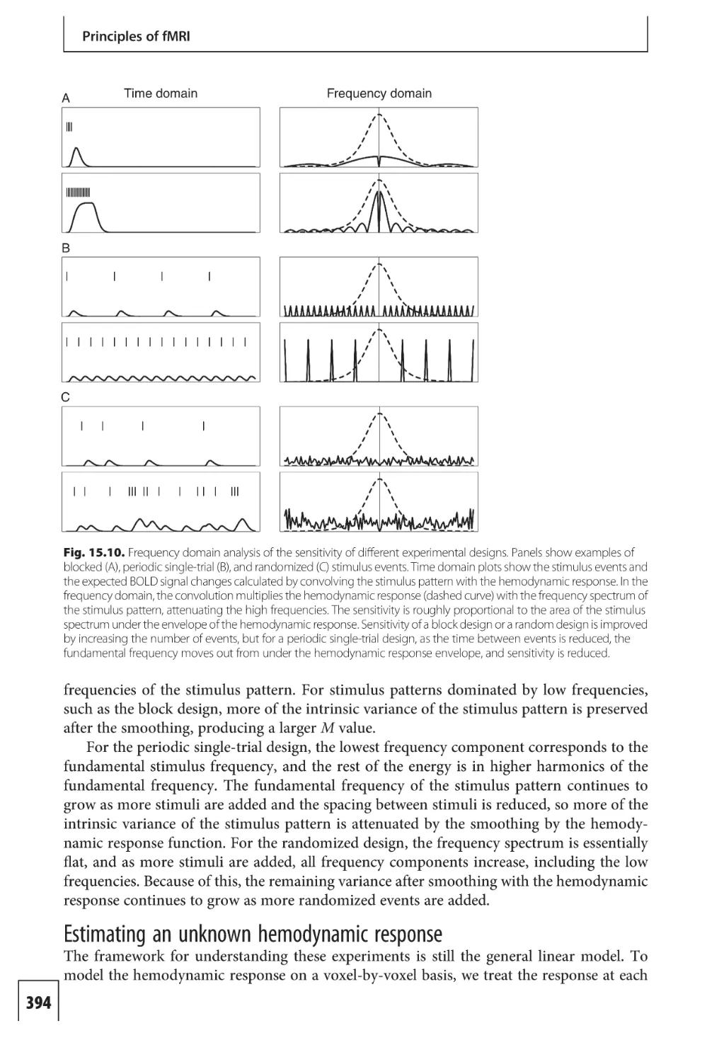
/


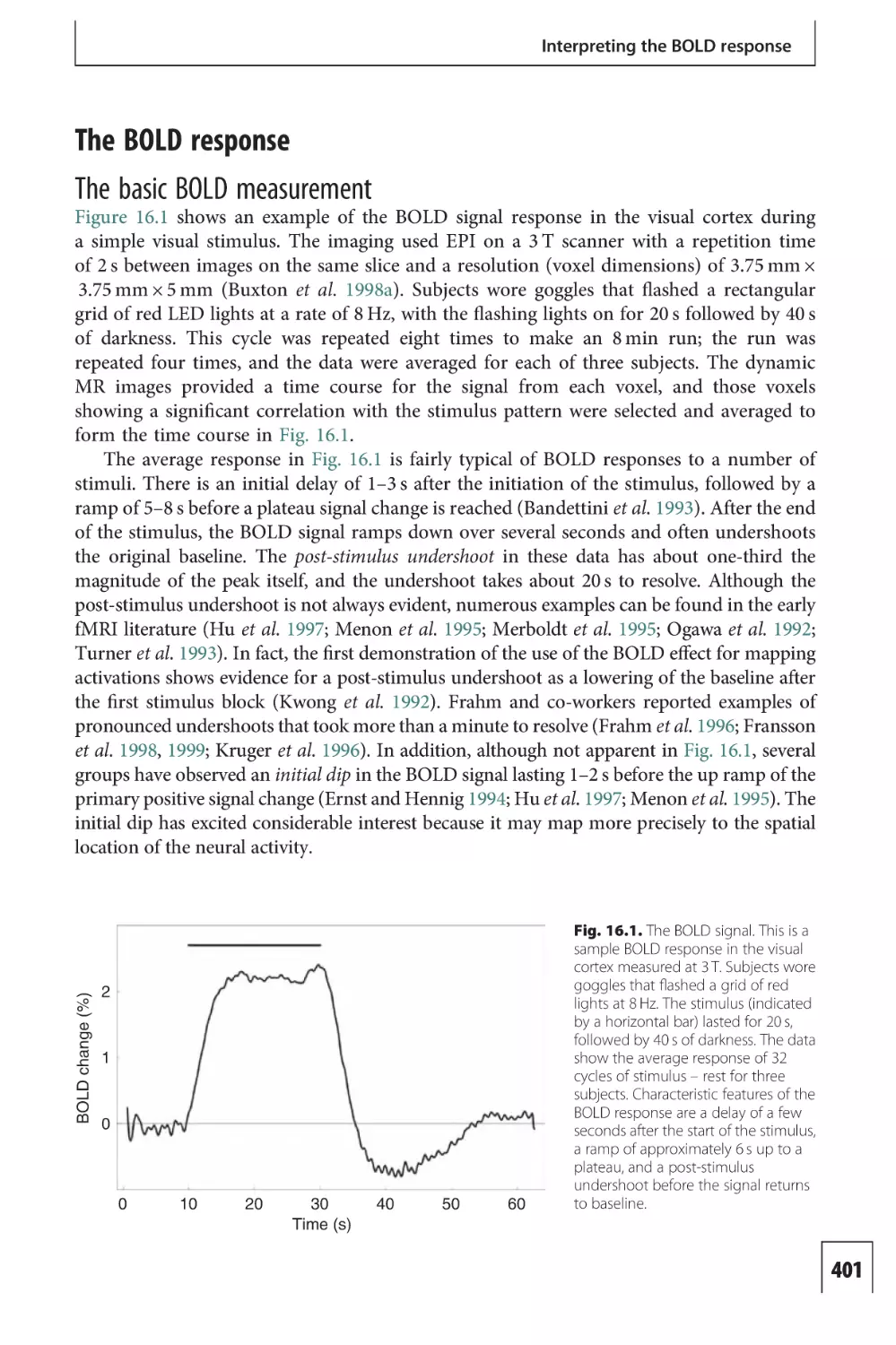
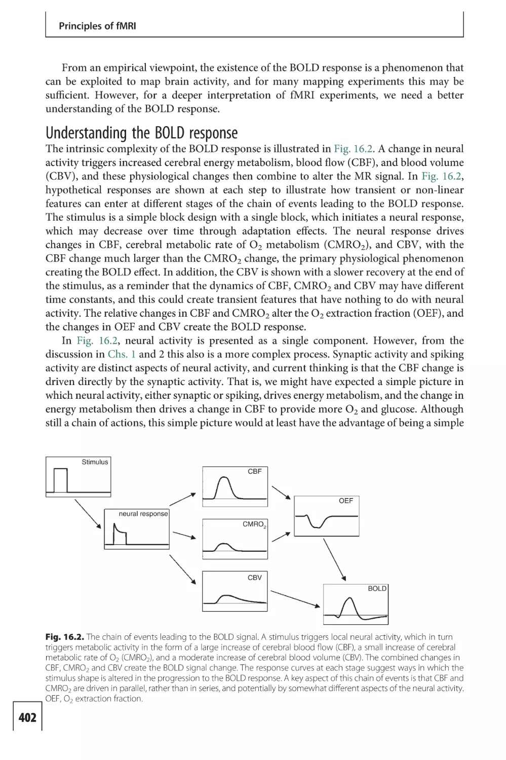


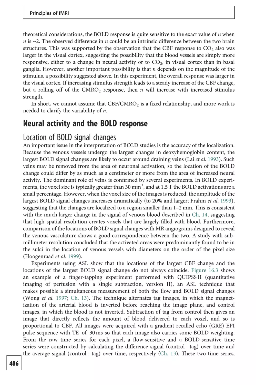


Text
This page intentionally left blank
Introduction to Functional
Magnetic Resonance Imaging
Principles and Techniques
Functional magnetic resonance imaging (fMRI) has become a standard
tool for mapping the working brain’s activation patterns, both in health
and in disease. It is an interdisciplinary field and crosses the borders of
neuroscience, psychology, psychiatry, radiology, mathematics, physics, and
engineering. Developments in techniques, procedures and our understanding of this field are expanding rapidly. In this second edition of Introduction
to Functional Magnetic Resonance Imaging, Richard Buxton – a leading
authority on fMRI – provides an invaluable guide to how fMRI works,
from introducing the basic ideas and principles to the underlying physics
and physiology. He covers the relationship between fMRI and other imaging
techniques and includes a guide to the statistical analysis of fMRI data. This
book will be useful both to the experienced neuroscientist, and the clinician
or researcher with no previous knowledge of the technology.
Ri ch ard B. B uxt on is Professor of Radiology at the University of
California at San Diego.
Introduction to
Functional Magnetic
Resonance Imaging
Principles and Techniques
SECOND EDITION
Richard B. Buxton
University of California, San Diego, USA
CAMBRIDGE UNIVERSITY PRESS
Cambridge, New York, Melbourne, Madrid, Cape Town, Singapore,
São Paulo, Delhi, Dubai, Tokyo
Cambridge University Press
The Edinburgh Building, Cambridge CB2 8RU, UK
Published in the United States of America by Cambridge University Press, New York
www.cambridge.org
Information on this title: www.cambridge.org/9780521899956
© R. B. Buxton 2009
This publication is in copyright. Subject to statutory exception and to the
provision of relevant collective licensing agreements, no reproduction of any part
may take place without the written permission of Cambridge University Press.
First published in print format 2009
ISBN-13
978-0-511-60302-0
eBook (Dawsonera)
ISBN-13
978-0-521-89995-6
Hardback
Cambridge University Press has no responsibility for the persistence or accuracy
of urls for external or third-party internet websites referred to in this publication,
and does not guarantee that any content on such websites is, or will remain,
accurate or appropriate.
For Lynn
Contents
Preface to the second edition ix
Preface to the first edition xi
Part I An overview of functional
magnetic resonance imaging
1
Part IA Introduction to the
9
10
Techniques in MRI
11
Noise and artifacts in MR
images 252
physiological basis of functional
neuroimaging 3
magnetic resonance imaging
65
3
Nuclear magnetic resonance
67
4
Magnetic resonance imaging
85
5
Imaging functional activity
101
12
Contrast agent techniques
13
Arterial spin labeling
techniques 307
117
Part IIA The nature of the
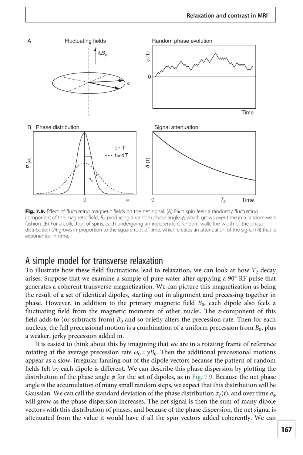
Relaxation and contrast in MRI
level dependent imaging
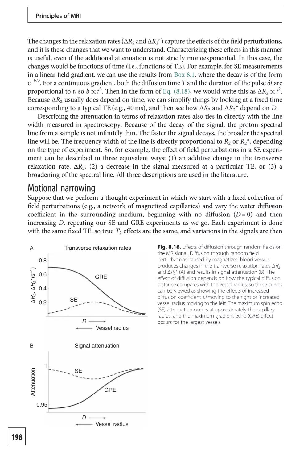
203
339
14
The BOLD effect
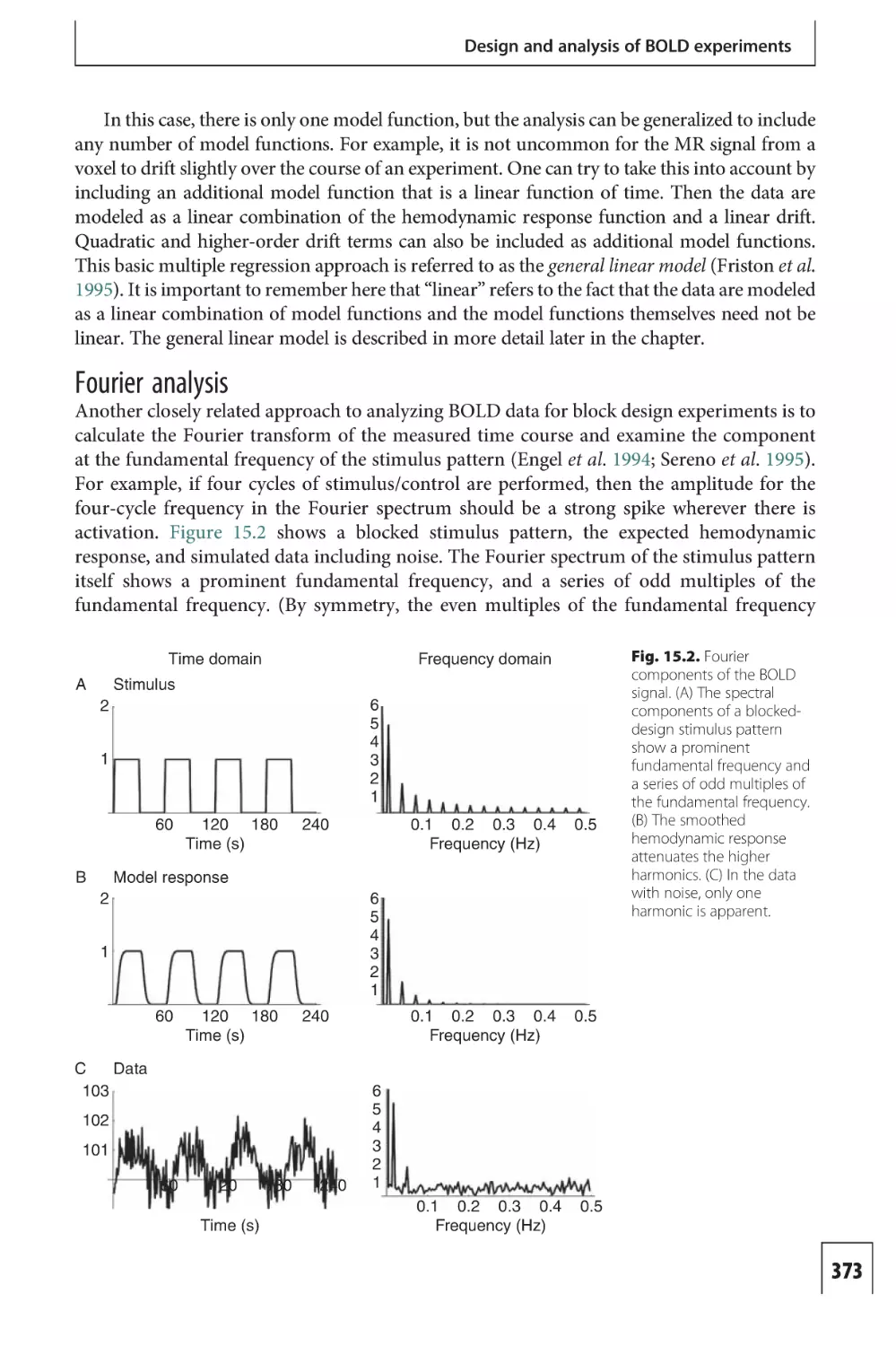
15
Design and analysis of BOLD
experiments 368
16
Interpreting the BOLD
response 400
Appendix
147
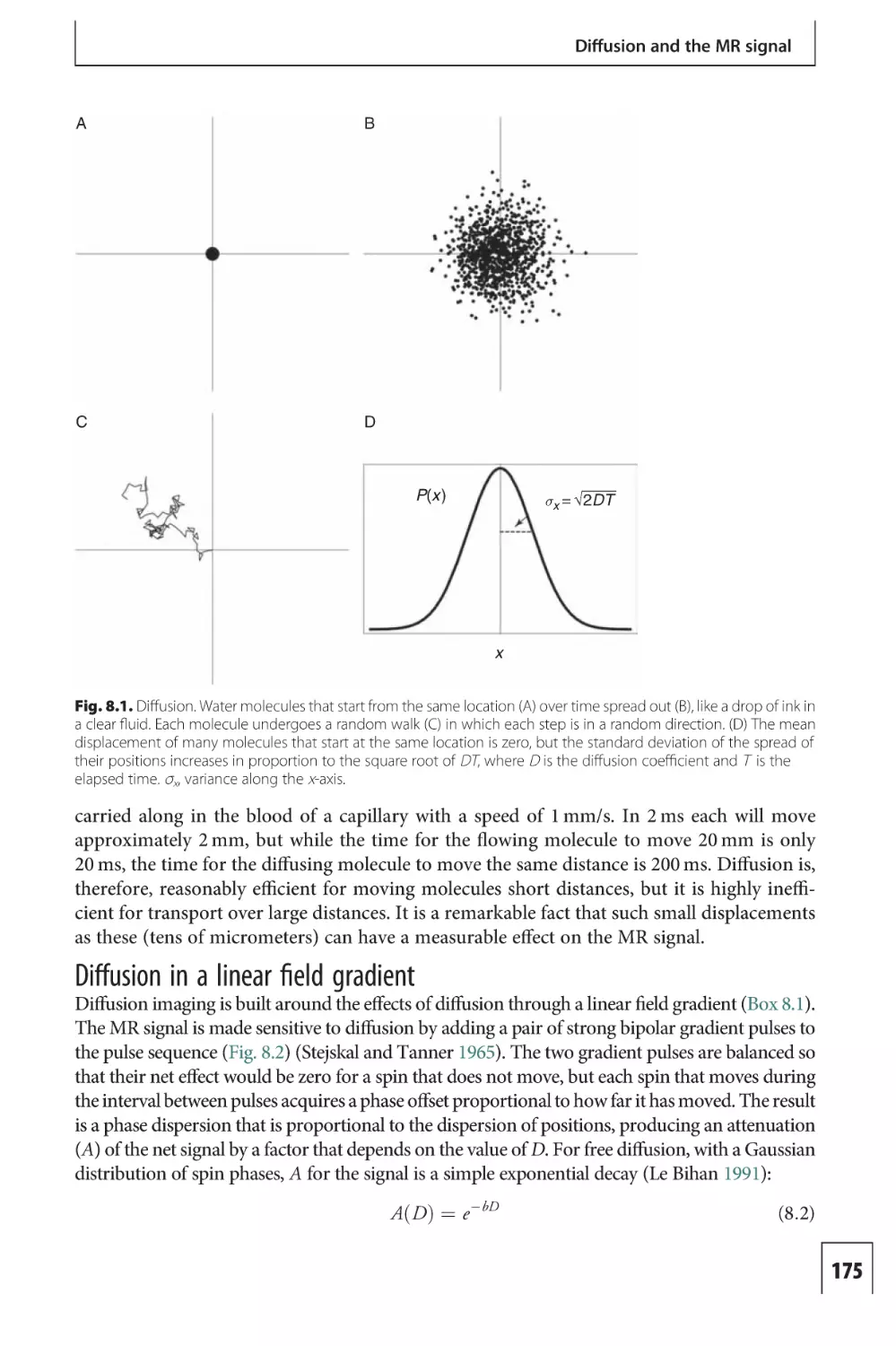
173
Part IIB Magnetic resonance
imaging
281
341
119
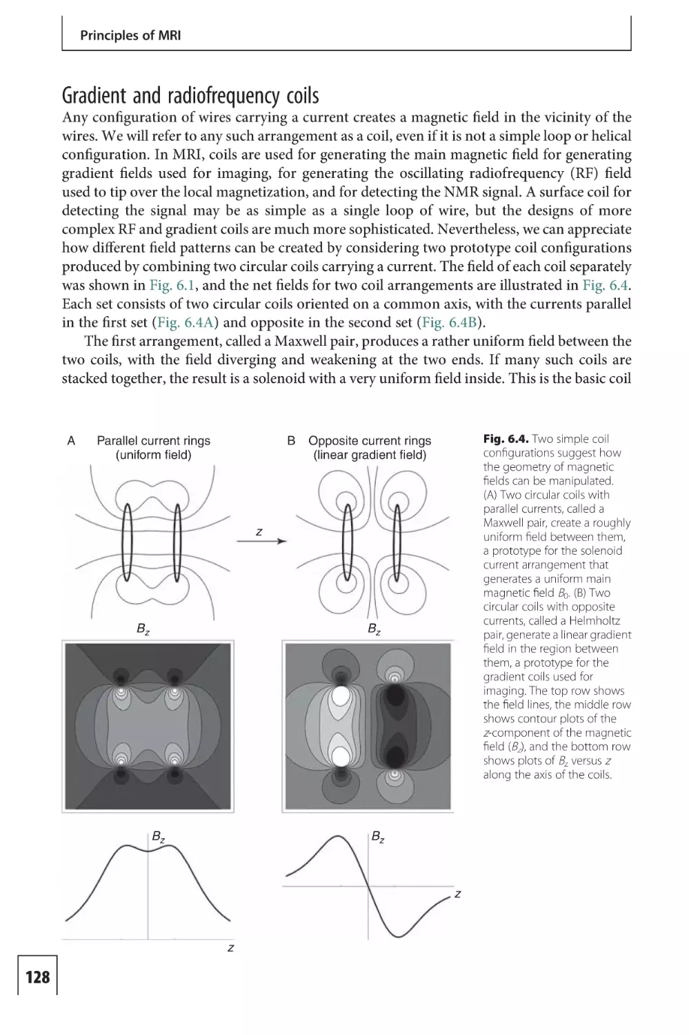
6 Basic physics of magnetism and
NMR 121
8 Diffusion and the MR signal
279
Part IIIB Blood oxygenation
Part II Principles of magnetic
7
277
Part IIIA Perfusion imaging
Part IB Introduction to functional
magnetic resonance signal
232
magnetic resonance imaging
Cerebral blood flow and brain
activation 34
resonance imaging
205
Part III Principles of functional
1 Neural activity and energy
metabolism 5
2
Mapping the MR signal
Index
The physics of nuclear
magnetic resonance 425
440
The color plates are between
pages 231 and 232
Preface to the second edition
The field of functional magnetic resonance imaging (fMRI) has expanded enormously since
the mid-1990s. The field is still dominated by basic neuroscience research, but increasingly
fMRI is being used to study disease, and clinical applications are growing rapidly. This book
is intended as an introduction to the basic ideas and techniques of fMRI. My goal was to
provide a guide to the principles of fMRI with sufficient depth to be useful to the active
neuroscience investigator using fMRI in research, but also to make the material accessible to
the new investigator or clinician with no prior knowledge of the field. To this end, the key
ideas are all presented in Part I as a general overview and then developed in more detail in
Parts II and III.
The second edition has been extensively revised to reflect new developments in the field
since publication of the first edition in 2002. As in the first edition, the emphasis is on
examples that illustrate the basic principles rather than a comprehensive review of the field.
The viewpoint of the book reflects my own background as a physicist, focusing on how the
techniques work and the physiological mechanisms underlying fMRI. The early sections on
the basic connections between neural activity, blood flow, and energy metabolism have been
completely revised to reflect the large body of the new work since the first edition was
published. The final chapter addresses what I think is the primary challenge for fMRI today:
how can we take fMRI from a mapping tool to a quantitative probe of brain physiology?
I have been fortunate to be able to work with an exceptional group of colleagues at UCSD,
and over the years the material in the book has been shaped by many helpful discussions with
Eric Wong, Larry Frank, Tom Liu, David Dubowitz, Miriam Scandeng, Giedrius Buracas,
Kun Lu, Adina Roskies, Karla Miller, Kamil Uludag, Marty Sereno, Joan Stiles, Frank Haist,
Greg Brown, Anna Devor, and Anders Dale. I have also benefited from numerous stimulating discussions with other colleagues in the field, particularly on ideas related to the
physiological foundations of fMRI, including Peter Bandettini, David Boas, Noam Harel,
Joe Mandeville, Marcus Raichle, Robert Turner, Essa Yacoub and many others.
Finally, this book could not have been completed without the loving support of Lynn
Hall, and the book is dedicated to her.
Richard B. Buxton
Preface to the first edition
The field of functional magnetic resonance imaging (fMRI) is intrinsically interdisciplinary,
involving neuroscience, psychology, psychiatry, radiology, physics, and mathematics. For
me, this is part of the pleasure in working in this area, providing an opportunity to
collaborate with scientists and clinicians with a wide range of backgrounds. This book is
intended as an introduction to the basic ideas and techniques of fMRI. My goal was to
provide a guide to the principles of fMRI with sufficient depth to be useful to the active
neuroscience investigator using fMRI in their research, but also to make the material
accessible to the new investigator or clinician with no prior knowledge of the field. The
viewpoint of the book reflects my own background as a physicist, focusing on how the
techniques work. The emphasis is on examples that illustrate the basic principles rather
than a more comprehensive review of the field or a more rigorous mathematical treatment
of the fundamentals.
This book grew out of courses I taught with my colleagues L. R. Frank and E. C. Wong,
and their insights have significantly shaped the way in which the material is presented. Our
courses were geared toward graduate students in neuroscience and psychology, but the book
should also be useful for clinicians who want to understand the basis of the new fMRI
techniques and potential clinical applications, and for physicists and engineers who are
looking for an overview of the ideas of fMRI. Some of the techniques described are not yet
part of the mainstream of basic neuroscience applications, such as arterial spin labeling,
bolus tracking, and diffusion tensor imaging. However, the clinical application of these
techniques is rapidly growing, and I think that over the next few years they will become
an integral part of many neuroscience fMRI studies. This book should also serve as an
introduction to recent excellent multiauthor works that present some of this material in
greater depth, such as Functional MRI edited by C. T. W. Moonen and P. A. Bandettini
(published in 1999 by Springer).
In writing this book, I have benefited from helpful discussions and critical readings
from several of my close colleagues, including Eric Wong, Larry Frank, Tom Liu,
Karla Miller, Antigona Martinez, and David Dubowitz. I am also fortunate to be able to
work with faculty and students in the San Diego neuroscience community, including
Geoff Boynton, Greg Brown, Adina Roskies, Marty Sereno, Joan Stiles, Dave Swinney, and
many others. Their insights, comments, and questions have stimulated me to think about
many of the topics discussed in the book. In addition, I have also benefited from numerous
discussions with colleagues in the field over the years, including Peter Bandettini,
Anders Dale, Arno Villringer, Robert Weisskoff, Joe Mandeville, Van Wedeen, Bruce Rosen,
Ken Kwong, Robert Turner, Gary Glover, Robert Edelman, Mark Henkelman, and many
others. Although these individuals have strongly influenced my own thinking, they are not
responsible for what appears here, particularly any errors that may remain.
Finally, this could not have been completed without the loving support of Lynn Hall, and
the book is dedicated to her.
Richard B. Buxton
Part
I
An overview of functional magnetic
resonance imaging
Part IA Introduction to the physiological basis of functional neuroimaging
1 Neural activity and energy metabolism
2 Cerebral blood flow and brain activation
Part IB Introduction to functional magnetic resonance imaging
3 Nuclear magnetic resonance
4 Magnetic resonance imaging
5 Imaging functional activity
IA
Part
Introduction to the physiological
basis of functional neuroimaging
The subject to be observed lay on a delicately balanced table which could tip downwards
either at the head or at the foot if the weight of either end were increased. The moment
emotional or intellectual activity began in the subject, down went the balance at the
head-end, in consequence of the redistribution of blood in his system …
… We must suppose a very delicate adjustment whereby the circulation follows the
needs of the cerebral activity. Blood very likely may rush to each region of the cortex
according as it is most active, but of this we know nothing.
William James (1890) The Principles of Psychology
1
Chapter
Neural activity and energy
metabolism
Introduction
page 5
Metabolic activity accompanies neural activity
5
Functional MRI
7
Neural signaling
7
Neural activity
8
The membrane potential
9
Synaptic activity
10
Electrophysiology measurements
12
Recovery from neural activity
14
Neural signaling is a thermodynamically downhill process
14
Metabolism of ATP is required to restore ionic gradients following
neural activity
14
The sodium/potassium pump
15
Astrocytes play a key role in recycling neurotransmitter
16
An ATP energy budget for neural activity
16
Energy metabolism
18
Glycolysis in the cytosol
18
Lactate production and the lactate shuttle
20
Mitochondrial pyruvate metabolism and the electron transfer chain
20
22
Delivery of glucose and O2 by blood flow
Measuring energy metabolism with PET
23
The deoxyglucose technique for measuring glucose metabolism
23
Measuring the cerebral metabolic rate for glucose
23
Increased glucose metabolism is closely associated with functional activity
24
25
Measuring cerebral blood flow and O2 metabolism
Balance of blood flow, glucose metabolism and O2 use in the brain at
rest and during activation
26
Introduction
Metabolic activity accompanies neural activity
The goal of understanding the functional organization of the human brain has motivated
neuroscientists for well over 100 years, but the experimental tools to measure and map brain
activity have been slow to develop. Neural activity is difficult to localize without placing
electrodes directly in the brain. Fluctuating electric and magnetic fields measured at the scalp
or near the head provide information on electrical events within the brain, and from these
data the location of a few sources of activity can be estimated, but the information is not
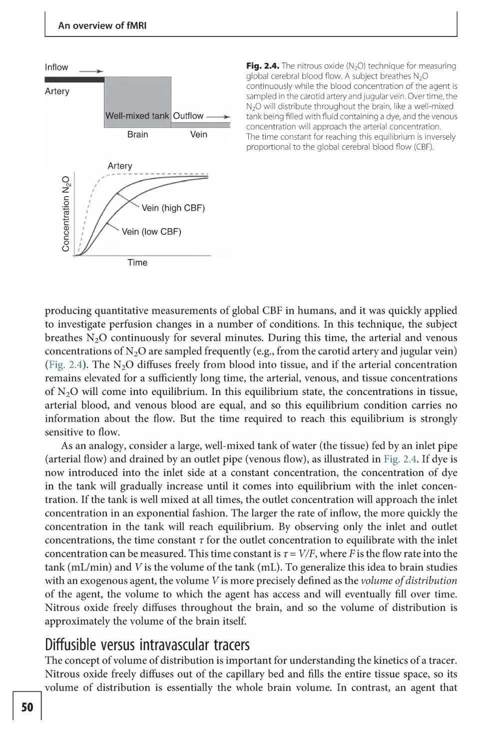
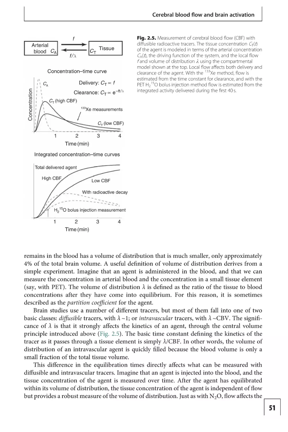
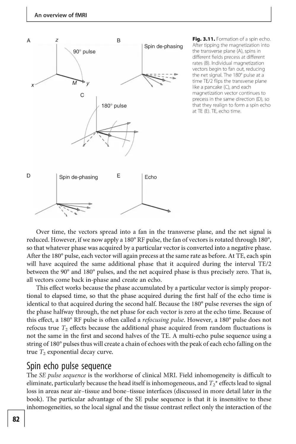
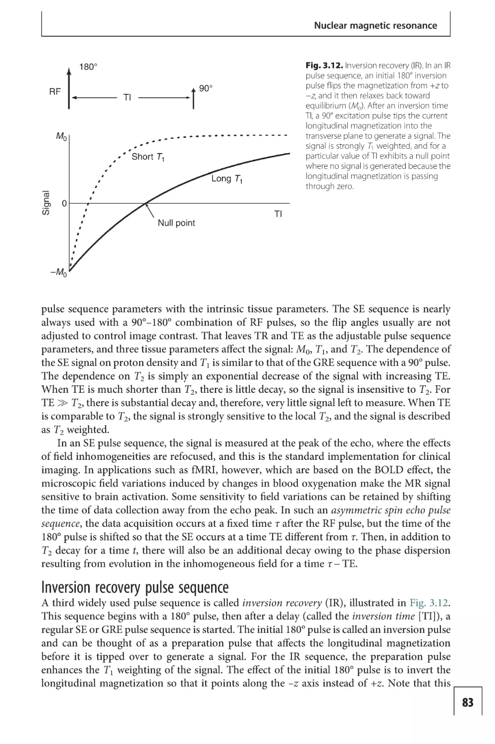
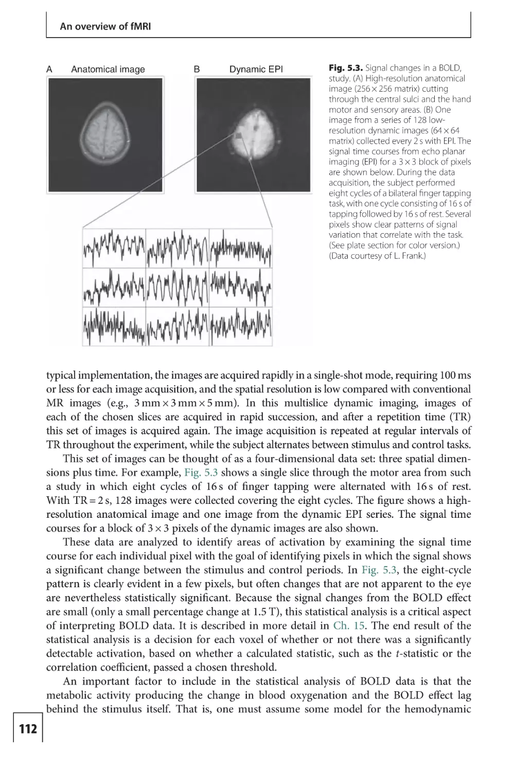
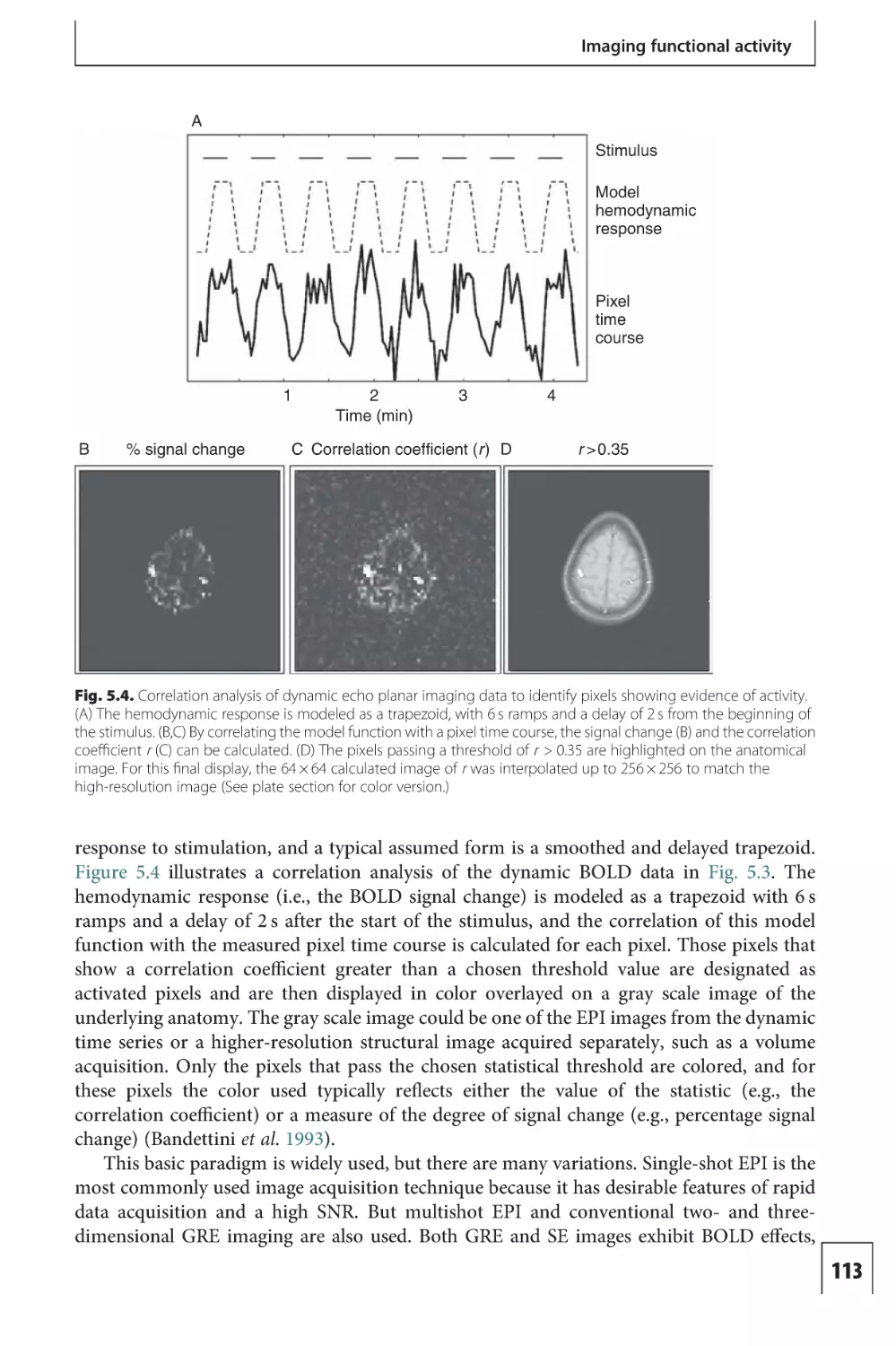
An overview of fMRI
sufficient to produce a detailed map of the pattern of activation. However, precise localization
of the metabolic activity and blood flow changes that follow neural activity are much more
feasible and form the basis for most of the functional neuroimaging techniques in use today,
including positron emission tomography (PET) and functional magnetic resonance imaging
(fMRI). Although comparatively new, fMRI techniques are now a primary tool for basic
studies of the organization of the working human brain, and clinical applications are growing.
In 1890, William James published The Principles of Psychology, a landmark in the development of psychology as a science grounded in physiology. The possibility of measuring changes
in brain blood flow associated with mental activity clearly lay behind the experiment performed
by Angelo Mosso and recounted by James in the quotation at the beginning of this section.
By current standards of blood flow measurement, this experiment is quaintly crude, but it
indicates that the idea of inferring neural activity in the brain from a measurement of changes
in local blood flow long preceded the ability to do such measurements (Raichle 1998).
In fact, this experiment is unlikely to have worked reliably for an important reason.
The motivation for this experiment may have been an analogy with muscle activity. Vigorous
exercise produces substantial muscle swelling through increased blood volume, and thus
a redistribution in weight. But the brain is surrounded by fluid and encased in a hard shell,
so the overall fluid volume within the cranium must remain nearly constant, a principle often
referred to as the Munro–Kellie doctrine. Blood volume changes do occur in the brain, and
the brain does move with cardiac pulsations, but these changes most likely involve shifts
of cerebrospinal fluid (CSF) as well. As a result, the weight of the head should remain
approximately constant.
Furthermore, this experiment depends on a change in blood volume, rather than blood
flow, and blood flow and blood volume are distinct quantities. Blood flow refers to the volume
per minute moving through the vessels, while blood volume is the volume occupied by the
vessels. In principle, there need be no fixed relation between blood flow and blood volume;
flow through a set of pipes can be increased by increasing the driving pressure without
changing the volume of the plumbing. Physiologically, however, experiments typically show
a strong correlation between cerebral blood flow (CBF) and cerebral blood volume (CBV),
and functional neuroimaging techniques are now available for measuring both of these
quantities.
The working brain requires a continuous supply of glucose and oxygen (O2), which must
be supplied by CBF. The human brain receives approximately 15% of the total cardiac output
of blood (approximately 700 mL/min) and yet accounts for only 2% of the total body weight.
Within the brain, the distribution of blood flow is heterogeneous, with gray matter receiving
several times more flow per gram of tissue than white matter. Indeed, the flow per gram of
tissue to gray matter is comparable to that in heart muscle, the most energetic organ in the
body. The activity of the brain generates approximately 11 W/kg of heat, and glucose and O2
provide the fuel for this energy generation. Yet the brain has virtually no reserve store of O2,
and is therefore dependent on continuous delivery by CBF. If the supply of O2 to the brain is
cut off, loss of consciousness quickly follows.
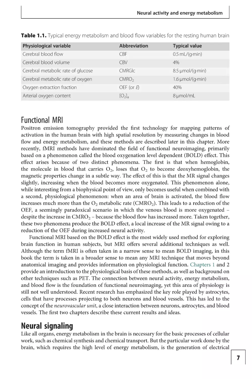
Table 1.1 lists the primary physiological variables associated with brain energy metabolism and blood flow, along with approximate values for the resting human brain. With brain
activation, glucose metabolism, O2 metabolism, blood flow and blood volume all increase in
the active area. Unexpectedly, however, the oxygen extraction fraction (OEF) – the fraction
of the delivered O2 that leaves the blood and is metabolized in the cells – decreases with
activation, and this phenomenon is exploited in fMRI.
6
Neural activity and energy metabolism
Table 1.1. Typical energy metabolism and blood flow variables for the resting human brain
Physiological variable
Abbreviation
Typical value
Cerebral blood flow
CBF
0.5 mL/(g·min)
Cerebral blood volume
CBV
4%
Cerebral metabolic rate of glucose
CMRGlc
8.5 µmol/(g·min)
Cerebral metabolic rate of oxygen
CMRO2
1.6 µmol/(g·min)
Oxygen extraction fraction
OEF (or E)
40%
Arterial oxygen content
[O2]a
8 µmol/mL
Functional MRI
Positron emission tomography provided the first technology for mapping patterns of
activation in the human brain with high spatial resolution by measuring changes in blood
flow and energy metabolism, and these methods are described later in this chapter. More
recently, fMRI methods have dominated the field of functional neuroimaging, primarily
based on a phenomenon called the blood oxygenation level dependent (BOLD) effect. This
effect arises because of two distinct phenomena. The first is that when hemoglobin,
the molecule in blood that carries O2, loses that O2 to become deoxyhemoglobin, the
magnetic properties change in a subtle way. The effect of this is that the MR signal changes
slightly, increasing when the blood becomes more oxygenated. This phenomenon alone,
while interesting from a biophysical point of view, only becomes useful when combined with
a second, physiological phenomenon: when an area of brain is activated, the blood flow
increases much more than the O2 metabolic rate (CMRO2). This leads to a reduction of the
OEF, a seemingly paradoxical scenario in which the venous blood is more oxygenated –
despite the increase in CMRO2 – because the blood flow has increased more. Taken together,
these two phenomena produce the BOLD effect, a local increase of the MR signal owing to a
reduction of the OEF during increased neural activity.
Functional MRI based on the BOLD effect is the most widely used method for exploring
brain function in human subjects, but MRI offers several additional techniques as well.
Although the term fMRI is often taken in a narrow sense to mean BOLD imaging, in this
book the term is taken in a broader sense to mean any MRI technique that moves beyond
anatomical imaging and provides information on physiological function. Chapters 1 and 2
provide an introduction to the physiological basis of these methods, as well as background on
other techniques such as PET. The connection between neural activity, energy metabolism,
and blood flow is the foundation of functional neuroimaging, yet this area of physiology is
still not well understood. Recent research has emphasized the key role played by astrocytes,
cells that have processes projecting to both neurons and blood vessels. This has led to the
concept of the neurovascular unit, a close interaction between neurons, astrocytes, and blood
vessels. The first two chapters describe these current results and ideas.
Neural signaling
Like all organs, energy metabolism in the brain is necessary for the basic processes of cellular
work, such as chemical synthesis and chemical transport. But the particular work done by the
brain, which requires the high level of energy metabolism, is the generation of electrical
7
An overview of fMRI
activity required for neuronal signaling. We begin by reviewing the basic processes involved
in neural activity from the perspective of thermodynamics, in order to emphasize the
essential role of energy metabolism. A more complete description can be found in standard
neuroscience texts (Nicholls et al. 1992).
Neural activity
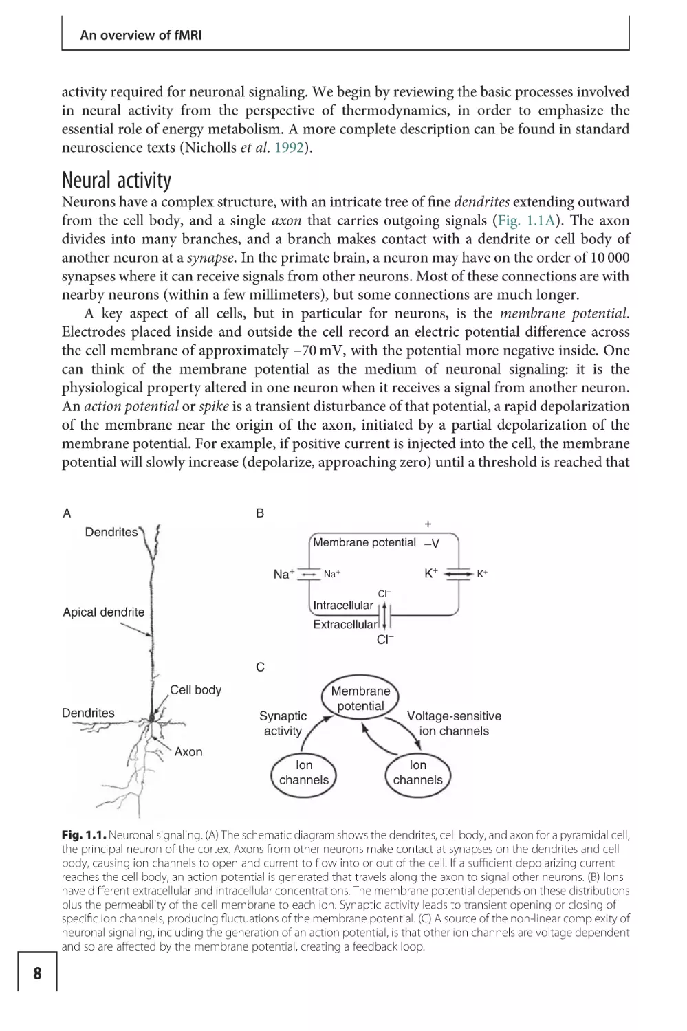
Neurons have a complex structure, with an intricate tree of fine dendrites extending outward
from the cell body, and a single axon that carries outgoing signals (Fig. 1.1A). The axon
divides into many branches, and a branch makes contact with a dendrite or cell body of
another neuron at a synapse. In the primate brain, a neuron may have on the order of 10 000
synapses where it can receive signals from other neurons. Most of these connections are with
nearby neurons (within a few millimeters), but some connections are much longer.
A key aspect of all cells, but in particular for neurons, is the membrane potential.
Electrodes placed inside and outside the cell record an electric potential difference across
the cell membrane of approximately −70 mV, with the potential more negative inside. One
can think of the membrane potential as the medium of neuronal signaling: it is the
physiological property altered in one neuron when it receives a signal from another neuron.
An action potential or spike is a transient disturbance of that potential, a rapid depolarization
of the membrane near the origin of the axon, initiated by a partial depolarization of the
membrane potential. For example, if positive current is injected into the cell, the membrane
potential will slowly increase (depolarize, approaching zero) until a threshold is reached that
A
B
+
Dendrites
Membrane potential –V
Na+
K+
Na+
K+
Cl–
Intracellular
Apical dendrite
Extracellular
Cl–
C
Cell body
Dendrites
Synaptic
activity
Membrane
potential
Voltage-sensitive
ion channels
Axon
Ion
channels
Ion
channels
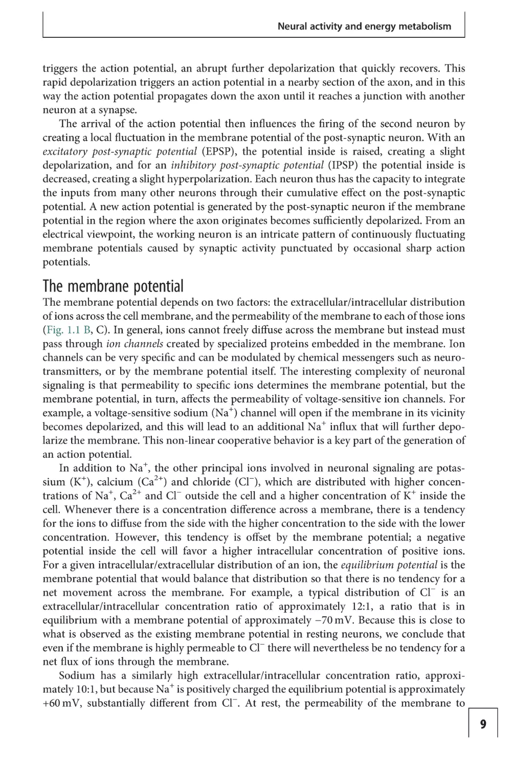
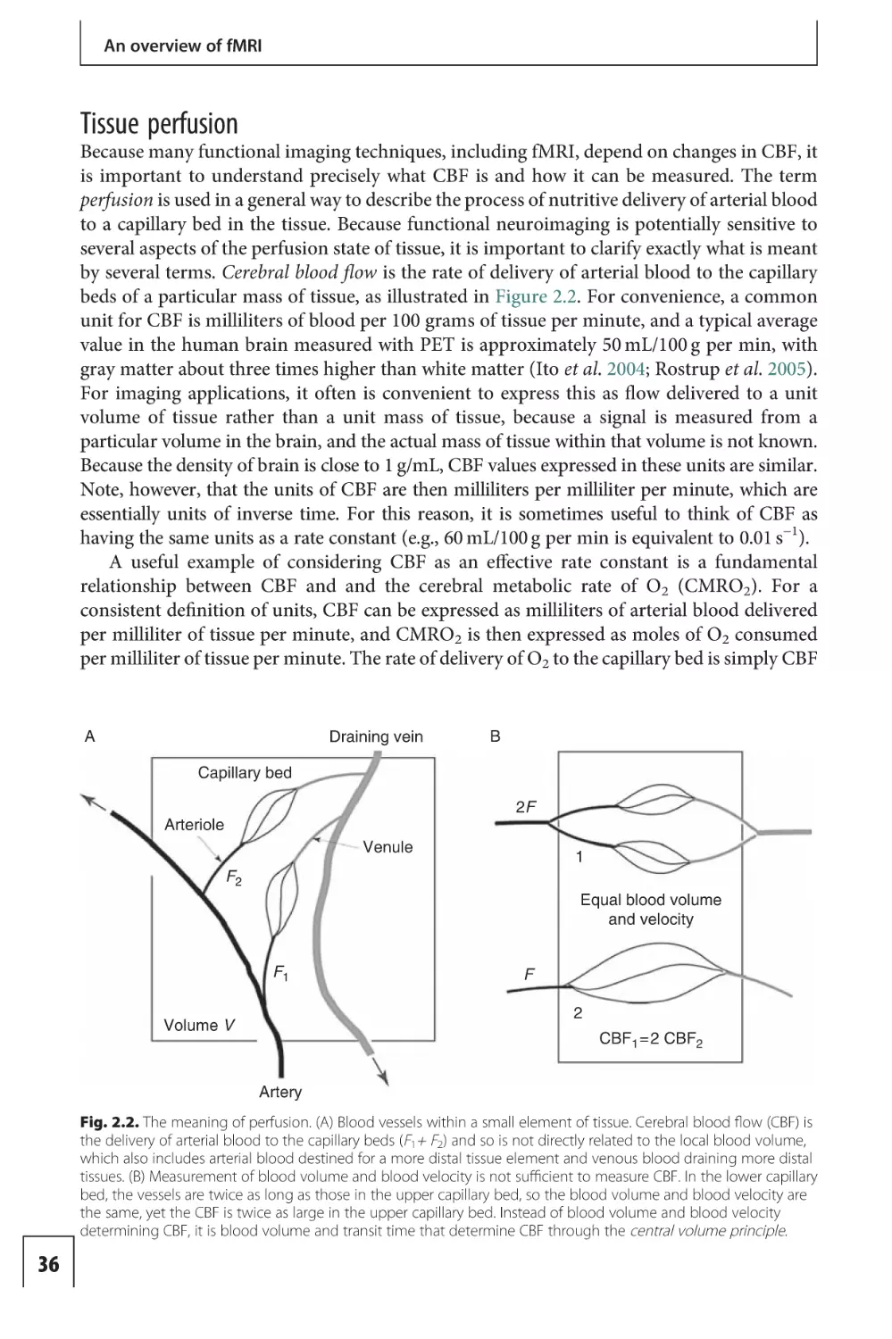
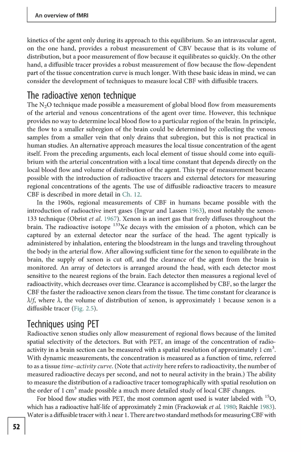
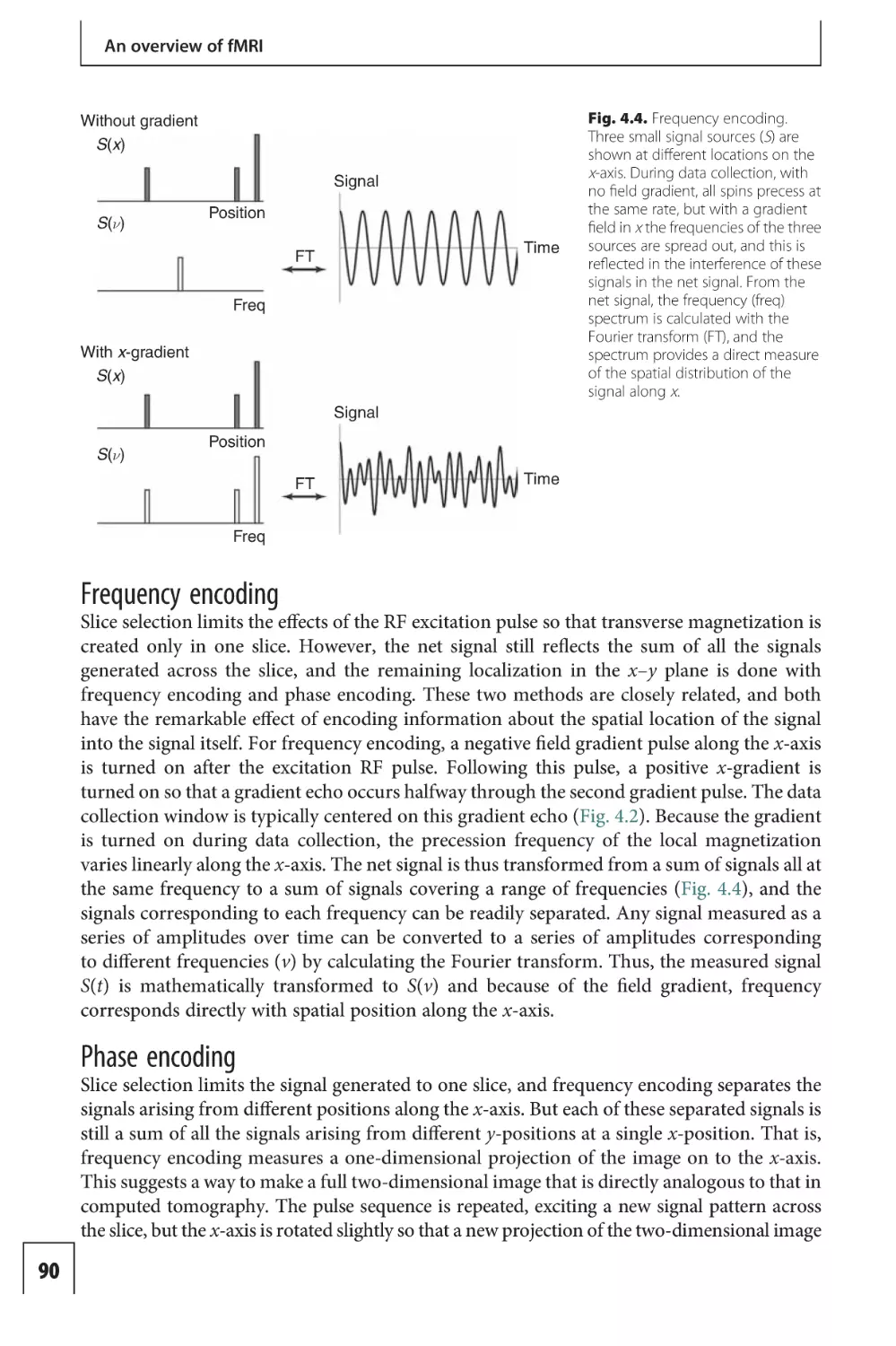
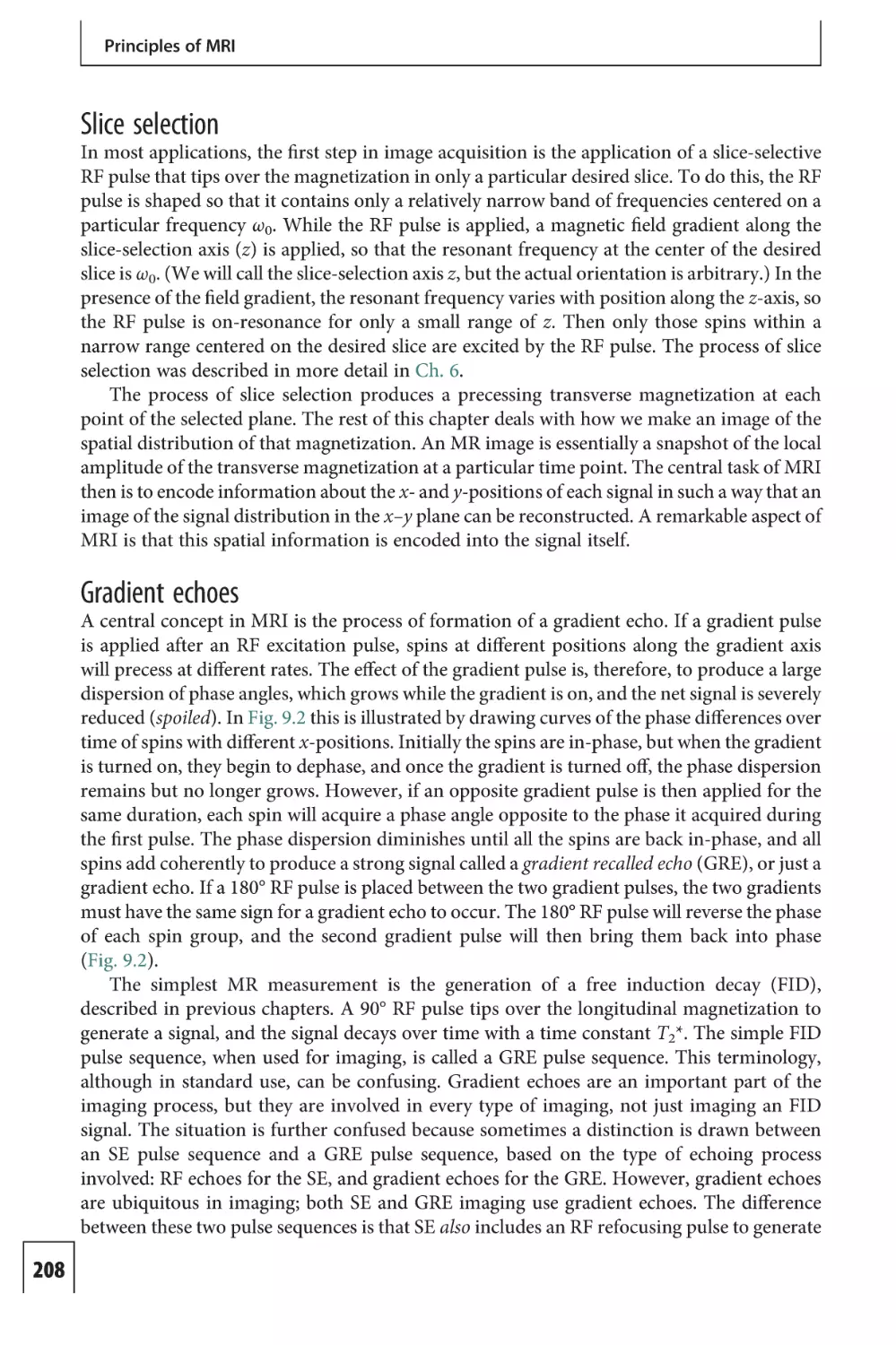
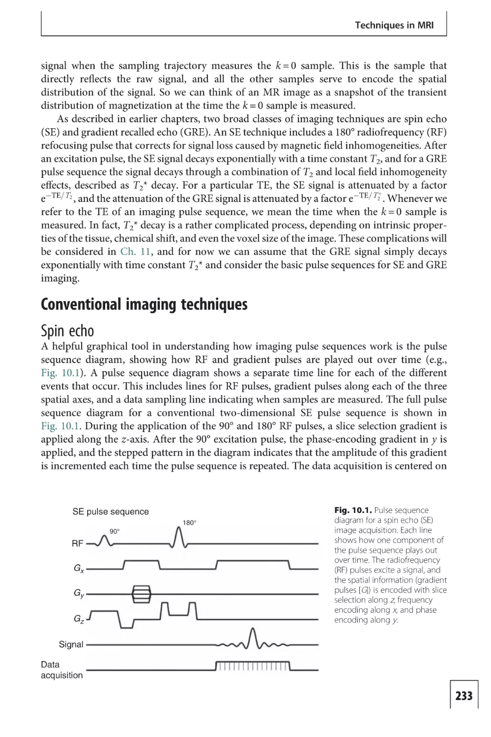
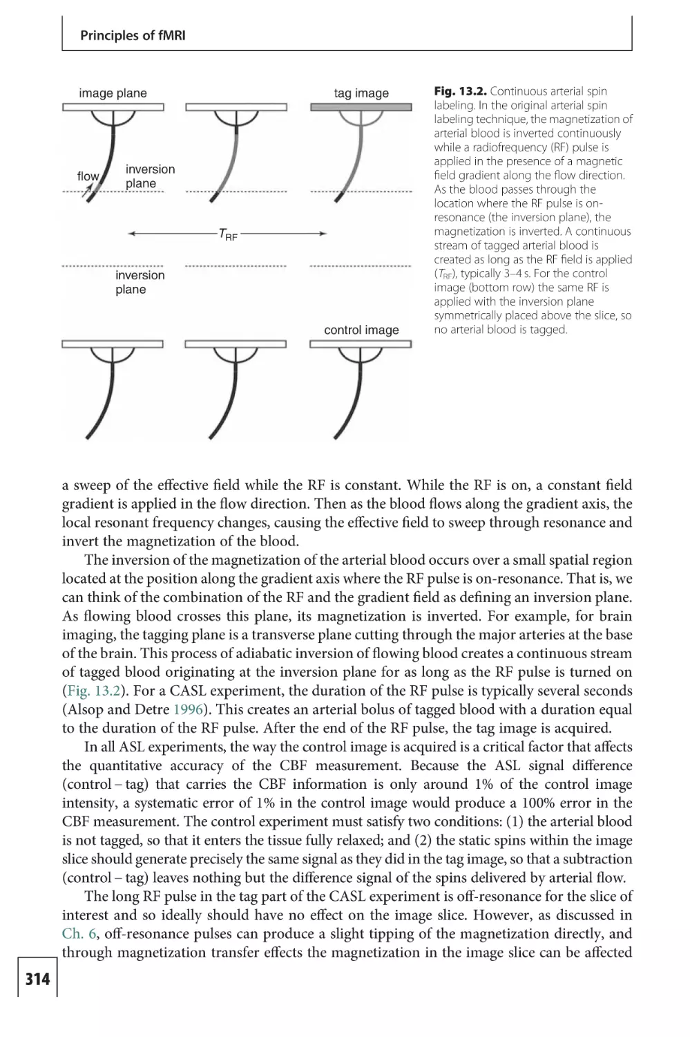
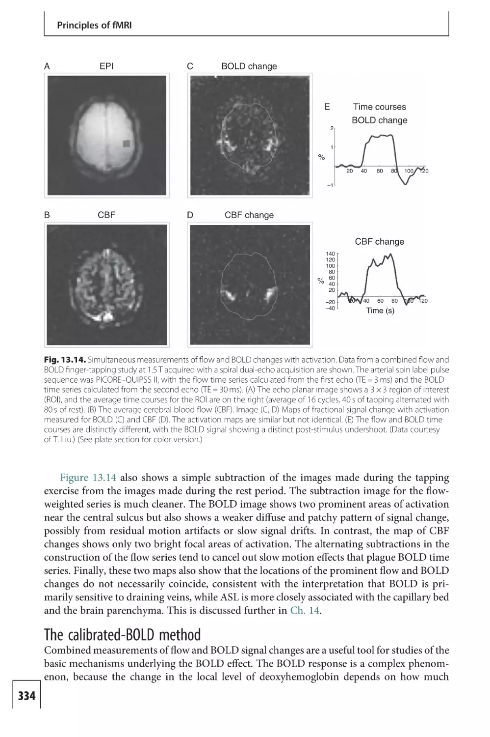
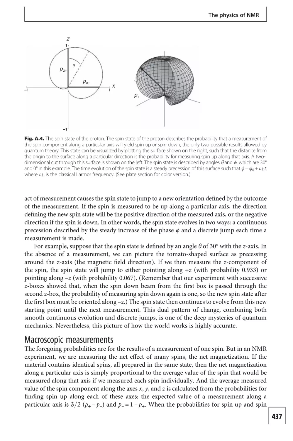
Fig. 1.1. Neuronal signaling. (A) The schematic diagram shows the dendrites, cell body, and axon for a pyramidal cell,
the principal neuron of the cortex. Axons from other neurons make contact at synapses on the dendrites and cell
body, causing ion channels to open and current to flow into or out of the cell. If a sufficient depolarizing current
reaches the cell body, an action potential is generated that travels along the axon to signal other neurons. (B) Ions
have different extracellular and intracellular concentrations. The membrane potential depends on these distributions
plus the permeability of the cell membrane to each ion. Synaptic activity leads to transient opening or closing of
specific ion channels, producing fluctuations of the membrane potential. (C) A source of the non-linear complexity of
neuronal signaling, including the generation of an action potential, is that other ion channels are voltage dependent
and so are affected by the membrane potential, creating a feedback loop.
8
Neural activity and energy metabolism
triggers the action potential, an abrupt further depolarization that quickly recovers. This
rapid depolarization triggers an action potential in a nearby section of the axon, and in this
way the action potential propagates down the axon until it reaches a junction with another
neuron at a synapse.
The arrival of the action potential then influences the firing of the second neuron by
creating a local fluctuation in the membrane potential of the post-synaptic neuron. With an
excitatory post-synaptic potential (EPSP), the potential inside is raised, creating a slight
depolarization, and for an inhibitory post-synaptic potential (IPSP) the potential inside is
decreased, creating a slight hyperpolarization. Each neuron thus has the capacity to integrate
the inputs from many other neurons through their cumulative effect on the post-synaptic
potential. A new action potential is generated by the post-synaptic neuron if the membrane
potential in the region where the axon originates becomes sufficiently depolarized. From an
electrical viewpoint, the working neuron is an intricate pattern of continuously fluctuating
membrane potentials caused by synaptic activity punctuated by occasional sharp action
potentials.
The membrane potential
The membrane potential depends on two factors: the extracellular/intracellular distribution
of ions across the cell membrane, and the permeability of the membrane to each of those ions
(Fig. 1.1 B, C). In general, ions cannot freely diffuse across the membrane but instead must
pass through ion channels created by specialized proteins embedded in the membrane. Ion
channels can be very specific and can be modulated by chemical messengers such as neurotransmitters, or by the membrane potential itself. The interesting complexity of neuronal
signaling is that permeability to specific ions determines the membrane potential, but the
membrane potential, in turn, affects the permeability of voltage-sensitive ion channels. For
example, a voltage-sensitive sodium (Na+) channel will open if the membrane in its vicinity
becomes depolarized, and this will lead to an additional Na+ influx that will further depolarize the membrane. This non-linear cooperative behavior is a key part of the generation of
an action potential.
In addition to Na+, the other principal ions involved in neuronal signaling are potassium (K+), calcium (Ca2+) and chloride (Cl−), which are distributed with higher concentrations of Na+, Ca2+ and Cl− outside the cell and a higher concentration of K+ inside the
cell. Whenever there is a concentration difference across a membrane, there is a tendency
for the ions to diffuse from the side with the higher concentration to the side with the lower
concentration. However, this tendency is offset by the membrane potential; a negative
potential inside the cell will favor a higher intracellular concentration of positive ions.
For a given intracellular/extracellular distribution of an ion, the equilibrium potential is the
membrane potential that would balance that distribution so that there is no tendency for a
net movement across the membrane. For example, a typical distribution of Cl− is an
extracellular/intracellular concentration ratio of approximately 12:1, a ratio that is in
equilibrium with a membrane potential of approximately −70 mV. Because this is close to
what is observed as the existing membrane potential in resting neurons, we conclude that
even if the membrane is highly permeable to Cl− there will nevertheless be no tendency for a
net flux of ions through the membrane.
Sodium has a similarly high extracellular/intracellular concentration ratio, approximately 10:1, but because Na+ is positively charged the equilibrium potential is approximately
+60 mV, substantially different from Cl−. At rest, the permeability of the membrane to
9
An overview of fMRI
Na+ is low, so there is little flux of Na+ down its gradient (although there is a slow leak). If
membrane ion channels open to allow passage of Na+, making the membrane permeable to
Na+, there is a strong inward current because both the concentration gradient and the
negative potential drive a Na+ flux into the cell. Potassium has an even more asymmetric
distribution, with an extracellular/intracellular concentration ratio of approximately 1:40,
and the corresponding equilibrium potential is approximately −95 mV. Opening a K+
channel will lead to an outward flux of K+ down its gradient. In short, relative to the resting
membrane potential, the Cl− distribution is near equilibrium; the K+ distribution is somewhat out of equilibrium; and the Na+ distribution is far from equilibrium.
Given this complex non-equilibrium system with multiple ions in different distributions,
what actually determines the membrane potential? Ultimately, the membrane potential
depends on a very slight imbalance of charge inside and outside the cell, but the amount of
charge involved is much smaller than the fluxes of charge across the membrane through ion
channels. One can think of the neuron as being in a steady state in which the net flux of
charge across the membrane is zero. That is, positive and negative charges are moving back
and forth through membrane channels, and for any particular ion there may be a steady flux
in one direction, such as a slow but steady leak of Na+ into the cell. Overall, however, there is
no net charge transfer across the membrane. Because the membrane potential is highly
sensitive to any imbalance of charge across the membrane, any departure from this steady
state, leading to a net flux of charge, will quickly alter the membrane potential. Then, for any
combination of ion distributions and membrane permeabilities, the membrane potential
takes on the value that will create this steady state with no net flux of charge.
For example, if the membrane is highly permeable to one ion, but only weakly permeable
to the others, the membrane potential will approach the equilibrium potential of that ion,
because that ion alone determines the net flux of charge. However, if the membrane also is
permeable to another ion with a different equilibrium potential, the resulting membrane
potential will be intermediate between the two equilibrium potentials, weighted by the
relative permeability to each of the different ions. That is, as the permeability to the second
ion increases, the membrane potential will shift toward the equilibrium potential of that ion.
In this case, because the membrane is permeable to both ions but the membrane potential
does not match either equilibrium potential, there will be a steady leak of ions that tends to
degrade the ionic distributions across the membrane, even though there is no net flux of
charge. The stability of the cell depends on maintaining these ionic distributions, so homeostasis requires that the ions be pumped back against their gradient, requiring energy
metabolism (see below). In short, the membrane potential depends on the ion distributions
across the membrane and the permeability of the membrane to each ion, and these ion
permeabilities are altered in neuronal signaling.
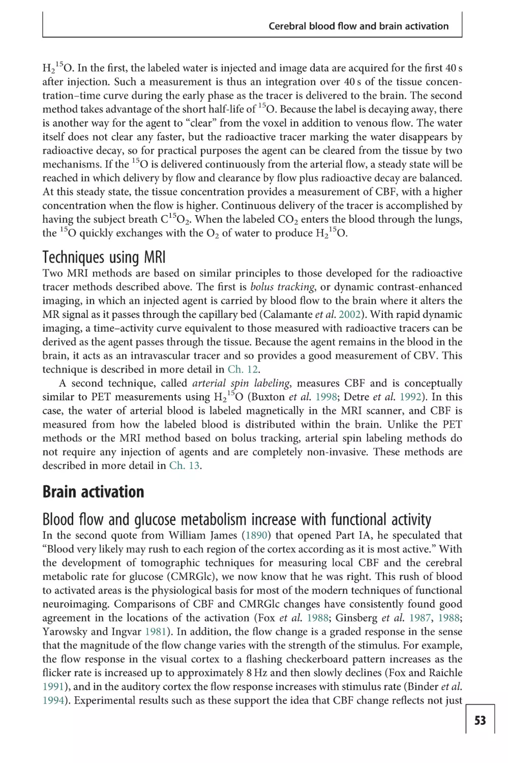
Synaptic activity
An action potential arriving at a synapse with another neuron initiates a process that causes
ion channels on the post-synaptic neuron to open or close (Fig. 1.2). This process begins on
the pre-synaptic side when the incoming action potential triggers an increase of the membrane permeability to Ca2+, allowing Ca2+ entry into the pre-synaptic terminal. Within the
pre-synaptic terminal, neurotransmitter molecules are concentrated in small packages called
vesicles, and the influx of Ca2+ triggers these vesicles to merge with the cell membrane and
spill their contents into the synaptic cleft separating the pre- and post-synaptic membranes.
The neurotransmitter molecules diffuse across this thin (20–40 nm) gap and bind to receptor
10
Neural activity and energy metabolism
Pre-synaptic terminal
1
Arteriole
Action potential
Ca2+
2
Glu
Blood
flow
3
Na+
Astrocyte
Ion
channel
5
Receptor
4
Smooth
muscle
Post-synaptic neuron
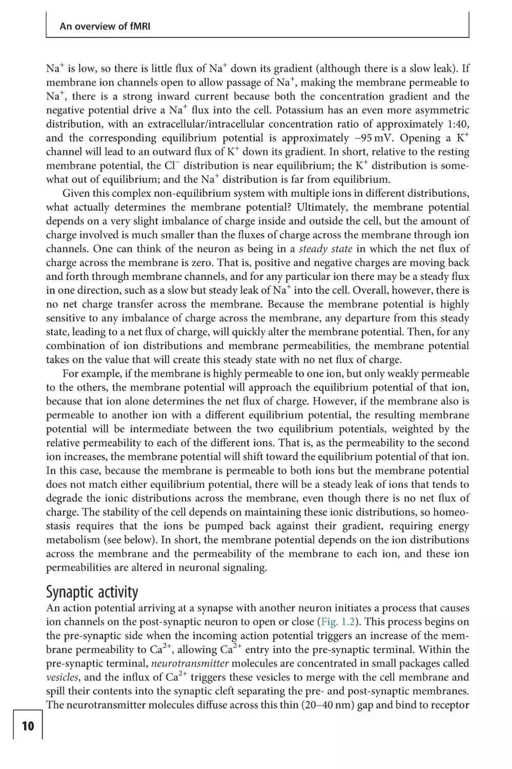
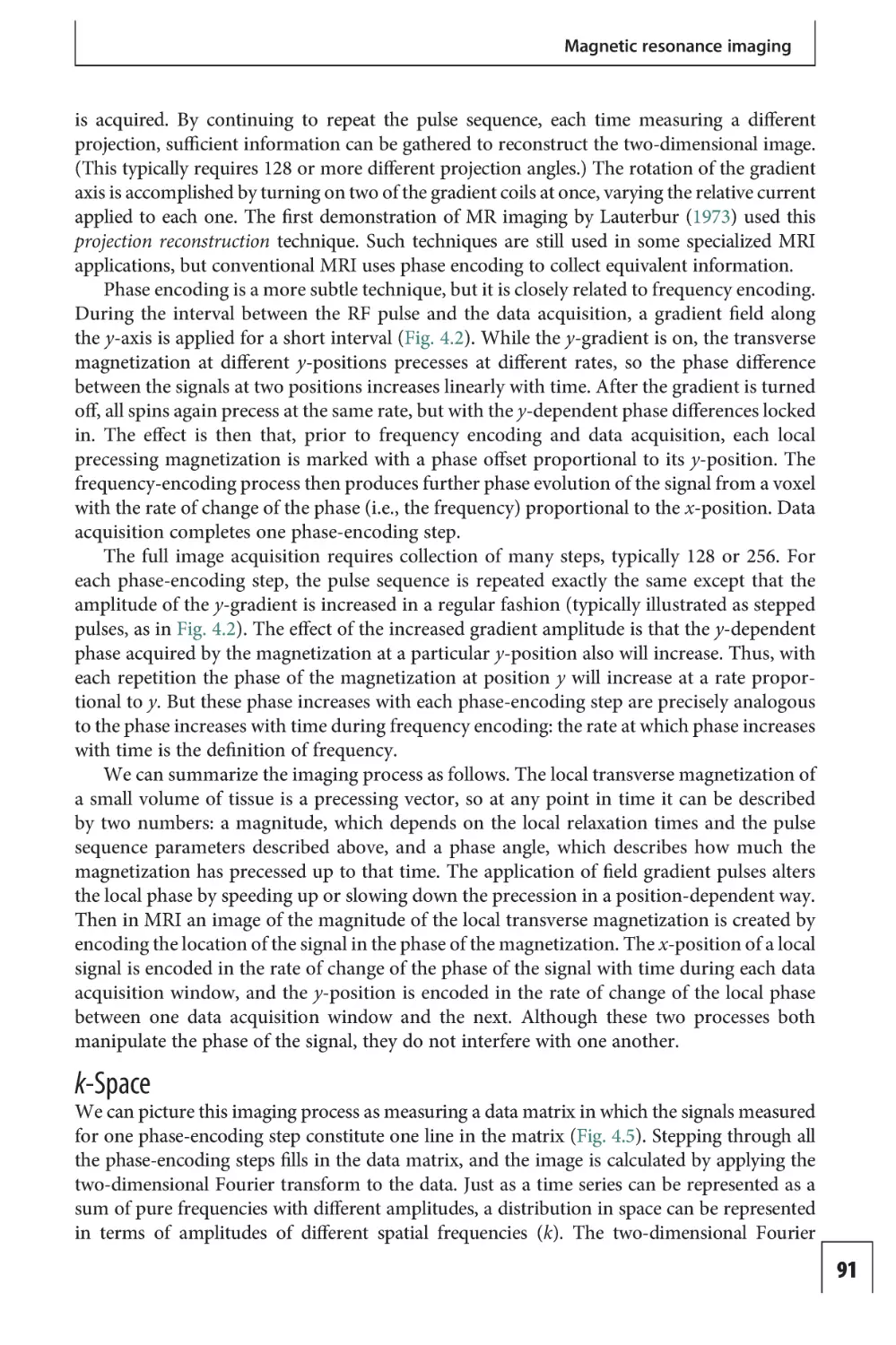
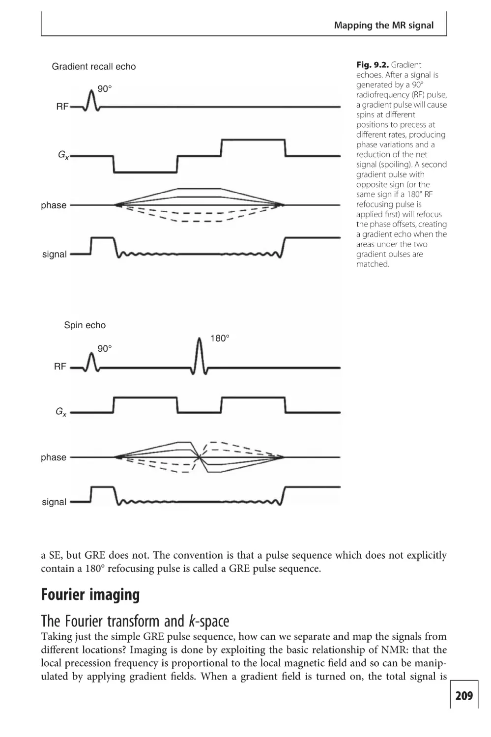
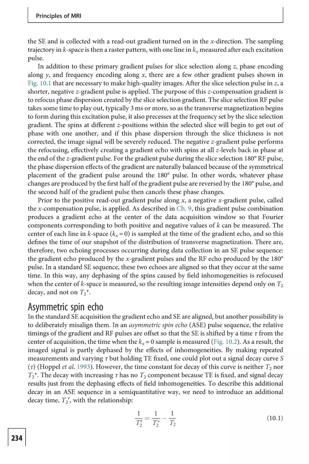
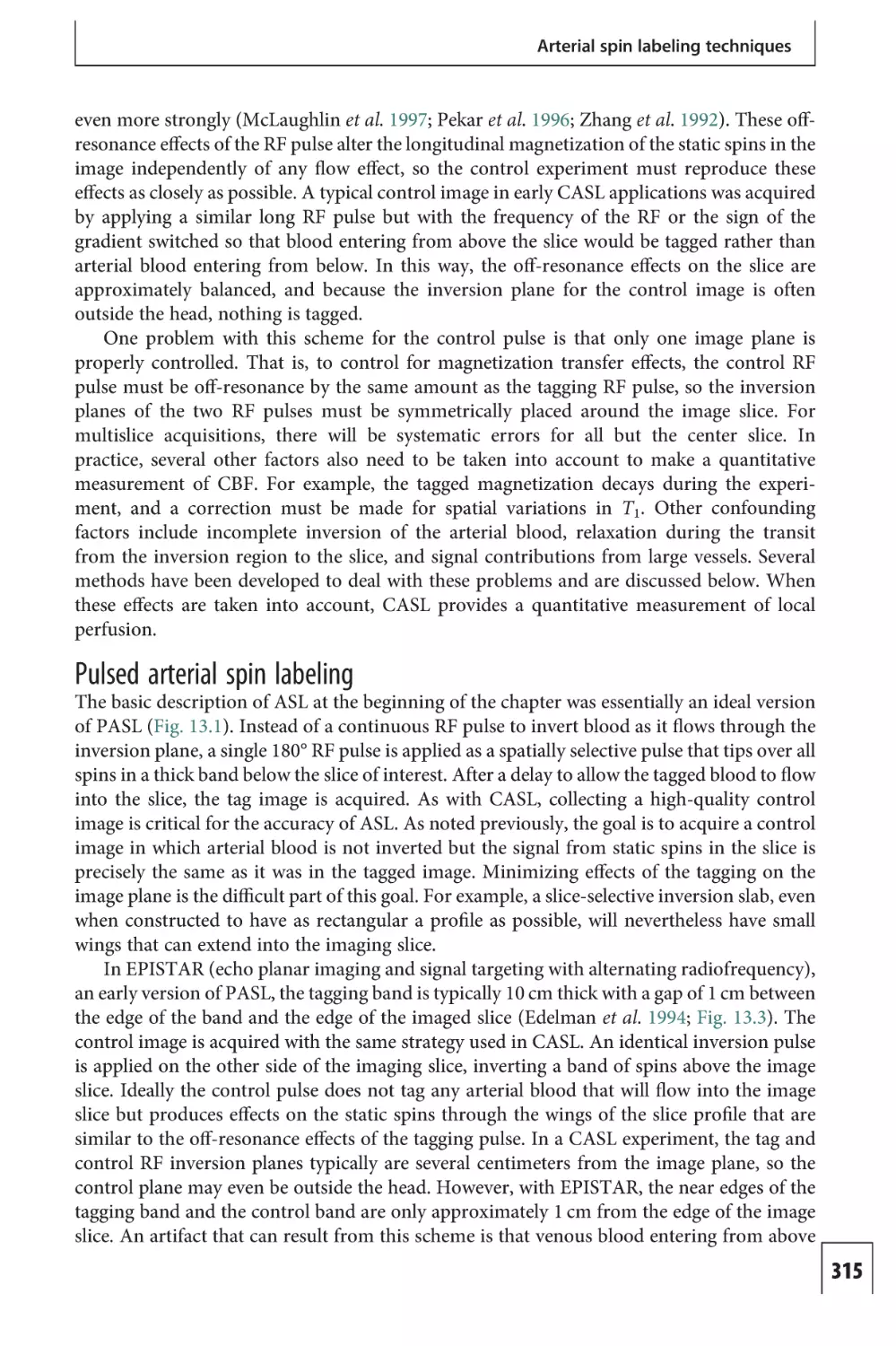
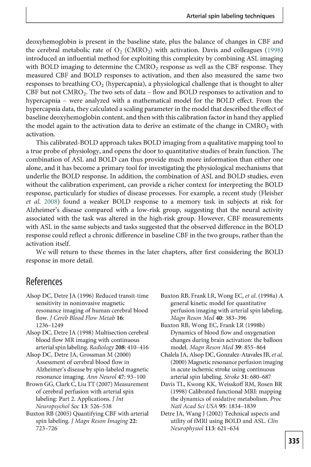
Fig. 1.2. Synaptic
signaling. An action
potential arriving at the
pre-synaptic terminal
(1) initiates Ca2+ influx
(2), triggering
neurotransmitter
(glutamate [Glu])
release into the
synaptic cleft (3),
binding of
neurotransmitter to
receptors on the postsynaptic neuron (4),
opening of Na+
channels (5), and
creation of a strong
influx of Na+ into the
post-synaptic neuron.
Astrocytes have
processes that project
to neuronal synapses
and also to blood
vessels, and are
involved in clearing
neurotransmitter and
signaling blood flow
changes (illustrated in
Figs. 1.4 and 2.4).
sites on the post-synaptic membrane. At each synapse, the neurotransmitter released is
characteristic of the pre-synaptic neuron. Glutamate is the most common excitatory neurotransmitter in mammalian cortex, and gamma-aminobutyric acid (GABA) is a common
inhibitory neurotransmitter (Erecinska and Silver 1990). Glutamatergic neurons include the
pyramidal cells, the principal neurons of the cortex. GABAergic neurons include a diverse
class of interneurons that are important for controlling the net activity of ensembles of
neurons.
There are two general classes of receptor. Ionotropic receptors are proteins that are
themselves ion channels, so binding of neurotransmitter leads to a conformational change
of the receptor that opens the ion channel, and the channel remains open while the neurotransmitter is bound. These receptors are very fast, operating on a time scale of milliseconds,
and many glutamate and GABA receptors operate in this way. In contrast, at metabotropic
receptors, binding of the neurotransmitter initiates a chemical cascade that changes the
concentration of intracellular second messengers, such as cyclic adenosine monophosphate
(cAMP), cyclic guanosine monophosphate (cGMP), and Ca2+. These receptors are also called
G-protein-coupled receptors, because the initiating step involves guanosine triphosphate
(GTP), an energy-rich molecule that is a close relative of ATP, which is discussed later in
this chapter. These signaling molecules then gate ion channels or exert other modulatory
effects on the post-synaptic neuron, and the time scale for these effects can be much slower
and longer lasting (seconds to minutes or more) compared with ionotropic receptors. For
this reason, activation of these receptors is often described as having a neuromodulatory role,
affecting different aspects of neuronal signaling from neurotransmitter release to postsynaptic effects, and these synapses are thought to play an important role in learning and
11
An overview of fMRI
memory. Examples include different types of glutamate and GABA receptor as well as a wide
range of other receptors including those for serotonin (5-hydroxytryptamine [5-HT]),
histamine, and dopamine.
In summary, binding of neurotransmitter to a receptor on the post-synaptic membrane
initiates a process that opens or modulates particular ion channels either directly or through
the action of second messengers. Opening Na+ channels creates a strong inward positive
current, which will tend to depolarize the membrane potential in the vicinity of the synapse,
creating an EPSP. If, however, the action at the synapse is to open K+ channels, the effect is to
make the potential more negative – hyperpolarizing the membrane – because the equilibrium potential for K+ is more negative, creating an IPSP. If Cl− channels are opened, there
may be no change in the membrane potential itself, because the resting membrane potential
is already close to the Cl− equilibrium potential. However, this also has an inhibitory effect on
the post-synaptic neuron, because now opening the same Na+ channels will have less of an
effect on the membrane potential. Opening Cl− channels pulls the potential more strongly
toward the Cl− equilibrium potential, which happens to be approximately the resting potential.
For this reason, more Na+ channels would need to open to achieve the same depolarization as
when the Cl− channels are not open. In short, opening many Na+ channels will depolarize the
membrane; opening many K+ channels will hyperpolarize the membrane; and opening many
Cl− channels will tend to peg the membrane potential near the resting value.
At any moment, the neuron may be receiving signals from many other neurons, creating
a complex pattern of flickering fluctuations of the membrane potential on the dendritic tree.
Along a dendrite, the currents and associated membrane potentials combine; and if there is a
sufficient net current that reaches the cell body, the membrane potential there will be
depolarized, generating an action potential and sending a new signal to other neurons.
Note, though, that there is likely to be a great deal of sub-threshold synaptic activity that
may not lead to spiking. Excitatory synapses generally are located on the dendrites, while
inhibitory synapses are generally closer to the cell body. Because of the complex geometry of
a neuron, incoming excitatory currents down a dendrite toward the cell body can be
dissipated by IPSPs nearer the cell body. For this reason, the output of the post-synaptic
cell is a complex combination of the inputs, and it is important to keep in mind the
distinction between synaptic activity and spiking activity. As discussed below, much of the
energy cost of neural signaling is thought to lie in the recovery from synaptic activity.
Electrophysiology measurements
The opening and closing of ion channels creates currents across the cell membrane and also
within the extracellular space. Because of Ohm’s law, these fluctuating currents are associated
with fluctuating electric potentials (Fig. 1.3). These extracellular potentials can be measured
invasively with an electrode with high temporal resolution. For example, opening a Na+
channel at a synapse near the electrode, creating a positive current into the cell, creates a
negative deflection of the potential at the location of the electrode. Extracellular potentials are
often analyzed by dividing the signal into low- and high-frequency components. The lowfrequency components, called local field potentials (LFPs), primarily reflect synaptic activity,
while the high-frequency activity, called multi-unit activity (MUA), primarily reflects spiking
activity (Logothetis 2002). While electrode studies are primarily carried out in animal models,
implanted electrodes in patients with epilepsy have made possible human recordings as well.
In addition, some components of extracellular potentials are detectable outside the
head with non-invasive techniques. The electroencephalogram (EEG) is produced from
12
Neural activity and energy metabolism
+
Current
dipole
Inward
currents
Extracellular
potentials
–
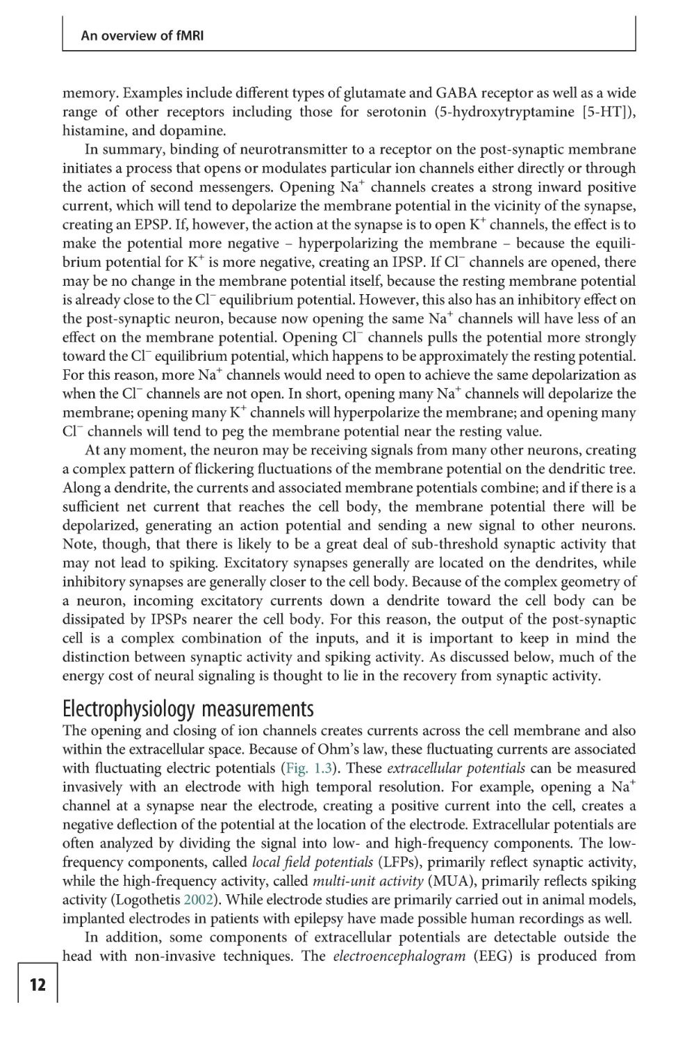
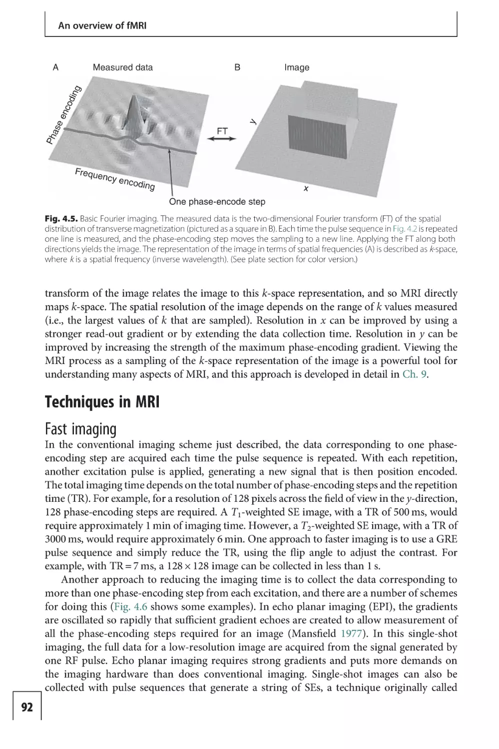
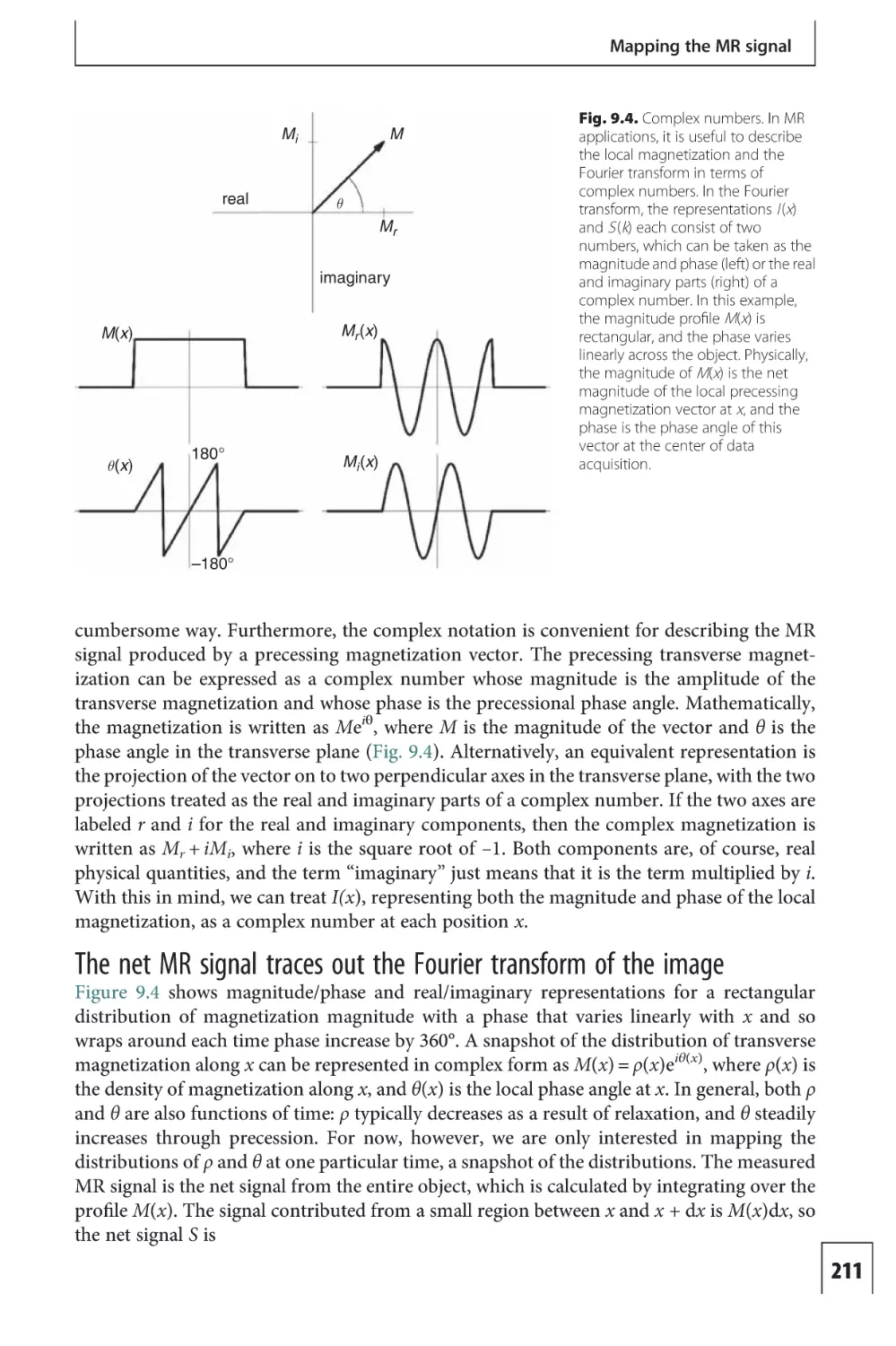
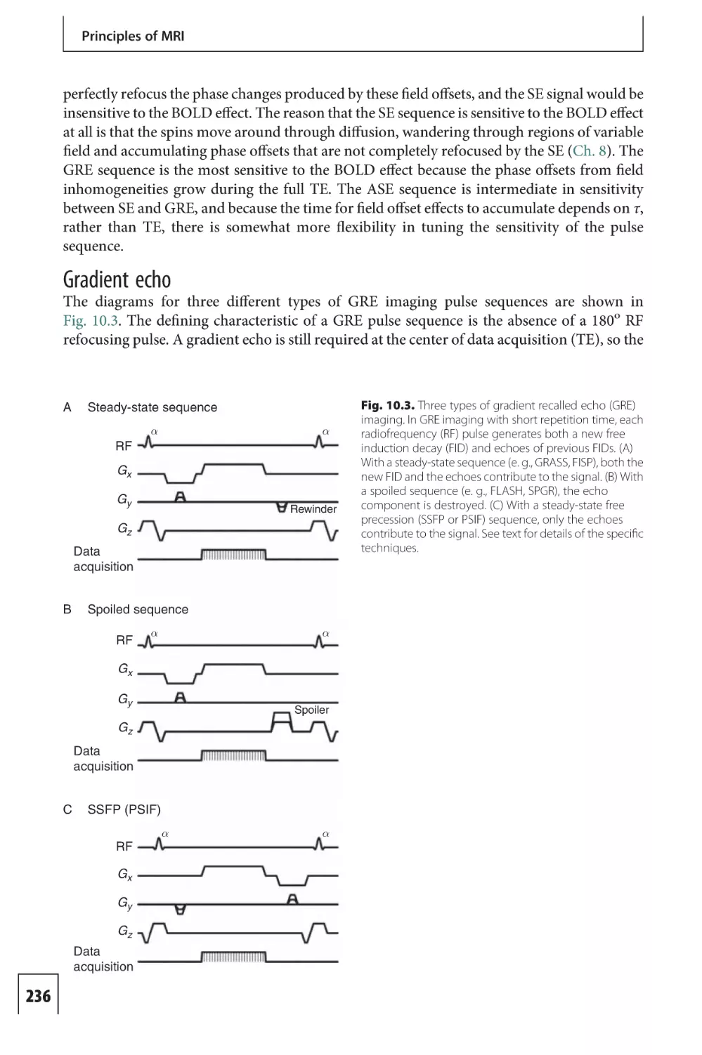
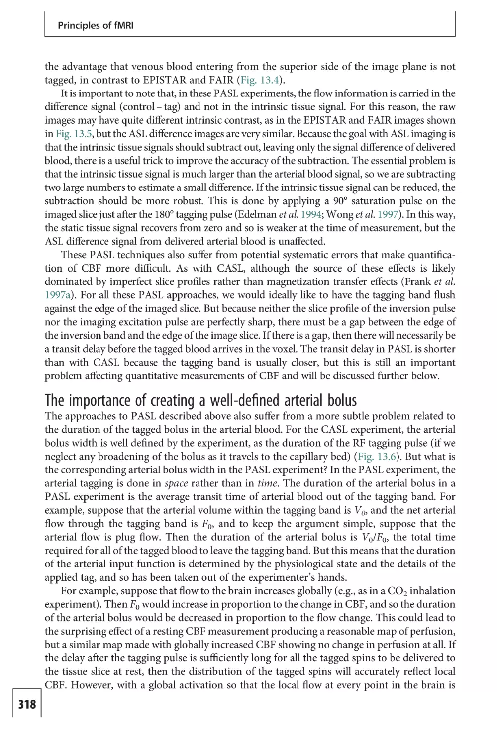
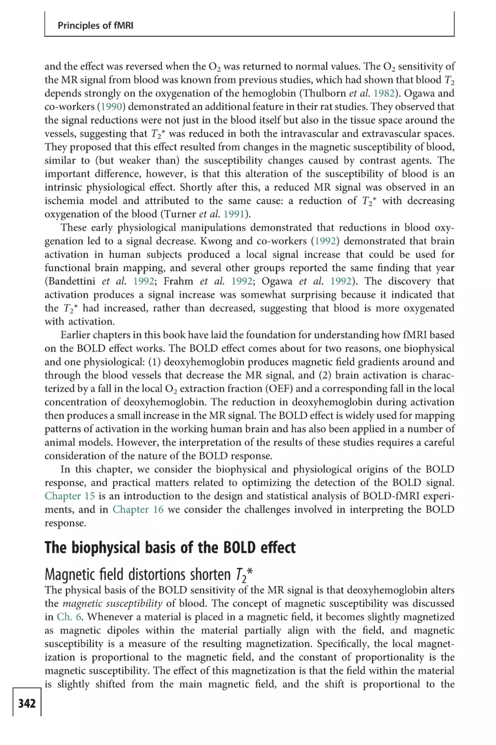
Fig. 1.3. Extracellular potentials. Pyramidal neurons, the principal
neurons of the cortex, have a long apical dendrite extending from the
cell body toward the cortical surface. Excitatory activity near the top
creates inward positive currents toward the cell body. This current
dipole in the apical dendrite creates extracellular return currents that
can be detected as fluctuations of the extracellular potential using
implanted electrodes. If the dendritic currents in a patch of cortex are
sufficiently coherent, the activity can be detected on the surface of the
head. Electroencephalography is sensitive to the extracellular currents
and magnetoencephalography is sensitive to the magnetic field
created by the current dipole.
Outward
currents
measurements with sensitive electrodes on the scalp. The primary source of these measured
potentials is coherent activity of the cortical pyramidal cells, which have a long apical
dendrite extending perpendicularly through the layers of cortex. Current entering the
dendritic tree at the top and exiting in the cell body creates a large current dipole within
the apical dendrite and a distributed extracellular return current through the rest of the
head. When a patch of cortex is active, the coherent activity of the roughly aligned pyramidal
cells produces currents that are detectable as potential fluctuations on the scalp, and from
measurements with an array of scalp electrodes the source location can be estimated. The
EEG signals are dominated by synaptic currents, rather than action potentials, and do not
distinguish between excitatory and inhibitory activity. In addition, the strength of the
detected potential depends on the geometry of the dendritic currents; an active neuron
with a more symmetric dendritic tree would not generate a strong net current dipole and
so likely would not be detected.
Another non-invasive technique for detecting electrical activity is magnetoencephalography (MEG), a technique for measuring very weak magnetic fields outside the head. The
MEG signal also is dominated by the current dipoles along the apical dendrites of the
pyramidal cells, but here it is the magnetic field produced by that dendritic current that is
measured. An important distinction between MEG and EEG is that with EEG the measured
potentials result from currents flowing through the head between the site of the activity and
the electrodes. For this reason, the electrodes must be in electrical contact with the scalp.
In addition, any variations in electrical conductivity, such as between the brain and the skull,
must be taken into account when modeling the source of the potentials from the measured
values on the scalp. In contrast, the magnetic field created by the current dipole in the cortex
extends through space, so the detectors do not need to be in contact with the head, and the
effects of intervening tissues are much less of a problem.
Temporal resolution with EEG and MEG is excellent, on the order of milliseconds.
However, spatial localization with EEG and MEG is more problematic because of the
13
An overview of fMRI
difficulty of solving the inverse problem: taking a set of measured potentials or magnetic fields
on the surface of the head and working backwards to deduce what pattern of activity in the
brain could give rise to the observed pattern of measurements. The central problem is that
potentially many distributions of activity within the brain could produce similar measured
EEG and MEG signals, and because of the intrinsic noise in the measurements these brain
spatial patterns cannot be distinguished. Nevertheless, substantial progress has been made on
this problem, particularly when high-resolution anatomical MRI data are used to constrain
the possible solutions of the inverse problem. In summary, current EEG and MEG methods
provide a useful window on brain function, particularly for analyzing the temporal evolution
of the response to a stimulus.
Recovery from neural activity
Neural signaling is a thermodynamically downhill process
From a thermodynamic point of view, each of the steps in neuronal signaling is a downhill
reaction in which a system held far from equilibrium is allowed to approach closer to
equilibrium. The high extracellular Na+ concentration leads to a spontaneous inward ion flow
once the trigger of a permeability increase occurs. Similarly, the Ca2+ influx occurs spontaneously once its membrane permeability is increased, and the neurotransmitter is already tightly
bundled in a small package waiting to disperse freely once the package is opened. We can think
of neuronal signaling as a spontaneous, but controlled, process. Nature’s trick in each case is
to maintain a system away from equilibrium, waiting for the right trigger to allow it to move
toward equilibrium.
The set of intracellular and extracellular ionic concentrations is a thermodynamic system
whose equilibrium state would be one of zero potential difference across the cell membrane,
with equal ionic concentrations on either side. Any chemical system that is removed from
equilibrium has the capacity to do useful work, and this capacity is called the free energy of
the system (see Box 1.1 at the end of this chapter). The neuronal system, with its unbalanced
ionic concentrations, has the potential to do work in the form of neuronal signaling. But
with each action potential and release of neurotransmitter at a synapse, the available free
energy is reduced. Returning the neurons to their prior state, with the original ion gradients
and neurotransmitter distributions, requires energy metabolism.
Metabolism of ATP is required to restore ionic
gradients following neural activity
Restoring the ion gradients requires active transport of each ion against its natural drift
direction, which is thermodynamically an uphill process, moving the system away from
equilibrium and increasing the free energy of the system (Fig. 1.4). For such a change to
occur, the transport must be coupled to another system whose free energy decreases
sufficiently in the process so that the total free energy decreases (see Box 1.1 at the end of
this chapter). The re-establishment of ionic gradients thus requires a source of free energy,
and in biological systems free energy is primarily stored in the relative proportions of the
three phosphorylated forms of adenosine: adenosine triphosphate (ATP), adenosine diphosphate (ADP), and adenosine monophosphate (AMP) (Siesjo 1978). Inorganic phosphate (Pi)
can combine with ADP to form ATP, but the thermal equilibrium of this system at body
temperature strongly favors the ADP form. Yet in the body, the ATP/ADP ratio is
14
Neural activity and energy metabolism
Pre-synaptic terminal
Arteriole
4
Na +
2+
Ca
ADP
K+
ATP
5
Glu
3
Glu
Na+
Gln
1
Ion
channel
+
Na
Blood
flow
2
Astrocyte
Receptor
5
+
K
5
+
Na
Post-synaptic neuron
+
K
Smooth
muscle
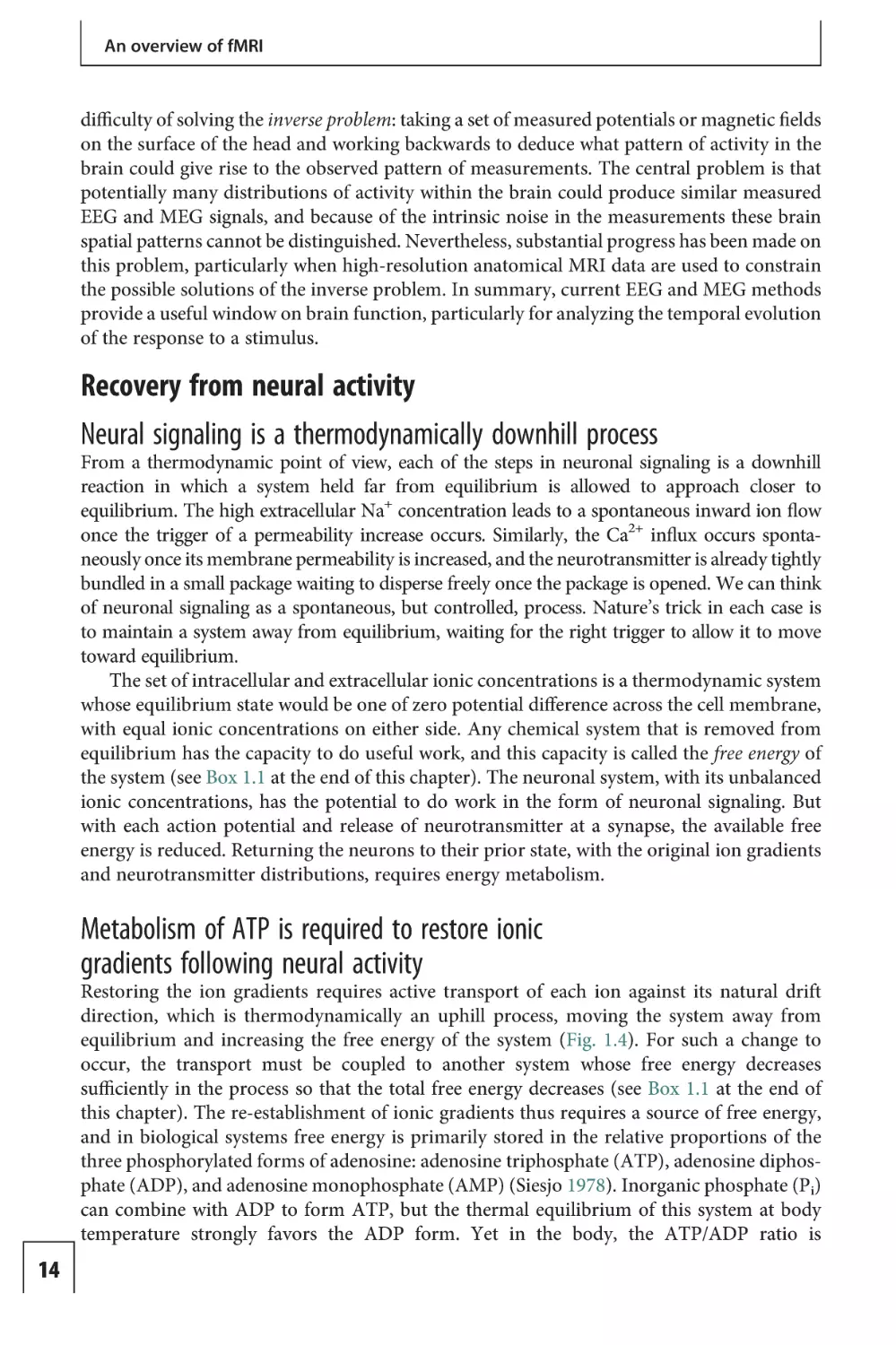
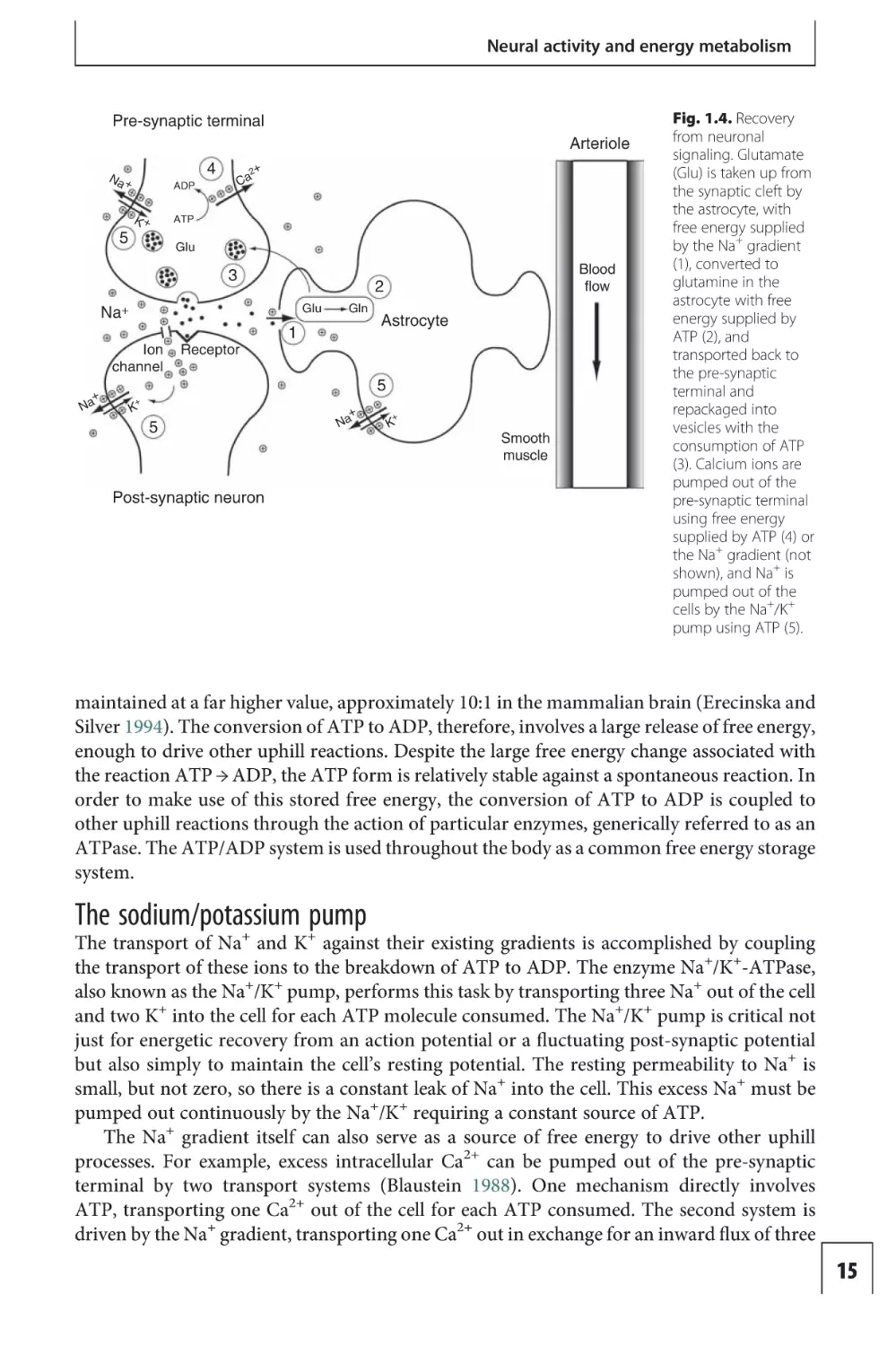
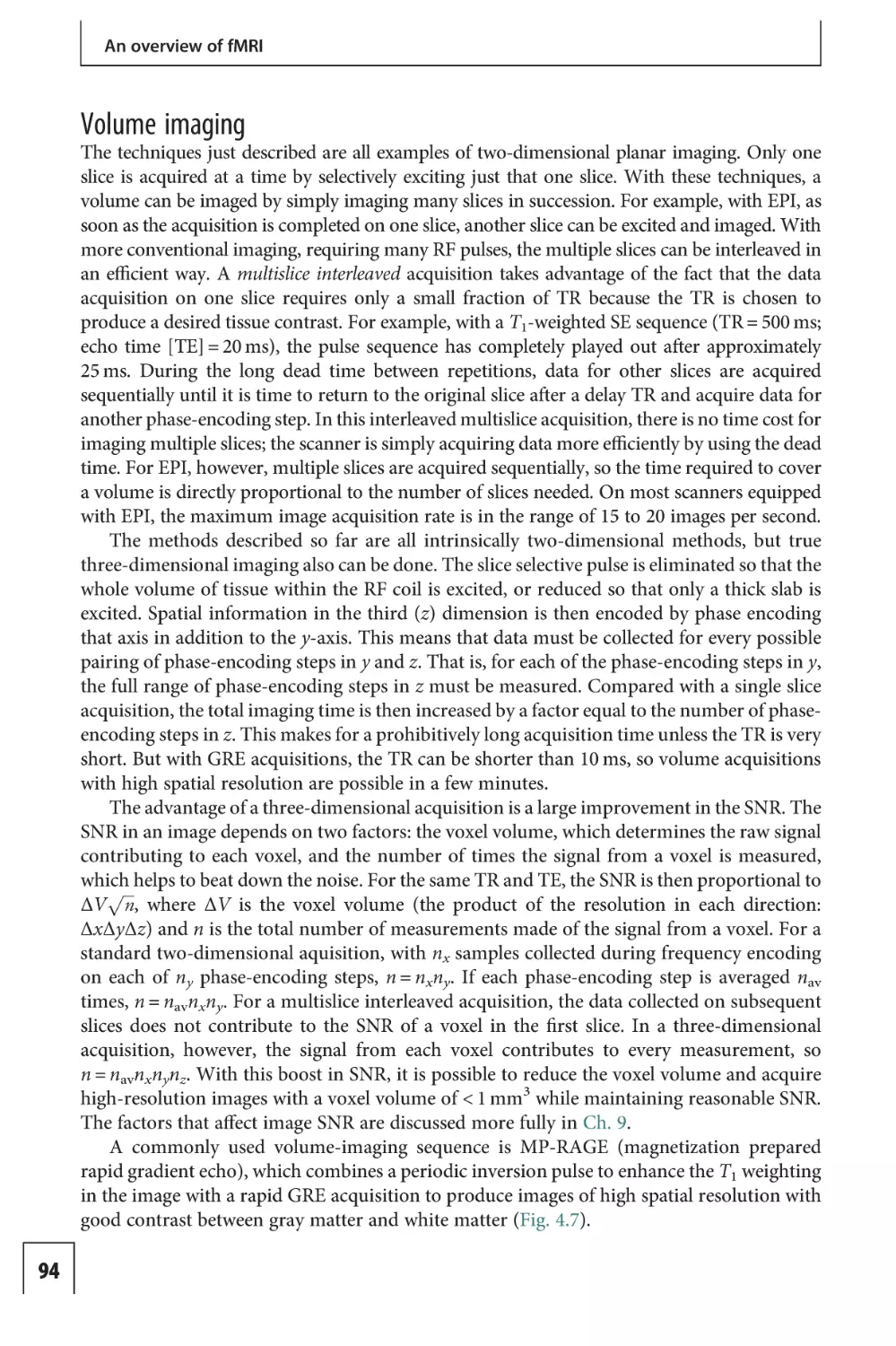
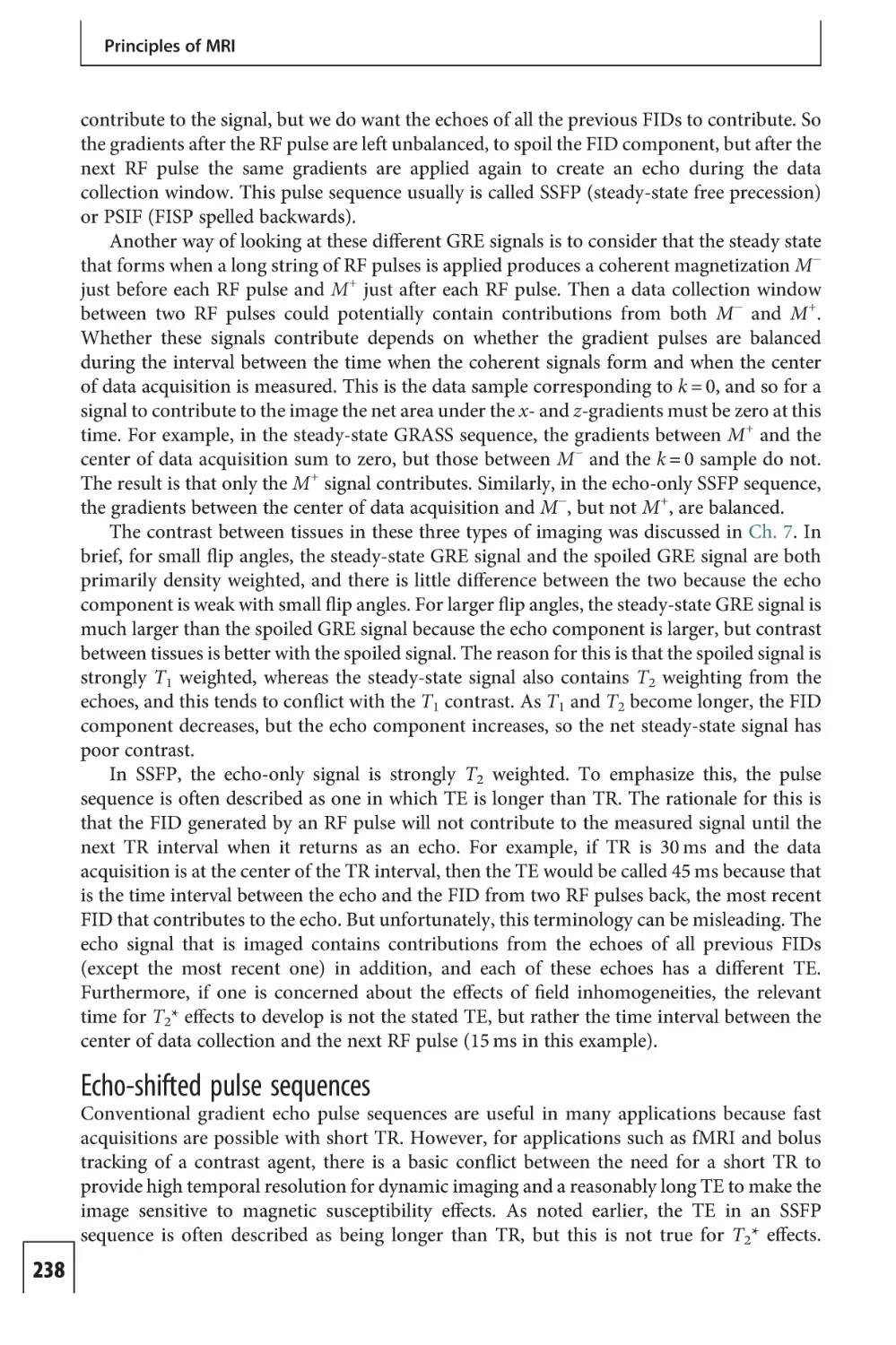
Fig. 1.4. Recovery
from neuronal
signaling. Glutamate
(Glu) is taken up from
the synaptic cleft by
the astrocyte, with
free energy supplied
by the Na+ gradient
(1), converted to
glutamine in the
astrocyte with free
energy supplied by
ATP (2), and
transported back to
the pre-synaptic
terminal and
repackaged into
vesicles with the
consumption of ATP
(3). Calcium ions are
pumped out of the
pre-synaptic terminal
using free energy
supplied by ATP (4) or
the Na+ gradient (not
shown), and Na+ is
pumped out of the
cells by the Na+/K+
pump using ATP (5).
maintained at a far higher value, approximately 10:1 in the mammalian brain (Erecinska and
Silver 1994). The conversion of ATP to ADP, therefore, involves a large release of free energy,
enough to drive other uphill reactions. Despite the large free energy change associated with
the reaction ATP → ADP, the ATP form is relatively stable against a spontaneous reaction. In
order to make use of this stored free energy, the conversion of ATP to ADP is coupled to
other uphill reactions through the action of particular enzymes, generically referred to as an
ATPase. The ATP/ADP system is used throughout the body as a common free energy storage
system.
The sodium/potassium
pump
+
+
The transport of Na and K against their existing gradients is accomplished by coupling
the transport of these ions to the breakdown of ATP to ADP. The enzyme Na+/K+-ATPase,
also known as the Na+/K+ pump, performs this task by transporting three Na+ out of the cell
and two K+ into the cell for each ATP molecule consumed. The Na+/K+ pump is critical not
just for energetic recovery from an action potential or a fluctuating post-synaptic potential
but also simply to maintain the cell’s resting potential. The resting permeability to Na+ is
small, but not zero, so there is a constant leak of Na+ into the cell. This excess Na+ must be
pumped out continuously by the Na+/K+ requiring a constant source of ATP.
The Na+ gradient itself can also serve as a source of free energy to drive other uphill
processes. For example, excess intracellular Ca2+ can be pumped out of the pre-synaptic
terminal by two transport systems (Blaustein 1988). One mechanism directly involves
ATP, transporting one Ca2+ out of the cell for each ATP consumed. The second system is
driven by the Na+ gradient, transporting one Ca2+ out in exchange for an inward flux of three
15
An overview of fMRI
Na+. Note that one ATP is required to move one Ca2+ out of the cell by either transport
system because in the second system the Na+/K+ will ultimately be required to consume one
ATP to transport the three Na+ back out of the cell.
Astrocytes play a key role in recycling neurotransmitter
At the synapse, neurotransmitter must be taken up by the pre-synaptic terminal, and
repackaged into vesicles. For glutamate, the process of re-uptake involves a shuttle between
the astrocytes and the neurons (Erecinska and Silver 1990; Iadecola and Nedergaard 2007).
Astrocytes are one of the most common glial cells in the brain, frequently located in areas of
high synaptic density. The glutamate from the synapse is transported into the astrocytes by
coupling the passage of one glutamate with the movement of three Na+ down the Na+
gradient. The transport of the Na+ back out of the cell requires the action of the Na+/K+ and
consumption of one ATP. In the astrocyte, the glutamate is converted to glutamine, which
requires an additional ATP, and the glutamine is then released.
The glutamine is passively taken up by the pre-synaptic terminal, where it is converted
back to glutamate. Repackaging the glutamate into the vesicles then requires transporting the
neurotransmitter against a strong concentration gradient, a process that requires more ATP.
One proposed mechanism for accomplishing this is that a strong concentration gradient
of hydrogen ions (H+) ions is first created, with the H+ concentration high inside the vesicle
(Erecinska and Silver 1990). The inward transport of neurotransmitter is then coupled to a
degradation of this gradient. The H+ gradient itself is created by an ATP-powered pump.
An ATP energy budget for neural activity
Theoretical estimates of the energy cost of different aspects of neuronal signaling by Attwell
and colleagues have provided a useful and influential guide in thinking about the energetics
of brain activity (Attwell and Iadecola 2002; Attwell and Laughlin 2001). To frame this
argument, consider the following basic processes: (1) maintenance of the cell at rest; (2) the
generation of an action potential and the propagation of that action potential to many
synapses with other neurons; (3) recovery on the pre-synaptic side of the synapse, including Ca2+ clearance and neurotransmitter recycling through the astrocytes; and (4) recovery
from post-synaptic potentials, primarily related to pumping Na+ out of the cell against
its gradient. We can think of the first process as basic housekeeping of the cell, and this
component is not directly related to neuronal signaling. The other three components are
directly related to signaling, broken down as the spiking activity and pre- and post-synaptic
activity. The overall costs of this signaling component will depend on the average spiking
rate in the brain, because this drives all three components. In addition, the relative costs
of spiking and synaptic activity will depend on the average number of synapses reached
by each action potential. For these reasons, the distribution of energy costs across these
components is estimated to be different for rats and primates because the primate brain
has a lower average spiking rate but approximately a three-fold larger ratio of synapses to
neurons.
The estimates derived by Attwell and colleagues (Attwell and ladecola 2002; Attwell and
Laughlin 2001) are based on a wide range of data, primarily from rat studies, relating the
different neuronal and glial processes to the ATP required for recovery and for maintenance
of the cell. For the primate brain, the dominant energy cost is recovery from post-synaptic
potentials (~74%). The costs of maintaining the cell, generating and transmitting action
potentials, and recycling neurotransmitter at the synapse are all relatively inexpensive
16
Neural activity and energy metabolism
compared with post-synaptic costs. At first glance this seems surprising, because we tend to
think of the essence of neural activity as spiking, and we might have expected that to be the
dominant energy cost. The overall energy consumption is closely related to the spiking rate
(Laughlin and Sejnowski 2003), but it is the downstream synaptic activity rather than the
generation of the spike itself that is costly. By these estimates, it is the integrative activity
associated with a neuron receiving many inputs that is costly.
The idea that synaptic activity dominates the energy costs potentially affects how we
should interpret a measured spatial distribution of changes in energy metabolism. Based on
this picture, the energy cost associated with the generation of a particular neuronal spike is
spatially distributed, depending on the projections from that neuron to synapses with other
neurons. Some of these projections are quite long, creating the possibility that the location
where the spike originated may not be detected, with energy metabolism changes seen only
at the downstream synaptic terminals. In practice, this phenomenon of missing the site
of generation of the spikes is probably rare in functional neuroimaging, because most of
the synaptic connections a neuron receives are from nearby neurons. Given the typical
resolution of neuroimaging methods of a few millimeters, most of the synaptic activity
within a resolution element of the imaging technique arises from spiking within that same
element.
However, Raichle and Mintun (2006) have emphasized an example of missing the spiking
location in a study by Schwartz and colleagues (1979). In this early deoxyglucose (DG) study
in rats, the animals were exposed to an osmotic load that would stimulate neurons in the
hypothalamus that have long-range projections to the pituitary gland. The result was that
there was no measurable change in glucose metabolism in the hypothalamus, the location of
the spiking neurons, while there was a strong increase in glucose metabolism in the pituitary,
the location of the synapses. This result supports the general picture that energy metabolism
changes are strongest at the site of increased synaptic activity, rather than the site of increased
spiking activity.
The high cost of post-synaptic processes reflects the need to pump Na+ out of the cell.
Estimates are that at least half of the ATP used in the brain is consumed in driving the Na+/
K+ pump (Ames 2000). One way to think about this high cost of Na+ pumping is to look at
the synapse as an amplifier for an excitatory signal. The action potential arriving at the
synapse is a weak electrical signal, which is first converted to an intracellular Ca2+ signal and
then converted to a chemical signal in the form of neurotransmitter released into the synaptic
cleft. These stages are relatively inexpensive because the number of molecules that must be
transported in the recovery phase is relatively small. The major amplification comes when a
neurotransmitter binds to a post-synaptic receptor and opens a Na+ channel, which may let a
thousand ions pass through before it closes again. In this way, the weak signal associated with
one neurotransmitter molecule binding to a receptor is amplified a thousand-fold. But all
that Na+ must be pumped back in the recovery stage. Very roughly, moving any molecule
against its gradient requires about one ATP, so it is perhaps not so surprising that the
primary signal amplification stage is the dominant energy cost in neural signaling.
In brief, a source of free energy is not required for the production of a neuronal signal,
but rather for the re-establishment of chemical and ionic gradients reduced by the signaling, particularly the costs of ion pumping for synaptic activity. Without this replenishment, the system eventually runs down like an old battery in need of charging. The
restoration of chemical gradients is driven either directly or indirectly by the conversion
of ATP to ADP. To maintain their activity, the cells must restore their supply of ATP by
17
An overview of fMRI
reversing this reaction and converting ADP back to ATP. This requires that the strongly
uphill conversion of ADP to ATP must be coupled to an even more strongly downhill
reaction. In the brain, virtually all of the ATP used to fuel cellular work is derived from
the metabolism of glucose and O2 (Siesjo 1978). Both O2 and glucose are in short supply in
the brain, and continued brain function requires continuous delivery of these metabolic
substrates by CBF.
Energy metabolism
In the discussion above and in Box 1.1 (at end of this chapter), neural activity is discussed
in terms of a thermodynamic framework, in which uphill chemical processes are coupled
to other, downhill, processes. For virtually all cellular processes, this chain of thermodynamic coupling leads to the ATP/ADP system within the body. But the next step in the
chain, the restoration of the ATP/ADP ratio, requires coupling the body to the outside
world through intake of glucose and O2. Despite the fact that a bowl of sugar on the dining
room table surrounded by air appears to be quite stable, glucose and O2 together are far
removed from equilibrium. When burned, glucose and O2 are converted into water and
CO2, releasing a substantial amount of heat. If a more controlled conversion is performed,
much of the free energy can be used to drive the conversion of ATP to ADP, with
metabolism of one glucose molecule generating enough free energy change to convert as
many as 38 ADP to ATP. As far as maintaining neural activity is concerned, the chain of
thermodynamically coupled systems ends with glucose and O2. As long as we eat and
breathe, we can continue to think.
The mechanisms for harnessing the free energy of glucose and O2 in oxidative metabolism can be divided into four stages: (1) glycolysis in the cytosol, in which glucose breaks
down into two pyruvate molecules; (2) the trans-carboxylic acid (TCA) cycle (also called the
Kreb’s cycle or the citric acid cycle) in the mitochondria, in which pyruvate is broken down to
form carbon dioxide (CO2) with the storage of energy in the form of reduced nicotinamide
adenine dinucleotide (NADH) and related compounds; (3) the electron transfer chain in the
mitochondria, in which the transfer of electrons from NADH to O2 to form water is coupled
to pumping of H+ across the inner membrane of the mitochondria against its gradient and
thus storing energy in the H+ gradient; and (4) the movement of H+ down its gradient
coupled with the combination of ADP and Pi to form ATP (Fig 1.5). Glycolysis does not
require O2 and produces only a small amount of ATP through reactions in the cytosol. The
further metabolism of pyruvate in the mitochondria produces much more ATP. Oxidative
glucose metabolism involves many steps, and the following is a sketch of only a few key
features. A more complete discussion can be found in Siesjo (1978).
Glycolysis in the cytosol
In glycolysis, the breakdown of a glucose molecule into two molecules of pyruvate is coupled
to the net conversion of two molecules of ADP to ATP. The process involves several steps,
with each step catalyzed by a particular enzyme. The first step in this process is the addition of
a phosphate group to the glucose, catalyzed by the enzyme hexokinase. The phosphate group
is made available by the conversion of ATP to ADP, so in this stage of glycolysis one ATP is
consumed and fructose 6-phosphate is produced. A second phosphorylation stage, catalyzed
by phosphofructokinase (PFK), consumes one more ATP molecule. Up to this point, two ATP
molecules have been consumed, but in the remaining steps the complex is broken down into
18
Neural activity and energy metabolism
Blood
Tissue
Cytosol
Glucose
Glucose
1 ATP
Hexokinase
1 ADP
1 ATP
PFK
Fructose
1,6-phosphate
1 ADP
Glycolysis
Glucose
6-phosphate
4 ATP
4 ADP
Pyruvate
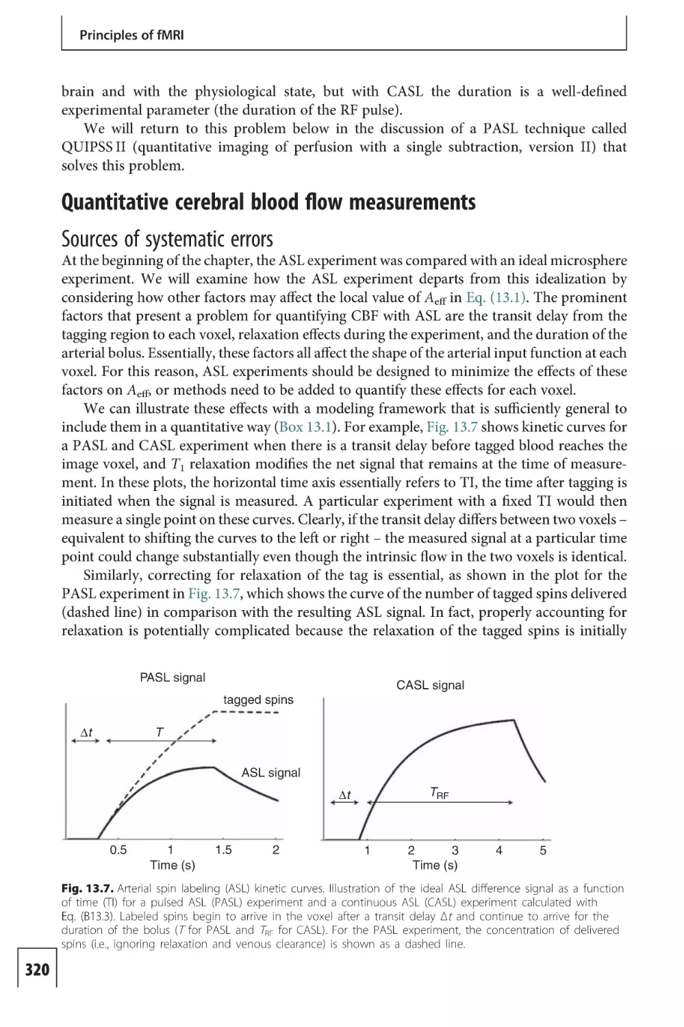
Fig. 1.5. Energy metabolism. The major steps of cerebral
energy metabolism are illustrated. Glucose is taken up
from blood and first undergoes glycolysis (the steps in
boxes) to produce pyruvate, for a net conversion of two
ADP to ATP. If pyruvate is not further metabolized, it
interchanges reversibly with lactate. Oxidative
metabolism occurs in the mitochondria, where pyruvate
enters the tricarboxylic acid (TCA) cycle and is broken
down to CO2 with electrons transferred to the electron
transfer chain (ETC). Electrons move down the ETC to a
final combination with O2, using the free energy available
to pump H+ across an internal membrane in the
mitochondria (not shown in the figure). Finally, the H+
gradient is tapped to convert an additional 36 ADP to ATP.
The waste products CO2 and heat are cleared from the
tissue by blood flow.
Lactate
O2
CO2
Mitochondria
TCA cycle
ETC
36 ATP
36 ADP
Water
two pyruvate molecules accompanied by the conversion of four ADP to ATP. The net
production of ATP is then two ATP for each glucose molecule undergoing glycolysis.
The cerebral metabolic rate of glucose (CMRGlc) is defined as the number of moles of
glucose metabolized per gram of tissue per minute. The activities of the key enzymes are
sensitive to the local environment and so provide several avenues for local control of
CMRGlc. Hexokinase is inhibited by its own product, so unless the fructose 6-phosphate
continues down the metabolic path, the activity of hexokinase is curtailed. The step
catalyzed by PFK is the major control point in glycolysis (Bradford 1986). The enzyme
PFK is stimulated by the presence of ADP and inhibited by the presence of ATP. In this
way, there is a simple mechanism for increasing glycolysis when the stores of ATP need
to be replenished. In addition, many other factors influence the activity of PFK, including
inhibition when the pH decreases, so CMRGlc can be adjusted to meet a variety of
demands.
In addition to storing energy in ATP, a second important mechanism for storing free
energy comes into play during glycolysis. The molecule nicotinamide adenine dinucleotide
(NAD+) can accept electrons to form NADH, a thermodynamically uphill process. During
glycolysis, the conversion of glucose to two pyruvate molecules is coupled to the conversion of two NAD+ molecules to two molecules of NADH. Essentially, two electrons are
transferred to each NAD+ molecule, and the NAD+ also picks up an H+ to make the neutral
form NADH. At equilibrium, NAD+ is present in higher concentration than NADH, so the
thermodynamically downhill process of glucose conversion to two pyruvate molecules is
coupled to the uphill process of NAD+ → NADH. The NADH serves as an intermediate
mechanism to carry electrons to other processes, donating the electrons and reverting to
the NAD+ form. The NADH/NAD+ system thus contains stored free energy that can be
tapped by other processes.
19
An overview of fMRI
Lactate production and the lactate shuttle
The end point of glycolysis is the production of two pyruvate molecules, two ATP, and two
NADH. For glycolysis to proceed, the negative free energy change associated with converting
glucose to pyruvate must be larger than the positive free energy changes associated with
ADP → ATP and NAD+ → NADH. If the NADH/NAD+ ratio grows too large, the free energy
required to convert more NAD+ to NADH will become too high to be provided by the
conversion of glucose → pyruvate, and glycolysis will stop. In each case, the free energies of
the individual reactions depend on ratios of reactants and products (see Box 1.1 at the end of
this chapter), so glycolysis is energetically favored if the glucose/pyruvate ratio is high or the
NADH/NAD+ ratio is low. Most of the pyruvate produced diffuses into the mitochondria,
where it is further metabolized (see the next section), and this tends to keep the glucose/
pyruvate ratio high. In addition, a transport mechanism, called the malate/aspartate shuttle,
transfers NADH from the cytosol to the mitochondria in exchange for NAD+, which tends to
keep the NADH/NAD+ ratio from getting too high in the cytosol.
These mechanisms both shuffle the products of glycolysis off to the mitochondria, as fuel
for oxidative metabolism. However, if the rate of pyruvate production by glycolysis exceeds
the rate of pyruvate metabolism in the mitochondria, the pyruvate concentration in the
cytosol will grow and another reaction becomes important: pyruvate is converted to lactate
by a reaction coupled to NADH → NAD+, reducing the problems of both pyruvate and
NADH build-up. This reversible reaction is catalyzed by the enzyme lactate dehydrogenase,
and the lactate produced diffuses out of the cell and is carried away in the blood. In principle,
this can also happen in reverse, with lactate from the blood diffusing into the cell, converting
to pyruvate, and diffusing into the mitochondria for further metabolism, and there is some
evidence that the brain can be a net consumer as well as producer of lactate during exercise
(Quistorff et al. 2008).
From the description above, the production of lactate may be a sign of an imbalance in
energy metabolism, indicating an over-metabolism of glucose relative to O2 metabolism. In
hypoxia, for example, glycolysis could continue to provide some ATP when O2 is scarce, with
the resulting production of lactate. In fact, though, lactate production may play a more direct
role in healthy energy metabolism through the action of a lactate shuttle (Pellerin et al. 2007).
Astrocytes play a key role in neuronal signaling by clearing neurotransmitter from the
synaptic cleft. There is a growing body of evidence indicating that astrocytes have a high
glucose metabolic rate compared with their O2 metabolic rate, with production of lactate.
However, rather than diffusing into the blood, the lactate diffuses into the neurons where it is
used as fuel. Lactate dehydrogenase converts the lactate to pyruvate, which is then metabolized in the mitochondria of the neuron.
In summary, the end point of glycolysis is the production of two ATP molecules and two
pyruvate molecules from each glucose molecule, plus the conversion of two NAD+ molecules
to two NADH molecules. But glycolysis alone taps only a small fraction of the available free
energy in the glucose, and utilization of this additional energy requires further metabolism of
pyruvate in the TCA cycle.
Mitochondrial pyruvate metabolism and the electron transfer chain
In the healthy resting brain, nearly all of the pyruvate produced by glycolysis is destined for
the TCA cycle. The TCA cycle involves many steps, each catalyzed by a different enzyme, and
the machinery of the process is housed in the mitochondria. The net balance sheet for the
20
Neural activity and energy metabolism
TCA cycle is that one pyruvate molecule is broken down to three molecules of CO2 with
the conversion of 12 molecules of NAD+ to NADH (or a related electron storage compound). These molecular transformations do not involve molecular O2. At this point, the
free energy is concentrated in the NADH/NAD+ system. In the next stage, this free energy is
converted to free energy of the H+ gradient in the mitochondria by the electron transfer
chain.
Historically, the conversion of free energy from the metabolism of pyruvate and O2 to
free energy of ATP presented a difficult puzzle, if nothing else, because of the numbers of
molecules involved: how can the metabolism of one pyruvate and three O2 be coupled to the
conversion of 18 ADP to ATP? For the free energy to be captured, the individual reactions
must be tightly coupled together so that at each step the net free energy change is negative. It
is unlikely that all of these molecules could be involved in one coupled reaction, so there must
exist another intermediate store of free energy that could be raised by coupling it to the
metabolism of pyruvate, and which could then be tapped to drive individual conversions of
ADP to ATP. In the early 1960s, Peter Mitchell made the radical proposal that the missing
intermediate was not a chemical reaction, but instead was a concentration gradient. In this
chemiosmotic hypothesis, the intermediate storage of free energy is an H+ (proton) gradient
across an inner membrane in the mitochondria. This proton gradient, with H+ at a higher
concentration in the intermembrane space, stores free energy both in the H+ concentration
difference and additionally in the electric potential difference that results from pumping
positively charged H+ across the membrane. This idea is now viewed as the central concept
underlying energy metabolism in the mitochondria (Nicholls and Ferguson 2002).
A mitochondrion is a complex organelle approximately 1 mm in diameter, and it is
thought to have originated as an independent cell that merged with early eukaryotic cells
in a symbiotic relationship. Over time, much of the original DNA of the mitochondria has
moved to the cell nucleus, but some mitochondrial DNA remains. The potential advantage
of a cell merger may have been that mitochondria were excellent machines for scavenging O2.
Today, the mitochondria are the powerhouses of the cell. The structure of a mitochondrion is
important: there are two membranes defining an inner matrix, and an intermembrane space.
The inner membrane is highly folded, with a large surface area, and contains several
molecular complexes that span the membrane. These complexes function as pumps, transporting H+ from the matrix to the intermembrane space, creating the strong gradient of both
H+ concentration and electric potential. The free energy to drive this uphill pumping is
provided by the NADH/NAD+ system, by the transfer of electrons from NADH to the
complexes, leaving NAD+. These complexes are arranged in a chain, and the electrons are
passed along the chain. At each step in the complex this electron transfer is a thermodynamically downhill process that is coupled to the uphill process of pumping H+ across the
membrane against its gradient.
At the end of the electron transfer chain, the electron reaches an enzyme called cytochrome oxidase, and the final step in this process is the transfer of four electrons from
cytochrome oxidase to an O2 molecule to form two molecules of water. The net result of the
electron transfer chain is that free energy has been transferred between different forms,
ending with the H+ gradient in the mitochondria and the conversion of O2 to water. The
necessary O2, of course, must be delivered by blood flow to the capillary bed, from which it
diffuses to the mitochondria.
Finally, the H+ gradient in the mitochondria is coupled to ATP synthase, located in the
inner membrane, to produce ATP. The ATP synthase has two components, a stalk that
21
An overview of fMRI
penetrates the membrane and serves as a channel for H+, and a head that couples this H+
transfer to the conversion of ADP to ATP.
At the end of the process, pyruvate and O2 are consumed, and CO2 and water are
produced, and up to an additional 36 ATP molecules are created by combining ADP and
Pi. The full oxidative metabolism of glucose thus produces approximately 18 times as much
ATP as glycolysis alone. The overall metabolism of glucose is then:
C6 H12 O6 þ 6O2 ! 6CO2 þ 6H2 O ðþ 38 ATPÞ
From a thermodynamic viewpoint, the original free energy that drives this process is based on
the conversion of glucose and O2 to CO2 and water. All of the other components of the system
are cycled: NAD+ to NADH and back, H+ pumped across the mitochondrial membrane and
back, etc. These other systems serve as intermediate storage for the free energy but at the end
of the process are left where they started. The key to harnessing the original free energy is that
the seemingly simple conversion, as written above, is broken into a long chain of coupled
reactions that make possible the transfer of free energy from one system to another. The
biological machinery underlying energy metabolism is a complex mechanism for combining
the slow burning of glucose and O2 in a stepwise fashion that captures the free energy in a
form which can then be coupled to the conversion of ADP to ATP.
Delivery of glucose and O2 by blood flow
Blood flow delivers glucose to the brain, carried in the plasma, but only approximately 30%
or less of the glucose that enters the capillary is extracted from the blood (Oldendorf 1971).
Glucose does not easily cross the blood–brain barrier, and a transporter system is required
(Robinson and Rapoport 1986). This type of transport is called facilitated diffusion, rather
than active transport, because no energy metabolism is required to move the glucose out of
the blood. Glucose simply diffuses down its gradient from a higher concentration in blood to
a lower concentration in tissue through particular channels (transporters) in the capillary
wall. The channels have no preference for which way the glucose is transported, and so also
transport unmetabolized glucose out of the tissue and back into the blood. Once across the
capillary wall, the glucose must diffuse through the interstitial space separating the blood
vessels and the cells and enter the intracellular environment. There the glucose enters into the
first steps of glycolysis. However, not all of the glucose that leaves the blood is metabolized.
Approximately half of the extracted glucose diffuses back out into the blood and is carried
away by venous flow (Gjedde 1987). That is, glucose is delivered in excess of what is required
at rest. The net extraction of glucose, the fraction of glucose delivered to the capillary bed that
is actually metabolized, is only approximately 15%.
Oxygen is carried by blood primarily in the erythrocytes, where most of it is bound to
hemoglobin. A small fraction (~2%) of total O2 is carried as dissolved gas in the plasma.
While this fraction typically is not important in terms of the amount of O2 carried by the
blood, the plasma concentration is important for O2 transport into the tissue. Oxygen
diffuses into the tissue down a concentration gradient between dissolved gas in capillary
plasma and dissolved gas in tissue. In the blood, the two pools of O2 – bound to hemoglobin
and dissolved in plasma – are in fast equilibrium, so that O2 diffusing out of the capillary is
quickly replenished by the release of hemoglobin-bound O2. In the healthy human brain,
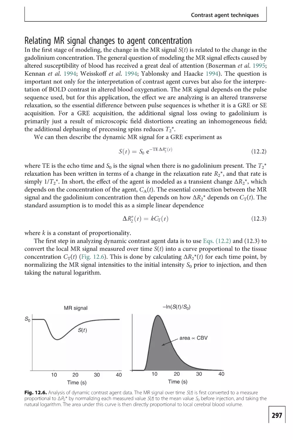
with subjects relaxed and lying still, the OEF is approximately 40%. Remarkably, this fraction
is relatively uniform across the brain in this basal state despite a several-fold variation of the
resting CMRO2 in different regions (Gusnard and Raichle 2001).
22
Neural activity and energy metabolism
Carbon dioxide, the end product of oxidative glucose metabolism, diffuses out of the cell,
into the blood, and is carried off to the lungs to be cleared from the body. In addition, heat
generated by metabolism is also carried away by the blood.
Measuring energy metabolism with PET
The deoxyglucose technique for measuring glucose metabolism
The development of the DG technique was a landmark in the evolution of functional
neuroimaging techniques (Sokoloff 1977; Sokoloff et al. 1977). With this method, it became
possible to map the pattern of glucose utilization in the brain with a radioactive tracer, whose
distribution in an animal brain can be measured by a process called autoradiography.
In autoradiography, a radioactive nucleus is attached to a molecule of interest and injected
into an animal. After waiting for a time to allow the tracer to distribute, the animal is
sacrificed and the brain cut into thin sections. Each section is laid on photographic film to
allow the photons produced in the decay of the radioactive nucleus to expose the film. The
result is a picture of the distribution of the agent at the time of sacrifice.
However, autoradiography cannot be used with labeled glucose itself because the brain
concentration of the tracer at any single time point is never a good reflection of the glucose
metabolic rate. Suppose that glucose is labeled with a radioactive isotope of carbon (e.g., 14C).
At early times after injection, the amount of tracer in the tissue does not reflect the local
metabolic rate because some of that tracer will diffuse back out into the blood and will not be
metabolized. If we wait a longer time, the unmetabolized tracer may have cleared, but some of
the 14C tracer that was attached to the glucose that was metabolized has also cleared as CO2. In
short, to measure the glucose metabolic rate with labeled glucose, measurements at multiple
time points are required, and this cannot be done with autoradiography.
It is this central problem of estimating the metabolic rate from a single concentration
measurement that was solved with the DG method. Deoxyglucose differs from glucose only in
the removal of one of the O2 atoms. This analog of glucose is similar enough to glucose that it
binds with the enzyme hexokinase catalyzing the first step of glycolysis. However, because of
the difference between DG and glucose, the DG cannot proceed down the glycolysis pathway,
and the process halts after the DG has been converted to fructose 6-phosphate. The result is that
the radioactive label on DG essentially sticks in the tissue. It cannot proceed down the
metabolic path, and the clearance of the compound from the tissue is very slow. After a
sufficient waiting period to allow clearance of the unmetabolized fraction, the tissue concentration of the label is a direct, quantitative reflection of local CMRGlc.
Measuring the cerebral metabolic rate for glucose
With the adaptation of the DG method for PET, studies of glucose metabolism were extended
to the working human brain. Carbon-14, the radioactive tracer used in the DG autoradiographic method, cannot be used in humans because the electron emitted in the decay of the
nucleus has a very short range in tissue, producing a large radiation dose in the subject but
virtually no detectable external signal. In PET, the radioactive tracers used are nuclei with an
excess ratio of protons to neutrons, and the decay produces a positron. A positron is the
antiparticle of an electron, with all the same properties as an electron except for an opposite
sign of its charge. Normal matter contains only electrons, so a positron is an exotic particle.
Positrons are emitted with substantial kinetic energy, which is dissipated within a few
23
An overview of fMRI
millimeters of travel through the tissue. When the positron has slowed sufficiently, it will
annihilate with an electron. In this process, the positron and the electron cease to exist, and
two high-energy photons are created. In this annihilation process, energy and momentum
are conserved, with the energy of each photon equal to the rest mass energy of an electron
(511 keV), and the photons are emitted in two directions close to 180° apart.
The emitted positron thus annihilates within a few millimeters of its origin, but the two
photons travel through the tissue and can be measured with external detectors. Furthermore,
because two photons travelling in opposite directions are produced, the detectors can be
coordinated to count only coincidence detections, the arrival of a photon in each of two
detectors within a very narrow window of time. The detection of such a coincidence then
determines the origin of the photons – the site of the radioactive nucleus – to lie on a line
between the two detectors. The total count of photons along a ray is proportional to the sum
of all of the activity concentrations along the ray. By measuring many of these projections of
the radioactivity distribution, an image of that distribution can be reconstructed in an
analogous way to X-ray computed tomography (CT) images.
Positron-emitting nuclei are particularly useful for human metabolic imaging because
the nuclei are biologically interesting (e.g., 11C, 15O), the radioactive half-lives are short, and
the decay photons readily pass through the body and so can be detected. A short half-life is
important because it reduces the radiation dose to the subject, but this also requires that the
isotope be prepared shortly before it is used, typically requiring an on-site cyclotron.
The PET version of the DG technique uses [18F]fluorodeoxyglucose (FDG) as the tracer
(Phelps and Mazziotta 1985; Reivich et al. 1979). Fluorine-18 decays by positron emission with a
half-life of approximately 2 h. The tracer is injected in a subject, and after a waiting period of
approximately 45 min to allow unmetabolized tracer to clear from the tissue, a PET image of the
distribution of the label is made. In fact, PET images can be acquired throughout this period in
order to measure the local kinetics of the FDG. Such time–activity curves can be analyzed with a
kinetic model to extract estimates of individual rate constants for uptake of glucose from the
blood and for the first stage of glycolysis. However, the power of the technique is that the
distribution of the tracer at a late time point directly reflects the local glucose metabolic rate.
In order to derive a quantitative measure of glucose metabolism with either the DG or
FDG technique, two other quantities are required. The first is a record of the concentration of
the tracer in arterial blood from injection up to the time of the PET image (or the time of
sacrifice of the animal in an autoradiographic study). The integrated arterial time–activity
curve describes how much of the agent the brain was exposed to and essentially provides a
calibration factor for converting the amount of activity measured in the brain into a measure
of the local metabolic rate. The second quantity needed is a correction factor to account for
the fact that it is really the metabolic rate of DG, rather than glucose, that is measured. This
correction factor is called the lumped constant, because it incorporates all of the factors that
make the uptake and phosphorylation rate of DG differ from glucose. An important question
for the interpretation of FDG-PET studies in disease states is whether the lumped constant
remains the same, and this question is still being investigated.
Increased glucose metabolism is closely associated
with functional activity
Since the late 1970s, numerous animal studies have clearly demonstrated a close link between
local functional activity in the brain and local CMRGlc (Kennedy et al. 1976; Sokoloff 1981).
24
Neural activity and energy metabolism
An early monkey study examining the effects of visual occlusion clearly demonstrated that
the striate cortex is organized in alternating ocular dominance columns. This organizational
pattern was known from previous, painstaking recordings from many cells, but the autoradiogram showed the full pattern in one experiment. These experiments also demonstrated
that CMRGlc decreases in association with a decrease of functional activity. When only one
eye was patched, the ocular dominance columns associated with the patched eye appeared
lighter (less exposed) on the autoradiogram than the columns corresponding to the open eye.
With reduced visual input from the patched eye, CMRGlc was also reduced.
Activation studies, in turn, showed an increase of CMRGlc in the functionally active
regions (Schwartz et al. 1979). Furthermore, with functional activity of different degrees, the
change in CMRGlc also showed a graded response (Kadekaro et al. 1985). The connection
between functional activity and glucose metabolism through ATP-dependent processes was
demonstrated by an experiment in which the activity of the Na+/K+ pump was blocked by a
specific inhibitor, with the result that the increase of glucose metabolism with electrical
stimulation was suppressed (Mata et al. 1980). In short, animal studies with DG and autoradiography, and human studies with FDG and PET (Phelps and Mazziotta 1985), have
found a close correspondence between local neural activity and local CMRGlc.
In the brain, the consumption of glucose is heterogeneous. The metabolic rate in gray
matter is three to four times higher than that in white matter. The low metabolic rate in white
matter suggests that the energy cost of sending an action potential down an axon is small,
most likely because of the efficient propagation along myelinated fibers. Instead, the energy
metabolism is more closely associated with the synapses, in keeping with the energy budget
estimates described above. Within the layers that make up cortical gray matter, the glucose
metabolic rate is highest in layer IV, an area rich in synaptic connections. This area also
shows the largest changes in glucose metabolism with activation. High-resolution studies of
the precise location of the increased glucose metabolism suggest that it is not the cell body of
the neuron but rather these areas of dense synaptic connections which show the largest
increase in metabolic rate (Sokoloff 1991).
Measuring cerebral blood flow and O2 metabolism
In addition to CMRGlc measurements, other PET techniques provide measurements of CBF
and CMRO2 as well. The basic idea is similar to FDG studies: a positron-emitting nucleus is
attached to a molecule of interest, and from the dynamics of that label as it moves through the
tissue, in combination with the measured dynamic curve in arterial blood, a relevant rate is
calculated. For DG, the relevant rate is the metabolic rate of glucose. For CBF measurements,
the relevant rate is the rate of delivery of arterial blood (discussed in more detail in Ch. 2).
The primary isotope used for these studies is 15O-labeled water in arterial blood.
For CMRO2 measurements, the relevant rate is the metabolic rate of O2, and these
measurements also use 15O as the radioactive tracer, but this time labeling O2 rather than
water. However, CMRO2 measurements are significantly more complicated by the fact that
the 15O label switches from labeling O2 to labeling water when O2 is metabolized. The
measured kinetics of the tracer depend on the interplay of delivery and clearance of 15O. By
introducing 15O2, the initial delivery of 15O does measure the delivery of O2, but clearance of
15
O from the tissue could be either from unmetabolized 15O2 returning to the blood, or from
water of metabolism, H215O. After a few circulation times, the labeled water builds up in the
blood and is re-delivered to the tissue, but now 15O is being delivered as a label of water rather
than molecular O2, so CBF also affects the distribution of the 15O. In addition, because
25
An overview of fMRI
much of the 15O is bound to hemoglobin in the blood, the CBV also affects the distribution of
15
O. To deal with these complications, measurement of CMRO2 with PET requires three
separate studies: the primary study, introducing 15O-labeled O2, plus a second study with
15
O-labeled water to assess CBF effects, and a third study with 15O-labeled carbon monoxide
to assess CBV effects (Frackowiak et al. 1980; Mintun et al. 1984). For this reason, CMRO2
studies with PET have been much less common than CMRGlc and CBF studies.
Balance of blood flow, glucose metabolism and O2
use in the brain at rest and during activation
Based on the discussion above, the ratio of CMRO2 to CMRGlc should be 6 for complete
oxidative metabolism of glucose. This ratio, called the oxygen/glucose index (OGI), has been
measured in the resting human brain with PET as approximately 5.3 (Raichle et al. 1970).
The slightly higher rate of glucose metabolism relative to O2 metabolism (i.e., OGI < 6)
means that not all of the carbons of glucose are going into CO2. Some could become part of
molecular synthesis pathways, and some may appear as a low-level lactate concentration,
with the excess flux of glucose into the brain balanced by a continuous clearance of lactate
from the brain. Nevertheless, the fact that the OGI is near 6 at rest suggests that the majority
of the net glucose metabolic rate is related to oxidative metabolism.
However, neural activation presents a surprisingly different picture. Because CMRO2
measurements are difficult, as noted above, CBF and CMRGlc measurements have provided
the primary windows on brain function. The close correspondence of these two measurements, described above, suggests a straightforward picture of a localized, balanced increase in
flow and metabolism with activation. This simple picture was challenged when Fox and
Raichle (1986) measured the change in CMRO2 associated with brain activation and made a
surprising discovery. In a somatosensory stimulation experiment, they found a focal CBF
increase of 29% in the appropriate area of the brain, but only a 5% increase in CMRO2. In a
later visual stimulation study, they again found a large imbalance in the CBF and CMRO2
changes and confirmed that the CMRGlc change was indeed large and comparable to the
CBF change (Fox et al. 1988).
More recent studies have examined the balance of CBF and CMRO2 changes with PET
and also with MRI methods (described in more detail in later chapters). Most of these studies
have found larger changes in CMRO2 with activation (as high as 20–30% with a strong
activation), but still a weaker CMRO2 change compared with the CBF change. Typical values
for the ratio of the fractional change in CBF to the fractional change in CMRO2 are in the
range 2–3. However, these are ratios of CBF changes to CMRO2 changes, and not CMRGlc
changes. Nevertheless, it is often assumed that CBF and CMRGlc changes are similar, based
on numerous PET studies. In short, with activation the OGI decreases.
The finding that glucose metabolism increases much more than O2 metabolism has
important implications for the magnitude of the energy metabolism changes during activation. Most of the increase in the metabolic rate of glucose is glycolysis alone, rather than full
oxidative metabolism. This means that the actual change in energy metabolism is much less
than would have been assumed from the increase in CMRGlc alone because glycolysis is
much less efficient in generating ATP. The observed imbalance also implies that there should
be a substantial production of lactate. This finding was confirmed with direct measurements
of lactate accumulation in human subjects measured with spectroscopic nuclear magnetic
resonance (NMR) studies (Prichard et al. 1991; Sappey-Marinier et al. 1992).
26
Neural activity and energy metabolism
What function is served by the large change in glucose metabolism?
Currently, there is no clear answer to the question of the function of such a large change in
glucose metabolism. The additional ATP production associated with glycolysis above and
beyond full oxidative metabolism is relatively small. For example, even with a large mismatch
of a 30% increase of CMRGlc combined with a 10% increase of CMRO2, the increase of ATP
production from the excess glycolysis is only approximately 1%. Although the excess
glycolysis likely provides only a small component of the total energy costs of neural activity,
it may provide needed ATP for particular tasks that cannot be fueled by ATP from oxidative
metabolism in the mitochondria. For example, dendritic spines may be too small to allow
local mitochondria to be near the synapse, and glycolysis potentially could provide the
needed ATP for activity at these synapses.
Another possibility is that the production of ATP in the astrocytes favors glycolysis
because it is fast, even though it is highly inefficient, and this may be important for rapid
clearance of neurotransmitter from the synaptic cleft (Raichle and Mintun 2006). However,
the free energy required for clearance of glutamate is provided by the Na+ gradient, rather
than ATP directly, with uptake of glutamate coupled to Na+ moving into the astrocyte. The
ATP is used to drive the Na+/K+ pump to transport the Na+ back out of the cell. It is possible
that the rapid recovery of the Na+ gradient within a confined space is important, and that the
Na+/K+ pump in the astrocytic processes at the synapse preferentially uses ATP from
glycolysis to accomplish this. However, this is unlikely to be a general requirement of the
Na+/K+ pump. Because at least 50% of the energy consumed in the brain is thought to be
linked to the action of this pump (Ames 2000; Attwell and Laughlin 2001), and glycolysis
provides less than 10% of the total ATP production, even during activation, most of the ATP
needed for the pump must come from oxidative metabolism.
The excess glucose metabolism, and associated production of lactate, may be associated
with the lactate shuttle discussed above. Excess lactate diffuses from the astrocytes to the
neurons, and increased lactate production would raise the tissue lactate and increase the
lactate gradient, driving the lactate flux into the neurons. Increased tissue lactate would also
increase the rate of lactate loss by blood flow, widening the gap between CMRGlc and
CMRO2. This raises the question of exactly what role is played by the lactate shuttle. If
lactate from astrocytes is a critical source of fuel for neurons, in addition to glucose delivered
by CBF, then a fall in the OGI and a rise in tissue lactate may be necessary to increase the
lactate flux into the neurons. Alternatively, if ATP derived from glycolysis is specifically
necessary for recycling neurotransmitter, either because of the speed required or the limitations imposed by the cramped space of a dendritic spine, increased tissue lactate may be an
unavoidable consequence. The lactate shuttle then may be a more secondary pathway to
avoid wasting the lactate produced.
Based on these considerations, we can speculate that the increase of CMRGlc is driven
by pre-synaptic activity, while CMRO2 reflects the overall energy costs of neural activity.
Because most of these energy costs are thought to be on the post-synaptic side, there could
be a dissociation of these responses depending on how the input excitatory activity
compares with the overall post-synaptic response. A common pattern of neural activity
is that as the stimulus intensity systematically increases the neuronal response increases but
tapers off. If the overall activity tapers off more quickly than the pre-synaptic activity, then
glucose metabolism would increase more than O2 metabolism as the stimulus intensity
increased.
27
An overview of fMRI
Current thinking about CBF changes also implicates synaptic activity itself in driving
acute CBF changes. This could potentially explain why CBF and CMRGlc have similar large
changes, while the CMRO2 change is more modest, because of a difference in the particular
aspects of neural activity that drive each response. These questions are considered again in
Chapter 2, after a more detailed discussion of CBF.
Box 1.1. The thermodynamics of neuronal signaling
Free energy and biological systems
All cellular processes, including neural signaling, are constrained by the physical laws of
thermodynamics: (1) energy is conserved and (2) entropy increases or at best stays the same.
Entropy is a subtle concept, but in broad terms it tends to increase if matter or energy are more
dispersed. The interplay of these two effects can make it difficult to see which way entropy
should change in a particular transformation. For example, consider a reaction in which a
compound AB can break up into separate molecules of A and B, or reform as A and B molecules
come together. Energy is distributed in the kinetic motion of all of the molecules, but there is
also a negative binding energy holding A and B together in the AB molecules. For this reason, on
the one hand, energy must be concentrated in the AB molecules in order to overcome the
binding energy and break them apart, and this concentration of energy would tend to decrease
the entropy. On the other hand, breaking AB into separate A and B molecules is a dispersal of
matter, tending to increase entropy. The outcome of these two effects – the actual change in
entropy – depends on the temperature. In general, the entropy associated with concentrating
energy becomes more dominant at lower temperatures, favoring the condensed form AB. For
any given temperature, there is an equilibrium in which the tendency for AB to break into A and
B is balanced by the tendency for A and B to recombine to form AB. This equilibrium is
characterized by a particular ratio of the reactants to the products, K0(T) = [A][B]/[AB]. If the
actual ratio differs from K0, then the favored direction of the reaction is the one that moves the
concentration ratio toward K0. Writing this equilibrium ratio as K0(T) reminds us that it
depends on temperature, but for mammalian cellular activity the temperature normally remains
approximately constant.
The concept of free energy change (or Gibbs free energy change [G]) neatly combines the first
and second laws of thermodynamics into a single useful relationship (see Nicholls and Ferguson
[2002] for an excellent discussion of free energy in biological systems). For any transformation,
such as a chemical reaction or movement of an ion across a membrane, there is an associated free
energy change ΔG. The free energy is a measure of how far a system is from equilibrium, with a
negative value of ΔG meaning that the transformation moves the system closer to equilibrium.
Cellular work refers to processes that have a positive ΔG, moving a part of the system away from
equilibrium, such as transport of an ion against its electrochemical gradient. A process with a
positive ΔG can only occur if it is tightly coupled to another process with a more strongly negative
ΔG, so that the net ΔG for the combined transformation is negative. That is, in order to move one
system farther from equilibrium, that transformation must be coupled to another system that is
moving closer to equilibrium.
For the transformation in which AB breaks into A and B, the free energy can be expressed as:
AB ! A þ B:
28
DG ¼ RT ln
K0 ½AB
½A½B
Neural activity and energy metabolism
where R is the gas constant, T is the temperature, and ln indicates the natural logarithm. Note that if
the concentration ratio is equal to the equilibrium ratio (1/K0), the argument of the logarithm is 1
and ΔG = 0. That is, a system at equilibrium has no capacity to do cellular work. If the system is
moved away from equilibrium owing to an excess of AB compared with A and B, then the break up
of AB is associated with a negative ΔG and the reaction as written is a downhill reaction in the
thermodynamic sense. If the system is shifted away from equilibrium in the other direction, with an
excess of A and B, then ΔG is positive for the reaction as written, but would be negative if written
backwards as A+B → AB. That is, the combination of A and B into AB would be the downhill
direction of the reaction.
The importance of considering ΔG is that this quantity incorporates both the energy and the
entropy changes involved, but this makes it a subtle concept. For example, the dependence of ΔG on
the ratio of reactant and product concentrations would not be expected if we were dealing just with
energy. In a transformation of one molecule of AB to molecules of A and B, the true energy involved
would depend just on changing bond energies, and would be the same regardless of the concentrations involved. The dependence on the concentrations comes from entropy considerations, and
the condition that ΔG must decrease for a transformation to happen is an embodiment of the
second law of thermodynamics.
In some systems, the rate at which a transformation happens is directly related to the ΔG
involved, with the rate increasing as ΔG grows more negative. There is a large body of literature
devoted to these relationships, typically in systems near equilibrium. However, biological systems
have evolved a different mechanism that often allows the rate of a transformation to be completely
divorced from the magnitude of ΔG. Specific proteins (enzymes) can serve as catalysts to speed up
chemical reactions, or as ion channels to change membrane permeability to specific ions. In this
role, they strongly affect the rate of the process without affecting the associated ΔG. For example,
the ΔG associated with diffusion of Na+ from outside to inside the cell depends on the concentration ratio, but the rate of Na+ diffusion depends on the number of open channels and on the
action of the Na+/K+ pump.
In short, the net ΔG tells us which way a particular transformation will go, and the primary use
of the magnitude of ΔG is to identify systems that are far from equilibrium and which, by moving
closer to equilibrium, can drive other processes away from equilibrium and perform useful cellular
work. That is, ΔG tells us which transformations can happen, but not necessarily how fast they will
happen. The ways by which biological sources of ΔG are tapped in cellular functions are controlled
by specific proteins, and thus by gene expression.
Free energy for life on Earth
For the brain, the ultimate source of free energy is that the concentrations of glucose, O2 and CO2
are far from equilibrium inside the cell. And these non-equilibrium concentrations must be
maintained by importing glucose and O2 into the cell from the environment and clearing CO2. In
a broad sense, the supplies of glucose and O2 in the environment are maintained by plants, which
convert CO2 and water into O2 and organic compounds, including glucose. The source of free
energy for this strongly uphill process is sunlight, and the degradation of sunlight is coupled to
these chemical reactions in photosynthesis. The source of the free energy of sunlight is that the
photons, which started off in thermodynamic equilibrium when they left the sun, are far from
equilibrium when they reach the earth. The energy density and the spectrum of photons in
thermal equilibrium are both determined by temperature, with a higher energy density and a
spectrum with more high-energy photons at higher temperatures. The distribution of photon
energies in the light leaving the sun is set by the sun’s surface temperature, approximately 5700 K.
As these photons travel away from the sun, they spread out; consequently, the density of photons
at the surface of the Earth is much reduced. As a result, the photons arriving at Earth have a
29
An overview of fMRI
spectrum characteristic of a 5700 K source but an energy density equivalent to thermodynamic
equilibrium at a temperature of only approximately 300 K. In other words, the photons arriving at
the surface of the Earth can be thought of as a system far from equilibrium, with the energy
concentrated in high-energy photons, while thermodynamic equilibrium favors a redistribution
of that energy to many more photons each with lower energy. The degradation of these highenergy photons thus releases a tremendous amount of free energy, which plants couple to
chemical processes through photosynthesis.
The process of photosynthesis can be thought of as splitting water according to the schematic
reaction:
Photon þ CO2 þ 2H2 O ! ðCH2 OÞ þ H2 O þ O2
In this scheme CH2O represents the basic building block of carbohydrates. For example, glucose
(C6H12O6) is composed of six of these blocks. We can think of this transformation as splitting the
two water molecules on the left side to form one O2 molecule and four H atoms, which then
combine with CO2 to form a CH2O unit and an additional water molecule (the bold face for O is a
reminder that the O2 molecule comes from water, not from CO2). Animals and plants make use of
the free energy stored in the separated O2 and CH2O units by reversing this reaction:
O2 þ ðCH2 OÞ þ H2 O ! CO2 þ 2H2 O
Note that the molecular O2 is converted back to water, rather than CO2.
Life on Earth thus depends on sunlight to drive chemical synthesis and provide a source of ΔG
for sustaining biological systems. It is interesting to note that it is not primarily the heat of the
sunlight that is critical, but rather the spectrum of the photons. Just as glucose and O2 can combine
when burned to produce heat, the energy of the photons from the sun warms the surface of the
Earth. The same amount of heating could, in principle, be supplied by a lower temperature source of
photons, such as a cooler star closer to the Earth, but these photons would be inadequate to drive
photosynthesis. So the existence of life on Earth ultimately depends on the fact that the sun is hot
enough to produce high-energy photons, but far enough away that the equilibrium temperature on
Earth is much lower.
Free energy and neuronal signaling
For understanding the thermodynamic basis of neuronal signaling, the two key types of transformation are chemical reactions and diffusion across a membrane. As described in the main text,
the ATP/ADP system is the primary source of a strongly negative ΔG. For this system, the
breakdown of ATP to ADP and inorganic phosphate (Pi) is associated with a free energy change
of the form:
ATP ! ADP þ Pi :
DGATP ¼ RT ln
KATP ½ATP
½ADP½Pi
The ratio of the concentrations in this expression is often called the phosphorylation potential.
Because the in vivo ATP concentration is much higher relative to ADP and Pi than it would be at
equilibrium, ΔG is strongly negative.
Diffusion of ions across the cellular membrane also has an associated ΔG. If there is an electrical
potential difference V across the membrane, then the ΔG associated with one ion moving across the
membrane depends on V and the extracellular (E) and intracellular (I) concentrations of the ion.
For example, for Na+, the ΔG for one Na+ to move from the extracellular space to the intracellular
space is:
30
Neural activity and energy metabolism
½Naþ E ! ½Naþ I :
DGNa ¼ RT ln
KNa ðVÞ½Naþ E
½Naþ I
where the equilibrium constant KNa(V) is the ratio of the concentrations (intracellular/extracellular)
that would be in equilibrium with the membrane potential V. If V = 0, there is no longer any
interaction with the ion’s charge, and at equilibrium the extracellular and intracellular concentrations
would be equal (KNa = 1). For a typical membrane potential of V = −70 mV, with the inside more
negative, the equilibrium for Na+ would be a higher concentration inside the cell because the negative
potential favors the accumulation of the positive ions, corresponding to KNa ~10. Because the in vivo
distribution is strongly skewed the other way, with a much higher extracellular concentration, there is
a strongly negative ΔG associated with Na+ moving into the cell. Correspondingly, moving Na+ out of
the cell against its gradient is a strongly uphill process and must be coupled with an even more
strongly downhill process, such as the conversion of ATP to ADP.
Biological batteries
In general, cellular processes often involve an interplay between these two basic sources of ΔG: a
chemical system in which the reactant/product concentration ratio is far from equilibrium, or an
ion distribution across a membrane that is far from equilibrium. In each case, we can think of the
system as a biological battery, with the “voltage” of the battery corresponding to how far that system
is from equilibrium as measured by the corresponding ΔG. Then as one system performs cellular
work, with a corresponding degradation of the relevant concentrations and reduction of the
equivalent voltage, that system can be “recharged” by coupling it with another system with a higher
voltage. The interplay of several systems involved in neuronal signaling discussed in Ch. 1 can be
viewed in terms of such biological batteries.
For example, to move Na+ back out of the cell in the recovery from signaling, the transport of
+
Na is coupled to the conversion of ATP to ADP, an example of using a chemical reaction source of
negative ΔG to recharge an ionic gradient. In the mitochondria, the conversion of ADP and Pi back
to ATP is coupled to transport of H+ across the mitochondrial membrane, an example of an ionic
gradient recharging a chemical reaction ratio. The idea of a system far from equilibrium is
important for another reason in addition to ΔG and energy metabolism: for a chemical messenger
to convey a “signal,” it must be part of a system that is far from equilibrium. For example, Ca2+ is
maintained at a much higher concentration outside the cell, and entry of Ca2+ is a common
chemical signal that triggers a chain of events within the cell, such as neurotransmitter release.
For Ca2+ entry to work as a signal, the intracellular concentration must be kept at a low level prior to
the signal, despite the high concentration outside the cell. One way the Ca2+ is removed is by
coupling the transport of Ca2+ out of the cell to Na+ transport into the cell, an example of the
extracellular/intracellular Na+ gradient being used as a source of negative ΔG to restore the Ca2+
signaling system. When a neurotransmitter opens a Na+ channel on the post-synaptic neuron, the
strong flux of Na+ down its gradient is a signaling mechanism.
In short, from a thermodynamic point of view, neuronal signaling involves an interconnected
set of biological batteries, systems far from equilibrium that can serve as sources of ΔG for either
energy metabolism or signaling. These batteries have different equivalent voltages and are linked in
a hierarchy in which one can recharge another. They include chemical reaction systems and ionic
gradients, coupled through particular enzymes such as the Na+/K+ pump. Ultimately, the battery
with the largest voltage is the system of glucose, O2 and CO2 within the cell, which is maintained in
a state far from equilibrium by continual delivery of glucose and O2 and clearance of CO2. The
overall conversion of glucose and O2 to CO2 and water taps the free energy originally stored in
carbohydrates when plants coupled photons of sunlight to the splitting of water.
31
An overview of fMRI
References
Ames A, III (2000) CNS energy metabolism as
related to function. Brain Res Brain Res Rev
34:42–68
Attwell D, Iadecola C (2002) The neural basis of
functional brain imaging signals. Trends
Neurosci 25:621–625
Attwell D, Laughlin SB (2001) An energy budget
for signaling in the grey matter of the brain.
J Cereb Blood Flow Metab 21:1133–1145
Blaustein MP (1988) Calcium transport and
buffering in neurons. Trends Neurosci
11:438–443
Bradford H (1986) Chemical Neurobiology. New
York: WH Freeman
Erecinska M, Silver IA (1990) Metabolism and
role of glutamate in mammalian brain. Prog
Neurobiol 35:245–296
Erecinska M, Silver IA (1994) Ions and energy in
mammalian brain. Prog Neurobiol 43:37–71
Fox PT, Raichle ME (1986) Focal physiological
uncoupling of cerebral blood flow and
oxidative metabolism during somatosensory
stimulation in human subjects. Proc Natl
Acad Sci USA 83:1140–1144
Fox PT, Raichle ME, Mintun MA, Dence C
(1988) Nonoxidative glucose consumption
during focal physiologic neural activity.
Science 241:462–464
Frackowiak RSJ, Lenzi GL, Jones T, Heather JD
(1980) Quantitative measurement of
regional cerebral blood flow and oxygen
metabolism in man using 15O and positron
emission tomography: theory, procedure,
and normal values. J Comput Assist Tomogr
4:727–736
Gjedde A (1987) Does deoxyglucose uptake in
the brain reflect energy metabolism?
Biochem Pharmacol 36:1853–1861
Gusnard DA, Raichle ME (2001) Searching for a
baseline: functional imaging and the resting
human brain. Nat Rev Neurosci 2:685–694
Iadecola C, Nedergaard M (2007) Glial
regulation of the cerebral microvasculature.
Nat Neurosci 10:1369–1376
James W (1890) The Principles of Psychology.
Cambridge, MA: Harvard University Press
Kadekaro M, Crane AM, Sokoloff L (1985)
Differential effects of electrical stimulation of
sciatic nerve on metabolic activity in spinal
cord and dorsal root ganglion in the rat. Proc
Natl Acad Sci USA 82:6010–6013
32
Kennedy C, Rosiers MHD, Sakurada O, et al.
(1976) Metabolic mapping of the primary
visual system of the monkey by means of the
autoradiographic [14C]deoxyhemoglobin
technique. Proc Natl Acad Sci USA
73:4230–4234
Laughlin SB, Sejnovski TJ (2003)
Communication in neural networks, Science
301: 1870–1874
Logothetis NK (2002) The neural basis of the
blood-oxygen-level-dependent functional
magnetic resonance imaging signal.
Philos Trans Roy Soc Lond B Biol Sci
357:1003–1037
Mata M, Fink DJ, Gainer H, et al. (1980) Activitydependent energy metabolism in rat
posterior pituitary primarily reflects sodium
pump activity. J Neurochem 34:213–215
Mintun MA, Raichle ME, Martin WRW,
Herscovitch P (1984) Brain O2 utilization
measured with O-15 radiotracers and
positron emission tomography. J Nucl Med
25:177–187
Nicholls DG, Ferguson SJ (2002) Bioenergetics 3.
London: Academic Press
Nicholls JG, Martin AR, Wallace BG (1992) From
Neuron to Brain. Sunderland, MA: Sinauer
Associates
Oldendorf WH (1971) Brain uptake of
radiolabeled amino acids, amines, and
hexoses after arterial injection. Am J Physiol
221:1629–1639
Pellerin L, Bouzier-Sore AK, Aubert A, et al.
(2007) Activity-dependent regulation of
energy metabolism by astrocytes: an update.
Glia 55:1251–1262
Phelps ME, Mazziotta JC (1985) Positron
emission tomography: human brain
function and biochemistry. Science 228:
799–809
Prichard J, Rothman D, Novotny E et al. (1991)
Lactate rise detected by 1H NMR in human
visual cortex during physiologic stimulation.
Proc Natl Acad Sci USA 88:5829–5831
Quistorff B, Secher NH, van Lieshout JJ (2008)
Lactate fuels the human brain during
exercise. FASEB J 22: 3443–3449
Raichle ME (1998) Behind the scenes of
functional brain imaging: a historical and
physiological perspective. Proc Natl Acad Sci
USA 95:765–772
Neural activity and energy metabolism
Raichle ME, Mintun MA (2006) Brain work and
brain imaging. Annu Rev Neurosci 29:449–476
Raichle ME, Posner JB, Plum F (1970) Cerebral
blood flow during and after hyperventilation.
Arch Neurol 23:394–403
Reivich M, Kuhl D, Wolf A, et al. (1979) The
[18F]-fluoro-deoxyglucose method for the
measurement of local cerebral glucose
measurement in man. Circ Res 44:127–137
Robinson P, Rapoport SI (1986) Glucose
transport and metabolism in the brain. Am J
Physiol 250: R127–R136
Sappey-Marinier D, Calabrese G, Fein G, et al.
(1992) Effect of photic stimulation on human
visual cortex lactate and phosphates using 1H
and 31P magnetic resonance spectroscopy. J
Cereb Blood Flow Metab 12:584–592
Schwartz WJ, Smith CB, Davidsen L, et al. (1979)
Metabolic mapping of functional activity in
the hypothalamo-neurohypophysial system
of the rat. Science 205:723–725
Siesjo B (1978) Brain Energy Metabolism. New
York: John Wiley
Sokoloff L (1977) Relation between physiological
function and energy metabolism in the
central nervous system. J Neurochem
29:13–26
Sokoloff L (1981) The relation between function
and energy metabolism: its use in the
localization of functional activity in the
nervous system. Neurosci Res Prog Bull
19:159–210
Sokoloff L (1991) Relationship between
functional activity and energy metabolism in
the nervous system: whether, where and
why? In Brain Work and Mental Activity:
Quantitative Studies with Radioactive
Tracers, Lassen NA, Ingvar DH, Raichle ME
et al., eds. Copenhagen: Munksgaard,
pp. 52–67
Sokoloff L, Reivich M, Kennedy C, et al. (1977)
The [14-C]deoxyglucose method for the
measurement of local cerebral glucose
utilization: theory, procedure, and normal
values in the conscious and anesthetized
albino rat. J Neurochem 28:897–916
33
2
Chapter
Cerebral blood flow
and brain activation
The blood supply of the brain
The vascular system
Tissue perfusion
Cerebral blood volume and blood velocity
The central volume principle
Cerebral blood flow is a measure of delivery of arterial blood
Changes in cerebral blood flow and blood volume
Blood flow is controlled by changing vascular resistance
The relationship between blood volume and blood flow during activation
Neural activity and the control of cerebral blood flow
The development of ideas about control of cerebral blood flow
Smooth muscle relaxation
Vasoactive agents
The neurovascular unit
Measuring cerebral blood flow
The microsphere technique
The nitrous oxide technique
Diffusible versus intravascular tracers
The radioactive xenon technique
Techniques using PET
Techniques using MRI
Brain activation
Blood flow and glucose metabolism increase with functional activity
Oxygen metabolism increases less than blood flow
Summary of physiological changes during brain activation
page 34
34
36
37
37
38
39
39
40
42
42
43
44
48
49
49
49
50
52
52
53
53
53
54
55
The blood supply of the brain
Cerebral blood flow (CBF) delivers glucose and O2 to the brain, so it is natural to suppose
that local CBF varies with neural activity, as suggested by James (1890) in the second quote at
the beginning of Part IA. Although we certainly know more about the changes in CBF with
activation and in disease states than was known in James’ time, we still lack a full understanding. Nevertheless, the change in CBF with a change in neural activity is the primary
signal used for mapping brain activity with functional neuroimaging.
The vascular system
The vascular system that supplies blood to the brain is organized on spatial scales that span a
size range of four orders of magnitude, from the diameter of a capillary (∼ 10 μm) to the
Cerebral blood flow and brain activation
A
B
C
Fig. 2.1. The vascular system of the brain. (A) A magnetic resonance angiogram showing the major vessels in the brain.
(B) A two photon microscopy image of the surface vasculature (to a depth of approximately 300 μm) in the rat
somatosensory cortex, showing the multidirectional orientation of the vascular network (image courtesy of A. Devor.)
(C) A photomicrograph of a stained section through the lamina of the primary visual cortex of a monkey (Zheng et al.
1991). The staining indicates areas with high concentrations of cytochrome oxidase, an enzyme involved in oxidative
metabolism, and highlights layers IV and VI and also blobs in layer II. The panel on the right also shows a camera lucida
drawing of the vessels in the stained section, showing higher capillary densities in the stained areas. (Figure C reproduced
with permission from Zheng et al., J. Neuroscience 11:2622–2629, 1991; copyright 1991 by the Society for Neuroscience.)
distribution volume of a major artery (∼ 10 cm3). The complexity of the vascular network
can be appreciated from Fig. 2.1. Figure 2.1A is a MR angiogram, showing the major arteries
delivering blood to the tissue, and the veins carrying it back toward the heart. This angiogram
shows vessels down to a few millimeters in diameter. Figure 2.1B is a microscopic view,
showing the complex geometry of the smallest vessels, the arterioles, capillaries, and venules.
This two-photon microscopic image of the somatosensory cortex of the rat is a maximum
intensity projection of a series of 2 μm images extending down to approximately 300 μm in
depth. The smallest capillaries have a diameter of approximately 6–8 μm, comparable to the
size of a red blood cell. Figure 2.1C shows images illustrating the distribution of capillary
density within the layers of the cortex (Zheng et al. 1991). The photomicrograph shows a
1 mm wide strip from a cytochrome oxidase-stained section of a slice through the primary
visual cortex (area 17) of a squirrel monkey, and the camera lucida tracing shows the blood
vessels (mostly capillaries). Cytochrome oxidase is one of the enzymes involved in oxidative
metabolism (Ch. 1), and the uneven distribution of the enzyme in the brain suggests a
heterogeneous distribution of O2 metabolism. In this study, the microvessel density, as
measured by the total length of vessels visible in the slice, showed a close correspondence
with the cytochrome oxidase-stained areas. The peak density in the cortex was in layer IV,
where the density was approximately 1.5–3 times higher than that of white matter.
The study of Zheng et al. (1991) also showed how the functional organization of the brain is
at least partially reflected in the blood vessel density. The border between the primary and
secondary visual cortex (areas 17 and 18) is distinguished by changes in the laminar structure,
and the microvessel density correspondingly was found to be approximately 25% higher in the
primary visual cortex. On an even smaller scale, in the primary visual cortex of primates,
functional units called blobs have been identified based on their higher concentration of
cytochrome oxidase. The blobs are located in layers II and III of the cortex and are approximately
250 μm in extent in the images in Figure 2.1C. The capillary density in the blobs was approximately 40% higher than that in the interblob regions. In short, the architecture of the vascular
tree shows distinct organization on a spatial scale as small as a few hundred micrometers.
35
An overview of fMRI
Tissue perfusion
Because many functional imaging techniques, including fMRI, depend on changes in CBF, it
is important to understand precisely what CBF is and how it can be measured. The term
perfusion is used in a general way to describe the process of nutritive delivery of arterial blood
to a capillary bed in the tissue. Because functional neuroimaging is potentially sensitive to
several aspects of the perfusion state of tissue, it is important to clarify exactly what is meant
by several terms. Cerebral blood flow is the rate of delivery of arterial blood to the capillary
beds of a particular mass of tissue, as illustrated in Figure 2.2. For convenience, a common
unit for CBF is milliliters of blood per 100 grams of tissue per minute, and a typical average
value in the human brain measured with PET is approximately 50 mL/100 g per min, with
gray matter about three times higher than white matter (Ito et al. 2004; Rostrup et al. 2005).
For imaging applications, it often is convenient to express this as flow delivered to a unit
volume of tissue rather than a unit mass of tissue, because a signal is measured from a
particular volume in the brain, and the actual mass of tissue within that volume is not known.
Because the density of brain is close to 1 g/mL, CBF values expressed in these units are similar.
Note, however, that the units of CBF are then milliliters per milliliter per minute, which are
essentially units of inverse time. For this reason, it is sometimes useful to think of CBF as
having the same units as a rate constant (e.g., 60 mL/100 g per min is equivalent to 0.01 s−1).
A useful example of considering CBF as an effective rate constant is a fundamental
relationship between CBF and and the cerebral metabolic rate of O2 (CMRO2). For a
consistent definition of units, CBF can be expressed as milliliters of arterial blood delivered
per milliliter of tissue per minute, and CMRO2 is then expressed as moles of O2 consumed
per milliliter of tissue per minute. The rate of delivery of O2 to the capillary bed is simply CBF
A
Draining vein
B
Capillary bed
2F
Arteriole
Venule
1
F2
Equal blood volume
and velocity
F1
F
2
Volume V
CBF1 = 2 CBF2
Artery
Fig. 2.2. The meaning of perfusion. (A) Blood vessels within a small element of tissue. Cerebral blood flow (CBF) is
the delivery of arterial blood to the capillary beds (F1+ F2) and so is not directly related to the local blood volume,
which also includes arterial blood destined for a more distal tissue element and venous blood draining more distal
tissues. (B) Measurement of blood volume and blood velocity is not sufficient to measure CBF. In the lower capillary
bed, the vessels are twice as long as those in the upper capillary bed, so the blood volume and blood velocity are
the same, yet the CBF is twice as large in the upper capillary bed. Instead of blood volume and blood velocity
determining CBF, it is blood volume and transit time that determine CBF through the central volume principle.
36
Cerebral blood flow and brain activation
times [O2]a, the concentration of O2 in arterial blood in units of moles of O2 per milliliter.
With these definitions, CMRO2 can be expressed as
CMRO2 ¼ OEF CBF ½O2 a
(2:1)
where OEF is the fraction of delivered O2 that is extracted and metabolized. In this
combination, the product of the OEF and CBF acts like a “rate constant” for metabolism
of a “substrate” represented by [O2]a. This equation essentially just follows from the
definitions of the terms involved, but it is a useful relationship to keep in mind when
considering the BOLD effect. If CBF increases more than CMRO2, then the OEF must
decrease, and this is the essential physiological phenomenon underlying the BOLD response.
Cerebral blood volume and blood velocity
The cerebral blood volume (CBV) is the fraction of the tissue volume occupied by blood
vessels, and a typical value for the brain is approximately 4% (CBV = 0.04) (Rostrup et al. 2005).
The CBV is a dimensionless number (milliliters of blood vessel per milliliter of tissue), and
usually refers to the entire vascular volume within the tissue. In some applications, however, it
is important to subdivide total CBV into arterial, capillary, and venous volumes. Reliable
measurements of the relative sizes of these volumes are scarce, but reported estimates for a
sheep brain for vessels smaller than approximately 2 mm in diameter are 20% for arterioles,
50% for capillaries, and 30% for venules (Sharan et al. 1998). The blood volume potentially can
change in any of these sub-compartments of the vascular system. The dilation of the arterioles
that leads to an increase in flow is a volume increase on the arterial side, and a number of
studies have shown significant changes in the arterial CBV associated with changes in CBF and
neural activity (Devor et al. 2007; Hillman et al. 2007; Ito et al. 2005; Kim et al. 2007).
Some early data suggested that only a fraction of the tissue capillaries are open channels
at rest and that capillary recruitment (i.e., opening the previously collapsed capillaries) is
involved in increasing CBF (Frankel et al. 1992; Shockley and LaManna 1988; Weiss 1988).
However, the accuracy of the techniques used in these early studies has been challenged
(Gobel et al. 1990), and a number of more recent studies have concluded that capillary
recruitment is a small effect, if it occurs at all (Bereczki et al. 1993; Gobel et al. 1989; Klein
et al. 1986; Pawlik et al. 1981; Vetterlein et al. 1990; Villringer et al. 1994; Wei et al. 1993).
Instead, changes of CBF are associated with changes in blood velocity in the capillaries. For
example, studies in rats have found increases during hypoxia (Bereczki et al. 1993; Krolo and
Hudetz 2000) and decreases with pentobarbital (Wei et al. 1993). Blood velocity varies from
tens of centimeters per second in large arteries to as slow as 1 mm/s in the capillaries. At the
capillary level, the pulsatility seen in the arterial vessels is largely damped out. Nevertheless,
studies of the passage of red blood cells through individual capillaries have found that the
flow is often irregular, rather than a smooth constant velocity (Kleinfeld et al. 1998; Villringer
et al. 1994). This likely reflects the fact that the red cell diameter is about the same as the
capillary diameter, and the red cells can clump together to produce transient blockages. In
addition, transit of larger white cells can also cause a transient slow down of flow. If one looks
just at an individual capillary, flow is an irregular process, and it is only when averaged over
thousands of capillaries that CBF takes on a well-defined, stable value.
The central volume principle
Although CBF, CBV, and blood velocity are all important aspects of the perfusion state
of tissue, they are distinct physiological quantities. With the preceding definitions, CBF does
37
An overview of fMRI
not explicitly depend on either blood volume or the velocity of blood in the vessels. An
increase in CBF with brain activation could occur through a number of different changes in
blood volume or blood velocity. For example, an increase of blood velocity in a fixed capillary
bed or an increase in the number of open capillaries but with blood moving at the same
velocity in each capillary would both lead to an increase in CBF. In both cases, more arterial
blood flows through the capillary bed. Furthermore, even specifying capillary velocity and
capillary volume is not sufficient to determine CBF, as illustrated in Fig. 2.2B. Two idealized
capillary beds are shown, one with two sets of shorter capillaries, and one with a single set
of capillaries twice as long. In both beds, the blood velocity is the same, and we have
constructed them to have the same capillary blood volume. However, the CBF is twice as
large in the upper bed with two sets of shorter capillaries because the volume of arterial blood
delivered to the bed per minute is twice as great.
Intuitively, it seems that specifying the blood volume and blood velocity ought to
determine CBF, but the preceding example shows that it does not. The missing piece that
does differ between the two scenarios is the capillary transit time. In the capillary bed with the
longer capillaries, the capillary transit time is twice as long. And it is transit time, rather than
blood velocity, that is directly connected to CBV and CBF. The important relationship,
known as the central volume principle, has been recognized for over a century (Stewart 1894):
¼ CBV=CBF
(2:2)
where τ is the mean transit time through the volume defined by CBV. For a CBF of
60 mL/100 g per min (0.01 s−1) and a typical CBV of 4%, the vascular transit time is
approximately 4 s from this equation. By restricting the volume to a subset of the entire
blood volume, such as the capillary volume, the relation still holds, with τ defined as the mean
transit time through the capillary volume.
Cerebral blood flow is a measure of delivery of arterial blood
These considerations indicate that the definition of CBF involves some subtleties important
for understanding how CBF is measured, as illustrated in Fig. 2.2. In this idealized tissue
vasculature, the flow rates through the two capillary beds are designated F1and F2 (expressed
in milliliters per minute), and if these beds feed a volume of tissue V, then CBF is simply
(F1 + F2)/V. However, an element of tissue will also contain arterial blood in larger arteries
that is just passing through, destined for a capillary bed in another location. The tissue
element may also contain venous blood passing through as it drains another tissue element.
For these reasons, it is difficult to make reliable measurements of CBF by looking at the
blood itself within a tissue element, although such techniques are in use. For example, laser
Doppler flowmetry measures a frequency shift in light reflected from moving red blood
cells (Dirnagl et al. 1989; Stern 1975). The proportion of the reflected light that is Doppler
shifted is a measure of the number of moving red blood cells, the total blood volume, and the
average frequency shift is a measure of the average red blood cell velocity. Taken together,
these data provide a measure of blood motion within an element of tissue. This general
motion of the blood does not, however, necessarily reflect CBF, the flow of arterial blood into
the capillary beds.
For example, an element of tissue could have no change in CBF (e.g., F1 and F2 remain
constant in Fig. 2.2) but show increased red blood cell motion if CBF increases in a distal
tissue element, with a corresponding increase in speed in the arteries and draining veins that
38
Cerebral blood flow and brain activation
also happen to pass through the first element. The laser-Doppler flowmetry technique is
useful for studies of the microvasculature in animal models, but estimates of CBF with this
technique should be interpreted with caution. The central problem is that the defining
characteristic of CBF is not blood motion within the tissue element but rather delivery of
arterial blood to the capillary bed. For this reason, a more accurate approach for estimating
CBF is to measure the rate of delivery of an agent carried to the tissue by flow.
Changes in cerebral blood flow and blood volume
Blood flow is controlled by changing vascular resistance
The rate of delivery of arterial blood to a small element of tissue depends on the pressure
driving the blood through the vascular tree and the resistance that must be overcome along
the way. Specifically, blood flow can be taken to be the ratio of the difference in pressure
between the arterial and venous blood (ΔP) to the cerebrovascular resistance: CBF = ΔP/CVR
(this is essentially the definition of cerebrovascular resistance). In the vascular system, the
resistance is not uniformly distributed across all of the branches of the network but, instead,
is dominated by the arterioles and the capillaries. The arterioles are the smallest of the arterial
branches, located just prior to the capillaries. For steady flow through the vascular tree, the
net resistance of each stage is reflected in the pressure fall across that stage. Starting with the
largest arteries, there is a gradual pressure decrease as the main arteries branch into smaller
vessels, a sharper drop across the arterioles and capillary bed, and then again a gradual
decrease across the venous branches as the blood collects from the smallest venules into
larger veins (Boas et al. [2008] give a recent model of the vascular tree). In the healthy brain,
autoregulation operates to maintain CBF at a nearly constant value despite alterations
in arterial pressure over a range from approximately 75 to 175 mmHg (Guyton 1981). As
pressure changes, cerebrovascular resistance changes in a compensatory way by dilating or
constricting the arterioles.
The arterioles are the seat of control of vascular resistance. A coat of smooth muscle
cells surrounds the arterioles, contracting to constrict the vessel and relaxing to dilate it.
To maintain control of the arteriolar diameter, and thus resistance, the smooth muscle must
be in a chronic state of moderate contraction, described as muscular tone, so that resistance
can be either increased or decreased (Andresen et al. 2006). Control of smooth muscle
tension is a complicated process but is closely involved with the intracellular Ca2+ concentration in the smooth muscle cell (Faraci and Sobey 1998). Increased cytosolic Ca2+, either
through opening Ca2+ channels to allow external Ca2+ to enter or through triggered release of
internal Ca2+ stores, initiates a contraction. Processes or agents that tend to interfere with these
Ca2+ increases or reduce cytosolic Ca2+ lead to relaxation. As discussed in the next section, a
large number of factors can affect the arteriolar smooth muscle and alter resistance.
Resistance is likely to be a steep function of arteriolar diameter. For laminar flow of a
simple fluid, the resistance is proportional to 1/r4, where r is the radius of the vessel.
Therefore, to decrease the resistance of the arterioles by 100%, the radius of the arteriole
need increase only 19%. Blood is not a simple fluid, and the flow is not likely to be purely
laminar; nevertheless, this argument suggests a sensitive mechanism to control blood flow. In
principle, dilation of just the arterioles would be sufficient to increase flow through a local
capillary bed fed by the arteriole. However, another process occurs that is not fully understood: the dilatation propagates upstream to larger arterial vessels. Several mechanisms have
been proposed for this effect, including signaling through gap junctions connecting smooth
39
An overview of fMRI
muscle cells and nitric oxide (NO) released from the walls of upstream vessels in response to
increased shear stress. A recent report indicates that the astrocytes play a direct role in
upstream dilatation (Xu et al. 2008). Although the mechanisms are unclear, the significance
of this effect is that the vessel dilatation associated with increased CBF extends upstream
from the initiating arterioles.
A possible function for the upstream dilatation is that this could serve to prevent a
phenomenon called vascular steal, in which increased flow in one area leads to a decreased
flow in other nearby areas. From the point of view of simple flow through a network of pipes,
a vascular steal could develop in the following way. Imagine a small artery that branches into
two smaller arterioles in parallel. If resistance decreases in one arteriole, the overall resistance
of the network decreases and net flow increases. However, if the upstream artery resistance
stays the same while the flow through it increases, the pressure drop across the artery will be
larger. This means that the pressure where it branches into the arterioles is reduced, and it is
this pressure that drives the flow through each of the branches. For the branch that dilated,
the resistance has decreased more than the fall in driving pressure, so the flow through that
branch increases. However, the branch that did not dilate has the same resistance, but now a
lower driving pressure, so the flow is reduced. This steal phenomenon would not happen if
the upstream artery also dilated, decreasing its resistance so that flow could increase without
reducing the driving pressure for the arterioles. That is, upstream dilatation would serve to
further increase CBF in the activated region while preventing a CBF reduction in nearby
regions through a vascular steal.
Dilating the arterioles also may increase the pressure in the downstream capillaries and
veins, and this may lead to CBV changes as a passive response to the CBF change. Depending
on the distensibility of the vessels, this pressure increase could dilate the veins and possibly
the capillaries as well. The result is that changes in blood volume are not likely to be evenly
distributed along the entire vascular tree, and the dynamics of the change may be different in
different vascular compartments. While the arterial CBV changes drive the change in CBF,
downstream capillary and venous CBV changes may be a slower, more passive, response to
increased pressure.
While the primary control point for CBF is thought to be the arterioles, recent studies
suggest that control at the capillary level may also exist. Some capillaries are surrounded by
small contractile elements called pericytes, which have been shown to constrict and dilate in
response to different stimuli in brain slice preparations (Peppiatt et al. 2006). Further work is
needed to determine whether pericytes represent a significant control point for CBF in the
intact brain.
The relationship between blood volume and blood flow
during activation
Based on the arguments above, the relationship between CBF and total CBV is potentially
complicated. It is helpful, however, to consider the simple example of laminar flow in a
straight cylindrical vessel introduced above. The resistance is proportional to 1/r4, where r is
the vessel radius, and the volume for a fixed length is proportional to r2. Suppose now that the
vessel dilates so that the radius doubles to reduce the resistance and increase the flow. For a
constant driving pressure, the flow increases by a factor of 24 (= 16), and the volume increases
by a factor of 4. More generally, the relationship between the change in blood flow and blood
volume for this example is that the volume change is proportional to the square root of the
40
Cerebral blood flow and brain activation
flow change. If the diameter of every vessel in the vascular tree increased by the same factor,
and the resistance to flow follows the 1/r4 law for every vessel, then the changes in CBF and
CBV would follow this square root relation.
Motivated by this simplified example, we can treat the relationship between CBV and
CBF in a more general way, and characterize it as a power law relation:
V
¼
V0
F
F0
(2:3)
where F0 is the resting flow, V0 is the resting blood volume, and α is a numerical exponent.
For our simple example above, α = 0.5. In a real vascular tree, we would expect that the
volume change necessary to produce a CBF change is much smaller because the cerebrovascular resistance is concentrated in the arterioles. Dilating the arterioles does increase CBV,
but because the arterioles are a small fraction of the total blood volume, the net change in
CBV is small. For example, suppose that the arterioles account for 20% of the blood volume
but 50% of the cerebrovascular resistance at rest. Then, if the diameter of the arterioles
increases by 20%, the resistance of the arterioles is reduced by approximately 50%. If there is
no change in the rest of the vascular tree, CBF increases by 25% from a change of only 4% in
total CBV.
From these arguments, the CBV change required to increase CBF may be quite small if it
occurs just in the arterioles, but a larger change in CBV could occur through upstream
arterial dilatation and downstream passive expansion of capillaries and veins. Note that the
magnitude of these additional CBV changes may depend on the extent of the activated area as
well. The classic paper of Grubb et al. (1974) is still the primary reference for the quantitative
relationship between CBF and CBV changes. These investigators altered the inspired partial
pressure of CO2 (pco2) in monkeys and measured global changes in blood flow and blood
volume. They then fitted the measured pairs of CBF and CBV values to Eq. (2.3) and found
that the data were best described by α = 0.38. In this experiment, the total CBV was measured,
so it was not possible to isolate the contributions of changes in the arterial, capillary, and
venous blood volumes. More recent animal studies have used several different approaches,
including fluorescent dyes (Vanzetta et al. 2004), optical methods (Hillman et al. 2007), and
MRI methods (Kim et al. 2007) to try to distinguish the CBV changes in different vascular
compartments. While there is evidence for changes at all levels of the vascular tree, the data
indicate that CBV changes are predominantly on the arterial side.
The simple empirical relationship in Eq. (2.3) is widely used, but it is only an approximation for a potentially complex relationship between CBF and CBV changes with activation
(Piechnik et al. 2008), and this relationship affects the interpretation of the BOLD effect.
Although the BOLD effect is primarily driven by changes in oxygenation of the blood,
changes in CBV are also thought to play a role. If CBV changes increase the total local
deoxyhemoglobin, this will tend to offset the drop in deoxyhemoglobin caused by the
decreased OEF. Although there is very little deoxyhemoglobin in the large arteries in a
healthy subject with no hypoxia, there is evidence that the arterioles are partly deoxygenated.
For this reason, CBV changes at the venous, capillary, and even arteriolar level could modify
local deoxyhemoglobin.
In addition, there may be hematocrit changes associated with increased flow that could
alter deoxyhemoglobin by a larger factor than the actual vessel volume increase, and thus
affect the BOLD signal. Because the red cell diameter is similar to the capillary diameter, a
41
An overview of fMRI
possible scenario is that some capillaries are perfused at rest with plasma but not red cells,
and that with activation a slight dilatation of the capillaries allows the distribution of red cells
to become more uniform (Krolo and Hudetz 2000). In this way, the total hemoglobin could
potentially increase more than the capillary volume itself. A recent study using optical
techniques in a rat model to measure the response to a brief stimulus found that changes
in total hemoglobin are dominated by the capillaries, and the dynamics of total hemoglobin
in the different compartments are rather different (Hillman et al. 2007). For all compartments total hemoglobin increased with the stimulus, but after the stimulus it recovered more
quickly in the arterioles and even decreased below the baseline level, while capillary and
venous total hemoglobin recovered more slowly. Different dynamics in the vascular compartments may be important for understanding a phenomenon often seen in BOLD imaging
called the post-stimulus undershoot – a reduction of the BOLD signal below baseline that may
persist for tens of seconds (discussed more fully in Ch. 16).
Neural activity and the control of cerebral blood flow
The development of ideas about control of cerebral blood flow
Over a century ago, Roy and Sherrington (1890) described the basic principle that, at least in
a general sense, motivated much of the early thinking about the local control of CBF:
We conclude then, that the chemical products of cerebral metabolism contained in the
lymph which bathes the walls of the arterioles of the brain can cause variations of the
calibre of the cerebral vessels: that in this re-action the brain possesses an intrinsic
mechanism by which its vascular supply can be varied locally in correspondence with
local variations of functional activity.
If we interpret the phrase “chemical products of cerebral metabolism” to mean the products
of energy metabolism, then this view presents a relatively simple concept of what happens:
neural activity increases the local rate of energy metabolism, and products of energy
metabolism, in turn, trigger increased flow to deliver more glucose and O2. In this way
there is a simple balance between the energy demands of neural activity and the local energy
supply, which depends on blood flow.
However, although this simple picture is direct and appealing, recent work is challenging
this view. In a recent review, Attwell and Iadecola (2002) concluded:
The view that the haemodynamic response is coupled to signaling processes represents a
conceptual shift from the traditional idea that the energy demands of the tissue directly
determine the flow increase associated with neural activation. In summary, we suggest
that understanding the BOLD response is a signaling problem, not an energy problem.
Specifically, the principle described by Attwell and Iadecola is that the CBF change triggered
by increased neural activity is not driven by a depletion of substrates for energy metabolism
but rather by the neural activity itself. Instead of a serial chain of events in which neural
activity drives energy metabolism which then drives blood flow, the CBF is driven directly by
aspects of neural signaling.
A connected and parallel change in thinking relates to the question: What chemical
agents mediate a change in CBF? The Roy and Sherrington principle suggests that there are
only a few mediators that act on the smooth muscle of the arteries to control blood flow. To
some extent, this view carried through to recent times with the discovery of NO as a
42
Cerebral blood flow and brain activation
candidate for the primary mediator controlling blood flow. However, recent studies have
shown that there is not a final common pathway, but rather multiple signaling pathways that
alter CBF. Although products of energy metabolism do modify CBF, the observations
underlying the second quotation above are that there are numerous pathways directly
involving aspects of neural activity. In addition, there has been a profound shift in our
understanding regarding the key role played by the astrocytes. Rather than playing a passive
role, they appear to be dynamic participants in neuronal signaling, and this has led to the
concept of the neurovascular unit, a close functional and structural integration of neurons,
astrocytes, and blood vessels (Anderson and Nedergaard 2003).
The current view that the CBF changes are not driven by energy metabolism has also
raised a basic question: What function is served by the change in CBF? Surprisingly, there is
currently no accepted answer to this question. The fact that large CBF changes accompany
changes in neural activity is well established, and this appears to serve some function
important to the organism, judging from the wide range of mechanisms that have evolved
to produce that flow change. Clearly, CBF is necessary to support energy metabolism, but the
central question is: If CBF is already high, why does it need to increase so dramatically when
neural activity increases? In short, we have a problem in which there are many mechanisms,
but these mechanisms do not tell us the underlying functional advantage of having a large
CBF change in response to a change in neural activity.
Although the two views expressed in the quotations above appear to be in opposition,
they are likely both aspects of a larger synthesis. The key to integrating these ideas may be the
time scale involved. A striking aspect of the brain is that the OEF is relatively uniform at rest,
despite a several-fold variation across the brain in the local rate of energy metabolism
(Gusnard and Raichle 2001). This suggests that during development the CBF to each region
adjusts to the basal level of energy metabolism in that region, creating a close coupling of
blood flow and energy metabolism such that the same fraction of O2 (approximately 40%) is
removed from the blood across the brain. This long-term basal adjustment of CBF and
energy metabolism is in keeping with the Roy and Sherrington principle.
However, for an acute change in neural activity it may be a disadvantage to the organism
to wait until substrates for energy metabolism are depleted before increasing blood flow.
Instead of such a feedback mechanism, a feedforward system in which neural activity drives
an increase of CBF in anticipation of a need for increased energy metabolism may be a useful
adaptation. In this way, acute CBF changes are closely tied to neuronal signaling, in keeping
with the Attwell and Iadecola principle. Note that in this view the function of the CBF change
is not directly related to the mechanisms that produce the change. Multiple feedforward
mechanisms provide increased CBF, which ultimately supports increased energy metabolism. Along these lines, a possible answer to the question of why CBF increases is that it serves
to maintain the O2 concentration in tissue despite increased energy metabolism. This
speculative idea is discussed further in Box 2.1 at the end of this chapter.
Numerous experiments have revealed particular pathways involved in the control of CBF
(Girouard and Iadecola 2006; Hamel 2006; Villringer and Dirnagl 1995), but how these
pathways function in a coordinated dynamic network is still largely unknown. The following
sections describe some of the current ideas.
Smooth muscle relaxation
As noted above, the relaxation or contraction of smooth muscle surrounding an artery depends
on the cytosolic free Ca2+ concentration in the smooth muscle cell. The Ca2+ concentration
43
An overview of fMRI
depends on exchange between the cytosol and Ca2+ stores within the cell, and on the influx
of Ca2+ from the extracellular space through voltage-sensitive Ca2+ channels, which tend to
open as the cellular membrane depolarizes. For this reason, cytosolic Ca2+ concentration tends
to follow the membrane potential, with a graded depolarization producing a graded increase
of Ca2+ and a corresponding contraction of the smooth muscle. Because of this sensitivity
to the membrane potential, a number of agents are thought to exert an effect on the arterial
diameter by opening K+ channels on the smooth muscle cell. Opening K+ channels hyperpolarizes the cell, reducing cytosolic Ca2+ and relaxing the muscle.
Potassium channels are remarkably diverse, and several distinct types are thought to be
involved in smooth muscle action (Faraci and Sobey 1998). Calcium-activated K+ channels
open when cytosolic Ca2+ rises, and these are thought to be the most abundant on the surface
of the smooth muscle cell. These channels may serve as a kind of buffer, or negative feedback
system, to limit contraction. If Ca2+ rises, Ca2+-activated K+ channels open, hyperpolarizing
the cell and reducing cytosolic Ca2+. ATP-sensitive K+ channels are thought to be sensitive to
the metabolic state of the cell. Intracellular ATP inhibits these channels, so a reduction of
ATP leads to channel opening, membrane depolarization, muscle relaxation, and increased
blood flow. Other factors related to metabolism, such as a fall in pH, also open these
channels. Voltage-dependent K+ channels open in response to membrane depolarization.
Like the Ca2+-activated K+ channels, these channels may serve as part of a buffer system to
balance contraction, and so may play a role in maintaining muscle tone. Inward-rectifier
K+ channels are characterized by a strong inward rectification, such that they carry inward
current more readily than outward current. The action of these channels is rather complex,
but the net effect is that these channels open in response to an increase in the K+ concentration outside the cell, leading to hyperpolarization (Quayle et al. 1997). By this mechanism,
extracellular K+ itself acts as a vasodilator.
While many agents that affect CBF act through the medium of the smooth muscle
membrane potential, by affecting K+ channels, other mechanisms interfere with the way
cytosolic Ca2+ couples to the enzymes that control muscle contraction. For example, NO,
initiates a chain of events leading to production of cGMP, and the cGMP is thought to affect
both K+ channels and the sensitivity of the contractile mechanism to Ca2+.
Vasoactive agents
A number of vasoactive agents are now known, including key ions, metabolic factors, and
factors related to neural activity. The factors most often considered are discussed below.
Carbon dioxide and pH
One of the first chemical agents found to have a strong effect on CBF was CO2, which fits in
nicely with Roy and Sherrington’s original proposal (1890) because CO2 is the end product of
oxidative glucose metabolism. Raising the arterial pco2 from its normal resting value of
approximately 40 mmHg to 60 mmHg by breathing a gas mixture enriched with CO2 nearly
doubles the global CBF in monkeys (Grubb et al. 1974). Carbon dioxide is a gas that readily
dissolves in water and also reacts with water to form bicarbonate ions (HCO3−) and H+. This
has two important consequences. The first is that the high solubility of CO2 allows blood to
carry it away efficiently from the tissue, with the bulk of it carried as bicarbonate ions. The CO2
diffuses down a concentration gradient from tissue to blood, where it is quickly converted to
bicarbonate ions through the action of carbonic anhydrase, thus maintaining a relatively low
concentration of CO2 as dissolved gas in blood and a strong gradient of CO2 from tissue to
44
Cerebral blood flow and brain activation
blood. If the conversion of CO2 to bicarbonate ions is slowed, as happens when the carbonic
anhydrase inhibitor acetazolamide is administered, CO2 builds up in the blood and the tissue
CO2 concentration must increase to maintain the diffusion gradient needed to clear CO2. Thus
acetazolamide (Diamox) acts as a vasodilator.
The second important consequence of the conversion of CO2 to bicarbonate ions and
H+ is that the amount of CO2 present directly affects the pH. Because CO2 passes easily across
the blood–brain barrier and cellular membranes (Siesjo 1978), it has a potent effect on the
intracellular pH of the brain. In contrast, charged molecules such as bicarbonate ions do not
easily cross the barrier. For this reason, increased CO2 in the blood has a strong effect on
intracellular pH, while a change in the pH of blood at a constant CO2 level has little effect
on the intracellular pH of brain. For these reasons, clearance of CO2 is effectively clearance of
acid, and the CO2/bicarbonate system serves as an important pH buffer.
The vasodilating action of CO2 is thought to be caused by the pH change at the arterial
smooth muscle. Numerous studies have shown that local acidosis causes dilatation and
alkalosis constriction of the brain arterioles. Furthermore, animal studies have shown
decreases in pH associated with the large flow changes accompanying induced seizures,
consistent with the idea that increased H+ (decreased pH) produces an increase in CBF
(Kuschinsky and Wahl 1979). The brain is evidently very sensitive to pH changes, and the
large CBF response may serve to increase the clearance rate of CO2 and provide some control
over pH.
Potassium ions
In addition to H+, other positively charged ions (cations) exhibit a strong vasodilatory effect.
Early studies found that increased K+ and decreased Ca2+ in the fluid space around the
cerebral arterioles both produce vessel dilatation. In addition, because neural activity
involves an increase of extracellular K+ and a decrease of extracellular Ca2+, there is a natural
mechanism for increasing CBF in response to neural activity, an early idea known as the
cation hypothesis for CBF regulation (Lassen 1991). Another early idea was that K+ taken up
by the astrocytes at a high concentration near the synapse could be siphoned to the end-feet
near the blood vessels where the concentration is lower, providing a possible mechanism for
communicating K+ concentration changes to the blood vessels (Paulson and Newman 1987).
Although more recent studies argue against this siphoning effect, a more recent model
suggests an important role for extracellular K+ in the signaling cascade from neurons to
blood vessels. This model emphasized the potential role of the astrocytes in integrating
neuronal activity signals (Filosa et al. 2006) (also see The neurovascular unit, below). In this
picture, a Ca2+ increase in the astrocyte, triggered by neuronal activity, opens Ca2+-activated
K+ channels on the astocytic end-feet. Potassium flows out of the astrocyte into the restricted
space between the end-feet and the blood vessel, increasing extracellular K+ and opening
inward-rectifier K+ channels on the smooth muscle. In this signaling cascade, local neuronal
activity is integrated by the cytosolic Ca2+ increase in the astrocyte and then translated to a
Ca2+ decrease in the smooth muscle cell, with associated vessel dilatation, by intercellular
signaling between K+ channels.
Adenosine
Adenosine has intertwined roles in both neural activity and energy metabolism. As discussed in
Ch. 1, the primary energy storage molecule is ATP. In addition to its role in energy metabolism,
ATP also serves as a neurotransmitter/neuromodulator (Haydon and Carmignoto 2006). In the
45
An overview of fMRI
extracellular space, ATP is sequentially broken down to produce adenosine, which then has a
potent effect by reducing neuronal excitability. Interestingly, ATP also is released by astrocytes
(Haydon and Carmignoto 2006). For example, in the retina, ATP released from glial cells
is broken down to adenosine, which then opens K+ channels that hyperpolarize ganglion
neurons (Newman 2003). Although details of the mechanism of ATP release from astrocytes
are still unclear, this suggests a potentially important mechanism of astrocyte-to-astrocyte and
astrocyte-to-neuron signaling. In cell cultures, Ca2+ waves propagate between astrocytes, even
when they do not make direct contact with one another, through release of ATP, which then
diffuses from the point of release. At the level of the neuronal synapse, adenosine binds to
receptors on the pre-synaptic side of the synapse and inhibits transmitter release, potentially
providing a basis for regulation of synaptic signaling. Adenosine accumulation is also involved
in lateral inhibition, in which activity at one synapse inhibits the activity of nearby synapses.
Adenosine has a strong vasodilatory effect (Dirnagl et al. 1994; Villringer and Dirnagl
1995; Winn et al. 1991). Caffeine competes for adenosine receptors (Fredholm et al. 1999),
and a number of studies have shown that caffeine reduces CBF (Perthen et al. 2008),
consistent with the idea of a reduction of the vasodilatory effect of adenosine.
Nitric oxide
Since the 1990s, the importance of NO in regulating CBF has been recognized (Iadecola 1993;
Watkins 1995). Nitric oxide is a powerful vasodilator. As a signaling molecule, it has the unique
property of being a simple gas that easily diffuses across cell membranes; consequently, it
can engage directly in intracellular reactions without having to bind to extracellular receptors.
It is a reactive molecule, so it is short lived in tissue. Nevertheless, the range of diffusion of
NO is thought to be on the order of 200 μm, so NO produced at one site can potentially signal
to many nearby cells. As noted above, the action of NO in a target cell is to produce an
intracellular second messenger, cGMP, which then triggers subsequent cellular pathways.
Nitric oxide is produced by activation of nitric oxide synthase (NOS), and there are three
forms of the enzyme: endothelial, neuronal and induced. Nitric oxide is produced locally from
neurons and astrocytes following glutamate receptor activity, and it has been implicated in
modulating the vasodilatory effects of virtually all the potential mediators of CBF control
discussed above: CO2, H+, K+, and adenosine. Thus, the full picture of the control of CBF may
involve complicated interrelationships between NO and other mediators (Lindauer et al. 1999).
Current thinking is that NO plays an important role in maintaining vascular tone, with a
continuous production of NO in the basal state. The role of NO in triggering acute CBF
changes is more complicated, and somewhat less clear. In part, this is because an experimental finding of a reduced CBF response to activation after NOS is blocked could be
because basal tone was affected, rather than the CBF response itself. For example, studies in
cortex found that the CBF response to activation was reduced when NOS was blocked, but
restored when NO was added non-specifically to the tissue, suggesting that the primary effect
was on basal tone (Lindauer et al. 1999). In contrast, however, a similar experiment in the
cerebellum found that blocking NOS reduced the CBF response and that it was not restored
by adding NO, suggesting a more fundamental involvement of NO in signaling the CBF
change (Akgoren et al. 1994).
Arachidonic acid derivatives
A number of studies have shown that CBF is modulated through an extended metabolic
pathway related to arachidonic acid and its derivatives (Girouard and Iadecola 2006; Straub
46
Cerebral blood flow and brain activation
and Nelson 2007). This is a widespread signaling pathway in human biology, particularly
involved in inflammation, fever, and pain associated with injury or disease. A family of
locally acting hormones called eicosanoids are derived from arachidonic acid through the
interaction with specific enzymes. The family name refers to the 20-carbon composition of
each (the same origin as icosahedron). An important class of eicosanoids, prostaglandins,
are formed from arachidonic acid by the enzyme cyclooxygenase (COX). Two forms of
this enzyme, COX-1 and COX-2, are structurally similar but play different roles in human
biology. For example, COX-1 is involved in protecting the stomach lining from acid, while
COX-2 is involved in inflammation and pain. Non-steroidal anti-inflammatory drugs
(NSAIDS), such as aspirin and ibuprofen, inhibit COX enzymes generally, and so a focus
of drug research is on the development of specific COX-2 inhibitors that could address pain
without damaging the stomach. In the brain, there is evidence for the involvement of both
COX-1 and COX-2 in CBF control. A second pathway involving arachidonic acid products,
called the P450 pathway, also is implicated in modulating CBF through the production of
epoxyeicosatrienoic acids.
The pathways described above are associated with vasodilation, but the involvement of
arachidonic acid and its derivatives appears to be more complicated. Another compound
derived from arachidonic acid, 20-hydroxyeicosatetraenoic acid, has a constricting effect on
the blood vessel (Koehler et al. 2006). For this reason, activation of the arachidonic acid
pathway can produce both vasodilation and vasoconstriction, and the potential significance
of this complicated behavior is still unclear.
Neural pathways affecting cerebral blood flow
In addition to the specific agents discussed above, neural pathways also affect CBF (Hamel
2006). The larger arteries receive neural input as part of system-wide control, described as the
extrinsic sources of innervation. The sympathetic pathway, involving release of norepinephrine and neuropeptide Y, produces vasoconstriction. This may serve to protect the brain in
the face of a system-wide increase in blood pressure associated with a fight or flight stimulus.
The parasympathetic pathway, operating through release of vasoactive intestinal peptide,
acetylcholine, NO, and other transmitters, produces vasodilation. This system does not
appear to have a prominent role in normal physiological regulation but has been implicated
in disease processes. Finally, the trigeminovascular pathway involves sensory nerves containing calcitonin gene-related peptide and other transmitters and produces vasodilation. This
system appears to be involved in restoring vascular tone after vasoconstrictive stimuli, but in
addition this system is the focus for studies of migraine headache. This pathway is implicated
in an intriguing phenomenon in brain physiology called cortical spreading depression, in
which a wave of reduced electrical activity and CBF spreads slowly across the cortex at a rate of
a few millimeters per minute. This phenomenon is thought to underlie the spreading visual
aura that sometimes precedes migraine attacks, and waves of cortical spreading depression
also appear to be involved in stroke. Current anti-migraine medications, called triptans, target
the trigeminovascular system by blocking release of calcitonin gene-related peptide.
In contrast to the extrinsic innervation of the larger arteries, the smaller arteries receive
more local intrinsic innervation (Hamel 2006). Cortical neurons receive input from several
deeper structures. Projections from the raphe nuclei in the brainstem release serotonin.
Projections from the locus coeruleus in the brainstem, a region associated with responses to
stress, release norepinephrine. Projections from the nucleus basalis in the basal forebrain,
a region that undergoes degeneration in Parkinson’s and Alzheimer’s diseases, release
47
An overview of fMRI
acetylcholine. The details of the pathways involved are still unclear but they may also involve
the astrocytes and other receptor pathways.
In addition, local interneurons, which provide important inhibitory connections in
neural networks, have been shown to produce either vasoconstriction or vasodilation. The
distinction depends on whether the interneurons are associated with vasoactive intestinal
peptide or NOS, eliciting dilation, or somatostatin, eliciting contraction (Cauli et al. 2004).
The neurovascular unit
Research over the last decade has demonstrated a diverse and important role for the glial
cells in brain function. These cells account for about half of the cells in the brain and were
originally thought to be primarily a structural scaffold. One subtype of glial cell, the astrocyte,
has proven to play an important role in neuronal signaling and in energy metabolism
(Haydon and Carmignoto 2006; Magistretti 2006). Although relatively quiet in terms of
electrophysiology compared with neurons, the astrocytes nevertheless have a sophisticated
signaling system based on changes in intracellular Ca2+. Astrocytes contain receptors for
numerous neurotransmitters, including glutamate, GABA, acetylcholine and adenosine, and
activation of these receptors induces changes in cytosolic Ca2+. With numerous processes
contacting neuronal synapses, the astrocytes are well positioned to play a key role in recycling
neurotransmitter, as described in Ch. 1, and also to monitor and integrate local neuronal
activity. Additional processes, called end-feet, make contact with blood vessels, so astrocytes
create a bridge between neuronal activity and blood flow. This close anatomical arrangement
has long suggested an important functional arrangement, and in recent years the mechanisms by which changes in neural activity translate into changes in CBF have become clearer.
Because of the close interactions between neurons, astrocytes, and blood vessels, this
combination is often referred to as the neurovascular unit (Andresen et al. 2006).
The basic picture of the coordinated action of the neurovascular unit is as follows.
Neurotransmitter, such as glutamate, released at a synapse binds to the astrocytic process
as well as the post-synaptic neuron, initiating a rise in cytosolic Ca2+ in the astrocyte. This
Ca2+ signal propagates to the end-feet and triggers two processes in parallel: the production
of arachidonic acid and the release of K+. Products of the arachidonic acid pathway, probably
prostaglandins and epoxyeicosatrienoic acids, are released and open K+ channels on the
smooth muscle cell, producing vessel dilation. In parallel, the Ca2+ rise in the astrocyte
triggers K+ release from the end-feet, opening inward-rectifier K+ channels on the smooth
muscle. Both of these mechanisms produce vasodilation (Fig. 2.3). However, the full picture
may be more complicated, as indicated above. The release of arachidonic acid at the endfeet may lead to production of 20-hydroxyeicosatetraenoic acid in the smooth muscle and
vasoconstriction. The effects of astrocyte signaling may thus be complex, involving both
relaxation and constriction (Filosa and Blanco 2007).
In summary, there is ample evidence for a direct involvement of astrocytic signaling,
through cytosolic Ca2+ changes and stimulation of arachidonic acid metabolic pathways,
in the matching of CBF with neuronal activity. However, the response is complicated, with
different studies showing dilatation (Zonta et al. 2003) or contraction (Mulligan and
MacVicar 2004) when the astrocytes are stimulated. Part of this complexity may be related
to the basal state of the vessels in the experiments in brain slice preparations (Blanco et al.
2008). When the vessels were pre-constricted, they tended to dilate, and when they were preexpanded they tended to contract in response to the stimulus. The basal state of the system is
an important factor for understanding the specific results of stimulating particular pathways.
48
Cerebral blood flow and brain activation
Pre-synaptic terminal
Arteriole
Action potential
1
Glu
Blood
flow
2
3
Na+
Receptor
Ion
channel
Astrocyte
K+, EETs
Receptor
Ca2+
4
5
Smooth
muscle
Post-synaptic neuron
Dilation
Fig. 2.3. Astrocyte signaling to the blood vessels. Arrival of an action potential at a glutamatergic synapse (1) triggers
glutamate (Glu) release (2), which binds to receptors on the astrocyte as well as the post-synaptic neuron (3), initiating
an increase of intracellular Ca2+ (4), triggering release of K+ and arachadonic acid products (EET, epoxyeicosatrienoic acids)
from the astrocyte end-feet (5) to relax the smooth muscle and dilate the arteriole.
Measuring cerebral blood flow
The microsphere technique
The most direct way to measure CBF is to inject labeled microspheres into the arterial
system. If these microspheres are carefully designed to be small enough to pass through the
arterioles but large enough that they will not fit through the capillaries, then they will be
trapped in the capillary bed. After injection in a large artery, the bolus of microspheres will be
delivered to each of the tissue elements served by that artery in proportion to their respective
local CBF. The number of microspheres lodged in an element of tissue is then a direct
measure of the local CBF. Typically, this method uses radioactive microspheres, sectioning of
the tissue, and then counting the radioactivity in each sample. For measurements at multiple
time points, microspheres labeled with different radioactive nuclei can be used and then
distinguished later based on differences in the energies of the radioactive decay photons
(Yang and Krasny 1995). More recently, colored microspheres have been used with photometric measurement of the concentrations of different colored spheres in tissue samples.
Although widely regarded as the gold standard for perfusion measurements, microspheres
are not appropriate for human subjects. However, a number of the techniques we will discuss
are closely related, to the extent that they use a tracer that stays in the tissue during the
experiment, like a microsphere, and can be measured externally and non-invasively.
The nitrous oxide technique
A milestone in the development of techniques for measuring CBF in humans was the nitrous
oxide (N2O) technique (Kety and Schmidt 1948). This was the first technique capable of
49
An overview of fMRI
Inflow
Artery
Well-mixed tank Outflow
Brain
Vein
Fig. 2.4. The nitrous oxide (N2O) technique for measuring
global cerebral blood flow. A subject breathes N2O
continuously while the blood concentration of the agent is
sampled in the carotid artery and jugular vein. Over time, the
N2O will distribute throughout the brain, like a well-mixed
tank being filled with fluid containing a dye, and the venous
concentration will approach the arterial concentration.
The time constant for reaching this equilibrium is inversely
proportional to the global cerebral blood flow (CBF).
Concentration N2O
Artery
Vein (high CBF)
Vein (low CBF)
Time
producing quantitative measurements of global CBF in humans, and it was quickly applied
to investigate perfusion changes in a number of conditions. In this technique, the subject
breathes N2O continuously for several minutes. During this time, the arterial and venous
concentrations of N2O are sampled frequently (e.g., from the carotid artery and jugular vein)
(Fig. 2.4). The N2O diffuses freely from blood into tissue, and if the arterial concentration
remains elevated for a sufficiently long time, the arterial, venous, and tissue concentrations
of N2O will come into equilibrium. In this equilibrium state, the concentrations in tissue,
arterial blood, and venous blood are equal, and so this equilibrium condition carries no
information about the flow. But the time required to reach this equilibrium is strongly
sensitive to flow.
As an analogy, consider a large, well-mixed tank of water (the tissue) fed by an inlet pipe
(arterial flow) and drained by an outlet pipe (venous flow), as illustrated in Fig. 2.4. If dye is
now introduced into the inlet side at a constant concentration, the concentration of dye
in the tank will gradually increase until it comes into equilibrium with the inlet concentration. If the tank is well mixed at all times, the outlet concentration will approach the inlet
concentration in an exponential fashion. The larger the rate of inflow, the more quickly the
concentration in the tank will reach equilibrium. By observing only the inlet and outlet
concentrations, the time constant τ for the outlet concentration to equilibrate with the inlet
concentration can be measured. This time constant is τ = V/F, where F is the flow rate into the
tank (mL/min) and V is the volume of the tank (mL). To generalize this idea to brain studies
with an exogenous agent, the volume V is more precisely defined as the volume of distribution
of the agent, the volume to which the agent has access and will eventually fill over time.
Nitrous oxide freely diffuses throughout the brain, and so the volume of distribution is
approximately the volume of the brain itself.
Diffusible versus intravascular tracers
The concept of volume of distribution is important for understanding the kinetics of a tracer.
Nitrous oxide freely diffuses out of the capillary bed and fills the entire tissue space, so its
volume of distribution is essentially the whole brain volume. In contrast, an agent that
50
Cerebral blood flow and brain activation
f
Arterial
blood CA
C T Tissue
f/λ
Concentration–time curve
Delivery: C T ∝ f
Concentration
CA
Clearance: C T ∝ e–ft/λ
Fig. 2.5. Measurement of cerebral blood flow (CBF) with
diffusible radioactive tracers. The tissue concentration CT(t)
of the agent is modeled in terms of the arterial concentration
CA(t), the driving function of the system, and the local flow
f and volume of distribution l using the compartmental
model shown at the top. Local flow affects both delivery and
clearance of the agent. With the 133Xe method, flow is
estimated from the time constant for clearance, and with the
PET H215O bolus injection method flow is estimated from the
integrated activity delivered during the first 40 s.
C T (high CBF)
133
Xe measurements
C T (low CBF)
1
2
3
4
Time (min)
Integrated concentration–time curves
Total delivered agent
High CBF
Low CBF
With radioactive decay
H215O bolus injection measurement
1
2
Time (min)
3
4
remains in the blood has a volume of distribution that is much smaller, only approximately
4% of the total brain volume. A useful definition of volume of distribution derives from a
simple experiment. Imagine that an agent is administered in the blood, and that we can
measure the concentration in arterial blood and the concentration in a small tissue element
(say, with PET). The volume of distribution λ is defined as the ratio of the tissue to blood
concentrations after they have come into equilibrium. For this reason, it is sometimes
described as the partition coefficient for the agent.
Brain studies use a number of different tracers, but most of them fall into one of two
basic classes: diffusible tracers, with λ ~1; or intravascular tracers, with λ ~CBV. The significance of λ is that it strongly affects the kinetics of an agent, through the central volume
principle introduced above (Fig. 2.5). The basic time constant defining the kinetics of the
tracer as it passes through a tissue element is simply λ/CBF. In other words, the volume of
distribution of an intravascular agent is quickly filled because the blood volume is only a
small fraction of the total tissue volume.
This difference in the equilibration times directly affects what can be measured with
diffusible and intravascular tracers. Imagine that an agent is injected into the blood, and the
tissue concentration of the agent is measured over time. After the agent has equilibrated
within its volume of distribution, the tissue concentration of the agent is independent of flow
but provides a robust measure of the volume of distribution. Just as with N2O, flow affects the
51
An overview of fMRI
kinetics of the agent only during its approach to this equilibrium. So an intravascular agent,
on the one hand, provides a robust measurement of CBV because that is its volume of
distribution, but a poor measurement of flow because it equilibrates so quickly. On the other
hand, a diffusible tracer provides a robust measurement of flow because the flow-dependent
part of the tissue concentration curve is much longer. With these basic ideas in mind, we can
consider the development of techniques to measure local CBF with diffusible tracers.
The radioactive xenon technique
The N2O technique made possible a measurement of global blood flow from measurements
of the arterial and venous concentrations of the agent over time. However, this technique
provides no way to determine local blood flow to a particular region of the brain. In principle,
the flow to a smaller subregion of the brain could be determined by collecting the venous
samples from a smaller vein that only drains that subregion, but this is not practical in
human studies. An alternative approach measures the local tissue concentration of the agent
itself. From the preceding arguments, each local element of tissue should come into equilibrium with the arterial concentration with a local time constant that depends directly on the
local blood flow and volume of distribution of the agent. This type of measurement became
possible with the introduction of radioactive tracers and external detectors for measuring
regional concentrations of the agents. The use of diffusible radioactive tracers to measure
CBF is described in more detail in Ch. 12.
In the 1960s, regional measurements of CBF in humans became possible with the
introduction of radioactive inert gases (Ingvar and Lassen 1963), most notably the xenon133 technique (Obrist et al. 1967). Xenon is an inert gas that freely diffuses throughout the
brain. The radioactive isotope 133Xe decays with the emission of a photon, which can be
captured by an external detector near the surface of the head. The agent typically is
administered by inhalation, entering the bloodstream in the lungs and traveling throughout
the body in the arterial flow. After allowing sufficient time for the xenon to equilibrate in the
brain, the supply of xenon is cut off, and the clearance of the agent from the brain is
monitored. An array of detectors is arranged around the head, with each detector most
sensitive to the nearest regions of the brain. Each detector then measures a regional level of
radioactivity, which decreases over time. Clearance is accomplished by CBF, so the larger the
CBF the faster the radioactive xenon clears from the tissue. The time constant for clearance is
λ/f, where λ, the volume of distribution of xenon, is approximately 1 because xenon is a
diffusible tracer (Fig. 2.5).
Techniques using PET
Radioactive xenon studies only allow measurement of regional flows because of the limited
spatial selectivity of the detectors. But with PET, an image of the concentration of radioactivity in a brain section can be measured with a spatial resolution of approximately 1 cm3.
With dynamic measurements, the concentration is measured as a function of time, referred
to as a tissue time–activity curve. (Note that activity here refers to radioactivity, the number of
measured radioactive decays per second, and not to neural activity in the brain.) The ability
to measure the distribution of a radioactive tracer tomographically with spatial resolution on
the order of 1 cm3 made possible a much more detailed study of local CBF changes.
For blood flow studies with PET, the most common agent used is water labeled with 15O,
which has a radioactive half-life of approximately 2 min (Frackowiak et al. 1980; Raichle 1983).
Water is a diffusible tracer with λ near 1. There are two standard methods for measuring CBF with
52
Cerebral blood flow and brain activation
H215O. In the first, the labeled water is injected and image data are acquired for the first 40 s
after injection. Such a measurement is thus an integration over 40 s of the tissue concentration–time curve during the early phase as the tracer is delivered to the brain. The second
method takes advantage of the short half-life of 15O. Because the label is decaying away, there
is another way for the agent to “clear” from the voxel in addition to venous flow. The water
itself does not clear any faster, but the radioactive tracer marking the water disappears by
radioactive decay, so for practical purposes the agent can be cleared from the tissue by two
mechanisms. If the 15O is delivered continuously from the arterial flow, a steady state will be
reached in which delivery by flow and clearance by flow plus radioactive decay are balanced.
At this steady state, the tissue concentration provides a measurement of CBF, with a higher
concentration when the flow is higher. Continuous delivery of the tracer is accomplished by
having the subject breath C15O2. When the labeled CO2 enters the blood through the lungs,
the 15O quickly exchanges with the O2 of water to produce H215O.
Techniques using MRI
Two MRI methods are based on similar principles to those developed for the radioactive
tracer methods described above. The first is bolus tracking, or dynamic contrast-enhanced
imaging, in which an injected agent is carried by blood flow to the brain where it alters the
MR signal as it passes through the capillary bed (Calamante et al. 2002). With rapid dynamic
imaging, a time–activity curve equivalent to those measured with radioactive tracers can be
derived as the agent passes through the tissue. Because the agent remains in the blood in the
brain, it acts as an intravascular tracer and so provides a good measurement of CBV. This
technique is described in more detail in Ch. 12.
A second technique, called arterial spin labeling, measures CBF and is conceptually
similar to PET measurements using H215O (Buxton et al. 1998; Detre et al. 1992). In this
case, the water of arterial blood is labeled magnetically in the MRI scanner, and CBF is
measured from how the labeled blood is distributed within the brain. Unlike the PET
methods or the MRI method based on bolus tracking, arterial spin labeling methods do
not require any injection of agents and are completely non-invasive. These methods are
described in more detail in Ch. 13.
Brain activation
Blood flow and glucose metabolism increase with functional activity
In the second quote from William James (1890) that opened Part IA, he speculated that
“Blood very likely may rush to each region of the cortex according as it is most active.” With
the development of tomographic techniques for measuring local CBF and the cerebral
metabolic rate for glucose (CMRGlc), we now know that he was right. This rush of blood
to activated areas is the physiological basis for most of the modern techniques of functional
neuroimaging. Comparisons of CBF and CMRGlc changes have consistently found good
agreement in the locations of the activation (Fox et al. 1988; Ginsberg et al. 1987, 1988;
Yarowsky and Ingvar 1981). In addition, the flow change is a graded response in the sense
that the magnitude of the flow change varies with the strength of the stimulus. For example,
the flow response in the visual cortex to a flashing checkerboard pattern increases as the
flicker rate is increased up to approximately 8 Hz and then slowly declines (Fox and Raichle
1991), and in the auditory cortex the flow response increases with stimulus rate (Binder et al.
1994). Experimental results such as these support the idea that CBF change reflects not just
53
An overview of fMRI
the location of the activated area but also the degree of activation. Direct comparisons of CBF
changes and electrophysiology involve complex experiments, but a number of studies have
now shown a close correlation with CBF and BOLD responses, in both activation and
deactivation (Devor et al. 2007; Logothetis et al. 2001; Shmuel et al. 2006).
There is ample evidence that both flow and glucose metabolism increase substantially
in activated areas of the brain. However, the observed correlation between changes in CBF
and CMRGlc does not necessarily imply a causal link between the two. Even though it is
tempting to suppose that the flow increases to support the change in glucose metabolism, this
is likely not the case. Several lines of evidence suggest that an increase in CBF is not required
to increase CMRGlc. The first is the observation that at rest glucose is delivered in excess of
what is required (Gjedde 1987). That is, about half of the glucose that crosses the capillary
wall is not metabolized and is eventually cleared from the tissue in the venous flow. This
means that from the point of view of glucose delivery, CMRGlc could, in principle, increase
by about a factor of two with no increase in CBF.
The second piece of evidence suggesting that glucose delivery is relatively independent
of flow comes from a study in which the change in CBF with activation was measured at
several levels of hypoglycemia (Powers et al. 1996). Despite the changes in glucose delivery to
the capillary bed, there was no change in the CBF response. These investigators concluded
that the CBF change is not regulated to match glucose supply with glucose demand. Finally,
a study in an animal model showed that blocking the production of NO in the neurons
suppressed the CBF change during activation but did not affect the change in CMRGlc
(Cholet et al. 1997), demonstrating that CMRGlc can increase without a change in CBF.
These arguments taken together suggest that the CBF change is not required to support the
CMRGlc change, even though the two physiological changes are closely correlated. Instead of
CBF being a prerequisite for increasing CMRGlc, the close correlation of the two responses
may be because both of them are being driven in parallel by synaptic activity, as discussed at
the end of Ch. 1.
Oxygen metabolism increases less than blood flow
The key finding that the CMRO2 increase with activation is smaller than the CMRGlc and
CBF increases was introduced in Ch. 1. There the emphasis was placed on the mismatch
of CMRGlc and CMRO2, and the associated decrease of the oxygen/glucose index with
activation. Here we can characterize the imbalance of CBF and CMRO2 in terms of a
different dimensionless number, the OEF. As noted above, at rest OEF is approximately
40% and is remarkably uniform across the brain, despite a several-fold variation of CBF and
CMRO2 (Gusnard and Raichle 2001; Marchal et al. 1992). The seminal work of Fox and
Raichle (1986), demonstrating a larger change in CBF than CMRO2, means that OEF
decreases with activation. That is, despite the increase of CMRO2, because the CBF increases
much more, less O2 is removed from each milliliter of blood, so the OEF decreases. Or,
referring back to Eq. (2.1), if CMRO2 and CBF both increase, but the CBF increase is larger,
the OEF must decrease.
The reduction of the OEF with activation is the physiological foundation of fMRI,
because this changes the O2 saturation of hemoglobin, which then produces a slight
change in the MR signal – the BOLD effect. In recent years fMRI has provided ample
confirmation that the imbalance of flow and O2 metabolism changes is not an artifact of
the PET techniques but is instead a widespread physiological phenomenon (Prichard and
Rosen 1994). Many studies using PET and MRI techniques have confirmed that the CBF
54
Cerebral blood flow and brain activation
change is larger than the CMRO2 change by a factor of two to three (although some larger
ratios have been reported as well) (Fox and Raichle 1986; Fox et al. 1988; Marrett and Gjedde
1997; Roland et al. 1987, 1989; Seitz and Roland 1992; Vafaee et al. 1998, 1999).
Despite the importance of this phenomenon for understanding the signals measured with
fMRI, we still do not understand the functional significance of the decrease of the OEF with
activation. This imbalance initially was described as an uncoupling of flow and O2 metabolism during activation, in the sense that the large change in CBF seemed to serve some need
other than increased O2 metabolism, leaving a fundamental question: Why does flow
increase so much with activation? From the arguments made above, the large change in
CBF is not required to support the CMRGlc change, and the magnitude of the change is out
of proportion to the smaller change in CMRO2. Note that this question of the function served
is a separate question from that of the mechanisms involved. A number of potential
mechanisms for triggering a CBF change were discussed earlier in the chapter, but these
mechanisms do not address why the CBF change is so large. A speculative explanation for
why the large CBF change is useful is that it could serve to maintain an approximately
constant O2 level in the tissue despite an increase in CMRO2. This idea is further developed in
Box 2.1 at the end of this chapter.
Summary of physiological changes during brain activation
The physiological picture of what happens during brain activation is still incomplete. The
evidence to date suggests the following scenario: CBF increases substantially; CBV increases
moderately; CMRO2 increases moderately; the OEF falls substantially; and the local blood
velocity in the arterioles, capillaries, and venules increases with an accompanying fall in the
blood transit time. With these changes in mind, we can begin to explore the ways in which
MRI can be made sensitive to these effects so that we can map patterns of brain activation.
Chapters 3–5 give an overview of how MRI works and how different fMRI techniques are
sensitive to these physiological changes during activation.
Box 2.1. Does the large change in CBF with activation serve to preserve the tissue
O2 level?
The physiological phenomenon at the heart of the BOLD effect is that the fractional increase in CBF
with activation is about twice as large as the fractional increase in CMRO2. This leads to a decrease
in OEF, and a resulting increase of the MR signal. Why this seeming imbalance of CBF and CMRO2
changes occurs is not known, but a possible explanation for the function served by decreasing OEF
with activation is that this preserves the O2 concentration in the tissue. The following is a development of this idea.
Oxygen transport to tissue
Local cellular metabolism requires constant delivery of O2 and constant clearance of CO2, since one
CO2 is produced for each O2 metabolized. To understand the transport of these gases, it is
important to look at their concentrations as dissolved gases in blood and tissue. A common way
to express the concentration of a dissolved gas in a liquid is in terms of the equivalent partial
pressure: the pressure of gas in a space above the liquid that would be in equilibrium with the
concentration of dissolved gas in the liquid. The partial pressure is usually expressed in torr (very
similar to millimeters of mercury [mmHg]) or kilopascals (kPa), with 1 kPa = 7.5 torr. For example,
55
An overview of fMRI
standard atmospheric pressure at sea level is 760 torr = 101.3 kPa, and this total pressure is the sum
of the partial pressures exerted by each of the gases that make up the air. The partial pressure of O2
(po2) is about 150 torr, and pco2 is about 5 torr. In the alveoli of the lungs, however, the pco2 is
higher and this reduces the po2 to about 100 torr. Blood equilibrates with the O2 in the gas phase in
the alveoli, and so the po2 of arterial blood delivered to the brain is also about 100 torr. In the
venous blood leaving the resting brain, the po2 is about 35 torr. However, while partial pressures are
a useful way to characterize equilibration between a gas and the dissolved component, another
factor is needed to describe the true concentration of the gas in a liquid: the solubility. The
concentration in the liquid of a dissolved gas is the partial pressure times the solubility.
The essential problem in transporting O2 through the body is that it has a low solubility in water
(Fig. 2.6). Carbon dioxide, in contrast, readily dissolves by chemically combining with water to
form bicarbonate ions. If O2 and CO2 as gases are maintained at the same partial pressure above a
surface of water, the concentration of dissolved CO2 in the water is about 30 times higher than that
of O2. The clearance of CO2 by blood flow is then relatively simple owing to this high CO2-carrying
po2 =1000mmHg
A
Hb saturation (%)
[O2] (µmol/m)
8
B
6
4
2
1.0
p-50 = 27
0.8
0.6
p-50 = 33
0.4
0.2
0
20
Air Plasma Blood
C
pO2 (mmHg)
150
Sea level
Artery
100
50
40 60 80 100 120
po2 (mmHg)
Mt. Everest
(8800 m)
OEF
Capillary
Vein
CMRO2
Brain tissue
Km
Fig. 2.6. Oxygen gradients in the brain. (A) The O2 concentration in water in equilibrium with a gas phase at a
particular partial pressure (po2) is very low because of the low solubility of O2. Binding of O2 to hemoglobin (Hb)
greatly increases the effective blood O2 concentration. (B) The O2 saturation fraction of Hb depends on po2 of the
plasma and a parameter p-50, the po2 that produces a saturation of 50%. (C) Typical po2 values for the atmosphere
and blood compartments are illustrated. The O2 extraction fraction (OEF) is proportional to the difference between
arterial and venous values, while the O2 metabolic rate (CMRO2) is proportional to the difference between the mean
capillary and tissue values. The observed fall in OEF with activation may serve to raise capillary po2 in order to support
a larger O2 gradient between capillary and tissue while preventing the tissue po2 from falling.
56
Cerebral blood flow and brain activation
capacity, and the delivery of O2 is the difficult task. Nature’s solution has been to develop carrier
molecules that readily bind O2 in the lungs and then release it in the capillary. In mammals, this
molecule is the hemoglobin contained in the red blood cells, and it increases the O2-carrying
capacity of blood by a factor of 30–50.
The hemoglobin O2-binding curve – the fractional saturation of hemoglobin as a function of
the plasma partial pressure of O2 – has a sigmoidal shape, as illustrated in Fig. 2.6. As long as po2 is
above approximately 80 mmHg, the arterial hemoglobin is nearly fully loaded with O2. The point at
which the hemoglobin is half-saturated is called the P-50 of the hemoglobin, approximately 27 torr
for human blood. A number of factors, such as pH or temperature, change the P-50 and shift the
dissociation curve to the left or right. For example, in the capillary, the increased CO2 diffusing in
from the tissue lowers the blood pH, and the combined effects of the CO2 and the pH change shifts
the O2-binding curve to the right. In this way, a given level of saturation is now in equilibrium with
a higher po2 in the capillary, creating a higher driving head for diffusion of O2 into the tissue. In the
lungs, the release of CO2 shifts the curve back to the left, so that a given po2 is now in equilibrium
with a higher O2 saturation, thus increasing O2 loading of the hemoglobin as it comes into
equilibrium with alveolar po2.
Figure 2.6 also shows typical po2 values for sea level, the top of Mt. Everest, and blood
compartment and tissue values for a healthy human at sea level to illustrate the gradients involved
in O2 transport. Although the dissolved gas component is relatively unimportant in terms of
carriage of O2 to the capillary bed, it is the key component for the actual transfer of O2 from
blood to tissue. When the blood reaches the capillaries (and to some degree the arterioles as well),
the dissolved O2 diffuses out of the vessel into the tissue. Because the O2 bound to hemoglobin and
the dissolved O2 are in rapid equilibrium, O2 is released from the hemoglobin and partly replenishes the dissolved gas in the plasma. As more O2 leaves the blood, the plasma po2 largely follows
the O2 saturation curve. However, as noted above, CO2 increasing in the blood also leads to a
rightward shift of this curve, which somewhat complicates modeling of the gas exchange.
Cerebral blood flow and tissue O2 content
The significance of the capillary plasma po2 is that this provides the driving pressure for diffusion
of O2 into the tissue, where it is consumed by the mitochondria. That is, we can think of CMRO2 as
a net diffusion of O2 from a high concentration in the capillary to a lower concentration in the
mitochondria. For this diffusive transport, the net flux of O2 is proportional to the O2 gradient. To
simplify this process, consider a system in which O2 diffuses from an average capillary plasma to an
average tissue po2 as illustrated in Fig. 2.6. The gradient is then the difference of these two values
divided by a characteristic distance between capillaries and mitochondria. We can think of this
distance as being controlled by capillary density: as capillary density increases, the diffusion
distance decreases. The CMRO2 is proportional to this gradient, so for CMRO2 to increase this
gradient must increase.
We can imagine three distinct ways in which this could happen: increased capillary density,
increased capillary po2, or decreased tissue po2. Although older studies indicated some degree of
capillary recruitment with activation, which would increase capillary density, current studies
indicate that capillary recruitment does not occur in the brain to any significant degree with
activation. A possibility noted in the main text is that hematocrit in the smallest capillaries could
increase with activation, and this could effectively shorten the diffusion distance between the red
cells and the mitochondria, but more work is needed to determine if this is a significant effect.
However, capillary density may well change on a slower time scale (weeks to years) to reflect
chronic changes in local metabolism, possibly as a result of disease or chronic conditions such as
mild hypoxia when living at high altitudes.
However, if the capillary distances are relatively fixed, for acute changes in CMRO2 the only
way to increase the O2 gradient is to raise the average capillary po2 or lower the average tissue po2
57
An overview of fMRI
(or some combination of the two). The average capillary po2 lies between the arterial po2 and the
venous po2, weighted toward the venous side. Because the arterial po2 is fixed by the lungs, the
local venous po2 must be raised in order to increase the local capillary po2, and to raise the venous
po2 the OEF must be reduced. Alternatively, if the OEF stays the same but CMRO2 increases, then
capillary po2 would remain constant and so tissue po2 would need to fall to increase the diffusion
gradient.
This suggests a different way of thinking about the larger increase of CBF compared with
CMRO2 observed with activation. Beyond simply delivering O2 to the capillary bed, CBF provides a
way to modulate the diffusion gradient by raising or lowering the capillary po2 by changing the
OEF. The capillary po2 combined with the O2 metabolic rate then determines what the tissue po2
must be to provide the necessary gradient for CMRO2, so we can think of CBF as a mechanism for
regulating tissue po2. This prompts the question: For a given CMRO2 change, how much larger
does the CBF change need to be to maintain the tissue po2 at a constant level? Mathematical
models, framed along the lines described above, suggest that the CBF change needs to be about
twice as large as the CMRO2 change in order to maintain tissue po2 at a constant level. The idea that
the capillary po2 must be raised to increase the driving pressure into the tissue was suggested as part
of an earlier model attempting to explain the large change in CBF (Buxton and Frank 1997). The
difference with the current description is that we are considering tissue po2 to be relatively high but
maintained during activation, while the earlier model assumed tissue po2 was zero.
Several groups have reported dynamic tissue po2 measurements in response to brief stimuli
(Ances et al. 2001; Offenhauser et al. 2005; Thompson et al. 2003, 2005). The responses show
interesting wiggles and transient features, but overall the magnitude of the changes in po2 are small,
less than 10% for all but the strongest stimuli. In short, a physiological consequence of the drop in
the OEF with activation is that tissue po2 remains approximately constant.
Why is maintaining constant tissue O2 partial pressure
important?
If the useful function served by the large increase in CBF with activation is to maintain a constant
po2, how does this provide an advantage for the organism? Interestingly, it does not appear to be
necessary to support the kinetics of O2 metabolism. In brain tissue, recent studies have found po2
values in the rough range 20–30 torr. However, studies in mitochondrial preparations have shown
that the O2 metabolic rate does not become compromised by low po2 until po2 is well below 1 torr
(the characteristic concentration is sometimes called Km, and is shown as a dashed line near zero in
Fig. 2.6C). For this reason, tissue po2 appears to be quite a bit higher than it needs to be. Instead of
raising capillary po2 to increase CMRO2, one could imagine letting tissue po2 drop to increase the
gradient, and this appears to be what happens in hypoxia. Yet with healthy activation the brain
raises capillary po2 instead.
One possible advantage of maintaining high po2 in the tissue is that this could reduce effects of
highly variable flow in individual capillaries. If tissue po2 is very low, then a mitochondrion will be
dependent on the nearest capillary for its O2, and with irregular capillary flow this could create
transient hypoxia. By maintaining a higher average po2, O2 can diffuse farther before being
consumed, and transient flow reductions in individual capillaries will not create dangerous local
dips of po2.
A speculative possibility is that the importance of maintaining a high tissue po2 relates to the
thermodynamics of oxidative metabolism (see Box 1.1). A low tissue po2 potentially can limit
oxidative metabolism in two distinct ways. The first is a kinetic limitation, as described above: if the
O2 concentration is too low, the O2 metabolic rate can be limited. The second potential limitation is
thermodynamic: as the O2 concentration falls, the free energy change ΔG available from oxidative
metabolism also falls because it depends on the O2 concentration. Ultimately, the continued
conversion of ADP to ATP, with an associated strong positive ΔG for the relative concentrations
58
Cerebral blood flow and brain activation
in brain, must be coupled with the more strongly negative ΔG associated with oxidative metabolism. If the ΔG available from oxidative metabolism falls too much, it will not be sufficient to
provide the ΔG required. However, if the ATP/ADP ratio degrades, the required ΔG is smaller, and
the process can continue despite the reduction of the ΔG available from oxidative metabolism. Then
as the O2 concentration declines, the O2 metabolic rate can be maintained, but the ATP phosphorylation potential also steadily declines. Some experimental support for this speculative scenario
comes from an early experimental finding that the ATP/ADP ratio fell with decreasing O2
concentration even at relatively high O2 concentrations (Wilson et al. 1977).
In Box 1.1, the analogy of biological batteries was introduced, with equivalent voltages related to
the ΔG associated with different systems such as the ATP/ADP system and the extracellular/
intracellular Na+ gradient. As different biological batteries are used for cellular work or signaling,
they are recharged by other batteries with a higher voltage. For example, transport of glutamate into
the astrocyte is driven by the Na+ gradient, and the Na+ gradient is then “recharged” from the ATP/
ADP battery by the Na+/K+ pump, which consumes ATP to pump Na+ against its gradient. In this
hierarchy of biological batteries, the one with the highest voltage is the one associated with oxidative
metabolism of pyruvate. For this reason, if the voltage available from this battery is degraded, the
effect could propagate down through all of the other batteries as well. Perhaps the important
function of the large CBF increase with activation is to maintain tissue po2 and preserve the ΔG
available from oxidative metabolism.
References
Akgoren N, Fabricius M, Lauritzen M (1994)
Importance of nitric oxide for local increases
of blood flow in rat cerebellar cortex during
electrical stimulation. Proc Natl Acad Sci
USA 91:5903–5907
Ances BM, Wilson DF, Greenberg JH, Detre JA
(2001) Dynamic changes in cerebral blood
flow, O2 tension, and calculated cerebral
metabolic rate of O2 during functional
activation using oxygen phosphorescence
quenching. J Cereb Blood Flow Metab
21:511–516
Anderson CM, Nedergaard M (2003)
Astrocyte-mediated control of cerebral
microcirculation. Trends Neurosci
26:340–344; author reply 344–345
Andresen J, Shafi NI, Bryan RM, Jr. (2006)
Endothelial influences on cerebrovascular
tone. J Appl Physiol 100:318–327
Attwell D, Iadecola C (2002) The neural basis of
functional brain imaging signals. Trends
Neurosci 25:621–625
Bereczki D, Wei L, Otsuka T, et al. (1993)
Hypoxia increases velocity of blood flow
through parenchymal microvascular systems
in rat brain. J Cereb Blood Flow Metab
13:475–486
Binder JR, Rao SM, Hammeke TA, et al. (1994)
Effects of stimulus rate on signal response
during functional magnetic resonance
imaging of auditory cortex. Cogn Brain Res
2:31–38
Blanco VM, Stern JE, Filosa JA (2008) Tonedependent vascular responses to astrocytederived signals. Am J Physiol Heart Circ
Physiol 294: H2855–H2863
Boas DA, Jones SR, Devor A, Huppert TJ, Dale
AM (2008) A vascular anatomical network
model of the spatio-temporal response to
brain activation. Neuroimage 40:1116–1129
Buxton RB, Frank LR (1997) A model for the
coupling between cerebral blood flow and
oxygen metabolism during neural
stimulation. J Cereb Blood Flow Metab
17:64–72
Buxton RB, Frank LR, Wong EC, et al. (1998) A
general kinetic model for quantitative
perfusion imaging with arterial spin labeling.
Magn Reson Med 40:383–396
Calamante F, Gadian DG, Connelly A (2002)
Quantification of perfusion using bolus
tracking magnetic resonance imaging in
stroke: assumptions, limitations, and
potential implications for clinical use. Stroke
33:1146–1151
Cauli B, Tong XK, Rancillac A, et al. (2004)
Cortical GABA interneurons in
neurovascular coupling: relays for
59
An overview of fMRI
subcortical vasoactive pathways. J Neurosci
24:8940–8949
Cholet N, Seylaz J, Lacombe P, Bonvento G
(1997) Local uncoupling of the
cerebrovascular and metabolic responses to
somatosensory stimulation after neuronal
nitric oxide synthase inhibition. J Cereb
Blood Flow Metab 17:1191–1201
Detre JA, Leigh JS, WIlliams DS, Koretsky AP
(1992) Perfusion imaging. Magn Reson Med
23:37–45
Devor A, Tian P, Nishimura N, et al. (2007)
Suppressed neuronal activity and concurrent
arteriolar vasoconstriction may explain
negative blood oxygenation level-dependent
signal. J Neurosci 27:4452–4459
Dirnagl U, Kaplan B, Jacewicz M, Pulsinelli W.
(1989) Continuous measurement of cerebral
cortical blood flow by laser-Doppler
flowmetry in a rat stroke model. J Cereb
Blood Flow Metab 9:589–596
Dirnagl U, Niwa K, Lindauer U, Villringer A
(1994) Coupling of cerebral blood flow to
neuronal activation: role of adenosine and
nitric oxide. Am J Physiol 267:H296–H301
Faraci FM, Sobey CG (1998) Role of potassium
channels in regulation of cerebral vascular
tone. J Cereb Blood Flow Metab 18:1047–1063
Filosa JA, Blanco VM (2007) Neurovascular
coupling in the mammalian brain. Exp
Physiol 92:641–646
Filosa JA, Bonev AD, Straub SV, et al. (2006)
Local potassium signaling couples neuronal
activity to vasodilation in the brain. Nat
Neurosci 9: 1397–1403
Fox PT, Raichle ME (1986) Focal physiological
uncoupling of cerebral blood flow and
oxidative metabolism during somatosensory
stimulation in human subjects. Proc Natl
Acad Sci USA 83:1140–1144
Fox PT, Raichle ME (1991) Stimulus rate
dependence of regional cerebral blood flow
in human striate cortex, demonstrated by
positron emission tomography.
J Neurophysiol 51:1109–1120
Fox PT, Raichle ME, Mintun MA, Dence C
(1988) Nonoxidative glucose consumption
during focal physiologic neural activity.
Science 241:462–464
Frackowiak RSJ, Lenzi GL, Jones T, Heather JD
(1980) Quantitative measurement of
regional cerebral blood flow and oxygen
metabolism in man using 15O and positron
60
emission tomography: theory, procedure,
and normal values. J Comput Assist Tomogr
4:727–736
Frankel HM, Garcia E, Malik F, Weiss JK, Weiss
HR (1992) Effect of acetazolamide on
cerebral blood flow and capillary patency.
J Appl Physiol 73:1756–1761
Fredholm BB, Battig K, Holmen J, Nehlig A,
Zvartau EE (1999) Actions of caffeine in the
brain with special reference to factors that
contribute to it widespread use. Pharmacol
Rev 51:83–133
Ginsberg MD, Dietrich WD, Busto R (1987)
Coupled forebrain increases of local cerebral
glucose utilization and blood flow during
physiologic stimulation of a somatosensory
pathway in the rat. Neurology 37:11–19
Ginsberg MD, Chang JY, Kelly RE, et al. (1988)
Increases in both cerebral glucose utilization
and blood flow during execution of a
somatosensory task. Ann Neurol 23:152–160
Girouard H, Iadecola C (2006) Neurovascular
coupling in the normal brain and in
hypertension, stroke, and Alzheimer disease.
J Appl Physiol 100:328–335
Gjedde A (1987) Does deoxyglucose uptake in
the brain reflect energy metabolism?
Biochem Pharmacol 36:1853–1861
Gobel U, Klein B, Schrock H, Kuschinsky W
(1989) Lack of capillary recruitment in the
brains of awake rats during hypercapnia.
J Cereb Blood Flow Metab 9:491–499
Gobel U, Theilen H, Kuschinsky W (1990)
Congruence of total and perfused capillary
network in rat brains. Circ Res 66:271–281
Grubb RL, Raichle ME, Eichling JO, TerPogossian MM (1974) The effects of changes
in Paco2 on cerebral blood volume, blood
flow, and vascular mean transit time. Stroke
5:630–639
Gusnard DA, Raichle ME (2001) Searching
for a baseline: functional imaging and the
resting human brain. Nat Rev Neurosci
2:685–694
Guyton AC (1981) Textbook of Medical
Physiology. Philadelphia, PA: WB Saunders
Hamel E (2006) Perivascular nerves and the
regulation of cerebrovascular tone. J Appl
Physiol 100:1059–1064
Haydon PG, Carmignoto G (2006) Astrocyte
control of synaptic transmission and
neurovascular coupling. Physiol Rev
86:1009–1031
Cerebral blood flow and brain activation
Hillman EM, Devor A, Bouchard MB, et al.
(2007) Depth-resolved optical imaging and
microscopy of vascular compartment
dynamics during somatosensory
stimulation. Neuroimage 35:89–104
Iadecola C (1993) Regulation of cerebral
microcirculation during neural activity: is
nitric oxide the missing link? Trend Neurosci
16:206–214
Ingvar DH, Lassen NH (1963) Regional blood
flow of the cerebral cortex determined by
85-krypton. Acta Physiol Scand 54:325–338
Ito H, Kanno I, Kato C, et al. (2004) Database of
normal human cerebral blood flow, cerebral
blood volume, cerebral oxygen extraction
fraction and cerebral metabolic rate of
oxygen measured by positron emission
tomography with 15O-labelled carbon
dioxide or water, carbon monoxide and
oxygen: a multicentre study in Japan.
Eur J Nucl Med Mol Imaging 31:635–643
Ito H, Ibaraki M, Kanno I, Fukuda H, Miura S
(2005) Changes in the arterial fraction of
human cerebral blood volume during
hypercapnia and hypocapnia measured by
positron emission tomography. J Cereb Blood
Flow Metab 25:852–857
James W (1890) The Principles of Psychology.
Cambridge, MA: Harvard Unversity Press
Kety SS, Schmidt CF (1948) Nitrous oxide
method for quantitative determination of
cerebral blood flow in man: theory,
procedure and normal values. J Clin Invest
27:475–483
Kim T, Hendrich KS, Masamoto K, Kim SG
(2007) Arterial versus total blood volume
changes during neural activity-induced
cerebral blood flow change: implication for
BOLD fMRI. J Cereb Blood Flow Metab
27:1235–1247
Klein B, Kuschinsky W, Schrock H, Vetterlein F
(1986) Interdependency of local capillary
density, blood flow, and metabolism in rat
brains. Am J Physiol 251:H1330–H1340
Kleinfeld D, Mitra PP, Helmchen F, Denk W
(1998) Fluctuations and stimulus induced
changes in blood flow observed in individual
capillaries in layers 2 through 4 of rat
neocortex. Proc Natl Acad Sci USA
95:15741–15746
Koehler RC, Gebremedhin D, Harder DR (2006)
Role of astrocytes in cerebrovascular
regulation. J Appl Physiol 100:307–317
Krolo I, Hudetz AG (2000) Hypoxemia alters
erythrocyte perfusion pattern in the cerebral
capillary network. Microvasc Res 59:72–79
Kuschinsky W, Wahl M (1979) Perivascular pH
and pial arterial diameter during bicuculline
induced seizures in cats. Pflugers Arch
382:81–85
Lassen NA (1991) Cations as mediators of
functional hyperemia in the brain. In Brain
Work and Mental Activity: Quantitative
Studies with Radioactive Tracers, Lassen NA,
Ingvar DH, Raichle ME et al., eds.
Copenhagen: Munksgaard, pp. 68–77
Lindauer U, Megow D, Matsuda H, Dirnagl U
(1999) Nitric oxide: a modulator, but not a
mediator, of neurovascular coupling in rat
somatosensory cortex. Am J Physiol 277:
H799–H811
Logothetis NK, Pauls J, Augath M, Trinath T,
Oeltermann A (2001) Neurophysiological
investigation of the basis of the fMRI signal.
Nature 412:150–157
Magistretti PJ (2006) Neuron-glia metabolic
coupling and plasticity. J Exp Biol
209:2304–2311
Marchal G, Rioux P, Petit-Taboue M-C, et al.
(1992) Regional cerebral oxygen
consumption, blood flow, and blood volume
in healthy human aging. Arch Neurol
49:1013–1020
Marrett S, Gjedde A (1997) Changes of blood
flow and oxygen consumption in visual
cortex of living humans. Adv Exp Med Biol
413:205–208
Mulligan SJ, MacVicar BA (2004) Calcium
transients in astrocyte endfeet cause
cerebrovascular constrictions. Nature
431:195–199
Newman EA (2003) Glial cells inhibition of
neurons by release of ATP. J Neurosci 23:
1659–1666
Obrist WD, Thompson HK, King CH, Wang HS
(1967) Determination of regional cerebral
blood flow by inhalation of 133-xenon. Circ
Res 20:124–135
Offenhauser N, Thomsen K, Caesar K, Lauritzen
M (2005) Activity-induced tissue
oxygenation changes in rat cerebellar cortex:
interplay of postsynaptic activation and
blood flow. J Physiol 565:279–294
Paulson OB, Newman EA (1987) Does the release
of potassium from astrocyte endfeet regulate
cerebral blood flow? Science 237:896–898
61
An overview of fMRI
Pawlik G, Rackl A, Bing RJ (1981) Quantitative
capillary topography and blood flow in the
cerbral cortex of cats: an in vivo microscopic
study. Brain Res 208:35–58
Peppiatt CM, Howarth C, Mobbs P, Attwell D
(2006) Bidirectional control of CNS capillary
diameter by pericytes. Nature 443:700–704
Perthen JE, Lansing AE, Liau J, Liu TT, Buxton
RB (2008) Caffeine-induced uncoupling of
cerebral blood flow and oxygen metabolism:
a calibrated BOLD fMRI study. Neuroimage
40:237–247
Piechnik SK, Chiarelli PA, Jezzard P (2008)
Modelling vascular reactivity to investigate
the basis of the relationship between cerebral
blood volume and flow under CO2
manipulation. Neuroimage 39:107–118
Powers WJ, Hirsch IB, Cryer PE (1996)
Hypoglycemia. Am J Physiol 270:H554-H559
Prichard JW, Rosen BR (1994) Functional study
of the brain by NMR. J Cereb Blood Flow
Metab 14:365–372
Quayle JM, Nelson MT, Standen NB (1997)
ATP-sensitive and inwardly rectifying
potassium channels in smooth muscle.
Physiol Rev 77:1165–1232
Raichle ME (1983) Brain blood flow measured
with intravenous H2-O-15: implementation
and validation. J Nucl Med 24:790–798
Roland PE, Eriksson L, Stone-Elander S, Widen L
(1987) Does mental activity change the
oxidative metabolism of the brain? J.
Neurosci. 7:2373–2389
Roland PE, Eriksson L, Widen L, Stone-Elander S
(1989) Changes in regional cerebral
oxidative metabolism induced by tactile
learning and recognition in man. Eur J
Neurosci 1:3–18
Rostrup E, Knudsen GM, Law I, et al. (2005) The
relationship between cerebral blood flow and
volume in humans. Neuroimage 24:1–11
Roy CS, Sherrington CS (1890) On the regulation
of the blood-supply of the brain. J Physiol
11:85–108
Seitz RJ, Roland PE (1992) Vibratory stimulation
increases and decreases the regional cerebral
blood flow and oxidative metabolism: a
positron emission tomography (PET) study.
Acta Neurol Scand 86:60–67
Sharan M, Popel AS, Hudak ML, et al. (1998) An
analysis of hypoxia in sheep brain using a
mathematical model. Ann Biomed Eng
26:48–59
62
Shmuel A, Augath M, Oeltermann A, Logothetis
NK (2006) Negative functional MRI
response correlates with decreases in
neuronal activity in monkey visual area
V1. Nat Neurosci 9:569–577
Shockley RP, LaManna JC (1988) Determination
of rat cerebral cortical blood volume changes
by capillary mean transit time analysis
during hypoxia, hypercapnia and
hyperventilation. Brain Res 454:170–178
Siesjo B. (1978) Brain Energy Metabolism.
New York: John Wiley
Stern MD (1975) In vivo evaluation of
microcirculation by coherent light
scattering. Nature 254:56–58
Stewart GN (1894) Researches on the circulation
time in organs and on the influences which
affect it, Parts I–III. J Physiol (Lond) 15: 1–30
Straub SV, Nelson MT (2007) Astrocytic Ca2+
signaling: the information currency coupling
neuronal activity to the cerebral
microcirculation. Trends Cardiovasc Med
17:183–190
Thompson JK, Peterson MR, Freeman RD
(2003) Single-neuron activity and tissue
oxygenation in the cerebral cortex. Science
299:1070–1072
Thompson JK, Peterson MR, Freeman RD
(2005) Separate spatial scales determine
neural activity-dependent changes in tissue
oxygen within central visual pathways.
J Neurosci 25:9046–9058
Vafaee M, Marrett S, Meyer E, Evans A, Gjedde
A (1998) Increased oxygen consumption
in human visual cortex: response to
visual stimulation. Acta Neurol Scand
98:85–89
Vafaee MS, Meyer E, Marrett S, et al. (1999)
Frequency-dependent changes in cerebral
metabolic rate of oxygen during activation of
human visual cortex. J Cereb Blood Flow
Metab 19:272–277
Vanzetta I, Slovin H, Omer DB, Grinvald A
(2004) Columnar resolution of blood volume
and oximetry functional maps in the
behaving monkey; implications for fMRI.
Neuron 42:843–854
Vetterlein F, Demmerle B, Bardosi A, Gobel U,
Schmidt G (1990) Determination of capillary
perfusion pattern in rat brain by timed
plasma labeling. Am J Physiol 258:H80–H84
Villringer A, Dirnagl U (1995) Coupling of brain
activity and cerebral blood flow: basis of
Cerebral blood flow and brain activation
functional neuroimaging. Cerebrovasc Brain
Metab Rev 7:240–276
Villringer A, Them A, Lindauer U, Einhaupl K,
Dirnagl U (1994) Capillary perfusion of the
rat brain cortex: an in vivo confocal
microscopy study. Circ Res 75:55–62
Watkins LD (1995) Nitric oxide and cerebral
blood flow: an update. Cerebrovasc Brain
Metab Rev 7:324–337
Wei L, Otsuka T, Acuff V, et al. (1993) The
velocities of red cell and plasma flows
through parenchymal microvessels of rat
brain are decreased by pentobarbital. J Cereb
Blood Flow Metab 13:487–497
Weiss HR (1988) Measurement of cerebral
capillary perfusion with a fluorescent label.
Microvasc Res 36:172–180
Wilson DF, Erecinska M, Drown C, Silver IA
(1977) Effect of oxygen tension on cellular
energetics. Am J Physiol 233:C135–C140
Winn HR, Ngai AC, Ko KR (1991) Role of
adenosine in regulating microvascular CBF
in activated sensory cortex. In Brain Work
and Mental Activity: Quantitative Studies
with Radioactive Tracers Lassen NA, Ingvar
DH, Raichle ME, et al., eds. Copenhagen:
Munksgaard pp. 80–91
Xu HL, Mao L, Ye S, et al. (2008) Astrocytes are a
key conduit for upstream signaling of
vasodilation during cerebral cortical
neuronal activation in vivo. Am J Physiol
Heart Circ Physiol 294:H622–H632
Yang SP, Krasny JA (1995) Cerebral blood flow
and metabolic responses to sustained
hypercapnia in awake sheep. J Cereb Blood
Flow Metab 15:115–123
Yarowsky PJ, Ingvar DH (1981) Neuronal
activity and energy metabolism. Fed Proc
40:2353–2362
Zheng D, LaMantia AS, Purves D (1991)
Specialized vascularization of the primate
visual cortex. J Neurosci 11:2622–2629
Zonta M, Angulo MC, Gobbo S, et al. (2003)
Neuron-to-astrocyte signaling is central to
the dynamic control of brain
microcirculation. Nat Neurosci 6:43–50
63
IB
Part
Introduction to functional magnetic
resonance imaging
Commonplace as such [NMR] experiments have become in our laboratories, I have not
yet lost a feeling of wonder, and of delight, that this delicate motion should reside in all
the ordinary things around us, revealing itself only to him who looks for it. I remember,
in the winter of our first experiments, just seven years ago, looking on snow with new
eyes. There the snow lay around my doorstep – great heaps of protons quietly
precessing in the earth’s magnetic field. To see the world for a moment as something
rich and strange is the private reward of many a discovery.
Edward M. Purcell (1953) Nobel Lecture
3
Chapter
Nuclear magnetic resonance
Introduction
The NMR signal
The basic NMR experiment
Precession
Relaxation
Equilibrium magnetization
The radiofrequency pulse
The free induction decay signal
The basic NMR experiment again
Basic pulse sequences
Pulse sequence parameters and image contrast
Gradient echo pulse sequence
The decay T2*
Spin echoes
Spin echo pulse sequence
Inversion recovery pulse sequence
Introduction
page 67
70
70
71
73
73
74
75
77
78
78
79
80
81
82
83
The field of NMR began in 1946 with the independent and simultaneous work of two physics
groups led by Edward Purcell and Felix Bloch (Bloch et al. 1946; Purcell et al. 1946). Building
on earlier work in nuclear magnetism, these groups performed the first successful experiments demonstrating the phenomenon of NMR. Certain nuclei (including hydrogen) possess an intrinsic magnetic moment, and when placed in a magnetic field, they rotate with a
frequency proportional to the field. This “delicate motion” first detected by Purcell and
Bloch has proved to have far-reaching applications in fields they could hardly have imagined
(see Box 3.1). In this chapter and the next, the basic concepts and techniques of MRI are
described. In Chapter 5, the different approaches to fMRI are described, including contrast
agent and arterial spin labeling techniques in addition to the intrinsic blood oxygenation
level dependent (BOLD) signal changes introduced in earlier chapters. Because these techniques depend on subtle properties of the NMR signal, it is necessary to understand in some
detail how MRI works.
Magnetic resonance imaging has become an indispensable tool in diagnostic radiology.
It reveals fine details of anatomy, and yet is non-invasive and does not require ionizing
radiation such as X-rays. It is a highly flexible technique so that contrast between one tissue
and another in an image can be varied simply by varying the way the image is made.
Figure 3.1 shows three MR images of the same anatomical section, exhibiting radically
different patterns of contrast. These three images are described as T1 weighted, density
An overview of fMRI
Box 3.1. The historical development of NMR and MRI
A new tool for physics
In the early part of the twentieth century, it became clear that classical physics could not account for
the world of atoms and subatomic particles. Experiments showed that the light emitted from
excited atoms consisted of discrete frequencies, suggesting that only certain energy states could
exist rather than a continuum of states. To explain subtle but distinct splittings of some of these
spectral lines, called the hyperfine structure, Pauli proposed in 1924 that atomic nuclei possess an
intrinsic angular momentum (spin) and an associated magnetic moment. The interaction of the
electrons in the atom with the magnetic field of the nucleus creates a slight shift in the energy levels
and a splitting of the spectral lines. The significance of these small effects is that they provide a
window to investigate the basic properties of matter. From the magnitude of this hyperfine
structure, one could estimate the magnitude of the nuclear magnetic moment, but the precision
of these experiments was poor. In the 1930s, new techniques were developed based on the deflection
of molecular beams in an inhomogeneous magnetic field (Bloch 1953), but these techniques were
still inadequate for precision measurements.
The Second World War brought a stop to all basic physics research and perhaps explains the
burst in creative activity just after the war that led to the seminal work of Purcell and Bloch. During
the war, Purcell worked at the Massachusetts Institute of Technology on radar development and
Bloch worked at Harvard on radar countermeasures, and their experience with RF techniques and
measurements may have contributed to the success of their NMR studies (Vleck 1970). In fact, the
experiments performed by Purcell and Bloch were rather different, but it was quickly realized that
they were looking at two different aspects of the same phenomenon: in a magnetic field nuclei
precess at a rate proportional to the field, with the spin axis rotating at a characteristic frequency.
Purcell showed that electromagnetic energy is absorbed by a material at this resonant frequency,
and Bloch showed that the precessing nuclei induce a detectable oscillating signal in a nearby
detector coil. In both experiments, magnetic properties of the nucleus are manifested in terms of a
frequency of electromagnetic oscillations, which can be measured with very high precision. In the
next few years, NMR became a key tool for investigating atomic and nuclear properties based on
these small effects of nuclear magnetization. In 1952, Purcell and Bloch were awarded the Nobel
Prize in Physics for the development of NMR techniques and the contributions to basic physics
made possible by NMR.
A new tool for chemistry
In Purcell’s Nobel award lecture, quoted at the beginning of the chapter, he eloquently describes the
feelings of a basic scientist who has discovered a previously unappreciated aspect of the world
(Purcell 1953). At this time, NMR was valued as a tool for fundamental physics research, but the
remarkable applications of NMR in other fields were still unimagined. In fact, much of the
subsequent development of the field of NMR can be viewed as turning artifacts in the original
techniques into powerful tools for measuring other properties of matter. The original application of
NMR was to measure magnetic moments of nuclei based on their resonant frequencies. However,
as experimenters moved up the periodic table to heavier atoms, it became clear that additional
corrections were necessary to take into account shielding of the nucleus by atomic electrons.
Electron orbitals create magnetic fields that alter the field felt by the nucleus, and the result is
that the resonant frequency is shifted slightly depending on the chemical form of the nucleus.
In time, this chemical shift artifact in the nuclear magnetic moment measurements became the
basis for applications of NMR in analytical chemistry, and NMR spectroscopy has now become an
enormously powerful tool for chemical analysis. For example, the 1H NMR spectrum of a sample of
tissue from the brain is split into numerous lines corresponding to the different chemical forms of
hydrogen. By far the most dominant line is from water, but if this strong signal is suppressed, many
68
Nuclear magnetic resonance
other lines appear. Although the frequency differences are small, only a few parts per million, they
are nevertheless readily measurable. The relative intensities of the different lines directly reflect the
proportion of the corresponding chemical in the sample. A key development in the methodology
used in these chemistry applications was the introduction by Richard Ernst of Fourier methods for
acquiring and analyzing the signal. Rather than sweeping the magnetic field to excite each spectral
line in turn, all of the nuclei are excited at once and the spectrum is sorted out from the combined
signals using the Fourier transform. This same basic methodology has carried through to current
MRI methods. In 1991, Ernst received the Nobel Prize in Chemistry for his work in applications of
NMR to basic chemistry studies.
A new tool for medicine
Because the resonant frequency of a nucleus is directly proportional to the magnetic field, any
inhomogeneities of the magnet translate into an unwanted broadening of the spectral lines. In 1973,
Paul Lauterbur proposed that NMR techniques could also be used for imaging by deliberately
altering the magnetic field homogeneity in a controlled way. By applying a linear gradient field to a
sample, the NMR signals from different locations are spread out in frequency, analogous to the way
that the signals from different chemical forms of the nucleus are spread in frequency. Measuring the
distribution of frequencies in the presence of a field gradient then provides a direct measure of the
distribution of signals within the sample: an image. Peter Mansfield (1977) showed how rapid
switching of gradients makes possible fast imaging with a technique called echo-planar imaging
(EPI). The first commercial MR imagers were built in the early 1980s, and MRI is now an essential
part of clinical radiology. In 2003, Lauterbur and Mansfield were awarded the Nobel Prize in
Physiology or Medicine for their contributions to the development of MRI.
A new tool for mapping brain activity
Even with a perfectly homogeneous magnet, the heterogeneity of the human body itself leads to
local variations in the magnetic field. These field inhomogeneities first appeared in images as
artifacts, either a distortion of the image or a reduction of the local signal because nuclear spins
precessing at different rates become out of phase with each other, reducing the net signal. In the
early 1990s, it was demonstrated that the oxygenation state of hemoglobin has a measurable effect
on the signal measured with MRI (Ogawa et al. 1990), and this soon led to the capability of mapping
brain activity based on blood oxygenation changes accompanying neural activation (Kwong et al.
1992). This technique of fMRI has become a standard tool for functional neuroimaging and is now
widely used for mapping the working human brain.
weighted, and T2 weighted (the meaning of these technical terms will be made clear shortly).
The source of the flexibility of MRI lies in the fact that the measured signal depends on
several properties of the tissue, as suggested by these descriptions. This is distinctly different
from other types of radiological imaging. For example, in computed tomography (CT)
the image is a map of one local property of the tissue: the X-ray absorption coefficient.
Similarly, with nuclear medicine studies, the image is a map of the radioactive tracer
concentration. But with MRI, the image is a map of the local transverse magnetization of
the hydrogen nuclei. This transverse magnetization, in turn, depends on several intrinsic
properties of the tissue. In fact, the transverse magnetization is a transient phenomenon; it
does not exist until we start the MRI process.
The fact that the MR signal depends on a number of tissue properties is the source of its
flexibility, but it is also a source of difficulty in developing a solid grasp of MRI. To
69
An overview of fMRI
T1-weighted
(TR = 600, TE = 11)
Density-weighted
(TR = 3000, TE = 17)
T2-weighted
(TR = 3800, TE = 102)
Fig. 3.1. Magnetic
resonance images of the
same anatomical section
showing a range of tissue
contrasts. In the first image,
cerebrospinal fluid is black,
whereas in the last image it
is bright. Contrast is
manipulated during image
acquisition by adjusting
several parameters, such as
the repetition time TR and
the echo time TE (times
given in milliseconds), which
control the sensitivity of the
signal to the local tissue
relaxation times T1 and T2
and the local proton density.
understand the full range of MRI applications, it is necessary to understand the basic physics
of NMR and how the MR signal can be manipulated experimentally.
The NMR signal
The basic NMR experiment
The phenomenon of NMR is not part of everyday experience, so it is helpful to set the stage
by considering a purely empirical description of the basic experiment. Every time an MR
image is made, it is a variation on this basic experiment. For the moment we are only
concerned with how the MR signal is generated; how that signal is mapped to create an image
is taken up in Chapter 4. The basic experimental setup is illustrated in Fig. 3.2. A sample is
placed in a large magnetic field, and a coil of wire is placed near the sample oriented such that
the axis of the coil is perpendicular to the magnetic field. The coil is used as both a transmitter
and a receiver. During the transmit phase of the experiment, an oscillating current is applied
to the coil for a brief time (a few milliseconds), which produces an oscillating magnetic
field in the sample. The oscillations are in the radiofrequency (RF) range, so the coil is often
referred to as an RF coil, and the brief oscillating magnetic field is referred to as an RF
pulse. For example, for clinical imaging systems with a magnetic field of 1.5 tesla (1.5 T; about
30 000 times stronger than the natural magnetic field at the surface of the earth), the
oscillating field has a magnitude of only a few microtesla, and the oscillations are at a
frequency of 64 MHz. During the receive phase of the experiment, the coil is connected to
a detector circuit that senses small oscillating currents in the coil.
The basic experiment consists of applying a brief RF pulse to the sample and then
monitoring the current in the coil to see if there is a signal returned from the sample. If
one were to try this experiment naively, with an arbitrary RF frequency, the result would
usually be that there is no returned signal. However, for a few specific frequencies there
would be a weak, transient oscillating current detected in the coil. This current, oscillating at
the same frequency as the RF pulse, is the NMR signal. The particular frequencies where it
occurs are the resonant frequencies of particular nuclei. At its resonant frequency a nucleus is
able to absorb electromagnetic energy from the RF pulse during the transmit phase and
return a small portion of that energy back to the coil during the receive phase. Only particular
70
Nuclear magnetic resonance
Transmit
Coil
B0
RF pulse
M
Fig. 3.2. The basic NMR experiment. A sample is placed in
a large magnetic field B0, and hydrogen nuclei partially
align with the field creating a net magnetization M. In the
transmit part of the experiment, an oscillating current in a
nearby coil creates an oscillating radiofrequency (RF)
magnetic field in the sample, which causes M to tip over
and precess around B0. In the receive part of the
experiment, the precessing magnetization creates a
transient oscillating current (the NMR signal) in the coil.
Sample
Receive
B0
NMR signal
M
nuclei, those with an odd number of either neutrons or protons, exhibit NMR. For example,
carbon-12 (12C) with six protons and six neutrons does not show the NMR effect, whereas
carbon-13 (13C) with seven neutrons does have a resonance. In MRI studies, the nucleus of
interest is almost always hydrogen.
As an analogy to the NMR experiment, imagine that we are sitting in a quiet room and
have a tuning fork with a precise resonant frequency. Our “coil” is a speaker/microphone that
can be used either for broadcasting a pure tone into the room or listening for a weak tone
coming back from the room. For most frequencies broadcast into the room, there will be no
return signal because the tuning fork is unaffected. But when the broadcast frequency
matches the resonant frequency of the tuning fork, the fork will begin to vibrate, absorbing
acoustic energy. Afterward, the microphone will pick up a weak sound coming back from the
vibrating tuning fork.
Precession
The source of the resonance in an NMR experiment is that the protons and neutrons
that make up a nucleus possess an intrinsic angular momentum called spin. The word spin
immediately brings to mind examples of our classical concept of angular momentum:
spinning tops, the spin of a curving baseball, and planets spinning on their axes. However,
the physical concept of nuclear spin is a purely quantum mechanical phenomenon and
is fundamentally different from these classical examples. For a spinning top, the “spin” is not
an intrinsic feature of the top. The top can be spun faster or slower or stopped altogether. But
for a proton, angular momentum is an intrinsic part of being a proton. All protons, neutrons,
and electrons have the same magnitude of angular momentum, and it cannot be increased or
decreased. The only feature that can change is the axis of spin, the direction of the angular
momentum. When protons combine to form a nucleus, they combine in pairs with oppositely oriented spins, and neutrons behave similarly. The result is that nuclei with an even
number of protons and an even number of neutrons, such as 12C, have no net spin, whereas
nuclei with an odd number, such as 13C, do have a net spin. Hydrogen, with only a single
71
An overview of fMRI
Fig. 3.3. Precession of a magnetic dipole in a magnetic
field. The magnetic field B0 exerts a torque on a nuclear
magnetic dipole that would tend to make it align with B0.
However, because the nucleus also has angular
momentum (spin), it instead precesses like a spinning top
at an angle to the gravitational field. The precession
frequency ν0 is proportional to the magnetic field and is the
resonant frequency of NMR.
B0
ν0
Spin axis
magnetic dipole
proton as its nucleus, has a net spin, and because it is far more abundant in the body than any
other nucleus, it is the primary focus of MRI.
Associated with the spin of the proton is a magnetic dipole moment. That is, the H nucleus
behaves like a tiny magnet, with the north–south axis parallel to the spin axis. Now consider a
proton placed in a magnetic field. Because of its magnetic dipole moment, the magnetic field
exerts a torque on the proton that, in the absence of other effects, would rotate the dipole into
alignment with the field, like a compass needle in the earth’s magnetic field. But because the
proton also possesses angular momentum, this alignment does not happen immediately.
Instead, the spin axis of the proton precesses around the field axis rather than aligning with it
(Fig. 3.3). This is an example of the peculiar nature of angular momentum: if one tries to twist
a spinning object, the change in the spin axis is at right angles to both the original spin axis
and the twisting axis. For example, the wheel of a moving bicycle has an angular momentum
around a horizontal axis perpendicular to the bike. If the bike starts to tip to the left it can be
righted by twisting the handle bars to the left. That is, applying a torque around a vertical axis
(twisting the handle bars) causes the wheel to rotate around a horizontal axis along the length
of the bike.
A more direct analogy is a spinning top whose axis is tilted from the vertical. Gravity
applies a torque that would tend to make the top fall over. But instead the top precesses
around the vertical, maintaining a constant tip angle. In thinking about this process, we must
be clear about the distinction between the direction of the field and the axis of the torque the
field creates. The gravitational field is vertical, but the torque it creates is around a horizontal
axis because it would tend to rotate the top away from vertical, pivoting around the point of
contact with the table.
Thus, when placed in a magnetic field, a proton with its magnetic dipole moment precesses
around the field axis. The frequency of this precession, ν0, is the resonant frequency of NMR,
and is often called the Larmor frequency after the nineteenth century physicist who investigated the classical physics of precession in a magnetic field. The precession frequency is
72
Nuclear magnetic resonance
Table 3.1. The gyromagnetic ratio for selected nuclei
Nucleus
Gyromagnetic ratio (MHz/T)
1
42.58
H
13
C
10.71
19
F
40.08
23
Na
11.27
31
P
17.25
directly proportional to the strength of the magnetic field because the torque applied to the
dipole is proportional to the field. The fundamental equation of magnetic resonance is then
ν0 ¼ γB0
(3:1)
where B0 is the main magnetic field strength and γ is a constant called the gyromagnetic ratio.
The factor γ is different for each nucleus and is usually expressed in units of megahertz per
tesla (Table 3.1). Equation (3.1) is the fundamental basis of MRI, which uses subtle manipulations of the resonant frequency to map the location of the signal.
Relaxation
The second important process that affects the orientation of the proton’s spin in addition to
precession is relaxation. If we place a proton in a large magnetic field, the precession rate is
very fast: ν0 = 64 MHz in a 1.5 T field. If we could observe the angle of the dipole axis for a few
rotations, we would see no change; it would appear as a pure precession with no apparent
tendency for the dipole to align with the field. But if we observed the precession for millions
of cycles, we would see that the dipole gradually tends to align with the magnetic field. The
time constant for this relaxation process is called T1, and after a time several times longer
than T1 the dipole is essentially aligned with B0.
Relaxation is an example of energy equilibration. A dipole in a magnetic field is at its
lowest energy when it is aligned with the field and at its highest energy when it is aligned
opposite to the field. As the dipole changes orientation from its initial angle to alignment with
the field, this orientational magnetic energy must be converted into other forms of energy,
such as the random thermal motions of the molecules. In other words, the initial orientational magnetic energy must be dissipated as heat. The time required for this energy
equilibration depends on how tightly coupled the random thermal motions are to the
orientation of the dipole. For H nuclei in water molecules, this coupling is very weak, so
T1 is long. A typical value for T1 in the human body is approximately 1 s, eight orders of
magnitude longer than the precession period in a 1.5 T magnet.
Equilibrium magnetization
Now consider a collection of magnetic dipoles, a sample of water, in a magnetic field. Each H
nucleus is a magnetic dipole; the oxygen nucleus (16O) contains an even number of protons
and neutrons and so has no net angular momentum nor a net magnetic moment. The spin
axes of the individual H nuclei precess around the field, and over time they tend to align with
the field. However, this alignment is far from complete. Exchanges of energy between the
orientation of the dipole and thermal motions prevent the dipoles from settling into their
73
An overview of fMRI
No field
In magnetic field
B0
M0 = 0
Fig. 3.4. Formation of an equilibrium
magnetization (M0) as a result of partial
alignment of nuclear magnetic dipoles. In
the absence of a magnetic field, the spins
are randomly oriented, and there is no net
magnetization. When placed in a magnetic
field B0, the spins partly align with the field,
a relaxation process with a time constant T1
of approximately 1 s, creating a net local
magnetization.
M0 =
lowest energy state. In fact, the energy difference between an H nucleus aligned with the field
and one opposed to the field at 1.5 T is only approximately 1% of the random thermal energy
of the water molecule. The result is that at equilibrium the difference between the number of
spins aligned with the field and the number opposed to the field is only approximately 1 part
in 105. Nevertheless, this creates a weak equilibrium magnetization M0 aligned with the field
(Fig. 3.4). The term M0 is the net dipole moment per cubic centimeter, and one can think of it
loosely as a weak, but macroscopic, local magnetic field that is the net result of summing up
the magnetic fields of each of the H nuclei. That is, each cubic centimeter of a uniformly
magnetized sample carries a net dipole moment M0. The magnitude of M0 is directly
proportional to the local proton density (or spin density).
The radiofrequency pulse
The local value of M0 is the net difference between dipoles aligned with the field and opposite
to the field, but it is not directly observable because it is many orders of magnitude weaker
than B0. However, if all the dipoles that contribute to M0 could be tipped 90°, they would all
precess around the field at the same rate. Thus, M0 would also tip 90° and begin to precess
around the main field. Tipping over the magnetization produces a measurable, transient
signal, and the tipping is accomplished by the RF pulse. During the transmit part of the basic
NMR experiment, the oscillating RF current in the coil creates in the sample an oscillating
magnetic field B1 perpendicular to B0. The field B1 is in general several orders of magnitude
smaller than B0. Nevertheless, this causes the net magnetic field, the vector sum of B1 and B0,
to wobble slightly around the B0 direction. Initially M0 is aligned with B0, but when the net
field is tipped slightly away from B0, M0 begins to precess around the new net field. If the
oscillation frequency of B1 is different from the precession frequency ν0, not much happens
to M0 except a little wobbling around B0. But if the RF frequency matches the precession
frequency, a resonance phenomenon occurs. As the net magnetic field wobbles back and
forth, the magnetization precesses around it in synchrony. The effect is that with each
precessional rotation M0 tips farther away from B0, tracing out a growing spiral (Fig. 3.5).
After a time, the RF field is turned off, and M0 then continues to precess around B0. The net
effect of the RF pulse is thus to tip M0 away from B0, and such pulses are usually described by
the flip angle they produce (e.g., a 90° pulse or a 30° pulse). The flip angle can be increased
either by increasing the amplitude of B1 or by leaving B1 on for a longer time.
It is remarkable that a magnetic field as weak as B1 can produce arbitrarily large flip
angles. From an energetic point of view, tipping the net magnetization away from B0
increases the orientational energy of the dipoles: the nuclei absorb energy from the RF
74
Nuclear magnetic resonance
Local magnetization
Oscillating RF field
B0
Z
Z
time
M
α
B1
y
x
NMR signal
e–t/T2
T2
y
Fig. 3.5. Tipping over the magnetization
with excitation by a radiofrequency (RF)
pulse. The RF pulse is a small oscillating
field B1 perpendicular to B0 that causes
the net magnetic field to wobble slightly
around the z-axis. As the magnetization
M precesses around the net field, it traces
out a widening spiral. It is tipped away
from the longitudinal axis, and the final
tip angle (or flip angle) α is controlled by
the strength and duration of the RF pulse.
Fig. 3.6. Free induction decay. After a 90°
radiofrequency pulse tips the longitudinal
magnetization into the transverse plane, a
detector coil measures an oscillating signal,
which decays in amplitude with a time
constant T2 in a perfectly homogeneous
magnetic field. (In an inhomogeneous field,
the signal decays more quickly, with a time
constant T2* < T2.) The plot is not to scale;
typically the signal will oscillate more than a
million times during the interval T2.
time
pulse. This transfer of energy is possible even with small B0 fields because B0 oscillates at the
resonant frequency of the nuclei, the precession frequency. This is much like pushing a child
on a swing. The swing has a natural resonant frequency, and giving very small pushes at that
frequency produces a large amplitude of motion. That is, the swing efficiently absorbs the
energy provided by the pusher when it is applied at the resonant frequency.
The free induction decay signal
A precessing macroscopic magnetization produces a magnetic field that is changing with
time. This will induce a current in a nearby coil, creating a measurable NMR signal that
is proportional to the magnitude of the precessing magnetization. This detected signal is
called a free induction decay (FID) and is illustrated in Fig. 3.6. Free refers to free precession of
the nuclei; induction is the electromagnetic process by which a changing magnetic field
induces a current in the coil, and decay describes the fact that the signal is transient. The
signal decays away because the precessing component of the magnetization itself decays
away. The reason for this is that the individual dipoles that sum to produce the magnetization
are not precessing at precisely the same rate. As a water molecule tumbles from thermal
motions, each H nucleus feels a small, randomly varying magnetic field in addition to B0
primarily from the other H nucleus in the molecule. When the random field adds to B0, the
dipole precesses a little faster, and when it subtracts from B0, it precesses a little slower. For
each nucleus, the pattern of random fields is different, so as time goes on the dipoles get
progressively more out of phase with one another, and as a result no longer add coherently.
The net precessing magnetization then decays away exponentially, and the time constant for
this decay is called T2.
75
An overview of fMRI
Longitudinal magnetization
NMR signal
long TR
short TR
Fig. 3.7. Effect of repetition time (TR).
Repeated radiofrequency (RF) pulses
generate repeated free induction decay
(FID) signals, but if TR is short, each repeated
signal will be weaker than the first (top). The
magnitude of the signal with a 90° RF pulse,
is proportional to the magnitude of the
longitudinal magnetization just prior to the
RF pulse. After a 90° RF pulse, the
longitudinal magnetization recovers toward
equilibrium with a relaxation time T1
(bottom). If this recovery is incomplete
because TR < T1, the next FID signal is
reduced.
long TR
1 – e–TR/T1
short TR
T1
time
For the human brain at a magnetic field strength of 1.5 T, some approximate characteristic values for T2 are 70 ms for white matter, 90 ms for gray matter, and 400 ms for
cerebrospinal fluid (CSF). From this we can begin to see how tissue contrast can be produced
in an MR image. By delaying measurement of the signal for 100 ms or so, the CSF signal will
be much larger than the brain parenchyma signal, and an image of the signal distribution at
that time will show CSF as bright and the rest of the brain as dark. The image on the right in
Fig. 3.1 is an example of such a T2-weighted image.
Now imagine repeating the experiment, after the signal has decayed away, to generate a
new signal. How does this new signal compare with the first? The answer depends on the time
between RF pulses, called the repetition time (TR). When TR is very long (say 20 s), the signal
generated by the second RF pulse is equal in magnitude to that generated by the first RF
pulse. As TR is shortened, the signal generated by the second RF pulse becomes weaker
(Fig. 3.7). To generate a second full-amplitude signal, a recovery time of several times longer
than T1 is required to allow the spins to relax back to equilibrium. The recovery process is
also exponential, described by the time constant T1. This relaxation time also varies among
tissues: at a magnetic field of 1.5 T, T1 is approximately 700 ms for white matter, 900 ms for
gray matter, and 4000 ms for CSF. Here we can see another way to produce contrast between
tissues in an MR image. If the repetition time is short (say, TR = 600 ms), the signal from
white matter will recover more fully than that of CSF, so white matter will appear bright and
CSF dark in an image, as illustrated in the image on the left in Fig. 3.1. This is described as a
T1-weighted image.
76
Nuclear magnetic resonance
A Equilibrium magnetization
B
M0
RF excitation
α
flip angle α
B0
C
Precession
M
MT
D
Relaxation
ML
Signal ∝ M T
Fig. 3.8. The basic physics of the
NMR experiment. (A) In a magnetic
field B0, an equilibrium
magnetization M0 forms from the
alignment of nuclear dipoles (B.C).
A radiofrequency (RF) pulse tips
over M0 (B), creating a longitudinal
component ML and a transverse
component MT (C). Then, MT
precesses around the direction of
B0, generating a detectable NMR
signal. (D) Over time, MT decays to
zero with a relaxation time T2 and
ML recovers to M0 with a relaxation
time T1.
M L = M 0 (1–e–t/T1)
M T ∝ e–t/T2)
The basic NMR experiment again
We can now return to the basic NMR experiment and describe it in terms of the basic physics
(Fig. 3.8). A sample of water is placed in a magnetic field B0. Over an interval of time several
times longer than T1, the magnetic dipole moments of the H nuclei tend to align with B0,
creating a local macroscopic M0 aligned with B0. An RF pulse is applied that tips M0 away
from B0, creating a transverse magnetization MT. The newly created transverse magnetization precesses around B0, generating a detectable signal in the coil (the FID) with an
amplitude proportional to MT. Over time, the precessing magnetization, and, therefore, the
signal, decreases exponentially, and after a time several times longer than T2 the signal is
essentially gone. Meanwhile, the longitudinal magnetization along B0 slowly re-forms, so that
after several T1 times we are back to where we started, with M0 aligned with B0.
However, if another RF pulse is applied before this recovery is complete, the longitudinal
magnetization will be less than M0. When this partially recovered magnetization is tipped
over, MT will be smaller, and, therefore, the detected MR signal will also be smaller. Again,
the longitudinal magnetization re-grows from zero, and if another RF pulse is applied after
the same interval TR, another FID will be created. However, if the RF flip angle is 90°, the
amount of recovery during each successive TR period is the same: the longitudinal magnetization is reduced to zero after each 90° pulse and then relaxes for a time TR before the next
RF pulse. So the signal generated after each subsequent RF pulse is the same as that after the
second pulse. This signal, regenerated with each RF pulse, is described as the steady-state
signal.
Nearly all MR imaging applications involve applying a series of RF pulses at a fixed
repetition time, so the steady-state signal typically is measured. In fact, the signals from the
first few pulses are usually discarded to allow the magnetization to reach a steady state. In this
example with 90° pulses, the steady state is reached after one RF pulse, but for other flip
angles several pulses are necessary. Thus, M0 determines the maximum signal that can be
generated; however, unless TR is much longer than T1, the measured steady-state signal is less
than this maximum.
77
An overview of fMRI
A quantitative description of the MR signal produced by a particular tissue will, therefore,
depend on at least three intrinsic tissue parameters: the proton density, which determines M0,
and the relaxation times T1 and T2. Note that for each of the brain tissues, T1 is on the order
of 10 times larger than T2, which is usually the case with biological specimens. This means
that the processes that lead to recovery are much slower than those that lead to signal decay.
We have just described a simple pulse sequence: an RF pulse is applied to the sample, and
after a repetition time TR the same RF pulse is applied again. The signal generated after the
second pulse depends on a pulse sequence parameter (TR) but also on properties of the
sample (e.g., T1). This basic theme runs throughout MRI. A particular pulse sequence will
involve several parameters that can be adjusted in making the image, and these parameters
interact with intrinsic parameters of the tissue to affect the measured signal. This dependence
of the signal on multiple parameters gives MRI its unique flexibility.
At this point, it is helpful to review some of the standard terminology used in NMR.
We are always dealing with a local three-dimensional magnetization vector M. This is
taken to have a longitudinal component parallel to B0 and a transverse component perpendicular to B0. The longitudinal axis is usually designated z, and the transverse plane is then
the x–y plane. The transverse component of M (Mxy or MT) is the part that precesses, so the
detected signal is always proportional to the transverse component. The transverse component decays away with a time constant T2, called the transverse relaxation time. At equilibrium the longitudinal magnetization has the value M0, and there is no MT. The time
constant for the longitudinal magnetization to grow to its equilibrium value is T1, the
longitudinal relaxation time.
Basic pulse sequences
Pulse sequence parameters and image contrast
In the preceding sections, we considered how an MR signal is generated in a small volume of
tissue. In MRI, the intensity of each pixel in the image is directly proportional to this local
MR signal. That is, every MR image is a picture of the local value for MT at the time the image
data were collected. And because MT is intrinsically a transient phenomenon, each MR image
is a snapshot of a dynamic process at a particular time. Indeed, before the first excitation
pulse there is no MT at all, and the RF pulse sequence itself creates the quantity that is imaged.
The MR signal depends on several intrinsic properties of the tissue (proton density and tissue
relaxation times) and also on particular parameters of the pulse sequence used (e.g., TR). The
power and flexibility of MRI derives from the fact that many pulse sequences are possible,
and by adjusting pulse sequence parameters such as TR, the sensitivity of the MR signal to
different tissue parameters can be adjusted to alter contrast in the image. For example, when
TR is longer than any of the tissue T1 values, each local magnetization recovers completely
between RF pulses, so the local magnetization is insensitive to the local T1. But if TR is shorter
than the tissue T1 values, recovery is incomplete, and the local magnetization depends
strongly on the local T1, creating a T1-weighted signal.
At first glance, it might appear that the optimal choice of pulse sequence parameters
would be those that maximize the signal. The MR signal is intrinsically weak, and noise in the
images is the essential limitation on spatial resolution. In fact, maximum signal to noise ratio
is not optimal for anatomical imaging as an image at such a ratio would be uniformly gray
and not of much use. Instead, the contrast to noise ratio is what determines whether one
tissue can be distinguished from another in the image. It is often useful for comparing
78
Nuclear magnetic resonance
Signal (% of M 0)
T1 = 700 ms
T1 = 900 ms
15
T1 =4000ms
10
Fig. 3.9. Gradient recalled echo (GRE)
signal. The dependence of the signal
on flip angle for a spoiled GRE pulse
sequence is illustrated for three values
of T1. For small flip angles, the signal is
insensitive to T1 (density weighted),
but it is strongly T1 weighted for larger
flip angles. The flip angle for peak
signal is substantially smaller than 90°
and depends on T1.
5
30
60
90
Flip angle (°)
different pulse sequences to evaluate the contrast to noise ratio between standard tissues such
as gray matter, white matter, and CSF. In the following section, we will consider the most
commonly used pulse sequences and how they generate image contrast.
Gradient echo pulse sequence
The simplest pulse sequence is the free induction decay described above: a series of RF
pulses creates a precessing MT and a measurable signal. When an FID pulse sequence is used
for imaging, it is called a gradient recalled echo (GRE) pulse sequence, for reasons that will be
explained in Ch. 4. In its basic form, the pulse sequence depends on just two parameters:
TR and the flip angle α. The strength of the signal depends on a combination of these adjustable
parameters and the intrinsic tissue parameters S0, the proton density, and T1. (If the signal is
measured soon after the RF pulse, there will be little time for the signal to decay away, and so it
will not depend strongly on T2.) The local MR signal is always proportional to the proton
density because the proton density determines M0 and thus sets the maximum value for MT
that could be produced. If TR is much longer than T1, the longitudinal magnetization will fully
recover during TR. Because the signal does not depend on T1, but only on the proton density
(M0), the contrast with such a pulse sequence is described as density weighted. The fraction of
the longitudinal magnetization that is tipped into the transverse plane is sin α, so a 90° RF pulse
puts all the magnetization into the transverse plane and generates the largest signal. Therefore,
for long TR the signal is density weighted and proportional to sin α.
However, with shorter TR values, the signal depends on TR, T1, and α in a more
interesting way (Fig. 3.9). In fact, the signal and contrast characteristics depend on precisely
how the pulse sequence is constructed, which is discussed in Ch. 6. In anticipation of
the terminology introduced there, the following discussion applies to a spoiled GRE
pulse sequence. With α = 90°, all the longitudinal magnetization is tipped over on each
pulse, and there is little time for it to recover before the next pulse if TR < T1. As a result,
the steady-state magnetization created after each RF pulse is weak. The degree of recovery
during TR depends strongly on T1, so the resulting signal is strongly T1 weighted. Note that
the signal is still proportional to M0, and so is also density weighted, but the popular
terminology is to describe such a pulse sequence as simply T1 weighted. However, the density
weighting is important for determining tissue contrast. For most tissues in the body, a larger
proton density is associated with a longer T1, and this produces an essential conflict for
achieving a good contrast to noise ratio between tissues: the density weighting would tend to
79
An overview of fMRI
make the tissue with the larger T1 brighter, but the T1 weighting would tend to make the same
tissue darker because there is less recovery for a longer T1. The two sources of contrast thus
conflict with each other. Nevertheless, T1-weighted imaging is very common because the
variability of T1 between tissues is much greater than the variability of proton density, and so
T1 weighting usually dominates the contrast.
Alternatively, to produce a proton density-weighted image, the sensitivity to T1 must be
reduced. As already discussed, this can be done simply by using a long TR so that tissues
with different T1 values all recover to their equilibrium values. But a long TR is a disadvantage in conventional MRI. To collect sufficient data to reconstruct an image, the pulse
sequence usually must be repeated many times, and so the total imaging time is proportional to TR. With a GRE pulse sequence there is another, somewhat surprising, way to
reduce the T1 sensitivity while keeping TR short: the flip angle can be reduced (Buxton et al.
1987). At first glance, this would seem to reduce just MT (and thus the signal) by tipping
only a part of the longitudinal magnetization into the transverse plane. But this also
modifies the steady-state amplitude of the longitudinal magnetization in a way that reduces
the sensitivity to T1. Consider the steady-state signal generated when TR is much smaller
than T1. For a 90° pulse, the recovery during TR is very small, and so the signal is weak (often
described as saturated). If the flip angle is small, however, the longitudinal magnetization is
hardly disturbed by the RF pulse. As a result, there is very little relaxation to do; the longitudinal
magnetization is already near its equilibrium value. The sensitivity of the resulting signal to
differences in T1 is then greatly reduced. In summary, for short TR, the signal is T1 weighted
for large flip angles but only proton density weighted for small flip angles. Figure 3.9
illustrates how the tissue contrast in an image can be manipulated by adjusting the flip angle.
The decay T2*
The simple GRE pulse sequence described above illustrates how pulse sequence parameters
and intrinsic tissue parameters interact to produce the MR signal. But one important tissue
parameter, T2, did not enter into the discussion. The reason T2 was left out was that we
assumed that the signal was measured immediately after the RF pulse. However, the GRE
sequence can be modified to insert a delay after the RF pulse before data acquisition begins.
During this delay, MT and thus the signal, would be expected to decrease exponentially with a
time constant T2 through transverse relaxation. If we performed this experiment, we would
indeed find that the signal decreased, but typically by much more than we would expect for a
known T2. This enhanced decay is described in terms of an apparent transverse relaxation
time T2* (read as “T2 star”) that is smaller than T2.
The source of this T2* effect is magnetic field inhomogeneity. Because the precession
frequency of the local MT is proportional to the local magnetic field, any field inhomogeneity
will lead to a range of precession rates. Over time, the precessing magnetization vectors will
get out of phase with one another so that they no longer add coherently to form the net
magnetization. As a result, the net signal is reduced because of this destructive interference.
At first glance this seems similar to the argument for T2 relaxation itself. It was argued above
that the net value of MT would decrease over time because each spin feels a random
fluctuating magnetic field in addition to B0. Because each spin feels a different pattern of
fluctuating fields, the spins gradually become out of phase with one another (the phase
dispersion increases) and net MT is reduced. The T2* effect, however, results from constant
field offsets rather than fluctuating fields. Because these field offsets are static, there is a clever
way to correct for these inhomogeneity effects.
80
Nuclear magnetic resonance
180°
180°
180°
90°
RF
Echo
T2 * =T2
Signal
T2 * <T2
T2 * <<T2
FID
Time
Fig. 3.10. Spin echo (SE). In an inhomogeneous field, spins precess at different rates, and the Free induction decay
(FID) signal created after a 90° excitation pulse decays with a time constant T2* that is less than T2. A 180°
radiofrequency (RF) pulse refocuses this signal loss owing to static field offsets and creates a transient SE. The SE signal
decays with the true T2 of the sample. Repeated 180° pulses generate repeated SEs.
Spin echoes
In 1950, Hahn showed that a remarkable phenomenon occurs when a second RF pulse is
applied following a delay after the first RF pulse. After the first RF pulse, an FID signal is
generated that decays away quickly because of a short T2*. A second RF pulse applied after a
delay TE/2 creates an echo (a spin echo [SE]) of the original FID signal at a time TE, the echo
time. This effect can be quite dramatic. The original FID signal can be reduced to an
undetectable level, but the second pulse will create a strong echo. However, the echo is reduced
in intensity from the original full FID by true T2 decay. As soon as the echo forms, it will again
decay quickly through T2* effects, but another RF pulse will create another echo. This can be
carried on indefinitely, but each echo is weaker than the last because of T2 decay (Fig. 3.10).
The phenomenon of echo formation from a second RF pulse is very general and occurs for
any flip angle, although for small flip angles the echo is weak. Hahn’s original demonstration
(1950) used 90° flip angles, but in most applications a 180° pulse is used because it creates the
strongest echo. The effect of a 180° pulse is illustrated in Fig. 3.11. After the initial 90° pulse, the
individual magnetization vectors corresponding to different parts of the sample are in-phase
and so add coherently. Owing to field inhomogeneity, however, each precesses at a slightly
different rate. The growing phase dispersion can be visualized by imagining that we ourselves
are precessing at the average rate. That is, we plot how these vectors evolve in time in a rotating
reference frame rotating at the average precession rate. Then a magnetization vector precessing
at precisely the average rate appears stationary, whereas vectors precessing faster rotate in one
direction and vectors precessing more slowly rotate in the other direction.
81
An overview of fMRI
z
A
B
Spin de-phasing
90° pulse
x
M
y
C
180° pulse
D
Spin de-phasing
E
Fig. 3.11. Formation of a spin echo.
After tipping the magnetization into
the transverse plane (A), spins in
different fields precess at different
rates (B). Individual magnetization
vectors begin to fan out, reducing
the net signal. The 180° pulse at a
time TE/2 flips the transverse plane
like a pancake (C), and each
magnetization vector continues to
precess in the same direction (D), so
that they realign to form a spin echo
at TE (E). TE, echo time.
Echo
Over time, the vectors spread into a fan in the transverse plane, and the net signal is
reduced. However, if we now apply a 180° RF pulse, the fan of vectors is rotated through 180°,
so that whatever phase was acquired by a particular vector is converted into a negative phase.
After the 180° pulse, each vector will again precess at the same rate as before. At TE, each spin
will have acquired the same additional phase that it acquired during the interval TE/2
between the 90° and 180° pulses, and the net acquired phase is thus precisely zero. That is,
all vectors come back in-phase and create an echo.
This effect works because the phase accumulated by a particular vector is simply proportional to elapsed time, so that the phase acquired during the first half of the echo time is
identical to that acquired during the second half. Because the 180° pulse reverses the sign of
the phase halfway through, the net phase for each vector is zero at the echo time. Because of
this effect, a 180° RF pulse is often called a refocusing pulse. However, a 180° pulse does not
refocus true T2 effects because the additional phase acquired from random fluctuations is
not the same in the first and second halves of the TE. A multi-echo pulse sequence using a
string of 180° pulses thus will create a chain of echoes with the peak of each echo falling on the
true T2 exponential decay curve.
Spin echo pulse sequence
The SE pulse sequence is the workhorse of clinical MRI. Field inhomogeneity is difficult to
eliminate, particularly because the head itself is inhomogeneous, and T2* effects lead to signal
loss in areas near air–tissue and bone–tissue interfaces (discussed in more detail later in the
book). The particular advantage of the SE pulse sequence is that it is insensitive to these
inhomogeneities, so the local signal and the tissue contrast reflect only the interaction of the
82
Nuclear magnetic resonance
Fig. 3.12. Inversion recovery (IR). In an IR
pulse sequence, an initial 180° inversion
pulse flips the magnetization from +z to
−z, and it then relaxes back toward
equilibrium (Mo). After an inversion time
TI, a 90° excitation pulse tips the current
longitudinal magnetization into the
transverse plane to generate a signal. The
signal is strongly T1 weighted, and for a
particular value of TI exhibits a null point
where no signal is generated because the
longitudinal magnetization is passing
through zero.
180°
90°
RF
TI
M0
Short T1
Signal
Long T1
0
TI
Null point
–M0
pulse sequence parameters with the intrinsic tissue parameters. The SE sequence is nearly
always used with a 90°–180° combination of RF pulses, so the flip angles usually are not
adjusted to control image contrast. That leaves TR and TE as the adjustable pulse sequence
parameters, and three tissue parameters affect the signal: M0, T1, and T2. The dependence of
the SE signal on proton density and T1 is similar to that of the GRE sequence with a 90° pulse.
The dependence on T2 is simply an exponential decrease of the signal with increasing TE.
When TE is much shorter than T2, there is little decay, so the signal is insensitive to T2. For
TE ≫ T2, there is substantial decay and, therefore, very little signal left to measure. When TE
is comparable to T2, the signal is strongly sensitive to the local T2, and the signal is described
as T2 weighted.
In an SE pulse sequence, the signal is measured at the peak of the echo, where the effects
of field inhomogeneities are refocused, and this is the standard implementation for clinical
imaging. In applications such as fMRI, however, which are based on the BOLD effect, the
microscopic field variations induced by changes in blood oxygenation make the MR signal
sensitive to brain activation. Some sensitivity to field variations can be retained by shifting
the time of data collection away from the echo peak. In such an asymmetric spin echo pulse
sequence, the data acquisition occurs at a fixed time τ after the RF pulse, but the time of the
180° pulse is shifted so that the SE occurs at a time TE different from τ. Then, in addition to
T2 decay for a time t, there will also be an additional decay owing to the phase dispersion
resulting from evolution in the inhomogeneous field for a time τ − TE.
Inversion recovery pulse sequence
A third widely used pulse sequence is called inversion recovery (IR), illustrated in Fig. 3.12.
This sequence begins with a 180° pulse, then after a delay (called the inversion time [TI]), a
regular SE or GRE pulse sequence is started. The initial 180° pulse is called an inversion pulse
and can be thought of as a preparation pulse that affects the longitudinal magnetization
before it is tipped over to generate a signal. For the IR sequence, the preparation pulse
enhances the T1 weighting of the signal. The effect of the initial 180° pulse is to invert the
longitudinal magnetization so that it points along the –z axis instead of +z. Note that this
83
An overview of fMRI
does not yet create a signal, because there is no MT. After the inversion pulse, the longitudinal
magnetization begins to re-grow toward its equilibrium value along +z. After a delay of TI a
90° pulse is applied; this pulse tips whatever longitudinal magnetization exists at that time
into the transverse plane. The resulting signal thus reflects the degree of recovery during the
time TI.
If TI is much longer than T1, the longitudinal magnetization recovers completely, and the
inversion has no effect on the resulting signal. But if TI is comparable to T1, the recovery is
incomplete, and the signal is strongly T1 weighted. The T1 weighting is more pronounced
than in a typical T1-weighted GRE or SE pulse sequence because the longitudinal magnetization is recovering over a wider dynamic range, from –M0 to M0 instead of from 0 to M0.
This is the essential difference between an IR experiment (following a 180° pulse) and a
saturation recovery experiment (following a 90° pulse). Indeed, because the longitudinal
magnetization in an IR experiment is recovering from a negative value to a positive value,
there is a particular value of TI, called the null point, when the longitudinal magnetization is
zero, and for this TI no signal is generated. A typical set of parameters for T1-weighted IR is
TI approximately equal to T1 and TR several times longer than T1 to allow recovery before
the pulse sequence is repeated, beginning with another inversion pulse.
The SE and IR pulse sequences illustrate two different uses of a 180° RF pulse, as reflected
in the descriptive terms: it is a “refocusing” pulse in the SE sequence and an “inversion” pulse
in the IR sequence. In both cases, it is the same RF pulse. The difference is whether we are
concerned with its effect on MT or on longitudinal magnetization. A 180° pulse flips MT like a
pancake, reversing the phase of the MT and producing an echo, but the same flip sends
the longitudinal magnetization from +z to –z. In the SE experiment, the inversion effect of
the 180° pulse is small because the longitudinal magnetization was reduced to zero by the
initial 90° pulse, so it has only recovered a small amount during the time TE/2 between the
90° and 180° pulses. In the IR experiment, there is no MT to refocus at the time of the 180°
pulse, and we are interested only in its inversion effect on the longitudinal magnetization.
References
Bloch F (1953) The principle of nuclear
induction. Science 118:425–430
Bloch F, Hansen WW, Packard M (1946)
Nuclear induction. Phys Rev 69:127
Buxton RB, Edelman RR, Rosen BR, Wismer GL,
Brady TJ (1987) Contrast in rapid MR
imaging: T1- and T2-weighted imaging.
J Comput Assist Tomogr 11:7–16
Hahn EL (1950) Spin echoes. Phys Rev
80:580–593
Kwong KK, Belliveau JW, Chesler DA, et al.
(1992) Dynamic magnetic resonance
imaging of human brain activity during
primary sensory stimulation. Proc Natl Acad
Sci USA 89:5675–5679
Lauterbur PC (1973) Image formation by
induced local interactions: examples
employing nuclear magnetic resonance.
Nature 242:190–191
84
Mansfield P (1977) Multi-planar image
formation using NMR spin echoes. J Phys C
10:L55–L58
Ogawa S, Lee TM, Nayak AS, Glynn P (1990)
Oxygenation-sensitive contrast in
magnetic resonance image of rodent brain
at high magnetic fields. Magn Reson Med
14:68–78
Purcell EM (1953) Research in nuclear
magnetism. Science 118:431–436
Purcell EM, Torrey HC, Pound RV (1946)
Resonance absorption by nuclear magnetic
moments in a solid. Phys Rev 69: 37
Vleck JHV (1970) A third of a century of
paramagnetic relaxation and resonance. In
International Symposium on Electron and
Nuclear Magnetic Resonance, Coogan CK,
Ham NS, Stuart SN et al., eds. Melbourne:
Plenum Press, pp. 1–10
4
Chapter
Magnetic resonance imaging
Principles of MRI
Radiofrequency coils
Magnetic field gradients and gradient echoes
Localization
Slice selection
Frequency encoding
Phase encoding
k-Space
Techniques in MRI
Fast imaging
Volume imaging
Beyond anatomy
Magnetic resonance angiography
Diffusion-weighted imaging
Magnetic susceptibility effects
page 85
85
86
88
89
90
90
91
92
92
94
95
95
97
98
Principles of MRI
In Ch. 3 we discussed how the local MR signal is produced as a result of the interaction of the
particular pulse sequence parameters with local tissue properties. The pulse sequence
produces a transient pattern of transverse magnetization across the brain. How do we map
that pattern? It is remarkable that MRI is able to image the distribution of transverse
magnetization in the human brain with a spatial resolution of better than 1 mm, even though
the coils used for generating the radiofrequency (RF) pulses and detecting the signal are
much larger. The heart of MRI can be stated in a beautifully simple way: the phase of the local
signal is manipulated in such a way that the net signal traces out the spatial Fourier transform
of the distribution of transverse magnetization. A full interpretation of what this statement
means is developed in Ch. 9, but the basic concepts involved in making an MR image are
described here.
Radiofrequency coils
In an MRI scanner the RF coil used to detect the MR signal is sensitive to a large volume of
tissue. For example, in brain imaging studies, the subject is placed in a cylindrical coil that
surrounds the head, and typically this coil is used both for the transmit and receive parts of
the experiment. When one of the simple pulse sequences described above is applied, the
entire head will be exposed to the RF pulses, and the resulting signal produced in the coil will
be the sum of the signals from each tissue element in the head. In some studies, the transmit
and receive functions are accomplished with separate coils: a large uniform coil to produce
An overview of fMRI
the RF pulses and a smaller receive coil placed near the part of the head of interest. A separate
receive coil is referred to as a surface coil. The advantage of using a surface coil is that the
signal to noise ratio (SNR) is improved because the coil is nearer to the source of the signal to
be detected. The cost of this, though, is that the coil is sensitive to only a small volume of
tissue rather than to the whole brain. Use of a surface coil thus achieves some degree of
volume localization because of its limited spatial sensitivity, but this level of localization is
still much coarser than that required for imaging.
In parallel imaging, many smaller RF coils arranged in an array each operate as a separate
receiver. This takes advantage of the high SNR of a surface coil and overcomes the problem of
limited coverage. In addition, different spatial sensitivity of each coil can be exploited to
reduce the time required to collect sufficient data to reconstruct an image. Current MRI
systems have 8- or 16-channel head coils (or more).
Magnetic field gradients and gradient echoes
In MRI, spatial localization of the signal is not dependent on the size of the coils used.
Instead, localization is based on the fundamental relationship of NMR (Eq. [3.1]): the
resonant frequency is directly proportional to the magnetic field at the location of the
nucleus. Magnetic resonance imaging is based on manipulations of the local resonant
frequency through control of the local magnetic field by applying magnetic field gradients.
In an MR scanner, there are three gradient coils in addition to the RF coils and the coils of the
magnet itself. Each gradient coil produces a magnetic field that varies linearly along a
particular axis. For example, a z-gradient coil produces a magnetic field that is zero at the
center of the magnet and becomes more positive moving along the +z direction and more
negative moving along the –z direction. The three gradient coils are designed to produce field
gradients along three orthogonal directions (x, y, and z) so that a field gradient along any
arbitrary direction can be produced by turning them on in appropriate combinations. The
fields produced by the gradient coils add to the main magnetic field B0 but are much weaker.
Nevertheless, these gradients have a pronounced effect on the MR signal.
A key concept in MRI is the phenomenon of a gradient echo (Fig. 4.1). The idea of a
gradient echo occurs often, and we have already noted that a simple free induction decay
(FID) imaging sequence is referred to as a gradient echo pulse sequence. As we will see, this
terminology is somewhat unfortunate, but it is now standard usage. To understand what a
gradient echo is, consider a simple FID experiment in which a signal is generated, and
suppose that a field gradient in x is then turned on for a few milliseconds (described as a
gradient pulse). How does this affect the signal? Prior to the field gradient there is a strong
coherent signal, as long as T2* is not too short. Each spin precesses at the same rate, so at any
instant of time the angle that each magnetization vector makes in the transverse plane (the
phase angle) is the same. But with the field gradient on, the magnetization vectors of the spins
at different x-positions precess at different rates. As the magnetization vectors get out of
phase with each other, the net signal drops to near zero. The gradient pulse thus acts as a
spoiler pulse, destroying the coherence of the transverse magnetization.
After the gradient is turned off, the spins again precess at the same rate, but the phase
differences induced by the gradient remain locked in. Now suppose that another gradient
pulse with the same amplitude is applied, but this time with opposite sign to the first one. By
opposite sign, we mean that the gradient runs in the opposite direction. If the first gradient
increases the precession rate at positive x-positions, the second decreases it. If this gradient
pulse is left on for the same amount of time as the first, it will precisely unwind the phase
86
Magnetic resonance imaging
Freq
Freq
Position
Position
Positive G
Positive G
Time
G
0
1
2
Local phase
Coherent
precession
1
Phase
dispersion
2
Gradient
echo
Time
0
Position
Fig. 4.1. Effect of a gradient pulse. In a uniform field, spins precess at the same rate and remain in phase (time point 0).
A gradient field produces a linear variation of the precession rate with position (top). At the end of the first gradient
pulse (time point 1), the local phase angle varies linearly across the object (phase dispersion). A gradient pulse of
opposite sign and equal area reverses these phase offsets and creates a gradient echo when the spins are back in
phase (time point 2). freq, frequency.
offsets produced by the first gradient pulse. The result is that the signals arising from different
x-positions come back into phase, creating a gradient echo at the end of the second gradient
pulse. For this reason, the second gradient pulse is called a refocusing pulse. A gradient echo
can occur even when the second pulse has a different amplitude or duration provided that the
area under the two pulses is the same. Or, put another way, a gradient echo occurs whenever
the net area under the gradient waveform is zero.
A gradient echo can also occur in a spin echo (SE) experiment. Suppose in the experiment
above that a 180° RF pulse is inserted after the first gradient pulse. This will change the sign
of each of the phases acquired during the first pulse, so now to unwind them the second
gradient pulse should have the same sign as the first. Again the gradient echo occurs when the
spins are back in phase after the second gradient pulse. The rule for an SE pulse sequence is
87
An overview of fMRI
that a gradient echo occurs when the areas under the gradient pulses are equal on the two
sides of the 180° pulse.
The phenomenon of a gradient echo is reminiscent of the process of a SE. The SE
refocuses phase offsets caused by static field inhomogeneities, and the gradient echo refocuses phase offsets produced by a gradient pulse. This was the original motivation for calling
an FID pulse sequence a gradient recalled echo (GRE) imaging sequence (i.e., that an SE pulse
sequence uses an RF echo, and a GRE sequence uses a gradient echo). But this is highly
misleading. All imaging pulse sequences, including SE, use gradient echoes as a basic part of
the imaging process. In fact, the SE is not directly involved in image formation at all; it simply
improves the local signal that is being mapped by refocusing the effects of inhomogeneities.
But this terminology is now ubiquitous: any imaging pulse sequence that lacks a 180°
refocusing pulse is called a gradient echo pulse sequence.
Localization
The central task of MRI is to extract information about the spatial distribution of the MR
signal. This is a three-dimensional problem: the source of each component of the signal must
be isolated to a particular location (x, y, z). Any spatial localization method has resolution
limits, so the imaging process will lead to some degree of uncertainty about the precise
location of the source of the signal. We can express this uncertainty in terms of a volume
resolution element (voxel) with dimensions (Δx, Δy, Δz). Each of these numbers characterizes the uncertainty of the localization along a particular spatial axis, and the product
ΔV = ΔxΔyΔz is called the voxel volume. It is often convenient to think of a voxel as a
rectangular block, but it is important to remember that the localization is never that precise.
The quantitative meaning of resolution will be discussed in greater detail in Ch. 9.
In MRI, localization is done in three ways corresponding to the three spatial directions:
slice selection, frequency encoding, and phase encoding. The gradient pulses used to
accomplish this encoding are shown in Fig. 4.2. The usual terminology is to describe
the slice selection axis as z, the frequency-encoded axis as x, and the phase-encoded axis
RF
Gx
Gy
Gz
Signal
Data
acquisition
Fig. 4.2. A basic imaging pulse sequence. During the radiofrequency (RF) excitation pulse, a gradient in z is applied
(slice selection), and during read-out of the signal a gradient in x is applied (frequency encoding). Between these
gradient pulses, a gradient pulse in y is applied, and the amplitude of this pulse is stepped through a different value
each time the pulse sequence is repeated (phase encoding). Typically 128 or 256 phase-encoding steps (repeats of the
pulse sequence) are required to collect sufficient information to reconstruct an image.
88
Magnetic resonance imaging
Fig. 4.3. Slice selection.
A radiofrequency (RF) excitation
pulse with a narrow bandwidth
(Δv) is applied in the presence of a
z-gradient. The RF pulse centered on
frequency (freq) ν0 is on-resonance
only for spins within a narrow band of
positions Δz centered on z0 so that
only these spins are tipped over.
Freq
G
RF pulse
∆ν
ν0
z0
z
∆z
as y. However, the actual orientation of this coordinate system in space is arbitrary. In
particular, this imaging coordinate system does not have any fixed relationship to the
coordinate system used to describe the magnetic field, in which the longitudinal axis along
the direction of B0 was called z and the transverse plane was called the x–y plane. The
imaging coordinate system can have any orientation relative to the magnetic field, even
though both the direction of B0 and the axis perpendicular to the image plane are usually
referred to as the z-axis. In transverse (or axial) images, the slice selection axis is along the
magnetic field direction in most scanners, but in coronal images the two directions are
perpendicular.
Slice selection
With slice selection, the effect of the RF pulse is limited to a single thin slice, typically
1–10 mm thick (Fig. 4.3). This is accomplished by turning on a gradient field along the slice
selection axis (z, perpendicular to the desired slice) while the RF pulse is applied. While the
gradient field is on, the resonant frequency will vary linearly along the z-axis. The RF pulse is
tailored so that it contains only a narrow range of frequencies, centered on a frequency v0.
Then because of the presence of the gradient field, only a narrow spatial band in the body will
have a resonant frequency within the bandwidth of the RF pulse. On one side of the slice, the
local resonant frequency will be too high, and on the other side too low. When the frequency
of the RF pulse differs from the local resonant frequency, the pulse has little effect on the local
longitudinal magnetization. As a result, the effect of a slice selective RF pulse is to tip over the
magnetization only in a restricted slice.
The location of the slice can be varied by changing the center frequency v0 of the
RF pulse, and the spatial thickness of the excited slice depends on the ratio of the
frequency width of the RF pulse to the strength of the field gradient. If the gradient is
increased, the resonant frequency becomes a steeper function of position along the
z-axis, and so the same RF band corresponds to a thinner slice. Similarly, reducing
the bandwidth of the RF pulse with the same gradient strength excites a thinner slice. In
practice, the slice width typically is adjusted by changing the gradient strength, and on
most MR imagers the maximum available gradient strength limits the thinness of
selected slices to 1–2 mm.
89
An overview of fMRI
Without gradient
S(x)
Signal
S(ν)
Position
Time
FT
Freq
With x-gradient
S(x)
Fig. 4.4. Frequency encoding.
Three small signal sources (S) are
shown at different locations on the
x-axis. During data collection, with
no field gradient, all spins precess at
the same rate, but with a gradient
field in x the frequencies of the three
sources are spread out, and this is
reflected in the interference of these
signals in the net signal. From the
net signal, the frequency (freq)
spectrum is calculated with the
Fourier transform (FT), and the
spectrum provides a direct measure
of the spatial distribution of the
signal along x.
Signal
S(ν)
Position
FT
Time
Freq
Frequency encoding
Slice selection limits the effects of the RF excitation pulse so that transverse magnetization is
created only in one slice. However, the net signal still reflects the sum of all the signals
generated across the slice, and the remaining localization in the x–y plane is done with
frequency encoding and phase encoding. These two methods are closely related, and both
have the remarkable effect of encoding information about the spatial location of the signal
into the signal itself. For frequency encoding, a negative field gradient pulse along the x-axis
is turned on after the excitation RF pulse. Following this pulse, a positive x-gradient is
turned on so that a gradient echo occurs halfway through the second gradient pulse. The data
collection window is typically centered on this gradient echo (Fig. 4.2). Because the gradient
is turned on during data collection, the precession frequency of the local magnetization
varies linearly along the x-axis. The net signal is thus transformed from a sum of signals all at
the same frequency to a sum of signals covering a range of frequencies (Fig. 4.4), and the
signals corresponding to each frequency can be readily separated. Any signal measured as a
series of amplitudes over time can be converted to a series of amplitudes corresponding
to different frequencies (v) by calculating the Fourier transform. Thus, the measured signal
S(t) is mathematically transformed to S(v) and because of the field gradient, frequency
corresponds directly with spatial position along the x-axis.
Phase encoding
Slice selection limits the signal generated to one slice, and frequency encoding separates the
signals arising from different positions along the x-axis. But each of these separated signals is
still a sum of all the signals arising from different y-positions at a single x-position. That is,
frequency encoding measures a one-dimensional projection of the image on to the x-axis.
This suggests a way to make a full two-dimensional image that is directly analogous to that in
computed tomography. The pulse sequence is repeated, exciting a new signal pattern across
the slice, but the x-axis is rotated slightly so that a new projection of the two-dimensional image
90
Magnetic resonance imaging
is acquired. By continuing to repeat the pulse sequence, each time measuring a different
projection, sufficient information can be gathered to reconstruct the two-dimensional image.
(This typically requires 128 or more different projection angles.) The rotation of the gradient
axis is accomplished by turning on two of the gradient coils at once, varying the relative current
applied to each one. The first demonstration of MR imaging by Lauterbur (1973) used this
projection reconstruction technique. Such techniques are still used in some specialized MRI
applications, but conventional MRI uses phase encoding to collect equivalent information.
Phase encoding is a more subtle technique, but it is closely related to frequency encoding.
During the interval between the RF pulse and the data acquisition, a gradient field along
the y-axis is applied for a short interval (Fig. 4.2). While the y-gradient is on, the transverse
magnetization at different y-positions precesses at different rates, so the phase difference
between the signals at two positions increases linearly with time. After the gradient is turned
off, all spins again precess at the same rate, but with the y-dependent phase differences locked
in. The effect is then that, prior to frequency encoding and data acquisition, each local
precessing magnetization is marked with a phase offset proportional to its y-position. The
frequency-encoding process then produces further phase evolution of the signal from a voxel
with the rate of change of the phase (i.e., the frequency) proportional to the x-position. Data
acquisition completes one phase-encoding step.
The full image acquisition requires collection of many steps, typically 128 or 256. For
each phase-encoding step, the pulse sequence is repeated exactly the same except that the
amplitude of the y-gradient is increased in a regular fashion (typically illustrated as stepped
pulses, as in Fig. 4.2). The effect of the increased gradient amplitude is that the y-dependent
phase acquired by the magnetization at a particular y-position also will increase. Thus, with
each repetition the phase of the magnetization at position y will increase at a rate proportional to y. But these phase increases with each phase-encoding step are precisely analogous
to the phase increases with time during frequency encoding: the rate at which phase increases
with time is the definition of frequency.
We can summarize the imaging process as follows. The local transverse magnetization of
a small volume of tissue is a precessing vector, so at any point in time it can be described
by two numbers: a magnitude, which depends on the local relaxation times and the pulse
sequence parameters described above, and a phase angle, which describes how much the
magnetization has precessed up to that time. The application of field gradient pulses alters
the local phase by speeding up or slowing down the precession in a position-dependent way.
Then in MRI an image of the magnitude of the local transverse magnetization is created by
encoding the location of the signal in the phase of the magnetization. The x-position of a local
signal is encoded in the rate of change of the phase of the signal with time during each data
acquisition window, and the y-position is encoded in the rate of change of the local phase
between one data acquisition window and the next. Although these two processes both
manipulate the phase of the signal, they do not interfere with one another.
k-Space
We can picture this imaging process as measuring a data matrix in which the signals measured
for one phase-encoding step constitute one line in the matrix (Fig. 4.5). Stepping through all
the phase-encoding steps fills in the data matrix, and the image is calculated by applying the
two-dimensional Fourier transform to the data. Just as a time series can be represented as a
sum of pure frequencies with different amplitudes, a distribution in space can be represented
in terms of amplitudes of different spatial frequencies (k). The two-dimensional Fourier
91
An overview of fMRI
Measured data
B
Image
Ph
ase
y
enc
odi
ng
A
FT
Frequ
e
ncy en
coding
x
One phase-encode step
Fig. 4.5. Basic Fourier imaging. The measured data is the two-dimensional Fourier transform (FT) of the spatial
distribution of transverse magnetization (pictured as a square in B). Each time the pulse sequence in Fig. 4.2 is repeated
one line is measured, and the phase-encoding step moves the sampling to a new line. Applying the FT along both
directions yields the image. The representation of the image in terms of spatial frequencies (A) is described as k-space,
where k is a spatial frequency (inverse wavelength). (See plate section for color version.)
transform of the image relates the image to this k-space representation, and so MRI directly
maps k-space. The spatial resolution of the image depends on the range of k values measured
(i.e., the largest values of k that are sampled). Resolution in x can be improved by using a
stronger read-out gradient or by extending the data collection time. Resolution in y can be
improved by increasing the strength of the maximum phase-encoding gradient. Viewing the
MRI process as a sampling of the k-space representation of the image is a powerful tool for
understanding many aspects of MRI, and this approach is developed in detail in Ch. 9.
Techniques in MRI
Fast imaging
In the conventional imaging scheme just described, the data corresponding to one phaseencoding step are acquired each time the pulse sequence is repeated. With each repetition,
another excitation pulse is applied, generating a new signal that is then position encoded.
The total imaging time depends on the total number of phase-encoding steps and the repetition
time (TR). For example, for a resolution of 128 pixels across the field of view in the y-direction,
128 phase-encoding steps are required. A T1-weighted SE image, with a TR of 500 ms, would
require approximately 1 min of imaging time. However, a T2-weighted SE image, with a TR of
3000 ms, would require approximately 6 min. One approach to faster imaging is to use a GRE
pulse sequence and simply reduce the TR, using the flip angle to adjust the contrast. For
example, with TR = 7 ms, a 128 × 128 image can be collected in less than 1 s.
Another approach to reducing the imaging time is to collect the data corresponding to
more than one phase-encoding step from each excitation, and there are a number of schemes
for doing this (Fig. 4.6 shows some examples). In echo planar imaging (EPI), the gradients
are oscillated so rapidly that sufficient gradient echoes are created to allow measurement of
all the phase-encoding steps required for an image (Mansfield 1977). In this single-shot
imaging, the full data for a low-resolution image are acquired from the signal generated by
one RF pulse. Echo planar imaging requires strong gradients and puts more demands on
the imaging hardware than does conventional imaging. Single-shot images can also be
collected with pulse sequences that generate a string of SEs, a technique originally called
92
Magnetic resonance imaging
FISP
EPI
HASTE
Fig. 4.6. Examples of techniques for fast MRI. The fast imaging with steady-state precession (FISP) pulse sequence
collects one phase-encoding step after each radiofrequency (RF) excitation, but the repetition time is very short
(7 ms), so the total data collection time is approximately 900 ms. The echo planar imaging (EPI) and half Fourier
acquisition single-shot turbo spin echo (HASTE) sequences are examples of single-shot imaging, in which all the
phase-encoding lines following one RF pulse are collected in fewer than 100 ms with a series of gradient
echoes (EPI) or collected in fewer than 300 ms with a series of spin echoes (HASTE). (Images courtesy of
D. Atkinson.)
rapid acquisition with relaxation enhancement (RARE) (Hennig et al. 1986). A more recent
descendent of RARE is HASTE (half Fourier acquisition single-shot turbo spin echo), which
is also a single-shot technique, and fast spin echo (FSE), which uses multiple excitations but a
train of SEs following each one, with each SE phase encoded differently. For example, if an
echo train of eight echoes is used, the imaging time is reduced by a factor of eight from that of
a conventional image. This reduction is not as dramatic as with the single-shot techniques,
but single-shot images are also low resolution. The FSE techniques are widely used in clinical
imaging because they greatly reduce the imaging time for T2-weighted imaging without
sacrificing resolution or SNR.
Although blood oxygenation level dependent (BOLD) activations have been demonstrated with many different imaging schemes, most fMRI work is done with single-shot
EPI. The image matrix is typically 64 × 64, so the spatial resolution is poorer than with
standard MR images, but the temporal resolution is far better. The entire data collection
window for the image can be as short as 30 ms. Spatial resolution can be improved by using
multishot EPI, in which a few RF pulses are used to collect data for more phase-encoding
steps, but at the expense of more imaging time. One of the key advantages of single-shot
imaging is that the data collection is so short that the images are insensitive to motions that
would create artifacts in standard images, such as pulsatile flow, swallowing, and other
patient motions.
Finally, as noted above, parallel imaging techniques can further reduce the imaging
time (de Zwart et al. 2006; Wiesinger et al. 2006). An array of coils provides some spatial
sensitivity, because each coil is most sensitive to the closest parts of the head. Effectively,
this known spatial sensitivity provides some of the information that sampling k-space
provides, and this makes it possible to reconstruct a full image from a reduced set of
k-space data. By reducing k-space sampling, the acquisition time typically can be reduced
by a factor of two or more.
93
An overview of fMRI
Volume imaging
The techniques just described are all examples of two-dimensional planar imaging. Only one
slice is acquired at a time by selectively exciting just that one slice. With these techniques, a
volume can be imaged by simply imaging many slices in succession. For example, with EPI, as
soon as the acquisition is completed on one slice, another slice can be excited and imaged. With
more conventional imaging, requiring many RF pulses, the multiple slices can be interleaved in
an efficient way. A multislice interleaved acquisition takes advantage of the fact that the data
acquisition on one slice requires only a small fraction of TR because the TR is chosen to
produce a desired tissue contrast. For example, with a T1-weighted SE sequence (TR = 500 ms;
echo time [TE] = 20 ms), the pulse sequence has completely played out after approximately
25 ms. During the long dead time between repetitions, data for other slices are acquired
sequentially until it is time to return to the original slice after a delay TR and acquire data for
another phase-encoding step. In this interleaved multislice acquisition, there is no time cost for
imaging multiple slices; the scanner is simply acquiring data more efficiently by using the dead
time. For EPI, however, multiple slices are acquired sequentially, so the time required to cover
a volume is directly proportional to the number of slices needed. On most scanners equipped
with EPI, the maximum image acquisition rate is in the range of 15 to 20 images per second.
The methods described so far are all intrinsically two-dimensional methods, but true
three-dimensional imaging also can be done. The slice selective pulse is eliminated so that the
whole volume of tissue within the RF coil is excited, or reduced so that only a thick slab is
excited. Spatial information in the third (z) dimension is then encoded by phase encoding
that axis in addition to the y-axis. This means that data must be collected for every possible
pairing of phase-encoding steps in y and z. That is, for each of the phase-encoding steps in y,
the full range of phase-encoding steps in z must be measured. Compared with a single slice
acquisition, the total imaging time is then increased by a factor equal to the number of phaseencoding steps in z. This makes for a prohibitively long acquisition time unless the TR is very
short. But with GRE acquisitions, the TR can be shorter than 10 ms, so volume acquisitions
with high spatial resolution are possible in a few minutes.
The advantage of a three-dimensional acquisition is a large improvement in the SNR. The
SNR in an image depends on two factors: the voxel volume, which determines the raw signal
contributing to each voxel, and the number of times the signal from a voxel is measured,
which helps to beat down the noise. For the same TR and TE, the SNR is then proportional to
pffiffiffi
ΔV n, where ΔV is the voxel volume (the product of the resolution in each direction:
ΔxΔyΔz) and n is the total number of measurements made of the signal from a voxel. For a
standard two-dimensional aquisition, with nx samples collected during frequency encoding
on each of ny phase-encoding steps, n = nxny. If each phase-encoding step is averaged nav
times, n = navnxny. For a multislice interleaved acquisition, the data collected on subsequent
slices does not contribute to the SNR of a voxel in the first slice. In a three-dimensional
acquisition, however, the signal from each voxel contributes to every measurement, so
n = navnxnynz. With this boost in SNR, it is possible to reduce the voxel volume and acquire
high-resolution images with a voxel volume of < 1 mm3 while maintaining reasonable SNR.
The factors that affect image SNR are discussed more fully in Ch. 9.
A commonly used volume-imaging sequence is MP-RAGE (magnetization prepared
rapid gradient echo), which combines a periodic inversion pulse to enhance the T1 weighting
in the image with a rapid GRE acquisition to produce images of high spatial resolution with
good contrast between gray matter and white matter (Fig. 4.7).
94
Magnetic resonance imaging
A
B
Fig. 4.7. Images of high spatial resolution collected with a volume-imaging pulse sequence. (A) Sagittal section 1 mm
thick from a volume collected in approximately 8 min. (B) Coronal section 3 mm thick from a volume collected in
approximately 12 min. Note the improved signal to noise ratio in the image on the right with the larger voxel and
longer acquisition time.
Beyond anatomy
In MRI, as described above, contrast in an image results from the interplay of a few
adjustable pulse sequence parameters (e.g., TR and TE) and physical properties of the
local tissue (e.g., proton density, T1, and T2). Because these physical quantities vary
between tissues, the resulting images provide a sensitive map of anatomy. However, MRI
is such a flexible technique that it is possible to make the MR signal sensitive to several
other physiological parameters, and this can carry MRI beyond anatomical imaging. These
techniques open the door to fMRI and the mapping of physiological activity as well as
anatomy. It is interesting to note that the physical effects that underlie these fMRI
techniques first appeared as artifacts in conventional anatomical MRI: sensitivity to motion
and magnetic field inhomogeneities.
Magnetic resonance angiography
Sensitivity of MRI to bulk motion makes possible direct imaging of blood flowing in large
vessels and the construction of MR angiograms for visualizing the vascular tree (Anderson
et al. 1993; Schellinger et al. 2007). These MR angiography (MRA) techniques are noninvasive and do not require administration of a contrast agent; the intrinsic motion of the
blood distinguishes it from the surrounding tissue.
Two effects of motion on the MR signal underlie MRA techniques. The time-of-flight
(TOF) effect results from refreshment of blood in the imaging slice by flow. Imagine an
image plane cutting through a blood vessel with fast flow. In the imaging process, the pulse
sequence is repeated at TR. For a static tissue, if TR is shorter than T1, the longitudinal
magnetization will not fully recover, so the steady-state magnetization will be reduced or
partly saturated. With a short TR gradient echo pulse sequence with a large flip angle, the
tissue signal is usually substantially reduced by this saturation. If, however, the flow in
the blood vessel is fast enough, the blood in the imaging plane will be replaced by fresh
blood carrying a fully relaxed magnetization during each TR interval. As a result, the
95
An overview of fMRI
A
B
C
D
Fig. 4.8. Time-of-flight MR angiography. In these thin-section (1 mm) volume acquisitions, the signal of flowing
blood is refreshed, but the signal of static tissue is saturated, creating strong contrast between blood and tissue
in the images. Data were collected as six slabs, with a saturation pulse applied above each slab to reduce the
refreshment effect for veins, so the visible vessels are primarily arteries. The sections shown illustrate cuts through
carotid and vertebral arteries in the neck (A), major cerebral arteries near the circle of Willis (B), and smaller
arteries (C). The maximum intensity projection through the full stack of 135 images (D) reveals the arterial vascular tree.
blood signal when this magnetization is tipped over will be much stronger than the signal
of the surrounding tissue, creating strong image contrast. Because of this inflow effect, the
MR image shows bright focal spots where the image plane cuts through blood vessels
(Fig. 4.8).
A common way to view these data, which brings out the structure of the vascular tree, is
to take a stack of such images and view them with a maximum intensity projection (MIP). The
projection image is constructed by viewing the three-dimensional data set along a chosen
axis, and taking the maximum intensity encountered along the ray for each ray through the
data as the intensity in the projection image (Fig. 4.8). Typically a series of projections from
different angles are calculated and viewed as a cine loop.
The second effect of motion on the MR signal is a phase effect, and this is the basis of
the phase contrast MRA techniques. The phase of the local MR signal is altered whenever
96
Magnetic resonance imaging
A
B
Fig. 4.9. Phase contrast MR angiography. This differs from time-of-flight (TOF) acquisitions by the addition of bipolar
gradient pulses along one of the spatial axes, and both the magnitude image (A) and the phase image (B) now carry
information on flow. The result is that the phase of the local signal (B) is proportional to the velocity along the axis of
the bipolar gradient. The magnitude image (A) shows some TOF contrast enhancement in both the carotid artery (CA)
and the jugular vein (JV), indicating flow refreshment in both vessels, but the phase image (B) also reveals the
magnitude and direction of the flow (note the opposite phase offsets in the artery and vein, indicated by arrows).
a bipolar gradient pulse is applied in the presence of motion. A bipolar pulse consists of a
gradient pulse followed by another of opposite sign and forms the basis of the idea of a
gradient echo (Fig. 4.1). For static spins, the first lobe of the gradient pulse creates a phase
offset that depends on the spins’ position. The second lobe with opposite sign reverses that
phase offset and brings all the spins back in phase. If, however, the spin moves along the
gradient axis during the interval between the two lobes, then the phase acquired during
the second lobe will not be precisely the opposite of the phase acquired during the first
lobe. The signal from moving spins will thus acquire a phase offset. This offset is proportional to the distance moved and so is proportional to the spins’ velocity. This has
two important results. First, this effect provides a way to measure quantitatively the
velocity of flowing blood by measuring the phase of the local signal. Second, any dispersion
of velocities within an imaging voxel will lead to a range of phase angles and attenuation of
the net signal. Consequently, in areas where the flow pattern is reasonably uniform on the
scale of a voxel,the phase effect can be used to map flow velocity, but in areas of complex
flow the signal may be destroyed by phase dispersion. Figure 4.9 shows an example of phase
contrast MRA.
Diffusion-weighted imaging
Sensitivity to motion also can be pushed to the microscopic scale with diffusion-weighted
imaging (DWI), which is sensitive to the intrinsic random thermal motions of water
molecules (Le Bihan 1991). Clinical applications of diffusion imaging have shown that the
local diffusion of water is altered in stroke and that this alteration is detectable before there
are changes in the MR relaxation times (Baird and Warach 1998; Schaefer et al. 2006). In
addition, diffusion is not always isotropic. In white matter, water diffuses more readily along
the fiber tracts, and this effect can be used to map fiber orientations (Jellison et al. 2004;
Moseley et al. 1990).
97
An overview of fMRI
Diffusion-weighted imaging methods also are based on the effect of motion on the
phase of the MR signal. Because of their intrinsic thermal energy, water molecules are in
constant random motion and so over time each molecule tends to drift away from its
starting location. As a result of this self-diffusion, a molecule moves only approximately
20 μm during a 100 ms interval, but this small displacement is sufficient to have a measurable effect on the MR signal with appropriate pulse sequences. With a sufficiently strong
bipolar gradient pulse, even these small displacements can create significant phase offsets,
and because the motions are random a range of phase offsets is produced. The net signal
from the voxel is attenuated by the phase dispersion, and the degree of attenuation depends
on the magnitude of the diffusional motions. In tissues, the diffusional motion of water is
often restricted by the presence of membranes and large protein molecules; as a result, the
magnitude of the diffusion varies among tissues and sometimes along different directions
within one tissue, such as white matter. Diffusion effects on the MR signal are considered in
more detail in Ch. 8.
Magnetic susceptibility effects
When a body is placed in a magnetic field B0 created by the magnet, the local field at a
particular location is not just B0. All materials become partly magnetized as magnetic
moments within the body tend to align with the field, and the net field at any location is
then B0 plus the field generated by the magnetized body itself. Magnetic susceptibility is a
measure of the degree to which a material becomes magnetized when placed in a magnetic
field. Whenever dissimilar materials are in close proximity, there are likely to be magnetic
field distortions because of different magnetic susceptibilities. This is often seen at interfaces
of air, bone, and other tissues, as illustrated in Fig. 4.10. This figure shows the magnitude
and phase of a coronal GRE image of the brain. Because each local spin precesses at a rate
proportional to the local field, an image of the phase of the signal is a map of the field offset.
The phase of a GRE image is thus a useful way to map the distortions of the magnetic field.
Fig. 4.10. Mapping the local magnetic field with gradient echo phase images. The local precession frequency
is proportional to the local magnetic field offset, so the local phase of the signal at the time of data collection is
proportional to the field offset. The abrupt changes from black to white in the phase image (right) are the result of the
cyclic nature of the phase angle and can be interpreted as contour lines of the magnetic field. The field offset
resembles a dipole field centered on the sinus cavity.
98
Magnetic resonance imaging
0.5%
1%
2%
4%
Gd-DTPA concentration
Fig. 4.11. Field distortions around a magnetized cylinder. Cylinders filled with different concentrations of gadolinium
diethylenetriaminepentaacetic acid (Gd-DTPA), a common MR contrast agent, were imaged with a gradient recalled
echo pulse sequence. These phantoms consist of concentric cylinders with the Gd-DTPA in the inner cylinder and
water in the outer cylinder. The top row of magnitude images illustrates the relaxivity effect of gadolinium: in low
concentrations the signal is increased on these T1-weighted images because T1 is reduced, and with a high
concentration the shortening of T2 becomes important and the signal is reduced. The phase images (bottom) show
the dipole field distortion caused by the magnetic susceptibility effect of gadolinium, creating field gradients around
the cylinder. Similar field distortions occur around magnetized blood vessels containing deoxyhemoglobin.
Because the phase angle is cyclic, the phase image shows abrupt transitions from black to
white as the phase changes from 359° to 0°. These transitions are, therefore, artifacts of the
display but can be thought of as contours of equal field offset. Figure 4.10 shows substantial
field variation caused, in large part, by the susceptibility difference between the sinus cavities
and the brain tissue.
Furthermore, the pattern of field distortion depends strongly on the geometry of the
tissues. A very simple field distortion is illustrated in Fig. 4.11. Each image shows a crosssection through two concentric cylinders. Both cylinders contain water, but the inner cylinder
was doped with gadolinium-linked diethylenetriaminepentaacetic acid (Gd-DTPA), a commonly used MR contrast agent, which has the effect of altering the magnetic susceptibility.
(Gadolinium also alters the relaxation times, but that is not the effect we are after here.)
Gradient echo MRI was used to map the field offsets. The field offset pattern is a dipole field,
and it becomes more pronounced as the susceptibility difference between the inner cylinder
and the surrounding medium is increased by increasing the concentration of Gd-DTPA. The
field distortion around a magnetized cylinder is a useful model for thinking about field
distortions around blood vessels. Susceptibility differences between blood and the surrounding
tissue, either caused by injected contrast agents or by intrinsic changes in blood oxygenation,
are at the heart of most fMRI techniques.
The MR signal is sensitive to magnetic field variations within a voxel produced by
magnetic susceptibility variations. Spins precess at a rate determined by the local magnetic
field, so with a gradient echo sequence the individual signals that make up the net voxel signal
become steadily more and more out of phase, and the signal is strongly attenuated. One
remedy for this T2* effect is to use an SE sequence to refocus the phase dispersion; this will
99
An overview of fMRI
restore signal dropouts caused by large-scale field variations such as those produced by the
sinus cavities. But when the spatial scale of the field variations is much smaller, comparable to
the distance a water molecule diffuses during TE, an SE is less effective at refocusing because
of the motions created by diffusion. An SE works only if the phase acquired by a spin during
the first half of the echo is the same as that acquired during the second half, and motion
through spatially varying magnetic fields will change this. The effect is analogous to that of a
bipolar gradient pulse described above, except that now the effect is caused by intrinsic field
variations within the tissue rather than applied gradients.
References
Anderson CM, Edelman RR, Turski PA (1993)
Clinical Magnetic Resonance Angiography.
New York: Raven Press
Baird AE, Warach S (1998) Magnetic resonance
imaging of acute stroke. J Cereb Blood Flow
Metab 18:583–609
de Zwart, JA van Gelderen P, Duyn JH (2006)
Receive coil arrays and parallel imaging for
functional magnetic resonance imaging of
the human brain. Conf Proc IEEE Eng Med
Biol Soc 1:17–20
Hennig J, Nauerth A, Friedburg H (1986)
RARE imaging: a fast imaging method for
clinical MR. Magn Reson Med 3:823–833
Jellison BJ, Field AS, Medow J, et al.
(2004) Diffusion tensor imaging of
cerebral white matter: a pictorial review of
physics, fiber tract anatomy, and tumor
imaging patterns. Am J Neuroradiol
25:356–369
Lauterbur PC (1973) Image formation by
induced local interactions: examples
employing nuclear magnetic resonance.
Nature 242:190–191
100
Le Bihan D (1991) Molecular diffusion nuclear
magnetic resonance imaging. Magn Reson Q
7:1–30
Mansfield P (1977) Multi-planar image
formation using NMR spin echoes. J Phys
C10:L55–L58
Moseley ME, Cohen T, Kucharczyk J
(1990) Diffusion weighted MR imaging
of anisotropic water diffusion in cat central
nervous system. Radiology 176:439–446
Schaefer PW, Copen WA, Lev MH, Gonzalez RG
(2006) Diffusion-weighted imaging in acute
stroke. Magn Reson Imaging Clin N Am
14:141–168
Schellinger PD, Richter G, Kohrmann M,
Dorfler A (2007) Noninvasive angiography
(magnetic resonance and computed
tomography) in the diagnosis of
ischemic cerebrovascular disease.
Techniques and clinical applications.
Cerebrovasc Dis 24 (Suppl 1): 16–23
Wiesinger F, van de Moortele PF, Adriany G, et al.
(2006) Potential and feasibility of parallel MRI
at high field. NMR Biomed 19:368–378
5
Chapter
Imaging functional activity
Magnetic resonance effects of brain activation
Blood velocity effects
Intravascular contrast agents
Deoxyhemoglobin effects
Cerebral blood flow measurement
Functional neuroimaging
Contrast agent methods
Alteration of local relaxation times
Signal fall with contrast agent in the vasculature
Brain activation measured with contrast agents
Arterial spin labeling
Imaging cerebral blood flow
Principles of arterial spin labeling
Imaging using BOLD-fMRI
Blood susceptibility depends on deoxyhemoglobin content
Mapping brain activation
page 101
101
102
102
103
104
104
104
105
107
107
107
108
110
110
111
Magnetic resonance effects of brain activation
In Ch 2. the basic physiological changes accompanying brain activation were described.
Cerebral blood flow (CBF) increases dramatically, and the metabolic rate of O2 consumption
(CMRO2) increases by a smaller amount. As a result, the O2 content of the capillary and
venous blood is increased. In addition, the blood volume (CBV) and blood velocity increase.
With this picture of brain activation in mind, what are the possible observable effects these
physiological changes might have on the MR signal that could form the basis for measuring
activation with MRI?
Blood velocity effects
The first potential effect is from increased velocity of the blood. By applying bipolar gradient
pulses, the intrinsic flow sensitivity of the MR signal can be exploited. Individual capillaries
cannot be resolved, so the flow effect is more analogous to diffusion imaging than to MR
angiography. An early conceptual model for functional imaging is to imagine that a capillary
bed consists of randomly oriented cylinders. Then the uniform motion of the blood, but
in random directions, is similar to the random walk of freely diffusing water molecules
(Le Bihan et al. 1988). The effect on the MR signal of this intravoxel incoherent motion
(IVIM) is qualitatively similar to the effect of diffusion: when a bipolar gradient is applied,
the signal is reduced because the spins move during the interval between the two lobes of
the gradient pulse so that refocusing is incomplete. Quantitatively, the IVIM effect is much
An overview of fMRI
larger than diffusion because the spins are carried farther by capillary flow than by true
random motions.
If the bipolar gradient pulse is sufficiently strong that the signal from moving blood
is completely destroyed, rather than just attenuated, the blood volume can be measured
by subtracting the signals measured with and without diffusion weighting. However, this
approach involves some complications. The total signal is viewed as the sum of the signals
from two pools: the intravascular spins and the extravascular spins. Ideally, we would
manipulate only the intravascular signal by applying the bipolar gradient pulse, so that the
extravascular signal would subtract out leaving just a measure of the intrinsic intravascular
signal. But the extravascular signal is also affected by the gradient pulse because of true
diffusion of the spins in the tissue. The attenuation of the extravascular signal by diffusion is
much less than the attenuation of the blood signal by flow, but the absolute signal change
associated with the two effects is similar because the intravascular signal is such a small
fraction of the total signal. For example, the net signal change resulting from a gradient pulse
that attenuates the tissue signal by 5% by diffusion is comparable to complete attenuation of
a blood signal that makes up 4% of the total signal. This approach, consequently, requires
accurate measurements of small signal changes, and careful corrections for confounding
effects such as diffusion attenuation of the tissue signal.
Intravascular contrast agents
An alternative approach to measuring blood volume is to use intravascular contrast agents,
such as gadolinium-linked diethylenetriaminepentaacetic acid (Gd-DTPA) (Rosen et al. 1989;
Villringer et al. 1988). As described in Ch. 4, gadolinium has a large magnetic moment and
so alters the magnetic susceptibility of the blood. The altered susceptibility in turn creates
field gradients within and around the vessels, leading to attenuation of the MR signal.
Although the agent is confined to the intravascular space, the total MR signal is affected
because the microscopic field gradients penetrate into the extravascular space. As a result, the
signal changes can be quite large (30–50%), much larger than the small changes associated
with the IVIM effect. Following a bolus injection of the agent, the local MR signal in the brain
drops transiently as the agent passes through the vasculature. This effect lasts only a brief
time (10 s or so) and fast dynamic imaging is required to measure it. For the same bolus, the
signal dip will be more pronounced in areas with a larger blood volume.
Deoxyhemoglobin effects
With contrast agents, a susceptibility difference between the intravascular and extravascular
space is induced by the experimenter. There is, however, also a natural physiological
mechanism for producing a susceptibility difference: deoxyhemoglobin is paramagnetic,
but oxyhemoglobin is not. As a result, the magnetic susceptibility of the blood is altered
depending on the blood concentration of deoxyhemoglobin (Ogawa et al. 1990a). At rest,
arterial blood arrives at the brain fully oxygenated, and approximately 40% of the O2 is
extracted in passing through the capillary bed. The venous blood, and to a lesser extent the
capillary blood, will, therefore, contains a significant concentration of deoxyhemoglobin.
The susceptibility change resulting from this amount of deoxyhemoglobin is about an order
of magnitude smaller than that caused by a concentrated bolus of gadolinium, so the signal
attenuation is weaker. In the resting brain the gradient recalled echo (GRE) signal attenuation
is estimated to be approximately 8% at a field strength of 1.5 T compared with what the signal
would be if the blood remained fully oxygenated (i.e., no O2 metabolism) (Davis et al. 1998).
102
Imaging functional activity
This signal attenuation is called the blood oxygenation level dependent (BOLD) effect (Ogawa
et al. 1990b).
However, the existence of a BOLD effect on the MR signal does not necessarily lead to a
way of measuring brain activation. If blood flow and O2 metabolism increase in a matched
way (e.g., a 20% increase in both), then the blood oxygenation remains the same and the
signal attenuation caused by the BOLD effect would also remain the same. However, the
nature of brain activation is that CBF increases much more than CMRO2 (Chs. 1 and 2),
leading to increased venous blood oxygenation and a reduced concentration of deoxyhemoglobin. As a result, the degree of attenuation from the BOLD effect is reduced, and the MR
signal increases. In a typical study to map patterns of brain activation based on the BOLD
effect, a series of dynamic images is acquired while the subject alternates between periods of
performing a task and periods of rest. The time series of images is then analyzed to identify
individual pixel time courses that show a significant correlation with the stimulus pattern
(i.e., a signal increase during performance of the task) (Bandettini et al. 1993). These pixels
are then colored to produce a map of the pattern of brain activation and overlayed on a
gray-scale image of the anatomy.
Cerebral blood flow measurement
The MR methods described so far all yield information about the perfusion state of the brain,
but none of them provides a direct measure of the perfusion itself: CBF. One approach to
measurement of CBF is to look more closely at the dynamic signal change curves measured
with contrast agents such as Gd-DTPA (Østergaard et al. 1996a,b). With such curves the
magnitude of the transient signal change is determined by the blood volume, and these data
yield a robust measurement of CBV, as described above. But the duration of the signal dip
depends on the vascular transit time, which, in turn, depends on CBF. The lower CBF, the
longer the transit time. However, pulling out a quantitative measurement of CBF from such
data is difficult because CBF is not the only factor that affects the width of the signal dip. The
dominant contribution to the width is the width of the bolus itself. The agent is injected into a
vein and so must pass through the heart before being delivered to the brain in arterial blood.
As a result, even if the injected bolus is sharply defined in time, the delivered bolus to the
brain is substantially broadened. To derive a measurement of CBF from contrast agent data,
an estimate of the intrinsic width of the bolus in the arterial blood arriving at the brain tissue
is required, and this usually involves imaging of the blood signal in a large artery (Duhamel
et al. 2006). The calculation of CBF is then more involved mathematically than computing
a map of CBV and is likely more prone to error.
An alternative approach to measuring CBF directly is related to the idea of the timeof-flight effects that are the basis of the MR angiography techniques described in Ch. 4.
In arterial spin labeling (ASL) techniques, the magnetization of the arterial blood is manipulated before it reaches the slice of interest (Detre et al. 1992). In a typical ASL experiment,
the arterial blood is tagged by inverting the magnetization, and after a delay this tagged blood
arrives at the image plane and an image is acquired. A control measurement is then made
without tagging the arterial blood. If the tag and control images are carefully adjusted so that
the signal from the static spins is the same in both, then the difference signal will be
proportional to the amount of arterial blood delivered, and thus proportional to CBF.
Like other fMRI techniques, the signal change associated with tagging the blood is small.
A rough estimate can be made by considering how much tagged water can enter the brain
during the experiment. The essential limitation on this is the short longitudinal relaxation
103
An overview of fMRI
time, which is of the order of 1 s. One can think of this as analogous to dealing with a tracer
with a very short half-life. The arterial inversion creates labeled water that can be measured,
but after a few seconds the label has disappeared. The amount of label that can be delivered
into a tissue voxel is then of the order of ƒT1, where ƒ is the local CBF and T1 is the longitudinal
relaxation time. For the human brain ƒ is around 0.01 s−1, and T1 is approximately 1 s, so the
fractional change in the total signal from arterial tagging is only around 1%. Nevertheless,
these small signal changes can be measured reliably, and ASL techniques can produce
quantitative maps of perfusion with high temporal and spatial resolution.
At first glance, the IVIM and ASL methods sound somewhat similar. In both cases, the
MR signal of blood is selectively manipulated so that a difference image isolates the signal
of blood from the net MR signal. Yet the IVIM method yields a measurement of blood
volume, and the ASL method yields a measurement of blood flow, a very different quantity.
The key difference between these methods is which pool of blood is manipulated. With the
IVIM method, all the blood in the voxel is affected, and so the method provides a measure
of how much blood is there. But this tells us nothing about how fast that blood is being
replaced by fresh arterial blood. In contrast, with the ASL methods, only the arterial blood
is manipulated before it arrives in the voxel. This gives a direct measure of how much
blood is delivered during the experiment and is independent of how much blood is within
the voxel.
Functional neuroimaging
These changes in the MR signal induced by changes in blood velocity, volume, flow, and
oxygenation are the basis for all the functional imaging methods to follow. Historically, the
IVIM methods were the first MR methods for examining the perfusion state of tissue,
but they have largely been superseded by the other methods. The first demonstration of
brain activation used two bolus injections of Gd-DTPA, with and without a visual stimulus
(Belliveau et al. 1991). However, because of the requirement for multiple injections, contrast
agent methods are not routinely used for brain activation studies. Such techniques have
become an important clinical tool for evaluating brain pathology associated with altered
blood volume, such as tumors and stroke. (Such studies are often described as “perfusion”
studies, even though blood volume, rather than blood flow, is usually measured.)
The discovery of the BOLD effect significantly broadened the field of functional neuroimaging (Bandettini et al. 1992; Frahm et al. 1992; Kwong et al. 1992; Ogawa et al. 1992).
Virtually all the fMRI studies performed to map patterns of brain activation are based on the
BOLD effect. However, the BOLD effect has an important drawback for clinical applications:
all that can be measured is a change in the perfusion state. That is, BOLD studies tell us
nothing about the resting perfusion, only which areas change when the subject performs a
different task. For clinical applications involving chronic changes in CBF, such as stroke, the
important measurement is the resting CBF. For this reason, clinical fMRI studies are likely to
require ASL techniques (Wolf and Detre 2007). The various fMRI techniques are described
in more detail in the following sections and in later chapters.
Contrast agent methods
Alteration of local relaxation times
Most MRI is done completely non-invasively, in the sense that nothing is injected into the
subject. Detailed anatomic images can be created based solely on intrinsic properties of the
104
Imaging functional activity
tissues. The use of a contrast agent, however, can further enhance the contrast in an image.
The most commonly used contrast agent in clinical studies is Gd-DTPA. The gadolinium is
the active part of the agent, and the DTPA is a chelating agent that prevents the gadolinium
from being toxic. Gadolinium has several unpaired electrons, and the interaction of the large
magnetic dipole moments of these electrons with the water molecules leads to a decrease in
the local relaxation times. In describing the effects of a contrast agent, it is convenient to talk
of the effect on the relaxation rate constant (R), the inverse of the relaxation time. In brain
tissues, the transverse relaxation rate R2 (= 1/T2) is approximately 10 times larger than the
longitudinal relaxation rate R1 (= 1/T1). The effect of gadolinium is to add to each of these
rates a change ΔR that is proportional to the concentration of gadolinium. But because R2 is
much larger than R1, for moderate concentrations of gadolinium the effect is a large change
in R1, but only a minor change in R2. For this reason, gadolinium acts primarily as a T1-agent,
altering the T1 of spins that come into contact with it.
The relaxivity effect of gadolinium is exploited in clinical studies to enhance the signal of
particular tissues in T1-weighted images, with the primary application being in brain tumor
imaging. An important criterion for evaluating brain masses is whether they have an intact
blood–brain barrier, and this can be directly assessed with Gd-DTPA. The relaxivity effect
of gadolinium only operates when the water comes into contact with the agent. With an
intact blood–brain barrier, the gadolinium cannot cross into the extravascular space and
so remains confined in the blood. The relaxation time of the blood is reduced, but because
the blood contributes only a few percent of the net signal, there is little enhancement in
a T1-weighted image. In contrast, if the blood–brain barrier is leaky, the gadolinium
enters the tissue and reduces T1. The result is a significant enhancement of the tumor in a
T1-weighted image.
More recently, Gd-DTPA-enhanced angiography has become a useful tool for visualizing
the large blood vessels. After a rapid injection of the agent, dynamic imaging is used to
capture the passage of the agent through the major vessels. Because the T1 of the blood is
greatly reduced, the blood signal relaxes quickly and so produces a strong signal and high
contrast between the vessels and the surrounding tissues.
Signal fall with contrast agent in the vasculature
The possibility of using Gd-DTPA to assess aspects of microvascular flow in the brain began
with the observation that a bolus of Gd-DTPA creates a transient drop in the MR signal
as it passes through the brain ((Villringer et al. 1988) (Fig. 5.1). This clearly suggested that
dynamic measurement of the kinetics of Gd-DTPA could provide information on the
perfusion state of the tissue. However, the observed effect was rather surprising given the
discussion above because Gd-DTPA is commonly used to enhance the MR signal by reducing
T1. In a normal brain with an intact blood–brain barrier, the gadolinium remains confined
to the vascular space, so there should be no effect on the T1 of tissue. This, combined with
the fact that the signal change is in the wrong direction for a T1 shortening effect, indicates
that the observed signal drop is caused by an effect of gadolinium that differs from its effect
on the longitudinal relaxation.
As described above, gadolinium possesses an additional physical property with magnetic
effects: a large magnetic dipole moment. The large magnetic moment of gadolinium alters
the magnetic susceptibility of the blood, creating a large susceptibility difference between the
vessels and the extravascular space. Field gradients are produced throughout the tissue, and
these field gradients lead to signal loss. Note that this susceptibility effect occurs for precisely
105
An overview of fMRI
A
B
Signal (%)
D
White matter
C
100
100
50
50
10
20
Time (s)
30
40
Gray matter
10
20
Time (s)
30
40
Fig. 5.1. Dynamic imaging of the passage of contrast agent through the vasculature. Echo planar single-shot images are
collected every second for 40 s following injection of the contrast agent gadolinium-diethylenetriaminepentaacetic acid
(Gd-DTPA). Gadolinium alters the magnetic susceptibility of the blood, creating field gradients around the vessels and a
transient drop in the signal. The magnitude of the signal drop reflects the local blood volume. The third image in the
series (A) shows little contrast between gray matter (GM) and white matter (WM), whereas the image at 20 s (B) shows a
deeper signal reduction in gray matter owing to the larger blood volume. The signal variations over time are plotted for a
region of white matter (C) and gray matter (D). (Data courtesy of B. Georgi.)
the same reason that the relaxivity effects of gadolinium are minor: the agent is confined
to the vascular space. If, instead, the gadolinium freely diffused into the extravascular
space, the intra- and extravascular concentrations would be about the same, and there
would be no susceptibility difference and no signal loss. The fact that there is a strong
susceptibility effect has been demonstrated by using a different contrast agent, dysprosium.
Dysprosium also has a large magnetic moment, even larger than gadolinium, but has
essentially no effect on relaxivity. Experiments with dysprosium show an even larger signal
drop for the same dose, as would be expected for a larger change in magnetic susceptibility
(Villringer et al. 1988).
The signal fall as gadolinium passes through the microvasculature is transient but it can
be measured with fast imaging techniques such as echo planar imaging (EPI). In qualitative
terms, we expect that the larger the amount of the agent within the voxel, the larger the signal
dip will be. Because the agent is confined to the blood vessels, the total amount present
is directly proportional to the local CBV. A full quantitative analysis of the kinetic curves of
Gd-DTPA is somewhat more involved and is discussed in Ch. 12, but the basic idea is that
the magnitude of the signal fall reflects local blood volume.
106
Imaging functional activity
Brain activation measured with contrast agents
The first measurement of brain activation with MRI used this basic analysis to measure
CBV in two states (Belliveau et al. 1991). In the resting state, the subject was lying quietly in
the dark. In the active state, the subject viewed a flashing grid of red lights through a goggle
system. In each state, Gd-DTPA was injected, and the kinetic curves were measured in a
slice through the visual cortex along the calcarine fissure. The dynamic curve for each voxel
was analyzed to produce a map of CBV, and image voxels showing a significant change in
CBV were highlighted. The results were that CBV increased on average by 24% in the visual
cortex.
For studies of brain activation, contrast agent techniques are technically demanding.
A separate injection is required for each measurement of CBV. The gadolinium quickly
spreads to other parts of the body, so it is present in the blood in sufficient concentration
to produce the desired susceptibility effect only in its first pass through the vasculature.
Because multiple injections are required, only a few states of activation can be examined
in one subject. Also, the dose and rate of injection must be carefully controlled to ensure
that each injection is identical. The administered dose, and even the rate of injection,
directly affect the shape of the tissue curve, so any difference in the injections could
produce an artifactual difference in the CBV measured in two states. Furthermore, the
gadolinium bolus injection technique cannot measure the dynamics of a changing CBV. In
each measurement, it is assumed that the CBV is constant, and the changing MR signal
then reflects the changing concentration of gadolinium as it passes through this fixed
volume.
These technical problems could be alleviated if the susceptibility agent remained in the
blood for a sufficiently long time that the blood concentration remains constant during a
study. For a fixed CBV, the signal would be offset from the signal without the agent but would
be constant once the agent had equilibrated in the blood. Dynamic changes in the signal then
would reflect changes in CBV. Experimental paradigms like those used for BOLD studies
could be used, and because the signal changes produced by contrast agents can be substantially larger than BOLD signal changes based on oxygenation changes, these techniques
could be quite sensitive to subtle brain activations. Such agents have been developed for
animal studies and used to measure dynamic CBV changes during activation (Mandeville
et al. 1998). If such agents are approved for human studies, they will provide a powerful tool
for investigating brain activation. For now, though, contrast agent methods for fMRI have
been superceded for activation studies in humans by the methods based on intrinsic blood
oxygenation changes. However, blood volume measurements with Gd-DTPA have become a
standard clinical tool for the evaluation of stroke and other brain lesions.
Arterial spin labeling
Imaging cerebral blood flow
The goal with ASL is to map CBF directly. The contrast agent methods described above are
primarily sensitive to CBV, and it is difficult to extract a CBF measurement from observations of the kinetics of an intravascular tracer. The BOLD methods are sensitive to changes in
blood oxygenation, which depends on the combined effect of changes in CBF, CBV, and
CMRO2. Even though the BOLD effect correlates strongly with changes in CBF, it does not
provide a direct quantitative measurement of CBF alone.
107
An overview of fMRI
In nuclear medicine studies, CBF is measured with a diffusible tracer that readily leaves
the capillary and diffuses throughout the tissue volume. The tracer is delivered to different
brain areas in proportion to the local CBF, and so the amount delivered to a tissue element
directly reflects the perfusion of that element. Over time, the tracer will clear from the tissue
element, and the rate of clearance is also proportional to local CBF. Blood flow can be found
by measuring the tissue concentration over time, monitoring either the delivery or the
clearance of the tracer. In PET studies with H215O, the tissue concentration of 15O is imaged
to determine the rate of delivery of the tracer to each image voxel, and in 133Xe studies, the
rate of clearance of the tracer from different brain regions is monitored with external
detectors (see Chapter 2).
In recent years, several MRI techniques have been developed that are similar in principle
to these nuclear medicine techniques (Detre et al. 1992; Edelman et al. 1994; Kim 1995; Wong
et al. 1998). With these ASL techniques, the water of arterial blood is labeled before it is
delivered to the imaging plane, and so these methods are similar in many respects to tracer
studies with H215O. Although the basic principles and approach to quantifying CBF carry
over from nuclear medicine techniques to MRI, a crucial difference between ASL methods
and radioactive tracer methods is that in ASL no tracer is injected. Instead, the arterial blood
is tagged magnetically with MR techniques, and the delivery of this tagged water to each
image voxel is measured. Because these techniques are completely non-invasive, the tagging
can be repeated many times for averaging to produce perfusion maps with a high SNR. In
addition, the ability to repeat the measurement every few seconds makes possible dynamic
imaging of blood flow, and for this reason ASL has the potential to produce maps of
perfusion in the human brain with higher spatial and temporal resolution than any other
existing technique.
Principles of arterial spin labeling
Arterial spin labeling is based on a simple idea, but in practice using this idea to create
quantitative perfusion maps requires careful attention to several sources of systematic error.
For this reason, dealing with these technical difficulties is a critical aspect of ASL methods,
and the implementation of these methods involves some subtle, but important, features. To
begin with, though, we will ignore these difficulties to clarify the basic idea behind the
method. The practical problems are discussed in Ch. 13.
Suppose that the goal is to measure the perfusion in each voxel of a transverse slice
through the brain. The ASL experiment involves making two images of this slice, referred
to as the tag and control images. For the tag image, the magnetization of the water in the
arterial blood is inverted before it reaches the slice. For example, a 180° RF pulse applied in
a slice-selective fashion to a thick slab below the imaging slice will invert all the spins,
including those of arterial blood that will eventually be delivered to the slice of interest.
After a delay inversion time (TI; typically 1–1.5 s) to allow inverted blood to flow into the
slice, an image of the slice itself is collected, creating the tag image. The control image
is acquired in exactly the same way but with one exception: the arterial magnetization is
not inverted. If this is done carefully, any difference in the signal of a voxel between
the tag and control images should result only from the difference in the signal of arterial
blood delivered during the interval TI. Specifically, in each image the voxel signal is
proportional to the longitudinal magnetization of the voxel at the time of the image. If
no arterial blood is delivered, the signals measured in the tag and control images should
be the same, and so the difference image should be zero. However, if arterial blood is
108
Imaging functional activity
delivered to a voxel, it will carry an inverted magnetization in the tag image but a fully
relaxed magnetization in the control image, and so the signals of blood will not cancel in
the subtraction image.
The ASL difference image is then proportional to how much arterial blood has entered
the slice during the interval TI. Extending the argument from above, if the local CBF is
denoted by ƒ (milliliters of blood per milliliter of tissue per second), and the volume of a
voxel is V (mL), then the total rate of arterial flow (mL/s) into the voxel is ƒV, and the volume
of arterial blood delivered during TI is ƒV × TI. Or, more simply, the fraction of the voxel
volume that is replaced with incoming arterial blood during the interval TI is ƒTI. For
example, for a typical CBF in the human brain, ƒ = 0.01 s, and so for a typical delay of TI = 1 s,
the delivered volume of arterial water is only 1% of the volume of the voxel. If CBF increases
by 50%, the amount of arterial water delivered will also increase by 50%, so the ASL difference
signal is directly proportional to CBF.
In practice, to make a quantitatively accurate measurement, several confounding factors
must be taken into account. Probably the most important correction that must be included
accounts for the fact that the blood requires some time to travel from the inversion band to
the imaging voxel (Alsop and Detre 1996; Buxton et al. 1998). This transit delay not only
varies across the brain but also changes in the same brain region with activation. If the transit
delay effect is not taken into account, the ASL image is only a semiquantitative map of
perfusion because the measured signal will reflect the transit delay as well. Another problem
is that some of the tagged arterial blood present in the slice when the image is acquired may
be in large vessels and destined to perfuse a more distal capillary bed, rather than the capillary
bed of the voxel in which it appears. This can lead to an overestimate of local perfusion.
The magnetization of the tagged blood decays in the time between the inversion pulse
and the measurement, reducing the ASL signal. This decay is analogous to radioactive
decay of a tracer, and a correction must be made to account for it. This is complicated,
however, because the decay rate initially is governed by the T1 of arterial blood, but after
the water molecule has left the capillary and entered the extravascular space, the decay is
governed by the T1 of tissue. This correction, depends therefore, on the time of exchange
of water from the blood to the tissue. Finally, an absolute calibration of the ASL difference signal in terms of CBF units requires information about the equilibrium magnetization of blood. All these factors must be taken into account to produce a quantitative
map of CBF, and much of the current research in this area focuses on how to deal with
these problems. When these effects are carefully controlled, ASL can produce accurate
maps of CBF.
There are several versions of ASL techniques, differing in how the tagging is done, the
nature of the control image, whether they are compatible with multislice imaging, and
sensitivity to the various confounding factors that complicate the determination of a quantitative CBF map. These techniques are discussed in detail in Ch. 13. Here, we can illustrate the
potential of ASL imaging of perfusion with a set of images made with a technique called
QUIPSS II (quantitative imaging of perfusion with a single subtraction, version II; Wong
et al. 1998). The images in Fig. 5.2 show five slices with the T1-weighted anatomical images
on the bottom and the ASL perfusion images on the top. The perfusion images were
acquired in a total imaging time of 3 min by alternating between tag and control images
every 2 s and constructing the average difference map. Because the ASL signal change is so
small, averaging is necessary to improve the SNR. The areas of highest perfusion closely
follow the gray matter.
109
An overview of fMRI
Fig. 5.2. Arterial spin labeling (ASL) images of cerebral blood flow. The top row shows five contiguous 8 mm sections
through the brain collected with the QUIPSS II pulse sequence (see text), and the bottom row shows conventional
anatomical images for comparison. Note that cerebral blood flow is highest in gray matter, as would be expected.
Averaging for the ASL images required 3 min of data acquisition. (Data courtesy of E. Wong.)
Imaging using BOLD-fMRI
Blood susceptibility depends on deoxyhemoglobin content
In studies using contrast agents, the susceptibility of the blood is manipulated by the
experimenter. But nature has also provided an intrinsic physiological agent that alters
blood susceptibility: deoxyhemoglobin. Fully oxygenated blood has about the same susceptibility as other brain tissues, but deoxyhemoglobin is paramagnetic and changes the susceptibility of the blood. As capillary and venous blood become more deoxygenated, field
distortions around the vessels are increased, and the local signal decreases. In a complementary fashion, if blood oxygenation increases, the local MR signal also increases. This BOLD
contrast is the basis of most of the fMRI studies of brain activation performed today.
The phenomenon of changes in blood oxygenation producing a measurable effect on
MR images was first observed by Ogawa and co-workers (1990a). In this pioneering study,
they imaged the brain of a mouse breathing different levels of O2, using a 7 T system with strong
gradients to produce a voxel resolution of 65 µm in plane and a slice thickness of 700 µm. They
found that when the mouse breathed 100% O2, the brain image was rather uniform and
featureless. But when the animal breathed only 20% O2, there was a dramatic change. Many
dark lines appeared, outlining the major structures in the brain. The dark lines corresponded to
the locations of blood vessels, and when the oxygenation of the blood was increased back to
100%, the lines reversibly disappeared. These investigators also noted that the signal loss around
the vessels was greater with increased echo time, and that the width of some of the lines grew
larger as the echo time was increased, suggesting that the presence of the deoxygenated blood in
the vessels affected the transverse relaxation outside as well as within the vessels. The observed
signal loss was interpreted to be a result of the change in the magnetic susceptibility of the blood
vessel compared with its surroundings owing to an increase in deoxyhemoglobin.
The fact that deoxyhemoglobin is paramagnetic, and that this creates magnetic field
gradients inside and around the red blood cells, was well known (Thulborn et al. 1982), but
110
Imaging functional activity
this was the first demonstration that this phenomenon could produce a measurable effect
in an MR image following a physiological manipulation. Subsequent studies in a cat model at
4 T using EPI further demonstrated that changes in brain oxygenation following respiratory
challenges could be followed with GRE imaging (Turner et al. 1991).
These animal studies in which blood oxygenation was manipulated by the experimenter
suggested that natural physiological processes that alter the oxygenation of blood also
might be detectable with MRI. Kwong and co-workers (1992) reported a demonstration of
mapping activation in the human brain using GRE MR imaging during visual stimulation
and a simple motor task. In these experiments a 1 min stimulus period alternated with a 1 min
rest period, and EPI images were collected throughout several periods of stimulus and rest.
The GRE signal in the visual cortex increased by approximately 3–4% during the photic
stimulation, and a similar increase was observed in the hand motor area during a handsqueezing task. This report, and several others published shortly afterward (Bandettini et al.
1993; Frahm et al. 1992; Ogawa et al. 1992), marked the beginning of functional human brain
mapping based on the BOLD effect.
At first glance, the observation of a signal increase during activation seems somewhat
surprising because it implies that the blood is more oxygenated in areas of focal brain activation.
Ogawa and colleagues in their earlier paper (1990a) had speculated that the deoxyhemoglobin
effect could be used to monitor regional O2 usage, suggesting that more active regions would
appear darker because of increased deoxyhemoglobin resulting from higher O2 consumption.
However, this plausible prediction turned out to be wrong because of the nature of the physiological changes that occur during brain activation. As discussed in Chs. 1 and 2, earlier PET
studies by Fox and co-workers (Fox and Raichle 1986; Fox et al. 1988) had found a pronounced
mismatch between the increases in blood flow and O2 metabolism during brain activation: CBF
increases much more than CMRO2. As a result, the delivery of O2 to the capillary bed is
substantially increased, but less is removed from the blood, so the blood is more oxygenated.
Our picture of the BOLD effect is then as follows. In the normal awake human brain,
approximately 40% of the O2 delivered to the capillary bed in arterial blood is extracted and
metabolized. There is consequently a substantial amount of deoxyhemoglobin in the venous
vessels, and so the MR signal is attenuated from what it would be if there were no deoxyhemoglobin. When the brain is activated, the local flow increases substantially, but O2
metabolism increases only by a small amount. As a result, the O2 extraction is reduced, and
the venous blood is more oxygenated. The fall in deoxyhemoglobin concentration leads to a
signal increase. At 1.5 T, the increase is typically small (a few percent or less). Nevertheless, with
careful statistical analysis such small changes can be reliably detected. At higher fields, such as
7 T, the signal changes can be several times larger because the field distortions from magnetic
susceptibility effects are proportional to the main magnetic field, so that the same amount of
deoxyhemoglobin causes a larger signal reduction.
Mapping brain activation
Since the discovery that brain activation creates small changes in the local MR signal through
the BOLD effect, a number of imaging approaches have been used to measure it. The
prototype brain mapping experiment consists of alternating periods of a stimulus task and
a control task (Bandettini et al. 1993). For example, in one of the most often repeated experiments, a subject rapidly taps the fingers of one hand against the thumb for a short period (e.g.,
30 s) and then rests for the same period. This cycle is repeated several times. Throughout these
stimulus–control cycles dynamic EPIs are collected covering all or part of the brain. For a
111
An overview of fMRI
A
Anatomical image
B
Dynamic EPI
Fig. 5.3. Signal changes in a BOLD,
study. (A) High-resolution anatomical
image (256 × 256 matrix) cutting
through the central sulci and the hand
motor and sensory areas. (B) One
image from a series of 128 lowresolution dynamic images (64 × 64
matrix) collected every 2 s with EPI. The
signal time courses from echo planar
imaging (EPI) for a 3 × 3 block of pixels
are shown below. During the data
acquisition, the subject performed
eight cycles of a bilateral finger tapping
task, with one cycle consisting of 16 s of
tapping followed by 16 s of rest. Several
pixels show clear patterns of signal
variation that correlate with the task.
(See plate section for color version.)
(Data courtesy of L. Frank.)
typical implementation, the images are acquired rapidly in a single-shot mode, requiring 100 ms
or less for each image acquisition, and the spatial resolution is low compared with conventional
MR images (e.g., 3 mm × 3 mm × 5 mm). In this multislice dynamic imaging, images of
each of the chosen slices are acquired in rapid succession, and after a repetition time (TR)
this set of images is acquired again. The image acquisition is repeated at regular intervals of
TR throughout the experiment, while the subject alternates between stimulus and control tasks.
This set of images can be thought of as a four-dimensional data set: three spatial dimensions plus time. For example, Fig. 5.3 shows a single slice through the motor area from such
a study in which eight cycles of 16 s of finger tapping were alternated with 16 s of rest.
With TR = 2 s, 128 images were collected covering the eight cycles. The figure shows a highresolution anatomical image and one image from the dynamic EPI series. The signal time
courses for a block of 3 × 3 pixels of the dynamic images are also shown.
These data are analyzed to identify areas of activation by examining the signal time
course for each individual pixel with the goal of identifying pixels in which the signal shows
a significant change between the stimulus and control periods. In Fig. 5.3, the eight-cycle
pattern is clearly evident in a few pixels, but often changes that are not apparent to the eye
are nevertheless statistically significant. Because the signal changes from the BOLD effect
are small (only a small percentage change at 1.5 T), this statistical analysis is a critical aspect
of interpreting BOLD data. It is described in more detail in Ch. 15. The end result of the
statistical analysis is a decision for each voxel of whether or not there was a significantly
detectable activation, based on whether a calculated statistic, such as the t-statistic or the
correlation coefficient, passed a chosen threshold.
An important factor to include in the statistical analysis of BOLD data is that the
metabolic activity producing the change in blood oxygenation and the BOLD effect lag
behind the stimulus itself. That is, one must assume some model for the hemodynamic
112
Imaging functional activity
A
Stimulus
Model
hemodynamic
response
Pixel
time
course
1
B
% signal change
2
Time (min)
3
C Correlation coefficient (r) D
4
r > 0.35
Fig. 5.4. Correlation analysis of dynamic echo planar imaging data to identify pixels showing evidence of activity.
(A) The hemodynamic response is modeled as a trapezoid, with 6 s ramps and a delay of 2 s from the beginning of
the stimulus. (B,C) By correlating the model function with a pixel time course, the signal change (B) and the correlation
coefficient r (C) can be calculated. (D) The pixels passing a threshold of r > 0.35 are highlighted on the anatomical
image. For this final display, the 64 × 64 calculated image of r was interpolated up to 256 × 256 to match the
high-resolution image (See plate section for color version.)
response to stimulation, and a typical assumed form is a smoothed and delayed trapezoid.
Figure 5.4 illustrates a correlation analysis of the dynamic BOLD data in Fig. 5.3. The
hemodynamic response (i.e., the BOLD signal change) is modeled as a trapezoid with 6 s
ramps and a delay of 2 s after the start of the stimulus, and the correlation of this model
function with the measured pixel time course is calculated for each pixel. Those pixels that
show a correlation coefficient greater than a chosen threshold value are designated as
activated pixels and are then displayed in color overlayed on a gray scale image of the
underlying anatomy. The gray scale image could be one of the EPI images from the dynamic
time series or a higher-resolution structural image acquired separately, such as a volume
acquisition. Only the pixels that pass the chosen statistical threshold are colored, and for
these pixels the color used typically reflects either the value of the statistic (e.g., the
correlation coefficient) or a measure of the degree of signal change (e.g., percentage signal
change) (Bandettini et al. 1993).
This basic paradigm is widely used, but there are many variations. Single-shot EPI is the
most commonly used image acquisition technique because it has desirable features of rapid
data acquisition and a high SNR. But multishot EPI and conventional two- and threedimensional GRE imaging are also used. Both GRE and SE images exhibit BOLD effects,
113
An overview of fMRI
although the GRE signal is more sensitive because the signal changes produced by activation
are larger. However, at higher magnetic fields, the SE signal changes are larger, and because
they are more likely to reflect microvascular changes, they may give a more precise spatial
map of the areas of activation (Yacoub et al. 2003). In addition, ASE is sometimes used
because the ASE signal is intermediate between the GRE and SE signals in terms of both
overall sensitivity and sensitivity to the microvasculature. The basic block design of stimulus
trials is often used, but single-trial (Dale and Buckner 1997) and continuously varying
(Sereno et al. 1995) stimulus paradigms also have been developed.
References
Alsop DC, Detre JA (1996) Reduced transittime sensitivity in non-invasive magnetic
resonance imaging of human cerebral
blood flow. J Cereb Blood Flow Metab 16:
1236–1249
Bandettini PA, Wong EC, Hinks RS, Tikofsky
RS, Hyde JS (1992) Time course EPI of
human brain function during task activation.
Magn Reson Med 25: 390–397
Bandettini PA, Jesmanowicz A, Wong EC, Hyde
JS (1993) Processing strategies for timecourse data sets in functional MRI of the
human brain. Magn Reson Med 30: 161–173
Belliveau JW, Kennedy DN, McKinstry RC, et al.
(1991) Functional mapping of the human
visual cortex by magnetic resonance imaging.
Science 254: 716–719
Buxton RB, Frank LR, Wong EC, et al. (1998)
A general kinetic model for quantitative
perfusion imaging with arterial spin labeling.
Magn Reson Med 40: 383–396
Dale AM, Buckner RL (1997) Selective averaging
of rapidly presented individual trials using
fMRI. Hum Brain Mapping 5: 329–340
Davis TL, Kwong KK, Weisskoff RM, Rosen BR
(1998) Calibrated functional MRI: mapping
the dynamics of oxidative metabolism. Proc
Natl Acad Sci USA 95: 1834–1839
Detre JA, Leigh JS, WIlliams DS, Koretsky AP
(1992) Perfusion imaging. Magn Reson Med
23: 37–45
Duhamel G, Schlaug G, Alsop DC (2006)
Measurement of arterial input functions for
dynamic susceptibility contrast magnetic
resonance imaging using echoplanar images:
comparison of physical simulations with
in vivo results. Magn Reson Med 55: 514–523
Edelman RR, Siewert B, Darby DG, et al. (1994)
Qualitative mapping of cerebral blood flow
and functional localization with echo-planar
MR imaging and signal targeting with
alternating radiofrequency (STAR)
114
sequences: applications to MR angiography.
Radiology 192: 513–520
Fox PT, Raichle ME (1986) Focal physiological
uncoupling of cerebral blood flow and
oxidative metabolism during somatosensory
stimulation in human subjects. Proc Natl
Acad Sci USA 83: 1140–1144
Fox PT, Raichle ME, Mintun MA, Dence C
(1988) Nonoxidative glucose consumption
during focal physiologic neural activity.
Science 241: 462–464
Frahm J, Bruhn H, Merboldt K-D, Hanicke W,
Math D (1992) Dynamic MR imaging of
human brain oxygenation during rest and
photic stimulation. J Magn Reson Imaging 2:
501–505
Kim S-G (1995) Quantification of regional
cerebral blood flow change by flow-sensitive
alternating inversion recovery (FAIR)
technique: application to functional
mapping. Magn Reson Med 34: 293–301
Kwong KK, Belliveau JW, Chesler DA, et al.
(1992) Dynamic magnetic resonance imaging
of human brain activity during primary
sensory stimulation. Proc Natl Acad Sci USA
89: 5675–5679.
Le Bihan D, Breton E, Lallemand D, et al. (1988)
Separation of diffusion and perfusion in
intravoxel incoherent motion MR imaging.
Radiology 168: 497–505
Mandeville JB, Marota JJA, Kosofsky BE, et al.
(1998) Dynamic functional imaging of
relative cerebral blood volume during rat
forepaw stimulation. Magn Reson Med 39:
615–624
Ogawa S, Lee TM, Nayak AS, Glynn P (1990a)
Oxygenation-sensitive contrast in magnetic
resonance image of rodent brain at
high magnetic fields. Magn Reson Med 14:
68–78
Ogawa S, Lee TM, Kay AR, Tank DW (1990b)
Brain magnetic resonance imaging with
Imaging functional activity
contrast dependent on blood oxygenation.
Proc Natl Acad Sci USA 87: 9868–9872
Ogawa S, Tank DW, Menon R, et al. (1992)
Intrinsic signal changes accompanying
sensory stimulation: functional brain
mapping with magnetic resonance imaging.
Proc Natl Acad Sci USA. 89: 5951–5955
Østergaard L, Sorensen AG, Kwong KK, et al.
(1996a) High resolution measurement of
cerebral blood flow using intravascular
tracer bolus passages. Part II: experimental
comparison and preliminary results. Magn
Reson Med 36: 726–736
Østergaard L, Weisskoff RM, Chesler DA,
Gyldensted C, Rosen BR (1996b) High
resolution measurement of cerebral blood
flow using intravascular tracer bolus
passages. Part I: mathematical approach
and statistical analysis. Magn Reson Med 36:
715–725
Rosen BR, Belliveau JW, Chien D (1989)
Perfusion imaging by nuclear magnetic
resonance. Magn Reson Quart 5: 263–281
Sereno MI, Dale AM, Reppas JB, et al. (1995)
Borders of multiple visual areas in humans
revealed by functional magnetic resonance
imaging. Science 268: 889–893
Thulborn KR, Waterton JC, Matthews PM,
Radda GK (1982) Oxygenation dependence
of the transverse relaxation time of water
protons in whole blood at high field. Biochim
Biophys Acta 714: 265–270
Turner R, LeBihan D, Moonen CTW, Despres D,
Frank J (1991) Echo-planar time course MRI
of cat brain oxygenation changes. Magn
Reson Med 27: 159–166
Villringer A, Rosen BR, Belliveau JW, et al.
(1988) Dynamic imaging with lanthanide
chelates in normal brain: contrast due to
magnetic susceptibility effects. Magn Reson
Med 6: 164–174.
Wolf RL, Detre JA (2007) Clinical neuroimaging
using arterial spin-labeled perfusion magnetic
resonance imaging. Neurotherapeutics 4:
346–359
Wong EC, Buxton RB, Frank LR (1998)
Quantitative imaging of perfusion using a
single subtraction (QUIPSS and QUIPSS II).
Magn Reson Med 39: 702–708
Yacoub E, Duong TQ, van de Moortele PF,
et al. (2003) Spin-echo fMRI in humans
using high spatial resolutions and high
magnetic fields. Magn Reson Med 49:
655–664
115
II
Part
Principles of magnetic resonance
imaging
Part IIA The nature of the magnetic resonance signal
6 Basic physics of magnetism and NMR
7 Relaxation and contrast in MRI
8 Diffusion and the MR signal
Part IIB Magnetic resonance imaging
9 Mapping the MR signal
10 Techniques in MRI
11 Noise and artifacts in MR images
Part
IIA
The nature of the magnetic
resonance signal
6
Chapter
Basic physics of magnetism
and NMR
Introduction
Electromagnetic fields
The field concept
Magnetic fields
Induction and NMR signal detection
Gradient and radiofrequency coils
Dynamics of nuclear magnetization
Interaction of a magnetic dipole with a magnetic field
Precession
Relaxation
Radiofrequency excitation
Frequency selective radiofrequency pulses: slice selection
Adiabatic radiofrequency pulses
Magnetic properties of matter
Paramagnetism, diamagnetism, and ferromagnetism
Magnetic susceptibility
Field distortions in the head
page 121
122
122
123
125
128
130
130
131
131
134
136
139
140
140
142
144
Introduction
In Ch. 3 the basic features of the NMR experiment were introduced, and in this chapter
the basic physics underlying NMR is presented in more detail. We begin with a review of
the basic physics of magnetic fields, including how coils are used to detect the NMR signal
and how gradient fields are produced for imaging. The dynamics of a magnetic dipole in a
magnetic field, which is the central physics underlying NMR, is considered next in terms of
the two important physical processes of precession and relaxation. Precession and relaxation
have quite different characteristics; precession is a rotation of the magnetization without
changing its magnitude, whereas relaxation creates and destroys magnetization. The interplay of these two processes leads to a rich variety of dynamic behavior of the magnetization.
In the final section of the chapter, the magnetic properties of matter are considered in terms
of how the partial alignment of dipoles with the magnetic field creates additional fields in the
body. These field variations caused by magnetic susceptibility differences between tissues
lead to unwanted distortions in MR images, but such effects are also the basis for most of the
fMRI techniques.
In trying to understand how NMR works, it is helpful to have an easily visualized model
for the process. The physical picture presented here is a classical physics view, and yet the
physics of a proton in a magnetic field is correctly described only by quantum mechanics. The
source of the NMR phenomenon is that the proton possesses spin, and spin is intrinsically
Principles of MRI
a quantum mechanical property. Despite the familiar sounding name, spin is fundamentally
different from the angular momentum of more familiar terrestrial scale objects. For example,
a spinning baseball possesses angular momentum, and yet we can easily imagine changing
that angular momentum by spinning it faster or stopping it altogether. In other words, the
spin is not an intrinsic part of the baseball. But for a proton, the spin is an intrinsic part of
being a proton. It never speeds up and never slows down, and the only aspect of the spin that
can be changed is the orientation of the spin axis. Neutrons also possess spin, and protons
and neutrons combine to form a nucleus such that their spins mutually cancel (opposite spin
axes), so that the nucleus has no net spin unless there are an odd number of protons or
neutrons. As a result, the nuclei of 1H (one proton) and 13C (six protons and seven neutrons)
have a net spin, but 12C does not.
Furthermore, the quantum view is still stranger, with only certain states allowed, and even
the definition of a state is rather different from the classical view. At first glance, the quantum
view seems to simplify the picture of the NMR phenomenon. The centerpiece of the quantum
view is that any measurement of one component of the spin of a proton will yield only one of
two possible values of the spin orientation: spin up or spin down. It seems as if this two-state
system ought to be easier to think about than magnetic moment vectors that can point in any
direction. However, this sort of partial introduction of quantum ideas into the description of
NMR often leads to confusion. After all, if the spin can only be up or down in a magnetic
field, how do we ever get transverse magnetization, precession, and the NMR signal? In short,
the quantum view is correct, but it is difficult to think about the wide range of phenomena
involved in NMR from a purely quantum viewpoint. Fortunately, however, the classical view,
although totally incorrect in its description of the behavior of a single proton, nevertheless
gives the correct physics for the average behavior of many protons, and accurately describes
most of the physics encountered in MRI. For this reason, we will develop a physical picture
of NMR based on a classical view, and the only feature from quantum mechanics that
is essential is the existence of spin itself. For the interested reader, the Appendix contains a
sketch of the quantum mechanical view of NMR.
Electromagnetic fields
The field concept
Nearly every aspect of the world around us is the result of the interactions of charged
particles. Electrons in an atom are bound to the nucleus by the electric force between the
charges, and light, and other forms of electromagnetic radiation, can be understood as the
cooperative interplay among changing electric and magnetic fields. The phenomenon of
NMR is, of course, deeply connected to magnetic field interactions, in particular the behavior
of a magnetic dipole in a magnetic field. In addition, a recurring theme in MRI is the
geometrical shape of the magnetic field, which underlies the design of coils for MRI, distortions
in fast MRI, and the microscopic field variations that are the basis for the blood oxygenation
level dependent (BOLD) signal changes measured during brain activation. To begin with, we
consider the nature of magnetic fields. (Excellent introductions to electromagnetic fields are
given by Purcell (1965) and Feynman et al. (1965).)
The concept of a field is a useful way of visualizing physical interactions, and the simplest
example is a gravitational field. In comparison with the complex interactions of charged
particles, the gravitational interaction of two massive bodies is relatively simple. The two
bodies attract each other with a force that is proportional to the product of their masses and
122
Basic physics of magnetism and NMR
inversely proportional to the square of the distance between them. We describe this interaction in terms of a field by saying that the second body interacts with the gravitational field
created by the first body. The field extends through all of space, and the strength of the field at
any point is proportional to the mass of the body and falls off with distance from the body
with an inverse square law.
The gravitational field is a vector field in which each point in space has a vector arrow
attached that describes the local strength and direction of the field. For visualizing a field, the
most direct way is to imagine such arrows at every point in space, but this is difficult to draw.
Instead, the usual way to show fields is to draw continuous field lines. A field line is an
imagined line running through space such that the direction of the local field at any point
on the line is tangent to the line. Each point in space has a field line running through it, but
the field pattern can be graphically depicted by showing only selected field lines. Field lines
naturally show the local field direction, but the magnitude of the local field is shown in a more
subtle way. The stronger the field, the more closely spaced the field lines. Therefore, for the
gravitational field around a spherical body, the field is drawn as radial lines pointed inward,
with the spread of the field lines indicating the weakening of the field with increasing distance.
The electric field is in some ways analogous to the gravitational field, with electric charge
playing the role of mass. The electric force between two charged bodies is proportional to the
product of their charges and falls off with the square of the distance between them. However,
there are two important differences between the electric field and the gravitational field:
(1) the electric force between two like charges is repulsive, rather than attractive; and (2) charges
can be either positive or negative, and the force between opposite charges is attractive. Because
mass is always positive, gravity is always attractive and tends to pull matter into large massive
bodies such as stars and planets. Because charges can be positive or negative, the electric force
tends to group matter into smaller stable structures with no net charge, such as atoms and
molecules.
The electric field can be represented graphically in the same way as the gravitational field,
with the local vector arrows indicating the direction of the force on a positively charged
particle (a negatively charged particle would feel a force in the opposite direction). For
example, Fig. 6.1A shows the electric field around a positive charge, a monopole field. The
field lines are radial and point outward, indicating that the force on another positive charge
is repulsive. If the central charge were negative, the field lines would point inward like a
gravitational field. However, because there are both positive and negative charges, there are
electric field configurations that have no counterpart in a gravitational field. For example,
Fig. 6.1B shows the field around two nearby charges with equal magnitude but opposite
sign, a pattern known as an electric dipole field. There is no corresponding dipole gravitational field.
Magnetic fields
The existence of both positive and negative charges introduces some complexities into the
interaction of charged particles, but the electric field is only a part of the picture. In addition
to the electric interactions, there are additional forces generated by the motions of the
charges. When a charged particle moves through a region where a magnetic field is present,
the particle will feel a force in addition to that of any electric field that may be present. For
example, consider two parallel wires carrying currents in the same direction. The positive
and negative charges in each wire are balanced, so there is no electric force between the two
wires. Yet experiments show that with parallel currents there is an attractive force between
123
Principles of MRI
A
Electric monopole
B
Electric dipole
+
+
–
C
Magnetic field around a current
Current
D
Magnetic dipole
Fig. 6.1. Basic electric and
magnetic field patterns.
The simplest electric fields
are the monopole field
produced by a single
charge (A) and the dipole
field produced by two
opposite and slightly
displaced charges (B).
There are no magnetic
monopoles, and the
simplest source of a
magnetic field is a straight
wire carrying a current (C).
If the wire is bent into a
small loop of current, the
field is a magnetic dipole
field (D). The electric and
magnetic dipole fields
are identical far from
the source but are quite
different near the source.
the two wires. If the current in one wire is reversed, the force becomes repulsive, and if the
current in one wire is reduced to zero, the force disappears. This additional force is a result of
the interaction of the moving charges in one wire interacting with the magnetic field created
by the current in the other wire.
The force on a wire carrying a current in a magnetic field is the basis for a loudspeaker
system, making possible the conversion of electrical signals into mechanical vibrations. It is
also the source of the loud acoustic noise in an MR scanner. Imaging depends on applying
pulsed gradient fields to the sample, which means that strong current pulses are applied to the
gradient coils. These wires carry substantial current and are in a large magnetic field, so there
are large forces produced, creating a sharp tapping sound when the gradients are pulsed. The
sound can be quite loud, particularly when strong gradients are used, and subjects to be
scanned must wear ear protection.
Magnetic fields are produced whenever there is a flow of electric charge creating a
current. Figure 6.1C shows the magnetic field around a long straight wire. The field lines
for this simple current are concentric circles in the plane perpendicular to the wire and
centered on the wire. The direction of the field lines depends on the direction of the current,
following a right-hand rule: with your right thumb pointing along the direction of the
current, your fingers curl in the direction of the magnetic field. The magnetic field strength
diminishes as the distance from the wire increases.
If a wire carrying a current is bent into a small circular loop, the magnetic field is distorted,
as shown in Fig. 6.1D. Near the wire, the concentric field lines are similar to the straight
wire. That is, if one is close enough to the current loop so that the curvature is not apparent,
the magnetic field is similar to that of a straight wire. However, far from the source this
124
Basic physics of magnetism and NMR
Fig. 6.2. The dipole field
of a spinning charged
sphere. A charged sphere
rotating around the z-axis
produces a magnetic
dipole field outside. The
field lines themselves are
shown (Bz) but usually just
the z-component of the
field is of interest. Contours
of equal Bz are shown on
the right.
z
Magnetic field lines
Contours of Bz
magnetic field pattern is identical to the electric dipole field, and, correspondingly, this
pattern is called a magnetic dipole field. In general, the term dipole field refers to the pattern
far from the source, and so two fields can be quite different near the source but still be
described as dipole fields. For the electric dipole field, all the field lines end on one or the
other of the two charges that make up the dipole. In contrast, the magnetic dipole field is
composed of continuous loops that pass through the ring of current. This is a general and
important difference in the geometry of electric and magnetic fields: magnetic field lines
always form closed loops.
A small ring of current is the prototype of a magnetic dipole, but another classical
example of a magnetic dipole is a spinning, charged sphere (Fig. 6.2). This is the basic picture
of an atomic nucleus (e.g., the proton, the nucleus of hydrogen) often used for visualizing
NMR. For simplicity, assume that the charge is uniformly distributed over the surface of the
sphere. This rotating sphere can be viewed as a stack of current loops, with the largest loop
area and highest current at the equator of the sphere. When these loops are summed, the net
magnetic dipole moment of the sphere turns out to be identical to that of a single current
loop at the center of the sphere. Figure 6.2 illustrates the magnetic dipole field by plotting
both the field lines and a contour map of just the z-component of the magnetic field (Bz). (For
most NMR applications, the z-component of additional fields are important because this is
what adds to the main magnetic field [B0] to create field variations.)
Induction and NMR signal detection
Our picture of electromagnetic fields so far is that charges create electric fields, and charges
in motion (currents) create magnetic fields. In the first half of the nineteenth century, Faraday
unraveled an additional feature: changing magnetic fields create electric fields. This phenomenon, called electromagnetic induction, is at the heart of many examples of electrical technology. For example, induction makes possible the generation of electricity from a mechanical
125
Principles of MRI
signal
Fig. 6.3. Induction signals in coils near a precessing
magnetic dipole. For a dipole rotating in the x–y plane,
coils along the x- and y-axis show oscillating signals
with a relative phase shift of 90° as the magnetic flux
of the dipole sweeps across the coils. For the coil along
the z-axis, the flux is constant, and so no current is
induced.
z
coil
precessing
dipole
y
x
energy source, such as hydroelectric power, and the conversion of acoustic signals into
electrical signals in a microphone.
In NMR, induction is the process that generates a measurable signal in a detector
coil. Imagine a small dipole moment, a spinning charged sphere, rotating around an axis
perpendicular to its spin axis. The spinning sphere creates a dipole magnetic field in its
vicinity, and as the magnet rotates the dipole field sweeps around as well. As a result, at any
fixed point in space near the magnetic dipole, the magnetic field changes cyclically with time.
If we now place a loop of wire, a detector coil, near the spinning dipole, the changing
magnetic field will create a current in the wire through the process of induction (Fig. 6.3).
The strength of the induced current in the coil depends on both the proximity and the
orientation of the coil with respect to the magnetic dipole. The quantitative relation is that
the induced current is proportional to the rate of change of the flux of the magnetic field
through the coil. For example, consider a circular coil and imagine the surface enclosed by
the wire. The net flux of the magnetic field is calculated by adding up the perpendicular
components of the magnetic field lines at each point on this surface. Or, more qualitatively,
the flux is proportional to the number of field lines enclosed by the coil.
The somewhat abstract concept of magnetic flux suggests a flow of something through
the coil, but the thing “flowing” is the magnetic field. The source of the terminology is a close
analogy between magnetic fields and velocity fields in a fluid. Velocity is also a vector, and the
velocity field within a fluid can be plotted as a field with the same conventions that we use
for the magnetic field. Velocity field lines in an incompressible fluid also form closed loops,
like magnetic field lines. Placing our coil in the fluid, the calculated flux is simply the volume
flow rate through the coil. When the coil is perpendicular to the local flow direction, the flux
is high; if the coil is placed so that the flow passes over it rather than through it, the flux
is zero.
Figure 6.3 illustrates a spinning magnetic dipole inducing currents in several nearby coils.
Note that when the coil is oriented such that the axis of the coil is the same as the axis of
rotation of the dipole, the flux is constant so there is no induced current. For other
orientations though, a cyclic signal is generated in the coil with the same frequency as the
126
Basic physics of magnetism and NMR
frequency of rotation of the dipole. The maximum signal is produced when the axis of the
coil is perpendicular to the axis of rotation of the dipole, because this orientation creates the
largest change in flux as the dipole field sweeps past the coil. When the coil is moved farther
from the source, the flux is diminished, and so the change in flux also is diminished, and the
signal created in the coil is weaker.
The two coils oriented 90° from each other, but with the axis of each coil perpendicular
to the rotation axis, show the same strength of induced current, but the signals are shifted
in time. This time shift of the signal is described as a phase shift, and in this case it is a phase
shift of 90°. For any periodic signal with a period T, a shift in time can be described as an
angular phase shift in analogy with circular motion. A phase shift of one full period T
corresponds to one complete cycle, while a phase shift of 360°, and a time shift of T/4
corresponds to a phase shift of 90°. Sometimes phase shifts are expressed in radians rather
than degrees, where 360° = 2 π radians.
The concept of phase recurs often in MRI. In particular, the concept of phase dispersion
and a resulting loss in signal is important in virtually all MRI techniques. Imagine a coil
detecting the signal from several rotating dipoles. If the dipoles are all rotating in phase with
one another, so that at any instant they are all pointing in the same direction, then the signals
induced by each in the coil add coherently and create a strong net signal. However, if there is
phase dispersion, so that at any instant the dipoles are not aligned, then there is destructive
interference when the signals from each dipole are added together in the coil, and the net
signal is reduced.
The configuration of two coils perpendicular to each other is an example of a quadrature
detector. Each coil is sensitive to the component of the magnetization perpendicular to the
coil because that is the component that creates a changing flux through the coil. Because of
their orientation, the signal measured in the second coil is phase-shifted 90° from the signal
in the first coil. By electronically delaying the second signal for one quarter of a cycle, the two
signals are brought back in phase and can be averaged to improve the signal to noise ratio
(SNR) before being sent to the amplifier. Noise comes about primarily from fluctuating
stray currents in the sample, which create random currents in the detector coil. Because the
two coils of a quadrature detector are oriented perpendicular to each other, the fluctuating
fields that cause noise in one coil have no effect on the other coil. If the fluctuating fields
along these two directions are statistically independent, the noise signals measured in the
two coils will also be independent. Then when the signals from
pffiffiffi the two coils are combined,
the incoherent averaging of the noise improves the SNR by 2 compared with a single-coil
measurement.
In a phased array coil arrangement, two or more coils send signals to separate amplifiers,
with the result that the detected signals are analyzed individually. Phased array coils are useful
for imaging as a way of improving the SNR beyond what can be achieved by quadrature
detection alone (Grant et al. 1998). The noise picked up by a coil is proportional to its sensitive
volume, which is linked to the size of the coil. Therefore, a small coil has a higher SNR, but
the drawback of a small coil is that only a small region can be imaged. With a phased array
system, several small coils can be used to achieve the coverage of a large coil but with the
SNR of a small coil. Each coil is sensitive to a different location and so provides a high SNR
for the signal from that location. Note that this requires separate amplifier channels for
each coil. If the signals from the different coils were combined before being sent to a single
amplifier, the noise from each coil would contaminate the signals from the other coils,
destroying the SNR advantage.
127
Principles of MRI
Gradient and radiofrequency coils
Any configuration of wires carrying a current creates a magnetic field in the vicinity of the
wires. We will refer to any such arrangement as a coil, even if it is not a simple loop or helical
configuration. In MRI, coils are used for generating the main magnetic field for generating
gradient fields used for imaging, for generating the oscillating radiofrequency (RF) field
used to tip over the local magnetization, and for detecting the NMR signal. A surface coil for
detecting the signal may be as simple as a single loop of wire, but the designs of more
complex RF and gradient coils are much more sophisticated. Nevertheless, we can appreciate
how different field patterns can be created by considering two prototype coil configurations
produced by combining two circular coils carrying a current. The field of each coil separately
was shown in Fig. 6.1, and the net fields for two coil arrangements are illustrated in Fig. 6.4.
Each set consists of two circular coils oriented on a common axis, with the currents parallel
in the first set (Fig. 6.4A) and opposite in the second set (Fig. 6.4B).
The first arrangement, called a Maxwell pair, produces a rather uniform field between the
two coils, with the field diverging and weakening at the two ends. If many such coils are
stacked together, the result is a solenoid with a very uniform field inside. This is the basic coil
A
Parallel current rings
(uniform field)
B
Fig. 6.4. Two simple coil
configurations suggest how
the geometry of magnetic
fields can be manipulated.
(A) Two circular coils with
parallel currents, called a
Maxwell pair, create a roughly
uniform field between them,
a prototype for the solenoid
current arrangement that
generates a uniform main
magnetic field B0. (B) Two
circular coils with opposite
currents, called a Helmholtz
pair, generate a linear gradient
field in the region between
them, a prototype for the
gradient coils used for
imaging. The top row shows
the field lines, the middle row
shows contour plots of the
z-component of the magnetic
field (Bz), and the bottom row
shows plots of Bz versus z
along the axis of the coils.
Opposite current rings
(linear gradient field)
z
Bz
Bz
Bz
Bz
z
z
128
Basic physics of magnetism and NMR
design used for creating B0 in an MRI system, and in a commercial scanner the field variation
over a central region of approximately 20 cm is less than a few tenths of a part per million. The
field strength depends on the total current flowing through the coil, and large, uniform
magnetic fields can be created when superconducting (zero resistance) coils are used.
The arrangement of two coils with currents running in opposite directions is known as
a Helmholtz pair. The effect of this arrangement is that the fields created by the two loops
tend to cancel in the region halfway between them. Moving off-center along the coil axis,
the field increases in one direction and decreases in the other direction. This type of field is
called a gradient field, and gradient fields are a critical part of MRI. In an MR imager, the
gradient coils produce additional fields, which add to B0. The direction of B0 is usually
defined as the z-axis, and the goal with a gradient coil is to produce an additional field along
z such that Bz varies linearly along one axis. In practice, the designs for linear imaging
gradients are more sophisticated than this simple Helmholtz pair to improve the linearity
and homogeneity of the field. That is, for an ideal linear gradient coil the field component
Bz varies linearly moving along the coil axis but is uniform moving perpendicular to the
coil axis.
In imaging applications, we are interested in just the z-component of the field offset
because that is the only component that will make a significant change in the net field
amplitude and so affect the resonant frequency. A weak field component, of the order of a few
parts per million, perpendicular to B0 will produce a change in the total field magnitude of the
order of 10–12, a negligible amount. But an offset in Bz itself of a few parts per million will
directly alter the total field strength, and thus the resonant frequency, by a few parts per
million. Offsets of this magnitude are comparable to the field offsets between one voxel and
its neighbor during frequency encoding in MRI. The important effect of gradient fields for
imaging is that they modify the z-component, producing a gradient of Bz.
The preceding discussion suggests how different coil configurations can be used to
generate different patterns of magnetic field. However, when a coil is used for signal detection,
the physics at first glance seems to be rather different. As described in the previous section of
this chapter, the current induced in a coil by a local precessing magnetization is proportional
to the changing magnetic flux through the coil. Fortunately, it turns out that there is a simple
relation between the magnetic field produced by a coil when a current is run through it and
the current induced in the coil by an external changing magnetic field. For any coil used as a
detector, an associated sensitivity pattern describes the strength of the signal produced in
the coil by sources at different locations in space. One could calculate the sensitivity map
by placing rotating dipoles at many positions relative to the coil and using the changing
magnetic flux rule to determine the induced current. However, this sensitivity pattern also
can be calculated from a useful rule called the principle of reciprocity: the sensitivity of any
coil to a rotating magnetic dipole at any point in space is directly proportional to the
magnetic field that would be produced at that point in space by running a current through
the coil. Specifically, imagine a precessing magnetic dipole M sitting near a coil, and consider
the magnetic field vector b that would be produced at the location of the dipole by running a
unit current through the coil. The signal produced in the coil by the dipole depends directly
on the vector b: the signal is proportional to the product of the magnitude of b and the
component of M that lies along b (i.e., the scalar product of b and M). For example, if the
arrangement of the coil is such that b is perpendicular to M (such as a circular coil with
its axis along z), no signal is generated. For any orientation, the magnitude of b is small far
from the coil, so the sensitivity of the coil is weak. Therefore, an RF coil can be thought of
129
Principles of MRI
as having two roles: a producer of magnetic fields and a detector of changing magnetic fields.
The geometrical pattern associated with each is the same.
Dynamics of nuclear magnetization
Interaction of a magnetic dipole with a magnetic field
In the previous discussion, we focused on the magnetic field created by a magnetic dipole. In
NMR, the fundamental interaction is between the magnetic dipole moment of the atomic
nucleus and the local external magnetic field, which is characterized by two basic effects. The
first is that the field exerts a torque on the dipole that tends to twist it into alignment with the
field, and the second is that in a non-uniform field there is a force on the dipole pulling it
toward the region of stronger field. These effects are most easily understood by considering
an electric dipole in an electric field. A magnetic dipole in a magnetic field behaves in the
same way as the electric dipole, but the physical arguments that demonstrate this are more
subtle (details are given in the Appendix).
An electric dipole can be thought of as two opposite charges attached to a rod of fixed
length, with the direction of the dipole vector running from the negative to the positive
charge. When the dipole is placed at an angle to a uniform electric field (Fig. 6.5), there is a
moment arm between the points where the two forces are applied, and the result is a torque
on the dipole. One end is pulled up, the other is pushed down, and the dipole pivots around
the center. The only stable configuration for the dipole is when it is aligned with the field.
When the dipole is placed in a non-uniform electric field, again the field will produce a torque
that will align the dipole with the field. However, because the field is not uniform, the forces
on the positive and negative charges do not balance even when the dipole is aligned with the
field; the force down on the lower charge is stronger than the force up on the positive charge
in Fig. 6.5. The result is that there is a net force downward on the dipole, pulling the dipole
toward the region of stronger field. If the dipole is aligned opposite to the field, the force also
is opposite, pushing the dipole toward the region of weaker field. However, such an alignment would be unstable for an electric dipole: the torque would twist it 180°, and it would be
pulled toward the region with a stronger field.
Both of these effects can be described in an equivalent way in terms of the energy of a
dipole in a field. The dipole has the lowest energy when it is aligned with the field, and the
energy progressively increases as the dipole is tipped away from the field. The highest energy
configuration is when the dipole is aligned opposite to the field. Similarly, the energy of the
+
+
electric
dipole
E
–
–
Uniform field:
torque aligning
dipole with field
130
Non-uniform field:
force pulling dipole
toward stronger field
Fig. 6.5. Dipole interactions with a field. The
nature of the forces is most easily illustrated by
an electric dipole placed in an electric field E.
An electric dipole consists of two opposite
charges separated by a short distance, and an
external field exerts a torque acting to align
the dipole with the field and a force drawing
the aligned dipole into regions of stronger
field. (Forces are shown as thin arrows.)
Basic physics of magnetism and NMR
dipole is lower when it is in a stronger field, so it is drawn toward regions with a larger field.
Both alignment with the field and moving toward stronger fields are then examples of the
system seeking a lower energy state.
Precession
A magnetic dipole placed in a magnetic field experiences the same two effects: a torque
tending to align the dipole with the field and a force drawing it toward regions of stronger
field. However, for a nuclear magnetic dipole the intrinsic angular momentum of the nucleus
changes the dynamics in a critical way. Viewing a magnetic dipole as a rotating charged
sphere brings out the close connection between the magnetic moment and the angular
momentum. Both the angular momentum and the magnetic dipole moment are proportional to the rate of spin of the sphere. Faster rotation increases the angular momentum as
well as the current produced by the charges on the surface, and so also increases the magnetic
moment. Because of this intimate link between angular momentum and the magnetic dipole
moment, the ratio of the two is a constant called the gyromagnetic ratio (γ). Each nucleus that
exhibits NMR has a unique value of γ.
The presence of angular momentum makes the dynamics of a magnetic dipole in a
magnetic field distinctly different from the dynamics of an electric dipole in an electric field.
As already described, the effect of the field is to exert on the dipole a torque that would tend
to twist it into alignment. Physically, torque is the rate of change of angular momentum,
analogous to Newton’s first law that force is the rate of change of momentum. Precession
comes about because the torque axis is perpendicular to the existing angular momentum
around the spin axis. The change in angular momentum then is along the direction of the
torque and so is always perpendicular to the existing angular momentum. In other words, the
change in angular momentum produced by the torque is a change in the direction of spin, not
the magnitude. Thus, the angular momentum (and the spin axis) precesses around the field.
(A more mathematical derivation of precession is given in the Appendix.)
This is an example of the peculiar nature of angular momentum and is exactly analogous
to the behavior of a spinning top or bicycle wheel. A spinning top tipped at an angle to the
vertical would be in a lower energy state if it simply fell over; instead, the rotation axis
precesses around a vertical line. For a nucleus in a magnetic field, the frequency of precession,
called the Larmor frequency (ω0), is γB0; the stronger the field, the stronger the torque on
the dipole and the faster the precession. We will use the convention that when frequency
is represented by ω, it is expressed as angular frequency (radians per second), and when it
is represented by ν, it is expressed as cycles per second (Hz), with the relation ω = 2π v. The
equation for the Larmor frequency holds regardless of whether we are using angular frequency
or cycles per second, with a suitable adjustment in the magnitude of γ. The precession
frequency ω0 = γB0 is the resonant frequency of NMR.
Relaxation
The foregoing considerations apply to a single nucleus in a magnetic field. From the precession
arguments alone, one might conclude that a proton would never align with the main field,
despite the fact that the energy is lower. However, in a real sample, B0 is not the only source
of magnetic field. The magnetic moments of other nuclei produce additional, fluctuating
magnetic fields. For example, in a water molecule, an H nucleus feels the field produced by the
other H nuclei in the molecule. Because the molecules are rapidly tumbling in their thermal
motions, the total field felt by a particular nucleus fluctuates around the mean field B0. These
131
Principles of MRI
fluctuations alter both the magnitude of the total magnetic field and the direction felt by that
nucleus. As a result, the proton’s precession is more irregular, and the axis of precession
fluctuates. Over time, the protons gradually tend to align more with B0, through the process
called relaxation. Note, though, that relaxation is a much slower process than precession:
relaxation times on the order of 1 s are approximately 108 times longer than the precession
period with a typical MRI magnet.
Because the energy associated with the orientation of the magnetic dipole moment of an
H nucleus in a magnetic field is small compared with the thermal energy of a water molecule,
the average degree of alignment with the field is small, corresponding to a difference of only
approximately 1 part in 105 between those nuclei aligned with the field and those opposite.
However, this is sufficient to produce a slight net equilibrium magnetization (M0) of the
water. The creation of M0 can be understood as a relaxation toward thermal equilibrium.
When a sample is first placed in a magnetic field, the magnetic dipoles are randomly oriented
so that the net magnetization is zero. This means that the dipoles possess a higher energy
based on their orientation than they would if they were partly aligned with the field. (The
lowest possible energy would correspond to complete alignment.) As the system relaxes, this
excess energy is dissipated as heat; the dipoles align more with the field, and the longitudinal
magnetization M grows toward its equilibrium value M0.
In a pure water sample, the main source of a fluctuating magnetic field that produces
relaxation is the field produced by the other H nucleus in the same water molecule. But the
presence of other molecules in the liquid (e.g., protein) can alter the relaxation rate by
changing either the magnitude or the frequency of the fluctuating fields. A large molecule will
tumble more slowly than a water molecule and, as a result, a water molecule that transiently
binds to the large molecule will experience more slowly fluctuating fields. The magnitude of
the fluctuating fields can be increased significantly in the presence of paramagnetic compounds. Paramagnetic compounds have unpaired electrons, and electrons have magnetic
moments more than a thousand times larger than a proton. This is the basis for the use
of paramagnetic contrast agents, such as gadolinium-labeled diethylenetriaminepentaacetic
acid (Gd-DTPA), as a way of reducing the local relaxation time. The physical sources of the
relaxation times are discussed more fully in Ch. 7.
The time constant for relaxation along the magnetic field, creating the net magnetization
M0, is T1 and varies from approximately 0.2 to 4.0 s in the body. The fact that T1 varies by an
order of magnitude between different tissues is important because this is the source of most
of the contrast differences between tissues in MR images. The T1 variations result from
differences in the local environment (e.g., chemical composition or biological structures). In
general, the higher the water content of a tissue, the longer the T1. The strong dependence of
the relaxation time on the local environment is exactly analogous to everyday experiences of
relaxation phenomena. A cup of hot coffee sitting in a cool room is not in thermal equilibrium. Over time, the coffee will cool to room temperature (thermal equilibrium), but the
time constant for this relaxation depends strongly on the local environment. If the coffee is in
a thin-walled open cup, it may cool in a few minutes, whereas if it is in a covered, insulated
vessel, it may take hours to cool. Regardless of how long it takes to get there, the final
equilibrium state (cold coffee) is the same. Similarly with NMR relaxation, the value of M0
depends on the density of dipoles and the magnetic field, but the value of T1 required to reach
this equilibrium depends on the environment of the spins.
The relaxation time T1 is called the longitudinal relaxation time because it describes the
relaxation of the component of the magnetization that lies along the direction of B0. Two
132
Basic physics of magnetism and NMR
other relaxation times, T2 and T2*, describe the decay of the transverse component of the
magnetization. At equilibrium, the magnetization is aligned with B0, so there is no transverse
component. Application of a 90° RF pulse tips the magnetization into the transverse plane,
where it precesses and generates a signal in a detector coil by induction. In a homogeneous
field, the transverse component, and therefore also the NMR signal, decays away with a time
constant T2, and this process often is abbreviated as transverse relaxation. In the human body
at field strengths typical of MR imagers, T1 is approximately 8–10 times larger than T2.
In practice, one finds experimentally that the NMR signal often decays more quickly than
would be expected for the T2 of the sample. This is qualitatively described by saying that the
decay time is T2*, with T2* less than T2. The reason for this is simply inhomogeneity of the
magnetic field. If two regions of the sample feel different magnetic fields, the precession rates
will differ, the local transverse magnetization vectors will quickly get out of phase with each
other, and the net magnetization will decrease through phase dispersion. However, this
signal decay results from constant field offsets within the sample and not the fluctuating fields
that produce T2 decay. Because of this, the additional decay caused by inhomogeneity is
reversible with a spin echo, introduced in Ch. 3 and discussed in more detail in Ch. 7.
The combined processes of precession and relaxation are mathematically described by
the Bloch equations, a set of differential equations for the three components of the magnetization (Box 6.1). These are the basic dynamic equations of NMR and are used frequently
to describe the behavior of the magnetization.
Box 6.1. The Bloch equations
Early in the development of NMR, Bloch proposed a set of differential equations to model the
dynamics of the magnetization produced by nuclear magnetic dipoles in a magnetic field. The
equations include precession, as derived above, and also exponential relaxation with relaxation
times T1 and T2. The representation of relaxation is essentially empirical, designed to reproduce the
experimentally observed exponential dynamics. The Bloch equations are still the basic equations
used to understand the magnitude of the NMR signal. The equations are written separately for the
three components of the magnetization, Mx, My and Mz in a magnetic field B0 along the z-axis:
dMx
Mx
¼ γB0 My
dt
T2
dMy
My
¼ γB0 Mx
dt
T2
dMz
Mz M0
¼
dt
T1
Precession is incorporated into the equations in the way that the rates of change of the two
transverse components, Mx and My, depend on the current values because precession rotates Mx
partly into My, and vice versa. Relaxation is described by a steady decrease of the transverse
component by the transverse relaxation rate, 1/T2, and relaxation with a rate 1/T1 of the Mz
component toward the equilibrium magnetization M0. If we start with an arbitrary magnetization
133
Principles of MRI
vector, with a transverse component Mxy(0) and a longitudinal component Mz(0), the magnitudes
of these components at later times given by the solution of the Bloch equations are:
Mxy ¼ Mxy ð0Þ et=T 2
Mz ¼ M0 ½M0 Mz ð0Þ et=T 1
In addition to these magnitude changes, the full solution also includes precession of the transverse
component with frequency γB0.
The transverse component decays exponentially with time constant T2. The relaxation of
the longitudinal component can be described as an exponential decay with time constant T1 of
the difference between the starting value Mz(0) and the equilibrium value M0. In fact, we could
describe both decay processes as an exponential decay of the difference between the initial state and
the equilibrium state, and the equilibrium state is M0 along Mz and a transverse component of zero.
The preceding equations describe relaxation and free precession when the only magnetic field
acting on the magnetization is B0. To describe what happens during the RF pulse, we must also
include the effects of an oscillating field B1. This is most easily represented in a frame of reference
rotating at the frequency of B1 oscillations, ω. This transformation essentially takes out the basic
precession and simplifies the equations. In this rotating frame, B1 appears to be constant, and we
can take it to lie along the x-axis. Also, the apparent precession rate of M caused by B0 in this
rotating frame is reduced to ωrot = ω0 – ω, and so it appears as if the magnetic field in the z-direction
has been reduced to Bz = B0 – ω1/γ. The effective magnetic field (Beff) in the rotating frame then has
two components, B1 along the x-axis and Bz along the z-axis, and the dynamics of M is then
precession around Beff plus relaxation. If we represent the amplitude of B1 as an equivalent
precession frequency ω1 = γ B1 (the rate at which M would precess around B1), the Bloch equations
in the rotating frame take the form:
dMx
Mx
¼ ωrot My
dt
T2
dMy
My
¼ ωrot Mx
þ ω1 My
dt
T2
dMz
Mz M0
¼
ω1 My
dt
T1
This form of the equations clearly shows how the dynamics of the magnetization depends on four
distinct rate constants: the off-resonance frequency of B1, ωrot; the amplitude of B1 expressed as
a precession frequency, ω1; and the two relaxation rates, 1/T2, and 1/T1. Different proportions
of these parameters produce a wide range of dynamics. Furthermore, in a tailored RF pulse, the
amplitude of B1 is a function of time, and in an adiabatic pulse the off-resonance frequency is also a
function of time.
Radiofrequency excitation
Nuclear magnetic resonance is a transient phenomenon. The fact that the magnetic dipole
moments of protons tend to align with the field, producing a net magnetization M0, does not
lead to any measurable signal (a constant magnetic field produces no currents). However, if
134
Basic physics of magnetism and NMR
M0 is tipped away from the direction of B0, it will precess; all the nuclear dipoles will precess
together if they are tipped over, so M0 also will precess at the same frequency. The transverse
component of M0 then produces a changing magnetic field and will generate a transient
NMR signal in a nearby detector coil by induction.
The tipping of the magnetization is accomplished by the RF pulse, an oscillating magnetic
field B1 perpendicular to B0 and oscillating at the proton precession frequency. It is simplest
to picture B1 as a small magnetic field with constant amplitude in the transverse plane that
rotates at a rate matched to the proton precession rate. Such a field is described as a circularly
polarized oscillating field. When B1 is turned on, the net field, the vector sum of B0 and B1, is
tipped slightly away from the z-axis and rotates over time. Because M0 along the z-axis is no
longer aligned with the net magnetic field, it begins to precess around the net field even as
that field itself rotates. In other words, the basic physical process involved with the RF pulse is
still just precession of M0 around a magnetic field, but it is now more difficult to picture
because the magnetic field itself is also rotating as the magnetization tries to precess around
it. To understand the complexity of this process, a useful conceptual tool is the rotating frame
of reference.
To introduce the rotating frame, forget B1 for the moment and picture a magnetization
vector M tipped away from the z-axis (Fig. 6.6). We know that in the laboratory frame of
reference, the magnetization will simply precess around the field B0 lying along the z-axis. We
will ignore relaxation effects for now as well and assume that we are watching the magnetization for a short enough time that relaxation effects are negligible. Because the time scale
for precession is so much shorter than that for relaxation, we could observe the precession for
thousands of cycles with no detectable effects from relaxation. Now imagine that we observe
this precession from a frame of reference that is itself rotating at the Larmor frequency
(ω0 = γ B0). In this frame, we are carried around at the same rate as the precession, as though
we were riding on a turntable, and so in the rotating frame the magnetization appears
to be stationary. Because there appears to be no precession in the rotating frame, it appears
as if there is no magnetic field (i.e., as if B0 is zero). Now suppose that we are in a rotating
frame rotating with an arbitrary angular frequency ω. In this new rotating frame, the
magnetization precesses around the z-axis, but with an effective angular frequency ω0 – ω.
Fig. 6.6. The rotating frame of reference. In
the laboratory frame of reference, the
magnetization (M) precesses around the
magnetic field (B0) with a frequency ω. In a
frame of reference rotating at the same rate,
the magnetization appears to be stationary,
so in this frame there appears to be no
magnetic field. A radiofrequency (RF) field
B1 rotating at the resonant frequency appears
stationary in the rotating frame, and RF
excitation is then a simple precession of
M around B1 in the rotating frame. In the
laboratory frame, this motion is a slowly
widening spiral.
Rotating frame
Laboratory frame
B0
ω
ω
M
M
ω
M
M
B1
135
Principles of MRI
In other words, the magnetization behaves in this rotating frame exactly as it would in a
stationary frame if the magnetic field were reduced from B0 to B0 – ω/γ. This is the power
of the rotating frame as a conceptual tool: the physics of precession is the same in a rotating
frame as in a stationary frame, but the apparent magnetic field in the rotating frame is
changed.
We can now return to the RF pulse and look at B1 in the frame rotating with angular
velocity ω, the oscillation frequency of B1. To begin with, we will assume that B1 is oscillating
on-resonance with the protons (ω = ω0), and we will return to consider off-resonance effects
later. In the rotating frame, B1 is constant, and we will call its direction the x-axis of the
rotating frame. When B1 is on-resonance, the apparent field along the z-axis is zero in the
rotating frame. This means that from this perspective there is only the field B1 along x, so M0
begins to precess around the x-axis in the rotating frame. The RF field B1 is much weaker than
B0, so the rate of precession around B1 is correspondingly slower. But if we wait long enough
(perhaps a few milliseconds for the RF pulses used in imaging), the magnetization will rotate
around B1, tipping away from the z-axis and toward the y-axis of the rotating frame. If B1 is
left on long enough to tip M0 fully on to the y-axis, the RF pulse is called a 90° pulse. If left
on longer, or if the amplitude of B1 is increased, the flip angle can be increased to 180° or
even 360°, which would leave M0 where it started along the z-axis. Thus, the complex picture
of precession around a time-varying magnetic field in the laboratory frame is reduced to a
simple precession around B1 in the rotating frame. To picture the full dynamics of the
magnetization as it would appear in the laboratory frame, this slow precession around B1
must be added to a rapid precession of the rotating frame itself around the z-axis. The
net result in the laboratory frame is a tight spiral that slowly increases the angle between M0
and B0 (Fig. 6.6).
After B1 is turned off, M0 continues to precess around B0 and generates a signal in the
detector coil. The signal is called a free induction decay (FID), where free relates to free
precession, induction is the physical process described above in which a varying magnetic
field (the precessing magnetization) produces a current in a coil, and decay indicates that the
signal eventually dies out. Over time, M0 will relax until it is again aligned with B0. Because
the action of an RF pulse is to tip M0 away from B0, such pulses usually are described by the
flip angle (or tip angle) they produce (e.g., a 90° RF pulse or a 180° RF pulse). The flip angle is
adjusted by changing either the duration or the amplitude of B1.
From the thermodynamic point of view, the process of tipping M0 can be interpreted as
the system of magnetic dipoles absorbing energy from the RF field because the alignment of
M0 is changing and then dissipating this energy over time as heat as the system relaxes back to
equilibrium. For this reason, the RF pulse is often described as an excitation pulse because it
raises the system to an excited (higher energy) state.
Frequency selective radiofrequency pulses: slice selection
In the previous description of the RF pulse, we assumed that B1 was oscillating at precisely
the resonant frequency of the protons, ω0. What happens if the RF pulse is off-resonance?
This is an important question for imaging applications because the process of slice selection,
which limits the effects of the excitation pulse to just a thin slice through the body, is based on
the idea that an RF pulse far off-resonance should have a negligible effect on the magnetization. Slice selection is accomplished by turning on a magnetic field gradient during the
RF pulse so that the resonant frequency of spins above the desired slice will be higher, and
that of spins below the slice will be lower, than the frequency of the RF pulse. The RF pulse
136
Basic physics of magnetism and NMR
Beff
B1
BZ
B1
M
M
∆ω = γB1
∆ω = 0
M
Beff
Beff
Fig. 6.7. Off-resonance excitation.
The effect of an off-resonance
radiofrequency (RF) pulse (B1) can be
understood as precession around the
effective field in the rotating frame.
Because the rotation of the frame
differs from the precession frequency
of the magnetization (M), the
precession of M in the rotating frame
is equivalent to precession in a
magnetic field Bz. The vector sum of
B1 and Bz is the effective field Beff. When
B1 is on-resonance (top left), the
effect is a simple 90° flip of M, but as
the off-resonance frequency Δω is
increased, the RF pulse is less effective
in tipping over M.
BZ
M
BZ
B1
∆ω = 2γ B1
B1
∆ω = 3γ B1
will then be on-resonance for the spins at the center of the slice, and only these will be
tipped over. However, for spins slightly removed from the central slice plane, the RF pulse
will only be a little off-resonance, so we would expect that these spins will be partly flipped,
but not as much as those at the center. The slice profile, the response of spins through the
thickness of the slice, will then depend on the degree of tipping produced by a slightly
off-resonance RF pulse. The most desirable slice profile is a perfect rectangle because this
means that the slice has a well-defined slice thickness and a sharp edge. In practice, this
cannot be achieved, but with carefully tailored RF pulses the slice profile approaches a
rectangle.
We can understand the physics of off-resonance excitation by returning to the frame
of reference rotating at the oscillation frequency ω of B1, and we will now relax our earlier
assumption that ω is equal to ω0 (Fig. 6.7). If ω and ω0 are different, then in the rotating
frame the magnetization behaves as though there were an apparent field along the z-axis
of Bz = B0 – ω/γ. In other words, in the absence of B1, the magnetization would precess in
the rotating frame around the z-axis with an angular frequency ω0 – ω. When B1 is turned on
along the x-axis in the rotating frame, the effective field Beff is the vector sum of Bz and B1, and
so is a vector lying somewhere in the x–z plane. If B1 is nearly on-resonance, then ω0 – ω is
small and Bz is small, so Beff points only slightly away from the x-axis. But if the frequency of
B1 is far off-resonance, Beff points nearly along the z-axis. The effective field is constant in the
rotating frame, so the motion of M0 is simply a precession around Beff with angular frequency
γBeff for the duration of the B1 pulse.
Qualitatively, then, we can see why a far off-resonance pulse does little tipping of the
magnetization because, with Beff nearly aligned with the z-axis, the precession around Beff
leaves M0 very near to its original orientation along the z-axis (Fig. 6.7). More quantitatively,
this picture can be used to calculate the effects of off-resonance excitation, and thus the slice
137
Principles of MRI
Slice selection
A
RF pulse profile
Slice profile
B
1
1
Mz
B1
Time
–1
0
Frequency offset
C
Adiabatic inversion pulse
1
0.8
0.6
0.4
Mz
0.2
0
0.2
0.4
0.6
T1 =∞ ,T2 =∞
T1 = 450,T2 = 40
0.8
1
2.5
2
1.5
1
0.5
0
0.5
1
Resonance offset (kHz)
1.5
2
Fig. 6.8. Slice selection with frequency-selective radiofrequency (RF) pulses. Slice selection in MRI uses RF pulses with
a narrow bandwidth in combination with a magnetic field gradient to tip over spins within a narrow range of
positions. For two RF pulse shapes (A) the resulting slice profiles are shown by plotting the remaining z-magnetization
(Mz) after the pulse (B). A simple rectangular RF pulse produces a poor slice profile, but a longer, shaped RF pulse
produces a profile closer to a rectangle. With even longer, adiabatic pulses, the profile is even better, as illustrated
by the inversion profile (C). With the adiabatic pulse the duration is long enough for relaxation to begin to have an
effect. (Adiabatic inversion plot courtesy of L. Frank.)
profile in an imaging experiment. Figure 6.8A shows Mz after an RF pulse with an amplitude
and duration matched to give a 90° flip angle on-resonance. Two curves are shown, one for
a constant amplitude B1 throughout the RF pulse and one for a tailored RF pulse in which
the amplitude of B1 is modulated. By modulating the amplitude of B1, the frequency
selectivity of the pulse, and thus the slice profile, can be improved considerably. The cost
of using a shaped pulse, however, is that the duration of the RF pulse is increased. The
on-resonance flip angle is proportional to the area under the RF pulse profile, so a constant
amplitude pulse is the most compact in time. To create a shaped RF pulse profile with the same
138
Basic physics of magnetism and NMR
duration and flip angle, the peak amplitude of B1 would have to be significantly increased,
but hardware limitations set the maximum peak amplitude. So it is usually necessary to extend
the duration of the RF pulse to produce a cleaner slice profile.
Adiabatic radiofrequency pulses
The slice profile can be further improved by allowing B1 to vary in frequency as well as
amplitude. An adiabatic RF pulse is an example that produces a particularly clean slice
profile (Frank et al. 1997; Silver et al. 1985). In an adiabatic pulse, the magnetization is not so
much precessing around the effective field as following it as it slowly rotates. To see how this
works, imagine starting B1 far off-resonance. Then Beff is nearly along the z-axis, and the
magnetization will precess around it, while remaining nearly parallel to Beff. If we now slowly
change the frequency of B1, moving it closer to resonance, the effective field will slowly tip
toward the x-axis. If this is done slowly enough, so that the magnetization precesses many
times around Beff during the process, then M0 will follow Beff, precessing in a tight cone
around it, as Beff slowly tips toward the x-axis. As soon as the frequency of B1 reaches ω0,
the effective field and M0 will lie along the x-axis, and the net effect will be a 90° pulse. If the
pulse is continued, moving beyond the resonance condition until M0 is rotated on to the
negative z-axis, the net effect is a 180° inversion pulse. As shown in Fig. 6.8C, the slice profile
can be quite good. The cost of this, however, is that such RF pulses take a long time to play
out because of the need to sweep slowly through frequency. In imaging applications, a
standard slice selection pulse may take 3 ms, whereas a good adiabatic pulse may require
20 ms or more.
Finally, an ingenious application of the idea of an adiabatic pulse is the selective
inversion of flowing blood using a continuous RF pulse. Calling something a continuous
pulse sounds like an oxymoron, but it is actually fairly descriptive: no RF field lasts forever,
so really any applied RF field is a pulse, and continuous just indicates that it is on for a much
longer time (e.g., several seconds) than is typical for a standard excitation pulse. Such
pulses are often used in arterial spin labeling (ASL) methods for measuring cerebral blood
flow (Alsop and Detre 1996). The goal in such experiments is to invert the magnetization of
arterial blood (i.e., flip it 180°) before the blood reaches the tissue of interest and then
subtract this tagged image from a control image in which the blood was not inverted. This
ASL difference signal is then directly proportional to the amount of blood delivered to the
tissue. Continuous inversion works on the same principle as an adiabatic RF pulse, except
that B1 is constant; it is the resonant frequency of the moving spins that is varied. This is
accomplished by turning on a gradient in the superior/inferior direction so that as an
element of blood moves up the artery toward the head its resonant frequency changes
because its position in the gradient field changes. The frequency of the RF pulse is set
to correspond to the resonant frequency in a particular transverse plane in the neck or
head. When an element of blood is far from this zero plane, B1 is off-resonance, and so
the effective field is nearly along the z-axis. As the blood approaches the zero plane, the
z-component of the effective field diminishes as the resonant frequency approaches the
RF frequency. When the blood crosses the zero plane, Beff is entirely along x, and as
the blood continues, moving off-resonance in the other direction, Beff tips down toward
the negative z-axis. If this sweep of Beff is slow enough, the magnetization will follow
Beff and end up inverted. This continuous labeling technique produces a steady stream
of inverted blood as long as the RF is turned on. Chapter 13 discusses ASL techniques in
greater detail.
139
Principles of MRI
Magnetic properties of matter
Paramagnetism, diamagnetism, and ferromagnetism
Matter contains several components that possess magnetic dipole moments, and the nuclear
spins that give rise to NMR are actually among the weakest. Far more important in determining the magnetic properties of materials are the magnetic dipole moments of unpaired
electrons. The dipole moment of an electron is three orders of magnitude larger than that of a
proton, and so the alignment of electron magnetic moments in a magnetic field leads to much
larger effects. Based on our preceding arguments about the interactions of a magnetic dipole
with a magnetic field, we would expect that when a sample is placed in a magnetic field B0,
the dipole moments in the sample would tend to align with the field, creating a net dipole
moment parallel to the field. If the magnetic field is non-uniform, we would expect there to
be a net force on the sample drawing it toward the region of higher field.
To test this prediction, that materials should feel a force in a non-uniform field, we
could perform an experiment using a standard MR imager. The magnet is typically
oriented horizontally, with a uniform magnetic field in the center but a diverging and
weakening field near the ends of the bore. Then we would expect that, as a sample of a
particular material is brought near to the bore, it would feel a force pulling it into the
magnet. Because the magnetization associated with the intrinsic magnetic dipoles is weak,
the force on most materials should also be weak, so a sensitive measuring system is
required. When this experiment is performed on a variety of materials, some, such as
aluminum, are pulled toward the bore with a force on the order of 1% of the weight of the
sample, and these materials are described as paramagnetic. However, many other materials,
such as water, are weakly repulsed by the magnetic field and pushed away from the bore
with weaker forces, and these materials are described as diamagnetic. Finally, a third class
of materials, including iron and magnetite, are strongly attracted toward the magnet, with
forces orders of magnitude larger than those of paramagnetic materials. These materials
are described as ferromagnetic.
From our foregoing arguments about the forces on dipoles in a field, paramagnetism is
easily understood and expected. Paramagnetism arises primarily from the effects of unpaired
electrons aligning with the magnetic field, with a small additional component from the
alignment of nuclear dipoles (Fig. 6.9). But the existence of diamagnetism is unexpected
because a repulsive force indicates a net dipole moment aligned opposite to the field.
Diamagnetism results from the effects of the magnetic field on the orbital motions of the
electrons. An electron orbiting an atom or molecule is effectively a current, and so there is a
magnetic dipole moment associated with the orbital state, as well as the spin state, of the
electron. The curious feature of these induced orbital dipole moments, however, is that the
net dipole moment is oriented opposite to the external magnetic field.
Diamagnetism can be understood in a rough classical physics way by looking at the
oversimplified picture of two atoms with electrons orbiting the nucleus in different directions
(Fig. 6.9). The orbital magnetic dipole moment is opposite for the two different orbital
directions, and both directions of rotation are equally likely. With no magnetic field, the net
magnetization is zero. The stability of the electron orbit results from the balance between the
inward electrical force and the outward centrifugal force from the electron’s velocity. When a
magnetic field is added, the additional magnetic force on the electron is inward for one sense
of orbital motion and outward for the other. If the velocities of the electrons adjust to
140
Basic physics of magnetism and NMR
A
Paramagnetism
B
B=0
+
M=0
Diamagnetism
–
+
–
+
–
M=0
B0
+
–
M=
M=
Fig. 6.9. Paramagnetism and diamagnetism. (A) Magnetic dipole moments (unpaired electrons and nuclei) align with
the magnetic field to produce a magnetization (M) aligned with the main magnetic field B0 (paramagnetism). (B) The
magnetic dipole moments resulting from the orbital motions of electrons are altered to produce a net magnetization
aligned opposite to the field (diamagnetism). For diamagnetism, the diagrams suggest how the added force from the
magnetic field either adds to or subtracts from the centrifugal force on the electron; consequently, the electron
velocity for stability increases or decreases depending on the direction of motion. The bottom row shows distortions
of uniform magnetic field lines by a magnetized sphere.
rebalance the forces, one is sped up and the other slowed down, increasing the magnetic
dipole moment aligned opposite to the field and decreasing the other. The net magnetization
is then opposite to the field.
All materials have diamagnetic effects as a result of orbital electron motions that
create a magnetization aligned opposite to the field, and some materials in addition have
paramagnetic effects from the spins of unpaired electrons, which create a magnetization aligned
with the field. The net magnetization that results reflects the balance between diamagnetic and
paramagnetic effects, and the classification of materials as diamagnetic or paramagnetic
reflects the outcome of this balance. But both diamagnetism and paramagnetism are relatively
weak effects, in that the magnetic forces on such materials, even in a magnetic field as high as
those used for imaging, are still only approximately 1% of the force of gravity.
A striking exception to this discussion of materials that interact weakly with a magnetic
field is a ferromagnetic material, which can be strongly magnetized when placed in a
magnetic field and can retain that magnetization when the field is removed. The very large
magnetization induced in such materials corresponds to the coordinated alignment of many
electron spins, although the magnetic interactions of the spins are not responsible for the
coordination. In ferromagnetic materials such as iron, unpaired electrons are in a lower
141
Principles of MRI
energy state when they are aligned with each other, for reasons related to the quantum nature
of the spins. The unpaired electron spins of nearby atoms in a crystal of iron then tend
to become aligned with each other, forming a small volume of material with a uniform
orientation, called a domain. A large block of material consists of many domains, with a
random direction of orientation within each domain. Each domain is still microscopic but
nevertheless contains billions of atoms, and so the magnetic field associated with the aligned
electrons is quite large. In the absence of an external magnetic field, there is no net magnetization because of the random orientation of the domains. When the iron is placed in a
magnetic field, the domains aligned with the field are energetically favored, and they begin to
grow at the expense of the other domains. That is, the electrons in a neighboring domain
switch their orientation to join the favored domains. The result is the creation of a very large
magnetization, and even after the external field is turned off the rearranged domain structure
tends to persist, leaving a permanent magnetization.
Ferromagnetic materials are always excluded from the vicinity of an MRI system. Small
fragments of ferromagnetic material can severely distort MR images. Even a sample as small
as a staple can produce a large area of signal dropout in an image. More seriously, the
inadvertent use of ferromagnetic tools in the vicinity of a large magnet is a severe safety risk.
In the field of a 1.5 T magnet, the magnetic force on a 2 lb (1 kg) iron wrench is more than
50 lb (23 kg), and the wrench will fly toward the scanner. Care should always be taken to
check carefully any equipment brought into the MR scan room to ensure that no ferromagnetic components can become dangerous projectiles. In addition, subjects must be carefully
screened to ensure that they have no ferromagnetic materials in their body, such as metal
plates, old surgical clips, or even small metal fragments from sheet metal work. From here on
we will focus only on materials that are weakly magnetized.
Magnetic susceptibility
In addition to the magnetic forces discussed above, a second effect of placing a sample of a
material in a magnetic field is that the local magnetic field is distorted by the interaction of the
internal dipole moments with the field. Each cubic millimeter of the material contains many
magnetic dipole moments, and each of these dipoles creates its own dipole field. In a magnetic field,
the dipole moments tend to align with the field if the material is paramagnetic, or opposite to the
field if it is diamagnetic, and the sum of the moments of each of these dipoles is the net magnetization of the material. The net magnetization is the equivalent dipole density in the material and so
depends on both the intrinsic dipole density and the degree of alignment of the dipoles.
The creation of a net magnetization has two important effects for MR imaging. The first is
that the part associated with the alignment of nuclear dipoles is the magnetization that can be
manipulated to generate the NMR signal. The second effect is that other dipole moments, such
as unpaired electrons, contribute a much larger net magnetization, and this creates an additional, non-uniform magnetic field that adds to the main field B0. For example, the effect on the
total magnetic field of placing a sphere of diamagnetic or paramagnetic material in a uniform
field is illustrated in the bottom row of Fig. 6.9. In the absence of the sphere, the field lines are
vertical and parallel. For a paramagnetic sphere, the field lines are pulled in and concentrated
within the sphere, and for the diamagnetic sphere the lines are pushed out from the sphere.
These field inhomogeneities produce distortions and signal loss in MR images, but they also are
the basis for functional imaging exploiting the BOLD effect or using injected contrast agents.
The degree to which a material becomes magnetized is measured by the magnetic susceptibility, χ, of the material: the local magnetization M is χB0. As M has the same dimensions as B0,
142
Basic physics of magnetism and NMR
χ is dimensionless. This can be a bit confusing because M is the equivalent density of magnetic
dipoles, rather than a magnetic field, despite the fact that they have the same units. The magnetic
fields produced in the neighborhood of a magnetized body are of the same order as M, but they
also depend on the geometrical shape of the body. For most materials, the value of χ is of the
order of a few parts per million, so the additional weak field that results from the alignment
of intrinsic magnetic dipoles in matter is typically only a few parts per million of B0. The
susceptibility χ may be positive (paramagnetic) or negative (diamagnetic), depending on whether
the component of magnetization resulting from the unpaired electrons or the component from
the orbital motions is dominant. Exogenous contrast agents used in MRI are paramagnetic.
It is important to maintain a clear distinction between the local magnetization of a
magnetized body and the magnetic field created by that magnetized body. Whenever a body
with a uniform composition is placed in a uniform magnetic field, it becomes uniformly
magnetized. This means that in any small volume of the body, the partial alignment of the
magnetic dipoles of the body is the same, so they add up to a uniform magnetization throughout. All this is independent of the shape of the body; it is a direct effect of the interaction of
each of the dipoles with the magnetic field, leading to partial alignment. A collection of partially
aligned dipoles, in turn, creates its own magnetic field through all of space, and this field
adds to B0. This additional field depends strongly on the geometry of the body.
However, if the local magnetization of a body depends on the partial alignment of the
dipoles with the local field, and the local field is then altered by the additional field produced
by the magnetized body, would this feed back on the local magnetization itself and alter it?
The presence of the magnetized body does alter the local field, and indeed this does alter the
local magnetization, but by a negligibly small amount. The field distortions in the human
head are only approximately 1 ppm of B0, so the variations in the local magnetization from
this additional field are only 1 ppm of 1 ppm, and so are negligibly small. For practical
purposes then, we can assume that a body of arbitrary shape but uniform composition,
when placed in a uniform magnetic field B0, becomes uniformly magnetized with a dipole
moment density M = χ B0.
The field distortions around a magnetized body depend on the shape of the body.
Figure 6.10 shows the pattern of field offsets around a uniformly magnetized sphere. For this
simple spherical geometry, field distortion is again a dipole field pattern. That is, adding up the
contributions from each of the individual dipoles produces a field that is equivalent to one big
dipole at the center of the sphere. However, this is only true for the perfect symmetry of a
sphere; a body with a more complex shape would produce a more complex field distortion.
Another simple geometrical shape that is relevant for fMRI is a long cylinder oriented
perpendicular to the magnetic field (Fig. 6.10). The field distortion is qualitatively similar to
the distortion around a sphere, although the radial dependence is different: the field offset falls
off as 1/r3 for the sphere, but 1/r2 for the cylinder (r is the radial distance). At the surface of the
cylinder, the maximum field offset ΔB is 2πΔχB0, where Δχ is the susceptibility difference
between the inside and the outside of the cylinder, and this maximum offset is independent of
the radius of the cylinder. A magnetized cylinder is a useful model for thinking about blood
vessels magnetized by the presence of deoxyhemoglobin and the resulting BOLD effect.
In the preceding discussion we have focused on the field distortions outside a magnetized
body, but for most shapes the field inside is distorted as well. The sphere and the infinitely
long cylinder are special cases in that they produce a uniform field offset inside. A short
cylinder produces an external field intermediate between that of a sphere and a long cylinder,
and the internal field is also distorted.
143
Principles of MRI
A Sphere
z
Fig. 6.10. Magnetic field
distortions around magnetized
objects. Contour plots of the
offset of the z-component of the
field, Bz, in a plane cutting through
a uniformly magnetized sphere
(A) and cylinder (B). Both patterns
have a dipole-like shape.
B Cylinder
z
B0
y
y
x
z
y
A
y
B
Fig. 6.11. Magnetic field
distortions in the head. A coronal
gradient echo image, showing
magnitude (A) and phase (B). The
phase map shows magnetic field
distortions owing to the
heterogeneity of the brain.
Distortions include a dipole-like
field near the sinus cavity and a
superior–inferior gradient.
Field distortions in the head
The significance of these magnetic susceptibility effects is that whenever a body is placed
in a uniform, external magnetic field B0, the net field is distorted both outside and inside
the body. This happens even if the body has a perfectly uniform composition and depends
strongly on the shape of the body. Furthermore, if the body is heterogeneous, composed
of materials with different magnetic susceptibilities, the field distortion is even worse.
Figure 6.11 (shown also as Fig. 4.10) shows the field distortion within a human head when
it is placed in a uniform magnetic field. To a first approximation, the head consists of three
types of material: water, bone, and air. Field distortions are evident in the vicinity of
interfaces between these materials. The large sinus cavities produce a local field distortion
rather like a dipole field, which extends through several centimeters of the brain, and also
there is a broad field gradient in the superior–inferior direction caused by the presence
144
Basic physics of magnetism and NMR
of the rest of the body. In general, the size of the field distortion in terms of the volume
affected is comparable to the size of the heterogeneity. The largest field offsets result from
the air–water interface near the sinus cavities. Detailed modeling of the air spaces of the head
predict field offsets of a few parts per million, in good agreement with what is measured
(Li et al. 1995).
In MRI such field distortions within the body are a nuisance. A central assumption of
MRI is that the magnetic field is uniform so that any field offsets measured when the field
gradients are applied are entirely a result of the location of the source of the signal, and not
caused by intrinsic field non-uniformity. Field distortions caused by magnetic susceptibility
variations between tissues thus lead to distortions in the MR images, and for some imaging
techniques (e.g., EPI) these distortions can be severe. For this reason, MR scanners are
equipped with additional coils called shim coils, which can be used to flatten the magnetic
field. This process is called shimming the magnetic field, and it is important to remember
that this involves correcting for the intrinsic inhomogeneities of the human body as well as
for non-uniformities of the magnet itself.
The macroscopic field distortions shown in Fig. 6.11 are an unwanted byproduct of
tissue heterogeneity. However, microscopic field distortions around small blood vessels are
the basis for both contrast agent studies of blood volume and BOLD-fMRI. A gadoliniumbased contrast agent alters the susceptibility of the blood, creating field offsets in the space
around the vessels (Villringer et al. 1988). At the peak of the passage of a bolus of
Gd-DTPA through the vasculature, the susceptibility change of the blood is approximately 0.1 ppm (Boxerman et al. 1995), and if we model the vessels as long cylinders, this
produces maximum field offsets of approximately 0.6 ppm. The BOLD effect is based on
the fact that during brain activation the O2 content of the venous blood is increased,
which in turn alters the blood susceptibility relative to the surrounding tissue water. The
susceptibility change owing to increased oxygenation of the blood in the activated state is
on the order of 0.01 ppm (Weisskoff and Kiihne 1992), so the maximum field offsets are
approximately 0.06 ppm. Because the susceptibility difference between the blood and
the surrounding water is reduced when the blood is more oxygenated, the signal
increases slightly. Magnetic susceptibility effects relevant to fMRI thus span nearly two
orders of magnitude, from the large-scale heterogeneity of the brain that produces field
variations of a few parts per million and image artifacts, to BOLD microscopic susceptibility differences of a few hundredths of a part per million, which reveal areas of
functional activity.
References
Alsop DC, Detre JA (1996) Reduced transit-time
sensitivity in non-invasive magnetic
resonance imaging of human cerebral
blood flow. J Cereb Blood Flow Metab 16:
1236–1249
Boxerman JL, Hamberg LM, Rosen BR,
Weisskoff RM (1995) MR contrast due
to intravascular magnetic susceptibility
perturbations. Magn Reson Med 34:
555–566
Feynman RP, Leighton RB, Sands M (1965) The
Feynman Lectures on Physics. New York:
Addison-Wesley
Frank LR, Wong EC, Buxton RB (1997) Slice
profile effects in adiabatic inversion:
application to multislice perfusion imaging.
Magn Reson Med 38: 558–564
Grant PE, Vigneron DB, Barkovich AJ (1998)
High resolution imaging of the brain. MRI
Clin N Am 6: 139–154
145
Principles of MRI
Li S, Williams GD, Frisk TA, Arnold BW,
Smith MB (1995) A computer simulation of
the static magnetic field distribution in the
human head. Magn Reson Med 34: 268–275
Purcell EM (1965) Electricity and Magnetism.
New York: McGraw-Hill
Silver MS, Joseph RI, Hoult DI (1985) Selective
spin inversion in nuclear magnetic resonance
and coherent optics through an exact
solution of the Bloch–Riccati equiation.
Phys Rev A 31: 2753–2755
146
Villringer A, Rosen BR, Belliveau JW,
et al. (1988) Dynamic imaging
with lanthanide chelates in normal
brain: contrast due to magnetic
susceptibility effects. Magn Reson Med
6: 164–174
Weisskoff RM, Kiihne S (1992) MRI
susceptometry: image-based measurement
of absolute susceptibility of MR contrast
agents and human blood. Magn Reson Med
24: 375–383
7
Chapter
Relaxation and contrast in MRI
Introduction
The spin echo signal
Spin echoes
Spin echo signal intensity
Image contrast
Generalized echoes
Stimulated echoes
Multiple echo pathways from a string of radiofrequency pulses
The gradient echo signal
Gradient echoes
Decay constant T2* and chemical shift effects
Controlling T1 weighting with the flip angle
Steady-state free precession
The varieties of gradient echo pulse sequences
Sources of relaxation
Fluctuating fields
A simple model for transverse relaxation
The difference between longitudinal and transverse relaxation rates
Contrast agents
page 147
148
148
150
150
156
156
158
159
159
160
162
163
165
166
166
167
168
170
Introduction
The contrast between one tissue and another in an MR image varies over a wide range
depending just on the pulse sequence used for imaging. This dramatic soft-tissue contrast
makes MRI sensitive to subtle differences in anatomy. In this chapter, we will consider the
basic factors that affect the MR signal and determine the contrast characteristics of an image.
How this signal is mapped to produce an MR image is taken up in Ch. 9, but it is helpful to
remember that an MR image is essentially a snapshot of the distribution of the MR signal,
and we will illustrate some of the signal characteristics with images.
The flexibility of MRI comes about largely because the MR signal depends on a number of
tissue properties. The utility of MRI for clinical studies stems from the variability of the
relaxation times between one tissue type and another and between healthy and diseased
tissue. The important questions for clinical imaging then tend to focus around issues of static
signal contrast, and pulse sequences for best emphasizing the tissue differences (Hendrick
et al. 1984). For functional imaging, however, physiological changes such as altered blood
oxygenation have more subtle effects on the MR signal, and the goal is to detect dynamic
changes in the signal over time. In the following sections, the sources of contrast in
an MR image are discussed in terms of how the intrinsic NMR properties of the tissue,
Principles of MRI
such as the relaxation times and the proton density, interact with different pulse sequence
parameters to affect the signal intensity. We then examine the physical factors and conditions
that determine these NMR properties.
The spin echo signal
Spin echoes
In a simple free induction decay (FID) experiment, the generated signal decays away faster
than it should as a result of T2 decay alone because of magnetic field inhomogeneity. Spins
sitting in different magnetic fields precess at different rates, and the resulting phase dispersion reduces the net signal. The apparent relaxation time T2* then is less than T2. We can
separate the decay of the net signal from a sample into two processes: the intrinsic decay of
the local signal from a small, uniform region, which is governed by T2, and the mutual
cancellation of signals from different nearby locations from the phase dispersion caused by
field inhomogeneities. The net decay is described by T2 *, but it is sometimes useful to isolate
the decay caused by inhomogeneities from that resulting from T2 (Hoppel et al. 1993). This
additional decay caused by inhomogeneities alone has been called T2′ decay. The assumed
relationship between these three quantities is: 1/T2* = 1/T2 + 1/T2′. The inverse of a relaxation
time is a relaxation rate constant, and it is the rates that add to give the net relaxation effects.
But it is important to remember that this relationship is really only qualitative. It would be a
correct quantitative description if inhomogeneities always create a monoexponential decay,
but that is rarely the case. Nevertheless, it is useful to think of signal decay in these terms.
As introduced in Ch. 3, signal loss as a result of field inhomogeneity can be reversed by
applying a second radiofrequency (RF) pulse that causes the magnetization vectors to come
back into phase and create an echo of the original FID signal (a spin echo, SE) at a time (the
echo time, TE) after the original excitation pulse. To review how this remarkable effect comes
about, imagine two small magnetized regions sitting in slightly different magnetic fields.
After a 90° excitation pulse, the magnetization vectors are tipped into the transverse plane. As
they begin to precess at slightly different frequencies, the phase difference between them
grows larger. After waiting a time TE/2, a 180° RF pulse is applied along the y-axis in the
rotating frame. The action of the 180° pulse is to flip the transverse plane like a pancake,
reversing the sign of the phase of each magnetization vector. In other words, the phase ϕ1 of
the first magnetization is changed to −ϕ1, and the phase ϕ2 of the second group is changed
to −ϕ2. After the RF pulse, the phase of each magnetization continues to evolve, just as before,
so that after another time delay TE/2 the first group again acquires an additional phase ϕ1,
and the second group again acquires an additional phase ϕ2. At this point, the net phase of
each group is then zero, meaning that they are back in phase and add coherently to form a
strong net signal (the echo) at time TE.
In fact, the echoing process is quite general, and any RF pulse will create an echo,
although with flip angles other than 180°, the refocusing is not complete. In particular,
repeated RF pulses generate a rich pattern of echoes, and we will consider this phenomenon
in more detail later in the chapter. To understand the formation of echoes, it is helpful to
examine how a 180° RF pulse rotating spin vectors around the same axis as the original
90° pulse (the x-axis of the rotating frame), also produces an echo. Figure 7.1 illustrates the
formation of an echo by a 180° pulse by following the fate of four representative spin vectors.
After a 90° pulse around x tips the spin vectors into the transverse plane, they each begin to
precess at a different rate owing to field inhomogeneity. In Fig. 7.1, spin vector 1 has the
148
Relaxation and contrast in MRI
z
90°
Phase dispersion
4
y
x
4
1
1, 2, 3, 4
1
2
3
2
3
180°
Echo
4
3
4
3
1, 2, 3, 4
2
2
1
1
Fig. 7.1. Formation of a spin echo. The separate fates of four representative spin vectors are depicted during a spin
echo pulse sequence. After being tipped into the transverse plane by a 90° pulse around the x-axis in the rotating
frame, the spins precess at different rates because of field inhomogeneities, spreading into a disk in the transverse
plane (top). A 180° pulse around x flips the disk, and the continued precession of each spin causes an echo to form
along the –y-axis.
highest offset of the precession frequency, vector 3 is on-resonance and so appears to be
stationary in the rotating frame, and vectors 2 and 4 have plus and minus precession frequency
offsets half as large as that for vector 1. After a time sufficient for vector 1 to accumulate a phase
offset of 180° from vector 3, the vectors have spread evenly in the transverse plane.
The 180° RF pulse then flips this plane around the x-axis, reversing the positions of
vectors 1 and 3 and leaving vectors 2 and 4 unchanged. Each vector then continues to precess,
and after an equal elapsed time they are all in phase along the –y-axis, creating an echo. The
distinction between this example and the first example is that the 180° pulse is applied along
the x-axis rather than the y-axis. In the first example, the echo formed along the + y-axis, and
in the second example (with the RF along the x-axis) the echo formed along the –y-axis, but
in both cases all of the spin vectors come back into phase to form a strong echo. In short, a
180° RF pulse applied along any axis will create a strong echo, but the orientation of this echo
depends on the axis of the RF pulse.
Note that although a 180° pulse will correct for field inhomogeneities, it will not refocus
true T2 decay. The reason an echo forms is that the phase acquired during the interval
before the 180° pulse is exactly the same as the phase acquired during the interval after the
pulse. But the phase variations associated with T2 decay are caused by fluctuating fields, and
the pattern of fluctuations is not repeated before and after the RF pulse. In short, an SE
reverses the de-phasing effects of static fields but not fluctuating fields. As a result, the echo
signal intensity is weaker than the initial FID signal due to T2 decay during the interval TE.
After the echo, the signal again decays because of T2* effects, but another 180° RF pulse will
create another echo. This can be continued indefinitely, but each echo will be weaker than
the last because of T2 decay.
149
Principles of MRI
The basic SE pulse sequence can be summarized as:
90 pulse wait TE=2 180 pulse wait TE=2 measure
Typically, this pulse sequence is repeated at a regular interval called the repetition time (TR).
In a conventional MRI setting, it is necessary to repeat the pulse sequence many times to
collect all the data needed to reconstruct the image. The contrast between one tissue and
another in the image will depend on the magnitude of the SE signal generated at each
location.
Spin echo signal intensity
The mathematical expression for the SE signal is derived in Box 7.1. The signal is always
proportional to the local proton density but also depends on the relaxation times. There are
two pulse sequence parameters that are operator controlled: TR and TE (Fig. 7.2). These
parameters control how strongly the local tissue relaxation times, T1 and T2, affect the signal.
The TE is the time when the SE occurs as a result of the refocusing effects of the 180° pulse
and is typically the time when the MR signal is measured. By lengthening TE (i.e., waiting a
longer time after the excitation pulse before applying the 180° refocusing pulse), there is
more time for transverse (T2) decay. The repetition time, by comparison, controls how much
longitudinal relaxation is allowed to happen before the magnetization is tipped over again
when the pulse sequence is repeated. During the period TR, a sample with T2 much shorter
than TR will relax nearly completely, and so the longitudinal magnetization just before the
next 90° pulse is large. But a sample with T1 longer than TR will be only partly relaxed, and
the longitudinal magnetization will be smaller. After the next 90° pulse, this longitudinal
magnetization becomes the transverse magnetization and generates a signal, so the sample
with the short T1 will produce a stronger signal.
The SE signal can be viewed as having some degree of proton density weighting,
T1 weighting, and T2 weighting in the sense that all these parameters contribute to the signal,
and different tissues can be distinguished in an image based on how their differences
in equilibrium magnetization (M0), T1, and T2 modify the local signal intensity. The SE
sequence is always proton density weighted because M0 is proportional to the proton density,
and the maximum signal that can be generated is proportional to M0. But this maximum
signal is only achieved when TR is much longer than T1 so that the longitudinal magnetization fully recovers between repetitions, and when TE is much smaller than T2 so that the
signal decay during TE is negligible. For other pulse sequence parameters, there will be some
degree of T1 weighting and T2 weighting in the local signal. The sensitivity of the signal to T1
is controlled by TR, with longer TR decreasing the T1 weighting of the signal, and the
sensitivity to T2 is controlled by TE, with shorter TE decreasing T2 weighting.
Image contrast
It seems plausible that we could maximize the contrast between two tissues by maximizing
the sensitivity to both T1 and T2 differences. However, this turns out to be a bad idea. In the
body, proton density, T1, and T2 are positively correlated, so that more watery tissues
(e.g., cerebrospinal fluid [CSF]) tend to have larger proton density and longer T1 and T2,
and this leads to conflicting contrast effects. T1 weighting produces a stronger signal from
tissues with short relaxation times, whereas T2 weighting tends to produce a stronger signal
from the tissues with long relaxation times (Fig. 7.2). If the signal is sensitive to both T1 and
150
Relaxation and contrast in MRI
Box 7.1. The magnetic resonance signal equations
From the Bloch equations (Box 6.1), the expected signal intensity for any pulse sequence can be
derived. From such signal equations, expressing the dependence on M0, T1, T2, and the pulse
sequence parameters, the expected image contrast between tissues can be calculated. We can
illustrate the procedure by deriving the signal intensity for an SE pulse sequence, a 90° RF pulse
followed by a 180° pulse after a delay TE/2, and with the pulse sequence repeated after TR. The
pulse sequence can be described in a compact way as
90 pulse wait TE=2 180 pulse wait TE=2 measure wait ðTRTEÞ
Note that TR is the interval between the initial 90° pulse and the next repeat of the 90° pulse, the
sum of each of the waiting intervals in this notation. If TR is not much longer than T1, then the
magnetization will not have fully recovered during the TR interval. After the pulse sequence is
repeated a few times, a steady state will develop such that the magnetization just before each 90° RF
pulse is the same, and the signal generated is then described as the steady-state signal for that pulse
sequence.
Our goal is to calculate this steady-state signal. If Mz(0) is the longitudinal magnetization just
before the 90° pulse, the initial magnitude of the transverse magnetization after the pulse will also be
Mz(0). The signal is measured at TE, and so the SE signal is Mz(0)e−TE/T2. The question then is what
is Mz(0)?
We can calculate the steady-state longitudinal magnetization by following through the pulse
sequence, rotating the components of the magnetization as required by the RF pulses, incorporating
relaxation in the intervals between RF pulses as dictated by the Bloch equations, and then applying
the steady-state condition that the resulting magnetization at time TR must be the same as that we
started with at time zero. Mathematically, the growth of z-magnetization can be described as an
exponential decay of the difference between the current value of Mz and the equilibrium value M0,
so that if the z-magnetization starts at Mz1 and relaxes for a time t, the final magnetization is
Mz ¼ M0 ðM0 Mz1 Þ et =T1 :
This rule is applied twice to calculate how the z-magnetization evolves. The progressive changes in
the z-component of the magnetization are as follows. The 90° pulse tips Mz(0) into the transverse
plane, and the longitudinal component then begins to grow from zero, reaching a value of
Mz ¼ M0 ½M0 Mz ð0Þ eTE =2T1
by time TE/2. The 180° pulse flips the regrown component from +z to –z, and it then begins to
regrow from this negative value. After relaxing for a time TR − TE/2, the longitudinal magnetization is back to the starting point, just before the 90° pulse, and so this magnetization is again
Mz(0) in the steady state. Applying the same relaxation rule for the period after the 180° pulse to the
expression for Mz directly gives an expression for Mz(0). The full SE signal intensity is then
SSE ¼ M0 eTE=T2 ð1 2 eðTRTE=2Þ=T1 þ eTR=T1 Þ
(B7:1)
Note that if TE is very short, the signal is approximately
SSE M0 eTE=T2 ð1 eTR=T1 Þ
(B7:2)
We can apply the same type of reasoning to other pulse sequences to derive appropriate expressions
for the NMR signal. For the inversion recovery (IR) pulse sequence with an SE acquisition, the form
of the pulse sequence is
151
Principles of MRI
180 pulse wait TI 90 pulse wait TE=2 180 pulse wait TE=2
measure wait ðTRTITEÞ;
where TI is the inversion time.
The initial 180° pulse acts as a preparation pulse, modifying the longitudinal magnetization,
and the transverse magnetization is not created until the 90° pulse is applied after TI. The second
180° pulse creates an SE of this transverse magnetization. The resulting signal intensity is
SIR ¼ M0 eTE=T2 ð1 2 eTI=T1 þ 2 eðTRTE=2Þ=T1 eTR=T1 Þ
(B7:3)
If TR >> TI, the IR signal is approximately
SIR M0 eTE=T2 ð1 2 eTI=T1 Þ
(B7:4)
The IR signal differs from the SE signal in two ways. First, the signal is more T1 weighted because of
the factor 2 in Eq. (B7.4) compared with Eq. (B7.2). This expresses the fact that the IR signal is
recovering over a range twice as large (–M0 to M0) as the range of the SE signal (0 to M0). The
second unique feature of the IR signal is that there is a null point when the longitudinal magnetization, relaxing from a negative value, passes through Mz = 0. A 90° pulse applied at this time will
generate no signal because the longitudinal magnetization is zero. The null point occurs when
TI = T1ln 2 = 0.693 T1 so that the expression in parentheses in Eq. (B7.4) is zero. This effect is used
in imaging to suppress the signal from particular tissues. For example, fat has a short T1, and so the
fat signal is nulled when TI is approximately 150 ms. This is described as a short TI inversion
recovery (STIR) pulse sequence.
The preceding calculations of signal intensities are relatively simple because of an implicit
assumption that TR is much greater than T2 and so the transverse magnetization has completely
decayed away before the pulse sequence is repeated. However, for GRE pulse sequences this is often
not true. The calculation of signal intensity is then quite a bit more complicated because all three
components of the magnetization must be considered (Buxton et al. 1989; Gyngell 1988). Another
way of stating the complexity of this problem is that when TR is shorter than T2, each RF pulse
creates echoes of the previous transverse magnetization, and these echoes add to form the net
signal. However, with a spoiled GRE pulse sequence, the formation of these echoes is prevented (the
echoes are spoiled), and for this case the signal can be calculated in the same manner as for the SE
and IR signals (Buxton et al., 1987). The pulse sequence is then very simple:
α wait TE measure wait ðTRTEÞ:
The flip angle is now taken to be an arbitrary angle α, and the effect of this is that the longitudinal
magnetization is not reduced to zero with each excitation pulse. Taking this into account, the
resulting signal intensity is
SGRE ¼ M0 eTE=T2 sin α
1 eTR=T1
1 cos α eTR=T1
(B7:5)
Note that the transverse decay now depends on T2*, rather than T2, because there is no SE to refocus
the effects of magnetic field inhomogeneity. This expression for the signal exhibits some interesting
properties that differ from the SE and IR cases. When TR is long, the maximum signal is produced
with a flip angle of 90°, as one would expect. But as TR becomes shorter, the flip angle that produces
the maximum signal is reduced. This flip angle for maximum signal is the Ernst angle αE (Ernst and
Anderson 1966) and is given by
cos αE ¼ eTR=T1
152
(B7:6)
Relaxation and contrast in MRI
For example, with TR = 30 ms and T1 = 1000 ms, the maximum signal is achieved with αE = 25°.
Furthermore, when α is smaller than αE the signal is relatively independent of the value of T1. In
the limit of small flip angle, so cos α is close to one, Eq. (B7.5) reduces to
SGRE M0 eTE=T2 sin α
(B8:7)
and the signal is independent of T1. Consequently, the flip angle is an important parameter for
manipulating contrast in GRE images. With large flip angles, the signal is strongly T1 weighted, but
with small flip angles the T1 sensitivity is suppressed, and the signal is just density and T2* weighted.
T2, these effects tend to cancel one another and produce poor tissue contrast. This means that
if one wants to produce a signal with strong T1 weighting, the sensitivity to T2 must be
suppressed. A T1-weighted SE sequence, therefore, uses short TR to increase T1 weighting
and short TE to minimize T2 weighting. Similarly, a T2-weighted SE sequence, uses long TR
to minimize T1 weighting and long TE (approximately equal to T2) to maximize T2 weighting. Finally, a purely density-weighted sequence uses long TR to suppress T1 weighting and
short TE to suppress T2 weighting.
TR
A
180°
90°
180°
90°
RF pulses
TE
SE signal
Data acquisition
B
Repetition time dependence
Signal (% of M0)
100
80
C
100
Echo time dependence
Short T1
80
long T1
60
Max. contrast
40
40
20
20
1000
2000
TR (ms)
long T2
60
3000
Max. contrast
Short T2
20
40
60
80 100 120 140
TE (ms)
Fig. 7.2. Spin echo (SE) signal. (A) The SE pulse sequence is defined by two operator-controlled parameters, the
repetition time (TR) and the echo time (TE). The SE signal increases with longer TR in a way that depends on T1 (B) and
decreases with increasing TE in a way that depends on T2 (C). Maximum T1-weighted contrast between tissues occurs
when TR is about equal to T1, and maximum T2-weighted contrast occurs when TE is about equal to T2.
153
Principles of MRI
A
T1 weighted
(TR = 600, TE = 11)
Density weighted
(TR = 3000, TE = 17)
T2 weighted
(TR = 3800, TE = 102)
B Raw contract
GM/WM contrast
GM/CSF contrast
100
80
80
60
60
40
40
20
20
TE (ms)
100
TE (ms)
1000 2000 3000 4000
C Contrast per unit time
1000 2000 3000 4000
100
100
80
80
60
60
40
40
20
20
1000 2000 3000 4000
1000 2000 3000 4000
TR (ms)
Fig. 7.3. Spin echo contrast. (A) Examples of T1-weighted, density-weighted, and T2-weighted contrast (timing
parameters echo time [TE] and repetition time [TR] given in milliseconds). (B,C) Contour plots show contrast in the
TR/TE plane for two tissue pairs: gray matter (GM) and white matter (WM) and GM and cerebrospinal fluid (CSF). (B)
Raw signal difference between tissues. (C) Contrast to noise ratio per unit time.
The contrast characteristics of the SE pulse sequence applied to brain imaging are
illustrated in Fig. 7.3. In the examples of T1-weighted, density-weighted, and T2-weighted
images (Fig. 7.3A), the contrasts between gray matter (GM), white matter (WM), and CSF
are radically different. White matter is brightest and CSF is darkest in the T1-weighted image,
and this pattern is reversed in the T2-weighted image. In the so-called density-weighted
image, GM is brightest despite the fact that CSF has the highest proton density. The reason
for this is that the T1 of CSF is so long that for TR = 3 s the CSF signal is still substantially
T1 weighted. In comparing these images, it is important to keep in mind that we have
154
Relaxation and contrast in MRI
Table 7.1. Typical NMR parameters in the brain at 1.5 T
Tissue
M0 (arbitrary units)
T1 (ms)
T2 (ms)
Gray matter
85
950
95
White
80
700
80
100
2500
250
Cerebrospinal fluid
followed the common practice of adjusting the window and level of each image individually
to best bring out the intrinsic tissue contrast. In other words, the gray scale is different for
each image so that even though it looks as though CSF is brighter on the T2-weighted image
than on the density-weighted image, the absolute signal is not. It is just that the CSF signal
has decayed much less than GM or WM with their long TE values so relative to these tissues it
is much brighter.
To see in a more continuous way how the contrasts change when the pulse sequence
parameters TR and TE are varied, we can calculate the contrast for a pair of tissues from the
SE signal intensity equation in Box 7.1 and assumed values for the NMR parameters for
particular tissues. These parameters are somewhat variable, but typical numbers are given
in Table 7.1. The contour plots in Fig. 7.3B, C show absolute values of the contrast between
GM and WM and between GM and CSF in the TR/TE plane. Figure 7.3B shows the raw
contrast calculated for one repetition of the pulse sequence. For GM/WM contrast there are
two islands of high contrast, corresponding to T1-weighted and T2-weighted images, with a
diagonal trough of poor contrast running between them. For GM/CSF contrast, there are
also two islands, but slightly shifted. Both contrasts are maximized using a T2-weighted
sequence with a very long TR and a moderately long TE.
However, this comparison of the raw signal differences between tissues does not address a
critical factor:the noise in the image. In most applications, the ability to distinguish one tissue
from another in an image depends not just on the raw contrast but rather on the contrast to
noise ratio (CNR) (Hendrick et al. 1984; Wehrli et al. 1984). The image noise is independent
of TR and TE, so for one repetition of the pulse sequence the noise will be approximately the
same for any TR or TE. But the total time required for a pulse sequence to play out is TR, so a
sequence with a short TR can be repeated several times and averaged in the same time it takes
a long TR sequence to play out once, and averaging reduces the noise in proportion to the
square root of the number of averages. For example, for the same total imaging time a
sequence with TR = 500 ms can be repeated four times as many times as a sequence with
TR = 2000 ms, so the noise is cut in half in the short TR sequence.
A figure of merit for comparing different pulse sequences that takes this
into
pffiffiffiffiffiffi
ffi account is
the CNR per unit time, which is just proportional to the CNR divided by TR . Figure 7.3C
shows the CNR per unit time for GM/WM contrast and GM/CSF contrast. In this example,
both contrasts are largest for the T1-weighted pulse sequence because the long TR required
for a T2-weighted sequence is inefficient. A substantial amount of clinical MR research is
directed toward identifying optimal pulse sequence parameters for different applications.
Other criteria in addition to CNR affect these decisions. For example, pathological tissue is
more readily detected when it is brighter than normal tissue, and so because many types of
lesion involve lengthening of the relaxation times, T2-weighted images are often used. In
practice, clinical imaging usually includes a mixture of T1-weighted, T2-weighted, and proton
density-weighted images.
155
Principles of MRI
The terminology of density weighted and T1 weighted is widely used but somewhat
misleading, as shown in Fig. 7.3. The MR signal is always proportional to the proton density,
and so to be precise all signals are density weighted. The important difference between the
long TR signal and the short TR signal is that with long TR there is only density weighting,
whereas with short TR there is T1 weighting as well. From Table 7.1, T2 weighting and density
weighting are mutually supportive, in the sense that both tend to make the signal with long T2
and high spin density larger. However, with short TR, the T1 weighting is in direct conflict
with density weighting and T2 weighting. For example, the proton density difference between
GM and CSF would tend to make the CSF signal stronger, whereas the T1 difference tends to
make the GM signal stronger, and the trough in the contour plots reflects the region where
these conflicting effects reduce the contrast. The terminology is also potentially misleading
because a particular TR may be longer than T1 for some tissues but comparable to T1 for
others. As noted above, with TR = 3 s, the T1 sensitivity is suppressed for GM and WM but is
strong for CSF. The descriptive terms T1 weighted, T2 weighted, and density weighted are
used frequently, but bear in mind that this terminology is imprecise.
Generalized echoes
The process of SE formation was described above in terms of the action of a 180° RF pulse. In
fact, the echoing process is much more general, and any RF pulse can create an echo of previous
transverse magnetization. To see how this comes about, consider two 90° pulses applied in
succession with a delay T between them, and assume that the RF pulse is applied along the
x-direction in the rotating frame. The original demonstration of spin echoes used such 90°
pulses, rather than 180° pulses (Hahn 1950). The first RF pulse rotates the longitudinal magnetization from the z-axis to the y-axis in the rotating frame, where it begins to precess (Fig. 7.4).
During the period T, the individual spin vectors precess at different rates owing to field
inhomogeneities. In the rotating frame precessing at the mean precession rate, the spin vectors
will spread into a fan and eventually a disk covering the plane and so the net magnetization is
reduced to zero. The second 90° pulse then rotates this disk around the x-axis, putting some of
the magnetization along the z-axis, but preserving some of the magnetization in the transverse
plane. To simplify the picture, the fates of four representative spin vectors are plotted in Fig. 7.4,
in a similar fashion to those in Fig. 7.1. By the time of the second 90° pulse, these vectors have
spread evenly in the transverse plane, lying along axes + x, –x, + y, and –y. After the second 90°
pulse, the x-axis vectors are unaffected, but the + y-vector is rotated to –z, and the –y-vector is
rotated to the +z-axis. After a second evolution period T, each of the x-vectors will acquire the
same phase offset as during the first T interval, + 90° for one and –90° for the other. They are
then back in phase along the –y-axis, creating a spin echo. But this SE is weaker than the echo
created by a 180° pulse because some of the original transverse magnetization is now stored
along the z-axis and so does not contribute to the echo. In general, the smaller the flip angle of
the refocusing pulse, the weaker the echo. Over time, the transverse components decay away.
Stimulated echoes
What happens to the magnetization that was “parked” along the z-axis in the experiment in
Fig. 7.4? Over time it also will relax back toward equilibrium, but with a time constant T1
instead of T2. However, if instead it is tipped back down to the transverse plane before it has
fully relaxed, another echo will be formed, called a stimulated echo. A third 90° pulse around x
returns this magnetization to the transverse plane, putting the original + y-vector along –y,
and the original –y-vector along +y. Now that these vectors are back in the transverse plane,
156
Relaxation and contrast in MRI
z
90°
4
1
4
y
x
90°
1, 2, 3, 4
3
1
1
1
1
Echo
4
4
3
2
2
2, 4
2
2
3
3
3
1
Transverse decay
3
Stimulated
echo
90°
3
3
1
1, 3
1
Fig. 7.4. Formation of echoes with 90° pulses. The fate of four spin vectors is shown during application of three 90°
pulses, presented as in Fig. 7.1. The first 90° pulse tips the spin vectors into the transverse plane, where they precess
at different rates and spread into a disk. The second 90° pulse tips the disk so that vectors 1 and 3 lie on the z-axis.
Spin vectors 2 and 4 continue to precess and form an echo along the –y-axis. Over time, the transverse components
decay away with time constant T2, but spin vectors 1 and 3 decay more slowly, with time constant T1. A third 90°
pulse tips these spin vectors back to the transverse plane, and resumed precession produces another echo, called a
stimulated echo.
157
Principles of MRI
they will begin to precess again at the same rate as before. After another interval T, the vector
that had originally precessed 180° to end up on the –y-axis will precess another 180° and
return to the –y-axis, where it adds to the vector that stays along the –y-axis to form the
stimulated echo. Like the direct SE that formed after the second RF pulse, the stimulated echo
is weaker than the full echo of a 180° pulse because only a part of the transverse magnetization is refocused.
Multiple echo pathways from a string of radiofrequency pulses
A series of RF pulses can thus generate both direct and stimulated echoes. An example that
suggests just how complicated this can become is illustrated in Fig. 7.5, which shows the echo
pattern formed by an initial 90° pulse followed by two α-degree pulses. To emphasize that
echo formation results simply from free precession, interrupted by occasional RF pulses, the
curves in Fig. 7.5 were calculated without including any relaxation effects. In these simulations, spin vectors with a random distribution of precession frequencies freely precess, and
the net signal is the average y-component of the ensemble of spins. When α = 180°, the
situation is the standard SE pulse sequence (Fig. 7.5A): the initial pulse generates an FID, and
each 180° pulse creates a full echo of the original transverse magnetization, for a total of two
echoes. The first echo is along the –y-axis and so appears negative in the plot, and the second
echo, being an echo of the first echo, is positive. In other words, with repeated 180° RF pulses
along the x-axis, the successive echoes alternate sign.
However, if α is reduced to 135° (Fig. 7.5B), the echo pattern develops an interesting
complexity. The original two echoes are reduced in amplitude, as we might expect, but in
addition two new echoes appear, both with a negative sign. The weak echo occurring before the
second of the original echoes is the stimulated echo described in Fig. 7.4. The second new echo,
occurring later than the original two echoes, is an echo of the original signal resulting from the
initial 90° pulse refocused by the second α-pulse. As the flip angle is reduced, the original two
echoes grow progressively weaker, with the second echo decreasing in amplitude more quickly
than the first. The reason for this is that this second echo is really an echo of an echo, so if each
echoing process is only partial, it will depend more strongly on the flip angle, and in this
example it is not detectable if the flip angle is reduced to as low as 45° (Fig. 7.5D). In contrast,
the stimulated echo increases as the flip angle is reduced, peaking at 90° but remaining as the
strongest echo for lower flip angles. Finally, the fourth echo also increases in amplitude with
decreasing flip angle, peaking at 90°. One can think of this echo (a bit loosely) as formed from
spin vectors that were not completely refocused by the first RF pulse but are then refocused by
the second RF pulse. This echo does not occur for a 180° pulse because all the spin vectors do
refocus after the first RF pulse, so the second RF pulse only creates an echo of the echo.
This example illustrates that the echo pattern formed by a string of RF pulses can be quite
complex. It also shows that a 180° pulse is in some sense an exception, in that the echo pattern
is fairly simple. This can present practical problems in a multi-echo pulse sequence because
real 180° pulses are never perfect. In imaging applications, the flip angle can vary through the
thickness of the slice, so in reality we must deal with refocusing pulses with a range of flip
angles. The resulting unwanted echoes can cause artifacts in the images if they are not
carefully controlled.
Furthermore, the foregoing example was simplified by ignoring relaxation effects. By
starting with a 90° pulse so that the longitudinal magnetization was reduced to zero and by
neglecting any regrowth of that magnetization, the role of each RF pulse as a refocusing pulse
was emphasized. In reality, each pulse (except for the special case of a perfect 180° pulse)
158
Relaxation and contrast in MRI
A
90°
180°
180°
My
Time
B
135°
135°
My
C
Time
90°
90°
STE
My
D
Fig. 7.5. Echo patterns from three radio frequency
pulses. Each row shows the echoes formed by two
successive α-degree pulses, with α = 180° (A), 135° (B), 90°
(C), and 45° (D). Each time course begins with a 90° pulse
and the resulting free induction decay. The curves show
a simulation of T2* losses and echo refocusing by
plotting the average value of the y-component of the
magnitization (My) for 2000 spins, each precessing at its
own constant rate, but with small random differences of
the precession frequency among the spins. The simple
double-echo pattern results from 180° pulses (A), but
with smaller RF pulses more echoes appear (B–D),
including a stimulated echo (STE).
Time
45°
45°
My
Time
would also produce new coherent transverse magnetization. This illustrates a basic feature of
RF pulses that is important for understanding the fast gradient echo imaging sequences
discussed below. Whenever a series of RF pulses is applied, each RF pulse does two things: it
produces a new FID itself, but it also contributes to creating an echo of previous FIDs.
Furthermore, if the RF pulses are equally spaced, the echoes occurring by different routes
occur at the same time, such as a direct echo from the previous FID and a stimulated echo of
the FID produced by the pulse two back. In fast imaging with short TR values, these echoes
can build up and strongly affect the measured signal, adding an interesting complexity to the
signal measured with gradient echoes and short TR.
The gradient echo signal
Gradient echoes
The simplest pulse sequence consists of a single RF pulse with arbitrary flip angle applied
repeatedly at TR, and with the signal measured at TE after each RF pulse. The prototype of
such a pulse sequence is FLASH (fast low-angle shot) (Haase et al. 1986). In an imaging
159
Principles of MRI
setting, such a pulse sequence is described as a gradient recalled echo (GRE) or simply a
gradient echo. The terminology refers to the fact that the gradient pulses used for imaging are
usually constructed with an initial negative lobe so that a gradient echo forms at the center of
data collection when the effects of the positive frequency-encoding gradient just balance
the effects of the initial gradient lobe. In other words, at the gradient echo the net effect of the
gradients applied up to that time is zero.
The term gradient echo imaging is somewhat unfortunate because it suggests that this
method uses gradient echoes instead of RF echoes. There is indeed no 180° RF pulse in GRE
imaging, but as described in the section above on generalized echoes, a series of closely
spaced RF pulses of any flip angle can also create echoes that affect the steady-state signal.
Furthermore, gradient echoes are an integral part of both SE and GRE imaging. The
distinction between the two is really just that GRE pulse sequences do not contain a 180°
refocusing pulse. We will adopt this standard terminology even though we will not be
considering the effects of imaging gradients until Ch. 9. For now we will simply explore
the signal and contrast properties of the GRE pulse sequence. Even though there is no 180°
refocusing pulse involved, and thus no explicit echo at the time when the signal is measured,
we still refer to the data collection time as TE for consistency with the SE pulse sequence.
Decay constant T2* and chemical shift effects
There are two important differences in the signal characteristics of the GRE and SE signals.
The first is a direct result of the fact that there is no 180° refocusing pulse in a GRE pulse
sequence. As a consequence, the dephasing effects of field inhomogeneities are not reversed,
and so the signal decays exponentially with increasing TE with a decay constant T2*, rather
than T2. Because the head itself is inhomogeneous, a GRE image with a long TE usually shows
areas with reduced signal where the local T2* is shortened by the inhomogeneous fields
(Fig. 7.6). This can be an asset in studies of brain iron (Wismer et al. 1988) or in studies of
hemorrhage, where the evolution and breakdown of blood products leads to measurable
variations in the GRE signal (Thulborn and Brady 1989). However, the sensitivity to field
inhomogeneities also leads to artifactual signal dropouts simply because of the nonuniformity of the head (e.g., near sinus cavities). Furthermore, the T2* of an imaging voxel
may depend on the size of the voxel, because a larger voxel may contain a larger spread of
precession frequencies causing the signal to decay more quickly (see the example in Fig. 7.6).
For this reason, the TE is usually kept short in GRE imaging, often as small as a few
milliseconds.
An exception to this is fMRI based on the blood oxygenation level dependent (BOLD)
effect, where the goal is to detect small local changes in T2* caused by microscopic field
variations between the intravascular and extravascular spaces, and within the blood itself,
arising from changes in blood oxygenation. For BOLD studies, TE is usually in the moderate
range 30–50 ms, as in the example in Fig. 7.6. Thus, there is always an essential conflict
involved in BOLD imaging based on T2* effects. A somewhat long TE is required so that the
signal will be sensitive to the T2* changes produced by the BOLD effect, but this brings in
added sensitivity to signal dropouts resulting from the non-uniformity of the head. For this
reason, shimming the magnet to try to flatten out the broad field inhomogeneities is an
important part of fMRI studies.
Gradient echo imaging also exhibits a chemical shift effect because the resonant frequencies of the hydrogen nuclei in fat and water differ by approximately 3.5 ppm (Wehrli
et al. 1987). Because there is no 180° RF pulse to refocus the phase differences that develop
160
Relaxation and contrast in MRI
A
Magnetic field mapping
Magnitude
Phase
T2* decay
B
EPI-GRE Image
10 mm slice
5 mm slice
10
20
30
TE (ms)
Chemical shift effect
data
theory
(T2* = 15 ms,
fat fraction = 40%)
10
20
30
TE (ms)
Fig. 7.6. Echo time (TE) effects on the gradient recall echo (GRE) signal. (A) With no 180° radiofrequency refocusing
pulse, the phase of the local GRE signal at the time of measurement (TE) is proportional to the local magnetic field
offset, as illustrated by the magnitude and phase images. (B) When the signals contributing to the net signal of an
imaging voxel have different resonant frequencies, phase dispersion leads to signal loss (T2* effect). When the voxel
contains both fat and water, the dependence of the signal on TE contains an oscillation as the fat and water signals
come in and out of phase (chemical effect). EPI, echo planar imaging.
161
Principles of MRI
between the fat and water signals, the net signal from a voxel containing both fat and water
shows oscillations in intensity with increasing TE as the fat and water signals come in and out
of phase. Fig. 7.6 shows an example of this chemical shift effect in a voxel in the scalp. Note
that the troughs of the signal, when fat and water are out of phase, are sharper than the peaks,
as illustrated in Figure 7.6 with both an experimental curve and a theoretical curve. At 1.5 T,
the cycle time for water to precess a full cycle relative to fat is only approximately 4.4 ms (2.2 s
at 3 T), and so this is the period of the oscillations in the signal decay curve. The interference
of the fat and water signals can be used to estimate the fat content of tissues or partly to
suppress the signal from tissues containing fat by choosing TE to be at a point where the fat
and water signals are out of phase. For example, in MR angiography applications in which
the goal is to achieve good contrast between blood and surrounding tissue, an out-of-phase
TE of 2.2 or 6.6 ms is often used partly to suppress the tissue signal. In the healthy brain, a fat
signal is seen only in the scalp and skull marrow. The lipids that make up the myelin sheath
of nerves are highly structured and so have a very short T2 and are not observed in
standard MRI.
Controlling T1 weighting with the flip angle
The second important difference between the GRE and SE signals arises because the TRs used
with GRE pulse sequences are usually much shorter than those used with SE pulse sequences.
The use of short TRs is made possible in part because there is no 180° RF pulse. The essential
limitation on how short TR can be is set by government guidelines limiting RF exposure to the
subject. Each time an RF pulse is applied, heat is deposited in the body. The amount of
deposited energy is proportional to the square of the flip angle, so one repetition of an SE pulse
sequence with a 90° and a 180° RF pulse deposits 45 times as much energy as one repetition of a
GRE pulse sequence with a single 30° RF pulse. For this reason, TR can be drastically shortened
while keeping the rate of energy deposition (the specific absorption rate) below the guidelines.
In practice, the TR for a GRE pulse sequence can be as short as 2 ms, and with a total imaging
time as short as 1 s; motion artifacts caused by respiration can be significantly reduced by
collecting the entire image during one breath-hold. Alternatively, three-dimensional volume
acquisitions with high spatial resolution can be collected in a few minutes.
An essential useful feature of GRE pulse sequences is thus the ability to use very short
TRs. Before tackling the more complex problem of understanding the signal with short TR,
we begin with the long TR case. When TR is much greater than T2, so any transverse
magnetization generated by one of the RF pulses has decayed away by the time of the next
pulse, the contrast characteristics are similar to those of the SE pulse sequence. If the flip
angle is 90°, all the longitudinal magnetization is flipped into the transverse plane. This is
often described as a saturation recovery pulse sequence, and the 90° pulse is called a saturation
pulse because it reduces the longitudinal magnetization to zero. If TR is much longer than T1,
the magnetization fully recovers between RF pulses, producing a proton-density-weighted
signal such that CSF is brightest and WM is darkest. As TR is reduced, the signal becomes
more T1 weighted, just as it does with an SE pulse sequence. If TR were the only way to
influence the degree of T1 weighting, the contrast characteristics of the GRE and SE pulse
sequences would be similar. But an additional parameter to vary in a GRE pulse sequence is
the flip angle.
Figure 7.7 shows the effect on the contrast of reducing the flip angle for short TR, when
TR is shorter than T1 but longer than T2 (curves were calculated from the equation derived in
Box 7.1). The plot shows signal curves for two tissues with the same proton density but with
162
Relaxation and contrast in MRI
A
Contrast for different TRs
Signal (% of M0)
100
TR = 4000 ms
80
60
40
TR = 500 ms
20
20
B
40
80
60
Flip angle (°)
100
120
100
120
Contrast for different GRE signals
Signal (% of M0)
12
+
10
Msp
8
Fig. 7.7. Effect of flip angle on
gradient recalled echo (GRE) signals.
(A) Curves are plotted for two tissues
with a 30% difference in both
relaxation times (solid line:
T1 = 1000 ms and T2 = 100 ms; dashed
line: T1 = 700 ms and T2 = 70 ms). The
T1 weighting can be minimized with
either a long repetition time (TR) or
with a small flip angle. (B) Curves
show the contrast between the same
two tissues for very short TR (20 ms)
for the three types of GRE signal (see
Fig. 7.8) (in each pair the bold lines are
for the tissue with longer relaxation
times). M0, equilibrium
magnetization; Msp, coherent spoiled
magnetization; Mss− and Mss+,
coherent magnetization before and
after each pulse, respectively.
Mss
6
4
2
Mss–
20
40
60
80
Flip angle (°)
T1 values of 1000 and 700 ms, calculated for TR = 4000 and 500 ms. As expected, for long TR
there is little T1 weighting, and the signals of the two tissues are nearly equal for all flip angles.
With shorter TR and a flip angle near 90°, the signal is strongly T1 weighted as described
above, with the tissue with a shorter T1 creating a larger signal.
However, as the flip angle is reduced, the signal becomes less and less T1 weighted until
for a small flip angle it is essentially just density weighted. For the calculated curves in
Fig. 7.7, the proton densities were assumed to be equal, so all the signal curves are the same
for small flip angles. That is, even though TR is smaller than T1, so that there is little time for
recovery of the longitudinal magnetization, the signal nevertheless can be made insensitive to
T1 by using a small flip angle (Buxton et al. 1987). The source of this useful effect is that
tipping the magnetization by a small angle leaves most of the longitudinal magnetization
intact near the equilibrium value, so T1 relaxation makes a negligible change in the longitudinal component and the resulting signal is then insensitive to T1. In short, the MR signal
can be made insensitive to T1 either by increasing TR or by decreasing the flip angle with
short TR.
Steady-state free precession
When TR is much greater than T2, the transverse magnetization decays away before the next
RF pulse. As a result, the measured signal is entirely the result of the FID generated by the
most recent RF pulse. But when TR is less than T2, this situation is changed in an interesting
way. Each pulse still produces new transverse magnetization, but the transverse magnetization from previous RF pulses will not have decayed away completely. Different components of this previous transverse magnetization will have acquired different phases through
163
Principles of MRI
Signal (% of M0)
A
Spoiled
0.6
0.4
TR
0.2
–0.1
Time
Signal (% of M0)
B Steady-state free precession (SSFP)
0.6
0.4
0.2
–0.1
Time
Fig. 7.8. The gradient recalled
echo (GRE) signal. When a
radio frequency (RF) pulse is
applied repeatedly at a set flip
angle and with a repetition time
(TR) < T2, a steady state develops
after several pulses. (A) If the
echoes are spoiled, a coherent
magnetization (Msp) is created
after each RF pulse. (B) If the
echoes are not spoiled, a
coherent magnetization forms
both before (Mss–) and after (Mss+)
each pulse. (C) There are thus
three distinct signals that could
be measured with a GRE pulse
sequence.
C GRE signals
0.2
Mss+
Mss–
Msp
– 0.1
local field offsets (e.g., applied gradients or main field inhomogeneity) so that this old
transverse magnetization may be incoherent. However, if these field offsets are the same
during each TR period, the RF pulses will create echoes of the previous transverse magnetization at multiples of TR. These echoes will add to the new transverse magnetization from
the most recent RF pulse, creating a strong coherent signal immediately before and after each
RF pulse (Fig. 7.8). After a number of RF pulses are applied, the magnetization will approach
a steady state in which the signal pattern is repeated in the same way during each TR period.
In this condition of steady-state free precession (SSFP), the coherent magnetization signal just
after the RF pulse, Mss+, and the signal just before the RF pulse, Mss–, are both constant
(Gyngell 1988; Patz 1989).
The value of Mss– is the net result of the echoes of all the FIDs generated by the previous
RF pulses. The next RF pulse then partly flips this coherent transverse magnetization and also
adds to it a new FID signal to create Mss+. So for an SSFP pulse sequence such as this, there are
two possible signals to measure, and both Mss+ and Mss– depend on the echoing process
resulting from many closely spaced RF pulses. However, in addition to these two signals, a
third possible signal is the spoiled signal that results when the echoes are suppressed. The
echoes occur because whatever phase precession occurs during one TR interval is exactly
repeated in the next. The echo formation can be blocked by inserting random gradient pulses
into each TR interval after data collection to produce a random additional precessional phase
before the next RF pulse (gradient spoiling). Alternatively, the echoes can be spoiled by
varying the flip axis of the RF pulse (RF spoiling), which also adds a variable phase angle to the
precession during each TR interval. With the echoes spoiled, there is no coherent magnetization before each RF pulse (Mss– = 0), and the signal just after the RF pulse, Msp, consists
only of the FID generated by that pulse with no echo component. Note that if the TR is very
164
Relaxation and contrast in MRI
long so that the echoes are naturally attenuated by T2 decay, the magnetization Mss+ is the
same as the spoiled magnetization Msp, and Mss− is zero.
The varieties of gradient echo pulse sequences
For imaging with short TR, different GRE pulse sequences are used depending on which of
the signals Mss+, Mss–, or Msp is to be measured. Unfortunately, each manufacturer of MR
imagers has given a different name to these pulse sequences, and this can lead to confusion.
Each of these names is an acronym, but the full names generally do not make the matter any
clearer. Although there are many variations of GRE pulse sequences, they can all be grouped
according to which of these three signals is being measured. Some common GRE pulse
sequence acronyms, and the associated signal being imaged, are:
*
Msp: FLASH, SPGR
Mss+: GRASS, FISP, FAST
*
Mss–: SSFP, PSIF, CE-FAST.
*
Figure 7.7B shows plots of the three signals Mss+, Mss–, and Msp as a function of flip angle
for a short TR for relaxation times similar to GM and WM. These curves illustrate several
interesting properties of the GRE signal. For small flip angles, the echoes are weak, and so
Mss–, which consists solely of echoes, is weak. Also, Mss+ is similar to Msp, again because the
echoes are weak. But notice that what small contribution there is from echoes actually
decreases the steady-state signal slightly compared with the spoiled signal (Msp). As the flip
angle increases, the Mss– signal increases, and the contrast between two tissues is essentially
T2 weighted and so the tissue with the longer T2, and thus the stronger echoes, is brighter.
Both the Mss+ and the Msp signals increase rapidly with increasing flip angle up to a
critical angle called the Ernst angle, αE (Box 7.1). The Ernst angle is the flip angle that
produces the maximum signal with a spoiled pulse sequence, and it is also the flip angle
where the steady-state and spoiled signals have equal intensities (the crossing point in
Fig. 7.7B). For flip angles greater than αE, the steady-state signal Mss+ is larger than Msp
because of the coherent addition of the echo signals. But notice that the contrast between two
tissues often is greater for Msp despite the fact that the signal itself is intrinsically weaker. This
is another example of the conflict between T1-weighted and T2-weighted signals that we
encountered when considering SE contrast. In this case, a long T1 tends to reduce the
magnitude of each FID because there is less longitudinal recovery during TR, but a long T2
tends to increase the signal because the echoes are stronger. The result is reduced contrast
between tissues with the steady-state signal.
The fact that a moderate flip angle (e.g., 30°) produces a larger spoiled signal than a 90°
pulse may at first seem somewhat surprising. After all, a 90° pulse flips all the longitudinal
magnetization into the transverse plane, whereas a 30° pulse flips only a fraction of it. Indeed,
if only one RF pulse were applied, the 90° pulse would create a larger signal. Here, however,
we are interested in the steady-state signal that develops when many RF pulses are applied in
succession. The signal still depends on how much of the longitudinal magnetization is flipped
into the transverse plane, but it also depends on how large that longitudinal magnetization is,
and that also depends on the flip angle. For a small flip angle, the longitudinal magnetization
is only slightly disturbed, whereas for a 90° flip angle it is destroyed completely, and so the
longitudinal magnetization that regrows during TR will be quite small. Consequently, for
large flip angles, the signal is a large part of a small magnetization, and for small flip angles it
165
Principles of MRI
is a small part of a larger magnetization. The optimal balance that produces the largest signal
is an intermediate flip angle, αE, which depends on the ratio TR/T1.
Sources of relaxation
Fluctuating fields
In the discussion of the physics of NMR in Ch. 6, the phenomenon of relaxation was
attributed to the effects of fluctuating fields. These fluctuations determine the relaxation
times T1 and T2 and the previous sections of this chapter have discussed how the SE and GRE
signals depend on these tissue parameters. In particular, by manipulating pulse sequence
parameters such as TR, TE, and the flip angle, the sensitivity of the MR signal to these
relaxation times can be controlled. Pulse sequences can be optimized to detect subtle differences between one tissue and another, as in anatomical imaging, or changes over time, as in
functional imaging. In this section, we will focus on the physical origins of these relaxation
times. Note that in this discussion we interchangeably refer to the relaxation times (T1, T2)
and the corresponding relaxation rates (1/T1, 1/T2).
Our goal is to understand, at least in part, why the observed relaxation times are what they
are. However, this is not a simple task, and despite the importance of relaxation effects for
medical imaging, a full understanding of NMR relaxation in the body is still lacking. In the
NMR literature, a considerable body of work has developed around the theory of relaxation
in NMR (Bloembergen 1957; Bloembergen et al. 1948; Solomon 1955). However, the sources
of relaxation in biological systems are an active area of research, and in this section we will
only brush the surface by introducing a few key concepts.
A natural first question when thinking about T1 and T2 is why are they so long? The most
basic time constant associated with NMR is the period of the precessional motion. Yet, broadly
speaking, the relaxation times are of the order of 1 s, nearly eight orders of magnitude longer
than the precession period in a 1.5 T magnetic field. If this were not so, MRI would be
extremely difficult. Frequency encoding depends on reliably measuring frequency differences
of the order of 1 ppm. This is only possible if the signal oscillates millions of times before it
decays to undetectable levels. There are two related questions. Why is T1 longer than T2? Why
do the relaxation times differ from one tissue to another? If the relaxation times of all tissues
were the same, the contrast in MR images would result just from differences in proton density,
which varies over a much more limited range than the relaxation times. The sensitivity of MRI
for detecting subtle pathological anatomy or functional activation would be greatly reduced.
To address these questions, we can examine the physical sources of relaxation. Relaxation
results from the effects of fluctuating magnetic fields, and the ultimate source of fluctuating
fields is the random thermal motions of the molecules. Each water molecule is in constant
motion, colliding with other molecules, rotating, vibrating, and tumbling randomly. The
basic conceptual model for understanding the effects of such fluctuations is the random walk.
We will use it both to understand how fluctuating fields lead to phase dispersion and signal
loss through relaxation, and also in Ch. 8 to understand how the MR signal is affected by
random motions of molecules through spatially varying magnetic fields. As a water molecule
tumbles, each hydrogen nucleus feels a fluctuating magnetic field. In a pure water sample, the
primary source of this fluctuating field is the dipole field of the other hydrogen nucleus in the
same water molecule. As the molecule rotates to a new position, the relative orientation of the
two nuclei changes, and because the dipole field produced by the proton has a strong
directional dependence, the magnetic field felt by a nucleus fluctuates randomly.
166
Relaxation and contrast in MRI
A
Fluctuating fields
Random phase evolution
φ (1)
∆Bz
φ
0
Time
B Phase distribution
P (φ)
t=T
t = 4T
A (t)
Signal attenuation
σφ
0
φ
0
T2
Time
Fig. 7.9. Effect of fluctuating magnetic fields on the net signal. (A) Each spin feels a randomly fluctuating
component of the magnetic field, Bz, producing a random phase angle ϕ, which grows over time in a random walk
fashion. (B) For a collection of spins, each undergoing an independent random walk, the width of the phase
distribution (P) grows in proportion to the square root of time, which creates an attenuation of the signal (A) that is
exponential in time.
A simple model for transverse relaxation
To illustrate how these field fluctuations lead to relaxation, we can look at how T2 decay
arises. Suppose that we examine a sample of pure water after applying a 90° RF pulse that
generates a coherent transverse magnetization. We can picture this magnetization as being
the result of a set of identical dipoles, starting out in alignment and precessing together in
phase. However, in addition to the primary magnetic field B0, each dipole also feels a
fluctuating field from the magnetic moments of other nuclei. The z-component of this
field adds to (or subtracts from) B0 and so briefly alters the precession rate. Then for each
nucleus, the full precessional motion is a combination of a uniform precession from B0, plus
a weaker, jerky precession added in.
It is easiest to think about this by imagining that we are in a rotating frame of reference
rotating at the average precession rate ω0 = γB0. Then the additional precessional motions
appear as a slow, irregular fanning out of the dipole vectors because the pattern of random
fields felt by each dipole is different. We can describe this phase dispersion by plotting the
distribution of the phase angle ϕ for the set of dipoles, as in Fig. 7.9. Because the net phase
angle is the accumulation of many small random steps, we expect that this distribution will be
Gaussian. We can call the standard deviation of the phase distribution σϕ(t), and over time σϕ
will grow as the phase dispersion increases. The net signal is then the sum of many dipole
vectors with this distribution of phases, and because of the phase dispersion, the net signal is
attenuated from the value it would have if all the spin vectors added coherently. We can
167
Principles of MRI
calculate an expression for this attenuation factor (A) by integrating cos ϕ over a Gaussian
distribution of phases, which gives:
2
Aðt Þ ¼ eϕ =2
(7:1)
The time dependence of the signal decay then depends on how σϕ(t) increases with time.
To understand the time dependence of the phase dispersion, we can simplify the physics
with a random walk model. Imagine that the water molecule stays in one position for a time τ,
called the correlation time, and then randomly rotates to a new position. During each interval τ, a
nucleus feels a constant magnetic field B added to the main field B0. During the first τ interval,
the magnitude of the random field is B1, during the second interval it is B2, and so on. Then
during the nth interval the dipole acquires a phase offset γBnτ, where γ is the gyromagnetic ratio,
and the net phase offset after a total time t is the sum of all of these random phase offsets.
Because each phase increment is directly proportional to Bn, the net phase is proportional
to the sum of all the B values. To calculate this sum, we can further simplify the physics and
assume that each value of Bn has the same magnitude Bav, but the sign switches randomly
between positive and negative. (This may sound like a gross oversimplification, but in fact it
is identical to letting the field take on a range of values if Bav2 is the average squared
magnitude.) The pattern of fluctuating fields can then be viewed as a random walk with
step size Bav. After N steps, the sum of the B values will be different for each nucleus, and the
standard deviation of the accumulated phase will be proportional to the standard deviation
offfi
pffiffiffiffi
the sum of the Bn. For a random walk the standard deviation of the sum of the Bn is Bav N .
We can relate the number of steps and the total time by N = t/τ, and putting all these
arguments together the variance of the phase is:
2
τt
2ϕ ðt Þ ¼ γ2 Bav
(7:2)
The key result of this equation is that the phase dispersion grows with the square root of time
(or the variance grows in proportion to time). When Eq. (7.2) is substituted into Eq. (7.1),
A(t) is a monoexponential decay, and we can identify the decay constant as:
1
1
2
¼ γ2 Bav
τ
T2 2
(7:3)
Although this is only a rough and somewhat simplified calculation, it nevertheless illustrates
the factors that give rise to T2. The transverse relaxation rate (1/T2) increases whenever the
magnitude of the fluctuating fields or the correlation time increases. For a hydrogen nucleus
in a sample of pure water, the primary source of fluctuating magnetic fields is the dipole
moment of the other hydrogen nucleus in the water molecule. In a more complex biological
fluid, the relaxation of hydrogen nuclei also is influenced by additional fluctuating dipole
fields from other nuclei and unpaired electrons. Furthermore, in this simple argument, we
only considered the slow fluctuations of the magnetic field. With a rapidly varying field, there
are also fluctuations at the Larmor frequency that contribute to relaxation, and these
fluctuations are critical for understanding T1 relaxation.
The difference between longitudinal and transverse relaxation rates
As previously noted, in a pure water sample T1 and T2 are similar and long. Why is T1 so
much longer than T2 in the body? To understand the difference between the two, we need to
168
Relaxation and contrast in MRI
Long τ
Larmor frequency
(1.5 T)
Short τ
2
4
6
8
Log frequency (Hz)
10
Fig. 7.10. Sources of relaxation. Schematic plots of the
frequency spectrum of fluctuating fields suggest how the
amplitudes at different frequencies depend on the
correlation time τ of the fluctuations. For shorter τ, the
energy of the fluctuations is spread over a wider frequency
range, and the amplitude at zero frequency is reduced.
Roughly speaking, 1/T2 is proportional to the amplitude at
zero frequency, and 1/T1 is proportional to the amplitude
at the Larmor frequency. Fluctuations with a long τ
promote transverse relaxation, making T2 short, but have
little effect on T1.
12
consider the magnitude of the fluctuating fields at different frequencies. In the previous
arguments, we only considered the average of the fluctuating fields over time, and this is
essentially just the field fluctuations at zero frequency. The key difference between T1 and T2
is that T2 depends on these zero-frequency fluctuations, but T1 does not. To produce T1
relaxation, the fluctuations must occur at the Larmor frequency. To see this, consider what is
required to cause transverse and longitudinal relaxation. Fluctuations in the z-component of
the magnetic field cause T2 relaxation, as already described because they produce added
random precession around the z-axis. But precession around the z-axis does not alter the
z-component of the magnetization and so does not contribute to T1 relaxation. To change the
z-component, the fluctuating field must act like an excitation RF pulse, producing a slight
tipping of the magnetization. But just as with the RF pulses applied in the NMR experiment,
this requires a magnetic field along the x - or y-axis fluctuating at the Larmor frequency.
Then in the rotating frame, the fluctuating field looks like a non-zero average field in the
transverse plane, and the magnetization will precess slightly around this field, changing the
z-component. Fluctuations at the Larmor frequency also affect T2, and so the fundamental
reason why T1 is longer than T2 is that transverse relaxation is promoted by fluctuations at
both zero frequency and the Larmor frequency, while longitudinal relaxation is unaffected by
the zero-frequency fluctuations.
In our earlier simplified analysis of T2, we effectively only considered the zero-frequency
fluctuations. A more complete theory, even for simple dipole–dipole interactions, must
include contributions at the Larmor frequency and also at twice the Larmor frequency.
Nevertheless, Eq. (7.3) captures the essential dependence of relaxation on the magnitude and
correlation time of the fluctuating fields. By comparing the intensity of the fluctuations at
zero frequency and at the Larmor frequency, we can see in a rough way why T1 and T2 are
different.
A useful way to characterize the frequency spectrum of the fluctuations is in terms of the
correlation time τ. Figure 7.10 suggests how the energy in different frequency components
for the same magnitude of fluctuating fields changes with different values of τ. The spectrum
is relatively flat up to frequencies around 1/τ and then rolls off to zero. The amplitude of the
initial plateau decreases as τ becomes shorter and the energy of the fluctuations is spread over
a wider range of frequencies.
From this plot we can get a rough idea of how the relaxation times vary by assuming that
1/T2 is proportional to the amplitude of the spectrum at zero frequency, and 1/T1 is
proportional to the amplitude at the Larmor frequency. For very long τ, the amplitude at
169
Principles of MRI
zero frequency is large, so T2 is short. But the Larmor frequency is past the roll-off frequency
of the spectrum, so fluctuations are ineffective in promoting longitudinal relaxation and T1 is
long. As τ decreases, the amplitude at zero frequency, on the one hand, steadily decreases,
lengthening T2. On the other hand, the amplitude at the Larmor frequency increases, so T1
becomes shorter. However, there is a minimum of T1 when 1/τ is approximately equal to the
Larmor frequency. For shorter τ, the amplitude at the Larmor frequency begins to decline
again, lengthening T1. If 1/τ is much larger than the Larmor frequency, both T1 and T2 are
long. The fact that the two relaxation times are comparable in a room temperature sample of
pure water indicates that the correlation time is very short. The fact that T1 is approximately
10 times longer than T2 in the body indicates that the more complex composition of tissue,
with slowly tumbling macromolecules and biological structures, produces fluctuating fields
with longer correlation times and so T2 is affected more than T1.
Considerations of the frequency spectrum of the fluctuating fields also help to explain
how the relaxation times change with different values of B0. Changing B0 changes the Larmor
frequency and so shifts the point on the frequency spectrum that controls T1 relaxation.
Because the amplitude of the fluctuating fields tends to decrease at higher frequencies, the T1
at higher magnetic fields tends to increase. However, the T2 is primarily determined by the
fluctuations at zero frequency and so is relatively independent of field strength. For example,
in going from 1.5 to 4 T, the T1 of gray matter increases from approximately 1000 ms to
approximately 1250 ms (Barfuss et al. 1988; Breger et al. 1989).
In short, the tissue relaxation times are determined by the magnitude and correlation
times of the local fluctuating magnetic fields, and these, in turn, depend on the local
environment of the water molecules. In general, for a more structured environment the
correlation times are long; as a result, field fluctuations are concentrated in the low frequencies, and the result is that T2 is shorter than T1. In the brain, for example, the more structured
environments of GM and WM have shorter relaxation times than the more fluid CSF.
Lesions in the brain of various kinds tend to have longer relaxation times. In very highly
organized structures, such as bone or the myelin sheath around nerves, the correlation times
are quite long. These longer correlation times drastically shorten T2 and lengthen T1. For
example, bone mineral contains calcium phosphate compounds, which potentially can be
imaged with 31P-NMR (Ackerman et al. 1992). But the challenge for imaging is that the T2
may be as short as a few hundred microseconds, whereas the T1 may be as long as 60 s.
Contrast agents
In clinical MRI studies, contrast agents are often used to enhance the contrast between
different tissues by altering the local relaxation times. These agents affect the magnitude
and correlation times of the fluctuating fields, and the basics of how these agents work can be
understood from the preceding arguments. The most commonly used contrast agents are
gadolinium compounds (Young et al. 1981; Yuh et al. 1992). There are different forms, but
each is essentially a gadolinium atom attached to a chelating agent, such as diethylenetriaminepentaacetic acid (DTPA), which binds the agent, which is toxic on its own, into a nontoxic form. Gadolinium alters the relaxation time because it contains unpaired electrons, and
the water molecules can approach near enough for the magnetic moment of the electrons to
have an effect on the relaxation of the protons. The magnetic field produced by an electron is
three orders of magnitude stronger than the field of the proton, so the magnitude of the
fluctuating fields is greatly increased. The correlation time is short, so gadolinium affects both
T1 and T2. In fact, the absolute change in the two relaxation rates is the same, but because the
170
Relaxation and contrast in MRI
initial transverse relaxation rate is typically 10 times larger than the longitudinal relaxation
rate, the fractional change in T1 is much larger than the fractional change in T2. For example, if
the initial transverse relaxation rate is 10 s–1 (T2 = 100 ms), and the longitudinal relaxation rate
is 1 s–1 (T1 = 1000 ms), and if gadolinium produces a change of 1 s–1 in each of the relaxation
rates, then this will be a 50% change in T1 (1000 to 500 ms) but only a 10% change in T2 (100 to
approximately 90 ms). For this reason, agents such as this are described as T1-agents.
A second class of contrast agents effectively reduces T2 more than T1 by producing large
spatial variations in the magnetic field. These agents possess a large magnetic moment,
and if they remain in the blood, they alter the blood magnetic susceptibility relative to
the surrounding tissue, creating field gradients through the tissue. This has a direct effect
on T2* because the heterogeneity of the field leads to signal decay from just the static
field offsets. However, T2 itself is also affected because diffusion of the water molecules leads
to random displacements of the dipoles, and as they move through the inhomogeneous
field, they precess at different rates and phase dispersion develops. Technically speaking,
this is a diffusion effect caused by the heterogeneity of the tissue, rather than a true
alteration of T2, but for classification purposes we can describe this as a T2 effect because
it produces large signal changes on a T2-weighted image. Such diffusion effects will be taken
up in Ch. 8.
The primary agent in clinical use that behaves in this fashion is in fact Gd-DTPA
(Villringer et al., 1988). That is, in addition to its relaxivity effect, which primarily alters
the local T1, gadolinium also creates a susceptibility effect when it is confined to the
vasculature, and this affects T2 and T2*. The effects of gadolinium on the signal intensity
can, therefore, be rather complex. Imagine that a bolus of Gd-DTPA is injected into a patient,
and a series of rapid images of the brain is acquired. In the healthy portions of the brain, the
blood–brain barrier prevents the gadolinium from leaving the vasculature. As the bolus
passes through the blood volume, the T2* and to a lesser extent the T2 are reduced, and the
signal intensity drops transiently as the bolus passes. This is the basis for using Gd-DTPA to
measure blood volume because the dip is accentuated when the cerebral blood volume is
larger (this is discussed more fully in Ch. 13). But now consider what happens if there is a
brain tumor with a leaky blood–brain barrier. The gadolinium then enters the tissue and
reduces the local T1, which increases the signal from the tumor in a T1-weighted image. This
enhancement of tumors is the primary diagnostic use of gadolinium.
Other agents lack the relaxivity effects of gadolinium but possess a similar large magnetic
moment and so produce only the T2* and T2 effects. For example, dysprosium (Dys) has a
larger magnetic moment than gadolinium, and Dys-DTPA produces a larger change in
transverse relaxation without a change in T1 (Villringer et al. 1988). Other compounds
exploit the magnetic properties of iron (Chambon et al. 1993; Kent et al. 1990; Majumdar
et al. 1988). Superparamagnetic particles carry a large magnetic moment and so strongly
affect transverse relaxation. Finally, a natural physiological agent is deoxyhemoglobin.
Deoxyhemoglobin is paramagnetic, but oxyhemoglobin is diamagnetic. As a result, if the
concentration of deoxyhemoglobin changes, the susceptibility of the blood changes, and this
produces weak field gradients through the tissue. As introduced in Ch. 5, this effect is the
basis for most of the fMRI studies done today to map patterns of brain activation, because
blood oxygenation changes with activation. The susceptibility differences produced naturally
by deoxyhemoglobin alterations during activation are approximately an order of magnitude
smaller than those produced by a typical bolus of gadolinium. As a result, the extravascular
signal change is only a small percentage.
171
Principles of MRI
References
Ackerman JL, Raleigh DP, Glimcher MJ (1992)
Phosphorous-31 magnetic resonance
imaging of hydroxyapatite: a model for
bone imaging. Magn Reson Med 25: 1–11
Barfuss H, Fischer A, Hentschel D, Ladebeck R,
Vetter J (1988) Whole-body MR imaging and
spectroscopy with a 4 T system. Radiology
169: 811–816
Bloembergen N (1957) Proton relaxation times
in paramagnetic solutions. J Chem Phys 27:
572–573
Bloembergen N, Purcell EM, Pound RV (1948)
Relaxation effects in nuclear magnetic
resonance absorption. Phys Rev 73,
679–712
Breger RK, Rimm AA, Fischer ME (1989) T1 and
T2 measurements on a 1.5 T commercial
imager. Radiology 71: 273–276
Buxton RB, Edelman RR, Rosen BR, Wismer GL,
Brady TJ (1987) Contrast in rapid MR
imaging: T1- and T2-weighted imaging.
J Comput Assist Tomogr 11: 7–16
Buxton RB, Fisel CR, Chien D, Brady TJ (1989)
Signal intensity in fast NMR imaging with
short repetition times. J Magn Reson 83:
576–585
Chambon C, Clement O, Blanche AL,
Schouman-Claeys E, Frija G (1993)
Superparamagnetic iron oxides as
positive MR contrast agents: in vitro and
in vivo evidence. Magn Reson Imaging 11:
509–519
Ernst RR, Anderson WA (1966) Application of
Fourier transform spectroscopy to magnetic
resonance. Rev Sci Instrum 37: 93–102
Gyngell ML (1988) The application of
steady-state free precession in rapid 2DFT
NMR imaging. Magn Reson Imaging 6:
415–419
Haase A, Frahm J, Matthaei D, Haenicke W,
Ferboldt K-D (1986) Flash imaging: rapid
NMR imaging using low flip-angle pulses.
J Magn Reson 67: 258–266
Hahn EL (1950) Spin echoes. Phys Rev 80:
580–593
Hendrick RE, Nelson TR, Hendee WR (1984)
Optimizing tissue differentiation in magnetic
resonance imaging. Magn Reson Imaging 2:
193–204
172
Hoppel BE, Weisskoff RM, Thulborn KR, et al.
(1993) Measurement of regional blood
oxygenation and cerebral hemodynamics.
Magn Reson Med 30: 715–723
Kent T, Quast M, Kaplan B, Lifsey RS, Eisenberg
HM (1990) Assessment of a
superparamagnetic iron oxide (AMI-25) as a
brain contrast agent. Magn Reson Med 13:
434–443
Majumdar S, Zoghbi SS, Gore JC (1988)
Regional differences in rat brain displayed
by fast MRI with superparamagnetic
contrast agents. Magn Reson Imaging 6:
611–615
Patz S (1989) Steady-state free precession: an
overview of basic concepts and applications.
Adv Magn Reson Imaging 1: 73–102
Solomon I (1955) Relaxation processes in a
system of two spins. Phys Rev 99: 559
Thulborn KR, Brady TJ (1989) Iron in magnetic
resonance imaging of cerebral hemorrhage.
Magn Reson Quart 5: 23–38
Villringer A, Rosen BR, Belliveau JW, et al.
(1988) Dynamic imaging with lanthanide
chelates in normal brain: contrast due to
magnetic susceptibility effects. Magn Reson
Med 6: 164–174
Wehrli FW, MacFall JR, Glover GH, et al. (1984)
The dependence of nuclear magnetic
resonance (NMR) image contrast on
intrinsic and pulse sequence timing
parameters. J Magn Reson Imaging 2: 3–16
Wehrli FW, Perkins TG, Shimakawa A, Roberts F
(1987) Chemical shift induced amplitude
modulations in images obtained with
gradient refocusing. Magn Reson Imaging 5:
157–158
Wismer GL, Buxton RB, Rosen BR, et al. (1988)
Susceptibility induced MR line broadening:
applications to brain iron mapping. J
Comput Assist Tomogr 12: 259–265
Young I, Clarke G, Bailes D, et al. (1981)
Enhancement of relaxation rate with
paramagnetic contrast agents in NMR
imaging. J Comput Assist Tomogr 5: 543–547
Yuh W, Engelken J, Muhonen M, et al. (1992)
Experience with high-dose gadolinium MR
imaging in the evaluation of brain
metastases. Am J Neuroradiol 13: 335–345
8
Chapter
Diffusion and the MR signal
Introduction
Diffusion imaging
The nature of diffusion
Diffusion in a linear field gradient
Techniques for diffusion imaging
Diffusion mechanisms in biological systems
Multicompartment diffusion
Restricted diffusion
Diffusion imaging in stroke
Diffusion tensor imaging
Anisotropic diffusion
The diffusion tensor
Measuring the trace of the diffusion tensor
Fiber tract mapping
Limitations of the diffusion tensor model
Beyond the diffusion tensor model
Diffusion effects in functional imaging
Diffusion around field perturbations
Motional narrowing
page 173
174
174
175
179
180
180
182
183
184
184
188
189
192
193
194
196
196
198
Introduction
Water molecules in the body are in constant motion. In Ch. 7, we considered how these
thermal motions lead to random rotations of the water molecule, producing fluctuations of the
local magnetic field felt by the hydrogen nucleus. These fluctuating fields lead to relaxation; in
particular, the low-frequency fields alter relaxation rates, reducing T2 without affecting T1.
However, in addition to random rotations of the molecule, thermal motions also produce
random displacements, the process of diffusion. In a non-uniform magnetic field, as a spin
moves randomly to another position, there are corresponding random changes in its precession rate, and thus an additional dephasing of the spins and greater signal loss. This additional
signal decay caused by diffusion through inhomogeneous fields is exploited in three ways in
MRI. First, by applying a strong linear field gradient and measuring the additional signal
attenuation, the local diffusion coefficient D can be measured. This is the basis of diffusion
imaging, and one of the primary applications of diffusion imaging is in early assessment of
injury in stroke (Baird and Warach 1998). Conventional MRI does not reveal the affected area
in stroke until several hours after the event, when T2 changes become apparent. As the
apparent D is reduced very early in the development of a stroke, maps of altered D in the
acute phase correlate well with the T2 maps of the affected area made several hours later.
Principles of MRI
Second, the ability to measure the local value of D provides a potentially powerful tool for
mapping the connections between brain regions (Jones 2008). In white matter fiber bundles,
the diffusion of water is anisotropic, with D approximately 10 times larger along the fibers
than across the fibers. Mapping the diffusion anisotropy with diffusion tensor imaging (DTI),
therefore, provides a way to map white matter fiber tracts. These methods provide a new
structural approach to the investigation of the functional organization of the brain that
complements fMRI studies of dynamic patterns of activation.
Finally, the third way in which diffusion effects enter MRI is that injected contrast agents or
intrinsic effects in the blood such as changes in deoxyhemoglobin, create microscopic
field perturbations around the small blood vessels leading to changes in T2* or T2. The random
motions of water molecules through these field gradients affect both relaxation rates (Weisskoff
et al. 1994). In fact, if the water molecules did not diffuse, such microscopic, static field offsets
would affect only T2*, and not T2. With diffusion, the spins move in a random way through
these field perturbations, and so the effects are not fully refocused with a spin echo (SE)
experiment. Spin echo fMRI methods based on these diffusion effects are potentially more
accurate in localizing the site of neuronal activity than the more commonly used gradient
recalled echo (GRE) fMRI techniques (Lee et al. 1999; Yacoub et al. 2003).
Diffusion imaging
The nature of diffusion
Water is a highly dynamic medium, with water molecules continuously tumbling and
colliding with one another and with other molecules. With each collision, a water molecule
is both rotated to a new angle and deflected to a new position. These effects are random, in the
sense that the small deflection or rotation in one collision is unrelated to the effects of the last
collision. Both of these effects are important in understanding the NMR signal. As a molecule
rotates, the relative orientation of a hydrogen nucleus in the magnetic field produced by the
other hydrogen nucleus in the molecule changes, and so each nucleus feels a randomly
fluctuating magnetic field. These fluctuations lead to relaxation, as described in Ch. 7. The
fact that each molecule also undergoes random displacements of position means that a group
of molecules that are initially close together will eventually disperse, like a drop of ink in
water (Fig. 8.1). This self-diffusion of water produces only small displacements of the spins,
but these displacements are nevertheless measurable with NMR.
The essential nature of diffusion is that a group of molecules that start at the same
location will spread out over time, with each molecule suffering a series of random displacements. For free diffusion, after a time T the spread of positions along a spatial axis x has a
Gaussian shape with a variance of
2x ¼ 2DT
(8:1)
where D, the diffusion coefficient, is a constant characteristic of the medium. (Box 8.1
contains a more complete discussion of this equation.) In other words, during the time
interval T, any particular molecule moves a distance on the order of σx, but it is equally likely
to move in either direction.
Furthermore, the typical displacement of a particle grows only as the square root of time.
This is fundamentally different from motion at a constant velocity, where displacement is
proportional to time. For example, compare the average displacement of a water molecule
diffusing with D = 0.001 mm2/s (a typical number for brain) and a water molecule being
174
Diffusion and the MR signal
A
B
C
D
P(x)
σx = √2DT
x
Fig. 8.1. Diffusion. Water molecules that start from the same location (A) over time spread out (B), like a drop of ink in
a clear fluid. Each molecule undergoes a random walk (C) in which each step is in a random direction. (D) The mean
displacement of many molecules that start at the same location is zero, but the standard deviation of the spread of
their positions increases in proportion to the square root of DT, where D is the diffusion coefficient and T is the
elapsed time. σx, variance along the x-axis.
carried along in the blood of a capillary with a speed of 1 mm/s. In 2 ms each will move
approximately 2 mm, but while the time for the flowing molecule to move 20 mm is only
20 ms, the time for the diffusing molecule to move the same distance is 200 ms. Diffusion is,
therefore, reasonably efficient for moving molecules short distances, but it is highly inefficient for transport over large distances. It is a remarkable fact that such small displacements
as these (tens of micrometers) can have a measurable effect on the MR signal.
Diffusion in a linear field gradient
Diffusion imaging is built around the effects of diffusion through a linear field gradient (Box 8.1).
The MR signal is made sensitive to diffusion by adding a pair of strong bipolar gradient pulses to
the pulse sequence (Fig. 8.2) (Stejskal and Tanner 1965). The two gradient pulses are balanced so
that their net effect would be zero for a spin that does not move, but each spin that moves during
the interval between pulses acquires a phase offset proportional to how far it has moved. The result
is a phase dispersion that is proportional to the dispersion of positions, producing an attenuation
(A) of the net signal by a factor that depends on the value of D. For free diffusion, with a Gaussian
distribution of spin phases, A for the signal is a simple exponential decay (Le Bihan 1991):
AðDÞ ¼ e bD
(8:2)
175
Principles of MRI
Box 8.1. The physics of diffusion and the magnetic resonance signal
The effects of diffusion can be understood with a simple random walk model, such that in each time
interval τ a molecule moves a distance s in a random direction. This view of diffusion as a random
walk may seem to have little to do with the classical concept of diffusion as a flux of particles down a
concentration gradient as described by Fick’s law:
J ¼ D
dC
dx
(B8:1)
where J is the particle flux (number of particles passing through a unit area per second), dC/dx is the
gradient of the particle concentration, and D is the diffusion coefficient. Based on this equation, it is
sometimes said that diffusion is “driven” by a concentration gradient. This seems inconsistent with
the random walk model in which each step is random regardless of the concentration. However, Eq.
(B8.1) is the natural result of random motions: there is a net flux from high to low concentrations
simply because more particles start out from the region of high concentration.
To relate the parameters of a random walk (s and τ) to D, consider a one-dimensional random
walk and the net flux past a particular point x. The local density of particles along the line is C(x).
Additionally, for one time step, we need only look at the particles within a distance s of x to calculate
the flux because these are the only particles that can cross x in one step. Let CL = C(x – s/2) be the
mean concentration on the left and CR = CL + s dC/dx is then the mean concentration on the right of
x. In a time interval τ (one step), on average half of the particles within a distance s to the left of x will
move to the right past x, so the number of particles crossing x from the left is sCL/2, giving a positive
flux (particles per unit time) of J+= sCL/2τ. Similarly, half of the particles within a distance s to the
right will move left to form a negative flux J – = sCR/2τ. The net flux J = J+ – J– is then
J ¼
s 2 dC
2τ dx
(B8:2)
The classical D is related to the parameters of a random walk as
D¼
s2
2τ
(B8:3)
For a one-dimensional random walk of N steps, the mean final displacement is zero because each
step is equally likely to be to the left or the right. But the variance of the final positions is σ2= Ns2.
That is, the width of the spread of final positions grows in proportion to the square root of the
number of steps. Noting that the total time T is simply the number of steps N multiplied by the step
interval τ of the random walk, we can complete the connection between D and the random walk:
2 ¼ 2 DT
(B8:4)
Diffusion imaging is built around the effects of diffusion through a linear field gradient. A basic
diffusion pulse sequence is shown in Fig. 8.2. After a 90° excitation pulse, a strong gradient pulse
is applied with amplitude G and duration δt. At a time T after the beginning of the first pulse, a
second pulse is applied with equal amplitude but opposite sign. If the spins did not diffuse, the
second pulse would exactly balance the effects of the first pulse, creating a gradient echo. The net
effect would be as if the gradient pulses were not applied at all. (If the experiment is done as a spin
echo [SE], with a 180° refocusing pulse between the two gradient pulses, then the second gradient
pulse also should be positive to balance the first pulse.) But with diffusion, each spin is likely to be in
a different location when the second pulse is applied than it was when the first pulse was applied.
The result is that the effects of the two gradient pulses will not balance, leaving each spin with a
176
Diffusion and the MR signal
small random phase offset that depends on how far it moved between the two pulses. The net signal
is then reduced because of these random phase offsets.
To quantify this diffusion effect on the MR signal, we can simplify the experiment so that δt is
very short. Then we do not have to worry about how diffusion during the gradient pulse affects the
signal. Instead, we can focus just on how far a spin has moved between the first pulse and the
second. That is, we can consider that the effect of each gradient pulse is to mark the current position
of a spin by its phase. The field offset at position x as a result of the gradient G is Gx, and the
corresponding frequency offset is γGx, where γ is the gyromagnetic ratio. Then a spin at position x
will acquire a phase ϕ = γGxδt during the first gradient pulse, and the second gradient pulse will add
a phase –ϕ if the spin does not move, unwinding the effect of the first pulse. If the spin has moved a
distance Δx by diffusion during the interval T, then the net effect of the two gradient pulses will be a
phase offset Δϕ, given by
Dϕ ¼ γG t Dx
(B8:5)
For simple free diffusion, the distribution of Δx is Gaussian with a variance given by Eq. (B8.4), so
the distribution of phase offsets is then also Gaussian with a variance σϕ2 proportional to the
variance of the displacements:
ϕ 2 ¼ 2ðγ G t Þ2 DT
(B8:6)
As noted in Ch. 7, a Gaussian distribution of phases produces an exponential attenuation (A) of the
signal. The result is that the additional attenuation caused by diffusion can be written as
AðDÞ ¼ ebD
(B8:7)
where the factor b incorporates all the amplitude and timing parameters of the gradient pulses.
From the preceding argument, b would be (γGδt)2T. A more careful analysis, taking account of the
diffusion effects during the application of the gradient pulse, yields (Stejskal and Tanner 1965)
b ¼ ðγG t Þ2 ðT t =3Þ
(B8:8)
By measuring the MR signal with no gradient pulses and by comparing that with the signal for a
reasonably large b, A(D) can be calculated. From the measured value of A, D can be calculated. By
incorporating such diffusion weighting into an imaging pulse sequence, the local value of D can be
mapped.
The arguments that led to Eq. (B8.6) and subsequent equations assumed that the distribution of
displacements Δx during the diffusion time T was Gaussian, which is the case for free diffusion.
However, in biological structures, the diffusion of water is often restricted by membranes and large
molecules. For example, if water is confined to a small space by impermeable membranes, then as T
grows larger the displacement of a molecule does not continue to grow as it would in free diffusion
because the molecule would be blocked by the membranes. With restricted diffusion, the actual
distribution of displacements will depend on the local structure, and so it is useful to be able to
determine that distribution. The technique to do that is called q-space imaging, also called diffusion
spectrum imaging (Callaghan 1991; Cory and Garroway 1990).
To see how this works, we return to Eq. (B8.5). The action of the two gradient pulses is to create
a phase offset Δϕ for each spin that depends on the displacement Δx. If we define q as the product of
the factors multiplying Δx (q = γGδt), the acquired phase is simply Δϕ = qΔx. The net signal is
derived by adding spin vectors with these phase offsets, weighted by the distribution of displacements. To simplify the notation, we use x for the displacement Δx, and call the unknown
distribution of those displacements p(x). By describing each vector as a complex exponential
with phase Δϕ and the same magnitude, the net signal is
Z
Z
(B8:9)
S ðqÞ ¼ eiDϕðxÞ pðxÞ dx ¼ eiqx pðxÞ dx
177
Principles of MRI
This is the mathematical form of the Fourier transform so if either S(q) or p(x) are known, the other
can be calculated by applying the appropriate Fourier transform. By stepping through many values
of q and measuring S(q), the distribution of displacements p(x) can be determined. Although
somewhat time consuming because of the need to measure A for many q values, this is a powerful
tool for exploring the complexities of restricted diffusion in biological structures.
The factor b is an experimental parameter that depends only on the amplitude and timing
parameters of the applied gradient pulses (Box 8.1). The local tissue D can be calculated by
measuring the signal with no gradients applied (b = 0) and again with a large value of b. The
ratio of the two signals is the attenuation factor A(D). Note that in these two measurements
the echo time (TE) must be kept the same, so that the effects of T2 decay are identical. In
practice, there are two ways of displaying diffusion-sensitive images (Fig. 8.3). The first is to
calculate pixel by pixel the value of D and then to create an image of D. Such an image is usually
called a map of the apparent diffusion coefficient (ADC), and in these images the tissues with
the largest D values are brightest. An alternative is to display the diffusion-weighted image
(DWI) itself (i.e., the image made with a large b-value), and in such an image the tissues with
the largest D values tend to be the darkest because they suffer the most attenuation. Note,
however, that a DWI will have other contrast characteristics as well (e.g., some degree of T2
weighting) and so is not a pure reflection of diffusion effects, in contrast to an ADC map.
A typical value of D in the brain is 0.001 mm2/s. To measure D, b must be sufficiently
large to produce a measurable value of A. For example, a b-value of 1000 s/mm2 would
attenuate the signal by a factor of e, but b = 100 s/mm2 would only attenuate it by 10%. The
b-factor depends on both the gradient strength and the duration, and so in principle a large
value of b can be created with weak gradients if they are on for a long enough time. However,
the time during which diffusion can act is limited by T2, the lifetime of the signal, so strong
A
90°
Acquisition
RF
T
G
δt
Gradient
B
b (s/mm2)
Signal
In A(b)
A(b) = e–bD
200
400
600
800 1000
–0.2
–0.4
–0.6
–0.8
–1
b
178
slope = –D (–0.001 mm2/s)
Fig. 8.2. Measuring the diffusion
coefficient with NMR. (A) The NMR
signal is made sensitive to diffusion
by applying a bipolar gradient
pulse between signal excitation
and signal detection. If spins were
stationary, the additional positiondependent phase acquired by
precession during the first gradient
pulse would be precisely unwound
by the second gradient pulse, and
there would be no effect on the
net measured signal. (B) With
diffusion, the random
displacements of water molecules
between the two gradient pulses
produce random phase offsets and
signal attenuation (A). The
attenuation is exponential in the
term bD, where b is an
experimental parameter that
depends on the gradient strength
and duration, and D is the local
diffusion coefficient.
Diffusion and the MR signal
A
B
b=0
C
Diffusion weighted
ADC map
Fig. 8.3. Diffusion-weighted imaging. (A) An image without diffusion weighting (b = 0) from a healthy human brain.
(B) When bipolar gradients are added to the imaging pulse sequence, each local signal is diffusion weighted.
Cerebrospinal fluid, with the largest apparent diffusion coefficient (ADC), is the most attenuated. (C) From two images
made with different b-values, a map of the ADC can be calculated on a voxel-by-voxel basis. Images were made with a
spiral acquisition. (Data courtesy of L. Frank.)
gradients are essential for creating large values of b. Example numbers for an MRI system are
a gradient amplitude of 20 mT/m, with each pulse lasting 27 ms and a diffusion time between
the start of the first pulse and the start of the second pulse of 57 ms (i.e., two 27 ms pulses with
a 30 ms gap between them), which produces b = 1000 s/mm2 (Shimony et al. 1999). Note that
it takes a substantial amount of time to play out the gradient pulses to achieve sufficient
diffusion sensitivity. For this example, TE was 121 ms.
The basic procedure for calculating D is to measure the signals with a range of b-values,
including b = 0. The value of A is calculated by dividing the signal for a particular b by the
signal with b = 0, and then a plot of the natural logarithm of A (ln A) versus b will yield a
straight line with a slope of –D (Fig. 8.2). The minimum data required are just two measurements, one with b = 0 and one with b sufficiently large to produce a measurable attenuation.
For a two-point measurement, the optimum choice of b to maximize the signal to noise ratio
(SNR) is 1/D, where D is the diffusion coefficient of the tissue being measured.
Techniques for diffusion imaging
Diffusion sensitivity can be added to any imaging pulse sequence by inserting a bipolar
gradient pulse after the excitation pulse and before the signal read-out. For example, the
gradient pulses shown in Fig. 8.2 could be directly inserted into a GRE pulse sequence. Note
that the axis of the diffusion-sensitizing gradient is arbitrary and can be adjusted by the
experimenter. For an SE pulse sequence, the two gradient pulses are usually put on opposite
sides of the 180° radiofrequency (RF) refocusing pulse. In this case, the two gradient pulses
have the same sign, such that the 180° pulse would create a full echo of the signal if there were
no motion. That is, the local phase change induced by the first gradient pulse would be reversed
by the 180° pulse, and the second gradient pulse would then unwind the local phase offset.
One of the limitations of diffusion imaging is the need to have long TEs in order to apply
the diffusion-sensitizing gradient pulses. In other words, the diffusion time, the time available
for spins to diffuse apart, is limited by TE and so ultimately is limited by the T2 of the tissue.
This makes it very difficult to study tissues with short T2 and small D. Stimulated echo (STE)
techniques offer a way to solve this problem (Merboldt et al. 1985; Tanner 1970). This
approach was introduced in Ch. 7. The simplest STE pulse sequence for diffusion imaging
179
Principles of MRI
uses three sequential 90° RF pulses, with gradient pulses after the first and third. Then the
first gradient pulse produces a transverse magnetization, and the gradient pulse changes
the local phase in proportion to the spins’ locations. The second 90° pulse tips a part of the
transverse magnetization back on to the longitudinal axis, and the part remaining in the
transverse plane decays away with time constant T2. But the components parked along the
longitudinal axis decay much more slowly, with a time constant T1. The third 90° pulse then
returns this magnetization to the transverse plane, and the second gradient pulse then
refocuses the signal to create the STE. The power of the STE method is that the diffusion
time, the time between the second and third 90° pulses, can be made quite long because the
magnetization decays only with T1 rather than T2.
Finally, diffusion imaging also can be done using steady-state free precession (SSFP)
pulse sequences (Le Bihan 1988). As described in Ch. 7, SSFP occurs in a string of closely
spaced RF pulses when TR is smaller than T2, so a steady-state signal forms both before and
after each pulse. Each of these signals has a strong contribution of echoes, with each RF pulse
forming a partial echo of the signals generated by the previous RF pulses. In particular, the
signal that forms just before each RF pulse (Mss− in the notation of Ch. 7) is composed
entirely of echoes. These echoes are a combination of direct SEs and STEs, and so the SSFP
signal is strongly sensitive to diffusion when diffusion-weighting gradients are added
(Buxton 1993). In fact, for the same b-value, the SSFP sequence is much more sensitive to
diffusion than either the straight SE or the STE pulse sequences, and this sensitivity is
improved with smaller flip angles, which will maximize the STE component of the echoes.
However, quantification of D is not straightforward with an SSFP pulse sequence because the
dependence of the attenuation on D is more complicated than Eq. (8.2) and involves the local
relaxation times as well. Nevertheless, recent work suggests that SSFP can provide a sensitive
measure of the directional dependence of diffusion (anisotropy, discussed below) with high
spatial resolution (McNab and Miller 2008).
In practice, diffusion imaging in the living human brain suffers from several potential
artifacts. The purpose of adding the bipolar gradient pulses is to sensitize the MR signal to the
small motions of diffusion. However, this also makes the signal sensitive to other motions,
such as blood flow in vessels and brain pulsations from arterial pressure waves. The potential
sensitivity of diffusion measurements to blood flow led to one of the earliest approaches to
measuring perfusion with MRI, the intravoxel incoherent motion method (Le Bihan 1988;
Le Bihan et al. 1988). This method has been superceded by newer approaches, described in
Chs. 12–13, but the technique was an important milestone in the development of MRI.
Because of the very high motion sensitivity of a DWI, brain motions from arterial pulsations
can severely degrade the images. Often diffusion imaging is done with the TR gated to the
cardiac cycle to minimize the effects of motions resulting from arterial pulsatility. Single-shot
echo planar imaging (EPI) avoids these motion artifacts, although EPI images can be
distorted when using strong gradient pulses by eddy current effects (Haselgrove and
Moore 1996; Jezzard et al. 1998).
Diffusion mechanisms in biological systems
Multicompartment diffusion
The linear decrease in ln A with increasing b (Eq. (8.2) and Fig. 8.2) describes the diffusion
behavior of a simple substance such as pure water. Brain tissues, however, are complex
structures, and this leads to a rich variety of diffusion effects that alter this basic picture. The
180
Diffusion and the MR signal
b (s/mm2)
1000 2000 3000 4000 5000 6000
In A(b)1
–1
Two compartments
–2
–3
One
compartment
Fig. 8.4. Diffusion in more complex systems. With
multiple compartments of diffusing water, the
diffusion attenuation (A) curve depends on how
rapidly the water molecules exchange between
compartments. With rapid exchange, the system
behaves like a single-compartment, and the decay
curve is a single exponential. With slow exchange,
the decay curve is similar to the single-compartment
decay curve for low b-values, but for higher b-values
the curve bends upward as the signal from the
compartment with the higher diffusion coefficient is
more attenuated.
–4
first effect is the heterogeneity of the tissue, with potentially multiple pools of water within a
resolution element of our imaging experiment (e.g., an image voxel of a few cubic millimeters). For example, a prominent hypothesis is that D for intracellular water is significantly
smaller than D for extracellular water. What type of diffusion decay curve would we expect to
measure for such a two-compartment system? The answer depends on two factors: (1) the
rate of exchange of water between the two compartments and (2) the range of b-values used.
If a typical water molecule moves back and forth between the two compartments multiple
times during the experiment, the system is described as being in the fast exchange state. In
this case, all the water molecules have similar histories, in the sense that each one spends
approximately the same amount of time in each compartment. As a result, the system
behaves like a uniform system with a D value equal to the volume-weighted average of the
D values of the two compartments (a and b):
Dav ¼ va Da þ vb Db
(8:3)
where va and vb are the volume fractions of the two compartments (e.g., 0.2 for the extracellular
space and 0.8 for the intracellular space), and Da and Db are the respective diffusion coefficients.
In this fast exchange limit, the diffusion attenuation curve is linear with a slope equal to –Dav.
However, if the exchange of water is slow, so the two compartments are effectively
isolated during the experiment, the attenuation takes on a biexponential form (Fig. 8.4):
A ¼ va ebDa þ vb ebDb
(8:4)
For small b-value, this biexponential curve is well approximated by a single exponential with
D = Dav, and so initially the slope of ln A is just –Dav. But for larger b-value, this approximation
breaks down, and the compartment with the larger D is more attenuated and so contributes less
to the signal. The result is that the slope of ln A approaches a value corresponding to the smaller
D, so there is an upward curvature of the diffusion attenuation curve (Fig. 8.4).
In short, this curve deviates from a straight line when two conditions are satisfied: (1)
there are multiple isolated or slowly exchanging water compartments with different values
for D and (2) large b-values are used. To probe multicompartment diffusion in a tissue, one
must make measurements with many b-values to characterize this curvature. Or, put another
way, with a two-point measurement of D in a multicompartment, slow-exchange system, the
value measured will vary depending on what b-value is used. The measured value will lie
somewhere between the true average, Dav, values and the smaller of the two D values. By
using a small b-value, one can ensure that the measured value is close to the true average, but
the cost of such a measurement is reduced SNR.
181
Principles of MRI
A number of studies have found diffusion curves that look like those in Fig. 8.4, and such
curves can be fit to a pair of exponentials as in Eq. (8.4) to determine “compartmental”
volumes and D values. For example, in one early study in the brain, two diffusing components were identified, with D differing by about a factor of five between the two components
(Niendorf et al. 1996). However, the volume fraction associated with the faster diffusing
component was approximately 70%, much larger than the expected extracellular water
fraction of around 20%. Instead of interpreting multi-exponential diffusion as resulting
from two compartments, several other studies suggest that the biexponential behavior can
occur within the intracellular compartment alone (Schwarcz et al. 2004; Sehy et al. 2002), and
that the intravascular and extravascular D values are similar (Duong et al. 2001). However,
measurements of intravascular and extravascular D values are difficult and often rather
indirect, so this remains a controversial issue.
In short, diffusion decay in brain tissue often is not monoexponential, as in Eq. (8.2).
Often this is described as biexponential, but these terms should not be taken too literally to
imply the existence of two compartments, even if the fits are quite good.
Restricted diffusion
There is another effect, common in measurements of D in biological tissues, that also affects
the diffusion attenuation curve. In biological structures, the motion of water molecules is
restricted by natural barriers such as cell membranes, an effect called restricted diffusion
(Cooper et al. 1974). The cause of this restricted diffusion effect is the heterogeneous
structure of tissue. With large macromolecules and numerous membranes and other barriers, water is not freely diffusing. To understand the implications of restricted diffusion, the
key is to focus on the final distribution of displacements after a specific diffusion time. For
example, imagine water molecules compartmentalized in a small box with impermeable
walls. For short diffusion times, the water molecules do not move far, and most of them do
not reach the edge of the box, so the barriers have little effect on how far a molecule diffuses.
But for longer diffusion times, more molecules reach the walls of the box and are bounced
back rather than diffusing past. The result is that, for the same diffusion time, the spread of
displacements is not as large as it would be if the water were freely diffusing, and so D appears
to be smaller with longer diffusion times. In addition, the presence of the restriction also can
change the shape of the distribution of displacements so that it is no longer Gaussian. The
simple monoexponential behavior described by Eq. (8.2) arises only for a Gaussian distribution of displacements.
The distribution of displacements in complex tissues as a result of restricted diffusion – a
narrowing and change of shape of the distribution – can be probed with several methods. The
first is to note that in the construction of a diffusion attenuation curve, such as those in
Fig. 8.4, the parameter b can be changed in two distinct ways. As described above and in Box
8.1, b can be increased either by increasing the gradient strength or by increasing the
diffusion time. For this reason, separate attenuation decay curves can be constructed for
different diffusion times by holding fixed the diffusion time while varying the gradient
amplitude. Suppose that two of these curves are constructed, for a shorter and a longer
diffusion time. For free diffusion, the curves will be identical, because from Eq. (8.2) the value
of A depends only on the magnitude of b, not on how it is varied. However, with restriction,
the curves will not be the same. For the short diffusion time, the curve may be reasonably
linear if the diffusion distances are sufficiently short that restriction is not yet having much of
an effect. But for the longer diffusion time, the reduced width of the distribution curve will
182
Diffusion and the MR signal
produce a shallower slope (a smaller apparent D) and curvature because of the non-Gaussian
shape of the distribution. Diffusion in complex tissues can be complicated, and sorting out
restriction and multicompartment effects is challenging.
Another approach, called diffusion spectrum imaging, is described in Box 8.1. With this
approach, the distribution of displacements caused by diffusion is measured with an elegant
mathematical formalism that relates the signal attenuation measured with different gradient
strengths to the Fourier transform of the distribution of displacements (Callaghan 1991;
Cory and Garroway 1990; Wedeen et al. 2005). However, collecting sufficient data for a full
evaluation of the local diffusion characteristics, with many b-values at each of many diffusion
axis angles, is quite time consuming.
Short of a full characterization of the distribution of displacements resulting from
diffusion, measurements with a limited number of b-values can provide quantitative estimates of how the distribution differs from a Gaussian. Diffusional kurtosis imaging estimates
the degree of kurtosis of the distribution (Jensen et al. 2005). Kurtosis is a measure of how the
fourth moment of a distribution compares with the second moment (the variance), and is
defined such that it is zero for a Gaussian distribution. If the distribution is more sharply
peaked than a Gausssian, the kurtosis is negative, and if it is more rounded than a Gaussian,
the kurtosis is positive. Early reports suggest that kurtosis may provide a useful way to
characterize neural tissue in both health and disease (Hui et al. 2008).
Diffusion imaging in stroke
One of the primary applications of diffusion imaging in clinical studies is in the early
assessment of stroke (Baird and Warach 1998; Moustafa and Baron 2007). A stroke begins
with a sudden interruption of blood flow to a region of the brain, starting a cascade of
destructive events that ultimately leads to ischemic injury and infarction. The therapeutic
window for delivering drugs to break up the embolus, and restore flow before irreversible
damage has occurred, is the first few hours after onset (Brott et al. 1992; Neumann-Haefelin
and Steinmetz 2007). In the acute stages of stroke, conventional MRI, such as T1-weighted,
T2-weighted, or density-weighted images, and computed tomography all appear normal.
These conventional techniques show the area of the stroke only several hours after the event.
However, diffusion-weighted imaging (DWI) shows a fall in the ADC within minutes of the
interruption of blood flow (Kucharczyk et al. 1991). In human studies, the size of the lesion
measured acutely with DWI correlated strongly with the neurologic deficit assessed 24 h after
the stroke onset (Tong et al. 1998). Other disorders such as status epilepticus (Zhong et al.
1993) and spreading depression (Takano et al. 1996) also exhibit early changes in the ADC
value. For this reason, DWI is widely used clinically for the early assessment of stroke and
other disorders and is also a standard technique for animal studies investigating the pathophysiological changes involved in stroke.
The reason for the abrupt decrease of the ADC in stroke is not understood. Early ideas
were based on the hypothesis noted above, that the D for intracellular water is substantially
lower than the D for extracellular water, so that the measured ADC is a weighted average of
these two different values. The change in the ADC with stroke then could be a result of
cytotoxic edema, with a water shift from the extracellular to the intracellular space, which
would move the average ADC toward the intracellular value (Benveniste et al. 1992; Moseley
et al. 1990). Other investigators have argued, on the basis of an observed biexponential
behavior, that a simple averaging of D values is not adequate to understand the ADC changes
fully (Niendorf et al. 1996). An alternative theory is that the intracellular swelling increases
183
Principles of MRI
the tortuosity of the diffusion paths in the extracellular space, decreasing the extracellular
ADC (Norris et al. 1994). Other data, though, indicate that D is reduced in both the
intracellular and the extracellular compartment (Goodman et al. 2008; Schwarcz et al.
2004). An intriguing alternative idea is that a part of the ADC of the intracellular water
results from active cytoplasmic motions driven by ATP-dependent mechanisms, and that
early in stroke these driven motions stop, leading to a reduced intracellular ADC (Duong
et al. 1998). All of these mechanisms may play a role in reducing the measured brain ADC,
but a quantitative understanding of the phenomenon is lacking.
Diffusion tensor imaging
Anisotropic diffusion
From the arguments above, we can expect that the ADC will vary between tissues, depending
on the structure of the tissues. Furthermore, in addition to being heterogeneous, tissues are
often anisotropic. That is, there are oriented structures, such as nerve fibers in white matter,
and this means that diffusion within a tissue also depends on the direction along which
diffusion is measured. Figure 8.5 shows DWI of a healthy brain. In the two images, the
diffusion-sensitizing gradients were perpendicular to each other. For many tissues, A is
approximately the same, indicating that the diffusion is reasonably isotropic. However, for
white matter, the diffusion attenuation depends strongly on the orientation. This diffusion
anisotropy can be both a problem and a useful tool. For stroke studies, where the goal is to
identify regions with low D, the natural anisotropy of white matter can produce false
identifications of affected areas. But the anisotropy also makes possible mapping of the
orientation of the fiber tracts.
The question, then, is how to measure anisotropic diffusion. Naively, we might imagine
that measurements of D along three perpendicular axes (e.g., x, y, and z) would completely
describe the diffusion at a point in the brain. However, diffusion is more subtle than this,
and three measurements are not sufficient to characterize diffusion fully. In fact, six
Fig. 8.5. Anisotropic diffusion. In some tissues, the magnitude of the signal reduction with diffusion weighting
depends on the orientation of the diffusion-sensitizing gradient (anisotropic diffusion). This is pronounced in white
matter, with the diffusion coefficient along the fiber direction as much as 10 times larger than that for the
perpendicular direction. Note the dramatic change (thick arrows) when the gradient direction (thin arrows) is changed
by 90°. (Data courtesy of L. Frank.)
184
Diffusion and the MR signal
parallel fibers
y′
y
D1
D2
x′
θ
x
Fig. 8.6. Diffusion in white matter fiber tracts. In a system with parallel fibers, the diffusion along the fibers is
greater than diffusion perpendicular to the fibers (D1 > D2). In this example, the fibers are oriented at an unknown
angle θ with respect to the x- and y-axes of the imager coordinate system. The coordinates aligned with the fibers,
x ′ and y ′, are the principal axes. To characterize local diffusion for this two-dimensional example, three
measurements of diffusion along different axes are required because there are three quantities to be measured
(D1, D2, and θ ).
measurements are required, each along a different axis (Basser and Pierpaoli 1998). To see why
this is so, it is helpful to simplify the problem to just two dimensions, x and y, and imagine that
diffusion takes place only in these two dimensions. For this case, three measurements are
required to characterize diffusion (instead of two). To illustrate this, imagine that we are
measuring a sample of white matter in which the fibers are oriented along an axis at an angle θ
to the x-direction (Fig. 8.6). We will call this axis x′, and the perpendicular axis y′. These are the
natural axes of symmetry of the diffusion process, called the principal axes. The D value along
the fibers (x′) is D1, and perpendicular to the fibers (y′) it is D2, a smaller value. Now suppose
that we measure D with a gradient oriented along the x-axis. What value of D will we measure?
Both D1 and D2 should contribute because diffusion both along the fibers and perpendicular
to the fibers contributes to the displacement of spins along the gradient direction (x).
We can think of any one molecule as undergoing two random and independent displacements, one along x′ and one along y′, and the projection of each of these on to the x-axis is the
contribution to the net displacement of that molecule along x. The displacements along x as a
result of diffusion along x′ are characterized by a standard deviation σ1 = (2D1T)1/2 cos θ, and the
displacements along the x-direction as a result of diffusion along y′ have a standard deviation
σ2 = (2D2T)1/2 sin θ. These two displacements are both random with zero mean, and so the net
standard deviation when two independent random variables are added together is given by
σ2 = σ12 + σ22. From Eq. (8.1), this variance is equivalent to an effective Dx along the x-axis of
Dx ¼ D1 cos2 θ þ D2 sin2 θ
(8:5)
Consequently, the effective D will lie between D1 and D2 and depend on the angle θ that
defines the orientation of the fibers. Equation (8.5) also demonstrates a somewhat surprising
property of these diffusion measurements. Suppose that D is measured along two arbitrary
but perpendicular axes. For example, in addition to the D measured along x, we also measure
D along the perpendicular axis y. Taking the projections of displacements along x′ and y′ onto
the y-axis, the measured D is
Dy ¼ D1 sin2 θ þ D2 cos2 θ
(8:6)
185
Principles of MRI
A
B
1
1
D(φ)
D(φ)
φ
–1
φ
1
–1
2D isotropic diffusion
–1
1
–1
2D anisotropic diffusion
C
3D anisotropic diffusion
D1:D2:D3 = 5:2:1
Fig. 8.7. Anisotropic diffusion. In
anisotropic diffusion, the measured
value of the diffusion coefficient D is
different for different directions. We can
visualize this by plotting a curve (in two
dimensions) such that the distance to
the curve along an angle f is
proportional to the value of D that
would be measured along that
direction. (A) For isotropic diffusion, this
curve is a circle. (B) For anisotropic
diffusion, it takes on a dumbbell shape.
(C) In three dimensions, the equivalent
curve is a peanut-shaped surface, for
two sets of ratios of the principal
diffusivities. (See plate section for color
version.)
3D anisotropic diffusion
D1:D2:D3 = 10:1:1
If we add these two measurements together, we find Dx + Dy = D1 + D2 (because
sin2 θ + cos2 θ = 1 for any θ). That is, regardless of the orientation of the fibers, the sum of
the D values measured along orthogonal axes is always the same. This fact is very useful for
measuring an ADC, averaged over different directions to remove anisotropy effects. In
mathematical terms, the sum of the D values along orthogonal directions is the trace of the
diffusion tensor (we will return to this mathematical formalism in the next section).
We can generalize the previous arguments with an expression for D measured along an
arbitrary axis at an angle ϕ to the x-axis:
DðϕÞ ¼ D1 cos2 ðθ ϕÞ þ D2 sin2 ðθ ϕÞ
(8:7)
Then ϕ = 0 corresponds to the D measured with a gradient along the x-axis, and ϕ = 90°
corresponds to the D measured with a gradient along the y-axis. We can illustrate this angular
dependence by plotting a curve such that the distance from the origin to the curve along an
axis at angle ϕ is proportional to the value of D along that axis, as in Fig. 8.7. For isotropic
diffusion with D1 = D2, the curve is a circle, but when D1 and D2 are distinctly different it takes
on more of a dumbbell (or peanut) shape.
From these arguments, we can see why three measurements of D along different axes are
necessary to characterize two-dimensional diffusion. There are three unknown quantities (θ,
D1, and D2) that characterize the underlying diffusion and must be determined, so at least
three different measurements of diffusion will be required. If only two measurements are
made, for example along x and y, the two measured points will be consistent with many
diffusion curves, as illustrated in Fig. 8.8. An additional measurement (e.g., at an angle of 45°)
is necessary to identify the correct curve. Note that a diffusion curve such as this characterizes
186
Diffusion and the MR signal
Fig. 8.8. Ambiguities of diffusion measurements. In two
dimensions, measurements of the diffusion coefficient D
along two axes (indicated by dots) are consistent with a
family of different diffusion curves (in this case an
isotropic diffusion curve and a highly anisotropic diffusion
curve). An additional measurement of diffusion along an
axis at 45° would resolve the ambiguity.
1
–1
1
–1
diffusion measurements made at one point in the brain. With imaging, many spatial points
can be measured at the same time, and each imaging voxel will have its own diffusion curve
that must be calculated from the image data.
The same ideas apply to three-dimensional anisotropic diffusion. The diffusion properties at one point in the tissue can be described by three principal diffusion coefficients (D1, D2,
and D3) along three perpendicular (but unknown) principal axes, as illustrated in Fig. 8.7. If
we now measure diffusion along an arbitrary direction, the projections of each of the
independent distributions of displacements along each of the principal axes will add to
form the net displacement along the gradient axis, and the net variance is the sum of each
of the projected variances (Hsu and Mori 1995). The measured D is then
D ¼ D1 cos2 θ1 þ D2 cos2 θ2 þ D3 cos2 θ3
(8:8)
where each θi is the angle between the ith principal axis and the measured axis. For the general
case of three-dimensional anisotropic diffusion, the measured diffusion along an arbitrary axis
depends on six quantities: three D values along the principal axes and three angles that specify
how these principal axes are oriented with respect to the measurement axis. The threedimensional curve of D as a function of orientation then looks like the peanut in Fig. 8.7.
In practice, the calculation of the local diffusion characteristics does not use Eqs. (8.6) or
(8.8) directly. Instead, the calculations are framed in terms of the diffusion tensor, which is
mathematically equivalent. Before turning to the diffusion tensor formalism, we should
clarify a subtle point that can be misleading in the literature. In most papers on DTI, the
geometrical shape of the diffusion tensor is described as an ellipse, and yet the fundamental
geometry we have described is closer to that of a peanut, distinctly different from an ellipse
(e.g., Fig. 8.7). The diffusion curves in Fig. 8.7 describe the variance of the displacements of
the water molecules along an arbitrary axis, and by Eq. (8.1) this variance is interpreted as an
effective D along a particular axis. However, this is not the same as the spatial distribution of
final positions of diffusing particles. That is, if the diffusion process leads to independent
displacements along three principal axes, the distribution of final positions is elliptical, and
the widths of the distribution along each of the principal axes are proportional to the square
root of the principal diffusivity along that axis. The diffusion tensor describes the variance of
187
Principles of MRI
the total distribution along one direction, however, not just those points that happen to end
up lying along that particular axis. In other words, what the diffusion tensor tells us is the
variance of the projection of the final positions of all the particles on to a particular axis. So if
we imagine projecting that elliptical distribution on to axes at different angles and then
calculating the variance of each projection, the resulting curve of D looks like our peanutshaped curve. In short, it is reasonable to think of anisotropic diffusion producing an elliptical
spread of particle positions, but it is important to remember that the quantity we measure,
the apparent diffusion attenuation along a particular axis D(ϕ), has a more complex shape.
The diffusion tensor
In mathematical terms, the added complexity of anisotropic diffusion is that D must be
considered to be a tensor, rather than a scalar. That is, instead of being characterized by a
single number, it is described by a 3 × 3 matrix of numbers. In a diffusion imaging experiment, diffusion is measured along a D particular axis, which we can indicate by a unit vector
u. For example, if the diffusion-sensitizing gradient pulses are applied along the x-axis,
u = (1,0,0), or if the measurement axis is at an angle θ to the x-axis and lies in the x–y plane,
u = (cos θ, sin θ, 0). Then the measured value of D along any axis u is given by (Hsu and Mori
1995):
0
10 1
Dxx Dxy Dxz
ux
(8:9)
D ¼ ðux uy uz Þ @ Dyx Dyy Dyz A @ uy A
Dzx Dzy Dzz
uz
With a more compact notation, we can use the symbol D to distinguish the diffusion matrix
from a particular value of D and the superscript T to indicate the transpose and write
D ¼ uT D u
(8:10)
The diffusion tensor is symmetric, with Dik = Dki, so there are six unknown quantities: the
elements down the diagonal, and the three elements in one corner. Measuring all six
components is described as measuring the full diffusion tensor. The values of these tensor
components depend on the coordinate system used (i.e., measurements are carried out in the
coordinate system defined by the imager gradients). In one special coordinate system, called
the principal axes, the diffusion tensor is diagonal (all the off-diagonal components are zero),
and the three values along the diagonal are called the principal diffusivities. The diffusion
tensor in this principal axis coordinate system then has the form
0
1
D1 0
0
(8:11)
Dpa ¼ @ 0 D2 0 A
0
0 D3
where D1, D2, and D3 are the principal diffusivities.
The diffusion tensor in any other coordinate system is directly related to the principal axis
form of the tensor and the rotation matrix R that converts coordinates in the principal axis
system into the coordinate frame in which the measurements are performed (i.e., the
coordinate system defined by the imager gradients) such that
D ¼ R Dpa R1
188
(8:12)
Diffusion and the MR signal
where R−1 is the matrix inverse of R. In practice, this procedure is done in reverse. The diffusion
tensor is measured in a particular coordinate system, and one must then find the coordinate
transformation that produces a diagonal matrix and thus identifies the principal axes. In other
words, the six measured components of the diffusion tensor are used to calculate the three
rotation angles that define the transformation to the principal axes system and the three
principal diffusivities. These computations are equivalent to solving for the six unknown
quantities in Eq. (8.8). Calculations are done pixel by pixel in an imaging experiment.
In practice, these calculations are done with a generalized version of Eq. (8.2), in which
the diffusion sensitivity of the pulse sequence is characterized by a matrix bik (called the
b-matrix) instead of a single scalar b (Mattiello et al. 1997). Then in the expression for
the decay of the signal, bD is replaced by a sum of terms in which each bik is multiplied by the
corresponding term Dik in the diffusion tensor. The accuracy of the diffusion tensor measurements can be improved by including in the b-matrix the diffusion effects of the imaging
gradients themselves in addition to the gradients applied specifically for diffusion weighting.
A common approach to measuring D is to acquire one image with b = 0 and six images
with b approximately equal to 1000 s/mm2 but with the gradient pulses applied along six
different directions (Basser and Pierpaoli 1998), and an example is shown in Fig. 8.9. From
these data, the local value of each of the six independent values of the diffusion tensor are
calculated for each voxel. Two useful combinations of these tensor components are the trace
and the fractional anisotropy index. The trace is simply the average Dav = (D1 + D2 + D3)/3 of
the principal diffusivities and represents the isotropic part of the diffusion tensor. Several
measures have been proposed to capture the degree of anisotropy of a diffusion tensor in a
single number, and the fractional anisotrophy is the most commonly used (Conturo et al.
1996; Pierpaoli and Basser 1996; Shrager and Basser 1998). The fractional anisotropy (FA) is
defined roughly as the ratio of the standard deviation of the three principal diffusivities to a
measure of the overall magnitude of diffusion (Basser and Pierpaoli 1998):
rffiffiffi
3
FA ¼
2
qffiffiffiffiffiffiffiffiffiffiffiffiffiffiffiffiffiffiffiffiffiffiffiffiffiffiffiffiffiffiffiffiffiffiffiffiffiffiffiffiffiffiffiffiffiffiffiffiffiffiffiffiffiffiffiffiffiffiffiffiffiffiffiffiffiffiffiffiffiffiffiffiffiffiffiffiffiffiffiffiffiffiffiffiffiffi
½ðD1 Dav Þ2 þ ðD2 Dav Þ2 þ ðD3 Dav Þ2
pffiffiffiffiffiffiffiffiffiffiffiffiffiffiffiffiffiffiffiffiffiffiffiffiffiffiffiffiffi
D12 þ D22 þ D32
(8:13)
The normalization is such that the fractional anisotrophy varies from zero, when there is no
anisotropy because the three principal diffusivities are equal, to one when one principal
diffusivity is much larger than the other two. Describing the full nature of the anisotropy,
including the directions of the principal axes, requires the full diffusion tensor, but the
advantage of reducing this to a single measure is that it is easy to construct and display maps
of fractional anisotrophy.
Measuring the trace of the diffusion tensor
The sum of the three components along the diagonal of the matrix is the trace of the diffusion
tensor, and the trace is the same regardless of the coordinate system used to represent the
tensor. In particular, in the principal axis coordinate system, the trace is the sum of the
principal diffusivities. Because the trace is independent of the coordinate system used to
measure D, it can be calculated from just three measurements of D along any set of
orthogonal axes. That is, measuring D along the x-, y-, and z-directions will yield the same
sum regardless of the orientation of the principal axes. This is a very useful way to derive an
isotropic, average value for D.
189
Principles of MRI
(1,0,1)
(–1,0,1)
(0,1,1)
(0,1,–1)
(1,1,0)
(–1,1,0)
b=0
Trace
Relative Anisotropy
Fig. 8.9. Diffusion tensor imaging. To measure the full three-dimensional diffusion tensor, a total of seven images are
required, six measured with a large b-value with the gradient along different axes (top two rows) and one with b = 0. Labels
indicate the (x, y, z) direction of the gradient. From these data, the six elements of the diffusion tensor are calculated, and
maps of the local values of these elements can be displayed as an image. The trace is the isotropic part of the diffusion tensor,
the average of the three principal diffusivities. The relative anisotropy index is a measure of how different the three principal
diffusivities are from one another. (Data courtesy of L. Frank.)
The trace can be measured with a single pulse sequence by successively applying bipolar
gradient pulses along separate axes. For example, for the simple two-dimensional case discussed in the previous section, we could apply a pair of bipolar x-gradient pulses followed by a
pair of y-gradient pulses, as shown in Fig. 8.10. The first pair will attenuate the signal by a factor
e−bDx, and the second pair will further attenuate the signal by a factor e−bDy. The logarithm of
the net attenuation is then −b(Dx + Dy), giving a direct measurement of the trace. In measuring
the trace, it is tempting to save time and apply the two pairs of gradient pulses at the same time,
as in Fig. 8.10. Intuitively, it seems that this ought to produce the same amount of diffusion
attenuation, but in fact the measured D with such a pulse sequence is not simply Dx + Dy. When
two equal gradient pulses are applied simultaneously along two orthogonal axes, this creates a
190
Diffusion and the MR signal
A Sequential gradient pulses
Gx
Gy
Fig. 8.10. Measuring the trace of the diffusion tensor. The
trace of the diffusion tensor is the sum of the diagonal
elements (the principal diffusivities) and reflects the
average diffusion coefficient in an anisotropic medium.
The plots illustrate gradient patterns for two-dimensional
diffusion imaging. (A) Sequential bipolar gradients along
different axes produce a net signal attenuation that
depends on the trace. (B) Applying the same gradient
pulses simultaneously is not sensitive to the trace but
instead is sensitive to diffusion along a single axis at an
angle of 45° to x and y.
B Simultaneous gradient pulses
Gx
Gy
gradient along an axis at 45° to the other two. This pulse sequence is, thus, sensitive to one set of
net displacements along this diagonal axis, whereas the original pulse sequence is sensitive to
two separate, sequential sets of displacements along x and y.
The reason the two measurements are different is that with anisotropic diffusion the
displacements along x and y during the same time interval are not statistically independent of
each other. If there were no correlation between the random displacements Δx and Δy, then
the aligned gradient scheme sensitive to one set of displacements would work because the
separate attenuations produced by the x- and y-gradients are independent processes. But the
problem is that, in general, the displacements along x and y are correlated. We can calculate
this correlation for our two-dimensional example with principal axes x′ and y′, with x′ tilted
at an angle θ with respect to the x-axis (as in Fig. 8.6). The displacements along the principal
axes, Δx′ and Δy′, are uncorrelated, but the measured displacements Δx and Δy have
contributions from both:
Dx ¼ Dx 0 cos θ Dy 0 sin θ
Dy ¼ Dx 0 sin θ þ Dy 0 cos θ
(8:14)
Each Δx ′ is drawn from a distribution with standard deviation σ1, and each Δy′ is drawn from
a distribution with standard deviation σ2. With this in mind, we can examine the correlation
between Δx and Δy by calculating the expected value of the product ΔxΔy:
Dx Dy ¼ ðDy 02 Dx 02 Þ sin θ cos θ þ Dx 0 Dy 0 ðcos2 θ sin2 θÞ
hDx Dy i ¼ ð22 21 Þ sin θ cos θ
(8:15)
The term in Δx ′Δy ′ is zero on average because these variables are truly uncorrelated, but the
remaining terms produce a non-zero average unless either σ1 = σ2 or the angle θ is zero or a
multiple of 90°. In other words, displacements along x and y are correlated unless the
diffusion is isotropic or our measurement axes happen to line up with the principal axes.
191
Principles of MRI
To avoid the effect of these correlations, a measurement of the trace must look at separate
displacements along orthogonal axes, such as the sequential measurement in Fig. 8.10A. This
pattern of gradients works but is not the most time efficient, and cleverer sets of gradient
pulses have been designed to pack the gradients in tightly while avoiding correlations in the
measured displacements (Chun et al. 1998; Wong et al. 1995).
Fiber tract mapping
One of the most promising applications of DTI in basic studies of the brain is mapping white
matter fiber tracts (Mori and Zhang 2006). In regions of oriented fibers, the local diffusion is
anisotropic, with a larger D along the fiber direction than perpendicular to it. Measurements
in monkeys found that in structures with a regular, parallel arrangement of fibers the average
value of D along the fibers was nearly a factor of 10 times larger than the D measured
perpendicular to the fibers (Pierpaoli and Basser 1996). Local fiber orientation can be
mapped by measuring the full diffusion tensor and identifying the first principal axis, the
one with the largest D. That is, DTI provides a vector at each image voxel that indicates the
dominant orientation (the first principal axis) of the local white matter fibers. Starting at a
particular seed point and connecting these vectors produces paths of apparent connectivity
between the seed point and other parts of the brain.
Since the mid 1990s, fiber tract mapping has grown into a very active area of research.
The resulting images of white matter connections are striking and often reproduce known
pathways (Fig. 8.11). The simple description above hides a number of real technical challenges that affect the accuracy of the fiber tract maps (Assaf and Pasternak 2008; Jones 2008).
Fig. 8.11. White
matter fiber tract
mapping. Fiber tracts
calculated from
diffusion tensor
images with seeds in
the central region of
the corpus callosum.
(Data courtesy of
L. Frank.) (See plate
section for color
version.)
192
Diffusion and the MR signal
There are two principal challenges. How should the local fiber orientations be estimated from
diffusion imaging data? How should these individual local measurements be connected up to
make pathways? The first question relates to the problem of crossing fibers within a voxel, a
problem that ultimately derives from the limited spatial resolution of the imaging data. This
problem is taken up in the next section. For constructing pathways, two general approaches
are used: deterministic or probabilistic. In a deterministic method, rules are adopted for
starting with a seed point and moving to the next point based on the local fiber orientation,
usually working with subvoxel step sizes. Probabilistic methods are more sophisticated in
that they try to deal with the inherent uncertainties in making decisions about how a pathway
deflects or branches (Behrens et al. 2007). There is not yet a consensus on the best approach
for constructing pathways.
The critical question is whether the reconstructed fiber tract maps are accurate. Often
they reproduce known tracts in exquisite detail, although there are examples of known tracts
that are not found with the diffusion data (Behrens et al. 2007; Jones 2008). Direct comparisons of tracts derived from diffusion data with tract mapping based on invasive methods in
the same brain are still relatively rare, although a recent study found a generally good
correspondence (Lawes et al. 2008). Nevertheless, mapping fiber tracts with DTI represents
an exciting approach to investigating connectivity in the brain, and this anatomical approach
is nicely complementary to the functional approach of fMRI.
Limitations of the diffusion tensor model
A critical problem in mapping fiber tracts with DTI is that the local geometry is not always
the simple one of parallel fibers. An imaging voxel may contain several sets of overlapping
fibers, and the interpretation of diffusion tensor measurements then becomes more complicated. The classical diffusion tensor is closely tied in with the idea of a Gaussian distribution
of displacements along an axis. Then the variance of this distribution is directly proportional
to D through (Eq. 8.1). However, if the distribution of displacements is not Gaussian, as it is
with multiple fiber orientations, how does this affect the measurements? Specifically, if we
think of the diffusion tensor as essentially describing the variance of displacements along an
axis, does this still capture what we see as attenuation of the MR signal even if the distribution
is not Gaussian? The answer is that the MR signal changes depend on more than just the
variance of the displacements resulting from diffusion, and this provides a sensitivity to
diffusion beyond what is described by the diffusion tensor.
As an example, suppose that a voxel contains equal proportions of two sets of parallel
fibers oriented at an angle of 90° to each other. In each set, the value of D along the fibers is D1
and perpendicular to the fibers it is D2. We will compare diffusion in this mixed system with
the case of isotropic diffusion with the average diffusion coefficient, D = (D1 + D2)/2, and for
simplicity we treat this example as two-dimensional diffusion. The crossed fiber arrangement
is highly symmetric, but the diffusion characteristics are nevertheless quite distinct from the
case of isotropic diffusion. Fig. 8.12 illustrates the diffusion pattern that would be found in
each of these two examples: isotropic diffusion leads to a spherical spread of displacements,
and the crossed fibers produce a cross-shaped diffusion pattern. However, despite the fact
that the diffusion patterns are distinct, the diffusion tensors are identical. That is, if we were
to measure D along any axis, the measured D would be constant for both systems. To see this,
suppose we calculate D along an axis at an angle ϕ to the first principal axis of one set of fibers,
which means that it is also at an angle ϕ to the second principal axis of the other set of fibers.
The net variance of displacements along the axis is then
193
Principles of MRI
1
1
DðϕÞ ¼ ðD1 cos2 ϕ þ D2 sin2 ϕÞ þ ðD1 sin2 ϕ þ D2 cos2 ϕÞ
2
2
D1 þ D2
DðϕÞ ¼
2
(8:16)
In other words, no matter which axis is chosen, the displacements along the principal axes of
both sets of fibers combine to produce the same net variance. Despite the underlying
structure, the apparent D along every axis, if we take D as simply proportional to the variance
of the displacements according to Eq. (8.1), is the same.
Beyond the diffusion tensor model
This example shows that the diffusion tensor does not fully describe the diffusion characteristics of a medium. It does describe the net variance of displacements along any direction, but
different diffusion patterns can create the same net variance. This brings us to the question of
precisely what is measured in MR diffusion imaging. If MRI is only sensitive to the mean
squared displacement along an axis, then diffusion imaging data is fully described by the
diffusion tensor. If this were the case, the example shown in Fig. 8.12 would be an insurmountable problem: the symmetric crossed fibers would be indistinguishable from isotropic
diffusion. Fortunately, however, MR measurements are potentially sensitive to aspects of
diffusion beyond what is described by the conventional diffusion tensor (Tuch et al. 1999).
In fact, we have already encountered this aspect of diffusion imaging in the earlier context
of multicompartment diffusion. If two compartments with different D values are both
present within an imaging voxel, then for small values of b the ADC is the true average of
the D values for the two compartments. For larger values of b, the decay becomes biexponential (as in Eq. (8.4)). The key result of this effect is that the MR signal attenuation does not
depend just on the net variance of the displacements but instead depends on the separate
A
Diffusion patterns
Isotropic
Crossed fiber anisotropic (90°)
1
1
B
Diffusion tensors
D(φ)
–1
–1
194
D(φ)
1 –1
1
–1
Fig. 8.12. Ambiguities of the diffusion
tensor. Isotropic diffusion (A) and
crossed-fiber anisotropic diffusion create
different patterns of displacements, yet
the net variance along any axis (and the
equivalent diffusion coefficient D from
Eq. (8.1)) is the same. (B) The diffusion
tensor describes diffusion along different
directions at an angle f D(f ), and this is
proportional to the variance of the
projection of the distribution shown at
the top on to the axis at angle f. For both
examples, these projections are
symmetric.
Diffusion and the MR signal
variances in the two compartments. This effect carries directly over to DTI. With large
b-values, the MR signal is no longer sensitive just to the net variance of displacements, which
is what the diffusion tensor describes, but depends on the separate variances of the different
compartments. For example, if the voxel contains equal fractions of two identical sets of
fibers at right angles to each other, the signal attenuation measured with diffusion sensitivity
b along an axis at an angle ϕ is
1
1
2
2
2
2
AðϕÞ ¼ ebðD1 cos ϕ þ D2 sin ϕÞ þ ebðD1 sin ϕ þ D2 cos ϕÞ
2
2
(8:17)
For small b-values, this expression is equivalent to Eq. (8.16), and the diffusion attenuation is
sensitive only to the average D. However, with large b-values, the non-linear form of Eq.
(8.17) becomes important.
Fig. 8.13 illustrates this effect for two-dimensional diffusion by plotting the MR signal
attenuation as a function of angle, A(ϕ), for the example of crossed fibers. (These plots are
analogous to the plots of D(ϕ): the distance to the curve is proportional to A, the ratio of the
signal measured with b > 0 to the signal with b = 0.) For a small b-value, the diffusion tensor
does approximately describe the diffusion effects, and the attenuation pattern is essentially
isotropic. However, as b is increased, the shape of A(ϕ) begins to change, and with very large
values of b (e.g., 3000 s/mm2) A(ϕ) reveals the true diffusion pattern.
High angular resolution diffusion imaging (HARDI) methods are the three-dimensional
implementation of this idea (Frank 2002; Tuch et al. 1999). By measuring diffusion attenuation along many axes, with a relatively large b-value, the surface equivalent of A(ϕ) can be
measured. In their original implementation of this idea, Tuch and co-workers (1999)
measured A along 126 different directions and used these data to plot the diffusion surface
A
Diffusion pattern
B
Signal attenuation b = 0.5/D1
1
A(φ)
φ
1
–1
Crossed fibers
D1:D2 = 10:1
C Signal attenuation b = 1/D1
1
D
–1
Signal attenuation b = 3/D1
1
A(φ)
–1
A(φ)
1 –1
–1
Fig. 8.13. Angular dependence of
the magnetic resonance signal
attenuation. (A) For the twodimensional example of crossed
fibers, the diffusion pattern has the
shape of a blurred cross. (B–D) The
other plots show the attenuation
(A) of the MR signal measured with
different values of b as a function of
the angle f of the diffusionencoding axis. For weak values of b,
the shape of A(f) is governed by
the diffusion tensor, and so A(f) is
reasonably symmetric. For larger
values of b, the pattern of A(f)
begins to reveal the true diffusion
pattern.
1
–1
195
Principles of MRI
Diffusion pattern
Signal attenuation b = 3/D1
1
–1
1
crossed fibers
D1:D2 = 10:1
–1
Fig. 8.14. Signal
attenuation in MR with
unequal proportions
of crossed fibers. The
interpretation of the
angular dependence
of the signal
attenuation A(f )
shown in Fig. 8.12
involves some
subtleties. When the
proportions of the two
sets of fibers are not
equal, the asymmetry
of the diffusion pattern
is opposite to the
asymmetry of A(f).
for each point in the brain. Moving beyond the diffusion tensor description of diffusion is
thus a potentially powerful approach for resolving ambiguities resulting from crossed fibers
and for fully exploiting the diffusion sensitivity of MRI. Frank (2002) showed that the
diffusion surface can be modeled in terms of spherical harmonic functions, similar to atomic
orbitals. Simple diffusion appears in the lowest harmonic, while complex tissues such as
crossing fibers have higher-order components.
However, the interpretation of A(ϕ) involves some subtleties. Fig. 8.14 shows the
diffusion pattern when the proportions of the two sets of crossed fibers are not equal.
In this example, 70% of the voxel volume is occupied by fibers running left–right, so the
cross-shaped diffusion pattern is elongated in this direction. However, the corresponding
plot of A(ϕ) is elongated along the vertical axis. The reason for this is that this direction is
dominated by the short axis of the left–right fibers, and so this direction shows the least
attenuation (i.e., A is largest). In short, A(ϕ) is sensitive to the more complex diffusion pattern
of crossed fibers, but the pattern must be interpreted carefully to identify the dominate
fiber direction. Tuch (2004) introduced a method for dealing with this problem, a modelindependent way to identify the direction of maximum diffusion, called Q-ball imaging.
Finally, another promising approach to dealing with diffusion in complex tissues is to
develop more detailed biophysical models for the diffusion process that take into account key
aspects of the microscopic structure. For example, Assaf and Basser (2005) introduced a
composite hindered and restricted model of diffusion (CHARMED) for white matter. In this
model, a pool of water outside the fibers is considered to be hindered by having to diffuse around
the fibers, but still exhibits a Gaussian distribution of displacements. A second pool is restricted
with a non-Gaussian distribution of displacements. More recently, Peled (2007) described a
model that included water in the intracellular and extracellular spaces plus the myelin sheath.
In general, these models treat the tissue as being composed of multiple diffusion tensors.
Diffusion effects in functional imaging
Diffusion around field perturbations
The preceding sections dealt with the effects on the MR signal of diffusion in a linear magnetic
field gradient. Random motions lead to a degree of signal attenuation that is directly related to
the strength of the gradient and the local value of D. In diffusion imaging, the field gradient is
applied by the experimenter and so is controllable in magnitude and orientation. However,
196
Diffusion and the MR signal
Fig. 8.15. Diffusion around magnetized capillaries. Small
blood vessels containing paramagnetic contrast agent or
deoxyhemoglobin create dipole-like magnetic field
distortions in their vicinity, shown as a contour plot of the
field. A diffusing water molecule undergoes a random
walk (jagged line), carrying the precessing nuclei through
different magnetic fields. The random phase changes
resulting from the varying field lead to attenuation of the
net signal.
there are a number of important situations in which the field variations are intrinsic to the
tissue, and these local field variations are generally non-linear. These might arise from the
intrinsic heterogeneity of the tissue or from the presence of contrast agents.
The primary effect of this type related to fMRI occurs when the susceptibility of the blood
differs from the surrounding tissue space, either because of an intrinsic change in deoxyhemoglobin or because of the presence of a contrast agent (Fisel et al. 1991; Hardy and
Henkleman 1991; Majumdar and Gore 1988; Ogawa et al. 1993; Weisskoff et al. 1994;
Yablonsky and Haacke 1994). Field gradients then develop around the vessels, and as the
water molecules diffuse around the vessels they move through different magnetic fields. This
physical picture is more complex than the simple case of diffusion in a linear field gradient
discussed above and is better described as diffusion through field perturbations. Because of
the complexity of this process, the discussion is necessarily more qualitative than the linear
gradient case described above.
The physical picture of this process is that the blood vessels are scattered randomly
throughout the medium, with each one creating a local field distortion in its vicinity
(Fig. 8.15). Without diffusion, spins near a vessel would precess at a different rate than
spins far away. For a simple GRE pulse sequence, this would produce a shortening of T2*
because the spins would dephase more quickly. However, for an SE pulse sequence, the 180°
RF pulse refocuses the effects of field offsets and so the signals from the near and far spins
come back into phase and create the SE. Without diffusion, the SE signal would be unaffected
by the presence of field perturbations.
With diffusion, though, both the SE and the GRE signals are affected. However, the
nature of the diffusion effect is quite different from the effects in a linear gradient, and, in fact,
the effects on SE and GRE signals can even be in opposite directions. It is helpful to describe
these effects as an effective change in the transverse relaxation rate. Normal T2 decay is a
simple exponential with a decay rate R2= 1/T2, and for a GRE experiment the decay rate is
R2* = 1/T2*. We can keep this form and describe the additional signal attenuation as a result
of the field perturbations by the term ΔR2. So for a decay time t, the additional attenuation is
ASE ðt Þ ¼ eDR2 t
AGRE ðt Þ ¼ eDR2 t
(8:18)
197
Principles of MRI
The changes in the relaxation rates (ΔR2 and ΔR2*) capture the effects of the field perturbations,
and it is these changes that we want to understand. Characterizing these effects in this manner
is useful, even if the additional attenuation is not strictly monoexponential. In this case, the
changes would be functions of time (i.e., functions of TE). For example, for SE measurements
in a linear field gradient, we can use the results from Box 8.1, where the decay is of the form
e−bD. For a continuous gradient, both the diffusion time T and the duration of the pulse δt are
proportional to t, so b ∝ t3. Then in the form of Eq. (8.18), we would write this as ΔR2 ∝ t2.
Because ΔR2 usually does depend on time, we can simplify things by looking at a fixed time
corresponding to a typical TE (e.g., 40 ms), and then see how ΔR2 and ΔR2* depend on D.
Describing the attenuation in terms of relaxation rates also ties in directly with the line
width measured in spectroscopy. Because of the decay of the signal, the proton spectral
line from a sample is not infinitely thin. The faster the signal decays, the broader the spectral
line will be. The frequency width of the line is directly proportional to R2 or R2*, depending
on the type of experiment. So, for example, the effect of field perturbations in a SE experiment can be described in three equivalent ways: (1) an additive change in the transverse
relaxation rate, ΔR2, (2) a decrease in the signal measured at a particular TE, or (3) a
broadening of the spectral line. All three descriptions are used in the literature.
Motional narrowing
Suppose that we perform a thought experiment in which we start with a fixed collection of
field perturbations (e.g., a network of magnetized capillaries) and vary the water diffusion
coefficient in the surrounding medium, beginning with no diffusion (D = 0) and then
increasing D, repeating our SE and GRE experiments as we go. Each experiment is done
with the same fixed TE, so true T2 effects are the same, and variations in the signals are then
A
Transverse relaxation rates
∆R2, ∆R2*(s–1)
0.8
0.6
GRE
0.4
0.2
SE
D
Vessel radius
Attenuation
B
Signal attenuation
1
SE
GRE
0.95
D
Vessel radius
198
Fig. 8.16. Effects of diffusion through random fields on
the MR signal. Diffusion through random field
perturbations caused by magnetized blood vessels
produces changes in the transverse relaxation rates ΔR2
and ΔR2* (A) and results in signal attenuation (B). The
effect of diffusion depends on how the typical diffusion
distance compares with the vessel radius, so these curves
can be viewed as showing the effects of increased
diffusion coefficient D moving to the right or increased
vessel radius moving to the left. The maximum spin echo
(SE) attenuation occurs at approximately the capillary
radius, and the maximum gradient echo (GRE) effect
occurs for the largest vessels.
Diffusion and the MR signal
due to ΔR2 and ΔR2*. Fig. 8.16 illustrates the effects of changing D by plotting the change in
the relaxation rates and the resulting signal attenuation as functions of D. The attenuation
plots show just the additional attenuation from ΔR2 and ΔR2* so that A = 1 corresponds to
the signal that would be measured without field perturbations.
Starting with D = 0 on the left side of the plots, there is substantial additional attenuation
of the signal in the GRE experiment and no signal loss in the SE experiment because the SE
refocuses the effects of the field perturbations. From the preceding discussion of diffusion in
linear field gradients, we might naively expect that as D increases we will have more signal
loss (increased ΔR2), and initially we do see the SE signal decrease. However, the GRE signal
increases with increasing D (i.e., ΔR2* decreases). As we continue to increase D, the GRE
signal continues to increase, but the SE signal exhibits a more complex behavior. As D
increases, the SE signal first decreases but then begins to plateau, and finally, when D is large
enough, the SE signal begins to increase. In this situation, the SE and GRE signals are nearly
the same.
The effect that leads to this behavior is called motional narrowing, referring to the
narrowing of the spectral line (reduction of ΔR2* or ΔR2) when D is large. It occurs when
the typical distance moved by a spin as a result of diffusion during the experiment is much
larger than the size of the local field perturbation, and, consequently, each spin samples a
range of field offsets. The key physical difference between diffusion through an array of
magnetized cylinders and diffusion in a linear field gradient is that with the cylinders the
range of fields a spin can experience is limited. The field offset is maximum at the surface of
the cylinder and diminishes with increasing distance. In a linear field gradient, the farther a
spin moves, the larger the field offset, and spins that tend to diffuse in different directions will
acquire large phase differences. If the cylinders are small enough (or D is high enough), it is
possible for a spin to diffuse past many cylinders and thus sample the full range of field
distortions. If all the diffusing spins also sample all the field variations, the net phase acquired
by each is about the same, corresponding to precession in the average field. With relatively
little phase dispersion present, the signal is only slightly decreased. If D increases (or the
cylinder diameter decreases), the averaging will be even more effective and there will be less
attenuation.
This argument addresses the question of why ΔR2* for the GRE experiment steadily
decreases as D increases. In the SE experiment, however, ΔR2 exhibits a more complicated
pattern, initially increasing as D increases, but decreasing again after reaching a peak. We can
think of this peak in ΔR2 as a cross-over point for two processes affecting the SE signal. The
intrinsic signal that could potentially be recovered by the 180° RF pulse is the GRE signal
decrease, and we have already seen how the GRE signal loss improves with increasing
D caused by motional narrowing. In addition, the ability of the SE to refocus the remaining
phase offsets decreases with increasing D. This decrease occurs because when spins are
moving through variable fields, the pattern of field fluctuations felt before the 180° pulse
will have increasingly less relation to the fields felt after the 180° pulse as D increases. The
result is that the SE is less effective in refocusing the phase offsets. In other words, the SE
signal is not attenuated at either extreme of D values. When D is small, the field offsets
are refocused by the 180° pulse. When D is large, there is little spread in the phase offsets
because each spin samples all the field offsets, so there is no need for refocusing. It is only
when the motional narrowing effect is not complete, but D is large enough to disrupt the
refocusing effect, that the SE signal is attenuated. This peak of the SE attenuation occurs
when the average distance a water molecule moves by diffusion during the experiment is
199
Principles of MRI
approximately the same size as the spatial scale of the field perturbations (i.e., neither much
larger nor much smaller).
This specificity of the SE diffusion effect is potentially useful in localizing signal
changes in the microvasculature rather than those in larger vessels. In the preceding
arguments, we imagined changing D for a fixed set of magnetized blood vessels. But the
same arguments apply when considering one value of diffusion but a range of vessel sizes
(Kennan et al. 1994). For any magnetized blood vessel, the spatial scale of the magnetic
field perturbations is on the scale of the vessel diameter. Then for a fixed D, the effects
around large vessels would correspond to the left side of the plots in Fig. 8.16, and
decreasing vessel size corresponds to moving right on the plots. During the course of
the experiment, a water molecule will move a distance Δx on the order of Δx2 = 2D TE, and
for TE = 40 ms and D = 0.001 mm2/s (1 μm2/s), this is approximately 9 μm. This distance is
close to the diameter of a capillary (5–8 μm), and so we would expect that an SE experiment would only show an appreciable attenuation from magnetized vessels of capillary
size, whereas a GRE experiment would be more sensitive to larger vessels (Lee et al. 1999;
Yacoub et al. 2003). We will return to this difference in the discussion of the blood
oxygenation level dependent (BOLD) effect in Ch. 15.
References
Assaf Y, Basser PJ (2005) Composite hindered
and restricted model of diffusion
(CHARMED) MR imaging of the human
brain. Neuroimage 27:48–58
Assaf Y, Pasternak O (2008) Diffusion tensor
imaging (DTI)-based white matter mapping
in brain research: a review. J Mol Neurosci
34:51–61
Baird AE, Warach S (1998) Magnetic resonance
imaging of acute stroke. J Cereb Blood Flow
Metab 18:583–609
Basser PJ, Pierpaoli C (1998) A simplified
method to measure the diffusion tensor from
seven MR images. Magn Reson Med
39:928–934
Behrens TE, Berg HJ, Jbabdi S, Rushworth MF,
Woolrich MW (2007) Probabilistic diffusion
tractography with multiple fibre orientations:
what can we gain? Neuroimage 34:144–155
Benveniste H, Hedlund LW, Johnson GA (1992)
Mechanism of detection of acute cerebral
ischemia in rats by diffusion-weighted
magnetic resonance microscopy. Stroke
23:746–754
Brott TG, Haley EC, Levy DE, et al. (1992)
Urgent therapy for stroke I: pilot study of
tissue plasminogen activator administered
within 90 minutes. Stroke 23:632–640
Buxton RB (1993) The diffusion sensitivity of fast
steady-state free precession imaging. Magn
Reson Med 29:235–243
200
Callaghan PT (1991) Principles of Magnetic
Resonance Microscopy. New York: Oxford
University Press
Chun T, Ulug AM, van Zijl PCM (1998) Singleshot diffusion-weighted trace imaging on a
clinical scanner. Magn Reson Med
40:622–628
Conturo TE, McKinstry RC, Akbudak E,
Robinson BH (1996) Encoding of
anisotropic diffusion with tetrahedral
gradients: a general mathematical diffusion
formalism and experimental results. Magn
Reson Med 35:399–412
Cooper RL, Chang DB, Young AC, Martin CJ,
Ancker-Johnson D (1974) Restricted
diffusion in biophysical systems.
Experiment. Biophys J 14:161–177
Cory DG, Garroway AN (1990) Measurement of
translational displacement probabilities by
NMR: an indicator of compartmentation.
Magn Reson Med 14:435–444
Duong TQ, Ackerman JJH, Ying HS, Neil JJ
(1998) Evaluation of extra- and intracellular
apparent diffusion in normal and globally
ischemic rat brain via 19F NMR. Magn Reson
Med 40:1–13
Duong TQ, Sehy JV, Yablonskiy DA, et al. (2001)
Extracellular apparent diffusion in rat brain.
Magn Reson Med 45:801–810
Fisel CR, Ackerman JL, Buxton RB, et al. (1991)
MR contrast due to microscopically
Diffusion and the MR signal
heterogeneous magnetic susceptibility:
numerical simulations and applications to
cerebral physiology. Magn Reson Med
17:336–347
Frank LR (2002) Characterization of anisotropy in
high angular resolution diffusion-weighted
MRI. Magn Reson Med 47:1083–1099
Goodman JA, Ackerman JJ, Neil JJ (2008) Cs +
ADC in rat brain decreases markedly at
death. Magn Reson Med 59:65–72
Hardy PA, Henkleman RM (1991) On the
transverse relaxation rate enhancement
induced by diffusion of spins through
inhomogeneous fields. Magn Reson Med
17:348–356
Haselgrove JC, Moore JR (1996) Correction for
distortion of echo-planar images used to
calculate the apparent diffusion coefficient.
Magn Reson Med 36:960–964
Hsu EW, Mori S (1995) Analytical expressions
for the NMR apparent diffusion coefficients
in an anisotropic system and a simplified
method for determining fiber orientation.
Magn Reson Med 34:194–200
Hui ES, Cheung MM, Qi L, Wu EX (2008)
Towards better MR characterization of
neural tissues using directional diffusion
kurtosis analysis. Neuroimage 42:122–134
Jensen JH, Helpern JA, Ramani A, Lu H,
Kaczynski K (2005) Diffusional kurtosis
imaging: the quantification of non-Gaussian
water diffusion by means of magnetic
resonance imaging. Magn Reson Med
53:1432–1440
Jezzard P, Barnett AS, Pierpaoli C (1998)
Characterization of and correction for eddy
current artifacts in echo planar diffusion
imaging. Magn Reson Med 39:801–812
Jones DK (2008) Studying connections in the
living human brain with diffusion MRI.
Cortex 44:936–952
Kennan RP, Zhong J, Gore JC (1994)
Intravascular susceptibility contrast
mechanisms in tissues. Magn Reson Med
31:9–21
Kucharczyk J, Mintorovitch J, Asgari HS,
Moseley M (1991) Diffusion/perfusion MR
imaging of acute cerebral ischemia. Magn
Reson Med 19:311–315
Lawes IN, Barrick TR, Murugam V, et al.
(2008) Atlas-based segmentation of white
matter tracts of the human brain using
diffusion tensor tractography and
comparison with classical dissection.
Neuroimage 39:62–79
Le Bihan D (1988) Intravoxel incoherent motion
imaging using steady-state free precession.
Magn Reson Med 7:346–351
Le Bihan D (1991) Molecular diffusion nuclear
magnetic resonance imaging. Magn Reson
Quart 7:1–30
Le Bihan D, Breton E, Lallemand D, et al. (1988)
Separation of diffusion and perfusion in
intravoxel incoherent motion MR imaging.
Radiology 168:497–505
Lee SP, Silva AC, Ugurbil K, Kim SG (1999)
Diffusion-weighted spin-echo fMRI at 9.4 T:
microvascular/tissue contribution to BOLD
signal changes. Magn Reson Med 42:919–928
Majumdar S, Gore JC (1988) Studies of diffusion
in random fields produced by variations in
susceptibility. J Magn Reson 78:41–55
Mattiello J, Basser PJ, Bihan DL (1997) The b
matrix in diffusion tensor echo-planar
imaging. Magn Reson Med 37:292–300
McNab JA, Miller KL (2008) Sensitivity of
diffusion weighted steady state free
precession to anisotropic diffusion. Magn
Reson Med 60:405–413
Merboldt KD, Hanicke W, Frahm J (1985) Selfdiffusion NMR imaging using stimulated
echoes. J Magn Reson 64:479–486
Mori S, Zhang J (2006) Principles of diffusion
tensor imaging and its applications to
basic neuroscience research. Neuron
51:527–539
Moseley ME, Cohen Y, Mintorovich J, et al.
(1990) Early detection of regional cerebral
ischemia in cats: comparison of diffusionand T2-weighted MRI and spectroscopy.
Magn Reson Med 14:330–346
Moustafa RR, Baron JC (2007) Clinical review:
imaging in ischaemic stroke – implications
for acute management. Crit Care 11:227
Neumann-Haefelin T, Steinmetz H (2007) Time
is brain: is MRI the clock? Curr Opin Neurol
20:410–416
Niendorf T, Dijkhuizen RM, Norris DG, van
Lookeren Campagne M, Nicolay K (1996)
Biexponential diffusion attenuation in
various states of brain tissue: implications for
diffusion-weighted imaging. Magn Reson
Med 36:847–857
Norris DG, Niendorf T, Leibfritz D (1994)
Healthy and infarcted brain tissues studied at
short diffusion times: the origins of apparent
201
Principles of MRI
restriction and the reduction in apparent
diffusion coefficient. NMR Biomed
7:304–310
Ogawa S, Menon RS, Tank DW, et al. (1993)
Functional brain mapping by blood
oxygenation level-dependent contrast
magnetic resonance imaging: a comparison
of signal characteristics with a biophysical
model. Biophys J 64:803–812
Peled S (2007) New perspectives on the sources
of white matter DTI signal. IEEE Trans Med
Imaging 26:1448–1455
Pierpaoli C, Basser PJ (1996) Toward a
quantitative assessment of diffusion
anisotropy. Magn Reson Med 36:893–906
Schwarcz A, Bogner P, Meric P, et al. (2004) The
existence of biexponential signal decay in
magnetic resonance diffusion-weighted
imaging appears to be independent of
compartmentalization. Magn Reson Med
51:278–285
Sehy JV, Ackerman JJ, Neil JJ (2002) Evidence
that both fast and slow water ADC
components arise from intracellular space.
Magn Reson Med 48:765–770
Shimony JS, McKinstry RC, Akbudak E, et al.
(1999) Quantitative diffusion-tensor
anisotropy brain MR imaging: normative
human data and anatomic analysis.
Radiology 212:770–784
Shrager RI, Basser PJ (1998) Anisotropically
weighted MRI. Magn Reson Med 40:160–165
Stejskal EO, Tanner JE (1965) Spin-diffusion
measurements: spin echoes in the presence of
a time-dependent field gradient. J Chem Phys
42:288–292
Takano K, Latour LL, Formato JE, et al. (1996)
The role of spreading depression in focal
ischemia evaluated by diffusion mapping.
Ann Neurol 39:308–318
202
Tanner JE (1970) Use of stimulated echo in NMR
diffusion studies. J Chem Phys 52:2523–2526
Tong DC, Yenari MA, Albers GW, et al. (1998)
Correlation of perfusion- and diffusionweighted MRI with NIHSS score in acute
(< 6.5 hour) ischemic stroke. Neurology
50:864–870
Tuch DS (2004) Q-ball imaging. Magn Reson
Med 52:1358–1372
Tuch DS, Weisskoff RM, Belliveau JW, Wedeen
VJ (1999) High angular resolution diffusion
imaging of the human brain. In Seventh
Meeting of the International Society for
Magnetic Resonance in Medicine,
Philadelphia, p. 321
Wedeen VJ, Hagmann P, Tseng WY, Reese TG,
Weisskoff RM (2005) Mapping complex
tissue architecture with diffusion spectrum
magnetic resonance imaging. Magn Reson
Med 54:1377–1386
Weisskoff RM, Zuo CS, Boxerman JL, Rosen BR
(1994) Microscopic susceptibility variation
and transverse relaxation: theory and
experiment. Magn Reson Med 31:601–610
Wong EC, Cox RW, Song AW (1995) Optimized
isotropic diffusion weighting. Magn Reson
Med 34:139–143
Yablonsky DA, Haacke EM (1994) Theory of
NMR signal behavior in magnetically
inhomogenous tissues: the static dephasing
regime. Magn Reson Med 32:749–763
Yacoub E, Duong TQ, van de Moortele PF, et al.
(2003) Spin-echo fMRI in humans using
high spatial resolutions and high magnetic
fields. Magn Reson Med 49:655–664
Zhong J, Petroff OAC, Prichard JW, Gore JC
(1993) Changes in water diffusion and
relaxation properties of rat cerebrum during
status epilepticus. Magn Reson Med
30:241–246
Part
IIB
Magnetic resonance imaging
9
Chapter
Mapping the MR signal
Introduction
Basics of imaging
Magnetic field gradients
Slice selection
Gradient echoes
Fourier imaging
The Fourier transform and k-space
The net MR signal traces out the Fourier transform of the image
Imaging as a snapshot of the transverse magnetization
Phase encoding
Mapping k-space
Properties of MR images
Image field of view
Image resolution
Pixels, voxels, and resolution elements
The point spread function
A more general definition of resolution
Gibbs artifact
page 205
207
207
208
208
209
209
211
212
214
216
219
219
220
222
223
226
229
Introduction
There are many techniques for producing an MR image, and new ones are continuously
being developed as the technology improves and the range of applications grows. The variety
of techniques available is in part an illustration of the intrinsic flexibility of MRI. The MR
signal can be manipulated in many ways: radiofrequency (RF) pulses as excitation pulses to
tip magnetization from the longitudinal axis to the transverse plane to generate a detectable
MR signal and as refocusing pulses to create echoes of previous signals; gradient pulses to
eliminate unwanted signals when used as spoilers and, in their most important role, to serve
to encode information about the spatial distribution of the signal for imaging. By manipulating the RF and gradient pulses, many pulse sequences can be constructed.
The large variety of available pulse sequences for imaging also reflects the variety of goals of
imaging in different applications. In most clinical imaging applications, the goal is to be able to
identify pathological anatomy, and this requires a combination of sufficient spatial resolution
to resolve small structures and sufficient signal contrast between pathological and healthy tissue
to make the identification. Because the MR signal depends on several properties of the tissue,
and the influence of these properties can be manipulated by adjusting the timing parameters of
the pulse sequence, MR images can be produced with strong signal contrast between healthy
and diseased tissue. For example, in Ch. 3, MRI was introduced with an illustration (Fig. 3.1) of
Principles of MRI
Fig. 9.1. Spatial and temporal resolution in MRI. On the left is a high-spatial-resolution image collected with a
magnetization prepared rapid acquisition gradient echo (MP-RAGE) pulse sequence in approximately 6 min, with a voxel
volume of 1 mm3. On the right is a rapid, but low-spatial-resolution, image collected with an echo planar imaging pulse
sequence in approximately 60 ms, with a voxel volume of 45 mm3.
the range of tissue contrast that results simply from manipulating the repetition time (TR) and
the echo time (TE) of a spin echo (SE) pulse sequence.
In other applications, the speed of imaging is critically important to be able to follow a
dynamic process or simply to minimize artifacts from subject motion. On modern scanners,
an image can be acquired in as little as 30 ms, and images can be collected continuously at
rates exceeding 20 images/s. Figure 9.1 shows an image collected with an echo planar imaging
(EPI) pulse sequence in only 60 ms. In morphometric mapping to measure the volumes of
brain structures with high precision, spatial resolution rather than imaging speed is the
primary concern. With volume imaging, the resolved volume element (voxel) can be smaller
than 1 mm3, although the time required to collect such high-resolution images of the whole
brain is 5–10 min. Figure 9.1 also shows one slice from a magnetization prepared rapid
acquisition gradient echo (MP-RAGE) volume acquisition with a voxel volume of 1 mm3,
requiring 6 min to acquire a full 140 slice data set covering the head. For comparison, the EPI
image of the same slice in Fig. 9.1 has a voxel volume of 45 mm3.
An ideal imaging technique would have rapid acquisition of data to provide good
temporal resolution, high spatial resolution to be able to resolve fine details of anatomy,
and a high signal to noise ratio (SNR) to distinguish tissues of interest by differences in the
MR signal they generate. Yet these goals directly conflict with one another. As spatial
resolution is improved, the smaller image voxel generates a weaker signal relative to the
noise. A very-high-resolution image, with voxel volumes much less than 1 mm3, could be
acquired with standard equipment, but the SNR would be so degraded that the anatomical
information would be lost. In addition, as the voxel size decreases, the total number of
voxels in the image increases, requiring a longer imaging time to collect the necessary
information. In some applications, the goal of achieving a particular tissue contrast
also requires a long imaging time. For example, with conventional imaging, T2-weighted
contrast requires a long TR, and, therefore, a long total imaging time. With newer
techniques for fast imaging, there is much more flexibility in dealing with the trade-offs
of image contrast and imaging time, but the essential conflicts involved in simultaneously
206
Mapping the MR signal
achieving high SNR, high spatial resolution, and high temporal resolution still remain.
The different imaging pulse sequences reflect different approaches to balancing these
conflicting goals.
The central concept in understanding how MRI works is the idea of k-space, the spatial
Fourier transform of the image. This, rather than the image itself, is directly measured in
MRI. Different imaging techniques are distinguished by two features: (1) how they sample
k-space to collect sufficient data to reconstruct an image of the transverse magnetization at
one time point, and (2) what the magnitude of the local magnetization is at that time point.
The k-space sampling determines the basic parameters of the image, such as field of view
(FoV), spatial resolution, and speed of acquisition. The second feature, the magnitude of the
local MR signal, determines whether an image will show useful contrast between one tissue
and another. The two features of imaging, how k-space is sampled and the nature of the local
signal, can be considered independently. In Ch. 7, the focus was on the signal itself, and this
chapter focuses on how an image of that signal distribution is created.
A brief word about the naming of pulse sequences is in order. Sometimes the naming is
based on the nature of the signal (e.g., SE), sometimes it is based on the acquisition technique
(e.g., EPI), and sometimes it is both to specify precisely the imaging (e.g., SE-EPI). Acronyms
are ubiquitous in MRI, and the sheer number of named pulse sequences is often daunting to
the novice trying to get a handle on how MRI works. Sometimes the acronyms are helpfully
descriptive, but usually they simply serve to distinguish one pulse sequence from another,
and this author, at least, can rarely remember exactly what the acronyms stand for. To add to
the confusion, the same pulse sequence sometimes has different names depending on the
manufacturer of the scanner (e.g., GRASS, FISP, and FAST). The goal of this chapter is to
clarify the basic principles on which MRI is based rather than to provide a comprehensive
survey of existing imaging techniques. Nevertheless, a number of imaging pulse sequences
are described along the way.
Basics of imaging
Magnetic field gradients
The MRI technique exploits the physical fact that the resonant frequency is directly proportional to the magnetic field. By altering the magnetic field in a controlled way so that it varies
linearly along a particular axis, the resonant frequency also will vary linearly with position
along that axis. Such a linearly varying field is called a gradient field and is produced by
additional coils in the scanner. An MR imager is equipped with three orthogonal sets of
gradient coils so that a field gradient can be produced along any axis. Because these gradient
fields usually are turned on for only a few milliseconds at a time, they are referred to as pulsed
gradients.
Compared with the main magnetic field B0, the field variations produced by the
gradients are small. Typical gradient strengths used for imaging are a few millitesla
per meter (mT/m), and conventional MR imagers usually have maximum strengths of
10–40 mT/m. At maximum strength, the magnetic field variation across a 30 cm object is
3 mT with a 10 mT/m gradient, only 0.2% of a typical B0 of 1.5 T. For the following
discussion of spatial encoding, it is convenient to express field gradients in units of the
resonant frequency change they produce per centimeter (Hz/cm): 10 mT/m = 4258 Hz/cm
for protons.
207
Principles of MRI
Slice selection
In most applications, the first step in image acquisition is the application of a slice-selective
RF pulse that tips over the magnetization in only a particular desired slice. To do this, the RF
pulse is shaped so that it contains only a relatively narrow band of frequencies centered on a
particular frequency ω0. While the RF pulse is applied, a magnetic field gradient along the
slice-selection axis (z) is applied, so that the resonant frequency at the center of the desired
slice is ω0. (We will call the slice-selection axis z, but the actual orientation is arbitrary.) In the
presence of the field gradient, the resonant frequency varies with position along the z-axis, so
the RF pulse is on-resonance for only a small range of z. Then only those spins within a
narrow range centered on the desired slice are excited by the RF pulse. The process of slice
selection was described in more detail in Ch. 6.
The process of slice selection produces a precessing transverse magnetization at each
point of the selected plane. The rest of this chapter deals with how we make an image of the
spatial distribution of that magnetization. An MR image is essentially a snapshot of the local
amplitude of the transverse magnetization at a particular time point. The central task of MRI
then is to encode information about the x- and y-positions of each signal in such a way that an
image of the signal distribution in the x–y plane can be reconstructed. A remarkable aspect of
MRI is that this spatial information is encoded into the signal itself.
Gradient echoes
A central concept in MRI is the process of formation of a gradient echo. If a gradient pulse
is applied after an RF excitation pulse, spins at different positions along the gradient axis
will precess at different rates. The effect of the gradient pulse is, therefore, to produce a large
dispersion of phase angles, which grows while the gradient is on, and the net signal is severely
reduced (spoiled). In Fig. 9.2 this is illustrated by drawing curves of the phase differences over
time of spins with different x-positions. Initially the spins are in-phase, but when the gradient
is turned on, they begin to dephase, and once the gradient is turned off, the phase dispersion
remains but no longer grows. However, if an opposite gradient pulse is then applied for the
same duration, each spin will acquire a phase angle opposite to the phase it acquired during
the first pulse. The phase dispersion diminishes until all the spins are back in-phase, and all
spins add coherently to produce a strong signal called a gradient recalled echo (GRE), or just a
gradient echo. If a 180° RF pulse is placed between the two gradient pulses, the two gradients
must have the same sign for a gradient echo to occur. The 180° RF pulse will reverse the phase
of each spin group, and the second gradient pulse will then bring them back into phase
(Fig. 9.2).
The simplest MR measurement is the generation of a free induction decay (FID),
described in previous chapters. A 90° RF pulse tips over the longitudinal magnetization to
generate a signal, and the signal decays over time with a time constant T2*. The simple FID
pulse sequence, when used for imaging, is called a GRE pulse sequence. This terminology,
although in standard use, can be confusing. Gradient echoes are an important part of the
imaging process, but they are involved in every type of imaging, not just imaging an FID
signal. The situation is further confused because sometimes a distinction is drawn between
an SE pulse sequence and a GRE pulse sequence, based on the type of echoing process
involved: RF echoes for the SE, and gradient echoes for the GRE. However, gradient echoes
are ubiquitous in imaging; both SE and GRE imaging use gradient echoes. The difference
between these two pulse sequences is that SE also includes an RF refocusing pulse to generate
208
Mapping the MR signal
Fig. 9.2. Gradient
echoes. After a signal is
generated by a 90°
radiofrequency (RF) pulse,
a gradient pulse will cause
spins at different
positions to precess at
different rates, producing
phase variations and a
reduction of the net
signal (spoiling). A second
gradient pulse with
opposite sign (or the
same sign if a 180° RF
refocusing pulse is
applied first) will refocus
the phase offsets, creating
a gradient echo when the
areas under the two
gradient pulses are
matched.
Gradient recall echo
90°
RF
Gx
phase
signal
Spin echo
180°
90°
RF
Gx
phase
signal
a SE, but GRE does not. The convention is that a pulse sequence which does not explicitly
contain a 180° refocusing pulse is called a GRE pulse sequence.
Fourier imaging
The Fourier transform and k-space
Taking just the simple GRE pulse sequence, how can we separate and map the signals from
different locations? Imaging is done by exploiting the basic relationship of NMR: that the
local precession frequency is proportional to the local magnetic field and so can be manipulated by applying gradient fields. When a gradient field is turned on, the total signal is
209
Principles of MRI
B
A
1
1
–a
a
1
–a
x
1
a
k
Fig. 9.3. The Fourier
transform. Any
function of position,
such as a profile
through an image I (x)
(A), can also be
described as a function
of spatial frequencies
S(k) (B) where k is the
inverse of the spatial
wavelength. The
functions I (x) and S (k)
are related by the
Fourier transform so
that given one
representation the
other can be
calculated.
spread out over a range of frequencies, and the precession frequency then varies linearly with
position along the gradient direction. This basic picture of frequency encoding was introduced qualitatively in Ch. 4, and the following is a more quantitative development in terms of
the Fourier transform and the important concept of k-space.
To begin with, consider the simple example of an object with a rectangular profile, as
illustrated in Fig. 9.3. We can think of this as a one-dimensional image I(x), with I(x)
representing the density of transverse magnetization at position x. That is, the net signal
produced by spins located within a small range dx centered on x is I(x)dx. By the Fourier
transform theorem, any function of position x can also be expressed as a sum of sine and
cosine waves of different wavelengths and amplitudes that spread across all of x. The different
spatial frequencies of these waves are denoted by k, the inverse of the wavelength, so that
small k-values correspond to low spatial frequencies and long wavelengths. Then, the profile
I (x) can be expressed as S(k), where S(k) is the amplitude of the wave with spatial frequency k.
The two representations I(x) and S(k) are equivalent, in the sense that both carry the same
information about the profile, just expressed in a different way. The importance of this
k-space representation for imaging is that S(k) is what is actually measured, and I(x) is
reconstructed from the raw data by calculating the Fourier transform.
The mathematical relationship between these two representations given by the Fourier
transform is (Bracewell 1965)
Z1
S ðkÞ ¼
I ðxÞ ei 2π k x dx
(9:1a)
S ðkÞ ei 2π k x dk
(9:1b)
1
Z1
I ðxÞ ¼
1
The simplicity of the form of Eq. (9.1) is in part a result of using complex numbers. The
Fourier transform could also be written in terms of real sines and cosines, but in a more
210
Mapping the MR signal
Mi
real
M
θ
Mr
imaginary
Mr (x)
M(x)
θ(x)
180°
Mi (x)
Fig. 9.4. Complex numbers. In MR
applications, it is useful to describe
the local magnetization and the
Fourier transform in terms of
complex numbers. In the Fourier
transform, the representations I (x)
and S (k) each consist of two
numbers, which can be taken as the
magnitude and phase (left) or the real
and imaginary parts (right) of a
complex number. In this example,
the magnitude profile M(x) is
rectangular, and the phase varies
linearly across the object. Physically,
the magnitude of M(x) is the net
magnitude of the local precessing
magnetization vector at x, and the
phase is the phase angle of this
vector at the center of data
acquisition.
–180°
cumbersome way. Furthermore, the complex notation is convenient for describing the MR
signal produced by a precessing magnetization vector. The precessing transverse magnetization can be expressed as a complex number whose magnitude is the amplitude of the
transverse magnetization and whose phase is the precessional phase angle. Mathematically,
the magnetization is written as Meiθ, where M is the magnitude of the vector and θ is the
phase angle in the transverse plane (Fig. 9.4). Alternatively, an equivalent representation is
the projection of the vector on to two perpendicular axes in the transverse plane, with the two
projections treated as the real and imaginary parts of a complex number. If the two axes are
labeled r and i for the real and imaginary components, then the complex magnetization is
written as Mr + iMi, where i is the square root of –1. Both components are, of course, real
physical quantities, and the term “imaginary” just means that it is the term multiplied by i.
With this in mind, we can treat I(x), representing both the magnitude and phase of the local
magnetization, as a complex number at each position x.
The net MR signal traces out the Fourier transform of the image
Figure 9.4 shows magnitude/phase and real/imaginary representations for a rectangular
distribution of magnetization magnitude with a phase that varies linearly with x and so
wraps around each time phase increase by 360°. A snapshot of the distribution of transverse
magnetization along x can be represented in complex form as M(x) = ρ(x)eiθ(x), where ρ(x) is
the density of magnetization along x, and θ(x) is the local phase angle at x. In general, both ρ
and θ are also functions of time: ρ typically decreases as a result of relaxation, and θ steadily
increases through precession. For now, however, we are only interested in mapping the
distributions of ρ and θ at one particular time, a snapshot of the distributions. The measured
MR signal is the net signal from the entire object, which is calculated by integrating over the
profile M(x). The signal contributed from a small region between x and x + dx is M(x)dx, so
the net signal S is
211
Principles of MRI
1
ð
S¼
MðxÞdx
(9:2)
1
All we can measure is this net MR signal from the object. Imaging is accomplished by turning
on a gradient field and measuring the evolution of this net signal for a short time centered on
our snapshot time. A gradient field has no effect on the center of the field of view (x = 0) but
causes the total field to vary linearly with x, adding to B0 for positive x and subtracting from
B0 for negative x. The magnitude G of the gradient is conveniently expressed in units of hertz
per centimeter and the resonant frequency offset of spins at position x is Gx. After precessing
for a time t in this gradient field, the magnetization of a spin at position x will acquire an
additional phase θ = 2πGxt. Because we are expressing the magnetization as a complex
number consisting of a magnitude and a phase, the mathematical equivalent of adding a
phase twist θ is a multiplication by eiθ. The gradient field thus modifies the local phase of the
magnetization in a position-dependent way, and the net signal at time t becomes
1
ð
S ðt Þ ¼
MðxÞei2πGxt dx
(9:3)
1
If we identify k = Gt, this is precisely the form of the Fourier transform in Eq. (9.1). That is,
while the gradient is on, the net signal over time traces out the spatial Fourier transform of
the object so that S(t) is a direct measure of S(k). After S(t) has been measured, the image I(x)
can be reconstructed by applying the inverse Fourier transform to the data. This remarkable
relationship lies at the heart of all of MRI and provides a powerful way of thinking about
different ways of doing imaging (Twieg 1983).
Imaging as a snapshot of the transverse magnetization
There are some subtleties involved in Fourier imaging. First of all, we described this imaging
procedure as taking a snapshot of the distribution of transverse magnetization at one time point,
yet it takes some time to collect the data. There must be sufficient time for phase evolution under
the influence of the gradient field to measure S(k). But during this data acquisition period,
the intrinsic transverse magnetization (i.e., the transverse magnetization without the effects
of the gradient) is not constant. The phase angle continues to increase by precession, and the
amplitude decreases by relaxation. Precession at the primary resonant frequency as a result of B0
is not a problem; the receiver accounts for this known precession. However, if the intrinsic
resonant frequency is altered from the nominal value, by chemical shift or field inhomogeneities, the result will be artifacts in the image. The essential assumption of imaging is that, prior
to turning on the gradient, all spins precess at precisely the same frequency. They are not
necessarily in-phase with one another, but these phase offsets are assumed to be constant. The
result when this ideal assumption does not hold is that spins with intrinsic resonant frequency
offsets are mapped to the wrong location. These off-resonance effects, and the decay of the signal
by relaxation during data acquisition, are sources of artifacts in imaging.
In short, MRI is built on an idealization that, during the data acquisition period, the
intrinsic local MR signals are constant in amplitude and oscillating at frequency f0 and, as a
result, any changes observed in the net signal are caused entirely by the effects of the applied
gradient. That is, the evolution of the signal over time is interpreted as being a result of the
212
Mapping the MR signal
distribution of magnetization in space interacting with the applied gradient, and not as
an intrinsic change in the local signal. Because this idealization is never true, artifacts will
result, and the magnitude of the artifacts will increase as the duration of data acquisition
increases. In conventional MRI, the data acquisition window is relatively short (approximately
8 ms), and these artifacts do not seriously degrade the image. With fast imaging techniques,
however, the data acquisition window typically is much longer (up to 100 ms); consequently,
these artifacts are more of a problem. Artifacts are discussed in more detail in Ch. 10.
The expression for the Fourier transform involves another somewhat subtle feature.
Note that Eq. (9.1b), the expression for the inverse Fourier transform used to reconstruct
the image from the measured data, requires adding up the contributions from both positive
and negative values of k. A negative spatial frequency may seem like a strange concept, but
mathematically it is perfectly straightforward. The sign of k simply describes whether the
phase increases or decreases with increasing x. The necessity of measuring negative as well as
positive spatial frequencies makes the data acquisition slightly more complicated. In the
simplest approach, a gradient is turned on and maintained at a constant value, and data are
collected during this read-out gradient. But remembering that k = Gt, this only measures the
positive spatial frequencies, and to measure the negative k-values requires that either G or t
must be negative. The negative frequencies could be measured by repeating the experiment
and reversing the sign of the gradient, but this would then require two shots to measure the
data from one profile.
Instead, both positive and negative k-values can be measured by creating a gradient
echo at the center of the data acquisition window (Fig. 9.5). Prior to applying the read-out
gradient, a gradient pulse with opposite sign and half the duration is applied, sometimes
called a compensation pulse. The physical effect of this is to wind up the local phase with the
90°
RF
t=0
Gx
signal
data
acquisition
Fig. 9.5. Frequency encoding. Pulse sequence diagram illustrating frequency encoding of position along the x-axis.
By applying a field gradient along x during data acquisition, the signals from different positions along x are spread
over different frequencies, with a one-to-one correspondence between position and temporal frequency. The
measured quantity is the net signal over time, S(t). The distribution of temporal frequencies is just the Fourier
transform of this signal, which is then directly proportional to I(x). In other words, the signal S(t) directly maps out the
spatial Fourier transform of the object, S(k), with the correspondence between time (t) and spatial frequency (k) given
by k = Gxt, where G is gradient. Both positive and negative spatial frequencies are measured by preceeding the data
acquisition with a negative gradient pulse so that the point where all spins are in-phase, corresponding to t = 0 (and
thus k = 0), is moved to the center of the data acquisition window.
213
Principles of MRI
compensation pulse prior to applying the read-out gradient so that during the first half of
data acquisition the phases unwind, with the effect of the compensation pulse neatly canceled
at the center of the data acquisition window, creating a gradient echo when all spins are back
in phase. In the second half of data acquisition, the local phases continue to increase. The
mathematical effect of this is that the first half of the data acquisition samples the negative
k-values, and the second half samples the positive k-values. Effectively, the zero of time,
corresponding to k = 0 when all the spins are back in phase, has been moved from the
beginning of the read-out window to the middle. If we think of MRI as a snapshot of the
distribution of transverse magnetization at a particular time point, that time point is the time
when the k = 0 sample is measured.
Phase encoding
The gradient echo is the basic tool of MRI. During data acquisition, the total signal maps out
k-space, the spatial Fourier transform of the distribution of transverse magnetization at one
instant of time. The time of this snapshot is when the data sample corresponding to k = 0 is
measured. Everything discussed up to this point has described one-dimensional imaging.
Frequency encoding alone measures a one-dimensional projection of a two-dimensional
image on to the x-axis. That is, all the signals with a given x-coordinate, regardless of their
y-position, contribute to the net signal corresponding to position x. How do we sort out the
y distribution of the signals to make a two-dimensional image? There are several ways, but
the most common is to use phase encoding for the second dimension (Edelstein et al. 1980;
Kumar et al. 1975). In fact, phase encoding is accomplishing the same thing as frequency
encoding, but in a more discrete way.
To see how phase encoding works, it is helpful to examine how frequency encoding works
in more detail. From the preceding discussion about the correspondence between temporal
frequency and position during the read-out gradient, one might conclude that the key feature
is the precession rate when a data sample is measured. This is not quite right; the key feature
is the accumulated phase differences between spins at the time of each sample. Imagine
breaking the read-out gradient used in frequency encoding into a series of short pulses, with a
data sample between each pulse (Fig. 9.6). The resulting data are identical to the original data
measured with the continuous gradient; relative phase changes between spins at different
locations grow only when the gradients are on because the spins precess at the same rate in
A Frequency encoding
1
B
2
3
2
3
1
Phase encoding
1
2
3
4
214
4
4
Fig. 9.6. Equivalence of frequency encoding and
phase encoding. (A) Frequency encoding employs a
constant gradient, but a series of short gradient pulses
interleaved with data samples would produce
identical measurements at times 1, 2, 3, and so on
because each sample measures the cumulative
effects of all the previous gradient pulses. (B), In phase
encoding the signal is measured after a single
gradient pulse, and the magnitude of the gradient
pulse is increased with each new excitation. The
phase twists produced by a gradient pulse depend
only on the area under the gradient pulse, so the
numbered samples would be identical to those
measured with frequency encoding. The primary
difference is that with frequency encoding the
samples are measured rapidly after one excitation
pulse, whereas with phase encoding they are
measured one at a time with separate excitations.
Mapping the MR signal
the gaps. So inserting the gaps has no effect on the cumulative phase offsets produced at the
time of each of the data samples, and indeed a sample could be collected at any time within
the gap. In other words, it is not necessary that a gradient is on when a data sample is
measured because the signal depends on the cumulative phase changes produced by previous
gradient pulses, which remain locked in after the gradient is turned off.
From the point of view of sampling in k-space, the sampling point moves when the
gradient pulses are on and then pauses during the gaps. Each of these data samples simply
records the cumulative effects of all the previous gradient pulses, and the net effect of a string
of gradient pulses is identical to that of a single gradient pulse with the same amplitude and
total duration. However, the phase effects of a gradient pulse are the same for any gradient
pulse that has the same area (the product of the gradient amplitude and duration) because the
phase produced at a point is proportional to Gt. The same sampling in k-space could then be
done one point at a time by applying gradient pulses of different amplitude followed by a data
sample, as shown in Fig. 9.6, and this process is called phase encoding. In short, the identical
data samples measured in frequency encoding could be measured with phase encoding by
repeating the pulse sequence to generate a new MR signal, applying a single gradient pulse
whose amplitude is incremented each time the pulse sequence is repeated, and measuring one
data sample for each generated MR signal.
Two-dimensional imaging is done by frequency encoding the x-axis and phase encoding
the y-axis, and it is a remarkable fact that these two processes do not interfere with one
another. Figure 9.7 shows the full pulse sequence diagram for a simple imaging sequence. Slice
selection is done by applying a frequency-selective RF pulse in conjunction with a gradient in z.
The selected z-plane is then mapped by frequency encoding and phase encoding, with the pulse
sequence repeated for each new phase-encoding step. From the Fourier transform view,
the measured data traces out the two-dimensional Fourier transform of the image in a twodimensional k-space (kx,ky). Each time the pulse sequence is repeated, one line in kx at a fixed ky
is measured with a gradient echo in x. Each phase-encoding pulse in y moves the k-space
RF
Gx
Gy
Gz
signal
data
acquisition
Fig. 9.7. Gradient echo imaging pulse sequence. Each line shows the time sequence for different events. The
radiofrequency (RF) pulse sequence begins with slice selection along the z-axis, followed by phase encoding along y
and frequency encoding along x. The phase-encoding gradient (G) is incremented each time the pulse sequence is
repeated, and each repetition measures one line in k-space. After sufficient repetitions (e.g., 128 or 256), the image is
calculated as the Fourier transform of the k-space matrix.
215
Principles of MRI
sampling to a new line at a new value of ky. The data collection fills in a block of samples in
k-space, and then the image is reconstructed by applying the Fourier transform to the data.
At first glance, phase encoding seems very inefficient compared with frequency encoding.
With frequency encoding, for each RF excitation pulse to generate a signal, the full distribution in one direction is collected; however, with phase encoding, only one sample is
collected for each RF pulse. Why is it not possible to simply rotate the read-out gradient
and use frequency encoding again along the y-axis? This would yield a projection of the
image on to the y-axis. However, projections of an image on to two axes are not sufficient
data to reconstruct the image. Projections on to many axes, with only a small angle of
rotation between them, are required. This method is called projection reconstruction and is
analogous to the technique used in X-ray computed tomography and positron emission
tomography. The first MR images were made with a projection reconstruction technique
(Lauterbur 1973). This technique is still in use for specialized applications, but most MRI
now uses some form of phase encoding.
Mapping k-space
With the preceding ideas, we can now formalize the idea of k-space and how it relates to the
local magnetization. Any image is a distribution of intensities in the x–y plane, represented
by I(x,y). In MRI, the physical quantity imaged is the local transverse magnetization.
Consequently, at each point (x,y), there are, in fact, two numbers needed to specify the
local signal: the magnitude of the local magnetization vector and its phase angle. The local
magnetization is precessing, so the phase angle is constantly changing, but we can think of an
MR image as a snapshot of the transverse magnetization at one instant of time. Then the local
phase angle may differ from one location to the next, if, for example, the main magnetic field
is different at the two locations so that the magnetization vectors precess at different rates.
This is a useful way to map the magnetic field distribution in the head by simply imaging the
relative phase angle distribution, as illustrated in Fig. 9.8. Note that the map of phase angle
Magnitude
Phase
Fig. 9.8. Magnitude and phase images. An MR image reflects the local transverse magnetization at the center of data
acquisition (when the k = 0 data sample is measured). The local magnetization is described by a magnitude and a
phase angle. Magnetic field variations across the brain create different precession rates, resulting in different phase
angles at the time of imaging with a gradient recalled echo pulse sequence (a spin echo pulse sequence refocuses
these phase offsets). The sharp transitions of the phase image are an artifact of the display caused by the cyclic nature
of phase, but they effectively serve as contour lines of the magnetic field distribution.
216
Mapping the MR signal
Image
k-Space
Fig. 9.9. Image space and
k-space. Any magnetic
resonance image can be
equivalently represented
as a matrix of intensities
I(x,y) or a matrix of spatial
frequency amplitudes
S(kx,ky). The central portion
of k-space describes the
low-spatial-frequency
components, and the
outer edges describe the
high frequencies, which
determine image
resolution. (Only the
magnitude images are
shown, and there is a
corresponding phase map
in each space.)
shows abrupt transitions between white and black, which simply result from the fact that
the phase is cyclic, so that moving from 359° to 0° is a smooth phase change, but the number
describing the phase jumps. One can think of the bands of black and white as contour levels
of phase, marking 360° phase changes.
With this in mind, we can treat I(x,y), representing both the magnitude and phase of the
local magnetization, as a complex number at each point of the x–y plane. Any distribution
I(x,y) can also be described as a function of spatial frequencies, S(kxky), in a k-space with axes
(kxky) (Fig. 9.9). At each point in k-space, there is also a complex number, with a magnitude
and a phase, and this number describes the amplitude and phase of a simple sine wave
extending across the entire image plane, as illustrated in Fig. 9.10. Each value of k is
associated with a distinct wave, with the wavelength equal to the inverse of the magnitude
of k, and the direction given by the location of the point in the kx–ky plane. Therefore, small
values of k correspond to long wavelengths, and large values of k correspond to short
wavelengths. The amplitude S(kxky) at each point in k-space describes the amplitude of the
wave with spatial frequencies (kx ky), and the phase describes how that wave pattern is shifted
in the x–y plane. Figures 9.9 and 9.10 illustrate the basic relationships between image space
and k-space. The low spatial frequencies usually have the largest amplitude and so contribute
most to the image intensity, but the high spatial frequencies provide spatial resolution in the
image. Given either distribution, I(x,y) or S(kxky), the other can be calculated with the Fourier
transform, using the two-dimensional form of Eq. (9.1).
The power of thinking about imaging from the perspective of k-space is that k-space is
actually measured in the imaging process, and image reconstruction just requires applying
the Fourier transform to the raw data. The relationship at the heart of MRI is that, by
applying magnetic field gradients, the net MR signal from the entire slice is itself a direct
measure of k-space. During data acquisition, as the local phase changes induced by the
gradient field continue to evolve, the net signal sweeps out a trajectory in k-space. Each
measured sample of the net signal is then a measured sample in k-space, and the task of
imaging is to measure sufficient samples in k-space to allow reconstruction of an image.
Earlier, k-space sampling was introduced by discussing frequency encoding and gradient
echoes, and we can now look at this as a k-space trajectory controlled by the applied
217
Principles of MRI
Image
k-Space
Fig. 9.10. Effect on the image of individual k-space values. Each point in k-space represents a sine wave pattern
across the image plane (illustrated for the two circled points), and the k-space amplitude is the amplitude of that wave
in the image. The wavelength gets shorter moving away from the center of k-space, and the angle of the point in
k-space determines the angle of the wave pattern in image space.
gradients. Each time a gradient echo is acquired, a line through k-space is measured. For an
x-gradient echo, the first sample starts at a large –kx value, moves through kx = 0 at the peak of
the gradient echo, and continues on to large +kx values at the end of data sampling. The
phase-encoding steps in y prior to each sampled gradient echo serve to bump the sampling
trajectory to a new ky line in k-space. Then by stepping through many phase-encoding steps
in y, and for each step acquiring a gradient echo with a frequency-encoding gradient turned
on in x, k-space is measured one line at a time with a raster scanning type of trajectory. This is
the basic sampling pattern in conventional MRI.
We can generalize this by defining k(t) as a vector in k-space defining the location that is
being sampled at time t. Then if G(t) is the total field gradient vector applied at time t,
including both x- and y-gradient components, the general expression for k(t) is
ðt
kðt Þ ¼ Gðt Þdt
(9:4)
0
The sampled point in k-space at time t depends on the full history of the gradients that have
been applied after the transverse magnetization was created at t = 0. When the gradients
218
Mapping the MR signal
along each axis are balanced (at the time of a gradient echo), the k = 0 point is sampled. In this
equation, G is expressed in hertz per centimeter. The more familiar units for a magnetic field,
gauss or tesla, are converted to an equivalent precession frequency by multiplying by the
gyromagnetic ratio. This conversion of units emphasizes that the important role of a
magnetic field gradient is to create a gradient of resonant frequency, so it is natural to
express a field strength in terms of the resonant frequency it produces.
This is the basic imaging equation for MRI. At each time point t, the net signal from
the entire slice measures the amplitude and phase at the point in k-space described by k(t).
A prescribed pulse sequence defines how the gradients are applied and so defines G(t) and the
trajectory through k-space. This equation is defined in two dimensions but is equally valid in
three dimensions. The intensity at each point in a volume of space can be described by I(x,y,z)
and in the corresponding k-space, S(kx,ky,kz). Field gradients along all three spatial axes can
be prescribed to create a three-dimensional trajectory in k-space.
Properties of MR images
Image field of view
Basic properties of the MR image, such as the FOV and resolution, are determined by how
k-space is sampled in the image acquisition process. To see how this comes about, we begin
with the FOV, the spatial extent of the image from one edge to the opposite edge. In
photography, the FOV is determined by a lens that restricts light entering the aperture so
that only light rays originating within a narrow cone reach the film to produce the image.
Light originating from outside the FOV is not a problem because it never reaches the film
plane. But in MRI, there is no lens to restrict which signals reach the detector coil. A small
surface coil is only sensitive to a small volume of tissue in its vicinity and so acts somewhat to
restrict the FOV. But uniform imaging of the brain requires a head coil that is sensitive to
signals generated anywhere within the head. The FOV of an MR image is not determined by
the geometry of the detector coil but, instead, by how k-space is sampled. Specifically, the
FOV is determined by the spacing Δk of measured samples in k-space.
To see how the k-space sampling interval determines the FOV, consider frequency
encoding along the x-direction and the phase changes that develop between one measured
sample of the signal and the next. Because of the gradient, spins at different x-positions
precess at different rates and acquire a phase offset proportional to GΔt, where Δt is the time
between data samples. Figure 9.11 shows several combinations of gradient strengths and
sampling rates and plots of the phase difference acquired between one sample and the next as
a function of position. The slope of this phase versus x curve depends just on the area under
the gradient between two successive samples, so the slope is twice as great in Fig. 9.11A it is in
Fig. 9.11B. As we move away from the center toward positive x, the phase difference grows
until it reaches 180°; then, it falls to –180° and continues to increase from there.
Because of this cycling of the phase angle, there is a characteristic separation distance that
produces a 360° phase difference between two points. This distance is the FOV. The cycling
of the phase means that the signal from any position x will be exactly in-phase with the signal
from x + FOV, x + 2FOV, and so on. During the interval before the next sample of the net
signal, the local signal at x + FOV will again acquire a 360° phase offset relative to the signal
at x, and so on for all the measured samples. But a 360° phase change is indistinguishable
from a 0° phase change; consequently, throughout the data acquisition, the signal at x + FOV
behaves precisely like the signal from x, so the two signals are indistinguishable in the data.
219
Principles of MRI
A
180°
Small FOV
phase
x
G
samples
–180°
Image
profile
∆t
aliasing
x
FOV
B
phase
180°
Large FOV
x
G
–180°
Image
profile
Fig. 9.11. Image field of view (FOV). The
FOV of an image is set by the area under the
frequency-encoding gradient (G) between
one data sample and the next, and this area
is simply the sampling interval (Δt) in
k-space: Δk = GΔt. (A) Two combinations of
gradient strength and sampling time that
produce the same small FOV (B) Two
combinations that produce a larger FOV.
The phase offset acquired between one
time sample and the next is plotted as a
function of position on the right for each
FOV. Two positions that acquire phase
offsets between time samples which differ
by 360° are indistinguishable in the data and
so are mapped to the same image point.
This creates a wraparound of signals outside
the FOV to the other side of the image. The
FOV can be increased by decreasing either G
or Δt.
x
FOV
The result is that the signal from x + FOV (and x + 2FOV etc.) is mapped to the same location
as the signal from x in the reconstructed image. The effect in the image is wraparound,
in which the signal arising outside the FOV on one side appears to be added in to the signal
from the other side. In signal processing, this phenomenon is called aliasing. The MP-RAGE
image in Fig. 9.1 shows an example of wraparound, with the back of the head appearing in
front of the nose.
The FOV is inversely proportional to the area under the gradient during the interval
between samples (GΔt, the shaded areas in Fig. 9.11). To enlarge the FOV, the gradient area
must be decreased. This can be done either by decreasing the gradient strength G or the
sampling interval Δt, as shown in Fig. 9.11. Returning to the k-space view and Eq. 9.4, this
area is just the sampling interval Δk in k-space. The wavelength corresponding to Δk is the
FOV, and because k is reciprocally related to wavelength, the FOV increases as Δk is reduced.
The same argument applies to all directions in k-space. An image with a rectangular FOV can
be acquired by sampling with different intervals Δkx and Δky. For example, an image in which
FOVx is half of FOVy would be created if Δkx is twice Δky.
In short, the FOV is determined by the sampling interval in k-space. If the object being
imaged extends farther than the FOV, the parts outside the FOV are wrapped around to the
other side.
Image resolution
The spatial resolution of an image determines how well two signals can be distinguished
when they originate close together in space and, in MRI, resolution is determined by the
largest values of k that are sampled. Consider again frequency encoding along the x-axis. To
distinguish between the signal arising at x and the signal from a short distance away Δx, there
must be some data sample collected where the signals from x and x + Δx have a significantly
different phase. At the center of the gradient echo, these two signals are in-phase; as time
continues, their relative phase will change through the effect of the gradient. But because
these two points are close together, the field difference between the two points caused by the
220
Mapping the MR signal
256 × 256
64 × 64
16 × 16
Fig. 9.12. Image resolution. Resolution is determined by the highest spatial frequencies that are measured, the outer
points in k-space. The image is progressively blurred (top) as the extent of sampling in k-space is reduced (bottom).
gradient is small, and so the phase evolution is slow. The maximum relative phase difference
will occur in the last measured data sample, where the cumulative effect of the gradient is
maximum. The resolution is defined as the distance Δx such that, for two signals separated by
Δx, the phase difference in the last data sample is 180°.
In k-space, the last data sample is a measurement at the highest sampled value of kx, which
we can call kmax. High spatial resolution requires sampling out to large values of kmax, as
illustrated in Fig. 9.12. Note that the wavelength associated with kmax is not Δx but rather 2Δx
because two points separated by a distance Δx differ in phase by 180°, not 360°. For example,
for a resolution of 1 mm, kmax must be 5 cycles/cm. As kmax increases, Δx becomes smaller,
and resolution improves. As with the FOV, the spatial resolution need not be the same in all
directions. If kmax in the ky-direction is smaller than kmax in the kx-direction, the resolution in
the y-direction will be worse. That is, a rectangular sampling pattern in k-space will create an
image with different spatial resolution in x and y. This relationship is symmetrical with that
for FOV. There, a rectangular array in image space was associated with different separations
in k-space, which is just the k-space “resolution.” In general, the Fourier transform relationship is completely symmetrical: the resolution in one domain is determined by the FOV in
the other domain (Fig. 9.13).
In summary, MRI consists of sampling in k-space. The spacing of the samples determines
the image FOV (1/Δk), and the largest k-value sampled determines the resolution (Δx = 1/
(2kmax). Because both –k and +k locations are sampled, the total number of data samples
along one axis in k-space is N = 2kmax /Δk = FOV/Δx. In other words, for N measured samples
in k-space, equally spaced along a line, the image FOV is divided into N resolution elements.
221
Principles of MRI
Image
k-Space
FOV
Fig. 9.13. The
symmetry between
image space and
k-space. The
resolution in one
domain is inversely
proportional to the
FOV in the other
domain, and vice
versa.
2k max
FOV =
1
∆k
1
∆x =
2kmax
Pixels, voxels, and resolution elements
When an image is reconstructed from the k-space data, it is presented as a matrix of signal
values. Each point in this matrix is called a pixel (from “picture element”), and on a display
screen each pixel is shown as a small square with uniform intensity. Because the imaging
process collects data from a certain slice thickness, there is a volume associated with each
pixel, called a voxel (loosely from “volume element”). In practice, from an N × N matrix of
measured signal values in k-space, an N × N matrix of image intensities is reconstructed using
an algorithm called the fast Fourier transform (FFT), which dramatically speeds up the
calculation of the Fourier transform (Brigham, 1974). For the FFT, it is most convenient to
work with matrices whose dimensions are a power of two, so it is common to deal with
matrices with dimensions of 64 × 64, 256 × 256, and so on. The availability of the FFT has had
a huge impact on many areas of technology, and it is difficult to overestimate its importance.
If the FFT did not exist, it is hard to imagine that MRI could have developed into the powerful
tool it is today.
Because the FFT naturally converts an N × N matrix of points in k-space into an N × N
matrix of points in image space, the image pixel size typically is the same as the resolution
element. But it is important to note that there is nothing fundamental about this, and that in
some applications it may be useful to reconstruct the image with the pixel size smaller than
the true resolution element. In other words, it is tempting to think that because the FFT
algorithm takes the N × N k-space data and calculates a specific grid of N × N points in the
image plane, there is something special about those particular points, and that our imaging
process has somehow produced measured samples of the image intensity at those particular
pixel locations. In fact, each measured point in k-space describes a continuous wave covering
every point in the image plane, so the data can be used to calculate the intensity at any point,
not just the pixel centers that naturally emerge from the FFT. The simplest way to reconstruct
the image with reduced pixel size is to place the measured, N × N k-space matrix in the center
of a larger matrix, such as 4N × 4N, put zeroes in all of the locations where data were not
measured (called zero padding), and apply the FFT to produce a 4N × 4N matrix of pixels in
222
Mapping the MR signal
A
Resolution = 1 pixel
B
Resolution = 4 pixels
Fig. 9.14. Pixels and resolution elements. (A) The pixel size in an image display is often matched to the resolution, but
the “tiled” look is entirely artifactual. (B) When the same image is displayed with a smaller pixel size, the intrinsic
blurring caused by finite resolution is better visualized.
the image plane (Fig. 9.14 illustrates this with a low resolution 32 × 32 image). The spacing
of samples in the k-space matrix has not changed, so the FOV of the larger image matrix is
the same. Similarly, the true spatial resolution set by the sampling of k-space also has not
changed, but now that resolution size is four pixels instead of one in the reconstructed image.
The effect of finite spatial resolution is to produce an image that is a blurred version of
the true distribution of intensities. The process of zero padding the data to create a smaller
pixel size does not add any information to that contained in the measured data; it simply
makes the blurring associated with the true resolution easier to see. The nature of this
blurring is described more fully in the next section. For now, it is important simply to
note that any MR image, although based on only a finite amount of k-space data, can be
reconstructed with any number of pixels that is desired. The imaging process creates a
continuous, blurred image of the true distribution, and the pixel size is simply a choice
of how to sample that blurred image for display. A pixel size that is matched to the true
resolution can at times be a poor representation of the data, in the sense that the image
described by the k-space data is nothing like a patchwork of square tiles. That is, the sharp
jumps in intensity at the borders of pixels are entirely an artifact of the display; the MRI
process creates a smoothed version of the true distribution rather than a sampled version.
A good rule of thumb is that the pixel size should be reduced if the individual pixels of the
display are readily apparent to the eye.
The point spread function
Spatial resolution in the image was defined above in terms of the k-space sampling done in
acquiring the image data. But how, precisely, does the blurring in the reconstructed image
depend on the k-space sampling? Consider imaging a single, small point source, and imagine
reconstructing an image with the pixel size much smaller than the true resolution Δx so the
blurring can be easily seen. Ideally, we would find only a single pixel lit up, no matter how
small we make the pixels in the reconstruction, because that is the true distribution. Instead,
what we find is that the point source is spread out over many pixels in the image, and the
shape that describes this is called, logically enough, the point spread function (PSF).
223
Principles of MRI
To see how the PSF comes about, it is helpful to use an important property of the Fourier
transform called the convolution theorem (Bracewell 1965). The most familiar example of
the mathematical process of convolution is smoothing. A function f(x) can be smoothed in x
by replacing the value at each location x with an average of the values in the vicinity of x. The
set of weights used for constructing the average can be described by a function w(x), such that
f(x) is smoothed with w(x) by sliding w(x) along the x-axis until it is centered on a point x,
multiplying the two functions together, integrating to calculate the average, and then sliding
w(x) to a new location in x and repeating the calculation. Then if h(x) is the resulting
smoothed function, we write h(x) = w(x) * f(x); h(x) is the convolution of w(x) and f(x). The
convolution theorem says that the Fourier transform of the convolution of two functions
is the product of the Fourier transforms of the two functions: H(k) = W(k)F(k), where the
capital letters denote the Fourier transform of the corresponding Function (i.e. H(k) is the
Fourier transform of h(x)). This is often a useful way to calculate convolutions, but for our
purposes here it provides a powerful way of thinking about how processes in k-space, where
MR data is measured, translate into effects on the reconstructed image.
To begin with, consider again the sampling in k-space during data acquisition. An ideal,
true image of a continuous distribution of magnetization would specify an intensity value for
every point in the plane, and the k-space representation of this distribution would similarly
be continuous and extend to infinitely large values of k (top row of Fig. 9.15). We can then
look at the imaging process and the sampling in k-space as modifying this true k-space
distribution to create a k-space representation of a different image, but one that approximates
the ideal image. There are two modifications in k-space: a discrete sampling with a spacing Δk
and a windowing created by the finite extent of sampling, described by kmax. The discrete
sampling leads to the wraparound problem: Δk defines the FOV, and if the extent of the
object is larger than the FOV, the signal wraps around. But as long as the FOV is sufficiently
large to avoid wraparound, a regularly sampled k-space, with samples extending out to
infinite values of k, would still represent the full resolution of the ideal image. Then the
fact that k-space is only measured out to a maximum of kmax, instead of infinite k, is
equivalent to multiplying the full k-space distribution by a rectangular windowing function
that has the value 1 between –kmax and +kmax and zero everywhere else (middle row of
Fig. 9.15). Because windowing (multiplication) in one domain is equivalent to convolution
in the other domain, multiplying the k-space distribution by this rectangular window is
equivalent to convolving the true image with the Fourier transform of the windowing
function. That is, the resulting reconstructed image is a smoothed version of the true
image (bottom row of Fig. 9.15), and the PSF that describes the smoothing is the Fourier
transform of the windowing function.
The resulting PSF, the Fourier transform of a rectangular window in k-space with an
amplitude of one and a width of 2kmax is
PSFðxÞ ¼
sinð2π kmax xÞ
πx
(9:5)
This form is called a sinc function, and Fig. 9.3 shows the shape of this function
(with a = 2kmax). It takes on both positive and negative values, with oscillating lobes that
diminish in intensity moving away from the center. Sampling farther out in k-space reduces
the width of the PSF, while preserving the same shape. The central value is 2kmax, and the net
area under PSF(x) is one. The first zero-crossing occurs at Δx = 1/2kmax, the resolution of the
224
Mapping the MR signal
A
B
Object profile
k-Space
FT
x
k
×
PSF
Acquisition window
–kmax
=
Image
=
Measured k-space
kmax
Fig. 9.15. The point spread
function. The production of a
blurred image is shown as
equivalent operations in the
image domain (A) and in k-space
(B). The limited extent of
sampling in k-space is described
by multiplying the full k-space
distribution by a windowing
function that cuts out the high
spatial frequencies. The resulting
image is the convolution of the
true image with the Fourier
transform (FT) of the windowing
function, the point spread
function PSF(x). The full
two-dimensional (2D) version of
the PSF is shown at the bottom.
(See plate section for color
version.)
2D PSF
image, and subsequent zero-crossings occur at integer multiples of Δx. The resulting image is
then a convolution of the true image with PSF(x). That is, the intensity at each point is a
weighted average of the true intensities in the vicinity of the point, with the weighting factors
defined by PSF(x). This is equivalent to replacing the intensity of each point in the true image
with a spread-out version of that intensity given by PSF(x), and then adding up each of these
blurred points to produce the final image. In other words, PSF(x) describes not just how a
point is spread out but also how much the signal at different locations contributes to the
reconstructed signal at one point. For example, the net signal measured at x = 0 comes mostly
from signals arising between –Δx and +Δx, which add coherently. But there are also negative
signal contributions from –1.5Δx and +1.5Δx. Finally, for display of this continuous, blurred
version of the true image, samples are selected at discrete points defined by the pixel size. If
the pixel is chosen to match the resolution so that the separation between pixels is Δx, then
for each pixel all the other pixel locations fall on the zero-crossings of PSF(x). This has
important consequences for the statistical correlations of the noise in the reconstructed pixels
and is considered in more detail in later sections.
225
Principles of MRI
Acquisition window
PSF from acquisition
FT
x
k
×
Post-processing window
=
Final PSF
=
Combined window
Fig. 9.16. Effect of image smoothing on the point spread function (PSF). The PSF is modified by additional image
smoothing in post-processing, illustrated here with a Gaussian smoothing. Convolving the image with a Gaussian
smoothing is equivalent to multiplying the k-space acquisition window by a Gaussian (the Fourier transform of a
Gaussian is another Gaussian) to create a combined windowing function. The final PSF is the Fourier transform of the
combined window.
A more general definition of resolution
The imaging process itself produces a blurred version of the image, but in practice the image
sometimes is further smoothed during reconstruction or in post-processing. In smoothing,
the image is convolved with a smoothing function, so this is equivalent to multiplying
by another window in k-space, as illustrated in Fig. 9.16. The rectangular block of data is
multiplied by a function that is 1 at the center but rolls off smoothly in the vicinity of kmax.
Again, the PSF is simply the Fourier transform of the windowing function, but because the
sharp edges of the intrinsic rectangular window produced by the k-space sampling have been
smoothed off, the sidelobes of the PSF are greatly reduced. The cost of this, however, is that
the central lobe of the PSF is reduced and broadened, so the resolution is somewhat coarser
because the high spatial frequencies are attenuated.
By altering the windowing function (i.e., filtering the k-space data), the shape of the
PSF is altered, so the question of how to define the spatial resolution becomes subtle. A full
description of the blurring of the image depends on the full shape of the PSF, but we would
like to be able to characterize the resolution by a single number in a meaningful way. A useful
approach is to think about the intensity distribution in the reconstructed image of a point
source. Imagine imaging a one-dimensional distribution of magnetization density M(x) in
which all the spins contributing to the signal are tightly clustered around the position x = 0. If
the total magnetization of these spins is m, and they are confined within an interval δx, then
the magnetization density is M(0) = m/δx. We can then imagine making δx smaller until it is
226
Mapping the MR signal
much less than any resolution distance Δx we will consider, so that M(x) is very large at x = 0
(approaching infinity as δx approaches zero) and zero everywhere else.
The imaging process then produces a smoothed version of M(x). For a resolution Δx, m
from the point source is effectively spread out over the range Δx, and so the signal density in
the image is I(0) = m/Δx in the pixel containing the point source. As the resolution distance
increases, the same net signal is further diluted in a larger Δx, and so the image intensity is
reduced. This brings up a somewhat subtle point: it is tempting to think of the image
intensity at a point in an MR image as the total signal arising from the voxel, but this is
not really correct. Instead, the image intensity is the apparent density of magnetization,
averaged over that voxel. In our example, the net signal m in the voxel at x = 0 is constant no
matter how the imaging is done, but because I(0) represents magnetization density, the pixel
intensity will depend on the resolution. Multiplying the image intensity by the resolution will
convert each density measurement into a measurement of the total signal from the voxel,
which for a single image just rescales all the intensity numbers. Therefore, for considering
just one resolution, I(x) can be taken as a measure of the net signal from each voxel. But when
comparing images with different resolutions, it is important to remember that I(x) is really
apparent magnetization density.
The result of the foregoing argument is that the image intensity in a pixel containing a
point source is inversely proportional to the resolution. We can now reverse this argument
and use it to define the characteristic resolution for any shape of the PSF. If the effect of an
altered PSF is to cut the image intensity of a point source in half, then the characteristic
resolution distance has doubled. We can also relate the image intensity of a point source
directly to the central value of the PSF. The true image, with a point source of net signal m at
x = 0, is convolved with PSF(x) to produce I(x). Because M(x) is a point source, the image
value at x = 0 is simply mPSF(0). That is, PSF(x) describes the contribution of M(x) to the net
signal at x = 0, and since all the spins are at x = 0, the total contribution to I(0) is m weighted
with PSF(0). So if I(0) = m/Δx from the original argument, and I(0) = mPSF(0) from the
viewpoint of the PSF, the central value of the PSF is directly related to the resolution: PSF
(0) = 1/Δx.
To summarize, the effect of filtering in k-space on resolution can be characterized in
a quantitative way by how the filtering affects the image intensity of a point source, and this
is described by the magnitude of the central value of the PSF. We can take this one step
farther and ask how the peak value of the PSF is related to the shape of the window in k-space.
A basic property of the Fourier transform is that, in either domain, the central value is equal
to the integral of the function in the other domain. So, the area under the window function,
Aw, is the central value of the PSF. For example, the image acquisition effectively multiplies
the k-space distribution of the true image by a window that has an amplitude of 1 and
a width of 2kmax. The area under the window Aw is then 2kmax, and so the resolution is
Δx = 1/Aw = 1/2kmax, in agreement with our original definition of resolution.
If another windowing function is applied to the data, such as a smoothing in postprocessing, the resolution changes in proportion to the change in area, Aw. Specifically, the
ratio of the area under the new windowing function to the original area is the same as the
ratio of the old resolution to the new resolution. For example, if the area under the window
is reduced by a factor of two, the characteristic resolution distance is increased by a factor
of two. This definition of the resolution can be stated in another way, as the width of an
equivalent rectangle that has the same area as the actual PSF and the same amplitude as the
central point. Because the area under the PSF is 1, the equivalent width must be the reciprocal
227
Principles of MRI
Image
k-Space window
PSF
A
4
B
∆x = 1
–kmax
C
kmax
∆x = 2
D
∆x = 2
Gaussian
(σ = 0.4kmax)
E
∆x = 1.5
Gaussian
(σ = 0.57 kmax)
Fig. 9.17. Effect of smoothing on image resolution. Examples of the effects of different combined k-space point
spread function (PSF) windowing functions (right column) on the PSF (middle column) and the resulting image (left
column) of an ideal image profile. (A) The ideal image profile is a rectangle with an intensity depression that is 4 mm
wide in the middle. (B) High-resolution acquisition with no post-processing. (C) Low-resolution acquisition with no
post-processing. (D, E) Examples of the high-resolution acquisition with two degrees of Gaussian smoothing. The
resolution Δx, as defined by the reduction in signal of a point source, is the reciprocal of the area under the combined
windowing function. The sharp edges of the acquisition window create significant ripples in the PSF and in the
resulting image, and the Gaussian smoothing damps them out.
of PSF(0). For the PSF given by Eq. (9.5), the equivalent width is the distance from the center
to the first zero-crossing (i.e., half the full width of the central lobe).
Fig. 9.17 illustrates this principle with different window functions. Figure 9.17A shows the
true profile through the object, represented by a full k-space distribution. The object is a
rectangle 32 mm wide, with a small area of reduced intensity in the middle that is 4 mm wide.
Figure 9.17B shows the image that results when the acquisition covers k-space out to kmax =
5 cm–1, giving a resolution of 1 mm. Note that the sidelobes of the PSF create a ringing pattern
in the image near the edges (discussed in the next section). Figure 9.17C–E shows examples
228
Mapping the MR signal
Fig. 9.18. Gibbs
artifact (or truncation
artifact). The ringing
pattern illustrated in
this brain image
occurs because of the
ripples of the point
spread function in
low-resolution
images.
of post-processing windows to smooth the data: Fig. 9.17C uses a narrower rectangular
window, whereas Fig. 9.17D,E show the effect of Gaussian smoothing. In each case, the
resolution is defined by the amplitude of PSF(0), but clearly the resolution itself does not
fully describe the effect on the reconstructed image, as can be seen by comparing Fig. 9.17C and
9.17D. Both have a resolution of 2 mm, but the sidelobes of the PSF and the ringing in the
image are suppressed by the Gaussian smoothing. We will return to the question of image
smoothing in the context of noise reduction in Ch. 10. But first we consider the source of the
ringing artifact in more detail.
Gibbs artifact
The filtering described above to reduce the sidelobes of the PSF illustrates a fundamental
property of the Fourier transform: a sharp edge in one domain requires many components to
represent it accurately in the other domain. In the filtering example, a sharp boundary to the
sampling in k-space produces an extended PSF with many sidelobes in image space. When
this PSF is convolved with a sharp edge in image space, such as the edge of the brain, the
resulting image of that edge is both blurred and shows a “ringing” pattern that looks like
small waves emanating from the edge into the brain (Fig. 9.18). Mathematically, this pattern
simply results from the lobes of the PSF. But another way of describing the problem is that a
sharp edge requires an infinite range of spatial frequencies, and with the finite k-space
sampling the highest frequencies are not measured.
We can then look at the process of building up a sharp edge by successively adding the
spatial frequencies up to a given cut-off frequency (Fig. 9.19). As more spatial frequencies are
229
Principles of MRI
Image
k-Space
Fig. 9.19. Gibbs phenomenon.
Effect of representing a sharp edge
(bottom row) with a finite range
of k-space values. Because a sharp
edge requires an infinite range
of frequencies for an accurate
description, any finite set of k-space
samples creates ripples.
Remarkably, the magnitude of the
overshoot at the edge does not
decrease with more samples,
although the wavelength of the
ripples becomes shorter.
added, the resulting curve approaches closer to the sharp step function, with the slope of the
blurred edge continuously increasing toward a vertical line. But there is a fascinating way
in which the resulting shape still differs from a clean step function. The wavelength of the
ripples on both sides of the edge decreases as more frequencies are added in, but the
amplitude of the ripples stays the same. Specifically, the overshoot at the top and the undershoot at the bottom are always approximately 9% of the amplitude of the step. This curious
effect of the Fourier transform was studied by the physicist Willard Gibbs around the turn
of the nineteenth century and is usually called Gibbs phenomenon (Bracewell 1965). The
ringing artifact near sharp edges in an MR image is usually referred to as a Gibbs artifact, or
truncation artifact, because it results from the truncation of sampling in k-space.
230
Mapping the MR signal
To look more closely at how the Gibbs artifact comes about, consider a non-ideal step in
which the transition from one intensity level to another is described by a linear change over a
distance δx. Such an edge is described by spatial frequencies up to approximately 1/δx. If the cutoff of k-space sampling is much smaller than this frequency, there will be a Gibbs artifact owing
to the missing spatial frequencies. If the k-space sampling extends out far enough to include
k = 1/δx, the edge is reproduced with reasonable fidelity. For a true step function, the required
values of k extend to infinity. In practice, edges of tissues in an MR image are not perfectly
sharp. The finite thickness of the imaged slice generally leads to some slight angling of tissue
boundaries, so the transition is broadened. As a result, Gibbs artifact can usually be
eliminated, or reduced to an acceptable level, by increasing spatial resolution. For dynamic
imaging, such as EPI for blood oxygenation level dependent (BOLD) fMRI studies, the
spatial resolution is coarse, and Gibbs artifact can be quite pronounced.
An interesting variation of the Gibbs artifact occurs when imaging a thin band embedded
in a background with a different intensity. When the width of the band is large, the Gibbs
artifact appears at both edges, but the center is reasonably flat. When the width begins to
approach the intrinsic resolution, the Gibbs artifacts from the two sides begin to overlap.
When the width is four resolution elements, the ripples reinforce each other, creating a
striking thin dark line down the middle of the band. This artifact can give a pronounced,
but false, impression of a trilaminar structure. Such an artifact is sometimes seen in imaging
of the spinal cord and articular cartilage (Frank et al. 1997).
References
Bracewell RN (1965) The Fourier Transform and
its Applications. New York: McGraw-Hill
Brigham EO (1974) The Fast Fourier Transform.
Englewood Cliffs, NJ: Prentice-Hall
Edelstein WA, Hutchison JMS, Johnson G,
Redpath T (1980) Spin warp NMR
imaging and applications to human
whole body imaging. Phys Med Biol 25:
751–756
Frank LR, Brossman J, Buxton RB, Resnick D
(1997) MR imaging truncation artifacts can
create a false laminar appearance in cartilage.
AM J Roentgenol 168: 547–554
Kumar A, Welti D, Ernst RR (1975) NMR Fourier
zeugmatography. J Magn Reson 18: 69–83
Lauterbur PC (1973) Image formation by induced
local interactions: examples employing nuclear
magnetic resonance Nature 242: 190–191
Twieg DB (1983) The k-trajectory formulation of
the NMR imaging process with applications
in analysis and synthesis of imaging
methods. Med Phys 10: 610–621
231
Measured data
B
Image
pha
se
y
enc
odi
ng
A
FT
freque
ncy en
coding
x
one phase-encode step
Plate 1 (Fig. 4.5). Basic Fourier imaging. The measured data is the two-dimensional Fourier transform (FT) of the
spatial distribution of transverse magnetization (pictured as a square in B). Each time the pulse sequence in Fig. 4.2
is repeated one line is measured, and the phase-encoding step moves the sampling to a new line. Applying the FT
along both directions yields the image. The representation of the image in terms of spatial frequencies (A) is described
as k-space, where k is a spatial frequency (inverse wavelength).
A
Anatomical image
B
Dynamic EPI
Plate 2 (Fig. 5.3). Signal changes in a
BOLD, study. (A) High-resolution
anatomical image (256 × 256 matrix)
cutting through the central sulci and
the hand motor and sensory areas.
(B) One image from a series of 128
low-resolution dynamic images
(64 × 64 matrix) collected every 2 s with
EPI. The signal time courses from echo
planar imaging (EPI) for a 3 × 3 block of
pixels are shown below. During the
data acquisition, the subject performed
eight cycles of a bilateral finger tapping
task, with one cycle consisting of 16 s of
tapping followed by 16 s of rest. Several
pixels show clear patterns of signal
variation that correlate with the task.
(Data courtesy of L. Frank.)
A
Stimulus
Model
hemodynamic
response
Pixel
time
course
1
B
% signal change
2
Time (min)
3
C Correlation coefficient (r ) D
4
r > 0.35
Plate 3 (Fig. 5.4). Correlation analysis of dynamic echo planar imaging data to identify pixels showing evidence of
activity. (A) The hemodynamic response is modeled as a trapezoid, with 6 s ramps and a delay of 2 s from the
beginning of the stimulus. (B,C) By correlating the model function with a pixel time course, the signal change (B) and
the correlation coefficient r (C) can be calculated. (D) The pixels passing a threshold of r > 0.35 are highlighted on the
anatomical image. For this final display the 64 × 64 calculated image of r was interpolated up to 256 × 256 to match
the high-resolution image.
A
B
1
1
D(φ)
D(φ)
φ
–1
φ
1
–1
2D isotropic diffusion
–1
1
–1
2D anisotropic diffusion
C
3D anisotropic diffusion
D1:D2:D3 = 5:2:1
3D anisotropic diffusion
D1:D2:D3 = 10:1:1
Plate 4 (Fig. 8.7). Anisotropic diffusion. In anisotropic diffusion, the measured value of the diffusion coefficent D is
different for different directions. We can visualize this by plotting a curve (in two dimensions) such that the distance to
the curve along an angle ϕ is proportional to the value of D that would be measured along that direction. (A) For
isotropic diffusion, this curve is a circle. (B) For anisotropic diffusion, it takes on a dumbbell shape. (C) In three
dimensions, the equivalent curve is a peanut-shaped surface, for two sets of ratios of the principal diffusivities.
Plate 5 (Fig. 8.11). White matter fiber tract mapping. Fiber tracts calculated from diffusion tensor images with seeds
in the central region of the corpus callosum. (Data courtesy of L. Frank.)
A
B
Object profile
k-Space
FT
k
x
×
PSF
Acquisition window
=
Image
–kmax
=
kmax
Measured k-space
2D PSF
Plate 6 (Fig. 9.15). The point spread function. The production of a blurred image is shown as equivalent operations
in the image domain (A) and in k-space (B). The limited extent of sampling in k-space is described by multiplying the
full k-space distribution by a windowing function that cuts out the high spatial frequencies. The resulting image is the
convolution of the true image with the Fourier transform (FT) of the windowing function, the point spread function
PSF(x). The full two-dimensional (2D) version of the PSF is shown at the bottom.
FLASH
FLASH (windowed)
Sagittal sinus
Ghosts
FLASH image profile
Sagittal sinus
EPI
0
50
100
150
200
250
Pixel number
EPI time series spectrum
Sagittal sinus
–2
–1
1
2
Frequency (Hz)
Plate 7 (Fig. 11.10).
Physiological motion
artifacts. Pulsatile flow in the
sagittal sinus creates ghost
images of the vessel in a
conventional fast low-angle
shot (FLASH) image acquired
in 32 s with a repetition time
of 250 ms, 128 phaseencoding steps (along a left/
right axis), and reconstructed
as a 256 matrix (so one
resolution element is 2
pixels). The spectrum of a
dynamic time series of echo
planar imaging (EPI) images
of the same section acquired
with the same repetition
time for an equal period of
time show strong cardiac
components at
approximately 1.2 Hz. The
ghosting pattern in the
FLASH image is directly
related to the spectrum of
the fluctuations graphs.
A
EPI
C
BOLD change
E
Time courses
2
BOLD change
1
%
20
40
60
80
100
120
–1
B
CBF
D
CBF change
140
120
100
80
% 60
40
20
–20
–40
CBF change
20
40
60
80
100 120
Time (s)
Plate 8 (Fig. 13.14). Simultaneous measurements of flow and BOLD changes with activation. Data from a combined
flow and BOLD finger-tapping study at 1.5 T acquired with a spiral dual-echo acquisition are shown. The arterial
spin label pulse sequence was PICORE–QUIPSS II, with the flow time series calculated from the first echo (TE = 3 ms)
and the BOLD time series calculated from the second echo (TE = 30 ms). (A) The echo planar image shows a 3 × 3
region of interest (ROI), and the average time courses for the ROI are on the right (average of 16 cycles, 40 s of tapping
alternated with 80 s of rest). (B) The average cerebral blood flow (CBF) image is on the lower left. (C, D) Maps of
fractional signal change with activation measured for BOLD (C) and CBF (D). The activation maps are similar but not
identical. (E) The flow and BOLD time courses are distinctly different, with the BOLD signal showing a distinct post
stimulus undershoot. (Data courtesy of T. Liu.)
Plate 9 (Fig. 14.2).
Field distortions
around a
magnetized blood
vessel. (A) A single
magnetized cylinder
oriented
perpendicularly to
the magnetic field B0
creates field offsets
(ΔB) in the
surrounding space,
with the field
increased along the
main field axis and
decreased along a
perpendicular axis.
(B) The distribution
of fields creates a
resonant frequency
spectrum with two
peaks. (C) The
Fourier transform of
the frequency
spectrum shows
how the net signal
evolves in time.
A
B0
∆B
z
x
B
Distribution of ∆B
0
C
1
Net signal
Frequency
Time
Z
1
pz+
θ
px+
–1
1
X
p+
–1
Plate 10 (Fig. A.4). The spin state of the proton. The spin state of the proton describes the probability that a
measurement of the spin component along a particular axis will yield spin up or spin down, the only two possible
results allowed by quantum theory. This state can be visualized by plotting the surface shown on the right, such that
the distance from the origin to the surface along a particular direction is the probability for measuring spin up along
that axis. A two-dimensional cut through this surface is shown on the left. The spin state is described by angles θ and ϕ,
which are 30° and 0° in this example. The time evolution of the spin state is a steady precession of this surface such that
ϕ = ϕ0 + ω0t, where ω0 is the classical Larmor frequency.
10
Chapter
Techniques in MRI
Introduction
Conventional imaging techniques
Spin echo
Asymmetric spin echo
Gradient echo
Echo-shifted pulse sequences
Volume imaging
Exploiting symmetries of k-space
Fast imaging techniques
k-Space sampling trajectories for fast imaging
Echo planar imaging
Safety issues
Introduction
page 232
233
233
234
236
238
240
241
242
242
243
249
Chapters 6–8 described the enormous flexibility of the MR signal, how it depends on several
tissue properties such as relaxation times and diffusion, and how it can be manipulated to
emphasize these different properties by adjusting pulse sequence parameters. The sensitivity
to the relaxation times is controlled by adjusting timing parameters such as the repetition
time (TR) or the echo time (TE), and the MR signal becomes sensitive to the self-diffusion of
water by adding additional field gradient pulses. Chapter 9 described how images are made
by using gradient fields and exploiting the fact that the NMR precession frequency is directly
proportional to the local magnetic field. The central idea of MRI is that the application of
field gradients makes the net signal over time trace out a trajectory in k-space, the spatial
Fourier transform of the distribution of the MR signal. The image is reconstructed by
applying the Fourier transform to the measured data. Because the gradients are under very
flexible control, many trajectories through k-space are possible.
In this chapter, we bring together these ideas from the previous chapters to describe
several techniques for imaging in terms of how they produce useful contrast and how they
scan through k-space. This review is selective, focusing on techniques that illustrate basic
concepts of imaging or that are commonly used for fMRI. Most fMRI work is done with
single-shot echo planar imaging (EPI), so this technique is presented in more detail.
A central idea running throughout MRI is that the signal is a transient phenomenon: it
does not exist until we start the experiment, and it quickly decays away. When we make an
image of that signal, we can think of it as a snapshot of the signal at a particular time. This is
necessarily an approximation because the imaging process requires some time for the signal
to evolve under the influence of the imaging gradients and trace out a trajectory in k-space.
However, the contrast in an image is primarily determined by the magnitude of the MR
Techniques in MRI
signal when the sampling trajectory measures the k = 0 sample. This is the sample that
directly reflects the raw signal, and all the other samples serve to encode the spatial
distribution of the signal. So we can think of an MR image as a snapshot of the transient
distribution of magnetization at the time the k = 0 sample is measured.
As described in earlier chapters, two broad classes of imaging techniques are spin echo
(SE) and gradient recalled echo (GRE). An SE technique includes a 180° radiofrequency (RF)
refocusing pulse that corrects for signal loss caused by magnetic field inhomogeneities. After
an excitation pulse, the SE signal decays exponentially with a time constant T2, and for a GRE
pulse sequence the signal decays through a combination of T2 and local field inhomogeneity
effects, described as T2* decay. For a particular TE, the SE signal is attenuated by a factor
eTE=T2 , and the attenuation of the GRE signal is attenuated by a factor eTE=T2 . Whenever we
refer to the TE of an imaging pulse sequence, we mean the time when the k = 0 sample is
measured. In fact, T2* decay is a rather complicated process, depending on intrinsic properties of the tissue, chemical shift, and even the voxel size of the image. These complications will
be considered in Ch. 11, and for now we can assume that the GRE signal simply decays
exponentially with time constant T2* and consider the basic pulse sequences for SE and GRE
imaging.
Conventional imaging techniques
Spin echo
A helpful graphical tool in understanding how imaging pulse sequences work is the pulse
sequence diagram, showing how RF and gradient pulses are played out over time (e.g.,
Fig. 10.1). A pulse sequence diagram shows a separate time line for each of the different
events that occur. This includes lines for RF pulses, gradient pulses along each of the three
spatial axes, and a data sampling line indicating when samples are measured. The full pulse
sequence diagram for a conventional two-dimensional SE pulse sequence is shown in
Fig. 10.1. During the application of the 90° and 180° RF pulses, a slice selection gradient is
applied along the z-axis. After the 90° excitation pulse, the phase-encoding gradient in y is
applied, and the stepped pattern in the diagram indicates that the amplitude of this gradient
is incremented each time the pulse sequence is repeated. The data acquisition is centered on
SE pulse sequence
180°
90°
RF
Gx
Gy
Gz
Fig. 10.1. Pulse sequence
diagram for a spin echo (SE)
image acquisition. Each line
shows how one component of
the pulse sequence plays out
over time. The radiofrequency
(RF) pulses excite a signal, and
the spatial information (gradient
pulses [G]) is encoded with slice
selection along z, frequency
encoding along x, and phase
encoding along y.
Signal
Data
acquisition
233
Principles of MRI
the SE and is collected with a read-out gradient turned on in the x-direction. The sampling
trajectory in k-space is then a raster pattern, with one line in kx measured after each excitation
pulse.
In addition to these primary gradient pulses for slice selection along z, phase encoding
along y, and frequency encoding along x, there are a few other gradient pulses shown in
Fig. 10.1 that are necessary to make high-quality images. After the slice selection pulse in z, a
shorter, negative z-gradient pulse is applied. The purpose of this z-compensation gradient is
to refocus phase dispersion created by the slice selection gradient. The slice selection RF pulse
takes some time to play out, typically 3 ms or more, so as the transverse magnetization begins
to form during this excitation pulse, it also precesses at the frequency set by the slice selection
gradient. The spins at different z-positions within the selected slice will begin to get out of
phase with one another, and if this phase dispersion through the slice thickness is not
corrected, the image signal will be severely reduced. The negative z-gradient pulse performs
the refocusing, effectively creating a gradient echo with spins at all z-levels back in phase at
the end of the z-gradient pulse. For the gradient pulse during the slice selection 180° RF pulse,
the phase dispersion effects of the gradient are naturally balanced because of the symmetrical
placement of the gradient pulse around the 180° pulse. In other words, whatever phase
changes are produced by the first half of the gradient pulse are reversed by the 180° pulse, and
the second half of the gradient pulse then cancels these phase changes.
Prior to the positive read-out gradient pulse along x, a negative x-gradient pulse, called
the x-compensation pulse, is applied. As described in Ch. 9, this gradient pulse combination
produces a gradient echo at the center of the data acquisition window so that Fourier
components corresponding to both positive and negative values of k can be measured. The
center of each line in k-space (kx = 0) is sampled at the time of the gradient echo, and so this
defines the time of our snapshot of the distribution of transverse magnetization. There are,
therefore, two echoing processes occurring during data collection in an SE pulse sequence:
the gradient echo produced by the x-gradient pulses and the RF echo produced by the 180°
pulse. In a standard SE sequence, these two echoes are aligned so that they occur at the same
time. In this way, any dephasing of the spins caused by field inhomogeneities is refocused
when the center of k-space is measured, so the resulting image intensities depend only on T2
decay, and not on T2*.
Asymmetric spin echo
In the standard SE acquisition the gradient echo and SE are aligned, but another possibility is
to deliberately misalign them. In an asymmetric spin echo (ASE) pulse sequence, the relative
timings of the gradient and RF pulses are offset so that the SE is shifted by a time τ from the
center of acquisition, the time when the kx = 0 sample is measured (Fig. 10.2). As a result, the
imaged signal is partly dephased by the effects of inhomogeneities. By making repeated
measurements and varying τ but holding TE fixed, one could plot out a signal decay curve S
(τ) (Hoppel et al. 1993). However, the time constant for decay of this curve is neither T2 nor
T2*. The decay with increasing τ has no T2 component because TE is fixed, and signal decay
results just from the dephasing effects of field inhomogeneities. To describe this additional
decay in an ASE sequence in a semiquantitative way, we need to introduce an additional
decay time, T2′, with the relationship:
1
1
1
¼
T20 T2 T2
234
(10:1)
Techniques in MRI
A
SE pulse sequence
RF
90°
180°
RF echo
Gradient echo
Gx
Signal
τ
B ASE pulse sequence
90°
180°
RF
Gx
Signal
Fig. 10.2. Asymmetric spin echo (SE) pulse sequence. In an SE imaging sequence, there are two echoing processes at
work: a radiofrequency (RF) echo from the 180° RF pulse and a gradient echo from the read-out gradient pulses. (A) In
a standard SE, these two echoes occur at the same time. (B) However, if the 180° pulse is shifted by a time τ/2, the time
of the RF echo is shifted by a time τ relative to the gradient echo. The time of the gradient echo marks the time when
the k = 0 sample is measured, so this is the time that determines contrast in the image. Because the RF echo is
displaced in this asymmetric (ASE) pulse sequence, the local phase evolves owing to field inhomogeneities for a time
τ, giving the ASE sequence a greater sensitivity to microscopic magnetic susceptibility effects.
In other words, T2′ describes the part of the full unrefocused relaxation rate described by T2*
that results only from field inhomogeneities, and not from T2 decay itself. The reason this is a
semiquantitative relation is that the effects of field inhomogeneities often do not produce a
pure monoexponential decay. Nevertheless, this relation is useful in thinking about the
different signal characteristics of SE, ASE and GRE pulse sequences. In short, the SE signal
decays with increasing TE by T2 effects alone; the GRE signal decays with TE by T2 and field
inhomogeneity effects, and the ASE signal decays with τ by the field inhomogeneity effects
alone.
The ASE pulse sequence was originally introduced as a way of separating the fat and water
signals in an image (Buxton et al. 1986; Dixon 1984). Roughly speaking, the protons in lipids
precess at a rate 3.5 ppm different from those of water. In fact, there are a number of lipid
proton resonances corresponding to different chemical forms of hydrogen, and there is even
a resonance near that of water. But the average effect can be approximated as though it were a
single resonance shifted from water. In an SE acquisition, these chemical shift effects are
refocused so that the fat and water signals are back in phase. (However, the fat signal is
displaced in the image because of the resonant frequency shift, as discussed in Ch. 11.) With
an ASE sequence, the fat and water signals precess relative to each other at a rate determined
by the resonant frequency shift. At 1.5 T, fat and water complete a full 360° relative phase
rotation every 4.4 ms. Then for a voxel containing both fat and water, the ASE signal will
oscillate as τ is increased: when τ = 2.2 ms, the two signals are out of phase, and so subtract
from each other, but at τ = 4.4 ms, they add coherently again. A GRE sequence also shows this
oscillation but it is superimposed on an overall decay from T2 (e.g., Fig. 7.6).
In fMRI studies based on the blood oxygenation level dependent (BOLD) effect, the goal
is to measure small changes in the MR signal produced by microscopic field inhomogeneities
caused by the presence of deoxyhemoglobin. The SE pulse sequence is the least sensitive to
these effects. In fact, if the spins generating the MR signal were perfectly static, the SE would
235
Principles of MRI
perfectly refocus the phase changes produced by these field offsets, and the SE signal would be
insensitive to the BOLD effect. The reason that the SE sequence is sensitive to the BOLD effect
at all is that the spins move around through diffusion, wandering through regions of variable
field and accumulating phase offsets that are not completely refocused by the SE (Ch. 8). The
GRE sequence is the most sensitive to the BOLD effect because the phase offsets from field
inhomogeneities grow during the full TE. The ASE sequence is intermediate in sensitivity
between SE and GRE, and because the time for field offset effects to accumulate depends on τ,
rather than TE, there is somewhat more flexibility in tuning the sensitivity of the pulse
sequence.
Gradient echo
The diagrams for three different types of GRE imaging pulse sequences are shown in
Fig. 10.3. The defining characteristic of a GRE pulse sequence is the absence of a 180o RF
refocusing pulse. A gradient echo is still required at the center of data acquisition (TE), so the
A
Steady-state sequence
α
α
RF
Gx
Gy
Rewinder
Gz
Data
acquisition
B
Spoiled sequence
RF
α
α
Gx
Gy
Spoiler
Gz
Data
acquisition
C
SSFP (PSIF)
α
RF
Gx
Gy
Gz
Data
acquisition
236
α
Fig. 10.3. Three types of gradient recalled echo (GRE)
imaging. In GRE imaging with short repetition time, each
radiofrequency (RF) pulse generates both a new free
induction decay (FID) and echoes of previous FIDs. (A)
With a steady-state sequence (e. g., GRASS, FISP), both the
new FID and the echoes contribute to the signal. (B) With
a spoiled sequence (e. g., FLASH, SPGR), the echo
component is destroyed. (C) With a steady-state free
precession (SSFP or PSIF) sequence, only the echoes
contribute to the signal. See text for details of the specific
techniques.
Techniques in MRI
sign of the initial x-compensation gradient is reversed from the SE sequence. Other than this
change, the rest of the pulse sequence is similar to the standard SE sequence, and the
sampling trajectory in k-space is the same: one line in kx is measured for each RF excitation
pulse. However, a critical practical difference between the conventional SE and GRE acquisitions is that TR can be made much shorter with a GRE sequence (Wehrli 1990). The limiting
factor on the TR of the SE sequence is the rate of deposition of RF energy in the subject. The
RF energy increases with the square of the flip angle, so a 90°–180° combination in an SE
sequence deposits 45 times as much energy as a single 30° RF pulse! So with a GRE sequence
with a reduced flip angle, the TR can be reduced to a very short time (< 10 ms) without
exceeding regulations on RF heating of the subject. With a TR of 10 ms, acquisition of an
image with 128 phase-encode steps requires only approximately 1.25 s. The prototype GRE
fast imaging sequence is called FLASH (fast low-angle shot) (Haase et al. 1986), but many
variations have now been developed.
In Ch. 7, the characteristics of the MR signal when TR is shorter than T2 were discussed.
With very short TR, there is a general echoing process such that each RF pulse both creates a
new free induction decay (FID) and generates echoes of the previous FIDs. When this process
reaches a steady state, the net signal after each RF pulse contains two components: the FID
from the most recent RF pulse plus echoes of the previous FIDs. The magnitudes of both
components depend strongly on the flip angle as well as TR. Furthermore, the contributions
of these two components to the imaged signal can be manipulated by applying appropriate
spoiler pulses. There are then three types of signal that one could choose to image with a
short-TR GRE sequence: both components, the FID component alone, or the echo component alone. Fig. 10.3A shows the pulse sequence for imaging the FID and echo components
together, the net steady-state signal. This pulse sequence is usually called GRASS (gradient
recalled acquisition in the steady state) or FISP (fast imaging with steady-state precession),
depending on the manufacturer of the MR imager. The key element for preserving the echo
component is a rewinder gradient pulse along the y-axis that reverses each of the phaseencoding gradients before the next RF pulse. For the echoes to form, the phase evolution
during each of the TR periods must be the same. An unbalanced phase-encoding gradient
pulse that varied with each TR would act as a spoiler, destroying the echoes.
Fig. 10.3B shows a spoiled-GRE sequence designed to image only the FID component of
the signal. By inserting a spoiler gradient pulse on the z-axis after the data collection and by
varying the strength of the pulse with each repetition of the pulse sequence, the echoes do not
form because the net phase accumulation in different TR periods is randomized. The FID
component is generated before the spoiler pulse is applied and so is not affected. On current
scanners, the spoiling is often done by varying the RF pulse so that the magnetization is
tipped on to a different axis with each TR. The flip angle stays the same, so the magnitude of
the transverse magnetization is the same. However, by varying the axis of rotation, the phase
in the transverse plane is altered with each phase-encode step, preventing the echoes from
forming. In its current form, FLASH is a spoiled sequence, and this pulse sequence is also
called SPGR (spoiled GRASS). Note that leaving the phase-encoding gradient unbalanced
would also produce some spoiling, but in a non-uniform way. Near y = 0 in the image, the
phase-encoding gradient has little effect on the local precession, so the spoiling would be
ineffective in this part of the image.
Finally, to image only the echoes, the odd-looking pulse sequence in Fig. 10.3C is used.
Note that the pattern of gradient pulses looks like a time-reversed version of the GRASS
sequence. The reason for this is that we do not want the FID from the most recent RF pulse to
237
Principles of MRI
contribute to the signal, but we do want the echoes of all the previous FIDs to contribute. So
the gradients after the RF pulse are left unbalanced, to spoil the FID component, but after the
next RF pulse the same gradients are applied again to create an echo during the data
collection window. This pulse sequence usually is called SSFP (steady-state free precession)
or PSIF (FISP spelled backwards).
Another way of looking at these different GRE signals is to consider that the steady state
that forms when a long string of RF pulses is applied produces a coherent magnetization M−
just before each RF pulse and M+ just after each RF pulse. Then a data collection window
between two RF pulses could potentially contain contributions from both M− and M+.
Whether these signals contribute depends on whether the gradient pulses are balanced
during the interval between the time when the coherent signals form and when the center
of data acquisition is measured. This is the data sample corresponding to k = 0, and so for a
signal to contribute to the image the net area under the x- and z-gradients must be zero at this
time. For example, in the steady-state GRASS sequence, the gradients between M+ and the
center of data acquisition sum to zero, but those between M− and the k = 0 sample do not.
The result is that only the M+ signal contributes. Similarly, in the echo-only SSFP sequence,
the gradients between the center of data acquisition and M−, but not M+, are balanced.
The contrast between tissues in these three types of imaging was discussed in Ch. 7. In
brief, for small flip angles, the steady-state GRE signal and the spoiled GRE signal are both
primarily density weighted, and there is little difference between the two because the echo
component is weak with small flip angles. For larger flip angles, the steady-state GRE signal is
much larger than the spoiled GRE signal because the echo component is larger, but contrast
between tissues is better with the spoiled signal. The reason for this is that the spoiled signal is
strongly T1 weighted, whereas the steady-state signal also contains T2 weighting from the
echoes, and this tends to conflict with the T1 contrast. As T1 and T2 become longer, the FID
component decreases, but the echo component increases, so the net steady-state signal has
poor contrast.
In SSFP, the echo-only signal is strongly T2 weighted. To emphasize this, the pulse
sequence is often described as one in which TE is longer than TR. The rationale for this is
that the FID generated by an RF pulse will not contribute to the measured signal until the
next TR interval when it returns as an echo. For example, if TR is 30 ms and the data
acquisition is at the center of the TR interval, then the TE would be called 45 ms because that
is the time interval between the echo and the FID from two RF pulses back, the most recent
FID that contributes to the echo. But unfortunately, this terminology can be misleading. The
echo signal that is imaged contains contributions from the echoes of all previous FIDs
(except the most recent one) in addition, and each of these echoes has a different TE.
Furthermore, if one is concerned about the effects of field inhomogeneities, the relevant
time for T2* effects to develop is not the stated TE, but rather the time interval between the
center of data collection and the next RF pulse (15 ms in this example).
Echo-shifted pulse sequences
Conventional gradient echo pulse sequences are useful in many applications because fast
acquisitions are possible with short TR. However, for applications such as fMRI and bolus
tracking of a contrast agent, there is a basic conflict between the need for a short TR to
provide high temporal resolution for dynamic imaging and a reasonably long TE to make the
image sensitive to magnetic susceptibility effects. As noted earlier, the TE in an SSFP
sequence is often described as being longer than TR, but this is not true for T2* effects.
238
Techniques in MRI
TR
α
RF
added
gradient
TE
signal
Gx
Fig. 10.4. Echo-shifted pulse
sequences. In fMRI applications of
conventional gradient recalled
echo imaging, there is a conflict
between the need for a short
repetition time (TR) to provide
high temporal resolution and the
need for a sufficiently long echo
time (TE) to provide sensitivity to
magnetic susceptibility (T2*)
effects. Echo shifting makes
possible a TE longer than TR by
adding additional gradient pulses
(Gx) so that the signal generated
from one RF pulse is dephased
during the read-out period in that
TR frame but refocused in the next
TR read-out period.
Echo-shifted sequences were introduced as a way to truly produce a TE for phase evolution
that is longer than the TR (Chung and Duerk 1999; Duyn et al. 1994; Liu et al. 1993a; Moonen
et al. 1992).
The basic idea of an echo-shifted pulse sequence is that additional gradient pulses are
added so that the transverse component produced by an RF pulse is dephased during the
read-out period right after it is generated, but rephased during the read-out in the next TR
period. Fig. 10.4 illustrates this idea with a stripped-down pulse sequence showing just the
gradient pulses used to shift the echo and the read-out gradient. The other imaging gradients
have been left out for simplicity, and the read-out gradient simply shows when data
acquisition occurs. The echo-shifting effect results entirely from the additional gradient
pulses. The FID generated by the first RF pulse is quickly spoiled by the first gradient
pulse, so it does not contribute to the signal in the first read-out window. However, as this
magnetization continues to precess in the transverse plane, the subsequent gradient pulses
create a gradient echo at the time of the second read-out window. That is, between the initial
RF pulse and the second read-out window, the gradient pulses are balanced so that the net
area under the gradients is zero. For all subsequent read-out windows, the net area is nonzero, so the signal generated by the first RF appears only in the next TR period. The TE in this
example is then equal to 1.5 TR.
The preceding argument ignored the effect of the second RF pulse on the transverse
magnetization. We simply imagined the transverse magnetization to carry through subsequent RF pulses and focused just on the effects of the gradient pulses. But each RF pulse does
have an effect on the transverse magnetization. Imagine an imaging voxel containing spins
precessing at the same rate. In the absence of any gradient pulses, these spins would remain
coherent as they precess, generating a strong signal. When a strong gradient pulse is applied,
spins at different locations within the voxel along the gradient axis precess at different rates; if
the gradient is strong enough, these spin vectors will fan out into a disk in the transverse
plane. The next RF pulse will tip this disk, reducing the amplitude of the vectors that remain
in the transverse plane. For example, if the RF pulse rotates the disk around x by an angle α,
then the y-component of each spin vector is reduced by a factor cos α. When the spin vectors
are refocused by the next gradient pulse, the amplitude of the net vector will be reduced.
However, if the flip angle of the RF pulse is small, this reduction in amplitude is relatively
239
Principles of MRI
minor. Most importantly, the phase of the refocused vector corresponds to precession for the
full time between the first RF pulse and the second read-out window. In other words, the
second RF pulse slightly reduces the amplitude of the echo but does not affect the phase.
Because of this, the effective TE for the development of magnetic susceptibility effects is
longer than TR.
Variations on this idea have been used to develop pulse sequences in which the echo can
be shifted by any number of TR periods (Liu et al. 1993a). The echo-shifted technique has
been adapted for fMRI studies in a version called PRESTO (principles of echo shifting with a
train of observations) (Duyn et al. 1994; Liu et al. 1993b) and also applied to bolus tracking
studies of contrast agent dynamics (Moonen et al. 1994).
Volume imaging
Volume acquisitions require trajectories that cover a three-dimensional k-space. Any twodimensional imaging trajectory can, of course, be used to acquire images of a volume by
acquiring separate images of the individual planes that make up the volume. In multislice
acquisitions, the data for multiple slices can be acquired in an interleaved fashion to improve
the time efficiency. However, true three-dimensional volume acquisitions in which the
scanning trajectory moves throughout a three-dimensional k-space are possible. The most
important difference between two- and three-dimensional approaches to measuring a volume of data is the signal to noise ratio (SNR). With the two-dimensional approach, signal
is collected from a particular voxel only when the slice containing that voxel is excited. The
acquisition of data from other slices does nothing to improve the SNR of that voxel. In
contrast, with a three-dimensional acquisition, each measured signal contains contributions
from every voxel in the volume, and so each contributes to the SNR of that voxel. The SNR in
an image is discussed more fully in Ch. 11, but for now the important point is that threedimensional acquisitions offer an SNR advantage over two-dimensional acquisitions, and
this SNR can be traded against resolution to acquire high-resolution images with very small
voxels.
The most commonly used trajectory in three-dimensional imaging is a rectilinear scanning with a gradient echo along x, with phase-encoding pulses along y and z to move the
scanning line to a new ky and kz position. A popular pulse sequence for acquiring highresolution anatomical images is SPGR, which provides good T1-weighted contrast between
white matter and gray matter and so is useful for segmenting brain images into tissue types.
With this type of acquisition, the typical scanning trajectory is to cover a kx–ky plane at one
value of kz and then to move to a new plane at a new kz. With each excitation RF pulse, one
line in kx is acquired at fixed ky and kz. From this k-space data, the images are usually
reconstructed and stored as a set of two-dimensional images in (x,y) corresponding to
different z-locations. If the data were acquired with the same resolution along each axis
(isotropic voxels), the three-dimensional block can be resliced in any orientation to create a
new set of slices. In doing this, the voxels that make up the image are often treated as small
blocks that are rearranged to form new slices, but it is important to remember the earlier
discussion in Ch. 9 of the point spread function. With this type of acquisition, the point
spread function is a sinc function along each axis (see Fig. 9.15).
Another popular pulse sequence for acquiring high-resolution structural images is
magnetization prepared rapid gradient echo (MP-RAGE) (Mugler and Brookeman 1990).
In MP-RAGE, the trajectory in k-space is again a rectilinear sampling, but RF inversion
pulses are added periodically to improve the T1-weighted contrast. After each sampling of a
240
Techniques in MRI
plane at fixed kz, an inversion pulse is added, so the longitudinal magnetization then follows
an inversion recovery curve during acquisition. The excitation pulses use small flip angles
that do not strongly disturb the longitudinal magnetization. As a result, during the acquisition of one plane in kx–ky, the signal is slowly varying owing to the relaxation of the
longitudinal component as the k-space sampling proceeds. The primary effect of the inversion pulses is to improve contrast by sampling the center of k-space at the part of the
inversion recovery curve that is most sensitive to T1. But a secondary effect is that the
changing intrinsic signal affects the measured net signal and so affects the sampling in
k-space. Such relaxation effects create an additional blurring in the image and are discussed
in more detail later in the chapter. Despite the complexities introduced by imaging a signal
that varies during image acquisition, the MP-RAGE pulse sequence produces highresolution images with superior contrast between gray matter and white matter.
Exploiting symmetries of k-space
In the preceding discussion of conventional SE and GRE imaging, the importance of
reducing TR in speeding up data acquisition was emphasized. With these conventional
techniques, the basic k-space sampling trajectory is unchanged: one line of k-space is sampled
following each RF excitation pulse, and with GRE imaging, this is simply done faster with a
shorter TR. A more general approach to performing fast imaging is to consider different
k-space trajectories, and in particular to develop trajectories that collect more than one k-line
for each RF pulse. However, before considering some of these ultrafast techniques, there are
ways to decrease acquisition time even with a conventional trajectory by exploiting some
symmetries of k-space.
In conventional imaging, one line of k-space is collected each time a signal is excited. For
a total of N lines of data, the total imaging time is N × TR. One approach to reducing the data
acquisition time is a partial k-space acquisition, which exploits a symmetry of k-space that
sometimes occurs (Feinberg et al. 1986; Haacke et al. 1990). If the intrinsic distribution of
transverse magnetization is all in-phase, as for example at the peak of an SE, then the negative
half of k-space is redundant. The value at –k is the same as that at +k, but with opposite phase,
so it is only necessary to measure half of k-space. The division of k-space into two parts can be
along either kx or ky. When only a part of the full kx range is measured, it is described as a
partial echo acquisition. By reducing the x-compensation gradient, the time TE of the
gradient echo, where the kx = 0 sample is measured, is moved closer to the beginning of
data sampling. When only half of the ky range is sampled, it is referred to as a half-NEX or
half-Fourier acquisition, where NEX is a common abbreviation for the number of excitations
used for each phase-encoding step (i.e., the number of averages). Because the signal from
each excitation is used to collect two lines in k-space, one measured directly and the other
inferred from the first, the number of excitations per line in k-space is only 1/2.
However, with a pure gradient echo acquisition, with no refocusing SE, the spins in
different locations continue to precess at different rates because of field inhomogeneities.
Nevertheless, the phase variations across the image plane are often relatively smooth, and the
central points in k-space can be used effectively to reconstruct a low-resolution image of the
phase distribution and to use this image to correct the full data. To do this, some data must
also be collected in the second half of k-space, but often collecting 60 or 70% of the total
k-space data is sufficient. The cost of partial k-space acquisition is a reduced SNR because
fewer measurements go into the reconstructed image (Hurst et al. 1992). But there are
advantages as well. A half-NEX acquisition reduces the total imaging time by a factor of
241
Principles of MRI
two. A partial echo acquisition does not shorten the imaging time because the same number
of phase-encoding steps are collected, but it does make possible a shorter TE, which can
improve the SNR. Short TE is especially important in angiography applications, where the
motion of the flowing spins through the applied gradient fields leads to a rapid phase
dispersion and a resulting loss in signal.
Fast imaging techniques
k-Space sampling trajectories for fast imaging
Partial k-space acquisitions can reduce the minimum imaging time by up to a factor of two.
Much larger reductions can be realized by acquiring more than one line in k-space from each
excited signal, and there are now a number of ways of doing this (Fig. 10.5). In fast spin echo
(FSE, also called turbo SE [TSE]), multiple 180° pulses are used to create a train of echoes, and
each echo is phase encoded differently to measure a different line in k-space (Atlas et al.
1993). For example, an echo train of eight echoes will reduce the minimum imaging time by a
factor of eight. This makes it possible to acquire T2-weighted images, which require a long
TR, in less than 1 min. By increasing the number of SEs, a low-resolution image can be
acquired in a single-shot mode by acquiring 64 echoes of one excited signal, a technique
called RARE (rapid acquisition with relaxation enhancement) (Hennig and Friedburg 1988;
Hennig et al. 1986). The RARE technique was the original version of a pulse sequence that
used multiple SEs to encode different lines in k-space, and FSE is essentially a multishot
version of RARE. Another version of this technique is HASTE (half-Fourier acquisition with
a single-shot turbo spin echo), which combines the idea of multiple SEs with a half-Fourier
acquisition, to take advantage of the symmetry of k-space to produce single-shot images
(Kiefer et al. 1994).
A
Conventional
B
EPI
C
242
FSE
Spiral
D
Fig. 10.5. k-space sampling trajectories.
(A) In conventional MRI one line in k-space is
measured with each excited signal. Each
time the pulse sequence is repeated the
phase-encoding gradient shifts the sampling
to a new line in k-space. (B) In fast spin echo
imaging, multiple echoes are generated for
each excited signal, and each echo is
separately phase encoded to measure
several lines in k-space with each shot. (C) In
echo planar imaging (EPI), the gradients are
rapidly switched so that with a single shot
the k-space trajectory scans back and forth
across the full range of k-space required for
an image. (D) Spiral trajectories use
sinusoidally varying gradients to create a
trajectory that spirals out from the center.
Both EPI and spiral trajectories can be used in
either single-shot mode for the highest
temporal resolution or in a multishot mode
for higher spatial resolution.
Techniques in MRI
In EPI, a rapid series of gradient echoes is generated to cover k-space in a back and forth
scanning pattern (Schmitt et al. 1998a). In single-shot EPI, a block of k-space equivalent to a
low-resolution image can be measured from one excitation pulse. To improve spatial
resolution, multishot EPI can be used to cover more of k-space. Combined SE and gradient
echo acquisition (GRASE) is achieved by generating a series of SEs and then generating
several gradient echoes under the envelope of each SE, with each gradient echo measuring a
new line in k-space (Feinberg and Oshio 1992). This pulse sequence is less sensitive to T2*
effects than a standard EPI acquisition.
The scanning trajectories for the foregoing pulse sequences are essentially a raster
scanning type. Each gradient echo samples one straight line across k-space, a new phaseencoding pulse moves the sampling to a new line, and a new straight line is sampled.
However, many scanning patterns are possible. By turning on gradients in x and y simultaneously, but varying the proportions, a radial pattern of sampling is produced. Each line
passes through the center of k-space, but at a different angle. This technique is called
projection reconstruction imaging (Glover and Lee 1995) and is analogous to X-ray computed
tomography. With projection reconstruction imaging, it is possible to collect each ray one
half at a time, using two excitation pulses with sampling starting in the center of k-space.
Each sampled line is then a ray starting out from zero. This is not very fast imaging, but it
makes possible an extremely short TE because the center of k-space is sampled right after the
excitation pulse. Such pulse sequences are useful when there are very short T2 or T2*
components in the signal that would be gone by the time of more standard image acquisitions. This type of pulse sequence is becoming available on standard imagers but is primarily
used in specialized research applications.
A useful strategy is spiral imaging, in which the sampling trajectory spirals out from the
center of k-space. This can be done in a single-shot fashion, or higher-resolution images can
be acquired with multiple spirals interleaved. Spiral imaging efficiently uses the available
gradient strength because the k-space trajectory is smoothly varying, and it is relatively
insensitive to motion (Glover and Lee 1995; Noll 1995). Spiral imaging is not widely available
on MR imagers, but a few institutions are using spiral imaging for fMRI studies with great
success (Cohen et al. 1994; Engel et al. 1994; Gabrieli et al. 1997; Noll et al. 1995). Another
novel approach to fast imaging is burst imaging, described in Box 10.1. and illustrated in
Fig. 10.6. This is much quieter than other imaging techniques but suffers from a poor SNR.
Echo planar imaging
The previous section suggests the diversity and flexibility of pulse sequences for MRI.
Virtually every type of imaging has been used in some form of functional MRI experiment.
But the most common imaging technique for fMRI is single-shot EPI, and so it is worth
looking more closely at how EPI works. The idea of EPI was proposed early in the history of
MRI (Mansfield 1977), but it is only since the mid 1990s that this technique has become
widely available. A comprehensive history and survey of current applications of EPI can be
found in Schmitt et al. (1998a). Fig. 10.7 shows a simplified pulse sequence diagram for a
single-shot (EPI) pulse sequence, and Fig. 10.8 shows how the basic gradient switching moves
the sampling point through k-space. Because of the rapid gradient reversals, it is not possible
to show the full diagram, and the small boxed region in Fig. 10.7 is repeated N/2 times, where
N is the total number of lines measured in k-space. Not shown in this diagram is the
preparation module to saturate fat that is almost always used in EPI. The initial negative
gradient pulses in x and y move the location of k-space sampling to –kmax on both the kx- and
243
Principles of MRI
Box 10.1. Quiet imaging with burst techniques
One of the most surprising features of MRI when one is first exposed to a scanner is the loud
acoustic noise associated with the image acquisition. The gradient coils used for imaging carry large
currents and are sitting in a large magnetic field, and so are subject to large forces. When the current
is pulsed in the coil, a sharp pulsed force is applied, and the acoustic noise results from the flexing of
the coils under this force. The gradient coil thus acts like a large loudspeaker system. This can be a
significant complicating factor in fMRI experiments. With EPI, the sound can reach levels of
130 dB, with the energy centered on the fundamental switching frequency of the EPI acquisition
(approximately 1000 Hz) (Savoy et al. 1999). This poses problems for any auditory fMRI study and
makes studies of sleep very difficult.
The acoustic noise is directly related to the fast gradient switching that makes possible fast
imaging with EPI. A single read-out period during an EPI acquisition is on the order of 1 ms, so the
read-out gradient is switched from a large negative amplitude to a large positive amplitude roughly
every millisecond during acquisition. This rapid switching drives the sampling trajectory in
k-space. With a constant gradient, the sampling trajectory is a straight line in k-space, and so to
scan back and forth and cover a plane in k-space the trajectory must bend. But bending the
trajectory requires switched gradients, so the loud acoustic noise is tightly connected to the ability
to do single-shot imaging. And indeed, from this argument, it is difficult to see how the acoustic
noise could be eliminated. Both the amplitude of the sound and the fundamental frequency can be
reduced by using weaker gradients and slower rise times, which then extends the image acquisition
time. Even though such an approach can reduce the noise, it cannot eliminate it. Remarkably,
however, there is a pulse sequence that is virtually silent and acquires an image in less than 50 ms.
The technique is called burst imaging (Hennig and Hodapp 1993; Jakob et al. 1998; Lowe and
Wysong 1993), and it has recently been applied to fMRI studies of sleep (Jakob et al. 1998; Lovblad
et al. 1999).
A simple pulse sequence for burst imaging is shown in Fig. 10.6. A series of RF pulses with low
flip angle α is applied in the presence of a constant x-gradient. A 180° RF pulse is then applied, and
afterwards the same x-gradient is turned on again as a read-out gradient. During this read-out, the
FIDs produced by each of the original α-RF pulses create a string of echoes. Each of these echoes is a
frequency-encoded signal and, in the absence of any other gradient, would simply scan across the
same line in k-space. By turning on a y-gradient as well during the read-out period, each successive
echo is shifted to a different line in k-space. Each scanned line is at an angle because the y-gradient is
also on during acquisition, but this tipped k-space sampling nevertheless covers the plane.
Burst imaging thus produces a rapid image with hardly any gradient switching. The reason it is
able to do this is that, unlike EPI, burst imaging does not generate one signal and then use that
signal to map a continuous trajectory through k-space. Instead, burst generates many signals and
then moves each one on a straight line through k-space. For example, consider the signal generated
by the first α-pulse. The remainder of the first x-gradient pulse moves this signal far out in kx, way
past the maximum of the image. The second x-gradient then reverses the trajectory, moving back
toward k = 0. When the y-gradient is turned on, the trajectory tips up slightly, and it is then this
straight but slightly angled line that passes through the region of k-space that will be used for
imaging. But this trajectory is never turned around to make another pass through. Instead, the next
line is measured with the second generated signal, and so on.
Burst imaging can, therefore, be viewed as a technique that generates a number of signals, and
each one provides a single line through k-space. However, this description brings out the problem
with burst imaging: the SNR is poor. We can think of the initial local longitudinal magnetization as
the available signal we have for imaging. With an EPI acquisition with a 90° RF pulse, all of this
signal is generated at once and then moved through k-space to generate the image. But with burst
imaging, this signal is broken into many small parts, with each one moved through k-space on a
244
Techniques in MRI
single line. For a rapid acquisition such as this, there is no time for any significant longitudinal
relaxation, so the flip angle α must be small so that the longitudinal magnetization is not completely
destroyed. Each generated signal is then smaller than the full available signal by at least a factor of
sin α (after each α-pulse the longitudinal magnetization is slightly reduced, so after the first pulse
the generated transverse magnetization is even less). Then for any line in k-space, the amplitude of
the signal used for mapping is much less with burst than with EPI, so the SNR is correspondingly
much less.
The signal loss of a full burst sequence compared with EPI is complicated to calculate because
each of the α-pulses has some effect on the transverse magnetization created by the previous pulses.
Careful optimization of the phase of each of the RF pulses is necessary to minimize the effects of
these interactions (Zha and Lowe 1995). For now we can ignore these complications to try to
estimate the highest SNR that could be achieved with this approach even if there were no
interactions. Specifically, suppose that each RF pulse generates an MR signal that is then unaffected
by subsequent RF pulses, and further suppose that relaxation is negligible during the experiment.
Then the amplitude of the signal produced with each pulse directly measures the intrinsic signal
amplitude when scanning through k-space. For EPI, this intrinsic signal is equal to the full
longitudinal magnetization because EPI uses a 90° pulse to put all the available magnetization
into the transverse plane. But for burst imaging, this signal is reduced by a factor sin α, so the key
question becomes how large α can be. The problem is that each α-pulse reduces the longitudinal
magnetization, so the signal generated by the next pulse is weaker. This is undesirable for scanning
through k-space because the idealization of imaging is that the intrinsic signal is constant, so that
any changes in the net signal are the result of the spatial distribution of the signal interacting with
the imaging gradients. In other words, a variable intrinsic signal while scanning through k-space
leads to distortions and blurring in the image.
We can imagine dealing with this variable signal problem by using progressively larger flip
angles in the RF pulse train so that each generates the same magnitude of transverse magnetization.
If this string of RF pulses is optimized to use all the available longitudinal magnetization for
imaging, then the final RF pulse should be 90° to bring the last bit of magnetization fully into the
transverse plane. This optimization of the RF flip angles is not standard in burst imaging, but it is a
fruitful way to think about how burst imaging could be optimized for SNR. So the key question then
becomes how we can design a string of N equally spaced RF pulses so that the full longitudinal
magnetization M is broken into N equal transverse magnetization components MT, leaving no
longitudinal magnetization at the end. This would divide up the available signal evenly among the
individual lines of k-space, and the SNR of burst relative to EPI will then be MT/M. Naively, we
might expect that if the longitudinal magnetization is divided into N transverse components, the
intrinsic burst signal would be M/N. However, this is not right, and it turns out that aplongitudinal
ffiffiffiffiffi
magnetization M can produce N transverse components each with amplitude M/ N . Clearly,
magnetization is not conserved when going from
to transverse! The SNR of burst is,
plongitudinal
ffiffiffiffiffi
therefore, reduced from that of EPI by a factor of N . Because N is the number of lines measured in
k-space, N also is the number of resolved voxels along the y-axis. In other words, as the resolution of
the image improves, the SNR of burst becomes even worse compared with EPI. Even for a lowresolution image matrix of 64 voxels, the SNR of EPI is eight times better. The cost of silent imaging
is consequently a very large hitpinffiffiffiffiSNR.
ffi
To see how this factor of N comes about, we start by imagining that we have a string of
optimized RF pulses with flip angle α1, α2, …, αN, each of which produces the same (but unknown)
transverse magnetization MT. The full longitudinal magnetization M is consumed in this process, so
the last pulse must put all the remaining longitudinal magnetization into the transverse plane
(αN = 90°). The first RF pulse produces a transverse magnetization MT = M sin α1, so the ratio of the
SNRs of burst compared with EPI is sin α1. To calculate the optimal flip angles, imagine that we are
looking somewhere in the middle of the pulse train. Let the remaining longitudinal magnetization
245
Principles of MRI
α
α
α
α
180°
RF
Signal
Gx
Gy
Gz
Fig. 10.6. Burst imaging. Burst imaging is a nearly silent imaging technique because it eliminates the rapid gradient
switching used in techniques such as echo planar imaging (EPI). A series of radiofrequency (RF) pulses of small flip
angle is applied in the presence of a constant gradient Gx. A slice-selective 180° pulse is then applied. With the same
x-gradient turned on again, a series of echoes forms from each of the signals excited by the original string of RF pulses.
Each of these echoes samples a single line in k-space. By collecting the data with a gradient in y (Gy) also turned on,
each line is effectively phase encoded differently. (The k-space trajectory is actually parallel lines but tipped at an angle
because of the constant Gy.) Although burst imaging is virtually silent and very rapid, it suffers from a much lower
signal to noise ratio compared with EPI.
just before the nth RF pulse be Mn. After the nth pulse, the transverse magnetization is
MT = Mn sin αn, and the remaining longitudinal magnetization is Mn cos αn. After the next RF
pulse, this remaining longitudinal component is tipped over to create a transverse component
MT = Mn cos αn sin αn+1. Equating these two expressions for MT, the relationship between subsequent flip angles is
sin αnþ1 ¼ tan αn
1
1
¼
1
sin2 αnþ1 sin2 αn
(B10:1)
where the second form shows the simple relation in terms of the sine of each flip angle. We can now
calculate the string of flip angles by starting with the last, which we know must be αN = 90°. Moving
toward the beginning of the train, 1/sin2 αn is simply one plus the value for αn+1. So, the initial flip
angle that produces the maximum attainable SNR of burst compared with EPI is
1
sin α1 ¼ pffiffiffiffiffi
N
(B10:2)
Consequently, although burst imaging has a number of unique and interesting features, it is not
optimal for general fMRI studies because of its intrinsically low SNR. Nevertheless, it is a promising
approach for sleep studies or other studies that are incompatible with the loud sounds of EPI.
ky-axes. After that, the repeated gradient echo module produces a back and forth scanning of
k-space. The small phase-encoding pulses along y are called blips.
Echo planar imaging requires strong gradients and rapid switching capabilities. A central
problem in doing single-shot imaging is that the data acquisition window is limited by T2*. If
246
Techniques in MRI
90°
RF
Gx
Gy
Gz
Data
acquisition
Repeated
N/2 times
Fig. 10.7. Echo planar imaging. The pulse sequence diagram shows the rapidly switched gradient pulses (G)
used for a back and forth scanning of k-space. The read-out gradient (x) alternates between positive and
negative values, creating a gradient echo at the center of each read-out window. During a constant gradient,
the scanning trajectory in k-space is a straight line in kx, with the sign of Gx determining whether the trajectory
moves to the left or the right. The small y-gradient pulses (blips) shift the k-space sampling to a new ky line, so
the full trajectory is as shown in Fig. 10.8.
A
Gx
EPI gradient waveform
B
k-Space trajectory
ky
Gradient plateau
kx
Gy
Fig. 10.8. The echo planar image (EPI) k-space trajectory. The correspondence between the timing of gradient
pulses (A) and the k-space trajectory (B) is illustrated for part of an EPI pulse sequence. The dots in k-space show
the location of the sampling point at equal time steps to give a sense of the varying speed of the trajectory
through k-space. The initial gradient pulses in x and y move the sampling to the left and down, and then the
oscillating gradient Gx creates the back and forth motion while the periodic blips in Gy move the sampling to a
new ky-line. The part of the trajectory corresponding to the plateaus of Gx are indicated in (B). Note that, during
the ramps, the trajectory extends to larger values of kx, and these data can also be used if corrections are applied
for the different speeds of the k-space trajectory.
it is much longer than T2*, the intrinsic signal will have significantly decayed during data
acquisition. The corresponding k-space samples will then be reduced because of the intrinsic
decay. Since the later samples are often the larger k-samples describing the high spatial
frequencies, this amounts to an additional blurring of the image. Such effects are considered
in more detail in Ch. 11, but for now the essential problem is that the acquisition window is
limited by T2* effects to approximately 100 ms to sample a block of k-space sufficient to
reconstruct an image.
247
Principles of MRI
From Eq. (9.4), the trajectory through k-space depends on the temporal pattern of the
applied gradient fields. Under the influence of the gradients, the evolving net signal is a direct
measure of the k-space distribution of the image. Choosing a desired field of view and
resolution for the image defines a grid of points in k-space that must be sampled. The total
imaging time required then depends on how quickly the sampling point can be moved over
the grid in k-space, and this depends on two properties of the gradient coils used for imaging:
the maximum gradient strength and how fast the gradient can be changed. The gradient
amplitude is usually expressed in units of millitesla per meter (mT/m) or gauss per centimeter (G/cm, with 1 G/cm = 10 mT/m), and the maximum gradient strength on current MR
imagers is typically in the range 20–40 mT/m. To put the gradient strength in perspective,
consider again frequency encoding in which samples from –kmax to +kmax are acquired
during a gradient echo. With stronger gradients, this k-space line can be sampled more
quickly, so a natural measure of the maximum gradient strength is the minimum time
required to scan over a specified range of kx. A convenient range is –kmax to +kmax, for the
kmax needed to achieve a resolution of 1 mm. With a gradient strength of 25 mT/m, the time
required to scan one line in k-space equivalent to a resolution of 1 mm is approximately 1 ms.
For increased gradient strength, this number is decreased in proportion; for higher spatial
resolution, this time is increased in proportion to the improvement of the resolution.
The second factor that affects the speed of scanning is how fast the gradient can be
reversed so that the direction of sampling in k-space can be reversed. There are two common
ways of expressing this: the slew rate, which describes the maximum rate of change of the
field gradient, usually expressed in tesla per meter per second, and the rise time, which
describes the time required to increase the gradient amplitude from zero to its positive
maximum value. Typical numbers for a 1.5 T scanner are a slew rate of 80–120 T/(m · s) and a
rise time of 200–300 μs. These parameters are, of course, related: the maximum gradient
strength divided by the rise time is the slew rate. The rise time directly measures how much
time must be spent in changing the direction of sampling in k-space. One can think of
sampling in k-space, as in Fig. 10.8, as analogous to a car racing along a winding track with
sharp turns. The time to complete the circuit depends on both how fast the car moves on the
straightaway (governed by the gradient strength) and how fast the car can corner (determined by the gradient rise time).
To see more specifically how gradient strength and rise times affect EPI data collection,
we can consider the primary gradient waveform used in EPI, the basic oscillating pattern
used to collect successive gradient echoes sampling a line in kx. Between gradient echoes,
phase-encoding blips in y are applied to shift the k-space sampling to a new ky-line. Ideally,
the oscillation of the x-gradient would be a square wave, but the gradient rise times limit the
possible shapes to more rounded forms (Fig. 10.8). For example, if the plateau duration is
1 ms and the rise time is 300 μs, a total of 1600 μs is required for each gradient echo. For an
image matrix size of N resolution elements, N gradient echoes are required for a full k-space
acquisition, giving a total data collection time of 102 ms for a 64 × 64 matrix.
In the earlier discussion of sampling in k-space, the sampling was done during application of a constant read-out gradient. But because the rise times are typically fairly long,
waiting for the gradient to reach the plateau means that data are collected during only a
fraction of the time (approximately 62% in the previous example). This waiting wastes some
of the gradient power that is available. One way to think about this is to note that the
resolution in x is inversely proportional to the area of the gradient pulse. In the previous
example, the area under the full trapezoidal gradient is 30% more than the area under the
248
Techniques in MRI
plateau portion alone. Instead of collecting data only on the gradient plateau, the signal also
can be sampled on the ramps to achieve better spatial resolution with the same gradient
waveforms. The problem then is that the samples are not uniformly spaced along kx
(Fig. 10.8). During the ramps, the sampling point moves more slowly through k-space
because the gradient is weaker, so for evenly spaced samples in time, the samples in
k-space are bunched together during the ramps. Before applying the fast Fourier transform
to reconstruct the image, the unevenly spaced k-space samples must be interpolated on to an
evenly spaced grid. This can slow down the reconstruction time because of the additional
computations required. Alternatively, the sampling in time can be adjusted to match the
trajectory through k-space, with a longer interval between the samples during the ramps so
that the measured samples in k-space are evenly spaced. This scheme requires a longer setup
time because the appropriate sampling intervals must be calculated before the sequence is
run, but the reconstruction is then faster.
Safety issues
In conventional MRI, safety concerns related to pulse sequences generally focus on heating
the body by the applied RF pulses (Shellock and Kanal 1996). Each RF pulse deposits energy
in the body, and the rate of energy deposition measured in watts per kilogram of tissue is
called the specific absorption rate (SAR). The US Food and Drug Administration provides
guidelines for the maximum SAR, and calculations of SAR are usually done in the pulse
sequence code so that the operator is informed if the RF heating of the prescribed sequence is
excessive. The limits on SAR are most critical for fast SE acquisitions, which use many 180°
refocusing pulses. The energy of an RF pulse depends on the square of the amplitude of the
electromagnetic field, so when the flip angle is changed by altering the strength of the RF field
with the duration held constant, the SAR depends on the square of the flip angle. Therefore,
GRE acquisitions with reduced flip angles deposit much less energy than SE acquisitions.
Ultrafast imaging with EPI acquisitions use fewer RF pulses and so are not significantly
limited by SAR guidelines.
In fast imaging with EPI, there are two safety concerns related to the fast gradient
switching necessary to scan rapidly through k-space. The first is the very loud acoustic
noise associated with fast gradient switching. Magnetic fields exert forces on currents, so
when a current is pulsed through the gradient coil, the force flexes the coil and produces a
sharp tapping sound. In fact, the gradient coil acts much like a loudspeaker, and the sound
level can be as high as 130 dB (Savoy et al. 1999). For this reason, subjects must always wear
ear protection such as ear plugs or close-fitting headphones.
The second safety concern with EPI is nerve stimulation by the rapid gradient switching, which depends on the gradient strength and the slew rate (Schmitt et al. 1998b). Nerve
stimulation can occur when the rate of change of the local magnetic field (dB/dt) exceeds a
threshold value (Reilly 1989). Note that it is not the amplitude of the magnetic field, but
rather its rate of change, that causes the problem. A large but constant magnetic field has
little effect on the human body, but a changing field induces currents in the body in the
same way that a precessing magnetization induces currents in a detector coil. When the
current in a gradient coil is reversed, and the gradient strength is ramped quickly between
its maximum negative and positive values, the rate of change of the local magnetic field can
be quite large.
The value of dB/dt depends on the slew rate and gradient strength, but it also depends on
location within the coil. At the center, the coil produces no additional field, so there is
249
Principles of MRI
nothing to change. The largest field changes are at the ends of the coil, at the maximum
distance along the gradient direction.
For imaging applications, only the z-component of the magnetic field matters, and when
we refer to a gradient field, we mean the gradient of the z-component. But for considerations
of dB/dt, we must also consider the fields perpendicular to z created by the coil. All magnetic
field lines must form closed loops, so the field lines running through the coil bend around at
the ends of the coil. For example, a transverse y-gradient coil creates a strong field near the
ends of the coil running in the y-direction, perpendicular to the main field. When the
gradient is pulsed, this perpendicular field creates a large dB/dt. Furthermore, nerve stimulation depends on the electric field created by the changing magnetic field. If we imagine a
loop of wire near the end of the coil, the current induced in the loop is proportional to the rate
of change of the flux of the magnetic field through the loop and so is proportional to the size
of the loop. Thinking of the body as a current loop, the larger the cross-section of the body
exposed to the changing magnetic field, the larger the induced currents will be. The largest
cross-section is in the coronal plane. Because the y-gradient produces a magnetic flux change
through this plane, the y-gradient is the most sensitive for generating nerve stimulation. For
this reason, the y-gradient is generally not used for frequency encoding in EPI (e.g., a sagittal
image with frequency encoding in the anterior–posterior direction).
Different governments and agencies have set different regulations on the maximum rate
of change of the magnetic field, but generally values of dB/dt below 6 T/m are considered a
level of no concern (see Schmitt et al. (1998b), for a review of current guidelines). Note that
this limit does not directly limit the slew rate because a shorter coil can operate with a larger
slew rate while keeping the maximum dB/dt below threshold (Wong et al. 1992). The
imaging speed of acquisition techniques such as EPI currently is limited by these concerns
about physiological effects rather than hardware performance.
References
Atlas SW, Hackney DB, Listernd J (1993) Fast
spin-echo imaging of the brain and spine.
Magn Reson Quart 9: 61–83
Buxton RB, Wismer GL, Brady TJ, Rosen BR
(1986) Quantitative proton chemical-shift
imaging. Magn Reson Med 3: 881–900
Chung YC, Duerk JL (1999) Signal formation in
echo shifted sequences. Magn Reson Med 42:
864–875
Cohen JD, Forman SD, Braver TS, et al. (1994)
Activation of the prefrontal cortex in a nonspatial working memory task with functional
MRI. Hum Brain Mapp 1: 293–304
Dixon WT (1984) Simple proton spectroscopic
imaging. Radiology 153: 189–194
Duyn JH, Mattay VS, Sexton RH, (1994)
3-Dimensional functional imaging of human
brain using echo-shifted FLASH MRI. Magn
Reson Med 32: 150–155
Engel SA, Rumelhart DE, Wondell BA, et al.
(1994) fMRI of human visual cortex. Nature
369, 370 [erratum 525, 106]
250
Feinberg DA Oshio K (1992) Gradient-echo
shifting in fast MRI techniques (GRASE)
for correction of field inhomogeneity
errors and chemical shift. J Magn Reson
97: 177–183
Feinberg DA, Hale JD, Watts JC, Kaufman L,
Mark A (1986) Halving MR imaging time by
conjugation: demonstration at 3.5 kG.
Radiology 161: 527–531
Gabrieli JD, Brewer JB, Desmond JE, Glover GH
(1997) Separate neural bases of two
fundamental memory processes in the
human medial temporal lobe. Science 276:
264–266
Glover GH, Lee AT (1995) Motion artifacts in
fMRI: comparison of 2DFT with PR and
spiral scan methods. Magn Reson Med 33:
624–635
Haacke EM, Mitchell J, Lee D (1990) Improved
contrast using half-Fourier imaging:
application to spin-echo and angiographic
imaging. Magn Reson Imaging 8: 79–90
Techniques in MRI
Haase A, Frahm J, Matthaei D, Hänicke W,
Merboldt KD (1986) Flash imaging: rapid
NMR imaging using low flip-angle pulses.
J Magn Reson 67: 258–266
Hennig J, Friedburg H (1988) Clinical
applications and methodological
developments of the RARE technique. Magn
Reson Imaging 6: 391–395
Hennig J, Hodapp M (1993) Burst imaging.
MAGMA 1: 39–48
Hennig J, Nauerth A, Friedberg H (1986) RARE
imaging: A fast imaging method for clinical
MR. Magn Reson Med 3: 823–833
Hoppel BE, Weisskoff RM, Thulborn KR (1993)
Measurement of regional blood oxygenation
and cerebral hemodynamics. Magn Reson
Med 30: 715–723
Hurst GC, Hua J, Simonetti OP, Duerk JL (1992)
Signal-to-noise, resolution and bias function
analysis of asymmetric sampling with zeropadded magnitude FT reconstruction. Magn
Reson Med 27: 247–269
Jakob PM, Schlaug G, Griswold KO (1998)
Functional burst imaging. Magn Reson Med
40: 614–621
Kiefer B, Grassner J, Hausmann R (1994) Image
acquisition in a second with half-Fourier
acquisition single shot turbo spin echo.
J Magn Reson Imaging 4(P): 86
Liu G, Sobering G, van Gelderen P, Olson AW,
Moonen CJW (1993a) Fast echo-shifted
gradient-recalled MRI: combining a short
repetition time with variable T2* weighting.
Magn Reson Med 30: 68–75
Liu G, Sobering G, Duyn JH, Moonen CTW
(1993b) A functional MRI technique
combining principles of echo shifting with a
train of observations (PRESTO). Magn Reson
Med 30: 764
Lovblad KO, Thomas R, Jakob PM, et al. (1999)
Silent functional magnetic resonance
imaging demonstrates focal activation in
rapid eye movement sleep. Neurology 53:
2193–2195
Lowe IJ, Wysong RE (1993) DANTE ultrafast
imaging sequence (DUFIS). J Magn Reson
101: 106–109
Mansfield P (1977) Multi-planar image formation
using NMR spin echoes. J Phys C10: L55–L58
Moonen CTW, Liu G, van Gelderen P, Sobering
G (1992) A fast gradient-recalled MRI
technique with increased sensitivity to
dynamic susceptibility effects. Magn Reson
Med 26: 184–189
Moonen CTW, Barrios FA, Zigun JZ, et al.
(1994) Functional brain MR imaging based
on bolus tracking with a fast T2*-sensitized
gradient echo method. Magn Reson Imaging
12: 379–385
Mugler JP, Brookeman JR (1990) Three
dimensional magnetization prepared rapid
gradient echo imaging (3D MP-RAGE).
Magn Reson Med 15: 152–157
Noll DC (1995) Methodologic considerations for
spiral k-space functional MRI. Int J Imaging
Syst Tech 6: 175–183
Noll DC, Cohen JD, Meyer CH, Schneider W
(1995) Spiral k-space MR imaging of cortical
activation. J Magn Reson Imaging 5: 49–56
Reilly J (1989) Peripheral nerve stimulation by
induced electric currents: exposure to time
varying magnetic fields. Med Biol Eng
Comput 27: 101–110
Savoy RL, Ravicz ME, Gollub R (1999). The
psychophysiological laboratory in the
magnet: stimulus delivery, response
recording, and safety. In Functional MRI,
Moonen CTW, Bandettini PA, eds. Berlin:
Springer, pp. 347–365
Schmitt F, Stehling MK, Turner R (1998a). Echo
Planar Imaging: Theory, Technique and
Application. Berlin: Springer
Schmitt F, Irnich W, Fischer H (1998b)
Physiological side effects of fast gradient
switching. In Echo Planar Imaging: Theory,
Technique and Application, Schmitt F,
Stehling MK, Turner R, eds. Berlin: Springer,
pp. 201–252
Shellock FG, Kanal E (1996) Bioeffects and safety
of MR procedures. In Clinical Magnetic
Resonance Imaging, Edelman RR, Hesselink
JR, Zlatkin MB, eds. Philadelphia, PA:
Saunders, pp. 391–434
Wehrli FW (1990) Fast-acan magnetic
resonance: principles and applications. Magn
Reson Quart 6: 165–236
Wong EC, Bandettini PA, Hyde JS (1992). Echoplanar imaging of the human brain using a
three axis local gradient coil. In Eleventh
Annual Meeting of the Society of Magnetic
Resonance in Medicine, Berlin, p. 105
Zha L and Lowe IJ (1995) Optimized ultra-fast
imaging sequence (OUFIS). Magn Reson
Med 33: 377–395.
251
11
Chapter
Noise and artifacts in MR images
Image noise
Image signal to noise ratio
Noise distribution
Spatial smoothing
Spatial correlations in noise
Smoothing compared with reduced resolution acquisitions
Image distortions and artifacts
Ghost images in echo planar imaging
Effects of T2* on image quality
Image distortion from off-resonance effects
Motion artifacts
Physiological noise
page 252
252
255
257
258
259
261
261
262
265
270
273
Image noise
Image signal to noise ratio
Chapter 9 described how the local MR signal is mapped with MRI. However, noise enters
the imaging process in addition to the desired MR signal, so the signal to noise ratio (SNR)
is a critical factor that determines whether an MR image is useful (Hoult and Richards 1979;
Macovski 1996; Parker and Gullberg 1990). The signal itself depends on the magnitude of the
current created in a detector coil by the local precessing magnetization in the body. The noise
comes from all other sources that produce stray currents in the detector coil, such as
fluctuating magnetic fields arising from random ionic currents in the body and thermal
fluctuations in the detector coil itself.
The nature of the noise in MR images is critical for the interpretation of fMRI data. The
signal changes associated with blood oxygenation changes are weak, and the central question
that must be addressed when interpreting fMRI data is whether an observed change is real, in
the sense of being caused by brain activation, or whether it is a random fluctuation caused by
the noise in the images. This remains a difficult problem in fMRI because the noise has several
sources and is not well characterized. Noise is a general term that describes any process that
causes the measured signal to fluctuate in addition to the intrinsic NMR signal of interest. In
MRI, there are two primary sources of noise: thermal noise and physiological noise. We will
begin with the thermal noise because it is better understood and take up physiological noise at
the end of the chapter. In many applications, the thermal noise is the primary source of noise,
but in dynamic imaging the dominant source of noise often is physiological.
The SNR depends strongly on the radiofrequency (RF) coil used for signal detection. A
small surface coil near the source of the signal picks up less stray noise from the rest of the
Noise and artifacts in MR images
body, and for focal studies, such as fMRI experiments measuring activation in the visual
cortex, the SNR can be improved by using a well-placed small surface coil for RF detection.
The limitation of small coils, however, is that they provide only limited coverage of the brain.
The trade-off between small coils for better SNR and large coils for better coverage can be
overcome by using multiple small coils in a phased array system (Grant et al. 1998). This
requires a scanner hardware configuration with multiple receiver channels to accommodate
the multiple coils, and this is now standard on most MRI systems. The result is the SNR of a
small coil but with more extended coverage, although the sensitivity pattern of a phased array
system is not as uniform as the pattern of a larger head coil optimized for uniformity.
Once the hardware has been optimized to provide the most sensitive detection of the MR
signal, the SNR in an image still depends strongly on the pulse sequence used to acquire the
data. Three factors affect this pulse-sequence-dependent SNR. The first is the intrinsic
magnitude of the generated transverse magnetization at the time of data acquisition. The
flexibility of MR as an imaging modality comes from the ease with which we can manipulate
this transverse magnetization so that its magnitude reflects different properties of the tissue,
as described in Chs. 6–8. Density-weighted, T1-weighted, and T2-weighted images all are
commonly used, and the transverse magnetization is manipulated to reflect these weightings
by adjusting pulse sequence parameters such as the repetition time (TR) and the echo time
(TE). The maximum value of the transverse magnetization is M0, the local equilibrium
magnetization. With higher magnetic field strengths (B0), M0 increases because of the greater
alignment of spins with the field. Because M0 sets the scale for the magnitude of the transverse magnetization, the SNR improves with increasing B0, and this is a primary motivation
for the development of high-field MRI systems.
The second factor that affects the SNR is the voxel volume. When more spins contribute
to the local signal, we would naturally expect the SNR to be larger. However, from the
discussion of the point spread function (PSF) of the image in Ch. 9, the voxel volume may
appear to be a somewhat slippery concept. Intuitively, we would like to be able to look at one
point in the reconstructed image and interpret the intensity there as an average of the signals
over a small volume. In general, however, the reconstructed signal at a point has contributions from the entire image plane, defined by the PSF, although the reconstructed intensity is
certainly dominated by the nearby signals. The definition of voxel volume is thus somewhat
approximate, describing the volume that contributes most of the signal to the intensity at a
point in the image.
A useful definition of voxel volume is to treat it as a rectangular block with dimensions on
each side equal to the corresponding resolution on each axis, giving a specific volume ΔV. In
the same fashion above, we defined the resolution along an axis as the equivalent width of a
rectangular PSF with the same central value as the actual PSF. For the standard sinc-shaped
PSF from a rectangular window in k-space (Eq. [9.5]), the resolution is the distance from the
center to the first zero-crossing. The voxel volume is then the product of these resolution
dimensions along each of the three spatial axes. This view, although only a rough approximation, is useful for manipulating data, such as reslicing a three-dimensional block of data
to construct a new plane. But it is important to remember that a rectangular block is only a
crude picture of the resolution of an MR image. The true resolved volume has a more
complicated appearance described by the PSF in each of the directions.
Finally, the third factor that affects the SNR of a voxel is the total time spent collecting
data from that voxel. The total time, T, depends on the length of the data acquisition window,
the number of repetitions of the acquisition required to sample k-space, and the number of
253
Principles of MRI
90°
RF
Image profile
Standard acquisition
signal
GX
Tacq
frequency
Low bandwidth acquisition
signal
GX
Tacq
frequency
Fig. 11.1. Changing the image
acquisition time. The diagrams
show two forms of the read-out
gradient pulses used for frequency
encoding that measure the same
points in k-space. In the lowbandwidth version, the gradient
amplitude (Gx) is reduced, and the
time between samples is increased
so that the area under the gradient
between samples is held constant.
With a weaker gradient, the signal
from the object being imaged is
spread over a narrower range of
frequencies. Because noise enters
the data uniformly at all frequencies,
the signal to noise ratio is improved
with the low-bandwidth sequence.
RF, radiofrequency; Tacq, acquisition
time.
averages performed for each of the sampled points in k-space. Specifically, if the pulse
sequence is repeated n times in collecting data for the image, and the acquisition time on
each repetition is Tacq, then T = nTacq. The SNR is then
pffiffiffiffi
SNR / M V T
(11:1)
where ΔV is the voxel volume and M the transverse magnetization. This expression is written
as a proportionality because the absolute number depends on the coil configuration used.
Equation (11.1) is useful for describing how changes in the pulse sequence will affect SNR for
the same coil setup. The SNR is directly proportional to the intrinsic signal of the transverse
magnetization and the volume of tissue contributing to each voxel, both of which are
intuitively clear. The SNR is also proportional to the square root of the time spent collecting
data, a dependence that is familiar from averaging data, in which the SNR increases with the
square root of the number of averages.
It may seem surprising that the expression for SNR is as simple as this. Imaging pulse
sequences use different gradient strengths and data sampling rates, and yet these parameters
do not enter directly into the expression for SNR. In fact, these parameters are important,
and one can look at SNR from the point of view of the bandwidth associated with each voxel.
For example, using a stronger frequency-encoding gradient produces a larger spread of
frequencies across the field of view (FOV) and so associates each voxel with a larger
bandwidth (Fig. 11.1). Noise enters uniformly at all frequencies, with a net amplitude
proportional to the square root of the bandwidth, and so the larger bandwidth means that
more noise enters each voxel. But to produce the same voxel size in the image (i.e., the same
sampling in k-space), the signal during the stronger read-out gradient would have to be
sampled more rapidly because the relative phases of signals at different locations would be
evolving more rapidly, and the total data collection time would be reduced. This is why we
can represent the SNR just in terms of the total time spent collecting data. All the manipulations of the gradients and sampling rates that modify the bandwidth per voxel, for the same
image resolution, simply translate into a change in the data acquisition time. A pulse
sequence that uses a longer read-out time with a reduced gradient amplitude to improve
SNR is often called a low-bandwidth sequence.
254
Noise and artifacts in MR images
Equation (11.1) explains some features of MRI that are not immediately obvious. An
important practical question is whether averaging the k-space samples for an image with a
small FOV gives a better SNR than collecting more k-space samples to image a larger FOV.
Consider two images of the same plane, made with the same resolution. In the first image, the
FOV is 20 cm measured with 128 phase-encoding steps, and each phase-encoding step is
measured twice to improve the SNR. In the second image, the FOV is 40 cm measured with
256 different phase-encoding steps, with each step measured only once. Then the total time
required to collect each image is the same (both acquisitions collect a total of 256 phaseencoding steps), and the resolution is the same. In the second image, the head appears smaller
in the frame because the FOV is larger, but it is a 256 matrix compared with the 128 matrix of
the first image. The central 128 matrix from the second image is then identical to the first
image in imaging time, FOV, and resolution. Which image has the higher SNR? Naively, it
seems that in the second image the extra work done by the additional phase-encoding steps
was to provide an extensive view of the empty space around the head, data that seem
irrelevant to the central image of the brain. The first image seems somehow more tightly
focused on imaging the head, and so it seems plausible that averaging this more critical data
should provide a better SNR. But in fact, the SNR is identical in the two images, as shown by
Eq. (11.1). The voxel volume is the same, and the total time spent collecting the data is the
same. In short, using different phase-encoding steps instead of repeating a more limited set
for the same resolution exacts no cost in SNR and yet provides an image of a larger FOV.
Noise distribution
In MRI, each measured signal intensity during data acquisition corresponds to a sample in
k-space, as described in Ch. 9. Our goal now is to understand how random noise in the
measured k-space samples produces noise in the reconstructed image intensities. Each
k-space sample can be thought of as a complex number with a real and an imaginary
component, and independent noise is added to each component. To clarify the nature of
the noise in a concrete way, consider a simple one-dimensional imaging experiment in which
128 samples are measured in k-space, with the data reconstructed as a 512-point onedimensional image. Furthermore, suppose that the intensity profile being imaged is perfectly
flat in the middle and somewhat rounded at the edges so that the Gibbs artifact is not
important, as illustrated in Fig. 11.2. The ideal, noiseless image is shown as a dashed line, and
A
Image profile
C
Noise distribution
25
20
15
10
SNR = 0
5
B
Noise
SNR = ∞
3
2
1
–1
–2
–3
–2 –1
1
2
3
Fig. 11.2. Noise in MR images.
Noise added to the measured
k-space samples is transformed
into noise in the reconstructed
images. The one-dimensional
profile of a magnitude image
illustrates how the noise appears
different in regions of high signal
to noise ratio (SNR) (A) and in the
background air space with no
intrinsic signal (B). For normal
Gaussian noise in the k-space data,
the noise in a magnitude image is
approximately Gaussian for high
SNR but distinctly non-Gaussian
when the SNR is low (C).
255
Principles of MRI
A
B
High SNR
Zero SNR
complex net signals
S
Mean signal = S
SD = σ
Mean signal = 1.26σ
SD = 0.65σ
Fig. 11.3. Noise in magnitude images.
The full net signal reconstructed in each
pixel is a complex number, and noise in
the measured k-space samples adds
independently to each of the complex
components (the variability of the
measured vector as a result of noise is
shown as dots). In a magnitude image,
the pixel intensity is the magnitude of
this complex number. (A) For high signal
to noise ratio (SNR), only the noise
component along the intrinsic signal
vector contributes, so the image noise
has a mean of zero and a standard
deviation σ. (B) However, when there is
no intrinsic signal, as in the air space
around the head, the mean of the noise
is 1.26σ instead of zero (because there
are no negative magnitudes) and the
standard deviation is 0.65σ (see
distributions in Fig. 11.2).
an image with noise is shown as a solid line. Subtracting the two gives an image of just the
noise component, amplified in Fig. 11.2 to make it clearer.
The first effect to notice is that the noise looks different outside the object than it does
inside. Inside, the noise has a mean of zero, and the distribution of values around zero has a
standard Gaussian shape. But outside the object, the noise distribution is distinctly nonGaussian, and the mean is not zero. This peculiar behavior results from the fact that we have
reconstructed a magnitude image. When the image is reconstructed with the Fourier transform, the noise signals in each component of the k-space signal are transformed into noise in
the real and imaginary components of the image. The net signal in a reconstructed voxel is
then the sum of the intrinsic MR signal and the complex noise signal, and we can think of this
as adding two vectors in the complex plane (Fig. 11.3).
When the SNR is large, a small random noise vector is added to a large signal vector. In
this case, only the component of the noise along the direction of the intrinsic signal vector
contributes significantly to changing the magnitude of the net vector, and the fluctuations of
any one component of the noise are normally distributed with a mean of zero. As a result, the
distribution of measured magnitudes is centered on the intrinsic magnitude and normally
distributed. But when the SNR is zero, there is no intrinsic signal, just a small randomly
oriented noise vector in the complex plane. In the magnitude image, the measured pixel value
will be the length of this random vector. However, the distribution of the lengths of a random
vector in a plane is very different from a Gaussian. The magnitude can never have a negative
amplitude, and the probability that the net vector will have a length near zero is small. If the
standard deviation with high SNR is σ, then in the background of the image, where there is no
intrinsic signal, the mean is 1.26σ and the standard deviation is 0.65σ.
In short, the noise distribution in the image is Gaussian only when the SNR is high. In
practice, for an SNR > 3, the assumption of a Gaussian distribution is a reasonable approximation, although it is good to remember that, strictly speaking, this is only true for infinite
SNR. This also illustrates that one must be careful when estimating the amplitude of the noise
from measurements in the background air space of the image. The mean of the background is
not zero, but this does not mean that an offset has been added to every point in the
256
Noise and artifacts in MR images
image; when the SNR is high, there is no offset of the mean. Furthermore, either the
background mean or the standard deviation can be used to estimate the noise in an image,
since both are proportional to σ, but the measured values must be appropriately scaled as
described above to measure the value of σ appropriate for the high SNR parts of the image.
Spatial smoothing
In most imaging applications, the raw SNR is sufficiently high that the alterations of the noise
distribution associated with working with a magnitude image are negligible, and we can
assume a normal distribution for the noise. The raw SNR is given by Eq. (11.1) and depends
on the image voxel size and the time spent collecting data from that voxel. In fMRI
applications, the goal is to be able to identify small changes in the signal, so to improve the
SNR of each voxel measurement, the images are often further smoothed in post-processing.
In Ch. 9, the effect of smoothing in post-processing on spatial resolution was considered.
Smoothing with a function w(x) is equivalent to multiplying the k-space distribution by a
windowing function W(k), the Fourier transform of w(x). Smoothing worsens the spatial
resolution, and the resolution distance is increased in proportion to the reduction in area
under W(k) compared with the original rectangular sampling window in k-space (see
Fig. 9.17). Then, for example, a rectangular sampling window extending out to only kmax/2
or a Gaussian window with σ = 0.404kmax will both reduce the area under the windowing
function by a factor of 2, and so double the resolution distance. Both of these smoothings
should improve the SNR at a point as well, but by how much?
To answer this question, we need to separate the effects of smoothing on the intrinsic
signal itself and on the noise. The effect of smoothing on the intrinsic signal depends on the
size and uniformity of the object. So for now we will restrict the question just to the noise
component. What is the effect of smoothing on the random noise component added to the
signal in a pixel? To further simplify matters, we will continue to consider one-dimensional
imaging. Based on our intuitive understanding of averaging, we might naively expect that the
noise should be reduced by the square root of the increase in the resolution distance. But the
behavior of the noise turns out to be somewhat subtle. The improvement in the noise
amplitude does not depend on the area under W(k), which governs how the resolution
changes with smoothing, but rather on the area under W2(k) (Fig. 11.4). For rectangular
windows, this distinction does not matter because the amplitude of the rectangle is one: the
square of the window function then is the same as the function itself. So, if the image is
smoothed by multiplying k-space by a narrower rectangle (i.e., by simply deleting the
samples corresponding to high spatial frequencies), the SNR improves by the square root
of the increase in the resolution distance, in agreement
pffiffiffi with our naive intuition, that
doubling the resolution distance decreases the noise by 2 ffi 1:41.
Multiplying k-space with a rectangular window is equivalent to smoothing the image with
a sinc function (Eq. [9.5]). Smoothing with any other function will affect the noise differently.
For example, a Gaussian window has a value of 1 at the center of k-space, but < 1 at all other
points (Fig. 11.4). That is, this window modifies the amplitudes in k-space, rather than
eliminating some of them entirely as with the rectangular window. The curve W2(k) is then
narrower than W(k). For the Gaussian with σ = 0.404kmax, the area under W(k) is reduced by
a factor of 2, but the area under W2(k) is reduced by a factor of approximatelyp2.8.
ffiffiffiffiffiffiffiThus, the
resolution distance is increased by a factor of 2, but the SNR is increased by 2:8 ffi 1:67.
The differential effect of smoothing on resolution and noise comes about because the postprocessing smoothing changes the shape of the PSF. If the new PSF were the same shape as
257
Principles of MRI
W(k)
W 2(k)
width = 0.5k max
A W2
AW
σ = 0.4k max
AW
A W2
σ = 0.57k max
AW
–k max
A W2
k max –k max
k max
Fig. 11.4. Effect of image smoothing on
resolution, noise correlations, and the
signal to noise ratio (SNR). Smoothing an
image is equivalent to multiplying the
k-space data by a windowing function
W(k). In these examples, the original
window resulting from k-space sampling
is shown as a rectangle with amplitude
one extending from –kmax to kmax. With
smoothing, the change in the resolution
distance is determined by Aw, the
fractional area under W(k) compared
with the area of the original rectangular
sampling window. However, the noise
correlation distance and the SNR depend
on Aw2, the fractional area under W2(k).
For a rectangular window, Aw = Aw2 (top
row), but for a Gaussian window (or any
window other than a rectangle), the two
are different. The Gaussian window that
increases the resolution distance by a
factor of 2 (middle) is narrower than the
Gaussian window that increases the
correlation distance by a factor of 2
(bottom). σ, standard deviation.
Resolution distance = 1/AW
Noise correlation distance = 1/AW 2
SNR = SNR0 /√AW 2
the original (i.e., if the new window is a narrower rectangle), the noise change would be
inversely proportional to the square root of the resolution change. However, the Gaussian
window alters the shape as well as broadening the PSF, and the result is that the benefit of
improved SNR is greater than one might naively expect given the cost in loss of resolution.
Spatial correlations in noise
The preceding arguments considered the noise that appears in one pixel of the reconstructed
image. That is, if we repeated the one-dimensional experiment in Fig. 11.2 many times,
looking at the noise values at one pixel, we would find SNR-dependent distributions like
those shown. In particular, if we look just at the high-SNR plateau, the noise is normally
distributed. However, we can reconstruct the image with as many pixels as we like, and
clearly the noise in two adjacent pixels cannot be entirely independent. Intuitively, we would
expect that N samples in k-space, each with an independent noise contribution, could lead to
no more than N independent noise signals in the image. In an image reconstructed with the
pixel size smaller than the intrinsic resolution, there will be correlations of the noise in nearby
pixels. The practical effect of noise correlations becomes clear when we try to average the data
on the plateau. For example, for two independent measurements of the same intrinsic signal,
we expect
is
pffiffiffi the noise samples to add incoherently, so the net increase in the noise
pffifficomponent
ffi
only 2 whereas the intrinsic signal doubles. The SNR then improves by 2. If the noise
samples are correlated, they add more coherently, and the improvement in SNR is not as
great. In the extreme case of perfectly correlated noise, there is no improvement with
averaging at all.
258
Noise and artifacts in MR images
Prior to any smoothing, the thermal noise in the raw image should be uncorrelated
between one resolution element and the next. Note, though, that physiological noise, and
systematic scanner fluctuations, can produce additional noise that can be highly correlated.
For the moment, we just want to consider how smoothing in post-processing alters the
spatial noise correlations. We can define an effective correlation distance xcorr as the distance
apart two points must be for there to be no correlation in the noise signals. Then for the
original image prior to smoothing, xcorr = Δx0, the intrinsic resolution of the image. After
smoothing with a windowing function W(k), the correlation distance and the resolution
diverge unless W(k) is a simple rectangle. This behavior is identical to the SNR itself, which
scales with the area under W2(k) (see the discussion above).
It is interesting that smoothing the image has different effects on resolution and noise
correlation. To summarize the arguments, we can think of three characteristic distances in
the image: (1) the intrinsic resolution Δx0, set by the initial acquisition in k-space; (2) the final
resolution Δx after smoothing with a windowing function W(k); and (3) the noise correlation
distance xcorr resulting from applying W(k). These three distances are
1
2kmax
1
Dx ¼
Aw
1
xcorr ¼
Aw 2
Dx0 ¼
(11:2)
where Aw is the area under W(k) and Aw2 is the area under W2(k). If no post-processing is done,
these three distances are the same, and if W(k) is rectangular in shape, these three distances
change by the same amount. If, for example, k-space is multiplied by a Gaussian window with
σw = 0.57kmax, then Δx ≌ 1.5Δx0, and xcorr ≌ 2Δx0. From the preceding arguments, the reduction
in image noise follows
pthe
ffiffiffi change in correlation length rather than the change in resolution, so
SNR is improved by 2 in this example. The changes in the three lengths are different because
smoothing with any function W(k) other than a rectangle changes the shape of the PSF.
Smoothing compared with reduced resolution acquisitions
These considerations of the effects of smoothing on resolution and noise bring us to an
important issue. Spatial smoothing occurs in the imaging process itself because of the finite
range of k-space sampling, but it can also be applied in post-processing. If the goal is to
maximize the SNR for a given spatial resolution, what is the most efficient way to collect and
process the data?
Consider three strategies for producing a one-dimensional image with a given resolution
in a fixed data acquisition time: (1) acquire an image with resolution twice as good as needed,
and then smooth the image with a sinc function to increase the resolution distance by a factor
of 2; (2) acquire the same image, but smooth with a Gaussian to achieve the same resolution
distance; or (3) acquire an image with the desired coarser resolution, and since this only takes
half as long as the first two, acquire it again, average to reduce the noise, and do no postprocessing. These three strategies produce images with the same resolution in the same total
data acquisition time, but which has the best SNR?
To begin with, let the raw SNR in the images acquired with better resolution than is
needed be SNR0, and we can then see how each strategy improves it. For strategy 3, there is no
259
Principles of MRI
smoothing in post-processing, but the raw voxel size is larger by a factor of 2, so by Eq. (11.1),
a sinc function to increase the resolution
SNR3 = 2SNR0. For strategy 1, smoothingpwith
ffiffiffi
distance by a factor of 2 increases SNR by 2 so SNR1 = 1.41SNR0. In fact, smoothing with a
sinc function is equivalent to throwing away the outer k-space samples (windowing with a
narrower rectangle), so the final k-space sampling locations are identical to those acquired
with strategy 3. But whatever time was spent collecting those large k samples was wasted, and
so strategy 3 is more efficient. Finally, strategy 2 produces SNR2 = 1.67SNR0, as discussed
above and so is intermediate between the other two strategies.
In short, collecting data sufficient to produce a high-resolution image, and then smoothing it to the desired coarser resolution, is an inefficient way to improve SNR. It is better to
collect only the data required for the desired resolution and then to use the extra time to
average that data. This seems to contradict the argument made above concerning acquisition
of extra k-space data to increase the FOV. There we argued that, for constant resolution,
acquiring extra points in k-space to reconstruct an image with a larger FOV produced the
same SNR as an image with a smaller FOV that was averaged for the same total time. The
argument was that in both cases the total acquisition time T in Eq. (11.1) was the same. But
here we are arguing the opposite for acquiring extra k-space samples to reconstruct an image
with better spatial resolution: that the SNR of the smoothed image is degraded compared
with what it could have been by focusing only on the desired k-space samples.
The root of this apparent paradox is whether the extra k-space samples are higher or
lower than the desired kmax. The extra samples that increase the FOV are between the original
samples, and so for all these samples, k < kmax. The samples that improve resolution beyond
what is desired are all high spatial frequencies with k > kmax. All k-space samples with k < kmax
contribute to the SNR, whereas samples with k > kmax are wasted. One way to think about this
is to imagine that we are imaging a single small cube with the dimensions of the desired voxel
(i.e., 1/2kmax) and to examine the amplitude of each of the measured samples of the signal by
considering the sine wave pattern across that cube corresponding to different values of k. For
low values of k, the wavelength is longer than the voxel dimension, so all the signals within
the voxel add approximately coherently, and the signal is strong. The image reconstruction
process then adds up each of these signals, so each contributes to the SNR in a way equivalent
to simple averaging. For high values of k, corresponding to wavelengths smaller than the
voxel dimension, there is substantial phase variation within the voxel, and so the net signal is
greatly reduced. If we imagine averaging these signals with the others, they do not improve
the SNR. They add very little of the intrinsic signal and yet contribute noise to the average.
So, in general, spatial smoothing in post-processing is a poor strategy for improving SNR.
Nevertheless, it is often done for practical reasons. For example, the available pulse sequences
on the MR scanner may not allow complete control over these parameters. Also, in the
preceding example comparing a Gaussian-smoothed high-resolution image with an
acquired and averaged low-resolution image, the final resolution distance is the same,
but the images are not identical because the PSFs have a different shape. The Gaussiansmoothed image shows much less of a Gibbs artifact (see Fig. 9.17). Furthermore, a
Gaussian-smoothed image may be easier to work with when considering the statistical
correlations of noise in the image. For example, to improve the sensitivity for detecting
small signal changes in fMRI, clustering algorithms that look for several nearby pixels
activated together are sometimes used. The rationale for this is that the probability of several
adjacent pixels all showing spurious activations from noise is much more unlikely than a
single pixel showing the same magnitude of random signal change (Lange 1996; Poline et al.
260
Noise and artifacts in MR images
1997). To interpret the significance of clusters of activated pixels, it is necessary to understand how the noise is correlated between one pixel and another. The statistical analysis of
Gaussian random fields is well developed, so Gaussian smoothing will put the images closer
to a more convenient form (Friston 1996). It is important to remember that choosing such a
strategy, of significant smoothing in post-processing, makes a sacrifice in the SNR that could
be attained by optimizing the image acquisition instead.
Image distortions and artifacts
Ghost images in echo planar imaging
One of the most common image artifacts encountered in fMRI studies with echo planar
imaging (EPI) are faint ghost images shifted by half an image (Fig. 11.5). Specifically, the
ghost appears as an image of the head shifted in the phase-encoded direction by N/2 pixels,
where N is the number of resolved voxels along this axis (we will refer to the phase-encoded
axis as y even if it is not the vertical axis of the image). The half of the ghost shifted out of the
image frame is wrapped around to the other side of the image. A useful way to understand
artifacts such as this is look at it from the viewpoint of how the sampling in k-space has been
affected. For the EPI ghost, the problem arises from the way the lines in k-space are sampled.
Fig. 11.5. Echo planar imaging (EPI) artifacts. Single-shot EPI images of several brain sections are shown with
the gray-scale window set to reveal the weak ghosts in the background. Any systematic effect that causes alternate
lines in k-space to differ produces N/2 ghosts, an image of the brain shifted by half an image frame and wrapped
around the other side. The inferior images also show signal dropouts from magnetic susceptibility variations and a
resulting shortening of T2*. (Data courtesy of E. Wong.)
261
Principles of MRI
With EPI, the k-space trajectory is a back and forth motion, with the k-space sampling
moving to the left for one line and back to the right for the next line. This alternation in
scanning direction can lead to a systematic difference between the odd and even lines in
k-space. For example, if the gradients are not precisely balanced, the gradient echo can be
displaced from the center of data acquisition in each read-out period. Furthermore, if the
gradient echo occurs earlier when the odd ky-space lines are collected, it will occur later when
the even lines are collected. Alternating lines in ky then are consistently different.
We can think about this periodic modulation of the k-space samples by imagining the full
data to consist of a true set of k-space samples that accurately reflect the true image plus
another set that consists of the true k-space values multiplied by another function H(k). That
is, the first set are the correct values, and the second set is the error set that will produce an
artifact in the image. The Fourier transform used to reconstruct the image is linear, so the
image is the sum of the separate images of these two sets of k-space samples. The true set of
samples produces the correct image, but added to this is the artifactual image. Then we can
look at the formation of the artifact just as we looked at smoothing (convolution) in the
image domain above as a multiplication by a windowing function W(k). The resulting
artifactual image is the convolution of the true image with the Fourier transform of H(k).
For the case of the N/2 ghosts, the effect of multiplying by H(k) is to produce a
modulation in ky that alternates with each line. We can see the general form of the Fourier
transform of H(k) just from the nature of the k-space description and the symmetry of the
Fourier transform. If we were to reverse domains, and instead look at a periodic modulation
of the image domain, we know that a pattern repeating with every other line in the image is in
fact the highest spatial-frequency component in the image, and it is described by a single
point at the maximum value of ky in the k-space domain. Then because the Fourier transform
is symmetric, the Fourier transform of a pattern that alternates with each line in ky is a single
point at the maximum value of y (i.e., at the edge of the image). And the convolution of the
true image with a spike (a δ-function) at the edge of the image simply moves the image to be
centered on the spike. In other words, the artifactual ghost image is shifted by half of the
image frame.
Note that this type of ghost could arise from any effect that causes alternate sampled lines
in k-space to vary. The structure of the artifact is directly related to the periodicity in k-space.
In the following, we examine a number of sources of artifacts in terms of how they affect the
k-space data.
Effects of T2* on image quality
Turning back now to the intrinsic SNR from image acquisition itself, Eq. (11.1) suggests that
the raw SNR can be improved by lengthening the data acquisition time. Consider again the
prototype measurement of a gradient echo to sample one line in k-space, as illustrated in
Fig. 11.1. The data acquisition window can be lengthened, while maintaining the same spatial
resolution and FOV, by reducing the gradient strength and sampling the signal more slowly
in time. The relative phase changes induced by the weaker gradient evolve more slowly, so the
total time needed to sample the same points in k-space is increased. Halving the read-out
gradient and the data sampling rate and doubling thepacquisition
window would yield the
ffiffiffi
same sampling in k-space, but with SNR improved by 2 as a result of the longer acquisition
time. By the SNR argument alone, using even weaker gradients and longer acquisition times
would continue to improve the image SNR. But two other effects become important as the
data acquisition window is increased: relaxation effects and off-resonance effects.
262
Noise and artifacts in MR images
As the data acquisition time is increased, we begin to come into direct conflict with one of
the basic assumptions of MRI, that the MR image is a snapshot of the distribution of
transverse magnetization at one instant of time. This cannot be perfectly true because
some time is required to allow the applied field gradients to induce local phase changes,
which creates the sampling in k-space. To be more precise, the basic premise of MRI is that
the intrinsic local magnetization has a constant amplitude during data acquisition so that the
measured signal changes all result from the controlled interference of these signals induced
by the gradients, and not from changes in the intrinsic signals themselves. This is a good
approximation if the acquisition time is much less than T2*, the apparent transverse
relaxation rate for a voxel. But as the acquisition time is increased, relaxation effects can
cause a signal change unrelated to the effects of the gradient pulses. Because the signal
measured over time is interpreted as samples in k-space, relaxation effects alter the k-space
data. In this way, they act like a natural filter, analogous to the applied filter for smoothing
discussed above. Relaxation effects, therefore, alter the windowing function in k-space and so
modify the PSF. In the extreme case of using a data acquisition window much longer than
T2*, the PSF is dominated by T2* effects rather than the applied gradients. Although large
values of kmax are measured, if the intrinsic signal has decayed away by the time these samples
are measured, the associated amplitude in k-space is near zero. The high spatial frequencies
are then suppressed, and the image is blurred. For this reason, T2* sets a practical upper limit
for the data acquisition time.
The blurring effect of T2* signal loss during data acquisition is, in fact, somewhat subtle.
In most acquisitions, the k-space trajectory moves from –kmax to +kmax, with the k = 0 sample
measured in the center of the acquisition window. The high positive k-values are attenuated
relative to the intrinsic signal at the time of the k = 0 sample through T2* decay. The samples
for negative k-values are enhanced relative to the k = 0 sample, however, in the sense that the
intrinsic signal has not decayed as much when these samples are measured. The added
windowing function in k-space as a result of T2* decay is, therefore, not symmetric around
the k = 0 sample. This effect is illustrated in Fig. 11.6. In effect, the amplified negative large
k-values partly offset the diminished positive large k-values so that the blurring for when the
acquisition time is equal to T2* is not very significant. For an acquisition time of 3T2*, the
PSF is more severely distorted.
The apparent transverse relaxation rate is a somewhat ill-defined number. The true,
intrinsic T2 is the natural decay time for transverse magnetization, and although it depends
on the type of tissue, it does not depend on the size of the imaging voxel. But T2* includes
both intrinsic relaxation and effects from field inhomogeneity, and the latter effects can
depend on the voxel size. For example, magnetic susceptibility differences between tissues
can produce broad field gradients running through the head. A larger voxel lying in this
intrinsic field gradient will include a wider range of frequencies; consequently, the spins
contributing to the net signal from the voxel will get out of phase with one another more
rapidly, producing a shorter T2*. This effect can be seen in the lower images in Fig. 11.5
showing transverse cuts through the brain near the sinus cavity. The susceptibility difference
between the sinus (air) and the brain (water) produces broad field gradients. The magnitude
of signal dropouts depends on the slice thickness and on the orientation of the frequency and
the phase-encoding gradients (Fig. 11.7). With thick slices, there is substantial signal dropout
as a result of the short T2*. With thinner slices, T2* is longer, and signal dropout is less of a
problem. For gradient recalled echo (GRE) acquisitions, signal dropouts are more severe than
with spin echo (SE) acquisitions because the SE refocuses the phase dispersion caused by field
263
Principles of MRI
A
Image space
Fig. 11.6. Effect of T2* decay during data
acquisition. The plots show a onedimensional image space and the
corresponding k-space. (A, B) The true shape
of the imaged object is described by an
infinite range of k-space (A), so the finite
rectangular acquisition window introduces
some ringing (Gibbs artifact) in the
reconstructed image (B). If the intrinsic signal
decreases during acquisition by T2* decay,
the effect on the image is equivalent to
smoothing with an asymmetric window in
k-space. (C) With the acquisition time Tacq
equal to T2* there is little additional effect on
the image except for the overallreduction of
the amplitude by a factor eTE=T 2 , where TE is
the time of the center of acquisition when
the k = 0 sample is measured. (D) For
Tacq = 3T2*, the distortion of the resulting
image is more severe.
k-space
B
Acquisition window
C
Tacq = T2*
D
Tacq = 3T2*
×3
×3
pulse sequence
GRE
GRE
GRE
ASE
SE
slice thickness
2 mm
2 mm
5 mm
2 mm
2 mm
orientation
S/I
R/L
R/L
R/L
R/L
Fig. 11.7. Signal dropouts in echo planar imaging. In regions of susceptibility variation, short T2* can produce signal
dropouts, as in the areas near the sinus cavities and the temporal lobes. Examples are shown for gradient recalled echo
(GRE), asymmetric spin echo (ASE), and spin echo (SE) acquisitions. The severity of the dropouts depends on slice
thickness and the orientation of the frequency-encoding gradient (S, superior; I, inferior; L, left; R, right). (Data courtesy
of E. Wong.)
offsets. An asymmetric spin echo (ASE) is intermediate between an SE and a GRE acquisition.
Note that the SE acquisition can also contain strong signal fluctuations independent of the T2*
effects caused by image distortions (discussed below).
The problem of signal dropouts with thicker slices illustrates the complicated effect of
voxel size on the SNR. From Eq. (11.1), the SNR is directly proportional to the voxel volume,
so an increase in the voxel size should increase SNR. However, the effective T2* of a voxel
264
Noise and artifacts in MR images
tends to decrease with increasing voxel size as spins with a wider range of precession
frequencies are included in the net signal. For example, if the field varies linearly across the
voxel, the range of field offsets would double if the voxel size doubled. The shorter T2* with
larger voxels tends to decrease the SNR. Because of this conflict, the optimal voxel size for
maximizing SNR depends on the part of the brain under examination.
Relaxation effects, consequently, have two separate, though related, effects on the reconstructed image: the local signal mapped to each point is attenuated by T2* decay, but in
addition the larger k-space samples are attenuated by signal decay during data acquisition,
leading to blurring in the image. These two effects are somewhat separable: signal dropout
depends primarily on TE when the k = 0 sample is measured, whereas the additional blurring
caused by T2* depends on the length of the data acquisition time. For example, if the shortest
T2* is around 30 ms, then an image made with a 10 ms acquisition window centered on
TE = 100 ms will show signal reductions as a result of T2* decay, but minimal blurring
from T2*.
However, when the data acquisition time is longer than the T2* values of the tissues, as it
often is in EPI, the local T2* affects the local spatial resolution as well. One can visualize the
full effect of this by imagining breaking up the full image plane into multiple image planes
segregated on the basis of local T2*. For example, as a first approximation, we can imagine a
slice through the brain to consist of three separate images of cerebrospinal fluid (CSF), gray
matter, and white matter, each characterized by a different T2*, and the full image is the sum
of these three images. We could then further subdivide the image based on variations in T2*
within a tissue type, such as gray matter or white matter near the sinus cavities with reduced
T2*. Then we can look at the effect of T2* on each of these subimages separately. In each case,
the relaxation effects modify the k-space samples and so alter the PSF. Then the imaging
process produces a convolution of each of the subimages with its appropriate T2*-dependent
PSF, and the net reconstructed image is then the sum of the individually blurred subimages.
In general, short local T2* will reduce the later measured samples in k-space, and because
these are large k-samples for most k-space sampling trajectories, this produces additional
blurring of the image. In areas where T2* is very short, the signal may drop out completely.
The result is that the net reconstructed image is blurred in a non-uniform way, with the
most blurring in the regions with short T2*, and with signal dropouts in regions with very
short T2*.
Image distortions from off-resonance effects
As the data acquisition time is increased, off-resonance effects, in addition to T2* effects,
become important. Like the T2* effects described in the previous section, these artifacts can
be viewed as arising because a basic premise of MRI is violated. In this case, the assumption is
that all spins precess at the same rate in the absence of the applied gradients. Then any relative
phase changes that develop during data acquisition are entirely the effects of the gradient
fields and so are directly related to the location of the signals. Any intrinsic resonant
frequency offset thus leads to errors in localizing the signal.
The primary example of a resonance offset in the body is the 3.5 ppm resonant frequency
difference of H nuclei (protons) in fat and water. This is a chemical shift effect, resulting from
the partial shielding of the nucleus by electronic molecular orbitals, so, when placed in the
same magnetic field B0, the H nuclei in lipids feel a slightly different magnetic field and so
precess at a slightly different rate than do the H nuclei in water. Although the frequency
difference is only a few parts per million, this is sufficient to produce large errors in the
265
Principles of MRI
localization of fat relative to water. In brain imaging, there is usually no detectable fat signal
from the brain itself. Although myelin consists of lipids, the highly structured environment
of the myelin creates a very short T2 for the lipid protons, so any signal generated in an
imaging experiment has decayed away by the time the imaging data are measured. So, in
imaging of the head, the measurable fat signal arises from the skull marrow and the scalp.
The artifact that results can be understood by again considering the basic gradient echo
measurement of one line in k-space (Fig. 11.1). Position along the axis of the gradient is
frequency encoded, so any intrinsic frequency offset will appear as a location offset. The
image of fat is, therefore, shifted along the frequency-encoded axis relative to water. In a
conventional image, the shift typically is about two resolution elements because the frequency
offset between fat and water is approximately twice the bandwidth per resolution element. This
chemical shift artifact can be reduced by increasing the bandwidth per resolution element
sufficiently that the shift is less than the resolution, but this damages the SNR. In practice, for
conventional clinical imaging, the radiologist simply learns to recognize the chemical shift
artifact and, in some cases, even to make use of it. The appearance of the artifact tends to
highlight the boundaries between fatty tissues and tissues composed mostly of water. At a fat–
water boundary, this can appear as a dark edge if the fatty tissue is moved away from the water,
or as a bright edge if the fat signal from one tissue is moved on top of the water signal from the
adjacent tissue so that the fat and water signals add.
However, in EPI, off-resonance artifacts are much more of a problem. In EPI, successive
lines in k-space are sampled in the kx-direction with successive gradient echoes, with a phaseencoding pulse along the y-direction inserted between the gradient echoes to shift the
sampling to a new value of ky. The gradient amplitude for the x-gradient echoes is usually
quite large, so the displacement of fat along the x-direction is much less than the resolution
and so is not apparent. Instead, there is a large shift of fat along the phase-encoded
y-direction. The nature of off-resonance effects in EPI at first glance seems puzzling. The
off-resonance of fat in a conventional image is a small displacement of the image of fat along
the frequency-encoded direction, but in EPI the effect is a large displacement of fat along the
phase-encoded direction. To understand how this comes about, we need to look at offresonance effects in a slightly different way.
In conventional MRI, the intrinsic MR signal is created fresh for each phase-encoding
step. Spins that are off-resonance acquire additional phase offsets as time evolves, but this
unwanted phase evolution is reset before each new phase-encoding step because a fresh signal
is generated with each new excitation pulse. There is no phase evolution across phaseencoding steps; whatever phase offsets are present when the signal is measured after the
first phase-encoding step are the same for all the steps. And a constant phase offset simply
appears in the phase of the reconstructed image and has no effect on the magnitude image.
Conventional phase encoding is, therefore, insensitive to errors from off-resonance effects,
and the chemical shift artifact appears as a pure shift in the frequency-encoded direction
alone.
However, in single-shot EPI, all k-space is sampled after one intrinsic MR signal is
generated. The phase offsets from off-resonance effects are not reset before each phaseencoding pulse, and because the phase-encoding blips are spread throughout the data
acquisition period, there is time for substantial unwanted phase offsets to accumulate.
Think of the blipped phase encoding done in EPI as equivalent to frequency encoding
using a very weak gradient during the entire acquisition time with widely spaced samples.
That is, the series of sharp gradient pulses, with a data sample after each pulse, is equivalent to
266
Noise and artifacts in MR images
A
B
Fig. 11.8. Off-resonance distortions in echo planar imaging. Coronal single-shot images for three slices (columns) are
shown. The phase-encoding gradient is vertical, but reversed in direction in (B) compared with (A) (compare with
Fig. 11.9 C, D). Note the vertical shift of the temporal lobes and the distortion of the top of the head. (Data courtesy of
E. Wong.)
a continuous gradient with the same integrated area between samples as the blipped gradient.
Because the equivalent gradient is so weak, the bandwidth per resolution element is small,
and the shift of the fat image along y is many resolution elements.
The magnitude of the off-resonance effect can be characterized in terms of how much
time is required to scan completely through one axis in k-space. In EPI, for example, a single
pass through the kx-direction might require approximately 1 ms or less, whereas a full pass
through ky might take approximately 60 ms (the full data acquisition time). Now consider
the signals from two positions separated by one resolution element in x. In moving from
the kx = 0 sample to the kx = kmax sample, the gradient-induced relative phase between
these two signals is 180°, so after a full pass along kx from –kmax to +kmax the induced
phase offset is 360°.
We can use this to calibrate the off-resonance effect, relating the observed shift in the
image to the amount of artifactual phase evolution from off-resonance precession. The fat is
shifted by one resolution element for each 360° of phase evolution during the time required
to sample from –kmax to +kmax, and the same argument applies to both the frequencyencoded and the phase-encoded directions. For fat at 1.5 T, the 3.5 ppm frequency offset is
approximately 220 Hz. Then, during a 1 ms scan through kx, the additional phase evolution is
only 0.22 cycles (79°), and so the displacement in the image is only 0.22 resolution elements
along x. But if a full scan from –kmax to +kmax in y requires 60 ms, the extra phase
accumulation of the fat signal is 13.2 cycles, and so the fat image is shifted approximately
13 resolution elements in y. For an image with only 64 total resolution elements across the
FOV, this is a substantial shift.
267
Principles of MRI
This discussion has focused on the chemical shift artifact from fat and water, but the
arguments also apply to other sources of off-resonance precession, such as field inhomogeneities caused by magnetic susceptibility differences. Unlike chemical shift effects, which
involve pure resonant frequency offsets, field inhomogeneities generally produce smooth
field variations, resulting in image distortions (Fig. 11.8). We can picture the full effect of
image distortions similar to the way that we described the effects of T2* variation across the
image plane by considering the full image to be a sum of subimages corresponding to one
value of T2*. Now we want to divide the full image into subimages corresponding to different
field offsets. Then each of these planes is shifted along the phase-encoded axis (y) in an EPI
acquisition in proportion to its field offset, and the resulting reconstructed image is then the
sum of each of these separately shifted images.
As described above, the shifts along the y-axis are proportional to the data acquisition
time and also to B0. Magnetic susceptibility differences between tissues create magnetic field
offsets that are proportional to B0, so it is convenient to define a dimensionless number ν,
such that the field offset ΔB = B0ν. Typical field offsets in the brain owing to inhomogeneous
tissues are on the order of 1 ppm, and so ν is expressed in parts per million. With B0 expressed
in Tesla and the acquisition time expressed in seconds, the local signal is shifted Δy pixels in
an EPI image (assuming one pixel is equal to the true resolution) given by
DyðpixelsÞ ¼ 42:6B0 ðTÞ υðppmÞ Tacq ðsÞ
(11:3)
The magnitude of the distortions in EPI images is proportional to the main magnetic field
and to the total data acquisition time. The magnitude of v is determined by the shape and
composition of the human head and is not affected by field strength. Equations (11.1) and
(11.3) illustrate the central conflict involved in trying to achieve both high SNR and minimal
distortions. The distortions can be minimized by decreasing the acquisition time, but this
also decreases SNR. Similarly, increasing the magnetic field strength increases the intrinsic
SNR but also increases the magnitude of the distortions. Consequently, there is always a
trade-off between SNR and image distortion, and the optimal balance depends on the part of
the brain being imaged. In the parietal and occipital lobes, the field is reasonably uniform, so
SNR in these regions can be improved with a longer acquisition time at the expense of
increased distortions in the frontal and temporal lobes.
One further complication results from these distortions of the image. In the preceding
thought experiment of adding up a stack of shifted subimages, each corresponding to a
different field offset, each subimage is a complex image. With a gradient echo acquisition, the
signal from each subimage also develops a phase offset proportional to the field offset and the
TE. When the subimages are added back together, these phase offsets can produce signal
cancellation, and will, therefore, affect how the net signal mapped to one pixel location
evolves in time. This effect on the net signal at a point is described as a T2* effect, but this
argument emphasizes that the nature of T2* effects is subtle. The signals that are combined in
one pixel of the image and interfere to cause T2* signal loss do not necessarily arise from the
same location! Field inhomogeneities, therefore, affect both image distortions and T2* effects
in a complicated way.
Fig. 11.9 illustrates how field inhomogeneities lead to distortions, signal dropouts, and T2*
effects. It shows simulations for a simple spherical object, representing the head, containing a
smaller spherical cavity near the bottom, representing a sinus cavity. The cavity creates a dipole
field distortion throughout the head, and Fig. 11.9A shows contours of the field offset ΔB. The
268
Noise and artifacts in MR images
True image
SE image
GE image
A
B
C
D
blipped PE
blipped PE
blipped PE
blipped PE
Fig. 11.9. Simulation of off-resonance distortions in echo planar imaging. Simulations show the distortions of
images of a sphere (representing the head) with a smaller off-center spherical air space inside (representing a
sinus cavity). (A) The magnetic field distribution and imaging plane; (B) the true (undistorted) image; (C) the spin echo
(SE) image; (D) the gradient recalled echo (GRE) image. The distorted maps were calculated by appropriately shifting
each local signal along the blipped phase-encoded (PE) direction, indicated by the arrows. For the GRE images, the
phase of each local signal was included in the calculations, so the GRE image shows signal dropouts in addition to the
distortions exhibited by the SE images. Grid lines indicate the distortions of the local voxel shapes.
strength of the dipole field was chosen to give ΔB = 1 ppm of B0 at the upper pole of the cavity.
This is a modest field distortion, and for conventional imaging the distortions are minor. But for
EPI the distortions are substantial, as shown in the simulated images.
In these simulations, it was assumed that the x- and z-coordinates of the local signal are
accurately mapped, and it is only the y-position that is mismapped. In each example, images
are shown for an SE acquisition and a GRE acquisition, to bring out the two distinct effects of
field distortions: (1) signals are mapped to the wrong locations in both SE and GRE
acquisitions; and (2) in GRE imaging, there is an additional T2* effect owing to phase
269
Principles of MRI
cancellation of signals from different locations mapped to the same voxel. In these simulations, we have neglected any T2* effects resulting from slice thickness, such as those
illustrated in Fig. 11.7, to show the effects that come just from the mismapping in y. In
these examples, the intrinsic signal is uniform, and any variations of intensity in the SE
images result from bunching or spreading of the mapped locations of the individual signals
(i.e., a distortion of the voxel shape). In the GRE images, the additional effects of phase
cancellation are included. The common pattern is that the field distortions will create some
bright spots in the SE images where signals are bunched together, but these same areas will
often show signal reductions in the GRE image because spins from a wider range of fields are
interfering. There are, therefore, two sources of signal dropouts in GRE images illustrated
here: a dispersion of the signal into a wider area, which lowers the intensity of both SE and
GRE images, and a T2* effect from phase variations within the voxel.
The nature of the distortion is quite simple in principle but rather complicated in
appearance. For a positive field offset, the signal is shifted toward the positive end of the
y-gradient axis, so the distortion depends on the direction of the gradient and also its sign (i.e,
the order of collection of k-space samples in ky). Figure 11.9A shows axial images collected just
above the cavity. At all points, the field offset is positive, and the central points are shifted
the most. Figure 11.9B and C shows the distortions when the blipped gradient is horizontal
and vertical, respectively, and Fig. 11.9D shows the effect of reversing the gradient. Note
that reversing the sign of the gradient has a significant effect. In the GRE image in
Fig. 11.9C, the regions near the sinus cavity are distorted but measurable because the
dominant displacement is down, spreading out the signals. But with the sign of the gradient
reversed (Fig. 11.9D), the regions near the sinus cavity are shifted up, bunching the signals
together, and the net signal is largely gone as a result of phase cancellation.
If the image signal is not lost through signal dropouts, it is possible to unwarp the spatial
distortions in EPI images by measuring a magnetic field map for each slice with a GRE pulse
sequence and using Eq. (11.3) to estimate the expected shift. With a GRE sequence, the phase
evolution from field offsets is not refocused, so the phase change between images with two
different TEs directly reflects the field offset. Because the distortion is directly related to the
local field offset, this provides the needed information to unwarp the EPI images (Jezzard and
Balaban 1995; Reber et al. 1998). However, it should be noted that there are limits to what can
be corrected. If the signals from two regions are mapped to the same voxel, it will not be
possible to separate the two contributions. Often, however, the distortion is a smooth local
stretching, and unwarping works reasonably well.
The preceding arguments emphasize the trade-offs between SNR and image distortions
in EPI acquisitions. Increasing the acquisition time can improve SNR, but this beneficial
effect must be balanced against the costs of increased distortions and signal dropouts. The
latter may entirely offset the nominal SNR gain, just as increasing the slice thickness will
increase SNR in a uniform field, but the decrease of T2* as a result of broad field gradients
through the voxel may nullify the SNR improvement. For fMRI at higher fields, the problems
of distortions and signal dropouts are a serious concern.
Motion artifacts
Any motion during the acquisition of an MR image will produce artifacts (Wood and
Henkelman 1985). Such motions include subject movement, such as head motion, coughing
or swallowing, and physiological motions such as pulsatile blood flow, CSF motions, and
respiratory motions. In a conventional MR image, motion artifacts appear as a ghosting or
270
Noise and artifacts in MR images
diffuse blurring that extends along the phase-encoded direction over the full FOV of the
image. Note that this is distinctly different from motion artifacts in other imaging settings,
such as photography. With a camera, any motion while the shutter is open produces a
blurred image on the film, but the blurring extends only over the range of motion of the
object, not over the whole frame.
In MRI, any motion during the image acquisition means that the different samples in k-space
are inconsistent with one another. If a subject tips his head slightly in the middle of a scan, the
early k-space samples are appropriate for an image of the head in the first position, but the later
samples are consistent with the new position. Each k-space sample describes a wave extending
across the entire image plane, and so inconsistencies in the sampling can lead to artifacts over the
full FOV. For example, with a consistent set of k-space samples, the contributions of all the
different wave patterns cancel outside the head and add constructively inside the head to give a
clear brain image. If the samples are inconsistent, the cancellation outside the head is incomplete,
and so the artifacts can appear far removed from the moving tissues themselves.
In conventional MRI, motion artifacts are spread out in the phase-encoded direction. The
reason the frequency-encoded direction is little affected is that each data line in kx is collected
quickly (i.e., in approximately 8 ms), so most motions are frozen during this short interval,
and all the collected samples are consistent with the same image. But the time between
ky-samples (i.e., TR between phase-encoding steps) is much longer, and so the inconsistencies that arise in the k-space data are between different ky-lines.
If the motion is periodic, such as pulsatile flow in blood vessels, the artifacts can appear as
distinct ghosts rather than just as a blurring. Figure 11.10 shows an example of a conventional axial fast low-angle shot (FLASH) image with TR = 0.25 s, windowed to expose the line
of ghosts arising from the sagittal sinus. The two largest ghosts are approximately 80
resolution elements on either side of the sagittal sinus. The spatial shift of the ghosts depends
on how the heart rate compares with the TR. To see how such ghosts arise, consider again
how the sampling in k-space is done in conventional imaging. Each kx-line is measured after
a separate RF excitation pulse, and the lines at different values of ky are measured in order
from –kmax to +kmax with a time interval TR between each measurement. Suppose that the
signal from a blood vessel varies sinusoidally with the frequency of the heart rate. If the heart
beats once per second, then the measured samples in k-space representing the image of the
vessel will have an additional sinusoidal modulation in the ky-direction.
For example, with a TR of 0.5 s, the modulation is very rapid, alternating with each
ky-line. If the TR is 1.0 s, the scanning is effectively gated to the heart rate and so there is no
modulation of the k-space samples. But if the TR is 1.1 s, there is a slow modulation of the
ky-samples because the sampling is slightly off in frequency from the heart rate. If the first
ky-sample is synchronous with a heartbeat, the next sample 1.1 s later will occur 1/10 of the
way into the next heart cycle, and each subsequent sample will occur an additional 1/10 of the
way into the heart cycle. The modulation period for the ky-samples is then 10 s, because that
is how long it will take for another measured sample to fall on the same phase of the heart
cycle.
This is another example of aliasing, in which a high-frequency oscillation appears to be a
much lower frequency in a set of measured samples because the sampling frequency was too
low. (Aliasing also leads to the wraparound effect associated with the FOV, as described in
Ch. 9.) The critical sampling frequency, called the Nyquist frequency, required to detect
accurately a maximum frequency fmax is 2fmax. In this example, the TR of 0.5 s (2 Hz sampling
rate) critically samples the heart rate with a period of 1 s (1 Hz), but in the other cases, the
271
Principles of MRI
FLASH
FLASH (windowed)
Sagittal sinus
Ghosts
FLASH image profile
Sagittal sinus
EPI
0
50
100
150
200
250
Pixel number
EPI time series spectrum
Fig. 11.10. Physiological
motion artifacts. Pulsatile
flow in the sagittal sinus
creates ghost images of the
vessel in a conventional fast
low-angle shot (FLASH)
image acquired in 32 s with a
repetition time of 250 ms,
128 phase-encoding steps
(along a left/right axis), and
reconstructed as a 256
matrix (so one resolution
element is 2 pixels). The
spectrum of a dynamic time
series of echo planar
imaging (EPI) images of the
same section acquired with
the same repetition time for
an equal period of time
show strong cardiac
components at
approximately 1.2 Hz. The
ghosting pattern in the
FLASH image is directly
related to the spectrum of
the fluctuations graphs (See
plate section for color
version.)
Sagittal sinus
–2
–1
1
2
Frequency (Hz)
heart frequency is aliased to a lower frequency. When the TR is the same as the heart period,
the apparent heart rate in the data is shifted to zero frequency, and when TR is 1.1 s the
apparent heart rate is shifted from a frequency of 1 Hz to a frequency of 0.1 Hz.
The effect of a periodic signal variation during a conventional MRI acquisition is, therefore, to create a periodic modulation of the k-space samples. But a periodically varying signal
looks exactly like a constant signal arising from a displaced position along y. We can look
at this effect in the same way as we looked at distortions in EPI images caused by field
inhomogeneities. The signals from two voxels separated by one resolution element will
acquire a phase difference of 360° between the first ky-line and the last. So any signal varying
periodically will be shifted in the image by one resolution element for each 360° of phase
evolution during data acquisition. Note, though, that this phase evolution is between k-space
samples, so the apparent periodicity with aliasing taken into account is important (e.g., if TR
is equal to the heart period, there are no artifacts).
The practical result of these arguments is a simple rule for the displacement of the ghost.
If the period of the pulsation is T, and there are N phase-encoding steps separated by a time
TR in the image acquisition, then the shift of the ghost image in resolution elements is
N × TR/T. This relation holds, even if the heart rate is not critically sampled, if the shift is
understood to mean the total number of pixels shifted, such that a shift past the edge of the
FOV is wrapped around to the other side (aliased). For example, if TR = T, the ghost is shifted
272
Noise and artifacts in MR images
by N pixels – one full image – and this leaves it in the same spot. Returning to the example
of Fig. 11.10, a shift of 40 pixels out of a FOV of 128 pixels with TR = 250 ms is consistent with
a heart period of 0.8 s (a heart rate of 75 beats/min).
In this simple example, we considered the blood signal to consist of a constant average
term plus one oscillatory term. In fact, these are just the first two terms of the Fourier series
expansion of the blood signal in terms of temporal frequencies. The contributions of higher
harmonics of the signal could also be included, and these terms would create additional
ghosts. These terms correspond to higher frequency modulation of the k-space samples, and
each will be shifted in proportion to the frequency (i.e., the ghost from the second harmonic
is shifted twice as far as the ghost from the first harmonic of the fundamental frequency).
The result is that the temporal Fourier transform of the local signal during data collection
is transformed into a string of ghost images in the image domain. The correspondence
between the pattern of ghosts and the Fourier spectrum of the time variations is illustrated in
Fig. 11.10. In addition to the conventional image showing the ghosting pattern from the
sagittal sinus, a set of dynamic EPI images were also acquired in the same subject. The
Fourier transform of the temporal variation of the sagittal sinus signal agrees reasonably well
with a profile through the conventional FLASH image showing the ghosting pattern. (The
EPI and the FLASH data were acquired in separate runs, so the spectrum of fluctuations is
not identical.)
In this example, we considered the case in which the signal variation is characterized by a
fundamental frequency and its harmonics, which produces distinct ghosts. But neither
cardiac pulsations nor respiration are truly periodic, and so we would expect that the more
general case of signal variation is described by a Fourier series with contributions from many
frequencies. The ghosting pattern is then a more diffuse spread of signal along y. This same
effect, in which the signal from a voxel is spread out in space in the image depending on the
temporal Fourier transform of the local signal, happens for every point in the image, and the
net image is then the sum of the spread-out image of each of the local signals.
In fact, this brings us back to the same way of looking at imaging and image artifacts that
we have used throughout this chapter. The effect of any process on an MR image can be
analyzed by looking at how the k-space representation of the true image is modified. Earlier
in the chapter we used this idea to understand the effects of finite k-space sampling,
smoothing the images in post-processing, and distortions caused by field offsets. This is
simply the generalization of that idea to any temporal variation of the signal during data
acquisition that modifies the k-space samples. It is important to remember that with motion
artifacts, as with distortions caused by field inhomogeneity, we are no longer dealing with a
global windowing function applied to the full image data. Instead, the image of each point in
the object is spread out in a way that depends on the Fourier transform of the signal from that
point. The signal from another point, with a different temporal pattern of signal variation,
will produce a different pattern of ghosts. The full image with motion artifacts is then the sum
of the spread-out signals from each of these points. Understandably, the resulting image can
be severely degraded, and even though the source of the ghosting patterns can sometimes be
easily recognized (such as pulsatile flow artifacts), motion artifacts are often uninterpretable
in practice.
Physiological noise
The earlier part of the chapter has dealt with the nature of the motion artifacts that can occur
in conventional imaging. Such artifacts can completely destroy the diagnostic value of the
273
Principles of MRI
image, and this has been a primary motivating factor in the development of fast imaging
techniques. If the total acquisition time is short, it is easier for the subject to hold still. If the
imaging time is short enough, the most problematic physiological motions (cardiac and
respiratory) are essentially frozen. With EPI and total data acquisition times of 30–50 ms,
there are virtually no motion artifacts.
However, fMRI studies are based on dynamic imaging, so a single image is not sufficient.
With contrast agent studies, rapidly repeated images are required to follow the kinetics of the
contrast agent. In blood oxygenation level dependent (BOLD) fMRI studies, dynamic images
are acquired over several minutes while a subject alternates between task and control states. In
these applications, we must deal with a time series of images, and although each image is free of
motion artifacts, fluctuations in the local signal over time now appear directly as shot-to-shot
variations of the local signal (as in Fig. 11.10). In other words, the temporal variation of the local
signal in a time series of EPI images will have a noise component resulting from physiological
motions in addition to the standard thermal noise discussed above (Glover and Lee 1995).
In the broadest sense, this physiological noise includes outright subject movement in
addition to effects of cardiac and respiratory motions. Movement of the subject’s head during
a BOLD-fMRI run is a critical problem. In BOLD studies, the signal change associated with
brain activation is only a small percentage. Head movement of only a small fraction of a voxel
can also produce signal changes of this order, particularly when the voxel is at the border of
two regions with different signal intensities (i.e., an edge in the image). Then a small shift of
the location of the voxel across this boundary as a result of motion can create substantial
changes in the voxel signal. If the motion is correlated with the stimulus (e.g., if the subject’s
head is tipped slightly each time a visual stimulus is presented), this can create large apparent
activations that are purely artifactual (Hajnal et al. 1994).
For this reason, the subject’s head is tightly restrained, and a bite-bar system is often used
to further stabilize the head. In addition, after the data are collected, the images are processed
with a motion correction algorithm that applies small translations and rotations to the
images to produce the best mutual alignment (Cox 1996; Friston et al. 1995; Woods et al.
1993). However, even with preventive measures and post-processing corrections such as
these, head movement remains one of the most common problems in BOLD studies,
particularly in patient populations (Friston et al. 1996).
Assuming that head motion can be prevented and/or corrected, the more physiological
sources of noise still remain. If physiological data (e.g., heart beats and respiration) are
recorded during the fMRI experiment, these data can be used to estimate retrospectively and
remove the physiological fluctuations from the fMRI time series (Glover et al. 2000; Hu et al.
1995; Restom et al. 2006). This approach can considerably improve the fMRI data, but it is
not always feasible to perform the necessary physiological monitoring. The effect of physiological noise is that the standard deviation of the local signal over time is larger than what one
would estimate from the variation of the background of a single image, which is an estimate
of the thermal noise alone. In fact, the temporal noise in images of the brain is often several
times larger than the thermal noise, suggesting a strong contribution from physiological
noise. If one maps the standard deviation of the temporal noise in different regions of the
brain, the distribution correlates strongly with brain structures; indeed, a map of the noise
standard deviation often looks much like a map of CSF.
In addition to increasing the magnitude of the noise, physiological fluctuations can also
introduce temporal and spatial correlations in the noise. For example, respiratory motions
have periods of several seconds and are likely to affect large regions in a similar way. Indeed,
274
Noise and artifacts in MR images
respiratory motions can affect the signal from the brain even if the head is still. Noll (1995)
concluded that signal variations at the respiratory frequency arise from magnetic field
variations in the brain of the order of a few parts per billion, likely caused by changes in
the shape of the body with respiration. As a result of such effects with long temporal
correlations and broad spatial patterns, the noise component of the signal from a voxel in
one image may not be independent of the noise in the next image in a time series. In addition,
the noise in the signal from one voxel may not be independent of the noise in nearby voxels.
The presence of temporal and spatial noise correlations substantially complicates the
analysis of the statistical significance of detected activations. The problem of correlated noise
is the problem outlined above: how much does the noise go down with averaging? The
detection of an activated voxel essentially depends on detecting a signal difference between
the task and control states, but the statistical significance of any measured average signal
difference depends on the number of degrees of freedom, the number of independent
measurements involved. The temporal correlations of the noise may significantly reduce
the degrees of freedom. Spatial correlations of the noise affect spatial smoothing and the
statistical significance of clusters of activated pixels (Friston et al. 1994). Often the statistical
threshold for defining activations is relaxed for clusters of adjacent pixels, on the theory that
clusters of random apparent activation are unlikely to occur if the noise is independent. But
stimulus-correlated motion regularly produces many contiguous, artifactually activated
pixels at the edge of the brain. So the statistical significance of clusters of activation critically
depends on the spatial correlations. Unfortunately, however, physiological noise is still not
understood in a quantitative way, and the full significance of noise correlations in BOLD
studies is still being investigated.
References
Cox RW (1996) AFNI: software for analysis and
visualization of functional magnetic
resonance neuroimages. Comput Biomed Res
29: 162–173
Friston KJ (1996) Statistical parametric mapping
and other analyses of functional imaging
data. In Brain Mapping: The Methods, Toga
AW, Mazziota JC, eds. New York: Academic
Press, pp. 363–386
Friston KJ, Worsley KJ, Frackowiak RSJ,
Mazziotta J, Evans A (1994) Assessing the
significance of focal activations using their
spatial extent. Hum Brain Mapping 1:
210–220
Friston KJ, Ashburner J, Poline JB et al. (1995)
Spatial registration and normalization of
images. Hum Brain Mapping 2: 165–189
Friston KJ, Williams S, Howard R, Frackowiak
RSJ, Turner R (1996) Movement related
effects in fMRI time-series. Magn Reson Med
35: 346–355
Glover GH, Lee AT (1995) Motion artifacts in
fMRI: comparison of 2DFT with PR and spiral
scan methods. Magn Reson Med 33: 624–635
Glover GH, Li TQ, Ress D (2000) Image-based
method for retrospective correction of
physiological motion effects in fMRI:
RETROICOR. Magn Reson Med 44:
162–167
Grant PE, Vigneron DB, Barkovich AJ (1998)
High resolution imaging of the brain. MRI
Clin N Am 6: 139–154
Hajnal JV, Myers R, Oatridge JE, et al.
(1994) Artifacts due to stimulus
correlated motion in functional imaging
of the brain. Magn Reson Med 31:
283–291
Hoult DI, Richards RE (1979) The signal to noise
ratio of the nuclear magnetic resonance
experiment. Magn Reson 24: 71–85
Hu X, Le TH, Parrish T, Erhard P (1995)
Retrospective estimation and correction of
physiological fluctuation in functional MRI.
Magn Reson Med 34: 201–212
Jezzard P, Balaban RS (1995) Correction for
geometric distortion in echo planar images
B0 from field distortions. Magn Reson Med
34: 65–73
275
Principles of MRI
Lange N (1996) Statistical approaches to human
brain mapping by functional magnetic
resonance imaging. Stat Med 15: 389–428
Macovski A (1996) Noise in MRI. Magn Reson
Med 36: 494–497
Noll DC (1995) Methodologic considerations for
spiral k-space functional MRI. Int J Imaging
Syst Tech 6: 175–183
Parker DL, Gullberg GL (1990) Signal to noise
efficiency in magnetic resonance imaging.
Med Phys 17: 250–257
Poline J-B, Worsley KJ, Evans AC, Friston KJ
(1997) Combining spatial extent and peak
intensity to test for activations in functional
imaging. Neuroimage 5: 83–96
276
Reber PJ, Wong EC, Buxton RB, Frank L (1998)
Correction of off resonance-related
distortion in echo-planar imaging using EPIbased field maps. Magn Reson Med 39
328–330
Restom K, Behzadi Y, Liu TT (2006) Physiological
noise reduction for arterial spin labeling
functional MRI. Neuroimage 31: 1104–1115
Wood ML, Henkelman RM (1985) MR image
artifacts from periodic motion. Med Phys 12:
143–151
Woods RP, Mazziota JC, Cherry S (1993)
MRI–PET registration with automated
algorithm. J Comput Assist Tomogr 17:
536–546
III
Part
Principles of functional magnetic
resonance imaging
Part IIIA Perfusion imaging
12 Contrast agent techniques
13 Arterial spin labeling techniques
Part IIIB Blood oxygenation level dependent imaging
14 The BOLD effect
15 Design and analysis of BOLD experiments
16 Interpreting the BOLD response
Part
IIIA
Perfusion imaging
12
Chapter
Contrast agent techniques
Introduction
Perfusion imaging
The beginning of fMRI
Basic concepts of tracer kinetics
Time–activity curves
Volume of distribution of the agent
Interpreting the tissue concentration–time curve
A simple example
Measuring cerebral blood flow and volume
The general form of the tissue concentration–time curve
The residue function
Sensitivity of the tissue concentration–time curve to local blood flow
and the volume of distribution
Bolus tracking
The bolus tracking experiment
Relating MR signal changes to agent concentration
Measuring cerebral blood volume from bolus tracking data
Recirculation of the agent
The mean transit time
Estimating cerebral blood flow from bolus tracking data
Other contrast agent methods
Clinical applications
page 281
281
282
283
283
284
285
285
287
288
292
294
296
296
297
298
298
299
300
302
303
Introduction
Perfusion imaging
The previous chapters considered MRI as a sensitive technique for depicting human
anatomy. The MR signal is intrinsically sensitive to several properties of tissues, such as
relaxation times and diffusion, and the flexibility of pulse sequence design makes
possible a variety of imaging techniques. Over time, the field of MRI has expanded to
include studies of tissue function in addition to anatomy. The remaining chapters
describe how subtle MR effects are exploited to measure different aspects of the
perfusion state of tissue. Although the blood oxygenation level dependent (BOLD) effect
is most often used in brain activation studies, a drawback of this technique is that it only
provides information on the change in activity between one state and another. For
example, measurements made while a subject alternates between a control state and a
task state reveal regions of the brain showing a significant signal difference between the
Principles of fMRI
two states. But BOLD techniques provide no information on the resting or chronic
perfusion state.
In this chapter and the following one we describe two classes of MRI technique that do
provide measures of the resting perfusion state. The first class, bolus tracking techniques, is
based on the use of intravascular contrast agents that alter the magnetic susceptibility of
blood and so affect the MR signal. The second class of techniques is arterial spin labeling
(ASL), in which arterial blood is magnetically tagged before it arrives in the tissue, and the
amount of blood delivered to the tissue is then measured. These two approaches are quite
different, and, as we will see, the two techniques essentially measure different aspects of the
perfusion state of the tissue. The contrast agent techniques provide a robust measurement
of cerebral blood volume (CBV), whereas the ASL techniques measure cerebral blood
flow (CBF).
In the healthy brain, CBF and CBV are believed to be closely correlated, in the sense that
an increase in CBF is accompanied by an increase in CBV (Grubb et al. 1974). However, as
discussed in Ch. 2, it is best to view this relationship simply as a correlation, rather than as a
tight link. Blood flow is controlled by changes in the caliber of the arterioles, but the small
blood volume changes associated with arteriolar dilatation are likely much smaller than the
measured total CBV changes. Furthermore, there is evidence that the correlation between
CBF and CBV found in the healthy brain is disrupted in disease. For example, ischemic states
are often marked by a reduced CBF but an elevated CBV, a situation described as a reduced
perfusion reserve (Gibbs et al. 1984; Kluytmans et al. 1998). For these reasons, measurements
of both CBF and CBV have important clinical roles.
The beginning of fMRI
In clinical MRI studies contrast agents are used to alter local relaxation times (Lauffer 1996).
Gadolinium (Gd) compounds such as gadolinium-linked diethylenetriaminepentaacetic acid
(Gd-DTPA) are the most commonly used agents. Gadolinium is a lanthanide metal ion with
the unique property of having seven unpaired electrons. In most atoms, electrons in an orbital
pair up with opposite spin so that the net magnetic moment from the electrons is zero.
Unpaired electrons create a strong, fluctuating magnetic field in their vicinity, which promotes
relaxation of nuclear magnetic moments. When gadolinium reaches a tissue water pool, the T1
of the local water protons is reduced, increasing the signal in a T1-weighted image. In the
healthy brain, Gd-DTPA does not cross the blood–brain barrier, and because the agent
remains confined to the vasculature, there is little relaxivity effect. The T1 of the intravascular
component is reduced, so the blood signal increases, but the extravascular spins are unaffected.
The typical blood volume in brain tissue is only around 4%, so the net signal increase from the
presence of gadolinium is small. However, in a tumor with leaky capillaries, the gadolinium
readily diffuses into the extravascular space, and the tumor enhances on the MR image.
In the late 1980s, Villringer and co-workers (1988) discovered an additional effect of
gadolinium that forms the basis for using contrast agents in fMRI. By observing the healthy
brain with rapid dynamic MRI, they were able to track the bolus of Gd-DTPA as it passed
through the brain in a rat model. The surprising result was that the MR signal dropped
transiently as the bolus passed through. Given the common use of Gd-DTPA as a relaxivity
agent to enhance the signal from specific tissues, it was clear that this effect was caused by
something other than the relaxation effect.
The source of the new effect is that gadolinium also possesses a large magnetic moment,
which alters the local magnetic susceptibility (Fisel et al. 1991; Rosen et al. 1990). Because the
282
Contrast agent techniques
gadolinium is confined to the blood vessels, the susceptibility difference between the intravascular and extravascular spaces creates microscopic field gradients in the tissue. As spins
precess at different rates in the inhomogeneous field, their signals get out of phase with one
another, and the net signal in a gradient recalled echo (GRE) image is reduced. This is
described as a shortening of T2*. Furthermore, the signal is also reduced in a spin echo (SE)
image because diffusion through the microscopic field gradients causes the SE to be less
effective in refocusing the phase offsets caused by field inhomogeneities (Ch. 8). The
magnetic susceptibility effect of gadolinium requires a sharp bolus injection to produce a
high-enough concentration of gadolinium in the vessels to produce a significant susceptibility change, and it also requires an intact blood–brain barrier to produce a susceptibility
difference between the intravascular and extravascular spaces.
The discovery of this magnetic susceptibility effect and the development of techniques to
follow the passage of an agent through the brain marked the beginning of fMRI, opening the
door to physiological studies in addition to anatomy (Rosen et al. 1989). The first demonstration of brain activation with MRI used serial injections of Gd-DTPA to measure the
increased blood volume in the visual cortex when subjects viewed a flashing light (Belliveau
et al. 1991). In the activated state, the signal drop as the gadolinium passed through the brain
was deeper and shifted slightly earlier. For brain activation studies, BOLD techniques have
superceded these contrast agent techniques, but as newer long-lasting agents are developed
and approved for human use, we are likely to see a resurgence in interest in using contrast
agents for fMRI studies. Dynamic contrast agent studies are now a standard clinical tool for
investigating a number of disease states involving altered perfusion (Edelman et al. 1990;
Rosen et al. 1991).
Given that we can measure such bolus-tracking curves as an agent passes through the
tissue, how can we interpret them in a quantitative way in terms of underlying physiological
quantities such as CBF and CBV? Answering this question involves some subtle complications. Bolus-tracking techniques draw heavily on ideas of tracer kinetics developed over the
last 50 years, and we will use these ideas as the framework for understanding the MR
methods. In addition, the principles of tracer kinetic methods are also the foundation for
understanding ASL methods discussed in Ch. 13.
Basic concepts of tracer kinetics
Time–activity curves
Tracer kinetic modeling has a long history in the study of physiology (Axel 1980; Lassen and
Perl 1979; Meier and Zierler 1954; Zierler 1962). In a tracer study, an agent is injected into the
blood, and the kinetics of the agent as it passes through the tissue are monitored. Radioactive
labels make possible a direct measurement of the tissue concentration of the agent, as in
positron emission tomography (PET) studies. Technically speaking, a tracer study usually
means that the agent is a labeled version of a metabolic substrate (e.g., [11C]-glucose or 15O2),
and the agent then traces the fate of that substrate. However, the same principles apply to
other agents that are not a modified form of a metabolic substrate (e.g., 133Xe or nitrous
oxide) but nevertheless distribute through the tissue in a way that reflects some underlying
physiological parameter, such as blood flow. In fact, the question of whether a particular
agent acts as a tracer of a particular metabolic substrate can be subtle. Deoxyglucose differs
from glucose yet it is used as a tracer of the early stages of glucose metabolism (Sokoloff et al.
1977). The differences between the two molecules appear in a correction factor called the
283
Principles of fMRI
lumped constant, as described in Ch. 1. In contrast, 11CO2 is a labeled form of CO2 but does
not act as a tracer of CO2 in the body because intrinsic CO2 is not only delivered to tissues by
blood flow, like the labeled agent, but also is created in the tissue by oxidative metabolism,
unlike the agent (Buxton et al. 1984).
In the following, we will take the broad view of tracer kinetics as a description of the
dynamic tissue concentration of any agent that is delivered to the tissue by blood flow. The
essential data in a tracer study then are the tissue concentration of the agent measured over
time, CT(t), and the agent concentration measured in arterial blood, CA(t). These curves are
described as time–activity curves, where activity refers to concentration of the agent, often
measured as an amount of radioactivity, and not to neural activity. A basic assumption of
tracer studies is that the physiological system is in a steady state during the measurement so
that neural activity and flow are constant. Then CA(t) is the driving function of the system,
and CT(t) is the output. Connecting the input and the output is a model for the kinetics of the
agent that involves several physiological parameters, and the goal of tracer kinetic analysis is
to estimate these parameters from the data.
Volume of distribution of the agent
For MR applications of tracer kinetics, we are primarily concerned with agents that are not
metabolized in the brain and so are simply passively distributed. For these agents, the two
physiological parameters that directly affect the kinetics are the local CBF and the partition
coefficient, or volume of distribution, of the agent. The local CBF is most often expressed as
the volume of arterial blood delivered per minute to 1 g tissue. But for imaging applications,
the natural unit for an element of tissue is volume, rather than mass, because an image voxel
refers to a volume of tissue. Expressed in these terms, the local CBF, which we will abbreviate
as f, is the milliliters of arterial blood delivered per milliliter of tissue per minute. The units of
f are, therefore, simply inverse time, and we can often think of f as a rate constant governing
the delivery of metabolic substrates, as described in Ch. 2. A typical value for the human
brain is 0.6 min− 1 (or 60 mL/min per 100 mL tissue, or 0.01 s− 1).
The partition coefficient λ describes how the agent would naturally distribute between
blood and tissue if allowed to equilibrate. Specifically, if the concentration of the agent in
blood is held constant for a very long time at a value C0, the total tissue concentration of the
agent in an element of brain tissue will approach a value CT(∞) such that λ = CT(∞)/C0. The
dimensions of λ (and the concentrations) must be defined in a way that is consistent with the
dimensions of f. If f is expressed as milliliters of blood per minute per gram of tissue, then λ
has the dimensions milliliters per gram (i.e., volume of distribution per gram of tissue),
arterial concentration is expressed as moles per milliliter, and tissue concentration is
expressed as moles per gram. But if, instead, f is defined as milliliters of blood per minute
per milliliter of tissue, so its dimensions are simply inverse time, then λ is dimensionless
(volume of distribution per volume of tissue). We will use the latter definition, so f is
expressed as inverse time, λ is dimensionless, and all concentrations are expressed in moles
per milliliter.
The simplest case is a freely diffusible agent that readily leaves the blood and diffuses into all the
tissue spaces; therefore, λ = 1. If the agent only distributes through a part of the tissue space, λ is
less than one. For example, if the agent freely diffuses into the interstitial space, but not the
intracellular space, at equilibrium the interstitial concentration will be equal to the arterial
concentration, but the intracellular concentration will be zero. The total tissue concentration
will be proportional to the interstitial plus blood volume fractions, which is typically
284
Contrast agent techniques
approximately 20%, and so λ will be approximately 0.2. This is the reason why λ is often described
as the volume of distribution of the agent, and for many agents this is a useful way to interpret λ.
However, thinking of λ as a tissue–blood partition coefficient, rather than a volume of
distribution, is a more general description that applies to any agent. An agent could have a
value for λ that is greater than one or much less than one even though it has access to the full
volume of the tissue. For example, O2 diffuses throughout the tissue space but is more soluble
in lipids than in water (Kassissia et al. 1995). At equilibrium, there is a higher concentration
in the tissue space than in blood plasma because of the greater concentration of cell
membranes, and so λ is greater than one. But the case of O2 is even more complicated
because most of the O2 in blood is bound to hemoglobin, and so if λ is defined in terms of the
total arterial blood content, rather than the plasma content, it will be less than one. Another
example is CO2, which freely enters all the tissue spaces but also combines with water to form
bicarbonate ions. If labeled CO2 is introduced into the blood, the label will distribute between
dissolved gas and bicarbonate ions, and this distribution depends on the local pH. The λ for
labeled CO2 then depends on the arterial and tissue pH values (Buxton et al. 1984) and can be
greater or less than one despite the fact that the CO2 enters all the tissue space.
These examples indicate that the interpretation of λ can involve some subtleties. But for
the agents of interest in MRI, it is reasonable to think of λ as a measure of the fraction of the
total tissue volume that the agent can enter. Then a diffusible tracer, such as tagged water,
that enters the full tissue space, has λ = 1. In contrast, an intravascular tracer, such as GdDTPA, that remains confined to the vasculature in the healthy brain, has λ = CBV (typically
approximately 4% in the brain).
Furthermore, if the agent readily fills its volume of distribution, in the sense that there is
no impediment to the agent (i.e., it freely diffuses into its volume of distribution), then a
useful time constant is τ = λ/f, the mean transit time of the agent. This time constant is also
the characteristic time required for the tissue to come into equilibrium with the blood. In
other words, for the same flow, the volume of distribution of an intravascular agent is quickly
filled because the blood volume is only a small fraction of the total volume, while the volume
of distribution of a freely diffusible agent requires a much longer time to fill. For example,
with a CBF of 60 mL/(min · mL) tissue (0.01 s− 1), τ for an intravascular tracer with a CBV of 4%
is approximately 4 s, but for a diffusible tracer the equilibrium time is approximately 100 s.
As we will see, this huge difference in the time constants is critical for interpreting tissue
time–activity curves in terms of local physiological parameters. The kinetics of an agent, as
reflected in the local tissue concentration–time curve, depend on both f and λ. The goal in
analyzing such curves is to derive a measurement of one or both of these physiological
quantities, and the quality of these measurements will depend on how sensitive the tissue
curve is to each quantity.
Interpreting the tissue concentration–time curve
A simple example
As the simplest example, suppose that the arterial concentration of the agent is maintained
at a constant level CA for a long time, after which the concentration falls abruptly to zero
(Fig. 12.1). What will the tissue time–activity curve look like? Initially, the curve will
smoothly increase as flow delivers the agent to the tissue element, and the slope can be directly
quantified in terms of the local flow f. In a short time Δt, the volume of blood delivered
per milliliter of tissue is fΔt, and because each unit volume of blood carries CA moles of
285
Principles of fMRI
Concentration
A
C T(t) (high flow)
∝λ
C A(t )
C T(t) (low flow)
∝ e–ft /λ
slope ∝ f
Fig. 12.1. Tracer kinetics. Idealized examples of tracer
kinetic curves are shown, with the arterial
concentration CA(t) represented as a perfectly
rectangular bolus. (A) Two tissue concentration CT(t)
curves for different local flows (ƒ) but the same volume
of distribution (λ). (B) Tissue curves for the same ƒ value
but different λ. The agent is delivered in proportion to
ƒ, so the slope of the early part of CT(t) depends just on
ƒ. After a steady-state plateau is reached, CT(t) is
proportional to λ and independent of ƒ. Finally, after
delivery stops, the clearance of the agent depends on
the ratio ƒ/λ.
Time
B
C A(t )
Concentration
large λ
small λ
Time
the agent, the change in the tissue concentration of the agent is ΔCT = f CAΔt. Thus, the slope
of the initial portion of the tissue concentration–time curve is simply proportional to f
and the arterial concentration. In this initial linear period, before any of the agent has had
a chance to leave the tissue volume, the tissue concentration depends only on f and is
independent of λ.
As time goes on, some of the agent that arrived early will begin to clear from the tissue by
venous flow, and the linear rise of the tissue concentration–time curve will begin to taper off.
Eventually, if the duration of the arterial input curve is long enough, the tissue curve will
reach a steady-state plateau. From this time on, the volume of distribution of the agent is
filled to the same concentration as in the artery, and the rate of delivery of new agent by
arterial flow is matched with the rate of clearance by venous flow. Within the volume of
distribution of the agent, the concentration is equal to the arterial concentration, CA, but
since this volume only occupies a fraction λ of the total volume of the tissue element, the net
tissue concentration at the plateau is λCA. Therefore, on the plateau, the tissue concentration
directly reflects λ and is independent of f.
After the arterial concentration is reduced to zero, with no more delivery of new agent,
the tissue concentration will decrease over time as the agent is cleared by venous flow. The
exact shape of this portion of the curve will depend on details of the particular agent and its
volume of distribution. But a simple model that is often used is to assume that the agent
passes rapidly from the blood throughout its volume of distribution, so that the venous blood
remains in equilibrium with the rest of the tissue even as the total concentration is decreasing. That is, the venous concentration CV quickly adjusts so that it is always equal to CT/λ
as CT decreases. In each short time interval Δt, the amount of the agent carried out is
286
Contrast agent techniques
fCVΔt = (f/λ)CTΔt; therefore, the fraction of the tissue concentration removed in Δt is fΔt/λ.
This produces an exponential decay of the tissue concentration, e-t/τ, with τ = λ/f; the
clearance of the agent does not depend on the exact value of either f or λ, but only on their
ratio.
To summarize, the tissue concentration–time curve depends on the local flow and the
volume of distribution of the agent to different degrees at different times. The initial upslope
of the curve depends only on f, the plateau depends only on λ, and the clearance portion
depends on the ratio f/λ. During the upslope portion of the curve, the tissue concentration
provides a pure measurement of local flow, independent of λ. Because none (or very little) of
the delivered agent has cleared, the agent is acting essentially like a microsphere, which is
delivered to the tissue in proportion to flow and then remains trapped in the capillary bed
(Ch. 2). On the plateau, the tissue concentration provides no information on the local flow
and, instead, provides a direct measurement of the local volume of distribution of the agent.
The clearance portion of the curve again provides information on flow, but only in the form
of f/λ. That is, from a clearance measurement alone, only the ratio λ/f can be measured, and to
extract a measurement of flow alone, the volume of distribution must be known or measured
separately.
Measuring cerebral blood flow and volume
With these arguments in mind, the essential difference between the kinetics of a diffusible
agent and an intravascular agent can be understood. The time to reach the plateau and the
time required for clearance are both on the order of λ/f. For an intravascular tracer this is
only approximately 4 s, but for a diffusible tracer it is over 1 min. For an intravascular tracer,
the transition periods before and after the equilibrium plateau are very short and so are
difficult to measure. In addition, because these are the only times when the curve is sensitive
to flow, it is difficult to measure flow with an intravascular agent. However, because the
plateau is quickly reached and can be maintained for a long time, the volume of distribution
is readily measured. And λ for an intravascular agent is simply the local CBV. In contrast, for
a diffusible agent the transition regions when the tissue curve depends strongly on flow are
much longer and so are much more easily measured.
In practice, a complete tissue concentration–time curve such as this is rarely measured.
Instead, different techniques focus on different aspects of the curve. In 133Xe studies, the
radioactive xenon is an inert gas that freely diffuses into the tissue (Obrist et al. 1967).
After breathing in the gas, the clearance of the agent from the subject’s brain is monitored
with external detectors that measure the gamma rays emitted by the radioactive xenon. By
placing an array of detectors around the head, the clearance from local regions can be
measured. However, this is not the same thing as a true measurement of tissue concentration. The sensitivity pattern of a single detector is indeed localized, so each activity
measurement can be taken as being proportional to the local tissue concentration of the
agent, but it is difficult to turn this into an absolute tissue concentration. However, for
measuring a decay time for the tissue activity, this type of proportional measurement is
sufficient. If the clearance is indeed exponential, then the measured activity will fall by a
factor of 1/e during the time τ = λ/f. To convert a measurement of τ into an estimate of
local flow, λ must be known, or a value must be assumed. Clearance studies with 133Xe can
thus provide a robust measurement of f/λ but uncertainties in the value of λ and how it
might vary from one tissue to another (e.g., gray matter compared with white matter)
make this a less robust measurement of blood flow.
287
Principles of fMRI
With PET and H215O, however, the local concentration of the agent is accurately
measured, and so it is possible to focus on the early part of the tissue time–activity curve.
In the bolus administration method, data are collected over the first 40 s following a rapid
injection of the tracer (Raichle 1983). Because the tissue concentration during this period is
dominated by delivery by arterial flow, the measured PET counts in each image voxel are
primarily sensitive just to local CBF and are only weakly sensitive to λ. For longer data
acquisition times, the signal to noise ratio (SNR) would improve, but the signal would
become more dependent on λ. The method is, thus, designed to provide a robust measurement of flow independent of any uncertainties about λ.
The general form of the tissue concentration–time curve
The earlier simple example assumed an ideal arterial concentration–time curve that
increases immediately to a plateau value, stays constant at that value for a time, and
then falls immediately back to zero. The delivery, plateau, and clearance portions of the
curve were determined by f, λ, and λ/f, respectively. However, in practice, the arterial
concentration–time curve is never a rectangular function, and the borders between
delivery, plateau, and clearance regions become blurred, and it is more difficult to see
directly how sensitive the tissue concentration–time curve is to these three physiological
parameters. In Box 12.1, a more general mathematical treatment of tracer kinetics is
developed for an arbitrary arterial concentration CA(t) from which it is possible to draw
some general conclusions about how blood flow, blood volume, and τ affect the tissue
concentration–time curve. In general, the tissue concentration–time curve can be
written as (from Eq. (B12.1))
CT ðt Þ ¼ CA ðt Þ ½ frðt Þ
(12:1)
where the * indicates convolution, CT(t) is the tissue concentration–time curve, CA(t) is
the arterial concentration–time curve, f is the local CBF, and r(t) is the local residue
function (Fig. 12.2), which contains most of the details of the distribution and kinetics of
the agent. Specifically, r(t2 − t1) is the fraction of the number of moles of the agent that
entered the tissue at time t1 that are still in the tissue at time t2. Then r(t) = 1 for t = 0
because there has been no time for any of the agent to leave, and with increasing t, it
must decrease monotonically. As shown in Box 12.1, the integral of r(t) over all t is equal
to τ. Using Eq. (12.1), one can show that for any shape of r(t), τ, f, and λ are always
related by the central volume principle as τ = λ/f.
It is useful to look at Eq. (12.1) in the context of linear systems, such that the arterial
concentration–time curve is the input function and the combination f r(t) is the impulse
response (the term in brackets in Eq. [12.1]). Then the output (the tissue concentration–time
curve) is the convolution of the input function with the impulse response, as illustrated in
Fig. 12.2. From the definition of r(t), we can see two important characteristics of the local
impulse response of the tissue. First, the initial amplitude of the impulse response is f, because r
(0) = 1. Second, because the integral of r(t) is τ (= λ/f), the area under the impulse response is λ.
The extent to which a tissue concentration–time curve depends on f or λ will then depend on
whether it depends on the peak value of the impulse response or just the area under it. This
approach is used to analyze the sensitivity of the curve for an intravascular agent to CBF and
CBV below.
288
Contrast agent techniques
Box 12.1. A general model for tracer kinetics
The goal in tracer kinetic modeling is to develop a mathematical relation between the arterial
concentration of the agent CA(t) and the resulting tissue concentration CT(t). One can think of
CA(t) as the driving function of the system, the input function, and CT(t) as the output. For the
agents of interest for MRI (both diffusible and intravascular tracers), the kinetic model will depend
primarily on just two local physiological parameters: the local cerebral blood flow f and the partition
coefficient (or volume of distribution) of the agent λ. We can construct a general expression for the
tissue concentration curve at time t by adding up the amount of agent delivered up to t weighted by
the probability that the agent is still in the tissue voxel at t. To do this, we define a residue function r
(t − t′), the probability that a molecule of the agent that entered the tissue voxel at time t′ is still there
at time t. We assume that the underlying physiology is in a steady state (e.g., constant flow
throughout the experiment) so that r only depends on the interval t − t′ and not the absolute values
of t or t′. Then the number of molecules of the agent delivered during a short interval between t′ and
dt′ is fCA(t′)dt′, and the probability that they are still in the tissue element at time t is r(t − t′). The
net tissue concentration at time t is then
ðt
CT ðt Þ ¼ f CA ðt 0 Þrðt t 0 Þdt 0 ¼ fCA ðt Þ rðt Þ
(B12:1)
0
where the * symbolizes convolution as defined by this equation.
The essential condition required for the validity of Eq. (B12.1) is that when each molecule of the
agent enters the capillary bed it has the same possible fates as every other molecule of the agent. This
condition could break down if the underlying physiology is not in a steady state (e.g., a changing f
during the experiment). Or, this equation could break down if the agent is present in such a high
concentration that there is competition for a saturable transport system, such as glucose extraction
from the capillary bed in the brain, which has a limited capacity. In the latter case, a molecule that
enters when the agent concentration is low would have a higher probability of being extracted than
one that entered when the concentration is high. But for most MRI studies, Eq. (B12.1) is
appropriate as a general expression for the tissue concentration of the agent as a function of time.
Equation (B12.1) applies to a wide range of agents, but we have achieved this generality by
lumping all the details of transport and uptake of the agent into the single function r(t). In
particular, Eq. (B12.1) hides the full dependence of the tissue concentration curve on perfusion
because r(t) depends on f as well. A more detailed consideration of the form of r(t) for
different agents is necessary to clarify how the measured kinetics of an agent can be used to
measure the local perfusion. By definition, r(t) is the probability that a molecule of the agent
that entered the capillary bed at t = 0 is still there at time t, so r(0) = 1 since there has been no
time for any of the agent to leave.
Furthermore, r(t) must monotonically decrease with increasing time because the probability
that a particular molecule is still present cannot be higher at a later time than at an earlier time. The
residue function is closely related to the distribution of transit times through the tissue voxel, h(t). If
many particles enter the tissue at the same moment, the fraction that will stay in the tissue voxel for
a total time between t and t + dt is h(t)dt. But this fraction that leaves at time t is also the change in
the fraction that remains at time t, which is (dr/dt)dt. Therefore, the relation between the residue
function and the distribution of transit times is
drðt Þ
¼ hðt Þ
dt
(B12:2)
The mean transit time, τ, is then
289
Principles of fMRI
1
ð
τ¼
1
ð
thðt Þdt ¼
0
rðt Þdt
(B12:3)
0
From Eq. (B12.1), we can derive an important general relationship called the central volume
principle, which was introduced in Ch. 2. Suppose that the arterial concentration is maintained at a
constant value CA for a very long time t. As t approaches infinity, the tissue concentration must
approach its equilibrium value λCA. From Eqs. (B.12.1) and (B12.3), as t approaches infinity with
CA held constant, CT approaches f τ CA; so equating this with the equilibrium condition requires
τ¼
λ
f
(B12:4)
This simple relationship between the flow, the volume of distribution, and the mean transit time is
completely general, regardless of the exact form of r(t). It also shows how the form of r(t) is
constrained by our two local physiological variables f and τ such that the integral of r(t) must be
equal to λ/f.
The distinction between h(t) and r(t) can be confusing because both appear in the literature of
tracer kinetics, but they actually play different roles, depending on the nature of the experiment. In
animal experiments, particularly those carried out before imaging techniques became available, the
measured quantity is often the venous outflow concentration of the agent rather than the tissue
concentration. The venous concentration can be modeled as the convolution of h(t) with the
arterial curve CA(t) because h(t) directly describes how long it is likely to take for a molecule of the
agent delivered to the vascular bed to transit the bed and show up in the venous concentration. But
for imaging studies, the tissue concentration is measured, and this is modeled as the convolution of
CA(t) with fr(t) rather than h(t).
To put this another way, we are treating the system as linear so that both the venous concentration
and the tissue concentration result from a convolution of the arterial input function with an appropriate
impulse response function. For the venous concentration, the impulse response is h(t); for the tissue
concentration, the impulse response is the product f r(t). The tissue impulse response depends on both
flow and the volume of distribution, with an initial amplitude of f and an area equal to λ. In contrast, h(t)
depends primarily on τ, which is the ratio λ/f. For this reason, the difference in the impulse responses for
the venous concentration and the tissue concentration is not a simple difference in form; the tissue
concentration curve actually carries more information than the venous concentration curve because the
impulse response depends on the values of both f and λ and not just on their ratio.
A common approach to modeling tracer kinetic curves is compartmental modeling, and it is
useful to consider how such models fit into the more general framework developed here. For
example, suppose that the tissue is modeled as a single well-mixed compartment. The rate of
delivery of agent to the tissue compartment is fCA(t), and the rate of clearance of the agent from
tissue is fCV(t), where CV(t) is the concentration of the agent in venous blood. If the exchange of the
agent between blood and tissue is very rapid, so that the two pools stay in equilibrium even as the
overall concentration is changing, then we can equate CT with λCV, and the rate of clearance then is
fCTλ. The rate of change of the tissue concentration is then the difference between the rate of
delivery and the rate of clearance:
dCT ðt Þ
f
¼ fCA ðt Þ CT ðt Þ
dt
λ
(B12:5)
The solution of this differential equation is given by Eq. (B12.1) with r(t) = e− ft/λ. In other words, a
single-compartment model is described by the general model with an exponential form for r(t).
Compartmental models are often useful in analyzing tracer kinetic data, but it is important to
determine which results strongly depend on the restrictive assumptions of compartmental models
290
Contrast agent techniques
and which follow from the more general model and, therefore, are more robust. An important
example concerns the interpretation of kinetic curves for an intravascular agent in terms of local
CBV. Suppose that an agent is delivered in a bolus form so that the arterial concentration falls back
down to zero after a time. The integral of the arterial concentration curve is then finite, and the
integral of the tissue concentration curve will also be finite. What is the relation between these two
integrated values? To answer this, we can turn to the general model. Mathematically, the integral of
a convolution of two functions is the product of the separate integrals of the two functions. Then
from Eq. (B12.1) we have
1
ð
1
ð
CT ðt Þdt ¼ λ CA ðt Þdt
0
(B12:6)
0
In other words, for any agent that is not metabolized, the integral of the local tissue concentration
curve over all time is proportional to the local partition coefficient multiplied by the integral of the
arterial concentration curve. If the agent remains confined to the vasculature, λ = CBV. So for an
intravascular agent, the integrated tissue concentration curve provides a robust measurement of
CBV, regardless of the exact form of either the tissue concentration curve or the arterial concentration curve. The arterial concentration curve is global, rather than local, so a map of the local
integrated tissue activity is, in fact, directly proportional to a map of CBV.
C A(t)
f r (t)
C T(t)
*
input function
=
impulse response
well-mixed compartment
f
output function
single transit time
f
λ
τ
λ
τ
Fig. 12.2. General form of the tissue concentration curve. From Eq. (12.1), for any agent, the tissue concentration
curve CT(t) is the convolution of the arterial concentration curve CA(t) with the local impulse response, which is the
product of the local flow ƒ and r(t), the probability that a molecule of the agent entering the tissue element at t = 0
will still be there at t = t. The peak of the impulse response is ƒ, and the area under the impulse response is the
partition coefficient or volume of distribution of the agent, λ. Two examples of the impulse response are shown. For
a well-mixed compartment, r(t) is an exponential, and for an intravascular agent with plug flow through identical
capillaries, so that the transit time is identical for all molecules of the agent, r(t) is a rectangle. For either case, the
mean transit time τ is λ/ƒ.
291
Principles of fMRI
A
Microspheres
B
1
1
r(t)
Intravascular agent
(single transit time)
r (t )
10
20
30
40
50
10
60
20
Time (s)
Diffusible agent
(ideal)
1
30
40
50
60
Time (s)
1
r(t)
Diffusible agent
(with extraction fraction 80%)
r (t )
10
20
30
40
Time (s)
50
60
10
20
30
40
50
60
Time (s)
Fig. 12.3. The shape of the residue function. The impulse response of the tissue curve is ƒr(t), where ƒ is the local flow
and r(t) is the probability that a molecule of agent entering a tissue element at t = 0 will still be there at t = t. Several
shapes for the residue function r(t) are illustrated. (A) Microspheres are trapped in the tissue, so r(t) = 1. (B) For an
intravascular agent traversing identical capillaries with plug flow, there is only one transit time, so r(t) is a narrow
rectangle. (C, D) For the ideal diffusible tracer, r(t) is an exponential (C), and for a partially extracted diffusible tracer, r(t)
must describe the fact that a fraction of the agent quickly traverses the capillary bed and is cleared, while the
remaining extracted fraction has a much longer transit time (D).
The residue function
The form of Eq. (12.1) may seem remarkably simple for a general description of tracer
kinetic curves, but we have achieved this simplicity by hiding all the complexities of the
transport and distribution of the agent in the shape of r(t). The shape of r(t) is constrained
such that r(0) = 1 and the integral is λ/f, but within these constraints a wide range of shapes
is possible. To give a sense of what r(t) looks like under different conditions, we can
examine several examples (Fig. 12.3). To begin with, consider the classic case of microsphere studies introduced in Ch. 2. Labeled microspheres are injected in an artery and
delivered to a capillary bed, but because the spheres are designed to be too large to fit
through the capillaries, they remain lodged in the tissue. For this agent, r(t) = 1 for all time
(since the microspheres never leave the tissue), and so by Eq. (12.1) the measured tissue
concentration is simply the perfusion f multiplied by the integral of the arterial concentration. This is a robust method for measuring f and is usually considered the gold standard
for perfusion measurements. The integrated arterial curve can be measured from any
convenient artery and need not be measured locally. Note that the form r(t) = 1 does satisfy
the central volume principle because both the integral of r(t) and λ are infinite. In other
words, a microsphere behaves as if it is filling an infinite volume of distribution so that none
of it ever leaves because τ is also infinite.
A diffusible tracer is one that freely crosses the blood–brain barrier and enters the
extravascular space, such as an inert gas (e.g., 133Xe) or labeled water (e.g., H215O). A simple
292
Contrast agent techniques
form for r(t) that satisfies the central volume principle and is commonly used to model the
kinetics of these agents is r(t) = e− ft/λ. This exponential form naturally arises in compartmental models in which the rate of transport out of a compartment is taken to be a rate
constant times the concentration in the compartment. This simple form is equivalent to
modeling the tissue as a single well-mixed compartment (Box 12.1).
This example shows how f affects the tissue concentration–time curve in two distinct
ways: the amount of agent delivered to the tissue is directly proportional to f, and the
clearance of the agent depends on f through the form of r(t). So either delivery or clearance
of the agent can be used as the basis for a measurement of f, as discussed above. With the
H215O method, the tracer is administered rapidly, and the initial concentration in the tissue
(averaged over the first 40 s) is measured locally with PET, directly yielding a measurement
proportional to f based on the delivery of the agent. The concentration maps can be calibrated
by also measuring the arterial curve. In the 133Xe method, the agent is administered by
inhalation, and the clearance curve is measured with an external detector. The measured
tissue curve can then be fit to a decaying exponential, and the time constant τ for clearance is
λ/f. Provided that λ is known (and for diffusible tracers it is near one), f can be measured
directly from the clearance curve.
Although perfusion can be measured with a diffusible tracer either from delivery or from
clearance of the agent, measurements based on delivery are more robust. Delivery is always
proportional to flow, as with microspheres, and is independent of r(t). That is, for delivery, f
enters directly as a multiplicative factor in Eq. (12.1), regardless of the form of r(t). But to
model clearance, a form of r(t) must be assumed, and calculated perfusion will always be
somewhat model dependent. For example, consider measuring f in a voxel that contains two
types of tissue with different values of perfusion (e.g., gray and white matter). Delivery of the
tracer is then governed simply by the average value of f in the voxel, but clearance is now
more complicated than the simple exponential form, and r(t) should be modeled as a
biexponential form.
An exponential form for r(t) is often used to model diffusible tracers, but what is an
appropriate form for an intravascular agent? One could use an appropriate exponential
(e.g., with λ = 0.04 instead of λ = 1). But a single well-mixed compartment seems to be a poor
approximation for blood flow through a vascular tree. As a counter-example, suppose that
the capillary bed consists of identical capillaries, with plug flow at the same velocity in each
one. Then τ through the tissue is identical for all molecules of the agent, with each molecule
spending precisely a time τ in the tissue, and r(t) is rectangular with a width τ (Figs. 12.2
and 12.3). This also is an extreme form for r(t), and the true form likely lies somewhere
between the rectangle and the exponential.
Even for a diffusible tracer with λ = 1, the exponential form of r(t) will only apply if the
agent rapidly enters its volume of distribution. What happens if, instead, there is an impediment to rapid filling? For example, if the permeability of the capillary wall to the agent is low,
some of the agent delivered to the capillary bed will not even leave the blood and will be
carried away by venous flow. For example, labeled water is not fully extracted in the brain and
so, even though its volume of distribution is the whole tissue volume, it can require some
time to diffuse into it. This leads to systematic errors in the estimation of CBF in PET studies
with H215O.
A useful measure of this effect is the unidirectional extraction fraction E, the fraction of
the delivered agent that leaves the blood during its passage through the capillary bed. If E is
close to 100%, then the exponential form for r(t) is likely to be accurate. But if E is only 80%,
293
Principles of fMRI
then 20% of the agent will clear much more rapidly. To describe the effects of limited
extraction, we must modify the form of r(t). Figure 12.3D illustrates what r(t) would look
like if 20% of the delivered agent passes through without entering the tissue, with each
unextracted molecule having a capillary transit time of 4 s. The remaining 80% of the
delivered agent is extracted and follows the exponential behavior of a diffusible tracer.
This example illustrates the importance of having a more general model for tracer
kinetics than that provided by compartmental models alone. The assumptions of compartmental models are often not true in practice, and the more general treatment makes possible
more accurate modeling and analysis of errors in the techniques. These examples also serve
as a reminder that even though we often adopt a model in which the kinetics of the agent are
described just by f and λ, the shape of r(t) also is important.
Sensitivity of the tissue concentration–time curve to local blood flow
and the volume of distribution
In tracer studies, or contrast agent studies in MRI, the goal is to derive estimates of f or λ from
the measured concentration–time curves. With a diffusible agent, λ is approximately equal to
one, and so the goal is to measure f. With an intravascular agent, such as Gd-DTPA in MR
studies of the brain, λ = CBV, so it is desirable to extract estimates of both f and λ from the
kinetic curves. The precision of any estimate of these physiological parameters depends on
how sensitive the shape and magnitude of the tissue concentration–time curve are to these
parameters. For example, if we can change CBF by a factor of two and this produces a
negligible change in the tissue concentration–time curve of an agent, then we have no hope of
measuring f from such data. Furthermore, for an intravascular agent, the curve is affected by
both f and λ, and we are concerned with how well we can separate these effects to produce
accurate measurements of each.
Equation (12.1) provides the basis for drawing some general conclusions about the
sensitivity of the tissue concentration–time curve to f and λ. In this equation, the tissue
concentration–time curve is represented as a convolution of the arterial input function CA(t)
and the tissue impulse response function f r(t). For any agent, the tissue impulse response has
an initial amplitude equal to f and an area of λ. Accurately measuring the shape of the tissue
concentration–time curve requires high temporal resolution and a good SNR. However, a
relatively straightforward quantity to measure is the area under the tissue concentration–time
curve. As discussed in Box 12.1, a useful mathematical property of convolutions is that the
integral of a convolution of two functions over all time is equal to the product of the separate
integrals of the two functions. The integral of the impulse response is λ, so the integral of
the tissue concentration–time curve over all time is simply λ multiplied by the integral of
the arterial concentration–time curve, independent of f or the shape of r(t). This means that λ
can be measured in a very robust way from the integral of the tissue concentration–time
curve, and this is the basis for using Gd-DTPA to measure CBV. Furthermore, even without
any measurements of the arterial concentration–time curve, just the integral of the tissue
concentration–time curve alone is directly proportional to local CBV because the integrated
arterial concentration–time curve should be the same for all capillary beds.
Deriving an estimate of CBF from the dynamics of an intravascular tracer is more problematic, because the characteristic time required for the tissue concentration to come into equilibrium with the blood concentration is τ. As discussed above, the tissue concentration–time
curve is only sensitive to flow during the approach to equilibrium, and at equilibrium the
294
Contrast agent techniques
A
Impulse response
1
0.5f
Tissue curve
B
CA(t)
0.8λ
C T(t)
λ
10
20
Time (s)
30
40
10
20
30
40
Time (s)
Fig. 12.4. Ambiguities in estimating cerebral blood flow (CBF) from the tissue concentration curve. The essential
difficulty in estimating CBF from the tissue concentration curve of an intravascular agent is that different values of
flow with different shapes of the impulse response function can nevertheless produce similar tissue concentration
curves. The two impulse response shapes describe local flow values that differ by a factor of two (A), yet the tissue
curves are nearly identical (B).
curve just depends on λ. So for a broad bolus, with the arterial concentration–time curve
changing slowly relative to τ, the tissue concentration of the agent quickly equilibrates with
the current value of the arterial concentration. The result is that the tissue concentration–
time curve is essentially a replica of the arterial concentration–time curve scaled by λ and
carries no information on flow. For the tissue concentration–time curve of an intravascular
agent to reflect f, a very narrow bolus is required, so that the arterial concentration is
changing so fast that the tissue concentration cannot catch up. The tissue concentration–
time curve then reflects how fast the local tissue concentration can change, which depends on
τ and thus depends on flow.
Because τ for a diffusible agent is very long, nuclear medicine techniques all employ diffusible
tracers to measure flow; it is easy to produce an arterial bolus that is much shorter than τ so that
the local tissue concentration–time curve will be sensitive to flow. To use an intravascular agent
for a flow measurement requires a much sharper arterial bolus because τ is so short (approximately 4 s). Indeed, it was suggested in the nuclear medicine literature that measurement of
CBF with an intravascular tracer is not possible (Lassen 1984). The slight delay in the peak of the
tissue concentration–time curve relative to the arterial concentration–time curve is difficult to
measure, and unless the arterial bolus is only a few seconds wide, the amplitude of the tissue
concentration–time curve will depend primarily on CBV rather than CBF. In addition, the shape
of r(t) is critical for interpreting such curves, as illustrated in Fig. 12.4. In this example, two forms
for r(t) are used to show that two regions with a CBF difference of a factor of two can yield nearly
identical tissue concentration–time curves. Even with an accurate estimate of the arterial input
curve, it would be very difficult to untangle the separate influences of r(t) and f on the tissue
concentration–time curve to derive a reliable estimate of CBF.
In summary, measurements of the kinetics of an intravascular agent provide a robust
measurement proportional to CBV based on the area under the tissue concentration–time
curve. That is, the area under the local tissue concentration–time curve is a direct reflection of
CBV, lacking only a global scaling factor: the area under the arterial concentration–time
curve. However, extracting an estimate of CBF from such data is more difficult, requiring
rapid imaging, a narrow arterial bolus of the agent, and a measurement of the arterial
concentration–time curve. The CBF estimate is likely to be more accurate in states of reduced
flow than in states of increased flow; consequently, it is more useful in ischemia studies than
in activation studies.
295
Principles of fMRI
Bolus tracking
The bolus tracking experiment
We now turn back to the bolus tracking experiment, in which an agent such as Gd-DTPA is
rapidly injected, and consider how to interpret the dynamic curves in the light of the
preceeding discussion of classical tracer kinetics. In qualitative terms, we expect that the
larger the concentration of the agent within the voxel, the greater the field gradients
produced, and the larger the signal dip will be. But how, exactly, is the dynamic MR signal
curve of an element of brain tissue related to the CBF and CBV of that tissue?
The underlying events in a dynamic contrast agent study are shown schematically in
Fig. 12.5. After a rapid venous injection, the agent passes through the heart and produces an
arterial bolus, shown as a plot of the time-dependent arterial concentration CA(t). This bolus
is delivered to each tissue element, creating a local tissue concentration–time curve CT(t). The
tissue concentration–time curve is the convolution of the arterial concentration–time curve
with a local impulse response function that depends on f, and r(t). The tissue concentration of
the agent, in turn, shortens the local T2*, creating a dip in the MR signal curve measured over
time. The signal fall as gadolinium passes through the microvasculature of the brain is
transient, but it can be measured with fast imaging techniques such as echo planar imaging
(EPI), with a typical temporal resolution of one image per second on each slice.
Modeling the dynamic curve of concentration of an intravascular agent was discussed in
the previous sections, but the MR experiment introduces a new element: the MR signal,
rather than the agent concentration, is the measured quantity. So the modeling requires two
steps: (1) relating agent concentration CT(t) to MR signal S(t), and (2) relating physiological
parameters such as blood flow and blood volume to CT(t). The first stage is modeling the
biophysics of MR signal loss caused by magnetized blood vessels, and the second stage is
modeling the kinetics of how inflow and outflow control the tissue concentration of an
injected intravascular agent.
Arterial curve
Local impulse response
f
area = λ
Time
Tissue concentration curve
Time
MR signal
S0
Time
296
Time
Fig. 12.5. Dynamics of
MR contrast agents. The
effects of an agent such as
Gd-DTPA are illustrated. A
rapid venous injection
produces an arterial bolus
of the agent. The local
tissue concentration curve
is the convolution of the
arterial concentration
curve with a local impulse
response function that
depends on the local
cerebral blood flow ƒ and
the cerebral blood volume
λ. As the agent passes
through the tissue, T2* is
shortened, creating a dip
in the local signal
measured with dynamic
MRI.
Contrast agent techniques
Relating MR signal changes to agent concentration
In the first stage of modeling, the change in the MR signal S(t) is related to the change in the
gadolinium concentration. The general question of modeling the MR signal effects caused by
altered susceptibility of blood has received a great deal of attention (Boxerman et al. 1995;
Kennan et al. 1994; Weisskoff et al. 1994; Yablonsky and Haacke 1994). The question is
important not only for the interpretation of contrast agent curves but also for the interpretation of BOLD contrast in altered blood oxygenation. The MR signal depends on the pulse
sequence used, but for this application, the effect we are analyzing is an altered transverse
relaxation, so the essential difference between pulse sequences is whether it is a GRE or SE
acquisition. For a GRE acquisition, the additional signal loss owing to gadolinium is
primarily just a result of microscopic field distortions creating an inhomogeneous field;
the additional dephasing of precessing spins reduces T2*.
We can then describe the dynamic MR signal for a GRE experiment as
S ðt Þ ¼ S0 eTE DR2 ðt Þ
(12:2)
where TE is the echo time and S0 is the signal when there is no gadolinium present. The T2*
relaxation has been written in terms of a change in the relaxation rate R2*, and that rate is
simply 1/T2*. In short, the effect of the agent is modeled as a transient change ΔR2*, which
depends on the concentration of the agent, CA(t). The essential connection between the MR
signal and the gadolinium concentration then depends on how ΔR2* depends on CT(t). The
standard assumption is to model this as a simple linear dependence
DR2 ðt Þ ¼ kCT ðt Þ
(12:3)
where k is a constant of proportionality.
The first step in analyzing dynamic contrast agent data is to use Eqs. (12.2) and (12.3) to
convert the local MR signal measured over time S(t) into a curve proportional to the tissue
concentration CT(t) (Fig. 12.6). This is done by calculating ΔR2*(t) for each time point, by
normalizing the MR signal intensities to the initial intensity S0 prior to injection, and then
taking the natural logarithm.
–In(S(t )/S0)
MR signal
S0
S(t )
area ∝ CBV
10
20
Time (s)
30
40
10
20
Time (s)
30
40
Fig. 12.6. Analysis of dynamic contrast agent data. The MR signal over time S(t) is first converted to a measure
proportional to ΔR2* by normalizing each measured value S(t) to the mean value S0 before injection, and taking the
natural logarithm. The area under this curve is then directly proportional to local cerebral blood volume.
297
Principles of fMRI
Although the simple modeling of the relationship between ΔR2* (or ΔR2) and the
concentration of the contrast agent expressed in Eq. (12.3) is widely used, there is substantial
evidence that this is too simple an approximation. Specifically, Springer and colleagues have
shown that an implicit assumption of the modeling is that there is fast exchange between
water compartments in the tissue, and there is strong evidence against this idea (Landis et al.
2000; Li et al. 2005; Yankeelov et al. 2003, 2005). In addition, the mechanisms that lead to
signal loss are complex, and different in tissue and blood (Kjolby et al. 2006). For these
reasons, the quantitative interpretation of bolus tracking curves, particularly in disease, is
potentially quite complicated. Nevertheless, the simple analysis outlined above is still the
standard one used in clinical applications.
Measuring cerebral blood volume from bolus tracking data
With the assumption that Eq. (12.3) applies, making the connection between the dynamic
MR curve and the local concentration of the agent, we can now apply the principles of tracer
kinetics. In particular, from Eq. (B12.6) in Box 12.1, the integral of the tissue concentration–
time curve is equal to λ multiplied by the integral of the arterial concentration–time.
Combining this with Eq. (12.3) gives
2 1
3
1
ð
ð
DR2 ðt Þdt ¼ λ4k CA ðt Þdt 5
(12:4)
0
0
where k is a proportionality constant. In the healthy brain, Gd-DTPA is an intravascular
agent, so λ = CBV.
This equation represents a simple relationship: the area under the ΔR2* curve is proportional to the local CBV. The constant of proportionality is k (from Eq. [12.3]) multiplied by
the integral of the arterial concentration–time curve. The constant k is generally unknown,
and the arterial concentration–time curve is usually not measured. However, the integral of
the arterial concentration–time curve is a global property, and so is the same everywhere. If k
also is the same in each region of the brain, then the overall proportionality constant,
represented by the terms in brackets in Eq. (12.4), is a global scaling factor. This means
that a pixel-by-pixel map of the integral of ΔR2* is a map of CBV, lacking only a global scaling
factor to convert the image intensities into units of absolute blood volume (i.e., milliliters of
blood per milliliter of tissue).
The preceding arguments specifically applied to GRE studies, for which we can assume
that ΔR2* varies approximately linearly with the local gadolinium concentration. For SE
studies, this relationship is likely to be non-linear. Nevertheless, Boxerman and co-workers
(1995) have argued that the integrated R2 curve should still yield an accurate measurement
proportional to local CBV as long as the form of this non-linearity is reasonably uniform
across the brain. In practice, dynamic SE data are analyzed in the same way as dynamic
GRE data.
Recirculation of the agent
In a typical implemention of a CBV measurement from Gd-DTPA kinetics, dynamic images
are collected for 40–60 s after rapid injection of the agent. To optimize the SNR of the CBV
measurement, it is important that a sufficiently long period of baseline images be collected
before the bolus of the agent arrives in the imaging voxel, so it is best to start the imaging
298
Contrast agent techniques
series well before the agent is injected (Boxerman et al. 1997). If the imaging is continued
for 30–60 s after the arrival of the initial bolus, a broad but weaker second signal dip
sometimes occurs from the recirculation of the agent. In principle, recirculation of the
agent and reappearance in tissue is not a concern for the preceding analysis. This just
makes the arterial concentration–time curve have a more complicated shape, but the
integrated tissue concentration–time curve should still be simply proportional to the integral
of this arterial concentration–time curve including the second pass.
However, if there is any leakage of the agent into the extravascular space, as might occur
in tumors, or any tendency for the agent to bind to the endothelium and remain in the voxel,
then recirculation poses a problem for accurate measurements of CBV. Furthermore, the
integral of the arterial concentration–time curve (or the tissue concentration–time curve) is
only a well-defined number if the curve returns to zero before the end of the experiment,
because otherwise it will depend on local transit delays as well. In practice, the tissue signal is
often reduced at the end of the dynamic imaging, indicating that the agent is still circulating
through the tissue. For these reasons, a useful approach is to fit the early part of the tissue
concentration–time curve, covering the initial first-pass bolus, to an assumed shape – usually
a gamma-variate function – and use the parameters of that fit to determine the area (Belliveau
et al. 1991; Boxerman et al. 1997). The gamma-variate fitting approach generally works well
when the SNR is reasonably high, but for very noisy data, it may actually make the SNR worse
(Boxerman et al. 1997).
The mean transit time
The mean transit time τ through a tissue element is equal to λ/f, as described by the central
volume principle in earlier sections of this chapter. But in the analysis of Gd-DTPA kinetic
curves, a different parameter has been introduced and called the “mean transit time,”
abbreviated as MTT. This quantity is the time from injection of the bolus to the mean of
the local tissue concentration curve and so is distinctly different from τ. The MTT parameter
is readily measured from the MR data and is routinely calculated. Furthermore, MTT is
lengthened in ischemia, so the measurement has important value in assessing low flow states.
However, it is unfortunate that this quantity is called the mean transit time because it creates
confusion with the true mean transit time τ (Weisskoff et al. 1993).
Most recent papers recognize that MTT as originally defined is not τ, and emphasize that
to get a true value of MTT, a deconvolution of the measured curve is required to separate the
effects of the arterial input function. These papers then refer correctly to the true MTT, but
the literature is confusing because one must read carefully to determine whether the
definition is the correct one or the original one. Data analysis software provided by the
scanner manufacturers often reports MTT or an equivalent number, because this is a readily
calculated empirical number. In the following, we will continue to use the original terminology of MTT for this quantity and consider how it is related to τ.
The concept of the MTT comes from thinking about a concentration curve as a kind of
probability distribution, with MTT as the mean value. However, relating MTT to other
physiological parameters is rather complicated. For example, suppose that the entire bolus
of the agent was delivered to a tissue voxel instantaneously. The tissue concentration–time
curve would then simply be proportional to r(t), the residue function discussed above.
Now consider the two forms of r(t) for an intravascular agent that were discussed above
(Fig. 12.2): a decaying exponential with mean τ, and a rectangular function, corresponding
to a capillary bed with an identical transit time τ in each capillary. Would these curves give
299
Principles of fMRI
the same MTT? Somewhat surprisingly, they do not. For the exponential decay, the mean
of r(t) is equal to τ, but for the rectangular function the MTT is τ/2 (the width of the
rectangular curve is τ, so the mean is τ/2). This example illustrates that while MTT is a
simple number to measure, it is difficult to interpret reliably in terms of basic physiological
parameters.
In practice, the problem of interpreting MTT is much greater because the agent is
delivered over an extended time. Even with a rapid venous injection, the bolus is broadened
and delayed as it passes through the heart and the arterial vasculature. And even if the
resulting shape of the arterial concentration–time curve can be taken to be global, and so the
same for each tissue voxel, the transit delay from the time of injection to the time of arrival at
the tissue voxel is really a local parameter, varying across the brain.
For these reasons, although the true mean transit time τ does contribute to MTT, the local
value of MTT is primarily driven by the arterial transit delay and the broadening of the
arterial concentration–time curve. So it is an incorrect application of the central volume
principle to take the ratio of CBV to MTT as a measure of CBF. For example, consider a
region of brain whose primary arterial delivery is somewhat compromised, but the region is
receiving adequate blood flow through collateral pathways. In this case, the local CBF and
CBV could be normal, but the blood takes longer to get there because of the collateral route,
and so MTT would be lengthened.
The measured MTT is, therefore, difficult to interpret in a rigorous quantitative way.
But it is, nevertheless, a useful measurement, as suggested by the example above. In
ischemic states, several factors may combine to create a lengthened MTT. A partial stenosis
of a major artery feeding the local capillary bed may result in a longer transit delay in
addition to a reduced perfusion. Collateral circulation feeding the affected area may also
lead to a longer delay because the blood follows a longer route in getting to the tissue
capillary bed. A decrease in local CBF will increase τ, and so this will lengthen MTT. In
addition, based on PET studies, it has been suggested that tissue at risk of infarction also
has an elevated CBV (Gibbs et al. 1984), and this would further increase τ and MTT.
Although the terminology is confusing, the MTT, nevertheless, is likely to be a sensitive
indicator of ischemia.
Estimating cerebral blood flow from bolus tracking data
The preceding arguments suggest that the effects of CBF on the tissue concentration of an
intravascular agent are subtle. Not only does the apparent MTT depend on CBF, but it
also depends more strongly on the width of the arterial bolus, the transit delays to the
tissue vascular bed, and the shape of r(t) in addition to τ. As discussed above, estimating
CBF from the dynamics of an intravascular agent is difficult because τ is so short; when
the arterial bolus is much broader than τ, the tissue concentration–time curve of the agent
depends only on CBV. However, with current MR imagers, it is possible to collect full
images at rates faster than one image per second. Furthermore, with a rapid venous
injection, it is possible to create an arterial bolus with a width of 4–8 s, which is
comparable to τ for an intravascular agent in the resting human brain. Even though
this is not sufficiently narrow to enter the regimen where the peak of the curve depends
only on CBF, it does produce some sensitivity of the tissue concentration–time curve to
the local CBF. However, estimating CBF generally requires an accurate estimate of the
local arterial input function (AIF, equivalent to our arterial concentration–time curve
CA(t)).
300
Contrast agent techniques
A possible approach to resolving these ambiguities, and obtaining a measurement of
CBF from measurements of the tissue concentration–time curve alone, is to measure the
initial slope as the agent first arrives in the tissue. During the initial delivery phase, before
any of the agent has had time to clear from the tissue, the quantity present in the tissue is
directly proportional to how much has been delivered and so is proportional to local CBF.
However, the measurement of this initial slope is difficult. The first arrival of the agent in a
voxel must be estimated, and the slope must be estimated over a narrow time window
smaller than τ (after a delay of τ, much of the initially delivered agent will have cleared
from the voxel). In the healthy brain, with τ of approximately 4 s, only a small part of the
measured tissue curve can be used. In ischemia, this measurement becomes more feasible
because τ is substantially lengthened. With this approach, the measured quantity is
proportional to local CBF, and the unknown proportionality constant depends on the
early shape of the arterial input curve. In other words, a map of the initial slope would be a
quantitative map of CBF, lacking only a global calibration factor to convert the map values
into units of absolute CBF, in the same sense that a map of the integral of ΔR2*(t) is a
quantitative map of CBV.
Given that CBF does have some effect on the shape of the entire tissue concentration–
time curve, a more general approach is to measure the arterial concentration–time curve in
addition to the tissue curve and then to model the tissue curve as a convolution of the arterial
curve with an unknown impulse response function. The goal is to deconvolve the measured
tissue concentration–time curve to produce an estimate of the impulse response (Østergaard
et al. 1996a, b; Rempp et al. 1994). From the foregoing modeling considerations, the impulse
response is f r(t), so the initial amplitude is the local CBF.
Measuring the arterial input function presents a number of technical challenges, particularly because it is not identical for every tissue element. As the example in Fig. 12.4 suggests,
an accurate estimate of the shape of the impulse response is required. However, since the only
data available are the convolution of the impulse response with the AIF, the AIF must be
known very accurately to deconvolve the tissue concentration–time curve. Any systematic
errors, such as a broadening or delay of the AIF for that particular voxel, can lead to
significant errors in the estimates of CBF. For this reason, an active field of research has
grown around questions of determining an accurate local AIF (Calamante 2005; Calamante
et al. 2004, 2006; Duhamel et al. 2006; Ko et al. 2007; Mouridsen et al. 2006; Rempp et al.
1994; Wu et al. 2003).
With an accurate estimate of the AIF in hand, the next problem is how to deconvolve the
arterial concentration–time curve from the tissue concentration–time curve to estimate the
local impulse response function. The difficulty in any deconvolution problem is that two
different impulse response functions may produce similar output curves when convolved
with the same input curve (an example is shown in Fig. 12.4.). This makes the deconvolution
process very sensitive to noise in that a small change in the data leads to a radically different
estimate of CBF. A number of approaches have been developed to try to deal with this
problem (Ostergaard 2004, 2005; Østergaard et al. 1996a, b).
The large body of literature that has focused on the problem of obtaining accurate
estimates of CBF from dynamic contrast agent data suggests that this approach can be
made to work, but deriving reliable routine measurements of CBF from the dynamics of
an intravascular agent remains a challenging task. In particular, resolving ambiguities such as
the one illustrated in Fig. 12.4 requires high SNR measurements and very accurate estimates
of the local arterial input function. As our understanding of the shape of the impulse
301
Principles of fMRI
response function in health and disease improves, our ability to estimate CBF from contrast
agent data will improve.
Other contrast agent methods
The foregoing description of contrast agent studies is shaped around a bolus injection of GdDTPA, and this is the standard approach. But a number of variations have also been
developed. Gadolinium has a T1 effect in addition to the T2* or T2 effect, and potentially
this can complicate the quantitative analysis of the dynamic data, particularly in tumor
studies in which there may be some leakage of the agent out of the vasculature. Dysprosium
agents have been used as an alternative to gadolinium agents because dsyprosium creates a
stronger T2* effect for the same dose but has no T1 effect (Lev et al. 1997; Villringer et al. 1988;
Zaharchuk et al. 1998).
A limitation of Gd-DTPA studies is the short lifetime of the agent in the blood.
Measurements of CBF with an intravascular agent are only possible when the agent is
delivered as a sharp bolus, but simpler measurements of CBV could be done with an agent
that remains in the blood for a longer time. If the agent exerts a susceptibility effect, then the
signal difference before and after the administration of the agent would provide a direct
measure of the local CBV. In contrast, with a dynamic injection, the tissue concentration
must be integrated over time, requiring fast dynamic imaging – and the cost of fast imaging is
reduced image resolution and SNR. For this reason, a blood pool agent that creates a T2*
effect could be used for higher-resolution imaging of CBV.
The approach to the measurement of CBV with Gd-DTPA described above is based
on the susceptibility effect of gadolinium, which alters local tissue T2 and T2*. However,
gadolinium also decreases the T1 of blood, and so in a T1-weighted image this will
increase the blood signal. This is the basis for using a bolus of Gd-DTPA to enhance
the signal of blood and improve MR angiography images. This can also serve as the basis
for measuring CBV with T1-weighted images (Lin et al. 1997, 1999; Moreno et al. 2007).
Images are acquired before and several minutes after administration of Gd-DTPA , and
the difference is interpreted as being the result of the altered signal of the blood from T1
shortening. To scale this difference image, the signal change in a voxel in the sagittal sinus
is used to estimate the full effect in a voxel full of blood. However, T1-based studies are
potentially more sensitive to the effects of water exchange between blood and tissue
because T1 relaxation is much slower than T2 relaxation (Donahue et al. 1997; Landis
et al. 2000).
Another important class of contrast agents are based on superparamagnetic iron oxide
crystals such as MION (Bjornerud and Johansson 2004; Majumdar et al. 1988; Weissleder
et al. 1989, 1990). These particles are small (4–25 nm) and structurally similar to magnetite.
The term superparamagnetic describes the fact that the magnetic properties of these crystals
lie between paramagnetism and ferromagnetism. As described in Ch. 6, in paramagnetism
individual magnetic moments tend to align with an externally applied magnetic field.
However, this alignment results from just the independent interaction of each magnetic
moment with the field; there is little interaction between the magnetic moments. In ferromagnetism, however, there is a strong interaction among the individual magnetic moments
and so neighboring particles align together.
This ordering extends over a certain range of distance and defines a domain of magnetization. A large crystal contains a number of domains, each with a different local orientation
of the magnetization. At the domain boundaries, there is a sharp change in the magnetization
302
Contrast agent techniques
orientation. When placed in a magnetic field, the domains aligned with the field grow at the
expense of the other domains, producing a net magnetization that remains after the magnetic
field is removed. Superparamagnetic crystals are sufficiently small that they only contain one
domain and so do not display all the ferromagnetic properties of a larger crystal. Because of
the iron spins, they become strongly magnetized in a magnetic field but do not retain the
magnetization when the field is removed. Superparamagnetic iron agents produce strong T2*
effects when confined to the vasculature, similar to gadolinium and dysprosium.
Most of the alternative blood pool agents already described are currently used only in
animal studies (Forsting et al. 1994; Kent et al. 1990; Mandeville et al. 1996, 1998; Simonsen
et al. 1999; Yacoub et al. 2006). If similar agents are approved for human studies, they will
provide a potentially important alternative to BOLD techniques for activation studies.
Clinical applications
Contrast agent techniques for assessing perfusion have become standard clinical tools and
have been applied to the study of a variety of disease states, including stroke, vascular
stenosis, arteriovenous malformation, cerebral neoplasm, and multiple sclerosis (Edelman
et al. 1990; Provenzale et al. 2006; Wuerfel et al. 2007). In particular, MR contrast agent
techniques have been used in many studies of ischemic disease and have helped to establish
the current view of the evolution of stroke (Baird and Warach 1998; Guadagno et al. 2004;
Hossmann and Hoehn-Berlage 1995; Kucharczyk et al. 1991; Muir et al. 2006). In embolic
stroke, the blockage of an artery reduces flow to a region of brain. If flow is not restored, an
infarction will develop. The current view of stroke is that there is often an ischemic core in
which the flow is reduced to such a low level that cellular ionic levels cannot be maintained,
leading over time to irreversible neuronal damage. However, surrounding this ischemic core
is a region called the ischemic penumbra, characterized by reduced flow that is unable to
supply sufficient metabolic energy to maintain electrical activity but is above the threshold
for breakdown of cellular ionic gradients (Obrenovitch 1995). This tissue is at risk of
infarction but potentially can be saved; consequently, it is the target for therapeutic
intervention.
The central idea associated with the evaluation of stroke by MRI techniques is that the
mismatch of diffusion and perfusion imaging identifies the penumbra. As noted in Ch. 8, a
clinically important finding is that the apparent diffusion coefficient decreases quickly, before
any change in the relaxation times, and the area of diffusion change is predictive of the area
that is infarcted. Perfusion imaging with dynamic susceptibility contrast also shows a rapid
fall, but over a larger region. The underlying idea is that the area with a perfusion fall but no
change in diffusion is the penumbra, an affected area that has not yet progressed to an
irreversible infarct and potentially could be saved with prompt therapy. The therapeutic
window for acute stroke is the first few hours, before irreversible damage is done (Brott et al.
1992; Neumann-Haefelin and Steinmetz 2007). While this basic picture is probably too
simple, the approach of combining diffusion and perfusion imaging is still the standard
method for evaluating stroke (Guadagno et al. 2004; Moustafa and Baron 2007).
References
Axel L (1980) Cerebral blood flow determination
by rapid-sequence computed tomography: a
theoretical analysis. Radiology 137: 679–686
Baird AE, Warach S (1998) Magnetic resonance
imaging of acute stroke. J Cereb Blood Flow
Metab. 18: 583–609
303
Principles of fMRI
Belliveau JW, Kennedy DN, McKinstry RC, et al.
(1991) Functional mapping of the human
visual cortex by magnetic resonance
imaging. Science 254: 716–719
Bjornerud A, Johansson L (2004) The utility of
superparamagnetic contrast agents in MRI:
theoretical consideration and applications in
the cardiovascular system. NMR Biomed 17:
465–477
Boxerman JL, Hamberg LM, Rosen BR,
Weisskoff RM (1995) MR contrast due to
intravascular magnetic susceptibility
perturbations. Magn Reson Med 34:
555–566
Boxerman JL, Rosen BR, Weisskoff RM (1997)
Signal-to-noise analysis of cerebral blood
volume maps from dynamic NMR imaging
studies. J Magn Reson Imaging 7: 528–537
Brott TG, Haley EC, Levy DE, et al. (1992)
Urgent therapy for stroke I: pilot study of
tissue plasminogen activator administered
within 90 minutes. Stroke 23: 632–640
Buxton RB, Wechsler LR, Alpert NM, et al.
(1984) The measurement of brain pH using
11-CO2 and positron emission tomography.
J Cereb Blood Flow Metab 4: 8–16
Calamante F (2005) Bolus dispersion issues
related to the quantification of perfusion
MRI data. J Magn Reson Imaging 22: 718–722
Calamante F, Morup M, Hansen LK (2004)
Defining a local arterial input function for
perfusion MRI using independent
component analysis. Magn Reson Med 52:
789–797
Calamante F, Willats L, Gadian DG, Connelly A
(2006) Bolus delay and dispersion in
perfusion MRI: implications for tissue
predictor models in stroke. Magn Reson Med
55: 1180–1185
Donahue KM, Weisskoff RM, Burstein D (1997)
Water diffusion and exchange as they
influence contrast enhancement. J Magn
Reson Imaging 7: 102–110
Duhamel G, Schlaug G, Alsop DC (2006)
Measurement of arterial input functions for
dynamic susceptibility contrast magnetic
resonance imaging using echoplanar images:
comparison of physical simulations with
in vivo results. Magn Reson Med 55: 514–523
Edelman RR, Mattle HP, Atkinson DJ, et al.
(1990) Cerebral blood flow: assessment with
dynamic contrast-enhanced T2*-weighted
MR imaging at 1.5 T. Radiology 176: 211–220
304
Fisel CR, Ackerman JL, Buxton RB, et al. (1991)
MR contrast due to microscopically
heterogeneous magnetic susceptibility:
numerical simulations and applications to
cerebral physiology. Magn Reson Med 17:
336–347
Forsting M, Reith W, Dorfler A, et al. (1994) MRI
in acute cerebral ischemia: perfusion
imaging with superparamagnetic iron oxide
in a rat model. Neuroradiology 36: 23–26
Gibbs JM, Wise RJ, Leenders KL, Jones T (1984)
Evaluation of cerebral perfusion reserve in
patients with carotid artery occlusion. Lancet
i: 310–314
Grubb RL, Raichle ME, Eichling JO, TerPogossian MM (1974) The effects of changes
in PaCO2 on cerebral blood volume, blood
flow, and vascular mean transit time. Stroke
5:630–639
Guadagno JV, Donnan GA, Markus R, Gillard
JH, Baron JC (2004) Imaging the ischaemic
penumbra. Curr Opin Neurol 17: 61–67
Hossmann KA, Hoehn-Berlage M (1995)
Diffusion and perfusion MR imaging of
cerebral ischemia. Cerebrovasc Brain Metab
Rev 7: 187–217
Kassissia IG, Goresky CA, Rose CP, et al. (1995)
Tracer oxygen distribution is barrier-limited
in the cerebral microcirculation. Circ Res 77:
1201–1211
Kennan RP, Zhong J, Gore JC (1994)
Intravascular susceptibility contrast
mechanisms in tissues. Magn Reson Med 31:
9–21
Kent T, Quast M, Kaplan B, et al. (1990)
Assessment of a superparamagnetic iron
oxide (AMI-25) as a brain contrast agent.
Magn Reson Med 13: 434–443
Kjolby BF, Ostergaard L, Kiselev VG (2006)
Theoretical model of intravascular
paramagnetic tracers effect on tissue
relaxation. Magn Reson Med 56: 187–197
Kluytmans M, van der Grond J, Viergever MA
(1998) Gray matter and white matter
perfusion imaging in patients with severe
carotid artery lesions. Radiology 209:
675–682
Ko L, Salluzzi M, Frayne R, Smith M (2007)
Reexamining the quantification of perfusion
MRI data in the presence of bolus dispersion.
J Magn Reson Imaging 25: 639–643
Kucharczyk J, Mintorovitch J, Asgari HS,
Moseley M (1991) Diffusion/perfusion MR
Contrast agent techniques
imaging of acute cerebral ischemia. Magn
Reson Med 19: 311–315
Landis CS, Li X, Telang FW, et al. (2000)
Determination of the MRI contrast agent
concentration time course in vivo following
bolus injection: effect of equilibrium
transcytolemmal water exchange. Magn
Reson Med 44: 563–574
Lassen NA (1984) Cerebral transit of an
intravascular tracer may allow measurement
of regional blood volume but not regional
flow. J Cereb Blood Flow Metab 4: 633–634
Lassen NA, Perl W (1979) Tracer Kinetic
Methods in Medical Physiology. New York:
Raven Press
Lauffer RB (1996) MR contrast agents: basic
principles. In Clinical Magnetic Resonance
Imaging, Edelman RR, Hesselink JR, Zlatkin
MB, eds. Philadelphia, PA: WB Saunders,
pp. 177–191
Lev MH, Kulke SF, Sorensen AG, et al. (1997)
Contrast-to-noise ratio in functional MRI of
relative cerebral blood volume with
sprodiamide injection. J Magn Reson
Imaging 7: 523–527
Li X, Huang W, Yankeelov TE, et al. (2005)
Shutter-speed analysis of contrast reagent
bolus-tracking data: preliminary
observations in benign and malignant breast
disease. Magn Reson Med 53: 724–729
Lin W, Paczynski RP, Kuppusamy K, Hsu CY,
Haacke EM (1997) Quantitative
measurements of regional cerebral blood
volume using MRI in rats: effects of arterial
carbon dioxide tension and mannitol. Magn
Reson Med 38: 420–428
Lin W, Celik A, Paczynski RP (1999) Regional
cerebral blood volume: a comparison of the
dynamic imaging and the steady state
methods. J Magn Reson Imaging 9: 44–52
Majumdar S, Zoghbi SS, Gore JC (1988)
Regional differences in rat brain displayed by
fast MRI with superparamagnetic contrast
agents. Magn Reson Imaging 6: 611–615
Mandeville JB, Marota J, Keltner JR, et al. (1996)
CBV functional imaging in rat brain using
iron oxide agent at steady state concentration.
In The Fourth Scientific Meeting of the
International Society for Magnetic Resonance
in Medicine, New York, p. 292
Mandeville JB, Marota JJA, Kosofsky BE, et al.
(1998) Dynamic functional imaging of
relative cerebral blood volume during rat
forepaw stimulation. Magn Reson Med 39:
615–624
Meier P, Zierler KL (1954) On the theory of the
indicator-dilution method for measurement
of blood flow and volume. J Appl Physiol 6:
731–744
Moreno H, Wu WE, Lee T, et al. (2007) Imaging
the Abeta-related neurotoxicity of Alzheimer
disease. Arch Neurol 64: 1467–1477
Mouridsen K, Christensen S, Gyldensted L,
Ostergaard L (2006) Automatic selection of
arterial input function using cluster analysis.
Magn Reson Med 55: 524–531
Moustafa RR, Baron JC (2007) Clinical review:
Imaging in ischaemic stroke: implications
for acute management. Crit Care 11: 227
Muir KW, Buchan A, von Kummer R, Rother J,
Baron JC (2006) Imaging of acute stroke.
Lancet Neurol 5: 755–768
Neumann-Haefelin T, Steinmetz H (2007) Time
is brain: is MRI the clock? Curr Opin Neurol
20: 410–416
Obrenovitch TP (1995) The ischaemic
penumbra: twenty years on. Cerebrovasc
Brain Metab Rev 7: 297–323
Obrist WD, Thompson HK, King CH, Wang HS
(1967) Determination of regional cerebral
blood flow by inhalation of 133-xenon. Circ
Res 20: 124–135
Ostergaard L (2004) Cerebral perfusion imaging
by bolus tracking. Top Magn Reson Imaging
15: 3–9
Ostergaard L (2005) Principles of cerebral
perfusion imaging by bolus tracking. J Magn
Reson Imaging 22: 710–717
Ostergaard L, Sorensen AG, Kwong KK, et al.
(1996a) High resolution measurement of
cerebral blood flow using intravascular tracer
bolus passages. Part II: experimental
comparison and preliminary results. Magn
Reson Med 36: 726–736
Ostergaard L, Weisskoff RM, Chesler DA,
Gyldensted C, Rosen BR (1996b) High
resolution measurement of cerebral blood
flow using intravascular tracer bolus
passages. Part I: mathematical approach and
statistical analysis. Magn Reson Med 36:
715–725
Provenzale JM, Mukundan S, Barboriak DP
(2006) Diffusion-weighted and perfusion
MR imaging for brain tumor
characterization and assessment of treatment
response. Radiology 239: 632–649
305
Principles of fMRI
Raichle ME (1983) Brain blood flow measured
with intravenous H2-O-15: implementation
and validation. J Nucl Med 24: 790–798
Rempp KA, Brix G, Wenz F, et al. (1994)
Quantification of regional cerebral blood
flow and volume with dynamic susceptibility
contrast-enhanced MR imaging. Radiology
193: 637–641
Rosen BR, Belliveau JW, Chien D (1989)
Perfusion imaging by nuclear magnetic
resonance. Magn Reson Quart 5: 263–281
Rosen BR, Belliveau JW, Vevea JM, Brady TJ
(1990) Perfusion imaging with NMR
contrast agents. Magn Reson Med 14:
249–265
Rosen BR, Belliveau JW, Aronen HJ, et al. (1991)
Susceptibility contrast imaging of cerebral
blood volume: human experience. Magn
Reson Med 22: 293–299
Simonsen CZ, Ostergaard L, VestergaardPoulsen P, et al. (1999) CBF and CBV
measurements by USPIO bolus tracking:
reproducibility and comparison with Gdbased values. J Magn Reson Imaging 9:
342–347
Sokoloff L, Reivich M, Kennedy C, et al. (1977)
The [14-C]deoxyglucose method for the
measurement of local cerebral glucose
utilization: theory, procedure, and normal
values in the conscious and anesthetized
albino rat. J Neurochem 28: 897–916
Villringer A, Rosen BR, Belliveau JW, et al.
(1988) Dynamic imaging with lanthanide
chelates in normal brain: contrast due to
magnetic susceptibility effects. Magn Reson
Med 6: 164–174.
Weisskoff RM, Chesler D, Boxerman JL, Rosen
BR (1993) Pitfalls in MR measurements of
tissue blood flow with intravascular tracers:
which mean transit time? Magn Reson Med
29: 553–559
Weisskoff RM, Zuo CS, Boxerman JL, Rosen BR
(1994) Microscopic susceptibility variation
and transverse relaxation: theory and
experiment. Magn Reson Med 31: 601–610
306
Weissleder R, Stark DD, Engelstad BL, et al.
(1989) Superparamagnetic iron oxide:
pharmokinetics and toxicity. Am J
Roentgenol 152: 167–173
Weissleder R, Elizondo G, Wittenberg J, et al.
(1990) Ultrasmall paramagnetic iron oxide:
characterization of a new class of contrast
agents for MR imaging. Radiology 175:
489–493
Wu O, Ostergaard L, Koroshetz WJ, et al. (2003)
Effects of tracer arrival time on flow
estimates in MR perfusion-weighted
imaging. Magn Reson Med 50: 856–864
Wuerfel J, Paul F, Zipp F (2007) Cerebral blood
perfusion changes in multiple sclerosis.
J Neurol Sci 259: 16–20
Yablonsky DA, Haacke EM (1994) Theory of
NMR signal behavior in magnetically
inhomogenous tissues: the static dephasing
regime. Magn Reson Med 32: 749–763
Yacoub E, Ugurbil K, Harel N (2006) The spatial
dependence of the poststimulus undershoot
as revealed by high-resolution BOLD- and
CBV-weighted fMRI. J Cereb Blood Flow
Metab 26: 634–644
Yankeelov TE, Rooney WD, Li X, Springer CS, Jr.
(2003) Variation of the relaxographic
“shutter-speed” for transcytolemmal water
exchange affects the CR bolus-tracking curve
shape. Magn Reson Med 50: 1151–1169
Yankeelov TE, Rooney WD, Huang W, et al.
(2005) Evidence for shutter-speed variation
in CR bolus-tracking studies of human
pathology. NMR Biomed 18: 173–185
Zaharchuk G, Bogdanov AA, Marota JJA, et al.
(1998) Continuous assessment of perfusion
by tagging including volume and water
extraction (CAPTIVE): a steady-state
contrast agent technique for measuring
blood flow, relative blood volume fraction,
and the water extraction fraction. Magn
Reson Med 40: 666–678
Zierler KL (1962) Theoretical basis of indicatordilution methods for measuring flow and
volume. Circ Res 10: 393–407
13
Chapter
Arterial spin labeling
techniques
Introduction
Arterial spin labeling
The basic experiment
Continuous arterial spin labeling
Pulsed arterial spin labeling
The importance of creating a well-defined arterial bolus
Quantitative cerebral blood flow measurements
Sources of systematic errors
Controlling for transit delay effects
Relaxation effects
Absolute cerebral blood flow calibration
Current issues
Tagged water in arteries
The arterial input function
Recent innovations
Applications in fMRI
Activation studies with arterial spin labeling
Simultaneous cerebral blood flow and O2 imaging
The calibrated-BOLD method
page 307
308
308
313
315
318
320
320
322
326
328
329
329
330
330
332
332
333
334
Introduction
Bolus tracking studies with intravascular contrast agents provide a robust measurement of
blood volume, but as discussed in Ch. 12 a measurement of cerebral blood flow (CBF) is
more difficult. The kinetic curve of an intravascular contrast agent is more sensitive to
decreases in CBF than increases, making these techniques a useful tool for clinical studies of
ischemia but less useful for measurements of CBF changes with activation in the healthy
brain. In recent years, a different class of techniques for measuring local tissue perfusion with
MRI has been developed based on arterial spin labeling (ASL) (Detre et al. 1992).
Arterial spin labeling techniques provide non-invasive images of local CBF with better
spatial and temporal resolution than any other technique, including nuclear medicine
methods. The development of ASL techniques is an active area of research, and although
they are not yet widely available on standard MR imagers, ASL applications are steadily
growing. The standard technique for mapping patterns of activation in the healthy brain is
still blood oxygenation level dependent (BOLD) imaging, but questions remain about the
accuracy of localization of BOLD changes and the quantitative interpretation of the magnitude of BOLD signal changes (see Part IIIB). Techniques using ASL have already become
standard tools for investigations of the mechanisms underlying the BOLD effect, and the
Principles of fMRI
applications of ASL to basic activation studies are continuing to expand. One limitation of
the BOLD technique is that it is sensitive only to changes in perfusion associated with a
particular task and insensitive to chronic alterations of perfusion. Because ASL provides a
direct measurement of CBF, methods based on ASL are likely to find wider clinical applications in studies of disease progression, in the evaluation of pharmacological treatments, and
in routine diagnosis of diseases marked by altered CBF (Alsop et al. 2000; Brown et al. 2007;
Wolf and Detre 2007).
For fMRI studies, ASL methods provide several advantages over BOLD methods (Liu
and Brown 2007). They measure a well-defined physiological parameter, CBF, and
provide measurements of both the chronic baseline value as well as acute changes with
activation. The nature of the ASL method requires a running subtraction of two images,
and this provides a great deal of stability against slow signal drifts, making possible
experiments with long stimuli. These methods can make use of imaging techniques
with reduced sensitivity to magnetic susceptibility effects, and thus improve over the
distortion and signal dropout effects that occur with BOLD imaging. Finally, because ASL
measures the delivery of arterial blood, the signal is better localized to the capillary beds
than with BOLD imaging, because the BOLD signal arises more from venous oxygenation
changes.
However, there are some significant disadvantages of ASL compared with BOLD imaging. The intrinsic signal to noise ratio (SNR) of ASL is worse than with BOLD imaging, so
sensitivity to weak activations is better with BOLD imaging. Technical requirements of ASL
make the temporal resolution poorer and the number of slices that can be measured is
reduced compared with BOLD imaging. For these reasons, ASL methods are not likely to
replace BOLD methods. Instead, a promising approach is to use ASL methods in conjunction
with BOLD methods. This provides a richer context for interpreting the observed BOLD
response, particularly in disease states (Fleisher et al. 2008). In addition, the combination of
ASL and BOLD imaging makes possible a calibrated-BOLD technique (Davis et al. 1998),
which provides measurements of the change in the cerebral metabolic rate of O2 (CMRO2)
with activation (discussed in Part IIIB).
Arterial spin labeling
The basic experiment
The principle behind ASL techniques is relatively simple (Fig. 13.1). The goal is to measure
CBF, the rate of delivery of arterial blood to a local brain voxel in an imaged slice of interest.
Before acquiring the image, a 180° radiofrequency (RF) inversion pulse is applied to flip the
magnetization of the water in arterial blood before the blood reaches the image slice. The
water molecules carrying the labeled magnetization flow into each tissue element in proportion to the local CBF. After a sufficient delay, the inversion time (TI) to allow the tagged
blood to reach the slice of interest, the tag image is made. The experiment is then repeated
without labeling the arterial blood to create a control image, and the two images are
subtracted to produce the ASL difference image. If the tag and control images are carefully
done, the signal from static spins subtracts out in the difference image, leaving just the signal
difference of arterial blood. The blood signal does not subtract out, because the arterial blood
signal was fully relaxed in the control image, but inverted in the tag image, and the resulting
ASL difference image signal is directly proportional to how much arterial blood was delivered
during the interval TI.
308
Arterial spin labeling techniques
image plane
tag image
flow inversion
band
TI
inversion
band
control image
Fig. 13.1. Arterial spin labeling (ASL).
The basic principle of ASL is to acquire
two images of a slice through the brain, a
tag image following inversion of the
magnetization of arterial blood and a
control image in which the
magnetization of arterial blood is not
inverted. The illustration shows one
implementation of this idea in which a
180° inversion pulse is applied to a band
below the image plane, and after a delay
TI (the inversion time) to allow the
tagged arterial blood (shown as a gray
vessel) to be delivered to the slice, the
tag image is acquired. For the control
image (bottom row), the inversion band
is applied above the slice so that blood is
not tagged (but off-resonance effects on
the static spins in the image plane are
balanced), and the control image is also
collected after a delay TI. If the control
experiment is carefully designed, the
static tissue subtracts out from the ASL
difference signal (control – tag) leaving a
direct image of the amount of arterial
blood delivered to each voxel of the slice
in the time interval TI.
This is the basic idea behind all ASL techniques. In the context of tracer kinetics, the
“agent” used here is labeled water, a diffusible tracer, and these ASL techniques closely
parallel positron emission tomography (PET) techniques using H215O (Frackowiak et al.
1980; Raichle 1983). In fact, we can think of the ASL difference signal as a measurement
of a tagged bolus of arterial blood that has been delivered to the tissue (Buxton et al.
1998a). However, there are two important differences between ASL and PET. First,
because there is little time during TI for tagged blood to move all the way through
the vasculature and exit on the venous side, the experiment is really closer to a microsphere experiment than a diffusible tracer study with PET (discussed further in Box 13.1)
(Buxton 2005). Second, while PET requires an injection of the appropriate agent, in ASL
the water is labeled magnetically and non-invasively, and the ASL experiment can be
repeated many times to improve the SNR or to follow the dynamics of CBF change with
activation.
To understand the ASL experiment more quantitatively, we can expand on the
comparison of ASL to the gold standard for measuring CBF, a microsphere study (see
Ch. 2 and Box 12.1). Labeled microspheres are injected into an artery, creating an arterial
concentration of the agent CA(t). When the microspheres reach the capillary bed they
stick, because they are too large to fit through the capillaries. If we wait long enough for all
of the arterial bolus to be delivered, the number of microspheres trapped in the tissue will
be directly proportional to f, the local CBF. The constant of proportionality relating the
microsphere content of tissue to f is the area under the arterial input curve (A, i.e., the
integral of CA(t)). In analogy with a microsphere study, we can define the ASL signal
difference (ΔS) as
S ¼ Aeff f
(13:1)
309
Principles of fMRI
The term Aeff plays the role of the effective area under the arterial bolus in the ASL experiment, analogous to the microsphere experiment.
We can think of Aeff as a calibration factor that converts the local flow into a measured
magnetization difference. This is a key factor, and much of the discussion of this chapter
will focus on trying to understand what Aeff is in practice. But we can already see that it
plays several important roles. The first is that Aeff controls the SNR of the experiment; for a
larger Aeff, the same local flow will produce a larger ASL signal difference. The second
critical aspect is that the extent to which the ASL signal reflects only local flow is described
by the sensitivity of Aeff to other factors, such as transit delays from the tagging region to the
image plane and relaxation times. Ideally, Aeff would only depend on global factors and so it
would be the same for all voxels. Then even if Aeff is not known precisely, a map of the ASL
difference signal would still be a quantitative reflection of the local CBF, lacking only the
global scaling factor to convert image difference measurements into appropriate units for
CBF. Finally, in order to convert the ASL signal into a measure of CBF in absolute units
(e.g., milliliters of blood per milliliter of tissue per minute), we must know what Aeff is for
the particular ASL experiment.
As a simple example of Aeff, consider the ideal case in which there is no relaxation and
no transit delay effect. Defining the intrinsic magnetization of fully relaxed arterial blood as
M0A, in the ideal case the delivered arterial blood carries a magnetization M0A in the control
image and –M0A in the tag image because of the inversion. Furthermore, the amount of
blood delivered during the interval TI is f TI. Then for the ideal case, the signal in the ASL
difference image results from a change in net magnetization ΔM = 2M0A f TI, so
Aeff = 2M0A TI. For a CBF of 60 mL/min per 100 mL of tissue (= 0.01 s−1) and a typical
experiment time of TI = 1 s, ΔM is on the order of 1% of M0A, so the ASL difference signal is
small compared with the raw image signal. Nevertheless, the signal intensity in the ASL
difference image is directly proportional to local CBF, and with sufficient averaging CBF
can be mapped reliably.
This simple example illustrates the basic components of Aeff. There must be a measure
of equilibrium magnetization in scanner intensity units and a time constant, because these
components are necessary to balance the dimensions in Eq. (13.1). Although the basic idea
behind ASL is simple, the implementation of this idea requires careful attention to the
details of the experimental design and to a number of confounding factors, which must be
taken into account for the measurement to be a quantitative reflection of CBF. The various
ASL techniques differ in how the tagging is done, how the control image is acquired, and
how potential systematic errors are handled. The form of Aeff under these more general
conditions is developed in Box 13.1. One advantage in thinking about Aeff is that it can be
interpreted as an appropriately scaled area under the arterial bolus, and so can be
visualized easily. We will use this approach throughout the chapter to illustrate how
different factors affect the quantification of ASL measurements of CBF through their effect
on Aeff.
Historically, two basic approaches to ASL perfusion imaging have been developed, which
can be classified as pulsed ASL (PASL) and continuous ASL (CASL). However, both of the
original approaches suffer from similar systematic errors caused by physiological factors
other than CBF that affect the measurement, in particular the transit delay from the tagging
region to the slice. For quantitative perfusion measurements, these techniques have been
modified to deal with this problem, and with these changes the two approaches are, in fact,
converging. For now, it is helpful to understand the original approaches.
310
Arterial spin labeling techniques
Box 13.1. Modeling the arterial spin labeling experiment
To extract a quantitative measurement of perfusion from ASL data, a detailed model of the
process combining kinetics and relaxation is needed. Detre and co-workers (1992) introduced
a modeling approach based on combining single-compartment kinetics with the Bloch
equations, and this approach was extended to the FAIR experiment by Kim (1995) and
Kwong and co-workers (1992, 1995). In this approach, the Bloch equation for the longitudinal magnetization is modified to include delivery and clearance terms proportional to the
local flow f:
dM ðt Þ M0 M ðt Þ
f
þ f MA ðt Þ M ðt Þ
¼
dt
T1
λ
(B13:1)
where M0 is the equilibrium longitudinal magnetization of tissue, λ is the partition coefficient
(or volume of distribution) for water, and M and MA are the time-dependent longitudinal
magnetizations of tissue and arterial blood, respectively. The flow-dependent parts of this
equation are similar to compartmental models used in tracer kinetics studies (Box 12.1), and
the implicit assumption is that water distribution in the brain can be treated as a single wellmixed compartment.
Equation (B13.1) has served as the basis for most of the early quantitative analyses of ASL.
However, this equation is based on a restrictive premise, that labeled water delivered to the
brain immediately mixes with the large pool of tissue water. This is the standard assumption
used in PET studies with H215O, so it seems plausible to apply the same model to ASL studies
since both deal with labeled water. However, PET studies follow the kinetics of labeled water
over a time period on the order of 1 min, while for ASL the kinetics over 1 s are important for
the analysis. For example, a critical problem with quantitative ASL experiments is the transit
delay of several hundred milliseconds from the tagging region to the image plane. Such small
time intervals are negligible in a PET experiment but are the primary source of systematic
errors in ASL. Other potential systematic errors in ASL include effects of capillary–tissue
exchange of water on the relaxation of the tag and the effects of incomplete water extraction
from the capillary bed.
A more general treatment is possible based on the kinetic model described in Box 12.1
(Buxton et al. 1998a) and we will use this approach here for describing both the pulsed
and the continuous labeling techniques. With appropriate assumptions, this general
model reproduces the earlier modeling work but is flexible enough to include the systematic
effects described above. The first question in applying the general kinetic model developed
in Box 12.1 to ASL is what precisely corresponds to agent concentration in the ASL
experiment.
Assuming that the control experiment is well designed, the magnetization difference
ΔM(t) (control – tag) measured with ASL can be considered to be a quantity of magnetization that is carried into the voxel by arterial blood. That is, we treat ΔM as a concentration of a tracer that is delivered by flow and then apply tracer kinetics principles as in
Box 12.1. The amount of this magnetization in the tissue at a time t will depend on the
history of delivery of magnetization by arterial flow and clearance by venous flow and
longitudinal relaxation. These physical processes can be described by defining three functions of time: (1) the delivery function c(t) is the normalized arterial concentration of
magnetization arriving at the voxel at time t; (2) the residue function r(t) is the fraction of
tagged water molecules that remain at a time t after their arrival; and (3) the magnetization
relaxation function m(t) is the fraction of the original longitudinal magnetization tag carried
by the water molecules that remains at a time t after their arrival in the voxel.
311
Principles of fMRI
The arterial input function c(t) is defined to be equal to one if the blood arrives fully
inverted in the tag experiment and fully relaxed in the control experiment. It will then be
zero until tagged blood begins to arrive, greater than zero for the duration T of the bolus,
and then return to zero again after the end of the bolus. The duration of the bolus T is a
key parameter, and as we will see one goal in correcting for systematic errors is to control
the value of T. In the CASL experiment T is the duration of the RF tagging pulse. But in the
classical PASL techniques, T is poorly defined, and the QUIPSS II method was designed to
create a well-defined bolus duration T (see the discussion in the main text).
As an example of how these functions are constructed, if there is no transit delay between
the tagging region and the image plane, then c(t) = exp[–t/T1A] for pulsed ASL, where T1A is
the longitudinal relaxation time of arterial blood. That is, c(t) is reduced from one because
as time goes on the magnetization of the arriving blood in the tag experiment is partly
relaxed. If the clearance of water from the tissue follows single-compartment kinetics, r(t) is
a single exponential. And if the labeled water immediately exchanges into the tissue space so
that further decay occurs with the time constant T1 of the tissue space, m(t) is a decaying
exponential with time constant T1.
With these definitions, ΔM(t) can be constructed as a sum over the past history of delivery
of magnetization to the tissue weighted with the fraction of that magnetization which
remains in the voxel. Following the inversion pulse, the arterial magnetization difference is
2M0A, where M0A is the equilibrium magnetization of arterial blood. The amount delivered
to a particular voxel between t ′ and t ′ + dt ′ is 2M0A f c(t ′) dt ′ where f is the cerebral
blood flow (expressed in units of milliliters of blood per milliliter of voxel volume per
second). The fraction of the magnetization that remains at time t is r(t – t ′) m(t – t ′). Then,
as in Box 12.1, we simply add up the contributions to ΔM(t) over the full course of the
experiment:
Zt
M ðt Þ ¼ 2M0A f
cðt 0 Þ rðt t 0 Þ mðt t 0 Þ dt 0
0
¼ 2M0A f cðt Þ ½rðt Þ mðt Þ
¼ f Aeff
(B13:2)
where * denotes convolution as defined in Eq. (B13.2). In the final line of Eq. (B13.2), all the
complexities of the kinetics have been combined into the term Aeff. Physically, this term is the
effective area of the arterial bolus. For example, if the delivered magnetization behaved like microspheres so that whatever is delivered to the voxel never leaves and never decays away, then Aeff is
simply the integral of the arterial curve. For this ideal case r(t) = m(t) = 1, and the convolution in
Eq. (B13.2) reduces to the integral of c(t).
To understand the potential systematic errors in ASL experiments with Eq. (B13.2), we must
first choose appropriate forms for the three functions c(t), r(t), and m(t). Two effects that we
want to include are a transit delay Δt from the tagging region to the image slice and a delay
Tex after the labeled water arrives in the voxel before it exchanges into the extravascular space.
The transit delay describes the fact that the tagged spins require some time to travel from the
tagging region to the image plane. When the tagged spins enter the voxel, they must continue
down the vascular tree until they reach the capillary bed before they can exchange into the
tissue. While they are still in blood, they relax with the longitudinal relaxation time of blood,
T1A, and after exchange they relax with T1, the tissue relaxation time. This is modeled in a
very simple way by assuming that the spins leave the capillary and enter the tissue space at a
time Tex after they were inverted. The mathematical forms of the functions that describe these
processes are
312
Arterial spin labeling techniques
cðt Þ ¼
8
>
0
>
>
>
>
>
< α et =T1A
05t 5t
ðPASLÞ
t 5t 5t þ T
>
>
α et =T1A ðCASLÞ
>
>
>
>
:0
t 5t 5t þ T
t þ T 5t
(B13:3)
f t =λ
rðt Þ ¼ e
8
< et =T1A
mðt Þ ¼
: eTex =T1A eðt Tex Þ=T1A
t 5Tex
t 4Tex
where T is the duration of the tagged bolus, Δt is the transit delay from the tagging region to the
image voxel, Tex is the delay after the labeled water arrives in the voxel before it exchanges into the
extravascular pool, T1A is the longitudinal relaxation time of water in blood, and T1 is the relaxation
time of water in the extravascular space.
For completeness, the expression for c(t) includes a factor α that describes the inversion efficiency
of the experiment (Alsop and Detre 1996; Zhang et al. 1993). Specifically, α is the achieved fraction
of the maximum possible change in longitudinal relaxation between the tag and control experiments. This describes the fact that the 180° inversion may not be complete (i.e., less than 180°) or
that the longitudinal magnetization in the control image may not be fully relaxed. For PASL
experiments, α is usually very close to one, but for CASL experiments this can be an important
correction. Figure 13.7 shows example kinetic curves of ΔM(t) based on Eq. (B13.3).
With these model functions, we can now examine how Aeff depends on different confounding
factors. We will use the notation TI for the time of the measurement in analogy with an inversion
recovery experiment, even though the way we interpret the data is in terms of delivery and decay of
the tag. The kinetic curves shown in Fig. 13.7 are essentially plots of how Aeff varies with the
inversion time TI. We can further illustrate how various factors influence Aeff by defining a function
a(t) as the contribution of magnetization that entered the voxel at time t to the final net magnetization difference measured at TI. From Eq. (B13.2), this function is
aðt Þ ¼ 2 M0A cðt Þ rðTI t Þ mðTI t Þ
(B13:4)
and the integral of a(t) is Aeff. By plotting a(t) for each time t between the beginning of the
experiment (t = 0) and the measurement time (t = TI), we can visualize Aeff directly as the area
under the curve. The area Aeff is our primary interest because this is what affects quantitative
measurements of CBF, but it is often helpful to see in detail how a particular systematic error affects
the contribution of spins entering at different times to the final measured signal.
Continuous arterial spin labeling
The original demonstrations of ASL were based on CASL (Detre et al. 1992; Williams et al.
1992). In this approach, the magnetization of arterial blood is continuously inverted in the
neck using a continuous RF pulse (Fig. 13.2). This technique of adiabatic inversion of flowing
blood was originally introduced as a blood labeling technique for MR angiography applications (Dixon 1984). The essential idea of adiabatic inversion is that the effective RF field in the
rotating frame is slowly swept from off-resonance to on-resonance and back to off-resonance
again (Ch. 6). When the effective field reaches resonance, the magnetization begins to follow
it and so can be cleanly inverted. In imaging applications, long adiabatic inversion pulses
(e.g., 20–30 ms in length) are used to produce sharp slice profiles by varying the RF during
the pulse. But in adiabatic inversion of flowing blood, the motion of the blood itself produces
313
Principles of fMRI
image plane
flow
tag image
inversion
plane
TRF
inversion
plane
control image
Fig. 13.2. Continuous arterial spin
labeling. In the original arterial spin
labeling technique, the magnetization of
arterial blood is inverted continuously
while a radiofrequency (RF) pulse is
applied in the presence of a magnetic
field gradient along the flow direction.
As the blood passes through the
location where the RF pulse is onresonance (the inversion plane), the
magnetization is inverted. A continuous
stream of tagged arterial blood is
created as long as the RF field is applied
(TRF), typically 3–4 s. For the control
image (bottom row) the same RF is
applied with the inversion plane
symmetrically placed above the slice, so
no arterial blood is tagged.
a sweep of the effective field while the RF is constant. While the RF is on, a constant field
gradient is applied in the flow direction. Then as the blood flows along the gradient axis, the
local resonant frequency changes, causing the effective field to sweep through resonance and
invert the magnetization of the blood.
The inversion of the magnetization of the arterial blood occurs over a small spatial region
located at the position along the gradient axis where the RF pulse is on-resonance. That is, we
can think of the combination of the RF and the gradient field as defining an inversion plane.
As flowing blood crosses this plane, its magnetization is inverted. For example, for brain
imaging, the tagging plane is a transverse plane cutting through the major arteries at the base
of the brain. This process of adiabatic inversion of flowing blood creates a continuous stream
of tagged blood originating at the inversion plane for as long as the RF pulse is turned on
(Fig. 13.2). For a CASL experiment, the duration of the RF pulse is typically several seconds
(Alsop and Detre 1996). This creates an arterial bolus of tagged blood with a duration equal
to the duration of the RF pulse. After the end of the RF pulse, the tag image is acquired.
In all ASL experiments, the way the control image is acquired is a critical factor that affects
the quantitative accuracy of the CBF measurement. Because the ASL signal difference
(control − tag) that carries the CBF information is only around 1% of the control image
intensity, a systematic error of 1% in the control image would produce a 100% error in the
CBF measurement. The control experiment must satisfy two conditions: (1) the arterial blood
is not tagged, so that it enters the tissue fully relaxed; and (2) the static spins within the image
slice should generate precisely the same signal as they did in the tag image, so that a subtraction
(control − tag) leaves nothing but the difference signal of the spins delivered by arterial flow.
The long RF pulse in the tag part of the CASL experiment is off-resonance for the slice of
interest and so ideally should have no effect on the image slice. However, as discussed in
Ch. 6, off-resonance pulses can produce a slight tipping of the magnetization directly, and
through magnetization transfer effects the magnetization in the image slice can be affected
314
Arterial spin labeling techniques
even more strongly (McLaughlin et al. 1997; Pekar et al. 1996; Zhang et al. 1992). These offresonance effects of the RF pulse alter the longitudinal magnetization of the static spins in the
image independently of any flow effect, so the control experiment must reproduce these
effects as closely as possible. A typical control image in early CASL applications was acquired
by applying a similar long RF pulse but with the frequency of the RF or the sign of the
gradient switched so that blood entering from above the slice would be tagged rather than
arterial blood entering from below. In this way, the off-resonance effects on the slice are
approximately balanced, and because the inversion plane for the control image is often
outside the head, nothing is tagged.
One problem with this scheme for the control pulse is that only one image plane is
properly controlled. That is, to control for magnetization transfer effects, the control RF
pulse must be off-resonance by the same amount as the tagging RF pulse, so the inversion
planes of the two RF pulses must be symmetrically placed around the image slice. For
multislice acquisitions, there will be systematic errors for all but the center slice. In
practice, several other factors also need to be taken into account to make a quantitative
measurement of CBF. For example, the tagged magnetization decays during the experiment, and a correction must be made for spatial variations in T1. Other confounding
factors include incomplete inversion of the arterial blood, relaxation during the transit
from the inversion region to the slice, and signal contributions from large vessels. Several
methods have been developed to deal with these problems and are discussed below. When
these effects are taken into account, CASL provides a quantitative measurement of local
perfusion.
Pulsed arterial spin labeling
The basic description of ASL at the beginning of the chapter was essentially an ideal version
of PASL (Fig. 13.1). Instead of a continuous RF pulse to invert blood as it flows through the
inversion plane, a single 180° RF pulse is applied as a spatially selective pulse that tips over all
spins in a thick band below the slice of interest. After a delay to allow the tagged blood to flow
into the slice, the tag image is acquired. As with CASL, collecting a high-quality control
image is critical for the accuracy of ASL. As noted previously, the goal is to acquire a control
image in which arterial blood is not inverted but the signal from static spins in the slice is
precisely the same as it was in the tagged image. Minimizing effects of the tagging on the
image plane is the difficult part of this goal. For example, a slice-selective inversion slab, even
when constructed to have as rectangular a profile as possible, will nevertheless have small
wings that can extend into the imaging slice.
In EPISTAR (echo planar imaging and signal targeting with alternating radiofrequency),
an early version of PASL, the tagging band is typically 10 cm thick with a gap of 1 cm between
the edge of the band and the edge of the imaged slice (Edelman et al. 1994; Fig. 13.3). The
control image is acquired with the same strategy used in CASL. An identical inversion pulse
is applied on the other side of the imaging slice, inverting a band of spins above the image
slice. Ideally the control pulse does not tag any arterial blood that will flow into the image
slice but produces effects on the static spins through the wings of the slice profile that are
similar to the off-resonance effects of the tagging pulse. In a CASL experiment, the tag and
control RF inversion planes typically are several centimeters from the image plane, so the
control plane may even be outside the head. However, with EPISTAR, the near edges of the
tagging band and the control band are only approximately 1 cm from the edge of the image
slice. An artifact that can result from this scheme is that venous blood entering from above
315
Principles of fMRI
EPISTAR
control
band
FAIR
selective
inversion
PICORE
off-resonance
control
image
plane
flow
inversion
band
nonselective
inversion
inversion
band
Fig. 13.3. Pulsed arterial spin labeling (PASL). Arterial magnetization is inverted all at once, and three variations of
PASL are shown (see text for details). In EPISTAR, the tag is created with a spatially selective inversion slab below the
image plane, and the control is the same inversion slab applied above the slice. In FAIR, the tag is created with a nonselective inversion that inverts everything within the RF coil, and the control is a selective inversion on the image
plane. In PICORE, the tag is done as in EPISTAR, but the control is the same radiofrequency pulse applied off-resonance
to the slice and with no gradient on, so nothing is inverted. All these schemes ideally invert the arterial magnetization
for the tag image and leave it fully relaxed for the control image.
will actually be tagged by the control pulse and so will appear as focal dark spots in the
subtraction image (Fig. 13.4).
In FAIR (flow-sensitive alternating inversion recovery), the tag image is acquired with a
non-selective inversion pulse, and the control image is acquired with a slice-selective
inversion pulse centered on the image slice (Kim 1995). If the two types of inversion pulse
are carefully designed to have the same effect on the static spins in the image slice, then the
entering arterial blood is inverted with the non-selective RF pulse but fully relaxed with the
selective RF pulse. The static spins in the image slice are identically inverted (ideally) in both
experiments, so their signal subtracts out.
As with all ASL experiments, the quality of the control experiment is critical. The
difficulty in performing a FAIR experiment is to ensure that the slice-selective inversion
produces a clean 180° pulse over the entire thickness of the imaged slice that matches the
non-selective inversion. Because the slice profile is not perfectly rectangular, the spatial width
of the selective inversion pulse is typically twice the width of the imaged slice so that the width
of the image plane falls under the uniform center of the selective inversion (Kim 1995).
Improvements in the design of slice-selective pulses may help to alleviate this problem,
moving the technique closer to the ideal experiment of perfectly matched selective and nonselective inversions over the imaged slice. However, it is likely that the selective inversion will
always have to be larger than the imaged slice thickness.
In comparison with the EPISTAR technique, instead of a tagging band with a set width,
FAIR attempts to invert all spins outside the image plane with the non-selective inversion
pulse. In practice, of course, there is a limit to the spatial extent of an RF pulse set by the size
of the coil even if no field gradients are applied. One can think of the FAIR experiment as
making the tagging band as large as the RF coil will allow in order to tip over the maximum
number of arterial spins. Also, with this scheme, blood entering from either side of the slice is
tagged, and so this technique is likely to be more robust when the imaging slice is fed by
arterial flow from both directions. Here, however, artifacts from tagged veins will appear
bright, rather than dark as in EPISTAR (Fig. 13.4).
316
Arterial spin labeling techniques
Fig. 13.4. Venous artifacts with pulsed
arterial spin label (PASL) techniques. (A)
One artifact in PASL is that venous blood
entering from above the slice appears
negative because it is inverted by the
control pulse in EPISTAR and appears
positive because it is inverted by the nonselective tagging pulse in FAIR. In PICORE,
nothing above the slice is tagged. (B) This
is illustrated by subtracting the EPISTAR
image from the FAIR image so that all
spins entering from above the slice
appear bright. The PICORE image is
essentially identical to the average of the
EPISTAR and FAIR images. Techniques are
described in the text. (Data courtesy of
E. Wong.)
EPISTAR
FAIR
PICORE
FAIR –
EPISTAR
FAIR +
EPISTAR
(FAIR + EPISTAR)/2 –
PICORE
A
B
EPISTAR
Raw
images
FAIR
EPISTAR
Control
–tag
FAIR
200
400
600
800
1000
1200
TI (ms)
Fig. 13.5. The arterial spin labeling (ASL) difference signal is independent of the raw image contrast. Image series
for a range of inversion times (TI) are shown for EPISTAR and FAIR to demonstrate that the cerebral blood flow
information is carried in the ASL difference image (control – tag). Despite the very different intrinsic contrast in EPISTAR
and FAIR, the difference images are quite similar. Techniques are described in the text. (Data courtesy of E. Wong.)
A third technique, PICORE (proximal inversion with a control for off-resonance effects),
uses a tag similar to that of EPISTAR (Wong et al. 1997). For the control image, the same RF
inversion pulse is applied as in the tag image with two exceptions: no field gradients are
turned on and the frequency of the RF pulse is shifted so that the image plane experiences the
same off-resonance RF pulse in both tag and control images. Because there are no gradients
applied, the RF pulse is off-resonance for all spins, so nothing is inverted. This technique has
317
Principles of fMRI
the advantage that venous blood entering from the superior side of the image plane is not
tagged, in contrast to EPISTAR and FAIR (Fig. 13.4).
It is important to note that, in these PASL experiments, the flow information is carried in the
difference signal (control – tag) and not in the intrinsic tissue signal. For this reason, the raw
images may have quite different intrinsic contrast, as in the EPISTAR and FAIR images shown
in Fig. 13.5, but the ASL difference images are very similar. Because the goal with ASL imaging is
that the intrinsic tissue signals should subtract out, leaving only the signal difference of delivered
blood, there is a useful trick to improve the accuracy of the subtraction. The essential problem is
that the intrinsic tissue signal is much larger than the arterial blood signal, so we are subtracting
two large numbers to estimate a small difference. If the intrinsic tissue signal can be reduced, the
subtraction should be more robust. This is done by applying a 90° saturation pulse on the
imaged slice just after the 180° tagging pulse (Edelman et al. 1994; Wong et al. 1997). In this way,
the static tissue signal recovers from zero and so is weaker at the time of measurement, but the
ASL difference signal from delivered arterial blood is unaffected.
These PASL techniques also suffer from potential systematic errors that make quantification of CBF more difficult. As with CASL, although the source of these effects is likely
dominated by imperfect slice profiles rather than magnetization transfer effects (Frank et al.
1997a). For all these PASL approaches, we would ideally like to have the tagging band flush
against the edge of the imaged slice. But because neither the slice profile of the inversion pulse
nor the imaging excitation pulse are perfectly sharp, there must be a gap between the edge of
the inversion band and the edge of the image slice. If there is a gap, then there will necessarily be
a transit delay before the tagged blood arrives in the voxel. The transit delay in PASL is shorter
than with CASL because the tagging band is usually closer, but this is still an important
problem affecting quantitative measurements of CBF and will be discussed further below.
The importance of creating a well-defined arterial bolus
The approaches to PASL described above also suffer from a more subtle problem related to
the duration of the tagged bolus in the arterial blood. For the CASL experiment, the arterial
bolus width is well defined by the experiment, as the duration of the RF tagging pulse (if we
neglect any broadening of the bolus as it travels to the capillary bed) (Fig. 13.6). But what is
the corresponding arterial bolus width in the PASL experiment? In the PASL experiment, the
arterial tagging is done in space rather than in time. The duration of the arterial bolus in a
PASL experiment is the average transit time of arterial blood out of the tagging band. For
example, suppose that the arterial volume within the tagging band is V0, and the net arterial
flow through the tagging band is F0, and to keep the argument simple, suppose that the
arterial flow is plug flow. Then the duration of the arterial bolus is V0/F0, the total time
required for all of the tagged blood to leave the tagging band. But this means that the duration
of the arterial input function is determined by the physiological state and the details of the
applied tag, and so has been taken out of the experimenter’s hands.
For example, suppose that flow to the brain increases globally (e.g., as in a CO2 inhalation
experiment). Then F0 would increase in proportion to the change in CBF, and so the duration
of the arterial bolus would be decreased in proportion to the flow change. This could lead to
the surprising effect of a resting CBF measurement producing a reasonable map of perfusion,
but a similar map made with globally increased CBF showing no change in perfusion at all. If
the delay after the tagging pulse is sufficiently long for all the tagged spins to be delivered to
the tissue slice at rest, then the distribution of the tagged spins will accurately reflect local
CBF. However, with a global activation so that the local flow at every point in the brain is
318
Arterial spin labeling techniques
CASL
Rest
Global flow increase
Arterial bolus
image plane
image plane
TA =TRF
rest
TA =TRF
inversion
plane
F0
inversion
plane
F
global
flow
increase
t
PASL
Rest
Global flow increase
image plane
image plane
Arterial bolus
TA=V0 /F0
rest
TA=V0 /F
V0
F0
inversion
band
V0
F
inversion
band
global
flow
increase
t
Fig. 13.6. Arterial bolus curves for pulsed arterial spin labeling (PASL) and continuous arterial spin labeling (CASL). A
fruitful approach to modeling the ASL signal is to treat the magnetically tagged arterial blood as an “agent” delivered
to the tissue. The driving function of such a kinetic model is the arterial concentration of the agent, the arterial bolus of
tagged spins. Ideally, the arterial bolus has a well-defined time width TA. The figure illustrates what happens when
there is a global flow increase that increases the flow rate F through the large tagged vessels. For CASL, inverted blood
is continuously produced for as long as the radiofrequency (RF) pulse is turned on (TRF), so TA = TRF independent of F.
But for PASL, a volume V0 of spins is tagged (the arterial blood within the tagging band), and so the time width of the
arterial bolus is set by V0/F, the time required for the tagged blood to leave the inversion band, which depends on the
physiological state. For this reason, TA is not a well-defined quantity in a standard PASL experiment.
increased, the number of tagged spins is still the same because the same volume V0 of blood is
inverted. These tagged spins are delivered in proportion to flow as before, and so the same
number of tagged spins will be delivered to each voxel, yielding an identical perfusion map
despite the global change in flow.
Note that this effect would not happen in a CASL experiment. In both PASL and CASL,
the number of tagged spins leaving the tagging region is proportional to F0T. But in PASL, the
duration of the arterial bolus isV0/F0 so the number of tagged spins is fixed, but with CASL, the
duration is determined by the experimenter and so is constant, independent of the physiological
conditions. With CASL, a global increase in flow and F0 then increases the number of tagged
spins produced, and the measured signal difference is larger, reflecting the global flow increase.
Another effect of a physiologically dependent duration for the arterial bolus in a PASL
experiment is that the local value of this duration may vary from one region of the brain to
another. The reason for this is that the tagging band will contain several arteries, and each
will have a different bolus duration depending on the volume of the artery within the tagging
band and the flow through that artery. The local width of the arterial input function may then
vary between tissue regions fed by different arteries. In short, with the original PASL
methods, the duration of the arterial bolus is poorly defined and varies with location in the
319
Principles of fMRI
brain and with the physiological state, but with CASL the duration is a well-defined
experimental parameter (the duration of the RF pulse).
We will return to this problem below in the discussion of a PASL technique called
QUIPSS II (quantitative imaging of perfusion with a single subtraction, version II) that
solves this problem.
Quantitative cerebral blood flow measurements
Sources of systematic errors
At the beginning of the chapter, the ASL experiment was compared with an ideal microsphere
experiment. We will examine how the ASL experiment departs from this idealization by
considering how other factors may affect the local value of Aeff in Eq. (13.1). The prominent
factors that present a problem for quantifying CBF with ASL are the transit delay from the
tagging region to each voxel, relaxation effects during the experiment, and the duration of the
arterial bolus. Essentially, these factors all affect the shape of the arterial input function at each
voxel. For this reason, ASL experiments should be designed to minimize the effects of these
factors on Aeff, or methods need to be added to quantify these effects for each voxel.
We can illustrate these effects with a modeling framework that is sufficiently general to
include them in a quantitative way (Box 13.1). For example, Fig. 13.7 shows kinetic curves for
a PASL and CASL experiment when there is a transit delay before tagged blood reaches the
image voxel, and T1 relaxation modifies the net signal that remains at the time of measurement. In these plots, the horizontal time axis essentially refers to TI, the time after tagging is
initiated when the signal is measured. A particular experiment with a fixed TI would then
measure a single point on these curves. Clearly, if the transit delay differs between two voxels –
equivalent to shifting the curves to the left or right – the measured signal at a particular time
point could change substantially even though the intrinsic flow in the two voxels is identical.
Similarly, correcting for relaxation of the tag is essential, as shown in the plot for the
PASL experiment in Fig. 13.7, which shows the curve of the number of tagged spins delivered
(dashed line) in comparison with the resulting ASL signal. In fact, properly accounting for
relaxation is potentially complicated because the relaxation of the tagged spins is initially
PASL signal
CASL signal
tagged spins
∆t
T
ASL signal
∆t
0.5
1
Time (s)
1.5
2
TRF
1
2
3
Time (s)
4
5
Fig. 13.7. Arterial spin labeling (ASL) kinetic curves. Illustration of the ideal ASL difference signal as a function
of time (TI) for a pulsed ASL (PASL) experiment and a continuous ASL (CASL) experiment calculated with
Eq. (B13.3). Labeled spins begin to arrive in the voxel after a transit delay Δt and continue to arrive for the
duration of the bolus (T for PASL and TRF for CASL). For the PASL experiment, the concentration of delivered
spins (i.e., ignoring relaxation and venous clearance) is shown as a dashed line.
320
Arterial spin labeling techniques
with the T1 of arterial blood (T1A), but as these spins leave the capillary and join the tissue
water pool, they begin to relax with a different T1 characteristic of the extravascular water. As
a simple way to approximate this effect we can define Tex as the typical time between the first
arrival of a tagged spin in an image voxel and the time when that spin leaves the capillary and
joins the extravascular pool. Then at time Tex, the relaxation rate constant changes from T1A
to T1. Note that Tex includes the time to move down the vascular tree within the voxel, plus
the time for a water molecule in capillary blood to diffuse across the capillary wall.
A useful way to visualize the effects of these factors on the ASL signal is to plot a function
a(t) defined as the contribution of spins that arrived in the voxel at time t to the net ASL signal
measured at time TI. Then Aeff is the area under this curve. This method of visualization is a bit
unusual, because t plays a subtle role here. We have described in Ch. 12 the idea of an arterial
input function, CA(t), that defines the concentration in arterial blood that arrives at time t.
The new function a(t) is not the same as CA(t), because we need to deal with relaxation and the
possibility that some of the delivered tagged blood has left through venous clearance before
PASL
CASL
A
Ideal (no relaxation)
2M0A
a(t )
2M0A
TI
Aeff
0.5
TRF
Aeff
a(t )
1
1.5
2
2.5
B
3
0.5
1
1.5
2
2.5
3
0.5
1
1.5
2
2.5
3
With relaxation
0.5
1
C
1.5
2
2.5
3
With relaxation, transit delays, and exchange
Tex
∆t
0.5
1
1.5
Time (s)
2
2.5
3
0.5
1
1.5
2
2.5
3
Time (s)
Fig. 13.8. The calibration factor Aeff. The arterial spin labeling (ASL) difference signal is modeled as ΔM = ƒ Aeff, where Aeff is
the effective area under the arterial curve. This is illustrated by plotting a(t), the contribution of the spins arriving in the voxel
at time t to the measured signal at time TI. The calibration factor Aeff is the shaded area under a(t). (A)(the ideal state) If there
were no relaxation, all delivered spins would contribute equally to the measured signal. (B) With relaxation, the signal from all
the delivered spins is attenuated in pulsed ASL (PASL) whereas the signal from recently arrived spins has decayed less for
continuous ASL (CASL). (C) The more general case includes a transit delay Δt and a delay to exchange of the tagged water
with tissue water, Tex.
321
Principles of fMRI
the signal is measured, both of which effectively make the delivered tag disappear over time.
For this reason, the ASL signal depends not just on how much tagged magnetization arrived at
time t, but also on how much of that tag survives to the time of measurement. Our definition of
a(t) incorporates both delivery and survival effects, and Aeff is visualized as the area under a(t).
This approach is illustrated in Fig. 13.8 for several examples of a PASL experiment with
TI = 1 s and a CASL experiment with a tagging time TRF = 3 s. For the ideal case of a perfect
inversion with no relaxation and no venous clearance (Fig. 13.8A), all time points contribute equally to the final magnetization in the voxel, so a(t) is a rectangle for both the PASL
and CASL experiments. Because of the longer tagging time with CASL, Aeff is larger and so
the SNR is larger than for PASL. In practice, of course, this ideal form could not occur
because relaxation does happen, but it serves to illustrate the meaning and interpretation of
a(t) and Aeff.
Figure 13.8B illustrates relaxation effects with the assumptions that tagged water molecules begin to enter the voxel immediately after the inversion (transit delay, Δt is 0), that
water molecules exchange into tissue and begin to relax with the T1 of tissue immediately
after they enter the voxel (Tex = 0), and that clearance by venous flow is described by a single
exponential. As shown in the figure, the effect of these assumptions is that spins that arrived
earlier contribute less to the final magnetization, as we would expect when relaxation effects
are included. Note, though, that the effect is different for PASL and CASL. In the PASL
experiment, the tagging is done all at once, so all spins contributing to the ASL signal suffer
the same relaxation decay. With CASL, new tagged magnetization is created continuously
during the RF pulse, so the earliest tagged spins to arrive at the voxel have suffered
significantly more attenuation. Note also that relaxation significantly decreases Aeff compared with the ideal form, and so relaxation strongly affects the SNR.
Figure 13.8C shows a more realistic model that illustrates the effects of the two parameters transit delay and Tex. The transit delay shifts a(t), and when the delay is long, the area
Aeff is significantly reduced. There is a more subtle effect for Tex, altering the slope of a(t) at a
time Tex before the image acquisition. This affects the area Aeff, but by a smaller amount than
the transit delay effect. In the following sections, we use plots like those in Fig. 13.8 to
illustrate the effects of potential systematic errors on the scaling factor Aeff.
Controlling for transit delay effects
Continuous arterial spin labeling
A key local variable that affects the ASL signal is the transit delay from the tagging region to
the imaged voxel (Alsop and Detre 1996; Buxton et al. 1998a; Wong et al. 1997; 1998a; Zhang
et al. 1993). If the transit delays to different parts of the imaged slice were all similar, this
parameter would affect the magnitude of Aeff but would not cause it to vary across the brain.
The ASL signal would then accurately reflect CBF differences between brain regions,
although the effect of the transit delay would have to be taken into account in determining
the value of Aeff to calibrate the flow measurement. Unfortunately, this is not the case
(Fig. 13.9). The transit delay can vary by several tenths of a second across a single image
plane (Wong et al., 1997). Based on studies with different gaps between the tagging band and
the slice, a rough estimate is that the transit delay increases by approximately 150 ms for each
additional 1 cm gap (Wong et al. 1997). Furthermore, the transit delay is likely to decrease
with activation. For these reasons, transit delays are a significant confounding factor for the
interpretation of the ASL signal in terms of CBF.
322
Arterial spin labeling techniques
600
850
1100
1350
1600
TI (ms)
1500ms
Anatomy
Perfusion
Delay
0
Fig. 13.9. Variable transit delays. Pulsed arterial spin labeling images made at different times TI after the inversion
pulse show early delivery in large vessels for short TI and a slower spread of the signal to the brain parenchyma. Note,
however, that the occipital region takes substantially longer to fill in because of a longer transit delay. The calculated
map of transit delays is shown on the lower right. (Data courtesy of E. Wong.)
A
2M0A
a(t )
Standard CASL
B
CASL with a delay
∆t
Aeff
0.5 1 1.5 2 2.5 3
0.5 1 1.5 2 2.5 3
0.5 1 1.5 2 2.5 3
Time (s)
0.5 1 1.5 2 2.5 3
Time (s)
Fig. 13.10. Controlling for transit delay
effects in continuous arterial spin labeling
(CASL). (A) The problem posed by variable
transit delays from the tagging plane to the
image plane is illustrated. The calibration
factor Aeff depends strongly on the delay
because fewer of the tagged spins have
reached the voxel with the longer transit
delay Δt (0.9 s at bottom plot compared with
0.5 s in the upper plot) and so creates a large
systematic error in the measurement of CBF.
(B) The solution to the problem is to insert a
delay δt after the end of the radiofrequency
pulse interval (TRF) before imaging to allow
complete delivery of the arterial bolus to all
the image voxels. Plots for TRF of 2.1 s and
0.9 s are shown. Note that the areas of the
two lower plots (Aeff) are nearly identical
despite the transit delay difference.
The effect of a transit delay on Aeff for CASL is illustrated in Fig. 13.10. Curves of a(t), the
contribution to the measured ΔM from spins arriving in the voxel at time t, are shown for
two transit delays (0.5 and 0.9 s). For the tissue with the longer transit delay, Aeff is
significantly reduced because many of the tagged spins have not reached the voxel by the
time of the image. The solution to this problem, proposed by Alsop and Detre (1996), is
illustrated in Fig. 13.10B. Instead of applying the long tagging pulse for a duration of the RF
323
Principles of fMRI
Standard PASL
A
2M0A
B
TI
a(t )
QUIPSS II
TI2
TI1
∆t
Aeff
0.5
1
1.5
0.5
1
TI
1.5
TI2
∆t
0.5
1
Time (s)
1.5
0.5
1
Time (s)
1.5
Fig. 13.11. Controlling for transit delay
effects in pulse arterial spin labeling (PASL).
(A) As with continuous arterial spin
labeling, variable transit delays (Δt) severely
affect the calibration factor Aeff, producing
systematic errors in the measurement of
CBF. In this example, the image is measured
at TI = 1.2 s, and the two illustrated delays
are 0.2 and 0.6 s, creating a large difference
in Aeff. (B) The solution to this problem in
QUIPSS II (quantitative imaging of
perfusion with a single subtraction,
version II) is to create a well-defined arterial
bolus width by applying a saturation pulse
to the tagging band after a delay TI1 and
then to acquire the image at a time TI2 after
the arterial bolus has been delivered to all
the voxels. Slight differences remain in Aeff
for the two cases because of different
relaxation times in blood and tissue, but
these differences have a small effect on the
CBF measurement.
pulse and then immediately acquiring an image, a delay δt is inserted after the end of tagging
before the image acquisition. The effect of this is to create nearly equal values of Aeff, despite
the large difference in transit delay. If the inserted delay is greater than the longest transit
delay, all the tagged arterial bolus will be delivered to all the image voxels. The only remaining
effect of the different transit times will result from differing relaxation rates in blood and
tissue. The tagged spins in the voxel with the longest transit delay spend more time in the
blood and so relax somewhat less than spins that quickly exchange into tissue. However, this
residual dependence of the local transit delay is small, and the trick of inserting a delay is
effective in controlling for variability of the transit delay.
Pulsed arterial spin labeling: QUIPSS II
Figure 13.11 shows the effect of transit delays in a PASL experiment. In these examples, smaller
transit delays were used (0.2 and 0.6 s) because the tagging region is generally closer to the
imaged slice with PASL than with CASL. Nevertheless, the area Aeff is still strongly affected by
the transit delay interval. The solution to the problem is similar to the CASL solution. By
waiting sufficiently long that all the tagged arterial bolus reaches all the voxels in the image, the
only remaining sensitivity to the transit delay will be a small relaxation effect similar to that in
CASL. However, there is a problem in applying this idea to PASL: the duration of the arterial
bolus is not a well-defined quantity. As described above, an essential difference between CASL
and PASL is that CASL tags spins in time so that the arterial bolus has a well-defined width set
by the duration of the tagging pulse. But PASL tags in space, inverting all spins in a fixed
volume, so the duration of the arterial curve depends on the flow in the large tagged arteries.
For this reason, the duration of the arterial bolus can vary across the brain.
To apply the idea of adding a delay to the pulse sequence to allow all the tagged spins to
arrive, the duration of the arterial bolus must be controlled. The technique QUIPSS II is
designed to provide this needed control over the arterial bolus width (Wong et al. 1998b).
The QUIPSS II modification to PASL is to add a 90° saturation pulse, after the inversion pulse
and before the imaging excitation pulse, that hits the same tagging band as the inversion
pulse. For example, with EPISTAR/QUIPSS II, the selective inversion pulse is applied in a
324
Arterial spin labeling techniques
tagging band below the slice at t = 0, a saturation pulse is applied in the same band at t = TI1,
and the image is made at t = TI2. The control image is done with the inversion band above the
slice so that arterial blood is not tagged, but again the saturation pulse is applied to the
original tagging band at t = TI1 (i.e., the saturation pulse is applied to the same spatial region
in both the tag and control experiments).
The effect of the saturation pulse is to snip off the end of the arterial bolus and produce a
well-defined bolus with a duration of TI1. To see this, it is helpful to follow the fate of the
arterial magnetization within the tagging band in the two parts of the experiment. For the tag
image, all the arterial magnetization in the tagging band is initially inverted, and it then begins
to flow out of the tagging band. But before all the labeled blood has had a chance to leave, the
saturation pulse is applied. The magnetization of the originally tagged spins remaining in the
tagging band is then flipped into the transverse plane, leaving a longitudinal magnetization of
zero. Now consider the same spins in the control experiment. The initial inversion pulse has no
effect on the arterial spins in the tagging band, so they remain fully relaxed and begin to flow
out of the band carrying full magnetization. But the saturation pulse reduces the longitudinal
magnetization of the remaining arterial spins to zero at time TI1, just as in the tag experiment.
The difference between the tag and control signals then drops to zero after a time TI1.
For QUIPSS II to yield a quantitative flow image, two conditions must be satisfied: (1) the
saturation pulse must be applied before all of the tagged spins have left the tagging band, and
(2) the delay after the saturation pulse must be long enough for all the arterial tagged spins to
reach the tissue voxel. If the natural duration of the tag is set by the volume and flow rate of
the arterial blood in the tagging band, then these conditions for QUIPSS II to be accurate are
that TI1 is less than this natural duration and that TI2 – TI1 is greater than the transit delay. In
practice, with the tagging band only 1 cm away from the image slice, typical values are
TI1 = 700 ms and TI2 = 1500 ms. With the QUIPSS II modification, the quantification problems of the original PASL techniques can be corrected. For example, with global flow
changes, the number of tagged spins is increased because more will flow out of the tagging
band before the saturation pulse is applied, so the number of tagged spins delivered to a voxel
will be proportional to the local flow. In other words, the QUIPSS II modification changes
PASL from tagging in space to tagging in time, like CASL.
If these conditions are satisfied, the calibration factor for the QUIPSS II experiment is
approximately
Aeff ¼ 2M0A TI1 eTI2 =T1A
(13:2)
The reason that this expression is only approximate is that the relaxation term really depends
on the time of exchange Tex. Equation (13.2) is accurate if Tex is greater than the difference
between TI2 and the transit delay, so that all the spins relax with the T1 of blood during the
experiment. If this is not true, then the amount of decay will depend on precisely when the
spins were extracted into the tissue, and this will depend on the transit delay as well as Tex.
We will consider these relaxation effects further in the next section.
In a typical multislice implementation of QUIPSS II, five to seven slices are imaged in
rapid succession with a single-shot echo planar imaging (EPI) acquisition after a single
tagging pulse is applied below the block of images (Wong et al. 1997). After a delay TI1, the
saturation pulse is applied to cut off the end of the arterial bolus, and after another delay, TI2,
the image of a slice is acquired. The imaging rate is approximately one image every 80 ms, so
if the image time (TI2) for the first slice is 1200 ms, it is 1520 ms for the last slice. To control
325
Principles of fMRI
for transit delays, TI2 – TI1 should be longer than the delay from the tagging band to the slice,
so the most distal slice with the longest delay should be collected last to allow time for the
tagged spins to arrive. This proximal to distal order of slice collection could potentially create
a problem if some of the tagged bolus destined for a more distal slice is still in a larger artery
in a more proximal slice when the latter is imaged. Consequently, it is important that TI2 is
sufficiently long that all tagged spins in large vessels that are simply flowing through the slice
have had sufficient time to clear. Each imaging excitation pulse also alters the magnetization
of the arterial blood within the slice, and so effectively retags the blood, which also could
create a problem if this newly tagged blood reaches more distal slices. However, with
sufficiently rapid image acquisition, there is not enough time for the blood saturated in
one image acquisition to reach the next slice before the next image is acquired.
In practice, a potential source of error with QUIPSS II is the quality of the saturation
pulse applied to the tagging band. Ideally, the edges of the 90° saturation pulse should
precisely match the edges of the 180° inversion pulse. The quality of the saturation can be
improved by replacing the single saturation pulse with a periodic train of thin-slice saturation pulses at the distal end of the tagging band to create a well-defined arterial bolus, a
technique called Q2TIPS (Luh et al. 1999).
Relaxation effects
For both CASL and PASL, the cost of controlling for transit delays is reduced sensitivity. As
can be seen in Figs. 13.10 and 13.11, there is more relaxation and a reduction in the
calibration factor Aeff with the added delays. Furthermore, because the T1 values of white
matter and gray matter are significantly different, we must consider the role of variations in
the local relaxation rate on Aeff. Initially, the tagged magnetization decays with the T1 of
blood (T1A), but as the tagged water molecules enter the extravascular space, they decay with
the T1 of tissue. In a CASL experiment, accounting for T1 decay is even more complicated
because of magnetization transfer effects. In the presence of an off-resonance RF field,
magnetization transfer effects alter the apparent T1 of the tissue, so the relevant apparent
T1 for CASL experiments must include these effects (Zhang et al. 1992).
The time of exchange Tex of labeled water molecules into the tissue space is not well
known. This question has been addressed experimentally with MRI by partly destroying the
signal from blood with diffusion-weighting gradients. The motion of blood leads to rapid
dephasing of the transverse magnetization, even for relatively weak diffusion-sensitizing
gradients. In effect, the apparent diffusion coefficient of water molecules in blood appears to
be much higher than the apparent diffusion coefficient in the extravascular space. Studies in a
rat model using CASL with a 3.5 s tagging time found that approximately 90% of the tagged
spins exhibited an apparent diffusion coefficient similar to tissue, indicating that these spins
had left the blood and joined the tissue water pool (Silva et al. 1997). In a human experiment
using CASL with diffusion-weighting gradient pulses to destroy the blood signal, the mean
time to exchange with tissue was found to be 0.94 s for a tagging plane 3 cm below the center
of the imaged slice (Ye et al. 1997). This delay is really Tex plus the transit delay as we have
defined the terms, suggesting that Tex may be on the order of a few tenths of a second.
Figure 13.12 illustrates the sensitivity of Aeff to differences in the tissue relaxation times
for PASL. The curves show examples for assumed relaxation times (T1) of 1.0 s for gray matter,
0.7 s for white matter, and 1.2 s for blood. Clearly, if Tex is long enough, the local relaxation
time will have no effect on Aeff because the tagged spins always remain in blood during the
experiment. Two values of the exchange time were used in Fig. 13.12, Tex = 0.2 s and Tex = 0.7 s,
326
Arterial spin labeling techniques
A
Tex = 0.2 s
Gray matter
White matter
2M0A
Tex
TI
a(t )
Aeff
0.5
B
1
1.5
0.5
1
TI2
Tex
0.5
1
Time (s)
A
2M0A
1.5
Tex = 0.6 s
1.5
0.5
1
Time (s)
Tex = 0.2 s
Gray matter
1.5
White matter
Tex
a(t )
Aeff
0.5
B
1
1.5
2
2.5
Fig. 13.12. Effects of relaxation on the
calibration factor Aeff with pulsed arterial
spin labeling. The tag is assumed to relax
with the T1 of blood (approximately1.2 s)
while the labeled spins are still in the
vasculature, and to relax with the T1 of
tissue (approximately 1.0 s for gray matter
and 0.7 s for white matter) after the spins
have exchanged into the tissue. The
calibration factor Aeff then depends
somewhat on the local value of T1
(e.g., gray matter or white matter), but
the magnitude of the effect also depends
on Tex, the time after arrival in the voxel
when spins exchange from blood to
tissue. For all these examples, relaxation
effects related to the exchange time Tex
have a relatively minor impact on Aeff.
3
0.5
1
1.5
2
2.5
3
3
0.5
1
1.5
2
2.5
3
Tex = 0.7 s
Fig. 13.13. Effects of relaxation on Aeff
with continuous arterial spin labeling
(CASL). Plots for CASL similar to those in
Fig. 13.12 show a stronger effect of
relaxation rate in the CASL experiment.
Because the duration of the tagging
(several seconds) is much longer with
CASL, there is more time for tagged spins
to exchange into tissue. The calibration
factor Aeff then depends more strongly on
the local T1, and a correction for spatial
variations in T1 is usually required.
Tex
0.5
1
1.5
2
Time (s)
2.5
Time (s)
with a measurement time of 1.1 s and a transit delay of 0.2 s. In these examples for a standard
PASL experiment, the fractional difference of Aeff for white matter compared with gray
matter is 6.5% when Tex = 0.2 s and 0.6% when Tex = 0.7 s. For the extreme case of Tex = 0
(curves not shown), Aeff differs between white matter and gray matter by only 10%. With
PASL, even for the worst case of rapid exchange into tissue, variations in the local T1 have a
relatively weak effect on the calibration factor Aeff.
For the CASL experiment, the examples in Fig. 13.13 were calculated with an RF pulse
of 2.6 s and transit delay of 0.4 s, and the sensitivity of Aeff to differences in the relaxation
times is quite a bit greater because of the long duration of the experiment. The fractional
difference of Aeff for white matter compared with gray matter is 32% when Tex = 0.2 s and
21% when Tex = 0.7 s. For the extreme case of Tex = 0, the fractional difference is 37%. For this
reason, it is more critical to measure a local tissue T1 map together with the ASL data in a
CASL experiment to correct for the variability in Aeff caused by variations in local T1.
327
Principles of fMRI
Absolute cerebral blood flow calibration
To convert the ASL signal into absolute units of CBF we must know the appropriate value of
Aeff. For pulsed ASL with QUIPSS II, the effects of water exchange into tissue are likely to be
small, based on the estimates in the previous section, and Eq. (13.2) is usually used (Liu et al.
2004). This expression involves pulse sequence parameters TI1 and TI2, plus two parameters
related to arterial blood: T1A and M0A. Typically an assumed value for T1A is used based on
literature values. The term M0A, the equilibrium magnetization of blood, could potentially be
estimated by imaging a voxel full of blood. Because such a calibration signal is difficult to
measure in a blood vessel, because of partial volume and motion effects, a useful approximation is to take the signal of cerebrospinal fluid (CSF) as a surrogate for blood (Chalela
et al. 2000). In practice, this requires an additional quick scan of long repetition time (TR)
with the slices shifted to capture CSF in the ventricles, holding the in-plane resolution
parameters constant (Liu et al. 2004; Perthen et al. 2008).
However, even for this simple case, there are two other factors that should be taken into
account. The first is receiver coil inhomogeneity. If the coil sensitivity pattern is not uniform
across the field of view, then the same magnetization at different locations will generate
different intensities in the ASL images, and this non-uniform scaling translates directly into a
non-uniform scaling of the estimated CBF. With multichannel array coils, such nonuniformity is always present. A useful method for correcting for this is to collect a minimum
contrast image designed to minimize the true contrast between different brain structures
so that signal variations across the image reflect coil sensitivity variations (Wang et al.
2005). From these data, a correction map can be calculated to remove the effect of coil
inhomogeneity.
A second factor that should be taken into account is T2* relaxation (St. Lawrence and
Wang 2005). Equation (13.2) really refers to the longitudinal magnetization, before it is
tipped over to generate a signal. This signal will decay by the local T2* (or T2 for a spin echo
[SE] acquisition) during the echo time TE. Although the exchange of tagged water spins from
blood into tissue has only a small effect on the T1 relaxation, because most of the time is spent
in blood, the relevant T2* depends on where the spin is when the signal is collected. For this
reason, T2* effects do depend strongly on exchange. Usually, a typical value of T2* is assumed.
A better approach to this problem is to use a short TE, so that the exact value of T2* has little
effect on the signal. This is difficult to accomplish with an EPI pulse sequence, but is possible
with a spiral k-space acquisition (Perthen et al. 2008).
For CASL experiments, the longer tagging intervals allow more time for exchange of
tagged spins between the intravascular and extravascular space, and quantifying CBF is more
difficult. Because exchange is more important, the local tissue T1 becomes important and
must be measured separately. In addition, a more complete model of exchange is needed to
quantify the signal (Parkes 2005). Nevertheless, a simple approximation that is often used is
to assume that the tagged spins immediately leave the vasculature as soon as they arrive in a
voxel (Tex = 0), so that the decay of the tag is entirely by the T1 of tissue after arrival (Detre
et al. 1992). This likely leads to a systematic error, but it is the usual method of analysis.
The analysis of CASL data also often involves the parameter λ, the partition coefficient of
water between blood and brain tissue, based on the original formulation of the ASL signal
model as an analogy with models used for diffusible tracers in PET (Buxton et al. 1998a;
Detre et al. 1992). This formulation is often called a single-compartment model (Box 13.1).
It differs from our current formulation by replacing M0A with M0T/λ, where M0T is the
328
Arterial spin labeling techniques
equilibrium magnetization of tissue. However, this usage is misleading in terms of the basic
physics and physiology, because it suggests that the ASL signal depends on how much total
water is in each voxel (M0T), which is a local parameter that varies across the brain.
Instead, by the basic reasoning underlying ASL, the signal difference is just a result of
the signal difference of arterial blood – the static water signal subtracts out. The essential
difference is that the approach taken in this chapter is to model the ASL signal in analogy
with a microsphere experiment, rather than a diffusible tracer experiment, and this brings
out the central role played by M0A (Buxton 2005). This is a global scaling factor and not a
property of the local tissue. Often in CASL experiments, M0T is estimated as part of the T1
measurement, and then used with an assumed value of λ. However, this is likely to
introduce systematic errors, because it amounts to a complicated way of measuring M0A.
The only way in which λ does enter the ASL signal equation is in the description of water
that has left the capillary, mixed with the extravascular water, and returned to the capillary
and cleared from the image voxel by venous flow. This is a negligibly small amount. In
contrast, unextracted water that never left the capillary and is cleared by venous flow may be
significant (Parkes 2005), but this does not depend on λ. In short, a fundamental strength of
the ASL technique is that the signal is proportional to a global property (M0A) and not an
unknown local property (M0T).
Several studies have compared quantitative CBF measurements from ASL with other
techniques and have found generally good agreement, although the CBF values with ASL
tend to be higher (Ewing et al. 2005; Koziak et al. 2008; Walsh et al. 1994; Ye et al. 2000a).
This could reflect partly the different partial volume effects between different methods.
Spatial resolution with ASL is better than with PET techniques, for example, and so with a
better isolation of gray matter it would not be surprising to find higher flows. Another
possibility is that the current modeling is systematically off in treating relaxation effects, as
described above. The T1 of blood is longer than that of tissue, so if the tagged spins spend
some time in the blood before exchanging into the tissue (Tex > 0), the assumption of
decay of the tag by the T1 of tissue will overestimate the degree of signal loss, and so
overestimate the CBF. And, as discussed in the next section, tagged blood in the larger
arteries destined for a more distal capillary bed also may lead to an overestimate (Donahue
et al. 2006).
In addition, a number of studies have examined the reproducibility of CBF measurements with ASL (Hermes et al. 2007; Jahng et al. 2005; Leontiev and Buxton 2007; Parkes
et al. 2004). Although there is a wide variation of values across subjects, repeated measurements in the same individuals are quite similar, with variation typically less than approximately 10%. For this reason ASL provides a reasonably robust measurement of CBF.
Current issues
Tagged water in arteries
In addition to the transit delay effects and relaxation effects described above, there are a few
other systematic factors that affect the accuracy of CBF measurements with ASL (Buxton
et al. 1998a; Donahue et al. 2006; Wong et al. 1997). The first is the issue of tagged spins in
large vessels that are simply flowing through the image voxel. The meaningful definition of
perfusion is the amount of arterial blood delivered to a capillary bed within a voxel. Tagged
spins in an artery within a voxel that are destined for a capillary bed in another region should
not be counted as perfusing that voxel. For example, PASL experiments with short TI often
329
Principles of fMRI
show focal bright spots in arteries because there has not been sufficient time for the tagged
spins to reach the brain parenchyma.
With both QUIPSS II and CASL with a delay, this flow-through effect is likely to be small
because both approaches use long delays to allow the tagged blood to distribute to the tissues.
The effect can be further reduced by applying diffusion weighting to spoil the signal from
large vessels (Ye et al. 1997). One might imagine that the best approach for ensuring that we
do not suffer from this problem would be to apply large gradient pulses to destroy all vascular
signal, so that only spins that have exchanged into tissue will contribute to the ASL signal.
But, in fact, this would be overkill. The signal from tagged blood in small arteries that are
feeding capillary beds within the voxel does not need to be destroyed because such spins are
properly counted as contributing to the perfusion of that voxel. In effect, excessive diffusion
weighting would increase the transit delay, in the sense that the tagged spins do not
contribute to the voxel signal until a later time after they have reached the capillary bed
and exchanged with tissue. In other words, for practical purposes, the transit delay is the time
from the beginning of the experiment to the first appearance of the signal from tagged spins
in the voxel. So excessive diffusion weighting will decrease the sensitivity of the measurement
because fewer spins are measured and this will exacerbate the problem of transit delays
without improving the accuracy.
The arterial input function
Off-resonance excitation effects are always a potential problem with quantitative ASL. For
PASL, the problem is primarily that the RF pulses do not have perfectly sharp slice profiles
(Frank et al. 1997b). The essential effect of this is that the arterial input function is then
not a simple rectangle. For example, in EPISTAR, the rounded edge of the tag slice profile
on the distal side means that the first tagged spins to arrive in the voxel are not fully
inverted, producing a rounded leading edge to the arterial curve. The same effect happens
in FAIR, but here it occurs because the slice-selective control slice profile has a rounded
edge. In both cases, the difference (control – tag) is important, so in both cases the effect is
a rounded arterial input function. Effectively, this means that less tagged magnetization
is delivered during the earlier part of the bolus than if the arterial curve had an ideal
rectangular shape.
In nearly all ASL studies, the arterial input function is modeled in some way (Gallichan
and Jezzard 2008). Yet these models are often quite simple (plug flow etc.) and may fail to
capture the full effects of partial inversion or physiological broadening as the bolus travels
down the vascular tree. An interesting approach to dealing with this problem is to collect
sufficient data to estimate individual input functions, a technique called QUASAR (Petersen
et al. 2006). By measuring a series of images with different inflow times both with and
without crusher gradients to destroy the blood signal, the arterial input function can be
measured directly and used in the calculation of CBF. Petersen and colleagues (2006) found
CBF values approximately 10% lower when analyzed with this method compared with the
standard method.
Recent innovations
Research in ASL technique development is growing rapidly, with many innovative
approaches to improve SNR, minimize systematic errors, and maximize coverage of the
brain (Liu and Brown 2007). The following is a brief description of some of the key ideas.
330
Arterial spin labeling techniques
Background suppression
In conventional ASL, the signal of interest is the small difference of two large signals. Any
systematic error that is proportional to the large signal, even if relatively small, can be a
serious error for the estimate of CBF. Because it is only the difference signal that carries
information on flow, suppression of the background signal can improve the quality of the
signal. With multiple inversion pulses, it is possible to null the signal of tissue over a
reasonably wide range of T1 values. Such techniques were originally developed in MR
angiography applications and have been applied quite effectively in ASL (Garcia et al.
2005a; Mani et al. 1997; Ye et al. 2000b).
Correction for physiological noise
An important feature of ASL methods for fMRI applications is that they can measure
dynamic CBF responses to activation with a time resolution of a few seconds, a significant
improvement over PET methods, which only provide CBF measurements in a few selected
states. However, the contamination of the ASL time series with physiological noise is a
significant problem that effectively lowers the sensitivity to weak activations. This problem
can be corrected by recording cardiac and breathing fluctuations during the scan and
removing these components from the data (Restom et al. 2006). Correcting for physiological
noise significantly improves ASL time series.
Separate labeling coil
Multislice imaging with CASL presents the problem of how to construct a control experiment that works for all slices. During the continuous RF, the spins in the image slice are offresonance by an amount that depends on their position because of the constant gradient used
for the adiabatic inversion. The off-resonance RF has a significant effect on the static
magnetization in the slice because of magnetization transfer effects, and image slices in
different locations will have different levels of off-resonance effects. In the original CASL, the
control experiment used a similar RF pulse applied to an inversion plane symmetrically
placed on the other side of the image plane, but this only works for one slice. A direct
approach to solving this problem for CASL is to use a second, small coil to apply the tag in the
neck (Silva et al. 1995). If the coil is sufficiently far away, the effects of the continuous RF are
localized and do not affect the image slice, so a simple control image without the RF inversion
works for all slices. Several groups have explored this approach (Mildner et al. 2003; Paiva
et al. 2008; Talagala et al. 2004; Trampel et al. 2002). Although very promising, this method
requires novel hardware that is not generally available on MR scanners.
Amplitude-modulated pulses
Alsop and co-workers proposed a novel control pulse to allow multislice perfusion imaging
without the additional hardware required for an extra RF coil (Alsop and Detre 1998). The
control pulse is the same as the tagging pulse, except that it is modulated at 250 Hz. This
amplitude modulation creates two closely spaced inversion planes so that flowing blood is
first inverted and then almost immediately flipped back. The RF power used in the tagging
pulses is the same, and the resonant frequency offset for any image plane is the same for the
two pulses because the gradient is the same, so the magnetization transfer effects should be
similar. However, one cost of this approach is that the tagging efficiency is reduced, which
cuts into the potential SNR advantage of CASL techniques over PASL techniques (Wong
et al. 1998a).
331
Principles of fMRI
Pseudo-continuous ASL
More recently, Garcia and colleagues (2005b) described a promising approach called pseudoCASL. Rather than a continuous RF pulse in the presence of a constant gradient, both the RF
and the gradient are broken into a series of very short pulses. This has the same effect of
producing an adiabatic inversion of the magnetization of blood as it flows through the zero
plane of the gradient. However, the gradient used during each pulse is stronger than the
constant gradient used in traditional CASL, and this means that the slice to be imaged is
farther off resonance, with reduced magnetization transfer effects.
Three-dimensional imaging with a GRASE acquisition
A technique for fast imaging that was introduced in Ch. 10, GRASE (combination of rapid
acquisition with relaxation enhancement [RARE] and gradient recalled acquisitions in a
single multi-echo sequence) has been applied to rapid collection of three-dimensional ASL
data (Gunther et al. 2005). Recently, this approach was combined with pseudo-continuous
ASL and background suppression in a method that makes possible high-quality threedimensional ASL images in under 1 min (Fernandez-Seara et al. 2008). This approach is
exceptionally promising for future clinical applications.
Vascular territory imaging
A number of vessel-selective methods have been developed to limit the RF pulses to particular
arteries, so that the ASL image will specifically reflect the territories fed by those particular
arteries (Golay et al. 2005; Hendrikse et al. 2004; Paiva et al. 2007; van Laar et al. 2008). A
recent vessel-encoding approach should offer a significant SNR advantage over vessel-selective
techniques because data are collected simultaneously for all vessels (Gunther 2006; Kansagra
and Wong 2008; Wong 2007). The technique developed by Wong (2007) uses a pseudocontinuous labeling scheme with additional gradient pulses inserted between the RF pulses to
differentially encode the signals from the main arteries feeding the brain. In post-processing,
the different vascular territories can be resolved. Compared with other pulsed methods, this
approach provides a significant SNR advantage through the use of pseudo-CASL and
improved spatial specificity by encoding vessels within a single tagging plane.
Velocity-selective imaging
The ASL approach is based on manipulations of the signal of arterial blood, and imaging this
labeled blood after it arrives in a tissue of interest. As discussed above, this leads to the problem
of transit delays from the tagging region to the image plane. This is potentially a serious
limitation of ASL methods in applications to disease where the transit delay problems may be
more severe, such as stroke. A radically different approach to measuring CBF is to use velocityselective RF pulses essentially to image spins that are slowing down, and thus directly acquire
signal from the arterial blood within the image plane (Wong et al. 2006). Although still in its
infancy, this class of methods has considerable promise for clinical applications.
Applications in fMRI
Activation studies with arterial spin labeling
Cerebral blood flow changes during simple motor and sensory tasks were first demonstrated
with flow-sensitive techniques by Kwong and co-workers and reported in the same seminal
332
Arterial spin labeling techniques
paper that described human brain activations measured with the BOLD effect (Kwong et al.
1992). They used a slice-selective inversion recovery and found small signal increases
consistent with increased inflow to the slice associated with simple activation tasks.
Although not truly an ASL technique, this early study demonstrated the potential of detecting the effect of CBF changes on the MR signal.
Methods using ASL have now reached a sufficient level of maturity that they have been
used for a number of basic studies of brain function. Two particular areas of promising
applications are studies in disease populations, where it is difficult to know how the disease
process alters the BOLD response, and studies where the time frame is longer than a few
minutes, such as assessment of the effects of treatment (Brown et al. 2007; Detre and Wang
2002). Because ASL is able to measure the baseline CBF, as well as the change with activation,
it is possible to make quantitative comparisons across groups. In addition, the repeated
collection of tag and control images that are subtracted makes the measured CBF time series
robust against slow drifts of the signal. In contrast, such drifts are a problem for BOLD
imaging, and some correction must be applied. A striking example of how stable the CBF
time series can be was provided by Wang and colleagues (2003). They asked subjects to
perform a simple finger tapping task, comparing a block of finger tapping with a block of
resting. They then increased the time between the blocks to as much as 24 h, and they were
still able to produce activation maps based on the difference in flow in the motor area
between the task and control conditions.
Simultaneous cerebral blood flow and O2 imaging
A powerful feature of ASL is that it is possible to map flow and BOLD activation patterns
simultaneously and independently with an appropriately modified ASL sequence (Buxton
et al. 1998b). The basic idea is that in a PASL data set, alternating between tag and control
images, the time course of signal differences (control – tag) is flow weighted, whereas the
time course of signal averages (control + tag) is BOLD weighted. For example, by collecting
the tag and control images of the ASL sequence with a gradient recalled echo EPI pulse
sequence with TE = 30 ms, each individual image is BOLD weighted. From the raw image
time series of a voxel, a BOLD-weighted time series is calculated by averaging the signal at
each time point with the mean of the signals just before and just after (Liu and Wong 2005).
For each time point, this is equivalent to adding a control and a tag signal. From the raw
time series, a flow-weighted time series is calculated by subtracting the mean of the two
nearest neighbors from the signal at each time point. This is equivalent to subtracting a
control and a tag signal at each time point. To produce a consistent time course, the sign
must be flipped for alternate time points to correct for the fact that they alternate between
control – tag and tag – control.
A better approach for simultaneous measurement of CBF and BOLD changes is the use
of a dual-echo spiral acquisition (Liu and Brown 2007). With a spiral trajectory through
k-space, the sampling starts with k = 0, so the effective TE can be very short (a few milliseconds), improving the SNR of the ASL measurement. The second echo is collected with a
TE more typical of a BOLD experiment (30–40 ms) to provide the BOLD time series.
Figure 13.14 shows an example of simultaneous measurements of flow and BOLD changes
during a simple sequential finger-tapping exercise measured with spiral QUIPSS II. The
separate flow and BOLD time courses were calculated from the raw data as previously
described. Note that the shapes of the two time courses are somewhat different, with the
BOLD time course showing a pronounced post-stimulus undershoot (Fig. 13.14E).
333
Principles of fMRI
A
EPI
C
BOLD change
E
Time courses
BOLD change
2
1
%
20
40
60
80
100
120
–1
B
CBF
D
CBF change
CBF change
140
120
100
80
% 60
40
20
–20
–40
20
40
60
80
100 120
Time (s)
Fig. 13.14. Simultaneous measurements of flow and BOLD changes with activation. Data from a combined flow and
BOLD finger-tapping study at 1.5 T acquired with a spiral dual-echo acquisition are shown. The arterial spin label pulse
sequence was PICORE–QUIPSS II, with the flow time series calculated from the first echo (TE = 3 ms) and the BOLD
time series calculated from the second echo (TE = 30 ms). (A) The echo planar image shows a 3 × 3 region of interest
(ROI), and the average time courses for the ROI are on the right (average of 16 cycles, 40 s of tapping alternated with
80 s of rest). (B) The average cerebral blood flow (CBF). Image (C, D) Maps of fractional signal change with activation
measured for BOLD (C) and CBF (D). The activation maps are similar but not identical. (E) The flow and BOLD time
courses are distinctly different, with the BOLD signal showing a distinct post-stimulus undershoot. (Data courtesy
of T. Liu.) (See plate section for color version.)
Figure 13.14 also shows a simple subtraction of the images made during the tapping
exercise from the images made during the rest period. The subtraction image for the flowweighted series is much cleaner. The BOLD image shows two prominent areas of activation
near the central sulcus but also shows a weaker diffuse and patchy pattern of signal change,
possibly from residual motion artifacts or slow signal drifts. In contrast, the map of CBF
changes shows only two bright focal areas of activation. The alternating subtractions in the
construction of the flow series tend to cancel out slow motion effects that plague BOLD time
series. Finally, these two maps also show that the locations of the prominent flow and BOLD
changes do not necessarily coincide, consistent with the interpretation that BOLD is primarily sensitive to draining veins, while ASL is more closely associated with the capillary bed
and the brain parenchyma. This is discussed further in Ch. 14.
The calibrated-BOLD method
Combined measurements of flow and BOLD signal changes are a useful tool for studies of the
basic mechanisms underlying the BOLD effect. The BOLD response is a complex phenomenon, because the change in the local level of deoxyhemoglobin depends on how much
334
Arterial spin labeling techniques
deoxyhemoglobin is present in the baseline state, plus the balance of changes in CBF and
the cerebral metabolic rate of O2 (CMRO2) with activation. Davis and colleagues (1998)
introduced an influential method for exploiting this complexity by combining ASL imaging
with BOLD imaging to determine the CMRO2 response as well as the CBF response. They
measured CBF and BOLD responses to activation, and then also measured the same two
responses to breathing CO2 (hypercapnia), a physiological challenge that is thought to alter
CBF but not CMRO2. The two sets of data – flow and BOLD responses to activation and to
hypercapnia – were analyzed with a mathematical model for the BOLD effect. From the
hypercapnia data, they calculated a scaling parameter in the model that described the effect of
baseline deoxyhemoglobin content, and then with this calibration factor in hand they applied
the model again to the activation data to derive an estimate of the change in CMRO2 with
activation.
This calibrated-BOLD approach takes BOLD imaging from a qualitative mapping tool to
a true probe of physiology, and opens the door to quantitative studies of brain function. The
combination of ASL and BOLD can thus provide much more information than either one
alone, and it has become a primary tool for investigating the physiological mechanisms that
underlie the BOLD response. In addition, the combination of ASL and BOLD studies, even
without the calibration experiment, can provide a richer context for interpreting the BOLD
response, particularly for studies of disease processes. For example, a recent study (Fleisher
et al. 2008) found a weaker BOLD response to a memory task in subjects at risk for
Alzheimer’s disease compared with a low-risk group, suggesting that the neural activity
associated with the task was altered in the high-risk group. However, CBF measurements
with ASL in the same subjects and tasks suggested that the observed difference in the BOLD
response could reflect a chronic difference in baseline CBF in the two groups, rather than the
activation itself.
We will return to these themes in the later chapters, after first considering the BOLD
response in more detail.
References
Alsop DC, Detre JA (1996) Reduced transit-time
sensitivity in noninvasive magnetic
resonance imaging of human cerebral blood
flow. J Cereb Blood Flow Metab 16:
1236–1249
Alsop DC, Detre JA (1998) Multisection cerebral
blood flow MR imaging with continuous
arterial spin labeling. Radiology 208: 410–416
Alsop DC, Detre JA, Grossman M (2000)
Assessment of cerebral blood flow in
Alzheimer’s disease by spin-labeled magnetic
resonance imaging. Ann Neurol 47: 93–100
Brown GG, Clark C, Liu TT (2007) Measurement
of cerebral perfusion with arterial spin
labeling: Part 2. Applications. J Int
Neuropsychol Soc 13: 526–538
Buxton RB (2005) Quantifying CBF with arterial
spin labeling. J Magn Reson Imaging 22:
723–726
Buxton RB, Frank LR, Wong EC, et al. (1998a) A
general kinetic model for quantitative
perfusion imaging with arterial spin labeling.
Magn Reson Med 40: 383–396
Buxton RB, Wong EC, Frank LR (1998b)
Dynamics of blood flow and oxygenation
changes during brain activation: the balloon
model. Magn Reson Med 39: 855–864
Chalela JA, Alsop DC, Gonzalez-Atavales JB, et al.
(2000) Magnetic resonance perfusion imaging
in acute ischemic stroke using continuous
arterial spin labeling. Stroke 31: 680–687
Davis TL, Kwong KK, Weisskoff RM, Rosen BR
(1998) Calibrated functional MRI: mapping
the dynamics of oxidative metabolism. Proc
Natl Acad Sci USA 95: 1834–1839
Detre JA, Wang J (2002) Technical aspects and
utility of fMRI using BOLD and ASL. Clin
Neurophysiol 113: 621–634
335
Principles of fMRI
Detre JA, Leigh JS, WIlliams DS, Koretsky AP
(1992) Perfusion imaging. Magn Reson Med
23: 37–45
Dixon WT (1984) Simple proton spectroscopic
imaging. Radiology 153: 189–194
Donahue MJ, Lu H, Jones CK, Pekar JJ, van Zijl
PC (2006) An account of the discrepancy
between MRI and PET cerebral blood flow
measures. A high-field MRI investigation.
NMR Biomed 19: 1043–1054
Edelman RR, Siewert B, Darby DG, et al. (1994)
Qualitative mapping of cerebral blood flow
and functional localization with echo-planar
MR imaging and signal targeting with
alternating radiofrequency (STAR)
sequences: applications to MR angiography.
Radiology 192: 513–520
Ewing JR, Cao Y, Knight RA, Fenstermacher JD
(2005) Arterial spin labeling: validity testing
and comparison studies. J Magn Reson
Imaging 22: 737–740
Fernandez-Seara MA, Edlow BL, Hoang A, et al.
(2008) Minimizing acquisition time of
arterial spin labeling at 3T. Magn Reson Med
59: 1467–1471
Fleisher AS, Podraza KM, Bangen KJ, et al.
(2008) Cerebral perfusion and oxygenation
differences in Alzheimer’s disease risk.
Neurobiol Aging 7: 812–826
Frackowiak RSJ, Lenzi GL, Jones T, Heather JD
(1980) Quantitative measurement of
regional cerebral blood flow and oxygen
metabolism in man using 15O and positron
emission tomography: theory, procedure,
and normal values. J Comput Assist Tomogr
4: 727–736
Frank LR, Wong EC, Buxton RB (1997a) Slice
profile effects in adiabatic inversion:
application to multislice perfusion imaging.
Magn Reson Med 38: 558–564
Frank LR, Wong EC, Buxton RB (1997b) Slice
profile effects in adiabatic inversion:
application to multi-slice perfusion imaging
using pulsed arterial spin labeling. In
Proceedings of the Fifth Meeting of the
International Society for Magnetic Resonance
in Medicine, Vancouver, p. 1755
Gallichan D, Jezzard P (2008) Modeling the
effects of dispersion and pulsatility of blood
flow in pulsed arterial spin labeling. Magn
Reson Med 60: 53–63
Garcia DM, Duhamel G, Alsop DC (2005a)
Efficiency of inversion pulses for background
336
suppressed arterial spin labeling. Magn
Reson Med 54: 366–372
Garcia DM, Bazelaire CD, Alsop D (2005b)
Pseudo-continuous flow driven adiabatic
inversion for arterial spin labeling.
Scientific Meeting of the International
Society for Magnetic Resonance in Medicine,
Miami, p. 37
Golay X, Petersen ET, Hui F (2005) Pulsed
star labeling of arterial regions (PULSAR):
a robust regional perfusion technique for
high field imaging. Magn Reson Med 53:
15–21
Gunther M (2006) Efficient visualization of
vascular territories in the human brain by
cycled arterial spin labeling MRI. Magn
Reson Med 56: 671–675
Gunther M, Oshio K, Feinberg DA (2005) Singleshot 3D imaging techniques improve arterial
spin labeling perfusion measurements. Magn
Reson Med 54: 491–498
Hendrikse J, van der Grond J, Lu H, van Zijl PC,
Golay X (2004) Flow territory mapping of
the cerebral arteries with regional perfusion
MRI. Stroke 35: 882–887
Hermes M, Hagemann D, Britz P, et al. (2007)
Reproducibility of continuous arterial spin
labeling perfusion MRI after 7 weeks.
MAGMA 20: 103–115
Jahng GH, Song E, Zhu XP, et al. (2005) Human
brain: reliability and reproducibility of
pulsed arterial spin-labeling perfusion MR
imaging. Radiology 234: 909–916
Kansagra AP, Wong EC (2008) Quantitative
assessment of mixed cerebral vascular
territory supply with vessel encoded arterial
spin labeling MRI. Stroke 39: 2980–2985
Kim S-G (1995) Quantification of regional
cerebral blood flow change by flow-sensitive
alternating inversion recovery (FAIR)
technique: application to functional
mapping. Magn Reson Med 34: 293–301
Koziak AM, Winter J, Lee TY, Thompson RT,
St. Lawrence KS (2008) Validation study
of a pulsed arterial spin labeling technique
by comparison to perfusion computed
tomography. Magn Reson Imaging 26:
543–553
Kwong KK, Belliveau JW, Chesler DA, et al.
(1992) Dynamic magnetic resonance
imaging of human brain activity during
primary sensory stimulation. Proc Natl Acad
Sci USA 89: 5675–5679
Arterial spin labeling techniques
Kwong KK, Chesler DA, Weisskoff RM, et al.
(1995) MR perfusion studies with T1weighted echo planar imaging. Magn Reson
Med 34: 878–887
Leontiev O, Buxton RB (2007) Reproducibility of
BOLD, perfusion, and CMRO(2)
measurements with calibrated-BOLD fMRI.
Neuroimage 35: 175–184
Liu TT, Brown GG (2007) Measurement of
cerebral perfusion with arterial spin labeling:
Part 1. Methods. J Int Neuropsychol Soc 13:
517–525
Liu TT, Wong EC (2005) A signal processing
model for arterial spin labeling functional
MRI. Neuroimage 24: 207–215
Liu TT, Behzadi Y, Restom K, et al. (2004)
Caffeine alters the temporal dynamics of the
visual BOLD response. Neuroimage 23:
1402–1413
Luh WM, Wong EC, Bandettini PA, Hyde JS
(1999) QUIPSS II with thin-slice TI1 periodic
saturation: a method for improving accuracy
of quantitative perfusion imaging using
pulsed arterial spin labeling. Magn Reson
Med 41: 1246–1254
Mani S, Pauly J, Conolly S, Meyer C, Nishimura
D (1997) Background suppression with
multiple inversion recovery nulling:
applications to projective angiography.
Magn Reson Med 37: 898–905
McLaughlin AC, Ye FQ, Pekar JJ, Santha AKS,
Frank JA (1997) Effect of magnetization
transfer on the measurement of cerebral
blood flow using steady-state arterial spin
tagging approaches: a theoretical
investigation. Magn Reson Med 37: 501–510
Mildner T, Trampel R, Moller HE, et al. (2003)
Functional perfusion imaging using
continuous arterial spin labeling with
separate labeling and imaging coils at 3 T.
Magn Reson Med 49: 791–795
Paiva FF, Tannus A, Silva AC (2007)
Measurement of cerebral perfusion
territories using arterial spin labelling. NMR
Biomed 20: 633–642
Paiva FF, Tannus A, Talagala SL, Silva AC (2008)
Arterial spin labeling of cerebral perfusion
territories using a separate labeling coil. J
Magn Reson Imaging 27: 970–977
Parkes LM (2005) Quantification of cerebral
perfusion using arterial spin labeling: twocompartment models. J Magn Reson Imaging
22: 732–736
Parkes LM, Rashid W, Chard DT, Tofts PS
(2004) Normal cerebral perfusion
measurements using arterial spin labeling:
reproducibility, stability, and age and gender
effects. Magn Reson Med 51: 736–743
Pekar J, Jezzard P, Roberts DA, et al. (1996)
Perfusion imaging with compensation for
asymmetric magnetization transfer effects.
Magn Reson Med 35: 70–79
Perthen JE, Lansing AE, Liau J, Liu TT, Buxton
RB (2008) Caffeine-induced uncoupling of
cerebral blood flow and oxygen metabolism:
a calibrated BOLD fMRI study. Neuroimage
40: 237–247
Petersen ET, Lim T, Golay X (2006) Model-free
arterial spin labeling quantification approach
for perfusion MRI. Magn Reson Med 55:
219–232
Raichle ME (1983) Brain blood flow measured
with intravenous H2-O-15: implementation
and validation. J Nucl Med 24: 790–798
Restom K, Behzadi Y, Liu TT (2006)
Physiological noise reduction for arterial
spin labeling functional MRI. Neuroimage
31: 1104–1115
Silva AC, Zhang W, Williams DS, Koretsky AP
(1995) Multi-slice MRI of rat brain perfusion
during amphetamine stimulation using
arterial spin labeling. Magn Reson Med
33: 209–214
Silva AC, Williams DS, Koretsky AP (1997)
Evidence for the exchange of arterial
spin-labeled water with tissue water in
rat brain from diffusion-sensitized
measurements of perfusion. Magn Reson
Med 38: 232–237
St. Lawrence KS, Wang J (2005) Effects of the
apparent transverse relaxation time on
cerebral blood flow measurements obtained
by arterial spin labeling. Magn Reson Med 53:
425–433
Talagala SL, Ye FQ, Ledden PJ, Chesnick S (2004)
Whole-brain 3D perfusion MRI at 3.0 T
using CASL with a separate labeling coil.
Magn Reson Med 52: 131–140
Trampel R, Mildner T, Goerke U, et al. (2002)
Continuous arterial spin labeling using a
local magnetic field gradient coil. Magn
Reson Med 48: 543–546
van Laar PJ, van der Grond J, Hendrikse J (2008)
Brain perfusion territory imaging: methods and
clinical applications of selective arterial spinlabeling MR imaging. Radiology 246: 354–364
337
Principles of fMRI
Walsh EG, Minematsu K, Leppo J, Moore SC.
(1994) Radioactive microsphere validation of
a volume localized continuous saturation
perfusion measurement. Magn Reson Med
31: 147–153
Wang J, Aguirre GK, Kimberg DY, et al. (2003)
Arterial spin labeling perfusion fMRI with
very low task frequency. Magn Reson Med 49:
796–802
Wang J, Qiu M, Constable RT (2005) In vivo
method for correcting transmit/receive
nonuniformities with phased array coils.
Magn Reson Med 53: 666–674
Williams DS, Detre JA, Leigh JS, Koretsky AP
(1992) Magnetic resonance imaging of
perfusion using spin-inversion of arterial
water. Proc Natl Acad Sci USA 89: 212–216
Wolf RL, Detre JA (2007) Clinical neuroimaging
using arterial spin-labeled perfusion
magnetic resonance imaging.
Neurotherapeutics 4: 346–359
Wong EC (2007) Vessel-encoded arterial spinlabeling using pseudocontinuous tagging.
Magn Reson Med 58: 1086–1091
Wong EC, Buxton RB, Frank LR (1997)
Implementation of quantitative perfusion
imaging techniques for functional brain
mapping using pulsed arterial spin labeling.
NMR Biomed 10: 237–249
Wong EC, Buxton RB, Frank LR (1998a) A
theoretical and experimental comparison of
continuous and pulsed arterial spin labeling
techniques for quantitative perfusion
imaging. Magn Reson Med 40: 348–355
338
Wong EC, Buxton RB, Frank LR (1998b)
Quantitative imaging of perfusion using a
single subtraction (QUIPSS and QUIPSS II).
Magn Reson Med 39: 702–708
Wong EC, Cronin M, Wu WC, et al. (2006)
Velocity-selective arterial spin labeling.
Magn Reson Med 55: 1334–1341
Ye FQ, Matay VS, Jezzard P, et al. (1997)
Correction for vascular artifacts in cerebral
blood flow values measured by using arterial
spin tagging techniques. Magn Reson Med
37: 226–235
Ye FQ, Berman KF, Ellmore T, et al. (2000a)
H(2)(15)O PET validation of steady-state
arterial spin tagging cerebral blood flow
measurements in humans. Magn Reson Med
44: 450–456
Ye FQ, Frank JA, Weinberger DR, McLaughlin
AC (2000b) Noise reduction in 3D perfusion
imaging by attenuating the static signal in
arterial spin tagging (ASSIST). Magn Reson
Med 44: 92–100
Zhang W, Williams DS, Detre JA, Koretsky AP
(1992) Measurement of brain perfusion by
volume-localized NMR spectroscopy using
inversion of arterial water spins: accounting
for transit time and cross-relaxation. Magn
Reson Med 25: 362–371
Zhang W, Williams DS, Koretsky AP (1993)
Measurement of rat brain perfusion by
NMR using spin labeling of arterial
water: in vivo determination of the degree
of spin labeling. Magn Reson Med 29:
416–421
Part
IIIB
Blood oxygenation level
dependent imaging
14
Chapter
The BOLD effect
The discovery of the BOLD effect
The biophysical basis of the BOLD effect
Magnetic field distortions shorten T2*
Field distortions around a magnetized cylinder
The moderating effect of diffusion on T2* changes
The intravascular contribution to the BOLD signal
Spin echo BOLD signal changes
The physiological basis of the BOLD effect
The BOLD effect depends on multiple physiological changes
What does the BOLD response measure?
The calibrated-BOLD method
Coupling of cerebral blood flow and O2 metabolism during activation
Optimizing BOLD image acquisition
Magnetic field dependence
Image acquisition parameters
Motion artifacts
Image distortions
The discovery of the BOLD effect
page 341
342
342
348
350
352
353
355
355
355
357
358
358
358
359
362
363
The previous chapters described MRI techniques for measuring cerebral blood flow (CBF)
and cerebral blood volume (CBV). By introducing contrast agents or manipulating the
magnetization of arterial blood before it arrives in a tissue voxel, the MR signal becomes
sensitive to aspects of local tissue perfusion. Such techniques are clinically valuable for
investigating disorders characterized by perfusion abnormalities, such as stroke and tumors,
and these techniques have also seen limited use in investigations of normal brain function.
But the fMRI technique that has created a revolution in research on the basic functions of the
healthy human brain is based on an intrinsic sensitivity of the MR signal to local changes in
perfusion and metabolism. When neural activity increases in a region of the brain, the local
MR signal produced in that part of the brain increases by a small amount owing to changes in
blood oxygenation. This blood oxygenation level dependent (BOLD) effect is the basis for
most of the fMRI studies done today to map patterns of activation in the working human
brain.
The BOLD effect is most pronounced on gradient recalled echo (GRE) images, indicating
that the effect is primarily an increase of the local value of T2*. The fact that the oxygenation
of the blood has a measurable effect on the MR signal from the surrounding tissue was
discovered by Ogawa and co-workers (1990) imaging a rat model at 7 T. They found that
the MR signal around veins decreased when the O2 content of the inspired air was reduced,
Principles of fMRI
and the effect was reversed when the O2 was returned to normal values. The O2 sensitivity of
the MR signal from blood was known from previous studies, which had shown that blood T2
depends strongly on the oxygenation of the hemoglobin (Thulborn et al. 1982). Ogawa and
co-workers (1990) demonstrated an additional feature in their rat studies. They observed that
the signal reductions were not just in the blood itself but also in the tissue space around the
vessels, suggesting that T2* was reduced in both the intravascular and extravascular spaces.
They proposed that this effect resulted from changes in the magnetic susceptibility of blood,
similar to (but weaker than) the susceptibility changes caused by contrast agents. The
important difference, however, is that this alteration of the susceptibility of blood is an
intrinsic physiological effect. Shortly after this, a reduced MR signal was observed in an
ischemia model and attributed to the same cause: a reduction of T2* with decreasing
oxygenation of the blood (Turner et al. 1991).
These early physiological manipulations demonstrated that reductions in blood oxygenation led to a signal decrease. Kwong and co-workers (1992) demonstrated that brain
activation in human subjects produced a local signal increase that could be used for
functional brain mapping, and several other groups reported the same finding that year
(Bandettini et al. 1992; Frahm et al. 1992; Ogawa et al. 1992). The discovery that
activation produces a signal increase was somewhat surprising because it indicated that
the T2* had increased, rather than decreased, suggesting that blood is more oxygenated
with activation.
Earlier chapters in this book have laid the foundation for understanding how fMRI based
on the BOLD effect works. The BOLD effect comes about for two reasons, one biophysical
and one physiological: (1) deoxyhemoglobin produces magnetic field gradients around and
through the blood vessels that decrease the MR signal, and (2) brain activation is characterized by a fall in the local O2 extraction fraction (OEF) and a corresponding fall in the local
concentration of deoxyhemoglobin. The reduction in deoxyhemoglobin during activation
then produces a small increase in the MR signal. The BOLD effect is widely used for mapping
patterns of activation in the working human brain and has also been applied in a number of
animal models. However, the interpretation of the results of these studies requires a careful
consideration of the nature of the BOLD response.
In this chapter, we consider the biophysical and physiological origins of the BOLD
response, and practical matters related to optimizing the detection of the BOLD signal.
Chapter 15 is an introduction to the design and statistical analysis of BOLD-fMRI experiments, and in Chapter 16 we consider the challenges involved in interpreting the BOLD
response.
The biophysical basis of the BOLD effect
Magnetic field distortions shorten T2*
The physical basis of the BOLD sensitivity of the MR signal is that deoxyhemoglobin alters
the magnetic susceptibility of blood. The concept of magnetic susceptibility was discussed
in Ch. 6. Whenever a material is placed in a magnetic field, it becomes slightly magnetized
as magnetic dipoles within the material partially align with the field, and magnetic
susceptibility is a measure of the resulting magnetization. Specifically, the local magnetization is proportional to the magnetic field, and the constant of proportionality is the
magnetic susceptibility. The effect of this magnetization is that the field within the material
is slightly shifted from the main magnetic field, and the shift is proportional to the
342
The BOLD effect
magnetic susceptibility. The full magnetic susceptibility of a material has several contributions: unpaired electron spins, orbital motions of electrons, and unpaired nuclear spins.
The last is, of course, the magnetization we exploit in NMR to generate a signal, but the
nuclear magnetization makes a negligible contribution to the total magnetic susceptibility.
In paramagnetic materials, the unpaired electrons are the primary determinant of the
magnetic susceptibility.
The magnetic properties of hemoglobin, and their dependence on the oxygenation
state of the heme groups, has been known for some time (Pauling and Coryell 1936).
Deoxyhemoglobin is paramagnetic, and when O2 binds to the heme group, the paramagnetic
effect is reduced. The result is that the magnetic susceptibility of blood varies linearly with the
blood oxygenation (Weisskoff and Kiihne 1992). However, the susceptibility shift caused by
deoxyhemoglobin is an order of magnitude smaller than the susceptibility shift produced by
a standard injection of a contrast agent such as gadolinium-linked diethylenetriaminepentaacetic acid (Gd-DTPA), and so the magnitude of the effect on the MR signal is much smaller
than the effects described in Ch. 12.
When two dissimilar materials are placed next to each other, field gradients are produced
as a result of the difference in magnetic susceptibility. This is commonly seen on a large
spatial scale in MRI, where field gradients occur in the vicinity of bone, air, and tissue
interfaces. In a non-uniform field, spins precess at different rates, and the local signals
gradually become out of phase with each other. For broad gradients, with spatial scales
much larger than an image voxel, such susceptibility effects show up as local phase variations
in a GRE image (Fig. 14.1). In these phase maps, the sharp jumps from white to black simply
reflect the fact that the phase angle is cyclic (i.e., the jump corresponds to the smooth phase
increase from 359° to 0°). The field distortions vary smoothly, and the black-to-white
transitions in the phase image are effectively contour lines of the field distribution. In the
case of broad field gradients, the spins within a voxel precess reasonably coherently, but at a
different rate from spins in another part of the brain. However, if the spatial scale of the field
gradients is microscopic (smaller than an image voxel), then the net signal from the voxel is
reduced through the dephasing of the spins that contribute to the voxel signal. This signal fall
is described as a T2* effect, a reduction in the apparent transverse relaxation time measured
with a GRE pulse sequence.
An imaging voxel in the brain contains blood in arteries, capillaries, and veins. Moving
down the vascular tree, the deoxyhemoglobin content steadily increases, from near zero in
the arteries to about 40% of the total hemoglobin concentration in the veins. Venous
blood suffers the largest change in magnetic susceptibility, but capillary blood is affected as
well. The presence of deoxyhemoglobin creates magnetic field gradients around the red
cells and in the tissue space surrounding the vessels. These field gradients shorten T2* and
reduce the MR signal at rest from what it would be if there were no deoxyhemoglobin
present. Based on calibration studies of the BOLD effect, described in more detail in
Box 14.1, the signal is reduced by approximately 8% at 1.5 T from the signal with
fully oxygenated blood (Davis et al. 1998). Brain activation leads to a much larger increase
in blood flow than O2 metabolism, so the net OEF drops with activation. The capillary
and venous blood is more oxygenated, and so there is less deoxyhemoglobin present in the
voxel. With less deoxyhemoglobin, the susceptibility of the blood moves closer to the
susceptibility of the surrounding tissue, and the field gradients are reduced. The T2*
becomes longer, and the signal measured with a T2*-weighted pulse sequence increases
by a small percentage.
343
Principles of fMRI
A
B
Fig. 14.1. Magnetic field distortions resulting from magnetic susceptibility differences. Gradient echo
magnitude (left) and phase (right) images of a coronal section through the brain (A) and two concentric
cylinders with different susceptibilities (B). With a gradient recalled echo acquisition, the image phase is
proportional to the local magnetic field offset (the sharp transition from black to white results from the cyclic
nature of the phase angle and not a jump in field offset). In the brain image, the field is distorted by the
different susceptibility of the air space in the sinus cavity. The magnetized cylinder is a model for a blood
vessel containing deoxyhemoglobin, showing a dipole field distortion in the surrounding space.
Box 14.1. Modeling the BOLD signal
The BOLD effect arises when the magnetic susceptibility of blood is altered by a change in
the concentration of deoxyhemoglobin, producing field gradients around the vessels and an
attenuation of the MR signal. A quantitative model of this process is important for understanding the basic mechanisms of the BOLD effect, for optimizing the image acquisition
technique to maximize sensitivity, and for calibrating the BOLD signal to measure local
cerebral metabolic rate for O2 (CMRO2). In this box, we will consider the gradient echo
signal only, because that is the most common technique used in fMRI and the modeling is
simplified because diffusion effects are not as pronounced. The simplest model of the MR
signal S involves two tissue parameters, an intrinsic local signal S0 and a transverse decay
rate R2*:
S ¼ S0 eTE R2
344
(B14:1)
The BOLD effect
where TE is the echo time. We can further break down R2* into a component R2*(dHb), which
depends on the concentration of deoxyhemoglobin in blood, and a component R2*(0), which
describes what the R2* would be if there was no deoxyhemoglobin present:
R2 ¼ R2 ð0Þ þ R2 ðdHbÞ
(B14:2)
Note that the part of the total R2* that depends on deoxyhemoglobin is small, with rough typical
values of about 25 s− 1 for R2*(0) and 2 s−1 for R2*(dHb). For this reason we cannot use the raw
baseline R2* as a reflection of baseline activity because R2*(0) is determined by other factors such as
the intrinsic tissue T2 and field inhomogeneities. However, we can detect dynamic modulations of
the signal with activation through changes in R2*(dHb).
The goal of modeling the BOLD signal is to describe the dependence of R2*(dHb) on blood
volume and blood oxygenation. This physical process has been extensively studied with Monte
Carlo simulations (Boxerman et al. 1995a, b; Ogawa et al. 1993; Weisskoff et al. 1994), analytical
calculations (Yablonsky and Haacke 1994), and experiments in model systems (Weisskoff and
Kiihne 1992; Weisskoff et al. 1994). A useful empirical model that has grown out of these studies has
a very simple dependence on blood volume V and the deoxyhemoglobin concentration in blood
[dHb] (Davis et al. 1998):
R2 ðdHbÞ ¼ kV ½dHbβ
(B14:3)
where k is a proportionality constant that depends on the magnetic field.
The exponent β indicates that the dependence on blood oxygenation is not necessarily a simple
proportionality. For the simplest case of looking just at the extravascular signal changes around
larger veins, β = 1 would be a good approximation. In this case, R2* depends just on the total
deoxyhemoglobin in the voxel (the product of the blood volume and the deoxyhemoglobin
concentration in blood). However, this simple picture does not adequately describe two other
effects. The first is diffusion of the water molecules through the field gradients around the vessels.
This effect is important for the capillaries, which have a radius smaller than typical diffusion
distances during an experiment. With diffusion, β >1, and this is usually given as the reason for
choosing β >1. Based on Monte Carlo simulations, the estimated value that is typically assumed for
β is 1.5 (Boxerman et al. 1995a; Davis et al. 1998).
However, a larger value for β also provides an approximate description for another important
effect, the signal change of the blood itself (Buxton et al. 2004). At 1.5 T, a large fraction of the
BOLD signal change results from the large change in the blood signal, resulting from both the
increased oxygenation and the increased blood volume. To see why it is important for β to be >1,
imagine the special case in which the increase of blood volume and the decrease of blood
deoxyhemoglobin concentration are perfectly balanced to leave the total amount of deoxyhemoglobin in the voxel unchanged. Then if β = 1, the model prediction would be that there is no BOLD
effect because the product V[dHb] is unchanged and so R2* is unchanged. This constancy of the
signal would be approximately correct for the extravascular signal around larger vessels, but it
would not account for the increase of the intrinsic blood signal resulting from the decrease in the
intravascular concentration of deoxyhemoglobin. That is, in this hypothetical scenario, the MR
signal would increase even though total deoxyhemoglobin did not change, because the MR signal
depends on both total deoxyhemoglobin and on the blood concentration of deoxyhemoglobin. For
this reason, β >1 provides a better empirical description of the signal change because it captures this
behavior: if the product V [dHb] stays constant, but [dHb] decreases, R2*(dHb) will decrease if β >1.
A reduction of R2*(dHb) produces a signal increase.
Consequently, Eq. (B14.3) is likely to be a better approximation than one might have thought
based on the original assumptions that led to it. Although the original derivation did not include
intravascular signal changes, the argument above suggests that with β = 1.5 the model can also
345
Principles of fMRI
describe these effects. A theoretical comparison of this model with a more complete model that
includes intravascular signal changes showed that the simple form in Eq. (B14.3) is a good
approximation with β = 1.5 (Buxton et al. 2004; Obata et al. 2004).
Armed with Eq. (B14.3) as a model for the deoxyhemoglobin contribution to R2*, the difference
ΔR2* between the activated and baseline states is
β
R2 ¼k V ½dHbβ V0 ½dHb0
(B14:4)
β
¼kV0 ½dHb0 vc β 1
where V0 and V are the venous blood volume in the baseline state and during activation,
respectively, and v = V/V0 is the normalized activated blood volume. Similarly, c = [dHb]/[dHb]0
is the normalized deoxyhemoglobin concentration in blood during activation. For small signal
changes, the measured fractional signal change is then
S S0
S
¼
TER2 ¼ M 1 v c β
S0
S0
β
M ¼ kV0 ½dHb0 TE
(B14:5)
(B14:6)
All the parameters in the final form of Eq. (B14.5) are dimensionless. If there is no change in
blood volume or deoxyhemoglobin concentration, then v = c = 1, and there is no signal change.
The constant M in front lumps together several factors and describes the maximum signal
change that could be observed. If blood flow increased by such an enormous amount that there is
no deoxyhemoglobin left in the voxel, then c = 0 and the fractional signal change is M. The
parameter M plays a critical role by setting the scale of BOLD signal changes, in the sense that
the same changes in blood volume and oxygenation can produce different BOLD signal changes
if M differs.
Equation (B14.6) represents the biophysical side of the modeling, relating the BOLD signal
to the change in blood volume and blood oxygenation. The physiological side of the modeling
involves relating the change in blood oxygenation to the changes in CMRO2 and CBF.
The former can always be written in terms of the local CBF and the net OEF (E) the fraction
of O2 delivered to the capillary bed by arterial flow that is consumed by metabolism in the
tissue:
CMRO2 ¼ E CBF½O2 art
(B14:7)
where [O2]art is the arterial concentration of O2. At this point, it is useful to normalize CMRO2 and
CBF to their values at baseline (as we already did with blood volume v), with
m = CMRO2(activation)/CMRO2(baseline) and f = CBF(activation)/CBF(baseline). Then the normalized CBF and CMRO2 ratios are related to OEF with activation (E) and at baseline (E0) by
E
m
¼
E0 f
(B14:8)
Nearly all of the O2 in blood is carried bound to hemoglobin, and assuming that arterial blood is fully
saturated, the deoxyhemoglobin concentration in venous blood is E[Hb], where [Hb] is the equivalent
hemoglobin concentration in blood (equivalent here means that [Hb] is the concentration of O2 when
hemoglobin is fully saturated with four O2 molecules per hemoglobin molecule). The deoxyhemoglobin ratio then is c = E/E0. Combining this with Eq. (B14.5), the BOLD signal expressed in terms of
the local normalized changes in blood volume v, blood flow f, and O2 metabolism m, is
"
β #
S
m
(B14:9)
¼M 1v
S0
f
346
The BOLD effect
Equation (B14.9) is the Davis model, with the parameter β = 1.5 (Davis et al. 1998). The parameter
M can be expressed in terms related to the baseline state through Eqs. (B14.6) and (B14.8) as
M ¼ k TE V0 ðE0 ½HbÞβ
(B14:10)
Note that M depends on magnetic field strength through the parameter k, the pulse sequence used
through TE, and the baseline physiological state through the baseline blood volume, the baseline
OEF, and the hemoglobin concentration in the subject’s blood. A useful way to think about M is
that it represents the amount of deoxyhemoglobin present in the baseline state, and so sets the scale
of any BOLD response from that baseline state.
Equation (B14.9) offers a way to estimate local CMRO2 from the BOLD signal change, if f, v, and
M can be determined independently (Davis et al. 1998). The blood flow change f can be measured
with arterial spin labeling (ASL) methods (Ch. 13). The blood volume change v is more difficult to
determine directly, although it can be measured with contrast agents in animal studies (Mandeville
et al. 1998). Instead, the usual procedure is to assume that v is tightly coupled to the flow change,
with v = f α. The value usually assumed is α = 0.4 based on early, whole-brain measurements in
monkeys (Grubb et al. 1974). It is not known how variable α is in the human brain. With this
assumption the BOLD signal model can be written as
S
¼M 1f
S0
αβ
mβ
(B14:11)
The central idea of the calibrated-BOLD method is that if the local value of the scaling parameter M
can be measured, then a combined measurement of the BOLD response (ΔS/S0) and the CBF
response (f) to activation would make it possible to calculate the CMRO2 response (m) from
Eq. (B14.11).
To measure M, and thus calibrate the BOLD effect, a CO2 inhalation (hypercapnia) experiment is
performed, measuring both the local BOLD change and the local CBF change with ASL. Breathing
CO2 elevates CBF throughout the brain, but for mild levels of hypercapnia is thought to leave
CMRO2 unchanged. For this experiment, then, m = 1, and from the measured BOLD change and
the measured flow change, M can be estimated locally using Eq. (B14.11). Following the calibration
experiment, an activation study is performed, again measuring both the BOLD change and the flow
change. From these measurements and the map of M from the CO2 experiment, the CMRO2
change during activation can be calculated. If CMRO2 increases with activation (m >1), then for the
same change in CBF, the BOLD change should be larger for the CO2 experiment than for the
activation experiment because the increased CMRO2 and the corresponding increased rate of
production of deoxyhemoglobin partially offsets the dilution of deoxyhemoglobin by the large
flow increase.
Finally, it is useful in thinking about the BOLD response to consider the ratio of the fractional
change in CBF to the fractional change in CMRO2, because this ratio n defines the mismatch of CBF
and CMRO2 that leads to the BOLD response, as described in the main text. However, in
formulating the Davis model in Eq. (B14.11), it was more convenient to use the full activated
values, normalized to their values at rest, rather than the fractional change values. In terms of these
normalized values,
n¼
f 1
m1
(B14:12)
The BOLD response then can be viewed as being driven by the change in CBF through Eq. (B14.11),
but modulated by the local values of M and n.
347
Principles of fMRI
Fig. 14.2. Field distortions
around a magnetized blood
vessel. (A) A single magnetized
cylinder oriented
perpendicularly to the
magnetic field B0 creates field
offsets (ΔB) in the surrounding
space, with the field increased
along the main field axis and
decreased along a
perpendicular axis. (B) The
distribution of fields creates a
resonant frequency spectrum
with two peaks. (C) The Fourier
transform of the frequency
spectrum shows how the net
signal evolves in time. (See
plate section for color version.)
A
B0
∆B
z
x
B
Distribution of ∆B
C
Net signal
1
0
Frequency
Time
Field distortions around a magnetized cylinder
To see more precisely how this T2* effect on the extravascular spins comes about, consider
the simplified picture of a long cylinder surrounded by a medium with a different magnetic
susceptibility, a model for a capillary or vein containing deoxyhemoglobin. If the capillary is
oriented perpendicular to the magnetic field, the z-component of the magnetic field is
distorted, as shown in the cross-sectional view image in Fig. 14.1. The field pattern has a
dipole shape, with opposite field offsets along the main field direction and perpendicular to
the main field. An important feature of this pattern is that the magnitude of the field offset at
the surface of the cylinder depends only on the susceptibility difference and not on the radius
of the cylinder, whereas the spatial extent of the field distortion is proportional to the radius.
Figure 14.2 shows the histogram of field offsets within a range of four times the vessel radius
(calculated by simply sampling many random points around the vessel). We can think of the
net signal from this volume as the signal measured in a single voxel. Because the rate of
precession of each of the spin groups within the box is directly proportional to the field offset,
this histogram is also the NMR spectrum that would be measured, and the net signal as a
function of time A(t) is simply the Fourier transform of this histogram. For simplicity, we
neglect the true T2 decay, so A(t) represents the additional attenuation of the signal caused by
the difference in magnetic susceptibility between the vessel and the surrounding space.
The decay curve shown in Fig. 14.2 is not a simple exponential because the distribution of
field offsets has a rather irregular shape. However, this simple model is for one vessel oriented
perpendicular to the magnetic field. A better model for a voxel containing many vessels is a
collection of randomly oriented cylinders. When the same cylinder is tipped at an angle to the
field, the same basic pattern of field offsets results but with a decreased range. Indeed, for a
cylinder parallel to the field, there is no field offset outside (the range is compressed to zero).
For a collection of randomly oriented cylinders, the field distribution and attenuation curves
348
The BOLD effect
A
Phase distribution at TE
B
Signal attenuation
1
effects
with diffusion e
0.98
A(t)
0.96
0.94
0.92
10
20
30
TE (ms)
40
50
Fig. 14.3. The net effect of many randomly oriented magnetized blood vessels on the gradient recalled echo signal.
(A) With many cylinders, the distribution of fields has only a single peak. (B) This produces an approximately
exponential decay of the signal. When diffusion effects are included, the signal is no longer the Fourier transform of
the field distribution, but for any echo time TE the signal attenuation A is the Fourier transform of the local phase
distribution. Without diffusion, the phase distribution is identical to the field distribution. But with diffusion effects
(dashed line), the phase distribution at any time point is narrower because the motion of the spins effectively averages
over the field distribution.
A
Fig. 14.4. The spectrum of field offsets
depends primarily on the total volume of
the blood vessels containing
deoxyhemoglobin. The magnetic field of
a magnetized cylinder falls off inversely
with the square of distance. A single large
vessel creates a larger pattern of field
offsets (A) than a smaller vessel (B), but the
magnitude of the field offset at the
surface of the cylinder is the same. For this
reason, the pattern of vessels in (B), with
the same total blood volume, affects the
same volume of spins as the single vessel
in (A). So when diffusion effects are
negligible, the BOLD effect is proportional
to the local venous blood volume.
B
are shown in Fig. 14.3. In this more realistic case, the attenuation is closer to exponential, and
we can write this attenuation as
Aðt Þ ¼ et R2
(14:1)
where ΔR2* is the change in the transverse relaxation rate R2* (= 1/T2*) resulting from the
magnetic susceptibility difference between the blood and the surrounding tissue.
To a first approximation, ΔR2* depends simply on the total venous volume of the vessels
within the voxel, and not on the size of the vessels. (This conclusion will be modified when we
consider the effects of diffusion next.) The reason for this is shown graphically in Fig. 14.4.
Figure 14.4A shows a single large vessel within the box, and Fig. 14.4B shows four cylinders
with half the radius but the same total blood volume. The extent of the field distortions is
scaled down in proportion to the radius for each of the smaller vessels, but the total volume
affected remains the same. So the spectrum of field offsets depends just on the total blood
volume and not on the vessel size. If there is no motion of the spins during the experiment,
then the net signal is simply the Fourier transform of this spectrum.
349
Principles of fMRI
3 µm
30 µm
Capillary
Venule
Fig. 14.5. Diffusion produces an averaging over field offsets that is more effective for the smallest vessels. The
random walk of a diffusing water molecule is shown as a wiggly black line overlaid on the field distortion pattern
around a capillary (radius 3 μm) and a venule (radius 30 μm). A molecule diffusing around a capillary will experience a
larger range of field offsets, and the net phase will reflect the average of these fields. This averaging reduces the phase
dispersion of all the diffusing spins. In contrast, a molecule diffusing near a larger venule or vein experiences a more
constant field, and the phase dispersion among spins then reflects the full distribution of magnetic field offsets. The
signal attenuation is greater around the venous vessels.
The moderating effect of diffusion on T2* changes
The argument presented in the previous section, that the extravascular signal attenuation
depends only on total blood volume and is independent of the size of the vessels holding that
blood, is not strictly true because of the effects of diffusion (Ch. 8). As a water molecule
randomly moves through spatially varying fields, the precession rate of the nuclei is always
proportional to the current value of the field, so the precession rate for each spin will vary
randomly (Fig. 14.5). Because the precession rate is not constant, the attenuation is not
simply the Fourier transform of the distribution of field offsets. Instead, one must follow each
spin as it randomly diffuses, adjusting its precession rate as it moves to a region with a
different field offset, and then adding up the net signal from each spin with its acquired phase
offset. Numerical analyses of just this sort (Monte Carlo simulations) have been done to
explore these effects of diffusion, and the results are in good agreement with analytical
calculations and experiments in model systems with small field perturbers (Boxerman
et al. 1995a; Fisel et al. 1991; Ogawa et al. 1993; Weisskoff et al. 1994; Yablonsky and
Haacke 1994).
The effect of these motions created by diffusion is an averaging of the field offset felt by
any one spin, resulting in a reduced phase dispersion (Fig. 14.3). It is really this dispersion of
phases after the spins have evolved for an echo time TE that determines the attenuation at TE.
One can think of this as plotting the histogram of phase offsets at TE, and then adding up
vectors with these phase offsets to produce a net signal. In the absence of diffusion, each spin
sits in the same location, with its phase evolving at a rate proportional to the local field offset.
For this case, the distribution of phases is simply proportional to the distribution of field
offsets. But if the spins move during the experiment and sample different field offsets, the net
phase at TE reflects the past history of motions of each spin. In the extreme case of very rapid
diffusion, each spin feels all of the field offsets, and so each has a similar history. But if all of
350
The BOLD effect
B
Gradient echo (TE = 40 ms)
capillaries
∆R2* (s–1)
0.6
58% HbO2
0.4
72% HbO2
0.2
3
10
Vessel radius (µm)
30
∆R2 (s–1)
venules
0.8
Spin echo (TE = 100 ms)
0.3
capillaries
A
0.2
venules
58% HbO2
0.1
72% HbO2
3
10
Vessel radius (µm)
30
Fig. 14.6. Calculated curves of the change in the extravascular transverse relaxation rate at 1.5 T as a function of
vessel size. Curves are shown for two levels of hemoglobin O2 saturation (HbO2) for the gradient recalled echo
(GRE) signal (A) and the spin echo (SE) signal (B). The two curves correspond approximately to the oxygenation of
venous blood at rest (solid line) and during strong activation (dashed line). For the GRE signal, diffusion effects
around the smallest vessels reduce the BOLD effect. For the SE signal, the BOLD effect is largest for the capillaries
and smaller venules. Note that the vertical scale is three times larger for the GRE effect, reflecting the weakness of
the extravascular SE-BOLD effect. (Adapted from Weisskoff 1999.)
the spins are experiencing the same range of field offsets, then there will be very little phase
dispersion and so very little attenuation, and it appears as if the range of field offsets has
narrowed (Fig. 14.3). In short, any diffusion of the water molecules will reduce the GREBOLD effect.
The magnitude of the diffusion effect on the signal depends on how far a water molecule
diffuses during the experiment, and how this distance compares with the spatial scale of the
field variations (Fig. 14.5). As described in Ch. 8, the “average” displacement of a water
molecule with diffusion coefficient D during a time interval T is given by Δx2 = 2DT. This is
the size of the expected displacement along any spatial axis, so the full displacement in space
is Δx2 + Δy2 + Δz2 = 6DT. For considering the diffusion effects around long magnetized blood
vessels, displacement along the length of the vessel does not alter the field offset, and so these
displacements do not affect the relaxation rate. For this reason, we can take as a typical
diffusion distance the expected displacement in a cross-sectional plane, 4DT. A typical TE in
a GRE-BOLD experiment is 40 ms. In the brain, with a water diffusion coefficient of
approximately 1 μm2/ms, the typical distance moved is then about 13 μm. This distance is
larger than the radius of a capillary, comparable to the radius of smaller venules, and smaller
than the radius of a small vein. The variation of ΔR2* with vessel size is shown in Fig. 14.6A. If
the vessel is a larger venule or vein, so the typical distance moved by a molecule through
diffusion is much smaller than the radius of the vessel, there will be little variation in the field
offset felt by the spin. In this case, the GRE-BOLD effect is large, and the attenuation factor is
simply the Fourier transform of the distribution of field offsets. By comparison, for capillaries, the distance moved is larger than the radius of the vessel, and ΔR2* is reduced by the
averaging caused by diffusion. For a gradient echo signal, the attenuation varies smoothly
between these two extremes.
Figure 14.7A shows calculated curves for the attenuation of the GRE-BOLD extravascular
signal around capillaries and veins as a function of the O2 saturation of the hemoglobin. The
two curves are based on the numerical simulations of Ogawa et al. (1993) for the same total
blood volume (2%) and for a magnetic field strength of 1.5 T. For the same level of O2
351
Principles of fMRI
A
Extravascular
B
0.98
around
capillaries
0.96
0.94
0.92
Intravascular
1
venous
range
around
small veins
50
60
70
80
HbO2 (%)
capillary
range
90
100
Signal attenuation
Signal attenuation
1
0.8
capillary
blood
0.6
0.4
0.2
venous
blood
50
venous
range
60
70
80
HbO2 (%)
capillary
range
90
100
Fig. 14.7. Extravascular and intravascular components of the gradient recalled echo (GRE) BOLD signal change. The
signal change of the extravascular (A) and intravascular (B) signals are plotted as a function of the O2 saturation of
hemoglobin (HbO2). In each plot, the bars indicate the range of variation of the venous and capillary oxygenation
between rest and activated states (taking the average capillary saturation to be the average of the arterial and venous
saturations). Signal is plotted as the attenuation from the signal with fully oxygenated blood. The signal changes in
blood itself are more than an order of magnitude larger than the extravascular signal changes; consequently, despite
the low volume fraction occupied by blood, the intravascular and extravascular contributions to the BOLD signal at
1.5 T are comparable. At higher fields, the blood contribution diminishes. (Extravascular curves are calculated from the
results of Ogawa et al. [1993]; the intravascular curves are adapted from Boxerman et al. [1995b].)
saturation of the hemoglobin, the attenuation around veins is typically about five times larger
than the attenuation around capillaries because of the effect of diffusion. Furthermore,
hemoglobin is significantly less saturated in the veins than in the capillaries. At rest, the
venous oxygenation in the brain is about 60%, corresponding to a typical OEF of 40%. With
activation, the venous hemoglobin saturation can increase to more than 70%. For the
capillaries, the changes are less dramatic. Assuming that the average capillary hemoglobin
saturation is midway between the arterial and venous saturation levels, the same range of
variation of the saturation from the resting state to the activated state is only 80–85%. It is
clear that the extravascular BOLD effect is dominated by the venous side of the vasculature,
resulting from both the reduced range of variation of the hemoglobin saturation in capillaries
and the moderating action of diffusion on the BOLD effect around capillaries. In short, GREBOLD experiments are primarily sensitive to the veins, and because the veins are large
compared with a typical diffusion distance, diffusion effects are small.
The intravascular contribution to the BOLD signal
The intravascular compartment is a small fraction of the total tissue volume (only approximately 4%), and so it is tempting to suppose that the intravascular spins would contribute a
comparably small amount to the net BOLD signal change. In fact, the vascular contribution
is comparable to the extravascular contribution at 1.5 T (Boxerman et al. 1995b). The reason
for this is that the intrinsic signal change in the blood is more than an order of magnitude
larger than the extravascular signal change (Fig. 14.7). Within the blood, large field gradients
are produced around the red blood cells carrying the deoxyhemoglobin (Thulborn et al.
1982); consequently, at rest, the venous blood signal may be reduced by as much as 50%
compared with what it would be if the blood were fully oxygenated (Boxerman et al. 1995b).
This provides a much wider dynamic range for the intravascular signal change, and even
though the blood occupies a small fraction of the volume, the absolute intravascular signal
change is comparable to the extravascular signal change at 1.5 T.
352
The BOLD effect
The intravascular contribution to the BOLD signal can be measured by performing a
BOLD experiment with and without bipolar gradient pulses added to the sequence. A
bipolar gradient pulse is simply two matched gradient pulses with the same amplitude and
duration, but opposite sign. Such pulses are commonly used to add diffusion weighting to
the signal because a bipolar gradient adds sensitivity to motion (Ch. 8). With a bipolar
gradient pulse, each spin acquires a phase offset proportional to the distance it moves
between the two pulses. The random motions from diffusion create a spread of phases and
an attenuation of the signal. For smaller vessels within a voxel, the uniform motion of the
blood, but in randomly oriented vessels, produces a dephasing effect similar to diffusion.
However, the distances moved by flowing blood are much greater than the displacements
from diffusion, so the blood signal can be destroyed with only modest diffusion weighting
(although fully suppressing the signal of the slow-moving capillary blood does require
significant gradient strength). So by adding a bipolar gradient pulse, most of the signal of
flowing blood can be selectively suppressed with only a small effect on the extravascular
signal.
Experiments comparing the BOLD signal with and without diffusion weighting have
confirmed that at lower fields (1.5–3 T) a significant fraction of the BOLD signal is reduced
with diffusion weighting. Boxerman and co-workers (1995a) found that about 70% of the
signal could be eliminated with a large degree of diffusion weighting. At 3 T, even a much
more modest level of diffusion weighting reduced the BOLD signal by about 35% (Buxton
et al. 1998). These data confirm that at field strengths of 1.5–3 T a substantial fraction of the
GRE signal change is intravascular.
In these sections, we have tried to dissect the BOLD effect into small-vessel and largevessel effects, and into separate contributions from extravascular and intravascular signal
changes. For practical applications, however, it is useful to combine these different sources of
the BOLD effect into one empirical relationship that describes the total BOLD signal change
as a function of blood volume and blood oxygenation. This relation is derived in Box 14.1 for
the GRE-BOLD signal (Davis et al. 1998). Using such a relationship we can model how the
physiological changes in CBF, CBV, and cerebral metabolic rate of O2 (CMRO2) combine to
produce a BOLD signal change.
Spin echo BOLD signal changes
With a spin echo (SE) pulse sequence, the 180° radiofrequency (RF) pulse refocuses the phase
offsets caused by precession in an inhomogeneous field, so at first glance it might appear that
there should be no BOLD effect with SE imaging. However, an SE works only if the spins
remain in the same field throughout the experiment. Phase offsets acquired during the first
half of the TE are reversed by the 180° pulse, and the same phase offset acquired in the second
half of the TE then precisely cancels the phase from the first half. But because of diffusion,
each water molecule wanders randomly during the course of the experiment. If the spatial
scale of the field inhomogeneities is smaller than the typical distance moved by a water
molecule, then the spins are in different fields (and precessing at different rates) during the
first and second half of the experiment. The SE does not refocus the phase offsets completely,
and the remaining phase dispersion will produce a reduction in the net signal. As with the
GRE signal, we can write this additional attenuation of the SE signal from deoxyhemoglobin
in the vessels as
Aðt Þ ¼ et R2
(14:2)
353
Principles of fMRI
where ΔR2 is the change in the transverse relaxation rate R2 (= 1/T2). Because of the partial
refocusing effect of the SE, ΔR2 is always less than ΔR2*, and so the SE-BOLD effect is always
weaker than the GRE-BOLD effect.
In a typical SE-BOLD experiment, TE is longer than in a GRE-BOLD experiment
(e.g., TE is 100 ms compared with 40 ms) to maximize the signal change resulting
from a small change in R2. The change in ΔR2 in an SE experiment is plotted in
Fig. 14.6B. Not only are the changes in R2 much smaller than the changes in R*2, but
the dependence on vessel size is also quite different. For the larger vessels, diffusion
effects are negligible, so the SE efficiently refocuses the field offsets that produce a large
GRE-BOLD effect. The change in R2 is minimal, so the SE-BOLD effect is negligible. As
we move to smaller vessels, diffusion makes the SE less effective at refocusing the phase
dispersion from field offsets, and ΔR2 becomes larger. However, the SE-BOLD effect
peaks for a vessel radius around 7 μm in these calculations and diminishes for smaller
vessels. In this situation, the SE does a poor job of refocusing, but the extensive field
averaging by diffusion narrows the range of phase offsets and reduces ΔR2 just as it
reduces ΔR2*.
Because of this sensitivity to vessel size, SE-BOLD is more selective for the smallest
vessels: the capillaries and small venules. This has been a primary motivation for using
SE-BOLD for brain mapping despite the lower sensitivity, based on the assumption that
the SE signal changes would map more tightly to the capillary bed than to draining
veins. In other words, the SE pulse sequence trades sensitivity for increased specificity.
In practice, an asymmetric SE sequence often is used (Ch. 7). An ASE sequence is
intermediate between a GRE and an SE pulse sequence in its sensitivity to local field
offsets.
However, the argument for the greater selectivity of the SE technique is based on
considerations of the extravascular signal change. As with the GRE technique, the total
BOLD effect has a strong contribution from the intravascular compartment. Theoretical
studies suggest that with an SE method the BOLD effect is strongly dominated by intravascular signal changes at 1.5 T (Oja et al. 1999; van Zijl et al. 1998). In addition, because the
venous blood exhibits the largest signal change with decreasing deoxyhemoglobin, the largest
SE-BOLD changes are in the veins as well. This implies that SE-BOLD may be more sensitive
to draining veins than GRE-BOLD, where the extravascular and intravascular contributions
are closer to being equal. In other words, although the extravascular SE-BOLD signal change
is likely to be more sensitive to the capillary changes, at lower fields this weak signal change is
swamped by the much larger signal change in the veins. To regain the capillary selectivity,
one could apply spoiler gradients to destroy the intrinsic signal of the veins. However, this
would reduce an already weak signal even further, and so in practice the method would be
very insensitive.
At higher fields (7 T and higher), the blood signal is naturally reduced because the T2 of
blood shortens with increasing field. The reduced blood signal, combined with the increased
signal to noise ratio (SNR) at high field, makes SE imaging a desirable technique at high field
(Yacoub et al. 2003). In short, although early studies of SE-BOLD indicated a greater
selectivity for the capillary bed compared with draining veins, this selectivity requires high
magnetic field strengths where the signal from blood is suppressed. One estimate is that if the
TE used is equal to the tissue T2, the fractional contribution of the venous blood signal
change itself to the net SE-BOLD signal change is 60% at 1.5 T, 8% at 4.7 T, and 1% at 9.4 T
(Lee et al. 1999).
354
The BOLD effect
The physiological basis of the BOLD effect
The BOLD effect depends on multiple physiological changes
The BOLD effect is not a direct measure of neural activity but rather depends on the blood
flow and energy metabolism changes that accompany neural activity. In this sense BOLDfMRI is similar to PET techniques, measuring indirect effects of neural activity. However,
positron emission tomography (PET) techniques at least have the advantage of measuring
well-defined physiological quantities such as CBF, the cerebral metabolic rate of glucose
(CMRGlc), CMRO2, or CBV. All these quantities increase with activation, as described in
Chs. 1 and 2. However, the BOLD effect is not a simple reflection of any one of these
physiological changes, because changes in CBF, CMRO2, and venous CBV all affect the local
deoxyhemoglobin content.
Furthermore, the complexity of the BOLD response is not just that it depends on the
changes in several physiological parameters, but also that the expected changes in these
parameters with activation have conflicting effects on the resulting BOLD signal. With
activation, CBF increases dramatically, CBV increases moderately, and CMRO2 increases
by a much smaller amount (Chs. 1 and 2). The increase of CBF produces a positive BOLD
response, but the increase of CMRO2 partly counteracts this, tending to produce a negative
BOLD response. With a large CBF change, the resulting drop in the OEF tends to increase the
MR signal, whereas an increase of venous CBV tends to decrease the MR signal. In the adult
brain, the oxygenation change overwhelms the volume change, and the result is a positive
BOLD effect (an increase of the MR signal). In addition, this complexity of the BOLD
response may account for some of the observed transient features of the response, if the
time courses for the changes in CBF, CMRO2, and CBV are not the same (discussed further
in Ch. 16).
What does the BOLD response measure?
Based on the discussion above, it is clear that the BOLD response is a complex phenomenon, and it is important to try to understand exactly what is being measured. To put the
question another way: If two regions have the same neural activity change, what could
make the BOLD response different? An instructive way to think about the BOLD response
is in terms of the Davis model, an early mathematical model that still is widely used (Davis
et al. 1998). The derivation and justification for the model are discussed in Box 14.1, but the
key implications can be understood rather simply. In this picture, the BOLD response
associated with brain activation depends on three physiological factors: (1) the CBF
response (f) expressed as the CBF during activation normalized to the CBF in the baseline
state; (2) the ratio n of the fractional change in CBF to the fractional change in CMRO2; and
(3) a local scaling factor M that depends on the amount of deoxyhemoglobin present in the
baseline state.
We can think of the BOLD response as primarily reflecting the flow change but strongly
modulated by the other two factors. The factor n is important because it is the mismatch of
CBF and CMRO2 changes with activation that lead to local changes in deoxyhemoglobin, and
n describes this mismatch. For example, if CBF increases by 20% but CMRO2 increases by
only 10%, then n = 2. Another way to think about n is that it describes how the OEF changes
with activation. If n = 1 there is no change in OEF with activation, because the ratio of CBF to
CMRO2 stays the same, but for n > 1 there is a fall in the OEF with activation. The factor n
355
Principles of fMRI
n= ∞
BOLD signal change (%)
3
n= 5
2
1
n= 2
20
40
60
CBF increase (%)
80
100
Fig. 14.8. Theoretical curves of the gradient recalled echo BOLD signal as a function of the change in cerebral blood
flow (CBF). Curves were calculated from the model in Box 14.1. All curves assume that the blood volume varies as ƒα
where ƒ is the normalized CBF and the exponent α is 0.4. All curves also assume that the change in the cerebral
metabolic rate of O2 (CMRO2) is coupled to the CBF change. For simplicity, this is expressed in terms of n, the ratio of the
fractional change in CBF to the fractional change in CMRO2 (e.g., if n = 2, then a 40% change in CBF is accompanied by a
20% change in CMRO2). The curve for n = 2 corresponds to the calibrated BOLD data of Hoge et al. (1999); the curve for
n = 5 corresponds approximately to the original PET data of Fox and Raichle (1986); and the curve for n = ∞ corresponds
to the case when there is no change in CMRO2, which occurs when breathing CO2.
thus describes the essentially conflicting roles of CBF and CMRO2 changes with activation in
terms of their effect on the BOLD signal. Increased CBF tends to increase the BOLD signal,
while increased CMRO2 tends to decrease the BOLD signal. In short, for the same CBF
change, a larger value of n will lead to a larger BOLD response (Fig. 14.8).
The parameter M also is important because it characterizes the maximum BOLD
response that could occur in a brain region. Because the BOLD response is driven by a
reduction of deoxyhemoglobin, there is a ceiling on how large the BOLD response can be,
corresponding to complete elimination of deoxyhemoglobin. That ceiling is set by M, so M is
typically expressed as a fraction. A typical value is 8%, meaning that the maximum possible
BOLD signal change is 8%. However, the exact value of M depends on field strength, the pulse
sequence, and the local physiology (Box 14.1).
We can visualize the effects of M and n on the BOLD response by plotting the BOLD
response as a function of the CBF response f, as in Fig. 14.8. The BOLD response increases as
the CBF response increases, but tends toward a plateau because of the BOLD ceiling effect.
The factor M directly scales this curve, so that if the fractional CBF change is identical in two
regions, but M differs by a factor of two, the BOLD response will be twice as large in the
region with higher M. The factor n affects the BOLD response in a less linear way. The BOLD
response for the same change in CBF increases as n grows larger, but once n is larger than 5 or
so it makes little difference. The reason is that the CMRO2 increase tends to counteract the
effect of the CBF increase, and so if this is small it has little effect. For this reason, the BOLD
signal is most sensitive to the exact value of n when n < 3. As described below, a number of
studies have found n values of around 2, so in this situation the magnitude of the BOLD
response is sensitive to the exact value of n.
Based on this description, we cannot think of the BOLD response as a simple reflection of
CBF changes because of the strong effects of M and n. An important complexity of the BOLD
response from this picture is the dependence on the baseline state. It is not the absolute CBF
356
The BOLD effect
change, but rather the fractional CBF change that matters in determining the BOLD
response. In addition, the parameter M depends directly on the baseline blood volume and
O2 extraction. For this reason, any change in the baseline physiological state could affect the
magnitude of the BOLD response. Medications, caffeine, disease processes, and even the
anxiety level of the subject can all potentially alter the baseline state. We will return to this
issue in Ch. 16 in the context of recent studies.
The calibrated-BOLD method
In the early thinking about the BOLD effect it was common to neglect the CMRO2 change
associated with activation. This was in part because in Fox and Raichle’s seminal work (1986)
discovering the mismatch between CBF and CMRO2 changes, the ratio of the two changes (n,
in our current terminology) was approximately 6. Although the CMRO2 change was statistically significant, it was quite small, and when n is that large the CMRO2 change does indeed
have a negligible effect on the BOLD signal. If that result is general for other parts of the brain
and activation tasks, then the BOLD response could be viewed as simply a surrogate for the
CBF response.
However, Davis and colleagues (1998) directly challenged this view in an influential
paper. They combined ASL and BOLD techniques to examine the relationship between
BOLD and CBF responses to activation. Their innovation was to compare these two
responses to brain activation with the same responses in the same part of the brain to a
physiological stimulus: breathing CO2. Breathing a gas mixture with 5% added CO2 increases
the partial pressure of CO2 of the arterial blood (hypercapnia), and this causes a sharp
increase in CBF (Ch. 2). However, it is thought that mild hypercapnia has no effect on
CMRO2, so this is a pure CBF change. The interesting finding was that, for the same CBF
response, the BOLD response was substantially weaker in the activation experiment than in
the hypercapnia experiment. This is consistent with the idea that CMRO2 increases with
activation, and by such a significant amount that it counteracts part of the CBF effect on the
BOLD response.
Davis and colleagues (1998) then proposed that this sensitivity of the BOLD signal to the
change in CMRO2 could be exploited to measure the CMRO2 response to activation (Box 14.1).
The essential idea was to exploit the fact that the ASL signal depended just on CBF, while
the BOLD signal depended on both the CBF and CMRO2 changes. With an appropriate
mathematical model for how the BOLD signal depended on these changes, the CMRO2
change could be calculated. The trick in doing this, however, is that there is an unknown
calibration factor (M, the scaling factor introduced above) in the Davis model that must first
be measured. With the assumption that mild hypercapnia does not change CMRO2, the factor
M can be calculated from the CO2 experiment and then applied to the measured activation
data. In short, the calibrated-BOLD approach requires four measurements: ASL and BOLD
responses to activation and to hypercapnia. From these measurements, the CMRO2 change
can be calculated, and from this the ratio of the fractional changes n can be calculated.
The calibrated-BOLD method depends on the assumption that mild hypercapnia does
not alter CMRO2. However, this is still somewhat controversial. The problem is that with
high enough levels CO2 acts as an anesthetic, and so it will reduce CMRO2. The primary
question is then whether mild hypercapnia as used in a calibrated-BOLD experiment changes
CMRO2. While some studies found that it does not (Sicard and Duong 2005), other studies
indicate that this question should be examined further (Zappe et al. 2008). Recently, an
alternative calibration approach was introduced based on using hyperoxia rather than
357
Principles of fMRI
hypercapnia (Chiarelli et al. 2007a), and a direct comparison of these methods could shed
light on the issue.
The calibrated-BOLD experiment provides measurements of the three primary factors, f,
M and n, that affect the BOLD response. For this reason, it has become a primary tool for
understanding the mechanisms underlying the BOLD effect, and for addressing basic questions regarding how we should interpret the BOLD response.
Coupling of cerebral blood flow and O2 metabolism
during activation
The observed mismatch in the changes of CBF and CMRO2 with activation was originally
termed an uncoupling, in the sense that it appeared that the CBF increased much more than
was necessary to support the small change in CMRO2 (Fox and Raichle 1986). Here we will
use the term coupling in a looser sense, described by the ratio n of the fractional changes in
CBF and CMRO2, and call n an index of CBF/CMRO2 coupling. In this sense, “coupling”
does not necessarily imply a mechanistic connection, and n simply quantifies the empirical
finding of a mismatch.
Following from the work of Fox and Raichle (1986), a number of later studies – testing
different brain regions, with different stimuli, and with different experimental techniques –
have found larger changes in CMRO2 (lower values of n, although still greater than one).
These are dicussed below.
Positron emission tomography studies. Measurements of CBF and CMRO2 using PET have
yielded a range of n values. Some PET studies found significant increases in CBF with little
or no CMRO2 increases accompanying brain activation, leading to relatively large n values
(Fox and Raichle 1986; Kuwabara et al. 1992). Other studies have observed larger CMRO2
changes, with n ~ 1 (Roland et al. 1987) or n ~ 2–4 (Marrett and Gjedde 1997; Seitz and
Roland 1992; Vafaee and Gjedde 2004; Vafaee et al. 1998).
Calibrated-BOLD studies. Several groups have adopted the fMRI calibrated-BOLD
approach and reported larger CMRO2 changes with n lying within the range 1.7–4.5 for
cortical regions including the motor and visual areas (Ances et al. 2008, 2009; Chiarelli
et al. 2007b; Davis et al. 1998; Hoge et al. 1999; Kastrup et al. 2002; Kim et al. 1999;
Leontiev and Buxton 2007; Leontiev et al. 2007; Pasley et al. 2007; St. Lawrence et al. 2002;
Stefanovic et al. 2004, 2005; Uludag and Buxton 2004).
In general, these studies support the basic physiological response that underlies the
BOLD effect: CBF increases much more than CMRO2, with n ~ 2–4. However, the important
result is that these smaller changes in CMRO2 are not negligible in terms of their effect on the
BOLD signal. Although the BOLD response is often described as a hemodynamic response,
this is an oversimplification. The BOLD response is better described as a combined hemodynamic/metabolic response. This more complex picture of the BOLD response complicates
the interpretation of BOLD-fMRI experiments, and this is discussed in Ch. 16.
Optimizing BOLD image acquisition
Magnetic field dependence
A critical aspect of the BOLD effect is that the fractional signal changes are larger with larger
main magnetic fields. A larger magnetic field creates a larger magnetization within a body,
358
The BOLD effect
and so the field gradients caused by magnetic susceptibility differences increase in proportion
to the field. On top of this, the intrinsic SNR also increases with increasing field, for a similar
reason. A larger field produces a more pronounced alignment of the nuclear spins and creates
a larger equilibrium magnetization. With any MRI pulse sequence, the signal is proportional
to the equilibrium magnetization, so the SNR increases with increasing field. The field
dependence of the BOLD effect has spurred much of the continuing interest in moving
MRI to higher fields, and there are now a number of instruments using 7 T and a few at even
higher fields.
The primary effect of increasing the magnetic field is an increase of the magnitude of the
BOLD effect, which naturally increases the SNR of a BOLD experiment. However, other
factors that conflict with this SNR increase also change and partially offset the increase in
practice. Two intrinsic tissue time constants that affect the timing parameters in an MRI
experiment are T2* and T1. The time available for measuring a signal after it is created by an
RF pulse is governed by the local T2*, which is determined by the magnitude of local field
inhomogeneities. Just as with the BOLD effect, the field offsets caused by large-scale magnetic
susceptibility effects (e.g., near air–tissue boundaries) are proportional to the main magnetic
field, so T2* is decreased with increasing field. Furthermore, in addition to T2* effects, these
field offsets produce distortions in the images (Ch. 11). To compensate for these larger effects
at higher field, the data acquisition time can be reduced, but this also reduces SNR. However,
even if some of the potential increase in SNR is sacrificed to compensate for increased
distortion and T2* effects from field inhomogeneities, there is still a net gain in SNR with
increasing the main magnetic field.
The longitudinal relaxation time T1 also increases with increasing the main magnetic
field. To produce the same degree of recovery of the magnetization between RF pulses, the
repetition time (TR) must be increased in proportion to T1, lengthening the duration of a
study. Other factors being equal, if fewer images are collected during a given time frame, the
SNR per unit time is reduced. This issue is considered in more detail below.
At 4 T and higher, another effect that alters the quality of the images comes into play in
human imaging. When imaging at 1.5 T, the wavelength of the RF pulse is larger than the
human head. However, at 4 T, this wavelength is comparable to the size of the head, and at
7 T it is smaller. This difference creates a more complicated coupling between the RF coil and
the head. Consequently, it is difficult to design an RF coil that produces a uniform RF field
over the whole brain. This leads to variable flip angles across the brain when the coil is used as
a transmitter, and a non-uniform sensitivity pattern for detection when it is used as a
receiver. In short, this effect makes uniform imaging of the entire brain more problematic
at high fields.
Despite these potential limitations of high-field imaging, it is clear that SNR for imaging
the human brain continues to increase at least to 7 T, improving the sensitivity for BOLD
experiments (Harel et al. 2006). With increased SNR, spatial resolution can be reduced to the
point that the columnar architecture of the brain can be resolved (Yacoub et al. 2008).
Image acquisition parameters
The SNR of the image acquisition is a critical factor in determining the sensitivity of BOLD
imaging, and the SNR depends on several parameters in addition to the main magnetic field
strength. As we will see, the choice of experimental parameters usually involves a trade-off
between SNR and a systematic artifact. Most BOLD studies use a GRE echo planar imaging
(EPI) single-shot acquisition, so we will focus on this technique in considering how to
359
Principles of fMRI
optimize the acquisition, but the basic ideas apply to other techniques as well. The primary
pulse sequence parameter that makes the MR signal sensitive to the BOLD effect is TE. If TE
is very short, the signal is insensitive to T2*, and so the signal change with activation is
minimal. If TE is very long, most of the signal decays away before it is measured, so again the
sensitivity is low because the signal is lost in the noise. To maximize the SNR, we must
maximize the signal change resulting from change in T2*. If the noise is purely additive and
so the magnitude of the noise fluctuations in a voxel is independent of the intrinsic resting
signal in the voxel, then the optimal TE is approximately equal to the local T2*. In the brain at
field strengths of 1.5–3 T, typical T2* values are in the range 40–60 ms, and most BOLD
studies use TEs in this range.
The voxel dimensions strongly affect the SNR. In general, the SNR is proportional to the
number of spins that contribute to the signal from a voxel, and so for a uniform tissue
the SNR is proportional to the voxel volume (Ch. 11). If the voxel volume is larger than the
activated area in a BOLD experiment, then the measured signal change will be diluted by
partial volume averaging. From this argument alone, the optimal voxel size for maximizing
SNR should be relatively large, just small enough to resolve the activated area but no smaller.
However, in practice, another factor comes into play: magnetic field inhomogeneities. Field
variations within a voxel lead to different precession rates and phase dispersion, so the net
signal can be drastically reduced from what it would be if all the spin signals added
coherently. In this case, increasing the voxel size can decrease the net signal by bringing in
a wider range of field variations. The microscopic field distortions caused by the BOLD effect
should be independent of voxel size, but for broader field gradients caused by macroscopic
susceptibility differences (e.g., near sinus cavities), the range of field variations is directly
proportional to voxel size. The effect on an image is a signal dropout (as discussed in Ch. 11).
For these reasons, the choice of voxel size is a trade-off between SNR and the need for
sufficient spatial resolution to reduce signal dropout problems to an acceptable level. The
SNR decreases with small voxels because there are fewer spins contributing to the signal; it
also decreases with very large voxels because of magnetic field variations within the voxel.
At 1.5 T, typical voxel volumes for fMRI range from approximately 20 to 100 mm3. The
optimum voxel size depends on the magnitude of the field variations in the area of the brain
under investigation. In regions of the brain prone to field distortions, such as the frontal and
temporal lobes, smaller voxels may produce better SNR.
The sensitivity of a BOLD signal measurement depends on the ratio of the absolute signal
change to the added noise amplitude. A change in blood oxygenation produces a corresponding fractional change in the MR signal; consequently, we should maximize the resting
MR signal to maximize the absolute signal change. The resting signal primarily depends on
two pulse sequence parameters, TR and the flip angle. The TR has two practical effects that
govern the SNR. The first effect is that TR controls how much longitudinal (T1) relaxation
occurs between RF pulses, which then affects the measured signal when the magnetization is
flipped into the transverse plane. In other words, there is a saturation effect with repeated
images with TR shorter than T1. This saturation effect also is partly controlled by the flip
angle: a smaller angle leaves some of the magnetization along the longitudinal axis and
produces less saturation.
In addition to the saturation effect, TR also controls how many separate measurements
can be made in a fixed time. The statistical analysis of BOLD voxel time series can be quite
involved (Ch. 15), but the detection of a BOLD signal change essentially amounts to
comparing the average signal during the stimulus intervals with the average signal during
360
The BOLD effect
Fig. 14.9. Optimizing the repetition time (TR)
and flip angle to maximize the signal to noise
ratio (SNR). For a gradient recalled echo pulse
sequence, the SNR that can be achieved in a
given total imaging time is shown as a contour
plot. The contours indicate the percentage of
the maximum possible SNR for each
combination of the ratio of TR to the
longitudinal relaxation time (TR/T1) and the flip
angle. The dashed line shows the optimal flip
angle for each value of TR/T1. Using a long TR is
costly in terms of SNR, but when the TR is
reduced to approximately the value of T1 there
is little gain in SNR in shortening it further
provided that the flip angle is appropriately
adjusted.
5
70%
TR/T1
4
3
80%
2
90%
0
0
20
40
60
80
Flip angle (°)
100
120
the control intervals.
pIf
ffiffiffiffiffithe noise in each measured image is independent, then the SNR will
be proportional to N , where N is the number of measurements that go into the average.
And N, in turn, is proportional to 1/TR: a shorter TR allows more averages to be done in the
same total experiment time. Taking this into account, the SNR that can be achieved depends
on the choice of TR/T1 and the flip angle, as shown in Fig. 14.9.
For any TR, there is an optimum flip angle that maximizes the available SNR. When TR is
long compared with T1, the optimum flip angle is 90°, which flips all the longitudinal
magnetization into the transverse plane, but the maximum SNR is less than that which can
be achieved with a shorter TR. As TR is reduced, the optimum flip angle also reduces. With
very short TR, the available SNR plateaus at a maximum level with small flip angles. So
shortening TR until it is approximately equal to T1 is desirable, but making it even shorter
does not produce much further improvement. It is helpful to consider some examples. For
gray matter with T1 of approximately 1 s, a TR of 1 s with a flip angle of 68° achieves 96% of
the theoretical maximum SNR, whereas a TR of 4 s and a 90° flip angle produces only 69% of
the maximum SNR. This is a large difference. To improve the SNR of the longer TR
experiment to the same level as the shorter TR experiment by averaging longer runs would
nearly double the total imaging time.
It is important to note that these examples are based on the assumption that the
relevant T1 is that of gray matter. However, because GRE images are primarily sensitive to
veins, and the largest field gradients occur in the perivascular space, the relevant T1 for
SNR optimization at lower fields may be that of cerebrospinal fluid (CSF), which is
approximately 3–5 s. The plot in Fig. 14.9 still applies because the shape of the curves
depends only on the ratio TR/T1. That is, if the relevant T1 is 4 s, then TR of 4 s and a flip
angle of 68° would yield 96% of the available SNR, just as in the preceding
pffiffiffiffiffi example.
However, the maximum available SNR also depends on T1, decreasing as 1/ T1 . If the TR
is increased in proportion to the T1, the signal generated with each repetition will be the
same, but fewer signals are generated for averaging during the same fixed total
pffiffiffi imaging
time. So the maximum available SNR for CSF is approximately half (1/ 4) of the
361
Principles of fMRI
maximum SNR for gray matter. In practice, the GRE-BOLD signal is likely a combination
of gray matter and perivascular CSF signal changes.
In practice, reducing the TR to approximately 1 s creates a conflict with coverage of the
brain. Most modern scanners have a maximum image acquisition rate of about 20 s−1. These
images could be repeated images on the same slice or cycling through a number of different
slice locations to cover the whole brain. For example, 40 sagittal slices 4 mm thick will cover
nearly all human brains, but if the maximum imaging rate is 20 s−1, the minimum TR that is
possible is 2 s, longer than the optimum for gray matter SNR. For more focal studies,
covering only a limited part of the brain, more optimal TRs are possible.
Motion artifacts
The simplest interpretation of a dynamic series of MR images is that each image is measuring
the net signal from an array of spatially defined voxels. In other words, the time course of a
particular voxel is the average signal in a small volume of space centered at position (x,y,z).
Ideally, this position also corresponds to a fixed location in the brain. For this reason, a
persistent problem in BOLD experiments is subject motion. Any slight movement of the
subject’s head will move parts of the subject’s brain to different voxel locations. If there are
sharp edges in the intensity pattern of the image, such as near the edge of the brain, then
movements much smaller than a voxel dimension can produce a signal change larger than
the expected signal change from the BOLD effect. This effect is particularly troublesome if the
motion is correlated with the stimulus (Friston et al. 1996; Hajnal et al. 1994). For example, if
the subject tips his head slightly when a visual stimulus is presented or if his head slides out
of the coil slightly during a motor task, the result can be signal changes that nicely correlate
with the stimulus but that are entirely artifactual. A useful check is to be sure that activations
are not right at a sharp boundary in the image. Often stimulus-correlated motion will present
as a positive correlation on one side of the brain and a negative correlation on the other side.
But this is not the only possible pattern. For example, superior axial slices at a level where the
cross-section of the brain is significantly different from one slice to the next could show
symmetric artifactual activation around the edge of the brain caused by motion in the slice
selection direction.
There are several approaches to dealing with motion artifacts. The best is perhaps to try to
prevent motion as much as possible by carefully coaching the subject about the importance
of remaining still and by using head restraints. These could include foam pads between the
coil and the head and restraining straps. A number of groups have found that a bite bar
molded to the subject’s teeth with dental plastic is very effective in stabilizing the head.
After data collection, motion effects can be somewhat corrected with post-processing
software (Ashburner and Friston 1999; Cox 1996; Friston et al. 1995; Woods et al. 1993). The
primary goal of such techniques is realignment of the individual images. If the motion is in
the plane of the images, then a two-dimensional registration is adequate. For example, if the
subject’s motion is a tipping forward of the head, with no rotational component, and the
images are sagittal in orientation, then the motion is entirely within the plane of the image.
The correction is then a translation and rotation to align optimally the image with a reference
image (e.g., the first image in the dynamic series or the average image of the series). The
corrections required are subpixel shifts, so the new image matrix is an appropriate interpolation of the original image on to the new registered grid. If the motion does not lie in
the image plane, then a three-dimensional registration is required. In addition to being a
more time-consuming calculation, a problem for three-dimensional registration is that the
362
The BOLD effect
two-dimensional images are acquired sequentially in time. This means that at any one time
point we do not have a complete three-dimensional image of the brain to compare with the
three-dimensional image at another time point. Nevertheless, three-dimensional registration
schemes have been developed to deal with these problems.
However, there are a few other problems caused by motion that need to be corrected in
addition to image registration (Ashburner and Friston 1999). The first is the spin history
effect. With a reasonably short TR, the MR signal is not fully relaxed, but if everything is
repeated exactly the same, a steady state develops such that with each repetition the signal
generated is the same. If motion causes a group of spins to move out of the selected slice, then
these spins will not feel the next RF pulse. If they are later moved back into the slice, their spin
history, the combined effects of RF pulses and relaxation, will be different from that of spins
that remained within the selected slice. This disrupts the steady-state signal in a way that
depends on the past motion. This effect can be estimated by using the history of the motion
estimated from the image registration algorithm (i.e., the translations and rotations necessary to put each image into alignment).
A more subtle motion-related problem is that the basic picture measured by MRI, the
signal from a set of fixed voxels in space, is not correct. Magnetic field variations within the
head distort the images, as discussed in Ch. 11. This creates problems in aligning EPI images
with higher-resolution anatomical images that are less sensitive to these distortions. Because
the source of the distortions is the head itself, any motion will also shift the pattern of
distortions. In other words, the location in space corresponding to a particular voxel is not
fixed. This fact adds another layer of complexity to motion correction (Jezzard and Clare
1999). The nature of these distortions and approaches for correction are described in the next
section.
Image distortions
Localization with EPI is based on the frequency of the local signal in the presence of field
gradients. The key assumption is that if no gradients are applied, all spins resonate at
precisely the same frequency. This is not true in general because the inhomogeneities of
the head create magnetic field variations, and the resulting image is distorted. Consider a
small sample of tissue in the brain in which the magnetic field is offset by these field
variations. The primary distortion of the image is that this signal will be displaced along
the phase-encoded axis by a distance proportional to the field offset (Ch. 11). Note that
this effect is in addition to the signal dropout effect described above, which also results
from local field gradients. The apparent location of the signal from a small element of
tissue is shifted in the reconstructed image in proportion to the mean field offset. If there
is a large spread in the field offsets within the tissue element, the signal will be reduced
as well.
The basic approach to correcting image distortions caused by field inhomogeneity is to
first map the field distribution within the brain. This can be done with a series of gradient
echo images with a progression of closely spaced TEs, reconstructing the phase images in
addition to the magnitude images. At each voxel, the phase change between one TE and the
next is proportional to the local field offset. The echo spacing must be short enough to
prevent phase ambiguities from precession greater than 360°. At 1.5 T, a 1 ppm field offset
(64 Hz) will produce a phase change of 23° if TE is changed by 1 ms, so the spacing should be
no more than a few milliseconds. Field maps can be made using standard two- or threedimensional imaging techniques, which are not strongly distorted, or with EPI images
363
Principles of fMRI
themselves. With the first approach, the true distribution of fields is calculated, and from this
map the location of where each tissue element will appear in the distorted EPI image can be
calculated (Jezzard and Balaban 1995). With EPI field maps, the locations are distorted, but
from the measured field offset one can calculate where that signal must have originated
(Reber et al. 1998).
With subject motion, the pattern of field offsets changes, creating a different pattern of
distortions in the EPI image. In this case, a single field map collected before the fMRI experiment will not be adequate for correcting the distortions of all the images. To deal with this
motion problem, which produces a dynamically changing pattern of distortions, Jezzard and
Clare (1999) suggested using the phase changes of the individual EPI images in the time series
to make the additional dynamic distortion corrections necessary in addition to realignment.
Correction for distortions with field mapping is often very helpful, particularly when
overlaying functional EPI images on higher-resolution structural images. However, it is
important to note that such distortions cannot always be corrected. The nature of these
distortions is that signals from two different regions can be added within the same distorted
voxel. This can happen if the imaging gradients and the intrinsic field inhomogeneity
combine to produce the same field in two separate regions. In this case, all we can measure
is the combined signal, and we have no way of knowing how much came from one region and
how much from the other. Because only the phase-encoded axis is strongly distorted in an
EPI image, the pattern of distortions can be altered radically by changing the orientation of
the phase-encoding axis. So for different parts of the brain, some imaging orientations may
work much better than others for minimizing the distortions and for making the distortions
more correctable.
The magnitude of image distortions depends on the total acquisition time for each image.
For an EPI acquisition, the total data collection time typically is in the range of 40–100 ms.
There is a simple rule for how far the signal from an area with an offset field will be displaced
in the reconstructed image: for each additional phase evolution of 360° during the data
acquisition time caused by the field offset, the signal is shifted one pixel along the y-axis. The
shift is, therefore, directly proportional to the data acquisition time, and minimizing that
time will minimize the distortions. The acquisition time can be reduced and still allow
sampling of the same points in k-space by increasing the read-out gradient strength
(Ch. 11). This spreads the signal from the head over a larger range of frequencies, and so
is described as increasing the bandwidth of the acquisition.
However, the problem with this approach is that the SNR of the acquisition is proportional to the square root of the acquisition time (one can think of the data acquisition time as
equivalent to averaging a continuous signal over that interval, and SNR increases with the
square root of the number of averages). So minimizing distortions also minimizes SNR, and
again we are faced with a trade-off between maximizing SNR and minimizing artifacts. Note
that the argument that SNR increases with increasing acquisition time does not hold when
the acquisition time becomes much larger than T2*. With such a long acquisition time, most
of the signal has decayed away, so additional measurements are simply adding noise. The
optimal choice for SNR is to have acquisition time approximately equal to T2* so that the full
available signal is used.
Parallel imaging provides a useful solution to reducing distortions (de Zwart et al. 2006).
Multiple small receiver coils are used in parallel to measure the signal. Because these coils
have some intrinsic spatial selectivity, the k-space sampling can be reduced. And by reducing
the acquisition time, the distortions are reduced. However, there is still some loss of SNR.
364
The BOLD effect
Most current scanners have head coils with at least eight channels, and some version of
parallel imaging available.
As with many aspects of MRI, optimizing the imaging protocol is a matter of balancing
the trade-offs between SNR and systematic artifacts, and this depends on the goals of the
study. For imaging a small region of the brain, more severe distortions in other parts of the
brain may be tolerable. But distortions in the EPI images always complicate detailed
comparisons with other images. It is common practice to display areas of activation calculated from the EPI images as a color overlay on a higher-resolution anatomical image. Highresolution MR images are not as distorted as the EPI images, so correction for distortions is
critical for accurate localization. Furthermore, correction for distortions and motion artifacts is important if the images of individual subjects are to be warped into a common brain
atlas (Woods et al. 1999).
References
Ances BM, Leontiev O, Perthen JE, et al. (2008)
Regional differences in the coupling of
cerebral blood flow and oxygen metabolism
changes in response to activation:
implications for BOLD fMRI. Neuroimage
39: 1510–1521
Ances BM, Liang CL, Leontiev O, et al. (2009)
Effects of aging on cerebral blood flow,
oxygen metabolism, and blood oxygenation
level dependent responses to visual
stimulation. Hum Brain Mapp,
30: 1120–1132
Ashburner J, Friston KJ (1999) Image
registration. In Functional MRI, Moonen
CTW, Bandettini P, eds. Berlin: Springer,
pp. 285–299
Bandettini PA, Wong EC, Hinks RS, Hyde JS
(1992) Time-course spin-echo and gradientecho EPI of the human brain during a breath
hold. In Proceedings of the Society of Magnetic
Resonance in Medicine, Berlin, p. 1104
Boxerman JL, Hamberg LM, Rosen BR,
Weisskoff RM (1995a) MR contrast due to
intravascular magnetic susceptibility
perturbations. Magn Reson Med 34: 555–566
Boxerman JL, Bandettini PA, Kwong KK, et al.
(1995b) The intravascular contribution to
fMRI signal change: Monte Carlo modeling
and diffusion-weighted studies in vivo.
Magn Reson Med 34: 4–10
Buxton RB, Luh W-M, Wong EC, Frank LR,
Bandettini PA (1998) Diffusion weighting
attenuates the BOLD peak signal change but
not the post-stimulus undershoot. In
Proceedings of the Sixth Meeting of the
International Society for Magnetic Resonance
in Medicine, Sydney, Australia, p. 7
Buxton RB, Uludag K, Dubowitz DJ, Liu TT
(2004) Modeling the hemodynamic response
to brain activation. Neuroimage 23 (Suppl 1):
S220–S233
Chiarelli PA, Bulte DP, Wise R, Gallichan D,
Jezzard P (2007a) A calibration method for
quantitative BOLD fMRI based on
hyperoxia. Neuroimage 37: 808–820
Chiarelli PA, Bulte DP, Gallichan D, et al.
(2007b) Flow-metabolism coupling in
human visual, motor, and supplementary
motor areas assessed by magnetic
resonance imaging. Magn Reson Med 57:
538–547
Cox RW (1996) AFNI: software for analysis and
visualization of functional magnetic resonance
neuroimages. Comput Biomed Res 29: 162–173
Davis TL, Kwong KK, Weisskoff RM, Rosen BR
(1998) Calibrated functional MRI: mapping
the dynamics of oxidative metabolism. Proc
Natl Acad Sci USA 95: 1834–1839
de Zwart JA, van Gelderen P, Duyn JH (2006)
Receive coil arrays and parallel imaging for
functional magnetic resonance imaging of
the human brain. Conf Proc IEEE Eng Med
Biol Soc 1: 17–20
Fisel CR, Ackerman JL, Buxton RB, et al. (1991)
MR contrast due to microscopically
heterogeneous magnetic susceptibility:
numerical simulations and applications to
cerebral physiology. Magn Reson Med 17:
336–347
Fox PT, Raichle ME (1986) Focal physiological
uncoupling of cerebral blood flow and
oxidative metabolism during somatosensory
stimulation in human subjects. Proc Natl
Acad Sci USA 83: 1140–1144
365
Principles of fMRI
Frahm J, Bruhn H, Merboldt K-D, Hanicke W,
Math D (1992) Dynamic MR imaging of
human brain oxygenation during rest and
photic stimulation. J Magn Reson Imaging 2:
501–505
Friston KJ, Ashburner J, Frith CD, et al. (1995)
Spatial registration and normalization of
images. Hum Brain Mapp 2: 165–189
Friston KJ, Williams S, Howard R, Frackowiak
RSJ, Turner R (1996) Movement related
effects in fMRI time-series. Magn Reson Med
35: 346–355
Grubb RL, Jr., Raichle ME, Eichling JO, TerPogossian MM (1974) The effects of changes
in Paco2 on cerebral blood volume, blood
flow, and vascular mean transit time. Stroke
5: 630–639
Hajnal JV, Myers R, Oatridge A, et al. (1994)
Artifacts due to stimulus correlated motion
in functional imaging of the brain. Magn.
Reson. Med 31: 283–291
Harel N, Ugurbil K, Uludag K, Yacoub E (2006)
Frontiers of brain mapping using MRI. J
Magn Reson Imaging 23: 945–957
Hoge RD, Atkinson J, Gill B, et al. (1999) Linear
coupling between cerebral blood flow and
oxygen consumption in activated human
cortex. Proc Natl Acad Sci USA 96:
9403–9408
Jezzard P, Balaban RS (1995) Correction for
geometric distortion in echo planar images
from B0 field distortions. Magn Reson Med
34: 65–73
Jezzard P, Clare S (1999) Sources of distortion in
functional MRI data. Hum Brain Mapp 8:
80–85
Kastrup A, Kruger G, Neumann-Haefelin T,
Glover GH, Moseley ME (2002) Changes of
cerebral blood flow, oxygenation, and
oxidative metabolism during graded motor
activation. Neuroimage 15: 74–82
Kim SG, Rostrup E, Larsson HBW, Ogawa S,
Paulson OB (1999) Determination of relative
CMRO2 from CBF and BOLD changes:
significant increase of oxygen consumption
rate during visual stimulation. Magn Reson
Med 41: 1152–1161
Kuwabara H, Ohta S, Brust P, Meyer E, Gjedde A
(1992) Density of perfused capillaries in
living human brain during functional
activation. Prog Brain Res 91: 209–215
Kwong KK, Belliveau JW, Chesler DA, et al.
(1992) Dynamic magnetic resonance
366
imaging of human brain activity during
primary sensory stimulation. Proc Natl Acad
Sci USA 89: 5675–5679.
Lee SP, Silva AC, Ugurbil K, Kim SG (1999)
Diffusion-weighted spin-echo fMRI at 9.4 T:
microvascular/tissue contribution to
BOLD signal changes. Magn Reson Med 42:
919–928
Leontiev O, Buxton RB (2007) Reproducibility of
BOLD, perfusion, and CMRO(2)
measurements with calibrated-BOLD fMRI.
Neuroimage 35: 175–184
Leontiev O, Dubowitz DJ, Buxton RB (2007)
CBF/CMRO2 coupling measured with
calibrated BOLD fMRI: sources of bias.
Neuroimage 36: 1110–1122
Mandeville JB, Marota JJA, Kosofsky BE, et al.
(1998) Dynamic functional imaging of
relative cerebral blood volume during rat
forepaw stimulation. Magn Reson Med 39:
615–624
Marrett S, Gjedde A (1997) Changes of blood
flow and oxygen consumption in visual
cortex of living humans. Adv Exp Med Biol
413: 205–208
Obata T, Liu TT, Miller KL, et al. (2004)
Discrepancies between BOLD and flow
dynamics in primary and supplementary
motor areas: application of the balloon
model to the interpretation of BOLD
transients. Neuroimage 21: 144–153
Ogawa S, Lee TM, Nayak AS, Glynn P (1990)
Oxygenation-sensitive contrast in magnetic
resonance image of rodent brain at high
magnetic fields. Magn Reson Med 14: 68–78.
Ogawa S, Tank DW, Menon R, et al. (1992)
Intrinsic signal changes accompanying
sensory stimulation: functional brain
mapping with magnetic resonance imaging.
Proc Natl Acad Sci USA. 89: 5951–5955
Ogawa S, Menon RS, Tank DW, et al. (1993)
Functional brain mapping by blood
oxygenation level-dependent contrast
magnetic resonance imaging: a comparison
of signal characteristics with a biophysical
model. Biophys J 64: 803–812
Oja JME, Gillen J, Kaupinnen RA, Kraut M, Zijl
PCMv (1999) Venous blood effects in spinecho fMRI of human brain. Magn Reson Med
42: 617–626
Pasley BN, Inglis BA, Freeman RD (2007)
Analysis of oxygen metabolism implies a
neural origin for the negative BOLD
The BOLD effect
response in human visual cortex.
Neuroimage 36: 269–276
Pauling L, Coryell CD (1936) The magnetic
properties and structure of hemoglobin,
oxyhemoglobin, and
carbonmonoxyhemoglobin. Proc Natl Acad
Sci USA 22: 210–216
Reber PJ, Wong EC, Buxton RB, Frank LR (1998)
Correction of off resonance-related
distortion in echo-planar imaging using EPIbased field maps. Magn Reson Med 39:
328–330
Roland PE, Eriksson L, Stone-Elander S, Widen L
(1987) Does mental activity change the
oxidative metabolism of the brain? J Neurosci
7: 2373–2389
Seitz RJ, Roland PE (1992) Vibratory stimulation
increases and decreases the regional cerebral
blood flow and oxidative metabolism: a
positron emission tomography (PET) study.
Acta Neurol Scand 86: 60–67
Sicard KM, Duong TQ (2005) Effects of hypoxia,
hyperoxia, and hypercapnia on baseline and
stimulus-evoked BOLD, CBF, and CMRO2
in spontaneously breathing animals.
Neuroimage 25: 850–858
St. Lawrence KS, Ye FQ, Lewis BK, et al. (2002)
Effects of indomethacin on cerebral blood
flow at rest and during hypercapnia: an
arterial spin tagging study in humans. J Magn
Reson Imaging 15: 628–635
Stefanovic B, Warnking JM, Pike GB. (2004)
Hemodynamic and metabolic responses to
neuronal inhibition. Neuroimage 22:
771–778
Stefanovic B, Warnking JM, Kobayashi E, et al.
(2005) Hemodynamic and metabolic
responses to activation, deactivation and
epileptic discharges. Neuroimage 28:
205–215
Thulborn KR, Waterton JC, Matthews PM,
Radda GK (1982) Oxygenation dependence
of the transverse relaxation time of water
protons in whole blood at high field. Biochim
Biophys Acta 714: 265–270
Turner R, LeBihan D, Moonen CTW, Despres D,
Frank J (1991) Echo-planar time course MRI
of cat brain oxygenation changes. Magn
Reson Med 27: 159–166
Uludag K, Buxton RB (2004) Measuring the
effects of indomethacin on changes in
cerebral oxidative metabolism and cerebral
blood flow during sensorimotor activation.
Magn Reson Med 51:1088–1089; author
reply 1090
Vafaee MS, Gjedde A (2004) Spatially dissociated
flow-metabolism coupling in brain
activation. Neuroimage 21: 507–515
Vafaee M, Marrett S, Meyer E, Evans A, Gjedde A
(1998) Increased oxygen consumption in
human visual cortex: response to visual
stimulation. Acta Neurol Scand 98: 85–89
van Zijl PCM, Eleff SE, Ulatowski JA, et al. (1998)
Quantitative assessment of blood flow, blood
volume and blood oxygenation effects in
functional magnetic resonance imaging.
Nature Med 4: 159–167
Weisskoff RM (1999) Basic theoretical models of
BOLD signal change. In Functional MRI,
Moonen CTW, Bandettini PA, eds. Berlin:
Springer, pp. 115–123
Weisskoff RM, Kiihne S (1992) MRI
susceptrometry: image based measurement
of absolute susceptibility of MR contrast
agents and human blood. Magn Reson Med
24: 375–383
Weisskoff RM, Zuo CS, Boxerman JL, Rosen BR
(1994) Microscopic susceptibility variation
and transverse relaxation: theory and
experiment. Magn Reson Med 31: 601–610
Woods RP, Mazziota JC, Cherry SR (1993) MRI–
PET registration with automated algorithm. J
Comput Assist Tomogr 17: 536–546
Woods RP, Dapretto M, Sicotte NL, Toga AW,
Mazziotta JC (1999) Creation and use of a
Talairach-compatible atlas for accurate,
automated, nonlinear intersubject
registration, and analysis of functional
imaging data. Hum Brain Mapp 8: 73–79
Yablonsky DA, Haacke EM (1994) Theory of
NMR signal behavior in magnetically
inhomogenous tissues: the static dephasing
regime. Magn Reson Med 32: 749–763
Yacoub E, Duong TQ, van de Moortele PF, et al.
(2003) Spin-echo fMRI in humans using
high spatial resolutions and high magnetic
fields. Magn Reson Med 49: 655–664
Yacoub E, Harel N, Ugurbil K (2008) High-field
fMRI unveils orientation columns in
humans. Proc Natl Acad Sci USA 105:
10607–10612
Zappe AC, Uludag K, Oeltermann A, Ugurbil K,
Logothetis NK (2008) The influence of
moderate hypercapnia on neural activity in
the anesthetized nonhuman primate. Cereb
Cortex 18: 2666–2673
367
15
Chapter
Design and analysis of BOLD
experiments
Introduction to the statistical analysis of BOLD data
Separating true activations from noise
The t-test
Correlation analysis
Fourier analysis
The Kolmogorov–Smirnov test
Noise correlations
Interpreting BOLD activation maps
The general linear model
The hemodynamic response
Fitting the data with a known model response
Statistical significance
Fitting the data with a more general linear model
The variance of the parameter estimates
Statistical significance revisited
Design of fMRI experiments
Block designs and event-related designs
Detection power for a known hemodynamic response
Estimating an unknown hemodynamic response
Detecting an unknown hemodynamic response
Detection and estimation sensitivity
page 368
369
371
372
373
374
375
376
376
377
378
380
381
385
388
389
389
391
394
396
397
Introduction to statistical analysis of BOLD data
The statistical analysis of blood oxygenation level dependent (BOLD) data is a critical part of
brain mapping with fMRI. Many creative statistical methods have been proposed and, given
the flexibility of fMRI and the range of experiments that is possible, it seems likely that a
number of different statistical processing approaches can be applied to yield useful data.
Indeed, a pluralistic analysis strategy applying several methods to the same data may be the
best approach for pulling out and evaluating the full information content of the fMRI data
(Lange et al. 1999). The goal of this chapter is to introduce some of the basic aspects of
statistical thinking about BOLD data analysis, rather than to provide a comprehensive review
of different approaches (e.g., see Price et al. 2006; Smith 2004; Smith et al. 2004). We will
focus on the general linear model, which encompasses many of the techniques commonly
used (Boynton et al. 1996; Friston et al. 1994, 1995; Worsley et al. 1997).
In the first section, we introduce the need for a statistical analysis and some of the basic
ideas and strategies. In the second section, the general linear model is considered in more
detail, emphasizing the geometrical view of the analysis. The third section focuses on how the
Design and analysis of BOLD experiments
statistical analysis sheds light on how to design an efficient experiment and provides a framework for comparing the relative merits of blocked and event-related stimulus paradigms.
Separating true activations from noise
The MR signal change during activation caused by the BOLD effect is quite small, on the order
of 1% for a 50% change in cerebral blood flow (CBF) at 1.5 T. To use these weak signals for brain
mapping, they must be reliably separated from the noise. With echo planar imaging (EPI), the
intrinsic signal to noise ratio (SNR) in a single-shot image is often quite large, in the range 100–
200, but this is still not large enough to reliably detect a 1% signal change in a voxel from a single
image in the stimulus state and a single image in the control state. For this reason, a large
number of images are required to allow sufficient averaging to detect the small signal changes.
An example of data from a BOLD experiment was shown in Fig. 5.3. The subject
performed a simple finger-tapping task for 16 s, followed by an equal rest period, with a
total of eight cycles of this task/control cycle repeated in one run. Echo planar imaging was
performed throughout the run measuring 128 images per slice, with a repetition time (TR) of
2 s. The voxel resolution of the EPI images was 3.75 × 3.75 × 5 mm. This experiment produced a four-dimensional data set (three spatial dimensions plus time). Figure 5.3 shows one
image plane and a grid of pixel time courses in the vicinity of the primary motor area.
Because the motor BOLD response is large, a number of clearly activated voxels are
detectable by eye. In general, however, we want to be able to detect activations that are not
apparent to the eye but that are nevertheless statistically significant.
The most obvious processing strategy to identify activated voxels would be to simply
subtract the average of all the images made during the control task from the average of all the
images made during the stimulus task. If the signal variations caused by noise are random
with a normal distribution and independent for each time point, this averaging will improve
the SNR and should provide a map of the activated areas. However, this naive approach to the
data processing does not work well, and in practice the data processing can become quite a bit
more involved.
The first problem with the simple averaging scheme is that the standard deviation of the
noise is different in different voxels and so the noise is not uniform across the image plane.
The noise that adds into the signal from a particular voxel has two sources: random thermal
noise and physiological fluctuations. The random thermal noise arises primarily from stray
currents in the body that induce random signals in the receiver coil. This thermal noise is
spread throughout the raw acquired data, and when the image is reconstructed this noise is
spread throughout the voxels of the image. The result is that this thermal noise can be
accurately described as uniform random Gaussian noise, with the noise in each voxel having
the same standard deviation and being independent of the noise in the other voxels. If this
thermal noise were the only source of fluctuations in the MR signal, the noise would have no
spatial structure. But, in fact, the variance of the signal over time measured in a human brain
is several times larger than would be expected from thermal noise alone, and it exhibits both
temporal and spatial structure (Purdon and Weisskoff 1998; Zarahn et al. 1997a).
The additional variance of the MR signal in vivo is attributed to physiological fluctuations,
which include several effects. Cardiac pulsations create a pressure wave that strongly affects the
signal of flowing blood, but it also creates pulsations in cerebrospinal fluid (CSF) and in the
brain parenchyma itself. Although these motions are small, they nevertheless can easily
produce signal fluctuations on the order of 1%, and the magnitude of the fluctuations varies
strongly across the image plane. Figure 15.1 shows the frequency spectrum for a voxel time
369
Principles of fMRI
A
700
low
600
activation
500
respiratory
cardiac
400
300
200
100
0
0
0.2
B
0.4
0.6
0.8
1
1.2
Frequency
1.4
1.6
1.8
2
Frequency
Low freq
Activation
Respiratory
Cardiac
Fig. 15.1. Spectrum of noise fluctuations in the brain. (A) The Fourier transform of the MR signal measured during a
simple block design, finger-tapping experiment with a repetition time of 250 ms shows a strong peak at the
fundamental period of the stimulus plus peaks from cardiac and respiratory pulsations. There is also considerable noise
power at low frequencies from baseline drifts and possibly also physiological vasomotion. (B) The images show the
amplitudes of different components in sagittal images, suggesting the strong spatial as well as temporal structure of
the noise. (Data courtesy of L. Frank.)
course measured in the primary visual cortex with a simple block design, flashing checkerboard
stimulus, showing a strong spike at the fundamental frequency of the stimulus. For simple
Gaussian noise, the frequency spectrum should be flat except for this spike and its harmonics,
but there are additional clear peaks that can be identified with cardiac and respiratory
fluctuations. Note that the cardiac peak is easily identified in this study because the TR was
unusually short in this experiment (250 ms). For a more typical TR of 2 s, the cardiac pulsations
would be aliased in the data and could appear at lower frequencies associated with the stimulus
presentation. In the spectrum, there are also true low-frequency variations that could result
from drifts caused by scanner hardware and that may also include additional slow physiological
pulsations. A regular oscillation of blood flow and oxygenation called vasomotion has been
observed in numerous optical studies at frequencies around 0.1 Hz (Mayhew et al. 1999). The
source and physiological significance of these vasomotion oscillations are poorly understood,
but because they involve slow oscillations in blood oxygenation, they can contribute to lowfrequency oscillations of the BOLD signal, particularly at high magnetic fields.
370
Design and analysis of BOLD experiments
This brings us to the central problem created by non-uniform noise. When two noisy
images are subtracted to calculate a difference image, the signals should subtract out if there
is no activation in a voxel. However, because of noise, there will be a residual difference, and
the size of this random residual is on the order of the local noise standard deviation. In other
words, the voxels with the largest signal fluctuations will show the largest random difference
signal, and so we would expect that a simple difference map would be dominated by vessel
and CSF artifacts. The maps of particular frequency components of the noise fluctuations
shown in Fig. 15.1A show substantial spatial structure. Therefore, the essential problem with
a simple image-difference approach is that there is no way to distinguish between a weak but
true activation and a strong but false physiological fluctuation. To put it another way, a
difference map alone carries no information on the statistical quality of the measured
difference in a voxel. If the run were repeated, a true activation would show up with
approximately the same signal difference, whereas the difference signal from a voxel dominated by a blood vessel or CSF fluctuations might vary over a wide range.
To remove these artifacts resulting from voxels with highly variable signals, we can
normalize each measured difference signal between task and control states by dividing by
an estimate of the intrinsic variability of the signal from that voxel. In effect, this creates a map
of the SNR of the difference measurement. Then voxels with a large signal difference only
because they have a large intrinsic variance will be suppressed, whereas true activations in
which the signal change is much larger than the intrinsic variance will remain. The resulting
map is, therefore, a map of the statistical quality of the measurement, rather than a map of the
effect itself (i.e., the fractional signal change). Such statistical parametric maps are the standard
statistical tool used for evaluating fMRI data (Friston et al. 1995; Gold et al. 1998).
The t-test
One of the standard statistical parameters used to quantify the validity of a measured
activation is the t-statistic, which is closely related to the SNR of the difference measurement.
In its simplest form, the signals measured from a particular voxel are treated as samples of
two populations (active and rest); the t-test is used to assess whether there is a significant
difference between the means of the two groups. The t-statistic is essentially a measure of how
large the difference of the means is compared with the variability of the populations; as t gets
larger, the probability that such data could have arisen from two populations with equal
means becomes more and more unlikely. This measure is quantified with the t-distribution,
from which one can calculate the probability that a particular value of t or larger could arise
by chance if the means really are identical. Then the procedure for analyzing BOLD data
begins with the calculation of the t-statistic for each voxel. One can then choose a threshold
value of probability, such as p < 0.01, which corresponds to a particular threshold on t, and
pick out all voxels whose t-value passes the threshold. These voxels are then displayed in color
on an underlying map of the anatomy for ease of visualization.
The choice of a threshold on t for constructing the activation map involves consideration
of the fact that the signals from many voxels are being measured simultaneously. For
example, if we were considering the difference of means of only a single voxel, we could
adopt the conventional criterion that if p < 0.05 the measured difference is considered to be
significantly different from zero. But at this level of significance, the same or larger value of t
will arise by chance 5% of the time. For a typical whole-brain fMRI study, there may be
around 10 000 brain voxels analyzed, and so at this level of significance approximately
500 voxels should appear to be activated by chance alone. To account for these multiple
371
Principles of fMRI
measurements, a more conservative p value is chosen. For example, to reduce the probability
of finding any false-positive activations to the 5% level, the p-value chosen should be 5%
divided by the number of voxels (Bonferroni correction), or p = 0.000005 for this example.
However, a second problem that must be dealt with when applying the t-test is that the
hemodynamic response of the brain does not precisely match the stimulus. For example, consider
a simple block-design experiment in which the stimuli are presented in long blocks alternated with
equal periods of rest. Then the stimulus as a function of time can be represented as a square wave
equal to one during the stimulus task and zero during the control task. The simplest assumption
we could make for the response of the BOLD function would be that it would follow the same
curve, with the signal changing immediately at the start of each cycle of the square wave and
returning cleanly to baseline at the end of each stimulus period. However, even if the neural activity
closely follows the stimulus (e.g., within a few hundred milliseconds or so), the hemodynamic
response is measurably delayed and broadened. A typical activated voxel will show a delay of
approximately 2 s after the beginning of the stimulus period before the BOLD response begins,
followed by a ramp of approximately 6 s duration before a new plateau of the signal is reached.
After the end of the stimulus period, the BOLD signal ramps back down to the baseline over several
seconds and often undershoots the baseline, with the undershoot lasting for 20 s or more (Ch. 16).
Correlation analysis
The statistical analysis can be enlarged to include the expected hemodynamic response with a
correlation analysis (Bandettini et al. 1993). Instead of assuming that the hemodynamic
response precisely matches the stimulus pattern, the delay and smoothing are incorporated
by defining a model response function. A simple approximation for the model response to a
block-stimulus pattern is a trapezoid with 6 s ramps delayed by 2 s from the onset of the
stimulus block. Having chosen a model response function, each measured voxel time course is
analyzed by calculating the correlation coefficient r between the data and the model function.
The value of r ranges from –1 to 1 and it expresses the degree to which the measured signal
follows the model function. The r-value is then used as the statistical parameter for mapping,
and a threshold on r is chosen to select pixels that are reliably activated. Figure 5.4 shows an
example of an activation map calculated from the correlation coefficient map.
In fact, a correlation analysis is closely related to the simple t-test comparison of means.
The previously described test, in which the time course data are divided into two groups and
the means compared, is equivalent to using a model reference function that precisely matches
the square-wave stimulus pattern (instead of a delayed trapezoid). Then there is a one-to-one
correspondence between the t-value calculated from the t-test and the r-value calculated from
the correlation analysis. Any threshold based on t would precisely correspond to a particular
threshold on r. The correlation analysis is more general, however, in that it allows one to use
any model function, so the true response can be better approximated.
Correlation analysis, in turn, is a component of a more general linear regression analysis.
In effect, what we are doing is trying to model the data as a linear combination of one or more
model functions plus noise. With the single model function described above, we are trying to
fit the data as well as we can by treating the data as a scaled version of the model function.
That is, we try to determine the best value for a multiplicative parameter a, such that when
the model function is multiplied by a the resulting time series best approximates the real data.
Ideally, if we subtract this best-fit model curve from the data, the residuals should result only
in noise. The r-value is then a measure of how much of the original variance of the data can be
removed by subtracting the best-fit estimate of the model function.
372
Design and analysis of BOLD experiments
In this case, there is only one model function, but the analysis can be generalized to include
any number of model functions. For example, it is not uncommon for the MR signal from a
voxel to drift slightly over the course of an experiment. One can try to take this into account by
including an additional model function that is a linear function of time. Then the data are
modeled as a linear combination of the hemodynamic response function and a linear drift.
Quadratic and higher-order drift terms can also be included as additional model functions.
This basic multiple regression approach is referred to as the general linear model (Friston et al.
1995). It is important to remember here that “linear” refers to the fact that the data are modeled
as a linear combination of model functions and the model functions themselves need not be
linear. The general linear model is described in more detail later in the chapter.
Fourier analysis
Another closely related approach to analyzing BOLD data for block design experiments is to
calculate the Fourier transform of the measured time course and examine the component
at the fundamental frequency of the stimulus pattern (Engel et al. 1994; Sereno et al. 1995).
For example, if four cycles of stimulus/control are performed, then the amplitude for the
four-cycle frequency in the Fourier spectrum should be a strong spike wherever there is
activation. Figure 15.2 shows a blocked stimulus pattern, the expected hemodynamic
response, and simulated data including noise. The Fourier spectrum of the stimulus pattern
itself shows a prominent fundamental frequency, and a series of odd multiples of the
fundamental frequency. (By symmetry, the even multiples of the fundamental frequency
Time domain
A
Frequency domain
Stimulus
6
5
4
3
2
1
2
1
60
B
120 180
Time (s)
240
0.1 0.2 0.3 0.4
Frequency (Hz)
0.5
0.1 0.2 0.3 0.4
Frequency (Hz)
0.5
Model response
6
5
4
3
2
1
2
1
60
120 180
Time (s)
240
C
Data
103
102
101
60
120
Time (s)
180
240
Fig. 15.2. Fourier
components of the BOLD
signal. (A) The spectral
components of a blockeddesign stimulus pattern
show a prominent
fundamental frequency and
a series of odd multiples of
the fundamental frequency.
(B) The smoothed
hemodynamic response
attenuates the higher
harmonics. (C) In the data
with noise, only one
harmonic is apparent.
6
5
4
3
2
1
0.1 0.2 0.3 0.4
Frequency (Hz)
0.5
373
Principles of fMRI
do not contribute to the stimulus waveform.) The smoothing effect of the hemodynamic
response attenuates the high frequencies of the stimulus pattern, and in the data only one or
two harmonics are apparent. Fourier analysis can be viewed as another variation on the
general linear model. Calculating the Fourier component at the fundamental stimulus
frequency is equivalent to a multiple regression analysis with a sine wave and a cosine
wave, both at the fundamental frequency, as the two model functions.
A Fourier analysis has the added advantage for some applications that the delay of the
response is easily calculated. There is accumulating evidence that the hemodynamic delay
may vary from one part of the brain to another, and this can present a problem with a
standard correlation analysis. If the delay used in the model for the hemodynamic response
function does not match the true delay, the value of r will be reduced, and activated pixels,
which should be identifiable, could be missed. To account for this problem, the r-value for
the same model shape but different delays can be calculated, and the one giving the highest
value of r chosen as the best fit to those voxel data. However, if the model response function is
a sine wave, the best fit of the delay can be calculated directly from the Fourier transform. For
a sine wave model function, a hemodynamic delay is equivalent to a phase offset, and the
Fourier transform directly provides the amplitude and phase at each frequency.
Another way of looking at a Fourier transform analysis in the context of a correlation
analysis is to note that the comparison of a data time course with a model response function
could be made in the frequency domain as well as in the time domain. The Fourier transform
of the model response function shows spikes at multiples of the fundamental stimulus
frequency, and the relative amplitudes and phases of these spikes depend on the shape of
the response function in the time domain (Fig. 15.2). The Fourier transform of an activated
pixel should also show spikes at the same frequencies as the model response function; however,
there will also be noise present in all the frequencies. The correlation analysis is then equivalent
to comparing the amplitudes of the model and data frequency spectra at the fundamental
frequency and each of its harmonics and determining whether these amplitudes in the data are
sufficiently larger than the noise. For a general model response function, all the harmonics can
contribute to the comparison and should be used to improve sensitivity. However, as the
model function approaches a single sine wave at the fundamental frequency, the Fourier
transform reduces to just a single spike at the fundamental frequency. For a sustained
activation of 30 s or more, the response function is better approximated with a trapezoid
than a sine wave, and so the more general correlation analysis that uses all the harmonics will
give a more sensitive estimate of activation than achieved with just the amplitude of the
fundamental frequency in the Fourier transform of the data. However, when the stimulus is
cycled more rapidly, a sine wave is a reasonable approximation to the response function, and a
simple Fourier analysis should yield comparable results to a correlation with a trapezoid.
The Kolmogorov–Smirnov test
Another statistical test used in the early days of fMRI (less so now) is to evaluate the statistical
significance of detected activations in block design experiments with the Kolmogorov–
Smirnov (KS) test. Like the t-test, the KS test treats the signal values measured during the
task and control periods as two populations and then tests whether the two populations are
significantly different. With the t-test, the focus is on whether the means of the two
populations are different. With the KS test, the focus is on whether the cumulative distributions of the two populations are significantly different. For each population (e.g., all signal
values measured in the activated state), the measured values are sorted into ascending order.
374
Design and analysis of BOLD experiments
An estimate of the cumulative distribution is formed by calculating P(x), the fraction of
signal values greater than x for each x. From the two distributions Pact(x) and Prest(x), the KS
statistic is calculated as the maximum difference between the two cumulative distributions.
Under the null hypothesis, the distribution of the KS statistic can be calculated, so the
significance of any measured value can be estimated.
In general, the KS test is less sensitive (or more conservative) than the other approaches
described. In other words, some weak activations could be missed with the KS test, but the
ones that are deemed to be significant are likely to be highly reliable. One potential interesting
aspect of the KS test is that, in principle, it could detect a difference between two populations
which have the same mean but different standard deviations. If the variance of the MR signal
changed with activation, even though the mean signal remained constant, the KS test could
potentially detect this change. Such a physiological effect has not been observed, so whether
this mathematical property has any significance for brain activation studies is not known.
Noise correlations
The foregoing discussion has focused on identifying whether the expected signal response is
present in the data. But a complete determination of the significance of a detected activation
depends on a full understanding of the noise in the data, and the noise in BOLD measurements
of the brain is still not understood in a quantitative way. To clarify the problem this creates, we
can return to the simplest method of a t-test comparison of the mean signals during stimulus
and rest conditions. To assess the significance of the measurement of a particular value of t, we
need to know the degrees of freedom, which are essentially the number of independent
measurements that went into the calculation. For example, with only two measurements
each in the stimulus and control states, a value of t > 3.0 or larger is borderline significant
(p = 0.029), but with 50 measurements in each state, t > 3.0 is highly significant (p = 0.0017).
However, these estimates of the significance of t are based on two assumptions about the noise:
the noise is normally distributed, and the noise in each measurement is independent of the
noise in the other measurements. Although these assumptions are good for the thermal noise
component, the physiological contribution is likely to violate both (Purdon and Weisskoff
1998; Zarahn et al. 1997a). For example, added low-frequency noise components from
respiration are likely to be quite structured and not normally distributed. Furthermore, because
this noise has low frequencies, the noise added into a measurement at one time point is likely to
be similar to the noise added in at the next time point, so the noise is not independent.
A similar question arises when we consider multiple voxels: is the noise in one voxel
independent of the noise in a neighboring voxel? Again, random thermal noise is independent,
but physiological noise is likely to have strong spatial correlations. For example, CSF pulsations
are likely to affect nearby pixels in a similar way. The nature of these correlations will have a
strong effect on calculating the significance of clusters of pixels. For example, any motion of the
subject’s head in synchrony with the stimulus will lead to a bulk shift in the MR images. At any
edge in the image where there is a contrast difference, even small subpixel shifts will lead to a
time-dependent signal that correlates strongly with the motion. Such stimulus-correlated
motion artifacts are a common problem in fMRI, and the spurious correlations tend to
occur in many contiguous pixels around the edge of the brain. As a result, clusters of falsepositive activations can occur much more frequently than would be expected for voxels with
independent noise.
In short, structured noise remains a problem for the analysis of BOLD data, and further
work is needed to understand these signal fluctuations so that they can be taken into account
375
Principles of fMRI
in the statistical analysis. For the remainder of this chapter, we will ignore these complications in order to clarify the basic ideas of the statistical analysis.
Interpreting BOLD activation maps
This chapter has introduced some of the complexities of the statistical analysis. Although it
often seems like many different approaches are used, in fact there is an underlying unity to
these methods. In this section, we will step back from the details of the analysis to look at how
the resulting maps can be interpreted. For this purpose, it is sufficient to return to the simple
t-test comparing means, and forget complications such as the hemodynamic response
function, systematic signal drift, and correlated noise. This basic approach is the simplest
type of analysis of BOLD data; nevertheless, it captures the basic reasoning behind the
analysis. The choice of the statistic and the justification for choosing a particular threshold
may differ, but the basic structure is the same. It is important to be clear on the philosophy
behind this approach. The goal is not to identify all voxels whose magnitude of change is
greater than some threshold (e.g., all voxels with a fractional signal change greater than 1%).
Instead, the goal is to identify all voxels whose signal change is sufficiently larger than what
would be expected by chance alone, and the level of our statistical confidence depends on the
threshold applied to the map of the statistical parameter.
But this makes the interpretation of activation maps such as Fig. 5.4, somewhat subtle,
and some of our natural impulses when viewing such maps need to be curbed. It is tempting
to look at such a map and interpret it as a map of the activated regions. We can say with
confidence, and we can specify exactly what level of confidence, that the voxels that are
colored are “activated” (we will ignore for the moment various artifacts that might lead to
false-positive activations). But we cannot conclude that the pixels that are not colored are not
activated. We can only say that the statistical quality of the measurements in those voxels is
too low for us to be confident that there is an activation. In other words, strictly speaking, our
failure to detect an activation in a particular voxel at a desired level of statistical quality
cannot be taken as evidence of a lack of activation in that voxel. For example, one can imagine
the simple, idealized case of two voxels with identical changes in CBF, which lead to identical
1% changes in the BOLD signal, but the intrinsic signal standard deviation in one voxel is
0.1% and in the other is 1%. The first would be detected and classified as an activated area,
whereas the second would not, even though the CBF change is the same.
Another way of explaining this approach is that in analyzing BOLD data we are primarily
concerned with eliminating false positives, such as vessels with high intrinsic signal variability.
But we are not concerned with false negatives, in the sense that the analysis is not directed at
eliminating false negatives. In fact, no negative finding is ever meaningful with this type of
analysis alone. It is possible to carry the analysis further, for example to define confidence
intervals for how much absolute activation (i.e., the signal change) might be present in a voxel
(Frank et al. 1998), but this is not usually done. Similarly, the value of the statistic itself, such as
t, should never be taken as a measure of the degree of activation: a larger value of t in one voxel
than another does not imply that the level of activation is larger in the first. To draw such a
conclusion, one must show that the difference in the t-values results from a difference in the
signal change, rather than a difference in the intrinsic variability of the signal.
The general linear model
With these basic ideas in mind, we can consider in more detail how the general linear model
works. This method provides a powerful and flexible tool for analyzing BOLD data and also for
376
Design and analysis of BOLD experiments
designing experiments to maximize the likelihood of detecting weak activations. As introduced
above, this approach models the data as a linear combination of a set of model functions plus
random noise. The model functions themselves have a known shape, but the amplitudes
multiplying each model function are unknown. The analysis consists of finding the estimates
of these amplitudes that provide the best fit of the model to the data in a least-squares sense.
That is, the quality of a particular set of model parameters is gauged by calculating the sum of
squares of the residuals after the model is subtracted from the data, and the best-fit set of
parameters is the one that minimizes this sum. The general linear model is the framework for
many commonly used statistical analysis techniques, including multiple regression analysis
and analysis of variance (ANOVA). In thinking about the statistical analysis of BOLD data, a
useful conceptual tool is to view the process as an exercise in multidimensional geometry, and
throughout this chapter we will emphasize this geometric view (Frank et al. 1998). A useful
introduction to this way of thinking is given by Saville and Wood (1991).
The hemodynamic response
The first step in applying a linear model analysis is to predict the shape of the BOLD response to
a given stimulus pattern so that only the amplitude of this response is unknown. The hemodynamic response is not a simple function of the stimulus pattern, as it often includes transient
features such as a post-stimulus undershoot. In addition, the response is not a linear function
of the stimulus duration, in the sense that the response to a sustained stimulus is not as large as
one would predict from the response to a brief stimulus (Boynton et al. 1996; Friston et al. 1998a;
Glover 1999; Vasquez and Noll 1998). Furthermore, the hemodynamic response varies among
individuals and regions of the brain (Aguirre et al. 1998). Nevertheless, a fruitful approach to the
analysis of the data is to ignore the complications and use the simplified assumption that the
hemodynamic response is linear with stimulus duration. Although not true, this assumption
likely does not introduce large errors, but this question requires further attention.
To emphasize how the analysis works, we will assume that the response to a brief stimulus
looks something like the curve shown in Fig. 15.3A. If this is the response to a single brief
stimulus, what is the response to a more complicated stimulus pattern? We can describe the
stimulus pattern as X(t), which takes on a value of 1 when the stimulus is on and 0 when the
stimulus is off. Assuming linearity, the response to a more complex stimulus is the convolution of the stimulus pattern X(t) and the hemodynamic response (or impulse response)
function h(t), written as X(t)*h(t). Figure 15.3B shows the model response for a sustained
A
Brief stimulus
B
Sustained stimulus
0.2
h(t )
0.1
BOLD signal
BOLD signal
1
X(t ) * h(t )
0.8
0.6
0.4
X(t )
0.2
0
2
4 6 8 10 12 14
Time (s)
0
10
20
30
40
Time (s)
50
60
Fig. 15.3. The hemodynamic response. (A) A brief stimulus produces a BOLD hemodynamic response that is
delayed and broadened, modeled as a gamma-variate function. (B) Assuming that the BOLD response is linear, the
response to a stimulus of longer duration is the convolution of the impulse response h(t) with the stimulus pattern X(t).
377
Principles of fMRI
stimulus. The signal ramps up to a plateau level and then remains constant until the end of
the stimulus. The ramp time is directly proportional to the width of h(t), and the plateau level
is proportional to the area under h(t).
The hemodynamic response model shown in Fig. 15.3 is a reasonable approximation to a
typical response, but there is nothing special about the mathematical form used (a gamma-variate
function in this case). Other forms have been suggested, but all are based just on the convenience
of the mathematical shape, rather than on a physiological model that would predict that particular
form (Boynton et al. 1996; Friston et al. 1994). There is not yet an underlying mathematical
theory of the blood flow response that would predict a particular flow response shape. For this
reason, choosing a particular shape is simply an empirical convenience, and other shapes may
work equally well. For now we consider the simple case of a known hemodynamic response h(t).
Fitting the data with a known model response
To be specific, suppose that we are examining a BOLD time series from one voxel, consisting
of N measurements of the signal, with a time separation TR between measurements. The
stimulus pattern consists of two cycles of stimulus and control, as illustrated in Fig. 15.4A. The
A Stimulus
B N -Dimensional data space
t3
Time
BOLD response (unit amplitude)
YE
Y
M
θ
M
YM
Data (Y=aM+noise)
t2
Y
t1
N time points
Vectors in data space:
Parameter estimates:
M=mode vector for unit amplitude response
Y=data vector
a=
YM =
( )( )
Y·M
M
M
=projection on-to model
M
YM
= response amplitude
M
2
YE
σ 2=
= noise variance
N–1
YE = Y– YM =error vector
Statistics:
YM
= correlation coefficient
Y
YM
t= √N –1 cos(θ) = t= √N –1
=t –statistic
Y
r =cos(θ) =
Fig. 15.4. The basic linear model analysis of BOLD data. For a time series of N measurements, the data Y and the
expected BOLD response M (A) are (B) viewed as vectors in an N-dimensional data space. (B) The data are modeled as
an unknown amplitude a M plus noise with standard deviation . The best-fit value of a is given by the projection of
the data on to the model vector, YM, and is calculated from the remainder of the data, YE. The t-statistic and the
correlation coefficient r are calculated from the triangle in the upper right. The mathematical relations are shown
below the figure.
378
Design and analysis of BOLD experiments
expected model response to this stimulus pattern is X(t)*h(t), a smoothed and delayed version
of the stimulus as shown in the second line. The activation signal is modeled as an unknown
amplitude a multiplied by the model response, and this BOLD response is sampled at each of
the measurement times. The full measured data include this sampled signal plus added noise at
each of the measurement times. We assume that each noise value is independently drawn from
a normal distribution with a mean of zero and a standard deviation ().
For this analysis, we focus on the variance of the data. Part of the variance results from the
activation, and so depends on the magnitude of a, and the rest comes from the noise
component. The goal of the analysis is to estimate a and the standard deviation and to assess
the significance of the estimate of a. Because we are only interested in the variance, the first
step is to remove the mean value of both the model function and the data, to create a vector of
model response values Mi (i = 1 to N) and a vector of data values Yi.
The essence of the geometric view of this analysis is to imagine an N-dimensional space in
which each axis corresponds to one time point. Of course, we cannot picture more than three
dimensions, but mathematically there is no problem in defining an N-dimensional space.
Each of the measured data values Yi is a coordinate along the ith axis, so the full measured
time course corresponds to one point in this space. We can think of this point as defining a
vector from the origin to the point, and the projection of this data vector Y onto the ith axis is
simply the measured signal Yi. We will use boldface symbols to denote a vector, and plain text
to denote a scalar, or the magnitude of a vector. In other words, Y denotes the full data vector,
whereas Y is the length of that vector.
In a similar fashion, the model response is also a vector (M) in the N-dimensional data
space, as illustrated in Fig. 15.4B. It is important to be clear about the meaning of the
magnitude M of this vector. As we will see, M is the key number that characterizes the
sensitivity of an experimental design. The model response M is the unit amplitude response.
For example, if the BOLD response is measured in image signal units, then M is the response
for an activation-induced hemodynamic response of one signal unit. If the best-fit value of a
is 2, this means that the signal change is twice as large as that described by M.
If there was no noise, then we would expect that the vector Y would lie along the same
direction as M, and the estimate of a then would be simply Y/M. With noise, however, Y no
longer lies along M, and so the analysis is slightly more difficult. For any value of a, we could
multiply the model function by a and subtract this prediction from the measured data to form
the residuals. Our goal is to find the value of a that minimizes the sum of the squared residuals.
But this process can be directly visualized with the geometric picture. Any value of a produces
a vector with amplitude aM along the axis defined by M. Subtracting this vector from Y
creates a residual vector (or error vector) YE. The sum of the squared residuals is the sum of
the squares of each component of YE, which is just YE2, the length squared of the vector YE. In
other words, the sum of the squared residuals is simply the distance squared from the point
defined by the model vector aM to the point defined by Y in the N-dimensional space. This is
minimized by minimizing YE, so the best fit of a is calculated by finding the point along the
direction defined by M that is closest to the data point defined by Y. It is this close connection
of least squares with distance that makes the geometric picture a natural conceptual tool.
For this case of a single model function, the best-fit amplitude is calculated by taking the
projection YM of the data onto the axis defined by M. The best-fit value of a is given directly
by the magnitude of YM, as a = YM /M. (Remember that the magnitude of M corresponds to a
unit amplitude response, so M essentially calibrates the projection of the data in signal
amplitude units.) Another way of looking at this is that we are breaking the data vector into
379
Principles of fMRI
two perpendicular components: the projection on to the model vector, YM, and a remaining
error component YE with Y2 = YM2 + YE2 (Fig. 15.4). Because the mean of the data has been
removed, Y2 is the total variance of the signal. The decomposition of Y into YM and YE thus
partitions the variance between the activation and the noise. The component of the variance
from the activation is YM2 and the remaining variance from noise is YE2.
From the magnitude of YE, we can estimate the noise variance σ2. The length squared YE2
is the sum of the squared values of each component of the vector, and each component
corresponds to the random noise signal added in at a particular measurement time. For each
of these noise signals, the expected squared value is σ2. So in calculating the magnitude of YE2,
each dimension adds in a value of σ2.
This brings us to a critical question: how many dimensions contribute? At first glance,
the answer appears to be N because that is the full dimensions of the data space. However, in the
construction of YE, we have first removed the component along a single dimension in the
direction of M, so YE is really a vector in an N – 1 dimensional space. One can think of this as
dividing the N - dimensional space into a model space and an error space. In this case, the model
space is a single dimension, and the error space has N – 1 dimensions. In a more general model
with m model functions (discussed below), the model space has m dimensions, and the error
space has N – m dimensions. The number of dimensions in the error space is usually called the
degrees of freedom, ν = N – m. Returning to our estimate of σ2, if the error space has ν dimensions,
then the expected magnitude of YE2 is νσ2 and so our estimate of the noise variance is σ2 = YE2/ν.
The decomposition of the data vector into a model component and a noise component leads
to direct estimates of the amplitude of the activation a and the noise variance σ2. On average, the
estimate of a should be the true value, but there will be some variance in the estimate owing to
the noise signal that falls along the direction of M. In other words, if we were to perform the
experiment many times, with the same activation response but different noise samples, the
estimates of a would have a variance we can call σa2. The statistical significance of a measured
value of a then depends directly on the magnitude of σa. For the current case of a single model
vector, the variance of the estimate of a can be calculated in a direct way. Noise contributes to all
dimensions of the data space equally, so there will be a noise component along M with variance
σ2. Scaling this variance to the units of the model function, the variance of a is σa2 = σ2/M2.
A natural measure of the statistical quality of a measurement of a is the ratio of the
measured value to the uncertainty of the measurement, the SNR,
SNR ¼
a
aM
¼
a
(15:1)
This is an important relationship, and, as we will see, it provides a useful way of comparing
the sensitivity of different experimental designs.
Statistical significance
So far we have considered statistical significance in terms of the SNR of the estimate of the
activation amplitude. A related and more common approach is to test how likely it is that a
given measured model amplitude could have arisen by chance owing to noise alone. In other
words, this approach tests the significance of the null hypothesis that a = 0 (i.e., that there is
no activation). This type of test can be done with either a t-test or an r-value, and both
statistics have a natural geometric interpretation as shown in Fig. 15.4.
Under the null hypothesis, the sum of squares of the data given by the magnitude Y2
results entirely from noise. The expected magnitude squared of each component of the
380
Design and analysis of BOLD experiments
N-dimensional data space is σ2. If we isolate any one axis of the N-dimensional data space, the
expected mean value of that component is zero with a variance σ2. The t-statistic with ν
degrees of freedom (tν) is the ratio of the amplitude measured along one axis to the noise
standard deviation estimated from the remaining v dimensions of the data space. If the
component along the model vector is caused only by noise, then its amplitude should be on
the order of σ, and t is approximately equal to one. As t grows larger, the probability of such a
large noise amplitude appearing along the model vector becomes less and less likely.
pffiffiFrom
ffi
the arguments in the previous sections, the estimatep
offfiffiffithe standard deviation is YE/ v , and
the component along the model vector is YM, so t = v YM/YE. In this way, t is proportional
to the ratio of two legs of the triangle in Fig. 15.4B. Furthermore, this expression for t reduces
precisely to the ratio of the estimate of a to the standard deviation of that estimate. In short, t
is identical to our expression for the SNR (Eq. (15.1)).
The r-value is the scalar product of Y and M, normalized by their respective magnitudes.
In other words, r = cos θ, where θ is the angle between Y and M in the data space. Because
both t and r are calculated from the same triangle, there is a simple relation between them:
t ¼
pffiffiffi
pffiffiffi
r
ν cot θ ¼ ν pffiffiffiffiffiffiffiffiffiffiffiffiffi
1 r2
(15:2)
The test of significance then amounts to asking how often a value greater than a given value of
t or r should occur as a result of noise. These distributions are calculated from the geometry
shown in Fig. 15.4 under the null hypothesis and are tabulated in standard statistics software
packages. Given a measured value of t or r and the degrees of freedom v, the calculated
probability of that result occurring by chance is the statistical significance. That is, the
statistical significance reflects the confidence with which we can reject the null hypothesis
that there is no activation.
Fitting the data with a more general linear model
The preceding sections introduced the basic ideas of the general linear model, but in the
limited context of a single model function. There are a number of experimental designs
where more than one model function is desirable. Some examples follow.
Removal of baseline trends In addition to the model response and noise, a real data time course
often shows a drift over time. This can be taken into account by including other model functions (e.g., a linear drift term, a quadratic term) to account for this added variance.
Two types of stimuli In more sophisticated BOLD experiments, multiple stimuli are used, and
it is desirable to separate the responses to the different stimuli. Or, it may be useful to treat
different aspects of the same stimulus as different events (e.g., in a simple motor task some
areas may activate only at the beginning and end of the task, whereas other areas are activated
throughout). Each type of stimulus can be modeled with a different response function.
Unknown hemodynamic response The exact shape of the hemodynamic response is unknown and is likely to vary across the brain. Rather than using a single model function, a
small set of model functions can be used to describe a range of shapes.
Event-related fMRI The hemodynamic response itself can be estimated for each voxel by
treating the response at each time point after an event as a separate model function.
To make the linear model more general by including these applications, we will consider the
case of two model functions. The jump from one function to two may not sound like much of
a generalization, but in fact this brings in all the new features of the general linear model that
381
Principles of fMRI
Y=M·a+ e
Y=data vector
M=matrix of model functions
a =amplitude vector
e =noise vector
N time points
2 model functions
M1(t1) M2(t1)
Y(t1)
Y(t2)
M1(t2) M2(t2)
=
...
...
...
Y (tN)
M1(tN) M2(tN)
data
e1(t1)
a1
e2(t2)
+
a2
...
eN (tN)
Fig. 15.5. The mathematical structure of the general linear
model. The data are modeled as a linear combination of a set
of model functions with unknown amplitudes plus noise. The
design matrix M contains one column for each model
function, and the amplitudes form a vector a. The best-fit
estimates of the amplitudes are calculated from the design
matrix as shown in the lower part of the figure, and the
variances of the estimated amplitudes are calculated from
the covariance matrix (see Box 15.1 for mathematical details).
amplitudes
design matrix
noise
a=(MTM)–1MT Y
c=(MTM)–1=covariance matrix
did not appear in the single model function, and with only two model functions it is still
possible to visualize the geometry.
The mathematical form of the general linear model is shown in Fig. 15.5, and the geometry
is illustrated in Fig. 15.6. Instead of a single model vector, we now have a matrix of model
vectors, with the first column representing M1 and the second column representing M2, the two
model vectors. We will denote the matrix with the symbol M, and continue to use the symbol M
for individual vectors that make up the design matrix. For example, if two types of stimulus are
intermixed during an experimental run, then M1 and M2 could represent the separate responses
to the two stimuli. That is, M1 is calculated by convolving the first stimulus pattern X1(t) with a
hemodynamic response function, and M2 is the convolution of the other stimulus pattern X2(t)
with the hemodynamic response. (More explicitly, M1 is the magnitude of X1(t)*h(t) with the
mean removed.) The implicit assumption here is that the responses simply add, so that the
response to both stimuli is the sum of the responses to each separate stimulus.
There are now two amplitudes to be estimated, so the single amplitude a is replaced with a
vector a consisting of two amplitudes, a1 and a2. We can think of a as a vector in a parameter
space that defines the amplitudes of the model functions (i.e., the vector a defines a point in a
two-dimensional parameter space in which one axis corresponds to a1 and the other corresponds
to a2). But the basic form of the model is the same. The data are modeled as a sum of two model
vectors with a known shape but with unknown amplitudes a1 and a2, plus noise with variance σ2.
From the geometric viewpoint (Fig. 15.6), the model space now has two dimensions, defined as
the plane that includes both M1 and M2, and the dimension of the error space is ν = N – 2.
The procedure for fitting the data is similar to the earlier case of a single model function.
The goal is to find the point in the model space that is closest to the data point defined by Y,
and this point is the projection YM on to the model plane. Although conceptually similar to
the case of the single model function, the mathematics is now more complicated because the
projection on to the model space does not fall on either of the model vectors, but rather the
plane formed by those vectors, and so YM cannot be calculated as readily. For the ideal case in
which M1 and M2 are perpendicular, the analysis is simple, and the projection of Y separately
on to M1 and M2 works just it did for the single model function case. If we call the magnitudes
of these two projections YM1 and YM2, then the amplitudes are simply the appropriately
scaled versions: a1 = YM1/M1 and a2 = YM1/M2.
382
Design and analysis of BOLD experiments
A
Data space
Y
YE
M2
y2
YM
M1
y1
B
Model space
C
a2
YM
M2
Parameter space
Yp
1
M1
a2
φ
a1
1
a1
Fig. 15.6. The geometric structure of the general linear model. The illustration shows two model functions that
define a two-dimensional model space. The projection YM of the data on to the model space (A) is modeled as a linear
combination of the two model functions, and the remaining component YE provides a measure of the noise. The
point YM in the model space (B) is transformed to a parameter space in which the axes correspond to the amplitudes
a1 and a2. (C) This transformation accounts for the different amplitudes of the model functions and the fact that they
may not be orthogonal (the mathematical details are in Box 15.1).
The complication comes in when the two model functions are not perpendicular, as
illustrated in Fig. 15.6B. Our goal is to find amplitudes a1 and a2 such that a1M1+ a2M2 = YM,
the full projection of the data onto the model space. But the correct amplitudes are not given
by the separate projections YM1 and YM2 on to M1 and M2. The correct values come from
the parallelogram shown because this represents the vector sum that produces YM.
Mathematically, we can think of representing the projection YM in two spaces: the model
space (the subspace of the full data space that is spanned by the model functions) and the
parameter space in which one axis corresponds to a1 and the other to a2. The goal is to
transform the coordinates of YM in the model space into the coordinates of the parameter
space. The essential problem is that in the general case the parameter space is defined by two
vectors that are not orthogonal to each other and that, in addition, have unequal lengths M1
and M2. Both these factors are taken into account in the coordinate transformation shown
graphically in Fig. 15.6. The mathematical details are described in Box 15.1.
383
Principles of fMRI
Box 15.1. Estimating the model function amplitudes and their variance
The calculation of the best-fit amplitudes a is done in terms of the matrices and vectors illustrated in
Fig. 15.6. The total data vector is Y = YM + YE, with YM = Ma, where M is the design matrix formed
from the model vectors M1 and M2. Now consider the scalar products of Y with each of the model
vectors M1 and M2. In matrix terms, these components are given as a vector by multiplying Y by the
transpose of M:
MT Y ¼ MT YM þ MT YE ¼ MT Ma
(B15:1)
Because we have constructed YE to be perpendicular to M1 and M2, the second term is zero, and we
have used the relation YM = Ma. The vector of best-fit amplitudes is then:
a ¼ ðMT MÞ1 MT Y LY
(B15:2)
where the superscript –1 indicates matrix inverse, and L is defined as the combined linear transformation matrix that converts the data to best-fit amplitude estimates.
If the model vectors are not perpendicular, then there will be some covariance in the errors of
each of the amplitude estimates. In some cases, we are interested only in the error of a particular
amplitude, such as when one model function is a known hemodynamic response and the second
model function is a linear drift of the signal. In this case, we do not care what the drift slope actually
is; we simply want to account for it and remove it in order to improve the estimate of a1, the
activation response. If, however, the two model functions represent the responses to two different
stimuli, the errors in each amplitude and different linear combinations are important. For example,
a1 – a2 is a measure of the differential response to the two stimuli, and so the uncertainty in the
estimate of a1 – a2 is of interest.
Now we can consider how noise in the data space propagates into uncertainties of the parameter
estimates. In general, any linear combination of the model amplitudes can be thought of as a
contrast of the form c = w1 a1 + w2 a2 and the weights w1 and w2 are treated as the components of a
vector in the parameter space (Friston et al. 1999). In matrix form, this contrast can be written as
c = aTw. For example, if the contrast of interest is simply the amplitude c = a1, then w1 = 1 and
w2 = 0, whereas if the contrast of interest is the differential response to the two stimuli c = a1 – a2,
then w1 = 1 and w2 = –1. The variance of the chosen contrast, σw2, is calculated from the expected
value of c2:
c2 ¼ ðaT wÞT ðaT wÞ ¼ w T ðaaT Þw
hc2 i ¼ w T haaT iw
(B15:3)
where we have used the matrix relation (AB)T = BT AT for matrices A and B, and the notation 〈b〉
indicates the expected value of a scalar b. Because only the projection of the data into the model
space determines the amplitudes, we can rewrite Eq. (B15.2) as a = LYM and substitute this in
Equation (B15.3):
aaT ¼ ðLYM ÞðLYM ÞT ¼ LðYM YTM ÞLT
haaT i ¼ LhYM YTM iLT
(B15:4)
If each component is independent Gaussian noise, then <YMYMT> = σ2I, where I is the identity
matrix with ones down the diagonal and zeroes everywhere else. Then
haaT i ¼ 2 L LT ¼ ½ðMT MÞ1 MT ½MðMT MÞ1
haaT i ¼ 2 ðMT MÞ1
384
(B15:5)
Design and analysis of BOLD experiments
So for any contrast of interest defined by a vector of weights w, the variance is
2w ¼ 2 wT ð MT MÞ1 w
(B15:6)
This is a very useful equation for evaluating the sensitivity of an fMRI experiment. As one would
expect, the variance of any combination of estimated amplitudes is proportional to the intrinsic
noise variance σ2, but there is an additional scaling factor determined by the design of the experiment through the matrix of model functions M (the design matrix). Combining this equation with
the estimated value of the contrast c = aTw, we can write a general expression for the SNR of this
contrast as
SNRðwÞ ¼
aT w
qffiffiffiffiffiffiffiffiffiffiffiffiffiffiffiffiffiffiffiffiffiffiffiffiffiffiffiffiffiffiffi
wT ðMT MÞ1 w
(B15:7)
This expression is the generalization of Eq. (15.1). Under the null hypothesis that the contrast is
zero, this quantity should follow a t-distribution with ν degrees of freedom.
The variance of the parameter estimates
With any statistical analysis, a critical question is whether the estimated amplitudes are
statistically significant. As we found in considering a single model function, there are two
related ways to address this question. The first is to estimate the SNR of the measurement, the
ratio of the measured amplitude to the expected variance in that measurement. The second
approach is to define a t-statistic and ask how likely it would be for that value of t or larger to
occur just through random noise even though the true amplitude of the model function is
zero (i.e., there is no activation). We found that these two dimensionless numbers, the SNR
and the t-statistic, were identical for the single model function. We now want to consider the
same question for the more general linear model.
Random noise occurs along all the axes of the data space, and so noise components also fall
in the model space and are transformed into variance of the model parameter estimates.
Figure 15.6 illustrates the transformation from the model space to the parameter space defined
by the amplitudes a1 and a2. To begin with, suppose that there is no activation, so the true
values of a1 and a2 are zero. In the model space, noise is isotropic, in the sense that the random
component along any axis has the same variance σ2. If the experiment were performed many
times, the random data points that fall in the model space would form a symmetric cloud
centered on the origin. We can represent this by drawing a circular set of points in the model
space with each point a distance σ from the origin and then ask how this ring of points is
transformed into the parameter space (i.e., transformed into values of a1 and a2).
Figure 15.7 illustrates this transformation into the parameter space for several examples. If
M1 and M2 have the same amplitude and are perpendicular to each other, the ring of noise
points transforms into another ring. But if M1 and M2 are not perpendicular, the noise points
are spread into an ellipse oriented at 45° to the a1- and a2-axes in the parameter space. As the
angle between M1 and M2 decreases, the ellipse becomes more elongated but remains at the
same orientation as long as the magnitudes M1 and M2 are equal. When M1 and M2 have
different magnitudes the axes are scaled differently, changing the orientation of the ellipse.
We can now return to the more general case in which the values of a1 and a2 are not
necessarily zero. If we performed the same experiment many times with the same stimuli and
the same true responses, the projections into the model space would transform into a cloud of
points in the parameter space centered on the correct values of a1 and a2 (shown as a contour
385
Principles of fMRI
A
B
Model space
2
2 a2
1
1
M2
–2
Parameter space
M1
–1
1
2
–2
–1
–1
–1
–2
–2
1
M2 M1
–1
2
–2
–1
–1
–1
–2
–2
–1
a1
2
2 a2
2
–2
1
1
1
1
M2
a1
2
2 a2
2
–2
1
Fig. 15.7. Noise transformations
from the model space (A) to the
parameter space (B). Noise
contributes to all dimensions of
the data space, including the
model space. The noise is assumed
to be isotropic and is illustrated as a
ring of points with a radius s to
represent the uncertainty of the
projected data point in the model
space (A). When transformed to
the parameter space (B), the ring is
distorted into an ellipse at an angle
of 45° (for equal amplitudes M1
and M2 when the model functions
are not orthogonal (right), and this
distortion increases the variance of
the estimated parameters.
1
a1
M1
1
2
–2
1
–1
–1
–1
–2
–2
2
map in Fig. 15.8). If the model functions are not orthogonal, the cloud is elongated as discussed
above. The variance of the estimate of a particular parameter or a linear combination of
parameters is calculated from this distribution by projecting the two-dimensional distribution
on to an appropriate axis (Fig. 15.8). For example, to find the variance of the estimate of a1
independent of the estimate of a2, we project all the points on to the a1-axis and calculate the
variance of this distribution. The same procedure applies to any linear combination of the
amplitudes. For example, suppose that M1 and M2 represent model functions for the responses
to two different stimuli. Then we would certainly be interested in the separate responses to the
two stimuli (a1 or a2), but we might also be interested in the combined response (a1 + a2) or the
differential response (a1 – a2) to the two stimuli. Any linear combination of a1 and a2 corresponds to a line in the a1–a2 plane, and the variance of the estimate of that linear combination is
the variance of the projection of the points on to that line. Fig. 15.8 shows examples of
projections for a1, a1 + a2 and a1 – a2 for two model functions with equal amplitudes oriented
45° apart (the example from the third row of Fig. 15.7). Note that for this case the variance of the
estimate of a1 + a2 is much smaller than the variance of the estimate of a1 – a2, and the variance
of a1 alone (or a2 alone) is intermediate between these two.
386
Design and analysis of BOLD experiments
Variance of the Model Amplitude Estimates
1
a1
–4
–2
2
4
–a
a1
4 a2
2
best-fit estimates
2
–4
–2
+a
a1
2
2
a1
4
–2
–4
1
–4
1
4
–2
2
+a
a1
2
–a
a1
2
2
–2
4
–4
Fig. 15.8. Variance of the estimated parameters. The variance of any parameter, or linear combination of
parameters, is calculated by projecting the two-dimension distribution of noise points onto the appropriate axis. In
this example, the model functions form an angle of 45°, and this nonorthogonality makes some projections have a
lower variance than others. For example, the estimate of a1 + a2 has a much lower variance (the narrower distribution
on the lower right) than the estimate of a1 – a2 (lower left).
These illustrations are meant to show graphically how the noise is amplified when the
model functions are not perpendicular to each other, increasing the variances of the estimates
of both a1 and a2. Furthermore, the sensitivity of the experimental design to different linear
combinations of the amplitudes clearly depends strongly on the geometry of the model
functions. For example, the pattern of two stimuli that yielded the model vectors M1 and M2
of Fig. 15.7 would be a poor design for measuring the differential response to the two stimuli
because the variance of such a measurement is so high. In practice, the calculation of the
variance of any linear combination of the model functions can be done in a straightforward
way with the covariance matrix of the model functions, as described in Box 15.1. From the
matrix calculations, a more general expression for the SNR can be derived (Eq. (B15.7)),
analogous to Eq. (15.1) for the single model function case.
Another equivalent way to look at the uncertainties of the parameter estimates is to
interpret the distribution shown in Fig. 15.8 as a two-dimensional probability distribution
387
Principles of fMRI
for particular amplitudes of a1 and a2 given the measured data, called the a-posteriori (or
simply posterior) probability (Frank et al. 1998). The posterior probability distribution has
the elliptical shape shown in Fig. 15.8 and peaks at the best-fit values of a1 and a2. This is a
two-dimensional probability distribution, and the one-dimensional probability distribution
for a particular amplitude is a projection on to the appropriate axis. For example, projecting
the two-dimensional distribution on to the a1-axis is equivalent to integrating over all
possible values of a2 and gives the one-dimensional probability distribution of a1 independent of the estimate of a2. The significance of the estimate can be calculated from the degree to
which these one-dimensional projected probability distributions overlap zero. Specifically,
the probability that the data could have arisen just from noise alone is the area under the
curve on the opposite side of zero from the peak. This is equivalent to sliding the onedimensional distribution until it is centered on zero (the null hypothesis) and calculating the
area from the estimated parameter value to infinity (or negative infinity, if the amplitude
estimate is negative), which is the probability of obtaining that value or greater by chance
alone. For example, in Fig. 15.8 the estimate of a1 + a2 is reasonably significant because there
is very little area under the curve to the left of zero. The estimate of a1 is somewhat less
significant, and the estimate of a1 – a2 is not significant at all.
Statistical significance revisited
In the previous section (and in Box 15.1), we discussed the variance of the parameter
estimates with a view toward deriving a more general expression for the SNR of the measurement of any combination of the model function amplitudes. As with the case of the single
model function, we can also approach the question of statistical significance by constructing
a statistic whose distribution is well known under the null hypothesis that there is no
activation. However, the appropriate statistic depends on what the model functions actually
represent. We can illustrate the basic reasoning with two examples.
For the first example, suppose that we are dealing with a single stimulus type and that we
know the hemodynamic response quite well but, in addition, that we want to account for a
linear drift of the signal. The activation response is modeled as M1, and M2 is the linear drift.
Both a1 and a2 are calculated from Eq. (B15.2), but we are primarily interested in just the
amplitude a1. In other words, we include a second model function to model the data better,
but we do not really care about the value of a2. In mathematical terms, we simply want to
project the two-dimensional probability distribution onto the a1-axis. The ratio of the
estimate of a1 to the expected variance of a1 is calculated from Eq. (B15.7), and just as with
the single model function, this SNR estimate follows a t-distribution under the null hypothesis. However, the degrees of freedom is now N – 2, because the model space has two
dimensions. So the SNR of the measurement of a1 can be taken as tv, and the significance
can be assessed just as for the single model function.
For the second example, we consider the case where both model functions are necessary
to describe the hemodynamic response to a single stimulus. Suppose that the shape of the
response is well known but that the delay after stimulus onset and the amplitude of the
response are unknown. This can be cast in the form of a linear model by the clever trick of
defining h(t) = h1(t) + h2(t), where h1(t) is the hemodynamic response for a fixed delay and
h2(t) is the first time derivative of h1(t) (Friston et al. 1998b). To first order, a linear
combination of a function and its first derivative simply shifts the same function shape
along the time axis. Then if X(t) is the stimulus pattern, the model function M1 is X(t)*h1(t)
with the mean removed, and M2 is X(t)*h2(t) with the mean removed. The amplitude a1 then
388
Design and analysis of BOLD experiments
describes the magnitude of the response, and the amplitude a2 is proportional to the delay
after stimulus onset.
The important difference with the first example is that now both amplitudes are necessary
to describe the activation response. In geometric terms, there is no longer a single axis in the
model space that is of interest. Instead, we are interested in the significance of the full model
estimate, including a1 and a2. To test the significance of the model fit, we use an F-statistic,
which is essentially a generalization of the t-statistic to model spaces with more than one
dimension (Friston et al. 1998b). By the null hypothesis, if there is no activation, then any
projection of the data into the model space is entirely from noise. For any subspace of the
data space, we can estimate the noise variance by dividing the length squared of the
projection onto that space by n, the dimensions of the space. (Again, this is just the argument
that, with independent Gaussian noise, each dimension of a subspace contributes a component σ2 to the net length squared of the vector in that subspace.) Now consider dividing the
data space into a model space with m dimensions and an error space with ν = N – m
dimensions. In each space, we can calculate an estimate of σ2, and the ratio of these two
estimates is F. Under the null hypothesis, F should be approximately equal to one, and the
question is whether F is sufficiently larger than one to justify rejection of the null hypothesis.
The distribution of F depends on the dimensions of the two spaces, and so is usually written
as Fm,ν.
Using our earlier notation in which YM is the magnitude of the projection onto the model
space and YE is the length of the component remaining in the error space, we have for our
example:
F2;ν ¼
YM2 =2
YE2 =ν
(15:3)
The connection between F and t is clear when the model space has only one dimension, so
F1,ν = tν2. From the value of F, the probability that such a large projection in the model space
could have arisen by chance alone can be calculated to determine the statistical significance.
Note that this test of significance does not depend on how we decompose YM into a set of
model amplitudes, and so does not depend on the orthogonality of the model functions
(Friston et al. 1998b). The model vectors define the model space, but F depends only on the
length of the projection in that space. This point will be important in the next section where
we consider event-related fMRI experimental paradigms.
Design of fMRI experiments
Block designs and event-related designs
The general linear model discussed in the previous section is a powerful and highly flexible
technique for analyzing fMRI data to estimate the strength and significance of activations. In
addition, it provides a useful framework for designing fMRI experiments and comparing the
sensitivity of different experimental paradigms. For most fMRI applications, the goal is to
detect a weak signal change associated with the stimulus, and a direct measure of the
sensitivity is the SNR of the measured activation amplitude. Much of the discussion of
the general linear model in the previous section was geared toward deriving expressions for
the SNR and for the associated statistical measures such as t and F. This section focuses on the
implications of these SNR considerations for the design of fMRI experiments.
389
Principles of fMRI
The classic design for an fMRI experiment is a block design of stimulus presentation, with
individual trials or events tightly clustered into “on” periods of activation alternated with
equally long “off” control periods. However, for many applications, a block design is not
feasible, or at least introduces an artificial quality into the stimulus that makes the results
difficult to interpret. An event-related (or trial-based) design significantly broadens the types
of neural processes that can be investigated (Buckner et al. 1996, 1998; Burock et al. 1998;
Dale 1999; Dale and Buckner 1997a; Friston et al. 1998, 1999; Josephs et al. 1997; Zarahn et al.
1997b). A block design, by definition, presents similar stimuli together, which makes it
difficult to study processes where predictability of the stimulus is an important consideration. For example, studies of recognition using familiar stimuli and novel stimuli are
hampered if all the familiar stimuli are presented together. An event-related design allows
randomization of different stimuli and a more sophisticated experimental design.
The general linear model approach described in the previous section can easily handle
either block or event-related designs. The appropriate model function is the convolution of
the arbitrary stimulus pattern X(t) with the hemodynamic impulse response function h(t),
and the analysis will identify voxels for which that model function describes a significant
amount of the variance. But this approach assumes that the hemodynamic response h(t) is
known, and it is likely to be variable across brain regions and subjects. Event-related
experiments offer a different way to approach the data: no assumptions are made about
the shape of the hemodynamic response, and instead the function h(t) is estimated from the
data.
One reason for this shift in the analysis approach is that the response to an event-related
design is more sensitive to the exact shape of h(t), because of the mathematical nature of a
convolution. When h(t) is convolved with a block design, the value of the response on the
plateau depends only on the area under h(t), and not the details of its shape. (We used this
same principle to discuss the sensitivity of tracer kinetic curves to blood volume and blood
flow in Ch. 12.) The shape of h(t) only affects the transition regions between blocks. In
contrast, with an event-related design, all time points are essentially transition regions,
because there is no equivalent of a plateau period. For this reason, the exact shape of the
assumed hemodynamic response function is not critical for block designs but is very critical
for event-related designs.
In the simplest approach for estimating h(t) from an event-related design, one can do an
fMRI experiment analogous to an evoked potential experiment. Single trials of a particular
stimulus are presented, and the responses are averaged time-locked to the stimulus presentation. That is, the images are rearranged into time order following a stimulus and appropriately averaged. If the separation between trials is sufficiently long so that there is no
overlap of responses, this selective averaging approach directly provides a measure of the
hemodynamic response on a voxel-by-voxel basis. In practice, though, a more sophisticated
approach corrects for overlap of responses and makes it possible to study randomized events
with average spacing much shorter than the width of h(t).
Given the possibilities of block designs versus event-related designs, and analysis strategies of assuming a form for h(t) or estimating it, what is the most sensitive design for an
fMRI study? This turns out to be a more subtle question than one might have thought. The
essential problem is that there are really two ways one could ask a question about sensitivity.
What is the most efficient design for detecting an activation? What is the most efficient design
for estimating the hemodynamic response? These are distinct questions, and it turns out that
the answers are different. The short answer is that block designs are better for detection, and
390
Design and analysis of BOLD experiments
event-related designs are better for estimation, and the rest of this section focuses on trying to
clarify these ideas (Dale 1999; Friston et al. 1999; Liu 2004; Liu and Frank 2004; Liu et al.
2001).
To explore these questions, we turn to a relatively simple example that allows us to examine a
range of designs. We consider an idealized stimulus that could be presented in a block design, as
periodic single trials, or in randomized single trials. This is somewhat artificial, because for many
applications the choice of experimental design is dictated by the cognitive processes under
investigation, and the experimenter may have little flexibility about when events occur. For
example, to correlate neural activity separately with correct and incorrect identifications of target
stimuli, the pattern of correct responses is not known until after the experiment is completed. For
such an experiment, there may be little room for optimizing the stimulus presentation.
However, it is important to consider the efficiency of different designs in a more general
way so that the potential costs of one design over another can be compared. In this section,
we will focus on this more general question of sensitivity, as if we have complete control over
when stimuli occur. In all cases, we assume that each trial (or event) elicits the same
hemodynamic response. With this simple model, we can address the two questions posed
earlier. Which design is best for estimating the hemodynamic response? Which design is best
for detecting an activation?
Detection power for a known hemodynamic response
Suppose that the hemodynamic response function h(t) is known. We can compare the sensitivity of different stimulus patterns for detecting a significant response in the data by looking at
the SNR of each design. From the earlier arguments for the case of a known hemodynamic
response represented by a single model function M, the SNR is given by the simple expression
aM/σ (Eq. (15.1)). The vector M is the unit amplitude response to the stimulus pattern with the
mean removed, and M is the amplitude of M. The true amplitude of the response in the data is a,
and is the standard deviation of the noise added in to each measurement. The intrinsic
activation amplitude is set by brain physiology, and the noise standard deviation is set by the
imaging hardware and the pulse sequence used for image acquisition, so we can think of these as
being fixed aspects of the experiment. But M, which is proportional to the standard deviation of
the data produced by a unit amplitude hemodynamic response, depends on how the stimuli are
presented and the shape of the hemodynamic response function.
To focus this point, consider a simple experiment with the goal of identifying areas of the
brain that respond to a brief stimulus, an event. For example, the stimulus could be a single
finger tap or a brief flash of light. Suppose that a single run of the experiment consists of a
fixed number of events. How should the timing of the events be designed to maximize the
sensitivity of the experiment for detecting weak activations? At first glance, it might appear
that the timing of the stimuli does not really matter because it will always be the responses to
the same number of events that are averaged. However, the somewhat surprising result is that
the sensitivity depends strongly on the design of the stimulus presentation.
To be concrete, suppose that we divide the time axis into steps of duration δt smaller than
any of the other time intervals of interest in the experiment. For any pattern of identical
events, we can describe the stimulus pattern by a function Xi, where Xi has a value of one if an
event occurs at the ith time step and zero if there is no event. The unit amplitude hemodynamic response is hi, where hi is the amplitude of the signal change at i time steps after
an event. The terminology “unit amplitude” means that this is the amplitude of response
corresponding to a = 1 in our analysis. Then the unit amplitude BOLD response to the stimulus
391
Principles of fMRI
A
B
C
Periodic stimuli
n=8
n = 16
E = 52
E = 21
M = 6.6
M = 5.4
E = 66
E = 89
M = 8.2
M = 10.3
Random stimuli
Blocked stimuli
E = 28
E = 28
M = 15
M = 21
Fig. 15.9. The sensitivity of different experimental designs. Timing patterns of stimuli and the expected hemodynamic
response are shown for periodic single trials (A), randomized single trials (B), and blocked stimuli (C). Examples for 8 trials
(left) and 16 trials (right) within a 1 min time frame are shown. The sensitivity of each pattern (the expected SNR) for
detecting an activation is proportional to the standard deviation of the response vector measured by M. The efficiency of
each pattern for estimating the shape of the hemodynamic response E is calculated from Eq. (15.4). Note that the
blocked design is best for detecting an activation; the randomized pattern is best for estimating the shape of the
hemodynamic response, and the periodic single trial pattern is poor for both tasks.
pattern is the convolution of the stimulus pattern with the hemodynamic response Xi*hi. This
response is then sampled at intervals of TR, and the vector M consists of these sampled values
with the mean subtracted. If there are N images in the experimental run, then M is a vector in
an N-dimensional data space. The magnitude of M directly reflects the variance in the data
from a unit amplitude response. Specifically, the variance is M2/(N – 1). The sensitivity for
detection of a response depends on how large this variance is compared with the noise variance
σ2, so the magnitude of M is a useful index of the sensitivity of an experiment.
Figure 15.9 shows three types of timing pattern for an fMRI experiment: evenly spaced
single trials, randomized single trials, and blocked stimuli, with examples for 8 and 16 stimuli
presented in a 1 min run. For each example, the hemodynamic response to each stimulus
(modeled as a gamma-variate function) is the same. However, the magnitude of M for these
different experimental designs differs by more than a factor of two for the example with eight
stimuli and by nearly a factor of four for the example with 16 stimuli! For the case of 16
stimuli, the hemodynamic response smoothes out the individual responses in the periodic
392
Design and analysis of BOLD experiments
single-trial paradigm, creating little variance in the net response and a corresponding low
value of M. In contrast, with the blocked design, the combination of long off-periods without
a response and overlapping responses from different events when they are bunched together
creates a large variance. Because M is four times larger with the blocked design, the SNR is
also four times larger for the same response. To match the sensitivity of the blocked design,
by repeating the single-trial paradigm and averaging, would require 16 times as many stimuli
because SNR increases only with the square root of the number of averages.
The sensitivity of the SNR to the exact stimulus pattern comes about because the hemodynamic response is broad compared with the minimum interval between the onsets of repeated
events. In this analysis, we assume that each event produces the same, stereotypical BOLD
response, and that overlapping responses to different events simply add. There is a limit to how
close together two events can be such that the neural activity evoked by each event is the same.
But this limiting interval typically is on the order of 1 s or less (Friston et al. 1999). If we take this
as a practical lower limit for event spacing to maintain approximate linearity of the response, this
minimum interval is still much less than the width of the hemodynamic response. If the
hemodynamic response had a comparable width of approximately 1 s, then the response to
each event would be essentially finished before the next event occurs. In this case, the exact timing
of the events would not make any difference. Each event would elicit a brief response, and the
SNR of the average response would just depend on the total number of events presented.
With a broader hemodynamic response, there is much more opportunity for responses to
overlap. Interestingly, this overlap can either increase or decrease M. In the block design, the
signal difference between the control and activated states is maximized because of the
constructive build up of overlapping responses during the activation; thus, M is maximized
with a block design for any given number of stimuli. However, for periodic single trials, the
regularity of the overlap of responses tends to smooth out the intrinsic variance of the
stimulus pattern and produces a minimum value for M for any given number of stimuli. For
a periodic single-trial design, the dependence of M on the number of stimuli is a little subtle.
Suppose that we start with a single stimulus, and each time we add another we rearrange
them into a periodic pattern. When the stimuli are widely separated, each new stimulus adds to
the variance and so increases M. However, once the responses from different stimuli begin to
overlap, the smoothing effect of the hemodynamic response reduces the variance, so M decreases
with any further increase in the number of stimuli (e.g., in going from 8 to 16 stimuli in
Fig. 15.9). For this reason, there is an optimal spacing of approximately 12–15 s between stimuli
that maximizes M for a periodic design. However, even at this optimal spacing, the sensitivity of
the periodic single-trial design is much less than a block design with the same number of stimuli.
Randomized events allow for longer off-periods and some constructive bunching of the
stimuli, creating a value of M intermediate between the optimal block design and a periodic
single-trial design. Increasing the number of events in a randomized design produces a rather
counterintuitive effect. Naively, we might expect that the overlap of responses would decrease
the sensitivity just as it does for periodic single trials. However, the result is just the opposite
(Fig. 15.9). Increasing the number of stimuli in a randomized pattern continues to increase
the variance of the response, creating a larger M and improved sensitivity.
One way to understand these effects of experimental design is to look at the frequency
content of the stimulus pattern (Fig. 15.10). For a fixed number of stimuli, the variance of the
stimulus pattern itself is always the same, but the distribution of that variance among
different frequency components depends strongly on the exact timing of the stimuli. The
hemodynamic response is essentially a smoothing function that attenuates the higher
393
Principles of fMRI
A
Time domain
Frequency domain
B
C
Fig. 15.10. Frequency domain analysis of the sensitivity of different experimental designs. Panels show examples of
blocked (A), periodic single-trial (B), and randomized (C) stimulus events. Time domain plots show the stimulus events and
the expected BOLD signal changes calculated by convolving the stimulus pattern with the hemodynamic response. In the
frequency domain, the convolution multiplies the hemodynamic response (dashed curve) with the frequency spectrum of
the stimulus pattern, attenuating the high frequencies. The sensitivity is roughly proportional to the area of the stimulus
spectrum under the envelope of the hemodynamic response. Sensitivity of a block design or a random design is improved
by increasing the number of events, but for a periodic single-trial design, as the time between events is reduced, the
fundamental frequency moves out from under the hemodynamic response envelope, and sensitivity is reduced.
frequencies of the stimulus pattern. For stimulus patterns dominated by low frequencies,
such as the block design, more of the intrinsic variance of the stimulus pattern is preserved
after the smoothing, producing a larger M value.
For the periodic single-trial design, the lowest frequency component corresponds to the
fundamental stimulus frequency, and the rest of the energy is in higher harmonics of the
fundamental frequency. The fundamental frequency of the stimulus pattern continues to
grow as more stimuli are added and the spacing between stimuli is reduced, so more of the
intrinsic variance of the stimulus pattern is attenuated by the smoothing by the hemodynamic response function. For the randomized design, the frequency spectrum is essentially
flat, and as more stimuli are added, all frequency components increase, including the low
frequencies. Because of this, the remaining variance after smoothing with the hemodynamic
response continues to grow as more randomized events are added.
Estimating an unknown hemodynamic response
The framework for understanding these experiments is still the general linear model. To
model the hemodynamic response on a voxel-by-voxel basis, we treat the response at each
394
Design and analysis of BOLD experiments
time lag ti as a separate model function. For example, if we assume that the hemodynamic
response to an event lasts for 10 s, and we want to measure this response at 1 s intervals, then
we need 10 model functions. It is easiest to visualize this in the simplified case in which
stimuli are presented and images are acquired on an evenly spaced grid of 1 s time intervals.
That is, the stimulus pattern Xi is a series of ones and zeros at regular time intervals of 1 s,
describing whether an event does or does not occur at that time point. Images also are
acquired with a regular interval of 1 s. (In fact, these assumptions can be substantially relaxed,
but this simple case illustrates the basic ideas.)
The most direct way to estimate the hemodynamic response is to average all the images
that are made 1 s after an event, all images that are measured 2 s after an event, and so on until
we have estimated the response at 10 s after an event. This selective averaging approach is
much like the approach used in evoked potential recordings, in which many stimuli are
presented and the responses averaged time-locked to the stimuli (Dale and Buckner 1997b).
However, the problem with the naive version of this approach is that overlap of responses is
not taken into account. For example, a particular image could be both 2 s after an event and
5 s after another event, and the two responses are, therefore, combined in that image.
We can analyze event-related data directly in terms of the general linear model using the
formalism developed in Box 15.1 by defining a design matrix M consisting of 10 model
functions. The model function corresponding to a lag of 0 s is simply the stimulus pattern Xi
itself, and the model function for a lag of n s is simply the pattern Xi shifted n steps to the
right. Each successive column of the design matrix is then Xi shifted down by one from the
previous column. (More completely, each column is a shifted version of Xi with zeroes added
at the beginning and with the mean removed.) The estimated hemodynamic response to a
single event then consists of a vector of amplitudes a, which is calculated with the general
linear model as described above. Note that if the model functions were all orthogonal to each
other, the covariance matrix (M TM)–1 would simply reduce to a diagonal matrix, and the
remaining term M TY in Eq. (B15.2) would be equivalent to a simple time-locked averaging
of the response to individual stimuli. In other words, the correction for response overlap that
is missing from the naive reordering approach is taken into account by the covariance matrix
in Eq. (B15.2).
The result of the model fitting is a set of 10 amplitudes defining the local hemodynamic
response. How precise is this estimate? As described in Box 15.1, the variance of any
parameter or combination of parameters can be calculated with the covariance matrix.
However, in the current formulation, each parameter is the amplitude of one time point of
the hemodynamic response, and we are really interested in the error of the whole estimated
response. A useful way to think about this is to consider the parameter space defined by the
set of amplitudes ai (i.e., each axis corresponds to one component of the vector a). The true
hemodynamic response then corresponds to a point in this 10-dimensional parameter space,
and our estimated hemodynamic response is another point displaced from the true point.
The two points do not coincide because noise produces some variance in each of the
estimates of ai, and the distance between the estimated point and the true point is a measure
of the error in the estimate of the hemodynamic response. The expected distance measured in
the parameter space is simply the sum of the variances for each of the ai-values, and this in
turn is proportional to the sum of the diagonal terms of the covariance matrix, called the
trace of the matrix (symbolized by “Tr”). So a useful measure of the efficiency (E) of our
experimental design for estimating the hemodynamic response is the inverse of the expected
error measured in the parameter space (Dale 1999):
395
Principles of fMRI
E ¼
1
qffiffiffiffiffiffiffiffiffiffiffiffiffiffiffiffiffiffiffiffiffiffiffiffiffiffi
T
Tr ðM MÞ
(15:4)
Maximizing the efficiency is equivalent to minimizing the sum of the squared errors at each
time point of the hemodynamic response. In practical terms, if the efficiency of one
experimental design is only half that of another, then the less efficient design would have
to be repeated and averaged four times to achieve the same statistical quality of the estimated
hemodynamic response. The efficiency is, of course, inversely proportional to the noise
standard deviation but also depends on a geometric factor through the covariance matrix.
Note that the actual hemodynamic response does not enter into the expression for the
efficiency. That is, the design matrix M is constructed directly from the stimulus pattern,
not the stimulus pattern convolved with a hemodynamic response function. Or to put it
another way, for any shape of the hemodynamic response, the efficiency for estimating that
response depends only on the stimulus pattern itself.
The efficiency can be used to rank the sensitivity of any pattern of stimuli (Fig. 15.9). For
example, one can compare different random sequences generated with different mean
interstimulus intervals. The remarkable result is that the efficiency continues to improve as
the interstimulus interval is decreased (i.e., as more stimuli are included in a run of the same
total duration) (Dale 1999). In other words, even though the interstimulus interval is
significantly less than the width of the hemodynamic response, the efficiency is improved.
However, even for a fixed average interstimulus interval, there is a wide variation in the
efficiency for different random patterns.
We can understand both of these effects from the arguments developed above. In
general, the larger the variance of the expected model response (i.e., the magnitude of the
vector M in our earlier analysis), the better the SNR will be. For this case, each model
function is essentially a shifted version of the stimulus pattern Xi, so the variance of the data
resulting from the response at each time point after an event (and thus the magnitudes of
M1, M2, M3, etc.) increases as more stimuli are added in and the interstimulus interval
decreases. However, we also found earlier that non-orthogonality of the model functions
can severely degrade the SNR of the amplitude estimates. So the variability of the efficiency
for different random patterns with the same number of stimuli (and, therefore, the same
intrinsic variance of the model vectors) results from the different degrees of nonorthogonality of the model functions. In practice, typically many stimulus patterns are
generated and their efficiency calculated to find a pattern with desirable properties (Dale
1999). Buracas and Boynton (2002) introduced a useful method for finding stimulus
patterns with high efficiency based on the concept of maximum length-shift-register
sequences (M-sequences), specific patterns of ones and zeroes with minimum autocorrelation. These M-sequences improve on randomly generated patterns, but there are some
constraints involved on the number of stimuli.
Detecting an unknown hemodynamic response
The preceding arguments show that the best pattern of stimuli for estimating the hemodynamic response is found by maximizing the efficiency. However, to determine the best design
for detecting an activation, we need to reason a little differently. Earlier in the chapter, we
considered this question for the case in which we know the hemodynamic response, and then
we consider this question for an event-related design in which h(t) is estimated. We return to
our original geometric view of the general linear model, in which YM is the projection of the
396
Design and analysis of BOLD experiments
data into a defined model space and YE is the remaining error component perpendicular to
the model space. In the current case, the model space has 10 dimensions and completely
describes any hemodynamic response that could occur within 10 s of an event. In other
words, the only assumptions we are making about the form of the hemodynamic response is
that it varies slowly enough that it is fully captured by describing its value at 1 s intervals, and
it does not last more than 10 s. Either of these assumptions could be relaxed by increasing the
number of time points defining the hemodynamic response, which would simply increase the
number of dimensions of the model space.
The important factor in determining the sensitivity for detecting activation is the
magnitude of the projection YM compared to YE. As described above, this ratio defines an
F-statistic that can be used to test whether the magnitude of the component of the data lying
in the model space can be attributed to chance alone. The important point is that we do not
care how the projection YM is modeled in terms of individual amplitude estimates; F is based
just on the magnitude of YM. In contrast, for estimating the hemodynamic response, we are
specifically interested in the amplitudes ai and the errors in the estimates of each of the ai. In
both cases, we are looking at the point YM, but the distinction is that F is evaluated in the
model space and the efficiency is evaluated in the parameter space. In addition, the added
feature of the parameter space is that noise is amplified in the transformation from the model
space to the parameter space if the model vectors are not perpendicular to each other in the
model space. Then it is possible for two stimulus patterns to produce identical expected
values of F but have radically different values for the efficiency because one pattern creates a
more regular pattern of overlap of the responses and a correspondingly more severe case of
non-orthogonality of the model functions.
We can further explore this distinction by estimating the magnitude we should expect for
F, as we did above. For any brain region, there is a true hemodynamic response, even if we do
not know its shape, and when this true response is convolved with the stimulus pattern, it
produces a vector M. Then, for a true activation with amplitude a, the expected magnitude of
the projection of the data into the model space is aM, and so the magnitude of F is directly
determined by M. To put it another way, the true model response corresponds to a particular
direction in the data space. We do not know what direction this is, but by using 10 model
functions to describe a general response, we are confident that the true model vector falls
within our model space. The F-statistic depends on the magnitude of the component of the
data vector in the model space and so depends directly on M (plus noise contributions from
the remaining dimensions of the model space). Because F is calculated just from the
magnitude of the projection into a well-defined model subspace, it is independent of whether
the model vectors that originally defined that space are orthogonal to each other.
Detection and estimation sensitivity
We can consider two figures of merit for evaluating the sensitivity of a particular experimental design, as illustrated in Fig. 15.9. As before, the factor M is a measure of the
sensitivity for detecting an activation and depends strongly on the hemodynamic response.
The factor E is a measure of the efficiency for estimating the shape of the hemodynamic
response and depends only on the stimulus pattern and not on the hemodynamic response.
Both factors are affected by overlapping responses, but in different ways. The expected value
of F primarily depends on the magnitude of M, the variance of the expected response. With a
block design, the addition of overlapping responses produces a large variance, but for a
rapidly cycled periodic single-trial paradigm, the variability of the response is damped out by
397
Principles of fMRI
the hemodynamic response, producing a low value of M. In a similar way, the efficiency
measure E depends on the intrinsic variance of the stimulus pattern, which continues to
increase as the number of stimuli increases. But in addition, the factor depends on overlap
through the non-orthogonality of the model functions.
Periodic single trials perform poorly by both measures of sensitivity. The smoothing of
the hemodynamic response reduces M, as described above. These designs also have a low
value for the efficiency factor because the regular overlap makes the model functions severely
non-orthogonal and noise is strongly amplified when transformed into the parameter space.
Also, for this reason, a blocked design has a poor efficiency for estimating the hemodynamic
response (low efficiency) even though it has a high sensitivity for detecting a response (high
factor F). Randomized trials are generally more efficient for estimating the hemodynamic
response than either periodic single trials or blocked trials, but a block design is more
sensitive for detecting activations. This distinction is critical for the optimal design of
event-related experiments, emphasizing that the design criteria depend on which question
is being asked.
Finally, the three types of stimulus pattern described here are really three points on a
continuum, and mixtures of these patterns may provide a more optimal balance. For
example, one goal would be to satisfy the combined needs of making the stimulus presentation sufficiently random so that the subject cannot predict the next stimulus and also produce
a sensitivity for detecting an activation that approaches that of a single-block design. Mixed
designs, part way between random and block designs, can accomplish this (Friston et al.
1999; Liu 2004; Liu and Frank 2004; Liu et al. 2001).
In summary, the sensitivity of an fMRI experiment is remarkably dependent on exactly
how the stimuli are presented. In this chapter, we made simple assumptions about the shape
and linearity of the hemodynamic response to emphasize ideas of how the approach to
analyzing the data also provides a useful tool for optimizing the design of experiments. In
fact, though, the hemodynamic response is more complicated than assumed here and is still
poorly understood, as discussed in Ch. 16. As our understanding of the BOLD response
improves, the analysis of the data will become more sophisticated, but the basic ideas of the
general linear model will still apply. It is clear that event-related paradigms will continue to be
a fruitful area of research, and future developments are likely to broaden significantly the
range of applications of fMRI.
References
Aguirre GK, Zarahn E, D’Esposito M (1998) The
variability of human, BOLD hemodynamic
responses. Neuroimage 8: 360–376
Bandettini PA, Jesmanowicz A, Wong EC, Hyde
JS (1993) Processing strategies for timecourse data sets in functional MRI of the
human brain. Magn Reson Med 30: 161–173
Boynton GM, Engel SA, Glover GH, Heeger DJ
(1996) Linear systems analysis of functional
magnetic resonance imaging in human V1. J
Neurosci 16: 4207–4221
Buckner RL, Bandettini PA, O’Craven KM,
et al. (1996) Detection of cortical activation
during averaged single trials of a cognitive
398
task using functional magnetic resonance
imaging. Proc Natl Acad USA Sci 93:
14878–14883
Buckner RL, Goodman J, Burock M, et al. (1998)
Functional–anatomic correlates of object
priming in humans revealed by rapid
presentation event-related fMRI. Neuron 20:
285–296
Buracas GT, Boynton GM (2002) Efficient design
of event-related fMRI experiments using
M-sequences. Neuroimage 16: 801–813
Burock MA, Buckner RL, Woldorff MG, Rosen
BR, Dale AM (1998) Randomized eventrelated experimental designs allow for
Design and analysis of BOLD experiments
extremely rapid presentation rates using
functional MRI. NeuroReport 9: 3735–3739
Dale AM (1999) Optimal experimental design
for event-related fMRI. Hum Brain Mapp 8:
109–114
Dale AM, Buckner RL (1997a) Selective averaging
of rapidly presented individual trials using
fMRI. Hum Brain Mapp 5: 329–340
Dale A, Buckner R. (1997b) Selective averaging
of individual trials using fMRI. In
Proceedings of the Third International
Conference on Functional Mapping of the
Human Brain, Copenhagen, p. S47
Engel SA, Rumelhart DE, Wandell BA, et al.
(1994) fMRI of human visual cortex. Nature
369, 370 [erratum, 525, 106]
Frank LR, Buxton RB, Wong EC (1998)
Probabilistic analysis of functional magnetic
resonance imaging data. Magn Reson Med
39: 132–148
Friston KJ, Jezzard P, Turner R (1994) Analysis
of functional MRI time-series. Hum Brain
Mapp 1: 153–171
Friston KJ, Holmes AP, Worsley KJ, et al. (1995)
Statistical parametric maps in functional
imaging: a general linear approach. Hum
Brain Mapp 2: 189–210
Friston KJ, Josephs O, Rees G, Turner R (1998a)
Non-linear event related responses in fMRI.
Magn Reson Med 39: 41–52
Friston KJ, Fletcher P, Josephs O, et al. (1998b)
Event-related fMRI: characterizing
differential responses. Neuroimage 7: 30–40
Friston KJ, Zarahn E, Josephs O, Henson
RNA, Dale AM. (1999) Stochastic designs
in event-related fMRI. Neuroimage 10:
607–619
Glover GH (1999) Deconvolution of impulse
response in event-related fMRI. Neuroimage
9: 416–429
Gold S, Christian B, Arndt S, et al. (1998)
Functional MRI statistical software packages:
a comparative analysis. Hum Brain Mapp 6:
73–84
Josephs O, Turner R, Friston KJ (1997) Event
related fMRI. Hum Brain Mapp 5: 243–248
Lange N, Strother SC, Anderson JR, et al. (1999)
Plurality and resemblance in fMRI data
analysis. Neuroimage 10: 182–303
Liu TT (2004) Efficiency, power, and entropy in
event-related fMRI with multiple trial types.
Part II: design of experiments. Neuroimage
21: 401–413
Liu TT, Frank LR (2004) Efficiency, power, and
entropy in event-related FMRI with multiple
trial types. Part I: theory. Neuroimage 21:
387–400
Liu TT, Frank LR, Wong EC, Buxton RB (2001)
Detection power, estimation efficiency, and
predictability in event-related fMRI.
Neuroimage 13: 759–773
Mayhew J, Zheng Y, Hou Y, et al. (1999)
Spectroscopic analysis of changes in remitted
illumination: the response to increased neural
activity in brain. Neuroimage 10: 304–326
Price CJ, Crinion J, Friston KJ (2006) Design and
analysis of fMRI studies with neurologically
impaired patients. J Magn Reson Imaging 23:
816–826
Purdon PL, Weisskoff RM (1998) Effect of
temporal autocorrelation due to
physiological noise and stimulus paradigm
on voxel-level false-positive rates in fMRI.
Hum Brain Mapp 6: 239–249
Saville DJ, Wood GR (1991) Statistical Methods:
The Geometric Approach. New York:
Springer-Verlag
Sereno MI, Dale AM, Reppas JR, et al. (1995)
Functional MRI reveals borders of multiple
visual areas in humans. Science 268:889–893
Smith SM (2004) Overview of fMRI analysis. Br J
Radiol 77 (Spec Issue 2): S167–S175
Smith SM, Jenkinson M, Woolrich MW, et al.
(2004) Advances in functional and
structural MR image analysis and
implementation as FSL. Neuroimage 23
(Suppl 1):S208–S219
Vasquez AL, Noll DC (1998) Nonlinear aspects
of the BOLD response in functional MRI.
Neuroimage 7: 108–118
Worsley KJ, Poline JB, Friston KJ, Evans AC
(1997) Characterizing the response of PET
and fMRI data using multivariate linear
models. Neuroimage 6: 305–319
Zarahn E, Aguirre GK, D’Esposito M (1997a)
Empirical analysis of BOLD fMRI statistics:
I. Spatially unsmoothed data collected under
null-hypothesis conditions. Neuroimage 5:
179–197
Zarahn E, Aguirre G, D’Esposito M (1997b) A
trial based experimental design for fMRI.
Neuroimage 5: 179–197
399
16
Chapter
Interpreting the BOLD
response
Introduction
The BOLD response
The basic BOLD measurement
Understanding the BOLD response
Variability of the BOLD response
Physiological baseline effects
Variability in coupling of cerebral blood flow and O2
metabolism
Neural activity and the BOLD response
Location of BOLD signal changes
The relationship between the BOLD response and neural activity
Linearity of the BOLD response
Mapping resting state networks with spontaneous BOLD
correlations
Dynamics of the BOLD response
The time scale of BOLD dynamics
Transients of the BOLD response
Interpreting the BOLD response in disease
page 400
401
401
402
403
403
405
406
406
408
409
410
411
411
412
418
Introduction
Functional MRI based on the blood oxygenation level dependent (BOLD) effect is now a
widely used tool for probing the working brain. The goal of fMRI studies is to map patterns
of local changes in the MR signal in the brain as an indicator of neural activity associated with
particular stimuli. The physical basis of the BOLD effect and how it is measured were
described in Ch. 14. The prototypical fMRI experiment alternates blocks of stimulus and
control periods while a series of dynamic images is collected with an echo planar imaging
(EPI) pulse sequence. The signal time course for each voxel of the image is analyzed to test
whether there is a significant correlation of the signal with the stimulus (i.e., whether the
signal increased during the stimulus). The statistical analysis of BOLD-fMRI data for reliable
identification of weak changes in the MR signal is a critical component of the experiment,
and the basic ideas were described in Ch. 15.
In this final chapter, we turn to the physiological interpretation of the BOLD response.
The BOLD response is a complex phenomenon. Although driven by neural activity, it also
depends strongly on vascular and metabolic factors. The central question is just how
faithfully does the BOLD response reflect neural activity. Answering this question remains
an important challenge, and the goal here is to describe the current issues rather than provide
definite answers.
Interpreting the BOLD response
The BOLD response
The basic BOLD measurement
BOLD change (%)
Figure 16.1 shows an example of the BOLD signal response in the visual cortex during
a simple visual stimulus. The imaging used EPI on a 3 T scanner with a repetition time
of 2 s between images on the same slice and a resolution (voxel dimensions) of 3.75 mm ×
3.75 mm × 5 mm (Buxton et al. 1998a). Subjects wore goggles that flashed a rectangular
grid of red LED lights at a rate of 8 Hz, with the flashing lights on for 20 s followed by 40 s
of darkness. This cycle was repeated eight times to make an 8 min run; the run was
repeated four times, and the data were averaged for each of three subjects. The dynamic
MR images provided a time course for the signal from each voxel, and those voxels
showing a significant correlation with the stimulus pattern were selected and averaged to
form the time course in Fig. 16.1.
The average response in Fig. 16.1 is fairly typical of BOLD responses to a number of
stimuli. There is an initial delay of 1–3 s after the initiation of the stimulus, followed by a
ramp of 5–8 s before a plateau signal change is reached (Bandettini et al. 1993). After the end
of the stimulus, the BOLD signal ramps down over several seconds and often undershoots
the original baseline. The post-stimulus undershoot in these data has about one-third the
magnitude of the peak itself, and the undershoot takes about 20 s to resolve. Although the
post-stimulus undershoot is not always evident, numerous examples can be found in the early
fMRI literature (Hu et al. 1997; Menon et al. 1995; Merboldt et al. 1995; Ogawa et al. 1992;
Turner et al. 1993). In fact, the first demonstration of the use of the BOLD effect for mapping
activations shows evidence for a post-stimulus undershoot as a lowering of the baseline after
the first stimulus block (Kwong et al. 1992). Frahm and co-workers reported examples of
pronounced undershoots that took more than a minute to resolve (Frahm et al. 1996; Fransson
et al. 1998, 1999; Kruger et al. 1996). In addition, although not apparent in Fig. 16.1, several
groups have observed an initial dip in the BOLD signal lasting 1–2 s before the up ramp of the
primary positive signal change (Ernst and Hennig 1994; Hu et al. 1997; Menon et al. 1995). The
initial dip has excited considerable interest because it may map more precisely to the spatial
location of the neural activity.
2
1
0
0
10
20
30
Time (s)
40
50
60
Fig. 16.1. The BOLD signal. This is a
sample BOLD response in the visual
cortex measured at 3 T. Subjects wore
goggles that flashed a grid of red
lights at 8 Hz. The stimulus (indicated
by a horizontal bar) lasted for 20 s,
followed by 40 s of darkness. The data
show the average response of 32
cycles of stimulus – rest for three
subjects. Characteristic features of the
BOLD response are a delay of a few
seconds after the start of the stimulus,
a ramp of approximately 6 s up to a
plateau, and a post-stimulus
undershoot before the signal returns
to baseline.
401
Principles of fMRI
From an empirical viewpoint, the existence of the BOLD response is a phenomenon that
can be exploited to map brain activity, and for many mapping experiments this may be
sufficient. However, for a deeper interpretation of fMRI experiments, we need a better
understanding of the BOLD response.
Understanding the BOLD response
The intrinsic complexity of the BOLD response is illustrated in Fig. 16.2. A change in neural
activity triggers increased cerebral energy metabolism, blood flow (CBF), and blood volume
(CBV), and these physiological changes then combine to alter the MR signal. In Fig. 16.2,
hypothetical responses are shown at each step to illustrate how transient or non-linear
features can enter at different stages of the chain of events leading to the BOLD response.
The stimulus is a simple block design with a single block, which initiates a neural response,
which may decrease over time through adaptation effects. The neural response drives
changes in CBF, cerebral metabolic rate of O2 metabolism (CMRO2), and CBV, with the
CBF change much larger than the CMRO2 change, the primary physiological phenomenon
creating the BOLD effect. In addition, the CBV is shown with a slower recovery at the end of
the stimulus, as a reminder that the dynamics of CBF, CMRO2 and CBV may have different
time constants, and this could create transient features that have nothing to do with neural
activity. The relative changes in CBF and CMRO2 alter the O2 extraction fraction (OEF), and
the changes in OEF and CBV create the BOLD response.
In Fig. 16.2, neural activity is presented as a single component. However, from the
discussion in Chs. 1 and 2 this also is a more complex process. Synaptic activity and spiking
activity are distinct aspects of neural activity, and current thinking is that the CBF change is
driven directly by the synaptic activity. That is, we might have expected a simple picture in
which neural activity, either synaptic or spiking, drives energy metabolism, and the change in
energy metabolism then drives a change in CBF to provide more O2 and glucose. Although
still a chain of actions, this simple picture would at least have the advantage of being a simple
Stimulus
CBF
OEF
neural response
CMRO2
CBV
BOLD
Fig. 16.2. The chain of events leading to the BOLD signal. A stimulus triggers local neural activity, which in turn
triggers metabolic activity in the form of a large increase of cerebral blood flow (CBF), a small increase of cerebral
metabolic rate of O2 (CMRO2), and a moderate increase of cerebral blood volume (CBV). The combined changes in
CBF, CMRO2 and CBV create the BOLD signal change. The response curves at each stage suggest ways in which the
stimulus shape is altered in the progression to the BOLD response. A key aspect of this chain of events is that CBF and
CMRO2 are driven in parallel, rather than in series, and potentially by somewhat different aspects of the neural activity.
OEF, O2 extraction fraction.
402
Interpreting the BOLD response
unbranched chain. However, a substantial body of work (Chs. 1 and 2) argues against this
simple picture.
Instead, it appears that CBF and CMRO2 are driven in parallel by neural activity. The
acute CBF changes seen in brain activation studies are driven by aspects of neuronal signaling
itself, such as neurotransmitter release at the synapse. We can think of this as a feedforward
coupling of CBF and neural activity, in the sense that the CBF change is not waiting for a
feedback signal from energy metabolism. In contrast, the change in CMRO2 may simply be
responding to the local energy demands of the neural activity. A large fraction of the energy
cost of neural activity is thought to result from the need to pump Na+, K+ and Ca++ across the
cell membrane against their existing electrochemical gradients (Ch. 1). This is a strongly
uphill thermodynamic process, requiring consumption of ATP, and most of the ATP is
recovered through oxidative metabolism. Because the required ion pumping is likely to be
dominated by synaptic activity, both CBF and CMRO2 are likely to increase together.
However, the idea that CBF and CMRO2 are driven in parallel by neural activity has
important implications for a quantitative understanding of the BOLD response. While
synaptic activity dominates the energy cost, spiking activity also exacts a cost. For this reason,
the CMRO2 and CBF changes may be driven, in part, by different aspects of neural activity.
That is, the CBF change is driven specifically by synaptic signaling, while the CMRO2
responds to the overall energy cost of synaptic activity and neural activity. The balance of
synaptic activity and total energy demands could vary with brain region, the type of stimulus,
or even the magnitude of the stimulus. For example, if synaptic activity continued to rise as
the stimulus intensity increased, but the overall neural response plateaus because of inhibitory or adaptation effects, the balance of CBF and CMRO2 changes could shift. That is, such
a phenomenon would directly affect the apparent CBF/CMRO2 coupling index n, defined as
the ratio of the fractional CBF change to the fractional CMRO2 change. As described in
Ch. 14, the value of this index strongly affects the magnitude of the BOLD response.
With this theoretical framework in mind, the following sections consider several practical
questions important for interpreting fMRI experiments.
1. Does the BOLD signal change accurately reflect the location of neural activity change?
2. Does the magnitude of the BOLD signal change accurately reflect the magnitude of the
neural activity change?
3. Do transients in the dynamic BOLD response reflect transients of neural activity or a
temporal mismatch of the changes in CBF, CBV, or CMRO2?
4. How is the BOLD response altered in disease?
Variability of the BOLD response
Physiological baseline effects
Variability of the BOLD response, either across the brain or across subjects, could result from
a number of factors. Certainly, a prominent cause could be variability of the neural activity
itself. However, this type of variability is essentially what we are trying to measure, in the
sense that the ability to detect subtle differences in the neural response would make fMRI a
powerful tool for investigating the brain. Here we want to focus instead on sources of
variability that are not related to neural activity, the effects that confound our interpretation
of observed differences in the BOLD response as differences in neural activity. This question
403
Principles of fMRI
is particularly important for interpreting the BOLD response in disease populations. If a
disease group has a different BOLD response to a particular task from that of a healthy
control group, what does that mean? Is it a difference in neural activity, or in some other nonneural factor that affects the BOLD signal?
In Ch. 14, the physical origins of the BOLD effect were considered. The basic picture
presented was that the BOLD response is primarily driven by the change in CBF, but strongly
modulated by two additional parameters, M and n. The parameter n is the apparent CBF/
CMRO2 coupling index mentioned above. The parameter M is an overall scaling factor that
essentially defines how much deoxyhemoglobin is present in the baseline state. The BOLD
effect has a ceiling, corresponding to the signal change that would result from complete
removal of deoxyhemoglobin, and M defines that ceiling. Based on this picture, there are
three ways in which the BOLD signal could be altered, even though the underlying neural
activity is the same: a different feedforward coupling of neural activity to CBF changes,
different values of M, or different values of n. The calibrated-BOLD method (Ch. 14), based
on combined measurements of the BOLD response and the CBF response with arterial spin
labeling (ASL), makes it possible to measure the CBF change, M, and n, as well as baseline
CBF. In recent years, this has become an important tool for experimentally addressing
questions related to the variability of the BOLD response.
In this section we focus on M, and how it can be altered by the baseline physiologic state.
The factor M is in some ways a catch-all that includes a number of factors that affect the
magnitude of the local BOLD response. That is, for the same physiological changes in CBF,
CBV, and CMRO2, the BOLD response could still be different in different brain regions or
subjects, and M attempts to capture the additional sources of variability. The value of M
depends on the magnetic field strength, the pulse sequence used, and the echo time (TE) of
the acquisition, so one needs to be careful in comparing reported values of M from different
studies. In addition to this technical dependence on details of the fMRI experiment, the more
important dependence is on the baseline physiological state. Because M reflects the level of
deoxyhemoglobin at baseline, it depends on the local venous CBV and on the baseline OEF. If
either of these are reduced, then M will be reduced, and the corresponding BOLD response
will be weaker.
This phenomenon is illustrated by an experiment in which subjects performed a simple
finger-tapping task before and after administration of a drug, acetazolamide (Diamox)
(Brown et al. 2003). This drug inhibits carbonic anhydrase, an enzyme that catalyzes the
conversion of CO2 to bicarbonate ions, a reaction that is important for the clearance of CO2
by CBF. The CO2 diffuses from the brain to blood, where most of it is quickly converted to
bicarbonate ions by carbonic anhydrase. This allows blood to carry a great deal of CO2, with
only a modest rise in the partial pressure of CO2 (pCO2) of blood. This in turn allows a strong
gradient of pCO2 from tissue to blood without having a high pCO2 in tissue. Interfering with
the activity of carbonic anhydrase is, therefore, likely to interfere with the clearance of CO2
from the brain, causing tissue pCO2 to rise. As described in Ch. 2, CBF is quite sensitive to
CO2, so the net effect of the acetazolamide injection is to increase CBF. However, this is
thought to be purely a CBF change, with no change in CMRO2. By raising CBF but not
CMRO2, the baseline OEF is reduced.
In this study, subjects repeatedly performed a finger tapping paradigm, both before
the acetazolamide was administered and for about 40 min after administration. During
the activation, both the BOLD response and the CBF response were measured, using an
arterial spin labeling (ASL) method. The results of this study were that CBF increased by
404
Interpreting the BOLD response
about 20% after injection of the drug, and the absolute change in CBF caused by the
activation stayed about the same. However, in the altered baseline state, the magnitude of
the BOLD response decreased by about 35%, consistent with a decreased M linked to the
decreased baseline value of the OEF.
Note that the change in baseline CBF may also have increased baseline local blood volume
which would tend to counteract the change in M resulting from the decreased baseline OEF.
Theoretical calculations for the expected change in the BOLD signal when baseline CBF
increases by 20%, with no change in CMRO2, and with no difference in the absolute CBF
change with activation, predict a large decrease in the magnitude of the BOLD response to
activation consistent with these experimental results (Buxton et al. 2004). In short, when
baseline CBF alone is changed, the dominant effect on M is from the change in the baseline
OEF, with increased baseline CBF reducing M. However, this picture would be different if a
change in baseline CBF is also accompanied by a corresponding change in CMRO2. If baseline
CBF and CMRO2 both increased by 20%, there would be no change in baseline OEF, and the
increase in the baseline CBV could then lead to an increase in M. For this reason, baseline
effects may be complicated, depending on the details of how the baseline is shifted.
A number of other commonly used drugs, such as caffeine and alcohol, alter baseline
CBF. In studies of disease populations, other drugs with vasoactive effects could also alter the
baseline state substantially and change M in a systematic way. For this reason, potential
differences in the baseline state need to be considered when comparing group results,
particularly in disease populations.
Variability in coupling of cerebral blood flow and O2 metabolism
The mismatch of CBF and CMRO2 changes with activation is the primary physiological
source of the BOLD response. As described in Ch. 14 and above, we can characterize CBF/
CMRO2 coupling by the ratio n of the fractional changes (a 20% change in CBF with a 10%
change in CMRO2 would be n = 2). Based on the theoretical discussion earlier in this chapter,
with the central idea that CBF and CMRO2 are driven in parallel, rather than being mechanistically coupled to each other, n is essentially an empirical index. The calibrated-BOLD
method has provided a useful way to measure n under different conditions, as described in Ch.
14, and typical values of n range from approximately 1.6 to approximately 4.
The potential significance of n as a source of variability of the BOLD response is
illustrated by a recent study that simultaneously measured BOLD and ASL responses in
visual cortex to a visual stimulus, and in basal ganglia structures to a complex motor task
(Ances et al. 2008). The result was that the BOLD response was approximately seven times
stronger in the visual cortex than the basal ganglia. This in itself does not mean much,
because the two responses were driven by different stimuli, so the different responses
could just represent different effective magnitudes of the stimuli. However, the measured
changes in CBF and CMRO2 suggested a different interpretation. The CBF change with
activation was only approximately 2.5 times larger in visual cortex compared with basal
ganglia, and the CMRO2 change was only approximately 1.8 times larger. The difference in
the BOLD signal magnitudes was thus a poor reflection of the underlying difference in CBF
or energy metabolism changes.
In addition, the M values for the two regions were similar (approximately 6%). Instead,
the primary source of the difference in the BOLD response magnitude was the difference in n,
which was approximately 2.2 in visual cortex and 1.6 in basal ganglia. In agreement with the
405
Principles of fMRI
theoretical considerations, the BOLD response is quite sensitive to the exact value of n when
n is ~2. The observed difference in n could be an intrinsic difference between the two brain
structures. This was supported by the observation that the CBF response to CO2 also was
larger in the visual cortex, suggesting the possibility that the blood vessels are simply more
responsive, either to a change in neural activity or to CO2, in visual cortex than in basal
ganglia. However, another important possibility is that n depends on the magnitude of the
stimulus, a possibility suggested above. In this experiment, the overall response was larger in
the visual cortex. If increasing stimulus strength leads to a steady increase of the CBF change,
but a rolling off of the CMRO2 response, then n will increase with increased stimulus
strength.
In short, we cannot assume that CBF/CMRO2 is a fixed relationship, and more work is
needed to clarify the variability of n.
Neural activity and the BOLD response
Location of BOLD signal changes
An important issue in the interpretation of BOLD studies is the accuracy of the localization.
Because the venous vessels undergo the largest changes in deoxyhemoglobin content, the
largest BOLD signal changes are likely to occur around draining veins (Lai et al. 1993). Such
veins may be removed from the area of neuronal activation, so the location of the BOLD
change could differ by as much as a centimeter or more from the area of increased neural
activity. The dominant role of veins is confirmed by several experiments. In BOLD experiments, the voxel size is typically greater than 30 mm3, and at 1.5 T the BOLD activations are a
small percentage. However, when the voxel size of the images is reduced, the amplitude of the
largest BOLD signal changes increases dramatically (to 20% and larger; Frahm et al. 1993),
suggesting that the changes are localized to a region smaller than 1–2 mm. This is consistent
with the much larger change in the signal of venous blood described in Ch. 14, suggesting
that high spatial resolution creates voxels that are largely filled with blood. Furthermore,
comparison of the locations of BOLD signal changes with MR angiograms designed to reveal
the venous vasculature shows a good correspondence between the two. A study with submillimeter resolution concluded that the activated areas were predominantly found to be in
the sulci in the location of venous vessels with diameters on the order of the pixel size
(Hoogenraad et al. 1999).
Experiments using ASL show that the locations of the largest CBF change and the
locations of the largest BOLD signal change do not always coincide. Figure 16.3 shows
an example of a finger-tapping experiment performed with QUIPSS II (quantitative
imaging of perfusion with a single subtraction, version II), an ASL technique that
makes possible a simultaneous measurement of both the flow and BOLD signal changes
(Wong et al. 1997; Ch. 13). The technique alternates tag images, in which the magnetization of the arterial blood is inverted before reaching the image plane, and control
images, in which the blood is not inverted. Subtraction of tag from control then gives an
image that directly reflects the amount of blood delivered to each voxel, and so is
proportional to CBF. All images were acquired with a gradient recalled echo (GRE) EPI
pulse sequence with TE of 30 ms so that each image also carries some BOLD weighting.
From the raw time series for each pixel, a flow-sensitive and a BOLD-sensitive time
series were constructed by calculating the difference signal (control – tag) over time and
the average signal (control + tag) over time, respectively (Ch. 13). These two time series,
406
Interpreting the BOLD response
Anatomy
Flow
activation
BOLD
activation
Fig. 16.3. The locations of BOLD and
cerebral blood flow (CBF) changes. An
example of an arterial spin labeling study of
the sensorimotor area during a fingertapping experiment at 1.5 T, showing an
anatomical image, a map of flow activation,
and a map of BOLD activation. An outline of
the sulci is added to the activation maps.
The foci of activation for BOLD and CBF are
similar but not identical, consistent with the
idea that BOLD changes are dominated by
veins, and a larger draining vein may be
displaced from the site of neural activity.
calculated from the same raw data, can be used to map independently the locations of
the flow and BOLD changes.
Figure 16.3 shows that the peaks of the flow and BOLD changes do not precisely coincide
in this example made at 1.5 T. On the left side of the image (the subject’s right hemisphere),
the BOLD change appears to lie directly in the sulcus, consistent with the signal being
dominated by a draining vein. But the flow change appears to be displaced to either side of
the sulcus, consistent with a CBF change that is more localized to the parenchyma. On the
right side of the image, the focus of BOLD activity and the focus of flow activity are shifted by
approximately 1 cm.
The localization of the BOLD signal changes can be improved, but at the expense of
sensitivity. At higher magnetic field strengths, the voxels with the largest signal changes can
simply be ignored, and only the weaker signal changes used for mapping (Menon et al. 1993).
For experiments at 1.5–3 T, however, the signal changes are initially small enough that
discarding the strongest signals would severely decrease the sensitivity. Given this constraint
on fMRI at lower fields, the experimental strategy should be governed by the goals of the
experiment. If the goal is simply to test whether a brain region is activated, then the
displacements caused by draining veins are not likely to be critical. For detailed mapping
studies in which the precise anatomical location is critical, however, an ASL experiment may
be more appropriate than a BOLD experiment.
As discussed in Ch. 14, the spin echo (SE) experiment has been proposed as a better
localized measurement because the extravascular signal change with SE is more sensitive
to the smallest vessels owing to diffusion effects. For this reason, an SE or an asymmetric
SE (which is intermediate between a standard SE and GRE signal in terms of sensitivity to
small vessels) should reveal changes at the capillary level. However, the large changes in
the intravascular signal in an SE experiment suggest that at 1.5 T the SE signal, like the
GRE signal, is dominated by signal changes in the veins (Oja et al. 1999; van Zijl et al.
1998). For this reason, the greater selectivity of the SE pulse sequence is not effective until
the main field strength is quite high so that the blood signal is suppressed by the
shortened T2 (Lee et al. 1999; Yacoub et al. 2003). A recent study reporting resolution
of orientation columns in human visual cortex at 7 T with high-resolution SE-BOLD
imaging shows how important such methods are likely to become at higher fields (Yacoub
et al. 2008).
407
Principles of fMRI
A promising approach for high-resolution fMRI is based on the steady-state free precession (SSFP) pulse sequence, a method that is very sensitive to the slight resonancefrequency changes associated with changes in deoxyhemoglobin (Miller et al. 2006, 2007).
Although the mechanisms underlying the signal changes are more complicated than for a
standard T2*-sensitive gradient echo pulse sequence, the SSFP approach has a number of
potential advantages in terms of reduced distortions and signal dropouts.
The relationship between the BOLD response and neural activity
In most BOLD experiments for mapping activation in the brain, the investigator is interested
in the pattern of neural activation rather than the pattern of blood flow and energy
metabolism changes that follow. So a critical question is how reliably the BOLD effect reflects
the underlying neural activity. We have already discussed the issue of the location of the
BOLD activation and the problem of draining veins, and now we want to address the
amplitude of the response. Does the magnitude of the BOLD response accurately reflect
the magnitude of the neural activity change? In every fMRI mapping experiment, we assume
that it does and that, if one area has a larger BOLD signal change than another, then the
change in neural activity is correspondingly larger. The agreement of the results of numerous
fMRI experiments with other techniques and with the well-established body of literature on
the functional organization of the brain clearly suggests that BOLD signal changes do reflect
some aspect of neural activity. However, the precise relationship between the BOLD response
and neural activity remains a primary question at the heart of fMRI (Logothetis 2008).
Neural activity is often characterized in a binary way: input versus output, excitatory
versus inhibitory, synaptic versus spiking, etc. While these dichotomies are sometimes
useful, they are oversimplifications of the integrated complexity of neural activity
(Logothetis 2008). If we think of a typical imaging voxel a few millimeters in size, there are
inputs to the neurons in the voxel that originate from more distant neurons, and there are
spiking outputs from the neurons in the voxel that terminate on more distant neurons. But
most of the synapses within the voxel are receiving input from other neurons within the same
voxel, so local processing always involves a great deal of correlated synaptic and spiking
activity. In addition, local processing involves a balance of inhibitory and excitatory activity,
so a direct association of a positive BOLD response with excitation and a negative BOLD
response with inhibition is an oversimplification. Above, we suggested that the CBF response
is primarily driven by the synaptic activity, while the CMRO2 response depends on the
overall energy cost, and this could also have a contribution from spiking. In addition, there is
evidence that signals from inhibitory neurons can act to reduce CBF (Ch. 2). For these
reasons, the BOLD response may have a complicated dependence on synaptic and spiking
activity.
The beginning of understanding how different aspects of neural activity affect the BOLD
response requires the combination of fMRI and direct electrode recording in the same
animal, and such experiments have become feasible with the demonstration of fMRI in
awake, behaving non-human primates (Dubowitz et al. 1998; Logothetis et al. 1999;
Stefanacci et al. 1998). These important, but difficult, experiments should provide a much
firmer foundation for the interpretation of BOLD signal changes in terms of the underlying
neural activity.
For example, an influential paper by Logothetis and colleagues (2001) reported a study in
which local field potentials (LFPs) and multi-unit activity (MUA) were recorded along with
BOLD responses in the visual cortex of an anesthetized primate. The LFP and MUA signals
408
Interpreting the BOLD response
are both derived from the fluctuating electrical potentials recorded by the electrode based on
the frequency, with the low-frequency LFPs reflecting fluctuating synaptic potentials, and the
high-frequency MUA component reflecting spiking activity. Both measures were correlated
with the BOLD response, with a better correlation for the LFP component. However, the time
course of the BOLD response was better matched by the time course of the LFP response for a
sustained stimulus, and the LFPs were a much better predictor of the BOLD response. Both
the BOLD response and the LFPs continued for the duration of the stimulus, while the MUA
component peaked at the beginning of the stimulus and then decreased to nearly zero. These
results gave empirical support to the idea that the BOLD response primarily reflects synaptic
activity rather than spiking activity.
Linearity of the BOLD response
In the absence of any direct measure of neural activity to compare with the BOLD response, a
number of investigators have examined the quantitative relationship between simple stimuli
and the resulting BOLD response. One approach is to vary the stimulus duration with a
constant stimulus magnitude, and the central question asked is whether the BOLD response
behaves linearly with stimulus duration. For example, if the BOLD response to a 2 s stimulus
is shifted and added to construct a simulated response to a 6 s stimulus, does this agree with
the true response measured with a 6 s stimulus? In mathematical terms, this question is
equivalent to asking whether the BOLD response is a linear convolution of the stimulus with
a fixed hemodynamic response function. This idea is at the heart of most of the dataprocessing schemes designed to pull weak signals out of a noisy background (Ch. 15), so it
is an important question.
Several studies have compared experimentally the response to brief stimuli with the
response to longer stimuli, using a number of different stimuli (Birn et al. 2001; Boynton
et al. 1996; Dale and Buckner 1997; Glover 1999; Miller et al. 2001; Robson et al. 1998;
Vasquez and Noll 1998). The consistent result of these studies is that, even though the
response is roughly linear, there is a definite non-linear component. The nature of the nonlinearity is that the response to a brief stimulus (e.g., < 4 s) appears stronger than would be
expected given the response to a longer stimulus.
There are several possible explanations for this non-linearity, and it is helpful to think
about the process that leads from the stimulus to the BOLD response as consisting of three
steps, as illustrated in Fig. 16.2. The first step is the translation of the stimulus pattern into a
temporal sequence of local neural activity. The second step is the translation of the neural
activity time course into changes in local CBF, CBV, and CMRO2. And the third step is the
translation of the CBF, CMRO2, and CBV time courses into the BOLD response. Each of
these steps could be either linear or non-linear (Miller et al. 2001).
The first step, from a stimulus time course to a neural activity time course is likely to be
non-linear. In recordings of the electrical activity of neurons, a common pattern of
response to a sustained stimulus is an initial peak of activity (firing rate) followed by a
reduction to a plateau level over a few seconds. This pattern of adaptation has been
observed in many systems and is a general feature of the spiking activity of neurons
(Adrian 1926; Bonds 1991; Maddess et al. 1988). In their original study of the nonlinearity of the BOLD signal, Boynton et al. (1996) suggested that this could be a natural
explanation for the larger BOLD signal for brief stimuli. If all the non-linearity comes in
during this first step, then the BOLD response could be a simple linear convolution with
the neural activity.
409
Principles of fMRI
However, non-linearities could also enter in the remaining two steps. In particular, the
step from metabolic changes to BOLD changes is likely to involve two types of non-linearity.
The first source comes directly from the ceiling of the BOLD effect. There is a maximum
signal that could be measured in a BOLD experiment, corresponding to full oxygenation of
hemoglobin. Consequently, any BOLD signal increase is an approach toward this ceiling.
The result is that if we plot the BOLD change as a function of the CBF change, the curve will
bend over for large flow changes (Fig. 14.8). Then any linear extrapolation of the BOLD
change measured with a small CBF change will overestimate the BOLD change for a large
CBF change. If the flow change in response to a brief stimulus is less than the fully developed
flow change to a longer stimulus, this would produce a non-linearity in the BOLD response
with the same general trend as the observed non-linearity.
A second potential source of non-linearity is that the metabolic and CBF changes may
follow different time courses, with the CBV change lagging behind the CBF change (Buxton
et al. 1998b; Mandeville et al. 1998). For this reason, the CBV change may be disproportionately smaller for a brief stimulus than for a more extended stimulus. Because a venous
volume increase tends to reduce the BOLD signal, this effect could also contribute to making
the response to a brief stimulus larger than that to a more extended stimulus.
The degree and nature of the non-linearity also may vary across the brain (Birn et al.
2001; Miller et al. 2001). In a study measuring the linearity of both the CBF and BOLD
responses, the CBF was reasonably linear in primary motor cortex but non-linear in primary
visual cortex (Miller et al. 2001). However, the BOLD response was non-linear in both
regions. The BOLD non-linearity in motor cortex, without a non-linearity of the CBF
response, was consistent with the non-linearity of the BOLD ceiling effect. In visual cortex,
the CBF non-linearity indicates that an earlier source of non-linearity contributes, either a
non-linearity of the neural response itself or a non-linearity in the step from neural activation
to CBF change.
In summary, the BOLD response is non-linear with respect to stimulus duration. There
are several plausible sources for this non-linearity, but the full role of each has not been
established. A likely source of non-linearity is the neural response itself, which often begins
with an initial peak of activity before settling down to a sustained plateau. A second likely
source of non-linearity is the transformation from CBF change to BOLD signal response,
owing to the flattening of the BOLD response at high flows.
Despite these non-linearities, it is common in the analysis of BOLD data to assume
linearity. This undoubtedly introduces some error into the analysis, but in many applications
the error is likely to be small. However, the effects are likely to be more significant for eventrelated experimental paradigms that involve the separation of overlapping responses. Further
studies designed to pinpoint the sources of the non-linearities will be important for assessing
the significance of non-linearity in typical BOLD experiments.
Mapping resting state networks with spontaneous BOLD correlations
A promising new area of application of BOLD-fMRI is to map brain networks based on
correlations between spontaneous fluctuations of the BOLD signal. The idea is to detect
functional connections between spatially remote areas based on their synchronous activity
(Biswal et al. 1995). In the standard fMRI paradigm, task and control states are carefully
constructed to isolate one component of brain function, and the analysis is then to look for
areas that correlate with the known stimulus. The paradigm for functional connectivity
studies is rather different. There is no controlled stimulus, and indeed if this analysis is
410
Interpreting the BOLD response
applied to data in which there was a known stimulus applied, the specific responses to that
stimulus are typically removed. The basic analysis then involves selecting a seed voxel (or an
average over a small region of interest) and correlating the corresponding time course with
the time course of every other voxel. Those that show a significant correlation are interpreted
as being part of an extended resting state network. The study of resting state networks has
blossomed into an active field, with these techniques applied to a number of different
networks and in different disease states (Auer 2008; De Luca et al. 2005, 2006; Fox and
Raichle 2007; Rogers et al. 2007; Supekar et al. 2008).
An important related concept is the idea of a default mode network in the brain (Raichle
et al. 2001). The origin of this concept came from thinking about the significance of
“deactivations,” a negative CBF or BOLD response to a task. Such deactivations were present
in many studies, but often ignored because it was not clear how to interpret them. By
examining a number of positron emission tomography (PET) studies, Raichle and colleagues
(2001) identified a consistent pattern of regions that showed higher activity during the
control state and then reduced activity during the performance of a task, and they called
this a default mode of brain function. A later study showed that one of the resting state
networks identified through BOLD fluctuations corresponds with the default mode network
(Greicius et al. 2003).
As these methods based on resting state networks have evolved, the processing required
has become more sophisticated. The spontaneous fluctuations that are used to identify the
networks are low frequency (< 0.1 Hz), and it is essential to remove other physiological
fluctuations that are not related to neural activity. These include cardiac and respiratory
fluctuations, as well as vasomotion, the low-frequency spontaneous oscillations of smooth
muscle. If the sampling rate (repetition time [TR]) is not fast enough, even the higherfrequency cardiac pulsations can be aliased to lower frequencies and contaminate the signals.
However, there remains some skepticism about whether these non-neuronal sources of
correlation are fully removed, because intrinsic vascular correlations also produce spatially
extended BOLD correlation maps (Birn et al. 2008). A recent study comparing functional
connectivity estimated with BOLD correlations with anatomical connectivity estimated from
diffusion tensor imaging (DTI) found agreement, lending support to the neuronal significance of the BOLD oscillations (Greicius et al. 2008).
In summary, these methods present an interesting and useful alternative paradigm for
fMRI studies, and the observations of network changes in disease states suggest that they
may have useful clinical applications. As these methods mature, they are likely to be applied
even more widely.
Dynamics of the BOLD response
The time scale of BOLD dynamics
The time scale of the BOLD response is much slower than the time scale of neural activity.
Even a brief subsecond neural stimulus produces a BOLD response that is delayed by a few
seconds and may take approximately 6 s to reach a peak. This slow response results, of course,
from the slow CBF response. This time scale for the BOLD response may vary across the
brain and across subjects, but a more interesting finding is that it can also vary in the same
subject depending on the physiological baseline state. The basic finding is that when baseline
CBF is increased, the BOLD dynamics slow down, and when CBF is decreased the BOLD
dynamics speed up.
411
Principles of fMRI
For example, Cohen and colleagues (2002) examined how the BOLD response changed
when the baseline state was altered by changing the blood pCO2 levels: raising the pCO2 level
(hypercapnia) by inhalation of CO2 added to air or decreasing pCO2 (hypocapnia) by having
the subjects hyperventilate. The effect of CO2 on the baseline state is that CBF is elevated
during hypercapnia and lowered during hypocapnia. Compared with breathing air, the
BOLD dynamics slowed during hypercapnia, in the sense that the BOLD response appeared
stretched in time. The results were the opposite for hypocapnia, with faster BOLD dynamics.
Other studies with caffeine, which lowers baseline CBF, found faster BOLD response
dynamics (Behzadi and Liu 2006; Liu et al. 2004).
This basic effect, of slower BOLD dynamics with increased baseline CBF, is not what one
might have expected. Naively, higher CBF would suggest a shorter time constant (the inverse
of CBF) and faster dynamics. A possible explanation for this phenomenon was proposed by
Behzadi and Liu (2005). They considered a biomechanical model in which the compliance of
the artery results from two factors: the tension of the smooth muscle and an elastic
component arising when the vessel is stretched. The essential physical idea of the model is
that when the vessel is constricted, so that the elastic components are not stretched, the
compliance is dominated by the smooth muscle and responds more quickly to changes in
smooth muscle tension. In contrast, when the artery is dilated, the elastic components make a
significant contribution to the overall compliance of the vessel, and the same relaxation of the
smooth muscle would not produce as large a change of the overall compliance.
Transients of the BOLD response
In fMRI experiments, stimuli are often presented in a block design, so the temporal stimulus
pattern is simply a square wave. To a first approximation, the BOLD response in many areas
of the brain looks like a delayed and smoothed version of the stimulus pattern. However, one
of the interesting features of the BOLD response is that a number of transient patterns have
been reported to occur at the transitions between rest and active states. These dynamic
aspects include signal overshoots and undershoots at both the beginning and end of the
stimuli. The two features that have received the most attention are a brief initial dip prior to
the primary BOLD signal increase, and a longer lasting post-stimulus undershoot.
Transients in the BOLD response could be an accurate reflection of transients in the
neural activity itself. However, because the BOLD signal depends on the combined changes
in CBF, CBV, and CMRO2, such transients also can arise if the respective time courses for
these physiological changes differ. For example, if the CMRO2 increases before the CBF
begins to change, the BOLD response could show an initial dip through the increase of
deoxyhemoglobin. A post-stimulus undershoot could occur if CBF transiently falls below the
baseline level, or if the CBF returns quickly to baseline but the CBV or CMRO2 returns more
slowly. Because of this dependence of the BOLD signal on multiple physiological changes, it
is not possible to identify the sources of these transients from BOLD measurements alone.
A useful approach for testing whether the transients of the BOLD response are neural in
origin or result from mismatches in the timing of the metabolic changes is to measure the
CBF change directly with ASL techniques. If a BOLD transient is not present in the flow
dynamics, then the source is likely to be in the relative time courses of the metabolic changes.
If the CBF dynamics also show the transient feature, then it is more likely to be a reflection of
a transient in the underlying neural activity. Such experiments combining BOLD and ASL
data have been performed to investigate several of these transient features, and both types of
result have been reported.
412
Interpreting the BOLD response
Hoge and co-workers (1999) used a range of different visual stimuli to compare the flow
and BOLD responses in the visual cortex. They found that some stimuli showed initial
overshoots and post-stimulus undershoots of the BOLD signal whereas other stimuli did not.
For those stimuli that evoked transients, the flow signal showed a corresponding pattern of
transients, although less pronounced than those in the BOLD signal. They concluded that
these features represented the temporal pattern of neural activity, which differed for different
stimuli, rather than time lags of the physiological changes. Other studies have found that the
post-stimulus undershoot is not present (or is at least much weaker) in the CBF signal
(Buxton et al. 1998b, 1999; Davis et al. 1994).
In short, we should expect that a sustained stimulus often will not elicit a uniform level of
neural activity, and variations of the BOLD signal during the stimulus may reflect such
variations in neural activity. A simultaneous measurement of the CBF response can provide
support for such an interpretation. However, one should be cautious about interpreting
transient features of the BOLD signal without also measuring the CBF response.
The post-stimulus undershoot
The cause and significance of the post-stimulus undershoot has been a source of speculation
since the beginning of fMRI, and it is still not clear whether this is a neural, vascular, or
metabolic effect. Clearly one possibility is that it is driven by a lowering of the neural activity
after a sustained response. Such rebound effects have been seen in electrophysiology data,
and the post-stimulus undershoot of the BOLD response could simply be a coupled reflection
of that lowering of neural activity. However, the observation that has driven much of the
speculation is that, at least in some circumstances, the CBF response does not show a
significant undershoot even though the BOLD response does. This would argue against a
neural interpretation in these cases, and so the question then becomes how a BOLD poststimulus undershoot can occur when there is no undershoot in CBF.
From the basic theory of the BOLD effect, a signal change is observed when the local
deoxyhemoglobin content is altered, so there are two ways in which the BOLD signal could
show an undershoot even though the flow signal does not. Either the CMRO2 remains
elevated after flow has returned to baseline, requiring an increased OEF (Frahm et al. 1996;
Kruger et al. 1996), or the venous CBV remains elevated (Buxton et al. 1998b; Mandeville
et al. 1998). Both effects would cause the deoxyhemoglobin content to remain elevated after
flow has returned to the resting level. The first is metabolic, suggesting an uncoupling of CBF
and CMRO2 in the post-stimulus period. Alternatively, the lag of the CBV change behind the
CBF change would reflect a biomechanical vascular phenomenon rather than a metabolic
effect. These two hypotheses represent the two ways in which the deoxyhemoglobin content
could change: a change in blood oxygenation or a change in venous blood volume.
Experiments by Mandeville and co-workers (1998) provided the initial motivation for the
hypothesis that CBV recovery lags behind CBF recovery. In studies in a rat model, they used a
long-lasting intravascular contrast agent (MION) to monitor the blood volume dynamics
during activation and laser Doppler flowmetry to measure CBF with a similar experimental
protocol. Combining these data, the dynamic curves showed a reasonably prompt return of
CBF to baseline, but an elevated CBV with a time lag that matches well with the duration of
the post-stimulus undershoot. In a subsequent set of experiments (Mandeville et al. 1998,
1999a), these investigators directly addressed the question of the dynamics of the CMRO2
change using a variation of the calibrated-BOLD technique (Box 14.1). Combining dynamic
measurements during activation with calibration data acquired after inhalation of CO2, the
413
Principles of fMRI
estimated dynamic curve of CMRO2 closely followed the CBF curve, but with a smaller
fractional change.
Two similar biophysical models were proposed to explain how such lags in the recovery
of CBV could occur, the balloon model (Buxton et al. 1998b) and the delayed compliance
model (Mandeville et al. 1999b). Both models attribute the effect to the biomechanical
properties of the vessels. To illustrate how this works, we consider the balloon model. In
the balloon model, the venous compartment is modeled as an expandable balloon, with an
inflow rate Fin and an outflow rate Fout. At steady state, Fin = Fout. During dynamic changes,
the two flows are different, and the balloon inflates when Fin > Fout and deflates when
Fin < Fout. The inflow rate Fin(t) is taken as the driving function of the system, and the
outflow rate is taken to be a function of the volume of the balloon, Fout(v). As the balloon
expands, the pressure inside increases, increasing the rate of outflow. The curve of Fout(v) is
then analogous to a stress–strain curve and depends on the biomechanical properties of the
balloon. The dynamic quantities of interest are the total deoxyhemoglobin content and the
blood volume, and the equations for the time evolution of these quantities are derived simply
from mass balance. Such a model is able to produce theoretical BOLD response curves
similar to experimentally observed curves.
However, more recent studies have challenged the idea of a slow recovery of CBV. Lu and
colleagues (2003) developed a novel approach for measuring CBV changes called VASO
(vascular space occupancy). The method is based on the idea that when CBV increases, it
must displace something else (perhaps cerebrospinal fluid). By using an inversion recovery
pulse sequence with the inversion time TI carefully chosen so that the signal of blood is at its
null point, the blood generates no signal. If CBV within a voxel increases and displaces water
with a T1 different from blood, the net MR signal will decrease. These authors demonstrated
that this method shows robust activation signals in an fMRI experiment, with signal
decreases of a small percentage with activation. They then used this method in conjunction
with BOLD and ASL imaging for the same stimuli (Lu et al. 2004). The BOLD response
exhibited a strong post-stimulus undershoot, but the CBV response showed a quick return to
baseline rather than a sustained elevation. More recently, Frahm and colleagues (2008) used a
multiple injection contrast agent technique and found no evidence of a sustained elevation of
CBV. And Schroeter and colleagues (2006), using near-infrared techniques, found evidence
for an oxygenation change but not a volume change during the post-stimulus period.
A recent study by Yacoub and colleagues (2006) provides some support for a sustained
CBV change, but in a way that suggests that the post-stimulus undershoot may be a rather
complicated phenomenon. Using high-field imaging in a cat model, they were able to isolate
responses from the middle layers of cortex and the surface layers, and they used an
intravascular contrast agent (MION) to measure CBV changes in conjunction with
BOLD changes. The interesting result was that BOLD undershoots occurred in both the
superficial and deeper layers, and the CBV showed a sustained elevation, but only in the
deeper layers. This suggests that a balloon effect may be part of the source of the undershoot
in the deeper layers, but it cannot be the exclusive source. Because the blood of the deeper
layers eventually reaches the veins in the upper layers, the observed dip there could be the
result of transport of venous blood with altered oxygenation from the lower layers. If so,
then the undershoot in the deeper layers could be a combination of an oxygenation and a
volume change. In addition, this more complicated interpretation was possible only because
the data were of a sufficiently high spatial resolution to reveal different patterns between
deeper and superficial layers of the cortex. In human studies, we must work with averages
414
Interpreting the BOLD response
over these regions with different behavior, and the average results may not conform to a
simple model.
As discussed in Ch. 2, a recent study with optical techniques in small animals also failed to
find any evidence of venous ballooning (Hillman et al. 2007). Interestingly, though, they did
find evidence for a sustained hematocrit change, a phenomenon that could have a similar
effect on the BOLD signal as the hypothesized slow recovery of CBV. It is really the red cell
density in tissue, rather than CBV itself, that is the critical factor in determining the
deoxyhemoglobin content. Such a phenomenon could occur if capillaries that are poorly
perfused by red cells in the baseline state dilate slightly to allow more red cells through, and
then recover to baseline more slowly after the stimulus. This study suggests that more
sophisticated models of the hemodynamic changes with activation are required to understand the dynamics.
Finally, it is important to remember that the undershoot could often be neural in origin,
and it is only puzzling when CBF measurements fail to show an undershoot. However, the
decision that there is not enough of a CBF undershoot to explain the BOLD undershoot
requires some care. First, the CBF time course has more noise (Fig. 16.4), so it is possible that
a weak undershoot could be present but not reach the level of statistical significance that
would allow one to confidently say that it is there. Second, a more subtle factor is related to
A
BOLD signal
Motor
0
0
B
20
0
100 120
0
20
40 60 80
Time HsL
100 120
Flow changes
Motor
80
Visual
80
60
Change (%)
Change (%)
40 60 80
Time HsL
Visual
1
Change (%)
Change (%)
1
40
20
0
60
40
20
0
–20
–20
0
20
40 60 80
Time HsL
100 120
0
20
40 60 80
Time HsL
100 120
Fig. 16.4. The post-stimulus undershoot. A common feature of the BOLD signal is an undershoot of the baseline after
the end of the stimulus. The data shown are from a study at 1.5 T of a single subject who tapped his fingers while
observing a checkerboard pattern reversing at 4 Hz. The stimulus lasted 20 s, followed by a 100 s rest period to allow
visualization of the undershoot. An arterial spin labeling pulse sequence (QUIPSS II) was used to measure flow and
BOLD changes simultaneously in an oblique plane cutting through both the visual and motor areas of the brain. Both
areas showed a pronounced post-stimulus undershoot in the BOLD signal (A), but there was no evidence of an
undershoot of flow (B).
415
Principles of fMRI
the non-linear dependence of the BOLD response on the CBF change. Because the BOLD
response has a ceiling, it tends to bend over as CBF increases, approaching a plateau. For this
reason, the ratio of the BOLD response to the CBF response tends to decrease as the
responses grow larger. Or, put it in the opposite way, a weak CBF change will produce a
proportionately larger BOLD response than a strong CBF change. Applied to the poststimulus undershoot, this means that a relatively weak CBF undershoot may produce a
comparatively large BOLD undershoot, disproportionate to the ratio of the CBF and BOLD
responses in the main part of the BOLD response.
In summary, there is still no consensus on a single explanation for the poststimulus undershoot. The post-stimulus undershoot may not have a unitary explanation,
with elements of neural, vascular, and metabolic effects contributing under different
circumstances.
The initial dip
The initial dip (also called the fast response) is potentially an important aspect of the BOLD
response, but it is also one of the most controversial. The interest in the initial dip stems from
studies using intrinsic optical signals that are sensitive to oxyhemoglobin and deoxyhemoglobin (Malonek and Grinvald 1996). In these studies, the brain of a cat was exposed, and the
reflectance spectrum from the exposed surface was measured. The reflectance spectrum is
composed of several sources, including characteristic spectra for oxyhemoglobin and deoxyhemoglobin and a less-specific scattering component. The measured spectra can be modeled
to extract separate signals reflecting the deoxyhemoglobin and oxyhemoglobin concentrations, and these signals are used to map local changes in the oxygenation state of hemoglobin,
with a spatial resolution of 50 μm. This study was performed with visual stimuli, oriented
full-field moving gratings, designed to excite differentially the orientation columns in the
cat visual cortex. Functional maps were calculated by taking the difference between
the responses to moving gratings with orthogonal orientations. The resulting dynamic
curves showed a biphasic response for deoxyhemoglobin, with an initial increase in deoxyhemoglobin peaking approximately 2 s after the stimulus onset, followed by a later decrease
of deoxyhemoglobin that was approximately three times larger. The delayed decrease of
deoxyhemoglobin corresponds to the usual BOLD effect, but the initial increase of deoxyhemoglobin should cause an initial dip of the BOLD signal.
In addition to the demonstration of an initial deoxyhemoglobin increase, a key result
of this optical study was that this fast response provided a better delineation of the
orientation column structure than did the later deoxyhemoglobin decrease. Malonek and
Grinvald (1996) hypothesized that the explanation of this result is that CBF is controlled
only on a coarse spatial scale, so that activity in one set of orientation columns nevertheless
increases flow to nearby columns. They further suggested that the fast response is the result
of a rapid increase in CMRO2 before the CBF has begun to increase. Because this early
CMRO2 change is better localized to the activated column, the fast response yields a better
map of the columnar structure. If this interpretation is correct, then the fast response of
the BOLD signal could provide a much more accurate map of neural activity in fMRI
experiments.
The initial dip of the BOLD response was first detected using a rapid spectroscopic
acquisition in which the MR signal from a single large voxel was measured (Ernst and Hennig
1994; Hennig et al. 1995). The original measurements were carried out at 2 T with a 2 cm ×
2 cm × 2 cm voxel located in the visual cortex, and the data showed a weak but significant dip
416
Interpreting the BOLD response
in the BOLD signal at 0.5 s after the onset of a brief visual stimulus. The subsequent positive
BOLD signal several seconds after the start of the stimulus was approximately 2.5 times larger
in magnitude than the initial dip.
The initial dip was first observed in an fMRI imaging experiment by Menon and coworkers (1995). They used an EPI acquisition at 4 T, measuring the response in the visual
cortex while subjects wore goggles that flashed red lights at a flicker rate of 8 Hz. They found
that the later positive BOLD change was rather widespread in the visual cortex, including
areas that could be identified as veins on higher-resolution images. However, voxels that
exhibited an initial dip mapped more accurately to gray matter. The average signal time
courses for voxels that showed the initial dip and those that showed only the later positive
BOLD signal showed some interesting differences. For the voxels with the initial dip, the late
BOLD response was approximately twice as large as the initial dip (a 2% signal increase
compared with a 1% signal dip), and there was a weak post-stimulus undershoot. In contrast,
the voxels without the initial dip showed a larger average late BOLD change of approximately 6% and no post-stimulus undershoot. These data suggest that the initial dip maps
more accurately to the site of neural activity than does the later positive BOLD signal, which
includes contributions from draining veins.
A subsequent study by Hu and co-workers (1997) at 4 T investigated the dependence of
the initial dip on stimulus duration, using a similar visual stimulus. They found that both the
initial dip and the post-stimulus undershoot were reduced for the shortest stimulus tested
(1.5 s) but that the magnitude of the initial dip remained approximately constant for longer
stimuli (3.6 and 4.8 s) despite the observation that the late BOLD response and the poststimulus undershoot continued to increase. The initial dip reached its maximum excursion
of 1–2% at 2–3 s after the stimulus onset. Additionally, the late positive BOLD response was
approximately three times larger than the initial dip. These results were similar to the results
of optical studies in the cat brain (Malonek and Grinvald 1996).
A much weaker initial dip has also been detected at 1.5 T, with an amplitude only
approximately 10% of the amplitude of the late positive response (Yacoub and Hu 1999).
This suggests that the initial dip scales much more strongly with the magnetic field than
does the late positive response. Such a superlinear dependence on field strength would be
expected if the BOLD effect is primarily occurring around the capillaries, where diffusion
effects are important (Ch. 14).
However, the initial dip is not always seen in either optical or fMRI studies, and this led
to early controversy over its existence (Buxton 2001). In an attempt to understand this
elusive quality of the initial dip, many explanations have been proposed, including methodological issues (Mayhew et al. 1999), species differences (Marota et al. 1999), and the
short timing intervals used (Fransson et al. 1998) among others. There has also been
controversy over the interpretation of the initial dip, when it is seen, as a reflection of an
early increase in CMRO2. Early studies with optical techniques often showed a pronounced
initial increase of deoxyhemoglobin, but without a corresponding decrease of oxyhemoglobin (Malonek et al. 1997). If the initial dip results from an early change in CMRO2 before
the CBF change has begun, we would expect to see a pure exchange of oxyhemoglobin for
deoxyhemoglobin. The lack of an early change in oxyhemoglobin would be more consistent
with an early CBV change.
A study by Devor and colleagues (2003) has provided the best evidence of an initial dip
caused by an early increase of CMRO2 before the CBF increase. They used optical imaging
methods with high temporal resolution in a rat model and found an early increase of
417
Principles of fMRI
deoxyhemoglobin accompanied by a clear decrease of oxyhemoglobin. The CBV change, as
estimated by the total hemoglobin signal, lagged behind these earlier changes.
By this picture, the initial dip is a transient feature resulting from the mismatch of the
onset times for CMRO2 and CBF, with CMRO2 responding more quickly. A more recent
study provides additional evidence that the sluggishness of the CBF response is a primary
factor (Behzadi and Liu 2006). As noted above, one of the surprising features of BOLD
dynamics is that the characteristic time scale varies with baseline CBF, although in a
counterintuitive way. As baseline CBF decreases, the temporal dynamics of the BOLD
response speed up. Behzadi and Liu (2006) showed that the initial dip, which they detected
at 3 T in human subjects, was significantly reduced when the subjects were given caffeine.
These results are consistent with the idea that the caffeine reduces baseline CBF and creates a
faster CBF response.
In short, the initial dip is likely a result of an early mismatch of the onset of CMRO2 and
CBF changes. The variable nature of the effect likely reflects the variability of the onset
kinetics of the CBF, which depend on the baseline conditions. The dip could then be varied
by drugs or inhaled gases in animal studies, or potentially just by the anxiety level of the
subject in human experiments. In this way, the initial dip is an interesting physiological
phenomenon, particularly for probing the mechanisms that underlie fMRI. With its sensitivity to the early CMRO2 change, it also could provide a more precise mapping signal that
avoids the draining vein problems of the primary positive BOLD response. However, because
it is a weak signal, it is not likely to replace the standard BOLD response for routine fMRI
studies.
Interpreting the BOLD response in disease
Perhaps the most difficult challenge facing the future development of fMRI is understanding
how to interpret the BOLD response in disease. Many studies are applying fMRI techniques
to try to shed light on disease mechanisms or to provide a means to assess the progression of
disease or the response to treatment. Yet there is a fundamental ambiguity underlying these
studies: if a disease group shows a different BOLD response to that of a healthy group in
response to a standard task, how should this be interpreted? It could represent a difference
in the neural activity associated with the task, but it could also be an effect of the disease on
vascular responsiveness, or the coupling of neural activity with CBF, or a chronic change in
the baseline state. Unfortunately, from the BOLD response alone, we cannot distinguish
between these possible scenarios.
The essential problem is that we would like to be able to interpret the magnitude of the
BOLD response in a meaningful way. That is, rather than a mapping study, where the central
goal is simply to detect where activation is happening, the goal in many disease studies is to
detect differences in the level of response. From the earlier discussions in this chapter, it is
clear that there are many factors other than neural activity that can cause significant
variations in the BOLD response. Probably the most important is the baseline state, which
could be altered by the disease or by medications.
A promising approach is to use ASL techniques in addition to BOLD-fMRI to acquire
measurements of baseline CBF. A more complicated study, but one that provides potentially valuable information, is to use ASL to measure the CBF response to activation as well
as the baseline CBF. An example of how combined ASL and BOLD studies can provide a
deeper interpretation of the BOLD response was briefly mentioned in Ch. 13. This study
compared subjects at risk for Alzheimer’s disease, based on family history and the presence
418
Interpreting the BOLD response
of at least one allele of the gene APOE4, with a low-risk control group (Fleisher et al. 2008).
The finding was that the high-risk group had a weaker BOLD response to a memory task,
showing that the BOLD response had sufficient sensitivity to detect a difference in the highrisk group before there was any evident disease. However, from the BOLD response alone,
the reason for the difference is still ambiguous. It could result from altered neural processing associated with the disease, but the CBF data suggest a different interpretation. The
absolute CBF during the task was similar in the two groups, suggesting a similar level of
task-related activity. Instead, the source of the reduced BOLD response was that the baseline
CBF differed between the groups, being higher in the high-risk group. Rather than the
disease affecting the acute processing of the task, this result suggests a chronic effect of the
disease, altering the baseline state. The combination of ASL with BOLD cannot remove all
of the ambiguities of the BOLD signal, but it can provide a richer context for interpreting
the BOLD response.
The combination of BOLD and ASL techniques may also open new applications in the
clinical setting. Functional MRI has had a relatively weak impact on clinical MRI, despite its
widespread use for basic science studies and for group studies of disease (Jezzard and Buxton
2006). For a successful clinical application, one must be able to make measurements in a
single individual and determine whether their responses differ from the norm. The intrinsic
variability of the BOLD response discussed in earlier sections of this chapter is the primary
impediment to such applications. However, the calibrated-BOLD approach, combining ASL
and BOLD imaging, provides a way to move fMRI from a mapping tool to a quantitative
probe of brain physiology. One approach would be to use these techniques as a kind of “stress
test,” activating the brain with simple stimuli and then measuring the physiological
responses. Such a study provides much more information than either a BOLD or ASL
study alone. In addition to the CBF and BOLD responses, such a study would provide
information on the chronic baseline state, the coupling of CBF and CMRO2, and the vascular
responsiveness to CO2.
In summary, a promising direction for the future development of fMRI, particularly for
applications in disease and clinical settings, is a close integration of BOLD and ASL methods.
In general, all of the available neuroscience imaging techniques, such as electroencephalography or magnetoencephalography, have their own limitations. The combination of
BOLD-fMRI with these other techniques in a multimodal approach offers the promise of
overcoming limitations of the individual techniques and providing more information than
either technique alone.
References
Adrian E (1926) The impulses produced by
sensory nerve endings. J Physiol 61: 49–72
Ances BM, Leontiev O, Perthen JE, et al. (2008)
Regional differences in the coupling of cerebral
blood flow and oxygen metabolism changes in
response to activation: implications for BOLD
fMRI. Neuroimage 39: 1510–1521
Auer DP (2008) Spontaneous low-frequency
blood oxygenation level-dependent
fluctuations and functional connectivity
analysis of the “resting” brain. Magn Reson
Imaging 26: 1055–1064
Bandettini PA, Jesmanowicz A, Wong EC,
Hyde JS (1993) Processing strategies for
time-course data sets in functional MRI of
the human brain. Magn Reson Med 30:
161–173
Behzadi Y, Liu TT (2005) An arteriolar
compliance model of the cerebral blood flow
response to neural stimulus. Neuroimage 25:
1100–1111
Behzadi Y, Liu TT (2006) Caffeine reduces the
initial dip in the visual BOLD response at 3 T.
Neuroimage 32: 9–15
419
Principles of fMRI
Birn RM, Saad ZS, Bandettini PA (2001) Spatial
heterogeneity of the nonlinear dynamics in
the FMRI BOLD response. Neuroimage 14:
817–826
Birn RM, Murphy K, Bandettini PA (2008) The
effect of respiration variations on
independent component analysis results of
resting state functional connectivity. Hum
Brain Mapp 29: 740–750
Biswal B, Yetkin FZ, Haughton VM, Hyde JS
(1995) Functional connectivity in the motor
cortex of resting human brain using echo
planar MRI. Magn Reson Med 34: 537–541
Bonds AB (1991) Temporal dynamics of contrast
gain in single cells of the cat striate cortex. Vis
Neurosci 6: 239–255
Boynton GM, Engel SA, Glover GH, Heeger DJ
(1996) Linear systems analysis of functional
magnetic resonance imaging in human V1.
J Neurosci 16: 4207–4221
Brown GG, Eyler Zorrilla LT, Georgy B, et al.
(2003) BOLD and perfusion response to
finger-thumb apposition after acetazolamide
administration: differential relationship to
global perfusion. J Cereb Blood Flow Metab
23: 829–837
Buxton RB (2001) The elusive initial dip.
Neuroimage 13: 953–958
Buxton RB, Luh W-M, Wong EC, Frank LR,
Bandettini PA (1998a) Diffusion weighting
attenuates the BOLD peak signal change but
not the post-stimulus undershoot. In
Proceedings of the Sixth Meeting of the
International Society for Magnetic Resonance
in Medicine, Sydney, Australia, p. 7
Buxton RB, Wong EC, Frank LR (1998b)
Dynamics of blood flow and oxygenation
changes during brain activation: the balloon
model. Magn Reson Med 39: 855–864
Buxton RB, Miller K, Wong E, Frank L (1999)
Application of the balloon model to the
BOLD response to stimuli of different
duration. In Proceedings of the Seventh
Scientific Meeting of the International Society
for Magnetic Resonance in Medicine.
Philadelphia, p. 1735
Buxton RB, Uludag K, Dubowitz DJ, Liu TT
(2004) Modeling the hemodynamic response
to brain activation. Neuroimage 23 (Suppl 1):
S220–S233
Cohen ER, Ugurbil K, Kim SG (2002) Effect of
basal conditions on the magnitude and
dynamics of the blood oxygenation level-
420
dependent fMRI response. J Cereb Blood
Flow Metab 22: 1042–1053
Dale A, Buckner R (1997) Selective averaging of
individual trials using fMRI. In Proceedings
of the Third International Conference on
Functional Mapping of the Human Brain,
Copenhagen, p. S47
Davis TL, Weisskoff RM, Kwong KK, Savoy R,
Rosen BR (1994) Susceptibility contrast
undershoot is not matched by inflow
contrast undershoot. In Proceedings of the
Second Annual Meeting of the Society for
Magnetic Resonance Imaging, San Francisco,
p. 435
De Luca M, Smith S, De Stefano N, Federico A,
Matthews PM (2005) Blood oxygenation
level dependent contrast resting state
networks are relevant to functional activity in
the neocortical sensorimotor system. Exp
Brain Res 167: 587–594
De Luca M, Beckmann CF, De Stefano N,
Matthews PM, Smith SM (2006) fMRI
resting state networks define distinct modes
of long-distance interactions in the human
brain. Neuroimage 29: 1359–1367
Devor A, Dunn AK, Andermann ML, et al.
(2003) Coupling of total hemoglobin
concentration, oxygenation, and neural
activity in rat somatosensory cortex. Neuron
39: 353–359
Dubowitz DJ, Chen DY, Atkinson DJ, et al.
(1998) Functional MR neuro-imaging in an
awake behaving macaque. In Proceedings of
the Sixth Annual Meeting of the International
Society for Magnetic Resonance in Medicine,
Sydney, Australia, p. 1417
Ernst T, Hennig J (1994) Observation of a fast
response in functional MR. Magn Reson
Med:146–149
Fleisher AS, Podraza KM, Bangen KJ, et al.
(2008) Cerebral perfusion and oxygenation
differences in Alzheimer’s disease risk.
Neurobiol Aging, in press [PMID 18325636]
Fox MD, Raichle ME (2007) Spontaneous
fluctuations in brain activity observed with
functional magnetic resonance imaging. Nat
Rev Neurosci 8: 700–711
Frahm J, Merboldt K-D, Hanicke W (1993)
Functional MRI of human brain activation at
high spatial resolution. Magn Reson Med 29:
139–144
Frahm J, Krüger G, Merboldt K-D, Kleinschmidt A
(1996) Dynamic uncoupling and recoupling of
Interpreting the BOLD response
perfusion and oxidative metabolism during
focal activation in man. Magn Reson Med 35:
143–148
Frahm J, Baudewig J, Kallenberg K, et al. (2008)
The post-stimulation undershoot in BOLD
fMRI of human brain is not caused by
elevated cerebral blood volume. Neuroimage
40: 473–481
Fransson P, Kruger G, Merboldt KD, Frahm J
(1998) Temporal characteristics of
oxygenation-sensitive MRI responses to
visual activation in humans. Magn Reson
Med 39: 912–919
Fransson P, Kruger G, Merboldt KD, Frahm J
(1999) Temporal and spatial MRI responses
to subsecond visual activation. Magn Reson
Imaging 17: 1–7
Glover GH (1999) Deconvolution of impulse
response in event-related fMRI. Neuroimage
9: 416–429
Greicius MD, Krasnow B, Reiss AL, Menon V
(2003) Functional connectivity in the resting
brain: a network analysis of the default mode
hypothesis. Proc Natl Acad Sci USA 100:
253–258
Greicius MD, Supekar K, Menon V, Dougherty
RF (2008) Resting-state functional
connectivity reflects structural connectivity
in the default mode network. Cereb Cortex
19: 72–78
Hennig J, Janz C, Speck O, Ernst T (1995)
Functional spectroscopy of brain activation
following a single light pulse: examinations
of the mechanism of the fast initial response.
Int J Imaging Syst Tech 6: 203–208
Hillman EM, Devor A, Bouchard MB, et al.
(2007) Depth-resolved optical imaging and
microscopy of vascular compartment
dynamics during somatosensory
stimulation. Neuroimage 35: 89–104
Hoge RD, Atkinson J, Gill B, et al. (1999)
Stimulus-dependent BOLD and perfusion
dynamics in human V1. Neuroimage 9:
573–585
Hoogenraad FGC, Hofman MBM, Pouwels PJW,
et al. (1999) Sub-millimeter fMRI at 1.5 T:
correlation of high resolution with low
resolution measurements. J Magn Reson
Imaging 9: 475–482
Hu X, Le TH, Ugurbil K (1997) Evaluation of the
early response in fMRI in individual subjects
using short stimulus duration. Magn Reson
Med 37: 877–884
Jezzard P, Buxton RB (2006) The clinical
potential of functional magnetic resonance
imaging. J Magn Reson Imaging 23: 787–793
Kruger G, Kleinschmidt A, Frahm J (1996)
Dynamic MRI sensitized to cerebral blood
oxygenation and flow during sustained
activation of human visual cortex. Magn
Reson Med 35: 797–800
Kwong KK, Belliveau JW, Chesler DA, et al.
(1992) Dynamic magnetic resonance
imaging of human brain activity during
primary sensory stimulation. Proc Natl Acad
Sci USA 89: 5675–5679
Lai S, Hopkins AL, Haacke EM, et al. (1993)
Identification of vascular structures as a
major source of signal contrast in high
resolution 2D and 3D functional activation
imaging of the motor cortex at 1.5 T:
preliminary results. Magn Reson Med 30:
387–392
Lee SP, Silva AC, Ugurbil K, Kim SG (1999)
Diffusion-weighted spin-echo fMRI at
9.4 T: microvascular/tissue contribution to
BOLD signal changes. Magn Reson Med 42:
919–928
Liu TT, Behzadi Y, Restom K, et al. (2004)
Caffeine alters the temporal dynamics of the
visual BOLD response. Neuroimage 23:
1402–1413
Logothetis NK (2008) What we can do and what
we cannot do with fMRI. Nature 453:
869–878
Logothetis NK, Guggenberger H, Peled S, Pauls J
(1999) Functional imaging of the monkey
brain. Nat Neurosci 2: 555–562
Logothetis NK, Pauls J, Augath M, Trinath T,
Oeltermann A (2001) Neurophysiological
investigation of the basis of the fMRI signal.
Nature 412: 150–157
Lu H, Golay X, Pekar JJ, van Zijl PC (2003)
Functional magnetic resonance imaging
based on changes in vascular space
occupancy. Magn Reson Med 50: 263–274
Lu H, Golay X, Pekar JJ, van Zijl PC (2004)
Sustained poststimulus elevation in cerebral
oxygen utilization after vascular recovery.
J Cereb Blood Flow Metab 24: 764–770
Maddess T, McCourt ME, Blakeslee B,
Cunningham RB (1988) Factors governing
the adaptation of cells in area-17 of the cat
visual cortex. Biol Cybern 59: 229–236
Malonek D, Grinvald A (1996) Interactions
between electrical activity and cortical
421
Principles of fMRI
microcirculation revealed by imaging
spectroscopy: implications for functional
brain mapping. Science 272: 551–554
Malonek D, Dirnagl U, Lindauer U, et al. (1997)
Vascular imprints of neuronal activity:
relationships between the dynamics of
cortical blood flow, oxygenation and volume
changes following sensory stimulation. Proc
Natl Acad Sci USA 94: 14826–14831
Mandeville JB, Marota JJA, Kosofsky BE, et al.
(1998) Dynamic functional imaging of
relative cerebral blood volume during rat
forepaw stimulation. Magn Reson Med 39:
615–624
Mandeville JB, Marota JJA, Ayata C, et al.
(1999a) MRI measurement of the temporal
evolution of relative CMRO2 during rat
forepaw stimulation. Magn Reson Med 42:
944–951
Mandeville JB, Marota JJA, Ayata C, et al.
Weisskoff RM (1999b) Evidence of a
cerebrovascular post-arteriole Windkessel
with delayed compliance. J Cereb Blood Flow
Metab 19: 679–689
Marota JJA, Ayata C, Moskowitz MA, Weisskoff
RM, Rosen BR (1999) Investigation of the
early response to rat forepaw stimulation.
Magn Reson Med 41: 247–252
Mayhew J, Zheng Y, Hou Y, et al. (1999)
Spectroscopic analysis of changes in remitted
illumination: the response to increased
neural activity in brain. Neuroimage 10:
304–326
Menon RS, Ogawa S, Tank DW, Ugurbil K
(1993) 4 tesla gradient recalled echo
characteristics of photic stimulation-induced
signal changes in the human primary visual
cortex. Magn Reson Med 30: 380–387
Menon RS, Ogawa S, Strupp JP, Anderson P,
Ugurbil K (1995) BOLD based functional
MRI at 4 tesla includes a capillary bed
contribution: echo-planar imaging
correlates with previous optical imaging
using intrinsic signals. Magn Reson Med
33:453–459
Merboldt KD, Kruger G, Hanicke W,
Kleinschmidt A, Frahm J (1995) Functional
MRI of human brain activation combining
high spatial and temporal resolution by a
CINE FLASH technique. Magn Reson Med
34: 639–644
Miller KL, Luh WM, Liu TT, et al. (2001)
Nonlinear temporal dynamics of the cerebral
422
blood flow response. Hum Brain Mapp 13:
1–12
Miller KL, Smith SM, Jezzard P, Pauly JM (2006)
High-resolution FMRI at 1.5 T using
balanced SSFP. Magn Reson Med 55:
161–170
Miller KL, Smith SM, Jezzard P, Wiggins GC,
Wiggins CJ (2007) Signal and noise
characteristics of SSFP FMRI: a comparison
with GRE at multiple field strengths.
Neuroimage 37: 1227–1236
Ogawa S, Tank DW, Menon R, et al. (1992)
Intrinsic signal changes accompanying
sensory stimulation: functional brain
mapping with magnetic resonance
imaging. Proc Natl Acad Sci USA. 89:
5951–5955
Oja JME, Gillen J, Kaupinnen RA, Kraut M,
van Zijl PCM (1999) Venous blood effects in
spin-echo fMRI of human brain. Magn Reson
Med 42: 617–626
Raichle ME, MacLeod AM, Snyder AZ, et al.
(2001) A default mode of brain function.
Proc Natl Acad Sci USA 98: 676–682
Robson MW, Dorosz JL, Gore JC (1998)
Measurements of the temporal fMRI
response of the human auditory cortex to
trains of tones. Neuroimage 7: 185–198
Rogers BP, Morgan VL, Newton AT, Gore JC
(2007) Assessing functional connectivity in
the human brain by fMRI. Magn Reson
Imaging 25: 1347–1357
Schroeter ML, Kupka T, Mildner T, Uludag K,
von Cramon DY (2006) Investigating the
post-stimulus undershoot of the BOLD
signal: a simultaneous fMRI and fNIRS
study. Neuroimage 30: 349–358
Stefanacci L, Reber P, Costanza J, et al. (1998)
fMRI of monkey visual cortex. Neuron 20:
1051–1057
Supekar K, Menon V, Rubin D, Musen M,
Greicius MD (2008) Network analysis of
intrinsic functional brain connectivity in
Alzheimer’s disease. PLoS Comput Biol 4:
e1000100
Turner R, Jezzard P, Wen H, et al. (1993)
Functional mapping of the human
visual cortex at 4 and 1.5 tesla using
deoxygenation contrast EPI. Magn Reson
Med 29: 277–279
van Zijl PC M, Eleff SE, Ulatowski JA, et al.
(1998) Quantitative assessment of blood
flow, blood volume and blood oxygenation
Interpreting the BOLD response
effects in functional magnetic resonance
imaging. Nat Med 4: 159–167
Vasquez AL, Noll DC (1998) Nonlinear aspects
of the BOLD response in functional MRI.
Neuroimage 7: 108–118
Wong EC, Buxton RB, Frank LR (1997)
Implementation of quantitative perfusion
imaging techniques for functional brain
mapping using pulsed arterial spin labeling.
NMR Biomed 10: 237–249
Yacoub E, Hu X (1999) Detection of the early
negative response in fMRI at 1.5 T. Magn
Reson Med 41: 1088–1092
Yacoub E, Duong TQ, van de Moortele PF, et al.
(2003) Spin-echo fMRI in humans using
high spatial resolutions and high magnetic
fields. Magn Reson Med 49: 655–664
Yacoub E, Ugurbil K, Harel N (2006) The spatial
dependence of the poststimulus undershoot
as revealed by high-resolution BOLD- and
CBV-weighted fMRI. J Cereb Blood Flow
Metab 26: 634–644
Yacoub E, Harel N, Ugurbil K (2008) High-field
fMRI unveils orientation columns in
humans. Proc Natl Acad Sci USA 105:
10607–10612
423
Appendix: The physics of nuclear
magnetic resonance
The classical physics view of NMR
The field of a magnetic dipole
Interactions of a dipole with an external field
Equilibrium magnetization
Precession
The quantum physics view of NMR
Quantum effects
The rules of quantum mechanics
Macroscopic measurements
page 425
425
426
427
428
429
430
433
437
The dynamics of NMR result primarily from the interplay of the physical processes of
precession and relaxation. The sources of relaxation were discussed in Ch. 7, but precession
has been treated more or less as a given physical fact. Precession is at the heart of NMR, and
in this appendix the physical origins of precession are developed in more detail for the
interested reader. The physical description of NMR presented in the earlier chapters is
classical physics, but in fact the interaction of a particle possessing spin with a magnetic
field is a hallmark example of quantum physics. The reader with NMR experience from
chemistry may well be wondering how this classical view of NMR relates to the more
fundamental quantum viewpoint. This appendix attempts to bridge that gap by describing
how precession arises from both the classical and the quantum physics viewpoints.
The classical physics view of NMR
The field of a magnetic dipole
The physics of NMR is essentially the physics of a magnetic dipole interacting with a
magnetic field. There are two basic models for a magnetic dipole that we will use: a small
circular current loop and a rotating charged sphere. The dipole moment μ has both a
magnitude (μ) and an associated direction and so is described as a vector. For the current
loop, μ is proportional to the product of the current and the area of the loop and points in
the direction perpendicular to the plane of the loop. A rotating charged sphere can be
thought of as a stack of current loops, produced as the charge on the sphere is carried around
by the rotation. Adding up the fields produced by all the current loops that make up the
Appendix
sphere yields outside the sphere a net field that is identical to the field of a single current loop
at the center. The spinning sphere is an easily visualized classical model for a proton and so is
useful in thinking about NMR. The dipole moment of the sphere is proportional to three
terms: the volume of the sphere, the charge Q, and the angular frequency ω. The direction of
the dipole moment is the spin axis of the sphere, defined by a right-hand rule (with the fingers
of your right hand curling in the direction of rotation, your thumb points along the direction
of the dipole moment μ).
The field produced by a magnetic dipole was illustrated in Fig. 6.2. Often in MR
applications, we are interested only in the z-component of the dipole field produced by a
dipole aligned along z. The form of this field (Bz) is
Bz ¼
μð3 cos2 θ 1Þ
r3
(A:1)
where r is radius. This field pattern recurs frequently in MRI applications (compare, for example,
with Figs. 4.10 and 4.11) because it is the prototype field distortion created by a magnetized
body. For example, consider a sphere of material, composed of many dipole moments, sitting in
an external magnetic field along z. The action of the field on the dipoles is to cause them to align
partly with the field. This creates a net dipole moment density within the sphere, and the result
is that the entire sphere creates a net field that is itself a dipole field. That is, a uniformly
magnetized sphere creates a dipole field outside, and the dipole moment that describes this field
is proportional to the volume of the sphere and the dipole density inside. For a less symmetrical
body, the field produced is more complicated, but for many shapes a good first approximation is
a dipole field. For example, a sinus cavity produces a dipole-like field distortion throughout the
head (Fig. 4.10) through the different magnetic susceptibilities of air and water.
Interactions of a dipole with an external field
In the preceding discussion, we focused on the field produced by a magnetic dipole, but to
understand how NMR works, we also need to know how a dipole moment μ behaves when
placed in an external field B. There are three interrelated effects. First, the energy (E) of the
dipole depends on its orientation:
E ¼ μ B ¼ μB cos θ
(A:2)
where θ is the angle between the dipole moment vector and the magnetic field. The energy of
a dipole in a magnetic field is lowest (most negative) when the dipole is aligned with the field
(θ = 0). Second, the natural effect of this orientation dependence is that the field creates on the
dipole a torque that would tend to align it with the magnetic field, just as a compass needle is
twisted into alignment with the earth’s magnetic field because that is its lowest energy state.
The torque W is the vector cross-product of the dipole moment and the field:
W ¼ μB
(A:3)
This torque acts to twist the dipole, but there is no net force if the magnetic field is uniform.
But if B varies with position, the third effect comes into play, and there will be a net force F
tending to draw the dipole toward a region of stronger field:
F ¼ μ
426
dB
dz
(A:4)
The physics of NMR
A
B
B
F
charged
particle
F
µ
magnetic dipole
(current loop)
F
field
gardient
B
v
net force toward
toward stronger field
C
D
B
B
µ
magnetic
dipole
(current loop)
dL
L, µ
θ
torque W from
unbalanced forces
Fig. A.1. Classical physics view of
precession: (A) A magnetic field B
exerts a force F on a positive charge
moving with velocity v that is
proportional to v × B and, therefore, is
always perpendicular to both v and B.
(B) A magnetic dipole μ can be viewed
as a small loop of current (moving
charges), with the direction of μ
perpendicular to the plane of the
current loop. In a non-uniform field,
there is a net force on a dipole in the
direction of the stronger field. (C)
When μ is at an angle to the magnetic
field, unbalanced forces on the
opposite sides of the loop create a
torque W on the dipole. (D) For a
nuclear magnetic dipole, the angular
momentum L is proportional to μ. The
change in angular momentum dL in a
short time dt is in the direction of W, so
the change dL creates precession, a
rotation of L around B without
changing its magnitude or the angle it
makes with B.
W
Precession
These physical interactions can be understood from the basic forces exerted on a current
loop placed in an external magnetic field. The force F (called the Lorentz force) on a particle
with charge Q moving with velocity v through a magnetic field B is
F / Qv B
(A:5)
Because F is proportional to the vector cross product of v and B, it is perpendicular to both.
Picturing a magnetic dipole as a small loop of current (electrons in motion), the forces on
opposite sides are not balanced unless the dipole moment is aligned with the external
magnetic field (Fig. A.1). The energy then depends on the orientation of the dipole with
respect to the field, and the moment arm between the unbalanced forces creates a torque. In a
non-uniform field, the forces are not balanced even when the dipole is aligned with the field
because of the curving field lines, creating a net force toward the region of stronger field.
Equilibrium magnetization
Both the torque produced by the field and the force produced by a non-uniform field can be
understood in terms of the energy of a dipole. In both cases, the effect of the external field is to
push the dipole toward a lower energy state, either by aligning it with the field or moving it to
a region of stronger field or both. Based on these energy arguments, we expect that the longterm behavior of a collection of dipoles will be to align with a uniform magnetic field because
this is the lowest energy state. However, in any thermodynamic system, energy is constantly
exchanged between different forms. For example, in a sample of pure water, the energy of the
molecules is distributed between translational motions, rotational motions, and vibrational
motions. If the water is also in a magnetic field, there is additional energy in the orientations
427
Appendix
of the magnetic dipole moments. At equilibrium, the net energy is distributed among these
different forms, and this prevents the dipoles from reaching their lowest energy state of
complete alignment with the field. The total energy of the water molecules is reflected in the
temperature, and as temperature is increased, the energy in each form increases. This means
that alignment of the dipoles will be most complete at very low temperatures, but as the
temperature increases, the alignment will become less pronounced.
We can quantify this dependence with a thermodynamic argument by assuming that each
dipole in the magnetic field B0 is either aligned with the field or opposite to the field, defining
these two states as + and –. This is a very non-classical assumption, but is in accord with the
quantum view described below. In any system in thermodynamic equilibrium, the ratio of
the populations of two states is given by
nþ
¼ eE =kT
n
(A:6)
where ΔE is the difference in energy between the two states, k is Boltzmann’s constant, and T
is temperature. At room temperature, the alignment of spins in a 1.5 T field is quite small,
with a difference of only about 1 in 105 between those spins aligned with the field and those
aligned opposite to the field. Nevertheless, this small difference creates a small equilibrium
magnetization M0 in the sample. This magnetization is simply the net dipole moment density
of the sample, proportional to the difference between n+ and n–, and we can derive an
expression for it from the thermodynamic equilibrium condition. For the two states of the
dipole, ΔE = –2 μB0 (it is negative because the energy of the + state is lower than the energy of
the – state). Because this energy difference is much smaller than kT at room temperature, we
can expand the exponential in Eq. (A.6) to give
M0 ¼ μðnþ n Þ
n μ2 B0
kT
(A:7)
where n is the total spin density (n+ + n–). Thus, the equilibrium magnetization, which
ultimately sets the scale for the magnitude of the NMR signal, increases in proportion to the
main magnetic field. This is a primary motivation for doing MRI at increasing field strengths,
and human imaging systems with a main magnetic field as high as 11 T are being planned.
Precession
The arguments so far indicate that a collection of magnetic dipoles will eventually reach a
thermal equilibrium state in which they are partially aligned with the magnetic field, and this
creates a uniform equilibrium magnetization of the body containing the dipoles. The time
required to reach this state of equilibrium is T1, the longitudinal relaxation time. But if this
alignment of the spins was the only effect of a magnetic field acting on a dipole, there would
be no NMR phenomenon and no MRI. What we have described is the final state of the spins.
The additional interesting physics is what happens along the way toward this equilibrium
state. The additional effect, which gives rise to the resonance of NMR, is precession of the
dipole.
The source of precession is that nuclear dipoles possess angular momentum in addition
to a magnetic moment. The association of a magnetic dipole moment with angular momentum is clearly seen in the prototype example of a spinning charged sphere. Both the angular
momentum and the dipole moment are proportional to how fast the sphere is spinning, the
428
The physics of NMR
angular frequency ω. Because of this, we can define a proportionality constant between the
two called the gyromagnetic ratio, γ:
γ ¼
μ
L
(A:8)
where L is the angular momentum vector (and L is the magnitude of that vector). Because the
dipole moment is also proportional to the charge Q, and angular momentum is also proportional to the mass of the particle, m, we would expect that the gyromagnetic ratio would vary
with the ratio Q/m. For nuclei, the largest ratio of Q/m is for hydrogen because it consists
of just a single proton. For any other nucleus, the neutrons add to m without contributing
to Q, so the gyromagnetic ratio is smaller. The hydrogen nucleus, therefore, has a higher
resonant frequency in a magnetic field than any other nucleus. For electrons, the charge is the
same as for the proton, but the mass is much smaller, so the gyromagnetic ratio is approximately three orders of magnitude larger.
The significance of the gyromagnetic ratio becomes clear when we consider the immediate behavior of a dipole when acted on by a torque and the resulting phenomenon of
precession. Imagine placing a dipole μ at an angle to a magnetic field B0. The angular
momentum L is in the direction of μ, with a magnitude μ/γ. The torque W is the rate of
change of angular momentum, and with γL substituted for μ in Eq. (A3), we have
W ¼
dL
¼ γ L B0
dt
(A:9)
Precession results because the change in angular momentum, dL, acquired in any brief
interval dt, is always perpendicular to the current direction of L. The new angular momentum is then L + dL, but this is simply a rotation of L rather than a change in magnitude.
In short, the dipole precesses around the main magnetic field B0 without changing the angle
that it makes with the field. The rate of change of the phase angle in the transverse plane is the
precession frequency. In a time dt, the precession angle is dϕ = dL/L = γB0dt. The fundamental relation of NMR is then that a magnetic dipole precesses in a magnetic field with a
frequency, called the Larmor frequency (ω0), of
ω0 ¼ γB0
(A:10)
Precession makes it possible to tip the net magnetization into the transverse plane and
generate a detectable NMR signal. If all the dipoles are tipped, then the net magnetization also
tips, and as the dipoles precess so does the net magnetization. Consequently, the net magnetization mimics the behavior of an individual dipole.
The two important processes in NMR are, therefore, precession and relaxation. Precession
does not change the angle between the dipole and the field, and so does not lead to alignment,
but over time relaxation does lead to a gradual alignment. The time scales for these two
processes are enormously different. The precession period for a proton in a 1.5 T field is about
10– 8 s, whereas the relaxation time T1 required to reach thermal equilibrium is about 1 s.
The quantum physics view of NMR
The previous section described a physical picture of the NMR phenomenon from the
viewpoint of classical physics. With the development of quantum mechanics in the twentieth
century, we know that this classical view is wrong. The correct view is much stranger, and
429
Appendix
unfortunately quantum mechanics does not offer an easily visualized physical picture of the
phenomenon in the same way that the classical view does. So important questions are: in
precisely what way is the classical view wrong, and, what kind of errors will we make if we
adopt the classical view in thinking about NMR? These questions are important because the
behavior of a particle with spin in a magnetic field is a quintessential example of quantum
mechanics. Based on the quantum view, one encounters statements suggesting that the
proton’s spin can only be up or down in a magnetic field. But if this is strictly true, it
would seem that a transverse, precessing magnetization can never arise, and yet this is the
crux of the classical view of NMR.
The answer to the question posed here is that the classical view is wrong in terms of
describing the behavior of a single spin but gives an accurate description of the average
behavior of many spins. This brings out a disturbing feature of quantum mechanics that
violates our intuitive sense of logic, that the average behavior of many identical particles in
precisely the same state can be so different from the behavior of any one of them. However, in
a sense, it is somewhat reassuring, in that it points toward the reasons why our experience
with the world on the macroscopic scale leads us to a view of physics that is so different from
the fundamental picture provided by quantum mechanics. The following is a sketch of how
the classical view of a precessing magnetization vector emerges from a quantum mechanical
description. A much more complete description is given by Feynman et al. (1965).
Quantum effects
To illustrate the fundamental strangeness of quantum mechanics, we begin with a thought
experiment that is an idealization of one of the key physics experiments of the twentieth
century, originally performed by Stern and Gerlach in the early 1920s. The experiment
involves a simple device for measuring the component of a particle’s magnetic moment
along a particular spatial axis. The device is a box with an entry opening on one end and a
wide exit opening on the other, and in the experiment particles are sent in one end and then
observed to see whether they are deflected from their original path as they emerge from
the exit (Fig. A.2). Inside the box, magnets are arranged to create a magnetic field that points
primarily perpendicular to the path of the particle. From our classical ideas about the
behavior of a magnetic dipole moment in a magnetic field, we would expect that the magnetic
moment would precess a little while it is in the field but that, if the field is uniform, it would
μz = +
μz = 0
proton
beam
Gz
deflection
proportional to μ
μz = –
magnetic field gradient
Classical prediction
z
430
Quantum result
z
Fig. A.2. The Stern–Gerlach
experiment to measure the
magnetic dipole moment of a
proton. Protons pass through a box
containing a magnetic field
gradient that deflects the proton in
proportion to the z-component of
its magnetic dipole moment, μz.
Classical physics predicts a
continuous range of μz, but
experiment shows that μz can take
on only one of two values,
corresponding to spin up or spin
down relative to the field.
The physics of NMR
not be deflected. This precession is, of course, the phenomenon we are interested in for NMR,
but this is not what we are after in this experiment. Here we want to explore the more
fundamental concept of the spin state of a particle. The precession is a secondary effect that
we will try to minimize by using a weak field and fast-moving particles that spend only a short
time inside the box. We will return to precession after illustrating how different quantum
effects are from our classical physics intuitions.
Our goal with this experiment is to deflect the particles by making the magnetic field
non-uniform, with a strong gradient running perpendicular to the path of the particle. When
a magnetic moment is placed in a non-uniform magnetic field, it feels a force in the direction
of the field gradient, and the magnitude of the force is proportional to the component of the
magnetic moment that lies along the gradient direction (Eq. [A.4]). The magnetic force thus
deflects the particle from its initial path as it passes through the box, and the amount of deflection
will be proportional to the component of the magnetic moment in the direction of the field
gradient. This box can then be used to measure one component of the magnetic moment
from the magnitude of the deflection, and the component along any axis can be measured by
rotating the box. The original experiment measured the electron magnetic moment, but for our
thought experiment we can as easily imagine doing the experiment with protons.
From a classical viewpoint, the physical picture of this experiment is clear. The magnetic
moment of the proton is simply a vector in three-dimensional space, and so it has a welldefined projection on to any spatial axis. We could measure the full vector by passing the
proton through three successive boxes appropriately arranged to measure the vector’s
components along three orthogonal directions, such as x, y, and z. Having measured a set
of three projections, we have complete information about the orientation and magnitude of
the magnetic moment, and we could then predict precisely what any other experiment would
yield if we measured the projection along an arbitrary axis. This classical view is so simple
that it seems intuitively obvious, and yet this is not the way nature works at all, as we can see
from a few experiments.
In the first experiment, we send a large number of protons through the box with the box
aligned so that the field gradient is along the z-axis. Each proton is then deflected by an angle
proportional to the z-component of its magnetic moment, so what would we expect to see
emerging from the box? If we have done nothing to prepare the protons (i.e., nothing to align
them initially), then the magnetic moment is equally likely to be pointing in any direction,
and if the magnitude of the vector is M, we would expect that the z-component could fall
anywhere between –M and +M. From the classical physics viewpoint, we would, therefore,
expect the beam of protons to spread into a fan, with the maximum deflections corresponding to those protons whose magnetic moment is perfectly aligned or antialigned with z and so
having the largest z-component.
Furthermore, from a classical view, we would expect that the angular momentum would
vary among the protons. That is, if we think of the angular momentum as just another form
of motion of the particle (rotational rather than translational), then we would expect for
thermodynamic reasons that the total energy would divide up among the various possible
forms. Then, just as there would be a distribution of translational velocities, with some
particles moving rapidly and some nearly still, there would be a distribution of rotational
velocities and a distribution of magnetic moments. A proton with weak spin would have a
weak magnetic moment and so would suffer only a small deflection. The full classical
prediction then would be that the beam of protons is spread into a fan distribution peaked
at the center (no deflection).
431
Appendix
However, when we carry out this experiment, we see the first surprise of quantum
mechanics (Fig. A.2). Instead of a fan of particle paths, the beam is split cleanly into two
precise beams, one deflected up and the other deflected down. By measuring the amount of
deflection, the z-component of the magnetic moment is measured, and because the magnetic
moment is proportional to the angular momentum, this provides a measurement of the
proton’s spin. The experimental result is that the spin of the proton is either +h =2 or h =2,
where
h (“h-bar”) is Planck’s constant h divided by 2π. This result is not at all consistent with
viewing the angular momentum as a randomly oriented vector. Instead of taking on any
value from the minimum to the maximum, the z-component takes on only one of two
particular values, and every particle is deflected. We can refer to these two values as spin up
and spin down, indicating whether the z-component is positive or negative. Suppose that we
now repeat the experiment, but first we heat up the gas of protons before sending them
through the box. From a classical viewpoint, each proton carries more energy; in particular,
there should be more energy in rotational motions, so more large angular momenta and
magnetic moments should be present. When we pass these heated protons through the
box, the results are precisely as before: the beam is split in two, with angular momenta
of +h =2 or
h =2. The angular momentum is independent of the energy of the protons.
From these results, we must conclude that spin, despite the familiar sounding name, is
unlike anything in classical physics. Rather than viewing it as a result of the state of the
proton (i.e., how fast it is rotating), we must instead look at it as an intrinsic property of the
proton, on an equal standing with the proton’s mass and charge as irreducible properties. All
protons carry an angular momentum and a magnetic moment, whose magnitude cannot be
changed. Furthermore, there is nothing special about the particular axis we used in our
experiment. If we had instead oriented our box to measure the x-component of the magnetic
moment, we would have measured the same result: the x-component also takes on only the
values +
h =2 or
h =2. At this basic level of fundamental particles, nature allows only discrete
values for the outcomes of measurements of some physical quantities. Whatever state a
proton is in, if the component of the angular momentum along any axis is measured, the
measurement will yield either +
h =2 or
h =2. Angular momentum is quantized, and the
measure of this quantization is
h . On the macroscopic scale, we are unaware of the quantized
nature of angular momentum because h is in fact quite small. For example, a spinning
curveball in a baseball game carries more than 1031 of these basic quanta of angular
momentum, so angular momentum on the terrestrial scale appears to be a continuously
varying quantity. The laws of classical physics, therefore, provide an approximate, but
extremely accurate, description of macroscopic phenomena. It is only when we look closely
at the behavior of individual particles that the quantum nature of the world becomes clear.
The experimental result so far is that the component of the angular momentum along any
spatial axis is quantized. What happens if we try to measure several components in succession? That is, what happens when we take the output of our z-box and send it into another
box? To begin with, suppose we simply measure the z-component a second time by passing
the spin down beam from the first box through a second z-box (Fig. A.3A). The result is that
all the protons are deflected down. In other words, all the protons that had spin down after
the first box still have spin down after the second box, and the spin up protons after the first
box also would still show spin up in a second z-box. This is not surprising; it is completely
consistent with our classical idea that the spin has a definite z-component. The first box
sorted the spins into the two states, and the second simply confirmed that the spins are still in
those states. Carrying this idea further, we might naively expect that the same holds true for
432
The physics of NMR
A
+
Z
–
Z
–
B
+
+
Z
–
+
X
–
Z
Fig. A.3. Quantum uncertainty.
(A) After measuring the zcomponent of the spin with one
box, sending the spin down
beam through a second z-box
shows that all the protons are still
in the spin down state. (B)
However, if another box is
inserted between these two to
measure the x-component of the
spin, the z-component becomes
unpredictable and can be either
up or down with equal
probability.
–
the other axes as well, so that, although the component along any axis is quantized and takes
on only one of two values, these components nevertheless have definite values determined by
the state of the particle. That is, we can imagine that it might be possible to describe the spin
state of the proton in terms of the spin components of the three axes, something like (+,+,–)
to indicate spin up along x and y and spin down along z. However, this idea is wrong, and the
behavior of the spins is even stranger.
We can show this second surprising feature of quantum mechanics by extending our
experiment. Now we replace the second box with an x-box to measure the x-component of
the magnetic moment (Fig. A.3B). Specifically, we let the spin down beam from the z-box
pass through the x-box. The result is that the beam is split into two beams corresponding to
spin up and spin down relative to the x-axis. This result is still highly non-classical, but it is at
least consistent with our earlier finding of quantization. But now we take it one step further
and add a third box to re-measure the z-component of the magnetization. Based on our naive
interpretation that the component of spin along any axis has a definite value, we should
expect that all the protons emerging from the second z-box should be deflected into the spin
down beam. Instead, the protons are split equally into the spin up and spin down beams.
Somehow the measurement of the x-component of the magnetization has changed the state
of the z-component. The initial z-box sorted the spins into up and down z-components,
and this was confirmed by another z-box. But when an x-box is inserted between the two
z-measurements, the state of the spin is jumbled so that the z-component becomes indefinite:
it is equally likely to be up or down after another measurement.
The rules of quantum mechanics
In the 1920s, physicists developed a mathematical framework for describing quantum phenomena such as those we have just sketched out. This framework can be expressed in a few rules
and has proven to be highly accurate in describing the physical world. However, in the process,
several ideas that were so entrenched in classical physics as to seem obviously true had to be
abandoned. For example, the picture of the angular momentum as a vector with three welldefined components along the x-, y-, and z-axes must be replaced by a view in which these
quantities cannot all have definite values. This introduces an uncertainty into the workings
of nature that is entirely different from the classical view. The most complete description of the
spin state of a proton only tells us the probabilities for measuring spin up or down along an axis.
And, indeed, the role of dynamical laws of physics is not to describe how the components of the
magnetic moment evolve in time but rather to describe how the probabilities evolve in time.
433
Appendix
This indeterminacy is not because of ignorance on our part. Even with a classical picture,
if we measured only one component of spin, there would be uncertainty about what another
measurement along a different axis would yield, but this uncertainty derives from our
ignorance of the full state of the spin, the three-dimensional vector. The uncertainty of
quantum mechanics is wholly different and more fundamental. If we measure the component of the spin along one axis, the component along a perpendicular axis is indefinite. That
is, if a spin has a definite component along z, which is how the spin is left after our initial
measurement of the z-component, then it is in a state in which there is no definite value for
the x-component. If we then measure the x-component, the spin will be left in a state with a
definite x-component (either up or down), but now the z-component is completely
indefinite.
This strange behavior can be described within the mathematical framework of quantum
mechanics. For the spin state of the proton, we have the following rules of quantum
mechanics.
1. A measurement of the component of the spin along any axis will yield a measurement of
either +h =2 or
h =2. The result of any one measurement is usually unpredictable, but a
full description of the spin state allows us to calculate probabilities for finding spin up or
spin down along any axis. After a measurement, the spin is left in a state such that a
subsequent identical measurement will yield the same value.
2. The spin state can always be described as a mixture of two states, corresponding to
spin up or spin down along any chosen spatial axis. The spin state is then completely
described by specifying two complex numbers, the amplitudes a+ and a–, which underlie
the probabilities for measuring the spin component to be up or down. Specifically,
the probability for finding the component up is |a+|2, the square of the magnitude of
a+, which we will write simply as a+2. And similarly, the probability for finding it down
is a–2. In practice, we will call the chosen axis z, and the corresponding amplitudes az+
and az–. Specifying these two complex numbers for one axis completely specifies the
spin state.
3. For any other axis, there are also two associated amplitudes. For example, for the x-axis
the amplitudes are ax+ and ax–, and from these amplitudes the probabilities for the results
of a measurement of the x-component of the spin are calculated using rule 2. The
amplitudes for finding the spin up or down along any other axis can be expressed as a
linear combination of the amplitudes for z. The transformation rules for x and y are
1
axþ ¼ pffiffiffi ðazþ þ az Þ
2
1
ax ¼ pffiffiffi ðazþ þ az Þ
2
1
ayþ ¼ pffiffiffi ðazþ þ i az Þ
2
1
ay ¼ pffiffiffi ði azþ þ az Þ
2
434
The physics of NMR
4. The amplitudes evolve over time depending on the energy associated with the two states.
Each amplitude must be multiplied by a factor eiωt, where the angular frequency ω is
directly proportional to the energy E of the corresponding state, ω ¼ E =h . This quantum mechanical time evolution is the source of the precession observed in NMR, as we
will see shortly.
These rules are presented baldly, without any supporting argument. Each requires some
amplification in order to deal with more complicated situations, but these bare rules are
sufficient to describe the behavior of the spin state of a proton. However, the rules involve
some subtlety. The first is the fact that the most complete specification of the spin state still
does not allow one to predict the outcome of a measurement, only the probabilities for
different outcomes. The only situation in which an experimental outcome is predictable is
when one of the probabilities is equal to one (e.g., when passing a beam of protons through
two successive z-boxes, as in the foregoing experiment, the result of the second box is
determined with a probability of one).
An important feature of these rules is that the amplitudes from which the probabilities
are calculated are complex numbers. In other words, each amplitude can be represented in
the form aeiϕ, where a is the magnitude and ϕ is the phase. The squared magnitude is then
calculated by multiplying aeiϕ by ae-iϕ. For the probabilities for the z-axis, the phase does not
matter because it cancels out in the calculation of the probabilities. But when amplitudes are
added, as in the calculation of ax+, the phases of the individual amplitudes will make a
difference in the calculated probabilities. Because the state of the system is described by two
complex numbers, and each complex number is composed of two real numbers (a magnitude
and a phase), it appears that the specification of the spin state requires four numbers. In fact,
only two numbers are required, for two reasons.
First, a measurement of the z-component must yield either spin up or spin down, so the
probabilities of the two outcomes must sum to one: az+2 + az–2 = 1. Therefore, the magnitude
of one amplitude fixes the magnitude of the other. The second reason is that the absolute
phase of each amplitude does not matter, only the phase difference between the two
amplitudes. For example, if the phase of az+ is ϕ+ and the phase of az– is ϕ–, one could always
factor out a phase eiϕ+ in the expressions for the x- and y-amplitudes, leaving az– with a phase
ϕ– – ϕ+. Then the factor involving ϕ+ alone would disappear from the calculation of any of the
probabilities. It is only the probabilities that are physically measurable, and these depend on
the magnitude squared of the net amplitude. So, the spin state of the proton can be
represented by just two numbers: one describing the magnitudes of the amplitudes and the
other describing the relative phase angle. Because the sum of the squares of the magnitudes
must be one, a natural choice is to describe the magnitudes in terms of the sine and cosine of
an angle. A convenient form to choose is
θ iωþ t
e
azþ ¼ cos
2
(A:12)
θ iðω t þϕÞ
az ¼ sin
e
2
These equations for the z-amplitudes, combined with the preceding transformation rules for
calculating the x- and y-probabilities, completely describe the proton spin state. The two
numbers θ and ϕ can be thought of as angles, and we will see below how this choice of
representation of the spin state leads to a physical interpretation of these angles.
435
Appendix
Note that the time dependence of the spin system depends entirely on the energy of the
two states. If there is no magnetic field, then the frequencies ω+ and ω– are both zero because
there is no energy difference between the two states. The amplitudes are then constant, and
the spin state does not change over time. Now suppose that a uniform magnetic field with
magnitude B0 is turned on pointing along the z-axis. From Eq. (A.2), the energy of a magnetic
dipole moment μ in a magnetic field is –μB0 for the spin up state and +μB0 for the spin down
state (the lowest energy configuration occurs when μ is aligned with B0). The angular
momentum of the proton is
h =2, and the dipole moment is proportional to the angular
momentum: μ ¼ γ
h =2. By our rule 4, the angular frequency ω associated with an energy E is
ω ¼ E =h , so the frequencies associated with the spin up and spin down states, respectively,
are ω+ = –γB0/2 and ω− = + γB0/2. Consequently, over time, the relative phases of the two
amplitudes steadily change at a rate ω0 = ω– – ω+ = γB0, which is precisely the Larmor
precession frequency we found in the classical view of precession (Eq. (A.10)). Because
only the relative phase of the amplitudes matters to the physics of the state, we can write the
spin state amplitudes as
θ
azþ ¼ cos
2
(A:13)
θ iðω0 t þϕÞ
e
az ¼ sin
2
From these expressions for the z-amplitudes, we can now calculate the probabilities for
measuring spin up along the x-, y-, or z-axes for an arbitrary spin state specified by the
numbers θ and ϕ:
1
½1 þ sin θ cosðω0 t þ ϕÞ
2
1
¼ ½1 þ sin θ cosðω0 t þ ϕÞ
2
θ
¼ cos2
2
pxþ ¼
pyþ
pzþ
(A:14)
Figure A.4 illustrates the spin state of a proton by plotting a surface such that the length of a
line drawn in any direction from the origin to this surface is the probability p+ of measuring
spin up along that direction. This tomato-shaped surface comes directly from the expression
above for pz+, because for any chosen direction we can choose a coordinate system with the
z-axis along that direction, and the probability of measuring spin up is then pz+. In other
words, the spin state of the proton is defined by a particular direction in space, and the
probability of measuring spin up along any axis is then cos2(θ′/2), where θ′ is the angle
between the measurement axis and the direction defining the spin state.
We can now describe the basic interactions of a spin in a magnetic field in terms of this
quantum picture. The spin state is described by a direction defined by two angles θ and ϕ.
Over time, the evolution of the spin state is a steady increase of the angle ϕ with the Larmor
frequency ω0. Only one spatial axis, the orientation direction of the spin state, has a definite
component of the spin. For all other axes, we can think of the state as being a mixture of spin
up and spin down states. If a component of the spin is measured along any axis, the
probability for measuring spin up is defined by the surface in Fig. A.4. Furthermore, the
436
The physics of NMR
Z
1
pz+
θ
px+
–1
1
X
p+
–1
Fig. A.4. The spin state of the proton. The spin state of the proton describes the probability that a measurement of
the spin component along a particular axis will yield spin up or spin down, the only two possible results allowed by
quantum theory. This state can be visualized by plotting the surface shown on the right, such that the distance from
the origin to the surface along a particular direction is the probability for measuring spin up along that axis. A twodimensional cut through this surface is shown on the left. The spin state is described by angles θ and ϕ, which are 30°
and 0° in this example. The time evolution of the spin state is a steady precession of this surface such that ϕ = ϕ0 + ω0t,
where ω0 is the classical Larmor frequency. (See plate section for color version.)
act of measurement causes the spin state to jump to a new orientation defined by the outcome
of the measurement. If the spin is measured to be up along a particular axis, the direction
defining the new spin state will be the positive direction of the measured axis, or the negative
direction if the spin is down. In other words, the spin state evolves in two ways: a continuous
precession described by the steady increase of the phase ϕ and a discrete jump each time a
measurement is made.
For example, suppose that the spin state is defined by an angle θ of 30° with the z-axis. In
the absence of a measurement, we can picture the tomato-shaped surface as precessing
around the z-axis (the magnetic field direction). If we then measure the z-component of
the spin, the spin state will jump to either pointing along +z (with probability 0.933) or
pointing along –z (with probability 0.067). (Remember that our experiment with successive
z-boxes showed that, when the spin down beam from the first box is passed through the
second z-box, the probability of measuring spin down again is one, so the new spin state after
the first box must be oriented along –z.) The spin state then continues to evolve from this new
starting point until the next measurement. This dual pattern of change, combining both
smooth continuous evolution and discrete jumps, is one of the deep mysteries of quantum
mechanics. Nevertheless, this picture of how the world works is highly accurate.
Macroscopic measurements
The foregoing probabilities are for the results of a measurement of one spin. But in an NMR
experiment, we are measuring the net effect of many spins, the net magnetization. If the
material contains identical spins, all prepared in the same state, then the net magnetization
along a particular axis is simply proportional to the average value of the spin that would be
measured along that axis if we measured each spin individually. And the average measured
value of the spin component along the axes x, y, and z is calculated from the probabilities for
finding spin up along each of these axes: the expected value of a measurement along a
particular axis is
h =2 (p+ – p–) and p– = 1 – p+. When the probabilities for spin up and spin
437
Appendix
down are equal, we expect to find a zero average spin component, and when the spin is in a
definite state along a particular axis, we expect to find h =2 along that axis. For intermediate
probabilities, the average for each spin lies between zero and h =2. From the expressions for
the probabilities, the components of the net average magnetization are
Mx / sin θ cos ðω0 t þ ϕÞ
My / sin θ sin ðω0 t þ ϕÞ
(A:15)
Mz / cos θ
With these three equations, we have arrived at our goal of relating the phenomenon of NMR
to the quantum behavior of a spin in a magnetic field. These three equations for the average
components of the spin describe a vector tipped at an angle θ to the z-axis, with the transverse
component in the x–y plane precessing with an angular frequency ω0. In other words, we
have reached a crucial connection between the quantum view and the classical view: the
average behavior of many quantum spins is precisely described by a classical, precessing
magnetization vector M. The two numbers that specify the quantum state, θ and ϕ, translate
into the angle between M and the z-axis and the angle between the transverse component of
M and the x-axis at t = 0, respectively. The precession itself arises from the time-dependent
phase of the quantum amplitudes for the spin up and spin down states, with the phase
changing cyclically with an angular frequency that is proportional to the energy difference of
the two states.
The result of this long argument is that, despite the quantum nature of spin interactions
with a magnetic field, the average behavior of many spins is accurately described by
classical physics concepts. Except for the existence of spin itself, which is indeed a quantum
phenomenon, the behavior of the net magnetization from protons in water is purely
classical. For this reason, classical reasoning is perfectly adequate for understanding
most of the NMR physics associated with MRI. However, in spectroscopy studies, and
virtually all applications of NMR in chemistry, the quantum nature of NMR is critical for
understanding the experimental phenomena. The reason for this is that liquid water, with
only a single proton resonance, is a very simple system. In more complex molecules,
protons in different chemical forms will have different resonant frequencies (chemical
shift effect), and often protons will interact with one another and other nuclei. In such
cases, the quantum nature of spin is evident even in a macroscopic experiment involving
averaging over many spins.
For example, in many molecules, the orientation of the spin at one location affects the
magnetic field in the vicinity of another spin in the same molecule, an effect called J-coupling.
In the interaction of the two spins, the first spin is either up or down and so causes the local
field at the second spin to be shifted either up or down by a discrete amount. As a result, the
resonant frequency is shifted up or down. Averaging over many spins, the NMR signal will
sample some spins whose resonance was shifted up, and some whose resonance was shifted
down in frequency. In the resulting NMR spectrum, the resonance line is split into two
slightly shifted lines, a direct reflection of the fact that the first spin has only two possible
states. In this example, the quantum nature of spin passes through to macroscopic measurements because the precession frequency of the second spin depends on its interaction with
the state of one other spin, not with the average behavior of many spins.
In conclusion, quantum mechanics is the most complete and accurate description of how
the physical world works that we have, and yet the description of observable phenomena is
438
The physics of NMR
often rather subtle and counterintuitive. One of the most profound implications of quantum
mechanics is that a physical system can exist in a kind of mixture of two states, a phenomenon called superposition. We encountered this phenomenon in our simple example of a spin
in a magnetic field, where the spin can be in a state that is neither purely a spin up nor a spin
down state, despite the fact that a measurement of the spin orientation will yield either
spin up or spin down. In this case, we describe the spin state as a mixture of the spin up and
spin down states, with associated amplitudes that give the probabilities for the measured
orientation to be up or down. Superposition brings an intrinsic indeterminacy into the
description of the world, and this is the source of the uncertainty principles of quantum
mechanics. In our spin example, this uncertainty principle takes the form that, if the spin
state is definite along one axis (e.g., spin up along z), it is indefinite along all other axes. For
these other axes, only probabilities can be given for what a measurement of the spin will yield.
There are classical examples of physical systems, such as a compound pendulum, whose state
can be described as a mixture of two more fundamental normal modes. But in a classical
mixed system, any measured quantity will be found to be between the two values associated
with the normal modes, not one or the other. The phenomenon of superposition has no analog
in classical physics. Fortunately, for understanding MRI, we can visualize the NMR phenomenon as a classical precessing magnetization vector, and virtually all the mathematical reasoning
that goes into the design of imaging pulse sequences is based on this classical view.
Reference
Feynman RP, Leighton RB, Sands M (1965) The Feynman Lectures on Physics. New York: AddisonWesley.
439
Index
Locators for headings with subheadings refer to general aspects of that topic
Locators in bold refer to major entries
Locators in italics refer to figures/tables
a-posteriori probability 388
absolute signal changes 360
acetazolamide 45, 404
acetylcholine 47
acronyms 165, 207
action potential 8, 11; see also
spiking
activation
maps 113, 376
studies 25, 332
activity, imaging see
functional activity
imaging; see also BOLD
fMRI; fMRI
ADC (apparent diffusion
coefficient) map 178,
183–184
adenosine; see also
thermodynamics:
neuronal signaling
diphosphate 14–15, 17,
58–59
monophosphate 14
triphosphate 14, 16, 44,
47, 403
as vasoactive agent 45
adiabatic
inversion 313–314
radiofrequency pulses
138, 139
ADP (adenosine diphosphate)
14–15, 17, 58–59; see also
thermodynamics:
neuronal signaling
Aeff (calibration factor)
310, 320, 327, 327
agent recirculation, bolus
tracking 298
AIF (arterial input function)
300, 312, 330
air–tissue interfaces 82,
98, 98
BOLD effect 359
distortion, magnetic field 99,
144, 144
gradient echo signal 160
T2 effects on image quality 263
alcohol, BOLD response
interpretation 405
aliasing 220, 271–273
Alzheimer’s disease 47,
335, 418
AMP (adenosine
monophosphate) 14
amplitude, estimating 384
amplitude modulated
pulses 331
analysis of variance
(ANOVA) 377
analytical chemistry 68
angiogram, brain vascular
system 35
angiography, magnetic
resonance 95, 96, 97,
101, 103
angular momentum 71, 72, 122,
131, 432–433; see also spin
anisotropic diffusion 174, 180,
184, 184, 185, 186, 187
ANOVA (analysis of
variance) 377
anxiety and imaging 355,
357, 418
APOE4 gene 419
apparent diffusion coefficient
map 178, 183–184
arachidonic acid 46
arterial spin labeling (ASL) 53,
103–104, 282, 307
activation studies 332
adiabatic radiofrequency
pulses 139
advantages 407
amplitude modulated
pulses 331
arterial bolus 318, 319
arterial input function 330
background suppression 331
basic ASL experiment 308,
309, 311
BOLD effect 308, 412; see also
calibrated-BOLD
method
calibration factor 310, 320,
327, 327
CBF 307, 328, 404
CBF/BOLD simultaneous
measurement 333, 334
continuous see continuous
ASL (CASL)
disease 418–419
equations 309, 311, 312,
313, 325
functional activity imaging
107, 108, 110
GRASE fast imaging 332
labeling coils 331
limitations 308
modeling 311, 320
physiological noise
corrections 331
and positron emission
photometry 309
post-stimulus undershoot
407, 413
pseudo-continuous 332
pulsed see pulsed ASL
(PASL)
QUIPSS 324, 324
recent innovations 330–332
relaxation effects 323,
326, 327
systematic errors 311, 320,
320, 321
tagged water in arteries 329
transit delay effects 322, 323,
324, 324
vascular territory imaging 332
velocity sensitive imaging 332
Index
arteries/arterial; see also
arterioles; capillaries;
vascular system; veins
blood delivery, measuring
36, 38
bolus 318, 319
input function (AIF) 300,
312, 330
oxygen content 6
pulsation, distortion effects 4,
180, 270, 271, 272
arterioles 39–40, 41
arteriovenus malformation 303
artifacts; see also distortion;
Gibbs artifact; noise;
ringing artifact; truncation
artifact
echo planar imaging
261, 261
Fourier imaging 212–213
motion 4, 270, 272,
274–275, 362
ASE (asymmetric spin echo)
pulse sequences 83,
114, 235–236, 264,
354, 407
ASL see arterial spin labeling
aspartate shuttle 20
astrocytes
blood flow control 43, 45,
46, 48
energy metabolism 7, 11, 13,
16, 20, 27
signaling 49
asymmetric spin echo (ASE)
pulse sequences 83,
114, 235–236, 264,
354, 407
atoms
hydrogen 65, 67, 71
nucleus 125, 125–126
ATP (adenosine triphosphate)
14, 16, 44, 47, 403; see also
thermodynamics: neural
signaling
attenuation 75, 136,
195, 196
curves 348, 349, 349,
351–352, 352; see also
diffusion
decay time 234
factor 178–179
rates 109
auditory noise 249
autoradiography 23
autoregulation 39
axis of spin 71
axons 8
background suppression 331
balloon model 414
bandwidth 254
basal ganglia 405–406
battery analogy 28, 31, 59
bicarbonate ions 404
bicycle wheel analogy 72, 131
biexponential diffusion
attenuation curves 181,
181, 182, 183, 194
biological batteries 28,
31, 59
biological systems
and diffusion 180
and free energy 28, 29
biophysical basis of BOLD
effect 342, 342, 346
bipolar gradient pulse 100,
101–102
BOLD effect 353
diffusion imaging 175,
178, 179
diffusion tensor trace
measurement 190, 191
blipped gradient 267
blips 246, 266
blobs 35
Bloch, Felix 67, 68
Bloch equations 133, 133
block-related experimental
design 389, 390, 392–393,
397, 398
blood; see also brain blood
supply
delivery, measuring
36, 38
flow see cerebral blood
flow
oxygenation level dependent
effect see BOLD
tagging 103–104, 108, 329;
see also arterial spin
labeling
velocity 37, 101
vessels see arteries;
capillaries; vascular
system; veins
blood–brain barrier 45, 282
volume see cerebral blood
volume
blurring, image 229; see also
artifacts; distortion
burst imaging 245
mapping the MR signal
223, 226
T2 effects on image quality
263, 265
BOLD (blood oxygenation level
dependent) effect 7; see
also BOLD experiment
design/analysis; BOLD
fMRI; BOLD response
interpretation; BOLD
weighting; calibratedBOLD method
activation maps 113, 376
arterial spin labeling 308,
333, 334, 412
asymmetric spin echo
pulse sequences
235–236
biophysical basis 342,
342, 346
CBF 54
CBF/CBV relationship
41–42
CBF/CMRO2 coupling
347, 358
and CMRO2 37
contrast agents 107
deoxyhemoglobin effects on
MR signal 103
diffusion effects 349, 350,
350, 351, 352
discovery 341
distortion, magnetic
field 145
electromagnetic fields 122
field distortions around
magnetized cylinder 344,
348, 348, 349
gradient echo effect 160, 343,
344, 354
image acquisition
parameters 359, 361
image distortions 363
intravascular contribution to
signal 352–353, 352
limitations 104, 107,
281–282, 307–308, 359
441
Index
BOLD (blood oxygenation level
dependent) effect (cont.)
magnetic field dependence
358, 361
magnetic susceptibility
effects 342, 344, 344
measurement parameters
344, 352, 355
modeling 344
motion artifacts 4, 272,
274–275, 362
motional narrowing 200
MR signal changes
related to agent
concentration 297
oxygen extraction fraction
54, 55
physiological basis
342, 355
physiological changes 355
as signaling effect 42, 43
single-shot echo planar
imaging 93
spin echo pulse sequences 83
spin echo-BOLD effect
351, 353
BOLD experiment design/
analysis 389; see also
BOLD fMRI; general
linear model; model
response function;
statistical data analysis
block/event-related designs
389, 392–393, 395,
397, 398
detection and estimation
sensitivity 392, 397
detection power for known
hemodynamic response
391, 392, 394
detecting unknown
hemodynamic
response 396
estimating model response
function amplitudes/
variance 384
estimating unknown
hemodynamic response
384, 392, 394
hemodynamic response
372, 373–374, 373,
377, 377, 388–389,
390–391
442
BOLD fMRI 110; see also
BOLD experiment design/
analysis
deoxyhemoglobin
content 110
Gibbs artifact 231
mapping brain activation
101, 111, 112
statistical data analysis 101,
112–113, 112
BOLD response interpretation
400
basic BOLD measurement
401, 401
BOLD dynamics, time
scales 411
CBF/CMRO2 coupling 405
disease 418
initial dip 401, 412, 416
linearity/non-linearity 387,
402, 409, 415
location of signal changes
406, 407
neural activity and BOLD
effect 408
physiological baseline
effects 403
post-stimulus undershoot
344, 401, 407, 412, 413,
413, 417
resting state networks 410
transient patterns 407, 412,
413, 416
understanding BOLD
response 402, 402
variability of BOLD
response 403
BOLD weighting 333, 406, 407
bolus, creating arterial
318, 319
bolus tracking 53, 282–283, 296,
296; see also contrast/
contrast agents
agent recirculation 298
CBF estimation 295, 300
CBV measurement 289, 298
contrast agents 238, 240
equations 297, 298
limitations 298
mean transit time 291, 299
MR signal changes related
to agent concentration
297, 297
bone, relaxation times 170
bone–tissue interfaces 82,
98, 98
BOLD effect 359
distortion, magnetic field 99,
144, 144
gradient echo signal 160
T2 effects on image quality
263
Bonferroni correction 372
brain activation, and CBF
53; see also neural
activity
brain atlas 365
brain blood supply 34; see also
cerebral blood flow;
cerebral blood volume
arterial blood delivery
measure 36, 38
central volume principle
36, 37
tissue perfusion 36, 36
vascular system 34, 35
brain hemorrhage 160; see also
stroke
brain tissue 178, 180, 181
diffusion mechanisms 180
brain tumors 104, 105, 171, 282,
302, 341
burst imaging 243,
244, 246
caffeine 46, 355, 357,
405, 412
calcium ions 9, 39, 43,
403; see also battery
analogy
calcium-activated K+
channels 44
calibrated-BOLD method 347,
357, 358
arterial spin labeling
techniques 334
BOLD effect 347,
357, 358
BOLD response
interpretation 404
calibration studies
343, 344
CBF/CMRO2 coupling
358, 405
calibration factor (Aeff) 310,
320, 327, 327
Index
capillaries 37, 40; see also
arteries; arterioles;
vascular system; veins
bed 334
diffusion 197
plasma oxygen levels 56,
57, 58
carbon dioxide
BOLD effect 357, 404
diffusion 285
inhalation (hypercapnia)
335, 347, 357, 412, 413
transport 23, 55
as vasoactive agent 44
carbonic anhydrase 44, 404
cardiac motion (heart
beat) 271, 274,
369–370, 411
CASL see continuous ASL
cat studies 111, 414–415, 416
cation hypothesis 45
CBF see cerebral blood flow
CBV see cerebral blood
volume
CE-FAST 165
cell membranes 177, 182
cellular work 28
central volume principle
(CVP) 36, 288,
289, 290
cerebral blood flow (CBF) 6, 34,
101; see also brain blood
supply
absolute calibration
311, 328
arterial spin labeling 110,
307, 328, 404
arterioles 39–40, 41
BOLD effect 353, 355, 358
BOLD response
interpretation 402, 404,
409–410
brain activation 53
calibrated-BOLD method
335, 344, 357
capillary plasma oxygen
levels 56, 57, 58
and cerebral blood volume/
velocity 37, 40, 101
contrast agent techniques
289, 294, 295
control see cerebral blood
flow control
definition 36
and disease 308
energy metabolism 6
function of large changes in
43, 55
and glucose metabolism 19,
23, 53
gray/white matter
comparison 6
hypercapnia experiment 412
measurement see cerebral
blood flow measurement
neurovascular unit 43
nitric oxide 39, 42,
44, 46
noise 407, 415
and oxygen metabolism
25, 26, 54, 55, 111, 358
oxygen transport to tissue
55, 56
post-stimulus undershoot
413
tissue perfusion 36, 36
tracers, diffusable/
intravascular 50, 51
transient patterns 412
vascular system 34, 35, 45
vasoactive agents 44,
45, 46
cerebral blood flow control
cerebrovascular resistance 39
mediation agents 42
and neural activity 42
neural pathways 47
neurovascular unit 48
research foundations 42
smooth muscle relaxation 43
vasoactive agents 44
cerebral blood flow
measurement 49; see also
arterial spin labeling
arterial blood delivery
measure 36, 38
BOLD effect 355
contrast agents 282, 287, 291,
295, 302
estimation, bolus tracking
295, 300
measurement tank analogy
49, 50
microsphere technique 49,
309–310, 311, 329
MRI technique 53, 103
nitrous oxide technique
49, 50
positron emission
photometry technique
52, 288
radioactive xenon technique
51, 52
systematic errors 311, 320,
320, 321
cerebral blood volume (CBV) 6
BOLD effect 41–42, 349, 349,
353, 355
BOLD response
interpretation 402, 404,
409–410
and CBF/velocity 37,
40, 101
contrast agents 282, 287,
289, 291, 294, 295,
295, 302
during activation 40
energy metabolism 6
equations 41
measurement, bolus tracking
289, 298
measurement, PET
technique 293
transient patterns 412
cerebral metabolic rate of
glucose (CMRGlc) see
glucose metabolism
cerebral metabolic rate of
oxygen (CMRO2) see
oxygen metabolism
cerebral neoplasm 303
cerebrospinal fluid (CSF) 6
BOLD effect 361–362
contrast, image 154–156,
154, 155
gradient echo signal 162
motion artifacts 270, 275
T2 effects on image
quality 265
cGMP (cyclic guanine
monophosphate) 44
CHARMED (composite
hindered and restricted
model of diffusion) 196
chelating agents 170
chemical shift effects 160, 161,
266–267, 438
chemiosmotic hypothesis 21
chemistry 68, 438
443
Index
child on a swing analogy 75
chloride ion channel 9, 12
circularly polarized oscillating
field 135
classical diffusion coefficient 176
classical physics 121–122,
425, 425, 429–430,
431–432, 433–434,
436, 439
quantum-classical
connection 438
clinical applications, contrast
agent techniques 303
clustering algorithms
260, 275
CMRGlc see glucose
metabolism
CMRO2 see oxygen metabolism
CNR (contrast to noise ratio)
78, 154, 155
coffee cup analogy 132
coincidence detections 24
compartmental modeling
290–291
compensation pulse 213
complex numbers 211
composite hindered and
restricted model of diffusion
(CHARMED) 196
computed tomography (CT)
69, 90, 183, 216, 243
connectivity studies,
functional 410
continuous ASL (CASL) 310,
313, 314; see also arterial
spin labeling
arterial bolus, creating welldefined 318, 319
CBF, absolute calibration
311, 328–329
CBF measurement,
systematic errors
320–322, 320, 321
labeling coils 331
modeling 311, 320
off-resonance effects 315
relaxation effects 323,
326, 327
tagged water in arteries 329
techniques 310, 313, 314,
318, 319, 320–322
transit delay effects,
controlling for 322, 323
444
contour maps 385, 387
contrast/contrast agents 99, 99,
302; see also bolus
tracking; gadoliniumDTPA; relaxation; T1/T2weighted images
BOLD effect 107
clinical applications 303
dysprosium 302
fMRI – diffusion effects 197
foundations of research 282
imaging functional activity
104
gradient echo pulse
sequences 238
imaging functional activity
107
intravascular 102, 413, 414
measuring CBF/CBV 282,
287, 291, 295, 302
motion artifacts 274
multiple injection 414
NMR 67–69, 70, 78
perfusion imaging 281
and relaxation 104, 150,
153, 170
residue function 288, 289,
291, 292, 292
signal drop 105
superparamagnetic iron
oxide 302–303
time–activity curves
283–284
tissue concentration–time
curve 288, 289, 291, 293
tissue concentration–time
curve interpretation
285, 286
tissue concentration–time
curve sensitivity 289,
294, 295
tracer kinetics 283,
283, 289
volume of distribution/
partition coefficient 284
contrast to noise ratio (CNR)
78, 154, 155
control images 108–109, 308,
314–315
control-tag signal 314,
318, 333
convolution see smoothing
function
convolution theorem 224
correlation
analysis 113, 372
coefficients 112
times 168, 169, 169
cortical spreading depression
(CSD) 47, 183
coupling 358
covariance matrix 395, 396
COX (cyclooxygenase) 47
CSF see cerebrospinal fluid
CT (computed tomography)
69, 90, 183, 216, 243
CVP (central volume principle)
36, 288, 289, 290
CVR (cerebrovascular
resistance) 39–40
cyclic guanine monophosphate
(cGMP) 44
cyclooxygenase (COX) 47
cytochrome oxidase 21, 35
cytotoxic edema 183
data acquisition time (TE)
236, 364; see also T1/T2weighted images
Davis model 344, 346, 347,
355, 357
DCE (dynamic contrast
enhanced) imaging 53
decay see attenuation
default mode networks 411
definitions
block-related experimental
design 390
cerebral blood flow 36
image noise 252
magnetic susceptibility 142
precession 72
resolution 226
voxel volume 253
degrees of freedom 380
delay inversion time 108
delayed compliance
model 414
‘delicate motion’ 65, 67
delivery function 311
dendrites 8
density of magnetization
226–227
density-weighted imaging
183, 253
deoxyglucose (DG) technique 23
Index
deoxyhemoglobin/hemoglobin
41–42, 57, 103, 171, 342,
345–346; see also BOLD
effect
BOLD fMRI 110
BOLD response
interpretation 404–405
calibrated-BOLD method 334
diffusion process 174
effects on MR signal
102, 197
initial dip 416, 417
magnetic susceptibility
effects 342, 344, 344
post-stimulus undershoot 413
transient patterns 412
diamagnetism 140, 141
Diamox see acetazolamide
diffusable tracers 50, 51
diffusion 173, 197, 198
biexponential attenuation
curves 181, 181, 182,
183, 194
biological systems 180
BOLD effect 349, 350, 350,
351, 352
display of images 178
effects 171, 196
fiber tract mapping 174,
184, 192
Fick’s law 176
field perturbations, fMRI
176, 196, 197
imaging 173, 174, 178,
179, 179
initial dip 417
linear field gradients 175,
176, 178, 179
location of BOLD signal
changes 407
motional narrowing 198, 198
multicompartment 178, 180,
181, 194
nature of 174, 175, 176
physics of 176, 178
process 173, 174
random walk model 176
restricted 176, 181, 182
time 179
white matter connectivity
estimation 192, 192
diffusion spectrum imaging
(DSI) 176, 177, 183
diffusion tensor imaging (DTI)
174, 184
anisotropic diffusion 174,
180, 184, 184, 185,
186, 187
mathematics of 187, 188, 190
model 193
model extensions 194, 194,
195, 196
model limitations 193, 194
trace 185, 186, 189, 189, 191
diffusion-weighted imaging
(DWI) 97, 101, 353
diffusional kurtosis imaging 183
dipole field 125
disease
arterial spin labeling
applications 333
BOLD effect 355, 357
BOLD response
interpretation 404,
405, 418
calibrated-BOLD method 335
and CBF 308
display of images 178
distortion 98, 99, 121, 124,
124; see also air–tissue
interfaces; artifacts;
bone–tissue interfaces;
noise
around magnetized cylinder
344, 348, 348, 349
arterial pulsation 4, 180, 270,
271, 272
BOLD effect 145, 342, 344,
344, 363
echo planar imaging 261, 261
equation 268
ferromagnetic materials 142
Fourier imaging 212–213
and geometric shape 143, 144
ghosts 261, 261
magnetic susceptibility
effects 98, 99, 142
microscopic 145
off-resonance effects 254,
264, 265, 267, 269
physics of magnetism/NMR
99, 144, 144
physiological noise 4,
272, 273
T2 effects on image quality
254, 261, 262, 264
distribution of displacements 183
domains 142
dopamine 12
downstream dilation 40
drugs, effects on initial dip 418
DSI (diffusion spectrum
imaging) 176, 177, 183
DTI see diffusion tensor
imaging
DTPA 170; see also gadolinium
(Gd-DPTA)
dual-echo spiral acquisitions 333
duration, signal 103
DWI (diffusion-weighted
imaging) 97, 101,
183, 353
dynamic contrast enhanced
(DCE) imaging 53
dysprosium 106, 171, 302
echo planar imaging (EPI) 92,
93, 113; see also EPISTAR
BOLD experiment design/
analysis 369
BOLD response
interpretation 400
bolus tracking 296
field maps 363–364
Gibbs artifact 231
image distortions/artifacts
261, 261
initial dip 417
mapping the MR signal 206,
206
motion artifacts 274
MRI techniques 243,
243, 247
noise associated 244
off-resonance effects
266–267, 270
signal drop 106
T2 effects on image quality 265
echo-shifted (ES) pulse
sequences 238, 239
echo time (TE) 81, 148, 149, 232
BOLD effect 360
spin echo pulse sequence
81, 206
echoes, generalized 149, 156
EEG (electroencephalography)
12–13, 13, 419
EETs (epoxyeicosatrianoic
acids) 47
445
Index
eicosanoids 47
electric dipole fields 123
electric fields 123, 124
electroencephalography (EEG)
12–13, 13, 419
electromagnetic fields
BOLD effect 122
field concept 122
gradient/radiofrequency
coils 128
induction/signal detection
125, 126
magnetic fields 123
physics of magnetism/NMR
121, 122, 124
electromagnetic induction
125, 126
electron transfer chains 18,
19, 20
electrons 71
electrophysiology
measurements 12
end-feet 48
energy equilibration 73
energy metabolism 6, 11, 18,
19, 42, 403; see also free
energy
astrocytes 7, 11, 13, 15, 16,
20, 27
ATP energy budget 14, 16
blood flow 5, 22
CBV/CBF 6
CMRGlc/CMRO2 balance
26, 27–28
deoxyglucose technique 23
electron transfer chains 18,
19, 20
electrophysiology
measurements 12
fMRI – functional basis
6, 7
glucose metabolism 22,
24, 27
glycolysis, cytolic 18,
18, 20
lactate production/lactate
shuttle 20, 27
membrane potential 8, 9,
9, 18
mitochondria 20, 27
Na+/K+ pump 15, 27
neural activity 8, 14, 15
neural signaling 7, 8, 14
446
physiological variables 6, 6
positron emission photometry
measurements 23, 25, 26
synaptic activity 10, 11,
27–28
thermodynamics perspective
8, 14, 18, 28
tricarboxylic acid (TCA)
cycle 18, 20
entropy concept 28
EPI see echo planar imaging
EPISTAR (echo planar
imaging and signal
targeting with alternating
radiofrequency) 292,
315–318, 316, 317,
324, 330
epoxyeicosatrianoic acids
(EETs) 47
EPSP (excitatory post-synaptic
potential) 9, 12
equations
Aeff 309
agent concentration, bolus
tracking 297
anisotropic diffusion 185,
186, 187
arterial spin labeling 311,
312, 313
Bloch equations 133, 133
blood volume–flow
relationship 41
BOLD effect 344, 345,
346, 347
BOLD experiment design/
analysis 384, 385, 395
CBV measurement, bolus
tracking 298
central volume principle 38
contrast 288, 289, 290, 291
decay time 234
diffusion 174, 176, 177,
188, 189
diffusion in linear field
gradient 175
diffusion tensor model 193
diffusion tensor model
extensions 195
diffusion tensor trace
measurement 191
equilibrium magnetization
428
Fick’s law 176
fMRI diffusion effects 198
Fourier transform 210,
211, 212
Gaussian distribution 168
general linear model 380,
381, 389
k-space mapping 218, 220
macroscopic measurements
438
magnetic dipole/external
field interactions 426, 427
magnetic dipole/magnetic
field interactions 426, 430
model response function
384, 385
MR signal 151
multicompartment
diffusion 181
neural signaling 30
NMR 73, 86
off-resonance effects 268
photosynthesis 30
point spread function 224
precession 133, 133, 429
quantum mechanics
434–435, 436
QUIPSS 325
random walk model 176
relaxation and contrast
151, 168
respiration 30
signal-to-noise-ratio 254
spatial noise correlations 259
thermodynamics of neuronal
signaling 28
tissue concentration–time
curve 288
tracer kinetics 289, 290, 291
equilibrium magnetization 73,
74, 427
equilibrium potential 9
Ernst, Richard 69
Ernst angle 151, 165
ES (echo-shifted) pulse
sequences 238, 239
evenly spaced single trials
392–393, 392
event-related experimental
designs 389, 390, 395, 398
event-related fMRI 381
excitation pulse 136
excitatory post-synaptic
potential (EPSP) 9, 12
Index
external field interactions
426, 427
extracellular potentials 12, 13
extrinsic innervation 47
[18F]-flurodeoxyglucose
(FDG) 24
F statistic 389, 397
FA (fractional anisotropy)
index 189
facilitated diffusion 22
FAIR (flow-sensitive
alternating inversion
recovery) 316–318, 317
arterial input function 330
modeling 311, 311
FAST 165, 207
fast exchange diffusion 181
fast Fourier transform
algorithm (FFT)
222–223
fast imaging techniques
bolus tracking 296
echo planar imaging
243, 247
FISP 165, 207, 236, 237
GRASE 243, 332
k-space sampling trajectories
242, 242, 244
MRI 92, 93, 242
motion artifacts 274
quiet imaging with burst
techniques 244, 246
safety issues 249
fast low-angle shot see FLASH
fast response see initial dip
fast spin echo (FSE) 93, 242
fat tissue 160, 161, 235,
265–266
FDG ([18F]-flurodeoxyglucose)
24
feed-back signal 403
feed-forward systems 43,
403, 404
ferromagnetism 140, 141
fever 47
FFT (fast Fourier transform
algorithm) 222–223
fiber tract mapping 174, 184,
192, 192
Fick’s law 176
FID see free induction decay
field concept 122
field distortions see distortion
field gradient pulses 232
field gradients 175, 176, 178,
179, 232
field lines 123
field maps 363–364
field of view see FOV
filtering k-space 226–229, 228
finger tapping task 112,
333, 369
BOLD response
interpretation 404–405,
406–407, 407
post-stimulus undershoot
407, 413
FISP (fast imaging with steady
state precession) 165, 207,
236, 237
FLASH (fast low-angle shot)
159, 165
gradient echo (GRE) pulse
sequences 236, 237
motion artifacts 271, 273
flip angles 80, 136
BOLD effect 361
burst imaging 245–246
equations, MR signal 151,
152–153
gradient echo signal 163,
165–166
multiple echo pathways 158
T1 -weighted images,
control with 151,
162, 163
flow-sensitive alternating
inversion recovery see
FAIR
fluctuating fields 166, 173
flux 126–127
fMRI (functional magnetic
resonance imaging) 65, 69;
see also arterial spin
labeling; BOLD fMRI;
bolus tracking; contrast;
nuclear magnetic
resonance; perfusion
arterial spin labeling
applications 332
diffusion effects 176,
196, 197
energy metabolism 6, 7
event-related 381
research foundations 282
mapping resting state
networks 410
signal-to-noise ratio,
image 252
Fourier analysis 373, 373
Fourier imaging 92, 209
phase encoding 214, 214
pulse sequence diagram
215, 215
as snapshot of transverse
magnetization 212, 213
Fourier transform (FT) 183,
232; see also k-space
BOLD effect 348, 350
BOLD experiment design/
analysis 374
convolution theorem 224
MRI 85, 90, 91, 92
mapping the MR signal 207,
211, 211
motion artifacts 4, 272, 273
noise distribution 256
physics of diffusion 178
properties 229
FOV (field of view) 9.45, 206,
220, 221, 224
echo planar imaging 248
signal-to-noise ratio, image
254, 255
spatial smoothing 260
fractional anisotropy (FA)
index 189
free energy 14, 27
and biological systems
28, 29
change 28
and neuronal signaling 30
free induction decay (FID)
pulse sequence 86, 88,
136, 208
gradient echo pulse
sequences 236–238, 236
multiple echo pathways 159
NMR 75, 75, 76
spin echoes 148
steady-state free
precession 163
freely diffusable agents 284
frequency domains 374
frequency encoding 88, 88, 90,
90, 210
FSE (fast spin echo) 93, 242
FT see Fourier transform
447
Index
functional activity, imaging
101, 104; see also BOLD
fMRI; fMRI
arterial spin labeling 107,
107, 108, 110
blood velocity effects on MR
signal 101
CBF measurement with
MRI 103
contrast agent methods 102,
104, 107
deoxyhemoglobin effects 102
relaxation times 104
signal drop 105, 106
functional magnetic resonance
imaging; see also BOLD
fMRI see fMRI
fundamental particles 432
G-protein-coupled receptors 11
GABA (gamma-aminobutyric
acid) 11, 12
gadolinium-DTPA 99, 99, 132,
170; see also bolus
tracking; contrast
agent recirculation 298
brain activation
measuring 107
diffusion process 174
distortion, magnetic field 145
foundations of research
282–283
functional activity imaging
102, 103, 104
limitations 302
magnetic susceptibility
effects 343
mean transit time
291, 299
relaxation/susceptibility
effects 104, 171
signal drop 105, 106
susceptibility effects 302
tissue concentration–time
curve sensitivity 294
volume of distribution/
partition coefficient 285
gamma-aminobutyric acid
(GABA) 11, 12
Gauss units 219
Gaussian distribution
diffusion imaging 175,
182–183
448
diffusion tensor model
193, 196
equation 168
noise distribution 256–257
spatial smoothing 257–258
Gaussian smoothing 229,
260–261
Gd-DTPA see gadoliniumDTPA
GE see gradient echo
general linear model 368, 373,
376, 395, 398
equations 380, 381
event-related fMRI 381
fitting data with known
model response 378, 378
hemodynamic response 377,
377, 381, 388–389,
390–391
removal of baseline trends
381
statistical significance 378,
380, 388
two model functions 381,
382, 383, 384
two types of stimulus 381
variance of parameter
estimates 383, 384, 385,
386, 387
geometric analysis 378, 383
BOLD experiments 368, 379,
381, 382, 396
and distortion 143, 144
ghosts; see also artifacts;
distortion
EPI 261, 261
motion artifacts 4, 271,
272–273, 272
Gibbs artifact 229, 229,
230, 255
Gibbs free energy 28
glial cells 48; see also astrocytes
global scaling factors 298
glucose metabolism 18, 19,
23, 53
and CBF 22, 53
deoxyglucose technique 23
equation 22
function of large
changes in 27
and functional activity 24
grey/white matter
comparison 25
and neural activity 42
and oxygen metabolism
balance 6, 26, 27–28,
54, 55
positron emission
photometry
measurements 23, 25
glutamate 11, 12, 27
glycolysis 18, 20
gradient coils 128, 128
gradient echo (GE) imaging
98, 233
BOLD effect 160, 341, 343,
344, 354
BOLD fMRI 111
diffusion process 174
Fourier imaging 213, 213
mapping the MR signal
208, 209
MRI 86, 87, 97, 98
terminological issues 160
gradient echo pulse sequence
86, 88, 92, 263
acronyms 165
CBV measurement 289, 298
diffusion imaging 178,
179, 180
location of BOLD signal
changes 406, 407
MR signal changes 297
MRI techniques 236, 236
off-resonance effects 268,
269–270
varieties 151, 163, 165
gradient echo signal 102
chemical shift effects
160, 161
relaxation and contrast 159,
159, 161, 166
steady-state free precession
163, 164
T1-weighted images 151,
162, 163
T2 effects 160, 161
gradient fields 129, 207, 209
gradient pulse 86, 233, 234
gradient recalled echo (GRE)
imaging 114, 160
gradient recalled echo (GRE)
pulse sequences
diffusion imaging 179
fMRI – diffusion effects
197–198
Index
mapping the MR signal
208–209
motional narrowing 198, 198
NMR 79, 79
gradient recalled echo (GRE)
signal 208
gradient spoiling 164
gradient strength 248
gradient switching 243, 247
gradient waveform 248
GRASE (gradient and spin
echo) 243, 332
GRASS (gradient recalled
acquisition in the steady
state) 165, 207, 236, 237
gravitational fields 122–123
gray matter (GM) 361–362,
417; see also white/gray
matter comparison
GRE see gradient recalled
echo
guanosine triphosphate
(GTP) 11
gyromagnetic ratio 131,
219, 429
half-NEX/half-Fourier
acquisition 241–242; see
also HASTE
HARDI (high angular
resolution diffusion
imaging) model
195–196
HASTE (half-Fourier
acquisition with singleshot turbo spin echo)
93, 242
head
distortions 98, 99, 144, 144;
see also air–tissue
interfaces, bone–tissue
interfaces
movements 270, 274, 362; see
also motion artifacts
heart beat 271, 274,
369–370, 411
heat 30; see also
thermodynamics
perspective
deposition 162, 249
removal 23
Helmholtz pair 128, 129
hematocrit 57, 415
hemodynamic response 372,
373–374, 377, 377,
388–389, 390–391
detection of known 391,
392, 394
detection of unknown 396
estimation of unknown 384,
392, 394
fMRI experimental design
391, 392, 394
neural activity 415
hemoglobin see
deoxyhemoglobin/
hemoglobin
hemorrhage, brain 160; see also
stroke
hexokinase 18
high angular resolution
diffusion imaging
(HARDI) model 195–196
histamine 12
hydrogen atoms 65, 67, 71
hydrogen ion gradient 21
hypercapnia experiment 335,
347, 357, 412, 413
hyperoxia 357; see also hypoxia
hypoglycemia 54
hypothalamus 17
hypoxia 20, 37, 57, 58; see also
ischemia; stroke
image properties;; see also
artifacts; blurring;
contrast; distortion; FOV;
noise; point spread
function; resolution
acquisition parameters,
BOLD effect 359, 361
display 178
Gaussian smoothing 229
Gibbs artifact 229, 229, 230
pixels/voxels 222, 223
resolution 220, 221, 222, 226,
226, 228
as snapshot assumption
232–233, 263
impulse response 288
induction 75, 125, 126, 136
infarction 303
inflammation 47
inflow effect 96
inhibitory post-synaptic
potential (IPSP) 9, 12
inhomogeneity effects 80, 82,
95, 233; see also air–tissue
interfaces; bone–tissue
interfaces
asymmetric spin echo
pulse sequences
234–235
BOLD effect 363–364
contrast agents 171
echo planar imaging 272
Fourier imaging 212
MR signal changes related to
agent concentration 297
off-resonance effects 267,
268–269
spin echoes 148–149
initial dip 401, 412, 416
interneurons 11, 48
intravascular
contrast agents 102, 413, 414
contribution to signal, BOLD
effect 352–353, 352
tracers 50, 51
intravoxel incoherent motion
(IVIM) effect 101–102,
104, 180
intrinsic innervation 47
intrinsic transverse
magnetization 212, 213
inverse problem 14
inversion plane 314
inversion recovery (IR)
curve 241
inversion recovery (IR)
pulse sequence 83, 83,
151–152
inversion time 83
inward-rectifier K+ channels 44
ion channels 9–10, 12
ionotropic receptors 11
IPSP (inhibitory post-synaptic
potential) 9, 12
IR see inversion recovery
iron 171
iron oxide 302–303
ischemia 295, 300, 303, 307,
342, 348; see also hypoxia;
stroke
isotropic diffusion 193; see also
anisotropic diffusion
IVIM (intravoxel incoherent
motion) effect 101–102,
104, 180
449
Index
James, William 3, 6
k-space 207, 210, 211, 221,
224–225, 232; see also
Fourier transform
fast imaging techniques 242,
242, 244
filtering 226–229, 228
image distortions/artifacts
261–262
mapping the MR signal 216,
216, 217, 218
motion artifacts 271
MRI techniques 91, 92,
93, 241
noise distribution
255–256, 260
off-resonance effects 266, 267
trajectory 247
volume imaging 225, 240
k–transform 209, 210, 211, 221,
224–225
kinetic limitations 58
kinetic model 289, 311
Kolmogorov–Smirnov (KS)
test 374
labeling coils 331
lactate dehydrogenase 20
lactate production/lactate
shuttle 20, 27
Larmor frequency 72, 131, 137,
137, 169–170, 429, 436
laser Doppler flowmetry
(LDF) 38
Lauterbur, Paul 69
laws of thermodynamics 28, 29
lesions 170
LFPs (local field potentials) 12,
408–409
life sciences see biological
systems
linear field gradients 175,
176, 178
linear regression analysis 372
local field potentials (LFPs) 12,
408–409
locus coerulus 47
longitudinal components 78
longitudinal relaxation
times 78, 132, 168,
169, 359
low-bandwidth sequences 254
450
macroscopic measurements
430, 432, 437
magnetic dipole
/external field interactions
426, 427
field 125, 125–126, 126
/magnetic field interactions
98, 125–126, 130, 130,
425–426, 436
moment 72
magnetic fields 123, 124, 126
dependence, BOLD effect
358, 361
distortion see distortion
gradients 86, 207
/magnetic dipole interactions
98, 125–126, 130, 130,
425–426, 436
magnetic flux 126–127
magnetic moments 430–433,
430, 433
magnetic properties of matter
140, 141, 145; see also
distortion; magnetic
susceptibility
magnetic resonance
angiography 95, 96, 97,
101, 103
magnetic resonance imaging see
MRI
magnetic susceptibility 141,
142, 144
BOLD effect 342, 344,
344, 359
definition 142
gadolinium-DTPA 171,
282–283, 302
MRI 98, 98, 99
off-resonance effects 267,
268, 269
physics of magnetism/NMR
141, 142, 144
T2 effects on image quality 263
magnetism 121
adiabatic radiofrequency
pulses 138, 139
Bloch equations 133
distortion, magnetic field 98,
99, 144, 144
electromagnetic fields 122,
124, 125–126
equations, precession/
relaxation 133, 133
field concept 122
gradient/radiofrequency
coils 128, 128
induction 125, 126, 136
magnetic dipole/magnetic
field interactions 130, 130
magnetic fields 123,
124, 126
magnetic properties of
matter 140
magnetic susceptibility
effects 141, 142, 144
nuclear magnetization
dynamics 130
paramagnetism/
diamagnetism/
ferromagnetism 140, 141
precession 121, 131,
133, 133
radiofrequency excitation 134
relaxation 121, 131,
133
signal detection 125, 126,
129–130
slice selection 136, 137
magnetization density
226–227
magnetization prepared
rapid gradient echo
(MP-RAGE) 94, 95, 206,
220, 240–241
magnetization relaxation
function 311
magnetoencephalography
(MEG) 13, 13, 419
magnitude images 256, 267
malate–aspartate shuttle 20
Mansfield, Peter 69
maps/mapping; see also MR
signal mapping
BOLD activation 113, 376
contour 385, 387
field distributions 363–364
resting state networks 410
matter, magnetic properties
140, 141; see also
distortion; magnetic
susceptibility
maximum intensity projection
(MIP) 96
Maxwell pair 128–129, 128
mean transit time (MTT)
291, 299
Index
medication and BOLD effect
355, 357
medicine, new tool for 69
MEG (magnetoencephalography) 13,
13, 419
membrane potential 8, 9,
9, 18
metabotropic receptors 11
microsphere blood flow
measurement technique
49, 309–310, 311, 329
migraine 47
MION (intravascular contrast
agents) 413, 414
MIP (maximum intensity
projection) 96
mitochondria 20, 27, 57
model response function
372, 373
amplitudes/variance,
estimating 384
BOLD experiment design/
analysis 378, 378; see also
general linear model
non-orthogonal model
functions 386, 396,
397, 398
modeling
arterial spin labeling
techniques 311, 320
BOLD effect 344
monopole field 123
Monte Carlo simulations
345, 350
motion artifacts 4, 270, 272,
274–275, 362; see also head
movements; physiological
noise
motion sensitivity 95, 95
motional narrowing
198, 198
motor cortex 407, 410
movements, head 270, 274,
362; see also motion
artifacts
MP-RAGE (magnetization
prepared rapid gradient
echo) 94, 95, 206, 220,
240–241
MR signal changes, and contrast
agent concentration 297,
297, 297
MR signal mapping 70, 205,
206; see also Fourier
imaging; Fourier
transform; MRI; MRI
techniques
equations 210, 211, 212, 218,
220, 224
Gibbs artifact 229, 229, 230
gradient echoes 208, 209
image field of view 206, 219,
220, 221, 224
image resolution 220, 221,
222, 226
k-space mapping 216, 216,
217, 218, 226, 228
magnetic field gradients 207
pixels/voxels/resolution
elements 222, 223
point spread function
210, 223, 225, 226,
228, 229
slice selection 208, 215
MRI (magnetic resonance
imaging); see also
diffusion; MR signal
mapping; MRI techniques
CBF measurement 53, 103
diffusion-weighted imaging 97
fast imaging 92, 93
Fourier transform 85, 90,
91, 92
frequency encoding 88, 88,
90, 90
gradient echo 86, 87, 97
historical development 68
k-space 91, 92, 93
localization 88, 88
magnetic field gradients 86,
207
magnetic susceptibility
effects 98, 98, 99
non-anatomical imaging 95
phase encoding 88, 88, 90
principles 85
radiofrequency coil 85
slice selection 88, 89, 89
terminological issues 86, 88
volume imaging 94
MRI techniques 161, 232, 234,
235; see also MR signal
mapping; MRI
echo planar imaging 243,
243, 244, 247
echo-shifted pulse sequences
238, 239
equations 151, 234
fast imaging techniques 242
gradient echo pulse
sequences 236, 236
k-space sampling trajectories
for fast imaging 242,
242, 244
k-space symmetry
exploitation 241
quiet imaging with burst
techniques 244, 246
safety issues 249
spin echo imaging
233, 233
volume imaging 225, 240
+
−
Msp/Mss
/Mss
163, 165
MTT (mean transit time)
291, 299
MUA (multiunit activity) 12,
408–409
multicompartment diffusion
178, 180, 181, 194
multishot echo planar
imaging 113
multiple echo pathways 157,
158, 159
multiple sclerosis 303
multislice interleaving 94
multiunit activity (MUA) 12,
408–409
Munro–Kellie doctrine 6
myelin sheath 170, 196
NAD+/NADH system 19,
21, 22
nerve stimulation 249–250
neural activity
BOLD response 402–403,
402, 408, 409
CBF/CMRO2
characterization 408
energy metabolism 8,
14, 15
feed-forward system 404
hemodynamic response 415
post-stimulus undershoot 415
temporal patterns 413
neural activity recovery 14
astrocytes 16
ATP energy budget 16
ATP metabolism 14
451
Index
neural activity recovery (cont.)
neural signalling
thermodynamics 14, 15
Na+/K+ pump 15
neural signalling 7, 8
astrocytes 46
electrophysiology
measurements 12
and free energy 30
membrane potential 8, 9
neural activity 8
synaptic activity 10, 11
thermodynamics perspective
14, 28
neuromodulatory receptors 11
neuronal signaling see neural
signaling
neurotransmitters 10; see also
acetylcholine;
norepinephrine; serotonin
adenosine triphosphate 47
blood flow control 48
recycling 16, 17
neurovascular unit 7,
43, 48
neutrons 71
NEX (number of excitations)
241–242
nicotinamide adenine
dinucleotide (NAD+/
NADH) system 19, 21, 22
nitric oxide 39, 42, 44,
46, 54
nitric oxide synthase
(NOS) 46
nitrous oxide blood flow
measurement technique
49, 50
NMR (nuclear magnetic
resonance) 425; see also
magnetism; nuclear
magnetization dynamics;
quantum physics
basic NMR experiment 70,
71, 77, 77
contrast 67–69, 70, 78
equation 73, 86
equilibrium magnetization
73, 74, 427
free induction decay signal
75, 75, 76
gradient recalled echo pulse
sequences 79, 79
452
historical development/
research foundations 67,
68, 70
inversion recovery pulse
sequence 83, 83
macroscopic measurements
430, 432, 437
magnetic dipole/external
field interactions 426, 427
magnetic dipole/magnetic
field interactions 98,
125–126, 130, 130,
425–426, 436
NMR signal 70
precession 71, 72, 425,
428, 436
pulse sequence parameters 78
pulse sequences 77–78, 78
radiofrequency pulse 74, 75
relaxation 73, 80, 166, 169,
425, 429
spin echoes 81, 81, 82
T1/T2 -weighted images
67–69, 70, 75–76
noise, image;; see also artifacts;
auditory noise; distortion;
physiological noise
BOLD experiment design/
analysis 375
CBF 407, 415
definition 252
equations 254, 259
non-uniform fluctuations
371
signal-to-noise ratio 252,
254, 255, 255, 256
spatial noise correlations
255, 258
spatial smoothing 228, 257,
258, 259, 275
spin echo signal 155
statistical data analysis
369, 370
temporal/spatial correlations
274–275
non-anatomical imaging 95
nonorthogonal model functions
386, 396, 397, 398
non-steroidal antiinflammatory drugs
(NSAIDs) 47
norepinephrine 47
NOS (nitric oxide synthesase) 46
NSAIDs (non-steroidal antiinflammatory drugs) 47
nuclear magnetic resonance see
NMR
nuclear magnetization
dynamics 130; see also
magnetism; NMR
adiabatic radiofrequency
pulses 138, 139
magnetic dipole/magnetic
field interactions 130, 130
precession 131
radiofrequency excitation 134
relaxation 131
slice selection, frequency
selective 122, 136, 137
nuclear medicine studies 108
nuclear spin see spin
nucleus, atomic 24, 65, 67, 125,
125–126
nucleus basalis 47
null point 84
number of excitations (NEX)
241–242
Nyquist frequency 271
off-resonance effects 212,
266–267
continuous ASL 315
distortions/artifacts 254, 264,
265, 267, 269
pulsed ASL 318, 330
T2 effects on image quality
OGI (oxygen/glucose index) 26,
54
oscillation patterns 248
oxygen diffusion 285
oxygen extraction fraction 6, 6,
7, 54–55, 55
oxygen metabolism/metabolic
rate 18, 36, 58, 103
BOLD effect 37, 347, 353,
355, 358
BOLD signal response 402,
404, 405
calibrated-BOLD method
335, 344, 357
and CBF 25, 26, 54,
111, 358
energy metabolism 6
equation 37
and glucose metabolism
balance 26
Index
index 404
initial dip 416, 417–418
linearity/non-linearity of
BOLD response 409–410
measurement 344, 346,
347, 355
neural activity 42, 403
positron emission
photometry
measurements 25, 111
post-stimulus undershoot
413–414
transient patterns 412
oxygen transport to tissue
55, 56
oxygen/glucose index (OGI)
26, 54
oxygen–hemoglobin binding
curve 56–57
oxyhemoglobin 102; see also
deoxyhemoglobin
pain 47
parallel imaging 86, 364–365
paramagnetism 140, 141
parasympathetic pathway 47
parenchyma, brain 334, 407
Parkinson’s disease 47
partial echo acquisition
241–242
partial k-space acquisition
241–242
partial pressure 55
particle physics 430–433, 430,
432, 433
partition coefficient 51, 284
PASL see pulsed ASL
penumbra, ischemic 303
perfusion 36, 104, 281; see also
arterial spin labeling;
tissue perfusion
pericytes 40
periodic single trials 393, 394,
397–398
PET see positron emission
photometry
pH 44
phase contrast 96
phase dispersion 127, 349,
350–351
phase effects 96–97
phase encoding 88, 88, 90, 214,
214, 215
phase shift 127
phased array coils 127
phosphofructokinase
(PFK) 18
phosphorylation potential 30
photon spectrum 30
photosynthesis 30
physics
classical see classical physics
of diffusion 176, 178
of magnetism see magnetism
new tool for 68
of NMR see NMR
quantum see quantum
physics
physiological baseline
effects 403
physiological basis, BOLD
effect 342, 355
physiological changes
BOLD effect 355
mapping resting state
networks 411
transient patterns 412
physiological noise 252, 259; see
also motion artifacts
arterial spin labeling
techniques 331
BOLD experiment design/
analysis 369–370, 375
image distortions/artifacts 4,
272, 273
physiological variables, energy
metabolism 6, 6
PICORE (proximal inversion
with a control for
off-resonance effects)
317–318, 317
pixels 222, 223
point spread function
(PSF) 210, 223, 226,
228, 229
volume imaging 225, 240
positron emission photometry
(PET) 6, 7
arterial spin labeling
techniques 309, 328, 329
CBF/CMRO2coupling 25,
26, 111, 358
CBF measurement 52, 288
CBV measurement 288, 293
CMRGlc 23
physiological basis 355
projection reconstruction
technique 216
radioactive labeling 283
residue function 293
positron-emitting nuclei 24
post-stimulus undershoot 42
BOLD response
interpretation 344, 401,
407, 412, 413, 413, 417
posterior probability 388
Potassium 9, 10, 12, 44, 45, 403;
see also battery analogy;
Na+/K+ pump
PR (projection reconstruction)
technique 91, 215, 243
precession 121, 131, 425,
428, 436
characteristics 121
equation 133, 133
Fourier imaging 212
Fourier transform/k-space 209
frequency, NMR 232
NMR 71, 72
spin echo signal 156, 157
steady-state free 163,
164, 408
PRESTO (principles of echo
shifting with a train of
observations) 240
primate studies 16–17, 24–25,
41, 347, 408
principal axes of symmetry 185
principal diffusivities 188
principle of reciprocity 129
principles of echo shifting with
a train of observations
(PRESTO) 240
The Principles of Psychology 3, 6
probability 388, 433–437; see
also quantum mechanics;
quantum physics
projection reconstruction (PR)
technique 91, 215, 243
prostaglandins 47
proton density 74
proton density weighting;; see
also T1/T2-weighted
images; transverse
relaxation time
contrast, image 150–155,
153, 156
gradient echo signal 162
spin echo signal intensity 150
453
Index
protons 71, 426, 432; see also
magnetism; NMR
proximal inversion with a
control for off-resonance
effects (PICORE)
317–318, 317
pseudo-continuous arterial
spin labeling 332
PSF see point spread function
PSIF 165 see steady-state free
precession
pulsation distortion, arterial 4,
180, 270, 271, 272; see also
vasomotion
pulse sequence diagram
233–234, 233,
243, 247
pulse sequence parameters 78,
85, 232
pulse sequences, NMR
77–78, 78
pulsed ASL (PASL) 292,
309, 310, 315,
316, 317
arterial bolus, creating welldefined 318–320
CBF/BOLD activation –
simultaneous
measurement 333, 334
CBF, absolute calibration 328
CBF measurement –
systematic errors 320–322,
320, 321
modeling 311, 320
off-resonance effects 330
relaxation effects 323,
326, 327
tagged water in arteries 329
transit delay effects,
controlling for 324, 324
pulsed gradients 207
Purcell, Edward M. 65,
67, 68
pyramidal cells 11, 13
pyruvate 20
Q-ball imaging 196
q-space imaging 177; see also
diffusion spectrum
imaging
quadrature detector 127
quantum mechanics
121–122, 438
454
quantum physics 425, 428, 429
quantum-classical
connection 438
quantum effects 430, 430, 433
rules of quantum mechanics
433, 437
QUASAR 330
quiet imaging with burst
techniques 244, 246
QUIPSS (quantitative imaging
of perfusion with a single
subtraction) 109, 324, 324
CBF/BOLD activation –
simultaneous
measurement 333
CBF, absolute calibration 328
location of BOLD signal
changes 406–407, 407
post-stimulus undershoot
407, 413
tagged water in arteries 329
radioactive labeling 51, 108,
283–284; see also xenon
blood flow measurement
technique
radiofrequency
radiofrequency pulse 70, 135
adiabatic 138, 139
frequency selective 122,
136, 137
mapping the MR signal 205
multiple echo pathways 157,
158, 159
in NMR 74, 75
spin echo signal 149, 156, 157
steady-state free
precession 163
random walk model 166, 168,
176, 176
randomized single trials
392–393, 392, 393, 398
raphe nuclei 47
rapid acquisition with
relaxation enhancement
(RARE) 92, 242
rate constants, relaxation 105
reciprocity principle 129
rectangular windows 257
rectilinear scanning 240
red blood cells 38
reduced perfusion reserve 282
refocusing pulse 82, 87
regression analysis 372
relaxation 147, 232
arterial spin labeling 321,
322, 323, 326, 327
characteristics 121
chemical shift effects 160, 161
and contrast 104, 150,
153, 170
and diffusion 174
equations 133, 133, 151, 168
fluctuating fields 166, 173
Gd-DTPA 171
generalized echoes 149,
156, 157
gradient echo pulse sequence
acronyms 165
gradient echo pulse sequence
varieties 151, 163, 165
gradient echo signal 159,
159, 161, 166
longitudinal relaxation times
78, 132
longitudinal/transverse
relaxation time differences
168, 169, 359
multiple echo pathways 157,
158, 158, 159
NMR 73
physics of magnetism/NMR
121, 131, 425, 429
rate constant 105, 148
sources 166
spin echo pulse sequence 150
spin echo signal 148, 150,
151, 153
steady-state free precession
163, 164
stimulated echoes 147, 157,
159
T1-weighted images 151,
162, 163
T2 effects 160, 161,
262–263, 265
transverse relaxation model
167, 167
repetition time (TR) 76, 76, 232
BOLD effect 359
gradient echo pulse sequences
151, 163, 165, 237
spin echo pulse sequence
70, 206
T1-weighted images 151,
162–163, 163
Index
residue function 288, 289, 291,
292, 292, 311
resistance, cerebrovascular 39
resolution, image 223
mapping the MR signal 226,
226, 228
MR image 220, 221, 222,
222, 223
spatial/temporal 85, 108
respiration 30, 270, 274–275, 411
resting state networks (RSNs)
restricted diffusion 176, 181, 182
ringing artifact 229, 230; see
also Gibbs artifact
rise time 248
rodent studies 16–17, 37, 110,
341–342
rotating reference frame 81,
135–136, 135, 156
RSNs (resting state networks)
410–411
safety issues, MRI 249
SAR (specific absorption rate)
of energy 162, 249
saturation effects 360
saturation recovery pulse
sequence 162
SE see spin echo
second messengers 11
sensitivity patterns 129
serotonin 12, 47
shape, geometric 143, 144; see
also geometric analysis
shim coils 145
shimming 145
short TI inversion recovery
(STIR) pulse sequence 152
sign, phase 148
signal detection 125, 126,
129–130
signal drop, and contrast agents
105, 106
signal dropout effect 363
signal loss 82, 198
signal to noise ratio (SNR) 78,
108, 127
agent recirculation, bolus
tracking 299
arterial spin labeling
308, 310
BOLD effect 359, 359,
361, 365
BOLD experiment design/
analysis 369, 378, 380
burst imaging 245–246
chemical shift effects 266
data acquisition time 262
fMRI experimental design,
389, 391, 392, 394
general linear model 380,
383, 384, 385, 386, 387
image distortion tradeoffs 270
mapping the MR signal
206–207
noise, image 252, 254
noise distribution 255,
255, 256
spatial noise correlations
255, 258
spatial smoothing 228, 257,
258, 259
volume imaging 240
voxel volume 264–265
signaling effect 42, 43
signaling, neural see neural
signaling
single compartment model
311, 328
single-shot imaging 92, 93, 113,
180, 232
sleep studies 244, 246
slew rate 248
slice selection
inversion recovery pulse
sequence 333
mapping the MR signal
208, 215
MRI 88, 89, 89
physics of magnetism/NMR
122, 136, 137
radiofrequency pulse 234
smooth muscle 39, 43,
411, 412
smoothing function 393–394,
398; see also spatial
smoothing
SNR see signal to noise ratio
sodium ion channel 9–10, 12;
see also battery analogy
sodium pump (Na+/K+) 15, 17,
27, 403
solubility, oxygen 56–57, 56
somatostatin 48
spatial resolution, ASL 329
spatial smoothing 228, 257, 258,
259, 275
specific absorption rate (SAR)
of energy 162, 249
spectroscopy 198, 438
spectrum, photon 30
SPGR (spoiled GRASS) pulse
sequence 165, 236, 237,
240
spiking 8, 408; see also action
potential
ATP energy budget 16–17
BOLD signal response 402,
403, 409
and synaptic activity
distinction 12
spin 68, 71–72, 121–122; see
also angular momentum
spin density 74
spin echo BOLD effect 351, 353
spin echo (SE) experiment 87
spin echo (SE) imaging 233
diffusion imaging 173, 174,
178, 179
diffusion process 174,
197–198
MRI techniques 148, 149,
150, 233, 233
nuclear magnetic resonance
81, 81, 82
terminological issues 160, 162
spin echo (SE) pulse sequence
99–100, 264
BOLD effect 83
CBV measurement 298
linear field gradients 176, 198
location of BOLD signal
changes 407
mapping the MR signal
208–209
motional narrowing
198, 198
NMR 82
off-resonance effects 269–270
repetition/echo time 70, 206
spin echo signal 148, 150,
151, 153
contrast, image 150, 153
generalized echoes 149,
156, 157
multiple echo pathways 157,
158, 159
stimulated echoes 147, 157, 159
455
Index
spin history, BOLD effect 363
spin states 431–433, 434–437;
see also NMR
equations 436
quantum mechanics
434–435, 437, 438
spinal chord 231
spinning top analogy 72, 131
spiral imaging 243
spoiled gradient echo
signals 208
spoiled gradient recalled echo
pulse sequences 79, 152,
165–166, 236, 237
spoiler pulse 86, 164
spreading depression 47, 183
SSFP see steady-state free
precession
statistical data analysis 368
BOLD effect 360–361, 361
correlation analysis 113, 372
Fourier analysis 373, 373
interpreting BOLD
activation maps 113, 376
Kolmogorov–Smirnov
test 374
noise correlations 375
separating true activations
from noise 112, 369, 370
t-test 371–372, 375, 376, 381
statistical parametric maps 371
statistical significance 378,
380, 388
status epilepticus 183
steady-state conditions 10
steady-state free precession
(SSFP) pulse sequences
165, 180
echo time 236, 238
gradient echo pulse
sequences 238
location of BOLD signal
changes 408
relaxation and contrast
163, 164
steady-state signals 165–166
stimulated echoes 147, 148, 157,
179–180
stimulus duration 417
stimulus patterns 393, 394, 396,
397, 398
stimulus–control task
experiment 111–112, 112
456
STIR (short TI inversion
recovery) pulse
sequence 152
stress test 419
stroke 104, 160, 341
contrast agent techniques 303
diffusion imaging 173, 183
sulcus 407
superparamagnetic iron oxide
302–303
superparamagnetic particles 171
superposition 439
surface coil 86
susceptibility effects see
magnetic susceptibility
sympathetic pathway 47
synapses 8
synaptic activity 10, 12, 27–28,
402, 403, 408
t-statistic 112
t-test 371–372, 375, 376, 381
T1/T2 -weighted images;; see
also contrast; transverse
relaxation time
image distortions/artifacts
261, 262, 264, 265
image quality 254, 262–263
gradient echo signal 151,
160, 161, 162, 163, 165
NMR 67–69, 70, 75–76
relaxation 151, 160, 161, 162,
163, 262–263, 265
repetition time 151,
162–163, 163
signal-to-noise ratio 253
spin echo signal 150–155, 153
stroke 183
tag images 108–109, 308
tagging blood 103–104, 108,
329; see also arterial spin
labeling
TCA (tricarboxylic acid) cycle
18, 20
TE (data acquisition time) 236,
364; see also T1/T2weighted images
TE (echo time) see echo time
temporal noise 274
terminological issues 208
coupling 358
gradient echo imaging 160
MRI 86, 88
mapping the MR signal 207
proton density weighting 156
spin echo/gradient echo
imaging distinction
160, 162
Tesla units 219
thermal equilibrium 132
thermal noise 252, 259, 274,
369, 375; see also noise;
image
thermodynamics perspective
equilibrium magnetization
428
laws of thermodynamics
28, 29
neural activity 8, 14, 18,
28, 403
neuronal signaling 14, 28
oxygen metabolism 28,
58–59
quantum effects 431
three-dimensional imaging 94
time–activity curves 24, 52,
283–284
data collection 253–254
diffusion 179
time-of-flight (TOF) effect
95–96, 96, 103
timescales, BOLD dynamics
411
tip angles 136; see also flip
angles
tissue concentration–time
curves 285, 286, 288,
291, 293
tissue interfaces see air–tissue
interfaces; bone–tissue
interfaces
tissue perfusion 36
TOF (time-of-flight) effect
95–96, 96, 103
tone, muscular 39
torque 131
TR see repetition time
trace, covariance matrix 395
tracer kinetics 283, 283, 289
tracers, diffusable 50, 51
tricarboxylic acid (TCA) cycle
18, 20
transient patterns 407, 412,
413, 416
transit delay effect 109, 322,
323, 324
Index
transmit phase 70
transverse components 78
transverse decay 152
transverse magnetization 69,
212, 213, 239–240, 253
transverse relaxation model
167, 167, 198, 263, 297
transverse relaxation time
78, 80, 168, 169; see also
T1/T2-weighted images
trilaminar structures 231
trigeminovascular pathway 47
triptans 47
truncation artifact 230; see also
Gibbs artifact
tumors, brain 104, 105, 171,
282, 302, 341
tuning fork analogy 71
turbo SE (TSE) see fast spin
echo (FSE)
unit amplitude 391
upstream dilation, arteries
39–40
variability, BOLD response
interpretation 403
variance estimates 384, 385,
386; see also ANOVA
vascular space occupancy 414
vascular steal 40
vascular stenosis 303
vascular system;; see also
arteries; veins
brain blood supply 34, 35
microscopic 200; see also
arterioles, capillaries
vascular territory imaging 332
VASO (vascular space
occupancy) 414
vasoactive agents 44
vasomotion 370, 411; see also
pulsation distortion
vector fields 123
veins 406
velocity fields 126
velocity sensitive imaging 332
vesicles 10
vessel encoding approach 332
visual cortex
BOLD response 401, 401,
405–406, 407, 410
cat studies 416
initial dip 417
post-stimulus undershoot
407, 413
voltage-dependent K+
channels 44
volume imaging 94, 95, 225,
240, 240
volume of distribution
50, 284
voxel volume 253, 264–265, 360
voxels 222, 223, 411
water molecules
chemical shift effects 160, 161
diffusion 174, 175, 176, 350,
351, 351
quantum mechanics 438
white matter (WM)
connectivity estimation
192, 192
gradient echo signal 162
white/gray matter comparison
CBF 6
contrast 79, 154–156, 154
contrast to noise ratio
154, 155
glucose metabolism 25
gradient echo signal 162
MP-RAGE 240–241
relaxation time differences 170
T2 effects on image
quality 265
windowing function 226–229,
228, 273
wraparound images 220, 224
x-compensation pulse 234
xenon blood flow measurement
technique 51, 52,
283–284, 287
z-compensation gradient pulse
234, 250
zero padding 222–223
457