/


Author: Cover Thomas M. Thomas Joy A.
Tags: informatics information technology
ISBN: 0-471-06259-6
Year: 1991


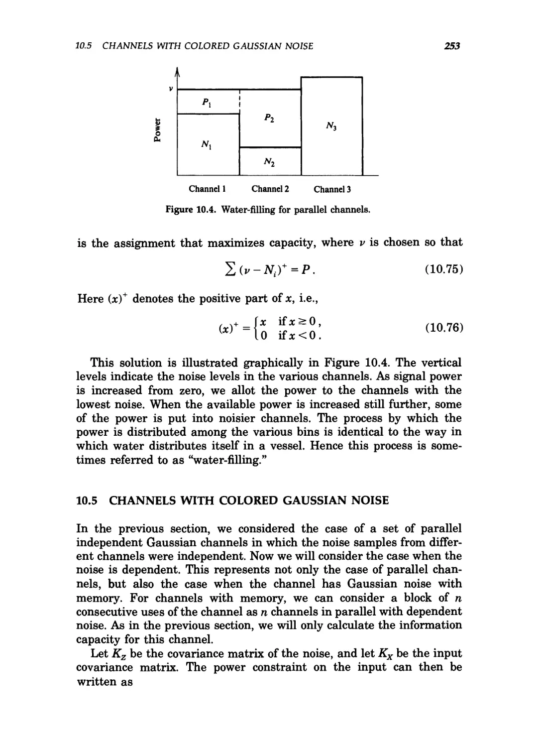
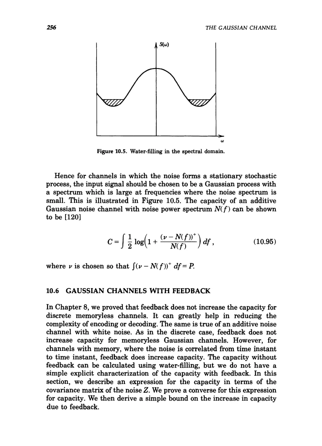
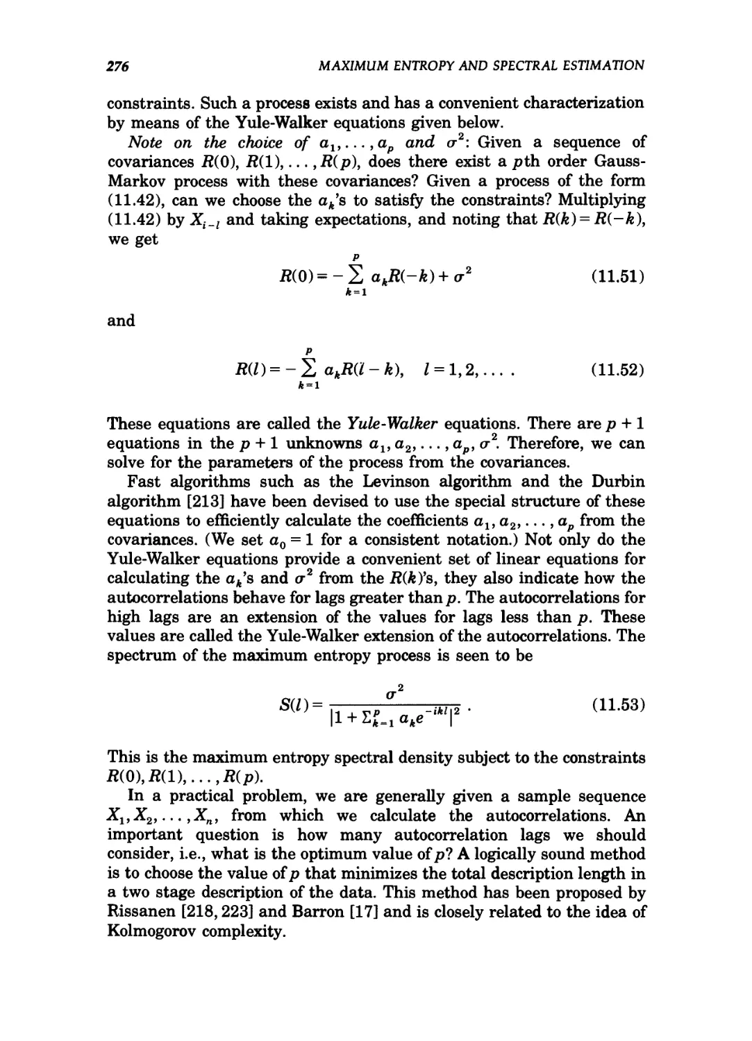
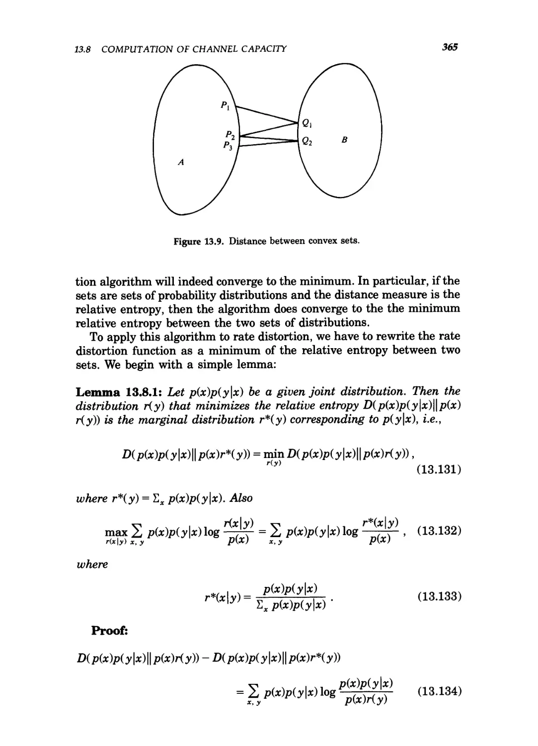
Text
Elements of Information Theory
Thomas M. Cover, Joy A. Thomas
Copyright © 1991 John Wiley & Sons, Inc.
Print ISBN 0-471-06259-6 Online ISBN 0-471-20061-1
Elements of Information
Theory
Elements of Information Theory
Thomas M. Cover, Joy A. Thomas
Copyright © 1991 John Wiley & Sons, Inc.
Print ISBN 0-471-06259-6 Online ISBN 0-471-20061-1
WILEY SERIES IN
TELECOMMUNICATIONS
Donald L. Schilling, Editor
City College of New York
Digital Telephony, 2nd Edition
John Bellamy
Elements of Information Theory
Thomas M. Cover and Joy A. Thomas
Telecommunication System Engineering, 2nd Edition
Roger L. Freeman
Telecommunication Transmission Handbook, 3rd Edition
Roger L. Freeman
Introduction to Communications Engineering, 2nd Edition
Robert M. Gagliardi
Expert System Applications to Telecommunications
Jay Liebowitz
Synchronization in Digital Communications, Volume 1
Heinrich Meyr and Gerd Ascheid
Synchronization in Digital Communications, Volume 2
Heinrich Meyr and Gerd Ascheid (in preparation)
Computational Methods of Signal Recovery and Recognition
Richard J. Mammone (in preparation)
Business Earth Stations for Telecommunications
Walter L. Morgan and Denis Rouffet
Satellite Communications: The First Quarter Century of Service
David W. E. Rees
Worldwide Telecommunications Guide for the Business Manager
Walter L. Vignault
Elements of Information
Theory
THOMAS M. COVER
Stanford University
Stanford, California
JOY A. THOMAS
IBM T. J. Watson Research Center
Yorktozvn Heights, New York
A Wiley-Interscience Publication
JOHN WILEY & SONS, INC.
New York / Chichester / Brisbane / Toronto / Singapore
Copyright © 1991 by John Wiley & Sons, Inc. All rights reserved.
No part of this publication may be reproduced, stored in a retrieval system or transmitted in
any form or by any means, electronic or mechanical, including uploading, downloading,
printing, decompiling, recording or otherwise, except as permitted under Sections 107 or 108 of
the 1976 United States Copyright Act, without the prior written permission of the Publisher.
Requests to the Publisher for permission should be addressed to the Permissions Department,
John Wiley & Sons, Inc., 605 Third Avenue, New York, NY 10158-0012, B12) 850-6011, fax
B12) 850-6008, E-Mail: PERMREQ@WILEY.COM.
This publication is designed to provide accurate and authoritative information in regard to the
subject matter covered. It is sold with the understanding that the publisher is not engaged in
rendering professional services. If professional advice or other expert assistance is required, the
services of a competent professional person should be sought.
ISBN 0-471-20061-1.
This title is also available in print as ISBN 0-471-06259-6
For more information about Wiley products, visit our web site at www.Wiley.com.
Library of Congress Cataloging in Publication Data:
Cover, T. M., 1938 —
Elements of Information theory / Thomas M. Cover, Joy A. Thomas.
p. cm. — (Wiley series in telecommunications)
"A Wiley-Interscience publication."
Includes bibliographical references and index.
ISBN 0-471-06259-6
1. Information theory. I. Thomas, Joy A. II. Title.
III. Series.
Q360.C68 1991
003'.54 —dc20 90-45484
CIP
Printed in the United States of America
20 19 18 17 16 15 14 13
To my father
Tom Cover
To my parents
Joy Thomas
Preface
This is intended to be a simple and accessible book on information
theory. As Einstein said, "Everything should be made as simple as
possible, but no simpler." Although we have not verified the quote (first
found in a fortune cookie), this point of view drives our development
throughout the book. There are a few key ideas and techniques that,
when mastered, make the subject appear simple and provide great
intuition on new questions.
This book has arisen from over ten years of lectures in a two-quarter
sequence of a senior and first-year graduate level course in information
theory, and is intended as an introduction to information theory for
students of communication theory, computer science and statistics.
There are two points to be made about the simplicities inherent in
information theory. First, certain quantities like entropy and mutual
information arise as the answers to fundamental questions. For exam-
example, entropy is the minimum descriptive complexity of a random vari-
variable, and mutual information is the communication rate in the presence
of noise. Also, as we shall point out, mutual information corresponds to
the increase in the doubling rate of wealth given side information.
Second, the answers to information theoretic questions have a natural
algebraic structure. For example, there is a chain rule for entropies, and
entropy and mutual information are related. Thus the answers to
problems in data compression and communication admit extensive
interpretation. We all know the feeling that follows when one investi-
investigates a problem, goes through a large amount of algebra and finally
investigates the answer to find that the entire problem is illuminated,
not by the analysis, but by the inspection of the answer. Perhaps the
outstanding examples of this in physics are Newton's laws and
vii
Viii PREFACE
Schrodinger's wave equation. Who could have foreseen the awesome
philosophical interpretations of Schrodinger's wave equation?
In the text we often investigate properties of the answer before we
look at the question. For example, in Chapter 2, we define entropy,
relative entropy and mutual information and study the relationships
and a few interpretations of them, showing how the answers fit together
in various ways. Along the way we speculate on the meaning of the
second law of thermodynamics. Does entropy always increase? The
answer is yes and no. This is the sort of result that should please
experts in the area but might be overlooked as standard by the novice.
In fact, that brings up a point that often occurs in teaching. It is fun
to find new proofs or slightly new results that no one else knows. When
one presents these ideas along with the established material in class,
the response is "sure, sure, sure." But the excitement of teaching the
material is greatly enhanced. Thus we have derived great pleasure from
investigating a number of new ideas in this text book.
Examples of some of the new material in this text include the chapter
on the relationship of information theory to gambling, the work on the
universality of the second law of thermodynamics in the context of
Markov chains, the joint typicality proofs of the channel capacity
theorem, the competitive optimality of Huffman codes and the proof of
Burg's theorem on maximum entropy spectral density estimation. Also
the chapter on Kolmogorov complexity has no counterpart in other
information theory texts. We have also taken delight in relating Fisher
information, mutual information, and the Brunn-Minkowski and en-
entropy power inequalities. To our surprise, many of the classical results
on determinant inequalities are most easily proved using information
theory.
Even though the field of information theory has grown considerably
since Shannon's original paper, we have strived to emphasize its coher-
coherence. While it is clear that Shannon was motivated by problems in
communication theory when he developed information theory, we treat
information theory as a field of its own with applications to communica-
communication theory and statistics.
We were drawn to the field of information theory from backgrounds in
communication theory, probability theory and statistics, because of the
apparent impossibility of capturing the intangible concept of infor-
information.
Since most of the results in the book are given as theorems and
proofs, we expect the elegance of the results to speak for themselves. In
many cases we actually describe the properties of the solutions before
introducing the problems. Again, the properties are interesting in them-
themselves and provide a natural rhythm for the proofs that follow.
One innovation in the presentation is our use of long chains of
inequalities, with no intervening text, followed immediately by the
PREFACE tX
explanations. By the time the reader comes to many of these proofs, we
expect that he or she will be able to follow most of these steps without
any explanation and will be able to pick out the needed explanations.
These chains of inequalities serve as pop quizzes in which the reader
can be reassured of having the knowledge needed to prove some im-
important theorems. The natural flow of these proofs is so compelling that
it prompted us to flout one of the cardinal rules of technical writing. And
the absence of verbiage makes the logical necessity of the ideas evident
and the key ideas perspicuous. We hope that by the end of the book the
reader will share our appreciation of the elegance, simplicity and
naturalness of information theory.
Throughout the book we use the method of weakly typical sequences,
which has its origins in Shannon's original 1948 work but was formally
developed in the early 1970s. The key idea here is the so-called asymp-
asymptotic equipartition property, which can be roughly paraphrased as
"Almost everything is almost equally probable."
Chapter 2, which is the true first chapter of the subject, includes the
basic algebraic relationships of entropy, relative entropy and mutual
information as well as a discussion of the second law of thermodynamics
and sufficient statistics. The asymptotic equipartition property (AEP) is
given central prominence in Chapter 3. This leads us to discuss the
entropy rates of stochastic processes and data compression in Chapters
4 and 5. A gambling sojourn is taken in Chapter 6, where the duality of
data compression and the growth rate of wealth is developed.
The fundamental idea of Kolmogorov complexity as an intellectual
foundation for information theory is explored in Chapter 7. Here we
replace the goal of finding a description that is good on the average with
the goal of finding the universally shortest description. There is indeed a
universal notion of the descriptive complexity of an object. Here also the
wonderful number Cl is investigated. This number, which is the binary
expansion of the probability that a Turing machine will halt, reveals
many of the secrets of mathematics.
Channel capacity, which is the fundamental theorem in information
theory, is established in Chapter 8. The necessary material on differen-
differential entropy is developed in Chapter 9, laying the groundwork for the
extension of previous capacity theorems to continuous noise channels.
The capacity of the fundamental Gaussian channel is investigated in
Chapter 10.
The relationship between information theory and statistics, first
studied by Kullback in the early 1950s, and relatively neglected since, is
developed in Chapter 12. Rate distortion theory requires a little more
background than its noiseless data compression counterpart, which
accounts for its placement as late as Chapter 13 in the text.
The huge subject of network information theory, which is the study of
the simultaneously achievable flows of information in the presence of
X PREFACE
noise and interference, is developed in Chapter 14. Many new ideas
come into play in network information theory. The primary new ingredi-
ingredients are interference and feedback. Chapter 15 considers the stock
market, which is the generalization of the gambling processes consid-
considered in Chapter 6, and shows again the close correspondence of informa-
information theory and gambling.
Chapter 16, on inequalities in information theory, gives us a chance
to recapitulate the interesting inequalities strewn throughout the book,
put them in a new framework and then add some interesting new
inequalities on the entropy rates of randomly drawn subsets. The
beautiful relationship of the Brunn-Minkowski inequality for volumes of
set sums, the entropy power inequality for the effective variance of the
sum of independent random variables and the Fisher information
inequalities are made explicit here.
We have made an attempt to keep the theory at a consistent level.
The mathematical level is a reasonably high one, probably senior year or
first-year graduate level, with a background of at least one good semes-
semester course in probability and a solid background in mathematics. We
have, however, been able to avoid the use of measure theory. Measure
theory comes up only briefly in the proof of the AEP for ergodic
processes in Chapter 15. This fits in with our belief that the fundamen-
fundamentals of information theory are orthogonal to the techniques required to
bring them to their full generalization.
Each chapter ends with a brief telegraphic summary of the key
results. These summaries, in equation form, do not include the qualify-
qualifying conditions. At the end of each we have included a variety of
problems followed by brief historical notes describing the origins of the
main results. The bibliography at the end of the book includes many of
the key papers in the area and pointers to other books and survey
papers on the subject.
The essential vitamins are contained in Chapters 2, 3, 4, 5, 8, 9, 10,
12, 13 and 14. This subset of chapters can be read without reference to
the others and makes a good core of understanding. In our opinion,
Chapter 7 on Kolmogorov complexity is also essential for a deep under-
understanding of information theory. The rest, ranging from gambling to
inequalities, is part of the terrain illuminated by this coherent and
beautiful subject.
Every course has its first lecture, in which a sneak preview and
overview of ideas is presented. Chapter 1 plays this role.
Tom Cover
Joy Thomas
Palo Alto, June 1991
Acknowledgments
We wish to thank everyone who helped make this book what it is. In
particular, Toby Berger, Masoud Salehi, Alon Orlitsky, Jim Mazo and
Andrew Barron have made detailed comments on various drafts of the
book which guided us in our final choice of content. We would like to
thank Bob Gallager for an initial reading of the manuscript and his
encouragement to publish it. We were pleased to use twelve of his
problems in the text. Aaron Wyner donated his new proof with Ziv on
the convergence of the Lempel-Ziv algorithm. We would also like to
thank Norman Abramson, Ed van der Meulen, Jack Salz and Raymond
Yeung for their suggestions.
Certain key visitors and research associates contributed as well,
including Amir Dembo, Paul Algoet, Hirosuke Yamamoto, Ben
Kawabata, Makoto Shimizu and Yoichiro Watanabe. We benefited from
the advice of John Gill when he used this text in his class. Abbas El
Gamal made invaluable contributions and helped begin this book years
ago when we planned to write a research monograph on multiple user
information theory. We would also like to thank the Ph.D. students in
information theory as the book was being written: Laura Ekroot, Will
Equitz, Don Kimber, Mitchell Trott, Andrew Nobel, Jim Roche, Erik
Ordentlich, Elza Erkip and Vittorio Castelli. Also Mitchell Oslick,
Chien-Wen Tseng and Michael Morrell were among the most active
students in contributing questions and suggestions to the text. Marc
Goldberg and Anil Kaul helped us produce some of the figures. Finally
we would like to thank Kirsten Goodell and Kathy Adams for their
support and help in some of the aspects of the preparation of the
manuscript.
xi
Xii ACKNOWLEDGMENTS
Joy Thomas would also like to thank Peter Franaszek, Steve
Lavenberg, Fred Jelinek, David Nahamoo and Lalit Bahl for their
encouragement and support during the final stages of production of this
book.
Tom Cover
Joy Thomas
Contents
List of Figures xix
1 Introduction and Preview 1
1.1 Preview of the book / 5
2 Entropy, Relative Entropy and Mutual Information 12
2.1 Entropy / 12
2.2 Joint entropy and conditional entropy / 15
2.3 Relative entropy and mutual information / 18
2.4 Relationship between entropy and mutual information / 19
2.5 Chain rules for entropy, relative entropy and mutual
information / 21
2.6 Jensen's inequality and its consequences / 23
2.7 The log sum inequality and its applications / 29
2.8 Data processing inequality / 32
2.9 The second law of thermodynamics / 33
2.10 Sufficient statistics / 36
2.11 Fano's inequality / 38
Summary of Chapter 2/40
Problems for Chapter 2 / 42
Historical notes / 49
3 The Asymptotic Equipartition Property 50
3.1 The AEP / 51
xiii
Xiv CONTENTS
3.2 Consequences of the AEP: data compression / 53
3.3 High probability sets and the typical set / 55
Summary of Chapter 3/56
Problems for Chapter 3 / 57
Historical notes / 59
4 Entropy Rates of a Stochastic Process 60
4.1 Markov chains / 60
4.2 Entropy rate / 63
4.3 Example: Entropy rate of a random walk on a weighted
graph / 66
4.4 Hidden Markov models / 69
Summary of Chapter 4/71
Problems for Chapter 4/72
Historical notes / 77
5 Data Compression 78
5.1 Examples of codes / 79
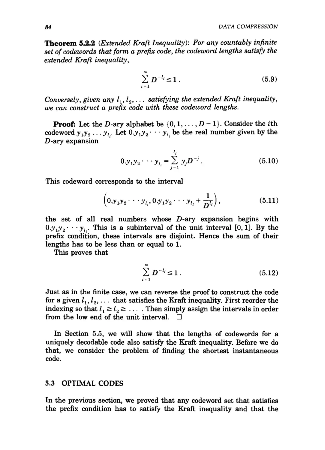
5.2 Kraft inequality / 82
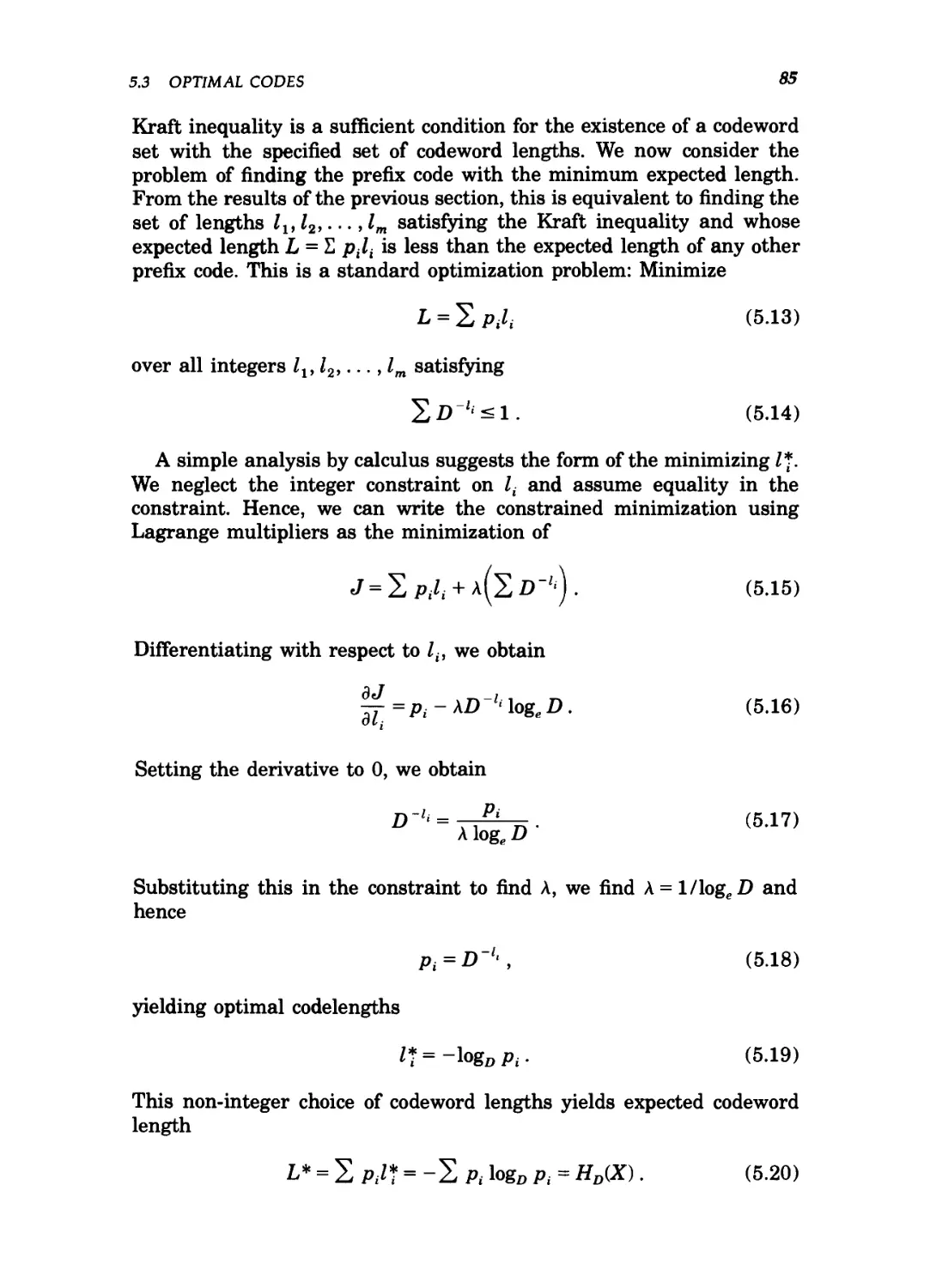
5.3 Optimal codes / 84
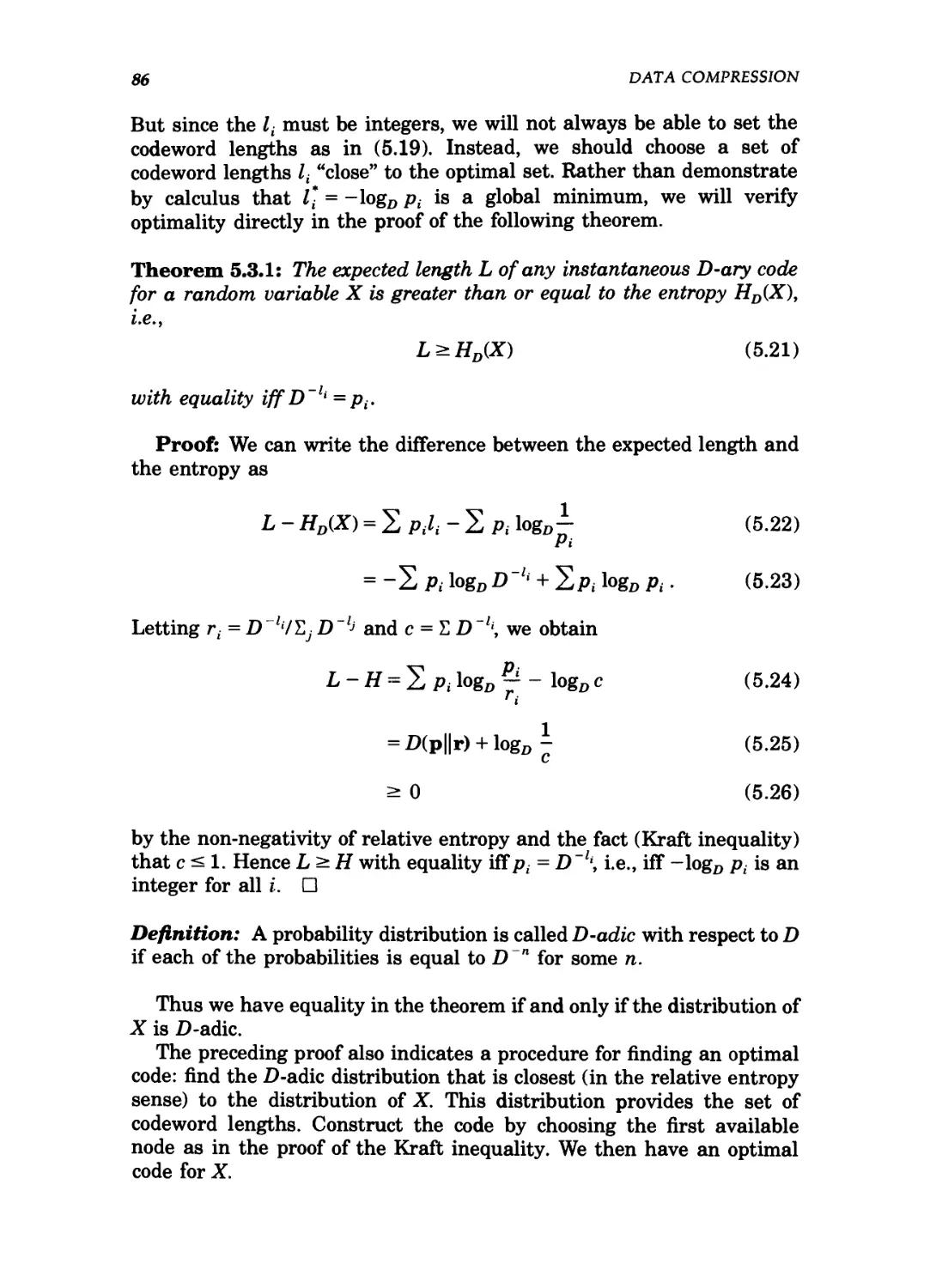
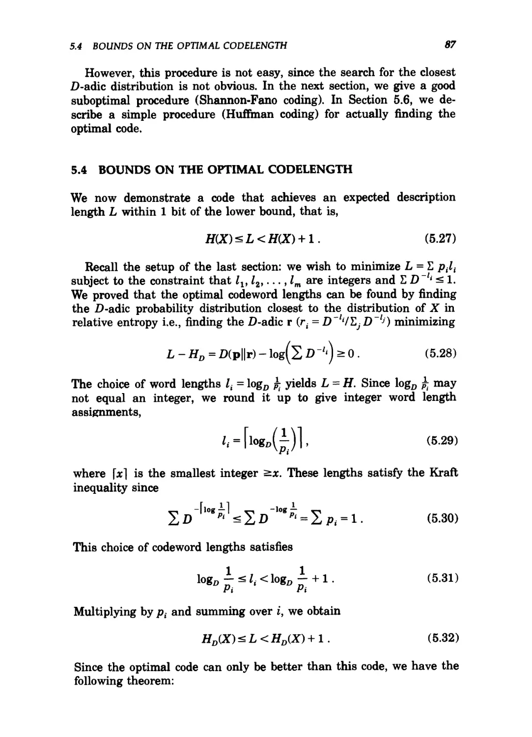
5.4 Bounds on the optimal codelength / 87
5.5 Kraft inequality for uniquely decodable codes / 90
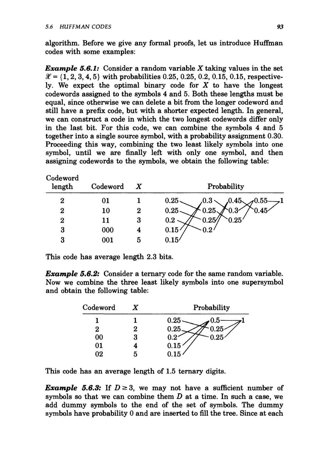
5.6 Huffman codes / 92
5.7 Some comments on Huffman codes / 94
5.8 Optimality of Huffman codes / 97
5.9 Shannon-Fano-Elias coding / 101
5.10 Arithmetic coding / 104
5.11 Competitive optimality of the Shannon code / 107
5.12 Generation of discrete distributions from fair
coins / 110
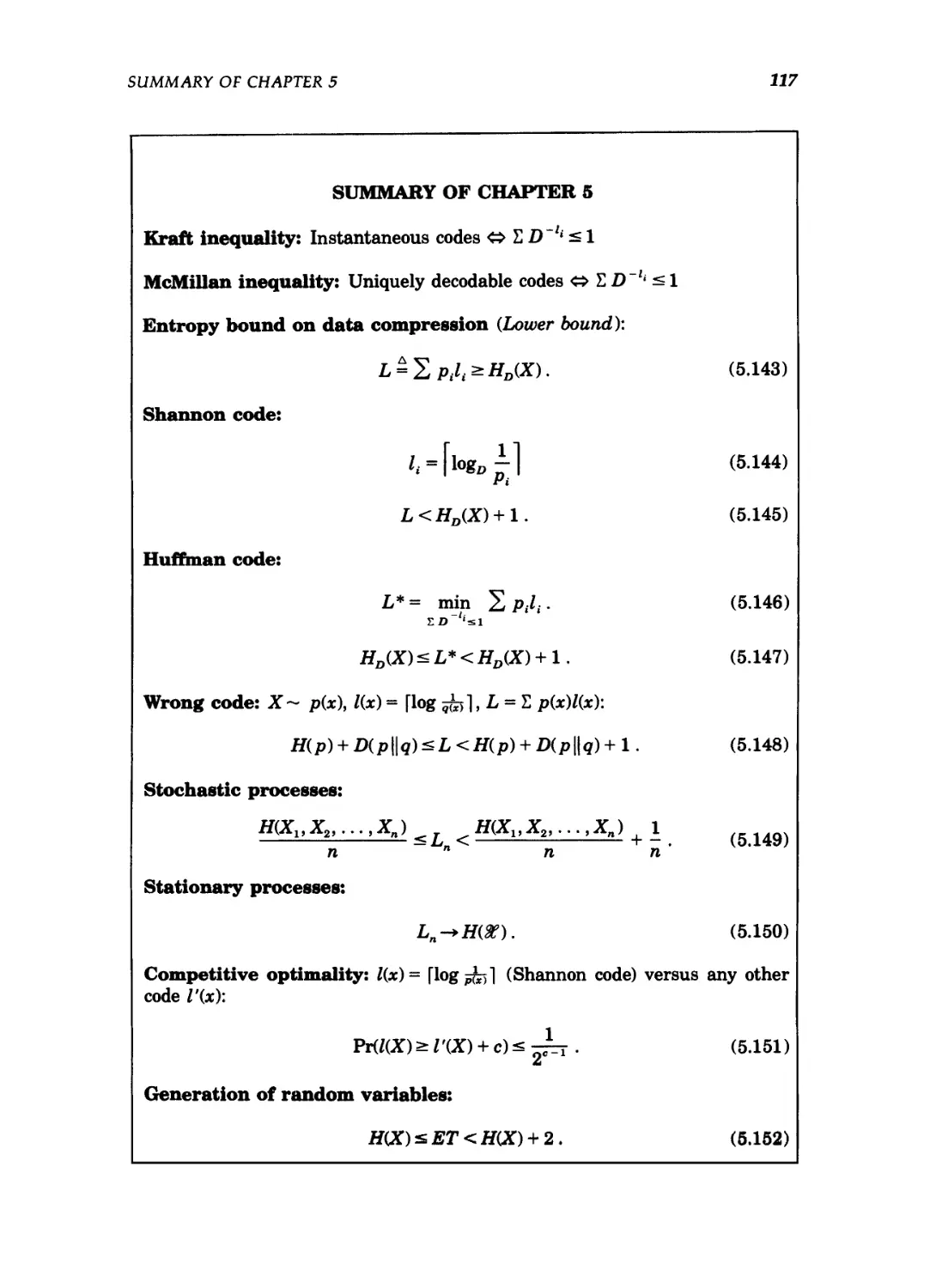
Summary of Chapter 5/117
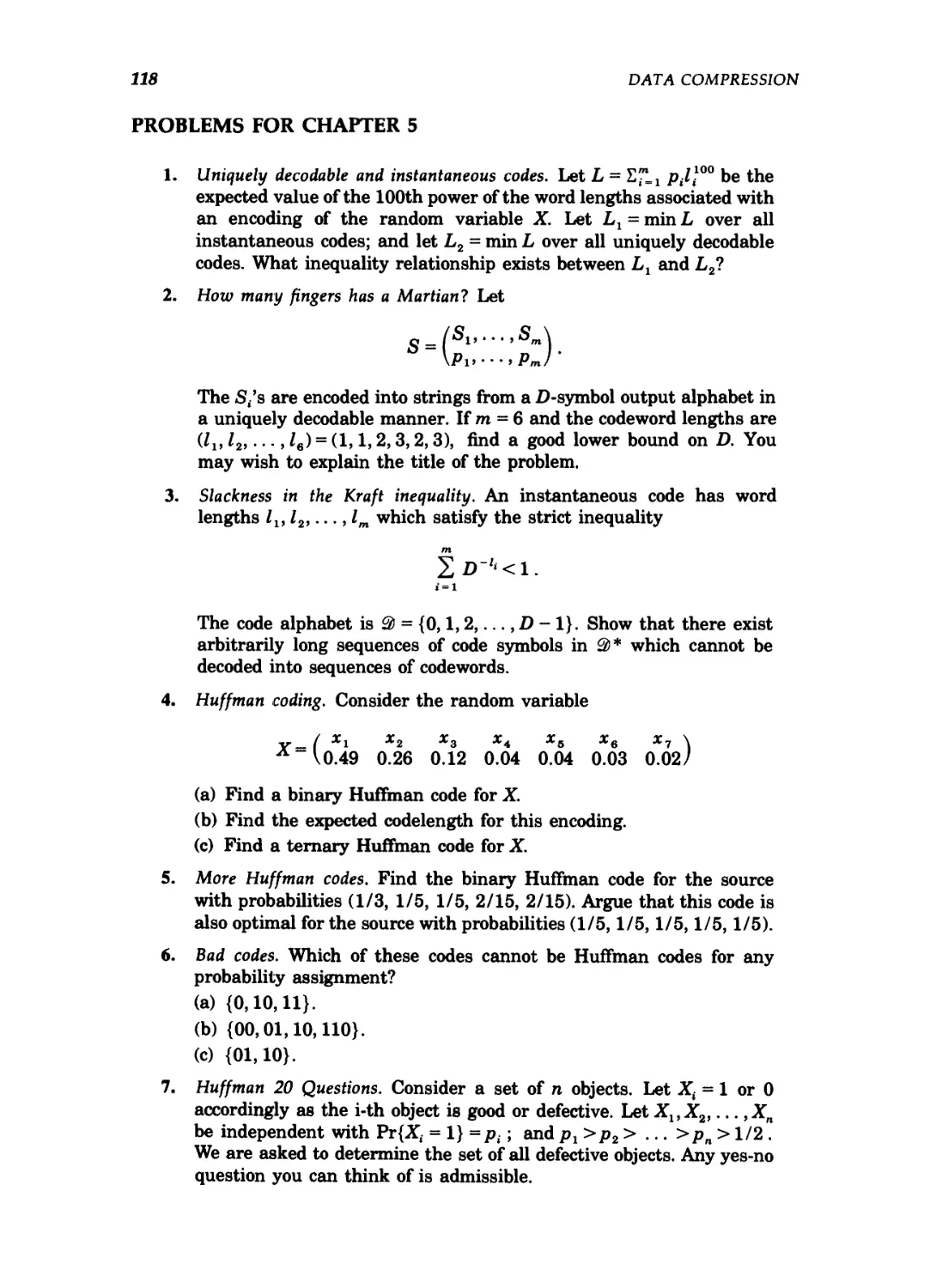
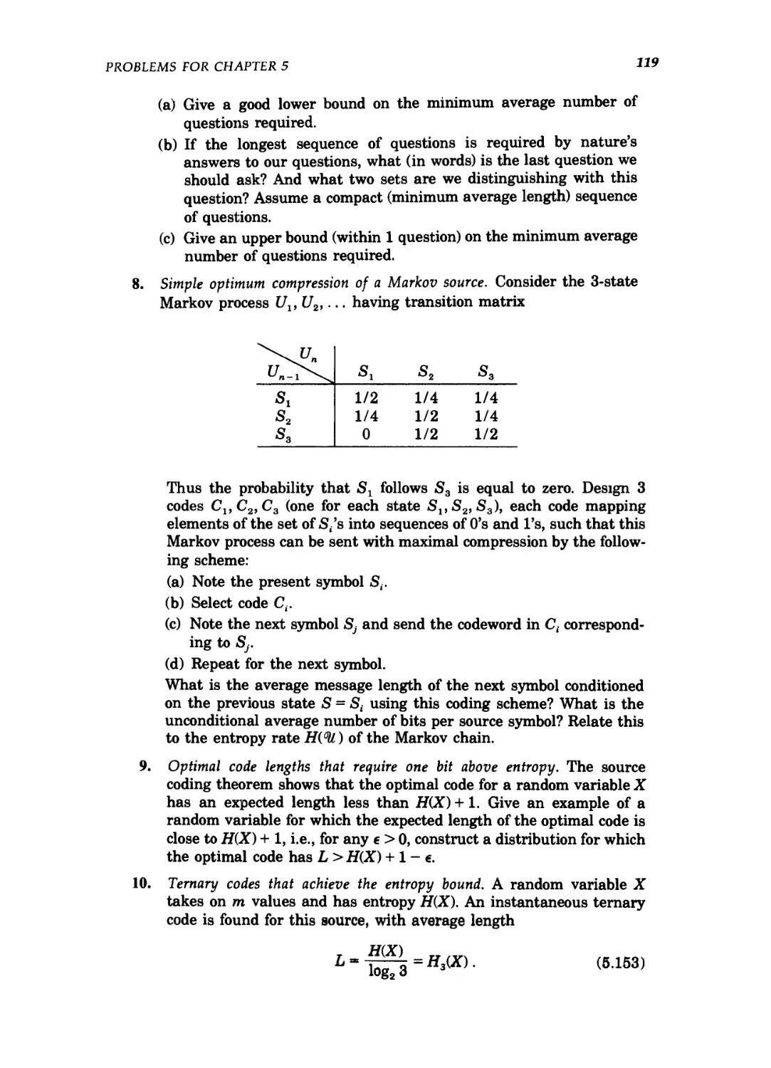
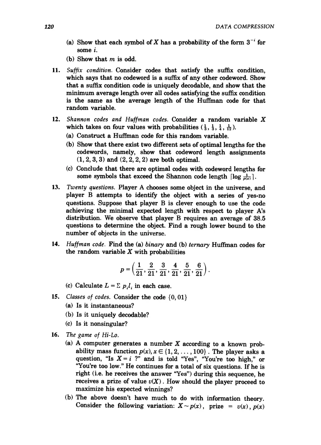
Problems for Chapter 5/118
Historical notes / 124
6 Gambling and Data Compression 125
6.1 The horse race / 125
6.2 Gambling and side information / 130
6.3 Dependent horse races and entropy rate / 131
6.4 The entropy of English / 133
6.5 Data compression and gambling / 136
CONTENTS
XV
6.6 Gambling estimate of the entropy of English / 138
Summary of Chapter 6/140
Problems for Chapter 6 / 141
Historical notes / 143
7 Kolmogorov Complexity 144
7.1 Models of computation / 146
7.2 Kolmogorov complexity: definitions and examples / 147
7.3 Kolmogorov complexity and entropy / 153
7.4 Kolmogorov complexity of integers / 155
7.5 Algorithmically random and incompressible
sequences / 156
7.6 Universal probability / 160
7.7 The halting problem and the non-computability of
Kolmogorov complexity / 162
7.8 a I 164
7.9 Universal gambling / 166
7.10 Occam's razor / 168
7.11 Kolmogorov complexity and universal probability / 169
7.12 The Kolmogorov sufficient statistic / 175
Summary of Chapter 7/178
Problems for Chapter 7 / 180
Historical notes / 182
8 Channel Capacity 183
8.1 Examples of channel capacity / 184
8.2 Symmetric channels / 189
8.3 Properties of channel capacity / 190
8.4 Preview of the channel coding theorem / 191
8.5 Definitions / 192
8.6 Jointly typical sequences / 194
8.7 The channel coding theorem / 198
8.8 Zero-error codes / 203
8.9 Fano's inequality and the converse to the coding
theorem / 204
8.10 Equality in the converse to the channel coding
theorem / 207
8.11 Hamming codes / 209
8.12 Feedback capacity / 212
xoi CONTENTS
8.13 The joint source channel coding theorem / 215
Summary of Chapter 8 / 218
Problems for Chapter 8 / 220
Historical notes / 222
9 Differential Entropy 224
9.1 Definitions / 224
9.2 The AEP for continuous random variables / 225
9.3 Relation of differential entropy to discrete entropy / 228
9.4 Joint and conditional differential entropy / 229
9.5 Relative entropy and mutual information / 231
9.6 Properties of differential entropy, relative entropy and
mutual information / 232
9.7 Differential entropy bound on discrete entropy / 234
Summary of Chapter 9 / 236
Problems for Chapter 9 / 237
Historical notes / 238
10 The Gaussian Channel 239
10.1 The Gaussian channel: definitions / 241
10.2 Converse to the coding theorem for Gaussian
channels / 245
10.3 Band-limited channels / 247
10.4 Parallel Gaussian channels / 250
10.5 Channels with colored Gaussian noise / 253
10.6 Gaussian channels with feedback / 256
Summary of Chapter 10 / 262
Problems for Chapter 10 / 263
Historical notes / 264
11 Maximum Entropy and Spectral Estimation 266
11.1 Maximum entropy distributions / 266
11.2 Examples / 268
11.3 An anomalous maximum entropy problem / 270
11.4 Spectrum estimation / 272
11.5 Entropy rates of a Gaussian process / 273
11.6 Burg's maximum entropy theorem / 274
Summary of Chapter 11 / 277
Problems for Chapter 11 / 277
Historical notes / 278
CONTENTS xvtt
12 Information Theory and Statistics 279
12.1 The method of types / 279
12.2 The law of large numbers / 286
12.3 Universal source coding / 288
12.4 Large deviation theory / 291
12.5 Examples of SanoVs theorem / 294
12.6 The conditional limit theorem / 297
12.7 Hypothesis testing / 304
12.8 Stein's lemma / 309
12.9 Chernoff bound / 312
12.10 Lempel-Ziv coding / 319
12.11 Fisher information and the Cramer-Rao
inequality / 326
Summary of Chapter 12 / 331
Problems for Chapter 12 / 333
Historical notes / 335
13 Rate Distortion Theory 336
13.1 Quantization / 337
13.2 Definitions / 338
13.3 Calculation of the rate distortion function / 342
13.4 Converse to the rate distortion theorem / 349
13.5 Achievability of the rate distortion function / 351
13.6 Strongly typical sequences and rate distortion / 358
13.7 Characterization of the rate distortion function / 362
13.8 Computation of channel capacity and the rate
distortion function / 364
Summary of Chapter 13 / 367
Problems for Chapter 13 / 368
Historical notes / 372
14 Network Information Theory 374
14.1 Gaussian multiple user channels / 377
14.2 Jointly typical sequences / 384
14.3 The multiple access channel / 388
14.4 Encoding of correlated sources / 407
14.5 Duality between Slepian-Wolf encoding and multiple
access channels / 416
14.6 The broadcast channel / 418
14.7 The relay channel / 428
xoiii contents
14.8 Source coding with side information / 432
14.9 Rate distortion with side information / 438
14.10 General multiterminal networks / 444
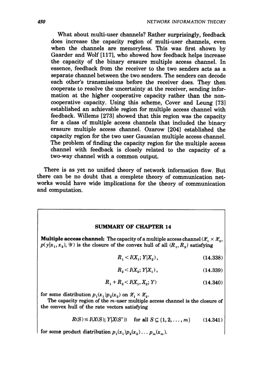
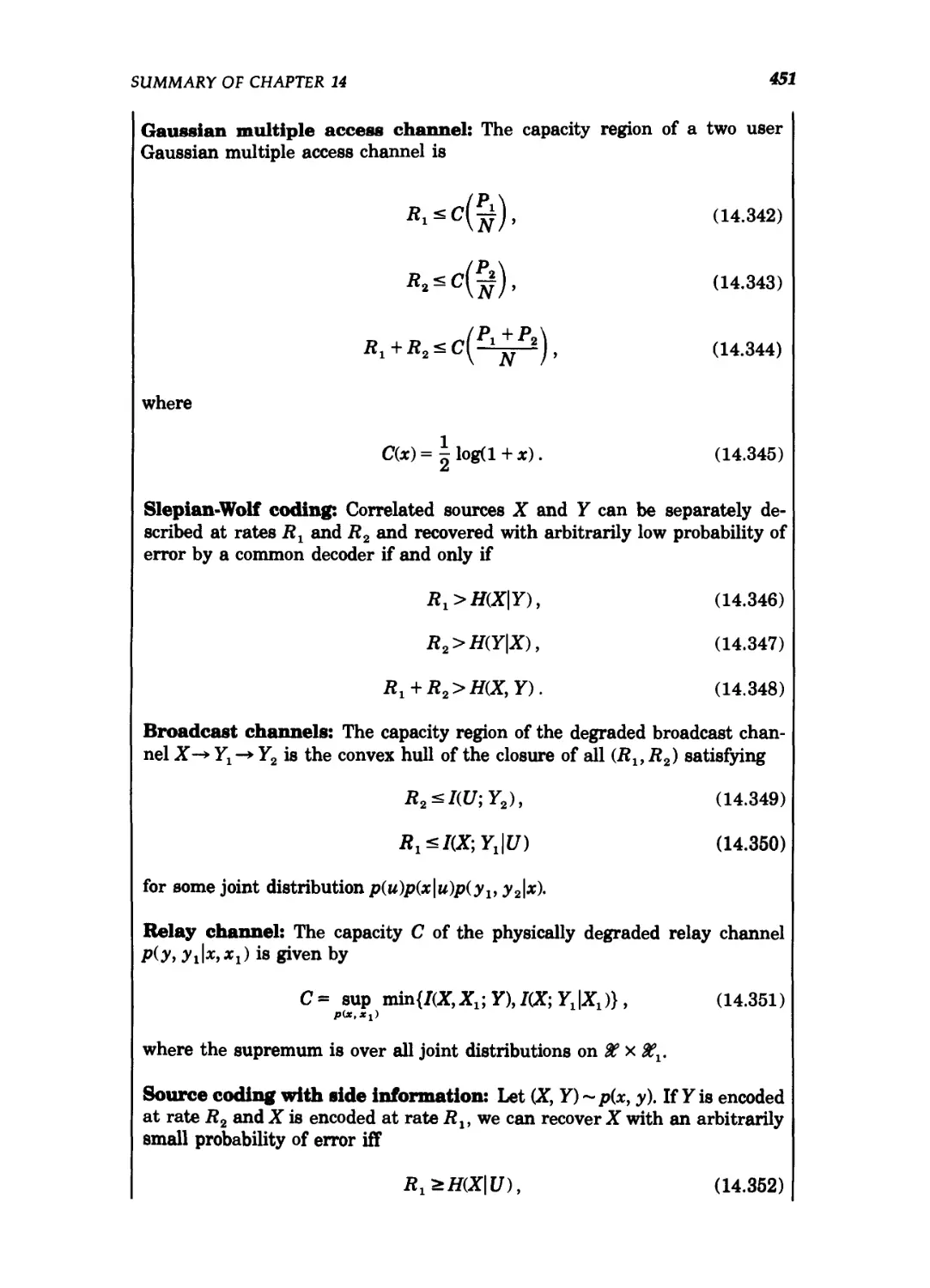
Summary of Chapter 14 / 450
Problems for Chapter 14 / 452
Historical notes / 457
15 Information Theory and the Stock Market 459
15.1 The stock market: some definitions / 459
15.2 Kuhn-Tucker characterization of the log-optimal
portfolio / 462
15.3 Asymptotic optimality of the log-optimal portfolio / 465
15.4 Side information and the doubling rate / 467
15.5 Investment in stationary markets / 469
15.6 Competitive optimality of the log-optimal portfolio / 471
15.7 The Shannon-McMillan-Breiman theorem / 474
Summary of Chapter 15 / 479
Problems for Chapter 15 / 480
Historical notes / 481
16 Inequalities in Information Theory 482
16.1 Basic inequalities of information theory / 482
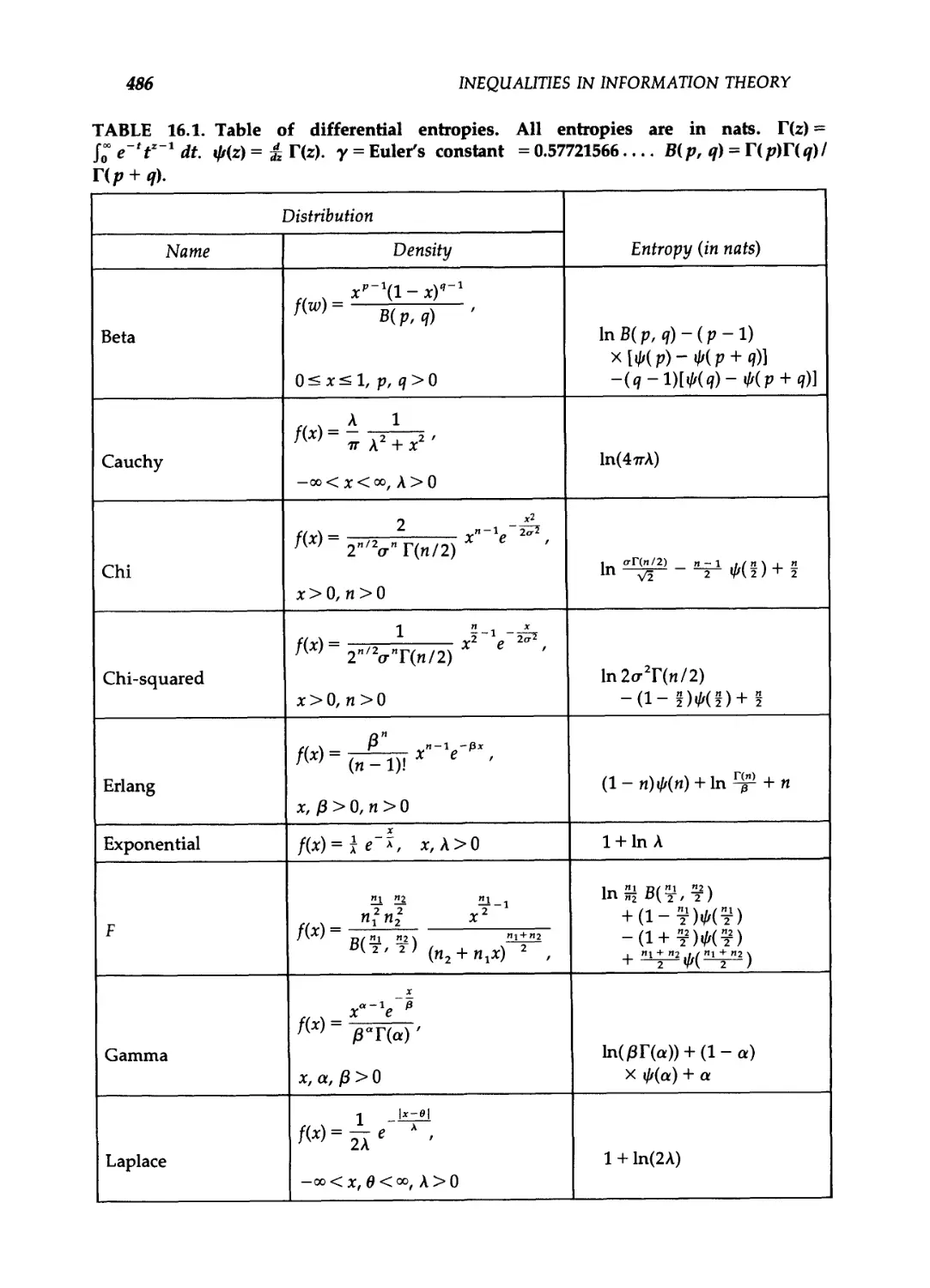
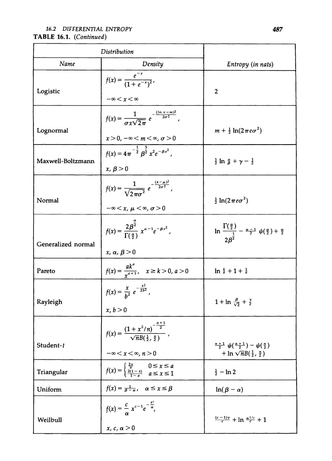
16.2 Differential entropy / 485
16.3 Bounds on entropy and relative entropy / 488
16.4 Inequalities for types / 490
16.5 Entropy rates of subsets / 490
16.6 Entropy and Fisher information / 494
16.7 The entropy power inequality and the Brunn-
Minkowski inequality / 497
16.8 Inequalities for determinants / 501
16.9 Inequalities for ratios of determinants / 505
Overall Summary / 508
Problems for Chapter 16 / 509
Historical notes / 509
Bibliography 510
List of Symbols 526
Index 529
List of Figures
1.1 The relationship of information theory with other fields 2
1.2 Information theoretic extreme points of communication
theory 2
1.3 Noiseless binary channel. 7
1.4 A noisy channel 7
1.5 Binary symmetric channel 8
2.1 H(p) versus p 15
2.2 Relationship between entropy and mutual information 20
2.3 Examples of convex and concave functions 24
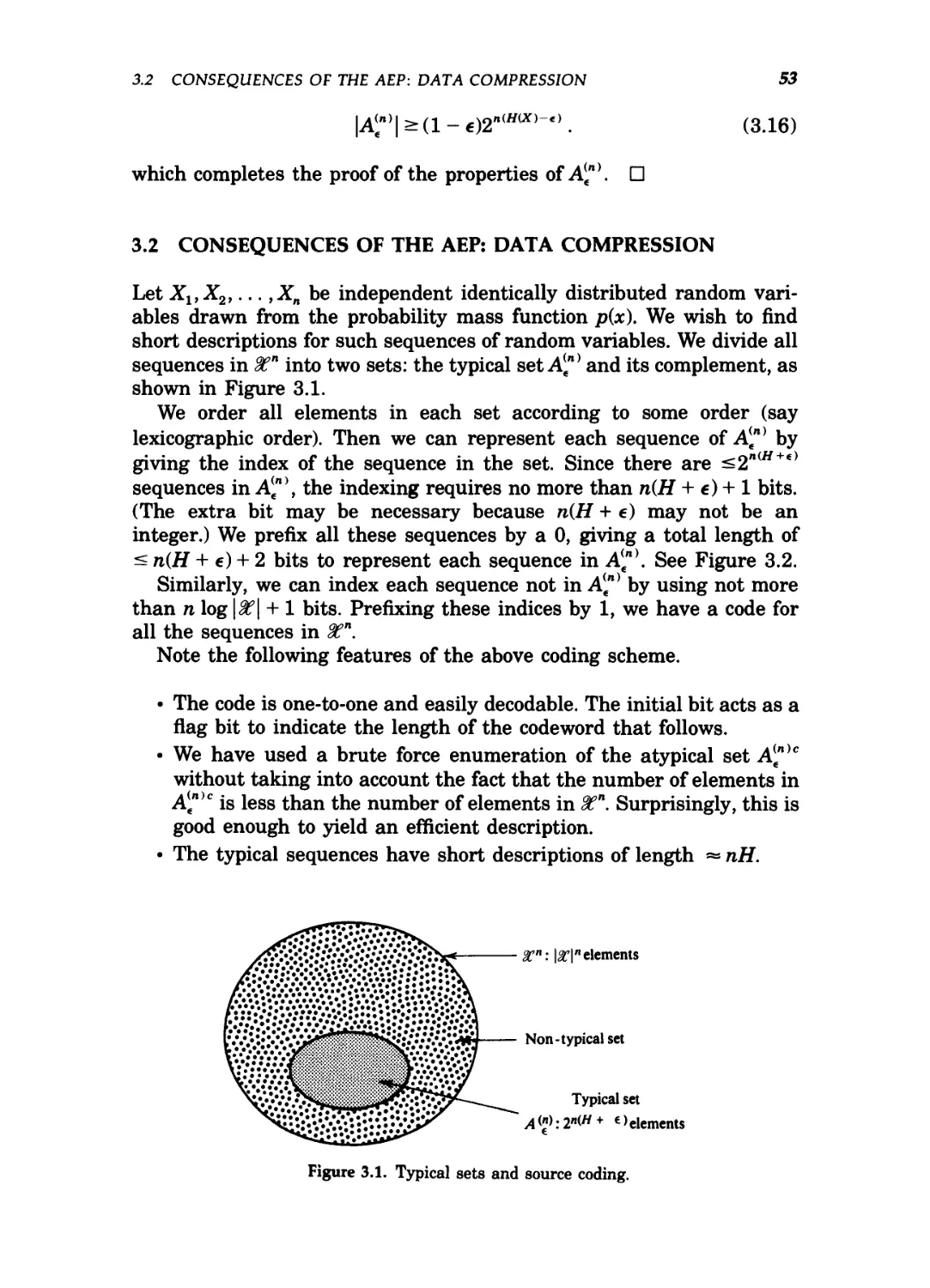
3.1 Typical sets and source coding 53
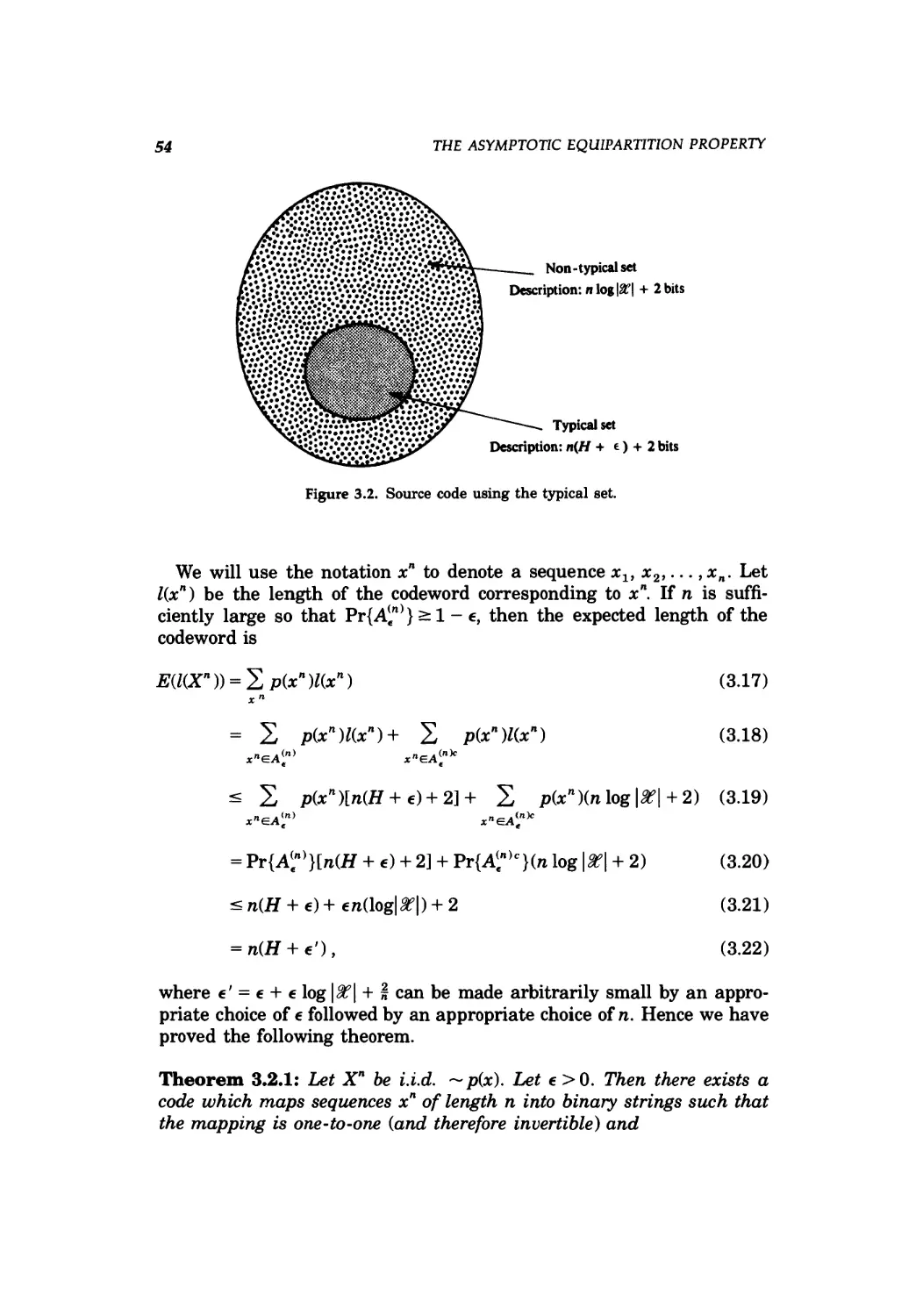
3.2 Source code using the typical set 54
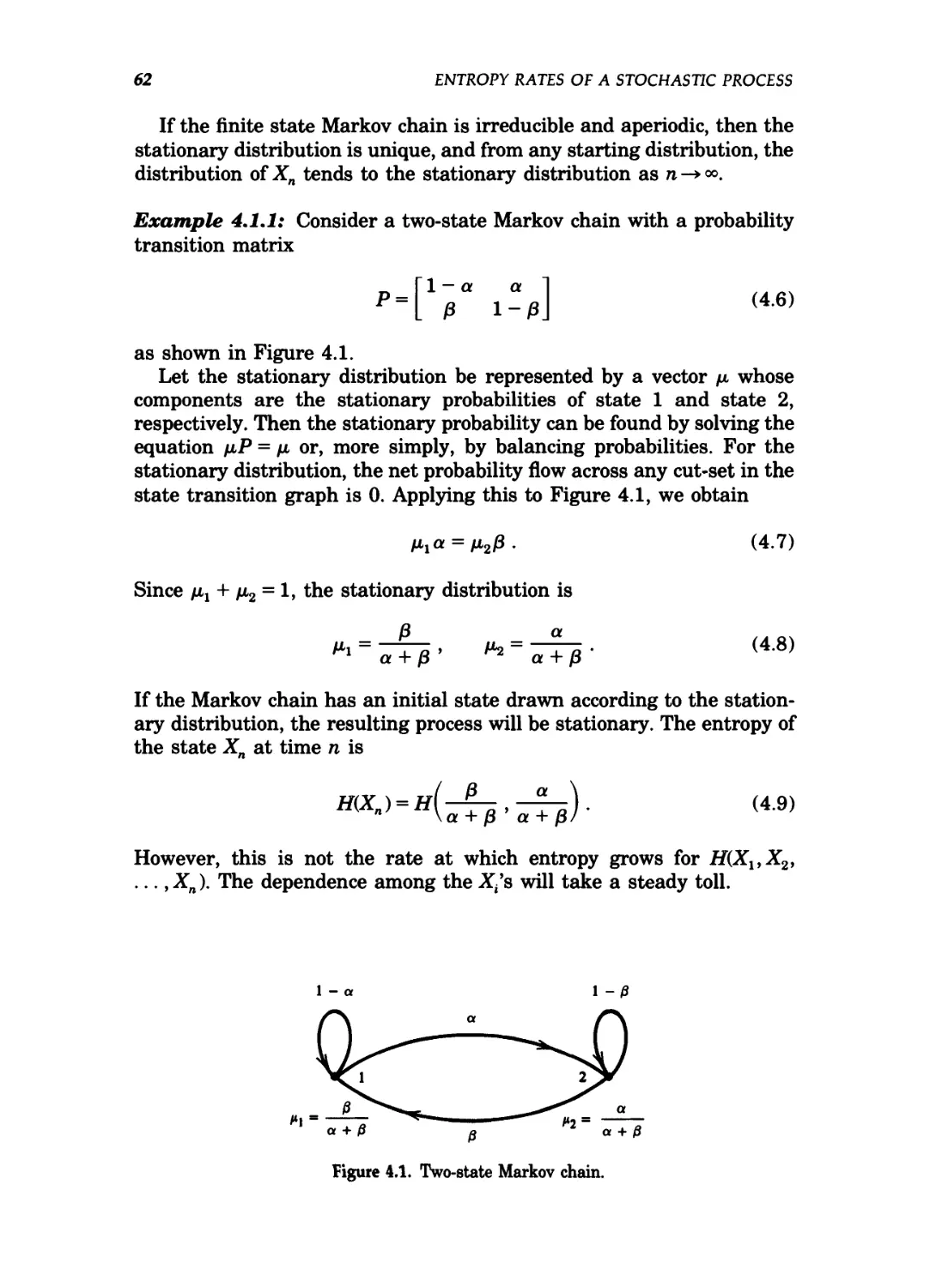
4.1 Two-state Markov chain 62
4.2 Random walk on a graph 66
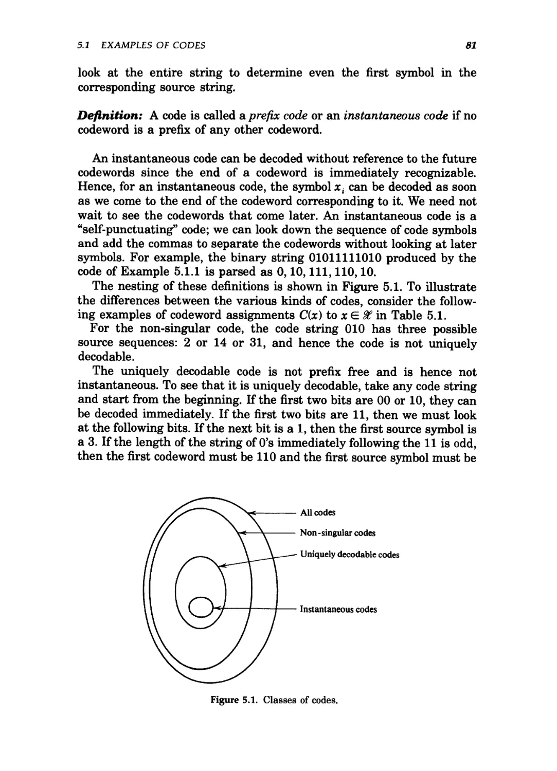
5.1 Classes of codes 81
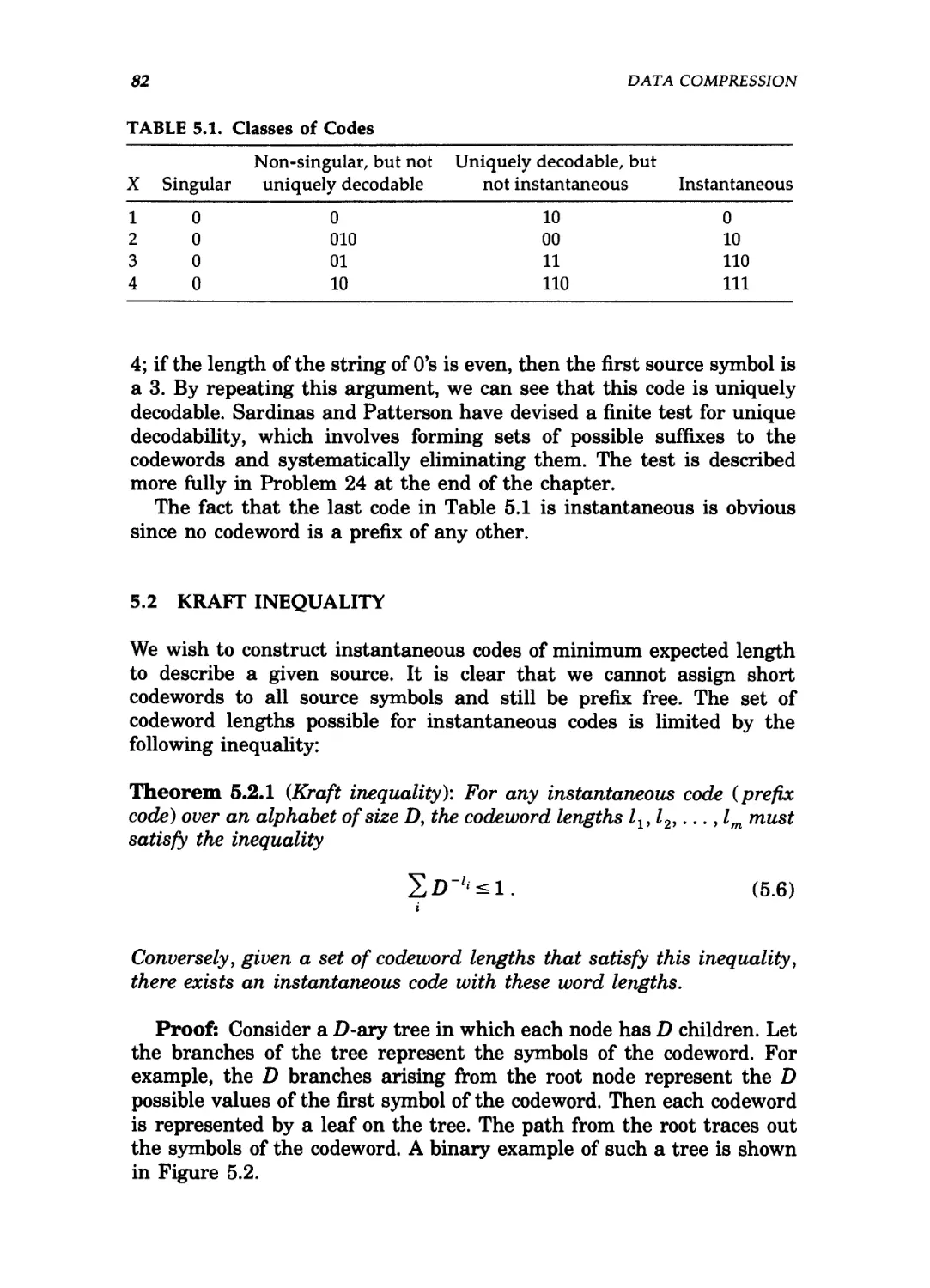
5.2 Code tree for the Kraft inequality 83
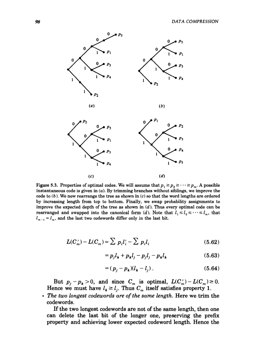
5.3 Properties of optimal codes 98
5.4 Induction step for Huffman coding 100
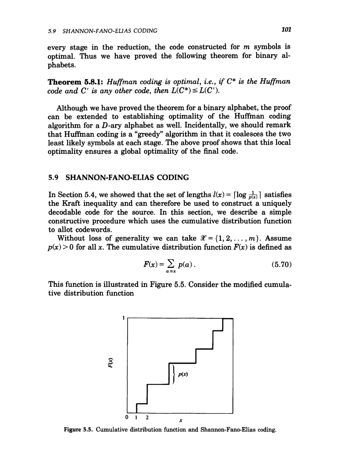
5.5 Cumulative distribution function and Shannon-Fano-
Elias coding 101
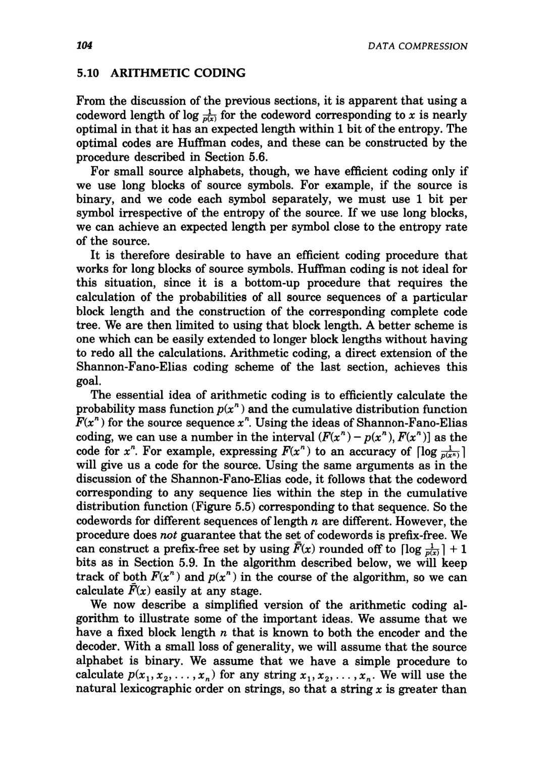
5.6 Tree of strings for arithmetic coding 105
5.7 The sgn function and a bound 109
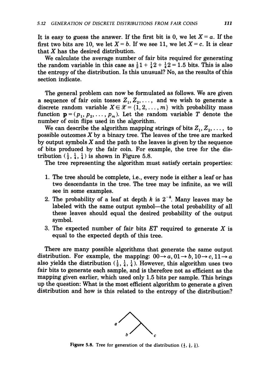
5.8 Tree for generation of the distribution (g, \, \) 111
5.9 Tree to generate a (§, g) distribution 114
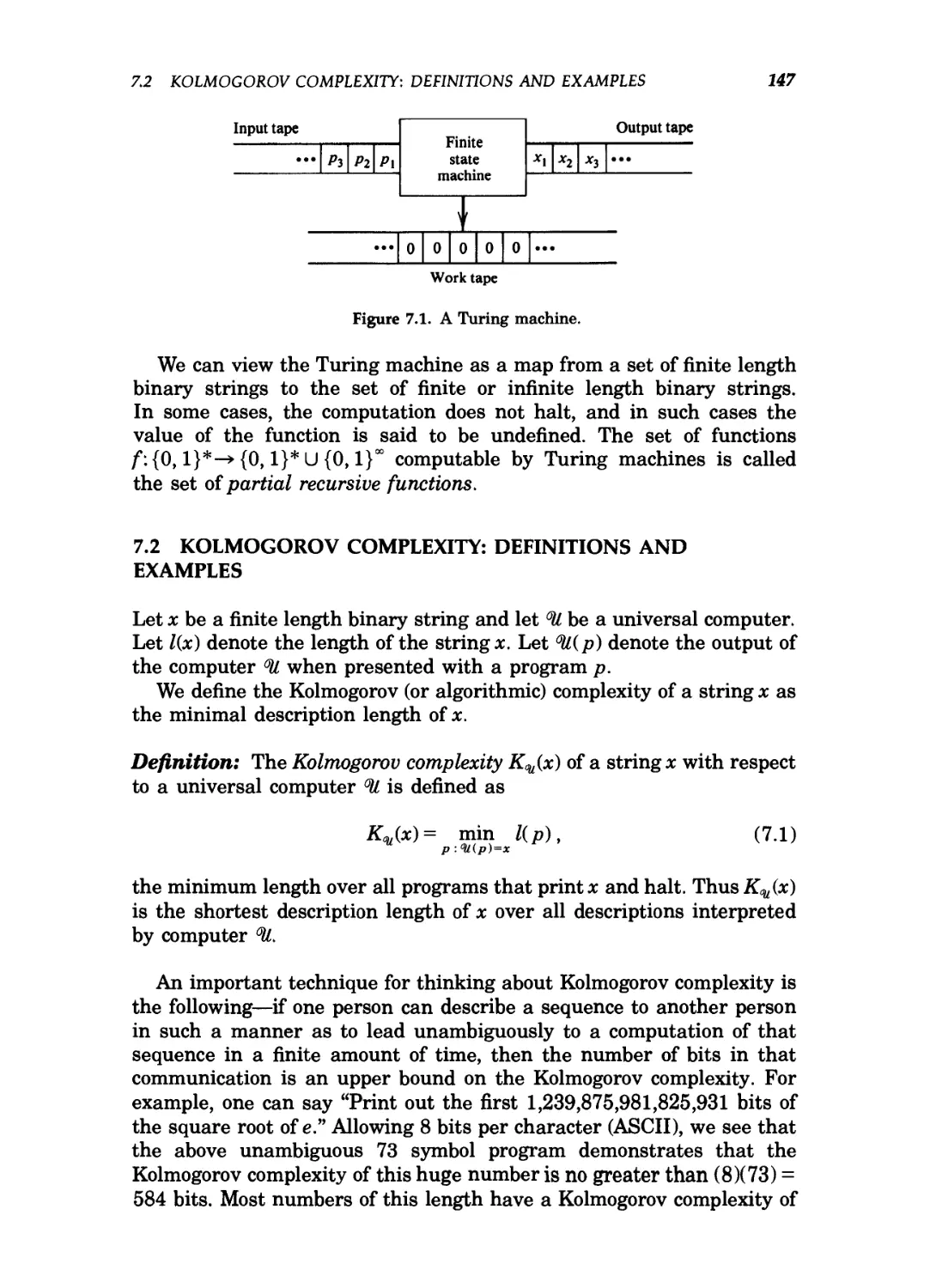
7.1 A Turing machine 147
xix
XX LIST OF FIGURES
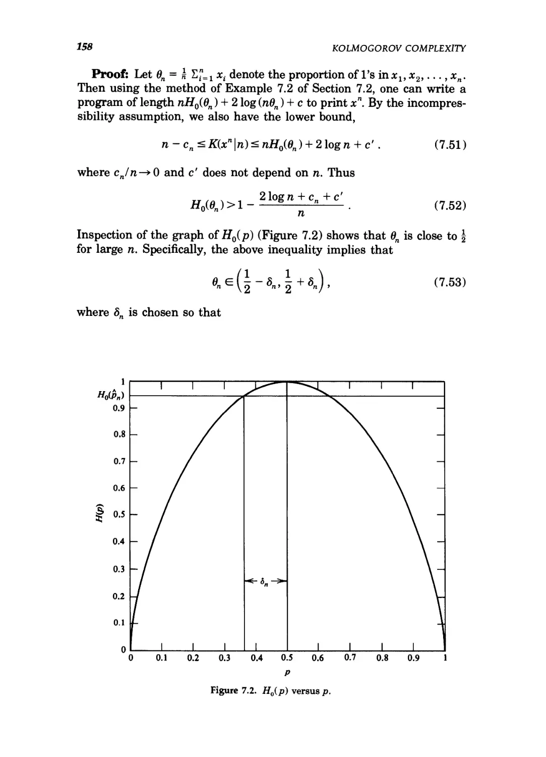
7.2 H0(p) versus p 158
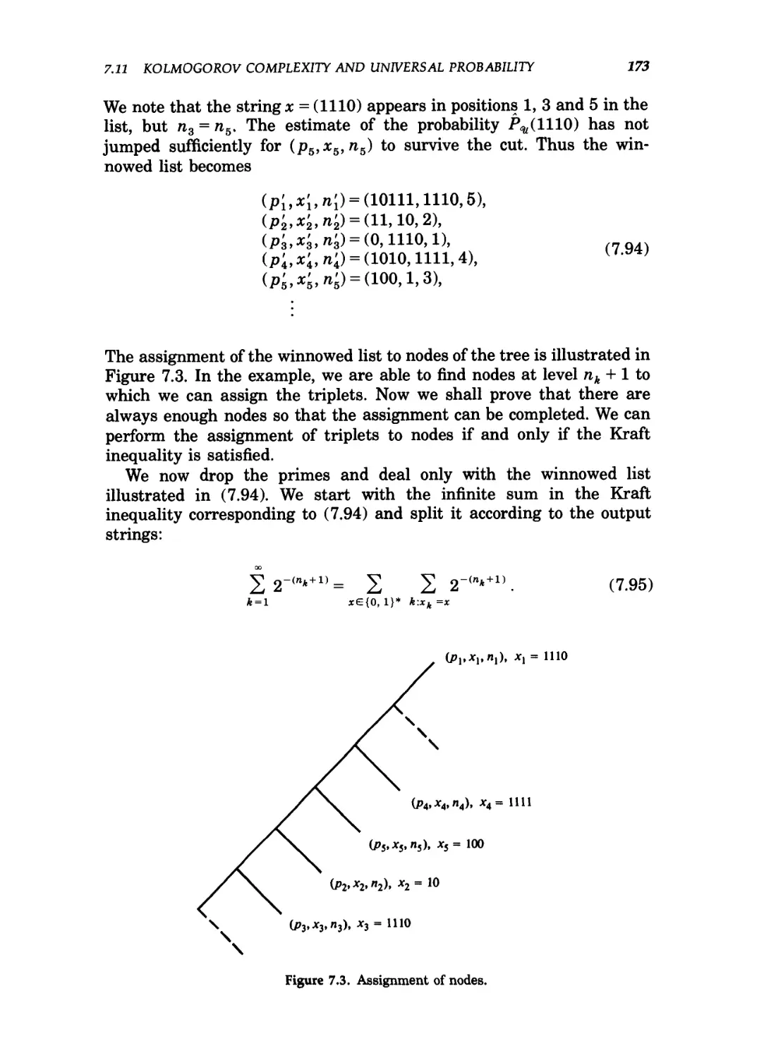
7.3 Assignment of nodes 173
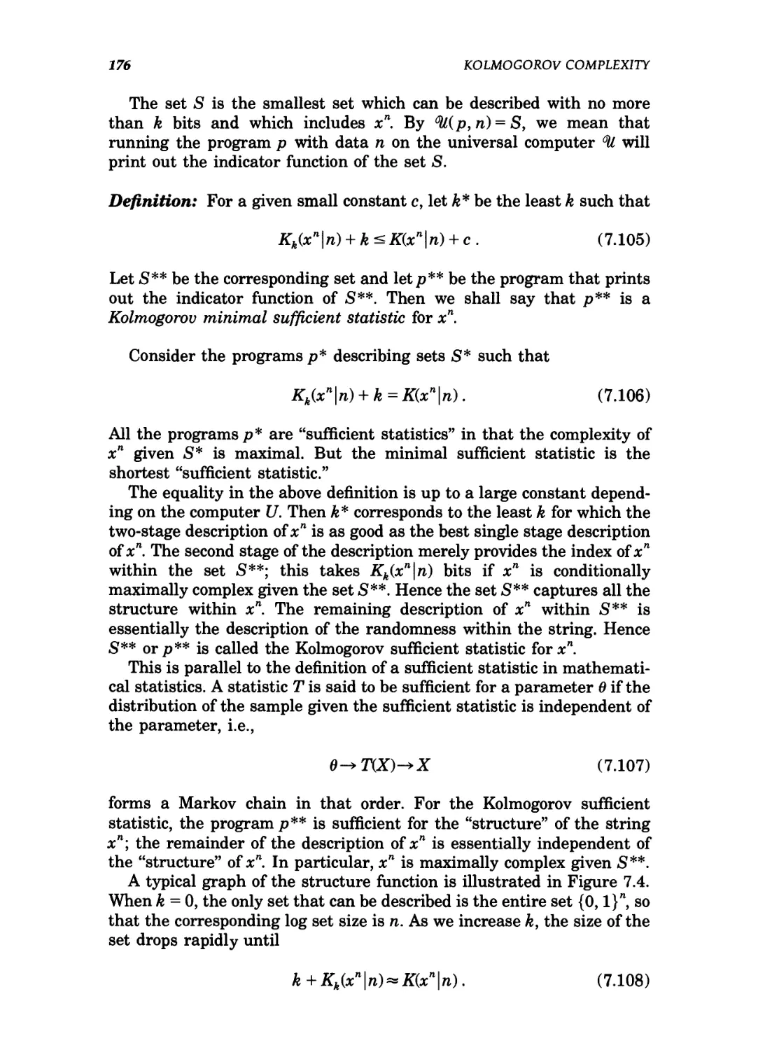
7.4 Kolmogorov sufficient statistic 177
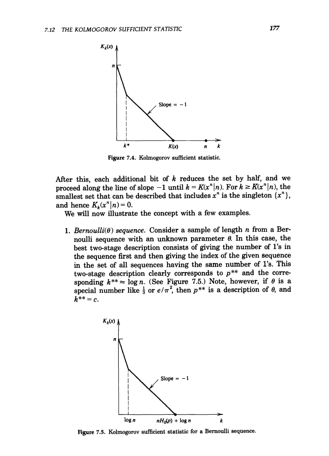
7.5 Kolmogorov sufficient statistic for a Bernoulli sequence 177
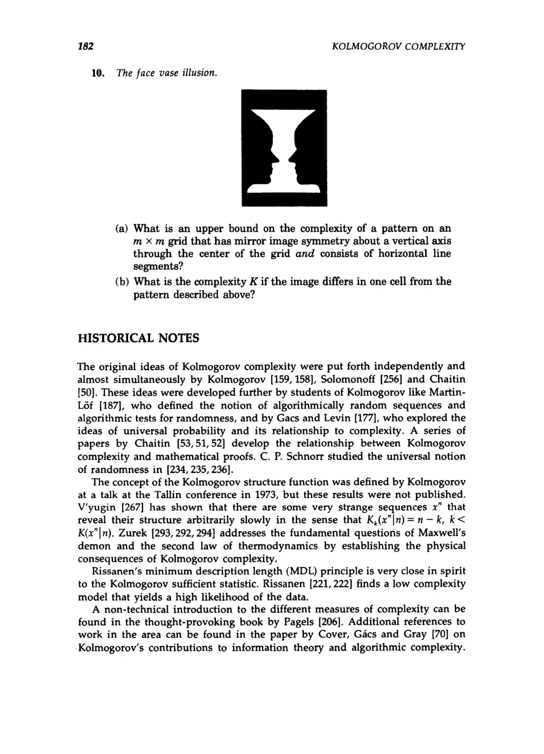
7.6 Mona Lisa 178
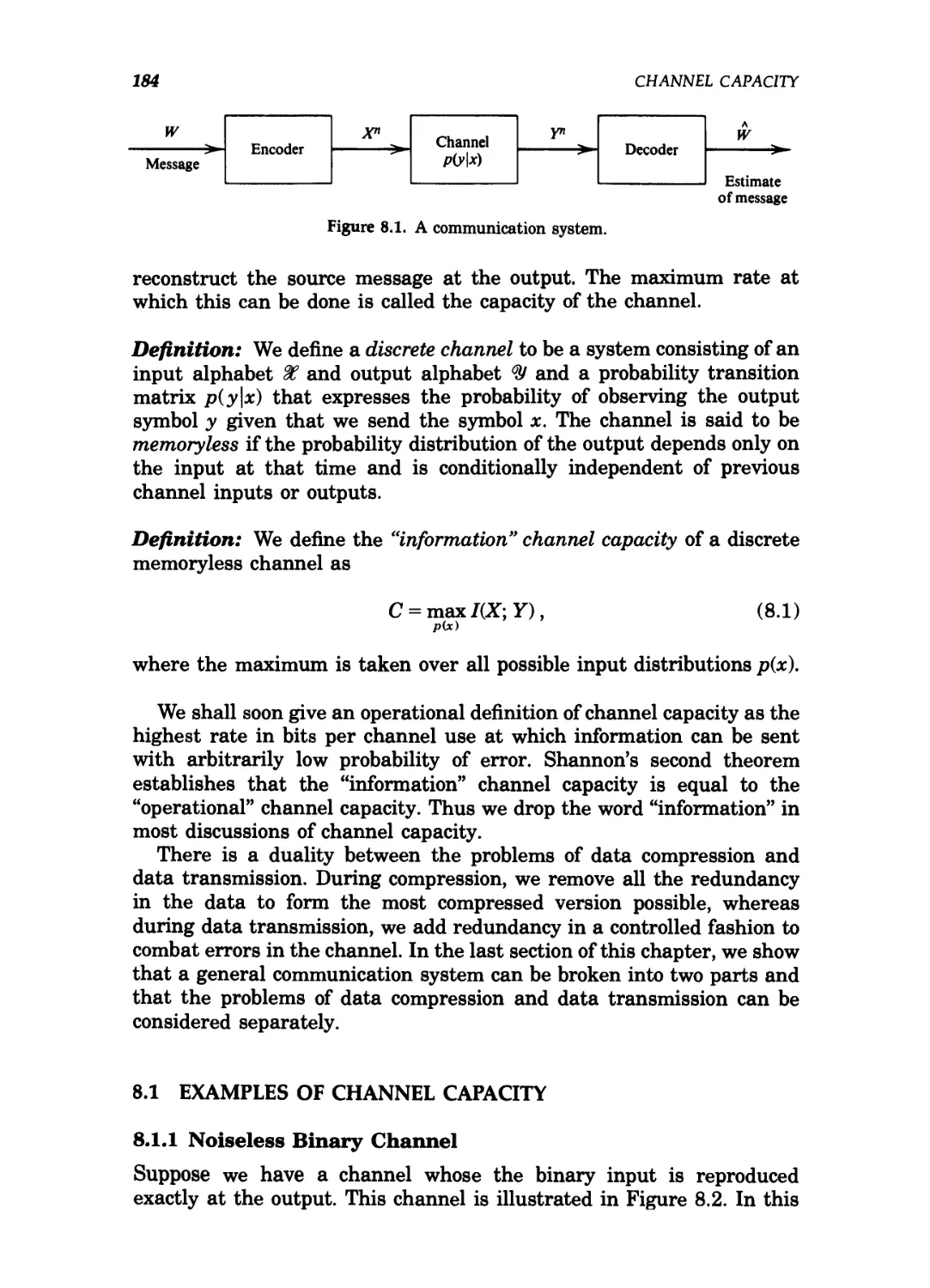
8.1 A communication system 184
8.2 Noiseless binary channel. 185
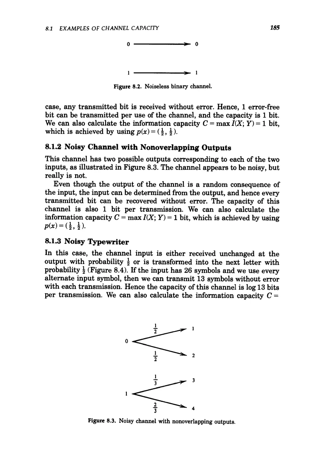
8.3 Noisy channel with nonoverlapping outputs. 185
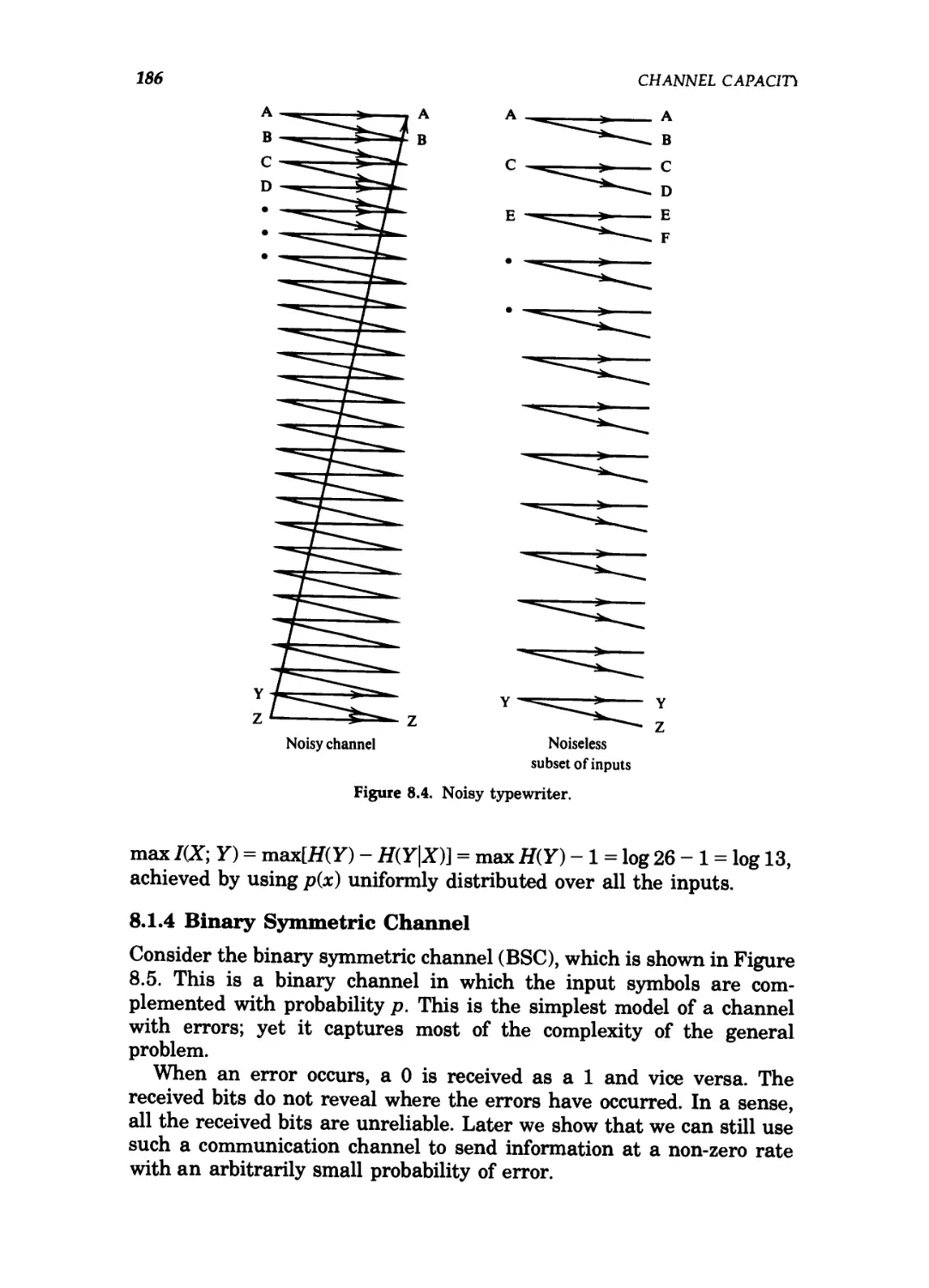
8.4 Noisy typewriter. 186
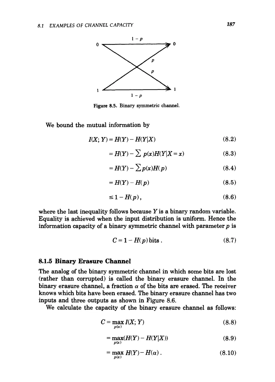
8.5 Binary symmetric channel. 187
8.6 Binary erasure channel 188
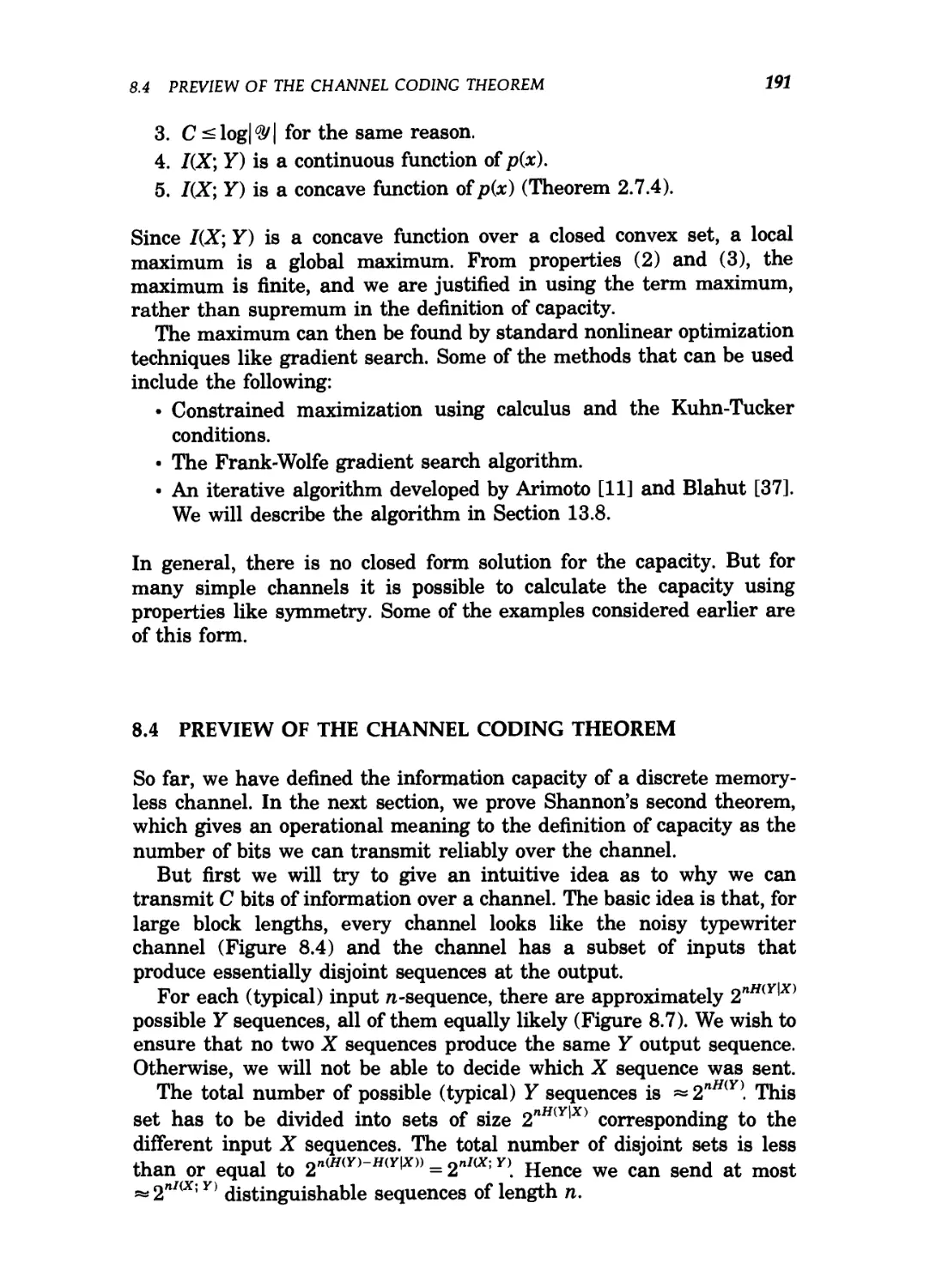
8.7 Channels after n uses 192
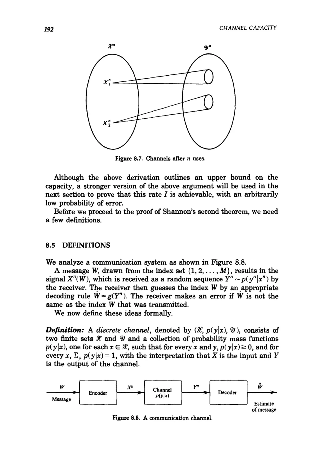
8.8 A communication channel 192
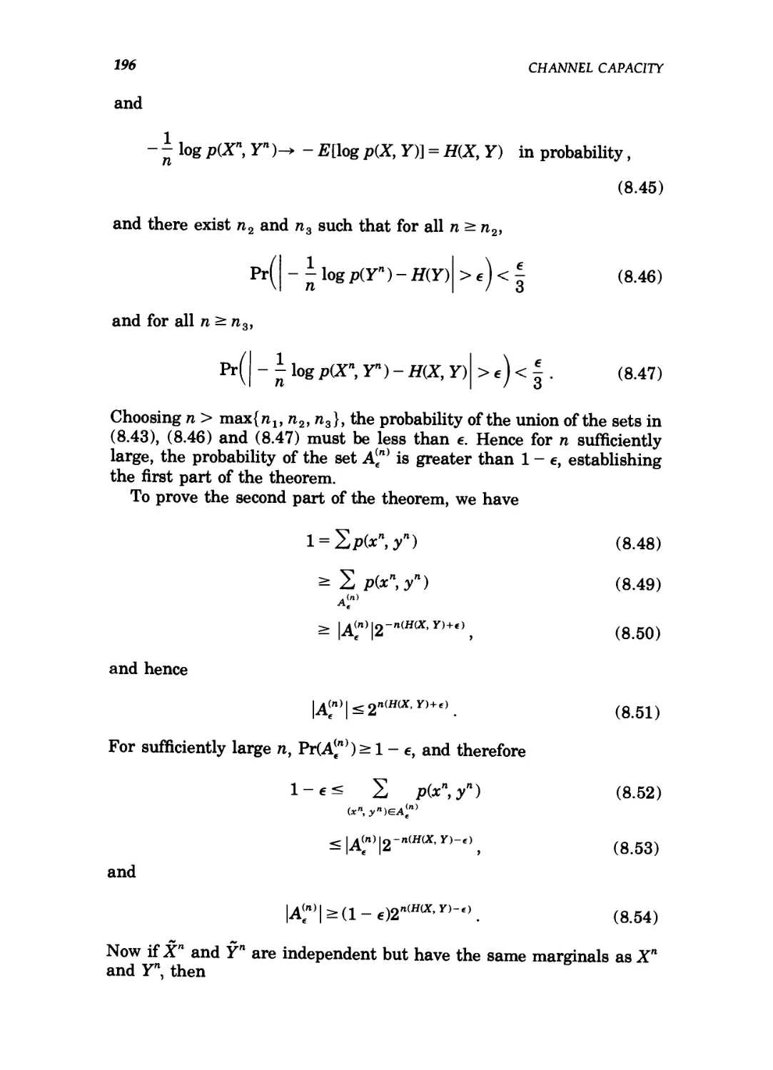
8.9 Jointly typical sequences 197
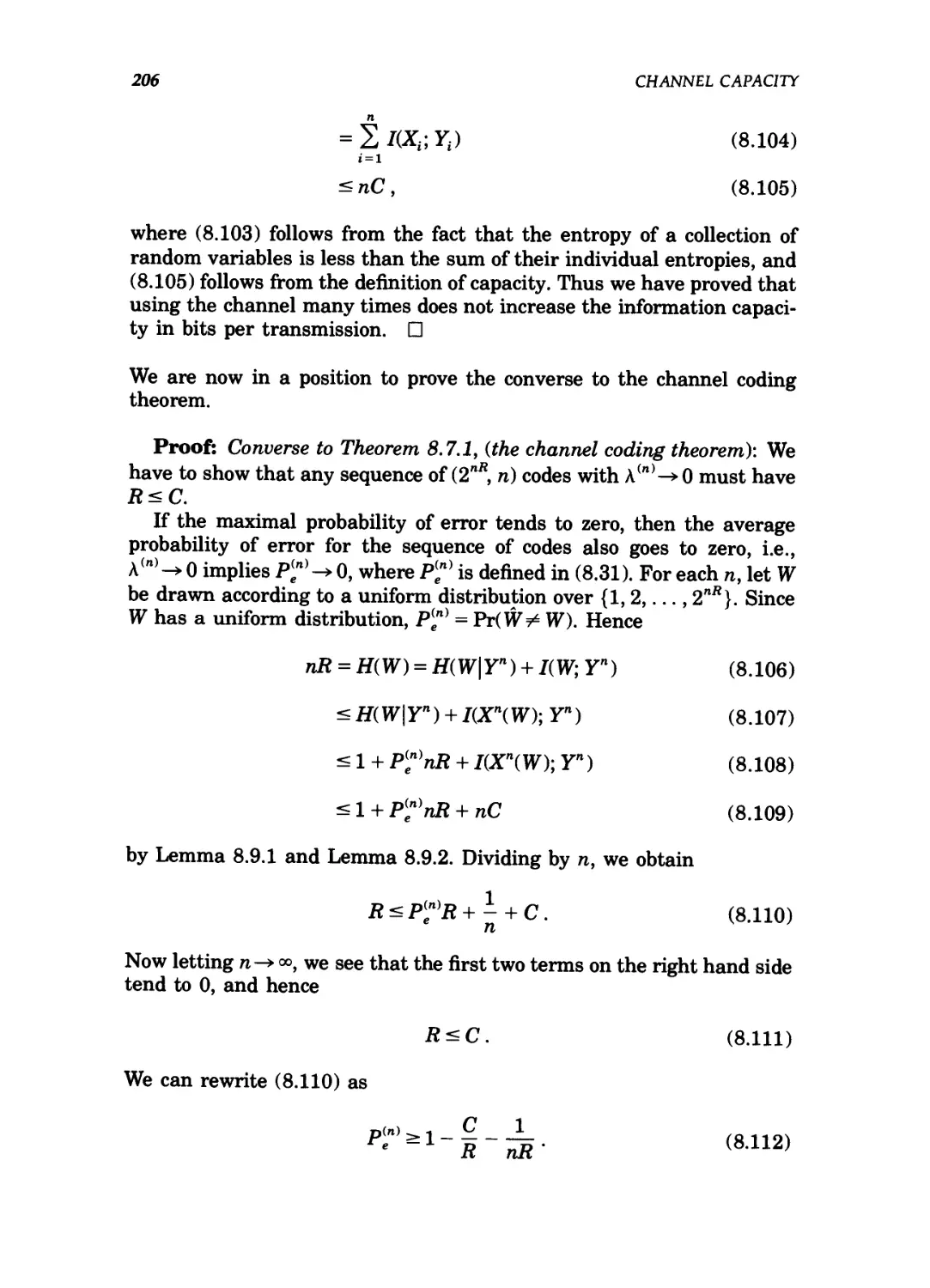
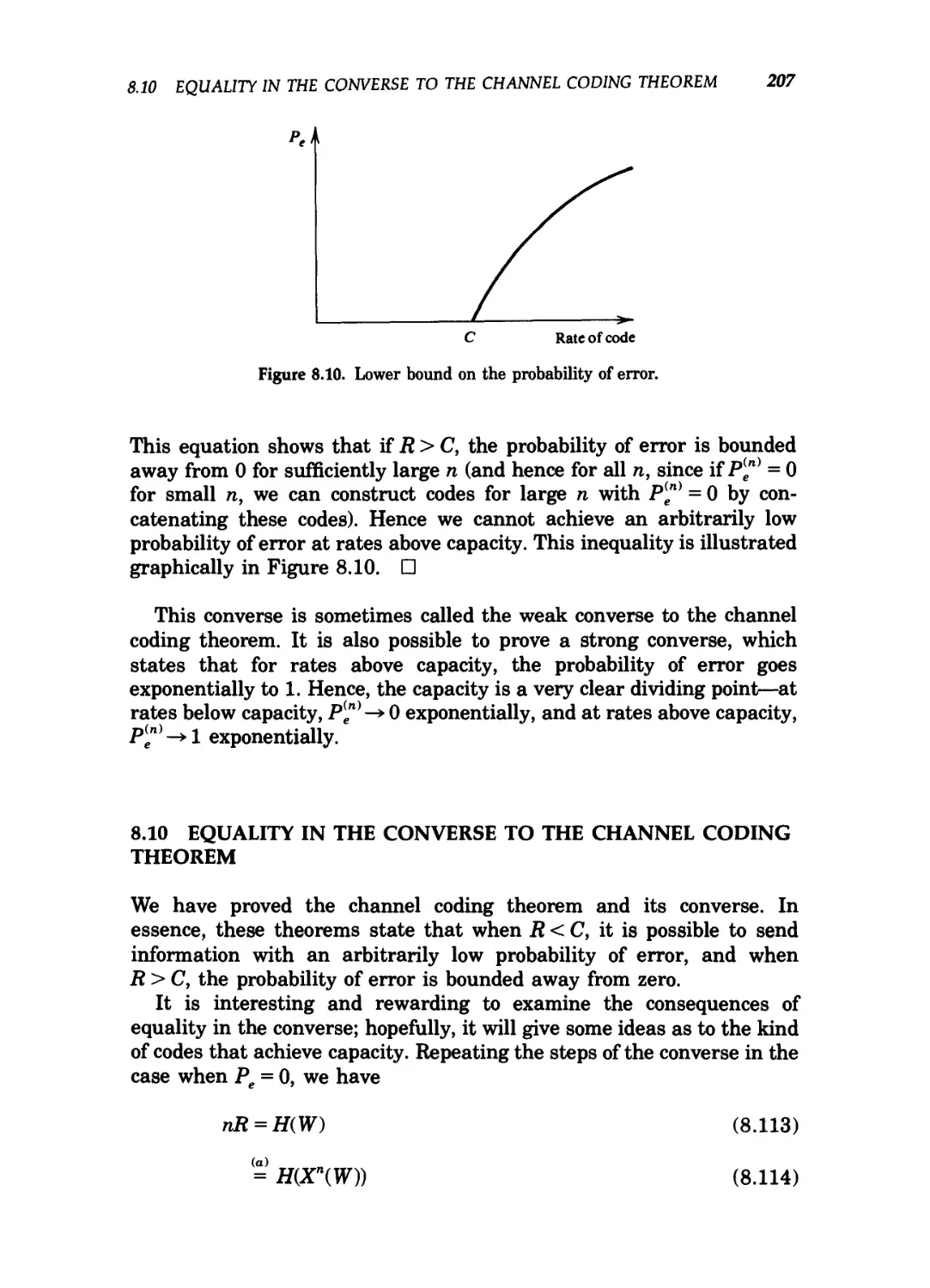
8.10 Lower bound on the probability of error 207
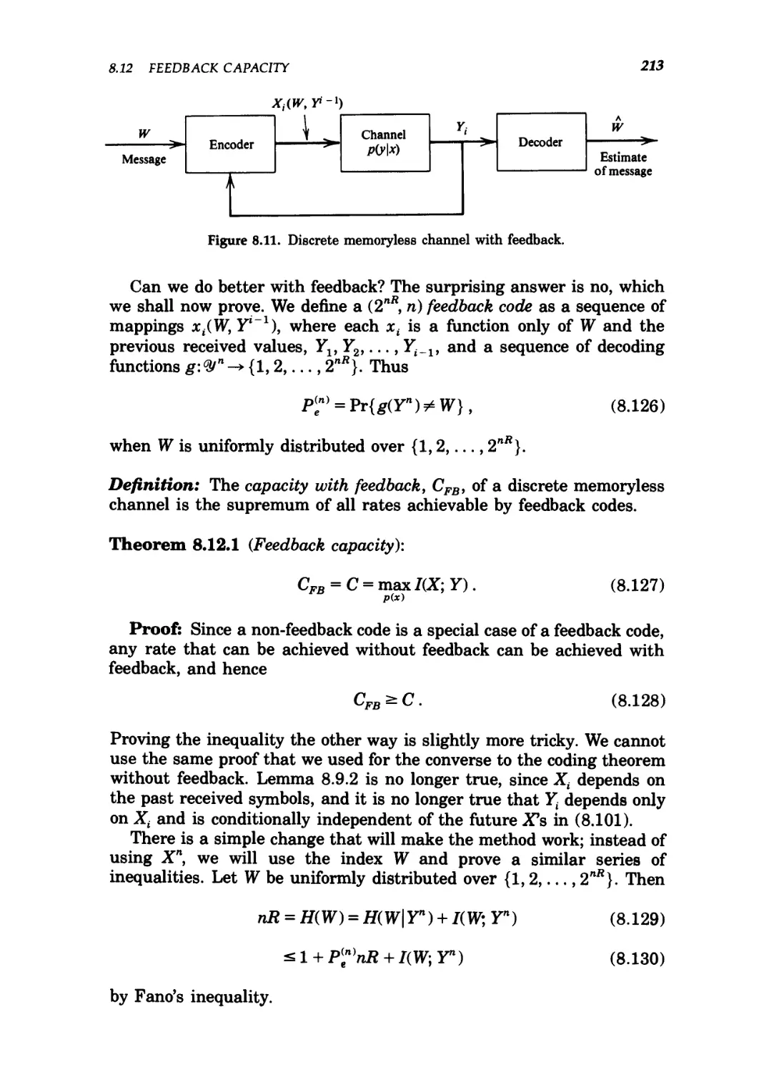
8.11 Discrete memoryless channel with feedback 213
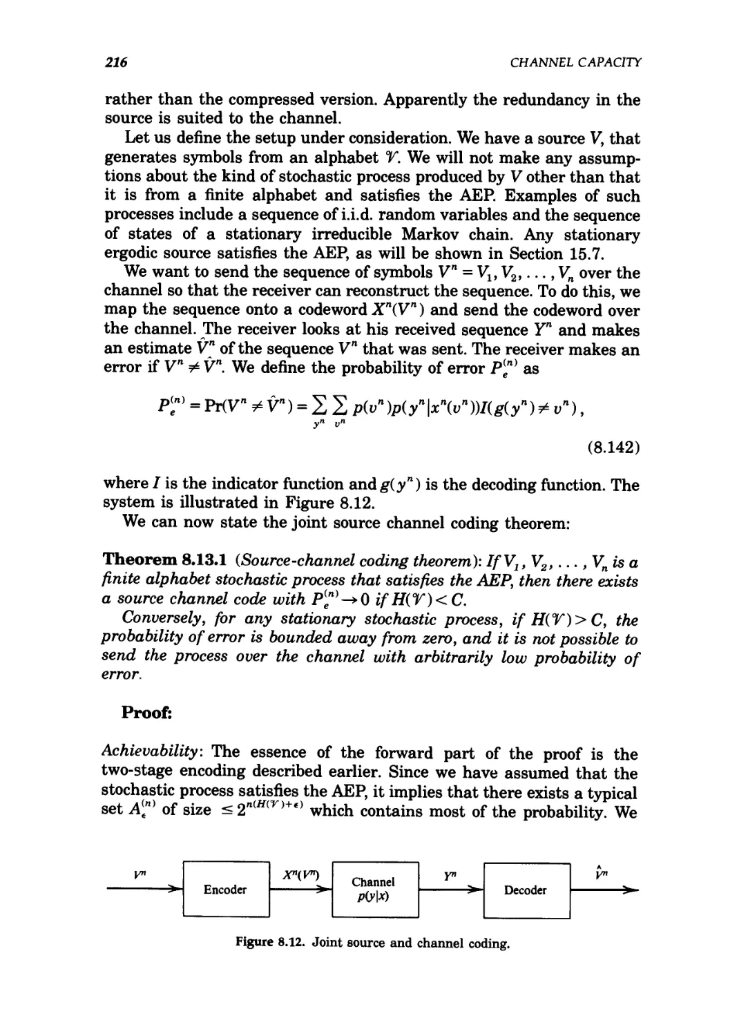
8.12 Joint source and channel coding 216
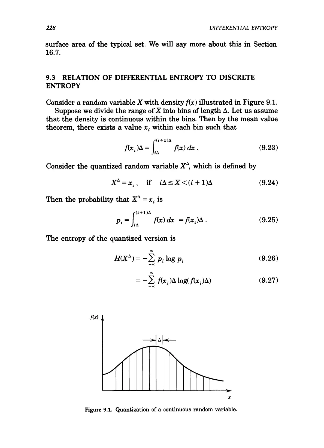
9.1 Quantization of a continuous random variable 228
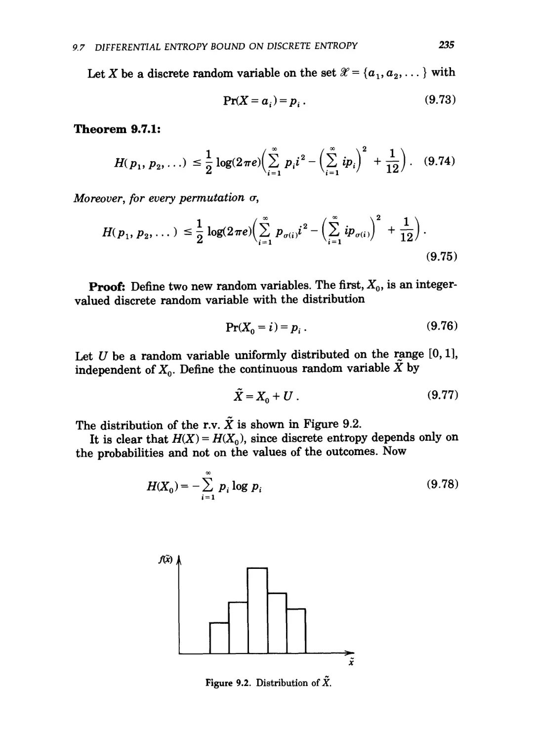
9.2 Distribution of X 235
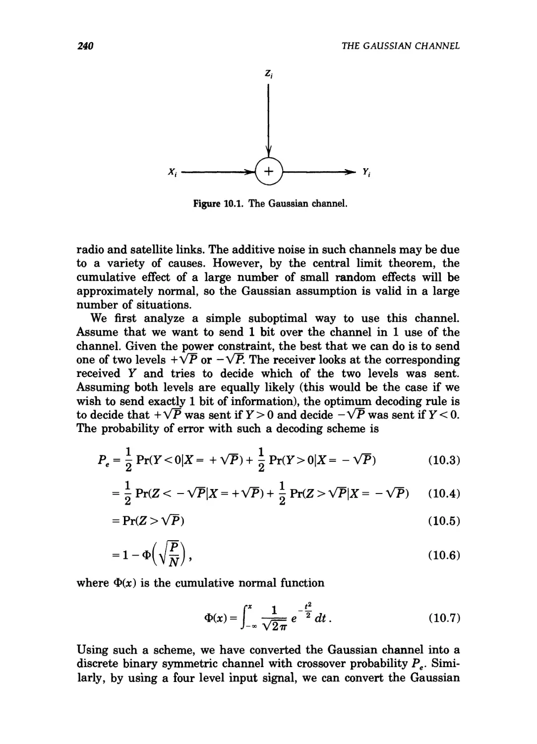
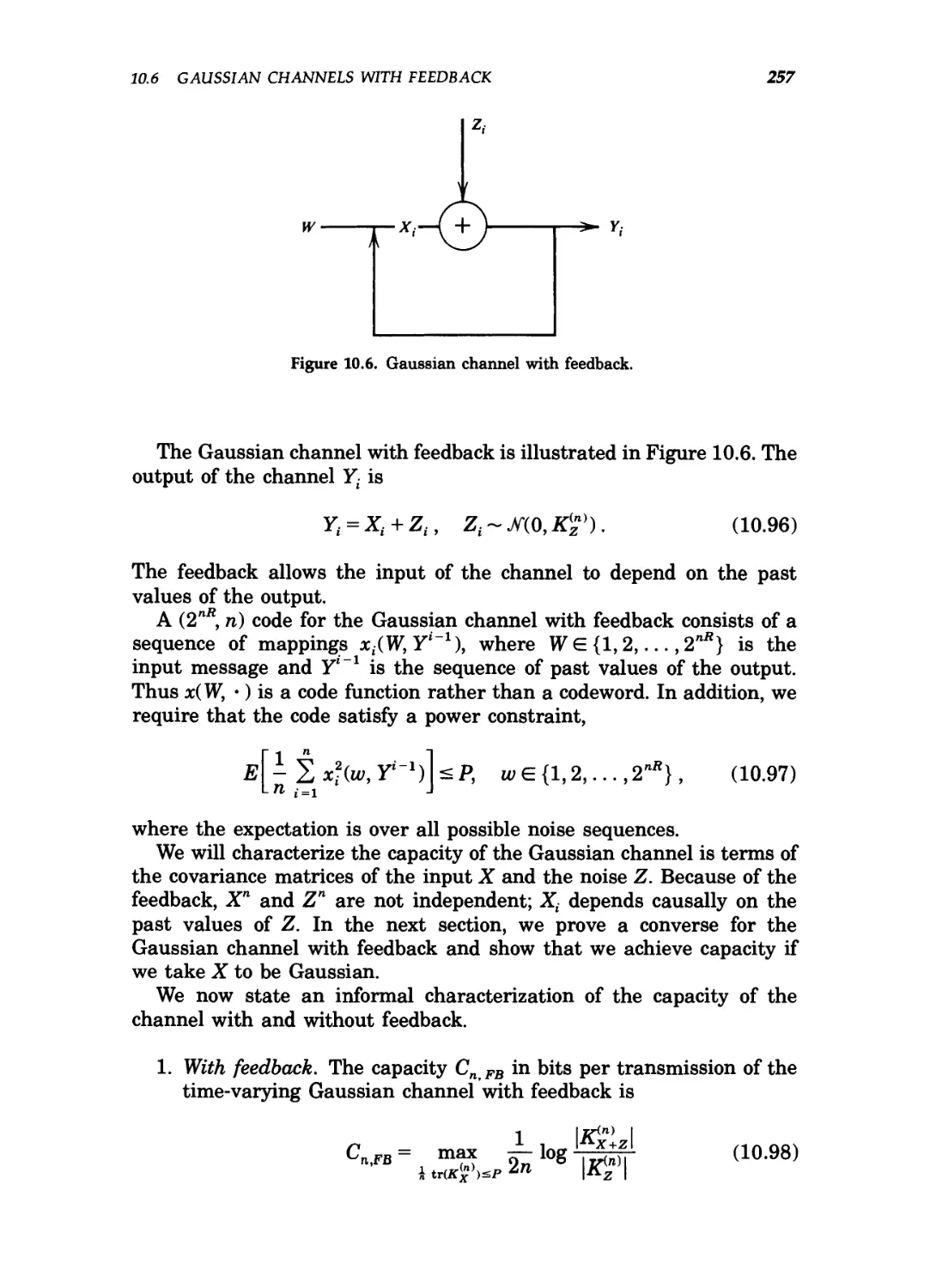
10.1 The Gaussian channel 240
10.2 Sphere packing for the Gaussian channel 243
10.3 Parallel Gaussian channels 251
10.4 Water-filling for parallel channels 253
10.5 Water-filling in the spectral domain 256
10.6 Gaussian channel with feedback 257
12.1 Universal code and the probability simplex 290
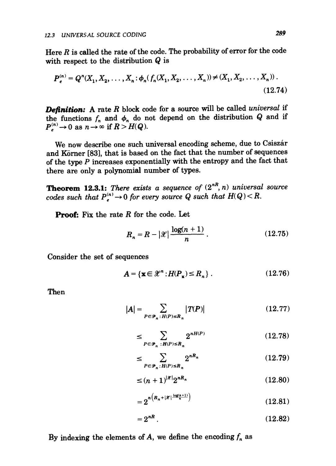
12.2 Error exponent for the universal code 291
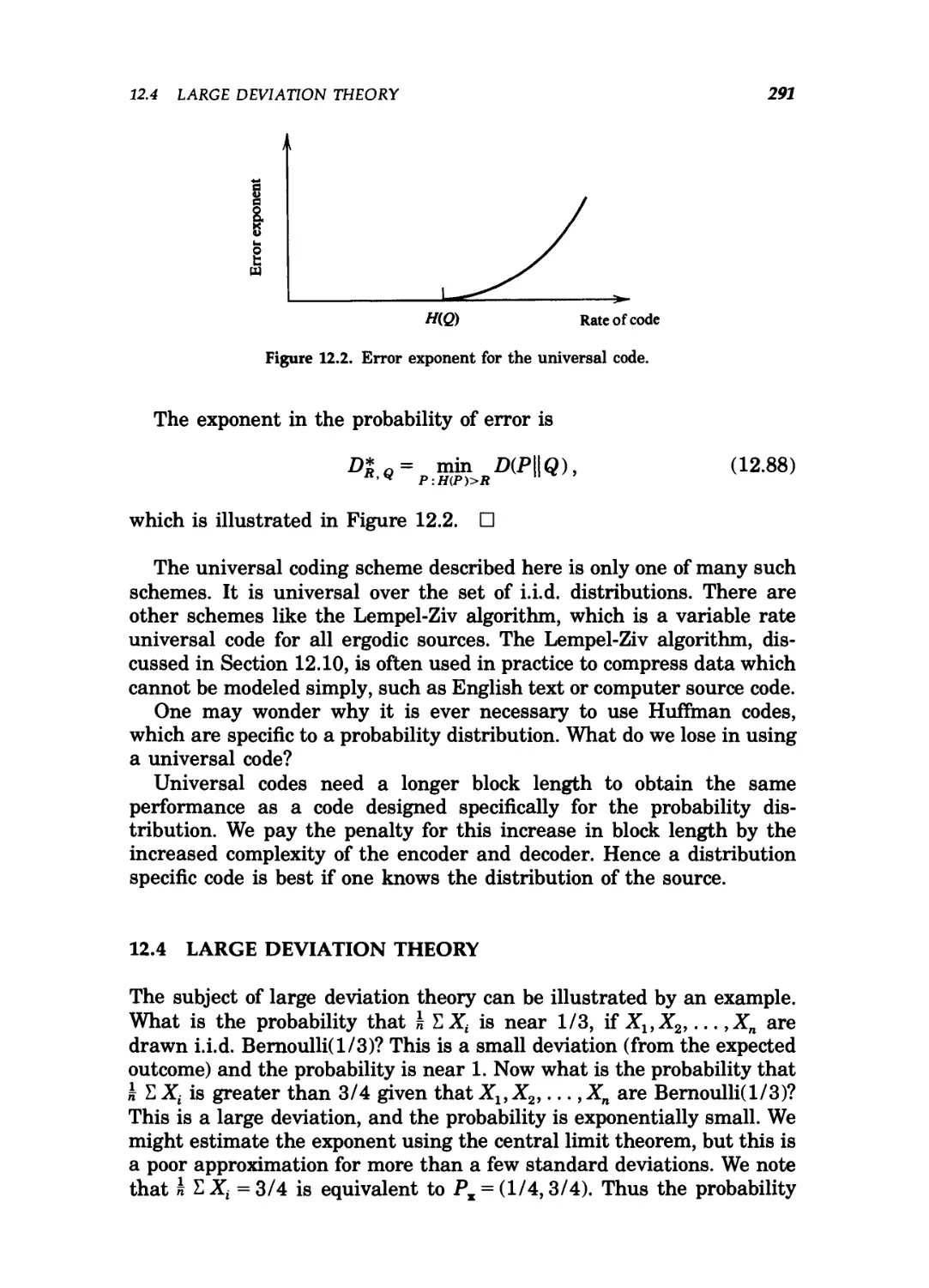
12.3 The probability simplex and Sanov's theorem 293
12.4 Pythagorean theorem for relative entropy 297
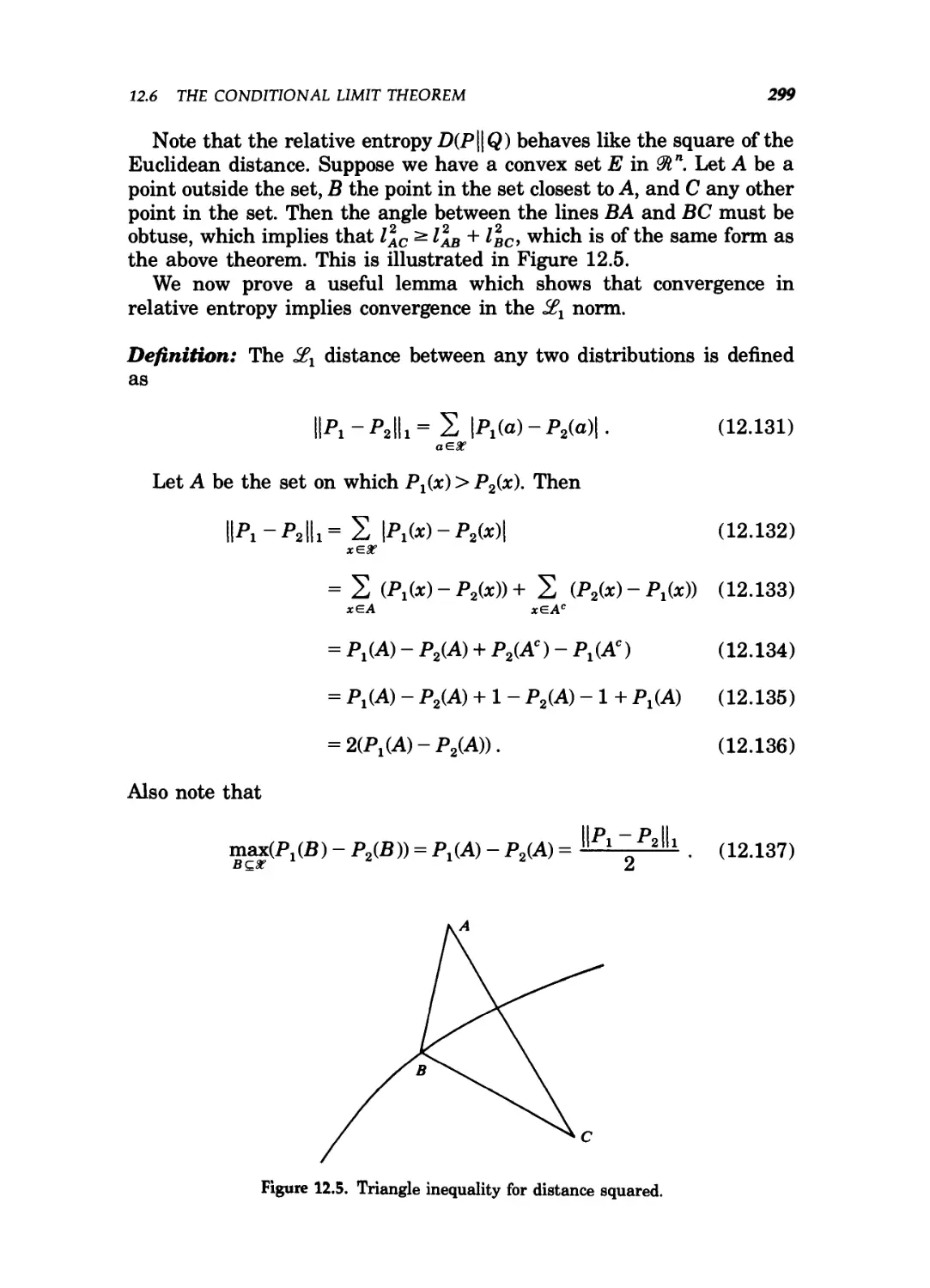
12.5 Triangle inequality for distance squared 299
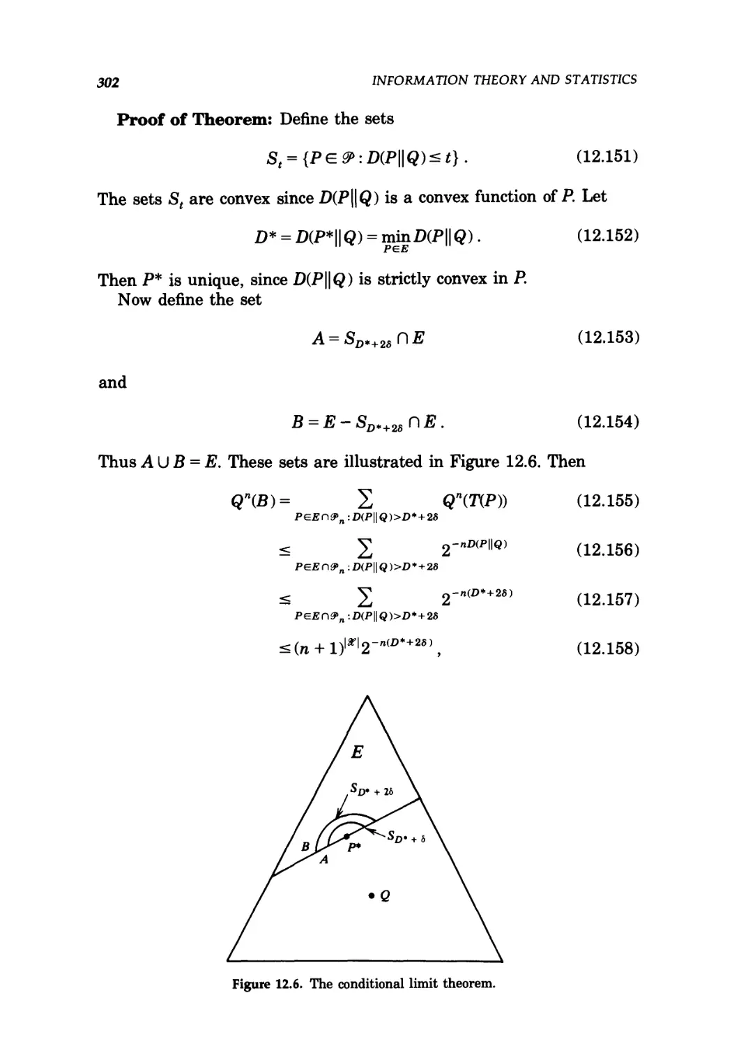
12.6 The conditional limit theorem 302
12.7 Testing between two Gaussian distributions 307
12.8 The likelihood ratio test on the probability simplex 308
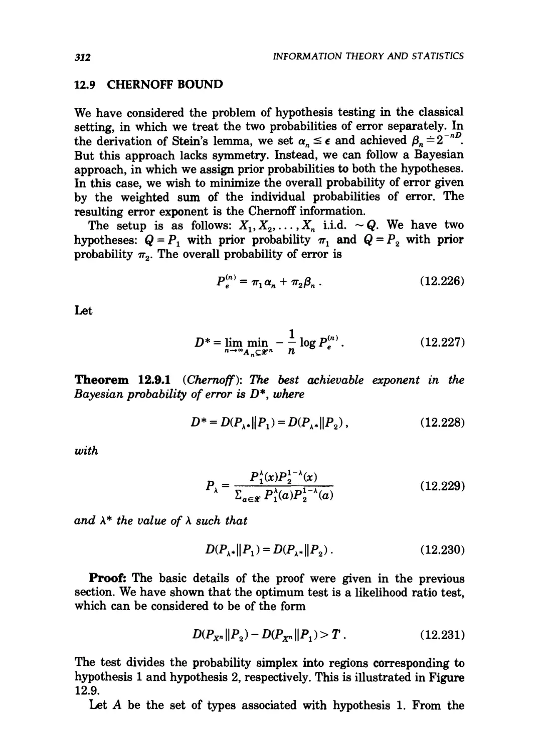
12.9 The probability simplex and Chernoff s bound 313
12.10 Relative entropy DiP^PJ and D(PX\\P2) as a function
of A 314
12.11 Distribution of yards gained in a run or a pass play 317
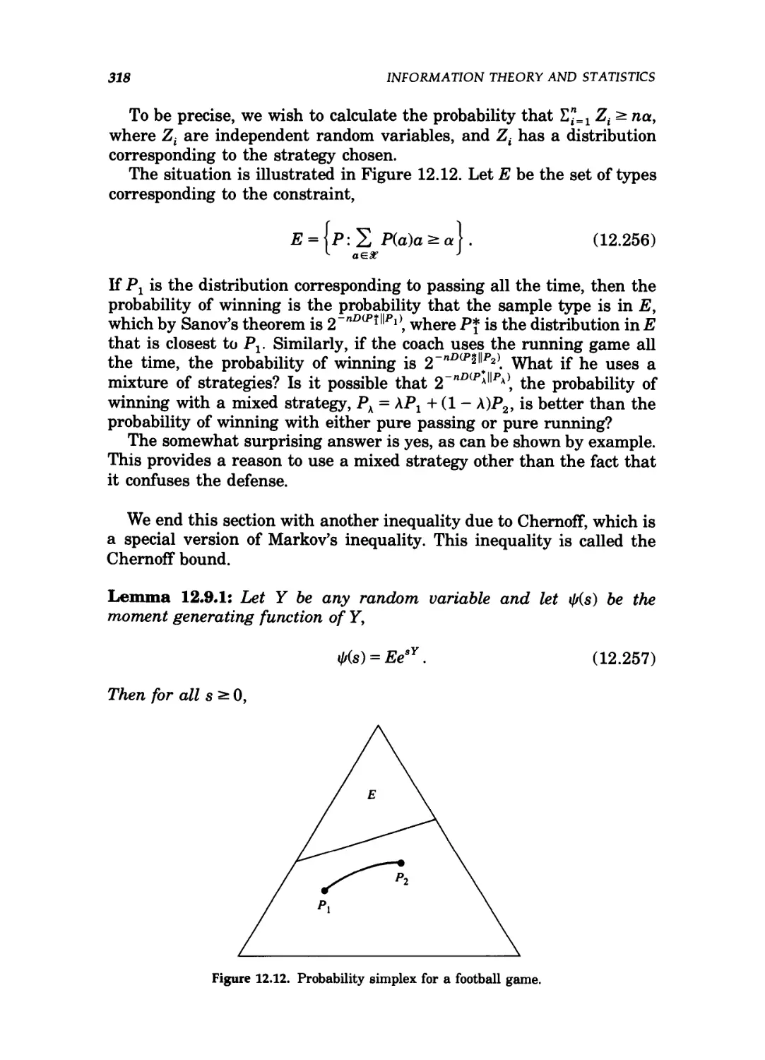
12.12 Probability simplex for a football game 318
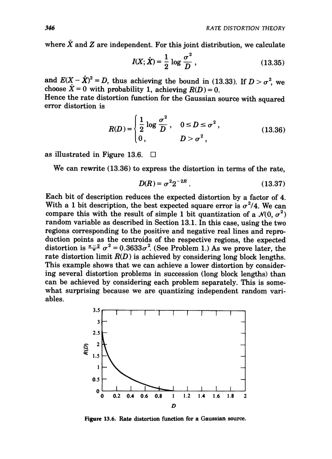
13.1 One bit quantization of a Gaussian random variable 337
LIST OF FIGURES
xxi
13.2 Rate distortion encoder and decoder 339
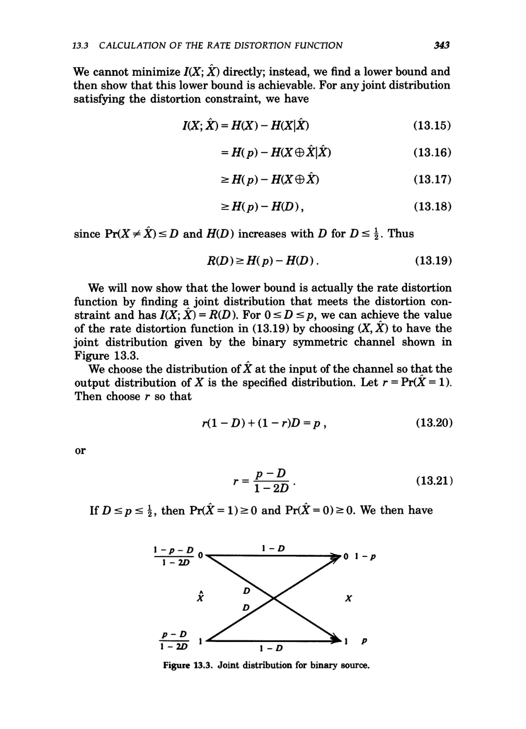
13.3 Joint distribution for binary source 343
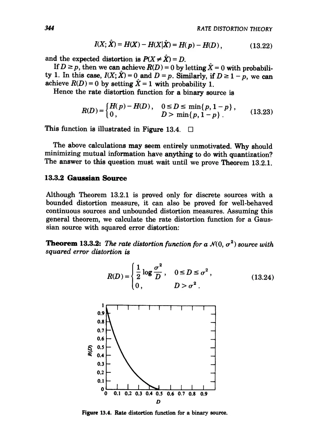
13.4 Rate distortion function for a binary source 344
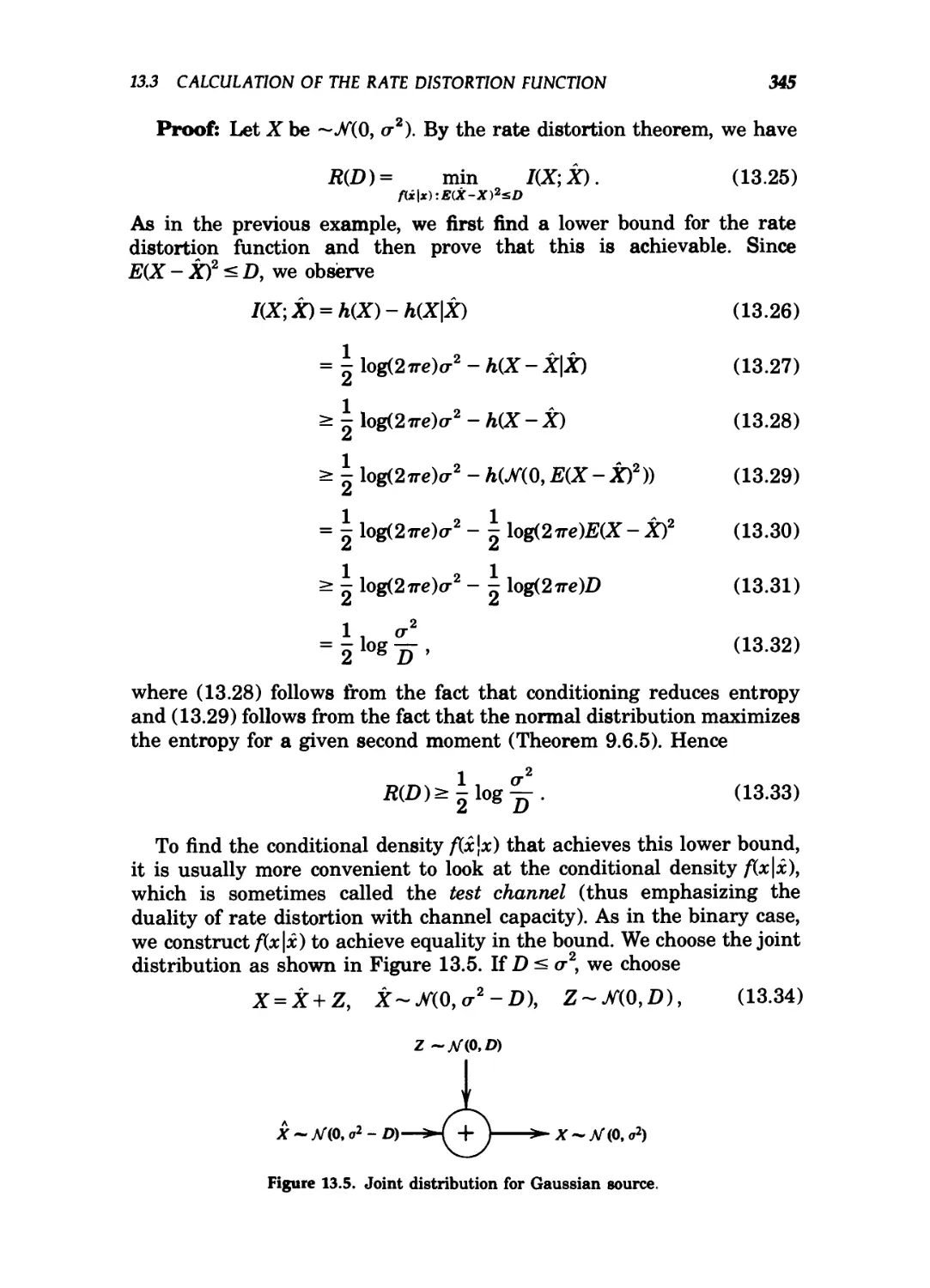
13.5 Joint distribution for Gaussian source 345
13.6 Rate distortion function for a Gaussian source 346
13.7 Reverse water-filling for independent Gaussian
random variables 349
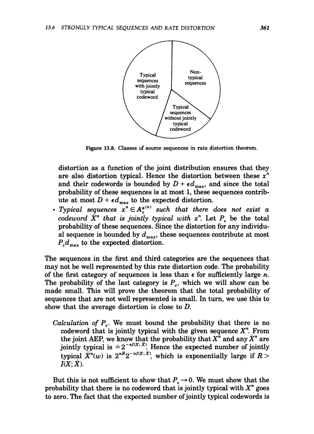
13.8 Classes of source sequences in rate distortion theorem 361
13.9 Distance between convex sets 365
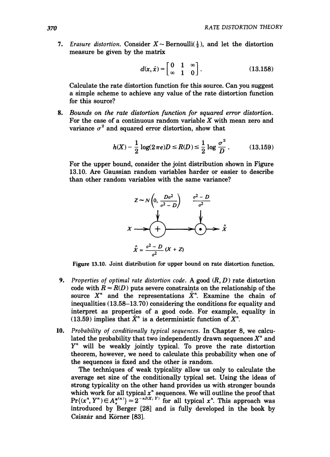
13.10 Joint distribution for upper bound on rate distortion
function 370
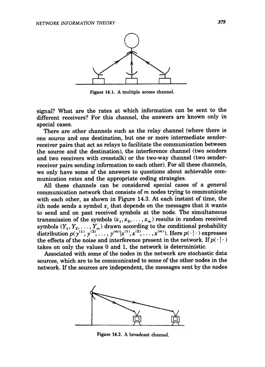
14.1 A multiple access channel 375
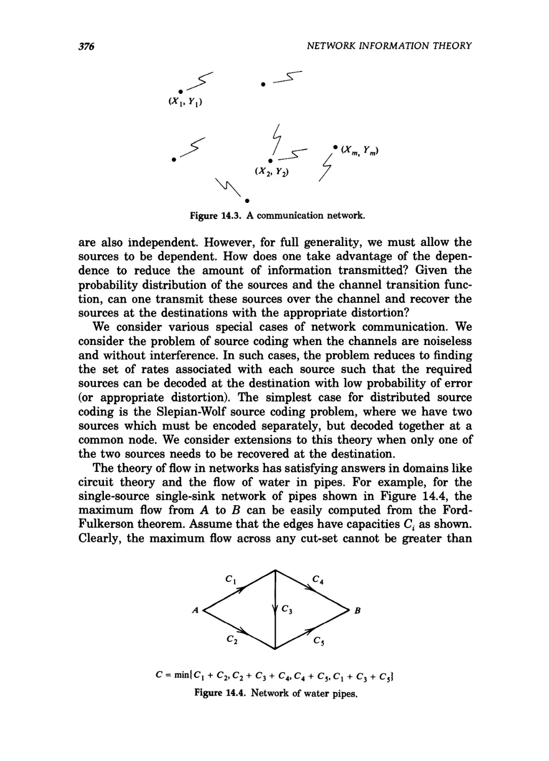
14.2 A broadcast channel 375
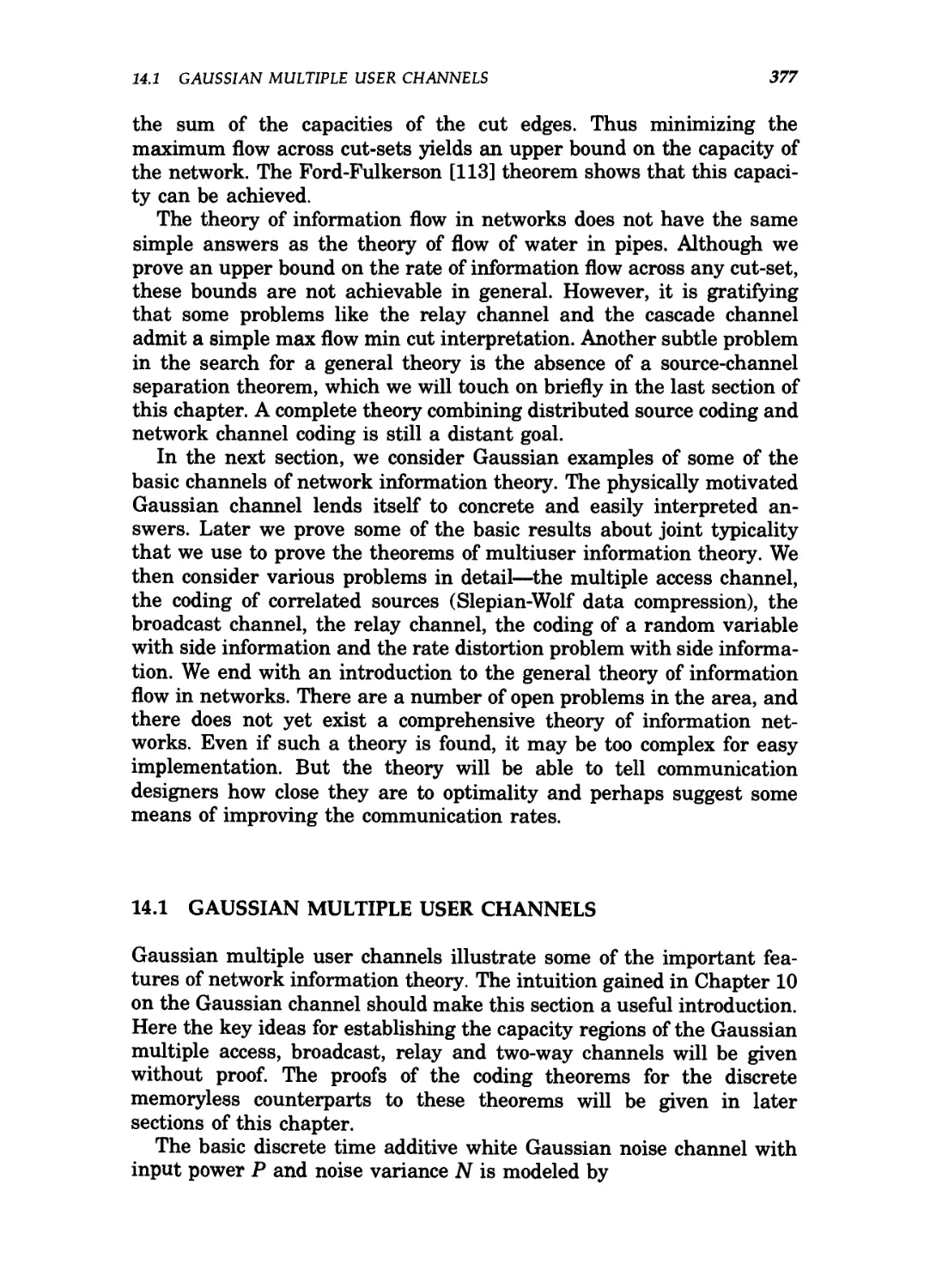
14.3 A communication network 376
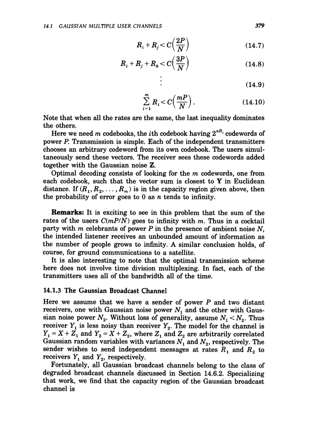
14.4 Network of water pipes 376
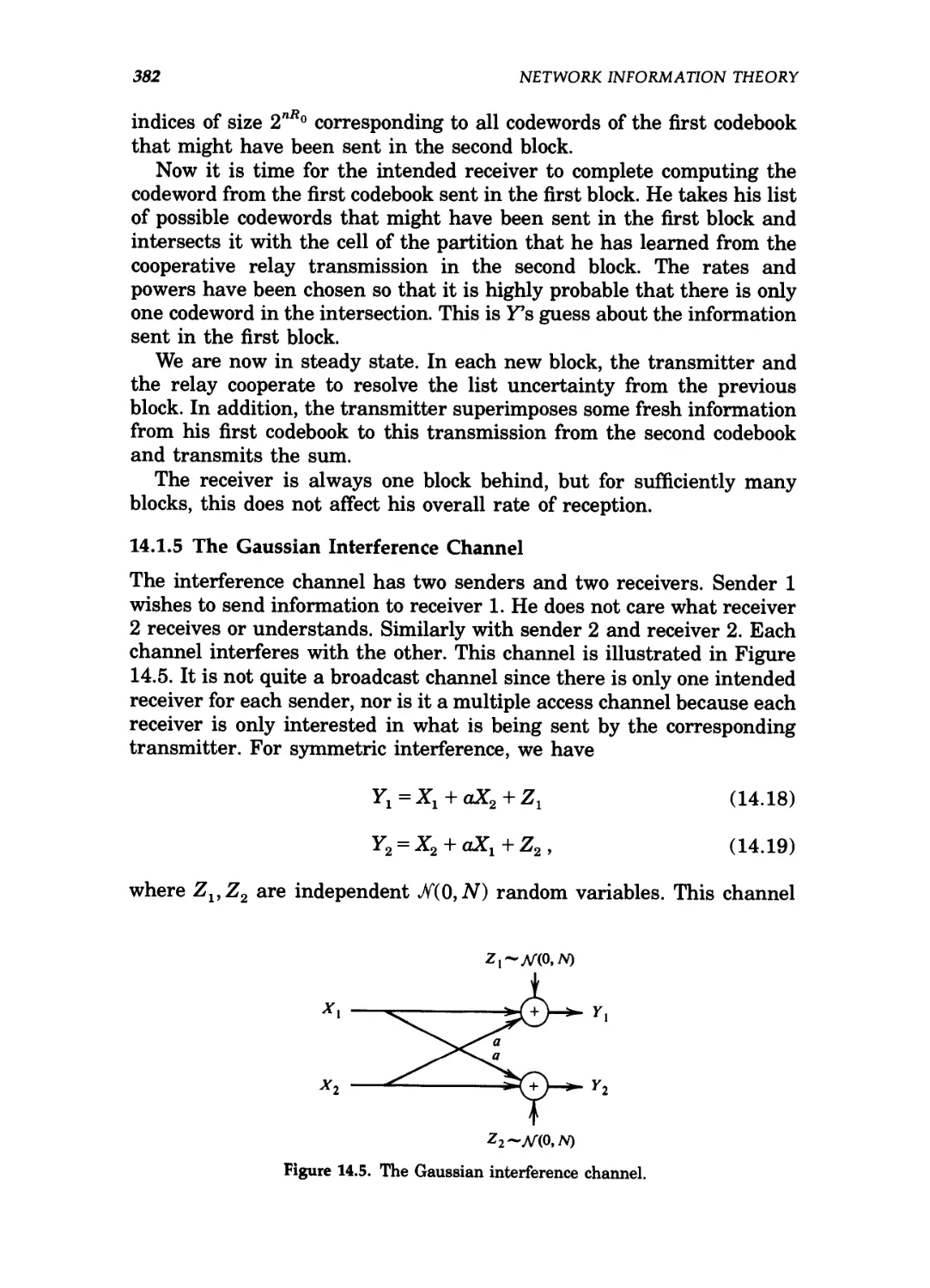
14.5 The Gaussian interference channel 382
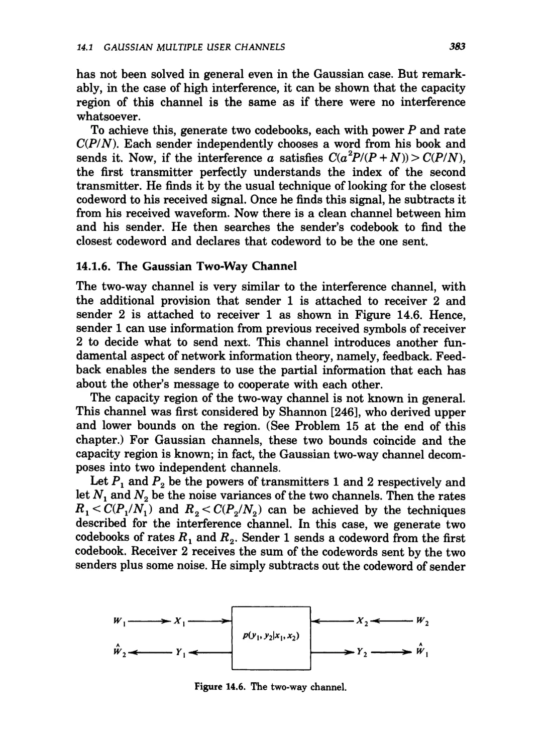
14.6 The two-way channel 383
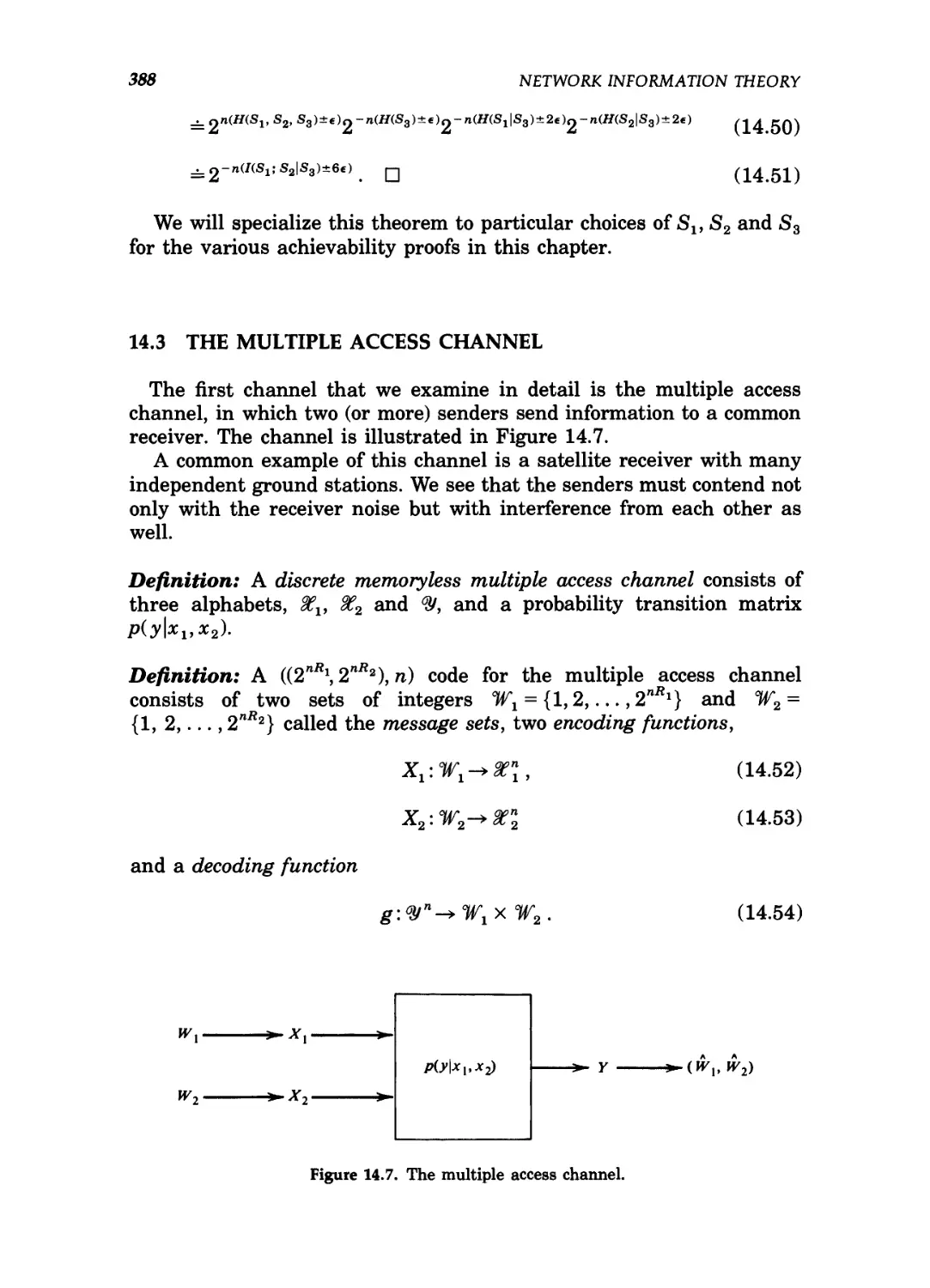
14.7 The multiple access channel 388
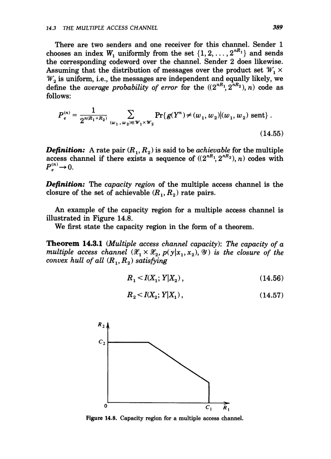
14.8 Capacity region for a multiple access channel 389
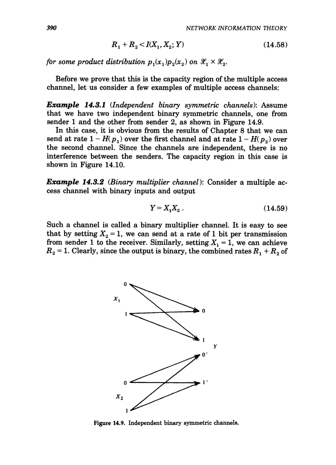
14.9 Independent binary symmetric channels 390
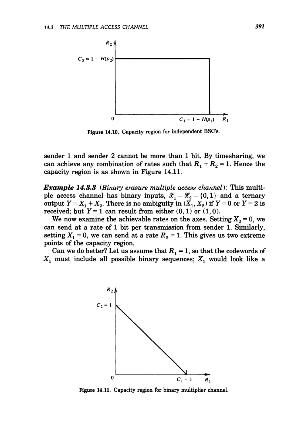
14.10 Capacity region for independent BSC's 391
14.11 Capacity region for binary multiplier channel 391
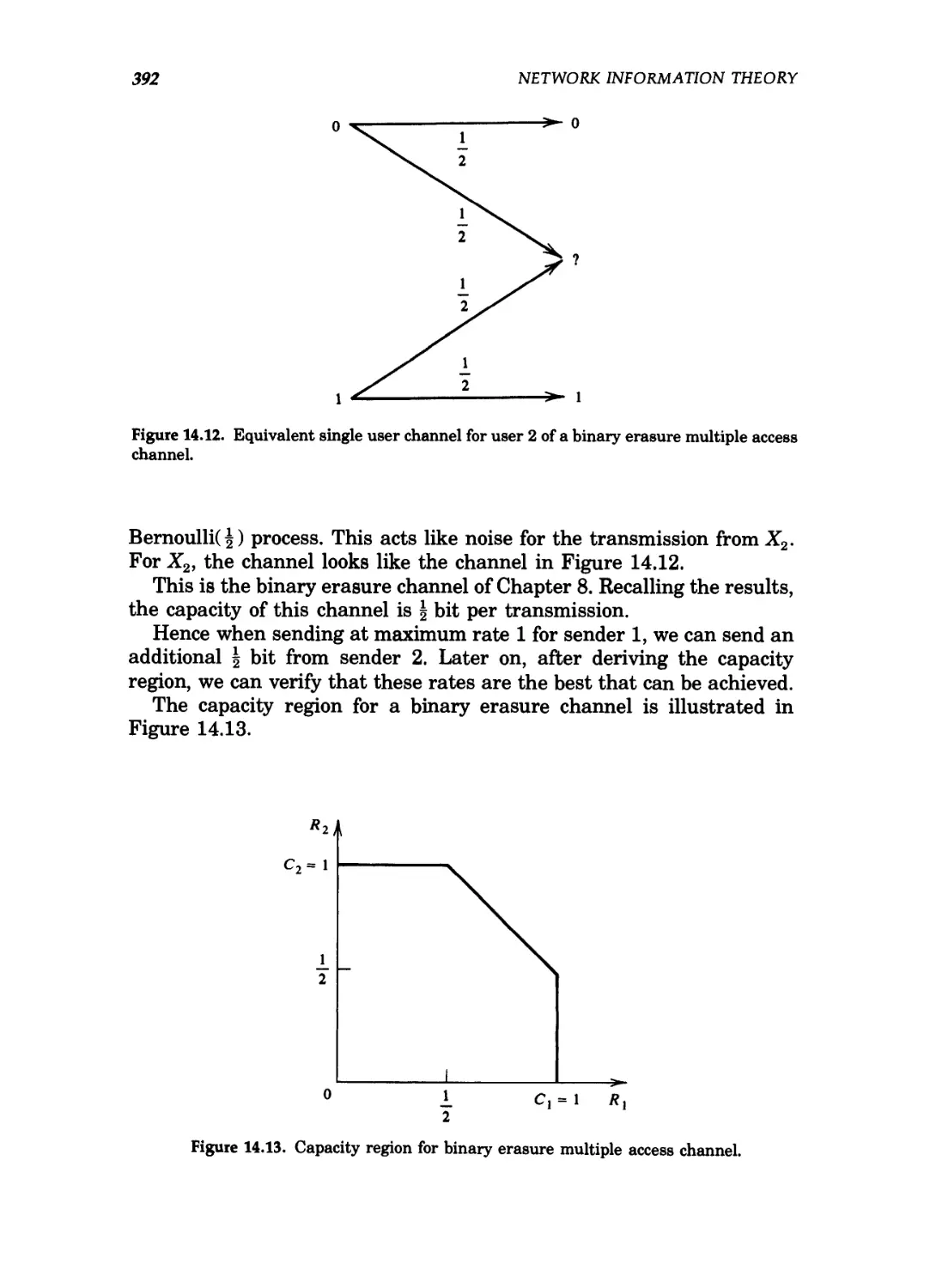
14.12 Equivalent single user channel for user 2 of a binary
erasure multiple access channel 392
14.13 Capacity region for binary erasure multiple access
channel 392
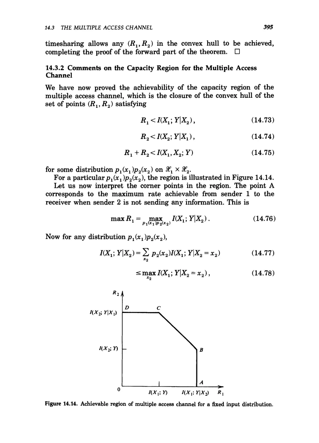
14.14 Achievable region of multiple access channel for a fixed
input distribution 395
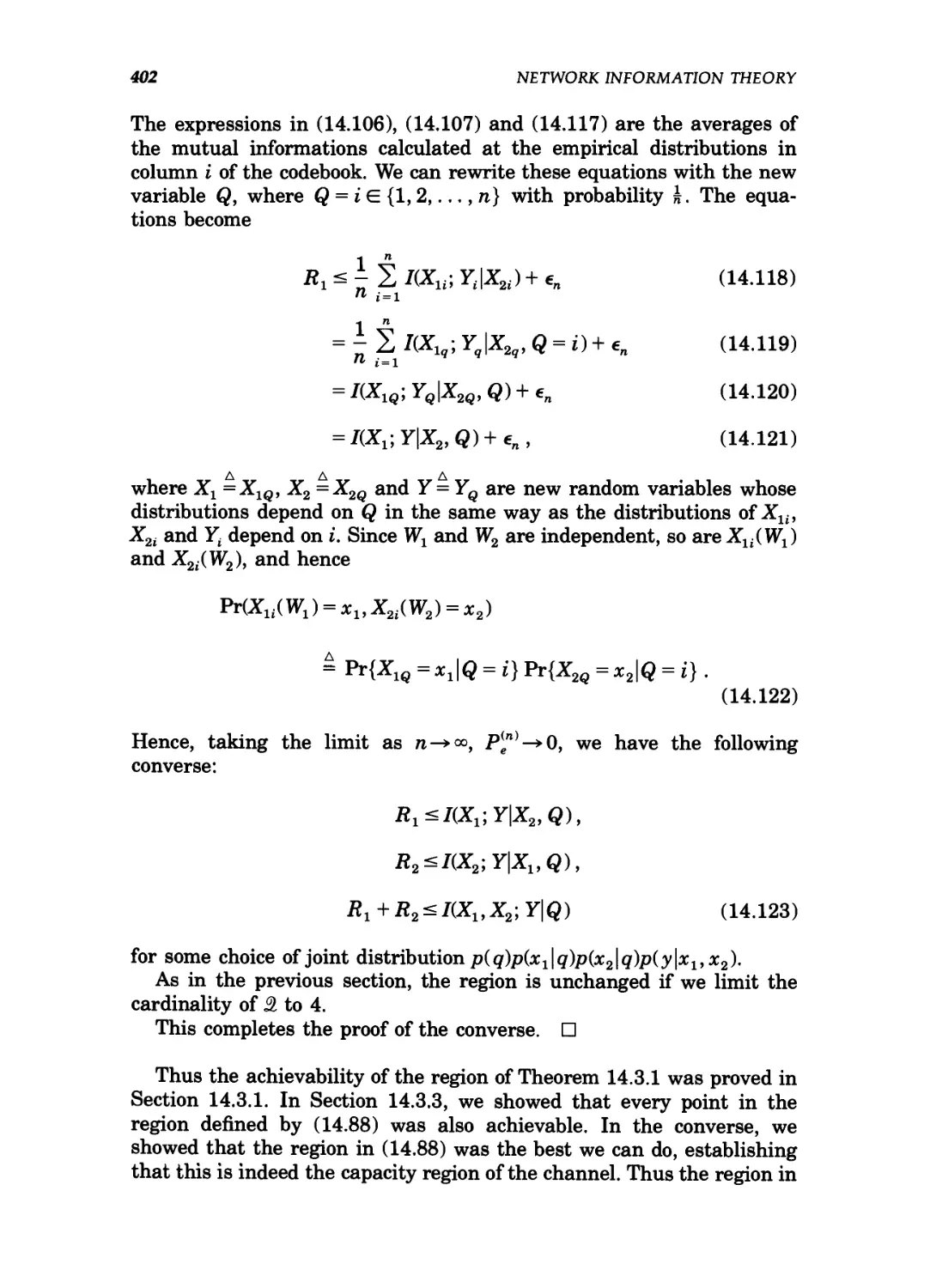
14.15 m-user multiple access channel 403
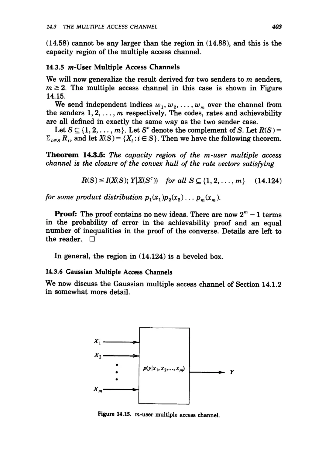
14.16 Gaussian multiple access channel 403
14.17 Gaussian multiple access channel capacity 406
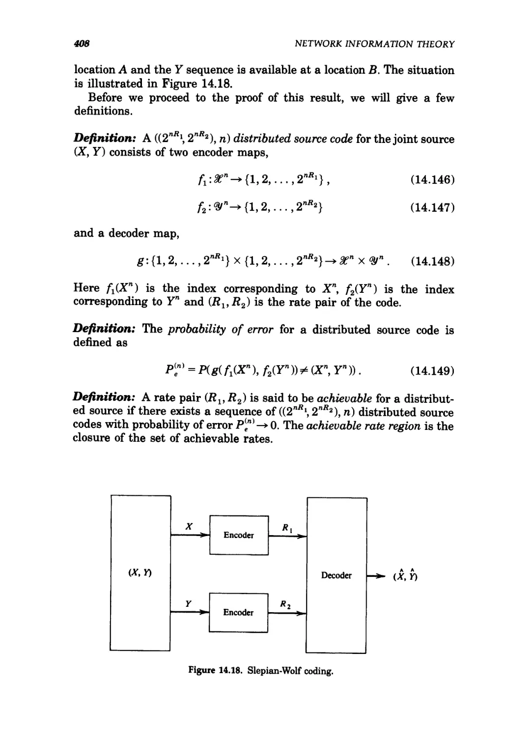
14.18 Slepian-Wolf coding 408
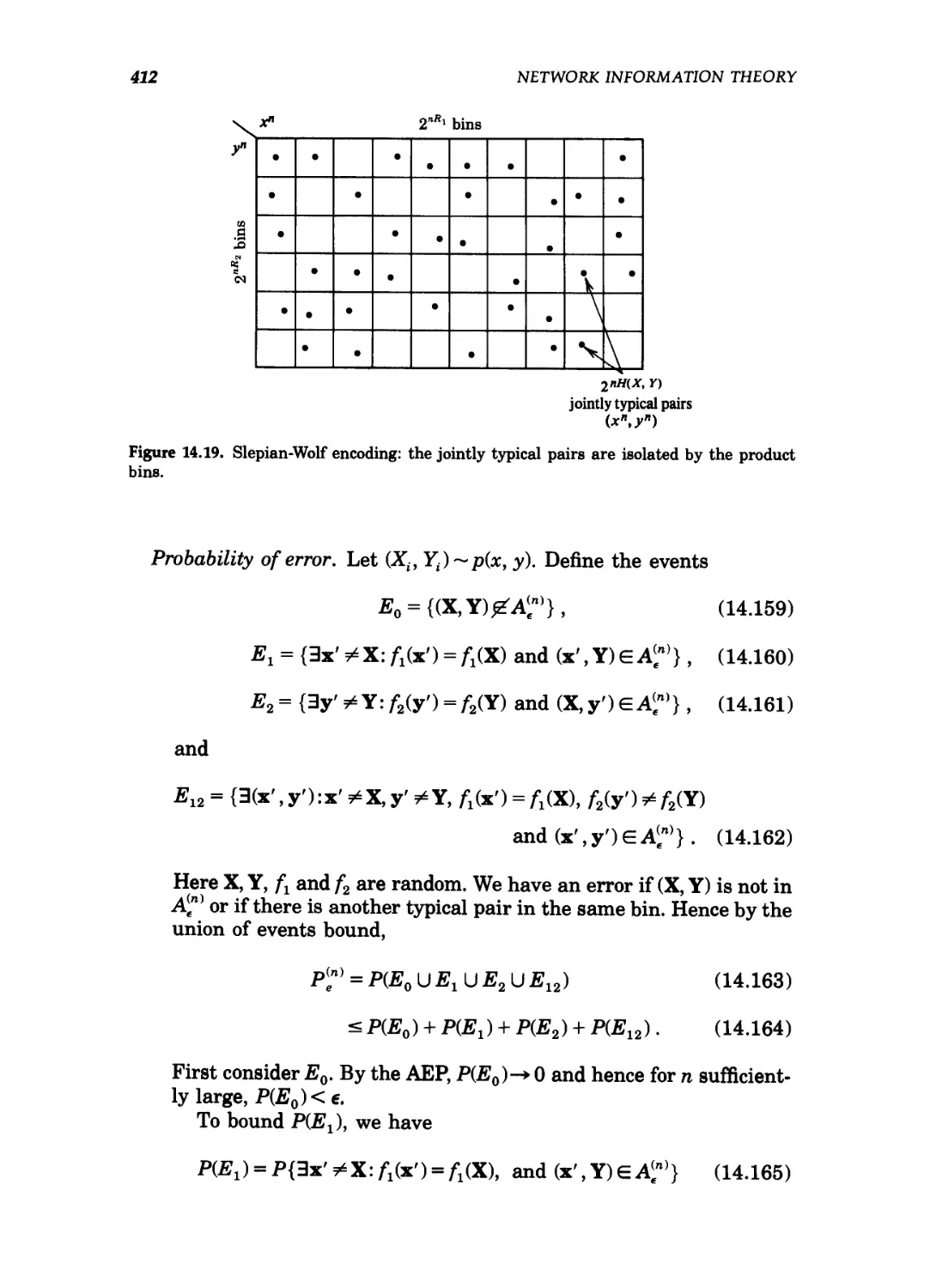
14.19 Slepian-Wolf encoding: the jointly typical pairs are
isolated by the product bins 412
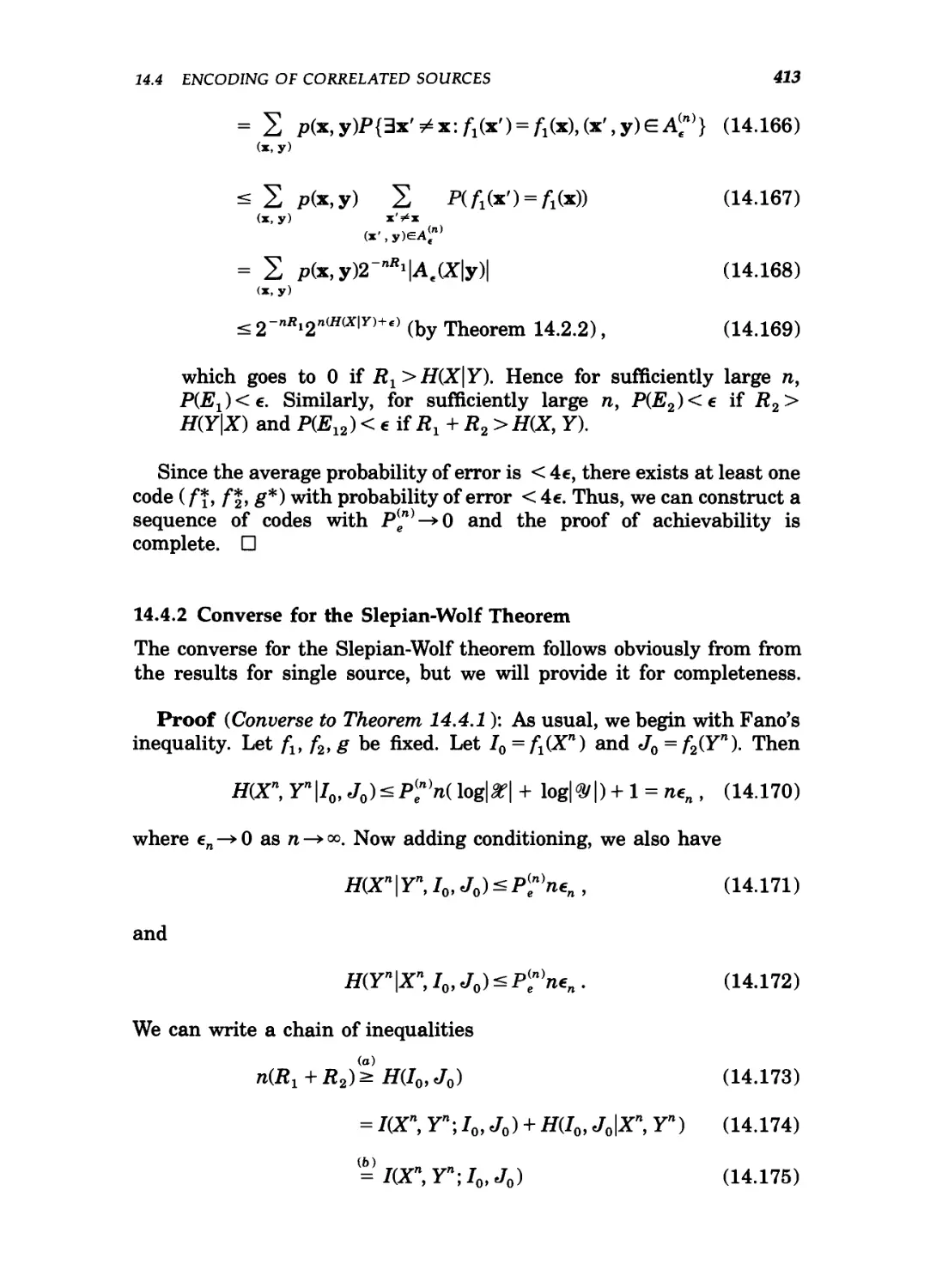
14.20 Rate region for Slepian-Wolf encoding 414
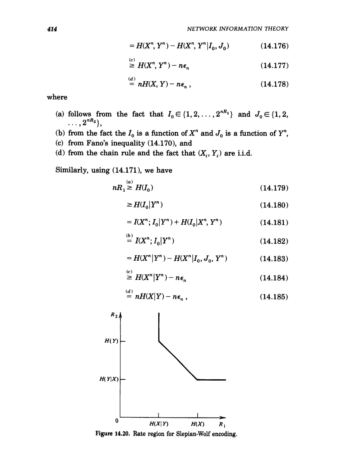
14.21 Jointly typical fans 416
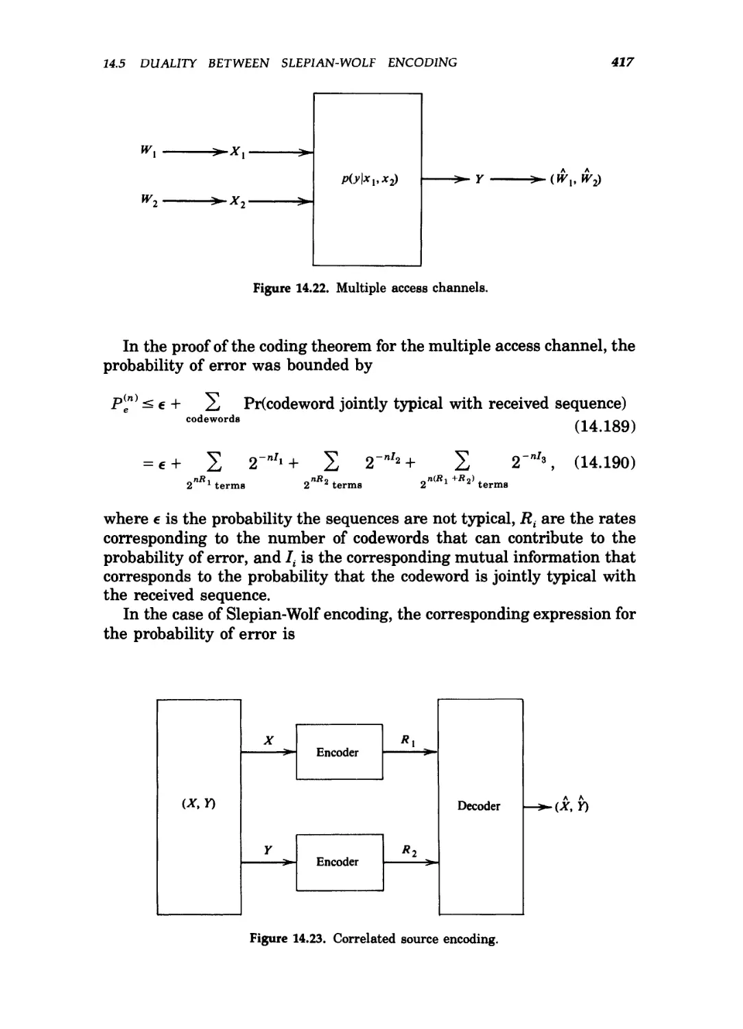
14.22 Multiple access channels 417
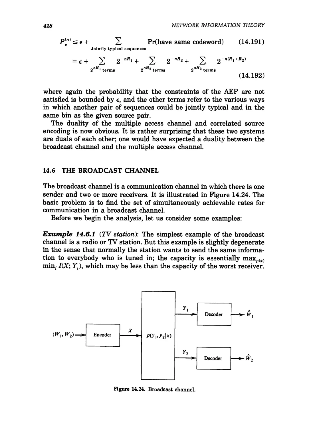
14.23 Correlated source encoding 417
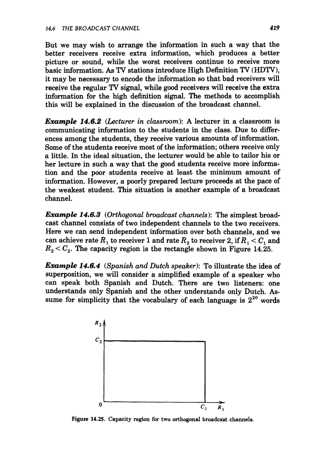
14.24 Broadcast channel 418
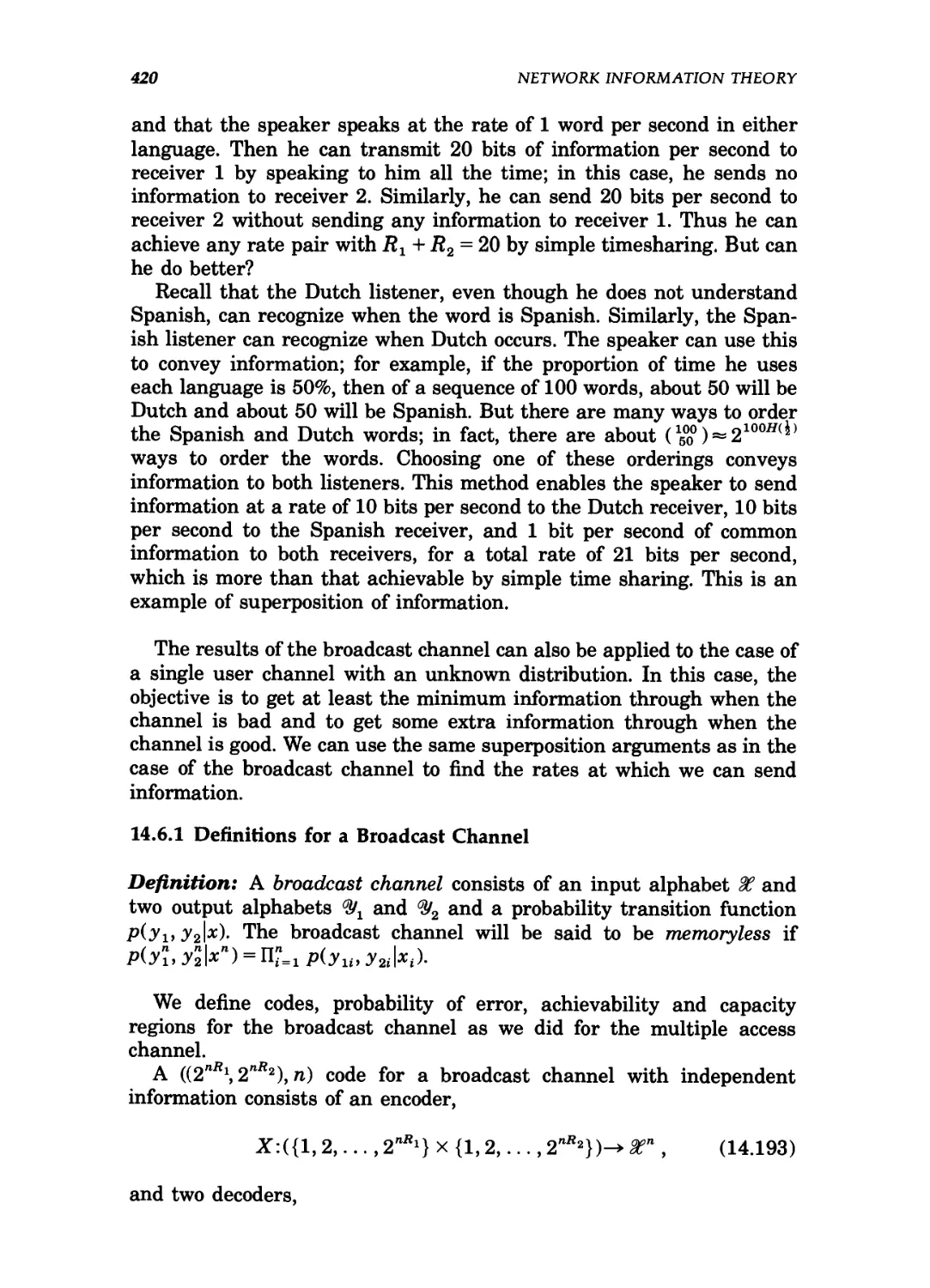
14.25 Capacity region for two orthogonal broadcast channels 419
xxii LIST OF FIGURES
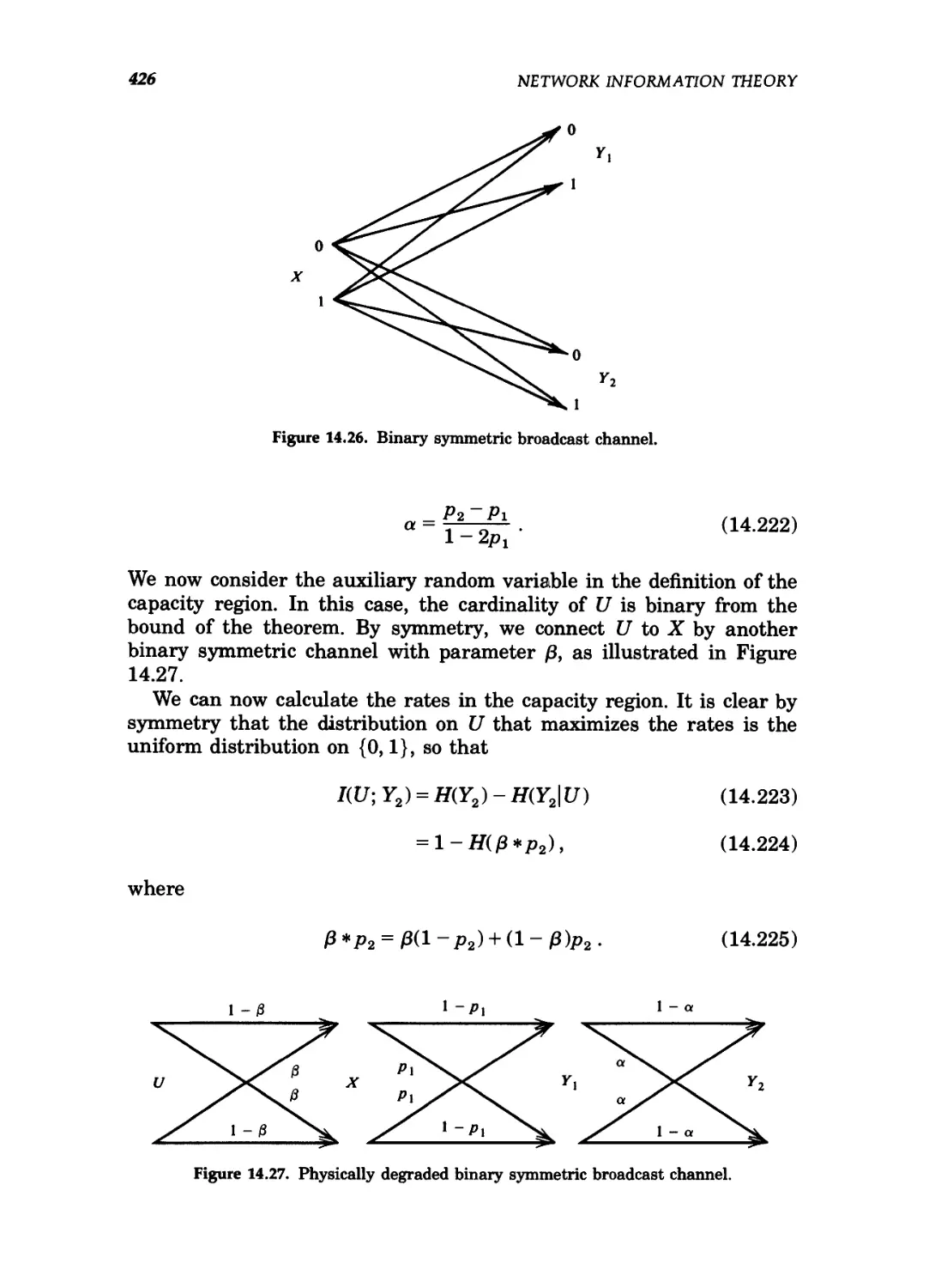
14.26 Binary symmetric broadcast channel 426
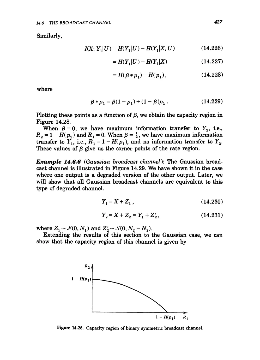
14.27 Physically degraded binary symmetric broadcast channel 426
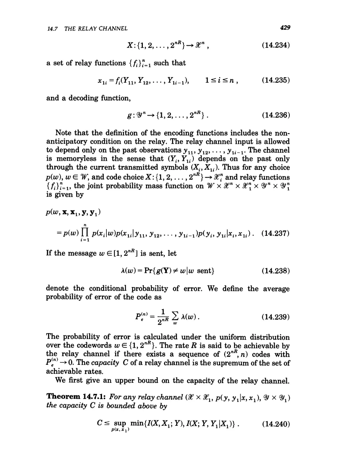
14.28 Capacity region of binary symmetric broadcast channel 427
14.29 Gaussian broadcast channel 428
14.30 The relay channel 428
14.31 Encoding with side information 433
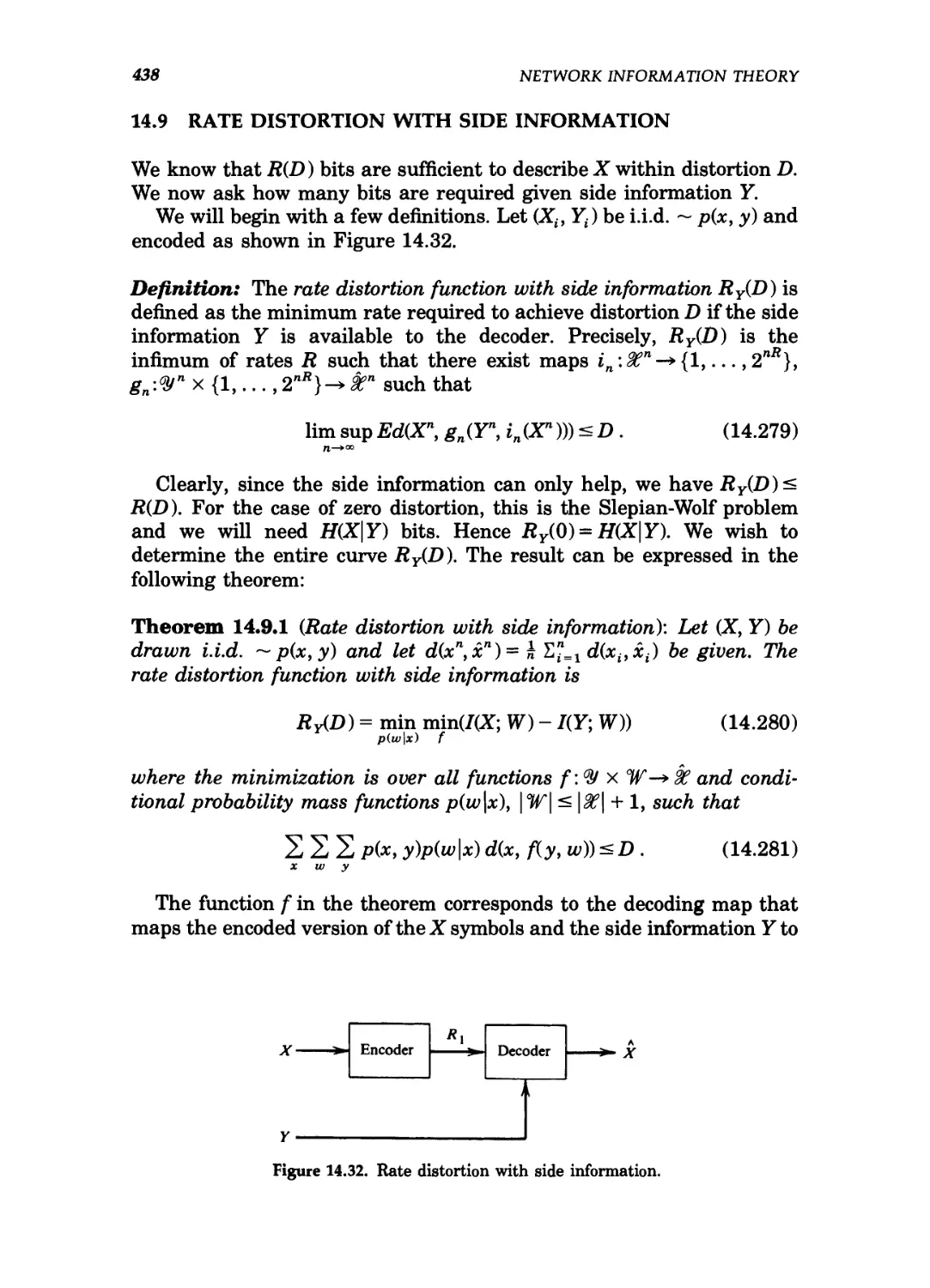
14.32 Rate distortion with side information 438
14.33 Rate distortion for two correlated sources 443
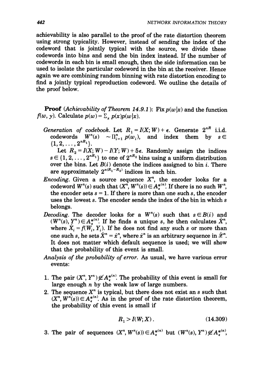
14.34 A general multiterminal network 444
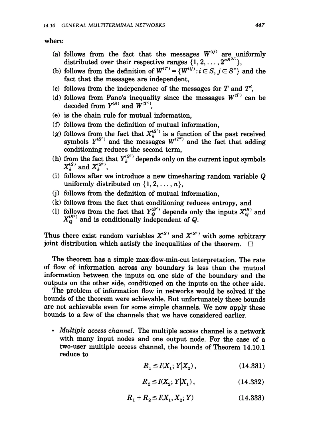
14.35 The relay channel 448
14.36 Transmission of correlated sources over a multiple
access channel 449
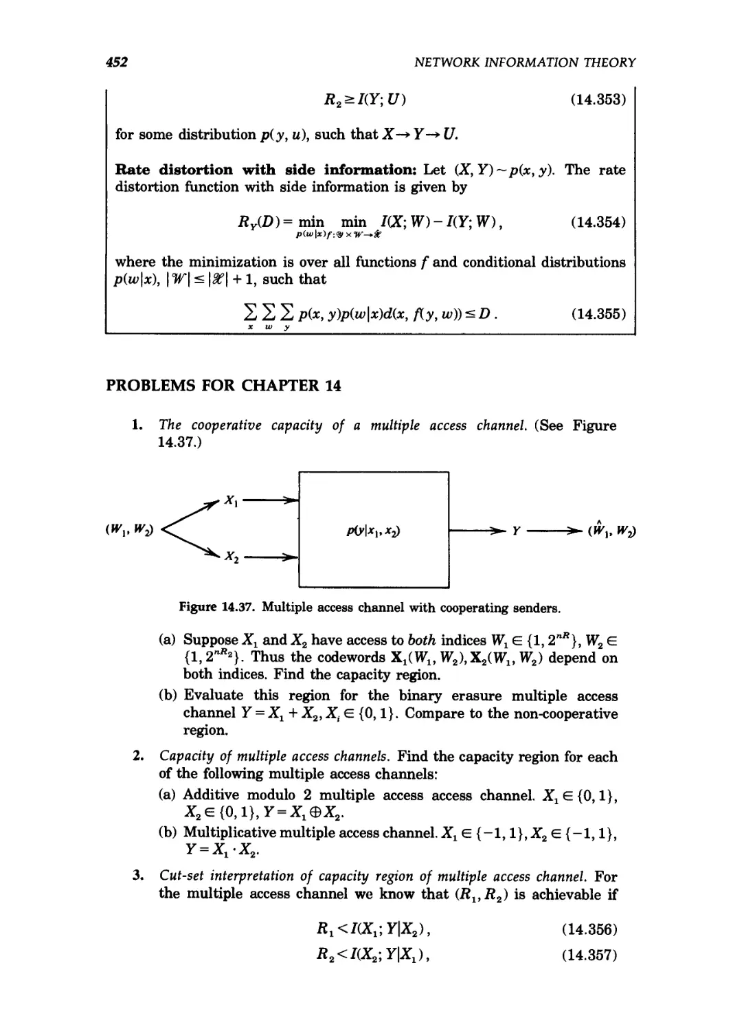
14.37 Multiple access channel with cooperating senders 452
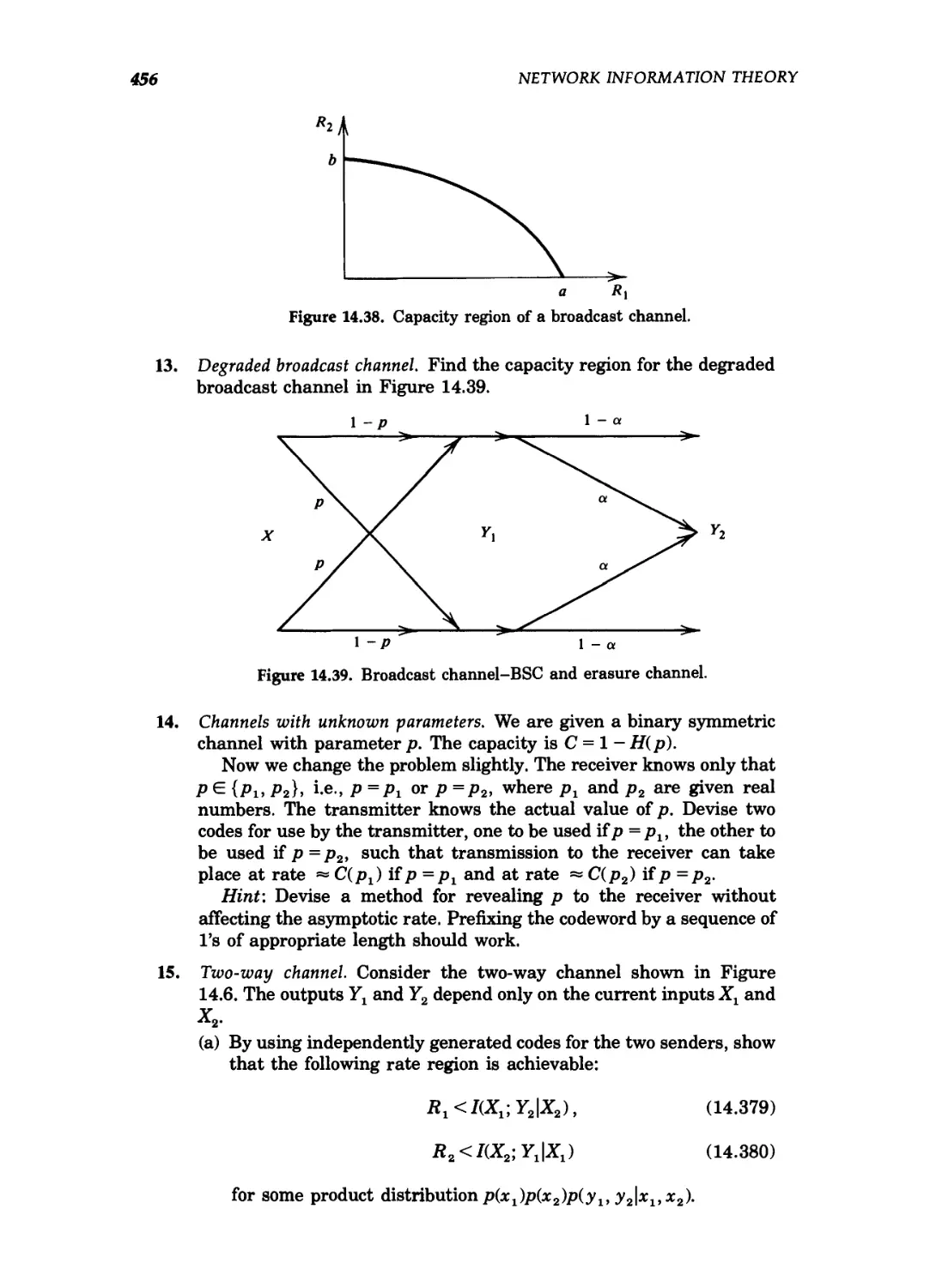
14.38 Capacity region of a broadcast channel 456
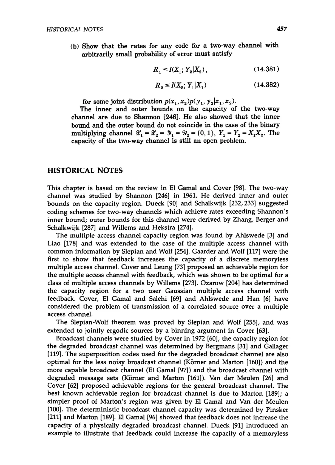
14.39 Broadcast channel—BSC and erasure channel 456
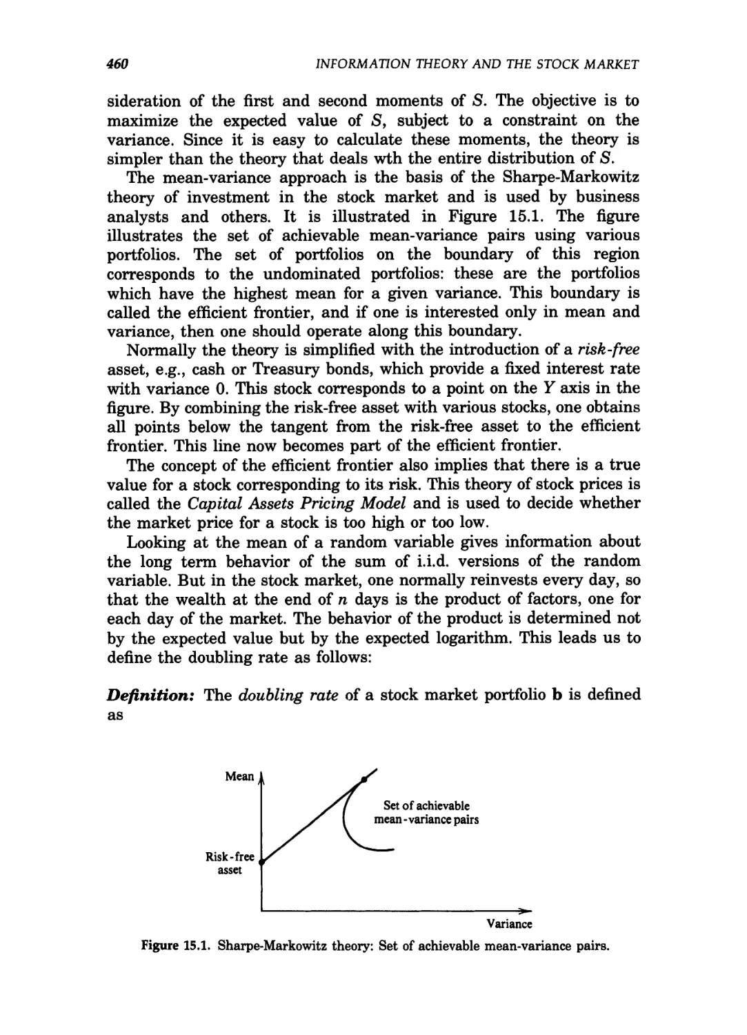
15.1 Sharpe-Markowitz theory: Set of achievable mean-
variance pairs 460
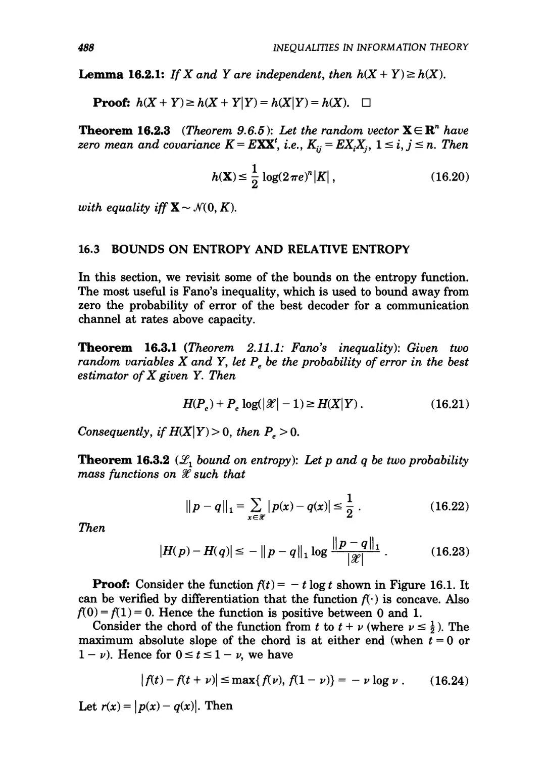
16.1 The function f{t)=-tlogt 489
Elements of Information Theory
Thomas M. Cover, Joy A. Thomas
Copyright © 1991 John Wiley & Sons, Inc.
Print ISBN 0-471-06259-6 Online ISBN 0-471-20061-1
Chapter 1
Introduction and Preview
This "first and last lecture" chapter goes backwards and forwards
through information theory and its naturally related ideas. The full
definitions and study of the subject begin in Chapter 2.
Information theory answers two fundamental questions in
communication theory: what is the ultimate data compression (answer:
the entropy H), and what is the ultimate transmission rate of
communication (answer: the channel capacity C). For this reason some
consider information theory to be a subset of communication theory. We
will argue that it is much more. Indeed, it has fundamental
contributions to make in statistical physics (thermodynamics), computer
science (Kolmogorov complexity or algorithmic complexity), statistical
inference (Occam's Razor: "The simplest explanation is best") and to
probability and statistics (error rates for optimal hypothesis testing and
estimation).
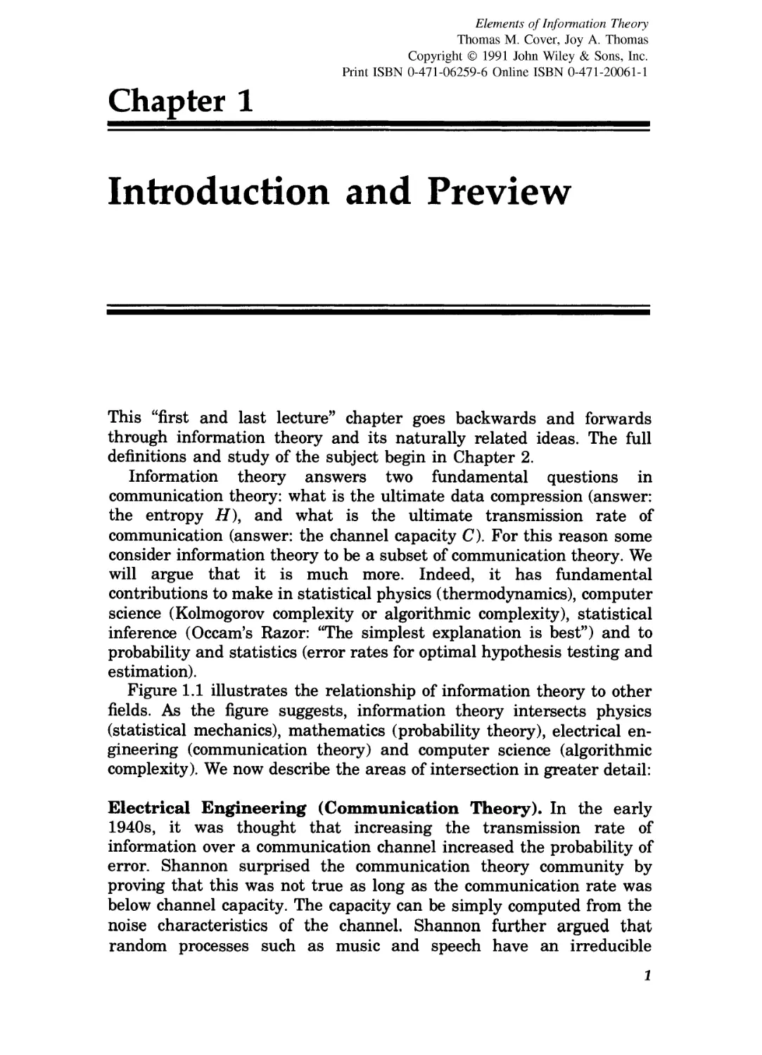
Figure 1.1 illustrates the relationship of information theory to other
fields. As the figure suggests, information theory intersects physics
(statistical mechanics), mathematics (probability theory), electrical en-
engineering (communication theory) and computer science (algorithmic
complexity). We now describe the areas of intersection in greater detail:
Electrical Engineering (Communication Theory). In the early
1940s, it was thought that increasing the transmission rate of
information over a communication channel increased the probability of
error. Shannon surprised the communication theory community by
proving that this was not true as long as the communication rate was
below channel capacity. The capacity can be simply computed from the
noise characteristics of the channel. Shannon further argued that
random processes such as music and speech have an irreducible
INTRODUCTION AND PREVIEW
Figure 1.1. The relationship of information theory with other fields.
complexity below which the signal cannot be compressed. This he named
the entropy, in deference to the parallel use of this word in
thermodynamics, and argued that if the entropy of the source is less
than the capacity of the channel, then asymptotically error free
communication can be achieved.
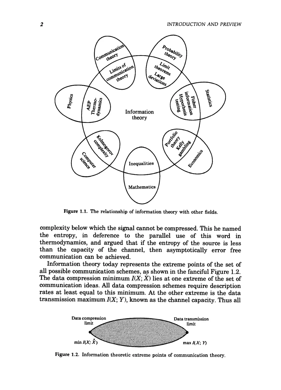
Information theory today represents the extreme points of the set of
all possible communication schemes, as shown in the fanciful Figure 1.2.
The data compression minimum I(X; X) lies at one extreme of the set of
communication ideas. All data compression schemes require description
rates at least equal to this minimum. At the other extreme is the data
transmission maximum I{X; Y), known as the channel capacity. Thus all
Data compression
limit
min I(X;X)
Data transmission
limit
max I(X; Y)
Figure 1.2. Information theoretic extreme points of communication theory.
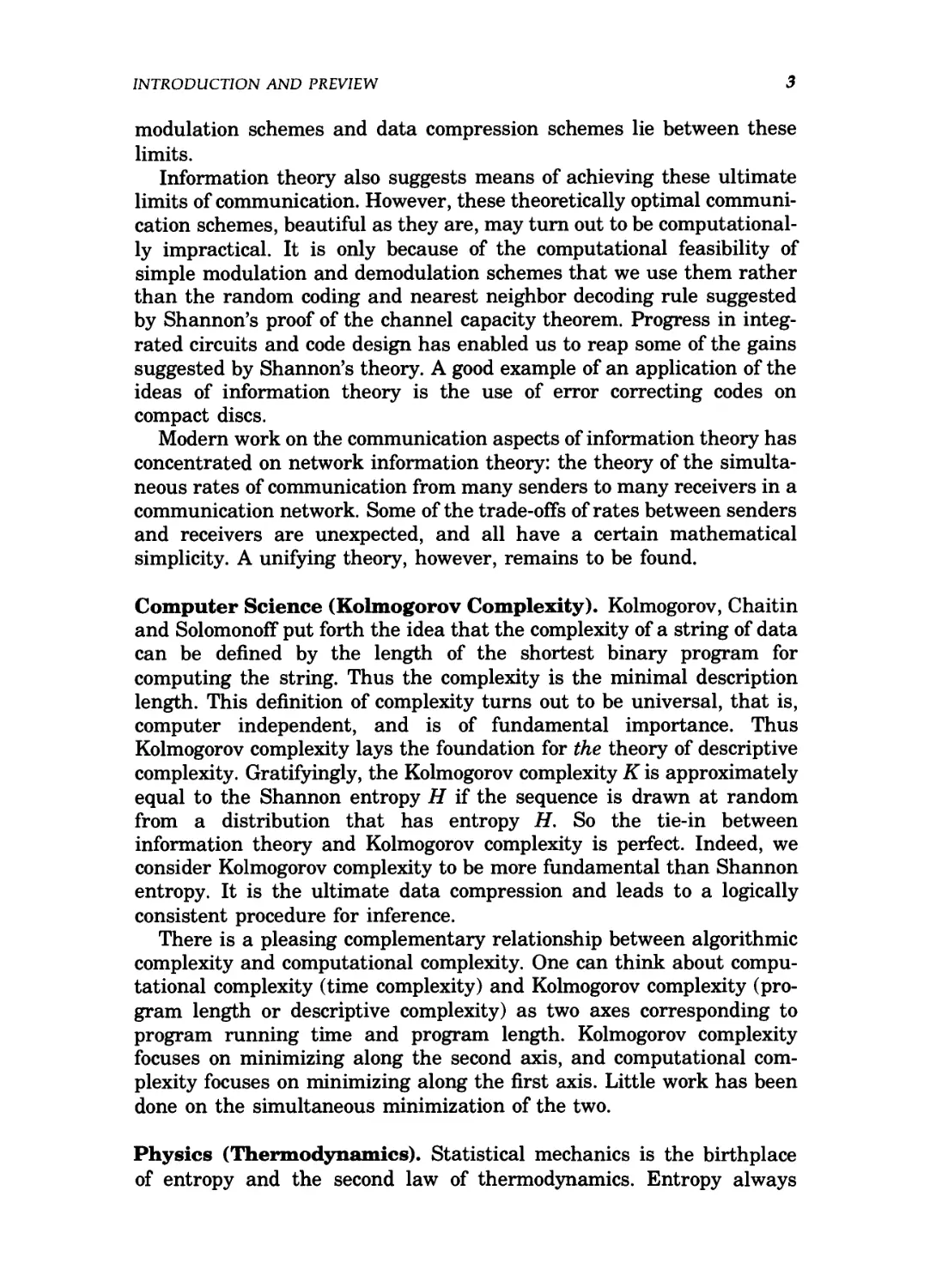
INTRODUCTION AND PREVIEW 3
modulation schemes and data compression schemes lie between these
limits.
Information theory also suggests means of achieving these ultimate
limits of communication. However, these theoretically optimal communi-
communication schemes, beautiful as they are, may turn out to be computational-
computationally impractical. It is only because of the computational feasibility of
simple modulation and demodulation schemes that we use them rather
than the random coding and nearest neighbor decoding rule suggested
by Shannon's proof of the channel capacity theorem. Progress in integ-
integrated circuits and code design has enabled us to reap some of the gains
suggested by Shannon's theory. A good example of an application of the
ideas of information theory is the use of error correcting codes on
compact discs.
Modern work on the communication aspects of information theory has
concentrated on network information theory: the theory of the simulta-
simultaneous rates of communication from many senders to many receivers in a
communication network. Some of the trade-offs of rates between senders
and receivers are unexpected, and all have a certain mathematical
simplicity. A unifying theory, however, remains to be found.
Computer Science (Kolmogorov Complexity). Kolmogorov, Chaitin
and Solomonoff put forth the idea that the complexity of a string of data
can be defined by the length of the shortest binary program for
computing the string. Thus the complexity is the minimal description
length. This definition of complexity turns out to be universal, that is,
computer independent, and is of fundamental importance. Thus
Kolmogorov complexity lays the foundation for the theory of descriptive
complexity. Gratifyingly, the Kolmogorov complexity K is approximately
equal to the Shannon entropy H if the sequence is drawn at random
from a distribution that has entropy H. So the tie-in between
information theory and Kolmogorov complexity is perfect. Indeed, we
consider Kolmogorov complexity to be more fundamental than Shannon
entropy. It is the ultimate data compression and leads to a logically
consistent procedure for inference.
There is a pleasing complementary relationship between algorithmic
complexity and computational complexity. One can think about compu-
computational complexity (time complexity) and Kolmogorov complexity (pro-
(program length or descriptive complexity) as two axes corresponding to
program running time and program length. Kolmogorov complexity
focuses on minimizing along the second axis, and computational com-
complexity focuses on minimizing along the first axis. Little work has been
done on the simultaneous minimization of the two.
Physics (Thermodynamics). Statistical mechanics is the birthplace
of entropy and the second law of thermodynamics. Entropy always
4 INTRODUCTION AND PREVIEW
increases. Among other things, the second law allows one to dismiss any
claims to perpetual motion machines. We briefly discuss the second law
in Chapter 2.
Mathematics (Probability Theory and Statistics). The fundamen-
fundamental quantities of information theory—entropy, relative entropy and
mutual information—are defined as functionals of probability
distributions. In turn, they characterize the behavior of long sequences
of random variables and allow us to estimate the probabilities of rare
events (large deviation theory) and to find the best error exponent in
hypothesis tests.
Philosophy of Science (Occam's Razor). William of Occam said
"Causes shall not be multiplied beyond necessity," or to paraphrase it,
"The simplest explanation is best". Solomonoff, and later Chaitin, argue
persuasively that one gets a universally good prediction procedure if one
takes a weighted combination of all programs that explain the data and
observes what they print next. Moreover, this inference will work in
many problems not handled by statistics. For example, this procedure
will eventually predict the subsequent digits of tt. When this procedure
is applied to coin flips that come up heads with probability 0.7, this too
will be inferred. When applied to the stock market, the procedure should
essentially find all the "laws" of the stock market and extrapolate them
optimally. In principle, such a procedure would have found Newton's
laws of physics. Of course, such inference is highly impractical, because
weeding out all computer programs that fail to generate existing data
will take impossibly long. We would predict what happens tomorrow a
hundred years from now.
Economics (Investment). Repeated investment in a stationary stock
market results in an exponential growth of wealth. The growth rate of
the wealth (called the doubling rate) is a dual of the entropy rate of the
stock market. The parallels between the theory of optimal investment in
the stock market and information theory are striking. We develop the
theory of investment to explore this duality.
Computation vs. Communication. As we build larger computers out
of smaller components, we encounter both a computation limit and a
communication limit. Computation is communication limited and
communication is computation limited. These become intertwined, and
thus all of the developments in communication theory via information
theory should have a direct impact on the theory of computation.
1.1 PREVIEW OF THE BOOK 5
1.1 PREVIEW OF THE BOOK
The initial questions treated by information theory were in the areas of
data compression and transmission. The answers are quantities like
entropy and mutual information, which are functions of the probability
distributions that underlie the process of communication. A few
definitions will aid the initial discussion. We repeat these definitions in
Chapter 2.
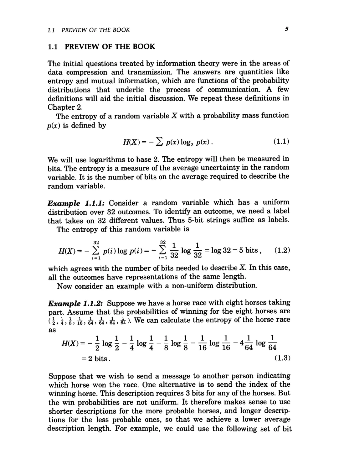
The entropy of a random variable X with a probability mass function
p(x) is defined by
H(X)=-^p(x)\og2p(x). A.1)
We will use logarithms to base 2. The entropy will then be measured in
bits. The entropy is a measure of the average uncertainty in the random
variable. It is the number of bits on the average required to describe the
random variable.
Example 1.1.1: Consider a random variable which has a uniform
distribution over 32 outcomes. To identify an outcome, we need a label
that takes on 32 different values. Thus 5-bit strings suffice as labels.
The entropy of this random variable is
32 32 1 1
H(X)=-J, p(i)logp(i)=-2 ^ log —= log 32 = 5 bits, A.2)
which agrees with the number of bits needed to describe X. In this case,
all the outcomes have representations of the same length.
Now consider an example with a non-uniform distribution.
Example 1.1.2: Suppose we have a horse race with eight horses taking
part. Assume that the probabilities of winning for the eight horses are
(|>i>!>ii>^>33>^>63)- We can calculate the entropy of the horse race
as
__.v. 111111 1 1 1 1
H{X)= - -log- — log^-glogg -_iog--4slogs
= 2 bits. A.3)
Suppose that we wish to send a message to another person indicating
which horse won the race. One alternative is to send the index of the
winning horse. This description requires 3 bits for any of the horses. But
the win probabilities are not uniform. It therefore makes sense to use
shorter descriptions for the more probable horses, and longer descrip-
descriptions for the less probable ones, so that we achieve a lower average
description length. For example, we could use the following set of bit
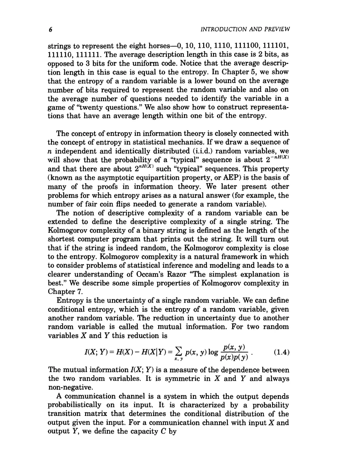
6 INTRODUCTION AND PREVIEW
strings to represent the eight horses—0, 10, 110, 1110, 111100, 111101,
111110, 111111. The average description length in this case is 2 bits, as
opposed to 3 bits for the uniform code. Notice that the average descrip-
description length in this case is equal to the entropy. In Chapter 5, we show
that the entropy of a random variable is a lower bound on the average
number of bits required to represent the random variable and also on
the average number of questions needed to identify the variable in a
game of "twenty questions." We also show how to construct representa-
representations that have an average length within one bit of the entropy.
The concept of entropy in information theory is closely connected with
the concept of entropy in statistical mechanics. If we draw a sequence of
n independent and identically distributed (i.i.d.) random variables, we
will show that the probability of a "typical" sequence is about 2~nH(X)
and that there are about 2nH(X) such "typical" sequences. This property
(known as the asymptotic equipartition property, or AEP) is the basis of
many of the proofs in information theory. We later present other
problems for which entropy arises as a natural answer (for example, the
number of fair coin flips needed to generate a random variable).
The notion of descriptive complexity of a random variable can be
extended to define the descriptive complexity of a single string. The
Kolmogorov complexity of a binary string is defined as the length of the
shortest computer program that prints out the string. It will turn out
that if the string is indeed random, the Kolmogorov complexity is close
to the entropy. Kolmogorov complexity is a natural framework in which
to consider problems of statistical inference and modeling and leads to a
clearer understanding of Occam's Razor "The simplest explanation is
best." We describe some simple properties of Kolmogorov complexity in
Chapter 7.
Entropy is the uncertainty of a single random variable. We can define
conditional entropy, which is the entropy of a random variable, given
another random variable. The reduction in uncertainty due to another
random variable is called the mutual information. For two random
variables X and Y this reduction is
/(X; Y) = H(X) - H(X\Y) = 2 p(*, y) log P,(*' f \ . A.4)
x,y p{x)p{.y)
The mutual information I(X; Y) is a measure of the dependence between
the two random variables. It is symmetric in X and Y and always
non-negative.
A communication channel is a system in which the output depends
probabilistically on its input. It is characterized by a probability
transition matrix that determines the conditional distribution of the
output given the input. For a communication channel with input X and
output Y, we define the capacity C by
1.1 PREVIEW OF THE BOOK 7
C = max I{X\Y). A.5)
p(x)
Later we show that the capacity is the maximum rate at which we can
send information over the channel and recover the information at the
output with a vanishingly low probability of error. We illustrate this
with a few examples.
Example 1.1.3 (Noiseless binary channel): For this channel, the bi-
binary input is reproduced exactly at the output. This channel is illus-
illustrated in Figure 1.3. Here, any transmitted bit is received without error.
Hence, in each transmission, we can send 1 bit reliably to the receiver,
and the capacity is 1 bit. We can also calculate the information capacity
C = max/(X;Y) = 1 bit.
Example 1.1.4 (Noisy four-symbol channel): Consider the channel
shown in Figure 1.4. In this channel, each input letter is received either
as the same letter with probability 1/2 or as the next letter with
probability 1/2. If we use all four input symbols, then inspection of the
output would not reveal with certainty which input symbol was sent. If,
on the other hand, we use only two of the inputs A and 3 say), then we
can immediately tell from the output which input symbol was sent. This
channel then acts like the noiseless channel of the previous example,
and we can send 1 bit per transmission over this channel with no errors.
We can calculate the channel capacity C = max/(X; Y) in this case, and
it is equal to 1 bit per transmission, in agreement with the analysis
above.
In general, communication channels do not have the simple structure
of this example, so we cannot always identify a subset of the inputs to
send information without error. But if we consider a sequence of
transmissions, then all channels look like this example and we can then
identify a subset of the input sequences (the codewords) which can be
used to transmit information over the channel in such a way that the
sets of possible output sequences associated with each of the codewords
Figure 1.3. Noiseless binary channel. Figure 1.4. A noisy channel.
8 INTRODUCTION AND PREVIEW
are approximately disjoint. We can then look at the output sequence and
identify the input sequence with a vanishingly low probability of error.
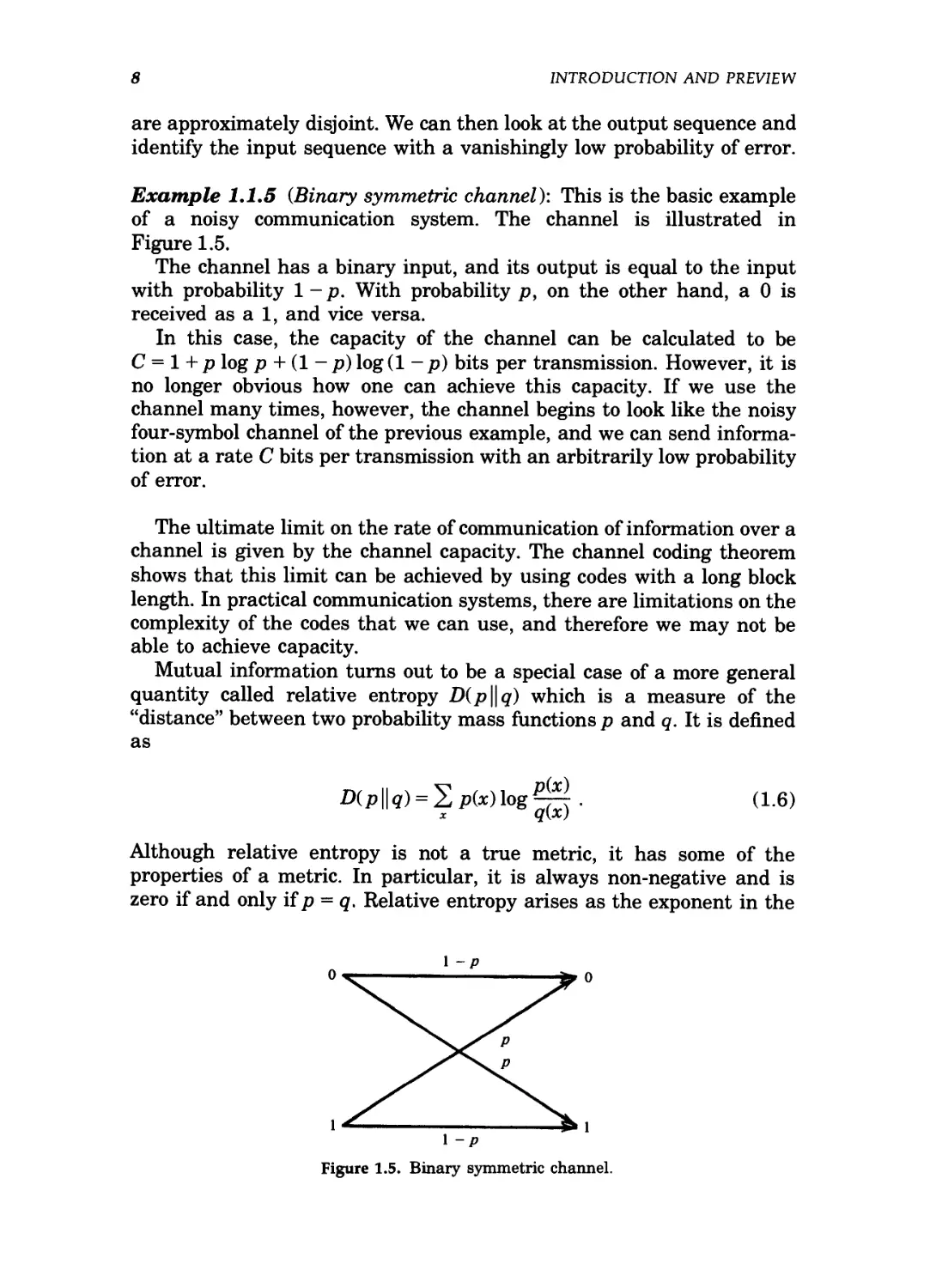
Example 1.1.5 (Binary symmetric channel): This is the basic example
of a noisy communication system. The channel is illustrated in
Figure 1.5.
The channel has a binary input, and its output is equal to the input
with probability 1 -p. With probability p, on the other hand, a 0 is
received as a 1, and vice versa.
In this case, the capacity of the channel can be calculated to be
C = 1+ p log p + A - p) log A - p) bits per transmission. However, it is
no longer obvious how one can achieve this capacity. If we use the
channel many times, however, the channel begins to look like the noisy
four-symbol channel of the previous example, and we can send informa-
information at a rate C bits per transmission with an arbitrarily low probability
of error.
The ultimate limit on the rate of communication of information over a
channel is given by the channel capacity. The channel coding theorem
shows that this limit can be achieved by using codes with a long block
length. In practical communication systems, there are limitations on the
complexity of the codes that we can use, and therefore we may not be
able to achieve capacity.
Mutual information turns out to be a special case of a more general
quantity called relative entropy D{p\\q) which is a measure of the
"distance" between two probability mass functions p and q. It is defined
as
S^ A.6)
Although relative entropy is not a true metric, it has some of the
properties of a metric. In particular, it is always non-negative and is
zero if and only if p = q. Relative entropy arises as the exponent in the
-P
l
-P
Figure 1.5. Binary symmetric channel.
1.1 PREVIEW OF THE BOOK 9
probability of error in a hypothesis test between distributions p and q.
Relative entropy can be used to define a geometry for probability
distributions that allows us to interpret many of the results of large
deviation theory.
There are a number of parallels between information theory and the
theory of investment in a stock market. A stock market is defined by a
random vector X whose elements are non-negative numbers equal to the
ratio of the price of a stock at the end of a day to the price at the
beginning of the day. For a stock market with distribution F(x), we can
define the doubling rate W as
W= max I logb'xdFCx). A.7)
The doubling rate is the maximum asymptotic exponent in the growth of
wealth. The doubling rate has a number of properties that parallel the
properties of entropy. We explore some of these properties in
Chapter 15.
The quantities H, I, C, D, K, W arise naturally in the following areas:
• Data compression. The entropy H of a random variable is a lower
bound on the average length of the shortest description of the
random variable. We can construct descriptions with average
length within one bit of the entropy.
If we relax the constraint of recovering the source perfectly, we
can then ask what rates are required to describe the source up to
distortion D? And what channel capacities are sufficient to enable
the transmission of this source over the channel and its reconstruc-
reconstruction with distortion less than or equal to D? This is the subject of
rate distortion theory.
When we try to formalize the notion of the shortest description
for non-random objects, we are led to the definition of Kolmogorov
complexity K. Later, we will show that Kolmogorov complexity is
universal and satisfies many of the intuitive requirements for the
theory of shortest descriptions.
• Data transmission. We consider the problem of transmitting
information so that the receiver can decode the message with a
small probability of error. Essentially, we wish to find codewords
(sequences of input symbols to a channel) that are mutually far
apart in the sense that their noisy versions (available at the output
of the channel) are distinguishable. This is equivalent to sphere
packing in high dimensional space. For any set of codewords it is
possible to calculate the probability the receiver will make an
error, i.e., make an incorrect decision as to which codeword was
sent. However, in most cases, this calculation is tedious.
10 INTRODUCTION AND PREVIEW
Using a randomly generated code, Shannon showed that one can
send information at any rate below the capacity C of the channel
with an arbitrarily low probability of error. The idea of a randomly
generated code is very unusual. It provides the basis for a simple
analysis of a very difficult problem. One of the key ideas in the
proof is the concept of typical sequences.
• Network information theory. Each of the topics previously
mentioned involves a single source or a single channel. What if one
wishes simultaneously to compress many sources and then put the
compressed descriptions together into a joint reconstruction of the
sources? This problem is solved by the Slepian-Wolf theorem. Or
what if one has many senders independently sending information
to a common receiver? What is the channel capacity of this
channel? This is the multiple access channel solved by Liao and
Ahlswede. Or what if one has one sender and many receivers and
wishes to simultaneously communicate (perhaps different)
information to each of the receivers? This is the broadcast channel.
Finally, what if one has an arbitrary number of senders and
receivers in an environment of interference and noise. What is the
capacity region of achievable rates from the various senders to the
receivers? This is the general network information theory problem.
All of the preceding problems fall into the general area of multiple-
user or network information theory. Although hopes for a unified
theory may be beyond current research techniques, there is still
some hope that all the answers involve only elaborate forms of
mutual information and relative entropy.
• Ergodic theory. The asymptotic equipartition theorem states that
most sample n -sequences of an ergodic process have probability
about 2~nH and that there are about 2nH such typical sequences.
• Hypothesis testing. The relative entropy D arises as the exponent
in the probability of error in a hypothesis test between two
distributions. It is a natural measure of distance between
distributions.
• Statistical mechanics. The entropy H arises in statistical
mechanics as a measure of uncertainty or disorganization in a
physical system. The second law of thermodynamics says that the
entropy of a closed system cannot decrease. Later we provide some
interpretations of the second law.
• Inference. We can use the notion of Kolmogorov complexity K to
find the shortest description of the data and use that as a model to
predict what comes next. A model that maximizes the uncertainty
or entropy yields the maximum entropy approach to inference.
• Gambling and investment. The optimal exponent in the growth
rate of wealth is given by the doubling rate W. For a horse race
1.1 PREVIEW OF THE BOOK 11
with uniform odds, the sum of the doubling rate W and the entropy
H is constant. The mutual information / between a horse race and
some side information is an upper bound on the increase in the
doubling rate due to the side information. Similar results hold for
investment in a stock market.
• Probability theory. The asymptotic equipartition property (AEP)
shows that most sequences are typical in that they have a sample
entropy close to H. So attention can be restricted to these
approximately 2nH typical sequences. In large deviation theory, the
probability of a set is approximately 2~nD, where D is the relative
entropy distance between the closest element in the set and the
true distribution.
• Complexity theory. The Kolmogorov complexity K is a measure of
the descriptive complexity of an object. It is related to, but different
from, computational complexity, which measures the time or space
required for a computation.
Information theoretic quantities like entropy and relative entropy
arise again and again as the answers to the fundamental questions in
communication and statistics. Before studying these questions, we shall
study some of the properties of the answers. We begin in the next
chapter with the definitions and the basic properties of entropy, relative
entropy and mutual information.
Chapter 2
Elements of Information Theory
Thomas M. Cover, Joy A. Thomas
Copyright © 1991 John Wiley & Sons, Inc.
Print ISBN 0-471-06259-6 Online ISBN 0-471-20061-1
Entropy, Relative Entropy
and Mutual Information
This chapter introduces most of the basic definitions required for the
subsequent development of the theory. It is irresistible to play with
their relationships and interpretations, taking faith in their later utility.
After defining entropy and mutual information, we establish chain
rules, the non-negativity of mutual information, the data processing
inequality, and finally investigate the extent to which the second law of
thermodynamics holds for Markov processes.
The concept of information is too broad to be captured completely by a
single definition. However, for any probability distribution, we define a
quantity called the entropy, which has many properties that agree with
the intuitive notion of what a measure of information should be. This
notion is extended to define mutual information, which is a measure of
the amount of information one random variable contains about another.
Entropy then becomes the self-information of a random variable. Mutual
information is a special case of a more general quantity called relative
entropy, which is a measure of the distance between two probability
distributions. All these quantities are closely related and share a
number of simple properties. We derive some of these properties in this
chapter.
In later chapters, we show how these quantities arise as natural
answers to a number of questions in communication, statistics, complex-
complexity and gambling. That will be the ultimate test of the value of these
definitions.
2.1 ENTROPY
We will first introduce the concept of entropy, which is a measure of
uncertainty of a random variable. Let X be a discrete random variable
12
2.1 ENTROPY 13
with alphabet % and probability mass function p(x) = Fr{X = x},xGf,
We denote the probability mass function by p{x) rather than px(x) for
convenience. Thus, p(x) and p(y) refer to two different random variables,
and are in fact different probability mass functions, px(x) and pY(y)
respectively.
Definition: The entropy H(X) of a discrete random variable X is denned
by
H{X) = - 2 p(x) log p(x). B.1)
We also write H(p) for the above quantity. The log is to the base 2
and entropy is expressed in bits. For example, the entropy of a fair coin
toss is 1 bit. We will use the convention that 0 log 0 = 0, which is easily
justified by continuity since xlogx->0 as x-»0. Thus adding terms of
zero probability does not change the entropy.
If the base of the logarithm is b, we will denote the entropy as Hb(X).
If the base of the logarithm is e, then the entropy is measured in nats.
Unless otherwise specified, we will take all logarithms to base 2, and
hence all the entropies will be measured in bits.
Note that entropy is a functional of the distribution of X It does not
depend on the actual values taken by the random variable X, but only
on the probabilities.
We shall denote expectation by E. Thus if X~p(x), then the expected
value of the random variable g(X) is written
Epg(X)= 2 g(x)p(x), B.2)
xex
or more simply as Eg(X) when the probability mass function is under-
understood from the context.
We shall take a peculiar interest in the eerily self-referential expecta-
expectation of g(X) under p(x) when g(X) = log -jjfi.
Remark: The entropy of X can also be interpreted as the expected
value of log ^, where X is drawn according to probability mass
function p{x). Thus
B.3)
.
This definition of entropy is related to the definition of entropy in
thermodynamics; some of the connections will be explored later. It is
possible to derive the definition of entropy axiomatically by defining
certain properties that the entropy of a random variable must satisfy.
This approach is illustrated in a problem at the end of the chapter. We
14 ENTROPY, RELATIVE ENTROPY AND MUTUAL INFORMATION
will not use the axiomatic approach to justify the definition of entropy;
instead, we will show that it arises as the answer to a number of natural
questions such as "What is the average length of the shortest descrip-
description of the random variable?" First, we derive some immediate con-
consequences of the definition.
Lemma 2.1.1: H(X)>0.
Proof: 0 <p(jc) < 1 implies log(l/p(jc)) > 0. ?
Lemma 2.1.2: Hb{X) = (log6 a)Ha(X).
Proof: log6 p = \ogb a log0 p. D
The second property of entropy enables us to change the base of the
logarithm in the definition. Entropy can be changed from one base to
another by multiplying by the appropriate factor.
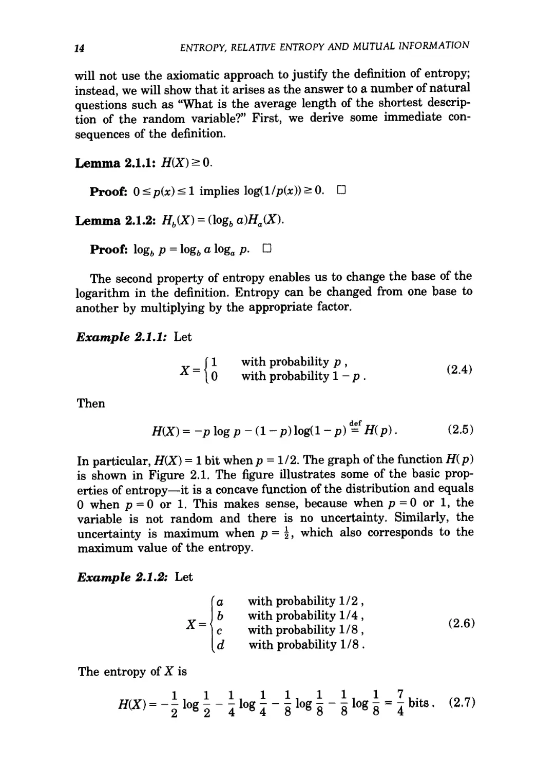
Example 2.1.1: Let
Then
f 1 with probability p ,
\0 with probability 1 - p .
H{X) = -p log p-(l-p)log(l -p) d=H(p). B.5)
In particular, H{X) = 1 bit whenp = 1/2. The graph of the function Hip)
is shown in Figure 2.1. The figure illustrates some of the basic prop-
properties of entropy—it is a concave function of the distribution and equals
0 when p = 0 or 1. This makes sense, because when p = 0 or 1, the
variable is not random and there is no uncertainty. Similarly, the
uncertainty is maximum when p = \, which also corresponds to the
maximum value of the entropy.
Example 2.1.2: Let
X =
a with probability 1/2 ,
b with probability 1/4 ,
c with probability 1/8, B'6)
d with probability 1/8.
The entropy of X is
rr/vx 1, 1 1, 1 1, 1 1, 1 7,. ,nn,
^)=--log--ilog---log---logrjbits. B.7)
2.2 JOINT ENTROPY AND CONDITIONAL ENTROPY
15
1
0.9
0.8
0.7
0.6
S 0.5
0.4
0.3
0.2
0.1
0
1 1 1 ^^^
I
! i i i i
r"^>4. i i i
V
\
iii'
0 0.1 0.2 0.3 0.4 0.5 0.6 0.7 0.8 0.9 1
P
Figure 2.1. H(p) versus p.
Suppose we wish to determine the value of X with the minimum number
of binary questions. An efficient first question is "Is X = a?" This splits
the probability in half. If the answer to the first question is no, then the
second question can be "Is X = bT The third question can be "Is X = c?"
The resulting expected number of binary questions required is 1.75.
This turns out to be the minimum expected number of binary questions
required to determine the value of X. In Chapter 5, we show that the
minimum expected number of binary questions required to determine X
lies between H(X) and H(X) + 1.
2.2 JOINT ENTROPY AND CONDITIONAL ENTROPY
We have defined the entropy of a single random variable in the previous
section. We now extend the definition to a pair of random variables.
There is nothing really new in this definition because (X, Y) can be
considered to be a single vector-valued random variable.
Definition: The joint entropy H(X, Y) of a pair of discrete random
variables (X, Y) with a joint distribution p(x, y) is defined as
B.8)
B.9)
p(x,y)\ogp(x,y),
which can also be expressed as
H(X,Y)=-E\ogp(X,Y).
16 ENTROPY, RELATIVE ENTROPY AND MUTUAL INFORMATION
We also define the conditional entropy of a random variable given
another as the expected value of the entropies of the conditional
distributions, averaged over the conditioning random variable.
Definition: If (X, Y)~p(x, y), then the conditional entropy H{Y\X) is
defined as
H{Y\X) = 2 p(x)H(Y\X = x) B.10)
= ~ 2 P(x) 2 p(y\x)\ogp(y\x) B.11)
xE% yEW
= -2 2 p(x, y)\og p(y\x) B.12)
xE% y&V
= -Ep{x,y)\ogp(Y\X). B.13)
The naturalness of the definition of joint entropy and conditional
entropy is exhibited by the fact that the entropy of a pair of random
variables is the entropy of one plus the conditional entropy of the other.
This is proved in the following theorem.
Theorem 2.2.1 (Chain rule):
H(X, Y) = H(X) + H(Y\X). B.14)
Proof:
H(X, Y) = - 2 2 p(x, y) log p(x, y) B.15)
= -2 2 p(x, y)log p(x)p(y\x) B.16)
2 p(x, y)\ogp(y\x) B.17)
ye<&
= -2 p(x)\ogp(x)- 2 2 p(x, y)log p(y\x) B.18)
B.19)
Equivalently, we can write
log p(X, Y) = log p(X) + log p(Y\X) B.20)
and take the expectation of both sides of the equation to obtain the
theorem. ?
2.2 JOINT ENTROPY AND CONDITIONAL ENTROPY
17
Corollary:
H(X, Y\Z) = H(X\Z) + H(Y\X, Z). B.21)
Proof: The proof follows along the same lines as the theorem. ?
Example 2.2.1: Let (X, Y) have the following joint distribution:
\ X
i
o
3
4
i—i
i
1-H
8
i—i
16
i—i
16
1
4
2
i-l
16
i—i
8
i-l
16
0
3
i—i
32
i-l
*32
i-l
16
0
4
i-l
32
i-l
32
i—i
16
0
The marginal distribution of X is (|, \, |, |) and the marginal
distribution of Y is {\,\,\,\), and hence #(X) = 7/4bits and #(Y) =
2 bits. Also,
H(X\Y) = 2 p(Y= i)H(X\Y=i)
~ 4 V2 ' 4 ' 8 ' 8/ + 4"V4 ' 2 ' 8 ' 8
, 0,0,0)
17171rtlrt
= 7x7 + 7x7 + 7 x2+ 7 x0
4 4 4 4 4 4
B.22)
B.23)
B.24)
B.25)
Similarly H(Y\X) = 13/8 bits and H(X, Y) = 27/8 bits.
Remark: Note that H(Y\X)*H(X\Y). However, H(X) - H(X\Y) =
H(Y) - H(Y\X), a property that we shall exploit later.
18 ENTROPY, RELATIVE ENTROPY AND MUTUAL INFORMATION
2.3 RELATIVE ENTROPY AND MUTUAL INFORMATION
The entropy of a random variable is a measure of the uncertainty of the
random variable; it is a measure of the amount of information required
on the average to describe the random variable. In this section, we
introduce two related concepts: relative entropy and mutual infor-
information.
The relative entropy is a measure of the distance between two
distributions. In statistics, it arises as an expected logarithm of the
likelihood ratio. The relative entropy D(p\\q) is a measure of the
inefficiency of assuming that the distribution is q when the true dis-
distribution is p. For example, if we knew the true distribution of the
random variable, then we could construct a code with average descrip-
description length H(p). If, instead, we used the code for a distribution q, we
would need H(p) + Dip \\q) bits oh the average to describe the random
variable.
Definition: The relative entropy or Kullback Leibler distance between
two probability mass functions p(x) and q(x) is defined as
B.26)
B.27)
In the above definition, we use the convention (based on continuity
arguments) that 0 log § = 0 and p log $ = <».
We will soon show that relative entropy is always non-negative and is
zero if and only if p = q. However, it is not a true distance between
distributions since it is not symmetric and does not satisfy the triangle
inequality. Nonetheless, it is often useful to think of relative entropy as
a "distance" between distributions.
We now introduce mutual information, which is a measure of the
amount of information that one random variable contains about another
random variable. It is the reduction in the uncertainty of one random
variable due to the knowledge of the other.
Definition: Consider two random variables X and Y with a joint
probability mass function p(x, y) and marginal probability mass func-
functions p(x) and p(y). The mutual information I(X;Y) is the relative
entropy between the joint distribution and the product distribution
p(x)p(y), i.e.,
KX;Y)=2 2 Pfc,y) log ^Jr B-28)
p\X)p\y)
2.4 RELATIONSHIP BETWEEN ENTROPY AND MUTUAL INFORMATION 19
= D(p(x,y)\\p(x)p(y)) B.29)
=E^^W)- B-30)
Example 2.3.1: Let %= {0,1} and consider two distributions/? and q
on %. Let p@) = 1 - r, p(l) = r, and let q@) = 1 - s, q(l) = s. Then
D(p\\ q) = (l- r) log f^ + r log ; B.31)
is s
and
Z)(q\\p) = A - s) log j^| + s log S- . B.32)
If r = s, then D(p||g) = D(g||p) = 0. If r = l/2, s = 1/4, then we can
calculate
2 "° 3 + 2 1Og I * 2
D(p\\q) = ^ log | + - log | = 1 - - log3 = 0.2075bits , B.33)
4 A 4
whereas
o In
#(g||p) = T log I + 7 log I = T Iog3 - 1 = 0.1887bits . B.34)
^ 2 ^ 2 ^
Note that D(p\\q)^D(q\\p) in general.
2.4 RELATIONSHIP BETWEEN ENTROPY AND MUTUAL
INFORMATION
We can rewrite the definition of mutual information I(X; Y) as
B.35)
f^ B.36)
*, y P\X)
= - 2 p(x, y) log p(«) + 2 p(*, y) log p(*|y) B.37)
*> y x,y
= -2 p(x) log p(x) - (-2 p(x, y) log p(*|y)) B.38)
* \ x,y I
= H(X)-H(X\Y). B.39)
20 ENTROPY, RELATIVE ENTROPY AND MUTUAL INFORMATION
Thus the mutual information I(X; Y) is the reduction in the uncertainty
of X due to the knowledge of Y.
By symmetry, it also follows that
I(X; Y) = H(Y) - H(Y\X). B.40)
Thus X says as much about Y as Y says about X.
Since H(X, Y) = H(X) + H(Y\X) as shown in Section 2.2, we have
I(X; Y) = H(X) + H(Y) - H(X, Y). B.41)
Finally, we note that
I(X; X) = H(X) - H(X\X) = H(X). B.42)
Thus the mutual information of a random variable with itself is the
entropy of the random variable. This is the reason that entropy is
sometimes referred to as self-information.
Collecting these results, we have the following theorem.
Theorem 2.4.1 (Mutual information and entropy):
I(X; Y) = H(X) - H(X\ Y), B.43)
I(X; Y) = H(Y) - H(Y\X), B.44)
I(X; Y) = H(X) + H(Y) - H(X, Y), B.45)
KX;Y) = KY;X), B.46)
I(X-,X) = H(X). B.47)
ff(X, Y)
H(X\Y) \I(X;Y)\ H(Y\X)
H(X) H(Y)
Figure 2.2. Relationship between entropy and mutual information.
2.5 CHAIN RULES FOR ENTROPY 21
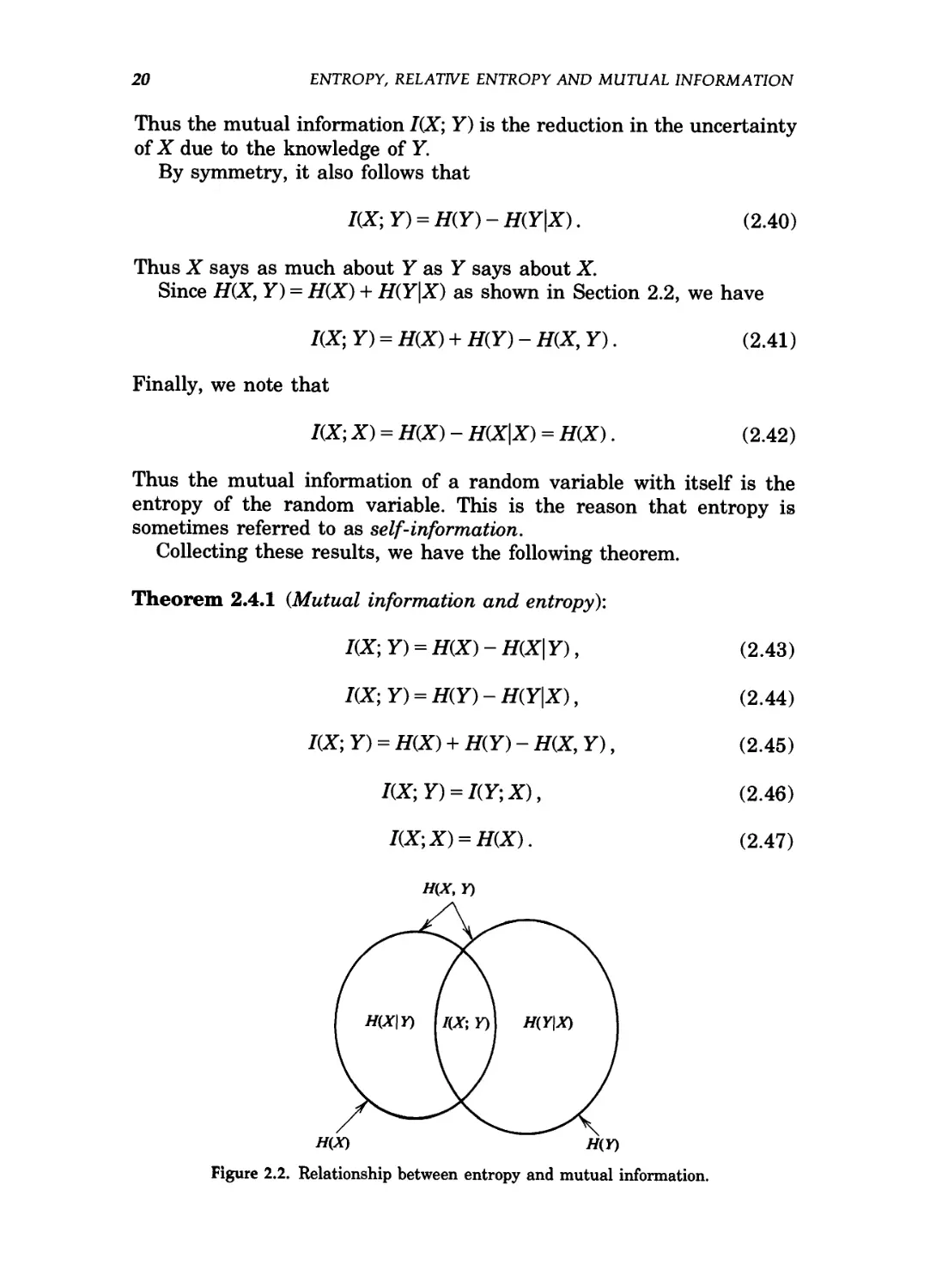
The relationship between H(X), H(Y), H(X, Y), H(X\Y), H(Y\X) and
I(X; Y) is expressed in a Venn diagram (Figure 2.2). Notice that the
mutual information I(X; Y) corresponds to the intersection of the infor-
information in X with the information in Y.
Example 2.4.1: For the joint distribution of example 2.2.1, it is easy
to calculate the mutual information I(X; Y) = H(X) - H(X\Y) = H(Y) -
H(Y\X) = 0.375 bits.
2.5 CHAIN RULES FOR ENTROPY, RELATIVE ENTROPY AND
MUTUAL INFORMATION
We now show that the entropy of a collection of random variables is the
sum of the conditional entropies.
Theorem 2.5.1 (Chain rule for entropy): Let XlfX2,... ,Xn be drawn
according to p(x1,x2,...,xn). Then
H(X1}X2, ...,Xn)=2 flCXi|Xi_lf... ,X,). B.48)
i = l
Proof: By repeated application of the two-variable expansion rule for
entropies, we have
1), B.49)
X3\X1) B.50)
1) + H(X3\X2,X1), B.51)
H(XX,X2,.. .,Xn) = H(X1) + H(X2\X1)+- ¦ ¦ + HiXjX^,... ,XX) B.52)
i_1,...,X1). B.53)
Alternative Proof: We write p(xlt..., xn) = n"=1 pix^x^, ...,Xl)
and evaluate
H(X1,X2,... ,Xn)
2 p(xltx2,...,xn)\ogp(x1,x2t...,xn) B.54)
xvx2, ... ,xn
n
2 p(x1,x2,...,xn)\ogl\ pC*,-!*..!,...,*!) B.55)
x1>x2, . . . ,xn i = i
22 ENTROPY, RELATIVE ENTROPY AND MUTUAL INFORMATION
n
2 *Z p(x1,x2,...,xn)\ogp(xi\xi_1,...,x1) B.56)
xl,x2, . . . ,xn i = i
n
= ~2 2 p(x1,x2,...,xn)\ogp(xi\xi_1,...,x1) B.57)
j = l xltx2, ¦ ¦ ¦ ,xn
n
= ~2 2 p(x1,x2,...,^logp(xlta_1,...,x1) B.58)
= 2^(XiK-i,...,^i). ? B.59)
i = l
We now define the conditional mutual information as the reduction in
the uncertainty of X due to knowledge of Y when Z is given.
Definition: The conditional mutual information of random variables X
and Y given Z is defined by
I(X; Y\Z) = H(X\Z) - H(X\Y, Z) B.60)
/¦y
Mutual information also satisfies a chain rule.
Theorem 2.5.2 (Chain rule for information):
n
I(X,,X2,... ,Xn; Y) = 2 /(Xi; YlX,^,*.^,... ,XX). B.62)
i=i
Proof:
Xs, ...,*„; y) = H(X1,X2,... ,XH)-H(XltX2,.. .,Xn\Y) B.63)
= 2j H(Xi\Xi_1,... yX^— 2j H(Xi\Xi-i> • • • >Xi> Y)
1,x2,...,x,_1). n B.64)
i = l
We define a conditional version of the relative entropy.
Definition: The conditional relative entropy D(p(y\x)\\q(y\x)) is the
average of the relative entropies between the conditional probability
mass functions p(y\x) and q(y\x) averaged over the probability mass
function p(x). More precisely,
D(p(y\x)\\q(y\x)) = 2 p
2.6 JENSEN'S INEQUALITY AND ITS CONSEQUENCES 23
The notation for conditional relative entropy is not explicit since it
omits mention of the distribution p(x) of the conditioning random
variable. However, it is normally understood from the context.
The relative entropy between two joint distributions on a pair of
random variables can be expanded as the sum of a relative entropy and
a conditional relative entropy. The chain rule for relative entropy will be
used in Section 2.9 to prove a version of the second law of thermo-
thermodynamics.
Theorem 2.5.3 (Chain rule for relative entropy):
D(p(x,y)\\q(x,y)) = D(p(x)\\q(x)) + D(p(y\x)\\q(y\x)). B.67)
Proof:
D(p(x, y)\\q(x, y)) = 2 2 p(x, y)log ^^ B.68)
= 2j2j p(x, y) log —— + Zj 2j p(x, y) log . B.70)
= ZXp(x)||g(x)) + ZXp(y|*)|kC'l*)). ? B.71)
2.6 JENSEN'S INEQUALITY AND ITS CONSEQUENCES
In this section, we shall prove some simple properties of the quantities
denned earlier. We begin with the properties of convex functions.
Definition: A function fix) is said to be convex over an interval (a, b) if
for every xx, x2B (a, b) and 0< A < 1,
fi\Xl + A - \)x2)< \f[Xl) + A - \)f\x2). B.72)
A function f is said to be strictly convex if equality holds only if A = 0 or
A = l.
Definition: A function f is concave if - f is convex.
A function is convex if it always lies below any chord. A function is
concave if it always lies above any chord.
24
ENTROPY, RELATIVE ENTROPY AND MUTUAL INFORMATION
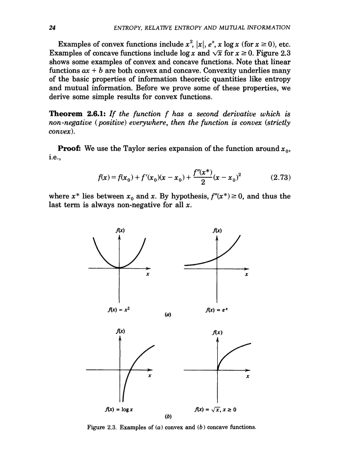
Examples of convex functions include x2, \x\, ex, x log* (for x ^ 0), etc.
Examples of concave functions include log* and Vx for x > 0. Figure 2.3
shows some examples of convex and concave functions. Note that linear
functions ax + b are both convex and concave. Convexity underlies many
of the basic properties of information theoretic quantities like entropy
and mutual information. Before we prove some of these properties, we
derive some simple results for convex functions.
Theorem 2.6.1: If the function f has a second derivative which is
non-negative (positive) everywhere, then the function is convex (strictly
convex).
Proof: We use the Taylor series expansion of the function around x0,
i.e.,
fix) = f(x0) + f'(xo)(x -xo)+
(x - xof
B.73)
where x* lies between x0 and x. By hypothesis, f"(x*) > 0, and thus the
last term is always non-negative for all x.
Ax)
Ax) = x2
(a)
Ax) = log*
AX) = yfx, X 2 0
(b)
Figure 2.3. Examples of (a) convex and F) concave functions.
2.6 JENSEN'S INEQUALITY AND ITS CONSEQUENCES 25
We let x0 = A*! + A - \)x2 and take x = xx to obtain
Similarly, taking x = x2, we obtain
f(x2)>f(x0) + f'(x0)[\(x2-Xl)]. B.75)
Multiplying B.74) by A and B.75) by 1 - A and adding, we obtain B.72).
The proof for strict convexity proceeds along the same lines. ?
Theorem 2.6.1 allows us to immediately verify the strict convexity of
x2, ex and x log* for x ^ 0, and the strict concavity of log* and Vx for
Let E denote expectation. Thus EX= T>xBSe p(x)x in the discrete case
and EX = J xf(x) dx in the continuous case.
The next inequality is one of the most widely used in mathematics
and one that underlies many of the basic results in information theory.
Theorem 2.6.2 (Jensen's inequality): If f is a convex function and X is
a random variable, then
Ef(X)>f(EX). B.76)
Moreover, if f is strictly convex, then equality in B.76) implies that
X = EX with probability 1, i.e., X is a constant.
Proof: We prove this for discrete distributions by induction on the
number of mass points. The proof of conditions for equality when f is
strictly convex will be left to the reader.
For a two mass point distribution, the inequality becomes
Pi/fri) + P2/fr2)^APi*i+P2*2)> B.77)
which follows directly from the definition of convex functions. Suppose
the theorem is true for distributions with k -1 mass points. Then
writing p\ = pj(l - pk) for i = 1,2,..., k - 1, we have
" " fa) B.78)
B.79)
B.80)
26 ENTROPY, RELATIVE ENTROPY AND MUTUAL INFORMATION
B.81)
;=i '
where the first inequality follows from the induction hypothesis and the
second follows from the definition of convexity.
The proof can be extended to continuous distributions by continuity
arguments. ?
We now use these results to prove some of the properties of entropy
and relative entropy. The following theorem is of fundamental impor-
importance.
Theorem 2.6.3 (Information inequality): Let p(x), q(x), x?f, be two
probability mass functions. Then
D(p\\q)>0 B.82)
with equality if and only if
p(x) = q(x) for all x . B.83)
Proof: Let A= {x: p(x) > 0} be the support set of p(x). Then
B.84)
< log 2 p(*)$? B.86)
i6A PW
= log 2 q(x) B.87)
xEA
^ log 2 q(x) B.88)
x<=se
= logl B.89)
= 0, B.90)
where B.86) follows from Jensen's inequality. Since log* is a strictly
concave function of t, we have equality in B.86) if and only if q(x)f
p(x) = 1 everywhere, i.e., p(x) = q(x). Hence we have D(p\\q) = 0 if and
only if p(x) = q(x) for all x. ?
2.6 JENSEN'S INEQUALITY AND ITS CONSEQUENCES 27
Corollary (Non-negativity of mutual information): For any two ran-
random variables, X, Y,
7(X;7)>0, B.91)
with equality if and only if X and Y are independent.
Proof: I(X; Y) = D(p(x, y)\\p(x) p(y)) > 0, with equality if and only if
p(x, y) = p(x) p(y), i.e., X and Y are independent. ?
Corollary:
D(p(y\x)\\q(y\x))>0, B.92)
with equality if and only ifp(y\x) = q(y\x) for all y and x with p(x) > 0.
Corollary:
7(X;Y|Z)>0, B.93)
with equality if and only if X and Y are conditionally independent given
Z.
We now show that the uniform distribution over the range #? is the
maximum entropy distribution over this range. It follows that any
random variable with this range has an entropy no greater than log \$6\.
Theorem 2.6.4: i/(X)<log|#?|, where \%\ denotes the number of ele-
elements in the range of X, with equality if and only if X has a uniform
distribution over #?.
Proof: Let u(x) = ^ be the uniform probability mass function over #?,
and let p(x) be the probability mass function for X. Then
B.94)
Hence by the non-negativity of relative entropy,
0 <D(p\\u) = log \%\-H(X). ? B.95)
Theorem 2.6.5 (Conditioning reduces entropy):
H(X\Y)<H(X) B.96)
with equality if and only if X and Y are independent.
28 ENTROPY, RELATIVE ENTROPY AND MUTUAL INFORMATION
Proof: 0 < I(X; Y) = H(X) - H(X\ Y). ?
Intuitively, the theorem says that knowing another random variable
Y can only reduce the uncertainty in X. Note that this is true only on the
average. Specifically, H(X\Y = y) may be greater than or less than or
equal to H(X), but on the average H(X\Y) = Zy p(y)H(X\Y = y) <H(X).
For example, in a court case, specific new evidence might increase
uncertainty, but on the average evidence decreases uncertainty.
Example 2.6.1: Let (X, Y) have the following joint distribution:
X
1 2
0 f
1 1
Then H(X) = H( J, I) = 0.544 bits, H(X\Y = 1) = 0 bits and H(X\Y = 2) =
1 bit. We calculate H(X\Y)= \H(X\Y= 1)+ \H(X\Y = 2) = 0.25 bits.
Thus the uncertainty in X is increased if Y = 2 is observed and de-
decreased if Y = 1 is observed, but uncertainty decreases on the average.
Theorem 2.6.6 (Independence bound on entropy): Let Xly X2,..., Xn be
drawn according to p(x1,x2,... ,xn). Then
H(XlfX2,... ,Xn)< 2, HGQ B.97)
u;#/i equality if and only if the Xi are independent.
Proof: By the chain rule for entropies,
n
XY \ — ^ %J(Y \Y Y \ (O QQ'i
±, 2, . . . , A-n ) — Z-i "v^-il-^-i —1> • • • > -^-1 / I.Z.I7CSJ
B.99)
where the inequality follows directly from the previous theorem. We
have equality if and only if Xt is independent ofX-.j,..., X1 for all i, i.e.,
if and only if the X-'s are independent. ?
2.7 THE LOG SUM INEQUALITY AND ITS APPLICATIONS 29
2.7 THE LOG SUM INEQUALITY AND ITS APPLICATIONS
We now prove a simple consequence of the concavity of the logarithm,
which will be used to prove some concavity results for the entropy.
Theorem 2.7.1 (Log sum inequality): For non-negative numbers, alf
a2,..., an and blt b2,..., bn,
? a. log ? > (S a,) log ^i|i B.100)
with equality if and only if^= const.
We again use the convention that 0 log 0 = 0, a log § = oo if a > 0 and
0 log § =0. These follow easily from continuity.
Proof: Assume without loss of generality that a- > 0 and 6^ > 0.
The function f[t) = ? log t is strictly convex, since fit) = \ log e > 0 for
all positive t. Hence by Jensen's inequality, we have
B.10D
for a- > 0, Sj at = 1. Setting at = bJTL*^ bj and tt = ajb^ we obtain
^'^^§'^^.
which is the log sum inequality. ?
We now use the log sum inequality to prove various convexity results.
We begin by reproving Theorem 2.6.3, which states that D(p\\q)^0
with equality if and only if p(x) = q(x).
By the log sum inequality,
= llogi = 0 B.105)
with equality if and only if p(x)lq(x) = c. Since both p and q are
probability mass functions, c = 1, and hence we have D(p\\q) - 0 if and
only if p(x) = q(x) for all x.
30 ENTROPY, RELATIVE ENTROPY AND MUTUAL INFORMATION
Theorem 2.7.2: D(p\\q) is convex in the pair (p, q), i.e., if(px,Q\) and
(P2> Q2) are iw0 pairs of probability mass functions, then
D(XPl + A - X)p2\\\q1 + A - A)g2)< \D(Pl\\qi) + A - X)D(p2\\q2)
B.106)
for all 0<A<l.
Proof: We apply the log sum inequality to a term on the left hand
side of B.106), i.e.,
(Ap.tr) + A - A)p,W) log ff'tn
Summing this over all x, we obtain the desired property. ?
Theorem 2.7.3 (Concavity of entropy): H(p) is a concave function of p.
Proof:
= \og\%\-D(p\\u), B.108)
where u is the uniform distribution on \%\ outcomes. The concavity of//
then follows directly from the convexity of D.
Alternative Proof: LetXx be a random variable with distribution px
taking on values in a set A. Let X2 be another random variable with
distribution p2 on the same set. Let
f 1 with probability A
°~\2 with probability 1 - A U-lW)
Let Z = X0. Then the distribution of Z is Ap1 + A-A)p2. Now since
conditioning reduces entropy, we have
H(Z)>H(Z\B), B.110)
or equivalently,
H(XPl + A - A)p2)> XH(Pl) + A - X)H(p2), B.111)
which proves the concavity of the entropy as a function of the dis-
distribution. ?
2.7 THE LOG SUM INEQUALITY AND ITS APPLICATIONS 31
One of the consequences of the concavity of entropy is that mixing
two gases of equal entropy results in a gas with higher entropy.
Theorem 2.7.4: Let (X,Y)~p(x, y) = p(x)p(y\x). The mutual informa-
information I(X; Y) is a concave function of p(x) for fixed p(y\x) and a convex
function ofp(y\x) for fixed p(x).
Proof: To prove the first part, we expand the mutual information
I(X; Y) = H(Y) - H(Y\X) = H(Y) - 2 p(x)H(Y\X = *). B.112)
X
If p(y\x) is fixed, then p(y) is a linear function of p(x). Hence H(Y),
which is a concave function of p(y), is a concave function of p(x). The
second term is a linear function of p(x). Hence the difference is a concave
function of p(x).
To prove the second part, we fix p(x) and consider two different
conditional distributions Pxiylx) and p2(y\x). The corresponding joint
distributions are p^x, y) = p(x) px(y\x) and p2(x, y) = p(x) p2(y\x), and
their respective marginals are p(x), p^y) and p(x), p2(y). Consider a
conditional distribution
Px(y\x) = \Pl(y\x) + A - \)p2(y\x) B.113)
that is a mixture of p^ylx) and p2(y\x). The corresponding joint dis-
distribution is also a mixture of the corresponding joint distributions,
Pa(*» y) = APi<*> y) + A - A)pa(x, y), B.114)
and the distribution of Y is also a mixture
Px(y) = Ap^y) + A" A)pa(y). B.115)
Hence if we let qx(x, y) = p(x)px(y) be the product of the marginal
distributions, we have
Qx(x, y) = A^Cx, y) + A - k)q2{x, y). B.116)
Since the mutual information is the relative entropy between the joint
distribution and the product of the marginals, i.e.,
I(X;Y) = D(px\\qx), B.117)
and relative entropy D(p\\q) is a convex function of (p, q), it follows that
the mutual information is a convex function of the conditional dis-
distribution. ?
32 ENTROPY, RELATIVE ENTROPY AND MUTUAL INFORMATION
2.8 DATA PROCESSING INEQUALITY
The data processing inequality can be used to show that no clever
manipulation of the data can improve the inferences that can be made
from the data.
Definition: Random variables X, Y, Z are said to form a Markov chain
in that order (denoted by X-> Y-+Z) if the conditional distribution of Z
depends only on Y and is conditionally independent of X. Specifically, X,
Y and Z form a Markov chain X-+ Y-> Z if the joint probability mass
function can be written as
p(x, y, z) = p(x)p(y\x)p(z\y). B.118)
Some simple consequences are as follows:
• X->Y->Z if and only if X and Z are conditionally independent
given y. Markovity implies conditional independence because
This is the characterization of Markov chains that can be extended
to define Markov fields, which are ra-dimensional random processes
in which the interior and exterior are independent given the values
on the boundary.
• X-^Y->Z implies that Z-»Y-»X. Thus the condition is some-
sometimes written X<-> F<-> Z.
• If Z = f\Y), then X->Y->Z.
We can now prove an important and useful theorem demonstrating
that no processing of Y, deterministic or random, can increase the
information that Y contains about X.
Theorem 2.8.1 (Data processing inequality): If X->Y->Z, then
Proof: By the chain rule, we can expand mutual information in two
different ways.
KX; Y, Z) = I(X; Z) + I(X; Y\Z) B.120)
= I(X;Z) + I(X;Y\Z). B.121)
2.9 THE SECOND LAW OF THERMODYNAMICS 33
Since X and Z are conditionally independent given Y, we have
I(X; Z\Y) = 0. Since I(X\ Y\Z) >0, we have
I(X',Y)>I(X;Z). B.122)
We have equality if and only if I(X; Y\Z) = 0, i.e., X->Z-^ Y forms a
Markov chain. Similarly, one can prove that I(Y; Z) ^ I(X; Z). ?
Corollary: In particular, ifZ = g(Y\ we have I(X; Y) > I(X; g(Y)).
Proof: X-> Y->g(Y) forms a Markov chain. ?
Thus functions of the data Y cannot increase the information about X.
Corollary: IfX-> Y-> Z, then I(X; Y\Z) <I(X; Y).
Proof: From B.120) and B.121), and using the fact that I(X; Z\Y) =
0 by Markovity and I(X; Z) ^ 0, we have
I(X;Y\Z)<I(X',Y). ? B.123)
Thus the dependence of X and Y is decreased (or remains unchanged)
by the observation of a "downstream" random variable Z.
Note that it is also possible that I(X; Y\Z)> I(X; Y) when X, Y and Z
do not form a Markov chain. For example, let X and Y be independent
fair binary random variables, and let Z = X + Y. Then I(X; Y) = 0, but
I(X; Y\Z) = H(X\Z) - H(X\Y, Z) = H(X\Z) = P(Z = 1) H(X\Z = 1) = \ bit.
2.9 THE SECOND LAW OF THERMODYNAMICS
One of the basic laws of physics, the second law of thermodynamics,
states that the entropy of an isolated system is non-decreasing. We now
explore the relationship between the second law and the entropy func-
function that we have defined earlier in this chapter.
In statistical thermodynamics, entropy is often defined as the log of
the number of microstates in the system. This corresponds exactly to our
notion of entropy if all the states are equally likely. But why does the
entropy increase?
We model the isolated system as a Markov chain (see Chapter 4) with
transitions obeying the physical laws governing the system. Implicit in
this assumption is the notion of an overall state of the system and the
fact that, knowing the present state, the future of the system is
independent of the past. In such a system, we can find four different
interpretations of the second law. It may come as a shock to find that
34 ENTROPY, RELATIVE ENTROPY AND MUTUAL INFORMATION
the entropy does not always increase. However, relative entropy always
decreases.
1. Relative entropy D(ixn\\fj,'n) decreases with n. Let fin and \x.'n be two
probability distributions on the state space of a Markov chain at
time 7i, and let fj,n+1 and fj,'n+1 be the corresponding distributions at
time Ti + 1. Let the corresponding joint mass functions be denoted
by p and q. Thus p(xn,xn+1) = p(xn) rixn+1\xn) and q(xn,xn+1) =
q(xn) rixn+1\xn), where K • | •) is the probability transition function
for the Markov chain. Then by the chain rule for relative entropy,
we have two expansions:
D(p(xn,xn+1)\\q(xn,xn+1))
= D(p(xn)\\q(xn)) + D(p(xn+1\xn)\\q(xn+1\xn))
=D(p(xn+1)\\q(xn+1)) + D(p(xn\xn+1)\\q(xn\xn+1)).
Since both p and q are derived from the Markov chain, the
conditional probability mass functions p(xn+1\xn) and q(xn + 1\xn)
are equal to rGcB+1|*B) and hence D(p(xn+1\xn)\\q(xn+1\xn)) = 0.
Now using the non-negativity of D(p(xn\xn+1)\\q(xn\xn+1)) (Corol-
(Corollary to Theorem 2.6.3), we have
D(p(xn)\\q(xn))>D(p(xn+1)\\q(xn+1)) B.124)
or
\\1\\^+1). B.125)
Consequently, the distance between the probability mass func-
functions is decreasing with time n for any Markov chain.
An example of one interpretation of the preceding inequality is
to suppose that the tax system for the redistribution of wealth is
the same in Canada and in England. Then if pn and fi'n represent
the distributions of wealth among individuals in the two countries,
this inequality shows that the relative entropy distance between
the two distributions decreases with time. The wealth distribu-
distributions in Canada and England will become more similar.
2. Relative entropy D( pn || n) between a distribution (j,n on the states at
time n and a stationary distribution \l decreases with n. In
B.125), ix'n is any distribution on the states at time n. If we let fin
be any stationary distribution n, then ix'n+1 is the same stationary
distribution. Hence
B.126)
2.9 THE SECOND LAW OF THERMODYNAMICS 35
which implies that any state distribution gets closer and closer to
each stationary distribution as time passes. The sequence
D( nn || fi) is a monotonically non-increasing non-negative sequence
and must therefore have a limit. The limit is actually 0 if the
stationary distribution is unique, but this is more difficult to
prove.
3. Entropy increases if the stationary distribution is uniform. In
general, the fact that the relative entropy decreases does not
imply that the entropy increases. A simple counterexample is
provided by any Markov chain with a non-uniform stationary
distribution. If we start this Markov chain from the uniform
distribution, which already is the maximum entropy distribution,
the distribution will tend to the stationary distribution, which has
a lower entropy than the uniform. Hence the entropy decreases
with time rather than increases.
If, however, the stationary distribution is the uniform dis-
distribution, then we can express the relative entropy as
- H(Xn). B.127)
In this case the monotonic decrease in relative entropy implies a
monotonic increase in entropy. This is the explanation that ties in
most closely with statistical thermodynamics, where all the mi-
crostates are equally likely. We now characterize processes having
a uniform stationary distribution.
Definition: A probability transition matrix [P^], P- = Pr{Xn+1 =
j\Xn = i} is called doubly stochastic if
2^ = 1, 7 = 1,2,... B.128)
i
and
2^ = 1, i = l,2,... B.129)
j
Remark: The uniform distribution is a stationary distribution
of P if and only if the probability transition matrix is doubly
stochastic. See Problem 1 in Chapter 4.
4. The conditional entropy H(Xn \Xj_) increases with n for a stationary
Markov process. If the Markov process is stationary, then H(Xn) is
constant. So the entropy is nonincreasing. However, we will prove
that HiX^Xi) increases with n. Thus the conditional uncertainty
of the future increases. We give two alternative proofs of this
result. First, we use the properties of entropy,
36 ENTROPY, RELATIVE ENTROPY AND MUTUAL INFORMATION
H(Xn \Xt) > H(Xn \Xj_, X2) (conditioning reduces entropy) B.130)
= H(Xn\X2) (by Markovity) B.131)
XJ (by stationarity). B.132)
Alternatively, by an application of the data processing inequality
to the Markov chain X1-+Xn_1->Xn, we have
^^^XJ. B.133)
Expanding the mutual informations in terms of entropies, we have
H(Xn_1)-H(Xn_1\X1)*H(Xn)-H(Xn\X1). B.134)
By stationarity, H(Xn_1) = H(Xn), and hence we have
H{Xn_1\X1)^H(Xn\X1). B.135)
(These techniques can also be used to show that H(X0\Xn) is
increasing in n for any Markov chain. See problem 35.)
5. Shuffles increase entropy. If T is a shuffle (permutation) of a deck
of cards and X is the initial (random) position of the cards in the
deck and if the choice of the shuffle T is independent of X, then
H(TX)>H(X), B.136)
where TX is the permutation of the deck induced by the shuffle T
on the initial permutation X. Problem 31 outlines a proof.
2.10 SUFFICIENT STATISTICS
This section is a sidelight showing the power of the data processing
inequality in clarifying an important idea in statistics. Suppose we have
a family of probability mass functions {fe(x)} indexed by 0, and let X be
a sample from a distribution in this family. Let T{X) be any statistic
(function of the sample) like the sample mean or sample variance. Then
0->X-> T(X), and by the data processing inequality, we have
I(d;T(X))<I@;X) B.137)
for any distribution on ft However, if equality holds, no information is
lost.
2.10 SUFFICIENT STATISTICS 37
A statistic T(X) is called sufficient for 0 if it contains all the informa-
information in X about ft
Definition: A function T{X) is said to be a sufficient statistic relative to
the family {fe(x)} if X is independent of 0 given T(X), i.e., 0-*T(X)->X
forms a Markov chain.
This is the same as the condition for equality in the data processing
inequality,
1@;X) = 1@; TOO) B.138)
for all distributions on ft Hence sufficient statistics preserve mutual
information and conversely.
Here are some examples of sufficient statistics:
1. Let XltX2,... ,Xn, Xt E {0,1}, be an independent and identically
distributed (i.i.d.) sequence of coin tosses of a coin with unknown
parameter 0 = Pr(Xj = 1). Given n, the number of l's is a sufficient
statistic for ft Here T(XlfX2,... ,Xn) = S"=1 Xt. In fact, we can
show that given T, all sequences having that many l's are equally
likely and independent of the parameter ft Specifically,
0 otherwise.
Thus 0 -» E Xi -> (Xx, X2,..., Xn) forms a Markov chain, and T is a
sufficient statistic for ft
The next two examples involve probability densities instead of prob-
probability mass functions, but the theory still applies. We define entropy
and mutual information for continuous random variables in Chapter 9.
2. If X is normally distributed with mean 0 and variance 1, i.e., if
fe(x) = -|= e-(x~dJ/2 = Jf@,1), B.140)
V L
and Xx,X2,...,Xn are drawn independently according to this
distribution, then a sufficient statistic for 0 is Xn = h S"=1 Xt. It
can be verified that the conditional distribution of XX,X2,... ,Xn,
conditioned on Xn and n does not depend on ft
38 ENTROPY, RELATIVE ENTROPY AND MUTUAL INFORMATION
3. If fg = Uniform@, 6 + 1), then a sufficient statistic for 6 is
T(XltX2,... ,Xn) = (max{X1,X2,... ,Xn},min {X,,X2,... ,Xn}).
B.141)
The proof of this is slightly more complicated, but again one can
show that the distribution of the data is independent of the
parameter given the statistic T.
The minimal sufficient statistic is a sufficient statistic that is a
function of all other sufficient statistics.
Definition: A statistic T(X) is a minimal sufficient statistic relative to
{f0(x)} if it is a function of every other sufficient statistic U. Interpreting
this in terms of the data processing inequality, this implies that
0->T(X)->U(X)->X. B.142)
Hence a minimal sufficient statistic maximally compresses the infor-
information about 0 in the sample. Other sufficient statistics may contain
additional irrelevant information. For example, for a normal distribu-
distribution with mean 0, the pair of functions giving the mean of all odd
samples and the mean of all even samples is a sufficient statistic, but
not a minimal sufficient statistic. In the preceding examples, the suffici-
sufficient statistics are also minimal.
2.11 FANO'S INEQUALITY
Suppose we know a random variable Y and we wish to guess the value of
a correlated random variable X. Fano's inequality relates the probability
of error in guessing the random variable X to its conditional entropy
H(X\Y). It will be crucial in proving the converse to Shannon's second
theorem in Chapter 8. From the problems at the end of the chapter, we
know that the conditional entropy of a random variable X given another
random variable Y is zero if and only if X is a function of Y. Hence we
can estimate X from Y with zero probability of error if and only if
H(X\Y) = 0.
Extending this argument, we expect to be able to estimate X with a
low probability of error only if the conditional entropy H(X\Y) is small.
Fano's inequality quantifies this idea.
Suppose we wish to estimate a random variable X with a distribution
p(x). We observe a random variable Y which is related to X by the
conditional distribution p{y\x). From Y, we calculate a function g(Y) =
2.11 FANO'S INEQUALITY 39
X, which is an estimate of X We wish to bound the probability that
X#X. We observe that X-> Y->X forms a Markov chain. Define the
probability of error
Pe=Pr{X^X}. B.143)
Theorem 2.11.1 (Fano's inequality):
H(Pe) + Pe log(|af| - 1)>tf(X|Y). B.144)
This inequality can be weakened to
1 + Pe log |#| >: H(X\Y) B.145)
or
¦. B.146)
Remark: Note that Pe = Q implies that H(X\Y) = Q, as intuition
suggests.
Proof: Define an error random variable,
o !ff=x' B'147)
Then, using the chain rule for entropies to expand H(E,X\Y) in two
different ways, we have
H(E,X\Y) = H(X\Y) + H(E\X,Y) B.148)
=o
= H(E\Y)+ H(X\E,Y) . B.149)
stf(Pe) sPelog(|aT|-l)
Since conditioning reduces entropy, H(E\Y)< H(E) = H(Pe). Now since
E is a function of X andg(Y), the conditional entropy H(E\X, Y) is equal
to 0. Also, since E is a binary-valued random variable, H(E) = H(Pe).
The remaining term, H(X\E, Y), can be bounded as follows:
H(X\E, Y) = Pr(E = 0)H(X\Y, E = 0) + Pr(E = 1)H(X\Y, E = 1)
B.150)
), B.151)
40 ENTROPY, RELATIVE ENTROPY AND MUTUAL INFORMATION
since given E = 0, X = g(Y), and given E = l, we can upper bound the
conditional entropy by the log of the number of remaining outcomes
{\%\ - 1 if^r(F) ? #, else |# |). Combining these results, we obtain Fano's
inequality. ?
Remark: Suppose that there is no knowledge of Y. Thus X must be
guessed without any information. Let X6{l,2,...,m} and pi>p2>
' ' ' -Pm- Then the best guess ofXisX= 1 and the resulting probability
of error is Pe = 1 -p1. Fano's inequality becomes
H(Pe) + Pe log(m -1J= H(X) • B.152)
The probability mass function
(Pi> Pi,-", pJ=U-Pe, -^y ,..., -^j) B.153)
v 771 — l 771 — 1 /
achieves this bound with equality. Thus Fano's inequality is sharp.
The following telegraphic summary omits qualifying conditions.
SUMMARY OF CHAPTER 2
Definition: The entropy H(X) of a discrete random variable X is defined by
H(X)= - X p(*)logp(*). - B.154)
Properties of H:
1. H(X)>0.
2.HbiX) = (logba)HaiX).
3. (Conditioning reduces entropy) For any two random variables, X and Y,
we have
H(X\Y)<H(X) B.155)
with equality if and only if X and Y are independent.
4. H(XX ,X2 XJsS;=1 H(Xt), with equality if and only if the random
variables X( are independent.
5. H(X)< \og\St\ with equality if and only if X is uniformly distributed
over St.
6. Hip) is concave in p.
Definition: The relative entropy D(p\\q) of the probability mass function p
with respect to the probability mass function q is defined by
SUMMARY OF CHAPTER 2 41
B.156)
Definition: The mutual information between two random variables X and Y
is defined as
HX', Y) = X X P(x, y) log -?^r . B.157)
Alternative expressions:
^ B.158)
, Y) = ?p log ^^ B.159)
B.160)
(p||g) pg^ B.162)
Properties of Z) and /:
1. I(X; Y) = H(X) - H(X\Y) = H(Y) - H(Y\X) = H(X) + H(Y) - H(X, Y).
2. Dip\\q)^ 0 with equality if and only if p(x) = g(x), for all x E St.
3. I(X; y) = D(p(x, y)||pix)p(y)) > 0, with equality if and only if p(x, y) =
p(x)p(y), i.e., X and Y are independent.
4. If \3?\ = mt and m is the uniform distribution over %, then D(p\\u) =
log m-H{p\
5. D(p||g) is convex in the pair (p, g).
Chain rules
Entropy: HiX,,X^... ,Xn)= l*_x HiX^X^ XY).
Mutual
information: I(Xl ,X2 Xn; Y) = E".t I(Xt; Y'|X1, X2 Xt:_t).
Relative entropy: Z)(p(x, y)||g(«, y)) = D(p(x)\\q(x)) + Z)(p(y|
Jensen's inequality: If/"is a convex function, then Ef{X)>f{EX).
Log sum inequality: For n positive numbers, ax,a2,..., an and 61;
62 bn>
I a,, log ^ ^ (? a,) log ?k? B.163)
with equality if and only ifajb^ constant.
42 ENTROPY, RELATIVE ENTROPY AND MUTUAL INFORMATION
Data processing inequality: If X—> Y-+ Z forms a Markov chain, then
Second law of thermodynamics: For a Markov chain,
1. Relative entropy D(fin\\fi'n) decreases with time.
2. Relative entropy D(fin\\fi) between a distribution and the stationary
distribution decreases with time.
3. Entropy H(Xn) increases if the stationary distribution is uniform.
4. The conditional entropy HiXJX^ increases with time for a stationary
Markov chain.
5. The conditional entropy H(X0\Xn) of the initial condition Xo increases
for any Markov chain.
Sufficient statistic: TXX) is sufficient relative to {f0(x)} if and only if
7@; X) = IF; 1XX)) for all distributions on ft
Fano's inequality: Let Pe =Pr{g(Y)=tX}, where g is any function of Y.
Then
H(Pe) + Pe log(|ff| - l)s= H(X\Y). B.164)
PROBLEMS FOR CHAPTER 2
1. Coin flips. A fair coin is flipped until the first head occurs. Let X
denote the number of flips required.
(a) Find the entropy H(X) in bits. The following expressions may be
useful:
nr =
(l-rf
(b) A random variable X is drawn according to this distribution. Find
an "efficient" sequence of yes-no questions of the form, "Is X
contained in the set S?" Compare H(X) to the expected number of
questions required to determine X.
2. Entropy of functions. Let X be a random variable taking on a finite
number of values. What is the (general) inequality relationship of
H(X) and HG) if
(a) Y = 2X?
(b) Y= cosX?
3. Minimum entropy. What is the minimum value of H(p1}..., pn) =
H(p) as p ranges over the set of n-dimensional probability vectors?
Find all p's which achieve this minimum.
4. Axiomatic definition of entropy. If we assume certain axioms for our
measure of information, then we will be forced to use a logarithmic
PROBLEMS FOR CHAPTER 2 43
measure like entropy. Shannon used this to justify his initial defini-
definition of entropy. In this book, we will rely more on the other properties
of entropy rather than its axiomatic derivation to justify its use. The
following problem is considerably more difficult than the other prob-
problems in this section.
If a sequence of symmetric functions Hm(p1, p2> • • • > /O satisfies
the following properties,
• Normalization: H2 (|, §) = 1,
• Continuity: H2(p, 1 —p) is a continuous function of p,
• Grouping: Hm{pup2 pJ = Hm_1(p1+p2,p3 pj +
(Pi + Pa) H2(p^p-2, P^hr),
prove that Hm must be of the form
Hm(Pi, P2 Pm)= ~ 2 Pi log Pi, m =2, 3
1=1 B.165)
There are various other axiomatic formulations which also result in
the same definition of entropy. See, for example, the book by Csiszar
and Korner [83].
5. Entropy of functions of a random variable. Let X be a discrete random
variable. Show that the entropy of a function of X is less than or
equal to the entropy of X by justifying the following steps:
H{X, g(X))=H(X) + H(g(X)\X) B.166)
{=H(X); B.167)
mx, g(X))=mg(X)) + mx\g(X)) B.168)
W)
>H(g(X)). B.169)
Thus H(g(X))<H(X).
6. Zero conditional entropy. Show that if H(Y\X) = 0, then Y is a function
of X, i.e., for all x with p(x)> 0, there is only one possible value of y
with p(x, y) > 0.
7. Pure randomness and bent coins. Let XltX2,... ,Xn denote the out-
outcomes of independent flips of a bent coin. Thus Pr{Xi = l}=p,
Pr{Xt =0} = 1 -p, where p is unknown. We wish to obtain a se-
sequence Z1} Z2,... , ZK of fair coin flips from Xlt X2,... ,Xn. Toward
this end let f:%n^ {0,1}* (where {0,1}* = {A, 0, 1, 00, 01,...} is
the set of all finite length binary sequences) be a mapping
fiXlfX2, ...,Xn) = (Z1,Z2,..., ZK), where Zt ~ Bernoulli (\), and K
may depend on (Xlf ...,Xn). In order that the sequence Z1,Z2t...
44 ENTROPY, RELATIVE ENTROPY AND MUTUAL INFORMATION
appear to be fair coin flips, the map f from bent coin flips to fair flips
must have the property that all 2* sequences (ZltZ2,...,Zk) of a
given length k have equal probability (possibly 0), for k = 1,2
For example, for n = 2, the map /101) = 0, /U0) = 1, /100) = fill) = A
(the null string), has the property that Prf^ = 1\K= 1} =Pr{Z1 =
0\K=l}=h-
Give reasons for the following inequalities:
F)
^H(Zlt Z2,..., ZK, K)
i ZK\K)
id)
= H(K)
Thus no more than nH(p) fair coin tosses can be derived from (Xlt
..., Xn), on the average.
(f) Exhibit a good map f on sequences of length 4.
8. World Series. The World Series is a seven-game series that terminates
as soon as either team wins four games. Let X be the random variable
that represents the outcome of a World Series between teams A and
B; possible values of X are AAAA, BABABAB, and BBBAAAA. Let Y
be the number of games played, which ranges from 4 to 7. Assuming
that A and B are equally matched and that the games are indepen-
independent, calculate H(X), H(Y), H(Y\X), and H(X\Y).
9. Infinite entropy. This problem shows that the entropy of a discrete
random variable can be infinite. Let A = E^=2 (n log2 n)~\ (It is easy
to show that A is finite by bounding the infinite sum by the integral of
(x log2 x)"\) Show that the integer-valued random variable X denned
by PrCX" =n) = (An log2 n) for n = 2,3,... has H(X) = + oo.
10. Conditional mutual information vs. unconditional mutual information.
Give examples of joint random variables X, Y and Z such that
(a) I(X; Y\Z) < I(X; Y),
(b) I(X;Y\Z)>I(X;Y).
11. Average entropy. Let H(p) = -p log2 p - A - p) Iog2(l - p) be the bi-
binary entropy function.
(a) Evaluate #A/4) using the fact that log2 3 «1.584. Hint: Con-
Consider an experiment with four equally likely outcomes, one of
which is more interesting than the others.
(b) Calculate the average entropy H(p) when the probability/? is
chosen uniformly in the range 0<p < 1.
PROBLEMS FOR CHAPTER 2 45
(c) (Optional) Calculate the average entropy H(pltp2,p3) where
(plt p2, p3) is a uniformly distributed probability vector. General-
Generalize to dimension n.
12. Venn diagrams. Using Venn diagrams, we can see that the mutual
information common to three random variables X, Y and Z should be
denned by
; Y; Z) = I(X; Y) - I(X; Y\Z).
This quantity is symmetric in X, Y andZ, despite the preceding
asymmetric definition. Unfortunately, I(X; Y\ Z) is not necessarily
nonnegative. Find X, Y and Z such that I(X; Y; Z) < 0, and prove the
following two identities:
I(X; Y; Z) = H(X, Y, Z) - H(X) - H(Y) - H(Z) + I(X; Y) + 7G; Z)
+ I(Z;X)
; Y; Z) = H(X, Y,Z)- H(X, Y) - H(Y, Z) - H(Z, X)
The first identity can be understood using the Venn diagram analogy
for entropy and mutual information. The second identity follows
easily from the first.
13. Coin weighing. Suppose one has n coins, among which there may or
may not be one counterfeit coin. If there is a counterfeit coin, it may
be either heavier or lighter than the other coins. The coins are to be
weighed by a balance.
(a) Find an upper bound on the number of coins n so that k weighings
will find the counterfeit coin (if any) and correctly declare it to be
heavier or lighter.
(b) (Difficult) What is the coin weighing strategy for k = 3 weighings
and 12 coins?
14. Drawing with and without replacement. An urn contains r red, w white,
and b black balls. Which has higher entropy, drawing k > 2 balls from
the urn with replacement or without replacement? Set it up and show
why. (There is both a hard way and a relatively simple way to do
this.)
15. A metric. A function p(x, y) is a metric if for all x, y,
• p(x,y)>0
• p(x, y) = p(y, x)
• p(x, y) = 0 if and only if x = y
• p(x,y) + p(y,z)>p(x,z).
46 ENTROPY, RELATIVE ENTROPY AND MUTUAL INFORMATION
(a) Show that p(X, Y) = H(X\Y) + H(Y\X) satisfies the first, second
and fourth properties above. If we say that X = Y if there is a
one-to-one function mapping X to Y, then the third property is
also satisfied, and p(X, Y) is a metric.
(b) Verify that p(X, Y) can also be expressed as
p(X, Y) = H(X) + H(Y) - WX; Y) B.170)
= mX,Y)-I(X;Y) B.171)
= 2H(X, Y) - H(X) - H{Y). B.172)
16. Example of joint entropy. Let p(x, y) be given by
0
1
0
3
0
1
3
3
Find
(a) H(X), H(Y).
(b) H(X\Y), H(Y\X).
(c) H(X,Y).
(d)H(Y)-mY\X).
(e) I(X; Y).
(f) Draw a Venn diagram for the quantities in (a) through (e).
17. Inequality. Show In x > 1 - h for x > 0.
18. Entropy of a sum. Let X and Y be random variables that take on
values xlt x2, ..., xr and ylt y2, ..., ya, respectively. Let Z = X + Y.
(a) Show that H(Z\X) = H(Y\X). Argue that if X, Y are independent,
then H(Y)<H(Z) and H(X)<H{Z). Thus the addition of in-
independent random variables adds uncertainty.
(b) Give an example (of necessarily dependent random variables) in
which HiX) > HiZ) and H(Y) > HiZ).
(c) Under what conditions does H(Z) = H{X) + H{YI
19. Entropy of a disjoint mixture. Let Xl and X2 be discrete random
variables drawn according to probability mass functions pt(-) and
P2( •) over the respective alphabets d?x = {1,2,..., m} and
Op / —. I 1 „ \ T cJL
l*'2 — \Tfl i X, . . . , «*/. JjCt
\Xlt with probability a ,
[X2, with probability 1 - a .
(a) Find H(X) in terms of HiX,) and H(X2) and a.
(b) Maximize over a to show that 2H(X) == 2H(Xl) + 2H(*2> and interpret
using the notion that 2H(X} is the effective alphabet size.
PROBLEMS FOR CHAPTER 2 47
20. A measure of correlation. Let Xx and X2 be identically distributed, but
not necessarily independent. Let
(a) Show p = HXX\
(b) Show 0==p==l.
(c) When is p = 0?
(d) When is p = 1?
21. Dflffl processing. Let Xx —> X2 —> X3 —> >Xn form a Markov chain in
this order; i.e., let
p(xlt x2,..., xn) = p(x1)p(x2\x1)- • • .p(xnk,-i) •
Reduce KX^, X2 Xn) to its simplest form.
22. Bottleneck. Suppose a (non-stationary) Markov chain starts in one of
n states, necks down to k <n states, and then fans back tom>A
states. Thus X1-»X2-»ZJ, ^?{1,2 n), X2e{l,2 k),
*3e{l,2 m).
(a) Show that the dependence of X1 and X3 is limited by the bottle-
bottleneck by proving that I(XX; X3) < log k.
(b) Evaluate I(XX\X3) for k = 1, and conclude that no dependence can
survive such a bottleneck.
23. Run length coding. Let XltX2 Xn be (possibly dependent) binary
random variables. Suppose one calculates the run lengths R =
(Rlt R2,... ) of this sequence (in order as they occur). For example,
the sequence x = 0001100100 yields run lengths R = C,2,2,1,2).
Compare H(XlfX2 Xn), H(R) and H(Xn, R). Show all equalities
and inequalities, and bound all the differences.
24. Markov's inequality for probabilities. Let p(x) be a probability mass
function. Prove, for all d > 0,
Pr{p(X) == d) log Q) == H(X). B.173)
25. Logical order of ideas. Ideas have been developed in order of need, and
then generalized if necessary. Reorder the following ideas, strongest
first, implications following:
(a) Chain rule for I{XX Xn\ Y) , chain rule for D(p(xl
*n)lk(*i> X2> • • • 7 XJ)> and chain rule for H(XlfX2,... ,Xn).
(b) D(f\\g)>0, Jensen's inequality, RX\ Y)>0.
26. Second law of thermodynamics. Let Xlt X2, X3 ... be a stationary first-
order Markov chain. In Section 2.9, it was shown that HiXjX^^
H(Xn_1\X1) for n = 2,3 Thus conditional uncertainty about the
future grows with time. This is true although the unconditional
48 ENTROPY, RELATIVE ENTROPY AND MUTUAL INFORMATION
uncertainty H(Xn) remains constant. However, show by example that
HiXJXj^ = xx) does not necessarily grow with n for every xx.
27. Conditional mutual information. Consider a sequence of n binary ran-
random variables Xlt X2 Xn. Each sequence with an even number of
l's has probability 2~("~1) and each sequence with an odd number of
l's has probability 0. Find the mutual informations
7(Xi;X2), KX^X^X,),.. .JiX^^XjX, Xn_2).
28. Mixing increases entropy. Show that the entropy of the probability
distribution, (Pi,.-.,pit ..., Pj,... ,pm), is less than the entropy of
p. +p. p. + p.
the distribution (p1 -L-^-L -L2-^ pm). Show that in
general any transfer of probability that makes the distribution more
uniform increases the entropy.
29. Inequalities. Let X, Y and Z be joint random variables. Prove the
following inequalities and find conditions for equality.
(a) H(X,Y\Z)^mX\Z).
(b)I(X,Y;Z)^I(X;Z).
(c) H(X, Y, Z) - H(X, Y) =s H(X, Z) - H(X).
(d) 7(X; Z\Y)> 7(Z; Y\X) - I(Z; Y) + I(X; Z).
30. Maximum entropy. Find the probability mass function p(x) that max-
maximizes the entropy H(X) of a non-negative integer-valued random
variable X subject to the constraint
EX=
for a fixed value A > 0. Evaluate this maximum H(X).
31. Shuffles increase entropy. Argue that for any distribution on shuffles T
and any distribution on card positions X that
H(TX)>H(TX\T) B.174)
B.175)
= H(X\T) B.176)
= H(X), B.177)
if X and T are independent.
32. Conditional entropy. Under what conditions does H(X\g(Y)) = H(X\ Y)?
33. Fano's inequality. Let PrC^= i) = Pi, i = l,2,...,m and \etp1 >p2 >
p3> • • • >pm. The minimal probability of error predictor of X is
X=l, with resulting probability of error Pe = 1 - px. Maximize H(p)
subject to the constraint l-p1=Peto find a bound on Pe in terms of
H. This is Fano's inequality in the absence of conditioning.
HISTORICAL NOTES 49
34. Monotonic convergence of the empirical distribution. Let pn denote the
empirical probability mass function corresponding to XltX2,... ,Xn
i.i.d. ~p(x), xESt. Specifically,
pn(x)=-2l(Xi=x) B.178)
is the proportion of times thatX^ = x in the first n samples, where / is
an indicator function.
(a) Show for % binary that
ED(p2n\\p)^ED(pJp). B.179)
Thus the expected relative entropy "distance" from the empirical
distribution to the true distribution decreases with sample size.
Hint: Writep2n = \pn + \p'n and use the convexity of D.
(b) Show for an arbitrary discrete 2? that
ED{pn\\p)^EIKpn^\\p). B.180)
35. Entropy of initial conditions. Prove that H(X0\Xn) is non-decreasing
with n for any Markov chain.
HISTORICAL NOTES
The concept of entropy was first introduced in thermodynamics, where it was
used to provide a statement of the second law of thermodynamics. Later,
statistical mechanics provided a connection between the macroscopic property of
entropy and the microscopic state of the system. This work was the crowning
achievement of Boltzmann, who had the equation S = k In W inscribed as the
epitaph on his gravestone.
In the 1930s, Hartley introduced a logarithmic measure of information for
communication. His measure was essentially the logarithm of the alphabet size.
Shannon [238] was the first to define entropy and mutual information as defined
in this chapter. Relative entropy was first defined by Kullback and Leibler [167].
It is known under a variety of names, including the Kullback Leibler distance,
cross entropy, information divergence and information for discrimination, and
has been studied in detail by Csiszar [78] and Amari [10].
Many of the simple properties of these quantities were developed by Shan-
Shannon. Fano's inequality was proved in Fano [105]. The notion of sufficient statistic
was defined by Fisher [111], and the notion of the minimal sufficient statistic was
introduced by Lehmann and Scheffe [174]. The relationship of mutual informa-
information and sufficiency is due to Kullback [165].
The relationship between information theory and thermodynamics has been
discussed extensively by Brillouin [46] and Jaynes [143]. Although the basic
theorems of information theory were originally derived for a communication
system, attempts have been made to compare these theorems with the fundamen-
fundamental laws of physics. There have also been attempts to determine whether there are
any fundamental physical limits to computation, including work by Bennett [24]
and Bennett and Landauer [25].
Elements of Information Theory
Thomas M. Cover, Joy A. Thomas
Copyright © 1991 John Wiley & Sons, Inc.
Print ISBN 0-471-06259-6 Online ISBN 0-471-20061-1
Chapter 3
The Asymptotic Equipartition
Property
In information theory, the analog of the law of large numbers is the
Asymptotic Equipartition Property (AEP). It is a direct consequence of
the weak law of large numbers. The law of large numbers states that for
independent, identically distributed (i.i.d.) random variables, k E"=1 Xf is
close to its expected value EX for large values of n. The AEP states that
* l°g P(xuX2,...,xn) is close to the entropy H, whereXX,X2,... ,Xn are i.i.d.
random variables and p(Xx,X2 Xn) is the probability of observing
the sequence XltX2,...,Xn. Thus the probability p(X1,X2,... ,Xn) as-
assigned to an observed sequence will be close to 2~nH.
This enables us to divide the set of all sequences into two sets, the
typical set, where the sample entropy is close to the true entropy, and
the non-typical set, which contains the other sequences. Most of our
attention will be on the typical sequences. Any property that is proved
for the typical sequences will then be true with high probability and will
determine the average behavior of a large sample.
First, an example. Let the random variable XE {0,1} have a prob-
probability mass function denned by p(l) = p and p@) = q. If XuX2,...,Xn
are i.i.d. according to p(x), then the probability of a sequence
x1,x2,...,xniB Il"=1 p(xt). For example, the probability of the sequence
A,0,1,1,0,1) is pZXiqn~ZXi=p4q2. Clearly, it is not true that all 2"
sequences of length n have the same probability.
However, we might be able to predict the probability of the sequence
that we actually observe. We ask for the probability p(XltX2,..., Xn) of
the outcomes XlfX2f... ,Xn, where XltX2l... are i.i.d. ~p(*). This is
insidiously self-referential, but well denned nonetheless. Apparently, we
are asking for the probability of an event drawn according to the same
probability distribution. Here it turns out thatpCX^, X2,..., Xn) is close
to Tnli with high probability.
50
3.1 THE AEP 51
We summarize this by saying, "Almost all events are almost equally
surprising." This is a way of saying that
Pr{(XltX2t... ,Xn):p(XuX2,... ,Xn) = 2-n(H±e)} « 1, C.1)
if Xlt X2,... ,Xn are i.i.d. ~p(x).
In the example just given, where p(Xlt X2,...,Xn) = pZXi qn~ZXi, we
are simply saying that the number of l's in the sequence is close to np
(with high probability), and all such sequences have (roughly) the same
probability 2"n//(p).
3.1 THE AEP
The asymptotic equipartition property is formalized in the following
theorem:
Theorem 3.1.1 (AEP): IfXuX2i... are i.i.d. ~p(x), then
- - log p(X1} X2,..., Xn)-» H(X) in probability. C.2)
Proof: Functions of independent random variables are also indepen-
independent random variables. Thus, since the Xt are i.i.d., so are logp(X^).
Hence by the weak law of large numbers,
1 1
— log p(X1}X2,..., X ) = — Zj log p(X}) C.3)
n n i
-+-E\og p(X) in probability C.4)
= H(X), C.5)
which proves the theorem. ?
Definition: The typical set A^n) with respect to p(x) is the set of
sequences (x1} x2,..., xn) E BPn with the following property:
C.6)
As a consequence of the AEP, we can show that the set A^n) has the
following properties:
Theorem 3.1.2:
1. If (Xl,x2,...,xn)EA[n\ then H(X)- e < - h \og p(xlt x2,...,
52 THE ASYMPTOTIC EQUIPARTITION PROPERTY
2. Pr{A(en)} > 1 - c for n sufficiently large.
3. \A[n)\<2n{mX)+e\ where \A\ denotes the number of elements in the
set A.
4. \Alen)\ > A - eJn(H(X)-e) for n sufficiently large.
Thus the typical set has probability nearly 1, all elements of the
typical set are nearly equiprobable, and the number of elements in the
typical set is nearly 2nH.
Proof: The proof of property A) is immediate from the definition of
A(?n). The second property follows directly from Theorem 3.1.1, since the
probability of the event (Xlt X2,..., Xn) E A[n) tends to 1 as n -»°°. Thus
for any 8 > 0, there exists an nQ, such that for all n ^ n0, we have
Pr
--\ogp(X1,X2,...,Xn)-H(X)
<e>l-5. C.7)
Setting 8 = e, we obtain the second part of the theorem. Note that we
are using e for two purposes rather than using both e and 8. The
identification of d = c will conveniently simplify notation later.
To prove property C), we write
1 = X p(x) C.8)
xef
2: X P(X) C.9)
> 2 2-niHiX)+e) C.10)
= 2-n{mX)+')\A{;)\, C.11)
where the second inequality follows from C.6). Hence
|Ain)|<2"(//(X)+e). C.12)
Finally, for sufficiently large n, Pr{A^n)} > 1 - e, so that
l-e<Pr{A[n)} C.13)
< 2 2-n(H(X)-e) C.14)
where the second inequality follows from C.6). Hence
3.2 CONSEQUENCES OF THE AEP: DATA COMPRESSION 53
|A;n)|>(l-€Jn(//(X)"?). C.16)
which completes the proof of the properties of A^n). ?
3.2 CONSEQUENCES OF THE AEP: DATA COMPRESSION
Let X1}X2,... ,Xn be independent identically distributed random vari-
variables drawn from the probability mass function p(x). We wish to find
short descriptions for such sequences of random variables. We divide all
sequences in %* into two sets: the typical set A[n) and its complement, as
shown in Figure 3.1.
We order all elements in each set according to some order (say
lexicographic order). Then we can represent each sequence of A^n) by
giving the index of the sequence in the set. Since there are <2nlH+e)
sequences in Al"\ the indexing requires no more than n(H + e) + 1 bits.
(The extra bit may be necessary because n(H + e) may not be an
integer.) We prefix all these sequences by a 0, giving a total length of
< n(H + e) + 2 bits to represent each sequence in A(en). See Figure 3.2.
Similarly, we can index each sequence not in A(en) by using not more
than n log |#?| + 1 bits. Prefixing these indices by 1, we have a code for
all the sequences in %*.
Note the following features of the above coding scheme.
• The code is one-to-one and easily decodable. The initial bit acts as a
flag bit to indicate the length of the codeword that follows.
• We have used a brute force enumeration of the atypical set A(")c
without taking into account the fact that the number of elements in
A[n}€ is less than the number of elements in %n. Surprisingly, this is
good enough to yield an efficient description.
• The typical sequences have short descriptions of length « nH.
": \3C\nelements
Non- typical set
Typical set
A(n):2n(H+ elements
Figure 3.1. Typical sets and source coding.
54
THE ASYMPTOTIC EQU1PARTITI0N PROPERTY
Non-typical set
Description: n log 1^1 + 2 bits
Typical set
Description: n(H + e ) + 2 bits
Figure 3.2. Source code using the typical set.
We will use the notation xn to denote a sequence x1} x2>... ,xn. Let
l(xn) be the length of the codeword corresponding to xn. If n is suffi-
sufficiently large so that Pr{A«n)}>l - e, then the expected length of the
codeword is
C.17)
xn
= 2 p(xn)l(xn)+ 2 pixn)l(xn) C.18)
^ 2 p(xn)[n(H+e) + 2]+ 2 p(xn)(n log |^f| + 2) C.19)
= Pr{A[n)}[n(H + e) + 2] + Pr{A[n)c}(n log |^f| + 2) C.20)
e)+e/i(log|^|) + 2 C.21)
e'), C.22)
where e' = e + elog|^f| + i can be made arbitrarily small by an appro-
appropriate choice of e followed by an appropriate choice of n. Hence we have
proved the following theorem.
Theorem 3.2.1: Let Xn be i.i.d. ~p(x). Let e >0. Then there exists a
code which maps sequences xn of length n into binary strings such that
the mapping is one-to-one (and therefore invertible) and
3.3 HIGH PROBABILITY SETS AND THE TYPICAL SET 55
E[ \ Z(X"}] ~ H(X) + € ' C'23)
for n sufficiently large.
Thus we can represent sequences Xn using nH(X) bits on the average.
3.3 HIGH PROBABILITY SETS AND THE TYPICAL SET
From the definition of A[n\ it is clear that A[n) is a fairly small set that
contains most of the probability. But from the definition it is not clear
whether it is the smallest such set. We will prove that the typical set
has essentially the same number of elements as the smallest set, to first
order in the exponent.
Definition: For each n = 1,2,..., let Blsn) C %H be any set with
^)}>l-5. C.24)
We argue that B™ must have significant intersection with A\n) and
therefore must have about as many elements. In problem 7, we outline
the proof of the following theorem:
Theorem 3.3.1: Let XltX2,... ,Xn be i.i.d. ~p(x). For 8 < \ and any
8'>0,if Pr{Bln)} > 1-8, then
- \og\B{sn)\>H-8' forn sufficiently large . C.25)
TL
Thus B(sn) must have at least 2nH elements, to first order in the
exponent. But A[n) has 2"(//±e) elements. Therefore, A[n) is about the
same size as the smallest high probability set.
We will now define some new notation to express equality to first
order in the exponent.
Definition: The notation an = bn means
1 a
lim - log -r1 = 0. C.26)
»-« n bn
Thus an = bn implies that an and bn are equal to the first order in the
exponent.
56 THE ASYMPTOTIC EQUIPARTITION PROPERTY
We can now restate the above results as
\B{sn)\^\A[n)\ = 2nH. C.27)
To illustrate the difference between A[n) and B{^\ let us consider a
Bernoulli sequence XltX2, ...,Xn with parameter p = 0.9. (A
Bernoulli@) random variable is a binary random variable with takes on
the value 1 with probability ft) The typical sequences in this case are the
sequences in which the proportion of l's is close to 0.9. However, this
does not include the most likely single sequence, which is the sequence
of all l's. The set Bgn) includes all the most probable sequences, and
therefore includes the sequence of all l's. Theorem 3.3.1 implies that A(en)
and Bgn) must both contain the sequences that have about 90% l's and
the two sets are almost equal in size.
SUMMARY OF CHAPTER 3
AEP ("Almost all events are almost equally surprising"): Specifically, if
X1}X2,... are i.i.d. —p(x), then
- - log p(X, ,Xa,...,XH)-> H(X) in probability. C.28)
TX
Definition: The typical set A[n) is the set of sequences xlt x2,..., xn satis-
satisfying:
2 — p(Xi, x2,..., xn) — 2 . C.29)
Properties of the typical set:
1. If (xlt x2,... ,xn)EA[n), ihenp(Xl, x2,... ,xn) = 2~n'H±t\
2. Pr{A^n)} > 1 - e, for n sufficiently large.
3. |A^| <2"<HOn+e)J where |A| denotes the number of elements in set A.
Definition: an = bn means k log ^ —> 0 as n —> «>.
Definition: Let B{sn) C #"" be the smallest set such that PriB^} ^ 1 - 8,
where X1,X2,...,Xn are i.i.d. ~p(x).
Smallest probable set: For 8 < h,
|B^B)| = 2"H. C.30)
PROBLEMS FOR CHAPTER 3 57
PROBLEMS FOR CHAPTER 3
1. Markov's inequality and Chebyshev's inequality.
(a) (Markov's inequality) For any non-negative random variable X and
any 8 > 0, show that
5}<^. C.31)
Exhibit a random variable that achieves this inequality with
equality.
(b) (Chebyshev's inequality) Let Y be a random variable with mean /i
and variance o-2. By letting X = (Y- fiJ, show that for any e > 0,
C.32)
(c) (The weak law of large numbers) Let Zlf Z2,..., Zn be a sequence
of i.i.d. random variables with mean fi and variance a2. Let
Zn = h E"=1 Zi be the sample mean. Show that
n\>e}<^-2. C.33)
Thus Pr{|Zn - fi\ > e}->0 as «-><». This is known as the weak law of
large numbers.
2. An AEP-like limit. Let Xlt X2,... be i.i.d. drawn according to probabili-
probability mass function p(x) . Find
3. The AEP and source coding. A discrete memoryless source emits a
sequence of statistically independent binary digits with probabilities
p(l) = 0.005 andp@) = 0.995. The digits are taken 100 at a time and a
binary codeword is provided for every sequence of 100 digits contain-
containing three or fewer ones.
(a) Assuming that all codewords are the same length, find the mini-
minimum length required to provide codewords for all sequences with
three or fewer ones.
(b) Calculate the probability of observing a source sequence for which
no codeword has been assigned.
(c) Use Chebyshev's inequality to bound the probability of observing a
source sequence for which no codeword has been assigned. Com-
Compare this bound with the actual probability computed in part (b).
4. Products. Let
58 THE ASYMPTOTIC EQUIPARTITION PROPERTY
Let Xlt X2,... be drawn i.i.d. according to this distribution. Find the
limiting behavior of the product
5. AEP. Let Xx, X2,... be independent identically distributed random
variables drawn according to the probability mass function p(x), x E
{1,2, ...,m}. Thus p(x1,x2,...,xn) = U"=1 p(x{). We know that
- h log p(Xlt X2,..., Xn)^H(X) in probability. Let q(xlt x2,...,xn) =
FI"=1 q(xt), where q is another probability mass function on {1,2,...,
m}.
(a) Evaluate lim - h log q(Xl, X2,... ,Xn\ where X1} X2,... are i.i.d.
(b) Now evaluate the limit of the log likelihood ratio k log p{Xl[...',xnn)
when Xlt X2,... are i.i.d. ~p(x). Thus the odds favoring q are
exponentially small when p is true.
6. Random box size. An n-dimensional rectangular box with sides Xlt X2,
X3, ..., Xn is to be constructed. The volume is Vn = FI"=1 Xt. The edge
length I of a n-cube with the same volume as the random box is
I = Vln'n . Let Xl, X2, ... be i.i.d. uniform random variables over the
unit interval [0,1] . Find limf,_o.vyi1, and compare to (EVnI/n. Clearly
the expected edge length does not capture the idea of the volume of the
box.
7. Proof of Theorem 3.3.1. Let X1, X2,..., Xn be i.i.d. ~ p(x). Let B{sn) C %n
such that Pr(fi^))> 1 - 5. Fix e < |.
(a) Given any two sets A, B such that Pr(A) > 1 - ex and Pr(B) > 1 - e2,
show that Pr(A DB)>l-e1-e2. Hence Pr(A[n) D B{sn)) > 1 - e - 6.
(b) Justify the steps in the chain of inequalities
) C.34)
C.35)
l<H~e) C.36)
.|2-»«-«> C37)
<|Bsn)|2~"<H~e). C.38)
(c) Complete the proof of the theorem.
HISTORICAL NOTES 59
HISTORICAL NOTES
The Asymptotic Equipartition Property (AEP) was first stated by Shannon in his
original 1948 paper [238], where he proved the result for i.i.d. processes and
stated the result for stationary ergodic processes. McMillan [192] and Breiman [44]
proved the AEP for ergodic finite alphabet sources. Chung [57] extended the
theorem to the case of countable alphabets and Moy [197], Perez [208] and Kieffer
[154] proved the if, convergence when {X,} is continuous valued and ergodic.
Barron [18] and Orey [202] proved almost sure convergence for continuous valued
ergodic processes; a simple sandwich argument (Algoet and Cover [8]) will be
used in Section 15.7 to prove the general AEP.
Chapter 4
Elements of Information Theory
Thomas M. Cover, Joy A. Thomas
Copyright © 1991 John Wiley & Sons, Inc.
Print ISBN 0-471-06259-6 Online ISBN 0-471-20061-1
Entropy Rates of a Stochastic
Process
The asymptotic equipartition property in Chapter 3 establishes that
nH(X) bits suffice on the average to describe n independent and
identically distributed random variables. But what if the random
variables are dependent? In particular, what if the random variables
form a stationary process? We will show, just as in the i.i.d. case, that
the entropy H(XlfX2,..., Xn) grows (asymptotically) linearly with n at
a rate H(%?), which we will call the entropy rate of the process. The
interpretation of H(#f) as the best achievable data compression will
await the analysis in Chapter 5.
4.1 MARKOV CHAINS
A stochastic process is an indexed sequence of random variables.
In general, there can be an arbitrary dependence among the ran-
random variables. The process is characterized by the joint probability
mass functions Pr{(Xl,X2,... ,Xn) = (x1,x2,... ,*„)} = p(xl,x2,... ,xn),
(xl,x2,...,xn)e%nforn = l,2,....
Definition: A stochastic process is said to be stationary if the joint
distribution of any subset of the sequence of random variables is
invariant with respect to shifts in the time index, i.e.,
i =xltX2 = x2,... ,Xn =xn}
/ = xltX2+l = x2,...,Xn+l = xn} D.1)
for every shift / and for all xlt x2,..., xn G %.
60
4.1 MARKOV CHAINS 61
A simple example of a stochastic process with dependence is one in
which each random variable depends on the one preceding it and is
conditionally independent of all the other preceding random variables.
Such a process is said to be Markov.
Definition: A discrete stochastic process XlfX2,... is said to be a
Markov chain or a Markov process if, for n = 1,2,...,
= X
n-1>
n l=xn + l\Xn=xn) D.2)
for a\\xl,x2,...,xn,xn+1 EX.
In this case, the joint probability mass function of the random
variables can be written as
p(xlfx2,... ,xn)= p(x1)p(x2\xl)p(x3\x2)- • • p(xn\xn_l). D.3)
Definition: The Markov chain is said to be time invariant if the
conditional probability p(xn + l\xn) does not depend on n, i.e., for n =
1,2,...
Pr{Xn+l = b\Xn = a} = Pr{X2 = b\Xl = a), for all a, b 6 X. D.4)
We will assume that the Markov chain is time invariant unless
otherwise stated.
If {Xt} is a Markov chain, then Xn is called the state at time n. A time
invariant Markov chain is characterized by its initial state and a
probability transition matrix P = [Py], i, j E{l,2,...,m}, where PtJ =
Pr{Xn+l=j\Xn = i}.
If it is possible to go with positive probability from any state of the
Markov chain to any other state in a finite number of steps, then the
Markov chain is said to be irreducible.
If the probability mass function of the random variable at time n is
p(xn), then the probability mass function at time n + 1 is
A distribution on the states such that the distribution at time n + 1 is
the same as the distribution at time n is called a stationary distribution.
The stationary distribution is so called because if the initial state of a
Markov chain is drawn according to a stationary distribution, then the
Markov chain forms a stationary process.
62 ENTROPY RATES OF A STOCHASTIC PROCESS
If the finite state Markov chain is irreducible and aperiodic, then the
stationary distribution is unique, and from any starting distribution, the
distribution of Xn tends to the stationary distribution asn-><».
Example 4.1.1: Consider a two-state Markov chain with a probability
transition matrix
p=[xV i-J <46>
as shown in Figure 4.1.
Let the stationary distribution be represented by a vector ix whose
components are the stationary probabilities of state 1 and state 2,
respectively. Then the stationary probability can be found by solving the
equation ixP = /a or, more simply, by balancing probabilities. For the
stationary distribution, the net probability flow across any cut-set in the
state transition graph is 0. Applying this to Figure 4.1, we obtain
D.7)
Since fix + ix2 = 1, the stationary distribution is
If the Markov chain has an initial state drawn according to the station-
stationary distribution, the resulting process will be stationary. The entropy of
the state Xn at time n is
D9)
However, this is not the rate at which entropy grows for H(XltX2,
...,Xn). The dependence among the X/s will take a steady toll.
1 - a 1-/8
Figure 4.1. Two-state Markov chain.
4.2 ENTROPY RATE 63
4.2 ENTROPY RATE
If we have a sequence of n random variables, a natural question to ask
is "how does the entropy of the sequence grow with n." We define the
entropy rate as this rate of growth as follows.
Definition: The entropy rate of a stochastic process {Xt} is denned by
Hi%)= lim - H(Xl}X2, ...,Xn) D.10)
when the limit exists.
We now consider some simple examples of stochastic processes and
their corresponding entropy rates.
1. Typewriter. Consider the case of a typewriter that has m equally
likely output letters. The typewriter can produce mn sequences of
length n, all of them equally likely. Hence H(Xlf X2,... ,Xn) =
log mn and the entropy rate is H(dC) = log m bits per symbol.
2. Xlt X2,... are i.i.d. random variables. Then
#(ff) = lim —-""»' '""* =lim "—^ =/f(XJ, D.11)
which is what one would expect for the entropy rate per symbol.
3. Sequence of independent, but not identically distributed random
variables. In this case,
n
H(Xl,X2,...,Xn)=^Z H(Xi) D.12)
i = \
but the HiXJs are all not equal. We can choose a sequence of
distributions <mXl,X2,... such that the limit of k ? HiX^ does not
exist. An example of such a sequence is a random binary sequence
where pt = P(Xt = 1) is not constant, but a function of i, chosen
carefully so that the limit in D.10) does not exist. For example, let
_ 0.5
pi~[0 if2fe + l<loglogi<2fe + 2
for k = 0,1,2, Then there are arbitrarily long stretches where
H(Xi) = l, followed by exponentially longer segments where
H(Xt) = 0. Hence the running average of the H(Xt) will oscillate
between 0 and 1 and will not have a limit. Thus H(%) is not
defined for this process.
64 ENTROPY RATES OF A STOCHASTIC PROCESS
We can also define a related quantity for entropy rate:
H'(%)=\imH(Xn\Xn_l,Xn_2, ...,X,), D.14)
when the limit exists.
The two quantities H(%) and H'(%) correspond to two different
notions of entropy rate. The first is the per symbol entropy of the n
random variables, and the second is the conditional entropy of the last
random variable given the past. We will now prove the important result
that for stationary processes both the limits exist and are equal.
Theorem 4.2.1: For a stationary stochastic process, the limits in D.10)
and D.14) exist and are equal, i.e.,
D.15)
We will first prove that \imH(Xn\Xn_1,... ,XJ exists.
Theorem 4.2.2: For a stationary stochastic process, H(Xn \Xn _ x,..., Xx)
is decreasing in n and has a limit H'(<%).
Proof:
H(Xn+1\XvX2,... ,Xn)<H(Xn+1\Xn,... ,X2) D.16)
=H(Xn\Xn_l,...,Xl), D.17)
where the inequality follows from the fact that conditioning reduces
entropy and the equality follows from the stationarity of the process.
Since H(Xn\Xn_l,..., Xt) is a decreasing sequence of non-negative num-
numbers, it has a limit, H'(%). ?
We now use the following simple result from analysis.
Theorem 4.2.3 (Cesdro mean): If an^>a and bn = k^=1 at, then
Proof (Informal outline): Since most of the terms in the sequence
{ak} are eventually close to a, then bn, which is the average of the first n
terms, is also eventually close to a.
Formal proof: Since an^>a, there exists a number N(e) such that
\an - a\ < e for all n ^N(e). Hence
\bn-a\= - 2
n i=
D.18)
4.2 ENTROPY RATE 65
-Z\(at-a)\ D.19)
n i=i
N(t)
- 2 kv - a\ + — € D.20)
n i=l n
1 AT(.)
D.21)
for all n^N(e). Since the first term goes to 0 as n-^» we can make
|6n - a| ^ 2e by taking n large enough. Hence 6n-*aasn->». ?
Proof of Theorem 4.2.1: By the chain rule,
gMi,..J.)=l^ffi,, jf,), D.22)
n n i=i
i.e., the entropy rate is the time average of the conditional entropies.
But we know that the conditional entropies tend to a limit H'(%).
Hence, by Theorem 4.2.3, their running average has a limit, which is
equal to the limit H'(<%) of the terms.
Thus, by Theorem 4.2.2.,
X^'''Xn) =limH(Xn\Xn_1,...,X1) = H'm. ?
D.23)
The significance of the entropy rate of a stochastic process arises from
the AEP for a stationary ergodic process. We will prove the general AEP
in Section 15.7, where we will show that for any stationary ergodic
process,
-- logp(XltX2t... ,XH)-*mX), D.24)
n
with probability 1. Using this, the theorems of Chapter 3 can be easily
extended to a general stationary ergodic process. We can define a typical
set in the same way as we did for the i.i.d. case in Chapter 3. By the
same arguments, we can show that the typical set has a probability
close to 1, and that there are about 2nH{X) typical sequences of length n,
each with probability about 2~nH(X\ We can therefore represent the
typical sequences of length n using approximately nH(<%) bits. This
shows the significance of the entropy rate as the average description
length for a stationary ergodic process.
The entropy rate is well denned for all stationary processes. The
entropy rate is particularly easy to calculate for Markov chains.
Markov Chains: For a stationary Markov chain, the entropy rate is
given by
66 ENTROPY RATES OF A STOCHASTIC PROCESS
H(%) = H'i%) = \imHiXn\Xn_l,... ,Xl) = \imH(Xn\Xn_1) = HiX2\Xx),
D.25)
where the conditional entropy is calculated using the given stationary
distribution. We express this result explicitly in the following theorem:
Theorem 4.2.4: Let {Xt} be a stationary Markov chain with stationary
distribution fx and transition matrix P. Then the entropy rate is
HiX) = -2 fi^ij logPt> D.26)
Proof: HiX) = H{X2\XX) = E. ^(E. -Ptj logP^). D
Example 4.2.1 (Two-state Markov chain): The entropy rate of the
two-state Markov chain in Figure 4.1 is
^^ D.27)
Remark: If the Markov chain is irreducible and aperiodic, then it
has a unique stationary distribution on the states, and any initial
distribution tends to the stationary distribution as n —> °°. In this case,
even though the initial distribution is not the stationary distribution,
the entropy rate, which is denned in terms of long term behavior, is
HiX) as denned in D.25) and D.26).
4.3 EXAMPLE: ENTROPY RATE OF A RANDOM WALK ON A
WEIGHTED GRAPH
As an example of a stochastic process, let us consider a random walk on
a connected graph (Figure 4.2). Consider a graph with m nodes labeled
{1,2,..., m}, with weight Wtj ^ 0 on the edge joining node i to node j.
5
Figure 4.2. Random walk on a graph.
4.3 EXAMPLE 67
(The graph is assumed to be undirected, so that Wtj = Wjt. We set Wtj = 0
if the pair of nodes i andj are not connected.)
A particle randomly walks from node to node in this graph. The
random walk {Xn}, Xn E {1, 2,..., m} is a sequence of vertices of the
graph. Given Xn = i, the next vertex j is chosen from among the nodes
connected to node i with a probability proportional to the weight of the
edge connecting i toj. Thus Ptj = Wu/Lk Wik.
In this case, the stationary distribution has a surprisingly simple
form which we will guess and verify. The stationary distribution for this
Markov chain assigns probability to node i proportional to the total
weight of the edges emanating from node i. Let
W^^Wij D.28)
j
be the total weight of edges emanating from node i and let
W= 2 Wu D.29)
be the sum of the weights of all the edges. Then ZiWi=2W.
We now guess that the stationary distribution is
^ D-30)
We verify that this is the stationary distribution by checking that
= ix. Here
Wi WU
^^; D.31)
D'32)
D.33)
= M,. D.34)
Thus the stationary probability of state i is proportional to the weight of
edges emanating from node i. This stationary distribution has an
interesting property of locality: it depends only on the total weight and
the weight of edges connected to the node and hence does not change if
the weights in some other part of the graph are changed while keeping
the total weight constant.
We can now calculate the entropy rate as
D.35)
68 ENTROPY RATES OF A STOCHASTIC PROCESS
II D.36)
i j
?#?^log^ D.37)
w w
#l
#l + ??#^# D'39)
=H\- • •' # '•••)" Hv •"#"••)• D-40)
If all the edges have equal weight, the stationary distribution puts
weight EJ2E on node i, where Ei is the number of edges emanating
from node i and E is the total number of edges in the graph. In this case,
the entropy rate of the random walk is
= logBE)-*(§,§ f|) D.41)
This answer for the entropy x^ is so simple that it is almost
misleading. Apparently, the entroHtX rate, which is the average transi-
transition entropy, depends only on the entropy of the stationary distribution
and the total number of edges.
Example 4,3,1 {Random walk on a chessboard): Let a king move at
random on an 8 x 8 chessboard. The king has 8 moves in the interior, 5
moves at the edges and 3 moves at the corners. Using this and the
preceding results, the stationary probabilities are respectively Jo* iio
and Jo > and the entropy rate is 0.92 log 8. The factor of 0.92 is due to
edge effects; we would have an entropy rate of log 8 on an infinite
chessboard.
Similarly, we can find the entropy rate of rooks (log 14 bits, since the
rook always has 14 possible moves), bishops and queens. The queen
combines the moves of a rook and a bishop. Does the queen have more or
less freedom than the pair?
Remark: It is easy to see that a stationary random walk on a graph
is time-reversible, that is, the probability of any sequence of states is the
same forward or backward:
D.42)
4.4 HIDDEN MARKOV MODELS 69
Rather surprisingly, the converse is also true, that is, any time-revers-
time-reversible Markov chain can be represented as a random walk on an undi-
undirected weighted graph.
4.4 HIDDEN MARKOV MODELS
Here is an example that can be very difficult if done the wrong way. It
illustrates the power of the techniques developed so far. Let Xt,
X2,...,Xn,... be a stationary Markov chain, and let Y( = <?(X.) be a
process, each term of which is a function of the corresponding state in
the Markov chain. Such functions of Markov chains occur often in
practice. In many situations, one has only partial information about the
state of the system. It would simplify matters greatly ifYl, Y2,..., Yn
also formed a Markov chain, but in many cases this is not true.
However, since the Markov chain is stationary, so is Ylt Y2,..., Yn, and
the entropy rate is well denned. However, if we wish to compute HC&),
we might compute H(Yn\Yn_l,... ,Yt) for each n and find the limit.
Since the convergence can be arbitrarily slow, we will never know how
close we are to the limit; we will not know when to stop. (We can't look
at the change between the values at n and n + 1, since this difference
may be small even when we are far away from the limit—consider, for
example, E 5.)
It would be useful computationally to have upper and lower bounds
converging to the limit from above and below. We can halt the computa-
computation when the difference between the upper bound and the lower bound
is small, and we will then have a good estimate of the limit.
We already know that H(Yn\Yn_l,..., YJ converges monotonically to
H(®) from above. For a lower bound, we will use H(Yn \ Yn _ t,..., Y2, Xx).
This is a neat trick based on the idea that Xl contains as much
information about Yn as YlfY0, Y_lf....
Lemma 4.4.1:
HiYjY^,..., Y2,Xx)^Hm D.43)
Proof: We have, for k = 1,2,...,
H(Ym\Ym_l,...,Y2,Xl)
= H(Yn\Yn_1,...,Y2,Y1,X1) D.44)
F)
H(Y\Yn^,..., YltXlfX0)X^ X_k) D.45)
r,., yl,x1,x0,^1,.,.,x.4>y0 y.») D.46)
70 ENTROPY RATES OF A STOCHASTIC PROCESS
id)
*H(Ym\Ym_l,...,Yl,Y0,...,Y_k) D.47)
H(Y \Yn+k,...,Yl), D.48)
where (a) follows from that fact that Yx is a function of Xlt and F)
follows from the Markovity of X, (c) from the fact that Yt is a function of
Xif (d) from the fact that conditioning reduces entropy, and (e) by
stationarity. Since the inequality is true for all k, it is true in the limit.
Thus
mYm\Ym_lt..., Y^XJxtimmY^jY^,..., YJ D.49)
. ? D.50)
The next lemma shows that the interval between the upper and the
lower bounds decreases in length.
Lemma 4.4.2:
H(Yn\Yn_l,...,Yl)-H(Yn\Yn_l,...,Y1,Xl)^0. D.51)
Proof: The interval length can be rewritten as
H(Yn\Yn_l,...,Yl)-H(Yn\Yn_l,...,Yl,Xl) = KXl;Yn\Yn_l,...,Yl).
D.52)
By the properties of mutual information,
/(Xi; Ylt Y2,..., Yn) < H(XX), D.53)
and hence
:x\ Ylt Y2,..., yjsHCXJ . D.54)
By the chain rule,
n
lim I(XX', Yl} Y2,..., Yn) = lim 2 /C^; Y.l^.p ..., YJ D.55)
.,...,y.). D.56)
i-l
SUMMARY OF CHAPTER 4 71
Since this infinite sum is finite and the terms are non-negative, the
terms must tend to 0, i.e.,
i; Yn\Yn_lf ...,Y1) = 0, D.57)
which proves the lemma. ?
Combining the previous two lemmas, we have the following theorem:
Theorem 4.4.1: IfXx, X2,... ,Xn form a stationary Markov chain, and
Yn_l,..., Yt) D.58)
and
= HmH(Ym\Ym_lt..., Y,). D.59)
SUMMARY OF CHAPTER 4
Entropy rate: Two definitions of entropy rate for a stochastic process are
H{X) = Iim ? H(XltX2, ...,Xn),
n—»cc
For a stationary stochastic process,
mx)=mx).
Entropy rate of a stationary Markov chain:
D.60)
D.61)
D.62)
H(X) = -2 PiPu logPu . D.63)
y
Functions of a Markov chain: lfXl,X2,...,Xn form a Markov chain and
Yt = <\>{Xi), then
«y.|y._, y,.x,)»fl(«)*H(y.y.......
and
limH(Yn|Yn_1,..., yi,X1) = H(C/)= lim^Y^lY^,!,
,YX) D.64)
....yj. D.65)
72 ENTROPY RATES OF A STOCHASTIC PROCESS
PROBLEMS FOR CHAPTER 4
1. Doubly stochastic matrices. AnnXn matrix P = [PtJ] is said to be
doubly stochastic if Pu > 0 and E,. Pu = 1 for all i and E, Py = 1 for all
j. Annx n matrix P is said to be a permutation matrix if it is doubly
stochastic and there is precisely one Ptj = 1 in each row and each
column.
It can be shown that every doubly stochastic matrix can be written
as the convex combination of permutation matrices.
(a) Let a' = (a1? a2,..., an\ at^0, Eaf = 1, be a probability vector.
Let b = aP, where P is doubly stochastic. Show that b is a
probability vector and that H(blf b2,..., 6n)>H(a1, a2,..., oB).
Thus stochastic mixing increases entropy.
(b) Show that a stationary distribution fx for a doubly stochastic
matrix P is the uniform distribution.
(c) Conversely, prove that if the uniform distribution is a stationary
distribution for a Markov transition matrix P, then P is doubly
stochastic.
2. Time's arrow. Let {XJ"=_00 be a stationary stochastic process. Prove
that
H(X0\X_1,X_2,... ,X_n) = H(X0\X1,X2,... ,Xn).
In other words, the present has a conditional entropy given the past
equal to the conditional entropy given the future.
This is true even though it is quite easy to concoct stationary
random processes for which the flow into the future looks quite
different from the flow into the past. That is to say, one can de-
determine the direction of time by looking at a sample function of the
process. Nonetheless, given the present state, the conditional uncer-
uncertainty of the next symbol in the future is equal to the conditional
uncertainty of the previous symbol in the past.
3. Entropy of a random tree. Consider the following method of generating
a random tree with n nodes. First expand the root node:
Then expand one of the two terminal nodes at random:
At time k, choose one of the k -1 terminal nodes according to a
uniform distribution and expand it. Continue until n terminal nodes
have been generated. Thus a sequence leading to a five node tree
might look like this:
PROBLEMS FOR CHAPTER 4
73
Surprisingly, the following method of generating random trees yields
the same probability distribution on trees with n terminal nodes.
First choose an integer ATX uniformly distributed on {1, 2,..., n - 1}.
We then have the picture.
Then choose an integer N2 uniformly distributed over {1,2,...,
ATX - 1}, and independently choose another integer N3 uniformly over
{1,2,..., (n - NJ - 1}. The picture is now:
Continue the process until no further subdivision can be made. (The
equivalence of these two tree generation schemes follows, for exam-
example, from Polya's urn model.)
Now let Tn denote a random n-node tree generated as described.
The probability distribution on such trees seems difficult to describe,
but we can find the entropy of this distribution in recursive form.
First some examples. For n = 2, we have only one tree. Thus
H(T2) = 0. For n = 3, we have two equally probable trees:
Thus i/(T3) = log 2. For n = 4, we have five possible trees, with
probabilities 1/3, 1/6, 1/6, 1/6, 1/6.
Now for the recurrence relation. Let N^T^ denote the number of
terminal nodes of Tn in the right half of the tree. Justify each of the
steps in the following:
H(Tn)=H(N1,Tn)
F)
1) + H(Tn\N1)
D.66)
D.67)
74t ENTROPY RATES OF A STOCHASTIC PROCESS
= login - 1) + H{Tn\Nx) D.68)
(= log(n - 1) + ^- 2 [H(Tk) + H(Tn_k)] D.69)
= log(n - 1) + —^r X H(Tk). D.70)
= log(n - 1) + —^- 2 #* . D.71)
n — l *=i
(f) Use this to show that
(n - l)#n = «!/„_! + (n - 1) log(n - 1) - (n - 2) log(n - 2),
D.72)
or
D73)
for appropriately denned cn. Since Ecn = c < °°, you have proved that
kH(Tn) converges to a constant. Thus the expected number of bits
necessary to describe the random tree Tn grows linearly with n.
4. Monotonicity of entropy per element. For a stationary stochastic pro-
process Xlt X2,... ,Xn, show that
2i... ,Xn) ^ H(XX,X2,... ,Xn_1)
n — n — 1
(b) H(XlfX2, ...,Xn) >H(XjXn^ >XJ D?5)
5. Entropy rates of Markov chains.
(a) Find the entropy rate of the two-state Markov chain with transi-
transition matrix
L
-Poi
Pio
(b) What values of pol,plo maximize the rate of part (a)?
(c) Find the entropy rate of the two-state Markov chain with transi-
transition matrix
1 0
(d) Find the maximum value of the entropy rate of the Markov chain
of part (c). We expect that the maximizing value of p should be
less than 1/2, since the 0 state permits more information to be
generated than the 1 state.
(e) Let N{t) be the number of allowable state sequences of length t for
the Markov chain of part (c). Find N(t) and calculate
PROBLEMS FOR CHAPTER 4 75
Ho = \im-\ogN{t).
t—*"> I
Hint: Find a linear recurrence that expresses N(t) in terms of
N(t - 1) and N(t - 2). Why is Ho an upper bound on the entropy
rate of the Markov chain? Compare Ho with the maximum en-
entropy found in part (d).
6. Maximum entropy process. A discrete memoryless source has alphabet
{1,2} where the symbol 1 has duration 1 and the symbol 2 has
duration 2. The probabilities ofl and 2 are p1 and p2, respectively.
Find the value of p1 that maximizes the source entropy per unit time
H(X)/Elx. What is the maximum value H?
7. Initial conditions. Show, for a Markov chain, that
Thus initial conditions Xo become more difficult to recover as the
future Xn unfolds.
8. Pairwise independence. Let Xlf X2,..., Xn_1 be i.i.d. random variables
taking values in {0,1}, with Pr{X. = 1} = \. Let Xn = 1 if E"^1 X. is
odd and Xn = 0 otherwise. Let n > 3.
(a) Show that Xi and Xj are independent, for i ^j, ije. {1,2,..., n}.
(b) Find H(Xt,Xj\ for i *j.
(c) Find H(Xlf X2, ...,Xn).ls this equal to nHCXJ?
9. Stationary processes. Let ..., X_lf Xo, Xlf... be a stationary (not
necessarily Markov) stochastic process. Which of the following state-
statements are true? State true or false. Then either prove or provide a
counterexample. Warning: At least one answer is false.
(a) J J
(c) HiXjX^1, Xn+1) is nonincreasing in n.
10. The entropy rate of a dog looking for a bone. A dog walks on the
integers, possibly reversing direction at each step with probability
p = .1. Let Xo = 0. The first step is equally likely to be positive or
negative. A typical walk might look like this:
(Xo, X1,...) = @,-1,-2,-3,-4,-3,-2,-1,0,1,...).
(a) FindH(X1,X2,...,Xn).
(b) Find the entropy rate of this browsing dog.
(c) What is the expected number of steps the dog takes before
reversing direction?
11. Random walk on chessboard. Find the entropy rate of the Markov
chain associated with a random walk of a king on the 3x3 chess-
chessboard
76
ENTROPY RATES OF A STOCHASTIC PROCESS
12.
1
4
7
2
5
8
3
6
9
What about the entropy rate of rooks, bishops and queens? There
are two types of bishops.
Entropy rate. Let {XJ be a discrete stationary stochastic process with
entropy rate H(d?). Show
n,... ,X1\X0,X_1,... ,X_k
D.76)
for k = 1, 2,
13. Entropy rate of constrained sequences. In magnetic recording, the mech-
mechanism of recording and reading the bits imposes constraints on the
sequences of bits that can be recorded. For example, to ensure proper
synchronization, it is often necessary to limit the length of runs of O's
between two l's. Also to reduce intersymbol interference, it may be
necessary to require at least one 0 between any two l's. We will
consider a simple example of such a constraint.
Suppose that we are required to have at least one 0 and at most
two O's between any pair of l's in a sequences. Thus, sequences like
101001 and 0101001 are valid sequences, but 0110010 and 0000101
are not. We wish to calculate the number of valid sequences of length
n.
(a) Show that the set of constrained sequences is the same as the set
of allowed paths on the following state diagram:
(b) LetX^n) be the number of valid paths of length n ending at state
i. Argue that X(n) = [Xx(n) X2(n) X3(n)]T satisfies the following
recursion:
0
1
0
1
0
1
1"
0
0.
x,
A
(n
(n
(n
- 1)
-1)
-1).
X2(n) =|l 0 0 X2(n-1) = AX(n-l) D.77)
Xa(n)
with initial conditions X(l) = [11 0]T.
(c) Then we have by induction
X(n) = AX(n - 1) = A2X(n - 2) = • • • = A^Xd). D.78)
Using the eigenvalue decomposition of A for the case of distinct
eigenvalues, we can write A-U'1 At/, where A is the diagonal
matrix of eigenvalues. Then A" = U A" U. Show that we
can write
HISTORICAL NOTES 77
X(n) = A""^! + Xl~xY2 + A^'Ya , D.79)
where Ylt Y2, Y3 do not depend on n. For large n, this sum is
dominated by the largest term. Therefore argue that for i = 1,2,3,
we have
^logX^n^logA, D.80)
where A is the largest (positive) eigenvalue. Thus the number of
sequences of length n grows as A" for large n. Calculate A for the
matrix A above. (The case when the eigenvalues are not distinct
can be handled in a similar manner.)
(d) We will now take a different approach. Consider a Markov chain
whose state diagram is the one given in part (a), but with
arbitrary transition probabilities. Therefore the probability tran-
transition matrix of this Markov chain is
P =
0 a 1
10 0
D.81)
LO l-a Oj
Show that the stationary distribution of this Markov chain is
3-a' 3-a' 3-a
D.82)
(e) Maximize the entropy rate of the Markov chain over choices of a.
What is the maximum entropy rate of the chain?
(f) Compare the maximum entropy rate in part (e) with log A in part
(c). Why are the two answers the same?
14. Waiting times are insensitive to distributions. Let X0,XlfX2,... be
drawn i.i.d. ~pGc), x E d? = {1, 2,..., m} and let N be the waiting
time to the next occurrence of Xo, where AT = minn {Xn =X0}.
(a) Show that EN = m.
(b) Show that E log N < H(X).
(c) (Optional) Prove part (a) for {X.} stationary and ergodic.
HISTORICAL NOTES
The entropy rate of a stochastic process was introduced by Shannon [238], who
also explored some of the connections between the entropy rate of the process
and the number of possible sequences generated by the process. Since Shannon,
there have been a number of results extending the basic theorems of information
theory to general stochastic processes.
Chapter 5
Elements of Information Theory
Thomas M. Cover, Joy A. Thomas
Copyright © 1991 John Wiley & Sons, Inc.
Print ISBN 0-471-06259-6 Online ISBN 0-471-20061-1
Data Compression
We now put content in the definition of entropy by establishing the
fundamental limit for the compression of information. Data compression
can be achieved by assigning short descriptions to the most frequent
outcomes of the data source and necessarily longer descriptions to the
less frequent outcomes. For example, in Morse code, the most frequent
symbol is represented by a single dot. In this chapter we find the
shortest average description length of a random variable.
We first define the notion of an instantaneous code and then prove
the important Kraft inequality, which asserts that the exponentiated
codeword length assignments must look like a probability mass func-
function. Simple calculus then shows that the expected description length
must be greater than or equal to the entropy, the first main result. Then
Shannon's simple construction shows that the expected description
length can achieve this bound asymptotically for repeated descriptions.
This establishes the entropy as a natural measure of efficient descrip-
description length. The famous Huffman coding procedure for finding minimum
expected description length assignments is provided. Finally, we show
that Huffman codes are competitively optimal and that it requires
roughly H fair coin flips to generate a sample of a random variable
having entropy H.
Thus the entropy is the data compression limit as well as the number of
bits needed in random number generation. And codes achieving H turn
out to be optimal from many points of view.
78
5.1 EXAMPLES OF CODES 79
5.1 EXAMPLES OF CODES
Definition: A source code C for a random variable X is a mapping from
#?, the range ofX, to 3)*, the set of finite length strings of symbols from a
D-ary alphabet. Let C(x) denote the codeword corresponding to x and let
l(x) denote the length of C(x).
For example, C(Red) = 00, C(Blue) = 11 is a source code for % = {Red,
Blue} with alphabet 3) = {0,1}.
Definition: The expected length L(C) of a source code C(x) for a random
variable X with probability mass function p(x) is given by
UC)= 2 P(x)l(x), E.1)
where l(x) is the length of the codeword associated with x.
Without loss of generality, we can assume that the D-ary alphabet is
9 = {O,1,...,Z>-1}.
Some examples of codes follow.
Example 5.1.1: Let X be a random variable with the following dis-
distribution and codeword assignment:
Pr(X=l)=l/2, codeword C(l) = 0
Pr(X=2) = l/4, codeword CB) = 10
Pr(X = 3) = l/8, codeword CC) = 110 E>2)
Pr(X = 4)=l/8, codeword CD) =
The entropy H(X) of X is 1.75 bits, and the expected length L(C) = El{X)
of this code is also 1.75 bits. Here we have a code that has the same
average length as the entropy. We note that any sequence of bits can be
uniquely decoded into a sequence of symbols of X. For example, the bit
string 0110111100110 is decoded as 134213.
Example 5.1.2: Consider another simple example of a code for a
random variable:
Pr(X = 1) = 1 /3, codeword C( 1) = 0
Pr(X = 2) = l/3, codeword CB) = 10 E.3)
Pr(X = 3) = 1/3, codeword CC) = 11.
Just as in the previous case, the code is uniquely decodable. However, in
this case the entropy is log 3 = 1.58 bits, while the average length of the
encoding is 1.66 bits. Here El(X)>H(X).
80 DATA COMPRESSION
Example 5.1.3 {Morse code): The Morse code is a reasonably efficient
code for the English alphabet using an alphabet of four symbols: a dot, a
dash, a letter space and a word space. Short sequences represent
frequent letters (e.g., a single dot represents E) and long sequences
represent infrequent letters (e.g., Q is represented by "dash, dash, dot,
dash"). This is not the optimal representation for the alphabet in four
symbols—in fact, many possible codewords are not utilized because the
codewords for letters do not contain spaces except for a letter space at
the end of every codeword and no space can follow another space. It is
an interesting problem to calculate the number of sequences that can be
constructed under these constraints. The problem was solved by Shan-
Shannon in his original 1948 paper. The problem is also related to coding for
magnetic recording, where long strings of O's are prohibited [2], [184].
We now define increasingly more stringent conditions on codes. Let xn
denote di,i iB).
Definition: A code is said to be non-singular if every element of the
range of X maps into a different string in 2>*, i.e.,
Xt*Xj^aXi)*C<Xj). E.4)
Non-singularity suffices for an unambiguous description of a single
value of X. But we usually wish to send a sequence of values of X. In
such cases, we can ensure decodability by adding a special symbol (a
"comma") between any two codewords. But this is an inefficient use of
the special symbol; we can do better by developing the idea of self-
punctuating or instantaneous codes. Motivated by the necessity to send
sequences of symbols X, we define the extension of a code as follows:
Definition: The extension C* of a code C is the mapping from finite
length strings of Hf to finite length strings of 2>, defined by
C{xxx2- • •jcJ = C(jc1)C(jc2). • -C(jcJ, E.5)
where C(xx)C(x2)- • • C(xn) indicates concatenation of the corresponding
codewords.
Example 5.1.4: If C(xx) = 00 and C(x2) = 11, then C{xxx2) = 0011.
Definition: A code is called uniquely decodable if its extension is
non-singular.
In other words, any encoded string in a uniquely decodable code has
only one possible source string producing it. However, one may have to
5.1 EXAMPLES OF CODES
81
look at the entire string to determine even the first symbol in the
corresponding source string.
Definition: A code is called a prefix code or an instantaneous code if no
codeword is a prefix of any other codeword.
An instantaneous code can be decoded without reference to the future
codewords since the end of a codeword is immediately recognizable.
Hence, for an instantaneous code, the symbol xt can be decoded as soon
as we come to the end of the codeword corresponding to it. We need not
wait to see the codewords that come later. An instantaneous code is a
"self-punctuating" code; we can look down the sequence of code symbols
and add the commas to separate the codewords without looking at later
symbols. For example, the binary string 01011111010 produced by the
code of Example 5.1.1 is parsed as 0,10, 111, 110,10.
The nesting of these definitions is shown in Figure 5.1. To illustrate
the differences between the various kinds of codes, consider the follow-
following examples of codeword assignments C(x) to x E Hf in Table 5.1.
For the non-singular code, the code string 010 has three possible
source sequences: 2 or 14 or 31, and hence the code is not uniquely
decodable.
The uniquely decodable code is not prefix free and is hence not
instantaneous. To see that it is uniquely decodable, take any code string
and start from the beginning. If the first two bits are 00 or 10, they can
be decoded immediately. If the first two bits are 11, then we must look
at the following bits. If the next bit is a 1, then the first source symbol is
a 3. If the length of the string of 0's immediately following the 11 is odd,
then the first codeword must be 110 and the first source symbol must be
All codes
Non- singular codes
Uniquely decodable codes
Instantaneous codes
Figure 5.1. Classes of codes.
82 DATA COMPRESSION
TABLE 5.1. Classes of Codes
X
1
2
3
4
Singular
0
0
0
0
Non-singular, but not
uniquely decodable
0
010
01
10
Uniquely decodable, but
not instantaneous
10
00
11
110
Instantaneous
0
10
110
111
4; if the length of the string of 0's is even, then the first source symbol is
a 3. By repeating this argument, we can see that this code is uniquely
decodable. Sardinas and Patterson have devised a finite test for unique
decodability, which involves forming sets of possible suffixes to the
codewords and systematically eliminating them. The test is described
more fully in Problem 24 at the end of the chapter.
The fact that the last code in Table 5.1 is instantaneous is obvious
since no codeword is a prefix of any other.
5.2 KRAFT INEQUALITY
We wish to construct instantaneous codes of minimum expected length
to describe a given source. It is clear that we cannot assign short
codewords to all source symbols and still be prefix free. The set of
codeword lengths possible for instantaneous codes is limited by the
following inequality:
Theorem 5.2.1 (Kraft inequality): For any instantaneous code (prefix
code) over an alphabet of size D, the codeword lengths llf l2,..., lm must
satisfy the inequality
SD'^!. E.6)
Conversely, given a set of codeword lengths that satisfy this inequality,
there exists an instantaneous code with these word lengths.
Proof: Consider a D-ary tree in which each node has D children. Let
the branches of the tree represent the symbols of the codeword. For
example, the D branches arising from the root node represent the D
possible values of the first symbol of the codeword. Then each codeword
is represented by a leaf on the tree. The path from the root traces out
the symbols of the codeword. A binary example of such a tree is shown
in Figure 5.2.
5.2 KRAFT INEQUALITY 83
Root
Figure 5.2. Code tree for the Kraft inequality.
The prefix condition on the codewords implies that no codeword is an
ancestor of any other codeword on the tree. Hence, each codeword
eliminates its descendants as possible codewords.
Let Zmax be the length of the longest codeword of the set of codewords.
Consider all nodes of the tree at level Zmax. Some of them are codewords,
some are descendants of codewords, and some are neither. A codeword
at level Z, has Dlm«*~li descendants at level Zmax. Each of these de-
descendant sets must be disjoint. Also, the total number of nodes in these
sets must be less than or equal to Z)'max. Hence, summing over all the
codewords, we have
or
S^'^l, E.8)
which is the Kraft inequality.
Conversely, given any set of codeword lengths lx,l2,...,lm which
satisfy the Kraft inequality, we can always construct a tree like the one
in Figure 5.2. Label the first node (lexicographically) of depth lx as
codeword 1, and remove its descendants from the tree. Then label the
first remaining node of depth Z2 as codeword 2, etc. Proceeding this way,
we construct a prefix code with the specified llf Z2,..., lm. ?
We now show that an infinite prefix code also satisfies the Kraft
inequality.
84 DATA COMPRESSION
Theorem 5.2.2 (Extended Kraft Inequality): For any countably infinite
set of codewords that form a prefix code, the codeword lengths satisfy the
extended Kraft inequality,
|D"''sl. E.9)
Conversely, given any lx,l2,... satisfying the extended Kraft inequality,
we can construct a prefix code with these codeword lengths.
Proof: Let the D-ary alphabet be {0,1,..., D - 1}. Consider the ith
codeword yxy2 • ¦ ¦ yt.. Let O.yxy2- ¦ ¦ yt. be the real number given by the
D-ary expansion
h
O.yxy2 • • • yh = 2 yjD~J. E.10)
This codeword corresponds to the interval
• -y/^O.y^a •'•yl. + jytj, E.11)
the set of all real numbers whose D-ary expansion begins with
0ji^2" ' " Vi,- This is a subinterval of the unit interval [0,1]. By the
prefix condition, these intervals are disjoint. Hence the sum of their
lengths has to be less than or equal to 1.
This proves that
SD~''<1. E.12)
Just as in the finite case, we can reverse the proof to construct the code
for a given lx,l2,... that satisfies the Kraft inequality. First reorder the
indexing so that 1^>12> ... . Then simply assign the intervals in order
from the low end of the unit interval. ?
In Section 5.5, we will show that the lengths of codewords for a
uniquely decodable code also satisfy the Kraft inequality. Before we do
that, we consider the problem of finding the shortest instantaneous
code.
5.3 OPTIMAL CODES
In the previous section, we proved that any codeword set that satisfies
the prefix condition has to satisfy the Kraft inequality and that the
5.3 OPTIMAL CODES 85
Kraft inequality is a sufficient condition for the existence of a codeword
set with the specified set of codeword lengths. We now consider the
problem of finding the prefix code with the minimum expected length.
From the results of the previous section, this is equivalent to finding the
set of lengths Ii,l2,--Jm satisfying the Kraft inequality and whose
expected length L = E ph is less than the expected length of any other
prefix code. This is a standard optimization problem: Minimize
L = 1Zpili E.13)
over all integers lx,l2,...,lm satisfying
2l>~''2=l. E.14)
A simple analysis by calculus suggests the form of the minimizing Z*.
We neglect the integer constraint on /• and assume equality in the
constraint. Hence, we can write the constrained minimization using
Lagrange multipliers as the minimization of
</ = 2 P^ + aB #"''). E.15)
Differentiating with respect to Z-, we obtain
E.16)
Setting the derivative to 0, we obtain
Dli= ..Pi n. E.17)
A loge D
Substituting this in the constraint to find A, we find A = l/\ogeD and
hence
Pi = D-l>, E.18)
yielding optimal codelengths
11=-logo Pi- E.19)
This non-integer choice of codeword lengths yields expected codeword
length
L* = 2 PJI = -2 Pt lofo Pi = HD(X). E.20)
86 DATA COMPRESSION
But since the /,. must be integers, we will not always be able to set the
codeword lengths as in E.19). Instead, we should choose a set of
codeword lengths l( "close" to the optimal set. Rather than demonstrate
by calculus that /,* = -log^ p, is a global minimum, we will verify
optimality directly in the proof of the following theorem.
Theorem 5.3.1: The expected length L of any instantaneous D-ary code
for a random variable X is greater than or equal to the entropy HD(X),
i.e.,
L>HD(X) E.21)
with equality iff D~li =pt.
Proof: We can write the difference between the expected length and
the entropy as
L - HD(X) = 2 Pth - 2 Pi logo- E.22)
= -2 Pi log,, D"'• + ?p. log,, pt. E.23)
Letting r- = IT'•/?,. IT'¦> and c = E D~\ we obtain
i log,, ^ - log,, c E.24)
' i
+ \ogD- E.25)
> 0 E.26)
by the non-negativity of relative entropy and the fact (Kraft inequality)
that c ^ 1. Hence L > H with equality iffp, = D~\ i.e., iff -log^ p, is an
integer for all i. D
Definition: A probability distribution is called D-adic with respect to D
if each of the probabilities is equal to D~n for some n.
Thus we have equality in the theorem if and only if the distribution of
X is Z)-adic.
The preceding proof also indicates a procedure for finding an optimal
code: find the D-adic distribution that is closest (in the relative entropy
sense) to the distribution of X. This distribution provides the set of
codeword lengths. Construct the code by choosing the first available
node as in the proof of the Kraft inequality. We then have an optimal
code for X.
5.4 BOUNDS ON THE OPTIMAL CODELENGTH 87
However, this procedure is not easy, since the search for the closest
Z)-adic distribution is not obvious. In the next section, we give a good
suboptimal procedure (Shannon-Fano coding). In Section 5.6, we de-
describe a simple procedure (Huffman coding) for actually finding the
optimal code.
5.4 BOUNDS ON THE OPTIMAL CODELENGTH
We now demonstrate a code that achieves an expected description
length L within 1 bit of the lower bound, that is,
H(X)^L<H(X) + 1. E.27)
Recall the setup of the last section: we wish to minimize L = E ptlt
subject to the constraint that lv l2 lm are integers and E D~li ^ 1.
We proved that the optimal codeword lengths can be found by finding
the D-adic probability distribution closest to the distribution of X in
relative entropy i.e., finding the Z)-adic r (r. = D'li/T,jD~lj) minimizing
L-HD = D(p||r) - logB D~l>) > 0 . E.28)
The choice of word lengths lt = \ogD p: yields L = H. Since log^ ^ may
not equal an integer, we round it up to give integer word length
assignments,
[(^)lE-29)
where \x\ is the smallest integer ^x. These lengths satisfy the Kraft
inequality since
Sd'^sSd'-S-Za-I. E.30)
This choice of codeword lengths satisfies
\ogD-<li<\ogD- + l. E.31)
Multiplying by p{ and summing over i, we obtain
HD(X) < L < HD(X) + 1. E.32)
Since the optimal code can only be better than this code, we have the
following theorem:
88 DATA COMPRESSION
Theorem 5.4.1: Let l\, /$,...,/* be the optimal codeword lengths for a
source distribution p and a D-ary alphabet, and let L* be the associated
expected length of the optimal code (L* = E ptl*). Then
HD(X) < L* < HD(X) + 1. E.33)
Proof: Let lt = [log^ p-t]. Then lt satisfies the Kraft inequality and
from E.32) we have
HD(X) < L = 2 Ph < HD(X) + 1. E.34)
But since L*, the expected length of the optimal code, is less than
L = Lpili, and since L*^HD from Theorem 5.3.1, we have the
theorem. ?
In the preceding theorem, there is an overhead which is at most 1 bit,
due to the fact that log ^ is not always an integer. We can reduce the
overhead per symbol by spreading it out over many symbols. With this
in mind, let us consider a system in which we send a sequence of n
symbols fromX The symbols are assumed to be drawn i.i.d. according to
p(x). We can consider these n symbols to be a supersymbol from the
alphabet %n.
Define Ln to be the expected codeword length per input symbol, i.e., if
l(xlt x2,..., xn) is the length of the codeword associated with
(xlfx2, ...,xj, then
Ln = — 2j p(xlfx2,... ,xn)l(x1,x2,... ,xn)= —El{,Xx,X2,... ,Xn).
ft ft
E.35)
We can now apply the bounds derived above to the code:
mx1,x2,...,xn)^Ei(xl,x2,...,xnxwx1,x2,...,xn) + i.
E.36)
Since XltX2,...,Xn are i.i.d., H(XX,X2,..., Xn) = E H(Xi) = nH(X). Di-
Dividing E.36) by n, we obtain
mX)<Ln<H(X)+-. E.37)
ft
Hence by using large block lengths we can achieve an expected
codelength per symbol arbitrarily close to the entropy.
We can also use the same argument for a sequence of symbols from a
stochastic process that is not necessarily i.i.d. In this case, we still have
the bound
5.4 BOUNDS ON THE OPTIMAL CODELENGTH 89
H(XX,X2,... ,Xn)^El(Xx,X2,.. .,Xn)<H(Xx,X2,... ,Xn) + 1.
E.38)
Dividing by n again and defining Ln to be the expected description
length per symbol, we obtain
H(XX,X2,... ,Xn) ^ ^ H(XX,X2,... ,Xn) [ 1 E39)
n ~ n n n '
If the stochastic process is stationary, then H(Xlf X2,... ,Xn)ln—*H(%!),
and the expected description length tends to the entropy rate as n —*¦ °°.
Thus we have the following theorem:
Theorem 5.4.2: The minimum expected codeword length per symbol
satisfies
Xn) ^ # H(Xl,X2,... ,Xn) 1
— n -
n n n n
Moreover, ifX1,X2,...,Xnisa stationary stochastic process,
L*^H(X), E.41)
where H(%) is the entropy rate of the process.
This theorem provides another justification for the definition of
entropy rate—it is the expected number of bits per symbol required to
describe the process.
Finally, we ask what happens to the expected description length if
the code is designed for the wrong distribution. For example, the wrong
distribution may be the best estimate that we can make of the unknown
true distribution.
We consider the Shannon code assignment Z(jc)= f log ^fc 1 designed
for the probability mass function q(x). Suppose the true probability mass
function is p(x). Thus we will not achieve expected length L^H(p) =
- E p(x) log p(x). We now show that the increase in expected description
length due to the incorrect distribution is the relative entropy D(p\\q).
Thus D(p\\q) has a concrete interpretation as the increase in descriptive
complexity due to incorrect information.
Theorem 5.4.3: The expected length under p(x) of the code assignment
l(x) = [log ^>1 satisfies
E.42)
90 DATA COMPRESSION
Proof: The expected codelength is
E.44)
E.45)
-1 E.46)
= D(p\\q) + H(p) + l. E.47)
The lower bound can be derived similarly. ?
Thus using the wrong distribution incurs a penalty of D(p\\q) in the
average description length.
5.5 KRAFT INEQUALITY FOR UNIQUELY DECODABLE CODES
We have proved that any instantaneous code must satisfy the Kraft
inequality. The class of uniquely decodable codes is larger than the class
of instantaneous codes, so one expects to achieve a lower expected
codeword length if L is minimized over all uniquely decodable codes. In
this section, we prove that the class of uniquely decodable codes does not
offer any further possibilities for the set of codeword lengths than do
instantaneous codes. We now give Karush's elegant proof of the follow-
following theorem.
Theorem 5.5.1 (McMillan): The codeword lengths of any uniquely de-
decodable code must satisfy the Kraft inequality
SD"'^1. E.48)
Conversely, given a set of codeword lengths that satisfy this inequality, it
is possible to construct a uniquely decodable code with these codeword
lengths.
Proof: Consider Ck, the Ath extension of the code, i.e., the code
formed by the concatenation of k repetitions of the given uniquely
decodable code C. By the definition of unique decodability, the fcth
extension of the code is non-singular. Since there are only Dn different
D-ary strings of length n, unique decodability implies that the number
5.5 KRAFT INEQUALITY FOR UNIQUELY DECODABLE CODES 91
of code sequences of length n in the fcth extension of the code must be no
greater than Dn. We now use this observation to prove the Kraft
inequality.
Let the codeword lengths of the symbols x E ?? be denoted by lix). For
the extension code, the length of the code-sequence is
lixx,x2, ...,xk)= 2 l(xt). E.49)
The inequality that we wish to prove is
2zr/(a:)<i. E.50)
The trick is to consider the fcth power of this quantity. Thus
2 0-"")*= S X ••• 2 D-"">D-"">¦ ¦ ¦ D-""> E.51)
= Zj j)-Uxi)i)-llx2). .. j)-'<**> E.52)
= 2 D-lixk\ E.53)
by E.49). We now gather the terms by word lengths to obtain
*'max
2 D-lixk)= 2 a(m)D-m, E.54)
where Zmax is the maximum codeword length and aim) is the number of
source sequences xk mapping into codewords of length m. But the code is
uniquely decodable, so there is at most one sequence mapping into each
code m-sequence and there are at most Dm code m-sequences. Thus
aim) ^Dm, and we have
, ,k "max
B D-l(x)) = 2 aim)D~m E.55)
s 2 DmD~m E.56)
= klmax E.57)
and hence
E.58)
92 DATA COMPRESSION
is inequality is true for all k, it is true in the limit as k—>°°.
Lax^l.wehave
S^^l, E.59)
Since this
Since (kl
which is the Kraft inequality.
Conversely, given any set of llfl2,... ,lm satisfying the Kraft
inequality, we can construct an instantaneous code as proved in Section
5.2. Since every instantaneous code is uniquely decodable, we have also
constructed a uniquely decodable code. ?
Corollary: A uniquely decodable code for an infinite source alphabet
8? also satisfies the Kraft inequality.
Proof: The point at which the preceding proof breaks down for
infinite |#?| is at E.58), since for an infinite code lmax is infinite. But
there is a simple fix to the proof. Any subset of a uniquely decodable
code is also uniquely decodable; hence, any finite subset of the infinite
set of codewords satisfies the Kraft inequality. Hence,
N
2 D"li = lim 2 D~1'' < 1. E.60)
Given a set of word lengths lx, l2,... that satisfy the Kraft inequality,
we can construct an instantaneous code as in the last section. Since
instantaneous codes are uniquely decodable, we have constructed a
uniquely decodable code with an infinite number of codewords. So the
McMillan theorem also applies to infinite alphabets. D
The theorem implies a rather surprising result—that the class of
uniquely decodable codes does not offer any further choices for the set of
codeword lengths than the class of prefix codes. The set of achievable
codeword lengths is the same for uniquely decodable and instantaneous
codes. Hence the bounds derived on the optimal codeword lengths
continue to hold even when we expand the class of allowed codes to the
class of all uniquely decodable codes.
5.6 HUFFMAN CODES
An optimal (shortest expected length) prefix code for a given distri-
distribution can be constructed by a simple algorithm discovered by
Huffman [138]. We will prove that any other code for the same alphabet
cannot have a lower expected length than the code constructed by the
5.6 HUFFMAN CODES 93
algorithm. Before we give any formal proofs, let us introduce Huffman
codes with some examples:
Example 5.6.1: Consider a random variable X taking values in the set
% = {1,2, 3,4,5} with probabilities 0.25, 0.25, 0.2, 0.15, 0.15, respective-
respectively. We expect the optimal binary code for X to have the longest
codewords assigned to the symbols 4 and 5. Both these lengths must be
equal, since otherwise we can delete a bit from the longer codeword and
still have a prefix code, but with a shorter expected length. In general,
we can construct a code in which the two longest codewords differ only
in the last bit. For this code, we can combine the symbols 4 and 5
together into a single source symbol, with a probability assignment 0.30.
Proceeding this way, combining the two least likely symbols into one
symbol, until we are finally left with only one symbol, and then
assigning codewords to the symbols, we obtain the following table:
Codeword
length
2
2
2
3
3
Codeword
01
10
11
000
001
X
1
2
3
4
5
0.25 >^
0.25^
0.2 -^A
0.15/
Probability
,0.3 \ ,0.45^
> 0.25^0.3^/
^-0.2/
.0.55—71
^0.45^
This code has average length 2.3 bits.
Example 5.6.2: Consider a ternary code for the same random variable.
Now we combine the three least likely symbols into one supersymbol
and obtain the following table:
Codeword
1
2
00
01
02
X
1
2
3
4
5
0.25-
0.25>
0.2^
0.15 y
0.15/
Probability
^^^0.5—-^1
^^^^0.25-</
/y^-0 25^
/
This code has an average length of 1.5 ternary digits.
Example 5.6.3: If D > 3, we may not have a sufficient number of
symbols so that we can combine them D at a time. In such a case, we
add dummy symbols to the end of the set of symbols. The dummy
symbols have probability 0 and are inserted to fill the tree. Since at each
94 DATA COMPRESSION
stage of the reduction, the number of symbols is reduced by D - 1, we
want the total number of symbols to be 1 + k(D - 1), where k is the
number of levels in the tree. Hence, we add enough dummy symbols so
that the total number of symbols is of this form. For example:
Codeword X Probability
1 1
2 2
01 3
02 4
000 5
001 6
002 Dummy 0.
This code has an average length of 1.7 ternary digits.
A proof of the optimality of Huffman coding will be given in Section 5.8.
5.7 SOME COMMENTS ON HUFFMAN CODES
1. Equivalence of source coding and 20 questions. We now
digress to show the equivalence of coding and the game of 20
questions.
Supposing we wish to find the most efficient series of yes-no
questions to determine an object from a class of objects. Assuming
we know the probability distribution on the objects, can we find
the most efficient sequence of questions?
We first show that a sequence of questions is equivalent to a
code for the object. Any question depends only on the answers to
the questions before it. Since the sequence of answers uniquely
determines the object, each object has a different sequence of
answers, and if we represent the yes-no answers by 0's and l's, we
have a binary code for the set of objects. The average length of this
code is the average number of questions for the questioning
scheme.
Also, from a binary code for the set of objects, we can find a
sequence of questions that correspond to the code, with the aver-
average number of questions equal to the expected codeword length of
the code. The first question in this scheme becomes "Is the first bit
equal to 1 in the object's codeword?"
Since the Huffman code is the best source code for a random
variable, the optimal series of questions is that determined by the
Huffman code. In Example 5.6.1, the optimal first question is "IsX
5.7 SOME COMMENTS ON HUFFMAN CODES 95
equal to 2 or 3?" The answer to this determines the first bit of the
Huffman code. Assuming the answer to the first question is "Yes,"
the next question should be "Is X equal to 3?" which determines
the second bit. However, we need not wait for the answer to the
first question to ask the second. We can ask as our second question
"Is X equal to 1 or 3?" determining the second bit of the Huffman
code independently of the first.
The expected number of questions EQ in this optimal scheme
satisfies
H(X) <EQ< H(X) + 1. E.61)
2. Huffman coding for weighted codewords. Huffman's al-
algorithm for minimizing S ptlt can be applied to any set of numbers
pt ^ 0, regardless of S pt. In this case, the Huffman code minimizes
the sum of weighted codelengths S w^i rather than the average
codelength.
Example 5.7.1: We perform the weighted minimization using the
same algorithm.
X Codeword Weights
1 00
2 01
3 10
4 11
In this case the code minimizes the weighted sum of the codeword
lengths, and the minimum weighted sum is 36.
3. Huffman coding and "slice" questions. We have described the
equivalence of source coding with the game of 20 questions. The
optimal sequence of questions corresponds to an optimal source
code for the random variable. However, Huffman codes ask arbi-
arbitrary questions of the form "Is XeA?" for any set AC
{l,2,...,m}.
Now we consider the game of 20 questions with a restricted set
of questions. Specifically, we assume that the elements of #? =
{1, 2,..., m} are ordered so that p1^p2>- - >pm and that the
only questions allowed are of the form "Is X> a?" for some a.
The Huffman code constructed by the Huffman algorithm may
not correspond to "slices" (sets of the form {jc:jc<a}). If we take
the codeword lengths (Zx < Z2 < • • • < lm, by Lemma 5.8.1) derived
from the Huffman code and use them to assign the symbols to the
96 DATA COMPRESSION
code tree by taking the first available node at the corresponding
level, we will construct another optimal code. However, unlike the
Huffman code itself, this code is a "slice" code, since each question
(each bit of the code) splits the tree into sets of the form {x: x > a}
and {jc:jc<a}.
We illustrate this with an example.
Example 5.7.2: Consider the first example of Section 5.6. The
code that was constructed by the Huffman coding procedure is not
a "slice" code. But using the codeword lengths from the Huffman
procedure, namely, {2,2,2,3, 3}, and assigning the symbols to the
first available node on the tree, we obtain the following code for
this random variable:
1^00, 2^01, 3^10, 4^110, 5^111
It can be verified that this code is a "slice" code. These "slice"
codes are known as alphabetic codes because the codewords are
alphabetically ordered.
4. Huffman codes and Shannon codes. Using codeword lengths of
[l°g p;] (which is called Shannon coding) may be much worse than
the optimal code for some particular symbol. For example, consider
two symbols, one of which occurs with probability 0.9999 and the
other with probability 0.0001. Then using codeword lengths of
[l°g k 1 implies using codeword lengths of 1 bit and 14 bits
respectively. The optimal codeword length is obviously 1 bit for
both symbols. Hence, the code for the infrequent symbol is much
longer in the Shannon code than in the optimal code.
Is it true that the codeword lengths for an optimal code are
always less than [log ^ 1 ? The following example illustrates that
this is not always true.
Example 5.7.3: Consider a random variable X with a distribution
C> it ii h)• The Huffman coding procedure results in codeword
lengths of B,2,2,2) or A,2,3,3) (depending on where one puts
the merged probabilities, as the reader can verify). Both these
codes achieve the same expected codeword length. In the second
code, the third symbol has length 3, which is greater than [log ^].
Thus the codeword length for a Shannon code could be less than
the codeword length of the corresponding symbol of an optimal
(Huffman) code.
This example also illustrates the fact that the set of codeword
lengths for an optimal code is not unique (there may be more than
one set of lengths with the same expected value).
5.8 OPTIMAUTY OF HUFFMAN CODES 97
Although either the Shannon code or the Huffman code can be
shorter for individual symbols, the Huffman code is shorter on the
average. Also, the Shannon code and the Huffman code differ by
less than one bit in expected codelength (since both lie between H
and H +1.)
5. Fano codes. Fano proposed a suboptimal procedure for construct-
constructing a source code, which is similar to the idea of slice codes. In his
method, we first order the probabilities in decreasing order. Then
we choose k such that |E*=1 p,,- E?Lft + 1 pj is minimized. This
point divides the source symbols into two sets of almost equal
probability. Assign 0 for the first bit of the upper set and 1 for the
lower set. Repeat this process for each subset. By this recursive
procedure, we obtain a code for each source symbol. This scheme,
though not optimal in general, achieves L(C)< H(X) + 2. (See
[137].)
5.8 OPTIMALITY OF HUFFMAN CODES
We prove by induction that the binary Huffman code is optimal. It is
important to remember that there are many optimal codes: inverting all
the bits or exchanging two codewords of the same length will give
another optimal code. The Huffman procedure constructs one such
optimal code. To prove the optimality of Huffman codes, we first prove
some properties of a particular optimal code.
Without loss of generality, we will assume that the probability
masses are ordered, so that px>p2>-- >pm. Recall that a code is
optimal if E pili is minimal.
Lemma 5.8.1: For any distribution, there exists an optimal instanta-
instantaneous code (with minimum expected length) that satisfies the following
properties:
1. Ifpj>pk, then lj^lk.
2. The two longest codewords have the same length.
3. The two longest codewords differ only in the last bit and corre-
correspond to the two least likely symbols.
Proof: The proof amounts to swapping, trimming and rearranging,
as shown in Figure 5.3. Consider an optimal code Cm:
j >pk, then Ij < lk. Here we swap codewords.
Consider C'm, with the codewords j and k of Cm interchanged.
Then
98
DATA COMPRESSION
(a)
(b)
(c)
(d)
Figure 5.3. Properties of optimal codes. We will assume thatpx ^p2 5: • • • ^pm- A possible
instantaneous code is given in (a). By trimming branches without siblings, we improve the
code to (b). We now rearrange the tree as shown in (c) so that the word lengths are ordered
by increasing length from top to bottom. Finally, we swap probability assignments to
improve the expected depth of the tree as shown in (d). Thus every optimal code can be
rearranged and swapped into the canonical form (d). Note that /x </2< •••</m, that
C-i = C> an^ the last two codewords differ only in the last bit.
E.62)
E.63)
E.64)
But pj-pk>0, and since Cm is optimal, L(C^)-L(Cm)>0.
Hence we must have lk > lj. Thus Cm itself satisfies property 1.
The two longest codewords are of the same length. Here we trim the
codewords.
If the two longest codewords are not of the same length, then one
can delete the last bit of the longer one, preserving the prefix
property and achieving lower expected codeword length. Hence the
5.8 OPTIMALITY OF HUFFMAN CODES 99
two longest codewords must have the same length. By property 1,
the longest codewords must belong to the least probable source
symbols.
• The two longest codewords differ only in the last bit and correspond
to the two least likely symbols. Not all optimal codes satisfy this
property, but by rearranging, we can find a code that does.
If there is a maximal length codeword without a sibling, then we
can delete the last bit of the codeword and still satisfy the prefix
property. This reduces the average codeword length and contradicts
the optimality of the code. Hence every maximal length codeword in
any optimal code has a sibling.
Now we can exchange the longest length codewords so the two
lowest probability source symbols are associated with two siblings
on the tree. This does not change the expected length E pj,^ Thus
the codewords for the two lowest probability source symbols have
maximal length and agree in all but the last bit.
Summarizing, we have shown that if px >p2 > • • • >pm, then there
exists an optimal code with lx-<l2-< • • • ^lm-1 = lm, and codewords
C(xm_1) and C(xm) that differ only in the last bit. ?
Thus we have shown that there exists an optimal code satisfying the
properties of the lemma. We can now restrict our search to codes that
satisfy these properties.
For a code Cm satisfying the properties of the lemma, we now define a
"merged" code Cm_l for ra-1 symbols as follows: take the common
prefix of the two longest codewords (corresponding to the two least likely
symbols), and allot it to a symbol with probability pm_1 + pm. All the
other codewords remain the same. The correspondence is shown in the
following:
Pi W[ l[ W1 = W[ ll = l[
p2 W'2 l2 W2 = W'2 Z2 = *2
: : : : : E.65)
Pm-2 "C-2 C-2 Wm_2 = Wm_2 lm-2 = l'm-1
Pm-l+Pm <-l C-l ">»-! = <-lO *m-i = C-i + l
wm = wm_1l lm = lm^ + l
where w denotes a binary codeword and I denotes its length. The
expected length of the code Cm is
m
=2 M E.66)
100
DATA COMPRESSION
m-2
= y
m-l
E-67)
E.68)
= L(Cm_l)+Pm-1+Pr
E.69)
Thus the expected length of the code Cm differs from the expected length
of Cm_1 by a fixed amount independent of Cm_l. Thus minimizing the
expected length L(Cm) is equivalent to minimizing L(Cm^1). Thus we
have reduced the problem to one with m-l symbols and probability
masses (plf p2,,..., pm_2, pm_x +Pm)- This step is illustrated in Figure
5.4. We again look for a code which satisfies the properties of Lemma
5.8.1 for these m-l symbols and then reduce the problem to finding the
optimal code for m - 2 symbols with the appropriate probability masses
obtained by merging the two lowest probabilities on the previous
merged list. Proceeding this way, we finally reduce the problem to two
symbols, for which the solution is obvious, i.e., allot 0 for one of the
symbols and 1 for the other. Since we have maintained optimality at
P4 + P5
(a)
(b)
P4 + P5
(c)
Figure 5.4. Induction step for Huffman coding. Letpx >pt > • • • >p5. A canonical optimal
code is illustrated in (a). Combining the two lowest probabilities, we obtain the code in F).
Rearranging the probabilities in decreasing order, we obtain the canonical code in (c) for
m-l symbols.
5.9 SHANNON-FANO-ELIAS CODING
101
every stage in the reduction, the code constructed for m symbols is
optimal. Thus we have proved the following theorem for binary al-
alphabets.
Theorem 5.8.1: Huffman coding is optimal, i.e., if C* is the Huffman
code and C is any other code, then L(C*)^L(C).
Although we have proved the theorem for a binary alphabet, the proof
can be extended to establishing optimality of the Huffman coding
algorithm for a D-ary alphabet as well. Incidentally, we should remark
that Huffman coding is a "greedy" algorithm in that it coalesces the two
least likely symbols at each stage. The above proof shows that this local
optimality ensures a global optimality of the final code.
5.9 SHANNON-FANO-ELIAS CODING
In Section 5.4, we showed that the set of lengths l(x) = [log ^] satisfies
the Kraft inequality and can therefore be used to construct a uniquely
decodable code for the source. In this section, we describe a simple
constructive procedure which uses the cumulative distribution function
to allot codewords.
Without loss of generality we can take #?= {1,2,... ,m}. Assume
p(x) > 0 for all x. The cumulative distribution function F(x) is defined as
F(x) = 2 p(a). E.70)
This function is illustrated in Figure 5.5. Consider the modified cumula-
cumulative distribution function
r
[ Pix)
J
0 1
Figure 5.5. Cumulative distribution function and Shannon-Fano-Elias coding.
102 DATA COMPRESSION
2 lp(x), E.71)
where F(x) denotes the sum of the probabilities of all symbols less than x
plus half the probability of the symbol x. Since the random variable is
discrete, the cumulative distribution function consists of steps of size
p(x). The value of the function F(x) is the midpoint of the step corre-
corresponding to x.
Since all the probabilities are positive, F(a) ^F(b) ifa^b, and hence
we can determine x if we know F(x). Merely look at the graph of the
cumulative distribution function and find the corresponding x. Thus the
value of F(x) can be used as a code for x.
But in general F(x) is a real number expressible only by an infinite
number of bits. So it is not efficient to use the exact value of F(x) as a
code for x. If we use an approximate value, what is the required
accuracy?
Assume that we round off F(x) to l(x) bits (denoted by [F(x)\ /(x)). Thus
we use the first l(x) bits of F(x) as a code for x. By definition of rounding
off, we have
LAx)Jlw<^-. E.72)
If/(x)= [log^l +1, then
JL-)<P^=F(x)-F(x-1), E.73)
and therefore [F(x)\ l(x) lies within the step corresponding to x. Thus l(x)
bits suffice to describe x.
In addition to requiring that the codeword identify the corresponding
symbol, we also require the set of codewords to be prefix-free. To check
whether the code is prefix-free, we consider each codeword zxz2 ... zt to
represent not a point but the interval [O.^^ .. ,zl,0.z1z2 ...zt+ J].
The code is prefix-free if and only if the intervals corresponding to
codewords are disjoint.
We now verify that the code above is prefix-free. The interval corre-
corresponding to any codeword has length 2~/(x), which is less than half the
height of the step corresponding to x by E.73). The lower end of the
interval is in the lower half of the step. Thus the upper end of the
interval lies below the top of the step, and the interval corresponding to
any codeword lies entirely within the step corresponding to that symbol
in the cumulative distribution function. Therefore the intervals corre-
corresponding to different codewords are disjoint and the code is prefix-free.
Note that this procedure does not require the symbols to be ordered
5.9 SHANNON-FANO-ELIAS CODING 103
in terms of probability. Another procedure that uses the ordered prob-
probabilities is described in Problem 25 at the end of the chapter.
Since we use l(x)= [log^fe] +1 bits to represent x, the expected
length of this code is
L = 2 p(x)l(x) = 2 P(*)([log -^] +1) < H(X) + 2 . E.74)
Thus this coding scheme achieves an average codeword length that is
within two bits of the entropy.
Example 5.9.1: We first consider an example where all the prob-
probabilities are dyadic. We construct the code in the following table:
X
1
2
3
4
pix)
0.25
0.5
0.125
0.125
Fix)
0.25
0.75
0.875
1.0
Fix)
0.125
0.5
0.8125
0.9375
Fix) in binary ft.
0.001
0.10
0.1101
0.1111
*)= llog^tel +
3
2
4
4
1 Codeword
001
10
1101
1111
In this case, the average codeword length is 2.75 bits while the entropy
is 1.75 bits. The Huffman code for this case achieves the entropy bound.
Looking at the codewords, it is obvious that there is some inefficiency—
for example, the last bit of the last two codewords can be omitted. But if
we remove the last bit from all the codewords, the code is no longer
prefix free.
Example 5.9.2: We now give another example for the construction for
the Shannon-Fano-Elias code. In this case, since the distribution is not
dyadic, the representation of F(x) in binary may have an infinite number
of bits. We denote 0.01010101... by 0.01.
We construct the code in the following table:
r i 1
ig -z-t + 1 Codeword
pix) '
3 001
3 011
4 1001
4 1100
4 1110
The above code is 1.2 bits longer on the average than the Huffman code
for this source (Example 5.6.1).
In the next section, we extend the concept of Shannon-Fano-Elias
coding and describe a computationally efficient algorithm for encoding
and decoding called arithmetic coding.
X
1
2
3
4
5
pix)
0.25
0.25
0.2
0.15
0.15
Fix)
0.25
0.5
0.7
0.85
1.0
Fix)
0.125
0.375
0.6
0.775
0.925
Fix) in binary
0.001
0.011
0.10011
0.1100011
0.1110110
104 DATA COMPRESSION
5.10 ARITHMETIC CODING
From the discussion of the previous sections, it is apparent that using a
codeword length of log ^ for the codeword corresponding to x is nearly
optimal in that it has an expected length within 1 bit of the entropy. The
optimal codes are Huffman codes, and these can be constructed by the
procedure described in Section 5.6.
For small source alphabets, though, we have efficient coding only if
we use long blocks of source symbols. For example, if the source is
binary, and we code each symbol separately, we must use 1 bit per
symbol irrespective of the entropy of the source. If we use long blocks,
we can achieve an expected length per symbol close to the entropy rate
of the source.
It is therefore desirable to have an efficient coding procedure that
works for long blocks of source symbols. Huffman coding is not ideal for
this situation, since it is a bottom-up procedure that requires the
calculation of the probabilities of all source sequences of a particular
block length and the construction of the corresponding complete code
tree. We are then limited to using that block length. A better scheme is
one which can be easily extended to longer block lengths without having
to redo all the calculations. Arithmetic coding, a direct extension of the
Shannon-Fano-Elias coding scheme of the last section, achieves this
goal.
The essential idea of arithmetic coding is to efficiently calculate the
probability mass function p(xn) and the cumulative distribution function
F(xn) for the source sequence xn. Using the ideas of Shannon-Fano-Elias
coding, we can use a number in the interval (F(xn) - p(xn), F(xn)] as the
code for xn. For example, expressing F(xn) to an accuracy of [log ^r> 1
will give us a code for the source. Using the same arguments as in the
discussion of the Shannon-Fano-Elias code, it follows that the codeword
corresponding to any sequence lies within the step in the cumulative
distribution function (Figure 5.5) corresponding to that sequence. So the
codewords for different sequences of length n are different. However, the
procedure does not guarantee that the set of codewords is prefix-free. We
can construct a prefix-free set by using F(x) rounded off to [log ^ ] + 1
bits as in Section 5.9. In the algorithm described below, we will keep
track of both F(xn) and p(xn) in the course of the algorithm, so we can
calculate F(x) easily at any stage.
We now describe a simplified version of the arithmetic coding al-
algorithm to illustrate some of the important ideas. We assume that we
have a fixed block length n that is known to both the encoder and the
decoder. With a small loss of generality, we will assume that the source
alphabet is binary. We assume that we have a simple procedure to
calculate p(x1,x2,..., xn) for any string xx, x2,..., xn. We will use the
natural lexicographic order on strings, so that a string x is greater than
5.10 ARITHMETIC CODING
105
a string y if xt, = 1, yt = 0 for the first i such that xt i* yt. Equivalently,
x>y if Ef*^" >Ejyj2~I, i.e., if the corresponding binary numbers
satisfy O.x>O.y. We can arrange the strings as the leaves of a tree of
depth n, where each level of the tree corresponds to one bit. Such a tree
is illustrated in Figure 5.6. In this figure, the ordering x >y corresponds
to the fact that x is to the right of y on the same level of the tree.
From the discussion of the last section, it appears that we need to
findp(yn) for all yn <xn and use that to calculate F(xn). Looking at the
tree, we might suspect that we need to calculate the probabilities of all
the leaves to the left of xn to find F(xn). The sum of these probabilities is
the sum of the probabilities of all the subtrees to the left of xn. Let
Tx x ...x o be a subtree starting with xxx2- • a^-iO. The probability of
12 h — 1
this subtree is
E.75)
= p(x1x2"'xk_10), E.76)
and hence can be calculated easily. Therefore we can rewrite F(xn) as
Figure 5.6. Tree of strings for arithmetic coding.
106 DATA COMPRESSION
F(xn)= 2 P(yn) E.77)
2 p(T) E.78)
T : Tis to the left of xn
= y n(y v • • • r fh (*» 7Q1
Thus we can calculate F(xn) quickly from p(xn).
Example 5.10.1: IfXltX2,... ,Xn are Bernoulli@) in Figure 5.6, then
F@1110) = p(Tx) + p(T2) + p(T3) = p@0) + p@10) + p@110) E.80)
= (l - ef + 0A - ef + 02(i - ef. E.81)
Note that these terms can be calculated recursively. For example,
03A - 0K = @2A - 0JHA - 0).
To encode the next bit of the source sequence, we need only calculate
p(xlxi + l) and update F(xlxi + l) using the above scheme. Encoding can
therefore be done sequentially, by looking at the bits as they come in.
To decode the sequence, we use the same procedure to calculate the
cumulative distribution function and check whether it exceeds the value
corresponding to the codeword. We then use the tree in Figure 5.6 as a
decision tree. At the top node, we check to see if the received codeword
F(xn) is greater than p@). If it is, then the subtree starting with 0 is to
the left of xn and hence x1 = l. Continuing this process down the tree, we
can decode the bits in sequence. Thus we can compress and decompress
a source sequence in a sequential manner.
The above procedure depends on a model for which we can easily
compute p(xn). Two examples of such models are i.i.d. sources, where
n
p(xn)=U p(Xi). E.82)
and Markov sources, where
n
p(xn) = p(x1)Up(xi\xi_1)- E-83)
;=2
In both cases, we can easily calculate p(xnxn+1) from p(xn).
Note that it is not essential that the probabilities used in the
encoding be equal to the true distribution of the source. In some cases,
such as in image compression, it is difficult to describe a "true" dis-
distribution for the source. Even then, it is possible to apply the above
5.11 COMPETITIVE OPTIMALITY OF THE SHANNON CODE 107
arithmetic coding procedure. The procedure will be efficient only if the
model distribution is close to the empirical distribution of the source
(Theorem 5.4.3). A more sophisticated use of arithmetic coding is to
change the model dynamically to adapt to the source. Adaptive models
work well for large classes of sources. The adaptive version of arithmetic
coding is a simple example of a universal code, that is, a code that is
designed to work with an arbitrary source distribution. Another exam-
example is the Lempel-Ziv code, which is discussed in Section 12.10.
The foregoing discussion of arithmetic coding has avoided discussion
of the difficult implementation issues of computational accuracy, buffer
sizes, etc. An introduction to some of these issues can be found in the
tutorial introduction to arithmetic coding by Langdon [170].
5.11 COMPETITIVE OPTIMALITY OF THE SHANNON CODE
We have shown that Huffman coding is optimal in that it has minimum
expected length. But what does that say about its performance on any
particular sequence? For example, is it always better than any other
code for all sequences? Obviously not, since there are codes which assign
short codewords to infrequent source symbols. Such codes will be better
than the Huffman code on those source symbols.
To formalize the question of competitive optimality, consider the
following two-person zero sum game: Two people are given a probability
distribution and are asked to design an instantaneous code for the
distribution. Then a source symbol is drawn from this distribution and
the payoff to player A is 1 or -1 depending on whether the codeword of
player A is shorter or longer than the codeword of player B. The payoff
is 0 for ties.
Dealing with Huffman codelengths is difficult, since there is no
explicit expression for the codeword lengths. Instead, we will consider
the Shannon code with codeword lengths l(x) = [log ^ ]. In this case, we
have the following theorem:
Theorem 5.11.1: Let l(x) be the codeword lengths associated with the
Shannon code and let I'ix) be the codeword lengths associated with any
other code. Then
Pr(/(X) > l'(X) + c) < -^ . E.84)
Thus, for example, the probability that l'(X) is 5 or more bits shorter
than l(X) is less than ^.
108 DATA COMPRESSION
Proof:
Pr(/(X) > l'(X) + c) = Pr(jlog -^rl > l'(X) + c) E.85)
\' pw*-) i
< Prflog —^ > l'(X) + c - 1) E.86)
\ p(A) /
= Pr(p(X)<2"r(X)"c+1) E.87)
" E.88)
-r(jc)-(c) E.89)
<Z2 r(xJ"(c 1} E.90)
X
<2'(c-1), E.91)
since S 2"z (r) < 1 by the Kraft inequality. ?
Hence, no other code can do much better than the Shannon code most
of the time.
We now strengthen this result in two ways. First, there is the term
+1 that has been added, which makes the result non-symmetric. Also,
in a game theoretic setting, one would like to ensure that l(x)<l'(x)
more often than l(x) > l'(x). The fact that l(x) < l'(x) + 1 with probability
2= \ does not ensure this. We now show that even under this stricter
criterion, Shannon coding is optimal. Recall that the probability mass
function p(x) is dyadic if log ^ is an integer for all x.
Theorem 5.11.2: For a dyadic probability mass function p(x), let l(x) =
log ^) be the word lengths of the binary Shannon code for the source,
and let l'(x) be the lengths of any other uniquely decodable binary code
for the source. Then
Pr(/(X) < l'(X)) > Pr(/(X) > I'(X)), E.92)
with equality iff l'{x)~ l(x) for all x. Thus the code length assignment
l(x) = log ^j is uniquely competitively optimal.
Proof: Define the function sgn(?) as follows:
f 1 if*>0
sgn(t) = 0 if t = 0 . E.93)
l-l if*<0
Then it is easy to see from Figure 5.7 that
5.11 COMPETITIVE OPTIMALITY OF THE SHANNON CODE
sgn(x)
109
Figure 5.7. The sgn function and a bound.
sgn(*)<2'-l for * = 0, ±1, ±2,....
E.94)
Note that though this inequality is not satisfied for all t, it is satisfied at
all integer values of t.
We can now write
2 p(x) - 2 p(x) E.95)
*:*'(*)<*(*) x:l'(x)>l(.x)
= 2 p(x) sgn(Z(x) - l
X
= Esgn(l(X)-r(X))
F)
< 1 - 1
= 0,
E.96)
E.97)
E.98)
E.99)
E.100)
E.101)
E.102)
E.103)
110 DATA COMPRESSION
where (a) follows from the bound on sgn(x) and (b) follows from the fact
that l'(x) satisfies the Kraft inequality.
We have equality in the above chain only if we have equality in (a)
and (b). We have equality in the bound for sgn(t) only if t is 0 or 1, i.e.,
l(x) = l'(x) or l(x) = l'(x) + 1. Equality in (b) implies that l'(x) satisfy the
Kraft inequality with equality. Combining these two facts implies that
for all*. ?
Corollary: For non-dyadic probability mass functions,
E sgn(/(X) - l'{X) - 1)< 0 E.104)
where lix) = [log ^] and l'(x) is any other code for the source.
Proof: Along the same lines as the preceding proof. ?
Hence we have shown that Shannon coding is optimal under a variety
of criteria; it is robust with respect to the payoff function. In particular,
for dyadic p, J?(/-/')<0, E sgn(Z - Z')<0, and by use of inequality
E.94), Ef{l-l')<0, for any function f satisfying f(t)< 2' - 1, t = 0, ± 1,
±2,....
5.12 GENERATION OF DISCRETE DISTRIBUTIONS FROM FAIR
COINS
In the early sections of this chapter, we considered the problem of
representing a random variable by a sequence of bits such that the
expected length of the representation was minimized. It can be argued
(Problem 26) that the encoded sequence is essentially incompressible,
and therefore has an entropy rate close to 1 bit per symbol. Therefore
the bits of the encoded sequence are essentially fair coin flips.
In this section, we will take a slight detour from our discussion of
source coding and consider the dual question. How many fair coin flips
does it take to generate a random variable X drawn according to some
specified probability mass function p? We first consider a simple ex-
example:
Example 5.12.1: Given a sequence of fair coin tosses (fair bits), sup-
suppose we wish to generate a random variable X with distribution
X =
a with probability | ,
b with probability \ , E.105)
c with probability \ .
5.12 GENERATION OF DISCRETE DISTRIBUTIONS FROM FAIR COINS 111
It is easy to guess the answer. If the first bit is 0, we let X = a. If the
first two bits are 10, we let X= b. If we see 11, we let X = c. It is clear
that X has the desired distribution.
We calculate the average number of fair bits required for generating
the random variable in this case as |1 + \2+ j2 = 1.5 bits. This is also
the entropy of the distribution. Is this unusual? No, as the results of this
section indicate.
The general problem can now be formulated as follows. We are given
a sequence of fair coin tosses Zlf Z2,..., and we wish to generate a
discrete random variable Xe#?={l,2,...,m} with probability mass
function p = (plt p2,..., pm). Let the random variable T denote the
number of coin flips used in the algorithm.
We can describe the algorithm mapping strings of bits Zl,Z2,..., to
possible outcomes X by a binary tree. The leaves of the tree are marked
by output symbols X and the path to the leaves is given by the sequence
of bits produced by the fair coin. For example, the tree for the dis-
distribution (|, L i) is shown in Figure 5.8.
The tree representing the algorithm must satisfy certain properties:
1. The tree should be complete, i.e., every node is either a leaf or has
two descendants in the tree. The tree may be infinite, as we will
see in some examples.
2. The probability of a leaf at depth k is 2"*. Many leaves may be
labeled with the same output symbol—the total probability of all
these leaves should equal the desired probability of the output
symbol.
3. The expected number of fair bits ET required to generate X is
equal to the expected depth of this tree.
There are many possible algorithms that generate the same output
distribution. For example, the mapping: 00-»a, 01->6,10-»c, ll-»a
also yields the distribution (\, \, \). However, this algorithm uses two
fair bits to generate each sample, and is therefore not as efficient as the
mapping given earlier, which used only 1.5 bits per sample. This brings
up the question: What is the most efficient algorithm to generate a given
distribution and how is this related to the entropy of the distribution?
a
b c
Figure 5.8. Tree for generation of the distribution (J, \, \).
112 DATA COMPRESSION
We expect that we need at least as much randomness in the fair bits
as we produce in the output samples. Since entropy is a measure of
randomness, and each fair bit has an entropy of 1 bit, we expect that the
number of fair bits used will be at least equal to the entropy of the
output. This is proved in the following theorem.
We will need a simple lemma about trees in the proof of the theorem.
Let <% denote the set of leaves of a complete tree. Consider a distribution
on the leaves, such that the probability of a leaf at depth k on the tree is
2~*. Let Y be a random variable with this distribution. Then we have the
following lemma:
Lemma 5.12.1: For any complete tree, consider a probability dis-
distribution on the leaves, such that the probability of a leaf at depth k is
2~k. Then the expected depth of the tree is equal to the entropy of this
distribution.
Proof: The expected depth of the tree
ET= 2 k{yJ~k(y) E.106)
and the entropy of the distribution of Y is
HG)=-S ^log^L E.107)
= 2 k{yJ~k(y), E.108)
y&V
where k(y) denotes the depth of leaf y. Thus
H{Y) = ET. ? E.109)
Theorem 5.12.1: For any algorithm generating X, the expected number
of fair bits used is greater than the entropy HiX), i.e.,
ET>H(X). E.110)
Proof: Any algorithm generating X from fair bits can be represented
by a binary tree. Label all the leaves of this tree by distinct symbols
yE<8/ = {l,2,...}. If the tree is infinite, the alphabet <& is also infinite.
Now consider the random variable Y defined on the leaves of the tree,
such that for any leaf;y at depth k, the probability that Y = y is 2~k. By
Lemma 5.12.1, the expected depth of this tree is equal to the entropy of
Y, i.e.,
ET = H(Y). E.111)
Now the random variable X is a function of Y (one or more leaves map
5.12 GENERATION OF DISCRETE DISTRIBUTIONS FROM FAIR COINS 113
onto an output symbol), and hence by the result of Problem 5 in Chapter
2, we have
H(X)^H(Y). E.112)
Thus for any algorithm generating the random variable X, we have
H{X)<ET. ? E.113)
The same argument answers the question of optimality for a dyadic
distribution.
Theorem 5.12.2: Let the random variable X have a dyadic distribution.
The optimal algorithm to generate X from fair coin flips requires an
expected number of coin tosses precisely equal to the entropy, i.e.,
ET = H(X). E.114)
Proof: The previous theorem shows that we need at least H(X) bits
to generate X.
For the constructive part, we use the Huffman code tree for X as the
tree to generate the random variable. For a dyadic distribution, the
Huffman code is the same as the Shannon code and achieves the entropy
bound. For any xE %?, the depth of the leaf in the code tree correspond-
corresponding to x is the length of the corresponding codeword, which is log ^.
Hence when this code tree is used to generate X, the leaf will have a
probability 2"loeA/p(x)) = p(x).
The expected number of coin flips is the expected depth of the tree,
which is equal to the entropy (because the distribution is dyadic). Hence
for a dyadic distribution, the optimal generating algorithm achieves
ET = H(X). U E.115)
What if the distribution is not dyadic? In this case, we cannot use the
same idea, since the code tree for the Huffman code will generate a
dyadic distribution on the leaves, not the distribution with which we
started. Since all the leaves of the tree have probabilities of the form
2" , it follows that we should split any probability pt that is not of this
form into atoms of this form. We can then allot these atoms to leaves on
the tree.
To minimize the expected depth of the tree, we should use atoms with
as large a probability as possible. So given a probability pt, we find the
largest atom of the form 2~k that is less than p., and allot this atom to
the tree. Then we calculate the remainder and find that largest atom
that will fit in the remainder. Continuing this process, we can split all
the probabilities into dyadic atoms. This process is equivalent to finding
114 DATA COMPRESSION
the binary expansions of the probabilities. Let the binary expansion of
the probability pt be
Pi = 2 P? , E.H6)
where p-j) = 2~J or 0. Then the atoms of the expansion are the {p(f):i =
l,2,...,m,j>l}.
Since E{ /^ = 1, the sum of the probabilities of these atoms is 1. We
will allot an atom of probability 2~J to a leaf at depth j on the tree. The
depths of the atoms satisfy the Kraft inequality, and hence by Theorem
5.2.1, we can always construct such a tree with all the atoms at the
right depths.
We illustrate this procedure with an example:
Example 5,12,2: Let X have the distribution
Y _ \a with probability § , r-117.
A " \b with probability § . {bii n
We find the binary expansions of these probabilities:
| =0.10101010... 2 E.118)
\= 0.01010101... 2 E.119)
«¦>
Hence the atoms for the expansion are
2/111
3 \2'8'32'"- ' E'120)
3~\4' 16' 64"^ E.121)
These can be allotted to a tree as shown in Figure 5.9.
This procedure yields a tree that generates the random variable X.
We have argued that this procedure is optimal (gives a tree of minimum
Figure 5.9. Tree to generate a (§, J) distribution.
5.12 GENERATION OF DISCRETE DISTRIBUTIONS FROM FAIR COINS 115
expected depth), but we will not give a formal proof. Instead, we bound
the expected depth of the tree generated by this procedure.
Theorem 5.12.3: The expected number of fair bits required by the
optimal algorithm to generate a random variable X lies between H(X)
andH(X) + 2, i.e.,
H(X) <ET< H(X) + 2 . E.122)
Proof: The lower bound on the expected number of coin tosses is
proved in Theorem 5.12.1.
For the upper bound, we write down an explicit expression for the
expected number of coin tosses required for the procedure described
above. We split all the probabilities (plf p2,..., pm) into dyadic atoms,
e.g.,
Pi^(P(i\p[2\-.-), E.123)
etc. Using these atoms (which form a dyadic distribution), we construct
a tree with leaves corresponding to each of these atoms. The number of
coin tosses required to generate each atom is its depth in the tree, and
therefore the expected number of coin tosses is the expected depth of the
tree, which is equal to the entropy of the dyadic distribution of the
atoms. Hence
ET = H(Y), E.124)
where Yhas the distribution, (p?\p?\ ... ,p?\p?\... tp*\p™,...).
Now since X is a function of Y, we have
H(Y) = H(Y, X) = H(X) + H{Y\X), E.125)
and our objective is to show that H(Y\X) < 2. We now give an algebraic
proof of this result. Expanding the entropy of Y, we have
m
H(Y) =-2 2 pf log p\J) E.126)
t=l;al
m
-2 2 J2'j, E.127)
i~1j-p<ij)>o
since each of the atoms is either 0 or 2"* for some k. Now consider the
term in the expansion corresponding to each i, which we shall call Tit
i.e.,
. E.128)
We can find an n such that 2~(n~1) >pt s= 2"n, or
J:p\J)>0
116 DATA COMPRESSION
n-l< -log p; < n . E.129)
Then it follows that p-j) > 0 only ifj > n, so that we can rewrite E.128)
as
Tt= 2 j2~J. E.130)
We use the definition of the atom to write p* as
p..= 2 2"'. E.131)
y:>an, p ••/) >0
In order to prove the upper bound, we first show that TV < —pf log pt +
2pt. Consider the difference
) (
<Ti-pi(n-l)-2pi
= Ti-(n-l + 2)pi
= 2 j2-j-(n + l)
j'.j^n, p/ >0 j:
2 0-/1-D2-;
= -2-n+0+ 2 (j
= -2"n+ 2 k2
(c) ¦^—
^ — z + ?j kz
ja:n.pJ-')>0
f-«-lJ
-(* + n + l)
E.132)
E.133)
2"J E.134)
E.135)
"J E.136)
E.137)
E.138)
= -2"n+2"(n+1J E.139)
= 0, E.140)
where (a) follows from E.129), (b) from a change of variables for the
summation and (c) from increasing the range of the summation. Hence
we have shown that
Ti<-pilogpi + 2pi. E.141)
Since ET=T,iTi, it follows immediately that
ET < -2 Pi log pt + 2 2 Pi = HiX) + 2 E.142)
i i
completing the proof of the theorem. ?
SUMMARY OF CHAPTER 5 117
SUMMARY OF CHAPTER 5
Kraft inequality: Instantaneous codes <=> ED"'*sl
McMillan inequality: Uniquely decodable codes O E D~li < 1
Entropy bound on data compression (Lower bound):
T — V « 7 -* IT fY\ (n 1AQ\
Li — ?, Pili^-tlD\JL) . K.O.l.'tO)
Shannon code:
I. = I logc -] E.144)
L<HD(X) + 1. E.145)
Huffman code:
L*= min 2 M • E.146)
i?D(X) < L* < HD(X) + 1. E.147)
Wrong code: X~ p(x), l(x)« [log ^1, L = E p(x)/(x):
H(p) + D(p\\q)^L<H(p) + D(p\\q)+1. E.148)
Stochastic processes:
H(X1}X2,... ,Xn) ^^ ^H(X1,X2,... ,Xn) t 1 E 149)
n n n n
Stationary processes:
Ln-*H(Se). E.150)
Competitive optimality: l(x)= [log^fel (Shannon code) versus any other
code l'(x):
2c-i •
Generation of random variables:
E.151)
E.152)
118 DATA COMPRESSION
PROBLEMS FOR CHAPTER 5
1. Uniquely decodable and instantaneous codes. Let L = ETLi pjj00 be the
expected value of the 100th power of the word lengths associated with
an encoding of the random variable X. Let L1 = min L over all
instantaneous codes; and let L2 = min L over all uniquely decodable
codes. What inequality relationship exists between L1 and L2?
2. How many fingers has a Martian! Let
(Slt...,Sm\
\Pl.---.Pm/*
The S/s are encoded into strings from a D-symbol output alphabet in
a uniquely decodable manner. If m = 6 and the codeword lengths are
(Z1( l2,.. -, /6) = A,1,2,3,2,3), find a good lower bound on D. You
may wish to explain the title of the problem.
3. Slackness in the Kraft inequality. An instantaneous code has word
lengths lltl2,...,lm which satisfy the strict inequality
The code alphabet is 2> = {0,1,2,..., D - 1}. Show that there exist
arbitrarily long sequences of code symbols in 2>* which cannot be
decoded into sequences of codewords.
4. Huffman coding. Consider the random variable
_ / Xj X2 X3 X4 X6 X6 X7 \
A~U.49 0.26 0.12 0.04 0.04 0.03 0.02/
(a) Find a binary Huffman code for X
(b) Find the expected codelength for this encoding.
(c) Find a ternary Huffman code for X.
5. More Huffman codes. Find the binary Huffman code for the source
with probabilities A/3, 1/5, 1/5, 2/15, 2/15). Argue that this code is
also optimal for the source with probabilities A/5,1/5,1/5,1/5,1/5).
6. Bad codes. Which of these codes cannot be Huffman codes for any
probability assignment?
(a) {0,10,11}.
(b) {00,01,10,110}.
(c) {01,10}.
7. Huffman 20 Questions. Consider a set of n objects. Let Xt = 1 or 0
accordingly as the i-th object is good or defective. LetX1}X2,...,Xn
be independent with Pr{X,. = 1} =p{; and px>p2> • • >pn > 1/2 .
We are asked to determine the set of all defective objects. Any yes-no
question you can think of is admissible.
PROBLEMS FOR CHAPTER 5 *
(a) Give a good lower bound on the minimum average number of
questions required.
(b) If the longest sequence of questions is required by nature's
answers to our questions, what (in words) is the last question we
should ask? And what two sets are we distinguishing with this
question? Assume a compact (minimum average length) sequence
of questions.
(c) Give an upper bound (within 1 question) on the minimum average
number of questions required.
8. Simple optimum compression of a Markov source. Consider the 3-state
Markov process U1,U2,... having transition matrix
Sl
S2
S3
s1
1/2
1/4
0
S2
1/4
1/2
1/2
S3
1/4
1/4
1/2
Thus the probability that S1 follows S3 is equal to zero. Design 3
codes ClfC2,C3 (one for each state SlfS2,S3), each code mapping
elements of the set of S/s into sequences ofO's and l's, such that this
Markov process can be sent with maximal compression by the follow-
following scheme:
(a) Note the present symbol S,.
(b) Select code Cr
(c) Note the next symbol Sj and send the codeword in C, correspond-
corresponding to Sj.
(d) Repeat for the next symbol.
What is the average message length of the next symbol conditioned
on the previous state S = Sf using this coding scheme? What is the
unconditional average number of bits per source symbol? Relate this
to the entropy rate H(°U) of the Markov chain.
9. Optimal code lengths that require one bit above entropy. The source
coding theorem shows that the optimal code for a random variable X
has an expected length less than H(X) +1. Give an example of a
random variable for which the expected length of the optimal code is
close to H(X) + 1, i.e., for any e > 0, construct a distribution for which
the optimal code has L > H(X) + 1 - e.
10. Ternary codes that achieve the entropy bound. A random variable X
takes on m values and has entropy H(X). An instantaneous ternary
code is found for this source, with average length
120 DATA COMPRESSION
(a) Show that each symbol of X has a probability of the form 3"' for
some i.
(b) Show that m is odd.
11. Suffix condition. Consider codes that satisfy the suffix condition,
which says that no codeword is a suffix of any other codeword. Show
that a suffix condition code is uniquely decodable, and show that the
minimum average length over all codes satisfying the suffix condition
is the same as the average length of the Huffman code for that
random variable.
12. Shannon codes and Huffman codes. Consider a random variable X
which takes on four values with probabilities (\,\,\,h)-
(a) Construct a Huffman code for this random variable.
(b) Show that there exist two different sets of optimal lengths for the
codewords, namely, show that codeword length assignments
A,2,3,3) and B,2,2,2) are both optimal.
(c) Conclude that there are optimal codes with codeword lengths for
some symbols that exceed the Shannon code length [log ^ty].
13. Twenty questions. Player A chooses some object in the universe, and
player B attempts to identify the object with a series of yes-no
questions. Suppose that player B is clever enough to use the code
achieving the minimal expected length with respect to player A's
distribution. We observe that player B requires an average of 38.5
questions to determine the object. Find a rough lower bound to the
number of objects in the universe.
14. Huffman code. Find the (a) binary and (b) ternary Huffman codes for
the random variable X with probabilities
= A. A A A. A JL)
P \21' 21' 21'21'21' 21/'
(c) Calculate L = E p,7, in each case.
15. Classes of codes. Consider the code {0,01}
(a) Is it instantaneous?
(b) Is it uniquely decodable?
(c) Is it nonsingular?
16. The game of Hi-Lo.
(a) A computer generates a number X according to a known prob-
probability mass function p(x), x E {1,2,..., 100}. The player asks a
question, "Is X=i ?" and is told 'Tes", "You're too high," or
"You're too low." He continues for a total of six questions. If he is
right (i.e. he receives the answer 'Tes") during this sequence, he
receives a prize of value v(X). How should the player proceed to
maximize his expected winnings?
(b) The above doesn't have much to do with information theory.
Consider the following variation: X ~ p(x), prize = v(x), p{x)
PROBLEMS FOR CHAPTER 5 121
known, as before. But arbitrary Yes-No questions are asked
sequentially until X is determined. ("Determined" doesn't mean
that a "Yes" answer is received.) Questions cost one unit each.
How should the player proceed? What is his expected return?
(c) Continuing (b), what if v(x) is fixed, but p(x) can be chosen by the
computer (and then announced to the player)? The computer
wishes to minimize the player's expected return. What should p(x)
be? What is the expected return to the player?
17. Huffman codes with costs. Words like Run! Help! and Fire! are short,
not because they are frequently used, but perhaps because time is
precious in the situations in which these words are required. Suppose
that X = i with probability pt, i = 1,2,..., m. Let lt be the number of
binary symbols in the codeword associated with X = i, and let c,
denote the cost per letter of the codeword when X = i. Thus the
average cost C of the description of X is C = ?™*i Pfih-
(a) Minimize C over all llfl2,... ,lm such that E2"''<1. Ignore any
implied integer constraints on /,. Exhibit the minimizing
l\, l*2,..., l*m and the associated minimum value C*.
(b) How would you use the Huffman code procedure to minimize C
over all uniquely decodable codes? Let CHuffman denote this
minimum.
(c) Can you show that
18. Conditions for unique decodability. Prove that a code C is uniquely
decodable if (and only if) the extension
C*(x1,x2,...,xJk)=CCx1)C(x2)- • -axk)
is a one-to-one mapping from #?* to D* for every k > 1. (The only if
part is obvious.)
19. Average length of an optimal code. Prove that L(plt..., pm), the
average codeword length for an optimal D-ary prefix code for prob-
probabilities {pt,..., pm}, is a continuous function ofpt,..., pm. This is
true even though the optimal code changes discontinuously as the
probabilities vary.
20. Unused code sequences. Let C be a variable length code that satisfies
the Kraft inequality with equality but does not satisfy the prefix
condition.
(a) Prove that some finite sequence of code alphabet symbols is not
the prefix of any sequence of codewords.
(b) (Optional) Prove or disprove: C has infinite decoding delay.
21. Optimal codes for uniform distributions. Consider a random variable
with m equiprobable outcomes. The entropy of this information
source is obviously log2m bits.
122 DATA COMPRESSION
(a) Describe the optimal instantaneous binary code for this source
and compute the average codeword length Lm,
(b) For what values of m does the average codeword length Lm equal
the entropy H = log2 m?
(c) We know that L < H +1 for any probability distribution. The
redundancy of a variable length code is defined to be p = L - H.
For what value(s) of m, where 2* =? m =? 2* + 1, is the redundancy of
the code maximized? What is the limiting value of this worst case
redundancy as m —> »?
22. Optimal codeword lengths. Although the codeword lengths of an opti-
optimal variable length code are complicated functions of the message
probabilities {plf p2,..., pm), it can be said that less probable
symbols are encoded into longer codewords. Suppose that the mes-
message probabilities are given in decreasing order pt >p2— ' ' ' —Pm-
(a) Prove that for any binary Huffman code, if the most probable
message symbol has probability pt > 2/5, then that symbol must
be assigned a codeword of length 1.
(b) Prove that for any binary Huffman code, if the most probable
message symbol has probability pt < 1/3, then that symbol must
be assigned a codeword of length s 2.
23. Merges. Companies with values Wlt W2,..., Wm are merged as fol-
follows. The two least valuable companies are merged, thus forming a
list of m -1 companies. The value of the merge is the sum of the
values of the two merged companies. This continues until one super-
company remains. Let V equal the sum of the values of the merges.
Thus V represents the total reported dollar volume of the merges.
For example, if W=C,3,2,2), the merges yield C,3,2,2)-»
D,3,3)-» F,4)-> A0), and V= 4 + 6 + 10 = 20.
(a) Argue that V is the minimum volume achievable by sequences of
pair-wise merges terminating in one supercompany. (Hint: Com-
Compare to Huffman coding.)
(b) Let W=ZWi,Wi = Wi/W, and show that the minimum merge
volume V satisfies
Wff(W) ^ V < WH(W) + W. E.154)
24. The Sardinas-Patterson test for unique decodability. A code is not unique-
uniquely decodable iff there exists a finite sequence of code symbols which
can be resolved in two different ways into sequences of codewords.
That is, a situation such as
I A, | A2 I A, ... Am |
I Bx | B2 | B3 ... Bn |
must occur where each A,, and each Bt is a codeword. Note that B1
must be a prefix of At with some resulting "dangling suffix." Each
dangling suffix must in turn be either a prefix of a codeword or have
PROBLEMS FOR CHAPTER 5 123
another codeword as its prefix, resulting in another dangling suffix.
Finally, the last dangling suffix in the sequence must also be a
codeword. Thus one can set up a test for unique decodability (which is
essentially the Sardinas-Patterson test [228]) in the following way:
Construct a set S of all possible dangling suffixes. The code is
uniquely decodable iff S contains no codeword.
(a) State the precise rules for building the set S.
(b) Suppose the codeword lengths are lt, i = 1,2,..., m. Find a good
upper bound on the number of elements in the set S.
(c) Determine which of the following codes is uniquely decodable:
i. {0,10,11}.
ii. {0,01,11}.
iii. {0,01,10}.
iv. {0,01}.
v. {00,01,10,11}.
vi. {110,11,10}.
vii. {110,11,100,00,10}.
(d) For each uniquely decodable code in part (c), construct, if possible,
an infinite encoded sequence with a known starting point, such
that it can be resolved into codewords in two different ways. (This
illustrates that unique decodability does not imply finite de-
decodability.) Prove that such a sequence cannot arise in a prefix
code.
25. Shannon code. Consider the following method for generating a code
for a random variable X which takes on m values {1,2,..., m} with
probabilities plt p2,..., pm. Assume that the probabilities are or-
ordered so that px > p2 > • • • > pm. Define
t-\
Fi = 2 Pi, E.155)
* = i
the sum of the probabilities of all symbols less than i. Then the
codeword for i is the number F, ? [0,1] rounded off to /¦ bits, where
(a) Show that the code constructed by this process is prefix-free and
the average length satisfies
H(X)<L<H(X) + 1. E.156)
(b) Construct the code for the probability distribution @.5, 0.25,
0.125, 0.125).
26. Optimal codes for dyadic distributions. For a Huffman code tree, define
the probability of a node as the sum of the probabilities of all the
leaves under that node. Let the random variable X be drawn from a
dyadic distribution, i.e., p(x) = 2~\ for some i, for all xE.%. Now
consider a binary Huffman code for this distribution.
124 DATA COMPRESSION
(a) Argue that for any node in the tree, the probability of the left
child is equal to the probability of the right child.
(b) Let XltX2,..., Xn be drawn i.i.d. ~p{x). Using the Huffman code
for p(x), we map Xlt X2,..., Xn to a sequence of bits Ylf Y2, ...,
Yk(Xi X2 Xn). (The length of this sequence will depend on the
outcome Xlt X2,..., Xn.) Use part (a) to argue that the sequence
yif Y2,..., forms a sequence of fair coin flips, i.e., that Pr{y, = 0}
= Prfo = 1} = h, independent of Ylt Y2,..., Y^.
Thus the entropy rate of the coded sequence is 1 bit/symbol.
(c) Give a heuristic argument why the encoded sequence of bits for
any code that achieves the entropy bound cannot be compressible
and therefore should have an entropy rate of 1 bit per symbol.
HISTORICAL NOTES
The foundations for the material in this chapter can be found in Shannon's
original paper [238], in which Shannon stated the source coding theorem and
gave simple examples of codes. He described a simple code construction proce-
procedure (described in Problem 25), which he attributed to Fano. This method is now
called the Shannon-Fano code construction procedure.
The Kraft inequality for uniquely decodable codes was first proved by
McMillan [193]; the proof given here is due to Karush [149]. The Huffman coding
procedure was first exhibited and proved to be optimal by Huffman [138].
In recent years, there has been considerable interest in designing source codes
that are matched to particular applications such as magnetic recording. In these
cases, the objective is to design codes so that the output sequences satisfy certain
properties. Some of the results for this problem are described by Franaszek [116],
Adler, Coppersmith and Hassner [2] and Marcus [184].
The arithmetic coding procedure has its roots in the Shannon-Fano code
developed by Elias (unpublished), which was analyzed by Jelinek [146]. The
procedure for the construction of a prefix-free code described in the text is due to
Gilbert and Moore [121]. Arithmetic coding itself was developed by Rissanen
[217] and Pasco [207]; it was generalized by Rissanen and Langdon [171]. See also
the enumerative methods in Cover [61]. Tutorial introductions to arithmetic
coding can be found in Langdon [170] and Witten, Neal and Cleary [275]. We will
discuss universal source coding algorithms in Chapter 12, where we will describe
the popular Lempel-Ziv algorithm.
Section 5.12 on the generation of discrete distributions from fair coin flips
follows the work of Knuth and Yao [155].
Elements of Information Theory
Thomas M. Cover, Joy A. Thomas
Copyright © 1991 John Wiley & Sons, Inc.
Print ISBN 0-471-06259-6 Online ISBN 0-471-20061-1
Chapter 6
Gambling and Data
Compression
At first sight, information theory and gambling seem to be unrelated.
But as we shall see, there is strong duality between the growth rate of
investment in a horse race and the entropy rate of the horse race.
Indeed the sum of the growth rate and the entropy rate is a constant. In
the process of proving this, we shall argue that the financial value of
side information is equal to the mutual information between the horse
race and the side information.
We also show how to use a pair of identical gamblers to compress a
sequence of random variables by an amount equal to the growth rate of
wealth on that sequence. Finally, we use these gambling techniques to
estimate the entropy rate of English.
The horse race is a special case of investment in the stock market,
studied in Chapter 15.
6.1 THE HORSE RACE
Assume that m horses run in a race. Let the ith horse win with
probability pt. If horse i wins, the payoff is ot for 1, i.e., an investment of
one dollar on horse i results in ot dollars if horse i wins and 0 dollars if
horse i loses.
There are two ways of describing odds: a-for-1 and 6-to-l. The first
refers to an exchange that takes place before the race—the gambler puts
down one dollar before the race and at a-for-1 odds will receive a dollars
after the race if his horse wins, and will receive nothing otherwise. The
second refers to an exchange after the race—at 6-to-l odds, the gambler
will pay one dollar after the race if his horse loses and will pick up b
125
126 GAMBLING AND DATA COMPRESSION
dollars after the race if his horse wins. Thus a bet at 6-to-l odds is
equivalent to a bet at a-for-1 odds if b = a - 1.
We assume that the gambler distributes all of his wealth across the
horses. Let bt be the fraction of the gambler's wealth invested in horse i,
where bt > 0 and E bt = 1. Then if horse i wins the race, the gambler will
receive ot times the amount of wealth bet on horse i. All the other bets
are lost. Thus at the end of the race, the gambler will have multiplied
his wealth by a factor 6?o? if horse i wins, and this will happen with
probability pt. For notational convenience, we use b(i) and bt inter-
interchangeably throughout this chapter.
The wealth at the end of the race is a random variable, and the
gambler wishes to "maximize" the value of this random variable. It is
tempting to bet everything on the horse that has the maximum expected
return, i.e., the one with the maximum p^. But this is clearly risky,
since all the money could be lost.
Some clarity results from considering repeated gambles on this race.
Now since the gambler can reinvest his money, his wealth is the product
of the gains for each race. Let Sn be the gambler's wealth after n races.
Then
F.1)
where S(X) = b(X)o(X) is the factor by which the gambler's wealth is
multiplied when horse X wins.
Definition: The wealth relative S(X) = b(X)o(X) is the factor by which
the gambler's wealth grows if horse X wins the race.
Definition: The doubling rate of a horse race is
m
W(b, p) = E(log S(X)) = 2 Pk log bkok . F.2)
The definition of doubling rate is justified by the following theorem.
Theorem 6.1.1: Let the race outcomes XX,X2,... ,Xn be i.i.d. ~ p(x).
Then the wealth of the gambler using betting strategy b grows exponen-
exponentially at rate W(h, p), i.e.,
Sn = 2nmh'p). F.3)
Proof: Functions of independent random variables are also indepen-
independent, and hence log S(X1), log S(X2),..., log S(Xn) are i.i.d. Then, by the
weak law of large numbers,
6.1 THE HORSE RACE 127
? = - 2j log S{Xt )-» E(log SGO) in probability. F.4)
n n i=1
Thus
Sn = 2nmh'p). n F.5)
Now since the gambler's wealth grows as 2nW{h< p), we seek to maxim-
maximize the exponent W(b, p) over all choices of the portfolio b.
Definition: The optimum doubling rate W*(p) is the maximum dou-
doubling rate over all choices of the portfolio b, i.e.,
m
W*(p) = max W(b, p) = max 2 Pi log bfit. F.6)
We maximize W(b, p) as a function of b subject to the constraint
E 6j = 1. Writing the functional with a Lagrange multiplier, we have
J(b) = 2 Pi log biOi + A 2 bt. F.7)
Differentiating this with respect to bt yields
tt- = ^ + A, i = l,2, ...,m. F.8)
Setting the partial derivative equal to 0 for a maximum, we have
b=-- F 9)
* A
Substituting this in the constraint E bt = 1 yields A = -1 and bL= pt.
Hence, we can conclude that b = p is a stationary point of the function
J(b). To prove that this is actually a maximum is tedious if we take
second derivatives. Instead, we use a method that works for many such
problems: guess and verify. We verify that proportional gambling b = p
is optimal in the following theorem.
Theorem 6.1.2 {Proportional gambling is log-optimal): The optimum
doubling rate is given by
W*(p) = 2 Pi log ot - Hip) F.10)
and is achieved by the proportional gambling scheme b* = p.
Proof: We rewrite the function W(h, p) in a form in which the
maximum is obvious:
128 GAMBLING AND DATA COMPRESSION
^ F.11)
F.12)
f log ot - H(p) - Z)(p||b) F.13)
F.14)
with equality iff p = b, i.e., the gambler bets on each horse in proportion
to its probability of winning. ?
Example 6.1.1: Consider a case with two horses, where horse 1 wins
with probability px and horse 2 wins with probability p2. Assume even
odds B-for-l on both horses). Then the optimal bet is proportional
betting, i.e., b1=pl, b2=p2. The optimal doubling rate is W*(p) =
E Pi log ot — H(p) = 1 - H(p), and the resulting wealth grows to infinity
at this rate, i.e.,
Sn = 2nil-mp)). F.15)
Thus, we have shown that proportional betting is growth rate optimal
for a sequence of i.i.d. horse races if the gambler can reinvest his wealth
and if there is no alternative of keeping some of the wealth in cash.
We now consider a special case when the odds are fair with respect to
some distribution, i.e., there is no track take and S 5: = 1. In this case,
we write rt = I., where rt can be interpreted as a probability mass
function over the horses. (This is the bookie's estimate of the win
probabilities.) With this definition, we can write the doubling rate as
F.16)
F.17)
= ZXp||r)-D(p||b). F.18)
This equation gives another interpretation for the relative entropy
"distance": the doubling rate is the difference between the distance of
the bookie's estimate from the true distribution and the distance of the
gambler's estimate from the true distribution. Hence the gambler can
make money only if his estimate (as expressed by b) is better than the
bookie's.
An even more special case is when the odds are m-for-1 on each
horse. In this case, the odds are fair with respect to the uniform
distribution and the optimum doubling rate is
6.1 THE HORSE RACE 129
W*(p) = l)(p||i) = log m - H(p). F.19)
In this case we can clearly see the duality between data compression
and the doubling rate:
Theorem 6.1.3 (Conservation theorem): For uniform fair odds,
W*(p) + H(p) = log m . F.20)
Thus the sum of the doubling rate and the entropy rate is a constant.
Every bit of entropy decrease doubles the gambler's wealth. Low entropy
races are the most profitable.
In the above analysis, we assumed that the gambler was fully
invested. In general, we should allow the gambler the option of retaining
some of his wealth as cash. Let 6@) be the proportion of wealth held out
as cash, and 6A), 6B),..., b(m) be the proportions bet on the various
horses. Then at the end of a race, the ratio of final wealth to initial
wealth (the wealth relative) is
S(X) = 6@) + b(X)o(X). F.21)
Now the optimum strategy may depend on the odds and will not
necessarily have the simple form of proportional gambling. We dis-
distinguish three subcases:
1. Fair odds with respect to some distribution. E 5: = 1. For fair odds,
the option of withholding cash does not change the analysis. This
is because we can get the effect of withholding cash by betting
bt = r.on the ith horse, i = 1,2,..., m. Then S(X) = 1 irrespective
of which horse wins. Thus whatever money the gambler keeps
aside as cash can equally well be distributed over the horses, and
the assumption that the gambler must invest all his money does
not change the analysis. Proportional betting is optimal.
2. Superfair odds. E 5; < 1. In this case, the odds are even better
than fair odds, so one would always want to put all one's wealth
into the race rather than leave it as cash. In this race too the
optimum strategy is proportional betting. However, it is possible to
choose b so as to form a "Dutch book" by choosing 6^ = 5-, to get
ofii = 1 irrespective of which horse wins. With this allotment,
there will be 1 - E ?¦. left over as cash, so that at the end of the
race, one has wealth 1 + A-E ^)>1 with probability 1, i.e., no
risk. Needless to say, one seldom finds such odds in real life.
Incidentally, a Dutch book, though risk-free, does not optimize the
doubling rate.
130 GAMBLING AND DATA COMPRESSION
3. Sub fair odds E ^ > 1. This is more representative of real life. The
organizers of the race track take a cut of all the bets. In this case,
it is usually desirable to bet only some of the money and leave the
rest aside as cash. Proportional gambling is no longer log-optimal.
6.2 GAMBLING AND SIDE INFORMATION
Suppose the gambler has some information that is relevant to the
outcome of the gamble. For example, the gambler may have some
information about the performance of the horses in previous races. What
is the value of this side information?
One definition of the financial value of such information is the
increase in wealth that results from that information. In the setting
described in the previous section, the measure of the value of informa-
information is the increase in the doubling rate due to that information. We will
now derive a connection between mutual information and the increase
in the doubling rate.
To formalize the notion, let horse X E {1,2,... ,m) win the race with
probability p(x) and pay odds of o(x) for 1. Let (X, Y) have joint
probability mass function p(x, y). Let b(x\y)>0, T,xb(x\y) = l be an
arbitrary conditional betting strategy depending on the side information
Y, where b(x\y) is the proportion of wealth bet on horse x when y is
observed. As before, let b(x) > 0, E b(x) = 1 denote the unconditional
betting scheme.
Let the unconditional and the conditional doubling rates be
W*(X) = max 2 p(x) log b(x)o(x), F.22)
b(*) x
W*(X\Y) = max 2 p(x, y)log b(x\y)o(x) F.23)
b(x\y) x,y
and let
AW= W*(X\Y) - W*(X). F.24)
We observe that for (Xit Yt) i.i.d. horse races, wealth grows like 2wW*(X|y)
with side information and like 2nW*{X) without side information.
Theorem 6.2.1: The increase AW in doubling rate due to side informa-
information Y for a horse race X is
1W=I(X;Y). F.25)
Proof: With side information, the maximum value of W*(X\Y) with
side information Y is achieved by conditionally proportional gambling,
i.e., h*(x\y) = p(x\y). Thus
6.3 DEPENDENT HORSE RACES AND ENTROPY RATE 131
W*(X\Y) = maxE[logS] = max2 p(x, y)logo(x)b(x\y) F.26)
b(x\y) b(x\y)
= 2 p(x, y) log o(x)p(x|y) F.27)
= 2 p(x)\ogo(x)-H(X\Y). F.28)
Without side information, the optimal doubling rate is
= 2 p(*) log o(x) - H(X). F.29)
Thus the increase in doubling rate due to the presence of side informa-
information Y is
AW= W*(X\Y) - W*(X) = H(X) - H(X\Y) = I(X; Y). ? F.30)
Hence the increase in doubling rate is equal to the mutual informa-
information between the side information and the horse race. Not surprisingly,
independent side information does not increase the doubling rate.
This relationship can also be extended to the general stock market
(Chapter 15). In this case, however, one can only show the inequality
AW ^ /, with equality if and only if the market is a horse race.
6.3 DEPENDENT HORSE RACES AND ENTROPY RATE
The most common example of side information for a horse race is the
past performance of the horses. If the horse races are independent, this
information will be useless. If we assume that there is dependence
among the races, we can calculate the effective doubling rate if we are
allowed to use the results of the previous races to determine the
strategy for the next race.
Suppose the sequence {Xk} of horse race outcomes forms a stochastic
process. Let the strategy for each race depend on the results of the
previous races. In this case, the optimal doubling rate for uniform fair
odds is
max E\\ogS(Xh)\Xh_1,Xh_2,...,X1l
-]Xk_1,Xk_2 Xx)
= logm-H(Xk\Xk_1,Xk_2,...,X1), F.31)
which is achieved by b*(xk\xk_ly... ,xl) = p(xk\xk_1,... ,x1).
At the end of n races, the gambler's wealth is
132 GAMBLING AND DATA COMPRESSION
n
n, F.32)
i = l
and the exponent in the growth rate (assuming m for 1 odds) is
-ElogSn = -2 ? log S(X;) F.33)
ft ft
= - 2 (\ogm-HQCt\Xt_ltXt-2,... ,X,)) F.34)
F.35)
The quantity kH(X1}X2,... ,Xn) is the average entropy per race. For a
stationary process with entropy rate H{d?), the limit in F.35) yields
lim - E log Sn + H{%) = log m . F.36)
Again, we have the result that the entropy rate plus the doubling rate is
a constant.
The expectation in F.36) can be removed if the process is ergodic. It
will be shown in Chapter 15 that for an ergodic sequence of horse races,
Sn = 2nW, with probability 1, F.37)
where W= log m - H{%) and
H{%) = lim - H{XX,X2, ...,Xn). F.38)
Example 6.3.1 (Red and Black): In this example, cards replace horses
and the outcomes become more predictable as time goes on.
Consider the case of betting on the color of the next card in a deck of
26 red and 26 black cards. Bets are placed on whether the next card will
be red or black, as we go through the deck. We also assume the game
pays 2-for-l, that is, the gambler gets back twice what he bets on the
right color. These are fair odds if red and black are equally probable.
We consider two alternative betting schemes:
1. If we bet sequentially, we can calculate the conditional probability
of the next card and bet proportionally. Thus we should bet (\, \)
on (red, black) for the first card, and (§f, if) for the second card, if
the first card is black, etc.
2. Alternatively, we can bet on the entire sequence of 52 cards at
once. There are (W) possible sequences of 26 red and 26 black
cards, all of them equally likely. Thus proportional betting implies
that we put 1 /(||) of our money on each of these sequences and let
each bet "ride."
6.4 THE ENTROPY OF ENGLISH 133
We will argue that these procedures are equivalent. For example, half
the sequences of 52 cards start with red, and so the proportion of money
bet on sequences that start with red in scheme 2 is also one half,
agreeing with the proportion used in the first scheme. In general, we can
verify that betting l/( H) of the money on each of the possible outcomes
will at each stage give bets that are proportional to the probability of red
and black at that stage. Since we bet l/( ||) of the wealth on each
possible output sequence, and a bet on a sequence increases wealth by a
factor of 25 on the observed sequence and 0 on all the others, the
resulting wealth is
^
=9.08. F.39)
Rather interestingly, the return does not depend on the actual sequence.
This is like the AEP in that the return is the same for all sequences. All
sequences are typical in this sense.
6.4 THE ENTROPY OF ENGLISH
An important example of an information source is English text. It is not
immediately obvious whether English is a stationary ergodic process.
Probably not! Nonetheless, we will be interested in the entropy rate of
English. We will discuss various stochastic approximations to English.
As we increase the complexity of the model, we can generate text that
looks like English. The stochastic models can be used to compress
English text. The better the stochastic approximation, the better the
compression.
For the purposes of discussion, we will assume that the alphabet of
English consists of 26 letters and the space symbol. We therefore ignore
punctuation and the difference between upper and lower case letters.
We construct models for English using empirical distributions collected
from samples of text. The frequency of letters in English is far from
uniform. The most common letter E has a frequency of about 13% while
the least common letters, Q and Z, occur with a frequency of about 0.1%.
The letter E is so common that it is rare to find a sentence of any length
that does not contain the letter. (A surprising exception to this is the
267 page novel, "Gadsby", by Ernest Vincent Wright, in which the
author deliberately makes no use of the letter E.)
The frequency of pairs of letters is also far from uniform. For
example, the letter Q is always followed by a U. The most frequent pair
is TH, which occurs normally with a frequency of about 3.7%. We can
use the frequency of the pairs to estimate the probability that a letter
follows any other letter. Proceeding this way, we can also estimate
higher order conditional probabilities and build more complex models
134 GAMBLING AND DATA COMPRESSION
for the language. However, we soon run out of data. For example, to
build a third order Markov approximation, we must estimate the values
of p(xi\xi_1xi_2xi_3). There are 274 = 531441 entries in this table, and
we would need to process millions of letters to make accurate estimates
of these probabilities.
The conditional probability estimates can be used to generate random
samples of letters drawn according to these distributions (using a
random number generator). But there is a simpler method to simulate
randomness using a sample of text (a book, say). For example, to
construct the second order model, open the book at random and choose a
letter at random on the page. This will be the first letter. For the next
letter, again open the book at random and starting at a random point,
read until the first letter is encountered again. Then take the letter after
that as the second letter. We repeat this process by opening to another
page, searching for the second letter, and taking the letter after that as
the third letter. Proceeding this way, we can generate text that simu-
simulates the second-order statistics of the English text.
Here are some examples of Markov approximations to English from
Shannon's original paper [138]:
1. Zero-order approximation. (The symbols are independent and
equiprobable.)
XFOML RXKHRJFFJUJ ZLPWCFWKCYJ
FFJEYVKCQSGXYD QPAAMKBZAACIBZLHJQD
2. First-order approximation. (The symbols are independent. Fre-
Frequency of letters matches English text.)
OCRO HLI RGWR NMIELWIS EU LL NBNESEBYA TH EEI
ALHENHTTPA OOBTTVA NAH BRL
3. Second-order approximation. (The frequency of pairs of letters
matches English text.)
ON IE ANTSOUTINYS ARE T INCTORE ST BE S DEAMY
ACHIN D ILONASIVE TUCOOWE AT TEASONARE FUSO
TIZIN ANDY TOBE SEACE CTISBE
4. Third-order approximation. (The frequency of triplets of letters
matches English text.)
IN NO 1ST LAT WHEY CRATICT FROURE BERS GROCID
PONDENOME OF DEMONSTURES OF THE REPTAGIN IS
REGOACTIONA OF CRE
6.4 THE ENTROPY OF ENGLISH 135
5. Fourth-order approximation. (The frequency of quadruplets of let-
letters matches English text. Each letter depends on the previous
three letters. This sentence is from Lucky's book, Silicon Dreams
[183].)
THE GENERATED JOB PROVIDUAL BETTER TRAND THE
DISPLAYED CODE, ABOVERY UPONDULTS WELL THE
CODERST IN THESTICAL IT DO HOCK BOTHE MERG.
(INSTATES CONS ERATION. NEVER ANY OF PUBLE AND TO
THEORY. EVENTIAL CALLEGAND TO ELAST BENERATED IN
WITH PIES AS IS WITH THE)
Instead of continuing with the letter models, we jump to word
models.
6. First-order word model. (The words are chosen independently but
with frequencies as in English.)
REPRESENTING AND SPEEDILY IS AN GOOD APT OR COME
CAN DIFFERENT NATURAL HERE HE THE A IN CAME THE TO
OF TO EXPERT GRAY COME TO FURNISHES THE LINE
MESSAGE HAD BE THESE.
7. Second-order word model. (The word transition probabilities
match English text.)
THE HEAD AND IN FRONTAL ATTACK ON AN ENGLISH
WRITER THAT THE CHARACTER OF THIS POINT IS
THEREFORE ANOTHER METHOD FOR THE LETTERS THAT THE
TIME OF WHO EVER TOLD THE PROBLEM FOR AN
UNEXPECTED
The approximations get closer and closer to resembling English. For
example, long phrases of the last approximation could have easily
occurred in a real English sentence. It appears that we could get a very
good approximation by using a more complex model.
These approximations can be used to estimate the entropy of English.
For example, the entropy of the zeroth-order model is log 27 = 4.76 bits
per letter. As we increase the complexity of e model, we capture more
of the structure of English and the conditional uncertainty of the next
letter is reduced. The first-order model gives an estimate of the entropy
of 4.03 bits per letter, while the fourth-order model gives an estimate of
136 GAMBLING AND DATA COMPRESSION
2.8 bits per letter. But even the fourth-order model does not capture all
the structure of English. In Section 6.6, we describe alternative methods
for estimating the entropy of English.
The statistics of English are useful in decoding encrypted English
text. For example, a simple substitution cipher (where each letter is
replaced by some other letter) can be solved by looking for the most
frequent letter and guessing that it is the substitute for E, etc. The
redundancy in English can be used to fill in some of the missing letters
after the other letters are decrypted. For example,
TH_R_ _S _NLY _N_ W_Y T_ F_LL _N TH_ V_W_LS _N TH_S S_NT_NC_.
Some of the inspiration for Shannon's original work on information
theory came out of his work in cryptography during World War II. The
mathematical theory of cryptography and its relationship to the entropy
of language is developed in Shannon [241].
Stochastic models of language also play a key role in some speech
recognition systems. A commonly used model is the trigram (second-
order Markov) word model, which estimates the probability of the next
word given the previous two words. The information from the speech
signal is combined with the model to produce an estimate of the most
likely word that could have produced the observed speech. Random
models do surprisingly well in speech recognition, even when they do
not explicitly incorporate the complex rules of grammar that govern
natural languages like English.
We can apply the techniques of this section to estimate the entropy
rate of other information sources like speech and images. A fascinating
non-technical introduction to these issues can be found in the book by
Lucky [183].
6.5 DATA COMPRESSION AND GAMBLING
We now show a direct connection between gambling and data compres-
compression, by showing that a good gambler is also a good data compressor.
Any sequence on which a gambler makes a large amount of money is
also a sequence that can be compressed by a large factor.
The idea of using the gambler as a data compressor is based on the
fact that the gambler's bets can be considered to be his estimate of the
probability distribution of the data. A good gambler will make a good
estimate of the probability distribution. We can use this estimate of the
distribution to do arithmetic coding (Section 5.10). This is the essential
idea of the scheme described below.
We assume that the gambler has a mechanically identical twin, who
will be used for the data decompression. The identical twin will place
6.5 DATA COMPRESSION AND GAMBLING 137
the same bets on possible sequences of outcomes as the original gambler
(and will therefore make the same amount of money). The cumulative
amount of money that the gambler would have made on all sequences
that are lexicographically less than the given sequence will be used as a
code for the sequence. The decoder will use the identical twin to gamble
on all sequences, and look for the sequence for which the same cumula-
cumulative amount of money is made. This sequence will be chosen as the
decoded sequence.
Let Xlt X2,..., Xn be a sequence of random variables that we wish to
compress. Without loss of generality, we will assume that the random
variables are binary. Gambling on this sequence will be denned by a
sequence of bets
b(xk+1\x1,x2,...,xk)>0, ^ b(xk+1\x1,x2,...,xk) = l, F.40)
where b(xk+1\xlf x2,..., xk) is the proportion of money bet at time k on
the event that Xk+1 = xk+1 given the observed past xltx2,... ,xk. Bets
are paid at uniform odds B-for-l). Thus the wealth Sn at the end of the
sequence is given by
n
Sn=2nUib(xk\x1,...,xk_1) F.41)
= 2nb(Xl,x2,...,xn), F.42)
where
n
b(x1,x2,...,xn)= II 6(xA!**_!,...,x^. F.43)
So sequential gambling can also be considered as an assignment of
probabilities (or bets) b(xlf x2,..., xn) > 0, E, Xn b(xlf..., xn) = 1, on
the 2n possible sequences.
This gambling elicits both an estimate of the true probability of the
text sequence (p(x1,...,xn) = SJ2n) as well as an estimate of the
entropy (H = - k log p) of the text from which the sequence was drawn.
We now wish to show that high values of wealth Sn lead to high data
compression. Specifically, we shall argue that if the text in question
results in wealth Sn, then logSn bits can be saved in a naturally
associated deterministic data compression scheme. We shall further
assert that if the gambling is log optimal, then the data compression
achieves the Shannon limit H.
Consider the following data compression algorithm that maps the
text x = xtx2 ... xn G {0,1}" into a code sequences cxc2 ... ck, ct E {0,1}.
Both the compressor and the decompressor know n. Let the 2n text
138 GAMBLING AND DATA COMPRESSION
sequences be arranged in lexicographical order. Thus, for example,
010010K 0101101. The encoder observes the sequence xn =
(xlt x2,..., xn). He then calculates what his wealth Sn(x'(n)) would have
been on all sequences x'(n)-^x(n) and calculates F(x(n)) = Lx, {n)Sx{n)
2~nSn(x'(n)l Clearly, F(x(n)) E [0,1]. Let k = \n - \ogSn(x(n))]. Now
express F(x(n)) as a binary decimal to k place accuracy: [F(x(n))\ =
.cxc2 • •. ck. The sequence c(k) = (c1? c2,...,ck) is transmitted to the
decoder.
The decoder twin can calculate the precise value S(x'(n)) associated
with each of the 2n sequences x'(n). He thus knows the cumulative sum
of 2~nS(x'(n)) up through any sequence x(n). He tediously calculates this
sum until it first exceeds .c(k). The first sequence x(n) such that the
cumulative sum falls in the interval [.c1... ck, .c1 ... ck + A/2)*] is
uniquely defined, and the size of S(x(n))/2n guarantees that this se-
sequence will be precisely the encoded x(n).
Thus the twin uniquely recovers x(n). The number of bits required is
k = \n - log S(x(n))]. The number of bits saved is n - k = [log S(x(n))\.
For proportional gambling, S(x(n)) = 2np(x(n)). Thus the expected num-
number of bits is Ek = ? p(x(n))\-log p(x(n))] < H(Xlt ...,Xn) + l.
We see that if the betting operation is deterministic and is known
both to the encoder and the decoder, then the number of bits necessary
to encode xx,... ,xn is less than n - logSn + 1. Moreover, if p(x) is
known, and if proportional gambling is used, then the expected descrip-
description length is E(n - \ogSJ^HiX^ ... ,Xn) + 1. Thus the gambling
results correspond precisely to the data compression that would have
been achieved by the given human encoder-decoder identical twin pair.
The data compression scheme using a gambler is similar to the idea
of arithmetic coding (Section 5.10) using a distribution b(xlt x2,..., xn)
rather than the true distribution. The above procedure brings out the
duality between gambling and data compression. Both involve estima-
estimation of the true distribution. The better the estimate, the greater the
growth rate of the gambler's wealth and the better the data com-
compression.
6.6 GAMBLING ESTIMATE OF THE ENTROPY OF ENGLISH
We now estimate the entropy rate for English using a human gambler to
estimate probabilities. We assume that English consists of 27 characters
B6 letters and a space symbol). We therefore ignore punctuation and
case of letters. Two different approaches have been proposed to estimate
the entropy of English.
1. Shannon guessing game. In this approach, the human subject is
given a sample of English text and asked to guess the next letter.
6.6 GAMBLING ESTIMATE OF THE ENTROPY OF ENGLISH 139
An optimal subject will estimate the probabilities of the next letter
and guess the most probable letter first, then the second most
probable letter next, etc. The experimenter records the number of
guesses required to guess the next letter. The subject proceeds this
way through a fairly large sample of text. We can then calculate
the empirical frequency distribution of the number of guesses
required to guess the next letter. Many of the letters will require
only one guess; but a large number of guesses will usually be
needed at the beginning of words or sentences.
Now let us assume that the subject can be modeled as a
computer making a deterministic choice of guesses given the past
text. Then if we have the same machine, and the sequence of guess
numbers, we can reconstruct the English text. Just let the ma-
machine run, and if the number of guesses at any position is k, choose
the kt\\ guess of the machine as the next letter. Hence the amount
of information in the sequence of guess numbers is the same as the
English text. The entropy of the guess sequence is the entropy of
English text. We can bound the entropy of the guess sequence by
assuming that the samples are independent. Hence the entropy of
the guess sequence is bounded above by the entropy of the histo-
histogram in the experiment.
The experiment was conducted by Shannon [242] in 1950, who
obtained a value of 1.3 bits per symbol for the entropy of English.
2. Gambling estimate. In this approach, we let a human subject
gamble on the next letter in a sample of English text. This allows
finer gradations of judgement than does guessing. As in the case of
a horse race, the optimal bet is proportional to the conditional
probability of the next letter. The payoff is 27-for-l on the correct
letter.
Since sequential betting is equivalent to betting on the entire
sequence, we can write the payoff after n letters as
Sn = B7)nb(X1,X2,...,Xn). F.44)
Thus after n rounds of betting, the expected log wealth satisfies
E - \ogSn = log27 + - E]ogb(XltX2t... ,Xn) F.45)
= log 27 + - 2 p(xn) log b(xn) F.46)
Tl xn
n x x
F.47)
140 GAMBLING AND DATA COMPRESSION
= \og27--D(p(xn)\\b(xn))--H(X1,X2>... ,Xn)
n n
F.48)
< log 27 - - H(X1}X2, ...,Xn) F.49)
< log 27-HOT, F.50)
where H(%) is the entropy rate of English. Thus log 27-
E h log Sn is an upper bound on the entropy rate of English. The
upper bound estimate, H = log 27 - h log Sn converges to H with
probability one if English is ergodic and the gambler uses b(xn) =
p(xn).
An experiment [72] with 12 subjects and a sample of 75 letters
from the book Jefferson the Virginian by Dumas Malone (the same
source used by Shannon) resulted in an estimate of 1.34 bits per
letter for the entropy of English.
SUMMARY OF CHAPTER 6
Doubling rate: W(b, p) = E( logS(X)) = E^=1 pk log bkok.
Optimal doubling rate: W*(p) = maxb Mb, p).
Proportional gambling is log-optimal:
W*(p) = max W(b,p) = ? Pi logo, - H(p) F.51)
b
is achieved by b* = p.
Growth rate: Wealth grows as Sn = 2"w*(p>.
Conservation law: For uniform fair odds,
i/(p) + W*(p) = log m . F.52)
Side information: In a horse race X, the increase AW in doubling rate due
to side information Y is
&W=I(X;Y). F.53)
PROBLEMS FOR CHAPTER 6 141
PROBLEMS FOR CHAPTER 6
1. Horse race. Three horses run a race. A gambler offers 3-for-l odds on
each of the horses. These are fair odds under the assumption that all
horses are equally likely to win the race. The true win probabilities are
known to be
2>4>4)' F-54)
Let b = FX, 62, b3), bt >0, E bt = 1, be the amount invested on each of
the horses. The expected log wealth is thus
Mb)=E p, log 36,. F.55)
(a) Maximize this over b to find b* and W*. Thus the wealth achieved
in repeated horse races should grow to infinity like 2nW* with
probability one.
(b) Show that if instead we put all of our money on horse 1, the most
likely winner, we will eventually go broke with probability one.
2. Horse race with unfair odds. If the odds are bad (due to a track take) the
gambler may wish to keep money in his pocket. Let 6@) be the amount
in his pocket and let 6A), 6B),..., b(m) be the amount bet on horses
1,2,... ,m, with odds o(l),oB),...,o(m), and win probabilities
p(l), pB), ...,p(m). Thus the resulting wealth is S(x)=6@) +
b(x)o(x), with probability p(x), x = l,2,...,m.
(a) Find b* maximizing E log S if E l/o(i) < 1.
(b) Discuss b* if E l/o(i)> 1. (There isn't an easy closed form solution
in this case, but a "water-filling" solution results from the applica-
application of the Kuhn-Tucker conditions.)
3. Cards. An ordinary deck of cards containing 26 red cards and 26 black
cards is shuffled and dealt out one card at at time without replace-
replacement. Let Xt be the color of the ith card.
(a) Determine H(Xt).
(b) Determine H(X2).
(c) Does H(Xk\XltX2,... ,Xk_t) increase or decrease?
(d) Determine H{XX,X2, ...,X52).
4. Beating the public odds. Consider a 3 horse race with win probabilities
'4'4
and fair odds with respect to the (false) distribution
I ±
4' 2
142 GAMBLING AND DATA COMPRESSION
Thus the odds are
(ox,o2,o3) = D,4,2).
(a) What is the entropy of the race?
(b) Find the set of bets FX, b2, b3) such that the compounded wealth
in repeated plays will grow to infinity.
5. A 3 horse race has win probabilities p = (px, p2, p3), and odds o =
A,1,1). The gambler places bets b = FX, b2, b3), bt s: 0, E bt = 1, where
6, denotes the proportion on wealth bet on horse i. These odds are very
bad. The gambler gets his money back on the winning horse and loses
the other bets. Thus the wealth Sn at time n resulting from indepen-
independent gambles goes exponentially to zero.
(a) Find the exponent.
(b) Find the optimal gambling scheme b.
(c) Assuming b is chosen as in (b), what distribution p causes Sn to go
to zero at the fastest rate?
6. Gambling. Suppose one gambles sequentially on the card outcomes in
Problem 3. Even odds of 2-for-l are paid. Thus the wealth Sn at time n
is Sn = 2n6(xx, x2,... ,xn), where 6(xx, x2,...,xn)is the proportion of
wealth bet on xx, x2,..., xn. Find max^., E log S52.
7. The St. Petersburg paradox. Many years ago in St. Petersburg the
following gambling proposition caused great consternation. For an
entry fee of c units, a gambler receives a payoff of 2* units with
probability 2"*, k = 1,2,
(a) Show that the expected payoff for this game is infinite. For this
reason, it was argued that c = » was a "fair" price to pay to play
this game. Most people find this answer absurd.
(b) Suppose that the gambler can buy a share of the game. For
example, if he invests c/2 units in the game, he receives 1/2 a
share and a return X/2, where PriX = 2k) = 2~k, k = 1,2, Sup-
Suppose Xt,X2,... are i.i.d. according to this distribution and the
gambler reinvests all his wealth each time. Thus his wealth Sn at
time n is given by
Sn = ft - • F.56)
i-l C
Show that this limit is » or 0, with probability one, accordingly as
c <c* or c >c*. Identify the "fair" entry fee c*.
More realistically, the gambler should be allowed to keep a proportion
6 = 1-6 of his money in his pocket and invest the rest in the St.
Petersburg game. His wealth at time n is then
F.57)
HISTORICAL NOTES 143
Let
W(b, c)= E 2"' log(l - b + —) . F.58)
, c)= E 2"' log(l - b + —) .
We have
Sn = 2nmb'c). F.59)
Let
W*(c) = max W(b, c). F.60)
Osftsl
Here are some questions about W*(c).
(c) For what value of the entry fee c does the optimizing value b* drop
below 1?
(d) How does b* vary with c?
(e) How does W*(c) fall off with c?
Note that since W*(c) > 0, for all c , we can conclude that any entry fee
c is fair.
8. Super St. Petersburg. Finally, we have the super St. Petersburg para-
paradox, where Pr{X = 22 ) = 2"*, k = 1,2,... . Here the expected log
wealth is infinite for all 6>0, for all c, and the gambler's wealth
grows to infinity faster than exponentially for any 6>0. But that
doesn't mean all investment ratios b are equally good. To see this,
we wish to maximize the relative growth rate with respect to some
other portfolio, say, b = (\, \). Show that there exists a unique b
maximizing
(S + bX/c)
Elna + hx/C)
and interpret the answer.
HISTORICAL NOTES
The original treatment of gambling on a horse race is due to Kelly [150], who
found AW= /. Log optimal portfolios go back to the work of Bernoulli, Kelly [150]
and Latane [172,173]. Proportional gambling is sometimes referred to as the Kelly
gambling scheme.
Shannon studied stochastic models for English in his original paper [238]. His
guessing game for estimating the entropy rate of English is described in [242].
Cover and King [72] described the gambling estimate for the entropy of English.
The analysis of the St. Petersburg paradox is from Bell and Cover [20]. An
alternative analysis can be found in Feller [110].
Chapter 7
Elements of Information Theory
Thomas M. Cover, Joy A. Thomas
Copyright © 1991 John Wiley & Sons, Inc.
Print ISBN 0-471-06259-6 Online ISBN 0-471-20061-1
Kolmogorov Complexity
The great mathematican Kolmogorov culminated a lifetime of research
in mathematics, complexity and information theory with his definition
in 1965 of the intrinsic descriptive complexity of an object. In our
treatment so far, the object X has been a random variable drawn
according to a probability mass function p(x). If X is random, there is a
sense in which the descriptive complexity of the event X = x is log -^,
because [log^j] is the number of bits required to describe x by a
Shannon code. One notes immediately that the descriptive complexity of
such an object depends on the probability distribution.
Kolmogorov went further. He defined the algorithmic (descriptive)
complexity of an object to be the length of the shortest binary computer
program that describes the object. (Apparently a computer, the most
general form of data decompressor, will use this description to exhibit
the described object after a finite amount of computation.) Thus the
Kolmogorov complexity of an object dispenses with the probability
distribution. Kolmogorov made the crucial observation that the defini-
definition of complexity is essentially computer independent. It is an amazing
fact that the expected length of the shortest binary computer description
of a random variable is approximately equal to its entropy. Thus the
shortest computer description acts as a universal code which is uniform-
uniformly good for all probability distributions. In this sense, algorithmic
complexity is a conceptual precursor to entropy.
This chapter is intellectually more demanding than the others in this
book, and indeed, it can be omitted in a first course on information
theory. Perhaps a proper point of view of the role of this chapter is to
consider Kolmogorov complexity as a way to think. One does not use the
shortest computer program in practice because it may take infinitely
144
KOLMOGOROV COMPLEXITY 145
long to find such a minimal program. But one can use very short, not
necessarily minimal, programs in practice. And the idea of finding such
short programs leads to universal codes, a good basis for inductive
inference, a formalization of Occam's Razor ("The simplest explanation
is best") and to clarity of thought in physics, computer science, and
communication theory.
Before formalizing the notion of Kolmogorov complexity, let us give
three strings as examples. They are
1. 0101010101010101010101010101010101010101010101010101010-
101010101
2. 0110101000001001111001100110011111110011101111001100100-
100001000
3. 1101111001110101111101101111101110101101111000101110010-
100111011
What are the shortest binary computer programs for each of these
sequences? The first sequence is definitely simple. It consists of thirty-
two 01's. The second sequence looks random and passes most tests for
randomness, but it is in fact the binary expansion of V2 - 1. Again, this
is a simple sequence. The third again looks random, except that the
proportion of l's is not near 1/2. We shall assume that it is otherwise
random. It turns out that by describing the number k of l's in the
sequence, then giving the index of the sequence in a lexicographic
ordering of those with this number of l's, one can give a description of
the sequence in roughly log n + nH( I) bits. This again is substantially
less than the n bits in the sequence. Again, we conclude that the
sequence, random though it is, is simple. In this case, however, it is not
as simple as the other two sequences, which have constant length
programs. In fact, its complexity is proportional to n. Finally, we can
imagine a truly random sequence generated by pure coin flips. There are
2" such sequences and they are all equally probable. It is highly likely
that such a random sequence cannot be compressed, i.e., there is no
better program for such a sequence than simply saying "Print the
following: 0101100111010 ... 0." The reason for this is that there are not
enough short programs to go around. Thus the descriptive complexity of
a truly random binary sequence is as long as the sequence itself.
These are the basic ideas. It will remain to be shown that this notion
of intrinsic complexity is computer independent, i.e., that the length of
the shortest program does not depend on the computer. At first, this
seems like nonsense. But it turns out to be true, up to an additive
constant. And for long sequences of high complexity, this additive
constant (which is the length of the pre-program that allows one
computer to mimic the other) is negligible.
146 KOLMOGOROV COMPLEXITY
7.1 MODELS OF COMPUTATION
To formalize the notions of algorithmic complexity, we first discuss
acceptable models for computers. All but the most trivial computers are
universal, in the sense that they can mimic the actions of other
computers. We will briefly touch on a certain canonical universal compu-
computer, the universal Turing machine. The universal Turing machine is the
conceptually simplest universal computer.
In 1936, Turing was obsessed with the question of whether the
thoughts in a living brain could equally well be held by a collection of
inanimate parts. In short, could a machine think? By analyzing the
human computational process, he posited some constraints on such a
computer. Apparently, a human thinks, writes, thinks some more,
writes, and so on. Consider a computer as a finite state machine
operating on a finite symbol set. (The symbols in an infinite symbol set
cannot be distinguished in finite space.) A program tape, on which a
binary program is written, is fed left to right into this finite state
machine. At each unit of time, the machine inspects the program tape,
writes some symbols on a work tape, changes its state according to its
transition table and calls for more program. The operations of such a
machine can be described by a finite list of transitions. Turing argued
that this machine could mimic the computational ability of a human
being.
After Turing's work, it turned out that every new computational
system could be reduced to a Turing machine, and conversely. In
particular, the familiar digital computer with its CPU, memory and
input output devices could be simulated by and could simulate a Turing
machine. This led Church to state what is now known as Church's
thesis, which states that all (sufficiently complex) computational models
are equivalent in the sense that they can compute the same family of
functions. The class of functions they can compute agrees with our
intuitive notion of effectively computable functions, that is, functions for
which there is a finite prescription or program that will lead in a finite
number of mechanically specified computational steps to the desired
computational result.
We shall have in mind throughout this chapter the computer illus-
illustrated in Figure 7.1. At each step of the computation, the computer
reads a symbol from the input tape, changes state according to its state
transition table, possibly writes something on the work tape or output
tape, and moves the program read head to the next cell of the program
read tape. This machine reads the program from right to left only, never
going back, and therefore the programs form a prefix-free set. No
program leading to a halting computation can be the prefix of another
such program. The restriction to prefix-free programs leads immediately
to a theory of Kolmogorov complexity which is formally analogous to
information theory.
72 KOLMOGOROV COMPLEXITY: DEFINITIONS AND EXAMPLES 147
Input tape
Pz
P\
Finite
state
machine
Output tape
*l *2
0 0 0
0
Work tape
Figure 7.1. A Turing machine.
We can view the Turing machine as a map from a set of finite length
binary strings to the set of finite or infinite length binary strings.
In some cases, the computation does not halt, and in such cases the
value of the function is said to be undefined. The set of functions
f:{0, l}*-»{0,1}*U {0,1}00 computable by Turing machines is called
the set of partial recursive functions.
7.2 KOLMOGOROV COMPLEXITY: DEFINITIONS AND
EXAMPLES
Let * be a finite length binary string and let % be a universal computer.
Let l(x) denote the length of the string*. Let ^l(p) denote the output of
the computer °U, when presented with a program p.
We define the Kolmogorov (or algorithmic) complexity of a string x as
the minimal description length of*.
Definition: The Kolmogorov complexity K^ix) of a string* with respect
to a universal computer °U, is defined as
Kqi(x)= min l(p), G.1)
p :%L(p)=x
the minimum length over all programs that print* and halt. Thus K^ix)
is the shortest description length of* over all descriptions interpreted
by computer %.
An important technique for thinking about Kolmogorov complexity is
the following—if one person can describe a sequence to another person
in such a manner as to lead unambiguously to a computation of that
sequence in a finite amount of time, then the number of bits in that
communication is an upper bound on the Kolmogorov complexity. For
example, one can say "Print out the first 1,239,875,981,825,931 bits of
the square root of e." Allowing 8 bits per character (ASCII), we see that
the above unambiguous 73 symbol program demonstrates that the
Kolmogorov complexity of this huge number is no greater than (8X73) =
584 bits. Most numbers of this length have a Kolmogorov complexity of
148 KOLMOGOROV COMPLEXITY
1,239,875,981,825,931 bits. The fact that there is a simple algorithm to
calculate the square root of e provides the saving in descriptive com-
complexity.
In the above definition, we have not mentioned anything about the
length of x. If we assume that the computer already knows the length of
x, then we can define the conditional Kolmogorov complexity knowing
l(x) as
Kqi(x\l(x))= min l(p). G.2)
This is the shortest description length if the computer % has the length
of x made available to it.
It should be noted that K^(x\y) is usually defined as K^ixly, y*\
where y* is the shortest program for y. This is to avoid certain slight
asymmetries in chain rules like K(x, y) = K(x) + K(y\x)«K(y) + K(x\y),
but we will not use this definition here.
We first prove some of the basic properties of Kolmogorov complexity
and then consider various examples.
Theorem 7.2.1 (Universality of Kolmogorov complexity): If ^l is a
universal computer, then for any other computer si,
Kifa)*KJx) + cM G.3)
for all strings xG{0,l}*, where the constant c^ does not depend on x.
Proof: Assume that we have a program pM for computer si to print x.
Thus si(psi) = x. We can precede this program by a simulation program
s^ which tells computer % how to simulate computer si. The computer %
will then interpret the instructions in the program for si, perform the
corresponding calculations and print out x. The program for °U is
P = sstPsi and its length is
= cs, + l(ps,), G.4)
where cd is the length of the simulation program. Hence,
Kqi(x)= min l(p)< min (l(p) + cJt) = KJt(x) + cJt G.5)
(p)
p:°U{p)=x p:sd{p)=x
for all strings x. ?
The constant c^ in the theorem may be very large. For example, d
may be a large computer with a large number of functions built into the
system. The computer °U can be a simple microprocessor. The simulation
program will contain the details of the implementation of all these
7.2 KOLMOGOROV COMPLEXITY: DEFINITIONS AND EXAMPLES 149
functions, in fact, all the software available on the large computer. The
crucial point is that the length of this simulation program is indepen-
independent of the length of x, the string to be compressed. For sufficiently long
x, the length of this simulation program can be neglected, and we can
discuss Kolmogorov complexity without talking about the constants.
If d and °ll are both universal, then we have
\Kau(x)-Ksd(x)\<c G.6)
for all x. Hence we will drop all mention of °U, in all further definitions.
We will assume that the unspecified computer % is a fixed universal
computer.
Theorem 7.2.2 (Conditional complexity is less than the length of the
sequence):
K(x\l(x))<l(x) + c. G.7)
Proof: We can exhibit the string x in the program. The program is
self-delimiting because l(x) is provided and the end of the program is
thus clearly defined. A program for printing x is
Print the following Z-bit sequence: xxx2 .. • */(x).
Note that no bits are required to describe / since / is given. The length of
this program is l(x) + c. ?
Without knowledge of the length of the string, we will need an
additional stop symbol or we can use a self-punctuating scheme like the
one described in the proof of the next theorem.
Theorem 7.2.3 (Upper bound on Kolmogorov complexity):
K(x) < K(x\l(x)) + 2 log l(x) + c . G.8)
Proof: If the computer does not know l(x), the method of Theorem
7.2.2 does not apply. We must have some way of informing the computer
when it has come to the end of the string of bits that describes the
sequence. We describe a simple but inefficient method which uses a
sequence 01 as a "comma."
Suppose l(x) = n. To describe l(x), repeat every bit of the binary
expansion of n twice; then end the description with a 01 so that the
computer knows that it has come to the end of the description of n. For
example, the number 5 (binary 101) will be described as 11001101. This
description requires 2[logn\ + 2 bits.
150 KOLMOGOROV COMPLEXITY
Thus, inclusion of the binary representation of l(x) does not add more
than 2 log l(x) + c bits to the length of the program, and we have the
bound in the theorem. ?
A more efficient method for describing n is to do so recursively. We
first specify the number (log n) of bits in the binary representation of n,
and then specify the actual bits of n. To specify log n, the length of
the binary representation of n, we can use the inefficient method
B log log n) or the efficient method (log log n + •••)• If we use the effi-
efficient method at each level, until we have a small number to specify, we
can describe n in \ogn+ log log n+ log log log n + • • • bits, where we
continue the sum until the last positive term. This sum of iterated
logarithms is sometimes written log* n. Thus Theorem 7.2.3 can be
improved to
K(x) < K(x\l(x)) + log* l(x) + c . G.9)
We now prove that there are very few sequences with low complexity.
Theorem 7.2.4 (Lower bound on Kolmogorov complexity): The number
of strings x with complexity K(x) < k satisfies
\{xE{0,l}*:K(x)<k}\<2k. G.10)
Proof: There are not very many short programs. If we list all the
programs of length < k, we have
k-i
A, 0,1, 00,01,10,11,...,..., lTTTl G.11)
T 2 4 2k-l
and the total number of such programs is
1 + 2 + 4 + • • • + 2* = 2* - 1< 2* . G.12)
Since each program can produce only one possible output sequence, the
number of sequences with complexity < k is less than 2*. ?
To avoid confusion and to facilitate exposition in the rest of this
chapter, we shall need to introduce a special notation for the binary
entropy function
H0(p) = -p log p-(l-p) log(l - p). G.13)
Thus, whenwe write H0(h T>?=1 Xt), we will mean -ZnlogXn-(l-
Xn)log(l -Xn) and not the entropy of random variable Xn. When there
is no confusion, we shall simply write H(p) for H0(p).
7.2 KOLMOGOROV COMPLEXITY: DEFINITIONS AND EXAMPLES 151
Now let us consider various examples of Kolmogorov complexity. The
complexity will depend on the computer, but only up to an additive
constant. To be specific, we consider a computer that can accept un-
unambiguous commands in English (with numbers given in binary nota-
notation). We will assume the inequality
<2nH{h, G.14)
n +1
which can be easily proved using Stirling's formula [110]. An alternative
proof can be found in Example 12.1.3.
Example 7.2.1 (A sequence ofn zeroes): If we assume that the compu-
computer knows n, then a short program to print this string is
Print the specified number of zeroes.
The length of this program is a constant number of bits. This program
length does not depend on n. Hence the Kolmogorov complexity of this
sequence is c, and
K@00...0\n) = c for all n. G.15)
Example 7.2.2 {Kolmogorov complexity of it): The first n bits of tt can
be calculated using a simple series expression. This program has a small
constant length, if the computer already knows n. Hence
K{TT1TT2...TTn\n) = C. G.16)
Example 7.2.3 (Gotham weather): Suppose we want the computer to
print out the weather in Gotham for n days. We can write a program
that contains the entire sequence x=x1x2 .. ,xn, where xt = 1 indicates
rain on day i. But this is inefficient, since the weather is quite depen-
dependent. We can devise various coding schemes for the sequence to take the
dependence into account. A simple one is to find a Markov model to
approximate the sequence (using the empirical transition probabilities)
and then code the sequence using the Shannon code for this probability
distribution. We can describe the empirical Markov transitions in
O( log n) bits, and then use log ^ bits to describe x, where p is the
specified Markov probability. Assuming that the entropy of the weather
is 1 /5 bits per day, we can describe the weather for n days using about
nib bits, and hence
if(Gotham weather|/i)« ^ + O(log n) + c . G.17)
5
152 KOLMOGOROV COMPLEXITY
Example 7.2.4 (A repeating sequence of the form 01010101 .. .01): A
short program suffices. Simply print the specified number of 01 pairs.
Hence
#@10101010 ... 0117i) = c . G.18)
Example 7.2.5 (A fractal): The fractal on the cover is part of the
Mandelbrot set, and is generated by a simple computer program. For
different points c in the complex plane, one calculates the number of
iterations of the map zn+l= z2n+ c (starting with z0 = 0) needed for \z\ to
cross a particular threshold. The point c is then colored according to the
number of iterations needed.
Thus the fractal is an example of an object that looks very complex
but is essentially very simple. Its Kolmogorov complexity is nearly zero.
Example 7,2.6 {The Mona Lisa): We can make use of the many
structures and dependencies in the painting. We can probably compress
the image by a factor of 3 or so by using some existing easily described
image compression algorithm. Hence, if n is the number of pixels in the
image of the Mona Lisa,
iftMona Lisa|/i) < ? + c . G.19)
o
Example 7.2.7 (An integer n): If the computer knows the number of
bits in the binary representation of the integer, then we need only
provide the values of these bits. This program will have length c + log n.
In general the computer will not know the length of the binary
representation of the integer. So we must inform the computer in some
way when the description ends. Using the method to describe integers
used to derive G.9), we see that the Kolmogorov complexity of an
integer is bounded by
K(n)< log*/i + c. G.20)
Example 7.2.8 (A sequence of n bits with k ones): Can we compress a
sequence of n bits with k ones?
Our first guess is no, since we have a series of bits that must be
reproduced exactly. But consider the following program:
Generate, in lexicographic order, all sequences with k ones;
Of these sequences, print the ith sequence.
This program will print out the required sequence. The only variables in
the program are k (with range {0,1,..., n}) and i (with conditional
range {nk)). The total length of this program is
7.3 KOLMOGOROV COMPLEXITY AND ENTROPY 153
2 log*
(
to express k to express i
G.22)
since (nk ) < 2n/^"' by G.14). We have used 2 log k + 2 bits to represent fc
by the inefficient method described in the proof of Theorem 7.2.3. Thus
if E?=1 xt = k, then
K(xlfx2 xn\n)^nH[-) +2\ogk + c. G.23)
We can summarize the last example in the following theorem:
Theorem 7.2.5: The Kolmogorov complexity of a binary string x is
bounded by
- 2 xt) + 2 log n + c . G.24)
n ,=1 /
Proof: Use the program described in the last example. ?
Remark: Let x?{0,l}* be the data we wish to compress, and
consider the program p to be the compressed data. We will have
succeeded in compressing the data only if l(p)<l(x), or
K(x)<l(x). G.25)
In general, when the length l(x) of the sequence x is small, the constants
that appear in the expressions for the Kolmogorov complexity will
overwhelm the contributions due to l(x). Hence the theory is useful
primarily when l(x) is very large. In such cases, we can safely neglect
the constants that do not depend on l(x).
7.3 KOLMOGOROV COMPLEXITY AND ENTROPY
We now consider the relationship between the Kolmogorov complexity of
a sequence of random variables and its entropy. In general, we show
that the expected value of the Kolmogorov complexity of a random
sequence is close to the Shannon entropy. First, we prove that the
ptogram lengths satisfy the Kraft inequality:
154 KOLMOGOROV COMPLEXITY
Lemma 7.3.1: For any computer %
2 2~'(P)<1. G.26)
p :%(p) halts
Proof: If the computer halts on any program, it does not look any
further for input. Hence, there cannot be any other halting program
with this program as a prefix. Thus the halting programs form a
prefix-free set, and their lengths satisfy the Kraft inequality (Theorem
5.2.1). D
We now show that ^EK{Xn\n)^H{X) for i.i.d. processes with a finite
alphabet.
Theorem 7.3.1 {Relationship of Kolmogorov complexity and en-
entropy): Let the stochastic process {X{} be drawn i.i.d. according to the
probability mass function f(x), xE$P, where % is a finite alphabet. Let
j\xn) = Y\"=1 f\xt). Then there exists a constant c such that
HOC)* " X f(xn)K(xn\n)<H(X)+]~*~o- + - G.27)
n n
for all n. Thus
E-K(Xn\n)-^H(X). G.28)
n '
Proof: Consider the lower bound. The allowed programs satisfy the
prefix property, and thus their lengths satisfy the Kraft inequality. We
assign to each xn the length of the shortest program p such that
%(p, n) = xn. These shortest programs also satisfy the Kraft inequality.
We know from the theory of source coding that the expected codeword
length must be greater than the entropy. Hence
2 fixn)K(xn\n)>H(XvX2,... ,Xn) = nH(X). G.29)
We first prove the upper bound when X is binary, i.e., Xlt X2,..., Xn are
i.i.d. ~ Bernoulli@). Using the method of Theorem 7.2.5, we can bound
the complexity of a binary string by
Hence
A n \
- 2 xA +2\ogn + c. G.30)
n i=1 /
EK(XXX2 .. .Xn\n)<nEH0(- 2 x) + 2\ogn + c G.31)
\n i=1 /
7.4 KOLMOGOROV COMPLEXITY OF INTEGERS 155
(a)
-Zi EXi)+2\ogn + c G.32)
= nH0F) + 2 log n + c, G.33)
where (a) follows from Jensen's inequality and the concavity of the
entropy. Thus we have proved the upper bound in the theorem for
binary processes.
We can use the same technique for the case of a non-binary finite
alphabet. We first describe the type of the sequence (the empirical
frequency of occurrence of each of the alphabet symbols as defined in
Section 12.1) using |?f|log7i bits. Then we describe the index of the
sequence within the set of all sequences having the same type. The type
class has less than 2nmp*n) elements (where Pxn is the type of the
sequence xn), and therefore the two-stage description of a string xn has
length
K(xn\n)<nH(Pxn) + \%\ log/i + c . G.34)
Again, taking the expectation and applying Jensen's inequality as in the
binary case, we obtain
EK(Xn\n)< nH(X) + \%\ log/i + c . G.35)
Dividing this by n yields the upper bound of the theorem. ?
7.4 KOLMOGOROV COMPLEXITY OF INTEGERS
In the last section, we defined the Kolmogorov complexity of a binary
string as the length of the shortest program for a universal computer
that prints out that string. We can extend that definition to define the
Kolmogorov complexity of an integer to be the Kolmogorov complexity of
the corresponding binary string.
Definition: The Kolmogorov complexity of an integer n is defined as
K(n)= min l(p). G.36)
p:aU{p)=n
The properties of the Kolmogorov complexity of integers are very
similar to those of the Kolmogorov complexity of bit strings. The
following properties are immediate consequences of the corresponding
properties for strings.
Theorem 7.4.1: For universal computers d and %
156 KOLMOGOROV COMPLEXITY
J^dO^dO + c*. G.37)
Also, since any number can be specified by its binary expansion, we
have the following theorem.
Theorem 7.4.2:
K(n)< log* n + c. G.38)
Theorem 7.4.3: There are an infinite number of integers n such that
K(n) > log n.
Proof: We know from Lemma 7.3.1 that
22~*(n)<l, G.39)
n
and
22-logn = 2-=°°. G.40)
n n n
But if K(n) < log n for all n > n0, then
00 00
2 2~Kin)> 2 2~logn = °o, G.41)
n = n0 i = io
which is a contradiction. D
7.5 ALGORITHMICALLY RANDOM AND INCOMPRESSIBLE
SEQUENCES
From the examples in Section 7.2, it is clear that there are some long
sequences that are simple to describe, like the first million bits of tt. By
the same token, there are also large integers that are simple to describe,
such as
or A00!)!.
We now show that although there are some simple sequences, most
sequences do not have simple descriptions. Similarly, most integers are
not simple. Hence if we draw a sequence at random, we are likely to
draw a complex sequence. The next theorem shows that the probability
that a sequence can be compressed by more than k bits is no greater
than 2~\
7.5 ALGORITHMICALLY RANDOM AND INCOMPRESSIBLE SEQUENCES 157
Theorem 7.5.1: Let XX,X2,... ,Xn be drawn according to a Ber-
noulli( \) process. Then
P(K{XXX2 .. .Xn\n)<n - k)<2~k . G.42)
Proof:
PiKiXJCz .. .Xn\n)<n - k)
2 p(xvx2,...,xn) G.43)
x1>x2, • • . ,xn:K(x1x2 ¦ ¦ ¦ xn\n)<n—k
2 2"n G.44)
Xj, x2, • • . , xn:K{x\ x2 ¦ ¦ ¦ xn\n)<n— k
= \{xltx2,.. .,xn:K(x1x2 .. .xn\n)<n -k}\2~n
< 2n"*2"n (by Theorem 7.2.4) G.45)
= 2"*. ? G.46)
Thus most sequences have a complexity close to their length. For
example, the fraction of sequences of length n that have complexity less
than n - 5 is less than 1/32. This motivates the following definition:
Definition: A sequence xlfx2,... ,xn is said to be algorithmically ran-
random if
K(x1x2 ...xn\n)>n. G.47)
Note that by the counting argument, there exists, for each n, at least
one sequence xn such that
K(xn\n)>n. G.48)
Definition: We call an infinite string x incompressible if
Theorem 7.5.2 (Strong law of large numbers for incompressible se-
sequences): If a string xxx2 ... is incompressible, then it satisfies the law of
large numbers in the sense that
n i=i z
Hence the proportions of O's and l's in any incompressible string are
almost equal.
158
KOLMOGOROV COMPLEXITY
Proof: Let 6n = h Sf=1 xt denote the proportion of l's in*!, x2,..., xn.
Then using the method of Example 7.2 of Section 7.2, one can write a
program of length nH0Fn) + 2 log (n6n) + c to print xn. By the incompres-
sibility assumption, we also have the lower bound,
n - cn<K(xn\n)<nH0(On) + 2 log/i + c'.
where cjn—>0 and c' does not depend on n. Thus
2\ogn + cn +c'
Hn@J>l-
n
G.51)
G.52)
Inspection of the graph of H0(p) (Figure 7.2) shows that $n is close to \
for large n. Specifically, the above inequality implies that
where Sn is chosen so that
G.53)
0.1 0.2
0.3
0.4 0.5 0.6
0.7
0.8 0.9
Figure 7.2. H0(p) versus p.
7.5 ALGORITHMICALLY RANDOM AND INCOMPRESSIBLE SEQUENCES 159
-^L^- , G.54)
which implies that 5n -> 0 as n —> oo. Thus ? E a^ -> § as /i -»oo. ?
We have now proved that incompressible sequences look random in
the sense that the proportion of O's and l's are almost equal. In general,
we can show that if a sequence is incompressible, it will satisfy all
computable statistical tests for randomness. (Otherwise, identification
of the test that x fails will reduce the descriptive complexity of x,
yielding a contradiction.) In this sense, the algorithmic test for random-
randomness is the ultimate test, including within it all other computable tests
for randomness.
We now prove a related law of large numbers for the Kolmogorov
complexity of Bernoulli@) sequences. The Kolmogorov complexity of a
sequence of binary random variables drawn i.i.d. according to a
Bernoulli@) process is close to the entropy Ho($).
Theorem 7.5.3: LetXl}X2,... ,Xnbe drawn i.i.d. ~ BernoulliF). Then
- K(XltX2,... ,Xn\n)-^H0F) in probability. G.55)
IV
Proof: Let Xn = \ EX- be the proportion of l's in XltX2,... ,Xn.
Then using the method described in G.23), we have
^(X1,X2,...,Xj/i)</iif0(Xn) + 21og/i + c, G.56)
and since by the weak law of large numbers, Xn —*¦ 6 in probability, we
have
- K(XltX2,.. .,Xn\n)-H0F)> ej^O. G.57)
Conversely, we can bound the number of sequences with complexity
significantly lower than the entropy. From the AEP, we can divide the
set of sequences into the typical set and the non-typical set. There are at
least A - €Jn{Ho{e^ sequences in the typical set. At most 2n(H°m~c) of
these typical sequences can have a complexity less than n(H0(8)-c).
The probability that the complexity of the random sequence is less than
n(H0F) - c) is
Pr(K(Xn | n)< n(H0@) -c))
<Pr(Xn0A(en)) + Pr(Xn ?A{fn\K(Xn\n)< n(H0@) - c))
160 KOLMOGOROV COMPLEXITY
<e+ 2 P(xn) G.58)
xneA((n\ K(xn\n)<n(Ho@)-c)
) G.60)
= e + 2""(c"e), G.61)
which is arbitrarily small for appropriate choice of e, n and c. Hence
with high probability, the Kolmogorov complexity of the random se-
sequence is close to the entropy, and we have
KiX1,X2,...,Xn\n)^ in probability. ? G.62)
7.6 UNIVERSAL PROBABILITY
Suppose that a computer is fed a random program. Imagine a monkey
sitting at a keyboard and typing the keys at random. Equivalently, feed
a series of fair coin flips into a universal Turing machine. In either case,
most strings will not make sense to the computer. If a person sits at a
terminal and types keys at random, he will probably get an error
message, i.e., the computer will print the null string and halt. But with
a certain probability he will hit on something that makes sense. The
computer will then print out something meaningful. Will this output
sequence look random?
From our earlier discussions, it is clear that most sequences of length
n have complexity close to n. Since the probability of an input program p
is 2~l(p\ shorter programs are much more probable than longer ones.
And shorter programs, when they produce long strings, do not produce
random strings; they produce strings with simply described structure.
The probability distribution on the output strings is far from uniform.
Under the computer induced distribution, simple strings are more likely
than complicated strings of the same length. This motivates us to define
a universal probability distribution on strings as follows:
Definition: The universal probability of a string x is
2 '() x), G.63)
which is the probability that a program randomly drawn as a sequence
of fair coin flips px, p2,... will print out the string x.
7.6 UNIVERSAL PROBABILITY 161
This probability is universal in many senses. We can consider it as the
probability of observing such a string in nature; the implicit belief is
that simpler strings are more likely than complicated strings. For
example, if we wish to describe the laws of physics, we might consider
the simplest string describing the laws as the most likely. This principle
is known as "Occam's Razor", and has been a general principle guiding
scientific research for centuries—if there are many explanations consis-
consistent with the observed data, choose the simplest. In our framework,
Occam's Razor is equivalent to choosing the shortest program that
produces a given string.
This probability mass function is called universal because of the
following theorem:
Theorem 7.6.1: For every computer si,
P%(*)>c^(x) G.64)
for every string x G {0,1}*, where the constant c'M depends only on <% and
Proof: From the discussion of Section 7.2, we recall that for every
program p' for si that prints x, there exists a program p for <% of length
not more than l(p') + cM produced by prefixing a simulation program for
si. Hence
P«(x) = S 2"'(p)> 2 2-|(p')-e- = ciPrf(x). ? G.65)
p:aU{p)=x p':si{p')=x
Any sequence drawn according to a computable probability mass
function on binary strings can be considered to be produced by some
computer si acting on a random input (via the probability inverse
transformation acting on a random input). Hence the universal prob-
probability distribution includes a mixture of all computable probability
distributions.
Remark {Bounded likelihood ratio): In particular, Theorem 7.6.1
guarantees that a likelihood ratio test of the hypothesis that X is drawn
according to P% versus the hypothesis that it is drawn according to PM
will have bounded likelihood ratio. If % and si are universal, then
Pqi(x)/P^(x) is bounded away from zero and infinity for all x. This is in
contrast to other simple hypothesis testing problems (like Bernoulli^)
versus Bernoulli 02)) where the likelihood ratio goes to 0 or °° as the
sample size goes to infinity. Apparently P% can never be completely
rejected as the true distribution of any data drawn according to some
computable probability distribution. In that sense, we cannot reject the
162 KOLMOGOROV COMPLEXITY
possibility that the universe is the output of monkeys typing at a
computer.
In Section 7.11 we will prove that
P^(x)~2-K(x), G.66)
thus showing that K(x) and log jnsy have equal status as universal
algorithmic complexity measures.
We will conclude this section with an example of a monkey at a
typewriter vs. a monkey at a computer keyboard. If the monkey types at
random on a typewriter, the probability that it types out all the works of
Shakespeare (assuming the text is 1 million bits long) is 2~li000>000. If the
monkey sits at a computer terminal, however, the probability that it
types out Shakespeare is now 2-*(Shake8peare)~2-250'000, which though
extremely small is still exponentially more likely than when the monkey
sits at a dumb typewriter.
The example indicates that a random input to a computer is much
more likely to produce "interesting" outputs than a random input to a
typewriter. We all know that a computer is an intelligence amplifier.
Apparently it creates sense from nonsense as well.
7.7 THE HALTING PROBLEM AND THE NON-COMPUTABILITY
OF KOLMOGOROV COMPLEXITY
Consider the following paradoxical statement:
This statement is false.
This paradox is sometimes stated in a two-statement form:
The next statement is false.
The preceding statement is true.
These paradoxes are versions of what is called the Epimenides Liar
Paradox, and it illustrates the pitfalls involved in self-reference. In
1931, Godel used this idea of self-reference to show that any interesting
system of mathematics is not complete; there are statements in the
system that are true but which cannot be proved within the system. To
accomplish this, he translated theorems and proofs into integers, and
constructed a statement of the above form, which can therefore not be
proved true or false.
The halting problem in computer science is very closely connected
with Godel's incompleteness theorem. In essence, it states that for any
7.7 THE HALTING PROBLEM 163
computational model, there is no general algorithm to decide whether a
program will halt or not (go on forever). Note that it is not a statement
about any specific program. Quite clearly, there are many programs that
can be easily shown to halt or go on forever. The halting problem says
that we cannot answer this question for all programs. The reason for
this is again the idea of self-reference.
To a practical person, the halting problem may not be of any immedi-
immediate significance, but it has great theoretical importance as the dividing
line between things that can be done on a computer (given unbounded
memory and time) and things that cannot be done at all (such as proving
all true statements in number theory). Godel's incompleteness theorem
is one of the most important mathematical results of this century, and
its consequences are still being explored. The halting problem is an
essential example of Godel's incompleteness theorem.
One of the consequences of the non-existence of an algorithm for the
halting problem is the non-computability of Kolmogorov complexity. The
only way to find the shortest program in general is to try all short
programs and see which of them can do the job. However, at any time
some of the short programs may not have halted and there is no
effective (finite mechanical) way to tell whether they will halt or not and
what they will print out. Hence, there is no effective way to find the
shortest program to print a given string.
The non-computability of Kolmogorov complexity is an example of the
Berry paradox. The Berry paradox asks for "the shortest number not
nameable in under ten words." No number like 1,101,121 can be a
solution since the defining expression itself is less than ten words long.
This illustrates the problems with the terms nameable and describable;
they are too powerful to be used without a strict meaning. If we restrict
ourselves to the meaning "can be described for printing out on a
computer," then we can resolve Berry's paradox by saying that the
smallest number not describable in less than ten words exists, but is not
computable. This so-called "description" is not a program for computing
the number. E. F. Beckenbach pointed out a similar problem in the
classification of numbers as dull or interesting; the smallest dull num-
number must be interesting.
As stated at the beginning of the chapter, one does not really
anticipate that practitioners will find the shortest computer program for
a given string. The shortest program is not computable, although as
more and more programs are shown to produce the string, the estimates
from above of the Kolmogorov complexity converge to the true Kol-
Kolmogorov complexity. (The problem, of course, is that one may have
found the shortest program and never know that no shorter program
exists.) Even though Kolmogorov complexity is not computable, it pro-
provides a framework within which to consider questions of randomness
and inference.
164 KOLMOGOROV COMPLEXITY
7.8 ft
In this section, we introduce Chaitin's mystical, magical number ft,
which has some extremely interesting properties.
Definition:
ft= 2 2"'(p). G.67)
p :%(p) halts
Note that ft = Pr(^(p) halts), the probability that the given universal
computer halts when the input to the computer is a binary string drawn
according to a Bernoulli( \) process.
Since the programs that halt are prefix-free, their lengths satisfy the
Kraft inequality, and hence the above sum is always between 0 and 1.
Let ftn = .<i)x<iJ ... o)n denote the first n bits of ft.
Properties of ft:
1. ft is non-computable. There is no effective (finite, mechanical) way
to check whether arbitrary programs halt (the halting problem), so
there is no effective way to compute ft.
2. ft is a "Philosopher's Stone". Knowing ft to an accuracy of n bits
will enable us to decide the truth of any provable or finitely
refutable mathematical theorem that can be written in less than n
bits. Actually all that this means is that given n bits of ft, there is
an effective procedure to decide the truth of w-bit theorems; the
procedure may take an arbitrarily long (but finite) time. Of course,
without knowing ft, it is not possible to check the truth or falsity of
every theorem by an effective procedure (Godel's incompleteness
theorem).
The basic idea of the procedure using n bits of ft is simple: we
run all programs until the sum of the masses 2~l(p) contributed by
programs that halt equals or exceeds ftn, the truncated version of
ft that we are given. Then, since
ft-ftn<2~n, G.68)
we know that the length of all further contributions of the form
2~Kp) to ft from programs that halt must also be less than 2~n.
This implies that no program of length <n that has not yet halted
will ever halt, which enables us to decide the halting or non-
halting of all programs of length <n.
To complete the proof, we must show that it is possible for a
computer to run all possible programs in "parallel" in such a way
7.8 n 165
that any program that halts will eventually be found to halt. First,
list all possible programs, starting with the null program, A:
A, 0,1,00,01,10,11,000,001,010, Oil,... G.69)
Then let the computer execute one clock cycle of A for the first
cycle. In the next cycle, let the computer execute two clock cycles of
A and two clock cycles of the program 0. In the third cycle, let it
execute three clock cycles of each of the first three programs, and
so on. In this way, the computer will eventually run all possible
programs and run them for longer and longer times, so that if any
program halts, it will eventually be discovered to halt. The compu-
computer keeps track of which program is being executed and the cycle
number so that it can produce a list of all the programs that halt.
This enables the computer to find any proof of the theorem or a
counterexample to the theorem if the theorem can be stated in less
than n bits. Knowledge of fl turns previously unprovable theorems
into provable theorems. Here il acts as an oracle.
Though fl seems magical in this respect, there are other num-
numbers that carry the same information. For example, if we take the
list of programs and construct a real number in which the ith bit
indicates whether program i halts, then this number also can be
used to decide any finitely refutable question in mathematics. This
number is very dilute (in information content) because one needs
approximately 2" bits of this indicator function to decide whether
an n-bit program halts or not. Given 2" bits, one can tell immedi-
immediately without any computation whether any program of length less
than n halts or not. However, (I is the most compact representa-
representation of this information since it is algorithmically random and
incompressible.
What are some of the questions that we can resolve using ft?
Many of the interesting problems in number theory can be stated
as a search for a counterexample. For example, it is straightfor-
straightforward to write a program that searches over the integers x, y, z and
n and halts only if it finds a counterexample to Fermat's last
theorem, which states that
xn+yn = zn G.70)
has no solution in integers for n s= 3. Another example is Gold-
bach's conjecture, which states that any even number is a sum of
two primes. Our program would search through all the even
numbers starting with 2, check all prime numbers less than it and
find a decomposition as a sum of two primes. It will halt if it comes
across an even number that does not have such a decomposition.
166 KOLMOGOROV COMPLEXITY
Knowing whether this program halts is equivalent to knowing the
truth of Goldbach's conjecture.
We can also design a program that searches through all proofs
and halts only when it finds a proof of the required theorem. This
program will eventually halt if the theorem has a finite proof.
Hence knowing n bits of ft, we can find the truth or falsity of all
theorems that have a finite proof or are finitely refutable and
which can be stated in less than n bits.
3. ft is algorithmically random.
Theorem 7.8.1: ft cannot be compressed by more than a constant, i.e.,
there exists a constant c such that
K{o)x (o2 ... <on) > n - c, for all n . G.71)
Proof: We know that if we are given n bits of ft, we can deter-
determine whether or not any program of length <n halts. Using
K(<j)x (o2 ... wn) bits, we can calculate n bits of ft, and then we can
generate a list of all programs of length <w that halt, together with
their corresponding outputs. We find the first string x0 that is not on
this list. The string x0 is then the shortest string with Kolmogorov
complexity K(xo)>n. The complexity of this program to print x0 is
K(iln) + c, which must be at least as long as the shortest program for x0.
Consequently,
K(nn) + c>K(x0)>n, G.72)
for all n. Thus K(aI a>2 ... a)n)>n — c, and ft cannot be compressed by
more than a constant.
7.9 UNIVERSAL GAMBLING
Suppose a gambler is asked to gamble sequentially on sequences x ?
{0,1}*. He has no idea of the origin of the sequence. He is given fair
odds B-for-l) on each bit. How should he gamble?
If he knew the distribution of the elements of the string, then he
might use proportional betting because of its optimal growth-rate prop-
properties, as shown in Chapter 6. If he believes that the string occurred
naturally, then it seems intuitive that simpler strings are more likely
than complex ones. Hence, if he were to extend the idea of proportional
betting, he might bet according to the universal probability of the string.
For reference, note that if the gambler knows the string x in advance,
then he can increase his wealth by a factor of 21<X) simply by betting all
7.9 UNIVERSAL GAMBLING 167
his wealth each time on the next symbol of x. Let the wealth S(x)
associated with betting scheme b(x), E b(x) = 1, be given by
Six) = 2l(x)b(x). G.73)
Suppose the gambler bets b(x) = 2~K{X) on a string x. This betting
strategy can be called universal gambling. We note that the sum of the
bets
2&Cx) = 22-JK*):S 2 2-^ = H<l, G.74)
x x p.p halts
and he will not have used all his money. For simplicity, let us assume
that he throws the rest away. For example, the amount of wealth
resulting from a bet 6@110) on a sequence x = 0110 is 2l(x)b(x) =
246@110) plus the amount won on all bets 6@110...) on sequences
consistent with x.
Then we have the following theorem:
Theorem 7.9.1: The logarithm of the amount of money a gambler
achieves on a sequence using universal gambling plus the complexity of
the sequence is no smaller than the length of the sequence, or
\ogS(x) + K(x)^l(x). G.75)
Remark: This is the counterpart of the gambling conservation
theorem W* + H = log m from Chapter 6.
Proof: The proof follows directly from the universal gambling
scheme, b(x) = 2~K(*\ since
S(x)= 2 2'te'N(*')==2'teJ-*te), G.76)
x'3 x
where x'3x means that x is a prefix of x'. Taking logarithms establishes
the theorem. ?
The result can be understood in many ways. For sequences with finite
Kolmogorov complexity,
S(x)>2l(x)-K(x) = 2l(x)-C G.77)
for all x. Since 2l(x) is the most that can be won in l(x) gambles at fair
odds, this scheme does asymptotically as well as the scheme based
on knowing the sequence in advance. Thus, for example, if x =
168 KOLMOGOROV COMPLEXITY
7rx tt2 ... TTn ..., the digits in the expansion of tt, then the wealth at time
n will be Sn = S(xn)> 2n~c for all n.
If the string is actually generated by a Bernoulli process with
parameter p, then
)-2logn"
n)— * — ^ , \ I. to)
which is the same to first order as the rate achieved when the gambler
knows the distribution in advance, as in Chapter 6.
From the examples, we see that the universal gambling scheme on a
random sequence does asymptotically as well as a scheme which uses
prior knowledge of the true distribution.
7.10 OCCAM'S RAZOR
In many areas of scientific research, it is important to choose among
various explanations of observed data. And after choosing the explana-
explanation, we wish to assign a confidence level to the predictions that ensue
from the laws that have been deduced.
For example, Laplace considered the probability that the sun will rise
again tomorrow, given that it has risen every day in recorded history.
Laplace's solution was to assume that the rising of the sun was a
Bernoulli 0) process with unknown parameter ft He assumed that 0 was
uniformly distributed on the unit interval. Using the observed data, he
calculated the posterior probability that the sun will rise again tomo-
tomorrow and found that it was
P(Y -ily -1 y —1 y —11
P(Y — 1 Y — 1 Y —1 Y — 11
i
n+1
en+1 dd
0 G.79)
1
endo
0
¦ fri • G-80)
which he put forward as the probability that the sun will rise on day
n +1 given that it has risen on days 1 through n.
Using the ideas of Kolmogorov complexity and universal probability,
we can provide an alternative approach to the problem. Under the
universal probability, let us calculate the probability of seeing a 1 next
7.11 KOLMOGOROV COMPLEXITY AND UNIVERSAL PROBABILITY 169
after having observed n l's in the sequence so far. The conditional
probability that the next symbol is a 1 is the ratio of the probability of
all sequences with initial segment ln and next bit equal to 1 to the
probability of all sequences with initial segment ln. The simplest pro-
programs carry most of the probability, hence we can approximate the
probability that the next bit is a 1 with the probability of the program
that says "Print l's forever". Thus
pdnly) ~p(l°°) = c>0. G.81)
y
Estimating the probability that the next bit is 0 is more difficult. Since
any program that prints ln0... yields a description of n, its length
should at least be K(n), which for most n is about \ogn + O(loglogw),
and hence ignoring second-order terms, we have
2 pdn0y) ~p(ln0)» 2~l0gn « - . G.82)
y n
Hence the conditional probability of observing a 0 next is
which is similar to the result p(O|ln) = l/(n + 1) derived by Laplace.
This type of argument is a special case of "Occam's Razor", which is a
general principle governing scientific research, weighting possible expla-
explanations by their complexity. William of Occam said "Nunquam ponenda
est pluralitas sine necesitate", i.e., explanations should not be multip-
multiplied beyond necessity [259]. In the end, we choose the simplest explana-
explanation that is consistent with the observed data. For example, it is easier
to accept the general theory of relativity than it is to accept a correction
factor of c/r3 to the gravitational law to explain the precession of the
perihelion of Mercury, since the general theory explains more with
fewer assumptions than does a "patched" Newtonian theory.
7.11 KOLMOGOROV COMPLEXITY AND UNIVERSAL
PROBABILITY
We now prove an equivalence between Kolmogorov complexity and
universal probability. We begin by repeating the basic definitions.
K(x)= min l(p). G.84)
p:°U(p)=x
P*u(x)= 2 2~l(p). G.85)
170 KOLMOGOROV COMPLEXITY
Theorem 7.11.1 (Equivalence of K(x) and logp^y): There exists a
constant c, independent of x, such that
t-Kix)
G.86)
for all strings x. Thus the universal probability of a string x is essentially
determined by its Kolmogorov complexity.
Remark: This implies that K{x) and log p-^y have equal status as
universal complexity measures, since
K(x) - c' < log ^-rr <K{x). G.87)
Recall that the complexity defined with respect to two different compu-
computers K^ and K^, are essentially equivalent complexity measures if
\Kq(x)-Kq.(x)\ is bounded. Theorem 7.11.1 shows that K^(x) and
l°g F^T are essentially equivalent complexity measures.
Notice the striking similarity between the relationship of K(x) and
log p^y in Kolmogorov complexity and the relationship of H(X) and
log ^j in information theory. The Shannon code length assignment
l(x)= flog^)] achieves an average description length H(X), while in
Kolmogorov complexity theory, log p^y is almost equal to K(x). Thus
log ^y is the natural notion of descriptive complexity of x in algorithmic
as well as probabilistic settings.
The upper bound in G.87) is obvious from the definitions, but the
lower bound is more difficult to prove. The result is very surprising,
since there are an infinite number of programs that print x. From any
program, it is possible to produce longer programs by padding the
program with irrelevant instructions. The theorem proves that although
there are an infinite number of such programs, the universal probability
is essentially determined by the largest term, which is 2~K(x\ If P^ix) is
large, then K(x) is small, and vice versa.
However, there is another way to look at the upper bound that makes
it less surprising. Consider any computable probability mass function on
strings p(x). Using this mass function, we can construct a Shannon-Fano
code (Section 5.9) for the source, and then describe each string by the
corresponding codeword, which will have length log ^. Hence for any
computable distribution, we can construct a description of a string using
not more than log ^ + c bits, which is an upper bound on the Kol-
Kolmogorov complexity K(x). Even though P%{x) is not a computable prob-
probability mass function, we are able to finesse the problem using the
rather involved tree construction procedure described below.
7.11 KOLMOGOROV COMPLEXITY AND UNIVERSAL PROBABILITY 171
Proof (of Theorem 7.11.1): The first inequality is simple. Letp* be
the shortest program for x. Then
P«C*)= S 2-Hp)>2-lip*) = 2-K{x\ G.88)
as we wished to show.
We can rewrite the second inequality as
l0g—!r-r+C. G.89)
Our objective in the proof is to find a short program to describe the
strings that have high P^ix).
An obvious idea is some kind of Huffman coding based on P^ix), but
P^ix) cannot be effectively calculated, and hence a procedure using
Huffman coding is not implementable on a computer. Similarly the
process using the Shannon-Fano code also cannot be implemented.
However, if we have the Shannon-Fano code tree, we can reconstruct
the string by looking for the corresponding node in the tree. This is the
basis for the following tree construction procedure.
To overcome the problem of non-computability of P^ix), we use a
modified approach, trying to construct a code tree directly. Unlike
Huffman coding, this approach is not optimal in terms of minimum
expected codeword length. However, it is good enough for us to derive a
code for which each codeword for x has a length that is within a constant
Before we get into the details of the proof, let us outline our approach.
We want to construct a code tree in such a way that strings with high
probability have low depth. Since we cannot calculate the probability of
a string, we do not know a priori the depth of the string on the tree.
Instead, we successively assign x to the nodes of the tree, assigning x to
nodes closer and closer to the root as our estimate of P^ix) improves. We
want the computer to be able to recreate the tree and use the lowest
depth node corresponding to the string x to reconstruct the string.
We now consider the set of programs and their corresponding outputs
{(p,x)}. We try to assign these pairs to the tree. But we immediately
come across a problem—there are an infinite number of programs for a
given string, and we do not have enough nodes of low depth. However,
as we shall show, if we trim the list of program-output pairs, we will be
able to define a more manageable list that can be assigned to the tree.
We now demonstrate the existence of programs for x of length
Tree construction procedure. For the universal computer % we simulate
all programs using the technique explained in Section 7.8. We list all
binary programs:
172 KOLMOGOROV COMPLEXITY
A, 0,1,00,01,10,11,000,001,010, Oil,... G.90)
Then let the computer execute one clock cycle of A for the first stage. In
the next stage, let the computer execute two clock cycles of A and two
clock cycles of the program 0. In the third stage, let the computer
execute three clock cycles of each of the first three programs, and so on.
In this way, the computer will eventually run all possible programs and
run them for longer and longer times, so that if any program halts, it
will be discovered to halt eventually. We use this method to produce a
list of all programs that halt in the order in which they halt together
with their associated outputs. For each program and its corresponding
output, (pk,xk), we calculate nk, which is chosen so that it corresponds
to the current estimate of P^ix). Specifically,
> V&f7\ ".91)
where
?*(**)= 2 2~l(Pi)- G.92)
{Pl ,xi):xi=xk, is,k
Note that P^ix^ f P^{x) on the subsequence of times k such that xk = x.
We are now ready to construct a tree. As we add to the list of triplets,
(pk,xk, nk), of programs that halt, we map some of them onto nodes of a
binary tree. For the purposes of the construction, we must ensure that
all the n/s corresponding to a particular xk are distinct. To ensure this,
we remove from the list all triplets that have the same x and n as some
previous triplet. This will ensure that there is at most one node at each
level of the tree that corresponds to a given x.
Let {(p'i,x\, 7i,'):? = 1,2,3,... } denote the new list. On the win-
winnowed list, we assign the triplet (p'k, x'k, n'k) to the first available node at
level n'k + 1. As soon as a node is assigned, all of its descendants become
unavailable for assignment. (This keeps the assignment prefix-free.)
We illustrate this by means of an example:
(Pi,*i,»i) = A0111,1110,5), n, = 5 because P^x,) >2-'(Pl) = 2
(p2,*2,n2) = (ll,10,2), n2 = 2 because J%(*2) >2"'(P2) = 2
(Pa. *a. »a) = @,1H0,1), n3 = 1 because ?%(x,) s 2~Ups) + 2""' = 2~5 + 2
(P4,*4,n4) = A010,1111,4), n4 = 4 because ?«(x4) ^2~Hp4) = 2~*
(p5,*5,n6) = A01101,1110,1), n5 = 1 because ?%(xB) &2+2 + 2
S2
n6 = 3 because Pv(x9) a2-'(P8) = 2-3
G.93)
7.11 KOLMOGOROV COMPLEXITY AND UNIVERSAL PROBABILITY 173
We note that the string* = A110) appears in positions 1, 3 and 5 in the
list, but n3 = n5. The estimate of the probability /\A110) has not
jumped sufficiently for (p5,x5,n5) to survive the cut. Thus the win-
winnowed list becomes
{p[,x'l,n[) = A0111,1110,5),
(pi,*i,/ii) = (ll,10,2),
(p's,x3,n'3) = @,1110,1),
(p4, *4> K) = A010,1111,4),
(*;, *;,*;> = (ioo, 1,3),
The assignment of the winnowed list to nodes of the tree is illustrated in
Figure 7.3. In the example, we are able to find nodes at level nk + 1 to
which we can assign the triplets. Now we shall prove that there are
always enough nodes so that the assignment can be completed. We can
perform the assignment of triplets to nodes if and only if the Kraft
inequality is satisfied.
We now drop the primes and deal only with the winnowed list
illustrated in G.94). We start with the infinite sum in the Kraft
inequality corresponding to G.94) and split it according to the output
strings:
G.95)
k=l
/
/:
\
x?{0, 1}* k:xk =x
(Pl.Jfl.n,), x, = 1110
/\
^\ (P4.*4.n4). ^4=1111
(Pj.Xj, n5), x5 = 100
3,x3,n3), x3 = 1110
Figure 7.3. Assignment of nodes.
174 KOLMOGOROV COMPLEXITY
We then write the inner sum as
2 2-(n*+1) = 2-1 S 2-n* G.96)
k:xk=x k:xk=x
G.97)
G.99)
=?fy*), G.100)
where G.97) is true because there is at most one node at each level that
prints out a particular x. More precisely, the nk's on the winnowed list
for a particular output string x are all different integers. Hence
22-(n*+1)<2 2 2-(n*+1)<Sw<i, G.10D
k x k:xk=x *
and we can construct a tree with the nodes labeled by the triplets.
If we are given the tree constructed above, then it is easy to identify a
given x by the path to the lowest depth node that prints x. Call this node
p. (By construction, l(p) < log p^j + 2.) To use this tree in a program to
print x, we specify p and ask the computer to execute the above
simulation of all programs. Then the computer will construct the tree as
described above, and wait for the particular node p to be assigned. Since
the computer executes the same construction as the sender, eventually
the node p will be assigned. At this point, the computer will halt and
print out the x assigned to that node.
This is an effective (finite, mechanical) procedure for the computer to
reconstruct x. However, there is no effective procedure to find the lowest
depth node corresponding to x. All that we have proved is that there is
an (infinite) tree with a node corresponding to x at level [log jnjyl + 1.
But this accomplishes our purpose.
With reference to the example, the description of x = 1110 is the path
to the node (p3, x3, n3), i.e., 01, and the description of x = 1111 is the
path 00001. If we wish to describe the string 1110, we ask the computer
to perform the (simulation) tree construction until node 01 is assigned.
Then we ask the computer to execute the program corresponding to node
01, i.e., p3. The output of this program is the desired string, x = 1110.
The length of the program to reconstruct x is essentially the length of
the description of the position of the lowest depth node p corresponding
to x in the tree. The length of this program for x is l(p) + c, where
7.12 THE KOLMOGOROV SUFFICIENT STATISTIC 175
and hence the complexity of x satisfies
yc. G.103)
Thus we have proved the theorem. ?
7.12 THE KOLMOGOROV SUFFICIENT STATISTIC
Suppose we are given a sample sequence from a Bernoulli@) process.
What are the regularities or deviations from randomness in this se-
sequence? One way to address the question is to find the Kolmogorov
complexity K(xn\n), which we discover to be roughly nH0F) + log n + c.
Since, for 6 ?" \, this is much less than n, we conclude that xn has
structure and is not randomly drawn Bernoulli( \). But what is the
structure? The first attempt to find the structure is to investigate the
shortest program p* for xn. But the shortest description ofp* is about as
long asp* itself; otherwise, we could further compress the description of
xn, contradicting the minimality ofp*. So this attempt is fruitless.
A hint at a good approach comes from examination of the way in
which p* describes xn. The program "The sequence has k l's; of such
sequences, it is the ith" is optimal to first order for Bernoulli@)
sequences. We note that it is a two-stage description, and all of the
structure of the sequence is captured in the first stage. Moreover, xn is
maximally complex given the first stage of the description. The first
stage, the description of k, requires login + 1) bits and defines a set
S = {x ? {0, l}n:E Xi; = k}. The second stage requires log |S| = log( nk)«
nHo(xn)~nHo@) bits and reveals nothing extraordinary about xn.
We mimic this process for general sequences by looking for a simple
set S that contains xn. We then follow it with a brute force description of
xn in S using log|S| bits.
We begin with a definition of the smallest set containing xn that is
describable in no more than k bits.
Definition: The Kolmogorov structure function Kk{xn\n) of a binary
string x ? {0, l}n is defined as
Kk(xn\n)= min log|S| G.104)
p :Up)sk
"U(p,n)=S
*neSC{0, l}n
176 KOLMOGOROV COMPLEXITY
The set S is the smallest set which can be described with no more
than k bits and which includes x11. By 6U{p,n) = S, we mean that
running the program p with data n on the universal computer <% will
print out the indicator function of the set S.
Definition: For a given small constant c, let k* be the least k such that
Kk(xn\n) + k<K(xn\n) + c . G.105)
Let S** be the corresponding set and letp** be the program that prints
out the indicator function of S**. Then we shall say that p** is a
Kolmogorov minimal sufficient statistic for xn.
Consider the programs p* describing sets S* such that
Kk(xn\n) + k = K(xn\n). G.106)
All the programs p* are "sufficient statistics" in that the complexity of
xn given S* is maximal. But the minimal sufficient statistic is the
shortest "sufficient statistic."
The equality in the above definition is up to a large constant depend-
depending on the computer U. Then k* corresponds to the least k for which the
two-stage description of xn is as good as the best single stage description
of xn. The second stage of the description merely provides the index of xn
within the set S**; this takes Kk(xn\n) bits if xn is conditionally
maximally complex given the set S**. Hence the set S** captures all the
structure within xn. The remaining description of xn within S** is
essentially the description of the randomness within the string. Hence
S** orp** is called the Kolmogorov sufficient statistic for*'1.
This is parallel to the definition of a sufficient statistic in mathemati-
mathematical statistics. A statistic T is said to be sufficient for a parameter 0 if the
distribution of the sample given the sufficient statistic is independent of
the parameter, i.e.,
d-»7XX)-»X G.107)
forms a Markov chain in that order. For the Kolmogorov sufficient
statistic, the program p** is sufficient for the "structure" of the string
xn; the remainder of the description of xn is essentially independent of
the "structure" of xn. In particular, xn is maximally complex given S**.
A typical graph of the structure function is illustrated in Figure 7.4.
When k = 0, the only set that can be described is the entire set {0, l}n, so
that the corresponding log set size is n. As we increase k, the size of the
set drops rapidly until
k+Kk(xn\n)**K(xn\n). G.108)
7.12 THE KOLMOGOROV SUFFICIENT STATISTIC
177
K(x) n k
Figure 7.4. Kolmogorov sufficient statistic.
After this, each additional bit of k reduces the set by half, and we
proceed along the line of slope -1 until k = K(xn\n). For k ^K(xn\n), the
smallest set that can be described that includes xn is the singleton {xn},
and hence Kk(xn\n) = 0.
We will now illustrate the concept with a few examples.
1. BernoulliO) sequence. Consider a sample of length n from a Ber-
Bernoulli sequence with an unknown parameter 0. In this case, the
best two-stage description consists of giving the number of l's in
the sequence first and then giving the index of the given sequence
in the set of all sequences having the same number of l's. This
two-stage description clearly corresponds to p** and the corre-
corresponding ?**« \ogn. (See Figure 7.5.) Note, however, if 6 is a
special number like 5 or e/ir2, then p** is a description of 6, and
log n nH^p) + log n k
Figure 7.5. Kolmogorov sufficient statistic for a Bernoulli sequence.
178
KOLMOGOROV COMPLEXITY
Figure 7.6. Mona Lisa.
2. Sample from a Markov chain. In the same vein as the preceding
example, consider a sample from a first-order binary Markov
chain. In this case again, p** will correspond to describing the
Markov type of the sequence (the number of occurrences of 00's,
Ol's, 10's and ll's in the sequence); this conveys all the structure
in the sequence. The remainder of the description will be the index
of the sequence in the set of all sequences of this Markov type.
Hence in this case, k*^2\ogn, corresponding to describing two
elements of the conditional joint type. (The other elements of the
conditional joint type can be determined from these two.)
3. Mona Lisa. Consider an image which consists of a gray circle on a
white background. The circle is not uniformly gray but Bernoulli
with parameter 8. This is illustrated in Figure 7.6.
In this case, the best two-stage description is to first describe
the size and position of the circle and its average gray level and
then to describe the index of the circle among all the circles with
the same gray level. In this case, p** corresponds to a program
that gives the position and size of the circle and the average gray
level, requiring about logn bits for each quantity. Hence k***
3 log n in this case.
SUMMARY OF CHAPTER 7
Definition: The Kolmogorov complexity K(x) of a string x is
K(x) = min l(p),
K(x\l(x))= min l(p).
G.109)
G.110)
Universality of Kolmogorov complexity: There exists a universal compu-
computer °U, such that for any other computer si,
G.111)
SUMMARY OF CHAPTER 7 179
for any string x, where the constant c^ does not depend on x. If °U and sd are
universal, iK^ix) - i?^Gc)| ^ c for all x.
Upper bound on Kolmogorov complexity:
K(x\l(x))<l(x) + c. G.112)
K(x) < K(x\l(x)) + 2 log l(x) + c G.113)
Kolmogorov complexity and entropy: If X1,X2,... are i.i.d. integer
valued random variables with entropy H, then there exists a constant c, such
that for all n,
EK(Xn\)<H + \%\^^ + G.114)
(\) \\
Lower bound on Kolmogorov complexity: There are no more than 2k
strings x with complexity K(x) < k. If Xlt X2 Xn are drawn according to a
Bernoulli( |) process, then
PriKiXjXt... Xn\n) < n - k) < 2~k . G.115)
Definition: A sequence xltx2 xn is said to be incompressible if
x2 xn\n)/n-+l.
Strong law of large numbers for incompressible sequences:
K(xltx2 xn) 1 v 1
Definition: The universal probability of a string x is
P(r) = y 9~/(p) = PW<9/( n) = r) G 117)
Oft V-?/ — /' ^ — A IV lH./'/ — X/ . V I . J. J. I /
Universality of P^ix): For every computer ^,
P (x)>c P (x) G 118)
for every string x G {0,1}*, where the constant c^ depends only on °U and sd.
Definition: ft = Ep.%(p) halt8 2~l(p) = Pr(%(p) halts) is the probability that the
computer halts when the input p to the computer is a binary string drawn
according to a BernoullK |) process.
Properties of ft:
1. ft is not computable.
2. ft is a "Philosopher's Stone".
3. ft is algorithmically random {incompressible).
180
KOLMOGOROV COMPLEXITY
Equivalence of K(x) and log fi^: There exists a constant c, independent of
x, such that
log
-K(x)
G.119)
for all strings x. Thus the universal probability of a string x is essentially
determined by its Kolmogorov complexity.
Definition: The Kolmogorov structure function Kk(xn\n) of a binary string
xG{0,1}" is denned as
Kk(xn\n)= min log|S|
p :/(p)<A
Definition: Let k* be the least k such that
G.120)
G.121)
Let S** be the corresponding set and letp** be the program that prints out
the indicator function of S**. Thenp** is the Kolmogorov minimal sufficient
statistic for x.
PROBLEMS FOR CHAPTER 7
1. Kolmogorov complexity of two sequences. Let x, y 6 {0,1}*. Argue that
2. Complexity of the sum.
(a) Argue that K(n) < log n + 2 log log n + c.
(b) Argue that K(n1 + n2)<K(n1) +K(n2) + c.
(c) Give an example in which n1 and n2 are complex but the sum is
relatively simple.
3. Images. Consider anrexn array x of 0's and l's . Thus x has n2 bits.
?
Find the Kolmogorov complexity K(x\n) (to first order) if
(a) x is a horizontal line.
(b) x is a square.
(c) x is the union of two lines, each line being vertical or horizontal.
PROBLEMS FOR CHAPTER 7
181
4.
5.
6.
7.
8.
9.
Monkeys on a computer. Suppose a random program is typed into a
computer. Give a rough estimate of the probability that the computer
prints the following sequence:
(a) 0" followed by any arbitrary sequence.
(b) n1n2... nn followed by any arbitrary sequence, where rrt is the
ith bit in the expansion of rr.
(c) 0nl followed by any arbitrary sequence.
(d) a^cusj... (on followed by any arbitrary sequence.
(e) (Optional) A proof of the 4-color theorem.
Kolmogorov complexity and ternary programs. Suppose that the input
programs for a universal computer % are sequences in {0,1,2}*
(ternary inputs). Also, suppose °tt prints ternary outputs. Let
K(x\l(x)) = mmViPtli3e»-x Kp)- Show that
(a) K{xn\n)<n + c.
(b) #{xnE{0,l}*:K(xn\n)<k}<Zk.
Do computers reduce entropy? Let X= %(P), where P is a Bernoulli
A/2) sequence. Here the binary sequence X is either undefined or is
in @,1}*. Let H(X) be the Shannon entropy of X. Argue that
H(X) = oo. Thus although the computer turns nonsense into sense, the
output entropy is still infinite.
A law of large numbers. Using ternary inputs and outputs as in
Problem 5, outline an argument demonstrating that if a sequence x is
algorithmically random, i.e., if K(x\l(x))»> l(x), then the proportion of
O's, l's, and 2's in x must each be near 1/3. You may wish to use
Stirling's approximation n!«(n/e)n.
Image complexity. Consider two binary subsets A and B (of an n x n
grid). For example,
Find general upper and lower bounds, in terms of K(A\n) and K(B\n),
for
(a) K(Ac\n).
(b) K(AUB\n).
(c) K(A0B\n).
Random program. Suppose that a random program (symbols i.i.d.
uniform over the symbol set) is fed into the nearest available com-
computer.
To our surprise the first n bits of the binary expansion of 1/V2 are
printed out. Roughly what would you say the probability is that the
next output bit will agree with the corresponding bit in the expansion
of 1/V2?
182 KOLMOGOROV COMPLEXITY
10. The face vase illusion.
(a) What is an upper bound on the complexity of a pattern on an
m x m grid that has mirror image symmetry about a vertical axis
through the center of the grid and consists of horizontal line
segments?
(b) What is the complexity K if the image differs in one cell from the
pattern described above?
HISTORICAL NOTES
The original ideas of Kolmogorov complexity were put forth independently and
almost simultaneously by Kolmogorov [159,158], Solomonoff [256] and Chaitin
[50]. These ideas were developed further by students of Kolmogorov like Martin-
Lof [187], who defined the notion of algorithmically random sequences and
algorithmic tests for randomness, and by Gacs and Levin [177], who explored the
ideas of universal probability and its relationship to complexity. A series of
papers by Chaitin [53,51,52] develop the relationship between Kolmogorov
complexity and mathematical proofs. C. P. Schnorr studied the universal notion
of randomness in [234,235,236].
The concept of the Kolmogorov structure function was defined by Kolmogorov
at a talk at the Tallin conference in 1973, but these results were not published.
V'yugin [267] has shown that there are some very strange sequences x" that
reveal their structure arbitrarily slowly in the sense that Kk(x"\n) — n — k, k<
K(x"\n). Zurek [293,292,294] addresses the fundamental questions of Maxwell's
demon and the second law of thermodynamics by establishing the physical
consequences of Kolmogorov complexity.
Rissanen's minimum description length (MDL) principle is very close in spirit
to the Kolmogorov sufficient statistic. Rissanen [221,222] finds a low complexity
model that yields a high likelihood of the data.
A non-technical introduction to the different measures of complexity can be
found in the thought-provoking book by Pagels [206]. Additional references to
work in the area can be found in the paper by Cover, Gacs and Gray [70] on
Kolmogorov's contributions to information theory and algorithmic complexity.
Elements of Information Theory
Thomas M. Cover, Joy A. Thomas
Copyright © 1991 John Wiley & Sons, Inc.
Print ISBN 0-471-06259-6 Online ISBN 0-471-20061-1
Chapter 8
Channel Capacity
What do we mean when we say that A communicates with S? We mean
that the physical acts of A have induced a desired physical state in B.
This transfer of information is a physical process and therefore is
subject to the uncontrollable ambient noise and imperfections of the
physical signalling process itself. The communication is successful if the
receiver B and the transmitter A agree on what was sent.
In this chapter we find the maximum number of distinguishable
signals for n uses of a communication channel. This number grows
exponentially with n, and the exponent is known as the channel
capacity. The channel capacity theorem is the central and most famous
success of information theory.
The mathematical analog of a physical signalling system is shown in
Fig. 8.1. Source symbols from some finite alphabet are mapped into
some sequence of channel symbols, which then produces the output
sequence of the channel. The output sequence is random but has a
distribution that depends on the input sequence. From the output
sequence, we attempt to recover the transmitted message.
Each of the possible input sequences induces a probability
distribution on the output sequences. Since two different input
sequences may give rise to the same output sequence, the inputs are
confusable. In the next few sections, we will show that we can choose a
"non-confusable" subset of input sequences so that with high
probability, there is only one highly likely input that could have caused
the particular output. We can then reconstruct the input sequences at
the output with negligible probability of error. By mapping the source
into the appropriate "widely spaced" input sequences to the channel, we
can transmit a message with very low probability of error and
183
184
w
Message
Encoder
X"
Channel
P(y\x)
yn
CHANNEL CAPACITY
Decoder
A
w
Estimate
of message
Figure 8.1. A communication system.
reconstruct the source message at the output. The maximum rate at
which this can be done is called the capacity of the channel.
Definition: We define a discrete channel to be a system consisting of an
input alphabet X and output alphabet <3/ and a probability transition
matrix p(y\x) that expresses the probability of observing the output
symbol y given that we send the symbol x. The channel is said to be
memoryless if the probability distribution of the output depends only on
the input at that time and is conditionally independent of previous
channel inputs or outputs.
Definition: We define the "information" channel capacity of a discrete
memoryless channel as
C = max I(X,Y),
()
(8.1)
where the maximum is taken over all possible input distributions p(x).
We shall soon give an operational definition of channel capacity as the
highest rate in bits per channel use at which information can be sent
with arbitrarily low probability of error. Shannon's second theorem
establishes that the "information" channel capacity is equal to the
"operational" channel capacity. Thus we drop the word "information" in
most discussions of channel capacity.
There is a duality between the problems of data compression and
data transmission. During compression, we remove all the redundancy
in the data to form the most compressed version possible, whereas
during data transmission, we add redundancy in a controlled fashion to
combat errors in the channel. In the last section of this chapter, we show
that a general communication system can be broken into two parts and
that the problems of data compression and data transmission can be
considered separately.
8.1 EXAMPLES OF CHANNEL CAPACITY
8.1.1 Noiseless Binary Channel
Suppose we have a channel whose the binary input is reproduced
exactly at the output. This channel is illustrated in Figure 8.2. In this
8.1 EXAMPLES OF CHANNEL CAPACITY 185
0 ^- 0
Figure 8.2. Noiseless binary channel.
case, any transmitted bit is received without error. Hence, 1 error-free
bit can be transmitted per use of the channel, and the capacity is 1 bit.
We can also calculate the information capacity C = max I{X\ Y) = 1 bit,
which is achieved by usingp(x) = (§, |).
8.1.2 Noisy Channel with Nonoverlapping Outputs
This channel has two possible outputs corresponding to each of the two
inputs, as illustrated in Figure 8.3. The channel appears to be noisy, but
really is not.
Even though the output of the channel is a random consequence of
the input, the input can be determined from the output, and hence every
transmitted bit can be recovered without error. The capacity of this
channel is also 1 bit per transmission. We can also calculate the
information capacity C = max I(X; Y) = l bit, which is achieved by using
8.1.3 Noisy Typewriter
In this case, the channel input is either received unchanged at the
output with probability \ or is transformed into the next letter with
probability \ (Figure 8.4). If the input has 26 symbols and we use every
alternate input symbol, then we can transmit 13 symbols without error
with each transmission. Hence the capacity of this channel is log 13 bits
per transmission. We can also calculate the information capacity C =
Figure 8.3. Noisy channel with nonoverlapping outputs.
186
CHANNEL CAPACITi
Noisy channel
Figure 8.4. Noisy typewriter.
Noiseless
subset of inputs
max I(X; Y) = max[#(Y) - H(Y\X)] = max H(Y) - 1 = log 26 - 1 = log 13,
achieved by using p(x) uniformly distributed over all the inputs.
8.1.4 Binary Symmetric Channel
Consider the binary symmetric channel (BSC), which is shown in Figure
8.5. This is a binary channel in which the input symbols are com-
complemented with probability p. This is the simplest model of a channel
with errors; yet it captures most of the complexity of the general
problem.
When an error occurs, a 0 is received as a 1 and vice versa. The
received bits do not reveal where the errors have occurred. In a sense,
all the received bits are unreliable. Later we show that we can still use
such a communication channel to send information at a non-zero rate
with an arbitrarily small probability of error.
8.1 EXAMPLES OF CHANNEL CAPACITY 187
\~p
\-p
Figure 8.5. Binary symmetric channel.
We bound the mutual information by
I(X;Y) = H(Y)-H(Y\X) (8.2)
= HOT) - X p(x)H(Y\X = x) (8.3)
= H(Y)-2p(x)H(p) (8.4)
= H(Y)~H(p) (8.5)
(8.6)
where the last inequality follows because Y is a binary random variable.
Equality is achieved when the input distribution is uniform. Hence the
information capacity of a binary symmetric channel with parameter p is
C = l-#(p)bits. (8.7)
8.1.5 Binary Erasure Channel
The analog of the binary symmetric channel in which some bits are lost
(rather than corrupted) is called the binary erasure channel. In the
binary erasure channel, a fraction a of the bits are erased. The receiver
knows which bits have been erased. The binary erasure channel has two
inputs and three outputs as shown in Figure 8.6.
We calculate the capacity of the binary erasure channel as follows:
C = max I(X;Y) (8.8)
p(x)
= max(H(Y) - H(Y\X)) (8.9)
p(x)
= maxH(Y)-H(a). (8.10)
p(x)
188 CHANNEL CAPACITY
1 - a
0
1 -a
Figure 8.6. Binary erasure channel.
The first guess for the maximum of H(Y) would be log 3, but we cannot
achieve this by any choice of input distribution p(x). Letting E be the
event {Y = e}, using the expansion
H(Y) = H(Y, E) = H(E) + H(Y\E), (8.11)
and letting Pr(X = 1) = tt, we have
H(Y) = H((l - 7r)(l - a), a, ttA - a)) = H(a) + A - a)H(ir).
(8.12)
Hence
C = max H(Y)-H(a) (8.13)
p(x)
= max(l - a)HGr) + H(a) - H(a) (8.14)
IT
= max(l - a)H(ir) (8.15)
IT
= l-a, (8.16)
where capacity is achieved by tt = \.
The expression for the capacity has some intuitive meaning: since a
proportion a of the bits are lost in the channel, we can recover (at most)
a proportion 1 - a of the bits. Hence the capacity is at most 1 - a. It is
not immediately obvious that it is possible to achieve this rate. This will
follow from Shannon's second theorem.
8.2 SYMMETRIC CHANNELS 189
In many practical channels, the sender receives some feedback from
the receiver. If feedback is available for the binary erasure channel, it is
very clear what to do: if a bit is lost, retransmit it until it gets through.
Since the bits get through with probability 1 - a, the effective rate of
transmission is 1 - a. In this way we are easily able to achieve a
capacity of 1 - a with feedback.
Later in the chapter, we will prove that the rate 1 - a is the best that
can be achieved both with and without feedback. This is one of the
consequences of the surprising fact that feedback does not increase the
capacity of discrete memoryless channels.
8.2 SYMMETRIC CHANNELS
The capacity of the binary symmetric channel is C = 1 - H(p) bits per
transmission and the capacity of the binary erasure channel is C =
1- a bits per transmission.
Now consider the channel with transmission matrix:
p(y\x) =
0.
0.
0.
3
5
2
0
0
0
.2
.3
.5
0
0
0
.5
.2
.3.
(8.17)
Here the entry in the jcth row and the y th column denotes the condition-
conditional probability p(y \x) thaty is received when x is sent. In this channel, all
the rows of the probability transition matrix are permutations of each
other and so are the columns. Such a channel is said to be symmetric.
Another example of a symmetric channel is one of the form
Y = X + Z (mode), (8.18)
where Z has some distribution on the integers {0,1,2,..., c - 1}, and X
has the same alphabet as Z, and Z is independent of X.
In both these cases, we can easily find an explicit expression for the
capacity of the channel. Letting r be a row of the transition matrix, we
have
I(X; Y) = H(Y) - H(Y\X) (8.19)
= H(Y)-H(r) (8.20)
<log|<3/|-#(r) (8.21)
with equality if the output distribution is uniform. But p(x) = l/\%\
achieves a uniform distribution on Y, as seen from
190 CHANNEL CAPACITY
p(y) = 2r Piy\x)p(.x) - ^ 2 jKy|«) = e i = |i| , (8.22)
where c is the sum of the entries in one column of the probability
transition matrix.
Thus the channel in (8.17) has capacity
C = max I(X; Y) = log 3 - #@.5,0.3,0.2), (8.23)
p(x)
and C is achieved by a uniform distribution on the input.
The transition matrix of the symmetric channel defined above is
doubly stochastic. In the computation of the capacity, we used the facts
that the rows were permutations of one another and that all the column
sums were equal.
Considering these properties, we can define a generalization of the
concept of a symmetric channel as follows:
Definition: A channel is said to be symmetric if the rows of the channel
transition matrix p{y\x) are permutations of each other, and the col-
columns are permutations of each other. A channel is said to be weakly
symmetric if every row of the transition matrix p( • \x) is a permutation
of every other row, and all the column sums Ex p(y\x) are equal.
For example, the channel with transition matrix
p(y\x) =
/I 1 1\
3 6 2
\s 2 6/
(8.24)
is weakly symmetric but not symmetric.
The above derivation for symmetric channels carries over to weakly
symmetric channels as well. We have the following theorem for weakly
symmetric channels:
Theorem 8.2.1: For a weakly symmetric channel,
C = log| % | - H(row of transition matrix), (8.25)
and this is achieved by a uniform distribution on the input alphabet.
8.3 PROPERTIES OF CHANNEL CAPACITY
1. C>0, since 7(X;Y)>0.
2. C <lQg|a?| since C = maxI(X; Y)<maxH(X) = \og\%\.
8.4 PREVIEW OF THE CHANNEL CODING THEOREM 191
3. C <log|<3/| for the same reason.
4. /(X; Y) is a continuous function of p(x).
5. I(X; Y) is a concave function of p(x) (Theorem 2.7.4).
Since I(X; Y) is a concave function over a closed convex set, a local
maximum is a global maximum. From properties B) and C), the
maximum is finite, and we are justified in using the term maximum,
rather than supremum in the definition of capacity.
The maximum can then be found by standard nonlinear optimization
techniques like gradient search. Some of the methods that can be used
include the following:
• Constrained maximization using calculus and the Kuhn-Tucker
conditions.
• The Frank-Wolfe gradient search algorithm.
• An iterative algorithm developed by Arimoto [11] and Blahut [37],
We will describe the algorithm in Section 13.8.
In general, there is no closed form solution for the capacity. But for
many simple channels it is possible to calculate the capacity using
properties like symmetry. Some of the examples considered earlier are
of this form.
8.4 PREVIEW OF THE CHANNEL CODING THEOREM
So far, we have defined the information capacity of a discrete memory-
less channel. In the next section, we prove Shannon's second theorem,
which gives an operational meaning to the definition of capacity as the
number of bits we can transmit reliably over the channel.
But first we will try to give an intuitive idea as to why we can
transmit C bits of information over a channel. The basic idea is that, for
large block lengths, every channel looks like the noisy typewriter
channel (Figure 8.4) and the channel has a subset of inputs that
produce essentially disjoint sequences at the output.
For each (typical) input /i-sequence, there are approximately 2nH(Y^X)
possible Y sequences, all of them equally likely (Figure 8.7). We wish to
ensure that no two X sequences produce the same Y output sequence.
Otherwise, we will not be able to decide which X sequence was sent.
The total number of possible (typical) Y sequences is » 2nH{Y\ This
set has to be divided into sets of size 2nH(Y|X) corresponding to the
different input X sequences. The total number of disjoint sets is less
than or equal to 2n(i/(y)"H(y|X)) = 2nI(X'Y). Hence we can send at most
«* 2nI(X'Y) distinguishable sequences of length n.
192
CHANNEL CAPACITY
Figure 8.7. Channels after n uses.
Although the above derivation outlines an upper bound on the
capacity, a stronger version of the above argument will be used in the
next section to prove that this rate / is achievable, with an arbitrarily
low probability of error.
Before we proceed to the proof of Shannon's second theorem, we need
a few definitions.
8.5 DEFINITIONS
We analyze a communication system as shown in Figure 8.8.
A message W, drawn from the index set {1,2,..., M}, results in the
signal Xn(W), which is received as a random sequence Yn ~p{yn\xn) by
the receiver. The receiver then guesses the index W by an appropriate
decoding rule W = g(Yn). The receiver makes an error if W is not the
same as the index W that was transmitted.
We now define these ideas formally.
Definition: A discrete channel, denoted by (#f, p(y\x), <3O, consists of
two finite sets 8? and % and a collection of probability mass functions
p(y\x), one for each xEl%, such that for every x andy, p(y\x) > 0, and for
every x, Y*y p{y\x) = 1, with the interpretation that X is the input and Y
is the output of the channel.
w
Message
Encoder
X"
Channel
P(y\x)
Y"
Decoder
A
w
Estimate
of message
Figure 8.8. A communication channel.
8.5 DEFINITIONS 193
Definition: The nth extension of the discrete memoryless channel
(DMC) is the channel (%n, p(yn\xn), <3O, where
p(yk\A y' )=p(y*l*»), * = 1,2,..., n. (8.26)
Remark: If the channel is used without feedback, i.e., if the input
symbols do not depend on the past output symbols, namely,
p(xk\xk~1,yk~1) = p(xk\xk~1), then the channel transition function for the
71-th extension of the discrete memoryless channel reduces to
n
p(yn\xn)=Ylp(yi\xl). (8.27)
1=1
When we refer to the discrete memoryless channel, we shall mean the
discrete memoryless channel without feedback, unless we explicitly
state otherwise.
Definition: An (M, n) code for the channel ($?, p(y\x), <3/) consists of the
following:
1. An index set {1,2,..., M}.
2. An encoding function Xn: {1,2,..., M) -*¦ #fn, yielding codewords
Xn(l\XnB\...,Xn(M). The set of codewords is called the
codebook.
3. A decoding function
g:®n-»{l,2,...,M}, (8.28)
which is a deterministic rule which assigns a guess to each
possible received vector.
Definition (Probability of error): Let
2\^i) (8.29)
be the conditional probability of error given that index i was sent, where
/(-) is the indicator function.
Definition: The maximal probability of error X(n) for an (M, n) code is
defined as
A(n)= max A,. (8.30)
i{l2 M]
194 CHANNEL CAPACITY
Definition: The (arithmetic) average probability of error P(en) for an
(M, n) code is defined as
1 M
p(? = tj1l,K- <8-31)
¦"* j = l
Note that
) (8.32)
if the index / is chosen uniformly on the set {1,2,..., M}. Also obvi-
obviously
(n)
(8.33)
One would expect the maximal probability of error to behave quite
differently from the average probability. But in the next section, we will
prove that a small average probability of error implies a small maximal
probability of error at essentially the same rate.
Definition: The rate R of an (M, n) code is
log M
R = —-— bits per transmission. (8.34)
n
Definition: A rate R is said to be achievable if there exists a sequence
of ([2ni?l, n) codes such that the maximal probability of error A(n) tends
to 0 as n -*¦ oo.
Later, we will write {2nR, n) codes to mean ([2ni*l, n) codes. This will
simplify the notation.
Definition: The capacity of a discrete memoryless channel is the sup-
remum of all achievable rates.
Thus rates less than capacity yield arbitrarily small probability of
error for sufficiently large block lengths.
8.6 JOINTLY TYPICAL SEQUENCES
Roughly speaking, we will decode a channel output Yn as the ith index if
the codeword Xn(i) is "jointly typical" with the received signal Yn. We
now define the important idea of joint typicality and find the probability
of joint typicality when Xn(i) is the true cause of Yn and when it is not.
8.6 JOINTLY TYPICAL SEQUENCES
195
Definition: The set A(en) of jointly typical sequences {(xn, yn)} with
respect to the distribution p(x, y) is the set of /i-sequences with empiri-
empirical entropies c-close to the true entropies, i.e.,
i(n)
where
[ix,:
1
n
1
n
1
n
y )Gf X0 :
logp(jcn)-/f(Z)
iogp(yn)-^(y)
* >
iogp(jcn,/)-/f(z,y)
<
(8.35)
(8.36)
(8.37)
(8.38)
p(xn,yn)=Up(xi>yi).
(8.39)
Theorem 8.6.1 (Joint AEP): Let (Xn,Yn) be sequences of length n
drawn i.i.d. according to p(xn, yn) = Ilf=1 p(xt, yt). Then
e
2 \A(n)\ <on(H(X'Y)+e)
3. //"(Zn, yn)~p(jcn)p(yn), i.e., Zn a/id yn are independent with the
same marginals as p(xn, yn), then
(8.40)
(8.41)
Also, for sufficiently large n,
Proof: By the weak law of large numbers,
— log p(Xn )-* -E[\og p(X)] = H{X) in probability. (8.42)
7b
Hence, given e > 0, there exists nx, such that for all n > nx,
Pr
--\ogp(Xn)-H(X)
n
>•)<§•
(8.43)
Similarly, by the weak law,
- - log p(Yn )-> -^[log p(Y)] = H(Y) in probability, (8.44)
71
196
and
CHANNEL CAPACITY
- - log p(Xn, Yn )-> - ?[log p(X, Y)] = H(X, Y) in probability,
fv
and there exist n2 and n3 such that for all n ^ n2,
and for all n ^ n3,
Pr
(8.45)
(8.46)
(8.47)
* 2 P(xn,yn)
Choosing n > maxin^ n2tn3}, the probability of the union of the sets in
(8.43), (8.46) and (8.47) must be less than e. Hence for n sufficiently
large, the probability of the set A[n) is greater than 1 - e, establishing
the first part of the theorem.
To prove the second part of the theorem, we have
(8.48)
(8.49)
(8.50)
(8.51)
(8.52)
(8.53)
(8.54)
and hence
|Ain)|<
For sufficiently large n, Pr(A*n))> 1 - e, and therefore
l-e< 2 P(xn,yn)
and
Now if Xn and Yn are independent but have the same marginals as Xn
and yn, then
8.6 JOINTLY TYPICAL SEQUENCES
nYn)EA[n)) =
Pri(Xn,Yn)EA\n>)= 2 p(xn)p(yn)
(xn ,yn)
An)
By similar arguments, we can also show that
n, Yn )EA[n))=J, p(xn)p{y
197
(8.55)
(8.56)
(8.57)
(8.58)
An)
> A - eJn(HCX'-y)~eJ~n(HCX')+eJ~n(H(y)+e) (8 59)
= (l-eJ-n(/(X;y)+3e). (8.60)
This completes the proof of the theorem. ?
The jointly typical set is illustrated in Figure 8.9. There are about
2nH{X) typical X sequences, and about 2niI(Y) typical Y sequences. How-
However, since there are only 2nIi(Xy Y) jointly typical sequences, not all pairs
of typical Xn and typical Yn are also jointly typical. The probability that
any randomly chosen pair is jointly typical is about 2~nI(X' Y\ Hence, for
a fixed Yn, we can consider about 2nI(X'Y) such pairs before we are likely
to come across a jointly typical pair. This suggests that there are about
2m(X,Y) distinguishable signals Xn.
2nH(Y) typical y" sequences
typical
x" sequences
jointly typical
(*", y") pairs
Figure 8.9. Jointly typical sequences.
198 CHANNEL CAPACITY
8.7 THE CHANNEL CODING THEOREM
We now prove what is perhaps the basic theorem of information theory,
the achievability of channel capacity. The basic argument was first
stated by Shannon in his original 1948 paper. The result is rather
counterintuitive; if the channel introduces errors, how can one correct
them all? Any correction process is also subject to error, ad infinitum.
Shannon used a number of new ideas in order to prove that informa-
information can be sent reliably over a channel at all rates up to the channel
capacity. These ideas include
• Allowing an arbitrarily small but non-zero probability of error,
• Using the channel many times in succession, so that the law of
large numbers comes into effect, and
• Calculating the average of the probability of error over a random
choice of codebooks, which symmetrizes the probability, and which
can then be used to show the existence of at least one good code.
Shannon's outline of the proof was based on the idea of typical
sequences, but the proof was not made rigorous until much later. The
proof given below makes use of the properties of typical sequences and is
probably the simplest of the proofs developed so far. As in all the proofs,
we use the same essential ideas—random code selection, calculation of
the average probability of error for a random choice of codewords, etc.
The main difference is in the decoding rule. In the proof, we decode by
joint typicality; we look for a codeword that is jointly typical with the
received sequence. If we find a unique codeword satisfying this property,
we declare that word to be the transmitted codeword. By the properties
of joint typicality stated previously, with high probability the trans-
transmitted codeword and the received sequence are jointly typical, since
they are probabilistically related. Also, the probability that any other
codeword looks jointly typical with the received sequence is 2~nI. Hence,
if we have fewer then 2nI codewords, then with high probability, there
will be no other codewords that can be confused with the transmitted
codeword, and the probability of error is small.
Although jointly typical decoding is suboptimal, it is simple to ana-
analyze and still achieves all rates below capacity.
We shall now give the complete statement and proof of Shannon's
second theorem:
Theorem 8.7.1 (The channel coding theorem): All rates below capacity
C are achievable. Specifically, for every rate R<C, there exists a se-
sequence of BnR, n) codes with maximum probability of error A(n)-*0.
Conversely, any sequence of BnR,n) codes with A(n)-»0 must have
8.7 THE CHANNEL CODING THEOREM 199
Proof: We prove that rates R<C are achievable and postpone the
proof of the converse to Section 8.9.
Achievability: Fix p{x). Generate a BnR, n) code at random according to
the distribution p{x). Specifically, we independently generate 2nR
codewords according to the distribution,
n
~ . (8.61)
We exhibit the 2nR codewords as the rows of a matrix:
xx(l) *aU) ¦•• *»(D
^B"*) x2BnR) ..." xnBnR)_
(8.62)
Each entry in this matrix is generated i.i.d. according to p(x). Thus the
probability that we generate a particular code % is
(8.63)
Consider the following sequence of events:
1. A random code % is generated as described in (8.63) according to
P(x).
2. The code % is then revealed to both sender and receiver. Both
sender and receiver are also assumed to know the channel transi-
transition matrix p(y\x) for the channel.
3. A message W is chosen according to a uniform distribution
Pr(W= w) = 2~nR, w = 1,2,..., 2nR . (8.64)
4. The wth codeword Xn(w), corresponding to the wth row of % is
sent over the channel.
5. The receiver receives a sequence Yn according to the distribution:
P(yn \xn(w)) = [I P(yt \Xi(w)). (8.65)
6. The receiver guesses which message was sent. (The optimum
procedure to minimize probability of error is maximum likelihood
decoding, i.e., the receiver should choose the a posteriori most
likely message. But this procedure is difficult to analyze. Instead,
we will use typical set decoding, which is described below. Typical
200 CHANNEL CAPACITY
set decoding is easier to analyze and is asymptotically optimal.)
The receiver declares that the index W was sent if the following
conditions are satisfied:
• (Xn(W), Yn) is jointly typical.
• There is no other index k, such that (Xn(k), Yn)EA{?\
If no such W exists or if there is more than one such, then an error
is declared. (We may assume that the receiver outputs a dummy
index such as 0 in this case.)
7. There is a decoding error if WV W. Let % be the event {W?> W}.
Analysis of the probability of error
Outline: We first outline the analysis.
Instead of calculating the probability of error for a single code, we
calculate the average over all codes generated at random according to
the distribution (8.63). By the symmetry of the code construction, the
average probability of error does not depend on the particular index that
was sent. For a typical codeword, there are two different sources of error
when we use typical set decoding: either the output Yn is not jointly
typical with the transmitted codeword or there is some other codeword
that is jointly typical with Yn. The probability that the transmitted
codeword and the received sequence are jointly typical goes to one as
shown by the joint AEP. For any rival codeword, the probability that it
is jointly typical with the received sequence is approximately 2~nI, and
hence we can use about 2nI codewords and still have low probability of
error. We will later extend the argument to find a code with low
maximal probability of error.
Detailed calculation of the probability of error: We will calculate the
average probability of error, averaged over all codewords in the
codebook, and averaged over all codebooks, i.e., we calculate
Pr(&) = 2 P(c€)P(en)(c€) (8.66)
(8.67)
2««
& w = \
2nR
(8.68)
2 w = l <€
where P^ifi) is defined for typical set decoding.
8.7 THE CHANNEL CODING THEOREM 201
By the symmetry of the code construction, the average probability of
error averaged over all codes does not depend on the particular index
that was sent, i.e., Lv P((^)Au;((^) does not depend on w. Thus we can
assume without loss of generality that the message W=l was sent,
since
2nR
Pr<?)=^ 2 S^WA^) (8.69)
^ (8.70)
(8.71)
Define the following events:
Et = {(Xn(i), Yn) is in A(en)}, i E {1,2,..., 2nR} , (8.72)
where Et is the event that the ith codeword and Yn are jointly typical.
Recall that Yn is the result of sending the first codeword Xn(l) over the
channel.
Then an error occurs in the decoding scheme if either E\ occurs (when
the transmitted codeword and the received sequence are not jointly
typical) or E2 U E3 U • • • U E2nR occurs (when a wrong codeword is jointly
typical with the received sequence). Hence, letting P(%) denote
Pr{g|W=l}, we have
Pr(g|W= 1) = P(E\ UE2UE3U--UE2nR) (8.73)
2nR
<P(E\)+ 2 P(Et), (8.74)
by the union of events bound for probabilities. Now, by the joint AEP,
P(E\)-*Q, and hence
P(E\) < e , for n sufficiently large . (8.75)
Since by the code generation process, Xn(l) and Xn(i) are independent,
so are Yn and Xn(i), i * 1. Hence, the probability that Xn(i) and Yn are
jointly typical is <2~nWX;Y)~3e) by the joint AEP. Consequently,
2nR
(8.76)
? = 2
(8.77)
202 CHANNEL CAPACITY
= € + BnR-lJ-n(I(X'Y)-3t) (8.78)
< e + 23ne2"n(/(X; Y)~R) (8.79)
<2e (8.80)
if n is sufficiently large and R < I{X\ Y) - 3e.
Hence, if R < I(X; Y), we can choose e and n so that the average
probability of error, averaged over codebooks and codewords, is less than
2e.
To finish the proof, we will strengthen this conclusion by a series of
code selections.
1. Choose p(x) in the proof to be p*(x), the distribution on X that
achieves capacity. Then the condition R < I(X; Y) can be replaced
by the achievability condition R<C.
2. Get rid of the average over codebooks. Since the average probabili-
probability of error over codebooks is small ( ^ 2e), there exists at least one
codebook %* with a small average probability of error. Thus
P"(<?*)<2e. Determination of <€* can be achieved by an exhaus-
exhaustive search over all BnR, n) codes.
3. Throw away the worst half of the codewords in the best codebook
<€*. Since the average probability of error for this code is less then
2e, we have
2e>-^lAl(^*), (8.81)
which implies that at least half the indices i and their associated
codewords Xn(i) must have conditional probability of error A, less
than 4e (otherwise, these codewords themselves would contribute
more than 2e to the sum). Hence the best half of the codewords
have a maximal probability of error less than 4e. If we reindex
these codewords, we have 2nR~1 codewords. Throwing out half the
codewords has changed the rate from R to R - h, which is neglig-
negligible for large n.
Combining all these improvements, we have constructed a code of rate
R' = R- k, with maximal probability of error A(n) < 4e. This proves the
achievability of any rate below capacity. ?
Random coding is the method of proof for the above theorem, not the
method of signalling. Codes are selected at random in the proof merely
to symmetrize the mathematics and to show the existence of a good
deterministic code. We proved that the average over all codes of block
8.8 ZERO-ERROR CODES 203
length n has small probability of error. We can find the best code within
this set by an exhaustive search. Incidentally, this shows that the
Kolmogorov complexity of the best code is a small constant. This means
that the revelation (in step 2) to the sender and receiver of the best code
<?* requires no channel. The sender and receiver merely agree to use the
best BnR, n) code for the channel.
Although the theorem shows that there exist good codes with ex-
exponentially small probability of error for long block lengths, it does not
provide a way of constructing the best codes. If we used the scheme
suggested by the proof and generate a code at random with the appro-
appropriate distribution, the code constructed is likely to be good for long
block lengths. However, without some structure in the code, it is very
difficult to decode (the simple scheme of table lookup requires an
exponentially large table). Hence the theorem does not provide a practi-
practical coding scheme. Ever since Shannon's original paper on information
theory, researchers have tried to develop structured codes that are easy
to encode and decode. So far, they have developed many codes with
interesting and useful structures, but the asymptotic rates of these
codes are not yet near capacity.
8.8 ZERO-ERROR CODES
The outline of the proof of the converse is most clearly motivated by
going through the argument when absolutely no errors are allowed. We
will now prove that P{en) = 0 implies R < C.
Assume that we have a BnR, n) code with zero probability of error,
i.e., the decoder output g(Yn) is equal to the input index W with
probability 1. Then the input index W is determined by the output
sequence, i.e., H(W\Yn) = 0. Now, to obtain a strong bound, we arbitrari-
arbitrarily assume that W is uniformly distributed over {1, 2,..., 2nR}. Thus
H(W)= nR. We can now write the string of inequalities:
nR = H(W) = H(W\Yn) + I(W; Yn) (8.82)
=o
= I(W;Yn) (8.83)
(a)
(8.84)
(8.85)
{<nC, (8.86)
204 CHANNEL CAPACITY
where (a) follows from the data processing inequality (since
W-> Xn(W)-» Yn forms a Markov chain), (b) will be proved in Lemma
8.9.2 using the discrete memoryless assumption, and (c) follows from the
definition of (information) capacity.
Hence, for any zero-error BnR, n) code, for all n,
R<C. (8.87)
8.9 FANO'S INEQUALITY AND THE CONVERSE TO THE
CODING THEOREM
We now extend the proof that was derived for zero-error codes to the
case of codes with very small probabilities of error. The new ingredient
will be Fano's inequality, which gives a lower bound on the probability
of error in terms of the conditional entropy. Recall the proof of Fano's
inequality, which is repeated here in a new context for reference.
Let us define the setup under consideration. The index W is uniformly
distributed on the set W = {1,2,... ,2nR}, and the sequence Yn is
probabilistically related to W. From Yn, we estimate the index W that
was sent. Let the estimate be W=g(Yn). Define the probability of error
e ). (8.88)
Define
(
o, ifw=w. (
Then using the chain rule for entropies to expand H(E, W\Yn) in two
different ways, we have
H(E,W\Yn) = H(W\Yn) + H(E\W,Yn) (8.90)
= H(E\Yn) + H(W\E, Yn). (8.91)
Now since E is a function of W and g(Yn), it follows that H(E | W, Yn) = 0.
Also, H(E) < 1, since E is a binary valued random variable. The remain-
remaining term, H(W\E, Yn), can be bounded as follows:
H(W\E, Yn) = P(E = 0)H(W\Yn, E = 0) + P(E = l)H(W\Yn,E = 1) (8.92)
< A - PfH + P(en) \og(\°W\ - 1) (8.93)
^P{en)nR, (8.94)
8.9 FANO'S INEQUALITY 205
since given E = 0, W = g(Yn), and when E = 1, we can upper bound the
conditional entropy by the logarithm of the number of outcomes. Com-
Combining these results, we obtain Fano's inequality:
H(W\Yn) < 1 + P{en)nR. (8.95)
Since for a fixed code Xn(W) is a function of W,
H(Xn(W)\Yn)<H(W\Yn). (8.96)
Then we have the following lemma.
Lemma 8.9.1 (Fano's inequality): For a discrete memoryless channel
with a codebook % and the input messages uniformly distributed, let
P{en) = Pr(W*g(Yn)). Then
H(Xn\Yn)< 1 + P{en)nR . (8.97)
We will now prove a lemma which shows that the capacity per
transmission is not increased if we use a discrete memoryless channel
many times.
Lemma 8.9.2: Let Yn be the result of passing Xn through a discrete
memoryless channel. Then
I(Xn; Yn) < nC, for all p(xn). (8.98)
Proof:
I(Xn',Yn) = H(Yn)- H(Yn\Xn) (8.99)
n
= H(Yn)- 2 ff(*i|Yi *)-!.*") (8.100)
= H(Yn)-2iH(Yi\Xi), (8.101)
since by the definition of a discrete memoryless channel, Yt depends only
on Xt and is conditionally independent of everything else. Continuing
the series of inequalities, we have
(8.102)
^ 2 H(Yt)- 2 HiY^) (8.103)
206 CHANNEL CAPACITY
= tl(Xi;Yi) (8.104)
</iC, (8.105)
where (8.103) follows from the fact that the entropy of a collection of
random variables is less than the sum of their individual entropies, and
(8.105) follows from the definition of capacity. Thus we have proved that
using the channel many times does not increase the information capaci-
capacity in bits per transmission. ?
We are now in a position to prove the converse to the channel coding
theorem.
Proof: Converse to Theorem 8.7.1, (the channel coding theorem): We
have to show that any sequence of BnR, n) codes with A(n)—» 0 must have
If the maximal probability of error tends to zero, then the average
probability of error for the sequence of codes also goes to zero, i.e.,
A(n)-> 0 implies P?B)-» 0, where P{en) is defined in (8.31). For each n, let W
be drawn according to a uniform distribution over {1, 2,..., 2nR}. Since
W has a uniform distribution, P{en) = Pr( WV W). Hence
nR = H(W) = H(W\Yn) + I(W; Yn) (8.106)
) + I(Xn(W);Yn) (8.107)
< 1 + P(en)nR + I(Xn(W); Yn) (8.108)
< 1 + P(en)nR + nC (8.109)
by Lemma 8.9.1 and Lemma 8.9.2. Dividing by n, we obtain
R<P™R+- + C. (8.110)
Now letting /t-»», we see that the first two terms on the right hand side
tend to 0, and hence
R<C. (8.111)
We can rewrite (8.110) as
8.10 EQUALITY IN THE CONVERSE TO THE CHANNEL CODING THEOREM 207
C Rate of code
Figure 8.10. Lower bound on the probability of error.
This equation shows that if R > C, the probability of error is bounded
away from 0 for sufficiently large n (and hence for all n, since if P{en) = 0
for small n, we can construct codes for large n with P{en) = 0 by con-
concatenating these codes). Hence we cannot achieve an arbitrarily low
probability of error at rates above capacity. This inequality is illustrated
graphically in Figure 8.10. ?
This converse is sometimes called the weak converse to the channel
coding theorem. It is also possible to prove a strong converse, which
states that for rates above capacity, the probability of error goes
exponentially to 1. Hence, the capacity is a very clear dividing point—at
rates below capacity, Pgn)—» 0 exponentially, and at rates above capacity,
P{en) ->1 exponentially.
8.10 EQUALITY IN THE CONVERSE TO THE CHANNEL CODING
THEOREM
We have proved the channel coding theorem and its converse. In
essence, these theorems state that when R<C, it is possible to send
information with an arbitrarily low probability of error, and when
R> C, the probability of error is bounded away from zero.
It is interesting and rewarding to examine the consequences of
equality in the converse; hopefully, it will give some ideas as to the kind
of codes that achieve capacity. Repeating the steps of the converse in the
case when P = 0, we have
= H(W)
= H(Xn(W))
(8.113)
(8.114)
208 CHANNEL CAPACITY
= H(Xn\Yn)+I(Xn;Yn) (8.115)
= 0, sincePe = 0
= I(Xn;Yn) (8.116)
= H(Yn)-H(Yn\Xn) (8.117)
n
= H(yn)-Y,H(Yi\Xi) (since channel is aDMC) (8.118)
i=i
< 2 H(Yt)- ? HiY^) (8.119)
i=i i=i
= 2/(xi;y,) (8.120)
i=i
StiC. (8.121)
We have equality in (a) only if all the codewords are distinct. We have
equality in (b) only if the Y/s are independent, and equality in (c) only if
the distribution of Xt is p*(x), the distribution on X that achieves
capacity. We have equality in the converse only if these conditions are
satisfied. This indicates that for an efficient code that achieves capacity,
the codewords are distinct and the distribution of the Y/s looks i.i.d.
according to
P*(y) = 2p*(x)p(y\x), (8.122)
X
the distribution on Y induced by the optimum distribution on X. The
distribution referred to in the converse is the empirical distribution on X
and Y induced by a uniform distribution over codewords, i.e.,
2 |i). (8-123)
I «;=i
We can check this result in examples of codes which achieve capacity:
1. Noisy typewriter. In this case, we have an input alphabet of 26
letters, and each letter is either printed out correctly or changed to
the next letter with probability \. A simple code that achieves
capacity (log 13) for this channel is to use every alternate input
letter so that no two letters can be confused. In this case, there are
13 codewords of blocklength 1. If we choose the codewords i.i.d.
according to a uniform distribution on {1,3,5,7,..., 25}, then the
output of the channel is also i.i.d. and uniformly distributed on
{1,2,..., 26}, as expected.
8.11 HAMMING CODES 209
2. Binary symmetric channel. Since given any input sequence, every
possible output sequence has some positive probability, it will not
be possible to distinguish even two codewords with zero probability
of error. Hence the zero-error capacity of the BSC is zero.
However, even in this case, we can draw some useful conclu-
conclusions. The efficient codes will still induce a distribution on Y that
looks i.i.d. ~ Bernoulli \). Also, from the arguments that lead up
to the converse, we can see that at rates close to capacity, we have
almost entirely covered the set of possible output sequences with
decoding sets corresponding to the codewords. At rates above
capacity, the decoding sets begin to overlap, and the probability of
error can no longer be made arbitrarily small.
8.11 HAMMING CODES
The channel coding theorem promises the existence of block codes that
will allow us to transmit information at rates below capacity with an
arbitrarily small probability of error if the block length is large enough.
Ever since the appearance of Shannon's original paper, people have
searched for such codes. In addition to achieving low probabilities of
error, useful codes should be "simple" so that they can be encoded and
decoded efficiently.
The search for simple good codes has come a long way since the
publication of Shannon's original paper in 1948. The entire field of
coding theory has been developed during this search. We will not be able
to describe the many elegant and intricate coding schemes that have
been developed since 1948. We will only describe the simplest such
scheme developed by Hamming [129]. It illustrates some of the basic
ideas underlying most codes.
The object of coding is to introduce redundancy so that even if some of
the information is lost or corrupted, it will still be possible to recover the
message at the receiver. The most obvious coding scheme is to repeat
information. For example, to send a 1, we send 11111, and to send a 0,
we send 00000. This scheme uses 5 symbols to sent 1 bit, and therefore
has a rate of \ bits per symbol. If this code is used on a binary
symmetric channel, the optimum decoding scheme is to take the majori-
majority vote of each block of 5 received bits. If 3 or more bits are 1, we decode
the block as a 1, otherwise we decode it as 0. An error occurs if and only
if more than 3 of the bits are changed. By using longer repetition codes,
we can achieve an arbitrarily low probability of error. But the rate of the
code also goes to zero with block length, and so even though the code is
"simple," it is really not a very useful code.
Instead of simply repeating the bits, we can combine the bits in some
intelligent fashion so that each extra bit checks whether there is an
210 CHANNEL CAPACITY
error in some subset of the information bits. A simple example of this is
a parity check code. Starting with a block of n - 1 information bits, we
choose the n-th bit so that the parity of the entire block is 0 (the number
of l's in the block is even). Then if there is an odd number of errors
during the transmission, the receiver will notice that the parity has
changed and detect the error. This is the simplest example of an error
detecting code. The code does not detect an even number of errors and
does not give any information about how to correct the errors that occur.
We can extend the idea of parity checks to allow for more than one
parity check bit and to allow the parity checks to depend on various
subsets of the information bits. The Hamming code that we describe
below is an example of a parity check code. We describe it using some
simple ideas from linear algebra.
To illustrate the principles of Hamming codes, we consider a binary
code of block length 7. All operations will be done modulo 2. Consider
the set of all non-zero binary vectors of length 3. Arrange them in
columns to form a matrix,
H =
0 0 0 1111
0 110 0 11
Ll 0 1 0 1 0 1
(8.124)
Consider the set of vectors of length 7 in the null space of if (the vectors
which when multiplied by H give 000). From the theory of linear spaces,
since H has rank 3, we expect the null space of H to have dimension 4.
We list these 24 codewords in Table 8.1.
Since the set of codewords is the null-space of a matrix, it is linear in
the sense that the sum of any two codewords is also a codeword. The set
of codewords therefore forms a linear subspace of dimension 4 in the
vector space of dimension 7.
Looking at the codewords, we notice that other than the all 0
codeword, the minimum number of l's in any codeword is 3. This is
called the minimum weight of the code. We can see that the minimum
weight of a code has to be at least 3 since all the columns of H are
different and so no two columns can add to 000. The fact that the
minimum distance is exactly 3 can be seen from the fact that the sum of
any two columns must be one of the columns of the matrix.
Table 8.1. The Hamming G,4) Code
0000000
0001111
0010110
0011001
0100101
0101010
0110011
0111100
1000011
1001100
1010101
1011010
1100110
1101001
1110000
1111111
8.11 HAMMING CODES 211
Since the code is linear, the difference between any two codewords is
also a codeword, and hence any two codewords differ in at least 3 places.
The minimum number of places in which two codewords differ is called
the minimum distance of the code. The minimum distance of the code is
a measure of how far apart the codewords are and will determine how
distinguishable the codewords will be at the output of the channel. The
minimum distance is equal to the minimum weight for a linear code. We
aim to develop codes that have a large minimum distance.
For the code described above, the minimum distance is 3. Hence if a
codeword c is corrupted in only one place, it will differ from any other
codeword in at least two places, and therefore be closer to c than to any
other codeword. But can we discover which is the closest codeword
without searching over all the codewords?
The answer is yes. We can use the structure of the matrix H for
decoding. The matrix H is called the parity check matrix and has the
property that for every codeword c, He = 0. Let eL be a vector with a 1 in
the ith position and 0's elsewhere. If the codeword is corrupted at
position i, then the received vector r = c + ej. If we multiply this
received vector by the matrix H, we obtain
Hr = H(c + ef) = He + Het = Het, (8.125)
which is the vector corresponding to the ith column of H. Hence looking
at Hr, we can find which position of the received vector was corrupted.
Reversing this bit will give us a codeword.
This yields a simple procedure for correcting one error in the received
sequence. We have constructed a codebook with 16 codewords of block
length 7, which can correct up to one error. This code is called a
Hamming code.
We have not yet identified a simple encoding procedure; we could use
any mapping from a set of 16 messages into the codewords. But if we
examine the first 4 bits of the codewords in the table, we observe that
they cycle through all 24 combinations of 4 bits. Thus we could use these
4 bits to be the 4 bits of the message we want to send; the other 3 bits
are then determined by the code. In general, it is possible to modify a
linear code so that the mapping is explicit, so that the first k bits in each
codeword represent the message, and the last n-k bits are parity check
bits. Such a code is called a systematic code. The code is often identified
by its block length n, the number of information bits k and the minimum
distance d. For example, the above code is called a G,4,3) Hamming
code, i.e., n = 7, k = 4 and d = 3.
We can easily generalize this procedure to construct larger matrices
H. In general, if we use I rows in H, then the code that we obtain will
have block length n = 2l - 1, k = 2l - I - 1, and minimum distance 3. All
these codes are called Hamming codes and can correct one error.
212 CHANNEL CAPACITY
Hamming codes are the simplest examples of linear parity check codes.
They demonstrate the principle that underlies the construction of other
linear codes. But with large block lengths it is likely that there will be
more than one error in the block. In the early 1950's, Reed and Solomon
found a class of multiple error correcting codes for non-binary channels.
In the late 1950's, Bose and Chaudhuri [42] and Hocquenghem [134]
generalized the ideas of Hamming codes using Galois field theory to
construct J-error correcting codes (called BCH codes) for any t. Since
then various authors have developed other codes and also developed
efficient decoding algorithms for these codes. With the advent of integ-
integrated circuits, it has become feasible to implement fairly complex codes
in hardware and realize some of the error correcting performance
promised by Shannon's channel capacity theorem. For example, all
compact disc players include error correction circuitry based on two
interleaved C2, 28, 5) and B8, 24, 5) Reed-Solomon codes that allow the
decoder to correct bursts of up to 4000 errors.
All the codes described above are block codes—they map a block of
information bits onto a channel codeword and there is no dependence on
past information bits. It is also possible to design codes where each
output block depends not only on the current input block, but also on
some of the past inputs as well. A highly structured form of such a code
is called a convolutional code. The theory of convolutional codes has
developed considerably over the last 25 years. We will not go into the
details, but refer the interested reader to textbooks on coding theory
[41], [179].
Although there has been much progress in the design of good codes
for the binary symmetric channel, it is still not possible to design codes
that meet the bounds suggested by Shannon's channel capacity theorem.
For a binary symmetric channel with crossover probability p, we would
need a code that could correct up to np errors in a block of length n and
have n(l-H(p)) information bits. None of the codes known so far
achieve this performance. For example, the repetition code suggested
earlier corrects up to n/2 errors in a block of length n, but its rate goes
to 0 with n. Until 1972, all known codes that could correct not errors for
block length n had asymptotic rate 0. In 1972, Justesen [147] described
a class of codes with positive asymptotic rate and positive asymptotic
minimum distance as a fraction of the block length. However, these
codes are good only for long block lengths.
8.12 FEEDBACK CAPACITY
The channel with feedback is illustrated in Figure 8.11. We assume that
all the received symbols are sent back immediately and noiselessly to
the transmitter, which can then use them to decide which symbol to
send next.
8.12 FEEDBACK CAPACITY
213
w
Message
Encoder
I
Channel
Piy\x)
Yi
Decoder
A
w
Estimate
of message
Figure 8.11. Discrete memoryless channel with feedback.
Can we do better with feedback? The surprising answer is no, which
we shall now prove. We define a BnR, n) feedback code as a sequence of
mappings xt(W, Y1'1), where each xt is a function only of W and the
previous received values, Ylt Y2,..., Yt_lt and a sequence of decoding
functions g\<yn^> {1,2,..., 2nR). Thus
(8.126)
nR
when W is uniformly distributed over {1,2,..., 2nR}.
Definition: The capacity with feedback, CFB, of a discrete memoryless
channel is the supremum of all rates achievable by feedback codes.
Theorem 8.12.1 (Feedback capacity):
= C = max/(X;Y).
p(x)
(8.127)
Proof: Since a non-feedback code is a special case of a feedback code,
any rate that can be achieved without feedback can be achieved with
feedback, and hence
aH ^ c.
(8.128)
Proving the inequality the other way is slightly more tricky. We cannot
use the same proof that we used for the converse to the coding theorem
without feedback. Lemma 8.9.2 is no longer true, since Xt depends on
the past received symbols, and it is no longer true that Yt depends only
on Xt and is conditionally independent of the future X*s in (8.101).
There is a simple change that will make the method work; instead of
using Xn, we will use the index W and prove a similar series of
inequalities. Let W be uniformly distributed over {1,2 2nR}. Then
(8.129)
(8.130)
by Fano's inequality.
214 CHANNEL CAPACITY
Now we can bound I(W; Yn) as follows:
= H(Yn)-H(Yn\W) (8.131)
= H(Yn) - 2 HiY^Y,, Y2,..., Yt_lt W) (8.132)
= H(Yn)- 2 HOT^, Y2 Yt.lt W,Xt) (8.133)
i=i
n
= H(Yn)-JZH(Yi\Xi) (8.134)
since Xt is a function of Yls..., Yt_x and W; and conditional on Xi} Yt is
independent of W and past samples of Y. Then using the entropy bound,
we have
1=1 1=1
(8.135)
(8.136)
i;i (8.137)
i = l
</iC (8.138)
from the definition of capacity for a discrete memoryless channel.
Putting these together, we obtain
nR < P{en)nR + l + nC, (8.139)
and dividing by n and letting n —> oo} we conclude
fl<C. (8.140)
Thus we cannot achieve any higher rates with feedback than we can
without feedback, and
CFB = C. ? (8.141)
As we have seen in the example of the binary erasure channel,
feedback can help enormously in simplifying encoding and decoding.
However, it cannot increase the capacity of the channel.
8.13 THE JOINT SOURCE CHANNEL CODING THEOREM 215
8.13 THE JOINT SOURCE CHANNEL CODING THEOREM
It is now time to combine the two main results that we have proved so
far: data compression (R>H: Theorem 5.4.2) and data transmission
(R< C: Theorem 8.7.1). Is the conditionH<C necessary and sufficient
for sending a source over a channel?
For example, consider sending digitized speech or music over a
discrete memoryless channel. We could design a code to map the
sequence of speech samples directly into the input of the channel, or we
could compress the speech into its most efficient representation, then
use the appropriate channel code to send it over the channel. It is not
immediately clear that we are not losing something by using the
two-stage method, since the data compression does not depend on the
channel and the channel coding does not depend on the source dis-
distribution.
We will prove in this section that the two-stage method is as good as
any other method of transmitting information over a noisy channel. This
result has some important practical implications. It implies that we can
consider the design of a communication system as a combination of two
parts, source coding and channel coding. We can design source codes for
the most efficient representation of the data. We can separately and
independently design channel codes appropriate for the channel. The
combination will be as efficient as anything we could design by consider-
considering both problems together.
The common representation for random data uses a binary alphabet.
Most modern communication systems are digital, and data is reduced to
a binary representation for transmission over the common channel. This
offers an enormous reduction in complexity. A system like ISDN (Integ-
(Integrated Services Digital Network) uses the common binary representation
to allow speech and digital data to use the same communication
channel.
The result that a two-stage process is as good as any one stage
process seems so obvious that it may be appropriate to point out that it
is not always true. There are examples of multiuser channels where the
decomposition breaks down.
We will also consider two simple situations where the theorem
appears to be misleading. A simple example is that of sending English
text over an erasure channel. We can look for the most efficient binary
representation of the text and send it over the channel. But the errors
will be very difficult to decode. If however we send the English text
directly over the channel, we can lose up to about half the letters and
yet be able to make sense out of the message. Similarly, the human ear
has some unusual properties that enable it to distinguish speech under
very high noise levels if the noise is white. In such cases, it may be
appropriate to send the uncompressed speech over the noisy channel
216
CHANNEL CAPACITY
rather than the compressed version. Apparently the redundancy in the
source is suited to the channel.
Let us define the setup under consideration. We have a source V, that
generates symbols from an alphabet V. We will not make any assump-
assumptions about the kind of stochastic process produced by V other than that
it is from a finite alphabet and satisfies the AEP. Examples of such
processes include a sequence of i.i.d. random variables and the sequence
of states of a stationary irreducible Markov chain. Any stationary
ergodic source satisfies the AEP, as will be shown in Section 15.7.
We want to send the sequence of symbols Vn = Vlt V2,..., Vn over the
channel so that the receiver can reconstruct the sequence. To do this, we
map the sequence onto a codeword Xn(Vn) and send the codeword over
the channel. The receiver looks at his received sequence Yn and makes
an estimate Vn of the sequence Vn that was sent. The receiver makes an
error if Vn * Vn. We define the probability of error P{en) as
P{en) = Pr(Vn * Vn) = 2 2 P(vn)p(yn\xn(vn))l(g(yn)* vn),
yn vn
(8.142)
where / is the indicator function and g(yn) is the decoding function. The
system is illustrated in Figure 8.12.
We can now state the joint source channel coding theorem:
Theorem 8.13.1 (Source-channel coding theorem): IfVlt V2,... ,Vnis a
finite alphabet stochastic process that satisfies the AEP, then there exists
a source channel code with P{en)^>0 ifH(V)<C.
Conversely, for any stationary stochastic process, if H(V)> C, the
probability of error is bounded away from zero, and it is not possible to
send the process over the channel with arbitrarily low probability of
error.
Proof:
Achievability: The essence of the forward part of the proof is the
two-stage encoding described earlier. Since we have assumed that the
stochastic process satisfies the AEP, it implies that there exists a typical
set A[n) of size < 2n{mr)+f) which contains most of the probability. We
yn
Encoder
Channel
PCI*)
Decoder
yn
Figure 8.12. Joint source and channel coding.
8.13 THE JOINT SOURCE CHANNEL CODING THEOREM 217
will encode only the source sequences belonging to the typical set; all
other sequences will result in an error. This will contribute at most e to
the probability of error.
We index all the sequences belonging to A(en). Since there are at most
2n{H+e) such sequences, n(H + e) bits suffice to index them. We can
transmit the desired index to the receiver with probability of error less
than e if
H(T)+e = R<C. (8.143)
The receiver can reconstruct Vn by enumerating the typical set A(en) and
choosing the sequence corresponding to the estimated index. This se-
sequence will agree with the transmitted sequence with high probability.
To be precise,
P{en) = P(Vn *Vn) (8.144)
^ P(Vn 0A[n)) + P(g(Yn) * Vn\Vn G A[n)) (8.145)
< e + e = 2e (8.146)
for n sufficiently large. Hence, we can reconstruct the sequence with low
probability of error for n sufficiently large if
H(Y)<C. (8.147)
Converse: We wish to show that P{en)-> 0 implies that H(V) < C for any
sequence of source-channel codes
Xn(Vn):Tn^>%n, (8.148)
gn(Yn):<2/n^Yn. (8.149)
By Fano's inequality, we must have
H(Vn\Vn)< 1 + P{en) log|Vn\ = 1 + P{en)n log|r|. (8.150)
Hence for the code,
(V"v° ^ (8.15D
n
H(Vn)
(8.152)
-H(Vn\Vn)+ -HVn;Vn) (8.153)
n n
218 CHANNEL CAPACITY
< - A + P(en)n log|r|) + - KVn\ Vn) (8.154)
< -a + P{en)n\og\T\) + -I(Xn',Yn) (8.155)
(d) 1
+Pln)l|r| + C, (8.156)
where (a) follows from the definition of entropy rate of a stationary
process, (b) follows from Fano's inequality, (c) from the data processing
inequality (since Vn-»Xn-» Yn-» Vn forms a Markov chain) and (d)
from the memorylessness of the channel. Now letting n —> °°, we have
P?B)-*0 and hence
iJCF)<C. ? (8.157)
Hence we can transmit a stationary ergodic source over a channel if
and only if its entropy rate is less than the capacity of the channel.
With this result, we have tied together the two basic theorems of
information theory: data compression and data transmission. We will
try to summarize the proofs of the two results in a few words. The data
compression theorem is a consequence of the AEP, which shows that
there exists a "small" subset (of size 2nH) of all possible source sequences
that contain most of the probability and that we can therefore represent
the source with a small probability of error using H bits per symbol. The
data transmission theorem is based on the joint AEP; it uses the fact
that for long block lengths, the output sequence of the channel is very
likely to be jointly typical with the input codeword, while any other
codeword is jointly typical with probability «2~n/. Hence we can use
about 2nI codewords and still have negligible probability of error. The
source channel separation theorem shows that we can design the source
code and the channel code separately and combine the results to achieve
optimal performance.
SUMMARY OF CHAPTER 8
Information capacity: C = maxp(;e) I(X; Y).
Examples:
• Binary symmetric channel: C = 1 - H(p).
• Binary erasure channel: C = 1- a.
• Symmetric channel: C = log| <3/| - H(row of transition matrix).
SUMMARY OF CHAPTER 8
Properties of C:
219
2. I(X; Y) is a continuous concave function of p(x).
Definition: The set Altn) of jointly typical sequences {(*", yn)} with respect to
the distribution p(x, y) is given by
--logp(xn)-H(X)
n
--log p(yn)-H(Y)
n
--log p(xn,yn)-H(X,Y)
n
(8.158)
(8.159)
(8.160)
(8.161)
where p(xn, yn) = n^1 p(xo yt).
Joint AEP: Let (Xn, Yn) be sequences of length n drawn i.i.d. according to
p(xn, yn) = n,n=1 p(xif yt). Then
1. Pr(CX"\ Yn)EAltn))->l as
3. If (Xn, Yn)~p(xn)p(yn), then PrC(Xn, y'»)eA(;))<2-"(/(X:y)-3€).
The channel coding theorem: All rates below capacity C are achievable,
that is, for every e > 0 and rate R<C, there exists a sequence of BnR, n)
codes with maximum probability of error
(8.162)
for n sufficiently large. Conversely, if A(n)-» 0, then
Feedback capacity: Feedback does not increase capacity for discrete me-
memoryless channels, i.e., CFB = C.
Source channel theorem: A stochastic process with entropy rate H(V)
cannot be sent reliably over a discrete memoryless channel if H(V)>C.
Conversely, if the process satisfies the AEP, then the source can be trans-
transmitted reliably if H{Y) < C.
220 CHANNEL CAPACITY
PROBLEMS FOR CHAPTER 8
1. Preprocessing the output. One is given a communication channel with
transition probabilities p(y\x) and channel capacity C =
maxp(;e) I(X; Y). A helpful statistician preprocesses the output by
forming Y = g(Y). He claims that this will strictly improve the
capacity.
(a) Show that he is wrong.
(b) Under what conditions does he not strictly decrease the capacity?
2. Maximum likelihood decoding. A source produces independent, equally
probable symbols from an alphabet (a1,a2) at a rate of one symbol
every 3 seconds. These symbols are transmitted over a binary sym-
symmetric channel which is used once each second by encoding the source
symbol a1 as 000 and the source symbol a2 as 111. If in the
corresponding 3 second interval of the channel output, any of the
sequences 000,001,010,100 is received, a1 is decoded; otherwise, a2 is
decoded. Let e < \ be the channel crossover probability.
(a) For each possible received 3-bit sequence in the interval corre-
corresponding to a given source letter, find the probability that ax
came out of the source given that received sequence.
(b) Using part (a), show that the above decoding rule minimizes the
probability of an incorrect decision.
(c) Find the probability of an incorrect decision (using part (a) is not
the easy way here).
(d) If the source is slowed down to produce one letter every 2n +1
seconds, a1 being encoded by 2n +1 0's and a2 being encoded by
2n +1 l's. What decision rule minimizes the probability of error
at the decoder? Find the probability of error as n -» ».
3. An additive noise channel. Find the channel capacity of the following
discrete memoryless channel:
X —
where Pr{Z = 0} = Pr{Z = a} = J. The alphabet for x is X = {0,1}.
Assume that Z is independent of X
Observe that the channel capacity depends on the value of a.
4. Channels with memory have higher capacity. Consider a binary sym-
symmetric channel with Yt = Xi(&Zi, where (B is mod 2 addition, and
X., 7f G {0,1}.
Suppose that {ZJ has constant marginal probabilities Pr{Zt = 1}
= p = 1 - Pr{Z, = 0}, but that Z1,Z2,'..,Zn are not necessarily in-
PROBLEMS FOR CHAPTER 8 221
dependent. Assume that Z" is independent of the input Xn. Let
C = l-mP,l-p). Show that maxp( x) I(XltX2,...,Xn;
Y1,Y2,...,Yn)>nC.
5. Channel capacity. Consider the discrete memoryless channel Y =
X + Z (mod 11), where
z_( 1, 2, 3
z~\l/3, 1/3, 1/3
and XE {0,1,..., 10}. Assume that Z is independent of X.
(a) Find the capacity.
(b) What is the maximizing p*(x)?
6. Using two channels at once. Consider two discrete memoryless
channels (%lt piy^x^, <8'1) and (%2, p(y2\x2), %) with capacities Cx
and C2 respectively. A new channel i^x ^2, piy^x^x p(y2\x2),
<&! x %) is formed in which ^e^ and x2 E 2T2, are simultaneously
sent, resulting in ylf y2. Find the capacity of this channel.
7. Noisy typewriter. Consider a 26-key typewriter.
(a) If pushing a key results in printing the associated letter, what is
the capacity C in bits?
(b) Now suppose that pushing a key results in printing that letter or
the next (with equal probability). Thus A-» A or B,..., Z-*Z or
A. What is the capacity?
(c) What is the highest rate code with block length one that you can
find that achieves zero probability of error for the channel in part
(b).
8. Cascade of binary symmetric channels. Show that a cascade of n identi-
identical binary symmetric channels,
BSC#1
BSC#n
each with raw error probability p, is equivalent to a single BSC with
error probability g(l - A - 2p)n) and hence that lim,^^ I(X0; Xn) = 0
if p #0,1. No encoding or decoding takes place at the intermediate
terminals X1,...,Xn_1. Thus the capacity of the cascade tends to
zero.
9. The Z channel. The Z channel has binary input and output alphabets
and transition probabilities p(y\x) given by the following matrix:
'2 1/2J J t( j
Find the capacity of the Z channel and the maximizing input prob-
probability distribution.
10. Suboptimal codes. For the Z channel of the previous problem, assume
that we choose a BnR, n) code at random, where each codeword is a
222 CHANNEL CAPACITY
sequence of fair coin tosses. This will not achieve capacity. Find the
maximum rate R such that the probability of error Plen\ averaged
over the randomly generated codes, tends to zero as the block length
n tends to infinity.
11. Zero-error capacity. A channel with alphabet {0,1,2,3,4} has transi-
transition probabilities of the form
, , . fl/2 if v=jc±lmod5
^l*) = l0 otherwise.
(a) Compute the capacity of this channel in bits.
(b) The zero-error capacity of a channel is the number of bits per
channel use that can be transmitted with zero probability of
error. Clearly, the zero-error capacity of this pentagonal channel
is at least 1 bit (transmit 0 or 1 with probability 1/2). Find a
block code that shows that the zero-error capacity is greater than
1 bit. Can you estimate the exact value of the zero-error
capacity?
(Hint: Consider codes of length 2 for this channel.)
The zero-error capacity of this channel was found by Lovasz [182].
12. Time-varying channels. Consider a time-varying discrete memoryless
channel. Let YlfY.2,...,Yn be conditionally independent given
XlfX2,... ,Xn, with conditional distribution given by p(y\x) =
n%, Pi(yt\xt).
Let X = (X1,X2,...,Xn), Y = (Y1,Y2,...,Yn). Find maxpU) /(X; Y).
HISTORICAL NOTES
The idea of mutual information and its relationship to channel capacity was first
developed by Shannon in his original paper [238]. In this paper, he stated the
channel capacity theorem and outlined the proof using typical sequences in an
argument similar to the one described here. The first rigorous proof was due to
Feinstein [107], who used a painstaking "cookie-cutting" argument to find the
number of codewords that can be sent with a low probability of error. A simpler
proof using a random coding exponent was developed by Gallager [118]. Our
proof is based on Cover [62] and on Forney's unpublished course notes [115].
HISTORICAL NOTES 223
The converse was proved by Fano [105], who used the inequality bearing his
name. The strong converse was first proved by Wolfowitz [276], using techniques
that are closely related to typical sequences. An iterative algorithm to calculate
the channel capacity was developed independently by Arimoto [11] and Blahut
[37].
The idea of the zero-error capacity was developed by Shannon [239]; in the
same paper, he also proved that feedback does not increase the capacity of a
discrete memoryless channel. The problem of finding the zero-error capacity is
essentially combinatorial; the first important result in this area is due to Lovasz
[182].
Chapter 9
Elements of Information Theory
Thomas M. Cover, Joy A. Thomas
Copyright © 1991 John Wiley & Sons, Inc.
Print ISBN 0-471-06259-6 Online ISBN 0-471-20061-1
Differential Entropy
We now introduce the concept of differential entropy, which is the
entropy of a continuous random variable. Differential entropy is also
related to the shortest description length, and is similar in many ways
to the entropy of a discrete random variable. But there are some
important differences, and there is need for some care in using the
concept.
9.1 DEFINITIONS
Definition: Let X be a random variable with cumulative distribution
function F(x) = Pr(X < x). If F(x) is continuous, the random variable is
said to be continuous. Let f\x) = F'(x) when the derivative is defined. If
/"„ fix) = 1, then fix) is called the probability density function forX. The
set where f{x)>0 is called the support set of X.
Definition: The differential entropy h(X) of a continuous random vari-
variable X with a density fix) is defined as
h(X)=-jsfix)\ogf{x)dx, (9.1)
where S is the support set of the random variable.
As in the discrete case, the differential entropy depends only on the
probability density of the random variable, and hence the differential
entropy is sometimes written as h( f) rather than h(X).
224
9.2 THE AEP FOR CONTINUOUS RANDOM VARIABLES 225
Remark: As in every example involving an integral, or even a
density, we should include the statement if it exists. It is easy to
construct examples of random variables for which a density function
does not exist or for which the above integral does not exist.
Example 9.1.1 {Uniform distribution): Consider a random variable
distributed uniformly from 0 to a, so that its density is I/a from 0 to a
and 0 elsewhere. Then its differential entropy is
h(X)
r° i i
= - - log - dx = log a . (9.2)
jo a a
Note: For a<l, loga<0, and the differential entropy is negative.
Hence, unlike discrete entropy, differential entropy can be negative.
However, 2h(X) = 2logo = a is the volume of the support set, which is
always non-negative, as we expect.
Example 9.1.2 (Normal distribution): Let X~ <f>(x) = A/V2tto-2) x
e-x2/2a2 (pjien caicuiating the differential entropy in nats, we obtain
(9.3)
(9.4)
(9.6)
(9.7)
I 2-2
= - In 2ireo-2 nats . (9.8)
Changing the base of the logarithm, we have
\ I2-2
h(<f>) = \ Iog27reo-2 bits . (9.9)
9.2 THE AEP FOR CONTINUOUS RANDOM VARIABLES
One of the important roles of the entropy for discrete random variables
is in the AEP, which states that for a sequence of i.i.d. random variables,
p(XltX2 Xn) is close to 2"nH(X) with high probability. This enables
226 DIFFERENTIAL ENTROPY
us to define the typical set and characterize the behavior of typical
sequences.
We can do the same for a continuous random variable.
Theorem 9.2.1: Let XlfX2,... ,Xn be a sequence of random variables
drawn i.i.d. according to the density fix). Then
--log f[XlfX2 Xn)^E[-\og f{X)] = h(X) in probability .
(9.10)
Proof: The proof follows directly from the weak law of large num-
numbers. ?
This leads to the following definition of the typical set.
Definition: For e > 0 and any n, we define the typical set A*n) with
respect to fix) as follows:
-- log fixlt x2,... ,xn) - h(X)
(n) \
(9.11)
where fixlf x2,..., xn) = n"=1 fix^.
The properties of the typical set for continuous random variables
parallel those for discrete random variables. The analog of the cardinali-
cardinality of the typical set for the discrete case is the volume of the typical set
in the continuous case.
Definition: The volume Vol(A) of a set AG $tn is denned as
VoKA) = I dx1 dx2 • • • dxn . (9.12)
JA
Theorem 9.2.2: The typical set A^n) has the following properties:
1. Pr(A(en)) > 1 - e for n sufficiently large.
2. Vol(Ain)) < 2n(h(X)+e) for all n.
3. Vol(Aln))>(l - eJn(h(X)-e) for n sufficiently large.
Proof: By the AEP, - h log fixx,x2 xn) = -AS log fix^
in probability, establishing property 1.
Also,
9.2 THE AEP FOR CONTINUOUS RANDOM VARIABLES 227
n A*i>x2,...,xn)dx1dx2...dxn (9.13)
L.>fl*i»*2 xn)dx1dx2...dxn (9.14)
JAe
dx1dx2...dxn (9.15)
\ dx1dx2...dxn (9.16)
Hence we have property 2.
We argue further that the volume of the typical set is at least this
large. If n is sufficiently large so that property 1 is satisfied, then
1~e- Leo fix1,x2,...,xn)dx1 dx2...dxn (9.18)
JAf
L))dx1dx2...dxn (9.19)
Af
= 2'n(hQ[)-€) \ M dx,dx2...dxn (9.20)
= 2'n(MX)'e)Vo\(A[n)), (9.21)
establishing property 3. Thus for n sufficiently large, we have
A- €Jn(h(X)-e)<Vo\(A?))<2n{hac)+e). ? (9.22)
Theorem 9.2.3: The set A(en) is the smallest volume set with probability
^ 1 - e, to first order in the exponent.
Proof: Same as in the discrete case. ?
This theorem indicates that the volume of the smallest set that
contains most of the probability is approximately 2nh. This is an n-
dimensional volume, so the corresponding side length is {2nhfn = 2h.
This provides an interpretation of the differential entropy: it is the
logarithm of the equivalent side length of the smallest set that contains
most of the probability. Hence low entropy implies that the random
variable is confined to a small effective volume and high entropy
indicates that the random variable is widely dispersed.
Note: Just as the entropy is related to the volume of the typical set,
there is a quantity called Fisher information which is related to the
228
DIFFERENTIAL ENTROPY
surface area of the typical set. We will say more about this in Section
16.7.
9.3 RELATION OF DIFFERENTIAL ENTROPY TO DISCRETE
ENTROPY
Consider a random variable X with density fix) illustrated in Figure 9.1.
Suppose we divide the range of X into bins of length A. Let us assume
that the density is continuous within the bins. Then by the mean value
theorem, there exists a value x( within each bin such that
;a
fix)dx.
(9.23)
Consider the quantized random variable XA, which is denned by
X* = xit if iA<X<(i + l)A (9.24)
Then the probability that XA =xt is
pt=l fix)dx =fixt)A. (9.25)
JiA
The entropy of the quantized version is
~ (9.26)
)A) (9.27)
Figure 9.1. Quantization of a continuous random variable.
9.4 JOINT AND CONDITIONAL DIFFERENTIAL ENTROPY 229
= -I,bf{xinogf(xi)-2f{xi)AlogA (9.28)
= -2 A/1*,)log/I*;)- logA, (9.29)
since ? fXx^h = J f\x) = 1. If/fa) log f\x) is Riemann integrable (a condi-
condition to ensure the limit is well denned [272]), then the first term
approaches the integral of -fix) log fix) by definition of Riemann integ-
rability. This proves the following.
Theorem 9.3.1: If the density f{x) of the random variable X is Riemann
integrable, then
#(XA) + log A^/*(/) = MX), as A^O. (9.30)
Thus the entropy of an n-bit quantization of a continuous random
variable X is approximately h(X) + n.
Examples:
1. If X has a uniform distribution on [0,1], and we let A = 2~n, then
h = 0, H(XA) = n and n bits suffice to describe X to n bit accuracy.
2. If X is uniformly distributed on [0, |], then the first 3 bits to the
right of the decimal point must be 0. To describe X to n bit
accuracy requires only n - 3 bits, which agrees with h(X) = -3.
In the above two examples, every value of X requires the same
number of bits to describe. In general, however h(X) + n is the number
of bits on the average required to describe X to n bit accuracy.
The differential entropy of a discrete random variable can be consid-
considered to be -°°. Note that 2~°° = 0, agreeing with the idea that the volume
of the support set of a discrete random variable is zero.
9.4 JOINT AND CONDITIONAL DIFFERENTIAL ENTROPY
As in the discrete case, we can extend the definition of differential
entropy of a single random variable to several random variables.
Definition: The differential entropy of a set X^X^ ... ,Xn of random
variables with density f\x1,x2,... ,xn) is defined as
h(XlfX2,... ,Xn)
= -J f(xlyx2, ...,xn)\ogf{x1,x2, ...,xn)dx1dx2...dxn. (9.31)
230 DIFFERENTIAL ENTROPY
Definition: If X, Y have a joint density function fix, y), we can define
the conditional differential entropy h(X\Y) as
h(X\Y) = -j fix, y) log f(x\y) dx dy. (9.32)
Since in general f(x\y) = fix, y)lfiy), we can also write
h(X\Y) = h(X, Y) - h(Y). (9.33)
But we must be careful if any of the differential entropies are infinite.
The next entropy evaluation is frequently used in the text.
Theorem 9.4.1 (Entropy of a multivariate normal distribution): Let
Xx,X2,...,Xn have a multivariate normal distribution with mean fi and
covariance matrix K. (We use Jfn(ii,K) or Jf(/ji,K) to denote this dis-
distribution.) Then
h(Xx,X2, ...,Xn) = h(Jfn( ii, K)) = | logB7re)n|#| bits , (9.34)
where \K\ denotes the determinant of K.
Proof: The probability density function of XX,X2,... ,Xn is
m~(V2^r\K\i/2e • (9-35)
Then
h(f)=-\ Ax)[ - | (x- »)TK-\x- »)-\n(V2^)n\K\1/2] dx (9.36)
\
\e\^Z (Xi - fiiXxj - toXK'1)^ + I lnB7r)n|X| (9.38)
n 2jE\_(Xj — fij)(Xi — ^^(K )•¦ + — lnB7r) |^C| (9.39)
0 Zi^iKAK'% + jr lnB7r)n|A'| (9.40)
1 i
(9.41)
(9.42)
9.5 RELATIVE ENTROPY AND MUTUAL INFORMATION 231
= | + |lnB7r)n|#| (9.43)
= \ lnB7re)n|#| nats (9.44)
= \ logB7re)n|#| bits . D (9.45)
9.5 RELATIVE ENTROPY AND MUTUAL INFORMATION
We now extend the definition of two familiar quantities, D(f\\g) and
I{X\ Y), to probability densities.
Definition: The relative entropy (or Kullback Leibler distance) D(f\\g)
between two densities / and g is denned by
D(f\\g) = j flogt. (9.46)
Note that D(f\\g) is finite only if the support set of/is contained in
the support set of g. (Motivated by continuity, we set 0 log § = 0.)
Definition: The mutual information I{X; Y) between two random vari-
variables with joint density fix, y) is denned as
IOC; Y) = \ fix, y) log ^^ dx dy. (9.47)
From the definition it is clear that
I{X; Y) = h(X) - hOC\Y) = h(Y) - h(Y\X) (9.48)
and
KX; Y) = Difix, y)\\fix)fiy)). (9.49)
The properties of D(f\\g) and I(X; Y) are the same as in the discrete
case. In particular, the mutual information between two random vari-
variables is the limit of the mutual information between their quantized
versions, since
; YA) = H(XA) - H(XA\YA) (9.50)
« h(X) - log A - (h(X\Y) - log A) (9.51)
= I(X;Y). (9.52)
232 DIFFERENTIAL ENTROPY
Certain authors (e.g., Gallager [120]) prefer to define the mutual
information between two continuous random variables directly as the
above limit, and not consider differential entropies at all.
9.6 PROPERTIES OF DIFFERENTIAL ENTROPY, RELATIVE
ENTROPY AND MUTUAL INFORMATION
Theorem 9.6.1:
D(f\\g)>0. (9.53)
with equality ifff = g almost everywhere {a.e.).
Proof: Let S be the support set off. Then
-D(f\\g)=\flog* (9.54)
f g
— log f 7 (by Jensen's inequality) (9.55)
Js f
= logfg (9.56)
JS
<logl = 0. (9.57)
We have equality iff we have equality in Jensen's inequality, which
occurs iff f = g a.e. ?
Corollary: I(X; Y) s= 0 with equality iffX and Y are independent.
Corollary: h(X\Y)<h(X) with equality iff X and Y are independent.
Theorem 9.6.2: Chain rule for differential entropy:
h(XlfX2,... ,Xn) = S hiX^Xz,... ,X^) (9.58)
i = l
Proof: Follows directly from the definitions. ?
Corollary:
h(XltX2 Xn)<2 MX,-), (9.59)
with equality iffXlfX2 Xn are independent.
9.6 PROPERTIES OF DIFFERENTIAL ENTROPY 233
Proof: Follows directly from Theorem 9.6.2 and the corollary to
Theorem 9.6.1. ?
Application (Hadamard's inequality): If we let X~ MO, K) be a multi-
variate normal random variable, then substituting the definitions of
entropy in the above inequality gives us
\K\^f[Kiit (9.60)
which is Hadamard's inequality. A number of determinant inequalities
can be derived from information theoretic inequalities in this fashion
(Chapter 16).
Theorem 9.6.3:
h(X + c) = h(X). (9.61)
Translation does not change the differential entropy.
Proof: Follows directly from the definition of differential en-
entropy. ?
Theorem 9.6.4:
h(aX) = h(X) + \og\a\. (9.62)
Proof: Let Y = aX. Then fY(y) =fafx($), and
h(aX) =-j fY(y) log fY(y) dy (9.63)
^))y (9-64)
= "J /*(*) kg fxb) + log|a| (9.65)
= MX) + log|a|, (9.66)
after a change of variables in the integral. ?
Similarly we can prove the following corollary for vector-valued
random variables:
234 DIFFERENTIAL ENTROPY
Corollary:
h(AX) = h(X) + \og\A\, (9.67)
where \A\ is the absolute value of the determinant.
We will now show that the multivariate normal distribution maxi-
maximizes the entropy over all distributions with the same covariance.
Theorem 9.6.5: Let the random vector XER" have zero mean and
covariance K = EXX', i.e., Ku=EXiXj, l<i, j<n. Then /i(X)<
\ logB7re)n|ijr|, with equality iffX~Jf@,K).
Proof: Let g(X) be any density satisfying J ^(x)*,*, dx = Ky, for all
i, j. Let <f>K be the density of a MO, K) vector as given in 9.35, where we
set fi = 0. Note that log <^(x) is a quadratic form and J xixj<ffK('?) dx =
Ku. Then
0<D(g\\<f>K) (9.68)
= jg\og{g/<t>K) (9.69)
= -h(g)-jg\og<t>K (9.70)
= -h(g)-j<t>K\og<f>K (9.71)
h(<f>K), (9.72)
where the substitution J g log <f>K = J <f>K log <f>K follows from the fact that
g and <f>K yield the same moments of the quadratic form log </>K(x). D
9.7 DIFFERENTIAL ENTROPY BOUND ON DISCRETE ENTROPY
Of all distributions with the same variance, the normal maximizes the
entropy. So the entropy of the normal gives a good bound on the
differential entropy in terms of the variance of the random variable. We
will use this bound to give a bound on the discrete entropy of a random
variable. It will not be in terms of the variance of the random variable
itself, since a discrete random variable can have arbitrarily small
variance and still have high discrete entropy. Instead, the bound is in
terms of an integer-valued random variable with the same probabilities
(and hence the same entropy).
9.7 DIFFERENTIAL ENTROPY BOUND ON DISCRETE ENTROPY 235
Let X be a discrete random variable on the set^f={a1>a2,...} with
Pr(X = ai) = pi. (9.73)
Theorem 9.7.1:
H(Pl, p2,...) < \ logB7re)(S
i = l
i = l
-3) • (9.74)
Moreover, for every permutation a,
(9.75)
Proof: Define two new random variables. The first, Xo, is an integer-
valued discrete random variable with the distribution
(9.76)
Let U be a random variable uniformly distributed on the range [0,1],
independent of Xo. Define the continuous random variable X by
x=xo
(9.77)
The distribution of the r.v. X is shown in Figure 9.2.
It is clear that H(X) = H(X0), since discrete entropy depends only on
the probabilities and not on the values of the outcomes. Now
(9.78)
Ax)
Figure 9.2. Distribution of X.
236 DIFFERENTIAL ENTROPY
= ~ 2 (I fyto) dx) log(| fox) dx) (9.79)
= " 2 I fate) log fox) dx (9.80)
« = 1 J*
*Cx)<fc (9.81)
, (9.82)
since /?(*) = p, for i < jc < i + 1.
Hence we have the following chain of inequalities:
H(X) = H(X0) (9.83)
= h(X) (9.84)
<|logB7re)Var(X) (9.85)
= \ logB7re)(Var(X0) + Var(C7)) (9.86)
= \ logB7re)(i Pii2 - B ip) +i). D (9.87)
Since entropy is invariant with respect to permutation of plt p2,...,
we can also obtain a bound by a permutation of the p/s. We conjecture
that a good bound on the variance will be achieved when the high
probabilities are close together, i.e, by the assignment ..., p5,
P3.P1.P2.P4>--- forp1>p2>- •-.
How good is this bound? Let X be a Bernoulli random variable with
parameter \, which implies that H(X) = 1. The corresponding random
variable Xo has variance \, so the bound is
H(X) < I logB7re)(i + ^) = 1-255 bits. (9.88)
SUMMARY OF CHAPTER 9
h(X) = h(f)=-\ fix) log fix) dx .
JS
fVTW*™ ,a.e.
(9.89)
(9.90)
(9.91)
PROBLEMS FOR CHAPTER 9
H(\X\a-n)~h(X) + n.
h(Jf@,<T2))=\log2Trea2.
h(Jfn(fi,K))=^logi27re)n\K\.
D(f\\g)=\ flog^O.
o
n
fl(JLx, Ji.2) . • • , **-n) = ' • MJ^i|^i> ^2» * * • > *^i—i' ¦
h(X\Y)<h(X).
A(aX") = /i(X) + log|a| .
max h(X)=llogBire)n\K\.
EXX*=K *
237
(9.92)
(9.93)
(9.94)
(9.95)
(9.96)
(9.97)
(9.98)
(9.99)
(9.100)
2mx) is the effective alphabet size for a discrete random variable.
2h(X) is the effective support set size for a continuous random variable.
2° is the effective alphabet size of a channel of capacity C.
PROBLEMS FOR CHAPTER 9
1. Differential entropy. Evaluate the differential entropy h(X) = -J fin f
for the following:
(a) The exponential density, f(x) = Ae~Ajc, x > 0.
(b) The Laplace density, f{x)= |Ae~A|jc|.
(c) The sum of Xx and X2, where Xx and X2 are independent normal
random variables with means fi. and variances erf, i = 1,2.
2. Concavity of determinants. Let Kx and K2 be two symmetric nonnega-
tive definite n x n matrices. Prove the result of Ky Fan [103]:
+ \K2\ >
for 0< A < 1, A = 1 - A ,
where \K\ denotes the determinant of if.
Hint: Let Z = X0, where Xx ~ MO, Kx), X2 ~ MO, K2) and 6 = Ber-
noulli(A). Then use if(Z|0)<iJ(Z).
3. Mutual information for correlated normals. Find the mutual information
I(X;Y), where
238 DIFFERENTIAL ENTROPY
Evaluate I(X; Y) for p = 1, p = 0, and p = -1, and comment.
4. Uniformly distributed noise. Let the input random variable X for a
channel be uniformly distributed over the interval -1/2<*< +1/2.
Let the output of the channel be Y = X + Z, where the noise random
variable is uniformly distributed over the interval -a/2<z< + a/2.
(a) Find I(X; Y) as a function of a.
(b) For a = 1 find the capacity of the channel when the input X is
peak-limited; that is, the range of X is limited to -1/2 < x < + 1/2.
What probability distribution on X maximizes the mutual informa-
information I(X; Y)?
(c) (Optional) Find the capacity of the channel for all values of
a, again assuming that the range of X is limited to -l/2<*<
+ 1/2.
5. Quantized random variables. Roughly how many bits are required on
the average to describe to 3 digit accuracy the decay time (in years) of
a radium atom if the half-life of radium is 80 years? Note that half-life
is the median of the distribution.
6. Scaling. Let h(X) = - J /lx) log f{x) dx. Show h(AX) = log|det(A)| +
h(X).
HISTORICAL NOTES
Differential entropy and discrete entropy were introduced in Shannon's original
paper [238]. The general rigorous definition of relative entropy and mutual
information for arbitrary random variables was developed by Kolmogorov [156]
and Pinsker [212], who defined mutual information as supp Q/([X]P; [V]Q), where
the supremum is over all finite partitions P and Q. The differential entropy
bound on discrete entropy was developed independently by J. Massey (un-
(unpublished) and by F. Willems (unpublished).
Chapter 10
Elements of Information Theory
Thomas M. Cover, Joy A. Thomas
Copyright © 1991 John Wiley & Sons, Inc.
Print ISBN 0-471-06259-6 Online ISBN 0-471-20061-1
The Gaussian Channel
The most important continuous alphabet channel is the Gaussian chan-
channel depicted in Figure 10.1. This is a time discrete channel with output
Yt at time i, where Yt is the sum of the input X, and the noise Zv. The
noise Z(. is drawn i.i.d. from a Gaussian distribution with variance N.
Thus
Yt = X, + Ziy Z, ~ M0, N). A0.1)
The noise Zv is assumed to be independent of the signal Xr This channel
is a good model for some common communication channels. Without
further conditions, the capacity of this channel may be infinite. If the
noise variance is zero, then the receiver receives the transmitted symbol
perfectly. Since X can take on any real value, the channel can transmit
an arbitrary real number with no error.
If the noise variance is non-zero and there is no constraint on the
input, we can choose an infinite subset of inputs arbitrarily far apart, so
that they are distinguishable at the output with arbitrarily small
probability of error. Such a scheme has an infinite capacity as well.
Thus if the noise variance is zero or the input is unconstrained, the
capacity of the channel is infinite.
The most common limitation on the input is an energy or power
constraint. We assume an average power constraint. For any codeword
(x1,x2, ... ,xn) transmitted over the channel, we require
-?*f<P. A0.2)
n i=i
This communication channel models many practical channels, including
239
240 THE GAUSSIAN CHANNEL
Xi
Figure 10.1. The Gaussian channel.
radio and satellite links. The additive noise in such channels may be due
to a variety of causes. However, by the central limit theorem, the
cumulative effect of a large number of small random effects will be
approximately normal, so the Gaussian assumption is valid in a large
number of situations.
We first analyze a simple suboptimal way to use this channel.
Assume that we want to send 1 bit over the channel in 1 use of the
channel. Given the power constraint, the best that we can do is to send
one of two levels +VP or —VP. The receiver looks at the corresponding
received Y and tries to decide which of the two levels was sent.
Assuming both levels are equally likely (this would be the case if we
wish to send exactly 1 bit of information), the optimum decoding rule is
to decide that + VP was sent if Y > 0 and decide - VP was sent if Y < 0.
The probability of error with such a decoding scheme is
Pe = ipr(Y<0|X= +VP)+ipr(Y>0|X= - VP) A0.3)
= ^ Pr(Z < - VP|X = + VP) + I Pr(Z > VP|X = - VP) A0.4)
= Pr(Z>VP) A0.5)
A0.6)
where O(jc) is the cumulative normal function
r
=
A0.7)
Using such a scheme, we have converted the Gaussian channel into a
discrete binary symmetric channel with crossover probability Pe. Simi-
Similarly, by using a four level input signal, we can convert the Gaussian
10.1 THE GAUSSIAN CHANNEL: DEFINITIONS 241
channel into a discrete four input channel. In some practical modulation
schemes, similar ideas are used to convert the continuous channel into a
discrete channel. The main advantage of a discrete channel is ease of
processing of the output signal for error correction, but some informa-
information is lost in the quantization.
10.1 THE GAUSSIAN CHANNEL: DEFINITIONS
We now define the (information) capacity of the channel as the max-
maximum of the mutual information between the input and output over all
distributions on the input that satisfy the power constraint.
Definition: The information capacity of the Gaussian channel with
power constraint P is
C= max I(X;Y). A0.8)
2
We can calculate the information capacity as follows: Expanding
I(X; Y), we have
I(X; Y) = h(Y) - h(Y\X) A0.9)
= h(Y)-h(X + Z\X) A0.10)
= h(Y)-h(Z\X) A0.11)
= h(Y)-h(Z), A0.12)
since Z is independent of X. Now, h(Z) = \ log27reiV. Also,
EY2 = E(X + Zf = EX2 + 2EXEZ + EZ2 = P + N, A0.13)
since X and Z are independent and EZ = 0. Given EY2 = P + N, the
entropy of Y is bounded by \ \og2'ne(P + N) by Theorem 9.6.5 (the
normal maximizes the entropy for a given variance).
Applying this result to bound the mutual information, we obtain
I(X;Y) = h(Y)-h(Z) A0.14)
< I log 2ire{P + N)-\ log 2-rreN A0.15)
A0.16)
242 THE GAUSSIAN CHANNEL
Hence the information capacity of the Gaussian channel is
C = max I(X; Y)=l log(l + ?) , A0.17)
and the maximum is attained when X~ Jf(O, P).
We will now show that this capacity is also the supremum of the
achievable rates for the channel. The arguments are similar to the
arguments for a discrete channel. We will begin with the corresponding
definitions.
Definition: A (M, n) code for the Gaussian channel with power con-
constraint P consists of the following:
1. An index set {1,2,..., M}.
2. An encoding function jc:{1,2, ..., M}—> $?", yielding codewords
xn(l), xnB),..., xn(M), satisfying the power constraint P, i.e., for
every codeword
n
2*?(w>)</iP, w = l,2,...,M. A0.18)
i = X
3. A decoding function
g:®n^>{l,2,... ,M} . A0.19)
The rate and probability of error of the code are denned as in Chapter
8 for the discrete case.
Definition: A rate R is said to be achievable for a Gaussian channel
with a power constraint P if there exists a sequence of BnR, n) codes
with codewords satisfying the power constraint such that the maximal
probability of error A(n) tends to zero. The capacity of the channel is the
supremum of the achievable rates.
Theorem 10.1.1: The capacity of a Gaussian channel with power con-
constraint P and noise variance N is
1 / P\
C = - logl 1 + -z-1 bits per transmission . A0.20)
a \ is i
Remark: We will first present a plausibility argument as to why we
may be able to construct BnC, h) codes with low probability of error.
Consider any codeword of length n. The received vector is normally
distributed with mean equal to the true codeword and variance equal to
10.1 THE GAUSSIAN CHANNEL: DEFINITIONS
243
the noise variance. With high probability, the received vector is con-
contained in a sphere of radius V^UV + e) around the true codeword. If we
assign everything within this sphere to the given codeword, then when
this codeword is sent, there will be an error only if the received vector
falls outside the sphere, which has low probability.
Similarly we can choose other codewords and their corresponding
decoding spheres. How many such codewords can we choose? The
volume of an rc-dimensional sphere is of the form Anrn where r is the
radius of the sphere. In this case, each of the decoding spheres has
radius y/nN. These spheres are scattered throughout the space of
received vectors. The received vectors have energy no greater than
n(P + N) so they lie in a sphere of radius V^CP + N). The maximum
number of non-intersecting decoding spheres in this volume is no more
than
A0.21)
and the rate of the code is | log A + ?). This idea is illustrated in Figure
10.2.
This sphere packing argument indicates that we cannot hope to send
at rates greater than C with low probability of error. However, we can
actually do almost as well as this, as is proved next.
¦JnP
Figure 10.2. Sphere packing for the Gaussian channel.
244 THE GAUSSIAN CHANNEL
Proof (Achievability): We will use the same ideas as in the proof of
the channel coding theorem in the case of discrete channels, namely,
random codes and joint typicality decoding. However, we must make
some modifications to take into account the power constraint and the
fact that the variables are continuous and not discrete.
1. Generation of the codebook. We wish to generate a codebook in
which all the codewords satisfy the power constraint. To ensure
this, we generate the codewords with each element i.i.d. according
to a normal distribution with variance P - e. Since for large n,
h S Xf -* P - e, the probability that a codeword does not satisfy the
power constraint will be small. However, we do not delete the bad
codewords, as this will disturb the symmetry of later arguments.
LetX^w), i = 1, 2,..., n, w = 1,2,..., 2nR be i.i.d. ~ MO, P - e),
forming codewords Xn(l),XnB),... ,XnBnR)E. 9tn.
2. Encoding. After the generation of the codebook, the codebook is
revealed to both the sender and the receiver. To send the message
index w, the transmitter sends the wth codeword Xn(w) in the
codebook.
3. Decoding. The receiver looks down the list of codewords {Xn(w)}
and searches for one that is jointly typical with the received vector.
If there is one and only one such codeword, the receiver declares it
to be the transmitted codeword. Otherwise the receiver declares an
error. The receiver also declares an error if the chosen codeword
does not satisfy the power constraint.
4. Probability of error. Without loss of generality, assume that
codeword 1 was sent. Thus Yn=Xn(l) + Zn.
Define the following events:
E0 = \-flXj(l)>p} A0.22)
and
Et = {(Xn(i), Yn) is in A[n)} . A0.23)
Then an error occurs if 2?0 occurs (the power constraint is violated)
occurs (the transmitted codeword and the received sequence are not
jointly typical) or E2 U E3 U ... U E2nR occurs (some wrong codeword is
jointly typical with the received sequence). Let % denote the event
W and let P denote the conditional probability given W= 1. Hence
U ••• UE2nn) A0.24)
10.2 CONVERSE TO THE CODING THEOREM FOR GAUSSIAN CHANNELS 245
O 1 ;, A0.25)
by the union of events bound for probabilities. By the law of large
numbers, P(E0)-*0 as /i-*oo. Now, by the joint AEP (which can be
proved using the same argument used in the discrete case), P{ECX) —»0,
and hence
P(E\)< e for n sufficiently large . A0.26)
Since by the code generation process, Xn(l) and Xn(i) are independent,
so are Yn and Xn(i). Hence, the probability that Xn(i) and Yn will be
jointly typical is <2~"(/(X; Y)~3e) by the joint AEP. Hence
Pln)=Pr(&) = Pr(&|W=l) = P(&) A0.27)
2nR
< P(E0) + P(E\) + 2 PiMi) A0.28)
<e + e+E2-"(/CX:Y)-3e) A0.29)
t = 2
= 2e + Bni?-lJ~n(/(X;Y)~3€) A0.30)
<2e + 23"€2~"(/(X;y)~'B) A0.31)
<3e A0.32)
for n sufficiently large and R < I(X\ Y) — 3e.
This proves the existence of a good BnR, n) code.
Now choosing a good codebook and deleting the worst half of the
codewords, we obtain a code with low maximal probability of error. In
particular, the power constraint is satisfied by each of the remaining
codewords (since the codewords that do not satisfy the power constraint
have probability of error 1 and must belong to the worst half of the
codewords).
Hence we have constructed a code which achieves a rate arbitrarily
close to capacity. The forward part of the theorem is proved. In the next
section, we show that the rate cannot exceed the capacity. ?
10.2 CONVERSE TO THE CODING THEOREM FOR GAUSSIAN
CHANNELS
In this section, we complete the proof that the capacity of a Gaussian
channel is C = \ logd + ?) by proving that rates R > C are not achiev-
246 THE GAUSSIAN CHANNEL
able. The proof parallels the proof for the discrete channel. The main
new ingredient is the power constraint.
Proof (Converse to Theorem 10.1.1): We must show that if P^-tO
for a sequence of BnR, n) codes for a Gaussian channel with power
constraint P, then
A0.33)
& \ iv /
Consider any BnR, n) code that satisfies the power constraint, i.e.,
1 n
— T* v2dn\< P Mfl 3^U
/ j X;\W) — A , \±\J.OilJ
n I=1
for w = 1,2,..., 2"*. Proceeding as in the converse for the discrete case,
the uniform distribution over the index set w E {1,2,..., 2nR} induces a
distribution on the input codewords, which in turn induces a dis-
distribution over the input alphabet. Since we can decode the index W from
the output vector Yn with low probability of error, we can apply Fano's
inequality to obtain
H(W\Yn)<l + nRP(en) = nen , A0.35)
where en-*0as P(en) -* 0. Hence
nR = H(W) = I(W; Yn) + H(W\Yn) A0.36)
A0.37)
A0.38)
= h(Yn) - h(Yn\Xn) + nen A0.39)
= h(Yn) - h(Zn) + nen A0.40)
n
~ ien A0.41)
+ nen A0.42)
A0.43)
i=i
Here X^X^W), where W is drawn according to the uniform dis-
distribution on {1,2,..., 2nR}. Now let Pt be the average power of the ith
column of the codebook, i.e.,
10.3 BAND-LIMITED CHANNELS 247
^Z* A0.44)
Then, since Y{ = Xt + Z{ and since Xt and Zt are independent, the
average power of Yt is Pt + N. Hence, since entropy is maximized by the
normal distribution,
MYJ* i log 2ire(P, + N). A0.45)
Continuing with the inequalities of the converse, we obtain
nR < 2 (h(Yt) - h(Zt)) + nen A0.46)
^ 2(| logBire(Pf + AT)) - | log27reAr) + wen A0.47)
^». dO.48)
Since each of the codewords satisfies the power constraint, so does their
average, and hence
-JjPi^P. A0.49)
n i
Since fix) = \ log(l + x) is a concave function of x, we can apply Jensen's
inequality to obtain
< I log(l + ^) . A0.51)
Thus R< \ log(l+ j5)+ en, en-»0, and we have the required con-
converse. ?
Note that the power constraint enters the standard proof in A0.44).
10.3 BAND-LIMITED CHANNELS
A common model for communication over a radio network or a telephone
line is a band-limited channel with white noise. This is a continuous
time channel. The output of such a channel can be described as
Y(t) = (X(t) + Z(t)) * h(t), A0.52)
248 THE GAUSSIAN CHANNEL
where X(t) is the signal waveform, Z(t) is the waveform of the white
Gaussian noise, and h(t) is the impulse response of an ideal bandpass
filter, which cuts out all frequencies greater than W. In this section, we
give simplified arguments to calculate the capacity of such a channel.
We begin with a representation theorem due to Nyquist [199] and
Shannon [240], which shows that sampling a band-limited signal at a
sampling rate aw is sufficient to reconstruct the signal from the samples.
Intuitively, this is due to the fact that if a signal is band-limited to W,
then it cannot change by a substantial amount in a time less than half a
cycle of the maximum frequency in the signal, that is, the signal cannot
change very much in time intervals less than ^ seconds.
Theorem 10.3.1: Suppose a function f{t) is band-limited to W, namely,
the spectrum of the function is 0 for all frequencies greater than W. Then
the function is completely determined by samples of the function spaced
2W seconds apart.
Proof: Let F(a>) be the frequency spectrum of f{t). Then
= J- I F((o)eiwtd(o A0.53)
= -?- in
277 J-2-nW
F((o)eiwt da>, A0.54)
W
since F((o) is 0 outside the band -2ttW ^ g><2ttW. If we consider
samples spaced aw seconds apart, the value of the signal at the sample
points can be written
A0-55)
The right hand side of this equation is also the definition of the
coefficients of the Fourier series expansion of the periodic extension of
the function F(co), taking the interval -2ttW to 2irW as the fundamen-
fundamental period. Thus the sample values f( ^) determine the Fourier coeffici-
coefficients and, by extension, they determine the value of F((o) in the interval
(-2ttW, 2ttW\ Since a function is uniquely specified by its Fourier
transform, and since F(w) is 0 outside the band W, we can determine the
function uniquely from the samples.
Consider the function
sindt) = 2V . A0.56)
This function is 1 at t = 0 and is 0 for t = n/2W, n # 0. The spectrum of
this function is constant in the band (-W,W) and is zero outside this
10.3 BAND-LIMITED CHANNELS 249
band. Now define
JLKW^) (io-57)
From the properties of the sine function, it follows that git) is band-
limited to W and is equal to f{n/2W) att = n/2W. Since there is only one
function satisfying these constraints, we must have git) = fit). This
provides an explicit representation of fit) in terms of its samples. ?
A general function has an infinite number of degrees of freedom—the
value of the function at every point can be chosen independently. The
Nyquist-Shannon sampling theorem shows that a band-limited function
has only 2W degrees of freedom per second. The values of the function at
the sample points can be chosen independently, and this specifies the
entire function.
If a function is band-limited, it cannot be limited in time. But we can
consider functions that have most of their energy in bandwidth W and
have most of their energy in a finite time interval, say @, T). We can
describe these functions using a basis of prolate spheroidal functions.
We do not go into the details of this theory here; it suffices to say that
there are about 2TW orthonormal basis functions for the set of almost
time-limited, almost band-limited functions, and we can describe any
function within the set by its coordinates in this basis. The details can
be found in a series of papers by Slepian, Landau and Pollak [169],
[168], [253]. Moreover, the projection of white noise on these basis
vectors forms an i.i.d. Gaussian process. The above arguments enable us
to view the band-limited, time-limited functions as vectors in a vector
space of 2TW dimensions.
Now we return to the problem of communication over a band-limited
channel. Assuming that the channel has bandwidth W, we can represent
both the input and the output by samples taken 1/2W seconds apart.
Each of the input samples is corrupted by noise to produce the corre-
corresponding output sample. Since the noise is white and Gaussian, it can
be shown that each of the noise samples is an independent, identically
distributed Gaussian random variable. If the noise has power spectral
density NJ2 and bandwidth W, then the noise has power -?2W = N0W
and each of the 2WT noise samples in time T has variance N0WT/
2WT = No/2. Looking at the input as a vector in the 2TW dimensional
space, we see that the received signal is spherically normally distributed
N
about this point with covariance -?I.
Now we can use the theory derived earlier for discrete time Gaussian
channels, where it was shown that the capacity of such a channel is
1 / P\
C = - logl 1 + -jt= I bits per transmission . A0.58)
250 THE GAUSSIAN CHANNEL
Let the channel be used over the time interval [0, T]. In this case, the
power per sample is PT/2WT = P/2W, the noise variance per sample is
?2W N/2, and hence the capacity per sample is
A0.59)
C=- log^l + jfj = - log^l + ^r^J bits per sample .
"
"
Since there are 2W samples each second, the capacity of the channel can
be rewritten as
P \
1 + ^r== I bits per second . A0.60)
= Wlog(
This equation is one of the most famous formulae of information theory.
It gives the capacity of a band-limited Gaussian channel with noise
spectral density NJ2 watts/Hz and power P watts.
If we let W-*oo in A0.60), we obtain
p
C = -JTJ- log2 e bits per second, A0.61)
as the capacity of a channel with an infinite bandwidth, power P and
noise spectral density No/2. Thus for infinite bandwidth channels, the
capacity grows linearly with the power.
Example 10.3.1 (Telephone line): To allow multiplexing of many chan-
channels, telephone signals are band-limited to 3300 Hz. Using a bandwidth
of 3300 Hz and a SNR (signal to noise ratio) of 20 dB (i.e., P/N0W = 100),
in A0.60), we find the capacity of the telephone channel to be about
22,000 bits per second. Practical modems achieve transmission rates up
to 19,200 bits per second. In real telephone channels, there are other
factors such as crosstalk, interference, echoes, non-flat channels, etc.
which must be compensated for to achieve this capacity.
10.4 PARALLEL GAUSSIAN CHANNELS
In this section, we consider k independent Gaussian channels in parallel
with a common power constraint. The objective is to distribute the total
power among the channels so as to maximize the capacity. This channel
models a non-white additive Gaussian noise channel where each paral-
parallel component represents a different frequency.
Assume that we have a set of Gaussian channels in parallel as
illustrated in Figure 10.3. The output of each channel is the sum of the
input and Gaussian noise. For channel j,
10.4 PARALLEL GAUSSIAN CHANNELS
251
with
Figure 10.3. Parallel Gaussian channels.
Yj=Xj
7 = 1,2,...,*,
A0.62)
A0.63)
and the noise is assumed to be independent from channel to channel. We
assume that there is a common power constraint on the total power
used, i.e.,
k
We wish to distribute the power among the various channels so as to
maximize the total capacity.
The information capacity of the channel C is
C= max
f(xvx2 xk)
I(X1,X2,...,Xk;Y1,Y2,...,Yk).
A0.65)
We calculate the distribution that achieves the information capacity for
this channel. The fact that the information capacity is the supremum of
achievable rates can be proved by methods identical to those in the proof
of the capacity theorem for single Gaussian channels and will be
omitted.
252
THE GAUSSIAN CHANNEL
Since Zx,Z2,...,Zk are independent,
I(X1,X2,. •. ,Xk', Ylf Y2, •.. , Yk)
= h(Y1,Y2,...,Yk)-h(Y1,Y2,...,Yk\X1,X2,...,Xk)
= h(Ylt Y2,..., Yk)-h(ZlfZ2,.. .,Zk\Xx,X2,.. .,Xk)
= h(Y1,Y2,...,Yk)-h(Z1,Z2,...,Zk)
= h(Y1,Y2,..,,Yk)-^h(Zi)
A0.66)
A0.67)
A0.68)
A0.69)
where P. = EX?, and S Pt = P. Equality is achieved by
<XltX2,...,Xh)~Jf
o,
0 P2
o b
A0.70)
lt • •., Ph) = 2 \ log(l + jf
and differentiating with respect to Pt, we have
So the problem is reduced to finding the power allotment that
maximizes the capacity subject to the constraint that S Pt = P. This is a
standard optimization problem and can be solved using Lagrange multi-
multipliers. Writing the functional as
A0.71)
A0.72)
A0.73)
or
2 P, + N-
Pt=v-Nt.
However since the P/s must be non-negative, it may not always be
possible to find a solution of this form. In this case, we use the
Kuhn-Tucker conditions to verify that the solution
A0.74)
10.5 CHANNELS WITH COLORED GAUSSIAN NOISE
253
Channel 1 Channel 2 Channel 3
Figure 10.4. Water-filling for parallel channels.
is the assignment that maximizes capacity, where v is chosen so that
2(v-iV.)+=P. A0.75)
Here (x)+ denotes the positive part of x, i.e.,
-{
x ifs>0,
0 if jc<0 .
A0.76)
This solution is illustrated graphically in Figure 10.4. The vertical
levels indicate the noise levels in the various channels. As signal power
is increased from zero, we allot the power to the channels with the
lowest noise. When the available power is increased still further, some
of the power is put into noisier channels. The process by which the
power is distributed among the various bins is identical to the way in
which water distributes itself in a vessel. Hence this process is some-
sometimes referred to as "water-filling."
10.5 CHANNELS WITH COLORED GAUSSIAN NOISE
In the previous section, we considered the case of a set of parallel
independent Gaussian channels in which the noise samples from differ-
different channels were independent. Now we will consider the case when the
noise is dependent. This represents not only the case of parallel chan-
channels, but also the case when the channel has Gaussian noise with
memory. For channels with memory, we can consider a block of n
consecutive uses of the channel as n channels in parallel with dependent
noise. As in the previous section, we will only calculate the information
capacity for this channel.
Let Kz be the covariance matrix of the noise, and let Kx be the input
covariance matrix. The power constraint on the input can then be
written as
254 THE GAUSSIAN CHANNEL
f<P, A0.77)
n i
or equivalently,
-tr(Kx)<P. A0.78)
n
Unlike the previous section, the power constraint here depends on n\ the
capacity will have to be calculated for each n.
Just as in the case of independent channels, we can write
1\X1,X2,' -. ,Xn\ Ylf Y2, • • • , Yn)
= h(Ylt Y2,...,Yn)- h(Zlt Z2,...,Zn). A0.79)
Here h(Zlf Z2,..., Zn) is determined only by the distribution of the
noise and is not dependent on the choice of input distribution. So finding
the capacity amounts to maximizing h(Ylf Y2,..., Yn). The entropy of
the output is maximized when Y is normal, which is achieved when the
input is normal. Since the input and the noise are independent, the
covariance of the output Y is KY = Kx + Kz and the entropy is
h{Ylt Y2,...,Yn)=^ \og(B7re)n\Kx + Kz\). A0.80)
Now the problem is reduced to choosingKx so as to maximize I-K^ + Kz\,
subject to a trace constraint on Kx. To do this, we decompose Kz into its
diagonal form,
Kz = QAQ\ where QQ< = /. A0.81)
Then
\KX + Kz\ = \KX + QAQ'\ A0.82)
= \Q\\QtKxQ + A\\Qt\ A0.83)
**\Q'KXQ + A\ A0.84)
= |A + A|, A0.85)
where A = Q(KXQ. Since for any matrices B and C,
tr(BC) = tr(CB), A0.86)
we have
10.5 CHANNELS WITH COLORED GAUSSIAN NOISE 255
tr(A) = tr(QtKxQ) A0.87)
= tr(QQtKx) A0.88)
= tr(Kx). A0.89)
Now the problem is reduced to maximizing \A + A| subject to a trace
constraint tr(A) < nP.
Now we apply Hadamard's inequality, mentioned in Chapter 9.
Hadamard's inequality states that the determinant of any positive
definite matrix K is less than the product of its diagonal elements, i.e.,
MK, A0.90)
i
with equality iff the matrix is diagonal. Thus
IA + AI^FKa^ + A,.) A0.91)
i
with equality iff A is diagonal. Since A is subject to a trace constraint,
U A0.92)
1 i
and A-- >0, the maximum value of II^A-- + A-) is attained when
Au + \i = v. A0.93)
However, given the constraints, it may not be always possible to satisfy
this equation with positive AH. In such cases, we can show by standard
Kuhn-Tucker conditions that the optimum solution corresponds to
setting
Au = (v-\i)+, A0.94)
where v is chosen so that E A,-,- = nP. This value of A maximizes the
entropy of Y and hence the mutual information. We can use Figure 10.4
to see the connection between the methods described above and "water-
filling".
Consider a channel in which the additive Gaussian noise forms a
stochastic process with finite dimensional covariance matrix jK^). If the
process is stationary, then the covariance matrix is Toeplitz and the
eigenvalues tend to a limit as n -* °°. The density of eigenvalues on the
real line tends to the power spectrum of the stochastic process [126]. In
this case, the above "water-filling" argument translates to water-filling
in the spectral domain.
256
THE GAUSSIAN CHANNEL
S(ai)
Figure 10.5. Water-filling in the spectral domain.
Hence for channels in which the noise forms a stationary stochastic
process, the input signal should be chosen to be a Gaussian process with
a spectrum which is large at frequencies where the noise spectrum is
small. This is illustrated in Figure 10.5. The capacity of an additive
Gaussian noise channel with noise power spectrum N(f) can be shown
to be [120]
where v is chosen so that j(v — N(f))+ df= P.
10.6 GAUSSIAN CHANNELS WITH FEEDBACK
In Chapter 8, we proved that feedback does not increase the capacity for
discrete memoryless channels. It can greatly help in reducing the
complexity of encoding or decoding. The same is true of an additive noise
channel with white noise. As in the discrete case, feedback does not
increase capacity for memoryless Gaussian channels. However, for
channels with memory, where the noise is correlated from time instant
to time instant, feedback does increase capacity. The capacity without
feedback can be calculated using water-filling, but we do not have a
simple explicit characterization of the capacity with feedback. In this
section, we describe an expression for the capacity in terms of the
covariance matrix of the noise Z. We prove a converse for this expression
for capacity. We then derive a simple bound on the increase in capacity
due to feedback.
10.6 GAUSSIAN CHANNELS WITH FEEDBACK
Z.
257
w
A K^y
r-M
Figure 10.6. Gaussian channel with feedback.
The Gaussian channel with feedback is illustrated in Figure 10.6. The
output of the channel Yi is
A0.96)
The feedback allows the input of the channel to depend on the past
values of the output.
A BnR, n) code for the Gaussian channel with feedback consists of a
sequence of mappings jc,-(W, Y*), where WE {1,2,... ,2nR} is the
input message and Y1 is the sequence of past values of the output.
Thus x(W, •) is a code function rather than a codeword. In addition, we
require that the code satisfy a power constraint,
2
JI I=1
w
""
{1,2,..., 2""},
A0.97)
where the expectation is over all possible noise sequences.
We will characterize the capacity of the Gaussian channel is terms of
the covariance matrices of the input X and the noise Z. Because of the
feedback, Xn and Zn are not independent; Xt depends causally on the
past values of Z. In the next section, we prove a converse for the
Gaussian channel with feedback and show that we achieve capacity if
we take X to be Gaussian.
We now state an informal characterization of the capacity of the
channel with and without feedback.
1. With feedback. The capacity Cn FB in bits per transmission of the
time-varying Gaussian channel with feedback is
A0.98)
258 THE GAUSSIAN CHANNEL
where the maximization is taken over all Xn of the form
X = S6i#Z/ + Vif i = l,2,...,n, A0.99)
and Vn is independent of Zn.
To verify that the maximization over A0.99) involves no loss of
generality, note that the distribution on Xn + Zn achieving the
maximum entropy is Gaussian. Since Zn is also Gaussian, it can be
verified that a jointly Gaussian distribution on (Xn,Zn,Xn +Zn)
achieves the maximization in A0.98). But since Zn = Yn —Xn, the
most general jointly normal causal dependence of Xn on Yn is of
the form A0.99), where Vn plays the role of the innovations
process. Recasting A0.98) and A0.99) using X = BZ + V and Y =
X + Z, we can write
\(B + I)^\B + I)f + Kv
logJ ^—^
CnFB=max — logJ ^—^ ^ A0.100)
where the maximum is taken over all nonnegative definite Kv and
strictly lower triangular B such that
triB^B* + Kv) < nP. A0.101)
(Without feedback, B is necessarily 0.)
2. Without feedback. The capacity Cn of the time-varying Gaussian
channel without feedback is given by
C.- max ^ log )**+*' ' . A0.102)
This reduces to water-filling on the eigenvalues { AJn)} of jKJ). Thus
A0-103)
where (y)+ = max{;y, 0} and where A is chosen so that
n
2 (A-ASn))+ = /iP. A0.104)
We now prove an upper bound for the capacity of the Gaussian
channel with feedback. This bound is actually achievable, and is there-
therefore the capacity, but we do not prove this here.
10.6 GAUSSIAN CHANNELS WITH FEEDBACK 259
Theorem 10.6.1: The rate Rn for any BnRn, n) code with Plen) -» 0 for the
Gaussian channel with feedback satisfies
1 i
» 5log
with en —» 0 as n —» °o.
Proof: By Fano's inequality,
H(W|yn) < 1 + rc#nPln) = wen , A0.106)
where en^0as P<n)->0. We can then bound the rate as follows:
nRn=H(W) A0.107)
= I(W-,Yn) + H( W\ T1) A0.108)
<I(W;Yn) + nen A0.109)
= 2 /(W; YilY*) + rcen A0.110)
S[My|r)MY;|wr-1xxi-1zi-1)] + (io.ni)
(= 2 [MYilr') - fc(Z,|W, y*, Al,^,^-1)] + nen A0.112)
I-1)] + /len A0.113)
= h(Yn) - h(Zn)+ nen , A0.114)
where (a) follows from the fact that Xt is a function of W and the past
Yt% and Z' is F -X1, (b) follows from Y- =Xi+Zi and the fact
that MX + Z|X) = MZ|X), and (c) follows from the fact Z,. and
(W, Y1, X1) are conditionally independent given Zl~\ Continuing the
chain of inequalities after dividing by n, we have
Rn < i [MY") - MZ")] + 6B < ^ log |^j| + en , A0.115)
by the entropy maximizing property of the normal. ?
We have proved an upper bound on the capacity of the Gaussian
channel with feedback in terms of the covariance matrix K$lz. We now
derive bounds on the capacity with feedback in terms of K^ and jfifj0,
260 THE GAUSSIAN CHANNEL
which will then be used to derive bounds in terms of the capacity
without feedback. For simplicity of notation, we will drop the
superscript n in the symbols for covariance matrices.
We first prove a series of lemmas about matrices and determinants.
Lemma 10.6.1: Let X and Z be n-dimensional random vectors. Then
Kx+Z + Kx_z = 2KX + 2KZ A0.116)
Proof:
Kx+Z = E(X + Z)(X + Zy A0.117)
= EXX* + EXZ< + EZX< + EZZ* A0.118)
= Kx + Kxz + Kzx + Kz. A0.119)
Similarly,
Kx_z = Kx — Kxz — Kzx + Kz. A0.120)
Adding these two equations completes the proof. D
Lemma 10.6.2: For two nxn positive definite matrices A and B, if
A — B is positive definite, then \A\ ^\B\.
Proof: Let C = A-B. Since B and C are positive definite, we can
consider them as covariance matrices. Consider two independent normal
random vectors X1-M0,B) and X2~^@, C). Let Y = X1 +X2. Then
h(Y)>h(Y\X2) A0.121)
= h(X1\X2) A0.122)
= h(Xx), A0.123)
where the inequality follows from the fact that conditioning reduces
differential entropy, and the final equality from the fact that Xx and X2
are independent. Substituting the expressions for the differential en-
entropies of a normal random variable, we obtain
10.6 GAUSSIAN CHANNELS WITH FEEDBACK 261
we,v-..«)n|A| > ¦= logBire)ll|B|, A0.124)
which is equivalent to the desired lemma. ?
Lemma 10.6.3: For two n-dimensional random vectors X and Z,
\Kx+z\<2n\Kx + Kz\. A0.125)
Proof: From Lemma 10.6.1,
2(KX + KZ)- Kx+Z = Kx_z > 0, A0.126)
where A>0 means that A is non-negative definite. Hence, applying
Lemma 10.6.2, we have
\KX+Z\ < \2(KX + Kz)\ = 2n\Kx + Kz\, A0.127)
which is the desired result. ?
We are now in a position to prove that feedback increases the capacity
of a non-white Gaussian additive noise channel by at most half a bit.
Theorem: 10.6.2:
Cn FB ^ Cn + — bits per transmission A0.128)
Zi
Proof: Combining all the lemmas, we obtain
\K
Z\
1 \K I
CnFB< max Tr-logj^ A0.129)
n'FB tr(Kx)*nP 2n 6 \K\
1 , 2n\Kx + Kz\
< max 7r log ' * . zl A0.130)
tr(K)^P 2n \K7\
= max i-iog|g^fgl+| A0.131)
2n \K\ 2
< Cn + — bits per transmission, A0.132)
where the inequalities follow from Theorem 10.6.1, Lemma 10.6.3 and
the definition of capacity without feedback, respectively. ?
262 THE GAUSSIAN CHANNEL
SUMMARY OF CHAPTER 10
Maximum entropy: maK.EX2=a h(X) = \ log 2-rrea.
The Gaussian channel: Y,=.Xi+ Zt, Z{~Jf@,N), power constraint
i / p\
C= -z log! 1 + t; 1 bits per transmission.
2 \ N)
Band-limited additive white Gaussian noise channel:
two-sided power spectral density N0/2, signal power P,
C -W log( 1 + TTTjrr) bits per second.
Water-filling (k parallel Gaussian channels): Yj = Xj + Z.
C ^2l0gA1 N,1 )
where v is chosen so that T,(v - N^ = P.
Additive non-white Gaussian noise channel: Yi = Xt + Z,
c=i2|iog(i + (l'-AA'r)
where A1? A2,..., An are the eigenvalues of Kz and v is
Capacity without feedback:
1 , \KX + KZ\
Cn - max ^- log ' * . zl .
Capacity with feedback:
Cn fb ~ max o log , ?+f .
' tr(Xjf)snP dill \"-Z\
Feedback bound:
cn,FB^cn + \.
A0.133)
Bandwidth W,
A0.134)
,7 = 1,2,..., A,
A0.135)
A0.136)
chosen so that
A0.137)
A0.138)
A0.139)
PROBLEMS FOR CHAPTER 10 263
PROBLEMS FOR CHAPTER 10
1. A mutual information game. Consider the following channel:
Z
Throughout this problem we shall constrain the signal power
EX=0, EX2 = P, A0.140)
and the noise power
EZ = 0, EZ2=N, A0.141)
and assume that X and Z are independent. The channel capacity is
given by I(X;X + Z).
Now for the game. The noise player chooses a distribution on Z to
minimize I(X; X + Z), while the signal player chooses a distribution on
X to maximize I(X; X + Z).
Letting X* ~ MO, P), Z* ~ Jf(O, N), show that X* and Z* satisfy
the saddlepoint conditions
I(X; X + Z*) < I(X*; X* + Z*) < I(X*\ X* + Z). A0.142)
Thus
min max I(X; X + Z) = max min I(X;X + Z) A0.143)
Z X X Z
= |log(l + |), A0.144)
and the game has a value. In particular, a deviation from normal for
either player worsens the mutual information from that player's
standpoint. Can you discuss the implications of this?
Note: Part of the proof hinges on the entropy power inequality from
Section 16.7, which states that if X and Y are independent random
n-vectors with densities, then
e**«+Y) > e**«) + eU(Y) _ A0.145)
2. A channel with two independent looks at Y. Let Yx and Y2 be conditional-
conditionally independent and conditionally identically distributed given X.
(a) Show I(X; Ylt Y2) = 2I(X; Y,)- KY,; Y2).
(b) Conclude that the capacity of the channel
264 THE GAUSSIAN CHANNEL
*->! Mr1fr.)
is less than twice the capacity of the channel
3. The two-look Gaussian channel.
Consider the ordinary Shannon Gaussian channel with two correlated
looks at X, i.e., Y = (Y1? Y2), where
YX=X + ZX A0.146)
Y2=X + Z2 A0.147)
with a power constraint P on X, and (Zlt Z2)~ Jf2@, K), where
k=[np n\- A0-148)
Find the capacity C for
(a) p = 1
(b) p = 0
(c) p = -l
4. Parallel channels and waterfilling. Consider a pair of parallel Gaussian
channels, i.e.,
A0.149)
where
and there is a power constraint E{X\ + X\) < 2P. Assume that o\> <j\.
At what power does the channel stop behaving like a single channel
with noise variance o\, and begin behaving like a pair of channels?
HISTORICAL NOTES
The Gaussian channel was first analyzed by Shannon in his original paper [238].
The water-filling solution to the capacity of the colored noise Gaussian channel
HISTORICAL NOTES 265
was developed by Holsinger [135]. Pinsker [210] and Ebert [94] showed that
feedback at most doubles the capacity of a non-white Gaussian channel; a simple
proof can be found in Cover and Pombra [76]. Cover and Pombra also show that
feedback increases the capacity of the non-white Gaussian channel by at most
half a bit.
Chapter 11
Elements of Information Theory
Thomas M. Cover, Joy A. Thomas
Copyright © 1991 John Wiley & Sons, Inc.
Print ISBN 0-471-06259-6 Online ISBN 0-471-20061-1
Maximum Entropy and
Spectral Estimation
The temperature of a gas corresponds to the average kinetic energy of
the molecules in the gas. What can we say about the distribution of
velocities in the gas at a given temperature? We know from physics that
this distribution is the maximum entropy distribution under the tem-
temperature constraint, otherwise known as the Maxwell-Boltzmann dis-
distribution. The maximum entropy distribution coiresponds to the mac-
rostate (as indexed by the empirical distribution) that has the most
microstates (the actual gas velocities). Implicit in the use of maximum
entropy methods in physics is a sort of AEP that says that all mi-
microstates are equally probable.
11.1 MAXIMUM ENTROPY DISTRIBUTIONS
Consider the following problem:
Maximize the entropy h( f) over all probability densities f satisfying
1. f(x)>0, with equality outside the support set S,
2. $sf{x)dx = l, (ll.D
3. Ss fix)ri(x)dx = ai, forl<i<m.
Thus f is a density on support set S meeting certain moment
constraints a1} a2,..., <xm.
Approach 1 {Calculus): The differential entropy h(f) is a concave
function over a convex set. We form the functional
266
11.1 MAXIMUM ENTROPY DISTRIBUTIONS 267
Jif)=-\ fin f + Ao| f + 2 A, | frt A1.2)
and "differentiate" with respect to fix), the xth component of fto obtain
= - In fix) - 1 + Ao + 2 A,r,(x). A1.3)
Setting this equal to zero, we obtain the form of the maximizing density
^) = evi^r.iw x(=s, (ii.4)
where Ao, A1?..., Am are chosen so that f satisfies the constraints.
The approach using calculus only suggests the form of the density
that maximizes the entropy. To prove that this is indeed the maximum,
we can take the second variation. It is simpler to use the information
inequality Dig\\ f) > 0.
Approach 2 ilnformation inequality): Ifg satisfies A1.1) and iff* is of
the form A1.4), then 0<Dig\\f*) = -hig)+ hif*). Thus hig)<hif*)
for all g satisfying the constraints. We prove this in the following
theorem.
Theorem 11.1.1 (Maximum entropy distribution): Let f*ix) = fxix) =
gAfl+j:r.iViW xES, where Ao,..., Am are chosen so that f* satisfies
ill.l). Then f* uniquely maximizes hif) over all probability densities f
satisfying constraints ill.l).
Proof: Let g satisfy the constraints A1.1). Then
hig)=~\sglng A1.5)
= -1 gin fir A1.6)
= -Dig\\f*)-lglnf* A1.7)
js
(a) f
< - glnf* A1.8)
JS
j(K 2\) A1.9)
'I/*(*2 V,
V,
268 MAXIMUM ENTROPY AND SPECTRAL ESTIMATION
= -j8f*lnf* A1.11)
= h(f*), A1.12)
where (a) follows from the non-negativity of relative entropy, (b) from
the definition of f* and (c) from the fact that both f* and g satisfy the
constraints. Note that equality holds in (a) if and only if g{x) = f*(x) for
all x, except for a set of measure 0, thus proving uniqueness. ?
The same approach holds for discrete entropies and for multivariate
distributions.
11.2 EXAMPLES
Example 11.2.1 {One dimensional gas with a temperature constraint):
Let the constraints be EX = 0, and EX2 = a2. Then the form of the
maximizing distribution is
/fr) = eAo+AlX+A2*2. A1.13)
To find the appropriate constants, we first recognize that this dis-
distribution has the same form as a normal distribution. Hence the density
that satisfies the constraints and also maximizes the entropy is the
Jf{0, a2) distribution.
Example 11.2.2 {Dice, no constraints): Let S = {1,2,3,4,5,6}. The
distribution that maximizes the entropy is the uniform distribution,
p(x) = i for x E S.
Example 11.2.3 {Dice, with EX= E ipt = a): This important example
was used by Boltzmann. Suppose n dice are thrown on the table and we
are told that the total number of spots showing is na. What proportion
of the dice are showing face i, i = 1,2,..., 6 ?
One way of going about this is to count the number of ways that n
dice can fall so that n{ dice show face i. There are (nvn2>n..,«,) such ways.
This is a macrostate indexed by (nlt n2,..., n6) corresponding to
(nv n2r..., n6) microstates, each having probability gjr. To find the most
probable macrostate, we wish to maximize (nvn^..„«,) under the ob-
observed constraint on the total number of spots,
6
2 ini = na . A1.14)
11.2 EXAMPLES 269
Using a crude Stirling's approximation, rc !«(§)", we find
\ e /
A1.16)
= e Kn'n nJ. A1.17)
Thus maximizing (Wl> n2>n.., n6) under the constraint A1.14) is almost
equivalent to maximizing H(plf p2,..., p6) under the constraint
E iPi = a. Using Theorem 11.1.1 under this constraint, we find the
maximum entropy probability mass function to be
where A is chosen so that E ip* = a. Thus the most probable macrostate
is (np*, np% , np%), and we expect to find n* = np* dice showing face
i.
In Chapter 12, we shall show that the reasoning and the approxima-
approximations are essentially correct. In fact, we shall show that not only is the
maximum entropy macrostate the most likely, but it also contains
almost all of the probability. Specifically, for rational a,
, A1.19)
asn-*<» along the subsequence such that na is an integer.
Example 11.2.4: Let S = [a, b], with no other constraints. Then the
maximum entropy distribution is the uniform distribution over this
range.
Example 11.2.5: S = [0, oo) and EX = /x. Then the entropy maximizing
distribution is
j\x)=-e~\ x>0. A1.20)
270 MAXIMUM ENTROPY AND SPECTRAL ESTIMATION
This problem has a physical interpretation. Consider the distribution of
the height X of molecules in the atmosphere. The average potential
energy of the molecules is fixed, and the gas tends to the distribution
that has the maximum entropy subject to the constraint that E[mgX] is
fixed. This is the exponential distribution with density fix) = Ae"**, x ^
0. The density of the atmosphere does indeed have this distribution.
Example 11.2.6: S = (-°°, °°), and EX= fi. Here the maximum entropy
is infinite, and there is no maximum entropy distribution. (Consider
normal distributions with larger and larger variances.)
Example 11.2.7: S = (-°°, °°), EX=a1 and EX2 = a2. The maximum
entropy distribution is Jfiau a2 — a\).
Example 11.2.8: S = 9tn, EXiXJ = Kij, l<i,j<n. This is a multi-
multivariate example, but the same analysis holds and the maximum entropy
density is of the form
/tx) = eAo+Ei->V^. A1.21)
Since the exponent is a quadratic form, it is clear by inspection that the
density is a multivariate normal with zero mean. Since we have to
satisfy the second moment constraints, we must have a multivariate
normal with covariance K{j, and hence the density is
fix) = -—^ r «Tix7*~lx , A1.22)
\ V ?iTT) \m\.\
which has an entropy
hiJfni0, K)) = i logB7rer\K\, A1.23)
as derived in Chapter 9.
11.3 AN ANOMALOUS MAXIMUM ENTROPY PROBLEM
We have proved that the maximum entropy distribution subject to the
constraints
L
hi(x)f\x)dx = ai A1.24)
s
is of the form
11.3 AN ANOMALOUS MAXIMUM ENTROPY PROBLEM 271
e*o+ZA,.A,fa) A1.25)
if Ao, A1?..., Ap satisfying the constraints A1.24) exist.
We now consider a tricky problem in which the Af cannot be chosen to
satisfy the constraints. Nonetheless, the "maximum" entropy can be
found. We consider the following problem: maximize the entropy subject
to the constraints
A1.26)
A1.27)
A1.28)
A1.29)
In this case, the maximum entropy distribution, if it exists, must be of
the form
*? (H.30)
But if A3 is non-zero, then /"«, f= °° and the density cannot be normal-
normalized. So A3 must be 0. But then we have four equations and only three
variables, so that in general it is not possible to choose the appropriate
constants. The method seems to have failed in this case.
The reason for the apparent failure is simple: the entropy has an
upper bound under these constraints, but it is not possible to attain it.
Consider the corresponding problem with only first and second moment
constraints. In this case, the results of Example 11.2.1 show that the
entropy maximizing distribution is the normal with the appropriate
moments. With the additional third moment constraint, the maximum
entropy cannot be higher. Is it possible to achieve this value?
We cannot achieve it, but we can come arbitrarily close. Consider a
normal distribution with a small "wiggle" at a very high value of x. The
moments of the new distribution are almost the same as the old one,
with the biggest change being in the third moment. We can bring the
first and second moments back to their original values by adding new
wiggles to balance out the changes caused by the first. By choosing the
position of the wiggles, we can get any value of the third moment
without significantly reducing the entropy below that of the associated
normal. Using this method, we can come arbitrarily close to the upper
bound for the maximum entropy distribution. We conclude that
272 MAXIMUM ENTROPY AND SPECTRAL ESTIMATION
, ot2 - a\))= | In27re(a2 - ot\). A1.31)
This example shows that the maximum entropy may only be e-
achievable.
11.4 SPECTRUM ESTIMATION
Given a stationary zero mean stochastic process {Xt}, we define the
autocorrelation function as
R(k) = EXiXi+k. A1.32)
The Fourier transform of the autocorrelation function for a zero mean
process is the power spectral density S(A), i.e.,
S(A)= 2 R(m)e~im\ -ir<A<ir. A1.33)
TO = — oo
Since the power spectral density is indicative of the structure of the
process, it is useful to form an estimate from a sample of the process.
There are many methods to estimate the power spectrum. The
simplest way is to estimate the autocorrelation function by taking
sample averages for a sample of length n,
^^S- (H-34)
If we use all the values of the sample correlation function R(-) to
calculate the spectrum, the estimate that we obtain from A1.33) does
not converge to the true power spectrum for large n. Hence this method,
called the periodogram method, is rarely used.
One of the reasons for the problem with the periodogram method is
that the estimates of the autocorrelation function from the data have
different accuracies. The estimates for low values of k (called the lags)
are based on a large number of samples and those for high k on very few
samples. So the estimates are more accurate at low k. The method can
be modified so that it depends only on the autocorrelations at low k by
setting the higher lag autocorrelations to 0. However this introduces
some artifacts because of the sudden transition to zero autocorrelation.
Various windowing schemes have been suggested to smooth out the
transition. However, windowing reduces spectral resolution and can give
rise to negative power spectral estimates.
In the late 1960s, while working on the problem of spectral estima-
11.5 ENTROPY RATES OF A GAUSSIAN PROCESS 273
tion for geophysical applications, Burg suggested an alternative method.
Instead of setting the autocorrelations at high lags to zero, he set them
to values that make the fewest assumptions about the data, i.e., values
that maximize the entropy rate of the process. This is consistent with
the maximum entropy principle as articulated by Jaynes [143]. Burg
assumed the process to be stationary and Gaussian and found that the
process which maximizes the entropy subject to the correlation con-
constraints is an autoregressive Gaussian process of the appropriate order.
In some applications where we can assume an underlying autoregres-
autoregressive model for the data, this method has proved useful in determining
the parameters of the model (e.g., linear predictive coding for speech).
This method (known as the maximum entropy method or Burg's
method) is a popular method for estimation of spectral densities. We
prove Burg's theorem in Section 11.6.
11.5 ENTROPY RATES OF A GAUSSIAN PROCESS
In Chapter 9, we defined the differential entropy of a continuous
random variable. We can now extend the definition of entropy rates to
real-valued stochastic processes.
Definition: The differential entropy rate of a stochastic process
{Xt}, Xt E 9t, is defined to be
MXlfX2, ...,Xn)
if the limit exists.
Just as in the discrete case, we can show that the limit exists for
stationary processes and that the limit is given by the two expressions
MX) = Urn MXi'X*' •••'X") (n.36)
n-»oo Yl
= l\mh(Xn\Xn_1,...,X1). A1.37)
For any sample of a stationary Gaussian stochastic process, we have
h{X,,X2,... ,Xn)= | \o&2Tre)n\K{n)\, A1.38)
where the covariance matrix &n) is Toeplitz with entries R@),
R(l), ...,R(n-l) along the top row. Thus &? = R(\i -j\) = E{Xt -
EXt)(Xj - EXj). As n-+°°, the density of the eigenvalues of the
274 MAXIMUM ENTROPY AND SPECTRAL ESTIMATION
covariance matrix tends to a limit, which is the spectrum of the
stochastic process. Indeed, Kolmogorov showed that the entropy rate of
a stationary Gaussian stochastic process can be expressed as
= i log2ire + -?- f logS( A) dk . A1.39)
The entropy rate is also limn_>ooh(Xn\Xn~1). Since the stochastic
process is Gaussian, the conditional distribution is also Gaussian and
hence the conditional entropy is \ \og2ireat, where at is the variance of
the error in the best estimate of Xn given the infinite past. Thus
A1.40)
where M#f) is given by A1.39). Hence the entropy rate corresponds to
the minimum mean squared error of the best estimator of a sample of
the process given the infinite past.
11.6 BURG'S MAXIMUM ENTROPY THEOREM
Theorem 11.6.1: The maximum entropy rate stochastic process
satisfying the constraints
h = ah, k = 0,l,...,p, for alii, A1.41)
is the pth order Gauss-Markov process of the form
i Zj o-k-^i-k + &i t A1.42)
*=i
where the Zt are Ltd. ~ MO, a2) and a1,a2,...,ap,a2 are chosen to
satisfy A1.41).
Remark: We do not assume that {XJ is (a) zero mean, (b) Gaussian,
or (c) wide-sense stationary.
Proof: Let X1? X2,..., Xn be any stochastic process that satisfies the
constraints A1.41). Let Zlf Z2,..., Zn be a Gaussian process with the
same covariance matrix as X1? X2,..., Xn. Then since the multivariate
normal distribution maximizes the entropy over all vector-valued
random variables under a covariance constraint, we have
11.6 BURG'S MAXIMUM ENTROPY THEOREM 275
hiXltX2,... ,Xn)^ h{Zlt Z2,..., Zn) A1.43)
n
= MZ1?...,Zp) + 2 h(Zi\Zi.ltZl.1tt...tZl)
i=p + l
A1.44)
n
*h(Zlt...,Zp)+ 2 hiZi\Zi.ltZi.2t...,Zi.p)
i=p + l
A1.45)
by the chain rule and the fact that conditioning reduces entropy. Now
define Z[, Z'2,..., Z'n as a pth order Gauss-Markov process with the
same distribution as Z1? Z2,..., Zn for all orders up to p. (Existence of
such a process will be verified using the Yule-Walker equations
immediately after the proof.) Then since h(Zi\Zi_1,... ,Z,_p) depends
only on the pth order distribution, h(Zi\Zi_lf... ,Zi_p) =
h(Z'i\Z'i_1,...,Zl_p), and continuing the chain of inequalities, we
obtain
p
i =p +1
A1.46)
i =p +1
A1.47)
. Z2,...,Z;), A1.48)
where the last equality follows from the pth order Markovity of the
{Z-}. Dividing by n and taking the limit, we obtain
1 1
lim — h(X,,X9,..., Xn) ^lim — h(Z', ,Z'2,..., Z') = h* , A1.49)
n 1 2 n n 1 n
where
h*= 7rlog2ireo-2, A1.50)
which is the entropy rate of the Gauss-Markov process. Hence, the
maximum entropy rate stochastic process satisfying the constraints is
the pth order Gauss-Markov process satisfying the constraints. ?
A bare bones summary of the proof is that the entropy of a finite
segment of a stochastic process is bounded above by the entropy of a
segment of a Gaussian random process with the same covariance
structure. This entropy is in turn bounded above by the entropy of the
minimal order Gauss-Markov process satisfying the given covariance
276 MAXIMUM ENTROPY AND SPECTRAL ESTIMATION
constraints. Such a process exists and has a convenient characterization
by means of the Yule-Walker equations given below.
Note on the choice of alf...,ap and a2: Given a sequence of
covariances R@), R(l),... ,R(p), does there exist a pth order Gauss-
Markov process with these covariances? Given a process of the form
A1.42), can we choose the ak's to satisfy the constraints? Multiplying
A1.42) by Xf_z and taking expectations, and noting that R(k) = R(-k),
we get
p
R@) = - 2 akR{-k) + a2 A1.51)
and
R(l) = - 2 akR(l -k), / = 1,2,... . A1.52)
*=i
These equations are called the Yule-Walker equations. There are p + 1
equations in the p + 1 unknowns alt a2,..., ap, a2. Therefore, we can
solve for the parameters of the process from the covariances.
Fast algorithms such as the Levinson algorithm and the Durbin
algorithm [213] have been devised to use the special structure of these
equations to efficiently calculate the coefficients alf a2,..., ap from the
covariances. (We set a0 = 1 for a consistent notation.) Not only do the
Yule-Walker equations provide a convenient set of linear equations for
calculating the ak's and cr2 from the R(k)'s, they also indicate how the
autocorrelations behave for lags greater than p. The autocorrelations for
high lags are an extension of the values for lags less than p. These
values are called the Yule-Walker extension of the autocorrelations. The
spectrum of the maximum entropy process is seen to be
This is the maximum entropy spectral density subject to the constraints
In a practical problem, we are generally given a sample sequence
X1}X2,... ,Xn, from which we calculate the autocorrelations. An
important question is how many autocorrelation lags we should
consider, i.e., what is the optimum value of p? A logically sound method
is to choose the value of p that minimizes the total description length in
a two stage description of the data. This method has been proposed by
Rissanen [218,223] and Barron [17] and is closely related to the idea of
Kolmogorov complexity.
PROBLEMS FOR CHAPTER 11 277
SUMMARY OF CHAPTER 11
Maximum entropy distribution: Let f be a probability density satisfying
the constraints
f f{x)ri(x) = ai, forl<i<m. A1.54)
Js
Let f*(x) = fx(x) = ex°+LJLl A'rj(x), x E S, and let Ao,..., Am be chosen so that f*
satisfies A1.54). Then f* uniquely maximizes h(f) over all f satisfying these
constraints.
Maximum entropy spectral density estimation: The entropy rate of a
stochastic process subject to autocorrelation constraints R0,Rlt... ,Rp is
maximized by the pth order zero-mean Gauss-Markov process satisfying
these constraints. The maximum entropy spectrum is
PROBLEMS FOR CHAPTER 11
1. Maximum entropy. Find the maximum entropy density f denned for
x^O satisfying EX= a1,E\nX= a2. That is, maximize -$ f]nf
subject to j xfix) dx = alf j(\nx)fix) dx = a2, where the integrals are
over 0 ^ x < °°. What family of densities is this?
2. Min D(P\\Q) under constraints on P. We wish to find the (parametric
form) of the probability mass function P(x), x G {1,2,... } that
minimizes the relative entropy D(P\\Q) over all P such that
XP(x)gi(x)=ai,i = l,2,....
(a) Use Lagrange multipliers to guess that
P*ix) = Q(x)eLT^ A«*<(*)+Ao A1.56)
achieves this minimum if there exist A-'s satisfying the a,
constraints. This generalizes the theorem on maximum entropy
distributions subject to constraints.
(b) Verify that P* minimizes D(P\\Q).
3. Maximum entropy processes. Find the maximum entropy rate
stochastic process {XJ!!^ subject to the constraints:
(a) EX* = 1, i = 1,2,...,
(b) EX? = 1, EXtXi+1 = \, i = 1,2,....
278
MAXIMUM ENTROPY AND SPECTRAL ESTIMATION
4. Find the maximum entropy spectrum for the processes in parts (a) and
(b) of Problem 3.
5. Maximum entropy with marginals. What is the maximum entropy
distribution p(x, y) that has the following marginals? Hint: You may
wish to guess and verify a more general result.
1
2
3
Pn
P21
P31
2/3
P12
P22
P32
1/6
Pl3
P23
P33
1/6
1/2
1/4
1/4
6. Processes with fixed marginals. Consider the set of all densities
with fixed pairwise marginals fXl,x?x\>x2>> fx2,x^x2>xz>> • •• >
fx _1%xSxn-i> *")• Show that the maximum entropy process with these
marginals is the first-order (possibly time-varying) Markov process
with these marginals. Identify the maximizing f*(xlfx2,...,xn).
7. Every density is a maximum entropy density. Let fo(x) be a given density.
Given rix), consider the parametric family of densities ga(x)
maximizing h(X) over all f satisfying J fl,x)H.x) dx = a. Now let rix) =
In fo(x). Show that ga(x) = fo(x) for an appropriate choice a = a0. Thus
fo(x) is a maximum entropy density under the constraint J f In f0 = a0.
HISTORICAL NOTES
The maximum entropy principle arose in statistical mechanics in the
nineteenth century and has been advocated for use in a broader context by Jaynes
[143]. It was applied to spectral estimation by Burg [47]. The information theoretic
proof of Burg's theorem is from Choi and Cover [56].
Chapter 12
Elements of Information Theory
Thomas M. Cover, Joy A. Thomas
Copyright © 1991 John Wiley & Sons, Inc.
Print ISBN 0-471-06259-6 Online ISBN 0-471-20061-1
Information Theory and
Statistics
We now explore the relationship between information theory and statis-
statistics. We begin by describing the method of types, which is a powerful
technique in large deviation theory. We use the method of types to
calculate the probability of rare events and to show the existence of
universal source codes. We also consider the problem of testing hypoth-
hypotheses and derive the best possible error exponents for such tests (Stein's
lemma). Finally, we treat the estimation of the parameters of a dis-
distribution and describe the role of Fisher information.
12.1 THE METHOD OF TYPES
The AEP for discrete random variables (Chapter 3) focuses our atten-
attention on a small subset of typical sequences. The method of types is an
even more powerful procedure in which we consider the sequences that
have the same empirical distribution. With this restriction, we can
derive strong bounds on the number of sequences of a particular
empirical distribution and the probability of each sequence in this set. It
is then possible to derive strong error bounds for the channel coding
theorem and prove a variety of rate-distortion results. The method of
types was fully developed by Csiszar and Korner [83], who obtained
most of their results from this point of view.
Let XltX2,...,Xn be a sequence of n symbols from an alphabet
% = {ax, a2,..., O|#|}. We will use the notation xn and x interchange-
interchangeably to denote a sequence xlfx2,...,xn.
Definition: The type Px (or empirical probability distribution) of a
sequence xltx2,...,xn is the relative proportion of occurrences of each
279
280 INFORMATION THEORY AND STATISTICS
symbol of %, i.e., Px(a) = Ma|x)/n for all a EX, where N(a\x) is the
number of times the symbol a occurs in the sequence x G #fn.
The type of a sequence x is denoted as Px. It is a probability mass
function on #?. (Note that in this chapter, we will use capital letters to
denote types and distributions. We will also loosely use the word
"distribution" to mean a probability mass function.)
Definition: Let &n denote the set of types with denominator n.
For example, if t%= {0,1}, then the set of possible types with de-
denominator n is
Definition: If P E 0*n, then the set of sequences of length n and type P
is called the type class of P, denoted 7\P), i.e.,
7XP) = (x 6 «n: Px = P}. A2.2)
The type class is sometimes called the composition class of P.
Example 12.1.1: Let %= {1,2,3}, a ternary alphabet. Let x= 11321.
Then the type Px is
Px(D=§, pxB)=|, pxC)=^- A2.3)
The type class of Px is the set of all sequences of length 5 with three l's,
one 2 and one 3. There are 20 such sequences, and
7XPX) = {11123,11132,11213,..., 32111} . A2.4)
The number of elements in T\P) is
The essential power of the method of types arises from the following
theorem, which shows that the number of types is at most polynomial in
n.
Theorem 12.1.1:
IPJsOi + II*1. A2.6)
12.1 THE METHOD OF TYPES 281
Proof: There are |#?| components in the vector that specifies Px. The
numerator in each component can take on only n +1 values. So there
are at most (n +1)'*' choices for the type vector. Of course, these choices
are not independent (for example, the last choice is fixed by the others).
But this is a sufficiently good upper bound for our needs. ?
The crucial point here is that there are only a polynomial number of
types of length n. Since the number of sequences is exponential in n, it
follows that at least one type has exponentially many sequences in its
type class. In fact, the largest type class has essentially the same
number of elements as the entire set of sequences, to first order in the
exponent.
Now, we will assume that the sequence XX,X2,... ,Xn is drawn i.i.d.
according to a distribution Q(x). All sequences with the same type will
have the same probability, as shown in the following theorem. Let
Qn(jcn) = n?=1 Q(x() denote the product distribution associated with Q.
Theorem 12.1.2: If XX,X2,... ,Xn are drawn i.i.d. according to Q(x),
then the probability of x depends only on its type and is given by
Q Q)). A2.7)
Proof:
n
Qn(x)=YlQ(xi) A2.8)
- II Q(a)N(a]x) A2.9)
aear
= II Q(a)nPx(a) A2.10)
= FT 2n(/>x(a)logQ(a)~Px(a)logPx(a)+Px(a)logPx(a)) A2 12)
W+Px(a) log Px(a))
= 2n(-D(Px\\Q)-H(Px)) ^ j-| A2 14)
Corollary: If x is in the type class of Q, then
A2.15)
282 INFORMATION THEORY AND STATISTICS
Proof: If xE7XQ), then PX = Q, which can be substituted into
A2.14). ?
Example 12.1.2: The probability that a fair die produces a particular
sequence of length n with precisely n/6 occurrences of each face (n is a
multiple of 6) is 2~nH(*' * J) = 6~n. This is obvious. However, if the die
has a probability mass function C, 3, g, ^, ^,0), the probability of
observing a particular sequence with precisely these frequencies is
precisely 2~nH(*•*'*'A> A>0) for /i a multiple of 12. This is more inter-
interesting.
We now give an estimate of the size of a type class T(P).
Theorem 12.1.3 (Size of a type class T(P)): For any type
Proof: The exact size of T(P) is easy to calculate. It is a simple
combinatorial problem—the number of ways of arranging
nP(a2),..., nP{a\x\) objects in a sequence, which is
\T(P)\ = ( " m X A2.17)
ynPiaJ, nP(a2),..., "D'~ w
This value is hard to manipulate, so we derive simple exponential
bounds on its value.
We suggest two alternative proofs for the exponential bounds.
The first proof uses Stirling's formula [110] to bound the factorial
function, and after some algebra, we can obtain the bounds of the
theorem.
We give an alternative proof. We first prove the upper bound. Since a
type class must have probability ^1, we have
A2.18)
= 2 Pn(x) A2.19)
= 2 2~nH(P) A2.20)
xeT(P)
= \T(P)\2~nH(P), A2.21)
using Theorem 12.1.2. Thus
\T{P)\<2nH(P). A2.22)
12.1 THE METHOD OF TYPES 283
Now for the lower bound. We first prove that the type class T(P) has the
highest probability among all type classes under the probability dis-
distribution P, i.e.,
Pn(T\P)) ^ Pn(T(P)), for all P E 0>n . A2.23)
We lower bound the ratio of probabilities,
Pn(T(P)) |!ZXP)|nfler P(a)nP{a)
Pn(T(P)) \T\P)\na^ P(a)np{a)
A2.24)
nP{a)
^ A2.25)
nP(al),nP(a2),...,nP(a]:
P(a)-P(a)) A2.26)
Now using the simple bound (easy to prove by separately considering
the cases m>n and m<n)
we obtain
n []
P (J\P)) ae.%
^¦^nm-n, A2.27)
n!
> [] (nP(a)rP(a)-nP{a)P(ar{P{a)-p{a)) A2.28)
nn(p(a)~P(a)) A2.29)
A2 30)
= /inA) A2.31)
= 1. A2.32)
Hence Pn(T(P)) > Pn(T\P)). The lower bound now follows easily from this
result, since
1=2 Pn(T(Q)) A2.33)
< 2 maxPn(T(Q)) A2.34)
= 2 Pn(T(P)) A2.35)
284 INFORMATION THEORY AND STATISTICS
<(n + l)wPn(T(P)) A2.36)
= (n + l)|ar| 2 Pn(x) A2.37)
A2.38)
A2.39)
where A2.36) follows from Theorem 12.1.1 and A2.38) follows from
Theorem 12.1.2. ?
We give a slightly better approximation for the binary case.
Example 12.1.3 {Binary alphabet): In this case, the type is defined by
the number of l's in the sequence, and the size of the type class is
therefore (I). We show that
71 + 1
A2.40)
These bounds can be proved using Stirling's approximation for the
factorial function. But we provide a more intuitive proof below.
We first prove the upper bound. From the binomial formula, for anyp,
n / \
\n — k
A2.41)
Since all the terms of the sum are positive for 0<p < 1, each of the
terms is less than 1. Setting p = I and taking the reth term, we get
n-k
A2.42)
A2.43)
rnmh. A2.45)
\ re /
Hence
A2.46)
12.1 THE METHOD OF TYPES 285
For the lower bound, let S be a random variable with a binomial
distribution with parameters n and p. The most likely value of S is
S = (np). This can be easily verified from the fact that
+ l)_n-i p
i) "i + n A2<47)
and considering the cases when i < np and when i> np. Then, since
there are n + 1 terms in the binomial sum,
1=2 (n)pka-pr-k<(n + l)max(nh)pka-p)n-k A2.48)
A2.49)
Now let p = I. Then we have
which by the arguments in A2.45) is equivalent to
1
71 + 1 '
or
A2.51)
A2.52)
2 w . A2.53)
Theorem 12.1.4 (Probability of type class): For any PE.2Pn and any
distribution Q, the probability of the type class 7\P) under Qn is
2 IIVf to first order in the exponent. More precisely,
k/ 71 + 1
Combining the two results, we see that
G1 + II*1
Proof: We have
Qn(T(P))= 2 Qn(x) A2.55)
xeT(P)
286 INFORMATION THEORY AND STATISTICS
= 2 2-nmm)+H(P)) A2.56)
= \T{P)\2-n{mnQ)+mP)), A2.57)
by Theorem 12.1.2. Using the bounds on \T(P)\ derived in Theorem
12.1.3, we have
1 2-nD(P\\Q)^Qn(T(p))^2-nD(P\\Q) ,-, ^ggj
We can summarize the basic theorems concerning types in four equa-
equations:
l^.l^di + lI*1, A2.59)
, A2.60)
\T(P)\ = 2nH{P), A2.61)
A2.62)
These equations state that there are only a polynomial number of types
and that there are an exponential number of sequences of each type. We
also have an exact formula for the probability of any sequence of type P
under distribution Q and an approximate formula for the probability of
a type class.
These equations allow us to calculate the behavior of long sequences
based on the properties of the type of the sequence. For example, for
long sequences drawn i.i.d. according to some distribution, the type of
the sequence is close to the distribution generating the sequence, and we
can use the properties of this distribution to estimate the properties of
the sequence. Some of the applications that will be dealt with in the
next few sections are as follows:
• The law of large numbers.
• Universal source coding.
• Sanov*s theorem.
• Stein's lemma and hypothesis testing.
• Conditional probability and limit theorems.
12.2 THE LAW OF LARGE NUMBERS
The concept of type and type classes enables us to give an alternative
interpretation to the law of large numbers. In fact, it can be used as a
proof of a version of the weak law in the discrete case.
12.2 THE LAW OF LARGE NUMBERS 287
The most important property of types is that there are only a
polynomial number of types, and an exponential number of sequences of
each type. Since the probability of each type class depends exponentially
on the relative entropy distance between the type P and the distribution
Q, type classes that are far from the true distribution have exponential-
exponentially smaller probability.
Given an e >0, we can define a typical set TeQ of sequences for the
distribution Qn as
TeQ = {xn:D(Pxn\\Q)<e}. A2.63)
Then the probability that xn is not typical is
l-Qn(T€Q)= 2 Qn(T(P)) A2.64)
P:D(P\\Q)>€
< 2 2~nD(m) (Theorem 12.1.4) A2.65)
P:D(P\\Q)>€
< 2 2~n€ A2.66)
P:D(P\\Q)>e
< (n + l)l^l2"n6 (Theorem 12.1.1) A2.67)
= 2-"(e-'^\ A2.68)
which goes to 0 as n—> °°. Hence, the probability of the typical set goes to
1 as 7i—> oo. This is similar to the AEP proved in Chapter 3, which is a
form of the weak law of large numbers.
Theorem 12.2.1: Let XltX2,...,Xn be i.i.d. ~P(x). Then
e}<2~n(eH*|!2!^\ A2.69)
and consequently, D(Pxn\\P)-*0 with probability 1.
Proof: The inequality A2.69) was proved in A2.68). Summing over
7i, we find
00
2 Pr{Z)(PJcn||P)>e}<oo. A2.70)
n = l
Thus the expected number of occurrences of the event {D(Pxn\\P)> e}
for all n is finite, which implies that the actual number of such
occurrences is also finite with probability 1 (Borel-Cantelli lemma).
Hence D(Pxn||P)->0 with probability 1. ?
We now define a stronger version of typicality.
288 INFORMATION THEORY AND STATISTICS
Definition: We will define the strongly typical set A("} to be the set of
sequences in #?n for which the sample frequencies are close to the true
values, i.e.,
-N(a\x)-P(a) <t^7, for all a e
n \3c\
A2.71)
Hence the typical set consists of sequences whose type does not differ
from the true probabilities by more than e/|#?| in any component.
By the strong law of large numbers, it follows that the probability of
the strongly typical set goes to 1 as n —> <».
The additional power afforded by strong typicality is useful in proving
stronger results, particularly in universal coding, rate distortion theory
and large deviation theory.
12.3 UNIVERSAL SOURCE CODING
Huffman coding compresses an i.i.d. source with a known distribution
p(x) to its entropy limit H(X). However, if the code is designed for some
incorrect distribution q{x), a penalty of D(p\\q) is incurred. Thus Huff-
Huffman coding is sensitive to the assumed distribution.
What compression can be achieved if the true distribution p(x) is
unknown? Is there a universal code of rate R, say, that suffices to
describe every i.i.d. source with entropy H(X)<R? The surprising
answer is yes.
The idea is based on the method of types. There are 2nH(P) sequences
of type P. Since there are only a polynomial number of types with
denominator n, an enumeration of all sequences xn with type Pxn such
that H(Pxn) < R will require roughly nR bits. Thus, by describing all
such sequences, we are prepared to describe any sequence that is likely
to arise from any distribution Q with H(Q)<R. We begin with a
definition.
Definition: A fixed rate block code of rate R for a source Xlt X2,..., Xn
which has an unknown distribution Q consists of two mappings, the
encoder,
?:#"-» {1,2,..., 2"*}, A2.72)
and the decoder,
4>n:{l,2,...,2n*}->r\ A2.73)
12.3 UNIVERSAL SOURCE CODING 289
Here R is called the rate of the code. The probability of error for the code
with respect to the distribution Q is
P? = Qn(Xl,X2,...,Xn:<f>n(fn(X1,X2,...,Xn))*(Xl,X2,...,Xn)).
A2.74)
Definition: A rate R block code for a source will be called universal if
the functions fn and <j>n do not depend on the distribution Q and if
P(en)-+0 as 7i-+oo if R>H(Q).
We now describe one such universal encoding scheme, due to Csiszar
and Korner [83], that is based on the fact that the number of sequences
of the type P increases exponentially with the entropy and the fact that
there are only a polynomial number of types.
Theorem 12.3.1: There exists a sequence of BnR, h) universal source
codes such that Pf}—>0 for every source Q such that H(Q)<R.
Proof: Fix the rate R for the code. Let
Rn=R-\Se\l0l*nn+1) . A2.75)
Consider the set of sequences
_ =sflB}- A2.76)
Then
\A\= 2 \T(P)\ A2.77)
E 2nH(P) A2.78)
Pel*,
2 2n*" A2.79)
Pe9>n:H(P)sJ?n
(n + l)w2nRn A2.80)
= 2 v " ' ' ' ; A2.81)
= 2nR. A2.82)
By indexing the elements of A, we define the encoding fn as
290 INFORMATION THEORY AND STATISTICS
f index of x in A ifxEA, A2 83)
'n ' ~ 10 otherwise.
The decoding function maps each index onto the corresponding element
of A. Hence all the elements of A are encoded correctly, and all the
remaining sequences result in an error. The set of sequences that are
encoded correctly is illustrated in Figure 12.1.
We will now show that this encoding scheme is universal. Assume
that the distribution of X1}X2,... ,Xn is Q and H(Q)<R. Then the
probability of decoding error is given by
P(en) = l-Qn(A) A2.84)
= 2 Qn(TXP)) A2.85)
P:H(P)>Rn
<(n + lI*1 max Qn(T(P)) A2.86)
P:H(P)>Rn
l<»>l -n minp. u/pwD D(P||Q)
<(n + l)l*l2 '•¦»«•»*- "* A2.87)
Since Rn]R and H(Q)<R, there exists n0 such that for all n^n0,
Rn > H(Q). Then for n > n0, minP.H{P)>RnD(P\\Q) must be greater than
0, and the probability of error P^ converges to 0 exponentially fast as
n—>w.
On the other hand, if the distribution Q is such that the entropy H( Q)
is greater than the rate R, then with high probability, the sequence will
have a type outside the set A. Hence, in such cases the probability of
error is close to 1.
Figure 12.1. Universal code and the probability simplex.
12.4 LARGE DEVIATION THEORY 291
H(Q) Rate of code
Figure 12.2. Error exponent for the universal code.
The exponent in the probability of error is
D*Q = min D(P\\Q), A2.88)
*•*"' P.H(P)>R "
which is illustrated in Figure 12.2. ?
The universal coding scheme described here is only one of many such
schemes. It is universal over the set of i.i.d. distributions. There are
other schemes like the Lempel-Ziv algorithm, which is a variable rate
universal code for all ergodic sources. The Lempel-Ziv algorithm, dis-
discussed in Section 12.10, is often used in practice to compress data which
cannot be modeled simply, such as English text or computer source code.
One may wonder why it is ever necessary to use Huffman codes,
which are specific to a probability distribution. What do we lose in using
a universal code?
Universal codes need a longer block length to obtain the same
performance as a code designed specifically for the probability dis-
distribution. We pay the penalty for this increase in block length by the
increased complexity of the encoder and decoder. Hence a distribution
specific code is best if one knows the distribution of the source.
12.4 LARGE DEVIATION THEORY
The subject of large deviation theory can be illustrated by an example.
What is the probability that h EX^ is near 1/3, if XltX2,... ,Xn are
drawn i.i.d. Bernoulli(l/3)? This is a small deviation (from the expected
outcome) and the probability is near 1. Now what is the probability that
k E X- is greater than 3/4 given that X1}X2,... ,Xn are Bernoulli 1/3)?
This is a large deviation, and the probability is exponentially small. We
might estimate the exponent using the central limit theorem, but this is
a poor approximation for more than a few standard deviations. We note
that h E Xt = 3/4 is equivalent to Px = A/4,3/4). Thus the probability
292 INFORMATION THEORY AND STATISTICS
that Xn is near 3/4 is the probability of the corresponding type. The
probability of this large deviation will turn out to be « 2~nD{(l l)Ul h\ In
this section, we estimate the probability of a set of non-typical types.
Let ? be a subset of the set of probability mass functions. For
example, E may be the set of probability mass functions with mean /x.
With a slight abuse of notation, we write
Qn(E)=Qn(En&n)= 2 Q"<*). A2.89)
If E contains a relative entropy neighborhood of Q, then by the weak law
of large numbers (Theorem 12.2.1), Qn(E)-»l. On the other hand, if E
does not contain Q or a neighborhood of Q, then by the weak law of large
numbers, Qn(E)—>0 exponentially fast. We will use the method of types
to calculate the exponent.
Let us first give some examples of the kind of sets E that we are
considering. For example, assume that by observation we find that the
sample average ofg(X) is greater than or equal to a, i.e., k Sf g(Xt) > a.
This event is equivalent to the event PXE.E n2Pn, where
E = \p: 2 g(a)P(a)>a] , A2.90)
L aese J
because
1 n
- 2 giXt) ^ a <S> 2 Px(a)g(a) > a A2.91)
x?fl^. A2.92)
Thus
Pr(- 2
2 ?(.)> a) = Qn(E D 3>n)= Qn(E). A2.93)
n i=1 /
Here E is a half space in the space of probability vectors, as illustrated
in Figure 12.3.
Theorem 12.4.1 (Sanov's theorem): Let XlyX2,...,Xn be Li.d. ~ Q(x).
Let E Q^ be a set of probability distributions. Then
Qn(E)=Qn(E n&n)<(n + dI^-"^*"^ , A2.94)
where
P* = argminZ>(P||Q), A2.95)
PEfi
is the distribution in E that is closest to Q in relative entropy.
12.4 LARGE DEVIATION THEORY 293
Figure 12.3. The probability simplex and Sanov's theorem.
If, in addition, the set E is the closure of its interior, then
- logQn(E)-+-D(P*\\Q). A2.96)
Proof: We first prove the upper bound:
Qn(E)= 2 Qn(T(P)) A2.97)
< 2 2-nD(PllQ) A2.98)
2
n
pe.Eng>n
pe?ns»
2
pmax 2~nD(nQ)
2~nmiRpeEn9"D{PllQ)
2-nmini,6jBZ)(P||Q)
2-«D(P-||Q)
A2.99)
A2.100)
A2.101)
A2.102)
Q) A2.103)
where the last inequality follows from Theorem 12.1.1.
Note that P* need not be a member of 0>n. We now come to the lower
bound, for which we need a "nice " set E, so that for all large n, we can
find a distribution in E D 9>n which is close to P*. If we now assume that
E is the closure of its interior (thus the interior must be non-empty),
294 INFORMATION THEORY AND STATISTICS
then since U n 2Pn is dense in the set of all distributions, it follows that
E fl 9n is non-empty for all n^n0 for some n0. We can then find
a sequence of distributions Pn such that PneEn&n and D(Pn\\Q)
-*D(P*\\Q). For each n>n0,
Qn(E)= 2 Qn(T(P)) A2.104)
Pe?ng»n
>QnGXPJ) A2.105)
Consequently,
liminf - log Qn(E) > liminf(- M h** + *> - D(Pn\\Q)
= -D(P*||Q). A2.107)
Combining this with the upper bound establishes the theorem. ?
This argument can also be extended to continuous distributions using
quantization.
12.5 EXAMPLES OF SANOV'S THEOREM
Suppose we wish to find Pr{k E"=1 #/X-) > aj} j = 1,2,..., k}. Then the
set E is denned as
E = \P:2.P(a)gj(a)> clJ = 1,2,..., k . A2.108)
I a J J J
To find the closest distribution in E to Q, we minimize D(P\\Q) subject
to the constraints in A2.108). Using Lagrange multipliers, we construct
the functional
J(P) = 2 P(x) log ^ + 2 A, 2 P(x)gt(x) + v2 PC*) ¦ A2.109)
tyX)
We then differentiate and calculate the closest distribution to Q to be of
the form
12.5 EXAMPLES OF SANOV'S THEOREM 295
where the constants A. are chosen to satisfy the constraints. Note that if
Q is uniform, then P* is the maximum entropy distribution. Verification
that P* is indeed the minimum follows from the same kind of arguments
as given in Chapter 11.
Let us consider some specific examples:
Example 12.5.1 (Dice): Suppose we toss a fair die n times; what is the
probability that the average of the throws is greater than or equal to 4?
From SanoVs theorem, it follows that
Q Q), A2.111)
where P* minimizes D(P\\Q) over all distributions P that satisfy
6
^ A2.112)
From A2.110), it follows that P* has the form
2A*
A2.113)
with A chosen so that EiP*(i) = 4. Solving numerically, we obtain
A = 0.2519, and P* = @.1031,0.1227,0.1461,0.1740,0.2072,0.2468),
and therefore D(P*\\Q) = 0.0624 bits. Thus, the probability that the
average of 10000 throws is greater than or equal to 4 is «224.
Example 12.5.2 (Coins): Suppose we have a fair coin, and want to
estimate the probability of observing more than 700 heads in a series of
1000 tosses. The problem is like the previous example. The probability is
P(Xn^0.7) = 2-nD(P*llQ) A2.114)
where P* is the @.7,0.3) distribution and Q is the @.5,0.5) dis-
distribution. In this case, Z>(P*||Q) = 1 - H(P*) = 1 - #@.7) = 0.119. Thus
the probability of 700 or more heads in 1000 trials is approximately
2-119
Example 12.5.3 (Mutual dependence): Let Q(x, y) be a given joint
distribution and let Q0(x, y) = Q(x)Q(y) be the associated product dis-
distribution formed from the marginals of Q. We wish to know the
likelihood that a sample drawn according to Qo will "appear" to be
jointly distributed according to Q. Accordingly, let (Xi} Yt) be i.i.d.
~Q0(x, y) = Q(x)Q(y). We define joint typicality as we did in Section 8.6,
296
INFORMATION THEORY AND STATISTICS
i.e., (xn, yn) is jointly typical with respect to a joint distribution Q(x, y)
iff the sample entropies are close to their true values, i.e.,
and
--\ogQ(xn)-H(X)
-- log Q(yn)-H(Y)
n
--\ogQ(xn,yn)-H(X,Y)
A2.115)
A2.116)
A2.117)
We wish to calculate the probability (under the product distribution) of
seeing a pair (xn, yn) that looks jointly typical of Q, i.e., {xn, yn) satisfies
A2.115)-A2.117). Thus (xn,yn) are jointly typical with respect to
Q(x, y) if Pxnt yn<EEn &n(X, Y), where
E = \p{x,y)\ -^P{x,y)\ogQ{x)-H{X)
^ x,y
-2P(x,y)\ogQ(y)-H(Y)
-^P(x,y)logQ(x,y)-H(X,Y) <ej. A2.118)
x, y J
Using SanoVs theorem, the probability is
0C&) = 2 ° , A2.119)
where P* is the distribution satisfying the constraints that is closest to
Qo in relative entropy. In this case, as e —> 0, it can be verified (Problem
10) that P* is the joint distribution Q, and Qo is the product dis-
distribution, so that the probability is 2-nD(Qix'ymx)Qiy)) = 2-nIOC;Y\ which
is the same as the result derived in Chapter 8 for the joint AEP.
In the next section, we consider the empirical distribution of the
sequence of outcomes given that the type is in a particular set of
distributions E. We will show that not only is the probability of the set E
essentially determined by D(P*\\Q), the distance of the closest element
of E to Q, but also that the conditional type is essentially P*, so that
given that we are in set E, the type is very likely to be close to P*.
12.6 THE CONDITIONAL LIMIT THEOREM 297
12.6 THE CONDITIONAL LIMIT THEOREM
It has been shown that the probability of a set of types under a
distribution Q is essentially determined by the probability of the closest
element of the set to Q; the probability is 2~nD* to first order in the
exponent, where
D* = minD(P\\Q). A2.120)
P<=E
This follows because the probability of the set of types is the sum of the
probabilities of each type, which is bounded by the largest term times
the number of terms. Since the number of terms is polynomial in the
length of the sequences, the sum is equal to the largest term to first
order in the exponent.
We now strengthen the argument to show that not only is the
probability of the set E essentially the same as the probability of the
closest type P* but also that the total probability of other types that are
far away from P* is negligible. This implies that with very high
probability, the observed type is close to P*. We call this a conditional
limit theorem.
Before we prove this result, we prove a "Pythagorean" theorem, which
gives some insight into the geometry of D(P\\Q). Since D(P\\Q) is not a
metric, many of the intuitive properties of distance are not valid for
D(P\\Q). The next theorem shows a sense in which D(P\\Q) behaves like
the square of the Euclidean metric (Figure 12.4).
Theorem 12.6.1: For a closed convex set EC^ and distribution
let P* E.E be the distribution that achieves the minimum distance to Q,
i.e.,
Figure 12.4. Pythagorean theorem for relative entropy.
298 INFORMATION THEORY AND STATISTICS
D(P*\\Q) = minD(P\\Q). A2.121)
Then
D(P\\Q)>D(P\\P*) + D(P*\\Q) A2.122)
for all P E ?.
Note: The main use of this theorem is as follows: suppose we have a
sequence PneE that yields D(Pn\\Q)-*D(P*\\Q). Then from the Py-
Pythagorean theorem, D(Pn\\P*)->0 as well.
Proof: Consider any PElE. Let
PA = AP + A - A)P* . A2.123)
Then PA -» P* as A -» 0. Also since E is convex, PA E E for 0 < A < 1. Since
D(P*\\Q) is the minimum of D(PX\\Q) along the path P*-*P, the
derivative of D(PX\\Q) as a function of A is non-negative at A = 0. Now
. Jto » A2.124)
and
L = > I (P(y\ — p*(yYl lncr - I- (P(v\ — P*(y\\ I M9 1 9^1
CtA \ (^(yC) /
Setting A = 0, so that PA = P* and using the fact that E P(x) = E P*(x) =
1, we have
(dD,
\ dk
O<l-^r)A=o A2.126)
= S (P(x) - P*(x)) log -^y A2.127)
= S P(x) log ^ - S P*(x) log ^ A2.128)
_ y PHx) ioe ^W
p(x) Z, P (*) log Q(x)
= D(P\\Q) - D(P\\P*) - D(P*\\Q), A2.130)
which proves the theorem. ?
12.6 THE CONDITIONAL LIMIT THEOREM 299
Note that the relative entropy D(P\\Q) behaves like the square of the
Euclidean distance. Suppose we have a convex set E in 9tn. Let A be a
point outside the set, B the point in the set closest to A, and C any other
point in the set. Then the angle between the lines BA and BC must be
obtuse, which implies that l\c 2» Z^ + l\c, which is of the same form as
the above theorem. This is illustrated in Figure 12.5.
We now prove a useful lemma which shows that convergence in
relative entropy implies convergence in the SEX norm.
Definition: The 2EX distance between any two distributions is defined
as
\ A2.131)
Let A be the set on which P^x) > P2(x). Then
ll^i-^alli= 2 ^CaO-PaM A2.132)
xtse
= 2 (P1(x)-P2(x))+ 2 (P2(*)-P!(*)) A2.133)
= PX(A) - P2(A) + P2(AC) - P^A0) A2.134)
= P^A) - P2(A) + 1 - P2(A) - 1 + P^A) A2.135)
= 2(P1(A)-P2(A)). A2.136)
Also note that
max(P1(B) - P2(B)) = Pt(A) - P2(A) = HPl"P»^ , A2.137)
Figure 12.5. Triangle inequality for distance squared.
300 INFORMATION THEORY AND STATISTICS
The left hand side of A2.137) is called the variational distance between
P1 and P2.
Lemma 12.6.1:
Wi\\p*)* 21bl|Pi "Pal1' A2138)
Proof: We first prove it for the binary case. Consider two binary
distributions with parameters p and q with p > q. We will show that
A2.139)
The difference g(p,q) between the two sides is
A2.140)
Then
A2142)
^0, A2.143)
since q(l -q)^\ and q <p. For q =p,g{p, q) = 0, and henceg(p, q)>0
for q <p, which proves the lemma for the binary case.
For the general case, for any two distributions Px and P2, let
A = {x:P1(x)>P2(x)} . A2.144)
Define a new binary random variable Y = <f>(X), the indicator of the set
A, and let Px and P2 be the distributions of Y. Thus Px and P2 correspond
to the quantized versions of P1 and P2. Then by the data processing
inequality applied to relative entropies (which is proved in the same way
as the data processing inequality for mutual information), we have
A2.145)
A2.146)
12.6 THE CONDITIONAL LIMIT THEOREM 301
bp>->>°ll> A2-147)
by A2.137), and the lemma is proved. ?
We can now begin the proof of the conditional limit theorem. We first
outline the method used. As stated at the beginning of the chapter, the
essential idea is that the probability of a type under Q depends exponen-
exponentially on the distance of the type from Q, and hence types that are
further away are exponentially less likely to occur. We divide the set of
types in E into two categories: those at about the same distance from Q
as P* and those a distance 25 farther away. The second set has
exponentially less probability than the first, and hence the first set has a
conditional probability tending to 1. We then use the Pythagorean
theorem to establish that all the elements in the first set are close to P*,
which will establish the theorem.
The following theorem is an important strengthening of the max-
maximum entropy principle.
Theorem 12.6.2 (Conditional limit theorem): Let E be a closed convex
subset of SP and let Q be a distribution not in E. Let Xu X2, ..., Xn be
discrete random variables drawn i.i.d. ~Q. Let P* achieve minPG?
D(P\\Q). Then
PrCX^ = a\Pxn GE)-+P*(a) A2.148)
in probability as n-+°°, i.e., the conditional distribution of Xlf given that
the type of the sequence is in E, is close to P* for large n.
Example 12.6.1: IfX; i.i.d. ~ Q, then
PrfXi = a-2x?> a}-+P*(a), A2.149)
v TV J
where P*(a) minimizes D(P\\Q) over P satisfying EP(a)a2>a. This
minimization results in
(i2-i5o)
where A is chosen to satisfy E P*(a)a2 = a. Thus the conditional dis-
distribution on Xx given a constraint on the sum of the squares is a
(normalized) product of the original probability mass function and the
maximum entropy probability mass function (which in this case is
Gaussian).
302 INFORMATION THEORY AND STATISTICS
Proof of Theorem: Define the sets
St = {??^: D(P\\Q) < t} . A2.151)
The sets St are convex since D(P\\Q) is a convex function of P. Let
D* = D(P*\\Q) = minD(P||Q). A2.152)
11 pe?
Then P* is unique, since D(P\\Q) is strictly convex in P.
Now define the set
and
A2.153)
= E-SD*+2SnE.
A2.154)
Thus AUB = E. These sets are illustrated in Figure 12.6. Then
Qn(B)= 2 Qn(TXP)) A2.155)
D(P||Q)>D* + 2«
2 2-ni3(P|lQ) A2.156)
A2.158)
Figure 12.6. The conditional limit theorem.
12.6 THE CONDITIONAL LIMIT THEOREM 303
since there are only a polynomial number of types. On the other hand,
Qn(A)>Qn(SD*+snE) A2.159)
2 Qn(T(P)) A2.160)
n:D(P\\Q)^D*+S
2 l~^i 2~nD(PllQ) A2.161)
s (n +1)
1 2-B(D*+8> for 7i sufficiently large, A2.162)
G1 + 1)
since the sum is greater than one of the terms, and for sufficiently large
n, there exists at least one type in SD*+S f)En^n. Then for n sufficient-
sufficiently large
PriPxneB\Pxn(EE)= Q^f) A2.163)
A2.164)
(n + i)l*>lo-n(
* i 9-(d»+«) ¦ A2.165)
= (/i + lJ|ir|2-n\ A2.166)
which goes to 0 as ti-»oo. Hence the conditional probability of B goes to
0 as 7i—» oo, which implies that the conditional probability of A goes to 1.
We now show that all the members of A are close to P* in relative
entropy. For all members of A,
D(P\\Q)^D* + 28 . A2.167)
Hence by the "Pythagorean" theorem (Theorem 12.6.1),
D(P\\P*) + D(P*\\Q)^D(P\\Q)<D* + 28, A2.168)
which in turn implies that
ZXP||P*)<25, A2.169)
since D(P*||Q) = D*. Thus P^eA implies that D(PX\\Q)<D* + 25, and
therefore that D(PX||P*)<25. Consequently, since Pr{Px* EA|Pxn <=
?}-*!, it follows that
304 INFORMATION THEORY AND STATISTICS
Pr(I>(Pxn||P*)<2S|Pxne?)-*l A2.170)
as n -* oo.
By Lemma 12.6.1, the fact that the relative entropy is small implies
that the !?x distance is small, which in turn implies that maxaGir
\Pxn(a) - P*(a)| is small. Thus Pr(|Pxn(a)-P*(a)| > e\PxnE:E)-+0 as
n —» oo. Alternatively, this can be written as
PrC^ = a\PXn E E)-*P*(a) in probability. A2.171)
In this theorem, we have only proved that the marginal distribution
goes to P* as n -* oo. Using a similar argument, we can prove a stronger
version of this theorem, i.e.,
m
Pr(X1 = ax,X2 = a2,... ,Xm = am\PXn^E)-* II P*(at) in probability.
A2.172)
This holds for fixed m as n —> oo. The result is not true for m = n, since
there are end effects; given that the type of the sequence is in E, the last
elements of the sequence can be determined from the remaining ele-
elements, and the elements are no longer independent. The conditional
limit theorem states that the first few elements are asymptotically
independent with common distribution P*.
Example 12.6.2: As an example of the conditional limit theorem, let us
consider the case when n fair dice are rolled. Suppose that the sum of
the outcomes exceeds 4n. Then by the conditional limit theorem, the
probability that the first die shows a number a E {1,2,..., 6} is approx-
approximately P*(a), where P*(a) is the distribution in E that is closest to the
uniform distribution, where E = {P: E P(a)a ^ 4}. This is the maximum
entropy distribution given by
qAx
A2.173)
- v/ yB OAl »
^1 = 1 Z
with A chosen so that EiP*(i) = 4 (see Chapter 11). Here P* is the
conditional distribution on the first (or any other) die. Apparently the
first few dice inspected will behave as if they are independently drawn
according to an exponential distribution.
12.7 HYPOTHESIS TESTING
One of the standard problems in statistics is to decide between two
alternative explanations for the observed data. For example, in medical
12.7 HYPOTHESIS TESTING 305
testing, one may wish to test whether a new drug is effective or not.
Similarly, a sequence of coin tosses may reveal whether the coin is
biased or not.
These problems are examples of the general hypothesis testing prob-
problem. In the simplest case, we have to decide between two i.i.d. dis-
distributions. The general problem can be stated as follows:
Problem: Let X1,X2,...,Xn be i.i.d. ~ Q(x). We consider two hy-
hypotheses:
. H2:Q = P2.
Consider the general decision function g(x1,x2,...,xn), where
g(xu x2,...,xn) = l implies that Hx is accepted and g(xx, x2,...,xn) = 2
implies that H2 is accepted. Since the function takes on only two values,
the test can also be specified by specifying the set A over which
g(x1,x2,... ,xn) is 1; the complement of this set is the set where
gixlt x2,...,xn) has the value 2. We define the two probabilities of error:
a = PrigiX^X^ ...,Xn) = 2\HX true) = Pnx{Ac) A2.174)
and
P = -Pr(g(X1,X2,... ,Xn) = 1\H2 true) = Pn2(A). A2.175)
In general, we wish to minimize both probabilities, but there is a
trade-off. Thus we minimize one of the probabilities of error subject to a
constraint on the other probability of error. The best achievable error
exponent in the probability of error for this problem is given by Stein's
lemma.
We first prove the Neyman-Pearson lemma, which derives the form of
the optimum test between two hypotheses. We derive the result for
discrete distributions; the same results can be derived for continuous
distributions as well.
Theorem 12.7.1 (Neyman-Pearson lemma): Let X1,X2,...,Xn be
drawn i.i.d. according to probability mass function P Consider the
decision problem corresponding to hypotheses Q = PX vs. Q = P2. For
T > 0, define a region
X:\>T\- (i2-i76)
, •.. ,xn) j
2\Xi,X2, •.. ,xn)
Let
a* = P1(Acn(T)), 0* = Pn2(An(T)), A2.177)
306 INFORMATION THEORY AND STATISTICS
be the corresponding probabilities of error corresponding to decision
region An. Let Bn be any other decision region with associated prob-
probabilities of error a and /3. If a < a*, then C ^ /3*.
Proof: Let A = An(T) be the region denned in A2.176) and let
B E %n be any other acceptance region. Let </>A and <f>B be the indicator
functions of the decision regions A and B respectively. Then for all
„__/•„ „ v \ er. opn
a-^j, A2, .. . ,An;t a, ,
) - TP2(x)] > 0. A2.178)
This can be seen by considering separately the cases xEA and
Multiplying out and integrating this over the entire space, we obtain
0 ^ 2( Wi" T<j>AP2 -P1<j>B + TP2<f>B) A2.179)
= 2 CPi - TP2) - 2 (Px - TP2) A2.180)
A B
= A - a*) - T/8* - A - a) + T/8 A2.181)
= T(P - 0*) - (a* - a). A2.182)
Since T > 0, we have proved the theorem. ?
The Neyman-Pearson lemma indicates that the optimum test for two
hypotheses is of the form
This is the likelihood ratio test and the quantity p^xu'x'a.'.'.'.'.xl) is called
the likelihood ratio.
For example, in a test between two Gaussian distributions, i.e.,
between /j = Ml, cr2) and f2 = M~ 1, a-2), the likelihood ratio becomes
* (V V V \ II P *"
1 ' 2 ^^ ^^ A2.184)
nf=1 ^-L_ e 2.2
e+ '"* A2.185)
= e . A2.186)
Hence the likelihood ratio test consists of comparing the sample mean
12.7 HYPOTHESIS TESTING
307
Xn with a threshold. If we want the two probabilities of error to be equal,
we should set T= 1. This is illustrated in Figure 12.7.
In the above theorem, we have shown that the optimum test is a
likelihood ratio test. We can rewrite the log-likelihood ratio as
Y yx_
A2, . . • , AnJ —
, . ¦ . ,Xn)
= 2 log
1=1
nPXn(a)logp-
P.ia) Pxni
= 2 nPXn(a) log *" - 2 nPXn(a) log
= nD(PXn\\P2)-nD(PXn\\P1),
A2.187)
A2.188)
A2.189)
A2.190)
PXn{a)
A2.191)
A2.192)
the difference between the relative entropy distances of the sample type
to each of the two distributions. Hence the likelihood ratio test
1(X1,X2,... ,Xn)
2\XX,X2,... ,Xn)
>T
is equivalent to
D(Pxn\\P2)-D(Pr.||P1)> - logT.
Yh
A2.193)
A2.194)
Ax)
5 x
Figure 12.7. Testing between two Gaussian distributions.
308 INFORMATION THEORY AND STATISTICS
We can consider the test to be equivalent to specifying a region of the
simplex of types which corresponds to choosing hypothesis 1. The
optimum region is of the form A2.194), for which the boundary of the
region is the set of types for which the difference between the distances
is a constant. This boundary is the analog of the perpendicular bisector
in Euclidean geometry. The test is illustrated in Figure 12.8.
We now offer some informal arguments based on Sanov's theorem to
show how to choose the threshold to obtain different probabilities of
error. Let B denote the set on which hypothesis 1 is accepted. The
probability of error of the first kind is
an = Pn1(PXnEBc). A2.195)
Since the set Bc is convex, we can use Sanov's theorem to show that the
probability of error is essentially determined by the relative entropy of
the closest member of Bc to Pv Therefore,
A2.196)
where Pf is the closest element of Bc to distribution Px. Similarly,
^2-mxPsilP^ A2.197)
where Pf is the closest element in B to the distribution P2.
Now minimizing D(P||P2) subject to the constraint D(P\\P2)-
DiPWPJ > k log T will yield the type in B that is closest to P2. Setting
up the minimization of D(P\\P2) subject to D(P||P2) - DiP^) = Hog T
using Lagrange multipliers, we have
J(P) = 2 P(x) log Pf\ + A2 P(x) log ^ + v2 P(x). A2.198)
AX) \X)
Figure 12.8. The likelihood ratio test on the probability simplex.
12.8 STEIN'S LEMMA 309
Differentiating with respect to P(x) and setting to 0, we have
+ v=0- A2199)
Solving this set of equations, we obtain the minimizing P of the form
p*-p Pi(x)P2 (*) M2 200)
2 A*~?Pt()Pr()'
where A is chosen so that DiP^WPJ -D(PA,||P2) =
From the symmetry of expression A2.200), it is clear that Pf = Pf
and that the probabilities of error behave exponentially with exponents
given by the relative entropies DiP^lPJ and D(P*||P2). Also note from
the equation that as A-* 1, PA-» P1 and as A-*0, PA-» P2. The line that
PA traces out as A varies is a geodesic in the simplex. Here PA is a
normalized convex combination, where the combination is in the expo-
exponent (Figure 12.8).
In the next section, we calculate the best error exponent when one of
the two types of error goes to zero arbitrarily slowly (Stein's lemma). We
will also minimize the weighted sum of the two probabilities of error and
obtain the Chernoff bound.
12.8 STEIN'S LEMMA
We now consider the case when one of the probabilities of error is fixed
and we wish to minimize the other probability of error. The best error
exponent in this case is given by Stein's lemma.
Theorem 12.8.1 (Stein's lemma): LetXltX2,...,Xnbe i.i.d. ~Q. Con-
Consider the hypothesis test between two alternatives, Q = P1 and Q = P2,
where D(P1 ||P2) < ». Let An C %n be an acceptance region for hypothesis
1. Let the probabilities of error be
an=Pl(Acn), Pn = Pn2(An). A2.201)
and for 0 < e < \, define
fa = pin fin . A2.202)
Then
lim Jim - log /3eh = - JXPJPg). A2.203)
310 INFORMATION THEORY AND STATISTICS
Proof: To prove the theorem, we construct a sequence of acceptance
regions An C %n such that an < e and pn = 2~ni3(Pll|P2). We then show that
no other sequence of tests has an asymptotically better exponent.
First, we define
A =
*2+nCD(P»l|P2)~6)< ^^ <2+n(Z)(Pillp2)+5)] A2.204)
Then we have the following properties:
1. P;(AB)->1. This follows from
Pl(An) = Pl(l t.log^reiDiP.WP,)- 8,D(P1\\P2) + 8))
A2.205)
^ 1 A2.206)
by the strong law of large numbers, since D(P1\\P2) =
.Epllog -ppa )- Hence for sufficiently large n, an < e.
2. P^(An)<2"n(i3(Pll|P2)). Using the definition of An, we have
P^(An) = 2P2(x) A2.207)
^ S P1(xJ"n(i3(Pll|P2)~6) A2.208)
Jpi(x) A2.209)
An
)A_otnh A2.210)
Similarly, we can show that
Pj(An)>2-n(i)(Pll|P2)+6)(l - an). A2.211)
Hence
and
\ log fin < - DiP.WP,) + 8 + l0gA aJ , A2.212)
g^ XJIP,)- 5 + lOeiln "J , A2.213)
12.8 STEIN'S LEMMA 311
Hence
lim lim - log ft, = - DCPJlPj). A2.214)
3. We now prove that no other sequence of acceptance regions does
better. Let Bn C %n be any other sequence of acceptance regions
with anB =P1(Bcn)<€. Let j3B B =PS(BB). We will show that
(D(P||P)) ' "
Here
/8BtflB=P;CBB)^P;(ABnBB) A2.215)
= 2 Pjta) A2.216)
> 2 P1(±J~n(D(P^)+s) A2.217)
~~ A2.218)
A2.219)
where the last inequality follows from the union of events bound as
follows:
2 P1(x) = P1(AnnBn) A2.220)
Anr\Bn
= l-P1(AcBUBcn) A2.221)
> 1 - P^A'J - P^BD A2.222)
= l-an-anBn. A2.223)
Hence
1 log(l - an-an B )
- log Pn B * ~ DiPx\\P2) -8 ^- , A2.224)
n ' n n
and since 8 > 0 is arbitrary,
lim lim - log j3nBn > -DiP^P^ . A2.225)
Thus no sequence of sets Bn has an exponent better than D(P1 ||P2). But
the sequence An achieves the exponent D(P1\\P2). Thus An is asymp-
asymptotically optimal, and the best error exponent is D(P1\\P2). ?
312 INFORMATION THEORY AND STATISTICS
12.9 CHERNOFF BOUND
We have considered the problem of hypothesis testing in the classical
setting, in which we treat the two probabilities of error separately. In
the derivation of Stein's lemma, we set an < € and achieved Pn=2~n .
But this approach lacks symmetry. Instead, we can follow a Bayesian
approach, in which we assign prior probabilities to both the hypotheses.
In this case, we wish to minimize the overall probability of error given
by the weighted sum of the individual probabilities of error. The
resulting error exponent is the Chernoff information.
The setup is as follows: X1,X2,...,Xn i.i.d. ~Q. We have two
hypotheses: Q = PX with prior probability ttx and Q = P2 with prior
probability tt2. The overall probability of error is
P™ = <*!<*„+ 7r2pn. A2.226)
Let
D* = lim min - - log P<n). A2.227)
n-J"xAnQXn Tl
Theorem 12.9.1 {Chernoff): The best achievable exponent in the
Bayesian probability of error is D*, where
D* = IKPk.\\Pi) = WPk.\\Pa), A2.228)
with
i4rr A2.229)
and A* the value of A such that
IIP-). A2.230)
Proof: The basic details of the proof were given in the previous
section. We have shown that the optimum test is a likelihood ratio test,
which can be considered to be of the form
D(PXn\\P2)-D(Pxn\\P1)>T. A2.231)
The test divides the probability simplex into regions corresponding to
hypothesis 1 and hypothesis 2, respectively. This is illustrated in Figure
12.9.
Let A be the set of types associated with hypothesis 1. From the
12.9 CHERNOFF BOUND 313
Figure 12.9. The probability simplex and Chernoffs bound.
discussion preceding A2.200), it follows that the closest point in the set
Ac to Px is on the boundary of A, and is of the form given by A2.229).
Then from the discussion in the last section, it is clear that PA is the
distribution in A that is closest to P2; it is also the distribution in Ac that
is closest to Pv By Sanov's theorem, we can calculate the associated
probabilities of error
p^ A2.232)
and
0n = P?(A) = 2~nZ)(iVI|P2). A2.233)
In the Bayesian case, the overall probability of error is the weighted
sum of the two probabilities of error,
p =n 2-nZ)(PAllpi> + ^ 2~nD(P^p2) = 2~n min{Z)(P*l|Pl)iZ)(P*l|p2)} A2 234)
since the exponential rate is determined by the worst exponent. Since
D(PA||P1) increases with A and D(PA||P2) decreases with A, the maximum
value of the minimum of {Z)(PA||P1), D(Pk\\P2)} is attained when they
are equal. This is illustrated in Figure 12.10.
Hence, we choose A so that
I>(PA||P1) = JD(PA||P2) = C(P1,P2). A2.235)
Thus C(P1} P2) is the highest achievable exponent for the probability of
error and is called the Chernoff information. ?
The above definition is equivalent to the standard definition of Chernoff
information,
314
INFORMATION THEORY AND STATISTICS
r
0 0.1 0.2 0.3 0.4 X* 0.5 0.6 0.7 0.8 0.9 1
Figure 12.10. Relative entropy DCPj|i\) and D(PjP2) as a function of A.
C(Plt P2)=~ min logB Pi
A2.236)
It is left as an exercise to the reader to show (algebraically) the
equivalence of A2.235) and A2.236). We will briefly outline the usual
derivation of the Chernoff bound. The maximum a posteriori probability
decision rule minimizes the Bayesian probability of error. The decision
region A for hypothesis 1 for the maximum a posteriori rule is
A2.237)
the set of outcomes where the a posteriori probability of hypothesis 1 is
greater than the a posteriori probability of hypothesis 2. The probability
of error for this rule is
= 2 ^ + 2 tt2p2
Ac A
= 2 min{7r1P1, tt2P2} .
Now for any two positive numbers a and b, we have
min{a, 6} < akb1~\ for all 0 < A < 1
Using this to continue the chain, we have
A2.238)
A2.239)
A2.240)
A2.241)
12.9 CHERNOFF BOUND 315
Pe = 2 minlTTiPi, tt2P2} A2.242)
^Sdr^WV1"* A2.243)
ssSPjPj"*. A2.244)
For a sequence of i.i.d. observations, P*(x) = Il"=1 P*(*i), and
P^S 7r}7r^AriPfe)P2"A(^) A2.245)
i
= irJirJ"A I! 2 PjOc^P^Oc,) A2.246)
A2.247)
> A2.248)
where (a) follows since 7rx ^ 1, tt2 ^ 1. Hence, we have
- log P{en) < log 2 Pj<x)Pj~A(x) A2.249)
/I-
Since this is true for all A, we can take the minimum over 0 ^ A ^ 1,
resulting in the Chernoff bound. This proves that the exponent is no
better than C(PX,P2). Achievability follows from Theorem 12.9.1.
Note that the Bayesian error exponent does not depend on the actual
value of ttx and tt2, as long as they are non-zero. Essentially, the effect of
the prior is washed out for large sample sizes. The optimum decision
rule is to choose the hypothesis with the maximum a posteriori prob-
probability, which corresponds to the test
7r1P1(X1,X2,...,Xn) ^ A2 250)
7r2P2(X1, X2,..., Xn)
Taking the log and dividing by n, this test can be rewritten as
where the second term tends to DiP^P^ or - DiP^P^ accordingly as
P1 or P2 is the true distribution. The first term tends to 0, and the effect
of the prior distribution washes out.
Finally, to round off our discussion of large deviation theory and
hypothesis testing, we consider an example of the conditional limit
theorem.
316 INFORMATION THEORY AND STATISTICS
Example 12.9.1: Suppose major league baseball players have a batting
average of 260 with a standard deviation of 15 and suppose that minor
league ballplayers have a batting average of 240 with a standard
deviation of 15. A group of 100 ballplayers from one of the leagues (the
league is chosen at random) is found to have a group batting average
greater than 250, and is therefore judged to be major leaguers. We are
now told that we are mistaken; these players are minor leaguers. What
can we say about the distribution of batting averages among these 100
players? It will turn out that the distribution of batting averages among
these players will have a mean of 250 and a standard deviation of 15.
This follows from the conditional limit theorem. To see this, we abstract
the problem as follows.
Let us consider an example of testing between two Gaussian dis-
distributions, f1 = JOX,(t2) and f2 = M - 1, a2), with different means and
the same variance. As discussed in the last section, the likelihood ratio
test in this case is equivalent to comparing the sample mean with a
threshold. The Bayes test is "Accept the hypothesis f=f± if k S"=1 Xt >
0."
Now assume that we make an error of the first kind (we say f=fx
when indeed f=f2) in this test. What is the conditional distribution of
the samples given that we have made an error?
We might guess at various possibilities:
. The sample will look like a (f, f) mix of the two normal dis-
distributions. Plausible as this is, it is incorrect.
• Xt « 0 for all i. This is quite clearly very very unlikely, although it is
conditionally likely that Xn is close to 0.
. The correct answer is given by the conditional limit theorem. If the
true distribution is f2 and the sample type is in the set A, the
conditional distribution is close to /"*, the distribution in A that is
closest to f2. By symmetry, this corresponds to A= | in A2.229).
Calculating the distribution, we get
(x + l)\l/2
TO = -^ ; L^ i A2.252)
' -'2 "~ (x + l)\l/2
[( 1 -WV'V 1 -*fr-Y
dx
A2.253)
dx
12.9 CHERNOFF BOUND
317
A2.254)
A2.255)
It is interesting to note that the conditional distribution is normal
with mean 0 and with the same variance as the original dis-
distributions. This is strange but true; if we mistake a normal popula-
population for another, the "shape" of this population still looks normal
with the same variance and a different mean. Apparently, this rare
event does not result from bizarre looking data.
Example 12.9.2 {Large deviation theory and football): Consider a very
simple version of football in which the score is directly related to the
number of yards gained. Assume that the coach has a choice between
two strategies: running or passing. Associated with each strategy is a
distribution on the number of yards gained. For example, in general,
running results in a gain of a few yards with very high probability,
while passing results in huge gains with low probability. Examples of
the distributions are illustrated in Figure 12.11.
At the beginning of the game, the coach uses the strategy that
promises the greatest expected gain. Now assume that we are in the
closing minutes of the game and one of the teams is leading by a large
margin. (Let us ignore first downs and adaptable defenses.) So the
trailing team will win only if it is very lucky. If luck is required to win,
then we might as well assume that we will be lucky and play according-
accordingly. What is the appropriate strategy?
Assume that the team has only n plays left and it must gain / yards,
where / is much larger than n times the expected gain under each play.
The probability that the team succeeds in achieving / yards is exponen-
exponentially small; hence, we can use the large deviation results and Sanov's
theorem to calculate the probability of this event.
T3
1
Yards gained in pass Yards gained in run
Figure 12.11. Distribution of yards gained in a run or a pass play.
318 INFORMATION THEORY AND STATISTICS
To be precise, we wish to calculate the probability that E"=1 Zt ^ na,
where Zt are independent random variables, and Zt has a distribution
corresponding to the strategy chosen.
The situation is illustrated in Figure 12.12. Let E be the set of types
corresponding to the constraint,
= JP: 2 P(a)a > a] .
I. /.era" J
A2.256)
If Px is the distribution corresponding to passing all the time, then the
probability of winning is the probability that the sample type is in E,
which by Sanov's theorem is 2~nD(P^Pl\ where Pf is the distribution in E
that is closest to Pv Similarly, if the coach uses the running game all
the time, the probability of winning is 2~nD(P^p*\ What if he uses a
mixture of strategies? Is it possible that 2~nmp^p"\ the probability of
winning with a mixed strategy, PA = APX + A - A)P2, is better than the
probability of winning with either pure passing or pure running?
The somewhat surprising answer is yes, as can be shown by example.
This provides a reason to use a mixed strategy other than the fact that
it confuses the defense.
We end this section with another inequality due to Chernoff, which is
a special version of Markov's inequality. This inequality is called the
Chernoff bound.
Lemma 12.9.1: Let Y be any random variable and let if/(s) be the
moment generating function of Y,
EesY. A2.257)
Then for all s s= 0,
Figure 12.12. Probability simplex for a football game.
12.10 LEMPEL-ZIV CODING 319
Pr(y > a) < e"s>(s). A2.258)
Proof: Apply Markov's inequality to the non-negative random vari-
variable esY. U
12.10 LEMPEL-ZIV CODING
We now describe a scheme for universal data compression due to Ziv and
Lempel [291], which is simple to implement and has an asymptotic rate
approaching the entropy of the source. The algorithm is particularly
simple and has become popular as the standard algorithm for file
compression on computers because of its speed and efficiency.
We will consider a binary source throughout this section. The results
generalize easily to any finite alphabet.
Algorithm: The source sequence is sequentially parsed into strings
that have not appeared so far. For example, if the string is
1011010100010 ..., we parse it as 1,0,11,01,010,00,10,.... After every
comma, we look along the input sequence until we come to the shortest
string that has not been marked off before. Since this is the shortest
such string, all its prefixes must have occurred earlier. In particular, the
string consisting of all but the last bit of this string must have occurred
earlier. We code this phrase by giving the location of the prefix and the
value of the last bit.
Let c(n) be the number of phrases in the parsing of the input
n-sequence. We need logc(/i) bits to describe the location of the prefix to
the phrase and 1 bit to describe the last bit. For example, the code for
the above sequence is @00,l)@00,0)@01,l)@10,l)A00,0)@10,0)@01,0),
where the first number of each pair gives the index of the prefix and the
second number gives the last bit of the phrase. Decoding the coded
sequence is straightforward and we can recover the source sequence
without error.
The above algorithm requires two passes over the string—in the first
pass, we parse the string and calculate c(n), the number of phrases in
the parsed string. We then use that to decide how many bits (log c(n)) to
allot to the pointers in the algorithm. In the second pass, we calculate
the pointers and produce the coded string as indicated above. The
algorithm described above allots an equal number of bits to all the
pointers. This is not necessary, since the range of the pointers is smaller
at the initial portion of the string. The algorithm can be modified so that
it requires only one pass over the string and uses fewer bits for the
initial pointers. These modifications do not affect the asymptotic ef-
320 INFORMATION THEORY AND STATISTICS
ficiency of the algorithm. Some of the implementation details are
discussed by Welch [269] and Bell, Cleary and Witten [22].
In the example, we have not compressed the string; instead, we have
expanded the number of bits by more than a factor of 2. But for long
strings the phrases will get longer, and describing the phrases by
describing the location of the prefix will be more efficient. We will show
that this algorithm asymptotically achieves the entropy rate for the
unknown ergodic source.
Without loss of generality, we will assume that the source alphabet is
binary. Thus ^f = {0,1} throughout this section. We first define a pars-
parsing of the string to be a decomposition into phrases.
Definition: A parsing S of a binary string xxx2 ... xn is a division of the
string into phrases, separated by commas. A distinct parsing is a
parsing such that no two phrases are identical.
For example, 0,111,1 is a distinct parsing of 01111, but 0,11,11 is a
parsing which is not distinct.
The Lempel-Ziv algorithm described above gives a distinct parsing of
the source sequence. Let c(n) denote the number of phrases in the
Lempel-Ziv parsing of a sequence of length n. Of course, c(n) depends on
the sequence Xn. The compressed sequence (after applying the Lempel-
Ziv algorithm) consists of a list of c(n) pairs of numbers, each pair
consisting of a pointer to the previous occurrence of the prefix of the
phrase and the last bit of the phrase. Each pointer requires log c(n) bits,
and hence the total length of the compressed sequence is c(n)(log c(n) +
1) bits. We will now show that c(wXlogwc(w) + 1) ^#(fff) for a stationary
ergodic sequence Xx, X2,..., Xn. Our proof is based on the simple proof
of asymptotic optimality of Lempel-Ziv coding due to Wyner and Ziv
[285].
We first prove a few lemmas that we need for the proof of the
theorem. The first is a bound on the number of phrases possible in a
distinct parsing of a binary sequence of length n.
Lemma 12.10.1 (Lempel and Ziv): The number of phrases c(n) in a
distinct parsing of a binary sequence Xlt X2,..., Xn satisfies
c(n) < ^-j A2.259)
where en —> 0 as n
Proof: Let
k
nk = E J2j = (k - 1J*+1 + 2 A2.260)
12.10 LEMPEL-ZIV CODING 321
be the sum of the lengths of all distinct strings of length less than or
equal to k. The number of phrases c in a distinct parsing of a sequence of
length n is maximized when all the phrases are as short as possible. If
n = nk, this occurs when all the phrases are of length <&, and thus
A2.261)
If nk ^ n < nk+1, we write n = nk + A, where A < (k + 1J*+1. Then the
parsing into shortest phrases has each of the phrases of length ^k and
M(h + 1) phrases of length k + 1. Thus
<12-262)
We now bound the size of k for a given n. Let nk ^ n < nk+1. Then
n > nk = (k - 1J*+1 + 2>2* , A2.263)
and therefore
*<logrc. A2.264)
Moreover,
n < nk+1 = k2k+2 + 2 < (A + 2J*+2 < (log n + 2J*+2 A2.265)
by A2.264), and therefore
*+2^l2' A2266)
or, for all n ^ 4,
A -1 > log n - log(log w + 2) - 3 A2.267)
= (l-en)logw. A2.271)
Note that en = min{l, 1^;)+4}. Combining A2.271) with A2.262), we
obtain the lemma. ?
322 INFORMATION THEORY AND STATISTICS
We will need a simple result on maximum entropy in the proof of the
main theorem.
Lemma 12.10.2: Let Z be a positive integer valued random variable
with mean /jl. Then the entropy H(Z) is bounded by
H(Z)<(fjL + DlogU + 1)- fxlog fx . A2.272)
Proof: The lemma follows directly from the results of Chapter 11,
which show that the probability mass function that maximizes entropy
subject to a constraint on the mean is the geometric distribution, for
which we can compute the entropy. The details are left as an exercise for
the reader. ?
Let {Xi}™=_a> be a stationary ergodic process with probability mass
function P(x1,x2,... ,xn). (Ergodic processes are discussed in greater
detail in Section 15.7.) For a fixed integer k, define the fcth order Markov
approximation to P as
Q,(x_(,_1},... ,xQ,xx,... ,*„) = P(*Vi>) I! «*,-|*j:D. A2.273)
where x\ = (xt,xi+1,... ,Xj), i ^j, and the initial state x°_ik_1) will be
part of the specification of Qk. Since P(Xn\XnnZ\) is itself an ergodic
process, we have
-\\ogQk{Xl,X2,...,Xn\X\k_l))=-\ ?logP(X,.|XJ:i) A2.274)
n n j=1
-* -E \ogPiXj\Xr_l) A2.275)
l). A2.276)
We will bound the rate of the Lempel-Ziv code by the entropy rate of the
fcth order Markov approximation for all k. The entropy rate of the
Markov approximation H(Xj\XjZ\) converges to the entropy rate of the
process as k —* °° and this will prove the result.
Suppose Xn_(k_1) = xn_(k-1), and suppose that x" is parsed into c dis-
distinct phrases, ylt y2,..., yc. Let vt be the index of the start of the ith
phrase, i.e., yt = xHjj*1. For each i = 1,2,..., c, define st = x"JZ\. Thus st
is the k bits of x preceding yt. Of course, sx =x°_(k_1).
Let cl8 be the number of phrases yt with length I and preceding state
st = s for 1 = 1,2,... and s G %k. We then have
^cl8 = c A2.277)
1,8
12.10 LEMPEL-ZIV CODING 323
and 5>/8 = /i. A2.278)
I, a
We now prove a surprising upper bound on the probability of a string
based on the parsing of the string.
Lemma 12.10.3 (Ziv's inequality): For any distinct parsing (in particu-
particular, the Lempel-Ziv parsing) of the string xxx2... xn, we have
logQiC*!,**, • •. ,*>i)* -2cfa logc/s. A2.279)
I, a
Note that the right hand side does not depend on Qk.
Proof: We write
Qk(filtx2,... ,xn\Sl) = Qtyu y2,..., yc\Sl) A2.280)
= 11 P(yi\Si), A2.281)
or
tt) A2.282)
= 2 2 logPiy^Si) A2.283)
v v 1
E/s 2 g^k) A2.284)
I, a i-.\y. \=l,at=a CU
( 2 TT^k))' A2.285)
i;|y. \=l,Si=a Cla '
where the inequality follows from Jensen's inequality and the concavity
of the logarithm.
Now since the yi are distinct, we have Ei:|y )=/ s ^Piy^Si)^ 1. Thus
logQk(xltx2,... ,*B|«1)^2c/8 log — , A2.286)
/, a Cla
proving the lemma. ?
We can now prove the main theorem:
Theorem 12.10.1: Let {Xn} be a stationary ergodicprocess with entropy
rate H(%), and let c(n) be the number of phrases in a distinct parsing of
a sample of length n from this process. Then
324 INFORMATION THEORY AND STATISTICS
A2.287)
n
with probability 1.
Proof: We will begin with Ziv's inequality, which we rewrite as
logQ*(*i,*2, • • • ,*J«i)* -2cfa log Cj?- A2.288)
l,s c
= -c log c - c 2 — log — . A2.289)
Writing tt1s = ^, we have
E tt/s = 1, E 1*1. = ~ , A2.290)
from A2.227) and A2.278). We now define random variables U, V, such
that
Pr(f/ = Z, V= s) = 7rla. A2.291)
Thus EU=$ and
logQk(x1,xa,...,xn\81)*cH(U,V)-clagc A2.292)
or
- i log Qk(xltx2,...,xn\Sl)> ^ logc - ?ff(tf, V).
A2.293)
Now
H(f/, V) < H(U) + H(V), A2.294)
and #(V)<log|^|* = ^. By Lemma 12.10.2, we have
H(U )< (EU + l)\og(EU +1)-EU log EU A2.295)
!^ A2.296)
Thus
= log- + (- + l)log(- + l). A2.297)
c \c / \n I
12.10 LEMPEL-ZIV CODING 3*5
- H(U, V) < - & + - log - + o(l). A2.298)
n n n c
For a given n, the maximum of ? log ? is attained for the maximum
value of c (for S < \). But from Lemma 12.10.1, c < ^A + o(l)). Thus
A2>299)
n c \ log/i
and therefore %H(U, V)-> 0 as n
Therefore
where eA(/i)^0 as /i—»«>. Hence, with probability 1,
c(/i)logc(«) 1 , o x
km sup < km - - log Qk(XltX2,.. .tXn\X_ik_u)
A2.301)
= H(X0\X_1,...,X_k) A2.302)
-+H{%) asife^oo. ? A2.303)
We now prove that Lempel-Ziv coding is asymptotically optimal.
Theorem 12.10.2: Let {XJ!^ be a stationary ergodic stochastic process.
Let l(X1,X2,...,Xn) be the Lempel-Ziv codeword length associated with
X1,X2,... ,Xn. Then
km sup - l(Xx, X2,..., Xn) < H(%) with probability 1
n—*°° n
A2.304)
where H(%) is the entropy rate of the process.
Proof: We have shown that l(Xx, X2,...,Xn) = c(/i)(logc(n) + 1),
where c(n) is the number of phrases in the Lempel-Ziv parsing of the
string XX,X2,... ,Xn. By Lemma 12.10.1, km sup c{n)/n = 0, and thus
Theorem 12.10.1 establishes that
Z(X1,X2,...,Xn) (c(n)\ogc(n) c(n)\
km sup —-— — = km sup I + <
n r \ n n I
witk probability 1. D A2.305)
326 INFORMATION THEORY AND STATISTICS
Thus the length per source symbol of the Lempel-Ziv encoding of an
ergodic source is asymptotically no greater than the entropy rate of the
source. The Lempel-Ziv code is a simple example of a universal code, i.e.,
a code that does not depend on the distribution of the source. This code
can be used without knowledge of the source distribution and yet will
achieve an asymptotic compression equal to the entropy rate of the
source.
The Lempel-Ziv algorithm is now the standard algorithm for com-
compression of files—it is implemented in the compress program in UNIX
and in the arc program for PC's. The algorithm typically compresses
ASCII text files by about a factor of 2. It has also been implemented in
hardware and is used to effectively double the capacity of communica-
communication links for text files by compressing the file at one end and decom-
decompressing it at the other end.
12.11 FISHER INFORMATION AND THE CRAMER-RAO
INEQUALITY
A standard problem in statistical estimation is to determine the param-
parameters of a distribution from a sample of data drawn from that dis-
distribution. For example, let X1,X2,... ,Xn be drawn i.i.d. ~JV@,1).
Suppose we wish to estimate 8 from a sample of size n. There are a
number of functions of the data that we can use to estimate 6. For
example, we can use the first sample Xx. Although the expected value of
Xx is 6, it is clear that we can do better by using more of the data. We
guess that the best estimate of 6 is the sample mean Xn = k T,Xt.
Indeed, it can be shown that Xn is the minimum mean squared error
unbiased estimator.
We begin with a few definitions. Let {fix; 0)}, 6 G®, denote an
indexed family of densities, fix; 6) > 0, J fix; 6) dx = 1 for all 6 G ©. Here
© is called the parameter set.
Definition: An estimator for 6 for sample size n is a function
n
An estimator is meant to approximate the value of the parameter. It
is therefore desirable to have some idea of the goodness of the approxi-
approximation. We will call the difference T - 6 the error of the estimator. The
error is a random variable.
Definition: The bias of an estimator 1\X1,X2,..., Xn) for the parame-
parameter 6 is the expected value of the error of the estimator, i.e., the bias is
E0T(X1,X2,... ,Xn)- B. The subscript 6 means that the expectation is
with respect to the density f{-; 0). The estimator is said to be unbiased if
12.11 FISHER INFORMATION AND THE CRAMER-RAO INEQUALITY 327
the bias is zero, i.e., the expected value of the estimator is equal to the
parameter.
Example 12.11.1: Let XX,X2,... ,Xn drawn i.i.d. ~ fix) = (I/A)\e~x'\
x > 0 be a sequence of exponentially distributed random variables.
Estimators of A include Xx and Xn. Both estimators are unbiased.
The bias is the expected value of the error, and the fact that it is zero
does not guarantee that the error is low with high probability. We need
to look at some loss function of the error; the most commonly chosen loss
function is the expected square of the error. A good estimator should
have a low expected squared error and should have an error that
approaches 0 as the sample size goes to infinity. This motivates the
following definition:
Definition: An estimator T(Xlt X2,..., Xn) for 0 is said to be consistent
in probability if T(XX,X2,..., Xn)—> 0 in probability as n—* °°.
Consistency is a desirable asymptotic property, but we are interested
in the behavior for small sample sizes as well. We can then rank
estimators on the basis of their mean squared error.
Definition: An estimator T1iX1,X2,... ,Xn) is said to dominate
another estimator T2iXlfX2,... ,Xn) if, for all 0,
J^eyl ilAj, A2, . . . , Art) — o) ^ ?j0A 2(A1,A.2, . . . ,An) — 6) , A2.o06)
This definition raises a natural question: what is the minimum
variance unbiased estimator of 0? To answer this question, we derive
the Cramer-Rao lower bound on the mean squared error of any es-
estimator. We first define the score function of the distribution fix; 0). We
then use the Cauchy-Schwarz inequality to prove the Cramer-Rao lower
bound on the variance of all unbiased estimators.
Definition: The score V is a random variable defined by
V = — In f(X: 0) = CKO QA7^
ou /v-A, u )
where X~fix;d\
The mean value of the score is
— f(
EV= I d° fix; 0) dx A2.308)
J f\X, v )
328 INFORMATION THEORY AND STATISTICS
= jyef(x;8)dx A2.309)
e)dX A2.310)
= Ai A2.311)
0G
= 0, A2.312)
and therefore EV2 = var(V). The variance of the score has a special
significance.
Definition: The Fisher information JF) is the variance of the score,
i.e.,
. A2.313)
If we consider a sample of n random variables X1,X2,... ,Xn drawn
i.i.d. ~ f{x; 6), we have
n
fix1,x2,...,xn;6)=T[ fiXi-,0), A2.314)
and the score function is the sum of the individual score functions,
V(XltX2,... ,Xn) = ye In fiXltX2,... ,Xn; 6) A2.315)
= S ye In fiXi\ 0) A2.316)
n
= ^ V(Y \ A9 <11 7^
where the V(X,-) are independent, identically distributed with zero
mean. Hence the Fisher information is
[« -|2
— In A*i,*a, •••,*»;«)] A2.318)
— W V2(Y Y Y \ C\9 31Q")
A2.320)
^^ A2.321)
i = l
= nJF>). A2.322)
12,11 FISHER INFORMATION AND THE CRAMER-RAO INEQUALITY 329
Consequently, the Fisher information for n i.i.d. samples is n times the
individual Fisher information. The significance of the Fisher informa-
information is shown in the following theorem:
Theorem: 12.11.1 (Cramer-Rao inequality): The mean squared error of
any unbiased estimator T(X) of the parameter 6 is lower bounded by the
reciprocal of the Fisher information, i.e.,
varCT)>-^. A2.323)
Proof: Let V be the score function and T be the estimator. By the
Cauchy-Schwarz inequality, we have
(Ee[(V- EeV)(T - EeT)]J < Ee(V- EeV)%(T - EeTJ.
A2.324)
By A2.312), EeV = 0 and hence Ee(V- EeV)(T -E0T) = Ee(VT). Also, by
definition, var(V) = J(d). Substituting these conditions in A2.324), we
have
[Ee(VT)]2 < JF) var(T). A2.325)
Now,
d „ _
^(y:r) = « *\ TWfr; 0) dx A2.326)
J f(X) 0)
f d
= T7 fix; 6)T(x) dx A2.327)
= 55 I ^X; 6)T^X) ** A2.328)
= ye EeT A2.329)
= Jq 0 A2.330)
= 1. A2.331)
where the interchange of differentiation and integration in A2.328) can
be justified using the bounded convergence theorem for appropriately
well behaved fix; 6) and A2.330) follows from the fact that the estimator
T is unbiased. Substituting this in A2.325), we obtain
330 INFORMATION THEORY AND STATISTICS
varCT)>j~, A2.332)
which is the Cramer-Rao inequality for unbiased estimators. ?
By essentially the same arguments, we can show that for any
estimator
Ee(T-6f * [1 +j^6)f + b\m, A2.333)
where bT(d) = EeT - 6 and b'^6) is the derivative ofbT(d) with respect to
6. The proof of this is left as an exercise at the end of the chapter.
Example 12.11.2: Let X1,X2,...,Xn be i.i.d. ~jV@, a2), <r2 known.
Here J@)= ?. Let T(XltX2,... ,Xn) = Xn = kT,Xi. Then E,(Xn - 6? =
ir = jtd)- Thus Xn is the minimum variance unbiased estimator of 6,
since it achieves the Cramer-Rao lower bound.
The Cramer-Rao inequality gives us the lowest possible variance for
all unbiased estimators. We now use it to define the most efficient
estimator.
Definition: An unbiased estimator T is said to be efficient if it meets
the Cramer-Rao bound with equality, i.e., if var(T')= j^).
The Fisher information is therefore a measure of the amount of
"information" about 6 that is present in the data. It gives a lower bound
on the error in estimating 6 from the data. However, it is possible that
there does not exist an estimator meeting this lower bound.
We can generalize the concept of Fisher information to the multi-
parameter case, in which case we define the Fisher information matrix
J(d) with elements
J^O) = J fix; 6) -^ In f(x; 6) -^ In fix; 6) dx . A2.334)
The Cramer-Rao inequality becomes the matrix inequality
X>J-\8), A2.335)
where 2 is the covariance matrix of a set of unbiased estimators for the
parameters 8 and 2 ^ Jr~\0) in the sense that the difference 2 - J~l is a
non-negative definite matrix. We will not go into the details of the proof
for multiple parameters; the basic ideas are similar.
SUMMARY OF CHAPTER 12 331
Is there a relationship between the Fisher information JF) and
quantities like entropy defined earlier? Note that Fisher information is
defined with respect to a family of parametric distributions, unlike
entropy, which is denned for all distributions. But we can parametrize
any distribution, f(x), by a location parameter 6 and define Fisher
information with respect to the family of densities {fix-8)} under
translation. We will explore the relationship in greater detail in Section
16.7, where we show that while entropy is related to the volume of the
typical set, the Fisher information is related to the surface area of the
typical set. Further relationships of Fisher information to relative
entropy are developed in the exercises.
SUMMARY OF CHAPTER 12
Basic identities:
On(-r\ — n-n(.D(.Px\\Q-) + mPx))
HMsOi + i)'",
|7XP)|-2—,
QW))-2—< »"«\
Universal data compression:
p(n)<2-nO(Pil|Q) foraUQ)
where
DiP%\\Q) = min DiP\\Q)
Large deviations (Sanov's theorem):
Qn(E) = Qn(E n 9n) <(n + i)l*l2-"il(J"li«>,
D(P*\\Q) = mm DiP\\Q),
If ^ is the closure of its interior, then
/^% ft/ jp \ * o tiD\P || Q)
^ bound on relative entropy:
Wxiip,)* 2112||/>1 pji;
A2.336)
A2.337)
A2.338)
A2.339)
A2.340)
A2.341)
A2.342)
A2.343)
A2.344)
A2.345)
332 INFORMATION THEORY AND STATISTICS
Pythagorean theorem: If E is a convex set of types, distribution Q 0E,
and P* achieves D(P*\\Q) = minPe?D(P\\Q), we have
LKP\\Q)^IXP\\P*) + D(P*\\Q) A2.346)
for all PEE.
Conditional limit theorem: UXltX2, ...,Xn i.i.d. ~ Q, then
PriX1=a\PXnEE)-^P*(a) in probability, A2.347)
where P* minimizes D(P\\Q) over PEE. In particular,
A2-348)
Neyman-Pearson lemma: The optimum test between two densities P, and
P2 has a decision region of the form "Accept P = Pt if pi(Xl,X2,..,,Xn) > T."
Stein's lemma: The best achievable error exponent pen if an < e:
/3'n= min /3n . A2.349)
a <«
lim lim - log /3en = - Z)(PX||P2). A2.350)
Chernoff information: The best achievable exponent for a Bayesian prob-
probability of error is
\P2), A2.351)
where
p;fa)p;-*fa) A2352)
with A = A* chosen so that
D(PA||P1) = D(PJ|P2). A2.353)
Lempel-Ziv: Universal data compression. For a stationary ergodic source,
lim sup ^"^ ¦¦'X")=lim*upC(n)hsc(n)SHW). A2.354)
n n
Fisher information:
J(d) = Ee[-^lnf{x;d)\ . A2.355)
Cramer-Rao inequality: For any unbiased estimator T of d,
EH(T(X)- dJ =var{T)^ ~^- . A2.356)
PROBLEMS FOR CHAPTER 12 333
PROBLEMS FOR CHAPTER 12
1. Stein's lemma. Consider the two hypothesis test
Hx:f=fx vs. H2:f=f2
Find ZXAH/;) if
(a) ft(x) = MO, <r*),i = 1,2
(b) /;.W=A,e-AiI,^0)i = lJ
(c) /i(x) is the uniform density over the interval [0,1] and f2(x) is the
uniform density over [a, a + 1]. Assume 0 < a < 1.
(d) fx corresponds to a fair coin and f2 corresponds to a two-headed
coin.
2. A relation between D(P\\Q) and chi-square. Show that the x% statistic
2v (P(x)-Q(x)J
Q(x)
is (twice) the first term in the Taylor series expansion of D(P\\Q)
about Q. Thus D(P\\Q) = \x% + • • • •
Hint: Write 9=1+ ^^ and expand the log.
3. Error exponent for universal codes. A universal source code of rate R
achieves a probability of error p^ = e'nDiP*^Q\ where Q is the true
distribution and P* achieves minD{P\\Q) over all P such that H(P) >
R.
(a) Find P* in terms of Q and R.
(b) Now let X be binary. Find the region of source probabilities
Q(x), xE {0,1}, for which rate R is sufficient for the universal
source code to achieve P^n)->0.
4. Sequential projection. We wish to show that projecting Q onto Px and
then projecting the projection Q onto Pj D P2 is the same as projecting
Q directly onto P1C\P2. Let 0\ be the set of probability mass
functions on % satisfying
2p(*)=l, A2.357)
X
Sp(x)A,-(x)ao,, i = l,2,...,r. A2.358)
Let 0*2 be the set of probability mass functions on % satisfying
l, A2.359)
jj = l,2,...,s. A2.360)
X
Suppose Q0P1UP2. Let P* minimize D(P||Q) over all Pe 0>X. Let
fl* minimize D(R \\Q) over all i? G 5^ n ^2. Argue that R* minimizes
D(R\\P*) over all R e Px n P2.
334 INFORMATION THEORY AND STATISTICS
5. Counting. Let #? = {1,2, ...,m}. Show that the number of sequences
xn e Xn satisfying |E*M gi.x^^a is approximately equal to 2nH*, to
first order in the exponent, for n sufficiently large, where
H*= max H(P). A2.361)
P:E^,1P(i)«(i)aa
6. Biased estimates may be better. Consider the problem of estimating /x
and o-2 from n samples of data drawn i.i.d. from a Jf(ix,a2) dis-
distribution.
(a) Show that X is an unbiased estimator of fi.
(b) Show that the estimator
Sl = - JLiXi-Xj A2.362)
is biased and the estimator
Sl-1 = -^r2(Xi-Xnf A2.363)
is unbiased.
(c) Show that Si has a lower mean squared error than Sf _x. This
illustrates the idea that a biased estimator may be "better" than
an unbiased estimator.
7. Fisher information and relative entropy. Show for a parametric family
{pe(x)} that
JSl (^7? «P.IIP.-)= ^ JW) ¦ A2.364)
8. Examples of Fisher information. The Fisher information J@) for the
family fe(x), 6 e R is defined by
~*V fe(X) )
Find the Fisher information for the following families:
(b) fe(x) = de~6x,x ^0
(c) What is the Cramer-Rao lower bound on E0F(X) - 0J, where diX)
is an unbiased estimator of 6 for (a) and (b)?
9. Two conditionally independent looks double the Fisher information. Let
ge(x1,X2) = feix^feiXz). Show Jg@) = 2Jf@).
10. Joint distributions and product distributions. Consider a joint distribu-
distribution Q(x, y) with marginals Q(x) and Q(y). Let E be the set of types
that look jointly typical with respect to Q, i.e.,
HISTORICAL NOTES 335
E = {P(x,y): -^Pix,ynogQ(x)-H(X) = 0,
*• y
- S Pix, y) log Q{y) - H(Y) = 0,
*. y
- 2 Pix, y) log Q(x, y) - H(X, Y) = 0}. A2.365)
*. y
(a) Let Q0(x, y) be another distribution on 3? x <&. Argue that the
distribution P* in E that is closest to Qo is of the form
p*(Xt y) = Q (x, y)eA°+Al log Q(JC)+
A2.366)
where Ao, Ax, A2 and A3 are chosen to satisfy the constraints.
Argue that this distribution is unique.
(b) Now let Q0(x, y) = Q(x)Q(y). Verify that Q(x, y) is of the form
A2.366) and satisfies the constraints. Thus P*(x, y) = Q(x, y), i.e.,
the distribution in E closest to the product distribution is the joint
distribution.
11. Cramer-Rao inequality with a bias term. LetX~f{x; 6) and let T\X) be
an estimator for 0. Let bT{6) = E0T-dbe the bias of the estimator.
Show that
J(e)
+ &?<«). A2.367)
12. Lempel-Ziv. Give the Lempel-Ziv parsing and encoding of 000000110-
10100000110101.
HISTORICAL NOTES
The method of types evolved from notions of weak typicality and strong
typicality; some of the ideas were used by Wolfowitz [277] to prove channel
capacity theorems. The method was fully developed by Csiszar and Korner [83],
who derived the main theorems of information theory from this viewpoint. The
method of types described in Section 12.1 follows the development in Csiszar and
Korner. The S?x lower bound on relative entropy is due to Csiszar [78], Kullback
[151] and Kemperman [227]. Sanov's theorem [175] was generalized by Csiszar
[289] using the method of types.
The parsing algorithm for Lempel-Ziv encoding was introduced by Lempel
and Ziv [175] and was proved to achieve the entropy rate by Ziv [289]. The
algorithm described in the text was first described in Ziv and Lempel [289]. A
more transparent proof was provided by Wyner and Ziv [285], which we have
used to prove the results in Section 12.10. A number of different variations of the
basic Lempel-Ziv algorithm are described in the book by Bell, Cleary and Witten
122].
Chapter 13
Elements of Information Theory
Thomas M. Cover, Joy A. Thomas
Copyright © 1991 John Wiley & Sons, Inc.
Print ISBN 0-471-06259-6 Online ISBN 0-471-20061-1
Rate Distortion Theory
The description of an arbitrary real number requires an infinite number
of bits, so a finite representation of a continuous random variable can
never be perfect. How well can we do? To frame the question
appropriately, it is necessary to define the "goodness" of a
representation of a source. This is accomplished by defining a distortion
measure which is a measure of distance between the random variable
and its representation. The basic problem in rate distortion theory can
then be stated as follows: given a source distribution and a distortion
measure, what is the minimum expected distortion achievable at a
particular rate? Or, equivalently, what is the minimum rate description
required to achieve a particular distortion?
One of the most intriguing aspects of this theory is that joint
descriptions are more efficient than individual descriptions. It is simpler
to describe an elephant and a chicken with one description than to
describe each alone. This is true even for independent random variables.
It is simpler to describe Xx and X2 together (at a given distortion for
each) than to describe each by itself. Why don't independent problems
have independent solutions? The answer is found in the geometry.
Apparently rectangular grid points (arising from independent descrip-
descriptions) do not fill up the space efficiently.
Rate distortion theory can be applied to both discrete and continuous
random variables. The zero-error data compression theory of Chapter 5
is an important special case of rate distortion theory applied to a
discrete source with zero distortion.
We will begin by considering the simple problem of representing a
single continuous random variable by a finite number of bits.
336
13.1 QUANTIZATION
337
13.1 QUANTIZATION
This section on quantization motivates the elegant theory of rate distor-
distortion by showing how complicated it is to solve the quantization problem
exactly for a single random variable.
Since a continuous random source requires infinite precision to repre-
represent exactly, we cannot reproduce it exactly using a finite rate code. The
question is then to find the best possible representation for any given
data rate.
We first consider the problem of representing a single sample from
the source. Let the random variable to be represented be X and let the
representation of X be denoted as X(X). If we are given R bits to
represent X, then the function X can take on 2R values. The problem is
to find the optimum set of values for X (called the reproduction points or
codepoints) and the regions that are associated with each value X.
For example, letX ~ jV(O, a2), and assume a squared error distortion
measure. In this case, we wish to find the function X(X) such that X
takes on at most 2R values and minimizes E(X - X(X)J. If we are given
1 bit to represent X, it is clear that the bit should distinguish whether
X > 0 or not. To minimize squared error, each reproduced symbol should
be at the conditional mean of its region. This is illustrated in Figure
13.1. Thus
X(x) =
-o-, ifx>0,
A3.1)
ifx<0.
-2.5 -2 -1.5 -1
-0.7979 0.7979
Figure 13.1. One bit quantization of a Gaussian random variable.
338 RATE DISTORTION THEORY
If we are given 2 bits to represent the sample, the situation is not as
simple. Clearly, we want to divide the real line into four regions and use
a point within each region to represent the sample. But it is no longer
immediately obvious what the representation regions and the recon-
reconstruction points should be.
We can however state two simple properties of optimal regions and
reconstruction points for the quantization of a single random variable:
• Given a set of reconstruction points, the distortion is minimized by
mapping a source random variable X to the representation X(w)
that is closest to it. The set of regions of #T defined by this mapping
is called a Voronoi or Dirichlet partition defined by the reconstruc-
reconstruction points.
• The reconstruction points should minimize the conditional expected
distortion over their respective assignment regions.
These two properties enable us to construct a simple algorithm to find
a "good" quantizer: we start with a set of reconstruction points, find the
optimal set of reconstruction regions (which are the nearest neighbor
regions with respect to the distortion measure), then find the optimal
reconstruction points for these regions (the centroids of these regions if
the distortion is squared error), and then repeat the iteration for this
new set of reconstruction points. The expected distortion is decreased at
each stage in the algorithm, so the algorithm will converge to a local
minimum of the distortion. This algorithm is called the Lloyd algorithm
[181] (for real-valued random variables) or the generalized Lloyd al-
algorithm [80] (for vector-valued random variables) and is frequently used
to design quantization systems.
Instead of quantizing a single random variable, let us assume that we
are given a set of n i.i.d. random variables drawn according to a
Gaussian distribution. These random variables are to be represented
using nR bits. Since the source is i.i.d., the symbols are independent,
and it may appear that the representation of each element is an
independent problem to be treated separately. But this is not true, as
the results on rate distortion theory will show. We will represent the
entire sequence by a single index taking 2nR values. This treatment of
entire sequences at once achieves a lower distortion for the same rate
than independent quantization of the individual samples.
13.2 DEFINITIONS
Assume that we have a source that produces a sequence X1,X2,... ,Xn
i.i.d. ~p(x),iGf. We will assume that the alphabet is finite for the
13.2 DEFINITIONS
339
proofs in this chapter; but most of the proofs can be extended to
continuous random variables.
The encoder describes the source sequence Xn by an index fn(Xn)E
{1,2,..., 2nR}. The decoder represents Xn by an estimate Xn G tn, as
illustrated in Figure 13.2.
Definition: A distortion function or distortion measure is a mapping
d:%xt^>R+ A3.2)
from the set of source alphabet-reproduction alphabet pairs into the set
of non-negative real numbers. The distortion d(x, x) is a measure of the
cost of representing the symbol x by the symbol x.
Definition: A distortion measure is said to be bounded if the maximum
value of the distortion is finite, i.e.,
def
= max d(x, x) < °° .
A3.3)
In most cases, the reproduction alphabet fc is the same as the source
alphabet #T. Examples of common distortion functions are
• Hamming (probability of error) distortion. The Hamming distortion
is given by
d(x,x) = {J ?*^?, A3.4)
which results in a probability of error distortion, since Ed(X, X) =
• Squared error distortion. The squared error distortion,
d(x, x) = (x- xf ,
A3.5)
is the most popular distortion measure used for continuous al-
alphabets. Its advantages are its simplicity and its relationship to
least squares prediction. But in applications such as image and
x» =»¦
Encoder
/„(*") G A,2,...,2"*)
Figure 13.2. Rate distortion encoder and decoder.
340 RATE DISTORTION THEORY
speech coding, various authors have pointed out that the mean
squared error is not an appropriate measure of distortion as ob-
observed by a human observer. For example, there is a large squared
error distortion between a speech waveform and another version of
the same waveform slightly shifted in time, even though both would
sound very similar to a human observer.
Many alternatives have been proposed; a popular measure of distor-
distortion in speech coding is the Itakura-Saito distance, which is the relative
entropy between multivariate normal processes. In image coding, how-
however, there is at present no real alternative to using the mean squared
error as the distortion measure.
The distortion measure is defined on a symbol-by-symbol basis. We
extend the definition to sequences by using the following definition:
Definition: The distortion between sequences xn and xn is defined b>
d(xn,xn)=- Sddi.Xi). A3.6)
n i=i
So the distortion for a sequence is the average of che per symbol
distortion of the elements of the sequence. This is not the only reason-
reasonable definition. For example, one may want to measure distortion
between two sequences by the maximum of the per symbol distortions.
The theory derived below does not apply directly to this case.
Definition: A BnR, n) rate distortion code consists of an encoding
function,
?:#"-» {1,2,..., 2"*}, A3.7)
and a decoding (reproduction) function,
?n:{l,2,...,2n*}^r\ A3.8)
The distortion associated with the BnR, n) code is defined as
D=Ed(Xn,gn(fn(Xn))), A3.9)
where the expectation is with respect to the probability distribution on
X, i.e.,
D = 2 P(xn)d(xn, gn(fn(xn))). A3.10)
13.2 DEFINITIONS 341
The set of /i-tuples gn(l), gnB\ ..., gnBnR), denoted by Xn(l), ...,
XnBnR), constitutes the codebook, and f-l{\),..., f~l{2nR) are the
associated assignment regions.
Many terms are used to describe the replacement of Xn by its
quantized version Xn(w). It is common to refer to Xn as the vector
quantization, reproduction, reconstruction, representation, source code,
or estimate of Xn.
Definition: A rate distortion pair (R, D) is said to be achievable if there
exists a sequence of BnR, n) rate distortion codes (fn,gn) with
Ed(Xn, gn( fn(Xn))) < D.
Definition: The rate distortion region for a source is the closure of the
set of achievable rate distortion pairs (R,D).
Definition: The rate distortion function R(D) is the infimum of rates R
such that (R, D) is in the rate distortion region of the source for a given
distortion D.
Definition: The distortion rate function D(R) is the infimum of all
distortions D such that (R,D) is in the rate distortion region of the
source for a given rate R.
The distortion rate function defines another way of looking at the
boundary of the rate distortion region, which is the set of achievable
rate distortion pairs. We will in general use the rate distortion function
rather than the distortion rate function to describe this boundary,
though the two approaches are equivalent.
We now define a mathematical function of the source, which we call
the information rate distortion function. The main result of this chapter
is the proof that the information rate distortion function is equal to the
rate distortion function defined above, i.e., it is the infimum of rates that
achieve a particular distortion.
Definition: The information rate distortion function R(I)(D) for a
source X with distortion measure d(x,x) is defined as
Ra\D)= min I(X;X) A3.11)
p(x\x): T.(x< i} p(x)p(x\x)d(x, x)^D
where the minimization is over all conditional distributions p(x\x) for
which the joint distribution p(x, x) = p(x)p(x\x) satisfies the expected
distortion constraint.
342 RATE DISTORTION THEORY
Paralleling the discussion of channel capacity in Chapter 8, we
initially consider the properties of the information rate distortion func-
function and calculate it for some simple sources and distortion measures.
Later we prove that we can actually achieve this function, i.e., there
exist codes with rate Ra\D) with distortion D. We also prove a converse
establishing that R>R{I\D) for any code that achieves distortion D.
The main theorem of rate distortion theory can now be stated as
follows:
Theorem 13.2.1: The rate distortion function for an i.i.d. source X with
distribution p(x) and bounded distortion function d(x,x) is equal to the
associated information rate distortion function. Thus
R(D) = Ra\D)= min I(X;X) A3.12)
p(x\x): Ete>i} p(x)p(x\x)d(x, x)<D
is the minimum achievable rate at distortion D.
This theorem shows that the operational definition of the rate distor-
distortion function is equal to the information definition. Hence we will use
R(D) from now on to denote both definitions of the rate distortion
function. Before coming to the proof of the theorem, we calculate the
information rate distortion function for some simple sources and distor-
distortions.
13.3 CALCULATION OF THE RATE DISTORTION FUNCTION
13.3.1 Binary Source
We now find the description rate R(D) required to describe a
Bernoulli(p) source with an expected proportion of errors less than or
equal to D.
Theorem 13.3.1: The rate distortion function for a Bernoulli(p) source
with Hamming distortion is given by
\H(p)-H(D), 0^Z)<
\0, D>mm{p,l-p}.
Proof: Consider a binary source X ~ Bernoulli(p) with a Hamming
distortion measure. Without loss of generality, we may assume that
p < |. We wish to calculate the rate distortion function,
R(D)= min I(X;X). A3.14)
p(x\x): T.(Xi i} p(x)p(x\x)d(x, i)<D
Let © denote modulo 2 addition. Thus X©X = 1 is equivalent to X^ X.
13.3 CALCULATION OF THE RATE DISTORTION FUNCTION 343
We cannot minimize I(X; X) directly; instead, we find a lower bound and
then show that this lower bound is achievable. For any joint distribution
satisfying the distortion constraint, we have
/(X; X) = H(X) - H(X\X) A3.15)
= H(p)- #(X®X|X) A3.16)
>H(p)-H(X®X) A3.17)
>H(p)-H(D), A3.18)
since Pr(X^ X) < D and H(D) increases with D for D < \. Thus
R(D)>H(p)-H(D). A3.19)
We will now show that the lower bound is actually the rate distortion
function by finding a joint distribution that meets the distortion con-
constraint and has /(X; X) = R(D). For 0 <D <p, we can achieve the value
of the rate distortion function in A3.19) by choosing (X,X) to have the
joint distribution given by the binary symmetric channel shown in
Figure 13.3.
We choose the distribution of X at the input of the channel so that the
output distribution of X is the specified distribution. Let r = Pr(X= 1).
Then choose r so that
r(l - D) + A - r)D = p , A3.20)
or
If D <p < J, then Pr(X= l)>0 and Pr(X = 0)>0. We then have
l -D
o l -p
1-2D
Figure 13.3. Joint distribution for binary source.
344
RATE DISTORTION THEORY
; X) = H(X) - H(X\X) = H(p)- H(D),
A3.22)
and the expected distortion is PiX ?>X) = D.
HD^-p, then we can achieve RiP) = 0 by lettingX = 0 with probabili-
probability 1. In this case, I(X;X) = 0 and D=p. Similarly, if D > 1 -p, we can
achieve R(D) = 0 by setting X = 1 with probability 1.
Hence the rate distortion function for a binary source is
lH(p)-H(D), 0<Z)<min{p,l-p},
H{D>-\0, D>min{p,l-p).
This function is illustrated in Figure 13.4. ?
A3.23)
The above calculations may seem entirely unmotivated. Why should
minimizing mutual information have anything to do with quantization?
The answer to this question must wait until we prove Theorem 13.2.1.
13.3.2 Gaussian Source
Although Theorem 13.2.1 is proved only for discrete sources with a
bounded distortion measure, it can also be proved for well-behaved
continuous sources and unbounded distortion measures. Assuming this
general theorem, we calculate the rate distortion function for a Gaus-
Gaussian source with squared error distortion:
Theorem 13.3.2: The rate distortion function for a
squared error distortion is
1
0.9
0.8
0.7
0.6
§ °'5
* 0.4
0.3
0.2
0.1
0
R(D) =
1 1
\
- \
\
\
1 1
I 0.1 0.2
.0,
!
V
N
i
0.3
1 I
Vj
0.4 0.3
D
D>
l I
I l
0.6 0.7
a2.
1 1
-
-
-
-
-
-
-
1 1
0.8 0.9
o-2) source with
A3.24)
Figure 13.4. Rate distortion function for a binary source.
13.3 CALCULATION OF THE RATE DISTORTION FUNCTION 345
Proof: Let X be ~^V@, cr2). By the rate distortion theorem, we have
R(D)= min I(X;X). A3.25)
fix\x):B(X-XJsD
As in the previous example, we first find a lower bound for the rate
distortion function and then prove that this is achievable. Since
E(X -Xf<D, we observe
/(X; X) = h(X) - h(X\X) A3.26)
= | logB7re)cr2 - h(X-X\X) A3.27)
> | logB7re)cr2 - h{X-X) A3.28)
> ^ logB7re)cr2 - hWO, E(X-XJ)) A3.29)
= | logB7re)cr2 - | \ogBire)E(X- X? A3.30)
> | logB7re)cr2 - | logB7re)D A3.31)
1 a2
= 2logl)> A332)
where A3.28) follows from the fact that conditioning reduces entropy
and A3.29) follows from the fact that the normal distribution maximizes
the entropy for a given second moment (Theorem 9.6.5). Hence
fl(D)>ilog^-. A3.33)
To find the conditional density f{x\x) that achieves this lower bound,
it is usually more convenient to look at the conditional density f{x\x),
which is sometimes called the test channel (thus emphasizing the
duality of rate distortion with channel capacity). As in the binary case,
we construct f(x\x) to achieve equality in the bound. We choose the joint
distribution as shown in Figure 13.5. If D ^ a2, we choose
X = X+Z, X~Jf(Q,cr2-D), Z~JV@,D), A3.34)
Z ~Af@,D)
X ~ Af(O, a2 - D)—*-l + \ ^ X - jV(O, a2)
Figure 13.5. Joint distribution for Gaussian source.
346
RATE DISTORTION THEORY
where X and Z are independent. For this joint distribution, we calculate
b=7rlog?r, A3.35)
and E{X-Xf = D, thus achieving the bound in A3.33). If D > a2, we
choose X = 0 with probability 1, achieving R(D) = 0.
Hence the rate distortion function for the Gaussian source with squared
error distortion is
R(D) =
o,
2
A3.36)
D>er2,
as illustrated in Figure 13.6. ?
We can rewrite A3.36) to express the distortion in terms of the rate,
-2R
A3.37)
Each bit of description reduces the expected distortion by a factor of 4.
With a 1 bit description, the best expected square error is er2/4. We can
compare this with the result of simple 1 bit quantization of a Jf(Q, a2)
random variable as described in Section 13.1. In this case, using the two
regions corresponding to the positive and negative real lines and repro-
reproduction points as the centroids of the respective regions, the expected
distortion is 1LJ^ a2 = 0.3633<r2. (See Problem 1.) As we prove later, the
rate distortion limit R(D) is achieved by considering long block lengths.
This example shows that we can achieve a lower distortion by consider-
considering several distortion problems in succession (long block lengths) than
can be achieved by considering each problem separately. This is some-
somewhat surprising because we are quantizing independent random vari-
variables.
0 0.2 0.4 0.6 0.8 1 12 1.4 1.6 1.8 2
Figure 13.6. Rate distortion function for a Gaussian source.
13.3 CALCULATION OF THE RATE DISTORTION FUNCTION 347
13.3.3 Simultaneous Description of Independent Gaussian
Random Variables
Consider the case of representing m independent (but not identically
distributed) normal random sources Xlf ...,Xm, where Xt are
~JV(O, erf), with squared error distortion. Assume that we are given R
bits with which to represent this random vector. The question naturally
arises as to how we should allot these bits to the different components to
minimize the total distortion. Extending the definition of the informa-
information rate distortion function to the vector case, we have
R(D)= min I(Xm;Xm), A3.38)
fixm\xm) :Ed(Xm, Xm)^D
where d(xm, xm) = Y.™=1(xi-xtJ. Now using the arguments in the previ-
previous example, we have
I(Xm; Xm) = h(Xm)- h(Xm\Xm) A3.39)
to to
= 2 h(Xt)- 2 WXilX1,*) A3.40)
* 2 h(Xt) - 2 «Xi|Xi) A3.41)
?=1 ?=1
TO
Xi) A3.42)
2(|«g) , A3.44)
where Dt = E(Xt - XtJ and A3.41) follows from the fact that condition-
conditioning reduces entropy. We can achieve equality in A3.41) by choosing
f[xm\xm) = Wp=l fix^) and in A3.43) by choosing the distribution of
each Xt ~ Jf(Q, <r2 — Dt), as in the previous example. Hence the problem
of finding the rate distortion function can be reduced to the following
optimization (using nats for convenience):
TO f -I 2 -j
R(D) = min 2 max ? In -=f, 0 f. A3.45)
Using Lagrange multipliers, we construct the functional
TO .a 2 TO
J(D) = 2 « In j± + A2 Dt, A3.46)
348 RATE DISTORTION THEORY
and differentiating with respect to Dt and setting equal to 0, we have
W= ~!^ + A = 0' A3'47)
or
Dt = A'. A3.48)
Hence the optimum allotment of the bits to the various descriptions
results in an equal distortion for each random variable. This is possible
if the constant A' in A3.48) is less than erf for all i. As the total
allowable distortion D is increased, the constant A' increases until it
exceeds erf for some i. At this point the solution A3.48) is on the
boundary of the allowable region of distortions. If we increase the total
distortion, we must use the Kuhn-Tucker conditions to find the mini-
minimum in A3.46). In this case the Kuhn-Tucker conditions yield
ig 11+A> A3.49)
i i
where A is chosen so that
' = 0, if Dt < erf ,
A3.50)
It is easy to check that the solution to the Kuhn-Tucker equations is
given by the following theorem:
Theorem 13.3.3 (Rate distortion for a parallel Gaussian source): Let
Xt ~ Jf(Q, erf), i = 1,2,..., m be independent Gaussian random variables
and let the distortion measure be d(xm,xm) = E™^ (xt - xtJ. Then the rate
distortion function is given by
m .. 2
R(D)= 2 o lQg7T' A
where
fA, i/Aof,
Dt= 2 ; A3.52)
[erf, i/-A>erf,
where A is chosen so that H™=lDi = D.
This gives rise to a kind of reverse "water-filling" as illustrated in
Figure 13.7. We choose a constant A and only describe those random
33.4 CONVERSE TO THE RATE DISTORTION THEOREM
349
Figure 13.7. Reverse water-filling for independent Gaussian random variables.
variables with variances greater than A. No bits are used to describe
random variables with variance less than A.
More generally, the rate distortion function for a multivariate normal
vector can be obtained by reverse water-filling on the eigenvalues. We
can also apply the same arguments to a Gaussian stochastic process. By
the spectral representation theorem, a Gaussian stochastic process can
be represented as an integral of independent Gaussian processes in the
different frequency bands. Reverse water-filling on the spectrum yields
the rate distortion function.
13.4 CONVERSE TO THE RATE DISTORTION THEOREM
In this section, we prove the converse to Theorem 13.2.1 by showing that
we cannot achieve a distortion less than D if we describe X at a rate less
than R(D), where
R(D) =
p(x\x):
mm
p(x)p(x\x)d(x,
A3.53)
The minimization is over all conditional distributions p(i|x) for which
the joint distribution p(x, x) = p(x)p(x\x) satisfies the expected distortion
constraint. Before proving the converse, we establish some simple
properties of the information rate distortion function.
Lemma 13.4.1 (Convexity of R(D)): The rate distortion function R(D)
given in A3.53) is a non-increasing convex function of D.
Proof: R(D) is the minimum of the mutual information over increas-
increasingly larger sets as D increases. Thus R(D) is non-increasing in D.
To prove that R(D) is convex, consider two rate distortion pairs
(R1,D1) and (R2,D2) which lie on the rate-distortion curve. Let the joint
350 RATE DISTORTION THEORY
distributions that achieve these pairs be px(x, x) = p(^)p1(?c\x) and
p2ix, x) = p(x)p2(x\x). Consider the distribution pA = \px + A - A)p2-
Since the distortion is a linear function of the distribution, we have
D(px) = ADX + A - X)D2. Mutual information, on the other hand, is a
convex function of the conditional distribution (Theorem 2.7.4) and
hence
/Pa(X; X) < A/Pi(X; X) + A - A)/P2(X; X). A3.54)
Hence by the definition of the rate distortion function,
</PA(X;X) A3.55)
< A/Pi(X; X) + A - A)/P2(X; X) A3.56)
>1) + (l-A)fl(D2), A3.57)
which proves that R(D) is a convex function of D. ?
The converse can now be proved.
Proof: (Converse in Theorem 13.2.1): We must show, for any source
X drawn i.i.d. ~p(x) with distortion measure d(x, x), and any Bnie, n)
rate distortion code with distortion < D, that the rate R of the code
satisfies R>R(D).
Consider any BnR, n) rate distortion code defined by functions fn and
gn. Let Xn =Xn(Xn) = gn(fn(Xn)) be the reproduced sequence corre-
corresponding to Xn. Then we have the following chain of inequalities:
(a)
nR>H(Xn) A3.58)
F)
> #(Xn)-#(Xn|Xn) A3.59)
= /(Xn;Xn) A3.60)
= H(Xn)-H(Xn\Xn) A3.61)
= 2 H(Xt)-H(Xn\Xn) A3.62)
1=1
(e) . . __ (X3.63)
fy A3.64)
i=l i=l
13.5 ACH1EVAB1L1TY OF THE RATE DISTORTION FUNCTION 351
2Xi) A3.65)
1=1
(e) n
~-» \^ THTPsMY Y W ciQ dd\
— ^j mX\j1iCL\A.^ A-i)) \1O.OK))
i = l
n -I
2 1 ^
"DCCrKY Y W /1Q C7*\
±\,\JllQ,\A.: , A.: )) \±O.K)t)
i = l n
> 7ii?( - 2 Ed(Xt, X)) A3.68)
«) ^n)) A3<69)
= nR(D), A3.70)
where
(a) follows from the fact that there are at most 2nie Xn's in the range
of the encoding function,
(b) from the fact that Xn is a function of X" and thus H(Xn\Xn) = 0,
(c) from the definition of mutual information,
(d) from the fact that the Xt are independent,
(e) from the chain rule for entropy,
(f) from the fact that conditioning reduces entropy,
(g) from the definition of the rate distortion function,
(h) from the convexity of the rate distortion function (Lemma 13.4.1)
and Jensen's inequality, and
(i) from the definition of distortion for blocks of length n.
This shows that the rate R of any rate distortion code exceeds the rate
distortion function R(D) evaluated at the distortion level D = Ed(Xn, Xn)
achieved by that code. ?
13.5 ACHIEVABILITY OF THE RATE DISTORTION FUNCTION
We now prove the achievability of the rate distortion function. We begin
with a modified version of the joint AEP in which we add the condition
that the pair of sequences be typical with respect to the distortion
measure.
Definition: Let p(x, x) be a joint probability distribution on #? x & and
let d{,x,x) be a distortion measure on $6 x §t. For any e >0, a pair of
sequences (xn, xn) is said to be distortion e-typical or simply distortion
typical if
352
RATE DISTORTION THEORY
— \ogP(xn,xn)-mx,x)
n
<€
<€
<€
\d(xn,xn)-Ed(X,X)\<€
A3.71)
A3.72)
A3.73)
A3.74)
The set of distortion typical sequences is called the distortion typical set
and is denoted Aj}e.
Note that this is the definition of the jointly typical set (Section 8.6)
with the additional constraint that the distortion be close to the expec-
expected value. Hence, the distortion typical set is a subset of the jointly
typical set, i.e., A{%\ CA(en). If (X^X^ are drawn i.i.d ~p(x,x), then the
distortion between two random sequences
n
A3.75)
is an average of i.i.d. random variables, and the law of large numbers
implies that it is close to its expected value with high probability. Hence
we have the following lemma.
Lemma 13.5.1: Let
as n—» oo.
be drawn Ltd. ~p(x,x). Then
Proof: The sums in the four conditions in the definition of A™e are
all normalized sums of i.i.d random variables and hence, by the law of
large numbers, tend to their respective expected values with probability
1. Hence the set of sequences satisfying all four conditions has probabili-
probability tending to 1 as n —»°°. ?
The following lemma is a direct consequence of the definition of the
distortion typical set.
(?
Lemma 13.5.2: For all (xn,xn)EA(?e,
A3.76)
Proof: Using the definition of A(dn)e, we can bound the probabilities
p(xn\ pix11) andp(*n,*n) for all (xn,in)EA^e, and hence
13.5 ACHIEVABILITY OF THE RATE DISTORTION FUNCTION 353
p(x \x )-— w. A3.77)
A3-78)
~n(H(X, X)-e)
p, A3.80)
and the lemma follows immediately. ?
We also need the following interesting inequality.
Lemma 13.5.3: For 0 < *, y < 1, n > 0,
a-xy)n<l-x + e-yn. A3.81)
Proof: Let A^) = e"y - 1+y. Then/U)) = 0 andf'(y)= -e"J/ +
for y>0, and hence f(y)>0 for y>0. Hence for O^y^l, we have
l—y<e~y, and raising this to the nth power, we obtain
{l-yf<e~yn. A3.82)
Thus the lemma is satisfied for x = 1. By examination, it is clear that the
inequality is also satisfied for x = 0. By differentiation, it is easy to see
that gy(x) = A - xy)n is a convex function of x and hence for 0 ^ x ^ 1, we
have
(l-xyT = gy(x) A3.83)
l) A3.84)
A3.85)
A3.86)
<l-x + eyn. ? A3.87)
We use this to prove the achievability of Theorem 13.2.1.
Proof (Achievability in Theorem 13.2.1): Let X1,X2,...,Xn be
drawn i.i.d. ~ p(x) and let d{,x,x) be a bounded distortion measure for
this source. Let the rate distortion function for this source be R(D).
354 RATE DISTORTION THEORY
Then for any D, and any R > R(D\ we will show that the rate distortion
pair (R, D) is achievable, by proving the existence a sequence of rate
distortion codes with rate R and asymptotic distortion D.
Fix p(x\x\ where p(x\x) achieves equality in A3.53). Thus I(X;X) =
R(D). Calculate p(x) = T.x p(x)p(x\x). Choose 5 >0. We will prove the
existence of a rate distortion code with rate R and distortion less than or
equal to D + 5.
Generation of codebook. Randomly generate a rate distortion
codebook % consisting of 2nR sequencesXn drawn i.i.d. ~ II"=1 p(xt).
Index these codewords by w ? {1,2,..., 2nR}. Reveal this codebook
to the encoder and decoder.
Encoding. Encode Xn by w if there exists a w such that (Xn, X"(m;)) ?
A^n)e, the distortion typical set. If there is more than one such w,
send the least. If there is no such w, let w = 1. Thus nR bits suffice
to describe the index w of the jointly typical codeword.
Decoding. The reproduced sequence is Xn(w).
Calculation of distortion. As in the case of the channel coding
theorem, we calculate the expected distortion over the random
choice of codebooks <# as
D = Exn<(€d0C,Xn) A3.88)
where the expectation is over the random choice of codebooks and
over Xn.
For a fixed codebook <# and choice of e > 0, we divide the sequences
xn ? #?n into two categories:
• Sequences xn such that there exists a codeword Xn(w) that is
distortion typical with xn, i.e., d(xn, xn(w))<D + e. Since the total
probability of these sequences is at most 1, these sequences contrib-
contribute at most D + e to the expected distortion.
• Sequences xn such that there does not exist a codeword Xn(w) that
is distortion typical with xn. Let Pe be the total probability of these
sequences. Since the distortion for any individual sequence is
bounded by dmax, these sequences contribute at most Pedmax to the
expected distortion.
Hence we can bound the total distortion by
Xn(Xn))<D + € + Pedmax, A3.89)
which can be made less than D + 5 for an appropriate choice of e if Pe is
small enough. Hence, if we show that Pe is small, then the expected
distortion is close to D and the theorem is proved.
33.5 ACH1EVABIL1TY OF THE RATE DISTORTION FUNCTION 355
Calculation of Pe. We must bound the probability that, for a random
choice of codebook % and a randomly chosen source sequence, there is no
codeword that is distortion typical with the source sequence. Let JC&)
denote the set of source sequences xn such that at least one codeword in
% is distortion typical with xn.
Then
2 2 P(xn). A3.90)
This is the probability of all sequences not well represented by a code,
averaged over the randomly chosen code. By changing the order of
summation, we can also interpret this as the probability of choosing a
codebook that does not well represent sequence xn, averaged with
respect to p(xn). Thus
A3.91)
:xn0J(<€)
Let us define
K(xn,xn) =
0 i
A3.92)
The probability that a single randomly chosen codeword Xn does not
well represent a fixed xn is
Pr((*n, X*HA$\) = Pr(K(xn, Xn) = 0) = l- 2p(*n )K(xn, xn), A3.93)
and therefore the probability that 2nR independently chosen codewords
do not represent xn, averaged over p(xn), is
2 2 A3.94)
A3.95)
r -\2nR
n)\l-*Z p(xn)K(xn,xn)\ .
We now use Lemma 13.5.2 to bound the sum within the brackets. From
Lemma 13.5.2, it follows that
2 p(xn)K(xn,xn)>lL p(xn\xnJ-n{I{xa)+3t)K(xn,xn), A3.96)
and hence
356 RATE DISTORTION THEORY
( \2nR
Hl -2-niIiX''X)+3e) 2 p(xn\xn)K(xn,xn)) . A3.97)
We now use Lemma 13.5.3 to bound the term on the right hand side of
A3.97) and obtain
11-2 2j p\x \x )K(x ,x ))
\ xn I
Xn
Substituting this inequality in A3.97), we obtain
Pe * 1 " 2 p(xn)p(xn\xn)K(xn, xn) + e-r'MXtti+U)vJt #
xn
The last term in the bound is equal to
e_2»(K-/CX;*)-3^ A3.100)
which goes to zero exponentially fast with n if R > /(X; X) + 3e. Hence if
we choose p(x\x) to be the conditional distribution that achieves the
minimum in the rate distortion function, then R > R(D) implies R >
/(X; X) and we can choose e small enough so that the last term in A3.99)
goes to 0.
The first two terms in A3.99) give the probability under the joint
distribution p(xn, xn) that the pair of sequences is not distortion typical.
Hence using Lemma 13.5.1,
1-22 p(xn, xn)K(xn, xn) = Pr((Xn,XnHA%\) A3.101)
<€ A3.102)
for n sufficiently large. Therefore, by an appropriate choice of e and n,
we can make Pe as small as we like.
So for any choice of 5 > 0 there exists an e and n such that over all
randomly chosen rate R codes of block length n, the expected distortion
is less than D + 5. Hence there must exist at least one code <?* with this
rate and block length with average distortion less than D + 5. Since 5
was arbitrary, we have shown that (R, D) is achievable if R >R(D). ?
We have proved the existence of a rate distortion code with an
expected distortion close to D and a rate close to R(D). The similarities
between the random coding proof of the rate distortion theorem and the
random coding proof of the channel coding theorem are now evident. We
13.5 ACHIEVAB1L1TY OF THE RATE DISTORTION FUNCTION 357
will explore the parallels further by considering the Gaussian example,
which provides some geometric insight into the problem. It turns out
that channel coding is sphere packing and rate distortion coding is
sphere covering.
Channel coding for the Gaussian channel. Consider a Gaussian chan-
channel, Yt =Xt + Zit where the Zt are i.i.d. ~ JV(O, N) and there is a
power constraint P on the power per symbol of the transmitted
codeword. Consider a sequence of n transmissions. The power
constraint implies that the transmitted sequence lies within a
sphere of radius VnP in $ln. The coding problem is equivalent to
finding a set of 2nR sequences within this sphere such that the
probability of any of them being mistaken for any other is small—
the spheres of radius y/nN around each of them are almost
disjoint. This corresponds to filling a sphere of radius y/n(P + N)
with spheres of radius VnN. One would expect that the largest
number of spheres that could be fit would be the ratio of their
volumes, or, equivalently, the nth power of the ratio of their radii.
Thus if M is the number of codewords that can be transmitted
efficiently, we have
nil
The results of the channel coding theorem show that it is possible
to do this efficiently for large n; it is possible to find approximately
A3104)
codewords such that the noise spheres around them are almost
disjoint (the total volume of their intersection is arbitrarily small).
Rate distortion for the Gaussian source. Consider a Gaussian source
of variance o~2. A BnR, n) rate distortion code for this source with
distortion D is a set of 2nR sequences in 9ln such that most source
sequences of length n (all those that lie within a sphere of radius
V/icr2) are within a distance VnD of some codeword. Again, by the
sphere packing argument, it is clear that the minimum number of
codewords required is
/ 2\ n/2
tnR(D) _ I a \
-\~d)
A3.105)
The rate distortion theorem shows that this minimum rate is
asymptotically achievable, i.e., that there exists a collection of
358 RATE DISTORTION THEORY
spheres of radius V/iZ) that cover the space except for a set of
arbitrarily small probability.
The above geometric arguments also enable us to transform a good code
for channel transmission into a good code for rate distortion. In both
cases, the essential idea is to fill the space of source sequences: in
channel transmission, we want to find the largest set of codewords
which have a large minimum distance between codewords, while in rate
distortion, we wish to find the smallest set of codewords that covers the
entire space. If we have any set that meets the sphere packing bound for
one, it will meet the sphere packing bound for the other. In the
Gaussian case, choosing the codewords to be Gaussian with the appro-
appropriate variance is asymptotically optimal for both rate distortion and
channel coding.
13.6 STRONGLY TYPICAL SEQUENCES AND RATE DISTORTION
In the last section, we proved the existence of a rate distortion code of
rate R(D) with average distortion close to D. But a stronger statement is
true—not only is the average distortion close to D, but the total
probability that the distortion is greater than D + 8 is close to 0. The
proof of this stronger result is more involved; we will only give an
outline of the proof. The method of proof is similar to the proof in the
previous section; the main difference is that we will use strongly typical
sequences rather than weakly typical sequences. This will enable us to
give a lower bound to the probability that a typical source sequence is
not well represented by a randomly chosen codeword in A3.93). This
will give a more intuitive proof of the rate distortion theorem.
We will begin by defining strong typicality and quoting a basic
theorem bounding the probability that two sequences are jointly typical.
The properties of strong typicality were introduced by Berger [28] and
were explored in detail in the book by Csiszar and Korner [83]. We will
define strong typicality (as in Chapter 12) and state a fundamental
lemma. The proof of the lemma will be left as a problem at the end of
the chapter.
Definition: A sequence xn ? #?n is said to be e-strongly typical with
respect to a distribution p(x) on 3? if
1. For all a ? #? with p(a) > 0, we have
-Wa\xn)-p(a)
n
€
< 7-7, A3.106)
2. For all a ? ^ with p(a) = 0, N(a\xn) = 0.
13.6 STRONGLY TYPICAL SEQUENCES AND RATE DISTORTION 359
N(a\xn) is the number of occurrences of the symbol a in the sequence
xn.
The set of sequences xn ? #?n such that xn is strongly typical is called
the strongly typical set and is denoted A*(n)(X) or A*(n) when the random
variable is understood from the context.
Definition: A pair of sequences (xn, yn) ? %n x <3/n is said to be e-
strongly typical with respect to a distribution p(x, y) on #? x <3/ if
1. For all (a, b) ? 3? x % with p(a, 6)> 0, we have
-N(a,b\xn,yn)-p(a,b)
n
€
\%\\<9\ '
A3.107)
2. For all (a, b)E % x # with p(a, 6) = 0, AT(a, 6|xn, /*) = 0.
AT(a, 6|xn, yn) is the number of occurrences of the pair (a, b) in the
pair of sequences (xn, yn).
The set of sequences (xn, yn)E%nx<&n such that (xn, yn) is strongly
typical is called the strongly typical set and is denoted A*(n)(X, Y) or
A*(n).
From the definition, it follows that if (xn, yn)EA*{n\X, Y), then
xnEA*in\X).
From the strong law of large numbers, the following lemma is
immediate.
Lemma 13.6.1: Let (Xit Yt) be drawn i.i.d. ~ p(x, y). Then Pr(A*(n))^-1
as /i-»<».
We will use one basic result, which bounds the probability that an
independently drawn sequence will be seen as jointly strongly typical
with a given sequence. Theorem 8.6.1 shows that if we choose Xn and Yn
independently, the probability that they will be weakly jointly typical is
«2~n/(X'y). The following lemma extends the result to strongly typical
sequences. This is stronger than the earlier result in that it gives a
lower bound on the probability that a randomly chosen sequence is
jointly typical with a fixed typical xn.
Lemma 13.6.2: Let YX,Y2,..., Yn be drawn i.i.d. ~Y\ p(y). For xn E
A*(n), the probability that (xn, Yn)EA*in) is bounded by
2~n{I{X'Y)+ei) <Pr{(xn, Yn)EAfn))<2~niI(X'Y)~ei), A3.108)
where ex goes to 0 as e—>0 and n—><x.
360 RATE DISTORTION THEORY
Proof: We will not prove this lemma, but instead outline the proof in
a problem at the end of the chapter. In essence, the proof involves
finding a lower bound on the size of the conditionally typical set. ?
We will proceed directly to the achievability of the rate distortion
function. We will only give an outline to illustrate the main ideas. The
construction of the codebook and the encoding and decoding are similar
to the proof in the last section.
Proof: Fix p(x\x). Calculate p(x) = Sx p(x)p(x\x). Fix e > 0. Later we
will choose e appropriately to achieve an expected distortion less than
D + 8.
Generation of codebook. Generate a rate distortion codebook % con-
consisting of 2nR sequences Xn drawn i.i.d. —n^pO^). Denote the
sequences Xn(l),..., XnBnR).
Encoding. Given a sequence Xn, index it by w if there exists a w such
that (Xn,Xn(w))EA*in), the strongly jointly typical set. If there is
more than one such w, send the first in lexicographic order. If there
is no such w, let w = 1.
Decoding. Let the reproduced sequence be Xn(w).
Calculation of distortion. As in the case of the proof in the last
section, we calculate the expected distortion over the random
choice of codebook as
D = E^ <gd(Xn, Xn) A3.109)
= E% 2 p(xn)d(xn,Xn(xn)) A3.110)
x"
= 2 pix^E^dix^X11), A3.111)
xn
where the expectation is over the random choice of codebook.
For a fixed codebook % we divide the sequences xn E $?n into three
categories as shown in Figure 13.8.
• The non-typical sequences xn 0A*in). The total probability of these
sequences can be made less than e by choosing n large enough.
Since the individual distortion between any two sequences is boun-
bounded by dmax, the non-typical sequences can contribute at most edmax
to the expected distortion.
• Typical sequences xn E A*(n) such that there exists a codeword Xn
that is jointly typical with xn. In this case, since the source sequence
and the codeword are strongly jointly typical, the continuity of the
13.6 STRONGLY TYPICAL SEQUENCES AND RATE DISTORTION
361
Typical
sequences
with jointly
typical
codeword
Typical
sequences
without jointly
typical
codeword
Figure 13.8. Classes of source sequences in rate distortion theorem.
distortion as a function of the joint distribution ensures that they
are also distortion typical. Hence the distortion between these xn
and their codewords is bounded by D + edmax, and since the total
probability of these sequences is at most 1, these sequences contrib-
contribute at most D + edmax to the expected distortion.
• Typical sequences xn E A*in) such that there does not exist a
codeword Xn that is jointly typical with xn. Let Pe be the total
probability of these sequences. Since the distortion for any individu-
individual sequence is bounded by dmax, these sequences contribute at most
Pedmax to the expected distortion.
The sequences in the first and third categories are the sequences that
may not be well represented by this rate distortion code. The probability
of the first category of sequences is less than e for sufficiently large n.
The probability of the last category is Pe, which we will show can be
made small. This will prove the theorem that the total probability of
sequences that are not well represented is small. In turn, we use this to
show that the average distortion is close to D.
Calculation of Pe. We must bound the probability that there is no
codeword that is jointly typical with the given sequence Xn. From
the joint AEP, we know that the probability thatX" and any X" are
jointly typical is ±2~nI(X'X). Hence the expected number of jointly
typical Xn(w) is 2nR2~nI(X'jt), which is exponentially large if R>
KX;X).
But this is not sufficient to show that Pe —> 0. We must show that the
probability that there is no codeword that is jointly typical with Xn goes
to zero. The fact that the expected number of jointly typical codewords is
362 RATE DISTORTION THEORY
exponentially large does not ensure that there will at least one with
high probability.
Just as in A3.93), we can expand the probability of error as
Pe= 2 p(xn)[l-Pr((xn,Xn)eA*in))]2nR. A3.112)
xn<=A*(n)
From Lemma 13.6.2, we have
{)aaci)+'l). A3.113)
Substituting this in A3.112) and using the inequality A - x)n ^ e~nx, we
have
Pe<e~B 2 } A3.114)
which goes to 0 as n-»» if R>I(X;X)+ ex. Hence for an appropriate
choice of e and n, we can get the total probability of all badly repre-
represented sequences to be as small as we want. Not only is the expected
distortion close to D, but with probability going to 1, we will find a
codeword whose distortion with respect to the given sequence is less
than D + 5. ?
13.7 CHARACTERIZATION OF THE RATE DISTORTION
FUNCTION
We have defined the information rate distortion function as
R(D)= min I(X;X), A3.115)
q(x\x):T,(xi)p(x)q(x\x)d(x,x)sD
where the minimization is over all conditional distributions q(x\x) for
which the joint distribution p(x)q(x\x) satisfies the expected distortion
constraint. This is a standard minimization problem of a convex func-
function over the convex set of all q(x\x) ^ 0 satisfying S? q(x\x) = 1 for all x
and Y,q(x\x)p(x)d(x, x) < D.
We can use the method of Lagrange multipliers to find the solution.
We set up the functional
= 2 2 p(x)q(x\x) log ? p(x)q(x\x) + A ^ ? P^^\x)d(pct x)
A3.116)
q(x\x), A3.117)
13.7 CHARACTERIZATION OF THE RATE DISTORTION FUNCTION 363
where the last term corresponds to the constraint that q(x\x) is a
conditional probability mass function. If we let qix) = T,x p(x)q(x\x) be
the distribution on X induced by q(x\x), we can rewrite J(q) as
J(q) = 22 p(x)q(x\x)\og ^$ + a2 2 p(x)q(x\x)d(x, x) A3.118)
x x q\x) x x
(x\x). A3.119)
* X
Differentiating with respect to q(x\x), we have
d^fe =^)l0g ^qW +^-2 p(x')q(x\x')-±-)P(x) + Xp(x)d(x,x)
+ v(x) = 0. A3.120)
Setting log /jl(x) = v(x)/p(x), we obtain
p(x)[ log ^- + \d(x, x) + log fx(x)\ = 0 A3.121)
or
a(x)e~xdix'i}
q{^X)=
Since H? q(x\x) = 1, we must have
p(x) = 2 q(x)e~xdix'x) A3.123)
X
or
-\d(x,x)
35TT • A3.124)
Multiplying this by p(x) and summing over all x, we obtain
-\d(x,x)
If g(i) > 0, we can divide both sides by q(x) and obtain
1,^-^.,,=! A3-126)
x lx, q{x )e
for all xE.k. We can combine these \k\ equations with the equation
364 RATE DISTORTION THEORY
defining the distortion and calculate A and the \&\ unknowns q{x). We
can use this and A3.124) to find the optimum conditional distribution.
The above analysis is valid if all the output symbols are active, i.e.,
q{x) > 0 for all x. But this is not necessarily the case. We would then
have to apply the Kuhn-Tucker conditions to characterize the minimum.
The inequality condition qix) > 0 is covered by the Kuhn-Tucker condi-
conditions, which reduce to
, (=0 ifg(?|x)>0,
-~n\ A3.127)
dq(x\x)\ >0
Substituting the value of the derivative, we obtain the conditions for the
minimum as
A3-128)
-Kd(x,x)
0- A3-129)
This characterization will enable us to check if a given q(x) is a solution
to the minimization problem. However, it is not easy to solve for the
optimum output distribution from these equations. In the next section,
we provide an iterative algorithm for computing the rate distortion
function. This algorithm is a special case of a general algorithm for
finding the minimum relative entropy distance between two convex sets
of probability densities.
13.8 COMPUTATION OF CHANNEL CAPACITY AND THE RATE
DISTORTION FUNCTION
Consider the following problem: Given two convex sets A and B in 91n as
shown in Figure 13.9, we would like to the find the minimum distance
between them
dmin= min d(a,6), A3.130)
where d(a, b) is the Euclidean distance between a and b. An intuitively
obvious algorithm to do this would be to take any point xEA, and find
the yE.B that is closest to it. Then fix this y and find the closest point in
A. Repeating this process, it is clear that the distance decreases at each
stage. Does it converge to the minimum distance between the two sets?
Csiszar and Tusnady [85] have shown that if the sets are convex and if
the distance satisfies certain conditions, then this alternating minimiza-
13.8 COMPUTATION OF CHANNEL CAPACITY
365
Figure 13.9. Distance between convex sets.
tion algorithm will indeed converge to the minimum. In particular, if the
sets are sets of probability distributions and the distance measure is the
relative entropy, then the algorithm does converge to the the minimum
relative entropy between the two sets of distributions.
To apply this algorithm to rate distortion, we have to rewrite the rate
distortion function as a minimum of the relative entropy between two
sets. We begin with a simple lemma:
Lemma 13.8.1: Let p(x)p(y\x) be a given joint distribution. Then the
distribution riy) that minimizes the relative entropy D(p(x)p(y\x)\\p(x)
r(y)) is the marginal distribution r*(y) corresponding to p(y\x), i.e.,
D(p(x)p(y\x)\\p(x)r*(y)) = minD(p(x)p(y\x)\\p(x)r(y)),
r(y)
where r*(y) = Hx p(x)p(y\x). Also
A3.131)
max 2 p(x)p(y\x)\og ^^ = 2 p(x)p(y\x)\og ^Jf^ , A3.132)
r(x\y) x, y P\X) PX)
x, y
where
Sx p{x)p(y\x) '
Proof:
D(p(x)p(y\x)\\p(x)riy)) - D(p(x)p(y\x)\\p(x)r*(y))
A3.133)
A3.134)
366
2 p(x)p(y\x)\og
x, y
- 2 p(x)p(y\x)\o?
Zj r iy;iog . v
> n.yJ
= ?Kr*||r)
>0.
RATE DISTORTION THEORY
p(x)p(y\x)
p(x)r*(y)
r r*(y)
' Ky)
)
A3.135)
A3.136)
A3.137)
A3.138)
A3.139)
The proof of the second part of the lemma is left as an exercise. ?
We can use this lemma to rewrite the minimization in the definition
of the rate distortion function as a double minimization,
R(D) = min min 2 2 p(x)q(x\x) log —rrr- .
r(x) q(x\x):T. p(x)q(x\x)d(x, x)sD x x r(X)
A3.140)
If A is the set of all joint distributions with marginal pix) that satisfy
the distortion constraints and if B the set of product distributions
p(x)r(x) with arbitrary rix), then we can write
= minminD(p\\q). A3.141)
We now apply the process of alternating minimization, which is called
the Blahut-Arimoto algorithm in this case. We begin with a choice of A
and an initial output distribution rix) and calculate the q(x\x) that
minimizes the mutual information subject to a distortion constraint. We
can use the method of Lagrange multipliers for this minimization to
obtain
~xd{x'*}
For this conditional distribution q(x\x), we calculate the output dis-
distribution rix) that minimizes the mutual information, which by Lemma
13.8.1 is
yZx). A3.143)
We use this output distribution as the starting point of the next
iteration. Each step in the iteration, minimizing over q( • \ •) and then
minimizing over r( •) reduces the right hand side of A3.140). Thus there
is a limit, and the limit has been shown to be R(D) by Csiszar [79],
SUMMARY OF CHAPTER 13 367
where the value of D and R(D) depends on A. Thus choosing A appropri-
appropriately sweeps out the R(D) curve.
A similar procedure can be applied to the calculation of channel
capacity. Again we rewrite the definition of channel capacity,
C = maxXX; Y) = max 2 2 rix)p(y\x)log
A3.144)
as a double maximization using Lemma 13.8.1,
C = max max 2 2 rix)p(y \x) log ^^ . A3.145)
In this case, the Csiszar-Tusnady algorithm becomes one of alternating
maximization—we start with a guess of the maximizing distribution rix)
and find the best conditional distribution, which is, by Lemma 13.8.1,
, . rjx)p(y\x)
For this conditional distribution, we find the best input distribution rix)
by solving the constrained maximization problem with Lagrange multi-
multipliers. The optimum input distribution is
(iai47)
which we can use as the basis for the next iteration.
These algorithms for the computation of the channel capacity and the
rate distortion function were established by Blahut [37] and Arimoto
[11] and the convergence for the rate distortion computation was proved
by Csiszar [79]. The alternating minimization procedure of Csiszar and
Tusnady can be specialized to many other situations as well, including
the EM algorithm [88], and the algorithm for finding the log-optimal
portfolio for a stock market [64].
SUMMARY OF CHAPTER 13
Rate distortion: The rate distortion function for a source X~p(x) and
distortion measure d(x, x) is
R(D)= min I(X;X), A3.148)
368 RATE DISTORTION THEORY
where the minimization is over all conditional distributions p(x\x) for which
the joint distribution p(x, x) = p(x)p(x\x) satisfies the expected distortion
constraint.
Rate distortion theorem: If R>R(D), there exists a sequence of codes
Xn(Xn) with number of codewords |Xn(- )| <2n* with Ed(Xn, Xn(Xn ))-*?>. If
R<R(D), no such codes exist.
Bernoulli source: For a Bernoulli source with Hamming distortion,
= H(p)-H(D). A3.149)
Gaussian source: For a Gaussian source with squared error distortion,
|log^-. A3.150)
Multivariate Gaussian source: The rate distortion function for a mul-
tivariate normal vector with Euclidean mean squared error distortion is
given by reverse water-filling on the eigenvalues.
PROBLEMS FOR CHAPTER 13
1. One bit quantization of a single Gaussian random variable. Let X~
jV@, o-2) and let the distortion measure be squared error. Here we do
not allow block descriptions. Show that the optimum reproduction
points for 1 bit quantization are ±y/%a, and that the expected
distortion for 1 bit quantization is :n-w2- o-2.
Compare this with the distortion rate bound D = a22~2R for R = l.
2. Rate distortion function with infinite distortion. Find the rate distortion
function R(D) = min J(X; X) for X~ Bernoulli (\) and distortion
d(x, x) =
0, x =x,
1, jc = 1 ,x = 0,
oo, X = 0 ,X = 1 .
3. Rate distortion for binary source with asymmetric distortion. Fix p(x\x)
and evaluate /(X; X) and D for
X~Bern(l/2),
*,«-[» «].
(R(D) cannot be expressed in closed form.)
4. Properties of R(D). Consider a discrete source XE ^f = {1,2,..., m)
with distribution plt p2,..., pm and a distortion measure d(i, j). Let
R(D) be the rate distortion function for this source and distortion
measure. Let d'(i,j) = d(i,j)-wi be a new distortion measure and
PROBLEMS FOR CHAPTER 13 369
let R'(D) be the corresponding rate distortion function. Show that
R'(D) = R(D + w), where w = E PjW^ and use this to show that there
is no essential loss of generality in assuming that min^ d(i, x) = 0, i.e.,
for each * E #?, there is one symbol x which reproduces the source
with zero distortion.
This result is due to Pinkston [209].
5. Rate distortion for uniform source with Hamming distortion. Consider a
source X uniformly distributed on the set {1,2,..., m}. Find the rate
distortion function for this source with Hamming distortion, i.e.,
m -\ TO
d(x, x) =
6. Shannon lower bound for the rate distortion function. Consider a source
X with a distortion measure d(x, x) that satisfies the following proper-
property: all columns of the distortion matrix are permutations of the set
{dlfd2,... ,dm}. Define the function
<f>(D)= max H(p). A3.151)
The Shannon lower bound on the rate distortion function [245] is
proved by the following steps:
(a) Show that <f>(D) is a concave function of D.
(b) Justify the following series of inequalities for I(X;X) if
Ed(X,X)<D,
I(X; X) = HiX) - H(X\X)
= H{X) - 2 p(x)H(X\X = x)
X
X
X
— H(X) — (pi.D)
A3.152)
A3.153)
A3.154)
A3.155)
A3.156)
where Di = Hx p(x\x)d(x, x).
(c) Argue that
R(D)>H(X)-4>(D), A3.157)
which is the Shannon lower bound on the rate distortion function.
(d) If in addition, we assume that the source has a uniform dis-
distribution and that the rows of the distortion matrix are permuta-
permutations of each other, then R(D) = H(X) - <f>(D), i.e., the lower
bound is tight.
370 RATE DISTORTION THEORY
7. Erasure distortion. Consider X ~ Bernoulli \), and let the distortion
measure be given by the matrix
[° ] A3-158)
Calculate the rate distortion function for this source. Can you suggest
a simple scheme to achieve any value of the rate distortion function
for this source?
8. Bounds on the rate distortion function for squared error distortion.
For the case of a continuous random variable X with mean zero and
variance a2 and squared error distortion, show that
h(X)- \ logBire)D <i2(D)< ^ log ^-. A3.159)
For the upper bound, consider the joint distribution shown in Figure
13.10. Are Gaussian random variables harder or easier to describe
than other random variables with the same variance?
o2-D
a*
Figure 13.10. Joint distribution for upper bound on rate distortion function.
9. Properties of optimal rate distortion code. A good OR, D) rate distortion
code with R = R(D) puts severe constraints on the relationship of the
source Xn and the representations Xn. Examine the chain of
inequalities A3.58-13.70) considering the conditions for equality and
interpret as properties of a good code. For example, equality in
A3.59) implies thatX" is a deterministic function of Xn.
10. Probability of conditionally typical sequences. In Chapter 8, we calcu-
calculated the probability that two independently drawn sequences X" and
Y" will be weakly jointly typical. To prove the rate distortion
theorem, however, we need to calculate this probability when one of
the sequences is fixed and the other is random.
The techniques of weak typicality allow us only to calculate the
average set size of the conditionally typical set. Using the ideas of
strong typicality on the other hand provides us with stronger bounds
which work for all typical xn sequences. We will outline the proof that
Pr{(*n, yn)eA*(n)}=2~n/(X;y) for all typical x". This approach was
introduced by Berger [28] and is fully developed in the book by
Csiszar and Korner [83].
PROBLEMS FOR CHAPTER 13 371
Let (Xi9 y.) be drawn i.i.d. ~pOc, y). Let the marginals of X and Y
be p(x) and p(y) respectively.
(a) Let A*(n) be the strongly typical set for X. Show that
2nH(X) A3.160)
Hint: Theorem 12.1.1 and 12.1.3.
(b) The joint type of a pair of sequences (*", yn) is the proportion of
times (xt, yi) = (a,b) in the pair of sequences, i.e.,
pxn yn(a, b)= -Ma, b\xn, y") = - 2 I(xt = a,yi = b). A3.161)
n n i=1
The conditional type of a sequence yn given xn is a stochastic
matrix that gives the proportion of times a particular element of
<3/ occurred with each element of d? in the pair of sequences.
Specifically, the conditional type Vy^xn(b\a) is defined as
Show that the number of conditional types is bounded by (n +
l*ll»l
(c) The set of sequences yn E <3/n with conditional type V with respect
to a sequence xn is called the conditional type class Tv(jc"). Show
that
2nH(Y\X) ^ \rri /„ n \ - o »«( Y \X) /1QiCq\
^= \1 V\X ;| — Z . VJ-O.lDo;
(d) The sequence yn E <3/n is said to be e-strongly conditionally typical
with the sequence xn with respect to the conditional distribution
V( • | •) if the conditional type is close to V. The conditional type
should satisfy the following two conditions:
i. For all (a, 6) E X x <3/ with VF|a)> 0,
, b\xn, yn) - V(b\a)N(a\xn)
. A3.164)
1*1
ii. Ma, 6|jc", yn) = 0 for all (a, 6) such that V(b\a) = 0.
The set of such sequences is called the conditionally typical set
and is denoted A*(n\Y\xn). Show that the number of sequences y"
that are conditionally typical with a given xn E #?" is bounded by
2
A3.165)
where e! -* 0 as e -* 0.
372 RATE DISTORTION THEORY
(e) For a pair of random variables (X, Y) with joint distribution
p(x, y), the e-strongly typical set A*(n) is the set of sequences
(*",/)eTxr satisfying
lMa,b\x",yn)-p(a,b)
TV
A3-166>
for every pair (a, b) E % x <3/ with p(a, 6) > 0.
ii. AT(a, 6|*n, y") = 0 for all (a, 6) E ^ x 3/ with p(a, 6) = 0.
The set of e-strongly jointly typical sequences is called the e-
strongly jointly typical set and is denoted A*(n\X, Y).
Let (X, Y) be drawn i.i.d. ~p(x, y). For any xn such that there
exists at least one pair (xn, yn)EA*(n\X, Y), the set of sequences
y" such that (*", y") E A*(n) satisfies
A3.167)
where 8(e)—»0 as e—»0. In particular, we can write
A3.168)
where we can make e2 arbitrarily small with an appropriate
choice of e and n.
(f) Let Y1,Y2,...,Yn be drawn i.i.d. ~Up(yi)- For xnEA*t(n\ the
probability that (*", Yn)E.A*(n) is bounded by
<2-na(X;y)-43), A3.169)
where e3 goes to 0 as e —> 0 and n —> °°.
HISTORICAL NOTES
The idea of rate distortion was introduced by Shannon in his original paper
[238]. He returned to it and dealt with it exhaustively in his 1959 paper [245],
which proved the first rate distortion theorem. Meanwhile, Kolmogorov and his
school in the Soviet Union began to develop rate distortion theory in 1956.
Stronger versions of the rate-distortion theorem have been proved for more
general sources in the comprehensive book by Berger [27].
HISTORICAL NOTES 373
The inverse water-filling solution for the rate-distortion function for parallel
Gaussian sources was established by McDonald and Schultheiss [190]. An itera-
iterative algorithm for the calculation of the rate distortion function for a general i.i.d.
source and arbitrary distortion measure was described by Blahut [37] and
Arimoto [11] and Csiszar [79]. This algorithm is a special case of general
alternating minimization algorithm due to Csiszar and Tusnady [85].
Chapter 14
Elements of Information Theory
Thomas M. Cover, Joy A. Thomas
Copyright © 1991 John Wiley & Sons, Inc.
Print ISBN 0-471-06259-6 Online ISBN 0-471-20061-1
Network Information Theory
A system with many senders and receivers contains many new elements
in the communication problem: interference, cooperation and feedback.
These are the issues that are the domain of network information theory.
The general problem is easy to state. Given many senders and receivers
and a channel transition matrix which describes the effects of the
interference and the noise in the network, decide whether or not the
sources can be transmitted over the channel. This problem involves
distributed source coding (data compression) as well as distributed
communication (finding the capacity region of the network). This gener-
general problem has not yet been solved, so we consider various special cases
in this chapter.
Examples of large communication networks include computer net-
networks, satellite networks and the phone system. Even within a single
computer, there are various components that talk to each other. A
complete theory of network information would have wide implications
for the design of communication and computer networks.
Suppose that m stations wish to communicate with a common satel-
satellite over a common channel, as shown in Figure 14.1. This is known as a
multiple access channel. How do the various senders cooperate with
each other to send information to the receiver? What rates of communi-
communication are simultaneously achievable? What limitations does interfer-
interference among the senders put on the total rate of communication? This is
the best understood multi-user channel, and the above questions have
satisfying answers.
In contrast, we can reverse the network and consider one TV station
sending information to m TV receivers, as in Figure 14.2. How does the
sender encode information meant for different receivers in a common
374
NETWORK INFORMATION THEORY
375
Figure 14.1. A multiple access channel.
signal? What are the rates at which information can be sent to the
different receivers? For this channel, the answers are known only in
special cases.
There are other channels such as the relay channel (where there is
one source and one destination, but one or more intermediate sender-
receiver pairs that act as relays to facilitate the communication between
the source and the destination), the interference channel (two senders
and two receivers with crosstalk) or the two-way channel (two sender-
receiver pairs sending information to each other). For all these channels,
we only have some of the answers to questions about achievable com-
communication rates and the appropriate coding strategies.
All these channels can be considered special cases of a general
communication network that consists of m nodes trying to communicate
with each other, as shown in Figure 14.3. At each instant of time, the
ith node sends a symbol xt that depends on the messages that it wants
to send and on past received symbols at the node. The simultaneous
transmission of the symbols Oe1,x2, • • • »*m) results in random received
symbols (Ylt Y2,..., Ym) drawn according to the conditional probability
distributionp(yn\ y{2\..., y{m)\x{1\ xi2\..., xim)). Herep( • | •) expresses
the effects of the noise and interference present in the network. If p( • | •)
takes on only the values 0 and 1, the network is deterministic.
Associated with some of the nodes in the network are stochastic data
sources, which are to be communicated to some of the other nodes in the
network. If the sources are independent, the messages sent by the nodes
Figure 14.2. A broadcast channel.
376
NETWORK INFORMATION THEORY
Figure 14.3. A communication network.
are also independent. However, for full generality, we must allow the
sources to be dependent. How does one take advantage of the depen-
dependence to reduce the amount of information transmitted? Given the
probability distribution of the sources and the channel transition func-
function, can one transmit these sources over the channel and recover the
sources at the destinations with the appropriate distortion?
We consider various special cases of network communication. We
consider the problem of source coding when the channels are noiseless
and without interference. In such cases, the problem reduces to finding
the set of rates associated with each source such that the required
sources can be decoded at the destination with low probability of error
(or appropriate distortion). The simplest case for distributed source
coding is the Slepian-Wolf source coding problem, where we have two
sources which must be encoded separately, but decoded together at a
common node. We consider extensions to this theory when only one of
the two sources needs to be recovered at the destination.
The theory of flow in networks has satisfying answers in domains like
circuit theory and the flow of water in pipes. For example, for the
single-source single-sink network of pipes shown in Figure 14.4, the
maximum flow from A to B can be easily computed from the Ford-
Fulkerson theorem. Assume that the edges have capacities Ct as shown.
Clearly, the maximum flow across any cut-set cannot be greater than
C = minjC, + C2, C2+ C3 + C4, C4 + C5, C^ +
Figure 14.4. Network of water pipes.
14.1 GAUSSIAN MULTIPLE USER CHANNELS 377
the sum of the capacities of the cut edges. Thus minimizing the
maximum flow across cut-sets yields an upper bound on the capacity of
the network. The Ford-Fulkerson [113] theorem shows that this capaci-
capacity can be achieved.
The theory of information flow in networks does not have the same
simple answers as the theory of flow of water in pipes. Although we
prove an upper bound on the rate of information flow across any cut-set,
these bounds are not achievable in general. However, it is gratifying
that some problems like the relay channel and the cascade channel
admit a simple max flow min cut interpretation. Another subtle problem
in the search for a general theory is the absence of a source-channel
separation theorem, which we will touch on briefly in the last section of
this chapter. A complete theory combining distributed source coding and
network channel coding is still a distant goal.
In the next section, we consider Gaussian examples of some of the
basic channels of network information theory. The physically motivated
Gaussian channel lends itself to concrete and easily interpreted an-
answers. Later we prove some of the basic results about joint typicality
that we use to prove the theorems of multiuser information theory. We
then consider various problems in detail—the multiple access channel,
the coding of correlated sources (Slepian-Wolf data compression), the
broadcast channel, the relay channel, the coding of a random variable
with side information and the rate distortion problem with side informa-
information. We end with an introduction to the general theory of information
flow in networks. There are a number of open problems in the area, and
there does not yet exist a comprehensive theory of information net-
networks. Even if such a theory is found, it may be too complex for easy
implementation. But the theory will be able to tell communication
designers how close they are to optimality and perhaps suggest some
means of improving the communication rates.
14.1 GAUSSIAN MULTIPLE USER CHANNELS
Gaussian multiple user channels illustrate some of the important fea-
features of network information theory. The intuition gained in Chapter 10
on the Gaussian channel should make this section a useful introduction.
Here the key ideas for establishing the capacity regions of the Gaussian
multiple access, broadcast, relay and two-way channels will be given
without proof. The proofs of the coding theorems for the discrete
memoryless counterparts to these theorems will be given in later
sections of this chapter.
The basic discrete time additive white Gaussian noise channel with
input power P and noise variance N is modeled by
378 NETWORK INFORMATION THEORY
Y^Xi + Zt, i = l,2,... A4.1)
where the Z{ are i.i.d. Gaussian random variables with mean 0 and
variance N. The signal X=(X1,X2,...,Xn) has a power constraint
^Sxf<P. A4.2)
The Shannon capacity C is obtained by maximizing I(X; Y) over all
random variables X such that EX2 ^ P, and is given (Chapter 10) by
1 / P\
C = - logl 1 + t; I bits per transmission. A4.3)
In this chapter we will restrict our attention to discrete-time memory-
less channels; the results can be extended to continuous time Gaussian
channels.
14.1.1 Single User Gaussian Channel
We first review the single user Gaussian channel studied in Chapter 10.
Here Y = X + Z. Choose a rate R< J logU + &). Fix a good BnR, n)
codebook of power P. Choose an index i in the set 2nR. Send the ith
codeword X(i) from the codebook generated above. The receiver observes
Y = X(i) + Z and then finds the index i of the closest codeword to Y. If n
is sufficiently large, the probability of error Pr(i ^ i) will be arbitrarily
small. As can be seen from the definition of joint typicality, this
minimum distance decoding scheme is essentially equivalent to finding
the codeword in the codebook that is jointly typical with the received
vector Y.
14.1.2 The Gaussian Multiple Access Channel with m Users
We consider m transmitters, each with a power P, Let
m
Y=*Zxt+Z. A4.4)
Let
denote the capacity of a single user Gaussian channel with signal to
noise ratio P/N. The achievable rate region for the Gaussian channel
takes on the simple form given in the following equations:
Ri<C\N
A4.6)
14.1 GAUSSIAN MULTIPLE USER CHANNELS 379
) A4.7)
N
N I
A4.8)
A4.9)
A4.10)
Note that when all the rates are the same, the last inequality dominates
the others.
Here we need m codebooks, the ith codebook having 2nRi codewords of
power P. Transmission is simple. Each of the independent transmitters
chooses an arbitrary codeword from its own codebook. The users simul-
simultaneously send these vectors. The receiver sees these codewords added
together with the Gaussian noise Z.
Optimal decoding consists of looking for the m codewords, one from
each codebook, such that the vector sum is closest to Y in Euclidean
distance. If (Rx, R2,...,Rm) is in the capacity region given above, then
the probability of error goes to 0 as n tends to infinity.
Remarks: It is exciting to see in this problem that the sum of the
rates of the users CimPIN) goes to infinity with m. Thus in a cocktail
party with m celebrants of power P in the presence of ambient noise N,
the intended listener receives an unbounded amount of information as
the number of people grows to infinity. A similar conclusion holds, of
course, for ground communications to a satellite.
It is also interesting to note that the optimal transmission scheme
here does not involve time division multiplexing. In fact, each of the
transmitters uses all of the bandwidth all of the time.
14.1.3 The Gaussian Broadcast Channel
Here we assume that we have a sender of power P and two distant
receivers, one with Gaussian noise power Nx and the other with Gaus-
Gaussian noise power N2. Without loss of generality, assume Nx <N2. Thus
receiver Yx is less noisy than receiver Y2. The model for the channel is
Yx = X + Zx and Y2 = X + Z2, where Zx and Z2 are arbitrarily correlated
Gaussian random variables with variances Nx and N2, respectively. The
sender wishes to send independent messages at rates Rx and R2 to
receivers Yx and Y2, respectively.
Fortunately, all Gaussian broadcast channels belong to the class of
degraded broadcast channels discussed in Section 14.6.2. Specializing
that work, we find that the capacity region of the Gaussian broadcast
channel is
380 NETWORK INFORMATION THEORY
R <c(A~a)P) A4 12)
where a may be arbitrarily chosen @ < a < 1) to trade off rate Rx for
rate R2 as the transmitter wishes.
To encode the messages, the transmitter generates two codebooks,
one with power aP at rate Rx, and another codebook with power aP at
rate R2, where Rx and R2 lie in the capacity region above. Then to send
an index i G {1,2,..., 2nRl} and j G {1,2,..., 2ni?2} to Y1 and Y2, respec-
respectively, the transmitter takes the codeword X(i) from the first codebook
and codeword X(j) from the second codebook and computes the sum. He
sends the sum over the channel.
The receivers must now decode their messages. First consider the bad
receiver Y2. He merely looks through the second codebook to find the
closest codeword to the received vector Y2. His effective signal to noise
ratio is aP/(aP + N2), since Y^s message acts as noise to Y2. (This can
be proved.)
The good receiver Yx first decodes Y2's codeword, which he can
accomplish because of his lower noise Nx. He subtracts this codeword X2
from Yj. He then looks for the codeword in the first codebook closest to
Yx - X2. The resulting probability of error can be made as low as
desired.
A nice dividend of optimal encoding for degraded broadcast channels
is that the better receiver Yx always knows the message intended for
receiver Y2 in addition to the message intended for himself.
14.1.4 The Gaussian Relay Channel
For the relay channel, we have a sender X and an ultimate intended
receiver Y. Also present is the relay channel intended solely to help the
receiver. The Gaussian relay channel (Figure 14.30) is given by
X X, A4.13)
Y=X + Z1+X1+Z2, A4.14)
where Zx and Z2 are independent zero mean Gaussian random variables
with variance NY and N2, respectively. The allowed encoding by the
relay is the causal sequence
lii11Y12,...,Yli_1). A4.15)
The sender X has power P and sender Xx has power Px. The capacity is
14.1 GAUSSIAN MULTIPLE USER CHANNELS 381
C=maxmin{c( ^ ^C^)}, A4.16)
where a = 1 - a. Note that if
^ - F ' A417)
it can be seen that C = CiP/Nj^),which is achieved by a = 1. The channel
appears to be noise-free after the relay, and the capacity CiP/N^ fromX
to the relay can be achieved. Thus the rate C(P/(N1+N2)) with-
without the relay is increased by the presence of the relay to CiP/N^. For
large iV2, and for P1/N2^P/N1, we see that the increment in rate is
from CiP/iNj^ + N2))« 0 to CiP/N^.
Let Rx < CiaP/N^. Two codebooks are needed. The first codebook has
2nRl words of power aP The second has 2nR° codewords of power aP. We
shall use codewords from these codebooks successively in order to create
the opportunity for cooperation by the relay. We start by sending a
codeword from the first codebook. The relay now knows the index of this
codeword since Rx < CiaPIN^), but the intended receiver has a list of
possible codewords of size 2n(R^C(aPIWl+Ni))\ This list calculation in-
involves a result on list codes.
In the next block, the transmitter and the relay wish to cooperate to
resolve the receiver's uncertainty about the previously sent codeword on
the receiver's list. Unfortunately, they cannot be sure what this list is
because they do not know the received signal Y. Thus they randomly
partition the first codebook into 2nR° cells with an equal number of
codewords in each cell. The relay, the receiver, and the transmitter
agree on this partition. The relay and the transmitter find the cell of the
partition in which the codeword from the first codebook lies and coopera-
cooperatively send the codeword from the second codebook with that index.
That is, both X and Xx send the same designated codeword. The relay, of
course, must scale this codeword so that it meets his power constraint
Px. They now simultaneously transmit their codewords. An important
point to note here is that the cooperative information sent by the relay
and the transmitter is sent coherently. So the power of the sum as seen
by the receiver Y is (VaP + y/~P[f.
However, this does not exhaust what the transmitter does in the
second block. He also chooses a fresh codeword from the first codebook,
adds it "on paper" to the cooperative codeword from the second
codebook, and sends the sum over the channel.
The reception by the ultimate receiver Y in the second block involves
first finding the cooperative index from the second codebook by looking
for the closest codeword in the second codebook. He subtracts the
codeword from the received sequence, and then calculates a list of
382 NETWORK INFORMATION THEORY
indices of size 2nR° corresponding to all codewords of the first codebook
that might have been sent in the second block.
Now it is time for the intended receiver to complete computing the
codeword from the first codebook sent in the first block. He takes his list
of possible codewords that might have been sent in the first block and
intersects it with the cell of the partition that he has learned from the
cooperative relay transmission in the second block. The rates and
powers have been chosen so that it is highly probable that there is only
one codeword in the intersection. This is Y*8 guess about the information
sent in the first block.
We are now in steady state. In each new block, the transmitter and
the relay cooperate to resolve the list uncertainty from the previous
block. In addition, the transmitter superimposes some fresh information
from his first codebook to this transmission from the second codebook
and transmits the sum.
The receiver is always one block behind, but for sufficiently many
blocks, this does not affect his overall rate of reception.
14.1.5 The Gaussian Interference Channel
The interference channel has two senders and two receivers. Sender 1
wishes to send information to receiver 1. He does not care what receiver
2 receives or understands. Similarly with sender 2 and receiver 2. Each
channel interferes with the other. This channel is illustrated in Figure
14.5. It is not quite a broadcast channel since there is only one intended
receiver for each sender, nor is it a multiple access channel because each
receiver is only interested in what is being sent by the corresponding
transmitter. For symmetric interference, we have
Y1=X1 + aX2+Z1 A4.18)
Y2 = X2 + aX1+Z2, A4.19)
where ZY,Z2 are independent Jf(Q,N) random variables. This channel
Figure 14.5. The Gaussian interference channel.
14.1 GAUSSIAN MULTIPLE USER CHANNELS
383
has not been solved in general even in the Gaussian case. But remark-
remarkably, in the case of high interference, it can be shown that the capacity
region of this channel is the same as if there were no interference
whatsoever.
To achieve this, generate two codebooks, each with power P and rate
C(P/N). Each sender independently chooses a word from his book and
sends it. Now, if the interference a satisfies C(a2P/(P + N)) > C(P/N),
the first transmitter perfectly understands the index of the second
transmitter. He finds it by the usual technique of looking for the closest
codeword to his received signal. Once he finds this signal, he subtracts it
from his received waveform. Now there is a clean channel between him
and his sender. He then searches the sender's codebook to find the
closest codeword and declares that codeword to be the one sent.
14.1.6. The Gaussian Two-Way Channel
The two-way channel is very similar to the interference channel, with
the additional provision that sender 1 is attached to receiver 2 and
sender 2 is attached to receiver 1 as shown in Figure 14.6. Hence,
sender 1 can use information from previous received symbols of receiver
2 to decide what to send next. This channel introduces another fun-
fundamental aspect of network information theory, namely, feedback. Feed-
Feedback enables the senders to use the partial information that each has
about the other's message to cooperate with each other.
The capacity region of the two-way channel is not known in general.
This channel was first considered by Shannon [246], who derived upper
and lower bounds on the region. (See Problem 15 at the end of this
chapter.) For Gaussian channels, these two bounds coincide and the
capacity region is known; in fact, the Gaussian two-way channel decom-
decomposes into two independent channels.
Let Px and P2 be the powers of transmitters 1 and 2 respectively and
let N-l and iV2 be the noise variances of the two channels. Then the rates
R1<C(P1/N1) and R2<C(P2/N2) can be achieved by the techniques
described for the interference channel. In this case, we generate two
codebooks of rates i^ and R2. Sender 1 sends a codeword from the first
codebook. Receiver 2 receives the sum of the codewords sent by the two
senders plus some noise. He simply subtracts out the codeword of sender
Figure 14.6. The two-way channel.
384 NETWORK INFORMATION THEORY
2 and he has a clean channel from sender 1 (with only the noise of
variance NJ. Hence the two-way Gaussian channel decomposes into two
independent Gaussian channels. But this is not the case for the general
two-way channel; in general there is a trade-off between the two senders
so that both of them cannot send at the optimal rate at the same
time.
14.2 JOINTLY TYPICAL SEQUENCES
We have previewed the capacity results for networks by considering
multi-user Gaussian channels. We will begin a more detailed analysis in
this section, where we extend the joint AEP proved in Chapter 8 to a
form that we will use to prove the theorems of network information
theory. The joint AEP will enable us to calculate the probability of error
for jointly typical decoding for the various coding schemes considered in
this chapter.
Let (Xl,X2,... ,Xk) denote a finite collection of discrete random
variables with some fixed joint distribution, p(xlyx2,... ,xk),
(xlf x2,..., xk) G %x x %2 x • • • x %k. Let S denote an ordered sub-
subset of these random variables and consider n independent copies of S.
Thus
For example, if S = (XpX^, then
pr{S = S} = Pr{(X,., X,) = (x,, xf)} A4.21)
= Up(xji,xli). A4.22)
To be explicit, we will sometimes use X(S) for S. By the law of large
numbers, for any subset S of random variables,
1 1 ^
log p(Slf S2, ...,SJ=-- Zj log piS^-^HiS), A4.23)
where the convergence takes place simultaneously with probability 1 for
all 2k subsets, S C {Xlf X2,..., Xk}.
Definition: The set Af] of e-typical /i-sequences (x1)x2,... ,xfe) is
defined by
24.2 JOINTLY TYPICAL SEQUENCES
= A[n)
385
I
HX1>X2> • • • >X*J'
--logpis)-H(S)
n
, VSQ{XltX2,...,Xk}}. A4.
24)
Let A(cn)(S) denote the restriction of A^ to the coordinates of S. Thus
if S = (X1,X2), we have
<€,
1
n
1
n
1
/i
ogpXl,x2
logp(x1)-H(X1)
logp(x2)-H(X2)
1» 2
<€,
<e|.
. nn(b±e)
Definition: We will use the notation an=2n to mean
-logan-6
n
<€
A4.25)
A4.26)
for n sufficiently large.
Theorem 14.2.1: For any e > 0, for sufficiently large n,
1. P(Ain)(S))>l-e, VSC{X1,X2,...,XJk}. A4.27)
2. 8<=A(?n\S)^>p(S) = 2-niHiS)±€). A4.28)
3. \A(cn)(S)\=2n(H(S)±2€). A4.29)
4. Let Slt S2 C {X,, X2,... ,Xk}. If (Sl, B2)eA?\Slt S2), then
p(s1\82) = 2-n(ms^)±2e). A4.30)
Proof:
1. This follows from the law of large numbers for the random vari-
variables in the definition of A[n)(S).
386 NETWORK INFORMATION THEORY
2. This follows directly from the definition of A(?\S).
3. This follows from
1^ 2 pis) A4.31)
^ Zj & (.14. oZ)
= A[n\S)\2-nmS)+€). A4.33)
If n is sufficiently large, we can argue that
l-e< 2 pis) A4.34)
] A4.35)
). A4.36)
Combining A4.33) and A4.36), we have \Af\S)\ = 2nmS)±2c) for
sufficiently large n.
4. For (Blta2)EAl^\SltS2X we have p(s1) = 2~'l(i/(Sl)±?) andp(s1,s2)
)±€\ Hence
D A4.37)
The next theorem bounds the number of conditionally typical se-
sequences for a given typical sequence.
Theorem 14.2.2: Let S1} S2 be two subsets of XY,X2,... ,Xk. For any
€>0, define A?\S1\b2) to be the set of 8^^ sequences that are jointly
e-typical with a particular s2 sequence. If s2 EA("\S2), then for suffici-
sufficiently large n, we have
|1|2|, A4.38)
and
A - eJ'l(i/(Sl|S2)-2?)<2 p(s2)|A^l)(S1|s2)|. A4.39)
Proof: As in part 3 of the previous theorem, we have
14.2 JOINTLY TYPICAL SEQUENCES 387
1^ 2 P(S1\S2) A4.40)
i
2-n(H(S1\S2) + 2e) A4.41)
= |Ai'l)(S1|s2)|2-'l("(Sl|S2)+2?). A4.42)
If n is sufficiently large, then we can argue from A4.27) that
l-e^2p(s2) 2 P(sils2) A4.43)
¦2 .1eAiB)(S1|«2)
^- X1 / \ ^* n — n(H(St |So)—2«) ex a a a\
— 2j p(s2) 2j 2 v 2 A4.44)
*2 A^ O I
= 2 p(s2)|Ai'l)(S1|s2)|2-'l(i/(SllS2)-2?). D A4.45)
»2
To calculate the probability of decoding error, we need to know the
probability that conditionally independent sequences are jointly typical.
Let Slf S2 and S3 be three subsets of {XlfX2,... ,Xk}. If S[ and S'2 are
conditionally independent given S3 but otherwise share the same pair-
wise marginals of (Su S2, S3), we have the following probability of joint
typicality.
Theorem 14.2.3: Let A{"] denote the typical set for the probability mass
function p(s1? s2, s3), and let
; = 8lt S2 = S2, S3 = 83) = [I p(»ii|»3i)p(*2il*3i)P(*3i) '
i=1 A4.46)
Then
i)(/(SS2|S3)±6?). A4.47)
Proof: We use the = notation from A4.26) to avoid calculating the
upper and lower bounds separately. We have
P{(S[,S'2,S'3)EA(€n)}
2 p(s3)p(s1|s3)p(s2|s3) A4.48)
(Si i 8oi 8q)EAj
= \A(n)(S S S )\2~n(H(S3)±€J~n(H(S^S3)±2€J~n(ms^S3)±2e) A4 49)
388
?
NETWORK INFORMATION THEORY
e) A4 50)
A4.51)
We will specialize this theorem to particular choices of Slf S2 and S3
for the various achievability proofs in this chapter.
14.3 THE MULTIPLE ACCESS CHANNEL
The first channel that we examine in detail is the multiple access
channel, in which two (or more) senders send information to a common
receiver. The channel is illustrated in Figure 14.7.
A common example of this channel is a satellite receiver with many
independent ground stations. We see that the senders must contend not
only with the receiver noise but with interference from each other as
well.
Definition: A discrete memoryless multiple access channel consists of
three alphabets, ^, $?2 and <2/, and a probability transition matrix
p(y\x^,x2).
Definition: A (BnR\2nR2),n) code for the multiple access channel
consists of two sets of integers <W1 = {1,2,... ,2nRl} and W2 =
{1, 2,..., 2rai?2} called the message sets, two encoding functions,
X1:W1-^^n1, A4.52)
X9:Wo-*%no A4.53)
and a decoding function
W2.
A4.54)
Figure 14.7. The multiple access channel.
14.3 THE MULTIPLE ACCESS CHANNEL
389
There are two senders and one receiver for this channel. Sender 1
chooses an index W1 uniformly from the set {1,2,..., 2nRl} and sends
the corresponding codeword over the channel. Sender 2 does likewise.
Assuming that the distribution of messages over the product set Wx x
°W2 is uniform, i.e., the messages are independent and equally likely, we
define the average probability of error for the {{2nR\ 2nRi), n) code as
follows:
pin) =
Pr{g(Yn)^(w1,w2)\(w1,w2) sent}.
A4.55)
Definition: A rate pair (Rx, R2) is said to be achievable for the multiple
access channel if there exists a sequence of (B7li?iJ7li?2), n) codes with
Pi"}->0.
Definition: The capacity region of the multiple access channel is the
closure of the set of achievable (Rlf R2) rate pairs.
An example of the capacity region for a multiple access channel is
illustrated in Figure 14.8.
We first state the capacity region in the form of a theorem.
Theorem 14.3.1 (Multiple access channel capacity): The capacity of a
multiple access channel (^ x #f2, p(y\x1,x2), <2/) is the closure of the
convex hull of all (R1}R2) satisfying
A4.56)
A4.57)
R2<I(Xa\Y\X1)t
Figure 14.8. Capacity region for a multiple access channel.
390
NETWORK INFORMATION THEORY
A4.58)
for some product distribution p1(x1)p2(x2) on %6X x
Before we prove that this is the capacity region of the multiple access
channel, let us consider a few examples of multiple access channels:
Example 14.3.1 {Independent binary symmetric channels): Assume
that we have two independent binary symmetric channels, one from
sender 1 and the other from sender 2, as shown in Figure 14.9.
In this case, it is obvious from the results of Chapter 8 that we can
send at rate 1 - HipJ over the first channel and at rate 1 - H(p2) over
the second channel. Since the channels are independent, there is no
interference between the senders. The capacity region in this case is
shown in Figure 14.10.
Example 14.3.2 (Binary multiplier channel): Consider a multiple ac-
access channel with binary inputs and output
= X1X2
A4.59)
Such a channel is called a binary multiplier channel. It is easy to see
that by setting X2 = 1, we can send at a rate of 1 bit per transmission
from sender 1 to the receiver. Similarly, setting X1 = l, we can achieve
R2 = 1. Clearly, since the output is binary, the combined rates Rx + R2 of
Figure 14.9. Independent binary symmetric channels.
14.3 THE MULTIPLE ACCESS CHANNEL
C2 = 1 -
391
Figure 14.10. Capacity region for independent BSC's.
sender 1 and sender 2 cannot be more than 1 bit. By timesharing, we
can achieve any combination of rates such that R1+R2 = l. Hence the
capacity region is as shown in Figure 14.11.
Example 14.3.3 (Binary erasure multiple access channel): This multi-
multiple access channel has binary inputs, %x = $?2 = {0,1} and a ternary
output Y = X1+X2. There is no ambiguity in (Xx, X2) if Y = 0 or Y = 2 is
received; but Y = 1 can result from either @,1) or A,0).
We now examine the achievable rates on the axes. Setting X2 = 0, we
can send at a rate of 1 bit per transmission from sender 1. Similarly,
setting Xx = 0, we can send at a rate R2 = 1. This gives us two extreme
points of the capacity region.
Can we do better? Let us assume that R1 = l,so that the codewords of
Xx must include all possible binary sequences; Xx would look like a
C, = 1
C, = 1
Figure 14.11. Capacity region for binary multiplier channel.
392
NETWORK INFORMATION THEORY
>- 0
Figure 14.12. Equivalent single user channel for user 2 of a binary erasure multiple access
channel.
Bernoulli^) process. This acts like noise for the transmission from X2-
For X2, the channel looks like the channel in Figure 14.12.
This is the binary erasure channel of Chapter 8. Recalling the results,
the capacity of this channel is \ bit per transmission.
Hence when sending at maximum rate 1 for sender 1, we can send an
additional | bit from sender 2. Later on, after deriving the capacity
region, we can verify that these rates are the best that can be achieved.
The capacity region for a binary erasure channel is illustrated in
Figure 14.13.
C, = 1
0
Figure 14.13. Capacity region for binary erasure multiple access channel.
14.3 THE MULTIPLE ACCESS CHANNEL 393
14.3.1 Achievability of the Capacity Region for the Multiple Access
Channel
We now prove the achievability of the rate region in Theorem 14.3.1; the
proof of the converse will be left until the next section. The proof of
achievability is very similar to the proof for the single user channel. We
will therefore only emphasize the points at which the proof differs from
the single user case. We will begin by proving the achievability of rate
pairs that satisfy A4.58) for some fixed product distribution p(x1)p(x2).
In Section 14.3.3, we will extend this to prove that all points in the
convex hull of A4.58) are achievable.
Proof (Achievability in Theorem 14.3.1): Fixp(xlt x2) = p1(x1)p2(x2).
Codebook generation. Generate 2nRl independent codewords X^i),
i? {1,2,... ,2nRl}, of length n, generating each element i.i.d.
~IIJl=1 /?! (#!;). Similarly, generate 2nR* independent codewords
X2O'), j e {1,2,... ,2rai?2}, generating each element i.i.d.
~nf=1 p2(x2i). These codewords form the codebook, which is re-
revealed to the senders and the receiver.
Encoding. To send index i, sender 1 sends the codeword X^i).
Similarly, to send,/, sender 2 sends X2(j).
Decoding. Let Af] denote the set of typical (x1? x2, y) sequences. The
receiver Yn chooses the pair (i, j) such that
(x1(i),x2(j),y)EA[n) A4.60)
if such a pair (i,j) exists and is unique; otherwise, an error is
declared.
Analysis of the probability of error. By the symmetry of the random
code construction, the conditional probability of error does not
depend on which pair of indices is sent. Thus the conditional
probability of error is the same as the unconditional probability of
error. So, without loss of generality, we can assume that (i,j) =
A,1) was sent.
We have an error if either the correct codewords are not typical with
the received sequence or there is a pair of incorrect codewords that are
typical with the received sequence. Define the events
tj .^^} . A4.61)
Then by the union of events bound,
394 NETWORK INFORMATION THEORY
\i,j)+a.i)Ey) A4.62)
2 P(En)+ 2 P(E1J)+ 2 PiEij), A4.63)
where P is the conditional probability given that A,1) was sent. From
the AEP, PCEcn)^>0.
By Theorem 14.2.1 and Theorem 14.2.3, for i ^ 1, we have
P(?a) = P((X1(i),X2(l),Y)eAl'l)) A4.64)
= 2 p(x!)p(x2,y) A4.65)
(x1 , x2, y)eA<n)
< \A(n)\2~n(H(Xi)~€J~niH(X2'Y)~€) A4 66)
2,y)-H(x1,x2,y)-3?) A4.67)
e) A4.68)
e), A4.69)
since Xx and X2 are independent, and therefore I(XX-,X2,Y) = I(XX; X2) +
Similarly, forj ^ 1,
r{?j1j)^Z z x , A4.7UJ
and for i^l,j^l,
PiEy) < 2-n(/afl'*2; y)e). A4.71)
It follows that
P(i) ^ D/JT10 \ _i_ QiRjn~i(Wil y|Jf2)~3«) I nnR2c\—n{I{X2; Y\X])— 3e)
Since e > 0 is arbitrary, the conditions of the theorem imply that each
term tends to 0 as /i—»°°.
The above bound shows that the average probability of error, aver-
averaged over all choices of codebooks in the random code construction, is
arbitrarily small. Hence there exists at least one code %* with arbitrari-
arbitrarily small probability of error.
This completes the proof of achievability of the region in A4.58) for a
fixed input distribution. Later, in Section 14.3.3, we will show that
14.3 THE MULTIPLE ACCESS CHANNEL
395
timesharing allows any (RltR2) in the convex hull to be achieved,
completing the proof of the forward part of the theorem. ?
14.3.2 Comments on the Capacity Region for the Multiple Access
Channel
We have now proved the achievability of the capacity region of the
multiple access channel, which is the closure of the convex hull of the
set of points (R1,R2) satisfying
A4.73)
A4.74)
A4.75)
for some distribution p^x^p^x^ on %x x $62.
For a particularpx{x^p2{x2), the region is illustrated in Figure 14.14.
Let us now interpret the corner points in the region. The point A
corresponds to the maximum rate achievable from sender 1 to the
receiver when sender 2 is not sending any information. This is
A4.76)
A4.77)
A4.78)
max R, = max J(X; Y\X2).
1 p/x^p^x^ !' 2'
Now for any distribution p1(x1)p2(x2),
KX,; Y\X2) = 2 p2(x2)I(Xi; Y\X2 = x2)
Y\XX)
I
D
-
C
\
1
B
A
I(XX\Y) /(*
Figure 14.14. Achievable region of multiple access channel for a fixed input distribution.
396 NETWORK INFORMATION THEORY
since the average is less than the maximum. Therefore, the maximum in
A4.76) is attained when we set X2 = x2, where x2 is the value that
maximizes the conditional mutual information between X1 and Y, The
distribution of Xx is chosen to maximize this mutual information. Thus
X2 must facilitate the transmission of X1 by setting X2 = x2.
The point B corresponds to the maximum rate at which sender 2 can
send as long as sender 1 sends at his maximum rate. This is the rate
that is obtained if X1 is considered as noise for the channel from X2 to Y.
In this case, using the results from single user channels, X2 can send at
a rate I(X2\ Y). The receiver now knows which X2 codeword was used
and can "subtract" its effect from the channel. We can consider the
channel now to be an indexed set of single user channels, where the
index is the X2 symbol used. The X1 rate achieved in this case is the
average mutual information, where the average is over these channels,
and each channel occurs as many times as the corresponding X2 symbol
appears in the codewords. Hence the rate achieved is
1, pix^iPd; Y\X2 = x2) = I(X1; Y\X2). A4.79)
The points C and D correspond to B and A respectively with the roles of
the senders reversed.
The non-corner points can be achieved by timesharing. Thus, we have
given a single user interpretation and justification for the capacity
region of a multiple access channel.
The idea of considering other signals as part of the noise, decoding
one signal and then "subtracting" it from the received signal is a very
useful one. We will come across the same concept again in the capacity
calculations for the degraded broadcast channel.
14.3.3 Convexity of the Capacity Region of the Multiple Access
Channel
We now recast the capacity region of the multiple access channel in
order to take into account the operation of taking the convex hull by
introducing a new random variable. We begin by proving that the
capacity region is convex.
Theorem 14.3.2: The capacity region % of a multiple access channel is
convex, i.e., if (R1,R2)EC€ and (R'VR2)E% then (\R1+A- \)R[,
\R2 + A - \)R'2) E % for 0 < A < 1.
Proof: The idea is timesharing. Given two sequences of codes at
different rates R= (RlfR2) and R' = (R[,R2), we can construct a third
codebook at a rate AR + A - A)R' by using the first codebook for the first
A/i symbols and using the second codebook for the last A - X)n symbols.
The number of Xx codewords in the new code is
14.3 THE MULTIPLE ACCESS CHANNEL 397
and hence the rate of the new code is AR + A - A)R'. Since the overall
probability of error is less than the sum of the probabilities of error for
each of the segments, the probability of error of the new code goes to 0
and the rate is achievable. ?
We will now recast the statement of the capacity region for the
multiple access channel using a timesharing random variable Q.
Theorem 14.3.3: The set of achievable rates of a discrete memoryless
multiple access channel is given by the closure of the set of all (RX,R2)
pairs satisfying
A4.81)
for some choice of the joint distribution p(q)p(x1\q)p(x2\q)p(y\x1,x2)
with |S| < 4.
Proof: We will show that every rate pair lying in the region in the
theorem is achievable, i.e., it lies in the convex closure of the rate pairs
satisfying Theorem 14.3.1. We will also show that every point in the
convex closure of the region in Theorem 14.3.1 is also in the region
denned in A4.81).
Consider a rate point R satisfying the inequalities A4.81) of the
theorem. We can rewrite the right hand side of the first inequality as
m
I(Xi; Y\X2, Q) = S piqWiX^, Y\X2, Q = q) A4.82)
k=i
m
= 2t Piqmx,; Y\X2)Pig> P2q, A4.83)
where m is the cardinality of the support set of Q. We can similarly
expand the other mutual informations in the same way.
For simplicity in notation, we will consider a rate pair as a vector and
denote a pair satisfying the inequalities in A4.58) for a specific input
product distributionPiqix^p^ix^ as Rq. Specifically, let R^ = (Rlq, R2q)
be a rate pair satisfying
A4.84)
A4.85)
398 NETWORK INFORMATION THEORY
' A4.86)
Then by Theorem 14.3.1, Rq = (Rlq, R2q) is achievable.
Then since R satisfies A4.81), and we can expand the right hand
sides as in A4.83), there exists a set of pairs R9 satisfying A4.86) such
that
A4.87)
Since a convex combination of achievable rates is achievable, so is R.
Hence we have proved the achievability of the region in the theorem.
The same argument can be used to show that every point in the convex
closure of the region in A4.58) can be written as the mixture of points
satisfying A4.86) and hence can be written in the form A4.81).
The converse will be proved in the next section. The converse shows
that all achievable rate pairs are of the form A4.81), and hence
establishes that this is the capacity region of the multiple access
channel.
The cardinality bound on the time-sharing random variable Q is a
consequence of Caratheodory's theorem on convex sets. See the discus-
discussion below. ?
The proof of the convexity of the capacity region shows that any
convex combination of achievable rate pairs is also achievable. We can
continue this process, taking convex combinations of more points. Do we
need to use an arbitrary number of points ? Will the capacity region be
increased? The following theorem says no.
Theorem 14.3.4 (Caratheodory): Any point in the convex closure of a
connected compact set A in a d dimensional Euclidean space can be
represented as a convex combination of d +1 or fewer points in the
original set A.
Proof: The proof can be found in Eggleston [95] and Griinbaum
[127], and is omitted here. ?
This theorem allows us to restrict attention to a certain finite convex
combination when calculating the capacity region. This is an important
property because without it we would not be able to compute the
capacity region in A4.81), since we would never know whether using a
larger alphabet 2L would increase the region.
In the multiple access channel, the bounds define a connected com-
compact set in three dimensions. Therefore all points in its closure can be
14.3 THE MULTIPLE ACCESS CHANNEL 399
defined as the convex combination of four points. Hence, we can restrict
the cardinality of Q to at most 4 in the above definition of the capacity
region.
14.3.4 Converse for the Multiple Access Channel
We have so far proved the achievability of the capacity region. In this
section, we will prove the converse.
Proof (Converse to Theorem 14.3.1 and Theorem 14.3.3): We must
show that given any sequence of (BnR\ 2ni?2), n) codes with P^-* 0, that
the rates must satisfy
i?1+i?2<J(X1,X2;Y|Q) A4.88)
for some choice of random variable Q denned on {1,2,3,4} and joint
distribution p(q)p(x1\q)p(x2\q)p(y\x1, x2).
Fix n. Consider the given code of block length n. The joint distribution
on W1 x W2 x %\ x %% x <3T is well denned. The only randomness is due
to the random uniform choice of indices V^ and W2 and the randomness
induced by the channel. The joint distribution is
11
p(wlt w2, x", xn2,yn)=—^[—r p(x"\wi)p(xn2\w2) [I P(yt\xu, x2i),
Z Z 1 = 1
A4.89)
where pix^w^ is either 1 or 0 depending on whether x\ = x1(m;1), the
codeword corresponding to wx, or not, and similarly, p(x2l\w2) = 1 or 0
according to whether xl = x2(m;2) or not. The mutual informations that
follow are calculated with respect to this distribution.
By the code construction, it is possible to estimate (WlfW2) from the
received sequence Yn with a low probability of error. Hence the condi-
conditional entropy of (W1,W2) given Yn must be small. By Fano's inequality,
H(Wlf W2\Yn) < n(R, + R2)P(;] + H(P(;]) = nen . A4.90)
It is clear that €n^0as P(en)-+ 0.
Then we have
A4.91)
400
NETWORK INFORMATION THEORY
H(W2\Yn)^H(WlfW2\Yn)^nen.
We can now bound the rate Rx as
nRx = H(W1)
= I(W1;Yn) + H(W1\Yn)
</(X^(W1);y'l) + 7ien
= HiXiiW,)) - HiXliW^Y") + nen
S H(Xn1(W1)\Xn2(W2))-H(Xn1(W1)\Yn,Xn2(W2)) + nen
= I(Xn1(W1);Yn\Xn2(W2)) + n€n
= H(Yn\Xn2(W2)) -
nen
A4.92)
A4.93)
A4.94)
A4.95)
A4.96)
A4.97)
A4.98)
A4.99)
A4.100)
= H(Yn\Xn2(W2))- S H(Yi\Yi-\Xn1(W1),Xn2(W2)) + nen A4.101)
(e)
= H(Yn\Xn2(W2))- 2 H(Yi\Xli,X2i)+ nen
•i'i
<«>
= 2 KXU; Yt\X2i)
A4.102)
A4.103)
A4.104)
A4.105)
where
(a) follows from Fano's inequality,
(b) from the data processing inequality,
(c) from the fact that since Wx and W2 are independent, so are X\{ Wx)
and Xn2(W2\ and hence H{Xn1{W1)\Xn2{W2)) = H{Xn1{W1)\ and
H{Xn1{W1)\Yn,Xn2{W2))^H{Xn1{W1)\Yn) by conditioning,
(d) follows from the chain rule,
(e) from the fact that Yt depends only on Xu and X2i by the memory-
less property of the channel,
(f) from the chain rule and removing conditioning, and
(g) follows from removing conditioning.
14.3 THE MULTIPLE ACCESS CHANNEL 401
Hence, we have
#!< i 2 KXU; Yi\X2i)+ en . A4.106)
Similarly, we have
1 ~ i+t,. A4.107)
n ?=1
To bound the sum of the rates, we have
n(R1 + R2) = H(Wlf W2) A4.108)
= I(Wlt W2; Yn) + H(Wlt W2\Yn) A4.109)
nen A4.110)
F)
< KXiiWJ.XZiWt); Yn)+nen A4.111)
= H(Yn)- H(Yn\Xn1(W1),Xn2(W2))+ nen A4.112)
= H(Yn)- 2 H(Yi\Yi~\Xn1(W1\Xn2(W2)) + ri€n A4.113)
? = 1
(= H(yn)- S H(y.|X1?,X2f) + 7ien A4.114)
i = l
(e) n n
where
A4.116)
(a) follows from Fano's inequality,
(b) from the data processing inequality,
(c) from the chain rule,
(d) from the fact that Yt depends only on Xu and X2i and is condition-
conditionally independent of everything else, and
(e) follows from the chain rule and removing conditioning.
Hence we have
^1 + ^4^ KXu,X2i; y.)+ en . A4.117)
402 NETWORK INFORMATION THEORY
The expressions in A4.106), A4.107) and A4.117) are the averages of
the mutual informations calculated at the empirical distributions in
column i of the codebook. We can rewrite these equations with the new
variable Q, where Q = iE {1,2,... ,n} with probability h. The equa-
equations become
R, < \ 2 I(XU', Yt\X2i)+ en A4.118)
i = 1
= I S KXlq; Yq\X2q,Q = i)+en A4.119)
= I(X1Q;YQ\X2Q,Q) + en A4.120)
= I(X1;Y\X2,Q)+€n, A4.121)
where Xx =X1Q, X2 =X2Q and Y=YQ are new random variables whose
distributions depend on Q in the same way as the distributions of Xu,
X2i and Yj depend on i. Since W1 and VT2 are independent, so are X^iW-^)
and X2i{W2), and hence
= Pr{X1Q = Xl\Q = i} Pr{X2Q = x2\Q = i) .
A4.122)
Hence, taking the limit as n—»o°, P{en)^0, we have the following
converse:
R, +R2^I(X1,X2; Y\Q) A4.123)
for some choice of joint distribution p(q)p(x1\q)p(x2\q)p(y\x1, x2).
As in the previous section, the region is unchanged if we limit the
cardinality of 2, to 4.
This completes the proof of the converse. ?
Thus the achievability of the region of Theorem 14.3.1 was proved in
Section 14.3.1. In Section 14.3.3, we showed that every point in the
region denned by A4.88) was also achievable. In the converse, we
showed that the region in A4.88) was the best we can do, establishing
that this is indeed the capacity region of the channel. Thus the region in
14.3 THE MULTIPLE ACCESS CHANNEL
403
A4.58) cannot be any larger than the region in A4.88), and this is the
capacity region of the multiple access channel.
14.3.5 m-User Multiple Access Channels
We will now generalize the result derived for two senders to m senders,
m > 2. The multiple access channel in this case is shown in Figure
14.15.
We send independent indices w1,w2,...,wm over the channel from
the senders 1,2,... ,m respectively. The codes, rates and achievability
are all defined in exactly the same way as the two sender case.
Let SC{1,2 m). Let Sc denote the complement of S. Let R(S) =
let X(S) = {Xi'.iES}. Then we have the following theorem.
Theorem 14.3.5: The capacity region of the m-user multiple access
channel is the closure of the convex hull of the rate vectors satisfying
< I(X(S); Y\X(SC)) for all S C {1,2,..., m} A4.124)
for some product distribution pl(x1)p2(x2) • •. pm(xm).
Proof: The proof contains no new ideas. There are now 2m - 1 terms
in the probability of error in the achievability proof and an equal
number of inequalities in the proof of the converse. Details are left to
the reader. ?
In general, the region in A4.124) is a beveled box.
14.3.6 Gaussian Multiple Access Channels
We now discuss the Gaussian multiple access channel of Section 14.1.2
in somewhat more detail.
Figure 14.15. m-user multiple access channel.
404 NETWORK INFORMATION THEORY
There are two senders, Xx and X2, sending to the single receiver Y.
The received signal at time i is
y.=X1?+X2. + Z., A4.125)
where {Z-} is a sequence of independent, identically distributed, zero
mean Gaussian random variables with variance N (Figure 14.16). We
will assume that there is a power constraint P. on sender j, i.e., for each
sender, for all messages, we must have
\ 2 xfrwj^Pj, WjE {1,2,... ,2"*'}, j = 1,2 . A4.126)
Just as the proof of achievability of channel capacity for the discrete
case (Chapter 8) was extended to the Gaussian channel (Chapter 10),
we can extend the proof the discrete multiple access channel to the
Gaussian multiple access channel. The converse can also be extended
similarly, so we expect the capacity region to be the convex hull of the
set of rate pairs satisfying
, A4.127)
, A4.128)
Rx + R2 < I{XX, X2; Y) A4.129)
for some input distribution f1ix1)f2(x2) satisfying EX\ ^Px and EX\ =s
Now, we can expand the mutual information in terms of relative
entropy, and thus
i; Y\X2) = h(Y\X2) - hiY^XJ A4.130)
= h(X1+X2 + Z\X2)-h(X1+X2 + Z\X,,X2) A4.131)
x2
Figure 14.16. Gaussian multiple access channel.
14.3 THE MULTIPLE ACCESS CHANNEL 405
= h(X1 + Z\X2) - h(Z\Xx,X2) A4.132)
= h(X1 + Z\X2)- h(Z) A4.133)
= h(X1 + Z)-h(Z) A4.134)
= h(X1 + Z)-\ logB7re)iV A4.135)
< 1log^e)^ + N) - | logB7reW A4.136)
= \ log(l + jfj , A4.137)
where A4.133) follows from the fact that Z is independent of Xx and X2,
A4.134) from the independence of^ andX2, and A4.136) from the fact
that the normal maximizes entropy for a given second moment. Thus
the maximizing distribution is Xx ~ oV@, Px) and X2 ~ Jf(Q, P2) with Xx
and X2 independent. This distribution simultaneously maximizes the
mutual information bounds in A4.127)-A4.129).
Definition: We define the channel capacity function
C(x)= ilog(l+*), A4.138)
corresponding to the channel capacity of a Gaussian white noise channel
with signal to noise ratio x.
Then we write the bound on Rx as
^(^) A4.139)
Similarly,
2(^), A4.140)
and
i21+^2<c(^^). A4.141)
These upper bounds are achieved whenXx ~ MO, Px) and X2 = MO, P2)
and define the capacity region.
The surprising fact about+ Jhese inequalities is that the sum of the
rates can be as large as C( *y *), which is that rate achieved by a single
transmitter sending with a power equal to the sum of the powers.
406
NETWORK INFORMATION THEORY
The interpretation of the corner points is very similar to the interpre-
interpretation of the achievable rate pairs for a discrete multiple access channel
for a fixed input distribution. In the case of the Gaussian channel, we
can consider decoding as a two-stage process: in the first stage, the
receiver decodes the second sender, considering the first sender as part
of the noise. This decoding will have low probability of error if R2 <
C( p-fjj). After the second sender has been successfully decoded, it can
1
be subtracted out and the first sender can be decoded correctly if
R1<C(j?). Hence, this argument shows that we can achieve the rate
pairs at the corner points of the capacity region.
If we generalize this to m senders with equal power, the total rate is
C( if )> which goes to °° as m -»oo. The average rate per sender, mC(if)
goes to 0. Thus when the total number of senders is very large, so that
there is a lot of interference, we can still send a total amount of
information which is arbitrarily large even though the rate per in-
individual sender goes to 0.
The capacity region described above corresponds to Code Division
Multiple Access (CDMA), where orthogonal codes are used for the
different senders, and the receiver decodes them one by one. In many
practical situations, though, simpler schemes like time division multi-
multiplexing or frequency division multiplexing are used.
With frequency division multiplexing, the rates depend on the band-
bandwidth allotted to each sender. Consider the case of two senders with
powers P1 and P2 and using bandwidths non-intersecting frequency
bands Wx and W2, where W1 + W2 = W (the total bandwidth). Using the
formula for the capacity of a single user bandlimited channel, the
following rate pair is achievable:
\
\
\
Figure 14.17. Gaussian multiple access channel capacity.
W I P
lA +
14.4 ENCODING OF CORRELATED SOURCES 407
A4142)
A4143)
As we vary W1 and W2, we trace out the curve as shown in Figure 14.17.
This curve touches the boundary of the capacity region at one point,
which corresponds to allotting bandwidth to each channel proportional
to the power in that channel. We conclude that no allocation of fre-
frequency bands to radio stations can be optimal unless the allocated
powers are proportional to the bandwidths.
As Figure 14.17 illustrates, in general the capacity region is larger
than that achieved by time division or frequency division multiplexing.
But note that the multiple access capacity region derived above is
achieved by use of a common decoder for all the senders. However in
many practical systems, simplicity of design is an important considera-
consideration, and the improvement in capacity due to the multiple access ideas
presented earlier may not be sufficient to warrant the increased com-
complexity.
For a Gaussian multiple access system with m sources with powers
Plf P2,..., Pm and ambient noise of power N, we can state the equiva-
equivalent of Gauss's law for any set S in the form
2 R{ = Total rate of information flow across boundary of S A4.144)
A4.145)
14.4 ENCODING OF CORRELATED SOURCES
We now turn to distributed data compression. This problem is in many
ways the data compression dual to the multiple access channel problem.
We know how to encode a source X. A rate R > H(X) is sufficient. Now
suppose that there are two sources (X, Y)~p(x, y). A rate H(X, Y) is
sufficient if we are encoding them together. But what if the X-source
and the Y-source must be separately described for some user who wishes
to reconstruct both X and Y? Clearly, by separate encoding X and Y, it is
seen that a rate R = Rx + Ry > H(X) + H(Y) is sufficient. However, in a
surprising and fundamental paper by Slepian and Wolf [255], it is
shown that a total rate R = H(X, Y) is sufficient even for separate
encoding of correlated sources.
Let (Xx, Yx), (X2, Y2),... be a sequence of jointly distributed random
variables i.i.d. ~ p(x, y). Assume that the X sequence is available at a
408
NETWORK INFORMATION THEORY
location A and the Y sequence is available at a location B. The situation
is illustrated in Figure 14.18.
Before we proceed to the proof of this result, we will give a few
definitions.
Definition: A {{2nR\ 2n*2), n) distributed source code for the joint source
(X, Y) consists of two encoder maps,
f2: #"-> A,2,..., 2nR*}
and a decoder map,
g: A,2,..., 2nRl} x A, 2,..., 2nR*}
x
A4.146)
A4.147)
A4.148)
Here f1(Xn) is the index corresponding to Xn, f2(Yn) is the index
corresponding to Yn and (Rlt R2) is the rate pair of the code.
Definition: The probability of error for a distributed source code is
defined as
= P(g(f1(Xn),
:n,Yn)).
A4.149)
Definition: A rate pair (Rl,R2) is said to be achievable for a distribut-
distributed source if there exists a sequence of {{2nR\ 2n*2), n) distributed source
codes with probability of error P{en) -» 0. The achievable rate region is the
closure of the set of achievable rates.
(X,Y)
X
»-
Y
Encoder
Encoder
Decoder
A A
(X,Y)
Figure 14.18. Slepian-Wolf coding.
14.4 ENCODING OF CORRELATED SOURCES
409
Theorem 14.4.1 (Slepian-Wolf): For the distributed source coding prob-
problem for the source (X, Y) drawn i.i.d ~ p(x, y), the achievable rate region
is given by
A4.150)
A4.151)
A4.152)
R2>H(Y\X),
Let us illustrate the result with some examples.
Example 14.4.1: Consider the weather in Gotham and Metropolis. For
the purposes of our example, we will assume that Gotham is sunny with
probability 0.5 and that the weather in Metropolis is the same as in
Gotham with probability 0.89. The joint distribution of the weather is
given as follows:
p(x, y)
Gotham
Rain
Shine
Metropolis
Rain Shine
0.445 0.055
0.055 0.445
Assume that we wish to transmit 100 days of weather information to the
National Weather Service Headquarters in Washington. We could send
all the 100 bits of the weather in both places, making 200 bits in all. If
we decided to compress the information independently, then we would
still need 100#@.5) = 100 bits of information from each place for a total
of 200 bits.
If instead we use Slepian-Wolf encoding, we need only H(X) +
H(Y\X) = 100#@.5) + 100H@.89) = 100 + 50 = 150 bits total.
Example 14.4.2: Consider the following joint distribution:
p(u, v)
0
1
0 1
1/3 1/3
0 1/3
In this case, the total rate required for the transmission of this source is
H(U) + H(V\U) = log3 = 1.58 bits, rather than the 2 bits which would
410 NETWORK INFORMATION THEORY
be needed if the sources were transmitted independently without Sle-
pian-Wolf encoding.
14.4.1 Achievability of the Slepian-Wolf Theorem
We now prove the achievability of the rates in the Slepian-Wolf theorem.
Before we proceed to the proof, we will first introduce a new coding
procedure using random bins.
The essential idea of random bins is very similar to hash functions:
we choose a large random index for each source sequence. If the set of
typical source sequences is small enough (or equivalently, the range of
the hash function is large enough), then with high probability, different
source sequences have different indices, and we can recover the source
sequence from the index.
Let us consider the application of this idea to the encoding of a single
source. In Chapter 3, the method that we considered was to index all
elements of the typical set and not bother about elements outside the
typical set. We will now describe the random binning procedure, which
indexes all sequences, but rejects untypical sequences at a later stage.
Consider the following procedure: For each sequence Xn, draw an
index at random from A,2,..., 2nR}. The set of sequences Xn which
have the same index are said to form a bin, since this can be viewed as
first laying down a row of bins and then throwing the Xn's at random
into the bins. For decoding the source from the bin index, we look for a
typical Xn sequence in the bin. If there is one and only one typical Xn
sequence in the bin, we declare it to be the estimate Xn of the source
sequence; otherwise, an error is declared.
The above procedure defines a source code. To analyze the probability
of error for this code, we will now divide the Xn sequences into two
types, the typical sequences and the non-typical sequences.
If the source sequence is typical, then the bin corresponding to this
source sequence will contain at least one typical sequence (the source
sequence itself). Hence there will be an error only if there is more than
one typical sequence in this bin. If the source sequence is non-typical,
then there will always be an error. But if the number of bins is much
larger than the number of typical sequences, the probability that there
is more than one typical sequence in a bin is very small, and hence the
probability that a typical sequence will result in an error is very small.
Formally, let f(Xn) be the bin index corresponding to Xn. Call the
decoding function g. The probability of error (averaged over the random
choice of codes f) is
[n), f(x') = f(x))p(x)
A4.153)
14.4 ENCODING OF CORRELATED SOURCES 411
<e + 2 2 2-nRp(x) A4.154)
x'eA€
= e+ 2 2"nfl2p(x) A4.155)
<€+ 2 2~n* A4.156)
<e + 2nWA)+t>2~nK A4.157)
<2e A4.158)
if R > H(X) + e and n is sufficiently large. Hence if the rate of the code is
greater than the entropy, the probability of error is arbitrarily small and
the code achieves the same results as the code described in Chapter 3.
The above example illustrates the fact that there are many ways to
construct codes with low probabilities of error at rates above the entropy
of the source; the universal source code is another example of such a
code. Note that the binning scheme does not require an explicit charac-
characterization of the typical set at the encoder; it is only needed at the
decoder. It is this property that enables this code to continue to work in
the case of a distributed source, as will be illustrated in the proof of the
theorem.
We now return to the consideration of the distributed source coding
and prove the achievability of the rate region in the Slepian-Wolf
theorem.
Proof (Achievability in Theorem 14.4.1): The basic idea of the proof
is to partition the space of %n into 2nRl bins and the space of <&" into 2nR%
bins.
Random code generation. Independently assign every x E $?n to one of
2nRl bins according to a uniform distribution on A,2,... ,2nRl).
Similarly, randomly assign every y E <&" to one of 2n*2 bins. Reveal
the assignments fx and f2 to both the encoder and decoder.
Encoding. Sender 1 sends the index of the bin to which X belongs.
Sender 2 sends the index of the bin to which Y belongs.
Decoding. Given the received index pair (i0, j0), declare (x, y) = (x, y),
if there is one and only one pair of sequences (x, y) such that
f1(x) = i0, f2iy)=j0 and (x,y)GA[n). Otherwise declare an error.
The scheme is illustrated in Figure 14.19. The set of X se-
sequences and the set of Y sequences are divided into bins in such a
way that the pair of indices specifies a product bin.
412
NETWORK INFORMATION THEORY
yn
bins
a;
X"
•
•
•
•
•
•
•
•
•
•
•
•
•
•
•
bins
•
•
•
•
•
•
•
•
\
\
V
•
•
•
, Y)
jointly typical pairs
(xn,yn)
Figure 14.19. Slepian-Wolf encoding: the jointly typical pairs are isolated by the product
bins.
Probability of error. Let (X-, Yt)~p{x, y). Define the events
[)}, A4.159)
and (x',Y)GA<n)} , A4.160)
2 2 and (X,y')eAf} , A4.161)
and
E12 = C(x',y'):
E1 = C
E2={3y'*Y:f2(y') =
), f2(y')*f2(Y)
and(x',y')EAln)}. A4.162)
Here X, Y, fx and f2 are random. We have an error if (X, Y) is not in
A^n) or if there is another typical pair in the same bin. Hence by the
union of events bound,
P[n) = P(E0 \JE1 \JE2 UE12) A4.163)
< P(E0) + PiE,) + P(E2) + P(E12). A4.164)
First consider Eo. By the AEP, P(E0)^> 0 and hence for n sufficient-
sufficiently large, P(E0)< e.
To bound P{EX), we have
, and(x',Y)EAln)} A4.165)
14.4 ENCODING OF CORRELATED SOURCES 413
= 2 p(x,y)P{3x'^x:/i(x') = /i(x),(x',y)GAln)} A4.166)
(x, y)
^ 2 p(x,y) 2 P(/l(x') = /i(x)) A4.167)
(x, y)
= 2 p(x,yJ-ni?1|Ae(X|y)| A4.168)
(x, y)
< 2-»jil2»(ffcy|y)+«) (by Theorem 14.2.2), A4.169)
which goes to 0 if R1>H(X\Y). Hence for sufficiently large n,
P(E1)<e. Similarly, for sufficiently large n, P(E2)<e if R2>
H(Y\X) and P(E12)< eifR1+R2>H(X, Y).
Since the average probability of error is < 4e, there exists at least one
code {f\, f%, g*) with probability of error < 4e. Thus, we can construct a
sequence of codes with Pgn)—»0 and the proof of achievability is
complete. ?
14.4.2 Converse for the Slepian-Wolf Theorem
The converse for the Slepian-Wolf theorem follows obviously from from
the results for single source, but we will provide it for completeness.
Proof (Converse to Theorem 14.4.1): As usual, we begin with Fano's
inequality. Let flf f2, g be fixed. Let I0 = f1(Xn) and J0 = f2(Yn). Then
l = 7ien, A4.170)
where en —> 0 as n —> °°. Now adding conditioning, we also have
H{Xn\Yn,I0,J0)^P^nen, A4.171)
and
tf(Yn|Xn,/0, J0)<Pln)m-n . A4.172)
We can write a chain of inequalities
i H{l0, Jo) A4.173)
= I(Xn, Yn; /0, Jo) + H(I0, J0\Xn, Yn) A4.174)
(ft)
= I(Xn,Yn;I0,J0) A4.175)
414
NETWORK INFORMATION THEORY
= H(Xn,Yn)-H(Xn,Yn\I0,J0)
(c)
>H{Xn,Yn)-nen
(d)
= nH(X,Y)-nen,
A4.176)
A4.177)
A4.178)
where
(a) follows from the fact that 70 G {1,2,..., 2nRl} and Jo G A,2,
¦¦¦X*2},
(b) from the fact the 70 is a function of Xn and «70 is a function of Yn,
(c) from Fano's inequality A4.170), and
(d) from the chain rule and the fact that (Xif Yt) are i.i.d.
Similarly, using A4.171), we have
(a)
= I(Xn;I0\Yn) + H(I0\Xn,Yn)
= I(Xn;I0\Yn)
= H(Xn\Yn)-H(Xn\I0,J0,Yn)
>H(Xn\Yn)-nen
(= nH(X\Y)-nen,
H(Y)
H( Y\X)
H(X\Y)
H(X)
Figure 14.20. Rate region for Slepian-Wolf encoding.
A4.179)
A4.180)
A4.181)
A4.182)
A4.183)
A4.184)
A4.185)
14.4 ENCODING OF CORRELATED SOURCES 415
where the reasons are the same as for the equations above. Similarly,
we can show that
nR2 > nH{Y\X) - nen . A4.186)
Dividing these inequalities by n and taking the limit as n -> °°, we have
the desired converse. ?
The region described in the Slepian-Wolf theorem is illustrated in
Figure 14.20.
14.4.3 Slepian-Wolf Theorem for Many Sources
The results of the previous section can easily be generalized to many
sources. The proof follows exactly the same lines.
Theorem 14.4.2; Let {Xu,X2i,... ,Xmi) be i.i.d. -p(xlfx2,... ,*„,).
Then the set of rate vectors achievable for distributed source coding with
separate encoders and a common decoder is defined by
R(S)>H(X(S)\X(SC)) A4.187)
for all SC{1,2 m} where
R(S)=2Rn A4.188)
andX(S)={Xj:jeS}.
Proof: The proof is identical to the case of two variables and is
omitted. ?
The achievability of Slepian-Wolf encoding has been proved for an
i.i.d. correlated source, but the proof can easily be extended to the case
of an arbitrary joint source that satisfies the AEP; in particular, it can
be extended to the case of any jointly ergodic source [63]. In these cases
the entropies in the definition of the rate region are replaced by the
corresponding entropy rates.
14.4.4 Interpretation of Slepian-Wolf Coding
We will consider an interpretation of the corner points of the rate region
in Slepian-Wolf encoding in terms of graph coloring. Consider the point
with rate Rx = H(X\ R2 = H(Y\X). Using nH(X) bits, we can encode Xn
efficiently, so that the decoder can reconstruct Xn with arbitrarily low
probability of error. But how do we code Yn with nH(Y\X) bits?
Looking at the picture in terms of typical sets, we see that associated
with every Xn is a typical "fan" of Yn sequences that are jointly typical
with the given Xn as shown in Figure 14.21.
416
NETWORK INFORMATION THEORY
Figure 14.21. Jointly typical fans.
If the Y encoder knows Xn, the encoder can send the index of the Yn
within this typical fan. The decoder, also knowing Xn, can then construct
this typical fan and hence reconstruct Yn. But the Y encoder does not
know Xn. So instead of trying to determine the typical fan, he randomly
colors all Yn sequences with 2n*2 colors. If the number of colors is high
enough, then with high probability, all the colors in a particular fan will
be different and the color of the Yn sequence will uniquely define the Yn
sequence within the Xn fan. If the rate R2 > H(Y\X), the number of
colors is exponentially larger than the number of elements in the fan
and we can show that the scheme will have exponentially small prob-
probability of error.
14.5 DUALITY BETWEEN SLEPIAN-WOLF ENCODING AND
MULTIPLE ACCESS CHANNELS
With multiple access channels, we considered the problem of sending
independent messages over a channel with two inputs and only one
output. With Slepian-Wolf encoding, we considered the problem of
sending a correlated source over a noiseless channel, with a common
decoder for recovery of both sources. In this section, we will explore the
duality between the two systems.
In Figure 14.22, two independent messages are to be sent over the
channel as X\ and X% sequences. The receiver estimates the messages
from the received sequence. In Figure 14.23, the correlated sources are
encoded as "independent" messages i and j. The receiver tries to
estimate the source sequences from knowledge of i and j.
In the proof of the achievability of the capacity region for the multiple
access channel, we used a random map from the set of messages to the
sequences X\ and X\. In the proof for Slepian-Wolf coding, we used a
random map from the set of sequences Xn and Yn to a set of messages.
14.5 DUALITY BETWEEN SLEP1AN-WOLF ENCODING
417
Figure 14.22. Multiple access channels.
In the proof of the coding theorem for the multiple access channel, the
probability of error was bounded by
P("] < e + 2 PKcodeword jointly typical with received sequence)
codewords A4.189)
= €+
2"n/l+
2"n/2+
2'n/\ A4.190)
"(/?1 +*2)
terms
where e is the probability the sequences are not typical, Rt are the rates
corresponding to the number of codewords that can contribute to the
probability of error, and lt is the corresponding mutual information that
corresponds to the probability that the codeword is jointly typical with
the received sequence.
In the case of Slepian-Wolf encoding, the corresponding expression for
the probability of error is
(X,Y)
X
Y
Encoder
Encoder
*¦>
Decoder
(X,Y)
Figure 14.23. Correlated source encoding.
418
NETWORK INFORMATION THEORY
Pr(have same codeword) A4.191)
Jointly typical sequences
= « + 2
A4.192)
where again the probability that the constraints of the AEP are not
satisfied is bounded by e, and the other terms refer to the various ways
in which another pair of sequences could be jointly typical and in the
same bin as the given source pair.
The duality of the multiple access channel and correlated source
encoding is now obvious. It is rather surprising that these two systems
are duals of each other; one would have expected a duality between the
broadcast channel and the multiple access channel.
14.6 THE BROADCAST CHANNEL
The broadcast channel is a communication channel in which there is one
sender and two or more receivers. It is illustrated in Figure 14.24. The
basic problem is to find the set of simultaneously achievable rates for
communication in a broadcast channel.
Before we begin the analysis, let us consider some examples:
Example 14.6.1 (TV station): The simplest example of the broadcast
channel is a radio or TV station. But this example is slightly degenerate
in the sense that normally the station wants to send the same informa-
information to everybody who is tuned in; the capacity is essentially maxp(x)
mint I(X\ Yj), which may be less than the capacity of the worst receiver.
Encoder
X
>¦
Decoder
Decoder
Figure 14.24. Broadcast channel.
14.6 THE BROADCAST CHANNEL
419
But we may wish to arrange the information in such a way that the
better receivers receive extra information, which produces a better
picture or sound, while the worst receivers continue to receive more
basic information. As TV stations introduce High Definition TV (HDTV),
it may be necessary to encode the information so that bad receivers will
receive the regular TV signal, while good receivers will receive the extra
information for the high definition signal. The methods to accomplish
this will be explained in the discussion of the broadcast channel.
Example 14.6.2 {Lecturer in classroom): A lecturer in a classroom is
communicating information to the students in the class. Due to differ-
differences among the students, they receive various amounts of information.
Some of the students receive most of the information; others receive only
a little. In the ideal situation, the lecturer would be able to tailor his or
her lecture in such a way that the good students receive more informa-
information and the poor students receive at least the minimum amount of
information. However, a poorly prepared lecture proceeds at the pace of
the weakest student. This situation is another example of a broadcast
channel.
Example 14.6.3 (Orthogonal broadcast channels): The simplest broad-
broadcast channel consists of two independent channels to the two receivers.
Here we can send independent information over both channels, and we
can achieve rate R1 to receiver 1 and rate R2 to receiver 2, if R1 < C1 and
R2<C2. The capacity region is the rectangle shown in Figure 14.25.
Example 14.6.4 (Spanish and Dutch speaker): To illustrate the idea of
superposition, we will consider a simplified example of a speaker who
can speak both Spanish and Dutch. There are two listeners: one
understands only Spanish and the other understands only Dutch. As-
Assume for simplicity that the vocabulary of each language is 220 words
Figure 14.25. Capacity region for two orthogonal broadcast channels.
420 NETWORK INFORMATION THEORY
and that the speaker speaks at the rate of 1 word per second in either
language. Then he can transmit 20 bits of information per second to
receiver 1 by speaking to him all the time; in this case, he sends no
information to receiver 2. Similarly, he can send 20 bits per second to
receiver 2 without sending any information to receiver 1. Thus he can
achieve any rate pair with R1 + R2 = 20 by simple timesharing. But can
he do better?
Recall that the Dutch listener, even though he does not understand
Spanish, can recognize when the word is Spanish. Similarly, the Span-
Spanish listener can recognize when Dutch occurs. The speaker can use this
to convey information; for example, if the proportion of time he uses
each language is 50%, then of a sequence of 100 words, about 50 will be
Dutch and about 50 will be Spanish. But there are many ways to order
the Spanish and Dutch words; in fact, there are about A500°)«2100H(i)
ways to order the words. Choosing one of these orderings conveys
information to both listeners. This method enables the speaker to send
information at a rate of 10 bits per second to the Dutch receiver, 10 bits
per second to the Spanish receiver, and 1 bit per second of common
information to both receivers, for a total rate of 21 bits per second,
which is more than that achievable by simple time sharing. This is an
example of superposition of information.
The results of the broadcast channel can also be applied to the case of
a single user channel with an unknown distribution. In this case, the
objective is to get at least the minimum information through when the
channel is bad and to get some extra information through when the
channel is good. We can use the same superposition arguments as in the
case of the broadcast channel to find the rates at which we can send
information.
14.6.1 Definitions for a Broadcast Channel
Definition: A broadcast channel consists of an input alphabet #f and
two output alphabets ^ and <3/2 and a probability transition function
p(yi> ^l*)- The broadcast channel will be said to be memoryless if
We define codes, probability of error, achievability and capacity
regions for the broadcast channel as we did for the multiple access
channel.
A (BnR\ 2"*2), 7i) code for a broadcast channel with independent
information consists of an encoder,
X:({1,2,..., 2nRl} x {1,2,..., 2"*2})-> %n , A4.193)
and two decoders,
14.6 THE BROADCAST CHANNEL 421
?1:<3/:|->{l,2,...,2'lfll} A4.194)
and
g2: <3/2-> {1,2,..., 2"*2} . A4.195)
We define the average probability of error as the probability the
decoded message is not equal to the transmitted message, i.e.,
! or g2(Yn2)* W2), A4.196)
where (Wlt W2) are assumed to be uniformly distributed over 2nRl x 2nR\
Definition: A rate pair (Rlf R2) is said to be achievable for the broad-
broadcast channel if there exists a sequence of (BnR\2nR2),n) codes with
Pf->0.
We will now define the rates for the case where we have common
information to be sent to both receivers.
A (BnR°,2nR\2nR*),n) code for a broadcast channel with common
information consists of an encoder,
X:({1, 2,..., 2nR°} x {1,2,..., 2nRl} x {1, 2,..., 2"*2}))-> %n ,
A4.197)
and two decoders,
gx: #!-» {1, 2,..., 2nR°} x {1,2,..., 2nRl} A4.198)
and
g2:<&l-*{l,2,..., 2nR°} x {1,2,..., 2"*2} . A4.199)
Assuming that the distribution on (Wo, WVW2) is uniform, we can define
the probability of error as the probability the decoded message is not
equal to the transmitted message, i.e.,
^YI) * (Wo, Wt) or g2(Zn) * (Wo, W2)). A4.200)
Definition: A rate triple (JR0, JR^ JR2) is said to be achievable for the
broadcast channel with common information if there exists a sequence
of (BnR°, 2nR\ 2nR*\ n) codes with P<?>-> 0.
Definition: The capacity region of the broadcast channel is the closure
of the set of achievable rates.
422 NETWORK INFORMATION THEORY
Theorem 14.6.1: The capacity region of a broadcast channel depends
only on the conditional marginal distributions piy^x) and p(y2\x).
Proof: See exercises. ?
14.6.2 Degraded Broadcast Channels
Definition: A broadcast channel is said to be physically degraded if
Definition: A broadcast channel is said to be stochastically degraded if
its conditional marginal distributions are the same as that of a phys-
physically degraded broadcast channel, i.e., if there exists a distribution
p'^bi)such that
P(y2\x) = 2 Piy^p'iy^y,). A4.201)
Note that since the capacity of a broadcast channel depends only on
the conditional marginals, the capacity region of the stochastically
degraded broadcast channel is the same as that of the corresponding
physically degraded channel. In much of the following, we will therefore
assume that the channel is physically degraded.
14.6.3 Capacity Region for the Degraded Broadcast Channel
We now consider sending independent information over a degraded
broadcast channel at rate RltoYl and rate R2 to Y2.
Theorem 14.6.2: The capacity region for sending independent informa-
information over the degraded broadcast channel X-*Y1-*Y2is the convex hull
of the closure of all (R1,R2) satisfying
R2<I(U;Y2), A4.202)
A4.203)
for some joint distribution p(u)p(x\u)p(y, z\x), where the auxiliary ran-
random variable U has cardinality bounded by |%|^ min{|#f|, \%\, \%\}.
Proof: The cardinality bounds for the auxiliary random variable U
are derived using standard methods from convex set theory and will not
be dealt with here.
We first give an outline of the basic idea of superposition coding for
the broadcast channel. The auxiliary random variable U will serve as a
cloud center that can be distinguished by both receivers Y1 and Y2. Each
14.6 THE BROADCAST CHANNEL 423
cloud consists of 2nRl codewords Xn distinguishable by the receiver Yv
The worst receiver can only see the clouds, while the better receiver can
see the individual codewords within the clouds.
The formal proof of the achievability of this region uses a random
coding argument: Fixp(w) and p(x\u).
Random codebook generation. Generate 2nR* independent codewords
of length 7i, U(w2), w2 ? {1,2,..., 2"*2}, according to n"=1 p(wf).
For each codeword U(w2), generate 2nRl independent codewords
X(wlf w2) according to n"=1 p(pci\ui(w2))'
Here u(i) plays the role of the cloud center understandable to
both Yx and Y2, while x(i, j) is the jth satellite codeword in the ith
cloud.
Encoding. To send the pair (WUW2), send the corresponding
codeword X(WltW2).
Decoding. Receiver 2 determines the unique W2 such that
(U(W2),Y2)EAj,ll). If there are none such or more than one such,
an error is declared.
Receiver 1 looks for the unique (Wlf W2) such that
(U(W2),X(W1, W2), Y^GA^. If there are none such or more than
one such, an error is declared.
Analysis of the probability of error. By the symmetry of the code
generation, the probability of error does not depend on which
codeword was sent. Hence, without loss of generality, we can
assume that the message pair (W1,W2) = A,1) was sent. Let P( ¦)
denote the conditional probability of an event given that A,1) was
sent.
Since we have essentially a single user channel from U to Y2, we
will be able to decode the U codewords with low probability of error
if R2 <I(U; Y2). To prove this, we define the events
EYi = {(U(i),Y2)GA^} . A4.204)
Then the probability of error at receiver 2 is
P(;\2) = P(ECY1 UUEYi) A4.205)
^P(EcY1)+^P(EYi) A4.206)
< e + 2nR*2-niIiU; y2H2e) A4.207)
^2e A4.208)
424 NETWORK INFORMATION THEORY
if 7i is large enough and R2 < I(U; Y2), where A4.207) follows from
the AER
Similarly, for decoding for receiver 1, we define the following
events
}, A4.209)
EYij = {(UdXXiUJXYJeA^} , A4.210)
where the tilde refers to events defined at receiver 1. Then, we can
bound the probability of error as
P{;\1) = p(eCy1 U U EYi U U iyy) A4.211)
2 P(EYi)+ 2 P(EYy). A4.212)
By the same arguments as for receiver 2, we can bound P(EYi) <
2-n(i(u-, y^-s.) Hence the Second term goes to 0 if R2 < I(U; YJ. But
by the data processing inequality and the degraded nature of the
channel, I(U;Y1)^I(U;Y2), and hence the conditions of the
theorem imply that the second term goes to 0. We can also bound
the third term in the probability of error as
P(?yv) = P((U(l),X(l,j),Y1)eA^)) A4.213)
O.YJ) A4.214)
z Ptud^pom.iJludWKYjud)) A4.215)
< 2 2~"(/f(f7)~?J~"(/f(X|f7)~?J~'l(/f(yi|f7H?) A4 216)
<2nmu>x>Yi)+tJ~nmU)~'J~n(H{X\U)~€J~n(H(Y^U)~€) C14 217)
= 2-n(KX;Y1\U)-4e) A4.218)
Hence, ifR1< I(X; Y^U), the third term in the probability of error
goes to 0. Thus we can bound the probability of error
P^"Vi ^ < c 4- OnIi2Q~nV(u'> yi>-3e) . nnRln-n(l(X; Y1\U)-4e) /-,* O1Q\
^3e A4.220)
14.6 THE BROADCAST CHANNEL 425
if n is large enough and R2<I(U; Yx) and Rx <I(X; Y^U). The
above bounds show that we can decode the messages with total
probability of error that goes to 0. Hence theres exists a sequence
of good (BnR\ 2nR2\ n) codes <?* with probability of error going to 0.
With this, we complete the proof of the achievability of the capacity
region for the degraded broadcast channel. The proof of the converse is
outlined in the exercises. ?
So far we have considered sending independent information to both
receivers. But in certain situations, we wish to send common informa-
information to both the receivers. Let the rate at which we send common
information be Ro. Then we have the following obvious theorem:
Theorem 14.6.3: If the rate pair (RX,R2) is achievable for a broadcast
channel with independent information, then the rate triple (Ro, Rx -
Ro, R2- Ro) with a common rate Ro is achievable, provided that Ro <
In the case of a degraded broadcast channel, we can do even better.
Since by our coding scheme the better receiver always decodes all the
information that is sent to the worst receiver, one need not reduce the
amount of information sent to the better receiver when we have common
information. Hence we have the following theorem:
Theorem 14.6.4: If the rate pair (RVR2) is achievable for a degraded
broadcast channel, the rate triple (Ro, RvR2 — R0) is achievable for the
channel with common information, provided that Ro < R2.
We will end this section by considering the example of the binary
symmetric broadcast channel.
Example 14.6.5: Consider a pair of binary symmetric channels with
parameters/>! andp2 that form a broadcast channel as shown in Figure
14.26.
Without loss of generality in the capacity calculation, we can recast
this channel as a physically degraded channel. We will assume that
Pi<P2< !• Then we can express a binary symmetric channel with
parameter p2 as a cascade of a binary symmetric channel with parame-
parameter px with another binary symmetric channel. Let the crossover prob-
probability of the new channel be a. Then we must have
Pl(l -a) + (l-Pl)a=p2, A4.221)
or
426
NETWORK INFORMATION THEORY
Figure 14.26. Binary symmetric broadcast channel.
a =
P2~Pi
A4.222)
We now consider the auxiliary random variable in the definition of the
capacity region. In this case, the cardinality of U is binary from the
bound of the theorem. By symmetry, we connect U to X by another
binary symmetric channel with parameter /3, as illustrated in Figure
14.27.
We can now calculate the rates in the capacity region. It is clear by
symmetry that the distribution on U that maximizes the rates is the
uniform distribution on {0,1}, so that
where
= H(Y2)-H(Y2\U)
A4.223)
A4.224)
A4.225)
1 - a
Figure 14.27. Physically degraded binary symmetric broadcast channel.
14.6 THE BROADCAST CHANNEL
Similarly,
I(X',Y1\U) = H(Yl\U)-H(Y1\X,U)
= H(Yl\U)-H(Y1\X)
= H(p*Pl)-mPl),
where
427
A4.226)
A4.227)
A4.228)
A4.229)
Plotting these points as a function of /3, we obtain the capacity region in
Figure 14.28.
When j8 = 0, we have maximum information transfer to Y2, i.e.,
R2 = 1 - H(p2) and Rx = 0. When j8 = ?, we have maximum information
transfer to Ylt i.e., Rx = 1 - H(px), and no information transfer to Y2.
These values of /3 give us the corner points of the rate region.
Example 14.6.6 (Gaussian broadcast channel): The Gaussian broad-
broadcast channel is illustrated in Figure 14.29. We have shown it in the case
where one output is a degraded version of the other output. Later, we
will show that all Gaussian broadcast channels are equivalent to this
type of degraded channel.
A4.230)
'2 >
A4.231)
where Zx ~ ^@, Nx) and Z'2 ~ ^"@, N2 - Nx).
Extending the results of this section to the Gaussian case, we can
show that the capacity region of this channel is given by
- H(p2)
Figure 14.28. Capacity region of binary symmetric broadcast channel.
428 NETWORK INFORMATION THEORY
Z, Z',
Figure 14.29. Gaussian broadcast channel.
A4.232)
where a may be arbitrarily chosen @ ^ a < 1). The coding scheme that
achieves this capacity region is outlined in Section 14.1.3.
14.7 THE RELAY CHANNEL
The relay channel is a channel in which there is one sender and one
receiver with a number of intermediate nodes which act as relays to
help the communication from the sender to the receiver. The simplest
relay channel has only one intermediate or relay node. In this case the
channel consists of four finite sets #f, #fx, <3/ and ^ and a collection of
probability mass functions p(•,• \x,xx) on <3/ x ^ one for each (x,xx)E
X x Ufj. The interpretation is that x is the input to the channel and y is
the output of the channel, y1 is the relay's observation and xx is the
input symbol chosen by the relay, as shown in Figure 14.30. The
problem is to find the capacity of the channel between the sender X and
the receiver Y.
The relay channel combines a broadcast channel (X to Y and Yx) and
a multiple access channel (X and Xx to Y). The capacity is known for the
special case of the physically degraded relay channel. We will first prove
an outer bound on the capacity of a general relay channel and later
establish an achievable region for the degraded relay channel.
Definition: A BnR, n) code for a relay channel consists of a set of
integers W = {1,2,..., 2"*}, an encoding function
Y,:X,
Figure 14.30. The relay channel.
14.7 THE RELAY CHANNEL 429
X: {1,2,..., 2nR}-*> %n , A4.234)
a set of relay functions {/-}"=1 such that
*u = fcYn> Y12, • • •, 3VA 1 =s i* n , A4.235)
and a decoding function,
?:<3/"-»{l,2,...,2'lfl}. A4.236)
Note that the definition of the encoding functions includes the non-
anticipatory condition on the relay. The relay channel input is allowed
to depend only on the past observations yn, yl2,..., yxi-x. The channel
is memoryless in the sense that (Yif Yu) depends on the past only
through the current transmitted symbols (XitXu). Thus for any choice
p(w), wSW, and code choice X: {1,2,..., 2"*} -* %" and relay functions
{/)}"=1, the joint probability mass function on W x %n x ge^x <&n x ^1
is given by
=p(w) n p(pci\w)p(xu\ynt :vi2> • • •»yu-i)p(yi, yu\xitxu). A4.237)
If the message w€.[l, 2nR] is sent, let
\(w) = Pr{g(Y)*w\w sent} A4.238)
denote the conditional probability of error. We define the average
probability of error of the code as
P(en) = rL 2 A(m>) . A4.239)
2 w
The probability of error is calculated under the uniform distribution
over the codewords w E {1,2"*}. The rate R is said to be achievable by
the relay channel if there exists a sequence of BnR, n) codes with
pM _^ q rpjie capacity C of a relay channel is the supremum of the set of
achievable rates.
We first give an upper bound on the capacity of the relay channel.
Theorem 14.7.1: For any relay channel {% x dCx, p(y, yx\x, xx), <& x <3/t)
the capacity C is bounded above by
C < sup min{/(X,Xi; Y), /(X; Y, Y^)} . A4.240)
430 NETWORK INFORMATION THEORY
Proof: The proof is a direct consequence of a more general max flow
min cut theorem to be given in Section 14.10. ?
This upper bound has a nice max flow min cut interpretation. The
first term in A4.240) upper bounds the maximum rate of information
transfer from senders X and Xx to receiver Y. The second terms bound
the rate from X to Y and Yv
We now consider a family of relay channels in which the relay
receiver is better than the ultimate receiver Y in the sense defined
below. Here the max flow min cut upper bound in the A4.240) is
achieved.
Definition: The relay channel (Uf x %xt p(y, yx\x, xx\ <3/ x tyj is said to
be physically degraded if p(y, y^x, xx) can be written in the form
x\x,xl) = p(y1\x,x1)p(y\yl,x1). A4.241)
Thus Y is a random degradation of the relay signal Yx.
For the physically degraded relay channel, the capacity is given by
the following theorem.
Theorem 14.7.2: The capacity Cofa physically degraded relay channel
is given by
C = sup min{/(X,Xi; Y),I(X; Y^XJ} , A4.242)
where the supremum is over all joint distributions on #f x #fr
Proof (Converse)'. The proof follows from Theorem 14.7.1 and by
degraded ness, since for the degraded relay channel, IiX\ Y, Yx \XX) =
XX; Y^).
Achievability. The proof of achievability involves a combination of the
following basic techniques: A) random coding, B) list codes, C)
Slepian-Wolf partitioning, D) coding for the cooperative multiple
access channel, E) superposition coding, and F) block Markov
encoding at the relay and transmitter.
We provide only an outline of the proof.
Outline of achievability. We consider B blocks of transmission, each
of n symbols. A sequence of B - 1 indices, ^?{1 2nR}, i =
1,2,..., B - 1 will be sent over the channel in nB transmissions.
(Note that as B ->», for a fixed n, the rate R(B - 1)/B is arbitrarily
close to R.)
14.7 THE RELAY CHANNEL 431
We define a doubly-indexed set of codewords:
« = {x(w\s\ Xl(s)}: w E {1,2nR}, s E {1,2"*°}, xE BT, xt E ^ .
A4.243)
We will also need a partition
SP = {Sx, S2,..., S^} of W = {1,2,..., 2"*} A4.244)
into 2nR° cells, with St H S,. = 0, i ?=j, and U Sf = W. The partition
will enable us to send side information to the receiver in the
manner of Slepian and Wolf [255].
Generation of random code. Fix pix^pixlx^.
First generate at random 2nR° i.i.d. /i-sequences in #f", each
drawn according to p(xl)~Ui=l p(xu). Index them as x^s), sE
{1,2,..., 2"*°}. For each x^s), generate 2nR conditionally indepen-
independent 7i-sequences x.(w\s), w E {1,2,..., 2nR}, drawn independently
according to p^x^s^n"^ pUi\xu(8)). This defines the random
codebook <# = {x(w\s), x^s)}.
The random partition Sf = {Sx, S2,..., S^J of {1,2,..., 2"^}
is defined as follows. Let each integer w E {1,2,..., 2nR} be as-
assigned independently, according to a uniform distribution over the
indices s = 1,2,..., 2nR°, to cells S8.
Encoding. Let wtE. {1,2,... ,2nR} be the new index to be sent in
block i, and let s( be defined as the partition corresponding to wt_lt
i.e., wi_lBSs.. The encoder sends xd^Js^). The relay has an
estimate wt_l of the previous index wi_l. (This will be made
precise in the decoding section.) Assume that wi_lE.Si. The relay
encoder sends x1(si) in block i.
Decoding. We assume that at the end of block i — 1, the receiver
knows (wlf w2,..., w(_2) and (s1( s2,..., s^) and the relay knows
(wx, w2,..., o;^!) and consequently (s1( s2,..., s^).
The decoding procedures at the end of block i are as follows:
1. Knowing s{ and upon receiving y^O, the relay receiver estimates
the message of the transmitter wi = w if and only if there exists a
unique w such that (xd^ls^x^s^y^i)) are jointly e-typical.
Using Theorem 14.2.3, it can be shown that wt = wt with an
arbitrarily small probability of error if
1|X1) A4.245)
and n is sufficiently large.
432 NETWORK INFORMATION THEORY
2. The receiver declares that Si = s was sent iff there exists one and
only one s such that (x^s), yd)) are jointly e-typical. From
Theorem 14.2.1, we know that s( can be decoded with arbitrarily
small probability of error if
RoKKX^Y) A4.246)
and n is sufficiently large.
3. Assuming that st is decoded correctly at the receiver, the receiver
constructs a list J?(y(i - 1)) of indices that the receiver considers to
be jointly typical with y(i - 1) in the (i — l)th block. The receiver
then declares wi_l = w as the index sent in block i — 1 if there is a
unique w in Ss. n i?(y(i - 1)). If n is sufficiently large and if
R<I(X;Y\X1) + R0, A4.247)
then u>i-i = wi_1 with arbitrarily small probability of error. Com-
Combining the two constraints A4.246) and A4.247), Ro drops out,
leaving
R <I(X; Y\XX) + /(Xi; Y) = I(X,X^Y). A4.248)
For a detailed analysis of the probability of error, the reader is
referred to Cover and El Gamal [67]. ?
Theorem 14.7.2 can also shown to be the capacity for the following
classes of relay channels.
(i) Reversely degraded relay channel, i.e.,
P(y, yi\*> *i) = p(y\x> xx)p(yx\y, xx). A4.249)
(ii) Relay channel with feedback,
(iii) Deterministic relay channel,
y1=f(x,x1\ y = g(x,xx). A4.250)
14.8 SOURCE CODING WITH SIDE INFORMATION
We now consider the distributed source coding problem where two
random variables X and Y are encoded separately but only X is to be
recovered. We now ask how many bits Rx are required to describe X if
we are allowed R2 bits to describe Y.
14.8 SOURCE CODING WITH SIDE INFORMATION
433
If R2 > H(Y), then Y can be described perfectly, and by the results of
Slepian-Wolf coding, Rx = H(X\Y) bits suffice to describeX. At the other
extreme, if R2 = 0, we must describe X without any help, and Rx = H(X)
bits are then necessary to describe X. In general, we will use R2 =
I(Y; Y) bits to describe an approximate version of Y. This will allow us to
describe X using H(X\Y) bits in the presence of side information Y. The
following theorem is consistent with this intuition.
Theorem 14.8.1: Let (X, Y) ~pOc, y). IfYis encoded at rate R2 and X is
encoded at rate Rx,we can recover X with an arbitrarily small probabili-
probability of error if and only if
RX>H(X\U), A4.251)
R2>I(Y;U) A4.252)
for some joint probability mass function p(x, y)p(u\y), where |%|^
We prove this theorem in two parts. We begin with the converse, in
which we show that for any encoding scheme that has a small probabili-
probability of error, we can find a random variable U with a joint probability
mass function as in the theorem.
Proof (Converse): Consider any source code for Figure 14.31. The
source code consists of mappings fn(Xn) and gn(Yn) such that the rates of
fn andgn are less than Rx and R2, respectively, and a decoding mapping
hn such that
(en) = Pr{hn(fn(Xn\gn
e .
A4.253)
Define new random variables S = fn(Xn) and T = gn(Yn). Then since we
can recover Xn from S and T with low probability of error, we have, by
Fano's inequality,
H(Xn\S,T)^nen.
A4.254)
Encoder
Encoder
R2
Decoder
Figure 14.31. Encoding with side information.
434 NETWORK INFORMATION THEORY
Then
7ifl2> if(T) A4.255)
> I(Yn; T) A4.256)
= 2 /(Y<; T|Ylt..., Yj.i) A4.257)
= 2 /(Y;; T, Y1?..., Yi_x) A4.258)
i=i
=}2i(Yi;^) A4.259)
i=i
where
(a) follows from the fact that the range of gH is {1,2,..., 2"*2},
(b) follows from the properties of mutual information,
(c) follows from the chain rule and the fact that Yt is independent of
Ylt...t Yt_x and hence I(Yt\ Ylt..., Yi_1) = 0, and
(d) follows if we define Ut = (T, Ylt..., Y^).
We also have another chain for i^,
(o)
nRx > H(S) A4.260)
F)
A4.261)
A4.262)
(c) _ _
A4.263)
A4.264)
(e) ^
,1,...,!,)-^ A4.265)
,Xi-\Yi-1)-nen A4.266)
14.8 SOURCE CODING WITH SIDE INFORMATION 435
n
= 2j H\X-i 1 > * )~n€n (.14.Z0/J
(*)^. _ A4.268)
where
(a) follows from the fact that the range of S is {1,2,..., 2"*1},
(b) follows from the fact that conditioning reduces entropy,
(c) from Fano's inequality,
(d) from the chain rule and the fact that S is a function of Xn,
(e) from the chain rule for entropy,
(f) from the fact that conditioning reduces entropy,
(g) from the (subtle) fact that X^iT, Yi~1)-*Xi~1 forms a Markov
chain since Xt does not contain any information about X1 that is
not there in Y" and T, and
(h) follows from the definition of U.
Also, since Xt contains no more information about Ut than is present in
Yif it follows that Xt -» Yt -» Ut forms a Markov chain. Thus we have the
following inequalities:
^Ctlt) A4.269)
n i=1
22(t;Ut). A4.270)
n i=i
We now introduce an timesharing random variable Q, so that we can
rewrite these equations as
Rx s - 2 H&AUi, Q = i) = H(XQ\UQ, Q) A4.271)
R2 > i 2 7G,; I7JQ = i) = /(^; UQ\Q) A4.272)
**¦ i=i
Now since Q is independent of YQ (the distribution of Y- does not depend
on i), we have
UQ,Q). A4.273)
Now XQ and YQ have the joint distribution p(x, y) in the theorem.
436 NETWORK INFORMATION THEORY
Defining U = (UQ, Q), X = XQ, and Y = YQ, we have shown the existence
of a random variable U such that
RX^H(X\U), A4.274)
R2>I(Y;U) A4.275)
for any encoding scheme that has a low probability of error. Thus the
converse is proved. ?
Before we proceed to the proof of the achievability of this pair of
rates, we will need a new lemma about strong typicality and Markov
chains. Recall the definition of strong typicality for a triple of random
variables X, Y and Z. A triplet of sequences xn, yn, zn is said to be
e-strongly typical if
-N(a,b,c\xn,yn,zn)-p(a,b,c)
n
A4.276)
In particular, this implies that (xn, yn) are jointly strongly typical and
that (yn,zn) are also jointly strongly typical. But the converse is not
true: the fact that (xn, yn)(=A*{n)(X,Y) and (yn,zn)EA?n\Y,Z) does
not in general imply that (x11, y\zn)(=Afn\X, Y,Z). But if X-»Y-»Z
forms a Markov chain, this implication is true. We state this as a lemma
without proof [28,83].
Lemma 14.8.1: Let (X,Y,Z) form a Markov chain X-+Y-*Z, i.e.,
p(x, y, z) =p(x, y)p(z\y). If for a given (yn, zn) G A*M(Y, Z\ Xn is drawn
~n?=1 p(*,|y,), then Pr{(X", y\ zn)E A*(n\X, Y, Z)} > 1 - e for n suffici-
sufficiently large.
Remark: The theorem is true from the strong law of large numbers
if Xn~Ul=1p(xi\yi,zi). The Markovity of X^Y^Z is used to show
that Xn ~p(Xi\yi) is sufficient for the same conclusion.
We now outline the proof of achievability in Theorem 14.8.1.
Proof (Achievability in Theorem 14.8.1): Fix p(u\y). Calculate
p(u) = T,y p(y)p(u\y).
Generation of codebooks. Generate 2nR<2 independent codewords of
length 7i, U(w2), w2 G {1,2,..., 2"*2} according to n"=1 p(w^).
Randomly bin all the Xn sequences into 2n 1 bins by indepen-
independently generating an index b uniformly distributed on
{1,2,..., 2nRl} for eachX". LetB(i) denote the set ofX" sequences
allotted to bin i.
14.8 SOURCE CODING WITH SIDE INFORMATION 437
Encoding. The X sender sends the index i of the bin in which Xn falls.
The Y sender looks for an index s such that (Yn,Un(s))€.
A*in\Y, U). If there is more than one such s, it sends the least. If
there is no such Un(s) in the codebook, it sends s = 1.
Decoding. The receiver looks for a unique Xn E.B(i) such that
(Xn, Un(s))eA*in)(X, U). If there is none or more than one, it
declares an error.
Analysis of the probability of error. The various sources of error are
as follows:
1. The pair (Xn, Yn) generated by the source is not typical. The
probability of this is small if n is large. Hence, without loss of
generality, we can condition on the event that the source produces
a particular typical sequence 6c", /NA*(n).
2. The sequence Yn is typical, but there does not exist a Un(s) in the
codebook which is jointly typical with it. The probability of this is
small from the arguments of Section 13.6, where we showed that if
there are enough codewords, i.e., if
R2 >I(Y; U), A4.277)
then we are very likely to find a codeword that is jointly strongly
typical with the given source sequence.
3. The codeword Un(s) is jointly typical with yn but not with xn. But
by Lemma 14.8.1, the probability of this is small since X-> Y-> U
forms a Markov chain.
4. We also have an error if there exists another typical Xn BB(i)
which is jointly typical with Un(s). The probability that any other
Xn is jointly typical with Un(s) is less than 2~niI{U''X)-3e\ and
therefore the probability of this kind of error is bounded above by
\B(i) D A*{n)(X)\2~n(I(X' U)~3t) < 2n(H(X)+€J~nRl2~n(I(X' U)~3c)
A4.278)
which goes to 0 if Rx >H(X\U).
Hence it is likely that the actual source sequence Xn is jointly typical
with Un(s) and that no other typical source sequence in the same bin is
also jointly typical with Un(s). We can achieve an arbitrarily low
probability of error with an appropriate choice of n and e, and this
completes the proof of achievability. ?
438 NETWORK INFORMATION THEORY
14.9 RATE DISTORTION WITH SIDE INFORMATION
We know that R(D) bits are sufficient to describe X within distortion D.
We now ask how many bits are required given side information Y.
We will begin with a few definitions. Let (Xt, Yt) be i.i.d. ~ p(x, y) and
encoded as shown in Figure 14.32.
Definition: The rate distortion function with side information RY(D) is
defined as the minimum rate required to achieve distortion D if the side
information Y is available to the decoder. Precisely, RY(D) is the
infimum of rates R such that there exist maps in:%H-*{l,...,2nR},
gn:^n x {1,..., 2nR}^ kn such that
lim sup Ed(Xn, gn(Yn, in(Xn)))<?. A4.279)
n—»°°
Clearly, since the side information can only help, we have RY(D)<
R(D). For the case of zero distortion, this is the Slepian-Wolf problem
and we will need H(X\Y) bits. Hence RY@) = H(X\Y). We wish to
determine the entire curve RY(D). The result can be expressed in the
following theorem:
Theorem 14.9.1 (Rate distortion with side information): Let (X, Y) be
drawn i.i.d. ~p(x, y) and let d(xn,xn)— k S"=1 dix^x^ be given. The
rate distortion function with side information is
Ry(D) = min min(/(X; W) - I(Y\ W)) A4.280)
p(w\x) f
where the minimization is over all functions f: <3/ x W-* §6 and condi-
conditional probability mass functionsp(w\x), \W\^\8?\ + 1, such that
222 p(x, y)p(w\x)d(x, f{y, w))^D. A4.281)
x w y
The function / in the theorem corresponds to the decoding map that
maps the encoded version of the X symbols and the side information Y to
Encoder
Decoder
Figure 14.32. Rate distortion with side information.
14.9 RATE DISTORTION WITH SIDE INFORMATION 439
the output alphabet. We minimize over all conditional distributions on
W and functions f such that the expected distortion for the joint
distribution is less than D.
We first prove the converse after considering some of the properties of
the function RY(D) defined in A4.280).
Lemma 14.9.1: The rate distortion function with side information
RY(D) defined in A4.280) is a non-increasing convex function of D.
Proof: The monotonicity of RY(D) follows immediately from the fact
that the domain of minimization in the definition of RY(D) increases
withD.
As in the case of rate distortion without side information, we expect
RY(D) to be convex. However, the proof of convexity is more involved
because of the double rather than single minimization in the definition
of RY(D) in A4.280). We outline the proof here.
Let Dx and D2 be two values of the distortion and let Wx, fx and W2, f2
be the corresponding random variables and functions that achieve the
minima in the definitions of RY(DX) and RY(D2), respectively. Let Q be a
random variable independent of X, Y, Wx and W2 which takes on the
value 1 with probability A and the value 2 with probability 1 - A.
Define W= (Q, WQ) and let f(W, Y) = fQ(WQ, Y). Specifically f(W, Y) =
fx(Wx,Y) with probability A and f(W,Y) = f2(W2,Y) with probability
1 - A. Then the distortion becomes
D = Ed(X,X) A4.282)
= \Ed(X, fx{Wx, Y)) + A - \)Ed(X, f2(W2, Y)) A4.283)
= AD1+A-A)D2, A4.284)
and A4.280) becomes
/(W; X) - /(W\ Y) = H(X) - H(X\W) - H(Y) + H(Y\W) A4.285)
= H(X)-H(X\WQ,Q)-H(Y) + H(Y\WQ,Q) A4.286)
= H(X) - XH(X\WX) - A - X)H(X\W2)
- H(Y) + XH(Y\Wx) + A - \)H(Y\W2) A4.287)
= \(I(WX,X)-I(WX;Y))
+ A - A)(/(W2, X) - I(W2; Y)) , A4.288)
and hence
440 NETWORK INFORMATION THEORY
RY(D)= min (I(U\X)-I(U\Y)) A4.289)
< I(W; X) - I(W; Y) A4.290)
= X(T(W Y} — T(W • VW + M — \YT(W 3T> — T(W • YYl
= \RyiDJ + A - \)RY(D2), A4.291)
proving the convexity of RY(D). D
We are now in a position to prove the converse to the conditional rate
distortion theorem.
Proof (Converse to Theorem 14.9.1): Consider any rate distortion
code with side information. Let the encoding function be /1n:#fn-»
{1,2,..., 2nR}. Let the decoding function be gn: °yn x {1,2,..., 2nR}^>
kn and let gni: <3/n x {1,2,..., 2n*}-» & denote the ith symbol produced
by the decoding function. Let T = fn(Xn) denote the encoded version of
Xn. We must show that if Ed(Xn, gJT, f^(Xn)))<D, then R>RY(D).
We have the following chain of inequalities:
(a)
nR>H(T) A4.292)
F)
> H(T\Yn) A4.293)
>I(Xn;T\Yn) A4.294)
fc>^ .-_,. A4>295)
A4.296)
W) ^
— > zjcv v" ^ jit/v It* v1 v vn vl~1^ ft a oo^
> 2 mx^-mx^T, r-1, yi} y?+1) A4.298)
(
= 2 HiXAYJ-HiXilWitYi) A4.299)
A4.300)
14.9 RATE DISTORTION WITH SIDE INFORMATION 441
= t,H(Wi\Yi)-H(Wi\Xi,Yi) A4.301)
(A) -A
= 2 HiW^-HiWilXi) A4.302)
= yZH(Wi)-H(Wi\Xi)-H(Wi) + H(Wi\Yi) A4.303)
Y) A4.304)
> 2 RY(Ed(Xit g'JWi, Yi))) A4.305)
= /I- 2 RY(Ed(Xit g'JWi, Y?))) A4.306)
> nRy(^ - 2 d(X{, g'JWt, Yt))) A4.307)
{>nRY(D), A4.308)
where
(a) follows from the fact that the range of T is {1,2,..., 2nR},
(b) from the fact that conditioning reduces entropy,
(c) from the chain rule for mutual information,
(d) from the fact thatX; is independent of the past and future Y*s and
X's given Yit
(e) from the fact that conditioning reduces entropy,
(f) follows by denning Wt = (T, Yi~\ Y^+1),
(g) follows from the defintion of mutual information,
(h) follows from the fact that since Yt depends only on Xt and is
conditionally independent of T and the past and future Y's, and
therefore Wt -* Xt -» Yt forms a Markov chain,
(i) follows from the definition of the (information) conditional rate
distortion function, since Xt =gni(T, Yn)=g'ni(Wi, Yt), and hence
(j) follows from Jensen's inequality and the convexity of the condi-
conditional rate distortion function (Lemma 14.9.1), and
(k) follows from the definition of D = Eh E".x d{Xt,Xt). ?
It is easy to see the parallels between this converse and the converse
for rate distortion without side information (Section 13.4). The proof of
442 NETWORK INFORMATION THEORY
achievability is also parallel to the proof of the rate distortion theorem
using strong typicality. However, instead of sending the index of the
codeword that is jointly typical with the source, we divide these
codewords into bins and send the bin index instead. If the number of
codewords in each bin is small enough, then the side information can be
used to isolate the particular codeword in the bin at the receiver. Hence
again we are combining random binning with rate distortion encoding to
find a jointly typical reproduction codeword. We outline the details of
the proof below.
Proof (Achievability of Theorem 14.9.1): Fix p(w\x) and the function
f{w, y). Calculate p(w) = Sx p(x)p(w\x).
Generation of codebook. Let R1 = I(X;W)+ e. Generate 2nR i.i.d.
codewords Wn(s) ~n"=1 piwj), and index them by sE.
, 6, . . . , & ).
Let R2 = I(X; W) - I(Y\ W) + 5e. Randomly assign the indices
s ? {1,2,..., 2nRl} to one of 2n*2 bins using a uniform distribution
over the bins. Let B(i) denote the indices assigned to bin i. There
are approximately 2n(Rl~R2) indices in each bin.
Encoding. Given a source sequence Xn, the encoder looks for a
codeword Wn(s) such that (Xn, Wn(s)) ? A*(n). If there is no such Wn,
the encoder sets s = 1. If there is more than one such s, the encoder
uses the lowest s. The encoder sends the index of the bin in which s
belongs.
Decoding. The decoder looks for a Wn(s) such that sEB(i) and
(Wn(s),Yn)E.A*{n). If he finds a unique s, he then calculates Xn,
where Xt=f{Wit Yt). If he does not find any such s or more than
one such s, he sets Xn = xn, where xn is an arbitrary sequence in fcn.
It does not matter which default sequence is used; we will show
that the probability of this event is small.
Analysis of the probability of error. As usual, we have various error
events:
1. The pair (Xn, Yn)&A*(n\ The probability of this event is small for
large enough n by the weak law of large numbers.
2. The sequence Xn is typical, but there does not exist an s such that
(Xn, W"l(s))eA*(n). As in the proof of the rate distortion theorem,
the probability of this event is small if
R^KWiX). A4.309)
3. The pair of sequences (Xn, Wn(s))eA*(n) but (Wn(s), Yn)gA*in\
34.9 RATE DISTORTION WITH SIDE INFORMATION
443
i.e., the codeword is not jointly typical with the Yn sequence. By
the Markov lemma (Lemma 14.8.1), the probability of this event is
small if n is large enough.
4. There exists another s' with the same bin index such that
(Wn(s'\ yn)eA*(n). Since the probability that a randomly chosen
Wn is jointly typical with Yn is ~2~nI{Y'w\ the probability that
there is another Wn in the same bin that is typical with Yn is
bounded by the number of codewords in the bin times the prob-
probability of joint typicality, i.e.,
A4.310)
which goes to zero since Rt— R2<I(Y;W)-Se.
5. If the index s is decoded correctly, then (Xn, Wn(s)) ? A*(n). By item
1, we can assume that (Xn, Yn) E A*(n). Thus by the Markov lemma,
we have (Xn, Yn, Wn) e A*(n) and therefore the empirical joint
distribution is close to the original distribution p(x, y)p(w\x) that
we started with, and hence (Xn, Xn) will have a joint distribution
that is close to the distribution that achieves distortion D.
Hence with high probability, the decoder will produce Xn such that the
distortion between Xn and Xn is close to nD. This completes the proof of
the theorem. ?
The reader is referred to Wyner and Ziv [284] for the details of the
proof.
After the discussion of the various situations of compressing distrib-
distributed data, it might be expected that the problem is almost completely
solved. But unfortunately this is not true. An immediate generalization
xn—
Y"
*-
Encoder 1
Encoder 2
i(xn) G
j(yn) G
2nR\
Decoder
(Xn, Y")
Figure 14.33. Rate distortion for two correlated sources.
444 NETWORK INFORMATION THEORY
of all the above problems is the rate distortion problem for correlated
sources, illustrated in Figure 14.33. This is essentially the Slepian-Wolf
problem with distortion in both X and Y. It is easy to see that the three
distributed source coding problems considered above are all special
cases of this setup. Unlike the earlier problems, though, this problem
has not yet been solved and the general rate distortion region remains
unknown.
14.10 GENERAL MULTITERMINAL NETWORKS
We conclude this chapter by considering a general multiterminal net-
network of senders and receivers and deriving some bounds on the rates
achievable for communication in such a network.
A general multiterminal network is illustrated in Figure 14.34. In
this section, superscripts denote node indices and subscripts denote time
indices. There are m nodes, and node i has an associated transmitted
variable X*0 and a received variable Y*0. The node i sends information at
rate R(lJ) to node j. We assume that all the messages W{lJ) being sent
from node i to node j are independent and uniformly distributed over
their respective ranges {1,2,..., 2aR(v)}.
The channel is represented by the channel transition function
p(ya\ • • • > y(m)\xa),... ,x(m)), which is the conditional probability mass
function of the outputs given the inputs. This probability transition
function captures the effects of the noise and the interference in the
network. The channel is assumed to be memoryless, i.e., the outputs at
any time instant depend only the current inputs and are conditionally
independent of the past inputs.
Sc
Figure 14.34. A general multiterminal network.
14.10 GENERAL MULTITERMINAL NETWORKS 445
Corresponding to each transmitter-receiver node pair is a message
W(O)e{l,2, ...,2nRW}. The input symbol X(i) at node i depends on
W(y), je.{l,... ,m}, and also on the past values of the received symbol
Y*0 at node i. Hence an encoding scheme of block length n consists of a
set of encoding and decoding functions, one for each node:
. Encoders. Xi°(Wwl), W(i2\..., W(im\ Yf, Y<*\ ..., Y^), k =
1,..., n. The encoder maps the messages and past received sym-
symbols into the symbol X^} transmitted at time k.
. Decoders. Woi)(Yi'},..., Y^\ WU1),..., W{im)), j = 1,2,... ,m. The
decoder./ at node i maps the received symbols in each block and his
own transmitted information to form estimates of the messages
intended for him from node j, j = 1,2,... ,m.
Associated with every pair of nodes is a rate and a corresponding
probability of error that the message will not be decoded correctly,
pinxij) = p^^yO-) wuv mmmf wu»>) ^ ww>) f A4.311)
where P(en)'J) is denned under the assumption that all the messages are
independent and uniformly distributed over their respective ranges.
A set of rates {R(ij)} is said to be achievable if there exist encoders
and decoders with block length n with P^^-^O as w^oo for all
i,je{l,2,...,m}.
We use this formulation to derive an upper bound on the flow of
information in any multiterminal network. We divide the nodes into two
sets, S and the complement Sc. We now bound the rate of flow of
information from nodes in S to nodes in Sc.
Theorem 14.10.1: If the information rates {R{iJ)} are achievable, then
there exists some joint probability distribution p(xa), xB),..., x(m)), such
that
A4.312)
for all S C {1,2,... ,m}. Thus the total rate of flow of information across
cut-sets is bounded by the conditional mutual information.
Proof: The proof follows the same lines as the proof of the converse
for the multiple access channel. Let T = {(i, j):ie.S, jeSc} be the set
of links that cross from S to Sc, and let Tc be all the other links in the
network. Then
446 NETWORK INFORMATION THEORY
n 2 R(ij) A4.313)
i(ES,j(ESc
= 2 H(W{iJ)) A4.314)
= H(W(T)) A4.315)
= H(W(T)\W{TC)) A4.316)
= I(W{T); yfc},..., if C)|W(TC)) A4.317)
+ H(WlT)\Yf\ ..., Yf\ W(TC)) A4.318)
< /(W{T); yfC),..., If C)|W{TC)) + nen A4.319)
(e> ^ —-/>r); yf }|yfe),..., yf_cJ, W(TC)) + nen A4.320)
- H(Yf }\Yf \ ..., y»!>, W(T°\ W(T)) + nen A4.321)
C),..., Yf_l W{TC),Xf})
k=i
*,..., if!;, W(T°\ W(T\Xf\XfC)) + nen A4.322)
Uf}) + nen A4.323)
;lf }|Xf }) + ncre A4.324)
(i) i "
— n — Zj ly-X-o I * a \<X-q ,ty — k) + ne (,14.o^5;
Q) + nen A4.326)
nen A4.327)
f ^'^ f )|XJ),XJ'), Q)) + n€n A4.328)
pi^XP)) + nen A4.329)
nen , A4.330)
14.10 GENERAL MULTITERMIN AL NETWORKS 447
where
(a) follows from the fact that the messages W(iJ) are. uniformly
distributed over their respective ranges {1,2,..., 2nR 'J },
(b) follows from the definition of W{T) = {W(ij):i<ES,jeSc} and the
fact that the messages are independent,
(c) follows from the independence of the messages for T and Tc,
(d) follows from Fano's inequality since the messages W(T) can be
decoded from Y{S) and W(TC\
(e) is the chain rule for mutual information,
(f) follows from the definition of mutual information,
(g) follows from the fact that XfC) is a function of the past received
symbols Y(SC) and the messages W(TC) and the fact that adding
conditioning reduces the second term,
(h) from the fact that YfC) depends only on the current input symbols
Xf andXf},
(i) follows after we introduce a new timesharing random variable Q
uniformly distributed on {1,2,..., n},
(j) follows from the definition of mutual information,
(k) follows from the fact that conditioning reduces entropy, and
A) follows from the fact that Y^C) depends only the inputs X^} and
X^} and is conditionally independent of Q.
Thus there exist random variables X{S) and X(S) with some arbitrary
joint distribution which satisfy the inequalities of the theorem. ?
The theorem has a simple max-flow-min-cut interpretation. The rate
of flow of information across any boundary is less than the mutual
information between the inputs on one side of the boundary and the
outputs on the other side, conditioned on the inputs on the other side.
The problem of information flow in networks would be solved if the
bounds of the theorem were achievable. But unfortunately these bounds
are not achievable even for some simple channels. We now apply these
bounds to a few of the channels that we have considered earlier.
• Multiple access channel. The multiple access channel is a network
with many input nodes and one output node. For the case of a
two-user multiple access channel, the bounds of Theorem 14.10.1
reduce to
, A4.331)
A4.332)
+ R2 < I(Xlt X2; Y) A4.333)
448 NETWORK INFORMATION THEORY
Yr.X
Figure 14.35. The relay channel.
for some joint distribution p(x1,x2)p(y\x1,x2). These bounds coin-
coincide with the capacity region if we restrict the input distribution to
be a product distribution and take the convex hull (Theorem
14.3.1).
• Relay channel. For the relay channel, these bounds give the upper
bound of Theorem 14.7.1 with different choices of subsets as shown
in Figure 14.35. Thus
C < sup min{/(X,Xx; Y), I(X; Y, Y^XJ}. A4.334)
This upper bound is the capacity of a physically degraded relay
channel, and for the relay channel with feedback [67].
To complement our discussion of a general network, we should
mention two features of single user channels that do not apply to a
multi-user network.
• The source channel separation theorem. In Section 8.13, we dis-
discussed the source channel separation theorem, which proves that
we can transmit the source noiselessly over the channel if and only
if the entropy rate is less than the channel capacity. This allows us
to characterize a source by a single number (the entropy rate) and
the channel by a single number (the capacity).
What about the multi-user case? We would expect that a distrib-
distributed source could be transmitted over a channel if and only if the
rate region for the noiseless coding of the source lay within the
capacity region of the channel. To be specific, consider the trans-
transmission of a distributed source over a multiple access channel, as
shown in Figure 14.36. Combining the results of Slepian-Wolf
encoding with the capacity results for the multiple access channel,
we can show that we can transmit the source over the channel and
recover it with a low probability of error if
H(U\V) < /(Xl5 Y\X2, Q), A4.335)
14.10 GENERAL MULTITERMINAL NETWORKS
449
, V)
Figure 14.36. Transmission of correlated sources over a multiple access channel.
A4.336)
A4.337)
for some distribution p(q)p(x1\q)p(x2\q)p(y\x1,x2). This condition
is equivalent to saying that the Slepian-Wolf rate region of the
source has a non-empty intersection with the capacity region of the
multiple access channel.
But is this condition also necessary? No, as a simple example
illustrates. Consider the transmission of the source of Example
14.4 over the binary erasure multiple access channel (Example
14.3). The Slepian-Wolf region does not intersect the capacity
region, yet it is simple to devise a scheme that allows the source to
be transmitted over the channel. We just let Xx = U, and X2 = V,
and the value of Y will tell us the pair (U, V) with no error. Thus
the conditions A4.337) are not necessary.
The reason for the failure of the source channel separation
theorem lies in the fact that the capacity of the multiple access
channel increases with the correlation between the inputs of the
channel. Therefore, to maximize the capacity, one should preserve
the correlation between the inputs of the channel. Slepian-Wolf
encoding, on the other hand, gets rid of the correlation. Cover, El
Gamal and Salehi [69] proposed an achievable region for transmis-
transmission of a correlated source over a multiple access channel based on
the idea of preserving the correlation. Han and Costa [131] have
proposed a similar region for the transmission of a correlated
source over a broadcast channel.
Capacity regions with feedback. Theorem 8.12.1 shows that feed-
feedback does not increase the capacity of a single user discrete
memoryless channel. For channels with memory, on the other
hand, feedback enables the sender to predict something about the
noise and to combat it more effectively, thus increasing capacity.
450 NETWORK INFORMATION THEORY
What about multi-user channels? Rather surprisingly, feedback
does increase the capacity region of multi-user channels, even
when the channels are memoryless. This was first shown by
Gaarder and Wolf [117], who showed how feedback helps increase
the capacity of the binary erasure multiple access channel. In
essence, feedback from the receiver to the two senders acts as a
separate channel between the two senders. The senders can decode
each other's transmissions before the receiver does. They then
cooperate to resolve the uncertainty at the receiver, sending infor-
information at the higher cooperative capacity rather than the non-
cooperative capacity. Using this scheme, Cover and Leung [73]
established an achievable region for multiple access channel with
feedback. Willems [273] showed that this region was the capacity
for a class of multiple access channels that included the binary
erasure multiple access channel. Ozarow [204] established the
capacity region for the two user Gaussian multiple access channel.
The problem of finding the capacity region for the multiple access
channel with feedback is closely related to the capacity of a
two-way channel with a common output.
There is as yet no unified theory of network information flow. But
there can be no doubt that a complete theory of communication net-
networks would have wide implications for the theory of communication
and computation.
SUMMARY OF CHAPTER 14
Multiple access channel: The capacity of a multiple access channel (^ x
p(y\xltx2), (&) is the closure of the convex hull of all (RltR2) satisfying
A4.338)
A4.339)
X2; Y) A4.340)
for some distribution Piixx)p2{x2) on $?x x $?2.
The capacity region of the m-user multiple access channel is the closure of
the convex hull of the rate vectors satisfying
R(S) < I(X(S); Y\X(SC)) for all S C {1,2,..., m} A4.341)
for some product distribution px(xx)pjix2)... pm(xm).
SUMMARY OF CHAPTER 14 451
Gaussian multiple access channel: The capacity region of a two user
Gaussian multiple access channel is
A4.342)
A4.343)
A4.344)
where
C(jc)=|log(l+jc). A4.345)
Slepian-Wolf coding: Correlated sources X and Y can be separately de-
described at rates R1 and R2 and recovered with arbitrarily low probability of
error by a common decoder if and only if
Rt>H(X\Y)t A4.346)
R2>H(Y\X), A4.347)
Ry+R2>H{X,Y). A4.348)
Broadcast channels: The capacity region of the degraded broadcast chan-
channel X-> Yx —*¦ Y2 is the convex hull of the closure of all (Rlf R2) satisfying
R2 </(!/; Y2), A4.349)
R^KXlY^U) A4.350)
for some joint distribution p(u)p(x\u)p(y1} y2\x).
Relay channel: The capacity C of the physically degraded relay channel
k
C = sup min{/(X,Xi; Y), I(X; YJX,)} , A4.351)
where the supremum is over all joint distributions on SC x $CX.
Source coding with side information: Let {X, Y) ~ p(x, y). If Y is encoded
at rate R2 and X is encoded at rate Rlt we can recover X with an arbitrarily
small probability of error iff
A4.352)
452 NETWORK INFORMATION THEORY
R2>I(Y;U) A4.353)
for some distribution p(y, u), such that X-> Y-* U.
Rate distortion with side information: Let (X,Y)~p(x, y). The rate
distortion function with side information is given by
RY(D) = min min I(X;W)- /(Y; W),
A4.354)
where the minimization is over all functions f and conditional distributions
p{w\x\ \W\ < \Se\ + 1, such that
2 2 2 p(*,
A4.355)
PROBLEMS FOR CHAPTER 14
1. The cooperative capacity of a multiple access channel. (See Figure
14.37.)
^- Y
(Wlt Wj)
Figure 14.37. Multiple access channel with cooperating senders.
(a) Suppose X1 and X2 have access to both indices Wx E {1,2nR}, W2 e
{l,2n*2}. Thus the codewords X1(W1, W2),X2(Wlt W2) depend on
both indices. Find the capacity region.
(b) Evaluate this region for the binary erasure multiple access
channel Y = X1 + X2, Xt E {0,1}. Compare to the non-cooperative
region.
2. Capacity of multiple access channels. Find the capacity region for each
of the following multiple access channels:
(a) Additive modulo 2 multiple access access channel. Xx E {0,1},
(b) Multiplicative multiple access channel. X1E{-1,1},X2E{-1,1},
Y = X1-X2.
3. Cut-set interpretation of capacity region of multiple access channel. For
the multiple access channel we know that (RltR2) is achievable if
A4.356)
A4.357)
PROBLEMS FOR CHAPTER 14 453
R1+R2<I(X1,X2\Y), A4.358)
^X-j independent. Show, forX^Xj independent, that
= /(Xi;Y,X2).
Interpret the information bounds as bounds on the rate of flow across
cutsets Slt S2 and S3.
4. Gaussian multiple access channel capacity. For the AWGN multiple
access channel, prove, using typical sequences, the achievability of
any rate pairs (R1,R2) satisfying
A4.359)
A4.360)
Rx+R2<\ log(l + ^T*) • A4.361)
The proof extends the proof for the discrete multiple access channel
in the same way as the proof for the single user Gaussian channel
extends the proof for the discrete single user channel.
5. Converse for the Gaussian multiple access channel. Prove the converse
for the Gaussian multiple access channel by extending the converse
in the discrete case to take into account the power constraint on the
codewords.
6. Unusual multiple access channel. Consider the following multiple ac-
access channel: %1 = X2 = <& = {0,1}. If (Xx, X2) = @,0), then Y = 0. If
(X1,X2) = @,l), then Y=l. If (X1,X2) = (l,0), then Y=1. If
(X1,X2) = A,1), then Y = 0 with probability \ and Y=l with prob-
probability 5.
(a) Show that the rate pairs A,0) and @,1) are achievable.
(b) Show that for any non-degenerate distribution p(^1)p(^2), we
(c) Argue that there are points in the capacity region of this multiple
access channel that can only be achieved by timesharing, i.e.,
there exist achievable rate pairs (R1,R2) which lie in the capacity
region for the channel but not in the region defined by
, A4.362)
454 NETWORK INFORMATION THEORY
, A4.363)
i?1+i?2</CX'1,X2;Y) A4.364)
for any product distribution p(x1)p(x2)- Hence the operation of
convexification strictly enlarges the capacity region. This channel
was introduced independently by Csiszar and Korner [83] and
Bierbaum and Wallmeier [33].
7. Convexity of capacity region of broadcast channel Let CcR2 be the
capacity region of all achievable rate pairs R = (R1,R2) for the
broadcast channel. Show that C is a convex set by using a timeshar-
timesharing argument.
Specifically, show that if RA) and RB) are achievable, then ARA) +
A - A)RB) is achievable for 0 < A < 1.
8. Slepian-Wolf for deterministically related sources. Find and sketch the
Slepian-Wolf rate region for the simultaneous data compression of
(X, Y), where y = fix) is some deterministic function of x.
9. Slepian-Wolf. Let Xt be i.i.d. Bernoullip). Let Zt be i.i.d. ~ Ber-
Bernoulli^), and let Z be independent of X. Finally, let Y = X©Z (mod 2
addition). Let X be described at rate Rx and Y be described at rate R2.
What region of rates allows recovery of X, Y with probability of error
tending to zero?
10. Broadcast capacity depends only on the conditional marginals. Consider
the general broadcast channel (X, Y1 x Y2, p(ylt y2\x)). Show that the
capacity region depends only on piy^x) and p(y2\x). To do this, for
any given (BnR\ 2n*2), n) code, let
^^Wj, A4.365)
P2n) = P{W2(Y2)*W2}, A4.366)
P(n) = P{(W1,W2)^(W1,W2)}. A4.367)
Then show
max{PiB), P2n)} < P(n) < P[n) + P2n\
The result now follows by a simple argument.
Remark: The probability of error P(n) does depend on the condi-
conditional joint distribution p(ylt y2\x). But whether or not P(n) can be
driven to zero (at rates (RlfR2)) does not (except through the condi-
conditional marginals piy^x), p(y2\x)).
11. Converse for the degraded broadcast channel. The following chain of
inequalities proves the converse for the degraded discrete memory-
less broadcast channel. Provide reasons for each of the labeled
inequalities.
PROBLEMS FOR CHAPTER 14 455
Setup for converse for degraded broadcast channel capacity
0*i. Wa W-**"Wi. W2)-+Yn-+Zn
Encoding
fn:2nRl x2nfl2-»r
Decoding
gn\%n-+2nR\ hn:%n-+2nR2
Let Ut =(W2,Y'~1). Then
A4.368)
A4.369)
W^Z'-1)) A4.370)
-\ y'-1)) A4.371)
t \w2, y-1)) (u.372)
= Z/«/,-; Z,.). A4.373)
i = l
Continuation of converse. Give reasons for the labeled in-
inequalities:
nR1^FanoI(W1;Yn) A4.374)
(/¦)
A4.375)
A4.376)
(A> -" A4.377)
A4.378)
12. Capacity points.
(a) For the degraded broadcast channel X-*Y1-*Y2, find the points
a and 6 where the capacity region hits the i^ and R2 axes (Figure
14.38).
(b) Show that b ^ a.
456
NETWORK INFORMATION THEORY
14.
15.
a /?,
Figure 14.38. Capacity region of a broadcast channel.
13. Degraded broadcast channel. Find the capacity region for the degraded
broadcast channel in Figure 14.39.
1 -p
1 - a
i-P I - a
Figure 14.39. Broadcast channel-BSC and erasure channel.
Channels with unknown parameters. We are given a binary symmetric
channel with parameter p. The capacity is C = 1 - H(p).
Now we change the problem slightly. The receiver knows only that
P e (Pi> Pz), i-e-> P=Pi or P =P2> where px and p2 are given real
numbers. The transmitter knows the actual value of p. Devise two
codes for use by the transmitter, one to be used ifp =plt the other to
be used if p =p2, such that transmission to the receiver can take
place at rate « C(px) if p =px and at rate ~ C(p2) if p =p2.
Hint: Devise a method for revealing p to the receiver without
affecting the asymptotic rate. Prefixing the codeword by a sequence of
l's of appropriate length should work.
Two-way channel. Consider the two-way channel shown in Figure
14.6. The outputs Yx and Y2 depend only on the current inputs X1 and
X2.
(a) By using independently generated codes for the two senders, show
that the following rate region is achievable:
A4.379)
A4.380)
R2<I(X2;Y1\X1)
for some product distribution p(x1)p(x2)p(y1,
HISTORICAL NOTES 457
(b) Show that the rates for any code for a two-way channel with
arbitrarily small probability of error must satisfy
^^Y^), A4.381)
R2^I(X2;Y1\X1) A4.382)
for some joint distribution p(x1)x2)p(y1, y2\xltX2>'
The inner and outer bounds on the capacity of the two-way
channel are due to Shannon [246]. He also showed that the inner
bound and the outer bound do not coincide in the case of the binary
multiplying channel Xx = X2 = % = % = {0,1}, Y1 = Y2 = XJ?2. The
capacity of the two-way channel is still an open problem.
HISTORICAL NOTES
This chapter is based on the review in El Gamal and Cover [98], The two-way
channel was studied by Shannon [246] in 1961. He derived inner and outer
bounds on the capacity region. Dueck [90] and Schalkwijk [232,233] suggested
coding schemes for two-way channels which achieve rates exceeding Shannon's
inner bound; outer bounds for this channel were derived by Zhang, Berger and
Schalkwijk [287] and Willems and Hekstra [274],
The multiple access channel capacity region was found by Ahlswede [3] and
Liao [178] and was extended to the case of the multiple access channel with
common information by Slepian and Wolf [254]. Gaarder and Wolf [117] were the
first to show that feedback increases the capacity of a discrete memoryless
multiple access channel. Cover and Leung [73] proposed an achievable region for
the multiple access channel with feedback, which was shown to be optimal for a
class of multiple access channels by Willems [273]. Ozarow [204] has determined
the capacity region for a two user Gaussian multiple access channel with
feedback. Cover, El Gamal and Salehi [69] and Ahlswede and Han [6] have
considered the problem of transmission of a correlated source over a multiple
access channel.
The Slepian-Wolf theorem was proved by Slepian and Wolf [255], and was
extended to jointly ergodic sources by a binning argument in Cover [63].
Broadcast channels were studied by Cover in 1972 [60]; the capacity region for
the degraded broadcast channel was determined by Bergmans [31] and Gallager
[119]. The superposition codes used for the degraded broadcast channel are also
optimal for the less noisy broadcast channel (Korner and Marton [160]) and the
more capable broadcast channel (El Gamal [97]) and the broadcast channel with
degraded message sets (Korner and Marton [161]). Van der Meulen [26] and
Cover [62] proposed achievable regions for the general broadcast channel. The
best known achievable region for broadcast channel is due to Marton [189]; a
simpler proof of Marton's region was given by El Gamal and Van der Meulen
[100], The deterministic broadcast channel capacity was determined by Pinsker
[211] and Marton [189]. El Gamal [96] showed that feedback does not increase the
capacity of a physically degraded broadcast channel. Dueck [91] introduced an
example to illustrate that feedback could increase the capacity of a memoryless
458 NETWORK INFORMATION THEORY
broadcast channel; Ozarow and Leung [205] described a coding procedure for the
Gaussian broadcast channel with feedback which increased the capacity region.
The relay channel was introduced by Van der Meulen [262]; the capacity
region for the degraded relay channel was found by Cover and El Gamal [67]. The
interference channel was introduced by Shannon [246]. It was studied by
Ahlswede [4], who gave an example to show that the region conjectured by
Shannon was not the capacity region of the interference channel. Carleial [49]
introduced the Gaussian interference channel with power constraints, and
showed that very strong interference is equivalent to no interference at all. Sato
and Tanabe [231] extended the work of Carleial to discrete interference channels
with strong interference. Sato [229] and Benzel [26] dealt with degraded interfer-
interference channels. The best known achievable region for the general interference
channel is due to Han and Kobayashi [132], This region gives the capacity for
Gaussian interference channels with interference parameters greater than 1, as
was shown in Han and Kobayashi [132] and Sato [230], Carleial [48] proved new
bounds on the capacity region for interference channels.
The problem of coding with side information was introduced by Wyner and
Ziv [283] and Wyner [280]; the achievable region for this problem was described
in Ahlswede and Korner [7] and in a series of papers by Gray and Wyner [125]
and Wyner [281, 282], The problem of finding the rate distortion function with
side information was solved by Wyner and Ziv [284]. The problem of multiple
descriptions is treated in El Gamal and Cover [99],
The special problem of encoding a function of two random variables was
discussed by Korner and Marton [162], who described a simple method to encode
the modulo two sum of two binary random variables. A general framework for
the description of source networks can be found in Csiszar and Korner [82], [83].
A common model which includes Slepian-Wolf encoding, coding with side
information, and rate distortion with side information as special cases was
described by Berger and Yeung [30].
Comprehensive surveys of network information theory can be found in El
Gamal and Cover [98], Van der Meulen [262,263,264], Berger [28] and Csiszar and
Korner [83].
Elements of Information Theory
Thomas M. Cover, Joy A. Thomas
Copyright © 1991 John Wiley & Sons, Inc.
Print ISBN 0-471-06259-6 Online ISBN 0-471-20061-1
Chapter 15
Information Theory and
the Stock Market
The duality between the growth rate of wealth in the stock market and
the entropy rate of the market is striking. We explore this duality in this
chapter. In particular, we shall find the competitively optimal and
growth rate optimal portfolio strategies. They are the same, just as the
Shannon code is optimal both competitively and in expected value in
data compression. We shall also find the asymptotic doubling rate for an
ergodic stock market process.
15.1 THE STOCK MARKET: SOME DEFINITIONS
A stock market is represented as a vector of stocks X = (Xl9 X2,..., Xm),
Xt s: 0, i = 1, 2,..., m, where m is the number of stocks and the price
relative Xt represents the ratio of the price at the end of the day to the
price at the beginning of the day. So typically Xt is near 1. For example,
X- = 1.03 means that the ith stock went up 3% that day.
Let X — F(x), where F(x) is the joint distribution of the vector of price
relatives.
A portfolio b = F1} b2,..., bm), bt >0, E bt = 1, is an allocation of
wealth across the stocks. Here 6, is the fraction of one's wealth invested
in stock i.
If one uses a portfolio b and the stock vector is X, the wealth relative
(ratio of the wealth at the end of the day to the wealth at the beginning
of the day) is S = b'X.
We wish to maximize S in some sense. But S is a random variable, so
there is controversy over the choice of the best distribution for S. The
standard theory of stock market investment is based on the con-
459
460 INFORMATION THEORY AND THE STOCK MARKET
sideration of the first and second moments of S. The objective is to
maximize the expected value of S, subject to a constraint on the
variance. Since it is easy to calculate these moments, the theory is
simpler than the theory that deals wth the entire distribution of S.
The mean-variance approach is the basis of the Sharpe-Markowitz
theory of investment in the stock market and is used by business
analysts and others. It is illustrated in Figure 15.1. The figure
illustrates the set of achievable mean-variance pairs using various
portfolios. The set of portfolios on the boundary of this region
corresponds to the undominated portfolios: these are the portfolios
which have the highest mean for a given variance. This boundary is
called the efficient frontier, and if one is interested only in mean and
variance, then one should operate along this boundary.
Normally the theory is simplified with the introduction of a risk-free
asset, e.g., cash or Treasury bonds, which provide a fixed interest rate
with variance 0. This stock corresponds to a point on the Y axis in the
figure. By combining the risk-free asset with various stocks, one obtains
all points below the tangent from the risk-free asset to the efficient
frontier. This line now becomes part of the efficient frontier.
The concept of the efficient frontier also implies that there is a true
value for a stock corresponding to its risk. This theory of stock prices is
called the Capital Assets Pricing Model and is used to decide whether
the market price for a stock is too high or too low.
Looking at the mean of a random variable gives information about
the long term behavior of the sum of i.i.d. versions of the random
variable. But in the stock market, one normally reinvests every day, so
that the wealth at the end of n days is the product of factors, one for
each day of the market. The behavior of the product is determined not
by the expected value but by the expected logarithm. This leads us to
define the doubling rate as follows:
Definition: The doubling rate of a stock market portfolio b is defined
as
Mean
Risk-free
asset
Set of achievable
mean-variance pairs
Variance
Figure 15.1. Sharpe-Markowitz theory: Set of achievable mean-variance pairs.
15.1 THE STOCK MARKET: SOME DEFINITIONS 461
W(b, F) = I logb'x dF(x) = Edogb'X). A5.1)
Definition: The optimal doubling rate W*(F) is defined as
W*(F) = max W(b, F), A5.2)
b
where the maximum is over all possible portfolios bt > 0, T,t bt = 1.
Definition: A portfolio b* that achieves the maximum of W(b, F) is
called a log-optimal portfolio.
The definition of doubling rate is justified by the following theorem:
Theorem 15.1.1: Let X1,X2,... ,Xn be i.i.d. according to F(x). Let
n
On- 11 D Af UO.OJ
be the wealth after n days using the constant rebalanced portfolio b*.
Then
- log S*-* W* with probability 1 . A5.4)
Fv
Proof:
1 " " A5>5)
gS
n n i=i
-*W* with probability 1, A5.6)
by the strong law of large numbers. Hence, S* = 2nW*. ?
We now consider some of the properties of the doubling rate.
Lemma 15.1.1: W(b, F) is concave in b and linear in F. W*(F) is convex
in F.
Proof: The doubling rate is
W(b, F) = j logb'x dF(x). A5.7)
Since the integral is linear in F, so is W(b, F).
Since
462 INFORMATION THEORY AND THE STOCK MARKET
log(Ab1+(l-A)b2)'X>Alogb'1X + (l-A)logb'2X, A5.8)
by the concavity of the logarithm, it follows, by taking expectations, that
W(b, F) is concave in b.
Finally, to prove the convexity of W*(F) as a function of F, let Fx and
F2 be two distributions on the stock market and let the corresponding
optimal portfolios be b*(Fx) and b*(F2) respectively. Let the log-optimal
portfolio corresponding to AFX + A - A)F2 be b*( AFX + A - A)F2). Then
by linearity of W(b, F) with respect to F, we have
W*( AFX + A - A)F2) = W(b*( AFX + A - A)F2), AFX + A - A)F2) A5.9)
= AW(b*( AFX + A - A)F2), Fx) + A - A)
xW(b*(AF1 + (l-A)F2),F2)
since b*(Fx) maximizes W(b, Fx) and b*(F2) maximizes W(b, F2). D
Lemma 15.1.2: The set of log-optimal portfolios forms a convex set.
Proof: Let bf and bf be any two portfolios in the set of log-optimal
portfolios. By the previous lemma, the convex combination of bf and b|
has a doubling rate greater than or equal to the doubling rate of bf or
b2, and hence the convex combination also achieves the maximum
doubling rate. Hence the set of portfolios that achieves the maximum is
convex. ?
In the next section, we will use these properties to characterize the
log-optimal portfolio.
15.2 KUHN-TUCKER CHARACTERIZATION OF THE
LOG-OPTIMAL PORTFOLIO
The determination b* that achieves W*(F) is a problem of maximization
of a concave function W{b,F) over a convex set bEB. The maximum
may lie on the boundary. We can use the standard Kuhn-Tucker
conditions to characterize the maximum. Instead, we will derive these
conditions from first principles.
Theorem 15.2.1: The log-optimal portfolio b* for a stock market X, i.e.,
the portfolio that maximizes the doubling rate W(b7 F), satisfies the
following necessary and sufficient conditions:
15.2 KUHN-TUCKER CHARACTERIZATION OF THE LOG-OPTIMAL PORTFOLIO 463
=1 if 6?>°' A5 11)
Proof: The doubling rate W(b) = E( logb'X) is concave in b, where b
ranges over the simplex of portfolios. It follows that b* is log-optimum
iff the directional derivative of W( •) in the direction from b* to any
alternative portfolio b is non-positive. Thus, letting bA = A - A)b* + Ab
for 0 < A < 1, we have
J^W(bA)|A=0+<0, be ®. A5.12)
These conditions reduce to A5.11) since the one-sided derivative at
A = 0+ of W(bA)is
A
?(log(b'AX))
A = 0 +
q-X)b*tX+XbtX
A5.13)
dX
A5.14)
A5.15)
where the interchange of limit and expectation can be justified using the
dominated convergence theorem [20]. Thus A5.12) reduces to
for all b e 38.
If the line segment from b to b* can be extended beyond b* in the
simplex, then the two-sided derivative at A = 0 of W(bA) vanishes and
A5.16) holds with equality. If the line segment from b to b* cannot be
extended, then we have an inequality in A5.16).
The Kuhn-Tucker conditions will hold for all portfolios b G 38 if they
hold for all extreme points of the simplex 38 since 2?(b'X/b*'X) is linear
in b. Furthermore, the line segment from the jth extreme point (b: bj =
1, bt = 0, i ?^j) to b* can be extended beyond b* in the simplex iff 6^ > 0.
Thus the Kuhn-Tucker conditions which characterize log-optimum b*
are equivalent to the following necessary and sufficient conditions:
Xt \=1 if 6?>0,
l if &? = 0 D A5'17)
This theorem has a few immediate consequences. One surprising
result is expressed in the following theorem:
464 INFORMATION THEORY AND THE STOCK MARKET
Theorem 15.2.2: Let S* = b*'X be the random wealth resulting from
the log-optimal portfolio b*. Let S = b'X be the wealth resulting from
any other portfolio b. Then
tfjjr^l. A5.18)
Conversely, ifE(S/S*) < 1 for all portfolios b, then E log S/S* < 0 for all
b.
Remark: This theorem can be stated more symmetrically as
Eln^^O, for allS <?> E-§^ <1, for all S . A5.19)
o o
Proof: From the previous theorem, it follows that for a log-optimal
portfolio b*,
(^)l A5-20)
for all i. Multiplying this equation by bt and summing over i, we have
m i -y \ m
? biE\}^x) ^ = 1, A5.21)
which is equivalent to
WY S
¦E-=-<l. A5.22)
The converse follows from Jensen's inequality, since
j J;:<logl = 0. ? A5.23)
Thus expected log ratio optimality is equivalent to expected ratio
optimality.
Maximizing the expected logarithm was motivated by the asymptotic
growth rate. But we have just shown that the log-optimal portfolio, in
addition to maximizing the asymptotic growth rate, also "maximizes"
the wealth relative for one day. We shall say more about the short term
optimality of the log-optimal portfolio when we consider the game
theoretic optimality of this portfolio.
Another consequence of the Kuhn-Tucker characterization of the
log-optimal portfolio is the fact that the expected proportion of wealth in
each stock under the log-optimal portfolio is unchanged from day to day.
15.3 ASYMPTOTIC OPTIMAL1TY OF THE LOG-OPTIMAL PORTFOLIO 465
Consider the stocks at the end of the first day. The initial allocation of
wealth is b*. The proportion of the wealth in stock i at the end of the
day is 6fXf/b*'X, and the expected value of this proportion is
b*X X
E v4= b1E b^x = 6?1 = b*' ¦ A524)
Hence the expected proportion of wealth in stock i at the end of the day
is the same as the proportion invested in stock i at the beginning of the
day.
15.3 ASYMPTOTIC OPTIMALITY OF THE LOG-OPTIMAL
PORTFOLIO
In the previous section, we introduced the log-optimal portfolio and
explained its motivation in terms of the long term behavior of a
sequence of investments in a repeated independent versions of the stock
market. In this section, we will expand on this idea and prove that with
probability 1, the conditionally log-optimal investor will not do any
worse than any other investor who uses a causal investment strategy.
We first consider an i.i.d. stock market, i.e., XlfX2>... ,Xn are i.i.d.
according to F(x). Let
Sn = f[ bfX, A5.25)
be the wealth after n days for an investor who uses portfolio bt on day i.
Let
W* = max W(b, F) = max E logb'X A5.26)
b b
be the maximal doubling rate and let b* be a portfolio that achieves the
maximum doubling rate.
We only allow portfolios that depend causally on the past and are
independent of the future values of the stock market.
From the definition of W*, it immediately follows that the log-optimal
portfolio maximizes the expected log of the final wealth. This is stated in
the following lemma.
Lemma 15.3.1: Let S* be the wealth after n days for the investor using
the log-optimal strategy on i.i.d. stocks, and let Sn be the wealth of any
other investor using a causal portfolio strategy b,-. Then
E log S* = nW* > E log Sn . A5.27)
166 INFORMATION THEORY AND THE STOCK MARKET
Proof:
n
max E\o%Sn = max E 2 logb-X; A5.28)
b1,b2, . . . , bn b1,b2, ...,bn i = 1
n
= 2 max j
i = 1 b^Xa Xj.j)
A5.29)
A5.30)
= nW*, A5.31)
and the maximum is achieved by a constant portfolio strategy b*. ?
So far, we have proved two simple consequences of the definition of
log optimal portfolios, i.e., that b* (satisfying A5.11)) maximizes the
expected log wealth and that the wealth S* is equal to 2nW* to first
order in the exponent, with high probability.
Now we will prove a much stronger result, which shows that S*
exceeds the wealth (to first order in the exponent) of any other investor
for almost every sequence of outcomes from the stock market.
Theorem 15.3.1 (Asymptotic optimality of the log-optimal portfolio):
Let Xj, X2,..., Xn be a sequence of Ltd. stock vectors drawn according to
F(x). Let S* = nb*'Xj, where b* is the log-optimal portfolio, and let
Sn = II b'Xj be the wealth resulting from any other causal portfolio. Then
lim sup - log -~J =? 0 with probability 1 . A5.32)
Proof: From the Kuhn-Tucker conditions, we have
e|j<1. A5.33)
Hence by Markov's inequality, we have
Fr(Sn > tnS*n) = Pr(^>tn)<^. A5.34)
n ft
Hence
/i .<? i \ i
: r- • A5.35)
15.4 SIDE INFORMATION AND THE DOUBLING RATE 467
Setting tn = n2 and summing over n, we have
Then, by the Borel-Cantelli lemma,
Pr(i log |j > 21^g/l, infinitely often) = 0 . A5.37)
This implies that for almost every sequence from the stock market,
r
§
there exists an N such that for all n>N, % log $§ < ^r^. Thus
1 S
lim sup - log -=J < 0 with probability 1. ? A5.38)
The theorem proves that the log-optimal portfolio will do as well or
better than any other portfolio to first order in the exponent.
15.4 SIDE INFORMATION AND THE DOUBLING RATE
We showed in Chapter 6 that side information Y for the horse race X can
be used to increase the doubling rate by IiX; Y) in the case of uniform
odds. We will now extend this result to the stock market. Here, IiX; Y)
will be a (possibly unachievable) upper bound on the increase in the
doubling rate.
Theorem 15.4.1: Let X^X^ ... ,Xn be drawn i.i.d. ~ fix). Let h*f be
the log-optimal portfolio corresponding to fix) and let b* be the log-
optimal portfolio corresponding to some other density gix). Then the
increase in doubling rate by using b* instead of b* is bounded by
AW=Wib*,F)-Wib*,F)^Dif\\g) A5.39)
Proof: We have
AW= j fix)\ogb*/x-j fix)\ogb*'x A5.40)
bfx
Tir- A5.41)
¦/
,, bfxgix) fix) ,,_^
C)logrfc^iw A5-42)
468 INFORMATION THEORY AND THE STOCK MARKET
A5-43)
(o) c
s logj
A5.44)
= \og \ g(x)T^+D(f\\g) A5.45)
"g x
F)
< \ogl+ D(f\\g) A5.46)
= D(f\\g), A5.47)
where (a) follows from Jensen's inequality and (b) follows from the
Kuhn-Tucker conditions and the fact that b* is log-optimal for g. ?
Theorem 15.4.2: The increase AW in doubling rate due to side
information Y is bounded by
AW</(X;Y). A5.48)
Proof: Given side information Y = y, the log-optimal investor uses
the conditional log-optimal portfolio for the conditional distribution
f\x\Y = y). Hence, conditional on Y = y, we have, from Theorem 15.4.1,
dx. A5.49)
Averaging this over possible values of Y, we have
AW< f fiy)\ f(x\Y = y)\og^^dxdy A5.50)
l ^^^ A5.51)
(l5-52)
= J(X;Y). A5.53)
Hence the increase in doubling rate is bounded above by the mutual
information between the side information Y and the stock market X. ?
15.5 INVESTMENT IN STATIONARY MARKETS 469
15.5 INVESTMENT IN STATIONARY MARKETS
We now extend some of the results of the previous section from i.i.d.
markets to time-dependent market processes.
Let Xx, X2,..., Xn,... be a vector-valued stochastic process. We will
consider investment strategies that depend on the past values of the
market in a causal fashion, i.e., b; may depend on X1,X2,... , X^. Let
Sn = f[ b^X,, ... .X^JX,. A5.54)
i = l
Our objective is to maximize E log Sn over all such causal portfolio
strategies {b^-)}. Now
n
max ElogSn = 2 max logbJX, A5.55)
n
= 2 logbf X,, A5.56)
; = i
where b* is the log-optimal portfolio for the conditional distribution of
Xt given the past values of the stock market, i.e., b*(xx, x2,..., x,-^) is
the portfolio that achieves the conditional maximum, which is denoted
by
maxE[logb%\(XuX2,... ,Xi_1) = (x1,x2,... ,1^)]
D
= W*(Xi|x1,x2,...,xi_1) A5.57)
Taking the expectation over the past, we write
^•(XjX^Xa,... ,Xi_1) = EmaxE[\ogb*tXi\(X1,X2,... ,Xi_1)]
b
A5.58)
as the conditional optimal doubling rate, where the maximum is over all
portfolio-valued functions b denned on Xx,... ,Xi_1. Thus the highest
expected log return is achieved by using the conditional log-optimal
portfolio at each stage. Let
W*(X1,X2,...,XJ= max E\ogSn A5.59)
b1;b2,. ,bn
where the maximum is over all causal portfolio strategies. Then since
logS* = Y,™=1 logbf Xiy we have the following chain rule for W*:
WCX^Xj,... ,Xn)= i WCXJX^Xj, ... ,1^). A5.60)
470 INFORMATION THEORY AND THE STOCK MARKET
This chain rule is formally the same as the chain rule for H. In some
ways, W is the dual of H. In particular, conditioning reduces H but
increases W.
Definition: The doubling rate W* is defined as
W*(Y Y X )
Wt = lim W (Al)A2 AJ A5.61)
if the limit exists and is undefined otherwise.
Theorem 15.5.1: For a stationary market, the doubling rate exists and
is equal to
Wt = lim W*(Xn\XvX2,... ,Xn_x). A5.62)
Proof: By stationarity, W*(XnIX^X^ ... ,Xn_!) is non-decreasing in
n. Hence it must have a limit, possibly <». Since
n j=1
A5.63)
it follows by the theorem of the Cesaro mean that the left hand side has
the same limit as the limit of the terms on the right hand side.
Hence W* exists and
Wt = lim ^i>^»-••>*»' =iimW*(Xn\XuX2,... .X..0 . ?
A5.64)
We can now extend the asymptotic optimality property to stationary
markets. We have the following theorem.
Theorem 15.5.2: Let S* be the wealth resulting from a series of
conditionally log-optimal investments in a stationary stock market {XJ.
Let Sn be the wealth resulting from any other causal portfolio strategy.
Then
limsup-log-^<0. A5.65)
n-,00 n o n
Proof: From the Kuhn-Tucker conditions for the constrained maxi-
maximization, we have
JsJ^l, A5.66)
15.6 COMPETITIVE OPTIMALITY OF THE LOG-OPTIMAL PORTFOLIO 471
which follows from repeated application of the conditional version of the
Kuhn-Tucker conditions, at each stage conditioning on all the previous
outcomes. The rest of the proof is identical to the proof for the i.i.d. stock
market and will not be repeated. ?
For a stationary ergodic market, we can also extend the asymptotic
equipartition property to prove the following theorem.
Theorem 15.5.3 (AEP for the stock market): Let X1,X2,... ,XB be a
stationary ergodic vector-valued stochastic process. Let S* be the wealth
at time n for the conditionally log-optimal strategy, where
S* = 11 bf (XX,X2,... .X,.^ . A5.67)
Then
- log S*-» W* with probability 1 . A5.68)
Proof: The proof involves a modification of the sandwich argument
that is used to prove the AEP in Section 15.7. The details of the proof
are omitted. ?
15.6 COMPETITIVE OPTIMALITY OF THE LOG-OPTIMAL
PORTFOLIO
We now ask whether the log-optimal portfolio outperforms alternative
portfolios at a given finite time n. As a direct consequence of the
Kuhn-Tucker conditions, we have
?-|j<l, A5.69)
n
and hence by Markov's inequality,
>tS*)<-. A5.70)
This result is similar to the result derived in Chapter 5 for the
competitive optimality of Shannon codes.
By considering examples, it can be seen that it is not possible to get a
better bound on the probability that Sn > S*. Consider a stock market
with two stocks and two possible outcomes,
472 INFORMATION THEORY AND THE STOCK MARKET
withprobabilityl-e,
^^ probability e
In this market, the log-optimal portfolio invests all the wealth in the
first stock. (It is easy to verify b = (l,0) satisfies the Kuhn-Tucker
conditions.) However, an investor who puts all his wealth in the second
stock earns more money with probability 1 - e. Hence, we cannot prove
that with high probability the log-optimal investor will do better than
any other investor.
The problem with trying to prove that the log-optimal investor does
best with a probability of at least one half is that there exist examples
like the one above, where it is possible to beat the log optimal investor
by a small amount most of the time. We can get around this by adding
an additional fair randomization, which has the effect of reducing the
effect of small differences in the wealth.
Theorem 15.6.1 (Competitive optimality): Let S* be the wealth at the
end of one period of investment in a stock market X with the log-optimal
portfolio, and let S be the wealth induced by any other portfolio. Let U*
be a random variable independent of X uniformly distributed on [0,2],
and let V be any other random variable independent of X and U with
V>0 and EV= 1. Then
LO, 2t\
f/*S*)<i . A5.72)
Remark: Here U and V correspond to initial "fair" randomizations of
the initial wealth. This exchange of initial wealth So = 1 for "fair"
wealth U can be achieved in practice by placing a fair bet.
Proof: We have
Pr(VS > U*8*) = Pr(|§ > f/*) A5.73)
= Pr(W >?/*), A5.74)
where W= p is a non-negative valued random variable with mean
EW= ?(V)e( Jj) =? 1, A5.75)
by the independence of V from X and the Kuhn-Tucker conditions.
Let F be the distribution function of W. Then since U* is uniform on
[0,2],
15.6 COMPETITIVE OPTIMAUTY OF THE LOG-OPTIMAL PORTFOLIO 473
f2
Pr(W>f/*) = Jo
-f
Jo
Jo
<r
~ Jo
1
" 2
1
< —
Pr(W >w)fv*{w) dw
Pr(W > u;) \ dw
'' 1 - F(w) „
2 dM;
0 1 - FdiO ,
2 rfM;
A5.76)
A5.77)
A5.78)
A5.79)
A5.80)
A5.81)
using the easily proved fact (by integrating by parts) that
EW= I A-F(w))dw A5.82)
Jo
for a positive random variable W. Hence we have
:f/*)<i ? A5.83)
This theorem provides a short term justification for the use of the
log-optimal portfolio. If the investor's only objective is to be ahead of his
opponent at the end of the day in the stock market, and if fair
randomization is allowed, then the above theorem says that the investor
should exchange his wealth for a uniform [0,2] wealth and then invest
using the log-optimal portfolio. This is the game theoretic solution to the
problem of gambling competitively in the stock market.
Finally, to conclude our discussion of the stock market, we consider
the example of the horse race once again. The horse race is a special
case of the stock market, in which there are m stocks corresponding to
the m horses in the race. At the end of the race, the value of the stock
for horse i is either 0 or o?, the value of the odds for horse i. Thus X is
non-zero only in the component corresponding to the winning horse.
In this case, the log-optimal portfolio is proportional betting, i.e.
b*t= Pj, and in the case of uniform fair odds
= logm-#(X). A5.84)
When we have a sequence of correlated horse races, then the optimal
474 INFORMATION THEORY AND THE STOCK MARKET
portfolio is conditional proportional betting and the asymptotic doubling
rate is
W* = log m-H(%), A5.85)
where H(%) = lim kH(XlyX2,..., Xn\ if the limit exists. Then Theorem
15.5.3 asserts that
S* = 2nW*. A5.86)
15.7 THE SHANNON-McMILLAN-BREIMAN THEOREM
The AEP for ergodic processes has come to be known as the Shannon-
McMillan-Breiman theorem. In Chapter 3, we proved the AEP for i.i.d.
sources. In this section, we offer a proof of the theorem for a general
ergodic source. We avoid some of the technical details by using a
"sandwich" argument, but this section is technically more involved than
the rest of the book.
In a sense, an ergodic source is the most general dependent source for
which the strong law of large numbers holds. The technical definition
requires some ideas from probability theory. To be precise, an ergodic
source is defined on a probability space (ft, 38, P), where 38 is a sigma-
algebra of subsets of ft and P is a probability measure. A random
variable X is defined as a function X(<o), <o G ft, on the probability space.
We also have a transformation T:ft-*ft, which plays the role of a time
shift. We will say that the transformation is stationary if fi(TA) = (i(A),
for all A G 38. The transformation is called ergodic if every set A such
that TA = A, a.e., satisfies fi(A) = 0 or 1. If T is stationary and ergodic,
we say that the process denned by Xn(co) = X(Tn<o) is stationary and
ergodic. For a stationary ergodic source with a finite expected value,
BirkhofFs ergodic theorem states that
1 n C
- 2 Xi(co)->EX= XdP with probability 1. A5.
TL i = 1 J
Thus the law of large numbers holds for ergodic processes.
We wish to use the ergodic theorem to conclude that
87)
H -1
\ gpCo,^,... ,Xn_1)= - \ t logp(X.|XI0-1)
\imE[-g pjl
A5.88)
But the stochastic sequence piX^X^ ) is not ergodic. However, the
15.7 THE SHANNON-McMILLAN-BRElMAN THEOREM 475
closely related quantitiesp(X{\X\Z\) andp(X{ \X*~*) are ergodic and have
expectations easily identified as entropy rates. We plan to sandwich
'o) between these two more tractable processes.
We define
Hk = E{-\ogp(Xk\Xk_1,Xk_2,...,X0)} A5.89)
\^,X^2,... ,X_k)} , A5.90)
where the last equation follows from stationarity. Recall that the
entropy rate is given by
H=\imHk A5.91)
- Z HK . A5.92)
n~*ao n k=o
Of course, Hk \ H by stationarity and the fact that conditioning does
not increase entropy. It will be crucial that Hk \H = H°°, where
H" = E{-\og p(XQ\X_uX_2,...)}. A5.93)
The proof that H°° = H involves exchanging expectation and limit.
The main idea in the proof goes back to the idea of (conditional)
proportional gambling. A gambler with the knowledge of the k past will
have a growth rate of wealth 1 - Hk, while a gambler with a knowledge
of the infinite past will have a growth rate of wealth of 1 - H°°. We don't
know the wealth growth rate of a gambler with growing knowledge of
the past Xq, but it is certainly sandwiched between 1 - Hk and 1 - H°°.
But Hk \H = H°°. Thus the sandwich closes and the growth rate must
bel-E
We will prove the theorem based on lemmas that will follow the proof.
Theorem 15.7.1 (AEP: The Shannon-McMillan-Breiman theorem):
IfH is the entropy rate of a finite-valued stationary ergodic process {Xn},
then
log p(X0,..., Xn_1)-* H, with probability 1 A5.94)
Proof: We argue that the sequence of random variables - k log
P(Xq-1) is asymptotically sandwiched between the upper bound Hk and
the lower bound iT for all k > 0. The AEP will follow since Hk -+ Hx and
The &th order Markov approximation to the probability is defined for
n>k as
476 INFORMATION THEORY AND THE STOCK MARKET
re-l
. *)• A5.95)
From Lemma 15.7.3, we have
lim sup i log P^n°J * 0, A5.96)
which we rewrite, taking the existence of the limit k log p*(Xq) into
account (Lemma 15.7.1), as
A597)
for & = 1, 2,... . Also, from Lemma 15.7.3, we have
lim sup i log ff?|yL =s 0 , A5.98)
which we rewrite as
lim inf - log . > lim ^ log \ . = .ff A5.99)
n p(X0 ) n p(X0 \X_X)
from the definition of H°° in Lemma 15.7.1.
Putting together A5.97) and A5.99), we have
/T^liminf- - log piXl'1)^ lim sup - - log piXl'^^H11 for all k .
Tv TV
A5.100)
But, by Lemma 15.7.2, Hk-+H°° = H. Consequently,
iim--iogp(x;;) = #. a A5.101)
Fv
We will now prove the lemmas that were used in the main proof. The
first lemma uses the ergodic theorem.
Lemma 15.7.1 (Markov approximations): For a stationary ergodic sto-
stochastic process {Xn},
- - log/Ax;)-*/^ with probability 1 , A5.102)
Fv
- - \ogp(Xl~l\X~_i)-^Hx with probability 1 . A5.103)
Fv
15.7 THE SHANNON-McMILLAN-BREIMAN THEOREM 477
Proof: Functions Yn=f(Xn_aa) of ergodic processes {XJ are ergodic
processes. Thus p(XjX^lJ) and log p(Xn\Xn_1,Xn_2,...,) are also er-
ergodic processes, and
1 1 1 "~1
- - \ogpk(Xn~1)=- - \ogp(Xk~1)-- 2 log p(Xi\X\Z1k) A5.104)
n n n 1=%
-» 0 + Hk, with probability 1 A5.105)
by the ergodic theorem. Similarly, by the ergodic theorem,
1 1 "~1
n ° -i» -2>•• • n _=k i i-*' -i> -2>• • •
A5.106)
-* H°° with probability 1. A5.107)
Lemma 15.7.2 (No gap): Hk \ H°° and H = H°°.
Proof: We know that for stationary processes, Hk \ H, so it remains
to show that Hk \ H°°, thus yielding H = H°°. Levy's martingale
convergence theorem for conditional probabilities asserts that
p(xo\XZl)^p(xo\XZl) with probability 1 A5.108)
for all x0 G St. Since St is finite and p log p is bounded and continuous in
p for all 0 ^p ^ 1, the bounded convergence theorem allows interchange
of expectation and limit, yielding
JXlJ)] A5.109)
p(x0\XZl)\og p(xo\XZi)} A5.110)
H°°. A5.111)
a
Lemma 15.7.3 (Sandwich):
limsup-log '. ^0, A5.112)
n^oo n
478 INFORMATION THEORY AND THE STOCK MARKET
Proof: Let A be the support set of piX^'1). Then
= 2 AC1) A5-115)
= p\A) A5.116)
<1. A5.117)
Similarly, let B(XZl) denote the support set of p( • \XZi). Then, we have
= 4 2 -T^TT pCx"|Xli)]
A5.119)
A5.120)
<1. A5.121)
By Markov's inequality and A5.117), we have
or
MN^r^Jr- A5-123)
>~W p(A0 ) W J fn
Letting tn = n2 and noting that E^=1 ^ < °°, we see by the Borel-Cantelli
lemma that the event
A5124)
occurs only finitely often with probability 1. Thus
lim sup - log P ' % < 0 with probability 1. A5.125)
n p(X0 )
SUMMARY OF CHAPTER 15 479
Applying the same arguments using Markov's inequality to A5.121), we
obtain
lim sup - log ?, t ^ 0 with probability 1,
n p\XQ A_oo)
A5.126)
proving the lemma. ?
The arguments used in the proof can be extended to prove the AEP
for the stock market (Theorem 15.5.3).
SUMMARY OF CHAPTER 15
Doubling rate: The doubling rate of a stock market portfolio
to a distribution F(x) is defined as
W(b, F) = j log b'x dF(x) = E(\og b'X).
Log-optimal portfolio: The optimal doubling rate is
b '
The portfolio b* that achieves the maximum of W(b, F) is
optimal portfolio.
Concavity: W(b,F) is concave in b and linear in F. W*(F)
b with respect
A5.127)
A5.128)
called the log-
is convex in F.
Optimality conditions: The portfolio b* is log-optimal if and only if
/ Xt \=l if6*>0,
Expected ratio optimality: Letting S* = I1"=1 b*'X;, Sn =
have
Growth rate (AEP):
- log S*-> W*(F) with probability 1.
TV
Asymptotic optimality:
1 S
lim sup — log tt| ^ 0 with probability 1.
„-+«, n on
A5.129)
nr=1b;x?, we
A5.130)
A5.131)
A5.132)
480 INFORMATION THEORY AND THE
Wrong information: Believing g when f is true loses
AW=W(b*,F)-W(b*,F)^D(f\\g).
Side information Y:
AW<J(X;Y).
Chain rule:
W*(X,.|X1,Xa,...,Xi_1)= max ^ Elogb^
W*CY Y v u V W*fY Y Y Y 1
fr \Ai ^ xVqj • * • j •*^n / ^^ '• ^¦^^i *^^1 9 "^^2 9***9 "^^i 1 >
Doubling rate for a stationary market:
Ti7* i- W*(XltX2,... ,XJ
Wx lim
n
Competitive optimality of log-optimal portfolios:
Pr(VS>C7*S*)<|.
AEP: If {Xt} is stationary ergodic, then
STOCK MARKET
A5.133)
A5.134)
X, A5.135)
A5.136)
A5.137)
A5.138)
- - logp(X1}X2,... ,Xn)^>H{%) with probability 1. A5.139)
n
PROBLEMS FOR CHAPTER 15
1. Doubling rate. Let
f A, a), with probability 1/2
X ~ {A,1 la), with probability 1 /2 '
where a > 1. This vector X represents a stock market vector of cash vs.
a hot stock. Let
and
W* = maxW(b,F)
b
be the doubling rate.
(a) Find the log optimal portfolio b*.
(b) Find the doubling rate W*.
HISTORICAL NOTES 481
(c) Find the asymptotic behavior of
for all b.
2. Side information. Suppose, in the previous problem, that
fl, K<XltXa)*(l,l),
-\0, ifCX^sd,!).
Let the portfolio b depend on Y. Find the new doubling rate W** and
verify that AW= W** - W* satisfies
AW<JCX";Y).
3. Stock market. Consider a stock market vector
X = (XltX2).
Suppose X1 = 2 with probability 1.
(a) Find necessary and sufficient conditions on the distribution of
stock X2 such that the log optimal portfolio b* invests all the
wealth in stock X2, i.e., b* = @,1).
(b) Argue that the doubling rate satisfies W* > 1.
HISTORICAL NOTES
There is an extensive literature on the mean-variance approach to investment in
the stock market. A good introduction is the book by Sharpe [250]. Log optimal
portfolios were introduced by Kelly [150] and Latane [172] and generalized by
Breiman [45]. See Samuelson [225,226] for a criticism of log-optimal investment.
An adaptive portfolio counterpart to universal data compression is given in
Cover [66].
The proof of the competitive optimality of the log-optimal portfolio is due to
Bell and Cover [20,21]. The AEP for the stock market and the asymptotic
optimality of log-optimal investment are given in Algoet and Cover [9]. The AEP
for ergodic processes was proved in full generality by Barron [18] and Orey [202].
The sandwich proof for the AEP is based on Algoet and Cover [8].
Chapter 16
Elements of Information Theory
Thomas M. Cover, Joy A. Thomas
Copyright © 1991 John Wiley & Sons, Inc.
Print ISBN 0-471-06259-6 Online ISBN 0-471-20061-1
Inequalities in Information
Theory
This chapter summarizes and reorganizes the inequalities found
throughout this book. A number of new inequalities on the entropy rates
of subsets and the relationship of entropy and !?p norms are also
developed. The intimate relationship between Fisher information and
entropy is explored, culminating in a common proof of the entropy power
inequality and the Brunn-Minkowski inequality. We also explore the
parallels between the inequalities in information theory and inequalities
in other branches of mathematics such as matrix theory and probability
theory.
16.1 BASIC INEQUALITIES OF INFORMATION THEORY
Many of the basic inequalities of information theory follow directly from
convexity.
Definition: A function f is said to be convex if
f(kxx + A - A)*2) < A/fri) + A - A)/fca) A6.1)
for all 0 ^ A < 1 and all xx and x2 in the convex domain of f.
Theorem 16.1.1 (Theorem 2.6.2: Jensen's inequality): If f is convex,
then
f(EX)<Ef(X). A6.2)
482
16.1 BASIC INEQUALITIES OF INFORMATION THEORY 483
Lemma 16.1.1: The function log x is a concave function and x log x is a
convex function of x, for 0 ^ x < °°.
Theorem 16.1.2 (Theorem 2.7.1: Log sum inequality): For positive
numbers, ax,a2, • • • ,an and blt b2, • ¦ •, bn,
?«, log ?*
with equality iffy = constant.
We have the following properties of entropy from Section 2.1.
Definition: The entropy H(X) of a discrete random variable X is
defined by
H(X) = - 2 p(x) log p(x). A6.4)
Theorem 16.1.3 (Lemma 2.1.1, Theorem 2.6.4: Entropy bound):
. log|ff| A6.5)
Theorem 16.1.4 (Theorem 2.6.5: Conditioning reduces entropy): For
any two random variables X and Y,
H(X\Y)<H(X), A6.6)
with equality iffX and Y are independent.
Theorem 16.1.5 (Theorem 2.5.1 with Theorem 2.6.6: Chain rule):
H(XltX2,... ,Xn)= S flexile, • • • ,^)< S H(Xt), A6.7)
i=i i=i
with equality iff Xlt X2,...,Xn are independent.
Theorem 16.1.6 (Theorem 2.7.3): H(p) is a concave function of p.
We now state some properties of relative entropy and mutual
information (Section 2.3).
Definition: The relative entropy or Kullback Leibler distance be-
between two probability mass functions p(x) and q(x) on the same set % is
defined by
484 INEQUALITIES IN INFORMATION THEORY
D(p\\q)= 2 p(x)log^\. A6.8)
Definition: The mutual information between two random variables X
and Y is defined by
= 2 2 p>yg?^p,y\\pp(y
p(.X)p(.y)
A6.9)
The following basic information inequality can be used to prove many
of the other inequalities in this chapter.
Theorem 16.1.7 (Theorem 2.6.3: Information inequality): For any two
probability mass functions p and q,
D(p||q)>0 A6.10)
with equality iff p{x) = q(x) for all xE.%.
Corollary: For any two random variables, X and Y,
I(X; Y) = D(p(x, y)\\p(x)p(y))> 0 A6.11)
with equality iff p{x, y) = p(x)p(y), i.e., X and Y are independent.
Theorem 16.1.8 (Theorem 2.7.2: Convexity of relative entropy):
D(p\\q) is convex in the pair (p, q).
Theorem 16.1.9 (Section 2.4):
I(X; Y) = H(X) - H(X\Y), A6.12)
I(X; Y) = H(Y) - H(Y\X), A6.13)
I(X; Y) = H(X) + H(Y) - H(X, Y), A6.14)
I(X;X) = H(X). A6.15)
Theorem 16.1.10 (Section 2.9): For a Markov chain:
1. Relative entropy D(fin\\fi'n) decreases with time.
2. Relative entropy D(fin\\fi) between a distribution and the
stationary distribution decreases with time.
3. Entropy H(Xn) increases if the stationary distribution is uniform.
16.2 DIFFERENTIAL ENTROPY 485
4. The conditional entropy H(Xn\Xx) increases with time for a
stationary Markov chain.
Theorem 16.1.11 {Problem 34, Chapter 2): Let XX,X2,... ,Xn be i.i.d.
~ p(x). Let pn be the empirical probability mass function of
X1}X2,...,Xn. Then
ED(pn\\p)<ED(pn_1\\p). A6.16)
16.2 DIFFERENTIAL ENTROPY
We now review some of the basic properties of differential entropy
(Section 9.1).
Definition: The differential entropy h(Xx,X2,... ,Xn), sometimes
written h( f), is defined by
h(X,,X2,.. .,Xn)=-j /lx)log f(x)dx. A6.17)
The differential entropy for many common densities is given in Table
16.1 (taken from Lazo and Rathie [265]).
Definition: The relative entropy between probability densities f and g
is
D(f\\g) = | fix)\og(f(x)/g(x))dx. A6.18)
The properties of the continuous version of relative entropy are
identical to the discrete version. Differential entropy, on the other hand,
has some properties that differ from those of discrete entropy. For
example, differential entropy may be negative.
We now restate some of the theorems that continue to hold for
differential entropy.
Theorem 16.2.1 (Theorem 9.6.1: Conditioning reduces entropy):
h(X\Y)<h(X), with equality iffX and Y are independent.
Theorem 16.2.2 (Theorem 9.6.2: Chain rule):
h(xltx2, ...,xn)=2 hxjx^x^, ....x^i h(xt)
A6.19)
with equality iff Xlt X2,..., Xn are independent.
486
INEQUALITIES IN INFORMATION THEORY
TABLE 16.1. Table of differential entropies. All entropies are in nats. F(z) =
Jo°° e~ff-* dt. ift(z) = ? T(z). y = Eider's constant = 0.57721566.... B(p,q) = r(p)r(q)/
Name
Distribution
Density
Entropy (in nats)
Beta
B(p,q)
lnB(p,q)-(p-l)
Cauchy
/ A>0
lnD7rA)
Chi
/W 2n/Vr(n/2)
x > 0, n > 0
Chi-squared
x > 0, n > 0
ln2o-2r(n/2)
Erlang
JK) (n -1)!
ac, /3 > 0, n > 0
Exponential
/(*)=*<?"*,
1 + ln A
(n
Gamma
Laplace
x, a, C > 0
1 l*-fll
-oo < ^, 0 < oo, A > 0
ln(/3r(o)) + (l
X t/r(a) + a
1 + lnBA)
16.2 DIFFERENTIAL ENTROPY
TABLE 16.1. (Continued)
487
Name
Logistic
Lognormal
Maxwell-Boltzmann
Normal
Generalized normal
Pareto
Rayleigh
Student-1
Triangular
Uniform
Weilbull
Distribution
Density
— x
—oo < x < °°
1 (ln»-mJ
X > 0, -oo < m < oo, cr > 0
1 3
x,/3>0
-* (at —|i,J
—oo < x, \i < oo, cr > 0
2/3f ^^
x, a, /3 > 0
flit"
/U)" VnB(\,ni) '
—00 < ^ < oo, n > 0
^, c, a > 0
Entropy (in nats)
2
m + \ lnB7reo-2)
ilnf+ y-2
| lnB77-e<T2)
r(f)
2/32
In § + 1 + ?
1 t in ^= t 2
^"— t^f( ^-j— ) — t^f( 2 )
+ In VnBd, f)
| -In2
ln(/3 - a)
488 INEQUALITIES IN INFORMATION THEORY
Lemma 16.2.1: If X and Y are independent, then h(X + Y)^h(X).
Proof; h(X + Y)> h(X +Y\Y) = h(X\Y) = hiX). ?
Theorem 16.2.3 {Theorem 9.6.5): Let the random vector XeR" have
zero mean and covariance K= EXXf, i.e., Ky = EXtXj, l^i,j^n. Then
MX)< i logi2ire)n\K\, A6.20)
with equality iffX~ Jf(Q,K).
16.3 BOUNDS ON ENTROPY AND RELATIVE ENTROPY
In this section, we revisit some of the bounds on the entropy function.
The most useful is Fano's inequality, which is used to bound away from
zero the probability of error of the best decoder for a communication
channel at rates above capacity.
Theorem 16.3.1 (Theorem 2.11.1: Fano's inequality): Given two
random variables X and Y, let Pe be the probability of error in the best
estimator of X given Y. Then
Pe\og(\%\-l)>H(X\Y). A6.21)
Consequently, if H(X\Y) > 0, then Pe > 0.
Theorem 16.3.2 (i^ bound on entropy): Let p and q be two probability
mass functions on $? such that
l|p-<7lli=2 |p(s)-<?(s)|<i A6.22)
xese &
Then
\\-\\p-q\\1\og^P~^1 . A6.23)
Proof; Consider the function f\t) = - tlogt shown in Figure 16.1. It
can be verified by differentiation that the function f{-) is concave. Also
f\0) = /U) = 0. Hence the function is positive between 0 and 1.
Consider the chord of the function from t to t + v (where v < \). The
maximum absolute slope of the chord is at either end (when t = 0 or
1 - v). Hence for 0 ^ t ^ 1 - v, we have
| fit) -f{t+ v)\ < max{ f{v), f{l - v)} = - v log v . A6.24)
Let r(x) = \p(x) - q(x)\. Then
1 1 1 1
489
\H(p)-H(q)\ =
0 0.1 0.2 0.3 0.4 0.5 0.6 0.7 0.8 0.9 1
t
Figure 16.1. The function fit) = -t\og t.
2 (- p(x) log p(x) + q(x) log q(x))
^2 \(-p(x)\ogp(x) + q(x
xese
=s 2 -fix)logrix)
log
x&%
= -\\p-q\\1\og\\p-q\\1 + \\p-q\\1H
\\p-q\\
r(x)
\\p-q\\
A6.25)
A6.26)
A6.27)
i A6.28)
\
J
A6.29)
A6.30)
< - ||p -q\\xlog||p-g||
where A6.27) follows from A6.24). ?
We can use the concept of differential entropy to obtain a bound on
the entropy of a distribution.
Theorem 16.3.3 (Theorem 9.7.1):
H(plt pa,... ) s i logBire)B; P^2 " (S ^) + ^) .
A6.31)
Finally, relative entropy is stronger than the S?x norm in the following
sense:
Lemma 16.3.1 (Lemma 12.6.1):
A6.32)
490 INEQUALITIES IN INFORMATION THEORY
16.4 INEQUALITIES FOR TYPES
The method of types is a powerful tool for proving results in large
deviation theory and error exponents. We repeat the basic theorems:
Theorem 16.4.1 (Theorem 12.1.1): The number of types with de-
denominator n is bounded by
&\<(n + l)m. A6.33)
Theorem 16.4.2 (Theorem 12.1.2): IfX1,X2,... ,Xn are drawn i.i.d.
according to Q(x), then the probability ofxn depends only on its type and
is given by
Qn(xn) = 2-nimP*")+mp*^)). A6.34)
Theorem 16.4.3 (Theorem 12.1.3: Size of a type class T(P)): For any
(n
onH(P)
Theorem 16.4.4 (Theorem 12.1.4): For any PE@n and any dis-
distribution Q, the probability of the type class T(P) under Qn is 2~nD(PllQ) to
first order in the exponent. More precisely,
1*1
(n + 1)
16.5 ENTROPY RATES OF SUBSETS
We now generalize the chain rule for differential entropy. The chain rule
provides a bound on the entropy rate of a collection of random variables
in terms of the entropy of each random variable:
n
h(Xx,X2,... ,XJ< 2 h(Xt). A6.37)
We extend this to show that the entropy per element of a subset of a set
of random variables decreases as the size of the set increases. This is not
true for each subset but is true on the average over subsets, as
expressed in the following theorem.
Definition: Let (XX,X2,... ,Xn) have a density, and for every Sc
{1,2, . . ., n], denote by X(S) the subset {Xi:i E S). Let
16.5 ENTROPY RATES OF SUBSETS 491
A6.38)
r* ) S:\S\-k K
Here h{^ is the average entropy in bits per symbol of a randomly drawn
&-element subset of {Xx, X2,..., Xn}.
The following theorem by Han [130] says that the average entropy
decreases monotonically in the size of the subset.
Theorem 16.5.1:
hi — h2 — * * * — hn . A6.39)
Proof: We first prove the last inequality, h™ ^ h^l^ We write
h(Xx,X2,... ,Xn) = h(X1,X2,... ,Xn_1) + h(Xn XX,X2,... ,Xn_1),
h(Xlt X2,...,Xn) = h(X1,X2,...,Xn_2,Xn)
+ h(Xn_1\X1,X2,... ,Xn_2,Xn)
— h(XltX2,... ,Xn_2,Xn) + h(Xn_1\X1,X2,...,Xn_2),
V%(Y Y Y \ ¦<: Vi(Y Y Y \ 4- V\(Y \
(HAj , Ang • • • , A. ) — lb\A.2) -^»-g, . . . , A.n ) ' •>'\**-\ ) •
Adding these n inequalities and using the chain rule, we obtain
n
nh\X1, X2,..., Xn) ^ 2j h(Xx, X2,... ,Xi_1, Xi+1,..., Xn)
+ h(X1,X2,...,Xn) A6.40)
or
A6.41)
which is the desired result ftj0 s &?_!•
We now prove that h^ ^ h{?lx for all k ^ ai by first conditioning on a
&-element subset, and then taking a uniform choice over its (k -1)-
element subsets. For each &-element subset, h{^ < /t^, and hence the
inequality remains true after taking the expectation over all &-element
subsets chosen uniformly from the n elements. ?
492 INEQUALITIES IN INFORMATION THEORY
Theorem 16.5.2: Let r > 0, and define
C = 7TT 2, e k . A6.42)
Then
t<?)>t%)>--->t(?). A6.43)
Proof: Starting from A6.41) in the previous theorem, we multiply
both sides by r, exponentiate and then apply the arithmetic mean
geometric mean inequality to obtain
-1 A6.44)
1 « rh(Xu X2 Xt_v Xi + 1,...,Xn)
<-2e "-1 forallr>0,
A6.45)
which is equivalent to t^ ^ ^^i- Now we use the same arguments as in
the previous theorem, taking an average over all subsets to prove the
result that for all k < n, t^ < tflv ?
Definition: The average conditional entropy rate per element for all
subsets of size k is the average of the above quantities for &-element
subsets of {1,2,..., n}, i.e.,
(n)_ 1 y h(X(S)\X(SC))
gk -7T\ ?> I • A6.4b)
Here ^(<S) is the entropy per element of the set S conditional on the
elements of the set Sc. When the size of the set S increases, one can
expect a greater dependence among the elements of the set S, which
explains Theorem 16.5.1.
In the case of the conditional entropy per element, as k increases, the
size of the conditioning set Sc decreases and the entropy of the set S
increases. The increase in entropy per element due to the decrease in
conditioning dominates the decrease due to additional dependence
among the elements, as can be seen from the following theorem due to
Han [130]. Note that the conditional entropy ordering in the following
theorem is the reverse of the unconditional entropy ordering in Theorem
16.5.1.
Theorem 16.5.3:
()<») <...<^). A6>47)
16.5 ENTROPY RATES OF SUBSETS 493
Proof: The proof proceeds on lines very similar to the proof of the
theorem for the unconditional entropy per element for a random subset.
We first prove that g^} ^g]?! x and then use this to prove the rest of the
inequalities.
By the chain rule, the entropy of a collection of random variables is
less than the sum of the entropies, i.e.,
n
h(XltX2,... ,XJ< 2 h(Xt). A6.48)
Subtracting both sides of this inequality from nh(Xx, X2,..., Xn), we
have
(n - l)h{X,,X2,... ,XJ> S(MX19X2,... ,Xn)- hiX,)) A6.49)
i=i
= 2 h{Xx,... ,X._1}Xi+1,... ,Xn\Xt). A6.50)
Dividing this by n(n - 1), we obtain
Y Y \ 1 n Vt(Y Y Y Y Y IY \
lt A2, . . . , A.n) > _1 y HKA.ly A2, . . . » Aj,!, Ai + 1> . . . , Ara|A^
w ~ n i=1 n-1 '
A6.51)
which is equivalent to g^ —g(n-i-
We now prove that g^—g^k-i f°r all ^ ^ m by first conditioning on a
&-element subset, and then taking a uniform choice over its (k -1)-
element subsets. For each &-element subset, g^ ^gf-i, and hence the
inequality remains true after taking the expectation over all &-element
subsets chosen uniformly from the n elements. ?
Theorem 16.5.4: Let
y I(X(S);X(SC))
S:\S\-k k
f(n) _ _j
/* (n
Then
/>A't)>/>B't)>...>/>^). A6.53)
Proof: The theorem follows from the identity I(X(S);X(SC)) =
h(X(S)) - h(X(S)\X(Sc)) and Theorems 16.5.1 and 16.5.3. ?
494 INEQUALITIES IN INFORMATION THEORY
16.6 ENTROPY AND FISHER INFORMATION
The differential entropy of a random variable is a measure of its
descriptive complexity. The Fisher information is a measure of the
minimum error in estimating a parameter of a distribution. In this
section, we will derive a relationship between these two fundamental
quantities and use this to derive the entropy power inequality.
Let X be any random variable with density fix). We introduce a
location parameter 0 and write the density in a parametric form as
fix- 0). The Fisher information (Section 12.11) with respect to 6 is
given by
dx. A6.54)
In this case, differentiation with respect to x is equivalent to
differentiation with respect to 0. So we can write the Fisher information
as
dx,
A6.55)
which we can rewrite as
dx. A6.56)
We will call this the Fisher information of the distribution of X. Notice
that, like entropy, it is a function of the density.
The importance of Fisher information is illustrated in the following
theorem:
Theorem 16.6.1 (Theorem 12.11.1: Cramer-Rao inequality): The mean
squared error of any unbiased estimator 7\X) of the parameter 0 is lower
bounded by the reciprocal of the Fisher information, i.e.,
^ A6.57)
We now prove a fundamental relationship between the differential
entropy and the Fisher information:
Theorem 16.6.2 (de Bruijn's identity: Entropy and Fisher infor-
information): Let X be any random variable with a finite variance with a
16.6 ENTROPY AND FISHER INFORMATION
495
density f{x). Let Z be an independent normally distributed random
variable with zero mean and unit variance. Then
^ he(X + VtZ) =^J(X + VtZ),
at ?i
A6.58)
where he is the differential entropy to base e. In particular, if the limit
exists as ?—»0,
ot
= ~ J(X).
t=o 2
Proof: Let Yt = X + VtZ. Then the density of Yt is
Then
L
2t
2t2
We also calculate
f00 1 1
— s (v) ~ I f(.x) —^——— ~~~~
(y~xJ
and
2>
Thus
A6.59)
A6.60)
A6.61)
A6.62)
A6.63)
A6.64)
A6.65)
1.66)
A6-67)
496 INEQUALITIES IN INFORMATION THEORY
We will use this relationship to calculate the derivative of the entropy
of Yt, where the entropy is given by
he(Yt)=-l gt(y)\ngt(y)dy. A6.68)
J-00
Differentiating, we obtain
yt he(Yt) = - j_ yt gt(y) dy - j_ yt gt(y)In gt(y) dy A6.69)
=~i~tLgt(y) dy~\ L ^gt{y) in gt(y) dy ¦ (i6-7o)
The first term is zero since J gt(y) dy = 1. The second term can be
integrated by parts to obtain
^ ^ JJy
A6.71)
The second term in A6.71) is \J(Yt). So the proof will be complete if we
show that the first term in A6.71) is zero. We can rewrite the first term
as
A6.72)
dy
The square of the first factor integrates to the Fisher information, and
hence must be bounded as y —» ± °°. The second factor goes to zero since
jclnx—»0 as jc—»0 and gt(y)^>0 as ;y—» ±°o. Hence the first term in
A6.71) goes to 0 at both limits and the theorem is proved.
In the proof, we have exchanged integration and differentiation in
A6.61), A6.63), A6.65) and A6.69). Strict justification of these ex-
exchanges requires the application of the bounded convergence and mean
value theorems; the details can be found in Barron [15]. ?
This theorem can be used to prove the entropy power inequality,
which gives a lower bound on the entropy of a sum of independent
random variables.
Theorem 16.6.3: (Entropy power inequality): If X and Y are inde-
independent random n-vectors with densities, then
(
16.7 THE ENTROPY POWER INEQUALITY 497
We outline the basic steps in the proof due to Stam [257] and
Blachman [34]. The next section contains a different proof.
Stam's proof of the entropy power inequality is based on a
perturbation argument. Let Xt = X + \Jfit)Zx, Yt = Y + \Jg(t)Z2, where
Zx and Z2 are independent Jf@,1) random variables. Then the entropy
power inequality reduces to showing that s@) < 1, where we define
n2h(Xt) ,
If f(t)-+<x andg(?)-*°° as t-*<*>, then it is easy to show that s(°°) = 1. If,
in addition, s'(t) > 0 for t > 0, this implies that s@) < 1. The proof of the
fact that s'(t)^ 0 involves a clever choice of the functions f{t) and g(t),
an application of Theorem 16.6.2 and the use of a convolution inequality
for Fisher information,
J(X+Y)~ J(X) J(Y)
A6.75)
The entropy power inequality can be extended to the vector case by
induction. The details can be found in papers by Stam [257] and
Blachman [34].
16.7 THE ENTROPY POWER INEQUALITY AND THE
BRUNN-MINKOWSKI INEQUALITY
The entropy power inequality provides a lower bound on the differential
entropy of a sum of two independent random vectors in terms of their
individual differential entropies. In this section, we restate and outline
a new proof of the entropy power inequality. We also show how the
entropy power inequality and the Brunn-Minkowski inequality are
related by means of a common proof.
We can rewrite the entropy power inequality in a form that
emphasizes its relationship to the normal distribution. Let X and Y be
two independent random variables with densities, and let X' and Y' be
independent normals with the same entropy as X and Y, respectively.
Then 22h(X) = 22h(X') = B'rre)<T2x. and similarly 22h(Y) = B<ire)a2Y,. Hence
the entropy power inequality can be rewritten as
22h(X+Y) > Bire)(v2x, + *2Y.) = 22h(X'+Y), A6.76)
since X' and Y' are independent. Thus we have a new statement of the
entropy power inequality:
498 INEQUALITIES IN INFORMATION THEORY
Theorem 16.7.1 (Restatement of the entropy power inequality): For two
independent random variables X and Y,
h(X + Y) > h(X' + T), A6.77)
where X' and Y' are independent normal random variables with h(X') =
h{X)andh{Y') =
This form of the entropy power inequality bears a striking
resemblance to the Brunn-Minkowski inequality, which bounds the
volume of set sums.
Definition: The set sum A + B of two sets A,Bd9tn is defined as the
set {x+y:xEA,yEB}.
Example 16.7.1: The set sum of two spheres of radius 1 at the origin is
a sphere of radius 2 at the origin.
Theorem 16.7.2 (Brunn-Minkowski inequality): The volume of the set
sum of two sets A and B is greater than the volume of the set sum of two
spheres A' and B' with the same volumes as A and B, respectively, i.e.,
V(A + B) >C/(A' + B'), A6.78)
where A' and B' are spheres with V(A') = V(A) and V(B') = V(B).
The similarity between the two theorems was pointed out in [58]. A
common proof was found by Dembo [87] and Lieb, starting from a
strengthened version of Young's inequality. The same proof can be used
to prove a range of inequalities which includes the entropy power
inequality and the Brunn-Minkowski inequality as special cases. We
will begin with a few definitions.
Definition: Let /"and g be two densities over $ln and let f*g denote the
convolution of the two densities. Let the S?r norm of the density be
defined by
cr(x)dx) \ A6.79)
Lemma 16.7.1 (Strengthened Young's inequality): For any two den-
densities f and g,
C
n/2
16.7 THE ENTROPY POWER INEQUALITY 499
where - = - + i A6.81)
r p q
and
Proof: The proof of this inequality is rather involved; it can be found
in [19] and [43]. ?
We define a generalization of the entropy:
Definition: The Renyi entropy hr(X) of order r is defined as
hr(X) = j^ log[{ fix) dx] A6.83)
for 0 < r < oo, r ^ 1. If we take the limit as r-» 1, we obtain the Shannon
entropy function
hiX) = KiX) = - J fix) log fix) dx . A6.84)
If we take the limit as r—» 0, we obtain the logarithm of the volume of
the support set,
hoiX) = \ogifi{x:fix)>0}). A6.85)
Thus the zeroth order Renyi entropy gives the measure of the support
set of the density f. We now define the equivalent of the entropy power
for Renyi entropies.
Definition: The Renyi entropy power VriX) of order r is defined as
2 r
[jfrix)dx] nr,
Theorem 16.7.3: For two independent random variables X and Y and
any 0 < r < °° and any 0 ^ A < 1, we have
500 INEQUALITIES IN INFORMATION THEORY
A6-87)
where p = r + Xa-r), q = r + A-rAX1_r) and H(\) = -A log A - A - A)log(l -
A).
Proof: If we take the logarithm of Young's inequality A6.80), we
obtain
p log Vr(X +Y)>± log Vp(X) + i- log Vq(Y)
+ log Cr - log Cp - log Cq . A6.88)
Setting A = r'/p' and using A6.81), we have 1 - A = r'/q', p = r + A(r1_r)
and q = r + A_rAX1_r). Thus A6.88) becomes
log Vr(X + Y) > A log Vp(X) + A - A) log Vq(Y) + j log r - log r'
" r~ log P + rr log p' ~ r~ log q + r~; log q' A6.89)
r r *i *i
r' r'
log p + A log p' log q + A - A) log q' A6.90)
r —
^1 l0g r + d-AXl-D A692)
A log Vp(Z) + A - A) log V;G) + H( A)
where the details of the algebra for the last step are omitted. ?
The Brunn-Minkowski inequality and the entropy power inequality
can then be obtained as special cases of this theorem.
16.8 INEQUALITIES FOR DETERMINANTS 501
• The entropy power inequality. Taking the limit of A6.87) as r-*l
and setting
A = y ^^ y y) , A6.94)
we obtain
V,(X + Y) > V^X) + V^Y), A6.95)
which is the entropy power inequality.
• The Brunn-Minkowski inequality. Similarly letting r-*0 and
choosing
A6.96)
VVoW-i-yVoU;
we obtain
y/V0(X + Y) ^ V V (X) + yJV (Y), A6.97)
Now let A be the support set of X and B be the support set of Y.
Then A + B is the support set of X + Y, and A6.97) reduces to
W , A6.98)
which is the Brunn-Minkowski inequality.
The general theorem unifies the entropy power inequality and the
Brunn-Minkowski inequality, and also introduces a continuum of new
inequalities that lie between the entropy power inequality and the
Brunn-Minkowski inequality. This furthers strengthens the analogy
between entropy power and volume.
16.8 INEQUALITIES FOR DETERMINANTS
Throughout the remainder of this chapter, we will assume that K is a
non-negative definite symmetric nxn matrix. Let \K\ denote the
determinant of K.
We first prove a result due to Ky Fan [103].
Theorem 16.8.1: log\K\ is concave.
502 INEQUALITIES IN INFORMATION THEORY
Proof: Let Xx and X2 be normally distributed n-vectors, X{. ~
N@,Kj), i = 1,2. Let the random variable 0 have the distribution
Pr{0 = l} = A, A6.99)
Pr{0 = 2} = l-A, A6.100)
for some 0 ^ A ^ 1. Let 0, Xx and X2 be independent and let Z = Xe. Then
Z has covariance Kz = \KX + A - X)K2. However, Z will not be
multivariate normal. By first using Theorem 16.2.3, followed by
Theorem 16.2.1, we have
| A - A)AT2| > h(Z) A6.101)
>h(Z\0) A6.102)
Ti + A - \)K2\ > iJSTj^JSrJ1-* , A6.103)
as desired. D
We now give Hadamard's inequality using an information theoretic
proof [68].
Theorem 16.8.2 (Hadamard): \K\<YIKH, with equality iff Ktj = Q,
Proof: Let X ~ M0, K). Then
\ lo^ireT\K\ = h(XlfX2 ZJ< S h{Xt) = 2 \ Iog27re|^|,
A6.104)
with equality iff XltX2 Xn are independent, i.e., K^ = 0, i ^j. D
We now prove a generalization of Hadamard's inequality due to Szasz
[196]. Let K(ilt i2,..., ik) be the ife x k principal submatrix of K formed
by the rows and columns with indices ilf i2,..., ik.
Theorem 16.8.3 (Szasz): If K is a positive definite nxn matrix and Pk
denotes the product of the determinants of all the principal k-rowed
minors of K, i.e.,
16.8 INEQUALITIES FOR DETERMINANTS 503
Pk= II \KLiltia,...,ik)\, A6.105)
then
1/r~ll)>Pl/r>1)>'">Pn. A6.106)
Proof: Let X ~Jf(Q, K). Then the theorem follows directly from
Theorem 16.5.1, with the identification h%) = ^i-i, logPk +
Jlog27re. ?
We can also prove a related theorem.
Theorem 16.8.4: Let K be a positive definite nx n matrix and let
s{k) = A] 2 \K(i1,i2,...,ik)\1/k. A6.107)
Then
1
n
Proof: This follows directly from the corollary to Theorem 16.5.1,
with the identification t™ = Bire)S(^) and r = 2. ?
Theorem 16.8.5: Let
QL = ( \\ —J—!—) A6 109)
II o-f) =Qi^Q2-• • •-Q»-i-Q« = l^l1/w- A6.110)
=i
Proof: The theorem follows immediately from Theorem 16.5.3 and
the identification
h(X(S)\X(Sc)) = I logB7re)* J^L . ? A6.111)
The outermost inequality, Qi^Qn, can be rewritten as
504 INEQUALITIES IN INFORMATION THEORY
where ^= |«l,2...,i-l,i + l,...,ii)| A6113)
is the minimum mean squared error in the linear prediction of Xt from
the remaining X*s. Thus erf is the conditional variance of Xt given the
remainingX/s ifX1,X2,...yXn are jointly normal. Combining this with
Hadamard's inequality gives upper and lower bounds on the
determinant of a positive definite matrix:
Corollary:
Y\^\K\^U(Tf. A6.114)
Hence the determinant of a covariance matrix lies between the
product of the unconditional variances Ku of the random variables Xt
and the product of the conditional variances erf.
We now prove a property of Toeplitz matrices, which are important as
the covariance matrices of stationary random processes. A Toeplitz
matrix K is characterized by the property that Ktj. = Krs if \i -j\ = \r - s\.
Let Kk denote the principal minor K(lt2,...,k). For such a matrix, the
following property can be proved easily from the properties of the
entropy function.
Theorem 16.8.6: If the positive definite n*n matrix K is Toeplitz, then
|jp-|--:>|rr|l/2^,/\ --,|E>- |l/(«-l) ^Irr ll/n /I ?? i i c\
l^il-l^l >0-••>|AW_1| ^\Kn\ A6.115)
and \Kk\/\Kk_1\ is decreasing in k, and
/w = lim J^t . A6.116)
Proof: Let (XX,X2,... ,Xn)~J(l0,Kn). We observe that
h{Xk\Xk_lt ...,X1) = h(Xk)- hiX*'1) A6.117)
i J^-t. A6.118)
Thus the monotonicity of l/fJ/l/if^J follows from the monotonocity of
h(Xk\Xk_1,... ,XX), which follows from
h(Xk\Xk_u ... ,X1) = h(Xk+1\Xk X2) A6.119)
^h(Xk+1\Xk,...,X2,X1), A6.120)
16.9 INEQUALITIES FOR RATIOS OF DETERMINANTS 505
where the equality follows from the Toeplitz assumption and the in-
inequality from the fact that conditioning reduces entropy. Since
h(Xk\Xk_1,... ,XX) is decreasing, it follows that the running averages
1 1 *
rhiX,,... ,Xk) = ± 2 h{Xt\Xt_u ...,XX) A6.121)
K K i = i
are decreasing in k. Then A6.115) follows from h(X1,X2,... ,Xk) =
Finally, since h(Xn\Xn_1,... ,Xt) is a decreasing sequence, it has a
limit. Hence by the Cesaro mean theorem,
i- h(X1,X2,... ,Xn) 1 ^ »,Y w v \
i1™* ~ ™ ~ ^ h&k\xk-i> • • • *Xi>
= lim h{Xn\Xn_u ...tXx). A6.122)
Translating this to determinants, one obtains
lim \Kn\lln = lim Ar^i • A6.123)
Theorem 16.8.7 (Minkowski inequality [195]):
\KX + K2\1/n > l^l17" + \K2\1/n . A6.124)
Proof: Let XX,X2 be independent with Xf~ Jf(O,Kt). Noting that
Xx +X2~ J{(Q, Kx + K2) and using the entropy power inequality
(Theorem 16.6.3) yields
K2\1/n = 2B/w)A(Xi+x*) A6.125)
= Bire)\K1\1/n + Bire)\K2\1/n. U A6.127)
16.9 INEQUALITIES FOR RATIOS OF DETERMINANTS
We now prove similar inequalities for ratios of determinants. Before
developing the next theorem, we make an observation about minimum
mean squared error linear prediction. If (XltX2,...,Xn)~ JV(O, Kn), we
know that the conditional density of Xn given (XlfX2,... ,Xn_x) is
506 INEQUALITIES IN INFORMATION THEORY
univariate normal with mean linear inXl,X2,...,Xn_1 and conditional
variance a2n. Here <j2n is the minimum mean squared error E(Xn -Xnf
over all linear estimators Xn based on Xlt X2,..., Xn_1.
Lemma 16.9.1: <r* = |
Proof: Using the conditional normality of Xn, we have
\ Iog2ire<r2n = h{Xn\XlyX2,... tXH_x) A6.128)
= h(XuX2,... ,Xn) - h{X,,X2,... ,*„_!) A6.129)
= | logB7rer|/rj - i logB7rer-1 IJ^.J A6.130)
= \\og27re\Kn\l\Kn_1\. D A6.131)
Minimization of <r^ over a set of allowed covariance matrices {Kn} is
aided by the following theorem. Such problems arise in maximum
entropy spectral density estimation.
Theorem 16.9.1 (Bergstr0m [23]): log(\Kn\/\Kn_p\) is concave in Kn.
Proof: We remark that Theorem 16.8.1 cannot be used because
log(|/irw|/|/iCw_p|) is the difference of two concave functions. Let Z = Xe,
where X1-Jf(OtSn)t X2~ MO, Tn), Pr{0 = 1} = A = 1 -Pr{0 = 2} and
let X1,X2, 6 be independent. The covariance matrix Kn of Z is given by
Kn = \Sn + A - \)Tn . A6.132)
The following chain of inequalities proves the theorem:
A \ \o&2Tre)p\Sn\l\Sn_p\ + A - A) \ logB7re)p|Tj/|Tw_p
(a)
w,Xx „_!,... ,Xln_p+1\X1 x,..., Xx n_p)
+ a-\)h(X2>n,X2n_1,...,X2>n_p+1\X2tl, ...,X2tn_p) A6.133)
= h(Zn, Zn_u ..., Zn_p+1\Zly..., Zn_p, 6) A6.134)
F)
*h(ZH,ZH_lt...,ZH_p+1\Z1,...,ZH_p) A6.135)
e)PTLiLl , A6.136)
16.9 INEQUALITIES FOR RATIOS OF DETERMINANTS 507
where(a) follows from h{XniXn_lt... ,Xn_p+1\X1 Xn_p) = h(Xlt...,
Xn) - h(Xlt... ,Xn_p), (b) from the conditioning lemma, and (c) follows
from a conditional version of Theorem 16.2.3. ?
Theorem 16.9.2 (Bergstr0m [23]): {Kj/lK^^ is concave in Kn.
Proof: Again we use the properties of Gaussian random variables.
Let us assume that we have two independent Gaussian random n-
vectors, X ~ Jf(Q, An) and Y ~ Jf(O, Bn). Let Z = X + Y.
Then
\ Iog27re JAn++lnl ¦ =h{Zn\Zn^Zn_2i... tZx) A6.137)
F)
— h(Zn\Zn-i,Zn-2> • •' >Zi,Xn_1,Xn_2,... ,Xlt Yn_1, Yn_2> • • • > Yi)
A6.138)
= h(Xn + Yn\Xn_ltXn_2, ...,Xlt YH_19 7W_2,..., YJ A6.139)
(d) i
= E - log[27re Var(Zw + Yn\Xn_l}Xn_2,... ,Xlt YH_lt Yn_2,..., 7,)]
A6.140)
= E \
+ Vaxiyn\Yn_lt Yn_2,..., YJ)] A6.141)
A6.143)
where
(a) follows from Lemma 16.9.1,
(b) from the fact the conditioning decreases entropy,
(c) from the fact that Z is a function of X and Y,
(d) since Xn + Yn is Gaussian conditioned on Xlt X2,...,Xn_1,
YlfY2 Yn_1, and hence we can express its entropy in terms of
its variance,
(e) from the independence of Xn and Yn conditioned on the past
^u ^2» • • • >^n-i> Ylt Y2, • • •, Yn_lt and
508 INEQUALITIES IN INFORMATION THEORY
(f) follows from the fact that for a set of jointly Gaussian random
variables, the conditional variance is constant, independent of the
conditioning variables (Lemma 16.9.1).
Setting A = \S and B = AT, we obtain
+ AT.I AJ^ A-J^
i.e., |.K'J/|.K'W_1| is concave. Simple examples show that \Kn\l\Kn_p\ is not
necessarily concave for p ^ 2. ?
A number of other determinant inequalities can be proved by these
techniques. A few of them are found in the exercises.
OVERALL SUMMARY
Entropy: H(X) = -E p(x)logp(x).
Relative entropy: D(p\\q) = E p(x)log§§.
Mutual information: I(X; Y) = E p(x, y) log jjgfcgj.
Information inequality: D(p\\q)^0.
Asymptotic equipartition property: - h log p(X1, X2,..., Xn) -»
Data compression: if(X) < L* < if(X) + 1.
Kolmogorov complexity: if(ai;) = niinCtt(p)=3C/(p).
Channel capacity: C = maxpCC) 7(X; Y).
Data transmission:
• R<C: Asymptotically error-free communication possible
• R> C: Asymptotically error-free communication not possible
Capacity of a white Gaussian noise channel: C = \ logll + ?).
Rate distortion: R(D) = min I(X; X)
over all p(x\x) such that Ep(x)p{.]x)d(X, X)<D.
Doubling rate for stock market: W* =maxb. E logb'X.
HISTORICAL NOTES 509
PROBLEMS FOR CHAPTER 16
1. Sum of positive definite matrices. For any two positive definite matrices,
Kx and K2, show that 1^ + K2\ > {K^.
2. Ky Fan inequality [104] for ratios of determinants. For all 1 <p ^ n, for a
positive definite K, show that
1*1 Sn^V'/,?'¦¦¦¦">'. A6.145)
HISTORICAL NOTES
The entropy power inequality was stated by Shannon [238]; the first formal
proofs are due to Stam [257] and Blachman [34], The unified proof of the entropy
power and Brunn-Minkowski inequalities is in Dembo [87].
Most of the matrix inequalities in this chapter were derived using information
theoretic methods by Cover and Thomas [59]. Some of the subset inequalities for
entropy rates can be found in Han [130].
Elements of Information Theory
Thomas M. Cover, Joy A. Thomas
Copyright © 1991 John Wiley & Sons, Inc.
Print ISBN 0-471-06259-6 Online ISBN 0-471-20061-1
Bibliography
[1] N. M. Abramson. Information Theory and Coding. McGraw-Hill, New
York, 1963.
[2] R. L. Adler, D. Coppersmith, and M. Hassner. Algorithms for sliding
block codes—an application of symbolic dynamics to information theory.
IEEE Trans. Inform. Theory, IT-29: 5-22, 1983.
[3] R. Ahlswede. Multi-way communication channels. In Proc. 2nd. Int.
Symp. Information Theory (Tsahkadsor, Armenian S.S.R.), pages 23—52,
Prague, 1971. Publishing House of the Hungarian Academy of Sciences.
[4] R. Ahlswede. The capacity region of a channel with two senders and two
receivers. Ann. Prob., 2: 805-814, 1974.
[5] R. Ahlswede, Elimination of correlation in random codes for arbitrarily
varying channels. Zeitschrift fur Wahrscheinlichkeitstheorie and ver-
wandte Gebiete, 33: 159-175, 1978.
[6] R. Ahlswede and T. S. Han. On source coding with side information via a
multiple access channel and related problems in multi-user information
theory. IEEE Trans. Inform. Theory, IT-29: 396-412, 1983.
[7] R. Ahlswede and J. Korner. Source coding with side information and a
converse for the degraded broadcast channel. IEEE Trans. Inform.
Theory, IT-21: 629-637, 1975.
[8] P. Algoet and T. M. Cover. A sandwich proof of the Shannon-McMillan-
Breiman theorem. Annals of Probability, 16: 899-909, 1988.
[9] P. Algoet and T. M. Cover. Asymptotic optimality and asymptotic
equipartition property of log-optimal investment. Annals of Probability,
16: 876-898, 1988.
[10] S. Amari. Differential-Geometrical Methods in Statistics. Springer-Verlag,
New York, 1985.
[11] S. Arimoto. An algorithm for calculating the capacity of an arbitrary
510
BIBLIOGRAPHY 511
discrete memoryless channel. IEEE Trans. Inform. Theory, IT-18: 14-20,
1972.
[12] S. Arimoto. On the converse to the coding theorem for discrete memory-
less channels. IEEE Trans. Inform. Theory, IT-19: 357-359, 1973.
[13] R. B. Ash. Information Theory. Interscience, New York, 1965.
[14] J. Axzel and Z. Daroczy. On Measures of Information and Their Charac-
Characterization. Academic Press, New York, 1975.
[15] A. Barron. Entropy and the Central Limit Theorem. Annals of Probabili-
Probability, 14: 336-342, April 1986.
[16] A. Barron and T. M. Cover. A bound on the financial value of information.
IEEE Trans. Inform. Theory, IT-34: 1097-1100, 1988.
[17] A. R. Barron. Logically smooth density estimation. PhD Thesis, Depart-
Department of Electrical Engineering, Stanford University, 1985.
[18] A. R. Barron. The strong ergodic theorem for densities: Generalized
Shannon-McMillan-Breiman theorem. Annals of Probability, 13: 1292-
1303, 1985.
[19] W. Beckner. Inequalities in Fourier Analysis. Annals of Mathematics,
102: 159-182, 1975.
[20] R. Bell and T. M. Cover. Competitive Optimality of Logarithmic Invest-
Investment. Mathematics of Operations Research, 5: 161-166, 1980.
[21] R. Bell and T. M. Cover. Game-theoretic optimal portfolios. Management
Science, 34: 724-733, 1988.
[22] T. C. Bell, J. G.Cleary, and I. H. Witten, Text Compression. Prentice-Hall,
Englewood Cliffs, NJ, 1990.
[23] R. Bellman. Notes on Matrix Theory—IV: An inequality due to Berg-
str0m. Am. Math. Monthly, 62: 172-173, 1955.
[24] C. H. Bennett. Demons, Engines and the Second Law. Scientific
American, 259E): 108-116, 1987.
[25] C. H. Bennett and R. Landauer. The fundamental physical limits of
computation. Scientific American, 255: 48—56, 1985.
[26] R. Benzel. The capacity region of a class of discrete additive degraded
interference channels. IEEE Trans. Inform. Theory, IT-25: 228-231,
1979.
[27] T. Berger. Rate Distortion Theory: A Mathematical Basis for Data Com-
Compression. Prentice-Hall, Englewood Cliffs, NJ, 1971.
[28] T. Berger. Multiterminal Source Coding. In G. Longo, editor, The Infor-
Information Theory Approach to Communications. Springer-Verlag, New York,
1977.
[29] T. Berger. Multiterminal source coding. In Lecture notes presented at the
1977 CISM Summer School, Udine, Italy, pages 569-570, Prague, 1977.
Princeton University Press, Princeton, NJ.
[30] T. Berger and R. W. Yeung. Multiterminal source encoding with one
distortion criterion. IEEE Trans. Inform. Theory, IT-35: 228-236, 1989.
512 BIBLIOGRAPHY
[31] P. Bergmans. Random coding theorem for broadcast channels with
degraded components. IEEE Trans. Inform. Theory, IT-19: 197-207,
1973.
[32] E. R. Berlekamp. Block Coding with Noiseless Feedback. PhD Thesis,
MIT, Cambridge, MA, 1964.
[33] M. Bierbaum and H. M. Wallmeier. A note on the capacity region of
the multiple access channel. IEEE Trans. Inform. Theory, IT-25: 484,
1979.
[34] N. Blachman. The convolution inequality for entropy powers. IEEE
Trans. Inform. Theory, IT-11: 267-271, 1965.
[35] D. Blackwell, L. Breiman, and A. J. Thomasian. The capacity of a class of
channels. Ann. Math. Stat., 30: 1229-1241, 1959.
[36] D. Blackwell, L. Breiman, and A. J. Thomasian. The capacities of certain
channel classes under random coding. Ann. Math. Stat., 31: 558-567,
1960.
[37] R. Blahut. Computation of Channel capacity and rate distortion func-
functions. IEEE Trans. Inform. Theory, IT-18: 460-473, 1972.
[38] R. E. Blahut. Information bounds of the Fano-Kullback type. IEEE
Trans. Inform. Theory, IT-22: 410-421, 1976.
[39] R. E. Blahut. Principles and Practice of Information Theory. Addison-
Wesley, Reading, MA, 1987.
[40] R. E. Blahut. Hypothesis testing and Information theory. IEEE Trans.
Inform. Theory, IT-20: 405-417, 1974.
[41] R. E. Blahut. Theory and Practice of Error Control Codes. Addison-
Wesley, Reading, MA, 1983.
[42] R. C. Bose and D. K. Ray-Chaudhuri. On a class of error correcting
binary group codes. Inform. Contr., 3: 68-79, 1960.
[43] H. J. Brascamp and E. J. Lieb. Best constants in Young's inequality, its
converse and its generalization to more than three functions. Advances in
Mathematics, 20: 151-173, 1976.
[44] L. Breiman. The individual ergodic theorems of information theory. Ann.
Math. Stat., 28: 809-811, 1957.
[45] L. Breiman. Optimal Gambling systems for favourable games. In Fourth
Berkeley Symposium on Mathematical Statistics and Probability, pages
65-78, Prague, 1961. University of California Press, Berkeley, CA.
[46] Leon. Brillouin. Science and information theory. Academic Press, New
York, 1962.
[47] J. P. Burg. Maximum entropy spectral analysis. PhD Thesis, Department
of Geophysics, Stanford University, Stanford, CA, 1975.
[48] A. Carleial. Outer bounds on the capacity of the interference channel.
IEEE Trans. Inform. Theory, IT-29: 602-606, 1983.
[49] A. B. Carleial. A case where interference does not reduce capacity. IEEE
Trans. Inform. Theory, IT-21: 569-570, 1975.
[50] G. J. Chaitin. On the length of programs for computing binary sequences.
J. Assoc. Comp. Mach., 13: 547-569, 1966.
BIBLIOGRAPHY 513
[51] G. J. Chaitin. Information theoretical limitations of formal systems. J.
Assoc. Comp. Mach., 21: 403-424, 1974.
[52] G. J. Chaitin. Randomness and mathematical proof. Scientific American,
232: 47-52, 1975.
[53] G. J. Chaitin. Algorithmic information theory. IBM Journal of Research
and Development, 21: 350-359, 1977.
[54] G. J. Chaitin. Algorithmic Information Theory. Cambridge University
Press, Cambridge, 1987.
[55] H. Chernoff. A measure of the asymptotic efficiency of tests of a hypoth-
hypothesis based on a sum of observations. Ann. Math. Stat., 23: 493-507,1952.
[56] B. S. Choi and T. M. Cover. An information-theoretic proof of Burg's
Maximum Entropy Spectrum. Proc. IEEE, 72: 1094-1095, 1984.
[57] K. L. Chung. A note on the ergodic theorem of information theory. Ann.
Math. Statist., 32: 612-614, 1961.
[58] M. Costa and T. M. Cover. On the similarity of the entropy power
inequality and the Brunn-Minkowski inequality. IEEE Trans. Inform.
Theory, IT-30: 837-839, 1984.
[59] T. M. Cover and J. A. Thomas. Determinant inequalities via information
theory. SIAM Journal of Matrix Analysis and its Applications, 9: 384-
392, 1988.
[60] T. M. Cover. Broadcast channels. IEEE Trans. Inform. Theory, IT-18:
2-14, 1972.
[61] T. M. Cover. Enumerative source encoding. IEEE Trans. Inform. Theory,
IT-19: 73-77, 1973.
[62] T. M. Cover. An achievable rate region for the broadcast channel. IEEE
Trans. Inform. Theory, IT-21: 399-404, 1975.
[63] T. M. Cover. A proof of the data compression theorem of Slepian and Wolf
for ergodic sources. IEEE Trans. Inform. Theory, IT-22: 226-228, 1975.
[64] T. M. Cover. An algorithm for maximizing expected log investment
return. IEEE Trans. Inform. Theory, IT-30: 369-373, 1984.
[65] T. M. Cover. Kolmogorov complexity, data compression and inference. In
Skwirzynski, J., editor, The Impact of Processing Techniques on Com-
Communications. Martinus-Nijhoff Publishers, Dodrecht, 1985.
[66] T. M. Cover. Universal Portfolios. Math. Finance, 16: 876-898, 1991.
[67] T. M. Cover and A. El Gamal. Capacity theorems for the relay channel.
IEEE Trans. Inform. Theory, IT-25: 572-584, 1979.
[68] T. M. Cover and A. El Gamal. An information theoretic proof of
Hadamard's inequality. IEEE Trans. Inform. Theory, IT-29: 930-931,
1983.
[69] T. M. Cover, A. El Gamal, and M. Salehi. Multiple access channels with
arbtirarily correlated sources. IEEE Trans. Inform. Theory, IT-26: 648-
657, 1980.
[70] T. M. Cover, P. Gacs, and R. M. Gray, Kolmogorov's contributions to
information theory and algorithmic complexity. Annals of Probability, 17:
840-865, 1989.
514 BIBLIOGRAPHY
[71] T. M. Cover and B. Gopinath. Open Problems in Communication and
Computation. Springer-Verlag, New York, 1987.
[72] T. M. Cover and R. King. A convergent gambling estimate of the entropy
of English. IEEE Trans. Inform. Theory, IT-24: 413-421, 1978.
[73] T. M. Cover and C. S. K. Leung. An achievable rate region for the
multiple access channel with feedback. IEEE Trans. Inform. Theory,
IT-27: 292-298, 1981.
[74] T. M. Cover and S. K. Leung. Some equivalences between Shannon
entropy and Kolmogorov complexity. IEEE Trans. Inform. Theory, IT-24:
331-338, 1978.
[75] T. M. Cover, R. J. McEliece, and E. Posner. Asynchronous multiple access
channel capacity. IEEE Trans. Inform. Theory, IT-27: 409-413, 1981.
[76] T. M. Cover and S. Pombra. Gaussian feedback capacity. IEEE Trans.
Inform. Theory, IT-35: 37-43, 1989.
[77] H. Cramer. Mathematical Methods of Statistics. Princeton University
Press, Princeton, NJ, 1946.
[78] I. Csiszar. Information type measures of difference of probability dis-
distributions and indirect observations. Studia Sci. Math. Hungar., 2:
229-318, 1967.
[79] I. Csiszar. On the computation of rate distortion functions. IEEE Trans.
Inform. Theory, IT-20: 122-124, 1974.
[80] I. Csiszar. Sanov property, generalized I-projection and a conditional
limit theorem. Annals of Probability, 12: 768-793, 1984.
[81] I. Csiszar, T. M. Cover, and B. S. Choi. Conditional limit theorems under
Markov conditioning. IEEE Trans. Inform. Theory, IT-33: 788-801, 1987.
[82] I. Csiszar and J. Korner. Towards a general theory of source networks.
IEEE Trans. Inform. Theory, IT-26: 155-165, 1980.
[83] I. Csiszar and J. Korner. Information Theory: Coding Theorems for
Discrete Memoryless Systems. Academic Press, New York, 1981.
[84] I. Csiszar and G. Longo. On the error exponent for source coding and for
testing simple statistical hypotheses. Hungarian Academy of Sciences,
Budapest, 1971.
[85] I. Csiszar and G. Tusnady. Information geometry and alternating
minimization procedures. Statistics and Decisions, Supplement Issue 1:
205-237, 1984.
[86] L. D. Davisson. Universal noiseless coding. IEEE Trans. Inform. Theory,
IT-19: 783-795, 1973.
[87] A. Dembo. Information inequalities and uncertainty principles. Technical
Report, Department of Statistics, Stanford University, 1990.
[88] A. P. Dempster, N. M. Laird, and D. B. Rubin. Maximum likelihood from
incomplete data via the EM algorithm. Journal Royal Stat. Soc, Series B,
39: 1-38, 1977.
[89] R. L. Dobrushin. General formulation of Shannon's main theorem of
information theory. Usp. Math. Nauk., 14: 3-104, 1959. Translated in
Am. Math. Soc. Trans., 33: 323-438.
BIBLIOGRAPHY 515
[90] G. Dueck. The capacity region of the two-way channel can exceed the
inner bound. Inform. Contr., 40: 258-266, 1979.
[91] G. Dueck. Partial feedback for two-way and broadcast channels. Inform.
Contr., 46: 1-15, 1980.
[92] G. Dueck and J. Korner. Reliability function of a discrete memoryless
channel at rates above capacity. IEEE Trans. Inform. Theory, IT-25:
82-85, 1979.
[93] G. Dueck and L. Wolters. Ergodic theory and encoding of individual
sequences. Problems Contr. Inform. Theory, 14: 329—345, 1985.
[94] P. M. Ebert. The capacity of the Gaussian channel with feedback. Bell
Sys. Tech. Journal, 49: 1705-1712, October 1970.
[95] H. G. Eggleston. Convexity. Cambridge University Press, Cambridge,
UK, 1969.
[96] A. El Gamal. The feedback capacity of degraded broadcast channels.
IEEE Trans. Inform. Theory, IT-24: 379-381, 1978.
[97] A. El Gamal. The capacity region of a class of broadcast channels. IEEE
Trans. Inform. Theory, IT-25: 166-169, 1979.
[98] A. El Gamal and T. M. Cover. Multiple user information theory. Proc.
IEEE, 68: 1466-1483, 1980.
[99] A. El Gamal and T. M. Cover. Achievable rates for multiple descriptions.
IEEE Trans. Inform. Theory, IT-28: 851-857, 1982.
[100] A. El Gamal and E. C. Van der Meulen. A proof of Marton's coding
theorem for the discrete memoryless broadcast channel. IEEE Trans.
Inform. Theory, IT-27: 120-122, 1981.
[101] P. Elias. Error-free Coding. IRE Trans. Inform. Theory, IT-4: 29-37,
1954.
[102] P. Elias. Coding for noisy channels. In IRE Convention Record, Pt. 4,
pages 37-46, 1955.
[103] Ky Fan. On a Theorem of Weyl concerning the eigenvalues of linear
transformations II. Proc. National Acad. Sci. U.S., 36: 31-35, 1950.
[104] Ky Fan. Some inequalities concerning positive-definite matrices. Proc.
Cambridge Phil. Soc., 51: 414-421, 1955.
[105] R. M. Fano. Class notes for Transmission of Information, Course 6.574.
MIT, Cambridge, MA, 1952.
[106] R. M. Fano. Transmission of Information: A Statistical Theory of Com-
Communication. Wiley, New York, 1961.
[107] A. Feinstein. A new basic theorem of information theory. IRE Trans.
Inform. Theory, IT-4: 2-22, 1954.
[108] A. Feinstein. Foundations of Information Theory. McGraw-Hill, New
York, 1958.
[109] A. Feinstein. On the coding theorem and its converse for finite-memory
channels. Inform. Contr., 2: 25-44, 1959.
[110] W. Feller. An Introduction to Probability Theory and Its Applications.
Wiley, New York, 1957.
516 BIBLIOGRAPHY
[111] R. A. Fisher. On the mathematical foundations of theoretical statistics.
Philos. Trans. Roy. Soc, London, Sec. A, 222: 309-368, 1922.
[112] R. A. Fisher. Theory of Statistical Estimation. Proc. Cambridge Phil.
Society, 22: 700-725, 1925.
[113] L. R. Ford and D. R. Fulkerson. Flows in Networks. Princeton University
Press, Princeton, NJ, 1962.
[114] G. D. Forney. Exponential error bounds for erasure, list and decision
feedback schemes. IEEE Trans. Inform. Theory, IT-14: 549-557, 1968.
[115] G. D. Forney. Information Theory. Unpublished course notes. Stanford
University, 1972.
[116] P. A. Franaszek. On synchronous variable length coding for discrete
noiseless channels. Inform. Contr., 15: 155-164, 1969.
[117] T. Gaarder and J. K. Wolf. The capacity region of a multiple-access
discrete memoryless channel can increase with feedback. IEEE Trans.
Inform. Theory, IT-21: 100-102, 1975.
[118] R. G. Gallager. A simple derivation of the coding theorem and some
applications. IEEE Trans. Inform. Theory, IT-11: 3-18, 1965.
[119] R. G. Gallager. Capacity and coding for degraded broadcast channels.
Problemy Peredaci Informaccii, 10C): 3-14, 1974.
[120] R. G. Gallager. Information Theory and Reliable Communication. Wiley,
New York, 1968.
[121] E. W. Gilbert and E. F. Moore. Variable length binary encodings. Bell Sys.
Tech. Journal, 38: 933-967, 1959.
[122] S. Goldman. Information Theory. Prentice-Hall, Englewood Cliffs, NJ,
1953.
[123] R. M. Gray. Sliding block source coding. IEEE Trans. Inform. Theory,
IT-21: 357-368, 1975.
[124] R. M. Gray. Entropy and Information Theory. Springer-Verlag, New York,
1990.
[125] R. M. Gray and A. Wyner. Source coding for a simple network. Bell Sys.
Tech. Journal, 58: 1681-1721, 1974.
[126] U. Grenander and G. Szego. Toeplitz forms and their applications.
University of California Press, Berkeley, 1958.
[127] B. Griinbaum. Convex Polytopes. Interscience, New York, 1967.
[128] S. Guiasu. Information Theory with Applications. McGraw-Hill, New
York, 1976.
[129] R. V. Hamming. Error detecting and error correcting codes. Bell Sys.
Tech. Journal, 29: 147-160, 1950.
[130] T. S. Han. Nonnegative entropy measures of multivariate symmetric
correlations. Inform. Contr., 36: 133-156, 1978.
[131] T. S. an and M. H. M. Costa. Broadcast channels with arbitrarily
correlated sources. IEEE Trans. Inform. Theory, IT-33: 641-650, 1987.
[132] T. S. Han and K Kobayashi. A new achievable rate region for the
interference channel. IEEE Trans. Inform. Theory, IT-27: 49-60, 1981.
BIBLIOGRAPHY 517
[133] R. V. Hartley. Transmission of information. Bell Sys. Tech. Journal, 7:
535, 1928.
[134] P. A. Hocquenghem. Codes correcteurs d'erreurs. Chiffres, 2: 147-156,
1959.
[135] J. L. Holsinger. Digital communication over fixed time-continuous chan-
channels with memory, with special application to telephone channels. Tech-
Technical Report, M. I. T., 1964.
[136] J. E. Hopcroft and J. D. Ullman. Introduction to Automata Theory,
Formal Languages and Computation. Addison Wesley, Reading, MA,
1979.
[137] Y. Horibe. An improved bound for weight-balanced tree. Inform. Contr.,
34: 148-151, 1977.
[138] D. A. Huffman. A method for the construction of minimum redundancy
codes. Proc. IRE, 40: 1098-1101, 1952.
[139] E. T. Jaynes. Information theory and statistical mechanics. Phys. Rev.,
106: 620, 1957.
[140] E. T. Jaynes. Information theory and statistical mechanics. Phys. Rev.,
108: 171, 1957.
[141] E. T. Jaynes. Information theory and statistical mechanics I. Phys. Rev.,
106: 620-630, 1957.
[142] E. T. Jaynes. On the rationale of maximum entropy methods. Proc.
IEEE, 70: 939-952, 1982.
[143] E. T. Jaynes. Papers on Probability, Statistics and Statistical Physics .
Reidel, Dordrecht, 1982.
[144] F. Jelinek. Buffer overflow in variable length encoding of fixed rate
sources. IEEE Trans. Inform. Theory, IT-14: 490-501, 1968.
[145] F. Jelinek. Evaluation of expurgated error bounds. IEEE Trans. Inform.
Theory, IT-14: 501-505, 1968.
[146] F. Jelinek. Probabilistic Information Theory. McGraw-Hill, New York,
1968.
[147] J. Justesen. A class of constructive asymptotically good algebraic codes.
IEEE Trans. Inform. Theory, IT-18: 652-656, 1972.
[148] T. Kailath and J. P. M. Schwalkwijk. A coding scheme for additive noise
channels with feedback—Part I: No bandwidth constraints. IEEE Trans.
Inform. Theory, IT-12: 172-182, 1966.
[149] J. Karush. A simple proof of an inequality of McMillan. IRE Trans.
Inform. Theory, IT-7: 118, 1961.
[150] J. Kelly. A new interpretation of information rate. Bell Sys. Tech.
Journal, 35: 917-926, 1956.
[151] J. H. B. Kemperman. On the Optimum Rate of Transmitting Information
pp. 126-169. Springer-Verlag, New York, 1967.
[152] M. Kendall and A. Stuart. The Advanced Theory of Statistics. MacMillan,
New York, 1977.
[153] A. Ya. Khinchin. Mathematical Foundations of Information Theory.
Dover, New York, 1957.
518 BIBLIOGRAPHY
[154] J. C. Kieffer. A simple proof of the Moy-Perez generalization of the
Shannon-McMillan theorem. Pacific J. Math., 51: 203-206, 1974.
[155] D. E. Knuth and A. C. Yao. The complexity of random number genera-
generation. In J. F. Traub, editor, Algorithms and Complexity: Recent Results
and New Directions. Proceedings of the Symposium on New Directions
and Recent Results in Algorithms and Complexity, Carnegie-Mellon Uni-
University, 1976. Academic Press, New York, 1976.
[156] A. N. Kolmogorov. On the Shannon theory of information transmission in
the case of continuous signals. IRE Trans. Inform. Theory, IT-2: 102-108,
1956.
[157] A. N. Kolmogorov. A new invariant for transitive dynamical systems.
Dokl. An. SSR, 119: 861-864, 1958.
[158] A. N. Kolmogorov. Three approaches to the quantitative definition of
information. Problems of Information Transmission, 1: 4—7, 1965.
[159] A. N. Kolmogorov. Logical basis for information theory and probability
theory. IEEE Trans. Inform. Theory, IT-14: 662-664, 1968.
[160] J. Korner and K. Marton. The comparison of two noisy channels. In
Csiszar, I. and Elias, P. , editor, Topics in Information Theory. Coll. Math.
Soc. J. Bolyai, No. 16, North Holland, Amsterdam, 1977.
[161] J. Korner and K. Marton. General broadcast channels with degraded
message sets. IEEE Trans. Inform. Theory, IT-23: 60-64, 1977.
[162] J. Korner and K. Marton. How to encode the modulo 2 sum of two binary
sources. IEEE Trans. Inform. Theory, IT-25: 219-221, 1979.
[163] V. A. Kotel'nikov. The Theory of Optimum Noise Immunity. McGraw-Hill,
New York, 1959.
[164] L. G. Kraft. A device for quantizing, grouping and coding amplitude
modulated pulses. Master's Thesis, Department of Electrical Engineer-
Engineering, MIT, Cambridge, MA, 1949.
[165] S. Kullback. Information Theory and Statistics. Wiley, New York, 1959.
[166] S. Kullback. A lower bound for discrimination in terms of variation.
IEEE Trans. Inform. Theory, IT-13: 126-127, 1967.
[167] S. Kullback and R. A. Leibler. On information and sufficiency. Ann.
Math. Stat., 22: 79-86, 1951.
[168] H. J. Landau and H. O. Pollak. Prolate spheroidal wave functions,
Fourier analysis and uncertainty: Part III. Bell Sys. Tech. Journal, 41:
1295-1336, 1962.
[169] H. J. Landau and H. O. Pollak. Prolate spheroidal wave functions,
Fourier analysis and uncertainty: Part II. Bell Sys. Tech. Journal, 40:
65-84, 1961.
[170] G. G. Langdon. An introduction to arithmetic coding. IBM Journal of
Research and Development, 28: 135-149, 1984.
[171] G. G. Langdon and J. J. Rissanen. A simple general binary source code.
IEEE Trans. Inform. Theory, IT-28: 800, 1982.
[172] H. A. Latane. Criteria for choice among risky ventures. Journal of
Political Economy, 38: 145-155, 1959.
BIBLIOGRAPHY 519
[173] H. A. Latane and D. L. Tuttle. Criteria for portfolio building. Journal of
Finance, 22: 359-373, 1967.
[174] E. L. Lehmann and H. Scheffe. Completeness, similar regions and
unbiased estimation. Sankhya, 10: 305-340, 1950.
[175] A. Lempel and J. Ziv. On the complexity of finite sequences. IEEE Trans.
Inform. Theory, IT-22: 75-81, 1976.
[176] L. A. Levin. On the notion of a random sequence. Soviet Mathematics
Doklady, 14: 1413-1416, 1973.
[177] L. A. Levin and A. K. Zvonkin. The complexity of finite objects and the
development of the concepts of information and randomness by means of
the theory of algorithms. Russian Mathematical Surveys, 25/6: 83-124,
1970.
[178] H. Liao. Multiple access channels. PhD Thesis, Department of Electrical
Engineering, University of Hawaii, Honolulu, 1972.
[179] S. Lin and D. J. Costello, Jr. Error Control Coding: Fundamentals and
Applications. Prentice-Hall, Englewood Cliffs, NJ, 1983.
[180] Y. Linde, A. Buzo. and R. M. Gray. An algorithm for vector quantizer
design. IEEE Transactions on Communications, COM-28: 84-95, 1980.
[181] S. P. Lloyd. Least squares quantization in PCM. Bell Laboratories
Technical Note, 1957.
[182] L. Lovasz. On the Shannon capacity of a graph. IEEE Trans. Inform.
Theory, IT-25: 1-7, 1979.
[183] R. W. Lucky. Silicon Dreams: Information, Man and Machine. St. Mar-
Martin's Press, New York, 1989.
[184] B. Marcus. Sofic systems and encoding data. IEEE Trans. Inform.
Theory, IT-31: 366-377, 1985.
[185] A. Marshall and I. Olkin. Inequalities: Theory of Majorization and Its
Applications. Academic Press, New York, 1979.
[186] A. Marshall and I. Olkin. A convexity proof of Hadamard's inequality.
Am. Math. Monthly, 89: 687-688, 1982.
[187] P. Martin-L6f. The definition of random sequences. Inform. Contr., 9:
602-619, 1966.
[188] K. Marton. Error exponent for source coding with a fidelity criterion.
IEEE Trans. Inform. Theory, IT-20: 197-199, 1974.
[189] K. Marton. A coding theorem for the discrete memoryless broadcast
channel. IEEE Trans. Inform. Theory, IT-25: 306-311, 1979.
[190] R. A. McDonald and P. M. Schultheiss. Information Rates of Gaussian
signals under criteria constraining the error spectrum. Proc. IEEE, 52:
415-416, 1964.
[191] R. J. McEliece. The Theory of Information and Coding. Addison-Wesley,
Reading, MA, 1977.
[192] B. McMillan. The basic theorems of information theory. Ann. Math. Stat.,
24: 196-219, 1953.
[193] B. McMillan. Two inequalities implied by unique decipherability. IEEE
Trans. Inform. Theory, IT-2: 115-116, 1956.
520 BIBLIOGRAPHY
[194] R. C. Merton and P. A. Samuelson. Fallacy of the log-normal approxima-
approximation to optimal portfolio decision-making over many periods. Journal of
Financial Economics, 1: 67-94, 1974.
[195] H. Minkowski. Diskontinuitatsbereich fur arithmetische Aquivalenz.
Journal fur Math., 129: 220-274, 1950.
[196] L. Mirsky. On a generalization of Hadamard's determinantal inequality
due to Szasz. Arch. Math., VIII: 274-275, 1957.
[197] S. C. Moy. Generalizations of the Shannon-McMillan theorem. Pacific
Journal of Mathematics, 11: 705-714, 1961.
[198] J. Neyman and E. S. Pearson. On the problem of the most efficient tests
of statistical hypotheses. Phil. Trans. Roy. Soc, London, Series A, 231:
289-337, 1933.
[199] H. Nyquist. Certain factors affecting telegraph speed. Bell Sys. Tech.
Journal, 3: 324, 1924.
[200] J. Omura. A coding theorem for discrete time sources. IEEE Trans,
Inform. Theory, IT-19: 490-498, 1973.
[201] A. Oppenheim. Inequalities connected with definite Hermitian forms. J.
London Math. Soc., 5: 114-119, 1930.
[202] S. Orey. On the Shannon-Perez-Moy theorem. Contemp. Math., 41:
319-327, 1985.
[203] D. S. Ornstein. Bernoulli shifts with the same entropy are isomorphic.
Advances in Math., 4: 337-352, 1970.
[204] L. H. Ozarow. The capacity of the white Gaussian multiple access
channel with feedback. IEEE Trans. Inform. Theory, IT-30: 623-629,
1984.
[205] L. H. Ozarow and C. S. K. Leung. An achievable region and an outer
bound for the Gaussian broadcast channel with feedback. IEEE Trans.
Inform. Theory, IT-30: 667-671, 1984.
[206] H. Pagels. The Dreams of Reason: The Computer and the Rise of the
Sciences of Complexity. Simon and Schuster, New York, 1988.
[207] R. Pasco. Source coding algorithms for fast data compression. PhD
Thesis, Stanford University, 1976.
[208] A. Perez. Extensions of Shannon-McMillan's limit theorem to more
general stochastic processes. In Trans. Third Prague Conference
on Information Theory, Statistical Decision Functions and Random
Processes, pages 545-574, Prague, 1964. Czechoslovak Academy of
Sciences.
[209] J. T. Pinkston. An application of rate-distortion theory to a converse to
the coding theorem. IEEE Trans. Inform. Theory, IT-15: 66-71, 1969.
[210] M. S. Pinsker. Talk at Soviet Information Theory Meeting, 1969.
[211] M. S. Pinsker. The capacity region of noiseless broadcast channels. Prob.
Inform. Trans., 14: 97-102, 1978.
[212] M. S. Pinsker. Information and Stability of Random Variables and
Processes. Izd. Akad. Nauk, 1960.
BIBLIOGRAPHY 521
[213] L. R. Rabiner and R. W. Schafer. Digital Processing of Speech Signals.
Prentice-Hall, Englewood Cliffs, NJ, 1978.
[214] C. R. Rao. Information and accuracy obtainable in the estimation of
statistical parameters. Bull. Calcutta Math. Soc., 37: 81-91, 1945.
[215] F. M. Reza. An Introduction to Information Theory. McGraw-Hill, New
York, 1961.
[216] S. 0. Rice. Communication in the presence of noise—Probability of error
for two encoding schemes. Bell Sys. Tech. Journal, 29: 60-93, 1950.
[217] J. Rissanen. Generalized Kraft inequality and arithmetic coding. IBM J.
Res. Devel. 20: 198, 1976.
[218] J. Rissanen. Modelling by shortest data description. Automatica, 14:
465-471, 1978.
[219] J. Rissanen. A universal prior for integers and estimation by minimum
description length. Ann. Stat., 11: 416-431, 1983.
[220] J. Rissanen. Universal coding, information, prediction and estimation.
IEEE Trans. Inform. Theory, IT-30: 629-636, 1984.
[221] J. Rissanen. Stochastic complexity and modelling. Ann. Stat., 14: 1080-
1100, 1986.
[222] J. Rissanen. Stochastic complexity (with discussions). Journal of the
Royal Statistical Society, 49: 223-239, 252-265, 1987.
[223] J. Rissanen. Stochastic Complexity in Statistical Inquiry. World Sci-
Scientific, New Jersey, 1989.
[224] P. A. Samuelson. Lifetime portfolio selection by dynamic stochastic
programming. Rev. of Economics and Statistics, 1: 236-239, 1969.
[225] P. A. Samuelson. The 'fallacy' of maximizing the geometric mean in long
sequences of investing or gambling. Proc. Nat. Acad. Science, 68: 214-
224, 1971.
[226] P. A. Samuelson. Why we should not make mean log of wealth big though
years to act are long. Journal of Banking and Finance, 3: 305-307, 1979.
[227] I. N. Sanov. On the probability of large deviations of random variables.
Mat. Sbornik, 42: 11-44, 1957.
[228] A. A. Sardinas and G. W Patterson. A necessary and sufficient condition
for the unique decomposition of coded messages. In IRE Convention
Record, Part 8, pages 104-108, 1953.
[229] H. Sato. The capacity of the Gaussian interference channel under strong
interference. IEEE Trans. Inform. Theory, IT-27: 786-788, 1981.
[230] H. Sato, On the capacity region of a discrete two-user channel for strong
interference. IEEE Trans. Inform. Theory, IT-24: 377-379, 1978.
[231] H. Sato and M. Tanabe. A discrete two-user channel with strong interfer-
interference. Trans. IECE Japan, 61: 880-884, 1978.
[232] J. P. M. Schalkwijk. The binary multiplying channel—a coding scheme
that operates beyond Shannon's inner bound. IEEE Trans. Inform.
Theory, IT-28: 107-110, 1982.
522 BIBLIOGRAPHY
[233] J. P. M. Schalkwijk. On an extension of an achievable rate region for the
binary multiplying channel. IEEE Trans. Inform. Theory, IT-29: 445-
448, 1983.
[234] C. P. Schnorr. Process, complexity and effective random tests. Journal of
Computer and System Sciences, 7: 376-388, 1973.
[236] C. P. Schnorr. A surview on the theory of random sequences. In Butts, R.
and Hinitikka, J. , editor, Logic, Methodology and Philosophy of Science.
Reidel, Dodrecht, 1977.
[237] G. Schwarz. Estimating the dimension of a model. Ann. Stat., 6: 461-
464, 1978.
[238] C. E. Shannon. A mathematical theory of communication. Bell Sys. Tech.
Journal, 27: 379-423, 623-656, 1948.
[239] C. E. Shannon. The zero-error capacity of a noisy channel. IRE Trans.
Inform. Theory, IT-2: 8-19, 1956.
[240] C. E. Shannon. Communication in the presence of noise. Proc. IRE, 37:
10-21, 1949.
[241] C. E. Shannon. Communication theory of secrecy systems. Bell Sys. Tech.
Journal, 28: 656-715, 1949.
[242] C. E. Shannon. Prediction and entropy of printed English. Bell Sys. Tech.
Journal, 30: 50-64, 1951.
[243] C. E. Shannon. Certain results in coding theory for noisy channels.
Inform. Contr., 1: 6-25, 1957.
[244] C. E. Shannon. Channels with side information at the transmitter. IBM
J. Res. Develop., 2: 289-293, 1958.
[245] C. E. Shannon. Coding theorems for a discrete source with a fidelity
criterion. IRE National Convention Record, Part 4, pages 142-163, 1959.
[246] C. E. Shannon. Two-way communication channels. In Proc. 4th Berkeley
Symp. Math. Stat. Prob., pages 611-644, University of California Press,
Berkeley, 1961.
[247] C. E. Shannon, R. G. Gallager, and E. R. Berlekamp. Lower bounds to
error probability for coding in discrete memoryless channels. I. Inform.
Contr., 10: 65-103, 1967.
[248] C. E. Shannon, R. G. Gallager, and E. R. Berlekamp. Lower bounds to
error probability for coding in discrete memoryless channels. II. Inform.
Contr., 10: 522-552, 1967.
[249] C. E. Shannon and W. W. Weaver. The Mathematical Theory of Com-
Communication. University of Illinois Press, Urbana, IL, 1949.
[250] W. F. Sharpe. Investments. Prentice-Hall, Englewood Cliffs, NJ, 1985.
[251] J. E. Shore and R. W. Johnson. Axiomatic derivation of the principle of
maximum entropy and the principle of minimum cross-entropy. IEEE
Trans. Inform. Theory, IT-26: 26-37, 1980.
[252] D. Slepian. Key Papers in the Development of Information Theory. IEEE
Press, New York, 1974.
[253] D. Slepian and H. O. Pollak. Prolate spheroidal wave functions, Fourier
BIBLIOGRAPHY 523
analysis and uncertainty: Part I. Bell Sys. Tech. Journal, 40: 43-64,
1961.
[254] D. Slepian and J. K. Wolf. A coding theorem for multiple access channels
with correlated sources. Bell Sys. Tech. Journal, 52: 1037-1076, 1973.
[255] D. Slepian and J. K. Wolf. Noiseless coding of correlated information
sources. IEEE Trans. Inform. Theory, IT-19: 471-480, 1973.
[256] R. J. Solomonoff. A formal theory of inductive inference. Inform. Contr.,
7: 1-22, 224-254, 1964.
[257] A. Stam. Some inequalities satisfied by the quantities of information of
Fisher and Shannon. Inform. Contr., 2: 101-112, 1959.
[258] D. L. Tang and L. R. Bahl. Block codes for a class of constrained noiseless
channels. Inform. Contr., 17: 436-461, 1970.
[259] S. C. Tornay. Ockham: Studies and Selections. Open Court Publishers,
La Salle, IL, 1938.
[260] J. M. Van Campenhout and T. M. Cover. Maximum entropy and condi-
conditional probability. IEEE Trans. Inform. Theory, IT-27: 483-489, 1981.
[261] E. Van der Meulen. Random coding theorems for the general discrete
memoryless broadcast channel. IEEE Trans. Inform. Theory, IT-21: 180-
190, 1975.
[262] E. C. Van der Meulen. A survey of multi-way channels in information
theory. IEEE Trans. Inform. Theory, IT-23: 1-37, 1977.
[263] E. C. Van der Meulen. Recent coding theorems and converses for multi-
way channels. Part II: The multiple access channel A976-1985). Depart-
Department Wiskunde, Katholieke Universiteit Leuven, 1985.
[264] E. C. Van der Meulen. Recent coding theorems for multi-way channels.
Part I: The broadcast channel A976-1980). In J. K. Skwyrzinsky, editor,
New Concepts in Multi-user Communication (NATO Advanced Study
Insititute Series). Sijthoff & Noordhoff International, 1981.
[265] A. C. G. Verdugo Lazo and P. N. Rathie. On the entropy of continuous
probability distributions. IEEE Trans. Inform. Theory, IT-24: 120-122,
1978.
[266] A. J. Viterbi and J. K. Omura. Principles of Digital Communication and
Coding. McGraw-Hill, New York, 1979.
[267] V V Vyugin. On the defect of randomness of a finite object with respect
to measures with given complexity bounds. Theory Prob. Appl., 32:
508-512, 1987.
[268] A. Wald. Sequential Analysis. Wiley, New York, 1947.
[269] T. A. Welch. A technique for high-performance data compression. Compu-
Computer, 17: 8-19, 1984.
[270] N. Wiener. Cybernetics. MIT Press, Cambridge MA, and Wiley, New
York, 1948.
[271] N. Wiener. Extrapolation, Interpolation and Smoothing of Stationary
Time Series. MIT Press, Cambridge, MA and Wiley, New York, 1949.
524 BIBLIOGRAPHY
[272] H. J. Wilcox and D. L. Myers. An introduction to Lebesgue integration
and Fourier series. R. E. Krieger, Huntington, NY, 1978.
[273] F. M. J. Willems. The feedback capacity of a class of discrete memoryless
multiple access channels. IEEE Trans. Inform. Theory, IT-28: 93-95,
1982.
[274] F. M. J. Willems and A. P. Hekstra. Dependence balance bounds for
single-output two-way channels. IEEE Trans. Inform. Theory, IT-35:
44-53, 1989.
[275] I. H. Witten, R. M. Neal, and J. G. Cleary. Arithmetic coding for data
compression. Communications of the ACM, 30: 520-540, 1987.
[276] J. Wolfowitz. The coding of messages subject to chance errors. Illinois
Journal of Mathematics, 1: 591-606, 1957.
[277] J. Wolfowitz. Coding Theorems of Information Theory. Springer-Verlag,
Berlin, and Prentice-Hall, Englewood Cliffs, NJ, 1978.
[278] P. M. Woodward. Probability and Information Theory with Applications
to Radar. McGraw-Hill, New York, 1953.
[279] J. M. Wozencraft and I. M. Jacobs. Principles of Communication En-
Engineering. Wiley, New York, 1965.
[280] A. Wyner. A theorem on the entropy of certain binary sequences and
applications II. IEEE Trans. Inform. Theory, IT-19: 772-777, 1973.
[281] A. Wyner. The common information of two dependent random variables.
IEEE Trans. Inform. Theory, IT-21: 163-179, 1975.
[282] A. Wyner. On source coding with side information at the decoder. IEEE
Trans. Inform. Theory, IT-21: 294-300, 1975.
[283] A. Wyner and J. Ziv. A theorem on the entropy of certain binary
sequences and applications I. IEEE Trans. Inform. Theory, IT-19: 769-
771, 1973.
[284] A. Wyner and J. Ziv. The rate distortion function for source coding with
side information at the receiver. IEEE Trans. Inform. Theory, IT-22:
1-11, 1976.
[285] A. Wyner and J. Ziv. On entropy and data compression. Submitted to
IEEE Trans. Inform. Theory.
[286] A. D. Wyner. The capacity of the band-limited Gaussian channel. Bell
Sys. Tech. Journal, 45: 359-371, 1965.
[287] Z. Zhang, T. Berger, and J. P. M. Schalkwijk. New outer bounds to
capacity regions of two-way channels. IEEE Trans. Inform. Theory,
IT-32: 383-386, 1986.
[288] J. Ziv. Coding of sources with unknown statistics—Part II: Distortion
relative to a fidelity criterion. IEEE Trans. Inform. Theory, IT-18: 389-
394, 1972.
[289] J. Ziv. Coding theorems for individual sequences. IEEE Trans. Inform.
Theory, IT-24: 405-412, 1978.
[290] J. Ziv and A. Lempel. A universal algorithm for sequential data compres-
compression. IEEE Trans. Inform. Theory, IT-23: 337-343, 1977.
BIBLIOGRAPHY 525
[291] J. Ziv and A. Lempel. Compression of individual sequences by variable
rate coding. IEEE Trans. Inform. Theory, IT-24: 530-536, 1978.
[292] W. H. Zurek. Algorithmic randomness and physical entropy. Phys. Rev.
A, 40: 4731-4751, October 15, 1989.
[293] W. H. Zurek. Thermodynamic cost of computation, algorithmic complexi-
complexity and the information metric. Nature, 341: 119-124, September 14,
1989.
[294] W. H. Zurek, editor. Complexity, Entropy and the Physics of Information.
Proceedings of the 1988 Workshop on the Complexity, Entropy and the
Physics of Information. Addison-Wesley, Reading, MA, 1990.
Elements of Information Theory
Thomas M. Cover, Joy A. Thomas
Copyright © 1991 John Wiley & Sons, Inc.
Print ISBN 0-471-06259-6 Online ISBN 0-471-20061-1
List of Symbols
X, x, %, 13 C, C(x), l(x), 79
p(x),p(y), 13 2>*, 79
H(X),H(p), 13 L(C), 79
E, Ep, 13 Zmax, 83
Hip), 13 L, 85
p(x, y), H(X, Y), 15 HD(X), 85
p(y\x\ H(Y\X), 16 M,87
H(Y\X=i), 17 L*, 88
?>(p||<7), 18 F(x), 101
7(X; Y), 18 F(x), 102
; Y\Z), 22 sgn(O, 108
||9(y|*)), 22 p\J\ 114
|ar|, 27 o.,p., 125
X^Y^Z, 32 6., 6(i), b, 126
/*„,/*;,/*, 34 W(b,p), 126
*V 35 Sn, 126
0, 7XX), 36 W*(p), b*, 127
^¦(/i, o-2), 37 W*(X|y), AW, 131
{0,1}*, 43 p, <%, Wp),Kp), 147
2n(//±?), 51 ^T(x), 147, 149
Kn), 51 ^(x), 147
%n, 51 «x|Z(x)), 149
x, 52 log* I, 150
xn, 54 H0(p), 150
Sln), 55 P^ix), 160
=,55 n, nn, 164
Bernoulli@), 56 A*(x"|7i), 175
H{d?), 63 Jfe*, S**, p**, 176
H'(^), 64 C, 184, 194
526
LIST OF SYMBOLS 527
iM, n) code, 193 V, 327
A4, A(n), 193 JiB), 328
P[n\ 194 bT@), 330
i?, \2nR], 194 </o@), 330
% 199 X, §?, 337, 340
?t, U, 201 d(x,x), <*„,„, 339
CFB, 213 D, 340
0,220 i?(Z», DCR), 341
F(x), fix), 224 i?G)(Z», 341
hiX), hi f), 224 A™, 352
0(x), 225 /ftcn,xn), 355
VoKA), 226 A*(n), 359
XA, 228 QiD), 369
A(X|Y), MX, Y), 230 V^|y.(o|6), A*(n)iY\xn), 371
Jfnifi,K), \K\, 230 C(P/AT), 378
^(/•||g), 231 S, C, 384
X, 233 an=2nF*?), 385
P, W, 239 Aln)(Sx|s2), 386
Fiat), 248 i?x,i?2, 388
W, 248 Eu, 393
sinc(O, 248 Q, 397
^249 RiS),XiS), 403
(jc)+, 253 #„, 421
iiTx, iTg, 253 C *p2, 426
tr(iO, 254 S, Sc, 444
CnFB, 257 X, 459
B,KV, Cn, 258 b, S, 459
«(*), ?(*), S(A), 272 W(b, F), W*, S*, 461
A(af), 273 b*, 461
a0,..., a*, 276 W*iXt\Xt_lt..., Xx), 469
Px, P^, 279, 287 W$, 470
Px(a), Nia\x), 280 C/*, 472
^n, 280 Hk, H~, 475
7XP), 280 Hz), iffiz), y, Bip, q), 486
Qn(x), 281 X(S), 490
T€Q, 287 A(X(S)), /t^n), 491
QniE), 292 4n)»^*n)»492
P*, 292 ^n), 493
II' Hi, #1, 299 J(X), 494
S(, Z>*, 302 V(A + S), 498
a, j8, an, j8n, 305, 308 ||/"||r, 498
D*,D(PA||P1)>PA>312 Cp, Cq, Cr, 499
Pa)» 314 hriX), VriX), 499
), 318 ^(^,12, ...,ik), 502
c(w), 320 Pk>Qk> 503
Q*,322 crf,^n, 504
?e, 326
Elements of Information Theory
Thomas M. Cover, Joy A. Thomas
Copyright © 1991 John Wiley & Sons, Inc.
Print ISBN 0-471-06259-6 Online ISBN 0-471-20061-1
Index
Page numbers set in boldface indicate the primary references.
Abramson, N. M., xi, 510
Acceptance region, 305, 306, 309-311
Achievable rate, 195, 404, 406, 454
Achievable rate distortion pair, 341
Achievable rate region, 389, 408,421
Aczel, J., 511
Adams, K., xi
Adaptive source coding, 107
Additive channel, 220, 221
Additive white Gaussian noise (AWGN)
channel, see Gaussian channel
Adler, R. L., 124, 510
AEP (asymptotic equipartition property), ix,
x, 6, 11, 51. See also
Shannon-McMillan-Breiman theorem
continuous random variables, 226, 227
discrete random variables, 51, 50-59, 65,
133,216-218
joint, 195, 201-204, 384
stationary ergodic processes, 474-480
stock market, 471
Ahlswede, R, 10, 457, 458, 510
Algoet, P., xi, 59, 481, 510
Algorithm:
arithmetic coding, 104-107,124,136-138
Blahut-Arimoto, 191, 223, 366, 367, 373
Durbin, 276
Frank-Wolfe, 191
generation of random variables, 110-117
Huffman coding, 92-110
Lempel-Ziv, 319-326
Levinson, 275
universal data compression, 107, 288-291,
319-326
Algorithmically random, 156, 157, 166, 179,
181-182
Algorithmic complexity, 1, 3, 144, 146, 147,
162, 182
Alphabet:
continuous, 224, 239
discrete, 13
effective size, 46, 237
input, 184
output, 184
Alphabetic code, 96
Amari, S., 49, 510
Approximation, Stirling's, 151, 181, 269, 282,
284
Approximations to English, 133-135
Arimoto, S., 191, 223, 366, 367, 373, 510, 511.
See also Blahut-Arimoto algorithm
Arithmetic coding, 104-107, 124, 136-138
Arithmetic mean geometric mean inequality,
492
ASCII, 147, 326
Ash, R. B., 511
Asymmetric distortion, 368
Asymptotic equipartition property (AEP),
see AEP
Asymptotic optimality of log-optimal
portfolio, 466
Atmosphere, 270
529
530
INDEX
Atom, 114-116, 238
Autocorrelation, 272, 276, 277
Autoregressive process, 273
Auxiliary random variable, 422, 426
Average codeword length, 85
Average distortion, 340, 356, 358, 361
Average power, 239, 246
Average probability of error, 194
AWGN (additive white Gaussian noise), see
Gaussian channel
Axiomatic definition of entropy, 13, 14, 42, 43
Bahl, L. R., xi, 523
Band, 248, 349, 407
Band-limited channel, 247-250, 262, 407
Bandpass filter, 247
Bandwidth, 249, 250, 262, 379, 406
Barron, A., xi, 59, 276, 496, 511
Baseball, 316
Base of logarithm, 13
Bayesian hypothesis testing, 314-316, 332
BCH (Bose-Chaudhuri-Hocquenghem)
codes, 212
Beckner, W., 511
Bell, R., 143,481,511
Bell, T. C, 320, 335, 517
Bellman, R., 511
Bennett, C. H., 49, 511
Benzel, R., 458, 511
Berger, T., xi, 358, 371, 373, 457, 458, 511, 525
Bergmans, P., 457, 512
Berlekamp, E. R., 512, 523
Bernoulli, J., 143
Bernoulli random variable, 14, 43, 56,106,
154, 157, 159, 164, 166, 175, 177, 236,
291, 392, 454
entropy, 14
rate distortion function, 342, 367-369
Berry's paradox, 163
Betting, 126-133, 137-138, 166, 474
Bias, 326, 334, 335
Biased, 305, 334
Bierbaum, M., 454, 512
Binary entropy function, 14, 44, 150
graph of, 15
Binary erasure channel, 187-189, 218
with feedback, 189, 214
multiple access, 391
Binary multiplying channel, 457
Binary random variable, see Bernoulli
random variable
Binary rate distortion function, 342
Binary symmetric channel (BSC), 8,186,
209, 212,218, 220, 240,343,425-427, 456
Binning, 410, 411, 442, 457
Birkhoff's ergodic theorem, 474
Bit, 13, 14
Blachman, N., 497, 509, 512
Blackwell, D., 512
Blahut, R. E., 191, 223, 367, 373, 512
Blahut-Arimoto algorithm, 191, 223, 366,
367, 373
Block code:
channel coding, 193, 209, 211, 221
source coding, 53-55, 288
Block length, 8, 104, 211, 212, 221, 222, 291,
356, 399, 445
Boltzmann, L., 49. See also
Maxwell-Boltzmann distribution
Bookie, 128
Borel-Cantelli lemma, 287, 467, 478
Bose, R. C, 212, 512
Bottleneck, 47
Bounded convergence theorem, 329, 477, 496
Bounded distortion, 342, 354
Brain, 146
Brascamp, H. J., 512
Breiman, L., 59, 512. See also
Shannon-McMillan-Breiman theorem
Brillouin, L., 49, 512
Broadcast channel, 10, 374, 377, 379, 382,
396, 420, 418-428, 449, 451,454-458
common information, 421
definitions, 420-422
degraded:
achievability, 422-424
capacity region, 422
converse, 455
physically degraded, 422
stochastically degraded, 422
examples, 418-420, 425-427
Gaussian, 379-380, 427-428
Brunn-Minkowski inequality, viii, x, 482, 497,
498, 500, 501, 509
BSC (binary symmetric channel), 186, 208,
220
Burg, J. P., 273, 278, 512
Burg's theorem, viii, 274, 278
Burst error correcting code, 212
Buzo, A., 519
Calculus, 78, 85, 86, 191, 267
Capacity, ix, 2, 7-10, 184-223, 239-265,
377-458, 508
channel, see Channel, capacity
Capacity region, 10, 374, 379, 380, 384, 389,
390-458
broadcast channel, 421, 422
multiple access channel, 389, 396
Capital assets pricing model, 460
INDEX
531
Caratheodory, 398
Cardinality, 226, 397, 398, 402, 422, 426
Cards, 36,132,133, 141
Carleial, A. B., 458, 512
Cascade of channels, 221, 377, 425
Castelli, V., xi
Cauchy distribution, 486
Cauchy-Schwarz inequality, 327, 329
Causal, 257, 258, 380
portfolio strategy, 465, 466
Central limit theorem, 240, 291
Central processing unit (CPU), 146
Centroid, 338, 346
Cesaro mean, 64, 470, 505
Chain rule, 16, 21-24, 28, 32, 34, 39, 47, 65,
70, 204-206, 232, 275, 351, 400, 401, 414,
435, 441, 447, 469, 470, 480, 483, 485,
490, 491, 493
differential entropy, 232
entropy, 21
growth rate, 469
mutual information, 22
relative entropy, 23
Chaitin, G. J., 3, 4, 182, 512, 513
Channel, ix, 3, 7-10, 183, 184, 185-223, 237,
239-265, 374-458, 508. See also Binary
symmetric channel; Broadcast channel;
Gaussian channel; Interference channel;
Multiple access channel; Relay channel;
Two-way channel
capacity:
computation, 191, 367
examples, 7, 8,184-190
information capacity, 184
operational definition, 194
zero-error, 222, 223
cascade, 221, 377, 425
discrete memoryless:
capacity theorem, 198-206
converse, 206-212
definitions, 192
feedback, 212-214
symmetric, 189
Channel code, 194, 215-217
Channel coding theorem, 198
Channels with memory, 220, 253, 256, 449
Channel transition matrix, 184, 189, 374
Chebyshev's inequality, 57
Chernoff, H., 312, 318, 513
Chernoff bound, 309, 312-316, 318
Chernoff information, 312, 314, 315, 332
Chessboard, 68, 75
X2 (Chi-squared) distribution, 333, 486
Choi, B. S., 278, 513, 514
Chung, K. L., 59, 513
Church's thesis, 146
Cipher, 136
Cleary, J. G., 124, 320, 335, 511, 524
Closed system, 10
Cloud of codewords, 422, 423
Cocktail party, 379
Code, 3, 6, 8, 10, 18, 53-55, 78-124, 136-137,
194-222, 242-258, 337-358, 374-458
alphabetic, 96
arithmetic, 104-107, 136-137
block, see Block code
channel, see Channel code
convolutional, 212
distributed source, see Distributed source
code
error correcting, see Error correcting code
Hamming, see Hamming code
Huffman, see Huffman code
Morse, 78, 80
rate distortion, 341
Reed-Solomon, 212
Shannon, see Shannon code
source, see Source code
Codebook:
channel coding, 193
rate distortion, 341
Codelength, 86-89, 94, 96,107, 119
Codepoints, 337
Codeword, 8, 10, 54, 57, 78-124,193-222,
239-256, 355-362, 378-456
Coding, random, see Random coding
Coin tosses, 13, 110
Coin weighing, 45
Common information, 421
Communication channel, 1, 6, 7, 183, 186,
215, 219, 239, 488
Communication system, 8,49,184, 193, 215
Communication theory, vii, viii, 1, 4, 145
Compact discs, 3, 212
Compact set, 398
Competitive optimality:
log-optimal portfolio, 471-474
Shannon code, 107-110
Compression, see Data compression
Computable, 147, 161, 163, 164, 170, 179
Computable probability distribution, 161
Computable statistical tests, 159
Computation:
channel capacity, 191, 367
halting, 147
models of, 146
rate distortion function, 366-367
Computers, 4-6, 144-181, 374
Computer science, vii, 1, 3, 145, 162
Concatenation, 80, 90
532
INDEX
Concavity, 14, 23, 24-27, 29, 31,40,155, 191,
219, 237, 247, 267, 323, 369, 461-463, 479,
483, 488, 501, 505, 506. See also
Convexity
Concavity of entropy, 14, 31
Conditional differential entropy, 230
Conditional entropy, 16
Conditional limit theorem, 297-304, 316, 317,
332
Conditionally typical set, 359, 370, 371
Conditional mutual information, 22, 44, 48,
396
Conditional relative entropy, 23
Conditional type, 371
Conditioning reduces entropy, 28, 483
Consistent estimation, 3, 161, 165, 167, 327
Constrained sequences, 76, 77
Continuous random variable, 224, 226, 229,
235, 237, 273, 336, 337, 370. See also
Differential entropy; Quantization; Rate
distortion theory
AEP, 226
Converse:
broadcast channel, 355
discrete memory less channel, 206-212
with feedback, 212-214
Gaussian channel, 245-247
general multiterminal network, 445-447
multiple access channel, 399-402
rate distortion with side information,
440-442
rate distortion theorem, 349-351
Slepian-Wolf coding, 413-415
source coding with side information,
433-436
Convex hull, 389, 393, 395,396, 403, 448,
450
Convexification, 454
Convexity, 23, 24-26, 29-31, 41, 49, 72, 309,
353, 362, 364, 396-398,440-442, 454,
461, 462, 479, 482-484. See also
Concavity
capacity region:
broadcast channel, 454
multiple access channel, 396
conditional rate distortion function, 439
entropy and relative entropy, 30-32
rate distortion function, 349
Convex sets, 191, 267, 297, 299, 330, 362,
416, 454
distance between, 464
Convolution, 498
Convolutional code, 212
Coppersmith, D., 124, 510
Correlated random variables, 38, 238, 256,
264
encoding of, see Slepian-Wolf coding
Correlation, 38,46, 449
Costa, M. H. M., 449, 513, 517
Costello, D. J., 519
Covariance matrix, 230, 254-256, 501-505
Cover, T. M., x, 59, 124, 143, 182, 222, 265,
278, 432, 449, 450, 457, 458, 481, 509,
510, 511, 513-515, 523
CPU (central processing unit), 146
Cramer, H., 514
Cramer-Rao bound, 325-329, 332, 335, 494
Crosstalk, 250, 375
Cryptography, 136
Csiszar, I., 42, 49, 279, 288, 335, 358,
364-367, 371, 454, 458, 514, 518
Cumulative distribution function, 101,102,
104, 106, 224
D-adic, 87
Daroczy, Z., 511
Data compression, vii, ix 1, 3-5, 9, 53, 60, 78,
117, 129, 136, 137, 215-217, 319, 331, 336,
374, 377, 407, 454, 459, 508
universal, 287, 319
Davisson, L. D., 515
de Bruijn's identity, 494
Decision theory, see Hypothesis testing
Decoder, 104, 137, 138, 184, 192, 203-220,
288, 291, 339, 354, 405-451, 488
Decoding delay, 121
Decoding function, 193
Decryption, 136
Degradation, 430
Degraded, see Broadcast channel, degraded;
Relay channel, degraded
Dembo, A., xi, 498, 509, 514
Demodulation, 3
Dempster, A. P., 514
Density, xii, 224, 225-231, 267-271, 486-507
Determinant, 230, 233, 237, 238, 255, 260
inequalities, 501-508
Deterministic, 32, 137, 138, 193, 202, 375, 432,
457
Deterministic function, 370, 454
entropy, 43
Dice, 268, 269, 282, 295, 304, 305
Differential entropy, ix, 224, 225-238,
485-497
table of, 486-487
Digital, 146, 215
Digitized, 215
Dimension, 45, 210
INDEX
533
Dirichlet region, 338
Discrete channel, 184
Discrete entropy, see Entropy
Discrete memoryless channel, see Channel,
discrete memoryless
Discrete random variable, 13
Discrete time, 249, 378
Discrimination, 49
Distance:
Euclidean, 296-298, 364, 368, 379
Hamming, 339, 369
2V 299
variational, 300
Distortion, ix, 9, 279, 336-372, 376, 377,
439-444,452, 458, 508. See also Rate
distortion theory
Distortion function, 339
Distortion measure, 336, 337, 339, 340-342,
349, 351, 352, 367-369, 373
bounded, 342, 354
Hamming, 339
Itakura-Saito, 340
squared error, 339
Distortion rate function, 341
Distortion typical, 352, 352-356, 361
Distributed source code, 408
Distributed source coding, 374, 377, 407.
See also Slepian-Wolf coding
Divergence, 49
DMC (discrete memoryless channel), 193,
208
Dobrushin, R. L., 515
Dog, 75
Doubling rate, 9, 10, 126, 126-131, 139, 460,
462-474
Doubly stochastic matrix, 35, 72
Duality, x, 4, 5
data compression and data transmission,
184
gambling and data compression, 125,128,
137
growth rate and entropy rate, 459, 470
multiple access channel and Slepian-Wolf
coding, 416-418
rate distortion and channel capacity, 357
source coding and generation of random
variables, 110
Dueck, G., 457, 458, 515
Durbin algorithm, 276
Dutch, 419
Dutch book, 129
Dyadic, 103,108, 110, 113-116, 123
Ebert, P. M.t 265, 515
Economics, 4
Effectively computable, 146
Efficient estimator, 327, 330
Efficient frontier, 460
Eggleston, H. G., 398, 515
Eigenvalue, 77, 255, 258, 262, 273, 349, 367
Einstein, A., vii
Ekroot, L., xi
El Gamal, A., xi, 432, 449, 457, 458, 513,
515
Elias, P., 124, 515, 518. See also
Shannon-Fano-Elias code
Empirical, 49, 133, 151, 279
Empirical distribution, 49, 106, 208, 266, 279,
296,402, 443, 485
Empirical entropy, 195
Empirical frequency, 139, 155
Encoder, 104, 137, 184,192
Encoding, 79, 193
Encoding function, 193
Encrypt, 136
Energy, 239, 243, 249, 266, 270
England, 34
English, 80,125,133-136,138,139,143,151,
215, 291
entropy rate, 138, 139
models of, 133-136
Entropy, vii-x, 1,3-6, 5, 9-13,13,14.
See also Conditional entropy;
Differential entropy; Joint entropy;
Relative entropy
and Fisher information, 494-496
and mutual information, 19, 20
and relative entropy, 27, 30
Renyi, 499
Entropy of English, 133,135,138,139,143
Entropy power, 499
Entropy power inequality, viii, x, 263, 482,
494, 496, 496-501, 505, 509
Entropy rate, 63, 64-78, 88-89,104,131-139,
215-218
differential, 273
Gaussian process, 273-276
hidden Markov models, 69
Markov chain, 66
subsets, 490-493
Epimenides liar paradox, 162
Epitaph, 49
Equitz, W., xi
Erasure, 187-189, 214, 370, 391, 392, 449, 450,
452
Ergodic, x, 10, 59, 65-67,133, 215-217,
319-326, 332, 457, 471, 473, 474, 475-478
Erkip, E., xi
534
INDEX
Erlang distribution, 486
Error correcting codes, 3, 211
Error exponent, 4, 291, 305-316, 332
Estimation, 1, 326, 506
spectrum, see Spectrum estimation
Estimator, 326, 326-329, 332, 334, 335, 488,
494,506
efficient, 330
Euclidean distance, 296-298, 364, 368, 379
Expectation, 13, 16, 25
Exponential distribution, 270, 304, 486
Extension of channel, 193
Extension of code, 80
Face vase illusion, 182
Factorial, 282, 284
function, 486
Fair odds, 129, 131, 132, 139-141, 166, 167,
473
Fair randomization, 472, 473
Fan, Ky, 237, 501, 509
Fano, R. M., 49, 87, 124, 223, 455, 515. See
also Shannon-Fano-Elias code
Fano code, 97, 124
Fano's inequality, 38-40, 39, 42, 48, 49,
204-206, 213, 223, 246,400-402, 413-415,
435, 446, 447, 455
F distribution, 486
Feedback:
discrete memoryless channels, 189, 193,
194, 212-214, 219, 223
Gaussian channels, 256-264
networks, 374, 383, 432, 448, 450, 457, 458
Feinstein, A., 222, 515, 516
Feller, W., 143, 516
Fermat's last theorem, 165
Finite alphabet, 59, 154, 319
Finitely often, 479
Finitely refutable, 164, 165
First order in the exponent, 55, 281, 285
Fisher, R. A., 49, 516
Fisher information, x, 228, 279, 327, 328-332,
482, 494, 496, 497
Fixed rate block code, 288
Flag, 53
Flow of information, 445, 446, 448
Flow of time, 72
Flow of water, 377
Football, 317, 318
Ford, L. R., 376, 377, 516
Forney, G. D., 516
Fourier transform, 248, 272
Fractal, 152
Franaszek, P. A., xi, 124, 516
Freque cy, 247, 248, 250, 256, 349, 406
empirical, 133-135, 282
Frequency division multiplexing, 406
Fulkerson, D. R., 376, 377, 516
Functional, 4, 13, 127, 252, 266, 294, 347, 362
Gaarder, T., 450, 457, 516
Gadsby, 133
Gallager, R. G., xi, 222, 232, 457, 516, 523
Galois fields, 212
Gambling, viii-x, 11, 12, 125-132, 136-138,
141, 143, 473
universal, 166, 167
Game:
baseball, 316, 317
football, 317, 318
Hi-lo, 120, 121
mutual information, 263
red and black, 132
St. Petersburg, 142, 143
Shannon guessing, 138
stock market, 473
twenty questions, 6, 94, 95
Game, theoretic optimality, 107, 108, 465
Gamma distribution, 486
Gas, 31, 266, 268, 270
Gaussian channel, 239-265. See also
Broadcast channel; Interference channel;
Multiple access channel; Relay channel
additive white Gaussian noise (AWGN),
239-247, 378
achievability, 244-245
capacity, 242
converse, 245-247
definitions, 241
power constraint, 239
band-limited, 247-250
capacity, 250
colored noise, 253-256
feedback, 256-262
parallel Gaussian channels, 250-253
Gaussian distribution, see Normal
distribution
Gaussian source:
quantization, 337, 338
rate distortion function, 344-346
Gauss-Markov process, 274-277
Generalized normal distribution, 487
General multiterminal network, 445
Generation of random variables, 110-117
Geodesic, 309
Geometric distribution, 322
Geometry:
Euclidean, 297, 357
relative entropy, 9, 297, 308
Geophysical applications, 273
INDEX
535
Gilbert, E. W., 124, 516
GUI, J. T., xi
Goldbach's conjecture, 165
Goldberg, M., xi
Goldman, S., 516
Godel's incompleteness theorem, 162-164
Goodell, K., xi
Gopinath, B., 514
Gotham, 151, 409
Gradient search, 191
Grammar, 136
Graph:
binary entropy function, 15
cumulative distribution function, 101
Kolmogorov structure function, 177
random walk on, 66-69
state transition, 62, 76
Gravestone, 49
Gravitation, 169
Gray, R. M., 182, 458, 514, 516, 519
Grenander, U., 516
Grouping rule, 43
Growth rate optimal, 459
Guiasu, S., 516
Hadamard inequality, 233, 502
Halting problem, 162-163
Hamming, R. V., 209, 516
Hamming code, 209-212
Hamming distance, 209-212, 339
Hamming distortion, 339, 342, 368, 369
Han, T. S., 449, 457, 458, 509, 510, 517
Hartley, R. V., 49, 517
Hash functions, 410
Hassner, M., 124, 510
HDTV, 419
Hekstra, A. P., 457, 524
Hidden Markov models, 69-71
High probability sets, 55, 56
Histogram, 139
Historical notes, 49, 59, 77, 124, 143, 182,
222, 238, 265, 278, 335, 372, 457, 481, 509
Hocquenghem, P. A., 212, 517
Holsinger, J. L., 265, 517
Hopcroft, J. E., 517
Horibe, Y., 517
Horse race, 5, 125-132, 140, 141, 473
Huffman, D. A., 92, 124, 517
Huffman code, 78, 87, 92-110, 114, 119,
121-124, 171, 288, 291
Hypothesis testing, 1, 4, 10, 287, 304-315
Bayesian, 312-315
optimal, see Neyman-Pearson lemma
iff (if and only if), 86
i.i.d. (independent and identically
distributed), 6
i.i.d. source, 106, 288, 342, 373, 474
Images, 106
distortion measure, 339
entropy of, 136
Kolmogorov complexity, 152, 178, 180, 181
Incompressible sequences, 110, 157,
156-158, 165, 179
Independence bound on entropy, 28
Indicator function, 49, 165, 176, 193, 216
Induction, 25, 26, 77, 97, 100, 497
Inequalities, 482-509
arithmetic mean geometric mean, 492
Brunn-Minkowski, viii, x, 482,497, 498,
500, 501, 509
Cauchy-Schwarz, 327, 329
Chebyshev's, 57
determinant, 501-508
entropy power, viii, x, 263, 482, 494, 496,
496-501, 505, 509
Fano's, 38-40, 39, 42, 48, 49, 204-206, 213,
223, 246, 400-402, 413-415, 435, 446, 447,
455, 516
Hadamard, 233, 502
information, 26, 267, 484, 508
Jensen's, 24, 25, 26, 27, 29, 41, 47, 155,
232, 247, 323, 351, 441,464, 468, 482
Kraft, 78, 82, 83-92, 110-124, 153,154,163,
171, 519
log sum, 29, 30, 31, 41, 483
Markov's, 47, 57, 318, 466, 471, 478
Minkowski, 505
subset, 490-493, 509
triangle, 18, 299
Young's, 498, 499
Ziv's, 323
Inference, 1, 4, 6, 10, 145,163
Infinitely often (i.o.), 467
Information, see Fisher information; Mutual
information; Self information
Information capacity, 7, 184, 185-190, 204,
206, 218
Gaussian channel, 241, 251, 253
Information channel capacity, see Information
capacity
Information inequality, 27, 267, 484, 508
Information rate distortion function, 341,
342, 346, 349, 362
Innovations, 258
Input alphabet, 184
Input distribution, 187, 188
Instantaneous code, 78, 81,82,85, 90-92,
96, 97, 107, 119-123. See also Prefix code
Integrability, 229
536
INDEX
Interference, ix, 10, 76, 250, 374, 388, 390,
406, 444, 458
Interference channel, 376, 382, 383, 458
Gaussian, 382-383
Intersymbol interference, 76
Intrinsic complexity, 144, 145
Investment, 4, 9, 11
horse race, 125-132
stock market, 459-474
Investor, 465, 466, 468, 471-473
Irreducible Markov chain, 61, 62, 66, 216
ISDN, 215
Itakura-Saito distance, 340
Jacobs, I. M., 524
Jaynes, E. T., 49, 273, 278, 517
Jefferson, the Virginian, 140
Jelinek, F., xi, 124, 517
Jensen's inequality, 24, 25, 26, 27, 29, 41,
47, 155, 232, 247, 323, 351, 441, 464, 468,
482
Johnson, R. W., 523
Joint AEP, 195, 196-202, 217, 218, 245, 297,
352, 361, 384-388
Joint distribution, 15
Joint entropy, 15, 46
Jointly typical, 195,196-202, 217, 218, 297,
334, 378, 384-387, 417, 418, 432, 437, 442,
443
distortion typical, 352-356
Gaussian, 244, 245
strongly, 358-361, 370-372
Joint source channel coding theorem,
215-218, 216
Joint type, 177, 371
Justesen, J., 212, 517
Kailath,T., 517
Karush, J., 124, 518
Kaul, A., xi
Kawabata, T., xi
Kelly, J., 143, 481, 518
Kemperman, J. H. B., 335, 518
Kendall, M., 518
Keyboard, 160, 162
Khinchin, A. Ya., 518
Kieffer, J. C, 59, 518
Kimber, D., xi
King, R., 143, 514
Knuth, D. E., 124, 518
Kobayashi, K, 458, 517
Kolmogorov, A. N., 3, 144, 147, 179, 181, 182,
238, 274, 373, 518
Kolmogorov complexity, viii, ix, 1,3,4,6,10,
11, 147, 144-182, 203, 276, 508
of integers, 155
and universal probability. 169-175
Kolmogorov minimal sufficient statistic, 176
Kolmogorov structure function, 175
Kolmogorov sufficient statistic, 175-179, 182
Korner, J., 42, 279, 288, 335, 358, 371, 454,
457, 458, 510, 514, 515, 518
Kotel'nikov, V. A., 518
Kraft, L. G., 124, 518
Kraft inequality, 78, 82, 83-92, 110-124, 153,
154, 163, 173
Kuhn-Tucker conditions, 141, 191, 252, 255,
348, 349, 364, 462-466, 468, 470-472
Kullback, S., ix, 49, 335, 518, 519
Kullback Leibler distance, 18, 49, 231, 484
Lagrange multipliers, 85, 127, 252, 277, 294,
308, 347, 362, 366, 367
Landau, H. J., 249, 519
Landauer, R., 49, 511
Langdon, G. G., 107, 124, 519
Language, entropy of, 133-136,138-140
Laplace, 168, 169
Laplace distribution, 237, 486
Large deviations, 4, 9, 11, 279, 287, 292-318
Lavenberg, S., xi
Law of large numbers:
for incompressible sequences, 157, 158,
179, 181
method of types, 286-288
strong, 288, 310, 359, 436, 442, 461, 474
weak, 50, 51, 57, 126,178,180,195,198,
226, 245, 292, 352, 384, 385
Lehmann, E. L., 49, 519
Leibler, R. A., 49, 519
Lempel, A., 319, 335, 519, 525
Lempel-Ziv algorithm, 320
Lempel-Ziv coding, xi, 107, 291, 319-326,
332, 335
Leningrad, 142
Letter, 7, 80, 122, 133-135,138, 139
Leung, C. S. K., 450, 457, 458, 514, 520
Levin, L. A., 182, 519
Levinson algorithm, 276
Levy's martingale convergence theorem, 477
Lexicographic order, 53, 83,104-105,
137, 145, 152, 360
Liao, H., 10, 457, 519
Liar paradox, 162, 163
Lieb, E. J., 512
Likelihood, 18, 161, 182, 295, 306
Likelihood ratio test, 161, 306-308, 312, 316
Lin, S., 519
INDEX
537
Linde, Y., 519
Linear algebra, 210
Linear code, 210, 211
Linear predictive coding, 273
List decoding, 382, 430-432
Lloyd, S. P., 338, 519
Logarithm, base of, 13
Logistic distribution, 486
Log likelihood, 18, 58, 307
Log-normal distribution, 487
Log optimal, 127, 130, 137, 140,143, 367,
461-473, 478-481
Log sum inequality, 29, 30, 31, 41, 483
Longo, G., 511, 514
Lovasz, L., 222, 223, 519
Lucky, R. W., 136, 519
Macroscopic, 49
Macrostate, 266, 268, 269
Magnetic recording, 76, 80, 124
Malone, D., 140
Mandelbrot set, 152
Marcus, B., 124, 519
Marginal distribution, 17, 304
Markov chain, 32, 33-38, 41, 47, 49, 61, 62,
66-77, 119, 178, 204, 215, 218, 435-437,
441, 484
Markov field, 32
Markov lemma, 436, 443
Markov process, 36, 61, 120, 274-277. See
also Gauss-Markov process
Markov's inequality, 47, 57, 318, 466, 471, 478
Markowitz, H., 460
Marshall, A., 519
Martian, 118
Martingale, 477
Marton, K., 457, 458, 518, 520
Matrix:
channel transition, 7, 184, 190, 388
covariance, 238, 254-262, 330
determinant inequalities, 501-508
doubly stochastic, 35, 72
parity check, 210
permutation, 72
probability transition, 35, 61, 62, 66, 72, 77,
121
state transition, 76
Toeplitz, 255, 273, 504, 505
Maximal probability of error, 193
Maximum entropy, viii, 10, 27, 35, 48, 75, 78,
258, 262
conditional limit theorem, 269
discrete random variable, 27
distribution, 266 -272, 267
process, 75, 274-278
property of normal, 234
Maximum likelihood, 199, 220
Maximum posteriori decision rule, 314
Maxwell-Boltzmann distribution, 266, 487
Maxwell's demon, 182
Mazo, J., xi
McDonald, R. A., 373, 520
McEliece, R. J.,514, 520
McMillan, B., 59, 124, 520. See also
Shannon-McMillan-Breiman theorem
McMillan's inequality, 90-92, 117, 124
MDL (minimum description length), 182
Measure theory, x
Median, 238
Medical testing, 305
Memory, channels with, 221, 253
Memoryless, 57, 75,184. See also Channel,
discrete memoryless
Mercury, 169
Merges, 122
Merton, R. C, 520
Message, 6,10,184
Method of types, 279-286, 490
Microprocessor, 148
Microstates, 34, 35, 266, 268
Midpoint, 102
Minimal sufficient statistic, 38, 49, 176
Minimum description length (MDL), 182
Minimum distance, 210-212, 358, 378
between convex sets, 364
relative entropy, 297
Minimum variance, 330
Minimum weight, 210
Minkowski, H., 520
Minkowski inequality, 505
Mirsky, L., 520
Mixture of probability distributions, 30
Models of computation, 146
Modem, 250
Modulation, 3, 241
Modulo 2 arithmetic, 210, 342, 452, 458
Molecules, 266, 270
Moments, 234, 267, 271, 345,403, 460
Money, 126-142, 166,167, 471. See also
Wealth
Monkeys, 160-162, 181
Moore, E. F., 124, 516
Morrell, M., xi
Morse code, 78, 80
Moy, S. C, 59, 520
Multiparameter Fisher information, 330
Multiple access channel, 10, 374, 377, 379,
382, 387-407, 416-418, 446-454, 457
538
INDEX
Multiple access channel (Continued)
achievability, 393
capacity region, 389
converse, 399
with correlated sources, 448
definitions, 388
duality with Slepian-Wolf coding, 416-418
examples, 390-392
with feedback, 450
Gaussian, 378-379, 403-407
Multiplexing, 250
frequency division, 407
time division, 406
Multiuser information theory, see Network
information theory
Multivariate distributions, 229, 268
Multivariate normal, 230
Music, 3, 215
Mutual information, vii, viii, 4-6, 9-12, 18,
19-33, 40-49,130,131,183-222, 231,
232-265, 341-457, 484-508
chain rule, 22
conditional, 22
Myers, D. L, 524
Nahamoo, D., xi
Nats, 13
Nearest neighbor, 3, 337
Neal, R. M., 124, 524
Neighborhood, 292
Network, 3, 215, 247, 374, 376-378, 384, 445,
447, 448, 450, 458
Network information theory, ix, 3, 10, 374-458
Newtonian physics, 169
Neyman, J., 520
Neyman-Pearson lemma, 305, 306, 332
Nobel, A., xi
Noise, 1, 10, 183, 215, 220, 238-264, 357, 374,
376, 378-384, 388, 391, 396, 404-407, 444,
450, 508
additive noise channel, 220
Noiseless channel, 7, 416
Nonlinear optimization, 191
Non-negativity:
discrete entropy, 483
mutual information, 484
relative entropy, 484
Nonsense, 162, 181
Non-singular code, 80, 80-82, 90
Norm:
i?lt 299, 488
if,, 498
Normal distribution, 38, 225, 230, 238-265,
487. See also Gaussian channels, Gaussian
source
entropy of, 225, 230, 487
entropy power inequality, 497
generalized, 487
maximum entropy property, 234
multivariate, 230, 270, 274, 349, 368,
501-506
Nyquist, H., 247, 248, 520
Nyquist-Shannon sampling theorem, 247, 248
Occam's Razor, 1, 4, 6, 145, 161,168,169
Odds, 11, 58,125,126-130,132, 136, 141,
142, 467, 473
Olkin, I., 519
n, 164, 165-167, 179, 181
Omura, J. K., 520, 524
Oppenheim, A., 520
Optimal decoding, 199, 379
Optimal doubling rate, 127
Optimal portfolio, 459, 474
Oracle, 165
Ordentlich, E., xi
Orey, S., 59, 520
Orlitsky, A., xi
Ornstein, D. S., 520
Orthogonal, 419
Orthonormal, 249
Oscillate, 64
Oslick, M., xi
Output alphabet, 184
Ozarow, L. H., 450, 457,458, 520
Pagels, H., 182, 520
Paradox, 142-143,162, 163
Parallel channels, 253, 264
Parallel Gaussian channels, 251-253
Parallel Gaussian source, 347-349
Pareto distribution, 487
Parity, 209, 211
Parity check code, 209
Parity check matrix, 210
Parsing, 81, 319, 320, 322, 323, 325, 332, 335
Pasco, R., 124, 521
Patterson, G. W., 82, 122, 123, 522
Pearson, E. S., 520
Perez, A., 59, 521
Perihelion, 169
Periodic, 248
Periodogram, 272
Permutation, 36, 189, 190, 235, 236, 369, 370
matrix, 72
Perpendicular bisector, 308
Perturbation, 497
Philosophy of science, 4
Phrase, 135, 319-325, 332
Physics, viii, 1, 4, 33, 49, 145, 161, 266
INDEX
539
Pinkston, J. T., 369, 521
Pinsker, M. S., 238, 265, 457, 521
Pitfalls, 162
Pixels, 152
Pollak, H. O., 249, 519, 523
Polya urn model, 73
Polynomial number of types, 280, 281, 286,
288, 297, 302
Pombra, S., 265, 514
Portfolio, 127, 143, 367, 459, 460, 461,
461-473, 478-481
competitively optimal, 471-474
log optimal, 127, 130, 137, 139, 143, 367,
461-473, 478-481
rebalanced, 461
Positive definite matrices, 255, 260, 501-507
Posner, E., 514
Power, 239, 239-264, 272, 353, 357, 378-382,
384, 403-407, 453, 458
Power spectral density, 249, 262, 272
Precession, 169
Prefix, 53, 81, 82, 84, 92, 98, 99, 102-104,
121-124, 146, 154, 164, 167, 172,
319, 320
Prefix code, 81, 82, 84, 85, 92, 122, 124
Principal minor, 502
Prior:
Bayesian, 312-316
universal, 168
Probability density, 224, 225, 230, 276
Probability mass function, 5, 13
Probability of error, 193, 305
average, 194, 199-202, 389
maximal, 193, 202
Probability transition matrix, 6, 35, 61,
62, 66, 72, 77, 121
Projection, 249, 333
Prolate spheroidal functions, 249
Proportional gambling, 127,129, 130, 137,
139, 143, 475
Punctuation, 133, 138
Pythagorean theorem, 297, 301, 332
Quantization, 241, 294, 336-338, 346, 368
Quantized random variable, 228
Quantizer, 337
Rabiner, L. R, 521
Race, see Horse race
Radio, 240, 247, 407, 418
Radium, 238
Random coding, 3, 198, 203, 222, 357, 416,
432
Randomization, 472, 473
Random number generator, 134
Rank, 210
Rao, C. R., 330, 334, 521
Rate, 1, 3, 4, 7, 9-11
achievable, see Achievable rate
channel coding, 194
entropy, see Entropy rate
source coding, 55
Rate distortion code, 340, 351-370
with side information, 441
Rate distortion function, 341, 342-369
binary source, 342
convexity of, 349
Gaussian source, 344
parallel Gaussian source, 346
Rate distortion function with side
information, 439, 440-442
Rate distortion region, 341
Rate distortion theory, ix, 10, 287, 336-373
achievability, 351-358
converse, 349
theorem, 342
Rate region, 393, 408, 411, 427, 448, 454,
456
Rathie, P. N., 485, 524
Ray-Chaudhuri, D. K., 212, 512
Rayleigh distribution, 487
Rebalanced portfolio, 461
Receiver, 3,7, 10, 183
Recurrence, 73, 75
Recursion, 73, 77, 97,106, 147, 150
Redistribution, 34
Redundancy, 122, 136, 184, 209, 216
Reed, I. S., 212
Reed-Solomon codes, 212
Reinvest, 126, 128, 142, 460
Relative entropy, 18, 231
Relative entropy "distance", 11, 18, 34, 287,
364
Relay channel, 376-378, 380-382, 430-434,
448, 451, 458
achievability, 430
capacity, 430
converse, 430
definitions, 428
degraded, 428, 430, 432
with feedback, 432
Gaussian, 380
physically degraded, 430
reversely degraded, 432
Renyi entropy, 499
Renyi entropy power, 499
Reverse water-filling, 349, 367
Reza, F. M., 521
Rice, S. O., 521
Rissanen, J. J., 124,182, 276, 519, 521
540
INDEX
Roche, J., xi
Rook, 68, 76
Run length, 47
Saddlepoint, 263
St. Petersburg paradox, 142-143
Salehi, M., xi, 449, 457, 513
Salz, J., xi
Sampling theorem, 248
Samuelson, P. A., 481, 520-522
Sandwich argument, 59, 471, 474, 475, 477,
481
Sanov, I. N., 522
Sanov's theorem, 286, 292, 291-296, 308, 313,
318
Sardinas, A. A., 122, 522
Satellite, 240, 374, 379, 388, 423
Sato, H., 458, 522
Scaling of differential entropy, 238
Schafer, R. W., 521
Schalkwijk, J. P. M., 457, 517, 522, 525
Schnorr, C. P., 182, 522
Schultheiss, P. M., 373, 520
Schwarz, G., 522
Score function, 327, 328
Second law of thermodynamics, vi, viii, 3,10,
12, 23, 33-36, 42, 47,49, 182. See also
Statistical mechanics
Self-information, 12, 20
Self-punctuating, 80, 149
Self-reference, 162
Sender, 10, 189
Set sum, 498
sgn function, 108-110
Shakespeare, 162
Shannon, C. E., viii, 1, 3, 4,10, 43, 49, 59, 77,
80, 87, 95, 124, 134, 138-140, 143, 198,
222, 223, 248, 249, 265,369, 372, 383,
457, 458, 499, 609, 522,523. See also
Shannon code; Shannon-Fano-Elias
code; Shannon-McMillan-Breiman
theorem
Shannon code, 89, 95, 96, 107,108,113,117,
118, 121, 124, 144, 151,168, 459
Shannon-Fano code, 124. See also Shannon
code
Shannon-Fano-Elias code, 101-104,124
Shannon-McMillan-Breiman theorem, 59,
474-478
Shannon's first theorem (source coding
theorem), 88
Shannon's second theorem (channel coding
theorem), 198
Shannon's third theorem (rate distortion
theorem), 342
Sharpe, W. F., 460, 481, 523
Shimizu, M., xi
Shore, J. E., 523
Shuffles, 36, 48
Side information, vii, 11
and doubling rate, 125, 130,131, 467-470,
479,480
and source coding, 377, 433-442, 451, 452,
458
Sigma algebra, 474
Signal, 3
Signal to noise ratio, 250, 380, 405
Simplex, 308, 309, 312, 463
Sine function, 248
Singular code, 81
Sink, 376
Slepian, D., 249, 407, 457, 523
Slepian-Wolf coding, 10, 377, 407-418, 433,
444, 449, 451, 454, 457
achievability, 410-413
achievable rate region, 408, 409
converse, 413-415
distributed source code, 408
duality with multiple access channels,
416-418
examples, 409-410,454
interpretation, 415
many sources, 415
Slice code, 96
SNR (signal to noise ratio), 250, 380, 405
Software, 149
Solomon, G., 212
Solomonoff, R. J., 3, 4, 182, 524
Source, 2, 9,10
binary, 342
Gaussian, 344
Source channel separation, 215-218, 377,
448,449
Source code, 79
universal, 288
Source coding theorem, 88
Spanish, 419
Spectral representation theorem, 255, 349
Spectrum, 248, 255, 272, 274, 275-278, 349
Spectrum estimation, 272-278
Speech, 1,135,136, 215, 273, 340
Sphere, 243, 357, 498
Sphere packing, 9, 243, 357, 358
Squared error, 274, 329, 334, 494, 503-505
distortion, 337, 338, 340, 345, 346, 367-369
Stam, A., 497, 509, 523
INDEX
541
State diagram, 76
Stationary:
ergodic process, 59, 319-326, 474-478
Gaussian channels, 255
Markov chain, 35, 36, 41, 47, 61-74, 485
process, 4, 47, 59, 60-78, 60, 89
stock market, 469-471
Statistic, 36, 36-38,176, 333
Kolmogorov sufficient, 176
minimal sufficient, 38
sufficient, 37
Statistical mechanics, 1, 3, 6, 10, 33, 49, 278
Statistics, viii-x, 1, 4, 11,12,18, 36-38, 134,
176, 279, 304
of English, 136
Stein's lemma, 279, 286, 305, 309, 310, 312,
332, 333
Stirling's approximation, 151,181, 269, 282,
284
Stochastic approximation to English, 133-136
Stochastic process, 60, 61-78, 88, 89,
272-277, 469, 471, 476
ergodic, see Ergodic
Gaussian, 255, 272-278
stationary, see Stationary
Stock, 9, 459, 460, 465, 466, 471, 473, 480
Stock market, x, 4, 9,11,125,131, 367,
459, 459-481, 508
Strategy, 45
football, 317, 318
gambling, 126, 129-131, 166
portfolio, 465-471
Strong converse, 207, 223
Strongly typical, 358, 359, 370-372, 436, 442
Strongly typical set, 287, 368
Stuart, A., 518
Student-t distribution, 487
Subfair odds, 130, 141
Submatrix, 502
Subset inequalities, 490-493, 509
Subspace, 210
Subtree, 105, 106
Sufficient statistic, 37, 38, 49, 175
Suffix, 120, 122, 123
Summary, 40, 56, 71,117,140,178, 218, 236,
262, 275, 276, 331, 367, 450, 479, 508
Superfair odds, 129, 141
Superposition coding, 422, 424, 430-432, 457
Support set, 224
Surface, 407
Surface area, 228, 331
Symbol, 7-9, 63
Symmetric channel, 190, 220
Synchronization, 76
Systematic code, 211
Szasz's lemma, 502, 503
Szego, G., 516
Table of differential entropies, 486, 487
Tallin, 182
Tanabe, M., 458, 522
Tang, D. L., 523
Tangent, 460
Telephone, 247, 250
channel capacity, 250
Temperature, 266, 268
Ternary, 93,118-120,181, 280, 391
Test channel, 345
Thermodynamics, 1, 3,13, 34, 35, 49. See
also Second law of thermodynamics
Thomas, J. A., x, xi, 509, 513
Thomasian, A. J., 512
Time, flow of, 72
Time division multiplexing, 379, 406, 407
Time invariant Markov chain, 61
Time reversible, 69
Timesharing, 391, 395, 396,406, 407, 420,
435, 447, 453
Toeplitz matrix, 255, 273, 504, 505
Tornay, S. C, 524
Trace, 254, 255
Transmitter, 183
Treasury bonds, 460
Tree, 72-74, 82, 84, 93, 96, 97, 98,104-106,
111-116, 124, 171-174
Triangle inequality, 18, 299
Triangular distribution, 487
Trigram model, 136
Trott, M., xi
Tseng, C. W., xi
Turing, A., 146, 147
Turing machine, ix, 146, 147,160
Tusnady, G., 364-367, 373, 514
Tuttle, D. L., 519
TV, 374, 418
Two-way channel, 375, 383, 384, 450, 456,
457
Type, 155, 169, 178, 279, 280-318, 490
Type class, 154, 280, 281-286, 490
Typewriter, 63, 161, 185, 191, 208, 220
Typical, 10, 11, 60, 51-54, 65, 226
Typical sequence, 386, 407, 437
Typical set, 50-56, 51, 65,159, 226, 227, 228
jointly typical set, see Jointly typical
strongly typical set, 370, 371
Typical set decoding, 200
542
INDEX
Ullman, J. D., 517
Unbiased, 326, 326-329, 332, 334, 494
Uncertainty, 5, 6, 10,12, 14,18-20, 22, 28, 35,
47,48, 72, 382, 450
Unfair odds, 141
Uniform distribution:
continuous, 229, 487
discrete, 5, 27, 30, 35, 41, 72, 73
Uniform fair odds, 129
Uniquely decodable, 79, 80, 81, 82, 85, 90-92,
101, 108, 117, 118, 120-124
Universal, ix, 3, 9,144-148,155,160-162,
170,174, 178-182
Universal gambling, 166,167
Universal probability, 160
Universal source coding, 107,124, 287-291,
288, 319, 326
UNIX, 326
Urn, 45, 73
V'yugin, V. V., 182, 524
Van Campenhout, J. M., 523
Van der Meulen, E. C, 457, 458, 515, 523, 524
Variance, 36, 57, 234-264, 270, 274, 316, 317,
327, 330. See also Covariance matrix
Variational distance, 300
Vase, 181
Venn diagram, 21, 45, 46
Verdugo Lazo, A. C. G., 485, 524
Vitamins, x
Viterbi, A. J., 523
Vocabulary, 419
Volume, 58, 225, 226, 226-229, 243, 331, 357,
498-501
Voronoi region, 338
Wald, A., 523
Wallmeier, H. M., 454, 512
Watanabe, Y., xi
Waterfilling, 264, 349
Waveform, 247, 340, 383
Weakly typical, see Typical
Wealth, x, 4, 9,10, 34, 125-142,166, 167,
459-480
Wealth relative, 126
Weather, 151, 409
Weaver, W. W., 523
Weibull distribution, 487
Welch, T. A., 320, 523
White noise, 247, 249, 256, 405. See also
Gaussian channel
Wiener, N., 523
Wilcox, H. J., 524
Willems, F. M. J., 238, 450,457, 524
William of Occam, 4,161
Witten, I. H., 124, 320, 335, 511, 524
Wolf, J. K., 407,450, 457, 516, 523
Wolfowitz, J., 223, 335, 524
Woodward, P. M., 524
World Series, 44
Wozencraft, J. M., 524
Wyner, A. D., xi, 320, 335,443, 458, 516, 524,
525
Yamamoto, H., xi
Yao, A. C, 124, 518
Yeung, R. W., xi, 458, 511
Young's inequality, 498, 499
Zero-error capacity, 222, 223
Zhang, Z., 457, 525
Ziv, J., xi, 107,124, 319, 335, 443, 458, 519,
524, 525. See also Lempel-Ziv coding
Ziv's inequality, 323
Zurek, W. H., 182, 525
Zvonkin, A. K., 519