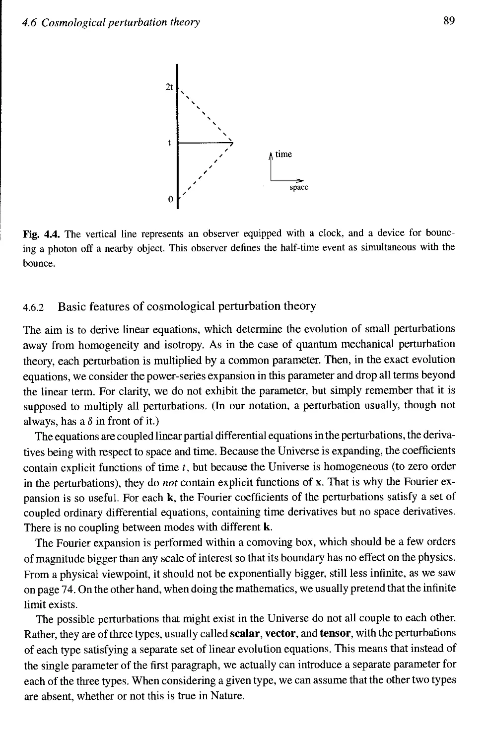
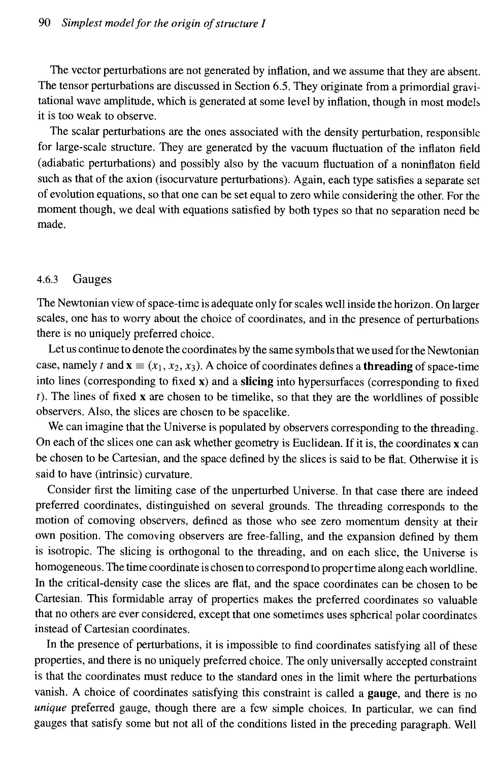
/
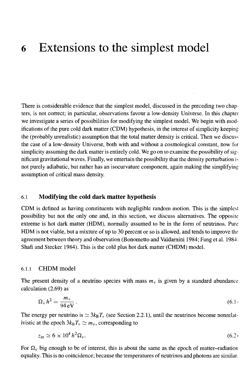

Author: Liddle A.R. Lyth D.H.
Tags: cosmological cosmological inflation
ISBN: 0-521-66022-X
Year: 2000


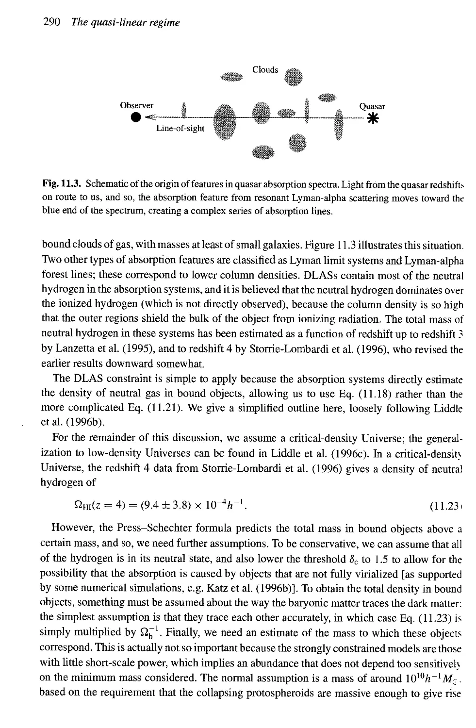
Text
Cosmological Inflation
and Large-Scale Structure
ANDREW R. LIDDLE
University of Sussex
DAVID H. LYTH
University of Lancaster
CAMBRIDGE
UNIVERSITY PRESS
PUBLISHED BY THE PRESS SYNDICATE OF THE UNIVERSITY OF CAMBRIDGE
The Pitt Building, Trumpington Street, Cambridge, United Kingdom
CAMBRIDGE UNIVERSITY PRESS
The Edinburgh Building, Cambridge CB2 2RU, UK http://www.cup.cam.ac.uk
40 West 20th Street, New York, NY 10011-4211, USA http://www.cup.org
10 Stamford Road, Oakleigh, Melbourne 3166, Australia
Ruiz de Alarcon 13, 28014 Madrid, Spain
© Cambridge University Press 2000
This book is in copyright. Subject to statutory exception
and to the provisions of relevant collective licensing agreements,
no reproduction of any part may take place without
the written permission of Cambridge University Press.
First published 2000
Printed in the United States of America
Typeface Times Roman 10/13 pt. System MeX 2e [tb]
A catalog record for this book is available from the British Library.
Library of Congress Cataloging in Publication Data
Liddle, Andrew R.
Cosmological inflation and large-scale structure / Andrew R.
Liddle and David H. Lyth.
p. cm.
Includes bibliographical references and index.
ISBN 0-521-66022-X
ISBN 0-521-57598 2 paperback
1. Inflationary universe. 2. Large scale structure (Astronomy)
I. Lyth, D. H. (David Hilary) II. Title.
QB991.I54L53 2000
523.1-dc21 99-14940
CIP
ISBN 0 521 66022 X hardback
ISBN 0 521 57598 2 paperback
Cosmological Inflation and Large-Scale Structure
This textbook provides graduate students with a thorough and up-to-date
introduction to the inflationary cosmology. Enormous progress has been
made in this area in the past few years and this book is the first to provide
a modern and unified overview. It covers all aspects of inflationary
cosmology - from the origin of density perturbations during the
inflationary epoch of the very early Universe, through the evolution of the
perturbations, up to the present for a range of possible cosmologies - and
carefully compares predictions with the latest observations, including
those of the cosmic microwave background, the clustering and velocities
of galaxies, and the epoch of structure formation. To help the student to
develop a thorough understanding, problems are provided at the end of
each chapter, and numerical answers and hints are included at the end of
the book.
With the host of international experiments being performed and
planned for the near future (including NASA's Microwave Anisotropy
Probe satellite and ESA's Planck mission), inflationary cosmology
promises to be one of the most exciting and fruitful topics of research in
science in the next decade. This book provides graduate students with the
ideal introduction.
Andrew Liddle is professor of astrophysics at the University of Sussex,
and has also worked as a lecturer at Imperial College, London. He
received his Ph.D. from the University of Glasgow in 1989 and has
published more than seventy-five papers in refereed journals, mostly on
the topics covered in this book. He travels widely in support of his
research, with collaborators in Europe, the United States, Canada, Japan,
and Australia.
David Lyth is a senior lecturer at the University of Lancaster. His
research career began in 1962 on what was then the very young subject of
particle theory. He is author of around 100 published papers and reviews.
He has played a leading role in several areas of particle cosmology,
especially inflation. Dr. Lyth has been a visiting fellow at the Isaac
Newton Institute at Cambridge University and a regular visitor to the
University of California at Berkeley.
To Amanda
and
to Margaret, John, and Duncan
Contents
Frequently used symbols page x
Preface xii
1 INTRODUCTION 1
1.1 This book 1
1.2 The Universe we see 2
1.3 Overview. From cosmological inflation to large-scale structure 4
1.4 Notes on examples 11
2 THE HOT BIG BANG COSMOLOGY 12
2.1 The expanding Universe 13
2.2 Epochs 18
2.3 Scales 23
2.4 The cosmic microwave background 26
2.5 Ingredients for a model of the Universe 27
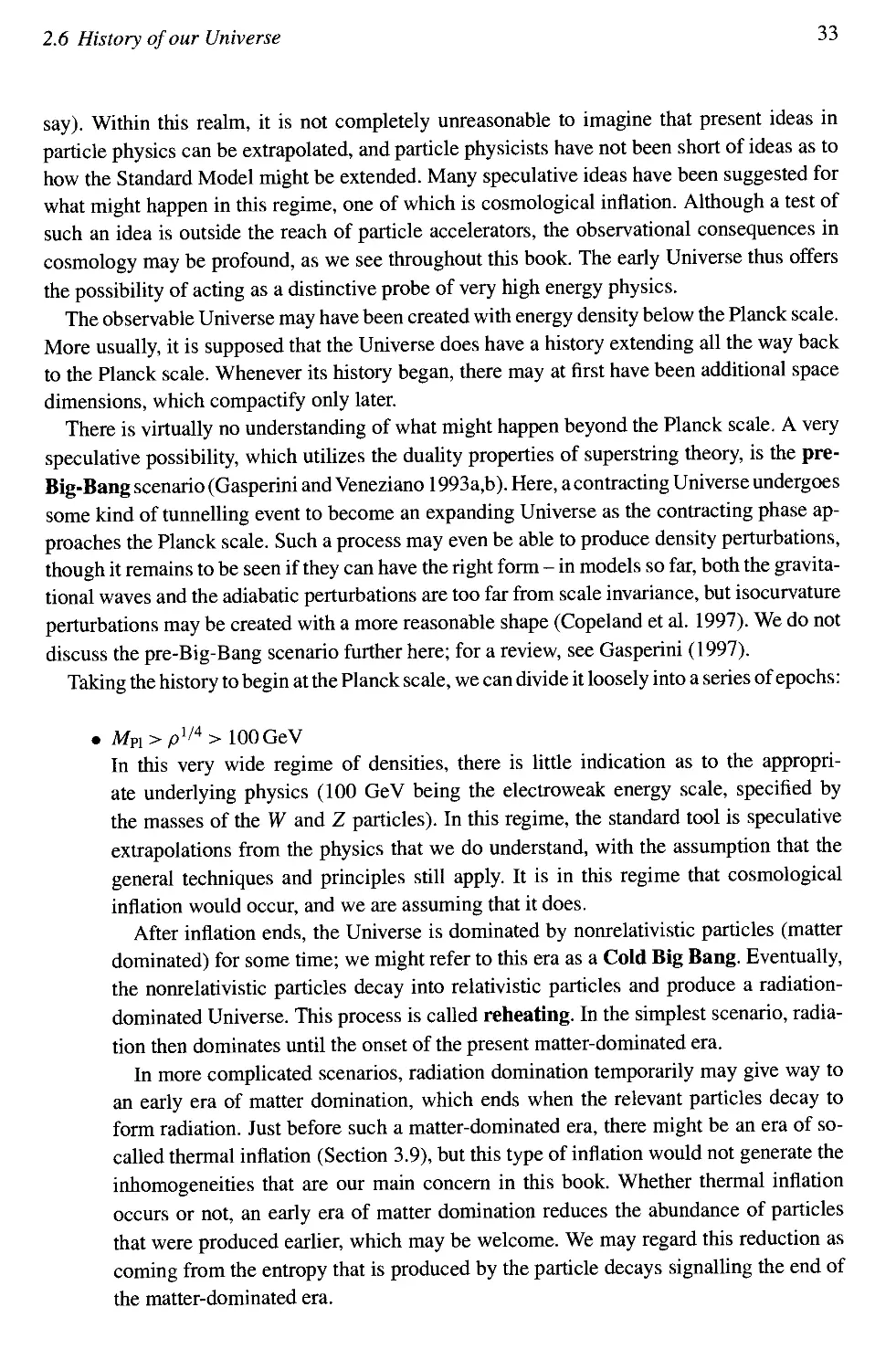
2.6 History of our Universe 32
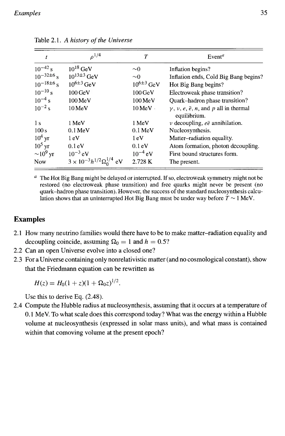
Examples 35
3 INFLATION 36
3.1 Motivation for inflation 36
3.2 Inflation in the abstract 38
3.3 Scalar fields in cosmology 40
3.4 Slow-roll inflation 42
3.5 Exact solutions 48
3.6 Hamilton-Jacobi formulation of inflation 50
3.7 Inflationary attractor 51
3.8 Reheating: Recovering the Hot Big Bang 53
3.9 Thermal inflation 55
Examples 56
4 SIMPLEST MODEL FOR THE ORIGIN OF STRUCTURE I 58
4.1 Introduction 58
4.2 Sequence of events 59
4.3 Gaussian perturbations 63
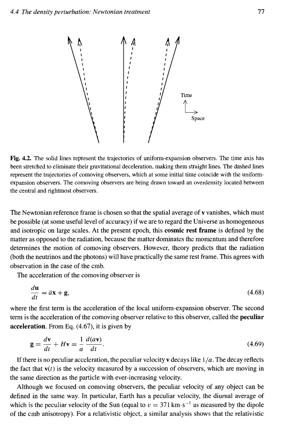
4.4 Density perturbation: Newtonian treatment 75
4.5 The Baryon density contrast: Newtonian treatment 84
4.6 Cosmological perturbation theory 87
4.7 Evolution equations 93
4.8 Outside the horizon 95
viii Contents
4.9 Peculiar velocity in the relativistic domain 102
Examples 104
5 SIMPLEST MODEL FOR THE ORIGIN OF STRUCTURE II 105
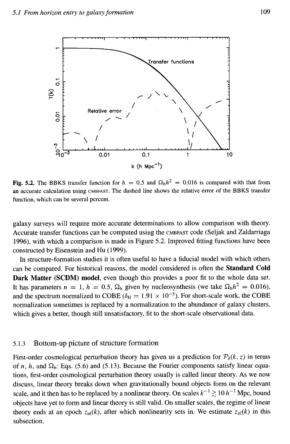
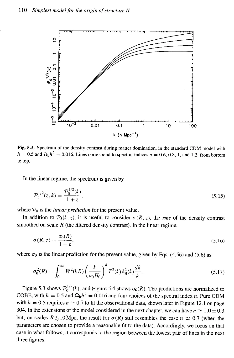
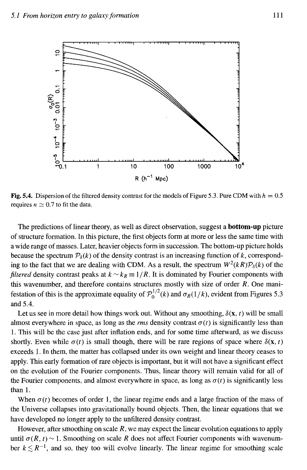
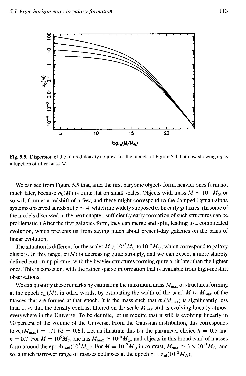
5.1 From horizon entry to galaxy formation 105
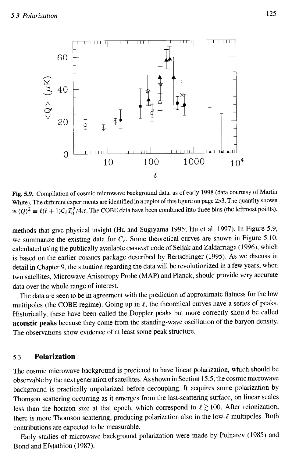
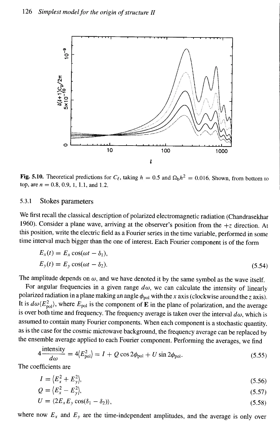
5.2 The cosmic microwave background anisotropy 115
5.3 Polarization 126
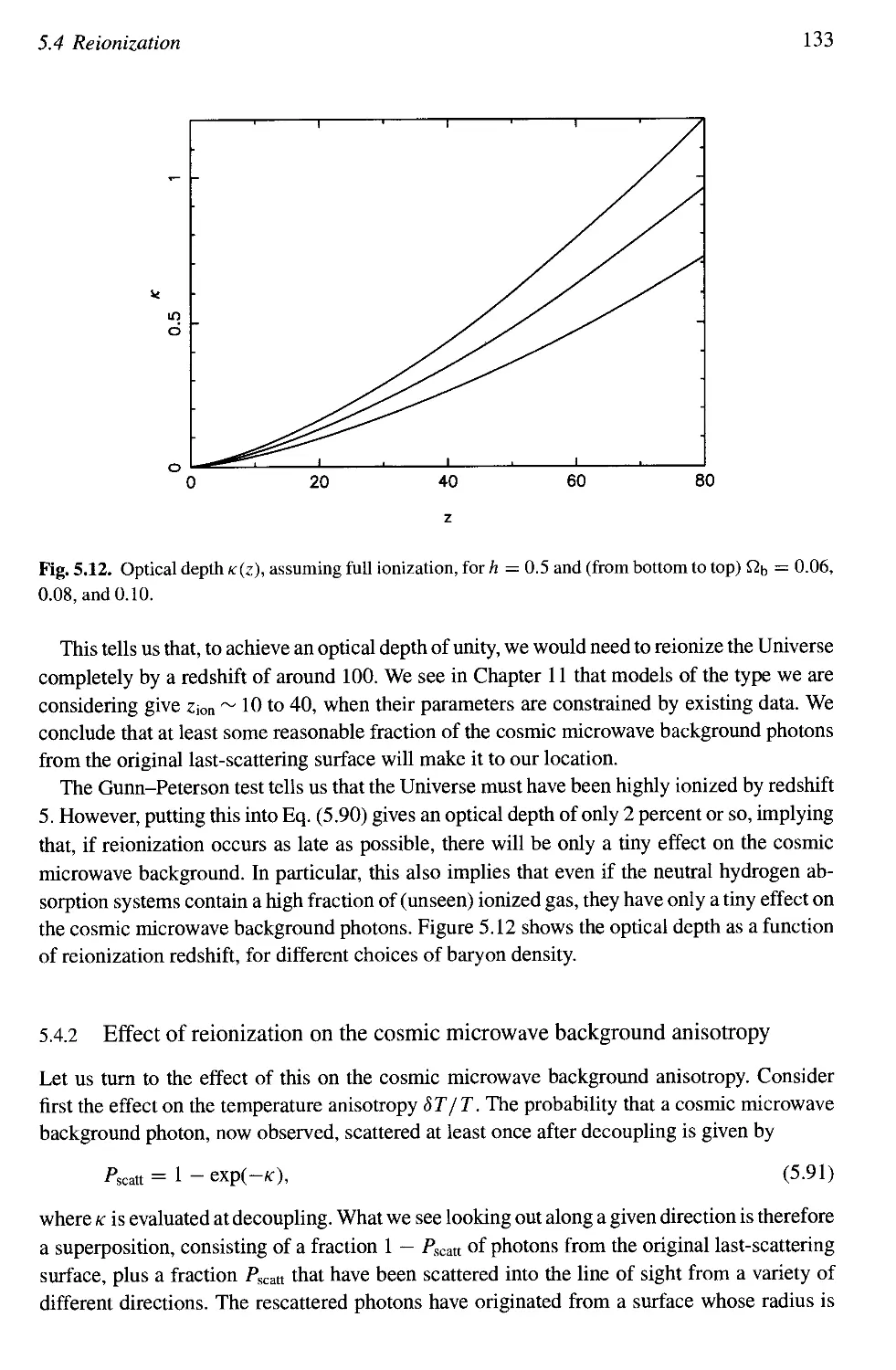
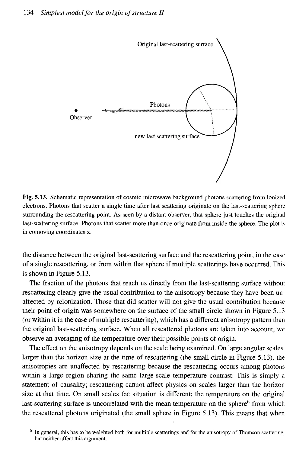
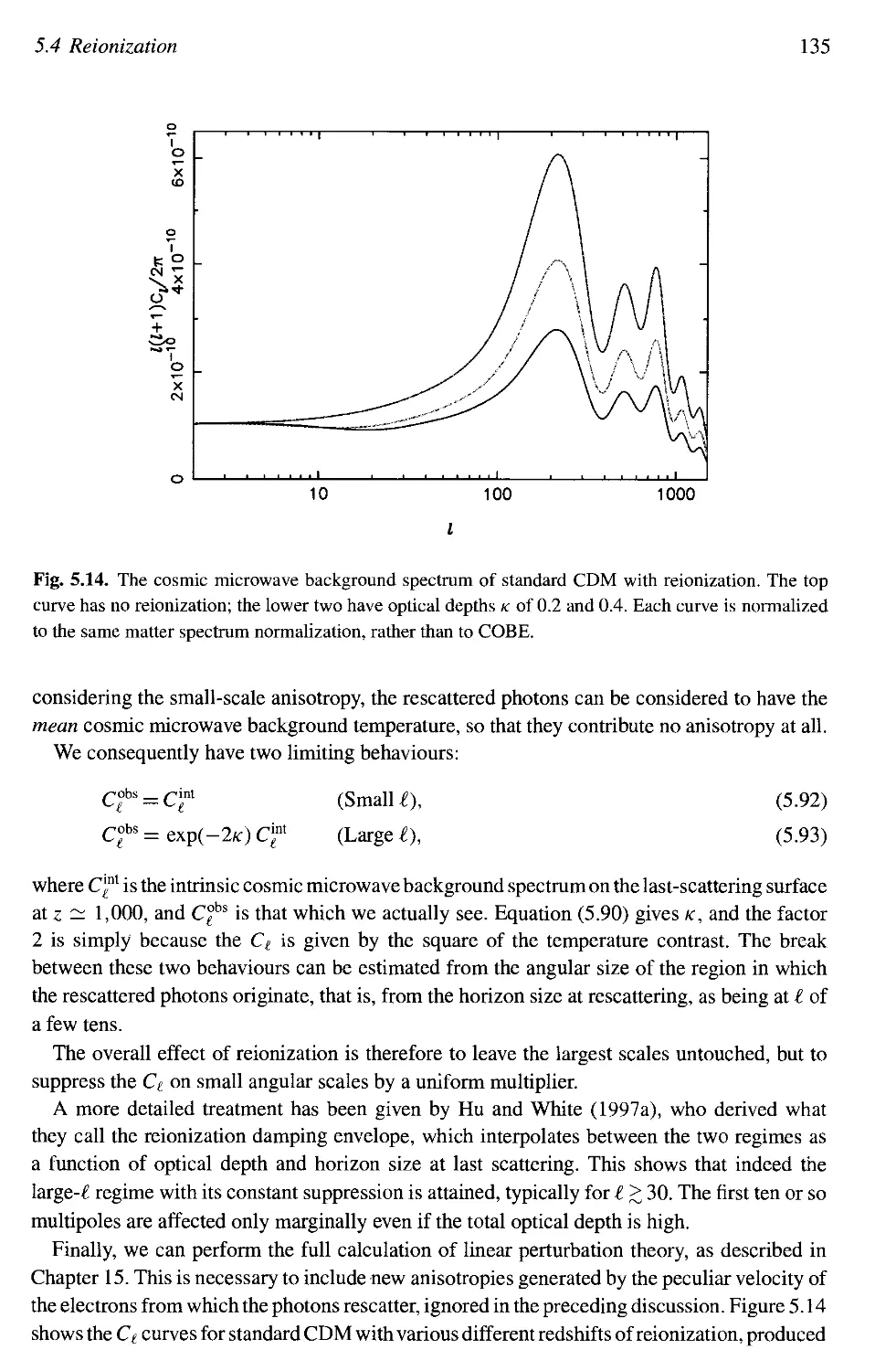
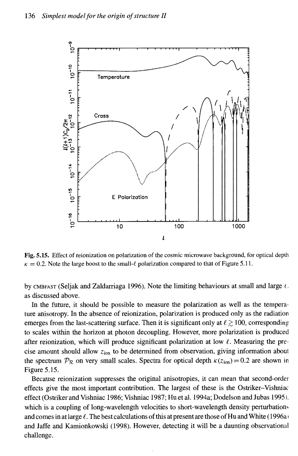
5.4 Reionization 130
Examples 137
6 EXTENSIONS TO THE SIMPLEST MODEL 138
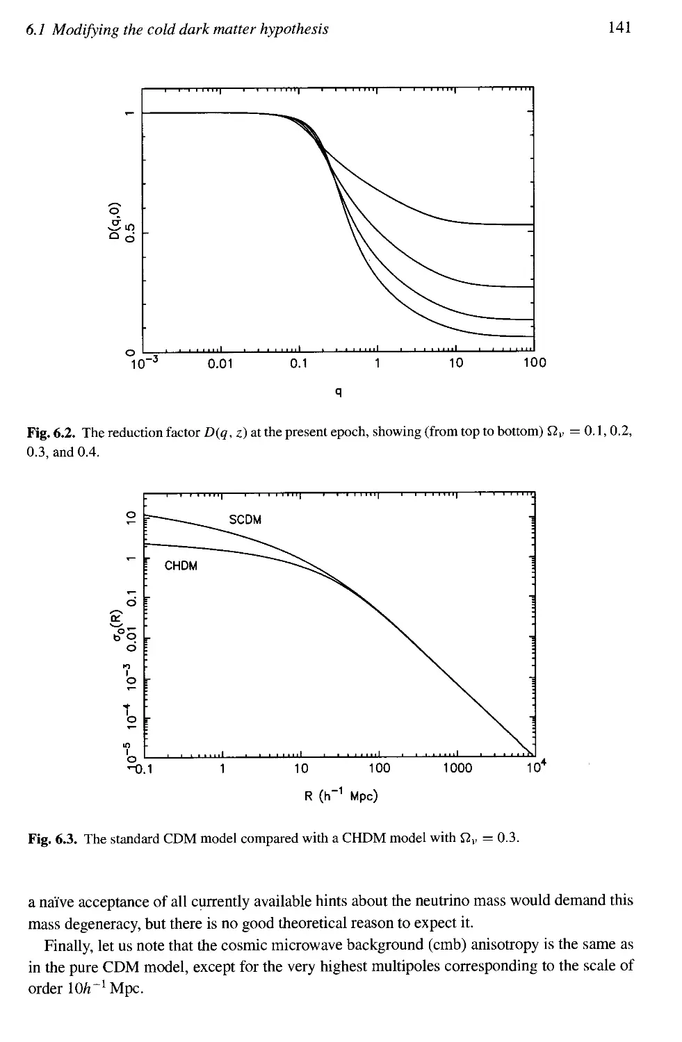
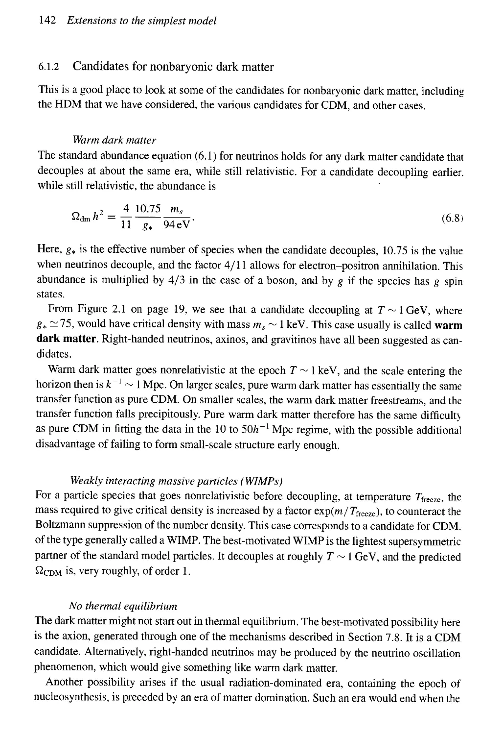
6.1 Modifying the cold dark matter hypothesis 138
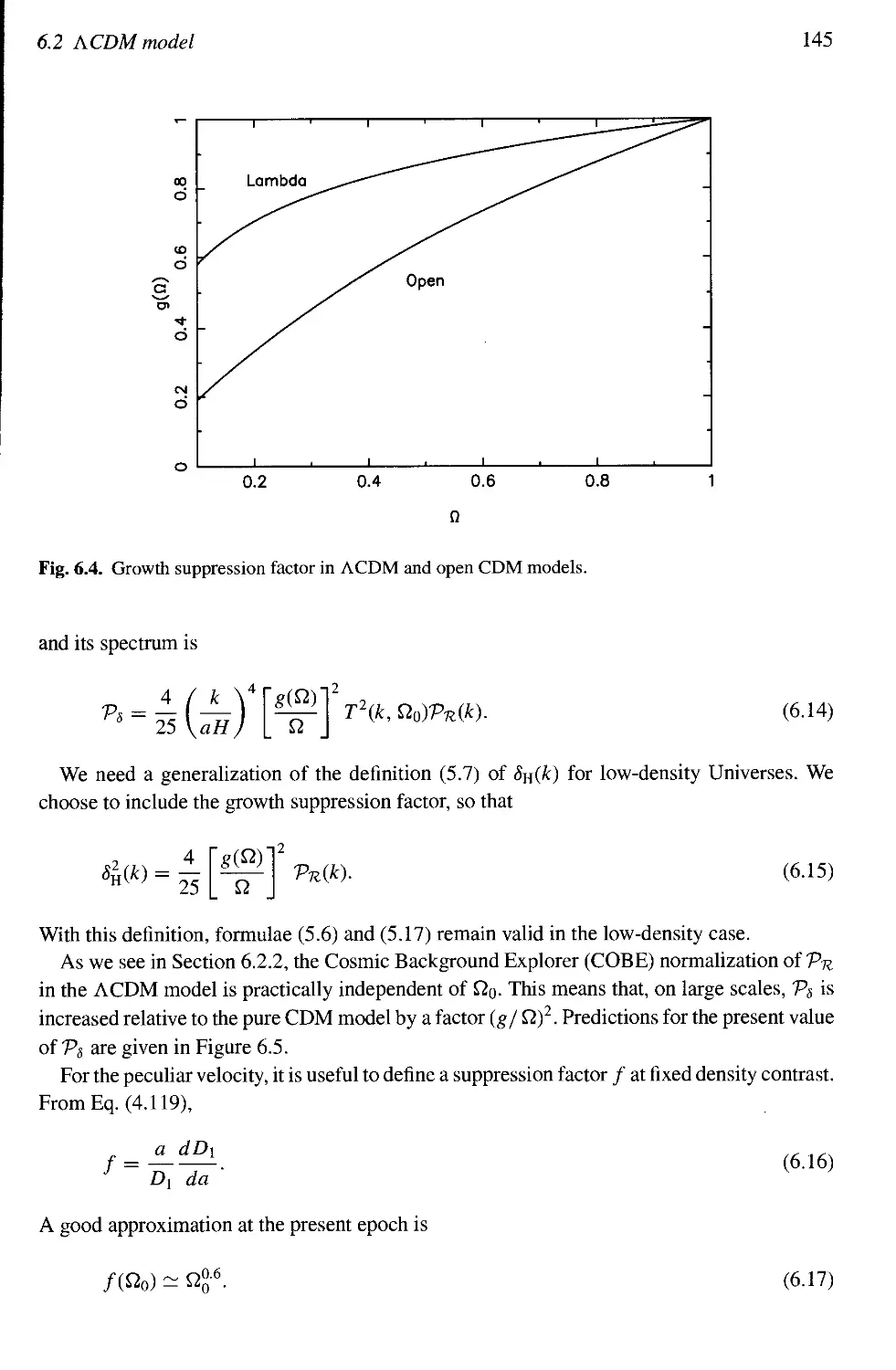
6.2 ACDM model 143
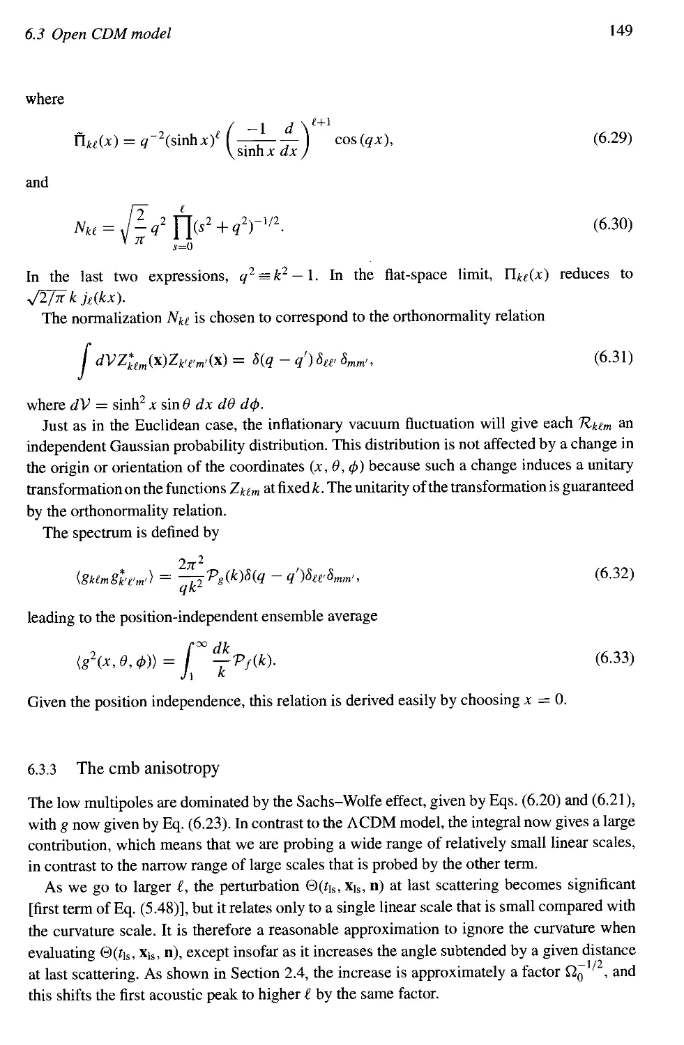
6.3 Open CDM model 147
6.4 Fine tuning issues 152
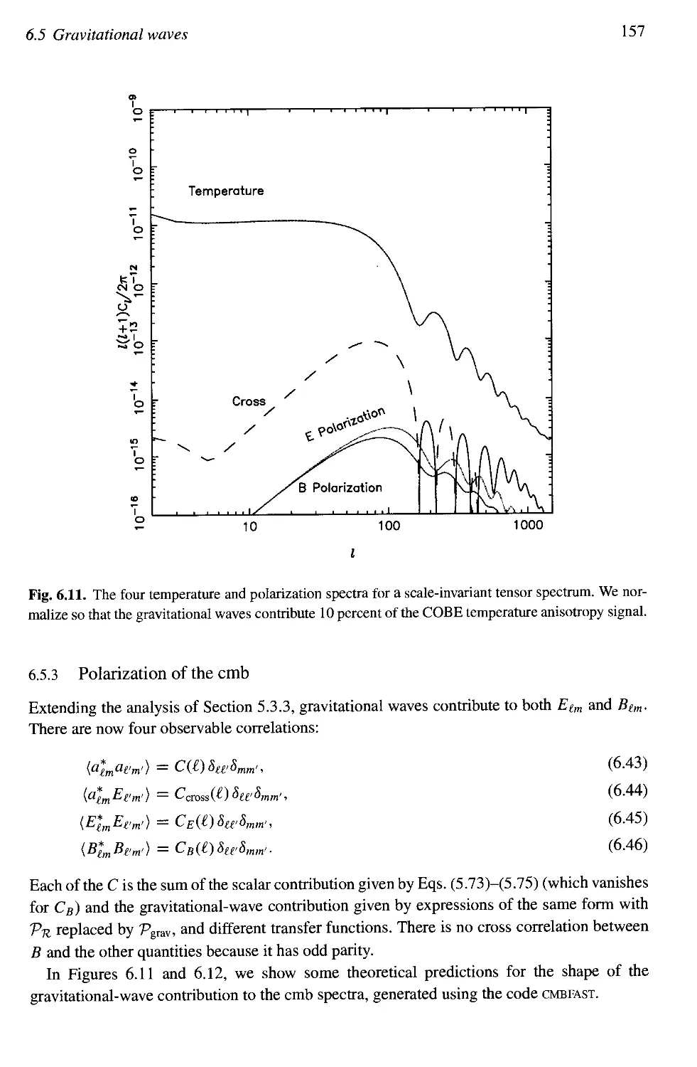
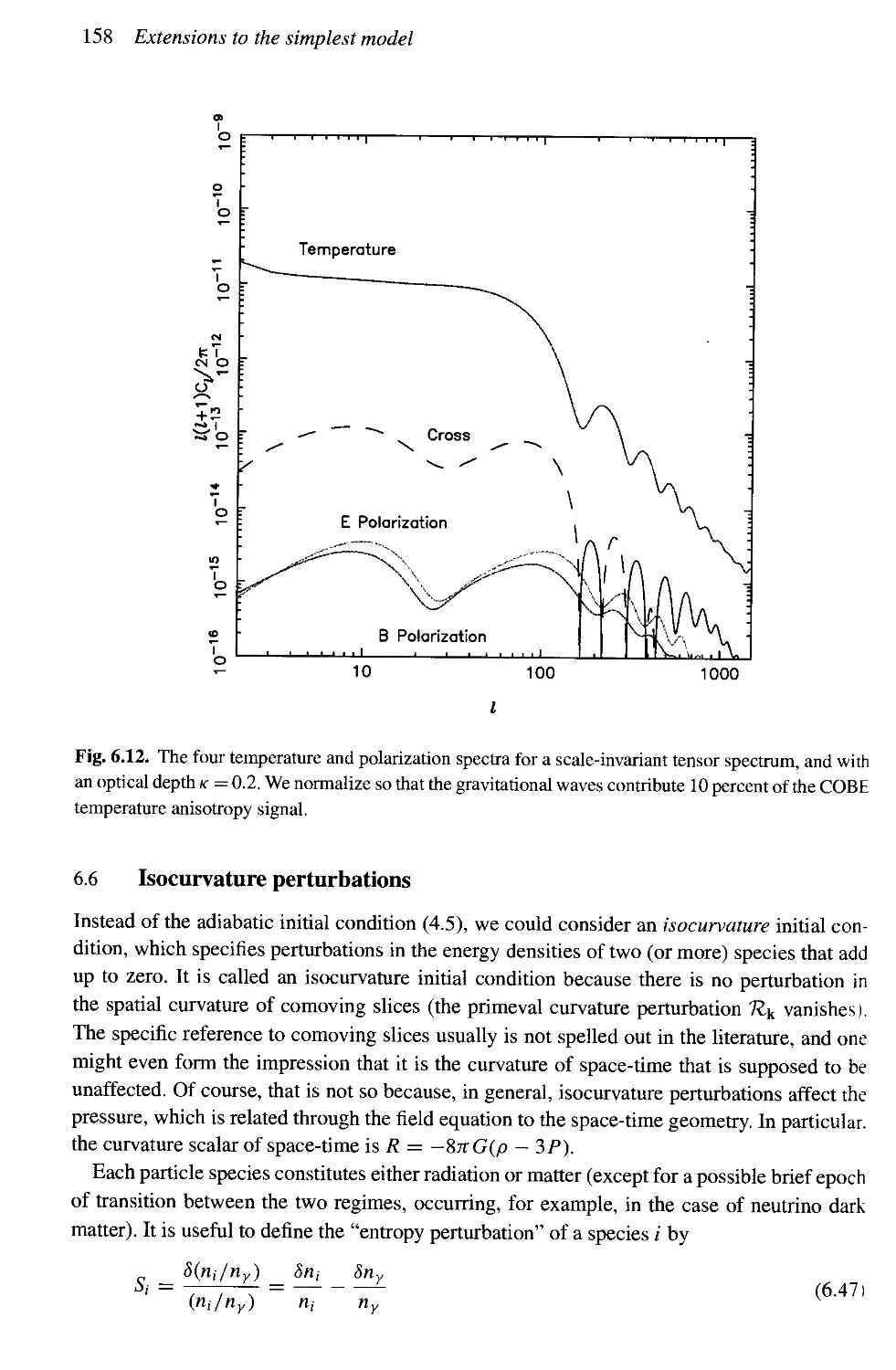
6.5 Gravitational waves 153
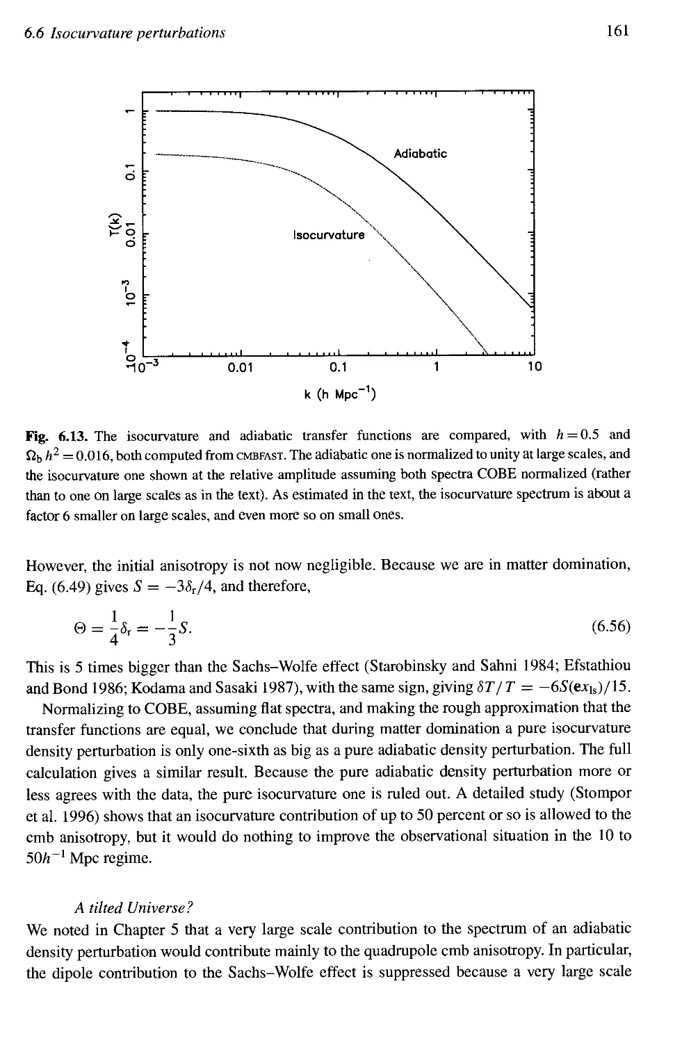
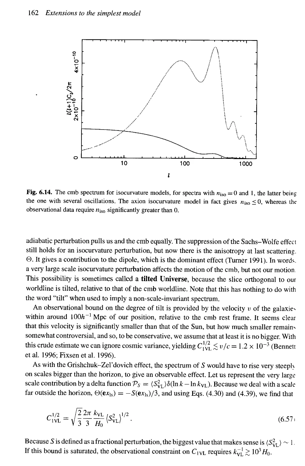
6.6 Isocurvature perturbations 158
Examples 163
7 SCALAR FIELDS AND THE VACUUM FLUCTUATION 164
7.1 Classical scalar field 164
7.2 Quantized free scalar field in flat space-time 168
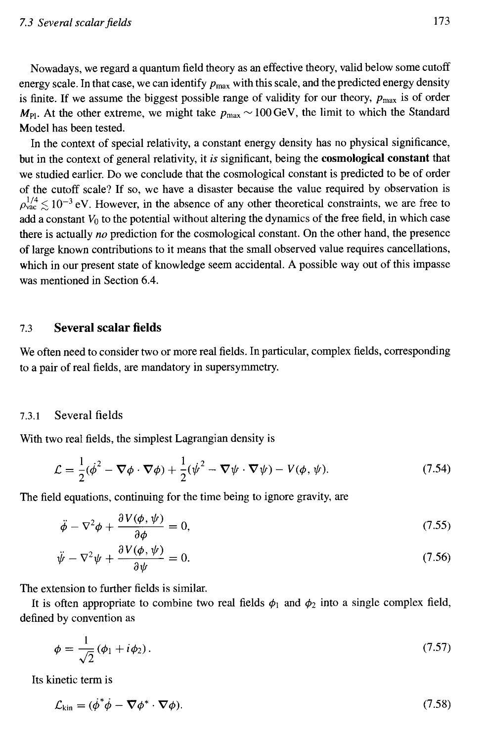
7.3 Several scalar fields 173
7.4 Vacuum fluctuation of inflaton field 177
7.5 Spectrum of the primordial curvature perturbation 186
7.6 Beyond the slow-roll approximation 189
7.7 Gravitational waves 193
7.8 Generating an isocurvature perturbation 195
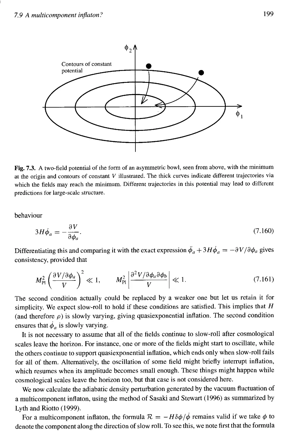
7.9 A multicomponent inflaton? 198
Examples 202
8 BUILDING AND TESTING MODELS OF INFLATION 203
8.1 Overview 203
8.2 Form of the scalar field potential 204
8.3 Single-field models 211
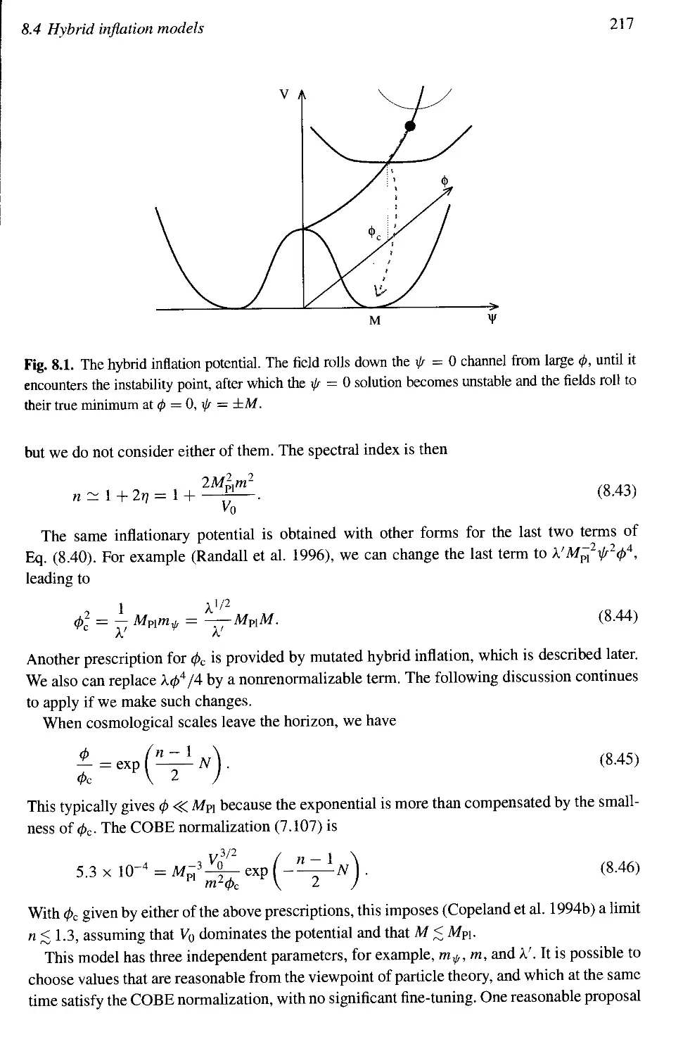
8.4 Hybrid inflation models 216
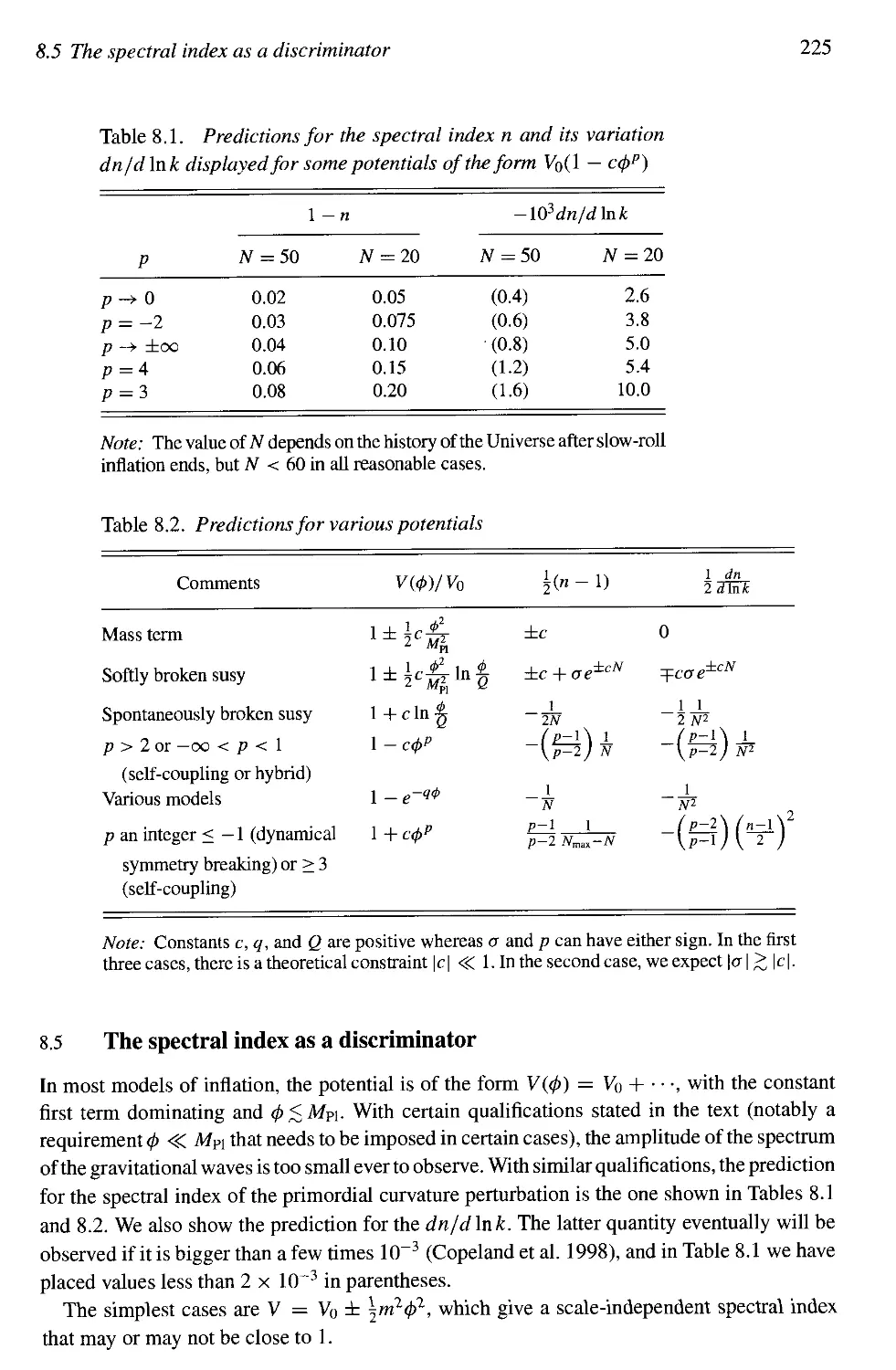
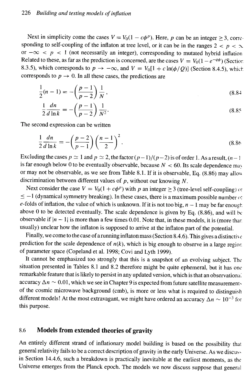
8.5 The spectral index as a discriminator 225
8.6 Models from extended theories of gravity 226
8.7 Open inflation models 236
Examples 243
9 THE COSMIC MICROWAVE BACKGROUND 244
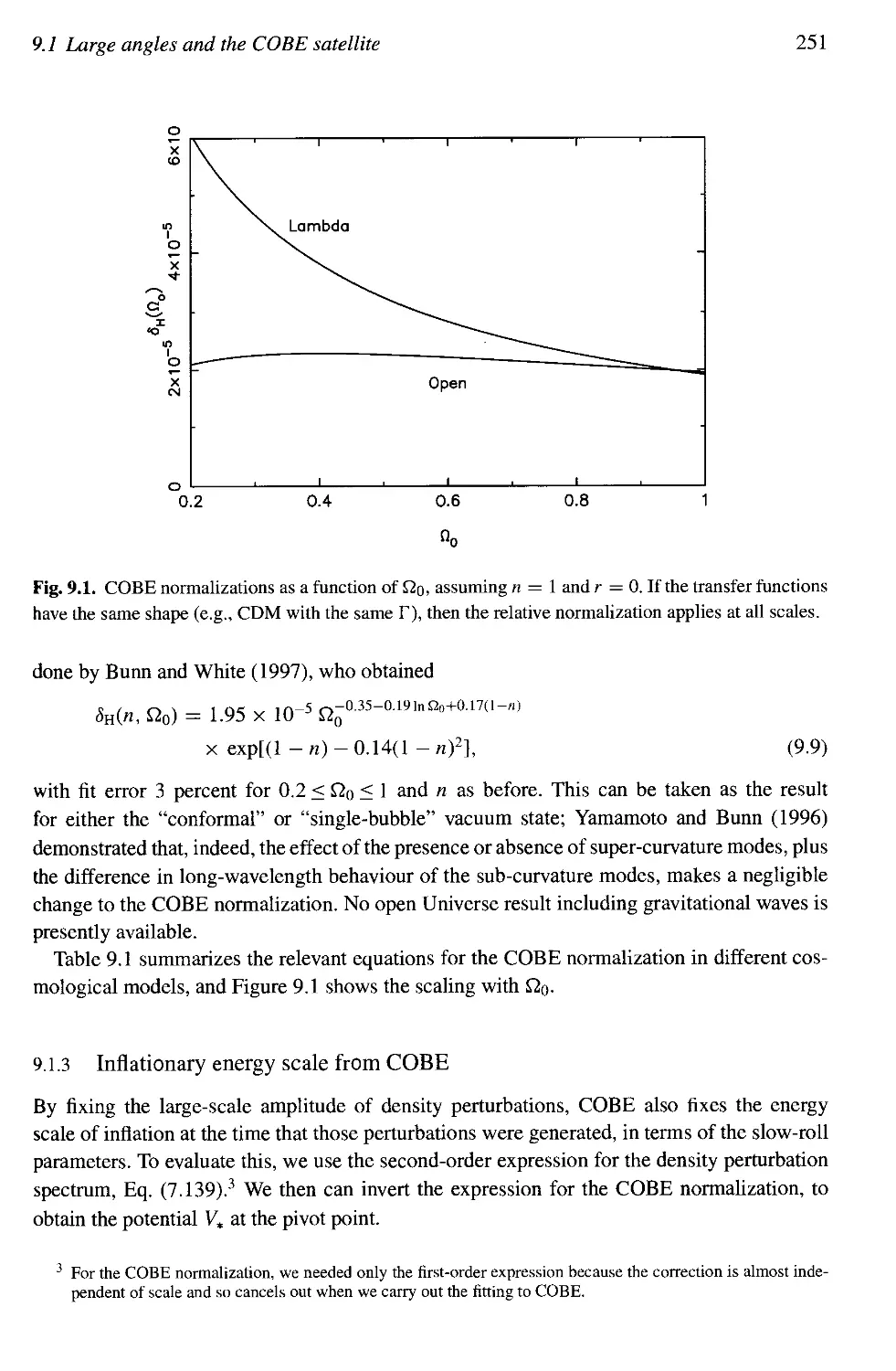
9.1 Large angles and the cosmic background explorer (COBE) satellite 244
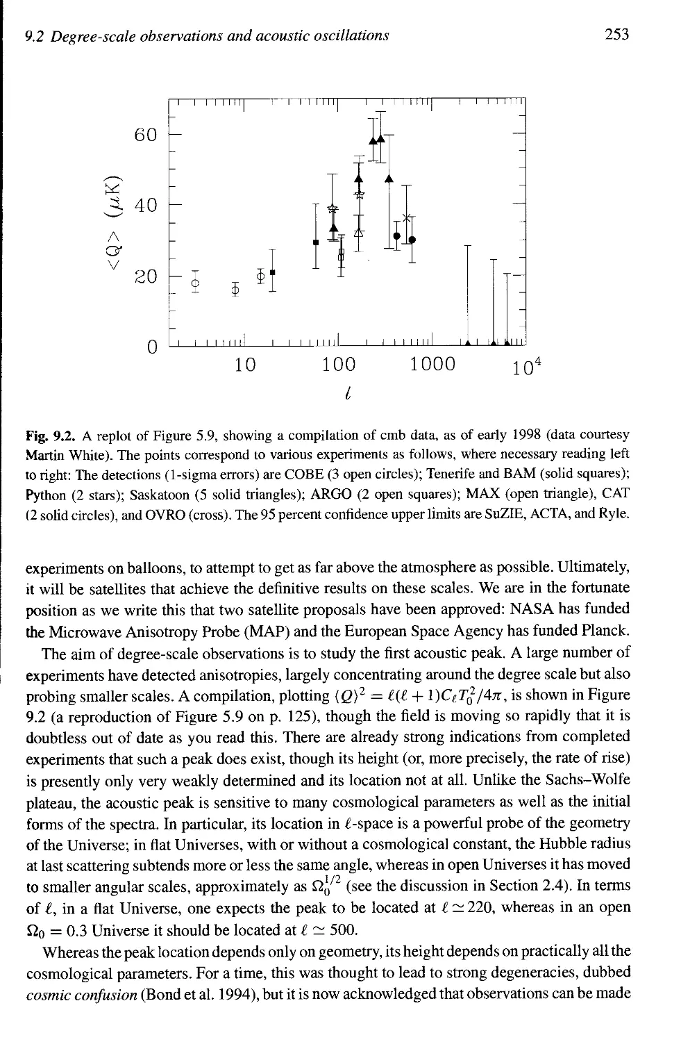
9.2 Degree-scale observations and acoustic oscillations 245
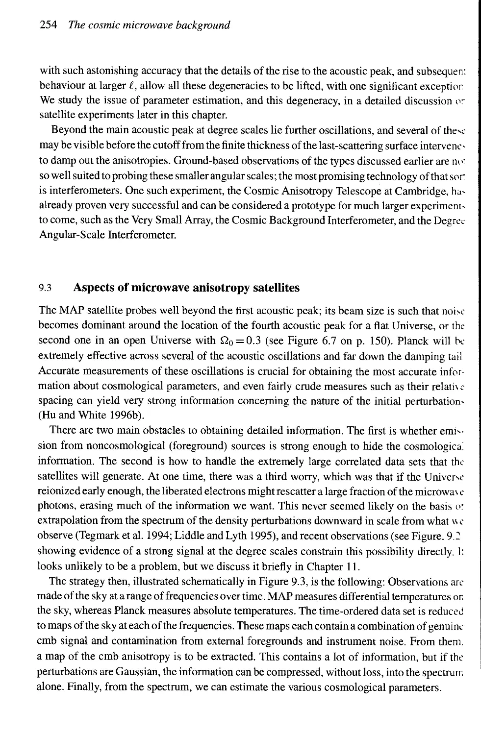
9.3 Aspects of microwave anisotropy satellites 254
Examples 261
10 GALAXY MOTIONS AND CLUSTERING 262
10.1 Clustering of galaxies 262
10.2 Galaxy velocities 270
Examples 276
Contents ix
11 THE QUASI-LINEAR REGIME 277
11.1 Gravitational collapse 277
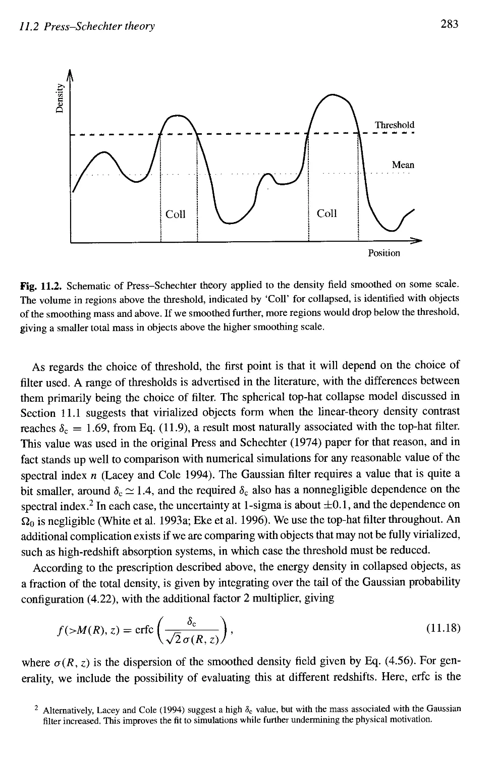
11.2 Press-Schechter theory 282
11.3 Theory of peaks 284
11.4 Numerical simulations 285
11.5 Applications of Press-Schechter theory 289
11.6 Reionization of the Universe 296
Examples 300
12 PUTTING OBSERVATIONS TOGETHER 301
12.1 Observations 302
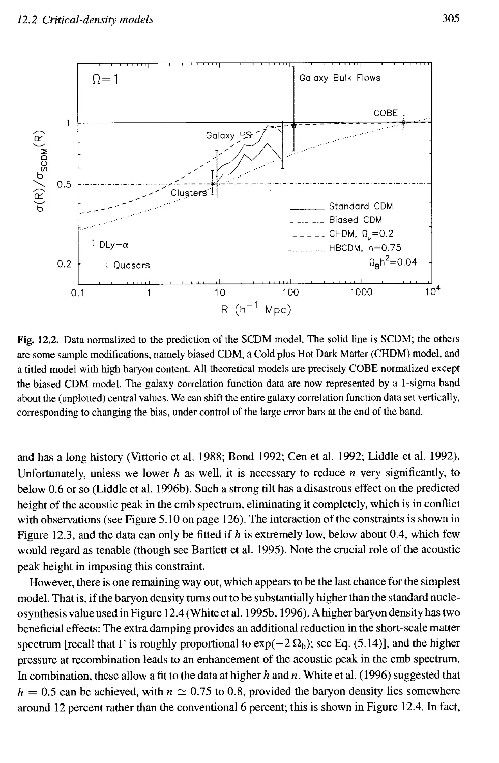
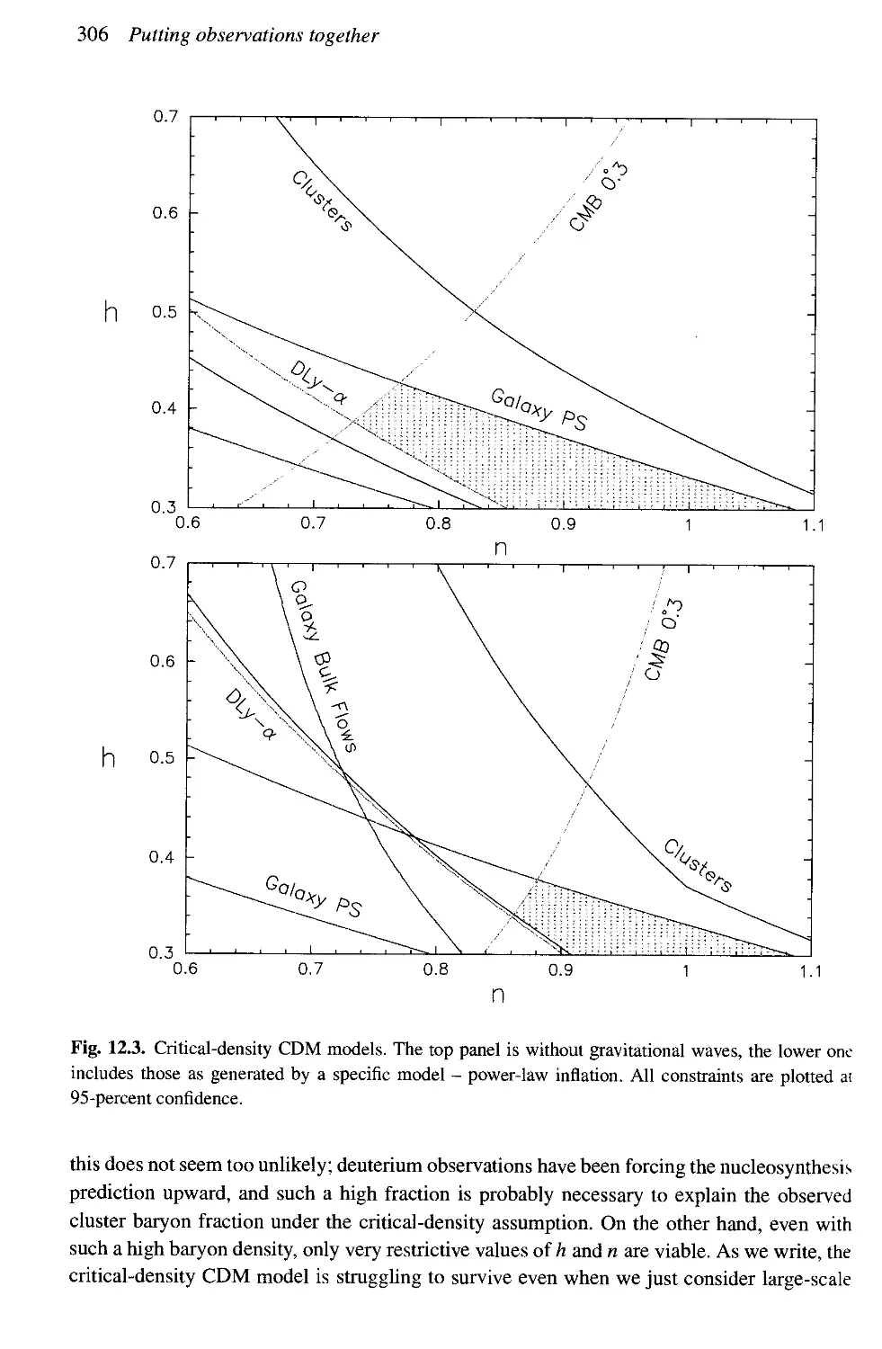
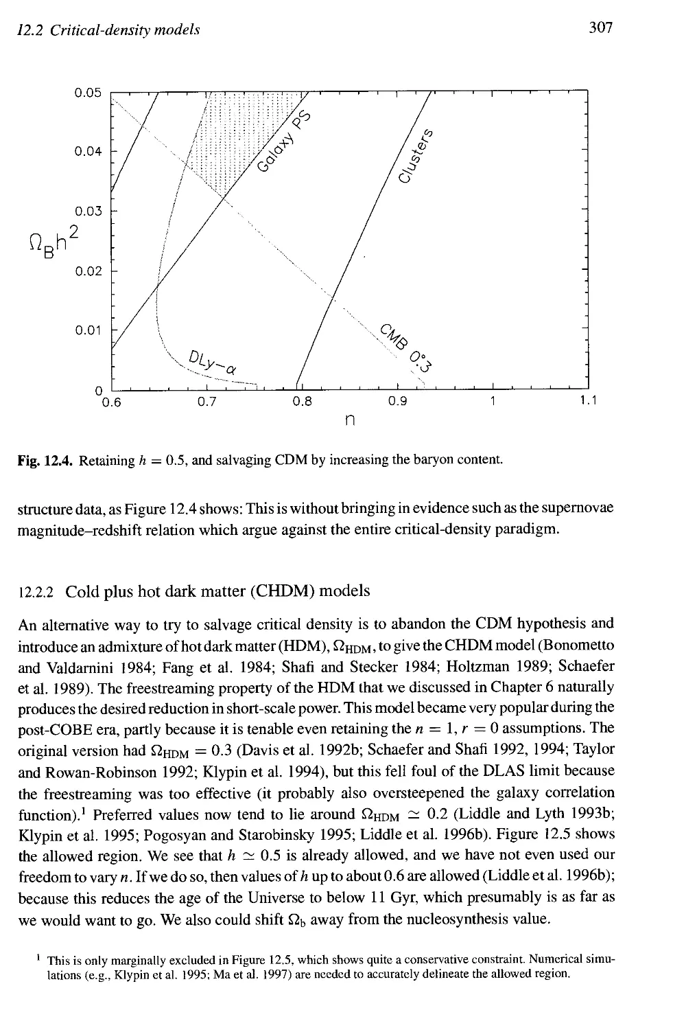
12.2 Critical-density models 304
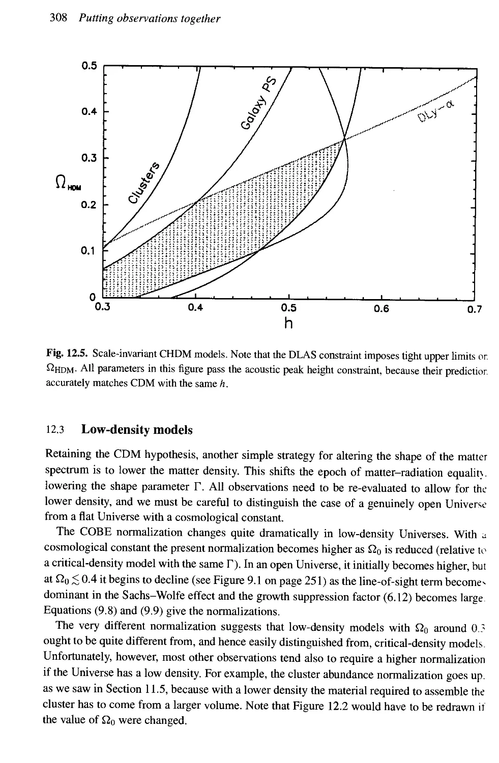
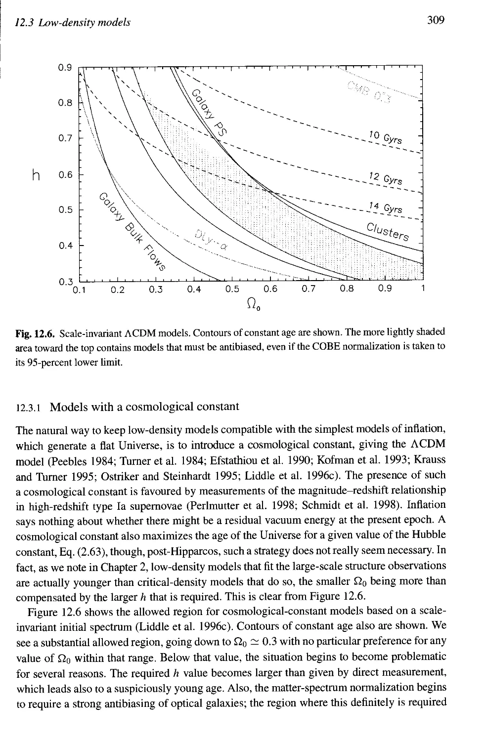
12.3 Low-density models 308
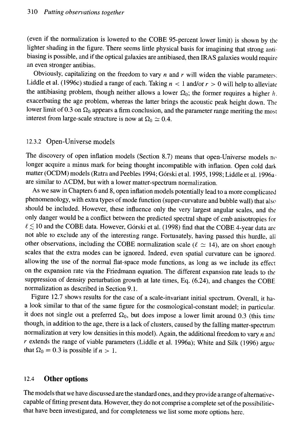
12.4 Other options 310
12.5 Summary 312
13 OUTLOOK FOR THE FUTURE 314
14 ADVANCED TOPIC: COSMOLOGICAL PERTURBATION THEORY 316
14.1 Special relativity 316
14.2 Fluid flow in special relativity 320
14.3 Special relativity using generic coordinates 323
14.4 General relativity 327
14.5 Cosmological perturbations 333
14.6 Evolution of the perturbations 341
Examples 347
15 ADVANCED TOPIC: DIFFUSION AND FREESTREAMING 348
15.1 Matter 348
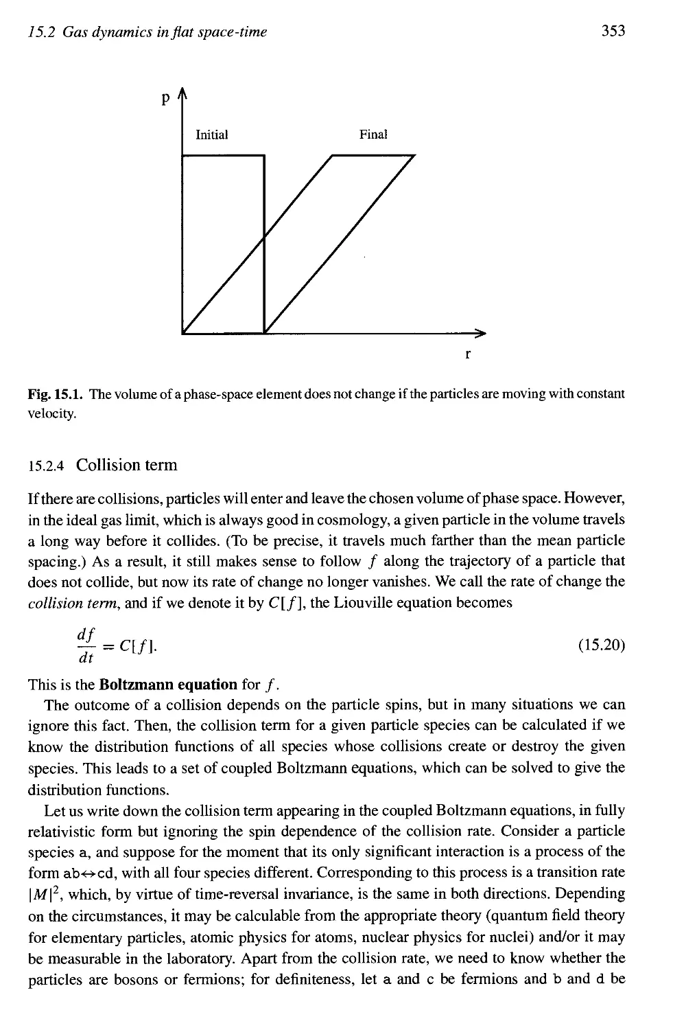
15.2 Gas dynamics in flat space-time 350
15.3 Gas dynamics in the perturbed Universe 356
15.4 Multipoles and the Boltzmann hierarchy 360
15.5 Polarization 364
15.6 Initial conditions and the transfer functions 368
Examples 371
Appendix: Constants and parameters 372
Numerical solutions and hints for selected examples 374
References 377
Index 393
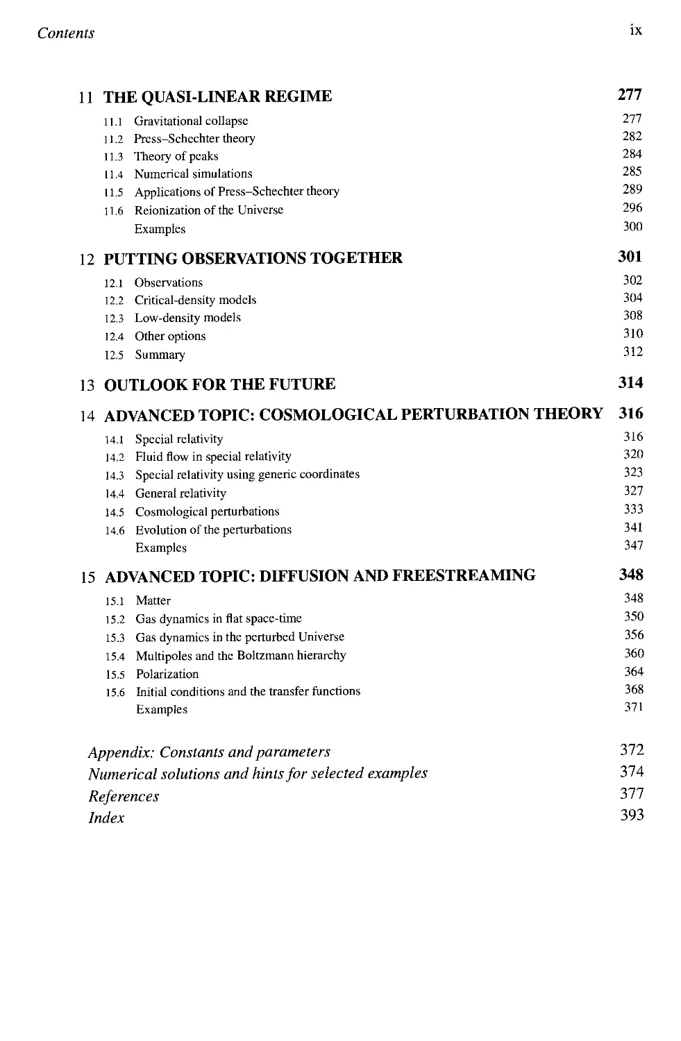
Frequently used symbols
Frequently used symbols and their place of definition
Symbol Definition Page
13
13
13
13,23
14
14
15
15
15
15
16
17
17
18
18,351
18
21
24
41
41
42
43
51
59
61
62
65
66
68
68
71
Mpi
G
a
t
X
H
H0,h
z
P,P
A
K
Pc
Q
T
n%
g*
w
1ior
4>
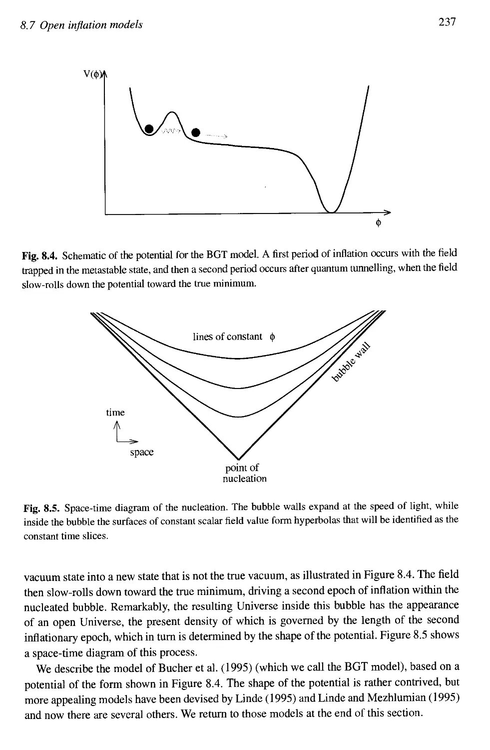
V((p)
e,r]
N
k
S
Tg(k)
Vg(k)
?,m
Ylm
W(kR)
Reduced Planck mass
(=2.436 x 10¹⁸ GeV)
Gravitational constant
Scale factor of the Universe
Time
Conformal time
Hubble parameter
Present Hubble parameter
Redshift
Density and pressure
Cosmological constant
Spatial curvature
Critical density
Density parameter
Temperature
Number density of any species g
Effective number of particle species
Pressure-to-density ratio (w = P/p)
Particle horizon distance
Scalar field
Scalar field potential
Slow-roll parameters
Number of e-foldings
Slow-roll parameters
Comoving wavenumber
Density contrast
Transfer function of any quantity g
Spectrum of any quantity g
Correlation function
Spherical expansion variables
Spherical harmonics
Window function
Continued
Frequently used symbols
XI
Symbol
n
V
<t>, *
V
cs
fpr
n
%(*)
r
Q
©
Q,U
E,B
K
«(«)
Wgrav
«iso
?
r
b,bi
Tjxv
Definition
Dispersion of any quantity g
Spectral index (density perturbations)
Peculiar velocity
Giravitational potentials
Peculiar velocity (irrotational part)
Sound speed
Proper time
Curvature perturbation
Anisotropic stress
Density perturbation amplitude
Cold dark matter transfer function
Shape parameter
Spectrum of the cosmic microwave
background anisotropy
Photon brightness function
Stokes' parameters
Polarization components
Optical depth
Growth suppression factor
Spectral index (gravitational waves)
Spectral index (isocurvature)
Action
Lagrangian density
Tensor-to-scalar ratio
Optical and infrared bias parameters
Stress-energy tensor
Page
72
75, 187
76
79, 101, 342
83, 338
84, 349
93,318
98, 341
101, 322, 337
106
107
108
116
123,359
126
128
131
144, 148
154, 193
159
164
165
193
264, 265
320, 331
Preface
The 1990s have seen substantial consolidation of theoretical cosmology, coupled with dramatic
observational advances, including the emergence of an entirely new field of observational
astronomy - the study of irregularities in the cosmic microwave background radiation. A key
idea of modern cosmology is cosmological inflation, which is a possible theory for the origin of
all structures in the Universe, including ourselves! The time is ripe for a new book describing
this field of research.
This book is based loosely on our 1993 Physics Reports article. We have widened the range
of discussion and have made much of the material more pedagogical. We believe that this book
will prove useful to starting graduate students in cosmology, to active researchers specializing
in the field, and to all levels in between.
Our view of the inflationary cosmology and its consequences has been influenced by many
people over the years. ARL especially thanks Alfredo Henriques and Gordon Moorhouse for
showing the way into this research area. DHL would like particularly to acknowledge a long-
term collaboration with Ewan Stewart. Much thanks is due to all our collaborators on the topics
within this book, namely Mark Abney, Domingos Barbosa, Tiago Barreiro, John Barrow, Marco
Bruni, Ted Bunn, Ed Copeland, Laura Covi, George Ellis, Mary Gaillard, Juan Garcia-Bellido,
Anne Green, Louise Griffiths, Ian Grivell, Rocky Kolb, Andrew Laycock, Jim Lidsey, Andrei
Linde, Anupam Mazumdar, Milan Mijic, Manash Mukherjee, Hitoshi Murayama, Paul Parsons,
Antonio Riotto, Dave Roberts, Leszek Roszkowski, Bob Schaefer, Franz Schunck, Douglas
Scott, Qaisar Shafi, Ewan Stewart, Will Sutherland, Michael Turner, Pedro Viana, David Wands,
Martin White, and Andrzej Woszczyna. Apart from our collaborators, we have had useful
conversations with many others, far too many to mention. We hope they know who they
are!
We are extremely grateful to Andrei Linde, Martin White, and especially Gordon Moorhouse
for their careful reading of the manuscript. The figures for Chapter 12 were made by Pedro
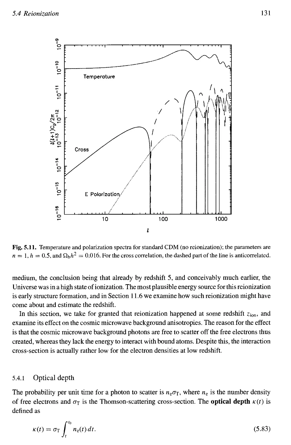
Viana, and the compilation of cosmic microwave background anisotropy data shown in Fig-
ures 5.9 and 9.2 was kindly provided by Martin White. Many figures were made using the
superb publically available cmbfast code (Seljak and Zaldarriaga 1996), which we strongly
recommend everyone to get.
Although we wrote most of the book at our home institutes, occasionally we were some-
where more glamorous. ARL would like to thank the Universita di Padova, the University of
New South Wales, and the Aspen Center for Physics, and DHL the University of California
at Berkeley. ARL acknowledges the generous support of the Royal Society throughout this
endeavour.
Preface
Of course, we have done our best to ensure that the contents of this book are accurate;
however, some errors may have slipped through. We would be very grateful if readers would
inform us of any they spot. We plan to keep an up-to-date record of any errors, accessible at
the book's World Wide Web Home Page at
http: //star-www. cpes. Sussex. ac. uk/~andrewl/inf book. html
which can be used to check for errors we already know about.
Andrew R. Liddle and David H. Lyth
October 1998
l Introduction
1.1 This book
The study of the early Universe came into its own as a research field during the 1980s. Though
there had been occasional forays during the seventies and even before that, it was during the
1980s that a wide range of topics, united by the adoption of modern particle physics ideas
in a cosmological context, were investigated in detail. This era of study culminated with the
publication in 1990 of the classic book The Early Universe by Kolb and Turner, in which
the authors described ideas across the whole range of what had become known as particle
cosmology or particle astrophysics, including such topics as topological defects, inflationary
cosmology, dark matter, axions, and even quantum cosmology.
Although all these topics matured during the 1980s, if we look back at the papers of that
era, we are struck by the rarity with which any detailed comparison with observations could be
made. In that regard, particle cosmology in the nineties and onward has become a very different
subject from what it was during the eighties because, for the first time, there are observations
of a quality that seriously constrains some of the possible physics of the early Universe. Those
observations are of structure in the Universe, and a starring role among them is played by the first
detection of microwave background anisotropies by the Cosmic Background Explorer (COBE)
satellite, announced in 1992. These were the first observations that could be more or less directly
interpreted as constraints on early Universe physics. As we will see, by the middle of the first
decade of the twenty-first century, we should have a wealth of data constraining our conceptions
of what may have occurred during the Universe's earliest stages, and, most likely, several of the
ideas described in Kolb and Turner's book will have been banished from serious discussion.
This book is not about particle cosmology as a whole, but rather is about a single topic,
inflationary cosmology, introduced in a seminal paper by Guth A981). This has been a research
field of lasting popularity; more papers have been written about inflation than any other area
of early Universe cosmology, and one of Guth's favourite transparencies in review talks charts
the rise of the publication count. Although introduced to resolve problems associated with
the initial conditions needed for the Big Bang cosmology, its lasting prominence is owed to a
property discovered soon after its introduction: It provides a possible explanation for the initial
inhomogeneities in the Universe that are believed to have led to all the structures we see, from
the earliest objects formed to the clustering of galaxies to the observed irregularities in the
microwave background.
Our aim is twofold. First, we wish to give a unified view of the entire process of modelling
the inflationary epoch, predicting the small irregularities that it generates, and evolving these
2 Introduction
irregularities using linear equations that are valid as long as the irregularities remain small. The
resulting theoretical structure, starting with the quantum fluctuations of a free field, continuing
with general-relativistic gas dynamics, and ending with the free fall of photons and matter, is
perhaps one of the most beautiful and complete in the entire field of physics. Certainly, it lies
at the opposite extreme from ad hoc models, not of course confined to physics, whose only
merit is sometimes to make the author feel better than if the desired result had been written
down immediately. Let us hope that the theory is true as well as beautiful!
Second, we wish to describe the state of the art, with respect to both inflation model-building
and the confrontation of theory with observation. In the former area, Kolb arid Turner's above
mentioned book and Linde's Particle Physics and Inflationary Cosmology were both written
in 1990, and since then, there have been many developments in the theoretical modelling
of inflation, including major shifts in the perception of which ideas are the most relevant.
Techniques for generating predictions for generic inflationary models also have come some
way during that period. The latter area is in the process of being revolutionized by observations
of the cosmic microwave background (cmb) anisotropy; the approval of two separate satellite
experiments, Microwave Anisotropy Probe (MAP) by the National Aeronautics and Space
Administration and Planck by the European Space Agency, to explore anisotropies down to
angular scales of a few arc-minutes promises data of a quality that will be hard to surpass
when it comes to constraining or excluding the inflationary cosmology. The rapid progress
in both areas means that we are providing something resembling a snapshot of the current
situation, though we believe that it will provide a useful orientation for at least some years to
come.
As mentioned already, our discussion focuses on the evolution of small irregularities. Be-
cause inflation ultimately is supposed to provide the origin of all structure, potentially any
measure of that structure can, in principle, be used to constrain inflation. This provides a
connection to a research area known variously as large-scale structure or physical cosmology,
which on its own is a much vaster research area than all of particle cosmology put together.
Much has been written on this topic; for example, four books produced after the crucial COBE
observations are those of Padmanabhan A993), Peebles A993), Coles and Lucchin A995),
and Peacock A999). By restricting ourselves almost entirely to the linear regime, our focus is
both narrower and deeper.
Incidentally, we use the phase "large-scale structure" to refer only to irregularities in mat-
ter density, such as the galaxy distribution and motions. The term usually does not include
microwave background anisotropies, the exception being the title of this book!
1.2 The Universe we see
Extensive discussion of the nature of the observed Universe has been given in the recent
textbooks just mentioned, and so, we will be brief in this introduction.
A description of our observed Universe can be broken into two parts: the global description
of the Universe, which is given in terms of a set of parameters that we call the cosmological
parameters, and the irregularities observed in the Universe.
1.2 The Universe we see
The cosmological parameters tell us about the geometry of the Universe, and about the mate-
rial contained within it. These parameters are defined in Chapter 2. The dynamics of an expand-
ing Universe are characterized by two quantities: the expansion rate, given by the Hubble para-
meter, and the spatial curvature. The latter, in fact, is determined by the amounts of different
types of material in the Universe. Direct observation shows that the Universe contains quite
a significant amount of baryonic matter, of which we are made, and also contains quite a bit
of radiation in the form of the cmb, which can be characterized by a thermal distribution at a
temperature Tq = 2.728 K. These are the only two forms of matter that are observed directly.
However, on the basis of standard particle physics, it is assumed that there is also a cosmic
neutrino background, contributing about the same energy density as the radiation. Beyond
that, there is substantial circumstantial evidence (though, as we write, no direct detection of
it) that the Universe contains a large (and probably dominant) amount of nonbaryonic dark
matter, of some as yet unknown form. The details of how the Universe, and particularly any
irregularities within it, will evolve depends on the nature of this dark matter. To get structure
formation models to work, it normally is assumed that there must be at least some so-called
cold dark matter, comprising particles with negligible velocity. However, there also may be a
component of hot dark matter (particles whose velocities are relativistic for at least some of
their evolution) or something more exotic yet. Another possibility, for which there is increasing
observational support, is that the Universe might possess a nonzero cosmological constant.
Determination of the various cosmological parameters is a key goal in cosmology, but one in
which much progress remains to be made. Of all those just listed, only the present microwave
background temperature is known to a satisfying level of accuracy. Other parameters, such
as the Hubble constant or the density parameter, remain the subjects of much controversy. In
Chapter 2, we briefly review the current observational status. We hope that, in the near future
(and for you the reader maybe even the recent past), the situation will become much more
definite; in particular, satellite measurements of cmb anisotropies promise to pin down many
of the cosmological parameters to a high degree of accuracy.
The second aspect of the observed Universe is the long-established realization that material
within it is distributed irregularly. Such irregularities are known as density perturbations.
An understanding of the origin and evolution of structure in the Universe is the outstanding
problem in cosmology at the moment, and this book is primarily about this topic in the con-
text of the inflationary cosmology. Measures of structure in the Universe now come from a
variety of sources. Historically, the distribution of galaxies was the most studied, popular-
ized though large galaxy redshift surveys such as the CfA survey in the mid-1980s. Nowa-
days, we have access to a much more diverse range of measures. The many observations of
anisotropies in the cmb, across a range of angular scales, tell us about structure in the Uni-
verse long ago when the microwave background was created. The velocities of galaxies can be
determined quite accurately, telling us about the gravitational attraction they experience. The
abundance of different types of object probes the size of the irregularities in the density of the
Universe - at the present epoch, clusters of galaxies are a useful probe, and the study of very
distant objects such as quasars can tell us about structure when the Universe was younger, as
can observations of distant galaxies with technology such as the Hubble Space Telescope and
the Keck telescope on Hawaii. All of these are discussed in Chapters 9 through 12.
4 Introduction
Within the context of inflation, all of these structures can be quantified by a small number
of parameters describing the initial perturbations, whose subsequent evolution is determined
by the cosmological parameters. Such parameters could be called the inflationary parame-
ters. They include as a minimum the overall amplitude and scale dependence of the density
perturbations; this might be, for example, a power law requiring two parameters that we aim to
fix through observation. In fact, the amplitude is already rather well determined by the COBE
satellite. In the simplest inflation models, this is all we need, but in more complicated versions,
some additional parameters might be necessary. If so, they too in principle can be determined
from observations.
1.3 Overview: From cosmological inflation to large-scale structure
This book can be divided loosely into four parts. In Chapters 2 and 3, we introduce the homo-
geneous Universe and the role that inflation plays in setting its initial conditions. The second
part, from Chapters 4 through 8, concerns the development of inhomogeneities in the Universe,
from their inception during inflation up to the present. The third part, from Chapters 9 through
13, concerns observations and the way in which they constrain the theoretical development in
the first eight chapters. This part ends with an overview. Finally, the last two chapters, separated
from the main flow of the book, give a more advanced treatment of inhomogeneities in the
Universe, including complete derivations of some results that were assumed for the simpler
treatment in the main body of the book.
1.3.1 Hot Big Bang cosmology
We begin our discussion proper in Chapter 2 with a rather rapid summary of the Hot Big
Bang theory. This sets down some of our notation and allows us quickly to summarize the
results that we use later. Anyone desiring a more leisurely account will find one in any of the
books mentioned in Section 1.1. We collect quite a range of different results; in particular,
we analyze low-density Universes, both with and without a cosmological constant, as well as
the case of a spatially flat Universe with a critical matter density. The last case is the simplest
but is disfavoured by observation; we show that there are both theoretical and observational
reasons for also considering the low-density cases. By contrast, there is little motivation from
either theory or observation to consider closed Universes, where there is greater than a critical
density of matter, and we do not concern ourselves with that situation.
1.3.2 Inflation
In Chapter 3, we move on to a discussion of inflationary cosmology (Guth 1981), looking at the
general properties rather than at specific models. The definition of inflation is extraordinarily
simple: it is any period of the Universe's evolution during which the scale factor, describing
the size of the Universe, is accelerating. This leads to a very rapid expansion of the Universe,
1.3 Overview: From cosmological inflation to large-scale structure
though perhaps a better way of thinking of this is that the characteristic scale of the Universe,
given by the Hubble length, is shrinking relative to any fixed scale caught up in the rapid
expansion. In that sense, inflation is actually akin to zooming in on a small part of the initial
Universe.
Inflation does not in any way replace the Hot Big Bang theory, but rather is an accessory
attached during its earliest stages. Inflation certainly cannot proceed forever; the great successes
of the Big Bang theory, such as nucleosynthesis (the formation of light elements) and the origin
of the thermal microwave background radiation, require the standard evolutionary progression
from radiation domination to matter domination, and it is assumed that inflation must end
some considerable time before that to allow generation of observed properties such as the
baryon-antibaryon asymmetry of the Universe.
As we see later, a sufficiently long period of inflation can resolve certain concerns about
the initial conditions necessary for the Big Bang cosmology to lead to a Universe such as our
own. In particular, it can explain why the Universe should be close to spatial flatness and why
it should appear homogeneous, at least on large scales. It was these problems that motivated
the original introduction of inflation by Guth A981); although accelerated expansion, in fact,
already had been considered, most notably by Starobinsky A980) but also much earlier, it was
the strong connection Guth made between rapid expansion and these problems that was the
true beginning of inflationary cosmology.
Nevertheless, these problems can no longer be regarded as the strongest motivation for
inflationary cosmology because it is not at all clear that they could ever be used to falsify
inflation. In fact, they have even been eroded to some extent; for example, it formerly was
thought that inflation necessarily gave a spatially flat Universe if it gave homogeneity, but
there now exist inflationary models that can give a homogeneous open Universe as well (see
Chapter 8). Linde in particular has been vocal (e.g., Linde 1997) in suggesting that the idea of
inflation as a theory of initial conditions may be very hard to exclude, and indeed only a few
possible observational signals, such as a global rotation of the observable Universe, would be
in conflict with inflation in this context (Albrecht 1997; Barrow and Liddle 1997).
By contrast to inflation as a theory of initial conditions, the model of inflation as a possible
origin of structure in the Universe is a powerfully predictive one. Different inflation models
typically lead to different predictions for the observed structures, and observations can discrim-
inate strongly between them. Future observations certainly will exclude most of the models
currently under discussion, and they are also capable of ruling out all of them. Inflation as
the origin of structure is therefore very much a proper science of prediction and observation,
meriting detailed examination. It is true that even if inflation fails as a model for structure
formation, one may be left with the possibility of inflation to fix the initial conditions and
some other mechanism for the origin of structure [topological defects being the only known
candidate, and a rather unpromising one at that; see Allen et al. A997) and Pen et al. A997)],
but if we learn that much, we have already learned a lot.
All the standard models of inflation are based on a type of matter known as a scalar field; scalar
fields are, among other things, thought to be responsible for the physics of symmetry breaking.
Particle physics has yet to offer a definitive view on the detailed properties of such fields and, in
particular, has not specified the potential energy, which, it turns out, is responsible for driving
6 Introduction
the inflationary expansion. The freedom exists to build a wide range of different inflationary
models, based on different choices of the potential energy and perhaps different motivations
for its particle physics origin. We reserve discussion of specific models until Chapter 8, to be
able to discuss them in relation to their predictions for structure formation. In Chapter 3, we
develop the machinery needed to deal with scalar fields in an expanding Universe, including
extensive discussion of an analytical scheme known as the slow-roll approximation, which is
used widely throughout the book. We also briefly discuss the end of inflation, an epoch known
as reheating, though its details are not important when considering structure formation from
inflation.
1.3.3 Simplest model of structure formation
The key idea in studying structure in the Universe is that of gravitational instability. Stated
simply, this notes that if the material in the Universe is distributed irregularly, then the overdense
regions provide extra gravitational attraction and draw material toward them, thus becoming
more overdense. That is, under the action of gravity, irregularities become more pronounced
as time passes. At the present epoch, we find that on moderate scales (e.g., less than 10
Mpc), the material in our Universe is very unevenly distributed, in the form of galaxies and
clusters of galaxies. On larger scales, it begins to appear homogeneous. On the other hand, at
very early times, as sampled by the cmb anisotropies, the Universe is distributed much more
evenly. Gravitational instability provides a mechanism to get from a fairly smooth distribution
at that time to the more irregular present Universe. It is a dramatic success that this simple
picture goes a long way to explaining what is observed, and current attention is focused
entirely on the details of the gravitational instability process. This depends on the nature of the
Universe as a whole, for example, on how rapidly it is expanding and on how much material
is in it to provide the gravitational attraction, and it also depends on the form of the initial
irregularities. As we see, inflation provides the most promising theory for the origin of these
initial irregularities.
The detailed study of cosmological perturbations is a highly technical topic, and we have
chosen to give a simplified treatment within the main body of the book, in order to keep
it at roughly the same technical level as the rest of the book. Ideas from general relativ-
ity are avoided as far as possible. From time to time, our simplified approach requires us
to quote and use results without proper mathematical justification. Because an understand-
ing of cosmological perturbations is so central to current developments in cosmology, we
also provide two advanced chapters, 14 and 15, at the end of the book. For readers who are
interested, these give a fully self-contained and mathematically rigorous general-relativistic
treatment of cosmological perturbations, in which all the results quoted within the book are
derived. These can be studied either in their own right or used to fill in the gaps of the earlier
discussion.
We begin our discussion of structure formation in Chapters 4 and 5 by setting up some
of the machinery for the description of perturbations in an expanding Universe. Our strategy
is to keep the discussion as simple as possible, and so we focus on the simplest model, the
1.3 Overview: From cosmological inflation to large-scale structure
cold dark matter (CDM) model. In this model the Universe contains a critical density of
material (making it spatially flat), all of the dark matter is cold, and the density perturbations
are of a type known as adiabatic. In these chapters, we carry out an analysis with minimal
reference to general relativity, really only needing the idea of a locally inertial frame in which
the laws of special relativity apply. Further, in certain circumstances perturbations on small
scales are amenable to a treatment using only Newtonian gravity. Here, small means relative
to the characteristic length scale of an expanding Universe, the Hubble length.
In these chapters, we do not concern ourselves with the origin of the perturbations, deferring
that until Chapter 7. We simply assume that there is an initial spectrum of perturbations that
can be taken to have power-law form. We discuss the statistical nature of the perturbations,
their description via their spectrum, and their evolution. This leads ultimately to predictions for
the present form of the perturbations, and for the anisotropies in the microwave background.
In addition to the temperature anisotropies, we discuss the polarization of the microwave back-
ground, which carries additional valuable information, as well as the effect on the microwave
background if the atoms in the Universe are reionized at some epoch well before the present,
enabling scattering of the microwave photons from the liberated electrons.
1.3.4 Extensions to the simplest model
Although theoretically the simplest scenario, a model in which the density is critical and all
dark matter is cold is not the only possibility, and we study extensions in Chapter 6. There is
considerable observational evidence that the density is less than critical, and the dark matter
need not all be cold. In particular, moving to a low-density Universe, either with or without a
cosmological constant, brings better concordance with large-scale structure observations.
Concerning the initial perturbations, an alternative to an adiabatic perturbation is an isocur-
vature perturbation, where the relative amounts of different materials are perturbed while
leaving the total density constant. However, this gives much larger microwave anisotropies for
a given size of density perturbation, and most likely cannot be the sole source of perturbations,
though they may accompany the usual adiabatic perturbation.
In Chapter 6, we also discuss gravitational wave perturbations. These are inevitable at some
level in all inflationary models. The amplitude of gravitational waves reduces rapidly once
they come within the Hubble length, and they can be important only on large angular scales
in the microwave background (those scales being larger than the Hubble radius at the time
the background was formed). As we write there is no way of telling whether a significant
fraction of the anisotropies that COBE sees are due to gravitational waves rather than density
perturbations, a possibility that has been given substantial attention in the literature [see Lidsey
et al. A997) for a review]. However, in most models of inflation, and in particular within the
context of a class of models known as hybrid inflation, the gravitational waves have a negligible
effect.
We do not consider magnetic fields, either their possible generation during inflation or
their possible effects on observations of structure such as early structure formation and the
polarization of the microwave background radiation.
8 Introduction
1.3.5 Scalar fields and the vacuum fluctuation
In Chapter 7 we carry out a detailed calculation of the density perturbations produced by
inflation. Inflation gives rise to irregularities in the Universe because we live in a quantum
world, not a classical one. Inflation is assumed to be driven by a scalar field and, classically,
the result of the accelerated expansion is to drive the observable Universe toward a state of
perfect homogeneity. However, in a quantum world, perfect homogeneity cannot be attained;
we are always left with some residual fluctuations in the scalar field. The typical size of these
fluctuations is a property of quantum mechanics, which means that they can be predicted using
standard techniques, as we demonstrate in detail in Chapter 7. In particular, they do not depend
on the initial conditions before inflation, and so, the theory is highly predictive.
It is an extravagant claim that quantum fluctuations, normally associated with microscopic
phenomena, can lead to structures such as clusters of galaxies. The quantum fluctuations
occurring in the space between you and this page certainly do not do anything of that sort.
And, although it is true that in the early Universe the quantum fluctuations are much bigger than
those we normally consider, because the timescales are so much shorter and the energy scales
higher, they still will turn out to be small in the sense of being only a very minor perturbation on
the classical behaviour. The crucial difference is rather that the Universe is accelerating, which
means that the quantum fluctuations can be caught up in the rapid expansion and stretched to
huge sizes, orders of magnitude larger than the Hubble scale, which sets the scale of causal
physics. Once the fluctuation is taken to such a large scale, it is unable to evolve and becomes
frozen-in; crucially, scales are pulled outside the horizon with such swiftness that the amplitude
has no chance to tend to zero, but instead is frozen-in at a fixed nonzero value.
In early work on inflationary perturbations, they normally were described as giving a type of
density perturbations known as a scale-invariant or Harrison-Zel'dovich spectrum (basically,
because physical conditions do not change much as perturbations on all relevant scales are
produced). Since then, observations have developed to such an extent that this approximation
can no longer be used, and must be replaced by something more accurate. For the observations
described in this book, it normally proves adequate to approximate the perturbations by a
power-law spectrum, with different inflation models leading to different spectral indices. Future
observations can measure the spectral index very precisely, and hence discriminate strongly
between different models of inflation.
By the same mechanism, inflationary models inevitably produce gravitational waves at some
level. In some models, these may be significant enough to be detectable.
Although the inflationary perturbations typically are calculated in terms of the scalar field
perturbation, this leads to a perturbation in the total energy density of the Universe, and hence
in the spatial curvature of the Universe. This last is the most useful when one comes to consider
how the perturbations will evolve; the scalar field is not useful because it decays long before
the present. In the standard scenario, where the perturbations are adiabatic, the perturbation
in the spatial curvature remains constant as long as the scale is larger than the Hubble length.
This allows us to evolve the perturbations forward in time until the Hubble length grows
to encompass them in the postinflationary Universe; for the scales of interest for structure
formation, this happens in the recent past, where the standard Big Bang model applies.
1.3 Overview: From cosmological inflation to large-scale structure
1.3.6 Models of inflation
The literature contains a large number of different models of inflation. A model of inflation
amounts to a choice for the potential of the scalar field (or fields) driving inflation, plus a means
of ending inflation. By this point in the book, we are able to predict the perturbations arising in
different models, using the results of Chapter 7, which enables a proper discussion to be made
in Chapter 8.
The main discussion focuses on two rather different paradigms. Throughout the early 1990s,
discussion was dominated by what we call single-field models. In these models, the scalar-
field potential often is chosen to be some convenient simple function, such as a monomial or
exponential, and the initial conditions are chosen such that the scalar field is well displaced from
any minimum (only obeying the condition that its energy density be less than the Planck energy,
where quantum gravity is thought to become important). In several such models, gravitational
waves may be produced at quite a significant level.
In the mid-1990s, however, this paradigm was challenged by a new wave of inflationary
model building, based on particle physics motivation such as the theories of supersymmetry,
supergravity, and superstrings. In the context of the last two of these, we do not expect inflation
to be possible for field values exceeding a Planck mass, regardless of whether the potential
energy there is larger than the Planck energy, because supergravity corrections tend to generate
a steep potential that is unable to sustain inflation. This consideration, among others, has led to
the popularity of a new class of models known generically as hybrid inflation, which rely on
interactions between two scalar fields and utilize the flat potentials expected in supersymmetry
theories. These models can give substantial inflation for a much more modest evolution of the
scalar field, remaining always much less than the Planck mass.
Although, as we write, the hybrid inflation models are a recent innovation under intense
investigation, we feel that they are the most important development in inflationary model
building for a considerable time, and we devote a large amount of space to them. If indeed they
secure their place as the modern inflationary paradigm, supplanting the single-field models
described earlier, they will lead to an important rethinking of the observational implications
of inflation. For example, in these models the gravitational wave production is expected to be
negligible.
We end our discussion of inflationary models with two less standard possibilities. First, we
briefly discuss models based on extended gravitational theories, the aim being to obtain the
scalar field driving inflation from the gravitational sector of the theory rather than from the
matter sector as we have assumed thus far. In most regards, however, these models are simply
a rewriting of the single-field inflation models, and share their drawbacks in comparison to the
hybrid scenarios.
Second, we discuss models of inflation leading to an open Universe. This was long thought
impossible, the belief being that, if a nonflat Universe was obtained it would show strong in-
homogeneities. However, it turns out that quantum tunnelling can lead to a homogeneous open
Universe. This is interesting because there is quite a lot of observational evidence supporting
low-density Universes, and it previously had been thought necessary to introduce a cosmolog-
ical constant to restore spatial flatness in order to be consistent with inflation. This is no longer
10 Introduction
the case; there is a whole class of inflationary models consistent with an open Universe. It is
even possible to realize the open inflation scenario within a hybrid inflation context.
1.3.7 Observations of structure
Having explored the theoretical side, we move on to comparison with observational data. This
retrospectively justifies the favoured models on which the earlier discussion focuses; they were
chosen, of course, to give a good representation of the observational data.
For the most part, we have sought to keep the discussion of specific observations short
because the observational situation doubtless will improve. The exception to this is the mi-
crowave background on large angular scales. The crucial COBE observations are the easiest
to interpret in the context of inflation, and they are also more or less definitive because, on the
largest angular scales, their accuracy is limited not by instrument noise, but by the statistical
uncertainty known as cosmic variance, arising from our having only a single microwave sky
to look at. Because the COBE experiment has reached its conclusion with the release of the
full four-year data set, the inflationary implications merit very detailed discussion and this is
done in Chapter 9.
In the future, it is expected that new microwave background anisotropy satellites will pro-
vide the best way to constrain cosmological parameters, including those describing the initial
perturbations. This is partly due to observational advances permitting a huge amount of useful
data to be taken, and partly because the theoretical interpretation is simple because it is all
linear perturbation theory. In anticipation of the future launch of the MAP and Planck satellites,
we make a detailed discussion of the prospects, also in Chapter 9.
Chapter 10 discusses galaxy motions and clustering. This material can be found in greater
detail in, for example, the books of Padmanabhan A993) and Coles and Lucchin A995). We
write at the commencement of two large galaxy redshift surveys - the 2dF survey and the Sloan
Digital Sky Survey - which will dramatically increase our knowledge of the geography of the
nearby Universe.
Chapter 11 is the only part of the book where we leave the linear regime, in order to discuss
the formation of gravitationally bound objects. Our main aim is to describe some of the methods
available to tackle this situation, the most prominent being the Press-Schechter theory, which
enables an estimate of the number density of objects as a function of their mass. The most
important constraint arising from this comes from the abundance of galaxy clusters, which
tightly constrains the spectrum on a scale of around 10 Mpc. In combination with COBE,
it leads to powerful conclusions, including the exclusion of the once-popular Standard CDM
model because it predicts far too many rich galaxy clusters. Press-Schechter theory also can be
used to estimate the abundance of high-redshift objects, such as quasars or the damped Lyman-
alpha systems seen in quasar absorption spectra. Finally, it can be used to say something about
when the Universe might have been reionized by radiation from the early stages of structure
formation; reionization that occurred sufficiently early, by a redshift of 20, for example, could
have quite a significant effect on microwave background anisotropies.
1.4 Notes on examples 11
Simply as an illustration, in Chapter 12 we combine observations from a range of sources.
This data compilation completes a circle in that it motivates a lot of the earlier discussion, in
particular, highlighting the failure of the Standard CDM model and indicating the most desirable
directions for modification. These detailed results doubtless will be superseded quickly, but
the general techniques for comparing theory and observation should continue to be useful. In
Chapter 13, we look toward the future.
1.3.8 Advanced topic: Perturbations in detail
We end the book with an advanced treatment of cosmological perturbations. The technical
level in these chapters is some way beyond that of the rest of the book, which is why we have
located this material away from the main flow, but the topic is of such central importance to
modern cosmology that we felt its inclusion imperative. These chapters use the full formalism
of general relativity and fully justify some of the results used, but left unproven, in Chapters
4 through 6.
The formalism set up is necessary for the computation of the present matter and radiation
spectra to sufficient accuracy to compare with presently available observations. Fortunately, to
work in these research areas, it is not necessary to understand fully their complexity because
there exist fitting functions and publically available computer programs [e.g., cmbfast by Seljak
and Zaldarriaga A996)] that can carry out these tasks. These can be treated as a black box -
you feed in the input and out comes the desired answer. Such tools are vital for the day-to-day
task of carrying out research in cosmology.
1.4 Notes on examples
Most chapters end with a few examples to allow the reader to practice applying the information
given within the chapters. Several of these examples require some simple numerical calcula-
tions for their solution; in cosmology these days, it is practically impossible to avoid carrying
out some numerical work at some stage. A typical task is the numerical computation of an
integral that cannot be done analytically, or the evaluation of some special functions. These
can be done via specially written programs, using library packages [e.g., Numerical Recipes
by Press et al. A992), which is also an invaluable source of general information on scientific
computation], or a computer algebra package such as Mathematica or Maple.
At the end of the book, we list numerical answers to the examples as well as provide some
hints as to how we think they should be solved.
2 The Hot Big Bang cosmology
The central premise of modern cosmology is that, at least on large scales, the Universe is
homogeneous and isotropic.1 This is borne out by a variety of observations, most spectacularly
the nearly identical temperature of microwave background radiation coming from different
parts of the sky. Despite the belief in homogeneity on large scales, it is all too apparent that
in nearby regions the Universe is highly inhomogeneous, with material clumped into stars,
galaxies, and galaxy clusters. It is believed that these irregularities have grown over time,
through gravitational attraction, from a distribution that was more homogeneous in the past.
It is convenient then to break up the dynamics of the Universe into two parts. The large-
scale behaviour of the Universe can be described by assuming a homogeneous and isotropic
background. On this background, we can superimpose the short-scale irregularities. For much
of the evolution of the Universe, these irregularities can be considered to be small perturbations
on the evolution of the background Universe, and can be tackled using linear perturbation
theory; we discuss this extensively, starting in Chapter 4. It is also possible to continue beyond
the realm of linear perturbation theory, via a range of analytic and numerical techniques, which
we discuss only briefly, in Chapter 11. In this chapter and the next, we concern ourselves solely
with the evolution of the background, isotropic Universe. This usually is called the Robertson-
Walker Universe, often with Friedmann and occasionally with Lemaitre also named.
Acornerstone of modern cosmology is the theory of nucleosynthesis (Pagel 1997; Schramm
and Turner 1998), explaining the primordial abundance of the very light elements. It relies on
the Hot Big Bang model of the Universe, and its success assures us that the model gives
an essentially correct description of the Universe starting at some epoch before (though not
necessarily long before) nucleosynthesis takes place. The Hot Big Bang model is described in
many books (e.g., Kolb and Turner 1990; Padmanabhan 1993; Peebles 1993; Coles and Lucchin
1995). Starting at some epoch well before nucleosynthesis, the Universe consists of a hot gas,
which cools with the expansion of the Universe. It has several components, corresponding to
the various particle species present, among which are the photons now observed as the cosmic
microwave background radiation. At first the energy density is dominated by the relativistic
particle species (including photons), collectively termed radiation, and later it is dominated
by the nonrelativistic species, termed matter.
1 By Universe, strictly speaking, we mean the region around us that can be explored by observation, limited by the
distance that light has been able to travel. We have no certain knowledge of more distant regions because light
from them is still on its way toward us. It is certainly reasonable to expect homogeneity and isotropy to persist
for quite some distance, but there is no reason why it should persist indefinitely and, as we see in Chapter 7,
there exist eternal inflation models saying that it definitely does not.
2.1 The expanding Universe 13
In sharp contrast to this well-defined picture, we have no certain knowledge of the Universe
well before nucleosynthesis. According to current thinking, based on the Standard Model2 of
particle physics and its most commonly considered extensions, the Universe is gaseous back
to some very early epoch, except possibly at brief phase transitions. In a loose sense, this entire
gaseous era often is termed the Big Bang, the adjective Hot now being omitted because it need
not be in thermal equilibrium or dominated by radiation. Before this, there is thought to have
been an era of inflation, during which the energy density of the Universe was dominated by
the potential of the scalar fields. Inflation is supposed to determine the initial conditions for
the Big Bang, including the perturbations.
In this chapter, we give some basic results for the Robertson-Walker Universe, focusing
particularly on the Hot Big Bang and the subsequent matter-dominated era. The aim is to
provide a brief summary, before moving on to inflation in the following chapter.
In keeping with conventional notation in cosmology, we set the speed of light c equal to
one, so that all velocities are measured as fractions of c. Where relevant, we also set the Planck
constant h to one, so that there is only one independent mechanical unit. In particular, the
phrases "mass density" and "energy density" become interchangeable. Often it is convenient
to take this unit as energy, and we usually set the Boltzmann constant % equal to 1 so that
temperature too is measured in energy units.
Newton's constant G can be used to define the reduced Planck mass MPl = (&7iG)~l/2.
Thought of as a mass, MPi—4.342 x 10~6 g, which converts into an energy of 2.436 x 10¹⁸
GeV. We use the reduced Planck mass throughout, normally omitting the word "reduced." It
is a factor a/8tt less than the alternative definition of the Planck mass (e.g., as in Kolb and
Turner 1990), never used in this book, which gives mp\ = 1.22 x 10¹⁹ GeV. We use M?\ and G
interchangeably, depending on the context. Inserting appropriate combinations of h and c, we
also can obtain the reduced Planck time TP\ = h/c2MP\ = 2.70 x 10~43 s and reduced Planck
length Lpi = h/cMPl = 8.10 x 1(T33 cm.
2.1 The expanding Universe
2.1.1 Scale factor and Hubble parameter
If the Universe is homogeneous and isotropic, the distance between any two comoving points
is proportional to a universal scale factor a (t), where t is cosmic time. A comoving point is one
moving with the expansion of the Universe, defined formally as the location of an observer
who measures zero momentum density. In most of the book, we deal with the case of a flat
(Euclidean) spatial geometry, and in that case it is convenient to normalize the scale factor to
be unity at the present epoch. Throughout, a subscript 0 indicates the present epoch.
The distance of a given comoving point, measured from our location, can be written r(t) =
xa(t). The constant x is called the comoving distance and is equal to the physical distance at
the present epoch.
2 Particle physics and cosmology are plagued by "standard models" of various sorts. When capitalized as here,
the phrase always refers to the Standard Model of particle interactions. This is distinct from, for example, the
Standard Cold Dark Matter model of structure formation.
14 The Hot Big Bang cosmology
A slightly different time variable, known as conformal time, often is useful. This is defined
by
dr = A B.1)
a(t)
For a freely moving particle with velocity c= 1, the coordinate distance travelled during
a conformal time interval At is simply At. We apply this result to photons and massless
neutrinos.
At any epoch, the rate of expansion of the Universe is given by the Hubble parameter
H = a/a. The Hubble time H~l and the Hubble distance or length cH~l (equal to H~l with
our chosen unit c — 1) are of crucial importance. The latter often is called the horizon because it
provides an estimate of the distance that light can travel while the Universe expands appreciably.
(Here, "light" indicates an idealized carrier of information, travelling at speed c = 1 without
collisions.) Later, we consider two more idealized quantities: the particle horizon, which is
the distance that light could have travelled since the beginning of the Universe at a = 0; and
the event horizon, which is the distance that light will be able to travel in the future. Of these
three, the Hubble distance is the most important, which is why it has come to be called simply
"the horizon."
For most purposes, we can ignore the expansion of the Universe in a region much smaller
than the Hubble distance, during a time interval much less than the Hubble time (in other words,
in a region of space-time that is small on the Hubble scale). In particular, causal processes such
as the propagation of waves and the establishment of thermal equilibrium occur as if there
were no expansion. Such processes cannot occur on much bigger scales.
Later in this book, when we study the inhomogeneous Universe, a crucial question is how
to quantify distance scales and, in particular, how a given scale compares with characteristic
scales such as the Hubble length. Perturbations usually are analyzed, as we see in Chapter 4,
by carrying out a Fourier expansion in comoving wavenumber k. The inverse wavenumber
defines a length scale corresponding to a particular mode of the inhomogeneities; at least while
perturbations have a small amplitude, they are stretched by the expansion, and comoving units
are the most appropriate ones to use. We can compare the modes with the comoving Hubble
length by forming the ratio k/aH; if this is greater than 1, the mode is said to be inside the
horizon, whereas if it is less than 1, the mode is outside the horizon, which means that the
scale is too large for causal processes to affect it. The key properties of inflation are due to
the way in which scales evolve in comparison to the Hubble scale; a scale can begin inside the
horizon and be stretched outside the horizon during inflation.
The relative velocity of a pair of nearby comoving observers, separated by distance
dr < H~l, is v = Hdr <S 1. With our chosen unit c = 1, this is equal to the redshift dX/X
of a photon passing between the observers. It is also equal to the fractional increase da /a in
the scale factor, and the wavelength A. of a photon as seen by a sequence of comoving observers
stretches with the scale factor.
At the present epoch, the redshift z of light from a cosmological source is defined by
l+z = ^, B.2)
2.1 The expanding Universe 15
where X0\,s is the observed wavelength and Aemit is the wavelength at the point of emission.
For z <$; 1, the redshift is given by Hubble's law as z = Hdr, which would allow an accurate
determination of the present value Ho if the distances of galaxies were known accurately.
Despite decades of observations, this still is not the case. The uncertainty in Ho usually is
parameterized by a quantity h defined by
Ho = 100/z km • s^Mpc ~ Mpc, B.3)
))
where the last equality uses c = 1. As we will see in Section 2.5.1, observations suggest that
it lies between 0.5 and 0.8. The present Hubble time and Hubble distance are
H~l = 9.78/z Gyr, B.4)
cH~l = 2998/T1 Mpc. B.5)
Whether or not z is small, the redshift z of light emitted at time t\ is given by
B.6)
Rather than years or megaparsecs, it is often desirable to specify both times and distances in
terms of redshift. When redshift is used to refer to a time, it simply means the time at which
the scale factor was a fraction 1 /A + z) of its present value. When used to refer to a distance, it
means the distance that light can have traveled since that time. Because the Universe expands
as the light propagates, the redshift distance is not equal to the redshift time multiplied by the
speed of light.
In cosmology, distances tend to be measured via redshifts, and because the Hubble parameter
is uncertain by a factor h, the true physical distances are uncertain by a factor h~x even if, as
is usually the case, the recession velocities are very well measured. To indicate this, distances
normally are given in units such as h~l Mpc.
2. l .2 Gravitational acceleration and the continuity equation
If gravity is negligible, a = 0 and the expansion neither accelerates nor decelerates. According
to Einstein's theory of general relativity, the acceleration (positive or negative) once gravity is
taken into account is
a P + 3P A
a 6Mp, 3
where, instead of Newton's constant G, we are using Mpi = (8nG)~1/2. Here, p is the energy
density of the Universe and P is its pressure. In addition, we include A, the cosmological
constant. Many textbooks ignore the possibility of including such a term, but, increasingly,
observational evidence has come to point in favour of a cosmological constant in our Universe.
We therefore include it, when present always taking it to have the value necessary to make the
Universe spatially flat.
16 The Hot Big Bang cosmology
The time dependence of p is given by the continuity (or fluid) equation,
p = -3-(p + P). B.8)
a
This also can be written
a^ = -3(p + P). B.9)
da
In turn, this is equivalent to the energy conservation law for adiabatic expansion, dE — —PdV,
where E = Vp is the energy in a comoving volume V ex a3. The expansion of an isotropic
Universe is indeed adiabatic because heat cannot flow.
After inflation, the Universe is assumed to be a gas, except at possible phase transitions,
which are supposed to be brief. If the constituents of the gas have mean-square velocity v2,
the pressure is P = pv2/3 (remember that we are setting c= 1). This applies separately to
each component of the gas, and a given component usually has either v <«C 1 (called matter or,
sometimes, dust) or v ~ 1 (called radiation). For the contribution of matter, the continuity
equation gives Pm oc a ~3, which expresses mass conservation. For the contribution of radiation,
it gives /Or oc a~4, the extra factor a~x coming from the redshift of particle energy between
collisions. In the absence of particle creation or annihilation, Pm/Pr <xa, and so the early
Universe is dominated by radiation.
It is useful to regard the cosmological constant as a possible time-independent contribution
to the energy density and pressure of the vacuum, so that
Aotal = P + /Ovac, B.10)
/'total = P + A-ac, B.H)
with pvac = —/'vac = M|,A.
According to present beliefs, p + P is never negative, which means that, as we go back in
time, p is always increasing. As a result, the cosmological constant is negligible in the early
Universe, even if it is significant now. After inflation, gravity decelerates the expansion rate.
In contrast, as we see in the next chapter, P typically is close to — p during inflation so that
gravity accelerates the expansion rate. Indeed, the formal definition of inflation is as an era of
accelerating expansion, corresponding to P < —p/3.
2.1.3 The Friedmann equation
Using the continuity equation, the equation for a can be replaced by the Friedmann equation
3 a2
where H =a/a is the Hubble parameter. This equation can be confirmed by multiplying it by
a2 and differentiating it using the continuity equation to obtain Eq. B.7). The constant K is
related to the spatial geometry of the Universe. The Universe is flat (Euclidean) if K = 0, finite
2.1 The expanding Universe 17
or closed if K > 0, and infinite or open if K < 0. (It is also infinite if K= 0, but, by custom,
one reserves the term open for the case of negative K.)
From the Friedmann equation, we see that, for a given value of the Hubble parameter, there
is a particular density, known as the critical density pc, for which the Universe is spatially flat
in the absence of a cosmological constant. This is given by
pc = 3M^2 B.13)
and is a function of time. Its present value is pc<0 = 1.88/z2 x 10~29 g • cm, which in astro-
physical units corresponds to
Pco = 2.775/T1 x l0nMo/(h-1 MpcK, B.14)
where Mo = 1.99 x 1033 g is the solar mass. This also can be written in particle physics units as
Pco = C.000 x 10~3 eVL/z2. B.15)
It is usually simplest to measure the energy density as a fraction of the critical density,
defining the density parameter Q = p/p0. This can be applied separately to different com-
ponents of matter in the Universe, such as nonrelativistic matter, radiation, and baryons. One
also can include a contribution Qa = A/3//2 corresponding to the cosmological constant, so
that fitotai = ?2 + ?2a • Then the Friedmann equation can be rewritten as
Normally, ?2totai is time dependent, but if it equals 1, corresponding to the spatially flat case,
then it retains this value forever.
The present value of Q is denoted Qo. As we will see in Section 2.5, observations suggest a
value of Qo between 0.2 and 0.5, and may well support the existence of a cosmological constant,
too. As we go back in time, QA converges rapidly to 0 and ?2 converges rapidly to 1 (unless and
until we reach the era of inflation),3 making K and A negligible in the Friedmann equation.
For K = A = 0, the Friedmann equation is solved easily during radiation or matter domina-
tion. We have, respectively,
pR ex a, a<xtl/2<xr, B.17)
PmOC<T3, aoct2/3<xz2. B.18)
More generally, if we know the dependence of p on a, the relation a = a H can be integrated
using
t = C+f^-, B.19)
Jo aH
where H(a, K, A) is given by the Friedmann equation. The constant C is taken to be 0, so that
t = 0 when a = 0.
3 This statement could be untrue in the recent past if there are both a cosmological constant and nonzero spatial
curvature, but this case is rarely considered.
18 The Hot Big Bang cosmology
2.2 Epochs
2.2.1 Radiation domination
We start with the era of radiation domination that contains nucleosynthesis, which is what we
generally mean by the term "Hot Big Bang."
Thermodynamics during the Hot Big Bang has been much discussed (e.g., by Kolb and
Turner 1990), and we only cover the topic briefly in this introduction. A more detailed discus-
sion appears in Chapter 15. For definiteness we assume that there is a single epoch of radiation
domination.
Provided that their momentum distribution has the blackbody form, the energy density and
temperature of a collection of photons are related by
7t2ey
Pr = -j^T4. B.20)
Here, gl = 2 is the number of spin states of the photon, and the Boltzmann constant has been
set equal to 1 (in normal units, it is 8.618 x 10~5 eV K). The corresponding photon number
density is
„ = i^[73; B21)
where the zeta function evaluates to ?C) = 1.202.
During the Hot Big Bang, photons and other relativistic species are in thermal equilibrium
at the same temperature, with zero chemical potential. This leads to blackbody distributions
for the photons and any other bosons, and the fermionic analogue for fermions. The energy and
number densities of each boson species are given by expressions B.20) and B.21), whereas
for fermions they are multiplied by 7/8 and 3/4, respectively. In both cases, the mean energy
per particle is of order T and these expressions apply to a given species until it becomes
nonrelativistic at the epoch T ~ m, where m is the mass. Then the energy and number density
fall exponentially until thermal equilibrium fails, and interactions effectively cease. During
radiation domination, the energy density is dominated by that of the relativistic species, given
by
PR = ^S*(T) T\ B.22)
where
bosons fermions
and the summation runs over all relativistic species.
The number of particle species, g*(T), depends on the underlying particle physics model
being considered. In the Standard Model of particle physics, at high temperature, g* = 106.75;
extensions such as supersymmetry or Grand Unified Theories may increase this to several
hundred. At low temperatures, the number of degrees of freedom drops as particles become
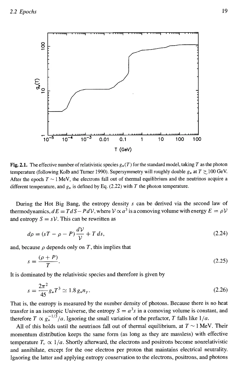
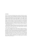
nonrelativistic. This is shown in Figure 2.1.
2.2 Epochs
19
100
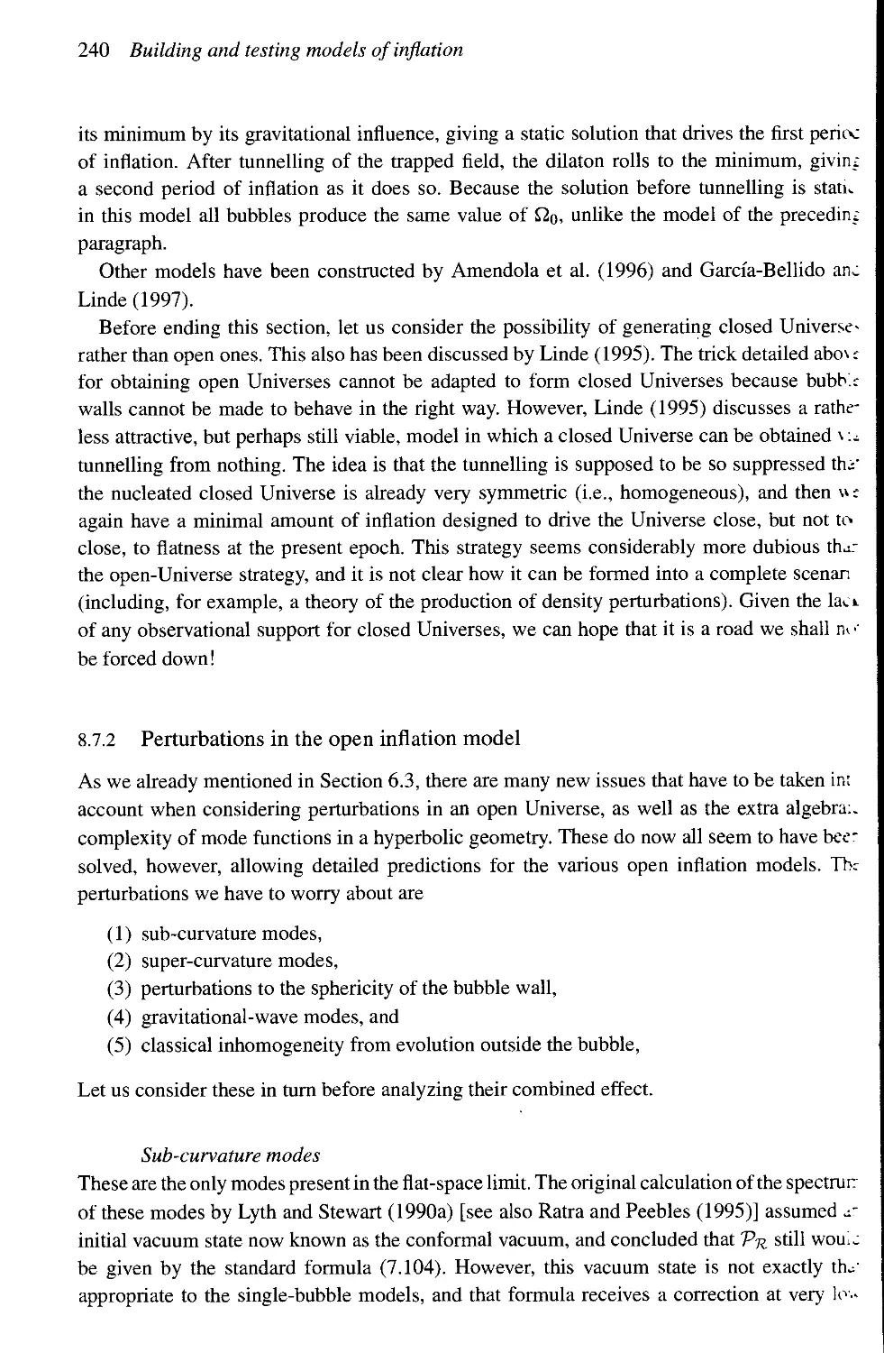
Fig. 2.1. The effective number of relativistic species g*(T) for the standard model, taking T as the photon
temperature (following Kolb and Turner 1990). Supersymmetry will roughly double g* at T >, 100 GeV.
After the epoch T ~ 1 MeV, the electrons fall out of thermal equilibrium and the neutrinos acquire a
different temperature, and g* is defined by Eq. B.22) with T the photon temperature.
During the Hot Big Bang, the entropy density s can be derived via the second law of
thermodynamics, dE = TdS— PdV, where V oca3 is a comoving volume with energy E = pV
and entropy S = s V. This can be rewritten as
dV
V
and, because p depends only on T, this implies that
(P + P)
B.24)
It is dominated by the relativistic species and therefore is given by
lit1 3
B-25)
B.26)
That is, the entropy is measured by the number density of photons. Because there is no heat
transfer in an isotropic Universe, the entropy S = a3s in a comoving volume is constant, and
therefore T oc g* /a. Ignoring the small variation of the prefactor, T falls like I/a.
All of this holds until the neutrinos fall out of thermal equilibrium, at T ~ 1 MeV. Their
momentum distribution keeps the same form (as long as they are massless) with effective
temperature Tv oc I/a. Shortly afterward, the electrons and positrons become nonrelativistic
and annihilate, except for the one electron per proton that maintains electrical neutrality.
Ignoring the latter and applying entropy conservation to the electrons, positrons, and photons
20 The Hot Big Bang cosmology
(the species in thermal equilibrium), we have gif=2-\- 7/2 =11/2 before annihilation (because
the electron and the positron each have two spin states) and g* = 2 after annihilation (because
only the photons are now relativistic). The photon temperature therefore is boosted relative
to the neutrino temperature by a factor ^/l 1/4. Each massless neutrino species now has a
temperature of 1.95 K, and if we continue to define #„ by Eq. B.22) with T the photon
temperature and assume that all three species are massless, its present value is
4X4/3
-J =3.36. B.27)
During radiation domination, Eq. B.17) holds giving H = 1/2?. This gives the timescale
1 jr2 T4
T^ = ™8*^r- B.28)
4f2 90 Ml
Substituting in values (see page 13) gives
2.2.2 From radiation to matter domination
The only particle species whose present density is known to high accuracy is the photon.
The energy density in photons is dominated by the energy in the microwave background, a
blackbody with T = 2.728 K (Fixsen et al. 1996), which gives
fiy,o h2 = 2.48 x 10 B.30)
with negligible uncertainty. Assuming in addition three massless species of neutrino, the total
energy density in relativistic particles (radiation) is
QRj0 = 4.17 x lO~5h~2. B.31)
Note that the number of massless species is being inferred from standard particle physics
models and is not being measured directly. In particular, one or more neutrino species may
have significant mass, changing ?2^,0 somewhat. Accepting Eq B.31) as a working hypothesis,
the redshift of matter-radiation equality is given by
1 + Zeq = —2_ = 24 000 Sloh2. B.32)
The corresponding temperature is
Teq = 7b(l + Zeq) = 65 500 fi0*2 K. B.33)
The definition of the density parameter indicates that at any epoch the matter component obeys
?2mA + z)~3H2 = const = Q,QH2 B.34)
2.2 Epochs 21
where the second equality assumes matter domination today. By definition, at equality the
radiation density matches the matter density, and the Friedmann equation gives the Hubble
parameter at equality as
Zeq)v2 = 5.25 x loWng, B.35)
yielding
B.36)
The comoving Hubble length at matter-radiation equality was therefore
(fleqHeq) = I4^lh~2 Mpc. B.37)
Now let us consider the evolution of the scale factor between radiation domination and
matter domination. If we take P = wp with constant w, then the continuity equation B.8) can
be rewritten
j (pa3{w+l)) = 0 B.38)
and solved to give
/ x 2/3(io+l) / N2/C«H-1)
'=;?*• •¦(;) -(i) •
where the solutions are shown for both cosmic time t and conformal time r. In particular, this
includes the classic solutions
a oc r2/3 oc t2 (matter), B.40)
a oc t1/2 oc t (radiation). B.41)
Including both matter and radiation, the Friedmann equation becomes
) B.43)
eq
where aeq is the scale factor when the densities of matter and radiation are the same, and peq is
the density in each component at that time. This can be solved exactly using conformal time:
— =B>/2-2)( — )+(l-2V2 + 2)(— ) ,
^eq \ ^eq / \ ^eq /
with
2V2-2 llMl
req = — J—El. B.44)
aeq y ..Nq
We see a smooth rollover between the two characteristic behaviours of radiation domination
and matter domination. There is no good way to rewrite this in terms of cosmic time.
22 The Hot Big Bang cosmology
2.2.3 Matter domination
Now we consider the matter-dominated era. We have already seen the famous solution a oc r2/3
for the critical-density case. We now look at the low-density case, both without and with a
cosmological constant.
Matter domination in an open Universe
Because the curvature term in the Friedmann equation falls off only as a2, whereas the matter
energy density falls as a3, domination by the curvature term is a stable situation with late-time
solution a oc t. However, we know that the present Universe is not a long way from the critical
density, and we should consider both terms. Again, use of conformal time facilitates a solution;
fixing K = — 1 gives
fl(T) = ?? (cosh r - 1) = 5^L (cosh T _ 1} _ B 45)
6Mp, 2
Here, To must be chosen to give the scale factor its present value; from Eq. B.16), this is
Unfortunately, in terms of cosmic time an analytic solution for the evolution of the scale
factor can be given only parametrically, as
fW (cosh*-l)-*L-, B.46)
2A Q)
(cosh*l)
a(t0) 2A -
^ B.47)
where \jr is a parameter whose present value again must give the correct a(to). The range of \fr
is [0, oo). A useful equation giving the evolution of fi with redshift, assuming that the Universe
only contains nonrelativistic matter, is
i±i B.48)
n0
1 +
Example 2.3 indicates how this is derived. Provided that 1 + z ^> 1/ Qo — 1, spatial curvature
can be ignored.
The cosmological constant
Many observations suggest that the density of matter in the Universe is less than the critical
density. If this is so, then an alternative to believing that the Universe has negative spatial cur-
vature is to introduce a cosmological constant A to restore spatial flatness. Then the Friedmann
equation reads
In much of the literature, one has to read rather closely to discern whether the phrase "low-
density Universe" does or does not include a cosmological constant to restore spatial flatness.
2.3 Scales 23
In a Universe dominated by the cosmological constant, the solution is an exponential ex-
pansion rate
a(t) ocexp I J— t 1 , B.50)
the effective density remaining constant by definition.
Even if our Universe does possess a cosmological constant, it cannot be dominated com-
pletely by it and we should consider both matter and A contributions. Again, invertible analytic
solutions are not available. Similarly to the open case, we can calculate the redshift dependence
of the matter density, which now is given by
The Universe is close to critical density at A + zK ;$> l/?2o — 1-
2.3 Scales
2.3.1 Characteristic scales
In general, a homogeneous and isotropic Universe is characterized by two length scales: the
Hubble scale and the curvature scale.
The Hubble scale is just the reciprocal of the Hubble parameter, H1. It can indicate either
time or distance (length scales being converted to timescales through division by c, which we
have set to 1). The Hubble time represents the characteristic timescale of evolution of the scale
factor; during a Hubble time, a(t) grows by a factor e (in the context of inflation, this often is
referred to as an e-folding).4 Because during normal evolution the scale factor is decelerating,
the Hubble time is usually a good estimate of the age of the Universe. Consequently, the Hubble
radius is normally a reasonable estimate of the size of the observable Universe, given by the
distance that light could have travelled since the Big Bang.
The curvature scale arises because the constant K in the Friedmann equation is related to
the spatial geometry. If K vanishes, the Universe is flat (Euclidean geometry); otherwise there
is spatial curvature, which becomes significant if we survey the Universe out to a distance of
order of the curvature scale
rcutv=a\K\-1/2. B.52)
This precise expression for the curvature scale comes from the form of the metric for a homo-
geneous Universe, the Robertson-Walker metric
[j~2 "I
*—^ + x2(d62 + sin2 6 d(j>2) , B.53)
1 — Kxl J
4 The continuous definition of time in Hubble units, including the variation of H, is given by (hub = /; dt/H~^ =
\n(af/a\).
24 The Hot Big Bang cosmology
which also can be written in a more convenient form by redefinition of the radial coordinate as
ds2 = -dt2 + a2(t)[dx2 + \K\~l sinh2(\K\1/2x)(d02 + sin2 6 d<p)] B.54)
for an open Universe. For a closed Universe, sinh is replaced by sin. For r <? rcurv, we see that
the Euclidean spatial geometry is recovered. If K vanishes, as is suggested by inflation, the
curvature scale is infinite, leaving only the Hubble scale.
The ratio of the two characteristic scales is related to ?2 via the Friedmann equation:
B.55)
'"curv
In open Universes the Hubble length is always less than the curvature scale, approaching it in
the limit Q -»• 0, which is the typical late-time behaviour. In a closed Universe, the Hubble
length can exceed the curvature scale (though in that case it has no particular interpretation
as a length). Equation B.55) needs slight modification for the contracting phase of a closed
Universe.
2.3.2 Particle horizon
The coordinate distance travelled by a freely moving photon, emitted at time t and observed
by us now, is
f" dt
x(t) = / —. B.56)
This integral converges rapidly as we go back through the matter-dominated era, and continues
to do so as we go further back into the Big Bang era, though of course photons really are not
moving freely during that era. Ignoring this fact and making the idealization that the Big Bang
started at the epoch a = 0, the present distance of an object emitting light at that epoch is
f'° dt
Jo a
rhol(t0) = a0 / —. B.57)
Jo a
This is called the particle horizon, and the same term is applied to the corresponding quantity,
with to replaced by an arbitrary epoch.
Evaluated at the present epoch, the particle horizon is crucially important because it defines
the size of the observable Universe. Assuming critical density and approximating the Universe
as always matter dominated, it is given by rh0r(?o) = 2//0~1.
The particle horizon changes if we move to a low-density Universe. Keeping the excellent
approximation of matter domination back to the Big Bang, then in an open Universe,
rhor(f0) = -=L= cosh ——^ . B.58)
The prefactor to the cosh is just the curvature distance; the particle horizon distance exceeds
the curvature distance if Qq < 0.79.
2.3 Scales 25
In a cosmological-constant model, even one giving spatial flatness, the answer is not available
analytically, but is given in integral form by (Carroll et al. 1992)
, 2 3" B9)
Hu and White A997a) quote a fitting function that proves accurate to better than 1 percent in
cases of interest, which (ignoring a correction for the time of the matter-radiation transition
and correcting a typo in the sign of the prefactor of the logarithm) is
. , OLJ_tl +0.084 In ftp
rhOr(r0) ~ 2HQ = . B.60)
V"o
In summary, and taking the critical-density case as an example, we have three important
scales:
A) t0 Age of the Universe,
B) Ho = 3ro/2 Hubble distance/horizon,
C) rhor(?o) = 3r0 = 2H0~l Particle horizon.
Note that the distance that light travels is greater than we would get by naively multiplying the
age of the Universe by the speed of light, because the Universe was physically smaller when
the light first set out.
2.3.3 Predicted ages
As we will see in Section 2.5.1, observations seem to require to > 10 Gyr. Taking ?2o = 1, the
age of the Universe is
2
to = - H~l = 2.06/T1 x 1017 s = 6.52/T1 Gyr. B.61)
The consensus is that this can be in agreement with observations only if the Hubble parameter
h is near the low end of the measurements made.
For a given h, the Universe can be older if we move to a low-density Universe, either with
or without a cosmological constant. In an open Universe, the age becomes, from Eqs. B.46)
and B.47),
= ° 1 O 3/2 C°S ( ~~O ) '
to = H0~l -j-f^- - 2 i _ ^ 3/2 cosh I ^^ 1 . B.62)
As ?2o tends to 1, the square bracket tends to 2/3, as it must. As ?2o is decreased, the square
bracket increases monotonically, reaching unity in the limit ?2o —> 0. So, an open Universe can
be, at most, 1.5 times as old as a flat one for the same h, giving an age equal to the Hubble
time. For a spatially flat Universe with a cosmological constant, the boost to the age is more
dramatic, given by (Carroll et al. 1992)
ro= "° ^ln' ^1_ "" , B.63)
26 The Hot Big Bang cosmology
0.2
0.4
0.6
0.8
Fig. 2.2. Predicted ages for open Universes and for flat Universes with a cosmological constant.
which diverges in the low Qo limit. In place of the logarithm, the last factor also can be written
— Q0)/?20). For Qo = 0.2, about the smallest conceivable value, the age is 1.6
times the ?2o = 1 value, for a given h. For ?2o = 0.26, the age equals the Hubble time. Ages
are shown in Figure 2.2.
2.4
The cosmic microwave background
Many of the most dramatic observational results in cosmology in recent years have related to
the cmb and, in particular, its anisotropies. The anisotropies are discussed extensively later in
the book. Here, we review some of the properties of the microwave background itself (Hogan
et al. 1982; White et al. 1994).
The details of last scattering have been long understood. We can model the time of last
scattering by a visibility function, which measures the probability that a particular photon last
scattered in a redshift interval dz- Conveniently, this proves to be well approximated by a
Gaussian at mean redshift zrec = 1100 with width Az ~ 80, pretty much independent of all
cosmological parameters (Jones and Wyse 1985).5
Even if the density parameter of the Universe is less than unity today, it would have been
very close to 1 at the time of last scattering. Because matter-radiation equality is at 1 + zeq =
5 This assumes that there is no very early reionization of the intergalactic medium by ultraviolet photons emitted
by the earliest generations of stars and quasars, which could create free electrons that can scatter the microwave
photons. In inflation-based models, it is thought very unlikely that reionization could be early enough to rescatter
all of the microwave background photons to create a new last-scattering surface, but it may well be that some
modest fraction are rescattered, altering the anisotropy pattern. We discuss this further in Chapters 5 and 11.
2.5 Ingredients for a model of the Universe 27
24000 Q^h2, then for normal parameters, matter domination occurs a reasonable amount of
time before recombination. The time of recombination therefore can be estimated from the
matter domination result of Eq. B.34) as
B.64)
The comoving particle horizon size at this time was 18O?2O h l Mpc, the comoving Hubble
length was half that size at 9O?2^ h~x Mpc, and the thickness of the last-scattering surface
was lQ,~ll2h~l Mpc.
The corresponding angular sizes on the last-scattering surface are also of interest. In an open
Universe, the distance to the last-scattering surface is given by Eq. B.58), and the "circum-
ference" of the sphere at that distance is obtained most directly from the metric B.54). The
trigonometric functions conveniently destroy each other to give the circumference as
B.65)
This is to be reduced by a small amount if we use the precise redshift of last scattering rather
than taking it to be at infinity; for example, if Qq = 1, then the distance to the last-scattering
surface is rlss = 5820/j Mpc, rather than 2Hq1 = 6000/z Mpc. The angle subtended by the
Hubble scale at last scattering is O.86?2O deg, and that by the scale corresponding to the
thickness of the last-scattering surface is 4Q0' arc-minutes. Finally, the curvature scale itself
subtends an angle of fio/2Vl — ^o rad. Experiments that probe scales larger than 1 deg,
such as COBE, are studying scales that were still larger than the horizon scale at the time the
microwave background was formed.
A cosmological-constant model has the standard Euclidean geometry, but the distance to the
horizon now is given by Eq. B.60). Ignoring the logarithm, we see that the angle subtended by
the Hubble scale at last scattering is 0.86 deg and the thickness of the last-scattering surface
corresponds to 4 arc-minutes, both independent of Qq to a reasonable approximation.
2.5 Ingredients for a model of the Universe
We now give a brief summary of the observational status of the various parameters required
to specify a cosmological model. This breaks up naturally into two parts: the parameters that
describe the global state of the Universe and the parameters needed to describe the matter in
the Universe, in particular, the dark matter assumed to pervade the Universe. These two in
combination are what we are calling the cosmological parameters. When we come to study
models of structure formation, a third set of information is required, which is a description of
the initial perturbations in the Universe from which structure grows.
As we write, there is still considerable uncertainty concerning an accurate description of the
Universe. In fact, there is only a single cosmological parameter that is uncontroversially well
determined to an accuracy that permits its variation to be neglected when we study models of
28 The Hot Big Bang cosmology
structure in the Universe, that being the present temperature of the microwave background,
To = 2.728 ± 0.004 K. All other cosmological parameters may be varied, consistently with
observations, sufficiently to affect large-scale structure predictions. We do not aim to provide
a detailed discussion here, but rather a rough guide to what is possible and a list of references
that the reader can pursue.
2.5.1 Hubble parameter and age
In recent years, progress appears finally to have been made toward a consensus on the value of
the Hubble constant, but the story remains some way from being closed. Many measurements
now are coming in at around h = 0.70, in particular, the Hubble Space Telescope observations
of Virgo Cepheids (Freedman 1997) and the type la supernovae method (Riess et al. 1996),
with uncertainties around 15 percent. On the other hand, values below h = 0.50 still appear
from time to time (e.g., Schechter et al. 1997). For reviews, see Jacoby et al. A992) and Hendry
and Tayler A996).
The age of the Universe was long thought problematic in the context of a critical-density
Universe, with many estimates of globular-cluster ages, based on stellar evolution, being up-
ward of 15 Gyr. This changed dramatically when the Hipparcos satellite measured a large
number of stellar parallaxes. The stars turned out to be farther, hence brighter and younger,
than previously thought, bringing down the age limits (Reid 1997; Feast and Catchpole 1997;
Chaboyer et al. 1998). (This also lowered the Hubble parameter estimated by distance ladder
techniques.) A safe lower limit from globular-cluster ages seems to be about 10 Gyr, with
perhaps an extra gigayear to be added to allow them to form in the first place.
A critical-density Universe with h = 0.70 has an age below 10 Gyr, incompatible with even
the lowest estimates of the age of the Universe. When theorists consider the critical-density
case, the usual choice is therefore h = 0.50, which comfortably passes the age constraint. The
advantages for structure formation of an even lower value have been spelled out by Bartlett
et al. A995), but such values sit uneasily with direct observations.
An interesting result is a demonstration that the local and global Hubble constants cannot
differ greatly, using type la supernovae (Kim et al. 1997). This counters arguments that if we
live in a significantly underdense region, the local expansion rate in the surrounding tens of
megaparsecs, which most measurement techniques sample, might be much higher than the true
expansion rate. Although such an effect may persist at the 10-percent level or so, it cannot be
large enough to reconcile a very high locally measured value with the age of a critical-density
Universe.
In conclusion, the view that we take is that the "reasonable" range for h is between 0.5 and
0.8, and although values outside that range are not inconceivable, they are disfavoured.
2.5.2 Density parameter
It has long been accepted that most of the mass in the Universe neither emits nor absorbs
radiation; it is dark as opposed to luminous. But observation of the luminous matter probes,
2.5 Ingredients for a model of the Universe 29
through gravity, the total mass density, and this allows us to estimate the density parameter
fi0 in a number of ways. In a rich galaxy cluster, observation of the luminous matter enables
us to infer the cluster mass density and hence the total cluster mass. As will be discussed in
connection with Eq. B.68), this leads to one way of estimating the density parameter. The
growth of perturbations in the Universe is affected by the mean mass density, and we will see
that this too provides useful information about the density parameter. Finally, observations of
supernovae at high redshift give information about the expansion rate of the Universe, and
hence about both the density parameter and the cosmological constant. Collectively, this body
of evidence suggests a value of fio in the range 0.2 to 0.5.
2.5.3 Cosmological constant
Direct measurements of the density parameter say nothing about the cosmological constant, but
compatibility with the simplest models of inflation requires a flat spatial geometry. The simplest
way to make a low-density Universe compatible with these models is to add a cosmological-
constant term. We only consider the cosmological constant with the value chosen to restore
spatial flatness.
A large cosmological constant has a very significant influence on the expansion rate at late
times, which can be probed observationally in several ways. The most important at present is
the magnitude-redshift relation for distant type la supernovae, which are believed to be good
standard candles once a correction for rate of decay of light emission is taken into account.
To many people's surprise, the evidence is strongly in favour of a cosmological constant
(Perlmutter et al. 1998; Schmidt et al. 1998). In particular, for spatially flat cosmologies,
the best-fit fio is about 0.3, with A comprising the remainder. One possibility is that this
cosmological constant may be an effective one rather than a true one, and indeed may be
varying slowly with time. Such behaviour can be modelled via the potential energy of a scalar
field, in exactly the same way as inflation is.
Another way of constraining A is via gravitational lensing (Kochanek 1996; Falco et al.
1998), which gives fiA < 0.74 at 2-ct confidence. We find that large-scale structure models
tend to support the lensing limit. If these measurements are all correct, then fio must be not
far from 0.3 to 0.4 or so.
2.5.4 Baryonic matter
In cosmology, ordinary matter is referred to as baryonic matter or simply baryons, because
the protons and neutrons (baryons) rather than the electrons account for practically all of its
density, denoted fib-
Nucleosynthesis [Alpher et al. 1948; Hoyle and Tayler 1964; Walker et al. 1991; see Pagel
A997) and Schramm and Turner A998) for reviews] provides the best estimate of the baryon
density. Although the theoretical calculations are well developed and accurate, the observa-
tional data require considerable interpretation. Consequently, although the theory of nucle-
osynthesis is undoubtedly one of the great successes of cosmology, the limits on the baryon
30 The Hot Big Bang cosmology
density are not as tight as we would like. A typical example (Copi et al. 1995a,b) gives
0.010 < ttbh2 < 0.022, B.66)
with even higher values obtained by some authors (Hata et al. 1995; Kernan and Sarkar 1996).
This range seems intended to correspond to the 95 percent confidence range (though without
any implication that the error bars can be treated as Gaussian within that range). When we
refer to the nucleosynthesis value of ?2b, we mean the central value of the Copi et al. range,
namely
n%uch2 = 0.016. B.67)
Observations (Tytler et al. 1996) of the deuterium abundance in quasar absorption systems
suggest that the true value may well be toward or even beyond the top of the quoted range.
(Results often are quoted in terms of the ratio of baryon and photon numbers 77; the conversion
is r) = 2.68 x lO~sQbh2.)
The ratio Qb/ ?20 can be estimated by looking to clusters of galaxies, an approach popularized
by White et al. A993b). Originally labelled the "baryon catastrophe," this is now normally given
the less emotive title of the "cluster baryon fraction." The majority of the baryons in clusters
tend to be in the form of hot X-ray-emitting gas, the distribution of which also can be used
to measure the total mass of the cluster from the condition for hydrostatic equilibrium in the
gravitational potential well, admittedly with some modelling uncertainties. Because clusters
are such large objects, we expect (with support from simulations) the balance of material within
them to be representative of the Universe as a whole. White and Fabian A995) compiled data
for thirteen clusters, and obtained a baryon fraction
B.68)
,0.5,'
at the 95 percent level.
Given the nucleosynthesis value of Qb, this implies that the Universe has a low density, per-
haps around 0.4. The cluster baryon fraction is inconsistent with nucleosynthesis in a critical-
density Universe, unless the theory of nucleosynthesis is somehow flawed, either through the
interpretation of observations (which seems rather unlikely) or through the intervention of new
physics (e.g., Gyuk and Turner 1994; Mathews et al. 1996). Alternatively, the cluster mass
determinations might be wrong, and there is evidence that X-ray mass determinations may be
too low (e.g., Gunn and Thomas 1996; Wu and Fang 1997), presumably because the true gas
distribution is more complicated than the modelling currently allows. Finally, we might worry
whether the earlier statement, that the cluster baryon fraction should accurately represent the
universal value, stands up to examination because determinations in different clusters do not
appear completely consistent (Loewenstein and Mushotzky 1996); it is not clear at present
whether the differences can be explained away through systematic errors (implying that the
uncertainties typically have been underestimated), or whether they genuinely undermine the
claim that clusters fairly sample the material content of the Universe.
2.5 Ingredients for a model of the Universe 31
An ambitious goal is to derive the baryon density from first principles, a topic known as
baryogenesis. It cannot be derived from decoupling from thermal equilibrium, as can the
massive neutrino case discussed shortly, because the density is determined not thermally but
because there is a conserved quantity, the baryon number, that is nonzero in our present
Universe. A common assumption is that, at high energies, the Universe has zero net baryon
number, and that the baryon number is generated by some baryon-number violating processes
in the early Universe. Within the Standard Model, only nonperturbative weak interactions
violate baryon number. Many extensions to the Standard Model violate baryon number. See
Dolgov A992) for a review. At present, there is not even an order-of-magnitude theoretical
understanding of the baryon number of the Universe.
The baryonic dark matter could reside in a number of forms, including cold gas and compact
objects, the latter having been detected via microlensing observations and therefore being
present in some reasonable abundance. A detailed account of the possibilities can be found in
Carr A994).
2.5.5 Cold and hot dark matter
Particle physics has offered no shortage of nonbaryonic dark matter candidates (e.g., Jungman
et al. 1996a), from massive neutrinos to axions or the lightest supersymmetric particle (Section
6.1.2). As far as large-scale structure is concerned, it is more fruitful to classify dark matter
by its random motion than by its particle physics origin.
CDM refers to particles with no significant random motion, at least as far as structure forma-
tion is concerned. To be precise, their random motion is nonrelativistic when even the smallest
cosmologically interesting scales come inside the horizon. It is the simplest option because,
by definition, the individual particle properties are unimportant, so that their cosmological
influence is specified fully by the density, ?2cdm- CDM candidates can be elementary particles
(the lightest supersymmetric particle being the favourite candidate) or much more massive
objects such as primordial black holes. As we see later, structure formation models based on
inflationary perturbations nearly always feature at least some CDM, and they often are referred
to generically as CDM models.
At the other extreme is hot dark matter, which is still relativistic when galaxy scales enter
the horizon, and between the two extremes lies warm dark matter. These are more complex
possibilities because the cosmological effects of such matter depend not only on the density
but also on the nature of the random motion. In particular, we need to know the freestreaming
length, measuring the typical distance that a particle is able to move.
Commonly, the need to introduce extra parameters describing the particle motions is avoided
by making a specific assumption, for example, that the hot dark matter takes the form of a mas-
sive neutrino. With this assumption, the relation between the particle mass (which determines
its random motion) and its density is fixed, namely
32 The Hot Big Bang cosmology
where the sum is over any neutrino types with mass less than about 1 MeV, implying that they
are relativistic at decoupling. That the density scales linearly with mass is easy to understand;
because the particles are relativistic at decoupling, the final number density is independent
of the particle mass. The detailed answer arises as follows (see, e.g., Kolb and Turner 1990).
We have nv = C/4) x D/11) nY, where the 4/11 comes from the difference in temperature
(Section 2.2.1) and the 3/4 because neutrinos are fermions and the photons are bosons. From
Eqs. B.20) and B.21) the mean photon energy is 2.7 Ty, and the present energy density in
radiation is given by Eq. B.30). Putting all of this together gives Eq. B.69).
For neutrinos of mass above 1 MeV, the assumption of decoupling while relativistic breaks
down and a much more sophisticated analysis becomes necessary; see, for example, Kolb and
Turner A990). The total energy density begins to fall below the linear extrapolation, because
Boltzmann suppression reduces the number density of neutrinos before they decouple. There
is, in fact, a second solution in which the neutrinos would give a critical density at a mass of a
few giga-electron volts; however, this mass exceeds the laboratory bounds on all three of the
known neutrino species.
For a hot component of sufficient density to be interesting, we expect a mass in the range
(depending somewhat on h) from a few electron volts to a few tens of electron volts. This is
around the current experimental bounds on the electron neutrino mass, but well below the limits
on the other two known species. (Neutrino oscillation experiments are providing increasing
evidence of nonzero neutrino masses, but only give the difference in the mass squared, rather
than the actual masses.) With such masses, the neutrinos will be relativistic early on but will
have become nonrelativistic by the present. Neutrinos are the only particles in the Standard
Model that, through its extension to allow them masses, also can be the dark matter. If they
are used in this way, we must be careful to make the appropriate modifications, in particular
to the effective number of massless species in the Universe.
There are hot (or warm) dark matter candidates other than neutrinos and, in that case, the
necessity of introducing extra parameters to describe them cannot be evaded. And that is only
the start of an increasing sequence of complexity; for example, the dark-matter particles could
decay (presumably into another form of invisible matter) or even annihilate. So far, however,
these options have not received a huge amount of attention; the standard assumption is that
the dark matter is either entirely cold or is a mixture of cold and hot. We return to some of the
more exotic examples in Chapter 6.
2.6 History of our Universe
We end this chapter with an overview of the history of the Universe, including the speculative
era before nucleosynthesis.
Nucleosynthesis can be considered as beginning at a time of order 1 s, corresponding to a
temperature of order 1 MeV and an energy density of order A MeVL. The regime of much
bigger energy density is the realm of the particle cosmologist. There is little prospect of ever
going more than a couple of orders of magnitude beyond 100 GeV through direct terrestrial
investigation (though probes of extremely high energy cosmic rays may have something to
2.6 History of our Universe 33
say). Within this realm, it is not completely unreasonable to imagine that present ideas in
particle physics can be extrapolated, and particle physicists have not been short of ideas as to
how the Standard Model might be extended. Many speculative ideas have been suggested for
what might happen in this regime, one of which is cosmological inflation. Although a test of
such an idea is outside the reach of particle accelerators, the observational consequences in
cosmology may be profound, as we see throughout this book. The early Universe thus offers
the possibility of acting as a distinctive probe of very high energy physics.
The observable Universe may have been created with energy density below the Planck scale.
More usually, it is supposed that the Universe does have a history extending all the way back
to the Planck scale. Whenever its history began, there may at first have been additional space
dimensions, which compactify only later.
There is virtually no understanding of what might happen beyond the Planck scale. A very
speculative possibility, which utilizes the duality properties of superstring theory, is the pre-
Big-Bang scenario (Gasperini and Veneziano 1993a,b). Here, a contracting Universe undergoes
some kind of tunnelling event to become an expanding Universe as the contracting phase ap-
proaches the Planck scale. Such a process may even be able to produce density perturbations,
though it remains to be seen if they can have the right form - in models so far, both the gravita-
tional waves and the adiabatic perturbations are too far from scale invariance, but isocurvature
perturbations may be created with a more reasonable shape (Copeland et al. 1997). We do not
discuss the pre-Big-Bang scenario further here; for a review, see Gasperini A997).
Taking the history to begin at the Planck scale, we can divide it loosely into a series of epochs:
• Mpi>p1/4>100GeV
In this very wide regime of densities, there is little indication as to the appropri-
ate underlying physics A00 GeV being the electroweak energy scale, specified by
the masses of the W and Z particles). In this regime, the standard tool is speculative
extrapolations from the physics that we do understand, with the assumption that the
general techniques and principles still apply. It is in this regime that cosmological
inflation would occur, and we are assuming that it does.
After inflation ends, the Universe is dominated by nonrelativistic particles (matter
dominated) for some time; we might refer to this era as a Cold Big Bang. Eventually,
the nonrelativistic particles decay into relativistic particles and produce a radiation-
dominated Universe. This process is called reheating. In the simplest scenario, radia-
tion then dominates until the onset of the present matter-dominated era.
In more complicated scenarios, radiation domination temporarily may give way to
an early era of matter domination, which ends when the relevant particles decay to
form radiation. Just before such a matter-dominated era, there might be an era of so-
called thermal inflation (Section 3.9), but this type of inflation would not generate the
inhomogeneities that are our main concern in this book. Whether thermal inflation
occurs or not, an early era of matter domination reduces the abundance of particles
that were produced earlier, which may be welcome. We may regard this reduction as
coming from the entropy that is produced by the particle decays signalling the end of
the matter-dominated era.
34 The Hot Big Bang Cosmology
• 100GeV>p1/4 > 10 eV
Barring very late decaying particles or other exceptional circumstances, the Hot Big
Bang begins at a temperature higher than 100 GeV, and we proceed on this assumption.
The relevant physics is described by the Standard Model, or some supersymmetric
extension of it. The first phenomenon is the electroweak phase transition, at which
electromagnetism and the weak interactions first gain their separate identities. If the
Hot Big Bang indeed begins before 100 GeV, this is the last possible time at which the
baryon asymmetry could be generated. Later, in the quark-hadron phase transition at
the QCD scale (~1012 K), it becomes energetically favourable for the free quarks that
existed in equilibrium with the radiation sea to condense in hadrons such as protons,
neutrons, and pions.
In principle, these two events could be avoided if the start of the Hot Big Bang
were delayed, for example, by long-lived massive particles from an earlier epoch. Such
particles, or the related scalar fields, would have to play some role in creating the baryon
asymmetry as well as delaying the onset of the Hot Big Bang.
At the very latest, the Hot Big Bang must begin by T ~ 10 MeV because otherwise
the standard nucleosynthesis calculation is invalidated. Nucleosynthesis occurs at T ~
0.1 MeV, when the protons and neutrons bind together into atomic nuclei, primarily
hydrogen and helium-4.
At around 10 eV, corresponding to 105 K, the nonrelativistic matter content in the
Universe reaches the same density as the relativistic, and the radiation era ends.
• 10eV>p1/4
With the onset of matter domination, the expansion rate increases to a(t) oc t2//3. From
that point on, the temperature decreases more quickly than the (fourth root of the)
energy density. The first significant event of this epoch occurs at around 3000 K, when
decoupling of the radiation from matter occurs. The first event in this sequence is
recombination (somewhat of a misnomer because the objects in question were never
previously combined), in which the majority of the electrons bind with nuclei to form
atoms, the photon energies being insufficient to dislodge them. At this point the photons
remain coupled to the ionized electrons that remain. Shortly afterward, as the ionized
fraction falls further, radiation decouples completely from the matter, and the photons
propagate freely. We see these today as the microwave background.
Between decoupling and the present, structure must form in the Universe, including
the first large gravitationally bound systems. Before this time, the Universe is close
to homogeneity on all scales, with linear perturbation theory easily adequate to deal
with any irregularities that exist. According to the inflationary cosmology, structure
formation is brought on by perturbations laid down in the early history of the Universe.
In Universes that are not flat, another transition occurs when the horizon scale is of
the order of the curvature scale, and the Universe becomes curvature dominated. In a
closed Universe, this is followed by collapse.
Table 2.1 provides a short summary of the most important epochs in the standard model for
the history of the Universe.
Examples
35
Table 2.1. A history of the Universe
t
102 s
1O-32±6S
1O-18±6S
10-10s
10S
10-2s
Is
100 s
104yr
105yr
~109yr
Now
PX'A
1018 GeV
1O13±3 GeV
106±3 GeV
100 GeV
100 MeV
lOMeV
lMeV
0.1 MeV
leV
0.1 eV
10 eV
3 x lO/;1^'/4 eV
T
-0
-0
106±3 GeV
100 GeV
100 MeV
10 MeV
lMeV
0.1 MeV
leV
0.1 eV
10eV
2.728 K
Event0
Inflation begins?
Inflation ends, Cold Big Bang begins?
Hot Big Bang begins?
Electroweak phase transition?
Quark-hadron phase transition?
y, v, e, e, n, and p all in thermal
equilibrium.
y decoupling, ee annihilation.
Nucleosynthesis.
Matter-radiation equality.
Atom formation, photon decoupling.
First bound structures form.
The present.
The Hot Big Bang might be delayed or interrupted. If so, electroweak symmetry might not be
restored (no electroweak phase transition) and free quarks might never be present (no
quark-hadron phase transition). However, the success of the standard nucleosynthesis calcu-
lation shows that an uninterrupted Hot Big Bang must be under way before T ~ 1 MeV.
Examples
2.1 How many neutrino families would there have to be to make matter-radiation equality and
decoupling coincide, assuming ?20 — 1 and h = 0.5?
2.2 Can an open Universe evolve into a closed one?
2.3 For a Universe containing only nonrelativistic matter (and no cosmological constant), show
that the Friedmann equation can be rewritten as
H(z)=Ho(l+z)(\+Sloz)l/2.
Use this to derive Eq. B.48).
2.4 Compute the Hubble radius at nucleosynthesis, assuming that it occurs at a temperature of
0.1 MeV. To what scale does this correspond today? What was the energy within a Hubble
volume at nucleosynthesis (expressed in solar mass units), and what mass is contained
within that comoving volume at the present epoch?
3 Inflation
3.1 Motivation for inflation
Primarily, this is a book about cosmological inflation, and one in which we intend to give as
up-to-date a viewpoint as possible. In the modern view, by far the most important property of
inflation is that it can generate irregularities in the Universe, which may lead to the formation
of structure. This allows the possibility of testing various aspects of the inflationary scenario,
and the bulk of our book is devoted to these topics.
However, the historical motivation for inflation was rather different, and arose largely on
more philosophical grounds concerning the question of whether the initial conditions required
for the Hot Big Bang seem likely or not. In this chapter, we begin by briefly discussing those
aspects of the historical motivation for inflation, before moving on to a description of the
classical dynamics of inflation.
3.1.1 Flatness problem
As we saw in Chapter 2, the Friedmann equation can be written as an equation for the density
parameter ?2, Eq. B.16). Ignoring the cosmological constant (or, if you like, including it in ?2),
it is
If the Universe is flat (Q = 1), then it remains so for all time. Otherwise, the density parameter
evolves. The flatness problem is simply that during radiation or matter domination, the com-
bination aH is a decreasing function of time.1 For example, in a nearly flat, matter-dominated
Universe, we have 11 — Q\ oc ?2//3, and in a nearly flat, radiation-dominated Universe, we have
11 — ?2\ oc t. We know observationally that, at the present, ?20 is not hugely different (certainly
not more than an order of magnitude) from unity, which implies that at much earlier times it
must have been extremely close to 1. To obtain our present Universe, then at nucleosynthesis,
for example, when the Universe was around 1 s old, we require that
)-1|<1(T16. C.2)
At early times, ?2 must be yet closer to 1.
1 The combination aH also decreases in more general circumstances, such as during a thermal phase transition.
3.1 Motivation for inflation 37
The flatness problem states that such finely tuned initial conditions seem extremely unlikely.
Almost all initial conditions lead either to a closed Universe that recollapses almost imme-
diately, or to an open Universe that very quickly enters the curvature-dominated regime and
cools to below 3 K within the first second of its existence. For this reason the flatness problem
also is phrased sometimes as an age problem - how did our Universe get to be so old?
3.1.2 Horizon problem
In Section 2.4, we saw that, in the Hot Big Bang model, the comoving distance over which
causal interactions can occur before the microwave background is released A8O?2^ h~x Mpc)
is considerably less than the comoving distance that the radiation travels after decoupling
[5820/z Mpc in a flat Universe, and somewhat more in a low-density Universe in accord with
Eq. B.58) or Eq. B.60)].
This means that microwaves coming from regions separated by more than the horizon
scale at last scattering, which typically subtends about a degree, cannot have interacted before
decoupling. The Hot Big Bang model therefore offers no prospect of explaining why the
temperature seen in different regions of the sky is so accurately the same; the homogeneity
must form part of the initial conditions.
A similar situation exists at nucleosynthesis: To preserve the success of the standard theory,
the Universe must be homogeneous on scales much larger than the horizon size at that time;
if there were fluctuations in the density from point to point then, because of the nonlinearity
of the nucleosynthesis process, the presently observed values would not be reproduced when
all these separate regions later were added together.
3.1.3 Unwanted relics
If the Hot Big Bang begins at a very high temperature, relics that are forbidden by observation
may survive to the present.
Perhaps the most problematic relic, from the modern viewpoint, is the gravitino. This particle
occurs in supergravity as the spin-| partner of the graviton, and has only gravitational-strength
interactions. In most versions of supergravity, the mass of the gravitino is of order 100 GeV,
in which case nucleosynthesis is upset if the Hot Big Bang begins before T > 109 GeV (Ellis
et al. 1986).
Another very troublesome class of relics comprises the moduli occurring in superstring
theory (de Carlos et al. 1993; Banks et al. 1994). These are spin-0 particles, correspond-
ing to the fields that parameterize the vacuum in the absence of supersymmetry breaking.
Their masses and lifetimes are typically of the same order as those of the gravitino but, be-
ing associated with scalar fields, they are even more likely to be overproduced in the early
Universe.
Depending on the theory, there also may be unwanted topological defects; for reviews, see
Vilenkin and Shellard A994) and Hindmarsh and Kibble A995). If the symmetry of a Grand
38 Inflation
Unified Theory is restored in the early Universe, magnetic monopoles are produced when it
is broken spontaneously. Their abundance typically is higher than observation allows, unless
they are connected by strings. Historically, getting rid of unwanted monopoles was one of
the main motivations for inflation. Cosmic strings, textures, and domain walls also may be
problematic, but that is more model dependent. Textures present no problem if their energy
scale is well below 1016 GeV, and neither do cosmic strings if the same is true of their energy
per unit length. Global strings need to be a couple of orders of magnitude lighter to avoid
problems. Stable domain walls are fatal unless their symmetry-breaking scale is less than a
million electron volts or so (Zel'dovich et al. 1975; Vilenkin and Shellard 1994), but they are
destabilized easily by giving one of the two vacua a slightly bigger energy density than the
other.
3.1.4 Homogeneity and isotropy
The horizon problem tells us that the large-scale homogeneity and isotropy of the Universe
must be part of the initial conditions. However, in practice, we know that the Universe is not
perfectly homogeneous, though it comes very close to it on large scales. A vital question then
is whether we can develop a theory of the origin of the inhomogeneity, or whether it too must
be consigned to the realm of initial conditions.
Within the Hot Big Bang model, the situation is not yet completely clear-cut. The simplest
interpretation of the anisotropies in the microwave background seen by the Cosmic Back-
ground Explorer (COBE) satellite is that they correspond to irregularities at the surface of last
scattering. Then their corresponding scale is much larger than the horizon size at that time.
With the Hot Big Bang model, such perturbations could not be generated causally, and again
would have to have been part of the initial conditions (Hu et al. 1994b; Liddle 1995). However,
it remains possible that these large-angle anisotropies are generated by gravitational effects
much closer to us than last scattering; this is what happens, for example, in topological defect
theories of structure formation.
So, the Hot Big Bang theory is unable to explain the large-scale homogeneity of the Universe.
It yet may be able to explain the generation of inhomogeneities, but as we see, the most attractive
way to generate the inhomogeneities is to go beyond the standard Hot Big Bang model.
3.2 Inflation in the abstract
The inflationary cosmology (Guth 1981; Albrecht and Steinhardt 1982; Linde 1982, 1983) is
not a replacement for the Hot Big Bang model, but rather an add-on that occurs at very early
times without disturbing any of its successes.
The precise definition of inflation is simply any epoch during which the scale factor of the
Universe is accelerating:
INFLATION <=> a > 0.
3.2 Inflation in the abstract
39
Not to scale!!
Start of
inflation
t
End of
inflation
t
Present
day
A Time
distant
future
Fig. 3.1. Schematic of the inflationary solution to the flatness problem. Whether there is a definite start
time to inflation or not is irrelevant. By definition, during inflation Q is driven toward 1, and with sufficient
inflation it will finish so close by the time inflation ends that in all the subsequent evolution up to the
present it remains indistinguishably close. Only in the distant future will it move away again.
Inflation sometimes is described just as a rapid expansion, though it is not very clear with
respect to what the expansion is supposed to be rapid.
There is an equivalent alternative expression of the condition for inflation that gives it a
more physical interpretation:
INFLATION
d H-
dt a
Because H ' /a is the comoving Hubble length, the condition for inflation is that the comov-
ing Hubble length, which is the most important characteristic scale of the expanding Universe, is
decreasing with time. Viewed in coordinates fixed with the expansion, the observable Universe
actually becomes smaller during inflation because the characteristic scale occupies a smaller
and smaller coordinate size as inflation proceeds.
If inflation occurs, then it is possible for all the aforementioned problems of the Big Bang
model to be solved. The easiest one to see is the flatness problem; the condition for inflation is
precisely the condition that Q is driven toward 1 rather than away from it [Eq. C.1)]. Figure 3.1
shows a schematic of the desired behaviour. Relic abundances can be reduced to a satisfactory
level by the expansion during inflation, provided that they are produced before the inflationary
epoch. The horizon problem can be solved because of the dramatic reduction in the comoving
Hubble length during inflation, which allows our present observable Universe to originate
from a tiny region that was well inside the Hubble radius early on during inflation, as shown
in Figure 3.2. A much more detailed account of these resolutions can be found in Kolb and
Turner A990) and Linde A990a).
40 Inflation
COMOVING
start
Fig. 3.2. Schematic of the inflationary solution to the horizon problem. The plot is in comoving units.
During inflation, the comoving Hubble radius decreases dramatically, allowing our entire observable
region (the ring marked "now" around the central dot indicating our position) to lie within a region
(the shaded smooth patch) that was well inside the Hubble radius at the start of inflation. Any initial
inhomogeneities (lying outside the smooth patch) finish up on scales vastly larger than our observable
Universe.
Assuming that we work within general relativity, the condition for inflation can be rewritten
as a requirement on the material driving the expansion. Directly from the acceleration equation
B.7), with A = 0 or absorbed into p and P, we find
INFLATION
3P
Because we always assume p to be positive, it is necessary for P to be negative to satisfy this
condition, which is independent of the curvature of the Universe.
3.3
Scalar fields in cosmology
To obtain inflation, we need material with the unusual property of a negative pressure. Such
a material is a scalar field, describing scalar (spin-0) particles. Although, as yet, there has
been no direct observation of a fundamental scalar particle (such as the Higgs particle), such
particles proliferate in modern particle theories. They play a crucial role in bringing about
symmetry breaking between the fundamental forces. Scalar fields were introduced by particle
physicists long before particle cosmology came into being as a subject, but were pounced upon
by the cosmology community because of the range of interesting phenomena in which they
3.3 Scalar fields in cosmology 41
may partake. Inflationary cosmology is one arena where they play a vital role; they possess
the unusual feature of a potential energy that may redshift extremely slowly as the Universe
expands. This corresponds to an effective equation of state with a negative pressure, which we
have just seen is exactly what we need for inflation. The scalar field responsible for inflation
is often called the inflaton.
The standard way to specify a particle theory is via its Lagrangian, from which the equations
of motion can be derived. We discuss this in detail for a scalar field in Chapters 7 and 14. For
now, as our starting point, we adopt expressions for the energy density and pressure of a
homogeneous scalar field 0 = 4>{t), which are
Pj, =-4>2 - VD>). C.4)
These eventually are derived as Eqs. A4.87) and A4.88). The term V@) is the potential
of the scalar field, which we might hope to derive from some particle physics motivation. For
now, we treat it more or less as a free function. Different inflationary models, as described in
Chapter 8, correspond to different choices for the potential.
Note that, although the scalar field acts as a perfect fluid, it does not possess an equation of
state relating P$ and p$ because the same energy density can correspond to different values of
the pressure if the energy density is distributed differently between the potential and kinetic
terms.
The equations of motion now can be derived directly by substituting these relations into the
Friedmann and continuity equations B.12) and B.8), respectively. Assuming a spatially flat
Universe, we obtain
^2 \ ] C-5)
3M^ L 2 J
and
dV
<P + 3Hcp = -—-, C.6)
dq>
which also is called the scalar wave equation. We remind the reader that throughout this book
we are using the reduced Planck mass Mpi, defined on page 13.
From the forms of the effective energy density and pressure, the condition for inflation is
satisfied, provided that cj> < V{<j>). With a suitably flat potential, then even if this condition
is not obeyed initially, it very quickly comes to be satisfied, provided that the scalar field is
displaced away from the minimum of its potential.
Once inflation gets under way, then by definition the curvature term in the Friedmann
equation becomes less and less important. Normally, it is assumed negligible from the start; if
it is not, then the beginning stages of inflation will render it so.
42 Inflation
3.4 Slow-roll inflation
The standard approximation technique for analyzing inflation is the slow-roll approximation.
This approximation throws away the last term of Eq. C.5) and the first term of Eq. C.6),
leaving
C.7)
3M2,
3H(j> ~ -V'@), . C.8)
where we have introduced the notation that primes are derivatives with respect to the scalar
field 0, and that ~ indicates that quantities are equal within the slow-roll approximation.
For this approximation to be valid, it is necessary for two conditions to hold. These are
l, C.9)
where the slow-roll parameters e and r\ are defined by (Liddle and Lyth 1992, 1993a)
y,x2
C.10)
= <— ¦ C.H)
V'
Notice that e is positive by definition. The slow-roll parameters prove to be a very useful way
of quantifying the predictions of inflation and we use this notation throughout the book.
That these conditions are necessary for the slow-roll approximation to be valid can be found
easily by substitution. However, note that they are not sufficient conditions because they only
restrict the form of the potential. Because the full scalar wave equation is second order, the
value of <p can be chosen freely and, in particular, can be chosen so as to violate the slow-roll
approximation. It is therefore an additional "assumption" that the solution for a given potential
satisfies Eq. C.8). However, we show in Section 3.7 that this assumption can be proven, by
considering the attractor behaviour of solutions to the equations of motion. In fact, the attractor
behaviour is vital for the success of the slow-roll approximation; otherwise, the fact that the
approximation reduces the order of the system by 1 would make it unable to represent generic
solutions.
Practically everything we need follows from Eqs. C.8) and C.9), which we refer to simply
as the slow-roll conditions. In particular, Eq. C.7) is an immediate consequence of Eq. C.8)
ande«: 1.
The slow-roll parameters make it is easy to see where inflation might occur on a given
potential. For example, for V@) = m202/2, they are satisfied provided that 02 > 2Mpj. For
such a potential, inflation proceeds until the scalar field gets too close to the minimum for the
slow-roll conditions to be maintained, and inflation comes to an end.
Only for a very few simple choices of potential can the full equations for the scalar field
evolution be solved exactly. On the other hand, from the slow-roll equations, it is easy to find
solutions, provided only that the relevant integrations can be performed analytically. However,
3.4 Slow-roll inflation 43
in most circumstances it is not even necessary to find solutions to the equations of motion, as
we see later.
3.4.1 Relation between inflation and slow roll
The slow-roll approximation is a sufficient condition for inflation. To see this, rewrite the
condition for inflation as
- = H + H2>0. C.12)
a
This is obviously satisfied if H is positive.2 Otherwise, we require
-^ < 1. C.13)
Meanwhile, substitution of the slow-roll equations yields
Consequently, if the slow-roll approximation is valid (e <? 1), then inflation is guaranteed.
As before, this condition is sufficient but not necessary, because the validity of the slow-roll
approximation is required in its derivation. It is therefore possible in principle for inflation to
continue even if the slow-roll conditions are violated, though in practice the amount of inflation
that occurs under this circumstance is very small.
An inflation model consists of a potential and a way of ending inflation. One way for inflation
to end is by violation of the slow-roll conditions as the field approaches a minimum with zero
or negligible potential energy. In such cases, it can be assumed that inflation comes to an end
when e@) reaches unity. This directly tells us the value of 0 where inflation comes to an end
and, because e diverges as the field approaches the minimum of the potential, this endpoint
will be displaced somewhat from the minimum. In models such as hybrid inflation, where
extra physics intervenes to end inflation, inflation can end while the slow-roll conditions are
still well respected.
3.4.2 Amount of inflation
The amount of inflation that occurs normally is quantified by the ratio of the scale factor at
the final time to its value at some initial time. Because this typically is a vast quantity, the
logarithm is taken to give the number of e-foldings N:
Nit) = ln-^-, C.15)
ait)
2 This would require P < — p in a general relativity theory and hence cannot be caused by a scalar field, though
it can occur in extended theories of gravity, which we explore in Chapter 8.
44 Inflation
where /end is the time at the end of inflation. This measures the amount of inflation that still
has to occur after time t, with N decreasing to 0 at the end of inflation. To solve the horizon
and flatness problems, around seventy e-foldings of inflation are required.
As we saw earlier, the best characterization of inflation is that the comoving Hubble length
1 /a H is decreasing. Therefore, there is a case to be made (Liddle et al. 1994) for quantifying the
amount of inflation by a slightly different quantity, that being the ratio of the initial comoving
Hubble length to the final one
Although technically more accurate, during inflation a(t) typically varies much faster than
H(t), and so, the difference is not very important. We stick to the usual convention and use
N(t) to quantify inflation.
For most purposes, the only knowledge we need is how much more inflation will occur from
a given scalar field value 0, rather than from a given time. This can be calculated immediately
via the slow-roll approximation, without any need to solve the equations of motion for the
expansion:
N = In = / Hdt ~—r- / —d<p, C.17)
where 0end is defined by e@end) = 1 if inflation ends through violation of the slow-roll condi-
tions.
3.4.3 Evolution of scales
When we later discuss the production and evolution of density perturbations, we will be inter-
ested in the history of each comoving wavenumber. An important question concerning a given
scale is whether it is larger or smaller than the horizon; strictly speaking, we always should refer
to the Hubble length, but we follow common practice in using "horizon" and "Hubble length"
interchangeably, with the understanding that the latter is intended. Density perturbations nor-
mally are identified by their comoving wavenumber k, arising from a Fourier decomposition
of the density perturbation. We define a scale to be equal to the horizon when k = aH.
Recall that, by definition, during inflation the comoving Hubble length is decreasing whereas
at all other times it is increasing. A fixed comoving length scale k~l therefore may begin its
evolution considerably smaller than H~} /a, and by the end of inflation be considerably larger.
For any scale that does cross the horizon during inflationary evolution, an important epoch to
quantify is the time that it equals the Hubble radius, k — aH. With some simple assumptions,
this can be related to the number of e-foldings of inflation that occur after that time. The
evolution of a scale k, which we might imagine, for example, to be the scale presently equalling
the Hubble radius, k = a^Ho, is shown in Figure 3.3.
To make the identification of scales, we require a model for the complete evolution of the
Universe up to the present. For example, in the simplest viable cosmology, we can break the
3.4 Slow-roll inflation
45
Physical
scale
Log (time)
Comoving
Hubble
length
Comoving
Scale
Log (time)
Fig. 3.3. Two views of the behaviour of a comoving scale k relative to the Hubble length (horizon scale).
By definition, the comoving Hubble length I/a// is decreasing during inflation and otherwise increasing.
The upper panel shows physical coordinates, the lower one comoving. The vertical axis covers many
powers of 10 in scale. A scale starts well inside the horizon, then crosses outside some time before the
end of inflation, reentering long after inflation is over.
evolution up into chunks as follows:
• From the time the scale k ' equals the Hubble radius to the end of inflation.
• From the end of inflation until the Hot Big Bang is restored. This epoch is considered in
Section 3.8. Here, we assume that the Universe behaves as if matter dominated during
it.
46 Inflation
• The radiation era from the end of reheating to the time of matter-radiation equality teq.
• The matter era from teq to the present.
This is far from the only possible evolution; for example, in Section 3.9 we discuss a modifi-
cation known as thermal inflation, in which one or more extra periods of inflation occur at low
energy scales.
We assume instantaneous transitions between the regimes. We use a subscript k to indicate
the value of quantities when k = aH during inflation, and the subscripts "end" and "reh"
to indicate values at the end of inflation and after reheating. Then, measuring all quantities
relative to the present comoving Hubble scale Ho~l/ao, we obtain
k _ akHk _ ak atnd areb aeq Hk
- —~~. (j.lo)
end ^reh ^6Q ^0 **0
The first fraction on the right-hand side gives the number of e-foldings N(k) of inflation
remaining when the scale k equals the Hubble radius. Substituting in typical values gives
k 1016GeV VI/4 1 V1/4
The final three terms of Eq. C.19) represent the uncertainty in the various energy scales
connected with inflation. In typical models of inflation, these factors are not expected to be
too large. Usually, it is not important to know the precise number of e-foldings at which our
present Hubble scale k = aoHo equalled the Hubble scale during inflation. With the standard
evolution, we normally take this number to be 50 for definiteness. Some authors, including
ourselves in some papers, use 60 instead. A modification to the full history of the Universe,
such as thermal inflation, can alter the prefactor, normally reducing it, the extreme lower end
perhaps being N = 25.
The smallest scale accessible to large-scale structure observations is about 1 Mpc. This scale
would equal the Hubble radius about nine e-foldings after a0#o does. So, all scales relevant for
large-scale structure crossed the Hubble radius during a fairly limited number of e-foldings,
some way before the end of inflation.
3.4.4 Initial conditions for inflation
Though not compulsory, it normally is imagined that an era of inflation begins at the Planck
scale, corresponding to V^4 ~ Mpi. This is indeed desirable for two reasons. One is to prevent
the Universe from collapsing within a Planck time or so, if Q is initially bigger than 1 (without
being fine-tuned to a value extremely close to 1). Note though that this need not be a problem
in a very chaotic situation where parts of the Universe are open and parts are effectively closed;
the latter may form black holes but the former remain viable initial conditions.
The other, which applies also to the case Q < 1, is that inflation protects an initially homoge-
neous region from invasion by its inhomogeneous surroundings. This invasion will propagate
3.4 Slow-roll inflation 47
with speed of order c = 1, and a patch that is homogeneous at time / will survive until time t2
only if its initial size is bigger than
f'2 dt f2 da
r(t) = a(t) —=a(t) -j-. C.20)
J, a Ja a2H
If inflation begins promptly, and we take t2 as the end of inflation, the integral is dominated by
the lower limit giving r(t) ~ H~l(t). In words, the invasion travels about a Hubble distance in
the first Hubble time, but then stops so that the initially homogeneous patch need not be much
bigger than the Hubble distance. In contrast, if inflation is delayed, the integral is dominated
by the upper limit (whereas t2 is before the beginning of inflation), leading to
-\t)»H-\t). C.21)
In words, the invasion continues indefinitely, and the initial patch needs to be huge to survive
until inflation eventually protects it.3
Slow-roll inflation is very effective at erasing memory of what went before it and, as a result,
our Universe retains no memory of the era before it left the horizon. However, this does not
mean that we should ignore this era completely. On the contrary, a complete model of inflation
should specify not only a potential, but a reasonable way in which the inflaton field can find itself
slow-rolling down the appropriate part of this potential, when our Universe leaves the horizon.
Let us start by asking what happens at the Planck scale. The almost universally accepted
proposal, due to Linde A983,1990a), is that conditions at this era are what he termed chaotic.
This does not refer directly to chaos theory; rather, it is intended to indicate that, initially,
the field takes on a wide range of different values in different regions of the Universe. One
imagines the Universe emerging from the Planck era with the scalar field well displaced from
any minimum, such that the typical energy is of order of the Planck energy. In regions where
the field has suitable values, inflation is able to begin. Some numerical investigation of the
details has been carried out, for example, testing to what extent spatial gradients in the scalar
field might inhibit the onset of inflation, with the conclusion that they cannot prevent inflation
from happening in at least some regions (Albrecht et al. 1985; Kung and Brandenberger 1990;
Yi and Vishniac 1993).
Because this early era of inflation does not lead to any directly observable consequences,
there is no necessity for the perturbations to be small, and indeed, it is perfectly possible for
the predicted density perturbations to be of order of unity even if the energy density of the
field is well below the Planck scale. Such a situation leads to a phenomenon known as eternal
inflation (Linde 1986; Linde et al. 1994), in which the quantum fluctuations in the scalar field
can dominate over the classical behaviour, allowing the field to diffuse up the potential as well
as to roll and diffuse down. Because the Universe expands more rapidly if the energy density is
3 In the mathematical limit ti —> oo, r(t) is called the event horizon, as opposed to the particle horizon introduced
earlier. During inflation, it makes sense to pretend that the event horizon exists (taking ti to be any late time
before the end of inflation, regarded as infinity). After inflation, it makes sense to pretend that the particle horizon
exists (taking the initial time to be any early time after the end of inflation, regarded as 0).
48 Inflation
higher, the physical volume may be dominated by regions moving up the potential. In this sit-
uation, parts of the Universe continue to inflate forever, emitting a constant stream of regions
where the field moves away from the eternal regime and enters a conventional inflationary
period. Any one of these regions could house our own Universe. Eternal inflation can occur
either at large field values or near a maximum of the potential, and we discuss it further (page
185) after we have derived formulae for the density perturbations.
Inflation need not be a common occurrence near the Planck scale. All we need is for our Uni-
verse to be an inflating region and, particularly with eternal inflation, the huge expansion of the
inflating region makes that in some sense likely, though admittedly this idea is hard to quantify.
Various things might happen between the Planck scale and the epoch when our Universe
leaves the horizon. The simplest possibility, and the one usually envisaged nowadays, is that
scalar fields continue to dominate the energy density of the Universe throughout this era, with
some form of inflation occurring most of the time. (It might perhaps be interrupted by one or
more periods when some field is oscillating around a minimum of the potential.) An alternative,
which used to be very popular, is that the Universe became dominated by radiation in thermal
equilibrium; in other words, a hot big bang begins, though not the Hot Big Bang as we have
defined it (page 12).
Whatever happens, our observable Universe is assumed to eventually undergo an era of
inflation, which starts while it is within the horizon and ends some tens of e-folds after it
leaves the horizon. This inflation must be of the slow-roll variety, if it is to explain the observed
large-scale structure. The field either will be rolling away from a maximum of the potential
or coming in from large field values; either way, it is quite likely that inflation is initially of
the eternal variety. If the field is rolling away from the maximum, an attractive possibility is
that the maximum corresponds to a fixed point under the symmetries of the model. This is the
usual case, normally signalled by the convention that the maximum is at 0 = 0. In that case,
the field can be driven to the maximum by its interaction with other scalar fields, or by thermal
effects if there is thermal equilibrium. Alternatively, one might imagine that the initial field
values are chaotic, just as was postulated near the Planck scale, with our Universe happening
to be near the maximum.
We provide examples of these different mechanisms for starting inflation when we review
the range of inflation models in Chapter 8.
3.5 Exact solutions
For almost all known inflationary models, the slow-roll approximation works so well that
nothing more is needed. Even though it must by definition fail toward the end of inflation,
this typically only gives a small misestimation of the number of e-foldings that occur, and this
uncertainty is subdominant to the uncertainties in this quantity from the various energy scales
in Eq. C.19).4 Nevertheless, it is useful to have some exact solutions to the full equations of
motion in order to study their properties, and several are known.
4 In a specific inflationary model, V* and Vend can be computed fairly accurately, but the physics of reheating is
less well understood at present.
3.5 Exact solutions 49
3.5.1 Power-law inflation
The most prominent exact solution is power-law inflation (Lucchin and Matarrese 1985),
which, as we see later, has the extra advantage that the equations for the generation of density
perturbations also can be solved exactly.
Power-law inflation arises when the potential is chosen to take the exponential form
V(<j>)=Voexpi-I--?-), C.22)
y y p MnJ
where Vo and p are constants. The spatially flat equations of motion then have the particular
solution
a = oof, C.23)
C.24)
The general homogeneous solution, with one extra initial condition, also can be found in a
parametric form (Salopek and Bond 1990), but solutions for any initial conditions rapidly
approach this particular solution, in accordance with the inflationary attractor behaviour.
Provided that p > 1, this solution satisfies the condition for inflation. The slow-roll param-
eters are simply e = /?/2 = 1/p, and are independent of <p. With this potential, inflation never
comes to an end (though we discuss ways of circumventing this problem in Chapter 8).
Provided that the scalar field is the only matter in the Universe, it acts as a perfect fluid with
w = 2/3p, using the language of Eq. B.7). This correspondence will break down if another
type of matter is also present, because the scale-factor evolution feeds into the effective equation
of state.
3.5.2 Other exact solutions
The technology exists to compute a variety of exact solutions, via the basic strategy of beginning
with the solution and deriving the potential necessary to support it. In this type of approach,
there is no control over the type of potential that emerges from such a procedure, and normally
the result does not take on a simple form.
The most investigated such solution is the intermediate inflation model (Barrow 1990;
Muslimov 1990). This gives rise to an expansion
a(t) oc exp(A^), 0 < / < 1, A > 0. . C.25)
It arises from the potential
MP1/ •- — - C-26)
50 Inflation
where /$ = 4(/ ' — 1). The expansion is faster than any power law and slower than exponential.
As with power-law inflation, there is no natural end to inflation in this model. Note that the
asymptotic potential is just the power-law form Vasymp@) oc <p~P.
The literature contains a variety of other exact inflationary solutions. There is only a single
case at present (Easther 1995) in which a model has been constructed so that the density
perturbation equations also can be solved, as they can for power-law inflation. In all other
cases, it is only the classical scalar field dynamics that have been solved exactly.
3.6 Hamilton-Jacobi formulation of inflation
The Hamilton-Jacobi formulation (Salopek and Bond 1990) is a powerful way of rewriting the
equations of motion, which allows an easier derivation of many inflation results. The formalism
has applications to the general inhomogeneous situation, though we concentrate here on the
homogeneous version as applied to spatially flat cosmologies.
The formulation can be derived by considering the scalar field itself to be the time variable.
This can be carried out during any slow-rolling epoch in which the scalar field varies monoton-
ically with time. In its simplest form, it will break down during the oscillatory epoch that ends
inflation (though it is usually possible to patch together solutions from separate monotonic
epochs).
For definiteness, throughout we take (j> > 0. If this is not satisfied, it can be brought about
by redefining (j) -* -cj>.
Differentiating Eq. C.5) with respect to t and substituting in Eq. C.6) gives
C.27)
Dividing both sides by <j>, permitted by the monotonicity assumption, gives
0 = -2 M\x H'CP), C.28)
which gives the relation between <p and t. This allows us to write the Friedmann equation in
the first-order form
^\ ^ C.29)
Equation C.29) is the Hamilton-Jacobi equation. It allows us to consider H(cj>), rather
than V((/>), as the fundamental quantity to be specified. Because H, unlike V, is a geometric
quantity, inflation is described more naturally in that language (Muslimov 1990; Salopek and
Bond 1990; Lidsey 1991). Once H((p) has been specified, we immediately can obtain the
corresponding potential from Eq. C.29). Also, Eq. C.28) gives the relation between cp and t,
which enables us to obtain H(t), which, if it is desired, can be integrated to a(t). Therefore,
this is the most direct route to obtaining a large set of exact inflationary solutions; for example,
3.7 Inflationary attractor 51
H(<p) oc 4> ^2 gives intermediate inflation, and
#«>)cxexp - /— -?-) C.30)
gives power-law inflation.
We can use the Hamilton-Jacobi formalism to write down a slightly different version of the
slow-roll approximation than we did earlier, defining slow-roll parameters eH and r]H as
In the slow-roll limit, eH -» e and /?„ -» /? — e.
Some manipulation allows these to be written in various ways, such as
V + cp /2
<j> dln<p dlnH'
3Hcp dlna dlna
C.33)
C.34)
Consequently, the smallness of eH and /?H is precisely the condition for neglecting the unwanted
terms in Eqs. C.5) and C.6); however, the derivation of these conditions is exact, whereas that
using e and r\ required the slow-roll approximation to be valid. We also can consider eH <^ 1
to be the condition to neglect the first term in Eq. C.29), and r]H ^C 1 to be the condition to
neglect the first term of its (p derivative.
With these new parameters, many results that were approximate in terms of V(cp) become
exact. First, the definition of inflation now is given precisely by
a >()¦$=>•€„< 1, C.35)
and the equation for the number of e-foldings becomes
t
C.36)
a{t) Jt 2Mp2,J0 H'
Notice that, in terms of the new slow-roll parameters, the validity of the slow-roll approxi-
mation does not depend on any additional assumptions regarding attractor behaviour. This is
because when we discuss H(<p), we are dealing with the solution directly.
3.7 Inflationary attractor
If inflation is to be truly predictive, the evolution when the scalar field is at some given point on
the potential has to be independent of the initial conditions. Otherwise, any result, such as the
52 Inflation
amplitude of density perturbations, would depend on the unknowable initial conditions. How-
ever, the scalar wave equation is a second-order equation, implying that 0, in principle, can take
on any value anywhere on the potential, and so, there certainly is not a unique solution at each
point on the potential. Inflation therefore can be predictive only if the solutions exhibit an at-
tractor behaviour, where the differences between solutions of different initial conditions rapidly
vanish. As we now see, the inflationary equations do indeed possess this vital property, though
it has not been discussed often in the literature (Salopek and Bond 1990; Liddle et al. 1994).
Related to this, we have noted already that the slow-roll approximation reduces by one the
order of the equations describing inflation. Written in the original form, this arises from the
dropping of the 4> term in Eq. C.6), and in the Hamilton-Jacobi form the dropping of the H'
term in Eq. C.29). This means that some initial value of 0(f) [or equivalently, H@)], instead
of being a free parameter, is determined by the slow-roll equations. The attractor behaviour is
necessary if the slow-roll solution is to have any chance of representing the entire one-parameter
family of solutions it replaces.
To demonstrate the attractor behaviour, we use the Hamilton-Jacobi formalism, which
greatly simplifies the analysis. This was carried out first by Salopek and Bond A990). We
restrict ourselves to linear homogeneous perturbations, which is all that is needed because,
classically at least, inflation does indeed generate large smooth patches. For simplicity, we also
assume that the perturbations do not reverse the sign of <p, though the result holds under more
general circumstances.
Because we have chosen <p to be increasing with time, our aim is to show that all solutions
rapidly approach one another as <p increases. Suppose Hq(<P) is any solution to Eq. C.29), which
can be either inflationary or noninflationary. Add to this a linear homogeneous perturbation
8H(<p); the attractor condition will be satisfied if it becomes small as <p increases. Substituting
H(<p) = Hq(<P) + SH(cp) into Eq. C.29) and linearizing, we find that the perturbation obeys
SH, C.37)
2MP2,
which has the general solution
SH(<P) = SH&dexp (-^r f §^ V), C.38)
where 8H(<pi) is the value at some initial point 4>\. Because Hq and d<p have opposing signs, the
integrand within the exponential term is negative definite, and hence all linear perturbations
do indeed die away.
When Hq(<P) is an inflationary solution, the behaviour is particularly dramatic because the
condition for inflation, eH < 1, bounds the integrand away from 0. We obtain
3 <j>-(pi\
—Z—^ . C.39)
V2 Mpi /
That is, if there is an inflationary solution, all linear perturbations approach it at least expo-
nentially fast as the scalar field rolls (Liddle et al. 1994).
3.8 Reheating: Recovering the Hot Big Bang 53
Whether inflationary or not, the solution can be expressed in terms of the amount of expansion
because the term inside the integral is related to the number of e-foldings of expansion as given
by Eq. C.36). This gives the following precise result (Salopek and Bond 1990):
8H(<j)) = 8H(<jH) exp[-3(M - N)], C.40)
where the e-foldings are evaluated for the background solution Ho(<p).
Neither the assumption of linearity nor the assumption that <p does not change sign is very
restrictive. The latter case can matter only if the perturbation takes the field over the top of a
maximum in the potential because otherwise it will simply roll up, reverse its direction, and
pass back down through the same point, where it can be regarded as a perturbation on the
original solution with the same sign of <p. If the perturbation is nonlinear, then the solution
is made more complicated but, because the full equation is only first order, it is easy to see
that solutions are compelled to approach one another regardless of whether the perturbation is
linear or not.
Notice that the slow-roll solution is not precisely the attractor solution that all solutions to
the full equations approach. Generically, though, it is a good approximation to it whenever the
slow-roll conditions are satisfied.
Returning to the original equations of motion C.5) and C.6), the attractor behaviour that
we have demonstrated indicates that, regardless of initial conditions, the late-time solutions
are the same up to a time shift, which cannot be measured.
3.8 Reheating: Recovering the Hot Big Bang
Reheating is the process whereby the period of inflationary expansion gives way to the standard
Hot Big Bang evolution. For the main focus of this book - density perturbations - the epoch of
reheating is not of particular importance. Although it does contribute an uncertainty in relating
present scales to the inflationary epoch through Eq. C.19), this typically has little impact on the
predictions from the inflationary scenario. On the other hand, an understanding of reheating
is crucial to our understanding of various other questions, such as whether topological defects
can be produced after inflation, whether gravitinos, for example, might be overproduced, and
whether baryogenesis can be brought about successfully.
The topic of reheating has seen some important developments during the 1990s, which have
led to a significant change of view since books such as Kolb and Turner's A990) were written.
For full accounts, see Kofman et al. A994,1997), Shtanov et al. A995), and Boyanovsky et al.
A996).
There are typically three parts to the reheating process:
A) noninflationary scalar field dynamics,
B) decay of inflaton particles, and
C) thermalization of the decay products.
It is the theory of the second of these stages that has changed recently.
54 Inflation
3.8.1 Scalar field oscillations
Once inflation is over, the scalar field begins to move rapidly on the Hubble timescale, and
begins to oscillate about the minimum of the potential. This is a coherent oscillation, the phase
being the same at all points in the large homogeneous region created by inflation. If there
are no rapid particle decays (a situation that we will see exists if the only decay channels are
into fermions), then this oscillating phase can last for some considerable time because the
particle decay time still may be much longer than the Hubble time. Such a situation can be
described by looking at the time-averaged behaviour of the scalar field. For a potential that can
be approximated as <p2 near its minimum, the equation is just that of a harmonic oscillator, and
the average energy p^ = {<p )t obeys the equation
^ + 3//p0 = 0. C.41)
This is exactly the equation for the density of nonrelativistic matter, and so, during the coherent
oscillation phase, the energy density falls as I/a3, represented by a decay of the amplitude of
the oscillations. This was the result used to obtain the e-folding relation C.19).
3.8.2 Coherent inflaton decays
The next step is to include the decay of inflaton particles, which will happen once the Hubble
time (i.e., the age of the Universe) reaches the decay time. One way of treating this is to insert
a phenomenological decay term V^cp directly into the left-hand side of Eq. C.6). However,
this turns out not to be a valid way of introducing particle decays, even in the slow-decay case
in which only fermionic decays are available. First, as noted in a cryptic footnote by Kolb and
Turner A990), it cannot be applied away from the oscillating phase. Second, it is not correct
to insert such a term directly into the equation for <p anyway, as noted by Kofman et al. A994).
However, in the slow-decay case, such an equation is correct, provided that it refers only to
the time-averaged scalar field
p$ + C77 + FV)^ = 0. C.42)
So, such an equation can be used to describe the "envelope" of the oscillations, if only fermionic
decay routes are available.
Much more interesting is the situation in which the inflaton may decay into bosonic particles.
Such a situation allows a decay by parametric resonance (Traschen and Brandenberger 1990),
which in many models can be broad (Kofman et al. 1994,1997). This permits an extremely rapid
decay of the inflaton particles, conceivably so rapid that the oscillating phase ends nearly as
soon as it has begun. This dramatically rapid decay has been termed preheating to distinguish
it from the later stage of particle decay and thermalization. The decays can be into a second
bosonic field, or into quanta of the inflaton field itself.
The occupation numbers generated by the parametric resonance typically are huge, so that
the bosons created are far from thermal equilibrium. The large occupation number explains
why preheating does not occur if the only decay routes are to fermions; the Pauli exclusion
principle will prevent further decays once the energy states are filled.
3.9 Thermal inflation 55
3.8.3 Decay and thermalization
Once parametric resonance has created the high occupation number states, or if parametric
resonance is ineffective, the remainder of reheating can proceed according to the standard slow-
decay picture (Abbott et al. 1982; Dolgov and Linde 1982). The bosonic particles should decay,
interact, and finally reach thermal equilibrium. The details will be strongly dependent on the
field theory adopted, which ultimately will determine the temperature at which the Universe can
be said to have reached thermal equilibrium, reentering the standard Hot Big Bang behaviour.
In this final regard, the new theory of reheating does not seem to give much change to the
final answer because the decay products of the resonance quickly become subdominant to
the energy density remaining in the oscillations after the resonance turns off (Kofman et al.
1997).
3.9 Thermal inflation
The idea of thermal inflation (Lyth and Stewart 1995, 1996a) is somewhat tangential to the
rest of the discussion in this book, but has one important consequence concerning the e-folding
relation C.19), and so, we mention it here.
Thermal inflation is a short period of inflation that may occur in addition to the period
of inflation that we have been discussing. It takes place while a light scalar field <p (with, for
example, m ~ 100 GeV), with nonzero vacuum expectation value, is trapped by thermal effects
in the false vacuum at <j> = 0. The requirement for inflation is T4 < Vb and the requirement for
trapping is T > m, and so, thermal inflation takes place if Vb > mA and it occurs in the regime
m < T < Vo . Because aocl/T during inflation, there are ln(V0 /m) e-folds of thermal
inflation, of order 10 for a typical value V0'/4 ~ 106 GeV.
Thermal inflation is desirable because it may solve relic abundance problems not solved
by the original inflationary epoch. In particular, it can solve the moduli problem of Section
3.1.3; normal inflation is unable to do this because its energy scale is required to be too high to
generate the right density perturbations. A fairly short period of thermal inflation can produce
an adequate dilution of these unwanted relics.
Because the effective mass during thermal inflation is T 3> H, there is no significant vacuum
fluctuation. Thermal inflation does have a modest impact on large-scale structure though,
because it affects the correspondence between a comoving scale k and the number of e-foldings
before the end of inflation at which it crossed outside the horizon, given by Eq. C.19). The
derivation of that relation depends on a model of the entire evolution of the Universe from the
end of inflation to the present, and thermal inflation is a serious revision of that evolution. It
stretches scales outside the horizon by a factor expGVthermai), while keeping the energy density
more or less fixed. The net effect is to reduce the prefactor of Eq. C.19) by thermal, which is
expected to be about 10. So, with thermal inflation, the scales we observe correspond to a later
stage of inflation than they would have had thermal inflation not occurred.
In general, there may be even more than one period of thermal inflation, driven by a different
scalar field. If there are several periods, then the perturbations that we see could correspond
to quite close to the end of inflation. (Indeed, the fact that we observe perturbations limits
56 Inflation
the amount of thermal inflation that could have occurred.) Except in models of the hybrid
inflationary type discussed extensively in Chapter 8, the closer to the end of inflation that we
are, the greater should be the deviations from a scale-invariant density perturbation spectrum
because the slow-roll parameters will become large.
Examples
3.1 Using the critical density, we can write the Friedmann equation as
Assume that the Universe contains only relativistic matter, and that we are allowed to
freely choose an initial density parameter at a very early epoch t = 10~40 s.
Choose Q at that time to be 0.99. Assuming the Universe expands as radiation dominated
whenever the first term in the Friedmann equation dominates, and as curvature dominated
whenever the second term dominates, estimate the age of the Universe when ?1 becomes
smaller than 0.01.
3.2 Immediately after the big bang, a ray of light is emitted from point A. It is received at
point B at the time of decoupling [A80000^ h years, fromEq. B.64)]. Assuming a
critical-density Universe that remained radiation dominated all the way from the big bang
to decoupling, calculate the physical separation of A and B at the time of decoupling. If
decoupling occurs at a redshift of 1100, what is the physical separation of A and B today?
Imagine A and B to be at two locations on the microwave background, located about
6OOO/1-1 Mpc away from us. What would be their apparent angular separation?
The area around point A of this angular separation is the largest region that can have
influenced A before the microwave background radiation from A was emitted. How many
separate such regions are there on the microwave sky?
3.3 A Universe that possesses a cosmological constant A but no other matter evolves according
to the Friedmann equation
2 k A _
+ a1~J~ '
Demonstrate that this gives the same solutions for the scale factor as a p = — p perfect
fluid, and relate p to A.
As the Universe expands, the curvature term rapidly becomes unimportant compared
to the density term. Indicate the evolution of the Hubble length in comoving coordinates.
Compare this with the evolution of the Hubble length in a matter-dominated Universe in
comoving coordinates. Name the principal qualitative difference.
3.4 A massless free scalar field is one for which the potential is identically zero. Find the
general solutions for homogeneous, spatially flat cosmologies containing such a scalar
field (and no other matter).
Does such a Universe become curvature dominated more or less easily than a matter-
dominated Universe?
Examples
57
3.5 Suppose monopoles form at a temperature of 1028 K (equivalently, 3 x 10 4MPi) with a
mass of 10~3MPi, and that the Universe behaves as in the standard Hot Big Bang. Assume
that annihilations between monopoles and antimonopoles can be neglected, and take the
present-day limit on monopoles to be Qmon < 10~6 (this is known as the Parker bound; see,
e.g., Kolb and Turner 1990), where ?2mon indicates the fraction of the total energy density
residing in monopoles. Calculate an upper bound on the number of monopoles per horizon
volume at formation, assuming gt ~ 100 at that time and that monopole annihilation is
negligible.
Suppose that monopoles form with a density of order 1 per horizon volume. If exponen-
tial inflation occurs after the monopoles have formed, how many e-foldings of inflation are
required to satisfy the Parker bound as stated. Compare this with the number of e-foldings
required to solve the horizon problem and briefly explain the origin of the difference.
3.6 Demonstrate that the two conditions in Eq. C.9) are necessary conditions for the slow-roll
approximation to be valid.
3.7 Consider V = X(p4, where X is the self-coupling. Assume that the field rolls toward 0 = 0
from the positive side. Calculate the value of <p where each of the slow-roll conditions in
Eq. C.9) first break down. Do they break down at the same place?
Assuming that inflation ends when e = 1, calculate the number of e-foldings of inflation
that occur for an initial value <&, using Eq. C.17).
Demonstrate that the slow-roll solutions with <j> = <j>i and a = a, at t — t\ are
<p = (pi exp
a = a\ exp
8M2
1 — exp
Use the solution for cp to calculate the time that inflation ends. Demonstrate that the
number of e-foldings calculated using the solution for a is the same as that which you
calculated above.
Expand the solution for a at small t —1\ to demonstrate that the inflation is approximately
exponential at the initial stage. Calculate the time constant k [from a~ exp(«rf)] and
demonstrate that it equals the (slow-roll) Hubble parameter during inflation.
3.8 For the potential V(<p) = m2<p2/2, calculate the ratio of the effective pressure P^ to the
energy density p$ sixty e-foldings before the end of inflation.
Simplest model for the origin
of structure I
4.1 Introduction
Thus far, we have seen how inflation can generate a flat and homogeneous Universe, from a
wide range of initial conditions, through the classical evolution of a Universe dominated by the
inflaton field. The true merit of inflation, however, is that it provides a theory of inhomogeneities
in the Universe, which may explain the observed structures. These inhomogeneities arise from
the quantum fluctuations in the inflaton field about its vacuum state, in other words, by the
vacuum fluctuation.
The vacuum fluctuation generates a primeval density perturbation, of the type that cosmol-
ogists call Gaussian and adiabatic, and whose spectral index is close to 1. Such a primeval
perturbation was regarded, even before the advent of inflation, as a viable candidate for the
origin of large-scale structure and the then-unobserved cosmic microwave background (cmb)
anisotropy (Peebles 1980). To understand the evolution of the primeval perturbation to the
present, we need to know the nature and amount of the nonbaryonic dark matter, as well as
the value of the cosmological constant. The simplest possibility is to have zero cosmological
constant, and cold nonbaryonic dark matter giving critical density. The result fairly can be said
to be the simplest plausible model for the origin of large-scale structure and the cmb anisotropy.
It is called the cold dark matter (CDM) model (Peebles 1982; Blumenthal et al. 1984; Davis
et al. 1985, 1992a).
In this chapter and the next, we study the simplest model, before describing some possible
extensions of it in Chapter 6. At this stage, we pay little attention to the inflationary origin of
the primeval density perturbation, largely reserving that topic for Chapters 7 and 8. Instead, we
explain in some detail what is meant by a Gaussian, adiabatic primeval density perturbation
with a spectral index close to 1. Then, we go on to give a compact account of the theory of
the subsequent evolution of the perturbations and, toward the end of Chapter 5, a very brief
comparison with observation.
Regarding the inflationary origin, we content ourselves at this stage with listing the features
of inflation that give rise to the simplest model:
A) While cosmologically interesting scales are leaving the horizon, there is slow-roll
inflation. The inflaton field on those scales starts out in the vacuum state (no inflaton
particles with the corresponding momenta), and its vacuum fluctuation has negligible
interaction with itself and other fields.
4.2 Sequence of events 59
This leads to a Gaussian adiabatic density perturbation, with a spectral index that is
close to 1.
B) The inflaton field has only one component.
This ensures that the perturbation to the spatial curvature is constant while outside the
horizon, leading to standard predictions for the spectrum and the spectral index.
C) The vacuum fluctuation of fields other than the inflaton has no significant effect after
inflation.
This implies that the adiabatic density perturbation is not accompanied by an isocur-
vature density perturbation.
D) The gravitational waves generated as a vacuum fluctuation have a negligible effect on
the cmb anisotropy.
E) The nonbaryonic dark matter is cold, the Universe has critical density, and there is no
cosmological constant.
This restates our assumptions about the Universe after inflation, which fix the evolution
of the perturbations once //0 and fib are specified.
Nature may or may not have chosen the simplest model, and indeed, as we see later in this
book, there is quite a lot of evidence from observation that at least the last assumption cannot
be quite right. It appears that either the dark matter is not purely cold or the Universe has a
subcritical matter density (most likely with, but possibly without, a cosmological constant).
These possibilities are considered in detail in Chapter 6, as is the possible relaxing of the other
assumptions.
4.2 Sequence of events
Because some of the calculations are quite long, we begin with an overview of the sequence of
events. At this stage, the main results are stated, without any justification except in the simplest
cases. The next four chapters put the flesh on this skeletal description.
4.2.1 Vacuum fluctuation
During inflation, classical physics predicts that the inflaton field <p becomes homogeneous and
isotropic on scales well inside the horizon. However, we live in a quantum Universe, and at
the quantum level, there remains the vacuum fluctuation 8<f>. It is useful to make a Fourier
expansion in a comoving box with sides of comoving length L (physical length aL):
8<t>(x,t) = J2S(l>k(t)eikx. D.1)
k
As usual, x is related to the physical position r by r = a(t)x, and so, the physical wavenumber
is k/a. The possible values of k form a cubic lattice, with spacing
2n
Afc = —. D.2)
60 Simplest model for the origin of structure I
Carrying out the expansion in a box imposes an artificial periodicity, but this will not matter
as long as the box is much larger than any scale in which we are interested.
The inverse wavenumber a/k defines a distance scale carried along with the expansion,
which is specified conveniently by its present value 1/k. A scale is said to be inside the
horizon if aH/k is less than 1, and outside the horizon if it is bigger. Scales of interest leave
the horizon at some epoch during inflation, and reenter it long after inflation ends, as we saw
in Figure 3.3 on page 45.
There is a vacuum fluctuation for each Fourier component 8(^A), which evolves indepen-
dently of the others. A few e-folds (Hubble times) after horizon exit, it can be regarded as a
classical quantity, with an almost constant value, which we denote as <50k(?*). Many e-folds
after horizon exit, Sfa may have had time to change significantly, but it will become clear
that we are interested only in its value at the epoch t*, taken to be only a/ew e-folds after
horizon exit. The reason is that the curvature perturbation, which is the important thing, will
have become frozen-in to a constant value by then.
4.2.2 Linear evolution of cosmological perturbations
The perturbation 8<p(x, t) is not the only departure from homogeneity and isotropy. It leads
to a perturbation in the energy density <5p(x, t) and hence the metric of space-time, and af-
ter inflation, when the inflaton field decays into conventional matter, there will be inherited
perturbations <5p;(x, t) in the densities of each individual particle species. There will be more
complicated perturbations too, such as the perturbation @(t, x, n) in the function specifying
the number of photons at position x, with momentum in the direction n. At our position and at
the present epoch, this is the cmb anisotropy.
All perturbations are determined by E</>kfe). Let us consider a generic perturbation g(\, t)
(in the case of ©, we focus on a fixed n), and make a Fourier expansion
k-x. D.3)
As long as they are small, the time dependence of the perturbations for a given k is given
by a set of linear differential equations, with no coupling between different k. For a given
k-mode of any quantity, the solution of these equations is determined by 50k(f«) and, because
the equations are linear, the solution is of the form
gk@ = 7i(f,fc)Wk(f.)- D-4)
The transfer function Tg(t, k) is fixed by the cosmological model under consideration; in the
case we are considering, we just need to specify Ho and Q.^. Note that Tg is independent of the
direction of k because the evolution equations are invariant under rotations.
Depending on the context, various prefactors are pulled out before defining the transfer
function. In particular, it often is defined to approach 1 on large scales.
4.2 Sequence of events 61
4.2.3 Approach of horizon entry and curvature perturbation 11
As we present in great detail, the magnitude and statistical nature of the vacuum fluctuation at
the epoch t* can be calculated in a given model of inflation. To confront the calculation with
observation, we need the appropriate transfer functions evaluated at the present epoch. How
do we bridge the gap between inflation and the present?
In its usual form, cosmological perturbation theory starts at an initial epoch, taken to be
somewhat before the epoch when scales of cosmological interest start to enter the horizon.
This initial epoch is well after nucleosynthesis, which means that we know the material content
of the Universe, except for the nonbaryonic dark matter. Assuming that the latter is cold, we
have photons, massless neutrinos, ordinary matter, and CDM. We discuss in Chapters 14 and
15 how cosmological perturbation theory determines the evolution of all perturbations after
the initial epoch, if we know the initial energy density perturbation of every species.
We want to know how to calculate the transfer functions, which determine these initial
density perturbations from the vacuum fluctuation Sfait*). We can only speculate about most
of what goes on between t* and the initial epoch, but it turns out that we can calculate the
required transfer functions. The reason is that, on scales well outside the horizon, each region
of the Universe evolves essentially as an independent unperturbed Universe, with no causal
contact between different regions. Moreover, by virtue of assumption 3 on page 59, the separate
Universes are identical, up to the convention for synchronizing their clocks.
We denote the energy densities of the four species by pY, pv, Pb, and pc. Instead of the
density itself, it is better to work with the density contrast 8 = 8p/p. At the initial epoch, we
find that the separate density contrasts and the total density contrast are related in the following
way:
T<5kb = T^kc = -<5ky = J&kv I = ~<5k j • D-5)
This relation among the separate density contrasts is called the adiabatic condition. It is
derived in Section 4.8.1. The relation to the total density contrast <5k comes from the fact that
the initial epoch is in the radiation-dominated era.
A set of density contrasts satisfying the adiabatic condition is called an adiabatic density
perturbation. We will show that the vacuum fluctuation of the inflaton field generates an adi-
abatic density perturbation. The most general possible set of density perturbations is a linear
combination of an adiabatic density perturbation and some isocurvature density perturba-
tion, which is defined as a set of individual density perturbations that add up to give zero 8p.
We see in Chapter 6 that an isocurvature density perturbation may be generated by the vacuum
fluctuation of a field other than the inflaton but, in the simplest model that we are considering
at the moment, it is assumed to be absent.
All that remains is to specify the transfer function relating the initial value of 8 to the vacuum
<50k(/*)- At this point, we introduce a crucial perturbation, which we denote 1Z(x, t) and call the
curvature perturbation. It plays a key role in this book. Its formal definition does not appear
until Eq. A4.132), where it is given in terms of the spatial curvature perturbation seen by
comoving observers. Equivalently, — B/3)fc27?k(O can be defined as the Fourier component of
62 Simplest model for the origin of structure I
the parameter K appearing in a locally defined version of the Friedmann equation [Eqs. D.165)
and D.167)].
The great virtue of TZk(t) is that it is constant, provided that the pressure perturbation is
negligible, which we see from Eq. D.166). By virtue of assumptions 2 and 3 on page 59, this
turns out to be the case on scales well outside the horizon, regardless of the (perhaps unknown)
matter content of the Universe. As a result, TZk(t) has a constant value between the epoch t*
and the initial epoch, which we call its primordial value. Most of the time, we take TZk to
denote the primordial value. It is related to the inflaton perturbation by
D.6)
We show in Section 4.6.4 how this equation can be rephrased as a statement about space-time
geometry, which is proved in Section 14.6. This equation encodes all the information we need
concerning the perturbations from inflation (in the absence of isocurvature modes), and in
Section 7.4 we compute the inflaton field perturbation Sfait*) that stands on its right-hand
side.
The curvature perturbation lZk(t) is a more useful quantity than the inflaton field perturbation
50k(f) because it is constant outside the horizon, whereas the latter is not. Also, it remains well
defined after the scalar field decays and S(pk ceases to exist. It is useful to think of the transfer
functions as being defined in terms of Tlk, so that, instead of Eq. D.4), a generic perturbation
gk(t) is given in terms of the primordial curvature perturbation by
gk(t) — Tg(t, k)Hk. D.7)
At the moment, we are focusing on the total density contrast 8 at the initial epoch. Ignoring
neutrino freestreaming, we find in Section 4.8.2 the simple result
[) Uk. D.8)
In Section 15.6, we show that neutrino freestreaming multiplies this by a numerical factor of
order 1, which must be included in an accurate calculation.
4.2.4 Large-angle cmb anisotropy
From the initial condition, we can calculate presently observable quantities. The simplest
prediction is for the cmb anisotropy observed by the Cosmic Background Explorer (COBE)
satellite. The angular resolution of COBE is a few degrees, which corresponds to scales that are
well outside the horizon at last scattering (see Section 2.4). On such scales, causal effects have
not had time to operate, and to a good approximation the anisotropy is given by the remarkable
formula
ST 1
— = --ft(xls), D.9)
4.3 Gaussian perturbations 63
where TZ^ is the primordial curvature perturbation. The subscript Is stands for last scattering,
so that X]S = 2//0~1e, where e is the unit vector in the direction of observation and 2//,, is a
good estimate of the distance to the last-scattering surface.
This is called the Sachs-Wolfe effect (Sachs and Wolfe 1967). It usually is written in terms
of the perturbation in the gravitational potential, which is given (during matter domination) by
Ok = -37?k/5, leading to
T 3
We derive it in two different ways, in Sections 5.2.6 and 15.3.1.
4.2.5 The Smaller-scale cmb anisotropy and structure formation
On smaller scales, we have to consider the causal effects that operate after horizon entry. There
is a competition between gravity, which tries to increase the density contrast by attracting more
matter to the overdense regions, and random particle motion.
For massless neutrinos the motion wins and their density contrast falls exponentially.
For CDM, random motion is negligible, and its density contrast grows. The growth is only
logarithmic during radiation domination, but proportional to a{t) after matter domination.
For baryons and photons the story is more complicated. By baryons, in this context we
mean nuclei and electrons, because the Coulomb interaction ensures that the number densities
of electrons and protons are practically equal at each point in space. We give an oversimplified
account at this point, for orientation. Until photon decoupling, there are free electrons and
nuclei, with frequent Thomson scattering of the photons and electrons. Because of the pressure,
the density contrast of this tightly coupled baryon-photon fluid oscillates as a standing acoustic
wave after horizon entry. At decoupling, the electrons bind into atoms and Thomson scattering
practically ceases, removing the pressure support. The acoustic oscillation then ends, and the
photons travel freely to become the cmb. As a function of angular scale the cmb anisotropy
exhibits a series of peaks and troughs, usually called acoustic or Doppler peaks, which provide
a snapshot of the acoustic oscillation just before it ends.
After decoupling, the baryons fall into the potential wells already created by the CDM,
acquiring the same density contrast. Ultimately, the density perturbation on a given scale may
evolve beyond the linear regime, and structures of the corresponding size become gravitation-
ally bound. On scales larger than about 8/z Mpc, this has yet to happen, and we can compare
the linearly evolved theory with observation. Most of this book concerns the linear evolution.
On smaller scales, we have to rely on numerical simulation or on semianalytic approximation
to the nonlinear evolution, which we discuss briefly in Chapter 11.
4.3 Gaussian perturbations
Now we begin to discuss the generation and evolution of the perturbations. First, we must set
up some formalism and, in particular, we must consider the statistical nature of the vacuum
fluctuation. It is crucial and forms the whole basis for the comparison of theory with observation.
64 Simplest model for the origin of structure I
The vacuum fluctuation is studied in detail in Chapter 7. We show there that the perturbations
generated by the vacuum fluctuation are Gaussian, which, roughly speaking, means that their
Fourier components are uncorrelated. The Gaussian property greatly simplifies the discussion
and is taken for granted throughout except for a brief discussion in Chapter 6. On the other hand,
most of the results continue to apply in the non-Gaussian case; in particular, we still can define
a spectrum and a correlation function, though they no longer provide a complete description
of the statistical properties. There are a variety of observational tests that can probe possible
non-Gaussianity, though the only one we mention is the topology of the galaxy distribution in
Section 10.1.4. As yet, all tests carried out are consistent with initial perturbations, which are
Gaussian, though the strength of this statement is unclear given the lack so far of well-motivated
and calculable non-Gaussian models.
4.3.1 Vacuum fluctuation
In the quantum vacuum state, at any instant, the Fourier coefficients 8<pk do not have well-
defined values. The vacuum state, however, can be expanded in terms of states in which they
do have well-defined values, and the probability of finding a given set of values is the modulus
squared of the relevant coefficient in the expansion.
In ordinary applications of quantum physics the vague phrase "probability of finding" can
be replaced by "probability that a measurement yields," but this appears unreasonable for
the Universe. The density perturbation, for example, surely exists independently of whether
we observe it. So, one instead asserts that our Universe corresponds to a typical member of
the ensemble of possible Universes, obtained when we expand the vacuum state into states
with a definite inflaton-field perturbation. Perhaps surprisingly, this allows us to make definite
predictions, which can be compared with observation.
Taking the usual attitude to quantum mechanics, we do not address the issue of how a
particular member of the ensemble comes to have been chosen. This is the Schrodinger cat
paradox, with the Universe replacing the cat. There is a substantial body of research on possible
solutions to the paradox, both for the cat and for the Universe, but it has not yet entered the
mainstream of physics.
According to quantum field theory, the real and imaginary parts of each component S(f>k
have the dynamics of a harmonic oscillator. In the vacuum state, each real and imaginary part
has a Gaussian probability distribution, with no correlation between them except for the reality
condition.1 The variances (mean squares) of the probability distributions can be calculated
from the model of inflation. They are independent of the direction of k, and for a given k they
are the same for the real and imaginary parts. Equivalently, for a given k, the phase of Sfa is
drawn randomly from a uniform distribution.
1 In fact, nothing depends on the shapes of the probability distributions of the Fourier coefficients; what matters is
their independence. The reason is that, in the limit of large box size, we will be summing over an infinite number
of values of k, within an infinitesimal cell of k-space. According to the central limit theorem, the probability
distribution of the sum will be Gaussian for any (reasonable) probability distributions of the individual terms.
Thus we lose no generality in writing the probability distributions as Gaussian. That the Gaussianity/or each
individual k is predicted by quantum field theory seems to be an accident with no deep meaning.
4.3 Gaussian perturbations 65
These properties are inherited by the Fourier components gk — Tg(t, fc)<50k(f*) of a generic
perturbation, and they define what is called a Gaussian perturbation. To be more precise, it
is the fact that the Fourier coefficients have independent probability distributions that makes
the perturbation what mathematicians call Gaussian. The additional fact that the variances
are independent of the direction of k and are equal for the real and imaginary parts gives the
perturbation the additional property that its stochastic properties are invariant under translations
and rotations. Cosmologists take this additional property for granted, taking the term Gaussian
to include it. We follow that practice.
The stochastic properties of a Gaussian perturbation are simple, as we now explain. Our
discussion is at the informal level that is usual in physics, and the relationship of this discussion
to quantum field theory is given in Chapter 7. A rigorous discussion can be found in mathematics
texts, such as Karlin and Taylor A975) for the elementary aspects or Adler A981) for an
advanced discussion.
4.3.2 Basic properties of Gaussian perturbations
Recall that we are carrying out the expansion in a large box, so that k takes on discrete values
ki, k2, Let us denote the real part of gkn by Rn and its imaginary part by /„. The probability
of finding Rn in a given interval is P(Rn)d(Rn), where
V(Rn)=-=—exp( 1). D.11)
V In an V 2 an )
Here a2 = {R2) is the ensemble average of R2, and the prefactor ensures that the total probability
is unity. The quantity an is known as the dispersion, and a2 is known as the variance or mean
square. Identical expressions hold for the imaginary part /„, and it is predicted to have the
same variance:
The phase of gkn is random, with a uniform probability distribution.
We also can write
This is the same as the preceding expression, except that it encodes both the independence of the
distributions and the random phase; the random phase sets to zero the term (g?_ gkj = (gf, ),
which otherwise would be present. Using it, we can calculate the ensemble average of g2(x):
Note that it is independent of x, and therefore invariant under translations and rotations.
In the limit of large box size, a2 is predicted to be independent of the direction of kn. It is
more convenient to consider a quantity Vg, known as the spectrum of g:
Vg(k)=l — J 47tki(\gk\2). D.15)
66 Simplest model for the origin of structure I
Using Eq. D.27) below to go to the limit of large box size in Eq. D.14), and using the volume
element d3k = 4nk2 dk, where k = |k|, we find
f°° dk
o-2(x) = (g2(x)) = / Vg(k) — . D.16)
Jo k
The definition of Vg was chosen to make this expression simple.
An alternative definition, used only for the matter density perturbation, is
Pg = L3(\gk\2) = '^-Vg(k), ¦ D.17)
leading to
ofa = -^ j Pg(k)k2 dk. D.18)
We also can work out the two-point correlation function, defined by
^i,x2)={g(x1)g(%2)). D.19)
It is given in the infinite box limit, using Eqs. D.3), D.13), and D.15), by
/
1 C°° rlk r
= i / 7^<*> /
? Jo *¦ J-
sin(kx) dk
D-20)
where x = |xx — x2|. Again, we see that it is invariant under translations and rotations.
The invariance under translations and rotations holds for all stochastic properties of the
ensemble. In general terms, it is a consequence of the invariance of the vacuum state. To be
specific, it follows from the randomness of the phases and the independence of the variances
(Igkl2) on the direction of k. To see this schematically, return to the finite box and consider
the probability of finding the Rn and /„ in given intervals. It is Y\\ndRn dln, where, from
D-21)
where Nn ={\f2nanY2. A translation of the origin of coordinates multiplies each Fourier
coefficient by a phase, and a rotation mixes the Fourier coefficients with a given k value, but
not those with different k. The mixing is an orthogonal (i.e., real and unitary) transformation,
which leaves the sum of squares of the relevant coefficients invariant. However, because an
depends only on k, the probability distribution D.21) involves just this sum of squares, and so,
4.3 Gaussian perturbations 67
it is invariant too. (To make this argument fully rigorous, we would need to go to the limit of
an infinite box.)
The probability distribution of g(x) at a given position is Gaussian, by virtue of the central
limit theorem. Thus the probability Pdg of finding g in a given interval at the position x is
D.22)
We also can write down simple expressions for the N-point correlation functions, and for the
probability distribution of a product g(xi) • • • gix^), but we do not need them.
Fourier integral
It is often more convenient to take the limit of large box size, so that the Fourier series becomes
a Fourier integral:
r r
^sd3k. D.23)
The same symbol can serve to denote both the quantity and its Fourier transform, with the
argument x or k showing which is which. The numerical prefactor is convenient because it
makes the basis functions orthonormal instead of just orthogonal, since
L_ [ ei(k-K)
where Si here is the Dirac delta function. The inverse is
The spectrum is given by
')) = 53(k - k')—Vg(k). D.26)
We can check that this definition is equivalent to the earlier one, Eq. D.15), by working out
(g2(x)) and checking that it agrees with Eq. D.16).
In going between the Fourier sum and Fourier integral, the following correspondences are
useful. First, from Eq. D.2),
From this we learn that
68 Simplest model for the origin of structure I
and
<53(k - k').
D.29)
The last relation can be verified by summing over n on the left-hand side and integrating over
(Pk on the right-hand side.
Spherical expansion
Rather than using a Cartesian expansion, we can use a spherical expansion. The spherical ex-
pansion provides the best way of understanding the cmb anisotropy because the last-scattering
surface is a sphere. Also, in contrast with the Fourier series, it can be generalized readily to
the case of an open or closed Universe; all that happens is that the radial functions become
different - see Section 6.3. Here we give the fiat-Universe version.
The expansion is of the form
g(x)=
where gem(k) are the expansion coefficients and
Zkim(x, 0, 0) = y § * Mkx)Ytm(e, cp).
D.30)
D.31)
Here, ji is the spherical Bessel function, F, <p) is the direction of x, and Yim is the spherical
harmonic defined in terms of the associated Legendre function P™ by (see, e.g., Press et al.
1992)
The spherical harmonics satisfy Yfm = (—l)m lf,_m, giving a reality condition glm = (-l)m x
g\ _m. Yio is independent of <f> and given by
D.33)
with Pt{\) = 1.
The basis functions ZUm are orthonormal,
where d3x = x2 sinOdO d(p dx. This is equivalent to the pair of relations
f
J lm tm> ~ W mm',
r
-kjdkx)
- k'jt(k'x) \x2dx= &{k - k').
D.34)
D.35)
D.36)
4.3 Gaussian perturbations 69
The spherical expansion is equivalent to the Fourier integral of Eq. D.23) because of the
identity2
exp(rk • x) = 4n J^ il ji(kx)Ylm(x)Ylm&), D.37)
where the hats denote unit vectors. Substituting this into Eq. D.23) and doing the angular
integration, we find
glm(k) = kil [ g(k, k)Ytm(k) dQk. D.38)
This shows that the transformation from gem(k) to kg(k, k) is unitary, as we also can see by
comparing the normalizations D.24) and D.34) and remembering that d3k = k2 dQk dk. The
transformation therefore preserves the sum of squares in Eq. D.21), which means that the
real and imaginary parts of each coefficient gtm(k) have a Gaussian probability distribution,
with no correlation between different coefficients except for the reality condition. Because the
transformation is unitary, it preserves the form of Eq. D.26), leading to
-k')&lc&mm,. D.39)
A more pedestrian way of verifying this formula is to work out (g2(x)} at x = 0 in the spherical
expansion and equate it with the one obtained from the Fourier integral Eq. D.16). The calcu-
lation in the spherical expansion is trivial because all ji vanish at the origin except jo = 1, and
In this account we relied on the Fourier expansion, but it is possible to do everything
without reference to it, which becomes essential if we go to an open or closed Universe. The
important point is that the functions Zktm are a complete orthonormal set of eigenfunctions
of the Laplacian operator V2, with eigenvalues —(k/aJ. Using the spherical expansion to
calculate the vacuum fluctuation, we find that the probability distribution of the real and
imaginary parts of each gim(k) are independent Gaussians, whose variance depends only on
k. Because the Zum are an orthonormal basis, the change of basis corresponding to a shift in
the origin or orientation of the coordinates will be unitary:
D.40)
I'm'
(The coordinate change does not affect k because —(k/aJ is an eigenvalue of V2, which is
invariant under the change.) This coordinate change has no effect on the scalar g, and so, its
coefficients must transform inversely3:
gklm -+ Y U;m\,m,(k) gU'm'- D.41)
I'm'
2 A more familiar form for this identity is obtained by summing over m, using the addition theorem D.45).
3 In this and the preceding equation, U is regarded as a matrix whose rows and columns are labelled by the pair
of indices (?, m).
70 Simplest model for the origin of structure I
By the argument after Eq. D.21), the coefficients still have the same probability distribution
after the change of coordinates. As a result, there is no change in the stochastic properties of
the perturbation g{x).
A special case is that of a rotation, which leads to a unitary transformation, mixing only the
m components:
J^/, D.42)
'- ¦ D.43)
Here Umm,{l) is the rotation matrix Vlm,m (a, f$, y), specified by the Euler angles a, f3, and
y. For the stochastic properties of g(x) to be invariant under rotations, it is enough to have
the spectrum independent of m. Its ?-independence gives the additional property of invariance
under translations.
For future reference, we note that, by virtue of the unitarity,
? YfJOi, fr)Ytm@2, </>2) = J^ Y;je[, (j>[)Ytm@'2, <\>'2X D.44)
m m
where the prime denotes a different choice of the polar coordinate system. This sum therefore
depends only on the angle 6\2 between the two points. It is evaluated conveniently by taking
one of them to be at the pole because only Yto is nonvanishing there. Using Eq. D.33), we find
2/ 4- 1
Y*m{eu fr)Ytm(e2,02) = Y;0@)Yeo(el2) = -^-pt(cosel2y D.45)
A similar trick works for the functions Z^m. The sum
i< 0\,(pi)ZUm{x2, 02, <h)
im
is invariant, and taking one of the points at the origin kills everything except Zk00. This leads
directly to Eq. D.20) for the correlation function.
4.3.3 Smoothing and the ergodic property
From Eq. D.16), we see that the mean square diverges if the spectrum fails to vanish in the
limit of either large or small k.
Smoothing
Failure to vanish in the limit of large k is no problem. It simply indicates that there is a lot of
structure on small scales, and we can get rid of such structure by smoothing. Instead of the
perturbation g(x), we consider a smoothed quantity
g(R, x) = V-1 j W(\x' - x\/R) g(x') d3x'. D.46)
4.3 Gaussian perturbations 71
That is, we replace the perturbation g with a weighted average over nearby points. In this
expression, the window function W(y) that governs the weighting is to fall off rapidly for
y > 1, and V is its volume:
V = f d3x W(x/R) = 4nR3 / y2W(y)dy. D.47)
The exact choice of window function is a matter of convenience. The simplest is the top hat,
defined by W = 1 for y < 1 and W — 0 for y > 1. Another simple possibility is the Gaussian,
W(y) = exP(-y2/2).
The Fourier component of the smoothed quantity is
g(R, k) = —~ ^ J W(\x'-x\/R)g(x')eikix'-x)e-ik-x'd3xd3x\ D.48)
where we have inserted a cancelling pair of factors e±lkx'. Doing the x integration first, we
find the convolution theorem
) = W(kR)g(k). D.49)
Here, W(kR) is the Fourier transform of W(x/R)/V:
fd3xW(x/R)eikK
W(kR) ee J / , D.50)
J dsx W(x/R)
and g(k) is the Fourier transform of g(x) with the normalization of Eq. D.25). If we change
the variables to y = x/R and q = k/?, this expression becomes W(kR) — W(q)/W@), where
W(q) is the three-dimensional Fourier transform of W{y),
-I
W(q)= / W(y)e'y(idiy. D.51)
We see that the window function W(kR) is equal to 1 at k = 0 and falls off rapidly at kR > 1.
For the top hat, we can perform the angular integration in Eq. D.51) first [cf. Eq. D.20)] to
find
W(kR) = 3 v / —-^ . D.52)
For the Gaussian, we can use Cartesian coordinates to find
/ k2R2\
W(kR) = exp( — . D.53)
These two filters are shown in Figure 4.1
For each window function, it is useful to define a mass M = Vpoc, which is the mass of
matter enclosed in comoving volume V. For the top hat,
M=1.16xlO12/r'f, R ) MQ; D.54)
\h~l Mpc/
72 Simplest model for the origin of structure I
To
7
o
r Gaussian
kR
Fig. 4.1. Top-hat and Gaussian filters in Fourier space.
and for the Gaussian,
M = 4.37 x lOnh~1
R
Mr,.
D.55)
The smoothing removes structure on scales <R without affecting structure on much bigger
scales. Correspondingly, it filters out the Fourier components with kR > 1 without significantly
affecting those with kR<g, 1. Typical observational procedures automatically include such
smoothing, for example, through finite resolution.
From Eq. D.49), the smoothed quantity has mean square
(g\R, x)> = a2(R)
= /
Jo
W2(kR)Vg{k)
dk
If Vg(k) is increasing with k, then W2Vg typically will have a maximum at kR ¦
roughly
cr2(R) ~ Vg(kR).
D.56)
1/R, giving
D.57)
So far we have focussed on a fixed time. Usually, we take R to be time independent,
corresponding to a smoothing scale that is expanding with the Universe. Then, if the evolution
of the original quantity is given on all scales by the linear equations of cosmological perturbation
theory, that of the smoothed quantity certainly will be. On the other hand, by choosing R big
enough, we can make the mean-square <r2(R) as small as desired and, after making it small
enough, we can expect the smoothed quantity to evolve linearly even if the evolution is nonlinear
below the smoothing scale. An application of this folk theorem to the bottom-up picture of
4.3 Gaussian perturbations 73
structure formation is described in Section 5.1.3, in connection with the presently observed
density perturbation.
Ergodic property
After any necessary smoothing, the mean square will be finite provided that the spectrum
vanishes sufficiently quickly on large scales, k —>• 0. Because we took the box size to infinity,
this requirement is essential from a purely mathematical viewpoint. However, if the spectrum
is roughly constant, we can make some sense of the physics by taking a large finite box.
Physically, there ultimately may be a very-large-scale cutoff set by the horizon at the start of
inflation, though that scale typically is vast.
As we see in the next section, the spectrum of the density perturbation is expected to vanish
on large scales. On the other hand, the spectra of both the curvature perturbation and the inflaton
field are roughly constant, the latter definitely increasing with scale.
We consider first the case in which the spectrum does vanish on large scales. Consider the
correlation function f (x) defined by Eq. D.19). If the spectrum becomes negligible for l/k
bigger than some scale 1/&*, the correlation function will fall off rapidly above the distance
xif = \/kif. This distance is called the correlation length, and the limit of large box size will be
attained if L is much bigger than x*. Then, because the Fourier coefficients gk have independent
probability distributions, the average of \gk\2 over a cell in k space will be the same as the
ensemble average. As a result, the spectrum of the ensemble, defined by Eq. D.15), can be
deduced by examining just one of its realizations. By checking that the gk have random phases,
we also check the Gaussianity.
Because there is no significant correlation between widely separated points in the box, the
brackets in the expression {g2) can be interpreted as an average over all space. Then, using
orthonormality
— / d3xeiKxe'ik-x = Snm, D.58)
Eq. D.14) becomes Parseval's theorem
J2- D-59)
Similarly, the correlation function %(\x\ — x21) = {g(x\ )g(x2)) can be interpreted as an average
over X] with, for example, X2 — Xi fixed. (In addition, we could average over the orientation
Ofx2-X].)
We can take this further. With the size L of the box fixed (and, for simplicity, its orientation
too), we can throw it down in random locations within a region whose size is much bigger than
L. Under weak assumptions about the spectrum, one can show that this is equivalent to taking
random samples of the ensemble for a fixed location of the box. This property of Gaussian
random fields is called the ergodic property.4
4 The term ergodic is a mathematical one, and its most familiar physics application comes in statistical mechanics,
where, given enough time, a closed system randomly samples all of phase space.
74 Simplest model for the origin of structure I
The density contrast S = Sp/p, at least of the galaxy distribution, is being measured in the
region around us with a radius of order 100/j Mpc, and these ideas are used routinely when
interpreting the observations. Taking the correlation function of S to be defined as a spatial
average, we find a correlation length of only about 5h~l Mpc.5 We therefore can deduce the
spectrum by computing the Fourier coefficients and identifying the brackets in Eq. D.15)
as the average over a cell in k space. Alternatively, we can deduce the spectrum from other
expressions. One is the inverse of Eq. D.20), giving the spectrum as the Fourier transform of
the correlation function. Another is the approximate inverse of Eq. D.56). These methods are
complementary in practice, though equivalent in principle.
Now, suppose instead that the spectrum is roughly constant on large scales. Cases of interest
are the curvature perturbation and the inflaton-field perturbation, whose spectra are roughly
constant on scales outside the horizon. After smoothing on the horizon scale, the mean square
within a region of size ah much larger than the horizon will be of order
, rH-...dk
f dk
(g2) ~ / Vg(k) — . D.60)
Jl/L k
For ah not too many orders of magnitude bigger than H ', this will, very roughly, give
(g2}~Vg, D.61)
where Vg is evaluated at, for example, the horizon scale k = aH. For instance, if Vg is constant
to good accuracy, we will have (g2) ~ Vg \n(aL/H~l). Using these considerations, we can
discuss the stochastic properties of the perturbation in a useful way, even though the things
may go wrong if we take the box size too large (Lyth 1992).
4.3.4 Spectrum of the primordial curvature perturbation
The spectrum Vg of a generic perturbation g is given in terms of the spectrum Viz of the primor-
dial curvature perturbation6 by Vg(t) = T2(t)Vii, where Tg is the transfer function appearing
in Eq. D.7). The calculation of Vn(k) in a given model of inflation provides the foundation
for all subsequent comparison of the model with observation, and is done from first principles
in Chapter 7.
In the slow-roll approximation, the result can be stated simply. From Eq. D.6),
D.62)
where t* is a few Hubble times after the epoch of horizon given by exit k = aH. We are
assuming that 5(/>k is a practically free field (assumption 1 on page 58). In slow-roll inflation,
5 The relevant observations, which we discuss in detail later, relate to the distribution and motion of galaxies
and galaxy clusters. The particular number quoted is actually the correlation length of the number density of
optically-selected galaxies, a rather well-determined quantity.
6 Recall that 72t(/) has a constant value well outside the horizon, which we denote as TZ^ and call the primordial
curvature perturbation.
4.4 The density perturbation: Newtonian treatment 75
50k also turns out to have negligible mass, at least until the epoch tt. As we see in Chapter 7,
any massless free field acquires, during slow-roll inflation, a Gaussian vacuum fluctuation. A
few Hubble times after horizon exit, the fluctuation settles down to a constant value, with a
spectrum given by
D.63)
k=aH
As indicated, H is to be evaluated at horizon exit, though it would make no significant difference
if it were evaluated at the epoch t* because, in slow-roll inflation, H has negligible variation in
a few Hubble times. Inserting this into Eq. D.62) gives the spectrum of the primordial curvature
perturbation,
D.64)
The factor (H/<p) comes from Eq. D.62), but it can be evaluated at the epoch of horizon
exit k = aH because, in the slow-roll approximation, (/> also has negligible variation in a few
Hubble times.
In almost all models of inflation, the spectrum can be taken to be a power law with scale
PK(k)ockn~l. D.65)
The constant n is the spectral index,7 and the value n = 1 corresponds to what is known as
the scale-invariant or Harrison-Zel'dovich spectrum (Harrison 1970; Zel'dovich 1970). The
reason for the simple power-law behaviour is that scales typically cross outside the horizon very
quickly during inflation, and there is not much chance for physical conditions, which govern
the size of the perturbations, to change very much. In Chapter 7, we show how to calculate n
in a given model of inflation, and in Chapter 8, we survey the models that have been proposed
so far. In the foreseeable future, cmb anisotropy satellites are expected to measure n with an
accuracy An ~ 0.01, which will discriminate strongly between different models of inflation.
The normalization of Viz on large scales already is known accurately from the COBE
observations, as described in detail in Chapter 9. This too is a powerful constraint on models of
inflation, though one that tends to be taken for granted because the rough order of magnitude was
already known, from large-scale structure, when inflation was first proposed. An understanding
of the order of magnitude is the best that particle theory can aspire to in its present state, and
even this is proving quite elusive.
4.4 The density perturbation: Newtonian treatment
We now turn to the time dependence of the perturbations, starting with a Newtonian treatment
of the matter density perturbation and related quantities. This treatment is valid on scales well
7 The form n — 1 is an historical accident, originating from the older definition D.17) of the spectrum Pg(k) of
the density contrast. With this definition, P$ oc k" on scales well outside the horizon.
76 Simplest model for the origin of structure I
within the horizon, and after matter domination. It therefore deals with the very end of the
story we outlined earlier. For larger scales and earlier times, one has to use general relativity
instead of Newtonian physics.
4.4.1 Cosmic fluid
We begin with some basic ideas that apply in both the Newtonian and relativistic settings.
The Universe is modelled as a fluid, so that all relevant quantities are smoothly varying
functions of position. This means that cosmic strings and other topological defects are assumed
to play no role in structure formation, because they are not amenable to such a description.
According to present ideas, the fluid after inflation is likely to have been a gas except during
phase transitions. Certainly, this must be true from nucleosynthesis onward. After bound
structures form (e.g., galaxies and galaxy clusters), they should be taken to be the "particles'"
of the cosmic "gas," along with those genuine particles that are not bound. The fluid concept
applies only after smoothing on a comoving scale containing many "particles."
A key concept of cosmology, which applies whether the cosmic fluid is gaseous or not, is
that of a comoving observer. Loosely speaking, a comoving observer is one moving with the
expansion of the Universe, including the effect of its inhomogeneities. To be precise, comoving
observers measure zero momentum density at their own location. Seen by any other observer,
they are moving with the flow of energy. If we are dealing with a gas, comoving observers
move with the average flow of the "particles."
4.4.2 Peculiar velocity
Now we adopt a Newtonian reference frame, specified by Cartesian space coordinates r and
a universal time coordinate t. At each point in space, the fluid velocity is the velocity of the
comoving observer, given by u = dr/dt, where r(f) is the physical position of the comoving
observer. This defines the fluid velocity field u(t, r). In the unperturbed Universe, we can take
r(f) — a(t)x, with x time-independent, and u = Hr. Taking into account the perturbations,
the comoving observer has position
r(?) = a(t)x(t), D.66)
with time-dependent comoving position x(t). The Hubble parameter H(t), and hence the scale
factor a(t), can be defined by looking at very large r, where the effect of the perturbation
becomes negligible. However, this procedure cannot be exact, if only because the Newtonian
viewpoint breaks down at r > H~l.
In the presence of the perturbations, it is useful to imagine that, in addition to the comoving
observers, the Universe is populated by uniform-expansion observers with position r(f) =
a(t)x (fixed x). This is illustrated in Figure 4.2. The peculiar velocity v(x) of a comoving
observer is its velocity as measured by the uniform-expansion observer at the same point. The
total velocity of the comoving observer is obtained by differentiating Eq. D.66):
u(x, t) = H(t)r + v(x, t). D.67)
4.4 The density perturbation: Newtonian treatment
11
A
Space
Fig. 4.2. The solid lines represent the trajectories of uniform-expansion observers. The time axis has
been stretched to eliminate their gravitational deceleration, making them straight lines. The dashed lines
represent the trajectories of comoving observers, which at some initial time coincide with the uniform-
expansion observers. The comoving observers are being drawn toward an overdensity located between
the central and rightmost observers.
The Newtonian reference frame is chosen so that the spatial average of v vanishes, which must
be possible (at some useful level of accuracy) if we are to regard the Universe as homogeneous
and isotropic on large scales. At the present epoch, this cosmic rest frame is defined by the
matter as opposed to the radiation, because the matter dominates the momentum and therefore
determines the motion of comoving observers. However, theory predicts that the radiation
(both the neutrinos and the photons) will have practically the same rest frame. This agrees with
observation in the case of the cmb.
The acceleration of the comoving observer is
dn
D.68)
where the first term is the acceleration of the local uniform-expansion observer. The second
term is the acceleration of the comoving observer relative to this observer, called the peculiar
acceleration. From Eq. D.67), it is given by
d\
dt
1 d(a\)
a dt
D.69)
If there is no peculiar acceleration, the peculiar velocity v decays like 1 /a. The decay reflects
the fact that v(f) is the velocity measured by a succession of observers, which are moving in
the same direction as the particle with ever-increasing velocity.
Although we focused on comoving observers, the peculiar velocity of any object can be
defined in the same way. In particular, Earth has a peculiar velocity, the diurnal average of
which is the peculiar velocity of the Sun (equal to v — 371 kms as measured by the dipole
of the cmb anisotropy). For a relativistic object, a similar analysis shows that the relativistic
78 Simplest model for the origin of structure I
momentum p decays like I/a. For a photon or other massless particle, the energy E = p has
the same behaviour, corresponding to the redshift.
We emphasize again that the present discussion is restricted to the nearby Universe, where
Hr <§; 1. This is essential because we are using Newtonian concepts. The choice of the origin
r — 0 is, of course, arbitrary; we are saying that the present discussion applies in a region that
is small compared to the Hubble distance.
4.4.3 Fluid-flow equations
Now we study the evolution of the perturbations, using Newtonian gravity. The Universe is
modelled as a gas, with mass density p(x, t) and pressure P <^p. An element of the gas has
position r(f) = a(t)x(t) and velocity u = dr/dt. The time derivative along the trajectory of
the element is
jt = Yt + ^^r DJ0)
with summation over x, understood.
The acceleration of the element is given by the Euler equation
dn 1
— = —VP-V<Dgr. D.71)
dt p
Here <J>gr(x, t) is the gravitational potential, which satisfies the Poisson equation
V2<t>gr = AnGp. D.72)
(We use G rather than Mpi here for familiarity; recall that, with our chosen units of h = c = 1.
= 1/Mpj.) The gradient operator has components
9 , 9
V, = — =<,-'—. D.73)
dr1 dx'
We also need the mass conservation or continuity equation
dp(x, t)
dt
= -3H(\, t)p(x, t). D.74)
In this equation, H(x, t) is a locally defined Hubble parameter, which measures the rate of
expansion of the Universe even though that expansion is inhomogeneous. It is defined by
H(x, t) = - V ¦ u. D.75)
If V is the volume of an element of the gas at position x and time t, we can integrate this using
the divergence theorem to find
3HV = fu-dS. D.76)
Jv
4.4 The density perturbation: Newtonian treatment 79
The right-hand side is just dV/dt, and so, we see that H(x, t) indeed measures the rate of
expansion
1 dV
=3//(x,r)- D-77)
V dt
This shows that the continuity equation is equivalent to mass conservation.
In the unperturbed Universe, we choose the origin x = 0 to move with the fluid. Then, <J>gr is
spherically symmetric, andfromEq. D.72) it is equal to 2irr2p/3. Also,du/dt = ax — (d/a)r.
Using this in Eq. D.71) and taking the divergence gives the Newtonian deceleration equation
°SH + H* = -*?.p. D.78)
a 3
As we note in Section 2.1, this plus the continuity equation Eq. D.74) give the Friedmann
equation
»' = 5?,_*. D.79,
3 a1
In this chapter and the next, we focus on the case of critical density, K = 0, but the evolution
equations that we develop hold for any K.
We introduce perturbations by writing
p(x, r) = p(t) + Sp(x, t), D.80)
P(x, t) = P(t) + SP(x, t), D.81)
H(x, t) = H(t) + SH(x, t), D.82)
<Dgr(x, t)=Y (axJp(t) + <D(x, 0, D.83)
u=H(t)r + \. D.84)
We have denoted the perturbation in $gr as <J> because this is the usual notation for the
corresponding relativistic quantity that we encounter later. We call <J> the peculiar gravitational
potential.
The unperturbed quantities satisfy the Friedmann equation, and to first order the perturbations
satisfy the linear equations
SH=-V-\, D.85)
v+#v = g= -V<J>-p-'V<5/\ D.86)
V2<D = AnG&p, D.87)
(Sp) = -3pSH - 3HSp, D.88)
where an overdot means 9/9? at fixed x. The second equation is just Eq. D.69), and the others
require no comment. Because spatial gradients appear, it is often convenient to write each
quantity as a Fourier series as in Eq. D.1). Then, for a given k, we can make the replacements
V->«-; V2^-f-V. D.89)
a \aj
80 Simplest model for the origin of structure I
Instead of 8p, it is more useful to work with the density contrast S = Sp/p. Remembering
that p oc I/a3, we find that Eq. D.88) becomes
5 = —3 5//. D.90)
This, together with Eqs. D.85), D.86), and D.87), provides the starting point for our calcula-
tions. For future reference, we note that, for critical density, Eq. D.87) can be written using
the Fourier expansion as
More generally,
2 / k \2
Sk = — Q[ cj>k. D.92)
3 \aH
AAA Density perturbation
Let (xj , X2, X3) = x be the space coordinates, and write Eq. D.85) as
SH = -a-^, D.93)
3 dXj
with a summation over / understood. Differentiating with respect to t gives
(8H)=-HSH + la-l^-p-. D.94)
3 dt dxt
On the other hand, taking the divergence of Eq. D.86) gives, to first order,
a~x v{ + Ha~l — = -V2cj> - p~lV2SP. D.95)
9x; dt dx{
Combining Eqs. D.94) and D.95), remembering Eq. D.87), we find that
(8H)=-2H8H -^-8p--p-]V28P. D.96)
Substituting Eq. D.90) and its derivative into Eq. D.96) gives
8k + 2HSk -47tGp8k+(-\ — = 0. D.97)
W p
Except on small scales before matter-radiation equality, the pressure is negligible, so that
Sk + 2H8\- An Gp 8k = 0. D.98)
This equation does not involve k. It has a growing solution, usually denoted by Di(t), and a
decaying solution denoted by D2(t). The most general solution is 8k = /ik A + /2kD2, with
the / arbitrary. The decaying part can be ignored, at least when 8k is generated by the vacuum
fluctuation.
4.4 The density perturbation: Newtonian treatment 81
At the moment, we are interested in the case of critical density. Accordingly, H = 2/3? and
3H2 = 8;r Gp. Then, we can check that the growing solution of Eq. D.98), giving the growth
rate of the density contrast, is
Dx oc t2/3. D.99)
Using Eq. D.91) and a oc t1^, we find that this corresponds to a time-independent peculiar
gravitational potential <J>k- The decaying solution is D^ oc t~l.
We have derived Eqs. D.97) and D.98) assuming Newtonian gravity, which requires matter
domination and no cosmological constant. However, it turns out that, as long as we restrict
ourselves to scales well within the horizon, they also describe a perturbation in the matter
density in the presence of a cosmological constant or a smooth background of, for example,
radiation. This happens because, in all cases, general relativity practically reduces to Newtonian
gravity near a free-falling observer whose motion is nonrelativistic with respect to the cosmic
fluid. The only difference (Peebles 1980) is that the right-hand side of the Poisson equation
becomes AnG(p + 3P) - A. This changes the unperturbed gravitational potential [so that it
gives Eq. D.78)], but not its perturbation, provided that the latter is due to the matter alone.
As a result, Eqs. D.97) and D.98) remain valid if p denotes only the matter density, and 8 the
matter density contrast.
4.4.5 Constant curvature perturbation
There is a clever trick for finding the solution of Eq. D.98) after matter domination (Peebles
1980). To arrive at it, consider the equation
, 4ttG 1
H(x, t) + H2(x, t) = — p(x, t) + - V • a, D.100)
where a = —p~xVSP is the nongravitational contribution to the peculiar gravitational ac-
celeration. This equation, valid to first order in the perturbations, is equivalent to Eqs. D.78)
and D.96). It is the Newtonian version of what in general relativity is called the (linearized)
Raychaudhuri equation (Raychaudhuri 1955, 1979).
In the absence of a pressure perturbation, the Raychaudhuri equation has the same form as
the unperturbed deceleration equation D.78). The continuity equation D.74) also has the same
form as in the unperturbed case. This means that, in the absence of a pressure perturbation,
each comoving region evolves like an unperturbed Universe. In particular, the deceleration and
continuity equations imply a locally denned Friedmann equation
, 8tiG K SK
H2(x,t)=——p(x,t)- — ---f—.. D.101)
3 a2(x, t) a2(t)
Here, SK is some constant that satisfies SK <JC (aHJ, so that it represents a perturbation. It
causes a perturbation SQ <5C 1 in the locally measured density parameter.
In contrast with the other equations, this one contains the locally denned scale factor (such
that a/a is the locally defined Hubble parameter). As indicated, the unperturbed quantity a(t)
still can be used when it multiplies the perturbation SK.
82 Simplest model for the origin of structure I
The continuity equation implies p oc a 3 for the locally defined quantities, leading to S =
38a/a. On the other hand, at each point in space, a is a solution of the Friedmann equation,
and we know that the most general solution of this equation during matter domination is given
by Eq. B.19). It depends on K, and on the constant C specifying the origin of time.
The conclusion is that Eq. D.98) has two independent solutions, given by
da(C,K,t) dadt(C,K,a)
Dx=a———— =a —-——, D.102)
dK dt dK
da(C,K,t) dadt(C,K,a)
D2 = a ' =a— ' ' . D.103)
aC dt dC
Using da/dt = aH and Eq. B.19), these solutions are
f r
Jo {a
A = H~x f r^r D-104)
J {Hy
D.105)
The first is the growing solution of Eq. D.98), and the second is the decaying one. They give
the evolution of the density perturbation in the presence of a cosmological constant and/or
noncritical density.
This trick does not work for a matter density perturbation living in a smooth background of.
for example, radiation, because the matter and radiation are not flowing together. This means
that the locally defined Hubble parameter appearing in the Raychaudhuri equation, identical
with the one appearing in the continuity equation for the total energy density, is different from
the one appearing in the continuity equation for the matter density. The trick works only for the
special case that the smooth background is a cosmological constant, equivalent to constants
pvac = — Pvac, which do not contribute to either side of the continuity equation.
4.4.6 Velocity gradient and vorticity
The velocity gradient of the cosmic fluid is defined by
Uij(r,t)=—, D.106)
where, as always, r = a(t)x is the physical coordinate system. As for any fluid, it is of the form
Uij =H8ij+a>ij +(Tij, D.107)
where the vorticity cotj is antisymmetric, the shear atj is traceless and symmetric, and H is
the locally defined Hubble parameter that we already discussed. The inverse relations are
dui dui
2coij = — J~, D.108)
laij = — + -^ - 2SijSH, D.109)
3// = V-u. D.110)
4.4 The density perturbation: Newtonian treatment 83
The vorticity corresponds to the quantity V X u. It measures the speed of rotation of a fluid
element, whereas the shear measures the anisotropy in its expansion rate. (The rate averaged
over all directions is measured by H.)
In the unperturbed Universe, u = Hr, leading to «,-y = H(t)8(j with zero vorticity and shear.
Including the perturbation, u is given by Eq. D.67). Then, reverting to the comoving coordinate
system x, the velocity gradient is
+ - — , D.111)
a oxj
where v is the peculiar velocity. The perturbation Sutj = a~l(dvj/dxj) is given by
Sutj = SH(x, t)Sij + coij(x, t) + (Ttjix, t), D.112)
and in terms of the peculiar velocity
1
i la a ¦• D-113)
2a L oxj oxj
:p. D.H5)
a t- dxi
Like any vector field that has a Fourier expansion, Vk can be uniquely decomposed into a
scalar part and a vector part:
Vk = vkc + v^c, D.116)
where the scalar part vkc is parallel to k whereas the vector part vkec is perpendicular to it.
The scalar part is so called because it can be written as the gradient of a scalar (the velocity
potential) whereas the vector part cannot. It is convenient, instead of the velocity potential
itself, to consider a quantity V such that
vkc = - — Vk. D.117)
k
Then the magnitude of Vk is just | Vkl • Note that
k. D.118)
The terms "scalar" and "vector" are the usual ones in relativistic cosmological perturbation
theory, and are the ones we adopt here. More generally, the scalar and vector parts often are
called "longitudinal" and "transverse" (to the k direction).
The vorticity comes entirely from the vector part of v and, conversely, is determined by
it (assuming that everything can be expanded in Fourier series). This leads to yet another
terminology where the scalar and vector parts are called "irrotational" and "rotational." The
vacuum fluctuation does not generate vorticity, and we assume that it is absent, so that the
peculiar velocity is v = vsc. We occasionally call V the peculiar velocity as well.
84 Simplest model for the origin of structure I
Equations D.90) and D.85) give V • v = -8, or
-Vk = -8k. D.119)
a
With critical density oar2'3, and with negligible pressure gradient, <J> is time independent.
Then, from Eq. D.86),
v=-?V<I> D.120)
or
4.5 The baryon density contrast: Newtonian treatment
In the preceding section, we studied the total density perturbation, making no distinction
between CDM and baryons. We also ignored the pressure in the end, which is not correct for
baryons on small scales. In this section, we treat the baryons and the CDM separately. We
estimate the Jeans scale, above which the pressure is negligible but below which it dominates
the effect of gravity. Above the Jeans scale, the baryon density contrast grows to match that of
the CDM, whereas below this scale it oscillates as a standing wave; by analogy with the case
of sound waves, this is called an acoustic oscillation.
4.5.1 Multifluid evolution equations
Quite generally, if the Universe consists of several fluids, interacting only through gravity, the
Newtonian evolution equations for the ith fluid are
Ski+2H8ki + (-) — =4nGp8k. D.122)
W Pi
Here, <5, = Spt/pi, and the derivation of these equations mimics that of the almost identical
Eq. D.97). Each species feels its own pressure gradient, but the total gravitational acceleration.
It is assumed that the stress of each fluid is isotropic, so that it is defined by the pressure.
For the baryons and CDM, we have
D.123)
D.124)
In the first equation, to invoke the adiabatic relation SP^/Sp^, = dP^/dp^ = c\, we use the fact
that heat flow is negligible in the baryon fluid.
Let us estimate the speed of sound cs. We are dealing with a monatomic gas because there
are only helium and hydrogen, with the latter monatomic at the relevant epochs; so,
cs2 = ^, D.125)
3m
4.5 The baryon density contrast: Newtonian treatment 85
with atomic mass m ~ 1 GeV because hydrogen atoms dominate. Until z ~ 100, residual free
electrons keep the baryon temperature Tb close to the photon temperature TY ¦ Afterward, we
have
— a —^—. D.126)
Ty l+z V
4.5.2 Growth of the baryon density contrast
At decoupling, <5C;§><5b, because Sc has been growing since horizon entry, whereas <5b has been
either oscillating or decaying. We now show that, after decoupling, <5b grows to match <5C,
provided that the baryon pressure is negligible.
Subtracting the baryon equation from the CDM equation, we find
Scb + 2HScb = 0, D.127)
where Scb = Sc—8b. (This is the difference between the CDM and baryon entropy perturbations,
as defined in Section 6.6.) The solution of this equation is Scb = A + Bt~1/3, and the solution of
the equation for <5C is Cr2/3 4- Dt~l. To determine the precise initial conditions, we would need
to solve the equations before the baryon pressure becomes negligible. However, we initially
will have <5C ^> <5b because the growth of <5C is not suppressed by the pressure. Also, there will
be no strong cancellation between the growing and decaying modes because both <5b/<5b and
<5C/<5C initially will be of order H. (This is the only scale in the problem, because the pressure
term starts to become insignificant precisely when it is of the same order as the gravitational
term.) As a result, we will have A ~ Cfin'itial, with the decaying terms becoming negligible after,
at most, a few Hubble times.
It follows that, after a few Hubble times, |5Cb| <«C \8\. Then S = Sb = 5C to high accuracy
because 8 = fb8b + fc8c, where fb = p^j'p is the baryon mass fraction, and similarly for fc.
4.5.3 Jeans mass
The above calculation assumes that the last term on the left-hand side of Eq. D.123) is negligible
compared with the right-hand side, right up to the point where 8b ~ 8C. The Jeans wavenumber
kj is defined as the value of k for which these terms are equal, and the corresponding wavelength
Xj is called the Jeans length,
Xj = 2ttcsDtt Gp)~1/2. D.128)
The Jeans mass Ms is defined as the mass of matter in a sphere of radius Xj/2,
TT5'2 C3
M ^ (
Using Eq. D.125), we obtain
n \3/2
M MQ. D.130)
86 Simplest model for the origin of structure I
Until z ~ 100, 71, = TY and Ms ~ 106MG. We see that, on the relevant scales, the density
contrast becomes of order 1 at z ~ 10. By that time, Eq. D.126) gives Ms ~ 1O5M0, which
provides an estimate of the mass of the lightest baryonic objects that can form through gravi-
tational collapse.
There is a cruder way of estimating the Jeans mass, which has wider applicability. Consider
a spherically symmetric density enhancement with radius R (defined, for example, as the
distance at which the density contrast has fallen by one-half). At a distance r from the centre, the
pressure gives an outward acceleration —[d(8P)/dr]/p, and the inward peculiar gravitational
acceleration is G 8M/r2, where 8M is the excess mass within radius r. For an estimate, we can
set r~R,8M~ 8pR3, and d(8P)/dr ~8P/R. An estimate of the Jeans length is provided by
the value of R for which pressure and gravity balance:
D.131)
The pressure perturbation is given by 8P — 8pv2/3, where v is the random motion of the
particles. This gives an alternative expression
X, ~ G~1/2p/2(iJ2I/2. D.132)
This formula applies even if diffusion or freestreaming causes the stress to be anisotropic,
because the components of the stress are still of order pv2, and the criterion is still that the
acceleration due to the stress shouldbalance that due to the gravity. (In the case of freestreaming,
one also can regard the formula as giving the velocity required to escape from the overdense
region.) We use it later when considering massive neutrinos.
4.5.4 Acoustic oscillations of the baryon fluid
On scales well below the Jeans scale, the pressure gradient dominates the effect of gravity. As
a result, Eq. D.97) applies to the baryon component of the gas with no gravity term
^ = 0. D.133)
Remember that, ultimately, everything is derived via linear equations from the initial curvature
perturbation, so that 8k will be of the form
8* = T(k,t)nk, D.134)
where T is a real linear transfer function. (The transfer function is always real because the
differential equations leading to it do not involve i.) The time dependence of T is given by
Eq. D.133) and, typically, it will oscillate, with slowly varying frequency and amplitude. Pairs
of modes with opposite k combine to give a standing wave,
^ik 8b_k(t)e"ikx = Ak cos(«tr + ak) cos(k • x + pk). D.135)
4.6 Cosmological perturbation theory 87
The spatial phase /?k is random, but the temporal phase ak of the transfer function can be
calculated.
This acoustic oscillation actually starts as soon as the scale enters the horizon, which for
such short scales occurs during radiation domination. The previously discussed Newtonian
treatment, on the other hand, is valid only well after matter domination, and well after the scale
enters the horizon. To describe the oscillation from the beginning, so as to calculate the phase
oik, one needs the general-relativistic equations of Chapter 15.
4.6 Cosmological perturbation theory
In the preceding two sections, we used Newtonian physics to follow the evolution of the
matter density perturbation. The result is valid on scales well within the horizon, after matter
domination. Now we extend the treatment to bigger scales and earlier times, where general
relativity is the appropriate framework.
We adopt what usually is called the covariant treatment, which is a direct extension of the
Newtonian treatment. The basic philosophy is to start with evolution equations for locally
defined quantities along each comoving worldline, which closely resemble the Newtonian
ones. Only afterward do we compare different worldlines.
The evolution equations along a given worldline are derived from a starting point consisting
of four equations. These are a relation between proper time and coordinate time, together
with general-relativistic versions of the Euler, continuity, and Raychaudhuri equations. At
this stage, we write down the four equations without proof, so dispensing with most of the
complicated formalism of general relativity. A full treatment of cosmological perturbation
theory, employing the more usual metric perturbation approach, is given in Chapter 14, where
we also derive the starting point for the present approach.
4.6.1 Geodesies, coordinates, and locally inertial frames
Although we have no need of the general relativity formalism, we do need some of its basic
ideas.
General relativity is required when we consider an extended region of space-time, such
that gravity cannot be ignored. Special relativity is the local description, valid in a region of
space-time small enough that gravity can be ignored.
As illustrated in Figure 4.3, there is a lightcone through each point in space-time, with
timelike lines going from the past cone to the future cone and spacelike lines lying outside
the cones. A timelike line represents the worldline of a possible observer. It is said to be
orthogonal to a spacelike line intersecting it, if events on the spacelike line are simultaneous
as seen by the observer. For an intersecting pair of spacelike lines, orthogonality has its usual
geometric meaning. (One way of defining simultaneity is to bounce a light signal between
nearby observers, as in Figure 4.4. The analogous construction for spacelike lines is to bisect
a triangle with two equal angles.) A spacelike line is said to be a geodesic if it corresponds
to the shortest distance between nearby points. A timelike line is said to be a geodesic if it
corresponds to the longest proper time, and it corresponds to an object in free fall.
Simplest model for the origin of structure I
Spacelike
Possible
worldline
Fig. 4.3. The worldline of a possible observer lies within the lightcone, which divides timelike separations
from spacelike separations.
In special relativity, there are globally preferred coordinate systems, the inertial frames, in
which the laws of physics become particularly simple. In general relativity the laws of physics,
which include the description of gravity, do not pick out any globally preferred coordinate
systems.8 One therefore should consider a generic coordinate system, defined simply as a
smooth labeling of space-time points. There is a time coordinate t and three space coordinates
(n> f~2, r^). The time-coordinate lines (lines along which only t varies) are timelike, and the
space-coordinate lines (lines along which only one of the r,- varies) are spacelike.
Near a given point in space-time, and more generally along the path of a given observer,
things become simpler if one uses a locally inertial coordinate system, defined as one whose
coordinate lines near the observer are geodesies. Such a system usually is called a locally
inertial frame.
In special relativity, we makes the idealization that the coordinate lines can be chosen to
be geodesies everywhere, thus defining a globally inertial coordinate system. According to
general relativity, such a choice is impossible. This is analogous to the statement that Cartesian
coordinates generally fail to exist on a curved surface, and so we say that, according to general
relativity, space-time is curved. It can be regarded as flat in the vicinity of any given space-time
point, and special relativity makes the idealization that it is flat everywhere.
Gravitational effects vanish in a locally inertial frame, as we approach the observer. This is
the equivalence principle, which is a consequence of general relativity.
The description of a given system might become simpler in particular coordinate systems. In particular, this
happens for a system with symmetry, if the coordinates share the symmetry. The usual coordinate system (x, t)
has this property for the unperturbed Universe, and we see later that there are only a few simple ways of
generalizing it to include perturbations. We focus for the moment on the fundamental laws of physics.
4.6 Cosmological perturbation theory
89
2t
time
space
Fig. 4.4. The vertical line represents an observer equipped with a clock, and a device for bounc-
ing a photon off a nearby object. This observer defines the half-time event as simultaneous with the
bounce.
4.6.2 Basic features of cosmological perturbation theory
The aim is to derive linear equations, which determine the evolution of small perturbations
away from homogeneity and isotropy. As in the case of quantum mechanical perturbation
theory, each perturbation is multiplied by a common parameter. Then, in the exact evolution
equations, we consider the power-series expansion in this parameter and drop all terms beyond
the linear term. For clarity, we do not exhibit the parameter, but simply remember that it is
supposed to multiply all perturbations. (In our notation, a perturbation usually, though not
always, has a S in front of it.)
The equations are coupled linear partial differential equations in the perturbations, the deriva-
tives being with respect to space and time. Because the Universe is expanding, the coefficients
contain explicit functions of time t, but because the Universe is homogeneous (to zero order
in the perturbations), they do not contain explicit functions of x. That is why the Fourier ex-
pansion is so useful. For each k, the Fourier coefficients of the perturbations satisfy a set of
coupled ordinary differential equations, containing time derivatives but no space derivatives.
There is no coupling between modes with different k.
The Fourier expansion is performed within a comoving box, which should be a few orders
of magnitude bigger than any scale of interest so that its boundary has no effect on the physics.
From a physical viewpoint, it should not be exponentially bigger, still less infinite, as we saw
on page 74. On the other hand, when doing the mathematics, we usually pretend that the infinite
limit exists.
The possible perturbations that might exist in the Universe do not all couple to each other.
Rather, they are of three types, usually called scalar, vector, and tensor, with the perturbations
of each type satisfying a separate set of linear evolution equations. This means that instead of
the single parameter of the first paragraph, we actually can introduce a separate parameter for
each of the three types. When considering a given type, we can assume that the other two types
are absent, whether or not this is true in Nature.
90 Simplest model for the origin of structure I
The vector perturbations are not generated by inflation, and we assume that they are absent.
The tensor perturbations are discussed in Section 6.5. They originate from a primordial gravi-
tational wave amplitude, which is generated at some level by inflation, though in most models
it is too weak to observe.
The scalar perturbations are the ones associated with the density perturbation, responsible
for large-scale structure. They are generated by the vacuum fluctuation of the inflaton field
(adiabatic perturbations) and possibly also by the vacuum fluctuation of a noninflaton field
such as that of the axion (isocurvature perturbations). Again, each type satisfies a separate set
of evolution equations, so that one can be set equal to zero while considering the other. For the
moment though, we deal with equations satisfied by both types so that no separation need be
made.
4.6.3 Gauges
The Newtonian view of space-time is adequate only for scales well inside the horizon. On larger
scales, one has to worry about the choice of coordinates, and in the presence of perturbations
there is no uniquely preferred choice.
Let us continue to denote the coordinates by the same symbols that we used for the Newtonian
case, namely t and x = (x\, x2, X3). A choice of coordinates defines a threading of space-time
into lines (corresponding to fixed x) and a slicing into hypersurfaces (corresponding to fixed
t). The lines of fixed x are chosen to be timelike, so that they are the worldlines of possible
observers. Also, the slices are chosen to be spacelike.
We can imagine that the Universe is populated by observers corresponding to the threading.
On each of the slices one can ask whether geometry is Euclidean. If it is, the coordinates x can
be chosen to be Cartesian, and the space defined by the slices is said to be flat. Otherwise it is
said to have (intrinsic) curvature.
Consider first the limiting case of the unperturbed Universe. In that case there are indeed
preferred coordinates, distinguished on several grounds. The threading corresponds to the
motion of comoving observers, defined as those who see zero momentum density at their
own position. The comoving observers are free-falling, and the expansion defined by them
is isotropic. The slicing is orthogonal to the threading, and on each slice, the Universe is
homogeneous. The time coordinate is chosen to correspond to propertime along each worldline.
In the critical-density case the slices are flat, and the space coordinates can be chosen to be
Cartesian. This formidable array of properties makes the preferred coordinates so valuable
that no others are ever considered, except that one sometimes uses spherical polar coordinates
instead of Cartesian coordinates.
In the presence of perturbations, it is impossible to find coordinates satisfying all of these
properties, and there is no uniquely preferred choice. The only universally accepted constraint
is that the coordinates must reduce to the standard ones in the limit where the perturbations
vanish. A choice of coordinates satisfying this constraint is called a gauge, and there is no
unique preferred gauge, though there are a few simple choices. In particular, we can find
gauges that satisfy some but not all of the conditions listed in the preceding paragraph. Well
4.6 Cosmological perturbation theory 91
Fig. 4.5. The lines indicate slices defined by two different coordinate systems, whose time coordinates t
and t have the same numerical value. The time displacement between such slices is supposed to be of first
order in the perturbations, and then its value St(x) is the same in every coordinate system. Without essen-
tial loss of generality, we can assume that its spatial average vanishes, so that the slices coincide on the
average.
after horizon entry, all gauges ever suggested become the same, corresponding to the Newtonian
description of space-time.
As will become clear, the only function of a gauge choice in cosmological perturbation theory
is to define a slicing and threading of space-time. The slicing and threading in turn define the
perturbations. For a perturbation g(x, t), the space-time coordinates can be regarded as those of
unperturbed space-time because to include their perturbation would be a second-order effect.
Once defined, the perturbations live in unperturbed space-time!
We can consider the gauge choices for scalar, vector, and tensor perturbations separately. It
turns out that the evolution equations for the tensor perturbations are gauge independent, and
we are taking the vector perturbations to vanish, which means that we actually are concerned
only with the gauge choice for scalar perturbations.
It is perfectly valid to write down an equation that relates quantities defined in different
gauges. Indeed, several of our equations are of that type. For the reason explained in Section
14.6.5, a formalism using such equations usually is said to be gauge invariant.
4.6.4 Changing the slicing
A slicing is needed to specify perturbations in quantities such as the energy density p, which
have nonzero (and time-varying) values in the unperturbed Universe.
Take for definiteness the energy density. Given a slicing, we write
p(x,t) = p(t) + Sp(x,t). D.136)
The first term is the unperturbed part, and it causes no confusion to use the same symbol
for it and the full quantity. As we have said, once Sp has been defined the coordinates x, t
can be identified with the standard ones in unperturbed space-time because the inclusion of
their perturbations would be a second-order effect. In other words, the perturbations live in
unperturbed space-time.
Now consider a different slicing, as illustrated in Figure 4.5. There will be a new time
coordinate
~t(x,t) = t + St(x,t). D.137)
The quantity St is taken to be of first order in the perturbations and, as is the case for any
92 Simplest model for the origin of structure I
perturbation, we can suppose that the spatial average of St vanishes without any essential loss
of generality. The perturbations on the two slicings are defined by
p(x, t) = p(t) + Sp(x, t), D.138)
~p(x, t) = p(t) + Sp(x, ~t). D.139)
If t and t have the same numerical values, the first terms on the right-hand side are the same
because they correspond to the unperturbed quantity.
To first order,
d~t
t[x, t - St(x, t)] = t(x, t) St(x, t)
dt
= i(x,t)-8t(x,t). D.140)
This shows that, to first order, St (x, t) is the time displacement in going from a slice of fixed t to
a slice of fixed t with the same numerical value (Figure 4.5). To the same order, we can regard
St as referring to the time coordinate of the unperturbed Universe. Subtracting Eq. D.138)
from Eq. D.139) gives, to first order,
Sp(x, t) = Sp(x, t) - p(t)8t(x, t). D.141)
Again, t can be taken to be the time coordinate of the unperturbed Universe.
In this analysis we have not specified the motion of the observer who, at a given space-
time point, is supposed to measure p(x, t). In the unperturbed Universe, p is to be measured
by comoving observers. Including the perturbations, p can be measured by the observers
corresponding to the threading of any gauge choice. We do not need to specify the threading
because observers with relative velocity v measure p that differ only by an amount of order v2
(Section 14.2).
We can summarize this situation by saying that, in the context of cosmological perturbation
theory, p is a Lorentz scalar (a quantity invariant under both rotations and changes in the
observer's velocity). The analysis leading to Eq. D.141) holds for any quantity that is a scalar
in this sense, including the pressure (defined, for example, as the trace of the stress tensor), as
well as scalar fields that are genuine Lorentz scalars.
For a scalar, the only effect of a change in threading is to change the values of the space
coordinates of each point. However, the spatial gradient of the scalar is already of first order in
the perturbation, and the shift is a second-order effect that is to be ignored. The perturbation
in a scalar quantity is independent of the threading.
Because the effect of a change in slicing depends on the time derivative of the unperturbed
quantity, it too vanishes if the unperturbed quantity is time independent. In particular, it vanishes
if the unperturbed quantity vanishes. This happens in some cases but it is atypical.
An important slicing is the comoving slicing, orthogonal to the worldlines of comoving
observers. In this book, the density and pressure perturbations, Sp and SP, always are defined
on the comoving slicing, unless otherwise stated, and so is the perturbation SH in the locally
4.7 Evolution equations 93
defined Hubble parameter. The curvature perturbation 1Z is specified, in terms of Sp and S P
on comoving slices, by Eqs. D.165) and D.167). Equivalently, it is specified in terms of the
spatial curvature perturbation on comoving slices by Eq. A4.132).
The perturbation in the inflaton field vanishes on comoving slices, as we see on page 179.
To define a nonzero perturbation, the best choice is the spatially flat slicing and, in this book,
&<p always denotes the perturbation on that slicing.
Equation D.6) gives IZ^ in terms of <50k(?*), which means that it relates quantities defined
on different slicings. Let us use Eq. D.141), with p replaced by <f>. Remembering that the
inflaton-field perturbation vanishes on comoving slices, we learn that on flat slices
D.142)
where St is the time displacement going from flat to comoving slices. As a result, Eq. D.6) is
equivalent to
HSt = Tl, D.143)
where, as always, H defines the rate of expansion of the comoving worldlines. We need not
include the perturbation in H because it would be a second-order effect. This remarkable
relation is a statement about space-time geometry, which is valid at all epochs. It is derived on
page 341.
4.7 Evolution equations
4.7.1 No anisotropic stress
We now derive equations for the evolution of the energy density perturbation. For the moment
we continue to assume that stress is isotropic, so that it is described solely by the pressure. This
is not actually valid before matter domination, owing to particle diffusion and freestreaming,
but we see in Section 4.8.4 that anisotropic stress is unimportant for the present purpose.
Our starting point consists of the general-relativistic versions of the continuity, Euler, and
Raychaudhuri equations. They are
— = -3H(p + P) (continuity), D.144)
dtp
VP
a = (Euler), D.145)
p + P
H(x, t) + H2(x, t) = -^-p(x, r) + IV • a. D.146)
The equations are valid at each point in space-time, and refer to quantities measured by a
free-falling observer, equipped with a locally inertial frame, who is instantaneously at rest
with respect to the fluid. The observer's time increment is dtw, which is also the proper time
increment along a comoving worldline. (Proper time is defined formally on page 318.) At the
observer's position the fluid velocity u vanishes, and its acceleration is a. Nearby, u is nonzero
and 3H = V ¦ u is the locally defined Hubble parameter.
94 Simplest model for the origin of structure I
The continuity equation is the same as in the unperturbed case, corresponding to the en-
ergy conservation condition dE — — P dV. The Raychaudhuri equation is the same as in the
Newtonian case, and so is the Euler equation, except that the inertial mass (force divided by
acceleration) is p + P instead of p.
In the above equations, p, P, and H are locally denned quantities. Given a slicing, they can
be split into an unperturbed part and a perturbation:
p(x,t) = p(t) + Sp(x,t), D.147)
P(x, t) = P(t) + SP(x, t), D.148)
H(x,t) = H(t) + SH(x,t). D.149)
We use the comoving slicing so that, in the Euler equation, V acts only on the pressure
perturbation SP. Then, to first order,
(Euier)' D-i5o)
where 3, = 3/3x, is the derivative with respect to the comoving coordinate x,. (Note that the
scale factor a converting x, into physical distance has nothing to do with the components a, of
the acceleration!) Here, as in any equation involving the perturbations, the coordinates t and
x, can be identified with the ones used to describe the unperturbed Universe.
Inserting Eq. D.150) into the Raychaudhuri equation D.146) gives
D,51,
3p + P'
where V2 = a~2 J2 d/dxf. We call this the Raychaudhuri equation as well.
We obtain the desired evolution equations by extracting the perturbations from this equation,
and from the continuity equation. However, here, we encounter an important difference from
the Newtonian case, which is that the coordinate time t labelling the slices generally cannot be
identified with the proper time ?pr along a comoving worldline. Rather, as we show in Chapter
14, the two are related by
' At \
D.152)
This relation is illustrated in Figure 4.6. Using the Euler equation for a and taking the divergence
gives, to first order,
However, to zero order, dt/dtpi = l,and V2 acts only on the perturbation [(dt/dtpI)— 1]. Also,
we are expanding everything in Fourier series, which means that V2/ = 0 implies 8f = 0 for
any /. It follows that, to first order,
— = 1 + , D.154)
dtpr p + P
4.8 Outside the horizon
95
time
space
Fig. 4.6. This space-time diagram shows the threads and slices of an orthogonal coordinate system.
Coordinate time t labels the slices and, because the threads are accelerating, its rate of variation with
respect to proper time fpr along a given worldline becomes slower in the direction of the acceleration
[Eq. D.152)]. In considering the sign of this effect, remember that in a space-time diagram a longer
timelike interval is represented by a shorter line on the paper.
leading to
df_
dtnr
D.155)
for a generic quantity /. (As always in this chapter, an overdot means d/dt at fixed x. We only
use this notation when t can be regarded as an unperturbed coordinate to first order.)
Using Eq. D.155) to extract the perturbations from the continuity and Raychaudhuri equa-
tions, we find
= -3(p + P)8Hk - 3HSPk,
AtzG 1 (k\ 8Pk
{8Hk) = -2H8Hk - 8pk + -{-) —-=-.
3 3 \aj p + P
In what follows, we use only Eq. D.156).
D.156)
D.157)
4.8
Outside the horizon
We now define the curvature perturbation and show that it is constant well outside the horizon.
We also show that the adiabatic condition D.5) holds in this regime.
96 Simplest model for the origin of structure I
4.8.1 Generalized adiabatic condition
At the beginning of Chapter 4 (pages 58 and 59), we listed the assumptions that define the
model under consideration. Among these were the assumption that the inflaton field has only
one component, and that the vacuum fluctuation of noninflaton fields has no significant effect
after inflation. In this subsection, we argue that these assumptions lead to condition Eq. D.160).
which is a generalized version of the adiabatic condition given earlier as Eq. D.5). The gener-
alized adiabatic condition gives Eq. D.5) as a special case, and also leads to an equation for
SP that will allow us to prove the constancy of TZ.
Our basic strategy is to argue that, on scales well outside the horizon, each region evolves
like a separate Friedmann-Robertson-Walker Universe, with the inflaton-field perturbation
determining the difference between the locally measured proper times. When the regions
come into causal contact at horizon entry, the proper time difference manifests itself as a
density perturbation, arising from the fact that different regions have evolved by different
amounts. This strategy was implicit in some early calculations (Guth and Pi 1982; Hawk-
ing 1982; Starobinsky 1982a). The precise version presented here is related to the work of
Starobinsky A985b) and Salopek A995), but follows most closely that of Sasaki and Stew-
art A996). On scales far outside the horizon, this approach is much more powerful than if
we try to rely exclusively on cosmological perturbation theory, as for instance in the work of
Mukhanov and Chibisov A981,1982), Bardeen et al. A983), Lyth A985), and Mukhanov et al.
A992).
The first step is to argue that the following conditions will hold outside the horizon:
A) After the Universe has been smoothed on a comoving scale much larger than the horizon
size, each comoving region somewhat smaller than the smoothing scale can be regarded
as an unperturbed Universe.
B) These unperturbed Universes are actually identical, if their clocks are synchronized on
slices of constant <f> a few Hubble times after horizon exit during inflation.
The first condition is to be expected in any reasonable model. There needs to be some smoothing
scale that makes the perturbations negligible or it would not make sense to talk about a
Robertson-Walker Universe. The horizon scale will be big enough, unless there is dramatic
new physics on a much bigger scale.9 The second condition, stating the irrelevance of anything
except the single inflaton field, is true by virtue of assumption 3 on page 59.
Given a detailed model of the Universe between horizon exit and nucleosynthesis, we could
check these two conditions. To do this, we would develop a closed system of equations de-
scribing the cosmological perturbations. If the Universe were a gas at all times, this would
be essentially the system that we develop in Chapters 14 and 15. A closed system also can
be developed during slow-roll inflation (it is trivial if the inflaton has only one component,
as we are presently assuming, but becomes less so in the case of a multicomponent infla-
ton). We are doing without such a system, which means that we do not need to specify how
9 Our later discussion of the absence of an observed Grishchuk-Zel'dovich effect (Section 5.2.5) or tilted-Universe
effect (Section 6.6) more or less assures us that there is no such scale.
4.8 Outside the horizon 97
inflation ends, nor what type of matter is present between then and the onset of nucleosyn-
thesis. In particular, there is no need to make the usual assumption that we are dealing with a
gas.
Taken together, the two conditions listed above imply that a given quantity g has practically
the same evolution along each comoving worldline, as long as the smoothing scale is well
outside the horizon. It is a function g(fpr) of the proper time fpr along the worldline, the same
for all worldlines if tpT for different worldlines is synchronized on slices of constant <p a few
Hubble times after horizon exit.
At any later epoch, we can choose a slicing that corresponds to constant fpr, and then every
quantity will be practically homogeneous. This slicing will not, however, be a convenient one
for calculations. With a different slicing, separated by a proper time interval St(t, x), there will
be a perturbation given by Eq. D.141):
Sg = -g(t)St(t,x). D.158)
It follows that the ratio Sg/g is the same for every quantity g. As a result, the perturbation in
every quantity is determined by, for example, the energy density perturbation,
*J- = 'A D.159)
g P
So far, we have been discussing smoothed quantities, but smoothing on a given scale has
no effect on Fourier modes well above that scale. Thus we have, for each Fourier mode well
outside the horizon,
^ = **. D.160)
8 P
We call this the generalized adiabatic condition. The term "adiabatic" is appropriate because
the condition relates to the evolution of the unperturbed Universe, which is indeed adiabatic
because there can be no heat flow in an isotropic Universe.
Taking g to be the density p, of a given particle species during radiation domination leads
to Eq. D.5), which we call simply the "adiabatic condition". Let us see how. It comes about
because each of the species separately satisfies the continuity equation pt = —3//(p, + /",-),
expressing energy conservation [Eq. B.8)].10 As a result, Eq. D.160) becomes
S * S D.161)
I + Pi/Pi l + p/p
Assuming radiation domination, P/p = 1/3. For a relativistic species (radiation), this gives
Si =8 (radiation). D.162)
10 The neutrinos have negligible interaction with other species, and so does the CDM. The photons and baryons
are in thermal equilibrium, which in this context ensures that there is no energy exchange between them.
98 Simplest model for the origin of structure I
For matter it gives
3
Si = -S (matter). D.163)
4
Equation D.5) states these results for the special cases of CDM, baryons, photons, and massless
neutrinos.
Taking g to be the total pressure, Eq. D.160) becomes
SPk Spk
-A = -^. D.164)
P p
We show in the next subsection that this leads to the constancy of the curvature perturba-
tion 1Zk.
Later, Eq. D.164) is encountered in an entirely different context. This is when it applies
to a single component of the fluid, which has a well-defined adiabatic equation of state P{p)
even in the presence of the perturbations. Because the evolution in an unperturbed Universe
is also adiabatic, this immediately leads to Eq. D.164), now valid even on scales inside the
horizon.
4.8.2 The curvature perturbation
At last we are ready to define the curvature perturbation 1Z, and to show that on each scale
it is time independent well outside the horizon. We consider only the case of critical energy
density, corresponding to K = 0 in the Friedmann equation.
The curvature perturbation 1Z is defined by
H2(x, t) = — P(x, 0 + 3 V2ft(x, t), D.165)
where, as usual, V2=a~2 ?\ d2/dxf. (An equivalent definition, relating 1Z to the spatial
curvature seen by comoving observers, is given on page 341.)
This is equivalent to introducing a perturbation S K in the constant K appearing in the
Friedmann equation, and then writing ^a2V21Z = <5 A". For the Fourier components, — \k2TZk =
S Kb, and 1Zk is constant if S Kk is constant. As we noted in Section 4.4.5, S K is indeed constant if
the pressure perturbation vanishes. The reason is that, with S P = 0, the Raychaudhuri equation
D.151) is the same as in the unperturbed case, so that together with the continuity equation it
implies the Friedmann equation with constant K.
We now argue that S P is negligible on scales far outside the horizon, so that H is practically
constant on such scales.
Let us multiply the local Friedmann equation D.165) by a2, and take its time derivative
using the continuity equation and the Raychaudhuri equation. If SP vanishes, we know that
this will give 11 = 0. It follows that
4.8 Outside the horizon 99
We want to argue that TZk is negligible in magnitude, compared with HTZk, so that TZk does
not change significantly even in a large number of Hubble times. To do this, we need to show
that SPk is sufficiently small compared with 1Zk.
Perturbing the local Friedmann equation, we find
8jtG. 2//tx2
2HSHk = —8pk - - 1-1 Uk. D.167)
In the relativistic setting, it is still useful to define the peculiar gravitational potential <E> by
Eq. D.91). Using it, we can write Eq. D.166) as
k V Ok
aHJ (l+wOek
.^ = 2^ { — } - , D.168)
at 3 dpi
where again w = P/p. This gives the fractional change in TZk per Hubble time. By virtue of the
adiabatic condition D.164), \SPk/Spk\ is of order 1 or, at any rate, scale independent, on scales
far outside the horizon. As a result, TZk will have negligible variation far outside the horizon,
provided that |<J>k| < 172*1, and we now argue that the latter condition indeed will be satisfied.
Using Eq. D.167), we can eliminate SHk in Eq. D.156) in favour of TZk. Using Eq. D.90),
this gives
-H-l<j>k + ^^t>k = -(l + w)TZk. D.169)
During any era when w is constant, this equation has the growing solution
<E>k = ~P^nk. D.170)
5 +3w
During inflation, 1 + w = <j> /V, which is both slowly varying and small for slow-roll infla-
tion. It follows that11
^ D.171)
with Ok and 1Zk practically constant and |<E>k| <^ |7
To see what happens after inflation, let us write Eq. D.169) as
3 F 3 In
where F satisfies
dlnF 5 + 3w
din a
D.172)
D.173)
11 One can be more explicit. The inflaton field <p is homogeneous on comoving slices because the momentum
density given by Eq. G.10) vanishes. As a result, the anisotropic stress vanishes. This result depends crucially
on the assumption that the inflaton field has only a single component (assumption 2 on page 59). The other
perturbations are Sp = —SP = <5(J0/<i?prJ/2. Using this result, we can obtain Eq. D.171) by direct calculation
(e.g., Lyth 1985).
100 Simplest model for the origin of structure I
Setting <J>k/7?k — 0 during inflation, the solution is
F<E>k --- I A + w)FHkd(\na). D.174)
2 Jin a,
For any reasonable w(a), this indeed will give |<J>k/7?-k| ~1. Therefore, 1Zk indeed will be
constant outside the horizon.
During radiation domination w — 1/3, and Eq. D.170) becomes
2
<E>k = --Hk. D.175)
Using Eq. D.91), this gives Eq. D.8) for Sk. We see in Sections 4.8.4 and 15.6 that anisotropic
stress multiplies this relation by a numerical coefficient of order 1.
4.8.3 Subtleties
It is important to recognize that the "separate Universe" assumption is not exact. All we are
saying is that the errors incurred by the assumption decrease with k/aH.12 Indeed, if the
assumption were really exact, it would follow immediately that 1Zk is constant (corresponding
to a small nonzero K in the Friedmann equation). However, in its definition D.167), Kk appears
in the combination (k/aHJ1Zk. As a result, an error of order (k/aHJ in the separate-Universe
assumption, in general, may give an error of order 1 in the statement that 7?k is constant. In
other words, the fractional change in 7?k per Hubble time, in general, may be of order 1. To
show that this change is small, we needed the additional assumption that there is a single
degree of freedom. In Chapter 6 we see how another degree of freedom, corresponding to an
isocurvature perturbation, can give a varying 7?k.
Because the separate-Universe assumption is not exact, the difference between the two
sides of the generalized adiabatic condition D.160) actually will be some nonzero quantity,
which, however, decreases with k/aH. Consider in particular the adiabatic condition D.163).
Because we are working on comoving slices, 8k decreases rapidly as we go outside the horizon
[5k ~ (k/aHJ1Zk]. As a result the fractional difference between the two sides of the adiabatic
condition D.163) need not decrease, but a careful examination of the way that the condition is
used in Section 15.6.1 reveals that this is not a problem. What is important is that the absolute
difference decreases or, in other words, that <5,- decreases. As we see in Chapter 6, the absolute
difference remains constant for an isocurvature perturbation.
4.8.4 Including anisotropic stress
Pressure defines a purely isotropic stress, which is the only kind that exists in a gas if particle
collisions are frequent. Anisotropic stress occurs in a gas if diffusion or freestreaming are
significant, and also can occur in a nongaseous fluid. We have no certain knowledge of the
12 The perturbations are functions of the two independent quantities k and t, the latter determining aH. We are
saying that the errors decrease as k decreases at fixed /, and also as aH increases at fixed k.
4.8 Outside the horizon 101
cosmic fluid before nucleosynthesis, though it normally is assumed to be gaseous after inflation
(apart from brief phase transitions). Let us see what happens when we include anisotropic stress.
The anisotropic stress tensor E,7 will be defined by Eq. A4.26). We see in Chapter 14 that,
when it is included, the Euler equation D.150) becomes
a,- = —+ j iJ (Euler). D.176)
a p + P
Taking the divergence of Eq. D.152) now gives
* sp-jpn
dtpT p + P
where |PIlk = —{kikj/k2)'71ijk.
In contrast to pressure, the anisotropic stress S,-^ is absent in the unperturbed Universe, and
so, its Fourier component ?,-_,-k must decrease with k/aH. The same is true of Uk because
| Pnk is smaller (in magnitude) than any component of the tensor E,y k. We are going to argue
that, as a result, it will not affect the constancy of 1Zk.
In the presence of anisotropic stress, the Raychaudhuri equation D.151) becomes
¦ 3P)-Vrf>~5fn . (
dtpT 3 3 __ .
As before, we can use Eq. D.177) to extract the perturbations from Eqs. D.144) and D.178).
The result can be written
4 - 3wHSk = -3A + w)SHk - 2HwUk, D.179)
2
(8Hk)+H8Hk = }-(-) (-i^--^-^-nk + *ky D.180)
3 \aj \p + P 3 1 + w )
where we have introduced another potential, *f, analogous to the potential <E> defined by
Eq. D.91). Repeating the former definition for convenience, the two of them are defined by
= 2\T) Sk' D'181)
k = -3(^—) wnk. D.182)
V k )
If anisotropic stress is negligible, <E>k = *IV This is the case for a gas in which there is
negligible diffusion or freestreaming. Including these effects, we are still likely to have | <E>k | ~
|*k| (Chapter 15).
Still defining the curvature perturbation 1Z by Eq. D.167), its time dependence is now
8Pk-\PUk
Tlk = -H— 3- -. D.183)
(p + P)
As we noted earlier, the anisotropic stress nk vanishes during inflation, and we need only
consider what happens afterward. We have found that if nk vanishes, lZk(t) is a constant
102 Simplest model for the origin of structure I
outside the horizon, of the same order as <E>k. From the above equation, we now see that this
conclusion will not be affected by nk(f), provided that |nk(r)| is, at most, of order |<t>k| at the
epoch of horizon entry, and decreases with k/aH as we go to earlier times. This certainly will
be true if |*fk| ~ |<E>k|, as we expect for a gas, but we can expect it to hold far more generally.
We have argued for the decrease of FIk with Ic/aH, and from Eqs. D.181) and D.182) the
condition |nk| < |<t>k| at k = aH is equivalent to
|/>nk|<|Spk|. D.184)
However, as we noted on page 99, 5pk will be the same order of magnitude as 5Pk well outside
the horizon. We can expect this to be roughly true at horizon entry, and then Eq. D.184) just
says that the stress should not be dominated completely by its anisotropic part. This seems
reasonable for any medium because the separation of the anisotropic part from the isotropic
part (pressure) is more mathematical than physical.
This argument that the generalized adiabatic condition leads to the constancy of 7?k far
outside the horizon is not absolutely conclusive, but neither is its earlier counterpart that
ignored anisotropic stress. What is being said is that the result will hold, provided that the
as-yet-unknown functions p(t), P(t), and nk@ have reasonable behaviour. In particular, we
expect it to hold in a gaseous Universe, and during single-component inflation.
4.9 Peculiar velocity in the relativistic domain
In this section we see how the concept of peculiar velocity can be extended to the domain of
superhorizon scales. The extension has no direct observational significance in the foreseeable
future because there is no prospect of measuring the peculiar motion of a region of the Universe
whose size is comparable with the Hubble distance. Nor is it relevant in the usual description of
cosmological perturbations employing a perturbed metric, which we describe in Chapters 14
and 15. However, in the main body of this book, we are using the alternative approach, which
avoids an explicit consideration of the metric. In that setting, we need the peculiar velocity
field to derive the famous Sachs-Wolfe effect in Section 5.2.6.
As with our earlier discussion, we need to quote without proof some results from general
relativity, which are established in Chapter 14. At the moment, we aim to explain the concepts.
4.9.1 Velocity gradient
The discussion of velocity in Section 4.4.6 remains valid in the region around a free-falling
observer equipped with a locally inertial frame. In the limit of zero perturbations, the observer
is taken to be comoving, with the spatial orientation of their locally inertial frame coinciding
with the global coordinate system x. This uniquely defines the velocity gradient Ujj at each
space-time point, to first order in the perturbations.
Through Eq. D.107), the velocity gradient defines the vorticity a>,y, the shear ct,7, and the
local Hubble parameter H(x, t). In the absence of perturbations, the vorticity and shear vanish
and the Hubble parameter H(t) is independent of position. Including the perturbations, we can
4.9 Peculiar velocity in the relativistic domain 103
write H(x, t) = H(t) + SH(x, t) after choosing a slicing, which defines the perturbation SH
and the unperturbed quantity H(t).
The vorticity and shear are also perturbations, which are independent of both slicing and
threading (gauge independent). We can split the velocity gradient into an unperturbed part and
a perturbation,
Hy(X, t) = Uij{t) + SUij(x, 0, D.185)
where utj{t) — H{t)Sij is the unperturbed part.
All of this is similar to the Newtonian case. The difference is that in the general-relativistic
case, one cannot, in general, find a globally defined peculiar velocity field v(x, t) such that
Siijj =a~ldvj/dxj. However, as we now describe, this turns out to be possible for the scalar
perturbations.
4.9.2 Threading and peculiar velocity
One can think of a threading as a population of the Universe by observers (not necessarily free
falling), who make measurements only at their own position. In particular, they measure the
fluid velocity v. A change in the threading corresponds to a coordinate change
x = x + Sx. D.186)
The velocity of the new observers relative to the old is (Sx)\ and the fluid velocity measured
by the former is
\ = \-(Sx)\ D.187)
In Section 4.9.1, we consider the shear, vorticity, and local Hubble parameter of the comov-
ing worldlines. In a similar way, we can define corresponding quantities for any threading,
though we had better not use the same symbols. To prevent confusion, we avoid the term
"local Hubble parameter" for a generic threading, using instead the term expansion para-
meter.
We show in Chapter 14 that, keeping only the scalar perturbations, there is a unique thread-
ing with zero shear (Section 14.6.3). We go on to show (in Section 14.6.4) that if v is taken to
denote the velocity of the cosmic fluid with respect to this threading, then the perturbation in
the velocity gradient defined with the comoving slicing is given by Siijj =a~ldvi/dxj. This
means that the zero-shear threading is the general-relativistic version of the Newtonian "uni-
form expansion" threading, and that v is the general-relativistic version of peculiar velocity.
In accordance with the fact that scalar perturbations do not contribute to the vorticity, v is the
gradient of a scalar, and so can be written in the form vk = — r'k Vy/k. This is the definition
of V that we used in the Newtonian context, Eq. D.117), which is equivalent to the relation
Eq. D.118) between SH and V. During matter domination, V is related to the density pertur-
bation by the Newtonian expression Eq. D.121). We use this fact in Section 5.2.6 to give a
simple derivation of the Sachs-Wolfe effect.
104 Simplest model for the origin of structure I
Examples
4.1 Use Eq. D.26) to show that the variance of a generic perturbation g(x) is given by Eq. D.16).
independently of x. For x = 0, check that the same result is obtained from the spherical
expansion Eq. D.30), with the definition Eq. D.39) of the spectrum.
4.2 Verify Eqs. D.54) and D.55). For this and the following question, you need
Jo
-1).
4.3 Suppose wavenumbers and scales are related bykR=a/R, where a is a constant. Assuming
that Vg{k) oc km, and using a Gaussian filter, find a such that Eq. D.57) is exact. For what
range of m is your calculation valid? Over roughly what range of k must the power-law
approximation be maintained to obtain an approximately correct result?
4.4 By considering a single Fourier component, show that the vector part of a velocity field is
determined by its vorticity.
4.5 Derive the Newtonian multifluid equation D.122) by mimicking the derivation of the
corresponding equation for the total density contrast.
4.6 Verify Eq. D.130), giving the Jeans mass as a function of the baryon and photon temper-
atures.
4.7 The sound speed in a fluid is defined by c\ = dP/dp. Demonstrate, using their redshift
evolution, that if one has a combination of radiation and matter components in the fluid,
then
s 3 V4 A
What is the sound speed at matter-radiation equality?
4.8 In the absence of anisotropic stress, the time dependence of the curvature perturbation is
related to the pressure perturbation by Eq. D.166). Derive this equation using the method
suggested in the text.
5 Simplest model for the origin
of structure II
5.1 From horizon entry to galaxy formation
At the end of the preceding chapter, we derived equations for the time dependence of the total
density perturbation 8pk, Eqs. D.179) and D.180). They can be solved for 8pk if the pressure
perturbation and anisotropic stress are known. Well before horizon entry these are negligible,
which allowed us to solve the equations and in particular to show that 7?* is constant. Using
the adiabatic condition D.5), this gave us the density perturbations of each particle species.
After horizon entry, the equations for the total density perturbation remain valid, but they
cannot be solved on their own because the pressure perturbation and the anisotropic stress
become significant. Rather, they become a small part of a complete system of equations,
involving the densities of each species and, for relativistic species, the distribution functions
specifying the particle motion. We develop this system in Chapter 15, and go on to see how it
can be solved given the single initial condition 1Z&. The result can be encoded in a set of linear
transfer functions, which form the main focus of the present chapter. We describe their origin
in a mostly qualitative way, and give a brief overview of their physical implications, paving
the way for the detailed discussion of Chapters 9 through 12. We begin with the matter density
perturbation, which is the origin of large-scale structure, and go on to consider the cosmic
microwave background (cmb) anisotropy.
5.1.1 The matter-density transfer function
We discuss the matter-density contrast during matter domination, assuming critical density
and zero cosmological constant.
On very large scales that enter the horizon after matter domination, we can use the analysis
of Section 4.8.2. During matter domination, Eq. D.170) becomes
Ok = -|ftk. E.1)
The density contrast, given by Eq. D.91), is
106 Simplest model for the origin of structure II
For the relevant scales, these relations continue to hold after horizon entry because the pressure
perturbation remains negligible.
On smaller scales, the pressure perturbation is still negligible during matter domination
(except at early times on scales below the Jeans scale). As a result, the argument in Sec-
tion 4.8.2 can again be invoked. The curvature perturbation has some constant value 7?(m), and
We derived these expressions for Sk by appealing to the relativistic analysis of Section 4.6.
and so, they are valid both before and after horizon entry. In the latter regime, however, they also
may be derived from the Newtonian analysis of Section 4.4. This is because the relativistic
continuity and Euler equations [Eqs. D.144) and D.145), respectively] coincide with the
Newtonian ones during matter domination, and we are defining the density perturbation on
comoving slices so that tpi and t coincide even before horizon entry [Eq. D.154) with SP = 0].
Had we used a different slicing, the evolution might have been non-Newtonian before horizon
entry; for example, this happens in the commonly employed conformal Newtonian gauge,
defined in Chapter 15. On the other hand, all of the usually considered slicings give the
Newtonian equations after horizon entry.
The matter-density transfer function T(k) is defined by
Tlf] = T(k)TZk. E.4)
It is equal to 1 on very large scales, where H^ has its primordial value TZk. The matter-density
contrast is
= ^ (?j) T(k)TZk. E.5)
Its spectrum is given by
k \4
— ) T2(k)8l(k), E.6)
art j
and its time dependence, carried by the aH factor, is Ts oc A + z)~2, corresponding to
S oc a oc 1/A + z). In the second line, we have introduced a quantity
8l(k) = ^Pvik). E.7)
The subscript H stands for horizon entry, and the idea is that SH is roughly the root mean square
(rms) value of 8 when it enters the horizon.
Standard practice is to normalize the spectrum to match the cosmic microwave background
anisotropy measured by the Cosmic Background Explorer (COBE) satellite. We derive this
result later, but it is useful to quote it now for use in this chapter. For critical-density Universes,
and assuming that the primordial spectrum can be approximated by a power law, it is given by
5.7 From horizon entry to galaxy formation 107
Eq. (9.6), ignoring gravitational waves:
, k \(«-0/2
SH(*)=1.91xl0-5(- , E.8)
\ * pivot /
where n is the spectral index and fcPivot = 7.5ao#o is the scale at which the normalization is
^-independent. This result is discussed fully in Section 9.1.2.
5.1.2 Calculating the transfer function
The matter-density transfer function T(k) is the vital link between theory and observations of
large-scale structure. Its detailed form depends on the cosmology under consideration, and to
calculate it, we have to consider what happens to each of the particle species present. There is
a competition between gravity, which tries to increase the density contrast by attracting more
matter to overdense regions, and random particle motion, which inhibits this increase.
The cold dark matter (CDM) has negligible random motion by definition, but until matter
domination, its gravitational interaction is too weak to increase its density very much. We can
get a rough estimate of the transfer function by pretending that no growth at all occurs between
horizon entry and matter domination. This gives
T(k) = 1 (k < /fceq = UQolh~2Mpc),
= (keq/kJ (k>keq). E.9)
The most direct route to this behaviour is from Eq. D.91); normally, <E>k is constant, but for scales
inside the horizon during radiation domination (k > keq) this is replaced by the Sk constant.
We have included Qo in the formula for keq, even though Qo = 1 in the simplest model
under consideration at the moment. The above estimate of T, and the more sophisticated ones
that we are about to consider, continue to hold for Qo < 1-
On scales below the Silk scale (defined on page 120), the photons diffuse so that their
density perturbation decays away. The photons carry the baryons with them, but the CDM is
unaffected. The density contrast Sc of the latter evolves under the action of its Newtonian self-
gravity, even though it lives in a uniform sea of radiation. The evolution is given by Eq. D.98),
with p the matter-density contrast. Because radiation dominates, we have H = l/2t. Defining
y = a/aeq, we obtain what is called the Meszaros equation:
I r- + B + 3;y) 3<5ck = 0. E.10)
The growing solution is
Sck = Ak(\ + l.5y), E.11)
and the decaying solution is
1/2+ -3(l+yI/2 , E.12)
where Ak and Bk are constants.
108 Simplest model for the origin of structure II
10'
0.01 0.1
k (h Mpc)
10
Fig. 5.1. The BBKS transfer function, showing (top to bottom) T = 0.5, 0.4, 0.3, and 0.2.
The growing solution increases only by a factor of order 2 between horizon entry [when
Eq. D.98) first becomes valid] and the epoch aeq when matter starts to dominate. However,
we should keep both modes, matching to the (approximately correct) time dependence Sck ex
(aH)~2 at horizon entry. We then have a logarithmic growth, corresponding to a transfer
function going like k~2 ln?.
To obtain an accurate transfer function over the full range of scales, we have to solve the
equations of Chapter 15 numerically. Transfer functions have been tabulated in the literature
for a wide range of cosmological models. For the CDM model, which we are considering at
the moment, a widely used parameterization of the result is that of Bardeen et al. A986), the
BBKS transfer function
T{q) =
{\6.\qf + {5A6qf
Here, q =kjYh Mpc , where the shape parameter is given by
E.13)
E.14)
The transfer function is plotted in Figure 5.1 for several F values, which simply corresponds
to sliding the horizontal scale.
In the limit Qb = 0, q is a multiple of keq, in accordance with the fact that the latter is the
only relevant scale. The coefficients were given for this case by Bardeen et al. A986). The
correction for the baryons is an empirical one, given for Qo = 1 by Peacock and Dodds A994)
and for low-density models by Sugiyama A995).
Although accurate enough for present data, the BBKS transfer function can give errors of
several percent, especially at the crucial bend in the spectrum. Future data sets such as large
5.7 From horizon entry to galaxy formation
109
: -»,
Relative error
. .../.... i . .
'¦'¦¦• i ¦
^^rans
s- y v
/
i
fer functions
x x ^ -
'/. A.:
n-3
0.01
0.1
k (h Mpc)
10
Fig. 5.2. The BBKS transfer function for h = 0.5 and ftb/j2 = 0.016 is compared with that from
an accurate calculation using cmbfast. The dashed line shows the relative error of the BBKS transfer
function, which can be several percent.
galaxy surveys will require more accurate determinations to allow comparison with theory.
Accurate transfer functions can be computed using the cmbfast code (Seljak and Zaldarriaga
1996), with which a comparison is made in Figure 5.2. Improved fitting functions have been
constructed by Eisenstein and Hu A999).
In structure-formation studies it is often useful to have a fiducial model with which others
can be compared. For historical reasons, the model considered is often the Standard Cold
Dark Matter (SCDM) model, even though this provides a poor fit to the whole data set.
It has parameters n = 1, h = 0.5, fib given by nucleosynthesis (we take ?2bh2 = 0.016),
and the spectrum normalized to COBE (<5H = 1.91 x 10~5). For short-scale work, the COBE
normalization sometimes is replaced by a normalization to the abundance of galaxy clusters,
which gives a better, though still unsatisfactory, fit to the short-scale observational data.
5.1.3 Bottom-up picture of structure formation
First-order cosmological perturbation theory has given us a prediction for Vs(k, z) in terms
of n, h, and fib: Eqs. E.6) and E.13). Because the Fourier components satisfy linear equa-
tions, first-order cosmological perturbation theory usually is called linear theory. As we now
discuss, linear theory breaks down when gravitationally bound objects form on the relevant
scale, and it then has to be replaced by a nonlinear theory. On scales k~l >10h~l Mpc, bound
objects have yet to form and linear theory is still valid. On smaller scales, the regime of linear
theory ends at an epoch Zni(k), after which nonlinearity sets in. We estimate zni(k) in this
subsection.
110 Simplest model for the origin of structure II
o .
100
Fig. 5.3. Spectrum of the density contrast during matter domination, in the standard CDM model with
h = 0.5 and Q,\,h2 — 0.016. Lines correspond to spectral indices n — 0.6, 0.8, 1, and 1.2, from bottom
to top.
In the linear regime, the spectrum is given by
-pV*iZtk)=L0_ZLt E.15)
where Vo is the linear prediction for the present value.
In addition to V$(k, z), it is useful to consider cr(R, z), the rms of the density contrast
smoothed on scale R (the filtered density contrast). In the linear regime,
E.16)
where a0 is the linear prediction for the present value, given by Eqs. D.56) and E.6) as
/ex. /
W2(kR)
V
-)* T2(k)8*(k)—.
a0H0J W HW k
E.17)
Figure 5.3 shows Vol/2(k), and Figure 5.4 shows ao(R). The predictions are normalized to
COBE, with h = 0.5 and Q,hh2 = 0.016 and four choices of the spectral index n. Pure CDM
with h = 0.5 requires n ~ 0.7 to fit the observational data, shown later in Figure 12.1 on page
304. In the extensions of the model considered in the next chapter, we can have n ~ 1.0 ± 0.3
but, on scales R < lOMpc, the result for cr(R) still resembles the case n ~ 0.7 (when the
parameters are chosen to provide a reasonable fit to the data). Accordingly, we focus on that
case in what follows; it corresponds to the region between the lowest pair of lines in the next
three figures.
5.7 From horizon entry to galaxy formation
111
-0.1
10 100
R (h~1 Mpc)
1000
Fig. 5.4. Dispersion of the filtered density contrast for the models of Figure 5.3. Pure CDM with h = 0.5
requires n ~ 0.7 to fit the data.
The predictions of linear theory, as well as direct observation, suggest a bottom-up picture
of structure formation. In this picture, the first objects form at more or less the same time with
a wide range of masses. Later, heavier objects form in succession. The bottom-up picture holds
because the spectrum Vs(k) of the density contrast is an increasing function of k, correspond-
ing to the fact that we are dealing with CDM. As a result, the spectrum W2(kR)Vs(k) of the
filtered density contrast peaks at k ~ ?r = \/R. It is dominated by Fourier components with
this wavenumber, and therefore contains structures mostly with size of order R. One mani-
festation of this is the approximate equality of "Po1/2(?) and aR(\/k), evident from Figures 5.3
and 5.4.
Let us see in more detail how things work out. Without any smoothing, <5(x, t) will be small
almost everywhere in space, as long as the rms density contrast a(t) is significantly less than
1. This will be the case just after inflation ends, and for some time afterward, as we discuss
shortly. Even while a(t) is small though, there will be rare regions of space where <5(x, t)
exceeds 1. In them, the matter has collapsed under its own weight and linear theory ceases to
apply. This early formation of rare objects is important, but it will not have a significant effect
on the evolution of the Fourier components. Thus, linear theory will remain valid for all of
the Fourier components, and almost everywhere in space, as long as a(t) is significantly less
than 1.
When a(t) becomes of order 1, the linear regime ends and a large fraction of the mass of
the Universe collapses into gravitationally bound objects. Then, the linear equations that we
have developed no longer apply to the unfiltered density contrast.
However, after smoothing on scale R, we may expect the linear evolution equations to apply
until a(R, t)~l. Smoothing on scale R does not affect Fourier components with wavenum-
ber k<R~l, and so, they too will evolve linearly. The linear regime for smoothing scale
112 Simplest model for the origin of structure II
R (equivalently, for a Fourier component with k < /?"') ends at roughly the epoch t = tD\(R).
defined by
a(R,tB](R))=l. E.18)
From Eq. E.16), this corresponds to redshift
1 + Za\ = (T0(R), E.19)
where cro(R) is calculated at the present era using linear theory. For each scale R, the nonlinear
regime begins at the epoch zD](R)-
From Figure 5.4, we see that, at the present, epoch scales >10/i—1 Mpc are still evolving
linearly. On smaller scales, linear evolution has ceased, and the linear theory prediction for &(,
is wrong, even though it is the one that should be used in Eq. E.19).
Now we come to the specific feature leading to the bottom-up picture of structure formation,
which is that on the relevant scales, the spectrum V-nik) is an increasing or roughly constant
function of k. As a result, cr(R) decreases significantly as we increase R. This means that, at
the epoch za\(R), when regions of the Universe with comoving size of order R are collapsing,
the density contrast smoothed on significantly bigger scales is still evolving linearly. In other
words, while regions of a given size are collapsing, significantly bigger ones are still expanding
with the Universe. This is the the bottom-up picture of structure formation.
An alternative is that the spectrum cuts off below some scale, called the coherence length.
Then, the bottom-up picture will apply only on scales bigger than the coherence length. In
the models we are considering, the coherence length corresponds to the scale entering the
horizon when the nonbaryonic dark matter first becomes nonrelativistic. For the case of CDM
that we are considering in this and the preceding chapter, the coherence length is by definition
negligibly small.
In view of the bottom-up picture, it is useful to specify a comoving scale R by the mass M(R).
which is enclosed by a sphere of radius a/k in the almost-homogeneous early Universe. This
is given by Eq. D.54), and shown in Figure 5.5. If one wants to associate a mass with a given k.
one can take R = 1/k, though this is less well defined, with different conventions appearing in
the literature, such as \/k replaced by A/2 or A/4 (where X = 2rt/k is the wavelength), which
increases M(k) by a factor jt3 or (jt/2K.
Let us now be more quantitative and see how the bottom-up picture refers to the various
objects in the Universe. As we discuss in Section 5.4.1, the CDM might collapse into very
light objects but, for the moment, let us consider only baryonic objects, formed when CDM
and baryons collapse. At z ~ 10, the Jeans mass equation D.130) is of order 105Mo, and it is
not wildly different if we consider the epoch z ~ 20 to 30. This provides a very crude estimate
of the mass of the first baryonic objects to form, though arguably the true value might be
an order of magnitude or two lower when nonlinear collapse is described properly. Looking
at Figure 5.5, and focusing on the case n ~ 0.7, we see that a large fraction of the mass of
the Universe collapses into baryonic objects at a relatively recent epoch, somewhat later than
z = 10. However, we see in Chapter 11 that even at z ~ 15 to 20, baryonic objects may be
sufficiently numerous to reionize the Universe in this model.
5.7 From horizon entry to galaxy formation
113
8
q
d
7
o
10 15
lag10(M/M(S))
20
Fig. 5.5. Dispersion of the filtered density contrast for the models of Figure 5.4, but now showing oq as
a function of filter mass M.
We can see from Figure 5.5 that, after the first baryonic objects form, heavier ones form not
much later, because <Jq(M) is quite flat on small scales. Objects with mass M ~ 10nMo or
so will form at a redshift of a few, and these might correspond to the damped Lyman-alpha
systems observed at redshift z ~ 4, which are widely supposed to be early galaxies. (In some of
the models discussed in the next chapter, sufficiently early formation of such structures can be
problematic.) After the first galaxies form, they can merge and split, leading to a complicated
evolution, which prevents us from saying much about present-day galaxies on the basis of
linear evolution.
The situation is different for the scales M > 1013Mo to 1015Mo, which correspond to galaxy
clusters. In this range, a(M) is decreasing quite strongly, and we can expect a more sharply
defined bottom-up picture, with the heavier structures forming quite a bit later than the lighter
ones. This is consistent with the rather sparse information that is available from high-redshift
observations.
We can quantify these remarks by estimating the maximum mass Mmax of structures forming
at the epoch zni(M), in other words, by estimating the width of the band M to Mmax of the
masses that are formed at that epoch. It is the mass such that ao(Mmax) is significantly less
than 1, so that the density contrast filtered on the scale Mmax still is evolving linearly almost
everywhere in the Universe. To be definite, let us require that it still is evolving linearly in
90 percent of the volume of the Universe. From the Gaussian distribution, this corresponds
to ab(Mmax) = 1/1.63 = 0.61. Let us illustrate this for the parameter choice h — 0.5 and
n — 0.7. For M = 106Mo one has Mmax ~ 1010Mo, and objects in this broad band of masses
form around the epoch znlA06Mo). For M = 1012Mo in contrast, Mmax ~ 3 x 10¹³Mo, and
so, a much narrower range of masses collapses at the epoch z = zniA012Mo).
114 Simplest model for the origin of structure II
5.1.4 Tiny scales
The scale k~} = a^1 Hq1 = 3000/z ' Mpc is now entering the horizon. At earlier times during
matter domination the scale entering the horizon was SOOO/i^ + z)~1^2 Mpc, and at matter-
radiation equality it is k~^ = I4h~2 Mpc, Eq. B.37). During the preceding radiation-dominated
era, the scale entering the horizon at a given epoch corresponded to a mass in nonrelativistic
particles of
A MeV \3
—^) ¦ E-20»
This era goes back to at least T ~ 1 MeV, the nucleosynthesis epoch, and we see that the scales
usually regarded as cosmologically interesting leave after that. However, smaller scales might
be important for two reasons:
A) Boson stars
CDM has negligible pressure, and so, it will collapse in any region where the matter-
density contrast exceeds 1. If it is bosonic, it may form what is sometimes called a
boson star (Jetzer 1992; Liddle and Madsen 1992). If, as is quite likely, inflation is
followed by a long era of matter domination, such collapse could occur on the very
small scales entering the horizon during that era.
Alternatively, the collapse might occur during a phase transition, perhaps associated
with topological defects. For example, it has been suggested that axion star formation
might be triggered by domain walls at the epoch T ~ 1 GeV, which would correspond
to a mass ~10~nMo (assuming that radiation domination has begun by then). It is
not known whether boson stars would survive to the present, nor whether they can be
cosmologically significant.
B) Primordial black holes
If n is significantly greater than 1, as predicted by some models of inflation, Vn(k) can
become comparable with unity (or bigger) on very small scales. In that case, there will
be regions where the density contrast is roughly of order unity at horizon entry, leading
to the formation of black holes (Carr 1975). Black holes formed this way decay by
Hawking radiation, and depending on their mass may be observationally constrained
either at nucleosynthesis or at the present epoch (MacGibbon and Carr 1991). It has
also been conjectured (MacGibbon 1987) that stable Planck-mass relics may remain,
again potentially leading to observational constraints.
Alternatively, a density contrast of order unity at horizon entry might be generated
by a phase transition long after inflation. This might occur because the sound speed
drops, allowing some modest growth of the radiation density contrast. It also might be
caused directly by the phase transition, if it is of first order. Assuming that the final
radiation-dominated era has begun, the mass of a black hole forming in this way at
temperature T is of order of the total energy Mtot(k) in a sphere of radius k~l. This
is bigger than the mass of the nonrelativistic matter Mm{k) by a factor T/T^, which
5.2 The cosmic microwave background anisotropy 115
means that Eq. E.20) is replaced by
E.21)
If the quark-hadron phase transition is first order (not considered to be very likely) it
could generate black holes with mass of order 1MO.
5.2 The cosmic microwave background anisotropy
Future observations of the cosmic microwave background anisotropy will be very sensitive,
achieving an accuracy roughly of order 1 percent on degree scales, and the extremely small
predicted polarization probably will also be measured, or at least its cross correlation with the
temperature anisotropy. Even at this level of sensitivity, the anisotropy and polarization for the
most part are well described by linear cosmological perturbation theory, at least if the redshift
of reionization is in the expected range ~10 to 30. The only significant exception, already
observed and well understood, is the Sunyaev-Zel'dovich effect (Sunyaev and Zel'dovich
1972, 1980; Rephaeli 1995), which occurs when a nearby galaxy cluster is in the line of sight.
This effect comes from photons gaining energy by scattering off hot gas on their way through
the cluster. It occurs on scales of order 1 arc-minute and is identified readily for nearby clusters
(Jones et al. 1993; Myers et al. 1997). The cumulative effect of distant clusters on the cosmic
microwave background spectrum is expected to be negligible.
In Chapter 15, we give the full details of the linear calculation; we devote the rest of this
chapter to an overview. We also give the basic formalism for analyzing the anisotropy and
polarization, which follows from general principles, independently of the detailed calculation.
5.2.1 Multipoles
The cosmic microwave background photons that we observe are characterized by the number of
photons per quantum state (known as the occupation number). Ignoring the perturbations, the
occupation number is a function f(p) of the magnitude of the photon momentum (equivalently,
of the photon energy). To high accuracy it is given by the blackbody distribution
E.22)
with T = 2.728 K.
The perturbation <5/(p) depends on both the magnitude and the direction of the photon
momentum. The total is then
f(P) = fiP) + Sf(p). E.23)
In Chapter 15, we show that, to first order in the perturbations, /(p) has the blackbody form
E.22), with a fractional temperature perturbation ST/T that is independent of p. It depends
on the direction n of the photon momentum or, equivalently, on the direction e — -n of
observation.
116 Simplest model for the origin of structure II
The multipoles a^m of the cosmic microwave background anisotropy are defined by
fl?my,m(e). E.24.
im
The monopole aoo is unobservable; although it is well denned if we consider a position-
dependent ST, there is no way of measuring it. The dipole would vanish if we were in the rest
frame of the cosmic microwave background, defined as the frame in which the momentum
density of the cosmic microwave background vanishes. Through the Doppler shift, it is equal to
e ¦ v, where v is our velocity relative to the cosmic microwave background rest frame. If the polar
axis is chosen along v, aio = uandai ,±i = 0. The diurnal average of the observed dipole gives
the velocity of the Sun as v = 371 kms = 1.2 x 10~3, the final figure in our chosen unite = 1.
The multipoles with ? > 2 represent the intrinsic anisotropy of the cosmic microwave
background, which is present even in the rest frame. To first order in v (measured in units
where c = 1), they are independent of our motion.'
5.2.2 Transfer function and spectrum
Later in this section, and in much more detail in Chapter 15, we see how to calculate the cosmic
microwave background multipoles in terms of the primeval curvature perturbation 72*. Because
the equations are linear, and are invariant under rotations, the result must be of the form
aim = **,,, f T@(k,?)Tlem(k)kdk. E.25.
Indeed, under a rotation of the coordinate system, aim and TZem(k) have the same transformation
law D.43). The transfer function T@(k, ?) is independent of m because of the invariance under
rotations, which mix different m according to Eq. D.43). We have chosen its normalization
and ^-dependence to fit the usual conventions of Chapter 15.
We saw in Section 4.3.2 that the real and imaginary parts of the coefficients TZem(k) have
Gaussian probability distributions, with no correlation between them except for the realit\
condition. The ensemble mean squares (variances) are the same for the real and imaginary
parts, and independent of both ? and m.
From Eq. E.25), these properties are bequeathed to the cosmic microwave background
multipoles aim, except that the variances Q = {\aim\2} now depend on ?. An alternative
definition of Q, encoding the random phases, is
(almalm,)=Ci8u>Smm>. E.261
We call Ci the spectrum of the cosmic microwave background. From Eq. D.39),
dk
= 4n
Jo
1 At higher orders, the relativistic Doppler effect changes each multipole by a fractional amount of order i1'
The COBE value of the quadrupole has taken this effect into account, but even there, the effect is insignificant
compared with the cosmic variance defined later.
5.2 The cosmic microwave background anisotropy 117
As usual, the hypothesis is that we observe a typical realization of the ensemble. This means
that we expect the difference between the observed values \aim \2 and the ensemble averages Q
to be of order of the mean-square deviation of \aem |2 from Q. The latter is called the cosmic
variance and, because we are dealing with a Gaussian distribution, it is equal to 2Q for each
multipole. For a single ?, averaging over the B1 + 1) values of m reduces the cosmic variance
by a factor B1 +1), but it remains a serious limitation for low multipoles.2
The correlation function of the cosmic microwave background anisotropy can be defined as
, E.28,
where On is the angle between the directions ej and e2. In this expression, the expectation
value is an ensemble average. It can be regarded as an average over the possible observer
positions, but not in general as an average over the single sky that we observe, because of
cosmic variance. Using the addition theorem Eq. D.45), we find
1 ? _i_ i
CF) = T -J—CtPt{ca&0). E.29)
47r
5.2.3 A small patch of sky
To describe the cosmic microwave background anisotropy on small angular scales, there is no
need to consider the whole sky simultaneously. Instead, we can focus on a small patch of sky.
In such a patch, taken without loss of generality to be near the pole of spherical coordinates,
we can lay down almost-Cartesian coordinates as in Figure 5.6:
0 = (x,y) = (9cos<p,esin(t>). E.30)
On angular scales much smaller than the patch, it makes sense to write
SI^1 = J_ I dH a(l)eiU. E.31)
I 2tt J
The Fourier integral is supposed to go over the whole ? plane so that the functions
exp(;'6> • ?)/2ji are orthonormal. The transformation from this expansion to the multipole
expansion is unitary (because both use orthonormal functions); therefore, the coefficients a(?)
have Gaussian distributions which are independent except for the reality condition.
To be more precise about the transformation, we need polar coordinates (?, fa) in the ? plane,
as shown in Figure 5.7. They are defined by ? = (?x, ?y) = (? cos fa, ? sin fa), so that ? = \?\.
As the notation suggests, ? is the continuous limit of the integer labelling the multipoles aim.
To see this, substitute into Eq. E.24) the small-angle approximation
P™@)~?mJ_m(?e), E.32)
2 In principle, we might indirectly detect at least the quadrupole at other places in the Universe, via polarization
induced by scattering from gas in clusters (Kamionkowski and Loeb 1997), which would allow some further
reduction of the cosmic variance.
118 Simplest model for the origin of structure II
Fig. 5.6. In a small patch of sky near the pole, we can lay down almost-Cartesian coordinates 9 =
(x, y) = F cos</>, 6 sin</>). A typical wavevector k points well away from the patch, so that there i>
a unique Cartesian vector 9^ pointing toward it. The contribution of TZ(k) to the cosmic microwave
background anisotropy ST(8)/T is constant on the lines perpendicular to this vector.
(valid for 6 -*¦ 0 with IB constant) and the two-dimensional relation between the spherical
and plane-wave expansions
J_m(l6)
~ 2tt Jo
After taking the continuous limit
1/2
f dl, this reproduces Eq. E.31) with
E.33)
E.34)
Given this interpretation of ?, the unitary of the transformation from the multipole expansion
to the small-patch expansion ensures that
with C(l) = Ct for large integer L
The correlation function can be calculated directly with one of the directions taken to be the
pole, or it can be read off from Eq. E.29) using the large-? limit. We find
l8T0i)8T(92)\
\ T T
= -f
2n Jo
C(l)J0(ie]2)ldl,
E.36)
where 9\2 = \9\ — 02\- Mimicking the discussion of the three-dimensional Fourier transform
in Section 4.3.3, we can effectively sample the ensemble (on small scales) by using a single
patch of sky. In particular, the ensemble average in the definition of CF) can be replaced by
5.2 The cosmic microwave background anisotropy
119
Fig. 5.7. The cosmic microwave background anisotropy within the patch may be written as a two-
dimensional Fourier integral. The position vector in Fourier space is ? = {lx, ?y) = (I cos<^|, ? sin^).
The contribution of 72.(k) to the anisotropy a(?) is nonvanishing only if ? points toward the direction of
k in the sky.
an average over positions in the sky because cosmic variance is negligible. It therefore can be
determined by observation, which provides one way of determining Q from observation, for
high I.
Rotational invariance requires that the contribution to 8T(e)/T, from a given component
7J(k), depends on e only through the combination e • k. Within a small patch, this means that
ST(9) is constant along lines in the sky perpendicular to the direction of k. (The direction is
unique, discounting the exceptional case that the direction of k is close to the direction of the
small patch.) As a result, the Fourier transform a(t) vanishes unless ? points along this same
direction.
5.2.4 Scales explored by the cosmic microwave background anisotropy
Between the epoch of decoupling and the epoch of reionization, the Universe is almost transpar-
ent to photons. As we discuss later, the probability that a given photon scatters after reionization
is expected to be significantly less than 1, and so, to a useful approximation, we can say that
all cosmic microwave background photons that we see originate on the surface of a precisely
defined sphere around us, called the last-scattering surface.
The cosmic microwave background anisotropy comes partly from the anisotropy already
present at last scattering, and partly from the additional anisotropy caused by gravity since
then. (The separation between these effects is gauge dependent, but that does not matter for
the present purpose.) With critical matter density, it turns out that the latter effect depends only
on conditions at last scattering. As a result, each angular scale explores the linear scale that it
subtends at the last-scattering surface, insofar as reionization can be ignored. This surface lies
practically at the particle horizon, whose comoving distance is 2//0~1 = 6,000/z~1 Mpc, and
120 Simplest model for the origin of structure II
so, an angle 9 (in radians) subtends a comoving distance x = 2H0 l9, or
100/zMpc I0'
o
E.37)
This is the relationship between linear and angular scale, ignoring reionization and the finite
thickness of the last-scattering surface.
A multipole of order I corresponds to an angular scale of orders ~ l/? [seeEq. E.31)], and
so, the Ith multipole probes the comoving scale x and the comoving wavenumber k, given b\
2
k~l ~ x ~ = 6,000/T1^ Mpc. E.38)
Hoi
In reality, the last-scattering surface has a finite thickness, which comes from the fact that, at
any epoch, a photon has had time to diffuse a certain distance. This distance is called the Silk
scale, and its value at decoupling is the thickness of the surface of last scattering. Let us estimate
the Silk scale. Before decoupling, the photons perform a random walk, as they Thomson-scatter
from one electron to another. The mean time between collisions is tc ~ {neaj)~l, where ne is the
electron number density and at is the Thomson-scattering cross-section. The average number
of steps in timer is N = f/fc,andinthattimeaphotondiffusesadistanceJ ~ ~/~Ntc ~ (ttcI/2.
At decoupling, with t ~ \/H, this is the thickness of the surface of last scattering. A careful
estimate using the transport equations developed in Chapter 15 gives a thickness of order
7Qq l/1h~l Mpc, corresponding to I
much smaller scales (much larger I).
g p q
q l/1h~l Mpc, corresponding to I ~ 103. As a result, the anisotropy will be wiped out on
5.2.5 COBE regime
The biggest scale on which causal processes can be relevant is the horizon scale at decou-
pling, which is 90h~l Mpc, corresponding to I ~ 70. On much larger scales (much smaller
t), the anisotropy is given by the Sachs-Wolfe effect, which we derive shortly. Comparing
Eqs. D.30) and E.25), we find that the Sachs-Wolfe effect, Eq. D.9), corresponds to the
transfer function
T9(k,?) = --M2k/HQ). E.39)
From Eq. E.27), this corresponds to the spectrum
dk
E'40>
where <5H is given by Eq. E.7) and jt is the spherical Bessel function. If the spectrum is a
power law, &\{k) a kn~x, the integration can be performed analytically [try Eq. F.574) of
Gradshteyn and Rhyzik A994), and the T function duplication formula] to give
5.2 The cosmic microwave background anisotropy
121
k/H0
Fig. 5.8. Spherical Bessel functions jfBk/H0) for 1 = 2,3, 4, 5, and 6, showing how the different Q
sample scales k. For a scale-invariant Su(k), the Q is just the area under the curve.
The term within the curly braces is equal to 1 for n = 1. For I 5>> 1 and I 5>> \n\, it can be
replaced by 1, if 5H(&) is evaluated on the scale k = I Ho/2, which dominates the integral; that is,
E.42)
Z \ Z /
If the spectrum 8n(k) is approximately flat, so too will 1A + \)Ct be flat.
Grishchuk-Zel 'dovich effect
With a flat spectrum the integrand in Eq. E.40) is proportional to k2e~l for small k, so that
scales far outside the horizon make practically no contribution to the predicted value of Q (see
Figure 5.8). The possible effect of a sharp increase of the spectrum, on some very large scale,
is called the Grishchuk-Zel'dovich effect (Grishchuk and Zel'dovich 1978). Because of the
factor kll~x, the dominant effect is in the quadrupole, and because the observed quadrupole
does not stick out above the others, we can say that no effect is observed.3 Let us ask what
constraint this places on the spectrum V-r of the primordial curvature perturbation.
To get a significant contribution, V-r has to increase rapidly on scales far outside the horizon.
These scales left the horizon long before the observable Universe, and so, in principle, the
absence of an effect represents a constraint on models of inflation at a very early epoch.
However, for a power-law increase, one needs k~A or faster, corresponding to the spectral
index falling to n < — 3 on scales far outside the horizon. Models of inflation so far proposed
do not have such violent behaviour, though things can be rather different in the context of an
open Universe, as discussed in Section 6.3.4.
3 One can show that, for the dipole, a very large scale contribution to Eq. E.40) would be cancelled by the Doppler
shift caused by its contribution to our motion. In plain language, a very distant gravitational source pulls us and
the cosmic microwave background equally.
122 Simplest model for the origin of structure II
Another way of quantifying the constraint is to represent the very large scale contribution
by a delta function on some very large scale kv\
Vn = (R2)8(lnk - ln*vl). E.43)
We are supposing that its contribution to the mean-square curvature perturbation dominates
the contribution of smaller scales. (Recall that the latter is of order 10~10 In (?vl///0), assuming
a flat spectrum for k < kv\.) Using the small-argument limit ji(x) = x2/15, and taking the
observational limit on the quadrupole to be Cj_ < 10~9, gives the constraint
The biggest curvature perturbation that makes physical sense is (TZ2) ~ 1. To see this, note
first that the dominant contribution to (R?) is supposed to come from k ~ ky\. As a result, TZ is
roughly constant in a region whose size is of order a/kv\. From the local Friedmann equation
D.165), the region looks like an unperturbed Universe, with spatial curvature corresponding
to K/a2 = B/3)(kvi/aJ7Z. The sign of TZ in the region is equally likely to be positive or
negative but, in the former case, it can be, at most, of order 1 because otherwise the region
we are considering would close on itself. (From Section 14.5.2, the size of a Universe with
positive K is of order \f~K /a, which would be less than the size of the patch we are considering
if TZ were > 1.) To avoid this catastrophe, at least over most of space, we indeed need (TZ2} < 1.
This bound will be roughly saturated in models in which slow-roll inflation begins after an
era of eternal inflation, with jfcvi the scale leaving the horizon at the transition era. The constraint
E.44) therefore suggests that eternal inflation must end more than a few e-folds (In 100 ~ 5)
before our Universe leaves the horizon.
More generally, the absence of an effect perhaps suggests that the observable Universe is part
of a smooth patch whose size is ^IOOHq . However, as the original authors emphasized, the
Grishchuk-Zel'dovich effect is a stochastic one that applies to our Universe on the assumption
that it is a fairly typical realization of an ensemble whose stochastic properties are invariant
under translations and rotations. The only known origin for such an ensemble is a vacuum fluc-
tuation during inflation, which is why we emphasized the connection with models of inflation.
The Grishchuk-Zel'dovich effect does not give model-independent knowledge of what lies
beyond the edge of the observable Universe, which would in fact be a violation of causality.
5.2.6 A derivation of the Sachs-Wolfe effect
We now give a derivation of the Sachs-Wolfe effect, Eq. D.10), using the comoving slicing and
ascribing the effect to the accumulated redshift seen by a succession of comoving observers
in the line of sight. In Chapter 15, we give a more conventional derivation using the metric
perturbation.
Brightness function
To proceed, we need to consider the cosmic microwave background anisotropy measured at
positions other than our own, and at earlier times. This is called the brightness function, and
5.2 The cosmic microwave background anisotropy 123
we denote it by &(t, x, n):
t, x, n)
E-45)
The photons with momentum p in a given range d3p have intensity / (power per unit area
perpendicular to p) proportional to T4(t, x, n). The fractional perturbation in this intensity is
therefore
SI
— =40. . E.46)
Some authors include the factor 4 in the definition of the brightness function.
The brightness function depends on the direction n of the photon momentum or, equivalently,
on the direction of observation e = -n. Using the latter, we expand it into multipoles at each
point in space-time. From Eq. E.46), the monopole is related to the photon energy density
contrast Sy = 8py/pY by
@00(t,x)=hY, E.47)
and one needs a slicing to define it. The dipole represents the motion of the observer relative to
the cosmic microwave background rest frame, and we need a threading to define it. The higher
multipoles are independent of both slicing and threading (gauge invariant).
Because the cosmic microwave background travels freely after last scattering, we can write
the observed anisotropy as
ST f8T\
— = ®{tb, xls, n) + I — I . E.48)
V /jour
Here, Xis = —xisn is the point of origin of the photon coming from direction e = —n. The
comoving distance of the last-scattering surface is xis = 2/Ho. The first term corresponds to
the anisotropy already existing at last scattering. The second term is the additional anisotropy
acquired on the journey toward us, equal to minus the fractional perturbation in the redshift of
the radiation. The separation between the two terms depends on the slicing, though the sum
does not. We use the comoving slicing and find that the second term gives the Sachs-Wolfe
effect, whereas the first term is negligible. In Chapter 15, we see how a different slicing leads
to a different separation between the two terms, though of course the same final result.
Redshift perturbation
Consider the redshift perturbation first. To calculate it, we imagine that the Universe is popu-
lated by comoving observers along the line of sight. The relative velocity of adjacent comoving
observers is equal to their distance, times the velocity gradient measured in the direction n of
the photon. Assuming that gravitational waves are negligible, the velocity gradient is given by
Eq. D.111), and the corresponding Doppler shift is
dX da 9 Vj
— = — +ninJ1—dx, E.49)
A a dxj
where v(x, t) is the peculiar velocity field of the cosmic fluid.
VIA Simplest model for the origin of structure II
As we note in Section 5.1.1, the evolution of the peculiar velocity is Newtonian even on
scales outside the horizon. It therefore is related to the peculiar gravitational potential by
Eq. D.120), giving
jour ^0 U UA.
The photon trajectory is adx/dt = n, and using a oc t2/3 gives
x(t)= I — = 3( — --). E.51)
it a \ao a)
Integrating Eq. E.50) by parts, we find
ST\ 1
— I =-[0(xis)-(D@)]+e-[v@,fo)-v(xls,fls)]. E.52)
' / jour ¦*
The potential at our position contributes only to the unobservable monopole and can be
dropped. On scales well outside the horizon at decoupling, Eq. D.121) shows that we also
can drop v at last scattering. The term e • v @, to) represents the effect of our peculiar velocity
calculated in linear theory, and it should be replaced by the actual peculiar velocity of Earth.
The remaining term is the Sachs-Wolfe effect, Eq. D.10),
^ = 1 O(xls) = -1 K(xu). E.53)
The last equality follows from Eq. E.1).
Anisotropy at last scattering
Finally, we need to see that the initial perturbation 0(?is, xls, n) is negligible compared with
O(xis). We are dealing only with low multipoles, which corresponds to smearing the direction
of xk over a patch of sky that corresponds to a linear scale well outside the horizon at decou-
pling. This smearing will leave only the superhorizon modes of O(Xis) [those with k <? (aH)is].
but that will not dramatically reduce its typical value because the spectrum V® = j^Vr is
practically flat. However, the same smearing will make the multipoles Qimit^, xk) of the bright-
ness function negligibly small. For all multipoles except the monopole, this is an immediate
consequence of our assumption that the Universe looks homogeneous when smoothed on a
superhorizon scale (Section 4.8.1), and is confirmed by the explicit calculation of Chapter 15.
The case of the monopole is more subtle. It is equal to SY/4, and from the adiabatic condition
D.161) (with P = 0 corresponding to matter domination), Sy/4 is equal to 5/3, which indeed
decreases as we go outside the horizon [Eq. E.3)].
We see in Section 6.6 that the monopole remains constant for an isocurvature perturbation,
which means that it gives a contribution comparable to the Sachs-Wolfe effect.
5.2.7 Acoustic peaks
On angular scales smaller than the COBE regime, a range of physical effects contribute and the
anisotropies can only be accurately calculated numerically, though there do exist semianalytic
5.3 Polarization
125
A
V
60
40
20
0
i 111
i 1111
I | I I I I I 11
111 I. I I: I I
10
100
I
1000
104
Fig. 5.9. Compilation of cosmic microwave background data, as of early 1998 (data courtesy of Martin
White). The different experiments are identified in areplot of this figure on page 253. The quantity shown
is {QJ = 1A + 1)Q ro2/47r. The COBE data have been combined into three bins (the leftmost points).
methods that give physical insight (Hu and Sugiyama 1995; Hu et al. 1997). In Figure 5.9,
we summarize the existing data for Ci. Some theoretical curves are shown in Figure 5.10,
calculated using the publically available cmbfast code of Seljak and Zaldarriaga A996), which
is based on the earlier cosmics package described by Bertschinger A995). As we discuss in
detail in Chapter 9, the situation regarding the data will be revolutionized in a few years, when
two satellites, Microwave Anisotropy Probe (MAP) and Planck, should provide very accurate
data over the whole range of interest.
The data are seen to be in agreement with the prediction of approximate flatness for the low
multipoles (the COBE regime). Going up in I, the theoretical curves have a series of peaks.
Historically, these have been called the Doppler peaks but more correctly should be called
acoustic peaks because they come from the standing-wave oscillation of the baryon density.
The observations show evidence of at least some peak structure.
5.3 Polarization
The cosmic microwave background is predicted to have linear polarization, which should be
observable by the next generation of satellites. As shown in Section 15.5, the cosmic microwave
background is practically unpolarized before decoupling. It acquires some polarization by
Thomson scattering occurring as it emerges from the last-scattering surface, on linear scales
less than the horizon size at that epoch, which correspond to I > 100. After reionization,
there is more Thomson scattering, producing polarization also in the low-l multipoles. Both
contributions are expected to be measurable.
Early studies of microwave background polarization were made by Polnarev A985) and
Bond and Efstathiou A987).
126 Simplest model for the origin of structure II
100
1000
Fig. 5.10. Theoretical predictions for Q, taking h = 0.5 and Q^h1 = 0.016. Shown, from bottom to
top, are n =0.8,0.9, 1, 1.1, and 1.2.
5.3.1 Stokes parameters
We first recall the classical description of polarized electromagnetic radiation (Chandrasekhar
1960). Consider a plane wave, arriving at the observer's position from the +z direction. At
this position, write the electric field as a Fourier series in the time variable, performed in some
time interval much bigger than the one of interest. Each Fourier component is of the form
Ex(t) = Excos(a)t -.SO,
Ey{t) = Ey cos(cot - <S2). E.54)
The amplitude depends on co, and we have denoted it by the same symbol as the wave itself.
For angular frequencies in a given range da>, we can calculate the intensity of linearly
polarized radiation in a plane making an angle (/>poi with the x axis (clockwise around the z axis).
It is da>(Ep0l), where Epoi is the component of E in the plane of polarization, and the average
is over both time and frequency. The frequency average is taken over the interval da>, which is
assumed to contain many Fourier components. When each component is a stochastic quantity,
as is the case for the cosmic microwave background, the frequency average can be replaced by
the ensemble average applied to each Fourier component. Performing the averages, we find
E.55)
= 4(?p20l) = / + Q cos 20poi + U sin 2<t>voh
The coefficients are
-yr
U = BExEycos(8i -
E.56)
E.57)
E.58)
where now Ex and Ey are the time-independent amplitudes, and the average is only over
5.3 Polarization 127
frequency. The total intensity is Idco/4, and Q and U are the Stokes parameters specifying
the plane polarization.
By detecting circular polarization, we can measure a third Stokes parameter:
V = {2ExEy sinEi - 52)) • E.59)
It vanishes if there is no circular polarization (equal intensity for right- and left-polarized
waves).
Rotating the x and y axes gives new Stokes parameters. If the rotation angle is rjr (in the
clockwise direction), then this will increase (/>pol by — i]r while leaving Evo\ unchanged, and so,
Q\ (co&lf +sin2^\/Q\
J ){) E-60)
Also, a reflection y -> —y or x ->• -x has the effect
g\ / g
c/; v-c/
This reflection is a parity transformation, changing the usual right-handed coordinate system
into a left-handed one. (The former was assumed when specifying the directions of (/>poi and rjr.)
There is a preferred choice for the orientation of the x-z plane that makes U vanish, and this
defines the "plane of polarization" of the radiation. The quantity (Q2 + U2) is independent of
the orientation and satisfies
E.62)
O1.
This is the degree of linear polarization.
We are interested in the cosmic microwave background, and the above description applies to
the photons coming from a given direction e, with frequency in a given range dco. We already
considered the total intensity, noting that, even in the perturbed Universe, it is given by the
blackbody distribution Eq. E.22) with the temperature perturbation ST(e)/T independent of
frequency. Since the intensity in a given interval da> is proportional to T4, we have ST(e)/ T —
\SI(e)/I, where / is given by Eq. E.56). The Stokes parameters vanish in the unperturbed
Universe, since there can be no polarization in the absence of a preferred direction. It is therefore
convenient to define "cosmological" Stokes parameters by
(8T(e)/T\
0cosm(e) ]= - \Q/I . E.63)
Wcosm(e)/ \U/I )
From now on we redefine Q and U to be the objects on the left, dropping the subscripts cosm.
As we see in Section 15.5, the quantities Q and U thus defined are predicted to be independent
of photon energy, just like 8T/ T.
For a given direction in the sky, the x axis can be any perpendicular direction. To define Q
and U over the whole sky, it is convenient to choose some spherical polar coordinate system
(9,4>), and then define the Stokes parameters in each direction with reference to an x axis that
points away from the pole 9 = 0.
128 Simplest model for the origin of structure II
As with ST/T, we can consider Q and U as functions of the observer's position x. We then
can consider just one Fourier component, Qk and Uk, and take the pole 9 = 0 to be along the
k direction. With this special choice of the polar direction, we define
Ek = Qk, E.64)
Bk = Uk. E.65)
We have introduced new symbols E and B because the definition holds only if the pole is along
the k direction.4
Through the equations that we will develop in Chapter 15, the polarization with given k is
caused by the perturbation in the electron density with the same k. We are assuming that this
perturbation comes from the primeval curvature perturbation TZk. In that case (and for the more
general scalar perturbation that might be caused by an isocurvature density perturbation) the
electron density is constant in each plane perpendicular to k. As a result, the polarization 5k
vanishes because it is odd under the parity transformation and there is nothing in the physics to
distinguish right- and left-handedness. Also, Ek is independent of 4>, depending only on e • k.
Gravitational waves, not present in the simplest model that we are considering at the moment,
generate to both Ek and 5k- Vector perturbations would do the same, but they are not generated
by inflation and we are taking them to be absent.
5.3.2 A small patch of sky
We need to add up the contributions from different k, and this is simple if we consider a small
patch of sky, as in Section 5.2.3. Within the small patch, each Stokes parameter can be written
as a Fourier integral,
Q0) = J- [d2lQ(l)elU, E.66)
U@) = — / dzW(l)ew-1. E.67)
2n J
Consider first the contribution from a given k, and temporarily choose the x axis in the sky
pointing towards the direction of k. We have just seen that Uk = Bk vanishes. We have also
seen that Qk(e) is independent of the azimuthal angle about the k direction, which means that,
within the small patch, Qk@) is constant along lines in the sky perpendicular to the direction
of k. (As always we discount the case that the direction of k is close to the direction of the
small patch.) As a result, the Fourier transform in the sky Qk{l) = Ek(l) is nonvanishing
only if I points towards k, which is the direction we have temporarily chosen for the x axis.
Transforming to the k-independent choice of x axis that is to be used to sum the Fourier
components, we will have Qk{l) = Ek{I) cosB(/>?-) and Uk(I) = Ek(l) sinB(/>?-). Adding up
4 We stress that this notation of E and B for the polarization components has nothing to do with the electric and
magnetic fields of the incident radiation. The notation is derived from an analogy with gravitational radiation.
5.3 Polarization 129
all components we therefore find
Q(l) = E(i) cosB<^-), E.68)
U(I) = E{1) sinB0^-). E.69)
This remarkable relation between the two Stokes parameters is here seen to follow from general
principles. Pedestrian derivations have been given in the literature, either working within a small
patch (e.g., Seljak 1997) or by taking the small-angle limit of the all-sky formalism that we
encounter in a moment (e.g., Zaldarriaga and Seljak 1997).
Within the small patch of sky, E(?) is a two-dimensional Gaussian random field, depending
linearly on 7?.(k) just like the temperature perturbation a(I). Including the latter for com-
pleteness, the correlations of temperature, polarization, and the cross correlation between
temperature and polarization are
(a*(l)a (?')> = C{1) S2B - I'), E.70)
= Ccross(?) S2(i - ?'), E.71)
= CE(i) S2(l - V), E.72)
where
JO
E.73)
Caoss(i) = 4?r / T@(k, t)TE(k, t)Vn(k)—, E.74)
Jo k
CE(i) = An \ TE(k, t)Vn{k)~, E.75)
Jo k
and Tsik, t) is some transfer function. From observation, we will be able to check that these
very special expressions are valid and to determine the three C(?). One route would be to use,
for Ccr0Ss and Ce, expressions analogous to Eq. E.36) for C. More simply, we could determine
the E{1) by performing the Fourier expansion in a finite patch of sky. All of this is analogous
to the situation for the density contrast observed around us, discussed in Section 4.3.3.
5.3.3 An all-sky analysis
As noted earlier, the polarization is expected also to be detectable on large angular scales,
in which case we cannot use a small patch of sky. For an all-sky analysis (Kamionkowski
et al. 1997a,b; Seljak and Zaldarriaga 1997; Zaldarriaga and Seljak 1997; Hu and White
1997c), we use spherical polar angles F, <$>), with some arbitrary choice for the pole and
the azimuthal orientation. Then, to define the Stokes parameters Q(e) and U(e) for a given
direction in the sky, we choose the x axis to point along the 8 direction. However, for each
Fourier component, we still take the polar axis to be in the direction of k, and use this axis to
define the contribution of that component to the Stokes parameters. We need a formalism that
allows the Fourier components to be added over the whole sky.
130 Simplest model for the origin of structure II
From Eq. E.60), a clockwise rotation by angle ijr, about a given direction e in the sky, has
the effect
Q(e) ± it/(e)^exp(=F2/i/f)[G(e) ± iU(e)]. E.761
The appropriate spherical expansion for these quantities is one in terms of the spin-weighted
harmonics ±2^m(e) (Sazhin and Shulga 1996). Under a rotation, they have the same trans-
formation law D.42) as the ordinary harmonics Yim(e), except for an additional factor
exp[=p2ii/f(e)], where ijr(e) is the rotation of the coordinate lines at a given point in the sky.
They also have the same orthonormality and completeness properties. They are defined in
Section 15.5.
We use the notation ±2^m = Yfm. Then the multipoles of the polarization are defined by
± iU(e) = J>±mF^(e). E.77)
Under a change in the coordinates F, 4>), the multipoles afm of Q ± i U have the same trans-
formation D.43) as the multipoles atm of the temperature anisotropy. In particular there is no
mixing between different t, nor between + and -.
It is useful to write
a±m=(Etm±iBtm). E.78)
From Eqs. E.64) and E.65) et seq., Blm vanishes5 and we have only Elm. Analogously with
Eq. E.25), there will be some transfer function TE(k, ?) such that
?^ = 7^7372 / TE(k,?)nlm(k)kdk. E.79)
This formalism neatly reproduces the results that we gave for the small patch of sk>
(Zaldarriaga and Seljak 1997). As the notation implies, TE(?) for large ? becomes the transfer
function that we considered for that case. However, we now can go to low ? as well. Each of
the multipoles Etm has an independent Gaussian distribution, except for the reality condition,
and the nonzero correlations are
(a*tmatm,) = C(?)8tt'8mm,, E.80)
{a\mEi'm>) = Ccmss(?)8u>8mm>, E.81)
(E*mEtm,) = CE{?)8U'8mm,, E.82)
with C, Ccross, and CE given by Eqs. E.73), E.74), and E.75), respectively.
In Figure 5.11, we show predictions for these correlations, again using cmbfast (Seljak and
Zaldarriaga 1996).
5.4 Reionization
The Gunn-Peterson test, which we discuss in more detail in Section 11.6, shows that there is.
at most, a very low level of absorption of quasar light by neutral hydrogen in the intergalactic
5 For each Fourier component, this is true with the pole in the k direction, and it remains true for an arbitran.
choice of the pole because each of afm transforms in the same way as an ordinary multipole.
5.4 Reionization
131
o
o
o
o
CM
t=7
CM O
+ "°
+
10
m
1
O
CO
T
: Temperature :
r / |
: /^^\ ^"""^
: Cross ^/
r/ /
: E Polarization/
: /
i / . , . ,
1111 i
/
/
/ |A
\i
l\ 1A
-
i
10
100
1000
Fig. 5.11. Temperature and polarization spectra for standard CDM (no reionization); the parameters are
n = 1, h = 0.5, and Q^h2 = 0.016. For the cross correlation, the dashed part of the line is anticorrelated.
medium, the conclusion being that already by redshift 5, and conceivably much earlier, the
Universe was in a high state of ionization. The most plausible energy source for this reionization
is early structure formation, and in Section 11.6 we examine how such reionization might have
come about and estimate the redshift.
In this section, we take for granted that reionization happened at some redshift Zjon, and
examine its effect on the cosmic microwave background anisotropies. The reason for the effect
is that the cosmic microwave background photons are free to scatter off the free electrons thus
created, whereas they lack the energy to interact with bound atoms. Despite this, the interaction
cross-section is actually rather low for the electron densities at low redshift.
5.4.1 Optical depth
The probability per unit time for a photon to scatter is neaj, where ne is the number density
of free electrons and aT is the Thomson-scattering cross-section. The optical depth K(t) is
defined as
f@ =
e(O<*f-
E.83)
132 Simplest model for the origin of structure II
The probability that a cosmic microwave background photon, now observed, has travelled
freely since time t is e~K(-'\ [To see this, note that k = —crTne, so that the probability P(t)
satisfies dP/dt — —KP, with P(to) = 1.] It is also useful to define the visibility function.
g = —lie'". Clearly, g(t)dt is the probability that a cosmic microwave background photon,
now observed, scattered in the time interval dt and has travelled freely since then.
In the absence of reionization, the optical depth is practically zero until we reach the de-
coupling epoch, when it rises sharply to k JJ> 1. Correspondingly, g is peaked at the epoch
of decoupling, its width corresponding to the thickness of the last-scattering surface. We are
interested in the effect of reionization.
We define the ionization fraction as
** E.84)
x(z)s
np 0.88 nh
where these are the number densities of electrons, protons, and baryons, and we take the helium
mass fraction as 24 percent. Assuming that helium as well as hydrogen becomes fully ionized
gives x = 1- Because the electron number density grows with redshift as A + zK, the optical
depth is
f (l+z'f -?- x(z), E.85)
Jo H(z)
where we used dz = -A + z)H dt. Using
and Eq. B.34) gives the optical depth to redshift z as
E.86)
E.87)
where the redshift dependence of ?2 is given by Eq. B.48) or Eq. B.51), depending on whether
the Universe is open or flat, and
E.88)
Let us assume instantaneous reionization at redshift Zjon, so that x(z) = 1 for z < zlOn and
zero otherwise. Then k(z) has a constant value between decoupling and reionization, equal
to A:(zion). We study the critical-density case, though Eq. E.87) also can be integrated in the
low-density cases. With critical density, it is given by
K(zion) ~ 0.033/z ?2b A + zionK/2. E.89)
[Equivalently, this expression gives k(z), assuming full reionization at all epochs.] If we insert
the central nucleosynthesis value for ?2b, this becomes
K(Zion) ~ 5 X KTV A + Zion)V2- E.90)
5.4 Reionization
133
Fig. 5.12. Optical depth k(z), assuming full ionization, for h = 0.5 and (from bottom to top) flb = 0.06,
0.08, and 0.10.
This tells us that, to achieve an optical depth of unity, we would need to reionize the Universe
completely by a redshift of around 100. We see in Chapter 11 that models of the type we are
considering give zion ~ 10 to 40, when their parameters are constrained by existing data. We
conclude that at least some reasonable fraction of the cosmic microwave background photons
from the original last-scattering surface will make it to our location.
The Gunn-Peterson test tells us that the Universe must have been highly ionized by redshift
5. However, putting this into Eq. E.90) gives an optical depth of only 2 percent or so, implying
that, if reionization occurs as late as possible, there will be only a tiny effect on the cosmic
microwave background. In particular, this also implies that even if the neutral hydrogen ab-
sorption systems contain a high fraction of (unseen) ionized gas, they have only a tiny effect on
the cosmic microwave background photons. Figure 5.12 shows the optical depth as a function
of reionization redshift, for different choices of baryon density.
5.4.2 Effect of reionization on the cosmic microwave background anisotropy
Let us turn to the effect of this on the cosmic microwave background anisotropy. Consider
first the effect on the temperature anisotropy ST/T. The probability that a cosmic microwave
background photon, now observed, scattered at least once after decoupling is given by
^scatt = 1 ~
E.91)
where k is evaluated at decoupling. What we see looking out along a given direction is therefore
a superposition, consisting of a fraction 1 — Pscatt of photons from the original last-scattering
surface, plus a fraction Pscatt that have been scattered into the line of sight from a variety of
different directions. The rescattered photons have originated from a surface whose radius is
134 Simplest model for the origin of structure II
Original last-scattering surface
Observer
Fig. 5.13. Schematic representation of cosmic microwave background photons scattering from ionized
electrons. Photons that scatter a single time after last scattering originate on the last-scattering sphere
surrounding the rescattering point. As seen by a distant observer, that sphere just touches the original
last-scattering surface. Photons that scatter more than once originate from inside the sphere. The plot is
in comoving coordinates x.
the distance between the original last-scattering surface and the rescattering point, in the case
of a single rescattering, or from within that sphere if multiple scatterings have occurred. This
is shown in Figure 5.13.
The fraction of the photons that reach us directly from the last-scattering surface without
rescattering clearly give the usual contribution to the anisotropy because they have been un-
affected by reionization. Those that did scatter will not give the usual contribution because
their point of origin was somewhere on the surface of the small circle shown in Figure 5.1?
(or within it in the case of multiple rescattering), which has a different anisotropy pattern than
the original last-scattering surface. When all rescattered photons are taken into account, we
observe an averaging of the temperature over their possible points of origin.
The effect on the anisotropy depends on the scale being examined. On large angular scales,
larger than the horizon size at the time of rescattering (the small circle in Figure 5.13), the
anisotropies are unaffected by rescattering because the rescattering occurs among photons
within a large region sharing the same large-scale temperature contrast. This is simply a
statement of causality; rescattering cannot affect physics on scales larger than the horizon
size at that time. On small scales the situation is different; the temperature on the original
last-scattering surface is uncorrelated with the mean temperature on the sphere6 from which
the rescattered photons originated (the small sphere in Figure 5.13). This means that when
6 In general, this has to be weighted both for multiple scatterings and for the anisotropy of Thomson scattering,
but neither affect this argument.
5.4 Reionization
135
100
1000
Fig. 5.14. The cosmic microwave background spectrum of standard CDM with reionization. The top
curve has no reionization; the lower two have optical depths k of 0.2 and 0.4. Each curve is normalized
to the same matter spectrum normalization, rather than to COBE.
considering the small-scale anisotropy, the rescattered photons can be considered to have the
mean cosmic microwave background temperature, so that they contribute no anisotropy at all.
We consequently have two limiting behaviours:
C°bs = exp(-2«r) C
(Small ?),
(Large I),
E.92)
E.93)
where Cfx is the intrinsic cosmic microwave background spectrum on the last-scattering surface
at z — 1,000, and C°bs is that which we actually see. Equation E.90) gives k, and the factor
2 is simply because the Ct is given by the square of the temperature contrast. The break
between these two behaviours can be estimated from the angular size of the region in which
the rescattered photons originate, that is, from the horizon size at rescattering, as being at ? of
a few tens.
The overall effect of reionization is therefore to leave the largest scales untouched, but to
suppress the Q on small angular scales by a uniform multiplier.
A more detailed treatment has been given by Hu and White A997a), who derived what
they call the reionization damping envelope, which interpolates between the two regimes as
a function of optical depth and horizon size at last scattering. This shows that indeed the
large-? regime with its constant suppression is attained, typically for ? > 30. The first ten or so
multipoles are affected only marginally even if the total optical depth is high.
Finally, we can perform the full calculation of linear perturbation theory, as described in
Chapter 15. This is necessary to include new anisotropies generated by the peculiar velocity of
the electrons from which the photons rescatter, ignored in the preceding discussion. Figure 5.14
shows the Q curves for standard CDM with various different redshifts of reionization, produced
136 Simplest model for the origin of structure II
Temperature
E Polarization
10
100
1000
Fig. 5.15. Effect of reionization on polarization of the cosmic microwave background, for optical depth
k = 0.2. Note the large boost to the small-? polarization compared to that of Figure 5.11.
by cmbfast (Seljak and Zaldarriaga 1996). Note the limiting behaviours at small and large t.
as discussed above.
In the future, it should be possible to measure the polarization as well as the tempera-
ture anisotropy. In the absence of reionization, polarization is produced only as the radiation
emerges from the last-scattering surface. Then it is significant only at ? > 100, corresponding
to scales within the horizon at photon decoupling. However, more polarization is produced
after reionization, which will produce significant polarization at low t. Measuring the pre-
cise amount should allow z;on to be determined from observation, giving information about
the spectrum Vn on very small scales. Spectra for optical depth A:(z;on) = 0.2 are shown in
Figure 5.15.
Because reionization suppresses the original anisotropies, it can mean that second-order
effects give the most important contribution. The largest of these is the Ostriker-Vishniac
effect (Ostriker and Vishniac 1986; Vishniac 1987; Hu et al. 1994a; Dodelson and Jubas 1995).
which is a coupling of long-wavelength velocities to short-wavelength density perturbations
and comes in at large t. The best calculations of this at present are those of Hu and White A996a i
and Jaffe and Kamionkowski A998). However, detecting it will be a daunting observational
challenge.
Examples 137
All of the above assumes that reionization occurs homogeneously throughout the Universe.
In reality, most existing models predict that it will occur through mergers of ionized bubbles
over a range of redshifts. Several estimates of the extent to which inhomogeneous reionization
can imprint anisotxopies onto the cosmic microwave background have been made (Aghanim
et al. 1996; Gruzinov and Hu 1998; Knox et al. 1998; Peebles and Juszkiewicz 1998).
Already, observation tells us that the Universe cannot have reionized very early, at z ~ 100
or so, because there is fairly clear evidence of the first acoustic peak (see Figure 5.9 on page
125). This is in accordance with the prediction of our models, and is of course enormously
good news for satellite experiments such as MAP and Planck. Very early reionization would
have erased almost all the cosmological information that they would aim to extract.
Examples
5.1 In Eq. D.98), during radiation domination, it is convenient to replace t by y = a/aeq, to
obtain what is called the Meszaros equation E.10). Derive it and verify the growing and
decaying solutions E.11) and E.12). Determine the ratio of the coefficients by imposing
the time dependence <5Ck oc (aH)~2 around horizon entry, and hence show that <5ck grows
logarithmically between horizon entry and matter domination.
5.2 Use Eq. E.34) for a(i), with the definition E.26) of Ce and the definition D.34) of Vn,
to show that, before taking the continuous limit for t, one has the ensemble average
i{a(i)a*(i')) = Ce8u>8(<l>i - </>p). After taking the continuous limit J2i -+ J dl, this
provides a pedestrian derivation of Eq. E.35), derived in the text from general principles.
5.3 Derive Eq. E.55), giving the intensity of polarized radiation in terms of the Stokes param-
eters.
5.4 Compute the present electron density, and hence the electron density at recombination.
Taking care to distinguish comoving and physical coordinates, use this to obtain a numer-
ical value for the thickness of the last-scattering surface, using d = (tc/HiecI/2 quoted in
Section 5.2.4. Compare this with the true value d = l^1/2h'1 Mpc.
5.5 Obtain Eq. E.52) giving the Sachs-Wolfe effect, by integrating Eq. E.50) by parts.
5.6 Integrate Eq. E.87) for the low-density case, both flat and open, to obtain the generalization
of Eq. E.89).
5.7 If we relax the assumption of critical density, what redshift of reionization would lead to
an optical depth of unity, as a function of ?2q?
6 Extensions to the simplest model
There is considerable evidence that the simplest model, discussed in the preceding two chap-
ters, is not correct; in particular, observations favour a low-density Universe. In this chapter
we investigate a series of possibilities for modifying the simplest model. We begin with mod-
ifications of the pure cold dark matter (CDM) hypothesis, in the interest of simplicity keeping
the (probably unrealistic) assumption that the total matter density is critical. Then we discuss
the case of a low-density Universe, both with and without a cosmological constant, now for
simplicity assuming the dark matter is entirely cold. We go on to examine the possibility of sig-
nificant gravitational waves. Finally, we entertain the possibility that the density perturbation is
not purely adiabatic, but rather has an isocurvature component, again making the simplifying
assumption of critical mass density.
6.1 Modifying the cold dark matter hypothesis
CDM is defined as having constituents with negligible random motion. This is the simplest
possibility but not the only one and, in this section, we discuss alternatives. The opposite
extreme is hot dark matter (HDM), normally assumed to be in the form of neutrinos. Pure
HDM is not viable, but a mixture of up to 30 percent or so is allowed, and tends to improve the
agreement between theory and observation (Bonometto and Valdarnini 1984; Fang et al. 1984:
Shaft and Stecker 1984). This is the cold plus hot dark matter (CHDM) model.
6.1.1 CHDM model
The present density of a neutrino species with mass mv is given by a standard abundance
calculation B.69) as
The energy per neutrino is ~ 3k^Tv (see Section 2.2.1), until the neutrinos become nonrelat-
ivistic at the epoch 3&b7v ~ mv, corresponding to
Znr-6x \04h2S2v. F.21
For ?2V big enough to be of interest, this is about the same as the epoch of matter-radiation
equality. This is no coincidence; because the temperatures of neutrinos and photons are similar.
6.7 Modifying the cold dark matter hypothesis
139
o C
k (h Mpc)
Fig. 6.1. The present spectrum Vo (k) for pure HDM compared to that of standard CDM, both computed
Using CMBFAST.
their densities are also similar, and we are requiring that the neutrinos have a density similar
to that of the nonrelativistic matter once they become nonrelativistic. In this case, we have
;eq = 2.8 x 10⁴ h2, slightly different from Eq. B.32) because now we have only two massless
neutrino species.
Consider first the case of pure HDM, Qv ~ 1. The scale entering the horizon at z = zeq
is k~x ~ 13/j~2Mpc, using Eq. B.35) modified for two neutrino types. Because zeq ~ znr,
the HDM freestreams on smaller scales (after horizon entry), which wipes out its density
perturbation, as shown in Figure 6.1. As a result, pure HDM is completely unviable; with no
surviving perturbations on galaxy scales, we cannot hope to match observations.
We therefore assume that CDM is also present. Then, the HDM can fall into the potential
wells already created by the CDM, so that the HDM density contrast grows to match that
of the CDM. At any epoch, this can occur on scales below a scale called the neutrino Jeans
length. The root mean square (rms) velocity vv of the HDM particles is comparable to c at
zm, and afterward falls like I/a. The comoving Jeans length kj = 2na/ks therefore is given by
Eq. D.132) as
kJ =
2.3xlO-2(l+z)
'/\
F.3)
On scales > (/j3?2v)~' Mpc (e.g., > 100 Mpc), the HDM falls into the potential wells straight
away, at the epoch zm ~ 104. On such scales, the transfer function is the same as for pure CDM.
As the scale is reduced, the transfer function falls because the growth of the HDM density
contrast is delayed. Finally, on scales <1 Mpc, it flattens out because the growth of the HDM
density contrast still has not begun by the present epoch z — 0.
140 Extensions to the simplest model
These estimates of the HDM density contrast are very crude; for an accurate calculation,
we need the formalism of Chapter 15. It is usual to define a transfer function for the CHDM
model by Eq. E.5), so that
2 / k \2
*k@ = 7 ( -^ I TCHDM(k, ZIlk. F.4'
The transfer function is now time dependent (equivalently, dependent on redshift z), and
S = Sp/p includes both HDM and CDM. In the limit of pure CDM (?2V = 0), we arrive at
the transfer function discussed in Chapter 5, which is usefully parameterized by Eq. E.13'
with ?20 = 1 • Denoting the pure CDM transfer function by 2~Cdm(?), we can define a reduction
factor D(q, z) function E.13), so that
t, z) = TCDM(k)D(k, z). F.5>
One parameterization is (Liddle et al. 1996b)
H + (AqJ +fleg(l +Z)A ~ ?2vI/0(BqLY
iq'Z)-[ \+{BqJ-{Bq? + (BqY J' ('
where
A = 1
B = 2.6823-
1+(9.259^
1.1435
2,-1-0.1435'
4.212 x 10~5
aeq = — , F.7)
and q = (k/h2) expB?2B) as before.1 The form of D(q) at the present epoch is illustrated in
Figure 6.2.
A more accurate parameterization, along with numerical codes for its implementation, is
given by Eisenstein and Hu A999).
In Figure 6.3, we compare the CHDM and CDM predictions for cro(M), taking a neutrino
density of 0.3 for the former. We see that the bottom-up structure formation will proceed more
or less as with pure CDM. The reduction of small-scale power means, though, that there is a
lack of high-redshift objects, and we find later that a value Qv significantly bigger than 0.3 is
excluded for this reason.
In the preceding account, we assume that only one neutrino species has significant mass. An
alternative is to suppose that two or even all three species have almost the same mass, and this
affects the detailed prediction without changing the qualitative picture. At the time of writing.
1 The epoch of matter-radiation equality here differs slightly from what we have been quoting because it wa:-
based on an older measurement of the microwave background temperature.
6.1 Modifying the cold dark matter hypothesis
141
100
Fig. 6.2. The reduction factor D(q, z) at the present epoch, showing (from top to bottom) Q,v = 0.1, 0.2,
0.3, and 0.4.
10 100
R (h~1 Mpc)
1000
10*
Fig. 6.3. The standard CDM model compared with a CHDM model with fiv = 0.3.
a naive acceptance of all currently available hints about the neutrino mass would demand this
mass degeneracy, but there is no good theoretical reason to expect it.
Finally, let us note that the cosmic microwave background (cmb) anisotropy is the same as
in the pure CDM model, except for the very highest multipoles corresponding to the scale of
order lO/j^
142 Extensions to the simplest model
6.1.2 Candidates for nonbaryonic dark matter
This is a good place to look at some of the candidates for nonbaryonic dark matter, including
the HDM that we have considered, the various candidates for CDM, and other cases.
Warm dark matter
The standard abundance equation F.1) for neutrinos holds for any dark matter candidate that
decouples at about the same era, while still relativistic. For a candidate decoupling earlier,
while still relativistic, the abundance is
, 4 10.75 ms
^dm/*2=— TTJ^T- F.8)
11 g* 94 eV
Here, g* is the effective number of species when the candidate decouples, 10.75 is the value
when neutrinos decouple, and the factor 4/11 allows for electron-positron annihilation. This
abundance is multiplied by 4/3 in the case of a boson, and by g if the species has g spin
states.
From Figure 2.1 on page 19, we see that a candidate decoupling at T ~ 1 GeV, where
g* ~ 75, would have critical density with mass ms ~ 1 keV. This case usually is called warm
dark matter. Right-handed neutrinos, axinos, and gravitinos have all been suggested as can-
didates.
Warm dark matter goes nonrelativistic at the epoch T ~ 1 keV, and the scale entering the
horizon then is k~l ~ 1 Mpc. On larger scales, pure warm dark matter has essentially the same
transfer function as pure CDM. On smaller scales, the warm dark matter freestreams, and the
transfer function falls precipitously. Pure warm dark matter therefore has the same difficult)
as pure CDM in fitting the data in the 10 to 50/j Mpc regime, with the possible additional
disadvantage of failing to form small-scale structure early enough.
Weakly interacting massive particles (WIMPs)
For a particle species that goes nonrelativistic before decoupling, at temperature Tfreeze, the
mass required to give critical density is increased by a factor exp(m/7freeze)> to counteract the
Boltzmann suppression of the number density. This case corresponds to a candidate for CDM.
of the type generally called a WIMP. The best-motivated WIMP is the lightest supersymmetric
partner of the standard model particles. It decouples at roughly T ~ 1 GeV, and the predicted
^cdm is, very roughly, of order 1.
No thermal equilibrium
The dark matter might not start out in thermal equilibrium. The best-motivated possibility here
is the axion, generated through one of the mechanisms described in Section 7.8. It is a CDM
candidate. Alternatively, right-handed neutrinos may be produced by the neutrino oscillation
phenomenon, which would give something like warm dark matter.
Another possibility arises if the usual radiation-dominated era, containing the epoch of
nucleosynthesis, is preceded by an era of matter domination. Such an era would end when the
6.2 ACDM model 143
relevant particles decay, and the decay products could include nonbaryonic dark matter and/or
baryons. If a nonbaryonic decay product is nonrelativistic, it is CDM; otherwise it is some
version of hot or warm dark matter, with a nonthermal distribution function.
For a single species, we might end up with both thermal and nonthermal components to
the distribution. This possibility has been explored both for a known neutrino species (Kaiser
et al. 1993) and for the axion's superpartner, the axino (Bonometto et al. 1994).
Finally, we might consider dark matter that originates as a quantum fluctuation during
inflation, or that is created during the reheating era after inflation.
Once we abandon the requirement of thermal equilibrium, almost any mass becomes possible
for the dark matter particles, depending on the production mechanism. The axion must be very
light, but candidates coming from decay or from quantum fluctuations might be very heavy.
Then they are necessarily CDM particles. Being very rare compared with nuclei, they could
be electrically charged, or even have colour (the quantum number carried by quarks). At least
in the latter case they would be combined with quarks, to give a very heavy and rare type of
atomic nucleus.
Finally, there is the possibility that CDM particles interact, at least in the early Universe,
through a new long-range force.
6.1.3 Producing additional radiation
We end this section by mentioning a somewhat different modification of the simplest model,
which has nothing to do with HDM. Going back to the idea that radiation domination is
preceded by an era of matter domination, the decay products of the matter might include
radiation that interacts too weakly to thermalize. (Photons, by contrast, thermalize to reach
the blackbody distribution if they are produced before a redshift of a million or so, leaving no
permanent effect.) Such radiation is very dangerous for nucleosynthesis, but a detailed study
of the case of a decaying r neutrino shows that it need not be fatal (Dodelson et al. 1994). We
also can make it completely safe, by having the relevant particle decay after nucleosynthesis
(White et al. 1995a), but a suitable candidate is hard to find.
How does such radiation affect structure formation? The point is that increasing the radiation
density by a factor a delays the onset of matter domination, increasing k~^ by a factor a1//2,
and decreases the shape parameter F of Eq. E.14) by the same factor. To obtain the favoured
value F ~ 0.3 with n = 1 and h = 0.5 requires a ~ 3. We therefore need a lot of radiation to
get a significant effect. The effect normally is described in terms of g* — 3.36a.
6.2 ACDM model
Now we contemplate the possibility that the present total matter density ?2o is less than 1,
with a cosmological-constant contribution ?2A0. For simplicity, the latter is chosen so that
Qo + ?2ao = 1» corresponding to a flat spatial geometry, consistent with standard inflation
models. At the completion of this book, the ACDM model (with Qo ~ 0-3) is widely regarded
as the model best capable of matching the observational data.
144 Extensions to the simplest model
In these models, it is useful to define the density transfer function T(k) by applying Eq. E.4)
at early times, before ?2 breaks away from 1 and hence before ?2A becomes significant. That is
because the shape of the spectrum already is determined before these things happen because
the growth of S is given by the scale-independent expression D.104).
The transfer function is independent of the cosmological constant because the latter is
negligible at early times. It does depend on ?2q, which determines the matter density and, in
particular, the epoch of matter-radiation equality. To good accuracy it is given by Eq. E.13).
It follows that lowering ?2o offers another way of decreasing F toward the observed range.
However, the normalization of the spectrum is changed when we go to a low-density Universe
because the interpretation of the microwave anisotropies changes.
6.2.1 Matter-density contrast
For nonzero cosmological constant, with or without critical matter density, the time dependence
of the matter-density contrast is given by Eq. D.104). Until ?2 breaks away from 1, S grows
like a, and then it grows more slowly. Equivalently, <t>k initially has some constant value (t>earl>.
and then is suppressed by some factor
From Eq. D.92), the corresponding suppression factor of S is g/?2. The suppression is given
by Eq. D.104), normalized so that D\ = a at early times; that is,
12 2 Jo
1 t f ^-, F.10)
12 2 Jo (any
with
2 *(^ \ F.11)
The integral can be written in terms of elliptic functions (Eisenstein 1997), but is more com-
monly performed numerically or parameterized. An accurate parameterization, shown in Fig-
ure 6.4, is (Carroll et al. 1992):
Note that Si is related to a'1 = 1 + z by Eq. B.51).
Combining these results, the matter-density contrast is
F.13)
6.2 ACDM model
145
Fig. 6.4. Growth suppression factor in ACDM and open CDM models.
and its spectrum is
vs = —
(
25\aH
f
Si J
T2{k, Sio)PR{k).
F.14)
We need a generalization of the definition E.7) of 8n(k) for low-density Universes. We
choose to include the growth suppression factor, so that
F.15)
With this definition, formulae E.6) and E.17) remain valid in the low-density case.
As we see in Section 6.2.2, the Cosmic Background Explorer (COBE) normalization
in the ACDM model is practically independent of Si0. This means that, on large scales, V$ is
increased relative to the pure CDM model by a factor (g/ SiJ. Predictions for the present value
of V$ are given in Figure 6.5.
For the peculiar velocity, it is useful to define a suppression factor / at fixed density contrast.
From Eq. D.119),
a
D
Dx da'
A good approximation at the present epoch is
F.16)
/(?20) -
F.17)
146 Extensions to the simplest model
10
,-3
0.01
0.1 1
k (h Mpc)
10
100
Fig. 6.5. Three spectra for the ACDM model, each normalized to COBE and with h = 0.5 and Qb h2 =
0.016. From top to bottom at the right, we show Qo = 1 (standard CDM, or SCDM), 0.6, and 0.3. Note
the higher COBE normalization at low density, offset on short scales by the larger-scale turnaround of
the spectrum. In models with the same-shape F, the low-density ones would be higher at all k.
6.2.2 The cosmic microwave background anisotropy
As in Eq. E.48), the cmb anisotropy can be separated into that which is present at last scattering,
and that which is acquired on the journey toward us. Using the comoving slicing, the former is
negligible for low t, corresponding to scales far outside the horizon at last scattering, whereas
the latter gives the Sachs-Wolfe effect. Taking into account the time dependence of <t>, we
show in Section 15.3.1 that the Sachs-Wolfe effect is
sw
•¦?
, r)
dx
dx.
F.18)
The second term is called the integrated Sachs-Wolfe effect (Sachs and Wolfe 1967). The
integral goes over the photon trajectory, so that dx = —dx {= —dt/a), leading to x(x) =
To — t. Using the spherical expansion D.30), this becomes
/o
JO
dx J
F.19)
where nw(x) = k^/2/n ji(kx) is the radial function. We have set the lower limit of the r
integral equal to 0, an excellent approximation. To find Q, we take the mean square of this
expression, and use the definition D.39) of the spectrum of TZ = — E/3)<t>early. This gives
/°° dk
-r
F.20)
6.3 Open CDM model
147
100
1000
I
Fig. 6.6. The ACDM and SCDM models are compared, for h = 0.5, Qb h2 = 0.016, and spectral index
n = l, with all curves normalized to COBE. From bottom to top, the lines are Q.q = 1 (SCDM), Q.q = 0.6,
and Qo =0.3.
where
5 Jo
dx
F.21)
Unless Qo is unfeasibly small, the first term dominates (Kofman and Starobinsky 1985),
corresponding to the first term in Eq. F.18), which is the ordinary Sachs-Wolfe effect.
Going back to Eq. E.48), the perturbation in the cmb already present at last scattering
becomes dominant as we move up to higher t. In Figure 6.6, we give a comparison be-
tween the SCDM and ACDM predictions for the cmb anisotropy, normalized to the COBE
data.
6.3
Open CDM model
The open CDM model reduces the matter density ?20, without introducing a cosmological
constant. The spatial geometry is then non-Euclidean, with a negative curvature scale of order
//0~'. It is convenient to normalize the scale factor so that K——\, and to use conformal
time r.
6.3.1 Matter-density contrast
We can ignore spatial curvature when considering the matter-density contrast, because it is
observed only on scales much less than the curvature scale. For zero cosmological constant,
148 Extensions to the simplest model
the equivalent of Eq. F.11) is
and the suppression factor given via Eq. F.10) is
sinh2 t — 3t sinh r + 4 cosh r — 4
(coshr — IK
An accurate parameterization of this result in terms of ?2, which proves more useful, is (Carrol:
et al. 1992)
F.24
5 / ?2 ,n\~l
= -nll + - + S24'7\ .
This is shown in Figure 6.4, where it is compared to the equivalent for the ACDM model
This can be applied at any redshift, provided the appropriate value of ?2(z) is used, given b\
Eq. B.48).
As in the ACDM case, we generalize the definition of <$h to the low-density case, including
the growth suppression factor F.15). As long as we do not venture near the curvature scale.
the dispersion o(R) still can be calculated using the flat-space formula E.17).
The velocity suppression factor F.17) is a good approximation in the open model as well
as the cosmological-constant one.
6.3.2 Radial functions
To handle the cmb anisotropy, we have to modify the spherical expansion D.30) to take
account of the non-Euclidean geometry. We continue to denote the eigenfunctions of the
spatial Laplacian by ZUm, so that V2ZMm = —(k/aJZUm.Withk > 1, these form a complete
orthonormal set, and the multipole expansion of a generic function g is
/oo oo I
dkJ2J2 SumZktm{x, 0, <t>). F.25.
1=0 m=-l
The mode functions are
Zkem(x, 9, <t>) = Y\u(x)Ytm@, <t>). F.26.
The radial functions Ylki(x) satisfy
T (sinh x T
x ax \ dx
They are given by
= Nu n«(Jt), F.281
6.3 Open CDM model 149
where
\ sinh x dx J
and
_ V+1
-H cos(9jc), F.29)
1/2. F30)
In the last two expressions, q2 = k2 — \. In the flat-space limit, Yluix) reduces to
s/l/H k jt{kx).
The normalization Nu is chosen to correspond to the orthonormality relation
/¦
dVZ*Un(jL)Zven.(jL) = S(q - q') hv W, F-31)
where dV = sinh2 a: sin# dx dO d(j>.
Just as in the Euclidean case, the inflationary vacuum fluctuation will give each IZum an
independent Gaussian probability distribution. This distribution is not affected by a change in
the origin or orientation of the coordinates (x,0,cp) because such a change induces a unitary
transformation on the functions Zu m at fixed k. The unitarity of the transformation is guaranteed
by the orthonormality relation.
The spectrum is defined by
2?T ~ ¦¦¦"' -q')8if8mm>, F.32)
qk2
leading to the position-independent ensemble average
/QQ 11
-^Vfik). F.33)
Given the position independence, this relation is derived easily by choosing x = 0.
6.3.3 The cmb anisotropy
The low multipoles are dominated by the Sachs-Wolfe effect, given by Eqs. F.20) and F.21),
with g now given by Eq. F.23). In contrast to the ACDM model, the integral now gives a large
contribution, which means that we are probing a wide range of relatively small linear scales,
in contrast to the narrow range of large scales that is probed by the other term.
As we go to larger ?, the perturbation ®{t\s, Xis, n) at last scattering becomes significant
[first term of Eq. E.48)], but it relates only to a single linear scale that is small compared with
the curvature scale. It is therefore a reasonable approximation to ignore the curvature when
evaluating ®(t\s, Xjs, n), except insofar as it increases the angle subtended by a given distance
at last scattering. As shown in Section 2.4, the increase is approximately a factor Qq , and
this shifts the first acoustic peak to higher ? by the same factor.
150 Extensions to the simplest model
100
1000
Fig. 6.7. Spectrum of the temperature anisotropy, comparing the open model with the SCDM model,
both normalized to COBE. The parameters are h =0.5, fib ^2 =0.016, and n = 1, corresponding to V\
being scale independent. SCDM has its first peak at t ~ 220; the others, with the peak location moving
rightward, are fio = 0.6 and fio = 0.3.
In Figure 6.7, the anisotropies in the open model are compared to those of the SCDM model,
taking Vn to be scale independent in both cases.
Similarly to the ACDM model, the matter-spectrum normalization is higher in the open
Universe case, at least as long as Qq is not too small. The enhancement is not quite as much as
g2(Q0)/ Ql because the line-of-sight term in the Sachs-Wolfe integral is not negligible unless
we are very close to the flat case. Note also that the growth suppression factor is larger than in
the cosmological-constant case. The COBE normalization of open models is given in detail in
Chapter 9. Some spectra are shown in Figure 6.8.
6.3.4 Subtleties
Super-curvature modes
According to single-bubble models of inflation, which give an open Universe as discussed
in Section 8.7, the preceding analysis needs two types of modification. The first is relativeh
trivial. When we calculate the vacuum fluctuation, we find that the usual formula for Vn(k) is
modified in the regime 1 < k < 2, so that a flat potential does not lead to a spectrum Vn{k) that
is independent of k. The change in the predicted Q turns out to be insignificant, essentially
because the integrated Sachs-Wolfe effect is dominant, so that the scales probed by even the
low multipoles are quite small.
The second point is more subtle. The mode functions discussed earlier form a complete
orthonormal set, in the sense that any square-integrable function has a unique expansion in
6.3 Open CDM model
151
100
Fig. 6.8. Three spectral for the open model, each normalized to COBE and with h = 0.5 and Qoh =
0.016. From top to bottom at the right, we show fio = 1 > 0.6, and 0.3. The change in COBE normalization
is much less dramatic than that in Figure 6.5.
terms of them. However, to produce the most general random Gaussian scalar field, we need
to include the range 0 < k < 1, using appropriate analytic continuations of the radial functions
(Lyth and Woszczyna 1995). These are called super-curvature modes because the inverse
eigenvalue k~l is bigger than the curvature scale.
The single-bubble inflation models produce a super-curvature mode with a discrete value of
k, the precise value depending on the details of the tunneling that creates the open Universe
(Bucher and Turok 1995; Yamamoto et al. 1996). It also may be absent, though it is present in
all the favourite models. Often, it can be approximated by a mode with k = 0.
There is more yet. To generate the most general random Gaussian tensor field, which can be
obtained by acting on a scalar field with an nth order differential operator, we need also discrete
modes with k2 = 1 — n2 (Garcfa-Bellido et al. 1997). The open inflation models generate a set
of these modes with n = 2, originating as perturbations of the nucleated bubble from perfect
sphericity. We can call these the bubble-wall modes (Cohn 1996; Garcfa-Bellido 1996; Garriga
1996; Hamazaki et al. 1996; Yamamoto et al. 1996). In fact, they should be interpreted directly
as tensor modes, though the cmb anisotropy can be computed either way (Garriga et al. 1998;
Sasaki et al. 1997; Tanaka and Sasaki 1997).
The super-curvature modes give the open-Universe version of the Grishchuk-Zel'dovich
effect. It now may significantly affect several of the lower multipoles, but is still excluded
by the data because it gives the wrong ^-dependence for the low multipoles (Garcfa-Bellido
et al. 1995; Lyth and Woszczyna 1995). In contrast to the flat case, the absence of the effect is
a significant constraint on some models, in particular, excluding a model introduced by Linde
as we describe in Section 8.7, though it is still small in most of them. The problematic models
are ones in which the vacuum energy after tunneling is much less than before.
152 Extensions to the simplest model
Barring that case, the bubble-wall modes typically give a larger contribution than the super-
curvature ones, though normally still small. Their amplitude depends on details of the tunneling
potential, on which nothing else depends, and so, in principle, it can be adjusted freely if we
are prepared to accept fine-tuning.
A nontrivial topology?
The spherical wave expansion assumes a trivial topology. For a nontrivial topology, where
periodicity is imposed on the Universe, the appropriate expansion becomes very complicated
The possible ways of imposing periodicity on an unperturbed open Universe are discrete and.
when the cmb is measured accurately, we will be able to search for periodicities of order of
the curvature scale. Remarkably, the volume of the periodic cell is bounded from below b>
@.550 c/curvK, and a periodicity is known that comes close to this bound (probably indicating
that it is actually the smallest periodicity). If for some reason small periods are favoured, we
might expect the periodicity to be detectable. It has been argued that periodicity offers an
alternative to the bubble model, in setting up the initial conditions for inflation in an open
Universe (Cornish et al. 1996).
We also can impose a nontrivial topology in the flat case, for example, by keeping a finite
box size L in the Fourier expansion. From the observed cmb anisotropy, we can deduce a lower
limit on L, somewhat larger than the size of the observable Universe (Stevens et al. 1993; de
Oliveira-Costa et al. 1996). This is less interesting than in the open case because there is no
reason to expect the period to be of order H^].
6.4 Fine-tuning issues
We have now considered three options for changing the simplest model. All of them involve
fine-tuning, but the type of fine-tuning is different in each of the three cases.
In the CHDM model, the ratio of HDM to CDM is fine-tuned. Assuming that the HDM and
CDM have independent origins, this fine-tuning is in addition to what already is required to
give critical matter density (or, stated more correctly, to give the Hubble parameter and the
cmb temperature simultaneously their observed values). The CDM and HDM might have a
common origin, which would alleviate the problem. In any case, the question is why Nature
has chosen particular values for certain couplings and masses, and this same question alread\
presents itself in several other cosmological contexts.
In the open CDM model, we have to ask why we live soon after the epoch when ?2 breaks
away from 1. In the context of a bubble model of inflation, our Universe must leave the
horizon not too long after the bubble nucleates. This involves a fine-tuning of particle physics
parameters, over and above what is needed in the usual inflation models.
In the ACDM model, a particle physics explanation would require an understanding of
why the vacuum energy density has the tiny value pvic ~ 10 eV. At present, no reasonable
proposal exists.
Instead of appealing to particle physics, we might invoke the anthropic principle. In its
most concrete setting, this supposes that the observable Universe is only one of many. The
6.5 Gravitational waves 153
others might be encountered as one moves around in space, for instance, in models giving an
early epoch of eternal inflation, or they might exist only as possible quantum states. The other
possible Universes might have different particle physics, meaning either different parameters
or completely different forms for the action. Then we note that most of the other possible
Universes would be inhospitable to life, and the possibility arises that the observable Universe
is the way it is because we are here to observe it.
The anthropic approach is particularly attractive for the cosmological constant (Efstathiou
1995), whose small value is proving so difficult to understand on the basis of particle physics.
Let us suppose that, at least in the cosmologically interesting regime pVac ;$ 10~3 eV, the
probability distribution of pvac is flat. (This distribution refers to a random choice among
the possible Universes, with some sensible choice for the probability measure.) Then the
probability P(pVac)^Pvac of us observing pvac in a given range will be something like
P(Pvac) dpvac = -^— — , F.34)
J N(Pc) dpmc
where N(pvac) is the number of galaxies that ever form in a given comoving region. The func-
tion P defined by this expression can be estimated using the Press-Schechter approximation,
discussed in Chapter 11. Present estimates indicate that it is fairly flat in the range correspond-
ing to 0 < ?2 ao < 0.8, falling off steeply only at higher values. The anthropic principle therefore
might explain why the cosmological constant is so small, and at the same time lead us to expect
a value significantly different from zero.
6.5 Gravitational waves
For the rest of this chapter we turn to modifications of the simplest model which are motivated
by theory rather than by observation.
Gravitational waves are an inevitable consequence of all inflationary models (Grishchuk
1974; Rubakov et al. 1982; Starobinsky 1982,1983; Abbott and Wise 1984), being created as
a vacuum fluctuation in exactly the manner of the density perturbations. In the classification
of Section 4.6.2, the gravitational waves are a tensor perturbation, and they cause anisotropy
and polarization of the cmb at some level.
6.5.1 The gravitational-wave spectrum
In the Robertson-Walker Universe, a gravitational wave corresponds to the spatial metric per-
turbation hij, defined by Eqs. A4.133) and A4.135). It is traceless, S'-'/zy = 0, and transverse,
djhjj = 0. This means that each Fourier component is of the form
h,j=h+e±+hxe?j. F.35)
In a coordinate system where k points along the z axis, the nonzero components of the polar-
ization tensors are defined by e+x = —e^y = 1 and e* = e* = 1.
154 Extensions to the simplest model
Like any perturbation, /z,j(x, t) can be taken to live in unperturbed space-time because it
would be a second-order effect to include the effect of metric perturbations on the coordinates
xand t.
From the Einstein action Eq. A4.82), we find that each of the amplitudes h+ and /zx in
Eq. F.35) has the same action as a free, massless, scalar field. To be precise, the canonicalh
normalized scalar fields corresponding to these amplitudes are
i/r+?x = —= ft+,x. F.36)
This result for the action is valid to second order, corresponding to a result for the field
equation that is valid to first order. One needs to go one order higher in the action than in the
field equations.
As we note on page 75, slow-roll inflation gives any free, massless, scalar field \jr a vacuum
fluctuation, whose spectrum well after horizon exit is
F.37)
Each of /z+]X therefore has a spectrum Vgmv, given by
F.38)
H-2
k-aH
Because H is slowly varying, V%TW is nearly scale independent, just like the spectrum Vk
of the primordial curvature perturbation. Its scale dependence normally can be taken to be a
power law,
PgravMa*11-". F.391
On each scale, the primordial gravitational wave amplitudes h+jX remain constant until the
approach of horizon entry. Then they start to vary, and well after horizon entry we have a
decaying oscillation, corresponding to redshifting gravitational waves.
The variation of the gravitational-wave amplitudes gives rise to anisotropy and polarization
of the cmb, which we now consider.
6.5.2 The cmb anisotropy
The dominant contribution to the cmb anisotropy is in the low multipoles ? <? 100 that corre-
spond to scales well outside the horizon at decoupling. For higher multipoles, corresponding to
smaller scales, the amplitude of the gravitational waves has been reduced from its primordial
value by the redshift. As in the case of the scalar perturbation, practically all of the anisotropv
on the large scales is acquired by the cmb on its journey toward us.2
2 Gravitational waves do not contribute to the monopole and dipole of the brightness function discussed in
Section 5.2.6. As we noted there, all multipoles except the monopole are expected to be small on scales well
outside the horizon.
6.5 Gravitational waves 155
As in Section 5.2.6, this anisotropy may be ascribed to the successive redshifts seen by a
sequence of observers. The fractional perturbation in the distance between adjacent observers,
with separation <5r, is /z,-;e,-e/, where e = <5r/|<5r|. (This is the definition, Eqs. A4.133) and
A4.135), of the gravitational-wave amplitude.) The perturbation in the velocity gradient is
therefore dhjj/dt, and the gravitational Sachs-Wolfe effect is
ar(.) r bj^t)^ (M0)
where the photon trajectory is x(x) — xq — x. A more standard derivation of this formula,
using the geodesic equation, is given in Chapter 15.
The evolution of the gravitational-wave amplitude during matter domination is given by the
massless field equation A4.136), whose solution is
Here, x — 2/(aH) is conformal time, and h+ x on the right-hand side denotes the primordial
amplitude well outside the horizon whose spectrum is given by Eq. F.38).
We can calculate the spectrum Q corresponding to Eq. F.40) by projecting out the multipole
atm and using the definition D.39) of Vg (applied with g = h+jX at the epoch ?*). This is best
done by using the spin-2 spherical harmonics considered in Section 5.3.3. For ? <sc 100, the
time dependence of h+ x is given by Eq. F.41), and we can take tjs = 0 under the pretense that
matter domination extends into the infinite past. This gives a result of the form (Starobinsky
1985a)
?(? + 1 )Ct = - ( 1 + — J PgravQ, F.42)
where c2 = 1.118, c3 = 0.878, and c4 = 0.819 with cx = 1-
A full calculation takes into account both photon scattering and the departure from matter
domination. We find that the above form works for ? < 10, with a close to 1 at I ~ 10. In this
regime, the above result is good also if V&m(k) has moderate scale dependence, provided that
it is evaluated at the scale k ~ lH0/2, which dominates the ?th multipole.
Figure 6.9 shows the result of a full calculation of the Ct spectrum for power-law
gravitational-wave spectra, using the cmbfast code (Seljak and Zaldarriaga 1996). The cutoff
is seen clearly, as is the shape correction [represented by ci in Eq. F.42)] at low ?.
In a given inflationary model, the crucial question is how this contribution to the cmb aniso-
tropies compares with that of the density perturbations, and we investigate this in detail in
Chapters 7 and 8. Obviously, there being only a single microwave sky, we would observe the
sum of the two contributions, rather than each separately. An illustrative example, not tied to
any particular inflationary model, is shown in Figure 6.10. As we see, in almost all current
inflationary models the contribution of gravitational waves is in fact negligible.
In the open model, the preceding results are modified. The cutoff will be moved to higher
? because a given scale at decoupling corresponds to a smaller angle, roughly as ? a Qq ' .
156 Extensions to the simplest model
100
Fig. 6.9. The Q for gravitational waves with n&as — 0, — 0.1, and —0.2 (reading upward at the left-hand
edge).
100
1000
I
Fig. 6.10. The Ci for scale-invariant scalars and tensors, plus the total, normalized to be 70 percent
scalars at the COBE scale.
Also, on very large angular scales, we have to include the effect of spatial curvature when
calculating the spectrum V%xw. Considerable care is needed in calculating the latter effect but.
as in the case of the adiabatic density perturbation, it has little observational significance when
cosmic variance is taken into account.
6.5 Gravitational waves
157
o
CM O
O
i?
^3" O
Temperature
100
1000
Fig. 6.11. The four temperature and polarization spectra for a scale-invariant tensor spectrum. We nor-
malize so that the gravitational waves contribute 10 percent of the COBE temperature anisotropy signal.
6.5.3 Polarization of the cmb
Extending the analysis of Section 5.3.3, gravitational waves contribute to both
There are now four observable correlations:
<aLat.m,) = C(l)8u>Smm',
= Cg(?)8u>8
and Btm.
F.43)
F.44)
F.45)
F.46)
Each of the C is the sum of the scalar contribution given by Eqs. E.73)-E.75) (which vanishes
for Cg) and the gravitational-wave contribution given by expressions of the same form with
Vn replaced by VgTm, and different transfer functions. There is no cross correlation between
B and the other quantities because it has odd parity.
In Figures 6.11 and 6.12, we show some theoretical predictions for the shape of the
gravitational-wave contribution to the cmb spectra, generated using the code cmbfast.
158 Extensions to the simplest model
o
i
o
Temperature
100
1000
Fig. 6.12. The four temperature and polarization spectra for a scale-invariant tensor spectrum, and with
an optical depth k = 0.2. We normalize so that the gravitational waves contribute 10 percent of the COBE
temperature anisotropy signal.
6.6 Isocurvature perturbations
Instead of the adiabatic initial condition D.5), we could consider an isocurvature initial con-
dition, which specifies perturbations in the energy densities of two (or more) species that add
up to zero. It is called an isocurvature initial condition because there is no perturbation in
the spatial curvature of comoving slices (the primeval curvature perturbation 7Zk vanishes).
The specific reference to comoving slices usually is not spelled out in the literature, and one
might even form the impression that it is the curvature of space-time that is supposed to be
unaffected. Of course, that is not so because, in general, isocurvature perturbations affect the
pressure, which is related through the field equation to the space-time geometry. In particular,
the curvature scalar of space-time is R = —8jtG(p — 3P).
Each particle species constitutes either radiation or matter (except for a possible brief epoch
of transition between the two regimes, occurring, for example, in the case of neutrino dark
matter). It is useful to define the "entropy perturbation" of a species i by
<5n,- Sny
F.47)
6.6 Isocurvature perturbations 159
5,- - lSY (matter),
F.48)
pi-py (radiation).
This term is indeed appropriate for a matter species because, then, —5, is the perturbation in
the entropy per matter particle (recall that the entropy is dominated by the radiation, with the
photons carrying a fixed fraction of it). Note that 5, is gauge independent because n,/ny is
time independent in the absence of perturbations. An isocurvature perturbation is specified
by giving the value of 5, for each species, at the same initial epoch that we use to specify an
adiabatic density perturbation.3
The most general density perturbation is a superposition of an isocurvature density pertur-
bation (specified by one or more initial entropy perturbations 5, with initial TZ = 0) and an
adiabatic density perturbation (specified by the initial curvature perturbation 1Z with all the
S, = 0). We see that, according to observation, the isocurvature component is subdominant if it
exists at all. In all probability it is zero or completely negligible, but its study is still important
from the viewpoint of particle physics. The reason is that the particle theory may be constrained
significantly by the requirement that the isocurvature perturbation be no bigger than what is
observed.
We focus exclusively on an isocurvature perturbation between the CDM density and the rest.
Thus, we assume that, for the isocurvature perturbation, there is initially a common radiation-
density contrast 5r, a baryon-density contrast 5b = 35r/4, and a CDM density contrast specified
by the initial value of
„ „ 3 Pt8Pc - lPcSPr Pr+jPc
S = Sc - -ST — = —Spc — Sc. F.49)
4 PrPc prpc
We have used the fact that Spr + Spc = 0, and the last equality holds because the initial epoch
is during radiation domination.
6.6.1 Observational consequences of an isocurvature perturbation
To calculate the effect of an isocurvature perturbation on large-scale structure, we need to know
the scale dependence of its spectrum. Motivated by the particle theory modelling described in
Section 7.8, we assume that the dependence is of power-law form
7?s(Jfc)«Jfc"i", F.50)
where scale invariance means «jS0 = 0. Note that some of the literature defines nlS0 so that it has
the value -3 for a scale-invariant entropy fluctuation, coming from the use of Eq. D.17) as the
definition of the spectrum; another part of the literature, including cmbfast A999 version), uses
3 Recall that this epoch is a few Hubble times before cosmological scales start to enter the horizon, and that it occurs
during radiation domination but well after nucleosynthesis. Recall also that along each comoving worldline, the
Universe on scales well outside the horizon is supposed to evolve in the same way as an unperturbed Universe.
This means that, on each scale, S, is time independent until the approach of horizon entry.
160 Extensions to the simplest model
«iso = 1, presumably to mimic the adiabatic case. Keeping to our convention, the spectral index
«iS0 is expected to be slightly below 0, though a value significantly above 0 is also possible.
In contrast to the case of an adiabatic perturbation, inflation can generate a non-Gaussian
isocurvature perturbation almost as easily as a Gaussian one. In what follows, we use the
formalism that we developed in the context of Gaussian perturbations, noting that much of it
applies also to the non-Gaussian case.
Isocurvature matter-density transfer function
For an isocurvature perturbation, 1Z vanishes during the radiation-dominated era preceding the
present matter-dominated era. However, a nonzero 7?(m) has appeared by the time of matter
domination. We can define a transfer function as
<m) = lriso(k)Sk. F.511
The right-hand side is evaluated well before horizon entry, which for most scales means during
matter domination.
We chose the normalization so that 7iso = 1 on the very large scales entering the horizon well
after matter domination. To check this normalization, we can integrate Eq. D.166), between
the initial epoch and one well after matter domination. The integrand is significant only around
the epoch pT ~ pc, and using Eq. F.49) with Spc — — SpT gives
\rdtHt F.52:
3 Jt] p + P
1 f°° dx
-aM 71 TT74 7' <6-53'
3 Jo (lt|i)(l+i)
= \\. F.54:
On the second line, x = pc/pT-
The situation on smaller scales is similar to the one that we described for the adiabatic case
To estimate the transfer function roughly, we note that <5C ~ S at horizon entry and that there is
little subsequent growth of <5C until matter domination. As a result, the transfer function again
is given roughly by Eq. E.9). For a more accurate calculation, we should use the formalism
of Chapter 15. In Figure 6.13, we compare this with the adiabatic transfer function.
The cosmic microwave background anisotropy
The Sachs-Wolfe effect, Eq. E.53), gives the anisotropy acquired by the radiation on its wa>
toward us, whether the initial condition is adiabatic or isocurvature. For the isocurvature case.
Eq. F.54) allows us to write it as
Jjour
15
6.6 Isocurvature perturbations
161
*10
,-3
0.01
Fig. 6.13. The isocurvature and adiabatic transfer functions are compared, with h = 0.5 and
fib h2 = 0.016, both computed from cmbfast. The adiabatic one is normalized to unity at large scales, and
the isocurvature one shown at the relative amplitude assuming both spectra COBE normalized (rather
than to one on large scales as in the text). As estimated in the text, the isocurvature spectrum is about a
factor 6 smaller on large scales, and even more so on small ones.
However, the initial anisotropy is not now negligible. Because we are in matter domination,
Eq. F.49) gives S = —3ST/4, and therefore,
F.56)
This is 5 times bigger than the Sachs-Wolfe effect (Starobinsky and Sahni 1984; Efstathiou
and Bond 1986; Kodama and Sasaki 1987), with the same sign, giving ST/ T = -6S(exh)/15.
Normalizing to COBE, assuming flat spectra, and making the rough approximation that the
transfer functions are equal, we conclude that during matter domination a pure isocurvature
density perturbation is only one-sixth as big as a pure adiabatic density perturbation. The full
calculation gives a similar result. Because the pure adiabatic density perturbation more or
less agrees with the data, the pure isocurvature one is ruled out. A detailed study (Stompor
et al. 1996) shows that an isocurvature contribution of up to 50 percent or so is allowed to the
cmb anisotropy, but it would do nothing to improve the observational situation in the 10 to
50/j Mpc regime.
A tilted Universe?
We noted in Chapter 5 that a very large scale contribution to the spectrum of an adiabatic
density perturbation would contribute mainly to the quadrupole cmb anisotropy. In particular,
the dipole contribution to the Sachs-Wolfe effect is suppressed because a very large scale
162 Extensions to the simplest model
100
1000
I
Fig. 6.14. The cmb spectrum for isocurvature models, for spectra with «iso =0 and 1, the latter being
the one with several oscillations. The axion isocurvature model in fact gives «iso <0, whereas the
observational data require hjso significantly greater than 0.
adiabatic perturbation pulls us and the cmb equally. The suppression of the Sachs-Wolfe effect
still holds for an isocurvature perturbation, but now there is the anisotropy at last scattering.
©. It gives a contribution to the dipole, which is the dominant effect (Turner 1991). In words,
a very large scale isocurvature perturbation affects the motion of the cmb, but not our motion
This possibility is sometimes called a tilted Universe, because the slice orthogonal to our
worldline is tilted, relative to that of the cmb worldline. Note that this has nothing to do with
the word "tilt" when used to imply a non-scale-invariant spectrum.
An observational bound on the degree of tilt is provided by the velocity v of the galaxies
within around \00h~1 Mpc of our position, relative to the cmb rest frame. It seems clear
that this velocity is significantly smaller than that of the Sun, but how much smaller remain--
somewhat controversial, and so, to be conservative, we assume that at least it is no bigger. With
this crude estimate we can ignore cosmic variance, yielding Cx(,L < v/c = 1.2 x 10~3 (Bennett
et al. 1996; Fixsen et al. 1996).
As with the Grishchuk-Zel'dovich effect, the spectrum of S would have to rise very steeph
on scales bigger than the horizon, to give an observable effect. Let us represent the very large
scale contribution by a delta function Vs = (SyL)S(ln k — ln kVL). Because we deal with a scale
far outside the horizon, ©(exis) = -S(exis)/3, and using Eqs. D.30) and D.39), we find that
.1/2 _ /ff^^VL/r.2 \l/2
'1VL ~ V 3 3 H0 ™ '
F.57:
Because S is defined as a fractional perturbation, the biggest value that makes sense is (SVL) ~ 1.
If this bound is saturated, the observational constraint on CiVl requires kyl > 103//0.
Examples 163
Examples
6.1 For any gas, Eq. D.132) gives an estimate of the Jeans length. Show that this leads to
Eq. F.3) for neutrino HDM.
6.2 In an open Universe, a generic perturbation has the spherical expansion F.25), and its
spectrum is defined by Eq. F.32). Show that, at the origin x =0, the ensemble mean
square of the perturbation is given by Eq. F.33).
6.3 In a flat Universe, the expansion and spectrum of a generic perturbation gix) are defined by
Eqs. D.30) and D.39). The cmb anisotropy due to a primordial isocurvature perturbation
S(x) is given by Eq. F.55), and the spectrum of the cmb anisotropy is defined by Eq. E.26).
Putting all this together, show that the cmb dipole due to a very large scale isocurvature
perturbation is given by Eq. F.57). Explain the physical origin of this contribution to
the dipole and contrast it with the physical origin that usually is ascribed to the observed
dipole.
7 Scalar fields and the
vacuum fluctuation
The analysis in the preceding three chapters used only the general features of the vacuum
fluctuation. There is a Gaussian primordial curvature perturbation with a nearly scale-invariant
spectrum, which gives rise to an adiabatic density perturbation. There is also, at some level,
a primordial gravitational-wave amplitude. Finally, there may be a primordial isocurvature
density perturbation, coming from the vacuum fluctuation of a non-inflaton field.
In this chapter, we calculate the vacuum fluctuations from first principles. We first derive
the slow-roll formula quoted in Section 4.3.4 for the spectrum of the primordial curvature
perturbation, and we calculate the corresponding spectral index n. We go on to consider a
more accurate calculation of this quantity, which takes into account the effect of departures
from the slow-roll approximation. Then we consider the prediction for gravitational waves,
and for an isocurvature perturbation, and finally consider the possibility of a multicomponent
inflaton.
In this chapter, we consider only models of inflation that give a spatially flat Universe. A
descriptive account of open-Universe inflation models is given in the next chapter.
Although we work in the settings of special and general relativity, we have little need at this
stage of the detailed formalism of either theory, which is left to Chapter 14. Results derived
there occasionally are quoted.
7. l Classical scalar field
7.1.1 Action principle
As far as we know, the properties of any system in fundamental physics are specified by its
action
/•oo
S= Ldt. G.1)
./-oo
The Lagrangian L depends on the "coordinates" (also called "degrees of freedom") needed
to specify the system. It has dimensions of energy, corresponding to a dimensionless action,
and this fixes the dimensions of the "coordinates" that appear in it. (Recall that we are set-
ting h—c=l.) Different actions may be physically equivalent. Actions differing by a total
divergence are physically equivalent at the classical level, and at least perturbatively at the
7.1 Classical scalar field 165
quantum level also. In gauge theories and gravity theories, there are additional possibilities
for equivalence. From the equivalence class, there is usually a simplest Lagrangian, and from
now on, we take it for granted that this has been chosen.
In Newtonian mechanics, and in ordinary quantum mechanics, we are dealing with N parti-
cles and the number of degrees of freedom is finite (corresponding to the position coordinates
of each particle, plus relevant internal degrees of freedom such as the two angles needed to
specify the orientation of a diatomic molecule). In classical or quantum field theory, we are
dealing with fields that are functions of position. The number of degrees of freedom is now
infinite because we need an infinite set of numbers to specify the field, namely, its value at
each point in space or, equivalently, the values of its Fourier components.
To have a Lorentz-invariant action, the Lagrangian for the fields must be of the form L =
f C d3r, where the Lagrangian density C is Lorentz invariant and has dimensions [energy]4.
It is a function of the fields and their first derivatives with respect to space and time. Higher
derivatives, or no derivatives at all, would not lead to sensible physics. Fields can be classified
according to the spin of the corresponding particles; in the Standard Model, we have spin-0
(Higgs boson), spin-| (quarks and leptons), and spin-1 (gauge bosons). Gravitational waves
correspond to the graviton with spin-2.
The spin-0 fields are called scalar fields, and they are what we need for inflation. Happily,
there are lots of scalar fields in supersymmetric extensions of the Standard Model. This is
because every spin-^ field is accompanied by either a spin-0 or a spin-1 field (respectively, a
chiral or a gauge multiplet), with the first case ubiquitous.
7.1.2 Scalar-field Lagrangian
In what follows, we consider the part of the action containing only scalar fields, though a
full description of them requires a knowledge of their coupling to other fields and to gravity.
The main effect of the other fields, as far as inflation is concerned, is likely to be in the loop
correction mentioned later.
For the moment, we consider only a single, real field 0, which is presumed to be decoupled
from the others. Then C is of the form
C = ^D>2 - V0 • V0) - V(<P). G.2)
In this expression, V((j>) is some function, called the potential, and the other term is called the
kinetic term, with the overdot denoting 3/3?. Note that V has dimension [energy]4, while <p
has dimension [energy]1. The names "potential" and "kinetic terms" are chosen because of
the analogy with the Lagrangian of a single particle moving in one dimension; if the position
coordinate is q, this is L = \m2q2 — V(q), where the first term is the kinetic energy and V{q)
is the potential.
Using relativistic index notation, so that the coordinates are x^ = (t, r) = (jc°, xl), we have
X G.3)
166 Scalar fields and the vacuum fluctuation
where 3^ denotes d/dx^. Up to a field redefinition, this is the only Lorentz-invariant expression
containing first derivatives but no higher.
The evolution of a Lagrangian system is given by the action principle. This states that
SS = 0, where SS is the change in S resulting from a small change in the time dependence
of the "coordinates," in this case 0 and 3^0. The change is arbitrary, except for a boundan
condition that depends on the system. In our case,
/4 \ dC
I 30
Integrating the second term by parts, in each of the four variables, x^, gives
G.5,
30 3*<4 30/10) JI J 3^L3C/.0)
We impose the boundary condition .50 = 0 at infinity, so that the last term vanishes. Then
SS = 0 is equivalent to
I1=0. G.61
30 dx» V3C0)/
This is the equation of motion of the field, called the field equation. Taking C from Eq. G.31
gives
0 - V20 + V'@) = 0, G.71
where, as before, the prime denotes d/d<p. For a spatially homogeneous field, continuing to
ignore gravity for the time being, this becomes
0 + y'@) = O. G.81
7.1.3 Energy and momentum
According to Newton's theory, the source of gravity is mass density. According to general
relativity, the sources are energy density, momentum density, pressure, and anisotropic stress.
These quantities appear as sources in Einstein's field equation, and ultimately are defined b>
that equation.
In Chapter 14, we show that the energy density p is
42
4> + V<PV<p + V(cP), G.9)
and the momentum density is
N=-0V0. G.10)
The total energy of an isolated system is
?total= f d3rp(r ^ G U)
= f
7.1 Classical scalar field 167
and the total momentum is
total
pt
= /"
As described in Chapter 14, these quantities are time independent (conserved) by virtue of
Einstein's field equation.
An alternative route to the total energy and momentum, which has nothing to do with
gravity, is through the Noether procedure. As described in the standard texts, an isolated
system possesses a conserved quantity corresponding to each invariance of the action, and we
can define energy and momentum as the quantities associated with invariance under time and
space translations, respectively. However, this determines the densities of energy and pressure
only up to a divergence, which is not good enough in the context of cosmology.
For a spatially homogeneous field, the momentum density vanishes, and the stress is purely
isotropic, corresponding to pressure
^ G.13)
The energy density in that case is
^j2 G.14)
The equation of motion is the same as for a unit-mass particle moving in one dimension, with
coordinate 0, under the influence of a potential V((p). Also, the expression for p is the same
as the expression for the energy of such a particle. That is why V(<p) is called the potential.
7.1.4 Free field
A noninteracting, or free, field has potential V =m2cp2/2, where m is the mass of the corre-
sponding particle.1 The field equation G.7) is then linear:
4> - V20 + m2<j> = 0. G.15)
This is the Klein-Gordon equation. Writing the Fourier series
0(r,f) = J]0p(fypr, G.16)
p
it becomes
where Ep = ^J p2 +m2, with p denoting the magnitude of p. This is the harmonic-oscillator
equation, with solutions 0P = exp(±iEpt). The most general solution of the original equation
1 The following development also goes through if m is time dependent. This case occurs if m is a function of other
fields with known time dependence. See also Section 7.4.6 for another occurrence.
168 Scalar fields and the vacuum fluctuation
is a superposition of plane waves, of the form
0(r, t) = V/2 J2 JtF~iavexP['(P • r " Ep1^ + a*P exPt-'(P • r - Ept)]},
where ap is a complex amplitude and V is the volume of the box used to make the Fourier
expansion. The factor V~^^2/^/2Ep is pulled out to make later expressions simpler.
Taking the integrals G.11) and G.12) over the box, and using the orthonormality relation
D.58), we find that
Ep ,
G-20'
where Np = |ap|2. In the quantum theory, which we look at next, these expressions have a ven
simple interpretation. Each plane wave is equivalent to Np particles, each particle carrying
momentum p and energy Ep.
If the potential contains higher-order terms, the equation of motion becomes nonlinear. For
instance, one could consider the potential
V = ^mV + T*04- G.2H
This adds a term A03 to the left-hand side of the field equation G.15). To obtain the same
expressions for the energy and momentum, we can still make the plane-wave expansion, but
the amplitude ap becomes time dependent. The plane waves are interacting with each other
and, after quantization, so are the particles.
It turns out that the interaction typically has a small effect if A <SC 1, whereas if A > 1, it is
so strong that the free-field theory is not useful. We therefore only consider values A < 1.
7.2 Quantized free scalar field in flat space-time
To arrive at the quantum theory of the free field, let us go back to the Lagrangian,
L = - I d3r((j>2 - V0 • V0 - mV). G.221
For each term, we insert the plane-wave expansion, and integrate using the orthonormalit}
relation D.58). This gives
In the second expression, the contribution of a given p is the same as that of —p because of
the reality condition </>* = 0_p. Let us replace J2 by J2'< where the prime means that we keep
7.2 Quantized free scalar field in flat space-time 169
only one of each pair p and —p. Also, we introduce the real and imaginary parts by writing
<pp = Rp + iIp. G.24)
Then the Lagrangian is
l = v EK - ElRl) + Vl - Ett)l <7-25)
p
Focussing on Rp, the Lagrangian is (q2 — E2pq2)/2, where q = \fl Vl/2RV. This is the same
as for a unit-mass particle moving in one dimension, with coordinate q and potential E2pq2/2.
The equation of motion is
q = ~E2pq, G.26)
which reproduces Eq. G.17).
In quantum theory, q becomes a Hermitian operator. In ordinary quantum mechanics, we take
operators such as q to be time independent, whereas the state vectors satisfy the Schrodinger
equation
i^\t) H\t), G.27)
dt
where H is the Hamiltonian operator. However, the only physically significant expressions are
the expectation values of Hermitian operators, which correspond to physical observables, and
they are unaltered if we make the replacement
10-HO) =*'*'10, G-28)
while making, for every Hermitian operator A, the replacement
A -* eiHtAe-iHt. G.29)
The original scheme is called the Schrodinger picture, whereas the new one is called the
Heisenberg picture. The latter is more convenient for our purpose.
From Eq. G.29), we learn that, in the Heisenberg picture,
dA
— = i[H, A]. G.30)
dt
The equivalence of this to the classical equation of motion q = dH/dp is ensured by imposing
the canonical commutation relation [q, p] = i, where the conjugate momentum p is defined
in terms of the Lagrangian by p = (dL/dq) = q, and H is defined by H = pq — L. In our
case, p = q = V2V3/2^P.
The expectation value of each observable also satisfies the classical equation of motion, hi
the Heisenberg picture, this happens because the state vector is time independent, so that the
time dependence of the expectation value is simply that of the operator. (In the Schrodinger
picture, the operator is time independent, and all of the time dependence comes from the state
vector.)
170 Scalar fields and the vacuum fluctuation
We focussed on the part of the Lagrangian involving Rp, but the considerations apply quite
generally and, in particular, they apply also to 7P. We conclude that, in quantum theory, Rp
and 7p become Hermitian operators, with the commutation relations
[RP, RP] = Up, Ip>] = BV)-1i5pP-> G.31.
[Rp, Ip] = [Rp, ip>] = [7P, Rp>] = 0. G.321
The Fourier component <pp is not itself Hermitian, but it satisfies the condition (pp = <p-p.
which ensures that 0(r, t) is Hermitian. In the plane-wave expansion G.18), ap is an operator,
and a* becomes ap, ensuring that <p is Hermitian. This expansion is equivalent to
<j)P = wp(t)ap + w*p(t)alp, G.331
where
exp(-iEpt). G.34i
p
Using this expression, we can verify that Eqs. G.31) and G.32) are equivalent to
[ap, ap,] = V' [«p< flP'] = 0. G.35.
To completely define the quantum theory, we need state vectors on which the operators
will act, and a correspondence between Hermitian operators and observables. At this point,
remember that the Fourier expansion in the box gives discrete momenta pi, P2,.... We there-
fore can write an = aPn and so on. Inspired by Eqs. G.19) and G.20), let us define the number
operator
Ni=a}ai. G.361
The plan is that Nt will be the operator corresponding to the number of particles with momen-
tum p,. Then there will be states \Ni, N2,...), such that
Nt\Ni,N2,...) = Nj\NuN2,...), G.371
where Nj is the number of particles with momentum p,. We can construct these states, assum-
ing that there is a vacuum state |0) s |0, 0,...). They are obtained by the repeated action of
the creation operators a], according to the formula
a\\Nu N2, ...)=(#! + l)^2^ + 1, N2,.. •), G.38i
and similarly for the action of a\, a\,
Let us check that these states have the required properties. Using the commutation relation
[Nt ,a]] = Sijoj, we see that a\ does indeed raise Nj by 1. What about the normalization? We
take the vacuum to be normalized:
@|0) = 1. G.39)
7.2 Quantized free scalar field in flat space-time 171
Taking the inner product of both sides of Eq. G.37) with a state \N[ + 1, N'2,...) gives
zero unless Nt = N- for all i. In the latter case, we can use ata\ = N,• + 1 (equivalent to the
commutation relation) to find that all states have the same norm. In summary, the states are
orthonormal. Acting on both sides with a\ gives, for N\ > 0,
al\NuN2,...) = /V11/2|/Vi - 1,-/V2, ...)• G.40)
This shows that the a, are annihilation operators. Finally, we define a, |0) to be the zero vector,
so that there are no states with negative TV,-. We say that o, "annihilates the vacuum."
The orthonormal states \N\, N2,...) are the basis of a vector space called the Fock space.
We assume that every state vector lives in this space.
Repeating the derivation of Eqs. G.19) and G.20), we find that the basis states have definite
energy:
?total = Wtfp + I) Ep, G.41)
> G-42)
p
Increasing /Vp by 1 increases the energy by Ep and the momentum by p, which justifies the
particle interpretation.
7.2.1 Vacuum fluctuation
In the vacuum state, the field components tf>p do not have definite values. The real and imaginary
parts of each <pv has a probability distribution, which is the modulus-squared of the ground-state
wavefunction of a simple harmonic oscillator. Using Eqs. G.33) and G.35), and remembering
that a, annihilates the vacuum, we find the expectation value
@| |tf>P|2 |0) = <|tf>p|2) = |wp|2- G-43)
Just as in Eq. D.15), we can define the spectrum
—dw»|2 G.44)
P G.45)
such that the mean-square field is
= f
Jo
f tp G.46)
o P
It diverges, but becomes finite after smoothing the field on a scale R because this filters out the
Fourier components with p~l < R. In the massless case Ep = p, we then find (<p2) ~ R~2.
In the present context of special relativity, the energy due to the vacuum fluctuation normally
can be ignored; indeed, according to the standard interpretation of quantum physics it has
172 Scalar fields and the vacuum fluctuation
absolutely no meaning until someone measures it, and there is no need to suppose that such a
measurement is made. However, if we take the extreme case of a smoothing scale R ~ 1/A/pi.
the typical magnitude of a positive fluctuation in the energy is enough to form a black hole,
which can hardly be ignored! The conclusion is presumably that distances, and therefore times,
below the Planck scale make no sense. This situation sometimes is described by saying that
space-time looks like a foam on such scales.
In the next section, we see that the situation is very different during inflation because the
quantum fluctuation becomes a classical quantity after it leaves the horizon.
7.2.2 Fourier integral
Some authors take the limit of large box size, writing
4>(r) = -y^]i / *(P)«'>rd V G-47
The creation operators are defined by
4>(p) = w(p)a(p) + w*(p)a\p), G.48
with
expi-iEpt). G.49
The commutation relations are
[a(p),aV)] = 53(p-p'), G-50
[a(p), a(p')] = 0, G.51
and the spectrum is
P3
V4p) = ~i\w(p)\2. G.52
Using Eqs. D.27), D.28), and D.29), we can check that these formulae are consistent with the
ones we gave. The last formula reproduces our result for V$.
1.23 Vacuum energy and the cosmological constant
In contrast to the classical expression G.19), the quantum expression G.41) does not give zen
energy in the vacuum state. The number of momentum states per unit volume is d?p/{2TtY.
and so, the vacuum energy due to quantum states with p < pmax is
p3dp~p4™- G-5?
7.3 Several scalar fields 173
Nowadays, we regard a quantum field theory as an effective theory, valid below some cutoff
energy scale. In that case, we can identify pmax with this scale, and the predicted energy density
is finite. If we assume the biggest possible range of validity for our theory, pmax is of order
Mn. At the other extreme, we might take pmax ~ 100GeV, the limit to which the Standard
Model has been tested.
In the context of special relativity, a constant energy density has no physical significance,
but in the context of general relativity, it is significant, being the cosmological constant that
we studied earlier. Do we conclude that the cosmological constant is predicted to be of order
of the cutoff scale? If so, we have a disaster because the value required by observation is
pile ? 10~3 eV. However, in the absence of any other theoretical constraints, we are free to
add a constant Vq to the potential without altering the dynamics of the free field, in which case
there is actually no prediction for the cosmological constant. On the other hand, the presence
of large known contributions to it means that the small observed value requires cancellations,
which in our present state of knowledge seem accidental. A possible way out of this impasse
was mentioned in Section 6.4.
7.3 Several scalar fields
We often need to consider two or more real fields. In particular, complex fields, corresponding
to a pair of real fields, are mandatory in supersymmetry.
7.3.1 Several fields
With two real fields, the simplest Lagrangian density is
? = I@2 - V<f> • V<p) + ^(ir2 - Vf ¦ Vi/0 - VD>, if). G.54)
The field equations, continuing for the time being to ignore gravity, are
^_H G.55)
* - VV + 7, V = 0. G.56)
The extension to further fields is similar.
It is often appropriate to combine two real fields <p\ and <p2 into a single complex field,
defined by convention as
4> = -= (<j>i + i<h) ¦ G-57)
Its kinetic term is
* G.58)
174 Scalar fields and the vacuum fluctuation
This form is particularly appropriate if the action is invariant under a U{\) transformation
corresponding to <p —>¦ e'a4>, which will be true if V depends only on \<p\.
With more than one field, it is no longer true that the most general Lorentz-invariant
Lagrangian density C can be reduced to the form of Eq. G.54) by a field redefinition. For
several real fields <j>n, the most general kinetic term involving derivatives is
Adn = J2 GmntV%^m 3v&,, G.59)
where Gmn is an arbitrary function of the fields. Equation G.54) is recovered only if Gmn = Smr,.
With more than one field, it generally is not possible to recover this form by a field redefinition.
If it is impossible, the space of the fields is said to be curved. At least for fields with only
gravitational-strength interaction, we expect (see Section 8.2) that the curvature scale will be
of order Mpi, allowing us to choose Gmn = Smn to high accuracy in the regime \<pn\ <g; Mp\.
7.3.2 Internal symmetry
In addition to Lorentz invariance, the action usually will be invariant under a group of trans-
formations acting exclusively on the fields, with no effect on the space-time indices. This is
called an internal symmetry. For a single real field, V is often an even function and then there
is invariance under <p —>• —<P (tne Z\ group). For a single complex field, V often depends only
on |0| and then there is invariance under
<p -» eia<p, G.60)
known as the U{\) group. If there are only scalar fields, a has to be independent of space-time
because of the derivatives in the kinetic term, and we say that there is a global symmetry. In
Nature though, there are also gauge fields such as the electromagnetic potential A*4, and they
transform in such a way that the full action is invariant with a space-time-dependent a. (In
other words, the change in the kinetic term is cancelled by a change in the part of the action
involving the gauge fields.) This is a local symmetry, also called a gauge symmetry. With
more fields, there can be higher symmetries, including the SUB) and 517C) gauge symmetries
present in the Standard Model of particle physics.
As in the preceding cases, the symmetry is defined conveniently by taking the origin 0=0
to be a point that is fixed under the action of the group, called a fixed point.
7.3.3 Spontaneously broken symmetry
Now we look at spontaneously broken symmetry. It is important for inflation modeJ buiJding,
and for many other aspects of cosmology.
The concept of spontaneously broken symmetry
We remarked earlier that the action will be invariant under some group of internal symmetries.
For instance, if there is a single reaJ field and V(cp) is an even function, the action is invariant
7.3 Several scalar fields
175
Fig. 7.1. The solid line illustrates schematically the potential equation G.61), and the dashed line shows
the potential equation G.63) with ij/2 > m2/X'.
under <p ->¦ —<P- The potential we just wrote down is one example of this case, but now, consider
instead
VD>) = V0- l-
G.61)
As shown in Figure 7.1, this potential has minima at <p = ±(m/\/I) and, taking for example
the positive one, we can define a new field <j> — <p — (m/vT). Then, if the constant Vo is chosen
to make the potential vanish at the minimum, near the minimum we have
V = -m24>2 + A<i>3
G.62)
where m = V2m and we are not interested in the precise values of A and B. The minima
represent possible vacuum values of the field, which in the quantum theory are called vacuum
expectation values. Oscillations around a given vacuum correspond to an almost-free field
if the higher terms are small. (It turns out that the criterion for this is A. < 1, which, as in the
previous case, we assume to be valid.) On the other hand, the original symmetry will not be
evident in this almost-free field theory, and we say that it has been spontaneously broken.
A slightly more complicated case is the t/(l) symmetry present if V is a function only of
the modulus of a complex field. The preceding discussion goes through if <p is replaced by
\<p |. Considered as a function defined in the complex (j> plane, V has a "Mexican-hat" shape,
shown in Figure 7.2. The vacuum now consists of the circle \<p \ = m/*/k at the bottom of the
rim. About any point in the vacuum, there is a radial mode of oscillation corresponding to the
one we have already have considered, plus an angular mode with zero frequency.
For a global symmetry, the zero-mass particle corresponding to the angular mode is called
the Goldstone boson of the symmetry; the particle corresponding to the radial mode has no
particular name. For a gauge symmetry the radial mode corresponds to the Higgs particle,
whereas the Goldstone boson loses its identity to become one of the degrees of freedom of
the gauge boson. This latter case, generalized to the SUB) group, occurs in the electroweak
sector of the Standard Model.
176 Scalar fields and the vacuum fluctuation
V /
Re
Fig. 7.2. Mexican-hat potential.
A global symmetry may be only approximate, in which case the Goldstone boson acquire^
mass to become a pseudo-Goldstone boson. A gauge symmetry must be exact.
Symmetry restoration and topological defects
Symmetries that are spontaneously broken in the present Universe may be present in the earh
Universe because of field interactions. This goes under the somewhat misleading name of
symmetry restoration. As the simplest example, consider real fields <p and i/r, with a potential
G.63i
1 2 2 1 4 1,22
0 2 4 2
With i/r = 0, this becomes Eq. G.61), and the symmetry <p —>• —<P is spontaneously broken.
However, if ifr2 is spatially homogeneous and time independent, the effective mass-squared of
<p (defined as the second derivative of the potential at the origin) is —m2-\-X'^2. It is positive for
ifr2 > m2/k', in which case the symmetry is restored as shown by the dashed line in Figure 7.1
The most common case is when i/f is in thermal equilibrium, in which case tjt2 ~ T2 and
symmetry is restored above some critical temperature Tc ~ m. (To be precise, i/r is fluctuat-
ing rapidly with the preceding as its mean-square value.) In that case, all fields in thermal
equilibrium (including <p itself) should be considered using finite-temperature field theory
Another case is when ijr is the inflaton field, leading to the hybrid inflation model described in
Section 8.4.1. In that case, we need to add an extra piece to the potential, so that the inflaton
field is rolling slowly toward the origin, inflation ending when i/r falls below the critical value
f2 = m2/k'.2
The epoch at which symmetry restoration fails is given by T = Tc for thermal equilibrium,
or by i/f2 = i\t2 for hybrid inflation. Symmetry restoration also occurs with U{\) or a higher
symmetry.
When a symmetry is restored in the early Universe, and then spontaneously broken, stable
field configurations called topological defects may form (Vilenkin and Shellard 1994), which
have <p = 0 at their centre. To see this, consider the simplest case of a real field. Just before
symmetry breaking, the spatial average of (j> is 0, but at any particular point, 4> will be nonzero
2 When we actually discuss inflation models, we exchange the labels 0 and ij/ to conform with our convention
that 0 denotes the inflaton field.
7.4 Vacuum fluctuation of the inflaton field ill
because of thermal or quantum fluctuations. Then, according to its sign, <j> rolls down to one
of the two vacua <p = ±(m/\/X). Separating the regions of positive and negative <p are two-
dimensional objects called domain walls, with (j> = 0 at the centre, and a thickness typically
of order m.
Topological defects also form in the case of a complex field possessing U{ 1) symmetry. Then
they are one-dimensional cosmic strings. For a higher symmetry, there may be domain walls
or strings, or else monopoles or textures that have zero dimension. The possible cosmological
significance of topological defects is considered briefly in Sections 3.1.3 and 12.4.
7.4 Vacuum fluctuation of the inflaton field
The central result of this section is Eq. G.87) for the spectrum of the inflaton field perturbation,
which we quoted without proof in Chapter 4.
In our development of field theory, we took the usual attitude that gravity is negligible, so
that the discussion takes place in the arena of special, as opposed to general, relativity. In the
cosmological setting, this means that the treatment applies on scales well within the horizon,
where space-time curvature is negligible. Outside the horizon, the equations undergo a simple
modification, which we quote without proof pending the full discussion of Chapter 14.
7.4.1 Scalar field equation in an expanding Universe
In Chapter 14, we show that the scalar field equation, in the absence of cosmological pertur-
bations, is
, dV
<f> + 3H<p + V2<j> + — =0. G.64)
d<p
This neglects the perturbation of the space-time geometry, caused by the inhomogeneity of
the field, but we see that such neglect introduces only a small correction. The overdot now
indicates differentiation with respect to t at fixed x, and
il. G.65)
dxf
This equation includes, through V{<p), the effect of any interaction of (j> with itself or other
scalar fields. In addition, there could be an interaction with the space-time curvature, for
example, a linear term —%R(j>2, where R = —(p — 3P)/M|, is the curvature scalar. During
inflation R = -l2H2 is practically constant. We therefore can take this term to be included
in V if it is present, but note that we must have |§ |< 1 if the term is not to spoil inflation,
assuming that it is not cancelled. Also, we should have |§ \<p2 <«( Mpj if the corresponding term
in the Lagrangian is not to change the effective value of Mn.
Some quantum effects can be taken into account by taking V(<p) to be an effective potential
that includes loop corrections, and depending on the inflation model, these may or may not be
significant. If they are, we assume that they have been included.
178 Scalar fields and the vacuum fluctuation
We now split the field into an unperturbed part and a perturbation:
<j>(x, t) = <p(t) + S(j)(x, t). G.661
For definiteness, we choose the spatially flat slicing, though the exact choice is unimportant at
this stage. Perturbing Eq. G.64) and linearizing, we find
3H(S(j)) - V28<p + m2S<p = 0, G.671
where m2(t) = V". For a given Fourier component, this becomes
k\2
(8<pky+ 3H(S<pk) +[-) 8<pk + -m^fa = 0. G.68>
\aj 2
Until a few Hubble times after horizon exit, the last term is negligible and we are dealing
with a massless field. To see this, compare the last term with the one before it. At the epoch of
horizon exit k = aH, it is negligible because the slow-roll condition M^V" <§C V is equivalent
to m2 <g H2. However, after horizon exit, aH increases like a oc exp(Ht), and so, after a few
Hubble times, the last term generally will no longer be negligible.
As long as the inflaton field has negligible mass,
k\2
j 5tf>k = 0. G.691
Well after horizon exit, the last term is negligible and Sfa settles down to a constant value.
Well before horizon exit, we recover the flat space-time equation
k\2
J W 0 G.701
7.4.2 Some subtleties
Effect of space-time curvature
In Chapter 14, we show that the field equation in a generic coordinate system is
D<p + V' = 0, G.711
where ? is given terms of the metric components by
? = -^=9^(V=ig^9u). G.72.
8
Inserting Eq. G.66) into this equation, and dropping the second-order term (So)(S<p), we find
D> + 3H<p - V2<?) + (8a)<p(t) + V' = 0, G.73 >
where the full 0(x, t) appears in the first three terms. The part of the differential operator SI
that acts on the space coordinates has no effect on <j>(t). Thus, we can ignore the perturbation
5n if (j>(t) is sufficiently slowly varying.
7.4 Vacuum fluctuation of the inflaton field 179
By explicit calculation (Section 7.6), we find that, for the inflaton field, the slow-roll con-
ditions ensure sufficiently slow variation, when 8cj> is defined on spatially flat slices. For a
massless field, V vanishes and <j>(t) is indeed time independent, apart from a decaying mode.
These are the only two cases of interest, and so, we can indeed ignore the perturbation in the
space-time curvature.
Almost any gauge will do!
Although we have stated that 8<j> is to be defined using the spatially flat slicing, this is not
essential in the present context. If we choose a different slicing, corresponding to a coordinate
t — t + St(t, x), the new perturbation is given by Eq. D.141) as
84>-8<t> = -<j>8t. G.74)
If the time displacement 8t remains finite in the slow-roll limit, the difference vanishes in
that limit. We can choose any slicing that remains nonsingular, and obtain the same result in
the slow-roll limit. Corrections to the slow-roll approximation, where the spatially flat slicing
becomes crucial, are considered later.
However, a very important point is that the comoving slicing could not have been chosen
because that would lead to a zero perturbation. The reason is that the momentum density seen
by any observer, given by Eq. G.10), vanishes by definition for a comoving observer. This
means that the spatial gradient vanishes for such an observer, making <j> homogeneous on
comoving slices.
In fact, the comoving slicing becomes singular in the slow-roll limit 0 —»¦ 0. To see this,
consider the time displacement St(x, t) required to switch between the flat and comoving
slicings. It is given by St — 8<j>/<j> [Eq. D.142)], where 8<j> is the perturbation on the flat
slicing. The typical value of 8<f> is of order H (because VXJ2 ~ H), which is independent of
<j>. The typical value of 8t therefore goes infinite in the slow-roll limit <j> -> 0, indicating that
the comoving slicing indeed becomes singular. For instance, the spatial curvature of comoving
slices is specified [Eq. D.143)] by 1Z = HSt, which becomes singular.
Is Scj> a free field?
We derived the field equation for 8cj> by assuming that it is linear. At first sight, this assumption
seems harmless because it is equivalent to the validity of cosmological perturbation theory.
However, it is also equivalent to the neglect of any interaction between 8<j> and other fields. It
might happen that the interaction is not negligible, in which case cosmological perturbation
theory breaks down during inflation, to become valid only later. In that case, the vacuum fluctu-
ations of different Fourier modes will couple, leading to a non-Gaussianity of the perturbations,
which might be observable. This point has been investigated by a few authors, who include the
.^//-interaction of 8<j> and find that it is small because of the flatness of the potential. [Indeed,
the higher-order terms in the expansion G.67) are 3V'"(8<j>J + ••••] It seems reasonable that
the same conclusion holds also for the interaction with other fields; either they have mass
much less than H, in which case the potential is very flat, making their interaction negligible,
or they have mass much greater than H, in which case their vacuum fluctuation is negligible.
180 Scalar fields and the vacuum fluctuation
However, as far as we know, this has not been verified in explicit models. Here, we simpl>
assume that higher-order terms are negligible.
7.4.3 Classical homogeneity before horizon exit
While it is well within the horizon, each Fourier component <50k is described by flat space-time
field theory.3 Our fundamental assumption is that the inflaton field is in the vacuum state,
corresponding to no inflaton particles. Let us ask about the status of this assumption.
The idea behind it is that, at any epoch during inflation, there is a cutoff kmm in the energ>
spectrum of inflaton particles. Such a cutoff obviously is present in order to avoid infinite
energy density, but the point at issue is its magnitude, in Hubble units. If inflation is preceded
by an epoch of thermal equilibrium, the equilibrium occupation number 2[exp(k/aT) ± 1]~-
(Kolb and Turner 1990) implies kmax/a ~ T. In that case, inflation begins when the radiation
energy ~T4 falls below the inflaton-field energy ~ V, and so, the cutoff is independent of the
epoch and is given by (kmax/aL ~ Vbegm- However, because V decreases during inflation, and
a increases rapidly, this implies that, once inflation is under way,
«V. G.75.
Irrespective of what happens before inflation, this condition is in any case necessary for con-
sistency, just to ensure that the radiation energy density due to the inflaton particles is much
less than the potential V, which is supposed to be dominant. Indeed, because the density ot
states in k space is Bti)~3, one inflaton per state up to kmsK implies a radiation energy densit\
given by
1 fk-fk\4dk 1 /*max\
2n2 Jo \aj k Sn2 \ a )
1 ffk\dk 1 /*max\
Prad = r~2 I I - I — = T~2 I ¦ G.76'
2n2 J \aj k Sn2 \ a )
Apart from the numerical factor this leads to the desired condition, Eq. G.75).
This condition is enough to justify the vacuum assumption. To see this, rewrite it in the form
m«mm-
We see that, typically, the right-hand side is of order 103, and so, assume this value for
definiteness. Now suppose that inflation begins some number M>efore of Hubble times before
the observable Universe leaves the horizon. Because the scale factor a grows like exp(Ht i.
with H slowly varying, Eq. G.77) applied at the beginning of inflation leads to
^<103exp(-M,efore). G.78.
3 One can verify this explicitly from the general-relativistic Lagrangian A4.85), but there is hardly any more reason
to do that in the present context than there is for terrestrial applications of fiat space-time field theory. Working
in a locally inertial frame, gravity can be ignored on time and distance scales much less than the space-time
curvature scale, which in cosmology is of order H~l.
7.4 Vacuum fluctuation of the inflaton field 181
The vacuum assumption therefore is ensured if inflation begins at least 7 or so Hubble times
before the observable Universe leaves the horizon. Clearly, the result is not very sensitive to
the assumed value of
7.4.4 Vacuum fluctuation after horizon exit
Well before horizon exit, the vacuum fluctuation of the inflaton field is given by the flat space-
time field theory of Section 7.2. We need to evolve it forward to the epoch a few Hubble times
after horizon exit. Generalizing Eq. G.33), it will be of the form
Scj>k(t) = wk(t)ak + w*k(t)alk , G.79)
where Wk(t) is a solution of the field equation G.69):
(k\2
wk + 3Hwk +[-) wk = 0. G.80)
This is the most general operator satisfying both the reality condition and the field equation.
To recover flat space-time field theory well before horizon exit, we adopt the same commu-
tation relation G.35) for the annihilation operator a^, and look for a solution Wk that matches
Eq. G.34) up to a phase factor that varies slowly on the Hubble timescale. The solution need
only be valid for a few Hubble times either side of horizon exit. During that era, we ignore the
variation of H, and then the appropriate solution is
«781)
We easily verify that it is a solution. Also, around some epoch t — T well before horizon exit,
we have
k k
aH aH t=T
(f — T) H , G.82)
where the remaining terms are negligible for 11 — T | <K H l. Thus, apart from a slowly varying
phase factor, we have, well before horizon exit,
G.83)
where Ek = k/a. This is precisely Eq. G.34), remembering that aL is the physical box size,
k/a is the physical momentum, and t'.ie mass m is negligible. Thus, we have the correct flat
space-time limit at early times.
We are assuming that the quantum state is the vacuum state, annihilated by ak. The mean-
square vacuum fluctuation is therefore
2> = l^l2- G.84)
182 Scalar fields and the vacuum fluctuation
At an epoch t = ?*, a few Hubble times after horizon exit, Eq. G.81) gives it as
G'85)
and the spectrum, from equation G.44), is
Because we are dealing with slow-roll inflation, H has negligible variation in a few Hubble
times, and we can replace this expression by
¦'¦><.
k=aH
G.87)
where H is evaluated simply at the epoch of horizon exit k = aH.
Except for the reality conditions, the phases of 0k are random, so that inflation has generated
a Gaussian perturbation.
7.4.5 Conformal-time formalism
An equivalent formalism uses conformal time, and works with u = a8<f>.
Conformal time r is often convenient in theoretical cosmology. It is defined, up to a constant,
by dx = dt/a. We can make the following choices during inflation, radiation domination, and
matter domination:
r = -{aH)~x (inflation), G.88)
x=(aH)~x (radiation domination), G.89)
r = 2(aH)~l (matter domination). G.90)
The first expression is the one we need for the moment. It ignores the variation of H, and so
may be valid only for a few Hubble times, but that will be enough.
To be in line with most of the literature, we use a Fourier integral instead of a sum. The
Fourier expansion is
«(*> r) = ^^ J d3k «(k, r)e'kr. G.91)
The creation operators are given by
w(k, t) = w(k, r)a(k) + w*(k, r)af(-k). G.92)
The equation of motion for w(k, r), also satisfied by w, is
r)_a ,7.93,
7.4 Vacuum fluctuation of the inflaton field 183
The commutation relation is taken to be
[a(k), at(k')] = <53(k - k'). G.94)
Well before horizon exit, we want to reproduce the flat space-time formulae of Section 7.2.
Because u = aS<j> and p = k/a, equating Eqs. G.47) and G.91) gives u(k) = a~2u(p). Remem-
bering that <5(k — k') = a~3<5(p - p'), we also have a(k) = aT3/2a(p). Combining these gives
w(k) = a~l/2w(p). Because Ep — p for a massless fluctuation, Eq. G.49) becomes
G-95)
up to a slowly-varying phase factor.
The appropriate solution is
G.96)
Well before horizon exit, it becomes
w(k, r) -> —= exp(-ikr), G.97)
j2k
which indeed has the right behaviour because dx = dt/a.
From Eq. G.52), the spectrum is
Ztcl
Well after horizon exit, \w\2 = BA:3r2)"' = a2H2Bk3yl, and 7^ = (H/2tiJ, in agreement
Eq. G.87).
7.4.6 Formalism using the Lagrangian in curved space-time
The preceding approaches calculate the vacuum fluctuation well before the horizon exit, and
then propagate the result forward in time using the perturbed classical field equation. The latter
was obtained from the full field equation, which came ultimately from the full action, which
we display as Eq. A4.85). Schematically,
action -> field equation -> perturbed field equation.
A different approach is to perturb the full action, to obtain the action for 8<j>. We find that
the perturbed action, in terms of u — aS(f> and conformal time, is simply (Mukhanov 1989;
Mukhanov et al. 1992)
S=\ [ I Or"J - (9;mJ + 2^1 dx d3x. G.99)
This has the same form as the action of a free field in flat space-time (with position coordinate
x, time coordinate r, and a time-dependent mass-squared —2r~2). Using the flat space-time
184 Scalar fields and the vacuum fluctuation
formulae with the replacements p -> k and t -» r, we then deduce the equations of the preceding
section. Note that this is a true derivation, not just "working by analogy"; the action determine^
the quantum theory, and any time parameter can appear in the integral.
This approach may be represented schematically by
action -» perturbed action —> perturbed field equation.
It looks more elegant, but the calculation of the perturbed action is very long, especially when
we go beyond the slow-roll approximation in the next section. Also, the approach rather lose^
sight of the fact that we need only invoke flat space-time quantum theory, plus the classica.
equation of motion.
7.4.7 Classicality
We noted earlier that the vacuum state is a superposition of states with well-defined field value v
of which our Universe is supposed to be a typical one. At that point, we took it for grantee
that these field values can be regarded as classical quantities, but is this really correct? In other
words, do there exist states that are the analogue of the "wave packets" that one consider^
in ordinary quantum mechanics, such that the fields have sharply defined values over a long
period of time?
Well before horizon exit, we have flat space-time field theory, and the answer to the question
is "no." The flat space-time vacuum fluctuation is an essentially quantum object, because it i-
not possible to put the field into a condition in which it remains sharply defined over an extender
period of time, unless the field strength is far out on the tail of the probability distribution
This is clear from the fact that the real and imaginary parts of each Fourier component ha\ e
the same dynamics as a quantum oscillator, the vacuum state being the ground state of the
oscillator. It is well known that it is not possible to make a wave packet that does not spread
significantly, unless its displacement from the origin is far in excess of the root mean square
(rms) value for the ground state.
The situation is quite different well after horizon exit. Then, we can check that it is possible
to give the field a sharply defined value, which is around the quantum expectation value (Guth
and Pi 1985; Lyth 1985; Grishchuk 1993; Albrecht et al. 1994). We can see this immediateh
from the formalism of Section 7.4.5, where the quantum theory is that of a nonrelativistk
particle in a harmonic oscillator potential k2 — 2{aH.J. After horizon exit, the second tern:
dominates and the particle moves away from the origin into the classical regime.
The underlying reason for the classical behaviour seems to be the fact that wk becomes almoM
real after horizon exit (Starobinsky 1982a, 1986), so that 0k has only trivial time dependence
(j>k~wk(t)(ak+alk). G.100
This quantum-to-classical behaviour is a tremendous success for the theory, which does noi
seem to have received adequate publicity. If it had failed, the prediction for the spectrum ot
the density perturbation would have had nothing to do with reality.
7.4 Vacuum fluctuation of the inflaton field 185
Of course there remains the usual interpretation problem, arising whenever we talk about
measurement in quantum theory. Even after horizon exit, we are not allowed to say that the
<fo have particular values before they are measured, because, in principle, we are supposed to
be able to have chosen instead to measure observables whose operators do not commute with
the 0k- A similar situation arises when we observe an electron created during, for example,
beta decay. Even if its observed position is a metre away from the source, we are not allowed
to say that it arrived at that position on the classical trajectory. The reason is that we might, in
principle, have chosen to measure, for example, its angular momentum, which involves the full
outgoing spherical wavefunction. The problem with the inflaton field perturbation is, however,
more severe because it defines the density perturbation. Opinions differ about an electron, but
probably nobody is willing to say that the density perturbation of the Universe is not there
until it is measured. The problem has been discussed by many authors using the concept of
decoherence (Sakagami 1988; Halliwell 1989; Padmanabhan 1989), but it seems far from a
satisfactory solution.
7.4.8 Stochastic approach
We have so far focused on a single Fourier component <50k, without paying much attention to the
total perturbation <50(x, t) or, more or less equivalently, the total field 0(x, t) = 0(f) + <50(x, t),
where the first term is the spatial average.
To have a classical quantity, we need to smooth 0(x, t) on a scale much bigger than the
horizon. If one chooses the scale to be comoving, 0(x, t) will obey the classical equation of
motion. During inflation though, it is of interest to choose instead an almost fixed physical
scale, equal to (sH), where e <K 1 is a constant.
Smoothing on the fixed scale filters out Fourier components with aH/k < e. As time
goes by, modes are constantly leaving the horizon, to become part of the smoothed 0(x, t).
Along a given worldline, specified by some value of x, they give the smoothed 0 random kicks,
which have to be added to the classical motion. During one Hubble time, scales in an interval
A In A: = 1 leave the horizon, and the rms size of the kick is Avac = H/2n. During the same
time, the classical evolution changes 0 by an amount Aciass = <j>H~]. The ratio is
Adass ±n 0
The formalism applies to any field satisfying the slow-roll conditions during inflation. Spe-
cializing to the inflaton field, the ratio in Eq. G.101) is just the predicted value of the spectrum
of the curvature perturbation V]l2{k), with k = aH. While astrophysically observable scales
are leaving the horizon, it must be small, but at much earlier or later times, it can become
bigger than unity.4 In that case, using the stochastic formalism, we can show that there is a
regime called eternal inflation (Linde 1986; Linde et al. 1994). The study of eternal inflation
4 In that case the identification of the ratio with V^ ceases to make sense because positive curvature in a region of
given size can never exceed the corresponding scale. However, this does not affect the validity of the stochastic
formalism.
186 Scalar fields and the vacuum fluctuation
for very large scales is important in principle because it may set the initial conditions (see
Section 3.4.4), but we do not pursue it here.
On very small scales, it may be that we can never get deep into the regime of eternal inflation,
for the following reason. Such scales leave the horizon toward the end of inflation, and even
a value Vn{k) of order 1 will be enough to cause a good fraction of the energy density of the
Universe to collapse into black holes, soon after the scale \/k reenters the horizon. Objects with
mass below 1010 g evaporate quickly by Hawking radiation, but if a good fraction of their mas-
is converted into stable (presumably Planck-mass) objects, the abundance of the black hole-
is constrained by the requirement that they contribute less than the critical density at present.
More interestingly, black holes of masses above 1010 g evaporate at nucleosynthesis or later and
are highly constrained by a number of observations (Carr 1985; MacGibbon and Carr 19911.
Because black holes normally form with the horizon mass, which for a radiation-dominated
Universe is given roughly by
the relevant mass scale depends on the inflationary energy scale. The conclusion is that 1Z i-
constrained to be a factor of a few below unity even on very short scales. The use of these
results in constraining inflationary perturbations was investigated by Carr et al. A994) and
Green and Liddle A997b).
7.5 Spectrum of the primordial curvature perturbation
7.5.1 Spectrum
The primordial curvature perturbation 7?k is equal to —(H/<j>)8<f>k evaluated at t = t* [Eq. D.6)]
Using Eq. G.87) for V$, this gives
where the right-hand side simply can be evaluated at the epoch of horizon exit k = aH. Using the
slow-roll formula 3H<j> = —V, and the critical-density relation 3H2M2l = V, this becomes
where e = jM^(V'/VJ is the slow-roll parameter introduced on page 42.
In terms of 8^ = D/25)PK [Eq. E.7)], this is
, IV3 IV
8l(k)~ -r—r = ; r —. G.105)
m ' V'2 1502M*
7.5 Spectrum of the primordial curvature perturbation 187
As we see in Chapter 9, the cosmic microwave background (cmb) anisotropy measured by the
Cosmic Background Explorer (COBE) satellite provides a good normalization of <5h(A:) on a
very large scale: k ~ A:pivot = 7.5ao#o- This is given by Eq. (9.6):
<5H(Vvot)= 1.91 x 1(T5, G.106)
assuming that adiabatic density perturbations give the only contribution (otherwise equalities
become upper limits). It gives
y3/2
—;— = 5.2 x 1(T4 G.107)
or, equivalently,
yi/4
— = 0.027MP1 = 6.6 x 10¹⁶GeV, G.108)
with a 1-sigma uncertainty of 90 percent; see Eq. (9.10) for a generalization. The left-hand
sides are to be evaluated at the epoch of horizon exit, aH = kPimU which can be calculated
via an equation such as Eq. C.19). This relation provides a crucial constraint on models of
inflation. In practice, it is used to eliminate one of the parameters in the potential, usually the
overall normalization. In principle, though, we would like to predict it from first principles in
terms of some fundamental parameters of particle physics. Suggestions as to how this might
come about are as yet very tentative and, unfortunately, provide at best an order-of-magnitude
explanation for what is a very accurate observational result.
Because e must be less than unity for inflation to occur, the inflationary energy scale
is at least a couple of orders of magnitude below the Planck scale (Lyth 1984).
7.5.2 Spectral index
Now we discuss the scale dependence of the spectrum. No matter what its form, we can define
an "effective spectral index" n{k) as
v/ dink
Over an interval oik, where n(k) is constant, this is equivalent to the power-law behaviour that
is assumed when defining the spectral index in the normal way,
VK(k)ockn^. G.110)
We can work out n{k) and its derivatives by using the slow-roll conditions. Because the
right-hand side of Eq. G.104) is evaluated when k = aH, and because the rate of change of
H is negligible compared with that of a, we have dink = H dt. From the slow-roll condition
dt = -CH/ V) d(f>, we find
d _ 2 V d
dink ~~ nYd~4>'
188 Scalar fields and the vacuum fluctuation
Derivatives of the slow-roll parameters are given by
de
= 2er/-4e2, G.112.
t2, G.113.
dink
where
dink
dr,
dink
-2ef2 + ^2 + cr3, G.114.
.v
Following, for instance, Liddle et al. A994), we have defined these as a square and a cube,
respectively, even though the quantity inside the root never itself appears in an equation. ThU
convenient device indicates their order in the slow-roll expansion. Also, in the case V" oc tpr.
with p ^= 1 or 2, we have \r)\ ~ |?| ~ \a\. The hierarchy can be continued, each new equation
introducing a new quantity M^ V'" (dn+l V/dcj>n+1).
Using Eqs. G.112) and G.104), we find (Liddle and Lyth 1992)
n - 1 = -6e + 2r). G.11"
As usual, the right-hand side is to be evaluated as the interesting scales cross outside the
horizon. We see in Chapter 8 that e is negligible in most models of inflation.5
Because slow-roll requires e«l and \r]\ «1, we draw an important conclusion: Inflatior
predicts that the variation of the spectrum is small in an interval A Ink ~ 1. This prediction
is amply verified by observation, which conservatively requires something like \n — 11 < 0.5
In a similar fashion, we can calculate the rate of change of n, to find (Kosowsky and Turner
1995)
^ 24e2+2f2. G.1 IS
dink
Cosmologically observable scales correspond to a fairly narrow range of In A:, abou:
A In k ~ 10. As we see in Section 9.3.4, cmb satellite observations can potentially measure n u
order 0.01. For the Planck satellite, A In A: is about 3 on either side of the central point, suggest-
ing that dn/d In k may be observable if it exceeds a few thousandths, and this is confirmed b>
a detailed analysis (Jungman et al. 1996c; Copeland et al. 1997). Such a variation is predicted
by some models of inflation, whereas in others the variation is negligible. So-called designer
inflation models (Salopek et al. 1989; Hodges and Blumenthal 1990; Hodges et al. 1990) ha\e
5 This equation also can be derived using the Hamilton-Jacobi version of the slow-roll approximation describe.;
in Section 3.6, yielding n — 1 = — 4eH + 2//H- The different coefficient arises from the relation //H — // — e '¦'
the slow-roll limit.
7.6 Beyond the slow-roll approximation 189
long been known to be given a dramatic scale dependence, but the running mass model of
Stewart A997b) gives the same result with better motivation.
If n has negligible variation, we can write V-r. oc k"~l, the usual definition of n. When n is
not equal to 1, it often is referred to as a tilted spectrum (Cen et al. 1992). When the tilt is to
n > 1, the terminology blue spectrum (Mollerach et al. 1994) often is used.
7.5.3 Errors in the slow-roll predictions
We end this section by estimating the uncertainty in the slow-roll predictions.
In deriving the prediction for Vr, we use the slow-roll conditions e<?C 1 and \t]\ <c 1,
as well as the slow-roll approximation 3H(j) = —V. Differentiating the last expression, we
find
-^=€-r1. G.119)
Hep
Comparing with the exact equation,
0 + 3H<j> + V = 0, G.120)
we see that this is the fractional error in the slow-roll approximation. As a result, we expect
Vn to pick up fractional errors of order e and rj,
^ = O(e, i,). G.121)
Using Eqs. G.112), G.113), and G.114), we therefore expect
n - 1 = 2r) - 6e + 0$2), G.122)
? 24e2 + 2?2 + 0(cr3). G.123)
dmk
In the first expression, we ignore errors that are quadratic in e and r\ because, barring can-
cellations, the corresponding fractional errors are small by virtue of the conditions e <?C 1 and
\r\\ <C 1. In the second expression, we ignore errors that are cubic in e, r\, and ?. Barring
cancellations, the accuracy of the prediction for n — 1 requires
|?2|«max(e, M), G.124)
and the accuracy of the prediction for its derivative requires, in addition,
G.125)
7.6 Beyond the slow-roll approximation
The slow-roll predictions given earlier in this chapter are very convenient because they involve
only V and its first few derivatives evaluated at the epoch of horizon exit. The use of slow-roll
190 Scalar fields and the vacuum fluctuation
is not mandatory, however; on the contrary, one can obtain predictions using essentially rk
assumptions beyond linear perturbation theory.
In linear perturbation theory, the quantity u = aScp satisfies the following exact equation:
2 ' \ /v !_-> i ~ — "• G.1-6
Here, t is conformal time and
zstt G-ir
from which we find
rf2z ._2rJ2A , . 3__ , 1__2 1 , 1 d«, 1 dr,H j Gi2s
rfr2 V " 2 m 2 'H 2 H'" 2// dt 2H dt ) '
where
are the Hamilton-Jacobi slow-roll parameters of Section 3.6 and an overdot denotes d/dt. T.
derive Eq. G.126), note first that u = —zTZ, so that the equation is equivalent to an expressicc
for 1t in terms of 1Z and 11. This expression may be obtained by differentiating Eq. D.166
with the aid of Eqs. D.156) and D.167) because on comoving slices cp, and therefore V(<p). '.*
constant, which from Eq. C.3) means that SP = Sp.
This relatively straightforward derivation was given (in slightly different forms) by Mukhano ¦
A985) and Sasaki A986). Later it was noted (Mukhanov 1989) that the equation also follow -
from the action of u:
This action is obtained by perturbing the full action equation A4.85) and dropping variou-
total derivatives, but the calculation is extremely long, and unnecessary in view of what ru-
been said.
These equations can be solved numerically (e.g., Grivell and Liddle 1996), but here \u
explore improved analytical calculations. We assume that inflation is near enough slow-nv
that k\r \ »la few Hubble times before horizon exit, and fc|r | <c 1 a few Hubble times after
Then, there is a solution u = w of Eq. G.126) that satisfies Eq. G.97) a few Hubble time-
before horizon exit. A few Hubble times after horizon exit, this solution has the behaviour
w
> constant. G.131
z
From Eq. G.98), the spectrum of TZ then is given by
yfc3
G.132
7.6 Beyond the slow-roll approximation 191
Given an inflationary trajectory defined by a(r) and </>(r), this method gives a practically
unique, and accurate, result in all reasonable cases. The trajectory in turn follows from the
potential practically independently of the initial conditions, if slow-roll becomes very accurate
at some early epoch.
We noted earlier that in the regime where the slow-roll predictions for Vn, n - 1, and
dnjd In k are approximately valid, the slow-roll conditions C.9), G.124), and G.125) are also
valid. In that case, the "exact" solution yields an improved version of the slow-roll predictions
for Vn and n - 1 (Stewart and Lyth 1993). Let us see how this goes.
Equations G.119), G.112), and G.113) and the slow-roll conditions give the approximation
G.133)
with eH and r]H slowly varying on the Hubble timescale. Solving Eq. G.126) with the appropriate
vacuum initial conditions leads to the approximation (Stewart and Lyth 1993)
V]l\k) = [1 - BC + 1)€H + Cr,H] ^-j- G.134)
where C = —2 + In 2 + b — —0.73, with b the Euler-Mascheroni constant. As always, the
right-hand side is evaluated atk = aH.
We want an expression involving V and its derivatives. Substituting Eq. C.8) into p =
V + \<$> gives
3MyH =1 + \€' G-135)
and substituting Eq. G.119) into Eq. G.120) gives
G.136)
These are improvements in the slow-roll formulae, valid to linear order in e and r\. Squaring
the last equation gives
j = 1 - h + l-r1, G.137)
and Eq. G.119) is
T]H=€-T]. G.138)
Inserting these four expressions into Eq. G.134) gives
/ 1\ 1
G.139)
The fractional error in this improved expression for V-r is expected to be of order ?2, plus
terms quadratic in e and r\ that we did not display. The ?2 term will be present because it
contributes to the variation of r\ per Hubble time, Eq. G.113).
192 Scalar fields and the vacuum fluctuation
Using k = aH with Eqs. G.135) and G.136), and the exact expression
2M2
one finds the improved formula
d<p
dink '
G.140)
G.1411
This leads to
n-1
5 + 36C
- 1
G.1421
The fractional error of order cr3 comes from differentiating the error of order ?2 in Eq. G.139)
[d$2/d Ink is given by Eq. G.114)]. There also will be error terms cubic in e, rj, and §, which
we do not display. The improved formula becomes exact in the case of V = Vo ± |w202, in
the limit $ -+ 0 when e ->• 0 and r;H becomes constant.
In the case of power-law inflation, for which eH = ?;„ is constant, there is an exact solution
to Eq. G.126) (Lyth and Stewart 1992a), which becomes a Bessel equation. The solution
satisfying the appropriate boundary conditions features a fractional-order Hankel function,
being
G.143i
, r) = ^ exp
exp
v + I) |] V=
k-3/2 .
rC/2)
aH
as > oo,
k
where
From this, the spectrum of It is obtained as
w(k)
= 2v-3/2
J>)
/ _ i
1 2;
G.144)
G.145i
G.146i
k=aH
which is valid for any constant eH < 1.
In some models, the improvement to the slow-roll result is big enough to measure with
fixed values of the parameters in the potential. However, in the cases that have been examined
to date, this change can be practically cancelled by varying the parameters. As a result, the
improvement is probably going to be useful only if gravitational waves are detected.
7.7 Gravitational waves 193
7.7 Gravitational waves
7.7.1 Gravitational-wave spectrum
We saw in Section 6.5 that the gravitational-wave amplitudes h+x have the same action as
massless scalar fields, up to a numerical factor. The analysis leading to Eq. G.87) remains
valid for any massless scalar field and, as a result, the spectrum Pgrav of the amplitudes is equal
to H2 evaluated at horizon exit, up to a numerical factor, the precise result being Eq. F.38),
namely
2 (HV
G.147)
k=aH
The spectral index is defined by
«grav = ,,g. ' G-148>
and using Eq. G.111), we find (Liddle and Lyth 1992) that
ngrav = -2e. G.149)
7.7.2 Relative amplitude of gravitational waves
We now have seen that inflation generates spectra of both density perturbations and gravitational
waves, and that, in particular, both spectra can generate microwave background anisotropies.
A crucial question therefore is how important the two contributions are, for a given inflationary
model. This comes from comparing Eqs. E.41) and F.42). Assuming that we look at an ?
value large enough to drop the correction coefficient q in the latter, we see that the ratio of
the contributions from the gravitational waves and the adiabatic density perturbation is given
by (Liddle and Lyth 1992)
Q(grav)
Q(ad)
We use r to indicate the relative amplitude of the gravitational waves and density perturbations.
The preceding treatment is approximate in several ways. First, it refers to scale-invariant
spectra, to give an ?-independent result. In general, the spectral indices of the two spectra will be
different, and r has to be evaluated at the scale corresponding to the ? value under consideration.
Second, both expressions used assume that only the Sachs-Wolfe effect applies, and that the
Universe is perfectly matter-dominated. In fact, both of these approximations break down at
the 10-percent level or so if ? is big enough for the q correction factors to be negligible. In
Chapter 9, we see that this has to be included in making precision comparisons with the COBE
data.
Often, r is defined as the ratio at the quadrupole and, including the correction factor, that
would give f = 13.8e.
194 Scalar fields and the vacuum fluctuation
Even if the gravitational waves have a large enough amplitude to be detectable in the cmb.
their amplitude on the much shorter scales probed by interferometer experiments such as
LIGO, VIRGO, and GEO will be far too small to allow their direct detection. This is a firm
result for the models we have been discussing, because the gravitational-wave spectral index
is necessarily negative.
7.7.3 Consistency relation
The results we have obtained show that the spectra of gravitational waves and density pertur-
bations are not independent, but rather are related, from Eqs. G.149) and G.150), by
r = -6.2ngrav. G.1511
Within the paradigm of single-field slow-roll inflation, this holds regardless of the scalar-field
potential, and has become known as the consistency equation. Let us stress that it is the spectra.
giving the typical size of perturbations on a given scale, that are related. There is no correlation
between the phases of the two perturbations in a given realization.
The idea of a consistency equation in single-field models is very general; it simply states
that, because both the density perturbation and the gravitational wave spectra are generated
during the same inflationary period from the potential V@), they must be connected because
we can solve to eliminate V (</>). However, we see later that even the simplest form as quoted
above is probably impossible to test. Further, if we generalize to multifield inflation models
(Section 7.9), the consistency equation is replaced by an inequality, even if slow-roll holds.
7.7.4 Why r is negligible in most models of inflation
In Section 8.2, we discuss some general expectations for the form of the inflaton potential
One important idea is that, in supergravity and superstring theories, we presently understand
the form of the potential only for field values at most of order of the Planck mass. As we now
explain, any model with an inflaton field variation <^ MPi will give undetectable gravitational
waves, and in practice, we expect that this will be true even if the variation is of order M?
(Lyth 1997).
We first need to decide what will be detectable. Presently, there is only a very weak limit,
perhaps r < 1, from the sorts of observations discussed in Chapter 12. The only way of signif-
icantly improving this is from the cmb anisotropy, and we must cope with the uncertainties in
all the cosmological parameters. We study this in detail in Section 9.3.4. Using the temperature
anisotropies alone is very unpromising (Jungman et al. 1996c; Bond et al. 1997), but things im-
prove somewhat once polarization is included as well, because it breaks a degeneracy between
the effects of reionization and gravitational-wave modes. Zaldarriaga et al. A997) estimate that
the Planck satellite with polarized detectors can measure r with an error Ar ~ 0.05, and so, w e
assume that a 95-percent confidence detection requires r > 0.1. Note that, from Eqs. G.108 >
and G.150), a detection of r at this level would give a value V1/4 = B to 6) x 1016 GeV.
7.8 Generating an isocurvature perturbation 195
In Eq. G.150), the right-hand side is evaluated when k = aH. Because the ?th multipole of
the cmb anisotropy corresponds to a scale k~l ~ 2/(Hoi), and gravitational waves only con-
tribute up to ? ~ 100, the relevant range corresponds to only Aln& ~ 4. Through Eq. G.111),
we can relate r to the change in the inflaton field per Hubble time, at the time the relevant
scales are leaving the horizon,
1
d(f>
In
While the scales corresponding to 2 < I < 100 are leaving the horizon, the amount of expansion
is AN ~ 4, and so, the corresponding field variation is
y 0.5(V. G.153)
pi 6.2/ VO.l/ V '
We see that a detectable r requires A0 >0.5Mpj; that is, the field has to move of order of a
Planck mass while the relevant perturbations are generated. This is a minimum estimate for
the total field variation because inflation must continue afterward for many more e-foldings.
We see in the next chapter that almost all of the particle physics-motivated models of inflation
proposed so far give negligible gravitational waves.
7.8 Generating an isocurvature perturbation
Now we see how an isocurvature perturbation might be generated, focussing particularly on the
axion, which is the best-motivated possibility. As we saw in Section 6.6, we do not expect that
such a perturbation is present in Nature at a significant level. However, even the requirement
that it be no bigger than the total density perturbation provides a significant constraint on axion
physics, for a given model of inflation.
7.8.1 The general picture
We begin by describing the general situation, which includes the axion as a special case. The
isocurvature perturbation comes from the vacuum fluctuation of a non-inflaton field /, and we
lose nothing essential by taking its potential during inflation to be simply V(x) = im^/2.For
the fluctuation to be significant (and to become classical after horizon exit), we need mx < H.
In the context of supergravity, the mass of a generic field is expected to be at least this big
(Section 8.2.5). However, we take for the moment the usual view that / is a special field,
the mass of which is so small that it has negligible classical motion during a few e-folds of
inflation, even though it is not sitting at the minimum of its potential. This corresponds to
m\ « V"(«#2), G.154)
where, as usual, V" is the second derivative of V in the direction of the inflaton field (p.
196 Scalar fields and the vacuum fluctuation
If X is a pseudo-Goldstone boson, as is the case for the axion, the smallness of mx during
inflation might be ensured by the relevant symmetry. At the end of this section we consider
what happens in the opposite case of V" <m2x<H2.
Because mx is negligible, the vacuum fluctuation Xk satisfies the massless field equation
G.69). It has a constant value after horizon exit, the spectrum of which is Vx{k) = {H/2n );
with H evaluated at the epoch of horizon exit. Its spectral index is the same as for gravitational
waves, nx = —2e [Eqs. G.148) and G.149)]. However, there is a big difference between the
two cases. To get significant gravitational waves, we need e > 0.1, and their spectral index will
not then be completely negligible. However, this happens only in special models of inflation,
which have no particular status in the context of isocurvature perturbations. Accordingly, we are
entitled to assume that nx is practically 0 (under our current assumption that mx is negligible).
If x survives after inflation, it might generate an isocurvature density perturbation in a variet>
of ways. The simplest case, and the only one that we consider, is if the x particles constitute
at least some mass fraction fx of the nonbaryonic dark matter.
The x particles are created when x starts to oscillate about the minimum of the potential.
This happens when H falls below mx, which is supposed to occur after inflation.6 In the case
of axion physics, this type of particle creation usually is referred to as misalignment (of the
field value with the value x = 0 corresponding to the minimum of the potential).
The initial isocurvature perturbation is given by Eq. F.49) as
SpC Spy
S = — = fx—- G.155 >
Po Px
(In this definition the adiabatic perturbation is ignored, so that Spc = Spx.) At each point in
space, the density px of the x particles is proportional to the square of the initial oscillation
amplitude x + $X> and two cases arise.
If |<5x | <?C Ix I. we have a Gaussian isocurvature perturbation S = 2&xlX- Its spectrum is
4/, (H\2
Vs = — \ — I , G.156i
X \2n)
with H evaluated at horizon exit during inflation. The spectral index njS0 [defined by Eq. F.50)]
is then equal to nx and presumably very close to 0. In this case, the observational requirement
Vs < 10~5 can be satisfied with fx ~ 1, which is what we generally assume in the case of the
axion.
In the opposite case of |<5x | > Ix I. we have
This is a non-Gaussian perturbation of a particular type, namely, chi-squared distributed.
Assuming that nx = 0, we again find niso ~ 0 (Lyth 1992). Also, Vs ~ fx\ for this case to be
viable, we need /^ < 10~5.
6 Here, mx still denotes the time-varying effective mass.
7.8 Generating an isocurvature perturbation 197
Finally, we mention the possibility V" < m2x < H1. In that case, we should assume that the
classical value of / is 0 because, otherwise, / becomes the inflaton (or at least, part of a
multicomponent inflaton as discussed in Section 7.9). Then Eq. G.157) still applies, but we
now have (Linde and Mukhanov 1997)
2m2
niso = -, G.158)
uo 3H2,
which is bigger than 0 and may be significant.
7.8.2 The axion
The axion is the only well-motivated candidate for generating an isocurvature perturbation,
and is also one of the best candidates for cold dark matter. It is the pseudo-Goldstone bo-
son of a spontaneously broken global ?/(l) symmetry, called Peccei-Quinn symmetry. This
symmetry usually is supposed to be present in extensions of the standard model because it
guarantees the charge-parity (CP) invariance of the strong interaction. Let us assume for sim-
plicity that only one field i/r is charged under Peccei-Quinn symmetry, though in the context
of supersymmetry there actually will be at least two. When the symmetry is spontaneously
broken, \jr = V2/a exp(i 8), where /a is some constant. There is then an axion, with canonically
normalized field / = fj).
In the early Universe, Peccei-Quinn symmetry usually is taken to be exact, making the
axion massless. However, at T ~ 1 GeV, nonperturbative quantum chromodynamic (instanton)
effects generate an axion mass m(t). The mass increases with time, levelling out to its true value
wby T ~ 100 MeV. One can show that m/a ~ m2, where mn is the pion mass, or, to be precise,
6.2xlOeV fJN ' G"l59)
where N is an integer that we take to be 1. Astrophysics and collider physics combine to give
the constraint m < 10~2 eV, corresponding to /a > 109 GeV.
The axion field exists only when the Peccei-Quinn symmetry is spontaneously broken. To
obtain an isocurvature perturbation, the symmetry needs to be spontaneously broken at all
epochs after our Universe leaves the horizon during inflation, so that the axion field has a
continuous existence.
This is the case only in a limited regime of parameter space. During inflation, the quantum
fluctuation will restore the symmetry if H > /a (Lyth and Stewart 1992b,c). Afterward, it will,
in any case, be restored if the reheat temperature is bigger than /a. If the symmetry is restored,
axions are produced mostly from radiation by axionic cosmic strings forming when it breaks
again.
We are interested in the case in which the symmetry is not restored, so that the axion can
give an isocurvature perturbation. In that case, axions are produced only by the misalignment
mechanism described earlier. We discount here the possibility of bubbles of domain wall,
which occur only in a very limited regime of parameter space (Linde and Lyth 1990).
198 Scalar fields and the vacuum fluctuation
In both cases, axion number is conserved after the mass starts to become significant. Thi-
allows us to calculate the present axion density ?2a in terms of the relevantparameters. Assuming
the standard cosmology after 1 GeV, with production either from cosmic strings or from the
misalignment mechanism with 6 not too small, the requirement that the present axion densit>
be Qa < 1 gives the constraint m > 10~3 to 10~4 eV. Combined with the astrophysics/collider-
physics constraint m < 10~2 eV, this leaves an allowed "window" of, at most, a couple of order*
of magnitude.
A late-decaying particle can widen the window by producing significant entropy after thc
massive axions first appear at 1 GeV. Alternatively, if there are no cosmic strings, we car
postulate that we live in a part of the Universe where the misalignment 6 is very small, which
reduces Q and again widens the window. (This is possible only if the vacuum fluctuation of ~
is also very small.) In the end, fa might be of order 1015 GeV, which may allow us to identity
the Peccei-Quinn axion with a similar field arising in superstring theory.
Finally, in the regime where there are no cosmic strings, a further constraint is placed b>
the requirement that the isocurvature density perturbation be no bigger than the total observed
density perturbation (Lyth 1990, 1992).
7.9 A multicomponent inflaton?
So far we have assumed that there is only one possible inflationary trajectory in the space or
the scalar fields, which is automatically true if there is only a single scalar field. However,
this is unlikely to be strictly correct; rather, there will be a whole family of possible inflaton
trajectories. On the other hand, the trajectories may all be physically equivalent, in which case
only one need be considered.
Let us see how this might work, taking the relevant fields to be canonically normalized. A
trivial example would be if, in addition to the inflaton field <f>, there are fields making practical 1>
no contribution to the potential during inflation (massless fields). The massless fields then labe:
an infinity of inflationary trajectories, but unless the fields survive and become significant after
inflation, all trajectories are physically equivalent. A more interesting example is if a symmetn
ensures the equivalence of the trajectories. For instance, the inflaton field might be the moduli^
of a complex field charged under a i/(l) symmetry. Then the possible inflaton trajectories are
the radial lines, but the ?/(l) symmetry ensures that they are all equivalent. More generally, the
trajectories will be equivalent if they are practically straight, and the transition from inflation
to a matter- or radiation-dominated Universe is the same for each trajectory.
In this section we briefly discuss models in which the trajectories are not equivalent. In such
models, the inflaton field is a multicomponent object with components cpa. In the context ot
Einstein gravity, they often are called double inflation models because there are typically two
components, with the trajectory turning a more or less sharp corner as in Figure 7.3. There
are also models involving modified gravity, and both kinds are mentioned briefly in the next
chapter.
Let us see how to calculate the spectrum of 1Z in these models. It is assumed that, while
cosmological scales are leaving the horizon, all components of the inflaton have the slow-roll
7.9 A multicomponent inflaton?
199
Contours of constant
potential
Fig. 7.3. A two-field potential of the form of an asymmetric bowl, seen from above, with the minimum
at the origin and contours of constant V illustrated. The thick curves indicate different trajectories via
which the fields may reach the minimum. Different trajectories in this potential may lead to different
predictions for large-scale structure.
behaviour
3H4>a = -
dV
G.160)
Differentiating this and comparing it with the exact expression 4>a + 2>H(f>a = —dV/d(j>a gives
consistency, provided that
\ V
« 1,
G.161)
The second condition actually could be replaced by a weaker one but let us retain it for
simplicity. We expect slow-roll to hold if these conditions are satisfied. This implies that H
(and therefore p) is slowly varying, giving quasiexponential inflation. The second condition
ensures that </>a is slowly varying.
It is not necessary to assume that all of the fields continue to slow-roll after cosmological
scales leave the horizon. For instance, one or more of the fields might start to oscillate, while
the others continue to support quasiexponential inflation, which ends only when slow-roll fails
for all of them. Alternatively, the oscillation of some field might briefly interrupt inflation,
which resumes when its amplitude becomes small enough. These things might happen while
cosmological scales leave the horizon too, but that case is not considered here.
We now calculate the adiabatic density perturbation generated by the vacuum fluctuation of
a multicomponent inflaton, using the method of Sasaki and Stewart A996) as summarized by
Lyth and Riotto A999).
For a multicomponent inflaton, the formula 72. = — H&(j)/(j> remains valid if we take cj> to
denote the component along the direction of slow roll. To see this, we note first that the formula
200 Scalar fields and the vacuum fluctuation
1Z = H8t from Chapter 14, which we have already advertised, is universally valid. Next, the
momentum density can be written 0 V<5</>, where </> is the component of the field parallel to the
direction of the classical trajectory [Eq. G.10)]. This means that the perturbation of cj> vanishes
in the comoving slicing, and so, with any other slicing, it is <$</> = —</> 8t, where St is the time
displacement.
A few Hubble times after horizon exit the spectrum of every inflaton field component, and in
particular the parallel one, is still (H/2nJ. If 1Z had no subsequent variation, this would lead
to the usual prediction, but we are considering the case in which the variation is significant. It
is given in terms of 8 P by Eq. D.166), and when S P is significant, it can be calculated from the
assumption that the evolution along each worldline is the same as for an unperturbed Universe
with the same initial inflaton field. This will give
dP
8P = —8cl>a, G.162)
d(j)a
where <$</>„ is evaluated at the initial epoch and P{4>\, fc,..., t) represents the evolution of P
in an unperturbed Universe. Choosing the basis so that one of the components is the parallel
one, and remembering that all components have spectrum (H/2nJ, we can calculate the final
spectrum of 1Z. The only input is the evolution of P in the unperturbed Universe, corresponding
to a generic initial inflaton field (close to the classical initial field).
Using this expression, we can track the evolution of 1Z until it stops varying significantly.
This will happen after inflation, assuming that the Universe is dominated by matter, radiation, or
by a single homogeneous field, because in those cases, 8P/8p has a definite ratio (respectively
0,1/3, and —1) and 8p is negligible. The crucial point is that, with a multicomponent inflaton
field, it need not happen before the end of inflation, whereas with a single component, it happens
soon after horizon exit.
In this discussion, we started with Eq. D.6) for the initial 1Z, and then invoked Eq. D.166)
to evolve it. The equations actually can be combined to give
1Z = SN, G.163)
where N is the number of Hubble times measured by a comoving observer passing from the
initial (flat) slice that defines 8cj> to the final (comoving) slice that defines 1Z. This remarkable
expression was given by Starobinsky A985b) and proved by Salopek A995) and Sasaki and
Stewart A996). The approach we are using is close to that of Sasaki and Stewart A996).
To see that this expression is indeed equivalent to Eqs. D.6) and D.166), note first that from
Eq. D.143) it certainly gives the correct result at the initial epoch. Thus we need only convince
ourselves that 8N gives the change in 1Z, if N is redefined to be the number of Hubble times
between the initial comoving slice and the final slice. Representing the initial time as usual by
?*, we find that the redefined N has a perturbation
8N(x,t) = 8\ I H(x,t)—dt\~ I H(x,t)8-^dt, G.164)
Ut, dt J Jtt dt
where we used the fact that 8H is negligible on scales far outside the horizon (Section 4.8).
7.9 A multicomponent inflaton? 201
However, Eq. D.154), evaluated to first order, shows that this is precisely the change in 1Z
given by Eq. D.166).7
Because the evolution of H along a comoving worldline will be the same as for a homoge-
neous Universe with the same initial inflaton field, N is a function only of this field and we
have
n=^84>a, G.165)
where repeated indices are summed over. The perturbations 8<pa are Gaussian random fields
generated by the vacuum fluctuation, and have a common spectrum (H/2jtJ. The spectrum
is therefore
, V dN dN
Sl = =- , G.166)
H 75jt2M& 3</> 30
again with summation over a.
In the single-component case, N' = Mp2 V/V', and we recover the usual expression. In the
multicomponent case, we can always choose the basis fields so that, while cosmological scales
are leaving the horizon, one of them points along the inflaton trajectory, and then its contribution
gives the standard result, with the orthogonal directions giving an additional contribution.
Because the spectrum of gravitational waves is independent of the number of components
(being equal to a numerical constant times V) the relative contribution r of gravitational waves
to the cmb is always smaller in the multicomponent case, and so, the consistency condition
G.151) is replaced by an inequality.
Using the slow-roll conditions, we can show that
M&y, 2 M2nNaN,bVab
VNN
B1 y
V2 M2{N,aN,a VNjNj
where ",a" indicates partial derivative with respect to cj>a. Again, we recover the single-field
case using N' — Mp2V/V. Corrections to these formulae, along the lines of the single-field
analysis of Section 7.6, are given by Nakamura and Stewart A996).
These formulae are quite different from the usual ones that hold for a single-component
inflaton. To evaluate them, we have to know the evolution of the homogeneous Universe
corresponding both to the classical inflaton trajectory and to nearby trajectories. An impor-
tant difference from the single-component case is that the classical trajectory is not uniquely
specified by the potential, but rather has to be given as a separate piece of information.
This treatment can be generalized straightforwardly (Sasaki and Stewart 1996) to the case
of noncanonical kinetic terms of the form of Eq. G.59), which is expected in supergravity.
However, in the small-field regime, we expect the curvature associated with the metric Gab to
7 This last step ignores anisotropic stress, which would contribute to dt/dtpl without affecting %, but as we
discusse in Section 4.8.4, anisotropic stress is indeed negligible, because after smoothing on a scale far outside
the horizon, the Universe looks locally like an unperturbed one.
202 Scalar fields and the vacuum fluctuation
be negligible, and then we can recover the canonical normalization Gab = Sab by redefining
the fields.
Examples
7.1 Use Eqs. G.9) and G.10) to calculate the energy density p and the momentum density N
of a scalar field </> = Acos(cot — kz). Then specialize to the case of a massive free field
and take the time average. Work out p2 — N2 and comment on the physical significance
of this result.
7.2 Derive the expressions for the total energy and momentum of a free scalar field, Eqs. G.19 >
and G.20).
7.3 Derive the general form of the potential that, within the slow-roll approximation, gives
scale-invariant density perturbations.
8 Building and testing models
of inflation
In the preceding chapter we were on firm ground. The calculation of the vacuum fluctuation
uses basic field theory, and is unlikely ever to be invalidated. Now we go to the more fluid
topic of inflation model building. The subject has seen a renaissance in recent years, with an
increasing emphasis on the particle-theory basis. After sketching the theoretical framework,
we give a rapid survey of currently favoured models, corresponding to a snapshot of the
present situation. More detail, with an extensive bibliography, is provided in a review by
Lyth and Riotto A999). The models give different predictions for the spectral index, which
means that Microwave Anisotropy Probe and Planck satellite observations will be able to reject
most of them. We end by discussing two special classes of model, not covered in the rest of
the chapter; these are models invoking non-Einstein gravity, and models leading to an open
Universe.
8.1 Overview
Although inflation most likely begins when V is at the Planck scale, we consider only the era
that begins when cosmologically interesting scales start to leave the horizon. By that time,
V1/4 is at least 2 orders of magnitude below the Planck scale, from Eq. G.108). Any memory
of what happened earlier has been wiped out, except insofar as it sets the initial conditions.
At its most minimal, a model of inflation simply gives the form of the effective potential V
during inflation (along with the kinetic term if it is nontrivial, and any modification of Einstein
gravity). However, we also would like it to be sensible in the context of particle physics, the
desire being that, in the end, it will belong to a complete field theory that describes all of the
particles and interactions occurring in Nature. It also should look as if the inflaton field can
reasonably find itself on the inflating portion, in the manner discussed in Section 3.4.4, though
that is not a very strong constraint.
It is useful to distinguish two broad classes of model. In single-field models, the potential
V(</>) is dominated by the slow-rolling inflaton field </>. It has a minimum corresponding to the
vacuum expectation value (vev) of </>, at which V vanishes (or anyhow is much smaller than
during inflation). Inflation ends when the minimum is approached, leading to a failure of the
slow-roll conditions; cj> then oscillates about its vev and the reheating process begins.
In hybrid models, we are dealing with at least one additional field, \jr, in addition to the
slow-rolling inflaton cj>. The potential V(</>, i/r) normally is dominated by \[r, which is held in
204 Building and testing models of inflation
place by its interaction with </> and gives a constant (or practically constant) contribution to V
Inflation ends only when the ij/ field is destabilized and relaxes to its true minimum, when o
falls below some critical value </>c.
Future measurements of n will distinguish strongly between different models. The prediction
for n, as well as the Cosmic Background Explorer (COBE) constraint, usually depends on the
number N of e-foldings of inflation occurring after the cosmologically interesting scales leave
the horizon. The reason is that the model itself will only give the value </>end of the inflaton field
at the end of inflation, whereas we need the value when cosmological scales leave the horizon,
which depends on all the subsequent evolution. This is given by Eq. C.17), as
V
—d4>. (8.1
V
Taking cosmologically interesting scales to go from Hq1 ~ 104 Mpc to 1 Mpc gives a range
AN = lnA04) ~ 9. As we saw in Chapter 3, a working hypothesis is that the central value of
N lies in the range 50 to 25, corresponding, respectively, to an uninterrupted Hot Big Bang,
and to a delayed Hot Big Bang preceded by one bout of thermal inflation.
8.2 Form of the scalar field potential
We begin by discussing some of the particle physics motivations, which readers may choose
to avoid if they prefer. More material can be found in the review by Lyth and Riotto A999).
8.2.1 Supersymmetry and supergravity
Although there is no unique prediction, particle theory does give guidance about the likeh
form of the scalar field potential. The theory relevant during inflation will be some extension
of the standard model, and practically all proposed extensions introduce supersymmetry (susy >.
because they invoke fundamental scalar fields. Without susy, quantum effects (Section 8.2.4
generically give each fundamental scalar field a mass of order Mpi, and it requires a delicate
cancellation to obtain sensible masses. This in general requires fine-tuning, but with susy, the
cancellation is automatic. In about ten years, the Large Hadron Collider (LHC) at CERN wil.
either discover susy, if it has not been discovered before then, or practically kill it.' In the latter
eventuality the task of understanding whatever is observed at the LHC will take precedence over
such relatively trivial matters as inflation model building, and so, let us suppose optimistical 1>
that susy is valid.
A brief account of susy can be found, for instance, in the review by Lyth and Riotto A999
and it is the subject of several texts such as those by Bailin and Love A994) and by Wess anc
Bagger A983). Let us note a few important points. Supersymmetry is an extension of Lorent/
invariance. Its outstanding prediction is that each fermion should have a bosonic superpartner
' An alternative, which may become attractive if susy is not observed at the LHC, is to invoke the anthrop:.
principle (Agrawal et al. 1998), arguing that such fine-tuning is required for our existence.
8.2 Form of the scalar field potential 205
and vice versa, with identical mass and couplings in the limit of unbroken susy. In particular,
each Standard Model particle has an undiscovered partner; there are squarks and sleptons with
spin-0, Higgsinos with spin- \, and gauginos with spin- \. It is expected to be a local symmetry,
and local susy is called supergravity because it automatically incorporates gravity, the graviton
(spin-2) being accompanied by the gravitino (spin-|).
In a supersymmetric theory, all scalar fields are complex because they are the partners of
left- or right-handed fermion fields with two components. Of course, we can still think in terms
of real fields, corresponding to, for example, the real and imaginary parts of the complex fields,
and the inflaton will be one of these, assuming that it has only one component.
Unbroken susy would require that each particle has the same mass as its partner. This is
not observed, and so, susy must be broken in the present vacuum. Presumably this is achieved
through the spontaneous breaking of supergravity, which at low energies looks like the explicit
breaking of global susy, through certain so-called soft susy breaking terms in the Lagrangian.
Soft susy breaking gives the sleptons and squarks masses very roughly of order 100 GeV,
much bigger than those of their supersymmetric partners, the leptons and quarks (except the
top quark, which is around that mass). The superpartners cannot be much lighter or they would
have been observed, and they cannot be much heavier if we are to understand the existence of
an elementary Higgs field without fine-tuning.
In the early Universe, additional susy breaking occurs. During inflation, it typically domi-
nates soft susy breaking if V1^4 3> Ms, where the scale Ms depends on the mechanism of susy
breaking in the vacuum. In the usual "gravity-mediated" scheme, Ms ~ A00 GeV x MpiI/2 ~
1010 GeV, but in "gauge-mediated" schemes it can be as low as 106 GeV.
Being merely a symmetry, susy does not fix the form of the field theory uniquely. For theoret-
ical guidance about the likely form, we can look to superstring theory, which gives field theory
as an approximation valid after the energy density falls significantly below the Planck scale.
8.2.2 Tree-level potential
In quantum field theory, the effective potential in the perturbative regime is given by a sum of
Feynman diagrams. They can be classified according to the number of loops, the no-loop (tree-
level) diagrams giving, roughly speaking, the classical object that appears in the Lagrangian.
In many cases the tree-level potential provides a good approximation.
It will be built out of powers of the fields, and at least in the context of supergravity, there
will be an infinite number of terms. We are interested in the potential as a function of the real
inflaton field </>, during inflation. In most models, all other fields are fixed at the origin, and
some symmetry usually forbids odd terms in the potential.2 Then the inflaton potential is of
the form
VD>) =V0± -m202 + -A04 + VMp-y + • ¦ ¦. (8.2)
2 Typically, <f> is the modulus of a complex field charged under a U( 1) (or higher) symmetry, which indeed forbids
odd terms. In general, odd terms will appear, though the linear term is still forbidden if the origin is the fixed
point of a subgroup Zn of a [/(I).
206 Building and testing models of inflation
As indicated, the quadratic term can be of either sign (so in principle can the others, but they are
usually positive). In accordance with what was said on page 203, the positive sign corresponds
to hybrid inflation, and the negative one to single-field inflation. A similar form holds for the
potential as a function of any field, with all other fields fixed.
The lower-order terms of Eq. (8.2), which do not involve MPi, are called renormalizable. The
higher-order terms, which disappear in the limit Mpi —>¦ oo, are called nonrenormalizable.
Typically, one expects the dimensionless couplings X, X' • • ¦ to be roughly of order 1, but
this need not be so in a supersymmetric theory. In particular, X is practically 0 in flat direc-
tions (Section 8.2.3). Also, superstring moduli fields are expected to have a potential of the
form V = A/(</>/Mpi), with / and its low-order derivatives of order 1, which corresponds to
dimensionless couplings of order V/Mpl 4C 1.
In the usual applications of particle theory, to such things as the Standard Model, neutrino
masses, Peccei-Quinn symmetry, or a Grand Unified Theory, the relevant fields have values
much less than MP\- In this regime, we expect the series to be dominated by a few low-order
terms. As we consider bigger field values, the justification for keeping only a few terms becomes
weaker. For values of order MP\ we may still argue for keeping only a few terms, giving for
instance a vev of order MP\. For field values orders of magnitude bigger than MP\, there is
no theoretical argument for such an assumption, and in general it is not known what form
the potential will take, or even if field theory is valid. The only case in which we have some
guidance is that of the moduli fields of superstring theory, which parameterize the vacuum in
the limit of unbroken susy. However, for moduli fields 3>Mpi, the potential becomes either
periodic in the fields, or is thought to be too steep to support inflation. Accordingly, models of
inflation based on particle physics are constructed in the regime where all fields are, at most,
of order Mpi.
The appearance of Mpi in the preceding discussion reflects the expectation that field theory
will be valid down to distance scales of order MpJ1. It may be that it breaks down already at
some larger scale A~', in which case Mpi should be replaced by A in the preceding discussion.
Even if this does not happen for a complete theory, it may happen for a partial ("effective")
theory containing only relatively light fields. We proceed on the assumption that Mpi is the
relevant scale for inflation model building.
8.2.3 Inflating with the tree-level potential
Let us see what constraint is imposed by the slow-roll conditions | r\ \ <^ 1 and e < 1, if inflation
is generated by a tree-level potential.
During inflation, the nonrenormalizable terms are usually negligible, and so, assuming that
there are no odd terms, we have
V(d>)~Vo±-m2d>2+-X<l>4. (8.3)
2 4
Because the slow-roll conditions have to hold over a range of </>, they can hardly come from
a cancellation between the two terms. Barring such a cancellation, the requirement |</>| < MPi
leads to e < \r]\, and so, we need only impose |/?|4C 1. Applied to each term separately.
8.2 Form of the scalar field potential 207
this gives
« 1, (8.4)
TT « L (8-5>
Vo
The first inequality depends on </>, and it must hold while cosmological scales are leaving
the horizon. Using Eq. (8.1) and the COBE normalization G.107), this implies k < 10"8 (Lyth
and Riotto 1999). The second inequality can be written as
-2 / Vn1/4 V
« 77^777 ¦ (8-6)
(lOOGeVJ \ 1010GeV
The constraint on k looks very strong, whereas the one on m looks quite mild, but su-
persymmetric theories have special features. In a globally supersymmetric theory with only
renormalizable terms, there typically are several fields in whose direction the tree-level po-
tential is exactly flat when all other fields are fixed at the origin. Such fields are referred to
as flat directions (in field space). So, in global susy we have a simple strategy for inflation
model building; choose the inflaton to be a flat direction in the above sense, and then give the
potential a small slope by invoking nonrenormalizable terms or quantum effects, or perhaps
by explicitly breaking susy.
However, susy is expected to be a local symmetry (i.e., supergravity) with renormalizable
global susy obtained only in the limiting case MPl ->• oo. We see in Section 8.2.5 that, when a
globally supersymmetric theory is promoted to a supergravity theory, flat directions are lifted
during inflation. Although k remains small, we typically find m2 ~ Vo/Mp{, which makes r\ ~ 1
and spoils slow-roll inflation. We discuss possible solutions of this problem in Section 8.2.5.
8.2.4 The one-loop correction
In the rest of this section, we consider the one-loop correction to the potential, which typically
dominates its slope unless the couplings are suppressed. Then we look at the problem of
keeping the inflaton mass sufficiently small, in the context of supergravity. In both cases, the
discussion involves more particle theory than appears elsewhere in the book, and the reader
may prefer to skip it on a first reading.
For the one-loop correction, global susy is supposed to be an adequate approximation. We
quote without comment a number of results. We are considering the correction to a tree-level
potential V (</>), all scalar fields except the real field </> being adjusted to minimize the potential.
The one-loop correction is3
[^]
3 In a nonsupersymmetric theory, there is the additional term of order M^(f>2 mentioned on page 204.
208 Building and testing models of inflation
The sum goes over all particle species, with the plus/minus sign for bosons/fermions, aiK
N't the number of spin states. The quantity Mf (</>) is the mass-squared of the species, in the
presence of the constant </> field. For a scalar, M2 = d2V/d4>2, which is valid for cj> itself --
well as other scalars.
Let us consider the case in which the loop correction comes from a fermion field and r.-
superpartner. The superpartner is a complex field i/f = (\fr\ + ix[f2)/V2, whose real component-
xjfi have true masses m,-. If there is an interaction ^X(p2\%lr2\, this gives M2 = m2 + |/.c
(i = 1, 2). The fermionic partner typically has true mass mf = 0, and we can show that it-
interaction with </> generates an effective mass-squared M2((j>) = ^Xf4>2, with Xf = X by virtue
of the susy. (This result is not affected by either spontaneous or soft symmetry breaking.) Whe-
</> is much bigger than m,-, the loop correction is therefore
The coefficient of </>4 vanishes by virtue of the susy. Two cases arise for the other terms.
In the case Vo1/4 3> 1010 GeV, susy breaking during inflation will not be directly relate.:
to susy in our vacuum, and we can expect it to be spontaneous. Then typically m\+m\ = {
implying one of the fields has a negative mass-squared, and that the coefficient of cj>2 in E*.
(8.8) vanishes as well, leaving
mmi a>
AV~
fln^. (8>
32tt2 Mpi
We will see how this correction might dominate the slope of the potential, leading to the
dramatic prediction n = 0.97 ±0.01.
In the opposite case, we may have soft susy breaking during inflation. Then one expect*
\mi\2 ~ Vb/Afpj. The quadratic term now dominates the loop correction, and adding it to the
tree-level potential Vb + \rn2^J gives an expression of the form
\ \m2 + cm2 In -?-1 02,
2 [ MpiJ
V = V0 + \ \m2 + cm2 In -?-1 02, (8.1-
2 [ MpiJ
where m2 = m2 + m\ and c = X2/l6n2.
These expressions hold only if the loop correction is small. The correction represented b;-
Eq. (8.10) becomes large when </> falls to a value of order exp(—l/c)MPi. In that regime
Eq. G.118) should be replaced by
V = V0 + ^m2D>L>2. (8.1 i
The form of the "running mass" m2(<p) is calculated from what are called renormalizatie-
group equations (RGEs).
Expressions such as Eqs. (8.10) and (8.11) are also obtained if the loop correction come-
from a gauge field and its superpartner, with c ~ g2/ I6n2 and g the gauge coupling. In contra-1
with the case for fermion couplings such as X, we expect that gauge couplings derived fro::
superstring theory will not be extremely small, which means that we actually expect Eq. (8.1:
8.2 Form of the scalar field potential 209
to be needed. We will see how this leads to an attractive model of inflation, the observational
signature of which might be a spectral index n with significant scale dependence.
Finally, we mention that actually all masses, and couplings, will have a dependence on the
scale 4> determined by the RGEs. As the scale is reduced, a gauge coupling can become of
order 1 at some value </>strong- We then reach the strong-coupling regime, where the analysis
that we just presented makes no sense. In the weak-coupling regime </> > </>strong, the analysis
makes sense, but the tree-level potential may acquire additional terms proportional to (j>~p,
with p an integer > 1. They are associated with an internal symmetry whose spontaneous
breaking comes from quantum effects rather than from the tree-level potential (dynamically
broken symmetry).
8.2.5 Keeping the inflaton mass small in supergravity
The opinion of the research community concerning almost every aspect of physics beyond
the Standard Model is constantly shifting, and in most respects supergravity is no exception.
Remarkably though, there is a definite prediction concerning the form of the tree-level potential,
and of the kinetic terms, which is true in any supergravity theory.4 As we now explain, this
generically lifts flat directions of global susy, giving |?j| ~ 1 in contradiction to the slow-roll
requirement \r]\ <? 1.
Renormalizable global susy
In a globally supersymmetric theory without renormalizable terms, the potential is of the form
V = VF + VD, where the terms are called, respectively, the F and D terms. The D term vanishes
during inflation except in special models. The F term is of the form
The superpotential W is a holomorphic function of the complex fields </>,, and a subscript i
denotes 3/3</>,.
We typically find that there are fields which appear in neither VF nor VD; these are the flat
directions referred to earlier. In building a supersymmetric model of inflation, one assumes
that the inflaton corresponds to a flat direction, making its tree-level potential exactly flat in
the limit of renormalizable global susy.
Form of V in supergravity
To simplify the discussion of supergravity, we ignore the gaugino condensate that often is
supposed to be responsible for susy breaking in our vacuum. This should be a good approxi-
mation in models of inflation where Vl/4 ^> 1010GeV, and in any case, inclusion of the gaugino
condensate essentially does not alter the situation.
4 To be precise, it is true in any supergravity theory of the type known as N = 1. This is the type needed to
construct extensions of the Standard Model.
210 Building and testing models of inflation
To specify V in supergravity, we need the superpotential W, and also a further potential
known as the Kahler potential K. The latter is a nonholomorphic function of the complex fields
</>„, taken to be a function of these fields and their complex conjugates </>„.
The Kahler function specifies the kinetic terms, which are now nontrivial:
?kin = Ys^^nWnmWQm)- (8.13
n,m
Here and in the following expressions, a subscript n denotes the derivative with respect to <pr.
whereas n denotes the derivative with respect to </>„.
The potential V again consists of a D term and an F term, and we ignore the former. The
latter gives
V=eK/M*V, (8.14
where
V = (Wn + Mp2WKn)Knlfl(Wm + Mp2WKm) - 3Mp2\W\2. (8.15
The matrix Knm is the inverse of Knm and a sum over repeated indices is understood. Globa!
susy corresponds to the limit MPi —>¦ oo.
Near the origin of field space, we may choose the fields to be canonically normalized,
corresponding to
J]>n|2 + ---, (8.16
n
giving
Knm = <5«m + ' ¦ ¦ ¦ (8.1.
If the equation looks strange, remember that the bar just indicates a derivative with respect u
4>n instead of </>„.
On the basis of superstring theory, we expect that the coefficients of the higher-order terrn^
in Eq. (8.16) are of order 1 in Planck units. In the regime \<j>n\ < MPi, where the field theon
is under control, we therefore can expect K ~ J2 |</>n|2. This gives roughly canonical kinetK
terms and the global susy expression (8.12) for the magnitude of V.5 As we now see though,
this is not an adequate approximation for the slope of V.
Keeping the inflaton mass small
The inflaton field </> is supposed to be y/l times the real part of one of the </>„, with exacth
canonical normalization at the origin. Then, Eq. (8.14) gives its mass m as
M2m2 M2V"
—Ei— = 1 H ^—, (8.18
V V
5 During inflation, there is no reason why the term —3M^2\W\2 should accurately cancel the other term, though
that is supposed to happen in our vacuum to ensure that V is practically zero (page 172).
8.3 Single-field models 211
with the potential and its derivative evaluated at the origin. The first term comes from the factor
exp(A'/Mp1). To have inflation, it must be cancelled by the second term, but this cancellation
will not occur in the generic case (Lyth and Riotto 1999).
The degree of cancellation required depends on the model in question. It must reduce the
generic prediction M2X \ m21 / Vo ~ 1 by at least an order of magnitude because the contribution
of the mass to r\ is 2Mp\ \m2 \/ Vo, and this is also the contribution to | \n — 11, which observations
conservatively constrain below 0.2. However, in some models of inflation, r\ is one or more
orders of magnitude smaller (n very close to 1), and so, a much higher degree of cancellation
is required.
The generic prediction Mpl\m2\/Vo ~ 1 clearly applies to any real field during inflation.
For cosmologically dangerous noninflaton fields, such as certain moduli, it may be welcome
and indeed was first noted in that connection. The difficulty that it poses for inflation model
building was first emphasized by Copeland et al. A994b).
Assuming that supergravity is indeed present in Nature, we can imagine four ways of keeping
the inflaton mass small:
A) Nature has chosen one of the special class of inflation models that have the D term
dominating.
B) The tree-level potential is not valid, because the one-loop correction or some other
quantum effect dominates.
C) The forms of K and/or W are such that the mass automatically vanishes in some
well-defined limit.
D) Some degree of cancellation occurs by accident. This has not been invoked much
explicitly, but we can charitably apply it in cases in which the supergravity problem is
ignored, and it may even be correct.
We encounter examples of all of these mechanisms, and see how a future measurement of the
spectral index might distinguish between them.
8.3 Single-field models
In the next two sections we give a rapid survey, which includes most of the Einstein-gravity
models proposed so far. In each case we give the prediction for the spectral index using
Eq. G.117), namely n = 1 + 2r\ — 6e, where e and r\ are the slow-roll parameters. In most
of the models, the parameter e is actually negligible, so that we can use the simpler formula
n ~ 1 + 2r\. We also give the constraint on the parameters corresponding to the COBE
normalization G.107), which usually boils down to a value for Vo .
Until recently, few model builders paid attention to the r\ problem of supergravity, and many
did not even work within the framework of global susy. In our survey, we consider different
forms for the inflationary potential that have been proposed, while paying comparatively little
attention to any particle theory background.
We begin with single-field models. Two kinds have been proposed so far. In one of them, the
inflaton field is of order 10MPi when cosmological scales leave the horizon, moving toward
212 Building and testing models of inflation
the origin, for example, under a monomial potential V (xcp01. A variant is the exponential
potential of power-law inflation, perhaps with modifications to generate a minimum. In the
other kind of model, the field is moving away from the origin under the influence of a potential
V ~ Vb(l — 1*4>V\ ending up at a value at most of order Mv\. The first case often is called
"chaotic" inflation because it provides a way of descending from the Planck scale with chaotic
initial field conditions (Linde 1983), and the second case is often called "new" inflation because
that was the name given to the first example of it (Albrecht and Steinhardt 1982; Linde 19821
In single-field models, inflation typically ends when one of the slow-roll parameters e or r
becomes of order 1. Then, Eq. (8.1) determines </> when cosmological scales leave the horizon
8.3.1 Monomial potentials
The simplest potential giving inflation is (Linde 1983, 1990a)
V = -m24>2. (8.19
An alternative is V = A.</>4/4, and the obvious generalization is to consider an arbitran
monomial (i.e., a potential consisting of a single power of </>). It is of the form V = A.Afpf "</>"
with a a positive (and usually even) integer, and A. dimensionless.
The slow-roll parameters of Section 3.4 are
a2 M™ Af™
e = — -H, n=a(a-l)-g. (8.20
2 q> q>z
Inflation ends with the violation of the slow-roll conditions at </>end — otM-p\, after which c
starts to oscillate about its vev 0 = 0. When cosmological scales leave the horizon, we fine
from Eq. (8.1) that </> — <j2Na MPh Utilizing the standard results G.117) and G.150) gives
r = —- = 6.2A -n) -. (8.22
N N
In this model the gravitational waves are big enough to be eventually observable (r >0.1.
see Section 9.3), especially if N turns out to be toward the low end of its range. The COBE
normalization G.107) corresponds torn = 1.8 x 10¹³GeV for the quadratic case, and tr
A. = 7 x 10~14 for the quartic case, taking N = 50 in each case.
Because the inflaton field is of order 10MPi when cosmologically interesting perturbation^
are generated, there is no particle physics motivation for these potentials. We could reasonabh
modify their shape, though of course the monomial is the simplest.
Finally, we note the proposal that the potential involves an inflaton with two or more com-
ponents, for example, V = A(f>[ + B<$>\. In such a model, slow-roll inflation can fail briefh.
producing a shoulder or spike in the spectrum.
8.3 Single-field models 213
8.3.2 Power-law inflation
In the limit of a high power, the monomial potential gives the same predictions as the exponential
potential:
V@)=Voexp (-/--?-). (8.23)
\ y P Mf
This is the power-law inflation model, which we discussed in Section 3.5.1 as a rare case of a
simple potential for which an exact solution is available. The slow-roll parameters are given
by
€ = -, 1=-, (8.24)
P P
and both are constants. The condition for inflation is p > 1. Because e is constant, inflation
never ends in the power-law inflation model, and so, clearly, this basic model requires some
modification. The only theoretically viable proposal is the extended inflation model discussed
later in this chapter, where power-law inflation arises after a conformal transformation of an
apparently different theory, but unfortunately, as we see later, such models now are excluded
by observations.
Because the slow-roll parameters are constant, the predictions for this model do not depend
on how inflation comes to an end (at least insofar as any modifications to the potential are
negligible when cosmologically interesting scales leave the horizon). The predictions are
n = l--, (8.25)
P
12 4
r = = 6.2A-n). (8.26)
P
That last relationship between n and r has received a lot of attention, and leads to observable
gravitational waves unless n is very close to 1. It has even been advertised as a generic
relationship, but as the rest of our summary shows, that is far from the case. On the contrary,
the generic behaviour in modern model building is that r is negligible but n — 1 is not.
Although these are slow-roll results, power-law inflation has been a popular focus for studies
of perturbation generation because the perturbation equations can be solved without making
the slow-roll approximation, giving Eq. G.146).
8.3.3 Inverted quadratic potential
Another possibility is the inverted quadratic potential:
V = Vo - -m2(p2 + ¦¦-. (8.27)
Inflation with such a potential was discussed first by Binetruy and Gaillard A986), and subse-
quently by many authors. The dots indicate the effect of higher powers, which are supposed
214 Building and testing models of inflation
to come in after cosmologically interesting scales leave the horizon. This potential gives
^1+2, = 1-^^. (8.28-
Vb
In this subsection, we suppose that the contribution of higher powers is positive, giving </> a
vev roughly of order
Vl/2 / O Nl/2
m \\ — n
(8.29^
The end of inflation will occur at </>end ~ </>min- The opposite case in which they steepen the
potential is considered briefly in Section 8.3.4.
If we are to understand the potential within the context of supergravity, the vev should not
be much bigger than MP1, which requires n — 1 to be of order 0.1 as opposed to a much
smaller value. (Recall that slow-roll inflation requires \n — 1| <C 1, and observation require^
\n — 1| <0.3.) In that case, \m2\ is only a factor 10 below the value Vo/Mp, associated with
a generic supergravity theory, and it may not be unreasonable to ascribe the factor 10 to an
accident.
The COBE normalization G.107) gives
Yll = 5.3 x io-4 /1^\ m) „ 5 x 1Q-4 JIEle-*t (8.30.
where x s N(l - n)/2. Because 11 — n| < 0.3 with tiny values excluded, the COBE normal-
ization requires V01/4 > 4 x 10¹⁴ GeV.
In contrast to the other forms for the potential that we consider, the origin of </> for thi-
one is not necessarily taken to be the natural origin. The latter, appearing for example in the
discussion in Section 8.2.5, is defined as the fixed point of the internal symmetries. Instead
of that choice, we may take the origin to be at the bottom of a Mexican-hat potential; this i*
the proposal of Freese et al. A990), who called it natural inflation. From the discussion in
Section 8.2.5, we might think that this proposal keeps the inflaton mass small in the context
of supergravity, but that is not the case, because of nonrenormalizable terms in the potential
(Lyth and Riotto 1999).
8.3.4 Cubic and higher potentials
If the quadratic term is heavily suppressed or absent, we will have
V ~ V0(l -nf + ¦¦¦), (8.31'
with p > 3. For this potential, we expect that the integral (8.1) for N is dominated by the limit
</>, as opposed to the limit </>eiKi- This leads to
~1 (8.321
H.3 Single-field models 215
and
-. (8.33)
The COBE normalization is
5.3 x It) = {ppLM$l(p~2\N{p - 2)\lr-»llr-V \. (8.34)
For p = 4 the dimensionless coupling is A. = 4V0M = 3 x 10~13E0/A03. Such a tiny value
is problematical, as was recognized in the new inflation model in which a quartic term was
first proposed. To be precise, the latter model invoked a loop-corrected potential roughly of
the form
V = V0+-Xcp4ln((P/Q). (8.35)
As we note in Section 8.2.4, such a potential, however, will not occur in a supersymmetric
theory because the massless scalar field </> will be accompanied by a massless fermion field,
the loop correction of which will cancel the one being invoked.
We also could consider combinations of powers. In particular, we could allow drastic steep-
ening of the quadratic potential, soon after cosmological scales leave the horizon. The simplest
example is (Dine and Riotto 1997)
V = Vo - -m V - j^<t>4 + ¦¦¦¦ (8.36)
The steepening can dramatically reduce the COBE normalization of Vo. This may be desir-
able from a particle physics viewpoint, provided that we can understand the smallness of
8.3.5 Another form for the potential
Another potential that has been proposed is
V.V0[l-exp (-,?)], (8.37)
with q of order 1. This form is supposed to apply in the regime where Vo dominates, which
is </> > Mpj. Inflation ends at </>end ~ MP\, and when cosmological scales leave the horizon, we
have (p — \n(q2N)Mn/q and
n ~ 1+2»7 = 1-—. (8.38)
TV
The potential is mimicked by V = V0(l - i^4>~p) with p ->¦ oo. It occurs if inflation takes
place near a singularity of the kinetic function, irrespective of the form of the potential (Stewart
1995a), with model-dependent values of q such as q = 1 or *Jl. We see later that it also occurs
with R2 gravity and scalar-tensor gravity, giving q = -J2/3.
216 Building and testing models of inflation
8.4 Hybrid inflation models
In hybrid inflation models (Linde 1990b, 1991), the slowly rolling inflaton field </> is not tb;
one responsible for most of the energy density. That role is played by another field, ^, whic-
is held in place by its interaction with </> until the latter falls below a critical value </>c. Wrier
that happens, ^ is destabilized, rolling to its true vacuum, and inflation ends.
The end of inflation can correspond either to a first-order phase transition (Linde 1990b
where the field tunnels through a potential barrier, or to a second-order phase transition (Linik
1991), where there is no barrier. In the context of Einstein gravity, which we are adopting ¦¦
this section and the next, the second-order case is the usual one, and the only one considered
here. In Section 8.6, we encounter the non-Einstein gravity model called extended inflatio:
(La and Steinhardt 1989; Kolb 1991); this is, in effect, a first-order hybrid model, insofar a> :¦
fits the description of the preceding paragraph, though the term hybrid usually is not applies
to it. Extended inflation actually predates Einstein-gravity hybrid inflation.
Because hybrid inflation ends with a phase transition, there is always the possibility * ¦
forming topological defects. In a sufficiently complete model, we could check whether th:-
is the case, and whether the defects are cosmologically forbidden, but the answer to thev:
questions may lie in a sector of the theory that is irrelevant for inflation itself.
8.4.1 Hybrid inflation with a quadratic potential
The potential for the original model of second-order hybrid inflation is (Linde 1991)
V = -m24>2 + -\{f2 - M2J + -k'ir24>2, (8.3^
which we also can write as
V = Vo + l-m24>2 - lm^2 + l-XfA + l-X'^24>2. (8.4.
Comparing the two expressions, we learn that Vo = m2.M2/4 and m2^ = XM2.
This potential is illustrated in Figure 8.1. The field i/r is fixed at the origin if </>2 > </>2, where
In this regime, slow-roll inflation can take place, with the quadratic potential
V = Vo + -m V- (8-41
We suppose that the first term dominates, because in the opposite limit we have a single
field model with a monomial potential. There is a fine-tuned intermediate regime in whitr
both terms are significant during inflation (Copeland et al. 1994b), and a less fine-tuned one :r
which the first term dominates inflation while the second term produces topological defect"
8.4 Hybrid inflation models
217
M
Fig. 8.1. The hybrid inflation potential. The field rolls down the \jf = 0 channel from large </>, until it
encounters the instability point, after which the \jr = 0 solution becomes unstable and the fields roll to
their true minimum at </> = 0, \jf = ±M.
but we do not consider either of them. The spectral index is then
n ~ 1 + 2r] = 1
(8.43)
The same inflationary potential is obtained with other forms for the last two terms of
Eq. (8.40). For example (Randall et al. 1996), we can change the last term to A.'M^j i/f204>
leading to
2 _ 1 M m _ *'/2
0c ~ k, """-'• ~
(8.44)
Another prescription for 0C is provided by mutated hybrid inflation, which is described later.
We also can replace A.04/4 by a nonrenormalizable term. The following discussion continues
to apply if we make such changes.
When cosmological scales leave the horizon, we have
<b
n-\
N
(8.45)
This typically gives (p <5C MP\ because the exponential is more than compensated by the small-
ness of 0c- The COBE normalization G.107) is
(8.46)
With 0C given by either of the above prescriptions, this imposes (Copeland et al. 1994b) a limit
n < 1.3, assuming that Vo dominates the potential and that M < MP\.
This model has three independent parameters, for example, m^, m, and A.'. It is possible to
choose values that are reasonable from the viewpoint of particle theory, and which at the same
time satisfy the COBE normalization, with no significant fine-tuning. One reasonable proposal
218 Building and testing models of inflation
for the masses is m^ ~ m ~ 100 GeV and M ~ MP[ (Randall et al. 1996). The big value o:
M is natural if 0 is a modulus. With this choice, the COBE normalization determines a value
k' not too many orders of magnitude below 1. This choice corresponds to V01/4 ~ 1010 GeY
which means that soft susy breaking can be invoked to generate m and m.f. Also, the loop
correction from the </> - ^ interaction is likely to be negligible with this choice. Note that ma^
of <f> in the vacuum is about a/a7m, which is much greater than m, which means that 0 canno:
be one of the fields in a supersymmetric Standard Model (Higgs, squark, and slepton fields i.
The criterion for inflation to end promptly at </>c is M <^C MPi, which is marginally violated b>
the choice M ~ MPi. As a result, there are a few additional e-foldings of inflation after </> = <p.
The density perturbation generated by them is liable to produce dangerous black holes (Garci'a-
Bellido et al. 1996), and the requirement that they be absent gives a significant upper limit or
n. To calculate this perturbation, we need to treat 0 and \js as components of a multicomponen:
inflation.
Another natural-looking choice of parameters (Linde 1991, 1994) is m^ ~ M ~ V01/4, cor-
responding to coupling A. = 1. To avoid the loop correction dominating, this probably require-
y !/4 > io16 GeV and <p ~ Mn (Lyth and Riotto 1999).
The only unusual feature of the potential V(</>, VO is the absence of a term X^4>4. Such ^
term spoils the model, unless the coupling is extraordinarily small. In the context of susy thi-
is no problem because there are many directions in field space where the term is indeed absent,
the so-called flat directions.
Finally, we note that we can construct inverted hybrid models (Lyth and Stewart 1996b
Bastero-Gil and King 1998), where </> rolls away from the origin until \js is destabilized b\ -
term —Xcp2^2.
8.4.2 Hybrid inflation with a cubic or higher potential
Instead of the quadratic potential (8.42), we might consider a potential
V = V0(l + c4>p), (8.4"
with p > 3 (and c > 0). Then,
r, = cM&pip - l)(Pp-\ (8.48
and inflation is possible only in the regime r\ <C 1 -6 It is not clear how the inflaton is supposed
to get into this regime.
The number of e-folds to the end of inflation is
(8-49.
We are assuming that V — Vo, when the expression for r\ is «K 1. As usual, we consider only the case (/) <
8.4 Hybrid inflation models 219
For 4> 5i> 4>Q, ND>) approaches a constant
(8.50)
,P~-
The spectral index is given by
n-1 fp-l\ 1
P-2J Nm,x-N
(8.51)
The quartic case has been considered in some detail (Roberts et al. 1995), including the
regime (j> 5>> Mr that we are ignoring here.
One also may consider the case where, for example, quadratic, cubic, and quartic terms are
all important during observable inflation, but that clearly will involve considerable fine-tuning.
8.4.3 Mutated hybrid inflation
In both ordinary and inverted hybrid inflation, the other field i/r is precisely fixed during
inflation. If it varies, an effective potential V@) can be generated even if the original potential
contains no piece that depends only on (/>. This mechanism was first proposed by Stewart
A995b), who called it mutated hybrid inflation. The potential considered was
- -A02i/f2 H • (8.52)
4
The dots represent one or more additional terms, which give V a minimum at which it vanishes
but play no role during inflation. All of the other terms are significant, with Vo dominating.
For suitable choices of the parameters, inflation takes place with ifr held at the instantaneous
minimum, leading to a potential
V = \
This gives
-1 = ~. (8-54)
and the COBE normalization G.107) is
5.2 x lO = (ZNy'Wk u ; ' . (8.55)
Mpl
A different version of mutated hybrid inflation (Lazarides et al. 1996) was called smooth
hybrid inflation, emphasizing that any topological defects associated with \fr will never be
produced. In that version, the potential is V = Vo — Ai/r4 + Bi/r602 + • • -. It leads to V =
Vo(l - M<T4)-
220 Building and testing models of inflation
Retaining the original name, the most general mutated hybrid inflation model with only tw c
significant terms is (Lyth and Stewart 1996b)
V = V0- -M*;pfP + -A4"*"V«0r + • • • • (8.56
In a suitable regime of parameter space, \fr adjusts itself to minimize V at fixed 0, and f «c
so that the slight curvature of the inflaton trajectory does not affect the field dynamics. Then
provided that Vb dominates the energy density, the effective potential during inflation is
V = Vb(l - M0~aX (8.5"
where
(n — n\ niRi-p)y-pl(i-p)
VJ—s—>0'
a =
(
q-p
For q > p, the exponent a is positive as in the examples already mentioned, but for p > *
it is negative with a < — 1. In both cases it can be nonintegral, though integer values are the
most common for low choices of the integers p and q. This potential is supposed to hold unt.
Vb ceases to dominate at
0end~V/a, (8.6<
after which slow-roll inflation ends.
The situation in the regime — 2 < a < — 1 is similar to the one that we discussed already U •*
the case a = —2; the prediction for n covers a continuous range below 1 because it depend-
on the parameters, but to have a model with 0 < MPi the potential has to be steepened after
cosmological scales leave the horizon. The COBE normalization in this case is
5.3 x 10- = ^f- [<-^» - l«l B - NIMH-"-*-1! (8.6:
In the cases a < — 2 and a > — 1, the situation is similar to the one that we encountered ::
Section 8.3.4 (except for the special cases a ~ —2anda ~ —1, which we do not consider). I-
the case a < —2, the integral (8.1) is dominated by the limit 0, provided that 0end <?C -fNMy
which we assume. In the case a > — 1, we have 0end < 0. and assuming (j> <§C Mpi while
cosmological scales leave the horizon again means that Eq. (8.1) is dominated by the limit c
In all of these cases, the COBE normalization (8.34) and the prediction (8.33) are valid, w itr
p replaced by —a.
A different example of mutated hybrid inflation has been given by Garcia-Bellido et a.
A996), in which i/c is a pseudo-Goldstone boson.
In this account, we assume that the original potential has no piece that depends only on c
If there is such a piece, it has to be added to the inflationary potential (8.57). If it dominate-
while cosmological scales leave the horizon, the only effect that the ifr variation has on the
inflationary prediction is to determine 0C through Eq. (8.60).
8.4 Hybrid inflation models 221
8.4.4 Hybrid inflation from dynamical susy breaking
At the end of Section 8.2.4, we noted that dynamical symmetry breaking could give a potential
such as
(^Y + ], (8.62)
where p is a positive integer, and the dots represent terms that are negligible during inflation.
This potential has been proposed (Kinney and Riotto 1998) as a model of inflation. It gives
n = ap(p + 1) (?p) . (8.63)
The potential satisfies the slow-roll conditions in the regime r\ <?C 1 ? As with the model of
Section 8.4.2, it is not clear how the inflaton is supposed to arrive on this part of the potential.
Inflation is supposed to end when (j> reaches a critical value <j>c, through some unspecified
hybrid inflation mechanism.
The spectral index in this model is given by Eq. (8.51), with p —> —p.
8.4.5 Hybrid inflation with a loop correction: Spontaneous susy breaking
The models considered so far work at tree level. This is valid only if the couplings of the
inflaton to other fields are suppressed strongly. In particular, the inflaton presumably has to be
a gauge singlet (no coupling to gauge fields), because gauge couplings are not supposed to be
suppressed.
In the absence of susy, the couplings indeed should be suppressed. The reason is that the
loop correction is then AV ~ 04ln@/<2) [as in Eq. (8.35) with k ~ 1], which would spoil
inflation. However with susy, there is no reason to suppose that the inflaton couplings are
suppressed.
As we saw in Section 8.2.4, the one-loop correction in a supersymmetric theory typically
has one of two forms: A V oc ln((/>/Q) or AV oc (j>2 \n{4>/ Q). We discuss the first form in this
subsection, and the second form in Section 8.4.6.
The first form typically arises if susy is broken spontaneously. Inflation with this form was
considered first by Dvali et al. A994) in an F-term inflation model proposed at tree level by
Copeland et al. A994b). It was first considered in a D-term inflation model by Binetruy and
Dvali A996), proposed at tree level by Stewart A995a). The D-term model avoids the generic
prediction m2 ~ Vo/M^ for the inflaton mass in the context of supergravity. The F-term model
does not have that feature (Copeland et al. 1994b; Lyth and Riotto 1999), which at first sight
appears to favour the D-term model. However, we see in a moment that the inflaton field in
the latter model has to be large. As a result, we have gained control over the mass term, only
to be in danger of losing it for the nonrenormalizable terms.
7 We are assuming that V ~ Vo as long as the right-hand side of expression (8.63) is much less than 1.
222 Building and testing models of inflation
Assuming that tree-level terms are negligible during inflation, we find that the potential
both models is of the form
In this expression, C may be taken to be the number of possible one-loop diagrams, in othtr
words the number of fields that have significant coupling to the inflaton. The other factor ? >
a typical coupling of these fields (times a numerical factor of order 1). In the D-term model.:
is a gauge coupling; in the F-term model, it is a Yukawa coupling. In the former case, g ~~
and C might be of order 100.
In both cases, this potential occurs as part of a hybrid inflation model. Depending on th<
parameters, inflation ends when either slow-roll fails G7 ~ 1) or the critical value is reaches
whichever is earlier.8 However, the precise value of 0end is irrelevant because the integral (8.!
is dominated by the limit (/>. It gives
N C N
2^ o2V
where the different expressions indicate the effect of different choices of N, C, and g2. Th>
makes 0 comparable to the Planck scale, and maybe bigger. We need 0<MP1 and prefer
ably <j> <3C Mpi, to keep the theory under control and in particular to justify the assumption 1 •
canonical normalization for the fields. Let us proceed on the assumption that 0 is not too bi-z
If we assume that the loop correction dominates the slope, and use Eq. (8.1), the slow-nx
parameters are
The COBE normalization G.107) is
V1/4 = 6-° ( 77 ) C1/4gxl015GeV. (8.6-
The spectral index is given by
Taking the parentheses to be close to 1, and N to be in the range 25 to 50, we obtain th*
distinctive prediction n = 0.96 to 0.98. With g = 1 and C = 100, 1 — n is increased b\ _
factor ~ 2, but it is clear anyhow that n is close to 1. This prediction eventually will be testeu
8 If slow-roll fails at a value 0end > 0c. inflation will continue until the amplitude of the oscillation become-
order0c. The number of e-folds of this type of inflation is AN ~ ln@emj/0c), which is typically negligible.
8.4 Hybrid inflation models 223
8.4.6 Hybrid inflation with a running mass
Now we turn to the case in which the loop correction is of the form <jJ ln(<j)/Q), which typically
arises when susy is softly broken. Models of inflation invoking such a correction have been
proposed by Stewart A997 a, b).
As we note in Section 8.2.4, this type of loop correction is equivalent to replacing the inflaton
mass by a slowly varying mass m2@), often called a running mass. At (j> = Mpi, the running
mass is supposed to have the magnitude \m21 ~ Vo/Mpj, which is the minimum one in a generic
supergravity theory. The inflaton is supposed to have couplings (gauge, or maybe Yukawa)
that are not too small, and for the most part we assume that m2(<j)) passes through zero before
it stops running.9 Because the couplings are small compared with unity, V then vanishes at
some relatively nearby point, which we denote as 0*.
It is useful to write Eq. (8.11) in the form
V(d>) =
,, 2 / j. \ '
2
(8.69)
where
/i2@) = S . (8.70)
We are supposing that Vo dominates because this is necessary for inflation in the regime
4> ^ M-p\, where the field theory is under control. Then,
(8.71)
(8.72)
While observable scales are leaving the horizon, fi2 is usually linear in'.
dt2 )'
where t = ln@/MPi).
[i — [i2+cln—, (8.73)
where \c\ <?C 1 is related to the couplings involved. This gives
(8.74)
(8.75)
Note that [i\ = -c/2 and that p} = 0 at ln@*/0) = -1/2, whereas V" = 0 at ln@*/0) = 1.
9 The running associated with a given loop will stop when <p falls below the mass of the particle in the loop.
'Vo
, V"
224 Building and testing models of inflation
The number N(cj)) of e-folds to the end of slow-roll inflation is given by
(8.76,
Using the linear approximation near 0*, we obtain
N(<f>)=—In (-In—) (8.77.
c \cr <fi )
or
(a/c)e~cN = ln*j. (8.78.
Knowing the functional form of m2((j>), and the value of 0end> we can evaluate the constant a
by taking the limit 0 -» 0* in the full expression (8.76). On theoretical grounds, we expect
(Covi and Lyth 1999)
kl<|ff|<l. (8.79.
The spectral index n = 1 + 2r\ is given in terms of c and a by
1zA=ae-c"-c. (8.80,
The COBE normalization is
-Sy- = 5.3 x 10MP1J—-. (8.81 ¦
Mpl Vo
In our case, it is convenient to define a constant r as
Afpi r
(8.82:
0* \c\
Assuming that \m2\ has the typical value Vo/M^ at the Planck scale, the linear approximation
(8.73) applied at that scale would give t ~ 1. Will the linear approximation apply at that
scale? If all relevant masses at the Planck scale are of order Vq/M^, we expect on dimensional
grounds that the linear approximation will be valid in the regime |cln@/0*)| <§; 1. Then the
approximation will be just beginning to fail at the Planck scale. At least in this case, we expeci
x to be very roughly of order 1.
Using the definition of r, Eqs. (8.74) and (8.78) give
-2— = e~xl^ exp (--g-^coBE^ lo-jg-ciVcoBE x 53 x 10-4_ (8 83,
M^ V c )
Four types of inflation model are possible, corresponding to whether 0* is a maximum or a
minimum, and whether (j> during inflation is smaller or bigger than 0*. In all cases (Covi and
Lyth 1999), there is a regime of parameter space that is allowed by the observational constraint
|« — 11 < 0.2, and it satisfies the theoretical expectation Eq. (8.79). In much of this regime.
\dn/d\nk\ is big enough eventually to be observable.
8.5 The spectral index as a discriminator 225
Table 8.1. Predictions for the spectral index n and its variation
dn/dlnk displayed for some potentials of the form Vb(l — ccj)p)
p
p->0
P = -2
p —> ±00
p = 4
p = 3
1
Af = 50
0.02
0.03
0.04
0.06
0.08
— n
N = 20
0.05
0.075
0.10
0.15
0.20
-\03dn/d\ak
N = 50
@.4)
@.6)
@.8)
A.2)
A.6)
N = 20
2.6
3.8
5.0
5.4
10.0
Note: The value of N depends on the history of the Universe after slow-roll
inflation ends, but N < 60 in all reasonable cases.
Table 8.2. Predictions for various potentials
Comments V (</>)/Vo \{n - 1)
Mass term 1 ± jc-^j- ±c
Softly broken susy l±ic^-ln| ±c + ae±cN
Spontaneously broken susy 1+cln^ —^
P>2or-™<p<\ \-c<t>>>
(self-coupling or hybrid)
Various models 1 - e~q*
an integer <-l (dynamical l+o^
symmetry breaking) or > 3
(self-coupling)
Note: Constants c, q, and Q are positive whereas a and p can have either sign. In the first
three cases, there is a theoretical constraint \c\ <g l.In the second case, we expect \a\ > \c\.
8.5 The spectral index as a discriminator
In most models of inflation, the potential is of the form V@) = Vb + • • •, with the constant
first term dominating and <j><MP\. With certain qualifications stated in the text (notably a
requirement cj> <§C Mpi that needs to be imposed in certain cases), the amplitude of the spectrum
of the gravitational waves is too small ever to observe. With similar qualifications, the prediction
for the spectral index of the primordial curvature perturbation is the one shown in Tables 8.1
and 8.2. We also show the prediction for the dn/dlnk. The latter quantity eventually will be
observed if it is bigger than a few times 10~3 (Copeland et al. 1998), and in Table 8.1 we have
placed values less than 2 x 10~3 in parentheses.
The simplest cases are V = Vo ± \ml§1, which give a scale-independent spectral index
that may or may not be close to 1.
226 Building and testing models of inflation
Next in simplicity come the cases V = Vb(l — ccj)p). Here, p can be an integer > 3, corre-
sponding to self-coupling of the inflaton at tree level, or it can be in the ranges 2 < p < >.
or —oo < p < 1 (not necessarily an integer), corresponding to mutated hybrid inflation
Related to these, as far as the prediction is concerned, are the cases V = Vb(l — e~q^) (Section
8.3.5), which corresponds to p -> -oo, and V = V0[l + c\n(<j)/Q)] (Section 8.4.5), which
corresponds to p -> 0. In all these cases, the predictions are
dn
2dlnk \p-2J N2'
The second expression can be written
I dn (p-2\(n-\
2dlnk \p-l
(8.:
(8.86
Excluding the cases p ~ 1 and p ~ 2, the factor (/? — 1)/(/? — 2) is of order 1. As a result, (n — 1
is far enough below 0 to be eventually observable, because N < 60. Its scale dependence ma>
or may not be observable, as we see from Table 8.1. If it is observable, Eq. (8.86) may allow
discrimination between different values of p, without our knowing N.
Next consider the case V = Vb(l + c<j)p) with p an integer > 3 (tree-level self-coupling) or
< — 1 (dynamical symmetry breaking). In these cases, there is a maximum possible number or
e-folds of inflation, the value of which is unknown. If it is not too big, re — 1 may be far enough
above 0 to be detected eventually. The scale dependence is given by Eq. (8.86), and will be
observable if \n — 11 is more than a few times 0.01. Note that, in these models, it is (more than
usually) unclear how the inflaton is supposed to arrive at the inflaton part of the potential.
Finally, we come to the case of arunning inflatonmass (Section 8.4.6). This gives a distincti\ e
prediction for the scale dependence of n(k), which is big enough to observe in a large region
of parameter space (Copeland et al. 1998; Covi and Lyth 1999).
It cannot be emphasized too strongly that this is a snapshot of an evolving subject. The
situation presented in Tables 8.1 and 8.2 therefore might be quite ephemeral, but it has one
remarkable feature that is likely to persist in any updated version, which is that an observational
accuracy An ~ 0.01, which we see in Chapter 9 is expected from future satellite measurement^
of the cosmic microwave background (cmb), is more or less what is required to distinguish
different models! At the most extravagant, we might have ordered an accuracy An ~ 10~3 for
this purpose.
8.6 Models from extended theories of gravity
An entirely different strand of inflationary model building is based on the possibility thai
general relativity fails to be a correct description of gravity in the early Universe. As we discus-
in Section 14.4.6, such a breakdown is practically inevitable at the earliest moments, as the
Universe emerges from the Planck epoch. The models we now discuss suppose that general
8.6 Models from extended theories of gravity 227
relativity still has not been restored when cosmological scales start to leave the horizon. Recall
that Vl^4 is then at least 2 orders of magnitude below the Planck scale.
Models of this type typically have been constructed without reference to particle theories
such as supergravity and superstrings. As in single-field inflation models, the question of
whether there is any problem in considering field values much bigger than of order of the
Planck mass is seldom asked.
In this section, we invoke the description of gravity based on an action S, which is described
in Sections 14.4.5 and 14.4.6. The evolution of the space-time metric, and of the matter fields,10
is determined from the action S by the action principle. Einstein gravity corresponds to the
Einstein-Hilbert action,
S = jd4x V=g (^ R + ?maX (8.87)
Here, ?matt is the Lagrangian of the matter fields. Gravity is described by the first term, where R
is the space-time curvature scalar, whose coefficient is Mp{ — (8jtG)~1, where G is Newton's
gravitational constant. We are talking about the possibility of replacing R by something more
complicated.
There have been primarily three separate approaches to looking at extended theories of
gravity. The first adds extra geometric terms to the Einstein-Hilbert action (terms constructed
entirely from the curvature tensor). The first model of inflation was devised in precisely this
form by Starobinsky A980). The second approach, giving what are called scalar-tensor the-
ories, amends gravity by making the gravitational "constant" a scalar field, thus permitting
both spatial and temporal variations of the strength of the gravitational interaction. A special
case of this second class of theories is the much investigated Jordan-Brans-Dicke theory.
Finally, there are approaches based on extra dimensions, which we do not consider in this
book.
All these theories have the advantage that, at the present epoch, general relativity is known
to hold very accurately, thus providing constraints on the theory that have nothing to do with
the way inflation proceeds (Will 1993). Particularly in the case of scalar-tensor theories, this
can be a vital constraint. There are also constraints that can be applied on the time variation
of the gravitational constant from several sources, such as nucleosynthesis, which provides a
strong temporal "lever arm" on the variation of the gravitational constant stretching back to
when the Universe was only 1 s old.
8.6.1 Conformal transformation
In analyzing these types of theories, there is an extremely powerful technique that can be
brought into play, known as the conformal transformation (Whitt 1984; Barrow and Cotsakis
1988; Maeda 1989; Wands 1994). This is a position-dependent transformation mapping the
10 The term "matter field" in general relativity is synonymous with the term "field" in particle physics. The point
is that, in the former case, the space-time metric also is regarded as a field.
228 Building and testing models of inflation
original metric g^ into a new metric g^v, according to
g^ = n2gllv. (8.88.
This transformation yields a new Ricci scalar,
- If 6 1
/? = — /? + —Dfl , (8.89'
where
L[] (8.901
is evaluated with the original metric. The function ?2 may depend both on the space-time
curvature and on the matter fields. The trick is that, by a careful choice of the function ?2, thi'-
mapping can restore general relativity. In this way, a nonstandard theory of gravity has been
mapped into a standard theory of gravity, with a more complicated behaviour in the matter
sector. Because general relativity, even with quite complicated matter contents, is a very well
explored theory, this is often a great aid to progress in analyzing these theories.
It should be made completely clear that the conformal transformation is not, in general,
a coordinate redefinition; such a redefinition would be trivial because general relativity is a
covariant theory. Rather, the conformal transformation is a field redefinition that mixes up
the gravitational and matter degrees of freedom. Each choice of field definitions is commonh
called a frame.11 The frame in which gravity takes the form of Einstein's theory is known
(when it exists) as the Einstein frame.
From the viewpoint of quantum field theory, the statement that Einstein gravity is valid at
the present epoch amounts to saying that there is an Einstein frame, and that in this frame ?ma:
is given by the Standard Model. We could use a different frame, but then ?mat would look more
complicated.
As in the preceding example, the change from one frame to another does not correspond
to a change in the physics. True, it changes the space-time curvature, but it also changes the
Lagrangian of the nongravitational (matter) fields and the latter provide the definition of the
ideal clocks that are to be used in measuring the space-time curvature. Phenomena that appear
to be due to gravity in one frame may appear to have their origin in the matter sector in another
8.6.2 R2 inflation
The original inflation model studied by Starobinsky A980) contained an action with both
powers and derivatives of the curvature, motivated by one-loop quantum corrections to the
Einstein-Hilbert action. We study a slightly simpler possibility, where the action is simply
1' Note that this use of the word frame has nothing to do with the usage in Chapters 4 and 14.
8.6 Models from extended theories of gravity 229
the first term in the parentheses being the usual Einstein-Hilbert action describing general
relativity. This action has been derived in the context of supergravity and, because of its
simplicity, has received a lot of attention over the years. A nice feature of the model is that
inflation is entirely a property of the gravitational sector, unlike in the case of scalar-tensor
theories, examined shortly, in which it is the interaction between the modified gravity sector
and the matter sector which leads to inflation.
In contrast to the other models we are considering, it is not possible to bring Eq. (8.91)
into the Einstein-Hilbert form with a conformal transformation. However, the presence of the
R2 term means that the field equation for R is of higher order, and that there are effectively
additional degrees of freedom. We can introduce a scalar field into the action, which takes care
of this problem (Wands 1994). Then, after a conformal transformation
a2 1 ^ (8-92)
a = 1 + 3^2.
the action is
= J
(8.93)
J \_ L L J
with
3M'|M2 ' " ' '" ^ •¦ (8.94)
where a tilde indicates the quantities in the transformed frame (Barrow 1988). The potential
is shown in Figure 8.2. In the slow-roll regime, the potential is
3Mp,M . , _ „ .
l-2exP l-^i^l , (8.95)
which reproduces Eq. (8.23) after redefining the origin of <j>.
8.6.3 Variable Planck mass model
A similar result arises in a model known as the variable Planck mass model (Salopek
et al. 1989). This is a half-way house between Einstein gravity and a scalar-tensor theory,
in that the Einstein term remains in the action, but there also is a term —^<p2R/2 coupling
the scalar field and gravity. Here, f is a coupling constant, taken to be large and negative in
this model. A conformal transformation to Einstein gravity, and a field redefinition to obtain a
230 Building and testing models of inflation
Fig. 8.2. The potential of Eq. (8.94).
canonical kinetic term, yields the potential (Salopek et al. 1989)
with
1 — exp —2a
a =
y
/2
(8.96
(8.9"
so that a approaches a/1/6 in the large |f | limit. This again can be treated as a version o:
Eq. (8.37), with q^jljl>.
A variant of this model has been proposed by Futamase and Tanaka A999), who invoke -
loop correction along the lines of Eq. (8.11).
8.6.4 Extended inflation
Dynamics
Extended inflation is an attempt to reintroduce the concepts behind the model that Alan Guth
used to introduce inflationary cosmology, a model now known as old inflation, which alreach
was recognized as unviable even in Guth's original paper (Guth 1981). The old inflation mode
assumed general relativity plus a single scalar field trapped in a metastable vacuum state
of nonzero potential energy, as illustrated in Figure 8.3. The initial conditions supposedly
were provided by thermal equilibrium, which at high temperature localizes the field in the
vicinity of the origin. Once inflation gets under way, all other matter redshifts away, cooling
the Universe and leaving the scalar field trapped at the origin. In such a situation, inflation
8.6 Models from extended theories of gravity
231
Fig. 8.3. Potential with a metastable vacuum state at the origin. Inflation ends when the field quantum
tunnels through to the true minimum.
proceeds exponentially, with
a(t) oc exp
(8.98)
Although classically stable, inflation can end by quantum tunnelling of the field into the true
vacuum, nucleating a bubble of true vacuum in the "sea" of false vacuum. Provided that enough
bubbles are nucleating, they will expand and meet, bringing the inflationary epoch to a close.
The problem is that the Universe is expanding at an exponential rate while the bubbles are
nucleating. Even though the bubbles nucleate at a constant rate per volume per time, they
will be unable to meet and percolate unless the nucleation rate F is high enough. However,
if it is, then the phase transition will be completed almost immediately, failing to provide
sufficient inflation to solve the cosmological problems. If inflation lasts long enough, it will
last forever.
The crucial parameter is not the nucleation rate itself, but the nucleation rate per Hubble
volume per Hubble time (not to be confused with the slow-roll parameter e):
e =
H4'
(8.99)
During old inflation, the perfect de Sitter expansion means that this remains constant. For the
phase transition to be completed, e must be of order unity; to obtain sufficient inflation, it must
be much less.
The extended inflation model came about when La and Steinhardt A989) realized that the
fundamental problem, the constancy of e, could be addressed by implementing the idea of
a trapped field in the context of an extended gravity theory, for which the solution need not
be perfect de Sitter. They chose to implement the theory in the simplest scalar-tensor theory,
known as the Jordan-Brans-Dicke theory.
The action for Jordan-Brans-Dicke theory is given by
= f
f
+ M
er] ¦
(8.100)
232 Building and testing models of inflation
When the action is written in this form, it is known as the Jordan frame. Here, $ is the Brans-
Dicke field, which gives the strength of the gravitational field, and co is a coupling constant. In
the limit of large co, the kinetic term becomes large and the energetically favoured situation is
that <S> be constant, recovering general relativity. Present-day tests of general relativity require
co > 500.
This action can be written in various equivalent forms, and we must be careful to keep track
of which is chosen. By keeping factors of Mpi explicit in the action, we have chosen to make
$ dimensionless; it is also common to see $ left with the rather unusual dimensions of mass-
squared. The correct interpretation of the solar system bound on co also requires care with the
form of the action. One way of rewriting this action is simply to redefine the Brans-Dicke field
in order to have the normal dimensions and kinetic term; this is brought about by defining a
new field and coupling parameter as
(A2 = 4&> $ Mp,, f =—, (8.1011
&co
to give
§ _ i d4x J n I —fc(h2R — dcbd^cb + C I (8 102)
In the extended inflation model, the matter is provided by a scalar field in a metastable
vacuum state, of the type shown in Figure 8.3; in that limit, the matter Lagrangian is simph
a constant that we denote V@) = M4. In that situation, the appropriate homogeneous solution
is well known:
a(t) = a0 A + BtT+xl1, (8.1031
<t>o(l + BfJ, (8.104)
where B1 = M4/6a2<S>0 and a = Bco + 3)F&> + 5)/12. This is not the most general solution,
but it is known to be a late-time attractor. After an initial transient, the solutions are power
laws.
The advantage of the power-law behaviour is clear from studying the behaviour of the
nucleation rate e, which in this theory grows as t4 at late times. Consequently, e can start
sufficiently small so as to allow enough inflation to occur, but will inevitably grow to reach
order unity and allow the phase transition to be completed. That is, the exponential production
of bubbles is always able eventually to overpower the power-law expansion of the volume.
This scenario bears many resemblances to a first-order hybrid inflation scenario.
An interesting new view of extended inflation comes from carrying out a conformal trans-
formation to Einstein gravity. The required conformal factor Q in this case is easy to spot from
Eq. (8.89), being Q = \/$. Along with this, we define a new scalar field, in order to obtain a
8.6 Models from extended theories of gravity 233
canonical kinetic term in the Einstein frame, as
¦^-=Jco+\ ln<D, (8.105)
which puts the action in the form
S = f dAx^l Yy*- \W* + VW] , (8.106)
where V(f) = M4/ QA becomes
\ 3
2 +
. (8.107)
2
This is exactly the power-law inflation potential of Eq. (8.23)! So, extended inflation is
actually a new way of obtaining the power-law inflation model, with one huge advantage -
power-law inflation as discussed in Section 8.3.2 would go on forever, but in extended inflation
the decay of the metastable vacuum state will bring inflation to an end. When the tunnelling
happens, the false vacuum energy M4 disappears and the \jr potential vanishes.
Big-bubble problem
It was quickly realized (Weinberg 1989; La et al. 1989) that ensuring percolation of the bubbles
was not sufficient to bring about a successful exit to the inflationary era. Because the nucleation
rate is increasing slowly (in comparison to the rate of expansion of the Universe), there is still
a reasonable probability of some bubbles nucleating long before the end of inflation. These
bubbles have an interesting evolution. After nucleating, they are much smaller than the Hubble
length and expand at the speed of light. Quickly though, they approach the Hubble radius and
from then on are swept up by the expansion of the Universe, which becomes the dominant
effect in the evolution of their size. Bubbles that nucleate very early, for example, 50 e-foldings
before the end of inflation, can be swept up to very large sizes, comparable indeed to our present
observable Universe. Such bubbles are unable to thermalize properly, and can lead to substantial
inhomogeneities, which would be visible, for example, in the microwave sky.
This constraint clearly favours low values of co because, then, e increases more quickly
relative to the expansion of the Universe (the former going as f4 and the latter going as
ta>+\/2 m me Jordan frame). The question is how low co must be. Early calculations imposed
a fairly crude criterion that a certain volume of the Universe (normally taken as 10~~4) is the
maximum allowed in bubbles over a certain comoving size (normally taken as the horizon size
at decoupling). Liddle and Wands A991) made a more sophisticated comparison by computing
the bubble spectrum and calculating the Sachs-Wolfe perturbations, but in fact finished with
more or less the same result. The bubble spectrum is only compatible with observations if
co <2Q. (8.108)
234 Building and testing models of inflation
The conclusion is clear. In this version of extended inflation, the constraint of avoiding big
bubbles is incompatible with the present-day constraints on co from our knowledge that general
relativity is an accurate descriptor of the physics within our solar system.
8.6.5 Extended inflation variants
The simplest way to try and resolve this conflict is to evade the solar system bound on co. That
is, we take advantage of the fact that these two conflicting constraints are applied at wildh
different epochs: one during inflation and one at the present day. In fact, this is quite easy to do.
by assuming that we can add a potential for the Brans-Dicke field 4>. This potential is assumed
to be unimportant during inflation, but long after inflation, when the energy scale is reduced,
it is responsible for anchoring the scalar field at its minimum. Such a potential will enforce
a constant 4> at late times, and the solar system bounds, which rely on a free $ field, will
no longer apply. Notice that if this step is taken, the present-day strength of the gravitational
interaction is fixed by the location of the minimum of the potential, rather than dynamicalh
as it is in the massless $ version of the theory.
This "fix" allows us to implement extended inflation with a low enough co to satisfy the
bubble constraint, without having to worry about the present-day bound. However, this model
has a further, fatal, flaw; it solves the big-bubble problem by breaking the scale invariance
of the bubble distribution, but in doing so, it destroys the scale invariance of the density
perturbation spectrum produced from quantum fluctuations, to an extent that is incompatible
with observations. We see this from the power-law inflation predictions
n = 1 - - = 1 i—, (8.109i
p co + 3/2
12.4 24.8
r = = , -.-¦ (8.110:
p co + 3/2
From Eq. (8.108), we find n < 0.81andr > 1.15, which we see in Chapter 12 are too extreme
to fit current data.
An alternative strategy is to have a genuinely large co, but make it look small during inflation:
this can be achieved (Holman et al. 1990) by postulating that the Brans-Dicke coupling to the
invisible sector, taken to include the inflaton, differs from that to the visible-matter sector.
Again, this evades the bubble constraint but will fall foul of the need to produce adequateh
scale-invariant density perturbations.
The best strategy therefore is to abandon completely the idea of a constant co. The most
general scalar-tensor theory automatically includes this possibility; its action is
where &>($) is an arbitrary function. Such an action was studied by Barrow and Maeda A990).
This theory can be written equivalently with a canonical scalar field, analogously to Eqs. (8.101)
8.6 Models from extended theories of gravity 235
and (8.102), as
r , r/@) i 1
5= / d x~J—g R — -9M(ft9M(ft + ?matter , (8.112)
with the transformation
(8.113)
This form of the action was discussed by Steinhardt and Accetta A990).
Although formally these are equivalent, they have led to rather different model building, for
the reason that, for example, &>($) can diverge while f(<p) remains perfectly well behaved.
The different possibilities have been analyzed by Liddle and Wands A992), who analyzed the
bubble constraint as well as the inflationary dynamics. In the Barrow-Maeda A990) version, co
is allowed to grow from a small value during inflation (compatible with the bubble constraint) to
a large present value. In practice, this seems difficult to arrange because the transition between
these regimes must be rapid (Liddle and Wands 1992). The Steinhardt-Accetta A990) strategy
is almost the opposite; they rely on reducing the effective co, until it becomes so low that
inflation stops. Bubbles then can safely nucleate in the postinfiationary era to remove the false
vacuum, without any danger of creating large ones. Then, further dynamics are used to drive
co back up to an acceptably large value. This is a perfectly workable scenario [see, e.g., the
extensive analysis by Liddle and Wands A992)], with the drawback that some of the original
motivation is lost because inflation is not ended by the first-order transition itself but must end
through dynamical reasons first.
It is clear that it is extremely difficult to design viable models based on the extended inflation
paradigm in which inflation actually is ended by the first-order phase transition (Liddle and
Lyth 1992, 1993a; Green and Liddle 1996).
8.6.6 Multifield inflation in scalar-tensor gravity
An alternative possibility is to implement a standard slow-roll inflation model in a scalar-tensor
theory. Assuming there is nothing to prevent it, the Brans-Dicke field also will evolve, and so,
we have a multicomponent inflaton as discussed in Section 7.9. Indeed, this is probably the most
natural implementation of the multicomponent scenario. The standard perturbation formulae
cease to apply in the multicomponent case and, in particular, Tl is no longer constant on scales
well above the horizon. A more complicated perturbation calculation needs to be carried
out, and this was done by Starobinsky and Yokoyama A995) for Brans-Dicke theory, and
by Garcia-Bellido and Wands A995) for general scalar-tensor theories. Using the conformal
transformation to the Einstein frame, we use these calculations as part of the general formalism
set out in Section 7.9.
236 Building and testing models of inflation
8.7 Open inflation models
Among the most recent additions to the pantheon of inflationary models are predictive models
that lead to open Universes, based on a combination of previous ideas. In these models there
are two inflationary periods, separated by a tunnelling event that does not end inflation.
Historically, it long had been realized that it is possible to obtain a Universe of any present
density from the standard inflationary paradigm, provided that suitable initial conditions are
chosen. Because we are perfectly entitled to run the present conditions back in time through an
inflationary cosmology to obtain the appropriate initial conditions, any present Universe can
be obtained. However, the initial conditions required to achieve a homogeneous open present
Universe by this route seem very contrived.
In an open Universe, the value of Q is given directly by the ratio of the Hubble length to the
curvature scale (Section 2.3.1). Because the curvature scale is a fixed comoving scale, we write
= ?~^- (8-l14(
Because the purpose of inflation is to make the present comoving Hubble length much less than
the one at some early stage in inflation, in order to solve the horizon problem, this equation
implies that the initial value of ?l0 has to be further from unity than the present one, and can
only be similar if a minimal amount of inflation takes place. On the face of it, it seems rather
unlikely that exactly enough inflation might have occurred to solve the horizon and flatness
problems at the present epoch, but not any subsequent one.12
Were such an inflationary epoch to have occurred, it would represent a serious blow to the
predictiveness of the inflationary scenario, which is supposed to have the advantage of removing
any dependence on initial conditions from our present observable Universe. Although there
is certainly no logical obstacle to present conditions depending on some unknowable initial
condition, it would be a major setback to the hopes of discerning information about physics a:
high energies from cosmological observations.
8.7.1 Dynamics of the open inflation model
In the light of preceding discussion, it is extremely interesting that there now exist model-
of inflation that give Qo < 1, but in which Qo is determined from parameters of the physical
theory rather than from the initial conditions. We call these open inflation models. The idea or
which they are based has a surprisingly long history. In 1980, Coleman and de Luccia realizec
that the inside of a nucleated bubble could look like an open Universe, and Gott A982) wa>
quick to make a connection to the inflationary cosmology. However, its incorporation into ^
working inflationary model was carried out much more recently, through papers by Sasak:
et al. A993) and Bucher et al. A995). The idea is to consider a tunnelling from a metastable
12 On the other hand, it also has been argued (Ellis et al. 1991) that if we did observe the Universe to be open, tht
initial conditions required, given a period of inflation, are less fine-tuned than had no inflation occurred. In th.
absence of any guidance toward a measure on the space of possible initial conditions, it seems hard to asse~-
this argument.
8.7 Open inflation models
237
Fig. 8.4. Schematic of the potential for the BGT model. A first period of inflation occurs with the field
trapped in the metastable state, and then a second period occurs after quantum tunnelling, when the field
slow-rolls down the potential toward the true minimum.
space
point of
nucleation
Fig. 8.5. Space-time diagram of the nucleation. The bubble walls expand at the speed of light, while
inside the bubble the surfaces of constant scalar field value form hyperbolas that will be identified as the
constant time slices.
vacuum state into a new state that is not the true vacuum, as illustrated in Figure 8.4. The field
then slow-rolls down toward the true minimum, driving a second epoch of inflation within the
nucleated bubble. Remarkably, the resulting Universe inside this bubble has the appearance
of an open Universe, the present density of which is governed by the length of the second
inflationary epoch, which in turn is determined by the shape of the potential. Figure 8.5 shows
a space-time diagram of this process.
We describe the model of Bucher et al. A995) (which we call the BGT model), based on a
potential of the form shown in Figure 8.4. The shape of the potential is rather contrived, but
more appealing models have been devised by Linde A995) and Linde and Mezhlumian A995)
and now there are several others. We return to those models at the end of this section.
238 Building and testing models of inflation
There are many important points to the BGT model.
• The first period of inflation solves the homogeneity problem, creating a perfect de Sitter
space in which the bubble nucleates.
• At the tunnelling, the density parameter inside the bubble actually is set instantaneously
to zero. However, this is because the curvature is infinite, not because the density is
zero.
• In fact, in the limit where the energy density is the same on each side of the bubble
wall, the wall has no dynamical effect at all on the space-time. It merely draws out
a new set of homogeneous hypersurfaces, which later are identified as the constant
time hypersurfaces. This selection is made by the scalar field dynamics inside the
bubble.
• The bubble wall forms the initial singularity (zero time) surface of the open Uni-
verse.
• The open de Sitter singularity is merely a coordinate singularity, not a real one; as we
see from the space-time diagram, it corresponds to the constant time (i.e., constant <p)
hypersurfaces rotating to become null.
• Consequently, there is a time before the Big Bang in these models, which is the initial
inflationary period. The open Universe is joined on perfectly smoothly.
• If another bubble nucleates nearby, the two Universes can collide! Presumably this must
not happen too quickly because the observational consequences would be catastrophic.
Gott and Statler A984) showed that this is not a problem for reasonable tunnelling
rates. On the other hand, because the nucleation rate in the de Sitter space is con-
stant, it is inevitable that any given bubble will meet and collide with others. As we
write this, no detailed evaluation of the constraint from colliding Universes has been
made!
• The present value of Q.o depends on the duration of the second epoch of inflation,
which should be around 50-60 e-foldings. Because this duration is a function of the
parameters governing the shape of the potential, and not the initial conditions, the BGT
model gives a predictive theory of Qo.
• The tuning of the length of the second period of inflation to obtain a plausible low-
density Universe is of order of a few percent. This is over and above any tuning
needed to ensure the right level of density perturbations, but does not seem especially
severe.
The unnatural appearance of the BGT model detracts from its appeal as an inflationary
model. Further, it turns out that unless the minimum, within which the first inflationary phase
happens, is very deep, tunnelling proceeds not by bubble formation but rather by tunnelling
to the top of the potential, the Hawking-Moss instanton. Hence, although influential, the
BGT model is not considered a very viable scenario. However, shortly after their paper ap-
peared, more elegant models were introduced by Linde A995) and were analyzed further by
Linde and Mezhlumian A995); these models rely on the dynamics of two separate scalar
fields.
8.7 Open inflation models
239
Fig. 8.6. Potential for Linde's open inflation model. The field rolls down the a = 0 channel; then, at some
point, a tunnels across to its true minimum. After the tunnelling, cf> continues to roll toward 0, driving a
second phase of inflation.
The first of these is, in many ways, even more natural than the simplest single-field models,
relying on the potential
V(a),
(8.115)
where V(a) is a potential giving a first-order transition. Notice that the a field is completely
uncoupled from the inflaton 4>; because we certainly believe in symmetry breakings other than
those directly connected to inflation, including this extra term requires almost no assumption
whatsoever. The potential is illustrated in Figure 8.6. The scenario is that 4>, as usual, starts well
up its potential, and a rests in its false vacuum state. At some point during the 4> field's travels
toward its minimum, the a field tunnels, nucleating a bubble as in the BGT model. Inside
the bubble, the inflaton continues to evolve, though at a different rate because the vacuum
energy of the a field has been removed, generating more inflation. If the appropriate amount
of inflation occurs inside the bubble, the present density can again fall anywhere between 0
and the critical density.
This model is more complicated than the BGT model because of the second field. In partic-
ular, the inflaton field continues to evolve outside the bubble, albeit more slowly than inside,
and this means that the bubble wall, forming the initial hypersurface for the open Universe, is
not perfectly homogeneous. We shortly see that this is a fatal problem for this model. However,
it can be solved in a variant, where, instead of the mass term, we include a cf>2a2 coupling, a
la hybrid inflation (Linde 1995). Then the potential in the false vacuum is completely flat (as
ii = 0), and the coupling term generates the slope down which the potential runs inside the
bubble after tunnelling.
Yet another implementation has been given by Green and Liddle A997a), who used a scalar-
tensor theory in which the Brans-Dicke field has a potential, along with a trapped scalar field.
While the scalar field is in the false vacuum, the Brans-Dicke field is held displaced from
240 Building and testing models of inflation
its minimum by its gravitational influence, giving a static solution that drives the first perkv
of inflation. After tunnelling of the trapped field, the dilaton rolls to the minimum, giviru
a second period of inflation as it does so. Because the solution before tunnelling is statu
in this model all bubbles produce the same value of ?2o> unlike the model of the preceding
paragraph.
Other models have been constructed by Amendola et al. A996) and Garcia-Bellido aiK
Linde A997).
Before ending this section, let us consider the possibility of generating closed Universe-
rather than open ones. This also has been discussed by Linde A995). The trick detailed abo\ c
for obtaining open Universes cannot be adapted to form closed Universes because bubb.c
walls cannot be made to behave in the right way. However, Linde A995) discusses a rathe-
less attractive, but perhaps still viable, model in which a closed Universe can be obtained \ ^
tunnelling from nothing. The idea is that the tunnelling is supposed to be so suppressed thy
the nucleated closed Universe is already very symmetric (i.e., homogeneous), and then »:
again have a minimal amount of inflation designed to drive the Universe close, but not tt>
close, to flatness at the present epoch. This strategy seems considerably more dubious trur
the open-Universe strategy, and it is not clear how it can be formed into a complete scenan
(including, for example, a theory of the production of density perturbations). Given the laci
of any observational support for closed Universes, we can hope that it is a road we shall ru •¦
be forced down!
8.7.2 Perturbations in the open inflation model
As we already mentioned in Section 6.3, there are many new issues that have to be taken in:
account when considering perturbations in an open Universe, as well as the extra algebra:,
complexity of mode functions in a hyperbolic geometry. These do now all seem to have bee
solved, however, allowing detailed predictions for the various open inflation models. Tb;
perturbations we have to worry about are
A) sub-curvature modes,
B) super-curvature modes,
C) perturbations to the sphericity of the bubble wall,
D) gravitational-wave modes, and
E) classical inhomogeneity from evolution outside the bubble,
Let us consider these in turn before analyzing their combined effect.
Sub-curvature modes
These are the only modes present in the flat-space limit. The original calculation of the spectrur
of these modes by Lyth and Stewart A990a) [see also Ratra and Peebles A995)] assumed --
initial vacuum state now known as the conformal vacuum, and concluded that Vn still woui^
be given by the standard formula G.104). However, this vacuum state is not exactly tru'
appropriate to the single-bubble models, and that formula receives a correction at very lo..
8.7 Open inflation models 241
it, which, in the simplest models, takes the form of a coth(jrg) multiplier, where q2 = k2 — 1
(Bucher et al. 1995; Sasaki et al. 1995; Yamamoto et al. 1996). In practice, the effect of this
tends to be hidden within the cosmic variance (Section 5.2.2) of the large-angle anisotropies.
Super-curvature modes
As discussed in Chapter 6, the most general Gaussian random scalar field requires the inclusion
of super-curvature modes, with 0 < k2 < 1 (Lyth and Woszczyna 1995). In general, there is
no reason why there should not be a continuous spectrum of these, but it turns out that open
inflation models either do not excite them at all, or only excite the modes with a single discrete
k value (Bucher and Turok 1995; Yamamoto et al. 1996). This mode only appears if the mass
of a scalar field satisfies m2 < 2//|jse, where //false is the expansion rate in the false vacuum,
and its wavenumber approaches k = 0 in the massless limit. This is exactly the type of mode
that gives the open-Universe Grishchuk-Zel'dovich effect discussed in Chapter 6. It affects
only the lowest few multipoles of the microwave background anisotropy.
Normally, its amplitude is negligibly small, the exception being when the vacuum energy
is much smaller after tunnelling than before (Sasaki and Tanaka 1996), whereupon it gets
enhanced by the ratio of the vacuum energies. In the model of Eq. (8.115), this enhancement
may be large, but in models such as the Green-Liddle model, it is small (Garcfa-Bellido and
Liddle 1997; Green and Liddle 1997a).
Bubble-wall modes
Although the nucleation of a perfectly spherical bubble has the smallest action and hence is
most likely, neighbouring configurations may not be greatly suppressed, and so, the bubble
may nucleate with asphericities (Hamazaki et al. 1996). The extent to which this happens is
extremely dependent on the precise details of the tunnelling potential. Under idealized circum-
stances, the bubble-wall modes give rise to a scalar perturbation with a negative eigenvalue
k2 = -3 (Cohn 1996; Garcfa-Bellido 1996; Garriga 1996; Yamamoto et al. 1996), which can
influence the lowest few multipoles of the microwave background anisotropy.
Scalar perturbations with this eigenvalue are actually equivalent to tensor modes (Gar-
riga 1996; Yamamoto et al. 1996) because the usual scalar-vector-tensor decomposition fails
(Stewart 1990; Garcfa-Bellido et al. 1997). A detailed analysis (Sasaki et al. 1997) shows
that the bubble-wall modes in realistic circumstances should be interpreted as a collection of
gravitational-wave modes with wavenumbers at the low wavenumber end of the sub-curvature
spectrum. The cmb anisotropies from the bubble-wall fluctuations are reproduced by the long-
wavelength gravitational wave modes, at least in the weak gravity limit (Tanaka and Sasaki
1997; Sasaki et al. 1997).
Gravitational-wave modes
The gravitational wave production is a subtle problem, finally solved by Sasaki et al. A997) and
Bucher and Cohn A997). A comprehensive analysis has been given by Garriga et al. A998).
As we just said, the bubble-wall modes should be interpreted strictly as low-wavenumber
gravitational-wave modes, though in fact the calculation of cmb anisotropies using the bubble-
242 Building and testing models of inflation
wall mode remains valid. The microwave anisotropy spectrum from the gravitational wave-
has been computed by Hu and White A997b). There are no super-curvature gravitational-wa\ si-
modes, which correspond to pure gauge modes (Tanaka and Sasaki 1997; Garriga et al. 1998
Classical inhomogeneity
In models such as Eq. (8.115), the inflaton field is not static outside the bubble, but rathe:
continues to roll. This breaks the homogeneity of the bubble wall, which can give a classic^
contribution to the inhomogeneities over and above the quantum ones we have so far discussed
This source of perturbations was estimated by Linde A995), Linde and Mezhlumian A995), anc
Sasaki and Tanaka A996), and finally calculated precisely by Garriga and Mukhanov A99"
Putting it all together
From all of the above, it is clear that the phenomenology of the open models is much more
complicated than the usual ones. However, all the extra features only come in at very large
scales, affecting the first few multipoles of the microwave anisotropy. For anything other thar
COBE then, we can ignore these subtleties. Indeed, it turns out that they are already negligible
by the COBE pivot point at I ~ 15, and so, even the COBE normalization is unaffected by the
precise form of these extra modes (Liddle et al. 1996a; Yamamoto and Bunn 1996).
What is affected though is the shape of the spectrum at very low multipoles. Although
the effect of cosmic variance is large, it still would be possible to see features above it were
they sufficiently prominent, for example, a particularly strong Grishchuk-Zel'dovich efTe^:
(Garcfa-Bellido et al. 1995; Lyth and Woszczyna 1995).
The most interesting conflict is between the classical inhomogeneity and the super-curvature
modes. We mentioned that the super-curvature modes are enhanced if the difference betweer
the energy density before and after tunnelling is large. However, such a large difference i*
exactly what is needed to suppress the classical rolling of the field outside the bubble (b>
increasing the friction term in the scalar field equation). Linde and Mezhlumian A995) notec
that these needs may be conflicting in the model of Eq. (8.115) unless Qq is uninteresting 1>
close to 1, and this indeed has been confirmed through more precise calculations of each effe*.'
by Sasaki and Tanaka A996) and Garriga and Mukhanov A997). Particular open inflation
models therefore can be predictive enough to find themselves in conflict with the data anc
be excluded. However, the other models we have mentioned remain viable at present, anc
cosmic variance will prevent the observational situation on the large-angle anisotropies fron
improving very much. On the other hand, the geometry of the Universe is very easy to measure
with high-resolution microwave background observations, which may render this whole cla^-
of models uninteresting in the near future.
8.7.3 Open inflation from instantons
Just as we were completing this book, another idea for creating an open Universe was intro-
duced, by Hawking and Turok A998). Rather than tunnelling from an initial de Sitter phase
they propose a tunnelling from nothing, using ideas from quantum cosmology. The tunnelling i»
8.7 Open inflation models 243
mediated by the Hawking-Turok instanton. Using the Hartle-Hawking no-boundary proposal,
they conclude that the favoured tunnelling is to a Universe with the lowest possible density,
that is, a completely empty Universe. Because that obviously is unacceptable, they then use
anthropic-principle arguments to say that at least some galaxies must form. Unfortunately, this
still gives a very low density Universe, ?2 ~ 0.01, in contradiction to observations.
Further, the instanton is unusual in being a singular one, albeit an integrable singularity
giving a finite action and tunnelling rate. The interpretation of the instanton, and the ways in
which it can be used, is highly controversial (Garriga 1998; Linde 1998; Turok and Hawking
1998; Vilenkin 1998).
Examples
8.1 For a nonhybrid model of inflation, the minimum of the potential corresponds to the true
vacuum. Use this fact to determine the height Vb of the potential, in terms of the mass and
the self-coupling, on the assumption that m2 is negative. What happens if it is positive?
8.2 In many models of inflation, the inflaton potential is of the form V(<p) = Vb + ¦ ¦ •, with
the constant term Vo dominating. Because (j> varies while cosmological scales leave the
horizon, it is reasonable to impose the slow-roll condition \V"\ <SC Vo/.Mpi separately on
each term of V. Use Eq. (8.1), and the COBE normalization G.107), to show that, as a
result, the coefficient of the term |A$4 can be, at most, of order 10~8.
8.3 In the text, hybrid inflation with a quadratic potential is worked out for the usual case
that m2 is positive. Another possibility is to have "inverted hybrid inflation" in which m2
is negative, and one way of achieving that is to reverse the signs of both m2 and X' in
Eq. (8.40). Work out the prediction for n and the COBE normalization, in that case.
8.4 In the model of Eq. (8.115), estimate the <f> value at which tunnelling must occur to give
an open but significantly non-empty Universe.
9 The cosmic microwave background
The remainder of the main body of the book concerns observations and the ways in which
they can be used to constrain the theoretical development we have made so far. The level
of technical detail will be considerably less, because the observational situation doubtless
will change. Roughly speaking, we shall be working from the largest scales to the smallest,
beginning here with the cosmic microwave background (cmb).
9.1 Large angles and the COBE satellite
When we study cmb anisotropies on large angular scales, we are as close as one can get to
directly studying the initial perturbations. In Section 2.4, we found that the Hubble length at
the time of last scattering subtends an angle of around 1 deg on the last-scattering surface itself
On scales significantly larger than this, we are directly studying the effects of perturbations or.
scales greater than the Hubble length at the time of decoupling, which therefore have retained
their primordial form.
The crucial observations in this regime are those of the Cosmic Background Explorer
(COBE) satellite, taken over four years, which rightly can be said to have revolutionized
cosmology. These observations provided, for the first time, an estimate of the spectrum oi
inhomogeneities in the Universe on very large scales, of order thousands of megaparsecs.
The COBE satellite carried three separate experiments. The Far Infra-Red Absolute Spec-
trometer (FIRAS; Mather et al. 1990) provided what is by far the most accurate measurement
of the frequency spectrum of the microwave background, confirming it as a blackbody within
experimental limits. This strongly supports the Hot Big Bang model, as other models achiev-
ing thermalization at this level of accuracy is problematic. The temperature of the microwave
background is measured as T = 2.728 ± 0.004 K at 95 percent confidence (Fixsen et al. 1996).
where the dominant error is the uncertainty in the temperature of the calibrating blackbodie-
carried on the satellite.
As well as showing that the maximum deviation from the blackbody spectrum across a wide
range of frequencies from the Rayleigh-Jeans (low-frequency) end of the spectrum over to the
Wien (high-frequency) region is an impressively small 50 parts per million (Fixsen et al. 1996 >
FIRAS also puts very strong constraints on two particular types of distortion, known as tlu
\x and y distortions. The former arises when there is an effective chemical potential, causes
by energy injection into the radiation fluid at a time when scattering processes can put the
photons into kinetic equilibrium, but photon-number changing interactions are too slow u
9.1 Large angles and the COBE satellite 245
establish full thermodynamic equilibrium. Energy injected between redshifts of about 107 and
104 satisfies this condition (Sunyaev and Zel'dovich 1970; Danese and de Zotti 1977; Daly
1991), and so, the FIRAS limits on fi strongly constrain energy injection at this time. The
v-distortion arises when microwave photons are Compton scattered by hot ionized gas after
last scattering, boosting photons from the low-energy part of the spectrum to the high-energy
part. The FIRAS limits are (Fixsen et al. 1996)
\i < 9 x 1(T5, (9.1)
y < 15 x 1(T6, . (9.2)
both at 95 percent confidence.
The Diffuse Infra-Red Background Experiment (DIRBE) sought to detect the cosmic
infrared background, against domination by foreground sources. Although many interesting
results have been obtained, and they also are used in the analysis of the results of both other
instruments, they do not impinge directly on the topics of this book and we shall not discuss
them.
The anisotropy experiment was the Differential Microwave Radiometer (DMR) experiment.
This measured the anisotropies in three frequency bands at 31.5, 53, and 90 GHz, with two
channels at each frequency. Having three frequencies allows discrimination against foreground
sources, primarily galactic dust and synchrotron emission, while the two independent channels
at each frequency enabled an estimate of the instrumental noise. The DMR experiment was
the longest running on the satellite, with results released after one year (Smoot et al. 1992),
two years (Bennett et al. 1994), and then finally the complete data set for four years of ob-
servations (Bennett et al. 1996 and refs therein). Intrinsic anisotropies were already detected
in the first year's data, announced in April 1992, and confirmed by the subsequent years'
data.
The radiometers did not measure the temperature of the sky absolutely, but instead compared
the temperatures of two regions of the sky 60 deg apart. The beam size was 7 deg, with an
accurately Gaussian profile in the centre but slightly wider side lobes. Each point on the sky was
compared with many points on the ring 60 deg away. In principle, we can attempt to compare
models with the full time-ordered COBE data set, but this is an immensely cumbersome task
and the principal tool of analysis has been sky maps made by the COBE team from the full data
set, bad data points having been removed and several systematic effects (such as the influence
of the Earth's magnetic field on the beam switching) having been accounted for.
The sky maps are generated by projecting the sky onto a cube, giving a total of 6,144 pixels.
In practice, however, the pixels lying too close to the galactic plane (within about 20 deg) are
totally dominated by foreground emission and contain no useful information. The early COBE
data simply featured a latitude cutoff, but the final four-year data set utilizes a custom galaxy
cut to remove further undesirable foreground emission features. This cut leaves final maps
consisting of 3,881 pixels.
The reduction of the full data set to sky maps has been done in two different coordinate
systems - galactic and ecliptic. Results based on these have been found to be slightly different,
suggesting a systematic error introduced by the reduction of the full data set. However, this
uncertainty is somewhat smaller than the statistical error.
246 The cosmic microwave background
The most prominent feature in the microwave sky is a dipole pattern, which has been know r
since the 1970s. It is a Doppler shift, caused by the motion of the Earth relative to the rest frame
of the cmb. The observed dipole is best measured by FIRAS, which gives a diurnal average
velocity (corresponding to that of the Sun) of 371 ± 1 km s~] in the direction (/, b) — Bf>-:
deg, 48 deg) (Fixsen et al. 1996). DMR gives a result in excellent agreement, with a velocin
of 368 ± 3kms~' in the same direction (Bennett et al. 1996; Lineweaver et al. 1996). The
preferred way of expressing this is to shift to the frame moving with the Local Group, giving -
velocity of 627 ± 27kms~1 in the direction / = 276 deg, & = 30deg (Lineweaver 1997). Thi-
turns out to be more or less what we predict on the basis of the matter distribution in the locu
region, a topic to which we return in Chapter 10.
9.1.1 Fitting to the COBE DMR observations
In the earliest incarnation, the first-year data, the COBE data could quite satisfactorily be
condensed to a single number, the one usually quoted being the fluctuation on a scale of 1'
deg. The COBE data contained very limited information on the slope of the spectrum becauv:
they covered only a small range of scales. At that time, it also was regarded as perfecth
satisfactory, when considering critical-density models, to compute the theoretical spectrum
in a given model using only the Sachs-Wolfe effect, which made the comparison completeh
analytical for a power-law initial spectrum.
With the release of the second year of data, and then ultimately the complete four-year dau
set, this approach became inadequate on both counts. It became appropriate instead to fit t>
the full COBE maps (Gorski 1994; Gorski et al. 1994), comprising 3,881 pixels of data once
the region contaminated by galactic emission has been masked out. To obtain the strange-:
constraints, it is also necessary to fit full theoretical spectra to the COBE data, including ai
contributions to the anisotropies, as the full COBE data set retain good enough signal-to-noi^'
in the region where the Sachs-Wolfe plateau is predicted to rise toward the first acoustic peak
The fitting of full model spectra is also particularly important if we generalize the discussion
to include low-density models, either with a cosmological constant or with an open geometn
as we have seen, in such models there are also line-of-sight contributions to the anisotropie-
particularly in the latter case, caused by the time-varying gravitational potentials, which car
affect even the largest angular scales.
The required sophistication of analysis has made it hard for individual researchers to utilize
the raw COBE data themselves. However, with the COBE satellite's mission now over, we d>
not expect new data on the largest scales for some time to come, and anyway, at the lowe<
multipoles the COBE observations are now cosmic-variance limited rather than instrumental-
noise limited. That means that the observations are about as good as it will ever be possible U
make them, and it is possible to quote results that should be fairly definitive.
The amplitude of anisotropies seen by COBE can always be matched by selecting the
appropriate normalization of the spectra that generate them. In addition, the four-year COBfc
data cover a large enough range of scales to give a modest amount of additional information
concerning the shape of the cmb spectrum, which then can be used to constrain cosmologies
9.1 Large angles and the COBE satellite 247
parameters. For example, if we simply used the Sachs-Wolfe formula for power-law initial
spectra in a critical-density Universe, then the index of those spectra is constrained by the
four-year data to n = 1.2 ±0.3 at 1-sigma (Bennett et al. 1996; Gorski et al. 1996). If we
compute the full spectra while staying with a critical-density Universe, then the constraint
(which to our knowledge has yet to be computed in detail) would change slightly and pick
up a dependence on h and ?2b from the rise to the acoustic peak, which modestly intrudes on
the COBE scales. To a first approximation (Bond 1995; Bunn et al. 1995), the constraint on n
changes to n = 1.05 ± 0.3 when the acoustic peak correction is taken into account.
A more dramatic change is to go to a low-density Universe, which changes the predicted low
multipoles, giving spectra further from scale invariance at the low ^-values COBE samples;
see Figures 6.6 and 6.7 on pages 147 and 150. Again, the full constraints on parameters from
COBE have not been derived, though it has been noted (Gorski et al. 1998) that, even at quite
low densities, COBE is unable to exclude open models, at least as long as the n = 1 assumption
is preserved. No one has yet examined limits on n as a function of ?2o from COBE.
It is with good reason that these constraints have not been fully calculated - already one can
obtain stronger constraints on the cosmological parameters simply by combining the COBE
data with observations of galaxies and galaxy clusters. Such observations probe far smaller
scales than COBE, and therefore provide a powerful "lever arm." In the remainder of this book,
we examine the ways in which this sort of analysis can be carried out. Ultimately, the most
accurate constraints, on n and several other parameters, will come from satellite measurements
of the small-scale cmb anisotropy, though an understanding of galaxies and clusters will remain
important in its own right.
9.1.2 The COBE normalization
For models in which the shape of the cmb spectrum provides a satisfactory fit to the COBE
data (which is pretty much any model of interest, as we commented earlier), we wish to use the
COBE observations to fix the normalization of the spectra of perturbations. In particular, we
desire the normalization of the matter spectrum because its amplitude is crucial for carrying
out comparison with a whole range of other observational data. Because COBE is the most
accurate single piece of observational data, it has become standard to choose models to be
COBE normalized. For many purposes, indeed, COBE is so accurate that we can ignore the
uncertainty in normalization, which at 1-sigma is under 10 percent.
To fit an inflationary model to the COBE data, we need to know both the spectral index n
[from Eq. G.117)] and the parameter r specifying the relative magnitude of any gravitational
wave contribution [from Eq. G.150)]. In this subsection, we closely follow an analysis of the
COBE four-year data, as applied to inflation-based models, given by Bunn et al. A996). This
work takes advantage of the detailed fitting techniques devised by Bunn and White A995,
1997). Many others (Bennett et al. 1996; Gorski et al. 1996, 1998; Hinshaw et al. 1996;
Wright et al. 1996) also have investigated the normalization from the four-year COBE data,
though without considering the gravitational wave contribution, and the results are in excellent
agreement.
248 The cosmic microwave background
The normalizations discussed here only apply to models producing a spectrum of adiaban.
perturbations that can be approximated by a power law; no matter of principle stops any other
inflation model, such as one also leading to an isocurvature component, from being accurateh
normalized, but once we leave the simplest paradigm, the different inflation models wouic
have to be examined on a case-by-case basis.
We specify the normalization of the matter spectrum using the quantity 5H defined by Ec
E.7). This proves extremely useful, because of its time independence in the critical-densm
case (we have to be a little more careful when generalizing to low density), which make>
the COBE normalization independent of h to an excellent approximation.1 Because COBE :-
mostly seeing primordial perturbations, unaffected by evolution, which depends on the choke
of matter content, the COBE normalization specified through <5h will be independent of P.-.
and any details of the dark matter content. This would not be true of a normalization specifier
on a shorter scale, say by erg, because the transfer function depends on all these parameters.
Critical-density Universes
We begin by considering a critical-density Universe with no gravitational waves. In the case o:
a scale-invariant spectrum, <5H is independent of A: as well as of time, and so is simply a number
Detailed fitting to COBE gives this number as (Bunn et al. 1996; Bunn and White 1997)
SH = 1.94 x 10~5, (9..;
with a 1-sigma statistical error bar of 7 percent (though we suggest later that this should be in-
creased to 9 percent). This result corresponds to an expected quadrupole <2rms = 17.1±1.5/iK
as can be verified using the Sachs-Wolfe formula alone, that expression being an exceller.-.
approximation for the quadrupole. This is somewhat lower than the expected quadrupole oh
tained in a fit of the pure Sachs-Wolfe spectrum (e.g., Bennett et al. 1996) because of the rix:
to the acoustic peak.
Generalizing this to a non-scale-invariant spectrum and to the case in which gravitation^
waves are allowed raises several issues. First, we must choose a scale on which to specif;.
the normalization, since <5h is now A:-dependent. Obviously, the result is independent of how
we choose to express it; for convenience, we specify the normalization at the present Hubbk-
scale, defining
&H = 8H(a0H0). (9.4
Much more important is the choice of scale at which we take the inflationary prediction u
apply. We assume, as discussed in Sections 7.5 and 7.7, that the two spectra are adequateh
described by power laws, with the spectral indices n and nj, plus the relative amplitude r.
given by Eqs. G.117), G.149), and G.150). For a general inflation model, these parameter-
are only approximately constant, and to make this approximation as good as possible, it i-
desirable to consider them to be evaluated at the centre point of the data rather than at one end
' To be precise, the Sachs-Wolfe plateau is independent of h, but the details of the rise to the acoustic peak, whu r
is of secondary importance in determining the COBE normalization, is not. However, if we adopt some 'average
rate of rise given by central parameter values, the change as the parameters are varied is not very significant.
9.1 Large angles and the COBE satellite 249
The centre (or pivot) point is denned by where COBE-normalized spectra tend to cross; this
can be found only after fitting of course. Bunn et al. A996) found that the pivot point (at fixed
r) is at around fc* = la^Ho. Consequently, n, nj, and r should be evaluated there.
Finally, we learned in Section 7.7 that the spectra are not independent, but rather are related
by Eq. G.151), the consistency equation. We must be careful to include this. The consistency
equation allows us to eliminate nj in favour of r; the normalization will depend on n and r,
or, equivalently, on the slow-roll parameters e and r\.
Carrying out the fitting, Bunn et al. A996) found that it can be condensed into a single fitting
function
The fit error is less than 1.5 percent for 0.7 < n < 1.3 and r < 2. The different coefficient from
Eq. (9.3) simply reflects the fitting error, which is nearly maximal at n = 1. The change from
varying the other cosmological parameters (except the density parameter, which we discuss
shortly) is within 4 percent. There is also an error of 3 percent from the way the COBE
maps are made, with different results being obtained depending on whether galactic or ecliptic
coordinates are used. Combining all these in quadrature with the 7 percent observational error
suggests that a realistic estimate of the uncertainty is 9 percent at 1-sigma.
The terms in Eq. (9.5) have a simple interpretation. The n term simply reflects the pivot
point mentioned earlier; at fixed r the spectra cross at &pivot = c2O2ao^o- This is actually slightly
higher than mentioned earlier, but the tensors give more weight to the lower multipoles, making
k% = 7aoHo a good choice for evaluating the spectra when they are present.
In the absence of gravitational waves, we have
aH(fcpivot) = 1.91 x lO, (9.6)
independent of n.
The denominator in Eq. (9.5) gives the reduction due to the gravitational waves. The factor
0.75 may come as a surprise because r was specifically defined in Section 7.7 to try and
make that factor unity. However, the definition of r was based on use of the Sachs-Wolfe
approximation for the density perturbations2 and on the assumption that the Universe was
perfectly matter dominated at last scattering. Neither of these approximations is good enough
for a really accurate calculation, and in fact, the rise to the acoustic peak increases the density
perturbation contribution to the Q at the pivot point by 5 percent, whereas correcting the latter
assumption lowers the gravitational wave contribution by 20 percent. In combination, these
give the 25 percent correction to the coefficient. The correction acts to make the impact of the
gravitational waves less than the naive estimate.
Low-density flat Universes
The generalization of these results to low-density flat Universes, for which the same assump-
tions about the inflationary spectra are valid, also can be made. It turns out that a good-quality
2 And for the gravitational waves, but it is exact there.
250 The cosmic microwave background
Table 9.1. Summary of COBE normalizations
Model Scaling Eq.
Critical density Scale-invariant (9.3)
Tilted (9.5)
Tilt with tensors (9.5)
Low density, flat (9.8)
Low density, open (9.9)
fitting function can be obtained simply by attaching an ?2q dependence to the formula abo\ e.
but first we need some generalization of the treatment of gravitational waves. In the critical-
density case, their relative impact at the pivot point was given by 0.75r; this changes with lou.
density. By direct evaluation of the Q spectra, Bunn et al. A996) found the fitting function
0 - ^ - • • A
for the coefficient. In the scale-invariant case, a good fit is obtained by inserting an ?2o de-
pendence; to allow for tilt and tensors, additional cross terms are required, yielding the fitting
function (Bunn et al. 1996)
M«,r, ?2o)= 1-91 x in-5«P [l-OKl-«)] q-o.so-o.osm^
VI + f(Si) °
x [1-0.18A-«)S2A-O.O3rS2A], (9.8.
valid for the same range of n and r, for 0.2 < ?20 < 1, and with the same 9 percent uncertaint}
Recall when using this result that, in our notation, 8n(k) is already the present-day spectrum,
incorporating the growth suppression factor, with the present density spectrum on large scalev
related to the initial curvature perturbation via Eq. F.15). Equation E.17) remains the correct
one to obtain the dispersion a.
Open Universes
There is no simple generalization of these results to open Universes, because there is no longer
a standard form for the spectrum, and hence the Q; in addition to the standard spectrum of so-
called sub-curvature modes, we also may have super-curvature modes and bubble-wall modes,
each of which is highly model dependent. Despite this, they tend to contribute primarily onh
to the lowest multipoles, and not to those multipoles near the pivot point to which the normal-
ization is primarily sensitive. Consequently, although they can seriously affect the goodnes--
of fit to the COBE observations, typically they do not much affect the normalization of models
that pass the fitting test.
We can simply postulate a power-law spectrum of density perturbations, extrapolated suit-
ably to large scales as discussed in Section 8.6.2, and apply the fitting procedure. This was
9.1 Large angles and the COBE satellite
251
Fig. 9.1. COBE normalizations as a function of Qrj> assuming n = 1 and r = 0. If the transfer functions
have the same shape (e.g., CDM with the same F), then the relative normalization applies at all scales.
done by Bunn and White A997), who obtained
«H(«, «0) = 1-95 X 10-5 n-0.35-0.191n0o-H).17(l-»)
x exp[(l -n)-0.14A - nJ],
(9.9)
with fit error 3 percent for 0.2 < Q,q < 1 and n as before. This can be taken as the result
for either the "conformal" or "single-bubble" vacuum state; Yamamoto and Bunn A996)
demonstrated that, indeed, the effect of the presence or absence of super-curvature modes, plus
the difference in long-wavelength behaviour of the sub-curvature modes, makes a negligible
change to the COBE normalization. No open Universe result including gravitational waves is
presently available.
Table 9.1 summarizes the relevant equations for the COBE normalization in different cos-
mological models, and Figure 9.1 shows the scaling with ^o-
9.1.3 Inflationary energy scale from COBE
By fixing the large-scale amplitude of density perturbations, COBE also fixes the energy
scale of inflation at the time that those perturbations were generated, in terms of the slow-roll
parameters. To evaluate this, we use the second-order expression for the density perturbation
spectrum, Eq. G.139).3 We then can invert the expression for the COBE normalization, to
obtain the potential V, at the pivot point.
3 For the COBE normalization, we needed only the first-order expression because the correction is almost inde-
pendent of scale and so cancels out when we carry out the fitting to COBE.
252 The cosmic microwave background
In the critical-density case, we find (remembering to scale <Sh from k = a0H0 to the pivo:
point k — 7a0H0) the fitting function (Bunn et al. 1996)
Vy4 = B.7 x 1(T2 MP1)e\/4 A - 3.2et + 0.5^)
= F.6 x 1016 GeV) e\/4 A - 3.2et + O.5ryJ. (9.10
This can be used further to impose limits on the energy scale at the end of inflation, by making
some assumptions as to how inflation comes to an end (Liddle 1994).
9.1.4 A worked example
As an example of the use of COBE to normalize inflationary models, we consider the simpler
single-field inflation model, with potential V{<p) = m2(f>2/2, as discussed in Section 8.2.1. The
slow-roll parameters are
giving 0end — V2Mpi. Taking, for simplicity, the pivot point to correspond to JVt = 5O
Eq. C.17) gives <pt = 14MP], from which Eqs. G.117) and G.150) give
« = 0.96, «T = -0.02, r=0.13. (9.12
The relevant fitting function, Eq. (9.5), yields
SH = 1.90 x 1(T5. (9.15
It seems that this model is very close to the scale-invariant limit. However, the short-scale
observations that we discuss in the following chapters are at scales far enough removed for the
tilt to make its presence felt. For example, if we evaluate the dispersion at 8/j Mpc, we find
that, in comparison to a scale-invariant spectrum without gravitational waves, it is reduced b>
13 percent, where we can interpret 8 percent as being due to the tilt and 5 percent as due to the
gravitational waves. This difference is large enough to be significant, and many inflationan
models give a larger effect.
Finally, the inflationary energy scale is
= 8.6 x 10MP] = 2.1 x 10¹⁶GeV, (9.14
which fixes m = 7.5 x 10 MP1 = 1.2 x 1O13 GeV.
9.2 Degree-scale observations and acoustic oscillations
As a very young topic, with detections only having been made over the previous few years, the
study of microwave anisotropies on degree scales is in rapid flux. Several different observational
strategies are in play, the main goal being to minimize atmospheric noise. Ground-based ex-
periments operate on sites of high altitude and extreme cold, such as the South Pole or northern
Canada, where there is less water vapour in the atmosphere. An alternative strategy is to mouni
9.2 Degree-scale observations and acoustic oscillations
253
A
Q"
V
60
40
20
0
i i i M 111
i i i 1111
i i i 1111
10
100
I
1000
Fig. 9.2. A replot of Figure 5.9, showing a compilation of cmb data, as of early 1998 (data courtesy
Martin White). The points correspond to various experiments as follows, where necessary reading left
to right: The detections A-sigma errors) are COBE C open circles); Tenerife and BAM (solid squares);
Python B stars); Saskatoon E solid triangles); ARGO B open squares); MAX (open triangle), CAT
B solid circles), and OVRO (cross). The 95 percent confidence upper limits are SuZIE, ACTA, and Ryle.
experiments on balloons, to attempt to get as far above the atmosphere as possible. Ultimately,
it will be satellites that achieve the definitive results on these scales. We are in the fortunate
position as we write this that two satellite proposals have been approved: NASA has funded
the Microwave Anisotropy Probe (MAP) and the European Space Agency has funded Planck.
The aim of degree-scale observations is to study the first acoustic peak. A large number of
experiments have detected anisotropies, largely concentrating around the degree scale but also
probing smaller scales. A compilation, plotting (QJ = 1A + \)CiT^jAn, is shown in Figure
9.2 (a reproduction of Figure 5.9 on p. 125), though the field is moving so rapidly that it is
doubtless out of date as you read this. There are already strong indications from completed
experiments that such a peak does exist, though its height (or, more precisely, the rate of rise)
is presently only very weakly determined and its location not at all. Unlike the Sachs-Wolfe
plateau, the acoustic peak is sensitive to many cosmological parameters as well as the initial
forms of the spectra. In particular, its location in ?-space is a powerful probe of the geometry
of the Universe; in flat Universes, with or without a cosmological constant, the Hubble radius
at last scattering subtends more or less the same angle, whereas in open Universes it has moved
to smaller angular scales, approximately as Q^1 (see the discussion in Section 2.4). In terms
of I, in a flat Universe, one expects the peak to be located at t — 220, whereas in an open
fio = 0.3 Universe it should be located at I ~ 500.
Whereas the peak location depends only on geometry, its height depends on practically all the
cosmological parameters. For a time, this was thought to lead to strong degeneracies, dubbed
cosmic confusion (Bond et al. 1994), but it is now acknowledged that observations can be made
254 The cosmic microwave background
with such astonishing accuracy that the details of the rise to the acoustic peak, and subsequen:
behaviour at larger ?, allow all these degeneracies to be lifted, with one significant exception
We study the issue of parameter estimation, and this degeneracy, in a detailed discussion or
satellite experiments later in this chapter.
Beyond the main acoustic peak at degree scales lie further oscillations, and several of the*-e
may be visible before the cutoff from the finite thickness of the last-scattering surface intervene*
to damp out the anisotropies. Ground-based observations of the types discussed earlier are no:
so well suited to probing these smaller angular scales; the most promising technology of that sor
is interferometers. One such experiment, the Cosmic Anisotropy Telescope at Cambridge, ha*
already proven very successful and can be considered a prototype for much larger experiment*
to come, such as the Very Small Array, the Cosmic Background Interferometer, and the Degree
Angular-Scale Interferometer.
9.3 Aspects of microwave anisotropy satellites
The MAP satellite probes well beyond the first acoustic peak; its beam size is such that noise
becomes dominant around the location of the fourth acoustic peak for a flat Universe, or the
second one in an open Universe with ?20 = 0.3 (see Figure 6.7 on p. 150). Planck will be
extremely effective across several of the acoustic oscillations and far down the damping tail
Accurate measurements of these oscillations is crucial for obtaining the most accurate infor-
mation about cosmological parameters, and even fairly crude measures such as their relath e
spacing can yield very strong information concerning the nature of the initial perturbation*
(Hu and White 1996b).
There are two main obstacles to obtaining detailed information. The first is whether emi-
sion from noncosmological (foreground) sources is strong enough to hide the cosmologica!
information. The second is how to handle the extremely large correlated data sets that the
satellites will generate. At one time, there was a third worry, which was that if the Universe
reionized early enough, the liberated electrons might rescatter a large fraction of the microwa\ e
photons, erasing much of the information we want. This never seemed likely on the basis o:
extrapolation from the spectrum of the density perturbations downward in scale from what v. e
observe (Tegmark et al. 1994; Liddle and Lyth 1995), and recent observations (see Figure. 9.2
showing evidence of a strong signal at the degree scales constrain this possibility directly. 1:
looks unlikely to be a problem, but we discuss it briefly in Chapter 11.
The strategy then, illustrated schematically in Figure 9.3, is the following: Observations are
made of the sky at a range of frequencies over time. MAP measures differential temperatures on
the sky, whereas Planck measures absolute temperatures. The time-ordered data set is reduced
to maps of the sky at each of the frequencies. These maps each contain a combination of genuine
cmb signal and contamination from external foregrounds and instrument noise. From them,
a map of the cmb anisotropy is to be extracted. This contains a lot of information, but if the
perturbations are Gaussian, the information can be compressed, without loss, into the spectrum
alone. Finally, from the spectrum, we can estimate the various cosmological parameters.
9.3 Aspects of microwave anisotropy satellites
255
Time-ordered data set
Sky maps in many frequency bands
Decomposition into foregrounds plus cmb anisotropies
Power spectrum estimator
Parameter estimates
Fig. 9.3. Flowchart of the path from the original data set to estimates of the inflationary and cosmological
parameters.
9.3.1 Foregrounds
There are several possible contaminants that might, in principle, degrade our ability to measure
the cosmological signal. Fortunately, there exist a range of frequencies (from around 30 GHz
to a little over 100 GHz) over which all the possible contaminants are subdominant to the
expected cosmological signal. More pertinently, they typically have a very different spectral
shape to the microwave background. The appropriate way to deal with them is therefore to
have many frequency channels, allowing one to fit out several components of noise against the
cosmological signal. Planck will have ten frequency channels extending all the way up to about
900 GHz, whereas MAP has five channels up to 90 GHz; Planck's extra range arises from the
combination of bolometer and HEMT detectors, whereas MAP carries HEMT detectors alone.
The lowest and highest frequencies are aimed at providing accurate estimates of the different
foreground components, which then can be removed from the central frequency region where
the cmb is dominant. In regions where the foregrounds are particularly strong (in particular,
the galactic plane), it is likely to be preferable simply to mask out (i.e., ignore) those regions,
as was done for COBE.
Although it is believed that foregrounds will not be an obstacle to extremely accurate de-
termination of the cmb anisotropies, this statement does depend on some modelling, because
available surveys are located at frequencies some distance away from the microwave region
and extrapolation is required to estimate the significance in the frequency band of interest. A
detailed analysis has been made by Tegmark and Efstathiou A996), who studied not just the
frequency dependence but also the angular dependence of several components:
256 The cosmic microwave background
• Galactic dust: Microwave emission from dust is most important at high frequencies
of 200 GHz and above, and can be traced using maps from an all-sky survey carrieo
out by the IRAS satellite at 100 //.m.
• Galactic free-free: This is most important at low frequencies below about 30 GHz
and has roughly a power-law frequency spectrum.
• Galactic synchrotron: Like free-free, this is most important at low frequencies, and
has a spectrum that is more or less a power law, falling faster with frequency than
free-free and expected to be comparable in amplitude at about 30 GHz. Synchrotron i-
highly polarized.
• Point sources: Radio and infrared point sources are somewhat less well understood
than the galactic emission, though there now exist all-sky surveys in both wavebands
Point sources are likely to become more important as we look to higher I, with radu
sources important at low frequencies and infrared emission from galaxies important a:
higher frequencies. The frequency dependence expected of the point sources is rather
uncertain.
Tegmark and Efstathiou A996) assume that all three galactic components have a coherence
scale of order 10 deg. If this is correct, they give the strongest interference at I ~ 10. At the
low-frequency end, the point sources become a more important contaminant from t ~ 100
However, for the entire ? range of Planck, there is a range of frequencies over which the cmb
is expected to be the largest contributor.
With the wide frequency range available, subtraction of the various foregrounds should be
very effective. Tegmark and Efstathiou A996) conclude that the uncertainties on the estimate
of Ci caused by foregrounds should be at worst a few percent, and at the first acoustic peak,
where the behaviour of the foregrounds is particularly favourable, they conclude that "even
power accuracies of 1 percent would be an extremely pessimistic prediction."
There are some other effects that can amend or create anisotropies, which must be con-
sidered. The main two are gravitational lensing and the Sunyaev-Zel'dovich effect. Gravita-
tional lensing acts to slightly smear out the acoustic oscillations (Kashlinsky 1988; Cole and
Efstathiou 1989; Seljak 1996); it preserves the total power, but shifts it slightly from the peak>
of the spectrum into the troughs. This effect is second order in the photon bending angle
(Seljak 1996).4 According to Zaldarriaga et al. A997), it does not significantly reduce the
ability to measure cosmological parameters. The Sunyaev-Zel'dovich effect (Sunyaev and
Zel'dovich 1972, 1980; Rephaeli 1995) arises from the scattering of cmb photons off hoi
gas within clusters. It leads to a decrement in intensity on the low-frequency side and an
increase on the high-frequency side of the blackbody distribution. In those specific direc-
tions, it can be quite a significant effect, and two-dimensional maps have been made (Jones
et al. 1993; Myers et al. 1997), but because clusters subtend a small part of the total solid angle,
the overall effect on the spectrum is small. The large frequency range of Planck is designed to
allow very accurate measurements of the Sunyaev-Zel'dovich effect in many clusters, which
4 Gravitational lensing may be observed more easily in cross correlations with the galaxy distribution (Suginohart
et al. 1998), where the effect is first order in the photon bending angle for some observables.
9.3 Aspects of microwave anisotropy satellites 257
promises many interesting scientific results. That the effect will be mapped in such detail
ensures that it will not interfere with the determination of the cmb anisotropy.
9.3.2 Data compression
The full time-ordered data sets from the new cmb satellites will be far too vast to be analyzed
directly, and significant compression of the data will be required. Fortunately, much progress
has already been made for the case in which the perturbations are assumed to have Gaussian
statistics. The first stage is the reduction of the time-ordered data set to a cmb sky map (Wright
1996a; Tegmark 1997a). For COBE, the bulk of the analysis has been done directly on the sky
maps produced by the COBE team.
The standard methods for analyzing the COBE data involve likelihood analyses, perhaps
using the Karhunen-Loeve data compression technique (e.g., Bond 1995; Bunn and Sugiyama
1995; Bunn and White 1995, 1997; Tegmark et al. 1997b). For each model, this requires
inversion of a large matrix, which is computationally time-consuming. The most simplistic
"brute force" method (Tegmark and Bunn 1995) inverts a matrix of dimension JVpjxei x Npixei,
which is computationally just feasible for the 4,000 or so pixels in the COBE data set. Even
so, with the large range of different parameter values that we might wish to explore, carrying
out a separate inversion for each set of model parameters is an imposing task.
For Planck, the sky maps will have order 107 pixels, and thus standard matrix inversion is no
longer feasible. Fortunately, if we assume that the underlying spectrum is Gaussian (something
that can be tested for in a number of ways), then considerable compression is possible without
throwing away any information, because we know that all the necessary information can be
encoded in the spectrum. Tegmark A997b) has shown that if the right spectrum estimator
is chosen, the data compression can indeed be "lossless," in the sense that the error bars on
determined parameters are as small as it is possible to obtain from the full data set. We can
arrange for the error bars on neighbouring points of the spectrum to be uncorrelated (Hamilton
1997; Tegmark and Hamilton 1997). Devising computationally feasible data analysis strategies
is an ongoing process (Bond et al. 1998; Borrill 1999; Oh et al. 1999).
9.3.3 Polarization
So far in this discussion, we have only mentioned the temperature anisotropy, but there is an
additional source of information from the cmb, which is the polarization of the radiation, as
discussed in Section 5.3. In addition to the temperature, we need two Stokes parameters to
describe the polarization (in general, there would be one more to describe circular polarization,
but it is not excited by Thomson scattering and so can be set to zero). The polarization turns
out to be very sensitive to the reionization history, and if it can be measured it can be used to
probe it. Both MAP and Planck will attempt to measure polarization.
In Chapter 5, we described the all-sky formalism for studying polarization (Hu and White
1997c; Kamionkowski et al. 1997a,b; Seljak and Zaldarriaga 1997; Zaldarriaga and Seljak
1997). In absolute generality, there are four spectra that can be determined: the temperature, the
258 The cosmic microwave background
E and B polarization, and the cross correlation between the temperature and the E polarization
Other cross correlations vanish (assuming parity invariance). The B polarization directly probe-,
gravitational waves because it is not induced by density perturbations (Seljak 1997), but the
anticipated signal is so small as to make it an extremely challenging observation (see, e.g., Hl
and White 1997d). Nevertheless, polarization helps to test whether or not a component of the
large-angle anisotropies originates from tensor perturbations, as the temperature-polarization
cross correlation, which has a much higher amplitude, probes the reionization history and car.
lift the degeneracy between that and the tensor contribution that exists when we look at the
temperature anisotropy alone (Hu and White 1997d; Zaldarriaga et al. 1997). Its observation
significantly improves the determination of all the parameters (see Table 9.2) through thi-
degeneracy breaking. A pedagogical discussion of polarization, including issues of foreground^
and detector sensitivities, has been given by Hu and White A997d).
The HEMT detection technology of MAP and of the lower-frequency Planck channeN
automatically measures photons of one polarization, but, of course, two detectors are needed
at each frequency to actually measure the polarization. The bolometers of Planck's high-
frequency instrument measure the full intensity of incident light; to measure polarization in
those channels, it is likely that one will have to throw away the "wrongly polarized" photons,
so that the gain in polarization information is accompanied by a loss in temperature anisotrop\
information. The question of the (largely unknown) polarization of foregrounds is the crucia!
one; unlike the temperature anisotropy, the polarization anisotropy may be buried well belou.
a contaminating foreground signal. The high polarization of synchrotron suggests that lou -
frequency detectors will find things difficult, but the dust foregrounds that intrude at the high
frequencies of Planck may have only a small polarization (guesses are a few percent), which
suggests that they will not be a problem. Theoretical calculations suggest the gain of measuring
polarization with Planck will outweigh the loss (especially because, by then, other observation-
may have tied down the temperature spectrum rather well).
9.3.4 Parameter estimation
The crucial role of cmb experiments as far as inflationary cosmology is concerned is parameter
estimation. Once we go to angular scales below the Sachs-Wolfe plateau, the predicted C
curve depends sensitively on a large number of parameters (Sunyaev and Zel'dovich 1970:
Bond et al. 1994), and contains sufficient structure to allow many of them to be determined to
unprecedented accuracy.
We have seen that structure formation in inflationary cosmologies typically leaves between
about five and twelve parameters to be fixed by comparison to the observational data, nameh.
Inflationary parameters: Sn, n, r, raT, dnjd In k,...,
Cosmological parameters: h, ?2b, ^o» ^a,
Of course, one would be very unlucky if all of these were relevant. On the inflationary side.
as an absolute minimum, we would consider a power-law spectrum of density perturbations,
the first two parameters. The general result to lowest order in slow roll also would include
9.3 Aspects of microwave anisotropy satellites 259
gravitational waves, introducing r, though in most models this is expected to be negligible.
At that order, «x is not independent, being related to r by the consistency relation G.151).
However, we might wish to fit for r and rij separately to try and test the consistency relation,
though this seems unlikely to be feasible (see, e.g., Lidsey et al. 1997). Finally, we can examine
departures from the power-law approximation by considering derivatives such as dn/dlnk.
In fact, it would be extremely interesting for inflation if these are significant, because adding
another parameter should not significantly harm the overall fitting (because there are so many
parameters anyway) and, if it can be determined, then it corresponds to additional information
learned about inflation and hence about high-energy physics (Copeland et al. 1998).
On the cosmological side, as a minimum, h and Qb must be considered, the Q spectrum
being quite sensitive to both. Especially if polarization is being measured, then the optical depth
k (equivalently, the reionization redshift z;on) needs to be included. The remaining parameters
could be fixed by assumption, for example, a critical-density, cold dark matter (CDM) Universe.
Better though is first to fit for them, and then, if they prove consistent with a simpler hypothesis,
the parameters can be refited under that assumption. The parameter g* represents the number
of relativistic species (which determines the epoch of matter-radiation equality), which can
be assumed to have the Standard Model value (g* = 3.36 at the photon temperature) or can be
varied (Section 6.1.2). Other parameters that we might add are the helium mass fraction in the
Universe and the cmb temperature. Finally, if reionization is significant, it may be necessary to
model it in a more sophisticated way than just as a single redshift of instantaneous reionization.
In conclusion, the minimum set of parameters we would envisage is Su, n, h, fit,, and k, and
the maximum is all of the above and more.
The first crucial ingredient in parameter estimation is accurate theoretical predictions for the
spectra as a function of the parameters. Fortunately, cmbfast (Seljak and Zaldarriaga 1996) is
publicly available and can predict the Q to within 1 percent. The vital information is how the
Ci curve varies as a function of parameters, which leads to a descriptor known as the Fisher
information matrix, the inverse of which, the covariance matrix, leads to estimates of the
errors on the different parameters and the correlations between them. The derivatives depend
on the fiducial model chosen, and so, the estimates of the accuracy of parameter determination
depend on the underlying model assumed. Estimates have been given for the Standard Cold
Dark Matter (SCDM) model and also for some others - the variation actually is not huge.
The first attempts at estimating the accuracy of parameter estimation were made by Knox
A995), who considered only the inflationary parameters and also derived an important equation
allowing one to deal with limited sky coverage. Interest was greatly stimulated by Jungman
et al. A996c), who looked at a large set of cosmological and inflationary parameters (having
earlier [Jungman et al. 1996b] considered the density parameter alone). They considered two
scenarios: one in which they assume that all but one parameter is known, and the more realistic
situation in which they attempt to simultaneously fit for all the parameters. Their analysis was
based on semianalytic approximation to the Q spectrum as a function of parameters, and a
more accurate estimate of parameter errors requires the use of full numerical calculations to
compute the derivatives with respect to parameters. This has been done by Bond et al. A997)
and Zaldarriaga et al. A997), the latter including an estimate of the effect of gravitational
lensing and also, more importantly, the inclusion of polarization.
260 The cosmic microwave background
Table 9.2. Estimated parameter uncertainties from
Planck, from Zaldarriaga et al. A997), both with and
without polarization
Uncertainty
Parameter
Ah
A(Ubh2)
AUA
Ak
Aln^H
An
Ar
A«T
Without Polarization
0.006
0.0001
0.04
0.09
0.08
0.007
0.26
0.97
With Polarization
0.004
0.00008
0.02
0.006
0.01
0.003
0.05
0.18
Note: These values assume a "correct" model, which is a
tilted CDM model with n = 0.98 and r = 0.1, and an opti-
cal depth k of 0.05. This optical depth is only "detected" if
polarization is measured.
Many parameters are expected to be determined to exquisite accuracy. Bond et al. A997 ¦
vary nine parameters about the SCDM model, and conclude that five of nine orthogonal
combinations can be determined to a relative accuracy of 0.01 by Planck, with two more with
0.1. In practice, these are not completely reflected in the uncertainty of parameters, because
each parameter is a linear sum of these "optimal" linear combinations, including some more
poorly determined ones as well as the better determined ones. In Table 9.2, we quote from
Zaldarriaga et al. A997) the estimated errors from Planck on various parameters, each obtained
by marginalizing over the other parameters, both with and without polarization. Because the
size of the errors depends on the derivatives of the spectrum about a fiducial model, some
assumption must be made - the results we show are for a tilted CDM model. Their paper
shows error estimates for several other cosmologies.
Note the dramatic improvement in the determinations of k, <Sh, and r when polarization is
included, due to its vital role in breaking the degeneracy between them. If we were able to
assume no gravitational waves, the uncertainty on k and <5h would drop further.
There is one significant degeneracy that cannot be lifted using the microwave background.
Models with the same physical densities at last scattering, and with the same angular diameter
distance to the last-scattering surface, give identical Q spectra (apart from the integrated
Sachs-Wolfe terms on large scales and gravitational lensing effects on small scales, both of
which are small corrections). This gives a degeneracy in the ^o-^a plane, which cannot be
broken by the cmb alone. Fortunately, including other data such as the magnitude-redshift
relation for type la supernovae can break the degeneracy (Tegmark et al. 1998). Note also that
the simplest models of inflation give a flat geometry, and we should restrict the parameters
to the flat spatial geometry before trying to constrain inflationary parameters, which parth
alleviates the degeneracy.
Examples 261
With the exception of this degeneracy, the accuracy attainable from the cmb is superior to
that which can be achieved by any other means, though obviously the best results combine all
the available data. The scientific results from MAP and Planck promise to be spectacular.
Examples
9.1 Equation (9.8) gives the COBE normalization for fiat cosmologies. For n = 1 and r = 0,
compare this result with what you would obtain from the approximate argument at the end
of Section 6.2.2.
9.2 Using Eq. (9.9), compute <r8 for some sample values of Qo for COBE-normalized open
CDM models with T = 0.25 and n = 1.
9.3 Consider Eq. (9.10), ignoring the higher-order corrections. Assuming that en does not
decrease after cosmologically interesting scales leave the horizon, limit Vend .
9.4 Compute the COBE normalization and the inflationary energy scale for the A.04 potential,
assuming a critical-density model.
io Galaxy motions and clustering
10.1 The clustering of galaxies
10.1.1 Overview
The developing understanding of the galaxy correlation function has played a pivotal role in
guiding research in large-scale structure for decades. Early work involved the cataloguing o:
galaxy positions on the sky, which revealed a complex pattern of clustering, which motivated the
early work on structure formation. Obtaining galaxy positions is a relatively easy observations
task, and this strategy has continued to be popular; for example, the APM galaxy survey (Mad-
dox et al. 1990, 1991) compiled using an automatic plate measuring device, played a crucia.
role in the downfall of the Standard Cold Dark Matter (SCDM) model. A positional cata-
logue is also an important part of the forthcoming Sloan Digital Sky Survey (SDSS; Loveda>
and Pier 1998; Margon 1998).
Such catalogues contain millions of galaxies, which accounts for their power in testin;:
cosmological models. Also, despite their two-dimensional nature, they can be used to sa>
something about the clustering of galaxies in three dimensions, provided that we make the
normal assumption of statistical isotropy of the clustering pattern and the plausible assump-
tion that the probability distribution for the brightness of a galaxy is independent of its posi-
tion (to prevent the catalogue from becoming distorted near its magnitude limits). Then the
angular correlation function can be deconvolved to give the full three-dimensional correla
tion function, via an equation known as Limber's equation. However, the angular correla
tion function cannot be used to say anything about the actual clustering pattern, only abou:
its statistical properties, and even for them the numerical inversion problem is a difficult
one.
To obtain full three-dimensional information, we require an estimate of the distance to -
galaxy, which is most simply achieved by measuring its redshift. Observationally, this is much
more time consuming than simply measuring positions, and, as we write, the number of galaxie^
with redshifts is of order 105 rather than in the millions. More important, these come from -
wide variety of surveys with different survey strategies concerning depth and completeness,
originating in addition from parent catalogues of different types (e.g., optical, infrared). Thi^
prevents them from being reliably combined to permit statistical analysis.
This will change with the appearance of large-scale systematic redshift surveys, well under
way as we write. The 2dF galaxy redshift survey uses the 2dF B-degree field) fiber spectrograph
on the Anglo-Australian Telescope to obtain several hundred redshifts simultaneously, aiming
10.1 The clustering of galaxies 263
at a total of 250,000 in the region of the sky of the APM survey. The SDSS uses a dedicated
telescope aiming to redshift a million galaxies, covering n steradians to a depth of several
hundred megaparsecs, selected from the parent positional survey mentioned earlier.
In the earlier literature, attention normally was focused on determining the two-point cor-
relation function. We have seen already in Eq. D.19) the definition of this for a continuous
field such as the matter-density distribution. For a discrete field, such as a collection of galaxy
locations, the definition must be phrased more carefully. The galaxy two-point correlation
function ?gai can be defined in terms of the (joint) probability of finding two galaxies within
small volumes dV\ and dV2 a distance r apart:
V2, A0.1)
where n is the mean galaxy number density. For a random (i.e., Poisson) distribution,
is clearly 0, by definition of the mean density. In the limit of a continuous field, this definition
coincides with that given earlier. Occasionally, quantities derived from the correlation function,
such as the moment
/
Jo
J3(R)= / ^i(r)r2dr, A0.2)
J
are measured instead, the integral nature of such statistics, it is to be hoped, offering some
control over statistical noise. Indeed, at one time the quantity ^(IO/i Mpc) was used as a
possible normalization of theoretical models for the galaxy spectrum, as a rival to a {%h ~l Mpc),
which often was used to normalize the matter spectrum before the advent of the Cosmic
Background Explorer (COBE).
Recently, however, it has been more fashionable to attempt to derive the spectrum of the
galaxy distribution, rather than the correlation function and related quantities. Although f (r)
and V(k) are equally easy to compute for a theoretical model, being related by a Fourier
transform, the latter has advantages for determination from a catalogue. Primarily, these are
in the determination of the large-scale behaviour, given errors induced by the uncertainty in
the underlying number density. This uncertainty affects the correlation function uniformly at
large r, and the oscillations that we might hope to see can be completely subdominant. For
the spectrum, this uncertainty only affects the modes very close to k = 0. A second advantage
is that error estimation is easier for the spectrum [where analytical formulae can be applied
(e.g., Feldman et al. 1994)]. Finally, the spectrum has the nice property of being everywhere
positive; in correlation-function language, this constraint is manifested rather untidily as an
infinite number of integral constraints.
10.1.2 Biased galaxy formation
Although galaxy catalogues in two and three dimensions form one of the most copious
data sets in cosmology, they have not, as we write, led to extremely powerful constraints,
though there is every reason to believe that the new large surveys mentioned earlier will
change that. The principal reason for this is that there is no a priori reason why the galaxy
264 Galaxy motions and clustering
distribution should be a good tracer of the mass distribution in the Universe. Indeed, observation*
show that it definitely cannot be; the correlation functions for, to give an example, galaxie*
selected optically and galaxies selected in the infrared are different and hence clearly can-
not both trace the mass distribution accurately. This effect is known as bias in the galax>
distribution, and it seriously impairs our abilities to use it to constrain the matter
spectrum.
The detailed problem of the formation of galaxies from initial density perturbations ha*
proven a difficult one, and only now is beginning to be seriously addressed, through detailed
analytical and semianalytical modelling [White A994), and references therein; Kauffmanr
et al. A997)] and through the enhancement of A?-body simulations to include hydrodynamk*
(Cen and Ostriker 1992a,b; 1996; Katz et al. 1992). However, it is possible to develop some
understanding of biasing without a detailed modelling of the galaxy formation process.
The key idea is that of peak biasing, introduced by Kaiser A984). In fact, he introduced the
idea in order to explain the clustering of galaxy clusters, but the same idea can be considered
in the context of galaxy clustering. The assumption is that galaxies are fairly rare objects,
forming from peaks in the matter distribution (smoothed on the appropriate scale). For a
Gaussian random field, it is clear that the probability of a peak being near another peak i*
enhanced. The rarer the peaks, the stronger this effect. Extremely detailed analyses of thi-
issue have appeared (Peacock and Heavens 1985; Bardeen et al. 1986). The conclusion is that,
in this simple model, the correlation function of the galaxies will be enhanced relative to the
mass by a scale-independent factor b, known as the bias parameter.
In fact, the literature contains at least three different usages of the bias parameter, which are
not equivalent to one another, and we must always be careful as to which is being used. The
simplest is
gal
b=°^, A0.3.
CT8
where a% = a{%h~l Mpc). Because the right-hand side is just a number, clearly this bias pa-
rameter is well defined. Historically, this definition often was used to normalize the theoretical
matter spectrum because the variance of the galaxy distribution was observed to be about
unity at %h~l Mpc. Therefore, it was demanded that <t8 = 1/&, where b is more or less a free
parameter. In this context, b invariably refers to the clustering of optically identified galaxies
This method of normalization has been almost totally eclipsed by the COBE normalization,
which refers directly to the matter spectrum.
The second definition refers to the relative size of the galaxy and matter correlation function*
^(r) = b2^(r). A0.4-
Because the correlation functions need not have the same scale dependence, in general b need
not be a constant. However, it may well be adequately represented by a constant across some
range of scales, and indeed there is observational evidence supporting this (e.g. Peacock and
Dodds 1994) as long as we look to large enough scales, which in practice more or less mean*
scales in the linear regime.
10.1 The clustering of galaxies 265
The final definition relates the relative perturbations in the galaxy field and the matter field
on a point-by-point basis:
^(x) = ^(x), A0.5)
n p
where n refers to the galaxy number density (obviously, some smoothing procedure is required
to render this a continuous field).
The definition A0.5) implies Eq. A0.4), which in turn implies Eq. A0.3); however, the
inverse implications do not apply. The first definition of b always exists and the second one
may be a useful approximation over some range of scales. The final one, however, seems rather
dubious even if considerable smoothing has been applied; nevertheless it has seen quite a lot
of use, particularly in connection with relating the density field to the peculiar velocity field,
because it is unclear what else one could do.
Another point that we must bear in mind concerning bias, which we alluded to earlier, is that
the bias parameter may depend on the type of object under study. For example, the spectra of
optically and infrared-identified galaxies satisfy the approximate relation (Peacock and Dodds
1994)
Popt(?)~ 1.7 7m A0.6)
across a reasonable range of k, corresponding to, for example, l0h~l Mpc up to 50h~l Mpc.
Here, the subscript I indicates either infrared or IRAS, the latter being the name of the satellite
(Infra-Red Astronomical Satellite) that made the positional survey upon which existing infrared
selected redshift catalogues (QDOT, 1.2 Jansky, and PSCz) were based. This implies that
b~l.3bi, A0.7)
where b without a subscript always refers to optical galaxies. The IRAS galaxies usually are
interpreted as being younger galaxies, with the high infrared flux being due to more active
star formation and with further circumstantial evidence coming from the fact that they are
underrepresented in clusters as compared to optical galaxies. In this picture the IRAS galaxies
would be forming later, and hence from lower peaks in the density distribution. The smaller bias
parameter for those galaxies thus has a natural explanation in terms of the peak biasing model.
Later, when we come to consider clusters, we see that they have an exceptionally high bias
parameter.
That the ratio of b to b\ is quite accurately independent of scale on measured scales from
\0h~l Mpc upward is encouraging because it provides circumstantial evidence that the assump-
tion of a constant bias parameter relating the galaxy and matter spectra may be a reasonable
one. More direct evidence for the constancy of the bias parameter has come from the analysis
of the three-point function by Gaztanaga and Frieman A994); although their analysis of the
APM survey is open to several interpretations, the simplest is that the bias is quite accurately
independent of scale on sufficiently large scales.
On the other hand, on short scales, there is quite considerable evidence that the bias is
not scale independent. Hydrodynamical simulations (Cen and Ostriker 1992b) show a marked
scale dependence below about %h~l Mpc and. more pertinently, Peacock A996) claims to have
266 Galaxy motions and clustering
detected the effect from a compilation of galaxy catalogues. Coles A993) investigated loca.
bias models in fairly general terms and concluded that the bias parameter must decrease with
increasing scale. On the other hand, nonlocal bias mechanisms [e.g., inhibited galaxy formation
in ionization spheres induced by quasars, as suggested by Babul and White A991), or coop-
erative galaxy formation as discussed by Bower et al. A993)] may be able to evade this trend
As a final word on this topic, we mention the likely redshift dependence of biasing. There
already exist some narrow-beam surveys measuring clustering to quite high redshift [e.g., the
positional analysis of the Hubble Deep field (Villumsen et al. 1997), the angular spectrum o:
the Canada-France Redshift Survey in different redshift bins (Hudon and Lilly 1996), and the
clustering of Lyman break galaxies (Adelberger et al. 1998)]. In interpreting these, we musi
ask whether the same biasing model still applies. Almost certainly it will not; at high redshift-.
objects of a given characteristic (e.g., bright galaxies) will be rarer, corresponding to higher
peaks in the density distribution, and hence are expected to exhibit stronger biasing. As time
passes, lower peaks collapse to form objects of the same type, filling in the "gaps" in the
distribution and hence lowering the bias toward its present value. It may well be that between
moderate redshifts such as 3 and the present, the decreasing bias more or less balances the
growth of the matter power spectrum, leading to a galaxy correlation function that is more or
less independent of redshift. Matarrese et al. A997) investigate a range of possible models for
redshift-dependent biasing.
10.1.3 Redshift distortions
A crucial aspect of determining the spectrum of galaxies is that their locations are given not
in real space but in redshift space. This is a consequence of their position being measured vi j
the redshift; any peculiar velocity that the galaxy has leads to it being associated an incorrect
distance s, related to its true distance by
s=r + H~xvvrec, A0.8-
where vfec is the component of the peculiar velocity in the radial direction away from the
observer. Because the distortion acts only in the radial direction, it serves to make the observed
redshift space spectrum anisotropic between the radial and angular coordinates. Because the
observed clustering is due to the velocities, redshift distortions give a systematic correction to
the spectrum.
Although sometimes redshift distortions are an irritant, preventing us from making a clean
determination of the spectrum in real space, which is the most easily predicted quantity from
a given model, in the long term they undoubtedly will be seen as enormously beneficial
because the induced anisotropy in the spectrum gives access to the statistics of the peculiar
velocities (though it says nothing about the peculiar velocities of individual galaxies), from the
assumption that the real space spectrum should be isotropic. The advent of very large galax\
redshift surveys will provide both accurate spectral determinations and velocity information
that can be used to probe biasing of the galaxy distribution and the growth rate of densit\
perturbations.
10.1 The clustering of galaxies 267
The original analysis of redshift distortions was made by Kaiser A987), who used a small-
angle approximation that permitted a plane-wave approximation. He showed that, in the linear
regime, the amplitude of a plane wave is enhanced, giving
[n0-6 "I
l + —pl2 s^k). A0.9)
The bracketed term is the redshift distortion; here the Q factor allows for the slower velocities
in a low-density Universe [either open or flat, Eq. F.17)], b allows for velocities being smaller
due to biasing, and pi is the cosine of the angle between the wavevector of the perturbation
and the line of sight. The effect is maximal for a wavevector aligned with the line of sight, and
zero if the velocities are tangential to the line of sight.
To obtain an expression for the spectrum, we have to average over a uniform distribution
for pi, which yields (Kaiser 1987)
[2 Q0.6 1 /QO.6\1
l + -A_ + -^_ j \v(k). A0.10)
Most of the early work on redshift distortions was carried out using this approximation,
even if the catalogues to which it was applied were so large that the small-angle approximation
was highly dubious. More recently, a much more natural framework has been devised using
a spherical expansion (along the lines of Section 4.3.2), which naturally captures the fact that
the distortion operates radially (Fisher et al. 1994; Heavens and Taylor 1995). The redshift
distortion couples modes of different k, and so, a relation such as Eq. A0.10), independent of
the spectrum, cannot exist, though the Kaiser result can be obtained in the appropriate limit
(Heavens and Taylor 1995).
So far, we have discussed linear theory, but there is another important effect that arises
when objects collapse and virialize. They attain a Maxwellian distribution with some velocity
dispersion, which smears out their redshift space position relative to real space. This effect
is especially noticeable from clusters of galaxies in redshift surveys, where linear structures
known as "fingers of God" are clearly visible. The effect on the observed density contrast can
be modelled as an exponential decay on scales below the velocity dispersion (e.g., Peacock
and Dodds 1994). The galaxy pairwise velocity at a separation of lh~l Mpc is a few hundred
kilometers per second (as we see shortly), suggesting that the damping effect of virialized
velocities is important for wavenumbers greater than a few tenths of inverse megaparsecs.
10.1.4 Topology of the galaxy distribution
A final use of the galaxy distribution, which we mention here but do not use further, is to
explore the statistics of the perturbations, which we expect to be Gaussian in an inflationary
cosmology for scales still in the linear regime. Nonlinear evolution, of course, necessarily
generates non-Gaussian statistics even if the initial distribution is Gaussian, at the very least
for no other reason than that the density contrast by definition exceeds —1, but is unbounded
above.
268 Galaxy motions and clustering
One interesting technique for exploring the statistics is a topological analysis, sometime*
called the genus test, developed originally by Gott and collaborators (Gott et al. 1986; Hamilton
et al. 1986; Melott et al. 1989) and subsequently studied by many researchers in both a two-
and a three-dimensional context [see Melott A990) for a review]. The basic idea is to set ^
threshold level for the density field, and find the surfaces that are the contours of this densit>
field at that threshold. The genus (or, more precisely, the genus density), which depends only or.
the topology and not the geometry of these surfaces, then is computed. The genus curve ploh
this quantity as a function of the threshold (in fact, normally it is the density of "genus mini>
one" that is plotted). The genus is a measure of the number of "handles" that the isosurface
has; it is related to the Euler number.
The advantage of this technique is that the shape of the genus curve is always the same if the
statistics are Gaussian; a different choice for the spectrum simply affects the overall amplitude
The Gaussian prediction is
g(v)cx(l-v2)exp(-y 1, A0.11
where v is the threshold measured in terms of the number of standard deviations from the
mean. This is, of course, symmetric between over- and underdensities.
A deviation from Gaussian statistics leads to a shift in the genus curve. A rightward shift i -
called a "swiss-cheese" shift, indicating that the low-density regions are predominantly simph
connected within a high-density "sea," whereas a leftward shift is termed a "meatball shift."
At present, all estimates of the genus curve from observational data have proven consistent
with Gaussian statistics (e.g., Colley 1997; Protogeros and Weinberg 1997). Unfortunately, thi *
is not as strong as one would like, because the surveys that exist are not on so large a scale as u
allow statistically strong measurements well within the linear regime. On short scales, there i -
an additional problem that substantial smoothing is needed to obtain a smooth distribution or.
which to carry out the analysis. On scales where the measurement carries reasonable weight,
there is a tendency to show a slight meatball shift, consistent with expectations from nonlinear
clustering. Because, generally, the amplitude of the underlying matter spectrum is unknov. r.
due to biasing, the precise size of the nonlinear effect is unknown and so it cannot be modelled
effectively to permit a strong test of whether or not the initial distribution was Gaussian.
The genus statistic also has been applied to microwave background maps (Colley et al. 1996 >.
again giving results consistent with Gaussianity.
A more general class of topological measures, the Minkowski functionals, has been intro-
duced into cosmology (Schmalzing et al. 1995; Schmalzing and Buchert 1997), but they have
yet to be applied widely.
10.1.5 Cluster correlation function
Studies of the correlation function of galaxy clusters have an extremely long history, datine
back to the compilation of a catalogue of clusters in the Northern sky by Abell A958). Thi^
catalogue included a richness class that estimated the number of galaxies lying within a certain
10.1 The clustering of galaxies 269
radius, now known as the Abell radius, of the cluster centre. To be in the catalogue at all, a cluster
requires sixty-five galaxies within an Abell radius, and such clusters have become known as
Abell clusters. They are the most massive gravitationally bound objects in the Universe. Much
more recently, a similar catalogue, the ACO catalogue, was compiled for the Southern sky
(Abell et al. 1989), using more automated methods.
The original Abell catalogue yields a galaxy-cluster correlation function of a shape very
similar to that of the galaxy correlation function. The correlation length was estimated by
Bahcall and Soniera A983) (see also Klypin and Kopylov 1983) as
r V1-8
- ) ' ro - 25/T1 Mpc, A0.12)
which is a very strong correlation indeed, suggesting a cluster bias of 5 times the optical galaxy
bias. Theoretical models do not anticipate such a high ratio. However, the usefulness of the
Abell catalogue has been a source of some controversy for many years, the claim being that
the correlations are enhanced artificially by systematic errors made during the compilation
process, including projection effects. Sutherland A988) revised the estimate of the correlation
length down to ro — I4h~l Mpc, though with potentially large uncertainties.
In attempts to eliminate the problems of the Abell catalogue, new surveys were used that
identified the clusters automatically, thus giving a uniform sampling. Two such are the APM
cluster catalogue (Dalton et al. 1992) and the Edinburgh/Durham cluster catalogue (Nichol et al.
1992). Both of these indicated substantially less clustering than the Abell catalogue; the former
gives r0 ~ A4±4)h~1 Mpc and the latter gives r0 — (I6±4)h~1 Mpc. They confirm the same
shape as the galaxy correlation function. These new results suggest a cluster bias of around 3
times the optical galaxy bias, in much better agreement with expectation.
We also mention the European Southern Observatory (ESO) cluster survey (Katgert et al.
1996), which is the largest compilation of redshifts for galaxies in clusters. However, the aim
there was primarily to redshift as many galaxies as possible within clusters (in several cases,
well over 100) in order to explore cluster substructure, rather than to identify the distance to
as many clusters as possible. This survey therefore is not so useful for determining cluster
correlations.
For our purposes here, clusters are interesting for the same reason as galaxies are, as a (biased)
tracer of the matter spectrum. Being much rarer objects than galaxies, they are to be associated
with higher peaks in the density distribution, and so, it is natural to expect that they will be cor-
related more strongly than galaxies, as is borne out by the observations we have just discussed.
In estimating the matter spectrum, we can treat clusters simply as another type of "galaxy."
10.1.6 Observational status
The spectrum now has been determined for a large number of different surveys, and the
agreement in the regions of overlap is very good provided that we bear in mind that different
types of object will feature different biasing. In our chapter on bringing observations together,
we use the compilation of Peacock and Dodds A994), as updated by Peacock A996). A later
270 Galaxy motions and clustering
paper by Peacock A997) studied only APM and IRAS galaxies; in the linear regime, the
agreement with the earlier work is good, and he also has interesting results in the nonlinear
regime, which we do not discuss, however. Peacock and Dodds bring together several dau
sets from disparate sources, including Abell clusters, radio galaxies, optical galaxies, ano
IRAS galaxies. The observational data are corrected for redshift distortions and also nonlinear
evolution of the spectrum on short scales, and are found to align well provided that the bia-
parameters follow the ratio (Peacock 1996)
? Abell
Because the shorter scales show signs of nonlinear biasing (Peacock 1996), and because
the nonlinear correction may vary depending on the cosmological model assumed (Smith
et al. 1998), the results that we show in Chapter 12 include only those points on large enough
scales for the linear approximation to apply.
One advantage of the Peacock-Dodds approach is that they draw from a wide range o:
sources that are subject to different systematic errors. However, there are advantages also
in using a single source of input data to ensure the best possible control of selection criteria
Power spectra have been determined for several different surveys: QDOT (Feldman et al. 1994.
Tadros and Efstathiou 1995), APM (deprojected) (Baugh 1996), Stromlo-APM (Tadros ano
Efstathiou 1996), and Las Campanas (Lin et al. 1996). The agreement with Peacock and Dodd-
is good in the regime where we use those data, with surveys, however, normally becoming:
controversial as the wavelength approaches the survey size. In the future, as we have intimated,
the best results are likely to come from large single surveys, such as 2dF and SDSS, rather
than from compilations, because they will comprise such large uniformly selected samples.
10.2 Galaxy velocities
The velocities of galaxies potentially provide more useful information than the galaxy location^
concerning clustering in the Universe; because of the universal gravitational attraction of matter
in any form, the galaxy velocity field directly probes the matter spectrum rather than the gala.x>
spectrum. Estimates therefore can be made that are independent of the bias parameter.
The drawback, however, is that galaxy velocities are far harder to measure than galax>
redshifts, because we require a reliable distance estimate to the galaxy. Combined with the
redshift, this can be used to measure the radial component of the peculiar velocity. Distance
estimates are available for only about 3,000 galaxies at present (the Mark III catalogue; Willick
et al. 1995, 1996,1997) and contain substantial uncertainties. Further, this is unlikely to be in-
creased dramatically through large dedicated surveys, as galaxy redshifts will be. Nevertheless,
it is interesting to see what can presently be said.
10.2.1 Bulk flows
For some years now, the leading method for analyzing the peculiar velocity field has been an
ingenious technique known as POTENT, pioneered by Bertschinger, Dekel, and collaborator^
10.2 Galaxy velocities 271
(Bertschinger and Dekel 1989; Bertschinger et al. 1990; Dekel et al. 1990; Dekel 1994). This
overcomes the problem that only the radial component of the peculiar velocity can be measured.
The assumption made is that the peculiar velocity field takes the form of a potential flow, and
hence can be written as the gradient of a scalar. We saw in Section 4.4.6 that in linear theory the
growing mode is exactly of this form. The value of the scalar at a given point can be determined
via a line integral of the peculiar velocity from our location to that point; in particular, if we
choose the radial path, then only the radial component of the peculiar velocity is required.
Having obtained the scalar, its gradient then gives the full three-dimensional velocity field.
The power and potential of this method has been demonstrated vividly via tests on simulated
data. Unfortunately, so far the method has been thwarted to a large extent by the inadequacies
of existing data, which suffer both from sparseness and noisiness. However, although the
fine details of the reconstructed bulk flow probably are not to be believed, the POTENT
reconstructions certainly capture the main characteristics of the local region as seen in galaxy
redshift surveys. We return to that in Section 10.2.2. And, in particular, the reconstructions
should provide good estimates of the bulk flow in spheres around our position.
Each component of the velocity field has a Gaussian distribution, inherited from the Gaus-
sianity of the density field. The variance of the magnitude of the velocity field, V, smoothed
on some scale R, is given by the usual expression
-[
2
dk
W\kR)Tv(k) — , A0.14)
K,
where W(kR) is one of the usual window functions. This can be written in terms of the matter
spectrum, using Eq. D.121) and the velocity suppression factor F.17) in the low-density case,
as
W\kR)^ — , A0.15)
where /(fio) — ^o'6> defined in Eq. F.17), gives the growth rate of perturbations with
/(f20 = 1) = 1. The dispersion of the velocity in one direction is given by the same expres-
sion multiplied by 1/V3. As compared to the equivalent expression for the dispersion of the
density contrast, Eq. D.56), the integrand contains two extra powers of k that increase the
relative influence of long wavelengths over short ones. So, the velocity field on a given scale
samples larger wavelength modes than the density contrast on that scale. Consequently, when
we compute the integrand, it is not as well dominated by scales of order of the smoothing scale
as is the density contrast; rather, it still samples from a wide range of scales. That tends to
correlate measurements of the velocity smoothed on different scales but measured at the same
location.
To apply the POTENT method, the first step required is to generate a smooth velocity field
over which the line-of-sight integral can be carried out. Because the data can be very sparse,
especially in some regions of the sky, this smoothing distance must be quite large. The POTENT
team use a Gaussian smoothing of I2h~l Mpc, over and above the smoothing already given
in Eq. A0.15). This is obtained by inserting an extra factor of exp[—(I2kh~l MpcJ] into the
integrand.
272 Galaxy motions and clustering
Because the bulk flows over spheres of different radii are correlated, we might as well
consider a single measurement, for example, that at R = 40/i Mpc. The value from the Mark
III POTENT analysis is (Dekel 1994)
Vpotent^O/!-1 Mpc) = 373 ± 50 km- s. A0.16
The quoted error arises from different ways of dealing with sampling-gradient bias, and esti-
mates the systematic uncertainty in the analysis. In addition there is a 15-percent uncertain!)
from random distance errors. For comparison, the SCDM model gives
VscdmD0/T' Mpc) = 409 km • s, A0.17
in excellent agreement.
However, in making the comparison, the most important uncertainty is neither the systematic
nor the random uncertainties mentioned earlier, but cosmic variance. Each component of the
velocity is a Gaussian random field of the same variance, and so, the velocity squared obeys -
X2 distribution with 3 degrees of freedom (i.e., a Maxwellian distribution), which possesses -
large cosmic variance. Liddle et al. A996b) estimate that cosmic variance, along with the other
subdominant errors, yields an overall 95-percent uncertainty on the estimate of the magnitude
of the density perturbation of —47 percent and +295 percent. The upper error bar is so large
as to make it useless (i.e., the velocity field is consistent with density fields of normalization^
much higher than permitted by other types of data), but the lower bar is able to constrain some
models.
This simple analysis is obviously some way from making use of the entire data set, but.
at this time, more complete analyses of the data have not been shown to offer significant^
stronger constraints; see, for example, the later brief discussion of the velocity power spectrum
We can use POTENT to illustrate the point that the velocity field samples longer scales than
the density field. Liddle et al. A996b) considered a set of CDM models with different spectral
indices n, and normalized each so as to reproduce the POTENT result quoted above. The)
found that the dispersions of the density fields for the models thus normalized cross at the
scale of 113/i Mpc, almost 3 times larger than we might guess from simply looking at the
smoothing length.
One of the early motivations for studying the velocity field, as seen in Eq. A0.15) recalling
/(?20) ~ ?2[j'6, is the possibility of probing fi0. What we see is that the velocities are expectec
to be substantially lower in a low-density Universe, for the same size of density perturbation
However, the shift to the use of the COBE normalization has rather changed the interpretation o:
this; COBE directly normalizes the matter spectrum and, what is more, the COBE normalization
depends on fi0 in a way similar to that for the velocities.1 COBE-normalized models therefore
predict similar magnitudes of velocity flow whatever the value of f2o; the principal difference i -
actually the amplitude of the matter spectrum rather than the velocity spectrum. Unfortunateh.
the matter spectrum is not measured independently, so instead, we get an estimate of the
1 To be more precise, from Eq. (9.8), the normalization in a low-density flat cosmology goes roughly as ?2q '
similar to the Qq ' behaviour of the velocities, for any reasonable Qq. For open models, the scaling is weak
and at lower densities, the COBE normalization behaves quite differently from the velocity flow.
10.2 Galaxy velocities 273
magnitude of the bias. This is useful to know, but not an actual constraint unless the inferred
bias proves unacceptably large or small. We investigate this further in Section 10.2.2.
More recent work (Kolatt and Dekel 1997; Zaroubi et al. 1997) has used POTENT to
obtain the matter spectrum rather than the bulk flow. Although more or less in agreement
with the galaxy spectrum and with the advantage of being independent of bias, the shape of
the spectrum, codified by the shape parameter F, is much more weakly constrained than by
galaxies. A model with free normalization is found to require V = 0.4 ± 0.20 at 90-percent
confidence (Zaroubi et al. 1997), with a slight change if models also are forced to satisfy the
COBE normalization; this does not significantly constrain any favoured model. They also find
er8 = @.88 ± 0.15)?\0-6, again at 90 percent, somewhat higher than other estimates (e.g., the
cluster abundance discussed in Section 11.5) tend to give.
10.2.2 Velocity/Density comparisons
Because the peculiar velocities are supposed to be induced by the density perturbations, whose
growth is of course induced by the velocity field they cause, it is interesting to ask whether
or not the two fields are indeed consistent with one another. This offers one possible test of
the gravitational instability picture, though it has been pointed out (Babul et al. 1994) that it
probably is not as strong a test as we would like because, even if the structures were induced
nongravitationally (e.g., by an explosion scenario), the galaxy motions still will be directed
toward regions of high density - "cause and effect" has been reversed as compared to the
gravitational instability picture. Nevertheless, a compelling agreement is seen to exist between
the velocity and density fields (Kaiser et al. 1991; Dekel et al. 1993). This tempts us to go on
and try to use the comparison to constrain cosmological parameters.
The main use of such comparisons has been to try and estimate the density parameter f2o
because, in a low-density Universe, peculiar velocities are smaller for a given size of density
perturbation. However, because observations invariably sample the galaxy distribution rather
than the matter distribution, the test becomes dependent on the biasing model. Normally, the
point-by-point linear bias model of Eq. A0.5) is utilized, and in that case, the only free parameter
in the velocity/density comparison, to be fixed by observations, is the combination fi = QP6 /b,
where the bias parameter inserted must be that appropriate for the type of galaxies used, for
example, j5\ = Q06 /b\ for IRAS galaxies. Remember though that this entire bias model is rather
dubious, which may be one way of accounting for the fact that different determinations of fi
are not always consistent, even if we bear in mind the different bias parameters for different
classes of object. Extensive compilations of results from these methods can be found in the
reviews of Dekel A994) and Strauss and Willick A995).
10.2.3 Cosmic Mach number
The cosmic Mach number is a statistic introduced by Ostriker and Suto A990) to try to probe
the shape of the spectrum using velocities, rather than its normalization. However, there has
not been much success in obtaining useful observational constraints from this quantity, and it
274 Galaxy motions and clustering
has not received much discussion in recent years. They defined a quantity
where \(R, x) is the velocity field smoothed on a scale R and the average is over all observe:
positions x. We can see that the normalization of the spectrum cancels out. The idea is that -
large value of MOs(R), greater than 1, for example, indicates a fairly coherent velocity flow
(where the velocity averaged about a point is not so different from the velocity at the point ¦
whereas a small value indicates a fairly random, hot flow where the averaged velocity is much
less than the velocity at a given point.
As always with such statistics, the problem arises from the need to smooth the existing dau
set very significantly to compute observational quantities, with a serious loss of discriminator,
power (Ostriker and Suto 1990; Suto and Fujita 1990; Suto et al. 1990, 1992). Ostriker anc
Suto also found that the statistic quoted above was, in any case, hard to determine, and insteac
computed an alternative quantity
A0.1,
which, in any case, corresponds more closely to a conventional description of the Mach num
ber. The observational estimates appear in agreement with those from the galaxy correlation
function, but with considerably larger uncertainties.
10.2.4 Pairwise velocities
The pairwise velocity of two galaxies is the relative velocity projected along the line of sigh:
joining them. It is estimated by studying redshift distortions in the two-point correlation func
tion on short scales (Davis and Peebles 1983). The dispersion of this can be computed for an>
separation r; for example, in linear theory it is given, using Eqs. D.121), D.91), D.16), anc
D.20), by
2H2/2(f20) f00 Vs(k) f sinkrl dk
=-^1 -wi'—b-h- A0-2"
where the factor of one-third accounts for the velocity being the line-of-sight componen:
only, which is the observationally convenient property. However, no attempt has been made
to estimate this quantity on a scale big enough to be in the linear regime; typically, it ha-
been quoted on the scale \h~l Mpc. Therefore, this must be evaluated numerically, which ha-
been attempted by various authors. In accordance with the preceding discussion of bulk flow -.
we expect that the dispersion of the pairwise velocity will be sensitive to longer scales than
the dispersion of the density contrast itself, and indeed, this is borne out by simulations. For
example, Gelb et al. A993) found that, if they normalized models with different spectral shape -
so as to produce the same pairwise velocity, then these models had more or less the same o>
10.2 Galaxy velocities 275
For a long time the standard measurement of the pairwise velocity was that of Davis and
Peebles A983), who obtained a value 340 ± 40 km • s at \h~x Mpc from the CfAl survey.
This turns out to be a very low value, requiring a% in the range 0.3 to 0.5 for reasonable spectra
in the critical-density case (Gelb et al. 1993), significantly lower than permitted by several
other types of observation. Concerns about this low value were influential in model building
for many years. Unfortunately, it has turned out that this original determination was somewhat
incorrect because of a programming error in implementing a correction for the flow into the
Virgo cluster (Somerville et al. 1997a). It now is accepted that the true value is significantly
higher and has a larger uncertainty, the new estimate being 453 ± 118 km • s. Further, it
has been realized that there is substantial cosmic variance on this measurement (Somerville
et al. 1997b), rendering a large uncertainty in the amplitude of the spectrum needed to match
the data. This may partly explain why the literature now contains a very diverse set of estimates
from different catalogues; see Somerville et al. A997a) for a compilation.
Another intended use of the pairwise velocity was as a probe of Qo because, in low-density
Universes, we expect slower velocities for a given size of density perturbation. This too seems
to have been thwarted, both by the large cosmic variance and because the pairwise velocity too
strongly weights toward clusters, where we are far more likely to find two galaxies the requisite
distance apart than in the field, and so, the pairwise velocity largely probes virialized systems
rather than perturbation growth in a regime where the background cosmological evolution is
important. A slightly different statistic, which is not pair weighted, has been devised (Davis
et al. 1997) but has yet to be applied widely.
10.2.5 Peculiar velocities and the hubble flow
Peculiar velocities disturb the Hubble flow, raising the possibility that the Hubble flow measured
in our local region may differ from the global value. However, provided that we look to a large
enough scale, the dispersion of the measured Hubble constant is small. Pioneering work was
done on this question using numerical simulations by Turner et al. A992). On large enough
scales, linear theory should be adequate, and Shi et al. A996) showed that, in linear theory, the
dispersion of the measured Hubble constant in a survey perfectly volume limited at radius R is
where the window function is
sin (&/?) — L dx sin(x)/x
Whab(kR) = 3 J° K-!L-. A0.22)
\K.K)
The conclusion from all these studies is that at 20h~x Mpc, the approximate scale of the Virgo
cluster, the dispersion can be tens of percent. This is well known to the observers, who use
further distance indicators to jump to the Coma supercluster at nearly 100/i Mpc. On such
a large scale, the theoretically expected dispersion is only a few percent (with some modest
dependence on the cosmological model and initial spectrum assumed).
276 Galaxy motions and clustering
The idea that the local and global values might be different also has been dealt a blow b>
direct observations. Distance estimates of Type la supemovae, incorporating a correction due
to light curve shape, have shown that the local and global values can differ by no more than
10 percent (Kim et al. 1997). The agreement of observation and theoretical expectation on thi-
point seems good.
Example
10.1 An outdated normalization technique evaluated the y3 integral of Eq. A0.2), setting
J^iWh'1 Mpc) = 270/T3 Mpc.
Compare this with its historical rival a^ = 1, for the SCDM model.
10.2 For the SCDM model, compute the effective spectral index of the density perturbation-
and plot it as a function of scale.
li The quasi-linear regime
ill Gravitational collapse
11.1.1 Overview
The bulk of this book has concerned the linear regime, and it is fair to say that, ultimately,
our main understanding of the parameters describing the Universe as a whole will come via
observations of that sort, especially those of microwave background anisotropies. However,
we would not exist were it not for structures having entered the nonlinear regime, ultimately
collapsing to form gravitationally bound objects, and so, it is interesting to ask about this
regime. In fact, at present, one of the most powerful constraints on the spectrum comes from
this regime, being the present abundance of galaxy clusters.
The nonlinear regime has been investigated using a variety of techniques. The most popular
of all is numerical simulations, particularly simulations of the gravitational force alone, known
as JV-body simulations, though recently many codes have been developed that also include
a range of hydrodynamical gas processes and sometimes even radiative processes such as
photoionization. We discuss some of these in this chapter, but not in any depth because this is
primarily a book about analytical and semianalytical techniques.
Among this latter class are theories designed to predict the number of collapsed objects of a
given mass. We discuss two such theories: the Press-Schechter A974) theory and the theory of
peaks (Bardeen et al. 1986). These are semianalytic (meaning that there usually exist integrals
that must be performed numerically to deal with realistic spectra, but that the basic structure of
the theory is analytic), though it is fair to say that they are only used with confidence because
they have been compared and calibrated using N-body simulations. Press-Schechter theory in
particular proves very useful in imposing constraints on the matter spectrum from the observed
abundances of objects, particularly if these observations can be made at a time when those
objects are only just forming and hence are relatively rare, thus probing the exponential tail
of the Gaussian density distribution. We study several constraints of this type, the most used
being the present abundance of galaxy clusters.
In addition to these, there exist a number of approximation schemes intended to capture
the nonlinear evolution of the entire density field at some level of approximation. These com-
prise a "halfway house" between linear theory and full TV-body simulations; usually they
require numerical computation, but not of the CPU-intensive type with which TV-body sim-
ulations have become associated. Examples are the famous Zel'dovich approximation, along
with various enhancements. For completeness, we give some brief discussion of these.
278 The quasi-linear regime
11.1.2 The spherical collapse model
A guideline to the behaviour of perturbations in the nonlinear regime is given by a simple
analytical model, the spherical collapse model, which we implement in a pressureless critical-
density Universe. In this model, we postulate a spherically symmetric perturbation with a top-
hat profile of radius R and initial overdensity S. The matter required to cause the overdensity 1-
taken from a narrow shell of zero density, in order to preserve the mean density. According to the
two famous theorems of Newton regarding spherical mass distributions, the Universe outside
the perturbation continues to evolve as a critical-density Universe, and the perturbed region
evolves independently of the behaviour of the exterior region, behaving as a Universe with
initial density f2 = A + <5). Such a closed Universe will recollapse in a finite time, remaining
homogeneous in the absence of pressure. The most extensive analysis is that of Peebles A980 -
following original calculations by Partridge and Peebles A967) and Gunn and Gott A972).
It would be nice to carry out the calculation using the analytic solution in terms of conforma.
time [the analytic continuation of Eq. B.45) to the closed case], but unfortunately we will wan:
to compare the evolution at fixed cosmological times rather than conformal times, and so
we need to use the parametric solution, which is the analytic continuation of Eqs. B.46) anc
B.47), namely
^U "" , A1.1
l)
a(t0)
where the development angle 0 runs from 0 to 2n. Expressing this instead in terms of the scale
factor and time of maximum expansion gives
a(t) 1 t 1
-±-L = -(l-cos0), = -@-sin0). A1.?
flmax ^ 'max ^
To study the linear regime, we need the small-parameter expansions of these to second order,
giving
] A14,
4 48' «„ ~ n \6 120/'
Combining these gives what we call the linearized scale factor,
flmax 4 \ t,
t
'max
2/3
1 " TT 6*
t
20 V u
2/3"
A1.5
This last expression is the important one. If we ignore the square-bracketed term, it gives the
expansion of the background spatially flat Universe. If we include both terms, that gives us the
linear theory expression for the growth of a perturbation. The full nonlinear evolution is given
by the preceding parametric solution. Note that amax is the maximum scale factor of the full
solution, and that all three models are normalized to the same scale factor at early times when
the perturbation is small. The three different scale factors are shown in Figure 11.1.
11.1 Gravitational collapse
279
Fig. 11.1. The evolution of the three scale factors, namely the background evolution, the full nonlinear
collapse, and the linearized evolution.
The first interesting event in the evolution of the full perturbation is turnaround, when
it reaches maximum expansion at 9 = n. Up until that point the general expansion of the
Universe has been dominating over the gravitational collapse and the physical size has con-
tinued to grow (though of course the comoving size is always decreasing). Suppose we had
continued to use the linear-theory expression. Because we are assuming matter domination
throughout, the energy density in our various model Universes always goes as a~3. The linear
density contrast (which, in this subsection, we subscript for extra clarity) therefore is given
by
1 + Slin =
'back
A1.6)
where aback is the background evolution given by the lowest-order truncation of Eq. A1.5).
Substituting in the preceding expressions and linearizing again gives
2/3
So, at turnaround, t = fmax, the linear density contrast is
A1-7)
A1.8)
Theoretically, it is always simplest to deal with linear theory; what this result tells us is that the
end of the linear regime, where 5ijn reaches unity, corresponds roughly to the time that struc-
tures break away from the general expansion, but at that time, gravitationally bound structures
have yet to form.
280 The quasi-linear regime
After turnaround, collapse proceeds symmetrically to the expansion phase, and the object
collapses to a point at t = 2 fmax. At this time, the linear-theory density contrast has become
S$l = |j (llnJ'3 = 1.686. A1.9
So, a linear density contrast of about 1.7 corresponds to the epoch of complete gravitational
collapse of a spherically symmetric perturbation.
In the real Universe, perfect spherical symmetry will not be respected. Lin et al. A965
showed that asphericities grow during the collapse of a spheroid from rest, so in fact v. e
genetically expect pancakes to form rather than collapse to a point. Ultimately, we expect
the object to reach a state of virial equilibrium, where its radius has shrunk by a factor oi
2 from that at turnaround. Numerical simulations show that this does indeed happen, and
that Sjj1 provides a good estimate of the epoch of virialization. This is when gravitation-
ally bound objects really can be said to have formed. This connection between linear and
nonlinear evolution plays a crucial part in the Press-Schechter theory that we shortly dis-
cuss.
We also can use the spherical collapse model to study the densities at various stages. The
actual nonlinear density contrast at turnaround is just
i . jturn aback y3^ ) c cc n 1 in
1 + "Wiiin = ~r~ = -jr = 5-55- AL1(I
max
In the spherical collapse model, the density goes infinite at the collapse time. However, if w e
assume that, instead, the collapsing object virializes at half the radius, its density will ha\e
gone up by a factor of 8. Meanwhile, the background density will have continued to fall,
through expansion, by a further factor of 4. In combination then, we expect the overdensity ai
virialization to be
l + Cnl.n-178. A1.11
This number is remarkably well verified by numerical simulations as dividing virialized region^
from those where matter is still infalling (Cole and Lacey 1996).
In a low-density Universe, the linear collapse threshold Sjj1 is almost unchanged, but the
true density contrast at virialization is increased1 to l+5^nlin ~ 178^06 (White etal. 1993a.
see also Eke et al. 1996).
Note that, although we used the expression for a homogeneous closed Universe, the result i-
actually somewhat more general than that because we can use the Newtonian theorems regard-
ing spherical configurations to say that they apply to any spherically symmetric distribution,
as long as the "shells" at different radii do not cross (in practice, this means that the densit\
should decrease outward with radius). Then the collapse criterion can be applied separately
shell by shell.
1 Note that the actual density is decreased; the increase is caused by the lower background density used to fonr
the density contrast.
11.1 Gravitational collapse 281
The final information that we extract from the spherical collapse model is the virial velocity
of the bound objects. The virial theorem states that
A1.12)
where M is the mass of the system and Rg the gravitational radius defined by the requirement
that the gravitational potential energy be -GM2/Rg. The mass within an initial comoving
radius Rcom before collapse is
M = —popcorn- A1.13)
The virial theorem tells us that the system will collapse by a factor of 2 from the radius at which
it is at rest (assuming no dissipation), and so, Rg = /?tUm/2. From Eq. A1.10), the turnaround
radius is given in physical units by
/J3 — /J3h = ^com- A1-14)
Because the virialization time is twice the time to maximum and we assume matter domination,
we have 1 + zturn = 22/3(l + zvir), leading to
*2 = Ws<TT^R™- AL15)
Combining Eqs. A1.12), A1.13), and A1.15) and substituting in values gives the scaling
relation
2 / l* \ 2/3
-1 , =(,»,„-,.. 1 A+Zvir). (H.16)
127km-s
The scalings in this expression are well verified by numerical simulations, though the precise
normalization really needs to be fixed by them rather than by the approximate analysis above.
Note that among objects of the same mass, those that form earlier have a higher virial velocity
because they are more compact through forming when the Universe was smaller and denser.
Galaxies have virial velocities of order 100 km-s, whereas those of clusters are of order
LOOOkm-s.
There is also a scaling relation for bound gas in hydrostatic equilibrium. Because the temper-
ature measures the kinetic energy of the gas, the appropriate scaling law comes from T oc v2.
The constant of proportionality can be estimated from first principles (see, e.g., Padmanabhan
1993), or can be obtained via fitting to hydrodynamic simulations such as those of White
etal. A993b), which give
M \2/3
A+Zvir). A1.17)
0.07 keV \\0nh-xMQ
The most interesting application of this is to rich clusters, where the gas is sufficiently copious
282 The quasi-linear regime
and hot enough to be observed in X rays, with energies of a few kilo-electron volts, by satellites
such as Einstein, ROSAT, and ASCA, and, it is hoped that, by the time you read this, Chandra
and XMM as well.
11.2 Press-Schechter theory
One of the most enduring theories of nonlinear evolution is Press-Schechter theory, introduced
by Press and Schechter in 1974. Indeed, its popularity has increased in recent years as it has
become apparent how well its results reproduce those of N-body simulations (Efstathiou
et al. 1988; Lacey and Cole 1994), despite misgivings concerning its dynamical motivation.
In fact, we might adopt the extreme view that the Press-Schechter formula, which we displa>
shortly, is simply a fitting function for the results of numerical simulations, which happens to
have some dynamical motivation.
Press-Schechter theory simply asserts that if we smooth the linear theory density field
on some mass scale M, then the fraction of space in which the smoothed density field ex-
ceeds some threshold Sc is in collapsed objects of mass greater than M. This is illustrated in
Figure 11.2. Under the assumption of Gaussian statistics for the linear-theory density field,
this is an extremely easy quantity to calculate. The only problem is that, for a Gaussian field,
half the volume of the Universe is necessarily underdense, and will never exceed the threshold
regardless of how much the density field evolves. Consequently, only half the mass in the
Universe is available to form bound objects, clearly not the case for the real Universe. To
remedy this difficulty, Press and Schechter simply multiplied the volume above the threshold
by a factor of 2. Although this generates the desired answer, it is obviously rather dubious on
dynamical grounds. Nevertheless, as stated earlier, this "corrected" version of Press-Schechter
theory gives a very good fit to the results of N-body simulations. In fact, justification of the
factor 2 also has come from analytic arguments using a variety of techniques (Peacock and
Heavens 1990; Bond et al. 1991; Bower 1991; Jedamzik 1995; Yano et al. 1996). A heuristic
explanation is as follows: A given point may turn out to be below the threshold when the
smoothing is carried out on a scale Mi, yet turn out to be above the threshold at a larger scale
M.2 — clearly it should be identified as being in an object of mass above M\, but is not. This is
sometimes known as the "cloud-in-cloud" problem.
To complete our description of Press-Schechter theory, we need to discuss two further
issues: What choice of filter should be used for the smoothing and what choice of threshold
should be used? The answer to the first is that we are free to choose different filters. In the
technical analysis of Press-Schechter theory, a popular choice is the sharp fc-space filter (i.e., a
filter chosen to give a top hat in Fourier space), which allows the proof of various results
(Peacock and Heavens 1990; Bond et al. 1991) because of the ease of evaluating the dispersion
and because the independence of the different Fourier modes means that as the filter width
increases the variance undergoes a random walk. Unfortunately, in real space, this filter has an
oscillatory nature Oust as the ?-space version of the real-space top hat) that makes the physical
interpretation difficult. Principally, then, the choice has been between the real-space top-hat
filter and the Gaussian filter, Eqs. D.52) and D.53) respectively.
11.2 Press-Schechter theory
283
Position
Fig. 11.2. Schematic of Press-Schechter theory applied to the density field smoothed on some scale.
The volume in regions above the threshold, indicated by 'Coll' for collapsed, is identified with objects
of the smoothing mass and above. If we smoothed further, more regions would drop below the threshold,
giving a smaller total mass in objects above the higher smoothing scale.
As regards the choice of threshold, the first point is that it will depend on the choice of
filter used. A range of thresholds is advertised in the literature, with the differences between
them primarily being the choice of filter. The spherical top-hat collapse model discussed in
Section 11.1 suggests that virialized objects form when the linear-theory density contrast
reaches <5C = 1.69, from Eq. A1.9), a result most naturally associated with the top-hat filter.
This value was used in the original Press and Schechter A974) paper for that reason, and in
fact stands up well to comparison with numerical simulations for any reasonable value of the
spectral index n (Lacey and Cole 1994). The Gaussian filter requires a value that is quite a
bit smaller, around Sc ~ 1.4, and the required Sc also has a nonnegligible dependence on the
spectral index.2 In each case, the uncertainty at 1-sigma is about ±0.1, and the dependence on
?20 is negligible (White et al. 1993a; Eke et al. 1996). We use the top-hat filter throughout. An
additional complication exists if we are comparing with objects that may not be fully virialized,
such as high-redshift absorption systems, in which case the threshold must be reduced.
According to the prescription described above, the energy density in collapsed objects, as
a fraction of the total density, is given by integrating over the tail of the Gaussian probability
configuration D.22), with the additional factor 2 multiplier, giving
f(>M(R), z)
= erfc|
\V2a(R,z)
A1.18)
where a(R, z) is the dispersion of the smoothed density field given by Eq. D.56). For gen-
erality, we include the possibility of evaluating this at different redshifts. Here, erfc is the
Alternatively, Lacey and Cole A994) suggest a high Sc value, but with the mass associated with the Gaussian
filter increased. This improves the fit to simulations while further undermining the physical motivation.
284 The quasi-linear regime
complementary error function, defined by (Press et al. 1992):
2 f°°
=—=\ exp(-u2)du.
In a critical-density Universe, /(>M, z) can be identified with Q(>M, z), the density of
material in objects of mass above M; in general, Q(>M, z) = Q(z)f(>M, z) where Q(z) is
given by Eq. B.48) or Eq. B.51).
The power of the Press-Schechter theory is that it leads to an expression for the mass function
of virialized objects (i.e, the number density of objects of a given mass), by comparing the
density in virialized objects at different values of the smoothing scale. If we shift the filtering
scale from M to M+dM, the dispersion a is reduced and hence so is the fraction of space above
the threshold; we associate the change in the fraction of the mass above the threshold with
objects of mass between M and M +dM. To obtain the comoving number density of objects of
mass M, per mass interval dM, at redshift z, we do the following. Differentiating Eq. A1.181
with respect to the filtering mass gives the change in the volume fraction of the Universe,
brought about by increasing the filter mass by dM. Multiplying this by po gives the change in
comoving mass density3 above the threshold, and because that mass density is to be assigned
to objects of mass M, we divide by M to get the comoving number density. Carrying this out
through seemingly endless application of the chain rule yields (Press and Schechter 1974)
dn(M,z) [2 po 5c da(M,z) ( S2C \
dM J exp - __ _ I dM, A1.20i
dM V n M o2(M, z) dM V 2ct2(M, z)
from which the number density of objects of mass above M is
n(>M, z) = r dn(M' Z) dM. A1.21.
Jm dM
For typical spectra, this has to be carried out numerically, though it can be done analyticalK
if we assume that the dispersion is given by a power law.
In the regions where the smoothed density field is still well in the linear regime, the number
density produced is extremely sensitive to the precise value of the dispersion because we are
operating well out on the tail of the Gaussian. For the applications that we consider, this is
of great advantage because it means that even if there are large uncertainties in the observed
densities (even by orders of magnitude in some cases), this typically translates into only a small
uncertainty in the dispersion and hence into a useful constraint. The theoretical uncertaint\
in the appropriate value of 5C, in contrast, appears within the exponential, and the fractional
uncertainty in Sc translates to the same fractional uncertainty in a.
11.3 Theory of peaks
An alternative to the Press-Schechter theory is the theory of peaks in the density field. In
this approach, it is the number of peaks in the smoothed density field above a given threshold
3 It is the present density that appears here, because we are using comoving units and, during matter domination,
the comoving mass density is a constant. We could equally well have used the physical mass density p(z) and
included a factor A + z)~3 to convert the density to comoving.
11.4 Numerical simulations 285
that is identified with the number of objects of that mass and above. Early discussion of this
possibility was made by Peacock and Heavens A985), and the theory was taken more or less
to its logical conclusion in a classic paper by Bardeen et al. A986), one of the few papers
instantly identified by the authors' initials (BBKS).
BBKS computed a number of statistics of three-dimensional Gaussian random fields. In
particular, they quoted the number densities for three quantities as a function of threshold. The
first is the Euler number of surfaces bounding regions at a certain threshold. The second is the
number density of upcrossing points on those surfaces, defined as one where V<5 points along
some arbitrarily chosen reference direction. Finally, they quoted the number density of peaks
at least v standard deviations high. They claimed that the number of upcrossing points is more
or less equivalent to the number of peaks, and easier to compute. In the limit of very high peaks,
"peak = «uP = «Euier/2; in this limit the bounding surfaces are all spheres (hence with Euler
number +2) surrounding single peaks. At lower densities the isodensity surfaces can take on
a more complicated geometrical or topological form, and this simple set of relationships is
broken.
Typically, the number density of objects predicted by the peaks theory is similar to that pre-
dicted by Press-Schechter theory; see, for example, Liddle and Lyth A993a) for a comparison
for some sample spectra. In the limit of very high peaks, the peaks theory begins to predict
a much larger number, and we can make arguments that, in this limit, the Press-Schechter
theory is underestimating the number of objects (Thomas and Couchman 1992; Liddle and
Lyth 1993 a). Even there though, the difference probably is not significant in terms of obtaining
constraints because other uncertainties dominate.
In the rest of this book, we use Press-Schechter rather than peaks theory in computing the
number densities of objects. The advantage is that Press-Schechter theory is easier to apply
and is known to be in good agreement with numerical simulations. Thus far, peaks theory has
not been subjected to numerical testing of the same level of rigour.
However, something that is accessible via peaks theory and not Press-Schechter is estimates
of the bias parameter; if a given class of objects forms from significantly high peaks, then
those peaks will exhibit excess clustering. In addition to this bias from the peak locations in
the initial density field, there is also a contribution from additional nonlinear clustering after
the objects form. If both effects are included, the bias parameter takes on quite a complex
form, depending both on the shape of the underlying spectrum on the relevant scale and on an
asphericity parameter measuring the failure of the peaks to be perfectly spherically symmetric.
Full definitions can be found in BBKS and Liddle and Lyth A993a). Generally speaking,
the bias parameters predicted by this method tend to be reasonable, but with too large an
uncertainty to say anything very precise, especially because further astrophysical effects are
expected to contribute to biasing (see, e.g., Kauffmann et al. 1997).
11.4 Numerical simulations
Although this is primarily a book about linear perturbation theory, for completeness we say
something here about numerical techniques that can be used to explore the nonlinear regime.
Numerical simulation of cosmological models has become a vast industry, and allows a model
286 The quasi-linear regime
to be subjected to the most stringent possible tests. The drawback is that numerical simulations
remain time consuming, and individual simulations are only able to test a particular combina-
tion of parameters. As we have seen, structure formation models have many free parameters
available for variation, concerning both the cosmological model and the form of the initial
perturbations, and it has not proven possible so far to use numerical simulation to properly
sample this parameter space.
We begin with a brief description, which we keep qualitative, of some approximate methods
for dealing with nonlinear evolution. Although these approximate methods can have an analytic
form, in most cases in practice, it is necessary to implement them numerically, the chief
advantage being computational speed as compared to that of full numerical simulations. An
extensive review is that of Sahni and Coles A995); see also Coles and Lucchin A995).
11.4.1 Approximate methods
Second-order perturbation theory
Linear theory applies from the time the perturbation was very small up until it reaches order
unity. It has become quite popular to extend linear theory by continuing the perturbation
expansion to second order (Peebles 1980; Fry 1984; Bouchet et al. 1992; Scoccimarro and
Frieman 1996), even though this clearly has validity only in a very limited regime before
all the higher-order terms become important. Second-order perturbation theory comes in two
versions, Eulerian or Lagrangian, depending on whether the coordinates are fixed or allowed
to follow the fluid. The most important use of these techniques at the moment appears to be
the analytic computation of the development of skewness and higher moments, as the density
field begins to become non-Gaussian on entering the nonlinear regime.
Zel 'dovich approximation
The Zel'dovich approximation (Zel'dovich 1970; Shandarin and Zel'dovich 1989) is a remark-
ably successful approximation to the entry to the nonlinear regime. It is used routinely to set
up the initial conditions for full numerical simulations. It takes the form of a mapping from
initial conditions to the final situation, of the form
x = q + D(t)u. A1.22)
In this expression, x and q are the final and initial (comoving) coordinates of the particle, u is
the initial velocity field, and D(t) is the growth factor for density perturbations, given by t2^ if
the Universe has critical density [Eq. D.99)], and including the growth suppression [Eq. F.12)
or Eq. F.24)] in the low-density case. Assuming domination by the growing mode, the velocity
term is the gradient of the potential, Eq. D.120). In the Zel'dovich approximation, the particles
move on straight-line trajectories.
The Zel'dovich formula reproduces linear theory when the displacements are small; the
crucial observation is that it might continue to be a reasonable approximation as the nonlinear
regime is entered, even though the particle motions are governed entirely by the initial condi-
tions and have no awareness of the developing structures. This indeed turns out to be the case,
as verified by detailed comparison to N-body simulations; the approximation holds well up
11.4 Numerical simulations 287
until "shell crossing," the time at which particle motions first intersect. At that point the den-
sity becomes formally infinite. The shell crossing occurs on two-dimensional surfaces known
as Zel'dovich pancakes or caustics, which are the first structures to form. In the Zel'dovich
approximation, the particles are unaware that this has happened, and continue to drift out the
far side of the pancake, broadening it in a way that is not seen in full simulations.
If we are interested in large scales, for example, to study galaxy clusters, we can prevent
the caustic formation by first smoothing out the short-scale power in the spectrum. This is
known as the truncated Zel'dovich approximation, and the improvement is seen in comparison
to N-body simulations.
Numerically, the power of the Zel'dovich approximation is that a simulation involves a
single time step, taking us directly from the initial configuration to the final one.
Finally, we remark that although the standard treatment is Newtonian, the Zel'dovich approx-
imation can be recovered from general relativity in the appropriate limit (Salopek et al. 1994).
Adhesion approximation
The adhesion approximation deals with the problem of caustics in another way, which is to
assume a viscosity that causes particles to "stick" when they reach caustics, mimicking the
enhanced gravitational forces that will be present there. Mathematically, this leads to Burger's
equation, and the geometric interpretation of the approximation is also very elegant.
Frozen-potential approximation
The frozen-potential approximation (Brainerd et al. 1993; Bagla and Padmanabhan 1994) takes
advantage of the fact that, in a critical-density Universe, the gravitational potential is constant
in the linear regime, from Eqs. D.91) and D.99), to make the assumption that the potential
might remain more or less constant even in the nonlinear regime. Here, the particle motion at
a given point during the simulation is governed by the gravitational potential at that point at
the beginning of the simulation. Unlike the Zel'dovich approximation, a simulation therefore
does involve a series of time steps, but, compared to what is required for a full simulation,
there is a huge saving in not having to recompute the gravitational potential at each time step.
The physical basis of the approximation is also much stronger.
Because the caustics tend to develop in the minima of the potential, the particles that reach
them oscillate about the caustic, with their velocities damped by the expansion, giving a
behaviour quite similar to that seen in N-body simulations.
There is also an approximation scheme known as frozen flow (Matarrese et al. 1992), where
it is assumed that the initial velocity field is fixed, but this approximation seems to fare the
worst in comparison with simulations.
11.4.2 N-bo&y simulations
Simulations that attempt to model only the gravitational force are known as N-body simula-
tions. Very early programs operated by direct calculation of the forces between all the particles
(von Hoerner 1960; Aarseth 1963), but this proves computationally costly. Modern codes tend
to be one of two types: P3M (particle-particle, particle-mesh) codes compute the gravitational
288 The quasi-linear regime
potential on a grid that is used for long-distance interactions, with only close interactions com-
puted using direct force summation. Tree codes, instead, group collections of particles into a
hierarchical structure, and compute long-distance forces by replacing the force from groups
of particles with a single force from the group. Both types of codes can be made "adaptive,'"
meaning that they automatically increase the grid resolution in those high-density regions that
most need it.
Simulations now can be run with very large numbers of particles indeed. Simulations of 64J
and 1283 particles are commonplace, and a group calling themselves the Virgo Consortium has
run the first billion-particle simulation (Colberg et al. 1998). Typically, the simulation box is
order 100 Mpc on a side for a full cosmological simulation, the size being necessary to ensure
that all of the necessary large-scale power from a cold dark matter (CDM)-like spectrum is
included. Smaller-scale simulations are used to probe situations such as cluster formation and
virialization, or in an attempt to model galaxy formation.
One very fast adaptive N-body code with gas hydrodynamics, which is publically available.
is Hydra (Couchman et al. 1995,1996). Simulation data obtained from large runs of this code
also are available (Thomas et al. 1996), which can be used, for example, to calibrate data
analysis techniques.
The use of N-body simulations, especially by Davis, Efstathiou, Frenk, and White in a
series of papers (White et al. 1983a,b, 1987; Davis et al. 1985; Frenk et al. 1988, 1990), was
the principal driving force in the development of the standard CDM (SCDM) model, because
observations available in the mid-eighties primarily referred to scales in the nonlinear regime.
In particular, these simulations brought an understanding of the galaxy correlation function,
and led to the introduction of biasing to explain the observations of the time. Since the demise
of SCDM, simulations have been employed to explore the nonlinear evolution in the many
variants that have surfaced in its wake. Although, undoubtedly, useful information has become
available this way, the present inability to probe the full parameter space available for structure
formation models means that simulations can be of use only when allied to the more economical
techniques to which the bulk of this book is devoted.
n.4.3 Hydrodynamical simulations
Recently, much of the work on numerical simulations has been devoted to extending N-
body simulations to include hydrodynamical processes influencing the behaviour of the bary-
onic component of the matter in the Universe. Again, two techniques are presently available.
Smoothed particle hydrodynamics (SPH) models the baryons as particles that carry certain
properties, such as temperature, at each time step generating a fluid by smoothing over neigh-
bouring gas particles (Evrard 1988; Hernquist and Katz 1989; Katz et al. 1992,1996a; Pearce
and Couchman 1997). The alternative technique, called Eulerian hydrodynamics, is to track
the gas behaviour on a grid (Cen 1992; Cen and Ostriker 1992a,b; Cen and Ostriker 1996).
The introduction of hydrodynamics introduces the possibility of analyzing a variety of effects
that are inaccessible to purely gravitational codes. For example, in hydrodynamical codes,
galaxy formation can be modeled more properly in terms of cooling conditions, whereas, in
77.5 Applications of Press-Schechter theory 289
N-body simulations, galaxies are identified by some ad hoc linking method (e.g., Lacey and
Cole 1994). This enables an investigation of biasing, including its scale dependence (Cen and
Ostriker 1992b). Other properties that can be studied include the gas distribution in clusters
(e.g., Navarro et al. 1995) and quasar absorption systems (Hernquist et al. 1996; Katz et al.
1996b; Zhang et al. 1998).
One worry with hydrodynamical simulations is that once you begin to put in hydrodynam-
ical processes you have to wonder where to stop, because so many processes are potentially
of importance. For example, only in some codes is photoionization of the intergalactic gas
by ultraviolet photons included, even though it is known that this process must completely
reionize4 the Universe by a redshift of 5, which surely influences the subsequent development
of structure. Energy feedback into the intergalactic gas from supernovae is another process
that almost certainly has important consequences.
11.5 Applications of Press-Schechter theory
Press-Schechter theory provides the shortest-scale constraints on the linear spectrum that
we have. Its most reliable application is on the scale that is just going nonlinear, so that
the abundance of the objects studied is small enough to be in the regime where it is very
sensitive to the matter spectrum normalization, yet large enough to be measured to reasonable
accuracy. At the present epoch, this means scales around 8/i-1 Mpc, corresponding to a mass
of around 1014MQ (depending somewhat on ?2o and h), the mass of a cluster of galaxies. The
galaxy cluster abundance is one of the most important cosmological constraints, in particular,
providing extremely strong evidence against the SCDM model. However, the technical details
of applying Press-Schechter theory to the cluster abundance are in fact the hardest of all, and
so, we leave them until last.
At the present epoch, galaxy clusters are the only type of object that can be studied by
Press-Schechter theory. However, we can go to shorter scales, provided that the observations
are made at an earlier epoch, when the matter spectrum was less evolved. Any high-redshift
object that can be identified as rare can be studied using Press-Schechter theory because the
rarity immediately implies that the scale is in the quasi-linear regime. Three types of object
have been studied, damped Lyman-alpha systems (DLASs), quasars, and, more recently, high-
redshift galaxies identified using the Lyman break. All of them sample the matter spectrum in
the redshift range 3 to 4. Of these, the first is the easiest to deal with theoretically and also the
most powerful, and so, we begin there.
11.5. l Damped Lyman alpha systems
DLASs are prominent absorption features seen in quasar spectra. They correspond to rather
high column densities of neutral hydrogen of upward of 1020 atoms per square centimeter, and
are the largest features seen in quasar spectra. They are believed to correspond to gravitationally
4 We discuss reionization in a semianalytic context later in this chapter.
290 The quasi-linear regime
Clouds
Observer A A Quasar
4
Line-of-sight
Fig. 11.3. Schematic of the origin of features in quasar absorption spectra. Light from the quasar redshifts
on route to us, and so, the absorption feature from resonant Lyman-alpha scattering moves toward the
blue end of the spectrum, creating a complex series of absorption lines.
bound clouds of gas, with masses at least of small galaxies. Figure 11.3 illustrates this situation.
Two other types of absorption features are classified as Lyman limit systems and Lyman-alpha
forest lines; these correspond to lower column densities. DLASs contain most of the neutral
hydrogen in the absorption systems, and it is believed that the neutral hydrogen dominates over
the ionized hydrogen (which is not directly observed), because the column density is so high
that the outer regions shield the bulk of the object from ionizing radiation. The total mass of
neutral hydrogen in these systems has been estimated as a function of redshift up to redshift ?
by Lanzetta et al. A995), and to redshift 4 by Storrie-Lombardi et al. A996), who revised the
earlier results downward somewhat.
The DLAS constraint is simple to apply because the absorption systems directly estimate
the density of neutral gas in bound objects, allowing us to use Eq. A1.18) rather than the
more complicated Eq. A1.21). We give a simplified outline here, loosely following Liddle
etal. A996b).
For the remainder of this discussion, we assume a critical-density Universe; the general-
ization to low-density Universes can be found in Liddle et al. A996c). In a critical-densit\
Universe, the redshift 4 data from Storrie-Lombardi et al. A996) gives a density of neutral
hydrogen of
ftHI(z = 4) = (9.4±3.8)x lCT4/?-1. A1.23.
However, the Press-Schechter formula predicts the total mass in bound objects above a
certain mass, and so, we need further assumptions. To be conservative, we can assume that all
of the hydrogen is in its neutral state, and also lower the threshold <5C to 1.5 to allow for the
possibility that the absorption is caused by objects that are not fully virialized [as supported
by some numerical simulations, e.g. Katz et al. A996b)]. To obtain the total density in bound
objects, something must be assumed about the way the baryonic matter traces the dark matter:
the simplest assumption is that they trace each other accurately, in which case Eq. A1.23) is
simply multiplied by ftjj. Finally, we need an estimate of the mass to which these objects
correspond. This is actually not so important because the strongly constrained models are those
with little short-scale power, which implies an abundance that does not depend too sensitiveh
on the minimum mass considered. The normal assumption is a mass of around lOloh~lMc.
based on the requirement that the collapsing protospheroids are massive enough to give rise
11.5 Applications of Press-Schechter theory 291
to rotationally supported gaseous discs. The corresponding linear scale is 0.2h ' Mpc, from
Eq. D.54).
If we put all of this together and take the central nucleosynthesis value for ftb, the observa-
tions give
/(>101V1A/o,z=4) = @.059±0.026)/i. A1.24)
The error bar is pretty big, and so, assuming Gaussian errors is not a good thing; the obser-
vational procedure suggests taking the error as Gaussian in the logarithm giving a 95-percent
lower limit / > 0.018 h. At some level, it does not really matter what we do, because the result
is so insensitive. Inserting this limit into Eq. A1.18), for h = 0.5, gives
o@.2h-1 Mpc, z = 4) > 0.65. A1.25)
In Chapter 12, we use the constraint given by Liddle et al. A996b), which fits the h -dependent
95-percent confidence lower limit as
a@.2h-1Mpc,z = 4) > 0.50 + 0.2h. A1.26)
This can be compared directly to the theoretical prediction. In a CDM Universe, this can be
scaled to the present simply by multiplying by 1 + z = 5; in a Cold plus Hot Dark Matter
(CHDM) Universe, the slower growth rate of perturbations on these short scales also could
be taken into account (as in, e.g., Liddle et al. 1996b). We therefore obtain a linear-theory
constraint on scales that, at the present epoch, are certainly far from linear.
The importance of the DLAS constraint is that it applies on very short scales, and excludes
models whose spectra fall very sharply in this limit. The CHDM model has this property, and
the constraint was applied first by Mo and Miralde-Escude A994) and by Kauffmann and
Chariot A994), who claimed that the then-standard CHDM model with 30-percent hot dark
matter was excluded. This was investigated further using numerical simulations by Ma and
Bertschinger A994) and Klypin et al. A995), and extended semianalytically to a wide class of
models by Liddle et al. A996a,b,c). We look at the constraints in detail in Chapter 12.
11.5.2 Quasars
Historically, quasars were the first objects to be used to constrain the spectrum in this way, by
Efstathiou and Rees A988). At that time the favoured structure formation model was a highly
biased CDM model at well below the Cosmic Background Explorer (COBE) normalization,
and these two features in combination made the situation quite marginal. The models now under
consideration are less biased and at higher normalization, and they pass the quasar constraint
comfortably. It turns out to be quite a bit weaker than the DLAS constraint.
Quasars are believed to be supermassive black holes powered by accretion near the Eddington
limit, with the bright ones hosted in galaxies of masses around 1012M© and above. A detailed
study has been given by Haehnelt A993). At redshift 4, the comoving number density of bright
quasars is about 5 x l0"s(h~l Mpc)~3. To compare with theory, we therefore have to evaluate
292 The quasi-linear regime
Eq. A1.21). This gives (Liddle et al. 1996b)
a@.95h~l Mpc, z = 4) > 0.26, A1.27)
which is quite a bit weaker than the DLAS constraint quoted in Section 11.5.1. We should not
be surprised; this calculation makes the conservative assumption that every suitably massive
galaxy will host a quasar, and that only a single generation of quasars is required to supply
the observed number density. In reality, both assumptions are likely to fail, and indeed, the
weakness of the constraint suggests that they do.
11.5.3 High-redshift galaxies
An exciting development is the identification of high-redshift galaxies between redshifts 3 and
3.5 via the location of the redshifted Lyman continuum break (Giavalisco et al. 1996; Steidel
et al. 1996a,b). Follow-up spectroscopy confirms that almost all candidates identified as
dropouts through Hubble Space Telescope filters are indeed in the redshift range given above.
They have been used by Mo and Fukugita A996) and White et al. A996) to constrain
cosmologies.
The comoving number density, taken to be at redshift 3.25, is observed to be 3 x 10 "
(h~l Mpc)~3, significantly higher than the quasar density, though at a slightly lower redshift. If
the observed velocity dispersions of around 200 to 300 km • s are entirely due to gravitational
motions, the masses have to be about 1012MQ [see Eq. A1.16)]. Additional line broadening,
such as shocks, would lower this mass estimate. White et al. A996) found for a certain class
of cosmological models that the constraint could be quite stringent if the masses are as high
as 1012MQ, but is comfortably passed if they are an order of magnitude lighter.
11.5.4 Galaxy clusters
The abundance of galaxy clusters is presently the most important application of Press-Schechter
theory, giving a matter spectrum constraint with uncertainty not much greater than COBE
and of course applying at a much shorter length scale. The technique was introduced b>
Evrard A989) and Henry and Arnaud A991) and was popularized through the paper of White
et al. A993a). Since then, attention has been focused on studying as wide a range of cosmolo-
gies as possible, recent papers including Bond and Myers A996), Eke et al. A996), Viana and
Liddle A996), and Pen A998). The calculations have reached a level of sophistication that is
impossible to reproduce here; we provide a short summary and refer the reader to those papers
for a full description.
The number density of clusters selected by different means is fairly accurately established;
the principal uncertainty is in determining the masses of the clusters. Three methods are
currently in use:
A) Virial mass. Redshifts of cluster galaxies are used to determine the virial velocity,
which is converted into a mass using more sophisticated versions of Eq. A1.16). The
77.5 Applications ofPress-Schechter theory 293
main drawback of this approach is that the virial velocity can be systematically over-
estimated through projection effects (see, e.g., van Haarlem et al. 1997), for example,
a small separate cluster in the foreground or background.
B) X-ray mass. X-ray images of the hot gas in clusters allow modelling of the gravita-
tional potential confining the gas. This technique is insensitive to projection, but may
underestimate the mass if the modelling of the gas distribution is too simplistic, with
extra mass needed to counteract additional sources of pressure support. The earliest
papers used this method, with data available from Edge et al. A990) and Henry and
ArnaudA991).5
C) Lensing mass. Weak gravitational lensing distorts the shapes of background galax-
ies, stretching the images tangentially to the cluster centre (Kaiser and Squires 1993;
Fahlman et al. 1994). Potentially, this is the most unambiguous mass determination,
the main problem at present being that existing charge-coupled device (CCD) cameras
are too small to allow a large enough image to be made with sufficient detail to measure
the mass at a large radius.
As we indicated, X-ray masses tend to be lower than the other two, which more or less agree,
on average (see, e.g., Wu and Fang 1997), though with some dispersion on a cluster-by-cluster
basis. The detailed results obtained therefore depend on precisely the type of observation used.
The simplest application is in a critical-density Universe, because there, density perturbations
have been growing significantly right up to the present and we can assume that rare objects are
just forming. In low-density Universes, structure ceased growing at moderate redshift, and the
clusters we see will have formed over a range of redshifts. From the usual scaling law A1.16),
clusters of the same mass but forming at different redshifts have different temperatures/virial
velocities, and a sophisticated treatment can attempt to allow for this.
For the X-ray temperature, calibration of the scaling laws via hydrodynamical simulations
is required, and this has been carried out by White et al. A993b). The data can be treated in
different ways. Viana and Liddle A996) concentrated on the most X-ray bright clusters (where
the assumption of spherical collapse is expected to be best). Eke et al. A996) used numerical
simulations to fit to the entire X-ray temperature function, and noted that the bright clusters
have a systematically higher number density than permitted by a fit to the full data.
The main application of the cluster abundance is to fix the power spectrum normalization,
usually expressed via the dispersion erg given by a top-hat smoothing on a scale %h~l Mpc. We
quote the results of Viana and Liddle A996), updated in Viana and Liddle A999), which we use
in the next chapter to constrain models. Because they make less use of numerical simulations
than Eke et al. A996), the uncertainties are somewhat greater due to the extra use of scaling laws.
To illustrate the simplest application of the method, we discuss only a simplified application
in the critical-density case. The number density of clusters at temperature 7 keV at the present
epoch is (Henry and Arnaud 1991)
«G keV,z = 0) = 2.0+^ x KrVMpc^keV, A1.28)
5 Eke et al. A996) note that there are two errors in the data analysis by Henry and Arnaud A991); although each
is quite significant, they fortunately nearly cancel.
294 The quasi-linear regime
where the uncertainty acts logarithmically. The simulations of White et al. A993b) indicate
that, in a critical-density Universe, a cluster with X-ray temperature T — 7.5 keV has a mass
within an Abell radius (i.e., 1.5/r1 Mpc) of MAbeii = A.1 ± 0.2) x 10l5h~lMe. Two things
have to be done to this result to get what we want. First, we want the mass within the virial
radius, not an Abell radius, which comes from assuming that this encloses an overdensity of 178
[fromEq. A1.11)] and a standard mass profile p oc r~2A from simulations (White et al. 1993b:
Navarro et al. 1995). Second, we need to scale from 7.5 keV to 7 keV, the temperatures being
close enough that the scaling in Eq. A1.17) is easily good enough. These give an equivalent
virial mass (Viana and Liddle 1996) of
Mvir = A.2±0.3)x lO^h^Mo. A1.29)
If we assume top-hat smoothing so that M = 4jtpqR3/3, this mass corresponds to a scale of
l0h~l Mpc. Equation A1.17) gives the transformation of the interval dT to dM, namely,
2 k T
d(kBT)=1-jrdM. A1.30)
3 M
To evaluate the Press-Schechter formula, we need to compute the derivative of ct(M); this
could be done using the full transfer function, but an adequate power-law fit (White et al. 1993a:
Viana and Liddle 1996) is
where, for a CDM spectrum,
Y ~ 2.9@.3r + 0.2). A1.32)
We take the shape parameter to be F = 0.25, giving y = 0.80.
The Press-Schechter formula A1.20) becomes
0.S Sc ( <SC \
)dM AL33)
Converting to temperatures, approximating the differentials as finite differences, and substi-
tuting in the values from Eqs. B.14), A1.28), and A1.29) gives
A1.34)
ctA0/?-1MPc) FV 2a2A0/?-1Mpc),
The solution is 8c/cr(l0h~l Mpc) = 3.2, which, for the usual assumption Sc = 1.7, gives
ctA0/! Mpc) = 0.53. A1.35)
Conventionally, the cluster abundance is quoted at the scale of 8/? Mpc; if we continue to
assume a CDM spectrum with F = 0.25, the ratio of powers at Sh~x Mpc and lOh'1 Mpc is
1.20, giving the final result,
CT8=0.64. A1.36)
11.5 Applications ofPress-Schechter theory
295
1.5
0.5
-
i.i.
i *
-
. . Open
i
0.2
0.4
0.6
0.8
Fig. 11.4. Abundance constraint on a% for flat and open cosmologies, with the central value shown as
solid lines and the 95-percent confidence range delimited by the dashed lines.
Despite the crudeness of the approach just described, it is in pretty good agreement with the
results of more sophisticated analyses.
For this approach to be useful, we also need to keep track of the uncertainties, as well as
to improve the sophistication of the method and to generalize to a range of cosmologies. The
results found by Viana and Liddle A996,1999) apply to both flat and open cosmologies. They
quote the result in terms of a fitting function
c
with C = 0.34 (open), C = 0.47 (flat).
A1.37)
The uncertainty quoted is +20Q°' 1Iogl°fio and -18ftoHoglofio in the open case, whereas it
is +20^o21oglofio and -lSQ:002]oewQo in the flat case, both at 95-percent confidence. This is
shown in Figure 11.4. The semianalytic nature of their calculation makes the uncertainty quite
large; other authors (Eke et al. 1996; Pen 1998) quote rather smaller uncertainties.
All of the preceding refers to clusters in the present Universe. A potentially very strong
diagnostic of the density parameter ?20 is the dependence of the cluster abundance on redshift
(Frenk et al. 1990; Oukbir and Blanchard 1992; Richstone et al. 1992), about which little is
known, the best observations being those of Luppino and Gioia A995), Carlberg et al. A997),
and Henry A997). Tentative indications of a population of high-redshift clusters come from
Deltorn et al. A997), Donahue et al. A998), and Jones et al. A997). In a critical-density
Universe, the density perturbation has been growing significantly right up to the present, and
so, we expect far fewer clusters at high redshift (for clusters, "high" meaning around z — 1),
whereas, in a low-density Universe, the perturbations have frozen out and a similar number
of clusters are expected at redshift 1 to redshift 0. Viana and Liddle A996) concluded by
296 The quasi-linear regime
N
10'
10'
-9
no=i.o. cdm
no=o.3, ocdm
no=O.3, ACDM
Fig. 11.5. Abundance of rich clusters as a function of redshift, with the leftmost line showing critical
density and the others showing open and flat models with ?2o = 0.3. The curves are normalized to repro-
duce the present observed abundance. In low-density Universes, the anticipated number of high-redshift
clusters is vastly higher than in critical-density models, with the open model giving the highest abundance
modelling mergers that we expect around 100 times as many rich clusters at redshift 1 in
a low-density model as in a critical-density one, assuming both are normalized to the same
number at redshift; see Figure 11.5. An extremely detailed analysis of a wide range of cluster
properties that may be useful at high redshift is that of Eke et al. A996).
11.6 Reionization of the universe
The final topic of nonlinear evolution that we study is reionization of the Universe, a phe-
nomenon of nonlinear collapse that can feed back into the linear-theory tests by affecting the
microwave background anisotropies as well as early structure formation. The effect of reion-
ization on the microwave background is particularly important for this book and we study its
effect in Section 5.4. The aim of this section is to complete the circle, by using quasi-linear
theory to estimate the likely redshift of reionization.
The crucial piece of observational input is the Gunn-Peterson test [Gunn and Peterson
A965); see Peebles A993) for a recent discussion]. When we look at a quasar spectrum
shortward of the Lyman-alpha emission, there is a complicated collection of absorption lines
(the Lyman-alpha forest, Lyman limit, and DLASs ), but, between these absorption lines, the
intensity returns more or less to a continuum level (normally obtained by extrapolation from
longward of the Lyman-alpha emission from the quasar). If we posit a smooth intergalactic
11.6 Reionization of the universe 297
medium (IGM), any neutral hydrogen component would absorb (and quickly isotropically
reemit) this continuum. Conservatively, observations allow an optical depth in the continuum
of no more than 10 percent at any redshift (Steidel and Sargent 1987; Webb et al. 1992); this
translates into the extraordinarily strong bound (Peebles 1993)
^m(z)<2 x Kr'n'^zyr'o + z)/2, A1.38)
where &hi(z) is the (redshift-dependent) density of neutral hydrogen in the form of a smooth
IGM (i.e., contributions from identified lines, such as the DLAS abundance quoted earlier, are
not included). Because the total baryon density is considerably higher than this, the conclusion
is that the Universe is already in a very high state of ionization by the redshifts of the most
distant known quasars, at z — 5.
In practice, the situation is complicated in that there is no particularly sharp distinction
between the IGM and the absorption lines in a hierarchical clustering model [see, e.g., the
simulations by Hernquist et al. A996) and Miralda-Escude et al. A996)], but the limit is so
strong that the conclusion remains the same.
Ionizing the entire Universe requires a considerable amount of energy, in the form of ionizing
ultraviolet photons. Despite the large energy requirement, there are actually three commonly
discussed sources able to do the job:
A) Massive stars. Very massive stars have temperatures sufficient to emit primarily in the
ultraviolet, and have lifetimes so short that they can be taken as negligible. Because
the energy release per nucleon during hydrogen burning is of order 1 MeV, a single
fusion event within a star can provide energy sufficient to ionize many thousands of
atoms remaining in the IGM.
B) Gravitational energy. Black-hole accretion, for example onto quasars, is potentially
an even more efficient way of converting the energy of a nucleon into radiation to
provide reionization.
C) Decaying particles. A completely different scheme is where the ionizing photons are
generated by late-decaying particles. The best-known example is the decaying-neutrino
scenario (Sciama 1990, 1993).
The decaying-neutrino scenario leads to several important changes in the structure formation
picture that we have been building. Because it has been described extensively by Sciama
A993), we do not consider it further here. There is also a fourth possibility that has received
less attention recently, which is collisional heating from explosive galaxy formation (Ikeuchi
and Ostriker 1986), and both cosmic rays and black hole evaporation products have also
been mentioned. Here we assume that one of the first two options must be responsible for
reionization. It generally is thought [though see Meiksin and Madau A993)] that, although
quasars may well provide sufficient radiation to keep the Universe ionized at low redshift, it is
likely to be massive stars that bring about the original reionization. We make that assumption
here.
Studies of reionization date back to pioneering work by Couchman and Rees A986), who
were interested primarily in the effect of the energy feedback on further structure formation.
298 The quasi-linear regime
More recent treatments are by Fukugita and Kawasaki A994), Shapiro et al. A994), Tegmark
et al. A994), andHaiman andLoeb A997). Our simplified description mostly follows Tegmark
et al. A994), who made a semianalytic treatment of the SCDM model and some other cos-
mologies [see also Tegmark and Silk A995)]. However, these cosmologies were not COBE
normalized, something to which the reionization redshift is sensitive; Liddle and Lyth A9951
used the techniques of Tegmark et al. A994) to study a range of models that were all COBE
normalized.
In a hierarchical model, where structure forms exponentially quickly at first, reionization is
expected to proceed rapidly. Reionization therefore can be considered to have happened at a
single redshift, where the ionization fraction jumps from almost 0 to almost unity. The time
at which this happens is tightly tied to the masses of the first objects that form, which is gov-
erned by a complex interaction of dynamical and cooling rates. Early work typically assumed
that the lightest objects to form would be about 106M© (the Jeans mass at recombination),
though Couchman and Rees A986) argued for an order of magnitude lower. More recenth.
detailed treatments by Tegmark et al. A997a) and Haiman and Loeb A997) have appeared,
the former more or less confirming the mass range given in the preceding sentence, the latter
arguing for smaller values. For illustration, we take the minimum mass to be M^n = 106Mt
Lowering it to 105M© gives a smaller uncertainty than others in the calculation (Liddle and
Lyth 1995).
The computation of the fraction of baryons that have to be in collapsed objects involves
a number of rather uncertain "efficiency factors." We need to estimate what fraction of the
baryons end up in stars massive enough to emit ultraviolet photons, and how effective these
photons are at escaping from the galaxy in which they are born into the IGM. Tegmark
et al. A994) put all of this together to come up with a best estimate,
/ion~ 0.008, A1.39i
with an uncertainty of potentially 2 orders of magnitude in either direction. Fortunately, these
large modelling uncertainties are not reflected in the accuracy of the final answer for the
reionization redshift.
The Press-Schechter formula A1.18) immediately gives us the collapse fraction as a function
of redshift; we want the redshift ziOn such that
y/2
, Zion) = — erfc^). A1.40.
It is because erfc~' (/) is such a weak function of / for small arguments that the huge modelling
uncertainties are not disastrous.
If we simplify further to a critical-density matter-dominated Universe, wehavecr oc 1/A+; >
giving
\/2<7(Mmin,0) i ... /ii/l,
1 + Zion = ~s erfc '(/ion) - 1.6a(Mmin, 0). A1.411
FromEq. B.14), our choice of minimum mass corresponds to a radius Rmin = 7x l0~3h~l Mpc
(for h = 0.5), by some way the shortest scale that we have yet considered. For a CDM-like
11.6 Reionization of the universe 299
Table 11.1. Estimated reionization redshifts in a range
of cosmologies, with a rough guide to the uncertainties
Model
SCDM
CDM, r = 0.25
CDM, n = 0.7
CHDM, fiv = 0.2
ACDM, fi0 = 0.3
OCDM, fio = 0.3
Estimated Reionization Redshift
Low
23
7
5
8
24
19
Central
37
13
8
13
40
33
High
56
19
13
20
61
49
Note: Based on Tegmark et al. A994) and Liddle and Lyth
A995). SCDM is included for illustration though it provides
a poor fit to observational data.
spectrum with T = 0.25 normalized to COBE, a@.001h~l Mpc) = 8.5, which gives an
estimated reionization redshift Zion = 13. This value is typically what is expected in any critical-
density CDM model because the matter spectrum shape is well determined by observations,
at least from a scale of 1 Mpc upward.
In other cosmologies, the appropriate redshift dependence of the dispersion must be taken
into account (Liddle and Lyth 1995). For CHDM, this is not much different from CDM,
and the estimated reionization redshift is very similar. In low-density models, the effect is
much more dramatic because of the growth suppression at low redshifts from Eqs. F.12)
and F.24), which is particularly important in the open case, plus the different COBE nor-
malizations (9.8) and (9.9), which are much higher in the flat case. There is also a slight
reduction because we have to go to a higher length scale to enclose the minimum mass. If we
choose ?2o = 0.3 and keep F = 0.25, then the redshift of reionization is predicted to increase
to
zion = 33 (open), A1.42)
zion = 40 (flat). A1.43)
Estimated reionization redshifts, with ranges, are shown in Table 11.1.
The preceding analysis is rather simplistic, though arguably the uncertainties are too great
to merit a high level of sophistication. The most detailed treatment to date, that by Haiman and
Loeb A997), suggests somewhat earlier reionization than the preceding estimate, primarily
because they assume a lower minimum galaxy mass and hence form structures earlier.
We saw in Section 9.3 that cosmic microwave background (cmb) satellite observations with
polarization may be able to measure the optical depth to within 1 percent. This is good enough
to measure the reionization redshift whatever it turns out to be, given the Gunn-Peterson
constraint.
300 The quasi-linear regime
Examples
11.1 Evaluate the integral Press-Schechter mass function n(>M) for the case in which the
dispersion o(M) is a power law in M. What range of power laws might be relevant
for observations? Plot the differential mass function dn/dM for such a power law and
describe its properties.
11.2 What is the fraction of the Universe in bound objects of mass above M if a(M) — 0.1.
0.5, 1, 2, assuming top-hat smoothing. Which of these results is most reliable?
11.3 How massive would the DLAS have to be to rule out a F = 0.25 COBE-normalized
critical-density CDM model, assuming Eq. A1.25) scaled to the appropriate mass.
11.4 Estimate the reionization redshift obtained in critical-density CDM models for some V
values in the range 0.2 to 0.5. In each case, compute the percentage suppression of the
cmb acoustic peak, using Eq. E.93), assuming h = T and ?2b given by nucleosynthesis
12 Putting observations together
In this chapter, we put together a set of observations presently available to us (i.e., in 1999),
which can be interpreted using the linear and quasi-linear approaches that we have described. At
present, no single type of observation is dominant in providing constraints on models of struc-
ture formation; instead, the best results come from compiling as wide a set of data as possible,
covering a range of scales from our present observable Universe down to the scales of galaxies.
No doubt, the observational details will be superseded quickly, but the general approaches to
using them are well established. We also give this discussion here as a post hoc motivation for
the models that we considered earlier, both the inflationary aspects and the structure formation
scenarios.
A detailed comparison of models with observations requires numerical investigation, to
probe the nonlinear regime where many of the observations of galaxy correlations and velocities
are made. However, we have seen that there remain a very significant number of undetermined
parameters on which the formation of structure depends; we might consider three inflationary
parameters, 5H, n, and r, and several cosmological parameters such as h, Qo, A, Qh, a possible
admixture of hot dark matter ?2hdm, and the redshift of reionization Zion- In all the models
that we discuss, we need cold dark matter (CDM); inflation-based models do not appear to
work without it. It always has whatever density is required to make the total add up correctly.
Unless otherwise stated, the baryon density always has the standard nucleosynthesis value
Q,hh2 = 0.016, fromEq. B.67).
Present computer technology does not permit a full numerical investigation of such a large
parameter space, and only a very small set of models, corresponding to specific choices of these
parameters, has been studied. To probe the parameter space more widely, it is necessary to use
more economical techniques, accessible to linear and quasi-linear theory (the latter assisted
by calibration to numerical simulations for specific parameter values). We have used such
techniques to investigate a range of cosmologies (Liddle et al. 1996a,b,c; White et al. 1996),
and this chapter is based largely on those works, which can be consulted if the reader desires
more detail.
As we see, present observations are not powerfully constraining, and all of the types of
model discussed in Chapter 6 are presently at least marginally viable, though it remains to
be seen how far into the future that will continue to be the case. Because many possibilities
remain, detailed numerical investigation has not yet come into its own as a way of further
analyzing promising models, and hence we do not mention this technique further, though it
undoubtedly will become more important as observations further improve.
302 Putting observations together
12.1 Observations
In the preceding three chapters, we outlined the most crucial observations accessible to semi-
analytical techniques. We use the following:
• Large-angle cosmic microwave background (cmb) anisotropies. The crucial Cosmic
Background Explorer (COBE) observations are discussed in some depth in Section 9.1
They give an accurate normalization for the matter spectrum applying on very large
scales, summarized for the different cosmologies in Table 9.1. The shape of the spec-
trum n and the actual amount of gravitational waves r are not significantly constrained
by COBE.
• Degree-scale cmb anisotropies. Many detections of intermediate-angle cmb aniso-
tropies have been reported, mostly around the 1-deg scale (I ~ 200). They indicate, in
a broad sense, that the rise to an acoustic peak from the Sachs-Wolfe plateau predicted
by theory does occur (see Figure 5.9), though the height of the peak is only very weakh
constrained. White A996; see also Liddle et al. 1996c) used a compilation of the data
to produce a constraint on the ratio of power at I = 220 and I = 10. Because the height
of the acoustic peak can be lowered by early reionization (Section 11.6), which is not
otherwise constrained, only the upper limit is of direct use.
• Galaxy and cluster correlations. We use the data compilation of Peacock and Dodds
A994), updated by Peacock A996), described in Section 10.1. We drop the four data
points corresponding to the shortest scales (in practice, those within the nonlinear
regime), which may be contaminated by nonlinear biasing (Peacock 1996). It also ha>
been commented (Smith et al. 1998) that the inversion of nonlinear evolution required
for these points may not be as independent of the assumed cosmological model as one
would desire. The galaxy data are useful primarily in constraining the shape of the spec-
trum rather than its amplitude, the latter being uncertain due to the bias parameter. The
shape is well determined by the data, assuming that the linear biasing model is adequate
on those scales [as suggested by higher-order correlations (Gaztanaga and Frieman
1994) and numerical simulations (Cen and Ostriker 1992b)]. For scale-invariant CDM
models, this can be expressed as a constraint on the shape parameter F = 0.23 ± 0.04
at 2-sigma (Liddle et al. 1996b), but we exhibit constraints from direct fitting to the
data points.
• Galaxy bulk flows. The best measures of large-scale motions come from the POTENT
method described in Section 10.2. Attempts have been made to determine the matter
spectrum from the velocity field (Kolatt and Dekel 1997) but present constraints are
very weak. POTENT provides estimates of the bulk flow in spheres of various radii
about our position. Because velocities sample a wider range of scales than the density
field, the points are correlated quite strongly and we use only one, the bulk flow in a
sphere of radius 40h~l Mpc. The interpretation of these data is given in Section 10.2.
• Galaxy cluster abundance. After COBE, the galaxy cluster abundance is the most
crucial piece of existing data. Luckily, clusters are rare enough to be in the regime
12.1 Observations 303
where their number density is very sensitive to the matter spectrum normalization,
but common enough for their number density to be determined accurately. In fact, the
biggest uncertainty comes from determining the masses of the clusters. Many authors
have looked at this constraint, beginning with Evrard A989) and Henry and Arnaud
A991), with the technique being popularized by apaperby White et al. A993a). We use
the constraints obtained by Viana and Liddle A996,1999). Their results have the advan-
tage of being available for a wide range of cosmologies, but the disadvantage that the
use of numerical calibration was minimal, which leads to larger modelling uncertainties
than those of other authors (e.g., Eke et al. 1996; Cole et al. 1997) and hence rather
conservative constraints. Conventionally, the cluster abundance is quoted as a limit on
cr8, and their results are quoted in Section 11.5, Eqs. A1.37), A1.37) and A1.37).
• Quasar, damped Lyman-alpha system (DLAS) and Lyman-break galaxy abun-
dance. Galaxy clusters are the smallest objects in the present Universe accessible to
linear theory. However, we can reach smaller scales by looking to high-redshift observa-
tions, which can probe scales around \h~l Mpc at a time when they were linear (by def-
inition, if we can find any rare object, it must be probing the quasi-linear regime). Three
types of object have been probed so far. Quasars were the first to be studied (Efstathiou
and Rees 1988), but have so many modelling uncertainties (host galaxy mass, lifetime,
formation probability) that only very weak constraints are found. Their use has been su-
perseded by DLAS abundance, which has a very easy interpretation in Press-Schechter
theory, and by the abundance of high-redshift galaxies identified by the Lyman break.
Figure 12.1 shows the observational data, in terms of the dispersion a (/?). This figure is valid
only for critical density, and is only for illustration and not for use in any statistical comparison.
Degree-scale cmb observations cannot be plotted in this way because they depend too strongly
on the cosmological parameters. This figure shows that observations exist across 4 orders of
magnitude in scale, covering 6 orders of magnitude in the dispersion. It is impressive to see
that the observational data occupy a smooth curve, and indeed one that is similar to some
theoretical curves plotted earlier (Figures 5.4 and 6.3).
To see more clearly what is going on, it is best to normalize this figure to a fiducial model,
which we take to be the Standard Cold Dark Matter (SCDM) model. We know that this model
does not fit the data in detail, but it is good to a factor of a few. In Figure 12.2, we see that the
data do indeed fall well below the prediction of SCDM on short scales, and that the galaxy
correlation function has the wrong shape. However, the data still track a fairly simple curve,
and in the figure, we illustrate a couple of ways in which a better fit can be obtained.
The data we have discussed are too disparate to be combined statistically, for example,
in some form of chi-square test. Instead, we constrain models by contouring the 95-percent
confidence levels in the parameter space for each type of data, and take the permitted models
to be those not excluded at more than 95 percent on any single piece of data. This gives
rather more conservative constraints than a statistical combination of the data, but is more
secure against the results being biased by badly estimated error bars on one of the sets of
observations.
304 Putting observations together
0.1
Fig. 12.1. Observational data, with 1-sigma uncertainties and 95-percent confidence lower limits. We
represent the COBE data schematically at 4,000/j Mpc; they are indicated by a solid square whose
size represents the uncertainty. The galaxy correlation function data are shown by circles; an uncertaint>
in overall normalization is not illustrated. The bulk flow constraint is represented by a star, and the cluster
abundance constraint by a cross. The lower limits are DLAS (left) and quasars (right).
12.2 Critical-density models
12.2.1 CDM models
The simplest paradigm, which we used as the basis for our discussion in Chapters 4 and 5.
is a Universe of critical density in which all the dark matter is cold. The most famous model
of this type is SCDM, which, in addition to those assumptions, takes n = 1, r = 0, and
h — 0.5. It is now well known to be excluded; for example, the galaxy correlation func-
tion has an unacceptable shape (F = 0.44, assuming ?2b from nucleosynthesis), and it wildh
overproduces clusters when normalized to COBE. This is immediately apparent from Fig-
ure 12.2; if SCDM is to be right, then all of the data should line up horizontally.
It would be highly desirable if this simplest scenario could be retained, by capitalizing on
the freedom to vary the other parameters listed above. Introducing gravitational waves proves
no help (Liddle et al. 1996b), though their presence is not strongly constrained, and so, the
main strategy is to lower n, which removes the excess short-scale power in the spectrum that
leads to the cluster overproduction. This strategy has become known as tilting the spectrum.
12.2 Critical-density models
305
Q
O
V)
b
1
0.5
0.2
11 i
0=1
Ga
„-'' Clus.ters'l
laxy FJS- /
, - " ' .•-••¦"'
.....-•¦•-"'¦¦¦
"¦' DLy-a
¦' Quasars
, . i i i , i , i i
II 1 | ¦ 1 1 T
-1
Galaxy Bulk Flows
COBE ,
9tnnHnrH C.PlU
.... Biased CDM
CHDM, nv=0.2
_ HBCDM, n=0.75
nBh2=0.04 -
0.1
10
100
1000
104
-1
R (h ' Mpc)
Fig. 12.2. Data normalized to the prediction of the SCDM model. The solid line is SCDM; the others
are some sample modifications, namely biased CDM, a Cold plus Hot Dark Matter (CHDM) model, and
a titled model with high baryon content. All theoretical models are precisely COBE normalized except
the biased CDM model. The galaxy correlation function data are now represented by a 1-sigma band
about the (unplotted) central values. We can shift the entire galaxy correlation function data set vertically,
corresponding to changing the bias, under control of the large error bars at the end of the band.
and has a long history (Vittorio et al. 1988; Bond 1992; Cen et al. 1992; Liddle et al. 1992).
Unfortunately, unless we lower h as well, it is necessary to reduce n very significantly, to
below 0.6 or so (Liddle et al. 1996b). Such a strong tilt has a disastrous effect on the predicted
height of the acoustic peak in the cmb spectrum, eliminating it completely, which is in conflict
with observations (see Figure 5.10 on page 126). The interaction of the constraints is shown in
Figure 12.3, and the data can only be fitted if h is extremely low, below about 0.4, which few
would regard as tenable (though see Bartlett et al. 1995). Note the crucial role of the acoustic
peak height in imposing this constraint.
However, there is one remaining way out, which appears to be the last chance for the simplest
model. That is, if the baryon density turns out to be substantially higher than the standard nucle-
osynthesis value used in Figure 12.4 (White et al. 1995b, 1996). A higher baryon density has two
beneficial effects: The extra damping provides an additional reduction in the short-scale matter
spectrum [recall that F is roughly proportional to exp(—2 ?2b); see Eq. E.14)], and the higher
pressure at recombination leads to an enhancement of the acoustic peak in the cmb spectrum.
In combination, these allow a fit to the data at higher h and n. White et al. A996) suggested that
h = 0.5 can be achieved, with n ~ 0.75 to 0.8, provided the baryon density lies somewhere
around 12 percent rather than the conventional 6 percent; this is shown in Figure 12.4. In fact,
306 Putting observations together
0
6
0.7
0.6
0.5
0.4
n 7
\
\\
"A
L \
<
0.7
ii. | i ¦
\ °
\ °-
\ o
\
\ \%
\ \*
> \ \ ^
W\i
¦ i . . i
0.8
\
\
n
\
\
\
\
X
0.9
1 '
1
¦ • i ¦ ¦
")
1
-
-
-
0.6
0.7
0.8
0.9
1.1
n
Fig. 12.3. Critical-density CDM models. The top panel is without gravitational waves, the lower one
includes those as generated by a specific model - power-law inflation. All constraints are plotted at
95-percent confidence.
this does not seem too unlikely; deuterium observations have been forcing the nucleosynthesis
prediction upward, and such a high fraction is probably necessary to explain the observed
cluster baryon fraction under the critical-density assumption. On the other hand, even with
such a high baryon density, only very restrictive values of h and n are viable. As we write, the
critical-density CDM model is struggling to survive even when we just consider large-scale
12.2 Critical-density models
307
0.05
0.04 -
0.03 -
nBh-
0.02 -
0.01 -
0.6
0.7
0.8 0.9
n
:7
/
/
/
- / i
/ \
¦
/
/
/
/
/
?/,, /
¦-- J/^P' /
'/' ' :
/ :
/ :
i , 1 . , ¦ , 1 . , , ,
1.1
Fig. 12.4. Retaining h = 0.5, and salvaging CDM by increasing the baryon content.
structure data, as Figure 12.4 shows: This is without bringing in evidence such as the supernovae
magnitude-redshift relation which argue against the entire critical-density paradigm.
12.2.2 Cold plus hot dark matter (CHDM) models
An alternative way to try to salvage critical density is to abandon the CDM hypothesis and
introduce an admixture of hot dark matter (HDM), ^hdm» to give the CHDM model (Bonometto
and Valdarnini 1984; Fang et al. 1984; Shafi and Stecker 1984; Holtzman 1989; Schaefer
et al. 1989). The freestreaming property of the HDM that we discussed in Chapter 6 naturally
produces the desired reduction in short-scale power. This model became very popular during the
post-COBE era, partly because it is tenable even retaining the n = 1, r = 0 assumptions. The
original version had ?2Hdm = 0.3 (Davis et al. 1992b; Schaefer and Shafi 1992, 1994; Taylor
and Rowan-Robinson 1992; Klypin et al. 1994), but this fell foul of the DLAS limit because
the freestreaming was too effective (it probably also oversteepened the galaxy correlation
function).1 Preferred values now tend to lie around S^hdm — 0-2 (Liddle and Lyth 1993b;
Klypin et al. 1995; Pogosyan and Starobinsky 1995; Liddle et al. 1996b). Figure 12.5 shows
the allowed region. We see that h ~ 0.5 is already allowed, and we have not even used our
freedom to vary n. If we do so, then values of h up to about 0.6 are allowed (Liddle et al. 1996b);
because this reduces the age of the Universe to below 11 Gyr, which presumably is as far as
we would want to go. We also could shift Q,^ away from the nucleosynthesis value.
1 This is only marginally excluded in Figure 12.5, which shows quite a conservative constraint. Numerical simu-
lations (e.g., Klypin et al. 1995; Ma et al. 1997) are needed to accurately delineate the allowed region.
308 Putting observations together
n
HOM
0.3
Fig. 12.5. Scale-invariant CHDM models. Note that the DLAS constraint imposes tight upper limits on
^HDM- All parameters in this figure pass the acoustic peak height constraint, because their prediction
accurately matches CDM with the same h.
12.3 Low-density models
Retaining the CDM hypothesis, another simple strategy for altering the shape of the matter
spectrum is to lower the matter density. This shifts the epoch of matter-radiation equality
lowering the shape parameter F. All observations need to be re-evaluated to allow for the
lower density, and we must be careful to distinguish the case of a genuinely open Universe
from a flat Universe with a cosmological constant.
The COBE normalization changes quite dramatically in low-density Universes. With a
cosmological constant the present normalization becomes higher as Qo is reduced (relative to
a critical-density model with the same F). In an open Universe, it initially becomes higher, but
at ?2o ^ 0.4 it begins to decline (see Figure 9.1 on page 251) as the line-of-sight term become^
dominant in the Sachs-Wolfe effect and the growth suppression factor F.12) becomes large
Equations (9.8) and (9.9) give the normalizations.
The very different normalization suggests that low-density models with ?2o around 0.5
ought to be quite different from, and hence easily distinguished from, critical-density models.
Unfortunately, however, most other observations tend also to require a higher normalization
if the Universe has a low density. For example, the cluster abundance normalization goes up.
as we saw in Section 11.5, because with a lower density the material required to assemble the
cluster has to come from a larger volume. Note that Figure 12.2 would have to be redrawn it
the value of ?2q were changed.
12.3 Low-density models
309
3
0.1 0.2 0.3 0.4 0.5 0.6 0.7 0.8 0.9 1
Fig. 12.6. Scale-invariant ACDM models. Contours of constant age are shown. The more lightly shaded
area toward the top contains models that must be antibiased, even if the COBE normalization is taken to
its 95-percent lower limit.
12.3.1 Models with a cosmological constant
The natural way to keep low-density models compatible with the simplest models of inflation,
which generate a flat Universe, is to introduce a cosmological constant, giving the ACDM
model (Peebles 1984; Turner et al. 1984; Efstathiou et al. 1990; Kofman et al. 1993; Krauss
and Turner 1995; Ostriker and Steinhardt 1995; Liddle et al. 1996c). The presence of such
a cosmological constant is favoured by measurements of the magnitude-redshift relationship
in high-redshift type la supernovae (Perlmutter et al. 1998; Schmidt et al. 1998). Inflation
says nothing about whether there might be a residual vacuum energy at the present epoch. A
cosmological constant also maximizes the age of the Universe for a given value of the Hubble
constant, Eq. B.63), though, post-Hipparcos, such a strategy does not really seem necessary. In
fact, as we note in Chapter 2, low-density models that fit the large-scale structure observations
are actually younger than critical-density models that do so, the smaller Qo being more than
compensated by the larger h that is required. This is clear from Figure 12.6.
Figure 12.6 shows the allowed region for cosmological-constant models based on a scale-
invariant initial spectrum (Liddle et al. 1996c). Contours of constant age also are shown. We
see a substantial allowed region, going down to fio — 0.3 with no particular preference for any
value of Qq within that range. Below that value, the situation begins to become problematic
for several reasons. The required h value becomes larger than given by direct measurement,
which leads also to a suspiciously young age. Also, the matter-spectrum normalization begins
to require a strong antibiasing of optical galaxies; the region where this definitely is required
310 Putting observations together
(even if the normalization is lowered to the COBE 95-percent lower limit) is shown by the
lighter shading in the figure. There seems little physical basis for imagining that strong anti-
biasing is possible, and if the optical galaxies are antibiased, then IRAS galaxies would require
an even stronger antibias.
Obviously, capitalizing on the freedom to vary n and r will widen the viable parameters:
Liddle et al. A996c) studied a range of each. Taking n < 1 and/or r > 0 will help to alleviate
the antibiasing problem, though neither allows a lower Qq; the former requires a higher /;.
exacerbating the age problem, whereas the latter brings the acoustic peak height down. The
lower limit of 0.3 on Qo appears a firm conclusion, and the parameter range meriting the most
interest from large-scale structure is now at Qo ~ 0.4.
12.3.2 Open-Universe models
The discovery of open inflation models (Section 8.7) means that open-Universe models no
longer acquire a minus mark for being thought incompatible with inflation. Open cold dark
matter (OCDM) models (Ratra and Peebles 1994; Gorski et al. 1995,1998; Liddle et al. 1996a >
are similar to ACDM, but with a lower matter-spectrum normalization.
As we saw in Chapters 6 and 8, open inflation models potentially lead to a more complicated
phenomenology, with extra types of mode function (super-curvature and bubble wall) that also
should be included. However, these influence only the very largest angular scales, and the
only danger would be a conflict between the predicted spectral shape of cmb anisotropies for
I < 10 and the COBE data. However, Gorski et al. A998) find that the COBE 4-year data are
not able to exclude any of the interesting range. Fortunately, having passed this hurdle, all
other observations, including the COBE normalization scale (I — 14), are on short enough
scales that the extra modes can be ignored. Indeed, even spatial curvature can be ignored,
allowing the use of the normal flat-space mode functions, as long as we include its effect
on the expansion rate via the Friedmann equation. The different expansion rate leads to the
suppression of density perturbation growth at late times, Eq. F.24), and changes the COBE
normalization as described in Section 9.1.
Figure 12.7 shows results for the case of a scale-invariant initial spectrum. Overall, it ha*
a look similar to that of the same figure for the cosmological-constant model; in particular,
it does not single out a preferred Qo, but does impose a lower limit around 0.3 (this time
though, in addition to the age, there is a lack of clusters, caused by the falling matter-spectrum
normalization at very low densities in this model). Again, the additional freedom to vary n and
r extends the range of viable parameters (Liddle et al. 1996a); White and Silk A996) argue
that Qq =0.3 is possible if n > 1.
12.4 Other options
The models that we have discussed are the standard ones, and they provide arange of alternative^
capable of fitting present data. However, they do not comprise a complete set of the possibilities
that have been investigated, and for completeness we list some more options here.
12.4 Other options
311
0.3 L-"-
0.1 0.2 0.3 0.4 0.5 0.6 0.7 0.8 0.9 1
Fig. 12.7. Scale-invariant OCDM models. Constant-age contours are shown.
Extra massless species. Low-density models fit the data well because they shift matter-
radiation equality to a later epoch, lengthening the time during which short-scale per-
turbations have their growth suppressed. Recall that the present density in relativistic
species, Eq. B.31), is assumed, not measured, because the neutrino background is not
detectable. So, another way of shifting matter-radiation equality is to add extra massless
species (Bardeen et al. 1987; Bond and Efstathiou 1991) to delay the onset of matter
domination. However, these are strongly constrained by nucleosynthesis, and so, some
trickery involving particle decays is necessary (Dodelson et al. 1994; McNally and
Peacock 1995; White et al. 1995a) to generate the extra relativistic energy density late
on. Normally, the tau neutrino does the decaying, and in the popular parameter region
it has a mass in the kilo-electron volt range and a lifetime of order of years, inject-
ing extra energy density into nonstandard neutrino species. An alternative (Dodelson
et al. 1994) is a much shorter lifetime, which can alter the nucleosynthesis dynamics
sufficiently to allow many extra massless species with a thermal energy density without
overproducing helium.
To fit the data, an approximate doubling of the number of massless species is required
because Feff oc g* . This generates a spectrum that looks like that of a low Hubble
constant, while keeping the actual Hubble constant that would be directly measured
higher.
Nonthermal hot component. The standard CHDM scenario fixes the relation between
the neutrino energy density and its mass (and hence freestreaming length) using the
standard relativistic decoupling abundance calculation. However, more elaborate parti-
cle physics model building may violate this, allowing extra freedom (Kaiser et al. 1993;
312 Putting observations together
Bonometto et al. 1994; Pierpaoli and Bonometto 1995; Pierpaoli et al. 1996). A par-
ticularly interesting situation is when both HDM and CDM are the same particle, with
a nonthermal velocity distribution.
• Decaying cosmological constant. In "realistic" particle physics models for the cos-
mological constant, it is possible that the energy density is actually a decaying function
of time, sometimes called quintessence. Structure formation models with such contri-
butions have been studied by Coble et al. A997), Turner and White A997), Caldwell
et al. A998), and Viana and Liddle A998). The extra freedom compared to ACDM of
being able to choose a decay rate for this extra matter clearly widens the possibilities.
• Isocurvature component. Models based on isocurvature fluctuations alone do not
seem very successful, but nothing prevents an admixture of adiabatic and isocurva-
ture perturbations. Stompor et al. A996) recently studied this, noting among other
things that the COBE 4-year data are not very discriminating against an isocurvature
component.
• Topological defects. Topological defects (Kibble 1976) such as cosmic strings, global
monopoles, and textures offer a radically different paradigm to inflation for the ori-
gin of structure. They are much more predictive in principle than inflation, but so far
have proven technically difficult and only recently has theoretical development begun
to catch up with observations. Their observational situation looks unpromising (Allen
et al. 1997; Pen et al. 1997). For reviews of defects, see Vilenkin and Shellard A994)
and Hindmarsh and Kibble A995).
12.5 Summary
12.5. l Implications for cosmological parameters
At present, compiled large-scale structure observations do not strongly constrain cosmological
parameters, though they do argue against certain combinations.
The density parameter is subject to a fairly firm lower bound of Qo ~ 0.30, regardless of
whether there is a cosmological constant, which is competitive with bounds from other sources
(see, e.g., Dekel 1994).
The Hubble parameter is not constrained, but a measured value would have important im-
plications, which independently reinforce conclusions drawn from the age-expansion rate
conflict. For example, if h is much above about 0.5, then critical-density CDM models will
be excluded. For h up to about 0.60, we will be able to retain critical density, but the CDM
hypothesis must be given up, CHDM being the natural alternative. To get h as high as 0.60
also will require that the initial spectrum be tilted, to n significantly less than 1. If h is higher
yet, both the age and structure formation evidence will independently require a low-density
Universe.
The baryon density is, at best, very weakly constrained, but especially if the Universe is to
have a critical density it had better be high rather than low, for a variety of reasons, the most
compelling of which is probably the cluster baryon fraction (White et al. 1993b) rather than
large-scale structure and the cmb spectrum.
12.5 Summary 313
12.5.2 Implications for inflation
For inflation the situation is more interesting - there are two strong conclusions. First, there
are models of inflation that fit the observational data, and second, there are models that do
not! Without the first, of course, this book would not exist; so, perhaps we can take it as read,
though we should remember that that could quite easily not have been true. However, it is the
second that reminds us that, nowadays, inflation is very much a proper, falsifiable science, and
that models that appear perfectly well founded in principle simply may not be relevant to our
Universe. The best example of this situation at present is the extended inflation model (La and
Steinhardt 1989) and its variants (Kolb 1991), which were very popular when first introduced.
However, as we saw in Chapter 8, this model gives power-law inflation, amodel that can produce
copious gravitational waves, and what is more, the dynamics of the phase transition ending
inflation require it to be far from the scale-invariant limit. This renders it incapable of producing
perturbations that may seed structure formation (Liddle and Lyth 1992; Green and Liddle 1996).
The main division of inflationary models is between those that predict n < 1 and those that
predict n > 1. The former is required if a critical-density CDM Universe is to be viable, and
indeed quite a large tilt is required without significant gravitational wave production.
Several hybrid inflation models predict n > 1. For them, we already have the strong conclu-
sion that there cannot be a critical density of CDM; it appears that a hot component, an open
Universe, or a cosmological constant is necessary. The last offers the highest n of all; Liddle
et al. A996c) found models allowing n as high as 1.4, though those models may be ruled out
through excessive black-hole production if the power law perseveres to very short scales.
One of the most distinctive signatures of inflation would be if a gravitational-wave component
could be identified (Copeland et al. 1993, 1994a). Unfortunately, the implication of modern
inflation model building, in which the scalar field is not allowed to travel more than order of
the Planck mass, is that the gravitational waves are likely to be negligible (Lyth 1997). Present
large-scale structure observations do not show any evidence in favour of gravitational waves,
but typically they have to be included at a very high amplitude before their effect on the COBE
normalization becomes disastrous, and so, they are weakly constrained, roughly to r < 0.5
depending on the cosmology chosen. Future cmb experiments, especially with polarization,
may be able to make quite a strong statement in this regard.
If the Universe turns out to be open, that immediately forces us to look at the much narrower
class of open inflation models. Many of these models give spectra with n < 1, which at
Qo — 0.3 is quite strongly disfavoured because the matter spectrum normalization is already
low (White and Silk 1996). At Qq — 0.4 though, things are fine unless n is very low, as we
can guess from Figure 12.7. If indeed Qq proves to be very low, it may be necessary to have
n > 1, for which models do exist (Garcia-Bellido and Linde 1997).
Ultimately, the matter spectrum probably will not prove to be the most useful way of
constraining models, partly because it is difficult to measure and partly simply because the
theoretical models under discussion do not predict it to have much structure; they simply give
a smooth curved line. By contrast, the microwave anisotropy spectrum contains significant
structure in the acoustic oscillations, promising much greater sensitivity to all of the inflationary
and cosmological parameters.
13 Outlook for the future
The present situation looks very good for the inflationary cosmology. As we hope that we have
demonstrated, the picture of structure formation based on the inflationary cosmology is very
complete and elegant, bringing together quantum theory for the origin of the perturbations,
general relativity for their evolution, and a variety of astrophysical processes to make the final
link to observations.
Inflation-based structure formation models appear an excellent paradigm within which to
understand the inhomogeneous Universe in which we live, even though, as we write, it is rather
unclear precisely which type of model might best fit the data. For instance, should the Universe
have critical density, and if so, is a component of hot dark matter necessary? Should it instead
have lower density, with or without a cosmological constant? What is clear is the success of
the basic paradigm, that everything originates from a Gaussian, adiabatic, density perturbation
with spectral index close to 1.
For the future, we await improved observations to see if this picture can be sustained. Man\
types of observation will probe the cosmological modelling and, for inflationary cosmologists.
none is more eagerly awaited than improved measurements of the microwave background
anisotropies, which directly probe linear perturbation theory. The Microwave Anisotropy Probe
and Planck satellites promise data of unprecedented quality when it comes to constraining
inflationary and cosmological parameters, and before then, many ground- and balloon-based
experiments should accurately probe at least the first acoustic peak; for them, any significant
spatial curvature is easy prey, and other parameters may be pinned down too.
Concerning the density perturbation spectrum, let us first stress that it is very easily possible
that the satellites might see something that is incompatible with any reasonable inflation
model. This is true even if the cosmological parameters are fairly undetermined, because the
Ct spectrum contains far more information than the various parameters. One adverse feature
would be a radical departure from the n ~ 1 paradigm, unless it were of a rather special kind,
and another would be a significant departure from Gaussianity. It will be a striking success for
inflation if it is still healthy after the satellite results are in.
If inflation does survive, then the prize should be a highly accurate (±0.01) measurement
of the spectral index of the density perturbations. As we saw in Chapter 8, such an accurate
measurement is highly discriminatory between inflationary models, and at a stroke will rule
most of them out. Inflationary model building will become a highly constrained business.
As we write, there is a strong renaissance in inflationary model building, incorporating ideas
from supersymmetry and its generalizations. At the moment, such model building is carried
out with considerable freedom, reproduction of the correct amplitude of density perturbations
Outlook for the future 315
being the only serious constraint. The implication of such models is that we are unlikely to
see the effect of gravitational waves in the microwave background, even if polarization is used
in addition to the temperature anisotropies. It is crucial, however, to test this expectation; if
gravitational waves are present, then they provide vital extra information, including a direct
measurement of the energy scale of inflation, which is independent of the form of the inflation
model.
Within the next few years, we ought to understand the details of the Universe in which we
live in a truly quantitative way, rather than the qualitative description we currently possess.
Obtaining definitive answers to such questions as the age of the Universe, and its ultimate fate,
will be dramatic indeed. Further, the direct link that inflation has forged between physics at
high energies and observations of the cosmic microwave background may provide the most
striking results that high-energy physics has seen for some considerable time. As cosmologists,
we live in interesting times!
14 Advanced topic: Cosmological
perturbation theory
In these final two chapters, we derive from first principles the equations describing the evolution
of the cosmological perturbations. In the present chapter, we focus on the energy density,
pressure, and anisotropic stress, deriving and generalizing some equations that were quoted
without proof in Chapters 4, 5, and 6. Then, in the next chapter, we describe diffusion and
freestreaming.
In both chapters, we use the same symbol to denote a quantity and its Fourier components.
For example, S (without any argument) can denote either the density contrast <5(x, t) or its
Fourier component Sk(t) or <5(k, t).
We begin with an overview of special and general relativity. Particular attention is paid to the
concept of a locally orthonormal frame, because it will be crucial when we come to describe
diffusion and freestreaming.
14.1 Special relativity
Special relativity can be viewed as a local description of physics, which leaves to general
relativity the task of matching up the different local descriptions. For simplicity, we make the
idealization that it holds in an infinite region of space-time, though its regime of validity is
always finite. In the context of cosmology, it holds in a space-time region that is small compared
to the Hubble scale.
14. l. 1 Inertial frames
A starting point for special relativity is provided by the space-time interval ds2 between nearby
points. Taking it for the moment as a given concept, an inertial frame is defined as a coordinate
system (t, x, y, z), in which
ds2 = -dt2 + dx2 + dy2 + dz2. A4.1)
This also is called a Minkowski coordinate system. It is convenient to use the index notation
14.1 Special relativity 317
(x°, x1, x2, x3) = (t, x, y, z), and to denote a generic coordinate by x^.1 Then we can define a
metric tensor rj^y as the diagonal matrix with elements (—1,1,1, 1). Using it, Eq. A4.1) can
be written
ds2 = rtllvdxlldxv. A4.2)
We adopt the summation convention, that there is a sum over every pair of identical space-time
indices. In this case there is a sum over fj, and another sum over v. The formalism requires that
one member of the pair be in the lower position while the other is in the upper position.
Note that here the x' are Cartesian space coordinates, corresponding to physical distance.
In most parts of this book, x' are comoving coordinates in the expanding Universe, in terms
of which the Cartesian coordinates (assuming spatial flatness) are r' =a(t)x'.
It is clear that ds2 will not have the form of Eq. A4.1) in a generic coordinate system. For
instance, replacing (x, y, z) by spherical polar coordinates, it becomes
ds2 = -dt2 + dr2 + r2(sin2 9 d92 + d<p2). A4.3)
The fact that we can choose coordinates that make Eq. A4.1) true is telling us something
about the nature of space-time, as specified by the interval ds2. This is reminiscent of the
situation for a two-dimensional surface, where the distance between nearby points is of the
form dl2 = dx2 + dy2 in Cartesian coordinates. Such coordinates exist if the surface is flat,
but in general fail to exist if it is curved. By analogy, space-time is said to be flat if we can find
an inertial frame. Just like the surface, space-time can be regarded as flat in a "small" region,
and special relativity holds in such a region.
By definition, a coordinate transformation from one inertial frame to another preserves the
form of Eq. A4.1). The most general such transformation is linear, so that if we keep the origin
fixed, it is of the form
ax"*
x"* = ~x\ A4.4)
dxv
This is a Lorentz transformation, characterized by the requirement
dx'a dx:fS
A45)
Excluding the discrete transformations t' = —t (time reversal) and x" = —x' (parity), the most
general Lorentz transformation is a rotation and/or a boost.
A boost along, for example, the x axis corresponds to
x' = y(x - vt), t' = y(t - vx), A4.6)
where
y = A - u2r1/2. A4.7)
1 We take Greek letters (n, v,...) to run over the values 0, 1,2, 3, and italic letters (i, j,...) to run over the values
1,2,3.
318 Advanced topic: Cosmological perturbation theory
Recall that we set c = 1. In elementary discussions the term Lorentz transformation denotes
a boost only, but the standard usage is that it denotes a boost and/or a rotation. Allowing
only boosts with v <? 1 gives the Galilean transformation t' = t and x' =x— vt. This is the
Newtonian description of space-time, in which there is a universal time coordinate.
An interval is timelike if ds2 < 0, spacelike if ds2 > 0, and lightlike (also sometimes called
"null") if ds2 = 0. A line is timelike, lightlike, or spacelike if ds2 has that property for all nearby
points. The set of all lightlike lines passing through a given space-time point is the lightcone.
which we illustrated in Figure 4.3 on page 88. It divides space-time into a future (ds2 < 0 with
t > 0), past (ds2 < 0 with t < 0), and elsewhere (ds2 > 0). (We are taking the arrow of time as
a given concept, and choosing t to increase with time.) Timelike lines represent the possible
motions of massive objects, such as observers, and often are called worldlines.
14.1.2 4-Vectors and tensors
An old-fashioned but perfectly serviceable definition of a4-vector AM is that it is a4-component
object transforming like xM:
3x'M
A = —A". A4.8)
dxv
Inagiveninertial frame, each4-vectorisoftheformAM = (A°, A) = (A°, A1). The components
A' form a 3-vector, defined as a quantity transforming under rotations in the same way as x'.
We denote the magnitude of A by A, so that A2 = ^(A1J. The inner product of two vectors
is defined as rjl^vAflBv, the vectors being orthogonal if it vanishes. It is the same in all inertial
frames, known as Lorentz invariant; such a quantity is called a scalar.
If xll(X) is a parameterized line in space-time, there is a tangent 4-vector eM = dx^/dk at
each point on the line. If the line is timelike (a worldline), it is a possible particle trajectory.
Then eM can be normalized to become the 4-velocity mm = dx^/dtVT, where dtpr — V'—ds2 is
the proper time interval, so that r)^vu^uv = — 1. The 4-acceleration is
du»- d2x»
a^s-—= ——. A4.9)
dtpr dt2r
This also can be written
a^s^d^. A4.10)
The worldline is a geodesic if aM = 0.
In a generic inertial frame, we can write
k" = k°A, v1'), A4.11)
where v' = dx' /dt is the 3-velocity. The time component is
u° = dt/dtpi = A - v2yy2, A4.12)
14.1 Special relativity 319
where the final equality comes from ?7MyMMMy = —1. This is the time dilation formula for a
moving clock. At a given point on the worldline, we can choose a local rest frame, defined
as an inertial frame in which v instantaneously vanishes. Then dt=dtpr, mm = A,0), and
aM = @, a'), where a' = dv'/dt is the 3-acceleration.
The unit tangent vector of a spacelike line is dx*1 /dl, where dl = ~Jds2 is the proper distance,
and the line is a geodesic if d2xfl/dl2 = 0. (A spacelike geodesic represents the shortest proper
distance I = f dl between nearby points, and a timelike one the longest proper time.) The
4-momentum of a particle with mass m is /?M = mwM, and we can say that a timelike geodesic
corresponds to constant 4-momentum. This definition works also for lightlike geodesies, cor-
responding to the limit of zero mass.
From all this, we learn that the coordinate lines of an inertial frame are orthogonal geodesies.2
For any 4-vector, it is useful to define the lower-component object AM = riflvAv; more ex-
plicitly, Ao = - A0, A, = A'. Then the scalar product is AMBM. Because A, = A', there is no
need to distinguish between upper and lower spatial indices for 3-vectors. We generally use
lower indices, with a sum over repeated spatial indices understood even if they are both in the
lower position. The transformation law for AM is
This is a special case of Eq. A4.44), which is proved later.
A product A^BV provides the simplest example of a second-rank tensor. More generally, a
second-rank tensor is any quantity CMV that transforms like a product AM Bv of two vectors. We
can lower any component with tj^ , for instance, C^v = rjvk C^x. Third- and higher-rank tensors
are defined in the same way, and it is useful to regard vectors and scalars as, respectively, first-
and zeroth-rank tensors.
From Eq. A4.5), the metric tensor tj^ is indeed a tensor, but a very special one. Its com-
ponents are the same in every inertial frame, and r\tlv — r}^ = 8%, where 8? is the Kronecker
delta, equal to 1 for equal indices and to 0 for unequal ones. Also, rj^v has the same components
as ?7MV.
Given some vectors and/or tensors, more complicated ones can be built by addition and
multiplication. Also, summing over a pair of identical indices ("contraction") changes a second-
rank tensor into a scalar, a third-rank tensor into a vector, a fourth-rank tensor into a second-rank
tensor, and so on, and we can repeat the process. A simple example is the expression riflvAflBv,
which is a scalar.
If the components of a vector or tensor vanish in one coordinate system, they vanish in all
coordinates systems (we see soon that this is true also for noninertial coordinates). This means
that a vector or tensor is defined uniquely by giving its components in any coordinate system.
The 4-gradient 9M = d/dx11 is a 4-vector with lower-index components because it transforms
according to Eq. A4.13) (the chain rule of partial differentiation). It turns a scalar (defined in
a region of space-time) into a vector, a vector into a second-rank tensor, and so on.
2 For any coordinate system, a coordinate line is a line along which only one of the coordinates is varying.
320 Advanced topic: Cosmological perturbation theory
14.1.3 The laws of physics
The special relativity formalism, which we have just summarized, is supposed to be adequate
in the approximation that gravity is negligible. The equations describing fundamental laws of
physics are assumed to have the same form in any inertial frame. This is called relativistic
invariance, and to achieve it, each equation has to be of the form "tensor = 0."
Let us see which laws we need for the purpose of this book. We need the statement that for
a free particle moves along a geodesic,
dtvt
where u^ = dxM /dtVI is the 4-velocity and aM is the 4-acceleration. In this case the left-hand
side is a vector (first-rank tensor).
We need some field theory, as described in Sections 7.1 and 7.2. Let us mention Eq. G.7)
for a scalar field. It can be written
where ? is the d'Alembertian
? = 77"vaMav = o. A4.16)
In this case, the left-hand side is a scalar (zero-rank tensor).
We also need the fluid-flow formalism developed in the next section, and the gas dynamics
described in Section 15.2. Finally, we need the description of Thomson scattering in Section
15.5.3.
At the deepest level, all of this, as well as the rest of nongravitational physics, is supposed to
follow from the Lagrangian density ?sm of the Standard Model of the fundamental interactions.
It specifies the action S = f dAxC, which gives the classical equations of motion through the
action principle SS = O, and quantum field theory through, for example, the path integral
formalism. Through Eq. A4.84), it also gives the stress-energy tensor, to which we now turn.
14.2 Fluid flow in special relativity
Relativistic fluid flow is described using the stress-energy tensor T^v. This is ultimateh
defined by asserting that %TtGT^v is the source of gravity, standing on the right-hand side
of the Einstein field equation A4.74). At the moment, we are considering the limit of flat
space-time, where Newton's gravitational constant G tends to 0, but this definition of T^v still
makes sense.
From the Einstein equation, we learn that the stress-energy tensor is symmetric:
T>IV = TV>1. A4.17)
At any point in space-time, the energy density is denned as T00, the momentum density is
denned as T0' = T'°, and the stress tensor is denned as 7y = 7),. If the stress is isotropic, the
14.2 Fluid flow in special relativity 321
pressure P is defined by Ttj = Sjj P. Remember that there is no distinction between upper and
lower components for spatial indices, in the inertial coordinate systems that we are considering
at the moment.
The Einstein equation also implies that
9/i7'Ml'=0. A4.18)
As we see shortly, this is the stress-energy conservation law, encoding both energy and mo-
mentum conservation.
For a particular system, there are usually expressions for the stress-energy tensor that make
no explicit reference to gravity. In particular, we see in Section 15.2 how to calculate it for a
relativistic gas in terms of the masses and velocities of the constituent particles. Also, we see
how Eq. A4.84) gives the stress-energy tensor of a field. However, for the moment, we keep
the discussion general, using only the two properties A4.17) and A4.18).
To see that Eq. A4.18) is the energy-momentum conservation law, let us warm up with the
simpler case of charge conservation. The electromagnetic 4-current is yM = (p, j'), where p is
the charge density and j' is the current density. It is defined as the source of electro magnetism
appearing in Maxwell's equations, which imply that
9MJM = dtp + dif = 0. A4.19)
This is the charge conservation equation because the charge in a fixed volume V is Q =
fv pd3r, and the preceding equation plus the divergence theorem assert that its rate of decrease
is the current fgv j'dSt flowing out of V. (Here, dV is the boundary of V and dSt points
outward.) Taking the boundary to enclose an isolated system, so that j' = 0, we learn that Q
is time independent.
Equation A4.18) has four components, corresponding to energy and the three momentum
components
9,7"°° + djTOj = 0 (energy conservation), A4.20)
dtT'° + djTij = 0 (momentum conservation). A4.21)
The 4-momentum in a fixed volume V is
pn = I f^^r, A4.22)
Jv
and its rate of decrease is
-djJT=\ T"dSj. A4.23)
dt J3V
We see that the momentum density TOj corresponds to the flow of energy, and the stress V'
to the flow of the ith component of momentum. Defining force F as the rate of increase of
momentum, we see that the contribution to F1 from area dSj is —T'^dSj, which is the usual
definition of stress. For an isolated system, 7"MV vanishes on the boundary, making energy and
momentum time independent.
322 Advanced topic: Cosmological perturbation theory
We are taking the stress-energy tensor to be a smoothly varying function of position, which
is equivalent to saying that we are dealing with a fluid. At any point in space-time, the local
rest frame of the fluid is denned as the frame in which the momentum density T'° vanishes:'
r°!=0 (local rest frame). A4.241
At each space-time point, the energy density in the local rest frame is denoted by p:
p = T°°. A4.25)
The fluid 4-velocity in this frame is mm — A, 0, 0, 0). A worldline with this 4-velocity is said
to be comoving (moving with the fluid).
In a local rest frame, with coordinates (t, /-,-), Eqs. D.108), D.109), and D.110) define the
shear and vorticity of the fluid flow, as well as a locally defined expansion parameter H, in
terms of the velocity gradient.
A perfect fluid is defined as one that is isotropic in the local rest frame, Ty = P&ij, where
P is the pressure. (The force on area dSj is —PdSi, the usual definition of pressure.) More
generally,
Tu = P8u + 'Etj, A4.26i
where the second term is traceless (?„• = 0) and is called the anisotropic stress.
For a perfect fluid, in a generic inertial frame, we have
T"v = (p + P)u>iuv + Pri>iV. A4.27)
This expression must be correct because it has the required form in the local rest frame. In am
inertial frame where the fluid 3-velocity satisfies v <? 1, Eqs. A4.25) and A4.26) remain valid
to first order in v, and, to the same order, the momentum density is
Ti0 = (p + P)vi. A4.28)
We see that both energy density and pressure contribute to the "inertial mass density," defined
as the momentum density divided by the 3-velocity.
Using these results, we find for a perfect fluid that energy conservation 9MrM° = 0 corre-
sponds, in the local rest frame, to the continuity equation
dtp = -3H(p + P) (continuity). A4.29)
We saw after Eq. B.8) that this is the familiar relation dE = —PdV. Momentum conservation
9M rM' = 0 corresponds to the Euler equation
&P
a, = ' (Euler). A4.30)
P + P
3 Such a frame always exists in practice, though we can devise idealized situations in which it does not, such as the
case of a plane electromagnetic wave in the vacuum. At the moment we are working with the total stress-energ\
tensor, so that there is a uniquely defined local rest frame. Later we split the stress-energy tensor into piece-,
corresponding to photons, baryons, etc., and then each component has its own local rest frame. Finally, as we
noted earlier, each timelike line passing through the point has its own local rest frame.
14.3 Special relativity using generic coordinates 323
This is just the Newtonian F = ma, except that the mass density is replaced by p + P.
If there is anisotropic stress, Eq. A4.27) becomes
Tfiv = (p + P)ufluv + Pr]flv + ?M\ A4.31)
where, in the local rest frame, the only nonzero components of EMy are the space-space
components. When this expression is used, the Euler equation becomes
A4.32)
In any inertial frame where the fluid 3-velocity satisfies v <^l, Eqs. A4.29) and A4.32)
receive corrections of only second order in v. As we see, this means that they can be used in
cosmological perturbation theory.
14.3 Special relativity using generic coordinates
In general relativity, we have to learn how to use generic coordinate systems because there are
no inertial ones. It is helpful to do this first in the familiar context of special relativity, where
inertial coordinates do exist. Consider therefore a generic coordinate system xM, related to an
inertial one x'M by
9x'M
dx'^ = —-dxv, A4.33)
where now the transformation is arbitrary. In this coordinate system,
ds2=gl,vdx>ldxv, A4.34)
where the metric tensor is now
dx'a dx'P
Frh*- A435)
Note that g^ = gVfl. Expression A4.34) is called the line element, and it is a convenient way
of defining the metric tensor in a given coordinate system.
14.3.1 Vectors, tensors, and the space-time volume
The transformation A4.33) remains valid when both xM and x'v are generic. In the generic
case, it leads to
dx' dx .
^- (R36)
In generic coordinates, the components of a 4-vector, defined at a given point, are taken to
transform like dxM:
A" = — A'v. A4.37)
dx'v '
324 Advanced topic: Cosmological perturbation theory
The archetype is the tangent vector rM = dx^/dX of a line x^{X), a particular example being
the 4-velocity mm = dxM/dtpr of a worldline.
The lower-component object is defined as
AM = gMVAv. A4.38)
The inverse transformation is
A" = gMVAv, A4.39)
where g^11 is the matrix inverse of g^v,
gtlXgxv=K- A4-40)
Let us find the transformation law for AM. In a new coordinate system, A^ — g'^vA'v. Using
Eqs. A4.36), A4.37), and A4.38), this becomes
Using
jc_ dx = dx = « A4.42)
3x/i; a** dxx x
this becomes
3xa ,
A^ = —fe/'A^ A4.43)
Finally, Eq. A4.40) gives
A'n = —^Av A4.44)
Tensors are defined to transform like products of vectors, so that for a second-rank tensor
Cfiv = -^7--^Cap. A4.45)
A tensor that vanishes in one coordinate system vanishes in all. Therefore, tensors having equal
components in one system have equal components in all.
In inertial coordinates, the space-time volume element is defined by the product d4x =
dx°dxldx2dx3. In generic coordinates it becomes Jd4x, where d4x is still given by the same
formula and the Jacobian J = \dx""/dx>J-\. From Eq. A4.35), regarded as the product of three
matrices, it follows that J = V3^, where g is the determinant of g^v. In generic coordinates
the space-time volume element is therefore ^^g d4x.
14.3.2 Covariant derivative
If / is a scalar, 9M/ defines a 4-vector in any coordinate system because it has the correct
transformation law A4.44). But if AM is a 4-vector, dvA^ does not define a tensor because it
14.3 Special relativity using generic coordinates 325
has the wrong transformation law. The covariant derivative DVA^ is defined as the tensor
that reduces to dvA^ in an inertial frame. This means that, in a generic coordinate system xM,
dx'a Bx11 BA'P
DVA» = ^L^L^?_ A446)
dxv dx'P dx'a '
where the prime denotes an arbitrarily chosen inertial frame. A'P =(dx'P/dxk)Ax and
Eq. A4.42) gives
DvA'" = dvA>1 + r^Aa, A4.47)
where the connection (Christoffel symbol) is defined by
92x'M
A4.48)
ri =•
va dxvdxa
It is symmetric in the lower indices, r(fa = Vgv.
The covariant derivative of a lower-index vector or a tensor is defined in the same way, and
it always can be expressed in terms of the connection. For example, we find
DvAll = 9vAll-TallvAa, A4.49)
D^(AVBX) = 9M(A A) - TlvAaBx - r^AvBa, A4.50)
D^AVBX) = d^AvB1) - TlvAaBx + r^AvB° . A4.51)
Acting on a scalar, D^ is equivalent to 9M.
The last two expressions give the covariant derivative of a tensor and, in particular,
D,,gvx = ^gvx - Tlvgak - rixgva. A4.52)
However, in an inertial frame, gMl, has the constant value ?7MV, and D^gvx vanishes in that and
hence all other frames, implying that
hsvx = rivgaX + ra^gva. A4.53)
This relation makes no mention of the inertial coordinates x'^, and it can be inverted to give
the connection in terms of the metric4
Note that the connection is not a tensor; its complicated transformation law, which may be
derived from Eq. A4.54), is not the same as the one for a product of three vector components.
14.3.3 Orthogonal coordinate systems
Typically, though not always, the coordinate system xll=(t,x')is chosen so that the coordinate
lines are orthogonal. If the time-coordinate lines (the lines along which only t varies) are
4 To obtain this, cyclically permute (/xvA) in Eq. A4.53) to give two more equations. Adding two of them and
subtracting the third, remembering that r(fa = r^, gives 2gal,r^ = 3/iga^+3^ga/i-3ag^/i.Then,contracting
with gya gives the desired result.
326 Advanced topic: Cosmologicalperturbation theory
geodesies, we can choose t to coincide with the proper time fpr along each line. If they are not
geodesies, this is impossible because ?pr and t increase at different rates (Figure 4.6).
To see this, consider a point in space-time, and use an inertial coordinate system (local rest
frame) x'M = (fpr, x"), in which the time-coordinate line of the coordinate system x^ = (t, x')
has zero velocity. Nearby time-coordinate lines have velocity v, and 4-velocity w'M =A, v)
(to first order in v). Because this 4-velocity is orthogonal to the surfaces of constant t, it is
proportional to the 4-gradient of /(x'M):
K = ~ A4-55)
for some /. Contracting both sides with m'm, and remembering that m'm =dxr>l/dtpi, we learn
that / = dt/dtvr. Differentiating with respect to x'v and antisymmetrizing, we find that
=0. ,,4.56,
dx'v dx'v
Near the space-time point under consideration, u'^ = (— 1, v). Evaluating the space-space
components of Eq. A4.56) at the origin, we find that the time-coordinate lines define a flow
with zero vorticity:
^ - ^ = 0. A4.57)
dx" dx'J
It is not difficult to show that, conversely, any threading that satisfies this equation is orthogonal
to some slicing.
The space-time components give
^+«,/ = 0, A4.58)
where a, = dvt/dtVT is the 3-acceleration of the time-coordinate line. Because f = — (dt/dtw).
this is Eq. D.152) that we wrote down earlier. It shows that, indeed, we can choose t = fpr if
and only if the acceleration vanishes.
As we note later, the preceding argument works also in the context of general relativity if
x'^ is taken to be a locally inertial frame.
In this book we have in mind the case that the time-coordinate lines are comoving, so that
their 4-velocity is that of the cosmic fluid.
14.3.4 Laws of nongravitational physics
Starting with equations that are valid in an inertial frame, we obtain equations that are valid in
a generic coordinate system by making the following substitutions:
??Mv ->¦ 8nv, A4.59)
9M -> ZV A4.60)
Let us see how this works in some simple cases.
14.4 General relativity 327
Geodesies
The most basic law of special relativity is that the worldline of a free particle (one without any
interaction) is a geodesic. Let us see how to write this law in a generic coordinate system.
In such a system, the 4-velocity of an object with worldline xM(fpr) continues to be wM =
dx^/dtpr, but Eq. A4.10) becomes
a^ = uvDvu^. A4.61)
A timelike geodesic may be denned as a worldline with aM = 0 and, if we use Eqs. A4.47)
and A4.54), this becomes
aup. A4.62)
In terms of the 4-momentum p^ = mu1^, we can write
-j-q = S^v ( jdvgap - dpgva ] —5—- A4.63)
This equation remains valid for zero-mass particles.
Fluid flow and the stress-energy tensor
In a generic coordinate system, Eq. A4.31) becomes
T^ =(p + P)u»uv + Pg^ + EMy. A4.64)
The energy-momentum conservation law 9M T^v — 0 becomes
DfJ^ = 0. A4.65)
Scalar field equation
The scalar field equation A4.15) remains the same, with the d' Alembertian now ? = g^v Z)M dv.
After some manipulation, the latter can be written in the more convenient form (Misner
et al. 1973)
1
dcp = — ?)„[^/— p g^dycp]. A4.66)
14.4 General relativity
14.4.1 Locally orthonormal and locally inertial frames
In general relativity, the laws of physics do not pick out a globally preferred class of coordinate
systems, and in particular, there are no inertial coordinate systems. However, near any point
in space-time, it is postulated that there are locally orthonormal coordinate systems (also
called locally orthonormal frames), in which ds2 = r]^v dx11 dxv. Transforming to a generic
coordinate system, this becomes ds2 = g^v dx^ dxv, where gMV is given by Eq. A4.34). At a
328 Advanced topic: Cosmologicalperturbation theory
given point in space-time, a locally orthonormal frame is distinguished from other coordinate
systems by having g^v = tj^ at the point.5 For convenience, this point is chosen as the origin
of coordinates, xM = 0.
Starting with a locally orthonormal frame, we can define the components of vectors and
tensors in a generic coordinate system as in Section 14.3.1. To define the derivative of a vector
or tensor, as in Section 14.3.2, we need to start with a locally inertial frame. At any space-time
point, a locally inertial frame is a coordinate system in which g^v = rj^v (the requirement for
a locally orthonormal frame), and in addition, dxg^ = 0 (equivalently, the connection F^,
vanishes).
The existence of a locally inertial frame, at every point, may be proved by construction as
follows: Let xM be locally orthonormal at a given point, taken to be the origin, and define new
coordinates by
x =xfl-rZfsxaxf>, A4.67)
where F^ is the connection defined by Eq. A4.54). The new metric components g'^v are given
by Eq. A4.34) and, differentiating this expression, we find that, at the origin,
This vanishes according to Eq. A4.53), so that the new coordinates are indeed locally inertial.
The existence of the locally inertial frame is called the local flatness theorem.
According to general relativity, this is as far as we can go; it is impossible to choose coordi-
nates so that all second derivatives of g^v vanish. As a result, we cannot choose globally inertial
coordinates, in which g^ = r]^v throughout space-time. This is analogous to the impossibility
of choosing Cartesian coordinates on a spherical surface, and we say that space-time is curved.
Although we cannot find a globally inertial coordinate system, it is possible to find a globalh
orthogonal coordinate system, in which g^v is diagonal. Pathological space-times exist in which
this is impossible, but it is always possible in situations of physical interest. Near a given point
X^, locally orthogonal coordinates then are given by
x = g-J/Hx11 - X") A4.69.
(with no summation over fi). This explicit construction of a locally orthonormal frame is
frequently useful. By contrast, there is little need of an explicit construction [e.g., using
Eq. A4.67)] of a locally inertial frame.
5 We are taking the interval ds2 initially as a given concept. An alternative route into general relativity is to take
the tensor g^v = gVfL as a given object, which then would define ds2 = g^v dx^ dx". We can choose g^v to be
symmetric and, because any real, symmetric matrix can be diagonalized, we can find at any space-time point,
coordinates in which g^v is diagonal with each element ±1. However, we still have to postulate that (with a
suitable choice for the sign of ds1 and for the ordering of coordinates) the elements are actually (— 1, 1, 1, 1).
14.4 General relativity 329
14.4.2 Special relativity as the local theory
In the context of general relativity, the laws of nongravitational physics are supposed to be
valid at each point in space-time, in a locally inertial frame. Given that this is true, the laws
can be written in a global coordinate system if we know the metric g^v, using the substitutions
n^v -* g^ and 3M -* ?>M.
We already gave a brief survey of these laws in Section 14.3.4, in the framework of special
relativity. The only significant change, in the context of general relativity, is that the geodesic
law applies to a free-falling particle (one with only the gravitational interaction). The "free
particle" of special relativity, defined as one with no interaction whatsoever, does not exist
according to general relativity.6
In the case of equations that do not involve derivatives of 4-vectors or tensors, the substitution
3M —> ?>M is unnecessary. In that case, it is enough to use a locally orthonormal frame. We make
essential use of the latter, in deriving the equations of cosmological perturbation theory.
Going the other way, it is crucial that the laws of nongravitational physics be written in
such a way that each vector and tensor is differentiated once at most. If repeated derivatives
were present, the replacement 3M —> ?>M generally would be ambiguous (Misner et al. 1973)
because, as we are about to see, repeated covariant derivatives do not commute.
14.4.3 Space-time curvature
Because space-time is curved, repeated covariant differentiation does not commute. Rather,
we find from Eq. A4.51) that
aA>") = R"vafiA\ A4.70)
where the curvature tensor is defined by7
#W = W, - d^a + r^r*, - r^rvv A4.71)
From the curvature tensor, we can form the Ricci tensor
R»v = R\xv, A4.72)
and the curvature scalar
R = J?%. A4.73)
6 The geodesic law follows from momentum conservation for a free-falling particle. This, in turn, follows from the
Einstein field equation A4.74), insofar as the particle motion can be described adequately using a locally inertial
frame. (Roughly speaking, that is the case when the spin of the particle has negligible gravitational effect.) As
has often been remarked, the above situation may be summarized by saying that the field equation gives both the
effect of matter on the space-time curvature and the effect of space-time curvature on matter. In other words, it
gives the gravitational field due to matter and the motion of matter in a gravitational field. In Newtonian gravity,
the Poisson equation that does the former job says nothing about the motion of matter.
7 We follow the conventions of Misner, Thorne & Wheeler A973).
330 Advanced topic: Cosmological perturbation theory
To see that Ra^ is actually a tensor, note first that Eq. A4.70) defines it uniquely in even
coordinate system because it is valid for all values of the indices a, ft, and fi, and for all 4-vector
fields Av. On the other hand, it is clear that Eq. A4.70) remains valid after transforming to a
new coordinate system, if we assume that /?%MW transforms as a tensor. Because Eq. A4.70)
uniquely defines Rap)lv, it follows that this assumption is correct.
It is reasonable to regard the curvature tensor as the relativistic analogue of the Newtonian
gravitational field. Special relativity makes the idealization that it vanishes, and applies only to
nongravitational physics. Any physics involving the curvature tensor can be regarded as being,
by definition, gravitational.
A given region of space-time is practically flat if we can choose almost-inertial coordi-
nates (gMV ~ rjpv), such that all components of the curvature tensor are much less than 1. The
maximum size of such a region is called the curvature scale, and is typically of order \R\~^2.
It does not make sense to take linear combinations of vectors defined in different regions of
space-time (separated by more than the curvature scale) because the transformation coefficients
dxIIJ-/dxv are different. The strictly local nature of vectors in curved space-time has striking con-
sequences. In cosmology, it prevents us from defining a useful "relative velocity" between our-
selves and a galaxy at a distance > //0~'. It also prevents us from adding up the 4-momenta of ev-
erything in the observable Universe, to obtain a total 4-momentum (in particular, a total energy).
In a given coordinate system, all of this can be repeated on a slice of fixed /, replacing Greek
indices with Roman ones. In this way, we arrive at the curvature scalar /?C) of the slice.
14.4.4 Einstein field equation
Einstein's field equation is
V - 28»vR = 8jtG V A4.74)
The quantity T^v is the stress-energy tensor, the source of gravity, and G is Newton's gravita-
tional constant, which we are using instead of the equivalent Af|, = (SnGy1.
The Einstein equation implies the energy-momentum conservation equation
D^T»v=0 A4.75)
because there is an identity
H. A4.76.
To prove it, we focus on one point in space-time, and work in a locally inertial frame, so that
we need only prove
) =0. A4.77)
(The more general expression is of the form "tensor = 0," and it reduces to Eq. A4.77) in a
locally inertial frame, and so, it is enough to prove the latter.) In the locally inertial frame.
14.4 General relativity 331
Dp = 9M and T^ = 0. Differentiating Eq. A4.71) gives
X*< vup = OxOa1 vp — OxOpl ?a, A4.16)
and therefore
r)i /?M a 4- claR^ i 4- r) /?M ai — 0 A4 79)
This is called the Bianchi identity. Contracting fi with a, and A with v, gives
2dvRvlx - d^R = 0. A4.80)
Contracting with rf11 now gives the desired Eq. A4.77).
14.4.5 General relativity and the action principle
During inflation the Universe contains fields as opposed to particles, and indeed, at the quantum
level, we can say that this is always the case because a particle can be regarded as a quantized
field oscillation.
With fields as the source of gravity, general relativity can be derived from the action principle
that we discussed on page 166. Because the volume element in generic coordinates is d4x +J—g,
the action of a system will be of the form
S= f dAx^g C, A4.81)
where the Lagrangian density ? is a scalar quantity.
The simplest possibility is
?=- M^R, A4.82)
where the space-time curvature R is to be regarded as a function of gMl), and its first and second
space-time derivatives. The reduced Planck mass appears as a constant of proportionality,
normalized so that ?mat below has the canonical form. Making a small variation Sg^v, whose
first derivatives vanish at infinity, the action principle SS = 0 gives the Einstein equation A4.74)
with TMV = 0.
The most general possibility leading to the Einstein equation is the Einstein-Hilbert action,
? = -M$iR + ?mat, A4.83)
2
where the second term is a function only of g^ and its first space-time derivatives. Varying
gMl) in the action principle gives the Einstein equation with (Misner et al. 1973)
T^ = -2—~ + gM1Xmat. A4.84)
Why should we expect ?mat to involve only first derivatives of g^v ? The idea is to identify ?mat
with the special-relativistic Lagrangian density, describing fields in the absence of gravity. The
332 Advanced topic: Cosmologicalperturbation theory
only change that we are supposed to make to the special-relativistic expression is to replace
r]^v by g^v, and 3M by ?>M. The latter contains only g^v and (for fields other than scalar fields)
its first derivatives. Acting on a scalar, ?>M is just 3M, and not even first derivatives of gM,
appear.8
Varying the fields in the action principle gives equations of motion, which reduce to the
special relativity (flat space-time) equations when g^v is replaced by tj^. In this way, we can
arrive at Maxwell's equations for the electromagnetic field, as well as its contribution to the
stress-energy tensor.
We need the case of a scalar field. Its Lagrangian density in a locally orthonormal frame is
given by Eq. G.3), and in a generic coordinate system it is
1 ¦-¦ "•¦¦ A4.85)
The stress-energy tensor of the scalar field is therefore
Tu.v = d^ dv(p - g»v I ^ga(lda<p dp4> + V((p)\ . A4.86)
In a locally orthonormal frame (gMV = rj^v), the momentum density is To> — — <pd, cp, as quoted
in Eq. G.10). Taking it to vanish, Eqs. A4.25) and A4.26) define the energy density p and
pressure P:
^ A4-87)
p ^ A4.88)
These are the equations that we used in Chapter 3, as a starting point for studying inflaton field
dynamics.
Varying <j) in the action principle gives Eq. G.6), valid now for generic coordinates. Us-
ing Eq. A4.85), we find the scalar field equation A4.15), with the d'Alembertian given b\
Eq. A4.66).
14.4.6 Beyond Einstein gravity?
The modern view is that we do not expect the Einstein-Hilbert action to be exactly correct, or
for that matter the action of a renormalizable field theory, such as the Standard Model. Rather,
the present paradigm is that the action will have the most general form consistent with some
set of symmetries, which allows an infinite number of terms.
For terms involving only the curvature, the only requirement is that ? be a scalar. The
simplest possibility is to add terms of the form XnM^~n)Rn+l, with n a positive integer and
8 We will not need to define the covariant derivative acting on fermionic fields (spinors), but all the above statement^
remain true in that case.
14.5 Cosmologicalperturbations 333
Xn a dimensionless constant.9 When considering gravity on a distance scale I ^> Mp,1, the effect
of such a term will be suppressed by a factor of order (Z Mpi)~2n, relative to the Einstein-Hilbert
term M^R/2. A similar argument applies to other terms involving only the curvature tensor.
We conclude that, in the absence of fields, Einstein gravity is likely to be a good approximation
at distances bigger than the Planck scale.
This is the same type of argument that we use in field theory. Considering, for instance,
the potential equation (8.2), we expect the nonrenormalizable terms to be negligible, for en-
ergies and field values that are small compared with Mpt. There, we are, of course, ignoring
gravity.
If we consider both the fields and gravity, the situation becomes more complicated. Using a
scalar field, we can write down reasonable-looking modifications of Einstein gravity, known
generically as scalar-tensor theories of gravity. The classic tests of general relativity provide
strong constraints on such theories at the present epoch, and we noted in Section 8.6.4 that the
cosmic microwave background (cmb) anisotropy constrains them also during inflation.
14.5 Cosmological perturbations
14.5.1 Coordinate versus "covariant" approaches
We are now ready to tackle cosmological perturbation theory. In the rest of this chapter the
focus is on the stress-energy tensor, and in the next on particle diffusion and freestreaming.
Roughly speaking, there are two approaches. The first one is based on globally defined
coordinates in the perturbed Universe. For the stress-energy tensor, this approach was given
in more or less complete form in the remarkable paper of Lifshitz A946). For diffusion and
freestreaming, it has evolved gradually, an influential early paper being that of Peebles and Yu
A970). As we see, it is essential in the latter case to consider also a locally orthonormal frame
at each space-time point, whose time direction is lined up with that of a suitable coordinate
system.
The other approach, generally known as the covariant approach, does not invoke any globally
defined coordinates. All that is used is a slicing and a threading (Section 4.6.3), plus at each
point in space-time a locally orthonormal frame. The basis for this approach was developed by
Ehlers A961), Hawking A966), and Ellis A971). Explicit equations for the density perturbation
and related quantities were first given for a perfect fluid by Olson A976), who used a slicing that
turned out (Lyth and Stewart 1990b) to be a particular synchronous slicing that we mention in
Section 14.6.7. The corresponding equations for the comoving slicing were first given by Lyth
and Mukherjee A988). Anisotropic stress was included by Ellis and Bruni A989), and later
works extended the analysis to noncritical density, uncoupled perfect fluids, peculiar velocity,
gravitational waves, diffusion, and freestreaming. An account focusing on the last two topics
isthatofDurrerA996).
9 We cannot tolerate n < — 1 because then C would blow up in the flat space-time limit. The case n = -1 corres-
ponds to a cosmological constant, which nowadays is regarded as a contribution to ?mat rather than as a
modification of Einstein gTavity.
334 Advanced topic: Cosmologicalperturbation theory
In both approaches, the evolution of the perturbation in the stress-energy tensor, which is the
subject of the present chapter, is given in principle by the Einstein field equation. However, it
is also useful to consider the energy-momentum conservation equation D^T^ — 0. Although
this is a consequence of the Einstein field equation, it is simpler because it contains only first
derivatives of g^v, whereas the field equation contains second derivatives. Yet, at the same
time, it encapsulates much of the physical information contained in the field equations. The
time component (v = 0) corresponds to the continuity equation (energy conservation) and the
space components to the Euler equation (momentum conservation, equivalent to the relativistic
acceleration law).
The covariant approach is essentially the one that we used to describe the density pertur-
bation in Chapter 4. In that context, the covariant approach is simpler than the usual metric
perturbation approach, but as we go through the list of topics mentioned at the end of the sec-
ond to last paragraph, it becomes progressively more complicated, and by the time we get to
diffusion and freestreaming, the usual approach is far simpler. This is the one that we use from
now on.
14.5.2 The unperturbed Universe
In the unperturbed Universe, the slices of fixed / can be chosen to be homogeneous. Its metric
is called the Robertson-Walker metric, and the unperturbed Universe is called the Robertson-
Walker Universe or, alternatively, the Friedmann-Lemaitre-Robertson-Walker (FLRW) Uni-
verse (Friedmann 1922; Lemaitre 1927; Robertson 1936; Walker 1936). The last two authors
emphasized that the metric is a consequence of the spatial homogeneity, whether or not the
Einstein equation is valid.
Only one parameter is needed to specify the geometry of a homogeneous three-dimensional
space, which we can take to be the parameter K appearing in the Friedmann equation. If AT =0.
the spatial slices are flat and the line element can be written
ds2 = -dt2 + a2{t)[dx2 + dy2 + dz2]- A4.89)
If K is positive, the spatial slices are closed, and a plane bisecting space has the geometn
of a sphere of radius aKx/2. This leads almost immediately to the expression
ds2 = -dt2 + a2(t) \dx2 + — sin2(/i:1/2A; )(«i6>2 + sin2 9 «#2I. A4.90)
If K is negative, the spatial slices are open and the line element can be written
ds2 = -dt2 + a2(t) \dx2 + — sinh2(|?|1/2Jt)(<^2 + sin2 9 «#2I . A4.91)
In all cases, x is the distance of a given point from the origin, and a\K\~1/2 is the curvature
scale, as defined in Section 2.2.3. The curvature scalar, calculated using the formulae of Section
14.4.3, is ^?C' = a2/6K2, but the curvature scale is the thing with the simple significance.
14.5 Cosmological perturbations 335
By changing the definition of the radial coordinate, we can bring these line elements into
the form
ds2 = -dt2 + a\t) ^+dy+dz) A4.92)
\ + \K\x2 + y2 + z2)
Despite the sum of squares in the numerator, x, y, and z are not Cartesian coordinates because
they also appear in the denominator. Another simple form often quoted is
ds2 = -dt2 + a2(t) \ 1 ^ + x2(d62 + sin29d</>2)\ . A4.93)
Using any of these forms for the metric, we can evaluate the connection and curvature
tensor, as well as the components of the stress-energy tensor given by Eq. A4.64). Then we
can derive the results about the unperturbed Universe that we quoted earlier. Equation G.64)
for a scalar field is just Eq. A4.15). The time component of D^T^ = 0 gives the continuity
equation B.8). Its space components vanish identically, corresponding to the fact that momen-
tum is conserved automatically in an isotropic Universe. The Friedmann equation B.12) is the
time-time component of the Einstein field equation, and the other components yield no further
information.
It is often convenient to use conformal time dx = dt la, so that a2 multiplies the entire
metric. In the spatially flat case,
ds2 = a2(r)(-dr2 + dx2 + dy2 + dz2). A4.94)
For the rest of this chapter, we consider only this case, and generally use conformal time r.
For the rest of this chapter, an overdot will denote 3/3 r, not 3/3/.
14.5.3 Perturbed metric
As we discussed in Section 4.6.3, there is no uniquely preferred coordinate system in the
presence of perturbations. The only essential requirement is that the coordinates reduce to
those of Eq. A4.94) in the limit of zero perturbation. A choice meeting this requirement is
called a gauge, and the transformation from one gauge to another is called a gauge transfor-
mation.10
For the moment we leave open the gauge choice, and consider the most general first-order
perturbation:
ds2 = a\r){-(l + 2A)dx2 - Bt dx dx1 + [A + 2D)SU + 2Eu]dx'dxj}. A4.95)
The term in square brackets specifies the curvature perturbation 2(D8ij + Etj), and ?,-_,¦ is
taken to be traceless so that the separation of the two terms is unique. The term Bt is the shift
function; as we show later, it specifies the relative velocity between the threading and the
10 In practice, a family of gauges may be regarded as equivalent. An example is the synchronous gauge discussed
later.
336 Advanced topic: Cosmological perturbation theory
thread
slice
Fig. 14.1. The coordinates (t, x' ) define a threading and a slicing (corresponding, respectively, to fixed
x' and fixed t). As indicated, the slicing generally is not orthogonal to the threading. The time direction of
the locally orthonormal frame considered in the text is lined up with the time coordinate line (thread). The
space directions of the locally orthonormal frame, not shown, are orthogonal to the time direction, and
they coincide with the space coordinate lines to zero order in the perturbation. In the locally orthonormal
frame, the velocity of a comoving observer (fluid velocity) is v, and the velocity of the worldline that is
normal (orthogonal) to the slices is B, where B, is the shift function defined by Eq. A4.95).
worldlines orthogonal to the slicing. The term A is the lapse function, which specifies the
relation between r and the proper time tpT along the threading. To first order,
A4.96)
14.5.4 Perturbed stress-energy tensor
The chosen coordinate system x^ = (r, x') applies throughout space-time; it is a global coor-
dinate system. In addition, at each space-time point we need a locally orthonormal coordinate
system (t, r') (locally orthonormal frame) with the following properties: The time directions
of the global and local coordinate systems are lined up to first order, and the spatial directions
are lined up to zero order. From the perturbed metric A4.95), this is equivalent to
dt =a(l + A)dx
dr{ = a dxl
(first order),
(zero order).
A4.97)
A4.98)
As illustrated in Figure 14.1, the fluid velocity in the locally orthonormal frame is v' =
dr'/dt. Reverting to the global coordinates, the components wM =dxlx/dt of the fluid
14.5 Cosmologicalperturbations 337
4-velocity are
k° = -1 (zero order), A4.99)
u'! = vl = vt (first order). A4.100)
There is no distinction between upper and lower indices for the 3-velocity v', but there is for
the 4-velocity. Indeed, for wM = g^vuv, we find
M0 = 1 (zero order), . A4.101)
Ui = Vj - Bt (first order). A4.102)
Using these expressions, we can work out Eq. A4.64) to first order. To simplify the expres-
sions, it is best to work with T^v = Tv M, and we then find
T°0 = -(p + Sp), A4.103)
T°,=(p + P)(vi-Bl), A4.104)
Ti0 = -(j) + P)v', A4.105)
Tj = (P + SP)S) + Vj. A4.106)
(Raising and lowering indices has no effect on either t>, or S,-7- because they are spatial com-
ponents defined in a locally orthonormal frame. Note that T' j = T7,-.) It is usual to define a
dimensionless version of the anisotropic stress by
ny = -jj-. A4.107)
We note for future reference that, in the locally orthonormal frame, the velocity of the
worldline orthogonal to the fixed-r slice is Bl. This is illustrated in Figure 14.1, and the
proof is very simple. Working with the coordinates (r, xl), the 4-velocity of the worldline with
velocity Bt is to first order of the form fiM = B°(l, B'). On the other hand, any 4-vector lying in
the fixed-r slice is of the form eM = @, el). One can check easily that indeed g^B^e" vanishes
to first order, for all choices of e'.
14.5.5 Scalar-vector-tensor decomposition
Using the metric perturbations A, Bj, D, and Etj, which were defined by Eq. A4.95), we
can work out the perturbation in the left-hand side of the Einstein equation, and equate it
with 8tt G S T^v . In this way, we obtain differential equations involving the metric perturba-
tion and the perturbations in the stress-energy tensor. They consist of evolution equations
(those that involve time derivatives) and constraint equations (those that do not involve time
derivatives).
It turns out that the equations break down into three independent sets, involving what are
called scalar, vector, and tensor perturbations, as listed in Table 14.1. The perturbations A, D,
338 Advanced topic: Cosmologicalperturbation theory
Table 14.1. Scalar, vector, and tensor perturbations
Metric Stress-Energy Tensor
Scalars A, B, D, E Sp, SP, V, U
Vectors B,v, ?,• v?, n,
Tensors Ejj=a-2hjj njj
Sp, and <5 P were defined already. To define the others, let us begin with t>,. As in the Newtonian
case (Section 4.4.6), it can be decomposed as
Vi = vf + vy, A4.108)
where vf is of the form
ik
vf = V, A4.109)
and &,u(v = 0. The superscripts S and V stand for scalar and vector, the idea being that vf can
be obtained by differentiating a scalar whereas vj cannot.
An analogous decomposition can be made for the traceless, symmetric anisotropic stress
n,y. It can be written
n/; = nf; + nx + nj, A4.110)
where nf is of the form
n^ is of the form
nl = -^{kiUj+kjni), A4.112)
with kj n,- = 0, and finally &, TlJ- = 0. Again, S and V stand for scalar and vector, and now
we have, in addition, T standing for tensor. These words are appropriate because Ylf: can be
obtained by differentiating a scalar, and 11^ can be obtained by differentiating a vector, but
Ujj cannot be obtained in either way.
This decomposition can always be made; choose the z axis to be along k to give k = @, 0, ?).
leading to
A4.H3)
3
J
n
o
0
n
0
0
0
-2n
ij =
• /
4
H
/nx
n+
lo
0 0
0 0
ni n2
n+
-nx
0
ni
n2
0
°\
0
0/
14.5 Cosmological perturbations 339
A4.114)
A4.H5)
It is clear that any traceless, symmetric matrix can be uniquely decomposed in this form. In
Eq. A4.115), we indicated the independent components by n+ and n x, which is the standard
notation for the similar case of gravitational waves.
Analogous decompositions can be made for the metric perturbations. We write ZJ, = Bf +
B^, where Bf is of the form
Bf = -l-^B, A4.116)
and it/By = 0. Also, E-l} = Efj + E^ + Ejj, where Efj is of the form
Ejj is of the form
Eyj = ~(klEJ+kjEi), A4.118)
with ktEi = 0, and finally, Jfc,-?T. = 0.
The three types of perturbation have a simple physical significance. The scalar perturbations
are the ones generated by the vacuum fluctuation of the inflaton field and are our main concern.
The tensor metric perturbations are gravitational waves, and the anisotropic stress that can
interact with them. They are generated at some level during inflation. Finally, the vector
perturbations consist of the relativistic generalization of purely rotational fluid flow, together
with the anisotropic stress that can interact with them; neither of these is generated by inflation
and we assume that they are absent.
Because the equations for the three types of perturbation are decoupled, we can assume
that the other two vanish when considering one type, even if that is not true in Nature. The
equations are written down in Section 14.6, but first we want to consider the effect of gauge
transformations.
14.5.6 Gauge transformations
Recall that a gauge transformation is a first-order change in the coordinates,
x° = x° + &x(x»), x> = x[ + Sx'ix"-). A4.119)
340 Advanced topic: Cosmological perturbation theory
As in Eq. D.141), the gauge transformation shifts the space-time position, but because we
now deal with tensors, it also transforms the components. Using the transformation law A4.36).
the result to first order for any tensor B^v is
B^r.x) = B^rSr^xSx)
= B^iz, xl) + Bavd^xa + Bmdvbxa - 5xxdxBflv. A4.120)
In this formula, we can decompose <5x(- into vector and scalar parts, <5x, = Sxf + Sx^, with
Sxf — —i(k'/k)8x and ki&xj = 0. These give, respectively, perturbations in the scalar and
vector parts of the metric tensor and the stress-energy tensor, but not in the tensor parts. The
tensor perturbations are gauge invariant.
We are not interested in vector perturbations, which leaves only the scalar perturbations.
Applying Eq. A4.120) to the metric tensor A4.95) gives
A = A-(ST)-aHSz, A4.121)
B = B + (8xJ+k8r, A4.122)
k
D = D- -8x -aHSz, A4.123)
E = E+k&x. A4.124)
Applying it to the stress-energy tensor, given by Eqs. A4.103), A4.104), A4.105), and
A4.106), gives
V = V + (8x)\ A4.125)
8 = 8 + 3(l + w)aH8r, A4.126)
8P = SP -PSt, A4.127)
ft = n. A4.128)
In the second equation, we used p = —3aH(p + P) and the definition w = P/p.
14.5.7 Spatial curvature for scalar perturbations
Let us consider the spatial curvature of the slices of fixed r, keeping only the scalar perturba-
tions. The spatial metric tensor is the coefficient of dxl dx* in Eq. A4.95). Using the formulae of
Section 14.4.3, now applied to the spatial slices, we can show that the corresponding curvature
scalar is
eY A4.129)
From Eqs. A4.123) and A4.124),
EJ = (d+ -Ej -aHSz. A4.130)
14.6 Evolution of the perturbations 341
This is independent of the change in the spatial coordinates, defined by Sx, in accordance with
the fact that the spatial curvature scalar R^ appearing in Eq. A4.129) is independent of these
coordinates.
By choosing Sx appropriately, we can make E vanish, and then Eq. A4.95) gives the
spatial curvature tensor in terms of D, and hence in terms of the spatial curvature scalar.
(This is not generic for 3-space; it holds only for scalar cosmological perturbations to first
order.)
The quantity V,, which has played a key role in this book, is simply D + | E, evaluated with
any coordinate choice that makes the slicing comoving:
Tl - D + -E (comoving). A4.131)
From Eq. A4.129), this definition of 1Z is equivalent to saying that the spatial curvature scalar
of the comoving slicing is
k2
R^=A — 1l. A4.132)
a1
We see soon that this is equivalent to the definition in terms of the locally defined Friedmann
equation D.167), which we used in the earlier chapters.
Equation A4.130), with the left-hand side equal to 0, shows that TZ=HSt, where St=a8r
is the time displacement going from the flat to the comoving slicing. This is Eq. D.143), which
we used in earlier chapters.
14.6 Evolution of the perturbations
Using all this, it is straightforward to work out the components of the Einstein equations to
first order. We are interested only in tensor and scalar perturbations, and the former turn out to
be very simple.
14.6.1 Evolution of the tensor perturbations
For tensor perturbations, the metric is simply
ds2 = a2(z) [~dx2 + (Sij + 2EJ-) dxldxj]. A4.133)
The tensor perturbations appear only in the space-space components of the Einstein equation,
which give
(Ejj)-+2aH(Ejj)-+k2Ejj=S7TGa2PnJj. A4.134)
After horizon entry, EJj oscillates, and represents a gravitational wave, with amplitude
hij=aEjj. A4.135)
342 Advanced topic: Cosmological perturbation theory
If n Jj is negligible, as it is after matter domination, the evolution of each Fourier component
in terms of cosmological time t is given by
o. 04,36,
dt2 dt \a.
This is the same equation as for a massless scalar field.
14.6.2 Scalar perturbations: General considerations
To define the scalar perturbations, we need to choose a gauge. Several are used in the literature
(all coinciding well after horizon entry) and the choice between them is a matter of convenience
and personal taste. To treat diffusion and freestreaming in Chapter 10, we use the conformal
Newtonian gauge, defined in Section 14.6.3.
In a given gauge, the first-order perturbation in the Einstein field equation provides the
evolution/constraint equations for the perturbations. However, much of the information is
encoded more usefully in the continuity and Euler equations. We saw how this works in the
unperturbed Universe, at the end of Section 14.5.2. With the continuity equation in place,
the field equation provides only one piece of additional information, which is the Friedmann
equation. In that case, the Euler equation is trivial, because momentum has to be conserved in
an isotropic Universe.
A similar thing happens in the perturbed Universe, except that both the conservation con-
dition and the Euler equation are nontrivial. With them in place, the field equations provide
no further evolution equations. Rather, they provide a set of constraint equations, giving the
metric perturbation (specified by A, B, D, and E) in terms of the quantities Sp, 8P, U, and V
that specify the stress-energy tensor.''
A slicing is needed to define the perturbations 8p and 8P, a threading is needed to define
the velocity perturbation V, and the anisotropic stress n is gauge invariant.
14.6.3 Conformal Newtonian gauge
The mathematically simplest choice is the conformal Newtonian (also called longitudinal)
gauge, defined by the line element12
ds2 = a2(r)[-(l + 2V)dT2 + A -2$)8ijdxidxj]. A4.137)
In this gauge the slicing and threading are orthogonal, and the worldlines defining the latter
have zero shear because the spatial part of the metric perturbation is isotropic.
1 We emphasize that this need apply only in a completely defined gauge. The synchronous gauge (Section 14.6.71
is not completely defined.
12 Starting with an arbitrary gauge, we can indeed uniquely choose Sx so that E vanishes, Eq. A4.124), and then
uniquely choose <5r so that B vanishes, Eq. A4.122).
14.6 Evolution of the perturbations 343
A subscript N is used to denote the conformal Newtonian gauge, and this line element is
equivalent to
AN = *, A4.138)
DN = -<t>, A4.139)
BN = EN = 0. A4.140)
This perturbation is used in the metric tensor, making it is easy to work out the components
of the connection to first order. Then we can use Eqs. A4.25), A4.26), and A4.28) for the
stress-energy tensor, to find the first-order perturbations in the continuity equation DlxTtJQ = Q
and in the Euler equation D^T^ = 0. These perturbations give, respectively, the two equations
8PN
«5N = -A + w)(kVs - 3<t>) + 3aHw8N - 3aH—-, A4.141)
P
w SPn 2 w
VN = -aH{\ -3w)VN VN + k k n + it*. A4.142)
1 + tu p + P 3 \ + w
The subscript N again reminds us that we are in the conformal Newtonian gauge.
The only additional information coming from the field equation consists of the constraint
equations
<5N + 3°— A + w)VN , A4.143)
3n. A4.144)
14.6.4 Total-matter gauge
In the earlier chapters, we used the comoving slicing. This is not orthogonal to the zero-shear
threading, yet remains useful. Let us therefore displace the slicing of the conformal Newtonian
gauge so that it becomes the comoving slicing, while leaving unaltered both the threading and
the spatial coordinates that label it. (The reader may find it useful to refer back to Figure 14.1
on page 336 at this point.) The resulting gauge has been called the total-matter gauge. (The
term "comoving gauge" is used occasionally to denote any gauge with the comoving slicing.)
The gauge transformation from the conformal Newtonian to the total-matter gauge is defined
by
«5x=0, Sz = ~. A4.145)
k
We see from Eq. A4.125) that the requirement of keeping V the same makes Sx a function
of the position coordinates only. Such a 8x would relabel the threads unless it vanished. Also,
putting <5r = V/k into Eq. A4.122) gives V — B — 0, which is the condition that the slicing
be comoving.
V
3
8P
= VN,
= <5N +
-8PN-
aH
PVN
344 Advanced topic: Cosmological perturbation theory
Perturbation in the stress-energy tensor
In the total-matter gauge,
A4.146)
w)VN, A4.147)
A A4.148)
k
where the subscript N again denotes the conformal Newtonian gauge. We use these quantities,
but retain the original metric perturbations <t> and *, so that the perturbations in the continuity
and Euler equations give
8 - 3waH8 = -A + w)kV - 2aHwU , A4.149)
V + aHV = k— — kTl+kV, A4.150)
p + P 31+w
and the constraint equations become
?2<t> = -AnGa2p8 , A4.151)
k2(^-^) = -i7tGa2PU. A4.152)
These are the four equations that we use in the next chapter, as part of a complete system of
equations.
Equations A4.151) and A4.152) are identical to Eqs. D.181) and D.182). Further, Eqs.
A4.149) are identical to Eqs. D.179) and D.180), provided that the Newtonian relation
38H = kV/a is satisfied [Eq. D.118)]. Because the two sets of equations were derived in-
dependently, this proves the last result. As we discussed in Section 4.9.2, that result in turn
implies that \ = — i (k/k) V is the general-relativistic version of peculiar velocity. We used it in
Chapter 5 to derive the Sachs-Wolfe effect. Note though that the usual approach, on which we
are now embarking, is self-contained and, in particular, also will give the Sachs-Wolfe effect.
From this viewpoint the relation 38H — kV/a is superfluous, and it is not even mentioned in
most accounts of cosmological perturbation theory.
Metric perturbation
Equations A4.124) and A4.145) show that the metric perturbation E continues to vanish in
the total-matter gauge. Because the slicing in this gauge is comoving, Eq. A4.131) becomes
D = n. Therefore, Eqs. A4.123), A4.138), and A4.145) give
n=-<b-V — . A4.153)
k
Use of 38H = kV/a makes this the alternative definition of 11 [Eq. D.167) along with the
Poisson equation], which we used in earlier chapters. For the spatially fiat case, we now have
derived all of the formulae assumed earlier in the book.
14.6 Evolution of the perturbations 345
Finally, let us note that Eqs. A4.145) and A4.121) give the lapse function A as
A = ty-k~lV- ^-j-V. A4.154)
We use Eq. A4.150) so that this becomes
SP-^PU
This provides an alternative derivation of Eq. D.177), through use of Eq. A4.96).
14.6.5 "Gauge-invariant" equations
Not all of the quantities appearing in a given equation need to be defined in the same gauge.
We already encountered an example in Section 14.6.4, which contains quantities defined in
the total-matter gauge, but also the potentials <t> and * that originally were defined in the
conformal Newtonian gauge. In that particular case the potentials can equally well be regarded
as defined within the total-matter gauge by Eqs .A4.151) and A4.152). We encountered a much
less trivial example in Eq. D.6), which relates the infiaton field perturbation on the spatially
fiat slicing to the spatial curvature perturbation in the total-matter gauge (comoving slicing).
From these examples, it is clear that mixing gauges in the same equation can be a very
useful device, and we employ it again in the next chapter. It was first used systematically by
Bardeen A980) for the stress-energy tensor perturbation, by Kodama and Sasaki A984,1987)
for diffusion and freestreaming, and by Sasaki A986) for the infiaton field perturbation. These
authors actually used a gauge-invariant formalism, in which all quantities are regarded as being
defined in a single gauge, with the form of the equations the same in all gauges. For instance,
instead of defining 8 as the density contrast on the comoving slices, we can define it in a generic
gauge as the following combination of the density perturbation, the peculiar velocity, and the
shift function:
SsH3(l + ioAl/-B), A4.156)
where the tilde denotes the generic gauge. From Eqs. A4.122), A4.125), and A4.126), the
right-hand side has the same form in every gauge (is gauge-invariant), and it reduces to the
density perturbation in a gauge in which the slicing is comoving. It is a matter of taste whether
this viewpoint is a useful one. On the other hand, the term gauge-invariant to describe the
actual equations is firmly established. So, in the usual language, we are using a gauge-invariant
formalism in this book.
14.6.6 Separate fluids
In addition to the total stress-energy tensor, in the next chapter we need to consider the
contribution of separate fluids. In this context, a fluid is a component of the gaseous Universe
346 Advanced topic: Cosmological perturbation theory
Table 14.2. The four fluids
Type of fluid Matter Radiation
Noninteracting CDM Neutrinos
Interacting Baryons Photons
with a well-defined equation of state Pj(pj), where i labels the fluid. Each fluid satisfies the
continuity and Euler equations, except that there may be collision terms describing the exchange
of energy and/or momentum between the fluids. The total stress-energy tensor is the sum of
the components
Sp = ^Spi, A4.157)
(j3 + P)V = J2(Pi + p>)vi> A4.158)
i
8P = J^8Pj, A4.159)
in,-. A4.160)
As summarized in Table 14.2, we are dealing with four fluids if the nonbaryonic dark matter
is cold. Two of these are "matter" with Pt — 0, and two are "radiation" with Pt — pi/3. For
matter, 8 Pi = 0 and P, FT,- = 0. The term "baryons" designates ordinary matter, including both
nuclei and electrons, and it constitutes a single fluid because electrical neutrality requires the
density contrast of the electrons to be the same as that of the protons.
For the individual fluids, the transformation from the conformal Newtonian to the total-
matter gauge is
Vt = VNi, A4.161)
5,- = Sni + 3^ A + Wi)VN, A4.162)
k
&Pt = SPW - ™. A4.163)
Note that the total VN (= V), defining the shift in the slicing, appears on the right-hand side of
the last two equations.
14.6.7 The synchronous gauge
The synchronous gauge was used by almost everyone before Bardeen's 1980 paper, and is still
quite popular. It corresponds to A — B = 0, so that the only nonzero perturbations are D and
E. The condition A = 0 says that the threading consists of geodesies, and B = 0 says that the
Examples 347
slicing is orthogonal to them. The threading is not unique, and we really should talk about a
synchronous gauge. There is a whole class of gauges with the property A — B = 0.
To impose an adiabatic or isocurvature initial condition in a simple way, the threading is
chosen to coincide with the comoving one far outside the horizon (Lyth and Stewart 1990b).
This corresponds to choosing particular solutions of the perturbed Einstein equations, a pro-
cedure known as "dropping the gauge modes" because it picks out a particular gauge.
Formulating the initial conditions requires considerable care; in addition, the equations are
more complicated than if there were no gauge modes. (The relation between the metric per-
turbation and the density perturbation is not algebraic, but takes the form of a differential
equation.) Although this caused great confusion historically, the synchronous gauge is now
well understood, and is perfectly serviceable as a way of understanding the evolution of the
perturbations after the "initial" epoch a few e-folds before horizon entry. For numerical com-
putation, it is at least as good as the gauge-invariant formalism, and better than the conformal
Newtonian gauge. The cmbfast code uses it.
Examples
14.1 Verify that the Lorentz boost A4.6) satisfies Eq. A4.5). Do the same for a rotation around
the z axis.
14.2 Sections 14.1-14.3 remain valid in the context of general relativity, provided that the
inertial frame is replaced by a locally inertial frame. In many cases, we can use instead
the more primitive concept of a locally orthonormal frame. Say whether that is possible,
for each of the following cases:
(a)Eq.A4.2),
(b) Eq. A4.9),
(c)Eq. A4.10),
(d)Eq. A4.14),
(e)Eqs. A4.15) and A4.16),
(f)Eqs. A4.18)-A4.21),
(g) Eqs. A4.26M14.29),
(h) Eq. A4.32),
(i) Eq. A4.35),
(j)Eq. A4.46),
(k) Eqs. A4.56) and A4.57).
14.3 Show that the gauge transformation of a generic 4-tensor B^v is given by Eq. A4.120).
For the metric tensor, show that this leads to Eqs. A4.121) and A4.124). For the stress-
energy tensor, verify that Eq. A4.125) is just the gauge transformation D.187) of a
3-vector, whereas each of Eqs. A4.126) and A4.127) is just the gauge transformation
A4.128) of a scalar.
15 Advanced topic: Diffusion
and freestreaming
In the preceding chapter, we found equations for the perturbation in the stress-energy tensor.
They generally cannot be solved in isolation, because there are too many unknowns. This
can be traced to the fact that the stress-energy tensor of a gas comes from the total effect of
all particles in a given volume element. To specify the state of the gas completely, we need
to specify the momentum distribution function of each particle species. We also need this
function (for the photons) to calculate the cosmic microwave background (cmb) anisotropy. In
this chapter we develop a complete system of equations for the scalar perturbations, which can
be solved given the primordial curvature perturbation. The similar case of tensor perturbations
is mentioned briefly.
We develop the equations in the conformal Newtonian gauge, though it is necessary to refer
back to the comoving slicing, at least for the initial conditions and preferably also for numerical
computation. We focus on the case in which the nonbaryonic dark matter is purely cold, though
the formalism is readily extended to handle a hot component or decaying dark matter.
15.1 Matter
15.1.1 Cold Dark Matter (CDM)
CDM is easily dealt with. Its random motion is, by definition, negligible, so that its pressure is
practically zero and the only quantities of interest are its density contrast, <5C, and its peculiar
velocity, K.1 It satisfies by itself the energy and momentum conservation equations A4.141)
and A4.142):
?—kVc + 3«L. (.5.1,
9r 3r
— = -fl#Vc+!fc*. A5-2)
dx
Once we have the potentials <t> and *!*, this tells us everything we need to know about the CDM.
1 To be precise, the peculiar velocity of a species (' is given by v,- = — i(k/k)Vi. For brevity, we also call Vi the
peculiar velocity.
75.7 Matter 349
15.1.2 Baryons
The nuclei and electrons have a common density contrast 5b because the Coulomb interaction
forces the charge density to be practically zero. As a result they also have a common peculiar
velocity Vb. Their energy conservation equation is the same as that of the CDM, but their
momentum conservation equation is different because of the pressure gradient, and also because
Thomson scattering transfers momentum between the baryons and photons.
Let us deal with the pressure first. It comes from the electrons because they are far lighter
than the nuclei. Baryons and photons are in thermal equilibrium, and there is a definite adiabatic
equation of state dPb/dpb = c%, so that 5Pb = c^Spb, with cs the sound speed. We are dealing
with a monatomic gas whose density is Pb = nm, where n is the number density of atoms,
and m ~ 1 GeV is the mean atomic mass number, whose time dependence can be ignored in
this context. Its pressure is Pb = nTb, and we can take n to refer to the unperturbed Universe
corresponding to n a a. (Remember that the unperturbed Universe expands adiabatically
because there can be no heat flow.) It follows that
?). A5.3,
3 dl )
The baryon temperature evolves according to
8 u o»
dx 5 me Pb
This follows (Peebles 1993, Chap. 6) from the first law of thermodynamics,
dQ = -d[-^) + Pbd[-\, A5.5)
2 \Pb/ \A>/
with specific heating rate
dQ Py
— 4 — ane(Tj{Ty — 7b). A5.6)
dx pb
Because the baryons have Pb <? Pb, the pressure can be dropped from the continuity and
Euler equations, except for the gradient term in the latter equation, which gives an additional
contribution c^kS^.
Including Thomson scattering, the final result is
3 <„.„
dx
^ = -aHVb + c2sk8™ + W + p^aneaT(Vy - Vb). A5.8)
ox 3pb
We see later that the final term, coining from Thomson scattering, amounts to the statement
that, in the electron/baryon rest frame, an average colliding photon loses all of its momentum.
350 Advanced topic: Diffusion and freestreaming
15.1.3 Recombination and reionization
The preceding equations contain the free electron density ne, and so do the ones that we develop
later to describe the photons. At early times, there is full ionization, so that ne is equal to the
total electron number density. Then first 4He and later H nuclei combine with electrons to
form atoms; in the usual parlance they "recombine," though that term is not really appropriate
because atoms never existed before.
At recombination, the function ne(t) falls abruptly to a small value, but we need to calcu-
late it accurately. Its profile during the abrupt fall is crucial for an accurate description of
the cmb anisotropy. The tail is important for determining the baryon temperature, and hence
the important result that there are enough free electrons to hold the baryons and photons at the
same temperature until z ~ 100. It is this result that determines the mass of the first baryonic
objects, estimated roughly as the Jeans mass D.130).
To describe the recombination process for helium, it is a good approximation to use the ther-
mal equilibrium distribution A5.23), which for atoms and nuclei leads to an equation called the
Saha equation. For hydrogen, we need to solve the coupled Boltzmann equations describing
the transitions between different levels (Peebles 1968; Jones and Wyse 1985; Pequignot et al.
1991).
According to the recombination calculation, ne becomes completely negligible after z ~ 100.
However, this calculation considers only the unperturbed Universe, which means that it ig-
nores structure formation. When enough baryonic structures have formed, practically complete
reionization takes place, and normally we assume that this happens suddenly at some redshift
Zion. The various models described in Chapters 4 to 6, with parameters in the observationally
allowed regime, predict a value z = zwn ~ 10 to 20 for critical density, rising to roughly around
30 in low-density Universes, as we saw in Section 11.6. Future satellite measurements of the
cmb polarization should be able to determine zion even if it is at the lower end of this range.
15.2 Gas dynamics in flat space-time
Our main task is to consider the radiation, and to do that, we need to treat diffusion and
freestreaming. As in the preceding chapter, the strategy is first to treat them in the context of
special relativity. The treatment remains valid in general relativity, at each space-time point, in
a locally orthonormal or locally inertial frame. The latter frame is needed if vectors or tensors
are being differentiated; otherwise the former is sufficient.
15.2.1 Distribution function
If we are uninterested in particle spin, the properties of an ideal gas are specified completely
by the distribution function f(t, r, p), which gives the number dN of particles with position r
and momentum p in specified ranges. We normalize it so that
dN = 7^8if(t,r,p)d3rd3p, A5.9)
Bny
75.2 Gas dynamics in flat space-time 351
where gt is the number of spin states. Because the density of momentum states is Bn) 3, this
makes / the number of particles per quantum state, often called the occupation number.
For a massive particle species with spin s, there are 2s + 1 spin states, and the same for
the antiparticle. For a photon, there are two spin states, which can be taken to correspond to
plane polarization in orthogonal directions. Neutrinos have left-handed spin and antineutrinos
right-handed, and counting them both gives g, = 2 for each neutrino species.
If E = yjm1 + p1 is the particle energy, then the quantities EcPr and d3p/E are Lorentz
invariant. (Starting in the rest frame of a given particle and boosting along the z axis, for
example, we see that, indeed, dz oc l/E, corresponding to the Lorentz contraction, and that
dpz oc E.) As a result, d^rd3p is Lorentz invariant, and so is /. The number density, which is
not Lorentz invariant, is given by
-^ J
f(t,r,p)d3p. A5.10)
15.2.2 Stress-energy tensor
All of the properties of the gas are determined by specifying the distribution function for each
particle species. We are interested in the stress-energy tensor, but let us warm up with the
simpler example of the electromagnetic 4-current.
Suppose that the particles all have the same charge q, and focus on a small region of space.
Consider first only those particles with momentum in some range d^p centred on a particular
value p. In the local rest frame, where p = 0, they contribute p(r) = qfd3p and j(r) = 0. In
an arbitrary frame, their contribution is therefore
¦
(The last factor is a scalar, making j^ a 4-vector that reduces to the required form in the local
rest frame.) Integrating over momentum gives
To get the stress-energy tensor, all we have to do is replace the charge q of each particle by
its 4-momentum pv. This gives
The 4-momentum density, as it should be, is
Using Eqs. A4.25), A4.26), and A4.28), we find that for each species the energy density p,
momentum density (p + P)\, pressure P, and anisotropic stress S,-7- are given in terms of the
352 Advanced topic: Diffusion and free streaming
occupation number by
fpd'p, A5.16)
These expressions are valid only if v is nonrelativistic, but that is the only case that we need.
Note that for radiation, p = E, and we have the familiar result P = p/3. If / is independent
of direction, then S,-7- vanishes and we have a perfect fluid. This is true in particular in thermal
equilibrium.
15.2.3 Collisionless Boltzmann equation
We now develop equations giving the evolution of the distribution functions. If there are no
collisions, each particle has constant momentum p. In that case the distribution function is
constant along a given particle trajectory r(f):
— =0. A5.19)
dt
This is the Liouville equation, also sometimes called the collisionless Boltzmann equation.
To see why / is constant, consider an initially rectangular region of phase space. As time
passes, the region moves and its shape is distorted, but the number of particles in it remains
constant; thus / will be constant if the volume of the region is constant. To see that this
is indeed the case, assume without loss of generality that the particle motion is in the r1
direction, as illustrated in Figure 15.1, and focus on the initially rectangular pair of faces with
sides drl and dp1. The coordinate pl of each corner is constant, but the other coordinate
rl moves with speed proportional to pl (p' =mdr'/dt). The rectangle therefore becomes a
parallelogram with the passage of time, but its area remains constant and so does the volume
that we are considering. (A more formal way of seeing the constancy of the volume is to
calculate the Jacobian of the transformation of variables that corresponds to the elapse of a time
interval dt.)
The constancy of / is a special case of the Liouville theorem, which says that / is constant
along each trajectory in phase space, if the interactions are described by a Hamiltonian, and / is
defined so that dN — d3q d3 p, where q and p are canonically conjugate variables. This more
general statement is not needed for cosmology because, in the absence of particle collisions,
the only interaction is gravity, which can be eliminated by going to a locally inertial frame.
75.2 Gas dynamics in flat space-time
353
Initial
Final
Fig. 15.1. The volume of a phase-space element does not change if the particles are moving with constant
velocity.
15.2.4 Collision term
If there are collisions, particles will enter and leave the chosen volume of phase space. However,
in the ideal gas limit, which is always good in cosmology, a given particle in the volume travels
a long way before it collides. (To be precise, it travels much farther than the mean particle
spacing.) As a result, it still makes sense to follow / along the trajectory of a particle that
does not collide, but now its rate of change no longer vanishes. We call the rate of change the
collision term, and if we denote it by C[f], the Liouville equation becomes
dt
A5.20)
This is the Boltzmann equation for /.
The outcome of a collision depends on the particle spins, but in many situations we can
ignore this fact. Then, the collision term for a given particle species can be calculated if we
know the distribution functions of all species whose collisions create or destroy the given
species. This leads to a set of coupled Boltzmann equations, which can be solved to give the
distribution functions.
Let us write down the collision term appearing in the coupled Boltzmann equations, in fully
relativistic form but ignoring the spin dependence of the collision rate. Consider a particle
species a, and suppose for the moment that its only significant interaction is a process of the
form ab-o-cd, with all four species different. Corresponding to this process is a transition rate
\M\2, which, by virtue of time-reversal invariance, is the same in both directions. Depending
on the circumstances, it may be calculable from the appropriate theory (quantum field theory
for elementary particles, atomic physics for atoms, nuclear physics for nuclei) and/or it may
be measurable in the laboratory. Apart from the collision rate, we need to know whether the
particles are bosons or fermions; for definiteness, let a and c be fermions and b and d be
354 Advanced topic: Diffusion and free streaming
bosons. Then the collision term is
l - /.)A + /b) - /a/b(l - /e)(l + /d)]- A5.21)
The right-hand side is Lorentz invariant, except for the factor l/?a, which accounts for the
time dilation of the time interval dt [in Eq. A5.20)] relative to its value in the rest frame of
particle a. The Dirac delta function S4 ensures 4-momentum conservation. The quantity Dp is
the Lorentz-invariant phase-space element defined by
Dp = f/ , A5.22)
with E = y/m2 + p2 the energy (we saw earlier that it is indeed Lorentz invariant). Inside
the square brackets in Eq. A5.21), the first term represents the process cd—>• ab, causing a
flow of particles into the momentum-space element d3pa, and the second term represents the
process ab —>• cd, causing an outward flow of particles. Focusing on the second term, there are
factors /a and /b because the rate is proportional to the occupation number of each initial state.
There is also a factor 1 — /c because transition to an occupied fermion state is forbidden, and a
factor 1 + /d because transition to an occupied boson state is amplified (this is the "stimulated
emission" that makes a laser work).
In general, the collision term is a sum of terms, each describing a separate collision process
that may have an arbitrary number of particles in the initial and final states. Provided that
neither the final nor the initial state contains identical particles, the collision term is the direct
generalization of the one we wrote down, with M the appropriate amplitude and the delta
function modified to include all of the 4-momenta. For each initial particle i, there is a factor
Dptfi, and for each final particle, there is a factor D/?,-(l ± ft). If there are identical particles,
the expression has a well-known modification corresponding to the symmetry or antisymmetry
of the corresponding wavefunction.
15.2.5 Thermal equilibrium
If appropriate processes occur with a sufficiently fast transition rate, the coupled Boltzmann
equations will lead to time-independent distribution functions, corresponding to thermal equi-
librium in which the square brackets of Eq. A5.21) vanish. (For exact thermal equilibrium
the temperature is position independent, but in practice, there is approximate local thermal
equilibrium, with T a function of position.) We assume that the angular momentum vanishes,
and consider an inertial frame in which the momentum vanishes as well. Then the distribution
functions in equilibrium are of the form
exP :—n ±i
A5-23)
15.2 Gas dynamics in flat space-time 355
with minus for a boson and plus for a fermion. At a given temperature T, the chemical potential
/i specifies the number density.
The chemical potentials are "conserved" in each process; for instance, if a process ab-^cd is
in equilibrium, then Ma+Mb = Me +Md-2 Also, total energy is conserved. As a result, Eq. A5.23)
indeed gives a vanishing square bracket in Eq. A5.21) and its generalizations. Moreover,
Eq. A5.23) is the most general form for / that makes the square bracket vanish (e.g., Bowler
1982), because energy and momentum are the only mechanical conserved quantities.
If a particle species carries no conserved charge, it can be freely created and destroyed. If
the relevant interactions are in equilibrium, its chemical potential then vanishes. A familiar
example is the photon, which is freely created and destroyed whenever a charged particle
accelerates.
Most particles carry a conserved charge. Electric charge is conserved, and so are baryon
number and the three lepton numbers (at least in the regime of the Standard Model of particle
interactions). Assuming that relevant interactions are in equilibrium, the particle and antipar-
ticle then have an equal and opposite chemical potential, which vanishes if and only if the
relevant charge density carried by that species vanishes. With enough interactions in equilib-
rium, there will be so many equations that all of the chemical potentials are determined once
the total charge densities are specified, and in particular they will all vanish if the densities do.
It is widely assumed that the chemical potentials indeed vanish in the very early Universe, with
perhaps only electric charge being actually conserved. Then we have to create baryon number
at the appropriate level, probably also creating lepton number at the same level.
In any case, we know that just before nucleosynthesis, the radiation (relativistic species) in
the Universe consists of the three neutrinos, photons, electrons, and positrons. The Standard
Model tells us which interactions take place, and we find that, indeed, there are enough reactions
to determine the chemical potentials in terms of the electric charge density and the three lepton
number densities. To have successful nucleosynthesis, we need \/x\ <*C T for each species, as
long as it is relativistic. (This is in conformity with the scenario outlined in the preceding
paragraph for the very early Universe.) As a result, their occupation numbers are given by
ftp) = /r)TS,,' A5-24)
exp(?/T) ± 1
with E = p.
15.2.6 Evolving the density matrix
The collision term cannot fully handle particle spin, or the mixing of different particle species.
Focusing on the spin, we can try to take account of it by letting the particle label / include the
spin state. However, we then are faced with the problem that different spin states interfere, so
that we should be adding the amplitudes M and not the rates \M\2. In this situation, we need
2 We put "conserved" in quotation marks because the chemical potentials are generally time dependent. For a
genuinely conserved quantity, they would be time independent.
356 Advanced topic: Diffusion and freestreaming
to replace the occupation number / by the density matrix T>, with dimensionality equal to the
number of spin states. The expectation value of an observable relating to spin, with matrix
A, is equal to the trace of VA. In particular, the occupation number is simply / =TrP. The
density matrix satisfies a Boltzmann equation, with the collision term of each matrix element
involving all of the others in general.
This complication can be ignored in many circumstances. It can be ignored in thermal
equilibrium because the interference terms will cancel, which shows that each spin state has
the same thermal distribution. Out of thermal equilibrium, it is often a good approximation to
use the Boltzmann equation, taking \M\2 as the unpolarized rate (the rate averaged over initial
spins and summed over final spins).
In our case, the collision term comes from Compton scattering, y e —>• ye. To good accuracy,
the electrons can be taken to be nonrelativistic, so that we are dealing with Thomson scattering
(the classical limit of Compton scattering, which conserves photon energy in the electron rest
frame). However, Thomson scattering does depend strongly on polarization, and we need the
density matrix of the photons for an accurate calculation. Solving the coupled Boltzmann
equations obtained from the unpolarized cross-section incurs errors in microwave anisotropy
predictions of order up to roughly 10 percent. To specify the photon density matrix, we need
the distribution function and the three Stokes parameters denned in Section 5.3. The collision
term for the photon then depends on / and the Stokes parameters.
15.3 Gas dynamics in the perturbed Universe
We now consider gas dynamics in the perturbed, expanding Universe. We work in the conformal
Newtonian gauge, whose coordinates are denoted by (t, x' ). We also consider, at each space-
time point, the locally orthonormal frame considered in Section 14.5.4.
In the absence of perturbations, the particle momentum p in this frame "redshifts" like I/a.
We are assuming that collisions do not alter the energy of a species, and do not create or
destroy particles. This is the case for Thomson scattering, which is the only collision relevant
in our application. It is therefore convenient, even in the presence of perturbations, to make
the following definitions:
q = ap, A5.25)
n = - (unit vector), A5.26)
q
e=aE = (q2+m2a2y/2. A5.27)
15.3.1 The geodesic equation and the Sachs-Wolfe effect
Our first task is to evaluate dq/dr, giving the deviation from the unperturbed "redshift"
p oc I/a. To handle it, we need to relate (E, p'), the 4-momentum components in the locally
orthonormal frame, to the 4-momentum components in the conformal Newtonian coordinate
15.3 Gas dynamics in the perturbed Universe 357
system (t, x'). We denote the latter by P^. The relation is3
A5.28)
P' =gl!2pi=a(l-4>)p\ A5.29)
with no summation over /. The geodesic equation A4.63) is
dP1*
dx 6 \2 dxv ox? J P° '
This is evaluated along the particle trajectory, dx' /dx = n'. Evaluating, for example, the time
component, we find to first order
1 dq 94> e 9*
q dx dx q dx'
This result leads to a simple derivation of the Sachs-Wolfe effect, Eq. F.18). For a photon,
e — q, and after matter domination, * = 4>. Since
dx ox dx
this leads to
,15.32)
1 dq 9<t> d<&
-—=2 . A5.33)
qdx ox dx
To evaluate the Sachs-Wolfe effect, we start from Eq. E.48):
8T /ST\
— =0(fls,xls,n)+(— ¦ A5.34)
•* V /jour
In Section 5.2.6, we use this equation with the comoving slicing. Now we use it instead with
the conformal Newtonian slicing. With this slicing,
Jjour ;ris qdx
P d<t>(ex x)
= «D(xh, rls) - 4.@, r0) + 2 / —y—^- dx. A5.35)
J dx
As before, the second term of this expression does not contribute to the anisotropy.
To evaluate the first term of Eq. A5.34), we again can keep only the monopole, which is 0q =
5^/4, the suffix N reminding us to use the conformal Newtonian slicing. If we use the adiabatic
condition again, and remember that decoupling occurs during matter domination, we obtain
= 5N/3. Finally, we go to the comoving slicing using Eqs. A4.146) and A4.147), and
2 k
V = - —*, A5.36)
3 all
3 This relation assumes that alignment of the two coordinate systems is exact. That cannot be the case for the
spatial directions because the spatial metric is perturbed, but the difference can be ignored when considering
first-order perturbations.
358 Advanced topic: Diffusion and freestreaming
which is the growing solution of Eq. A4.150).4 This gives
©o(xis, ti,) = ^(xls, rls) - -<D(xu, r,s). A5.37)
The first term is negligible, as we saw in Section 5.2.6, and the second one combines with
Eq. A5.35) to give Eq. F.18), namely,
f«r(e)"l 1
——- =-
L T Jsw 3
p 9<t>(ex, r)
<t>(exls) + 2 / dr, A5.38)
simplifying to Eq. D.10) if <t> is time independent.
15.3.2 Distribution function
Recall that, in addition to the global coordinates x^ = (t, x'), we are invoking at each space-
time point the locally orthonormal frame denned in Section 14.5.4. The latter frame defines
the distribution function f(r, x, n, q). For the argument leading to the collisionless Boltzmann
equation, we need the corresponding locally inertial frame. We also need that frame to work
out the collision term appearing in the Boltzmann equation A5.20). Knowing the collision
term, the chain rule gives
9/ 3/tf dj_dq ^dt^_ = dtpLdf_
dr dxl dr dqdr dnl dr dr dtpt'
On the right-hand side, df/dtpi is the collision term that we previously denoted as C[f]. This
is the Boltzmann equation, now valid in the context of general relativity. Having justified it, we
have no further need of a locally inertial frame, and we can revert to the locally orthonormal
frame that defines /(t, x, n, q).
Consider first the unperturbed Universe, where / is independent of x and n. If each collision
conserves the energy of the species under consideration, and neither creates nor destroys
it, then q — ap is time independent and so is /. This is the case for us because the only
significant process is Thomson scattering. Expressed as functions of q, the photon and neutrino
distributions corresponding to Eq. A5.24) are
fY(q) = , ITS ., A5.40)
fv{q) = . ,!!,,,, A5.41)
exp(g/7;)+l
where Tv0 = D/llI/37b and To is the present photon temperature. The second expression is
also valid for a massive neutrino species, at early times when the mass is negligible, provided
that Tv0 is defined to be D/1 lI/3r0.
4 In Eqs. A4.147) and A4.150), we set n = SP = w = 0 and <I< = <I>, appropriate to matter domination. Note
also that the present flat-space formalism is adequate even in the case of an open Universe, because we are
evaluating quantities at the epoch Teq.
15.3 Gas dynamics in the perturbed Universe 359
Now consider the perturbation. Taking q and n as the variables, we split / into an unperturbed
part plus a perturbation,
/(r, x, n, q) = /(r, q) + Sf(z, x, n, q). A5.42)
For photons and massless neutrinos, the unperturbed quantity f(z, q) is given by Eq. A5.40)
or Eq. A5.41), and is independent of r.
Because the collision term in Eq. A5.39) affects only perturbations, we can use the zero-
order result dtvr/dz = a for its coefficient. The last term on the left-hand side is of second
order, and so, we drop it. In the second term, 3//3x! is of first order. We therefore can identify
dx'/dz with the particle velocity dr'/dt — q'/e = n'q/e. In the third term, dq/dz is given
by Eq. A5.31). It is of first order, and so, we can replace df/dq by df(q)/dq, where f(q) is
now the unperturbed quantity given by Eq. A5.40) or Eq. A5.41).
Putting all this into Eq. A5.39) gives
— + -nidi(Sf) + q — ( -n'diV) = a—Sf. A5.43)
dz e dq \dz q J dt
As usual, we make the Fourier expansion for Sf by writing
Sf(z,x,n,q)= m l.n f d3k8f(z,k,n,q)eikx. A5.44)
Bny>1 J
The Boltzmann equation becomes
Id) c \ r]
A5.45)
A5.46)
dz e J ^ dq \dz q J dt
where [i is the cosine of the angle between n and k,
kq
15.3.3 Brightness function
In the case of photons, it is useful to work with the brightness function @(r, x, n), denned
as the fractional perturbation in the effective temperature of the distribution function (Sec-
tion 5.2). As we now see, the evolution equation of the brightness function does not involve
q, and because the initial conditions do not either, the brightness function is independent
ofq-
To work out the evolution equation, note first that
df
8f(z, x, n, q) = -q — &(z, x, n, q). A5.47)
dq
This is the result of substituting Tq —>• Tq{\ + ©) into the unperturbed expression A5.40). Now
substitute this into Eq. A5.45). The collision term on the right-hand side is a linear functional
360 Advanced topic: Diffusion and free streaming
of Sf with no explicit q dependence.5 We therefore have
30 .. „ /3$ .. \^ d®
+ikfi®(ikijL^]& = a . A5.48)
3r \ 3r / dt
As advertised, this equation has no q dependence.
There is an alternative expression for the brightness function, coming from the relation
/'
Jo
' T4(z x n)
/(r, x, n, q)q3dq — const x '-1—. A5.49)
a
[We don't need the numerical constant, which in fact is given by Eqs. A5.15) and B.20).] It
gives
46 -€^. A5-50)
In the literature, this usually is taken as the definition of the brightness function (sometimes
without the factor 4), but to do that is to hide the important prediction that the fractional tem-
perature perturbation is independent of q. Nevertheless, Eq. A5.50) is of crucial importance
because, as we see in Eqs. A5.67)-A5.69), it directly relates the brightness function to the per-
turbation in the stress-energy tensor. For massless neutrinos, there is an analogous brightness
function ©„ satisfying Eq. A5.48) with no collision term.
15.4 Multipoles and the Boltzmann hierarchy
15.4.1 Transfer function
We are going to end up with a closed system of equations, which determines everything
in terms of the initial curvature perturbation 11. Alternatively, we could have considered an
isocurvature initial condition, with TZ = 0 replaced by some nonzero entropy perturbation S.
If both were present, they would correspond to independent Gaussian perturbations with the
following applying to each one separately.
The form of the equations is invariant under rotations, and the result for the presently
observed cmb anisotropy will be of the form
A5.51)
It is convenient to make the Legendre expansion
J2Y A5.52)
i
The brightness function is then of the form
0(ro, x, n) = —l— ?(-i)<B* + 1) I Te(k, ?)Pt(jiIl0i)eik-xd3k. A5.53)
5 To be more precise, it is a linear functional of Sf and the corresponding quantity specifying the photon polar-
ization. The specific form of the collision term is given later.
15.4 Multipoles and the Boltzmann hierarchy 361
We can take our position as the origin x = 0. Then, inserting Eq. D.38) and using the addition
theorem D.45), we find Eq. E.25) for the multipoles aim.
15.4.2 Boltzmann hierarchy
We also make the Legendre expansion for the brightness function
00
0(r, k, n) = J](-()€B? + lH,(k, T)Pt(ii). A5.54)
1=0
Then the transfer function T®(k, I) is just 0^(k, r0), evaluated with the initial condition TZk = 1.
If we use
(I + l)ft+i(/i) = B? + l)iJLPt(iJL) - lPt-i{{i), A5.55)
the Boltzmann equation becomes
»9»»»!?¦ A5.56)
3r 3r dt
30! k k
(©20)
k d&i
+-*+fl—-, A5.57)
3 dt
(©o202)+*+fl
3t 3 3 dt
a^i (€>2). A5.58)
The last term in each equation is the collision term. This set of equations is called the Boltzmann
hierarchy.
Identical equations are satisfied by the neutrino brightness function, with no collision term.
That is all we need for the pure CDM model, but otherwise we need to consider particles
that start out as radiation (relativistic motion corresponding to negligible mass) and end up as
matter (nonrelativistic motion). An example that we study in some detail in Chapter 6 is that
of Hot Dark Matter, in the form of massive neutrinos.
In such a case, there is no brightness function and we have to work with the original
distribution function. We can define multipoles Ft through the expansion
c r OO
~ = ?(-i)'B? + l)Fi(z, k, q)Pt(n). A5.59)
* i=o
The Boltzmann hierarchy for them is
dt
dt
362 Advanced topic: Diffusion and free streaming
15.4.3 Stress-energy tensor
In the locally orthonormal frame, we can calculate the perturbation in the stress-energy tensor
through Eqs. A5.15) to A5.18). Using Eqs. A4.109) and A4.111), we find that the vacuum
fluctuation generates only the scalar part of vt and n^, so that the perturbation is defined by
5N, V, <5PN, and n. The contribution of a given particle species is
Q> A5-63)
A5.64)
(P+spN)=3&h I qTfA+Fo)q2dq' A5-65)
A566)
The superscripts N remind us that we are, at this point, defining the density and pressure
perturbations on the conformal Newtonian slicing.
For massless particles, we can use Eq. A5.50) to write these equations in terms of the
brightness function. For photons one has, remembering gt = 2,
^ A5.67)
V = 3@u A5.68)
n = 12 02. A5.69)
Identical expressions hold for massless neutrinos.
This is all the information we need to write down the Boltzmann hierarchy for the neutrinos
in final form, because there is no collision term. The hierarchy reads
A5.70)
A5.71)
Vv = 3&vl, A5.72)
ny = 120v2, A5.73)
[?0 {l
The first two are just the energy and momentum conservation equations A4.141) and A4.142).
Similar equations hold for the photons, with the addition of the collision term which we now
go on to evaluate.
15.4 Multipoles and the Boltzmann hierarchy 363
15.4.4 Collision term: Simplified treatment ignoring polarization
The only significant collision is the Compton scattering process ye —> ye. As discussed in
Section 15.2.6, there is no real need to go beyond the classical limit of Thomson scattering,
but it is necessary to take polarization into account. We do that in the next section, but first
let us give a simplified treatment that ignores both polarization and the angular dependence of
Thomson scattering.
If there are ne free electrons per unit volume, with zero velocity, the probability per unit
time (rate) for an unpolarized photon to undergo Thomson scattering is just ne°T- Here or is
the cross-section for Thomson scattering, given by
<rT=y«2, A5.75)
where a = e2/An = 1/137 is the fine-structure constant. With c restored, the rate is necaT,
and <tt = 6.652 x 10~25 cm2. In the rest frame of the electron, a Thomson-scattered photon
loses, on average, all of its momentum, but none of its energy.
We are ignoring polarization, and pretending that in the electron rest frame the scattered wave
is isotropic. The photon distribution function / is a scalar. Because df/dt is a perturbation,
we can take t to be frame independent to first order, making the collision term a scalar as well.
It therefore can be evaluated in any frame. Working in the electron rest frame, Eq. A5.21) is
simply
df(n)
dt An
j d2n'{f(ri)[l + /(n)] - /(n)[l + /(n')]}
= ^ f d2n' [Sf(ri) - Sf(n)] = ^-Sf(n). A5.76)
An J dt
The random motion of the electrons, ignored at this point, will cancel because the final result
is linear in the electron velocity. To obtain the second line, we cancelled a pair of factors
/(n')/(n), remembering that the unperturbed quantity is independent of n. The tilde denotes
the electron rest frame, and is necessary because the separation of / into an average plus a
perturbation is frame dependent.
The collision term becomes
e(n)) A5.77)
j d2n'&(n')\ . A5.78)
This gives d&0/dt - 0, and d&t/dt = -neaT&e for ? > 1.
We are defining 0 in the locally orthonormal frame lined up with the coordinates, in which
the electron velocity is Vb- This affects only the dipole, ©i, or equivalently, VY, and in terms
of the latter we have VY = VY + Vb.
364 Advanced topic: Diffusion and freestreaming
To summarize, the simplified treatment gives
?->,.
/ 1 \
- W + aneaT(Vb - Vy), A5.80)
Uy = 1202, A5.81)
d&e k
17 2?TT ^®(') (i + 1H(€+1)] fln^x©€ (* > 2). A5.82)
15.5 Polarization
15.5.1 Spin-weighted spherical harmonics
As described in Section 5.3, the plane polarization of electromagnetic radiation travelling from
the direction e is described by two Stokes parameters, Q and U. To define them, we need an
orthogonal pair of axes x and y, perpendicular to e. We take them to be right-handed about
the direction e of observation, and so, the combinations Q± = (Q ± iU) transform as c^Xe)
under a clockwise rotation of the axes through i]/ radians.
The neatest way of working with these quantities is to use the spin-weighted harmonics
sY?m, with s = ±2. These harmonics are defined in terms of the rotation matrices Vl_s m as
(It + 1 \ '^2
The explicit expression is
They share the orthonormality and completeness properties of the ordinary harmonics
Yim = oY^m. They also transform in the same way except that they pick up the phase fac-
tore""^, where ir(t) is the rotation of the coordinate lines. The transformation is unitary, and
so, Eq. D.44) generalizes to
J^rYLWi* <Pi)'Yem(&2, 02) = e1'™"'*1* X)rlM, <P'x)sYU9^ d>'2). A5.85)
m m
The conjugation condition is sY?m = (—\)m+s_sYim, and under a reversal of direction sY(m
becomes (—\)l-sYim.
We use the notation ±2Ytm = Yfm. The generalization of Eq. D.33) is
Y^O) = J±t^Z-=? P{(cos9), A5.86)
15.5 Polarization 365
Table 15.1. Quadrupole (I = 2) harmonics for spin-0 and
spin-2
m
2
1
0
-1
-2
u.
i /7
4V2
Y2m
? sin2 9 e2'^
sin 9 cos 0 e'^
;Ccos20-l)
sin0 cos0e~"^
f sin20e-2^
l
8
1
4\
8'
yia-
/§sin0
f sin0
- c
A
A
-Ci
1m
;os0Je2'^
-cos9)eitt>
sin20
+ cos 0) e~'^
Os0J,-^
where /*/ is the associated Legendre function (no? the Legendre function squared).
The ? = 2 harmonics are shown in Table 15.1.
15.5.2 Transfer function
The presently observed Stokes parameters are given by a transfer function
<2±(ro, k, n) = T±(k, ijl) 7?(k). A5.87)
The appropriate generalization of Eq. A5.52) is
T±(k, ijl) = An y^(-i)e T±(k, l)Ym@)Y?((*). A5.88)
We are going to find that T±(k, I) are equal, and we denote them as Ts{k, ?). Then, using
Eq. A5.85), we find that TE(k, I) is indeed the transfer function appearing in Eq. E.79).
15.5.3 Polarized Thomson scattering
Given the Stokes parameters of an incident wave, we then can calculate those of a Thomson-
scattered wave. The parameter V decouples from the others and, in particular, Thomson scat-
tering does not generate circular polarization if there is none initially. Henceforth we drop V.
Consider first the Thomson scattering of a wave with definite frequency, with components
given by Eq. E.54). A free electron, oscillating about the origin under the influence of the
electric field, emits dipole radiation. At large distances, using spherical polar coordinates
(r, 9, (p) and setting </> = 0, the scattered wave has the form
Esx(t) = -Excos(cot -Si)cos9, A5.89)
Ey(t) = -Ey sin(wt - S2), A5.90)
where a is the fine-structure constant.
366 Advanced topic: Diffusion and freestreaming
Fig. 15.2. Schematic of Thomson scattering. The scattering angle is aligned with the x axis.
We temporarily adopt the standard definition E.55) of the quantities (/, Q, U). Using the
above formula, we can work out the effect of Thomson scattering on these quantities. We
choose the same y axis for the scattered wave (as in Figure 15.2). Then, after averaging over
time and frequency, we find that the parameters of the scattered wave are related to those of
the incoming wave by
+ Q)cos29, A5.91)
A5.92)
A5.93)
The superscript "s" refers to the scattered wave, and we used Eq. A5.75) to replace a by <rT. For
unpolarized incoming radiation, this gives the differential cross-section specifying the fraction
of power scattered into solid angle dQ,
r. Is
r
A5.94)
Integrating over solid angle reproduces the total cross-section <rT.
For the cosmological application, Eqs. A5.91)—A5.93) can be taken to apply to the pertur-
bation in the cmb, with the unperturbed part playing no role. We revert to the cosmological
redefinition E.63) of the Stokes parameters, so that we are dealing with @, Q, U). Also, it is
better to work with the combinations Q± = (Q ± if/), which simply acquire a phase factor
e^2if un(ier a rotation of the axes. As we are working in the electron rest frame, we should
write 0 and Q±, but as before we drop the tildes, since the only effect of the electron velocity
will be to change Vy to Vy — Vi, in the final equations. The effect of Thomson scattering is then
, .'1 + cos 6)@ H—(cos 9 —
An 4 8
9 -
A5.95)
dQ±
4;r
20 - 1H + \{cos6 ± 1JG+ + \
8 8
IJ 2- . A5.96)
15.5 Polarization 367
We need to consider a generic initial photon direction n' and final photon direction n,
referred to some spherical polar coordinate system (9, 0), with the Stokes parameters for a
given direction defined using an x axis pointing away from the pole. The preceding expression
applies if the scattering plane corresponds to </> =</>' = 0,with#' = 0 (strictly speaking, with 9'
infinitesimally small so that the x axis is well defined). Using the spin-weighted harmonics, it is
easy to write down the generalization of Eqs. A5.95) and A5.96). All we need are expressions
with the right transformation properties, which reduce to those equations when 9' = <p = 0. It
follows from Table 15.1 that the appropriate expressions are
d&
^ + ^YlmY'2n)j 0' - ^~(Y2mYtQ'+ + Y2mY^Q'-)
A5.97)
= a \ * ( —y^y* Y' &' + 3Y^ yV 0' + "iY^ Y~' 0' ) A5 98)
Here, unprimed quantities are functions of n, primed quantities are functions of n', and an
overline denotes complex conjugation.
15.5.4 Collision term
The generalization of Eq. A5.78) to include polarization and the angular dependence of the
scattering is
d®(n)
dt
A5.99)
and similarly for (Q ± iU).
For a given Fourier component, there is azimuthal symmetry about the k axis, so that we
only need Y^ given by Eq. A5.86). Also, the plus and minus multipoles are the same. We
denote them as Ei, and define them analogously to Eq. A5.88):
G±(r, k, n) = 4jt ^(-O'^^o(O)^(m)- A5.100)
e
Then the transfer function T?(k, €) is simply Ei(k), evaluated with initial condition 7?k = 1.
However, the collision terms and the Boltzmann hierarchy become simpler if we use
(m01)
Projecting out the multipoles, we find the collision terms
1
dt v 10
A5.102)
dt -¦"M— 20
Et - ^-St2A) , A5.103)
368 Advanced topic: Diffusion and freestreaming
where
A = ®2-l2E2. A5.104)
This classical treatment needs extending to the quantum regime if we wish to keep higher-
order terms in the electron random motion (Compton as opposed to Thomson scattering). Such
a treatment starts by taking the Stokes parameters to define the 2 x 2 photon density matrix,
whose collision term then is computed using quantum field theory.
15.5.5 Boltzmann hierarchy
Using the identities
(i + l)Pt+i(ti) = B1 + l)fiPt(jj,) - tPt-i(fi), A5.105)
V ^ [ i] • A5-106)
we now can obtain a Boltzmann hierarchy. It reads
T21 = -\kVv> A5.101)
OX J
—^- = -aHVy + k I -by — -Uy I + ?* + aneaT(Vb - VY), A5.108)
3r \4 6 y J y
UY = 1202, A5.109)
9©2 2 ,„ 3,^ ,
kVyk&3 + aneaT(&2 + A), A5.110)
ox 1j y i j
S [Z®(Z l)®]® (? > 3), A5.111)
A5.112)
Had we retained separate multipoles for Q±, they would have appeared symmetrically in the
Boltzmann hierarchy, leading to identical solutions.
15.6 Initial conditions and the transfer functions
We finally have a closed system of equations. These are
A) the energy and momentum conservation equations for the CDM [Eqs. A5.1)andA5.2)]
and for the baryons [Eqs. A5.7) and A5.8)];
B) the Boltzmann hierarchy for the neutrino brightness function [Eqs. A5.70)-A5.74)],
and for the photon brightness function and polarization [Eqs. A5.107)—A5.113)];
C) Eqs. A4.157)-A4.160), which give 5N,V,SPN, and n, along withEq. A4.147), which
then gives S (defined on comoving slices);
15.6 Initial conditions and the transfer functions 369
D) the algebraic expressions A4.151) and A4.152), giving <t> in terms of <5 and ^ — <t> in
terms of Fl;
E) the various equations describing the evolution of the homogeneous background Uni-
verse, including the reionization redshift zion, which we can take to be given either by
the quasi-linear calculation of Section 11.6 or as a free parameter.
15.6.1 Initial conditions
For each scale k, this system of equations can be solved uniquely, given suitable initial condi-
tions during radiation domination and well before horizon entry. As discussed in Section 4.8,
we suppose that each comoving region of the Universe looks practically the same as some
unperturbed Universe. In the absence of an isocurvature contribution, this means that lZk has
some constant value, with the density contrasts of the various species satisfying the adiabatic
condition. In this subsection, we restore the subscripts k.
In the presence of anisotropic stress, Eq. D.169) becomes
pj nk. A5.113)
Well outside the horizon Ilk oc (k/aHJ, and during an era of constant w we have
5 + 3u>
3
2w (aH\
From the definition D.167) of Tlk and Eqs. A4.149), A4.151), and A4.152) (with w = 1/3),
we find the following results well before horizon entry:
*k = -5TrW^k' (mi5)
<fk = ~^|^k, A5.116)
Vk= *k, A5.117)
2aH
^(^\ *k, A5.118)
(mi9)
Here, Xv = pv/(py + pv) = G/8)D/l 1L/3NV ~ 0.68, where Nv = 3 is the number of neutrino
species. The peculiar velocity of each species is V,- = V, and its density contrast is given by
the adiabatic condition (<5, = 8 for radiation, <5, = 38/4 for matter). The photon contribution
to Flk is negligible because of the frequent collisions (perfect fluid), and all higher moments
of the brightness function are negligible for photons and neutrinos.
370 Advanced topic: Diffusion and free streaming
To use these conditions as the starting point for numerical integration, it is necessary to
modify the system of equations somewhat. Staying within the conformal Newtonian gauge,
we can replace one (Ma and Bertschinger 1995) or both (Seljak 1994) of Eqs. A4.151) and
A4.152) by components of the Einstein field equation involving time derivatives of the po-
tentials. Alternatively (Kodama and Sasaki 1984; Sugiyama and Gouda 1992), we can use
Eqs. A4.162) and A4.163) for each species individually, before implementing the equations
on a computer. This latter procedure constitutes what generally is called the gauge-invariant
formalism, and is generalized to the case of massive neutrinos by Schaefer and de Laix
A996).
Alternatively, we might set TS* equal to zero and consider a constant initial entropy per-
turbation, such as the quantity 5k of Section 6.6. The isocurvature initial condition is very
simple; all perturbations are negligible except for Sk, which is practically equal to <5C (the
same in all gauges). With this condition, the gauge-invariant equations can be integrated
numerically.
15.6.2 Transfer functions
The object of all this is to calculate the transfer functions. To obtain them, we should solve
the system of equations with the initial condition 1Z^—\. Then, as we noted earlier, the cmb
transfer functions T& and TE are, respectively, ®t and Et evaluated at the present epoch. The
matter-density transfer function T{k) denned by Eq. E.4) is just 7?km).
15.6.3 Line-of-sight integral
The matter transfer function is easy to evaluate because it involves only the lowest multipole
of the matter density contrast, which means that we can truncate the Boltzmann hierarchy at a
low order in I.
The cmb transfer functions are more difficult because we are interested in high multipoles.
Codes have been written that solve the Boltzmann hierarchy to sufficiently high order (Bond
and Efstathiou 1987; Hu et al. 1995; Ma and Bertschinger 1995), but they are too slow to
permit an exploration of the parameter space. In the approximation of ignoring reionization,
an alternative is to decompose the anisotropy as in Eq. E.48), choosing a surface just after last
scattering so that only a few multipoles need to be calculated from the Boltzmann hierarchy
(Bond and Efstathiou 1987; Schaefer and de Laix 1996). This is still slow and, more seriously,
reionization is likely to be important.
The most efficient approach, which is also of interest in its own right, is to express the transfer
functions T&(k, fj,) and TE(k, fj,) as integrals along the line of sight (Seljak and Zaldarriaga
1996; Zaldarriaga and Seljak 1997). After making the Legendre expansion, we find expressions
of the following form:
Te,E(
(k, *)= [ Se,E(k> r)jt[k(to - r)]dr, A5.120)
J
Examples 371
where
S@(k, t) = Sog + Slg + S2g + e-K(<t> + ^), A5.121)
¦) = -~T8- A5.122)
Here A2 = @2 - 12^2 is gauge invariant, and so are the three terms 5,. Evaluated in the
conformal Newtonian gauge, they are
D = eJ-f + *"f-§. A5.123)
<>=-(?+§)•
r) = -3^. A5.125)
The quantities 5@ and 5? involve only low-order multipoles, which can be obtained by solving
the Boltzmann hierarchy.
In these expressions, k is the optical depth and g = {d.K/dx)e~K is the visibility function. We
encountered these quantities in Section 5.4.1, except that there, we denned g = (dic/dt)e~K
(i.e., coordinate rather than conformal time), which is a~l times the present g. In the absence of
reionization, k is practically zero after decoupling, whereas the scattering probability g(r) ~
<5(t — Tis) is peaked there. Reionization moves some of the scattering probability to the era
Z < Zion-
Because 5@ is practically zero before decoupling, it is quite a good approximation to set
il> = o, with both constant. Then, because / gdx = 1, the term g(&™ + ^) gives the ordinary
Sachs-Wolfe effect [Eq. A5.37) plus Eq. A5.35)]. The term e~K(^ + *) is the integrated
Sachs-Wolfe effect, corrected for reionization.
The expressions can be derived from the formalism we have presented, or by a more direct,
intuitive approach (Seljak and Zaldarriaga 1996). The latter does not make the full formalism
redundant, because we still need it to actually evaluate the expressions.
The output of these equations, with most of the relevant parameters as freely chosen input, is
publicly available as the cmbfast code [Seljak and Zaldarriaga A996), partly built on an earlier
code described by Bertschinger A995)], and it has been used for all the numerical calculations
in this book.
Examples
15.1 Verify that, with the distribution function of the form Eq. A5.23), the collision term given
by Eq. A5.21) vanishes if and only if /*a + /xb = /xc + /j,d.
15.2 Verify the geodesic equation A5.31), for a free particle in the perturbed Universe.
15.3 In the perturbed Universe, the angle-dependent photon temperature seen by any observer is
related to the photon occupation number by Eq. A5.49). Calculate the constant appearing
in this expression.
Appendix: Constants and parameters
As experienced readers of Kolb and Turner A990), we know which part of their book is used
the most! Here is our much less extensive version. See also Scott et al. A999) for even more
constants and formulae. Where necessary, our numerical values assume a current microwave
background temperature of To = 2.728 K (Fixsen et al. 1996) and three massless neutrino
species. Many of the parameters are derived in Chapter 2.
Constants
Reduced Planck constant
Speed of light
Newton's constant
Reduced Planck mass
(Planck mass
Reduced Planck length
Reduced Planck time
Boltzmann constant
Thomson cross section
Electron mass
Neutron mass
Proton mass
Solar mass
Megaparsec
Parameters
Hubble constant
Present Hubble distance
Present Hubble time
Present critical density
h- 1.055 x lO-^cm^g-s
c- 2.998 x lO^cm-s
G = 6.672 x 10⁻⁸cm3g-1s-2
Mpi = 4.342 x 10~6 g
= 2.436 x 10¹⁸ GeV/c2
mPi = V8nMPl = 2.177 x 10~5 g)
Ln = 8.101 x 10⁻³³cm
Tpi = 2.702 x 10~43 s
kB = 1.381 x lO^ergKT1
= 8.618 x lO^eVK
ctt = 6.652 x 10⁻²⁵ cm2
me = 0.511 MeV/c2
mn = 939.6 MeV/c2
mv = 938.3 MeV/c2
Afo = 1.99x 1033g
lMpc = 3.086 x 1024cm
Ho = lOOMan.s-1Mpc-1
cHq1 =2998/i''Mpc
H~l =9.78h-lGyr
pc0= 1.88 A2 x 10-29g-cm
Present photon density
= 2.775 /T1 x 10nMQ/(h-lMpcK
= C.000 x 10-3 eV/c2L h2
= 2.48 x 10~5
Constants and parameters 373
Present relativistic density ?2r,o h2 = 4.17 x 1O~5
Baryon-to-photon ratio r\ = 2.68 x 10~8 Q,bh2
Matter-radiation equality 1 + zeq = 24 000 Q,oh2
Hubble length at equality (aeqHeii)~l = 14 Qq 1h~2 Mpc
Top-hat filter/1012 MQ M(R) = 1.16h-\R/I h~x MpcK
Gaussian filter/1012 Mo M(R) = 4.37 h'^R/l h~l MpcK
Conversion from natural units
1 cm = 5.068 x lO^GeV/*
ls= 1.519 x 1024GeV-]Vc
lg = 5.608 x 1025GeV/c2
1 erg = 6.242 x 10²GeV
1 K = 8.618 x 10⁻¹⁴GeV/kB
Numerical solutions and hints
for selected examples
2.1 Thirty-six families of neutrinos would be required.
2.4 Figure 2.1 indicates g*(l MeV) ~ 10. Use this in the Friedmann equation.
Horizon size at nucleosynthesis: 10~12 Mpc ~ 108 km.
Corresponding scale today: 10~3 Mpc.
Horizon mass at nucleosynthesis: 107MG (see also page 114).
Mass within that scale now: 100M© (the radiation has redshifted away, leaving only
the matter).
3.1 First find teq, the time when matter and curvature contribute equally to the Friedmann
equation. You should find t = 9.7 x 10⁵ s when Q, = 0.01.
3.2 At decoupling, the physical separation is 0.17h~l Mpc
Stretched to 180/T1 Mpc by the present.
Corresponding to about 2 deg.
Giving about 10000 separate regions.
3.3 A =
3.4 <p-<po = foto ln(t/t0), where f0 = <j>(t0); a(t) = (r/70I/3.
3.5 Begin by noting S2mon(to) = fimonCeq) = &mon(T) x T/ Teq. You then need to use the radi-
ation density formula B.20), to work out both ?2mon and the horizon distance. The final
answer is that the number of monopoles per horizon volume should be less than about
jq-20 jj^ SUggests ^at inflation by a factor of 107 or so A6 e-foldings) will solve the
monopole problem.
3.6 Use the slow-roll equations to substitute and check for consistency.
3.7 The slow-roll breakdown is not at the same <j>. N = (pf/SM^ - 1.
3.8 At sixty e-foldings, P0/p0 = -0.995.
4.2 Use the value of pc in the Appendix.
4.3 Equation D.57) is exact if 2am = T(m/2), provided m > 0.
4.4 Choose the z axis to be in the k direction.
4.6 Check that the expression has the correct dependence on a, and then work out the numerical
coefficient at the present epoch using values quoted in the Appendix.
Numerical solutions and hints for selected examples 375
4.7 At matter-radiation equality, cs = *J4/2\.
5.1 Although you are interested in radiation domination, you should not set the matter density
equal to zero. Use Eq. B.42) for the Hubble parameter.
5.4 The present electron density is about the present baryon density, 2 x 10~7crrr3. At
decoupling, the density is 11003 larger, //dec is given by Eq. B.64). Ignoring the ?20 and
h dependencies, you should get about 10 Mpc.
5.7 To get k ~ 1, we need
2/V. E.1)
This is the same for flat or open, because during the relevant epochs ?1 ~ 1.
6.1 Check that Eq. F.3) has the correct dependence on redshift, and then evaluate it at
z = Zm using the Appendix, assuming an rms velocity of c and matter domination from
zm to the present.
7.1 In the particle interpretation, each particle has energy co and momentum k in the +z
direction. Remember the relation between mass, energy, and momentum.
7.3 Simply integrate Eq. G.105) with a constant S^(k).
8.4 Assuming that sixty e-foldings are required to give fio ~ 1, it needs to tunnel at <p ~
15AfPi.
9.1 Agreement is good to a few percent down to fi0 = 0.3, then deteriorates.
9.2 For ?2o = 1, we have og = 0.60. For the rest, the power spectrum is the same, and so,
the relative normalization is just given via Eq. (9.9).
9.3 See (Liddle 1994) for a full discussion of this question.
9.4 You should find n ~ 0.94 and r ~ 0.24, for which the relevant COBE normalization is
<5H = 1.87 x 10. This gives VJ/4 = 9.6 x lO^Mp,, and so, X ~ 5 x 10⁴.
10.1 The /3 normalization is about 10 percent lower.
10.2 The required definition is Eq. G.109). The effect of the transfer function rolls it from
+ 1 on large scales to around —3 on short ones, the transition happening around k^.
11.1 The easy case is if the power law exceeds — 1, for which the answer is an incomplete
gamma function.
11.2 The fraction would be 103, 7 x 10, 0.09, and 0.4. The second is most likely to
be reliable because it is in both the linear regime and the regime tested by numerical
simulations.
11.3 For this model, a(r) = 3.25 at r = 0.31A Mpc. This length scale corresponds to a mass
of 3.5 x 10¹⁰Mo, from Eq. D.54). However, allowing for the uncertainty in the COBE
normalization, and other theoretical uncertainties, will increase this.
11.4 Using Eq. A1.41), zion = 8, 13, 18, 24, 31, 38, and 47, for r =0.2, 0.25, ..., 0.5. The
corresponding peak suppressions from Eq. E.93) are 15, 23, 28, 34, 42, 47, and 54
percent.
14.2 We can always use the locally orthonormal frame for expressions that do not involve the
space-time gradient of a vector or tensor. Cases (a), (b), (d), (g), and (i) are of this form,
and require only the locally orthonormal frame. Case (k) is a tricky one; space-time
derivatives of vectors do appear, but they are always antisymmetric D-curls) so that the
Christoffel symbols cancel and we can still use a locally orthonormal frame. A locally
376 Numerical solutions and hints for selected examples
inertial frame is essential in the remaining cases. Note that in cases (i) and (j), the frame
is invoked only on the right-hand side of the equation.
14.3 Writing xM = xM + <5xM, and taking the right-hand side to be a function of jcM, work out
(dxa/dx>x) (dxP/dxv) to first order.
15.3 In Eq. A5.49), / and T are related by Eq. E.22), with p = aq. The integral over q can
be read off from the blackbody formula p = jr2r4/15.
References
As well as journal references, wherever possible we also have given a reference to the e-print archive at
http: //xxx. lanl. gov/ which has mirror sites in several countries.
Aarseth, S. J., 1963, Mon. Not. R. Astron. Soc. 126,
223.
Abbott, L. F., and Wise, M. B., 1984, Nucl. Phys.
B 244, 541.
Abbott, L. E, Fahri, E., and Wise, M. B., 1982,
Phys. Lett. B 117, 29.
Abell, G. O., 1958, Astrophys. J. Supp. 3, 211.
Abell, G. O., Corwin, H. G., and Olowin, R. P.,
1989, Astrophys. J. Supp. 70, 1.
Adelberger, K., Steidel, C, Giavalisco, M.,
Dickinson, M., Pettini, M., and Kellogg, M., 1998,
Astrophys. J. 505, 18, astro-ph/9804236.
Adler, R. J., 1981, The Geometry of Random Fields,
Wiley, Chichester, UK.
Aghanim, N., Desert, F. X., Puget, J. L., and
Gispert, R., 1996, Astron. Astrophys. 311, 1,
astro-ph/9604083.
Agrawal, V., Barr, S. M., Donoghue, J. E, and
Seckel, D., 1998, Phys. Rev. Lett. 80, 1822,
hep-ph/9801253.
Albrecht, A., 1997, in Critical Dialogues in Cos-
mology, ed. N. Turok, World Scientific, Singapore,
astro-ph/9612017.
Albrecht, A., and Steinhardt, P. J., 1982, Phys. Rev.
Lett. 48, 1220.
Albrecht, A., Brandenberger, R. H., and Matzner,
R. A., 1985, Phys. Rev. D 32, 1280.
Albrecht, A., Ferriera, P., Joyce, M., and
Prokopec, T., 1994, Phys. Rev. D 50, 4807,
astro-ph/9303001.
Allen, B., Caldwell, R. R., Dodelson, S.,
Knox, L., Shellard, E. P. S., and Stebbins,
A., 1997, Phys. Rev. Lett. 79, 2624, astro-ph/
9704160.
Alpher, R. A., Bethe, H. A., and Gamov, G., 1948,
Phys. Rev. 73, 803.
Amendola, L., Baccigalupi, C, and Occhionero,
E, 1996, Phys. Rev. D 54,4760, gr-qc/9609032.
Babul, A., and White, S. D. M., 1991, Mon. Not.
R. Astron. Soc. 253, 3 lp.
Babul, A., Weinberg, D. H., Dekel, A., and
Ostriker, J. P., 1994, Astrophys. J. 427, 1,
astro-ph/9311052.
Bagla, J. S., andPadmanabhan, T., 1994, Mon. Not.
R. Astron. Soc. 266, 227.
Bahcall, N., and Soniera, R., 1983, Astrophys. J.
270, 20.
Bailin, D., and Love, A., 1994, Supersymmetric
Gauge Field Theory and String Theory, Institute
of Physics Publishing, Bristol.
Banks, T., Kaplan, D. B., and Nelson, A., 1994,
Phys. Rev. D 49, 779, hep-ph/9308292.
Bardeen, J. M., 1980, Phys. Rev. D 22, 1882.
Bardeen, J. M., Steinhardt, P. J., and Turner, M. S.,
1983, Phys. Rev. D 28, 679.
Bardeen, J. M., Bond, J. R., Kaiser, N., and Szalay,
A. S., 1986, Astrophys. J. 304, 15 [BBKS].
Bardeen, J. M., Bond, J. R., and Efstathiou, G.,
1987, Astrophys. J. 321, 28.
Barrow, J. D., 1988, Nucl. Phys. B 296, 697.
Barrow, J. D., 1990, Phys. Lett. B 235, 40.
Barrow, J. D., and Cotsakis, S., 1988, Phys. Lett.
B 214, 515.
378 References
Barrow, J. D., andMaeda, K., 1990, Nucl. Phys. B
341, 294.
Barrow, J. D., and Liddle, A. R., 1997, Gen. Rel.
Grav. 29, 1503, gr-qc/9705048.
Bartlett, J. G., Blanchard, A., Silk, J., and
Turner, M. S., 1995, Science 267, 980,
astro-ph/9407061.
Bastero-Gil, M., and King, S. R, 1998, Phys. Lett.
B 423, 27, hep-ph/9709502.
Baugh, C. M, 1996, Mon. Not. R. Astron. Soc.
280, 267, astro-ph/9512011.
Bennett, C. L., et al., 1994, Astrophys. J. 436,423,
astro-ph/9401012.
Bennett, C. L., etal., 1996, Astrophys. J. 464, LI,
astro-ph/9601067.
Bertschinger, E., 1995, "COSMICS," astro-ph/
9506070.
Bertschinger, E., and Dekel, A., 1989, Astrophys.
J. 336, L5.
Bertschinger, E., Dekel, A., Faber, S. M., Dressier,
A., andBurstein, D., 1990, Astrophys. J. 364, 370.
Binetruy, P., and Dvali, G., 1996, Phys. Lett. B
388, 241, hep-ph/9606342.
Binetruy, P., and Gaillard, M. K., 1986, Phys. Rev.
D 34, 3069.
Blumenthal, G. R., Faber, S. M., Primack, J. R.,
and Rees, M. J., 1984, Nature 311, 517.
Bond, J. R., 1992, in Highlights in Astronomy, Vol.
9, Proceedings of the IAU Joint Discussion, ed. J.
Berjeron, Kluwer, Dordrecht.
Bond, J. R., 1995, Phys. Rev. Lett. 74, 4369,
astro-ph/9407044.
Bond, J. R., and Efstathiou, G., 1987, Mon. Not.
R. Astron. Soc. 226, 655.
Bond, J. R., and Efstathiou, G., 1991, Phys. Lett.
B 265, 245.
Bond, J. R., and Myers, S. T., 1996, Astrophys. J.
Supp. 103, 63.
Bond, J. R., Cole, S., Efstathiou, G., and Kaiser,
N., 1991, Astrophys. J. 379,440.
Bond, J. R., Crittenden, R., Davis, R. L., Efstathiou,
G., and Steinhardt, P. J., 1994, Phys. Rev. Lett. 72,
13, astro-ph/9309041.
Bond, J. R., Efstathiou, G., and Tegmark, M.,
1997, Mon. Not. R. Astron. Soc. 291, L33,
astro-ph/9702100.
Bond, J. R., Jaffe, A. J., and Knox, L., 1998, Phys.
Rev. D 57, 2117, astro-ph/9708203.
Bonometto, S. A., and Valdarnini, R., 1984, Phys.
Lett. A 103, 369.
Bonometto, S. A., Gabbiani, F., and Masiero, A.,
1994, Phys. Rev. D49,3918, astro-ph/9305010.
Borrill, J., 1999, Phys. Rev. D 59, 027302,
astro-ph/9712121.
Bouchet, F. R., Juszkiewicz, R., Columbi, S., and
Pellat, R., 1992, Astrophys. J. 394, L5.
Bower, R. G., 1991, Mon. Not. R. Astron. Soc. 248,
332.
Bower, R. G., Coles, P., Frenk, C. S., and White,
S. D. M., 1993, Astrophys. J. 405, 403.
Bowler, M. G., 1982, Lectures on Statistical
Mechanics, Pergamon Press, Oxford.
Boyanovsky, D., de Vega, H., Holman, R., and
Salgado, J. F. J., 1996, "Preheating and reheating
in inflationary cosmology," astro-ph/9609007.
Brainerd, T. G., Scherrer, R. J., and Villumsen,
J. V, 1993, Astrophys. J. 418, 570.
Bucher, M., and Cohn, J. D., 1997, Phys. Rev. D
55, 7461, astro-ph/9701117.
Bucher, M., andTurok, N., 1995, Phys. Rev. D 52,
5538, hep-ph/9503393.
Bucher, M., Goldhaber, A. S., and Turok, N., 1995,
Phys. Rev. D 52, 3314, hep-ph/9411206.
Bunn, E. F, and Sugiyama, N., 1995, Astrophys.
J. 446, 49, astro-ph/9407069.
Bunn, E. F., and White, M., 1995, Astrophys. J.
450, 477, [E] 460, 1071, astro-ph/9503054.
Bunn, E. F., and White, M., 1997, Astrophys. J.
480, 6, astro-ph/9607060.
Bunn, E. R, Scott, D., and White, M., 1995, Astro-
phys. J. 441, L9, astro-ph/9409003.
Bunn, E. R, Liddle, A. R., and White, M., 1996,
Phys. Rev. D 54, 5917R, astro-ph/9607038.
Caldwell, R. R., Dave, R., and Steinhardt,
P. J., 1998, Phys. Rev. Lett. 80, 1586,
astro-ph/9708069.
References
379
Carlberg, R. G., Morris, S. L., Yee, H. K. C,
and Ellingson, E., 1997, Astrophys. J. 479, L19,
astro-ph/9612169.
Carr, B. J., 1975, Astrophys. J. 201, 1.
Carr, B. J., 1985, in Observational and Theoretical
Aspects of Relativistic Astrophysics and Cosmol-
ogy, ed. J. L. Sanz and L. J. Goicoechea, World
Scientific, Singapore.
Carr, B. J., 1994, Ann. Rev. Astron. Astrophys. 32,
531.
Carr, B. J., Gilbert, J. H., and Lidsey, J. E., 1994,
Phys. Rev. D 50, 4853, astro-ph/9405027.
Carroll, S. M., Press, W. H., and Turner, E. L.,
1992, Ann. Rev. Astron. Astrophys. 30, 499.
Cen, R., 1992, Astrophys. J. Supp. 78, 341.
Cen, R., and Ostriker, J. P., 1992a, Astrophys. J.
393, 22.
Cen, R., and Ostriker, J. P., 1992b, Astrophys. J.
399, LI 13.
Cen, R., and Ostriker, J. P., 1996, Astrophys. J.
464, 27, astro-ph/9601021.
Cen, R., Gnedin, N. Y., Kofman, L. A., and
Ostriker, J. P., 1992, Astrophys. J. 399, Lll.
Chaboyer, B., Demarque, P., Kernan, P., and
Krauss, L. M., 1998, Astrophys. J., 494, 96,
astro-ph/9706128.
Chandrasekhar, S., 1960, Radiative Transport,
Dover, New York.
Coble, K., Dodelson, S., and Frieman, J. A.,
1997, Phys. Rev. D 55, 1851, astro-ph/
9608122.
Cohn, J. D., 1996, Phys. Rev. D 54, 7215,
astro-ph/9605132.
Colberg, J. M., et al., 1998, "Galaxy clusters
in the Hubble volume simulations," astro-ph/
9808257.
Cole, S., and Efstathiou, G., 1989, Mon. Not. R.
Astron. Soc. 239, 195.
Cole, S., andLacey, C, 1996, Mon. Not. R. Astron.
Soc. 281, 716, astro-ph/9510147.
Cole, S., Weinberg, D. H., Frenk, C. S., and Ratra,
B., 1997, Mon. Not. R. Astron. Soc. 289, 37,
astro-ph/9702082.
Coleman, S., and de Luccia, F., 1980, Phys. Rev.
D 21, 3305.
Coles, P., 1993, Mon. Not. R. Astron. Soc. 262,
1065.
Coles, P., and Lucchin, F., 1995, Cosmology: The
Origin and Evolution of Cosmic Structure, Wiley,
Chichester, UK.
Colley, W. N., 1997, Astrophys. J. 489, 471,
astro^-ph/9612106.
Colley, W. N., Gott, J. R., and Park, C,
1996, Mon. Not. R. Astron. Soc. 281, L82,
astro-ph/9601084.
Copeland, E. J., Kolb, E. W, Liddle, A. R.,
and Lidsey, J. E., 1993, Phys. Rev. D 48, 2529,
hep-ph/9303288.
Copeland, E. J., Kolb, E. W, Liddle, A. R., and
Lidsey, J. E., 1994a, Phys. Rev. D 49, 1840,
astro-ph/9308044.
Copeland, E. J., Liddle, A. R., Lyth, D. H., Stewart,
E. D., and Wands, D., 1994b, Phys. Rev. D, 49,
6410, astro-ph/9401011.
Copeland, E. J., Easther, R., and Wands, D., 1997,
Phys. Rev. D 56, 874, hep-th/9701082.
Copeland, E. J., Grivell, I. J., and Liddle, A.
R., 1998, Mon. Not. R. Astron. Soc. 298, 1233,
astro-ph/9712028.
Copi, C. J., Schramm, D. N., and Turner,
M. S., 1995a, Science 267, 192, astro-ph/
9407006.
Copi, C. J., Schramm, D. N., and Turner, M. S.,
1995b, Phys. Rev. Lett. 75, 3981, astro-ph/
9508029.
Cornish, N. J., Spergel, D. N., and Starkman,
G., 1996, Phys. Rev. Lett. 77, 215, astro-ph/
9601034.
Couchman, H. M. P., and Rees, M., 1986, Mon.
Not. R. Astron. Soc. 221, 53.
Couchman, H. M. P., Pearce, F. R., and
Thomas, P. A., 1995, Astrophys. J. 452, 797,
astro-ph/9409058.
Couchman, H. M. P., Pearce, F. R., and Thomas, P.
A., 1996, astro-ph/9603116.
Covi, L., and Lyth, D. H., 1999, Phys. Rev. D 59,
063515, hep-ph/9809562.
380 References
Dalton, G. B., Efstathiou, G., Maddox, S. J., and
Sutherland, W. J., 1992, Astrophys. J. 390, LI.
Daly, R. A., 1991, Astrophys. J. 371, 14.
Danese, L., and de Zotti, G., 1977, Riv. Nuovo
Cimento 7, 277.
Davis, M., and Peebles, P. J. E., 1983, Astrophys.
J. 267, 465.
Davis, M., Efstathiou, G., Frenk, C. S., and White,
S. D. M, 1985, Astrophys. J. 292, 371.
Davis, M., Efstathiou, G., Frenk, C. S., and White,
S. D. M., 1992a, Nature 356, 489.
Davis, M., Summers, F., and Schlegel, D., 1992b,
Nature 359, 393.
DaVis, M., Miller, A., and White, S. D. M., 1997,
Astrophys. J. 490, 63, astro-ph/9705224.
de Oliveira-Costa, A., Smoot, G. F, and
Starobinsky, A. A., 1996 Astrophys. J. 468, 457,
astro-ph/9510109.
Dekel, A., 1994, Ann. Rev. Astron. Astrophys. 32,
371,astro-ph/9401022.
Dekel, A., Bertschinger, E., andFaber, S. M., 1990,
Astrophys. J. 364, 349.
Dekel, A., Bertschinger, E., Yahil, A., Strauss, M.
A., Davis, M., and Huchra, J. P., 1993, Astrophys.
J. 412, 1.
de Carlos, B., Casas, J. A., Quevedo, F, and
Roulet, E., 1993, Phys. Lett. B 318, 447,
hep-ph/9308325.
Deltorn, J.-M., Le Fevre, O., Crampton, D., and
Dickinson, M., 1997, Astrophys. J. 483, L21,
astro-ph/9704086.
Dine, M., and Riotto, A., 1997, Phys. Rev. Lett. 79,
2632, hep-ph/9705386.
Dodelson, S., and Jubas, J., 1995, Astrophys. J.
439, 503, astro-ph/9308019.
Dodelson, S., Gyuk, G., and Turner, M. S., 1994,
Phys. Rev. Lett. 72, 3754, astro-ph/9402028.
Dolgov, A. D., 1992, Phys. Rep. 222, 309.
Dolgov, A. D., and Linde, A. D., 1982, Phys. Lett.
B 116, 329.
Donahue, M., Voit, G. M., Gioia, I. M., Luppino,
G., Hughes, J. P., and Stocke, J. T., 1998, Astro-
phys. J. 502, 550, astro-ph/9707010.
Durrer, R., 1996, Helv. Phys. Acta 69, 417,
astro-ph/9610234.
Dvali, G., and Riotto, A., 1998, Phys. Lett. B 417
20, hep-ph/9706408.
Dvali, G., Shafi, Q., and Schaefer, R., 1994, Phys.
Rev. Lett. 73, 1886, hep-ph/9406319.
Easther, R., 1995, Class. Quant. Grav. 13, 1775,
astro-ph/9511143.
Edge, A. C, Stewart, G. C, Fabian, A. C, and
Arnaud, K. A., 1990, Mon. Not. R. Astron. Soc.
245, 559.
Efstathiou, G., 1995, Mon. Not. R. Astron. Soc.
274, L73.
Efstathiou, G., and Bond, J. R., 1986, Mon. Not.
R. Astron. Soc. 218, 103.
Efstathiou, G., and Rees, M. J., 1988, Mon. Not.
R. Astron. Soc. 230, 5p.
Efstathiou, G., Frenk, C. S., White, S. D. M., and
Davis, M., 1988, Mon. Not. R. Astron. Soc. 235,
715.
Efstathiou, G., Sutherland, W. J., and Maddox,
S. J., 1990, Nature 348, 705.
Ehlers, J., 1961, Abh. Mainz. Akad. Wiss. Lit.
(Math. Nat. Kl.) 11, 792.
Eisenstein, D. J., 1997, "An analytic expression for
the growth function...," astro-ph/9709054.
Eisenstein, D. J., and Hu, W., 1999, Astrophys.
J. 511, 5, astro-ph/9710252.
Eke, V., Cole, S., and Frenk, C. S., 1996, Mon.
Not. R. Astron. Soc. 282, 263, astro-ph/
9601088.
Ellis, G. F. R., 1971, in General Relativity and
Cosmology, Proceedings of the 47th Enrico Fermi
Summer School, ed. R. K. Sachs, Academic Press,
New York.
Ellis, G. F. R., and Bruni, M., 1989, Phys. Rev.
D 140, 1804.
Ellis, J., Nanopoulos, D., and Quir6s, M., 1986,
Phys. Lett. B 174, 176.
Ellis, G. F. R, Lyth, D. H., and Mijic, M. B., 1991,
Phys. Lett. B 271, 52.
Evrard, A. E., 1988, Mon. Not. R. Astron. Soc. 235,
911.
References
381
Evrard, A. E., 1989, Astrophys. J. 341, L71.
Fahlman, G., Kaiser, N., Squires, G., and Woods,
D., 1994, Astrophys. J. 437, 56, astro-ph/
9402017.
Falco, E. E., Kochanek, C. S., and Munoz,
J. M., 1998, Astrophys. J. 492, L9, astro-ph/
9707032.
Fang, L. Z., Li, S. X., and Xiang, S. P., 1984,
Astron. Astrophys. 140, 77.
Feast, M. W., and Catchpole, R. M., 1997, Mon.
Not. R. Astron. Soc. 286, LI.
Feldman, H. A., Kaiser, N., and Peacock, J.
A., 1994, Astrophys. J. 426, 23, astro-ph/
9304022.
Fisher, K. B., Scharf, C. A., and Lahav, O.,
1994, Mon. Not. R. Astron. Soc. 266, 219,
astro-ph/9309027.
Fixsen, D. J., Cheng, E. S., Gales, J. M., Mather,
J. C, Shafer, R. A., and Wright, E. L., 1996,
Astrophys. J. 473, 576, astro-ph/9605054.
Freedman, W. L., 1997, in Critical Dialogues
in Cosmology, ed. N. Turok, World Scientific,
Singapore, astro-ph/9612024.
Freese, K., Frieman, J. A., and Olinto, A. V., 1990,
Phys. Rev. Lett. 65, 3233.
Frenk, C. S., White, S. D. M., Davis, M., and
Efstathiou, G., 1988, Astrophys. J. 327, 507.
Frenk, C. S., White, S. D. M., Efstathiou, G., and
Davis, M., 1990, Astrophys. J. 351, 10.
Friedmann, A., 1922, Z. Phys. 10, 377.
Fry, J. N., 1984, Astrophys. J. 279, 499.
Fukugita, M., and Kawasaki, M., 1994, Mon. Not.
R. Astron. Soc. 269, 563, astro-ph/9309036.
Futamase, T., and Tanaka, M., 1999, Phys. Rev. D
60, 063511, hep-ph/9704303.
Garcia-Bellido, J., 1996, Phys. Rev. D 54, 2473,
astro-ph/9510029.
Garcia-Bellido, J., and Liddle, A. R., 1997, Phys.
Rev. D 55, 4603, astro-ph/9610183.
Garcia-Bellido, J., and Linde, A. D., 1997, Phys.
Rev. D 55, 7480, astro-ph/9701173.
Garcia-Bellido, J., and Wands, D., 1995, Phys. Rev.
D 52, 6739, gr-qc/9506050.
Garcia-Bellido, J., Liddle, A. R., Lyth, D. H.,
and Wands, D., 1995, Phys. Rev. D 52, 6750,
astro-ph/9508003.
Garcia-Bellido, J., Linde, A. D., and Wands, D.,
1996, Phys. Rev. D 54,6040, astro-ph/9605094.
Garcia-Bellido, J., Liddle, A. R., Lyth, D. H.,
and Wands, D., 1997, Phys. Rev. D 55, 4596,
astro-ph/9608106.
Garriga, J., 1996, Phys. Rev. D 54, 4764,
gr-qc/9602025.
Garriga, J., 1998, "Open inflation and the singular
boundary," hep-th/9803210.
Garriga, J., and Mukhanov, V. F., 1997, Phys. Rev.
D 56, 2439, astro-ph/9702201.
Garriga, J., Montes, X., Sasaki, M., and
Tanaka, T., 1998, Nucl. Phys. B 513, 343,
astro-ph/9706229.
Gasperini, M., 1997, in Fourth Paris Cosmology
Colloquium, eds. H. J. de Vega and N. Sanchez,
World Scientific, Singapore, gr-qc/9706037.
Gasperini, M., and Veneziano, G., 1993a,
Astropart. Phys. 1, 317, hep-th/9211021.
Gasperini, M., and Veneziano, G., 1993b, Mod.
Phys. Lett. A8, 3701, hep-th/9309023.
Gaztafiaga, E., and Frieman, J. A., 1994,
Astrophys. J. 437, L13, astro-ph/9407079.
Gelb, J. M., Gradwohl, B.-A., and Frieman, J. A.,
1993, Astrophys. J. 403, L5, hep-ph/9208239.
Giavalisco, M., Steidel, C. C, and Macchetto,
F. D., 1996, Astrophys. J. 470, 189, astro-ph/
9603062.
Gorski, K. M., 1994, Astrophys. J. 430, L85,
astro-ph/9403066.
Gorski, K. M., et al, 1994, Astrophys. J. 430, L89,
astro-ph/9403067.
Gorski, K. M., Ratra, B., Sugiyama, N., and
Banday, A. J., 1995, Astrophys. J. 444, L65,
astro-ph/9502034.
Gorski, K. M., et al., 1996, Astrophys. J. 464, Lll,
astro-ph/9601063.
Gorski, K. M., Ratra, B., Stompor, R., Sugiyama,
N., and Banday, A. J., 1998, Astrophys. J. Supp.
114, 1, astro-ph/9608054.
Gott, J. R., 1982, Nature 295, 304.
382 References
Gott, J. R., Melott, A. L., and Dickinson, M., 1986,
Astrophys. J. 306, 341.
Gott, J. R., and Statler, T. S., 1984, Phys. Lett.
B 136, 157.
Gradshteyn, I. S., and Rhyzik, I. M., 1994, Tables
of Integrals, Series and Products, Academic Press,
London.
Green, A. M., and Liddle, A. R., 1996, Phys. Rev.
D 54, 2557, astro-ph/9604001.
Green, A. M., and Liddle, A. R., 1997a, Phys. Rev.
D 55, 609, astro-ph/9607166.
Green, A. M., and Liddle, A. R., 1997b, Phys. Rev.
D 56, 6166, astro-ph/9704251.
Grishchuk, L. P., 1974, Zh. Eksp. Teor. Fiz. 67,825
[Sov. Phys. JETP 40, 409].
Grishchuk, L. P., 1993, Phys. Rev. Lett. 70, 2371,
gr-qc/9304001.
Grishchuk, L. P., and Zel'dovich, Ya. B., 1978,
Astron. Zh. 55, 209 [Sov. Astron. 22, 125 A978)].
Grivell, I. J., and Liddle, A. R., 1996, Phys. Rev. D
54, 7191, astro-ph/9607096.
Gruzinov, A., and Hu, W., 1998, Astrophys. J. 508,
435, astro-ph/9803188.
Gunn, J. E., and Gott, J. R., 1972, Astrophys.
J. 176, 1.
Gunn, J. E., and Peterson, B. A., 1965, Astrophys.
J. 142, 1633.
Gunn, K. R, and Thomas, P. A., 1996, Mon. Not.
R. Astron. Soc. 281, 1133, astro-ph/9510082.
Guth, A. H., 1981, Phys. Rev. D 23, 347.
Guth, A. H., and Pi, S.-Y, 1982, Phys. Rev. Lett.
49, 1110.
Guth, A. H., and Pi, S.-Y, 1985, Phys. Rev. D 32,
1899.
Gyuk, G., and Turner, M. S., 1994, Phys. Rev.
D 50, 6130, astro-ph/9403054.
Haehnelt, M. G., 1993, Mon. Not. R. Astron. Soc.
265, 727.
Haiman, Z., and Loeb, A., 1997, Astrophys.
J. 483, 21, astro-ph/9611028.
Halliwell, J. J., 1989, Phys. Rev. D 39, 2912.
Halyo, E., 1996, Phys. Lett. B 387, 43,
hep-ph/9606423.
Hamazaki, T, Sasaki, M., Tanaka, T, and
Yamamoto, K., 1996, Phys. Rev. D 53, 2045,
gr-qc/9507006.
Hamilton, A. J. S., 1997, Mon. Not. R. Astron. Soc.
289, 295, astro-ph/9701009.
Hamilton, A. J. S., Gott, J. R., and Weinberg,
D. H., 1986, Astrophys. J. 309, 1.
Harrison, R., 1970, Phys. Rev. D 1, 2726.
Hata, N., Scherrer, R. J., Steigman, G., Thomas,
D., Walker, T. P., Bludman, S., and Langacker,
P., 1995, Phys. Rev. Lett. 75, 3977, hep-ph/
9505319.
Hawking, S. W., 1966, Astrophys. J. 145, 544.
Hawking, S. W., 1982, Phys. Lett. B 115, 339.
Hawking, S. W., and Turok, N., 1998, Phys. Lett.
B 425, 25, astro-ph/9802030.
Heavens, A. R, and Taylor, A. N., 1995, Mon.
Not. R. Astron. Soc. 275, 483, astro-ph/
9409027.
Hendry, M. A., and Tayler, R. J., 1996, Contemp.
Phys. 37, 263.
Henry, J. P., 1997, Astrophys. J. 489, LI.
Henry, J. P., and Arnaud, K. A., 1991, Astrophys.
J. 372, 410.
Hernquist, L., and Katz, N., 1989, Astrophys.
J. Supp. 70, 419.
Hernquist, L., Katz, N., Weinberg, D. H., and
Miralda-Escud6, J., 1996, Astrophys. J. 457, L51,
astro-ph/9509105.
Hindmarsh, M. B., and Kibble, T. W. B., 1995, Rep.
Prog. Phys. 58, 477, hep-ph/9411342.
Hinshaw, G., et al., 1996, Astrophys. J. 464, L25,
astro-ph/9601058.
Hodges, H. M, andBlumenthal, G. R., 1990, Phys.
Rev. D 42, 3329.
Hodges, H. M., Blumenthal, G. R., Kofman, L.,
and Primack, J., 1990, Nucl. Phys. B 335, 197.
Hogan, C. J., Kaiser, N., and Rees, M. J., 1982,
Philos. Trans. R. Soc. London Ser. A 307, 97.
Holman, R., Kolb, E. W, and Wang, Y, 1990, Phys.
Rev. Lett. 65, 17.
Holtzman, J., 1989, Astrophys. J. Supp. 71, 1.
References
383
Hoyle, R, andTayler, R. J., 1964, Nature 203,1108.
Hu, W., and Sugiyama, N., 1995, Phys. Rev. D 51,
2599, astro-ph/9411008.
Hu, W., and White, M., 1996a, Astron. Astrophys.
315, 33, astro-ph/9507060.
Hu, W., and White, M., 1996b, Astrophys. J. 471,
30, astro-ph/9602019.
Hu, W., and White, M., 1997a, Astrophys. J. 479,
568, astro-ph/9609079.
Hu, W., and White, M., 1997b, Astrophys. J. 486,
LI, astro-ph/9701210.
Hu, W., and White, M., 1997c, Phys. Rev. D 56,
596, astro-ph/9702170.
Hu, W., and White, M., 1997d, New Astron. 2,323,
astro-ph/9706147.
Hu, W, Scott, D., and Silk, J., 1994a, Phys. Rev.
D 49, 648, astro-ph/9305038.
Hu, Y., Turner, M. S., and Weinberg, E. J., 1994b,
Phys. Rev. D 49, 3830, astro-ph/9302002.
Hu, W., Scott, D., Sugiyama, N., and White,
M., 1995, Phys. Rev. D 52, 5498, astro-ph/
9505043.
Hu, W., Sugiyama, N., and Silk, J., 1997, Nature
386, 37, astro-ph/9504057.
Hudon, J. D., and Lilly, S. J., 1996, Astrophys.
J. 469, 519, astro-ph/9605056.
Ikeuchi, S., and Ostriker, J. P., 1986, Astrophys.
J. 310, 522.
Jacoby, G. H., et al., 1992, Pub. Astron. Soc. Pac.
104, 599.
Jaffe, A. H., and Kamionkowski, M., 1998, Phys.
Rev. D 58, 043001, astro-ph/9801022.
Jedamzik, K., 1995, Astrophys. J., 448, 1,
astro-ph/9408080.
Jetzer, P., 1992, Phys. Rep. 220, 165.
Jones, B. J. T., and Wyse, R. R G., 1985, Astron.
Astrophys. 149, 144.
Jones, M., et al., 1993, Nature 365, 320.
Jones, M., et al., 1997, Astrophys. J. 479, LI,
astro-ph/9611218.
Jungman, G., Kamionkowski, M., and Griest, K.,
1996a, Phys. Rep. 267, 195, hep-ph/9506380.
Jungman, G., Kamionkowski, M., Kosowsky, A.,
and Spergel, D. N., 1996b, Phys. Rev. Lett. 76,
1007, astro-ph/9507080.
Jungman, G., Kamionkowski, M., Kosowsky, A.,
and Spergel, D. N., 1996c, Phys. Rev. D 54, 1332,
astro-ph/9512139.
Kaiser, N., 1984, Astrophys. J. 284, L9.
Kaiser, N., 1987, Mon. Not. R. Astron. Soc. 227,1.
Kaiser, N., and Squires, G., 1993, Astrophys.
J. 404, 441.
Kaiser, N., Efstathiou, G., Ellis, R., Frenk,
C, Lawrence, A., Rowan-Robinson, M., and
Saunders, W., 1991, Mon. Not. R. Astron. Soc.
252, 1.
Kaiser, N., Malaney, R. A., and Starkman,
G. D., 1993, Phys. Rev. Lett. 71, 1128, hep-ph/
9302261.
Kamionkowski, M., andLoeb, A., 1997, Phys. Rev.
D 56, 4511, astro-ph/9703118.
Kamionkowski, M., Kosowsky, A., and Stebbins,
A., 1997a, Phys. Rev. Lett. 78, 2058, astro-ph/
9609132.
Kamionkowski, M., Kosowsky, A., and Stebbins,
A., 1997b, Phys. Rev. D 55, 7368, astro-ph/
9611125.
Karlin, S., and Taylor, H. M., 1975, A First
Course on Stochastic Processes, Academic Press,
New York.
Kashlinsky, A., 1988, Astrophys. J. 331, LI.
Katgert, P., et al., 1996, Astron. Astrophys. 310, 8,
astro-ph/9511051.
Katz, N., Hernquist, L., and Weinberg, D. H., 1992,
Astrophys. J. 399, 109.
Katz, N., Weinberg, D. H., Hernquist, L., and
Miralda-Escud6, J., 1996a, Astrophys. J. 457, L57,
astro-ph/9509106.
Katz, N., Weinberg, D. H., and Hernquist, L.,
1996b, Astrophys. J. Supp. 105, 19, astro-ph/
9509107.
Kauffmann, G., and Chariot, S., 1994, Astrophys.
J. 430, L97, astro-ph/9402015.
Kaufrmann, G., Nusser, A., and Steinmetz, M.,
1997, Mon. Not. R. Astron. Soc. 286, 795,
astro-ph/9512009.
384 References
Kernan, P. J., and Sarkar, S., 1996, Phys. Rev.
D 54, 3861, astro-ph/9603045.
Kibble, T. W. B., 1976, J. Phys. A9, 1387.
Kim, A. G., et al., 1997, Astrophys. J. 476, L63,
astro-ph/9701188.
Kinney, W. H., and Riotto, A, 1998, Phys. Lett.
B 435, 272, hep-ph/9802443.
Klypin, A., and Kopylov, A. I., 1983, Sov. Astron.
Lett. 9,41.
Klypin, A., Holtzman, J., Primack, J. R., and
Regos, E., 1994, Astrophys. J. 416, 1, astro-ph/
9305011.
Klypin, A., Borgani, S., Holtzman, J., and Primack,
J. R., 1995, Astrophys. J. 444, 1, astro-ph/
9405003.
Knox, L., 1995, Phys. Rev. D 52,4307, astro-ph/
9504054.
Knox, L., Scoccimarro, R., andDodelson, S., 1998,
Phys. Rev. Lett. 81, 2004, astro-ph/9805012.
Kochanek, C. S., 1996, Astrophys. J. 466, 638,
astro-ph/9510077.
Kodama, H., and Sasaki, M., 1984, Prog. Theor.
Phys. Supp. 78, 1.
Kodama, H., and Sasaki, M., 1987, Int. J. Mod.
Phys. A2, 491.
Kofman, L., and Starobinsky, A. A., 1985, Sov.
Astron. Lett. 11,271.
Kofman, L., Gnedin, N. Y., and Bahcall, N. A.,
1993, Astrophys. J. 413, 1.
Kofman, L., Linde, A. D., and Starobinsky,
A. A., 1994, Phys. Rev. Lett. 73, 3195, hep-th/
9405187.
Kofman, L., Linde, A. D., and Starobinsky,
A. A., 1997, Phys. Rev. D 56, 3258, hep-ph/
9704452.
Kolatt, T., and Dekel, A., 1997, Astrophys. J. 479,
592, astro-ph/9512132.
Kolb, E. W., 1991, Phys. Scr. T36, 199.
Kolb, E. W., and Turner, M. S., 1990, The
Early Universe, Addison-Wesley, Redwood City,
California.
Kosowsky, A., and Turner, M. S., 1995, Phys. Rev.
D52, 1739, astro-ph/9504071.
Krauss, L. M., and Turner, M. S., 1995, Gen. Rel.
Grav. 27, 1137, astro-ph/9504003.
Kung, J. H., and Brandenberger, R. H., 1990, Phys.
Rev. D 42, 1008.
La, D., and Steinhardt, P. J., 1989, Phys. Rev. Lett.
62, 376.
La, D., Steinhardt, P. J., and Bertschinger, E., 1989,
Phys. Lett. B 231, 231.
Lacey, C, and Cole, S., 1994, Mon. Not. R. Astron.
Soc. 271, 676, astro-ph/9402069.
Lanzetta, K. M., Wolfe, A. M., and Turnshek, D.
A., 1995, Astrophys. J. 440, 435.
Lazarides, G., Panagiotakopoulos, C, and
Vlachos, N. D., 1996, Phys. Rev. D 54, 1369,
hep-ph/9606297.
Lemaitre, G., 1927, Ann. Soc. Sci. Bruxelles A47,
49. [Translated in Mon. Not. R. Astron. Soc. 91,
483 A931).]
Liddle, A. R., 1994, Phys. Rev. D 49, 739,
astro-ph/9307020.
Liddle, A. R., 1995, Phys. Rev. D 51, R5347,
astro-ph/9410083.
Liddle, A. R., and Lyth, D. H., 1992, Phys. Lett. B
291, 391, astro-ph/9208007.
Liddle, A. R., and Lyth, D. H., 1993a, Phys. Rep.
231, 1, astro-ph/9303019.
Liddle, A. R., and Lyth, D. H., 1993b, Mon. Not.
R. Astron. Soc. 265, 379, astro-ph/9304017.
Liddle, A. R., and Lyth, D. H., 1995, Mon. Not. R.
Astron. Soc. 273, 1177, astro-ph/9409077.
Liddle, A. R., andMadsen, M. S., 1992, Int. J. Mod.
Phys. Dl, 101.
Liddle, A. R., and Wands, D., 1991, Mon. Not. R.
Astron. Soc. 253, 637.
Liddle, A. R., and Wands, D., 1992, Phys. Rev. D
45, 2665.
Liddle, A. R., Lyth, D. H., and Sutherland, W.,
1992, Phys. Lett. B 279, 244.
Liddle, A. R., Parsons, P., and Barrow, J. D., 1994,
Phys. Rev. D 50, 7222, astro-ph/9408015.
Liddle, A. R., Lyth, D. H., Roberts, D., and Viana,
P. T. P., 1996a, Mon. Not. R. Astron. Soc. 278,644,
astro-ph/9506091.
References
385
Liddle, A. R., Lyth, D. H., Schaefer, R. K., Shafi,
Q., and Viana, P. T. P., 1996b, Mon. Not. R. Astron.
Soc. 281, 531, astro-ph/9511057.
Liddle, A. R., Lyth, D. H., Viana, P. T. P., and White,
M., 1996c, Mon. Not. R. Astron. Soc. 282, 281,
astro-ph/9512102.
Lidsey, J. E., 1991, Phys. Lett. B 273,42.
Lidsey, J. E., Liddle, A. R., Kolb, E. W., Copeland,
E. J., Barreiro, T., and Abney, M., 1997, Rev. Mod.
Phys. 69, 373, astro-ph/9508078.
Lifshitz, E. M., 1946, J. Phys. Moscow 10, 116.
Lin, C. C, Mestel, L., and Shu, F. H., 1965,
Astrophys. J. 142, 1431.
Lin, H., et al., 1996, Astrophys. J. 471, 617,
astro-ph/9606055.
Linde, A. D., 1982, Phys. Lett. B 108, 389.
Linde, A. D., 1983, Phys. Lett. B 129, 177.
Linde, A. D., 1986, Phys. Lett. B 175, 395.
Linde, A. D., 1990a, Particle Physics and Infla-
tionary Cosmology, Harwood, Chur, Switzerland.
Linde, A. D., 1990b, Phys. Lett. B 249, 18.
Linde, A. D., 1991, Phys. Lett. B 259, 38.
Linde, A. D., 1994, Phys. Rev. D 49, 748,
astro-ph/9307002.
Linde, A. D., 1995, Phys. Lett. B 351, 99,
hep-th/9503097.
Linde, A. D., 1997, in Critical Dialogues in
Cosmology, ed. N. Turok, World Scientific,
Singapore, astro-ph/9610077.
Linde, A. D., 1998, Phys. Rev. D 58, 083514,
gr-qc/9802038.
Linde, A. D., and Lyth, D. H., 1990, Phys. Lett.
B 246, 353.
Linde, A. D., and Mezhlumian, A., 1995, Phys.
Rev. D 52, 6789, astro-ph/9506017.
Linde, A. D., and Mukhanov, V., 1997, Phys. Rev.
D 56, R535, astro-ph/9610219.
Linde, A. D., Linde. D., and Mezhlumian, A., 1994,
Phys. Rev. D 49, 1783, gr-qc/9306035.
Lineweaver, C. H., 1997, in Microwave Back-
ground Anisotropies, eds. F. R. Bouchet, et al.,
Editions Frontiers, Git-sur-Yvette, France,
astro-ph/9609034.
Lineweaver, C. H., Tenorio, L., Smoot, G. F,
Keegstra, P., Banday, A. J., and Lubin, P., 1996,
Astrophys. J. 470, 38, astro-ph/9601151.
Loewenstein, M., and Mushotzky, R. F, 1996,
Astrophys. J. 471, L83, astro-ph/9608111.
Loveday, J., and Pier, J., 1998, "The Sloan Digital
Sky Survey," astro-ph/9809179.
Lucchin, F., and Matarrese, S., 1985, Phys. Rev.
D 32, 1316.
Luppino, G. A., and Gioia, I. M., 1995, Astrophys.
J. 445, L77, astro-ph/9502095.
Lyth, D. H., 1984, Phys. Lett. B 147, 403, (E) 150,
465.
Lyth, D. H., 1985, Phys. Rev. D 31, 1792.
Lyth, D. H., 1990, Phys. Lett. B 236, 408.
Lyth, D. H., 1992, Phys. Rev. D 45, 3394.
Lyth, D. H., 1997, Phys. Rev. Lett. 78, 1861,
hep-ph/9606387.
Lyth, D. H., and Mukherjee, M., 1988, Phys. Rev.
D 38, 485.
Lyth, D. H., and Riotto, A., 1997, Phys. Lett.
B 412, 28, hep-ph/9707273.
Lyth, D. H., and Riotto, A., 1998, Phys. Rep. 314,
1, hep-ph/9807278.
Lyth, D. H., and Stewart, E. D., 1990a, Phys. Lett.
B 252, 336.
Lyth, D. H., and Stewart, E. D., 1990b, Astrophys.
J. 361, 343.
Lyth, D. H., and Stewart, E. D., 1992a, Phys. Lett.
B 274, 168.
Lyth, D. H., and Stewart, E. D., 1992b, Phys. Lett.
B 283, 189.
Lyth, D. H., and Stewart, E. D., 1992c, Phys. Rev.
D 46, 532.
Lyth, D. H., and Stewart, E. D., 1995, Phys. Rev.
Lett. 75, 201, hep-ph/9502417.
Lyth, D. H., and Stewart, E. D., 1996a, Phys. Rev.
D 53, 1784, hep-ph/9510204.
Lyth, D. H., and Stewart, E. D., 1996b, Phys. Rev.
D 54, 7186, hep-ph/9606412.
Lyth, D. H., and Woszczyna, A., 1995, Phys. Rev.
D 52, 3338, astro-ph/9501044.
386 References
Ma, C.-R, and Bertschinger, E., 1994, Astrophys.
J. 434, L5, astro-ph/9407085.
Ma, C.-R, and Bertschinger, E., 1995, Astrophys.
J. 455, 7, astro-ph/9506072.
Ma, C.-R, Bertschinger, E., Hemquist, L.,
Weinberg, D. H., and Katz, N., 1997, Astrophys.
J. 484, LI, astro-ph/9705113.
MacGibbon, J. H., 1987, Nature 329, 308.
MacGibbon, J. H., andCarr, B. J., 1991, Astrophys.
J. 371, 447.
Maddox, S. J., Efstathiou, G., Sutherland, W. J.,
and Loveday, J., 1990, Mon. Not. R. Astron. Soc.
242, 43p.
Maddox, S. J., Sutherland, W. J., Efstathiou, G.,
Loveday, J., and Peterson, B. A., 1991, Mon. Not.
R. Astron. Soc. 247, lp.
Maeda, K., 1989, Phys. Rev. D 39, 3159.
MAP Satellite, home page at http: //map. gsf c.
nasa.gov/
Margon, B., 1998, "The Sloan Digital Sky Survey,"
astro-ph/9805314.
Matarrese, S., Lucchin, L., Moscardini, L., and
Saez, D., 1992, Mon. Not. R. Astron. Soc. 259,437.
Matarrese, S., Coles, P., Lucchin, R, and
Moscardini, L., 1997, Mon. Not. R. Astron. Soc.
286, 115, astro-ph/9608004.
Mather, J. C, et al., 1990, Astrophys. J. 354,
L37.
Mathews, G. J., Kajino, T., and Orito, M., 1996,
Astrophys. J. 456, 98.
McNally, S. J., and Peacock, J. A., 1995, Mon. Not.
R. Astron. Soc. 277, 143, astro-ph/9506075.
Meiksin, A., and Madau, P., 1993, Astrophys. J.
412, L53.
Melott, A. L., 1990, Phys. Rep. 193, 1.
Melott, A. L., Cohen, A. P., Hamilton, A. J. S.,
Gott, J. R., and Weinberg, D. H., 1989, Astrophys.
J. 345, 618.
Miralda-Escude, J., Cen, R., Ostriker, J. P.,
and Rauch, M., 1996, Astrophys. J. 471, 582,
astro-ph/9511013.
Misner, C. W., Thome, K. S., and Wheeler, J. A.,
1973, Gravitation, Freeman, New York.
Mo, H. J., and Fukugita, M., 1996, Astrophys. J.
467, L9, astro-ph/9604034.
Mo, H. J., and Miralda-Escude, J., 1994,
Astrophys. J. 430, L25, astro-ph/9402014.
Mollerach, S., Matarrese, S., andLucchin, R, 1994,
Phys. Rev. D 50, 4835, astro-ph/9309054.
Mukhanov, V. R, 1985, JETP Lett. 41, 493.
Mukhanov, V. P., 1989, Phys. Lett. B 218, 17.
Mukhanov, V. R, and Chibisov, G. V., 1981, JETP
Lett. 33, 532.
Mukhanov, V. P., and Chibisov, G. V., 1982, Sov.
Phys. JETP 56, 258.
Mukhanov, V. R, Feldman, H. A., and
Brandenberger, R. H., 1992, Phys. Rep. 215, 203.
Muslimov, A. G., 1990, Class. Quant. Grav. 7,
231.
Myers, S. T., Baker, J. E., Readhead, A. C. S.,
Leitch, E. M., and Herbig, T., 1997, Astrophys.
J. 484, 1, astro-ph/9703123.
Nakamura, T. T., and Stewart, E. D., 1996, Phys.
Lett. B 381, 413, astro-ph/9604103.
Navarro, J. P., Frenk, C. S., and White, S. D.
M., 1995, Mon. Not. R. Astron. Soc. 275, 720,
astro-ph/9408069.
Nichol, R. C, Collins, C. A., Guzzo, L., and
Lumsden, S. L., 1992, Mon. Not. R. Astron. Soc.
255, 21p.
Oh, S. P., Spergel, D. N., and Hinshaw, G, 1999,
Astrophys. J. 510, 551, astro-ph/9805339.
Olive, K., 1990, Phys. Rep. 190, 307.
Olson, D. W., 1976, Phys. Rev. D 14, 32.
Ostriker, J. P., and Steinhardt, P. J., 1995, Nature
377, 600, astro-ph/9505066.
Ostriker, J. P., and Suto, Y, 1990, Astrophys.
J. 348, 378.
Ostriker, J. P., and Vishniac, E. T., 1986, Astrophys.
J.Lett. 306, L51.
Oukbir, J., and Blanchard, A., 1992, Astron.
Astrophys. 262, L21.
Padmanabhan, T., 1989, Phys. Rev. D 39, 2924.
Padmanabhan, T., 1993, Structure Formation
in the Universe, Cambridge University Press,
Cambridge, UK.
References
387
Pagel, B. E. J., 1997, Nucleosynthesis and Chem-
ical Evolution of Galaxies, Cambridge University
Press, Cambridge, UK.
Partridge, R. B., and Peebles, P. J. E., 1967,
Astrophys. J. 147, 868.
Peacock, J. A., 1996, "Inflationary cosmology and
structure formation," astro-ph/9601135.
Peacock, J. A., 1997, Mon. Not. R. Astron. Soc.
284, 885, astro-ph/9608151.
Peacock, J. A., 1999, Cosmological Physics,
Cambridge University Press, Cambridge, UK.
Peacock, J. A., and Dodds, S. J., 1994, Mon.
Not. R. Astron. Soc. 267, 1020, astro-ph/
9311057.
Peacock, J. A., and Heavens, A. R, 1985, Mon.
Not. R. Astron. Soc. 217, 805.
Peacock, J. A., and Heavens, A. E, 1990, Mon.
Not. R. Astron. Soc. 243, 133.
Pearce, F. R., and Couchman, H. M. P., 1997, New
Astron. 2, 411, astro-ph/9703183.
Peebles, P. J. E., 1968, Astrophys. J. 153, 1.
Peebles, P. J. E., 1980, The Large Scale Struc-
ture of the Universe, Princeton University Press,
Princeton, NJ.
Peebles, P. J. E., 1982, Astrophys. J. 263, LI.
Peebles, P. J. E., 1984, Astrophys. J. 284, 439.
Peebles, P. J. E., 1993, Principles of Physical
Cosmology, Princeton University Press, Princeton,
NJ.
Peebles, P. J. E., and Juszkiewicz, R., 1998,
Astrophys. J. 509, 483, astro-ph/9804260.
Peebles, P. J. E., and Yu, J. T., 1970, Astrophys.
J. 162, 815.
Pen, U.-L., 1998, Astrophys. J. 498, 60,
astro-ph/9610147.
Pen, U.-L., Seljak, U., and Turok, N., 1997, Phys.
Rev. Lett. 79, 1611, astro-ph/9704165.
Pequignot, D., Petitjean, P., and Boisson, C, 1991,
Astron. Astrophys. 251, 680.
Perlmutter, S., et al., 1998, Nature 391, 51,
astro-ph/9712212.
Pierpaoli, E., and Bonometto, S. A., 1995, Astron.
Astrophys. 300, 12, astro-ph/9410059.
Pierpaoli, E., Coles, P., Bonometto, S. A., and
Borgani, S., 1996, Mon. Not. R. Astron. Soc. 470,
92, astro-ph/9603150.
Planck Surveyor satellite, home page at
http://astro.estec.esa.nl/Planck
Pogosyan, D. Yu., and Starobinsky, A. A., 1995,
Astrophys. J. 447, 465, astro-ph/9409074.
Polnarev, A. G., 1985, Sov. Astron. 29, 607.
Press, W. H., and Schechter, P., 1974, Astrophys.
J. 187, 452.
Press, W. H., Teukolsky, S. A., Vetterling, W. T.,
andFlannery, B. P., 1992, Numerical Recipes, 2nd
ed., Cambridge University Press, Cambridge, UK.
Protogeros, Z. A. M., and Weinberg, D. H., 1997,
Astrophys. J. 489, 457, astro-ph/9701147.
Randall, L., Soljacic, M., and Guth, A. H., 1996,
Nucl. Phys. B 472, 377, hep-ph/9512439.
Ratra, B., and Peebles, P. J. E., 1994, Astrophys.
J. 432, L5.
Ratra, B., and Peebles, P. J. E., 1995, Phys. Rev.
D 52, 1837.
Raychaudhuri, A. K., 1955, Phys. Rev. 98, 1123.
Raychaudhuri, A. K., 1979, Theoretical Cosmol-
ogy, Clarendon, Oxford.
Reid, I. N., 1997, Astron. J. 114, 161, astro-ph/
9704078.
Rephaeli, Y, 1995, Ann. Rev. Astron. Astrophys.
33,541.
Richstone, D., Loeb, A., and Turner, E. L., 1992,
Astrophys. J. 393, 559.
Riess, A., Press, W., and Kirshner, R., 1996,
Astrophys. J. 473, 88, astro-ph/9604143.
Roberts, D., Liddle, A. R., and Lyth, D. H., 1995,
Phys. Rev. D 51, 4122, astro-ph/9411104.
Robertson, H. P., 1936, Astrophys. J. 83, 187.
Rubakov, V. A., Sazhin, M. V., and Veryastin, A. V.,
1982, Phys. lett.B 115, 189.
Sachs, R. K., and Wolfe, A. M., 1967, Astrophys.
J. 147, 73.
Sahni, V., and Coles, P., 1995, Phys. Rep. 262, 1,
astro-ph/9505005.
Sakagami, M., 1988, Prog. Theor. Phys. 79, 442.
388 References
Salopek, D. S., 1995, Phys. Rev. D 52, 5563,
astro-ph/9506146.
Salopek, D. S., and Bond, J. R., 1990, Phys. Rev.
D 42, 3936.
Salopek, D. S., Bond, J. R., and Bardeen, J. M.,
1989, Phys. Rev. D 40, 1753.
Salopek, D. S., Stewart, J. M., and Croudace, K.
M., 1994, Mon. Not. R. Astron. Soc. 271, 1005,
astro-ph/9403053.
Sasaki, M., 1986, Prog. Theor. Phys. 76, 1036.
Sasaki, M., and Stewart, E. D., 1996, Prog. Theor.
Phys. 95, 71, astro-ph/9507001.
Sasaki, M, and Tanaka, T., 1996, Phys. Rev.
D 54, R4705, astro-ph/9605104.
Sasaki, M., Tanaka, T, Yamamoto, K., and
Yokoyama, J., 1993, Phys. Lett. B 317, 510.
Sasaki, M., Tanaka, T., and Yamamoto, Y, 1995,
Phys. Rev. D 51, 2979, gr-qc/9412025.
Sasaki, M., Tanaka, T., and Yakushige, Y, 1997,
Phys. Rev. D 56, 616, astro-ph/9702174.
Sazhin, M. V, and Shulga, V. V., 1996, Vestn. MSU
N3, 69; N4, 87.
Schaefer, R. K., and de Laix, A. A., 1996,
Astrophys. J. Supp. 105, 1, astro-ph/9507003.
Schaefer, R. K., and Shafi, Q., 1992, Nature 359,
199.
Schaefer, R. K., and Shafi, Q., 1994, Phys. Rev.
D 49, 4990, astro-ph/9310025.
Schaefer, R. K., Shafi, Q., and Stecker, F. W., 1989,
Astrophys. J. 347, 575.
Schechter, P. L., et al, 1997, Astrophys. J. 475,
L85, astro-ph/9611051.
Schmalzing, J., and Buchert, T., 1997, Astrophys.
J. 482, LI, astro-ph/9702130.
Schmalzing, J., Kerscher, M., and Buchert, T.,
1995, in Proceedings of "International School
of Physics Enrico Fermi," eds. S. Bonometto,
J. Primack, and A. Provenzale, IOP Press,
Amsterdam, astro-ph/9508154.
Schmidt, B. P., et al., 1998, Astrophys. J. 507, 46,
astro-ph/9805200.
Schramm, D. N., and Turner, M. S., 1998, Rev.
Mod. Phys. 70, 303, astro-ph/9706069.
Sciama, D. W., 1990, Astrophys. J. 364, 549.
Sciama, D. W., 1993, Modern Cosmology and
the Dark Matter Problem, Cambridge University
Press, Cambridge, UK.
Scoccimarro, R., and Frieman, J. A., 1996,
Astrophys. J. Supp. 105, 37, astro-ph/9509047.
Scott, D., Silk, J., Kolb, E. W., and Turner, M. S.,
1999, in Astrophysical Quantities, ed. A. N. Cox,
Springer, Berlin.
Seljak, U., 1994, Astrophys. J. 435, L87,
astro-ph/9406050.
Seljak, U., 1996, Astrophys. J. 463, 1, astro-ph/
9505109.
Seljak, U., 1997, Astrophys. J. 482, 6, astro-ph/
9608131.
Seljak, U., andZaldarriaga, M., 1996, Astrophys. J.
469, 1, astro-ph/9603033 [see also the cmbfast
WWW site at http://www.sns.ias.edu/
~matiasz/CMBFAST/cmbfast .html].
Seljak, U., and Zaldarriaga, M, 1997, Phys. Rev.
Lett. 78, 2054, astro-ph/9609169.
Shafi, Q., and Stecker, F. W., 1984, Phys. Rev. Lett.
53,1292.
Shandarin, S. R, andZel'dovich, Ya. B., 1989, Rev.
Mod. Phys. 61, 185.
Shapiro, P. R., Giroux, M. L., and Babul, A., 1994,
Astrophys. J. 427, 25.
Shi, X., Widrow, L. M., and Dursi, L. J.,
1996, Mon. Not. R. Astron. Soc. 281, 565,
astro-ph/9506120.
Shtanov, Y, Traschen, J., and Brandenberger, R.,
1995, Phys. Rev. D 51, 5438, hep-ph/9407247.
Smith, C. C, Klypin, A., Gross, M. A. K., Primack,
J. R., and Holtzman, J., 1998, Mon. Not. R. Astron.
Soc. 297, 910, astro-ph/9702099.
Smoot G. R, et al., 1992, Astrophys. J. 396, LI.
Somerville, R. S., Davis, M., and Primack, J.
R., 1997a, Astrophys. J. 479, 616, astro-ph/
9604041.
Somerville, R. S., Primack, J. R., and
Nolthenius, R., 1997b, Astrophys. J. 479,
606, astro-ph/9604051.
Starobinsky, A. A., 1980, Phys. Lett. B 91, 99.
References
389
Starobinsky, A. A., 1982a, Phys. Lett. B 117, 175.
Starobinsky, A. A., 1982b, in Quantum Gravity,
Inst. Nuc. Res. USSR Acad. Sci., Moscow, p. 58.
Starobinsky, A. A., 1983, Sov. Astron. Lett. 9,
302.
Starobinsky, A. A., 1985a, Sov. Astron. Lett. 11,
133.
Starobinsky, A. A., 1985b, JETP Lett. 42, 152.
Starobinsky, A. A., 1986, in Lecture Notes in
Physics, Vol. 242, eds. H. J. de Vega and N.
Sanchez, Springer, Berlin.
Starobinsky, A. A., and Sahni, V, 1984, in Modern
Theoretical and Experimental Problems of General
Relativity (Moscow University Press, in Russian),
quoted by Shandarin and Zel'dovich A989).
Starobinsky, A. A., and Yokoyama, J., 1995, in
Fourth Workshop on General Relativity and Grav-
itation, eds. K. Nakao, et al., astro-ph/9502002.
Steidel, C. C, Giavalisco, M., Pettini, M.,
Dickinson, M., and Adelberger, K. L., 1996a,
Astrophys. J. 462, L17, astro-ph/9602024.
Steidel, C. C, Giavalisco, M., Dickinson, M., and
Adelberger, K. L., 1996b, Astron. J. 112, 352,
astro-ph/9604140.
Steidel, C. C, and Sargent, W. L. W., 1987,
Astrophys. J. 318, LI 1.
Steinhardt, P. J., and Accetta, R, 1990, Phys. Rev.
Lett. 64, 2740.
Stevens, D., Scott, D., and Silk, J., 1993, Phys. Rev.
Lett. 71, 20.
Stewart, E. D., 1995a, Phys. Rev. D 51, 6847,
hep-ph/9405389.
Stewart, E. D., 1995b, Phys. Lett. B 345, 414,
astro-ph/9407040.
Stewart, E. D., 1997a, Phys. Lett. B 391, 34,
hep-ph/9606241.
Stewart, E. D., 1997b, Phys. Rev. D 56, 2019,
hep-ph/9703232.
Stewart, E. D., and Lyth, D. H., 1993, Phys. Lett.
B 302, 171, gr-qc/9302019.
Stewart, J. M., 1990, Class. Quant. Grav. 7, 1169.
Stompor, R., Gorski, K. M., and Banday, A. J.,
1996, Astrophys. J. 463, 8, astro-ph/9511087.
Storrie-Lombardi, L. J., McMahon, R. G., and
Irwin, M. J., 1996, Mon. Not. R. Astron. Soc. 283,
L79, astro-ph/9608147.
Strauss, M. A., and Willick, J. A., 1995, Phys. Rep.
261, 271, astro-ph/9502079.
Suginohara, M., Suginohara, T., and Spergel, D.
N., 1998, Astrophys. J. 495, 511, astro-ph/
9705134.
Sugiyama, N., 1995, Astrophys. J. Supp. 100, 281,
astro-ph/9412025.
Sugiyama, N., and Gouda, N., 1992, Prog. Theor.
Phys. 88, 803.
Sunyaev, R., and Zel'dovich, Ya. B., 1970,
Astrophys. Space Sci. 9, 368.
Sunyaev, R., and Zel'dovich, Ya. B., 1972,
Commun. Astrophys. Space Phys. 4, 173.
Sunyaev, R., and Zel'dovich, Ya. B., 1980, Ann.
Rev. Astron. Astrophys. 18, 537.
Sutherland, W., 1988, Mon. Not. R. Astron. Soc.
234, 159.
Suto, Y, and Fujita, M., 1990, Astrophys. J. 360,7.
Suto, Y, Gouda, N., and Sugiyama, N., 1990,
Astrophys. J. Supp. 74, 665.
Suto, Y, Cen, R., and Ostriker, J. P., 1992,
Astrophys. J. 395, 1.
Tadros, H., and Efstathiou, G., 1995, Mon.
Not. R. Astron. Soc. 276, L45, astro-ph/
9507050.
Tadros, H., and Efstathiou, G., 1996, Mon.
Not. R. Astron. Soc. 282, 1381, astro-ph/
9603016.
Tanaka, T., and Sasaki, M., 1997, Prog. Theor.
Phys. 97, 243, astro-ph/9701053.
Taylor, A. N., and Rowan-Robinson, M., 1992,
Nature 359, 396.
Tegmark, M., 1997a, Astrophys. J. 480, L87,
astro-ph/9611130.
Tegmark, M., 1997b, Phys. Rev. D 55, 5895,
astro-ph/9611174.
Tegmark, M., and Bunn, E. E, 1995, Astrophys. J.
455, 1, astro-ph/9412005.
Tegmark, M., and Efstathiou, G., 1996, Mon. Not.
R. Astron. Soc. 281, 1297, astro-ph/9507009.
390 References
Tegmark, M., and Hamilton, A. J. S., 1997, "Uncor-
related measurements of the cmb power spectrum,"
astro-ph/9702019.
Tegmark, M, and Silk, J., 1995, Astrophys. J. 441,
458, astro-ph/9405042.
Tegmark, M., Silk, J., and Blanchard, A., 1994,
Astrophys. J. 420, 484, astro-ph/9307017.
Tegmark, M, Silk, J., Rees, M, Blanchard, A.,
Abel, T., and Palla, R, 1997a, Astrophys. J. 474,
1, astro-ph/9603007.
Tegmark, M., Taylor, A., and Heavens, A., 1997b,
Astrophys. J. 480, 22, astro-ph/9603021.
Tegmark, M., Eisenstein, D. J., Hu, W., and
Kron, R., 1998, "Cosmic complementarity,"
astro-ph/9805117.
Thomas, P. A., and Couchman, H. M. P., 1992,
Mon. Not. R. Astron. Soc. 257, 11.
Thomas, P. A., Couchman, H. M. P., and Pearce,
F. R., 1996, "Release of data from cosmological
N-body simulations," astro-ph/9610095.
Traschen, J. H., and Brandenberger, R. H., 1990,
Phys. Rev. D42, 2491.
Turner, E. L., Cen, R., and Ostriker, J. P., 1992,
Astron. J. 103, 1427.
Turner, M. S., 1991, Phys. Rev. D 44, 3737.
Turner, M. S., Steigman, G., and Krauss, L. M.,
1984, Phys. Rev. Lett. 52, 2090.
Turner, M. S., and White, M., 1997, Phys. Rev.
D 56, R4439, astro-ph/9701138.
Turok, N., and Hawking, S. W., 1998, Phys. Lett.
B 432, 271, hep-th/9803156.
Tytler, D., Buries, S., and Kirkham, D., 1996,
"Annulling the case for high deuterium abun-
dances," astro-ph/9612121.
van Haarlem, M. P., Frenk, C. S., and White, S.
D. M, 1997, Mon. Not. R. Astron. Soc. 287, 817,
astro-ph/9701103.
Viana, P. T. P., and Liddle, A. R., 1996, Mon. Not.
R. Astron. Soc. 278, 644, astro-ph/9511007.
Viana, P. T. P., and Liddle, A. R., 1998, Phys. Rev.
D 57, 674, astro-ph/9708247.
Viana, P. T. P., and Liddle, A. R., 1999, Mon. Not.
R. Astron. Soc. 303, 535, astro-ph/9803244.
Vilenkin, A., 1998, Phys. Rev. D 57, 7069,
hep-th/9803084.
Vilenkin, A., and Shellard, E. P. S., 1994, Cosmic
Strings and Other Topological Defects, Cambridge
University Press.
Villumsen, J. V, Freundling, W., and da Costa,
L. N., 1997, Astrophys. J. 481, 578, astro-ph/
9606084.
Vishniac, E. T., 1987, Astrophys. J. 322, 597.
Vittorio, N., Matarrese, S., and Lucchin, F, 1988,
Astrophys. J. 328, 69.
von Hoerner, S., 1960, Zeit. Astrophys. 50, 184.
Walker, A. G., 1936, Proc. London Math. Soc.
42, 90.
Walker, T. P., Steigman, G., Schramm, D. N., Olive,
K. A., and Kang, H.-S., 1991, Astrophys. J. 376,51.
Wands, D., 1994, Class. Quant. Grav. 11, 269,
gr-qc/9307034.
Webb, J. K., Barcons, X., Carswell, R. F, and
Parnell, H. C, 1992, Mon. Not. R. Astron. Soc.
255,319.
Weinberg, E. J., 1989, Phys. Rev. D 40, 3950.
Wess, J., and Bagger, J., 1983, Supersymme-
try and Supergravity, Princeton University Press,
Princeton, NJ.
White, D. A., and Fabian, A., 1995, Mon. Not. R.
Astron. Soc. 273, 72, astro-ph/9502092.
White, M., 1996, Phys. Rev. D 53, 3011,
astro-ph/9601158.
White, M., and Silk, J., 1996, Phys. Rev. Lett. 77,
4704, astro-ph/9608177.
White, M., Scott, D., and Silk, J., 1994, Ann. Rev.
Astron. Astrophys. 32, 319.
White, M., Gelmini, G., and Silk, J., 1995a, Phys.
Rev. D 51, 2669, astro-ph/9411098.
White, M., Scott, D., Silk, J., and Davis, M.,
1995b, Mon. Not. R. Astron. Soc. 276, L69,
astro-ph/9508009.
White, M., Viana, P. T. P., Liddle, A. R., and Scott
D., 1996, Mon. Not. R. Astron. Soc. 283, 107,
astro-ph/9605057.
White, S. D. M., 1994, "Formation and evolution
of galaxies," astro-ph/9410043.
References
391
White, S. D. M, Frenk, C. S., and Davis, M,
1983a, Astrophys. J. 274, LI.
White, S. D. M, Frenk, C. S., and Davis, M, 1983b,
Astrophys. J. 287, 1.
White, S. D. M, Frenk, C. S., Davis, M., and
Efstathiou, G., 1987, Astrophys. J. 313, 505.
White, S. D. M, Efstathiou, G., and Frenk, C. S.,
1993a, Mon. Not. R. Astron. Soc. 262, 1023.
White, S. D. M., Navarro, J. F, Evrard, A. E., and
Frenk, C. S., 1993b, Nature 366, 429.
Whitt, B., 1984, Phys. Lett. B 145, 176.
Will, C. M., 1993, Theory and Experiment in Grav-
itational Physics, Cambridge University Press,
Cambridge, UK.
Willick, J. A., Courteau, S., Faber, S. M., Burstein,
D., and Dekel, A., 1995, Astrophys. J. 446, 12,
astro-ph/9411046.
Willick, J. A., Courteau, S., Faber, S. M, Burstein,
D., Dekel, A., and Kolatt, T., 1996, Astrophys. J.
457, 460.
Willick, J. A., Courteau, S., Faber, S. M., Burstein,
D., Dekel, A., and Strauss, M. A., 1997, Astrophys.
J. Supp. 109, 333.
Wright, E. L., 1996, "Scanning and mapping
strategies for cmb experiments," astro-ph/
9612006.
Wright, E. L., Bennett, C. L., Gorski, K., Hinshaw,
G., and Smoot, G. F, 1996, Astrophys. J. 464, L25,
astro-ph/9601059.
Wu, X.-P, and Fang, L.-Z., 1997, Astrophys. J.
483, 62, astro-ph/9701196.
Yamamoto, K., and Bunn, E. F, 1996, Astrophys.
J. 461, 8, astro-ph/9508090.
Yamamoto, K., Sasaki, M., and Tanaka, T., 1996,
Phys. Rev. D 54, 5031, astro-ph/9605103.
Yano, T. H., Nagashima, M., and Gouda, N., 1996,
Astrophys. J. 466, 1, astro-ph/9504073.
Yi, I., and Vishniac, E. T., 1993, Phys. Rev. 47,
5280.
Zaldarriaga, M, and Seljak, U., 1997, Phys. Rev.
D 55, 1830, astro-ph/9609170.
Zaldarriaga, M, Spergel, D., and Seljak, U., 1997,
Astrophys. J. 488, 1, astro-ph/9702157.
Zaroubi, S., Zehavi, I., Dekel, A., Hoffman, Y.,
and Kolatt, T., 1997, Astrophys. J. 486, 21,
astro-ph/9610226.
Zel'dovich, Ya. B., 1970, Astron. Astrophys. 5, 84.
Zel'dovich, Ya. B., Kobzarev, I. Yu., and Okun, L.
B., 1975, Sov. Phys. JETP 40, 1.
Zhang, Y, Meiksin, A., Anninos, P., and
Norman, M. L., 1998, Astrophys. J. 495, 63,
astro-ph/9706087.
Index
Abell clusters 268
Abell radius 294
acceleration equation 15
acoustic oscillations 86, 252
acoustic peaks 124
spacing 254
acoustic wave 63
action 164
action principle 166,331
addition theorem (for spherical harmonics) 70
adhesion approximation 287
adiabatic condition 61,96
adiabatic density perturbation 61
age 25
observed 28
open Universe 25
with cosmological constant 25
age problem 37
anisotropic stress 100, 322, 337
annihilation operators 171
anthropic principle 152
APM cluster catalogue 269
APM galaxy survey 262
ASCA 282
associated Legendre function 68
attractor, inflationary 51
axino 143
axion 142, 197
misalignment 197
strings 197
window 198
axion star 114
baryogenesis 31
baryon catastrophe, see cluster baryon
fraction
baryon density contrast
Newtonian 84
baryon number 355
baryon temperature 349
baryon-to-photon ratio 30
baryonic matter 29
baryons 349
BBKS transfer function 108
Bianchi identity 331
bias parameter (b) 264
nonlocal 266
optical and infrared 265
redshift dependence 266
scale dependence 265
biased galaxy formation 263
Big Bang
Cold 33
Hot 12
problems 36
black holes 114
blackbody distribution 115
Rayleigh-Jeans 244
Wien 244
blue spectrum 189
bolometers 255
Boltzmann equation 353
collisionless 352
Boltzmann hierarchy 360, 368
boson star 114
bottom-up structure formation 109
Brans-Dicke field 232
Brans-Dicke theory, see Jordan-Brans-Dicke theory
brightness function @) 123, 360
bubble-wall modes 151, 241
bulk flows 270
Canada-France Redshift Survey 266
Chandra 282
chemical potential O) 355
Christoffel symbol, see connection
classicality of perturbations 184
closed Universe 46, 240
cluster abundance constraint 295
cluster baryon fraction 30
cluster correlation function 268
cmbfast code 109,130, 136, 155, 157, 259, 371
COBE normalization 106, 187, 247
cosmological constant 249
critical density 248
inflationary energy scale 251
open Universe 250
uncertainty 249
worked example 252
COBE satellite 1,244
anisotropies detected by 120,244
DIRBE instrument 245
DMR instrument 245
FIRAS instrument 244
fits 246
sky maps 245
394 Index
coherence length 112
Cold Big Bang 33
cold dark matter 3,31,63
cold dark matter (CDM) model 7, 58
cosmological constant (ACDM) 143, 309
critical-density 304
high baryon 305
open(OCDM) 147,310
standard 109
cold plus hot dark matter (CHDM) model
7, 138, 307
collision term 353, 367
ignoring polarization 363
comoving distance 13
comoving observer 76
Compton scattering 356
conformal Newtonian gauge 342
conformal time 14,182
conformal transformation 227
conformal vacuum 240
connection (r(fa) 325
conserved charge 355
consistency equation 194, 201, 259
constants, table of 372
continuity equation 16, 93
Newtonian 78
conventional matter 29
coordinate line 319
coordinate system, orthogonal 325
correlation function 66
cluster 268
galaxy 263
radiation angular 117
three-point 265
correlation length 73
Cosmic Anisotropy Telescope 254
Cosmic Background Interferometer 254
cosmic confusion 253
cosmic infrared background 245
cosmic Mach number 273
cosmic microwave background (cmb) 26, 244
foregrounds 255
/x distortion 244
temperature 244
y distortion 244
cosmic microwave background anisotropy 115, 244
cosmological constant 146
degree scales 252
dipole 123,246
Doppler peaks, see acoustic peaks
experiments 253
fits 246
gravitational waves 154
isocurvature 160
large angular scales 120, 244
multipoles (aim) 116
observational data 125, 25 3
open Universe 149
polarization 126
reionization 133
scales explored by 119
cosmic rest frame 77
cosmic strings 38, 177
cosmic variance 117
cosmological constant (A) 3, 15, 22, 29
decaying 29, 312
density parameter (?2 a ) 17
supernova evidence for 29
vacuum energy as 172
cosmological parameters 2, 27, 258
cosmological perturbation theory 316
basic features 89
coordinate versus covariant 333
cosmological solutions
cosmological constant 22
matter domination 17
open Universe 22
our Universe 18
radiation domination 17
two fluids 21
coupling to space-time curvature 177
covariant derivative 324
creation operators 170
critical density 17
curvature perturbation (H) 61,98,344
multifield models 201
primordial 62
relation to metric perturbation 341
relation to spatial curvature 341
spectrum 74, 186
curvature scalar 329
curvature scale 23
angle subtended by 27
curvature tensor 329
D term 210
damped Lyman-alpha systems (DLAS)
113,289
dark matter 3,31
candidates 142
cold, see cold dark matter 3,31
hot(HDM) 3,31, 138
nonthermal 311
warm 31, 142
decaying cosmological constant 29, 312
Degree Angular-Scale Interferometer 254
density 15
density contrast (8) 61, 80
density field
dispersion (a) 72
spectral index (n) 75, 187
spectrum (V) 65
density matrix 355
density parameter (?2) 17, 28
of cosmological constant 17
redshift dependence 22
density perturbations 3
adiabatic 61
amplitude CH) 106, 145
isocurvature 61
Newtonian treatment 75
diffusion 348
Index
395
dipole anisotropy 123
dispersion 65
distance measurements 15
distribution function
flat space-time 350
perturbed Universe 358
domain walls 38, 177
Doppler peaks, see acoustic peaks
^--foldings 23,43
number of 44, 46, 51
e-print archive 377
Edinburgh/Durham cluster catalogue 269
effective spectral index 187
Einstein field equation 330
Einstein-Hilbert action 331
Einstein satellite 282
electroweak scale 33
energy density 15
energy-momentum conservation 321
ensemble average 65
entropy 19
equation of motion 166
equivalence principle 89
ergodic property 73
ESO cluster survey 269
eternal inflation 47, 185
Euler equation 93
Newtonian 78
Euler number 268
event horizon 47
expansion parameter 103
extended inflation 230
big-bubble problem 233
variants 234
extra massless species 311
Fterm 210
fiducial model 109
field equation 166
filters, see window functions
fine-tuning 152
fingers of God 267
Fisher information matrix 259
fixed point 174
flat directions 207
flatness problem 36, 39
fluid equation, see continuity equation
fluid velocity 76
Fock space 171
foregrounds 255
galactic dust 256
galactic free-free 256
galactic synchrotron 256
point sources 256
Fourier expansion 59
Fourier integral 67
frame 228
Einstein 228
locally inertial 89, 327
locally orthonormal 327
freestreaming 348
Friedmann equation 16
Newtonian 79
frozen-potential approximation 287
galaxy clustering 262
galaxy clusters 292
abundance 295
high-redshift 295
lensing mass 293
number density 293
virial mass 292
X-ray mass 293
galaxy velocities 270
gas dynamics
flat space-time 350
perturbed Universe 356
gauge 90, 335
comoving 343
conformal Newtonian 342
longitudinal 342
modes 347
synchronous 346
total-matter 343
transformation 335, 339
gauge invariant 345
Gaussian perturbations 63
general relativity 327
generic coordinates 323
genus test 268
geodesic 318,327
Goldstone boson 175
grand unified theory 206
gravitational constant (G) 13
gravitational instability 6
gravitational lensing 29, 256
gravitational potentials 79, 101, 342
gravitational waves 7, 153, 193
consistency equation 194
detectability
interferometers 194
microwave anisotropies 194
evolution 341
open Universe 241
relative amplitude 193
spectral index 154
spectrum 153
supercurvature 242
gravitino 37, 53
Grishchuk-Zel'dovich effect 121
open Universe 151
growth suppression factor (g)
cosmological constant 144
open Universe 148
velocity 145, 148
Gunn-Peterson test 130, 296
Hamilton-Jacobi
equation 50
formalism 50
Hamiltonian operator 169
396 Index
Hawking-Moss instanton 238
Hawking radiation 114
Hawking-Turok instanton 243
Heisenberg picture 169
HEMT amplifiers 255
Hermitian operator 169
Higgs field 40
Hipparcos satellite 28
Home Page of this book xiii
homogeneity 12, 38
horizon 14, 44
crossing 44
event 14,47
particle 14, 24
horizon distance 24
inside and outside 14
open Universe 24
with cosmological constant 25
horizon problem 37, 39
Hot Big Bang 12,18
hot dark matter, see dark matter
hot dark matter model 139
Hubble flow 275
Hubble length, see Hubble radius
Hubble parameter (H) 14,28
locally denned 78
present value (Ho, h) 15
Hubble radius 14,23
crossing, see horizon crossing
Hubble scale 23
Hubble Space Telescope 3
Hubble time 23
hybrid inflation 9,216
Hydra code 288
inertial frame 316
inertial mass density 322
inflation 36, 41
amount 43
chaotic 47, 212
decays 53
definition 38,51
designer 188
double 198
end of 43
energy scale of 251
eternal 47, 185
exact solutions 48
hybrid models 9,216
inverted 218
mutated 219
one-loop 221
running mass 223
tree-level 216
initial conditions 46
models 203
cubic potential 214
extended gravity theories 226
extended inflation 230
hybrid, see inflation, hybrid models
intermediate 49
inverted quadratic potential 213
monomial potential 212
multicomponent 198
multifield scalar-tensor 235
natural 214
old 230
open 236
oscillations 54
potential with no name 215
power-law 49,213
R2 228
running mass 223
variable Planck mass model 229
new 212
single-field models 9, 211
slow-roll 42
thermal 55
inflationary attractor 51
inflationary cosmology 1
inflationary parameters 4, 258
initial conditions
for inflation 46
for structure formation 368
integrated Sachs-Wolfe effect 146
intergalactic medium 297
IRAS 265
IRAS galaxies 265
isocurvature density perturbation 61,
158
particle theory models 195
isotropy 12, 38
Jeans length (Xj) 85
neutrino 139
Jeans mass (Afj) 85
Jeans wavenumber 85
Jordan-Brans-Dicke theory 231
Kahler potential 210
Karhunen-Loeve compression 257
Keck telescope 3
Klein-Gordon equation 167
Kronecker delta 319
Lagrangian (L) 164
Lagrangian density (C) 165
lapse function 336
Large Hadron Collider 204
large-angle cmb anisotropies 120
large-scale structure
meaning 2
observations 302
last-scattering surface 26, 119
thickness 27, 120
late-decaying particles 297
length scales 22
lepton number 355
lightcone 87, 318
Limber's equation 262
line element 323
line-of-sight integral 370
Index
397
linear regime 109
Liouville equation 352
local flatness theorem 328
local rest frame 319, 322
locally inertial frame 89, 327
locally orthonormal frame 327
longitudinal gauge, see conformal Newtonian gauge
Lorentz invariant 318
Lorentz transformation 317
lossless estimators 257
Lyman break galaxies 292
clustering of 266
magnetic fields 7
Mark III catalogue 270
mass function 284
mass, running 223
massive neutrino 31
present density 31,138
matter-radiation equality 20
mean-square 65
Meszaros equation 107
metric tensor 317
perturbed 335
microlensing 31
Microwave Anisotropy Probe (MAP) satellite
2,253
Minkowski coordinates 316
Minkowski functionals 268
mode functions
bubble-wall 151,241
open Universe 148, 240
super-curvature 150, 241
moduli 37,55,206
monopoles 37, 177
multicomponent inflaton 198
multifluid equations 84
multipoles 116, 360
of polarization 130
neutrino
decaying t 143
freestreaming 62
Jeans length 139
massive 31
present density 31, 138
massless 19,63
Noether's theorem 167
nonbaryonic dark matter 142
non-Gaussian perturbations 64
from the axion 196
nonrenormalizable interactions 206
nucleosynthesis 12, 29, 34
number operator 170
numerical simulations 285
hydrodynamical 288
W-body 287
observable Universe 12, 24
observers
comoving 76
uniform-expansion 76
occupation number 115,351
open cold dark matter model 147
open inflation models 236
BGT model 237
colliding Universes 238
dynamics 236
initial singularity 238
instanton models 242
perturbations 240
bubble-wall 241
. classical inhomogeneity 242
gravitational wave 241
sub-curvature 240
super-curvature 241
optical depth (*•) 131
Ostriker-Vishniac effect 136
pairwise velocities 274
parameter estimation 258
parameters
cosmological 258
inflationary 258
table of 372
parametric resonance 54
Parseval's theorem 73
particle astrophysics 1
particle cosmology 1
particle horizon 24
particle species 18
particle spin 355
peak biasing 264
peaks theory 284
Peccei-Quinn symmetry 197
peculiar acceleration 77
peculiar gravitational potential 79
peculiar velocity 76, 79
irrotational part 83, 338
of Earth or Sun 77
perfect fluid 322
perturbations
adiabatic 61
classicality 184
evolution of 341
exact calculation 192
isocurvature 158
scalar, vector, and tensor 89, 337
second-order 286
perturbed action 183
perturbed metric 335
lapse function 336
shift function 335
photon
energy density (p,,) 18
number density (n y) 18
Planck density 54
Planck length 13
Planck mass (Mpi) 13
Planck mass relics 114
Planck Surveyor satellite 2, 253
Planck time 13
398 Index
plane-wave spherical expansion 69
Poisson equation 78
polarization 126, 364
all-sky analysis 129
circular 127, 365
E and B components 128
gravitational waves 157
linear 126
multipoles 130
plane of 127
power spectra 129
small patch of sky 128
polarization-temperature
cross correlation 129
POTENT 270
potential (V)
exponential 49
Mexican hat 175
scalar field 41,204
power-law inflation 49, 51
pre-big-bang scenario 33
preferred coordinates 90
preheating 54
Press-Schechter theory 10, 282
applications 289
choice of filter 282
choice of threshold 283
number density
differential 284
integral 284
total density 283
pressure (P) 15
primordial black holes 114
primordial curvature perturbation, see curvature
perturbation
probability distribution of density 67
proper time (fpr) 90, 93, 318
quantum fluctuations 58
quantum-to-classical transition 184
interpretation problem 185
quark-hadron phase transition 34,115
quasars 291
quasi-linear regime 277
quintessence 312
radial mode functions (open) 148
radiation angular correlation function 117
radiation angular power spectrum, see spectrum of the
cmb
Raychaudhuri equation 93
Newtonian 81
recombination 34, 350
redshift (z) 14
of reionization (z;on) 132
redshift distortions 266
Reduced Planck mass 13
reduction factor (for CHDM) 140
reheating 33, 53
reionization 130, 296, 350
damping envelope 135
effect on cmb anisotropy 133
estimated redshift 299
inhomogeneous 137
redshift of 132
sources 297
relative velocity 330
relativistic Doppler effect 116
relativistic invariance 320
relics 37,39
Planck-mass 114
renormalizable interactions 206
Ricci tensor 329
richness class (of clusters) 268
Robertson-Walker metric 23
Robertson-Walker Universe 12, 334
ROSAT 282
running mass 223
Sachs-Wolfe effect 63, 149
derivation 122, 357
for power-law spectra 120
gravitational waves 154
integrated 146
isocurvature 160
open Universe 149
Sana equation 350
satellite cmb experiments 254
data compression 257
parameter estimation 258
polarization 257
strategy 254
scalar field 5,40, 164, 165
classical 164
effective pressure 41,332
energy density 41,166,332
free 167
momentum density 166
potential 41, 165
quantized free 168
spatially homogeneous 166
wave equation 41
scalar particle 40
scalar-tensor theory 234
scale factor (a) 16
scales, comoving 14
scattering
Compton 356
polarized Thomson 365
Thomson 356
Schrodinger equation 169
Schrodinger picture 169
Schrodinger's cat 64
separate Universe 96, 100
shape parameter (F) 108
shear 82
shift function 335
Silk scale 107, 120
single-field inflation 9,211
slicing 91
comoving 92
spatially flat 93
Index
399
Sloan Digital Sky Survey 262
slow-roll
approximation 42,51,189
conditions 42
expansion 189
inflation 42
parameters 42, 51
smoothed particle hydrodynamics 288
smoothing 70
solar mass (Af0) 17, 372
sound speed 84, 349
spacelike lines 87, 318
space-time curvature 329
space-time volume element 324
spatial curvature 16
spatial geometry 16
special relativity 316
spectral index («)
constraint from COBE 247
density perturbations 75, 187
effective 187
scale dependence 188
gravitational waves («g) 154, 193
isocurvature (nsso) 159, 195
multifield models 201
spectrum 65
blue 189
cmb(Q) 116
with polarization 129
curvature perturbation 186
definition as V 65, 145
density perturbation (Ps) 106
definition as Sh 106, 145
gravitational wave 153
Harrison-Zel'dovich 75
isocurvature 159
scale-invariant 75
tilted 189,304
spherical collapse model 278
spherical expansion 68
spherical harmonics (Y(m) 68
spin-weighted 130, 364
Standard Model (of particle physics) 18
stochastic inflation 185
Stokes'parameters 126,364
"cosmological" 127
stress-energy tensor G""") 320, 330, 351
perturbed 336,362
Sunyaev-Zel'dovich effect 115, 256
maps 256
super-curvature modes 150, 241
supergravity 204
t) problem 209
potential 209
superstrings 205
supersymmetry 204
breaking
gauge-mediated 205
gravity-mediated 205
potential
one-loop 207
tree-level 205
symbols in this book x
symmetry
gauge 174
global 174
internal 174
local, see gauge
restoration 176
spontaneously broken 174
synchronous gauge 346
temperature (T) 18
temperature contrast (S T) 123
temperature-time relation 20
tensor, second-rank 319
tensor perturbations, see gravitational waves
evolution 341
tensor to scalar ratio (r) 193
texture 38, 177
thermal equilibrium 354
thermal inflation 55
thermalization 55
thermodynamics 18
Thomson scattering 356
cross-section (err) 120
differential cross-section 366
optical depth to 131
polarization induced by 126
threading 90
tilted spectrum 189, 304
tilted Universe 161
time
conformal 182
proper 90,93,318
timelike lines 87, 318
timescales 22
tiny scales 114
topological defects 37, 53, 176, 312
and hybrid inflation 216
topology (of the galaxy distribution) 267
topology (of the Universe) 152
total-matter gauge 343
transfer function 62, 107
BBKS 108
cold dark matter 108
cold plus hot dark matter 140
radiation 116,360
turnaround 279
density contrast at 280
two-degree field BdF) galaxy survey 262
two-point correlation function (?) 66
galaxy (?gal) 263
moment G3) 263
type la supernovae 29
uniform expansion observers 76
Universe
age 25
closed 46, 240
observable 12, 24
tilted 161
topology 152
400 Index
vacuum assumption 180
vacuum expectation value (vev) 175
vacuum fluctuation 59, 64, 164, 171
after horizon exit 181
classicality of 184
noninflaton field 195
stochastic approach 185
using conformal time 182
using Lagrangian in curved space-time 183
variance (a2) 65
velocity (v,V)
longitudinal and transverse 83
of the Sun 116
rotational and irrotational 83
scalar and vector 83
velocity/density comparisons 273
velocity gradient 102
Newtonian 82
Very Small Array 254
virial equilibrium 280
overdensity at 280
virial theorem 281
Vishniac effect see Ostriker-Vishniac effect
visibility function 26, 132
vorticity 82
warm dark matter 142
wavenumber, comoving (k) 59
WIMP 142
window function (W) 71
associated mass 71
Gaussian 71
sharp fc-space 282
top hat 71
worldline 87
WWW Home Page xiii
X-ray clusters 282
Zel'dovich approximation 286
zero-shear 103