/


Text
Handbook
of Algorithms
and
Data Structures
In Pascal and C
Second Edition
INTERNATIONAL COMPUTER SCIENCE SERIES
Consulting editors A D McGettrick University of Strathclyde
J van Leeuwen University of Utrecht
SELECTED TITLES IN THE SERIES
Programming Language Translation: A Practical Approach P D Terry
Data Abstraction in Programming Languages / M Bishop
The Specification of Computer Programs W M Turski and T S E Maibaum
Syntax Analysis and Software Tools K J Gough
Functional Programming A J Field and P G Harrison
The Theory of Computability: Programs, Machines, Effectiveness and Feasibility
R Sommerhalder and S C van Westrhenen
An Introduction to Functional Programming through Lambda Calculus G Michaelson
High-Level Languages and their Compilers D Watson
Programming in Ada Crd Edn) J G P Barnes
Elements of Functional Programming C Reade
Software Development with Modula-2 D Budgen
Program Derivation: The Development of Programs from Specifications R G Dromey
Object-Oriented Programming with Simula B Kirkerud
Program Design with Modula-2 S Eisenbach and C Sadler
Real Time Systems and Their Programming Languages A Burns and A Wellings
Fortran 77 Programming Bnd Edn) T M R Ellis
Prolog Programming for Artificial Intelligence Bnd Edn) / Bratko
Logic for Computer Science S Reeves and M Clarke
Computer Architecture M De Blasi
The Programming Process / T Latham, V J Bush and ID Cottam
Handbook
of Algorithms
and
Data Structures
In Pascal and C
Second Edition
G.H. Gonnet
ETH, Zurich
ADDISON -WESLEY
PUBLISHING
COMPANY
Wokingham, England • Reading, Massachusetts • Menlo Park, California • New York
Don Mills, Ontario • Amsterdam • Bonn • Sydney • Singapore
Tokyo • Madrid • San Juan • Milan • Paris • Mexico City • Seoul • Taipei
© 1991 Addison-Wesley Publishers Ltd.
© 1991 Addison-Wesley Publishing Company Inc.
All rights reserved. No part of this publication may be reproduced, stored in a retrieval system,
or transmitted in any form or by any means, electronic, mechanical, photocopying, recording
or otherwise, without prior written permission of the publisher.
The programs in this book have been included for their instructional value. They have been
tested with care but are not guaranteed for any particular purpose. The publisher does not offer
any warranties or representations, nor does it accept any liabilities with respect to the
programs.
Many of the designations used by manufacturers and sellers to distinguish their products are
claimed as trademarks. Addison-Wesley has made every attempt to supply trademark
information about manufacturers and their products mentioned in this book. A list of the
trademark designations and their owners appears on p. xiv.
Cover designed by Crayon Design of Henley-on-Thames and
printed by The Riverside Printing Co. (Reading) Ltd.
Printed in Great Britain by Mackays of Chatham plc, Chatham, Kent
First edition published 1984. Reprinted 1985.
Second edition printed 1991. Reprinted 1991.
British Library Cataloguing in Publication Data
Gonnet, G. H. (Gaston H.)
Handbook of algorithms and data structures : in Pascal and
C.-2nd. ed.
1. Programming. Algorithms
I. Title II. Baeza-Yates, R. (Ricardo)
005.1
ISBN 0-201-41607-7
Library of Congress Cataloging in Publication Data
Gonnet, G. H. (Gaston H.)
Handbook of algorithms and data structures : in Pascal and C /
G.H. Gonnet, R. Baeza-Yates. - - 2nd ed.
p. cm. - - (International computer science series)
Includes bibliographical references (p. ) and index.
ISBN 0-201-41607-7
1. Pascal (Computer program language) 2. (Computer program
language) 3. Algorithms. 4. Data structures (Computer science)
I. Baeza-Yates, R. (Ricardo) II. Title. III. Series.
QA76.73.P2G66 1991 90-26318
005. 13'3--dc20 CIP
To my boys: Miguel, Pedro Julio and Ignacio
and my girls: Ariana and Marta
Preface
Preface to the first edition
Computer Science has been, throughout its evolution, more an art than a sci-
science. My favourite example which illustrates this point is to compare a major
software project (like the writing of a compiler) with any other major project
(like the construction of the CN tower in Toronto). It would be absolutely
unthinkable to let the tower fall down a few times while its design was being
debugged: even worse would be to open it to the public before discovering
some other fatal flaw. Yet this mode of operation is being used everyday by
almost everybody in software production.
Presently it is very difficult to 'stand on your predecessor's shoulders',
most of the time we stand on our predecessor's toes, at best. This handbook
was written with the intention of making available to the computer scien-
scientist, instructor or programmer the wealth of information which the field has
generated in the last 20 years.
Most of the results are extracted from the given references. In some cases
the author has completed or generalized some of these results. Accuracy is
certainly one of our goals, and consequently the author will cheerfully pay
$2.00 for each first report of any type of error appearing in this handbook.
Many people helped me directly or indirectly to complete this project.
Firstly I owe my family hundreds of hours of attention. All my students
and colleagues had some impact. In particular I would like to thank Maria
Carolina Monard, Nivio Ziviani, J. Ian Munro, Per-Ake Larson, Doron Rotem
and Derick Wood. Very special thanks go to Frank W. Tompa who is also the
coauthor of chapter 2. The source material for this chapter appears in a joint
paper in the November 1983 issue of Communications of the ACM.
Montevideo GH- Gonnet
December 1983
vu
viii PREFACE
Preface to the second edition
The first edition of this handbook has been very well received by the com-
community, and this has given us the necessary momentum for writing a second
edition. In doing so, R. A. Baeza-Yates has joined me as a coauthor. Without
his help this version would have never appeared.
This second edition incorporates many new results and a new chapter on
text searching. The area of text managing, in particular searching, has risen in
importance and matured in recent times. The entire subject of the handbook
has matured too; our citations section has more than doubled in size. Table
searching algorithms account for a significant part of this growth.
Finally we would like to thank the over one hundred readers who notified us
about errors and misprints, they have helped us tremendously in correcting
all sorts of blemishes. We are especially grateful for the meticulous, even
amazing, work of Lynne Balfe, the proofreader. We will continue cheerfully
to pay $4.00 (increased due to inflation) for each first report of an error.
Zurich G.H. Gonnet
December 1990
Santiago de Chile R.A. Baeza-Yates
December 1990
Contents
Preface
vu
1 Introduction 1
1.1 Structure of the chapters 1
1.2 Naming of variables 3
1.3 Probabilities . 4
1.4 Asymptotic notation 5
1.5 About the programming languages 5
1.6 On the code for the algorithms 6
1.7 Complexity measures and real timings 7
2 Basic Concepts 9
2.1 Data structure description 9
2.1.1 Grammar for data objects 9
2.1.2 Constraints for data objects 12
2.1.2.1 Sequential order 13
2.1.2.2 Uniqueness 13
2.1.2.3 Hierarchical order 13
2.1.2.4 Hierarchical balance 13
2.1.2.5 Optimality 14
2.2 Algorithm descriptions 14
2.2.1 Basic (or atomic) operations 15
2.2.2 Building procedures 17
2.2.2.1 Composition 17
2.2.2.2 Alternation 21
2.2.2.3 Conformation 22
2.2.2.4 Self-organization 23
2.2.3 Interchangeability 23
ix
CONTENTS
Searching Algorithms 25
3.1 Sequential search 25
3.1.1 Basic sequential search 25
3.1.2 Self-organizing sequential search: move-to-front method 28
3.1.3 Self-organizing sequential search: transpose method 31
3.1.4 Optimal sequential search 34
3.1.5 Jump search 35
3.2 Sorted array search 36
3.2.1 Binary search 37
3.2.2 Interpolation search 39
3.2.3 Interpolation-sequential search 42
3.3 Hashing 43
3.3.1 Practical hashing functions 47
3.3.2 Uniform probing hashing 48
3.3.3 Random probing hashing 50
3.3.4 Linear probing hashing 51
3.3.5 Double hashing 55
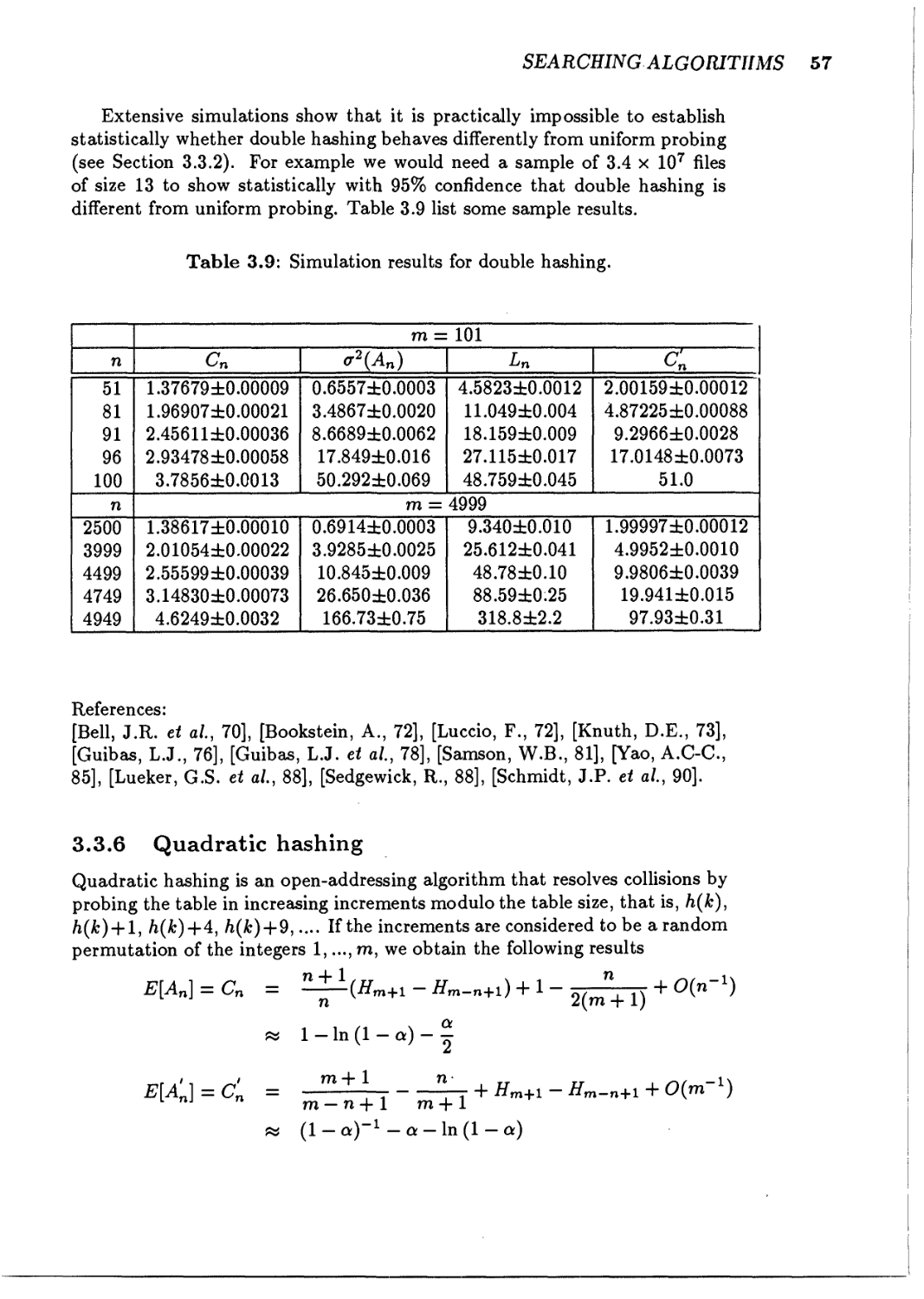
3.3.6 Quadratic hashing 57
3.3.7 Ordered and split-sequence hashing 59
3.3.8 Reorganization schemes 62
3.3.8.1 Brent's algorithm 62
3.3.8.2 Binary tree hashing 64
3.3.8.3 Last-come-first-served hashing 67
3.3.8.4 Robin Hood hashing 69
3.3.8.5 Self-adjusting hashing 70
3.3.9 Optimal hashing 70
3.3.10 Direct chaining hashing 71
3.3.11 Separate chaining hashing 74
3.3.12 Coalesced hashing 77
3.3.13 Extendible hashing 80
3.3.14 Linear hashing 82
3.3.15 External hashing using minimal internal storage 85
3.3.16 Perfect hashing 87
3.3.17 Summary 90
3.4 Recursive structures search 91
3.4.1 Binary tree search 91
3.4.1.1 Randomly generated binary trees 94
3.4.1.2 Random binary trees 96
3.4.1.3 Height-balanced trees 97
3.4.1.4 Weight-balanced trees 100
3.4.1.5 Balancing by internal path reduction 102
3.4.1.6 Heuristic organization schemes on binary trees 105
3.4.1.7 Optimal binary tree search 109
3.4.1.8 Rotations in binary trees 112
3.4.1.9 Deletions in binary trees 114
CONTENTS xi
3.4.1.10 m-ary search trees 116
3.4.2 B-trees 117
3.4.2.1 2-3 trees 124
3.4.2.2 Symmetric binary B-trees 126
3.4.2.3 1-2 trees 128
3.4.2.4 2-3-4 trees 129
3.4.2.5 B-tree variations 130
3.4.3 Index and indexed sequential files 130
3.4.3.1 Index sequential access method 132
3.4.4 Digital trees 133
3.4.4.1 Hybrid tries 137
3.4.4.2 Tries for word-dictionaries 138
3.4.4.3 Digital search trees 138
3.4.4.4 Compressed tries 140
3.4.4.5 Patricia trees 140
3.5 Multidimensional search 143
3.5.1 Quad trees 144
3.5.1.1 Quad tries 146
3.5.2 K-dimensional trees 149
153
153
154
156
158
161
164
166
168
170
171
173
174
176
179
180
181
181
182
182
183
184
185
186
Sorting Algorithms
4.1
4.2
4.3
Techniques for sorting arrays
4.1.1
4.1.2
4.1.3
4.1.4
4.1.5
4.1.6
4.1.7
4.1.8
Bubble sort
Linear insertion sort
Quicksort
Shellsort
Heapsort
Interpolation sort
Linear probing sort
Summary
Sorting other data structures
4.2.1
4.2.2
4.2.3
4.2.4
4.2.5
4.2.6
Merge sort
Quicksort for lists
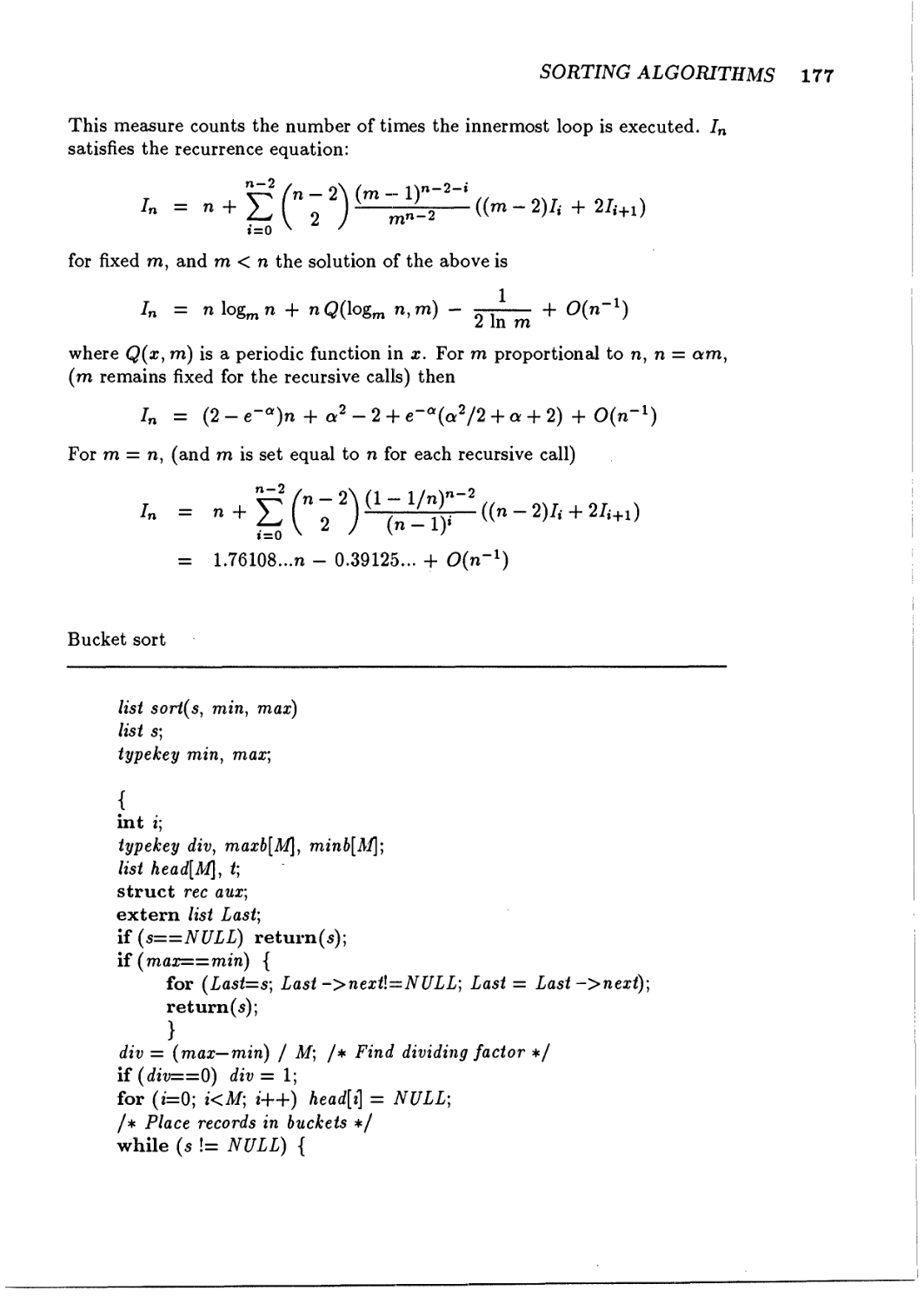
Bucket sort
Radix sort
Hybrid methods of sorting
4.2.5.1 Recursion termination
4.2.5.2 Distributive partitioning
4.2.5.3 Non-recursive bucket sort
Treesort
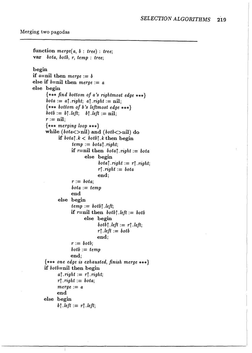
Merging
4.3.1
4.3.2
4.3.3
List merging
Array merging
Minimal-comparison merging
xii CONTENTS
4.4 External sorting 187
4.4.1 Selection phase techniques 189
4.4.1.1 Replacement selection 189
4.4.1.2 Natural selection 190
4.4.1.3 Alternating selection 191
4.4.1.4 Merging phase 192
193
195
196
200
201
205
205
206
209
211
216
218
221
221
223
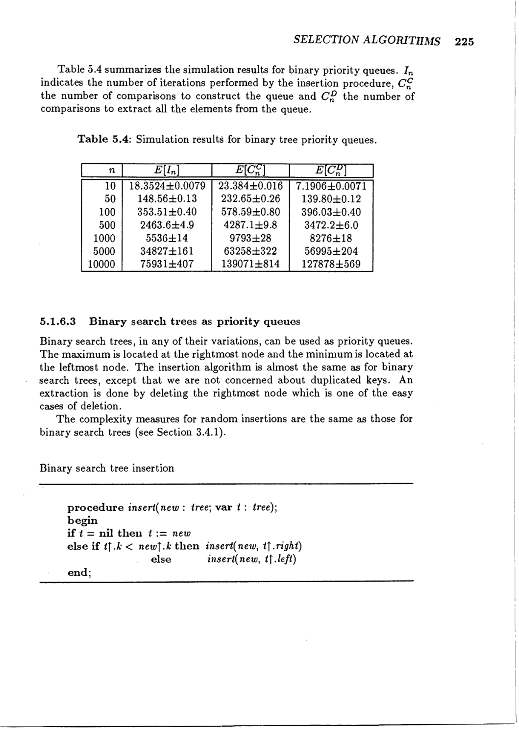
225
226
227
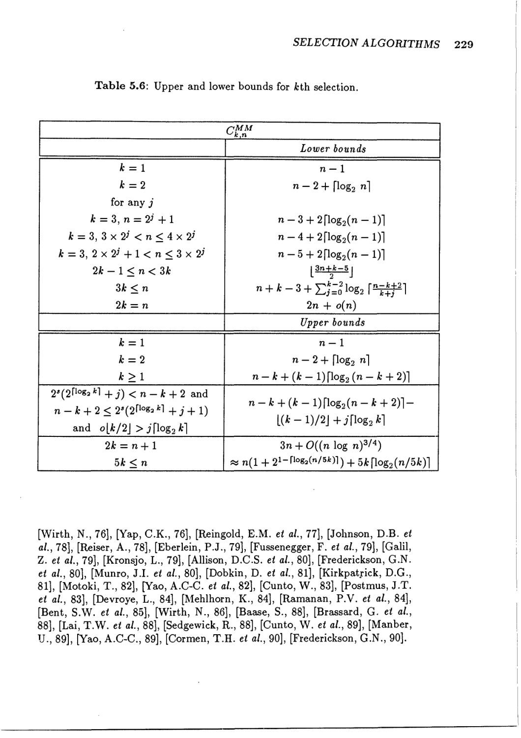
228
230
230
232
Arithmetic Algorithms 235
6.1 Basic operations, multiplication/division 235
6.2 Other arithmetic functions 240
6.2.1 Binary powering 240
6.2.2 Arithmetic-geometric mean 242
6.2.3 Transcendental functions 243
6.3 Matrix multiplication 245
6.3.1 Strassen's matrix multiplication 246
6.3.2 Further asymptotic improvements 247
6.4 Polynomial evaluation 248
4.4.2
4.4.3
4.4.4
4.4.5
4.4.6
Selection
Balanced merge sort
Cascade merge sort
Polyphase merge sort
Oscillating merge sort
External Quicksort
Algorithms
5.1 Priority queues
5.1.1
5.1.2
5.1.3
5.1.4
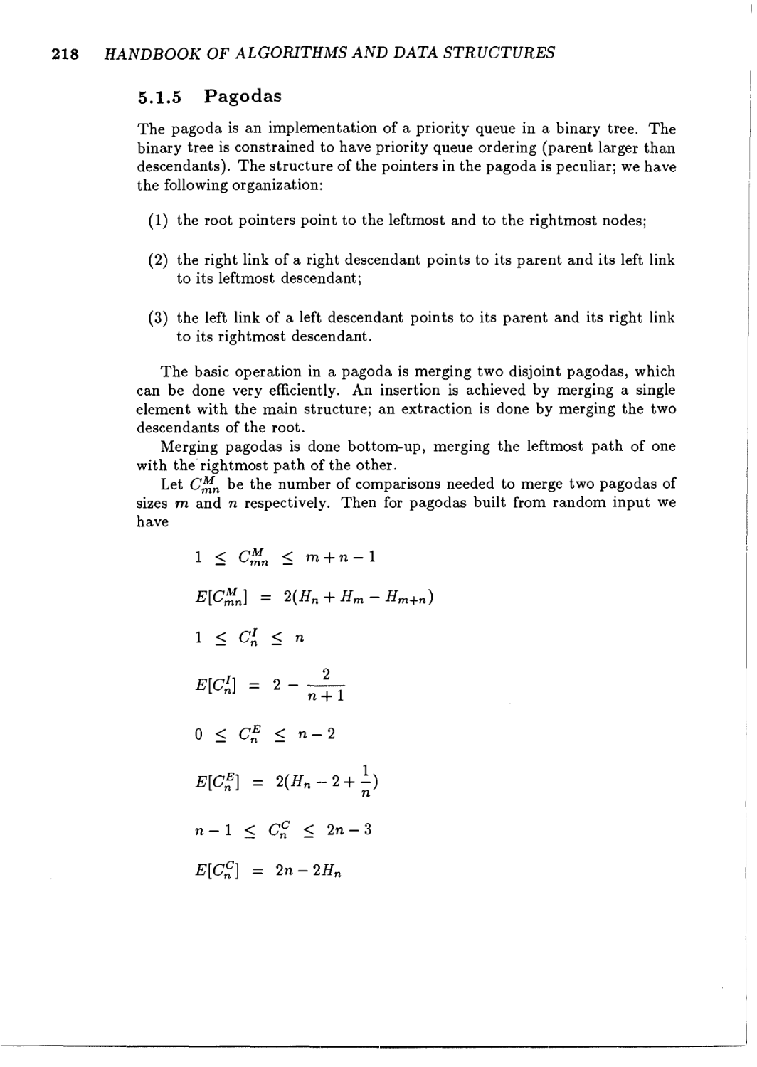
5.1.5
5.1.6
5.1.7
5.1.8
Sorted/unsorted lists
P-trees
Heaps
Van Emde-Boas priority queues
Pagodas
Binary trees used as priority queues
5.1.6.1 Leftist trees
5.1.6.2 Binary priority queues
5.1.6.3 Binary search trees as priority queues
Binomial queues
Summary
5.2 Selection of kth element
5.2.1
5.2.2
5.2.3
Selection by sorting
Selection by tail recursion
Selection of the mode
CONTENTS xiii
Text
7.1
7.2
Algorithms
Text searching without preprocessing
7.1.1
7.1.2
7.1.3
7.1.4
7.1.5
7.1.6
7.1.7
7.1.8
7.1.9
Brute force text searching
Knuth-Morris-Pratt text searching
Boyer-Moore text searching
Searching sets of strings
Karp-Rabin text searching
Searching text with automata
Shift-or text searching
String similarity searching
Summary of direct text searching
Searching preprocessed text
7.2.1
7.2.2
7.2.3
7.2.4
7.2.5
7.2.6
7.2.7
Inverted files
Trees used for text searching
Searching text with automata
Suffix arrays and PAT arrays
DAWG
Hashing methods for text searching
P-st rings
7.3 Other text searching problems
7.3.1 Searching longest common subsequences
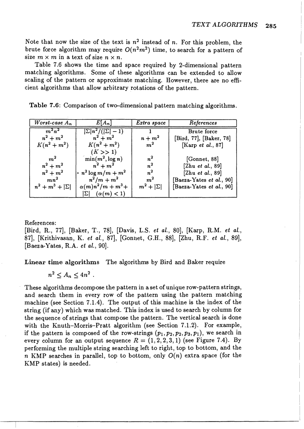
7.3.2 Two-dimensional searching
I Distributions Derived from Empirical Observation
1.1 Zipf's law
1.1.1 First generalization of a Zipfian distribution
1.1.2 Second generalization of a Zipfian distribution
1.2 Bradford's law
1.3 Lotka's law
1.4 80%-20% rule
II Asymptotic Expansions
II. 1 Asymptotic expansions of sums
11.2 Gamma-type expansions
11.3 Exponential-type expansions
11.4 Asymptotic expansions of sums and definite integrals contain-
inge
11.5 Doubly exponential forms
11.6 Roots of polynomials
11.7 Sums containing descending factorials
11.8 Summation formulas
III References
111.1 Textbooks
111.2 Papers
251
251
253
254
256
259
260
262
266
267
270
270
271
273
275
277
279
280
281
283
283
284
289
289
290
290
291
293
293
297
298
300
301
302
303
304
305
307
309
309
311
xiv CONTENTS
IV Algorithms coded in Pascal and C 375
IV. 1 Searching algorithms 375
IV.2 Sorting algorithms 387
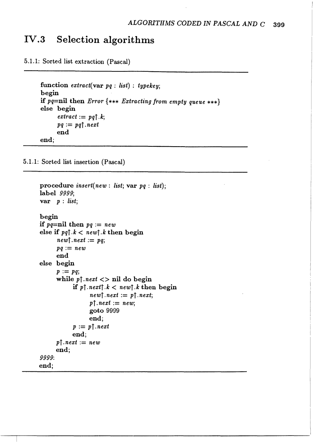
IV.3 Selection algorithms 399
IV.4 Text algorithms 408
Index 415
Trademark notice
SUN 3™ and SunOS™ are trademarks of Sun Microsystems, Inc.
Introduction
This handbook is intended to contain most of the information available on
algorithms and their data structures; thus it is designed to serve a wide spec-
spectrum of users, from the programmer who wants to code efficiently to the
student or researcher who needs information quickly.
The main emphasis is placed on algorithms. For these we present their
description, code in one or more languages, theoretical results and extensive
lists of references.
1.1 Structure of the chapters
The handbook is organized by topics. Chapter 2 offers a formalization of the
description of algorithms and data structures; Chapters 3 to 7 discuss search-
searching, sorting, selection, arithmetic and text algorithms respectively. Appendix
I describes some probability distributions encountered in data processing; Ap-
Appendix II contains a collection of asymptotic formulas related to the analysis
of algorithms; Appendix III contains the main list of references and Appendix
IV contains alternate code for some algorithms.
The chapters describing algorithms are divided into sections and subsec-
subsections as needed. Each algorithm is described in its own subsection, and all
have roughly the same format, though we may make slight deviations or omis-
omissions when information is unavailable or trivial. The general format includes:
A) Definition and explanation of the algorithm and its classification (if ap-
applicable) according to the basic operations described in Chapter 2.
B) Theoretical results on the algorithm's complexity. We are mainly inter-
interested in measurements which indicate an algorithm's running time and
2 HANDBOOK OF ALGORITHMS AND DATA STRUCTURES
its space requirements. Useful quantities to measure for this information
include the number of comparisons, data accesses, assignments, or ex-
exchanges an algorithm might make. When looking at space requirements,
we might consider the number of words, records, or pointers involved
in an implementation. Time complexity covers a much broader range
of measurements. For example, in our examination of searching algo-
algorithms, we might be able to attach meaningful interpretations to most
of the combinations of the
average
variance
minimum
worstcase
average w.c.
number of <
comparisons
accesses
assignments
exchanges
function calls
> when we <
query
add a record into
delete a record from
modify a record of
reorganize
build
read sequentially
the structure. Other theoretical results may also be presented, such as
enumerations, generating functions, or behaviour of the algorithm when
the data elements are distributed according to special distributions.
C) The algorithm. We have selected Pascal and C to describe the algo-
algorithms. Algorithms that may be used in practice are described in one
or both of these languages. For algorithms which are only of theoretical
interest, we do not provide their code. Algorithms which are coded both
in Pascal and in C will have one code in the main text and the other in
Appendix IV.
D) Recommendations. Following the algorithm description we give several
hints and tips on how to use it. We point out pitfalls to avoid in coding,
suggest when to use the algorithm and when not to, say when to expect
best and worst performances, and provide a variety of other comments.
E) Tables. Whenever possible, we present tables which show exact values
of complexity measures in selected cases. These are intended to give
a feeling for how the algorithm behaves. When precise theoretical
results are not available we give simulation results, generally in the
form xxx ± yy where the value yy is chosen so that the resulting interval
has a confidence level of 95%. In other words, the actual value of the
complexity measure falls out of the given interval only once every 20
simulations.
F) Differences between internal and external storage. Some algorithms may
perform better for internal storage than external, or vice versa. When
this is true, we will give recommendations for applications in each case.
Since most of our analysis up to this point will implicitly assume that
internal memory is used, in this section we will look more closely at the
external case (if appropriate). We analyze the algorithm's behaviour
INTRODUCTION 3
when working with external storage, and discuss any significant practical
considerations in using the algorithm externally.
G) With the description of each algorithm we include a list of relevant
references. General references, surveys, or tutorials are collected at the
end of chapters or sections. The third appendix contains an alphabetical
list of all references with cross-references to the relevant algorithms.
1.2 Naming of variables
The naming of variables throughout this handbook is a compromise between
uniformity of notation and accepted terminology in the specific areas.
Except for very few exceptions, explicitly noted, we use:
n for the number of objects or elements or components in a structure;
m for the size of a structure;
b for bucket sizes, or maximum number of elements in a physical block;
d for the digital cardinality or size of the alphabet.
The complexity measures are also named uniformly throughout the hand-
handbook. Complexity measures are named X% and should be read as 'the number
of Xs performed or needed while doing Z onto a structure of size n\ Typical
values for X are:
A : accesses, probes or node inspections;
C : comparisons or node inspections;
E : external accesses;
h : height of a recursive structure (typically a tree);
I : iterations (or number of function calls);
L : length (of path or longest probe sequence);
M '. moves or assignments (usually related to record or key movements);
T : running time;
5* : space (bytes or words).
Typical values for Z are:
null (no superscript): successful search (or default operation, when there
is only one possibility);
' unsuccessful search;
C : construction (building) of structure;
D : deletion of an element;
E : extraction of an element (mostly for priority queues);
I : insertion of a new element;
4 HANDBOOK OF ALGORITHMS AND DATA STRUCTURES
M : merging of structures;
Opt : optimal construction or optimal structure (the operation is usually
implicit);
MM : minimax, or minimum number of X's in the worst case: this is
usually used to give upper and lower bounds on the complexity of a
problem.
Note that X^ means number of operations done to insert an element into a
structure of size n or to insert the n + 1st element.
Although these measures are random variables (as these depend on the
particular structure on which they are measured), we will make exceptions
for Cn and Cn which most of the literature considers to be expected values.
1.3 Probabilities
The probability of a given event is denoted by Pr{event}. Random vari-
variables follow the convention described in the preceding section. The expected
value of a random variable X is written E[X] and its variance is <T2{X). In
particular, for discrete variables X
E[X] = /ii =
{X) = J2i2priX = i} ~ E[X]2 = E[X2] - E[X]2
We will always make explicit the probability universe on which expected
values are computed. This is ambiguous in some cases, and is a ubiquitous
problem with expected values.
To illustrate the problem without trying to confuse the reader, suppose
that we fill a hashing table with keys and then we want to know about the
average number of accesses to retrieve one of the keys. We have two potential
probability universes: the key selected for retrieval (the one inserted first, the
one inserted second, ...) and the actual values of the keys, or their probing
sequence. We can compute expected values with respect to the first, the
second, or both universes. In simpler terms, we can find the expected value
of any key for a given file, or the expected value of a given key for any file, or
the expected value of any key for any file.
Unless otherwise stated, A) the distribution of our elements is always
random independent uniform U@,1); B) the selection of a given element
is uniform discrete between all possible elements; C) expected values which
relate to multiple universes are computed with respect to all universes. In
terms of the above example, we will compute expected values with respect to
randomly selected variables drawn from a uniform U@,1) distribution.
1.4 Asymptotic notation
Most of the complexity measures in this handbook are asymptotic in the si/.o
of the problem. The asymptotic notation we will use is fairly standard and i,<<
given below:
/(n) = O(g(n))
implies that there exists k and no such that | f(n) \ < kg(n) for n > 7iu.
/(n) = o(g(n)) -»• lim 4"T = 0
n—*<x> gin)
f(n) = e(g(n))
implies that there exists ki,k2, (k±xk2 > 0) and n0 such that kig(n) < f(n) <
k2g{n) for n > n0, or equivalently that f(n) = O(g(n)) and g(n) = O(f(n)).
f(n) = n(g(n)) - g(n) = O(f(n))
f(n) = u(g(n)) - g{n) = o(f(n))
f(n) « g(n) -»• /(n)-?f(n) = o(flf(n))
We will freely use arithmetic operations with the order notation, for ex-
example,
/(n) = h{n) + O(g(n))
means
f(n) - h(n) = O(g(n))
Whenever we write /(n) = 0{g{n)) it is with the understanding that we
know of no better asymptotic bound, that is, we know of no h(n) = o(g(n))
such that f(n) = 0{h{n)).
1.5 About the programming languages
We use two languages to code our algorithms: Pascal and C. After writing
many algorithms we still find situations for which neither of these languages
present a very 'clean' or understandable code. Therefore, whenever possible,
we use the language which presents the shortest and most readable code. We
intentionally allow our Pascal and C style of coding to resemble each other.
A minimal number of Pascal programs contain goto statements. These
statements are used in place of the equivalent C statements return and
break, and are correspondingly so commented. Indeed we view their absence
6 HANDBOOK OF ALGORITHMS AND DATA STRUCTURES
from Pascal as a shortcoming of the language. Another irritant in coding
some algorithms in Pascal is the lack of order in the evaluation of logical ex-
expressions. This is unfortunate since such a feature makes algorithms easier to
understand. The typical stumbling block is
while (p <> nil) and (key <> p^.k) do ...
Such a statement works in C if we use the sequential and operator (&&),
but for Pascal we have to use instead:
while p <> nil do begin
if key = p^.k then goto 999 {*** break *** } ;
999:
Other minor objections are: the inability to compute addresses of non-
heap objects in Pascal (which makes treatment of lists more difficult); the
lack of variable length strings in Pascal; the lack of a with statement in C;
and the lack of var parameters in C. (Although this is technically possible to
overcome, it obscures the algorithms.)
Our Pascal code conforms, as fully as possible, to the language described
in the Pascal User Manual and Report by K. Jensen and N. Wirth. The C
code conforms to the language described in The C Programming Language by
B.W. Kernighan and D.M. Ritchie.
1.6 On the code for the algorithms
Except for very few algorithms which are obviously written in pseudo-code,
the algorithms in this handbook were run and tested under two different
compilers. Actually the same text which is printed is used for compiling, for
testing, for running simulations and for obtaining timings. This was done in
an attempt to eliminate (or at least drastically reduce!) errors.
Each family of algorithms has a 'tester set' which not only checks for
correct behaviour of the algorithm, but also checks proper handling of limiting
conditions (will a sorting routine sort a null file? one with one element? one
with all equal keys? ...).
In most cases the algorithms are described as a function or a procedure
or a small set of functions or procedures. In a few cases, for very simple
algorithms, the code is described as in-line code, which could be encapsulated
in a procedure or could be inserted into some other piece of code.
Some algorithms, most notably the searching algorithms, are building
blocks or components of other algorithms or programs. Some standard actions
should not be specified for the algorithm itself, but rather will be specified
once that the algorithm is 'composed' with other parts (chapter 2 defines
INTRODUCTION 7
composition in more detail). A typical example of a standard action is an
error condition. The algorithms coded for this handbook always use the same
names for these standard actions.
Error detection of an unexpected condition during execution. Whenever
Error is encountered it can be substituted by any block of statements. For
example our testers print an appropriate message.
found(record) function call that is executed upon completion of a successful
search. Its argument is a record or a pointer to a record which contains the
searched key.
noifound(key) function called upon an unsuccessful search. Its argument is
the key which was not found.
A special effort has been made to avoid duplication of these standard actions
for identical conditions. This makes it easier to substitute blocks of code for
them.
1.7 Complexity measures and real timings
For some families of algorithms we include a comparison of real timings. These
timings are to be interpreted with caution as they reflect only one sample point
in the many dimensions of hardwares, compilers, operating systems, and so
on. Yet we have equally powerful reasons to present at least one set of real
complexities.
The main reasons for including real timing comparisons are that they take
into account:
A) the actual cost of operations,
B) hidden costs, such as storage allocation, and indexing.
The main objections, or the factors which may invalidate these real timing
tables, are:
A) the results are compiler dependent: although the same compiler is used
for each language, a compiler may favour one construct over others;
B) the results are hardware dependent;
C) in some cases, when large amounts of memory are used, the timings may
be load dependent.
The timings were done on a Sun 3 running the SunOS 4.1 operating system.
Both C and Pascal compilers were run with the optimizer, or object code
improver, to obtain the best implementation for the algorithms.
There were no attempts made to compare timings across languages. All
the timing results are computed relative to the fastest algorithm. To avoid the
incidence of start up-costs, loading, and so on, the tests were run on problems
8 HANDBOOK OF ALGORITHMS AND DATA STRUCTURES
of significant size. Under these circumstances, some 0{n2) algorithms appear
to perform very poorly.
Basic Concepts
2.1 Data structure description
The formal description of data structure implementations is similar to the
formal description of programming languages. In defining a programming
language, one typically begins by presenting a syntax for valid programs in
the form of a grammar and then sets further validity restrictions (for example,
usage rules for symbolic names) which give constraints that are not captured
by the grammar. Similarly, a valid data structure implementation will be one
that satisfies a syntactic grammar and also obeys certain constraints. For
example, for a particular data structure to be a valid weight-balanced binary
tree, it must satisfy the grammatical rules for binary trees and it must also
satisfy a specific balancing constraint.
2.1.1 Grammar for data objects
A sequence of real numbers can be defined by the BNF production
<S> ::= [ real , <S> ] | nil
Thus a sequence of reals can have the form nil, [real,nil], [real,[real,nil]], and
so on. Similarly, sequences of integers, characters, strings, boolean constants,
... could be defined. However, this would result in a bulky collection of
production rules which are all very much alike. One might first try to eliminate
this repetitiveness by defining
<S> ::= [ <D> , <S> ] | nil
where <D> is given as the list of data types
<D> ::= real | int | bool | string | char
9
10 HANDBOOK OF ALGORITHMS AND DATA STRUCTURES
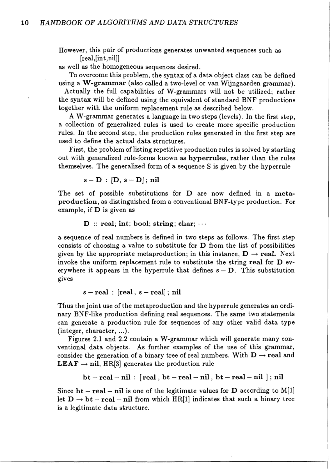
However, this pair of productions generates unwanted sequences such as
[real, [in t, nil]]
as well as the homogeneous sequences desired.
To overcome this problem, the syntax of a data object class can be defined
using a W-grammar (also called a two-level or van Wijngaarden grammar).
Actually the full capabilities of W-grammars will not be utilized; rather
the syntax will be defined using the equivalent of standard BNF productions
together with the uniform replacement rule as described below.
A W-grammar generates a language in two steps (levels). In the first step,
a collection of generalized rules is used to create more specific production
rules. In the second step, the production rules generated in the first step are
used to define the actual data structures.
First, the problem of listing repetitive production rules is solved by starting
out with generalized rule-forms known as hyperrules, rather than the rules
themselves. The generalized form of a sequence S is given by the hyperrule
s - D : [D, s - D]; nil
The set of possible substitutions for D are now defined in a meta-
production, as distinguished from a conventional BNF-type production. For
example, if D is given as
D :: real; int; bool; string; char; •••
a sequence of real numbers is defined in two steps as follows. The first step
consists of choosing a value to substitute for D from the list of possibilities
given by the appropriate metaproduction; in this instance, D —> real. Next
invoke the uniform replacement rule to substitute the string real for D ev-
everywhere it appears in the hyperrule that defines s —D. This substitution
gives
s — real : [real, s — real]; nil
Thus the joint use of the metaproduction and the hyperrule generates an ordi-
ordinary BNF-like production defining real sequences. The same two statements
can generate a production rule for sequences of any other valid data type
(integer, character, ...).
Figures 2.1 and 2.2 contain a W-grammar which will generate many con-
conventional data objects. As further examples of the use of this grammar,
consider the generation of a binary tree of real numbers. With D —> real and
LEAF —> nil, HR[3] generates the production rule
bt — real — nil : [ real, bt — real — nil, bt — real — nil ] ; nil
Since bt — real — nil is one of the legitimate values for D according to M[l]
let D —> bt — real — nil from which HR[1] indicates that such a binary tree
is a legitimate data structure.
BASIC CONCEPTS 11
Metaproductions
M[l] D :: real; int;bool; string; char;...;
M[2] DICT ::
M[3] REC ::
M[4] LEAF ::
M[5] N ::
M[6] DIGIT ::
M[7] KEY ::
REC ; (REC);
[D];
s-D;
gt - D - LEAF;
DICT;
{KEY}$; s-KEY;
bt - KEY - LEAF;
mt - N - KEY - LEAF;
tr - N - KEY.
# atomic data types
# array
# record
# reference
# sequence
# general tree
# dictionary structures
# other structure classes
such as graphs, sets,
priority queues.
# sequential search
# binary tree
# multiway tree
# digital tree
# record definition
D; D, REC.
nil; D.
DIGIT; DIGIT N.
0;l;2;3;4;5;6;7;8;9.
real; int; string; char; (KEY, REC). # search key
Figure 2.1: Metaproductions for data objects.
Secondly consider the specification for a hash table to be used with direct
chaining. The production
s — (string,int) : [(string,int), s — (string,int)] ; nil
and M[l] yield
D -> {s-(string, int)}§6
Thus HR[1] will yield a production for an array of sequences of string/integer
pairs usable, for example, to record NAME/AGE entries using hashing.
Finally consider a production rule for structures to contain B-trees (Section
3.4.2) of strings using HR[4] and the appropriate metaproductions to yield
mt — 10 — string — nil :
[int, {string} J°, {mt - 10 - string - nil} J°] ; nil
12 HANDBOOK OF ALGORITHMS AND DATA STRUCTURES
Hyperrules
HR[1]
HR[2]
HR[3]
HR[4] mt
HR[5]
HR[6]
data structure
bt-
-N-
gt-
-D-
-D-
-D-
tr
s-D
-LEAF
-LEAF
-LEAF
-N-D
: D.
[D,s-D]
[ D, bt - D
[int, {D}N
[D,s-gt-
[{tr-N-
; nil.
- LEAF, bt - D - LEAF ]; LEAF.
, {mt - N - D - LEAF}N]; LEAF.
-D-LEAF]; LEAF.
D }N ]; [D]; nil.
Figure 2.2: Hyperrules for data objects.
In this multitree, each node contains 10 keys and has 11 descendants. Certain
restrictions on B-trees, however, are not included in this description (that
the number of actual keys is to be stored in the int field in each node, that
this number must be between 5 and 10, that the actual keys will be stored
contiguously in the keys-array starting at position 1, ...); these will instead be
defined as constraints (see below).
The grammar rules that we are using are inherently ambiguous. This is
not inconvenient; as a matter of fact it is even desirable. For example, consider
D - {D}N - {real}™ B.1)
and
D -> DICT -> {KEY}?} -> {real}^0 B.2)
Although both derivation trees produce the same object, the second one de-
describes an array used as a sequential implementation of a dictionary structure,
while the first may just be a collection of real numbers. In other words, the
derivation tree used to produce the data objects contains important semantic
information and should not be ignored.
2.1.2 Constraints for data objects
Certain syntactic characteristics of data objects are difficult or cumbersome to
define using formal grammars. A semantic rule or constraint may be regarded
as a boolean function on data objects (S : D —> bool) that indicates which are
valid and which are not. Objects that are valid instances of a data structure
implementation are those in the intersection of the set produced by the W-
grammars and those that satisfy the constraints.
Below are some examples of semantic rules which may be imposed on data
structures. As phrased, these constraints are placed on data structures that
have been legitimately produced by rules given in the previous section.
BASIC CONCEPTS 13
2.1.2.1 Sequential order
Many data structures are kept in some fixed order (for example, the records
in a file are often arranged alphabetically or numerically according to some
key). Whatever work is done on such a file should not disrupt this order. This
definition normally applies to s — D and {D}K.
2.1.2.2 Uniqueness
Often it is convenient to disallow duplicate values in a structure, for example
in representing sets. At other times the property of uniqueness can be used
to ensure that records are not referenced several times in a structure (for
example, that a linear chain has no cycles or that every node in a tree has
only one parent).
2.1.2.3 Hierarchical order
For all nodes, the value stored at any adjacent node is related to the value at
the node according to the type of adjacency. This definition normally applies
to bt - D - LEAF, mt - N - D - LEAF and gt - D - LEAF.
Lexicographical trees
A lexicographical tree is a tree that satisfies the following condition for every
node s: if s has n keys (keyi,key2,..., keyn) stored in it, s must have n + 1
descendant subtrees to,ti,.. .,tn. Furthermore, if do is any key in any node
of to, d\ any key in any node of t\, and so on, the inequality do < key\ <
^l < ••• < keyn < dn must hold.
Priority queues
A priority queue can be any kind of recursive structure in which an order
relation has been established between each node and its descendants. One
example of such an order relation would be to require that keyp < keyj, where
keyp is any key in a parent node, and keyd is any key in any descendant of
that node.
2.1.2.4 Hierarchical balance
Height balance
Let s be any node of a tree (binary or multiway). Define h(s) as the height
of the subtree rooted in s, that is, the number of nodes in the tallest branch
starting at s. One structural quality that may be required is that the height of
a tree along any pair of adjacent branches be approximately the same. More
formally, the height balance constraint is | h(s\) — h(s2) | < f> where si and
$2 are any two subtrees of any node in the tree, and 8 is a constant giving
14 HANDBOOK OF ALGORITHMS AND DATA STRUCTURES
the maximum allowable height difference. In B-trees (see Section 3.4.2) for
example, 8 = 0, while in AVL-trees <$ = 1 (see Section 3.4.1.3).
Weight balance
For any tree, the weight function w(s) is defined as the number of external
nodes (leaves) in the subtree rooted at s. A weight balance condition requires
that for any two nodes si and S2, if they are both subtrees of any other node
in the tree, r < w(si)/w(s2) < 1/r where r is a positive constant less than 1.
2.1.2.5 Optimality
Any condition on a data structure which minimizes a complexity measure
(such as the expected number of accesses or the maximum number of com-
comparisons) is an optimality condition. If this minimized measure of complexity
is based on a worst-case value, the value is called the minimax; when the
mininiized complexity measure is based on an average value, it is the minave.
In summary, the W-grammars are used to define the general shape or
pattern of the data objects. Once an object is generated, its validity is checked
against the semantic rules or constraints that may apply to it.
References:
[Pooch, U.W. et ai, 73], [Aho, A.V. et ai, 74], [Rosenberg, A.L., 74], [Rosen-
[Rosenberg, A.L., 75], [Wirth, N., 76], [Claybrook, B.G., 77], [Hollander, C.R., 77],
[Honig, W.L. et ai, 77], [MacVeigh, D.T., 77], [Rosenberg, A.L. et ai, 77],
[Cremers, A.B. et ai, 78], [Gotlieb, C.C. et ai, 78], [Rosenberg, A.L., 78], [Bo-
brow, D.G. et ai, 79], [Burton, F.W., 79], [Rosenberg, A.L. et ai, 79], [Rosen-
[Rosenberg, A.L. et ai, 80], [Vuillemin, J., 80], [Rosenberg, A.L., 81], [O'Dunlaing,
C. et ai, 82], [Gonnet, G.H. et ai, 83], [Wirth, N., 86].
2.2 Algorithm descriptions
Having defined the objects used to structure data, it is appropriate to de-
describe the algorithms that access them. Furthermore, because data objects
are not static, it is equally important to describe data structure manipulation
algorithms.
An algorithm computes a function that operates on data structures. More
formally, an algorithm describes a map S—*RotSxP—*R, where S, P,
and R are all data structures; S is called the input structure, P contains
parameters (for example, to specify a query), and R is the result. The two
following examples illustrate these concepts:
A) Quicksort is an algorithm that takes an array and sorts it. Since there
are no parameters,
BASIC CONCEPTS 15
Quicksort: array —> sorted-array
B) B-tree insertion is an algorithm that inserts a new record P into a B-tree
S, giving a new B-tree as a result. In functional notation,
B-tree-insertion: B-tree x new-record —> B-tree
Algorithms compute functions over data structures. As always, different
algorithms may compute the same functions; sinB:c) and 2sin(:c) cos(:c) are
two expressions that compute the same function. Since equivalent algorithms
have different computational requirements however, it is not merely the func-
function computed by the algorithm that is of interest, but also the algorithm
itself.
In the following section, we describe a few basic operations informally in
order to convey their flavour.
References:
[Aho, A.V. et ai, 74], [Wirth, N., 76], [Bentley, J.L., 79], [Bentley, J.L., 79],
[Saxe, J.B. et ai, 79], [Bentley, J.L. et ai, 80], [Bentley, J.L. et ai, 80], [Remy,
J.L., 80], [Mehlhorn, K. et ai, 81], [Overmars, M.H. et ai, 81], [Overmars,
M.H. et ai, 81], [Overmars, M.H. et ai, 81], [Overmars, M.H. et ai, 81],
[Overmars, M.H., 81], [Rosenberg, A.L., 81], [Overmars, M.H. et ai, 82],
[Gonnet, G.H. et ai, 83], [Chazelle, B. et ai, 86], [Wirth, N., 86], [Tarjan,
R.E., 87], [Jacobs, D. et ai, 88], [Manber, U., 88], [Rao, V.N.S. et ai, 88],
[Lan, K.K., 89], [Mehlhorn, K. et ai, 90].
2.2.1 Basic (or atomic) operations
A primary class of basic operations manipulate atomic values and are used to
focus an algorithm's execution on the appropriate part(s) of a composite data
object. The most common of these are as follows:
Selector and constructor
A selector is an operation that allows access to any of the elements corre-
corresponding to the right-hand side of a production rule from the corresponding
left-hand side object. A constructor is an operation that allows us to assemble
an element on the left-hand side of a production given all the corresponding
elements on the right. For example, given a {string}? and an integer, we
can select the ith element, and given two bt — real — ml and a real we can
construct a new bt — real — nil.
Replacement non-scalar x selector x value —> non-scalar
A replacement operator removes us from pure functions by introducing the
assignment statements. This operator introduces the possibility of cyclic and
shared structures. For example, given a bt-D-LEAF we can form a threaded
16 HANDBOOK OF ALGORITHMS AND DATA STRUCTURES
binary tree by replacing the nil values in the leaves by (tagged) references back
to appropriate nodes in the tree.
Ranking set of scalars x scalar —> integer
This operation is defined on a set of scalars Xi,X2,..., Xn and uses another
scalar X as a parameter. Ranking determines how many of the Xj values are
less than or equal to X, thus determining what rank X would have if it were
ordered with the other values. More precisely, ranking is finding an integer
i such that there is a subset A C {X\,X2, ...,Xn} for which | A \ — i
and Xj 6 A if and only if Xj < X. Ranking is used primarily in directing
multiway decisions. For example, in a binary decision, n = 1, and i is zero if
X < X\, one otherwise.
Hashing value x range —> integer
Hashing is an operation which normally makes use of a record key. Rather
than using the actual key value however, an algorithm invokes hashing to
transform the key into an integer in a prescribed range by means of a hashing
function and then uses the generated integer value.
Interpolation numeric-value x parameters —> integer
Similarly to hashing, this operation is typically used on record keys. Interpo-
Interpolation computes an integer value based on the input value, the desired range,
the values of the smallest and largest of a set of values, and the probability
distribution of the values in the set. Interpolation normally gives the statisti-
statistical mode of the location of a desired record in a random ordered file, that is,
the most probable location of the record.
Digitization scalar —> sequence of scalars
This operation transforms a scalar into a sequence of scalars. Numbering
systems that allow the representation of integers as sequences of digits and
strings as sequences of characters provide natural methods of digitization.
Testing for equality value x value —> boolean
Rather than relying on multiway decisions to test two values for equality, a
distinct operation is included in the basic set. Given two values of the same
type (for example, two integers, two characters, two strings), this operation
determines whether they are equal. Notice that the use of multiway branching
plus equality testing closely matches the behaviour of most processors and
programming languages which require two tests for a three-way branch (less
than, equal, or greater than).
BASIC CONCEPTS 17
2.2.2 Building procedures
Building procedures are used to combine basic operations and simple algo-
algorithms to produce more complicated ones. In this section, we will define four
building procedures: composition, alternation, conformation and self-
organization .
General references:
[Darlington, J., 78], [Barstow, D.R., 80], [Clark, K.L. et al., 80], [van Leeuwen,
J. et al., 80], [Merritt, S.M., 85].
2.2.2.1 Composition
Composition is the main procedure for producing algorithms from atomic op-
operations. Typically, but not exclusively, the composition ofFi:SxP-+R and
F2 : SxP —> R can be expressed in a functional notation as F2(F1(S, Pi), P2).
A more general and hierarchical description of composition is that the descrip-
description of F2 uses F\ instead of a basic operation.
Although this definition is enough to include all types of composition,
there are several common forms of composition that deserve to be identified
explicitly.
Divide and conquer
This form uses a composition involving two algorithms for any problems that
are greater than a critical size. The first algorithm splits a problem into
(usually two) smaller problems. The composed algorithm is then recursively
applied to each non-empty component, using recursion termination (see be-
below) when appropriate. Finally the second algorithm is used to assemble the
components' results into one result. A typical example of divide and conquer
is Quicksort (where the termination alternative may use a linear insertion
sort). Diagrammatically:
Divide and conquer
solve—problem(A):
if size(A) <— Critical—Size
then End—Action
else begin
Split—problem;
solve—problem(Ai);
solve—problem(A2);
Assemble—Results
end;
18 HANDBOOK OF ALGORITHMS AND DATA STRUCTURES
Special cases of divide and conquer, when applied to trees, are tree traver-
sals.
Iterative application
This operates on an algorithm and a sequence of data structures. The algo-
algorithm is iteratively applied using successive elements of the sequence in place
of the single element for which it was written. For example, insertion sort
iteratively inserts an element into a sorted sequence.
Iterative application
solve—problem(S):
while not empty (S) do begin
Apply algorithm to next element of sequence S',
Advance S
end;
End— Action
Alternatively, if the sequence is in an array:
Iterative application (arrays)
solve—problem(A):
for i:=l to size(A) do
Action on A[t\;
End—Action
Tail recursion
This method is a composition involving one algorithm that specifies the crite-
criterion for splitting a problem into (usually two) components and selecting one
of them to be solved recursively. A classical example is binary search.
Tail recursion
solve—problem(A):
if size(A) <= Critical—Size
then End—Action
else begin
Split and select subproblem i;
solve—problem(Ai)
end
BASIC CONCEPTS 19
Alternatively, we can unwind the recursion into a while loop:
Tail recursion
solve—problem(A):
while size(A) > Critical—Size do begin
Split and select subproblem i;
A := Ai
end;
End— Action
It should be noted that tail recursion can be viewed as a variant of di-
divide and conquer in which only one of the subproblems is solved recursively.
Both divide and conquer and tail recursion split the original problem into sub-
problems of the same type. This splitting applies naturally to recursive data
structures such as binary trees, multiway trees, general trees, digital trees, or
arrays.
Inversion
This is the composition of two search algorithms that are then used to search
for sets of records based on values of secondary keys. The first algorithm is
used to search for the selected attribute (for example, find the 'inverted list'
for the attribute 'hair colour' as opposed to 'salary range') and the second
algorithm is used to search for the set with the corresponding key value (for
instance, 'blonde' as opposed to 'brown'). In general, inversion returns a set
of records which may be further processed (for example, using intersection,
union, or set difference).
Inverted search
inverted— search(S, A, V):
{*** Search the value V of the attribute A in
the structure S *** }
search (search(S, A), V)
The structure S on which the inverted search operates has to reflect these
two searching steps. For the generation of S, the following metaproductions
should be used:
S _> D -> DICT -> (KEYattr, Dattr)
Dattr _^ mcT _^ . .(KEYvalue, Dvalue) •••
20 HANDBOOK OF ALGORITHMS AND DATA STRUCTURES
Dvalue _^ SET _^ ...
Digital decomposition
This is applied to a problem of size n by attacking preferred-size pieces (for
example, pieces of size equal to a power of two). An algorithm is applied to
all these pieces to produce the desired result. One typical example is binary
decomposition.
Digital decomposition
Solve—problem(A, n)
{*** n has a digital decomposition n = rikftk + •¦¦ + n\j3\ + no *** }
Partition the problem into subsets
{*** where size{A\) = /?,- *** }
for i:= 0 to k while not completed do
simplei—solve(Aj, Af,..., A"');
Merge
The merge technique applies an algorithm and a discarding rule to two or
more sequences of data structures ordered on a common key. The algorithm
is iteratively applied using successive elements of the sequences in place of
the single elements for which it was written. The discarding rule controls the
iteration process. For example, set union, intersection, merge sort, and the
majority of business applications use merging.
Merge
Merge(Si, S2, ...,
while at least one Si is not empty do
kmin := minimum value of keys in Si, ..., Sk]
for i := 1 to k do
if kmin = head(S{)
then t[t\ := head(Si)
else t[i\ := nil;
processing—rule( t[ 1], t[ 2],..., t[k]);
End—Action
Randomization
This is used to improve a procedure or to transform a procedure into a proba-
BASIC CONCEPTS 21
bilistic algorithm. This is appealing when the underlying procedure may fail,
may not terminate, or may have a very bad worst case.
Ran domiz at ion
solve—problem (A)
repeat begin
randomize(A);
solve(randomized(A), t(A) units—of—time);
end until Solve—Succeeds or Too—Many— Iterations;
if Too—Many— Iterations
then return{No—Solution—Exists)
else return(Solution);
The conclusion that there is no solution is reached with a certain proba-
probability, hopefully very small, of being wrong. Primality testing using Fermat's
little result is a typical example of this type of composition.
References:
[Bentley, J.L. et al, 76], [Yao, A.C-C, 77], [Bentley, J.L. et al, 78], [Dwyer,
B., 81], [Chazelle, B., 83], [Lesuisse, R., 83], [Walah, T.R., 84], [Snir, M., 86],
[Karlsson, R.G. et al, 87], [Veroy, B.S.,
2.2.2.2 Alternation
The simplest building operation is alternation. Depending on the result of a
test or on the value of a discriminator, one of several alternative algorithms
is invoked. For example, based on the value of a command token in a batch
updating interpreter, an insertion, modification, or deletion algorithm could
be invoked; based on the success of a search in a table, the result could be
processed or an error handler called; or based on the size of the input set, an
O(N2) or an O(AHog N) sorting algorithm could be chosen.
There are several forms of alternation that appear in many algorithms;
these are elaborated here.
Superimposition
This combines two or more algorithms, allowing them to operate on the same
data structure more or less independently. Two algorithms Fi and F2 may be
superimposed over a structure S if Fi(S, Q\) and F2(S, Q2) can both operate
together. A typical example of this situation is a file that can be searched by
one attribute using i*i and by another attribute using F2. Unlike other forms
of alternation, the alternative to be used cannot be determined from the state
of the structure itself; rather superimposition implies the capability of using
22 HANDBOOK OF ALGORITHMS AND DATA STRUCTURES
any alternative on any instance of the structure involved. Diagrammatically:
Superimposition
solve—problem(A):
case 1: solve—problemi(A);
case 2: solve—probleni2(A);
case n: solve—problemn(A)
Interleaving
This operation is a special case of alternation in which one algorithm does not
need to wait for other algorithms to terminate before starting its execution.
For example one algorithm might add records to a file while a second algorithm
makes deletions; interleaving the two would give an algorithm that performs
additions and deletions in a single pass through the file.
Recursion termination
This is an alternation that separates the majority of the structure manipu-
manipulations from the end actions. For example, checking for end of file on input,
for reaching a leaf in a search tree, or for reduction to a trivial sublist in a
binary search are applications of recursion termination. It is important to
realize that this form of alternation is as applicable to iterative processes as
recursive ones. Several examples of recursion termination were presented in
the previous section on composition (see, for example, divide and conquer).
2.2.2.3 Conformation
If an algorithm builds or changes a data structure, it is sometimes necessary
to perform more work to ensure that semantic rules and constraints on the
data structure are not violated. For example, when nodes are inserted into
or deleted from a tree, the tree's height balance may be altered. As a result
it may become necessary to perform some action to restore balance in the
new tree. The process of combining an algorithm with a 'clean-up' operation
on the data structure is called conformation (sometimes organization or
reorganization). In effect, conformation is a composition of two algorithms:
the original modification algorithm and the constraint satisfaction algorithm.
Because this form of composition has an acknowledged meaning to the algo-
algorithm's users, it is convenient to list it as a separate class of building operation
rather than as a variant of composition. Other examples of conformation in-
include reordering elements in a modified list to restore lexicographic order,
percolating newly inserted elements to their appropriate locations in a prior-
priority queue, and removing all dangling (formerly incident) edges from a graph
BASIC CONCEPTS 23
after a vertex is deleted.
2.2.2.4 Self-organization
This is a supplementary heuristic activity that an algorithm may often per-
perform in the course of querying a structure. Not only does the algorithm do
its primary work, but it also re accommodates the data structure in a way
designed to improve the performance of future queries. For example, a search
algorithm may relocate the desired element once it is found so that future
searches through the file will locate the record more quickly. Similarly, a page
management system may mark pages as they are accessed, in order that 'least
recently used' pages may be identified for subsequent replacement.
Once again, this building procedure may be viewed as a special case of
composition (or of interleaving); however, its intent is not to build a func-
functionally different algorithm, but rather to augment an algorithm to include
improved performance characteristics.
2.2.3 Interchangeability
The framework described so far clearly satisfies two of its goals: it offers
sufficient detail to allow effective encoding in any programming language,
and it provides a uniformity of description to simplify teaching. It remains
to be shown that the approach can be used to discover similarities among
implementations as well as to design modifications that result in useful new
algorithms.
The primary vehicle for satisfying these goals is the application of inter-
interchangeability. Having decomposed algorithms into basic operations used in
simple combinations, one is quickly led to the idea of replacing any component
of an algorithm by something similar.
The simplest form of interchangeability is captured in the static objects'
definition. The hyperrules emphasize similarities among the data structure
implementations by indicating the universe of uniform substitutions that can
be applied. For example, in any structure using a sequence of reals, the hyper-
rule for s — D together with that for D indicates that the sequence of reals can
be replaced by a sequence of integers, a sequence of binary trees, and so on.
Algorithms that deal with such modified structures need, at most, superficial
changes for manipulating the new sequences, although more extensive modi-
modifications may be necessary in parts that deal directly with the components of
the sequence.
The next level of interchangeability results from the observation that some
data structure implementations can be used to simulate the behaviour of oth-
others. For example, wherever a bounded sequence is used in an algorithm, it
may be replaced by an array, relying on the sequentially of the integers to
access the array's components in order. Sequences of unbounded length may
24 HANDBOOK OF ALGORITHMS AND DATA STRUCTURES
be replaced by sequences of arrays, a technique that may be applied to adapt
an algorithm designed for a one-level store to operate in a two-level memory
environment wherein each block will hold one array. This notion of inter-
changeability is the one usually promoted by researchers using abstract data
types; their claim is that the algorithms should have been originally specified
in terms of abstract sequences. We feel that the approach presented here does
not contradict those claims, but rather that many algorithms already exist for
specific representations, and that an operational approach to specifying algo-
algorithms, together with the notion of interchangeability, is more likely to appeal
to data structure practitioners. In cases where data abstraction has been ap-
applied, this form of interchangeability can be captured in a meta-production,
as was done for DICT in Figure 2.1.
One of the most common examples of this type of interchange is the im-
implementation of linked lists and trees using arrays. For example, an s — D is
implemented as an {D,int}v* and a bt — D —nil as an {D,int,int}v\ In
both cases the integers play the same role as the pointers: they select a record
of the set. The only difference is syntactic, for example
p^.nexi -> next[p]
pf. right -> right[p].
Typically the value 0 is reserved to simulate a null pointer.
The most advanced form of interchangeability has not been captured by
previous approaches. There are classes of operations that have similar intent
yet behave very differently. As a result, replacing some operations by others in
the same class may produce startling new algorithms with desirable properties.
Some of these equivalence classes are listed below.
Basic algorithms {hashing; interpolation; direct addressing }
{collision resolution methods }
{binary partition; Fibonaccian partition;
median partition; mode partition }
Semantic rules {height balance; weight balance }
{lexicographical order; priority queues }
{ordered hashing; Brent's hashing;
binary tree hashing }
{minimax; minave }
Searching Algorithms
3.1 Sequential search
3.1.1 Basic sequential search
This very basic algorithm is also known as the linear search or brute force
search. It searches for a given element in an array or list by looking through
the records sequentially until it finds the element or reaches the end of the
structure. Let n denote the size of the array or list on which we search.
Let An be a random variable representing the number of comparisons made
between keys during a successful search and let An be a random variable for
the number of comparisons in an unsuccessful search. We have
A < i < n)
Pr{An
E[An]
cr2(An)
Ai =
= i}
n
i
n
=
+
2
1
n
1
-1
Below we give code descriptions of the sequential search algorithm in sev-
several different situations. The first algorithm (two versions) searches an array
r[i] for the first occurrence of a record with the required key; this is known as
primary key search. The second algorithm also searches through an array,
but does not stop until it has found every occurrence of the desired key; this
25
26 HANDBOOK OF ALGORITHMS AND DATA STRUCTURES
is known as secondary key search. The third algorithm inserts a new key
into the array without checking if the key already exists (this must be done
for primary keys). The last two algorithms deal with the search for primary
and secondary keys in linked lists.
Sequential search in arrays (non-repeated keys)
function search(key : typekey; var r : dataarray) : integer;
var i : integer;
begin
i := 1;
while (i<n) and (key <> r[i\.k) do i := i+1;
if r[t].k=key then search := i {*** found(r[i\) ***}
else search := — 1; {*** notfound(key) ***}
end;
For a faster inner loop, if we are allowed to modify location n + 1, then:
Sequential search in arrays (non-repeated keys)
function search(key : typekey; var r : dataarray) : integer;
var i : integer;
begin
r[n+l].k := key;
i := 1;
while key <> r[t\.k do i := i+1;
if i <= n then search := i {*** found(r[t\) ***}
else search := —1; {*** notfound(key) ***}
end;
Sequential search in arrays (secondary keys)
for j:=1 to n do
if key = r[i\.k then found(r[t\);
SEARCHING ALGORITHMS 27
Insertion of a new key in arrays (secondary keys)
procedure insert(key : typekey; var r : dataarray);
begin
if n> = m then Error {*** Table is full ***}
else begin
n := n+1;
r[n].k := fcey
end
end;
Sequential search in lists (non-repeated keys)
datarecord *search(key, list)
typekey key; datarecord *list;
{ datarecord *p;
for (p=list; p != NULL &zk key != p ->k; p = p ->next);
return (p);
Sequential search in lists (secondary keys)
p := list;
while p <> nil do
begin
if key = p\.k then found(p'\);
p := pi.next
end;
The sequential search is the simplest search algorithm. Although it is not
very efficient in terms of the average number of comparisons needed to find a
record, we can justify its use when:
A) our files only contain a few records (say, n < 20);
B) the search will be performed only infrequently;
28 HANDBOOK OF ALGORITHMS AND DATA STRUCTURES
C) we are looking for secondary keys and a large number of hits @(n)) is
expected;
D) testing extremely complicated conditions.
The sequential search can also look for a given range of keys instead of
one unique key, at no significant extra cost. Another advantage of this search
algorithm is that it imposes no restrictions on the order in which records are
stored in the list or array.
The efficiency of the sequential search improves somewhat when we use it
to examine external storage. Suppose each physical I/O operation retrieves b
records; we say that b is the blocking factor of the file, and we refer to each
block of b records as a bucket. Assume that there are a total of n records
in the external file we wish to search and let k = \n/b\. If we use En as a
random variable representing the number of external accesses needed to find
a given record, we have
E[En] = * + i
References:
[Knuth, D.E., 73], [Berman, G. et ai, 74], [Knuth, D.E., 74], [Clark, D.W.,
76], [Wise, D.S., 76], [Reingold, E.M. et ai, 77], [Gotlieb, C.C et ai, 78],
[Hansen, W.J., 78], [Flajolet, P. et ai, 79], [Flajolet, P. et ai, 79], [Kronsjo,
L., 79], [Flajolet, P. et ai, 80], [Willard, D.E., 82], [Sedgewick, R., 88].
3.1.2 Self-organizing sequential search: move-to-front
method
This algorithm is basically the sequential search, enhanced with a simple
heuristic method for improving the order of the list or array. Whenever
a record is found, that record is moved to the front of the table and the
other records are slid back to make room for it. (Note that we only need to
move the elements which were ahead of the given record in the table; those
elements further on in the table need not be touched.) The rationale behind
this procedure is that if some records are accessed more often than others,
moving those records to the front of the table will decrease the time for future
searches. It is, in fact, very common for records in a table to have unequal
probabilities of being accessed; thus, the move-to-front technique may often
reduce the average access time needed for a successful search.
We will assume that there exists a probability distribution in which
Pr{accessing key /<",} = p,-. Further we will assume that the keys are
SEARCHING ALGORITHMS 29
numbered in such a way that pi > P2 > ¦ ¦ ¦ > pn > 0. With this model
we have
E[An] = Cn = i
Pipj
2 ' j^Pi+Pj
CT2(An) = B-Cn)(Cn-l)
+4 V^ PiPiPk
( + + M
* +PJ+Pk \Pi + Pi Pi +Pk Pj+Pk
A'n = n
CS- ft S^lOpt ft \ "* „•_ ft ,,'
n S: TT^n 7T / P* "n^l
where //x = C°v% = ^ ipi is the first moment of the distribution.
If we let T(z) = ??=1 z^< then
Cn = C z[T\z)]2dz
Jo
Let Cn(<) be the average number of additional accesses required to find a
record, given that t accesses have already been made. Starting at t = 0 with
a randomly ordered table we have
l<7n@-O, I = 0{n2/t)
Below we give a code description of the move-to-front algorithm as it can
be implemented to search linked lists. This technique is less suited to working
with arrays.
Self-organizing (move-to-front) sequential search (lists)
function search{key : typekey; var head : list) : list;
label 999;
var p, q : list;
begin
if head = nil then search := nil
else if key = head\.k then search := head
else begin
{*** Find record ***}
p := head;
30 HANDBOOK OF ALGORITHMS AND DATA STRUCTURES
while p\.next <> nil do
if p].next\.k = key then begin
{*** Move to front of list ***}
q := head;
head := p'l.next;
p\.next := p\ .nexf\ .next;
head].next := q;
search := head;
goto 999 {*** Break ***}
end
else p := p\.next;
search := nil
end;
999:
end;
Insertion of a new key on a linked list
function insert(key : typekey; head : list) : list;
var p : list;
begin
n := n+1;
new(p);
p\.k :- key;
p^.next := head;
insert := p;
end;
There are more sophisticated heuristic methods of improving the order
of a list than the move-to-front technique; however, this algorithm can be
recommended as particularly appropriate when we have reasons to suspect
that the accessing probabilities for individual records will change with time.
Moreover, the move-to-front approach will quickly improve the organiza-
organization of a list when the accessing probability distribution is very skewed.
If we can guarantee that the search will be successful we can obtain an
efficient array implementation by sliding elements back while doing the search.
When searching a linked list, the move-to-front heuristic is preferable to
the transpose heuristic (see Section 3.1.3).
Below we give some efficiency measures for this algorithm when the ac-
accessing probabilities follow a variety of distributions.
Zipf's law (harmonic): pi =
SEARCHING ALGORITHMS 31
Bn + l)H2n - 2(n + l)ffn _ 21nB)n 1
Lotka's law: p,- = (i2^)
Cn = - Inn- 0.00206339 ... +O(—)
7T n
Exponential distribution: p,- = A —a)a*~1
_ 21n 2 _ 1_ _ In a _ In3 a 5
n " In a 2 24 2880 + ( a)
Wedge distribution: p,- = 2%*\^9
r - f4n + 2 1 "\ nr Bn + l)(8n2 + 14n - 3)
3 8n(n + l)y " 12n(n
4n + 4 13
~~3 12(n + 1)
.,
2n
71
Generalized Zipf's: p,- oc i
where //x is the optimal cost (see Section 3.1.4). The above formula is maxi-
maximized for A = 2, and this is the worst-case possible probability distribution.
Table 3.1 gives the relative efficiency of move-to-front compared to the op-
optimal arrangement of keys, when the list elements have accessing probabilities
which follow several different 'folklore' distributions.
References:
[McCabe, J., 65], [Knuth, D.E., 73], [Hendricks, W.J., 76], [Rivest, R.L.,
76], [Bitner, J.R., 79], [Gonnet, G.H. et al., 79], [Gonnet, G.H. et al, 81],
[Tenenbaum, A.M. et al, 82], [Bentley, J.L. et al, 85], [Hester, J.H. et al,
85], [Hester, J.H. et al, 87], [Chung, F.R.K. et al, 88], [Makinen, E., 88].
3.1.3 Self-organizing sequential search: transpose
method
This is another algorithm based on the basic sequential search and enhanced
by a simple heuristic method of improving the order of the list or array.
In this model, whenever a search succeeds in finding a record, that record is
32 HANDBOOK OF ALGORITHMS AND DATA STRUCTURES
Table 3.1: Relative efficiency of move-to-front.
n
5
10
50
100
500
1000
10000
Cn/CW
Zipf's law
1.1921
1.2580
1.3451
1.3623
1.3799
1.3827
1.3858
80%-20%
rule
1.1614
1.2259
1.3163
1.3319
1.3451
1.3468
1.3483
Bradford's law
F = 3)
1.1458
1.1697
1.1894
1.1919
1.1939
1.1942
1.1944
Lotka's law
1.2125
1.2765
1.3707
1.3963
1.4370
1.4493
1.4778
transposed with the record that immediately precedes it in the table (provided
of course that the record being sought was not already in the first position).
As with the move-to-front (see Section 3.1.2) technique, the object of this
rearrangement process is to improve the average access time for future searches
by moving the most frequently accessed records closer to the beginning of the
table. We have
E[An] = Cn = Prob(In)J2
where tt denotes any permutation of the integers 1,2,...,n. t(j) is the location
of the number j in the permutation ir, and Prob(In) is given by
This expected value of the number of the accesses to find an element can be
written in terms of permanents by
c =
n
perm(P)
where P is a matrix with elements pitj = p~J and Pk is a matrix like P except
that the kth row is pk j = 3p}T* • We can put a bound on this expected value
by
Cn <
<
n
where /i'x is the optimal search time (see Section 3.1.4).
SEARCHING ALGORITHMS 33
In general the transpose method gives better results than the move-to-front
(MTF) technique for stable probabilities. In fact, for all record accessing
probability distributions, we have
Qtranspose < qMTF
When we look at the case of the unsuccessful search, however, both methods
have the identical result
A'n = n
Below we give a code description of the transpose algorithm as it can be
applied to arrays. The transpose method can also be implemented efficiently
for lists, using an obvious adaptation of the array algorithm.
Self-organizing (transpose) sequential search (arrays)
function search(key : typekey; var r : dataarray) : integer,
var i : integer;
tempr : datarecord;
begin
i := 1;
while (i<ri) and (r[i].fc <> key) do i := i+1;
if key = r[i\.k then
begin
if i> 1 then
begin
{*** Transpose with predecessor ***}
tempr := r[i\;
j
r[i— 1] := tempr;
i := i—1
end;
search := i {*** found(r[i\) ***}
end
else search := —1; {*** notfound(key) ***}
end;
It is possible to develop a better self-organizing scheme by allocating extra
storage for counters which record how often individual elements are accessed;
however, it is conjectured that the transpose algorithm is the optimal heuristic
organization scheme when allocating such extra storage is undesirable.
It should be noted that the transpose algorithm may take quite some time
to rearrange a randomly ordered table into close to optimal order. In fact, it
34 HANDBOOK OF ALGORITHMS AND DATA STRUCTURES
may take Q(n2) accesses to come within a factor of 1 + e of the final steady
state.
Because of this slow adaptation ability, the transpose algorithm is not
recommended for applications where accessing probabilities may change with
time.
For sequential searching of an array, the transpose heuristic is preferable
over the move-to-front heuristic.
Table 3.2 gives simulation results of the relative efficiency of the trans-
transpose method compared to the optimal arrangement of keys, when the list
elements have accessing probabilities which follow several different 'folklore'
distributions. It appears that for all smooth distributions, the ratio between
transpose and the optimal converges to 1 as n —* oo.
Table 3.2: Simulation results on the relative efficiency of transpose.
n
5
10
50
100
500
1000
Zipf's law
1.109897
1.08490±0.00003
1.03213±0.00004
1.01949±0.00004
1.00546±0.00003
1.00311±0.00004
Cn
80%-20%
rule
1.071890
1.06788±0.00004
1.03001±0.00006
1.01790±0.00007
1.00458±0.00005
1.00252±0.00005
/C
1
1
1.
1.
1.
r»
Bradford's law
F = 3)
1.097718
.07073 ±0.00002
.01949 ±0.00004
011039±0.000009
002411±0.000004
001231±0.000003
]
1.
1.
1
1
1
Lotka's law
L. 110386
10041±0.00005
01790±0.00007
.0645±0.0003
0503±0.0011
0444±0.0021
References:
[Hendricks, W.J., 76], [Rivest, R.L., 76], [Tenenbaum, A.M., 78], [Bitner, J.R.,
79], [Gonnet, G.H. et al, 79], [Gonnet, G.H. et al, 81], [Bentley, J.L. et al,
85], [Hester, J.H. et al, 85], [Hester, J.H. et al, 87], [Makinen, E.,
3.1.4 Optimal sequential search
When we know the accessing probabilities for a set of records in advance,
and we also know that these probabilities will not change with time, we can
minimize the average number of accesses in a sequential search by arranging
the records in order of decreasing accessing probability (so that the most often
required record is first in the table, and so on). With this preferred ordering
of the records, the efficiency measures for the sequential search are
E[An] =
t=i
cr\An) =
SEARCHING ALGORITHMS 35
A, = n
n
Naturally, these improved efficiencies can only be achieved when the ac-
accessing probabilities are known in advance and do not change with time. In
practice, this is often not the case. Further, this ordering requires the over-
overhead of sorting all the keys initially according to access probability. Once the
sorting is done, however, the records do not need reorganization during the
actual search procedure.
3.1.5 Jump search
Jump search is a technique for searching a sequential ordered file. This tech-
technique is applicable whenever it is possible to jump or skip a number of records
at a cost that is substantially less than the sequential read of those records.
Let a be the cost of a jump and b the cost of a sequential search. If the
jumps have to be of a fixed size, then the optimum jump size is ^/na/b, and
consequently
Cn = Vnab + O(l)
Doing uniform size jumps is not the best strategy. It is better to have
larger jumps at the beginning and smaller jumps at the end, so that the
average and worst-case searching times are minimized.
For the optimal strategy the ith jump should be of \f2anjb — ai/b records;
then:
Cn =
Jump search algorithm
re a djirstjre cord;
while key > r.k do Jump_records;
while key < r.k do readjpreviousjrecord;
if key—r.k then found(r)
else notfound(key);
This method can be extended to an arbitrary number of levels; at each
level the size of the jump is different. Ultimately when we use log2 n levels
this algorithm coincides with binary search (see Section 3.2.1).
There are two situations in which this algorithm becomes an appealing
alternative:
A) Tape reading where we can command to skip physical records almost
without cost to the computer.
36 HANDBOOK OF ALGORITHMS AND DATA STRUCTURES
B) Sequential files with compressed and/or encoded information when the
cost of decompressing and/or decoding is very high.
When binary search is possible there is no reason to use jump searching.
References:
[Six, H., 73], [Shneiderman, B., 78], [Janko, W., 81], [Leipala, T., 81],
[Guntzer, U. et ai, 87].
General references:
[Shneiderman, B., 73], [Lodi, E. et ai, 76], [Shneiderman, B. et ai, 76], [Wirth,
N., 76], [Nevalainen, 0. et ai, 77], [Allen, B. et ai, 78], [Claybrook, B.G. et
ai, 78], [McKellar, A.C et ai, 78], [Standish, T.A., 80], [Mehlhorn, K., 84],
[Manolopoulos, Y.P. et ai, 86], [Wirth, N., 86], [Papadakis, T. et ai, 90],
[Pugh, W., 90].
3.2 Sorted array search
The following algorithms are designed to search for a record in an array whose
keys are arranged in order. Without loss of generality we will assume an
increasing order.
We will discuss only the searching algorithms. The insertion of new ele-
elements or direct construction of a sorted array of size m is the same for all
algorithms. These searching algorithms are not efficient when the table un-
undergoes a lot of insertions and deletions. Both updating operations cost O(n)
work each. It is then implicit that these tables are rather static.
Insertion into an ordered array
procedure insert(key : typekey; var r : dataarray);
label 999;
var i : integer,
begin
a := n;
if n>=m then Error {*** Table full ***}
else begin
n := n+1;
while i>0 do
if r[t\.k > key then begin
SEARCHING ALGORITHMS 37
i := i-1
end
else goto 999; {*** fcreait ***}
{*** Insert new record ***}
999:
r[i+l].fc := key
end
end;
The above algorithm will not detect the insertion of duplicates, that is,
elements already present in the table. If we have all the elements available
at the same time, it is advantageous to sort them in order, as opposed to
inserting them one by one.
General references:
[Peterson, W.W., 57], [Price, C.E., 71], [Overholt, K.J., 73], [Horowitz, E. et
ai, 76], [Guibas, L.J. et ai, 77], [Flajolet, P. et ai, 79], [Flajolet, P. et ai,
80], [Mehlhorn, K., 84], [Linial, N. et ai, 85], [Manolopoulos, Y.P. et ai, 86],
[Yuba, T. et ai, 87], [Pugh, W., 90].
3.2.1 Binary search
This algorithm searches a sorted array using the tail recursion technique.
At each step of the search, a comparison is made with the middle element of
the array. Then the algorithm decides which half of the array should contain
the required key, and discards the other half. The process is repeated, halving
the number of records to be searched at each step until only one key is left.
At this point one comparison is needed to decide whether the searched key is
present in the file. If the array contains n elements and k = Ij°g2 nJ then we
have:
[log2 (n + 1)J < An = A'n < k+1
Cn = Cn = k + 2-—- « log2n
*HAn) < 1
If we use three-way comparisons and stop the search on equality, the number
of comparisons for the successful search changes to:
1 < An < k+l
38 HANDBOOK OF ALGORITHMS AND DATA STRUCTURES
ofc+l _ u _ o
C ib + 1=
log2 (n) -
g2 ()
n n
2, a n _ 3x2t+1-(H2J-2 f2k+1-k-2
*{An) ~ n v—n—
« 2.125 ±.125 + o(l)
(The random variables yin and An are as defined in Section 3.1; Cn and Cn
are the expected values of An and ^4^ respectively.)
Binary search algorithm
function search(key : typekey; var r : dataarray) : integer,
var /»<7/i, j, low : integer,
begin
/ou; := 0;
Ai^rA := n;
while high—low > 1 do begin
j := (high+low) div 2;
if key <= rj)].A; then high := j
else /or/; := j
end;
if r[Ai^A].Jb = key then search := high {*** found(r[high]) ***}
else search := —1; {*** notfound(key) ***}
end;
There are more efficient search algorithms than the binary search but
such methods must perform a number of special calculations: for example,
the interpolation search (see Section 3.2.2) calculates a special interpolation
function, while hashing algorithms (see Section 3.3) must compute one or
more hashing functions. The binary search is an optimal search algorithm
when we restrict our operations only to comparisons between keys.
Binary search is a very stable algorithm: the range of search times stays
very close to the average search time, and the variance of the search times
is 0A). Another advantage of the binary search is that it is well suited to
searching for keys in a given range as well as searching for one unique key.
One drawback of the binary search is that it requires a sorted array. Thus
additions, deletions, and modifications to the records in the table can be
expensive, requiring work on the scale of O(n).
SEARCHING ALGORITHMS 39
Table 3.3 gives figures showing the performance of the three-way compar-
comparison binary search for various array sizes.
Table 3.3: Exact results for binary search.
n
5
10
50
100
500
1000
5000
10000
Cn
2.2000
2.9000
4.8600
5.8000
7.9960
8.9870
11.3644
12.3631
*2(An)
0.5600
0.8900
1.5204
1.7400
1.8600
1.9228
2.2004
2.2131
c'n
2.6667
3.5455
5.7451
6.7327
8.9780
9.9770
12.3619
13.3618
References:
[Arora, S.R. et ai, 69], [Flores, I. et ai, 71], [Jones, P.R., 72], [Knuth, D.E.,
73], [Overholt, K.J., 73], [Aho, A.V. et ai, 74], [Berman, G. et ai, 74], [Bent-
ley, J.L. et ai, 76], [Reingold, E.M. et ai, 77], [Gotlieb, C.C. et ai, 78],
[Flajolet, P. et ai, 79], [Kronsjo, L., 79], [Leipala, T., 79], [Yao, A.C-C, 81],
[Erkioe, H. et ai, 83], [Lesuisse, R., 83], [Santoro, N. et ai, 85], [Arazi, B.,
86], [Baase, S., 88], [Brassard, G. et ai, 88], [Sedgewick, R., 88], [Manber, U.,
89].
3.2.2 Interpolation search
This is also known as the estimated entry search. It is one of the most
natural ways to search an ordered table which contains numerical keys. Like
the binary search (see Section 3.2.1), it uses the 'tail recursion' approach, but
in a more sophisticated way. At each step of the search, the algorithm makes
a guess (or interpolation) of where the desired record is apt to be in the array,
basing its guess on the value of the key being sought and the values of the
first and last keys in the table. As with the binary search, we compare the
desired key with the key in the calculated probe position; if there is no match,
we discard the part of the file we know does not contain the desired key and
probe the rest of the file using the same procedure recursively.
Let us suppose we have normalized the keys in our table to be real numbers
in the closed interval [0,1] and let a 6 [0,1] be the key we are looking for. For
any integer k < n, the probability of needing more than k probes to find a is
given by
40 HANDBOOK OF ALGORITHMS AND DATA STRUCTURES
Pr{An>k} a f[(l- V')
I.. 2
where ? =
E[An] = log2 log2 n + 0A)
« log2 log2 (n + 3)
<r2(^n) = O(log2 log2 n)
n + 0.58
When implementing the interpolation search, we must make use of an
interpolating formula. This is a function <f>(a, n) which takes as input the
desired key oc(oc 6 [0,1]) and the array of length n, and which yields an array
index between 1 and n, essentially a guess at where the desired array element
is. Two of the simplest linear interpolation formulas are <f>(a, n) = [not] and
(f>{a, n) = [not + lj. Below we give a description of the interpolation search.
Interpolation search algorithm
function search(key : typekey; var r : dataarray) : integer,
var high, j, low : integer,
begin
low := 1;
high :— n;
while (r[high].k>= key) and (key > r[low].k) do
begin
; := trunc((key— r[low].k) / (r[high].k— r{low].k) *
(high—low)) + low;
if key > r\j\.k then low := j+1
else if key < r\j\.k then high := j—\
else low := ;'
end;
if r[low].k — key then search :— low {*** found(r[low]) ***}
else search := —1; {*** notfound(key) ***}
end;
The interpolation search is asymptotically optimal among all algorithms
which search arrays of numerical keys. However, it is very sensitive to a
non-uniform [0,1] distribution of the keys. Simulations show that the interpo-
interpolation search can lose its O(log log n) behaviour under some non-uniform key
distributions.
SEARCHING ALGORITHMS 41
While it is relatively simple in theory to adjust the algorithm to work
suitably even when keys are not distributed uniformly, difficulties can arise in
practice. First of all, it is necessary to know how the keys are distributed and
this information may not be available. Furthermore, unless the keys follow a
very simple probability distribution, the calculations required to adjust the
algorithm for non-uniformities can become quite complex and hence imprac-
impractical.
Interpolation search will not work if key values are repeated.
Table 3.4 gives figures for the efficiency measures of the interpolation
search for various array sizes. The most important cost in the algorithm is
the computation of the interpolation formula. For this reason, we will count
the number of times the body of the while loop is executed (An). The amount
Ln is the average of the worst-case An for every file.
Table 3.4: Simulation results for interpolation search.
n
5
10
50
, 100
500
1000
5000
10000
50000
E[An]
0.915600±0.000039
1.25143±0.00010
1.91624±0.00029
2.15273±0.00040
2.60678±0.00075
2.7711±0.0010
3.0962±0.0018
3.2173±0.0023
3.4638±0.0043
Ln
1.45301±0.00014
2.18449±0.00024
3.83115±0.00083
4.5588±0.0013
6.1737±0.0029
6.8265±0.0040
8.2185±0.0084
8.749 ±0.012
9.937 ±0.025
E[A'n]
1.28029±0.00009
1.50459±0.00015
2.02709±0.00032
2.23968±0.00042
2.67133 ±0.00073
2.83241±0.00094
3.1551±0.0017
3.2760±0.0022
3.5221±0.0043
From the above results we can see that the value for i?[.<4n] is close to the
value of log2 log2 n; in particular under the arbitrary assumption that
E[An] = a log2 log2 n + C
for n > 500, then
a = 1.0756 ±0.0037 j3 = -0.797 ±0.012
References:
[Kruijer, H.S.M., 74], [Waters, S.J., 75], [Whitt, J.D. et al, 75], [Yao, A.C-C.
et al, 76], [Gonnet, G.H., 77], [Perl, Y. et al, 77], [Gotlieb, C.C. et al, 78],
[Perl, Y. et al, 78], [Franklin, W.R., 79], [van der Nat, M., 79], [Burton, F.W.
et al, 80], [Gonnet, Gil. et al, 80], [Ehrlich, G., 81], [Lewis, G.N. et al,
81], [Burkhard, W.A., 83], [Mehlhorn, K. et al, 85], [Santoro, N. et al, 85],
[Manolopoulos, Y.P. et al, 87], [Carlsson, S. et al, 88], [Manber, U., 89].
42 HANDBOOK OF ALGORITHMS AND DATA STRUCTURES
3.2.3 Interpolation-sequential search
This algorithm is a combination of the interpolation (see Section 3.2.2) and
sequential search methods (see Section 3.1). An initial interpolation probe is
made into the table, just as in the interpolation algorithm; if the given element
is not found in the probed position, the algorithm then proceeds to search
through the table sequentially, forwards or backwards depending on which
direction is appropriate. Let An and An be random variables representing the
number of array accesses for successful and unsuccessful searches respectively.
We have
V32/
V32
As with the standard interpolation search (see Section 3.2.2), this method
requires an interpolation formula <f> such as <j){ot,n) — \na\ or (f>(a,n) =
[net + lj; for the code below we use the latter.
Interpolation-sequential search
function search(key : typekey; var r : dataarray) : integer,
var _;' : integer,
begin
if n > 1 then
begin
{*** initial probe location ***}
j := trunc((key-r[l].k) / (r[n].k-r[l].k) * (n-1)) + 1;
if key < r\j\.k then
while (;>1) and (key<r\j\.k) do ; := j—1
else while (j<n) and (key>r\j\.k) do ; := j+l
end
else j :— 1;
SEARCHING ALGORITHMS 13
if r\j\.k = key then search :
else search :=
end;
= j {*** found(r\j\) ***}
— 1; {*** notfound{key) ***}
Asymptotically, this algorithm behaves significantly worse than the pure
interpolation search. Note however, that for n < 500 it is still more efficient
than binary search.
When we use this search technique with external storage, we have a signif-
significant improvement over the internal case. Suppose we have storage buckets of
size b (that is, each physical I/O operation reads in a block of b records); then
the number of external accesses the algorithm must make to find a record is
given by
In addition to this reduction the accessed buckets are contiguous and hence
the seek time may be reduced.
Table 3.5 lists the expected number of accesses required for both successful
and unsuccessful searches for various table sizes.
Table 3.5: Exact results for interpolation-sequential search.
n
5
10
50
100
500
1000
5000
10000
E[An]
1.5939
1.9207
3.1873
4.1138
7.9978
10.9024
23.1531
32.3310
E[A'n]
1.9613
2.3776
3.7084
References:
[Gonnet, G.H. et ai, 77].
3.3 Hashing
Hashing or scatter storage algorithms are distinguished by the use of a hash-
hashing function. This is a function which takes a key as input and yields an
integer in a prescribed range (for example, [0, m— 1]) as a result. The function
is designed so that the integer values it produces are uniformly distributed
44 HANDBOOK OF ALGORITHMS AND DATA STRUCTURES
throughout the range. These integer values are then used as indices for an
array of size m called the hashing table. Records are both inserted into
and retrieved from the table by using the hashing function to calculate the
required indices from the record keys.
When the hashing function yields the same index value for two different
keys, we have a collision. Keys which collide are usually called synonyms.
A complete hashing algorithm consists of a hashing function and a method
for handling the problem of collisions. Such a method is called a collision
resolution scheme.
There are two distinct classes of collision resolution schemes. The first
class is called open-addressing. Schemes in this class resolve collisions by
computing new indices based on the value of the key; in other words, they
'rehash' into the table. In the second class of resolution schemes, all elements
which 'hash' to the same table location are linked together in a chain.
To insert a key using open-addressing we follow a sequence of probes in the
table. This sequence of probe positions is called a path. In open-addressing
a key will be inserted in the first empty location of its path. There are at
most m! different paths through a hashing table and most open-addressing
methods use far less paths than m! Several keys may share a common path or
portions of a path. The portion of a path which is fully occupied with keys
will be called a chain.
The undesirable effect of having chains longer than expected is called clus-
clustering. There are two possible definitions of clustering.
A) Let p = Q(mk) be the maximum number of different paths. We say that
a collision resolution scheme has k + 1 clustering if it allows p different
circular paths. A circular path is the set of all paths that are obtained
from circular permutations of a given path. In other words, all the paths
in a circular path share the same order of table probing except for their
starting position.
B) If the path depends exclusively on the first k initial probes we say that
we have fc-clustering.
It is generally agreed that linear probing suffers from primary clustering,
quadratic and double hashing from secondary clustering, and uniform and
random probing from no clustering.
Assume our hashing table of size m has n records stored in it. The quantity
a = n/m is called the load factor of the table. We will let An be a random
variable which represents the number of times a given algorithm must access
the hashing table to locate any of the n elements stored there. It is expected
that some records will be found on the first try, while for others we may have
to either rehash several times or follow a chain of other records before we
locate the record we want. We will use Ln to denote the length of the longest
probe sequence needed to find any of the n records stored in the table. Thus
our random variable An will have the range
SEARCHING ALGORITHMS 45
< Ln
Its actual value will depend on which of the n records we are looking for.
In the same way, we will let An be a random variable which represents the
number of accesses required to insert an n + lth element into a table already
containing n records. We have
1 < A'n < n+1
The search for a record in the hashing table starts at an initial probe
location calculated by the hashing function, and from there follows some pre-
prescribed sequence of accesses determined by the algorithm. If we find an empty
location in the table while following this path, we may conclude that the de-
desired record is not in the file. Thus it is important that an open-addressing
scheme be able to tell the difference between an empty table position (one
that has not yet been allocated) and a table position which has had its record
deleted. The probe sequence may very well continue past a deleted position,
but an empty position marks the end of any search. When we are inserting
a record into the hashing table rather than searching for one, we use the first
empty or deleted location we find.
Let
Cn = E[An]
and
< = E[A'n].
Cn denotes the expected number of accesses needed to locate any individual
record in the hashing table while Cn denotes the expected number of accesses
needed to insert a record. Thus
A n — 1 A n— 1
»=0 »=0
Below we give code for several hash table algorithms. In all cases we will
search in an array of records of size m, named r, with the definition in Pascal
being
Search array definition
type datarecord — record ... k : typelcey; ... end;
dataarray = array [O..m— 1] of datarzcord;
var n : integer, {*** Number of keys in hash table ***}
46 HANDBOOK OF ALGORITHMS AND DATA STRUCTURES
procedure insert(new : typekey; var r : dataarray);
function search(key : typekey; var r: dataarray) : —1 .. ro—1;
{*** auxiliary functions ***}
function deleted(r[i\ : datarecord) : boolean;
function empty(r[i\ : datarecord) : boolean;
function hashfunction(key : typekey) : 0 ,. m—1;
function increment(key : typekey) : 1 .. m— 1;
and in C being
Search array definition
typedef struct { ... typekey k; ... } datarecord, dataarray[];
typedef int boolean;
int n; /*** Number of keys in hash table ***/
void insert(new, r) typekey new; dataarray r;
int search(key, r) typekey key; dataarray r,
/*** auxiliary functions ***/
boolean deleted(ri) datarecord *ri;
boolean empty(ri) datarecord *ri;
int hashfunction(key) typekey key;
int increment(key) typekey key;
The key value being searched is stored in the variable key. There ex-
exist functions (or default values) that indicate whether an entry is empty
(empty(r[i])) or indicate whether a value has been deleted (deleted(r[i])).
The.hashing functions yield values between 0 and m— 1. The increment func-
functions, used for several double-hashing algorithms, yield values between 1 and
m — 1.
General references:
[Peterson, W.W., 57], [Schay, G. et al, 63], [Batson, A., 65], [Chapin, N., 69],
[Chapin, N., 69], [Bloom, B.H., 70], [Coffman, E.G. et al, 70], [Collmeyer, A.J.
et al, 70], [Knott, G.D., 71], [Nijssen, G.M., 71], [Nijssen, G.M., 71], [Price,
C.E., 71], [Williams, J.G., 71], [Webb, D.A., 72], [Bays, C, 73], [Knuth, D.E.,
73], [Aho, A.V. et al, 74], [Bayer, R., 74], [Montgomery, A.Y., 74], [Roth-
nie, J.B. et al, 74], [Bobrow, D.G., 75], [Deutscher, R.F. et al, 75], [Ghosh,
S.P. et al, 75], [Maurer, W.D. et al, 75], [Goto, E. et al, 76], [Guibas, L.J.,
76], [Horowitz, E. et al, 76], [Sassa, M. et al, 76], [Severance, D.G. et al,
SEARCHING ALGORITHMS 47
76], [Clapson, P., 77], [Reingold, E.M. et al, 77], [Rosenberg, A.L. et al, 77],
[Gotlieb, C.C. et al, 78], [Guibas, L.J., 78], [Halatsis, C. et al, 78], [Kollias,
J.G., 78], [Kronsjo, L., 79], [Mendelson, H. et al, 79], [Pippenger, N., 79], [Ro-
mani, F. et al, 79], [Scheurmann, P., 79], [Larson, P., 80], [Lipton, R.J. et al,
80], [Standish, T.A., 80], [Tai, K.C. et al, 80], [Bolour, A., 81], [Litwin, W.,
81], [Tsi, K.T. et al, 81], [Aho, A.V. et al, 83], [Nishihara, S. et al, 83], [Rein-
gold, E.M. et al, 83], [Larson, P., 84], [Mehlhorn, K., 84], [Torn, A.A., 84],
[Devroye, L., 85], [Szymanski, T.G., 85], [Badley, J., 86], [Jacobs, M.C.T. et
al, 86], [van Wyk, C.J. et al, 86], [Felician, L., 87], [Ramakrishna, M.V., 87],
[Ramakrishna, M.V. et al, 88], [Ramakrishna, M.V., 88], [Christodoulakis, S.
et al, 89], [Manber, U., 89], [Broder, A.Z. et al, 90], [Cormen, T.H. et al,
90], [Gil, J. et al, 90].
3.3.1 Practical hashing functions
For all the hashing algorithms we assume that we have a hashing function
which is 'good', in the sense that it distributes the values uniformly over the
table size range m. In probabilistic terms for random keys k\ and k2 this is
expressed as
Pr{h(h) = h(k2)} < -
m
A universal class of hashing functions is a class with the property that
given any input, the average performance of all the functions is good. The
formal definition is equivalent to the above if we consider h as a function
chosen at random from the class. For example, h(k) = (ak + b) mod m with
integers a ^ 0 and b is a universal class of hash functions.
Keys which are integers or can be represented as integers, are best hashed
by computing their residue with respect to m. If this is done, m should be
chosen to be a prime number.
Keys which are strings or sequences of words (including those which are
of variable length) are best treated by considering them as a number base b.
Let the string s be composed of k characters sis2 • • -Sk- Then
h(s) = [ j>BzSk-i j mod m
To obtain a more efficient version of this function we can compute
h(s)= ( E^5'sfc_i) mod 2WJ mod m
where w is the number of bits in a computer word, and the mod 2W operation
is done by the hardware. For this function the value B = 131 is recommended,
as Bl has a maximum cycle mod 2fc for 8 < k < 64.
48 HANDBOOK OF ALGORITHMS AND DATA STRUCTURES
Hashing function for strings
int hashfunction(s)
char *s;
{ int i;
for(i=0; *s; s++) i = 131 *af 4- *s;
return(i % m);
References:
[Maurer, W.D., 68], [Bjork, H., 71], [Lum, V.Y. et al, 71], [Forbes, K., 72],
[Lum, V.Y. et al, 72], [Ullman, J.D., 72], [Gurski, A., 73], [Knuth, D.E., 73],
[Lum, V.Y., 73], [Knott, G.D., 75], [Sorenson, P.G. et al, 78], [Bolour, A.,
79], [Carter, J.L. et al, 79], [Devillers, R. et al, 79], [Wegman, M.N. et al,
79], [Papadimitriou, C.H. et al, 80], [Sarwate, D.V., 80], [Mehlhorn, K., 82],
[Ajtai, M. et al, 84], [Wirth, N., 86], [Brassard, G. et al, 88], [Fiat, A. et al,
88], [Ramakrishna, M.V., 88], [Sedgewick, R., 88], [Fiat, A. et al, 89], [Naor,
M. et al, 89], [Schmidt, J.P. et al, 89], [Siegel, A., 89], [Mansour, Y. et al,
90], [Pearson, P.K., 90], [Schmidt, J.P. et al, 90].
3.3.2 Uniform probing hashing
Uniform probing hashing is an open-addressing scheme which resolves colli-
collisions by probing the table according to a permutation of the integers [l,m].
The permutation used depends only on the key of the record in question. Thus
for each key, the order in which the table is probed is a random permutation of
all table locations. This method will equally likely use any of the m! possible
paths.
Uniform probing is a theoretical hashing model which has the advantage
of being relatively simple to analyze. The following list summarizes some of
the pertinent facts about this scheme:
Pr{A'n>k} = ~
where n^- denotes the descending factorial, that is, n^- = n(n — l) • • • (n—k + 1).
E[An] = Cn = (ffm+1 - ffm-n+l) « -C* In A - C*)
n
In A - a) - ct~2 In2(l - a)
SEARCHING ALGORITHMS 49
m+ 1
m
<r2(Am) = m + 1 - Cm(Cm 4-1) = m - In2 m 4- A - 27) ln m 4- 0A)
orst file
W + 1
m+1
1
m-n + 1 1 —
(m 4- l)n(m — n)
-n + lJ(m - n + 2)
" —
= m
>'worst file _
m
- a)
Ln = max A:
0<i<n
1 < Ln < n
E[Ln] = - loga m + loga (- loga m) + 0A)
E[Lm] = 0.631587... x m + 0A)
. ... •, n%- f(m-n)i + m+l\
Eykeys requiring i accesses] = —r rrr—tt
ml \ i(i + l) J
Table 3.6 gives figures for some of the quantities we have been discussing
in the cases m = 100 and m = oo.
Table 3.6: Exact results for uniform probing hashing.
a
50%
80%
90%
95%
99%
m= 100
Cn
1.3705
1.9593
2.4435
2.9208
3.7720
<r2{An)
0.6358
3.3837
8.4190
17.4053
44.7151
Cn
1.9804
4.8095
9.1818
16.8333
50.0
m = oo
Cn
1.3863
2.0118
2.5584
3.1534
4.6517
<T2(An)
0.6919
3.9409
10.8960
26.9027
173.7101
Cn
2.0
5.0
10.0
20.0
100.0
It does not seem practical to implement a clustering-free hashing function.
Double hashing (see Section 3.3.5) behaves very similarly to uniform prob-
probing. For all practical purposes they are indistinguishable.
50 HANDBOOK OF ALGORITHMS AND DATA STRUCTURES
References:
[Furukawa, K., 73], [Knuth, D.E., 73], [Ajtai, M. et al, 78], [Gonnet, G.H., 80],
[Gonnet, G.H., 81], [Greene, D.H. et al, 82], [Larson, P., 83], [Yao, A.C-C,
85], [Ramakrishna, M.V., 88], [Schmidt, J.P. et al, 90].
3.3.3 Random probing hashing
This is an open-addressing hashing scheme in which collisions are resolved by
additional probes into the table. The sequence of these probes is considered
to be random and depends only on the value of the key. The difference
between this scheme and uniform probing is that here some positions may
be repeated in the probe sequence, whereas in uniform probing no position
is examined more than once. Random probing is another theoretical model
which is relatively simple to analyze.
The pertinent formulas for this scheme are given by:
Pr{A'n>k} = ak
E[An] = Cn = -(Hm - Hm-n) = -a In A - a) + O ( * ^
n v \m — n
m- n
& \Am) — ?m Hm> — Hm — nm
^3
1 < X <
All collision resolution schemes that do not take into account the future probe
sequences of the colliding records have the same expected successful search
time under random probing.
SEARCHING ALGORITHMS 51
Table 3.7: Exact results for random probing hashing.
a
50%
80%
90%
95%
99%
m = 100
Cn
1.3763
1.9870
2.5093
3.0569
4.2297
<r2(An)
0.6698
3.7698
10.1308
23.6770
106.1598
cn
2.0
5.0
10.0
20.0
100.0
m = oo
Cn
1.3863
2.0118
2.5584
3.1534
4.6517
<T2(An)
0.6919
3.9409
10.8960
26.9027
173.7101
Cn
2.0
5.0
10.0
20.0
100.0
Table 3.7 gives figures for some of the basic complexity measures in the
case of m = 100 and m = oo.
Notice that the asymptotic results (m —* co; a fixed) coincide with uniform
probing, while for finite values of m, uniform probing gives better results.
Random probing could be implemented using pseudo-random probe lo-
locations; it does not seem, however, to be a good alternative to the double
hashing algorithm described in Section 3.3.5.
References:
[Morris, R., 68], [Furukawa, K., 73], [Larson, P., 82], [Celis, P. et al, 85],
[Celis, P., 85], [Celis, P., 86], [Poblete, P.V. et al, 89], [Ramakrishna, M.V.,
89].
3.3.4 Linear probing hashing
Linear probing is an open-addressing hashing algorithm that resolves colli-
collisions by probing to the next table location modulo m. In other words, it
probes sequentially through the table starting at the initial hash index, pos-
possibly running until it reaches the end of the table, rolling to the beginning of
the table if necessary, and continuing the probe sequence from there. This
method resolves collisions using only one circular path. For this model:
E[An) = Cn = i
<T2(An) =
52 HANDBOOK OF ALGORITHMS AND DATA STRUCTURES
- q(q2 -3c* + 6) 3c* + 1
12A - c*K 2A - afm
0{m-2)
f,(worst file) _ n+ 1
2
^ + 0(m/2)
o
_ 3A-a)-* 2(l-a)-a 1 c*(8c* + 9) 2
4 3 12 2(l-aNm+ K ]
Ln = O{\ogn) («<1)
C'(worst file) _ 1 | "("
We denote the hashing table as an array r, with each element r[i] having
a key k.
Linear probing hashing: search
function search(key ; typekey; var r : dataarray) : integer,
var i, last : integer,
begin
i := hashfunction(key) ;
last := (i+n—l) mod m;
while (iolast) and (not empty(r[i\)) and (r[i].fc<>fcey) do
i := (i+1) mod m;
if r[i\.h=key then search ;= i {*** found(r[i\) ***}
else search := —1; {*** notfound(key) ***}
end;
SEARCHING ALGORITHMS 53
Linear probing hashing: insertion
procedure insert(key : typekey; var r : dataarray);
var i, last : integer,
begin
i := hashfunction(key) ;
last := (i+m—1) mod m;
while (iolast) and (not emp^(r[i]))
and (not deleted(r\§)) and (r[i].?<>?ey) do
i := (i+1) mod m;
if ejnp<j/(r[j]) or de/e<ed(r[i]) then
begin
{*** insert here ***}
r[i\.k := fcey;
n := n+1
end
else Error {*** <a6/e /«//, or fcey already in table ***};
end;
Linear probing hashing uses one of the simplest collision resolution tech-
techniques available, requiring a single evaluation of the hashing function. It
suffers, however, from a piling-up phenomenon called primary clustering.
The longer a contiguous sequence of keys grows, the more likely it is that
collisions with this sequence will occur when new keys are added to the table.
Thus the longer sequences grow faster than the shorter ones. Furthermore,
there is a greater probability that longer chains will coalesce with other chains,
causing even more clustering. This problem makes the linear probing scheme
undesirable with a high load factor a.
It should be noted that the number of accesses in a successful or unsuc-
unsuccessful search has a very large variance. Thus it is possible that there will be a
sizable difference in the number of accesses needed to find different elements.
It should also be noted that given any set of keys, the order in which the
keys are inserted has no effect on the total number of accesses needed to install
the set.
An obvious variation on the linear probing scheme is to move backward
through the table instead of forward, when resolving collisions. Linear probing
can also be used with an increment q > 1 such that q is co-prime with m.
More generally, we could move through a unique permutation of the table
entries, which would be the same for all the table; only the starting point
of the permutation would depend on the key in question. Clearly, all these
variations would exhibit exactly the same behaviour as the standard linear
probing model.
54 HANDBOOK OF ALGOBJTHMS AND DATA STRUCTURES
As noted previously, deletions from the table must be marked as such for
the algorithm to work correctly. The presence of deleted records in the table is
called contamination, a condition which clearly interferes with the efficiency
of an unsuccessful search. When new keys are inserted after deletions, the
successful search is also deteriorated.
Up until now, we have been considering the shortcomings of linear prob-
probing when it is used to access internal storage. With external storage, the
performance of the scheme improves significantly, even for fairly small stor-
storage buckets. Let b be the blocking factor, that is, the number of records per
storage bucket. We find that the number of external accesses (En) is
An-I
En = 1 +
b
while the number of accesses required to insert an n 4- lth record is
E'n = 1 + A'n~l
n b
Furthermore, for external storage, we may change the form of the algo-
algorithm so that we scan each bucket completely before examining the next
bucket. This improves the efficiency somewhat over the simplest form of the
linear probing algorithm.
Table 3.8 gives figures for the efficiency of the linear probing scheme with
m = 100, and m = oo.
Table 3.8: Exact results for linear probing hashing.
a
50%
80%
90%
95%
99%
m = 100
Cn
1.4635
2.5984
3.7471
4.8140
6.1616
<T2(An)
1.2638
14.5877
45.0215
87.1993
156.583
Cn
2.3952
9.1046
19.6987
32.1068
50.5
m = oo
Cn
1.5
3.0
5.5
10.5
50.5
<T2(An)
1.5833
35.3333
308.25
2566.58
330833.0
Cn
2.5
13.0
50.5
200.5
5000.5
References:
[Schay, G. et al, 62], [Buchholz, W., 63], [Tainiter, M., 63], [Konheim, A.G.
et al, 66], [Morris, R., 68], [Krai, J., 71], [Knuth, D.E., 73], [van der Pool,
J.A., 73], [Bandyopadhyay, S.K., 77], [Blake, I.F. et al, 77], [Lyon, G.E., 78],
[Devillers, R. et al, 79], [Larson, P., 79], [Mendelson, H. et al, 80], [Quittner,
P. et al, 81], [Samson, W.B., 81], [Larson, P., 82], [Mendelson, H., 83], [Pflug,
G.C. et al, 87], [Pittel, B., 87], [Poblete, P.V., 87], [Aldous, D., 88], [Knott,
G.D., 88], [Sedgewick, R., 88], [Schmidt, J.P. et al, 90].
SEARCHING ALGORITHMS 55
3.3.5 Double hashing
Double hashing is an open-addressing hashing algorithm which resolves colli-
collisions by means of a second hashing function. This second function is used to
calculate an increment less than m which is added on to the index to make
successive probes into the table. Each different increment gives a different
path, hence this method uses m — 1 circular paths. We have
E[An] = Cn = -a-1ln(l-a) + o(l) (a < 0.319...)
E[A'n) = C'n = (l-a^+oCl) (a < 0.319...)
lim Pr{Ln = O(logn)} = 1
n—+oo
Actually, double hashing is not identical to uniform probing (see Sec-
Section 3.3.2). For example, if m = 13 then
CDoub.ha.h. _ QUnif.prob. _ Q.0009763...
_ Q
Vilb.} _ (J.001371...
Below we give descriptions of search and insertion algorithms which im-
implement the double hashing scheme. Both algorithms require the table size
m to be a prime number; otherwise there is the possibility that the probe
sequence, for some keys, will not cover the entire table.
Double hashing: search
function search(key : typekey; var r : dataarray) : integer,
var i, inc, last : integer;
begin
i := hashfunction(key) ;
inc := increment(key) ;
last := (i+(n— l)*inc) mod m;
while (iolast) and (not empty(r[i\)) and (r[i\.k<>key) do
i := (i+inc) mod m;
if r[t\.k=key then search := i {*** found(r[i\) ***}
else search := —1; {*** notfound(key) ***}
end;
56 HANDBOOK OF ALGORITHMS AND DATA STRUCTURES
Double hashing: insertion
procedure insert(key : typekey; var r : dataarray);
var i, inc, last : integer;
begin
i := hashfunction{key) ;
inc := increment[key);
last := (i+(m—l)*inc) mod m;
while (iolast) and (not empty(r[i\))
and (not deleted(r[{\)) and (r[i\.k<>key) do
i := (i+inc) mod m;
if emp<j/(r[j]) or de/etfed(r[i]) then
begin
{*** insert here ***}
r[i\.k := key;
n := n+1
end
else Error {*** table full, or key already in table ***};
end;
Double hashing is a practical and efficient hashing algorithm. Since the
increment we use to step through the table depends on the key we are searching
for, double hashing does not suffer from primary clustering. This also implies
that changing the order of insertion of a set of keys may change the average
number of accesses required to do the inserting. Thus several reorganization
schemes have been developed to reorder insertion of keys in ways which make
double hashing more efficient.
If the initial position and the increment are not independent, the resulting
search path cannot be considered random. For example if the initial position
and the increment have the same parity, the i + inc, i + Z*inc, i + 5*inc, etc.
will all be even. This is called the parity problem in hashing. This problem
is solved by insisting that hashfunction(k) and increment(k) behave like
independent random variables.
As with linear probing (see Section 3.3.4), deletion of records leads to
contamination and decreases the efficiency of the unsuccessful search. When
new keys are inserted after deletions, the successful search is also deteriorated.
The unsuccessful search can be improved by keeping in a counter the length
of the longest probe sequence (lips) in the file. Thus the search algorithm is
the same as before, except that the variable last is computed as
last := (i+(llps— l)*inc) mod m;
Whenever we insert a new key we may need to update this counter.
SEARCHING ALGORITHMS 57
Extensive simulations show that it is practically impossible to establish
statistically whether double hashing behaves differently from uniform probing
(see Section 3.3.2). For example we would need a sample of 3.4 x 10⁷ files
of size 13 to show statistically with 95% confidence that double hashing is
different from uniform probing. Table 3.9 list some sample results.
Table 3.9: Simulation results for double hashing.
n
51
81
91
96
100
n
2500
3999
4499
4749
4949
Cn
1.37679±0.00009
1.96907±0.00021
2.45611±0.00036
2.93478±0.00058
3.7856±0.0013
1.38617±0.00010
2.01054±0.00022
2.55599±0.00039
3.14830±0.00073
4.6249±0.0032
m =
*2{An)
0.6557±0.0003
3.4867±0.0020
8.6689±0.0062
17.849±0.016
50.292±0.069
m =
0.6914±0.0003
3.9285±0.0025
10.845±0.009
26.650±0.036
166.73±0.75
101
Ln
4.5823±0.0012
11.049±0.004
18.159±0.009
27.115±0.017
48.759±0.045
4999
9.340±0.010
25.612±0.041
48.78±0.10
88.59±0.25
318.8±2.2
C'n
2.00159±0.00012
4.87225±0.00088
9.2966±0.0028
17.0148±0.0073
51.0
1.99997±0.00012
4.9952±0.0010
9.9806±0.0039
19.941±0.015
97.93±0.31
References:
[Bell, J.R. et al, 70], [Bookstein, A., 72], [Luccio, F., 72], [Knuth, D.E., 73],
[Guibas, L.J., 76], [Guibas, L.J. et al, 78], [Samson, W.B., 81], [Yao, A.C-C,
85], [Lueker, G.S. et al, 88], [Sedgewick, R., 88], [Schmidt, J.P. et al, 90].
3.3.6 Quadratic hashing
Quadratic hashing is an open-addressing algorithm that resolves collisions by
probing the table in increasing increments modulo the table size, that is, h(k),
h(k) + l, h(k)+A, h(k) + 9,.... If the increments are considered to be a random
permutation of the integers 1,..., m, we obtain the following results
E[An) = Cn = —(ffm+1 ~ Hm-n+l) + 1 ~ J*1)
n
2(m
E[A'n] =
m+ 1
m — n+1
a
n
m
Hm+1 -
58 HANDBOOK OF ALGORITHMS AND DATA STRUCTURES
Quadratic hashing: search
function search(key : typekey; var r : dataarray) : integer;
var i, inc : integer;
begin
i := hashfunction(key) ;
inc := 0;
while (inc<m) and (not empty(r[{\)) and (r[t\.k<>key) do
begin
i := (i+inc+1) mod m;
inc := inc + 2
end;
if r[i].A=Arcy then search := i {*** found(r[i\) ***}
else search := —1; {*** notfound(key) ***}
end;
Quadratic hashing: insertion
procedure insert(key : typekey, var r : dataarray);
var i, inc : integer;
begin
i := hashfunction(key);
inc := 0;
while (inc<m) and (not cmp/y(r[i])) and
(not deleted(r[t\)) and (r[i].ArOfcey) do begin
i := (i+inc+1) mod m;
inc := inc + 2;
end;
if empty(r[i\) or c?c/c<cc?(r[i]) then
begin
{*** insert here ***}
r[i\.k := Arej/;
n := n+1
end
else Error {*** <a&/e /w//, or Arcj/ already in table ***};
end;
Quadratic hashing requires a single hashing function evaluation per search.
It suffers, however, from a slight piling-up phenomenon called secondary
SEARCHING ALGORITHMS 59
clustering.
This algorithm may fail to insert a key after the table is half full. This is
due to the fact that the ith probe coincides with the m — zth probe. This can
be solved by the use of the probe sequence h(k), h(k) + 1, h(k) - 1, h(k) + 4,
h(k) — 4, ... whenever m is a prime of the form 4k - 1.
Table 3.10 show some simulation results for quadratic hashing. Fn indi-
indicates the average number of times that the algorithm failed during insertion.
These simulation results are not in close agreement with the proposed formu-
formulas for secondary clustering.
Table 3.10: Simulation results for quadratic hashing.
n
51
81
91
96
100
2499
3999
4499
4749
4949
Cn
1.41410±0.00011
2.06278±0.00025
2.56693±0.00040
3.03603±0.00061
3.69406±0.00098
1.42869±0.00012
2.15350±0.00032
2.77974±0.00064
3.4385±0.0012
4.9699±0.0040
m =
Ln
4.9875±0.0013
11.5711±0.0043
18.5212±0.0090
26.569±0.015
37.217±0.020
m = '
10.380±0.011
28.165±0.043
51.98±0.11
91.85±0.27
317.3±2.2
101
C'
2.11837±0.00008
5.12986±0.00031
9.52385±0.00062
16.9118±0.0012
38.871287
4999
2.13732±0.00010
5.6080±0.0009
11.2084±0.0038
21.6824±0.0094
99.261±0.027
Fn
< 10"b
<10
< lO
< 0.00026
0.5709±0.0019
< 0.000027
< 0.000055
< 0.000089
< 0.00014
< 0.00048
References:
[Maurer, W.D., 68], [Bell, J.R., 70], [Day, A.C., 70], [Radke, C.E., 70], [Hop-
good, F.R.A. et al, 72], [Knuth, D.E., 73], [Ackerman, A.F., 74], [Ecker,
A., 74], [Nishihara, S. et al, 74], [Batagelj, V., 75], [Burkhard, W.A., 75],
[Santoro, N., 76], [Wirth, N., 76], [Samson, W.B. et al, 78], [Wirth, N., 86],
[Wogulis, J., 89].
3.3.7 Ordered and split-sequence hashing
It is easy to verify that the average access time for uniform probing (see
Section 3.3.2), double hashing (see Section 3.3.5), and quadratic hashing (see
Section 3.3.6) depends not only on the keys, but also on the order in which
these keys are inserted. Although the absolute order of insertion is difficult to
alter, the algorithms described in this and the following sections will simulate
60 HANDBOOK OF ALGORITHMS AND DATA STRUCTURES
altering the order of insertion. That is, if convenient, keys already in the table
are moved to make room for newly inserted keys.
In this section we present two techniques that assume we can define an
order relation on the keys in the table.
Ordered hashing is a composition of a hashing step, followed by double
hashing collision resolution. Furthermore, ordered hashing reorders keys to
simulate the effect of having inserted all the keys in increasing order. To
achieve this effect, during insertion, smaller value keys will cause relocation
of larger value keys found in their paths.
For the analysis of ordered hashing we assume, as for uniform probing (see
Section 3.3.2), that the hashing function produces probing sequences without
clustering. Let x be the probability that a randomly selected key in the file
is less than the searched key. Then
a = n/m
Pr{A'n(x) > k} = ^xk
E[A'n(x)] = Y ^xk = -^ a(l - a)x 0(n-2)
L "WJ ^ mi 1 - ax A - aarKm v '
" «) " l~ (^|j " ±^ Ml - a))
cm = E[A'm] = Hm+i
The values for An and Cn are the same as those for double hashing (see
Section 3.3.5).
Ordered hashing: search
function search(key : typekey; var r : dataarray) : integer;
var i, inc, last : integer;
begin
i := hashfunction(key) ;
inc := increment(key) ;
last := (i+(n— l)*inc) mod m;
while (iolast) and (not empty(r[i\)) and (r[i\.k<key) do
i := (i+inc) mod m;
SEARCHING ALGORITHMS 61
if r[i\.k=key then search := i {*** found(r[i\) ***}
else search := —1; {*** notfound(key) ***}
end;
Ordered hashing: insertion
procedure insert(key : typekey; var r : daiaarray);
var i : integer,
temp : typekey;
begin
if n>=m then Error {*** <a&/e is /«// ***}
else begin
i := hashfunction(key) ;
while (not empty(r[i])) and (not de/e<ed(r[z]))
and (r[i\.k<>key) do begin
if r[i\.k > key then begin
{*** Exchange key and continue ***}
temp := key; key := r[i\.k; r[{\.k :=
end;
i := (i+increment(key)) mod m
end;
if empty(r[i]) or deleted(r[i\) then begin
{*** do insertion ***}
n := n+1
end
else Error {*** key already in table ***}
end
end;
This variation of double hashing (see Section 3.3.5) reduces the complexity
of the unsuccessful search to roughly that of the successful search at a small
cost during insertion.
Table 3.11 shows simulation results for ordered hashing. We present the
values for C'n since the values for Cn and Ln are expected to be the same as
those for double hashing.
Split-sequence hashing chooses one of two possible collision resolution
sequences depending on the value of the key located at the initial probe posi-
position. When we search for a key k, we first compare k with the key k' stored
in position h(k). If k = k' or h(k) is empty, the search ends. Otherwise we
62 HANDBOOK OF ALGORITHMS AND DATA STRUCTURES
Table 3.11: Simulation results on unsuccessful searches for ordered hashing.
n
51
81
91
96
100
m = 101
1.38888 ±0.00008
2.00449±0.00022
2.53016±0.00039
3.07959±0.00063
4.2530±0.0014
n
2500
3999
4499
4749
4949
m = 4999
1.38639±0.00007
2.01137±0.00022
2.55787±0.00041
3.15161±0.00071
4.6415±0.0021
follow one of two possible probe sequences depending on k < k' or k > k'.
For example, split linear probing uses an increment qi if k < k', or q^ if
k > k', where q\ and qi are both co-prime with m. Similarly, we can define
split quadratic hashing, split double hashing, and so on.
Simulations show that split linear probing hashing can improve the average
search time of linear probing by more than 50% for values of a near 1, for
random keys.
References:
[Amble, O. et ai, 74], [Lodi, E. et al, 85].
3.3.8 Reorganization schemes
3.3.8.1 Brent's algorithm
Brent's reorganization scheme is based on double hashing (see Section 3.3.5).
This scheme will place a new key by moving forward at most one other key.
The placement is done such that the total number of accesses (new key and
old keys moved forward) is minimized. This is achieved by searching for the
first empty location in the probing path of the new key or the paths of any of
the keys in the path of the new key.
Considering
cn »
C/m &
uniform probing,
a a3 a4
1+2+4+15
2.4941...
Table 3.12 shows some values for
It has been
and a
18
ca.
conjectured and verified
O(y/m)
= n/m
2a6
¦ i
1 15 '
(the load factor)
9a7
80
by simulation
293a8
5670
that
, then
319a9
5600 '
SEARCHING ALGORITHMS 63
Table 3.12: Exact values for Ca.
a
0.50
0.80
0.90
0.95
0.99
1.00
Ca
1.2865
1.5994
1.8023
1.9724
2.2421
2.4941
The values for the unsuccessful search are identical to those for double
hashing (see Section 3.3.5).
Brent's reorganization hashing: insertion
procedure insert(key : typekey; var r : dataarray);
label 999;
var i, ii, inc, init, j, jj : integer,
begin
init := hashfunction(key);
inc := increment(key);
for i:=0 to n do
for j:=i downto 0 do begin
jj := (init + inc*j) mod m;
ii := (jj + increment(r\jj\.k) * (i—j)) mod m;
if empty(r[ii\) or deleted(r[ii\) then begin
{*** move record forward ***}
r[ii\ := r\jj];
{*** insert new in r\jj\ ***}
r\jj\.k:= key;
n := n+1;
goto 999 {*** return ***}
end
end;
Error {*** table full ***};
999:
end;
The above algorithm will not detect the insertion of duplicates, that i>
64 HANDBOOK OF ALGORITHMS AND DATA STRUCTURES
elements already present in the table.
The searching algorithm is identical to double hashing (see Section 3.3.5).
This method improves the successful search at the cost of additional work
during the insertion of new keys. This reorganization scheme allows us to
completely fill a hashing table, while still keeping the average number of ac-
accesses bounded by 2.5. The length of the longest probe sequence, which is the
actual worst case for a random file, is also significantly reduced.
For a stable table where its elements will be searched several times after
insertion, this reorganization will prove very efficient.
Table 3.13 summarizes simulation results for Brent's reorganization
scheme. The columns headed by In count the number of elements accessed
to insert a new key in the table. In gives an accurate idea of the cost of
the reorganization. Note that the variance on the number of accesses is also
greatly reduced. The simulation results are in excellent agreement with the
predicted theoretical results.
Table 3.13
: Simulation results for Brent's hashing.
m= 101
n
51
81
91
96
100
101
2499
3999
4499
4749
4949
4999
Cn
1.27590±.00O05
1.57687±.00009
1.76674±.00011
1.91961±.00014
2.13671±.00018
2.24103±.00022
1.28628±.00005
1.60044±.00009
1.80448±.00012
1.97535±.00014
2.24480±.00021
2.47060±.00030
<T<(An)
0.28021±.00007
0.76473±.00020
1.25604±.00038
1.82723±.00062
3.1374±.0014
4.1982±.0024
m = 499<
0.29164±.00007
0.80739±.00021
1.35682±.00041
2.03962±.00071
3.9949±.0021
10.195±.018
Ln
2.9782±.0004
4.8400±.0010
6.2819±.0015
7.7398±.0021
10.7624±.0040
13.0843±.0060
In
1.48412±.00012
2.49529±.00035
3.50016±.00063
4.6333±.0010
7.1536±.0023
9.1732±.0038
)
4.5115±.0030
7.7687±.0064
10.587±.010
13.876±.O15
24.240±.037
85.72±.29
1.49637±.00012
2.55468±.00036
3.64497±.00067
4.9424±.0011
8.4245±.0032
18.468±.027
References:
[Brent, R.P., 73], [Feldman, J.A. ei a/., 73], [Knuth, D.E., 73], [Tharp, A.L.,
79].
3.3.8.2 Binary tree hashing
Binary tree hashing is based on double hashing (see Section 3.3.5). This
scheme will insert a new key in the table by moving forward, if necessary,
other keys. The placement is done such that the total number of accesses
(new key and old keys moved forward) is minimized. This is achieved by
searching for empty locations in the probing path of the new key or the paths
SEARCHING ALGORITHMS 65
of the keys in its path or the paths of any keys in the path of the path, and
so on. The name 'binary tree' comes from the fact that the algorithm probes
locations following a binary tree pattern.
Considering uniform probing, and a = n/m (the load factor), then
cn
Cm
+ 2+ 4
2.13414...
15 18 105
^ 613a8 69a9
720 5760 1120
If Mn is the number of keys that are moved forward for an insertion, then
a
a5
+ T
105
720
506a8
2831
Mm « 0.38521...
Table 3.14 shows exact values for these complexity measures.
Table 3.14: Exact values for comparisons and moves.
a
0.50
0.80
0.90
0.95
0.99
1.00
ca
1.28517
1.57886
1.75084
1.88038
2.04938
2.13414
Ma
0.06379
0.17255
0.24042
0.29200
0.35819
0.38521
It is conjectured, and supported by simulation, that
Lm = log2 m
Binary tree reorganization hashing: insertion
procedure insert(key : typekey; var r : dataarray);
var i, inc, init, j : integer;
function SearchMove (init, inc, level: integer) : integer;
{*** Find the first hole (empty location) at the given depth
in the binary tree spanned by a key ***}
label 999;
var i, incl, j, k : integer;
begin
66 HANDBOOK OF ALGORITHMS AND DATA STRUCTURES
i := (init + inc*level) mod m;
if empty(r[{\) or deleted(r[i\) then SearchMove := i
else begin
for j:=level—l downto 0 do begin
i := (init + inc*j) mod m;
incl := increment(r[i\.k);
k := 5earc/iAf0t;e((i+incl) mod m, incl, level—j— 1);
if &>—1 then begin
{*** .A Ao/e tyas found, move forward ***}
r[*] := r[z];
SearchMove := i;
goto 999 {*** return ***}
end
end;
{*** Could not find hole ***}
SearchMove := — 1;
end;
999:
end;
begin
init := hashfunction(key);
inc := increment(key);
i := 0; j := -1;
while (i<=n) and (j<0) and (n<m) do begin
j := SearchMove(init, inc, i);
i := i+l
end;
if j>—1 then begin
{*** A hole was found, insert key ***}
r\j\.k'.= key;
n := n+1
end
else Error {*** <a&/e is full ***);
end;
Binary tree reorganization hashing: movement of entries
function SearchMove (init, inc, level: integer) : integer;
{*** Find the first hole (empty location) at the given depth
in the binary tree spanned by a key ***}
label 999;
SEARCHING ALGORITHMS 67
var i, incl, j, k : integer,
begin
i := (init + inc*level) mod m;
if empty(r[t\) or deleted(r[i\) then SearchMove := i
else begin
for j:=level—l downto 0 do begin
i := (init + inc*j) mod m;
incl := increment^r[i\.k);
k := SearchMove((i+incl) mod m, incl, level— j— 1);
if Ar>—1 then begin
{*** A hole was found, move forward ***}
r[*] := r[i\;
SearchMove := i;
goto 999 {*** return ***}
end
end;
{*** Could not find hole ***}
SearchMove := — 1;
end;
999:
end;
The above algorithm will not detect the insertion of duplicates, that is,
elements already present in the table.
This reorganization scheme significantly reduces the number of accesses for
a successful search at the cost of some additional effort during the insertion
of new keys. This algorithm is very suitable for building static tables, which
will be searched often.
Table 3.15 summarizes simulation results for the binary tree hashing reor-
reorganization scheme. The column headed by In counts the average number of
elements accessed to insert a new key in the table. In gives an accurate idea
of the cost of the reorganization. Note that the expected length of the longest
probe sequence (Ln) is very short. On the other hand, the cost of inserting
new elements is particularly high for full or nearly full tables. The simulation
results are in excellent agreement with the predicted theoretical results.
References:
[Gonnet, G.H. et al, 77], [Mallach, E.G., 77], [Rivest, R.L., 78], [Gonnet, G.H.
et ah, 79], [Lyon, G.E., 79], [Madison, J.A.T., 80].
3.3.8.3 Last-come-first-served hashing
In open-addressing hashing, a new element is usually inserted in the first
empty location found in its probe sequence (or first-come-first-served). The
68 HANDBOOK OF ALGORITHMS AND DATA STRUCTURES
Table 3.15: Simulation results for binary tree hashing.
m = 101
n
51
81
91
96
100
101
cn
1.27475±. 00005
1.55882±. 00008
1.72359±.00010
1.84624±.00011
1.99963±.00017
2.06167±.00023
Ln
2.9310±.0004
4.3938±.0007
5.2899±.0010
6.0181±.0013
7.0822±.0022
7.6791±.0034
In
1.48633±.00011
2.56876±.00038
3.83135±.00085
5.6329±.0019
12.837±.O14
31.54±.29
Mn
0.061774±.000023
0.165760±.000039
0.228119±.000049
0.273611±.000058
0.327670±.000082
0.34760±.00011
m = 4999
2499
3999
4499
4749
4949
4999
1.28485±.00005
1.57955±.00008
1.75396±.00010
1.88698±.00013
2.06221±.00019
2.14844±.00067
4.3213±.0026
6.6825±.0051
8.1678±.0071
9.4163±.0094
11.403±.016
13.344±.069
1.49835±.00012
2.62862±.00040
3.98929±.00092
6.0202±.0021
15.729±.O17
495±49
0.063668±.000024
0.171101±.000041
0.236601±.000052
0.285576±. 000063
0.347749±.000093
0.37645±.00032
last-come-first-served (LCFS) technique exchanges the new element with the
first element in its probe sequence, if there is a collision. The displaced key
is then considered the new element, and the insertion continues in the same
fashion. Therefore, an element stored in a table location is always the last
one to have probed there.
Assuming random probing, we have
n\ — Isn — —
n
- n
1))C»
— a)
— a
<T2(Am) = \nm + 7
+ 0
where a = n/m. In comparison with random probing, the successful search
time is the same, but the variance is logarithmic instead of linear.
We can take advantage of this small variance by doing a centred search.
That is, instead of searching the probe sequence hi,fi2,..., we search the
probe sequence in decreasing probability order, according to the probability
SEARCHING ALGORITHMS 69
of finding the key in the ith location of the sequence. For LCFS hashing,
the probability distribution is a positive Poisson distribution with parameter
A = — ln(l — a). Instead of following the optimal order, it is simpler to use a
mode-centred search. In this case the mode is d = max(l, [AJ). Thus, we
search the probe sequence in the order d, d+l, d—l, d+ 2, d— 2,..., Id —
1, 1, 2c?, 2d+ 1,... . For a < 1 - e2 « 0.86466, mode-centred search is
equivalent to the standard search. For a > 1 — e2, we have
This bound is not tight, but shows that Cn for mode-centred search is roughly
the square root of that of the standard algorithm when the table becomes full.
A generalization of LCFS hashing is to probe s times before displacing a
stored key. In this case, the optimal s is s = [—a ln(l — a)J. However, the
variance only decreases by a constant smaller than 1.473, for any a.
A disadvantage of LCFS, is that the number of data movements is larger
than in random probing.
References:
[Cunto, W. et al, 88], [Poblete, P.V. et al, 89].
3.3.S.4 Robin Hood hashing
Robin Hood hashing is another technique used to reduce the variance of the
expected successful search time. During an insertion, when two keys collide,
the key that has probed the most number of locations stays in that position,
and the other continues probing. The name of this method reflects the fact
that the key with the longer probe sequence (the poor) wins over the other
key (the rich). Under random probing, we have the following results
¦^[-^n] = Cn = —(Hm — Hm-n)
a2{An) < <T2(Am) < 1.883
E[Ln] < 3Cn + fln(m - 2)] for n < m
As for LCFS, we can replace the standard search by a centred search. For
the optimal order we have Cn < 2.57. Using a mean-centred search we
have Cn < 2.84.
A disadvantage of Robin Hood hashing is that during an insertion we have
to compute the length of the probe sequence for one of the keys. This can be
done by traversing the probe sequence of that key until the current location is
found. For double hashing, this can also be obtained by performing a division
over a finite field.
70 HANDBOOK OF ALGORITHMS AND DATA STRUCTURES
References:
[Celis, P. et al, 85], [Celis, P., 85], [Celis, P., 86].
3.3.8.5 Self-adjusting hashing
This family of algorithms applies the ideas of self-organizing lists (Sections
3.1.2 and 3.1.3) to hashing. In any form of hashing with chaining, we can
directly apply the move-to-front or transpose methods to every chain during a
successful search (see Sections 3.3.10 to 3.3.12). This is a form of composition,
as described in Section 2.2.2.
In the case of open-addressing techniques, during a successful search, we
can exchange elements with the same hashing value in the probe sequence of
the search key (using either the move-to-front or the transpose method). In
the particular case of linear probing (Section 3.3.4), the condition of having
the same hashing value is not needed because the probe sequence for all keys
follows the same pattern. Although the move-to-front technique may work
well for some cases, it is better to use the transpose technique. For the latter
case, simulations show that the average search time improves for the Zipf and
80%-20% probability distributions, using either linear probing (Section 3.3.4)
or random probing (Section 3.3.3).
This technique can also be combined with split-sequence hashing (Sec-
(Section 3.3.7). However, the improvements are modest compared with the com-
complexity of the code.
References:
[Pagli, L., 85], [Wogulis, J., 89].
3.3.9 Optimal hashing
Optimal hashing based on double hashing (see Section 3.3.5) or uniform prob-
probing (see Section 3.3.2) is the logical conclusion of the previous reorganization
algorithms. Two complexity measures can be minimized: the average number
of probes (C°pt), or the number of accesses in the longest probe sequence
The insertion algorithm is translated into an assignment problem (assign-
(assignment of keys into table locations) and the cost of each assignment of K% to
location j is the number of probes necessary to locate the key Ki into location
3-
For the minimax arrangement for random probing (see Section 3.3.3) we have
1
lnm + 7 + - + o(l) < E[Lm]
lim Pr{Lm < 41nm} = 1
m—*oo
SEARCHING ALGORITHMS 71
For the minimax arrangement for uniform probing (see Section 3.3.2), we have
the lower bound
m-l
i=o
< E[Ln]
^
For the minimum-average arrangement for random probing (see Section 3.3..'{)
and for uniform probing (see Section 3.3.2) we have:
1.688382... < Cm = 0A)
These optimal algorithms are mostly of theoretical interest. The algo-
algorithms to produce these optimal arrangements may require 0(m) additional
space during the insertion of new elements.
Tables 3.16 and 3.17 show some simulation results on optimal arrange-
arrangements.
Table 3.16: Simulation results for optimal hashing (minave).
n
798
897
947
987
19
41
101
499
997
m
997
997
997
997
19
41
101
499
997
a
80%
90%
95%
99%
100%
100%
100%
100%
100%
QOpt
1.4890±0.0041
1.6104±0.0043
1.6892±0.0059
1.7851±0.0058
1.729±0.011
1.783±0.011
1.798±0.011
1.824±0.011
1.8279±0.0064
4.40±0.11
5.147±0.089
5.68±0.12
6.77±0.13
4.385±0.071
5.29±0.11
6.30±0.18
7.92±0.36
8.98±0.38
References:
[Gonnet, G.H. et al, 77], [Gonnet, G.H., 77],
[Lyon, G.E.,
G.H. et a/., 79], [Gonnet, G.H., 81], [Krichersky, R.E., 84],
85], [Poblete, P.V. et a/., 89].
3.3.10 Direct chaining hashing
This method makes use of both hashing functions
in the following way. The hashing function first
78], [Gonnet,
[Yao,
and sequential lists
computes an
index
A.C-C,
(chains)
into the
72 HANDBOOK OF ALGORITHMS AND DATA STRUCTURES
Table 3.17: Simulation results for optimal hashing (minimax).
n
399
449
474
494
19
41
101
499
m
499
499
499
499
19
41
101
499
a
80%
90%
95%
99%
100%
100%
100%
100%
Cn
1.4938±0.0067
1.6483±0.0079
1.6995±0.0070
1.7882±0.0077
1.749±0.011
1.796±0.010
1.807±0.010
1.8300±0.0081
3.000±0.030
3.050±0.043
3.990±0.020
5.120±0.089
3.929±0.062
4.665±0.088
5.53±0.14
7.38±0.29
hashing table using the record key. This table location does not hold an actual
record, but a pointer to a linked list of all records which hash to that location.
This is a composition of hashing with linked lists. The data structure used
by this algorithm is described by
where s — D represents a linked list of data elements D. Let Pn and Pn
be random variables which represent the number of pointers (chain links)
inspected for the successful and unsuccessful searches respectively. Thus
mi =
rn =
The pertinent facts about this algorithm are listed below:
E[An] = Cn = 1 +
n- 1
2m
a
12
2
m
_ n(m — 1)
E[Ln] = T-
SEARCHING ALGOlllTHMS 73
where Q{x) is a periodic function of x and very small in magnitude.
Let Sr and Sp be the size of a record and the size of a pointer, then tho
expected storage used, E[Sn], is
E[Sn] • = (m + n)Sp + nSr
Whenever
Sp <(ll/m)n«e-«
Sr + Sp v ' ' '
this algorithm uses less storage than separate chaining hashing (see Sec-
Section 3.3.11).
Descriptions of the search and insert algorithms are given below. For this
algorithm, we will not use r, the array of records, but ptrs an array of heads
of linked lists. The nodes of the linked list are the ones which contain the
keys.
Direct chaining hashing: search
datarecord *search(key, ptrs)
typekey key; datarecord *ptrs[ ];
{ int i, last;
datarecord *p;
p = ptrs[hashfunction(key)];
while (p\=NULL kk key\=p ->k) p = p ->next;
return(p);
Direct chaining hashing: insertion
void insert(key, ptrs)
typekey key; datarecord *ptrs[ ];
{ extern int n;
int i;
i = hashfunction(key);
ptrs[i\ = NewNode(key, ptrs[t\);
74 HANDBOOK OF ALGORITHMS AND DATA STRUCTURES
The above algorithm will not detect the insertion of duplicates, that is,
elements already present in the table.
The direct chaining method has several advantages over open-addressing
schemes. It is very efficient in terms of the average number of accesses for
both successful and unsuccessful searches, and in both cases the variance of
the number of accesses is small. Ln grows very slowly with respect to n.
Unlike the case with open-addressing schemes, contamination of the table
because of deletions does not occur; to delete a record all that is required is
an adjustment in the pointers of the linked list involved.
Another important advantage of direct chaining is that the load factor a
can be greater than 1; that is, we can have n > m. This makes the algorithm
a good choice for dealing with files which may grow beyond expectations.
There are two slight drawbacks to the direct chaining method. The first is
that it requires additional storage for the (m + n) pointers used in linking the
lists of records. The second is that the method requires some kind of memory
management capability to handle allocation and deallocation of list elements.
This method is very well suited for external search. In this case we will
likely keep the array of pointers in main memory. Let E^ be the expected
number of buckets accessed when direct chaining hashing is used in external
storage with bucket size 6. Then
a = n/m
b _
mF2-l)
m
T 1
26m + 126n
b — l /
+
— ^^2
m
26 12c*6
where loj = e""^ is a root of unity.
References:
[Morris, R., 68], [Tai, K.C. et ai, 80], [Gonnet, G.H., 81], [Knott, G.D., 84],
[Vitter, J.S. et al., 85], [Graham, R.L. et al, 88], [Knott, G.D. et al, 89].
3.3.11 Separate chaining hashing
This method uses a hashing function to probe into an array of keys and
pointers. Collisions are resolved by a linked list starting at the table entry.
The data structure used is described by {1— D}^ where
SEARCHING ALGORITHMS 75
1-D : (D,[l-D]);(D,nil).
Let An and An denote the number of accesses to records 1 — D. Thr pertinent
facts about this algorithm are
.E[A'n] = C'n = ?L
m
The values for An, Ln and Lm coincide with those for direct chaining hashing
(see Section 3.3.10).
Let Sr and Sp be the size of a record and the size of a pointer, then the
expected storage used, E[Sn], is
E[Sn] = (n + m(l-l/m)n)(Sr+Sp) « m(a + e"a)Er + Sp)
Whenever
this algorithm uses less storage than direct chaining hashing (see Sec-
Section 3.3.10).
Descriptions of the search and insert algorithms are given below.
Separate chaining hashing: search
datarecord *search(key, r)
typekey key; dataarray r;
{ datarecord *p;
p = &,r[hashfunction(key)];
while (p\=NULL && key\=p ->k) p = p ->next;
return (p);
Separate chaining hashing: insertion
void insert(key, r)
typekey key; dataarray r;
76 HANDBOOK OF ALGORITHMS AND DATA STRUCTURES
{ extern int n;
int i;
i = hashfunction(key);
if (empty(r[i\)) /*** insert in main array ***/
r[t\.k= key;
else /*** insert in new node ***/
r[i\.next= NewNode(key, r[i\.next);
The above algorithm will not detect the insertion of duplicates, that is,
elements already present in the table.
This method has several advantages over open-addressing schemes. It is
very efficient in terms of the average number of accesses for both successful
and unsuccessful searches, and in both cases the variance of the number of
accesses is small. The length of the longest probe sequence, that is to say, the
actual worst-case, grows very slowly with respect to n.
Unlike open-addressing schemes, contamination of the table because of
deletions does not occur.
The load factor can go beyond 1 which makes the algorithm a good choice
for tables that may grow unexpectedly.
This method requires some extra storage to allocate space for pointers.
It also requires a storage allocation scheme to allocate and return space for
records.
As mentioned in Section 3.3.8.5, it is possible to use self-organizing tech-
techniques on every chain. For separate chaining, using the transpose technique,
we have
where a = n/m > 1.
Similarly, the split-sequence technique mentioned in Section 3.3.7 can be
applied to separate chaining. That is, when we search for a key k, we first
compare it with the key k' stored in location h(k). If k = k' or h(k) is empty,
the search terminates. Otherwise, we follow one of two lists, depending on
whether k > k' or k < k'. For this we have
E[An] = Cn =
SEARCHING ALGORITHMS 77
References:
[Johnson, L.R., 61], [Morris, R., 68], [Olson, C.A., 69], [Bookstein, A., 72],
[van der Pool, J.A., 72], [Bays, C, 73], [Gwatking, J.C., 73], [Knuth, D.E.,
73], [van der Pool, J.A., 73], [Behymer, J.A. et ai, 74], [Devillers, R. et
al, 79], [Quittner, P. et al, 81], [Larson, P., 82], [Norton, R.M. et ai, 85],
[Ramakrishna, M.V., 88], [Sedgewick, R.,
3.3.12 Coalesced hashing
Coalesced hashing is a hashing algorithm which resolves collisions by chaining.
The chain pointers point to elements of the hashing array itself. The data
structure used by this algorithm is described by {D,int}?* where the int
is taken to be a 'pointer' to the next element in the chain (an index into
the array). The name 'coalesced hashing' comes from the fact that colliding
records are stored in the main table, and keys hashing to other locations may
share part of a chain.
The complexity measures for this algorithm are:
l
m
- 1 - 2a) + | +
27a 64a2
E[A'n] = C'n = 1 + \ (A + 2/my " 1 " ^)
= 1 + 1 (e2a - 1 - 2a) + Oim-1)
2/ai\ 35 a a2 2a - 5 2a 4 3a e4a _, _lN
" iA"] m 144 "IS -T +-^e +9e -"W + °(m }
Descriptions of the search and insert algorithms are given below. The
insertion algorithm uses the variable nextfree to avoid a repetitive search of
the table for empty locations. This variable should be initialized to m — 1
before starting to fill the table.
78 HANDBOOK OF ALGORITHMS AND DATA STRUCTURES
Coalesced hashing: search
int search(key, r)
typekey key; dataarray r;
{ int i;
i = hashfunction(key);
while (i!=(—1) &;&; \empty(r[t\) &;&; r[i\.k\=key) i = r[i\.next;
if (i==(—1) || empty(r[i])) return(—1);
else return (i);
Coalesced hashing: insertion
void insert(key, r)
typekey key; dataarray r;
{ extern int n, nextfree;
int i;
i = hashfunction(key);
if (empty(r[i\)) {
r[i\.k= key;
r[t\.next = (—1);
}
else { /*** Find end of chain ***/
while (r[i\.next\=(—1) &;&; r[t\.k\=key) i = r[i\.next;
if (r[t\.k==key) Error /*** key already in table ***/;
else {
/*** Find next free location ***/
while (\empty(r[nextfree\) &;&; nextfree>=Q) nextfree ;
if (nextfree<0) Error/*** Table is full ***/;
else {
r[i].nex< = nextfree;
r[nextfree].k = key;
r[nextfree].next = (—1);
SEARCHING ALGORITHMS 79
Coalesced hashing is an efficient internal hashing algorithm at the cost of
one integer (pointer to an array) per entry. Average and variance values for
the successful and unsuccessful cases are very low.
This algorithm has some of the advantages of chaining methods without
the need for dynamic storage allocation.
Owing to the use of the variable nextfree the first collisions will fill the top
of the table more quickly than the rest. This observation leads to a variation
of the algorithm called coalesced hashing with cellar. In this variation
we leave the top part of the table (called the 'cellar') to be filled only by
collisions. The hashing function is now restricted to generate addresses in the
lower part ('address region') of the table. The algorithms to perform searching
and insertion with cellars are identical to the above; the only difference lies
in the hashfunction which now generates integers over a restricted range.
Let us call m' the total size of the table (m 'address' entries and m' — m
'cellar' entries). Let
a = n/rn
f3 = m/m'
and A be defined as the positive solution of e~A + A = 1//?. Then the
complexity measures become:
E[An] = Cn = 1 + | if c* < A
= 1 + ~ (e2(«"A) - 1 - 2(a - A)) C - 2//? + 2A)
, a + 2A-A2/q , „ flog m'\
+ +U)
otherwise;
E[A'n] = C'n = a +e"a if a < A
= _L+1 (e2(«~A) - l) C - 2//? + 2A)
a- A +Q flog m''
otherwise.
For every value of a we could select an optimal value for /? which minimizes
either the successful or unsuccessful case. The value C = 0.853... minimizes
the successful case for a full table while C = 0.782... does similarly for the
unsuccessful case. The value /? = 0.86 appears to be a good compromise for
both cases and a wide range of values for a.
80 HANDBOOK OF ALGORITHMS AND DATA STRUCTURES
ai, 75],
ai, 82],
a/., 86], [Murthy,
3.3.13 Extendible hashing
Extendible hashing is a scheme which allows the hashing table to grow and
guarantees a maximum of two external accesses per record retrieved. This
scheme is best understood in terms of external storage searching. The struc-
structure is composed of a directory and leaf-pages.
directory : (N, {[leafpage]}q ).
leafpage : (int, {KEY}^).
where the directory consists of a set of pointers to leaf-pages and the leaf-
pages are buckets of size b with an additional depth indicator. Both directory
and leaf depth indicators show how many bits of the hashing address are
being considered; that is, at depth d the hashing function returns a value
in 0, ...,2d — 1. The depth of the leaf-pages is always less than or equal to
the depth of the directory. Several directory entries may point to the same
leaf-page.
Basically this algorithm uses a composition of a hashing step with se-
sequential search in buckets. Every key resides in the bucket pointed by the
directory entry indexed by the hashing value of the key. Collisions (overflow
in the buckets) are handled by duplicating the directory.
Let Db(n) be the expected depth of the directory, rrid be the number of
entries in the directory, and mj be the number of leaf-pages (buckets). We will
assume that the number of keys is random, Poisson distributed with expected
value n, then
d(n) =
E[md] =
k>0
SEARCHING ALGORITHMS 81
and
ifc>0
= j (|^2 + GsOofc n)) + 0{nWlog n)
The functions Q,(x) are complicated periodic functions with period 1 and
average value 0 (that is, J* Q,(x) dx = 0).
Extendible hashing search
i := hashfunction(key) mod md;
read—directory—entry(i) into npage;
read—leaf—page(npage) into r,
i := 1;
while (i<b) and (r[i\.k <> key) do i := i+l;
if r[i\.k = key then /o«n
else notfound(key);
The insertions are straightforward if the corresponding bucket is not full.
When an insertion causes a bucket to overflow, this bucket will be split into
two and its depth increased by one. All the records in the bucket are then
rehashed with the new depth. Some of the pointers in the directory pointing to
the splitting bucket may have to be redirected to the new bucket. If the depth
of the bucket exceeds the depth of the directory, the directory is duplicated
and its depth increased by one. Duplicating the directory implies a simple
copy of its contents; no buckets are split. Certainly most buckets will be
pointed to by two or more directory entries after the directory duplicates.
Assuming the existence of a fixed hash function hi(K), which returns an
integer in a sufficiently large interval, the hashing function for level d can be
implemented as
ht(K) mod 2d
This method allows graceful growth and shrinkage of an external hashing
table. Assuming that the directory cannot be kept in internal storage, this
method guarantees access to any record in two external accesses. This makes
it a very good choice for organizing external files.
82 HANDBOOK OF ALGORITHMS AND DATA STRUCTURES
In case the directory can be kept in main memory, we can access records
with a single external access, which is optimal.
The directory is OFn1+1/*) in size. This means that for very large n
or for relatively small bucket sizes, the directory may become too large. It is
not likely that such a directory can be stored in main memory.
Insertions may be direct or may require the splitting of a leaf-page or may
even require the duplication of the directory. This gives a bad worst-case
complexity for insertion of new records.
Deletions can be done easily by marking or even by 'folding' split buckets.
Shrinking of the directory, on the other hand, is very expensive and may
require 0(n) overhead for every deletion in some cases.
Table 3.18 gives numerical values for several measures in extendible hash-
hashing with Poisson distributed keys, for two different bucket sizes.
Table 3.18: Exact values for extendible hashing.
n
100
1000
10000
100000
b= 10
Db(n)
4.60040
8.45970
12.1860
16.0418
E[md]
25.8177
374.563
4860.14
68281.7
E[mb]
14.4954
144.022
1438.01
14492.6
6 = 50
Db(n)
1.71109
5.02284
8.99995
12.0072
E[md]
3.42221
32.7309
511.988
4125.43
E[mb]
2.92498
31.0519
265.644
2860.62
References:
[Fagin, R. et al, 79], [Yao, A.C-C, 80], [Regnier, M., 81], [Scholl, M., 81],
[Tamminen, M., 81], [Flajolet, P. et al, 82], [Lloyd, J.W. et al, 82], [Tam-
minen, M., 82], [Burkhard, W.A., 83], [Flajolet, P., 83], [Lomet, D.B., 83],
[Lomet, D.B., 83], [Bechtald, U. et al, 84], [Mullen, J., 84], [Kawagoe, K.,
85], [Mullin, J.K., 85], [Ouksel, M., 85], [Tamminen, M., 85], [Veklerov, E.,
85], [Enbody, R.J. et al, 88], [Salzberg, B., 88], [Sedgewick, R., 88], [Weems,
B.P., 88], [Henrich, A. et al, 89].
3.3.14 Linear hashing
Linear hashing is a scheme which allows the hashing table to grow or shrink
as records are inserted or deleted. This growth or shrinkage is continuous,
one entry at a time, as opposed to extendible hashing (see Section 3.3.13)
where the directory may duplicate due to a single insertion.
This scheme is best understood in terms of external representations. An
external bucket is a physical record, convenient for performing input/output
operations which may contain up to b records.
SEARCHING ALGORITHMS 83
linear - hash - file : {bucket}^,
bucket : ({KEY}^, overflow).
overflow : [{KEY}**0,overflow]; nil.
A bucket may receive more than b records, in which case the excess records
are placed in a list of overflow buckets.
A file undergoes a full expansion when it grows from mo to Ituq. The
process of growing from 2mo to 4mo, and so on, is an exact replica of the first
full expansion.
This algorithm requires a control function m = g(z), which regulates
the growth of the array based on the number of records per storage used. We
will use a control function that guarantees a constant storage utilization. For
the storage utilization we will also consider the overflow buckets, that is, we
want to guarantee that
n n
— ¦ r- = a or m = 7 mov
o(m + mov) oa
where mov is the number of overflow buckets.
The following formulas indicate the limiting behaviour of linear hashing,
that is, the limit when n, m —> oo while n/m remains constant.
Cn = - f \g(z)s(z/2) + (l-g(z))s(z))dz
ZO Jzo
°(g(z)u(z/2) + (l-g(z))u(z))dz
zo
1 p
E[mov] = q^iJz Bg(z)t(z/2) + (l-g(z))t(z))dz
where
is the expected number of accesses for a successful search in a single chain
with relative load z and similarly
for the unsuccessful search and
bo
t(z) = &oX> + l)X>(& + **o+.7» = bo(u(z)-l)
k>o
84 HANDBOOK OF ALGORITHMS AND DATA STRUCTURES
is the expected space taken by the overflow records of a single chain. P(i, z)
is a Poisson probability distribution with parameter zb:
P{i,z) = fT^l
and finally g(z) is the control function resulting from the policy of constant
total storage utilization:
. . zblo. —t(z) — b
The hashing function for this algorithm depends on m and on m0 as well as
on the key. Each time that m increases by one, the hashing function changes,
but this change is minimal in the following sense:
(K) = [ hm(K) iff hm(K) ^ m-rriQ
^ ' [ m or m - mo otherwise
A common implementation of this function, assuming that we have avail-
available a basic hash function hi(K) which transforms the key into an integer in
a sufficiently large interval, is:
Hashing function for linear hashing
i := hl(key);
if (i mod mO) < m—mO then hashfunction :— i mod B*mO);
else hashfunction := i mod mO;
The algorithm, as described, suffers from a discontinuity. At the beginning
of a full expansion most chains are of the same expected length, while at the
end of an expansion, the last chains to be expanded will have an expected
length about twice the average. This problem may be remedied by splitting
the full expansion into partial expansions. For example, we can expand first
from mo to 3mo/2 using the entries from 0 to mo/2 - 1 and from mo/2 to
m0 — 1 and secondly from 3mo/2 to 2m0 using the entries from 0 to (mo/2) —1,
mo/2 to m0 — 1 and mo to Cmo/2) — 1. By doing partial expansions the
discontinuities are much less pronounced.
Linear hashing is a descendant of virtual hashing. In virtual hashing
the main difference is that the file is duplicated in size in a single step, when
appropriate, rather than entry by entry.
Dynamic hashing is a term used to describe these type of algorithms
which will grow/shrink the file while keeping roughly the same access cost.
Dynamic hashing is also the name of another predecessor of linear hashing,
an algorithm using the following data structure:
directory : {bucketbinarytrie}m~
SEARCHING ALGORITHMS 85
bucketbinarytrie : [{key}j]; [{bucket binary trie
where hashing is done at the directory level, and overflow in buckets produce a
new internal node in the binary trie (see Section 3.4.4) with the corresponding
bucket split.
These methods are supposed to be excellent methods for storing large
tables which require quick access in external storage.
References:
[Larson, P., 78], [Litwin, W., 78], [Litwin, W., 79], [Larson, P., 80], [Litwin,
W., 80], [Muffin, J.K., 81], [Scholl, M., 81], [Larson, P., 82], [Larson, P., 82],
[Lloyd, J.W. et ai, 82], [Ramamohanarao, K. et ai, 82], [Ouksel, M. et ai,
83], [Kjellberg, P. et ai, 84], [Mullen, J., 84], [Ramamohanarao, K. et ai,
84], [Kawagoe, K., 85], [Larson, P., 85], [Larson, P., 85], [Ramamohanarao,
K. et ai, 85], [Tamminen, M., 85], [Veklerov, E., 85], [Litwin, W, et ai, 86],
[Robinson, J.T., 86], [Litwin, W. et ai, 87], [Enbody, R.J. et ai, 88], [Larson,
P., 88], [Larson, P., 88], [Lomet, D.B., 88], [Ouksel, M. et ai, 88], [Salzberg,
B., 88], [Baeza-Yates, R.A., 89].
3.3.15 External hashing using minimal internal storage
These algorithms are designed to work for external files. Under this assump-
assumption, all internal computations are viewed as insignificant when compared to
an external access to the file. The goal is to minimize the number of external
accesses, at the cost of maintaining some additional 'indexing' information in
main memory.
The algorithms described in this section act as 'filters' on the external
accesses of most other hashing algorithms (uniform probing, random probing,
double hashing, ...). In other words, the searching is conducted as in the basic
hashing algorithms, except that instead of accessing the external table directly,
we first 'consult' the internal information. When an access to external storage
is allowed, it is either guaranteed to succeed, or has a very high probability
of succeeding.
These algorithms will use the signature of a key. A signature function
is a hashing function that returns a sequence of bits. It can be viewed as
returning a uniformly distributed real number in [0,1) and the sequence of
bits is given by its binary representation.
The minimization of resources can be approached in two distinct ways:
A) guarantee exactly one external access (optimal) for each key while min-
minimizing the additional internal storage required; or
B) given a fixed amount of internal storage, minimize the number of exter-
external accesses.
86 HANDBOOK OF ALGORITHMS AND DATA STR UCTURES
Let us call k-prefix the first k bits of the signature of a key. To solve the
first problem we will construct the following table. For each table location
we will code the following information: A) the location is empty or B) the
location is occupied and the key stored in this location has a prefix of length
k. The prefix stored is the shortest possible required to distinguish the stored
key from all other keys that probe this location. Note that on average, only
Cn — 1 other keys probe an occupied location. This algorithm requires build-
building a table of variable length prefixes, hence we will call it variable-length
signatures.
Let mb(n) be the average number of internal bits required by these algo-
algorithms; if the main hashing algorithm is uniform probing (see Section 3.3.2)
or random probing (see Section 3.3.3) we have the following lower and upper
bounds (the upper bounds represent the behaviour of the above algorithm):
ot = n/m
(pa l \
a + A — a) In A — a) — / dx) +0A)
Jo 1 - x J
mb(n) < Iog2(-ln(l-a)) + 0A)
r2
A better lower bound is obtained for memoryless hashing algorithms. Let us
call an algorithm memoryless if it does not store any information gained from
previous probes, except the implicit fact that they failed. All the hashing
algorithms in this section are memoryless.
)(^)mi(n)
where /? = — In A — a) and
log2 Hm + 0(^~) < mb(m)
For the second problem we now restrict ourselves to using a fixed, small
number, d, of bits per location. The goal is now to reduce the number of
external accesses. If we store in each location the d-prefix of the stored key,
we reduce the unnecessary accesses by a factor of 2d. For this algorithm
C* = 1 - 2"«(ln A - a)/a + 1) + O (^)
This algorithm can be extended for external buckets containing b records
each. For this extension, we cannot keep a signature of all the records in
the bucket, but instead we keep a separator. A separator is a prefix long
enough to distinguish between the signatures of the records which are stored
SEARCHING ALGORITHMS 87
in the bucket (lower prefixes) and those of the records which overflowed to
other buckets (larger prefixes). This algorithm may displace records with high
prefixes as records with smaller prefixes are inserted.
Finally, by selecting a fixed length separator and by moving forward
records that would force a larger separator, an optimal and very economi-
economical algorithm is obtained. In this last case, there is a limit on the load of the
external file. In other words, an insertion may fail although there is still room
in the table (this happens when all the buckets are full or their separators are
fully utilized).
Although these algorithms require internal tables, the actual sizes for real
situations are affordable by almost any system. The reduction in the number
of external accesses is very attractive. These methods are more economical in
internal storage than extendible hashing (see Section 3.3.13) with an internally
stored directory.
References:
[Larson, P. et al, 84], [Gonnet, G.H. et al, 88], [Larson, P., 88].
3.3.16 Perfect hashing
A perfect hashing function is a function which yields no collisions. Hence a
single table probe is required, and all keys require exactly the same accessing
time. Normally, the hashing function has to be tailored to the keys and
consequently this algorithm is practical only for static sets of keys (such as
keywords for a compiler). A minimal perfect hashing function is a perfect
hashing function in which the number of keys is equal to the number of table
entries (n = m).
For an arbitrary set of n keys, single-probe perfect hashing functions re-
require Bnim bits of information (in the form of subtables or selected parameters
of the function)
= nlog2e 4- (m - n)log2(l — n/ra) 4- 0A)
O(log m)
Table 3.19 shows different functions that have been proposed for perfect hash-
hashing, where k is the key, assumed to be an integer and a, b, c,... are parameters
to be chosen appropriately.
To construct a minimal perfect hashing function efficiently we will use
an auxiliary integer array (A) of size m2 which will store parameters of the
hashing function.
The hashing function is (A[k mod m2] k) mod m where m2 & m and
gcd(m, m2) = 1. This function uses a particular multiplicative factor for each
88 HANDBOOK OF ALGORITHMS AND DATA STRUCTURES
Table 3.19: Perfect hashing functions.
Hash function
[(ak + b)/c\
[((ak + b) mod c)ld\
|*| + a[ki] + a[kla.t]
[{a/(bk + c)\ mod d
(ak mod b) mod m
(Jb mod 2a + 100m + 1)
mod m
(*o(*)+y(M*))+y(M*)))
mod m
(A[k mod a] k) mod m
Comments
Depends too much on key
distribution
Good and practical for less
than 100 keys
Exponential time to com-
compute the a table, may not
work for some set of keys
Exponential time to com-
compute a, and a may be of
O(n) size
O(n3\ogn) to build, m «
6n
Uses an extra header
table
Polynomial time for
minimal function
O(m2) building time, uses
extra array of size a
Reference
[Sprugnoli, 77]
[Sprugnoli, 77]
[Cichelli, 80]
[Jaeschke, 81]
[Fredman et al., 84]
[Cormack et ai, 85]
[Sager, 85]
Section 3.3.16
cluster of keys (all keys having the same k mod ra2 value form a cluster). The
algorithm will use at most m? clusters (dimension of the array A).
Perfect hashing search
int search(key, r, A)
int key; daiaarray r, int *A;
SEARCHING ALGORITHMS 89
{ int i;
extern int m, ml;
i = hashfunction(A[key%m2], key);
if(r[z].?== key) return(i);
else return (—1);
The insertion algorithm has to insert all keys at once. The building is
done by inserting the largest clusters first and the smaller later. The insertion
algorithm returns true or false depending on whether it could build the table
for the given keys, and the integers m and m^. If it could not, another
can be tried. The probability of failure is O(l/m).
Perfect hashing insertion
int insert(input, n, r, A)
dataarray input, r, int n, *A;
{ extern int m, m2;
int d, i, ia, ib, iup, j;
datarecord tempr,
if(m < n) return @);
for(«=0; i<m2; »++) A[i\ - 0;
for(»=0; i<n; »++) A[input[i].k %
/* Shellsori input array based on collision counts */
for (d=n; d>l;) {
if (rf<5) d= 1;
else d = E*rf-l)/ll;
for (i=n-l-d; i>=0; i-—) {
tempr = input[i\;
ia = tempr.k % m2;
for (j=i+d; j<n kt (A[ia] < A[ib-input\j\.k % m2]
A[ia] == A[ib] kk ia > ib); j+=d)
input\j—d] = input\j\;
input\j—d] = tempr,
for(i=0; i<n; i=iup) {
ia = input[i\.k % ml;
iup = i -f A[ia];
90 HANDBOOK OF ALGORITHMS AND DATA STRUCTURES
for(A[ia]=ib=l; ib < 9*m; A[ia] += ib
for(y=i; j<iup &&; empty(r[hashfunction(A[ia],input\j\.k)]);
j++) r[hashfunction(A[ia],input\j\.k)] = input\j\;
if(y >= iup) break;
for(; ; j >= i; j )
r[hashfunction(A[ia],input\j\.k)].k = NOKEY;
if(»6 >= 9*m)
/* Cannot build optimal hashing table with m and m2 */
return(O);
}
return A);
References:
[Sprugnoli, R., 77], [Anderson, M.R. et al, 79], [Tarjan, R.E. et al, 79],
[Cichelli, R.J., 80], [Jaeschke, G. et al., 80], [Jaeschke, G., 81], [Yao, A.C-C,
81], [Mehlhorn, K., 82], [Bell, R.C. et al., 83], [Du, M.W. et al., 83], [Mairson,
H.G., 83], [Chang, C.C., 84], [Fredman, M.L. et al., 84], [Fredman, M.L. et
al., 84], [Yang, W.P. et al., 84], [Cercone, N. et al., 85], [Cormack, G.V. et al.,
85], [Larson, P. et al., 85], [Sager, T.J., 85], [Yang, W.P. et al., 85], [Aho, A.V.
et al., 86], [Berman, F. et al., 86], [Chang, C.C. et al., 86], [Dietzfelbinger, M.
et al., 88], [Gori, M. et al., 89], [Ramakrishna, M.V. et al., 89], [Schmidt, J.P.
et al., 89], [Brain, M.D. et al., 90], [Pearson, P.K., 90], [Winters, V.G., 90].
3.3.17 Summary
Table 3.20 shows the relative total times for inserting 10007 random keys
and performing 50035 searches (five times each key). We also include other
searching algorithms, to compare them with hashing.
SEAIICHING ALGORITHMS 91
Table 3.20: Relative total times for searching algorithms.
Algorithm
Sequential search in arrays
Sequential search in arrays (with sentinel)
Self-organizing (transpose)
Binary search
Interpolation search
Interpolation-sequential search
Linear probing hashing
Double hashing
Quadratic hashing
Ordered hashing
Brent's hashing
Binary tree hashing
Direct chaining hashing
Separate chaining hashing
Coalesced hashing
Perfect hashing
C
182
32
2.4
2.3
2.3
1.2
1
1.3
47
Pascal
149
90
153
26
26
26
1.4
1.4
1
1.4
1.4
1.5
3.4 Recursive structures search
3.4.1 Binary tree search
The binary tree search is an algorithm for searching a lexicographically ordered
binary tree. Without loss of generality we may assume that the left descendant
nodes of any node contain keys whose values are less than or equal to the root,
and that the right descendant nodes contain keys whose values are greater
than the root.
Let An be the number of accesses (or node inspections) made in the course
of a successful search for a given key in a binary tree of size n, and let An be
the number of accesses made in the course of an unsuccessful search of size n.
The symbol h(n) denotes the height of a tree of size n, that is, the number
of nodes in the longest path through the tree. With this definition, a null tree
has height 0, a single node tree has height 1. The depth of a node in a tree
is the distance from the root to that node; thus the depth of the root is 0.
Several variations on the basic binary tree structure arise with the in-
introduction of semantic rules or constraints such as height balance, weight
balance, or heuristic organization schemes. The Pascal data definition and
search algorithm for all binary search trees are given below.
92 HANDBOOK OF ALGORITHMS AND DATA STRUCTURES
Tree definition
type tree = \node;
node = record
k : typekey;
left, right : tree
end;
Binary tree search
procedure search{key : typekey; t : tree);
begin
if t=nil then {*** Not Found ***}
notfound(key)
else if tf.k = key then {*** Found ***}
found(t])
else if t\.k < key then search(key, t].right)
else search(key, t\.left)
end;
The number of different binary trees with n nodes is
t - J-M
n ~ n+l\n)
and the associated generating function is:
T(z) = ^
The internal path length, In, of a tree with n nodes is defined as the sum
of the depths of all its nodes. The external path length, En, of a tree is the
sum of the depths of all its external nodes. For any binary tree
En = In + 2n.
We have
n(log2n+ 1 + 0-2') < En < !^L±H - 1
where 9 = flog2 n\ — log2 n @ < 9 < 1). If A is the maximal path length
difference in the tree (that is, the number of levels between the deepest and
shallowest external node), then
SEARCHING ALGORITHMS 93
En < n(log2 n + A - log2 A -
where
= log2 e - log2 log2 e - o(l) > 0.6622 .
This bound is tight to an O(n) term for A <
Let Ojk be the expected number of nodes at depth k and let bk be the
expected number of external nodes at depth k in a binary tree with n nodes.
Then we have the associated generating functions
A(z) =
k
B(z) = Y,hzk = B* - l)A{z) + 1
k
and
A{\) = 5A) -1 = n
A'(l) = E[In]
B'(l) = E[En]
For a successful search we have
n
I < An < h(n)
and for an unsuccessful search
c' - f\a'\ - I "J - ^ >
L>n — &[An\ — —— — ^
1 < A'n < h(n)
The ordered binary tree is a structure which allows us to perform many
operations efficiently: inserting takes a time of O(h(n)); deleting a record
also takes O(h(n)); finding the maximum or minimum key requires O(h(n))
comparisons; and retrieving all the elements in ascending or descending order
can be done in a time of O(n). With small changes, it permits the retrieval
of the kih ordered record in the tree in O(h(n)).
94 HANDBOOK OF ALGORITHMS AND DATA STRUCTURES
General references:
[Hibbard, T.N., 62], [Batson, A., 65], [Bell, C, 65], [Lynch, W.C., 65], [Arora,
S.R. et al, 69], [Coffman, E.G. et al, 70], [Stanfel, L., 70], [Nievergelt, J. et
al, 71], [Price, C.E., 71], [Knuth, D.E., 73], [Nievergelt, J. et al, 73], [Robson,
J.M., 73], [Aho, A.V. et al, 74], [Nievergelt, J., 74], [Burkhard, W.A., 75],
[Burge, W.H., 76], [Horowitz, E. et al, 76], [Wilson, L.B., 76], [Wirth, N., 76],
[Knott, G.D., 77], [Payne, H.J. et al, 77], [Ruskey, F. et al, 77], [Snyder, L.,
77], [Soule, S., 77], [Driscoll, J.R. et al, 78], [Gotlieb, C.C. et al, 78], [Rotem,
D. et al, 78], [Flajolet, P. et al, 79], [Flajolet, P. et al, 79], [Kronsjo, L.,
79], [Rosenberg, A.L., 79], [Strong, H.R. et al, 79], [Yongjin, Z. et al, 79],
[Dasarathy, B. et al, 80], [Flajolet, P. et al, 80], [Gill, A., 80], [Kleitman, D.J.
et al, 80], [Lee, K.P., 80], [Proskurowski, A., 80], [Solomon, M. et al, 80],
[Standish, T.A., 80], [Stephenson, C.J., 80], [Fisher, M.T.R., 81], [Cesarini,
F. et al, 82], [Ottmann, T. et al, 82], [Aho, A.V. et al, 83], [Andersson, A.
et al, 83], [Kirschenhofer, P., 83], [Lescarne, P. et al, 83], [Munro, J.I. et al,
83], [Reingold, E.M. et al, 83], [Sleator, D.D. et al, 83], [van Leeuwen, J. et
al, 83], [Brown, G.G. et al, 84], [Mehlhorn, K., 84], [Munro, J.I. et al, 84],
[Ottmann, T. et al, 84], [Brinck, K., 85], [Ottmann, T. et al, 85], [Pittel,
B., 85], [Zerling, D., 85], [Brinck, K., 86], [Culberson, J.C., 86], [Gordon, D.,
86], [Langenhop, C.E. et al, 86], [Lee, C.C. et al, 86], [Stout, Q.F. et al,
86], [Wirth, N., 86], [BurgdorfF, H.A. ei al, 87], [Levcopoulos, C. et al, 88],
[Sedgewick, R., 88], [Andersson, A., 89], [Aragon, C. et al, 89], [Klein, R. et
al, 89], [Lentfert, P. et al, 89], [Makinen, E., 89], [Manber, U., 89], [Slough,
W. ei al, 89], [Andersson, A. et al, 90], [Cormen, T.H. et al, 90], [Francon,
J. et al, 90], [Fredman, M.L. et al, 90], [Ottmann, T. et al, 90], [Papadakis,
T. et al, 90], [Pugh, W., 90].
3.4.1.1 Randomly generated binary trees
These structures are also known as random search trees. Such trees are gener-
generated by taking elements in a random order and inserting them into an empty
tree using the algorithm described below. Ordered binary search trees are
normally considered to be created in this way. The efficiency measures for
searching such trees are
1=1
B{z)
2z-l
n-l
A(z) =
i=0
E[An] = Cn = 2A + l/n)Hn - 3 « 1.3863 log2 n - 1.8456
SEARCHING ALGORITHMS 95
<r2(An) = B
« 1.3863 log2 n- 1.4253
= C« = 2Hn+1-2 » 1.3863 log2 n-0.8456
= 2Hn+1 - 4#$1 + 2 * 1-3863 log2 n - 3.4253
where #n = 52 "=11/« is the nth harmonic number, and #?2) = 52r=i V*2 i
the nth biharmonic number.
)*] = D.31107...)* In* n + o(ln* n)
)] = 4.31107...Inn + O(\/lognloglogn)
< 4.31107... Inn - 2.80654... In In n + 0A)
for any positive k, where the constant 4.31107... is a solution of the equation
clnBe/c) = 1.
Binary tree insertion
procedure insert(key : typekey; var t : tree);
begin
if t = nil then
t ;= NewNode(key, nil, nil)
else if tf .k = key then
Error {*** Key already in table ***}
else if t\.k < key then insert(key, tf.right)
else inseri(key, t\.left)
end;
At the cost of two extra pointers per element, randomly generated binary
trees display excellent behaviour in searches. Unfortunately, the worst case
can be generated when the elements are sorted before they are put into the
tree. In particular, if any subset of the input records is sorted, it will cause
the tree to degenerate badly. Compared to the random binary trees of the
next section, however, ordered binary trees generated from random input are
exceptionally well behaved.
Table 3.21 gives numerical values for several efficiency measures in trees
of various sizes.
References:
[Knuth, D.E., 73], [Knuth, D.E., 74], [Palmer, E.M. et a/., 74], [Guibas, L.J.,
75], [Wilson, L.B., 76], [Francon, J., 77], [Reingold, E.M. et ai, 77], [Meir,
A. et ai, 78], [Robson, J.M., 79], [Brinck, K. et ai, 81], [Sprugnoli, R., 81],
96 HANDBOOK OF ALGORITHMS AND DATA STRUCTURES
Table 3.21: Exact complexity measures for binary search trees.
n
5
10
50
100
500
1000
5000
10000
Cn
2.4800
3.4437
6.1784
7.4785
10.6128
11.9859
15.1927
16.5772
1.1029
2.1932
5.6159
7.2010
10.7667
12.2391
15.5608
16.9667
c'n
2.900
4.0398
7.0376
8.3946
11.5896
12.9729
16.1894
17.5754
0.9344
1.8076
4.5356
5.8542
9.0179
10.3972
13.6105
14.9961
E[h(n)]
3.8000
5.6411
10.8103
13.2858
19.3359
22.0362
28.4283
31.2216
[Wright, W.E., 81], [Bagchi, A. et al., 82], [Knott, G.D., 82], [Robson, J.M.,
82], [Ziviani, N., 82], [Eppinger, J.L., 83], [Devroye, L., 84], [Mahmoud, H.M.
et al., 84], [Pittel, B., 84], [Flajolet, P. et al., 85], [Devroye, L., 86], [Mahmoud,
H.M., 86], [Cunto, W. et al., 87], [Devroye, L., 87], [Devroye, L.,
3.4.1.2 Random binary trees
When discussing random binary trees, we consider the situation where all
possible trees with the same number of nodes are equally likely to occur. In
this case,
An _ 3n±lBn\
= ^ =
.
3-1
n
E[h(n)] =
s
9A - ;r/4)n2
(for any 6 > 0)
O(n)
If tnth is the number of trees of height h and size n, then the associated
generating function is
oo
Bh(z) = J^tn>hzn =
n=0
When all trees of height h are considered equally likely to occur, then
E[nodes] = @.62896...J* - 1 + OF~2h) F > 1)
SEARCHING ALGORITHMS 97
This situation is primarily a theoretical model. In practice, very few situ-
situations give rise to random trees.
References:
[Knuth, D.E., 73], [Kemp, R., 79], [Flajolet, P. et ai, 80], [Kemp, R., 80],
[Flajolet, P. et ai, 82], [Flajolet, P. et ai, 84], [Kirschenhofer, P. et ai, 87],
[Kemp, R., 89].
3.4.1.3 Height-balanced trees
These are also known as AVL trees. Height-balanced trees have the property
that any two subtrees at a common node differ in height by 1 at the most. This
balance property can be efficiently maintained by means of a counter in each
node, indicating the difference in height between the right and left subtrees,
h(right) — h(left). The data structure used by an AVL tree is defined by bt-(
int, KEY)-LEAF.
Because of the height balancing, the total height of a tree with n nodes is
bounded by
+ ll < h(n) < 1.44042... log2 (n + 2) - 0.32772...
There are AVL trees for which
Cn > 1.4404...(log2n-log2log2n)+0A)
and this is also an upper bound.
Let Rn indicate the average number of rotations per insertion required
during the insertion of n keys into a random AVL tree. Then
0.3784... < Rn < 0.7261...
Let Bn be the average number of AVL nodes that are completely height
balanced. Then
0.5637...n+o(n) < Bn < 0.7799...n + o(n)
Let tn>h be the number of height-balanced trees of height h and size n.
The associated generating function is
Th(z) =
n>0
If we assume that all trees of height h are equally likely to occur, the average
number of nodes in a balanced tree of height h is
E[nodes] = @.70118. ..Jh
Below we give the description of the AVL insertion algorithm. The inser-
insertion algorithm uses an additional balance counter in each node of the tree, 6a/.
98 HANDBOOK OF ALGORITHMS AND DATA STRUCTURES
The range of this balance field is -2...2 . The procedures rroi{) and irotQ
which perform right and left rotations are common to several algorithms and
are described in Section 3.4.1.8.
Height-balanced tree (AVL) insertion
function insert(key : typekey; var t : tree) : integer,
var incr: integer,
begin
insert := 0;
if t = nil then begin
t := NewNode(key, nil, nil);
ttbal:= 0;
insert := 1
end
else if tf.k = key then
Error {*** Key already in table ***}
else with tf do begin
if k < key then incr := insert(key, right)
else incr := —insert(key, left);
bal := 6a/ + incr,
if (incr <> 0) and (bal <> 0) then
if 6 a/< -1 then
{*** left subtree too tall: right rotation needed ***}
if left].bal < 0 then rrot(t)
else begin lrot(left); rrot(t) end
else if 6a/ > 1 then
{*** right subtree too tall: left rotation needed ***}
if right].bal > 0 then lrot(t)
else begin rrot(right); lrot(t) end
else insert := 1;
end
end;
AVL trees are of practical and theoretical importance as they allow
searches, insertions and deletions in O(log n) time in the worst case.
The balance information in an AVL tree needs to represent three cases
(five cases for some particular implementations). This requires two (or three)
bits per node. It is not likely that this unit of storage is available, and a
larger amount will be allocated for this purpose. Although a lot of emphasis
has been placed on reducing the amount of extra storage used, the storage
required by balance information is of little practical significance. If enough
space is available it is best to store the height of the subtree, which contains
SEARCHING ALGORITHMS 99
more useful information and leads to simpler algorithms. Note that using six
bits for height information we could store trees with up to 0.66 x 10¹³ nodes.
The constraint on the height balance can be strengthened to require that
either both subtrees be of the same height or the right-side one be taller by
one. These trees are called one-sided height balanced (OSHB), trees. In
this case only one bit per node is required to store the balance information. In-
Insertions in OSHBs become more complicated though; in particular, insertions
in 0(log n) time are extremely complicated.
Similarly, the constraint on the balance may be relaxed. One option is
to allow the height of subtrees to differ at most by k. These trees are called
^-height balanced, HB[k], trees.
Table 3.22 shows some simulation results for AVL trees. Cn indicates
the average number of comparisons required in a successful search, Rn is the
average number of rotations (single or double) required by an insertion, and
E[h(n)] indicates the average height of a tree of size n.
Table 3.22: Exact and simulation results for AVL trees.
n
5
10
50
100
500
1000
5000
10000
50000
2.2
2.907143
4.930346±0.000033
5.888611±0.000042
8.192021±0.000087
9.20056±0.00012
11.55409±0.00028
12.57009±0.00041
14.92963±0.00094
E[h(n)}
3.0
4
6.94667±0.00017
7.998905±0.000043
10.92515±0.00073
11.99842±0.00020
14.9213±0.0026
15.99885±0.00072
18.9165±0.0096
Rn
0.21333
0.318095
0.42731±0.00005
0.44439±0.00005
0.46103±0.00006
0.46329 ±0.00006
0.46529±0.00007
0.46552±0.00007
0.46573±0.00007
The values for C'n can be calculated from the above, for example, for all
binary trees Cn = (Cn + 1)/A + 1/n).
From the above results we can see that the value for Cn is close to the
value of log2 n; in particular, under the arbitrary assumption that
Cn = d log2 n + 0
for n > 500, then
a = 1.01228 ± 0.00006 ; and f3 = -0.8850 ± 0.0006 .
References:
[Adel'son-Vel'skii, G.M. et al, 62], [Foster, C.C., 65], [Knott, G.D., 71],
[Tan, K.C., 72], [Foster, C.C., 73], [Knuth, D.E., 73], [Aho, A.V. et al, 74],
[Hirschberg, D.S., 76], [Karlton, P.L. et al, 76], [Luccio, F. et al, 76], [Baer,
100 HANDBOOK OF ALGORITHMS AND DATA STRUCTURES
J.L. et ai, 77], [Reingold, E.M. et ai, 77], [Brown, M.R., 78], [Guibas, L.J.
et ai, 78], [Kosaraju, S.R., 78], [Luccio, F. et ai, 78], [Luccio, F. et ai,
78], [Ottmann, T. et ai, 78], [Zweben, S.H. et ai, 78], [Brown, M.R., 79],
[Ottmann, T. et ai, 79], [Ottmann, T. et ai, 79], [Pagli, L., 79], [Raiha, K.J.
et ai, 79], [Luccio, F. et ai, 80], [Ottmann, T. et ai, 80], [Wright, W.E., 81],
[Mehlhorn, K., 82], [Ziviani, N. et ai, 82], [Ziviani, N., 82], [Gonnet, G.H. et
ai, 83], [Richards, R.C., 83], [Zaki, A.S., 83], [Tsakalidis, A.K., 85], [Chen,
L., 86], [Li, L., 86], [Mehlhorn, K. et ai, 86], [Klein, R. et ai, 87], [Wood, D.,
, [Manber, U., 89], [Baeza-Yates, R.A. et ai, 90], [Klein, R. et ai, 90].
3.4.1.4 Weight-balanced trees
These are also known as BB(a) trees. Weight-balanced trees are binary search
trees which obey a balance criterion on the subtrees of every node. Each node
of the tree has a weight attached to it. A tree is said to be of weighted
balance a or of bounded balance a, or in the set BB[a], for 0 < a < 1/2,
if every node in the tree has balance, p(t), between a and I — a. The balance
of a node is defined as
/x _ number of leaves in < | .left
^ number of leaves in t
The empty binary tree is in BB[a] by convention.
The set BB[a] becomes more restricted as a goes from 0 to 1/2. BB[0]
is the class of all binary search trees, and BB[l/2] is the class of completely
balanced binary search trees of n = 2^ — 1 nodes. Interesting 55[a] trees
are the ones with 2/11 < a < 1 — y/2/2. For these a, a balanced tree which
is updated by an insertion or a deletion can be rebalanced with at most one
rotation per level.
For any value of a,
(n+l)l < h(n) < -lo^g{l^Q) +0A)
Cn < lQS2" 2
~ a log2 a+(l- a) log2 A - a)
For any sequence of n updates (insertions and/or deletions), the worst-case
average number of rotations is bounded by a constant which depends only on
a:
Rn < c(a)
For the class of trees BB[1 - V2/2]
pog2(n+l)l < h(n) < 21og2(n + l)
< 21og2(n + 3) - 2.44549...
¦?¦
M SEARCHING ALGORITHMS 101
,G
Cn < 1.14622... log2 n + 0A)
Let Rn be the average number of rotations per insertion in a BB[l — y/2/2]
tree after the random insertion of n keys into the empty tree. Let /(/?) be the
fraction of internal nodes with weight balance factor exactly /? or 1 — /? in a
random BB[1 - \/2/2] tree with n keys. Then
Rn > 0.40238...
0.54291... < /A/2) < 0.72593...
0.17231... < /A/3) < 0.34801...
0.05405... < /B/5) < 0.22975...
Below we give a description of the insertion algorithm for weight-balanced
trees with a = 1 - >/2/2 = 0.292893... The procedures rrot() and irotQ which
perform right and left rotations, are common to several algorithms and are
described in Section 3.4.1.8. The insertion algorithm uses a weight counter
in each node of the tree, weight. For any node t, t | .weight contains the
number of external nodes in the subtree rooted at t. We use for convenience
the function wt(t) which returns 1 if the tree t is nil or t j .weight otherwise.
Weight-balanced tree insertion
procedure insert(key : typekey; var i : tree);
begin
if i = nil then begin
t := NewNode{key, nil, nil);
t\.weight := 2
end
else if t\.k = key then
Error {*** Key already in table ***}
else with <| do begin
if k < key then insert{key, right)
else insert(key, left);
weight := wt(left) + wt(right);
checkrots(t)
end
end;
Although the insertion algorithm is coded using real arithmetic, this is not
really needed. For example, \/2/2 can be approximated by its convergents 2/3,
5/7, 12/17, 29/41, 70/99, .... In case integer arithmetic must be used, the first
test can be rewritten, for example, as
102 HANDBOOK OF ALGORITHMS AND DATA STRUCTURES
if 99*wt(t] .left) > 70*wi(i) then ...
Table 3.23 shows some simulation results on weight-balanced trees for
a = 1 — \/2/2. Cn indicates the average number of comparisons required in
a successful search, Rn is the average number of rotations (single or double)
required by an insertion and E[h(n)] indicates the average height of a tree of
size n.
Table 3.23: Exact and simulation results for weight-balanced trees.
n
5
10
50
100
500
1000
5000
10000
50000
Cn
2.2
2.9
4.944142±0.000046
5.908038±0.000067
8.23015±0.00017
9.24698±0.00025
11.62148±0.00061
12.64656±0.00091
15.0300±0.0022
E[h(n)]
3
4
7.02363±0.00027
8.20895±0.00063
11.2552±0.0018
12.6081±0.0031
15.6991±0.0076
17.0366±0.0089
20.110±0.022
Rn
0.21333
0.3252381
0.40861±0.00006
0.42139±0.00007
0.43204±0.00008
0.43343±0.00009
0.43455±0.00010
0.43470±0.00010
0.43476±0.00011
From the above results we can see that the value for Cn is close to the
value of log2 n; in particular, under the arbitrary assumption that
Cn = a log2 n + 0
for n > 500, then
a = 1.02107 ± 0.00013 ; and f3 = -0.9256 ± 0.0012 .
References:
[Knuth, D.E., 73], [Nievergelt, J. et ai, 73], [Baer, J.L. et ai, 77], [Reingold,
E.M. et ai, 77], [Unterauer, K., 79], [Blum, N. et ai, 80], [Bagchi, A. et al,
82].
3.4.1.5 Balancing by internal path reduction
These are also known as weight-balanced or path-balanced trees. These
trees are similar to the trees described in the previous section, except that
rotations are made only when they can reduce the total internal path of the
tree. For this reason these trees are also known as path trees. In summary,
a single left rotation is performed whenever
wt(t\.left) < wt(t].right].right)
SEARCHING ALGORITHMS 103
and a double left rotation when
wt(t].left) < wt(t\ .right] .left)
and right rotations for the symmetric cases. For these balance conditions we
have:
[log2 (n + 1)] < h(n) < 1.44042... log2 n- 0.32772...
Cn < 51°f32log2 n + O(l) = 1.05155...log2n + 0A)
o
The amortized worst-case number of rotations per insertion is bounded by
Rn < 0.44042... log2 n + 0A)
The amortized worst-case number of rotations per deletion is bounded by
Rn < 0.42062... log2 n + 0A)
In the worst case, for a single insertion or deletion,
Rn = O(n)
Below we give a description of the insertion algorithm. The insertion code
uses the procedure checkrot which checks the balancing, performs any nec-
necessary rotation and checks whether further rotations may be needed. The
procedures rrotQ and irotQ, which perform right and left rotations, are com-
common to several algorithms and are described in Section 3.4.1.8. For any node
t, t ] .weight contains the number of external nodes in the subtree rooted at
t. We use for convenience the function wt(t) which returns 1 if the tree t is
nil or t ] .weight otherwise.
Internal path reduction trees: insertion
procedure checkrots(va.r t : tree);
{*** check need for rotations ***}
var wl, wll, wr, wrr : integer;
begin
if t <> nil then with t] do begin
wl := wt(left);
wr :— wt(right);
if wr > wl then begin
{*** left rotation needed ***}
wrr := wt(right\.right);
if (wrr > wl) and B*wrr >= wr) then
begin lrot(t); checkrots(left) end
104 HANDBOOK OF ALGORITHMS AND DATA STRUCTURES
else if wr—wrr > wl then begin
rrot(right); lroi(i);
Rots := Rots—I;
checkrots(left); checkrots(right)
end
end
else if wl > wr then begin
{*** right rotation needed ***}
wll:= wt(left\ .left);
if (wll > wr) and B*wll >= wl) then
begin rrot(t); checkrots(right) end
else if wl—wll > wr then begin
Irot(left); rrot(t);
Rots := Rots—1;
checkrots(left); checkrots(right)
end
end
end
end;
procedure insert(key : typekey; var < : tree);
begin
if < = nil then begin
t -.= NewNode(key, nil, nil);
tf.weight := 2
end
else if tf.k = key then
else with <| do begin
if k < key then insert(key, right)
else insert(key, left);
weight := wt(left) + wt(right);
checkrots(t)
end
end;
Although these trees are in the class B5(l/3), there are some important
restrictions on the rotations. This makes their performance superior to the
??A/3) trees.
A natural extension of this algorithm is to perform rotations only when
the difference in weights is k or larger. This extension is called ^-balancing.
For these trees the main complexity measures remain of the same order, while
the number of rotations is expected to be reduced by a factor of k.
hk(n) < 1.44042... Iog2(n-it+ 2) + k - 1.32772...
SEARCHING ALGORITHMS 105
< 1.05155... log2 n + 0A)
Table 3.24 shows simulation results for these trees. Cn indicates the aver-
average number of comparisons required in a successful search, Rn is the average
number of rotations (single or double) required by an insertion and E[h(n)]
indicates the average height of a tree of size n.
Table 3.24: Exact and simulation results for path-trees.
n
5
10
50
100
500
1000
5000
10000
50000
Cn
2.2
2.9
4.904496±0.000027
5.857259±0.000038
8.151860±0.000090
9.15670±0.00013
11.50285±0.00032
12.51640±0.00048
14.8702±0.0011
E[h(n)}
3
4
6.93788±0.00026
8.00408±0.00015
10.9169±0.0012
12.0191±0.0010
14.9529±0.0039
16.0477±0.0052
18.995±0.011
Rn
0.213333
0.33
0.469722±0.000078
0.494494±0.000090
0.51836±0.00011
0.52177±0.00012
0.52476±0.00014
0.52521±0.00014
0.52564±0.00016
From the above results we can see that the value for Cn is close to the
value of log2 n; in particular, under the arbitrary assumption that
Cn = a log2 n + E
for n > 500, then
a = 1.00892 ±0.00007; and 0 = -0.8963 ± 0.0007 .
References:
[Baer, J.L., 75], [Robson, J.M., 80], [Gonnet, G.H., 83], [Gerash, T.E.,
3.4.1.6 Heuristic organization schemes on binary trees
When the keys in a binary tree have different accessing probabilities, a ran-
randomly generated tree or a balanced tree may not be fully satisfactory. The
following heuristic organization schemes offer ways to build better trees when
the accessing probabilities are known.
For all these heuristics we will denote by pi the accessing probability of
the ith key. We will denote by qi the probability of an unsuccessful access,
searching for a key with value in between the ith and i + lst keys. In all cases,
Yli Pi + Yli 9* = *• The entroPy> or uncertainty of the set of p^s (or p{S and
qis), is
106 HANDBOOK OF ALGORITHMS AND DATA STRUCTURES
H(P) = ~
H{P,q) = -
i
Heuristics for known probabilities
The first four algorithms allow a top-down construction, and share the com-
common pseudo-code construction:
Top-down binary tree construction
BuildTree(SetOfKeys) : tree;
begin
K := select(SetOfKeys);
Al := Keys in SetOfKeys < K;
A2 := Keys in SetOfKeys > K;
return(NewNode(K, BuildTree(Al), BuildTree(A2)))
end;
A) Insert in decreasing probability order In this way, the keys most
likely to be sought are closer to the root and have shorter search paths.
This method requires either a reordering of the keys before they are
put into the tree or the selection of the maximum probability at each
step. For this analysis, we will assume that the keys are numbered in
decreasing probability order, that is, (p\ > p2 > ... > pn)- Then for a
random tree
Cn =
where Hi = ?T}=i 1/j is the ith harmonic number.
B) Median split In this scheme we choose the root so that the total
accessing probabilities of both the left and right subtrees are as close
as possible to 1/2. This is repeated recursively on both subtrees. This
arrangement gives the information theoretic optimum. For this heuristic
coPt < cms < 2 + 1.44042...H(p,q)
C) It is possible to mix approaches A) and B). We allow a tolerance S,
and examine the elements for which the accessing probabilities of the
left and right subtrees fall into the range 1/2 ± 6. From these elements,
SEARCHING ALGORITHMS 107
we choose the one with the highest accessing probability to be the root.
This selection procedure is repeated recursively for the nodes in each
subtree. Experimental results indicate that these trees are within 2% to
3% from optimal.
D) Another way of combining approaches A) and B) produces trees which
are also called median split trees. At every node we store two keys;
the first one, the 'owner' of the node, is the one with higher probability
in the subtree, and the second one is the median of all the values in
the subtree. The searching algorithm is almost identical to the normal
algorithm:
Median split trees: search
procedure search(key : typekey; t : tree);
begin
if i=nil then {*** Not Found *** }
notfound(key)
else if t] .OwnerKey = key then {*** Found *** }
found(t | )
else if t\.SplitKey < key then search(key, tf .right)
else search(key, i\.left)
end;
Using this approach we benefit from the advantages of both A) and B)
above, at the cost of one extra key per node. The 'median split' may
be interpreted as the statistical median (a key which splits the tree into
two subtrees in such a way that both halves are the closest possible to
equiprobable) or as the counting median (a key which splits the tree in
equal size halves). Known algorithms to construct optimal median split
trees are not very efficient (at least O(n4)).
E) Greedy trees This is a heuristic which constructs trees bottom-up.
The construction resembles the Huffman encoding algorithm. At each
step we select the three consecutive external/internal/external nodes
which add to the lowest accessing probability. A node is constructed
with the two external nodes as direct descendants and the triplet is
replaced by a single external node with the sum of the accessing prob-
probabilities. Under this heuristic
< 2 + 1.81335...jy(p,g)
108 HANDBOOK OF ALGORITHMS AND DATA STRUCTURES
Self-organizing heuristics
When we do not know the accessing probabilities we may try heuristic or-
organization schemes similar to the transpose and move-to-front techniques in
sequential searching.
F) Exchange with parent or simple exchange The transpose
method can be adapted for trees by exchanging a node with its par-
parent each time the node is accessed. This is achieved by performing a
single rotation on the parent node (a left rotation if the searched node
is at its right, a right rotation otherwise). This is not a good heuristic,
however, as it tends to be very unstable in some cases. For example,
if the probability of accessing any key is uniform, pi = 1/n, then this
exchange-with-parent technique produces a random binary tree and
- 3
G) Move-to-root Corresponding to the move-to-front scheme in linear
searching, we have the technique of moving an accessed element to the
root. This is achieved, while maintaining the lexicographical order of
the tree, by several single rotations on the ancestors of the accessed
element. With this move-to-root approach we have
CMR _ 1 + 2
<r2{A*tR) < 2Inn + 0A)
(8) Dynamic trees (or D-trees) Dynamic trees use a self-organizing
technique based on estimating the accessing probabilities by keeping
counters for the number of successful/unsuccessful searches at each in-
internal/external node. The tree is balanced with respect to these coun-
counters, like the balance done for BB[a] trees (see Section 3.4.1.4). If /,•
denotes the relative accessing frequency of node i, then the number of
access needed to locate node i is O(log A//,)).
(9) Splay trees This scheme is similar to the move-to-root technique
G). Splay trees are reorganized whenever they are accessed or updated.
The basic reorganizing operation (splaying) moves the accessed node
towards the root by a sequence of rotations. Therefore, frequently ac-
accessed keys tend to be near the root. For the worst sequence of splayings,
the number of operations is O(log n) per node in the tree, where n is
the number of nodes.
SEARCHING ALGORITHMS 109
Shape heuristics
A0) Fringe reorganization This type of heuristics guarantees that any
subtree with size k or smaller is of minimal height (or, equivalently,
of minimal internal path). The simplest heuristic is for k = 3 which
reorganizes any subtree with three nodes which is not in perfect balance.
Under random insertions, a tree constructed using k = 3 will have
C'n = —Hn+1 - — * 1.18825...log2 n - 0.54109... for n>6
2 , _ 300 144 B) 5056 2304
{ n) ~ 343^n+1 l9~""+1 + 240l +
for n > 13.
In general, if A: = 2< — 1 (t > 1) then
Z-f + 0A)
References:
[Gotlieb, C.C. e< a/., 72], [Martin, W.A. d a/., 72], [Knuth, D.E., 73], [Fred-
man, M.L., 75], [Mehlhorn, K., 75], [Walker, W.A. et al., 76], [Baer, J.L. et
al, 77], [Mehlhorn, K., 77], [Allen, B. et al., 78], [Sheil, B.A., 78], [Horibe, Y.
et al, 79], [Mehlhorn, K., 79], [Comer, D., 80], [Eades, P. et al., 81], [Korsh,
J.F., 81], [Allen, B., 82], [Korsh, J.F., 82], [Poblete, P.V., 82], [Greene, D.H.,
83], [Huang, S-H.S. et al, 83], [Chang, H. et al, 84], [Huang, S-H.S. et al,
84], [Huang, S-H.S. et al, 84], [Huang, S-H.S. et al, 84], [Perl, Y., 84], [Bent,
S.W. et al, 85], [Hermosilla, L. et al, 85], [Poblete, P.V. et al, 85], [Sleator,
D.D. et al, 85], [Hester, J.H. et al, 86], [Huang, S-H.S., 87], [Levcopoulos, C.
et al, 87], [Makinen, E., 87], [Hester, J.H. et al, 88], [Moffat, A. et al, 89],
[Sherk, M., 89], [Cole, R., 90].
3.4.1.7 Optimal binary tree search
When we want to minimize the average case search and all the nodes in the tree
are equally probable, or when we want to minimize the worst case, it is easy
to see that the optimal tree is the one with minimum height. Equivalently,
such an optimal tree has all its leaves at a maximum of two consecutive levels.
When the nodes in the tree have different accessing probabilities, and these
probabilities are known, we can construct an optimal (minave) search tree.
For these optimal trees,
110 HANDBOOK OF ALGORITHMS AND DATA STRUCTURES
H(p) - log2 (etf (p)) + 1 < CSpt < H(p) + 1
H{q) < CSpt < 2 + H(q)
ifpt = 0.
The following algorithm constructs an optimal tree given the probabilities
of successful searches (p,-) and the probabilities of unsuccessful searches (qi).
This algorithm due to Knuth uses a dynamic programming approach, comput-
computing the cost and root of every tree composed of contiguous keys. To store this
information, the algorithm uses two upper triangular matrices dimensioned
n x n. Both its storage and time requirements are O(n2).
Optimal binary tree construction (Knuth)
function OptTree(keys : ArrayKeys; p : ArrayCosi; q : ArrayCost) : tree;
var wk, wki, min : cost;
i, ik, indxmin, j, k : integer,
{*** r[i,j\ indicates the root of the optimal tree formed
with keys from i to j ***}
r : array[O..n,O..n] of integer;
{*** c[i,j\ indicates the optimal cost of the tree with
keys from i to j ***}
c : array[0..n,0..n] of cost;
function CreateTree(i, j : integer) : tree;
{*** Create optimal tree from information in r[i,j\ ***}
var t : tree;
begin
if i=j then CreateTree := nil
else begin
new(t);
t\.k:= keys[r[i,j]];
t\.left := CreateTree(i, r[i,j\-l);
t\.right := CreateTree(r[i,j\, j);
CreateTree := t
end
end;
begin
{*** Initializations ***}
c[0,0] := q[0];
for i:=l to n do begin
c[i,i\ := q[i\;
SEARCHING ALGORITHMS 111
l] + q[i\) + p[i\;
r[i— l,i] := i
end;
{*** Main loop to compute r[i,j\ ***}
wk := q[0];
for k:=2 to n do begin
wk := wit + q[k-l] + p[k—l];
wki := wk;
for i:=0 to n—ifc do begin
lib := i+k;
wki := wki + ?[»&] + p[ik];
min := maxin<;
{*** Select root with lowest cost ***}
for j:=r[i,ik— 1] to r[i+l,ifc] do
if c[ij— l]+c[/,i?] < min then begin
min := c[i,j—\]+c\j,ik];
indxmin := j
end;
c[i,ifc] := min + wki;
r[i,ik] := indxmin;
wki := wki — q[i\ — p[i+l];
end
end;
OptTree := CreateTree(O, n);
end;
If we are interested in the unsuccessful probabilities alone (p» = 0), the
Hu—Tucker algorithm algorithm will construct an optimal tree in O(n log n)
time and O(n) space.
References:
[Bruno, J. et al., 71], [Hu, T.C. et al., 71], [Knuth, D.E., 71], [Hu, T.C. et al.,
72], [Kennedy, S., 72], [Hu, T.C, 73], [Knuth, D.E., 73], [Garey, M.R., 74],
[Hosken, W.H., 75], [Itai, A., 76], [Wessner, R.L., 76], [Choy, D.M. et al, 77],
[Garsia, A.M. et al, 77], [Horibe, Y., 77], [Reingold, E.M. et al, 77], [Choy,
D.M. et al, 78], [Bagchi, A. et al, 79], [Horibe, Y., 79], [Hu, T.C. et al, 79],
[Wikstrom, A., 79], [Kleitman, D.J. et al, 81], [Allen, B., 82], [Hu, T.C, 82],
[Akdag, H., 83], [Shirg, M., 83], [Bender, E.A. et al, 87], [Larmore, L.L., 87],
[Levcopoulos, C. et al, 87], [Baase, S., 88], [Brassard, G. et al, 88], [Kingston,
J.H., 88], [Sedgewick, R., 88], [Levcopoulos, C et al, 89].
112 HANDBOOK OF ALGORITHMS AND DATA STRUCTURES
3.4.1.8 Rotations in binary trees
Rotations in binary trees are operations that modify the structure (shape)
of the tree without altering the lexicographical ordering in the tree. These
transformations are very useful in keeping the tree structure balanced.
The simplest rotation, which is usually called single rotation, is illus-
illustrated by Figure 3.1.
Figure 3.1: Single left rotation.
There are two possible such situations, the one shown in Figure 3.1 and
its symmetric which are called left and right single rotations respectively.
The procedures to perform these rotations are
Single left rotation
procedure lrot(var t : tree);
var temp : tree;
begin
temp := t;
t := t].right;
tempi .right := t\.left;
i\.left := temp;
end;
Single right rotation
procedure rrot(var t : tree);
SEARCHING ALGORITHMS 113
var temp : tree;
begin
temp := t;
t := t\.left;
tempi.left := tf.right;
t\.right := temp;
end;
Figure 3.2: Double left rotation.
A double rotation is a more complicated transformation. Figure 3.2
illustrates a transformation called double left rotation. Its symmetric is called
a double right rotation. Both rotations can be described in terms of two
single rotations, for example a double left rotation at the node pointed by t
is achieved by
Double left rotation
rrot{t] .right); lrot(i);
In many cases the nodes carry some information about the balance of
their subtrees. For example, in AVL trees (see Section 3.4.1.3), each node
contains the difference in height of its subtrees; in weight-balanced trees (see
Section 3.4.1.4) each node contains the total number of nodes in its sub-
subtree. This information should be reconstructed by the single rotation, and
consequently double rotations or more complicated rotations based on single
rotations do not need to reconstruct any information.
Let bal contain the difference in height between the right subtree and the
left subtree (h(t ] .right)-h(t | .left)), as in AVL trees (see Section 3.4.1.3).
For example, after a single left rotation, the new balance of the nodes A
114 HANDBOOK OF ALGORITHMS AND DATA STRUCTURES
and B (Figure 3.1) is given by:
NewBal(A) = OldBal(A) - 1 - max(OldBal(B),0)
NewBal(B) = min(OldBal(A) - 2, OldBal(A) + OldBal(B) - 2,
OldBal(B) - 1)
The complete code for a single left rotation becomes
Single left rotation
procedure lrot(va.r I : tree);
var temp : tree;
a : integer;
begin
temp := t;
t := t\. right;
tempi .right := tf-lzft;
t\.left := temp;
{*** adjust balance ***}
a := temp\.bal;
temp\.bal := a — 1 — max(t\.bal, 0);
f|".fta/:= min(a-2, a+f|".6a/-2, t\.bal-l);
end;
References:
[Tarjan, R.E., 83], [Zerling, D., 85], [Sleator, D.D. et al., 86], [Stout, Q.F. et
ai, 86], [Wilber, R., 86], [Bent, S.W., 90], [Cormen, T.H. et al, 90], [Ottmann,
T. et ai, 90].
3.4.1.9 Deletions in binary trees
The operation of deleting a node in a binary tree is relatively simple if the
node to be deleted has a null descendant. In this case the node is replaced
by the other descendant. If both descendants are non-null the node has to be
moved down the tree until it has a non-null descendant.
One way of moving the node to the fringe of the tree is to swap it with
one of its lexicographically ordered neighbours. Experimental and theoretical
evidence suggests that always choosing the successor (or the predecessor) may
degenerate to a tree of O(\/n) height after a big number of updates, for a
random tree containing n keys (after the updates). On the other hand, using
a random choice (or alternating) seems to maintain the height of the tree
SEARCHING ALGORITHMS 115
logarithmic. Another strategy, better suited for balanced trees, is to gradually
move the node towards the fringe by the use of rotations.
The following procedure performs deletions on weight-balanced (see Sec-
Section 3.4.1.4) or path-balanced trees (see Section 3.4.1.5).
Deletions on weight-balanced trees
procedure delete(key : typekey; var t : tree);
begin
if t = nil then Error {*** key not found ***}
else begin
{*** search for key io be deleted ***}
if f\ .k < key then delete(key, tf .right)
else if tf.k > key then delete(key, t] .left)
{*** key found, delete if a descendant is nil ***}
else if t].left = nil then t := t].right
else if tf .right = nil then t := t].left
{*** no descendant is null, rotate on heavier side ***}
else if wt{t\.left) > wt(t].right) then
begin rrot(t); delete(key, t].right) end
else begin lrot{t); delete(key, t].left) end;
{*** reconstruct weight information ***}
if t <> nil then begin
t].weight := wt(t].left) + wt(t].right);
checkrots{t)
end
end
end;
For height balanced (AVL) trees (see Section 3.4.1.3) we simply replace
the function wt() by the height of the subtree.
References:
[Knuth, D.E., 73], [Knott, G.D., 75], [Knuth, D.E., 77], [Jonassen, A.T. et
al, 78], [Brinck, K., 86], [Baeza-Yates, R.A., 89], [Culberson, J.C. ei al, 89],
[Cormen, T.H. et al., 90], [Culberson, J.C. et al., 90].
116 HANDBOOK OF ALGORITHMS AND DATA STRUCTURES
3.4.1.10 m-ary search trees
An m-ary search tree is a multiway tree where:
A) every internal node has m — 1 keys and m descendants;
B) every external node has between 0 and m — 2 keys.
The lexicographical order is given by the fact that, in each internal node, all
the keys stored in the ith descendant are greater than the i — lth key and less
than the ith key of the node. The relation between the internal path length,
In, and the external path length, ?„, on a tree with n internal nodes, is
En = In + mn
The average internal path length of an m-ary search tree built from n
random insertions is:
E[In] = (JL+M, _(»+»+ 0A)) „ + o(n)
Hm — 1 \m— 1 tim — 1 /
with variance:
* f(m+l)H^-2 f\ 2 2
m- 1 (
For the expected height, we have the following limit (in probability)
m-*oo In n Hm — 1
The average space utilization of an m-ary search tree is
A surprising result is that the variance of the above complexity measure is
linear in n for 3 < m < 26, but superlinear for m > 26 (almost quadratic for
large m).
There exist several variations that improve the storage utilization of these
trees, making them suitable for use as external data structures.
References:
[Ruskey, F., 78], [Szwarcfiter, J.L. et al., 78], [Pagli, L., 79], [Vaishnavi, V.K.
et al., 80], [Culik II, K. et al., 81], [Arnow, D. et al, 84], [Szwarcfiter, J.L., 84],
[Mahmoud, H.M., 86], [Baeza-Yates, R.A., 87], [Huang, S-H.S., 87], [Cunto,
W. et al., 88], [Mahmoud, H.M. et al, 89], [Sherk, M., 89].
SEARCHING ALGORITHMS 117
3.4.2 B-trees
A B-tree is a balanced multiway tree with the following properties:
A) Every node has at most 2m + 1 descendants.
B) Every internal node except the root has at least m +1 descendants, the
root either being a leaf or having at least two descendants.
C) The leaves are null nodes which all appear at the same depth.
B-trees are usually named after their allowable branching factors, that is,
m + l-2m + 1. For example, 2-3 trees are B-trees with m = 1; 6-11 trees are
B-trees with m = 5. B-trees are used mainly as a primary key access method
for large databases which cannot be stored in internal memory. Recall the
definition of multiway trees:
mt - N - D - LEAF : [int, {D}^, {mt - N - D - LEAF}^]; LEAF.
Then the data structure for a general B-tree is mt — 2m — D — nil. For our
C algorithms we will use the definition:
B-tree data structure
typedef struct binode { /*** B— Tree Definition ***/
int d; /*** number of active entries ***/
typekey k[2*M\; /*** Keys ***/
struct btnode *p[2*M+l]; /*** Pointers to subtrees ***/
} node, *btree;
Note that, in C, arrays always start with index 0, consequently the array
containing the keys runs from 0 to 2M — 1. The lexicographical order is given
by the fact that all the keys in the subtree pointed by p[i] are greater than
k[i — 1] and less than k[i\.
Let En and En represent the number of nodes accessed in successful and
unsuccessful searches respectively. Let h(n) be the height of a B-tree with n
keys. Then
1 < En < h(n)
K = h(n)
118 HANDBOOK OF ALGORITHMS AND DATA STRUCTURES
<r2(En) <
m+ 1
Let in be the number of different B-trees with n leaves. We have
oo
where
and
B(z) = ^tnz» = B(P(z))+z
n=Q
P{z) =
tn =
z —
where 0 < <f>m < 1 and <f>m is a root of P(z) = z and Q(x) is a periodic function
in x with average value <f>m/ In P'(^m) and period In P (<f>m). Table 3.25 shows
some exact values.
Table 3.25: Parameters for counting different B-trees.
m
1
2
5
10
0.61803...
0.68232...
0.77808...
0.84439...
In P\4>m)
0.86792...
1.01572...
1.21563...
1.34229...
<^m/ln P (<j>m)
0.71208...
0.67176...
0.64006...
0.62907...
m
where w(m)ew(m) = m, and
tn = O
n
m
0((W(m)/mf)
Let Nn be the expected number of nodes in a randomly generated B-tree
with n keys. Then
2m+ 1 ^ Nn ^ 1
4m(m H
n 2mln 2
- Hm+1) n 2m(H2m+2 - Hm+i)
O(m->)
Let Sn be the average number of node-splits produced by an insertion into
a randomly generated B-tree with n keys.
SEARCHING ALGORITHMS 119
<
Below we present a description of the algorithm for searching B-1,rocs.
Note that in this case we can convert the 'tail recursion' into an iteration very
easily.
B-tree search
search(key, t)
typekey key;
biree t;
{ int i;
while (t != NULL) {
for (i=0; i<t->dkk key>t->k[i];
if (key == i->k[i])
{ found(t, i); i-eturn; }
t = t -
}
notfound(key);
B-tree insertion
biree inseri(key, i)
typekey key;
biree i;
{
typekey ins;
extern biree NewTree;
typekey IniernallnseriQ;
ins = Iniernallnseri(key, i);
/*** check for growth at the root ***/
if (ins != NoKey) return(NewNode(ins, t, NewTree));
return (t);
typekey Internallnsert(key, t)
typekey key;
120 HANDBOOK OF ALGORITHMS AND DATA STRUCTURES
btree t;
{int i, j;
typekey ins;
btree tempr,
extern btree NewTree;
if (t == NULL) { /*** the bottom of the tree has been reached:
indicate insertion to be done ***/
NewTree = NULL;
return(key);
}
else {
for (i=0; i<t ->d kk key>t -
if (i<t ->d kk key == t ->k[{\)
Error, /*** Key already in table ***/
else {
ins = Internallnsert(key, t ->p[t\);
if (ins != NoKey)
/*** the key in "ins" has to be inserted in present node ***/
if (t ->d < 2*M) InsInNode(t, ins, NewTree);
else /*** present node has to be split ***/
{/*** create new node ***/
if (i<=M) {
tempr = NewNode(t->k[2*M-l], NULL, t ->p[2*M\);
t->d ;
InsInNode(t, ins, NewTree);
}
else tempr = NewNode(ins, NULL, NewTree);
/*** move keys and pointers ***/
for (j=M+2; j<=2*M; j++)
InsInNode(tempr, t->k\j-l], t->p\j\);
t->d= M;
tempr->p[0] = t ->p[M+l];
NewTree = tempr;
return (t->k[M\);
}
return (NoKey);
The above algorithm is structured as a main function insert and a sub-
subordinate function Internal Insert. The main function handles the growth at
the root, while the internal one handles the recursive insertion in the tree.
The insertion function returns a pointer to the resulting tree. This pointer
may point to a new node when the B-tree grows at the root.
SEARCHING ALGORITHMS 121
The insertion algorithm uses the global variable NewNode to keep track of
newly allocated nodes in the case of node splitting. The function InsInNode
inserts a key and its associated pointer in lexicographical order in a given
node. The function CreaieNode allocates storage for a new node and inserts
one key and its left and right descendant pointers. The value NoKey is an
impossible value for a key and it is used to signal that there is no propagation
of splittings during an insertion.
Although B-trees can be used for internal memory dictionaries, this struc-
structure is most suitable for external searching. For external dictionaries, each
node can be made large enough to fit exactly into a physical record, thus
yielding, in general, high branching factors. This produces trees with very
small height.
B-trees are well suited to searches which look for a range of keys rather
than a unique key. Furthermore, since the B-tree structure is kept balanced
during insertions and deletions, there is no need for periodic reorganizations.
Several variations have been proposed for general B-trees with the inten-
intention of improving the utilization factor of the internal nodes. Note that a
better storage utilization will result in a higher effective branching factor,
shorter height and less complexity. The variations can be loosely grouped in
three different classes.
Overflow techniques
There are several overflow techniques for B-trees. The most important
are B*-trees and solutions based on multiple bucket sizes. Both cases are
variations which try to prevent the splitting of nodes.
In B*-trees, when an overflow occurs during an insertion, instead of split-
splitting the node we can:
A) scan a right or left brother of the node to see if there is any room, and, if
there is, we can transfer one key-pointer pair (the leftmost or rightmost
respectively) to make room in the overflowed node;
B) scan both left and right siblings of a node;
C) scan all the descendants of the parent of the node.
If splitting is still necessary, the new nodes may take some keys from their
siblings to achieve a more even distribution of keys in nodes. In the worst-
case a 67% node storage utilization is achieved, with an average value of
approximately 81%.
When we have multiple bucket sizes, instead of splitting the node, we
expand it. This is called a partial expansion. When the bucket reaches the
maximum size, we split it into two buckets of minimum size. The simplest
case is having two bucket sizes of relative size ratio 2/3. This also gives a
67% worst-case storage utilization and around 80% average storage utilization
(including external fragmentation owing to two bucket sizes). There are also
adaptive overflow techniques that perform well for sorted or non-uniformly
distributed inputs based on multiple bucket sizes.
122 HANDBOOK OF ALGORITHMS AND DATA STRUCTURES
Variable-length array implementations
These variations replace the arrays used to store keys and pointers at every
node for some other structure which allows variable length, and may save
space when the node is not full. For example, we could use a linked list where
each node in the list contains a key and a pointer to the subtree at its left and
the last pointer of the list points to the rightmost subtree. The sequence, in
this case, is defined by:
s-D : [KEY, [D], s-D]; [D]
Each node in the B-tree contains one of these sequences. These sequences can
be viewed as restricted binary trees, with two types of pointers: vertical point-
pointers (those which point to nodes down the tree) and horizontal pointers (those
pointing at the next link of the list). This type of tree is called symmetric
binary tree (see Section 3.4.2.2).
When the keys are themselves of variable length, we can slightly relax the
conditions on B-trees and require that each node be between 50% and 100%
full, without any explicit reference to the actual number of keys stored.
Let m be the total number of characters that can be stored in a node, and
let k be the maximum size of a key. Then we can guarantee that the number
of characters per node will be between [(m + 1)/2J — k and m.
Index B-trees, B-f-trees or B*-trees
The idea behind these trees is to move all the data which is normally associated
with a record to the leaves of the tree. The internal nodes contain only
keys which are used to direct the searching; the complete records reside at
the leaves. The keys in the internal nodes may not even belong to the file.
Typically the leaves are pointers to external buckets of uniform size b. The
data structure is now represented as:
mt-N-D-LEAF -> mt - 2m- KEY - [D^].
The above variations are somewhat orthogonal, in the sense that these
can be applied simultaneously to achieve varying degrees of optimization.
Note that the limits of the range for any gain in efficiency are from about
70% occupation (for randomly generated trees) to 100% occupation (optimal
trees). The coding complexity of some of these implementations may not
justify the gains.
Table 3.26 presents simulation results of 6-11 trees for several sizes, and
Table 3.27 shows simulation results for various branching factors and a con-
constant size. In both cases, En indicates the number of nodes accessed, h(n)
indicates the height of the tree, Nn is the average number of nodes in the tree,
and Sn is the average number of splits that the n + 1th insertion will require.
The simulation results indicate that the variance on the number of nodes
accessed is very small. Induced by the formula for the upper bound on the
variance, and with the arbitrary assumption that
SEARCHING ALGORITHMS 123
Table 3.26: Simulation results for 6-11 trees.
n
5
10
50
100
500
1000
5000
10000
50000
E[En]
1
1
1.889599±0.000007
2.83386±0.00016
2.860087±0.000008
3.857201±0.000009
3.8792±0.0011
4.854505±0.000011
5.85293±0.00079
E[h(n)]
1
1
2±0.0000003
2.9623±0.0002
3±0.000003
4±0.000007
4.0243±0.0011
5±0.000089
5.9990±0.0008
Nn/n
0.2
0.1
0.150401±0.000007
0.158109±0.000009
0.145913±0.000008
0.146799±0.000009
0.145827±0.000011
0.145995±0.000011
0.146199±0.000012
0
1
0.12718±0.00009
0.13922±0.00013
0.13623±0.00012
0.13972±0.00013
0.14724±0.00015
0.14704±0.00016
0.14651±0.00016
Table 3.27: Simulation results for B-trees with 10000 keys.
type
2-3
6-11
11-21
21-41
51-101
E[En]
10.25436±0.00032
4.854505±0.000011
3.927589±0.000008
2.963877±0.000006
2.986036±0.000005
E[h(n)]
10.9993±0.0003
5.00000±0.00009
4.00000±0.00009
3.00000±0.00010
3.00000±0.00016
Nn/n
0.746064±0.000039
0.145995±0.000011
0.072811±0.000008
0.036423±0.000006
0.014264±0.000005
Sn
0.74588±0.00029
0.14704±0.00016
0.07636±0.00016
0.03806±0.00016
0.01278±0.00016
m-1
for n = 10000 we find that
a = 0.6414 ±0.0005; and 0 = 0.0053 ± 0.0005 .
General references:
[Bayer, R., 71], [Bayer, R. et ai, 72], [Knuth, D.E., 73], [Wagner, R.E., 73],
[Wong, C.K. et ai, 73], [Bayer, R., 74], [Bayer, R. et ai, 76], [Horowitz, E. et
ai, 76], [Samadi, B., 76], [Shneiderman, B. et ai, 76], [Wirth, N., 76], [Bayer,
R. et ai, 77], [Guibas, LJ. et ai, 77], [McCreight, E.M., 77], [Reingold, E.M.
et ai, 77], [Gotlieb, C.C. et ai, 78], [Held, G. et ai, 78], [Maly, K., 78],
[Snyder, L., 78], [Comer, D., 79], [Frederickson, G.N., 79], [Strong, H.R. et
ai, 79], [Quitzow, K.H. et ai, 80], [Standish, T.A., 80], [Wright, W.E., 80],
[Batory, D.S., 81], [Culik II, K. et ai, 81], [Gotlieb, L.R., 81], [Hansen, W.J.,
81], [Huddleston, S. et ai, 81], [Ouksel, M. et ai, 81], [Robinson, J.T., 81],
124 HANDBOOK OF ALGORITHMS AND DATA STRUCTURES
[Rosenberg, A.L. et ai, 81], [Eisenbarth, B. et ai, 82], [Ottmann, T. et ai,
82], [Ziviani, N., 82], [Aho, A.V. et ai, 83], [Cesarini, F. et ai, 83], [Gupta,
U.I. et ai, 83], [Kuspert, K., 83], [Tamminen, M., 83], [van Leeuwen, J. et
ai, 83], [Arnow, D. et ai, 84], [Bell, D.A. et ai, 84], [Diehr, G. et ai, 84],
[Leung, H.C., 84], [Mehlhorn, K., 84], [Bagchi, A. et ai, 85], [Huang, S-H.S.,
85], [Langenhop, C.E. et ai, 85], [Wright, W.E., 85], [Gupta, G.K. et ai, 86],
[Wirth, N., 86], [Driscoll, J.R. et ai, 87], [Litwin, W. et ai, 87], [Lomet, D.B.,
87], [Aldous, D. et ai, 88], [Pramanik, S. ei ai, 88], [Ramakrishna, M.V. et
ai, 88], [Salzberg, B., 88], [Sedgewick, R., 88], [Veroy, B.S., 88], [Baeza-Yates,
R.A. et ai, 89], [Baeza-Yates, R.A., 89], [Baeza-Yates, R.A., 89], [Burton,
F.W. et ai, 89], [Johnson, T. et ai, 89], [Langenhop, C.E. et ai, 89], [Baeza-
Yates, R.A. et ai, 90], [Baeza-Yates, R.A., 90], [Cormen, T.H. et ai, 90],
[Huang, S-H.S. et ai, 90], [Odlyzko, A.M., to app.].
3.4.2.1 2-3 trees
2-3 trees are the special case of B-trees when m = 1. Each node has two or
three descendants, and all the leaves are at the same depth.
riog3 n + l] < h(n) < |>g2 n + 1J
Let tn be the number of different 2-3 trees with n leaves. Then
oo
B(z) = ?
n=Q
Tn — ^v v
n
where <f> = A + \/5)/2 is the 'golden ratio', and Q{x) is a periodic function
with period In D — <f>) and mean value (^ln D — ^))~1.
Let Nn be the expected number of nodes in a 2-3 tree built by the insertion
of a random permutation of n keys. Then
0.7377... + O(l/n) < — < 0.7543... + O(l/n)
Let Sn be the number of node-splits produced by an insertion into a random
2-3 tree with h keys, then
0.7212... + O(l/n) < Sn < 0.5585... + 0.03308... Iog2(n + 1) + O(l/n)
If Sn converges when n —> oo then
Soo < 0.7543...
If we assume all trees of height h are equally likely, then
Nn = @.48061. ..K*
SEARCHING ALGORITHMS 125
E[keys] = @.72161...)
The algorithm for searching and performing insertions in 2-3 trees is the
same as the general algorithm for B-trees with m = 1.
As opposed to general B-trees, 2-3 trees are intended for use in main
memory.
In Table 3.28, we give figures showing the performance of 2-3 trees con-
constructed from random sets of keys.
Table 3.28: Exact and simulation results for 2-3 trees.
n
5
10
50
100
500
1000
5000
10000
50000
E[En]
1.68
2.528571
4.18710±0.00023
4.71396±0.00047
6.46226±0.00093
7.27715±0.00042
9.25824±0.00040
10.25436±0.00032
12.2518±0.0014
E[h(n)]
2
3
4.84606±0.00025
5.40699±0.00049
7.19371±0.00094
8.01493±0.00042
10.0023±0.0004
10.9993±0.0003
12.9977±0.0014
Nn/n
0.72
0.771429
0.755878±0.000032
0.747097±0.000035
0.745831±0.000035
0.745800±0.000035
0.746027±0.000038
0.746064±0.000039
0.746090±0.000043
0.40
0.522078
0.71874±0.00021
0.75062±0.00023
0.74726±0.00025
0.74550±0.00025
0.74591±0.00028
0.74588±0.00029
0.74610±0.00031
2—3 brother trees
2-3 brother trees are 2-3 trees with the additional constraint that a binary
node has to have ternary brothers. With this restriction it is still possible,
albeit complicated, to update a tree in O(log n) time. Let iVjf be the number
of nodes and hB(n) the height of a 2-3 brother tree with n keys. Then
flog3(n
< hB(n) < [0.78644... log2 n - 0.39321...J
NB
n
72
= 0.70710...
1 <
E[NB]
< 1.4142.
n
References:
[Aho, A.V. et a/., 74], [Brown, M.R. et a/., 78], [Brown, M.R., 78], [Kriegel,
H.P. et ai, 78], [Rosenberg, A.L. et a/., 78], [Yao, A.C-C., 78], [Brown, M.R.,
79], [Larson, J.A. et ai, 79], [Miller, R. et ai, 79], [Reingold, E.M., 79],
[Vaishnavi, V.K. et ai, 79], [Bent, S.W. et ai, 80], [Brown, M.R. et ai, 80],
[Olivie, H.J., 80], [Bitner, J.R. et ai, 81], [Kosaraju, S.R., 81], [Maier, D. et
ai, 81], [Eisenbarth, B. et ai, 82], [Gupta, U.I. et ai, 82], [Huddleston, S. et
126 HANDBOOK OF ALGORITHMS AND DATA STRUCTURES
ai, 82], [Mehlhorn, K., 82], [Ziviani, N., 82], [Kriegel, H.P. et ai, 83], [Murthy,
Y.D. et ai, 83], [Zaki, A.S., 83], [Zaki, A.S., 84], [Baeza-Yates, R.A. et ai,
85], [Bagchi, A. et ai, 85], [Klein, R. et ai, 87], [Aldous, D. et ai, 88], [Wood,
D.,
3.4.2.2 Symmetric binary B-trees
Symmetric binary B-trees (SBB trees) are implementations of 2-3 trees. A
2^3 tree node with a single key is mapped into a binary tree node directly; a
2-3 node with two keys is mapped into two nodes as indicated in Figure 3.3.
=?>
Figure 3.3: Transformation of 2-3 node into an SBB node.
SBB trees are binary search trees in which the right and left pointers may
be either vertical pointers (normal pointers) or horizontal pointers. In
an SBB tree all paths have the same number of vertical pointers (as in a
true B-tree). All nodes except the leaves have two descendants and there
are no two consecutive horizontal pointers in any path. In order to maintain
the SBB tree property one bit per node is needed to indicate whether the
incoming pointer is horizontal or vertical.
Random retrievals, insertions and deletions of keys in an SBB tree with n
keys can be done in time of O(log n). If we let k(n) be the maximum number
of keys in any path and h(n) be the height of the SBB tree (calculated by
counting only vertical pointers plus one), we have
h(n) < k(n) < 2h(n)
riog2(n + l)l < k(n) < 2Llog2(n + 2)J-2
Let Sn indicate the number of split transformations (a split transforma-
transformation for SBB trees is similar to a rotation for AVL trees, see Section 3.4.1.3)
required during the insertion of the nth key into a random tree. Let HIn
indicate the number of local height increase transformations required during
the insertion of the nth key into the tree. Then
0.35921...+ O(n~5) < E[Sn] < 0.55672... + O(n)
E[HIn] =
SEARCHING ALGORITHMS 127
Let Vn be the number of nodes visited to process n random insertions/
deletions into the empty tree. Then
E[Vn] < |n
Table 3.29 shows some simulation results for SBB trees. Cn is the average
number of nodes visited during a successful search and Sn, Vn and h(n) have
the meaning described earlier.
Table 3.29: Simulation results for SBB trees.
n
5
10
50
100
500
1000
5000
10000
Cn
2.2000±0.0003
2.9057±0.0035
4.9720±0.0051
5.9307±0.0054
8.2419±0.0059
9.2537±0.0062
11.6081±0.0073
12.6287±0.0083
Sn
0.213±0.023
0.293±0.015
0.3594±0.0050
0.3733±0.0046
0.3868±0.0027
0.3872±0.0023
0.3876±0.0013
0.3880±0.0011
Vn/n
1.213±0.023
1.663±0.021
2.1692±0.0073
2.2757±0.0072
2.3801±0.0047
2.3975±0.0042
2.4088±0.0023
2.4109±0.0019
E[h(n)]
3.000±0.020
4.023±0.022
7.009±0.016
8.093±0.033
11.027±0.026
12.140±0.068
15.014±0.028
16.180±0.108
From the simulation results we can see that the value for Cn is close to
the value of log2 n; in particular, under the arbitrary assumption that
then
Cn = cn\og2 n + C
a = 1.0186 ±0.0010; and C = -0.909 ±0.011
While every AVL tree (see Section 3.4.1.3) can be transformed into an SBB
tree, the converse is not true. Thus the class of AVL trees is a proper subclass
of the SBB trees. Experimental results show that, on the average, SBB trees
perform approximately as well as AVL trees. Indeed SBB trees require less
work than AVL trees to maintain balance, but this is at the expense of search
time. (The search time is only slightly longer and the maintenance time is in
some areas significantly less.) As a practical structure SBB trees should be
considered as an option for representing dictionaries.
References:
[Bayer, R., 72], [Olivie, H.J., 80], [Ziviani, N. et ai, 82], [Ziviani, N., 82],
[Tarjan, R.E., 83], [Ziviani, N. et ai, 85].
128 HANDBOOK OF ALGORITHMS AND DATA STRUCTURES
3.4.2.3 1-2 trees
1-2 trees are a special case of B-trees in which every node can have either one
key or no keys. Consequently, every node has either two or one descendants.
A node with no keys and one descendant is called a unary node. Since we
allow nodes without keys, some additional restrictions are usually imposed so
that a tree containing n keys is of bounded size (number of nodes).
1—2 brother trees
1-2 brother trees are 1-2 trees with the additional constraint that every unary
node has a binary brother.
There is a close correspondence between 1-2 brother trees and AVL trees
(see Section 3.4.1.3), as any 1-2 brother tree can be easily converted into an
AVL tree and vice versa. This correspondence is a very natural one and con-
consists in deleting the unary nodes (brother—>-avl) or inserting a unary node on
the shorter subtree (avl —i-brother) of every node. Moreover, for some methods
of insertion and deletion, any sequence of operations (insertions/deletions) on
AVL trees and 1-2 brother trees will produce equivalent trees.
Let N& be the number of nodes in a 1-2 brother tree with n keys, then
for a tree constructed from a set of random keys:
n < N* < 1.61803...n
for n > 6.
1—2 son trees
1-2 son trees are 1-2 trees with the additional constraint that in no parent-
descendant pair are both nodes unary. There is a close correspondence be-
between 1-2 son trees and SBB trees (see Section 3.4.2.2) as any son tree can
be converted to an SBB tree and vice versa. With this restriction, letting
denote the number of nodes used by a tree with n keys
n < N? < Sn
<
for n > 6.
1—2 neighbour trees
Neighbour trees of order k are 1-2 trees with the additional constraint that
every unary node has at least one right neighbour and its first k right neigh-
neighbours, if these exist, are binary. For these trees the height is bounded by
SEARCHING ALGORITHMS 129
References:
[Maurer, H.A. et ai, 76], [Ottmann, T. et ai, 78], [Ottmann, T. et ai, 79],
[Olivie, H.J., 80], [Ottmann, T. et ai, 80], [Ottmann, T. et ai, 80], [Olivie,
H.J., 81], [Ottmann, T. et ai, 81], [Mehlhorn, K., 82], [Ottmann, T. et ai,
84], [Klein, R. et ai, 87], [Wood, D.,
3.4.2.4 2-3-4 trees
2-3-4 trees are similar to B-trees. We allow nodes having two, three, or four
children. As for B-trees, all the leaves are at the same level, and this property
is maintained through node splitting when we perform an insertion.
It is possible to represent 2-3-4 trees as binary trees. These are called
red-black trees. A red-black tree is a binary search tree where every node
has a colour, which can be either red or black. The correspondence with 2-3-4
trees is as follows:
A) A black node with two red children is equivalent to a four children node;
B) a black node with one red child (the other must be black) corresponds
to a three children node;
C) a black node with no red children is a two-child node (both children are
black).
According to the above, the colouring of the nodes satisfies the following
properties:
A) Every leaf (external node) is black.
B) A red node must have black children.
C) Every path from a node to a leaf contains the same number of black
nodes.
With these restrictions, we have
Llog2(n + 1)J < h(n) < 21og2(n + 1)
Maintaining the colouring properties (that is, balancing the tree) of red-
black trees, during an insertion or a deletion, is done through rotations (Sec-
(Section 3.4.1.8).
References:
[Guibas, L.J. et ai, 78], [Sedgewick, R., 88], [Cormen, T.H. et ai, 90].
130 HANDBOOK OF ALGORITHMS AND DATA STRUCTURES
3.4.2.5 B-tree variations
As the B-tree is one of the most popular external data structures, many
variations have been devised. Of particular interest has been the combination
of the fast access time of hashing, with the lexicographic order of B-trees. The
most important variations are:
A) Prefix B-trees this is a B-tree oriented to store strings (or variable
length keys). Every internal node has a variable number of keys, with
each key being the minimal length string that satisfies the lexicograph-
lexicographical order condition of the B-tree.
B) Bounded disorder this is an index B-tree where each bucket is or-
organized as a multipage hashing table. Inside each page the keys are
maintained in sorted order.
C) Digital B-trees in this case, the access to the buckets of an index B-tree
is done using the digital decomposition of the keys.
References:
[Lomet, D.B., 81], [Scheurmann, P. et ai, 82], [Lomet, D.B., 83], [Litwin, W.
et ai, 86], [Hsiao, Y-S. et ai, 88], [Baeza-Yates, R.A., 89], [Christodoulakis,
S. et ai, 89], [Lomet, D.B. et ai, 89], [Baeza-Yates, R.A., 90], [Lomet, D.B.
et ai, 90].
3.4.3 Index and indexed sequential files
An indexed file is a superimposition of a dictionary structure called the main
file upon another dictionary structure called the index file. The index file
is constructed on a subset of the keys of the main file. Using our notation for
data structures, a single level index is defined by:
main - file (KEY) : SET(bucket(KEY))
index(KEY) : DICT1( KEY, [bucket(KEY)])
bucket(KEY) : DICT2(KEY);
In the above definition, DICT1 stands for the organization of the index file
and DICT2 for the organization of each individual bucket (both mapping to
DICT), while the collection of all the bucket(KEY) forms the main file.
Indexed files can be organized in several levels. By adding an index of the
index we increase the number of levels by one. This is formally described by
mapping the bucket(KEY) to
bucket(KEY) : index(KEY)
SEARCHING ALGORITHMS 131
instead. If the same DICT structures for each level of indexing are chosen,
the file has homogeneous indexing. In practice, the number of levels is
very small and homogeneous (typically one or two levels).
The typical choices for the DICT structure in the index file are arrays and
trees. The typical choice for the bucket is a sequential array. An indexed file
can, however, be implemented using any selection for the DICT structures
in the index file and bucket and the SET representation for the main file.
Normally the following constraints are imposed on the structure:
A) each index entry contains as key the maximum key appearing in the
pointed bucket(KEY).
B) the index file structure should perform range searches, or nearest-
neighbour searches efficiently, the type of search of most interest being
'search the smallest key > X\
C) the bucket(KEY) should allow some type of dynamic growth (overflow
records, chaining, and so on), which should not be of bounded size.
D) it should be possible to scan all the components in a bucket sequentially
and all the components of the set sequentially, or, in other words, it
should be possible to scan all the main file sequentially.
E) the index contains an artificial key (oo) which is larger than any other
key in the file.
Searching an array index
function Searchlndex(key : typekey) : BucketAddress;
var low, high, j : integer;
begin
low := 0;
high := n; {*¦* highest index entry ***}
while high—low > 1 do begin
j := (high+low) div 2;
if key <= index\j\.k then high := j
else low := j
end;
Searchlndex := index[high].BuckAddr
end;
132 HANDBOOK OF ALGORITHMS AND DATA STRUCTURES
Searching array buckets with overflow
procedure SearchBucket(key : typekey; p : BucketAddress);
label 999;
var i : integer,
begin
while p <> nil do begin
ReadBucket{p) into bucket;
i := B;
while (i>l) and (bucket.r[i\.k>key) do i := i—1;
if bucket.r[i\.k = key then goto 999 {*** break ***}
else if i—B then p := bucket.next
else p := nil
end;
999:
if p <> nil then /o«7id(&ucfce<.r[i])
else notfound(key)
end;
The goal of indexed files is to have an index small enough to keep in main
memory, and buckets small enough to read with a single access. In this ideal
situation, only one external access per random request is needed.
B*-trees (see Section 3.4.2) are a generalization of a special implementation
of index files.
Searching a single-level indexed file
SearchBucket(key, Searchlndex(key));
Typically the index part of the file is considered to be a fixed structure
and no updates are performed on it. In case the file grows or shrinks or alters
its distribution significantly, it is easier to reconstruct the index entirely.
3.4.3.1 Index sequential access method
A particular implementation of indexed files are the index sequential access
method (ISAM) files. For these files the index file and set are both arrays.
The buckets are composed of an array of records of fixed maximum size and
an additional pointer to 'overflow' buckets. Since the index file and main file
are both arrays, there is no need to keep pointers in the index. The array
index in the index file corresponds to the array index (bucket index) on the
SEARCHING ALGORITHMS 133
main file.
index(KEY) : {KEY}^
main-file : {bucket(KEY)}N+W. •
bucket(KEY) : ({KEY, D}B,int);
In the above definition, B is the bucket size, N denotes the number of buckets
in the main file, and W denotes the number of buckets reserved for overflow.
The integer in the bucket (KEY) is the index of the corresponding overflow
bucket.
The buckets are designed to match closely the physical characteristics of
devices, for example, typically a bucket fully occupies a track in a disk. In
some cases the index is organized as an indexed file itself, in which case the
ISAM becomes a two-level index. For two-level indices the same array struc-
structures are used. The top level index is made to match a physical characteristic
of the device, for example, a cylinder in a disk.
General references:
[Chapin, N., 69], [Chapin, N., 69], [Ghosh, S.P. et al, 69], [Senko, M.E. et al,
69], [Collmeyer, A.J. et al, 70], [Lum, V.Y., 70], [Mullin, J.K., 71], [Nijssen,
G.M., 71], [Mullin, J.K., 72], [Cardenas, A.F., 73], [Casey, R.G., 73], [Wag-
[Wagner, R.E., 73], [Behymer, J.A. et al, 74], [Grimson, J.B. et al, 74], [Keehn,
D.G. et al, 74], [Shneiderman, B., 74], [Schkolnick, M., 75], [Schkolnick, M.,
75], [Whitt, J.D. et al, 75], [Wong, K.F. et al, 75], [Yue, P.C. et al, 75],
[Gairola, B.K. et al, 76], [Shneiderman, B. et al, 76], [Anderson, H.D. et al,
77], [Cardenas, A.F. et al, 77], [Maruyama, K. et al, 77], [Schkolnick, M.,
77], [Senko, M.E., 77], [Severance, D.G. et al, 77], [Gotlieb, C.C. et al, 78],
[Kollias, J.G., 78], [Nakamura, T. et al, 78], [Mizoguchi, T., 79], [Strong, H.R.
et al, 79], [Zvegintzov, N., 80], [Batory, D.S., 81], [Larson, P., 81], [Leipala,
T., 81], [Leipala, T., 82], [Willard, D.E., 82], [Burkhard, W.A., 83], [Cooper,
R.B. et al, 84], [Manolopoulos, Y.P., 86], [Willard, D.E., 86], [Ramakrishna,
M.V. et al, 88], [Rao, V.N.S. et al, 88].
3.4.4 Digital trees
Digital trees or tries are recursive tree structures which use the characters,
or digital decomposition of the key, to direct the branching. The name trie
comes from the word retrieval. A node in a trie is either an external node and
contains one record, or it is an internal node and contains an array of pointers
to nodes or null pointers. The selection of the subtries of a node (entries of
the array) is done by the ordering of the ith character of each key, where i
is the depth of the node. The root node uses the first character of the key,
the direct descendants of the root use the second character, and so on. At
134 HANDBOOK OF ALGORITHMS AND DATA STRUCTURES
any level where the remaining subtrie has only one record, the branching is
suspended. A trie of order M is defined by
tr - M - D : [{tr - M - D}M]; [D]; nil
The basic trie tree, if the underlying alphabet is ordered, is a lexicograph-
lexicographically ordered tree. The character set is usually the alphabet or the decimal
digits or both. Typically the character set has to include a string-terminator
character (blank). If a string terminator character is available, tries can store
variable length keys. In particular, as we use the smallest prefix of the key
which makes the key unique, digital trees are well suited for handling un-
unbounded or semi-infinite keys.
Let Cn and Cn denote the average number of internal nodes inspected
during a successful search and an unsuccessful search respectively. Let Nn
denote the number of internal nodes in a trie with n keys, and let h(n) denote
its height. The digital cardinality will be denoted by m; this is the size of
the alphabet and coincides with the dimension of the internal-node arrays.
In all the following formulas, P(x) denotes complicated periodic (or con-
convergent to periodic) functions with average value 0 and very small absolute
value. These functions should be ignored for any practical purposes. Although
we use P(x) for all such functions, these may be different.
For tries built from random keys, uniformly distributed in U@,1) (or keys
composed of random-uniform digits) we have:
E[Nn] = l + ml-"?(?)(m-l)"-'?[JVi] (No = N, = 0)
*=o ^*'
= j^(l + P(logm n)) + 0A)
Cn = 1 + m1-"]^ (".Zl)(m- l)n~iC* ' (C° = <7i = 0)
?
C'n = l + m-»jr fn\m - 1)»-«CJ (C'o =
- —¦- — —¦- r~ i n im 11. i —¦- i ji i*
In ro
E[h(n)] = 2\ogmn + o(logn)
where Hn = T^"_i l/« denote the harmonic numbers. Table 3.30 shows some
exact values.
SEARCHING ALGORITHMS 135
Digital tree (trie) search
search(key, t)
typekey key;
trie t;
{
int depth;
for(depth=l; t\=NULL && \IsData(t); depth++)
t = t ->p[charac(depth,key)];
i?{t != NULL kk key == t ->k)
found(t);
else notfound(key);
Digital tree (trie) insertion
trie insert(key, t, depth)
typekey key;
trie t;
int depth;
{
int ;;
trie tl;
if (t==NULL) return(NewDataNode(key));
if (IsData(t))
tt(t->k== key)
Error /*** Key already in table ***/;
else { il = NewIntNodeQ;
tl ->p[charac(depth,t ->k)] = t;
t = inseri(key, tl, depth);
}
else { j = charac(depth,key);
t->p\j\ = insert(key, t->p\j\, depth+l)\
}
return (t);
The function charac(i, key) returns the ith character of a key. It is ex-
expected that the result is an integer in the range 0 to m — 1. The function
136 HANDBOOK OF ALGORITHMS AND DATA STRUCTURES
insert uses the level indicator depth to facilitate the search. The user should
call this function with depth 1; for example, insert(key, trie, 1). The function
IsData(t) tests whether a pointer points to an internal node or to a data
node. The functions NewIntNode and NewDataNode create new nodes of
the corresponding types.
In cases where there is no value associated with the key, we can avoid
the data records completely with a special terminator (such as nil*) which
indicates that a string key terminates there. The key, if desired, can be
reconstructed from the path in the tree.
There is a very close correspondence between a trie tree and top-down
radix sort, as the trie structure reflects the execution pattern of the sort, each
node corresponds to one call to the sorting routine.
Table 3.30: Exact results for general tries.
n
10
50
100
500
1000
5000
10000
50000
10
50
100
500
1000
5000
10000
50000
m = 2
E[Nn]
13.42660
71.13458
143.26928
720.34810
1441.69617
7212.47792
14425.95582
72133.67421
Cn
4.58131
6.96212
7.96937
10.29709
11.29781
13.62031
14.62039
16.94237
cn
3.28307
5.54827
6.54110
8.85727
9.85655
12.17792
13.17785
15.49970
E[h(n))
6.92605±0.00068
11.6105 ±0.0017
13.6108±0.0025
18.2517±0.0060
20.2566±0.0087
24.877±0.020
26.769±0.027
30.246±0.031
m = 10
4.11539
20.92787
42.60540
210.60300
427.45740
2107.33593
4275.97176
21074.66351
1.70903
2.43643
2.73549
3.44059
3.73802
4.44100
4.73827
5.44104
1.26821
2.05685
2.26860
3.05159
3.26849
4.05106
4.26847
5.05100
2.42065±0.00022
3.84110±0.00059
4.43724±0.00082
5.8418±0.0021
6.4373±0.0029
7.8286±0.0071
8.3965±0.0091
9.494±0.020
When the cardinality of the alphabet is large and consequently internal
nodes are of significant size compared to a record, the trie becomes inefficient
in its use of storage. For example, if only two keys reach a given internal
node, we have to include a complete internal node which will be mostly under-
underutilized. In some sense, tries are efficient close to the root where the branching
is dense, but inefficient close to the leaves.
SEARCHING ALGORITHMS 137
General references:
[de la Brandais, R., 59], [Fredkin, E., 60], [Sussenguth, E.H., 63], [Patt,
Y.N., 69], [Knuth, D.E., 73], [Burkhard, W.A., 76], [Horowitz, E. et al, 76],
[Maly, K., 76], [Stanfel, L., 76], [Burkhard, W.A., 77], [Comer, D. et al, 77],
[Miyakawa, M. et al, 77], [Nicklas, B.M. et al, 77], [Reingold, E.M. et al,
77], [Gotlieb, C.C. et al, 78], [Comer, D., 79], [Mehlhorn, K., 79], [Tarjan,
R.E. et al, 79], [Comer, D., 81], [Litwin, W., 81], [Lomet, D.B., 81], [Reg-
nier, M., 81], [Tamminen, M., 81], [Devroye, L., 82], [Flajolet, P. et al, 82],
[Knott, G.D., 82], [Orenstein, J.A., 82], [Comer, D., 83], [Flajolet, P. et al,
83], [Flajolet, P., 83], [Devroye, L., 84], [Mehlhorn, K., 84], [Flajolet, P. et
al, 85], [Flajolet, P. et al, 86], [Jacquet, P. et al, 86], [Kirschenhofer, P. et
al, 86], [Litwin, W. et al, 86], [Pittel, B., 86], [Szpankowski, W., 87], [de la
Torre, P., 87], [Kirschenhofer, P. et al, 88], [Lomet, D.B., 88], [Sedgewick,
R., 88], [Szpankowski, W., 88], [Szpankowski, W., 88], [Luccio, F. et al, 89],
[Szpankowski, W., 89], [Murphy, O.J., 90].
3.4.4.1 Hybrid tries
It is for the above reason that tries are usually composed with some other
structure to allow for their efficient behaviour at the root but to switch to
some other data structure closer to the leaves. All these compositions have
the common definition:
tr - M - D : [{tr - M - D} J1]; [D]; DICT(D); nil
Common compositions are with external buckets (DICT(D) —*¦ {D}k), called
bucket tries, and with binary search trees (DICT(D) —*¦ bt — D — nil, see
Section 3.4.1).
For bucket tries, after the insertion of n random keys uniformly distributed
in U@,1), we have
Nn = 6l^A +
X + \
\ + mogmn) + 0@
The exact formulas for the above quantities are the same as the ones for
general tries but with the extended initial condition: No = N\ = ... = JV& = 0.
For bucket binary tries, that is, when m = 2 we have
E[h(n)] = (l ^
+P((l+l/6)log2n)
138 HANDBOOK OF ALGORITHMS AND DATA STRUCTURES
Bucket binary tries are used as the collision resolution mechanism for dy-
dynamic hashing (see Section 3.3.14).
A different type of hybrid trie is obtained by implementing the array in
the internal nodes with a structure which takes advantage of its possible spar-
sity: for example, a linked list consisting of links only for non-empty subtries.
Almost any technique of those used for economizing storage in B-tree nodes
can be applied to the internal nodes in the tries (see Section 3.4.2).
3.4.4.2 Tries for word-dictionaries
Digital trees seem very appropriate to implement language dictionaries. The
most important reason, besides their efficiency, is that tries allow for efficient
prefix searching. Prefix search is searching for any word which matches a
given prefix, for example, searching for compute where the asterisk can be
matched by any string (see Section 7.2.2).
There are some problems associated with this particular application
though: long common prefixes tend to create unnecessary additional levels
with very little (maybe unary) branching. For example, the words compu-
computation, computational, computations will force 11 levels of branching before
these words can be separated. If prefix searching is not needed, this problem
can be remedied by organizing the scan of the characters of the key in reverse
order (as suffixes are shorter and less common than prefixes).
More generally and much better, if we are prepared to lose the lexicograph-
lexicographical ordering of the keys, is to consider the function charac(i, key) as a hashing
function which operates on the key and returns an integer value with a rather
uniform distribution. This option may be particularly appealing when the
cardinality of the alphabet is large and the usage distribution is uneven (as
would be the case for a full ASCII set under normal circumstances). In this
latter case the hashing function can be applied to the characters individually.
3.4.4.3 Digital search trees
Digital search trees are a particular implementation of tries where a record is
stored in each internal node. The hyperrule which defines these trees is
dst - M - D : [D, {dst - M - D} J1]; nil
The binary digital search trees use the same structure as the binary search
trees (see Section 3.4.1); the only difference between them is that the selection
of subtrees is not based on comparisons with the key in the node, but on bit
inspections.
Let Cn and C'n be the average number of nodes inspected during a suc-
successful and an unsuccessful search respectively. Then for digital search trees
constructed from random uniform keys (or keys composed of random digits)
we have:
SEARCHING ALGORITHMS 139
m 2
n) + O
Cn = (n + l)Cn+i - nCn - 1
^(logm n)
lim E[h(n)] = logm n
(in probability)
where
Ar> 1
a2 = 1.60669...
Table 3.31 shows some exact values.
The selection of which key is placed in each node is arbitrary among all the
keys of its subtree. As the selected key does not affect the branching (other
than by not being in the subtree), any choice will give almost equivalent sub-
subtrees. This fact leaves room for optimizing the trees. The most common, and
possibly the best, strategy is to choose the key with highest probability. This
is equivalent to building the tree by inserting keys in descending probability
order.
Table 3.31: Exact results for digital search trees.
n
10
50
100
500
1000
5000
10000
m
Cn
3.04816
5.06061
6.00381
8.26909
9.26011
11.57373
12.57250
= 2
Cn
3.24647
5.41239
6.39134
8.69616
9.69400
12.01420
13.01398
m =
Cn
2.19458
2.90096
3.19015
3.89782
4.18865
4.89731
5.18840
= 10
C'n
1.64068
2.32270
2.61841
3.31913
3.61622
4.31876
4.61600
140 HANDBOOK OF ALGORITHMS AND DATA STRUCTURES
3.4.4.4 Compressed tries
A compressed trie is a static tree for which the array of pointers at each
internal node is represented by one base address and a bit array. Each bit
indicates whether the corresponding entry points to a non-null subtrie or not.
All non-null subtries are stored consecutively starting at the base address.
The easiest way of guaranteeing contiguity is by storing the trie as an
array of records. The base address is an integer used as an index into the
array. The hyperrule which defines the compressed trie is:
tr - M - D : {int, {bool}^1}^
By convention the root of the trie is at location 1. Given an internal node,
its zth descendant will be found by adding the base integer plus the count of
'1' bits in the array at the left of location i.
Compressed tries have the same complexity measures as the basic tries.
Compressed tries achieve a good efficiency in searching and a very compact
representation at the cost of being static structures.
3.4.4.5 Patricia trees
A Patricia tree is a particular implementation of a binary trie. The Patricia
tree uses an index at each node to indicate the bit used for that node's branch-
branching. By using this index, we can avoid empty subtrees and hence guarantee
that every internal node will have non-null descendants, except for the totally
empty tree. A Patricia tree is defined by
pat - D : [int, pat - D, pat - D]; [D] = bt - int - [D]
As a binary tree, the Patricia tree stores all its data at the external nodes
and keeps one integer, the bit index, in each internal node.
Let Cn be the average number of internal node inspections during a suc-
successful search and Cn for an unsuccessful search. Then for trees constructed
from n randomly distributed keys in U@,1) we have:
Nn = n - 1
= log2n + r-^r - \ + P(\og2n)
In Z Z
n-1
< = ^F^ECJ^ (ci = c|=o)
= log2n + 7~ °ff + o + ^(logsn) + OCn-1)
SEARCHING A LCORITIIMS 141
lim E[h(n)] = log2 n
n—*oo
Table 3.32 shows some exact values.
(in probability)
Patricia tree search
search(key, t)
typekey key;
patricia t;
{
if (t==NULL) notfound(key);
else { while (UsData(t))
t = bit(t ->level,key) ? t->right : t->left;
if (key == t ->k) found(i);
else notfound(key);
Patricia tree insertion
patricia insert(key, t)
typekey key;
patricia t;
{patricia p;
patricia InsBetweenQ;
int i;
if (i==NULL) return(NewDataNode(key));
for(p=t; \IsData(p)\)
p = bit(p -> level, key) ? p -> right : p ->left ;
/* find first different bit */
for (t=l; i<=D && bit(i,key)==bti(i>P ->kY> *
if (i>D) { Error/* Key already in table */;
return(<); }
else retum(InsBetween(key, t, i));
patricia InsBetween(key, t, i)
142 HANDBOOK OF ALGORITHMS AND DATA STRUCTURES
typekey key;
patricia t;
int i;
{patricia p;
if (IsData(t) || i < t~>levet) {
/* create a new internal node */
p = NewDataNode(key);
retum(bit(i,key) ? NewIntNode(i,t,p) : NewIntNode(i,p,t));
}
if (bit(t ->level,key)==l)
t ->right = InsBetween(key, t~>right, i);
else t->left = InsBetween(key, t->left, i);
return (t);
};
The function bit(i, key) returns the ith bit of a key. The functions IsData,
NewIntNode and NewDataNode have the same functionality as the ones for
tries.
Some implementations keep the number of bits skipped between the bit in-
inspected by a node and the bit inspected by its parent, instead of the bit index.
This approach may save some space, but complicates the calling sequence and
the algorithms.
Patricia trees are a practical and efficient solution for handling variable
length or very long keys; they are particularly well suited for text search-
searching. Note that the problem generated by very long common prefixes virtually
disappears for Patricia trees.
The structure generated by building a Patricia tree over all the semi-
infinite strings resulting from a base string (or base text) is called a PAT tree
and has several important uses in text searching (see Section 7.2.2).
Given a set of keys, the shape of the tree is determined, so there cannot
be any conformation or reorganization algorithm.
In summary, digital trees provide a convenient implementation for several
database applications. The most important reasons are:
A) short searching time (successful or unsuccessful);
B) they allow searching on very long or unbounded keys very efficiently;
C) flexibility, as they allow composition with many other structures;
D) they allow search of interleaved keys and hence they are amenable to
multidimensional search.
SEARCHING ALGORITHMS 143
Table 3.32: Exact and simulation results for Patricia trees.
n
10
50
100
500
1000
5000
10000
50000
Cn
3.58131
5.96212
6.96937
9.29709
10.29781
12.62031
13.62039
15.94237
C'n
3.07425
5.33950
6.33232
8.64847
9.64775
11.96910
12.96903
15.29091
E[h(n)}
4.63400±0.00023
7.88927±0.00060
9.21029±0.00080
12.1681±0.0018
13.3669±0.0029
16.2120±0.0059
17.382±O.O1O
20.147±0.018
References:
[Morrison, D.R., 68], [Knuth, D.E., 73], [Merrett, T.H. et al, 85],
pankowski, W., 86], [Kirschenhofer, P. et al, 88], [Sedgewick, R.,
[Kirschenhofer, P. et al, 89].
[Sz-
3.5 Multidimensional search
The algorithms which allow non-atomic search keys, or keys composed of
several subkeys, are called multidimensional search algorithms.
Any searching algorithm could, in principle, deal with composite keys,
just by considering the composed key as a single block. For this reason only
those search algorithms which treat the subkeys individually are called multi-
multidimensional search algorithms. In particular, the most important property of
multidimensional search is to allow searching when only some of the subkeys
are specified. This problem is called partial-match searching or partial-
match retrieval. Retrieval on ranges of subkeys also requires special multi-
multidimensional searching algorithms.
Partial-match queries may have multiple answers, that is, more than one
record may match part of the key. We will define two types of searches:
positive search, when we search an element which is in the tree and we stop
as soon as the record is found (denoted by Cn)\ negative search, when we
do not know how many matches there will be and we search all of them (the
rsearch function searches for all possible matches), denoted by Cn.
Partial-match queries can be treated as a special case of range queries;
for a specified subkey, the range is defined by a single value (upper bound =
lower bound), and for an unspecified key the range is infinite (or sufficiently
large to include all keys).
144 HANDBOOK OF ALGORITHMS AND DATA STRUCTURES
Partial-match query using range searching
lowk[0] = uppk[O] = value; /*** specified value ***/
/ott;&[l] = —infinity;
uppk{l] = infinity; /*** unspecified value ***/
rsearch(lowk, uppk, t);
General references:
[Lum, V.Y., 70], [Dobkin, D. et al, 74], [Rothnie, J.B. et al, 74], [Dobkin,
D. et al, 76], [Raghavan, V.V. et al, 77], [Bentley, J.L. et al, 79], [Kosaraju,
S.R., 79], [Ladi, E. et al, 79], [Lipski, Jr., W. et al, 79], [Bentley, J.L., 80],
[Guting, R.H. et al, 80], [Hirschberg, D.S., 80], [Lee, D.T. et al, 80], [Guting,
R.H. et al, 81], [Ouksel, M. et al, 81], [Eastman, CM. et al, 82], [Orenstein,
J.A., 82], [Scheurmann, P. et al, 82], [Willard, D.E., 82], [Guttman, A., 84],
[Madhavan, C.E.V., 84], [Mehlhorn, K., 84], [Kent, P., 85], [Cole, R., 86],
[Faloutsos, C. et al, 87], [Karlsson, R.G. et al, 87], [Munro, J.L, 87], [Sacks-
Davis, R. et al, 87], [Sellis, T. et al, 87], [Willard, D.E., 87], [Fiat, A. et al,
, [Seeger, B. et al, 88], [Henrich, A. et al, 89], [Lomet, D.B. et al, 89].
3.5.1 Quad trees
A quad search tree is an extension of the concept of binary tree search in which
every node in the tree has 2k descendants. While searching for a ^-dimensional
key, the corresponding descendant is selected based on the result of k com-
comparisons. Each internal node of the quad tree contains one ^-dimensional key
and associated data. The hyperrule defining the quad trees is:
qt - N - D : nil; [D, {qt - N -
The descendants of a quad tree node are numbered from 0 to 2k — 1. Let
bob\...bk-i be the binary representation of a descendant number. If 6; is 1
then the ith subkeys in the descendant subtree are all larger than the ith key
at the node; if 6j = 0 the subkeys are less or equal. For example, in two
dimensions, say x and y, descendant 2 = IO2 contains the south-east sector
of the plane.
Cn = (l + ±)Hn - 2±1 (for* = 2)
' = Hn - n~1 (for k = 2)
n 6(n+l) V
SEARCHING ALGORITHMS 145
n + 2 + 9 9n2 T { k~
/ v
= 3)
J ^n + 0.588226.
Cn = | In n + T, + O (l2?H + lOgn n-2+2c- ^) (for any Jb)
where jk is independent of n.
For partial matches, for k = 2 when only one key is specified,
C'n =
^n 1 +
= 1.595099...n0561552- - 1 + o(l)
where a — ^ 2 l
Quad tree search
search(key, t)
typekey key[K\;
tree i;
{
int i, indx, noteq;
while(< != NULL) {
indx = noteq = 0;
for (i=0; i<ff; i
mrfx = indx << 1;
if (key[i\ > t ~>k[i\) indx++;
if (key[i] != t ->k[i]) noteq++;
}
if (noteq) t — t ->p[indx];
else { found(t); return; }
}
notfound(key);
146 HANDBOOK OF ALGORITIIMS AND DATA STR UCTURES
Quad tree insertion
tree insert(key, t)
typekey key[];
tree t;
{
int i, indx, noteq;
if (t==NULL) t = NewNode(key);
else { indx = noteq = 0;
for (i=0; i<K; i++) {
indx = indx << 1;
if (key[i\ > t ->k[i\) indx++;
if (key[i] != t ->k[i]) noteq++;
}
if (noteq) t ->p[indx] = insert(key, t ->p[indx]);
else Error; /*** Key already in table ***/
}
return(<);
There are no efficient or simple methods for performing 'rotations' in quad
trees. Consequently it is difficult to maintain a quad tree balanced.
There are no simple methods for performing deletions either. The best
method for deletions is to mark the nodes as deleted, and reconstruct the tree
whenever too many nodes have been deleted.
Quad trees with dimension three or higher become excessively expensive
in terms of storage used by pointers. A quad tree has B* — l)n + 1 null
pointers.
Table 3.33 displays simulation results on randomly generated quad trees.
Cn denotes the average successful search and E[h(n)] the average height of a
quad tree with n nodes.
3.5.1.1 Quad tries
Quad tries are similar to quad trees, but instead of using comparisons to select
the descendant, they use the bits of the keys, as in a digital trie or a Patricia
tree. Quad tries are usually called quad trees. The quad trie has no data in
the internal nodes, these are used just for branching, the record information
is stored in the external nodes.
Quad tries are generated by the hyperrule:
qt - N - D : nil; [D]; [{qt - N - ^
In all the following formulas, P(x) denotes complicated periodic (or con-
SEARCHING ALGORITHMS 147
Table 3.33: Exact and simulation results for quad trees of two and three
dimensions.
n
5
10
50
100
500
1000
5000
10000
50000
k = 2
cn
2.23556
2.84327
4.35920
5.03634
6.63035
7.32113
8.92842
9.62125
11.2304
E[h(n)]
3.28455±0.00014
4.41439±0.00025
7.30033±0.00075
8.6134±0.0011
11.7547±0.0029
13.1337±0.0043
16.382±0.011
17.784±0.015
21.106±0.038
* = 3
Cn
2.09307
2.53845
3.59019
4.04838
5.11746
5.57895
6.65135
7.11336
8.18624
E[h(n)
2.97251±0.00013
3.78007±0.00022
5.81713±0.00058
6.72123±0.00086
8.8586±0.0021
9.7953±0.0031
11.9847±0.0076
12.942±0.011
15.140±0.027
vergent to periodic) functions with average value 0 and very small absolute
value. These functions should be ignored for any practical purposes. Although
we use P(x) for all such functions, these may be different. The behaviour of
quad tries is identical to those of digital tries of order 2k:
E[Nn] =
n
k In 2
i] (No = Nt = 0)
»=o
P((log2n)/*))
Cn =
=0)
t=i
± + P((\og2n)/k)
C' =
(C'o = C[=0)
\ + P((log2n)A)
148 HANDBOOK OF ALGORITHMS AND DATA STRUCTURES
Quad trie search
search(key, t)
typekey key[K\;
tree t;
{int bn, i, indx;
for Fn=l; t != NULL kk UsData(t); bn++) {
indx = 0;
for (i=0; i<K; i++) indx = 2*indx + bit(bn,key[{\);
t = t ->p[indx];
}
if(t != NULL) for (t=0; i<K kk key[t]==t~>k[{\; i
if (i==NULL || t < K) notfound(key);
else found(t);
Quad trie insertion
tree insert(key, t)
typekey key[K\\
tree t;
{ tree Insertlndx();
return (Insertlndx(key, t,l));
tree Insertlndx(key, t, lev)
typekey key[K\;
tree t;
int lev;
{ int i, indx;
tree tl;
if (t == NULL) return(NewDataNode(key));
if (IsData(t)) {
for(i=0; i<K kk key[t] == t->k[{\; i++
if (i >= K) {
Error /*** Key already in table ***/;
return (t);
}
else { tl = NewIntNodeQ;
SEARCHING ALGORITHMS 149
indx = 0;
for (i=0; i<K; i++) indx = 2*indx
tl ->p[indx] = t;
t = tl;
}
indx = 0;
for (i=0; i<K; i++) indx = 2*indx + bit(lev,key[i\);
t ->p[indx] = Insertlndx(key, t ->p[indx], lev+1);
return (t);
Quad tries have been successfully used to represent data associated with
planar coordinates such as maps, graphics, and bit-map displays. For
example, in describing a planar surface, if all the surface is homogeneous, then
it can be described by an external node, if not, the surface is divided into four
equal-size quadrants and the description process continues recursively.
References:
[Finkel, R.A. et al, 74], [Bentley, J.L. et al, 75], [Lee, D.T. et ai, 77], [Over-
mars, M.H. et al, 82], [Flajolet, P. et ai, 83], [Beckley, D.A. et a/., 85], [Fla-
jolet, P. et ai, 85], [Fabbrini, F. et al, 86], [Nelson, R.C. et al, 87], [Cunto,
W. et al, 89], [Flajolet, P. et al, 91].
3.5.2 K-dimensional trees
A k-d tree is a binary tree which stores ^-dimensional keys in its nodes. The
subkeys are used to direct the searching in the same way they are used in a
binary search tree. The only difference is that the subkeys are used cyclically,
one subkey per level. In our algorithm we use the first subkey at the root, the
second subkey for the direct descendants of the root, and so on.
For k-d trees built from random insertions, the complexity measures are
the same as for binary search trees (see Section 3.4.1):
E[An] = Cn = 2(l + l/n)Hn-3 « 1.3863 log2 n - 1.8456
<x2(An) = B
» 1.3863 log2 n- 1.4253
E[A'n] = C'n = 2#n+i-2 « 1.3863 log2 n- 0.8456
(T2(A'n) = 2Hn+i-4H^%+2 « 1.3863 log2 n- 3.4253
150 HANDBOOK OF ALGORITHMS AND DATA STRUCTURES
K-d tree search
search(key, t)
typekey key[K];
tree t;
{
int lev, i;
for (lev=0; t != NULL; lev=(lev+l)%K) {
for (*=0; i<K kk key[t]==t ->k[{\; i
if (i==K) { found(t); return; }
if (key[lev] > t ->k[lev]) t = t ->right;
else t = t->left;
}
notfound(key);
K-d tree insertion
tree insert(key, t, lev)
typekey key[];
tree t;
int lev;
{
int i;
if (t==NULL) t = NewNode(key);
else { for (i=0; i<K kk key[t]==t ->k[t]; i++);
if (i==IC) Error /*** Key already in table ***/;
else if (key[lev] > t ->k[lev])
t ->right — insert{key, t ->right, (lev+l)%I{);
else t->lefi = insert(key, t ->left, (lev+l)%K);
}
return (t);
};
For a k-d tree grown from random keys, a partial-match query which
involves p of the k subkeys will require
E[Cn] = O(nx)
where A is the only positive root of
k k
SEARCHING ALGORITHMS 151
We have
k
with 0 < 0 < 0.07. Table 3.34 shows some values for A.
The constant which multiplies the nA term depends on which subkeys are
used in the partial-match query. This constant is lowest when the subkeys
used for the search are the first subkeys of the key.
Table 3.34: Order of magnitude of partial-match queries in k-d trees.
A
k
2
3
4
p=l
0.56155
0.71618
0.78995
p = 2
0.39485
0.56155
p = 3
0.30555
K-d trees allow range searches; the following algorithm searches a k-d tree
for values contained between lowk and uppk. The function foundQ is called
for each value in the tree within the range.
Range search in k-d trees
rsearch(lowk, uppk, t, lev)
typekey lowk[], uppk[ ];
tree t;
int lev;
j;
if (t==NULL) return;
if (lowk[lev] <= i ->k[lev])
rsearch(lowk, uppk, i->left, (lev+l)%I();
for 0=0; j<Kkk lowk{j\<=t ->k\j\ kk uppk\j\>=t ->k\j\;
if (j==K) found(t);
if (uppk[lev] > t->k[lev])
rsearch(lowk, uppk, t->right, (lev+l)%K);
There are no efficient or simple methods for performing 'rotations' in k-d
trees. Consequently it is difficult to maintain a k-d tree balanced.
152 HANDBOOK OF ALGORITHMS AND DATA STRUCTURES
There are no efficient or simple methods for performing deletions either.
The best method for deletions is to mark the nodes as deleted, and reconstruct
the tree whenever too many nodes have been deleted.
It is possible to construct a perfectly balanced k-d tree in O(n log n) time.
This is done by a divide-and-conquer approach:
Construction of perfectly balanced k-d tree
function MakeBalTree(S: SetOfKeys; lev : integer) : tree;
var med : typekey;
median : KDKey;
A : SetOfKeys;
i, n : integer;
SubKey : array [L.Max] of typekey;
begin
if 5=[ ] then MakeBalTree := nil
else begin
n := SizeOJ{S);
{*** Select subkeys to find median **¦}
for i:=l to n do SubKey[i\ := element(i,S)[lev];
{*** find median of subkeys ***}
med := select(n div 2+1, SubKey, 1, n);
A:=[];
for i:=l to n do
if element(i,S)[lev] > med then
A := A + element(i,S)
else if element(i,S)[lev] = med then
median := element(i,S);
MakeBalTree := NewNode(median,
MakeBalTree(S-A-[median], (lev+1) mod K),
MakeBalTree(A, (lev+1) mod K))
end
end;
References:
[Bentley, J.L., 75], [Friedman, J.H. et al, 77],s[Lee, D.T. et al, 77], [Bentley,
J.L., 79], [Silva-Filho, Y.V., 79], [Eastman, CM., 81], [Robinson, J.T., 81],
[Silva-Filho, Y.V., 81], [Eastman, CM. et al., 82], [Hoshi, M. et al., 82],
[Overmars, M.H. et al., 82], [Flajolet, P. et al., 83], [Beckley, D.A. et al., 85],
[Flajolet, P. et al., 86], [Murphy, O.J. et al., 86], [Lea, D.,
Sorting Algorithms
4.1 Techniques for sorting arrays
The typical definition for procedures to sort arrays in place is, in Pascal:
Procedure definition for sorting arrays
procedure sort(vax r : ArrayToSori; lo, up : integer);
and in C:
Procedure definition for sorting arrays
sori(r, lo, up)
ArrayToSori r;
int lo, up;
where r is the array to be sorted between r[lo] and r[up]. The sorting is done
'in place', in other words, the array is modified by permuting its components
into ascending order.
153
154 HANDBOOK OF ALGORITHMS AND DATA STRUCTURES
4.1.1 Bubble sort
The bubble sort algorithm sorts an array by interchanging adjacent records
that are in the wrong order. The algorithm makes repeated passes through
the array probing all adjacent pairs until the file is completely in order. Every
complete pass sets at least one element into its final location (in an upward
pass the maximum is settled, in a downward the minimum). In this way, every
pass is at least one element shorter than the previous pass.
Let Cn be the number of comparisons needed to sort a file of size n using
the bubble sort, and let In be the number of interchanges performed in the
process. Then
E[Cn] =
0 < 7. <
jprr i n(n-l)
4
E\passes] = n-\/im/2 + 5/3 + of-p|
\vn/
The simplest form of the bubble sort always makes its passes from the top of
the array to the bottom.
Bubble sort
procedure sori(xax r : ArrayToSori; lo, up : integer);
var i, j : integer,
tempr : Array Entry;
begin
while up>lo do begin
j := lo;
for i:=lo to up— 1 do
if r[i\.k> r[i+l].k then begin
tempr := r[i\;
r[i\ := r[t+l];
r[i+l] := tempr,
j := i
end;
SORTING ALGORITHMS 155
up := j
end
end;
A slightly more complicated algorithm passes from the bottom to the top,
then makes a return pass from top to bottom.
Bubble sort (double direction)
sori(r, lo, up)
ArrayToSori r,
int lo, up;
{int i, j;
while (up>lo) {
j = lo;
for (i=lo; i<up; i
if (r[t].Jb> r[t+l].Jb)
exchange(r, i, i
j = «;}
up = j;
for (i=up; i>lo; i )
if(r[t].Jb< r[i-l].k) {
exchange(r, i, i—1);
j = *;}
lo = j;
The bubble sort is a simple sorting algorithm, but it is inefficient. Its
running time is O(n2), unacceptable even for medium-sized files. Perhaps for
very small files its simplicity may justify its use, but the linear insertion sort
(see Section 4.1.2) is just as simple to code and more efficient to run.
For files with very few elements out of place, the double-direction bubble
sort (or cocktail shaker sort) can be very efficient. If only ,k of the n elements
are out of order, the running time of the double-direction sort is O(kn). One
advantage of the bubble sort is that it is stable: records with equal keys remain
in the same relative order after the sort as before.
References:
[Knuth, D.E., 73], [Reingold, E.M. et al., 77], [Dobosiewicz, W., 80], [Meijer,
H. et al, 80], [Sedgewick, R., 88], [Weiss, M.A. et al,
156 HANDBOOK OF ALGORITHMS AND DATA STRUCTURES
4.1.2 Linear insertion sort
The linear insertion sort is one of the simplest sorting algorithms. With a
portion of the array already sorted, the remaining records are moved into
their proper places one by one. This algorithm uses sequential search to find
the final location of each element. Linear insertion sort can be viewed as the
result of the iterative application of inserting an element in an ordered array.
Let Cn be the number of comparisons needed to sort an array of size n using
linear insertion sort. Then sorting a randomly ordered file requires
- Hn
±ll + 2Hn- H%
Linear insertion sort
sori(r, lo, up)
Array To Sort r,
int lo, up;
{int i, j;
Array Entry tempr,
for (i=up—\; i>=lo; i ) {
tempr = r[i\;
for (j=i+l; j<=up kk (tempr.k>r\j\.k);
Aj-l] = r\j\\
r\j— 1] = tempr,
If the table can be extended to add one sentinel record at its end (a record
with the largest possible key), linear insertion sort will improve its efficiency
by having a simpler inner loop.
Linear insertion sort with sentinel
sort(r, lo, up)
ArrayToSort r,
hit lo, up;
SORTING ALGORITHMS 157
{int i, j;
Array Entry tempr,
r[up+l].k = MaximumKey;
for (i=up—l; i>=h; i ) {
tempr = r[i\;
for 0=1+1; tempr.k>r\j\.k;
r\j-l] = r\j\;
r\j—l] = tempr,
The running time for sorting a file of size n with the linear insertion sort
is O(n2). For this reason, the use of the algorithm is justifiable only for
sorting very small files. For files of this size (say n < 10), however, the linear
insertion sort may be more efficient than algorithms which perform better
asymptotically. The main advantage of the algorithm is the simplicity of its
code.
Like the bubble sort (see Section 4.1.1), the linear insertion sort is stable:
records with equal keys remain in the same relative order after the sort as
before.
A common variation of linear insertion sort is to do the searching of the
final position of each key with binary search. This variation, called binary
insertion sort, uses an almost optimal number of comparisons but does not
reduce the number of interchanges needed to make space for the inserted key.
The total running time still remains O(n2).
Binary insertion sort
/* Binary insertion sort */
sort(r, lo, up)
ArrayToSort r,
int lo, up;
{int i, j, h, I;
Array Entry tempr;
for (i=lo+l; i<—up; i++) {
tempr = r[i\;
for (l=lo-l, h=i; h-l > 1;) {
if (tempr.k < r\j\.k) h = j; else / = j;
}
for (j=i; j>h; j—) rfo] = rfo-l];
158 HANDBOOK OF ALGORITHMS AND DATA STRUCTURES
r[h] = tempr,
References:
[Knuth, D.E., 73], [Horowitz, E. et ai, 76], [Janko, W., 76], [Reingold, E.M.
et ai, 77], [Gotlieb, C.C. et ai, 78], [Melville, R. et ai, 80], [Dijkstra, E.W.
et ai, 82], [Doberkat, E.E., 82], [Panny, W., 86], [Baase, S., 88], [Sedgewick,
R.,
4.1.3 Quicksort
Quicksort is a sorting algorithm which uses the divide-and-conquer technique.
To begin each iteration an element is selected from the file. The file is then
split into two subfiles, those elements with keys smaller than the selected one
and those elements whose keys are larger. In this way, the selected element
is placed in its proper final location between the two resulting subfiles. This
procedure is repeated recursively on the two subfiles and so on.
Let Cn be the number of comparisons needed to sort a random array of
size n, let /„ be the number of interchanges performed in the process (for the
present algorithm /„ will be taken as the number of record assignments), and
let k = [log2 n\. Then
(n + l)k - 2*+x + 2 < Cn
2 n-1
i^|GnJ = n — 1 + — > -C'IC/jfcl = 2(n + ljiin — 4n
o-2(Cn) = nx/7-2*2/3 + 0(n)
_ n + 3 2^i _
jfc=i
Table 4.1 shows some exact results.
We now present the Pascal code for Quicksort. Note that one of the
two recursions of the divide-and-conquer method has been transformed into
a while loop, like the transformations for tail recursions.
SORTING ALGORITHMS 159
Table 4.1: Exact average results for Quicksort.
n
10
100
1000
10000
E[Cn]
24.437
647.85
10985.9
155771.7
E[In]
24.885
456.59
6825.6
91218.5
n
50
500
5000
50000
E[Cn]
258.92
4806.41
70963.3
939723.2
E[In]
195.46
3069.20
42147.6
536527.6
Quicksort algorithm
procedure sori{ var r : Array To Sort; lo, up : integer);
var i, j : integer,
tempr : Array Entry;
begin
while up>lo do begin
i := h;
j := up;
tempr := r[lo];
{*** Split file in two ***}
while i<j do begin
while r\j\.k > tempr.k do
3 '•= 3-U
r[i\ := r\j\;
while (i<j) and (r[t\.k<=tempr.k) do
i := i+1;
r\j\ := r[i\
end;
r[i\ := tempr,
{*** 5oH recursively ***}
sort(r,lo,i—l);
lo := i+1
end
end;
The above algorithm uses the same technique even for very small files. As
it turns out, very small subfiles can be sorted more efficiently with other tech-
techniques, such as, linear insertion sort or binary insertion sort (see Section 4.1.2).
It is relatively simple to build a hybrid algorithm which uses Quicksort for
large files and switches to a simpler, more efficient, algorithm for small files.
160 HANDBOOK OF ALGORITHMS AND DATA STRUCTURES
Composition of Quicksort
begin
while up—lo > M do begin
.... body of quicksort; ....
end;
if up > lo then begin
.... simpler—sort ....
end
end;
Quicksort is a very popular sorting algorithm; although its worst case is
O(n2), its average performance is excellent.
Unfortunately, this worst case occurs when the given file is in order al-
already, a situation which may well happen in practice. Any portion of the file
that is nearly in order will significantly deteriorate Quicksort's efficiency. To
compensate for this, small tricks in the code of the algorithm can be used to
ensure that these worst cases occur only with exponentially small probability.
It should be noted that for the worst case, Quicksort may also use O(n)
levels of recursion. This is undesirable, as it really implies O(n) additional
storage. Moreover, most systems will have a limited stack capacity. The above
algorithm can be protected to force it to use a O(log n) stack (see Appendix
IV). In its present form, it will not use O(n) levels of recursion for a file in
increasing order.
Quicksort allows several variations, improvements, or mechanisms to pro-
protect from its worst case. Most of these variations rely on different methods
for selecting the 'splitting' element.
A) The standard (Quicksort, Quickersort) algorithms select the split-
splitting element from a fixed location (as in the algorithm above: the first
element of the array). Selecting the element in the middle of the ar-
array does not deteriorate the random case and improves significantly for
partially ordered files.
B) The variation called Samplesort selects a small sample (for example,
size 3) and determines the median of this sample. The median of the
sample is used as a splitting element.
C) The selection of the splitting element can be replaced by a pair of values
which determine the range of the median. As the array is scanned, every
time an element falls in between the pair, one of the values is updated to
maintain the range as close to the median as possible. At the end of the
splitting phase we have two elements in their final locations, dividing
the interval.
SORTING ALGORITHMS 161
D) Arithmetic averages, or any other method which selects a value that is
not part of the array, produce algorithms that may loop on equal keys.
Arithmetic operations on keys significantly restrict the applicability of
sorting algorithms.
References:
[Hoare, C.A.R., 61], [Hoare, C.A.R., 62], [Scowen, R.S., 65], [Singleton, R.C.,
69], [Frazer, W.D. et al, 70], [van Emden, M.H., 70], [van Emden, M.H.,
70], [Knuth, D.E., 73], [Aho, A.V. et al, 74], [Knuth, D.E., 74], [Loeser, R.,
74], [Peters, J.G. et al, 75], [Sedgewick, R., 75], [Horowitz, E. et al, 76],
[Reingold, E.M. et al., 77], [Sedgewick, R., 77], [Sedgewick, R., 77], [Apers,
P.M., 78], [Gotlieb, C.C. et al., 78], [Sedgewick, R., 78], [Standish, T.A., 80],
[Rohrich, J., 82], [Motzkin, D., 83], [Erkio, H., 84], [Wainwright, R.L., 85],
[Bing-Chao, H. et al., 86], [Wilf, H., 86], [Verkamo, A.I., 87], [Wegner, L.M.,
87], [Baase, S., 88], [Brassard, G. et al, 88], [Sedgewick, R., 88], [Manber, U.,
89], [Cormen, T.H. et al, 90].
4.1.4 Shellsort
Shellsort (or diminishing increment sort) sorts a file by repetitive application
of linear insertion sort (see Section 4.1.2). For these iterations the file is
seen as a collection of d files interlaced, that is, the first file is the one in
locations 1, d+ 1, 2d+ 1, ..., the second in locations 2, d+ 2, 2d+ 2, ..., and
so on. Linear insertion sort is applied to each of these files for several values
of d. For example d may take the values in the sequence {n/3, n/9,..., 1}.
It is crucial that the sequence of increment values ends with 1 (simple linear
insertion) to guarantee that the file is sorted.
Different sequences of increments give different performances for the algo-
algorithm.
Let Cn be the number of comparisons and /„ the number of interchanges
used by Shellsort to sort n numbers.
Ford = {h,k, 1}
where c = gcd(h, k).
Ford = {2fc - l,2fc-x - 1,...7,3,1}
E[In] = O(n3'2)
For d = {2k, 2*,..., 8,4,2,1} and n = 2k,
_ n ST rB ) yr(y
16 2 WB0
t=l v r=l
= 0.534885...ny/n - 0.4387...n - 0.097...V^+ 0A)
162 HANDBOOK OF ALGORITHMS AND DATA STRUCTURES
E[Cn] = E[In] + n log2 n -
For d = {4k+1 + 3-2* + 1,..., 77, 23, 8, 1}
E[In] = O(n4'3)
Ford = {2P3V-, 9,8,6,4,3,2,1}
?[/„] = O(n(lognJ)
For d = {qP(q - 1)*,..., a, a - 1} when a = 2v/1°Sa n
E[In] = 0(n1+B+e)/Vlog3 ")
for any c > 0. There exist sequences of increments that achieve
E[In] = O(n1+1/(c+1)) and O(
for any c > 0 and e > 0.
The version we present here is closer to the original algorithm suggested by
Shell; the increments are \noc\, [[najaj,... . Extensive experiments indicate
that the sequence defined by a = 0.45454 < 5/11 performs significantly better
than other sequences. The easiest way to compute [0.45454nJ is by E * n —
1)/11 using integer arithmetic. Note that if a < 1/2, some sequences will not
terminate in 1, but in 0; this has to be corrected as a special case.
Shellsort
sort(r, lo, up)
Array To Sort r,
int lo, up;
{int d, i, j;
Array Entry tempr;
for (d=up-lo+l\ d>l;) {
if (rf<5) d= 1;
else d = E*rf-l)/ll;
/*** Do linear insertion sort in steps size d ***/
for {i—up—d\ i>=lo; i ) {
tempr = r[i\;
for (j=i+d; j<=up && (tempr.k>r\j\.k); j+=d)
r\j-d] = r[j\;
r\j— d] = tempr,
SORTING ALGORITHMS 163
Table 4.2 presents simulation results of the sequence of increments d =
{^-...,40,13,4,1} («fe+i = Zdk + 1) and for the sequence d = {|na|,..., 1}
(a = 0.45454).
Table 4.2: Exact and simulation results for Shellsort.
n
5
10
50
100
500
1000
5000
10000
50000
100000
djb+i = 3djb + l
E[Cn]
7.71667
25.5133
287.489±0.006
731.950±0.017
5862.64±0.24
13916.92±0.88
101080±16
235619±56
1671130±1163
3892524±4336
E[ln.
4.0
14.1333
164.495±0.007
432.625±0.018
3609.33±0.25
8897.19±0.88
68159±16
164720±56
1238247±1163
2966745±4336
a = 0
E[Cn]
8.86667
25.5133
292.768±0.006
738.589±0.013
5674.38±0.11
13231.61±0.30
89350.7±3.4
194063.8±6.7
1203224±58
2579761±113
.45454
E[In]
3.6
14.1333
151.492±0.006
365.939±0.013
2832.92±0.12
6556.54±0.31
46014.1±3.4
97404.5±6.7
619996±58
1313319±113
The simulation results indicate that the performance of both algorithms is
rather discontinuous in the size of the file. Consequently, any approximation
formula is applicable only in the computed range and will not reflect any
discontinuities. For the above simulations, selecting the results with n > 500
we find the empirical formulas:
E[In] » 0.41 n In (n) (In (In n) + 1/6)
E[In] » 1.54T11-257 - 190
(for a = 0.45454)
(for dk+i = Zdk + 1)
Shellsort is not a stable sorting algorithm since equal keys may not preserve
their relative ordering.
Shellsort seems a very attractive algorithm for internal sorting. Its coding
is straightforward and usually results in a very short program. It does not have
a bad worst case and, furthermore, it does less work when the file is partially
ordered. These arguments make it a good choice for a library sorting routine.
References:
[Shell, D.L., 59], [Boothroyd, J., 63], [Espelid, T.O., 73], [Knuth, D.E., 73],
[Ghoshdastidar, D. ei ai, 75], [Erkio, H., 80], [Yao, A.C-C, 80], [Incerpi, J. ei
ai, 85], [Sedgewick, R., 86], [Incerpi, J. ei ai, 87], [Baase, S., 88], [Sedgewick,
R., 88], [Weiss, M.A. ei ai, 88], [Selmer, E.S., 89], [Weiss, M.A. ei ai, 90].
164 HANDBOOK OF ALGORITHMS AND DATA STRUCTURES
4.1.5 Heapsort
Heapsort (or Treesort III) is a sorting algorithm that sorts by building a
priority queue and then repeatedly extracting the maximum of the queue
until it is empty. The priority queue used is a heap (see Section 5.1.3) that
shares the space in the array to be sorted. The heap is constructed using all
the elements in the array and is located in the lower part of the array. The
sorted array is constructed from top to bottom using the locations vacated by
the heap as it shrinks. Consequently we organize the priority queue to extract
the maximum element.
Cn < 2n [log2 n\ + Zn
[ nj + 2.5n
The complexity results for the heap-creation phase can be found in Section
5.1.3.
Heapsort
procedure sort(var r : ArrayToSori; lo, up : integer);
var i : integer,
tempr : Array Entry;
begin
{*** construct heap ***}
for i := (up div 2) downto 2 do siftup(r,i,up);
{*** repeatedly extract maximum ***}
for i := up downto 2 do begin
siftup(r,l,i);
tempr := r[l];
r[l] := r[z];
r[i\ := tempr
end
end;
The above algorithm uses the function siftup (defined in Section 5.1.3).
A call to siftup(r, i, n) constructs a subheap in the array r at location i not
beyond location n assuming that there are subheaps rooted at 2i and 2i + 1.
Although the above procedure accepts the parameter lo for conformity with
other sorting routines, Heapsort assumes that lo = 1.
Heapsort is not a stable sorting algorithm since equal keys may be trans-
transposed.
Heapsort is guaranteed to execute in 0(n log n) time even in the worst case.
Heapsort does not benefit from a sorted array, nor is its efficiency significantly
SORTING ALGORITHMS 165
affected by any initial ordering. As indicated by simulation, its running time
has a very small variance.
This algorithm does not use any extra storage or require languages sup-
supporting recursion. Although its average performance is not as good as some
other sorting algorithms, the advantages noted indicate that Heapsort is an
excellent choice for an internal sorting algorithm.
Heapsort can be modified to take advantage of a partially ordered table.
This variation is called Smoothsort, and has an 0(n) performance for an
ordered table and an 0(n log n) performance for the worst case.
Table 4.3 shows simulation results on the total number of comparisons
used by Heapsort (Cn) and the total number of interchanges (In)-
Table 4.3: Exact and simulation results for Heapsort.
n
5
10
50
100
500
1000
5000
10000
50000
100000
E[Cn]
10.95
38.6310
414.7498±0.0027
1027.6566±0.0060
7426.236±0.034
16852.652±0.070
107686.13±0.38
235372.42±0.81
1409803.8±4.5
3019621.8±9.5
1.1475
3.84698
36.664±0.023
81.281±0.077
431.7±1.0
876.3±3.0
4320±36
8624±106
45628±1363
94640±4175
E[In]
8.86667
26.6893
241.9939±0.0022
581.5611±0.0049
4042.502±0.028
9081.915±0.058
57105.41±0.31
124205.77±0.66
737476.2±3.7
1574953.6±7.6
The following are approximate formulas computed from the simulation
results.
E[Cn] « In log2 n - 3.0233n
E[In] « n log2 n - 0.8602n
References:
[Floyd, R.W., 64], [Williams, J.W.J., 64], [Knuth, D.E., 73], [Aho, A.V. ei al,
74], [Horowitz, E. ei al, 76], [Reingold, E.M. ei al, 77], [Doberkat, E.E., 80],
[Standish, T.A., 80], [Dijkstra, E.W. ei al, 82], [Dijkstra, E.W., 82], [Hertel,
S., 83], [Doberkat, E.E., 84], [Carlsson, S., 87], [Baase, S., 88], [Sedgewick, R.,
, [Manber, U., 89], [Cormen, T.H. ei al, 90], [Xunuang, G. ei al, 90].
166 HANDBOOK OF ALGORITHMS AND DATA STRUCTURES
4.1.6 Interpolation sort
This sorting algorithm is similar in concept to the bucket sort (see Sec-
Section 4.2.3). An interpolation function is used to estimate where records should
appear in the file. Records with the same interpolation address are grouped
together in contiguous locations in the array and later linear insertion sorted
(see Section 4.1.2). The main difference between this algorithm and the bucket
sort is that the interpolation sort is implemented in an array, using only one
auxiliary index array and with no pointers.
Let Cn be the number of comparisons needed to sort an array of size n
using the interpolation sort, and let Fn be the total number of interpolation
function evaluations made in the process. Then
Fn = 2n
n-l < Cn < 2&LLl>
-
2 _ B0n-13)(n-l)
* {Cn) ~ 72^
The algorithm below uses the interpolation function phi(key, lo, up) to sort
records of the array. A good interpolation formula for uniformly distributed
keys is
General interpolation formula
phi(key, lo, up)
typekey key;
int lo, up;
{int i;
i = (key—MinKey) * (up—lo+1.0) / (MaxKey— MinKey) + lo;
ret\irn(i>up ? up : i<lo ? lo : i);
Note that if the above multiplication is done with integers, this operation
is likely to cause overflow.
The array iwk is an auxiliary array with the same dimensions as the array
to be sorted and is used to store the indices to the working array.
The array iwk does not need to be as big as the array to be sorted. If
we make it smaller, the total number of comparisons during the final linear
insertion phase will increase. In particular, if iwk has m entries and m < n
then
SORTING ALGORITHMS 167
E[Cn] = 2n — m — 1 -f-
Am
Interpolation sort
sort(r, lo, up)
ArrayTo Sort r;
int lo, up;
{Arraylndices iwk;
Array To Sort out;
Array Entry tempr,
int i, j;
for (i=lo+l; i<=up; i++) iwk[i\ = 0;
iwk[Io] = lo— 1;
for (i=up; i>=Io; i ) out[iwk[phi(r[t\.k,lo,up)]—] = r[i\;
for (i=lo; i< = up; »'++) r[i\ = out[i\;
for (i=ttp—.1; i> = lo; i ) {
tempr = r[i\;
for (j=i+l; j<=up && (<empri>r|)]i); J++)
r[/— 1] = tempr;
The above implementation uses the array out to copy the sorted elements.
This array can be avoided completely if we can add a flag to each location
indicating whether the record has been moved or not.
Because the standard deviation of Cn is « 0.53711/2, the total number of
comparisons used by the interpolation sort is very stable around its average.
One of the restrictions of the interpolation sort is that it can only be used
when records have numerical keys which can be handled by the interpolation
function. Even in this case, if the distribution of the record key values departs
significantly from the uniform distribution, it may mean a dramatic difference
in running time. If, however, the key distribution is suitable and we can afford
the extra storage required, the interpolation sort is remarkably fast, with a
running time of O(n).
The above implementation of interpolation sort is stable since equal keys
are not transposed.
168 HANDBOOK OF ALGORITHMS AND DATA STRUCTURES
References:
[Isaac, E.J. et ai, 56], [Flores, I., 60], [Kronmal, R.A. et ai, 65], [Tarter, M.E.
et ai, 66], [Gamzon, E. et ai, 69], [Jones, B., 70], [Ducoin, F., 79], [Ehrlich,
G., 81], [Gonnet, G.H., 84], [Lang, S.D., 90].
4.1.7 Linear probing sort
This is an interpolation sort (see Section 4.1.6) based on a collision resolution
technique similar to that of linear probing hashing. Each key is interpolated
into one of the first m positions in an array. (Note that m will be taken to be
greater than n unlike most other interpolation sort methods.) If a collision
arises, then the smaller element takes the location in question and the larger
element moves forward to the next location, and the process repeats until we
find an empty location. (This may, ultimately, cause elements to overflow
beyond position m.) After insertion of all elements, a single pass through
the array compresses the file to the first n locations. The sorting process
can be described as creating a table with linear probing hashing, using an
interpolation function as a hashing function and using the technique of ordered
hashing.
Let the size of our table bem + w; we will use the first m locations to
interpolate the keys and the last w locations as an overflow area. We will let n
denote the total number of keys to be sorted and a = n/m be the load factor.
Let Cn be the number of comparisons needed to sort the n keys using the
linear probing sort, and let Fn be the total number of interpolation function
evaluations performed in the process. Then
Fn = n
a(a4 - 4a3 + 6a2 + 6) , _., _u
- 12A -«)» l + °(m >
Let Wn be the number of keys in the overflow section beyond the location
m in the table. We have
1=2
where n*- = n(n — 1) • • • (n — i + 1) denotes the descending factorial
E[Wm] =
6a2 - 2a3 - a4
12A -ay
_,,.
SORTING ALGORITHMS 169
ln(Pr{Wn > Jfe}) « -2Jfe(l-a)
The expected value of the total number of table probes to sort n elements
using linear probing sort is minimized when n/m = 2 — y/2 = 0.5857.... At
this point the expected number of probes is
Cn + m + Wn = B + >/2)n + 0A)
Below we describe the linear probing sort using the interpolation func-
function phi(key,lo,up). This sorting function depends on two additional global
parameters: m, which is the size of the interpolation area, and UppBoundr,
which is the upper bound of the input array (UppBoundr > m + w). Selecting
m « y/n x UppBoundr minimizes the probability of failure due to exceeding
the overflow area.
Linear probing sort
procedure sort(vav r : ArrayToSori; lo, up : integer);
var i, j : integer;
rl : ArrayToSori;
begin
rl := r,
for j:=lo to UppBoundr do r\j\.k := NoKey;
for j:=lo to up do begin
i := phi(rl\j\.k,lo,m);
while r[i\.k <> NoKey do begin
if rl\j\.k < r[t\.k then begin
rlfo-1] := r[z];
r[i\ := rib];
rl\j\ := rlD-1]
end;
i := i+1;
if i > UppBoundr then Error
end;
end;
i := /o-l;
for j:=lo to UppBoundr do
if r[;].Jt <> NoKey then begin
i := i+1;
170 HANDBOOK OF ALGORITHMS AND DATA STRUCTURES
end;
for,;':=»'+l to UppBoundr do r\j\.k := NoKey;
end;
With a good interpolation formula, this algorithm can rank among the
most efficient interpolation sort (see Section 4.1.6) algorithms.
The application of this algorithm to external storage appears to be promis-
promising; its performance, however, cannot be improved by using larger buckets.
Letting En be the number of external accesses required to sort n records, we
have
E[En] =
26A-a).
m
T
Table 4.4 gives the efficiency measures for two table sizes with various load
factors. In denotes the number of interchanges performed owing to collisions
while building the table.
Table 4.4: Exact and simulation results for linear probing sort.
a
50%
80%
90%
95%
99%
100%
m = 100
E[Cn]
72.908
200.696
310.184
399.882
499.135
528.706
E[Wn]
.23173
1.27870
2.47237
3.62330
5.10998
5.60498
E[In]
13.785±0.003
84.795±0.019
164.387±O.O39
234.827±0.056
315.823±0.074
340.260±0.080
m = 5000
E[Cn]
3747.65
11932.90
24149.77
45518.47
118134.0
169087.0
E[Wn]
.24960
1.59014
3.96477
8.39737
26.46562
43.64542
E[In]
765.29±0.18
5917.0±2.4
16168±12
35731±43
105444±236
154945±385
References:
[Melville, R. et ai, 80], [Gonnet, G.H. et al, 81], [Gonnet, G.H. et ai, 84],
[Poblete, P.V., 87].
4.1.8 Summary
Table 4.5 shows an example of real relative total times for sorting an array
with 49998 random elements.
There are algorithms specially adapted to partially sorted inputs. That
is, they run faster if the input is in order or almost in order. Several measures
of presortedness have been defined, as well as optimal algorithms for each
measure.
SORTING ALGORITHMS 171
Table 4.5: Relative total times for sorting algorithms.
Algorithm
Bubble sort
Shaker sort
Linear insertion sort
Linear insertion sort with sentinel
Binary insertion sort
Quicksort
Quicksort with bounded stack usage
Shellsort
Shellsort for fixed increments
Heapsort
Interpolation sort
Interpolation sort (in-place, positive numbers)
Linear probing sort
C
2370
544
450
443
1.0
1.9
1.9
2.4
2.5
2.6
1.4
Pascal
125J
541
366
1.0
1.0
2.0
2.4
2.1
1.2
References:
[Warren, H.S., 73], [Meijer, H. et ai, 80], [Gonzalez, T.F. et ai, 82], [Mannila,
H., 84], [Skiena, S.S., 88], [Estivill-Castro, V. et ai, 89], [Levcopoulos, C. et
al., 89], [Levcopoulos, C. et ai, 90].
General references:
[Friend, E.H., 56], [Flores, I., 61], [Boothroyd, J., 63], [Hibbard, T.N., 63]
[Flores, I., 69], [Martin, W.A., 71], [Nozaki, A., 73], [Knuth, D.E., 74], [Lorin
H., 75], [Pohl, I., 75], [Preparata, F.P., 75], [Fredman, M.L., 76], [Wirth
N., 76], [Trabb Pardo, L., 77], [Horvath, E.C., 78], [Borodin, A. et ai, 79]
[Kronsjo, L., 79], [Manacher, G.K., 79], [Mehlhorn, K., 79], [Cook, C.R. et ai
80], [Erkio, H., 81], [Borodin, A. et ai, 82], [Aho, A.V. et ai, 83], [Reingold
E.M. et ai, 83], [Mehlhorn, K., 84], [Bui, T.D. et ai, 85], [Merritt, S.M., 85]
[Wirth, N., 86], [Beck, I. et ai, 88], [Richards, D. et ai, 88], [Richards, D.
88], [Huang, B. et ai, 89], [Munro, J.I. et ai, 89], [Douglas, C.C. et ai, 90]
[Fredman, M.L. et ai, 90], [Munro, J.I. et ai, 90].
4.2 Sorting other data structures
The second most popular data structure used to store sorted data is the
linked list, or linear list. The corresponding data structure is described by
the production:
s - KEY . [KEY, s - KEY] ; nil
172 HANDBOOK OF ALGORITHMS AND DATA STRUCTURES
A typical Pascal definition of a linked list, containing a key field A:, is:
Linked list definition
type
list = | rec;
rec = record
k : typekey;
next : list
end;
Linked lists can be implemented in arrays; in this case a pointer to a
record is an integer indexing into the array. The only non-trivial operation
when implementing lists in arrays is to reorder the array according to the
order given by the list. This is particularly useful for the case of sorting. The
following algorithm reorders the array r based on the list rooted at root.
Reordering of arrays
i := 1;
while root <> 0 do begin
tempr := r[root];
r[root] := r[i\;
r[i\ := tempr,
r[i\.next := root;
root := tempr.next;
i := 2+1;
while (root<i) and (root>0) do root := r[root].next;
end;
end;
General references:
[Friend, E.H., 56], [Flores, I., 69], [Tarjan, R.E., 72], [Harper, L.H. et al., 75],
[Munro, J.I. et al., 76], [Wirth, N., 76], [Gotlieb, C.C. et al, 78], [Sedgewick,
R., 78], [Tanner, R.M., 78], [Borodin, A. et al., 79], [Nozaki, A., 79], [Bentley,
J.L. et al, 80], [Chin, F.Y. et al, 80], [Colin, A.J.T. et al, 80], [Power, L.R.,
80], [Borodin, A. et al, 82], [Aho, A.V. et al, 83], [Goodman, J.E. et al, 83],
[Reingold, E.M. et al, 83], [Mehlhorn, K., 84], [Wirth, N., 86].
SORTING ALGORITHMS 173
4.2.1 Merge sort
Merge sort is a natural way of sorting lists by repeated merging of sublists.
By counting the total number of records in the list, each merging step can be
as balanced as possible. At the deepest level of the recursion, single element
lists are merged together to form two element lists and so on.
Let Cn be the total number of comparisons used by merge sort, then
n-l
1=1
where A: = flog2 n] and u{i) is the number of Is in the binary representation
of i.
Lnk-i <¦ r>
4 • 2~* 8•4~* 1fi.R~k
E[C2h] = (k- aJk + 2 - 1-f~ + ?-j ° + OA6"*)
(log2 n - a)n + 2 + ^(n-1) < E[Cn] < (log2 n - p)n + 2 + O^-1)
where a = 1.26449... = 2 - V)i>0 ,jrj.iS and /? = 1.24075... .
Merge sort
function sori{var r : list; n : integer) :
var /emp : list;
begin
if r = nil then sort := nil
else if n>l then
sort := merge(sort(r, n div 2),
sori(r, (n+1) div 2))
else begin
temp := r;
r := rf.next;
temp].next := nil;
sort :=
end
end;
It is assumed that we know the number of elements in the list, which is
given as the second parameter. If this number is not known, it can be overes-
overestimated without deteriorating significantly the performance of the algorithm.
The function merge merges two ordered lists into a single list and is de-
described in Section 4.3.1.
174 HANDBOOK OF ALGORITHMS AND DATA STRUCTURES
If the merging routine is stable, that is, in the output of merge(a, b) equal
keys are not transposed and those from the list a precede those from the list
b, merge sort will be a stable sorting algorithm and equal keys will not be
transposed.
Merge sort uses extra storage: the pointers that are associated with the
list.
Merge sort can take advantage of partially ordered lists (Natural merge)
as described in Appendix IV. For this variation, the algorithm will do a single
pass on totally ordered (or reversely ordered) files and will have a smooth
transition between O(n) and O(n log n) complexity for partially ordered files.
Merge sort is guaranteed to execute in O(n log n) even in the worst case.
In view of the above, merge sort is one of the best alternatives to sorting
lists.
Table 4.6 illustrates some exact counts of the number of comparisons for
merge sort. The average values are computed for random permutations of the
input file.
Table 4.6: Number of comparisons used by merge sort.
n
5
10
50
100
500
1000
5000
10000
50000
min Cn
5
15
133
316
2216
4932
29804
64608
382512
E[Cn]
7.1667
22.667
221.901
541.841
3854.58
8707.17
55226.3
120450.7
718184.3
max Cn
8
25
237
573
3989
8977
56809
123617
734465
References:
[Jones, B., 70], [Bron, C, 72], [Knuth, D.E., 73], [Aho, A.V. et ai, 74], [Dewar,
R.B.K., 74], [Horowitz, E. et ai, 76], [Peltola, E. et ai, 78], [Todd, S., 78],
[Erkio, II., 80], [Baase, S., 88], [Brassard, G. et ai, 88], [Manber, U., 89].
4.2.2 Quicksort for lists
A natural way of sorting a list is by the use of the divide-and-conquer tech-
technique. This will produce an algorithm similar to Quicksort (see Section 4.1.3);
that is, pick an element of the list (the head of the list), split the remaining
list according to elements being smaller or larger than the selected one, sort
the two resulting lists recursively, and finally concatenate the lists.
SORTING ALGORITHMS 175
The execution pattern (sizes of subfiles, and so on) of this algorithm is the
same as for Quicksort for arrays. Let In be the number of times the inner
loop is executed to sort a file with n elements. The inner loop involves one
or two comparisons and a fixed number of pointer manipulations. Let Cn be
the number of comparisons and A: = [log2 n\, then
(n+l)k-2k+l+2 < /„ < n(n" 1}
2Vi
E[Cn] = ^
<r2(Cn) = 72^/7-2^/3 + o(n)
Quicksort for lists
function sort (r : list) : list;
var lowf,lowl, midf,midl, highf,highl: list;
begin
if r = nil then begin Last := nil; sort := r end
else begin
lowf := nil; midf := nil; highf := nil;
{*** First key becomes splitter ***}
tailins(r, midf, midt);
r := rf.next;
while rOnil do begin
if r].k<midf\.k then tailins(r,lowf,lowl)
else if f\.h=-midf\.k then tailins(r,midf,midl)
else tailins(r,highf,highl);
r := r^.next
end;
{*** Assemble resulting list ***}
if /oit/ < > nil then begin
lowl\.next := nil;
sort := sort(lowf);
Last].
end
else sort :-
if highf <>
next := m
= midf,
nil then
idf
highl\.next := nil;
176 HANDBOOK OF ALGORITHMS AND DATA STRUCTURES
midl\.nexi := sori(highf);
if Last = nil then Last := midl
end
end;
This algorithm keeps track of lists by keeping a pair of pointers to each
list: one to the head and one to the tail. This is particularly useful for
concatenating lists together. The global variable Last is used to return a
pointer to the last element of a sorted list. The procedure tailins inserts a
record at the end of a list given by a pair of pointers.
Insert a record at the end of a list
procedure tailins (rec : list; var first,last : list);
begin
if first = nil then first := rec
else last].next := rec;
last := rec
end;
The worst case, 0(n2) comparisons, happens, among other cases, when we
sort a totally ordered or reverse-ordered list.
The above implementation of Quicksort keeps a list of all the elements that
are equal to the splitting record. By doing this, and by growing the lists at
the tail, Quicksort for lists becomes a stable sorting algorithm, that is, equal
keys are not transposed.
When sorting lists with Quicksort we cannot easily prevent the worst case.
Consequently, portions of the list that are already in order will deteriorate the
algorithm's performance significantly.
References:
[Motzkin, D., 81], [Wegner, L.M., 82].
4.2.3 Bucket sort
Bucket sort (or address-calculation sort) uses an interpolation formula on
the keys to split the records between m buckets. The buckets are sets of
records, which we implement using lists. After the splitting pass, the records
in the first bucket will have smaller keys than the records in the second bucket
and so on. The buckets are then sorted recursively and finally all the buckets
are concatenated together.
Let In denote the number of times that a key is placed into a bucket.
SORTING ALGORITHMS 177
This measure counts the number of times the innermost loop is executed. /„
satisfies the recurrence equation:
*=o ^ '
for fixed m, and m < n the solution of the above is
In = n logmn + nQ(logm n,m) -
where Q(x, m) is a periodic function in x. For m proportional to n, n = am,
(m remains fixed for the recursive calls) then
/„ = B-e-a
For m = n, (and m is set equal to n for each recursive call)
- 1.76108...n - 0.39125... + O(n~x)
Bucket sort
list sort(s, min, max)
list s;
iypekey min, max;
{
int i;
typekey div, maxb[M\, minb[Af\;
list head[M\, t;
struct rec aux;
extern list Last;
if(s==NULL) return(s);
if (max==min) {
for (Last=s; Last ->next\=NULL; Last = Last ->next);
return(s);
}
div = (max—min) / M; /¦ Find dividing factor */
if (div==Q) div = 1;
for (i=0; i<M; i++) head[i] = NULL;
/* Place records in buckets */
while E != NULL) {
178 HANDBOOK OF ALGORITHMS AND DATA STRUCTURES
i = E ->k—min) / div;
if (i<0) i = 0; else if (i>=M) i = Af—1;
< = 5;
s = s->next;
t ->next = head[i\;
if (head[i\==NULL) minb[i] = maxb[i\ = t ->k;
head[t\ = t;
if (t->k > maxb[i\) maxb[i\ = t->k;
if (t->k < minb[i\) minb[i\ = t->k;
}
/* sort recursively */
t = &awx;
for (i=0; i<M; i++) if (head[i]l=NULL) {
t->next = sori(head[t\, minb[{\, maxb[i\);
t = Last;
}
return(awx.nex/);
The above algorithm computes the maximum and minimum key for each
bucket. This is necessary and convenient as it allows correct sorting of files
containing repeated keys and reduces the execution time. Bucket sort requires
two additional parameters, the maximum and minimum key. Since these are
recomputed for each pass, any estimates are acceptable; in the worst case, it
will force bucket sort into one additional pass.
The above function sets the global variable Last to point to the last record
of a sorted list. This allows easy concatenation of the resulting lists.
Bucket sort can be combined with other sorting techniques. If the number
of buckets is significant compared to the number of records, most of the sorting
work is done during the first pass. Consequently we can use a simpler (but
quicker for small files) algorithm to sort the buckets.
Although the worst case for bucket sort is O(n2), this can only happen
for particular sets of keys and only if the spread in values is n!. This is
very unlikely. If we can perform arithmetic operations on keys, bucket sort is
probably the most efficient alternative to sorting lists.
References:
[Isaac, E.J. et ai, 56], [Flores, I., 60], [Tarter, M.E. et ai, 66], [Knuth, D.E.,
73], [Cooper, D. et al, 80], [Devroye, L. et al, 81], [Akl, S.G. et ai, 82],
[Kirkpatrick, D.G. et ai, 84], [Suraweera, F. et ai, 88], [Manber, U., 89],
[Cormen, T.H. et ai, 90].
SORTING ALGORITHMS 179
4.2.4 Radix sort
Radix sort (or distributions sort), sorts records by examining the digital
decomposition of the key. This algorithm does one pass of the file for each
digit in the key. In each pass, the file is split according to the values of
the corresponding digit. The sorting can be done top-down or bottom-up
depending on the relative order of the splitting and recursive sorting of the
subfiles.
If we split, sort recursively and concatenate, the resulting algorithm, which
we will call top-down radix sort, resembles bucket sort (see Section 4.2.3),
where instead of computing a 'bucket address' the bucket is selected based on
a digit of the key.
The bottom-up radix sort, where we sort recursively, split and concate-
concatenate, is the most common version of radix sort. This method was at one time
very popular in the data-processing field as it is the best method for sorting
punched cards.
There is a close correspondence between the top-down radix sort and dig-
digital trees or tries (see Section 3.4.4). The number of times a given record
is analyzed corresponds to the depth of the record in an equivalent trie tree.
The total complexity, that is, total number of records passed, coincides with
the internal path in an equivalent trie. These results can be found in Section
3.4.4.
For the bottom-up algorithm, let m be the base of the numbering system,
let D be the number of digits in the key and let /„ be the number of times
the innermost loop is repeated (number of records passed through). Then
/„ = nD
It is possible to group several digits together, in which case D and m could
vary as long as
mD = Kx
(where K\ is a constant for a given file). Given this constraint, the tradeoffs
are simple: the time complexity is linear in D and the additional storage is
linear in m.
Bottom-up radix sort
function sorter : list) : list;
var head, tail: array[l..A/] of list]
i, j, h : integer;
begin
for i:=D downto 1 do begin
180 HANDBOOK OF ALGORITHMS AND DATA STRUCTURES
for j:=l to M do head\j\ := nil;
while r <> nil do begin
h := charac(i, rf.fc);
if head[h]=nil then Aead[^] := r
else /ai/[A]t.nex/ := r,
tai][h] := r,
r := r\.next\
end;
{*** Concatenate lists ***}
r := nil;
for j:=M downto 1 do
if head\j\ <> nil then begin
<flu7[7]t.next := r,
r := head\j\
end
end;
sort := r
end;
The above sorting algorithm uses the function charac(i, key) which re-
returns the fth digit from the key key. The top-down radix sorting function is
described in Appendix IV.
If D log m is larger than log n then bottom-up radix sort is not very effi-
efficient. On the other hand, if D log m < log n (some keys must be duplicated),
radix sort is an excellent choice.
References:
[Hibbard, T.N., 63], [MacLaren, M.D., 66], [Knuth, D.E., 73], [Aho, A.V. et
al, 74], [Reingold, E.M. et al, 77], [McCulloch, CM., 82], [van der Nat, M.,
83], [Devroye, L., 84], [Baase, S., 88], [Sedgewick, R., 88], [Manber, U., 89],
[Cormen, T.H. et a/., 90].
4.2.5 Hybrid methods of sorting
Most of the sorting algorithms described so far are basic in the sense that
their building blocks are more primitive operations rather than other sorting
algorithms. In this section we describe algorithms which combine two or more
sorting algorithms. The basic sortings usually have different properties and
advantages and are combined in a way to exploit their most advantageous
properties.
SORTING ALGORITHMS 181
4.2.5.1 Recursion termination
This is a general technique which has been described for Quicksort (see Sec-
Section 4.1.3) in particular. Many recursive sorting algorithms have good general
performance, except that they may do an inordinate amount of work for a file
with very few elements (such as Quicksort or bucket sort for two elements).
On the other hand, being efficient for the tail of the recursion is very
important for the total complexity of the algorithm.
The general scheme for hybrid recursive sorts is then
Hybrid termination
function sori(keys);
begin
if size(keys) > M then
< ...main sorting algorithm... >
else simplersort(keys);
end;
The simplersortQ part may be just an analysis of one, two, and three elements
by brute force or another sorting algorithm which does well for small files. In
the latter case, linear insertion sort (see Section 4.1.2) is a favourite candidate.
4.2.5.2 Distributive partitioning
Distributive partitioning sort is a composition of a balanced Quicksort with
bucket sort (see Sections 4.1.3 and 4.2.3). The file is split by the median
element (or an element chosen to be very close to the median, for example,
median of medians) and then the lower and upper elements, separately, are
bucket sorted. The procedure may be applied recursively, or we may use still
another composition for sorting the individual buckets.
The motive for this composition is to profit from the good average perfor-
performance of bucket sort, while guaranteeing an 0(n log n) time by splitting the
file by the median at each step.
Cn = 0(n log n)
If the median is too costly to compute we could split the file into two equal-
size parts and apply bucket sort twice. We then sort the buckets recursively
and finally merge the two halves. This has the same effect as computing the
median for the worst case, but it is much more efficient.
182 HANDBOOK OF ALGORITHMS AND DATA STRUCTURES
4.2.5.3 Non-recursive bucket sort
When the number of buckets is relatively large, bucket sort achieves an excel-
excellent average performance @(n)). Not only is the time linear, but the constant
in the linear term is reasonably small; the first pass does most of the sorting.
However, the 0(n2) worst case is clearly unwanted. A family of hybrid
algorithms can be derived from compositions of a single pass of bucket sorting
and a second algorithm. This second algorithm should: (a) sort small files
efficiently, as this is what it will do most; (b) have an 0(n log n) worst-case
performance, in case bucket sort hits an 'unlucky' distribution.
Again, we could have a double composition, one algorithm good for case
(a) and one good for case (b). For example we could use linear insertion sort
for less than 10 elements and Heapsort (see Section 4.1.5) otherwise.
Another alternative is to use natural merge sort (see Section 4.2.1). The
worst case for bucket sort (batches of equal keys) is almost the best case for
natural merge sort.
References:
[Dobosiewicz, W., 78], [Peltola, E. et al, 78], [Dobosiewicz, W., 79], [Huits,
M. et al, 79], [Jackowski, B.L. et al, 79], [Meijer, H. et al, 80], [van der Nat,
M., 80], [Akl, S.G. et al, 82], [Allison, D.C.S. et al, 82], [Noga, M.T. et al,
85], [Tamminen, M., 85], [Handley, C, 86].
4.2.6 Treesort
A Treesort sorting algorithm sorts by constructing a lexicographical search
tree with all the keys. Traversing the tree in an infix order, all the nodes
can be output in the desired order. Treesort algorithms are a composition of
search tree insertion with infix tree traversal.
The number of comparisons required to sort n records is related to the
specific type of search tree. Let Cn be the average number of comparisons in
a successful search, then
C>nort = nCn
Almost any of the tree structures described in Section 3.4 can be used for
this purpose. The following algorithm is based on binary trees.
Binary treesort
tree := nil;
for i:=l to n do insert(tree, <ith—key>);
output_infix(tree);
SORTING ALGORITHMS 183
where the function outputJnfix is
Scan binary tree in infix order
procedure output_infix(t : tree);
begin
if t <> nil then begin
output_infix(f\. left);
output(t\ .key);
output_infix(f\ .right);
end
end;
These algorithms require two pointers per record and consequently are sig-
significantly more expensive than other methods in terms of additional storage.
There is one circumstance when this structure is desirable, and that is when
the set of records may grow or shrink, and we want to be able to maintain it
in order at low cost.
To guarantee an 0(n log n) performance it is best to select some form of
balanced tree (such as AVL, weight-balanced or B-trees).
References:
[Frazer, W.D. et ai, 70], [Woodall, A.D., 71], [Aho, A.V. et ai, 74], [Szwarc-
fiter, J.L. et ai, 78].
4.3 Merging
A special case of sorting is to build a single sorted file from several sorted
files. This process is called merging of files and it is treated separately, as it
normally requires simpler algorithms.
Merging a small number of files together is easily achieved by repeated
use of a function which merges two files at a time. In most cases, an optimal
strategy is to merge the two smallest files repeatedly until there is only one
file left. For this reason, the merging of two ordered files is the main function
which we will analyze in this section. Algorithms for merging large numbers
of files are studied in conjunction with external sorting. In particular, the
second phases of the merge sort algorithms are good merging strategies for
many files.
A stable merging algorithm is one which preserves the relative orderings
of equal elements from each of the sequences. The concept of stability can
be extended to enforce that equal elements between sequences will maintain
184 HANDBOOK OF ALGORITHMS AND DATA STRUCTURES
a consistent ordering; this is called full stability.
General references:
[Floyd, R.W. et ai, 73], [Schlumberger, M. et ai, 73], [Hyafil, L. et ai, 74],
[Harper, L.H. et ai, 75], [Yao, A.C-C. et ai, 76], [Fabri, J., 77], [Reingold,
E.M. et ai, 77], [Sedgewick, R., 78], [Tanner, R.M., 78], [Brown, M.R. et ai,
79], [van der Nat, M., 79], [Mehlhorn, K., 84], [Munro, J.I. et ai, 87], [Salowe,
J.S. et ai, 87], [Huang, B. et ai, 88], [Sedgewick, R., 88], [Huang, B. et ai,
89].
4.3.1 List merging
Merging two ordered lists is achieved by repeatedly comparing the top ele-
elements and moving the smallest key one to the output list.
Assuming that all the possible orderings of the lists are equally likely, then:
E[Cna,nh] = na + nb - a - -——
2( . _ nbBnb + na) naBna + nb)
{ n"nb) (na + l)(na + 2) + (nb + l)(nb + 2)
2
na , nb
= na + nb —
List merging
function merge (a, b : list) : list;
var first, last, temp : list;
begin
first := nil;
while b <> nil do
if a = nil then begin a := b; b := nil end
else begin
if bj.k > a].k then
begin temp := a; a := a].next end
else begin temp := b; b := b].next end;
temp].next := nil;
tailins(temp, first, last)
end;
SORTING ALGORITHMS 185
tailins(a, first, last);
merge := first
end;
The above function uses the procedure tailins which inserts a node into a
list defined by its first and last pointers. Such a procedure is useful in general
for working with lists and is described in Section 4.2.
The above algorithm is stable but not fully stable.
References:
[Knuth, D.E., 73], [Horowitz, E. et al, 76], [Huang, B. et al., 88], [Huang, B.
et al., 89].
4.3.2 Array merging
Array merging is a simple operation if enough additional space is available.
For example, merging two arrays with additional space amounting to the
smallest of the arrays can be accomplished in na + nj — 1 comparisons. The
next algorithm merges arrays a and b of size na and nj respectively into the
array a.
Merging of arrays
merge(a, b, na, nb)
RecordArray a, b;
int na, nb;
{ /*** Merge array b (O...nb— 1) into array a (O...na— 1) ***/
while (nb > 0)
if (na<=0 || a[na-l].k < b[nb-l].k)
{ nb ; a[na+n&] = b[nb]; }
else { na ; a[na+n&] = a[)ia]; }
There are several algorithms to merge arrays with little or no additional
storage. However, these are quite complex. The problem can be slightly
rephrased, and in that case is usually referred to as in-place merging: given
an array a which contains two sequences of ordered elements, one in locations
1 to na and the other in locations na + 1 to na + nj, merge them into one
sequence using only m units of additional storage.
Most of these algorithms, although asymptotically better, will not compete
with an in-place sorting method for practical purposes. In particular, Shellsort
186 HANDBOOK OF ALGORITHMS AND DATA STRUCTURES
(see Section 4.1.4) will do less work for the merging of two sequences than for
sorting a random array, and is thus recommended.
Table 4.7: Characteristics of in-place merging algorithms.
Comparisons
0{n)
0{n)
O(n)
O(kn)
O(nb log (na/nb+ 1))
O(n)
0{n)
Extra
space
0A)
O(log n)
0A)
0{n^k)
O(log nb)
0A)
0A)
Stable
No
Yes
Yes
Yes
Yes
No
Yes
Reference
[Kronrod, 69]
[Horvarth, 74]
[Trabb Pardo, 77]
[Wong, 81]
[Dudzinski & Dydek, 81]
[Huang &; Langston, 88]
[Huang &; Langston, 89]
Table 4.7 lists the properties and references for some in-place merging
algorithms, where na and nb denote the sizes of the two arrays to be merged,
na + nb = n, and without loss of generality we assume na > nb.
References:
[Kronrod, M.A., 69], [Knuth, D.E., 73], [Horvath, E.C., 74], [Trabb Pardo, L.,
77], [Horvath, E.C., 78], [Murphy, P.E. et al., 79], [Dudzinski, K. et al., 81],
[Wong, J.K., 81], [Alagar, V.S. et al., 83], [Mannila, H. et al., 84], [Carlsson,
S., 86], [Thanh, M. et al, 86], [Dvorak, S. et al., 87], [Salowe, J.S. et al, 87],
[Dvorak, S. et al, 88], [Dvorak, S. et al, 88], [Huang, B. et al, 88], [Huang,
B. et al, 89], [Sprugnoli, R., 89].
4.3.3 Minimal-comparison merging
Let CUf^. denote the minimum-maximum, or the minimum worst-case num-
ber of comparisons required to merge two files of sizes na and nb. It is known
that
(n + 1I
w -> =
,2
17
43
+ 5
(n>9)
SORTING ALGORITHMS 187
=na + nb-l (if min(na, n6) > 2 | na - nb | -2)
The Hwang and Lin merging algorithm, sometimes called binary merg-
merging, merges two files with an almost optimal number of comparisons. This
algorithm is optimal for merging a single element into a sequence, two equal
sequences and other cases. Compared to the standard algorithm, it reduces
the number of comparisons significantly for files with very different sizes, how-
however the number of movements will not be reduced, and hence this algorithm
is mostly of theoretical interest.
The basic idea of binary merging is to compare the first element of the
shorter file with the 1st or 2nd or 4th or 8th... element of the longer file
depending on the ratio of the file sizes. If na > nb then we compare the first
element of file 6 with the 2* element of a, where t = Ll°g2n<»/n&J- ^ the
key from file 6 comes first, then a binary search between 2* — 1 elements is
required; otherwise 2* elements of file a are moved ahead. The procedure is
repeated until one of the files is exhausted.
In its worst case, Hwang and Lin's algorithm requires
where t = [\og2 na/nb\.
Manacher introduced an improvement to the Hwang and Lin algorithm
when na/nb > 8, which reduces the number of comparisons by nb/Yl + 0A).
References:
[Hwang, F.K. et ai, 71], [Hwang, F.K. et ai, 72], [Knuth, D.E., 73], [Christen,
C, 78], [Manacher, G.K., 79], [Hwang, F.K., 80], [Stockmeyer, P.K. et ai, 80],
[Schulte Monting, J., 81], [Thanh, M. et a/., 82], [Manacher, G.K. et a/., 89].
4.4 External sorting
Sorting files that do not fit in internal memory, and are therefore stored in
external memory, requires algorithms which are significantly different from
those used for sorting internal files. The main differences are:
A) the most expensive operation is accessing (or storing) a record;
B) the intermediate files may not support direct (or random) access of
elements, and even if they do support direct accesses, sequential accesses
are more efficient.
188 HANDBOOK OF ALGORITHMS AND DATA STRUCTURES
Our main measure of complexity is the number of times that the file has
been copied, or read and written. A complete copy of the file is called a pass.
The algorithms we will describe use the following interface with the file
system:
Interface with file system
function ReadFile(i: integer) : record;
procedure Write File(i : integer, r : record);
procedure OpenWrite(i: integer);
function OpenRead(i: integer);
function Eof(i : integer) : boolean;
ReadDirect(i: integer) : record;
WriteDirect(i: integer, r : record);
In all cases the argument i refers to a unit number, an integer in the range
l...maxfiles. The function Eof(i) returns the value 'true' when the last
ReadFile issued failed. The functions OpenWrite and OpenRead set the
corresponding indicator to the letters 'o' (output unit) and 'i' (input unit)
respectively in the global array FilStat. The direct access operations use
an integer to select the record to be read/written. These operations use the
input file only. Without loss of generality we will assume that the input file
is in unit 1, which can be used later for the sorting process. Furthermore, the
output file will be placed in any file whose index is returned by the sorting
procedure. In the worst case, if this is not desired and cannot be predicted, a
single copy is sufficient.
The external merge sorting algorithms are the most common algo-
algorithms and use two phases: distribution phase and merging phase. During
the distribution phase or dispersion phase the input file is read and sorted
into sequences, each sequence as long as possible. These sequences, sometimes
called strings or runs, are distributed among the output files. The merging
phase merges the ordered sequences together until the entire file is a single
sequence; at this point the sorting is completed.
The options available for creating the initial sequences (runs), for dis-
distributing them and organizing the merging phase (which files to merge with
which, and so on) give rise to many variations of external merge sorting.
The distribution phase's objective is to create as few sequences as possible,
and at the same time distribute these sequences in a convenient way to start
the merging phase. There are three main methods for constructing the ordered
sequences: replacement selection, natural selection and alternating
selection.
SORTING ALGORITHMS 189
General references:
[Friend, E.H., 56], [Gotlieb, C.C., 63], [Flores, I., 69], [Martin, W.A., 71],
[Frazer, W.D. et ai, 72], [Barnett, J.K.R., 73], [Schlumberger, M. et ai, 73],
[Hyafil, L. et ai, 74], [Lorin, H., 75], [Kronsjo, L., 79], [Munro, J.I. et ai,
80], [McCulloch, CM., 82], [Tan, K.C. et ai, 82], [Reingold, E.M. et ai, 83],
[Mehlhorn, K., 84], [Six, H. et ai, 84], [Aggarwal, A. et ai, 88], [Baase, S.,
, [Sedgewick, R., 88], [Salzberg, B., 89].
4.4.1 Selection phase techniques
4.4.1.1 Replacement selection
The replacement selection algorithm keeps records in an internal buffer of
size M. When the buffer is full, the smallest key record is output and a new
record is read. Subsequently, the smallest key record in the buffer, whose key
is larger than or equal to the last written, is output, and a new record is read.
When this is no longer possible, that is, when all keys in the buffer are smaller
than the last output, a new sequence is initiated.
The expected length of the ith run, denoted by n,-, is
E[m] = LiM = 2M + 0(8-' M)
E[m] = (c-l)M
where the values ?,,- are given by the generating function
The simplest way to manage the buffers is to keep a priority queue with
the elements larger than the last output key, and a pool with the others. The
following code describes the function distribute which uses a heap as a priority
queue.
Replacement selection distribution
distribute^)
{int i, hbot, s;
typekey lastout;
for (i=0;
Buff[i\ = ReadFile(l);
if (EoJ{l)) break;
190 HANDBOOK OF ALGORITHMS AND DATA STRUCTURES
while («>=0) {
for (hbot=0; hbot<i;) insert(++hbot, Buff);
/*** Start a new sequence ***/
s = nextfileQ;
while (hbot >= 0) {
lastout = Buff[0].k;
WriteFile(s, Buff[0]);
Buff[0] = Buffjibot);
siftup(Buff, 0, hbot-1);
if (\EoJ{l)) Buff[hbot] = ReadFile(l);
if(Eoj{l)) Buffjibot—] = Buff[i—];
else if (Buff[hbot].k < lastout) hbot—;
else insert(hbot, Buff);
The function next file returns the file number on which the next sequence
or run should be placed. The functions insert and siftup are described in
the priority queue Section 5.1.3.
4.4.1.2 Natural selection
Natural selection is a mechanism for producing runs, similar to replacement
selection, which uses a reservoir of records to increase the efficiency of the
internal buffer. Until the reservoir is full, new records with keys smaller than
the last output record are written into the reservoir. Once the reservoir is full,
the current sequence is completed as with replacement selection. When a new
sequence is initiated, the records from the reservoir are read first. Table 4.8
shows the average run length on function of the reservoir size.
It is assumed that the reservoir is on secondary storage, as, if main memory
is available, pure replacement selection with a bigger buffer is always better. If
the reservoir is in secondary storage, there is a cost associated with its usage,
and there is an interesting trade off: for a larger reservoir, more records will be
passed through it, but longer sequences will result and fewer merging passes
will be required.
If the number of passes in the sorting algorithm is
E[Pn] = log6 n + 0A)
then the optimal reservoir size is the value r which minimizes
SORTING ALGORITHMS 191
Table 4.8: Average run lengths for natural selection.
Reservoir
size
Af/2
M
ZM/2
1M
hM/2
ZM
Average
run length
2.15553. ..M
2.71828...M
3.16268. .M
3.53487. ..M
3.86367. ..M
4.16220...M
where L(r) is the average run length with reservoir size r. Table 4.9 shows
some values for the optimal reservoir size. The above function is very 'flat'
around its minimum, so large variations in the reservoir size do not depart
significantly from the optimum.
Table 4.9: Optimum reservoir sizes for various sorting orders.
b
2
3
4
Reservoir
6.55M
2.22M
1.29M
Average
run length
5.81M
3.68M
2.99M
Passes
saved
1.409
0.584
0.358
4.4.1.3 Alternating selection
Some algorithms require that sequences be stored in ascending and descending
order alternatively. The replacement selection algorithm can be used for this
purpose with a single change: the last if statement should be
if (Bufl[hbot].k < lastout | direction == 'a')
where direction is a global variable which contains the letter a or the letter
d. The priority queue functions should also use this global indicator.
The alternation between ascending and descending sequences should be
commanded by the function next file. As a general rule, longer sequences are
obtained when the direction is not changed, so the function next file should
be designed to minimize the changes in direction. If the direction is changed
for every run, the average length of run is
192 HANDBOOK OF ALGORITHMS AND DATA STRUCTURES
E[m] =
4.4.1.4 Merging phase
During the merging phase, the only difference between the algorithms is the
selection of the input and output units. The function merge merges one run
from all the input units (files with the letter i in their corresponding FilStat[]
entry) into the file given as parameter. This function will be used by all the
external merge sorts.
Merge one ordered sequence
merge(out)
int out;
{
int i, is ml;
typekey lastout;
extern struct rec LastRec[];
extern char FilStat[ ];
lastout = MinimumKey;
LastRec[O].k = MaximumKey;
while {TRUE) {
isml = 0;
for (i=l; i<=maxfiles;
if (FilStat[i\==>i> kk \Eoj{i) kk
LastRec[t\.k >= lastout kk
LastRec[t\.k < LastRec[ismf[.k)
isml = i;
i?(isml==0) {
for (i=l; i<=maxfiles; i++)
if (/tiJS'<o<[i|==>i> kk \Eoj(i)) return(O);
return ('done');
}
WriteFile(out, LastRec[ism§);
lastout = LastRec[isml\.k;
LastRec[ism§ = ReadFile(isml);
Merge uses the global record array LastRec. This array contains the last
SORTING ALGORITHMS 193
record read from every input file. When all the input files are exhausted
simultaneously, this function returns the word done.
References:
[Goetz, M.A., 63], [Knuth, D.E., 63], [Dinsmore, R.J., 65], [Gassner, B.J.,
67], [Frazer, W.D. et ai, 72], [McKellar, A.C. et ai, 72], [Knuth, D.E., 73],
[Espelid, T.O., 76], [Ting, T.C. et ai, 77], [Dobosiewicz, W., 85].
4.4.2 Balanced merge sort
Balanced merge sorting is perhaps the simplest scheme for sorting external
files. The files are divided into two groups, and every pass merges the runs
from one of the groups while distributing the output into the other group of
files.
Let T be the number of sequential files available and let P^ denote the
number of passes necessary to sort n runs or strings. Then we have:
Pj = f2 l°g|T/2j fT/21 nl
Balanced merge sort
sortQ
{
int i, runs;
extern int maxfiles, unit;
extern char FilStat[ ];
extern struct rec LastRec[ ];
/*** Initialize input/output files ***/
OpenRead(l);
for (j=2; i<=maxfiles; i++)
if (i <= maxfiles/1) FilStat[i\ = '-';
else Open Write{ i);
distribute();
do { /*** re—assign files ***/
for (i=l; i<=maxfiles; i++)
if (FilStat[i\ == 'o') {
OpenRead(i);
LastRec[i] = ReadFile(i);
}
else Open Write(i);
for (runs=l; merge(nexifileQ) != 'done'; runs++);
194 HANDBOOK OF ALGORITHMS AND DATA STRUCTURES
} while (runs>l);
retum(unit);
The function that performs the selection of the files to output the runs is
very simple and just alternates between all possible output files.
Selection of next file for balanced merge sort
nextfile()
{extern hit maxfiles, unit;
extern char FilStat[ ];
do unit = unit%maxfiles + 1;
while (FilStat[unit] != 'o');
return (unit);
For simplicity, the current output unit number is kept in the global variable
unit.
For some particular values of n and T, the balanced merge may not be
optimal, for example P| = 5, but an unbalanced merge can do it in four
passes. Also it is easy to see that Pj = 2 for n < T — 1. The difference
between the optimal and normal balanced merge is not significant.
Table 4.10 shows the maximum number of runs that can be sorted in a
given number of passes for the optimal arrangement of balanced merge sort.
Table 4.10: Maximum number of runs sorted by balanced merge sort.
Files
3
4
5
6
7
8
10
Number of passes
3
2
4
6
9
12
16
25
4
4
9
18
32
50
75
147
5
4
16
36
81
144
256
625
6
8
32
108
256
576
1125
3456
7
8
64
216
729
1728
4096
15625
References:
[Knuth, D.E., 73], [Horowitz, E. et ai, 76].
SORTING ALGORITHMS 195
4.4.3 Cascade merge sort
Cascade merge sort distributes the initial sequences or runs among the output
files in such a way that during the merging phase the following pattern can
be maintained: each merging pass consists of the merging of T — 1 files
into one, until one of the input files is exhausted, then the merging of the
T — 2 remaining files into the emptied one, and so on. The final pass finds
one sequence in every file and merges them into a single file.
A perfect distribution is a set of numbers of runs which allow this
process to be carried to the end without ever having two files exhausted at
the same time, except when the process is completed. Perfect distributions
depend on the number of files, T, and the number of merging steps, k. For
example {0,3,5,6} is a perfect distribution for T = 4 and k = 3.
Let {0, s\, s|,..., sj} be a perfect distribution for k merging steps and
T files, then
co8akco8((T-i)ak)
where ak =
-T/2<*<[T/2J /V "'
4 =
T-l
E
j=T-i
4 7T (T-i)T ( . T \ k
4 « 7^ 7 cos .^ o X COS Am' o X
4T-2
2T-1 7T
2sin7r/DT-2) t 24BT-1)
Let <jb be the total number of runs sorted by a T-file cascade merge sort in k
merging passes or the size of the Arth perfect distribution. Then
*(*) = Ylikzk
k
sin 2Tak cos akB sin Qrjb)~^+1)
k
~ -T/2<*<[T/2J
Table 4.11 shows the maximum number of runs sorted by cascade merge sort
for various values of T and k.
196 HANDBOOK OF ALGORITHMS AND DATA STR UCTURES
Table 4.11: Maximum number of runs sorted by cascade merge sort.
Files
3
4
5
6
7
8
10
Number of passes
3
3
6
1.0
1.5
21
28
45
4
7
14
30
55
91
140
285
5
13
32
85
190
371
658
1695
6
23
97
257
677
1547
3164
10137
7
54
261
802
2447
6495
15150
62349
References:
[Knuth, D.E., 73], [Kritzinger, P.S. et a/., 74].
4.4.4 Polyphase merge sort
Polyphase merge sort distributes the initial sequences or runs among the out-
output files in such a way that during the merging phase all merges are done
from T — 1 files into 1. Once the proper distribution has been obtained, the
merge proceeds from T — 1 to 1 until one of the input files is exhausted. At
this point the output file is rewound and the empty file is opened for output.
The merging continues until the whole file is merged into a single sequence.
A perfect distribution is a set of numbers of runs which allow this process
to be carried to the end without ever having two files exhausted at the same
time, except when the process is completed. Perfect distributions depend on
the number of files, T, and the number of merging steps, k. Perfect numbers
are a generalization of Fibonacci numbers. For example {0,2,3,4} is a perfect
distribution for T = 4 and k = 3.
Let {0, s\, si,..., sj} be a perfect distribution for k merging steps and
T files, then
*'-
-1 _2T
oT-le0 _
l-oc?
* 2 - 2T + TaT
where 1/qt is the smallest positive root of 1z — 1 — zT = 0 and
SORTING ALGORITHMS 197
aT = 2-
Let <jb be the total number of runs sorted by a T-file polyphase merge in
k merging steps, or the size of the kih perfect distribution, then
k
T-2
B* - 1 - zT)(z - 1)
A
The number of merging steps, Afn, for a perfect distribution with n se-
sequences is then
/nB-2r + r<*T)\
log2 n + 1 - log2(T - 2) + 0(T2
2Tln2
for some positive e.
Let rjt be the total number of runs passed (read and written) in a fc-step
merge with a perfect distribution. Then
_ (zT -Tz + T-l)z
Bz - 1 - zTy
(aT - 2)T(T2 -2T + 2) + 2T\ (aT - l)(aT)k
2-2T + TocT ) B-2T + TaTJ
Let Pn be the total number of passes of the entire file required to sort n
initial runs in k merging steps. Then
When the actual number of sequences or runs is not a perfect distribution,
the sequences can be increased by dummy sequences (empty sequences)
arbitrarily inserted in the files. Since it is possible to predict how many times
each sequence will be processed, we can insert the dummy sequences in those
positions which are processed the largest number of times. Of course, the
sequences are not literally 'inserted' in the files, since the files are assumed
to be in sequential devices and no merging is done with these. The selection
of the best placement of dummy sequences together with the selection of the
best possible order (any number of merges larger or equal to the minimum
required) gives rise to the optimal polyphase merge.
198 HANDBOOK OF ALGORITHMS AND DATA STRUCTURES
Polyphase merge sort
sortQ
int i, j, some;
extern int maxfiles, maxruns[ ], actruns[ ];
extern struct rec LastRec[];
/*** Initialize input/output files ***/
OpenRead(\);
for (i=2; i<=maxfiles; i++) OpenWrite(i);
/*** Initialize maximum and actual count of runs ***/
for (i=0; i<=maxfiles; i++) maxruns[i\ = actruns[i\ = 0;
maxruns[0] = maxruns[maxfiles] = 1;
distributeQ;
/*** Initialize merging phase ***/
for (i=2; i<=maxfiles; i++)
{ OpenRead(i); LastRec[i\ = ReadFile(i); }
for (i=l; maxr«ns[0]>l; i = (i%maxfiles)+l) {
OpenWrite(i);
while (maxruns[(i%maxfiles)+i\ > 0) {
for (j=l; j<=maxfiles; j++)
if (,1=0 {
if (mazruns[;]>ac<nms[;])
FilStat\j\ = '-';
else { fiJSfa<[)] = ' i';
some = TRUE;
}
maxruns\j\ ; maxruns[0] ;
}
maxruns[i\++; maxruns[Q]++;
if (some) { merge(i); actruns[i\++; }
}
OpenRead(i)\ LastRec[t] = ReadFile(i);
};
return(z==l ? maxfiles : i— 1);
SORTING ALGORITHMS 199
Selection of next file for polyphase merge sort
nextfile()
{extern int maxfiles, maxruns[ ], actruns[ ];
int i, j, inc;
actruns[0]++;
if (actruns[O]>maxruns[O]) {
/*** Find next perfect distribution ***/
inc = maxruns[maxfiles];
maxruns[Q] += (maxfiles—2) * inc;
for (i=maxfiles; i>l; i )
maxruns[t\ = maxruns[i—l] + inc;
}
j = 2;
/*** select file farthest from perfect ***/
for (i=3; i<=maxfiles; i++)
if (maxruns[i\ — actruns[i\ > maxruns\j\ — actruns\j\)j
actruns\j\++;
return (j);
Table 4.12 shows the maximum number of runs sorted by polyphase merge
sort for various numbers of files and passes.
Table 4.12: Maximum number of runs sorted by polyphase merge sort.
Files
3
4
5
6
7
8
10
Number of passes
3
3
7
11
15
19
23
31
4
7
17
40
57
74
90
122
5
13
55
118
209
291
355
487
6
26
149
378
737
1066
1400
1942
7
54
355
1233
2510
4109
5446
7737
References:
[Gilstad, R.L., 60], [Gilstad, R.L., 63], [Malcolm, W.D., 63], [Manker, H.H.,
63], [McAllester, R.L., 64], [Shell, D.L., 71], [Knuth, D.E., 73], [MacCallum,
I.R., 73], [Kritzinger, P.S. et a/., 74], [Horowitz, E. et a/., 76], [Zave, D.A.,
200 HANDBOOK OF ALGORITHMS AND DATA STRUCTURES
77], [Colin, A.J.T. et ai, 80], [Er, M.C. et a/., 82].
4.4.5 Oscillating merge sort
Oscillating sort interleaves the distribution or dispersion phase together with
the merging phase. To do this it is required that the input/output devices be
able to:
A) read backwards;
B) switch from writing to reading backwards;
C) switch from reading backwards to writing, without rewinding and with-
without destroying what is at the beginning of the file.
Oscillating sort will always do the mergings reading backwards from T — 2
units into one. Furthermore, the merging steps are done with balanced files,
in the sense that their expected number of records in each is the same. A
sequence, ascending (or descending), with (T — 2)n initial runs is constructed
by a T — 2-way merge from T — 2 sequences (each containing n runs) in
descending (or ascending) order.
A perfect distribution for oscillating sort can be produced when n =
(T — 2)k. The number of passes required to sort n initial runs is:
Pn = Roger.! n] + 1
Oscillating sort
procedure sort(n, unit, direction : integer);
var i, r : integer;
begin
if n=0 then {*** Mark as dummy entry ***}
FilStat[unit] := '-'
else if n=l then
ReadOneRun(unit, direction)
else for i:=l to T— 2 do begin
r:=n div (T-i-1);
n := 7i— r,
sort(r, (unit+i—2) mod T+ 2, —direction);
MergeOneRunInto(unit, —direction)
end
end;
SORTING ALGORITHMS 201
Table 4.13 shows the maximum number of runs sorted by oscillating sort
or any of its modified versions, for various numbers of files and passes. Note
that since the input unit remains open during most of the sorting process, it
is not possible to sort with less than four units.
Table 4.13: Maximum number of runs sorted by oscillating merge sort.
Files
3
4
5
6
7
8
10
Number of passes
3
4
9
16
25
36
64
4
8
27
64
125
216
512
5
16
81
256
625
1296
4096
6
32
243
1024
3125
7776
32768
7
64
729
4096
15625
46656
262144
References:
[Sobel, S., 62], [Goetz, M.A. et aL, 63], [Knuth, D.E., 73], [Lowden, B.G.T.,
77].
4.4.6 External Quicksort
External Quicksort is a completely different type of procedure for external
sorting. The basic algorithm is the same as the internal Quicksort: the file
is split into two parts, the lower and the upper, and the procedure is applied
to these recursively. Instead of keeping one single record to do the splitting,
this procedure keeps an array of size M of splitting elements. This array of
records is maintained dynamically as the splitting phase progresses. Its goal
is to produce an even split and to place as many records as possible in their
final position (all records in the buffer will be placed in their final location).
For a file consisting of random records, assuming that each pass leaves the
records in random order,
E[Pn] =
In n
H2M —
0A)
202 HANDBOOK OF ALGORITHMS AND DATA STRUCTURES
External Quicksort
sort(a, b)
int a, b;
{int i, j, rlow, rupp, wlow, wupp, InBufj)
typekey MaxLower, Minllpper,
struct rec LastRead;
extern struct rec Buf/[ ];
while (b>a) {
rupp = wupp = b;
rlow = wlow = a;
InBuff= 0;
MaxLower = MinimumKey;
Minllpper = MaximumKey;
i = a—I;
j= HI;
/*** Partition the file ***/
while (rupp >= rlow) {
if (rlow— wlow < wupp—rupp)
LastRead = ReadDirect(rlow++);
else LastRead = ReadDirect(rupp );
if (InBuff < M) {
Buff[InBuff++] = LastRead;
intsort(Buff, 0, InBuff-1);
}
else {
if (LastRead.k > Buff[M-l].k) {
if (LastRead.k > MinUpper) j = wupp;
else MinUpper = LastRead.k;
WriteDirect(wupp , LastRead);
}
else if (LastRead.k < Buff[0].k) {
if (LastRead.k < MaxLower) i = wlow;
else MaxLower = LastRead.k;
WriteDirect(wlow++, LastRead);
}
else if (wlow— a < b—wupp) {
WriteDirect(wlow++, BufftQ]);
MaxLower = Buff[0].k;
BujflQ] = LastRead;
intsort(Buff, 0, M-l);
SORTING ALGORITHMS 203
else { WriteDirect(wupp , Buff[M-l])
Min Upper = Buff[M— 1]. it;
Buff[M-l] = LastRead;
intsort(Buff, 0, Af-1);
}
while (InBuff>0) Write Direct(wupp—, Buff[—InBuff\);
/*** sort the shortest subfile first ***/
if (i-a < b-f) { sort(a,i); a = j; }
else { sort(j,b); b = i; }
}
return(l);
The most noticeable differences between internal and external quicksort
are:
A) the records kept in the buffer are maintained as close to the centre as
possible, that is, deletions are done on the left or on the right depending
on how many records were already passed to the left or right.
B) the reading of records is also done as balanced as possible with respect
to the writing positions. This is done to improve the performance when
the file is not random, but slightly out of order.
C) two key values are carried during the splitting phase: MaxLower and
MinUpper. These are used to determine the largest interval which can
be guaranteed to be in order. By this mechanism it is possible to sort a
totally ordered or reversely ordered file in a single pass.
The function intsort is any internal sorting function. Its complexity is not
crucial as this function is called about M In n times per pass of size n. An
internal sorting function which does little work when the file is almost totally
sorted is preferred (for example, the linear insertion sort of Section 4.1.2).
Table 4.14 shows simulation results on external Quicksort. From these
results we find that the empirical formula
E[Pn] = log2 (n/M) - 0.924
gives an excellent approximation for files with 1000 or more elements.
For very large internal buffers, a double-ended priority queue should be
used, instead of the function intsort.
External Quicksort requires an external device which supports direct ac-
access. This sorting procedure sorts records 'in-place', that is, no additional
204 HANDBOOK OF ALGORITHMS AND DATA STRUCTURES
Table 4.14: Simulation results (number of passes) for external Quicksort.
n
100
500
1000
5000
10000
M = b
3.5272±0.0011
5.7057±0.0015
6.6993±0.0021
9.0555±0.0051
10.0792±0.0071
M = 10
2.73194±0.00076
4.74526±0.00077
5.69297±0.00095
7.9773±0.0016
8.9793±0.0026
M = 20
2.09869±0.00090
3.88463±0.00057
4.77862±0.00059
6.99252±0.00063
7.97913±0.00090
files are required. External Quicksort seems to be an ideal sorting routine for
direct access files.
This version of Quicksort will have an improved efficiency when sorting
partially ordered files.
References:
[Monard, M.C., 80], [Cunto, W. et al., to app.].
Selection Algorithms
5.1 Priority queues
We define priority queues as recursive data structures where an order re-
relation is established between a node and its descendants. Without loss of
generality this order relation will require that the keys in parent nodes be
greater than or equal to keys in the descendant nodes. Consequently the root
or head of the structure will hold the maximum element.
The algorithms that operate on priority queues need to perform two basic
operations: add an element into the queue; extract and delete the maximum
element of the queue. Additionally we may require other operations: construct
a priority queue from a set of elements; delete and insert a new element in a
single operation; inspect (without deleting) the maximum element and merge
two queues into a single priority queue. Certainly some of these operations
may be built using others. For each algorithm we will describe the most
efficient or basic ones.
Typical calling sequence for these functions in Pascal
procedure insert(new : typekey; var pq : queue);
function extract(veir pq : queue) : typekey;
function inspect{pq : queue) : typekey;
procedure delete(var pq : queue);
function merge(a, b : queue) : queue;
procedure delinsert(new : typekey; var pq : queue);
205
206 HANDBOOK OF ALGORITHMS AND DATA STRUCTURES
For the C implementation, the procedures which use var parameters are
changed into functions which return the modified priority queue.
For some applications we may superimpose priority queue operations with
the ability to search for any particular element; search for the successor (or
predecessor) of a given element; delete an arbitrary element, and so on.
Searching structures which accept lexicographical ordering may be used
as priority queues. For example, a binary search tree may be used as a pri-
priority queue. To add an element we use the normal insertion algorithm; the
minimum is in the leftmost node of the tree; the maximum is in the rightmost
node.
In all cases CTn will denote the number of comparisons required to insert
an element into a priority queue of size n, Cjjj the number of comparisons to
extract the maximum element and reconstruct the priority queue, and C% the
number of comparisons needed to construct a priority queue from n elements.
5.1.1 Sorted/unsorted lists
A sorted list is one of the simplest priority queues. The maximum element
is the head of the list. Insertion is done after a sequential search finds the
correct location. This structure may also be constructed using any list-sorting
algorithm.
CS = 0
n(n + 3)
- n(n+5)
n _ _
where In is the average number of records inspected for all sequences of n
operations which start and finish with an empty queue.
Sorted list insertion
list insert(new, pq)
list new, pq;
{struct rec r;
list p\
r.next = pq;
p = kr;
while (p ->next != NULL kk p ->next ->k > new ->k)
p = p ->next;
SELECTION ALGORITHMS 207
new ->next = p ->next;
p ->next = new;
return (r.next);
Sorted list deletion
list delete(pq)
list pq;
{if (pq==NULL) Error /*** Delete from empty PQ ***/;
else return(pq->next);
Sorted list inspection
typekey inspect(pq)
list pq;
{if (pq==NULL) Error /* inspect an empty PQ */;
else return(pq->k);
A sorted list used as a priority queue is inefficient for insertions, because
it requires O(n) operations. However it may be a good choice when there are
A) very few elements in the queue;
B) special distributions which will produce insertions near the head of the
list;
C) no insertions at all (all elements are available and sorted before any
extraction is done).
An unsorted list, at the other extreme, provides very easy addition of
elements, but a costly extraction or deletion.
Cl = 0
208 HANDBOOK OF ALGORITHMS AND DATA STRUCTURES
Unsorted list insertion
list insert(new, pq)
list new, pq;
{new ->next = pq;
return (new);}
Unsorted list deletion
list delete(pq)
list pq;
{struct rec r;
list p, max;
if (pq==NULL) Error /*** Deleting from empty PQ ***/;
else {r.next = pq]
max = &;r;
for (p=pq; p ->next != NULL; p—p ->next)
if (max ->next ->k < p ->next ->k) max = p;
max ->next = max ->next ->next;
retum(r.next);
Unsorted list inspection
typekey inspect(pq)
list pq;
{listp;
typekey max;
if (pq==NULL) Error /*** Empty Queue ***/;
else {max = pq->k;
for (p=pq~>next; pl=NULL; p—p ->next)
if (max < p ->k) max = p ->k;
veturn(max);
SELECTION ALGOMTll M$ 209
An unsorted list may be a good choice when
A) the elements are already placed in a list by some other criteria;
B) there are very few deletions.
Merging sorted lists is an O(n) process; merging unsorted lists is also an
O(n) process unless we have direct access to the tail of one of the lists.
References:
[Nevalainen, O. et al, 79].
5.1.2 P-trees
P-trees or priority trees are binary trees with a particular ordering con-
constraint which makes them suitable for priority queue implementations. This
ordering can be best understood if we tilt the binary tree 45° clockwise and
let the left pointers become horizontal pointers and the right pointers become
vertical. For such a rotated tree the ordering is lexicographical.
We also impose the condition that the maximum and minimum elements
of the tree both be on the leftmost branch, and so on recursively. This implies
that any leftmost node does not have right descendants.
The top of the queue, the maximum in our examples, is kept at the leftmost
node of the tree. The minimum is kept at the root. This requires some
additional searching to retrieve the top of the queue. If we keep additional
pointers and introduce pointers to the parent node in each node, the deletion
and retrieval of the top element become direct operations. In any case, a
deletion does not require any comparisons, only pointer manipulations.
Let Ln be the length of the left path in a queue with n elements. For
each node inspected a key comparison is done. Then for a queue built from
n random keys:
E[Ln] = 2Hn-l
+ 10Hn+1
+
3 9 3 27
(n > 2)
(n>2)
»=2
where Hn = J2?=i VJ denotes harmonic numbers and H\ = Ya=i V*2
denotes biharmonic numbers.
210 HANDBOOK OF ALGORITHMS AND DATA STRUCTURES
P-tree insertion
tree insert(new, pq)
tree new, pq;
tree p;
it (pq == NULL) return (new);
else if (pq ->k >=: new ->k) {
/*** Insert above subtree ***/
new ->left = pq;
return(new);
}
else {
p = pq;
while (p ->left != NULL)
if (p ->left ->k >= new ->k) {
/*** Insert in right subtree ***/
p ->right = insert(new, p ~>right);
return (pq);
}
else p = p ->left;
/*** Insert at bottom left ***/
p ->left = new;
};
return (pq);
P-tree deletion of maximum
tree delete(pq)
tree pq;
{
if (pq == NULL) Error /*** deletion on an empty queue ***/;
else ii(pq->left == NULL) return(NULL);
else if (pq ->left ->left == NULL) {
pq ->left = pq ->right;
pq-> right
else pq ->left =
retuvn(pq);
= NULL;
delete(pq->left);
SELECTION ALGORITHMS 211
P-tree, retrieval of head of queue
typekey inspect(pq)
tree pq;
{
if (pq == NULL) Error /*** Inspecting an empty queue ***/;
while (pq ->left != NULL) pq = pq ~>left;
return (pq~>k);
With a relatively small change, P-trees allow the efficient extraction of the
minimum as well as the maximum, so this structure is suitable for handling
double-ended priority queues.
This priority queue is stable; equal keys will be retrieved first-in first-out.
Table 5.1 contains exact results (rounded to six digits). Simulation results
are in excellent agreement with the theoretical ones.
Table 5.1: Exact results for P-trees.
n
5
10
50
100
500
1000
5000
10000
E[C%]
7.66667
27.1935
347.372
939.017
8207.70
20001.3
147948.6
342569.2
E[Ln]
3.56667
4.85794
7.99841
9.37476
12.5856
13.9709
17.1890
18.5752
References:
[Jonassen, A.T. et al., 75], [Nevalainen, O. et al, 78].
5.1.3 Heaps
A heap is a perfect binary tree represented implicitly in an array. This binary
tree has priority queue ordering: the key in the parent node is greater than or
equal to any descendant key. The tree is represented in an array without the
use of pointers. The root is located in position 1. The direct descendants of
the node located in position i are those located in 2i and 2i +1. The parent of
node i is located at [i/2\ ¦ The tree is 'perfect' in the sense that a tree with n
212 HANDBOOK OF ALGORITHMS AND DATA STRUCTURES
nodes fits into locations 1 to n. This forces a breadth-first, left-to-right filling
of the binary tree.
For Williams' insertion algorithm, let C^ denote the number of compar-
comparisons and Mn the number of interchanges needed to insert the n+lth element,
then
1 < C'n < [\og2n\
n-l
E[Mn) =
n
For an insertion into a random heap (all possible heaps being equally likely),
when n is in the range 2k~1 — 1 < n < 2k — I we have:
E[C{k_2] < E[C'n] < E
E[C{k_2] = 2 + O(*2-*)
-!^] = 2.60669... + 0(Jb2"*)
A heap built by random insertions using Williams' insertion algorithm is not
a random heap.
Williams' heap-insertion algorithm
procedure insert(new : ArrayEntry; var r : RecordArray);
var i, j : integer,
flag : boolean;
begin
n := n+1;
j := n;
flag := true;
while flag and (j>l) do begin
i := j div 2;
if r[i\.k >= new.k then flag := false
else begin r\j\ := r[t\', j := i end
end;
r\j\ := new
end;
If all the elements are available at the same time, we can construct a heap
more efficiently using Floyd's method. In this case
SELECTION ALGORITHMS 213
n - 1 < C% < In - 2v(n) - <j>(n)
- 2J* - 2k - 1 -
where Ql =
= 1.88137...n + O(log n)
^ = 1.60669... and a2
- 2J* - k -
0 < M° < n -
ps^r = 1.13733.
E[M%] = 0.74403...n + O(log n)
where u{n) is the number of Is in the binary representation of n and <p{n) is
the number of trailing Os of the binary representation of n.
Floyd's heap-construction algorithm
procedure siftup(var r: RecordArray, i,n : integer);
var j : integer,
tempr : Array Entry;
begin
while 2*i<=n do begin
j := 2*i;
if j<n then
if r\j\.k < r[j+l].k then j := j+1;
if r[i\.k < r\j\.k then begin
tempr := r\j\;
rfo] := r[i];
r[e] := tempr,
i := >
end
else i := n+1
end
end;
for i := (n div 2) downto 1 do siftup(r,i,n);
Worst-case lower and upper bounds:
C'n = [Iog2([log2nj + l)j + l
CS = [\og2n\+g(n)
214 HANDBOOK OF ALGORITHMS AND DATA STRUCTURES
where g@) = 0 and g(n) = 1 + g([\og2 nj).
C% = —n + O(log n)
Average lower and upper bound:
1.36443...n + O(log n) < C% < 1.52128...n + o(n)
Extraction and reorganization:
CS < 2[log2(n-l)J-p(n-l)
where p(n) is 1 if n is a power of 2, 0 otherwise.
Heap extraction and reorganization
function extract(vav r : RecordArray) : typekey;
begin
if n<l then Error {*** extracting from an empty Heap ***}
else begin
extract :=
n := n— 1;
siftup(r, 1, n)
end
end;
For a random delete-insert operation into a random heap we have:
2 < CS < 2[log2nJ-p(n)
E[CS] =
where k = [log2 nj + 1.
? _ Bfc - 3J* + 2
i'L^2fc-iJ - 2* - 1
Heap delete-insert algorithm
procedure delinsert(new : RecordEntry; var r : RecordArray);
begin
r[l] := new;
SELECTION ALGORITHMS 215
siftup(r, 1, n)
end;
The heap does not require any extra storage besides the elements them-
themselves. These queues can be implemented just by using arrays and there are
no requirements for recursion.
The insertion and extraction operations are guaranteed to be O(log n).
Whenever we can allocate vectors to store the records, the heap seems to
be an ideal priority queue.
Merging two disjoint heaps is an 0{n) operation.
We can generalize the heap to any branch factor b other than two; in this
case the parent of node i is located at [(i — 2)/6j + 1 and the descendants are
located at \b(i— l) + 2],..., \bi+1]. This provides a tradeoff between insertion
and extraction times: the larger b, the shorter the insertion time and longer
the extraction time.
Table 5.2 gives figures for the number comparisons, C%, required to build
a heap by repetitive insertions, the number of comparisons required to insert
the n + lth element, C^ and the number of comparisons required to extract
all the elements from a heap constructed in this manner,
Table 5.2: Complexity of heaps created by insertions.
n
5
10
50
100
500
1000
5000
10000
E[C<<]
5.133333
13.95278
96.60725
206.0169
1103.952
2237.752
11348.8±3.2
22749.8±6.6
E[Ck\
1.583333
1.667027
1.983653
2.135882
2.116126
2.253290
2.330±0.015
2.401±0.022
E[C»]
5.8
25.54239
330.165±0.029
850.722±0.062
6501.21±0.26
14989.06±0.53
98310.6±3.2
216592.0±6.2
References:
[Floyd, R.W., 64], [Williams, J.W.J., 64], [Knuth, D.E., 73], [Porter, T. et ai,
75], [Gonnet, G.H., 76], [Kahaner, D.K., 80], [Doberkat, E.E., 81], [Doberkat,
E.E., 82], [Carlsson, S., 84], [Doberkat, E.E., 84], [Bollobas, B. et ai, 85],
[Sack, J.R. et ai, 85], [Atkinson, M.D. et ai, 86], [Fredman, M.L. et ai,
86], [Gajewska, H. et ai, 86], [Gonnet, G.H. et ai, 86], [Sleator, D.D. et ai,
86], [Carlsson, S., 87], [Fredman, M.L. et ai, 87], [Fredman, M.L. et ai, 87],
[Hasham, A. et ai, 87], [Stasko, J.T. et ai, 87], [Brassard, G. et ai, 88],
[Draws, L. et ai, 88], [Driscoll, J.R. et ai, 88], [Frieze, A.M., 88], [Sedgewick,
R., 88], [Carlsson, S. et ai, 89], [Manber, U., 89], [McDiarmid, C.J.H. et ai,
216 HANDBOOK OF ALGORITHMS AND DATA STRUCTURES
89], [Strothotte, T. et al., 89], [Weiss, M.A. et al, 89], [Cormen, T.H. et al.,
90], [Frederickson, G.N., 90], [Sack, J.R. et al., 90].
5.1.4 Van Emde-Boas priority queues
Van Emde-Boas priority queues are queues which perform the operations in-
insert, delete, extract maximum or minimum and find predecessor or successor
in O(log log N) operations. For these queues, N represents the size of the
universe of keys and n the actual size of the subset of keys we include in the
queue. It makes sense to use these queues when the keys are subsets of the
integers 1 to N.
These queues are represented by one of various possible data structures.
A queue is either
A) empty, in which case it is represented by nil;
B) a single element, in which case it is represented by the integer element
itself;
C) a boolean array of size N, if the universe is small (N < m);
D) a structure composed of a queue of queues. The queue of queues is called
the top part, and the element queues, which are arranged as an array,
are called the bottom queues. Additionally we keep the maximum and
minimum value occurring in the queue. The sizes of the top and bottom
queues are as close to the square root of the cardinality of the universe
as possible.
As a hyperrule, these priority queues have the definition:
vEB - N : [int, int, vEB - s(N), {vEB - s(N)}|(N)]; {bool^jintjiiil
where s(N) = [>/Nl- The top queue is a queue on the indices of the bottom
array. The index of every non-empty queue in the bottom is a key in the top
queue.
Van Emde-Boas priority queue insertion
insert(new : integer, var pq);
case pq is nil:
pq := NewSingleNode(new);
case pq is boolean array:
turn on corresponding entry;
case pq is single element:
expand entry to full node;
SELECTION ALGORITHMS 217
seep into next case;
case pq is full node:
compute index based on "new"
if bottom[index] <> nil then
insert in bottom[index]
else bottom[index] := NewSingleNode(new);
insert index in top queue;
adjust max and min if necessary;
end;
Van Emde-Boas priority queue extraction
extract{yax pq) : integer;
case pq is nil:
Error,
case pq is boolean array:
Find last true entry;
if only one entry remains then transform to SingleEntry;
case pq is single element:
return element;
pq := nil;
case pq is full node:
return maximum;
if bottom queue corresponding to maximum is single element
then extract from top queue;
max := max of bottom[max of top];
else extract from bottom;
max := max of bottom;
end;
Let Sn be the storage utilized by a queue with n elements from a universe
of size N. Then
The functions extract minimum, test membership, find successor and find
predecessor can also be implemented in the same time and space.
References:
[van Emde-Boas, P. et al., 77], [van Emde-Boas, P., 77].
218 HANDBOOK OF ALGORITHMS AND DATA STRUCTURES
5.1.5 Pagodas
The pagoda is an implementation of a priority queue in a binary tree. The
binary tree is constrained to have priority queue ordering (parent larger than
descendants). The structure of the pointers in the pagoda is peculiar; we have
the following organization:
A) the root pointers point to the leftmost and to the rightmost nodes;
B) the right link of a right descendant points to its parent and its left link
to its leftmost descendant;
C) the left link of a left descendant points to its parent and its right link
to its rightmost descendant.
The basic operation in a pagoda is merging two disjoint pagodas, which
can be done very efficiently. An insertion is achieved by merging a single
element with the main structure; an extraction is done by merging the two
descendants of the root.
Merging pagodas is done bottom-up, merging the leftmost path of one
with the rightmost path of the other.
Let Cj%n be the number of comparisons needed to merge two pagodas of
sizes m and n respectively. Then for pagodas built from random input we
have
1 < C?n < m + n-1
E[C%n] = 2(Hn + Hm - Hm+n)
1 < C'n < n
E[C>n] = 2 - -1-
0 < C;f < n-2
n
n-1 < C% < 2n-3
E[C$] = 2n-2Hn
SELECTION ALGORITHMS 219
Merging two pagodas
function merge(a, b : tree) : tree;
var bota, botb, r, temp : tree;
begin
if a=nil then merge := b
else if 6=nil then merge := a
else begin
{*** find bottom of a's rightmost edge ***}
bota := a].right; a].right := nil;
{*** bottom of b's leftmost edge ***}
botb:= b].left; b\.lefl := nil;
r := nil;
{*** merging loop ***}
while (botaOnil) and (botbOnil) do
if bota\.k < botb].k then begin
temp := botd\.right;
if r=nil then bota\.right := bota
else begin
botd\.right := r].right;
rf.right := bota
end;
r := bota;
bota := temp
end
else begin
temp := botb].left;
if r=nil then botb].left := botb
else begin
botb].left := r].left;
r\.left := botb
end;
r := botb;
botb :— temp
end;
{*** one edge is exhausted, finish merge ***}
if botb=nil then begin
a].right := r].right;
rj.right := bota;
merge := a
end
else begin
b\.left := r].left;
220 HANDBOOK OF ALGORITHMS AND DATA STRUCTURES
r].left := both]
merge := b
end
end
end;
Insertion in a pagoda
procedure insert(new : tree; var pq : tree);
begin
new].left := new; new].right := new;
pq := merge(pq, new)
end;
Deletion of head in a pagoda
procedure delete(vav pq : tree)',
var le, ri : tree;
begin
if pq=nil then Error {*** deletion on empty queue ***}
else begin
{*** find left descendant of root ***}
if pq].left = pq then le := nil
else begin
le := pq].left;
while le].left <> pq do le := le].left\
le].left := pq].left
end;
{*** find right descendant of root ***}
if pq].right = pq then ri := nil
else begin
ri := pq].right;
while ri].right <> pq do ri := ri].right;
ri].right := pq\.right
end;
{*** merge descendants ***}
pq := merge(le, ri)
end
end;
SELECTION ALGORITHMS 221
Pagodas are remarkably efficient in their average behaviour with respect
to the number of comparisons.
References:
[Francon, J. et a/., 78].
5.1.6 Binary trees used as priority queues
5.1.6.1 Leftist trees
A leftist tree is a binary tree with a priority queue ordering, which uses a
count field at every node. This count field indicates the height (or distance)
to the closest leaf. Leftist trees are arranged so that the subtree with the
shortest path to a leaf is on the right descendant.
These trees are called leftist as their left branches are usually taller than
their right ones.
An insertion can be done in the path to any leaf, so it is best to do it
towards the rightmost leaf which is the closest to the root. A deletion is done
through merging the two immediate descendants for the root. Leftist trees
allow efficient, O(log n), merging of different trees.
Leftist tree insertion
procedure insert {new : tree; var pq : tree);
begin
if pq = nil then pq := new
else if pq\,k > new] .k then begin
insert(new, pq\.right);
fixdist(pq)
end
else begin
new].left :— pq;
pq := new
end
end;
222 HANDBOOK OF ALGORITHMS AND DATA STRUCTURES
Leftist tree deletion
function merge(a, b : tree) : tree;
begin
if a = nil then merge := b
else if b = nil then merge := a
else if a].k > b] .k then begin
a].right := merge(a] .right, b);
fixdist(a);
merge := a
end
else begin
b].right := merge(a, b].right);
fixdist(b);
merge := b
end
end;
procedure delete (var pg : <ree);
begin
if pq = nil then Error {*** de/e<e on an empty queue ***}
else pq := merge(pq].left, pq].right)
end;
Leftist tree distance
function distance(pq : tree) : integer,
begin
if pq=nil then distance := 0
else distance := pg|.rfi5<
end;
procedure fixdist(pq : tree);
var <emp : <ree;
begin
if distance(pq].left) < distance{pq].right) then begin
temp := pq].right;
pq].right := pq].left;
pq].left := temp
end;
pgt".dis< "•= distance{pq].right) + 1
end;
SELECTION ALGORITHMS 223
The function fixdist recomputes the distance to the closest leaf by inspect-
inspecting at the right descendant, if any.
All operations on the leftist trees require O(log n) time even in the worst
case.
Table 5.3 summarizes simulation results on leftist trees. C% indicates
the number of comparisons required to build a leftist tree, dist indicates the
distance from the root to the closest leaf and C% the number of comparisons
required to extract all the elements from the tree.
Table 5.3: Simulation results for leftist trees.
n
10
50
100
500
1000
5000
10000
E[C%]
14.5955±0.0099
131.44±0.14
317.11±0.41
2233.6±4.7
5036±14
31845±155
69500±395
E[dist]
2.4314±0.0029
3.6807±0.0097
4.211±0.015
5.497±0.041
6.071±0.063
7.45±0.16
7.97±0.23
E[C»] .
11.992±0.010
176.056±0.081
469.35±0.18
3779.2±1.0
8817.3±2.2
58797±13
130312±22
5.1.6.2 Binary priority queues
We can construct a binary tree with a priority queue ordering instead of a
lexicographical ordering. By doing this, most of the algorithms for binary
trees can also be used for priority queues. There is a contradiction of goals
however. While the best binary tree for searching is a tree as height balanced
as possible, the best tree for a priority queue is one which is as thin or as tall
as possible. With this in mind we can devise an algorithm to produce rather
tall trees.
For simplicity of the algorithms we will impose the following conditions:
A) the key in the node is larger than any other key in the descendant
subtrees;
B) if a subtree is non-null, then the left subtree is non-null;
C) the key in the direct left descendant (if any) is larger than the key in
the direct right descendant.
224 HANDBOOK OF ALGORITHMS AND DATA STRUCTURES
Binary priority queue insertion
procedure insert (new : tree; var pq : tree);
begin
if pq = nil then pq := new
else if pq].k <= new].k then begin
new].left := pq;
pq := new
end
else if pq].left = nil then
pq] .left := new
else if pgf-fe#T-& <= new].k then
inser<(nei«;, pq].left)
else inseri(nei«;, pq\.right)
end;
Binary priority queue deletion
procedure delete (var pg : <ree);
var temp : <ree;
begin
if pq = nil then Error {*** deletion on an empty queue ***}
else if pq\.right = nil then
P? := pq].left
else begin
{*** promote left descendant up ***}
delete(pq] .left);
{*** rearrange according to constraints ***}
if pq\.left = nil then begin
pqi-left := pq].right; pq].right := nil end;
if pq].right <> nil then
if pgf-fe/^T-^ < f>?T-n<7^T-? then begin
{*** descendants in wrong order ***}
temp := pq].right;
pq].right := pq].left;
pq].left :=
end
end
end;
SELECTION ALGORITHMS 225
Table 5.4 summarizes the simulation results for binary priority queues. /„
indicates the number of iterations performed by the insertion procedure, C%
the number of comparisons to construct the queue and C% the number of
comparisons to extract all the elements from the queue.
Table 5.4: Simulation results for binary tree priority queues.
n
10
50
100
500
1000
5000
10000
E[In]
18.3524±0.0079
148.56±0.13
353.51±0.40
2463.6±4.9
5536±14
34827±161
75931±407
E[<%]
23.384±0.016
232.65±0.26
578.59±0.80
4287.1±9.8
9793±28
63258±322
139071±814
E[C»]
7.1906±0.0071
139.80±0.12
396.03±0.40
3472.2±6.0
8276±18
56995±204
127878±569
5.1.6.3 Binary search trees as priority queues
Binary search trees, in any of their variations, can be used as priority queues.
The maximum is located at the rightmost node and the minimum is located at
the leftmost node. The insertion algorithm is almost the same as for binary
search trees, except that we are not concerned about duplicated keys. An
extraction is done by deleting the rightmost node which is one of the easy
cases of deletion.
The complexity measures for random insertions are the same as those for
binary search trees (see Section 3.4.1).
Binary search tree insertion
procedure insert(new : tree; var i : tree);
begin
if t = nil then i := new
else if <t".? < new\.k then inseri(new, i].right)
else inseri(new, t].left)
end;
226 HANDBOOK OF ALGORITHMS AND DATA STRUCTURES
Binary search tree, extraction of maximum
function extract(vav pq : tree) : typekey;
begin
if pq=nil then Error {*** extraction from empty queue ***}
else if pq].right = nil then begin
extract := pq].k;
pq : = pq].left
end
else extract := extract{pq] .right)
end;
Binary search trees used as queues behave as double-ended priority queues,
since we can extract both the maximum and the minimum element. Binary
search trees are not easy to merge as they require linear time in their total
size.
This priority queue is stable; equal keys will be retrieved first-in first-out.
When used for insertions intermixed with extractions, this type of queue
tends to degenerate into a skewed tree. For this reason it appears to be much
safer to use any type of balanced binary tree.
References:
[Knuth, D.E., 73], [Aho, A.V. et a/., 74], [McCreight, E.M., 85], [Sleator, D.D.
et a/., 85], [Atkinson, M.D. et a/., 86].
5.1.7 Binomial queues
Binomial queues use binary decomposition to represent sets of values with
special structures of sizes 1, 2, 4, ... 2fc. A structure of size 2k is called a Bk
tree and has the following properties:
A) the maximum element of the set is the root;
B) the root has k descendants; one Bo, one B\, ... , one Bk-i tree.
Bk trees are the natural structure that arises from a tournament between
2k players.
Two Bk trees can be joined into a single Bk+i tree with one single com-
comparison. Consequently a Bk tree can be constructed using 2k — 1 comparisons.
This construction is optimal.
A binomial queue of size n is represented as a forest of Bk trees where
there is at most one Bk tree for each k. This corresponds to the binary
decomposition of n. For example, n = 13 = HOI2 is represented by B3, B2, Bo
SELECTION ALGORITHMS 227
The maximum element of a binomial queue can be found by inspecting
the head of all of its Bk trees which requires u{n) — 1 < [log2 n\ comparisons
(where v(n) is the number of '1' digits in the binary representation of n).
Two binomial queues can be merged into a single queue by joining all
equal-size Bk trees in a process which is identical to binary addition. Merging
two queues with sizes m and n requires
CUn = "(«) + "M " Hm + n)
An insertion of a single element into a queue with n elements is treated as a
merge and hence requires
Ci = i/(n)+ 1 - i/(n+l)
Constructing a binomial queue by repetitive insertions requires
C% = n- „(„)
A deletion of an extraction is accomplished by removing the largest root
of the Bk trees and merging all its descendants with the original queue. This
operation requires
i/(n) - 1 < CS < 2i/(n) + |k>g2 n\ - i/(n - 1) - 1
Binomial queues can be implemented using binary trees. These imple-
implementations are simplified if we include the size of each Bk tree in the root
node.
Binomial queues give excellent worst-case behaviour for insertions, con-
constructions by insertions, deletions and merging of queues at the cost of two
pointers per entry.
References:
[Brown, M.R., 77], [Brown, M.R., 78], [Vuillemin, J., 78], [Carlsson, S. et al,
88], [Cormen, T.H. et al, 90].
5.1.8 Summary
Table 5.5 shows an example of real relative total times for constructing a
priority queue with 10007 elements by repetitive insertions and then extracting
all its elements.
General references:
[Johnson, D.B., 75], [Pohl, I., 75], [Brown, M.R. et al, 79], [Flajolet, P. et al.,
79], [Flajolet, P. et al, 80], [Standish, T.A., 80], [Itai, A. et al, 81], [Ajtai, M.
et al, 84], [Fischer, M.J. et al, 84], [Mehlhorn, K., 84], [Mairson, H.G., 85],
[Huang, S-H.S., 86], [Jones, D.W., 86], [Lentfert, P. et al, 89], [Sundar, R.,
89].
228 HANDBOOK OF ALGORITHMS AND DATA STRUCTURES
Table 5.5: Relative total times for priority queue algorithms.
Algorithm
Sorted lists
Unsorted lists
P-trees
Heaps
Pagodas
Leftist trees
Binary priority queues
B.S.T as priority queues
C
55.1
240.2
3.4
1.0
1.5
4.3
2.1
Pascal
52.9
146.7
3.4
1.0
1.6
4.2
2.3
1.7
5.2 Selection of kth element
The selection of the kth element is defined as searching for an element X in
an unordered set such that k—l elements from the set are less than or equal
to X and the rest are greater than or equal to X.
Finding the first or last (minimum or maximum) is the most important
special case and was treated in the first section of this chapter. Finding the
median (or closest to the median) is another special case of selection.
Let Ck,n denote the number of comparisons needed to find the kth element
in a set containing n unordered elements. Let C^J? denote the minimum max-
maximum or minimum worst-case number of comparisons for the same problem.
For the Floyd and Rivest algorithm we have:
E[Ck,n] = n + min(fc,n - k) + O(^/7i)
For small k,
E[Ck,n] < n + O(k In In n)
For any selection algorithm we have the following average-case lower bound:
E[Ckjn] > n + min(Jb, n-k)- 0A)
Table 5.6 summarizes the worst-case upper and lower bounds on the prob-
problem.
In the following algorithms, we assume that all the records are stored in
an array. This array can be shuffled if necessary.
General references:
[Hoare, C.A.R., 61], [Blum, N. et al, 73], [Knuth, D.E., 73], [Nozaki, A., 73],
[Pratt, V. et al., 73], [Aho, A.V. et al., 74], [Noshita, K., 74], [Floyd, R.W. et
al, 75], [Fussenegger, F. et al, 76], [Hyafil, L., 76], [Schonhage, A. et al, 76],
SELECTION ALGORITHMS 229
Table 5.6: Upper and lower bounds for kih selection.
qMM
k = \
k = 2
for any j
k = 3, n = 2i + 1
Jfe = 3,3x2J'<n<4x2J'
k = 3, 2 x 2> + 1< n < 3 x V
2k - 1 < n< 3k
3k <n
2k = n
k = l
k = 2
k>l
2*Bn°g3 *1 + j) < n - k + 2 and
n - k + 2 < 2*Bn°g3 *1 + j + 1)
and o[k/2\ >in°S2^1
2A; = n+l
5A; < n
Lower bounds
n-1
n — 2+ ("log2 n]
n-3 + 2|"log2(n-l)l
n_4 + 2|-log2(n-l)l
n-5 + 2|"log2(n-l)l
| 3n+fc-5 1
n + k-3 + Y:kjZo^g2\^f]
2n + o(n)
Upper bounds
n-1
n-2+ flog2 n]
n-k + (k-l) flog2 (n - k + 2)]
n-k + (k- I)|"log2(n - k + 2I-
L(*-i)/2j+ypog2*l
3n + O((n log nK/4)
» n(l + 21-n°g3(»/5*)l) + 5Arflog2(rz/5^)l
[Wirth, N., 76], [Yap, C.K., 76], [Reingold, E.M. et al, 77], [Johnson, D.B. et
al, 78], [Reiser, A., 78], [Eberlein, P.J., 79], [Fussenegger, F. et al, 79], [Galil,
Z. et al, 79], [Kronsjo, L., 79], [Allison, D.C.S. et al, 80], [Frederickson, G.N.
et al, 80], [Munro, J.I. et al, 80], [Dobkin, D. et al, 81], [Kirkpatrick, D.G.,
81], [Motoki, T., 82], [Yao, A.C-C. et al, 82], [Cunto, W., 83], [Postmus, J.T.
et al, 83], [Devroye, L., 84], [Mehlhorn, K., 84], [Ramanan, P.V. et al, 84],
[Bent, S.W. et al, 85], [Wirth, N., 86], [Baase, S., 88], [Brassard, G. et al,
88], [Lai, T.W. et al, 88], [Sedgewick, R., 88], [Cunto, W. et al, 89], [Manber,
U., 89], [Yao, A.C-C, 89], [Cormen, T.H. et al, 90], [Frederickson, G.N., 90].
230 HANDBOOK OF ALGORITHMS AND DATA STRUCTURES
5.2.1 Selection by sorting
One of the simplest strategies for selection is to sort all the array and then
directly select the desired element.
Selection by sorting
function select(i : integer, var r : RecordArray;
lo, up : integer) : typekey;
begin
i := i+lo-1;
if (i<lo) or (i>up) then Error {*** selection out of bounds ***}
else begin
sort(r, lo, up);
select '.= r[i\.k
end
end;
This method is expensive for selecting a single element but should be
preferred whenever several successive selections are performed.
5.2.2 Selection by tail recursion
This function uses a tail recursion technique. Each iteration starts by select-
selecting a splitter element from the file. The file is then split into two subfiles:
those elements with keys smaller than the selected one, and those elements
with larger keys. In this way, the splitting element is placed in its proper
final location between the two resulting subfiles. This procedure is repeated
recursively on the subfile which contains the element to be selected.
For a randomly ordered file, the first selection of the &th element will
require
E[Ck,n] = 2((n + l)Hn - (n + 3 - k)Hn+1-k - (n + 2)/ffc + n + 3)
E[Cn/2,n] « 3.38629...n
Selection by tail recursion
function select(s : integer, var r : RecordArray;
lo, up : integer) : typekey;
SELECTION ALGORITHMS 231
var i, j : integer;
tempr : ArrayEntry;
begin
5 := s+lo— 1;
if (s<lo) or (s>up) then Error {*** selection out of bounds ***}
else begin
while (u/»=s) and (s>=/o) do begin
a := lo;
j := wp;
tempr := r[s]; r[s] := r[lo]; r[lo] :=
{*** split file in two ***}
while i<j do begin
while r\j\.k > tempr.k do
while (k/) and (r[i].&<=<empr.A:) do
i := i+l;
rfr] := r[i]
end;
r[i] := tempr;
{*** se/ec^ subfile ***}
if sO then up := i—1
else /o := z'+l
end;
select := r[s].k
end
end;
The above algorithm uses as a splitting element the one located at the se-
selected position. For a random file, any location would provide an equivalently
good splitter. However, if the procedure is applied more than once, any other
element (for example, the first) may produce an almost worst-case behaviour.
As selections are done, the array is sorted into order. It is expected that
later selections will cost less, although these will always use O(n) comparisons.
Strategies which select, in place, a smaller sample to improve the splittings,
cause an almost worst-case situation and should be avoided. Sampling, if done,
should not alter the order of elements in the array.
Any of the distributive methods of sorting, for example, such as bucket
sort (see Section 4.2.3) or top-down radix sort (see Section 4.2.4), can be
modified to do selection. In all cases the strategy is the same: the sorting
algorithms split the file into several subfiles and are applied recursively on to
each subfile (divide and conquer). For selection, we do the same first step,
but then we select only the subfile that will contain the desired element (by
counting the sizes of the subfiles) and apply recursion only on one subfile (tail
recursion).
Arithmetic Algorithms
6.1 Basic operations, multiplication/division
In this section we will discuss arithmetic algorithms to perform the basic op-
operations. Given that addition and subtraction are relatively straightforward,
we will concentrate on multiplication/division and other operations.
Our model of computation can be called multiple-precision, as we are
interested in describing arithmetic operations in terms of operations in a much
smaller domain. For example, some algorithms may implement decimal
operations using ASCII characters as basic symbols, or we may implement
extended precision using basic integer arithmetic, or integer arithmetic using
bits, and so on. Without loss of generality we will call the basic unit of
implementation a digit, and a logical collection of digits a number. Our
complexity measures will be given in number of operations on digits as a
function of the number of digits involved.
Let M(n) denote the complexity of multiplying two n-digit numbers and
let Qf(x)(n) denote the complexity of computing the function f(x) with n-
digit precision. (Qx(") = M(n)). Then we have the following results:
Q+(n) = Q-(n) = Qkx(n) = O(n)
for an integer constant k. The classical method of multiplication gives
M(n) = O(n2)
By splitting the factors in two (n/2)-digit numbers and using
a = axBnl2 + a2, b = bxBnl2 + b2
Pi =
235
236 HANDBOOK OF ALGORITHMS AND DATA STRUCTURES
ab = piBn + (p3-P2-Pi)Bn/2 + p2
where B is the base of the numbering system, we obtain
M(n) = 3M(n/2) + 0(n) = O(n158496-)
Similarly, by splitting the numbers in k (n/&)-digit components,
M(kn) = Bk - l)M(n) + O(n) = O(nlo^Bk~1))
By the application of a technique resembling the fast Fourier transform
and modular arithmetic,
M(n) = O(n log(n) log (log n))
Note that the complexity of multiplication is bounded above by the com-
complexity of squaring and by the complexity of computing inverses. That is to
say
Qx(n) < 2Qx,(n) + O(n)
since
ab = (a + bJ-(a-bJ
4
and
Qx*(n) < 3Qi/x(n) + O(n)
since
- i i +a
X— 1 X
For the next complexity results we will assume that we use an asymptoti-
asymptotically fast multiplication algorithm, that is, one for which
M(n) = O(n(\og n)k)
In such circumstances,
k>0
Inverses (x = I/a) can be computed using variable-precision steps with
the second-order iterative formula:
Each step requires two multiplications and one addition. Since this Newton-
type iteration converges quadratically, the last iteration is done with n digits,
the previous to the last with \n/2], the previous with \n/4], and so on.
Qi/x(n) =
« 3M(n)
If we use a third-order method:
ARITHMETIC ALGORITHMS 237
xi+i = *,•(«? - Ci + 1) €{ = axt - 1
then Q\/X(n) « 3M(n) also. Consequently divisions can be computed in
Q/(n) « 4M(n)
To evaluate x = a/2 we can use the third-order iteration:
Ci = ax] - 1
«i+l = ?i — X{€i
for which
, 9M(n)
Consequently
, HM(n)
Derivatives can be computed from the formula
by making h = O(f'(x)B~n/3). For this method
Qf(x)(n) = 2Q/(a.)Cn/2) + O(n)
The inverse of a function can be computed by using any iterative zero-finder
with variable precision. By using the secant method:
. . X{ — ?{_1
f{)
then
where p = A + VE)/2 is the golden ratio.
For the purpose of describing the algorithms we will use a common rep-
representation, based on arrays of digits. The digits may take values from 0 to
BASE — 1 in their normalized form, although a digit may hold a maximum
value MAXD. For example, for eight-bit characters on which we want to
represent decimal numbers, BASE = 10 and MAXD = 255." The bound
MAXD may be any value including BASE — 1. For our algorithms we will
assume that MAXD > 2BASE2. With this assumption we do not have to
use temporary variables for the handling of digits.
The data definition for our C algorithms is
238 HANDBOOK OF ALGORITHMS AND DATA STRUCTURES
typedef digit mp[ ];
mp[O] will be called the header and will be used to store control informa-
information about the number. Typical control information is sign, length, exponent
(for floating-point implementations), and so on. We are not concerned about
the organization of bits in the header, as long as we can store and retrieve
its values. The lowest order digit is stored in mp[l]; the highest order digit is
stored in mp[length(mp) — 1]. This organization, although not very common,
is quite convenient.
The following procedure normalizes a multiple-precision number, adjusts
its length, propagates carries and adjusts sign if needed.
Normalization of a multiple-precision number
normalize(a)
mp a;
{int cy, i, la;
la = length(a);
start:
cy = 0;
for (i=l; i<la; i
cy = (a[t\ += cy) / BASE;
a[i\ -= cy*BASE;
if(a[i]<0) {a[i\ += BASE; cy ;}
}
while (cy>0) {
a[i++] = cy%BASE;
cy /= BASE;}
if(q/<0) {
a[la-l] += cy*BASE;
for 0=1; i<la; i++) a[i\ = -a[i\;
storesign(a, sign(a)==POS ? NEG : POS);
goto start;
while (a[i-l}==0 &k i>2) i—;
storelength(a, i);
if (i==2 && a[l]==0) storesign{a, POS);
The following procedure computes a linear combination of two multiple-
precision numbers. The integer coefficients should be in the range —BASE
to BASE. The result is computed, destructively, on the first argument.
ARITHMETIC Ale;oiUTHMS 239
Linear combination of two numbers
linear(a, ka, b, kb)
mp a, b;
int ka, kb;
/*** compute a*ka + b*kb > a ***/
{int i, la, lb;
la = length(a); lb = length(b);
for (a=l; i<la; i++) a[t\ *= ka;
if (sign(a)\=sign(b)) kb = —kb;
storelength(a, lb);
for (i=la; i<lb; i++) a[t\ = 0;
for (i=l; i<lb; i++) a[i\ += ib
normalize(a);
Multiple-precision multiplication
mulint(a, b, c)
mp a, b, c;
/*** multiply two integers. a*b >c ***/
{int i, j, la, lb;
/*** b and c may coincide ***/
la = length(a); lb = length(b);
for (i=0; i<la-2; i++) c[lb+i\ = 0;
for (i=/6-l; i>0; i—) {
for (;=2; ;</a; ;++)
if ((c[i+j-l]+= b[i\*a[j\)>
MAXD-(BASE-1)*(BASE-1)-MAXD/BASE)
c[i+j-l] -= (MAXD/BASE)*BASE;
c[i+j\ += MAXD/BASE;
}
storelength(c, la+lb—2);
storesign(c, sign(a)==sign(b) ? POS : NEG);
normalize(c);
240 HANDBOOK OF ALGORITHMS AND DATA STRUCTURES
References:
[Knuth, D.E., 69], [Aho, A.V. et al, 74], [Borodin, A. et al, 75], [Floyd, R.W.,
75], [Artzy, E. et al, 76], [Brent, R.P., 76], [Brent, R.P., 76], [Collins, G.E. et
al, 77], [Dhawan, A.K. et al, 77], [Knuth, D.E., 78], [Morris, R., 78], [Ja'Ja',
J., 79], [Alt, H., 80], [Bruss, A.R. et al, 80], [Head, A.K., 80], [Linnainmaa,
S., 81], [Alt, H., 83], [Stockmeyer, L.J., 83], [Regener, E., 84], [Flajolet, P. et
al, 85], [Flajolet, P., 85], [Kaminski, M., 87], [Alt, H., 88], [Robertazzi, T.G.
et al,
6.2 Other arithmetic functions
6.2.1 Binary powering
Binary powering is a tail recursion technique for powering a number. To
compute a given power, we first compute the power to half the exponent and
then square the result. If the exponent is odd, we additionally multiply the
result by the base. Let QbP(n) denote the number of multiplications required
to compute the nth power of a number using binary powering. Then
QbP(n) = LloS2 "J + v(n) ~ !
where v(n) is the number of 'one' digits in the binary representation of n.
Let Qopt(n) be the number of multiplications required by the optimal
method of powering, that is, the method which minimizes the number of
multiplications. Then
log2 log2 log2 n
I < < ! + + 0
~ [log2 n\ ~ log2 log2 n V (loS2 loS2 nJ )
and
QoPt(n) < Qbp(n)
The first inequality is tight, but the latter is not. n = 15 is the smallest
example for which they differ: we can compute x15 by computing x2, x3, xe,
x12 and x15 giving QoptA5) = 5 while Q&pA5) = 6. Similarly, the smallest
exponent for which the difference is 2 is 63, QOptF3) = 8 while Q&pF3) = 10.
(One of the optimal sequences of powers is 2,4,5,9,18,27,45,63.)
The problem of computing the optimal strategy for powering is related
to the addition chain problem, which is how to construct an increasing
sequence ai,a2,...,a& for which every element is the sum of two previous
elements and a\ = 1 and a,k = n for a minimal k.
Using the fact that (ax)y = axy, if the power is a composite number, then
QoPt(pq) < QoPt(p) + QoPt(q)
ARITHMETIC ALGORITHMS 241
This inequality is not tight. For example, QoptC3) = 6 but QoptC) = 2 and
Qopt(n) = 5.
It is always possible to do a squaring as the last step, which gives
QoPtBn) < Qopt(n) + 1
but this bound is not tight either since QoptA9l) = 11 and QoptC82) = 11.
For binary powering we can define an average value of the complexity, as
if the bits of the power were randomly selected. For this definition
Qbp(i) = 6±
where k = [log2 raj.
When powering integers, as the powers grow in size, it is important to
know the complexity of the multiplication method used. Let ra denote the
exponent and TV the number of digits in the base number to be powered. If
we use the classical algorithm, M(N) = O(N2) then
The iterative version of the powering algorithm runs in the order
Qiter(n) = V^LZA
If we use an asymptotically fast multiplication algorithm, (M(N) =
O(N(\og N)k)), then binary powering is definitely better than iterative pow-
powering:
Qbp(n) » 2M(Nn)
as opposed to
ra2
Qiur(n) « ---MiN)
2
In the above cases it is assumed that the size of the result of powering an
TV-digit number to the rath power is an TVra-digit number. This may be too
pessimistic sometimes.
Binary powering
function power(b : number; e : integer) : number,
begin
if e<0 then power := l/power(b,—e)
242 HANDBOOK OF ALGORITHMS AND DATA STRUCTURES
else if e=0 then power := 1
else if e=l then power := b
else if (e mod 2) = 0 then
power := sqr[power[b, e div 2))
else power := sqr[power[b, e div 2)) * b
end;
6.2.2 Arithmetic-geometric mean
The arithmetic-geometric mean (AG mean) constructs two sequences of num-
numbers a,- and &,• from starting values ao and &o and the iteration formulas:
a,- + bi
=
For 0 < ao < 1 and 0 < bo <1 the sequences converge quadratically to their
common limit denoted by AG(a,Q,bo). Computing one step of the iteration
requires one multiplication and one square root plus other O(n) operations.
Consequently the complexity of the AG computation is
13
QAG(n) » -~-M{n) log2 n
where n is the number of digits in the answer. The AG mean is related to the
complete elliptic integrals as
7T
-I.
2i4G(l,cos^) 70 y/l - sin2 <f> sin2 9
The Brent—Salamin method for computing tt which uses the AG mean
and a Legendre's identity requires
15
Qn{n) « yM(n) log2 n
Fast computation of tt
function pi : number,
var a, b, t, x, tempa : number;
begin
a:= 1;
ARITHMETIC ALGORITHMS 243
b := sqrt@.5);
t := 0.25;
x := 1;
while a—b>epsilon do begin
tempa := a;
a := (a+b) / 2;
6 := sqrt(tempa*b);
t := t — x*sqr[a—tempo);
x := 2*x
end;
pi := sqr(a+b) / D*t)
end;
Other classical methods for evaluating x are based on identities of the type
7T = 16 arctan(l/5) - 4 arctan(l/239)
The function arctan(l/z) for integer i can be evaluated in time proportional to
O(n2/ log i) using the Maclaurin expansion of arctan(x) = x — x3/3 + x5/5 —
6.2.3 Transcendental functions
Assuming that x and \n(BASE) are precomputed to the desired accuracy,
we can compute In (x) using the formula
If x is not large enough, we can simply scale it by multiplying by a suitable
power of the BASE (just a shift). For this method
) » 13M(n) log2 n
Computation of natural logarithms by AG means
function In (x : number) : number;
var a, b, temp : number;
shift, logbase : integer;
begin
logbase := crude_estimate_of_ln(x)/ln(BASE);
if 2*logbase<Digits then begin
shift := Digits div 2 — logbase + 1;
244 HANDBOOK OF ALGORITHMS AND DATA STRUCTURES
In := ln(x * BASE**shift) - shift*LNBASE
end
else begin
a := 1.0; b := 4/x;
while a—b>sqrteps do begin
temp := a;
a := (a+b) / 2;
b := sqrt(temp*b)
end;
In := Pi I (a+b)
end
end;
The above algorithm uses two pre-computed constants: Pi and LNBASE,
with their obvious meanings. LNBASE can be computed with the above
function by computing the logarithm of BASED%9%ts and then dividing the
result by Digits. The global variable Digits indicates the precision of the
computation, or how many significant digits in base BASE are kept, epsilon
is a bound on the desired error and sqrteps is the square root of epsilon.
By computing inverses with a method of high order of convergence (in this
case all the derivatives are easy to compute) we obtain
Qe*(n) « 13M(n) log2 n
By doing all the arithmetic operations with complex numbers, or by com-
computing the arctan(x) as below, we can compute all the trigonometric functions
and their inverses. For example,
sin x =
2i
then
34M(n) log2
Computation of arctan(x) by AG means
function arctan (x : number) : number;
var q, s, v, w : number;
begin
5 := sqrteps;
v := x j A + sqrt(l+x*x));
q:=l;
while 1—5 > epsilon do begin
ARITHMETIC A l,( IORITHMS 245
q := 2*q / A+s);
w := 2*s*v I (l+v*v);
w := w I A + sqrt{\—vu*w));
w := (v+w) I A—v*w);
v := w I A + sqrt(l+w*w));
s := 2*sqrt(s) / A+s)
end;
arctan := q * ln((l+v)/(l—v))
end;
References:
[Knuth, D.E., 69], [Horowitz, E., 73], [Kedem, Z.M., 74], [Borodin, A. el ai,
75], [Winograd, S., 75], [Brent, R.P., 76], [Brent, R.P., 76], [Yao, A.C-C, 76],
[Pippenger, N., 79], [Pippenger, N., 80], [Downey, P. et al., 81], [Borwein, J.M.
et ai, 84], [Brassard, G. et al, 88], [Tang, P.T.P., 89].
6.3 Matrix multiplication
For any matrices
a : array [l..m, l..p] of basetype;
b : array [\..p, l..n] of basetype;
c : array [l..m, l..n] of basetype;
we define the matrix product c = a x b by
p
Jfe=i
The classical algorithm for matrix multiplication requires mnp multiplications
and mn(p— 1) additions. Let Mx (n) be the number of multiplications used to
multiply two n x n matrices. Then Mx (n) = n3 for the classical algorithm.
Classical algorithm
for i:=l to m do
for j:—\ to n do begin
c[i,j\ := 0;
for k.=l to p do
c[i,j] := c[i,j]
end;
a[i,k]*b[k,j\
246 HANDBOOK OF ALGORITHMS AND DATA STRUCTURES
Winograd's method of general matrix multiplication reduces the number
of multiplications to about half with the formula:
p/2
ai,2k + hk-i,j)(ait2k-i + b2kj) - di - tj + aipbpn\
Jfe=i
where
P/2
Jfe=i
P/2
Jfe=l
and the last term (f) is present only if p is odd. Winograd's matrix multipli-
multiplication uses
Mx(m,p,n) = mnfp/2] +(m +
multiplications and
Ax(m,p,n) = mn(p + 2) + (mn + m + n)([p/2\ - 1)
additions/subtractions.
6.3.1 Strassen's matrix multiplication
When m = n = p = 2, the product can be computed using 7 multiplications
instead of 8 but using 15 additions instead of 4.
51 =
52 =
53 =
54 =
55 =
56 =
57 =
«21 +
5l - C
an -
01 2 **""*
622 -
622 —
O22
»11
O2l
52
6ll
55
6l2
Pi =
P2 =
P3 =
P4 =
P5 =
P6 =
P7 =
5256
ail6u
012621
5357
5l55
54622
°2258
58 =
59 =
510 =
Cll =
C12 =
C21 =
C22 =
56 — 621
Pi +P2
59 +P4
P2 +P3
59 + P5 + P6
510 — P7
510+P5
This can be applied not only to 2 x 2 matrices, but to any n x n matrix,
partitioned into 4 (ra/2) x (n/2) matrices (with proper 0 padding if necessary).
The number of multiplications required by a recursive application of Strassen's
algorithm to multiply two 2k x 2k matrices is
MxBk) = 7k
and in general
ARITHMETIC ALGORITHMS 247
Mx(n) = 7Mx(\n/2]) = O(n280735-)
Let Ax{n) be the number of additions used to multiply two n x n matrices,
then
AxBk) = 5G*-4*)
Ax(n) = 7^x(fn/2l) + 15fn/2l2 = O(n2-80735-)
For the implementation of this algorithm we are interested in the total
number of additions/ multiplications. Noticing that when n is odd, one of the
recursive matrix multiplications can be done on [n/2j x [n/2\ matrices and
by shifting to the classical algorithm whenever it is more efficient, we obtain
that the total number of operations is
Mx(n) = min(Mx([n/2J) + 6Mx(fn/2]) + 15|Vi/2l2, n2Bn - 1))
« 3.73177...n2-80735-
Even for this optimized implementation, n has to be larger than 1580 to save
50% or more of the operations with respect to the classical method.
6.3.2 Further asymptotic improvements
The following methods present asymptotic improvements to the number of op-
operations necessary tq do matrix multiplication. These improvements are only
of theoretical interest, as their complexity for normal size problems is much
worse than the classical algorithm. Furthermore, their numerical properties
are unknown.
Pan devised a general multiplication scheme using trilinear forms which
requires n3/3 + 6n2 — 4n/3 multiplications to multiply two n x n matrices.
His method does not rely on product commutativity and can be composed in
the same way as Strassen's. By selecting as a base 70 x 70 matrices we obtain
Mx(n) = O(nw)
where u = In 143640/ In70 = 2.79512... .
Bini etal. use an approximate (arbitrary precision approximating) method
to multiply 12 x 12 matrices with 1000 multiplications and hence, extending
their method gives
„ = !2i°°° = 2.77988...
Schonhage generalized the above method to obtain
u = 2.54799...
where 16W/3 + 9W/3 = 17. Pan further improved this with a construction
that achieves
250 HANDBOOK OF ALGORITHMS AND DATA STRUCTURES
Table 6.2: Lower bounds for polynomial evaluation with preconditioning.
Degree
n > 2
odd, n >
any
4,6,8
odd, n >
odd, n >
7
11
3
(x. +)
(f(n + i)/2]
((n + 3)/2,
(-, n)
((n + 2)/2,n
((n + l)/2, n
((n + 3)/3,
...
+
+
n)
.)
)
1)
2)
References
[Motzkin,65]
[Motzkin,65], [Knuth,81], [Revah,75]
[Belaga,58]
[Knuth,81], [Pan,79]
[Knuth,62], [Revah,75]
[Belaga.58], [Revah,75]
74], [Shaw, M. et al, 74], [Strassen, V., 74], [Aho, A.V. et al, 75], [Borodin,
A. et al., 75], [Hyafil, L. et al., 75], [Lipton, R.J. et al, 75], [Revah, L., 75],
[Borodin, A. et al, 76], [Chin, F.Y., 76], [Lipton, R.J. et al, 76], [Schonhage,
A., 77], [Shaw, M. et al, 77], [Lipton, R.J., 78], [Pan, V.Y., 78], [van de Wiele,
J.P., 78], [Kronsjo, L., 79], [Nozaki, A., 79], [Rivest, R.L. et al, 79], [Brown,
M.R. et al, 80], [Dobkin, D. et al, 80], [Heintz, J. et al, 80], [Heintz, J. et al,
80], [Mescheder, B., 80], [Schnorr, C.P. et al, 80], [Pan, V.Y., 81], [Schnorr,
C.P., 81], [Baase, S., 88], [Sedgewick, R., 88], [Hansen, E.R. et al, 90].
Text Algorithms
Text searching is the process of finding a pattern within a string of charac-
characters. The answer may be A) whether a match exists or not, B) the place of
(the first) match, C) the total number of matches or D) the total number of
matches and where they occur.
We will divide the algorithms between those which search the text as given,
those which require preprocessing of the text and other text algorithms. Text
preprocessing is preferred for large static text databases (such as bibliographic
databases, dictionaries or corpora), while smaller dynamic text (such as text
editing or casual browsing) will benefit from direct text searching.
In this chapter, n will denote the length of the text to be searched, m
will denote the length of the pattern being searched, k the number of errors
allowed, and |E| > 1 the size of the underlying alphabet. A random string is
a sequence of symbols chosen with uniform probability from the alphabet E.
The average results are computed for searching random patterns over random
strings.
7.1 Text searching without preprocessing
Direct text searching algorithms accept a pattern and a string of text, and
will locate an exact match of the pattern in the given string. The pattern is
itself a string. When successful the search function returns a pointer p to the
matching text in C (p[0], p[l], ... is the first occurrence of the pattern in the
text) or an offset i into the given text in Pascal (text[i\, text[i + 1], ... is the
first match). When the pattern is not present in the text, search returns the
null pointer in C and -1 in Pascal.
For each algorithm we will describe the most efficient or basic variations.
251
252 HANDBOOK OF ALGORITHMS AND DATA STRUCTURES
The typical calling sequence for these functions in C is:
char *search(pat, text) char *pat, *texi;
void preprocpai(pat, ....) char *pat;
and in Pascal:
function search(pat : PATTERN; text : TEXT) : integer,
procedure preprocpat(pat : PATTERN; ...);
The Pascal compiler must support variable length strings to have the pro-
programs given here working.
These functions can be composed to search on external text files:
Composition to search external text files
int extsearch(pat, filedesc)
char *pat;
int filedesc;
{ int offs, i, m, nb, nr;
char buff[BUFSlZ\, *p;
m = strlen(pat);
if(m == 0) return @);
if(ro >= BUFSIZ)
return(—2); /*** Buffer is too small ***/
/*** Assume that the file is open and positioned ***/
offs = 0; /*** number of characters already read ***/
nb = 0; /*** number of characters in buffer ***/
while(TRUE) {
if(n& >= m) {
/*** try to match ***/
p = search(pat,buff);
ii(p != NULL)
return(p—buff+offs); /*** found ***/
for(i=0; i < m; i++) buff[i] = buff[i+nb-m+l];
offs += nb—m+1;
TEXT ALGORITHMS 253
nb = m—1;
/*** read more text ***/
nr= read(filedesc, buff+nb, BUFSIZ-l-nb);
if(nr <= 0) return(—1); /*** not found ***/
nb += nr;
buf/[nb] = EOS;
Any preprocessing of the pattern should be done only once, at the begin-
beginning. Especially, if the buffer size is small. Also, the knowledge of the length
of the buffer (text) should be used (for example, see Section 7.1.3).
Similarly, these functions can be adapted or composed to count the total
number of matches. We use two special constants: MAXPATLEN which
is an upper bound on the size of the pattern, and MAXCHAR which is the
size of the alphabet (a power of 2).
Let An be the number of comparisons performed by an algorithm, then in
the worst case we have the following lower and upper bounds
4 1
n — m+1 <An<T?n — -m
For infinitely many n's, |E| > 2, and odd m > 3 we have
For random text
E[An] > e
General references:
[Karp, R.M. et al., 72], [Slisenko, A., 73], [Fischer, M.J. et ai, 74], [Sellers,
P., 74], [Galil, Z., 76], [Rivest, R.L., 77], [Seiferas, J. et al, 77], [Galil, Z. et
al, 78], [Yao, A.C-C, 79], [Aho, A.V., 80], [Galil, Z. et al, 80], [Main, M. et
al, 80], [Sellers, P., 80], [Slisenko, A., 80], [Crochemore, M., 81], [Galil, Z. et
al, 81], [Galil, Z., 81], [Galil, Z. et al, 83], [Galil, Z., 85], [Pinter, R., 85], [Li,
M. et al, 86], [Abrahamson, K., 87], [Baeza-Yates, R.A., 89], [Baeza-Yates,
R.A., 89], [Vishkin, U., 90].
7.1.1 Brute force text searching
Brute force text searching scans the text from left to right and tries to match
the pattern at every text position.
254 HANDBOOK OF ALGORITHMS AND DATA STRUCTURES
n < ^n < "i(w — m + 2) — 1
_ (n-m
E[An] ~
Brute force text searching
function search(pat PATTERN; text: TEXT): integer;
var i, j, m, n: integer,
found: boolean;
begin
m := length(pat);
if m = 0 then search := 1
else begin
n := length(text); search := 0;
y := 1; i := 1; /ou/ii := FALSE;
while not found and (i <= n—m+1) do begin
if pat = substr(iext, i, m) then begin
search := i; found := TRUE; end;
i :- i+ 1;
end;
end;
end;
It is easy to force this algorithm into its 0{nm) worst-case by searching a
pattern of all a's ended by a b in a text which is all a's. This function may
inspect text characters more than once and may backtrack to inspect previous
characters.
References:
[Barth, G., 84], [Wirth, N., 86], [Baase, S., 88], [Sedgewick, R., 88], [Baeza-
Yates, R.A., 89], [Baeza-Yates, R.A., 89], [Manber, U., 89], [Cormen, T.H. et
al, 90].
7.1.2 Knuth-Morris-Pratt text searching
This algorithm scans the text from left to right. It uses knowledge of the
previous characters compared to determine the next position of the pattern
to use. A table of size m is computed preprocessing the pattern before the
search. This table is used to decide which character of the pattern should be
used. For this algorithm we have
TEXT ALGORITHMS 255
< An < In + 0(m)
< E[An] <
Knuth-Morris-Pratt text searching
void preprocpat(pat, next)
char *pat;
int next[ ];
i, j;
t = 0;
j = next[0] = —1;
do { if(i==(-l) || pai[i\==pat\j})
next[i\ - (pat[jl==pat[i\) ? next\j\
}
else j = nexi[j\; }
while(pat[i] != EOS);
char *search(pai, text)
char *pai, *texi;
{ int next[MAXPATLEN\, j;
if(*pat == EOS) return (text);
preprocpat(pat, next);
for(y=0; *text != EOS;) {
if(>==(_l) II pat[j\ == *text) {
text++; j++;
\i(pat\j] == EOS) return(text-j);
}
else j — next\j\;
}
return (NULL);
This function may inspect some characters more than once, but will never
backtrack to inspect previous characters. It is an on-line algorithm, that
256 HANDBOOK OF ALGORITHMS AND DATA STRUCTURES
is, characters are inspected (may be more than once) strictly left to right.
References:
[Aho, A.V. et al, 74], [Knuth, D.E. et al, 77], [Barth, G., 81], [Salton, G. et
al, 83], [Barth, G., 84], [Meyer, B., 85], [Takaoka, T., 86], [Wirth, N., 86],
[Baase, S., 88], [Brassard, G. et al, 88], [Sedgewick, R., 88], [Baeza-Yates,
R.A., 89], [Baeza-Yates, R.A., 89], [Manber, U., 89], [Cormen, T.H. et al,
90].
7.1.3 Boyer—Moore text searching
This algorithm performs the comparisons with the pattern from the right to
the left. After a mismatching position is found, it computes a shift, that is,
an amount by which the pattern is moved to the right, before a new matching
attempt is tried. This shift is computed using two heuristics, one based in
the table used in the Knuth-Morris-Pratt algorithm (see Section 7.1.2), and
the second based on matching the next character of the pattern that matches
the character of the text that caused the mismatch. Both heuristic tables are
built before the search using O(m + |E|) comparisons and extra space.
Boyer-Moore preprocessing
void preprocpat(pat, skip, d)
char *pat;
int skip[], d[];
{ int j, k, m, t, t\, q, ql;
int j[MAXPATLEN\; /*** auxiliary table ***/
m = strlen(pat);
for(fc=0; k<MAXCHAR; k++) skip[k] = m;
for(k=l; k<=m; k++) {
d[k-l] = (m « 1) - k;
skip[pat[k— 1]] = m—k;
}
t= m + 1;
for(j=m; j > 0; j ) {
while(* <= m kk pat\j-\] != pat[t-\})
{
d[t~l] - min(d[t-l], m-j);
t = J[t-1];
TEXT ALGORITHMS 257
q=t; i = m + 1 - q; q\ = 1; tl = 0;
for(j=l; j<=t; j++) {
ftj-l] = tl;
while(*l >= 1 kk pat\j-l] != pai[il-l])
tl = #1-1];
;
while(q < m)
fop(*=jl; k<=q;
q\ = q + 1; q = q + i
-l] = min(d[k-l], m+q-k);
j[t-\]- t = j[t-l];
There are several versions of this algorithm. The one presented here is the
one given in Knuth-Morris-Pratt's paper. The running time is O(n + rm)
where r is the number of occurrences found. For any version of this algorithm
we have
n
m
Table 7.1 shows the best known upper bound for different variations of the
Boyer-Moore algorithm when there are no occurrences of the pattern in the
text.
Table 7.1: Worst-case of Boyer-Moore type algorithms.
An
3n
14n
In
3n/2
4n/3
References
Boyer et al, 77], [Knuth et al, 77]
[Galil, 79]
[Apostolico ei al., 86]
[Colussi ei al., 90]
[Colussi ei al, 90]
For several variations of this algorithm
E[An] = O
m
which is optimal. For large patterns, the maximum shift will also depend on
the alphabet size.
258 HANDBOOK OF ALGORITHMS AND DATA STRUCTURES
The idea of this algorithm can be extended to a Boyer-Moore automaton
a finite state machine that compares the pattern from right to left in the text.
By keeping all the comparison information this automaton never inspects a
character twice, and always shifts the pattern as much as possible. However,
there are patterns such that the associated automaton needs O(m3) states
(for any alphabet size bigger than 1). It is not known if this bound is tight (a
trivial upper bound is 2m — 1).
Boyer-Moore text searching
char *search(pat, text, n)
char *pat, *text;
int n;
{ int j, k, m, skip[MAXCHAR], d[MAXPATLEN];
m = strlen(pat);
if(m == 0) return (text);
preprocpat(pat, skip, d);
for(k=m-l; k<n; k += max(skip[text[k] k(MAXCHAR-l)],d[j\)) {
for(j=m-l; j >= 0 kk text[k] == pat\j\; j—) k—;
if(y==(_l)) retuvn(text+k+l);
}
return (NULL);
_J
This function may inspect text characters more than once and may back-
backtrack to inspect previous characters. We receive the length of the text as a
paremeter, such that we do not need to compute it. Otherwise, we lose the
good average performance of this algorithm. This function works even if the
text contains a character code that is not in the alphabet. If we can ensure
that the text only has valid characters, the anding with MAXCHAR— 1 can
be eliminated.
In practice, it is enough to use only the heuristic which always matches
the character in the text corresponding to the mth character of the pattern.
This version is called the Boyer-Moore-Horspool algorithm. For large m,
TEXT ALGORITHMS 259
Boyer-Moore-IIorspool text searching
char *search(pat, text, n)
char *pat, *text;
int n;
{ int i, j, k, m, skip[MAXCHAR];
m = strlen(pat);
if(m==0) return(^ea:/);
for(it=0; k<MAXCHAR; k++) skip[k] = m;
for(fc=0; k<m-l; k++) skip[pat[k]] = m-k-1;
for(Jfc=ro-l; k< n; k += skip[text[k] k (MAXCHAR-1)]) {
for(y=m—1, i=t, j>=0 &&; text[t] == pat\j\; j ) i ;
if(y== (-1)) retum(<ezM-i+l);
}
retuvn(NULL);
This algorithm may require O(nm) comparisons in the worst-case, but this
happens with very low probability or for pathological cases. Recently it has
been suggested that the first character in the text after the actual position of
the pattern should be used. In practice, this is equivalent to having a pattern
one character longer. [Sunday, D.M., CACM, 33:132-142, 1990]
References:
[Boyer, R. et al, 77], [Galil, Z., 79], [Bailey, T.A. et al, 80], [Guibas, L.J. et
ai, 80], [Horspool, R.N.S., 80], [Rytter, W., 80], [Salton, G. et al, 83], [Moller-
Nielsen, P. et al, 84], [Apostolico, A. et al, 86], [Wirth, N., 86], [Baase, S.,
88], [Brassard, G. et al, 88], [Schaback, R., 88], [Sedgewick, R., 88], [Baeza-
Yates, R.A., 89], [Baeza-Yates, R.A., 89], [Baeza-Yates, R.A., 89], [Manber,
U., 89], [Baeza-Yates, R.A. et al, 90], [Cormen, T.H. et al, 90].
7.1.4 Searching sets of strings
A natural extension of the Knuth-Morris-Pratt algorithm, without being as
general as a deterministic finite automaton (DFA), is to define a pattern
matching machine (PMM). Pattern matching machines search for any of
several strings simultaneously. A pattern matching machine consists of a
current state, a transition table ('go to' table) as in a finite automaton,
a failure function to economize transitions and an output function to
determine, upon reaching an accepting state, which string actually matched.
260 HANDBOOK OF ALGORITHMS AND DATA STRUCTURES
While searching, if the character read is one of the go to transitions, we
change state accordingly, and we read the next character. Otherwise, we use
the failure transition, and we compare the current character again in the new
state. Let m be the total number of characters in the strings being searched.
The size of the transition table is O(m), independent of the alphabet size.
The number of character inspections is independent of m,
n < An < In
Pattern matching machine
state := 1;
for i := 1 to n do begin
while trans(state, text[i\) — FAIL do
state := failure(state);
state := trans(state, text[i\);
if butput(state) <> {} then
{*** a match was found ***};
end;
The advantage of the PMM ovet a DFA is that the transition table is
smaller at the cost of sometimes inspecting characters more than once. This
function will never backtrack to inspect previous characters. It is an on-line
algorithm.
The construction and optimizations of the table are beyond the scope of
this handbook. More efficient automata are fully described in Section 7.1.6.
There also exist pattern matching machines based on the Boyer-Moore
algorithm (Section 7.1.3). In this case, the search is done from right to left in
the set of strings. If a mismatch is found, the set of strings is shifted to the
right.
References:
[Aho, A.V. et ai, 74], [Aho, A.V. et al, 75], [Comrnentz-Walter, B., 79],
[Bailey, T.A. et al, 80], [Meyer, B., 85], [Sedgewick, R., 88], [Baeza-Yates,
R.A. et al, 90].
7.1.5 Karp-Rabin text searching
This algorithm searches a string by computing a signature or a hashing value,
of each m characters of the string to be searched. A signature is an integer
value computed from a string, which is useful for quickly detecting inequality.
This algorithm achieves its efficiency by computing the signature for position
i from the signature in position i — 1.
TEXT ALGORITHMS 261
The number of characters inspected is
An = In
Karp-Rabin text searching
function search(pat PATTERN; text: TEXT): integer,
const B = 131;
var hpat, htext, Bm, j, m, n: integer,
found: boolean;
begin
found := FALSE; search := 0;
m := length(pat);
if m=0 then begin
search := 1; found := TRUE; end;
Bm := 1;
hpat := 0; htext := 0;
n := length(text);
if n >= m then {*** preprocessing ***}
for 7 := 1 to m do begin
Bm := Bm*B;
hpat := hpat*B + ord{pat\j\);
htext := htext*B + ord(text\j\);
end;
j := m; {*** search ***}
while not found do begin
if (Apa/ = Mez/) and (pat = substr(text,j— m+l,m)) then
begin search := j—m+1; found := TRUE; end;
if j' < n then begin
:= htexUB — ord(text\j—m])*Bm +
end
else found := TRUE;
end;
end;
The above implementation avoids the computation of the mod function
at every step, instead it uses the implicit modular arithmetic given by the
hardware. The value of B is selected such that Bk mod T has maximal cycle
(cycle of length 2r~2) for r in the range 8 to 64. B = 131 has this property.
262 HANDBOOK OF ALGORITHMS AND DATA STRUCTURES
References:
[Harrison, M.C., 71], [Karp, R.M. et ai, 87], [Sedgewick, R., 88], [Baeza-Yates,
R.A., 89], [Cormen, T.H. et ai, 90], [Gonnet, G.H. et ai, 90].
7.1.6 Searching text with automata
Any regular language can be recognized by a DFA, hence it is interesting to
construct and search with such automata. We will use the following definition
of an automaton:
Automata definition
typedef struct auiomrec {
short d; /*** size of ihe alphabet @, ..., d— 1) ***/
short st; /*** number of states @, ..., st— 1) ***/
short **nextst; /*** transition function: nextst[st][ch] ***/
short *final; /*** state i is final if final[i\ != 0 ***/
} ^automata;
automata stringautom(str) char *str;
automata starautom(aut) automata aut;
automata unionautom(autl, aut2) automata autl, aut2;
automata concatautom(autl, aut2) automata autl, aut2;
In addition to the above definition, when automata are used for string
matching, we will encode final states in the transition table as the complement
of the state number. This allows a single quick check in a crucial part of the
search loop. For an accepting state, final will encode the length of the match,
whenever this is possible.
With this definition, the searching function is:
Deterministic-finite-automata text searching
char *search(pat, text)
char *pat, *text;
{ short st, **states;
automata a;
if(pat[0] == EOS) return(/e;rf);
a = stringautom(pat);
TEXT ALGORITHMS 263
states = a ->nextst;
for(st=Q; si < a ->st; st++) siates[st][EOS\ = -1;
st = 0;
while((s< = states[st][*text++ & (MAXCHAR-1)]) >= 0);
if(*(texi-l) == EOS)
return(iVULL);
else return(text — a ->final[— si\);
This function will inspect each character once, and will never backtrack to
inspect previous characters. This function works even if the text contains a
character code that is not in the alphabet. If we can ensure that the text only
has valid characters, the anding with MAXCHAR— 1 can be eliminated. It is
an on-line algorithm. The automata is modified to produce a false acceptance
upon recognition of the end-of-string (EOS) character.
Regular expressions can be built from strings, concatenation, union,
Kleene's closure or star (*) and complement. We will therefore give functions
to perform the above operations, and consequently any regular expression can
be built using them.
To generate an automaton which recognizes a string we use the
stringautom function.
Build an automaton which recognizes a string
automata stringautom(pat)
char *pat;
{ short back, i, st;
char ch;
automata a;
a = (automaia)malloc(sizeof(struct automrec));
a->d= MAXCHAR;
a ->st = strlen(pat)+l;
a->nextst = (short **)calloc(a->st, sizeof(short *));
a->final = (short *)calloc(a->st, sizeof(short));
for(st=Q; st < a ->st; st++) {
a->nextst[st] = (short *)calloc(MAXCHAR, sizeof(short));
if'(st < a ->st-2) a ->nextst[st][pat[si\] = st+1;
}
a ->nextst[a ->st-2][pat[a ->st-2]] = l-a ->st;
/* set final state (with the match length) */
264 HANDBOOK OF ALGORITHMS AND DATA STRUCTURES
a ->final[a ->st— 1] = a ->st—l;
/* Set backwards transitions */
for(s<=l; st < a ->st; st++)
for(back=st—l; back >= 0; back ) {
ch = pat[back];
if(a ->nextst[st][ch] == 0)
for(i=l; i<=st; i++)
if((st==i || strncmp(pat,pat+i,st—i)==O)
&.&C ch == pat[st—t\) {
a ->nextst[st][ch] = st—i+l;
break;
return (a);
_}
The next function produces the union of two automata.
Build the union of two automata
short mergestatesQ;
automata unionautom(autl, aut2)
automata autl, aut2;
{ short *stl, *st2, ts;
automata a;
if(autl ->d != aut2->d)
vetxirn(NULL); /*** different alphabets ***/
a = (automata)ma//oc(sizeof(struct automrec));
a ->d = autl ->d;
a ->st = 0;
ts = autl ->st + aut2 ~>st;
a ->nextst = (short**) malloc(ts * sizeof(short*));
a ->final = (short*) malloc(ts * sizeof(short));
stl = (short*) calloc(ts, sizeof(short));
st2 = (short*) calloc(ts, sizeof (short));
mergestates@, 0, autl, aut2, a, stl, st2);
free(stl); free(st2);
TEXT ALGORITHMS 265
return (a);
short mergestates(sl, s2, autl, aut2, newaut, stl, st2)
short si, s2, *stl, *st2;
automata autl, aut2, newaut;
{ short asl, as2, i, j;
/*** find if state is already stored ***/
for(j=0; i < newaut ->st; i++)
if(stl[i\==sl kk st2[i\==s2)
return(sl<0 || s2<0 ? -i : i);
/*** create new state ***/
stl[i\ = si; st2[t] = s2;
newaut ->st++;
asl = si < 0 ? -si : si; as2 = s2 < 0 ? -s2 : s2;
newaut ->nextst[i\ — (short*) malloc(newaut ->d * sizeof(short));
for(_/=0; j<newaut ->d; j++)
newaut ->nextst[t\\j\ =
mergestates(autl ->nextst[asl][j\, aut2 ->nextst[as2]\j\,
autl, aut2, newaut, stl, st2);
if(sl < 0) {
newaut ->final[i\ =
(s2<0) ? max(autl ->final{— si], aut2 ->final[—s2])
: autl ->final[— si];
return (—i);
}
else if(s2 < 0) {
newaut ->final[i\ = aut2 ->final[— s2];
return (—i);
}
return (i);
References:
[Thompson, K., 68], [Aho, A.V. et al., 74], [Hopcroft, J.E. et al, 79], [Salton,
G. et al., 83], [Sedgewick, R., 88], [Myers, E. et al, 89], [Cormen, T.H. et al.,
90].
266 HANDBOOK OF ALGORITHMS AND DATA STRUCTURES
7.1.7 Shift-or text searching
This algorithm uses a word of m bits, one bit for every character in the pattern,
to represent the state of the search. The ith bit is a zero if the first i characters
of the pattern have matched the last i character of the text, otherwise it is a
one. A match is detected when the mth bit is a zero. We have
U = n [21
where w is the word size.
To update the current state after a new character is read, we perform a bit
shift of the state and a logical or with a precomputed table indexed on the new
character. This table depends on the pattern and the alphabet. The following
program uses the variable bits to keep track of the state of the search, and the
table mas k[M AX CHAR] to update the state after reading a new character.
The value of mask[x] (x € S) is such that it has a zero bit in the ith position
if pat[t] = x, otherwise it is a one bit. For example, if x does not appear in
the pattern, mask[x] is a sequence of Is.
Shift-or text searching
char *search(pat, text)
char *pat, *text;
{ int B, bits, i, m, mask[MAXCHAR]\
if(pai[0]==EOS) retum(*e:rf);
B=l;
for(m=0; m<MAXCHAR; m++) mask[m] = '0;
for(m=0; B != 0 kk pai[m] != EOS; m++) {
mask[pat[m]] k= ~B;
B«= 1;
B = l«(m-l);
for(biis=~0; *iext != EOS; text++) {
bits = bits«l | mask[*text k (MAXCHAR-1)];
if((bitskB) == 0) {
for(i=0; pai[m+i\ != EOS kk pat[m+i]==tezt[i+i];
if(pat[m+t]==EOS) veturn(iext-m+l);
}
return (NULL);
TEXT ALGORITHMS 267
This function will inspect each character once, and will never backtrack to
inspect previous characters. This function works even if the text contains a
character code that is not in the alphabet. If we can ensure that the text only
has valid characters, the anding with MAXCHAR— 1 can be eliminated. It
is an on-line algorithm.
This algorithm extends to classes of characters, by modifying the prepro-
preprocessing of the table mask, such that every position in the pattern can be a
class of characters, a complement of a class or a 'don't care' symbol. Similarly,
we may allow 'don't care' symbols in the text, by defining a special symbol
x such that mask[x] = 0. This is the fastest algorithm to solve this gener-
generalization of string searching. There exist algorithms with better asymptotic
complexity to solve this problem, but these are not practical.
References:
[Abrahamson, K., 87], [Baeza-Yates, R.A. et al, 89], [Baeza-Yates, R.A., 89],
[Kosaraju, S.R., 89].
Table 7.2: Algorithms for string matching with mismatches.
Worst-case An
kn + km log m
kn + m log m
m(n + m — 2k)
nlogm + m^lEI
mlog k(n + |E|)/u>
n log m + rm
mn + fc|E|
E[An]
kn + km log m
kn + m log m
a(m)(Jb+ l)n
nlogl'+m^^EI
mlogk(n + |E|)/ty
n log m + rm
Jfcn(fc/|E| +
l/(m - Jb)) + Jb|E|
Extra space
km
m
m
m^lEI
|E|mlog k/w
m
Jb|E|
Reference
[Landau et al, 85]
[Galil et al, 85]
[Baeza-Yates, 89]
[Baeza-Yates, 89]
[Baeza-Yates et al, 89]
[Grossi et al, 89]
[Tarhio et al, 90]
7.1.8 String similarity searching
There are two main models of string similarity. The simplest one just counts
characters which are unequal. That is, the distance, or the editing cost be-
between two strings of the same length m, is defined as the number of corre-
corresponding characters that mismatch (this is also called Hamming distance).
The problem of string searching with k mismatches consists in finding the first
substring of length m in the text, such that the Hamming distance between
the pattern and the substring is at most k. When k = 0 the problem reduces
to simple string searching.
Table 7.2 shows the worst-case and expected-case complexity of algorithms
268 HANDBOOK OF ALGORITHMS AND DATA STRUCTURES
that solve this problem, where w denotes the computer word size and r the
number of occurrences found.
The brute force algorithm for this problem is presented below. We have
(k + l)n < An < mn
E[An] < —7=r,—r— n < 2(k + l)n
Brute force text searching with k mismatches
char *search(k, pat, text)
int k;
char *pat, *text;
{ int,;, m, count;
m = strlen(pat);
if(m <= k) return (text);
for(; *text != EOS; text++) {
for(count=j=0; j < m &&; count <= k;
if(pat\j\ != text\j\) count++;
\i{count <¦=. k) vetum(text);
The second model is more general and considers that characters could be
inserted, deleted, or replaced to produce the matching. Let Ad be the cost
of deleting a character from the pattern, Ai the cost of inserting a character,
and Ax,y the cost of replacing symbol x for symbol y. We define the distance,
d(a, b), between two strings a and b as the minimal cost of transforming a into
b.
Let Tij be the minimal distance between the first i characters of the
pattern and the substring of the text ending at j such that
Tij =m\n(d(p1...i,tq...j))
Clearly TOij = 0 (no errors because q = j) and T^o = iAo (i deletions).
The problem of string searching with errors of cost fc or less consists in
finding all substrings of the text such that Tmj < k. The table Tmj can be
computed using dynamic programming with the following formula:
TEXT ALGORITHMS 269
AD)
with the initial conditions indicated above. The starting position(s) of each
occurrence must be computed by backtracking each of the Tmj.
The most commonly used cost values are Ad = Ai = 1, and Ax>y = 1 if
x / y or 0 otherwise (this is called Levenshtein distance). In this case, the
searching problem is called approximate string matching with k errors.
The following function shows the dynamic programming algorithm for the
Levenshtein distance. Instead of storing the complete T matrix of size n x m,
the function uses just one column of it, needing only O(m) extra space. The
total number of operations is O(nm).
String matching with k errors
char *search(k, pat, text, n) /*** at most k errors ***/
int k, n;
char *pat, *text;
{ int T\MAXPATLEN+i\;
int i, j, m, tj, tjl;
m = strlen(pat);
if(m <= k) return (text + n);
T[0] = 0;
for(;=1; j<=m; j
for(i—1; i<=n; i
tjl = 0;
for(;=l; ;<=m; ;
T\j\ = j;
{
/*** initial values ***/
/*** search ***/
if(text[n-i\ != pat[m-j\) tjl
if(tj+l < tjl) tjl = tj+1;
if(TD-l]+l < tjl) tjl = TD-1R1;
tjl = tj;
}
if(T[m] <= k) veturn(text+n— i);
Table 7.3 shows the worst-case and expected time complexity of several
algorithms for solving the Levenshtein case (see also Section 7.3.1), where
Q<minCm,2*|?|*m*+1).
270 HANDBOOK OF ALGORITHMS AND DATA STRUCTURES
Table 7.3: Algorithms for string matching with errors.
Worst-case An
mn
mn
n log m + rnQ log Q
k2n + mlogm
kn + m2
kn + m2 + |E|
mn + (m + *)|E|
nfc + m
mn
kn
n log m + mQ log Q
&2n + mlogm
kn + m2
kn + m2 + |E|
*n(*/(|E| + 2*a)+
2( A; + 1)« log6 m/[m — A;)
(A; < m/(logbm + O(l)))
ZJatfra apace
m2
m2
mQ
fcm
fcm
m2 + |2|
m|E|
m
Reference
Dynamic prog.
[Ukkonen, 85]
[Ukkonen, 85]
[Landau et al, 88]
[Galil et al, 89]
[Ukkonen et al., 90]
[Tarhio et al, 90]
[Chang et al, 90]
[31st FOCS, 116-124]
References:
[Levenshtein, V., 65], [Levenshtein, V., 66], [Sellers, P., 74], [Wagner, R.E. et
al, 74], [Wagner, R.E., 75], [Wong, C.K. et al, 76], [Hall, P.A.V. et al, 80],
[Bradford, J., 83], [Johnson, J.IL, 83], [Sankoff, D. et al, 83], [Ukkonen, E.,
83], [Landau, G.M. et al, 85], [Ukkonen, E., 85], [Ukkonen, E., 85], [Galil,
Z. et al, 86], [Landau, G.M. et al, 86], [Landau, G.M. et al, 86], [Landau,
G.M., 86], [Krithivasan, K. et al, 87], [Baase, S., 88], [Ehrenfeucht, A. et al,
88], [Baeza-Yates, R.A. et al, 89], [Baeza-Yates, R.A., 89], [Galil, Z. et al,
89], [Grossi, R. et al, 89], [Manber, U., 89], [Eppstein, D. et al, 90], [Tarhio,
J. et al, 90], [Ukkonen, E. et al, 90].
7.1.9 Summary of direct text searching
Table 7.4 shows relative total times of direct text searching algorithms written
in C. These values were generated from searching the patterns 'to be or not
to be' and 'data' in the whole text of The Oxford English Dictionary Bnd
Edition), about 570 million characters in length. The timings consider the
preprocessing and search time, and the reading of the file.
7.2 Searching preprocessed text
Large, static, text files may require faster searching methods than the ones
described in the previous section, which are all basically linear in the length
of the text.
In this section we will describe algorithms which require preprocessing of
the text, most often building an index or some other auxiliary structure, to
speed up later searches.
TEXT ALGORITHMS 271
Table 7.4: Direct searching over The Oxford English Dictionary.
Algorithm
Brute force
Knuth-Morris-Pratt
Boyer-Moore
Boyer-Moore-Horspool
Karp-Rabin
Automaton
Shift-or
Brute force (k = 1)
Dynamic programming (k = 1)
Ho be or not to be'
1.23
2.16
1.33
1.00
2.64
1.19
1.41
2.81
7.52
'data'
1.74
2.93
1.16
1.00
3.69
1.67
2.10
4.03
36.90
Usually there are some restrictions imposed on the indices and conse-
consequently on the later searches. Examples of these restrictions are: a control
dictionary is a collection of words which will be indexed. Words in the text
which are not in the control dictionary will not be indexed, and hence are
not searchable. Stop words are very common words (such as articles or
prepositions) which for reasons of volume or precision of recall will not be
included in the index, and hence are not searchable. An index point is the
beginning of a word or a piece of text which is placed into the index and is
searchable. Usually such points are preceded by space, punctuation marks or
some standard prefixes. In large text databases, not all character sequences
are indexed, just those which are likely to be interesting for searching.
The most important complexity measures for preprocessed text files are:
the extra space used by the index or auxiliary structures Sn, the time required
to build such an index Tn and the time required to search for a particular
query, An. As usual, n will indicate the size of the text database, either
characters or number of index points.
General references:
[Gonnet, G.H., 83], [Larson, P., 83], [Faloutsos, C, 85], [Galil, Z., 85].
7.2.1 Inverted files
Inversion is a composition (as described in Section 2.2.2.1) of two searching
algorithms, where we first search for an attribute name, which returns an
index and on this index we search for an attribute value. The result of a
search on an inverted file is a set of records (or pointers to records).
In text databases the records to be searched are variable-length portions of
text, possibly subdivided in fields. For example, in a bibliographic database
272 HANDBOOK OF ALGORITHMS AND DATA STRUCTURES
each work is a record and fields can be title, abstract, authors, and so on.
Every word in any of the fields, is considered an index point.
The result of searching a term in an inverted index is a set of record num-
numbers. All these sets are typically stored sequentially together in an external
file. The set can be identified by its first and last position in the external file.
Let n be the total number of words indexed. The complexity of building
the index is that of sorting n records, each one of length P°g2 n/&l bits
where k is the size of the control dictionary and / is the number of fields in
any record.
Sn = ra[log2rcfc| bits
Tn = O(n log npog2n/*"|)
An = O{\og2k)
The data structures defining an inverted index are:
ControlDict : {[word]}J.
Fieldlndex : {FieldName, {first, last}J}? .
word : string. FieldName : string,
first : int. last : int.
Building inverted files can be done following these steps:
A) Assume that the control dictionary can be kept in main memory. Assign
a sequential number to each word, call this the word number (an
integer between 1 and k).
B) Scan the text database and for each word, if in the control dictionary,
output to a temporary file the record number, field number, and its
word number.
C) Sort the temporary file by field number, word number, and record num-
number.
D) For each field, compact the sorted file to distinct record numbers alone.
During this compaction, build the inverted list from the end points of
each word. This compacted file becomes the main index for that field.
E) For certain applications the multiplicity of occurrences is also interest-
interesting. The multiplicities can be easily recorded during the compaction
phase.
TEXT ALGORITHMS 273
For a single term search, the location of the answer and the size of the
answer are immediately known. Further operations on the answers, inter-
intersections, unions, and so on, will require time proportional to the size of the
sets.
The operations of union, intersection and set difference can be made over
the set of pointers directly (all these sets will be in sorted order) without any
need for reading the text.
References:
[Knuth, D.E., 73], [Grimson, J.B. et al, 74], [Stanfel, L., 76], [McDonell,
K.J., 77], [Nicklas, B.M. et al, 77], [Jakobsson, M., 80], [Salton, G. et al, 83],
[Sankoff, D. et al, 83], [Waterman, M.S., 84], [Blumer, A. et al, 87], [Rao,
V.N.S. et al, 88], [Coulbourn, C.J. et al, 89].
7.2.2 Trees used for text searching
A semi-infinite string (or sistring) is a substring of the text database, de-
defined by a starting position and continuing to the right as far as necessary.
(The database may be viewed as having an infinite number of null charac-
characters at its right end.) Sistrings are compared lexicographically, character by
character. For any database, no two sistrings in different positions compare
equal. Since a sistring is defined by an offset and the text in the database,
then assuming that the text is available, each sistring can be represented by
an integer. An index of the text database will be any search structure based
on the sistrings of all the index points.
Any search structure which allows for range searches can be used to search
on the set of all sistrings. In particular, most algorithms based on trees are
good candidates. Note that hashing algorithms are not suitable, as these
neither allow range searching, nor an easy way of computing a hashing value
for a semi-infinite string.
The most suitable trees to store this information are digital trees (Section
3.4.4), in particular Patricia trees. A Patricia tree built on all the sistrings of
a text database is called a PAT tree. The PAT structure has two advantages:
A) the search is done over the tree alone scanning bits of the string to be
searched, but it does not need to compare the text during the search; B)
the whole set of sistrings answering a query is contained in a single subtree
and hence the searching time is independent of the size of the answer. For a
Patricia tree we have
Sn = n ExtNodes + (n — \)IntNodes
Tn = O(nlogn)
Prefix searching Every subtree of the PAT tree contains all the sistrings
with a given prefix, by construction. Hence prefix searching in a PAT tree
274 HANDBOOK OF ALGORITHMS AND DATA STRUCTURES
consists of searching the prefix in the tree up to the point where we exhaust
the prefix or up to the point where we reach an external node. At this point we
need to verify whether we could have skipped bits. This is done with a single
comparison of any of the sistrings in the subtree (considering an external node
as a subtree of size one). If this comparison is successful then all the sistrings
in the subtree (which share the common prefix) are the answer, otherwise
there are no sistrings in the answer. We have
E[An] < min(?n, log2 n + 1 + O(?i~1))
where m is the bit length of the prefix.
The search ends when the prefix is exhausted or when we reach an external
node and at that point all the answer is available (regardless of its size) in
a single subtree. By keeping the size of each subtree in each internal node
we can trivially find the size of any matched subtree (knowing the size of the
answer is very appealing for information retrieval purposes.)
Range searching Searching for all the strings within a certain range of
values (lexicographical range) can be done equally efficiently. More precisely,
range searching is defined as searching for all strings which lexicographically
compare between two given strings. For example the range 'abc' .. 'ace' will
contain strings like 'abracadabra', 'acacia', 'aboriginal' but not 'abacus' or
'acrimonious'.
To do range searching on a PAT tree we search each of the defining in-
intervals and then collect all the subtrees between (and including) them. Only
O(heighi) subtrees will be in the answer even in the worst-case (the worst-
case is 2 height — 1) and hence only O(log n) time is necessary in total on the
average.
Longest repetition searching The longest repetition of a text is defined
as the match between two different positions of a text where this match is the
longest (the most number of characters) in the entire text. For a given text the
longest repetition will be given by the tallest internal node in the PAT tree.
Hence, the tallest internal node gives a pair of sistrings which match for the
most number of characters. In this case tallest means considering not only
the shape of the tree but also the skipped bits. For a given text the longest
repetition can be found while building the tree and it is a constant, that is,
it will not change unless we change the tree (that is, the text).
It is also possible to search for the longest repetition not just for the entire
tree/text, but for a subtree. This means searching for the longest repetition
among all the strings which share a common prefix. This can be done in
O(height) time by keeping one bit of information at each internal node, which
will indicate on which side we have the tallest subtree. By keeping such a bit
we can find one of the longest repetitions starting with an arbitrary prefix in
O(logra) time. If we want to search for all of the longest repetitions we need
TEXT ALGORITHMS 275
two bits per internal node (to indicate equal heights as well) and the search
becomes logarithmic in height and linear in the number of matches.
'Most significant' or 'most frequent' searching This type of search
has great practical interest, but is slightly difficult to describe. By 'most
significant' or 'most frequent' we mean the most frequently occurring strings
within the text database. For example, finding the 'most frequent' trigram is
finding a sequence of three letters which appears the greatest number of times
within our text.
In terms of the PAT tree, and for the example of the trigrams, the num-
number of occurrences of a trigram is given by the size of the subtree at distance
three characters from the root. So finding the most frequent trigram is equiv-
equivalent to finding the largest subtree at distance three characters from the root.
This can be achieved by a simple traversal of the PAT tree which is at most
O(n/'average size of the answer) but usually much faster.
Searching for trigrams (or n-grams) is simpler than searching, for example,
for the 'most common' word. A word could be defined as any sequence of
characters delimited by a blank space. This type of search will also require a
traversal, but in this case the traversal is only done in a subtree (the subtree
of all sistrings starting with a space) and does not have a constant depth; it
traverses the tree at the place where the second blank appears.
We may also apply this algorithm over any arbitrary subtree. This is
equivalent to finding the most frequently occurring trigram, word, ... that
follows some given prefix.
In all cases, finding the most frequent string with a certain property re-
requires a subtree selection and then a tree traversal which is at most O(n/k)
but typically is much smaller. Here k is the average size of each group of
strings of the given property. Techniques similar to alpha-beta pruning can
be used to improve this search.
References:
[Fredkin, E., 60], [Morrison, D.R., 68], [Weiner, P., 73], [Aho, A.V. et ai,
74], [McDonell, K.J., 77], [Nicklas, B.M. et ai, 77], [Majster, M. et ai, 80],
[Comer, D. et ai, 82], [Orenstein, J.A., 82], [Gonnet, G.H., 83], [Salton, G.
et ai, 83], [Apostolico, A. et ai, 85], [Apostolico, A., 85], [Chen, M.T. et
ai, 85], [Merrett, T.H. et ai, 85], [Kemp, M. et ai, 87], [Gonnet, G.H.,
[Baeza-Yates, R.A., 89].
7.2.3 Searching text with automata
In this section we present an algorithm which can search for arbitrary regular
expressions in an indexed text of size n in time sublinear in n on the average.
For this we simulate a DFA on a binary trie built from all the sistrings of a text
(searching an arbitrary regular expression in O(n) is done in Section 7.1.6).
276 HANDBOOK OF ALGORITHMS AND DATA STRUCTURES
Automaton
Trie
Figure 7.1: Simulating the automaton on a binary digital tree.
The main steps of the algorithm are:
A) Convert the query regular expression into a partial DFA (a partial DFA
will not represent transitions which can never reach an accepting state).
B) Eliminate outgoing transitions from final states, eliminate all dead
states, and minimize the DFA. This may require exponential space/time
with respect to the query size but is independent of the size of the text.
C) Convert the character DFA into a binary DFA using the binary encoding
of the input alphabet; each state will then have at most two outgoing
transitions, one labelled 0 and one labelled 1.
D) Simulate the binary DFA on the binary trie from all sistrings of text
using the same binary encoding as in step B). That is, associate the root
of the tree with the initial state, and, for any internal node associated
with state i, associate its left descendant with state j if i —* j for a bit
0 on the DFA, and associate its right descendant with state k if i —* k
for a 1 (see Figure 7.1).
E) For every node of the index associated with a final state, accept the
whole subtree and halt the search in that subtree. (For this reason, we
do not need outgoing transitions in final states.)
F) On reaching an external node, run the remainder of the automaton on
the single string determined by this external node.
TEXT ALGORITHMS 111
A depth-first traversal to associate automaton states with trie nodes en-
ensures O(log n) space for the simulation in the case of random text.
The expected number of internal nodes visited is
E[Nn] = O(\ogm-1(n)na)
where a = log2 |A|, and A is the largest eigenvalue of the incidence matrix of
the DFA with multiplicity m. For any binary DFA |A| < 2 and hence a < 1.
The expected number of external nodes visited is proportional to Nn, and
the expected number of comparisons needed in every external node is 0A).
Therefore, the total searching time is given by 0(Nn).
References:
[Gonnet, G.H., 88], [Baeza-Yates, R.A. et al, 89], [Baeza-Yates, R.A., 89],
[Baeza-Yates, R.A. et al, 90].
7.2.4 Suffix arrays and Pat arrays
A PAT array is a compact representation of a PAT tree (Section 7.2.2), because
it stores only the external nodes of the tree. Thus, we need only one pointer
per indexing point. The definition for PAT arrays is
{[string]}*'1 .
Building a PAT array is similar to sorting variable-length records, thus
Tn = O(n log n)
Any Patricia tree operation can be simulated in a PAT array within a
factor of O(log n) time (by doing a binary search on the next bit to determine
the left and right subtrees). However, it turns out that it is not necessary to
simulate the PAT tree for prefix and range searching and we obtain algorithms
which are O(logn) instead of O(log2n) for these operations. Actually prefix
searching and range searching become very similar operations. Both can be
implemented by doing an indirect binary search over the array with the results
of the comparisons being less than, equal (or included in the case of range
searching) and greater than. In this way the searching takes at most
An < mB1og2rc — 1) (character comparisons)
An < 4 log2 n (disk accesses)
where m is the length of given prefix (query).
278 HANDBOOK OF ALGORITHMS AND DATA STRUCTURES
Prefix searching in a PAT array
int search(pat, index, n)
char *pat, *index[ ];
int n; /* size of the PAT array ¦/
{ int m, left, right, low, high, i;
m = strlen(pat);
/* search left end */
if(strncmp(pat, index[O], m) != 1) left = 0;
else i?(strncmp(pat, index[n—l], m) == 1) left = n;
else { /* binary search */
for(low=0, high=n; high—low > 1;) {
i = (high+low)/2;
i?(strncmp(pat, index[t\, m) != 1) high = i;
else low = i;
}
left = high;
}
/* search right end */
if(strncmp(pat, index[0], m) == -1) right = — 1;
else if(strncmp(pat, index[n~ 1], m) != -1) right = n—1;
else { /¦ binary search */
for(low=0, high=n; high-low > 1;) {
i = (high+iow)/2;
if(strncmp(pat, index[i\, m) != —1) low = i;
else high = i;
}
right = low;
}
return (right—left+1);
PAT arrays are also called suffix arrays. With additional information
about the longest common prefixes of adjacent index points in the array, it is
possible to speed up a prefix search to
An = m + flog2 n]
Searching for two strings Si and s2 (|si| < m) such that s2 is at most k
characters after si can be done in time O(n1/4) using a PAT array and extra
information of size O((k + 7n)n). If we are interested only in the number of
occurrences, the query time is reduced to O(logn). This kind of search is
called proximity searching.
TEXT ALGORITHMS 279
References:
[Gonnet, G.H., 86], [Manber, U. et al, 90], [Manber, U. et al, to app.].
7.2.5 DAWG
The Directed Acyclic Word Graph (DAWG) is a deterministic finite automa-
automaton that recognizes all possible substrings of a text. All states in the DAWG
are accepting (final) states. Transitions which are not defined are assumed to
go to a non-accepting dead state.
For any text of size n > 2 we have
n+ 1 < states < In — 1
n < transitions < Zn — 4
(|S|l|S|(|S|l)l(|S|-l)) + nP(n)
+ n(l + P(n))
where P(n) is an oscillating function with an exponentially increasing period,
small amplitude, and averages to zero.
Building DAWGs for a fixed finite alphabet E requires
Sn = 0(n)
Tn = 0(n)
To search a substring in the DAWG we simply run the string through the
DFA as in the search function of Section 7.1.6. If the DAWG is implemented
as DFAs like in Section 7.1.6, the running time is
An = m
transitions for a string of length in.
Figure 7.2 shows the DAWG for the string sciences.
A similar DFA can be defined for nil possible subsequences in a text:
the Directed Acyclic Subsequence Graph (DASG). The DASG has at most
0(n log2 n) states and transitions.
References'.
[Blumer, A. et al, 85], [Crochemore, M-, 85], [Blumer, A. et al, 87], [Baeza-
Yates, R.A., to app.].
280 HANDBOOK OF ALGORITHMS AND DATA STRUCTURES
Figure 7.2: DAWG for sciences.
7.2.6 Hashing methods for text searching
The main idea of hashing methods (signature encoding) is to build a signature
from the set of all words associated with each record (usually a document)
in the text. A signature file is a file with all the signatures of the records.
The signature of a word is (usually) a fixed-length bit sequence, that has a
prespecified number of bits set to 1.
A signature file is basically a probabilistic membership tester. Using the
signature file we can know if a word is not in the text. A positive answer
does not necessarily mean that the word is in the record. The probability of
error can be made arbitrarily small by adequately choosing the length of the
signature, the number of bits set to 1, etc.
Independently of the signature method used, a search works as follows.
We scan the signature file sequentially searching for the signature value of the
given query. Qualifying records are either checked (to verify that they are
part of the answer) or they are accepted as is (in this case there may be a
small number of incorrect answers, or false drops). The size of signature files
can be set to be around 10% to 20% of the text size. Although the search is
linear, it is much faster than the algorithms presented in Section 7.1 for most
queries. An, Tn and Sn are all O(n).
The simplest signature record is to hash every word in a document to a
fixed-length signature, and then to concatenate all the signatures. To improve
space and retrieve performance stop words are usually ignored. Let B be the
size of each signature. Then
Sn = nB , . bits .
average word size
A different signature technique is based on superimposed coding. The
TEXT ALGORITHMS 281
signature for the record is the superimposition (logical or) of all the word
signatures. For this method the signatures of the words shoul<| have fewer 1
bits. This method is particularly attractive for searching queue* with an 'and'
condition, that is, all records which have two or more given words. An 'and'
search is done by searching the 'or' of all the word signatures of the query.
In this method we divide each document into sets of words of size W (log-
(logical blocks), and we hash every distinct word from each block in bit patterns
of length B. The signature of a block is obtained by superimposing those bit
patterns. Finally, the document signature is the concatenation of all block sig-
signatures. In this case, the optimal number of bits set to 1 (that is, to minimize
false drops) is
Bln2
W
for single word queries. We have
c Bn u-4.
Sn = — —-__ bits .
W x average word size
These techniques can be extended to handle subword searches, and other
boolean operations. Other variations include compression techniques.
References:
[Harrison, M.C., 71], [Bookstein, A., 73], [Knuth, D.E., 73], [Rivest, R.L., 74],
[Rivest, R.L., 76], [Burkhard, W.A., 79], [Cowan, R. et al, 79], [Comer, D. et
al, 82], [Tharp, A.L. et al, 82], [Larson, P., 83], [Ramamohanarao, K. et al,
83], [Sacks-Davis, R. et al, 83], [Salton, G. et al, 83], [Faloutsos, C. et al,
84], [Faloutsos, C. et al, 87], [Karp, R.M. et al, 87], [Sacks-Davis, R. et al,
87], [Faloutsos, C,
7.2.7 P-strings
Text is sometimes used to describe highly structured information, such as,
dictionaries, scientific papers, and books. Searching such a text requires
not only string searching, but also consideration of the structure of the text.
Large structured texts are often called text-dominated databases. A text-
dominated database is best described by a schema expressed as a grammar.
Just as numeric data is structured in a business database, string data
must be structured in a text-dominated database. Rather than taking the
form of tables, hierarchies, or networks, grammar-based data takes the form
of parsed strings, or p-strings.
A p-string is the main data structure of a text-dominated database and it
is formed from a text string and its parse tree (or derivation tree, see [Hopcroft
et al 79, pages 82-87]). Notice that we do not require to have a parseable
string (with the schema grammar) but instead we keep both the string and
its parsing tree together.
282 HANDBOOK OF ALGORITHMS AND DATA STRUCTURES
Since p-strings represent database instances, they are subject to alteration
via operations in a data manipulation language. It follows that as a result of
data manipulation, the text in a p-string may not be unambiguously parseable
by the associated grammar; thus it is necessary to implement p-strings con-
containing both the text and the parse tree.
A p-string is an abstract data type with three logical components: text,
an implicit grammar, and parse structure.
Example grammar:
author :=
surname :=
initial :=
name :=
surname
char + ;
char '.'
char + :
initial I
name) +
For the string Doe, John E. we have the p-string shown in Figure 7.3.
Parse
tree
author
String
surname
Doe
John
initial
E.
Figure 7.3: P-string example.
Data conversion between strings and p-strings is fundamental to text pro-
processing. The operator string returns the complete text of the p-string passed
as its argument. Conversely the operator parsed by takes a string and a non-
nonterminal symbol and creates an instance associated with the string and having
a parse tree constructed according to the schema and rooted by the nonter-
nonterminal. Thus, for example string((Jones' parsed by surname) yields 'Jones'.
Other operators allow us to manipulate, construct and split p-strings as
required.
The operator in takes a non-terminal symbol and a p-string and returns
the p-string whose root is the non-terminal that is first encountered when the
argument parse tree is traversed by a pre-order search. For example, surname
in E (or equivalently surname in author in E) thus returns the first p-string
with root labelled surname in E.
The every ... in operator retrieves a vector of p-strings representing each
subtree whose root is the non-terminal, in order of encounter in a pre-order
TEXT ALGORITHMS 283
traversal.
The above operators allow structured search within the text database.
String searching algorithms can be composed with the above. For example,
search ('Doe' , siring(every surname in author in E));
References:
[Gonnet, G.H. et al, 87], [Smith, J. et ai, 87].
7.3 Other text searching problems
Most of the problems in this section are on general sequences of symbols (for
example, genetic sequences) or extensions of text searching to other dimen-
dimensions (for example, 2-dimensional text searching). The problems with genetic
sequences are heavily biased towards approximate matching, while the inter-
interest in 2-dimensional searching comes from picture searching where every pixel
(or small groups of pixels) can be considered a character.
General references:
[Maier, D., 78], [Tzoreff, T. et ai, 88], [Myers, E. et ai, 89], [Amir, A. et ai,
90], [Manber, U. et ai, to app.].
7.3.1 Searching longest common subsequences
A subsequence of a string s is any sequence of characters from s obtained
by deleting 0 or more characters from s. The longest common subsequence
(LCS) of two strings si and s2 is the longest string that is both a subsequence
of si and S2- This problem can be solved by using dynamic programming (as
in Section 7.1.8). The matching of two strings by their longest common sub-
subsequence is a subset of the alignment problem of the genetic/biochemical
community.
Consider two strings of the same length n. Let r be the number of matching
points (that is, all pairs (i, j) such that si[i] = s2[j]), and I the length of the
longest common subsequence. For every matching point (i, j), we say that its
rank is k if the LCS of si[l..i] and S2[l--j] has length k. The matching point
(i,j) is ^-dominant if it has rank k and for any other matching point (i',j')
with the same rank either i' > i and j' < j or i' < i and j' > j. Let d be the
total number of dominant points (all possible ranks). We have
0<?<d<r<n2
and ? < n.
284 HANDBOOK OF ALGORITHMS AND DATA STRUCTURES
To compute the LCS of two strings it is enough to determine all dominant
points. Table 7.5 shows the time and space complexities of several algorithms
that find the length of the LCS (in general, more time and space is needed to
find one LCS).
Table 7.5: Complexity of algorithms for finding the length of a LCS.
Worst-case time
n2
n? + n log n
(n + 1 -?)?logn
(r + n) log n
(n - ?)n
(r + n) log n
?n + d(l+\og(?n/d))
(n — ?)n
nlogn + (n — ?J
n log n + d log(n2 /d)
n(n - ?)
Space
n2 or n
n?
(n + 1 - ?J + n
(r + n)
n2
(r + n)
d
(n — ?)n or n
n
d + n
n
References
[Hirschberg, 75]
[Hirschberg, 77]
[Hirschberg, 77]
[Hunt et al, 77]
[Nakatsu et al., 82]]
[Mukhopadhay, 80]
[Hsu et al, 84], [Apostolico, 87]
[Myers, 86]
[Myers, 86]
[Apostolico, 86], [Apostolico et al., 87]
[Kumar et al, 87]
The dynamic programming algorithm can be extended to find the longest
common subsequence of a set of strings, also called the multiple alignment
problem. The algorithm for this case has complexity O(nL) for L strings of
length n.
A related problem is to find the shortest common supersequence (SCS) of
a set of strings. That is, the shortest string such that every string in the set
is a subsequence of it.
References:
[Hirschberg, D.S., 75], [Aho, A.V. et al, 76], [Hirschberg, D.S., 77], [Hunt,
J. et al, 77], [Hirschberg, D.S., 78], [Maier, D., 78], [Dromey, R.G., 79],
[Mukhopadhay, A., 80], [Nakatsu, N. et al, 82], [Hsu, W.J. et al, 84], [Hsu,
W.J. et al, 84], [Apostolico, A., 86], [Crochemore, M., 86], [Myers, E., 86],
[Apostolico, A. et al, 87], [Apostolico, A., 87], [Kumar, S.K. et al, 87], [Cor-
men, T.H. et al, 90], [Eppstein, D. et al, 90], [Baeza-Yates, R.A., to app.],
[Myers, E., to app.].
7.3.2 Two-dimensional searching
The problem consists in finding a 2-dimensional pattern in a 2-dimensional
text. Two-dimensional text will be defined as a rectangle n\ x n^ consisting
in n\ lines, each one ni characters long. For example, finding a small bit
pattern in a bit-mapped screen. To simplify the formulas we use n\—ni— n.
TEXT ALGORITHMS 285
Note that now the size of the text is n2 instead of n. For this problem, the
brute force algorithm may require O(n2m2) time, to search for a pattern of
size m x m in a text of size n x n.
Table 7.6 shows the time and space required by 2-dimensional pattern
matching algorithms. Some of these algorithms can be extended to allow
scaling of the pattern or approximate matching. However, there are no effi-
efficient algorithms that allow arbitrary rotations of the pattern.
Table 7.6: Comparison of two-dimensional pattern matching algorithms.
Worst-case An
m2n2
n2 +m2
K(n2 + m2)
m2
n2 +m2
n2 + m2
mn2
n2 + m3 + |S|
E[An]
|E|n^/(|E| -1)
n2 + Tn2
K(n2 + m2)
min(m2,log n)
n2 + m2
• n2 log m/m + m2
n2 /m + m2
a(m)n2 /m + m3 +
Extra space
1
n + m2
m2
n2
n2
n2
m2
m2 + m
References
Brute force
[Bird, 77], [Baker, 78]
[Karp et al, 87]
[Gonnet, 88]
[Zhu et al, 89]
[Zhu et al, 89]
[Baeza-Yates et al, 90]
[Baeza-Yates et al, 90]
References:
[Bird, R., 77], [Baker, T., 78], [Davis, L.S. et al., 80], [Karp, R.M. et al,
87], [Krithivasan, K. et al, 87], [Gonnet, G.H., 88], [Zhu, R.F. et al, 89],
[Baeza-Yates, R.A. et al, 90].
Linear time algorithms The algorithms by Bird and Baker require
n2 < An < An2 .
These algorithms decompose the pattern in a set of unique row-pattern strings,
and search them in every row of the pattern using the pattern matching
machine (see Section 7.1.4). The output of this machine is the index of the
string (if any) which was matched. This index is used to search by column for
the sequence of strings that compose the pattern. The vertical search is done
with the Knuth-Morris-Pratt algorithm (see Section 7.1.2). For example,
if the pattern is composed of the row-strings {p\,P2,P2,Pz,P\), we search in
every column for an output sequence R = A,2,2,3,1) (see Figure 7.4). By
performing the multiple string searching left to right, top to bottom, and the
n KMP searches in parallel, top to bottom, only O(n) extra space (for the
KMP states) is needed.
286 HANDBOOK OF ALGORITHMS AND DATA STRUCTURES
1
4 2
KMP states
1
1
1
1
1
Next
3
0
1
¦r
2
2
0
2
r
0'
2'
i |
X
\
character to read
Pattern machine
output
Text
Figure 7.4: Linear time 2-dimensional searching.
Fast algorithm on average An algorithm using
<An= O(n2
m7
is obtained by searching the patterns only in rows m, 2m,..., L^Jm °f tne
text using any multiple-string searching algorithm (see Section 7.1.4). If a
row-string is found, the algorithm checks above/below that row for the rest
of the pattern (see Figure 7.5). On average we have
with /(m) < 1.
This algorithm can be improved to avoid repeating comparisons in the
checking phase if we have overlapped occurrences. It can also be extended to
non-rectangular pattern shapes, or higher dimensions.
Algorithm with preprocessing of the text In this section we will de-
describe how PAT trees can be used to search in two dimensions, in particular
search for subpictures (mxm text squares) inside a bigger picture (an ni x n2
text rectangle), or among many bigger pictures.
TEXT ALGORITHMS 287
Row m
Row 2m
Figure 7.5: Faster 2-dimensional pattern matching.
Let a collection of disjoint pictures be an album. The size of an album is
n, the total number of pixels of all its pictures. We will solve the problem of
exact matching of a given subpicture into any of the pictures of an album in
O(logn) time. To do this we will preprocess the album using at most 0(n)
storage and 0(n log n) time.
The crux of the algorithm is in devising the equivalent of semi-infinite
strings for each of the pixels. The sistrings had the right context (linear to
the right) for text, but for pictures, the context is two dimensional. Hence
the equivalent of the sistring for a pixel is a semi-infinite spiral centred at
the pixel.
The comparing sequence for a semi-infinite spiral, sispiral is:
7
8
9
10
6
1
2
11
...
5
4
3
12
17
16
15
14
13
where the integers indicate the ordinal position of the comparison for the pixel
marked as 1 (the sispiral comparing sequence).
The main data structure for subpicture searching is a PAT tree (see Sec-
Section 7.2.2 for the complexity measures) built on sispirals for each pixel. As
with sistrings, every time that we step outside the picture we should use a
'null' character which is not used inside any of the pictures.
To search a square in the album, we just locate its centre, that is, a pixel
that will develop a spiral which covers the square, and search the sispiral
starting at this pixel in the PAT tree. The searching time is independent of
the number of matches found.
288 HANDBOOK OF ALGORITHMS AND DATA STRUCTURES
There are many interesting extensions of this algorithm:
A) The sispiral PAT tree can be relativized to its grey scale, by computing
the whole sispiral sequence relative to the value of the first pixel (instead
of pixel values, difference between pixel values and initial pixel). Then
off-grey (but consistent) searches can be done in time proportional to
the height of the tree as before.
B) 90°, 180° and 270° rotations can be searched at the cost of one extra
search per rotation and no extra memory. Similarly, mirror images can
be searched at the cost of one extra search (by searching the mirror
image of the sispiral on the searched square).
C) The concept of longest repetition in this case means the largest identical
square that repeats in the album.
APPENDIX
Distributions Derived
from Empirical
Observation
In this appendix we will describe some probability distributions arising from
empirical situations. The distributions described here may be used with other
well-known distributions to test algorithms under various conditions. Some
of these distributions are related directly to data processing.
I.I Zipf's law
Zipf observed that the frequency of word usage (in written English) follows
a simple pattern. When word frequencies are listed in decreasing order, we
have the relation
h ~ ifi
where /,• denotes the frequency of the ith. most frequent word. Zipf observed
that the population of cities in the USA also follows this relation closely. From
this observation we can easily define a Zipfian probability distribution as
Pi = ~~ l<i<n
The first moments and variance of this distribution are
/ n
289
290 HANDBOOK OF ALGORITHMS AND DATA STRUCTURES
n(n + l)
Mi -
2
2Hn
(
Hn V 2 Hn)
This distribution can be generalized in the two following ways.
1.1.1 First generalization of a Zipfian distribution
In this case the probabilities are defined by
a{i + 0)
here a = ip(n + b + 1) — V1^ + 1)- The first moments and variance are
n a
-1)
Mi = -
a
-2nb + 2ab2
a2 = — (n + 1 + 26 - 2n/a)
2a
Choosing 6 to be an integer allows us to represent truncated Zipfian dis-
distributions. Giving b a small non-integer value may provide a better fit for the
first few frequencies.
1.1.2 Second generalization of a Zipfian distribution
This generalization introduces a parameter 6 so that we may define
Pi =
Zipf found that some word frequencies matched this distribution closely
for values of 0 other than 1. In this case the first moments and variance are
Z1 " W " -2=T + °(n)
hO(n1+e)
3-0
2 _ lln lln ~v-tJ» ) _ n A — 0) n(ni+9'
DISTRIBUTIONS DERIVED FROM EMPIRICAL OBSERVATION 291
References:
[Zipf, G.K., 49], [Johnson, N.L. et a/., 69], [Knuth, D.E., 73].
1.2 Bradford's law
Bradford's law was first observed in experiments dealing with the number
of references made to a selection of books in search of information. This
principle can be described in the following way. Assume that we have a
collection of n books which treat a given topic, and that these books are
placed on a shelf in decreasing order according to the number of times each
book is referenced. Thus the most referenced book is first and so on. We then
divide these books into k contiguous groups such that each group receives the
same number of references. Bradford's law now states that the number of
books in each successive division follows the ratio 1 : m : m2 : ... : mk~1 for
some constant m.
To translate this description into mathematical terms, we let r^ be the
expected value of the number of references to the ith most referenced book
on our shelf. Thus we have ri > r^ > ... > rn. Let R(j) be the partial sum of
the expected values of these references:
and so
R(n) = T
where T is the total expected number of references. To divide the n books
into k divisions satisfying the given ratio, the number of books in each division
must be "ffil^, "ffiL"^, - ^"Cffi*- Since each division receives the
same number of references, this number must be T/k. Consequently the total
expected number of references to the first division will be
k
In general, for the first j divisions we have the equation
= q. CD
k
Now the quantities k and m are related to one another, since for any valid
k, Bradford's law predicts the existence of a unique m. Examination of R(x)
for different values of k and m shows that in order for the law to be consistent,
the quantity mk — 1 = b must be constant. This constant b defines the shape
of the distribution. From equation I.I we can solve for R(x) and obtain
292 HANDBOOK OF ALGORITHMS AND DATA STRUCTURES
R(x) = l^
n
Let pi be the probability that a random reference refers to the ith book.
From the above discussion we have
R(i) - R(i - 1) 1
i = f =
n
Pi = fk™ {b(i-l) + nj
Since mk — 1 = 6, we have k\n m = In F + 1); this allows us to simplify the
given probability to
f bi + n \
{ )
The first moment of the above distribution is
^ f [T(n(b+l)/b)
{b) + { T{n/b{ ) A-2)
62
/I \\ 1
" " VlnF+1) 6y + 2 +
The second moment is given by
, _ n2 n 1 1 (n2{b-2)
}
6F+1)
The variance is
26 +n
O(ni A.3)
This distribution behaves very much like the generalized harmonic (or
the first generalization of Zipf's distribution). When the parameter 6 —> 0
Bradford's distribution coincides with the discrete rectangular distribution.
Although the process of accessing information from books is rarely au-
automated, there is a significant number of automatic processes in which the
accessing of information is similar to the situation of referencing books. In
these cases Bradford's law may provide a good model of the access probabili-
probabilities.
References:
[Pope, A., 75].
DISTRIBUTIONS DERIVED FROM EMPIRICAL OBSERVATION 293
1.3 Lotka's law
Lotka observed that the number of papers in a given journal written by the
same author closely followed an inverse square distribution. In other words,
if we were to choose an author at random from the list of contributors to
the journal, the probability that he or she had contributed exactly i papers
would be proportional to i~2. Later it was observed that for some journals an
inverse cube law fit the data more precisely. We will generalize these two laws
in the following way. Let n be the total number of authors who published at
least one paper in a given journal. The probability that a randomly chosen
author contributed exactly i papers will be given by
1
Pi =
The first moment of this distribution corresponds to the average number of
papers published by each author; it is given by
oo
«=1
We immediately conclude that this law will be consistent only for 0 > 2, as
has been noted by several other authors; otherwise this first moment will be
unbounded, a situation which does not correspond with reality. Note that
71/ij denotes the expected number of papers published in a journal which has
n contributors.
For 9 < 3, the variance of the distribution under discussion diverges. For
9 > 3, the variance is given by
The median number of papers by the most prolix author can be approxi-
approximated by
I n y/<*-'>
median UJ
References:
[Lotka, A.J., 26], [Murphy, L.J., 73], [Radhakrishnan, T. et al, 79].
1.4 80%-20% rule
The 80%-20% rule was proposed as a probabilistic model to explain certain
data-processing phenomena. In computing folklore it is usually given as: 80%
294 HANDBOOK OF ALGORITHMS AND DATA STRUCTURES
of the transactions are on the most active 20% of the records, and so on
recursively. Mathematically, let px > p2 > pz > ... > pn be the independent
probabilities of performing a transaction on each of the n records. Let R(j)
be the cumulative distribution of the Pi's, that is,
> = R(j) R(n) = 1
The 80%-20% rule is expressed in terms of the function R(j) by
72G1X20%) = 80%
This rule may be applied recursively by requiring that the relation hold
for any contiguous subset of p,s that includes p\. This requirement yields the
necessary condition:
R@.2j) = 0.8R(j)
More generally we may consider an a% — A — a)% rule given by
R((l-<x)j) = aR(j), i<*<l A.5)
The above functional equation defines infinitely many probability distribu-
distributions for each choice of a. One simple solution that is valid for all real j
is
where 9 = J"^. Thus 0 < 9 < 1. This formula for R(i) implies
Note that this probability distribution also possesses the required monotone
behaviour, that is, pi > pi+i.
The parameter 9 gives shape to the distribution. When 9 = 1 (a =
^) the distribution coincides with the discrete rectangular distribution. The
moments and variance of the distribution described by equation 1.6 are
A . 9n 1 t(-0) 9 „, 3x
- On2 9n 2-9
^ \ t * n • —— t t
9 + 2 + 9 + 1 + 6 n»
t=i
DISTRIBUTIONS DERIVED FROM EMPIRICAL OBSERVATION 295
^ 9(S - 9)n ^
n
/^3 =
< = JTs
' - V '* - 9nk
1 0{k-0)knk-2
hi^ + )b 2(^ + fc 1) + 12@ + fc - 2)
+0(nk-3) + 0{n-9)
For large n, the tail of the distribution coincides asymptotically with Pi «
i9'1. For the 80%-20% rule, 9 - 0.138646...; consequently the distribution
which arises from this rule behaves very similarly to the second generalization
of Zipf's distribution.
References:
[Heising, W.P., 63], [Knuth, D.E., 73].
APPENDIX II
Asymptotic Expansions
This appendix contains a collection of asymptotic expansions of functions or
expressions commonly used in the analysis of algorithms. The criterion used
for the length of the expansion, that is order, is rather artificial and depends
upon computability and number of terms in the numerator, and is at most 7.
It is assumed that the expansions are for n —+ oo unless otherwise specified.
It is also assumed that a, b, c and z are all 0A) when n —+ oo.
In the following, ?(z) is the classical Riemann zeta function, defined by
T(z) denotes the gamma function, defined by
Jo
ip(z) denotes the psi function, defined by
and 7 will denote Euler's constant,
7 = lim Hn-\n(n) = 0.5772156649.
n—*oo
297
298 HANDBOOK OF ALGORITHMS AND DATA STRUCTURES
II. 1 Asymptotic expansions of sums
T>(n - fc)]-1'2 = 7T + n/2 ( 2C(l/2) + C(~1/2) + 3C(~3/2) (II.l)
ti V 4n2 ^
5C(-5/2) 35C(-7/2) 63C(-9/2) 231C(-ll/2) \
8n3 64n4 128n5 + 512n6 J
^[fc(n-fc)]1/2 = y + y^ BC(-l/2) - C(~3/2) - 42 (H.2)
ifc=i ^ n n
C(~7/2) 5C(~9/2) 7C(-ll/2) 21C(-13/2) \
8n3 64n4 128n5 512n6 '")
n — \
k = l ' ~S
9e3 + 160e2 + 216e + 48 743e4 + 30720e3 + 84240e2 + 46080e + 5760
48e4n4 5760e5n5
1075e5 + 97792e4 + 486000e3 + 491520e2 + 144000e + 11520 \
11520e6n6 J
e(e + 5)(lle2 + 2e -
+
e-1 2(e~lKn+ 24(e -1)^
kzzl
30240r(s)?i5 1209600r(s)n'
ASYMPTOTIC EXPANSIONS 299
(z-l)n V {z-\)n
(* + 1)(*2 + 10* + 1)
+
(Z - 1KW3 + B - lLn4
z4 + 26z3 + 66z2 + 26z + 1 ,
ifc = l «=
/ j
\ 2n 24n2 48n3
230z5 - 2z4 - 8z3 - 24z2 - 48-g - 48
•) [z > 0]
where .C^z) = f?° ^j-dt is the exponential integral.
- 1) (^ (H.9)
I)ln22 Ca4 + 3a2 + 10) In3 z (a2 + 3)(a4 - 2a2 + 7) In4 z
120 5040 30240
(a8 + a6 + a4-21a2+210) ln5z \ ,,,*
+ • • j + °(ln
Y 1 = -
665280+ j
^\ 7 3 51nz 311n3z
1) + + +
°(ln Z)
(II.ll)
300 HANDBOOK OF ALGORITHMS AND DATA STRUCTURES
a(a-l)(z-iy al(z-iy\ < g <
4 i i! J
where a- = a(a — l)(a — 2) • • • (a — i + 1) denotes the descending factorial.
00
k 2
= ^- -\n(l-z)\n(z)-I(l-z) A1.12)
7T2
-\n(l-z)\nz - (l-z) -
ifc = l x ' m>0
[a = -1,-2,-3,...]
II.2 Gamma-type expansions
A1.14)
,
252n6 240n8
n i 2 1 1
T^ 1 -.,,"^ _ ? _ 1 1
6 ' n +
In* = lnT(n+l) = (n + 1/2) In n - n + ^^- A1.16)
J 1__ __1 ^_
+12n 360n3 + 1260n5 1680n7
ASYMPTOTIC EXPANSIONS 301
288n2
571 163879
?\ f\ /*\ f\ f\ f\ f\ /\ ET '
2488320n4 209018880n5
II.3 Exponential-type expansions
fl^ (.us)
(z + 4)(z3 + 68z2 + 408-g + 480) 6
Z
5760n4 Z 11520n5
63z5 + 2520z4 + 35280-g3 + 211456-g2 + 526176z + 414720
2903040n6
A+ !/»)» = '(l-S+SJ-iy + s^ (H.19)
959 238043
2304n5 580608n6
^ A1.20)
137 67177 \
3840n5 2903040n6
M" 6 62 6-3,2 6-12,3 mo^
1+— = 1+- + -_ + —— b2 + —— b3 A1.21)
n2 J n 2n2 on3 24n4
62-306+ 40 3 62-606+330 4
+ 120n5 720n6
n C C2 C2 C3 C3 /T
1+ (I
302 HANDBOOK OF ALGORITHMS AND DATA STRUCTURES
II.4 Asymptotic expansions of sums and defi
nite integrals containing e~*2
f00 - 3/
/ o / gf OF* ^~
Jx
i:
X
x*
1 1
Zn
2 * 2 2n
36n3
e_1/n 2 .
= - — /
s - 1 (s - l)n Jx
E>1)
A1.24)
A1.25)
•/o
"x
CO
7
lnn
+¦
+ ^ +
* « At
¦Kin lnn + 5/3 - 7
= - / c?x [see 11.29]
«/0 i
A1.26)
A1.27)
A1.28)
l + X
¦dx =
In n — 7
1
In n + 1 — 7
Inn+ 3/2-7 4Jir/n5
1
4n2
15
A1.29)
CO _
e
[s-m< ^ 1 for ?7i = 0,1,2,...]
A1.31)
ASYMPTOTIC EXPANSIONS 303
and ?(s — mi) interpreted as 7]
———lnfc = 1 — i ?'(s) + ^-i 1 A1.32)
ks t2 v ' n v '
C(s - 2t)
+ ... [s - mt ^ 1 for m = 0,1,2, • • •]
U; n
[s — mt = 1 and ?'(s — mi) interpreted as
where *yx = - limC'(^) +
l
II.5 Doubly exponential forms
In the functions below, it is assumed that P(x) is some periodic function with
period 1.
jk>o - n n ; 2 In 2
!Lz?^ ? -il 4z3 41z4 • 136z5
n )) n
P{x) I < 0.00000316...
A1,34)
z /?z2
- l)n ' 2(/?2 - l)n2
2/?2)z3 /?F +/? + 13/?2 +/?3 + 6/?4)z4
- l)n3 + 24(/?4 -
304 HANDBOOK OF ALGORITHMS AND DATA STRUCTURES
k>0
| P{x) | < 0.0001035
(In n)) + n-^ A1.36)
= n\og2n+l+{JL-7r + -)n A1.37)
+nP(log2 n) -
e-2n
2 4
< 0.000000173
_-f- (H.38)
where
——,— and
24a
A: = — ex)
II.6 Roots of polynomials
For the following polynomials we find an asymptotic expression of the real root
closest to 1. We use the transcendental function w(x) defined by
= x
It is known that w(x) = In x — In (In x) + o(l) when x —* oo.
ax" + 6x"-1 + /(n) = 0 A1.39)
ASYMPTOTIC EXPANSIONS 305
where y = In ( —
f(n)
3)
a + b
xn -
= 0
V
23y2 + 40y + 24)y3
where y = w(—nf(n))
= 0
x =
y — a — b
n
A1.40)
n )
A1.41)
where y = w(-ea+hf(n))
(a + n)xn + (b-cn)xn-1+f(n) = 0 [c ^ 1] A1.42)
n n2 \c— 1 2
+ —
n3
where y = In
- l/2)y
(c - I)
II.7 Sums containing descending factorials
For the following formulas we will denote
g(x) =
306 HANDBOOK OF ALGORITHMS AND DATA STRUCTURES
or alternatively
the sum being convergent in some region around 0, and
Descending factorials are denoted by i- — i(i — l)(i — 2)...(i — k + 1).
In all cases, a = n/rn.
Zajgiia) - g'i(a) + g (a)) - g2{<x) - 9i(<x) + g (a)
24 mn
+ O(n-3)
*>0
yf(^) = g(a) + UW-SiW)V-«) (IL45)
*>0
A - a)[3a(l - a)((fr - ^ + /) - Ga + l)g'2 + Ea - 1)(^ - g'))
2Amn
*>0
•[3a(l — oc)glv -\- 8A — 2a)<jf —
¦[-a2(l - a)V* - 8a(l - a)(l -
24/]
-12A - 6a + 6a V" + 4^A - 2a)/ - 24</] + O(m~4)
ASYMPTOTIC EXPANSIONS 307
(,47)
(k - l)(k + l)G3fc2 - 240fc + 143)
5760n3
48n2
240n3
(k - Z)(k -
where
- 17)
576n3
720n3
Z)
II.8 Summation formulas
Euler-Maclaurin summation formula
n-l
fc = ]
»=1
where B-x are the Bernoulli numbers Bo = 1, B\ —
-1/30, 56 = 1/42, B8 = -1/30, ... .
f(x)dx + ^-
+ / I2"
x=l
¦1/2, B2 = 1/6, B4
n{x)_ /E)(X)
7 720 30240
1209600
x=l
308 HANDBOOK OF ALGORITHMS AND DATA STRUCTURES
If we write
f(x)dx + C(f, a) + V Bi} „ W
n — l
k = l
then, if f(x) = Y^i aixi + ]C» biln x ** + ]C» c* In2(x)x*' + • • • (i varying over
the reals),
i<i>\i)'" A1.49)
ha\ ay 31a3
+ 5 + 252 ++ 2 +<"
where ^(i) = C(-«) + j^;, ^(-1) = 7; ^'(-1) = ~7i, and if a_i = 0,
_ _ao ai 3 _ _a5_ feoln 2tt
~T ~ 12 120 252
General references:
[de Bruijn, N.G., 70], [Abramowitz, M. ei ai, 72], [Knuth, D.E., 73], [Knuth,
D.E., 73], [Bender, E.A., 74], [Gonnet, G.H., 78], [Greene, D.H. ei ai, 82],
[Graham, R.L. ei ai, 88].
APPENDIX
References
III.l Textbooks
The following are fine textbooks recommended for further information on their
topics.
1. Aho, A.V., Hopcroft, J.E. and Ullman, J.D.: The Design and Analysis of
Computer Algorithms; Addison-Wesley, Reading, Mass, A974). B.1, 2.2, 3.2.1,
3.3, 3.4.1, 3.4.1.3, 3.4.2.1, 4.1.3, 4.1.5, 4.2.1, 4.2.4, 4.2.6, 5.1.6, 5.2, 5.2.2, 6.1,
6.3, 6.4, 7.1.2, 7.1.4, 7.1.6, 7.2.2).
2. Aho, A.V., Hopcroft, J.E. and Ullman, J.D.: Data Structures and Algorithms;
Addison-Wesley, Reading, Mass, A983). C.3, 3.4.1, 3.4.2, 4.1, 4.2).
3. Baase, S.: Computer Algorithms: Introduction to Design and Analysis;
Addison-Wesley, Reading, Mass, A988). C.2.1, 3.4.1.7, 4.1.2, 4.1.3, 4.1.4,
4.1.5, 4.2.1, 4.2.4, 4.4, 5.2, 6.3, 6.4, 7.1.1, 7.1.2, 7.1.3, 7.1.8).
4. Borodin, A. and Munro, J.I.: The Computational Complexity of Algebraic and
Numeric Problems; American Elsevier, New York, NY, A975). F.1, 6.2, 6.3,
6.4).
5. Brassard, G. and Bratley, P.: Algorithmics - Theory and Practice; Prentice-
Hall, Englewood Cliffs, NJ, A988). C.2.1, 3.3.1, 3.4.1.7, 4.1.3, 4.2.1, 5.1.3,
5.2, 6.2, 7.1.2, 7.1.3).
6. Cormen, T.H., Leiserson, C.E. and Rivest, R.L.: Introduction to Algorithms;
MIT Press, Cambridge, Mass., A990). C.3, 3.4.1, 3.4.1.8, 3.4.1.9, 3.4.2,
3.4.2.4, 4.1.3, 4.1.5, 4.2.3, 4.2.4, 5.1.3, 5.1.7, 5.2, 6.3, 7.1.1, 7.1.2, 7.1.3, 7.1.5,
7.1.6, 7.3.1).
7. de Bruijn, N.G.: Asymptotic Methods in Analysis; North-Holland, Amsterdam,
A970). (II).
8. Flores, I.: Computer Sorting; Prentice-Hall, Englewood Cliffs, NJ, A969).
D.1, 4.2, 4.4).
309
310 HANDBOOK OF ALGORITHMS AND DATA STRUCTURES
9. Gotlieb, C.C. and Gotlieb, L.R.: Data Types and Structures; Prentice-Hall
Englewood Cliffs, NJ, A978). B.1, 3.1.1, 3.2.1, 3.2.2, 3.3, 3.4.1, 3.4.2, 3.4 3*
3.4.4,4.1.2,4.1.3,4.2).
10. Greene, D.H. and Knuth, D.E.: Mathematics for the Analysis of Algorithms-
Birkhauser, Boston, Mass, A982). C.3.2, 3.3.12, II).
11. Graham, R.L., Knuth, D.E. and Patashnik, O.: Concrete Mathematics: A
Foundation for Computer Science; Addison-Wesley, Reading, Mass, A988)
C.3.10, II).
12. Hopcroft, J.E. and Ullman, J.D.: Introduction to Automata Theory, Lan-
Languages, and Computation; Addison-Wesley, Reading, Mass, A979). G.1.6).
13. Horowitz, E. and Sahni, S.: Fundamentals of Data Structures; Computer Sci-
Science Press, Potomac, Maryland, A976). C.2, 3.3, 3.4.1, 3.4.2, 3.4.4, 4.1.2,
4.1.3, 4.1.5, 4.2.1, 4.4.2, 4.4.4, 4.3.1).
14. Hu, T.C.: Combinatorial Algorithms; Addison-Wesley, Reading, Mass, A982).
C.4.1.7, 6.3).
15. Jensen, K. and Wirth, N.: Pascal User Manual and Report; Springer-Verlag,
Berlin, A974). A).
16. Johnson, N.L. and Kotz, S.: Discrete Distributions; Houghton Mifflin, Boston,
Mass, A969). (I.I).
17. Kernighan, B.W. and Ritchie, D.M.: The C Programming Language; Prentice-
Hall, Englewood Cliffs NJ, A978). A).
18. Knuth, D.E.: The Art of Computer Programming, vol. I: Fundamental Algo-
Algorithms; Addison-Wesley, Reading, Mass, A973). C.4.1.2, II).
19. Knuth, D.E.: The Art of Computer Programming, vol. II: Seminumerical
Algorithms; Addison-Wesley, Reading, Mass, A969). F.1, 6.2, 6.3, 6.4).
20. Knuth, D.E.: The Art of Computer Programming, vol. HI: Sorting and Search-
Searching; Addison-Wesley, Reading, Mass, A973). C.1.1, 3.1.2, 3.1.4, 3.2.1, 3.3,
3.3.2, 3.3.4, 3.3.5, 3.3.6, 3.3.8.1, 3.3.11, 3.3.12, 3.3.1, 3.4.1, 3.4.1.1, 3.4.1.6,
3.4.1.7, 3.4.1.3, 3.4.1.4, 3.4.1.9, 3.4.2, 3.4.4, 3.4.4.5, 4.1.1, 4.1.2, 4.1.3, 4.1.4,
4.1.5, 4.2.1, 4.2.3, 4.2.4, 4.3.1, 4.3.2, 4.3.3, 4.4.1, 4.4.2, 4.4.3, 4.4.4, 4.4.5, 5.1.3,
5.1.6, 5.2.2, 5.2, 7.2.1, 7.2.6, I.I, 1.4, II).
21. Kronsjo, L.: Algorithms: their complexity and efficiency; John Wiley, Chich-
ester, England, A979). C.1.1, 3.2.1, 3.3, 3.4.1, 4.1, 4.4, 5.2, 6.3, 6.4).
22. Lorin, H.: Sorting and Sort Systems; Addison-Wesley, Reading, Mass, A975).
D.1,4.4).
23. Manber, U.: Introduction to Algorithms: A Creative Approach; Addison-
Wesley, Reading, Mass, A989). C.2.1, 3.2.2, 3.3, 3.4.1, 3.4.1.3, 4.1.3, 4.1.5,
4.2.1, 4.2.3, 4.2.4, 5.1.3, 5.2, 6.3, 7.1.1, 7.1.2, 7.1.3, 7.1.8).
24. Mehlhorn, K.: Data Structures and Algorithms, vol. I: Sorting and Searching;
Springer-Verlag, Berlin, A984). C.1, 3.2, 3.3, 3.4.1, 3.4.2, 3.4.4, 4.1, 4.2, 4.3,
4.4, 5.1, 5.2).
25. Mehlhorn, K.: Data Structures and Algorithms, vol. Ill: Multidimensional
Searching and Computational Geometry; Springer-Verlag, Berlin, A984). C.5,
3.6).
26. Reingold, E.M. and Hansen, W.J.: Data Structures; Little, Brown, Boston,
Mass, A983). C.3, 3.4.1, 4.1, 4.2, 4.4).
27. Reingold, E.M., Nievergelt, J. and Deo, N.: Combinatorial Algorithms: Theory
and Practice; Prentice-Hall, Englewood Cliffs NJ, A977). C.1.1, 3.2.1, 3.3,
3.4.1.1, 3.4.1.3, 3.4.1.4, 3.4.1.7, 3.4.2, 3.4.4, 4.1.1, 4.1.2, 4.1.3, 4.1.5, 4.2.4, 4.3,
5.2).
REFERENCES 311
28. Salton, G. and McGill, M.J.: Introduction to Modern Information Retrieval;
McGraw-Hill, New York NY, A983). G.1.2, 7.1.3, 7.1.6, 7.2.1, 7.2.2, 7.2.6).
29. Sankoff, D. and Kruskal, J.B.: Time Warps, String Edits and Macromolecules;
Addison-Wesley, Reading, Mass, A983). G.1.8, 7.2.1).
30. Sedgewick, R.: Algorithms; Addison-Wesley, Reading, Mass, A988). C.1.1,
3.2.1, 3.3.4, 3.3.5, 3.3.11, 3.3.13, 3.3.1, 3.4.1, 3.4.1.7, 3.4.2, 3.4.2.4, 3.4.4,
3.4.4.5, 3.6, 4.1.1, 4.1.2, 4.1.3, 4.1.4, 4.1.5, 4.2.4, 4.3, 4.4, 5.1.3, 5.2, 6.4, 7.1.1,
7.1.2, 7.1.3, 7.1.4, 7.1.5, 7.1.6).
31. Stan dish, T.A.: Data Structure Techniques; Addison-Wesley, Reading, Mass,
A980). C.1, 3.3, 3.4.1, 3.4.2, 4.1.3, 4.1.5, 5.1).
32. Salzberg, B.: File Structures: An Analytic Approach; Prentice-Hall, A988).
C.3.13, 3.3.14, 3.4.2).
33. Wilf, H.: Algorithms and Complexity; Prentice-Hall, Englewood Cliffs, NJ,
A986). D.1.3, 6.3).
34. Wirth, N.: Algorithms + Data Structures — Programs; Prentice-Hall, Engle-
Englewood Cliffs, NJ, A976). B.1, 2.2, 3.1, 3.3.6, 3.4.1, 3.4.2, 4.1, 4.2, 5.2).
35. Wirth, N.: Algorithms and Data Structures; Prentice-Hall, Englewood Cliffs,
NJ, A986). B.1, 2.2, 3.1, 3.3.6, 3.3.1, 3.4.1, 3.4.2, 4.1, 4.2, 5.2, 7.1.1, 7.1.2,
7.1.3).
36. Zipf, G.K.: Human Behaviour and the Principle of Least Effort; Addison-
Wesley, Cambridge, Mass, A949). (I.I).
III.2 Papers
The following are research papers that contain some in-depth information on
the topics covered in the indicated sections of the handbook. Technical reports
and unpublished manuscripts are not included in this list.
1. Abrahamson, K.: Generalized String Matching; SIAM J on Computing,
16:1039-1051, A987). G.1, 7.1.7).
2. Abramowitz, M. and Stegun, I.: Handbook of Mathematical Functions; Dover,
New York, A972). (II).
3. Ackerman, A.F.: Quadratic Search for Hash Tables of Size pn; C.ACM,
17C):164, (Mar 1974). C.3.6).
4. Adel'son-Vel'skii, G.M. and Landis, E.M.: An Algorithm for the organiza-
organization of information; Dokladi Akademia Nauk SSSR, 146B):263-266, A962).
C.4.1.3).
5. Adleman, L., Booth, K.S., Preparata, F.P. and Ruzzo, W.L.: Improved
Time and Space Bounds for Boolean Matrix Multiplication; Acta Informat-
ica, ll(l):61-70, A978). F.3).
6. Aggarwal, A. and Vitter, J.S.: The Input/Output Complexity of Sorting and
Related Problems; C.ACM, 31(9):1116-1127, (Sep 1988). D.4).
7. Aho, A.V. and Corasick, M.: Efficient String Matching: An Aid to Biblio-
Bibliographic Search; C.ACM, 18F):333-340, (June 1975). G.1.4).
8. Aho, A.V., Hirschberg, D.S. and Ullman, J.D.: Bounds on the Complexity of
the Longest Common Subsequence Problem; J.ACM, 23:1-12, A976). G.3.1).
312 HANDBOOK OF ALGORITHMS AND DATA STRUCTURES
9. Aho, A.V. and Lee, D.T.: Storing a Sparse Dynamic Table; Proceedings FOCS,
Toronto, Canada, 27:55-60, (Oct 1986). C.3.16).
10. Aho, A.V., Steiglitz, K. and Ullman, J.D.: Evaluating Polynomials at Fixed
Points; SIAM J on Computing, 4D):533-539, (Dec 1975). F.4).
11. Aho, A.V.: Pattern Matching in Strings; Formal Language Theory: Perspec-
Perspectives and Open Problems, Academic Press, London, :325-347, A980). G.1).
12. Ajtai, M., Fredman, M.L. and Komlos, J.: Hash Functions for Priority Queries;
Information and Control, 63C):217-225, (Dec 1984). C.3.1, 5.1).
13. Ajtai, M., Komlos, J. and Szemeredi, E.: There is no Fast Single Hashing
Algorithm; Inf. Proc. Letters, 7F):270-273, (Oct 1978). C.3.2).
14. Akdag, H.: Performance of an Algorithm Constructing a Nearly Optimal Bi-
Binary Tree; Acta Informatica, 20B):121-132, A983). C.4.1.7).
15. Akl, S.G. and Meijer, H.: On the Average-Case Complexity of Bucketing Al-
Algorithms; J of Algorithms, 3A):9-13, (Mar 1982). D.2.3).
16. Akl, S.G. and Meijer, H.: Recent Advances in Hybrid Sorting Algorithms;
Utilitas Mathematica, 2lC:325-343, (May 1982). D.2.5).
17. Alagar, V.S., Bui, T.D. and Thanh, M.: Efficient Algorithms for Merging;
BIT, 23D):410-428, A983). D.3.2).
18. Alagar, V.S. and Probst, D.K.: A Fast, Low-Space Algorithm for Multiplying
Dense Multivariate Polynomials; ACM TOMS, 13(l):35-57, (Mar 1987). F.3).
19. Aldous, D., Flannery, B. and Palacios, J.L.: Two Applications of Urn Pro-
Processes: The Fringe Analysis of Search Trees and the Simulation of Quasi-
Stationary Distributions of Markov Chains; Probability in the Eng. and Inf.
Sciences, 2:293-307, A988). C.4.2, 3.4.2.1).
20. Aldous, D.: Hashing with Linear Probing, Under Non-Uniform Probabilities;
Probability in the Eng. and Inf. Sciences, 2:1-14, A988). C.3.4).
21. Alekseyed, V.B.: On the Complexity of Some Algorithms of Matrix Multipli-
Multiplication; J of Algorithms, 6(l):71-85, (Mar 1985). F.3).
22. Allen, B. and Munro, J.I.: Self-Organizing Search Trees; J.ACM, 25D):526-
535, (Oct 1978). C.4.1.6, 3.1).
23. Allen, B.: On the Costs of Optimal and Near-Optimal Binary Search Trees;
Acta Informatica, 18C):255-263, A982). C.4.1.6, 3.4.1.7).
24. Allison, D.C.S. and Noga, M.T.: Selection by Distributive Partitioning; Inf.
Proc. Letters, ll(l):7-8, (Aug 1980). E.2).
25. Allison, D.C.S. and Noga, M.T.: Usort: An Efficient Hybrid of Distributive
Partitioning Sorting; BIT, 22B):135-139, A982). D.2.5).
26. Alt, H., Mehlhorn, K. and Munro, J.I.: Partial Match Retrieval in Implicit
Data Structures; Inf. Proc. Letters, 19B):61-65, (Aug 1984). C.6.2).
27. Alt, H.: Comparing the Combinatorial Complexities of Arithmetic Functions;
J.ACM, 35B):447-460, (Apr 1988). F.1).
28. Alt, H.: Functions Equivalent to Integer Multiplication; Proceedings ICALP,
Lecture Notes in Computer Science 85, Springer-Verlag, Noordwijkerhovt, Hol-
Holland, 7:30-37, A980). F.1).
29. Alt, H.: Multiplication is the Easiest Nontrivial Arithmetic Function; Pro-
Proceedings FOCS, Tucson AZ, 24:320-322, (Nov 1983). F.1).
30. Amble, O. and Knuth, D.E.: Ordered Hash Tables; Computer Journal,
17B):135-142, (May 1974). C.3.7).
REFERENCES 313
31. Amir, A., Landau, G.M. and Vishkin, U.: Efficient Pattern Matching with
Scaling; Proceedings SODA, San Francisco CA, 1:344-357, (Jan 1990). G.3).
32. Anderson, H.D. and Berra, P.B.: Minimum Cost Selection of Secondary In-
Indexes for Formatted Files; ACM TODS, 2(l):68-90, A977). C.4.3).
33. Anderson, M.R. and Anderson, M.G.: Comments on Perfect Hashing Func-
Functions: A Single Probe Retrieving Method for Static Sets; C.ACM, 22B):104-
105, (Feb 1979). C.3.16).
34. Andersson, A. and Carlsson, S.: Construction of a Tree from Its Traversals in
Optimal Time and Space; Inf. Proc. Letters, 34(l):21-25, A983). C.4.1).
35. Andersson, A. and Lai, T.W.: Fast Updating of Well Balanced Trees; Pro-
Proceedings Scandinavian Workshop in Algorithmic Theory, SWAT'90, Lecture
Notes in Computer Science 447, Springer-Verlag, Bergen, Norway, 2:111-121,
(July 1990). C.4.1).
36. Andersson, A.: Improving Partial Rebuilding by Using Simple Balance Crite-
Criteria; Proceedings Workshop in Algorithms and Data Structures, Lecture Notes
in Computer Science 382, Springer-Verlag, Ottawa, Canada, 1:393-402, (Aug
1989). C.4.1).
37. Apers, P.M.: Recursive Samplesort; BIT, 18B):125-132, A978). D.1.3).
38. Apostolico, A. and Giancarlo, R.: The Boyer-Moore-Galil String Searching
Strategies Revisited; SIAM J on Computing, 15:98-105, A986). G.1.3).
39. Apostolico, A. and Guerra, C: The Longest Common Subsequence Problem
Revisited; Algorithmica, 2:315-336, A987). G.3.1).
40. Apostolico, A. and Preparata, F.P.: Structural Properties of the String Statis-
Statistics Problem; JCSS, 31:394-411, A985). G.2.2).
41. Apostolico, A.: Improving the Worst-Case Performance of the Hunt-Szymanski
Strategy for the Longest Common Subsequence of two Strings; Inf. Proc.
Letters, 23:63-69, A986). G.3.1).
42. Apostolico, A.: Remark on the Hsu-Du New Algorithm for the Longest Com-
Common Subsequence Problem; Inf. Proc. Letters, 25:235-236, A987). G.3.1).
43. Apostolico, A.: The Myriad Virtues of Subword Trees; Combinatorial Al-
Algorithms on Words, NATO ASI Series, Springer-Verlag, Fl2:85-96, A985).
G.2.2).
44. Aragon, C. and Seidel, R.: Randomized Search Trees; Proceedings FOCS,
Research Triangle Park, NC, 30:540-545, A989). C.4.1).
45. Arazi, B.: A Binary Search with a Parallel Recovery of the Bits; SIAM J on
Computing, 15C):851-855, (Aug 1986). C.2.1).
46. Arnow, D. and Tenenbaum, A.M.: An Empirical Comparison of B-Trees, Com-
Compact B-Trees and Multiway Trees; Proceedings ACM SIGMOD, Boston, Mass,
14:33-46, (June 1984). C.4.2, 3.4.1.10).
47. Arora, S.R. and Dent, W.T.: Randomized Binary Search Technique; C.ACM,
12B):77-80, A969). C.2.1, 3.4.1).
48. Artzy, E., Hinds, J.A. and Saal, H.J.: A Fast Technique for Constant Divisors;
C.ACM, 19B):98-101, (Feb 1976). F.1).
49. Atkinson, M.D., Sack, J.R., Santoro, N. and Strothotte, T.: Min-Max Heaps
and Generalized Priority Queues; C.ACM, 29A0):996-1000, (Oct 1986). E.1.3,
5.1.6).
50. Atkinson, M.D. and Santoro, N.: A Practical Algorithm for Boolean Matrix
Multiplication; Inf. Proc. Letters, 29(l):37-38, (Sep 1988). F.3).
314 HANDBOOK OF ALGORITHMS AND DATA STRUCTURES
51. Aviad, Z. and Shamir, E.: A Direct Dynamic Solution to Range Search and Re-
Related Problems for Product Regions; Proceedings FOCS, Nashville TN, 22:123-
126, (Oct 1981). C.6.2).
52. Badley, J.: Use of Mean distance between overflow records to compute average
search lengths in hash files with open addressing; Computer Journal, 29B):167-
170, (Apr 1986). C.3).
53. Baer, J.L. and Schwab, B.: A Comparison of Tree-Balancing Algorithms;
C.ACM, 20E):322-330, (May 1977). C.4.1.3, 3.4.1.4, 3.4.1.6).
54. Baer, J.L.: Weight-Balanced Trees; Proceedings AFIPS, Anaheim CA, 44:467-
472, A975). C.4.1.5).
55. Baeza-Yates, R.A., Gonnet, G.H. and Regnier, M.: Analysis of Boyer-Moore-
type String Searching Algorithms; Proceedings SODA, San Francisco CA,
1:328-343, (Jan 1990). G.1.3).
56. Baeza-Yates, R.A., Gonnet, G.H. and Ziviani, N.: Expected Behaviour Analy-
Analysis of AVL Trees; Proceedings Scandinavian Workshop in Algorithmic Theory,
SWAT'90, Lecture Notes in Computer Science 447, Springer-Verlag, Bergen,
Norway, 2:143-159, (July 1990). C.4.1.3).
57. Baeza-Yates, R.A. and Gonnet, G.H.: A New Approach to Text Searching;
Proceedings ACM SIGIR, Cambridge, Mass., 12:168-175, (June 1989). G.1.7,
7.1.8).
58. Baeza-Yates, R.A. and Gonnet, G.H.: Efficient Text Searching of Regular
Expressions; Proceedings ICALP, Lecture Notes in Computer Science 372,
Springer-Verlag, Stresa, Italy, 16:46-62, (July 1989). G.2.3).
59. Baeza-Yates, R.A. and Gonnet, G.H.: Average Case Analysis of Algorithms
using Matrix Recurrences; Proceedings ICCI, Niagara Falls, Canada, 2:47-51,
(May 1990). C.4.2, 7.2.3).
60. Baeza-Yates, R.A. and Larson, P.: Performance of B+-trees with Partial Ex-
Expansions; IEEE Trans, on Knowledge and Data Engineering, lB):248-257,
(June 1989). C.4.2).
61. Baeza-Yates, R.A. and Poblete, P.V.: Reduction of the Transition Matrix of
a Fringe Analysis and Its Application to the Analysis of 2-3 Trees; Proceed-
Proceedings SCCC Int. Conf. in Computer Science, Santiago, Chile, 5:56-82, A985).
C.4.2.1).
62. Baeza-Yates, R.A. and Regnier, M.: Fast Algorithms for Two Dimensional
and Multiple Pattern Matching; Proceedings Scandinavian Workshop in Algo-
Algorithmic Theory, SWAT'90, Lecture Notes in Computer Science 447, Springer-
Verlag, Bergen, Norway, 2:332-347, (July 1990). G.1.4, 7.3.2).
63. Baeza-Yates, R.A.: Efficient Text Searching; PhD Dissertation, Department
of Computer Science, University of Waterloo, (May 1989). G.1, 7.1.1, 7.1.2,
7.1.3, 7.1.5, 7.1.7, 7.1.8, 7.2.2, 7.2.3).
64. Baeza-Yates, R.A.: A Trivial Algorithm Whose Analysis Isn't: A Continua-
Continuation; BIT, 29:88-113, A989). C.4.1.9).
65. Baeza-Yates, R.A.: An Adaptive Overflow Technique for the B-tree; Proceed-
Proceedings Extending Data Base Technology Conference, Lecture Notes in Computer
Science 416, Springer-Verlag, Venice, :16-28, (Mar 1990). C.4.2).
66. Baeza-Yates, R.A.: Expected Behaviour of B+-trees under Random Insertions;
Acta Informatica, 26E):439-472, A989). C.4.2).
67. Baeza-Yates, R.A.: Improved String Searching; Software - Practice and Expe-
Experience, 19C):257-271, A989). G.1.3).
REFERENCES 315
68. Baeza-Yates, R.A.: Modeling Splits in File Structures; Acta Informatica,
26D):349-362, A989). C.3.14, 3.4.2, 3.4.2.5).
69. Baeza-Yates, R.A.: Some Average Measures in m-ary Search Trees; Inf. Proc.
Letters, 25:375-381, (July 1987). C.4.1.10).
70. Baeza-Yates, R.A.: String Searching Algorithms Revisited; Proceedings Work-
Workshop in Algorithms and Data Structures, Lecture Notes in Computer Science
382, Springer-Verlag, Ottawa, Canada, 1:75-96, (Aug 1989). G.1, 7.1.1, 7.1.2,
7.1.3).
71. Baeza-Yates, R.A.: A Storage Allocation Algorithm suitable for File Struc-
Structures; Inform. Systems, 15E):515-521, A990). C.4.2.5).
72. Baeza-Yates, R.A.: Searching Subsequences; Theoretical Computer Science,
to app.. G.2.5, 7.3.1).
73. Bagchi, A. and Pal, A.K.: Asymptotic normality in the generalized Polya-
Eggenberger urn model, with an application to computer data structures;
SIAM J Alg Disc Methods, 6:394-405, A985). C.4.2, 3.4.2.1).
74. Bagchi, A. and Reingold, E.M.: Aspects of Insertion in Random Trees; Com-
Computing, 29:11-29, A982). C.4.1.4, 3.4.1.1).
75. Bagchi, A. and Roy, J.K.: On V-Optimal Trees; SIAM J on Computing,
8D):524-541, (Nov 1979). C.4.1.7).
76. Bailey, T.A. and Dromey, R.G.: Fast String Searching by Finding Subkeys in
Subtext; Inf. Proc. Letters, 11:130-133, A980). G.1.3, 7.1.4).
77. Baker, T.: A Technique for Extending Rapid Exact String Matching to Ar-
Arrays of More than One Dimension; SIAM J on Computing, 7:533-541, A978).
G.3.2).
78. Bandyopadhyay, S.K.: Comment on Weighted Increment Linear Search for
Scatter Tables; C.ACM, 20D):262-263, (Apr 1977). C.3.4).
79. Banerjee, J. and Ramaraman, V.: A Dual Link Data Structure for Random
File Organization; Inf. Proc. Letters, 4C):64-69, (Dec 1975). C.3.12).
80. Barnett, J.K.R.: A Technique for Reducing Comparison Times in Certain
Applications of the Merging Method of Sorting; Inf. Proc. Letters, 2E):127-
128, (Dec 1973). D.4).
81. Barstow, D.R.: Remarks on A Synthesis of Several Sorting Algorithms; Acta
Informatica, 13C):225-227, A980). B.2.2).
82. Barth, G.: An Alternative for the Implementation of Knuth-Morris-Pratt Al-
Algorithm; Inf. Proc. Letters, 13:134-137, A981). G.1.2).
83. Barth, G.: An Analytical Comparison of two String Searching Algorithms; Inf.
Proc. Letters, 18:249-256, A984). G.1.1, 7.1.2).
84. Batagelj, V.: The Quadratic Hash Method When the Table Size is Not a Prime
Number; C.ACM, 18D):216-217, (Apr 1975). C.3.6).
85. Batory, D.S.: B+Trees and Indexed Sequential Files: A Performance Com-
Comparison; Proceedings ACM SIGMOD, Ann Arbor MI, 11:30-39, (Apr 1981).
C.4.3, 3.4.2).
86. Batson, A.: The Organization of Symbol Tables; C.ACM, 8B):111-112, A965).
C.3, 3.4.1).
87. Bayer, R. and McCreight, E.M.: Organization and Maintenance of Large Or-
Ordered Indexes; Acta Informatica, 1C):173-189, A972). C.4.2).
88. Bayer, R. and Metzger, J.K.: On the Encipherment of Search Trees and Ran-
Random Access Files; ACM TODS, l(l):37-52, A976). C.4.2).
316 HANDBOOK OF ALGORITHMS AND DATA STRUCTURES
89. Bayer, R. and Unterauer, K.: Prefix B-trees; ACM TODS, 2(l):ll-26, (Mar
1977). C.4.2).
90. Bayer, R.: Binary B-trees for virtual memory; Proceedings ACM SIGFIDET
Workshop on Data Description, Access and Control, San Diego CA, :219-235
(Nov 1971). C.4.2).
91. Bayer, R.: Symmetric Binary B-trees: Data Structure and Maintenance Algo-
Algorithms; Acta Informatica, lD):290-306, A972). C.4.2.2).
92. Bayer, R.: Storage Characteristics and Methods for Searching and Addressing;
Proceedings Information Processing 74, North-Holland, Stockholm, Sweden,
:440-444, A974). C.3, 3.4.2).
93. Bays, C: A Note on When to Chain Overflow Items Within a Direct-Access
Table; C.ACM, 16(l):46-47, (Jan 1973). C.3.11).
94. Bays, C: Some Techniques for Structuring Chained Hash Tables; Computer
Journal, 16B):126-131, (May 1973). C.3.12).
95. Bays, C: The Reallocation of Hash-Coded Tables; C.ACM, 16A):11-14, (Jan
1973). C.3).
96. Bechtald, U. and Kuspert, K.: On the use of extendible Hashing without
hashing; Inf. Proc. Letters, 19(l):21-26, (July 1984). C.3.13).
97. Beck, I. and Krogdahl, S.: A select and insert sorting algorithm; BIT,
28D):726-735, A988). D.1).
98. Beckley, D.A., Evans, M.W. and Raman, V.K.: Multikey Retrieval from K-d
Trees and Quad Trees; Proceedings ACM SIGMOD, Austin TX, 14:291-303,
A985). C.5.1, 3.5.2).
99. Behymer, J.A., Ogilive, R.A. and Merten, A.G.: Analysis of Indexed Sequen-
Sequential and Direct Access File Organization; Proceedings ACM SIGMOD Work-
Workshop on Data Description, Access and Control, Ann Arbor MI, :389-417, (May
1974). C.3.11, 3.4.3).
100. Belaga, E.G.: Some Problems Involved in the Computation of Polynomials;
Dokladi Akademia Nauk SSSR, 123:775-777, A958). F.4).
101. Bell, C: An Investigation into the Principles of the Classification and Analysis
of Data on an Automatic Digital Computer; PhD Dissertation, Leeds Univer-
University, A965). C.4.1).
102. Bell, D.A. and Deen, S.M.: Hash trees vs. B-trees; Computer Journal,
27C):218-224, (Aug 1984). C.4.2).
103. Bell, J.R. and Kaman, C.H.: The Linear Quotient Hash Code; C.ACM,
13(ll):675-677, (Nov 1970). C.3.5).
104. Bell, J.R.: The Quadratic Quotient Method: A Hash Code Eliminating Sec-
Secondary Clustering; C.ACM, 13B):107-109, (Feb 1970). C.3.6).
105. Bell, R.C. and Floyd, B.: A Monte Carlo Study of Cichelli Hash-Function
Solvability; C.ACM, 26(ll):924-925, (Nov 1983). C.3.16).
106. Bender, E.A., Praeger, C.E. and Wornald, C.N.: Optimal worst case trees;
Acta Informatica, 24D):475-489, A987). C.4.1.7).
107. Bender, E.A.: Asymptotic methods in enumeration; SIAM Review, 16:485-
515, A974). (II).
108. Bent, S.W. and John, J.W.: Finding the median requires 2n comparisons;
Proceedings STOC SIGACT, Providence, RI, 17:213-216, (May 1985). E.2).
109. Bent, S.W., Sleator, D.D. and Tarjan, R.E.: Biased 2-3 Trees; Proceedings
FOCS, Syracuse NY, 21:248-254, (Oct 1980). C.4.2.1).
REFERENCES 317
110. Bent, S.W., Sleator, D.D. and Tarjan, R.E.: Biased Search Trees; SIAM J on
Computing, 14C):545-568, (Aug 1985). C.4.1.6).
111. Bent, S.W.: Ranking Trees Generated by Rotations; Proceedings Scandinavian
Workshop in Algorithmic Theory, SWAT'90, Lecture Notes in Computer Sci-
Science 447, Springer-Verlag, Bergen, Norway, 2:132-142, (July 1990). C.4.1.8).
112. Bentley, J.L. and Brown, D.J.: A General Class of Resource Tradeoffs; Pro-
Proceedings FOCS, Syracuse NY, 21:217-228, (Oct 1980). B.2).
113. Bentley, J.L. and Friedman, J.H.: Data Structures for Range Searching; ACM
C. Surveys, llD):397-409, (Dec 1979). C.6).
114. Bentley, J.L. and Maurer, H.A.: A Note on Euclidean Near Neighbor Searching
in the Plane; Inf. Proc. Letters, 8C):133-136, (Mar 1979). C.5).
115. Bentley, J.L. and Maurer, H.A.: Efficient Worst-Case Data Structures for
Range Searching; Acta Informatica, 13B):155-168, A980). C.6).
116. Bentley, J.L. and McGeoch, C.C.: Amortized Analyses of Self-Organizing Se-
Sequential Search Heuristics; C.ACM, 28D):404-411, (Apr 1985). C.1.2, 3.1.3).
117. Bentley, J.L. and Saxe, J.B.: Decomposable Searching Problems. I. Static-to-
Dynamic Transformation; J of Algorithms, lD):301-358, (Dec 1980). B.2).
118. Bentley, J.L. and Saxe, J.B.: Generating Sorted Lists of Random Numbers;
ACM TOMS, 6C):359-364, (Sep 1980). D.2).
119. Bentley, J.L. and Shamos, M.I.: Divide and Conquer for Linear Expected
Time; Inf. Proc. Letters, 7B):87-91, (Feb 1978). B.2.2.1).
120. Bentley, J.L. and Shamos, M.I.: Divide and Conquer in Multidimensional
Space; Proceedings STOC-SIGACT, Hershey PA, 8:220-230, (May 1976).
B.2.2.1).
121. Bentley, J.L. and Stanat, D.F.: Analysis of Range Searches in Quad Trees;
Inf. Proc. Letters, 3F):170-173, (July 1975). C.5.1).
122. Bentley, J.L. and Yao, A.C-C: An Almost Optimal Algorithm for Unbounded
Searching; Inf. Proc. Letters, 5C):82-87, (Aug 1976). C.2.1).
123. Bentley, J.L.: An Introduction to Algorithm Design; IEEE Computer,
12B):66-78, (Feb 1979). B.2).
124. Bentley, J.L.: Decomposable Searching Problems; Inf. Proc. Letters, 8E):244-
251, (June 1979). B.2).
125. Bentley, J.L.: Multidimensional Binary Search Trees in Database Applications;
IEEE Trans. Software Engineering, 5D):333-340, (July 1979). C.5.2).
126. Bentley, J.L.: Multidimensional Binary Search Trees Used for Associative
Searching; C.ACM, 18(9):509-517, (Sep 1975). C.5.2).
127. Bentley, J.L.: Multidimensional Divide-and-Conquer; C.ACM, 23D):214-229,
(Apr 1980). C.5).
128. Bentley, J.L.: Programming Pearls: Selection; C.ACM, 28A1):1121-1127,
(Nov 1985). E.2.2).
129. Berman, F., Bock, M.E., Dittert, E., O'Donell, M.J. and Plank, P.: Collections
of functions for perfect hashing; SIAM J on Computing, 15B):604-618, (May
1986). C.3.16).
130. Berman, G. and Colijn, A.W.: A Modified List Technique Allowing Binary
Search; J.ACM, 21B):227-232, (Apr 1974). C.1.1, 3.2.1).
131. Bing-Chao, H. and Knuth, D.E.: A one-way, stackless quicksort algorithm;
BIT, 26(l):127-130, A986). D.1.3).
318 HANDBOOK OF ALGORITHMS AND DATA STRUCTURES
132. Bini, D., Capovani, M., Romani, F. and Lotti, G.: O(n**2.7799) Complexity
for n x n Approximate Matrix Multiplication; Inf. Proc. Letters, 8E):234-235,
(June 1979). F.3).
133. Bird, R.: Two Dimensional Pattern Matching; Inf. Proc. Letters, 6:168-170,
A977). G.3.2).
134. Bitner, J.R. and Huang, S-H.S.: Key Comparison Optimal 2-3 Trees with Max-
Maximum Utilization; SIAM J on Computing, 10C):558-570, (Aug 1981). C.4.2.1).
135. Bitner, J.R.: Heuristics that Dynamically Organize Data Structures; SIAM J
on Computing, 8(l):82-110, (Feb 1979). C.1.2, 3.1.3).
136. Bjork, H.: A Bi-Unique Transformation into Integers of Identifiers and Other
Variable-Length Items; BIT, ll(l):16-20, A971). C.3.1).
137. Blake, I.F. and Konheim, A.G.: Big Buckets Are (Are Not) Better!; J.ACM,
24D):591-606, (Oct 1977). C.3.4).
138. Bloom, B.H.: Space/Time Trade-offs in Hash Coding with Allowable Errors;
C.ACM, 13G):422-426, A970). C.3).
139. Blum, N., Floyd, R.W., Pratt, V., Rivest, R.L. and Tarjan, R.E.: Time Bounds
for Selection; JCSS, 7D):448-461, (Aug 1973). E.2).
140. Blum, N. and Mehlhorn, K.: On the Average Number of Rebalancing Opera-
Operations in Weight-Balanced Trees; Theoretical Computer Science, llC):303-320,
(July 1980). C.4.1.4).
141. Blumer, A., Blumer, J., Haussler, D., Ehrenfeucht, A., Chen, M.T. and
Seiferas, J.: The Smallest Automaton Recognizing the Subwords of a Text;
Theoretical Computer Science, 40:31-55, A985). G.2.5).
142. Blumer, A., Blumer, J., Haussler, D., McConnell, R. and Ehrenfeucht, A.:
Complete Inverted Files for Efficient Text Retrieval and Analysis; J.ACM,
34C):578-595, (July 1987). G.2.1, 7.2.5).
143. Bobrow, D.G. and Clark, D.W.: Compact Encodings of List Structure; ACM
TOPLAS, lB):266-286, (Oct 1979). B.1).
144. Bobrow, D.G.: A Note on Hash Linking; C.ACM, 18G):413-415, (July 1975).
C.3).
145. Bollobas, B. and Simon, I.: Repeated Random Insertion in a Priority Queue;
J of Algorithms, 6D):466-477, (Dec 1985). E.1.3).
146. Bolour, A.: Optimal Retrieval Algorithms for Small Region Queries; SIAM J
on Computing, 10D):721-741, (Nov 1981). C.3).
147. Bolour, A.: Optimality Properties of Multiple-Key Hashing Functions; J.ACM,
26B):196-210, (Apr 1979). C.3.1, 3.5.4).
148. Bookstein, A.: Double Hashing; J American Society of Information Science,
23F):402-405, A972). C.3.5, 3.3.11).
149. Bookstein, A.: On Harrison's Substring Testing Technique; C.ACM, 16:180-
181, A973). G.2.6).
150. Boothroyd, J.: Algorithm 201, Shellsort; C.ACM, 6(8):445, (Aug 1963).
D.1.4).
151. Boothroyd, J.: Algorithm 207, Stringsort; C.ACM, 6A0):615, (Oct 1963).
D.1).
152. Borodin, A. and Cook, S.: A Time-Space Tradeoff for Sorting on a General Se-
Sequential Model of Computation; SIAM J on Computing, llB):287-297, (May
1982). D.1, 4.2).
REFERENCES 319
153. Borodin, A. and Cook, S.: On the Number of Additions to Compute Specific
Polynomials; SIAM J on Computing, 5A):146-157, (Mar 1976). F.4).
154. Borodin, A., Fischer, M.J., Kirkpatrick, D.G., Lynch, N.A. and Tompa, M.P.:
A Time-Space Tradeoff for Sorting on Non-Oblivious Machines; Proceedings
FOCS, San Juan PR, 20:319-327, (Oct 1979). D.1, 4.2).
155. Borwein, J.M. and Borwein, P.M.: The Arithmetic-Geometric Mean and Fast
Computation of Elementary Functions; SIAM Review, 26C):351-366, A984).
F.2).
156. Boyer, R. and Moore, S.: A Fast String Searching Algorithm; C.ACM, 20:762-
772, A977). G.1.3).
157. Bradford, J.: Sequence Matching with Binary Codes; Inf. Proc. Letters,
34D):193-196, (July 1983). G.1.8).
158. Brain, M.D. and Tharp, A.L.: Perfect Hashing Using Sparse Matrix Packing;
Inform. Systems, 15C):281-290, A990). C.3.16).
159. Brent, R.P.: Fast Multiple-Precision Evaluation of Elementary Functions;
J.ACM, 23B):242-251, A976). F.1, 6.2).
160. Brent, R.P.: Multiple-Precision Zero-Finding Methods and the Complexity of
Elementary Function Evaluation; Analytic Computational Complexity, Aca-
Academic Press, .-151-176, A976). F.1, 6.2).
161. Brent, R.P.: Reducing the Retrieval Time of Scatter Storage Techniques;
C.ACM, 16B):105-109, (Feb 1973). C.3.8.1).
162. Brinck, K. and Foo, N.Y.: Analysis of Algorithms on Threaded Trees; Com-
Computer Journal, 24B):148-155, (May 1981). C.4.1.1).
163. Brinck, K.: Computing parent nodes in threaded binary trees; BIT, 26D):402-
409, A986). C.4.1).
164. Brinck, K.: On deletion in threaded binary trees; J of Algorithms, 7C):395-
411, (Sep 1986). C.4.1.9).
165. Brinck, K.: The expected performance of traversal algorithms in binary trees;
Computer Journal, 28D):426-432, (Aug 1985). C.4.1).
166. Brockett, R.W. and Dobkin, D.: On the Number of Multiplications Required
for Matrix Multiplication; SIAM J on Computing, 5D):624-628, (Dec 1976).
F.3).
167. Broder, A.Z. and Karlin, A.R.: Multilevel Adaptive Hashing; Proceedings
SODA, San Francisco CA, 1:43-53, (Jan 1990). C.3).
168. Bron, C: Algorithm 426: Merge Sort Algorithm (Ml); C.ACM, 15E):357-358,
(May 1972). D.2.1).
169. Brown, G.G. and Shubert, B.O.: On random binary trees; Math. Operations
Research, 9:43-65, A984). C.4.1).
170. Brown, M.R. and Dobkin, D.: An Improved Lower Bound on Polynomial
Multiplication; IEEE Trans, on Computers, 29E):337-340, (May 1980). F.4).
171. Brown, M.R. and Tarjan, R.E.: A Fast Merging Algorithm; J.ACM, 26B):211-
226, (Apr 1979). D.3, 5.1).
172. Brown, M.R. and Tarjan, R.E.: A Representation for Linear Lists with Mov-
Movable Fingers; Proceedings STOC-SIGACT, San Diego CA, 10:19-29, (May
1978). C.4.2.1).
173. Brown, M.R. and Tarjan, R.E.: Design and Analysis of a Data Structure for
Representing Sorted Lists; SIAM J on Computing, 9C):594-614, (Aug 1980).
C.4.2.1).
320 HANDBOOK OF ALGORITHMS AND DATA STRUCTURES
174. Brown, M.R.: A Partial Analysis of Random Height-Balanced Trees; SIAM J
on Computing, 8A):33-41, (Feb 1979). C.4.1.3).
175. Brown, M.R.: A Storage Scheme for Height-Balanced Trees; Inf. Proc. Letters,
7E):231-232, (Aug 1978). C.4.1.3, 3.4.2.1).
176. Brown, M.R.: Implementation and Analysis of Binomial Queue Algorithms;
SIAM J on Computing, 7C):298-319, (Aug 1978). E.1.7).
177. Brown, M.R.: Some Observations on Random 2-3 Trees; Inf. Proc. Letters,
9B):57-59, (Aug 1979). C.4.2.1).
178. Brown, M.R.: The Complexity of Priority Queue Maintenance; Proceedings
STOC-SIGACT, Boulder CO, 9:42-48, (May 1977). E.1.7).
179. Bruno, J. and Coffman, E.G.: Nearly Optimal Binary Search Trees; Proceed-
Proceedings Information Processing 71, Ljubjana, Yugoslavia, :99-103, (Aug 1971).
C.4.1.7).
180. Bruss, A.R. and Meyer, A.R.: On Time-Space Classes and their Relation to the
Theory of Real Addition; Theoretical Computer Science, ll(l):59-69, A980).
F.1).
181. Buchholz, W.: File Organization and Addressing; IBM Systems J, 2B):86-lll,
(June 1963). C.3.4).
182. Bui, T.D. and Thanh, M.: Significant improvements to the Ford-Johnson
algorithm; BIT, 25(l):70-759, A985). D.1).
183. Burgdorff, H.A., Jajodia, S., Sprigstell, N.F. and Zalcstein, Y.: Alternative
methods for the reconstruction of trees from their traversals; BIT, 27B):134-
140, A987). C.4.1).
184. Burge, W.H.: An Analysis of Binary Search Trees Formed from Sequences of
Nondistinct Keys; J.ACM, 23C):451-454, (July 1976). C.4.1).
185. Burkhard, W.A.: Full Table Quadratic Quotient Searching; Computer Journal,
18A):161-163, (Feb 1975). C.3.6).
186. Burkhard, W.A.: Hashing and Trie Algorithms for Partial Match Retrieval;
ACM TODS, 1B):175-187, (June 1976). C.4.4, 3.5.4).
187. Burkhard, W.A.: Interpolation-based index maintenance; BIT, 23C):274-294,
A983). C.2.2, 3.3.13, 3.4.3).
188. Burkhard, W.A.: Non-uniform partial-match file designs; Theoretical Com-
Computer Science, 5(l):l-23, A977). C.6.2).
189. Burkhard, W.A.: Nonrecursive Traversals of Trees; Computer Journal,
18C):227-230, A975). C.4.1).
190. Burkhard, W.A.: Partial-Match Hash Coding: Benefits of Redundancy; ACM
TODS, 4B):228-239, (June 1979). C.5.4, 7.2.6).
191. Burkhard, W.A.: Associative Retrieval Trie Hash-Coding; JCSS, 15C):280-
299, (Dec 1977). C.4.4, 3.5.4).
192. Burton, F.W., Kollias, J.G., Matsakis, D.G. and Kollias, V.G.: Implemen-
Implementation of Overlapping B-trees for Time and Space Efficient Representation
of Collection of Similar Files; Computer Journal, 33C):279-280, (June 1989).
C.4.2).
193. Burton, F.W. and Lewis, G.N.: A Robust Variation of Interpolation Search;
Inf. Proc. Letters, 10D):198-201, (July 1980). C.2.2).
194. Burton, F.W.: Generalized Recursive Data Structures; Acta Informatica,
12B):95-108, A979). B.1).
REFERENCES 321
195. Cardenas, A.F. and Sagamang, J.P.: Doubly-Chained Tree Data Base Or-
Organization - Analysis and Design Strategies; Computer Journal, 20A): 15-26,
A977). C.4.3).
196. Cardenas, A.F.: Evaluation and Selection of File Organization - A Model and
a System; C.ACM, 16(9):540-548, (Sep 1973). C.4.3).
197. Carlsson, S., Chen, J. and Strothotte, T.: A note on the construction of the
data structure deap; Inf. Proc. Letters, 31F):315-317, (June 1989). E.1.3).
198. Carlsson, S. and Mattsson, C: An Extrapolation on the Interpolation Search;
Proceedings SWAT 88, Halmstad, Sweden, 1:24-33, A988). C.2.2).
199. Carlsson, S., Munro, J.I. and Poblete, P.V.: An Implicit Binomial Queue with
Constant Insertion Time; Proceedings SWAT 88, Halmstad, Sweden, 1:1-13,
A988). E.1.7).
200. Carlsson, S.: Average-case results on heapsort; BIT, 27A):2-16, A987).
D.1.5).
201. Carlsson, S.: Improving worst-case behavior of heaps; BIT, 24A):14-18,
A984). E.1.3).
202. Carlsson, S.: Split Merge-A Fast Stable Merging Algorithm; Inf. Proc. Letters,
22D):189-192, (Apr 1986). D.3.2).
203. Carlsson, S.: The Deap - A double-ended heap to implement double-ended
priority queues; Inf. Proc. Letters, 26(l):33-36, (Sep 1987). E.1.3).
204. Carter, J.L. and Wegman, M.N.: Universal Classes of Hash Functions; JCSS,
18B):143-154, (Apr 1979). C.3.1).
205. Casey, R.G.: Design of Tree Structures for Efficient Querying; C.ACM,
16(9):549-556, (Sep 1973). C.4.3).
206. Celis, P., Larson, P. and Munro, J.L: Robin Hood Hashing; Proceedings FOCS,
Portland OR, 26:281-288, (Oct 1985). C.3.3, 3.3.8.4).
207. Celis, P.: External Robin Hood Hashing; Proceedings SCCC Int. Conf. in
Computer Science, Santiago, Chile, 6:185-200, (July 1986). C.3.3, 3.3.8.4).
208. Celis, P.: Robin Hood Hashing; PhD Dissertation, University of Waterloo,
A985). C.3.3, 3.3.8.4).
209. Cercone, N., Boates, J. and Krause, M.: An Interactive System for Finding
Perfect Hashing Functions; IEEE Software, 2F):38-53, A985). C.3.16).
210. Cesarini, F. and Sada, G.: An algorithm to construct a compact B-tree in case
of ordered keys; Inf. Proc. Letters, 17A):13-16, (July 1983). C.4.2).
211. Cesarini, F. and Soda, G.: Binary Trees Paging; Inform. Systems, 7:337-334,
A982). C.4.1).
212. Chang, C.C. and Lee, R.C.T.: A Letter-oriented minimal perfect hashing;
Computer Journal, 29C):277-281, (June 1986). C.3.16).
213. Chang, C.C: The Study of an Ordered Minimal Perfect Hashing Scheme;
C.ACM, 27D):384-387, (Apr 1984). C.3.16).
214. Chang, H. and Iyengar, S.S.: Efficient Algorithms to Globally Balance a Binary
Search Tree; C.ACM, 27G):695-702, (July 1984). C.4.1.6).
215. Chapin, N.: A Comparison of File Organization Techniques; Proceedings
ACM-NCC, New York NY, 24:273-283, (Sep 1969). C.3, 3.4.3).
216. Chapin, N.: Common File Organization Techniques Compared; Proceedings
AFIPS Fall JCC, Las Vegas NE, :413-422, (Nov 1969). C.3, 3.4.3).
322 HANDBOOK OF ALGORITHMS AND DATA STRUCTURES
217. Chazelle, B. and Guibas, L.J.: Fractional Cascading: I. A Data Structuring
technique; Algorithmica, 1B):133-162, A986). B.2).
218. Chazelle, B.: Filtering Search: A New Approach to Query-Answering; Pro-
Proceedings FOCS, Tucson AZ, 24:122-132, (Nov 1983). B.2.2.1).
219. Chazelle, B.: Lower Bounds in the Complexity of Multidimensional Searching;
Proceedings FOCS, Toronto, Canada, 27:87-96, (Oct 1986). C.6.2).
220. Chazelle, B.: Polytope Range Searching and Integral Geometry; Proceedings
FOCS, Los Angeles CA, 28:1-10, (Oct 1987). C.6).
221. Chen, L.: Space complexity deletion for AVL-trees; Inf. Proc. Letters,
22C):147-149, (Mar 1986). C.4.1.3).
222. Chen, M.T. and Seiferas, J.: Efficient and Elegant Subword Tree Construc-
Construction; Combinatorial Algorithms on Words, NATO ASI Series, Springer-Verlag,
F12:97-1O7, A985). G.2.2).
223. Chen, W-C. and Vitter, J.S.: Analysis of Early-Insertion Standard Coalescing
Hashing; SIAM J on Computing, 12D):667-676, (Nov 1983). C.3.12).
224. Chen, W-C. and Vitter, J.S.: Deletion algorithms for coalesced hashing; Com-
Computer Journal, 29E):436-450, (Oct 1986). C.3.12).
225. Chen, W-C. and Vitter, J.S.: Analysis of New Variants of Coalesced Hashing;
ACM TODS, 9D):616-645, A984). C.3.12).
226. Chin, F.Y. and Fok, K.S.: Fast Sorting Algorithms on Uniform Ladders (Mul-
(Multiple Shift-Register Loops); IEEE Trans, on Computers, C29G):618-631, (July
1980). D.2).
227. Chin, F.Y.: A Generalized Asymptotic Upper Bound on Fast Polynomial Eval-
Evaluation and Interpolation; SIAM J on Computing, 5D):682-690, (Dec 1976).
F.4).
228. Choy, D.M. and Wong, C.K.: Bounds for Optimal a - /? Binary Trees; BIT,
17A):1-15, A977). C.4.1.7).
229. Choy, D.M. and Wong, C.K.: Optimal a — j3 trees with Capacity Constraint;
Acta Informatica, 10C):273-296, A978). C.4.1.7).
230. Christen, C: Improving the Bounds on Optimal Merging; Proceedings FOCS,
Ann Arbor MI, 19:259-266, (Oct 1978). D.3.3).
231. Christodoulakis, S. and Ford, D.A.: File Organizations and Access Methods for
CLV optical disks; Proceedings ACM SIGIR, Cambridge, Mass., 12:152-159,
(June 1989). C.3, 3.4.2.5).
232. Chung, F.R.K., Hajela, D.J. and Seymour, P.D.: Self-Organizing Sequential
search and Hilbert's Inequalities; JCSS, 36B):148-157, (Apr 1988). C.1.2).
233. Cichelli, R.J.: Minimal Perfect Hash Functions Made Simple; C.ACM,
23A):17-19, (Jan 1980). C.3.16).
234. Clapson, P.: Improving the Access Time for Random Access Files; C.ACM,
20C):127-135, (Mar 1977). C.3).
235. Clark, D.W.: An Efficient List-Moving Algorithm Using Constant Workspace;
C.ACM, 19F):352-354, (June 1976). C.1.1).
236. Clark, K.L. and Darlington, J.: Algorithm Classification Through Synthesis;
Computer Journal, 23(l):61-65, (Feb 1980). B.2.2).
237. Claybrook, B.G. and Yang, C-S.: Efficient Algorithms for Answering Queries
with Unsorted Multilists; Inform. Systems, 3:93-57, A978). C.1).
238. Claybrook, B.G.: A Facility for Defining and Manipulating Generalized Data
Structures; ACM TODS, 2D):370-406, (Dec 1977). B.1).
REFERENCES 323
239. Coffman, E.G. and Bruno, J.: On File Structuring for Non-Uniform Access
Frequencies; BIT, 10D):443-456, A970). C.4.1).
240. Coffman, E.G. and Eve, J.: File Structures Using Hashing Functions; C.ACM,
13G):427-436, A970). C.3).
241. Cohen, J. and Roth, M.: On the Implementation of Strassen's Fast Multipli-
Multiplication Algorithm; Acta Informatica, 6:341-355, A976). F.3).
242. Cohen, J.: A Note on a Fast Algorithm for Sparse Matrix Multiplication; Inf.
Proc. Letters, 16E):247-248, (June 1983). F.3).
243. Cole, R.: On the Dynamic Finger Conjecture for Splay Trees; Proceedings
STOC-SIGACT, Baltimore MD, 22:8-17, (May 1990). C.4.1.6).
244. Cole, R.: Searching and Storing similar lists; J of Algorithms, 7B):202-220,
(June 1986). C.5).
245. Colin, A.J.T., McGettrick, A.D. and Smith, P.D.: Sorting Trains; Computer
Journal, 23C):270-273, (Aug 1980). D.2, 4.4.4).
246. Collins, G.E. and Musser, D.R.: Analysis of the Pope-Stein Division Algo-
Algorithm; Inf. Proc. Letters, 6E):151-155, (Oct 1977). F.1).
247. Collmeyer, A.J. and Shemer, J.E.: Analysis of Retrieval Performance for Se-
Selected File Organization Techniques; Proceedings AFIPS, Houston TX, 37:201-
210, A970). C.3, 3.4.3).
248. Comer, D. and Sethi, R.: The Complexity of Trie Index Construction; J.ACM,
24C):428-440, (July 1977). C.4.4).
249. Comer, D. and Shen, V.: Hash-Bucket Search: A Fast Technique for Searching
an English Spelling Dictionary; Software - Practice and Experience, 12:669-
682, A982). G.2.2, 7.2.6).
250. Comer, D.: A Note on Median Split Trees; ACM TOPLAS, 2A):129-133, (Jan
1980). C.4.1.6).
251. Comer, D.: Analysis of a Heuristic for Full Trie Minimization; ACM TODS,
6C):513-537, (Sep 1981). C.4.4).
252. Comer, D.: Effects of Updates on Optimality in Tries; JCSS, 26A):1-13, (Feb
1983). C.4.4).
253. Comer, D.: Heuristics for Trie Index Minimization; ACM TODS, 4C):383-395,
(Sep 1979). C.4.4).
254. Comer, D.: The Ubiquitous B-tree; ACM C. Surveys, 11B):121-137, (June
1979). C.4.2).
255. Commentz-Walter, B.: A String Matching Algorithm Fast on the Average;
Proceedings ICALP, Lecture Notes in Computer Science 71, Springer-Verlag,
Graz, Austria, 6:118-132, (July 1979). G.1.4).
256. Cook, C.R. and Kim, D.J.: Best Sorting Algorithm for Nearly Sorted Lists;
C.ACM, 23(ll):620-624, (Nov 1980). D.1).
257. Cooper, D., Dicker, M.E. and Lynch, F.: Sorting of Textual Data Bases: A
Variety Generation Approach to Distribution Sorting; Inf. Processing and
Manag., 16:49-56, A980). D.2.3).
258. Cooper, R.B. and Solomon, M.K.: The Average Time until Bucket Overflow;
ACM TODS, 9C):392-408, A984). C.4.3).
259. Coppersmith, D. and Winograd, S.: Matrix Multiplication via Arithmetic Pro-
Progressions; Proceedings STOC-SIGACT, New York, 19:1-6, A987). F.3).
260. Coppersmith, D. and Winograd, S.: On the Asymptotic Complexity of Matrix
Multiplication; SIAM J on Computing, llC):472-492, (Aug 1982). F.3).
324 HANDBOOK OF ALGORITHMS AND DATA STRUCTURES
261. Coppersmith, D.: Rapid Multiplication of Rectangular Matrices; SIAM J on
Computing, 11C):467-471, (Aug 1982). F.3).
262. Cormack, G.V., Horspool, R.N.S. and Kaiserswerth, M.: Practical perfect
hashing; Computer Journal, 28(l):54-55, (Feb 1985). C.3.16).
263. Coulbourn, C.J. and van Oorshot, P.C.: Applications of Combinatorial Designs
in Computer Science; ACM C. Surveys, 21B):223-250, (June 1989). C.6,
7.2.1).
264. Cowan, R. and Griss, M.: Hashing: the key to rapid pattern matching; Pro-
Proceedings EUROSAM, Lecture Notes in Computer Science 72, Springer-Verlag,
Marseille, France, :266-278, (June 1979). G.2.6).
265. Cremers, A.B. and Hibbard, T.N.: Orthogonality of Information Structures;
Acta Informatica, 9C):243-261, A978). B.1).
266. Crochemore, M.: An Optimal Algorithm for Computing the Repetitions in a
Word; Inf. Proc. Letters, 12:244-250, A981). G.1).
267. Crochemore, M.: Computing LCF in linear time; Bulletin EATCS, 30:57-61,
A986). G.3.1).
268. Crochemore, M.: Optimal Factor transducers; Combinatorial Algorithms on
Words, NATO ASI Series, Springer-Verlag, Fl2:31-44, A985). G.2.5).
269. Culberson, J.C. and Munro, J.I.: Analysis of the standard deletion algorithm
in exact fit domain binary search trees; Algorithmica, 5C):295-312, A990).
C.4.1.9).
270. Culberson, J.C. and Munro, J.I.: Explaining the behavior of Binary Search
Trees under Prolonged Updates: A Model and Simulations; Computer Journal,
32(l):68-75, (Feb 1989). C.4.1.9).
271. Culberson, J.C: The Effect of Asymmetric Deletions on Binary Search Trees;
PhD Dissertation, Department of Computer Science, University of Waterloo,
(May 1986). C.4.1).
272. Culik II, K., Ottmann, T. and Wood, D.: Dense Multiway Trees; ACM TODS,
6C):486-512, (Sep 1981). C.4.2, 3.4.1.10).
273. Cunto, W. and Gascon, J.L.: Improving Time and Space Efficiency in Gener-
Generalized Binary Search Trees; Acta Informatica, 24E):583-594, A987). C.4.1.1).
274. Cunto, W., Gonnet, G.H. and Munro, J.I.: EXTQUICK: An In Situ Dis-
Distributive External Sorting Algorithm; Information and Computation, to app..
D.4.6).
275. Cunto, W., Lau, G. and Flajolet, P.: Analysis of KDT-Trees: KD-Trees im-
improved by Local Reorganizations; Proceedings Workshop in Algorithms and
Data Structures, Lecture Notes in Computer Science 382, Springer-Verlag,
Ottawa, Canada, 1:24-38, (Aug 1989). C.5.1).
276. Cunto, W. and Munro, J.I.: Average Case Selection; J.ACM, 36B):270-279,
(Apr 1989). E.2).
277. Cunto, W. and Poblete, P.V.: Transforming Unbalanced Multiway trees into
a Practical External Data structure; Acta Informatica, 26C):193-212, A988).
C.4.1.10).
278. Cunto, W. and Poblete, P.V.: Two Hybrid Methods for Collision Resolution in
Open Addressing Hashing; Proceedings SWAT 88, Halmstad, Sweden, 1:113-
119, A988). C.3.8.3).
279. Cunto, W.: Lower Bounds in Selection and Multiple Selection Problems; PhD
Dissertation, University of Waterloo, (Dec 1983). E.2).
REFERENCES 325
280. Darlington, J.: A Synthesis of Several Sorting Algorithms; Acta Informatica,
ll(l):l-30, A978). B.2.2).
281. Dasarathy, B. and Yang, C: A Transformation on Ordered Trees; Computer
Journal, 23B):161-164, (Feb 1980). C.4.1).
282. Davis, L.S. and Roussopoulos, N.: Approximate Pattern Matching in a Pattern
Database System; Inform. Systems, 5:107-120, A980). G.3.2).
283. Day, A.C.: Full Table Quadratic Searching for Scatter Storage; C.ACM,
13(8):481-482, A970). C.3.6).
284. de la Brandais, R.: File Searching Using Variable Length Keys; Proceedings
AFIPS Western JCC, San Francisco CA, :295-298, (Mar 1959). C.4.4).
285. de la Torre, P.: Analysis of Tries; PhD Dissertation, University of Maryland,
(July 1987). C.4.4).
286. Deutscher, R.F., Sorenson, P.G. and Tremblay, J.P.: Distribution dependent
hashing functions and their characteristics; Proceedings ACM SIGMOD, Ann
Arbor MI, 11:224-236, A975). C.3).
287. Devillers, R. and Louchard, G.: Hashing Techniques, a Global Approach; BIT,
19D):302-311, A979). C.3.4, 3.3.11, 3.3.1).
288. Devroye, L. and Klincsek, T.: Average Time Behavior of Distributive Sorting
Algorithms; Computing, 26(l):l-7, A981). D.2.3).
289. Devroye, L.: A Note on the Average Depth of Tries; Computing, 28:367-371,
A982). C.4.4).
290. Devroye, L.: A Note on the Height of Binary Search Trees; J.ACM, 33C):489-
498, (July 1986). C.4.1.1).
291. Devroye, L.: A Probabilistic Analysis of the Height of Tries and of the Com-
Complexity of Triesort; Acta Informatica, 21C):229-237, A984). C.4.1.1, 3.4.4,
4.2.4).
292. Devroye, L.: Applications of the theory of records in the study of random
trees; Acta Informatica, 26(l-2):123-130, A988). C.4.1.1).
293. Devroye, L.: Branching Processes in the Analysis of the Heights of Trees; Acta
Informatica, 24C):277-298, A987). C.4.1.1).
294. Devroye, L.: Exponential Bounds for the Running Time of a Selection Algo-
Algorithm; JCSS, 29(l):l-7, (Aug 1984). E.2).
295. Devroye, L.: The expected length of the longest probe sequence for bucket
searching when the distribution is not uniform; J of Algorithms, 6(l):l-9, (Mar
1985). C.3).
296. Dewar, H.B.K.: A Stable Minimum Storage Sorting Algorithm; Inf. Proc.
Letters, 2F):162-164, (Apr 1974). D.2.1).
297. Dhawan, A.K. and Srivastava, V.K.: On a New Division Algorithm; BIT,
17D):481-485, A977). F.1).
298. Diehr, G. and Faaland, B.: Optimal Pagination of B-Trees with Variable-
Length Items; C.ACM, 27C):24l-247, (Mar 1984). C.4.2).
299. Dietzfelbinger, M., Karlin, A.R., Mehlhorn, K., Meyer aufder Heide, F., Rohn-
ert, H. and Tarjan, R.E.: Dynamic Perfect Hashing; Proceedings FOCS, White
Plains NY, 29:524-531, (Oct 1988). C.3.16).
300. Dijkstra, E.W. and Gasteren, A.J.M.: An Introduction to Three Algorithms
for Sorting in Situ; Inf. Proc. Letters, 15C):129-134, (Oct 1982). D.1.2,
4.1.5).
326 HANDBOOK OF ALGORITHMS AND DATA STRUCTURES
301. Dijkstra, E.W.: Smoothsort, an Alternative for Sorting In Situ; Science of
Computer Programming, lC):223-233, (May 1982). D.1.5).
302. Dinsmore, R.J.: Longer Strings from Sorting; C.ACM, 8A):48, (Jan 1965).
D.4.1).
303. Doberkat, E.E.: An average case analysis of Floyd's Algorithm to construct
heaps; Information and Control, 61B):114-131, (May 1984). D.1.5, 5.1.3).
304. Doberkat, E.E.: Asymptotic Estimates for the Higher Moments of the Ex-
Expected Behavior of Straight Insertion Sort; Inf. Proc. Letters, 14D):179-182,
(June 1982). D.1.2).
305. Doberkat, E.E.: Deleting the Root of a Heap; Acta Informatica, 17C):245-265,
A982). E.1.3).
306. Doberkat, E.E.: Inserting a New Element in a Heap; BIT, 21C):255-269,
A981). E.1.3).
307. Doberkat, E.E.: Some Observations on the Average Behavior of Heapsort;
Proceedings FOCS, Syracuse NY, 21:229-237, (Oct 1980). D.1.5).
308. Dobkin, D. and Lipton, R.J.: Addition Chain Methods for the Evaluation of
Specific Polynomials; SIAM J on Computing, 9A):121-125, (Feb 1980). F.4).
309. Dobkin, D. and Lipton, R.J.: Multidimensional Searching Problems; SIAM J
on Computing, 5B):181-186, (June 1976). C.5).
310. Dobkin, D. and Lipton, R.J.: Some Generalizations of Binary Search; Pro-
Proceedings STOC-SIGACT, Seattle WA, 6:310-316, (Apr 1974). C.5).
311. Dobkin, D. and Munro, J.I.: Determining the Mode; Theoretical Computer
Science, 12C):255-263, (Nov 1980). E.2.3).
312. Dobkin, D. and Munro, J.I.: Optimal Time Minimal Space Selection Algo-
Algorithms; J.ACM, 28C):454-461, (July 1981). E.2).
313. Dobkin, D. and van Leeuwen, J.: The Complexity of Vector-Products; Inf.
Proc. Letters, 4F):149-154, (Mar 1976). F.3).
314. Dobkin, D.: On the Optimal Evaluation of a Set of N-Linear Forms; Proceed-
Proceedings SWAT (FOCS), Iowa City IO, 14:92-102, (Oct 1973). F.3).
315. Dobosiewicz, W.: A Note on natural selection; Inf. Proc. Letters, 21E):239-
243, (Nov 1985). D.4.1).
316. Dobosiewicz, W.: An Efficient Variation of Bubble Sort; Inf. Proc. Letters,
ll(l):5-6, (Aug 1980). D.1.1).
317. Dobosiewicz, W.: Sorting by Distributive Partitioning; Inf. Proc. Letters,
7(l):l-6, (Jan 1978). D.2.5).
318. Dobosiewicz, W.: The Practical Significance of D.P. Sort Revisited; Inf. Proc.
Letters, 8D):170-172, (Apr 1979). D.2.5).
319. Douglas, C.C. and Miranker, W.L.: The multilevel principle applied to sorting;
BIT, 30B):178-195, A990). D.1).
320. Downey, P., Leong, B.L. and Sethi, R.: Computing Sequences with Addition
Chains; SIAM J on Computing, 10C):638-646, (Aug 1981). F.2).
321. Draws, L., Eriksson, P., Forslund, E., Hoglund, L., Vallner, S. and Strothotte,
T.: Two New Algorithms for Constructing Min-Max Heaps; Proceedings
SWAT 88, Halmstad, Sweden, 1:43-50, A988). E.1.3).
322. Driscoll, J.R., Gabow, H.N., Shrairman, R. and Tarjan, R.E.: Relaxed Heaps:
an alternative to Fibonacci heaps with applications to parallel computations;
C.ACM, 31A1):1343-1354, (Nov 1988). E.1.3).
REFERENCES 327
323. Driscoll, J.R., Lang, S.D. and Bratman, S.M.: Achieving Minimum Height
for Block Split Tree Structured Files; Inform. Systems, 12:115-124, A987)
C.4.2).
324. Driscoll, J.R. and Lien, Y.E.: A Selective Traversal Algorithm for Binary
Search Trees; C.ACM, 21F):445-447, (June 1978). C.4.1).
325. Dromey, R.G.: A Fast Algorithm for Text Comparison; Australian Computer
J, 11:63-67, A979). G.3.1).
326. Du, M.W., Hsieh, T.M., Jea, K.F. and Shieh, D.W.: The Study of a New
Perfect Hash Scheme; IEEE Trans. Software Engineering, SE-9C):305-313,
(Mar 1983). C.3.16).
327. Ducoin, F.: Tri par Adressage Direct; RAIRO Informatique, 13C):225-237,
A979). D.1.6).
328. Dudzinski, K. and Dydek, A.: On a Stable Minimum Storage Merging Algo-
Algorithm; Inf. Proc. Letters, 12(l):5-8, (Feb 1981). D.3.2).
329. Dvorak, S. and Durian, B.: Merging by decomposition revisited; Computer
Journal, 31F):553-556, (Dec 1988). D.3.2).
330. Dvorak, S. and Durian, B.: Stable linear time sublinear space merging; Com-
Computer Journal, 30D):372-374, (Aug 1987). D.3.2).
331. Dvorak, S. and Durian, B.: Unstable linear time 0A) space merging; Computer
Journal, 31C):279-282, (June 1988). D.3.2).
332. Dwyer, B.: One More Time-How to Update a Master File; C.ACM, 24(l):3-8,
(Jan 1981). B.2.2.1).
333. Eades, P. and Staples, J.: On Optimal Trees; J of Algorithms, 2D):369-384,
(Dec 1981). C.4.1.6).
334. Eastman, CM. and Weiss, S.F.: Tree Structures for High Dimensionality Near-
Nearest Neighbor Searching; Inform. Systems, 7:115-122, A982). C.5).
335. Eastman, CM. and Zemankova, M.: Partially Specified Nearest Neighbor
Searches Using k-d Trees; Inf. Proc. Letters, 15B):53-56, (Sep 1982). C.5.2).
336. Eastman, CM.: Optimal Bucket Size for Nearest Neighbor Searching in k-d
Trees; Inf. Proc. Letters, 12D):165-167, (Aug 1981). C.5.2).
337. Eberlein, P.J.: A Note on Median Selection and Spider Production; Inf. Proc.
Letters, 9(l):19-22, (July 1979). E.2).
338. Ecker, A.: The Period of Search for the Quadratic and Related Hash Methods;
Computer Journal, 17D):340-343, (Nov 1974). C.3.6).
339. Ehrenfeucht, A. and Haussler, D.: A new distance metric on strings com-
computable in linear time; Discr App Math, 20:191-203, A988). G.1.8).
340. Ehrlich, G.: Searching and Sorting Real Numbers; J of Algorithms, 2A):1-12,
(Mar 1981). C.2.2, 4.1.6).
341. Eisenbarth, B., Ziviani, N., Gonnet, G.H., Mehlhorn, K. and Wood, D.: The
Theory of Fringe Analysis and Its Application to 2-3 Trees and B-Trees; In-
Information and Control, 55A):125-174, (Oct 1982). C.4.2, 3.4.2.1).
342. Enbody, R.J. and Du, H.C: Dynamic Hashing Schemes; ACM C. Surveys,
20B):85-114, (June 1988). C.3.13, 3.3.14).
343. Eppinger, J.L.: An Empirical Study of Insertion and Deletion in Binary Search
Trees; C.ACM, 26(9):663-669, (Sep 1983). C.4.1.1).
344. Eppstein, D., Galil, Z., Giancarlo, R. and Italiano, G.: Sparse Dynamic
Programming; Proceedings SODA, San Francisco CA, 1:513-522, (Jan 1990).
G.1.8, 7.3.1).
328 HANDBOOK OF ALGORITHMS AND DATA STRUCTURES
345. Er, M.C. and Lowden, B.G.T.: The Theory and Practice of Constructing an
Optimal Polyphase Sort; Computer Journal, 25(l):93-101, (Feb 1982). D.4.4).
346. Erkio, H.: A Heuristic Approximation of the Worst Case of Shellsort; BIT,
20B):130-136, A980). D.1.4).
347. Erkio, H.: Internal Merge Sorting with Delayed Selection; Inf. Proc. Letters,
llC):137-140, (Nov 1980). D.2.1).
348. Erkio, H.: Speeding Sort Algorithms by Special Instructions; BIT, 21A):2-19,
A981). D.1).
349. Erkio, H.: The worst case permutation for median-of-three quicksort; Com-
Computer Journal, 27C):276-277, (Aug 1984). D.1.3).
350. Erkioe, H. and Terkki, R.: Binary Search with Variable-Length Keys Within
an Index Page; Inform. Systems, 8:137-140, A983). C.2.1).
351. Espelid, T.O.: Analysis of a Shellsort Algorithm; BIT, 13D):394-400, A973).
D.1.4).
352. Espelid, T.O.: On Replacement Selection and Dinsmore's Improvement; BIT,
16B):133-142, A976). D.4.1).
353. Estivill-Castro, V. and Wood, D.: A new measure of presortedness; Informa-
Information and Computation, 83A):111-119, (Oct 1989). D.1.8).
354. Eve, J.: The Evaluation of Polynomials; Numer Math, 6:17-21, A974). F.4).
355. Fabbrini, F. and Montani, C: Autumnal Quadtrees; Computer Journal,
29E):472-474, (Oct 1986). C.5.1).
356. Fabri, J.: Some Remarks on p-Way Merging; SIAM J on Computing, 6B):268-
271, (June 1977). D.3).
357. Fagin, R., Nievergelt, J., Pippenger, N. and Strong, H.R.: Extendible Hashing-
A Fast Access Method for Dynamic Files; ACM TODS, 4C):315-344, (Sep
1979). C.3.13).
358. Faloutsos, C. and Christodoulakis, S.: Description and Performance Analysis
of Signature File Methods; ACM TOOIS, 5C):237-257, A987). G.2.6).
359. Faloutsos, C. and Christodoulakis, S.: Signature Files: An Access Method
for Documents and Its Analytical Performance Evaluation; ACM TOOIS,
2D):267-288, (Oct 1984). G.2.6).
360. Faloutsos, C, Sellis, T. and Roussopoulos, N.: Analysis of Object Oriented
Spatial Access Methods; Proceedings ACM SIGMOD, San Francisco CA,
16:426-439, (May 1987). C.5).
361. Faloutsos, C: Access Methods for Text; ACM C. Surveys, 17:49-74, A985).
G.2).
362. Faloutsos, C. and Roseman, S.: Fractals for Secondary Key Retrieval; Pro-
Proceedings ACM PODS, Philadelfia PA, 8, (Mar 1989). C.5.4).
363. Faloutsos, C: Multiattribute Hashing using Gray Codes; Proceedings ACM
SIGMOD, Washington DC, 15:227-238, (May 1986). C.5.4).
364. Faloutsos, C: Signature Files : an integrated access method for text and
attributes suitable for optical disk storage; BIT, 28D):736-754, A988). G.2.6).
365. Feig, E.: Minimal Algorithms for Bilinear Forms May Have Divisions; J of
Algorithms, 4(l):81-84, (Mar 1983). F.3).
366. Feig, E.: On Systems of Bilinear Forms Whose Minimal Division-Free Algo-
Algorithms are all Bilinear; J of Algorithms, 2C):261-281, (Sep 1981). F.3).
REFERENCES 329
367. Feldman, J.A. and Low, J.R.: Comment on Brent's Scatter Storage Algorithm;
C.ACM, 16(ll):703, (Nov 1973). C.3.8.1).
368. Felician, L.: Linked-hashing: an Improvement of Open Addressing Techniques
for Large Secondary Storage Files; Inform. Systems, 12D):385-390, A987).
C.3).
369. Fiat, A., Naor, M., Schaffer, A., Schmidt, J.P. and Siegel, A.: Storing and
Searching a Multikey Table; Proceedings STOC-SIGACT, Chicago IL, 20:344-
353, (May 1988). C.5).
370. Fiat, A., Naor, M., Schmidt, J.P. and Siegel, A.: Non-Oblivious Hashing;
Proceedings STOC-SIGACT, Chicago IL, 20:367-376, (May 1988). C.3.1).
371. Fiat, A. and Naor, M.: Implicit O(l) Probe Search; Proceedings STOC-
SIGACT, Seattle, Washington, 21:336-344, (May 1989). C.3.1).
372. Finkel, R.A. and Bentley, J.L.: Quad Trees: A Data Structure for Retrieval
on Composite Keys; Acta Informatica, 4(l):l-9, A974). C.5.1).
373. Fischer, M.J. and Paterson, M.S.: Fishpear: A priority queue algorithm; Pro-
Proceedings FOCS, Singer Island FL, 25:375-386, (Oct 1984). E.1).
374. Fischer, M.J. and Paterson, M.S.: String Matching and Other Products; Com-
Complexity of Computation (SIAM-AMS Proceedings 7), American Mathematical
Society, Providence, RI, 7:113-125, A974). G.1).
375. Fisher, M.T.R.: On universal binary search trees; Fundamenta Informaticae,
4A):173-184, A981). C.4.1).
376. Flajolet, P., Francon, J. and Vuillemin, J.: Computing Integrated Costs of Se-
Sequences of Operations with Applications to Dictionaries; Proceedings STOC-
SIGACT, Atlanta GA, 11:49-61, (Apr 1979). C.1.1, 3.2.1, 3.4.1).
377. Flajolet, P., Francon, J. and Vuillemin, J.: Sequence of Operations Analysis for
Dynamic Data Structures; J of Algorithms, 1B):111-141, (June 1980). C.1.1,
3.2, 3.4.1, 5.1).
378. Flajolet, P., Francon, J. and Vuillemin, J.: Towards Analysing Sequences of
Operations for Dynamic Data Structures; Proceedings FOCS, San Juan PR,
20:183-195, (Oct 1979). C.1.1, 3.2, 3.4.1, 5.1).
379. Flajolet, P. and Martin, N.G.: Probabilistic Counting Algorithms for Data
Base Applications; JCSS, 31B):182-209, (Oct 1985). F.1).
380. Flajolet, P. and Odlyzko, A.M.: Exploring Binary Trees and Other Simple
Trees; Proceedings FOCS, Syracuse NY, 21:207-216, (Oct 1980). C.4.1.2).
381. Flajolet, P. and Odlyzko, A.M.: Limit Distributions for Coefficients of Iterates
of Polynomials with Applications to Combinatorial Enumerations; Math Proc
Camb Phil Soc, 96:237-253, A984). C.4.1.2).
382. Flajolet, P. and Odlyzko, A.M.: The Average Height of Binary Trees and
Other Simple Trees; JCSS, 25B):171-213, (Oct 1982). C.4.1.2).
383. Flajolet, P., Ottmann, T. and Wood, D.: Search Trees and Bubble Memories;
RAIRO Informatique Theorique, 19B):137-164, A985). C.4.1.1).
384. Flajolet, P. and Puech, C: Partial Match Retrieval of Multidimensional Data;
J.ACM, 33B):371-407, (Apr 1986). C.5.2, 3.6.2).
385. Flajolet, P. and Puech, C: Tree Structures for Partial Match Retrieval; Pro-
Proceedings FOCS, Tucson AZ, 24:282-288, (Nov 1983). C.5.1, 3.5.2, 3.6.2).
386. Flajolet, P., Gonnet, G.H., Puech, C. and Robson, M.: The Analysis of Mul-
Multidimensional Searching in Quad-Trees; Proceedings SODA'91, San Francisco
CA, 2, (Jan 1991). C.5.1).
330 HANDBOOK OF ALGORITHMS AND DATA STRUCTURES
387. Flajolet, P., Regnier, M. and Sotteau, D.: Algebraic Methods for Trie Statis-
Statistics; Annals of Discrete Mathematics, 25:145-188, A985). C.4.4, 3.5.1).
388. Flajolet, P. and Saheb, N.: Digital Search Trees and the Generation of an
Exponentially Distributed Variate; Proceedings CAAP, L'Aquila, Italy, 10:221-
235, A983). C.4.4).
389. Flajolet, P. and Sedgewick, R.: Digital Search Trees Revisited; SIAM J on
Computing, 15:748-767, A986). C-4.4).
390. Flajolet, P. and Steyaert, J.M.: A Branching Process Arising in Dynamic
Hashing, Trie Searching and Polynomial Factorization; Proceedings ICALP,
Aarhus, 9:239-251, (July 1982). C.3.13, 3.4.4).
391. Flajolet, P.: Approximate Counting: A Detailed Analysis; BIT, 25:113-134,
A985). F.1).
392. Flajolet, P.: On the Performance Evaluation of Extendible Hashing and Trie
Search; Acta Informatica, 20D):345-369, A983). C.3.13, 3.4.4).
393. Flores, I. and Madpis, G.: Average Binary Search Length for Dense Ordered
Lists; C.ACM, 14(9):602-603, (Sep 1971). C.2.1).
394. Flores, I.: Analysis of Internal Computer Sorting; J.ACM, 8(l):41-80, (Jan
1961). D.1).
395. Flores, I.: Computer Time for Address Calculation Sorting; J.ACM, 7D):389-
409, (Oct 1960). D.1.6, 4.2.3).
396. Floyd, R.W. and Rivest, R.L.: Expected Time Bounds for Selection; C.ACM,
18C):165-172, (Mar 1975). E.2).
397. Floyd, R.W. and Smith, A.J.: A Linear Time Two Tape Merge; Inf. Proc.
Letters, 2E):123-125, (Dec 1973). D.3).
398. Floyd, R.W.: Algorithm 245, Treesort3; C.ACM, 7A2):701, (Dec 1964). D.1.5,
5.1.3).
399. Floyd, R.W.: The Exact Time Required to Perform Generalized Addition;
Proceedings FOCS, Berkeley CA, 16:3-5, (Oct 1975). F.1).
400. Forbes, K.: Random Files and Subroutine for Creating a Random Address;
Australian Computer J, 4(l):35-40, A972). C.3.1).
401. Foster, C.C.: A Generalization of AVL Trees; C.ACM, 16(8):513-517, (Aug
1973). C.4.1.3).
402. Foster, C.C.: Information Storage and Retrieval Using AVL Trees; Proceedings
ACM-NCC, Cleveland OH, 20:192-205, A965). C.4.1.3).
403. Francon, J., Randrianarimanana, B. and Schott, R.: Analysis of dynamic
algorithms in Knuth's model; Theoretical Computer Science, 72B/3):147-168,
(May 1990). C.4.1).
404. Francon, J., Viennot, G. and Vuillemin, J.: Description and Analysis of an
Efficient Priority Queue Representation; Proceedings FOCS, Ann Arbor MI,
19:1-7, (Oct 1978). E.1.5).
405. Francon, J.: On the analysis of algorithms for trees; Theoretical Computer
Science, 4B):155-169, A977). C.4.1.1).
406. Franklin, W.R.: Padded Lists: Set Operations in Expected O(log log N) Time;
Inf. Proc. Letters, 9D):161-166, (Nov 1979). C.2.2).
407. Frazer, W.D. and Bennett, B.T.: Bounds of Optimal Merge Performance, and
a Strategy for Optimality; J.ACM, 19D):641-648, (Oct 1972). D.4).
408. Frazer, W.D. and McKellar, A.C.: Samplesort: A Sampling Approach to Min-
Minimal Storage Tree Sorting; J.ACM, 17C):496-507, (July 1970). D.1.3, 4.2.6).
REFERENCES 331
409. Frazer, W.D. and Wong, C.K.: Sorting by Natural Selection; C.ACM,
15A0):910-913, (Oct 1972). D.4.1).
410. Frederickson, G.N. and Johnson, D.B.: Generalized Selection and Ranking;
Proceedings STOC-SIGACT, Los Angeles CA, 12:420-428, (Apr 1980). E.2).
411. Frederickson, G.N.: Improving Storage Utilization in Balanced Trees; Proceed-
Proceedings Allerton Conference, Monticello, IL, 17:255-264, A979). C.4.2).
412. Frederickson, G.N.: The Information Theory Bound is Tight for Selection in
a Heap; Proceedings STOC-SIGACT, Baltimore MD, 22:26-33, (May 1990).
E.1.3, 5.2).
413. Fredkin, E.: Trie Memory; C.ACM, 3(9):490-499, (Sep 1960). C.4.4, 7.2.2).
414. Fredman, M.L., Komlos, J. and Szemeredi, E.: Storing a Sparse Table with
0A) Worst Case Access Time; J.ACM, 31C):538-544, (July 1984). C.3.16).
415. Fredman, M.L. and Komlos, J.: On the Size of Separating Systems and Fam-
Families of Perfect Hash Functions; SIAM J Alg Disc Methods, 5(l):61-68, (Mar
1984). C.3.16).
416. Fredman, M.L., Sedgewick, R., Sleator, D.D. and Tarjan, R.E.: The Pairing
Heap: A New Form of Self-Adjusting Heap; Algorithmica, 1A):111-129, (Mar
1986). E.1.3).
417. Fredman, M.L. and Spencer, T.H.: Refined complexity analysis for heap op-
operations; JCSS, 35C):269-284, (Dec 1987). E.1.3).
418. Fredman, M.L. and Tarjan, R.E.: Fibonacci Heaps and Their Uses in Im-
Improved Network Optimization Algorithms; J.ACM, 34C):596-615, (July 1987).
E.1.3).
419. Fredman, M.L. and Willard, D.E.: Blasting Through the Information Theo-
Theoretic Barrier with Fusion Trees; Proceedings STOC-SIGACT, Baltimore MD,
22:1-7, (May 1990). C.4.1, 3.5.3, 4.1).
420. Fredman, M.L.: A Lower Bound on the Complexity of Orthogonal Range
Queries; J.ACM, 28D):696-705, (Oct 1981). C.6.2).
421. Fredman, M.L.: A Near Optimal Data Structure for a Type of Range Query
Problem; Proceedings STOC-SIGACT, Atlanta GA, 11:62-66, (Apr 1979).
C.6.2).
422. Fredman, M.L.: How good is the information theory bound in sorting?; The-
Theoretical Computer Science, 1D):355-361, A976). D.1).
423. Fredman, M.L.: The Inherent Complexity of Dynamic Data Structures Which
Accommodate Range Queries; Proceedings FOCS, Syracuse NY, 21:191-199,
(Oct 1980). C.6.2).
424. Fredman, M.L.: Two Applications of a Probabilistic Search Technique: Sort-
Sorting X+Y and Building Balanced Search Trees; Proceedings STOC-SIGACT,
Albuquerque NM, 7:240-244, (May 1975). C.4.1.6).
425. Freeston, M.: Advances in the design of the BANG file; Proceedings Foun-
Foundations of Data Organisation and Algorithms, Lecture Notes in Computer
Science 367, Springer-Verlag, Paris, France, 3:322-338, (June 1989). C.5.4).
426. Freeston, M.: The Bang file: a new kind of grid file; Proceedings ACM SIG-
MOD, San Francisco CA, 16:260-269, (May 1987). C.5.4).
427. Friedman, J.H., Bentley, J.L. and Finkel, R.A.: An Algorithm for Finding
Best Matches in Logarithmic Expected Time; ACM TOMS, 3C):209-226, (Sep
1977). C.5.2, 3.6).
428. Friend, E.H.: Sorting on Electronic Computer Systems; J.ACM, 3C):134-168,
(July 1956). D.1, 4.2, 4.4).
332 HANDBOOK OF ALGORITHMS AND DATA STRUCTURES
429. Frieze, A.M.: On the random construction of heaps; Inf. Proc. Letters,
27B):103-109, (Feb 1988). E.1.3).
430. Furukawa, K.: Hash Addressing with Conflict Flag; Information Proc. in
Japan, 13A):13-18, A973). C.3.2, 3.3.3).
431. Fussenegger, F. and Gabow, H.N.: A Counting Approach to Lower Bounds for
Selection Problems; J.ACM, 26B):227-238, (Apr 1979). E.2).
432. Fussenegger, F. and Gabow, H.N.: Using Comparison Trees to Derive Lower.
Bounds for Selection Problems; Proceedings FOCS, Houston TX, 17:178-182,
(Oct 1976). E.2).
433. Gairola, B.K. and Rajaraman, V.: A Distributed Index Sequential Access
Method; Inf. Proc. Letters, 5(l):l-5, (May 1976). C.4.3).
434. Gajewska, H. and Tarjan, R.E.: Dequeues with Heap Order; Inf. Proc. Let-
Letters, 22D):197-200, (Apr 1986). E.1.3).
435. Galil, Z. and Giancarlo, R.: Improved String Matching with k Mismatches;
SIGACT News, 17:52-54, A986). G.1.8).
436. Galil, Z. and Megiddo, N.: A Fast. Selection Algorithm and the Problem of
Optimum Distribution of Effort; J.ACM, 26(l):58-64, (Jan 1979). E.2).
437. Galil, Z. and Park, K.: An Improved Algorithm for Approximate String Match-
Matching; Proceedings ICALP, Stressa, Italy, 16:394-404, (July 1989). G.1.8).
438. Galil, Z. and Seiferas, J.: A linear-time on-line recognition algorithm for Pal-
star; J.ACM, 25:102-111, A978). G.1).
439. Galil, Z. and Seiferas, J.: Linear-Time String Matching Using Only a Fixed
Number of Local Storage Locations; Theoretical Computer Science, 13:331-
336, A981). G.1).
440. Galil, Z. and Seiferas, J.: Saving Space in Fast String-Matching"; SIAM J on
Computing, 9:417-438, A980). G.1).
441. Galil, Z. and Seiferas, J.: Time-Space-Optimal String Matching; JCSS, 26:280-
294, A983). G.1).
442. Galil, Z.: On Improving the Worst Case Running Time of the Boyer-Moore
String Matching Algorithm; C.ACM, 22:505-508, A979). G.1.3).
443. Galil, Z.: Open Problems in Stringology; Combinatorial Algorithms on Words,
NATO ASI Series, Springer-Verlag, F12:l-8, A985). G.1, 7.2).
444. Galil, Z.: Real-Time Algorithms for String-Matching and Palindrome Recog-
Recognition; Proceedings STOC-SIGACT, Hershey, PA, 8:161-173, A976). G.1).
445. Galil. Z.: String Matching in Real Time; J.ACM, 28:134-149, A981). G.1).
446. Gamzon, E. and Picard, C.F.: Algorithme de Tri par Adressage Direct; C.R.
Academie Sc. Paris, 269A, :38-41, (July 1969). D.1.6).
447. Gardy, D., Flajolet, P. and Puech, C: On the performance of orthogonal range
queries in multiattribute and double chained trees; Proceedings Workshop in
Algorithms and Data Structures, Lecture Notes in Computer Science 382,
Springer-Verlag, Ottawa. Canada, 1:218-229, (Aug 1989). C.6.2).
448. Garey, M.R.: Optimal Binary Search Trees with Restricted Maximal Depth;
SIAM J on Computing, 3B):101-110, (June 1974). C.4.1.7).
449. Gargantini, I.: An Effective Way to Represent Quadtrees; C.ACM, 25A2):905-
910. (Dec 1982). C.5.1.1).
450. Garsia, A.M. and Wachs, M.L.: A New Algorithm for Minimum Cost Binary
Trees: SIAM J on Computing, 6D):622-642, (Dec 1977). C.4.1.7).
REFERENCES 333
451. Gassner, B.J.: Sorting by Replacement Selecting; C.ACM, 10B):89-93, (Feb
1967). D.4.1).
452. Gerash, T.E.: An Insertion Algorithm for a Minimal Internal Path Length
Binary Search Tree; C.ACM, 31E):579-585, (May 1988). C.4.1.5).
453. Ghosh, S.P. and Lum, V.Y.: Analysis of Collisions when Hashing by Division;
Inform. Systems, l(l):15-22, A975). C.3).
454. Ghosh, S.P. and Senko, M.E.: File Organization: On the Selection of Random
Access Index Points for Sequential Files; J.ACM, 16D):569-579, (Oct 1969).
C.4.3).
455. Ghoshdastidar, D. and Roy, M.K.: A Study on the Evaluation of Shell's Sorting
Technique; Computer Journal, 18C):234-235, (Aug 1975). D.1.4).
456. Gil, J., Meyer auf der Heide, F. and Wigderson, A.: Not all Keys can be Hashed
in Constant Time; Proceedings STOC-SIGACT, Baltimore MD, 22:244-253,
(May 1990). C.3).
457. Gill, A.: Hierarchical Binary Search; C.ACM, 23E):294-300, (May 1980).
C-4.1).
458. Gilstad, R.L.: Polyphase Merge Sorting - an Advanced Technique; Proceedings
AFIPS Eastern JCC, New York NY, 18:143-148, (Dec 1960). D.4.4).
459. Gilstad, R.L.: Read-Backward Polyphase Sorting; C.ACM, 6E):220-223, (May
1963). D.4.4).
460. Goetz, M.A. and Toth, G.S.: A Comparison Between the Polyphase and Os-
Oscillating Sort Techniques; C.ACM, 6E):223-225, (May 1963). D.4.5).
461. Goetz, M.A.: Internal and Tape Sorting Using the Replacement-Selection
Technique; C.ACM, 6E):201-206, (May 1963). D.4.1).
462. Gonnet, G.H. and Baeza-Yates, R.A.: An Analysis of the Karp-Rabin String
Matching Algorithm; Inf. Proc. Letters, 34:271-274, A990). G.1.5).
463. Gonnet, G.H. and Larson, P.: External Hashing with Limited Internal Storage;
J.ACM, 35A):161-184, (Jan 1988). C.3.15).
464. Gonnet, G.H., Munro, J.I. and Suwanda, H.: Exegesis of Self-Organizing Lin-
Linear Search; SIAM J on Computing, 10C):613-637, (Aug 1981). C.1.2, 3.1.3).
465. Gonnet, G.H., Munro, J.I. and Suwanda, H.: Toward Self-Organizing Linear
Search; Proceedings FOCS, San Juan PR, 20:169-174, (Oct 1979). C.1.2,
3.1.3).
466. Gonnet, G.H. and Munro, J.I.: A Linear Probing Sort and its Analysis; Pro-
Proceedings STOC-SIGACT, Milwaukee WI, 13:90-95, (May 1981). D.1.7).
467. Gonnet, G.H. and Munro, J.I.: Efficient Ordering of Hash Tables; SIAM J on
Computing, 8C):463-478, (Aug 1979). C.3.9, 3.3.8.2).
468. Gonnet, G.H. and Munro, J.I.: Heaps on Heaps; SIAM J on Computing,
15D):964-971, (Nov 1986). E.1.3).
469. Gonnet, G.H. and Munro, J.I.: The Analysis of an Improved Hashing Tech-
Technique; Proceedings STOC-SIGACT, Boulder CO, 9:113-121, (May 1977).
C.3.8.2, 3.3.9).
470. Gonnet, G.H. and Munro, J.I.: The Analysis of Linear Probing by the Use of
a New Mathematical Transform; J of Algorithms, 5:451-470, A984). D.1.7).
471. Gonnet, G.H., Olivie, H.J. and Wood, D.: Height-Ratio-Balanced Trees; Com-
Computer Journal, 26B):106-108, (May 1983). C.4.1.3).
334 HANDBOOK OF ALGORITHMS AND DATA STRUCTURES
472. Gonnet, G.H., Rogers, L.D. and George, J.A.: An Algorithmic and Complexity
Analysis of Interpolation Search; Acta Informatica, 13(l):39-52, (Jan 1980)
C.2.2).
473. Gonnet, G.H. and Rogers, L.D.: The Interpolation-Sequential Search Algo-
Algorithm; Inf. Proc. Letters, 6D):136-139, (Aug 1977). C.2.3).
474. Gonnet, G.H. and Tompa, F.W.: A Constructive Approach to the Design of
Algorithms and Their Data Structures; C.ACM, 26(ll):912-920, (Nov 1983)
B.1, 2.2).
475. Gonnet, G.H. and Tompa, F.W.: Mind your Grammar: A New Approach
to Modelling Text; Proceedings VLDB, Brighton, England, 13:339-346, (Aug
1987). G.2.7).
476. Gonnet, G.H.: Average Lower Bounds for Open Addressing Hash Coding;
Proceedings Theoretical Computer Science, Waterloo, Ont, :159-162, (Aug
1977). C.3.9).
477. Gonnet, G.H.: Balancing Binary Trees by Internal Path Reduction; C.ACM,
26A2):1074-1081, (Dec 1983). C.4.1.5).
478. Gonnet, G.H.: Efficient Searching of Text and Pictures; (Technical Report
OED-88-02)A988). G.2.2, 7.2.3, 7.3.2).
479. Gonnet, G.H.: Expected Length of the Longest Probe Sequence in Hash Code
Searching; J.ACM, 28B):289-304, (Apr 1981). C.3.2, 3.3.9, 3.3.10).
480. Gonnet, G.H.: Heaps Applied to Event Driven Mechanisms; C.ACM,
19G):417-418, (July 1976). E.1.3).
481. Gonnet, G.H.: Interpolation and Interpolation-Hash Searching; PhD Disser-
Dissertation, University of Waterloo, (Feb 1977). C.2.2).
482. Gonnet, G.H.: Notes on the Derivation of Asymptotic Expressions from Sum-
Summations; Inf. Proc. Letters, 7D):165-169, (June 1978). (II).
483. Gonnet, G.H.: On Direct Addressing Sort; RAIRO TSI, 3B):123-127, (Mar
1984). D.1.6).
484. Gonnet, G.H.: Open Addressing Hashing with Unequal Probability Keys;
JCSS, 21C):354-367, (Dec 1980). C.3.2).
485. Gonnet, G.H.: PAT Implementation; A986). G.2.4).
486. Gonnet, G.H.: Unstructured Data Bases or Very Efficient Text Searching;
Proceedings ACM PODS, Atlanta, GA, 2:117-124, (Mar 1983). G.2, 7.2.2).
487. Gonzalez, T.F. and Johnson, D.B.: Sorting Numbers in Linear Expected Time
and Optimal Extra Space; Inf. Proc. Letters, 15C):119-124, (Oct 1982).
D.1.8).
488. Goodman, J.E. and Pollack, R.: Multidimensional Sorting; SIAM J on Com-
Computing, 12C):484-507, (Aug 1983). D.2).
489. Gordon, D.: Eliminating the flag in threaded binary search trees; Inf. Proc.
Letters, 23D):209-214, (Apr 1986). C.4.1).
490. Gori, M. and Soda, G.: An algebraic approach to Cichelli's perfect hashing;
BIT, 29A):2-13, A989). C.3.16).
491. Gotlieb, C.C. and Walker, W.A.: A Top-Down Algorithm for Constructing
Nearly Optimal Lexicographical Trees; Graph Theory and Computing, Aca-
Academic Press, :303-323, A972). C.4.1.6).
492. Gotlieb, C.C: Sorting on Computers; C.ACM, 6E):194-201, (May 1963).
D.4).
REFERENCES 335
493. Gotlieb, L.R.: Optimal Multi-Way Search Trees; SIAM J on Computing,
10C):422-433, (Aug 1981). C.4.2).
494. Goto, E. and Kanada, Y.: Hashing Lemmas on Time Complexity; Proceedings
ACM Symp. on Algebr. and Symbolic Comp., Yorktown Heights NY, :154-
158, (Aug 1976). C.3).
495. Greene, D.H.: Labelled Formal Languages and Their Uses; PhD Dissertation,
Stanford University, (June 1983). C.4.1.6).
496. Grimson, J.B. and Stacey, G.M.: A Performance Study of Some Directory
Structures for Large Files; Inf. Storage and Retrieval, 10(ll/12):357-364,
A974). C.4.3, 7.2.1).
497. Grossi, R. and Luccio, F.: Simple and Efficient string matching with k mis-
mismatches; Inf. Proc. Letters, 33C):113-120, (July 1989). G.1.8).
498. Guibas, L.J., McCreight, E.M., Plass, M.F. and Roberts, J.R.: A New Repre-
Representation for Linear Lists; Proceedings STOC-SIGACT, Boulder CO, 9:49-60,
(May 1977). C.2, 3.4.2).
499. Guibas, L.J. and Odlyzko, A.M.: A New Proof of the Linearity of the Boyer-
Moore String Searching Algorithm; SIAM J on Computing, 9:672-682, A980).
G.1.3).
500. Guibas, L.J. and Sedgewick, R.: A Dichromatic Frameworkfor Balanced Trees;
Proceedings FOCS, Ann Arbor MI, 19:8-21, (Oct 1978). C.4.1.3, 3.4.2.4).
501. Guibas, L.J. and Szemeredi, E.: The Analysis of Double Hashing; JCSS,
16B):226-274, (Apr 1978). C.3.5).
502. Guibas, L.J.: A Principle of Independence for Binary Tree Searching; Acta
Informatica, 4:293-298, A975). C.4.1.1).
503. Guibas, L.J.: The Analysis of Hashing Algorithms; PhD Dissertation, Stanford
University, (Aug 1976). C.3.5, 3.3).
504. Guibas, L.J.: The Analysis of Hashing Techniques that Exhibit k-ary Cluster-
Clustering; J.ACM, 25D):544-555, (Oct 1978). C.3).
505. Guntzer, U. and Paul, M.C.: Jump interpolation search trees and symmetric
binary numbers; Inf. Proc. Letters, 26D):193-204, (Dec 1987). C.1.5).
506. Gupta, G.K. and Srinivasan, B.: Approximate Storage utilization of B-trees;
Inf. Proc. Letters, 22E):243-246, (Apr 1986). C.4.2).
507. Gupta, U.I., Lee, D.T. and Wong, C.K.: Ranking and Unranking of 2-3 Trees;
SIAM J on Computing, llC):582-590, (Aug 1982). C.4.2.1).
508. Gupta, U.I., Lee, D.T. and Wong, C.K.: Ranking and Unranking of B-trees;
J of Algorithms, 4(l):51-60, (Mar 1983). C.4.2).
509. Gurski, A.: A Note on Analysis of Keys for Use in Hashing; BIT, 13(l):120-
122, A973). C.3.1).
510. Guting, R.H. and Kriegel, H.P.: Dynamic k-dimensional Multiway Search Un-
Under Time-varying Access Frequencies; Lecture Notes in Computer Science 104,
Springer-Verlag, :135-145, A981). C.5).
511. Guting, R.H. and Kriegel, H.P.: Multidimensional B-tree: An Efficient Dy-
Dynamic File Structure for Exact Match Queries; Informatik Fachberichte,
33:375-388, A980). C.5).
512. Guttman, A.: R-Trees: A Dynamic Index Structure for Spatial Searching;
Proceedings ACM SIGMOD, Boston, Mass, 14:47-57, (June 1984). C.5).
513. Gwatking, J.C.: Random Index File Design; Australian Computer J, 5A):29-
34, A973). C.3.11).
336 HANDBOOK OF ALGORITHMS AND DATA STRUCTURES
514. Halatsis, C. and Philokypru, G.: Pseudo Chaining in Hash Tables; C.ACM
21G):554-557, (July 1978). C.3).
515. Hall, P.A.V. and Dowling, G.R.: Approximate String Matching; ACM C. Sur-
Surveys, 12:381-402, A980). G.1.8).
516. Handley, C: An in-situ distributive sort; Inf. Proc. Letters, 23E):265-270
(Apr 1986). D.2.5).
517. Hansen, E.R., Patrick, M.L. and Wong, R.L.C.: Polynomial evaluation with
scaling; ACM TOMS, 16(l):86-93, (Mar 1990). F.4).
518. Hansen, W. J.: A Cost Model for the Internal Organization of B+ Tree Nodes*
ACM TOPLAS, 3D):508-532, (Oct 1981). C.4.2).
519. Hansen, W.J.: A Predecessor Algorithm for Ordered Lists; Inf. Proc. Letters,
7C):137-138, (Apr 1978). C.1.1).
520. Harper, L.H., Payne, T.H., Savage, J.E. and Straus, E.: Sorting X+Y; C.ACM,
18F):347-349, (June 1975). D.2, 4.3).
521. Harrison, M.C.: Implementation of the Substring Test by Hashing; C.ACM,
14:777-779, A971). G.1.5, 7.2.6).
522. Hasham, A. and Sack, J.R.: Bounds for min-max heaps; BIT, 27C):315-323,
A987). E.1.3).
523. Head, A.K.: Multiplication Modulo n; BIT, 20(l):115-116, A980). F.1).
524. Heintz, J. and Schnorr, C.P.: Testing Polynomials Which are Easy to Com-
Compute; Proceedings STOC-SIGACT, Los Angeles CA, 12:262-272, (Apr 1980).
F.4).
525. Heintz, J. and Sieveking, M.: Lower Bounds for Polynomials with Algebraic
Coefficients; Theoretical Computer Science, 11:321-330, A980). F.4).
526. Heising, W.P.: Note on Random Addressing Techniques; IBM Systems J,
2B):112-116, (June 1963). A.4).
527. Held, G. and Stonebraker, M.: B-trees re-examined; C.ACM, 21B):139-143,
(Feb 1978). C.4.2).
528. Hendricks, W.J.: An account of self-organizing systems; SIAM J on Comput-
Computing, 5D):715-723, (Dec 1976). C.1.2, 3.1.3).
529. Henrich, A., Six, H. and Widmayer, P.: The LSD tree: spatial access to mul-
multidimensional point- and non-point objects; Proceedings VLDB, Amsterdam,
Netherlands, 15:45-54, (Aug 1989). C.3.13, 3.5).
530. Hermosilla, L. and Olivos, J.: A Bijective Approach to Single rotation trees;
Proceedings SCCC Int. Conf. in Computer Science, Santiago, Chile, 5:22-30,
A985). C.4.1.6).
531. Hertel, S.: Smoothsort's Behavior on Presorted Sequences; Inf. Proc. Letters,
16D):165-170, (May 1983). D.1.5).
532. Hester, J.H., Hirschberg, D.S., Huang, S-H.S. and Wong, C.K.: Faster con-
construction of optimal binary split trees; J of Algorithms, 7C):412-424, (Sep
1986). C.4.1.6).
533. Hester, J.H., Hirschberg, D.S. and Larmore, L.L.: Construction of optimal
Binary Split trees in the presence of bounded access probabilities; J of Algo-
Algorithms, 9B2):245-253, (June 1988). C.4.1.6).
534. Hester, J.H. and Hirschberg, D.S.: Self-Organizing Linear Search; ACM C.
Surveys, 17C):295-311, (Sep 1985). C.1.2, 3.1.3).
535. Hester, J.H. and Hirschberg, D.S.: Self-Organizing Search Lists Using Proba-
Probabilistic Back-Pointers; C.ACM, 30A2):1074-1079, (Dec 1987). C.1.2, 3.1.3).
REFERENCES 337
536. Hibbard, T.N.: An Empirical Study of Minimal Storage Sorting; C.ACM,
6E):206-213, (May 1963). D.1, 4.2.4).
537. Hibbard, T.N.: Some Combinatorial Properties of Certain Trees with Appli-
Applications to Searching and Sorting; J.ACM, 9(l):13-28, (Jan 1962). C.4.1).
538. Hinrichs, K.: Implementation of the grid file: design concepts and experience;
BIT, 25D):569-592, A985). C.5.4).
539. Hirschberg, D.S.: A linear space algorithm for computing maximal common
subsequences; C.ACM, 18:341-343, A975). G.3.1).
540. Hirschberg, D.S.: Algorithms for the longest common subsequence problem;
J.ACM, 24:664-675, A977). G.3.1).
541. Hirschberg, D.S.: An information-theoretic lower bound for the longest com-
common subsequence problem; Inf. Proc. Letters, 7:40-41, A978). G.3.1).
542. Hirschberg, D.S.: An Insertion Technique for One-Sided Height-Balanced
Trees; C.ACM, 19(8):471-473, (Aug 1976). C.4.1.3).
543. Hirschberg, D.S.: On the Complexity of Searching a Set of Vectors; SIAM J
on Computing, 9A):126-129, (Feb 1980). C.5).
544. Hoare, C.A.R.: Algorithm 63 and 64; C.ACM, 4G):321, (July 1961). D.1.3).
545. Hoare, C.A.R.: Algorithm 65 (FIND); C.ACM, 4G):321-322, (July 1961).
E.2).
546. Hoare, C.A.R.: Quicksort; Computer Journal, 5D):10-15, (Apr 1962). D.1.3).
547. Hollander, C.R.: Remark on Uniform Insertions in Structured Data Structures;
C.ACM, 20D):261-262, A977). B.1).
548. Honig, W.L. and Carlson, C.R.: Toward an Understanding of (actual) Data
Structures; Computer Journal, 21B):98-104, A977). B.1).
549. Hopgood, F.R.A. and Davenport, J.: The Quadratic Hash Method when the
Table Size is a Power of 2; Computer Journal, 15D):314-315, A972). C.3.6).
550. Horibe, Y. and Nemetz, T.O.H.: On the Max-Entropy Rule for a Binary Search
Tree; Acta Informatica, 12(l):63-72, A979). C.4.1.6).
551. Horibe, Y.: An Improved Bound for Weight-Balanced Tree; Information and
Control, 34B):148-151, (June 1977). C.4.1.7).
552. Horibe, Y.: Weight Sequences and Individual Path Length in a Balanced Bi-
Binary Tree; J. of Combinatorics, Information and System Sciences, 4(l):19-22,
A979). C.4.1.7).
553. Horowitz, E.: A Unified View of the Complexity of Evaluation and Interpola-
Interpolation; Acta Informatica, 3B):123-133, A974). F.4).
554. Horowitz, E.: The Efficient Calculation of Powers of Polynomials; JCSS,
7E):469-480, (Oct 1973). F.2, 6.4).
555. Horspool, R.N.S.: Practical Fast Searching in Strings; Software - Practice and
Experience, 10:501-506, A980). G.1.3).
556. Horvath, E.C.: Some Efficient Stable Sorting Algorithms; Proceedings STOC-
SIGACT, Seattle WA, 6:194-215, (Apr 1974). D.3.2).
557. Horvath, E.C.: Stable Sorting in Asymptotically Optimal Time and Extra
Space; J.ACM, 25B):177-199, (Apr 1978). D.1, 4.3.2).
558. Hoshi, M. and Yuba, T.: A Counter Example to a Monotonicity Property of
k-d Trees; Inf. Proc. Letters, 15D):169-173, (Oct 1982). C.5.2).
559. Hosken, W.H.: Optimum Partitions of Tree Addressing Structures; SIAM J
on Computing, 4C):341-347, (Sep 1975). C.4.1.7).
338 HANDBOOK OF ALGORITHMS AND DATA STRUCTURES
560. Hsiao, Y-S. and Tharp, A.L.: Adaptive Hashing; Inform. Systems, 13AI11
128, A988). C.4.2.5).
561. Hsu, W.J. and Du, M.W.: Computing a Longest Common Subsequence for A
Set of Strings; BIT, 24:45-59, A984). G.3.1).
562. Hsu, W.J. and Du, M.W.: New algorithms for the longest common subsequence
problem; JCSS, 29:133-152, A984). G.3.1).
563. Hu, T.C., Kleitman, D.J. and Tamaki, J.K.: Binary Trees Optimum Under
Various Criteria; SIAM J Appl Math, 37B):246-256, (Oct 1979). C.4.1.7).
564. Hu, T.C. and Shing, M.T.: Computation of Matrix Chain Products. Part I-
SIAM J on Computing, llB):362-373, (May 1982). F.3).
565. Hu, T.C. and Tan, K.C.: Least Upper Bound on the Cost of Optimum Binary
Search Trees; Acta Informatica, lD):307-310, A972). C.4.1.7).
566. Hu, T.C. and Tucker, A.C.: Optimal Computer Search Trees and Variable-
Length Alphabetical Codes; SIAM J Appl Math, 21D):514-532, (Dec 1971).
C.4.1.7).
567. Hu, T.C: A New Proof of the T-C Algorithm; SIAM J Appl Math, 25A):83-
94, (July 1973). C.4.1.7).
568. Huang, B. and Langston, M.A.: Practical In-Place Merging; C.ACM,
31C):348-352, (Mar 1988). D.3, 4.3.1, 4.3.2).
569. Huang, B. and Langston, M.A.: Fast Stable Merging and Sorting in Constant
Extra Space; Proceedings ICCI'89, 71-80, A989). D.3, 4.3.1, 4.3.2).
570. Huang, B. and Langston, M.A.: Stable Duplicate-key Extraction with Optimal
Time and Space bounds; Acta Informatica, 26E):473-484, A989). D.1).
571. Huang, S-H.S. and Viswanathan, V.: On the construction of weighted time-
optimal B-trees; BIT, 30B):207-215, A990). C.4.2).
572. Huang, S-H.S. and Wong, C.K.: Binary search trees with limited rotation;
BIT, 23D):436-455, A983). C.4.1.6).
573. Huang, S-H.S. and Wong, C.K.: Generalized Binary Split Trees; Acta Infor-
Informatica, 21A):113-123, A984). C.4.1.6).
574. Huang, S-H.S. and Wong, C.K.: Optimal Binary Split Trees; J of Algorithms,
5(l):65-79, (Mar 1984). C.4.1.6).
575. Huang, S-H.S. and Wong, C.K.: Average Number of rotation and access cost
in iR-trees; BIT, 24C):387-390, A984). C.4.1.6).
576. Huang, S-H.S.: Height-balanced trees of order (/?,7,6); ACM TODS,
10B):261-284, A985). C.4.2).
577. Huang, S-H.S.: Optimal Multiway split trees; J of Algorithms, 8A):146-156,
(Mar 1987). C.4.1.6, 3.4.1.10).
578. Huang, S-H.S.: Ordered priority queues; BIT, 26D):442-450, A986). E.1).
579. Huddleston, S. and Mehlhorn, K.: A New Data Structure for Representing
Sorted Lists; Acta Informatica, 17B):157-184, A982). C.4.2.1).
580. Huddleston, S. and Mehlhorn, K.: Robust Balancing in B-Trees; Lecture Notes
in Computer Science 104, Springer-Verlag, :234-244, A981). C.4.2).
581. Huits, M. and Kumar, V.: The Practical Significance of Distributive Parti-
Partitioning Sort; Inf. Proc. Letters, 8D):168-169, (Apr 1979). D.2.5).
582. Hunt, J. and Szymanski, T.G.: A fast algorithm for computing longest common
subsequences; C.ACM, 20:350-353, A977). G.3.1).
REFERENCES 339
583. Hutflesz, A., Six, H. and Widmayer, P.: Globally Order Preserving Multidi-
Multidimensional Linear Hashing; Proceedings IEEE Conf. on Data Eng., Los Angeles
CA, 4:572-579, A988). C.5.4).
584. Hutflesz, A., Six, H. and Widmayer, P.: Twin Grid Files: Space Optimizing
Access Schemes; Proceedings ACM SIGMOD, Chicago IL, 17:183-190, (June
1988). C.5.4).
585. Hwang, F.K. and Lin, S.: A Simple Algorithm for Merging Two Disjoint Lin-
Linearly Ordered Sets; SIAM J on Computing, l(l):31-39, (Mar 1972). D.3.3).
586. Hwang, F.K. and Lin, S.: Optimal Merging of 2 Elements with n Elements;
Acta Informatica, 1B):145-158, A971). D.3.3).
587. Hwang, F.K.: Optimal Merging of 3 Elements with n Elements; SIAM J on
Computing, 9B):298-320, (May 1980). D.3.3).
588. Hyafil, L., Prusker, F. and Vuillemin, J.: An Efficient Algorithm for Comput-
Computing Optimal Disk Merge Patterns; Proceedings STOC-SIGACT, Seattle WA,
6:216-229, (Apr 1974). D.3, 4.4).
589. Hyafil, L. and van de Wiele, J.P.: On the Additive Complexity of Specific
Polynomials; Inf. Proc. Letters, 4B):45-47, (Nov 1975). F.4).
590. Hyafil, L.: Bounds for Selection; SIAM J on Computing, 5(l):109-114, (Mar
1976). E.2).
591. Incerpi, J. and Sedgewick, R.: Improved Upper Bounds on Shellsort; JCSS,
31B):210-224, (Oct 1985). D.1.4).
592. Incerpi, J. and Sedgewick, R.: Practical Variations of Shellsort; Inf. Proc.
Letters, 26(l):37-43, (Sep 1987). D.1.4).
593. Isaac, E.J. and Singleton, R.C.: Sorting by Address Calculation; J.ACM,
3C):169-174, (July 1956). D.1.6, 4.2.3).
594. Itai, A., Konheim, A.G. and Rodeli, M.: A Sparse Table Implementation of
Priority Queues; Proceedings ICALP, Lecture Notes in Computer Science 115,
Springer-Verlag, Acre, 8:417-430, (July 1981). E.1).
595. Itai, A.: Optimal Alphabetic Trees; SIAM J on Computing, 5A):9-18, (Mar
1976). C.4.1.7).
596. Ja'Ja', J. and Takche, J.: Improved Lower Bounds for some matrix multipli-
multiplication problems; Inf. Proc. Letters, 21C):123-127, (Sep 1985). F.3).
597. Ja'Ja', J.: On the Complexity of Bilinear Forms with Commutativity; SIAM
J on Computing, 9D):713-728, (Nov 1980). F.3).
598. Ja'Ja', J.: On the Computational Complexity of the Permanent; Proceedings
FOCS, Tucson AZ, 24:312-319, (Nov 1983). F.3).
599. Ja'Ja', J.: Optimal Evaluation of Pairs of Bilinear Forms; SIAM J on Com-
Computing, 8C):443-462, (Aug 1979). F.1, 6.3).
600. Jackowski, B.L., Kubiak, R. and Sokolowski, S.: Complexity of Sorting by
Distributive Partitioning; Inf. Proc. Letters, 9B):100, (Aug 1979). D.2.5).
601. Jacobs, D. and Feather, M.: Corrections to A synthesis of Several Sorting
algorithms; Acta Informatica, 26(l--2):19-24, A988). B.2).
602. Jacobs, M.C.T. and van Emde-Boas, P.: Two results on Tables; Inf. Proc.
Letters, 22(l):43-48, (Jan 1986). C.3).
603. Jacquet, P. and Regnier, M.: Trie Partitioning Process: Limiting Distribu-
Distributions; Proceedings CAAP, Nice, 13:196-210, A986). C.4.4).
604. Jaeschke, G. and Osterburg, G.: On Cichelli's Minimal Perfect Hash Functions
Method; C.ACM, 23A2):728-729, (Dec 1980). C.3.16).
340 HANDBOOK OF ALGORITHMS AND DATA STRUCTURES
605. Jaeschke, G.: Reciprocal Hashing: A Method for Generating Minimal Perfect
Hashing Functions; C.ACM, 24A2):829-833, (Dec 1981). C.3.16).
606. Jakobsson, M.: Reducing Block Accesses in Inverted Files by Partial Cluster-
Clustering; Inform. Systems, 5(l):l-5, A980). G.2.1).
607. Janko, W.: A List Insertion Sort for Keys with Arbitrary Key Distribution-
ACM TOMS, 2B):143-153, A976). D.1.2).
608. Janko, W.: Variable Jump Search: The Algorithm and its Efficiency; Ange-
wandte Informatik, 23A):6-11, (Jan 1981). C.1.5).
609. Johnson, D.B. and Mizoguchi, T.: Selecting the Kth Element in X+Y and
Xl+X2+...+Xm; SIAM J on Computing, 7B):147-153, (May 1978). E.2).
610. Johnson, D.B.: Priority Queues with Update and Finding Minimum Spanning
Trees; Inf. Proc. Letters, 4C):53-57, (Dec 1975). E.1).
611. Johnson, J.H.: Formal Models for String Similarity; PhD Dissertation, Uni-
University of Waterloo, Waterloo, Ontario, Canada, A983). G.1.8).
612. Johnson, L.R.: An Indirect Chaining Method for Addressing on Secondary
Keys; C.ACM, 4E):218-222, (May 1961). C.3.11).
613. Johnson, T. and Shasha, D.: Utilization of B-trees with Inserts, Deletes and
Modifies; Proceedings ACM PODS, Philadelphia PN, 8:235-246, (Mar 1989).
C.4.2).
614. Jonassen, A.T. and Dahl, O-J.: Analysis of an Algorithm for Priority Queue
Administration; BIT, 15D):409-422, A975). E.1.2).
615. Jonassen, A.T. and Knutli, D.E.; A Trivial Algorithm Whose Analysis Isn't;
JCSS, 16C):301-322, (June 1978). C.4.1.9).
616. Jones, B.: A Variation on Sorting by Address Calculation; C.ACM, 13B):105-
107, (Feb 1970). D.1.6, 4.2.1).
617. Jones, D.W.: An Empirical Comparison of Priority-Queue and Event-Set Im-
Implementations; C.ACM, 29D):300-311, (Apr 1986). E.1).
618. Jones, P.R.: Comment on Average Binary Search Length; C.ACM, 15(8):774,
(Aug 1972). C.2.1).
619. Kahaner, D.K.: Algorithm 561-Fortran Implementation of Heap Programs for
Efficient Table Maintenance; ACM TOMS, 6C):444-449, (Sep 1980). E.1.3).
620. Kaminski, M.: A Linear Time Algorithm for Residue Computation and a Fast
Algorithm for Division with a Sparse Divisor; J.ACM, 34D):968-984, (Oct
1987). F.1).
621. Karlsson, R.G. and Overmars, M.H.: Normalized Divide-and-Conquer: A scal-
scaling technique for solving multi-dimensional problems; Inf. Proc. Letters,
26F):307-312, (Jan 1987). B.2.2.1, 3.5).
622. Karlton, P.L., Fuller, S.H., Scroggs, R.E. and Kaehler, E.B.: Performance of
Height-Balanced Trees; C.ACM, 19(l):23-28, (Jan 1976). C.4.1.3).
623. Karp, R.M., Miller, R. and Rosenberg, A.L.: Rapid Identification of Repeated
Patterns in Strings, Trees, and Arrays; Proceedings STOC-SIGACT, Boulder
CO, 4:125-136, (May 1972). G.1).
624. Karp, R.M. and Rabin, M.O.: Efficient Randomized Pattern-Matching Algo-
Algorithms; IBM J Res. Development, 31B):249-260, (Mar 1987). G.1.5, 7.2.6,
7.3.2).
625. Katz, M.D. and Volper, D.J.: Data structures for retrieval on square grids;
SIAM J on Computing, 15D):919-931, (Nov 1986). C.6.2).
REFERENCES 341
626. Kawagoe, K.: Modified Dynamic Hashing; Proceedings ACM SIGMOD,
Austin TX, 14:201-213, A985). C.3.13, 3.3.14).
627. Kedem, Z.M.: Combining Dimensionality and Rate of Growth Arguments for
Establishing Lower Bounds on the Number of Multiplications; Proceedings
STOC-SIGACT, Seattle WA, 6:334-341, (Apr 1974). F.2).
628. Keehn, D.G. and Jacy, J.O.: VSAM Data Set Design Parameters; IBM Sys-
Systems J, 13C):186-212, A974). C.4.3).
629. Kemp, M., Bayer, R. and Guntzer, U.: Time optimal Left to Right construc-
construction of position Trees; Acta Informatica, 24D):461-474, A987). G.2.2).
630. Kemp, R.: A Note on the Stack Size of Regularly Distributed Binary Trees;
BIT, 20B):157-163, A980). C.4.1.2).
631. Kemp, R.: The Average Number of Registers Needed to Evaluate a Binary
Tree Optimally; Acta Informatica, llD):363-372, A979). C.4.1.2).
632. Kemp, R.: The Expected additive weight of trees; Acta Informatica, 26(8):711-
740, A989). C.4.1.2).
633. Kennedy, S.: A Note on Optimal Doubly-Chained Trees; C.ACM, 15A1):997-
998, (Nov 1972). C.4.1.7).
634. Kent, P.: An efficient new way to represent multidimensional data; Computer
Journal, 28B):184-190, (May 1985). C.5).
635. Kingston, J.H.: A new proof of the Garsia-Wachs algorithm; J of Algorithms,
9A):129-136, (Mar 1988). C.4.1.7).
636. Kirkpatrick, D.G. and Reisch, S.: Upper bounds for sorting integers on random
access machines; Theoretical Computer Science, 28C):263-276, (Feb 1984).
D.2.3).
637. Kirkpatrick, D.G.: A Unified Lower Bound for Selection and Set Partitioning
Problems; J.ACM, 28(l):150-165, (Jan 1981). E.2).
638. Kirschenhofer, P., Prodinger, H. and Szpankowski, W.: Do we Really Need
to Balance Patricia Tries; Proceedings ICALP, Lecture Notes in Computer
Science 317, Springer-Verlag, Tampere, Finland, 15:302-316, A988). C.4.4.5).
639. Kirschenhofer, P., Prodinger, H. and Szpankowski, W.: On the balance prop-
property of Patricia trees: External path length view point; Theoretical Computer
Science, 68A):1-18, (Oct 1989). C.4.4.5).
640. Kirschenhofer, P. and Prodinger, H.: Further results on digital search trees;
Theoretical Computer Science, 58A-3):143-154, A988). C.4.4).
641. Kirschenhofer, P. and Prodinger, H.: On the recursion depth of special Tree
traversal algorithms; Information and Computation, 74(l):15-32, (July 1987).
C.4.1.2).
642. Kirschenhofer, P. and Prodinger, H.: Some Further Results on Digital Trees;
Proceedings ICALP, Lecture Notes in Computer Science 226, Springer-Verlag,
Rennes, France, 13:177-185, A986). C.4.4).
643. Kirschenhofer, P.: On the Height of Leaves in Binary Trees; J. of Combina-
Combinatorics, Information and System Sciences, 8(l):44-60, A983). C.4.1).
644. Kjellberg, P. and Zahle, T.U.: Cascade Hashing; Proceedings VLDB, Singa-
Singapore, 10:481-492, (Aug 1984). C.3.14).
645. Klein, R. and Wood, D.: A tight upper bound for the path length of AVL
trees; Theoretical Computer Science, 72B/3):251-264, (May 1990). C.4.1.3).
646. Klein, R. and Wood, D.: The Node Visit Cost of Brother Trees; Information
and Computation, 75B):107-129, (Nov 1987). C.4.1.3, 3.4.2.1, 3.4.2.3).
342 HANDBOOK OF ALGORITHMS AND DATA STRUCTURES
647. Klein, R. and Wood, D.: On the Path Length of Binary Trees; J.ACM,
36B):280-289, (Apr 1989). C.4.1).
648. Kleitman, D.J., Meyer, A.R., Rivest, R.L., Spencer, J. and Winklmann, K.:
Coping with Errors in Binary Search Procedures; JCSS, 20C):396-404, (June
1980). C.4.1).
649. Kleitman, D.J. and Saks, M.E.: Set Orderings Requiring Costliest Alphabetic
Binary Trees; SIAM J Alg Disc Methods, 2B):142-146, (June 1981). C.4.1.7).
650. Knott, G.D. and de la Torre, P.: Hash table collision resolution with direct
chaining; J of Algorithms, 10(l):20-34, (Mar 1989). C.3.10).
651. Knott, G.D.: A Balanced Tree Storage and Retrieval Algorithm; Proceedings
ACM Symposium of Information Storage and Retrieval, College Park MD,
175-196, A971). C.4.1.3).
652. Knott, G.D.: A Numbering System for Binary Trees; C.ACM, 20B):113-115,
(Feb 1977). C.4.1).
653. Knott, G.D.: Deletions in Binary Storage Trees; PhD Dissertation, Computer
Science Department, Stanford University, (May 1975). C.4.1.9).
654. Knott, G.D.: Direct-chaining with coalescing lists; J of Algorithms, 5A):7-21,
(Mar 1984). C.3.10, 3.3.12).
655. Knott, G.D.: Fixed-Bucket Binary Storage Trees; J of Algorithms, 3C):276-
287, (Sep 1982). C.4.1.1, 3.4.4).
656. Knott, G.D.: Hashing Functions; Computer Journal, 18C):265-278, (Aug
1975). C.3.1).
657. Knott, G.D.: Linear open addressing and Peterson's theorem rehashed; BIT,
28B):364-371, A988). C.3.4).
658. Knott, G.D.: Expandable Open Addressing Hash Table Storage and Retrieval;
Proceedings ACM SIGFIDET Workshop on Data Description, Access and
Control, San Diego CA, :186-206, (Nov 1971). C.3).
659. Knuth, D.E., Morris, J. and Pratt, V.: Fast Pattern Matching in Strings;
SIAM J on Computing, 6:323-350, A977). G.1.2).
660. Knuth, D.E.: Deletions that Preserve Randomness; IEEE Trans. Software
Engineering, 3:351-359, A977). C.4.1.9).
661. Knuth, D.E.: Evaluating Polynomials by Computers; C.ACM, 5:595-599,
A962). F.4).
662. Knuth, D.E.: Length of Strings for a Merge Sort; C.ACM, 6(ll):685-688, (Nov
1963). D.4.1).
663. Knuth, D.E.: Optimum Binary Search Trees; Acta Informatica, l(l):14-25,
A971). C.4.1.7).
664. Knuth, D.E.: Structured Programming with Go To Statements; ACM C. Sur-
Surveys, 6D):261-301, (Dec 1974). C.1.1, 3.4.1.1, 4.1, 4.1.3).
665. Knuth, D.E.: The Average Time for Carry Propagation; P. Kon Ned A,
81B):238-242, A978). F.1).
666. Kollias, J.G.: An Estimate of Seek Time for Batched Searching of Random or
Index Sequential Structured Files; Computer Journal, 21B):132-133, A978).
C.3, 3.4.3).
667. Konheim, A.G. and Weiss, B.: An Occupancy Discipline and Applications;
SIAM J Appl Math, 14:1266-1274, A966). C.3.4).
REFERENCES 343
668. Korsh, J.F.: Greedy Binary Search Trees are Nearly Optimal; Inf. Proc.
Letters, 13A):16-19, (Oct 1981). C.4.1.6).
669. Korsh, J.F.: Growing Nearly Optimal Binary Search Trees; Inf. Proc. Letters,
14C):139-143, (May 1982). C.4.1.6).
670. Kosaraju, S.R.: Insertions and Deletions in One-Sided Height-Balanced Trees;
C.ACM, 21C):226-227, (Mar 1978). C.4.1.3).
671. Kosaraju, S.R.: Localized Search in Sorted Lists; Proceedings STOC-SIGACT,
Milwaukee WI, 13:62-69, (May 1981). C.4.2.1).
672. Kosaraju, S.R.: On a Multidimensional Search Problem; Proceedings STOC-
SIGACT, Atlanta GA, 11:67-73, (Apr 1979). C.5).
673. Kosaraju, S.R.: Efficient Tree Pattern Matching; Proceedings FOCS, Research
Triangle Park, NC, 30:178-183, A989). G.1.7).
674. Krai, J.: Some Properties of the Scatter Storage Technique with Linear Prob-
Probing; Computer Journal, 14B):145-149, A971). C.3.4).
675. Krichersky, R.E.: Optimal Hashing; Information and Control, 62(l):64-92,
(July 1984). C.3.9).
676. Kriegel, H.P. and Kwong, Y.S.: Insertion-Safeness in Balanced Trees; Inf.
Proc. Letters, 16E):259-264, (June 1983). C.4.2.1).
677. Kriegel, H.P. and Seeger, B.: Multidimensional Order Preserving Linear Hash-
Hashing with Partial Expansions; Proceedings Int. Conf. on Database Theory, Lec-
Lecture Notes in Computer Science, Springer-Verlag, Rome, 243:203-220, A986).
C.5.4).
678. Kriegel, H.P. and Seeger, B.: PLOP-Hashing: A Grid File without Directory;
Proceedings IEEE Conf. on Data Eng., Los Angeles, CA, 4:369-376, A988).
C.5.4).
679. Kriegel, H.P., Vaishnavi, V.K. and Wood, D.: 2-3 Brother Trees; BIT,
18D):425-435, A978). C.4.2.1).
680. Krithivasan, K. and Sitalakshmi, R.: Efficient Two-Dimensional Pattern
Matching in the Presence of Errors; Information Sciences, 43:169-184, A987).
G.1.8, 7.3.2).
681. Kritzinger, P.S. and Graham, J.W.: A Theorem in the Theory of Compromise
Merge Methods; J.ACM, 21(l):157-160, (Jan 1974). D.4.4, 4.4.3).
682. Kronmal, R.A. and Tarter, M.E.: Cumulative Polygon Address Calculation
Sorting; Proceedings ACM-NCC, Cleveland OH, 20:376-384, A965). D.1.6).
683. Kronrod, M.A.: An Optimal Ordering Algorithm Without a Field of Opera-
Operation; Dokladi Akademia Nauk SSSR, 186:1256-1258, A969). D.3.2).
684. Kruijer, H.S.M.: The Interpolated File Search Method; Informatie, 16A1):612-
615, (Nov 1974). C.2.2).
685. Kumar, S.K. and Ranzon, C.P.: A linear space algorithm for the LCS problem;
Acta Informatica, 24C):353-362, A987). G.3.1).
686. Kung, H.T.: A New Upper Bound on the Complexity of Derivative Evaluation;
Inf. Proc. Letters, 2E):146-147, (Dec 1973). F.4).
687. Kuspert, K.: Storage Utilization in 2?*-trees with a Generalized Overflow Tech-
Technique; Acta Informatica, 29(l):35-56, A983). C.4.2).
688. Ladi, E., Luccio, F., Mugnai, C. and Pagli, L.: On two dimensional data
organization I; Fundamenta Informaticae, 3B):211-226, A979). C.5).
689. Lai, T.W. and Wood, D.: Implicit Selection; Proceedings SWAT 88, Halmstad,
Sweden, 1:14-23, A988). E.2).
344 HANDBOOK OF ALGORITHMS AND DATA STRUCTURES
690. Lan, K.K.: A note on synthesis and Classification of Sorting Algorithms; Acta
Informatica, 27(l):73-80, A989). B.2).
691. Landau, G.M. and Vishkin, U.: Efficient String Matching in the Presence of
Errors; Proceedings FOCS, Portland OR, 26:126-136, (Oct 1985). G.1.8).
692. Landau, G.M. and Vishkin, U.: Efficient String Matching with k Mismatches;
Theoretical Computer Science, 43:239-249, A986). G.1.8).
693. Landau, G.M. and Vishkin, U.: Introducing efficient parallelism into approxi-
approximate string matching and a new serial algorithm; Proceedings STOC-SIGACT,
Berkeley CA, 18:220-230, (May 1986). G.1.8).
694. Landau, G.M.: String Matching in Erroneous Input; PhD Dissertation, Tel
Aviv University, Tel Aviv, Israel, A986). G.1.8).
695. Lang, S.D.: Analysis of recursive batched interpolation sort; BIT, 30(l):42-50,
A990). D.1.6).
696. Langenhop, C.E. and Wright, W.E.: A model of the Dynamic Behavior of
B-trees; Acta Informatica, 27(l):41-60, A989). C.4.2).
697. Langenhop, C.E. and Wright, W.E.: An Efficient Model for Representing and
Analyzing B-Trees; Proceedings ACM-NCC, Denver CO, 40:35-40, A985).
C.4.2).
698. Langenhop, C.E. and Wright, W.E.: Probabilities related to Father-Son Dis-
Distances in Binary search; SIAM J on Computing, 15B):520-530, (May 1986).
C.4.1).
699. Larmore, L.L.: A Subquadratic algorithm for constructing approximately op-
optimal binary search trees; J of Algorithms, 8D):579-591, (Dec 1987). C.4.1.7).
700. Larson, J.A. and Walden, W.E.: Comparing Insertion Schemes Used to Update
3-2 Trees; Inform. Systems, 4:127-136, A979). C.4.2.1).
701. Larson, P. and Kajla, A.: File Organization: Implementation of a Method
Guaranteeing Retrieval in one Access; C.ACM, 27G):670-677, (July 1984).
C.3.15).
702. Larson, P. and Ramakrishna, M.V.: External Perfect Hashing; Proceedings
ACM SIGMOD, Austin TX, 14:190-200, (June 1985). C.3.16).
703. Larson, P.: A Method for Speeding up Text Retrieval; Proceedings ACM
SIGMOD, San Jose CA, 12:117-123, (May 1983). G.2, 7.2.6).
704. Larson, P.: A Single-File Version of Linear Hashing with Partial Expansions;
Proceedings VLDB, Mexico City, 8:300-309, (Sep 1982). C.3.14).
705. Larson, P.: Analysis of Hashing with Chaining in the Prime Area; J of Algo-
Algorithms, 5(l):36-47, A984). C.3).
706. Larson, P.: Analysis of Index-Sequential Files with Overflow Chaining; ACM
TODS, 6D):671-680, (Dec 1981). C.4.3).
707. Larson, P.: Analysis of Repeated Hashing; BIT, 20(l):25-32, A980). C.3).
708. Larson, P.: Analysis of Uniform Hashing; J.ACM, 30D):805-819, (Oct 1983).
C.3.2).
709. Larson, P.: Dynamic Hash Tables; C.ACM, 31D):446-457, (Apr 1988).
C.3.14).
710. Larson, P.: Dynamic Hashing; BIT, 18B):184-201, A978). C.3.14).
711. Larson, P.: Expected Worst-Case Performance of Hash Files; Computer Jour-
Journal, 25C):347-352, (Aug 1982). C.3.3, 3.3.4, 3.3.11).
REFERENCES 345
712. Larson, P.: Frequency Loading and Linear Probing; BIT, 19B):223-228,
A979). C.3.4).
713. Larson, P.: Linear Hashing with Overflow-Handling by Linear Probing; ACM
TODS, 10(l):75-89, (Mar 1985). C.3.14).
714. Larson, P.: Linear Hashing with Partial Expansions; Proceedings VLDB, Mon-
Montreal, 6:224-232, A980). C.3.14).
715. Larson, P.: Linear Hashing with Separators - A Dynamic Hashing Scheme
Achieving One-Access Retrieval; ACM TODS, 13C):366-388, A988). C.3.14,
3.3.15).
716. Larson, P.: Performance Analysis of a Single-File Version of Linear Hashing;
Computer Journal, 28C):319-329, A985). C.3.14).
717. Larson, P.: Performance Analysis of Linear Hashing with Partial Expansions;
ACM TODS, 7D):566-587, (Dec 1982). C.3.14).
718. Lea, D.: Digital and Hilbert A'-D trees; Inf. Proc. Letters, 27A):35-41, (Feb
1988). C.5.2).
719. Lee, C.C., Lee, D.T. and Wong, C.K.: Generating Binary Trees of Bounded
Height; Acta Informatica, 23E):529-544, A986). C.4.1).
720. Lee, D.T. and Wong, C.K.: Quintary Trees: A File Structure for Multi-
Multidimensional Database System; ACM TODS, 5C):339-353, (Sep 1980). C.5).
721. Lee, D.T. and Wong, C.K.: Worst-Case Analysis for Region and Partial Region
Searches in Multidimensional Binary Search Trees and Balanced Quad Trees;
Acta Informatica, 9(l):23-29, A977). C.5.1, 3.5.2, 3.6.2).
722. Lee, K.P.: A Linear Algorithm for Copying Binary Trees Using Bounded
Workspace; C.ACM, 23C):159-162, (Mar 1980). C.4.1).
723. Leipala, T.: On a Generalization of Binary Search; Inf. Proc. Letters,
8E):230-233, (June 1979). C.2.1).
724. Leipala, T.: On Optimal Multilevel Indexed Sequential Files; Inf. Proc. Let-
Letters, 15E):191-195, (Dec 1982). C.4.3).
725. Leipala, T.: On the Design of One-Level Indexed Sequential Files; Int. J of
Comp and Inf Sciences, 10C):177-186, (June 1981). C.1.5, 3.4.3).
726. Lentfert, P. and Overmars, M.H.: Data structures in a real time environment;
Inf. Proc. Letters, 31C):151-155, (May 1989). C.4.1, 5.1).
727. Lescarne, P. and Steyaert, J.M.: On the Study of Data Structures: Binary
Tournaments with Repeated Keys; Proceedings ICALP, Lecture Notes in Com-
Computer Science 154, Springer-Verlag, Barcelona, Spain, 10:466-477, (July 1983).
C.4.1).
728. Lesuisse, R.: Some Lessons Drawn from the History of the Binary Search
Algorithm; Computer Journal, 26B):154-163, (May 1983). C.2.1, 2.2.2.1).
729. Leung, H.C.: Approximate storage utilization of B-trees: A simple derivation
and generalizations; Inf. Proc. Letters, 19D):199-201, (Nov 1984). C.4.2).
730. Levcopoulos, C, Lingas, A. and Sack, J.R.: Heuristics for Optimum Binary
Search Trees and Minimum Weight Trangulation problems; Theoretical Com-
Computer Science, 66B):181-204, A989). C.4.1.7).
731. Levcopoulos, C, Lingas, A. and Sack, J.R.: Nearly Optimal heuristics for Bi-
Binary Search Trees with Geometric Applications; Proceedings ICALP, Lecture
Notes in Computer Science 267, Springer-Verlag, Karslruhe, West Germany,
14:376-385, A987). C.4.1.6, 3.4.1.7).
346 HANDBOOK OF ALGORITHMS AND DATA STRUCTURES
732. Levcopoulos, C. and Overmars, M.H.: A balanced search tree with 0A) worst
case update time; Acta Informatica, 26C):269-278, A988). C.4.1).
733. Levcopoulos, C. and Petersson, O.: Heapsort - adapted for presorted files; Pro-
Proceedings Workshop in Algorithms and Data Structures, Lecture Notes in Com-
Computer Science 382, Springer-Verlag, Ottawa, Canada, 1:499-509, (Aug 1989).
D.1.8).
734. Levcopoulos, C. and Petersson, O.: Sorting shuffled monotone sequences; Pro-
Proceedings Scandinavian Workshop in Algorithmic Theory, SWAT'90, Lecture
Notes in Computer Science 447, Springer-Verlag, Bergen, Norway, 2:181-191,
(July 1990). D.1.8).
735. Levenshtein, V.: Binary Codes capable of correcting deletions, insertions and
reversals; Soviet Phys. Dokl, 6:126-136, A966). G.1.8).
736. Levenshtein, V.: Binary codes capable of correcting spurious insertions and
deletions of ones; Problems of Information Transmission, 1:8-17, A965).
G.1.8).
737. Lewis, G.N., Boynton, N.J. and Burton, F.W.: Expected Complexity of Fast
Search with Uniformly Distributed Data; Inf. Proc. Letters, 13(l):4-7, (Oct
1981). C.2.2).
738. Li, L.: Ranking and Unranking AVL-Trees; SIAM J on Computing, 15D):1025-
1035, (Nov 1986). C.4.1.3).
739. Li, M. and Yesha, Y.: String matching cannot be done by a two-head one way
deterministic finite automaton; Inf. Proc. Letters, 22:231-235, A986). G.1).
740. Li, S. and Loew, M.H.: Adjacency Detection Using Quad codes; C.ACM,
30G):627-631, (July 1987). C.5.1.1).
741. Li, S. and Loew, M.H.: The Quadcode and its Arithmetic; C.ACM, 30G):621-
626, (July 1987). C.5.1.1).
742. Linial, N. and Saks, M.E.: Searching ordered structures; J of Algorithms,
6(l):86-103, (Mar 1985). C.2).
743. Linnainmaa, S.: Software for Doubled-Precision Floating-Point Computations;
ACM TOMS, 7C):272-283, (Sep 1981). F.1).
744. Lipski, Jr., W., Ladi, E., Luccio, F., Mugnai, C. and Pagli, L.: On two dimen-
dimensional data organization II; Fundamenta Informaticae, 3C):245-260, A979).
C.5).
745. Lipton, R.J. and Dobkin, D.: Complexity Measures and Hierarchies for the
Evaluation of Integers, Polynomials and N-Linear Forms; Proceedings STOC-
SIGACT, Albuquerque NM, 7:1-5, (May 1975). F.4).
746. Lipton, R.J., Rosenberg, A.L. and Yao, A.C-C: External Hashing Schemes
for Collection of Data Structures; J.ACM, 27(l):81-95, (Jan 1980). C.3).
747. Lipton, R.J. and Stockmeyer, L.J.: Evaluation of Polynomials with Super-
Preconditioning; Proceedings STOC-SIGACT, Hershey PA, 8:174-180, (May
1976). F.4).
748. Lipton, R.J.: Polynomials With 0-1 Coefficients That are Hard to Evaluate;
SIAM J on Computing, 7(l):61-69, (Feb 1978). F.4).
749. Litwin, W. and Lomet, D.B.: A New Method for Fast Data Searches with
Keys; IEEE Software, 4B):16-24, (Mar 1987). C.3.14, 3.4.2).
750. Litwin, W. and Lomet, D.B.: The Bounded Disorder Access Method; Pro-
Proceedings IEEE Conf. on Data Eng., Los Angeles CA, 2:38-48, A986). C.3.14,
3.4.2.5, 3.4.4).
REFERENCES 347
751. Litwin, W.: Linear Hashing: A New Tool for File and Table Addressing
Proceedings VLDB, Montreal, 6:212-223, A980). C.3.14).
752. Litwin, W.: Linear Virtual Hashing: A New Tool for Files and Tables Imple-
Implementation; Proceedings IFIP TC-2 Conference, Venice, Italy, A979). C.3.14).
753. Litwin, W.: Trie Hashing; Proceedings ACM SIGMOD, Ann Arbor MI, 11:19-
29, (Apr 1981). C.4.4, 3.3).
754. Litwin, W.: Virtual Hashing: A Dynamically Changing Hashing; Proceedings
VLDB, Berlin, 4:517-523, (Sep 1978). C.3.14).
755. Lloyd, J.W. and Ramamohanarao, K.: Partial-Match Retrieval for Dynamic
Files; BIT, 22B):150-168, A982). C.3.13, 3.3.14, 3.6.2).
756. Lloyd, J.W.: Optimal Partial-Match Retrieval; BIT, 20D):406-413, A980).
C.6.2).
757. Lodi, E., Luccio, F., Pagli, L. and Santoro, N.: Random Access in a List
Environment; Inform. Systems, 2:11-17, A976). C.1).
758. Lodi, E. and Luccio, F.: Split sequence hash search; Inf. Proc. Letters,
20C):131-136, (Apr 1985). C.3.7).
759. Loeser, R.: Some Performance Tests of Quicksort and Descendants; C.ACM,
17C):143-152, (Mar 1974). D.1.3).
760. Lomet, D.B. and Salzberg, B.: Access Methods for Multiversion Data; Pro-
Proceedings ACM SIGMOD, Portland OR, 18:315-324, (May 1989). C.4.2.5).
761. Lomet, D.B. and Salzberg, B.: The hB-tree: A robust multiattribute search
structure; Proceedings IEEE Conf. on Data Eng., Los Angeles CA, 5, (Feb
1989). C.5).
762. Lomet, D.B. and Salzberg, B.: The Performance of a Multiversion Access
Method; Proceedings ACM SIGMOD, Atlantic City NJ, 19:353-363, (May
1990). C.4.2.5).
763. Lomet, D.B.: A High Performance, Universal, Key Associative Access Method;
Proceedings ACM SIGMOD, San Jose CA, 13:120-133, (May 1983). C.3.13,
3.4.2.5).
764. Lomet, D.B.: A Simple Bounded Disorder File Organization with Good Per-
Performance; ACM TODS, 13D):525-551, A988). C.3.14, 3.4.4).
765. Lomet, D.B.: Bounded Index Exponential Hashing; ACM TODS, 8A):136-
165, (Mar 1983). C.3.13).
766. Lomet, D.B.: Digital B-Trees; Proceedings VLDB, Cannes, 7:333-344, (Sep
1981). C.4.2.5, 3.4.4).
767. Lomet, D.B.: Partial Expansions for file organizations with an index; ACM
TODS, 12:65-84, A987). C.4.2).
768. Lotka, A.J.: The Frequency Distribution of Scientific Production; J of the
Washington Academy of Sciences, 16A2):317-323, A926). A.3).
769. Lotti, G. and Romani, F.: Application of Approximating Algorithms to
Boolean Matrix Multiplication; IEEE Trans, on Computers, C29A0):927-928,
(Oct 1980). F.3).
770. Lowden, B.G.T.: A Note on the Oscillating Sort; Computer Journal, 20(l):92,
(Feb 1977). D.4.5).
771. Luccio, F. and Pagli, L.: Comment on Generalized AVL Trees; C.ACM,
23G):394-395, (July 1980). C.4.1.3).
348 HANDBOOK OF ALGORITHMS AND DATA STRUCTURES
772. Luccio, F. and Pagli, L.: On the Height of Height-Balanced Trees; IEEE Trans,
on Computers, C25(l):87-90, (Jan 1976). C.4.1.3).
773. Luccio, F. and Pagli, L.: Power Trees; C.ACM, 21(ll):941-947, (Nov 1978).
C.4.1.3).
774. Luccio, F. and Pagli, L.: Rebalancing Height Balanced Trees; IEEE Trans, on
Computers, C27E):386-396, (May 1978). C.4.1.3).
775. Luccio, F., Regnier, M. and Schott, R.: Disc and other related data struc-
structures; Proceedings Workshop in Algorithms and Data Structures, Lecture
Notes in Computer Science 382, Springer-Verlag, Ottawa, Canada, 1:192-205,
(Aug 1989). C.4.4).
776. Luccio, F.: Weighted Increment Linear Search for Scatter Tables; C.ACM,
15A2):1045-1047, (Dec 1972). C.3.5).
777. Lueker, G.S. and Molodowitch, M.: More Analysis of Double Hashing; Pro-
Proceedings STOC-SIGACT, Chicago IL, 20:354-359, (May 1988). C.3.5).
778. Lueker, G.S. and Willard, D.E.: A Data Structure for Dynamic Range Queries;
Inf. Proc. Letters, 15E):209-213, (Dec 1982). C.6.2).
779. Lueker, G.S.: A Data Structure for Orthogonal Range Queries; Proceedings
FOCS, Ann Arbor MI, 19:28-34, (Oct 1978). C.6.2).
780. Lum, V.Y., Yuen, P.S.T. and Dodd, M.: Key-to-Address Transform Tech-
Techniques: a Fundamental Pez-formance Study on Large Existing Formatted Files;
C.ACM, 14D):228-239, A971). C.3.1).
781. Lum, V.Y. and Yuen, P.S.T.: Additional Results on Key-to-Address Transform
Techniques: A Fundamental Performance Study on Large Existing Formatted
Files; C.ACM, 15(ll):996-997, (Nov 1972). C.3.1).
782. Lum, V.Y.: General Performance Analysis of Key-to-Address Transformation
Methods Using an Abstract File Concept; C.ACM, 16A0):603-612, (Oct 1973).
C.3.1).
783. Lum, V.Y.: Multi-Attribute Retrieval with Combined Indexes; C.ACM,
13(ll):660-665, (Nov 1970). C.4.3, 3.5).
784. Lynch, W.C.: More combinatorial problems on certain trees; Computer Jour-
Journal, 7:299-302, A965). C.4.1).
785. Lyon,G.E.: Batch Scheduling From Short Lists; Inf. Proc. Letters, 8B):57-59,
(Feb 1979). C.3.8.2).
786. Lyon, G.E.: Hashing with Linear Probing and Frequency Ordering; J Res.
Nat. Bureau of Standards, 83E):445-447, (Sep 1978). C.3.4).
787. Lyon, G.E.: Packed Scatter Tables; C.ACM, 21A0):857-865, (Oct 1978).
C.3.9).
788. MacCallum, I.R.: A Simple Analysis of the nth Order Polyphase Sort; Com-
Computer Journal, 16A):16-18, (Feb 1973). D.4.4).
789. MacLaren, M.D.: Internal Sorting by Radix Plus Shifting; J.ACM, 13C):404-
411, (July 1966). D.2.4).
790. MacVeigh, D.T.: Effect of Data Representation on Cost of Sparse Matrix
Operations; Acta Informatica, 7:361-394, A977). B.1).
791. Madhavan, C.E.V.: Secondary attribute retrieval using tree data structures;
Theoretical Computer Science, 33(l):107-116, A984). C.5).
792. Madison, J.A.T.: Fast Lookup in Hash Tables with Direct Rehashing; Com-
Computer Journal, 23B):188-189, (Feb 1980). C.3.8.2).
REFERENCES 349
793. Mahmoud, H.M. and Pittel, B.: Analysis of the space of search trees under
the random insertion algorithm; J of Algorithms, 10(l):52-75, (Mar 1989).
C.4.1.10).
794. Mahmoud, H.M. and Pittel, B.: On the Most Probable Shape of a Search Tree
Grown from a Random Permutation; SIAM J Alg Disc Methods, 5A):69-81,
(Mar 1984). C.4.1.1).
795. Mahmoud, H.M.: On the Average Internal Path length of m-ary search trees;
Acta Informatica, 23A):111-117, A986). C.4.1.10).
796. Mahmoud, H.M.: The expected distribution of degrees in random binary
search trees; Computer Journal, 29(l):36-37, (Feb 1986). C.4.1.1).
797. Maier, D. and Salveter, S.C.: Hysterical B-Trees; Inf. Proc. Letters, 12D):199-
202, (Aug 1981). C.4.2.1).
798. Maier, D.: The Complexity of some Problems on Subsequences and Superse-
quences; J.ACM, 25:322-336, A978). G.3.1, 7.3).
799. Main, M. and Lorentz, R.: An O(n log n) Algorithm for Finding all Repetitions
in a String; J of Algorithms, 1:359-373, A980). G.1).
800. Mairson, H.G.: Average Case Lower Bounds on the Construction and Search-
Searching of Partial Orders; Proceedings FOCS, Portland OR, 26:303-311, (Oct
1985). E.1).
801. Mairson, H.G.: The Program Complexity of Searching a Table; Proceedings
FOCS, Tucson AZ, 24:40-47, (Nov 1983). C.3.16).
802. Majster, M. and Reiser, A.: Efficient On-Line Construction and Correction of
Position Trees; SIAM J on Computing, 9:785-807, A980). G.2.2).
803. Makarov, O.M.: Using Duality for the Synthesis of an Optimal Algorithm
Involving Matrix Multiplication; Inf. Proc. Letters, 13B):48-49, (Nov 1981).
F.3).
804. Makinen, E.: Constructing a binary tree from its traversals; BIT, 29C):572-
575, A989). C.4.1).
805. Makinen, E.: On Linear Search Heuristics; Inf. Proc. Letters, 29(l):35-36,
(Sep 1988). C.1.2, 3.1.3).
806. Makinen, E.: On top-down splaying; BIT, 27C):330-339, A987). C.4.1.6).
807. Malcolm, W.D.: String Distribution for the Polyphase Sort; C.ACM, 6E):217-
220, (May 1963). D.4.4).
808. Mallach, E.G.: Scatter Storage Techniques: A Unifying Viewpoint and a
Method for Reducing Retrieval Times; Computer Journal, 20B):137-140, (May
1977). C.3.8.2).
809. Maly, K.: A Note on Virtual Memory Indexes; C.ACM, 21(9):786-787, (Sep
1978). C.4.2).
810. Maly, K.: Compressed Tries; C.ACM, 19G):409-415, (July 1976). C.4.4).
811. Manacher, G.K., Bui, T.D. and Mai, T.: Optimum Combinations of Sorting
and Merging; J.ACM, 36B):290-334, (Apr 1989). D.3.3).
812. Manacher, G.K.: Significant Improvements to the Hwang-Lin Merging Algo-
Algorithm; J.ACM, 26C):434-440, (July 1979). D.3.3).
813. Manacher, G.K.: The Ford-Johnson Sorting Algorithm is Not Optimal;
J.ACM, 26C):441-456, (July 1979). D.1).
814. Manber, U. and Baeza-Yates, R.A.: An Algorithm for String Matching with a
Sequence of Don't Cares; Inf. Proc. Letters, to app.. G.2.4, 7.3).
350 HANDBOOK OF ALGORITHMS AND DATA STRUCTURES
815. Manber, U. and Myers, G.: Suffix Arrays: A new method for on-line
string searches; Proceedings SODA, San Francisco CA, 1:319-327, (Jan 1990)
G.2.4).
816. Manber, U.: Using Induction to Design Algorithms; C.ACM,31(ll):1300-1313,
A988). B.2).
817. Manker, H.H.: Multiphase Sorting; C.ACM, 6E):214-217, (May 1963). D.4.4).
818. Mannila, H. and Ukkonen, E.: A Simple Linear-time algorithm for in-situ
merging; Inf. Proc. Letters, 18D):203-208, (May 1984). D.3.2).
819. Mannila, H.: Measures of Presortedness and Optimal Sorting Algorithms; Pro-
Proceedings ICALP, Lecture Notes in Computer Science 267, Springer-Verlag,
Antwerp, Belgium, 11:324-336, A984). D.1.8).
820. Manolopoulos, Y.P., Kollias, J.G. and Burton, F.W.: Batched interpolation
search; Computer Journal, 30F):565-568, (Dec 1987). C.2.2).
821. Manolopoulos, Y.P., Kollias, J.G. and Hatzupoulos, M.: Sequential vs. Binary
Batched searching; Computer Journal, 29D):368-372, (Aug 1986). C.1, 3.2).
822. Manolopoulos, Y.P.: Batched search of index sequential files; Inf. Proc. Let-
Letters, 22E):267-272, (Apr 1986). C.4.3).
823. Mansour, Y., Nisan, N. and Tiwari, P.: The Computational Complexity of
Universal Hashing; Proceedings STOC-SIGACT, Baltimore MD, 22:235-243,
(May 1990). C.3.1).
824. Martin, W.A. and Ness, D.N.: Optimizing Binary Trees Grown with a Sorting
Algorithm; C.ACM, 15B):88-93, (Feb 1972). C.4.1.6).
825. Martin, W.A.: Sorting; Computing Surveys, 3D):147-174, (Dec 1971). D.1,
4.4).
826. Maruyama, K. and Smith, S.E.: Analysis of Design Alternatives for Virtual
Memory Indexes; C.ACM, 20D):245-254, (Apr 1977). C.4.3).
827. Maurer, H.A., Ottmann, T. and Six, H.: Implementing Dictionaries Using
Binary Trees of Very Small Height; Inf. Proc. Letters, 5A):11-14, (May 1976).
C.4.2.3).
828. Maurer, W.D. and Lewis, T.G.: Hash table methods; ACM C. Surveys, 7A):5-
19, (Mar 1975). C.3).
829. Maurer, W.D.: An Improved Hash Code for Scatter Storage; C.ACM, 11A):35-
38, (Jan 1968). C.3.1, 3.3.6).
830. McAllester, R.L.: Polyphase Sorting with Overlapped Rewind; C.ACM,
7C):158-159, (Mar 1964). D.4.4).
831. McCabe, J.: On serial files with relocatable records; Operations Research,
13D):609-618, A965). C.1.2).
832. McCreight, E.M.: Pagination of B*-trees with variable-length records;
C.ACM, 20(9):670-674, (Sep 1977). C.4.2).
833. McCreight, E.M.: Priority search trees; SIAM J on Computing, 14B):257-276,
(May 1985). E.1.6).
834. McCulloch, CM.: Quickshunt - A Distributive Sorting Algorithm; Computer
Journal, 25(l):102-104, (Feb 1982). D.2.4, 4.4).
835. McDiarmid, C.J.H. and Reed, B.A.: Building Heaps Fast; J of Algorithms,
10C):352-365, (Sep 1989). E.1.3).
836. McDonell, K.J.: An Inverted Index Implementation; Computer Journal,
20B):116-123, A977). G.2.1, 7.2.2).
REFERENCES 351
837. McKellar, A.C. and Wong, C.K.: Bounds on Algorithms for String Generation-
Acta Informatica, lD):311-319, A972). D.4.1).
838. McKellar, A.C. and Wong, C.K.: Dynamic Placement of Records in Linear
Storage; J.ACM, 25C):421-434, (July 1978). C.1).
839. Mehlhorn, K. and Naher, S.: Dynamic Fractional cascading; Algorithmica,
5B):215-141, A990). B.2).
840. Mehlhorn, K. and Overmars, M.H.: Optimal Dynamization of Decomposable
Searching Problems; Inf. Proc. Letters, 12B):93-98, (Apr 1981). B.2).
841. Mehlhorn, K. and Tsakalidis, A.K.: An Amortized Analysis of Insertions into
AVL-Trees; SIAM J on Computing, 15(l):22-33, (Feb 1986). C.4.1.3).
842. Mehlhorn, K. and Tsakalidis, A.K.: Dynamic Interpolation Search; Proceed-
Proceedings ICALP, Lecture Notes in Computer Science 194, Springer-Verlag, Naf-
plion, Greece, 12:424-434, A985). C.2.2).
843. Mehlhorn, K.: A Best Possible Bound for the Weighted Path Length of Binary
Search Trees; SIAM J on Computing, 6B):235-239, (June 1977). C.4.1.6).
844. Mehlhorn, K.: A Partial Analysis of Height-Balanced Trees Under Random
Insertions and Deletions; SIAM J on Computing, llD):748-760, (Nov 1982).
C.4.1.3, 3.4.2.1, 3.4.2.3).
845. Mehlhorn, K.: Dynamic Binary Search; SIAM J on Computing, 8B):175-198,
(May 1979). C,4.1.6, 3.4.4).
846. Mehlhorn, K.: Nearly Optimal Binary Search Trees; Acta Informatica, 5:287-
295, A975). C.4.1.6).
847. Mehlhorn, K.: On the Program Size of Perfect and Universal Hash Functions;
Proceedings FOCS, Chicago IL, 23:170-175, (Oct 1982). C.3.16, 3.3.1).
848. Mehlhorn, K.: Sorting Presorted Files; Proceedings GI Conference on Theoret-
Theoretical Computer Science, Lecture Notes in Computer Science 67, Springer-Verlag,
Aachen, Germany, 4:199-212, A979). D.1).
849. Meijer, H. and Akl, S.G.: The Design and Analysis of a New Hybrid Sorting
Algorithm; Inf. Proc. Letters, 10D):213-218, (July 1980). D.1.1, 4.1.8, 4.2.5).
850. Meir, A. and Moon, J.W.: On the Altitude of Nodes in Random Trees; Canad
J Math, 30E):997-1015, A978). C.4.1.1).
851. Melville, R. and Gries, D.: Controlled Density Sorting; Inf. Proc. Letters,
10D):169-172, (July 1980). D.1.2, 4.1.7).
852. Mendelson, H. and Yechiali, U.: A New Approach to the Analysis of Linear
Probing Schemes; J.ACM, 27B):474-483, (July 1980). C.3.4).
853. Mendelson, H. and Yechiali, U.: Performance Measures for Ordered Lists in
Random-Access Files; J.ACM, 26D):654-667, (Oct 1979). C.3).
854. Mendelson, H.: Analysis of Linear Probing with Buckets; Inform. Systems,
8:207-216, A983). C.3.4).
855. Merrett, T.H. and Fayerman, B.: Dynamic Patricia; Proceedings Int. Conf.
on Foundations of Data Organization, Kyoto, Japan, :13-20, A985). C.4.4.5,
7.2.2).
856. Merritt, S.M.: An Inverted Taxonomy of Sorting Algorithms; C.ACM,
28(l):96-99, (Jan 1985). B.2.2, 4.1).
857. Mescheder, B.: On the Number of Active ^-Operations Needed to Compute the
Discrete Fourier Transform; Acta Informatica, 13D):383-408, A980). F.4).
858. Mesztenyi, C. and Witzgall, C: Stable Evaluation of Polynomials; J Res. Nat.
Bureau of Standards, 71BA):11-17, (Jan 1967). F.4).
352 HANDBOOK OF ALGORITHMS AND DATA STRUCTURES
859. Meyer, B.: Incremental String Matching; Inf. Proc. Letters, 21:219-227,
A985). G.1.2, 7.1.4).
860. Miller, R., Pippenger, N., Rosenberg, A.L. and Snyder, L.: Optimal 2-3 trees;
SIAM J on Computing, 8(l):42-59, (Feb 1979). C.4.2.1).
861. Miyakawa, M., Yuba, T., Sugito, Y. and Hoshi, M.: Optimum Sequence Trees;
SIAM J on Computing, 6B):201-234, (June 1977). C.4.4).
862. Mizoguchi, T.: On Required Space for Random Split Trees; Proceedings Aller-
ton Conference, Monticello, IL, 17:265-273, A979). C.4.3).
863. Moenk, R. and Borodin, A.: Fast Modular Transforms Via Division; Proceed-
Proceedings FOCS, College Park Md, 13:90-96, (Oct 1972). F.4).
864. Moffat, A. and Port, G.: A fast algorithm for melding splay trees; Proceedings
Workshop in Algorithms and Data Structures, Lecture Notes in Computer Sci-
Science 382, Springer-Verlag, Ottawa, Canada, 1:450-459, (Aug 1989). C.4.1.6).
865. Moller-Nielsen, P. and Staunstrup, J.: Experiments with a Fast String Search-
Searching Algorithm; Inf. Proc. Letters, 18:129-135, A984). G.1.3).
866. Monard, M.C.: Design and Analysis of External Quicksort Algorithms; PhD
Dissertation, PUC University of Rio de Janeiro, (Feb 1980). D.4.6).
867. Montgomery, A.Y.: Algorithms and Performance Evaluation of a New Type of
Random Access File Organisation; Australian Computer J, 6A):3-11, A974).
C.3).
868. Moran, S.: On the complexity of designing optimal partial-match retrieval
systems; ACM TODS, 8D):543-551, A983). C.6).
869. Morris, R.: Counting Large Numbers of Events in Small Registers; C.ACM,
21A0):840-842, (Oct 1978). F.1).
870. Morris, R.: Scatter Storage Techniques; C.ACM, ll(l):38-44, (Jan 1968).
C.3.3, 3.3.4, 3.3.10, 3.3.11).
871. Morrison, D.R.: PATRICIA - Practical Algorithm to Retrieve Information
Coded in Alphanumeric; J.ACM, 15D):514-534, (Oct 1968). C.4.4.5, 7.2.2).
872. Motoki, T.: A Note on Upper Bounds for the Selection Problem; Inf. Proc.
Letters, 15E):214-219, (Dec 1982). E.2).
873. Motzkin, D.: A Stable Quicksort; Software- Practice and Experience, 11:607-
611, A981). D.2.2).
874. Motzkin, D.: Meansort; C.ACM, 26D):250-251, (Apr 1983). D.1.3).
875. Motzkin, T.S.: Evaluation of Polynomials and Evaluation of Rational Func-
Functions; Bull of Amer Math Soc, 61:163, A965). F.4).
876. Mukhopadhay, A.: A Fast Algorithm for the Longest-Common-Subsequence
Problem; Information Sciences, 20:69-82, A980). G.3.1).
877. Mullen, J.: Unified Dynamic Hashing; Proceedings VLDB, Singapore, 10:473-
480, A984). C.3.13, 3.3.14).
878. Mullin, J.K.: An Improved Index Sequential Access Method Using Hashed
Overflow; C.ACM, 15E):301-307, (May 1972). C.4.3).
879. Mullin, J.K.: Retrieval-Update Speed Tradeoffs Using Combined Indices;
C.ACM, 14A2):775-776, A971). C.4.3).
880. Mullin, J.K.: Spiral Storage: Efficient Dynamic Hashing with Constant Per-
Performance; Computer Journal, 28C):330-334, A985). C.3.13).
881. Mullin, J.K.: Tightly Controlled Linear Hashing Without Separate Overflow
Storage; BIT, 21D):390-400, A981). C.3.14).
REFERENCES 353
882. Munro, J.I. and Paterson, M.S.: Selection and Sorting with Limited Storage;
Theoretical Computer Science, 12C):315-323, A980). D.4, 5.2).
883. Munro, J.I. and Poblete, P.V.: A Discipline for Robustness or Storage Reduc-
Reduction in Binary Search Trees; Proceedings ACM PODS, Atlanta GA, 2:70-75,
(Mar 1983). C.4.1).
884. Munro, J.I. and Poblete, P.V.: Fault Tolerance and Storage reduction in
Binary search trees; Information and Control, 62B-3):210-218, (Aug 1984).
C.4.1).
885. Munro, J.I. and Poblete, P.V.: Searchability in merging and implicit data
structures; BIT, 27C):324-329, A987). D.3).
886. Munro, J.I., Raman, V. and Salowe, J.S.: Stable in-situ sorting and mini-
minimum data movement; BIT, 30B):220-234, A990). D.1).
887. Munro, J.I. and Raman, V.: Sorting with minimum data movement; Pro-
Proceedings Workshop in Algorithms and Data Structures, Lecture Notes in Com-
Computer Science 382, Springer-Verlag, Ottawa, Canada, 1:552-562, (Aug 1989).
D.1).
888. Munro, J.I. and Spira, P.M.: Sorting and Searching in Multisets; SIAM J on
Computing, 5(l):l-8, (Mar 1976). D.2).
889. Munro, J.I.: Searching a Two Key Table Under a Single Key; Proceedings
STOC-SIGACT, New York, 19:383-387, (May 1987). C.5, 3.6.2).
890. Murphy, L.J.: Lotka's Law in the Humanities; J American Society of Informa-
Information Science, 24F):461-462, A973). A.3).
891. Murphy, O.J. and Selkow, S.M.: The efficiency of using k-d trees for finding
rearest neighbours in discrete space; Inf. Proc. Letters, 23D):215-218, (Apr
1986). C.5.2).
892. Murphy, O.J.: A Unifying Frame work for Trie Design Heuristics; Inf. Proc.
Letters, 34:243-249, A990). C.4.4).
893. Murphy, P.E. and Paul, M.C.: Minimum Comparison Merging of sets of ap-
approximately equal size; Information and Control, 42(l):87-96, (July 1979).
D.3.2).
894. Murthy, D. and Srimani, P.K.: Split Sequence Coalesced Hashing; Inform.
Systems, 13B):211-218, A988). C.3.12).
895. Murthy, Y.D., Bhattacharjee, G.P. and Seetaramanath, M.N.: Time- and
Space-Optimal Height Balanced 2-3 Trees; J. of Combinatorics, Information
and System Sciences, 8B):127-141, A983). C.4.2.1).
896. Myers, E. and Miller, W.: Approximate Matching of Regular Expressions;
Bulletin of Mathematical Biology, 5l(l):5-37, A989). G.1.6, 7.3).
897. Myers, E.: An O(ND) Difference Algorithm and Its Variations; Algorithmica,
1:251-266, A986). G.3.1).
898. Myers, E.: Incremental Alignment Algorithms and Their Applications; SIAM
J on Computing, taapp.. G.3.1).
899. Nakamura, T. and Mizoguchi, T.: An Analysis of Storage Utilization Factor in
Block Split Data Structuring Scheme; Proceedings VLDB, Berlin, 4:489-495,
(Sep 1978). C.4.3).
900. Nakatsu, N., Kambayashi, Y. and Yajima, S.: A Longest Common Subse-
Subsequence Algorithm Suitable for Similar Text Strings; Acta Informatica, 18:171-
179, A982). G.3.1).
354 HANDBOOK OF ALGORITHMS AND DATA STRUCTURES
901. Naor, M. and Yung, M.: Universal One-Way Hash Functions and their Cryp-
Cryptographic Applications; Proceedings STOC-SIGACT, Seattle WA, 21:33-43
(May 1989). C.3.1).
902. Nelson, R.C. and Samet, H.: A Population Analysis for Hierarchical Data
Structures; Proceedings ACM SIGMOD, San Francisco CA, 16:270-277, (May
1987). C.5.1).
903. Nevalainen, O. and Teuhola, J.: Priority Queue Administration by Sublist
Index; Computer Journal, 22C):220-225, (Mar 1979). E.1.1).
904. Nevalainen, O. and Teuhola, J.: The Efficiency of Two Indexed Priority Queue
Algorithms; BIT, 18C):320-333, A978). E.1.2).
905. Nevalainen, O. and Vesterinen, M.: Determining Blocking Factors for Sequen-
Sequential Files by Heuristic Methods; Computer Journal, 20C):245-247, A977).
C.1).
906. Nicklas, B.M. and Schlageter, G.: Index Structuring in Inverted Data Bases
by Tries; Computer Journal, 20D):321-324, (Nov 1977). C.4.4, 7.2.1, 7.2.2).
907. Nievergelt, J., Hinterberger, H. and Sevcik, K.: The Grid File: An Adapt-
Adaptable, Symmetric Multikey File Structure; ACM TODS, 9A):38-71, (Mar 1984).
C.5.4).
908. Nievergelt, J. and Reingold, E.M.: Binary Search Trees of Bounded Balance;
SIAM J on Computing, 2(l):33-43, A973). C.4.1.4).
909. Nievergelt, J. and Wong, C.K.: On Binary Search Trees; Proceedings Infor-
Information Processing 71, Ljubjana, Yugoslavia, :91-98, (Aug 1971). C.4.1).
910. Nievergelt, J. and Wong, C.K.: Upper bounds for the total path length of
binary trees; J.ACM, 20(l):l-6, (Jan 1973). C.4.1).
911. Nievergelt, J.: Binary Search Trees and File Organization; ACM C. Surveys,
6C):195-207, (Sep 1974). C.4.1).
912. Nijssen, G.M.: Efficient Batch Updating of a Random File; Proceedings ACM
SIGFIDET Workshop an Data Description, Access and Control, San Diego
CA, :174-186, (Nov 1971). C.3).
913. Nijssen, G.M.: Indexed Sequential versus Random; IAG Journal, 4:29-37,
A971). C.3, 3.4.3).
914. Nishihara, S. and Hagiwara, H.: A Full Table Quadratic Search Method Elim-
Eliminating Secondary Clustering; Int. J of Comp and Inf Sciences, 3B):123-128,
A974). C.3.6).
915. Nishihara, S. and Ikeda, K.: Reducing the Retrieval Time of Hashing Method
by Using Predictors; C.ACM, 26A2):1082-1088, (Dec 1983). C.3).
916. Noga, M.T. and Allison, D.C.S.: Sorting in linear expected time; BIT,
25C):451-465, A985). D.2.5).
917. Norton, R.M. and Yeager, D.P.: A Probability Model for Overflow Sufficiency
in Small Hash Tables; C.ACM, 28A0):1068-1075, (Oct 1985). C.3.11).
918. Noshita, K.: Median Selection of 9 Elements in 14 Comparisons; Inf. Proc.
Letters, 3A):8-12, (July 1974). E.2).
919. Nozaki, A.: A Note on the Complexity of Approximative Evaluation of Poly-
Polynomials; Inf. Proc. Letters, 9B):73-75, (Aug 1979). F.4).
920. Nozaki, A.: Sorting Using Networks of Deques; JCSS, 19C):309-315, (Dec
1979). D.2).
921. Nozaki, A.: Two Entropies of a Generalized Sorting Problem; JCSS, 7E):615-
621, (Oct 1973). D.1, 5.2).
REFERENCES 355
922. O'Dunlaing, C. and Yap, C.K.: Generic Transformation of Data Structures;
Proceedings FOCS, Chicago IL, 23:186-195, (Oct 1982). B.1).
923. Odlyzko, A.M.: Periodic Oscillations of Coefficients of Power Series that Sat-
Satisfy Functional Equations; Advances in Mathematics, to app.. C.4.2).
924. Olivie, H.J.: On a Relationship Between 2-3 Brother Trees and Dense Ternary
Trees; Int. J Computer Math, 8:233-245, A980). C.4.2.1).
925. Olivie, H.J.: On Random Son-trees; Int. J Computer Math, 9:287-303, A981).
C.4.2.3).
926. Olivie, H.J.: On the Relationship Between Son-trees and Symmetric Binary
B-trees; Inf. Proc. Letters, 10(l):4-8, (Feb 1980). C.4.2.2, 3.4.2.3).
927. Olson, C.A.: Random Access File Organization for Indirectly Addressed
Records; Proceedings ACM-NCC, New York NY, 24:539-549, (Sep 1969).
C.3.11).
928. Orenstein, J.A.: Multidimensional Tries Used for Associative Searching; Inf.
Proc. Letters, 14D):150-157, (June 1982). C.4.4, 3.5, 7.2.2).
929. Otoo, E.J.: A Multidimensional Digital Hashing Scheme for Files with Com-
Composite Keys; Proceedings ACM SIGMOD, Austin, TX, 14:214-231, (May
1986). C.5.4).
930. Otoo, E.J.: Balanced Multidimensional Extendible Hash Tree; Proceedings
ACM PODS, Cambridge, Mass., 5:100-113, (Mar 1986). C.5.4).
931. Ottmann, T., Parker, D.S., Rosenberg, A.L., Six, H. and Wood, D.: Minimal-
Cost Brother trees; SIAM J on Computing, 13A):197-217, (Feb 1984).
C.4.2.3).
932. Ottmann, T., Rosenberg, A.L., Six, H. and Wood, D.: Binary Search Trees
with Binary Comparison Cost; Int. J of Comp and Inf Sciences, 13B):77-101,
(Apr 1984). C.4.1).
933. Ottmann, T., Schrapp, M. and Wood, D.: Purely Top-Down Updating Al-
Algorithms for Stratified Search Trees; Acta Informatica, 22(l):85-100, A985).
C.4.1).
934. Ottmann, T., Six, H. and Wood, D.: On the Correspondence Between AVL
Trees and Brother Trees; Computing, 23(l):43-54, A979). C.4.2.3, 3.4.1.3).
935. Ottmann, T., Six, H. and Wood, D.: One-Sided k-Height-Balanced Trees;
Computing, 22D):283-290, A979). C.4.1.3).
936. Ottmann, T., Six, H. and Wood, D.: Right Brother Trees; C.ACM, 21(9):769-
776, (Sep 1978). C.4.2.3).
937. Ottmann, T., Six, H. and Wood, D.: The Implementation of Insertion and
Deletion Algorithms for 1-2 Brother Trees; Computing, 26:369-378, A981).
C.4.2.3).
938. Ottmann, T. and Stucky, W.: Higher Order Analysis of Random 1-2 Brother
Trees; BIT, 20C):302-314, A980). C.4.2.3).
939. Ottmann, T. and Wood, D.: 1-2 Brother Trees or AVL Trees Revisited; Com-
Computer Journal, 23C):248-255, (Aug 1980). C.4.1.3, 3.4.2.3).
940. Ottmann, T. and Wood, D.: A Comparison of Iterative and Defined Classes
of Search Trees; Int. J of Comp and Inf Sciences, 11C):155-178, (June 1982).
C.4.1, 3.4.2).
941. Ottmann, T. and Wood, D.: Deletion in One-Sided Height-Balanced Search
Trees; Int. J Computer Math, 6D):265-271, A978). C.4.1.3).
356 HANDBOOK OF ALGORITHMS AND DATA STRUCTURES
942. Ottmann, T. and Wood, D.: How to update a balanced binary tree with a con-
constant number of rotations; Proceedings Scandinavian Workshop in Algorithmic
Theory, SWAT'90, Lecture Notes in Computer Science 447, Springer-Verlag
Bergen, Norway, 2:122-131, (July 1990). C.4.1, 3.4.1.8).
943. Ouksel, M. and Scheuermann, P.: Implicit Data Structures for linear Hashing-
Inf. Proc. Letters, 29E):187-189, (Nov 1988). C.3.14).
944. Ouksel, M. and Scheuermann, P.: Multidimensional B-Trees: Analysis of Dy-
Dynamic Behavior; BIT, 21D):401-418, A981). C.4.2, 3.5).
945. Ouksel, M. and Scheuermann, P.: Storage Mappings for Multidimensional
Linear Dynamic Hashing; Proceedings ACM PODS, Atlanta GA, 2:90-105,
(Mar 1983). C.3.14).
946. Ouksel, M.: The interpolation-based grid file; Proceedings ACM PODS, Port-
Portland OR, 4:20-27, (Mar 1985). C.3.13).
947. Overholt, K.J.: Efficiency of the Fibonacci Search Method; BIT, 13(l):92-96,
A973). C.2).
948. Overholt, K.J.: Optimal Binary Search Methods; BIT, 13A):84-91, A973).
C.2.1).
949. Overmars, M.H., Smid, M., de Berg, M. and van Kreveld, M.: Maintain-
Maintaining Range Trees in Secondary Memory. Part I: Partitions; Acta Informatica,
27:423-452, A990). C.6).
950. Overmars, M.H. and van Leeuwen, J.: Dynamic Multidimensional Data Struc-
Structures Based on Quad- and K-D Trees; Acta Informatica, 17C):267-285, A982).
B.2, 3.5.1, 3.5.2).
951. Overmars, M.H. and van Leeuwen, J.: Dynamizations of Decomposable
Searching Problems Yielding Good Worst-Case Bounds; Lecture Notes in
Computer Science 104, Springer-Verlag, :224-233, A981). B.2).
952. Overmars, M.H. and van Leeuwen, J.: Some Principles for Dynamizing De-
Decomposable Searching Problems; Inf. Proc. Letters, 12(l):49-53, (Feb 1981).
B.2).
953. Overmars, M.H. and van Leeuwen, J.: Two General Methods for Dynamizing
Decomposable Searching Problems; Computing, 26B):155-166, A981). B.2).
954. Overmars, M.H. and van Leeuwen, J.: Worst-Case Optimal Insertion and
Deletion Methods for Decomposable Searching Problems; Inf. Proc. Letters,
12D):168-173, (Aug 1981). B.2).
955. Overmars, M.H.: Dynamization of Order Decomposable Set Problems; J of
Algorithms, 2C):245-260, (Sep 1981). B.2).
956. Overmars, M.H.: Efficient Data Structures for range searching on a grid; J of
Algorithms, 9B):254-275, (June 1988). C.6.2).
957. Pagli, L.: Height-balanced Multivvay Trees; Inform. Systems, 4:227-234,
A979). C.4.1.3, 3.4.1.10).
958. Pagli, L.: Self Adjusting Hash Tables; Inf. Proc. Letters, 21(l):23-25, (July
1985). C.3.8.5).
959. Palmer, E.M., Rahimi, M.A. and Robinson, R.W.: Efficiency of a Binary
Comparison Storage Technique; J.ACM, 21C):376-384, (July 1974). C.4.1.1).
960. Pan, V.Y.: A Unified Approach to the Analysis of Bilinear Algorithms; J of
Algorithms, 2C):301-310, (Sep 1981). F.3).
961. Pan, V.Y.: Computational Complexity of Computing Polynomials Over the
Field of Real and Complex Numbers; Proceedings STOC-SIGACT, San Diego
CA, 10:162-172, (May 1978). F.4).
REFERENCES 357
962. Pan, V.Y.: New Combinations of Methods for the Acceleration of Matrix
Multiplication; Comput Math with Applic, 7:73-125, A981). F.3).
963. Pan, V.Y.: New Fast Algorithms for Matrix Operations; SIAM J on Comput-
Computing, 9B):321-342, (May 1980). F.3).
964. Pan, V.Y.: New Methods for the Acceleration of Matrix Multiplication; Pro-
Proceedings FOCS, San Juan PR, 20:28-38, (Oct 1979). F.3).
965. Pan, V.Y.: Strassen's Algorithm is not Optimal: Trilinear Technique of Ag-
Aggregating, Uniting and Canceling for Constructing Fast Algorithms for Matrix
Operations; Proceedings FOCS, Ann Arbor MI, 19:166-176, (Oct 1978). F.3).
966. Pan, V.Y.: The Additive and Logical Complexities of Linear and Bilinear
Arithmetic Algorithms; J of Algorithms, 4(l):l-34, (Mar 1983). F.3).
967. Pan, V.Y.: The Bit-Complexity of Arithmetic Algorithms; J of Algorithms,
2B):144-163, (June 1981). F.4).
968. Pan, V.Y.: The Techniques of Trilinear Aggregating and the Recent Progress
in the Asymptotic Acceleration of Matrix Operations; Theoretical Computer
Science, 33A):117-138, A984). F.3).
969. Panny, W.: A Note on the higher moments of the expected behavior of straight
insertion sort; Inf. Proc. Letters, 22D):175-177, (Apr 1986). D.1.2).
970. Papadakis, T., Munro, J.I. and Poblete, P.V.: Analysis of the expected search
cost in skip lists; Proceedings Scandinavian Workshop in Algorithmic Theory,
SWAT'90, Lecture Notes in Computer Science 447, Springer-Verlag, Bergen,
Norway, 2:160-172, (July 1990). C.1, 3.4.1).
971. Papadimitriou, C.H. and Bernstein, P.A.: On the Performance of Balanced
Hashing Functions When Keys are Not Equiprobable; ACM TOPLAS, 2(l):77-
89, (Jan 1980). C.3.1).
972. Patt, Y.N.: Variable Length Tree Structures Having Minimum Average Search
Time; C.ACM, 12B):72-76, (Feb 1969). C.4.4).
973. Payne, H.J. and Meisel, W.S.: An Algorithm for Constructing Optimal Binary
Decision Trees; IEEE Trans, on Computers, 26(9):905-916, A977). C.4.1).
974. Pearson, P.K.: Fast Hashing of Variable-Length Text Strings; C.ACM,
33F):677-680, (June 1990). C.3.16, 3.3.1).
975. Peltola, E. and Erkio, IL: Insertion Merge Sorting; Inf. Proc. Letters, 7B):92-
99, (Feb 1978). D.2.1, 4.2.5).
976. Perl, Y., Itai, A. and Avni, H.: Interpolation Search - A Log Log N Search;
C.ACM, 21G):550-553, (July 1978). C.2.2).
977. Perl, Y. and Reingold, E.M.: Understanding the Complexity of Interpolation
Search; Inf. Proc. Letters, 6F):219-221, (Dec 1977). C.2.2).
978. Perl, Y.: Optimum split trees; J of Algorithms, 5C):367-374, (Sep 1984).
C.4.1.6).
979. Peters, J.G. and Kritzinger, P.S.: Implementation of Samplesort: A Minimal
Storage Tree Sort; BIT, 15(l):85-93, A975). D.1.3).
980. Peterson, W.W.: Addressing for Random-Access Storage; IBM J Res. Devel-
Development, lD):130-146, (Apr 1957). C.2, 3.3).
981. Pflug, G.C. and Kessler, H.W.: Linear Probing with a Nonuniform Address
Distribution; J.ACM, 34B):397-410, (Apr 1987). C.3.4).
982. Pinter, R.: Efficient String Matching with Don't-Care Patterns; Combinatorial
Algorithms on Words, NATO ASI Series, Springer-Verlag, Fl2:ll-29, A985).
G.1).
358 HANDBOOK OF ALGORITHMS AND DATA STRUCTURES
983. Pippenger, N.: Computational Complexity in Algebraic Functions Fields; Pro-
Proceedings FOCS, San Juan PR, 20:61-65, (Oct 1979). F.2).
984. Pippenger, N.: On the Application of Coding Theory to Hashing; IBM J Res
Development, 23B):225-226, (Mar 1979). C.3).
985. Pippenger, N.: On the Evaluation of Powers and Monomials; SIAM J on
Computing, 9B):230-250, (May 1980). F.2).
986. Pittel, B.: Asymptotical Growth of a Class of Random Trees; Annals of Prob-
Probability, 13B):414-427, A985). C.4.1).
987. Pittel, B.: Linear Probing: the probable largest search time grows logarithmi-
logarithmically with the number of records; J of Algorithms, 8B):236-249, (June 1987)
C.3.4).
988. Pittel, B.: On Growing Random Binary Trees; J of Mathematical Analysis
and Appl, 103B):461-480, (Oct 1984). C.4.1.1).
989. Pittel, B.: Paths in a Random Digital Tree: Limiting Distributions; Advances
Appl Probability, 18:139-155, A986). C.4.4).
990. Poblete, P.V. and Munro, J.I.: Last-Come-First-Served Hashing; J of Algo-
Algorithms, 10B):228-248, (June 1989). C.3.3, 3.3.8.3, 3.3.9).
991. Poblete, P.V. and Munro, J.I.: The analysis of a fringe heuristic for binary
search trees; J of Algorithms, 6C):336-350, (Sep 1985). C.4.1.6).
992. Poblete, P.V.: Approximating functions by their Poisson Transform; Inf. Proc.
Letters, 23C):127-130, (July 1987). C.3.4, 4.1.7).
993. Poblete, P.V.: Fringe Techniques for Binary Search Trees; PhD Dissertation,
Department of Computer Science, University of Waterloo, A982). C.4.1.6).
994. Pohl, I.: Minimean Optimality in Sorting Algorithms; Proceedings FOCS,
Berkeley CA, 16:71-74, (Oct 1975). D.1, 5.1).
995. Pooch, U.W. and Nieder, A.: A Survey of Indexing Techniques for Sparse
Matrices; ACM C. Surveys, 5B):109-133, (June 1973). B.1).
996. Pope, A.: Bradford's Law and the Periodical Literature of Information Sci-
Sciences; J American Society of Information Science, 26D):207-213, A975). A.2).
997. Porter, T. and Simon, I.: Random Insertion into a Priority Queue Structure;
IEEE Trans. Software Engineering, lC):292-298, (Sep 1975). E.1.3).
998. Postmus, J.T., Rinnooy Kan, A.H.G. and Timmer, G.T.: An Efficient Dy-
Dynamic Selection Method; C.ACM, 26A1):878-881, (Nov 1983). E.2).
999. Power, L.R.: Internal Sorting Using a Mimimal Tree Merge Strategy; ACM
TOMS, 6(l):68-79, (Mar 1980). D.2).
1000. Pramanik, S. and Kin, M.H.: HCB-tree : a height Compressed B-tree for
parallel processing; Inf. Proc. Letters, 29E):213-220, (Nov 1988). C.4.2).
1001. Pratt, V. and Yao, F.F.: On Lower Bounds for Computing the ith Largest
Element; Proceedings SWAT (FOCS), Iowa City IO, 14:70-81, (Oct 1973).
E.2).
1002. Pratt, V.: The Power of Negative Thinking in Multiplying Boolean Matrices;
Proceedings STOC-SIGACT, Seattle WA, 6:80-83, (Apr 1974). F.3).
1003. Preparata, F.P.: A fast stable-sorting algorithm with absolutely minimum
storage; Theoretical Computer Science, lB):185-190, A975). D.1).
1004. Price, C.E.: Table Lookup Techniques; ACM C. Surveys, 3B):49-65, A971).
C.2, 3.3, 3.4.1).
REFERENCES 359
1005. Probert, R.L.: An Extension of Computational Duality to Sequences of Bilin-
Bilinear Computations; SIAM J on Computing, 7(l):91-98, (Feb 197B). (g.3)
1006. Probert, R.L.: Commutativity, Non-Commutativity and Bilinearity luf Proc
Letters, 5B):46-49, (June 1976). F.3).
1007. Probert, R.L.: On the Additive Complexity of Matrix Multiplication- SIAM J
on Computing, 5B):187-203, (June 1976). F.3).
1008. Probert, R.L.: On the Composition of Matrix Multiplication Algorithms-
Proceedings Manitoba Conference on Num Math, Winnipeg, 6:357-366, (Sep
1976). F.3).
1009. Proskurowski, A.: On the Generation of Binary Trees; J.ACM, 27(l):l-2, (Jan
1980). C.4.1).
1010. Pugh, W.: Skip Lists: A probabilistic alternative to balanced trees; C.ACM,
33F):668-676, A990). C.1, 3.4.1).
1011. Pugh, W.: Slow Optimally Balanced Search Strategies vs. Cached fast Uni-
Uniformly Balanced Search Strategies; Inf. Proc. Letters, 34:251-254, A990).
C.2).
1012. Quittner, P., Csoka, S., Halasz, S., Kotsis, D. and Varnai, K.: Comparison of
Synonym Handling and Bucket Organization Methods; C.ACM, 24(9):579-583,
(Sep 1981). C.3.4, 3.3.11).
1013. Quitzow, K.H. and Klopprogge, M.R.: Space Utilization and Access Path
Length in B-Trees; Inform. Systems, 5:7-16, A980). C.4.2).
1014. Radhakrishnan, T. and Kernizan, R.: Lotka's Law and Computer Science
Literature; J American Society of Information Science, 30(l):51-54, (Jan 1979).
A.3).
1015. Radke, C.E.: The Use of Quadratic Residue Research; C.ACM, 13B):103-105,
(Feb 1970). C.3.6).
1016. Raghavan, V.V. and Yu, C.T.: A Note on a Multidimensional Searching Prob-
Problem; Inf. Proc. Letters, 6D):133-135, (Aug 1977). C.5).
1017. Raiha, K.J. and Zweben, S.H.: An Optimal Insertion Algorithm for One-Sided
Height-Balanced Binary Search Trees; C.ACM, 22(9):508-512, (Sep 1979).
C.4.1.3).
1018. Ramakrishna, M.V. and Larson, P.: File Organization using Composite Perfect
Hashing; ACM TODS, 14B):231-263, (June 1989). C.3.16).
1019. Ramakrishna, M.V. and Mukhopadhyay, P.: Analysis of Bounded Disorder
File Organization; Proceedings ACM PODS, San Francisco, 8:117-125, A988).
C.4.2, 3.4.3, 3.3).
1020. Ramakrishna, M.V.: An Exact Probability Model for Finite Hash Tables;
Proceedings IEEE Conf. on Data Eng., Los Angeles, 4:362-368, A988). C.3).
1021. Ramakrishna, M.V.: Analysis of Random probing hashing; Inf. Proc. Letters,
3lB):83-90, (Apr 1989). C.3.3).
1022. Ramakrishna, M.V.: Computing the probability of hash table/urn overflow;
Comm. in Statistics - Theory and Methods, 16:3343-3353, A987). C.3).
1023. Ramakrishna, M.V.: Hashing in Practice, Analysis of Hashing and Universal
Hashing; Proceedings ACM SIGMOD, Chicago IL, 17:191-199, (June 1988).
C.3.2, 3.3.11, 3.3.1).
1024. Ramamohanarao, K. and Sacks-Davis, R.: Partial match retrieval using recur-
recursive linear hashing; BIT, 25C):477-484, A985). C.3.14, 3.6).
360 HANDBOOK OF ALGORITHMS AND DATA STRUCTURES
1025. Ramamohanarao, K., Lloyd, J.W. and Thorn, J.A.: Partial-Match Retrieval
Using Hashing and Descriptors; ACM TODS, 8D):522-576, A983). C.5.4
7.2.6).
1026. Ramamohanarao, K. and Lloyd, J.W.: Dynamic Hashing Schemes; Computer
Journal, 25D):478-485, (Nov 1982). C.3.14).
1027. Ramamohanarao, K. and Sacks-Davis, R.: Recursive Linear Hashing; ACM
TODS, 9C):369-391, A984). C.3.14).
1028. Ramanan, P.V. and Hyafil, L.: New algorithms for selection; J of Algorithms,
5D):557-578, (Dec 1984). E.2).
1029. Rao, V.N.S., Iyengar, S.S. and Kashyap, R.L.: An average case analysis of
MAT and inverted file; Theoretical Computer Science, 62C):251-266, (Dec
1988). C.4.3, 7.2.1).
1030. Rao, V.N.S., Vaishnavi, V.K. and Iyengar, S.S.: On the dynamization of data
structures; BIT, 28(l):37-53, A988). B.2).
1031. Regener, E.: Multiprecision Integer Division Examples using Arbitrary Radix;
ACM TOMS, 10C):325-328, A984). F.1).
1032. Regnier, M.: Analysis of grid file algorithms; BIT, 25B):335-357, A985).
C.5.4).
1033. Regnier, M.: On the Average Height of Trees in Digital Search and Dynamic
Hashing; Inf. Proc. Letters, 13B):64-66, (Nov 1981). C.4.4, 3.3.13).
1034. Reingold, E.M.: A Note on 3-2 Trees; Fibonacci Quarterly, 17B):151-157,
(Apr 1979). C.4.2.1).
1035. Reiser, A.: A Linear Selection Algorithm for Sets of Elements with Weights;
Inf. Proc. Letters, 7C):159-162, (Apr 1978). E.2).
1036. Remy, J.L.: Construction Evaluation et Amelioration Systematiques de Struc-
Structures de Donnees; RAIRO InformatiqueTheorique, 14A):83-118, A980). B.2).
1037. Revah, L.: On the Number of Multiplications/Divisions Evaluating a Poly-
Polynomial with Auxiliary Functions; SIAM J on Computing, 4C):381-392, (Sep
1975). F.4).
1038. Richards, D. and Vaidya, P.: On the distribution of comparisons in sorting
algorithms; BIT, 28D):764-774, A988). D.1).
1039. Richards, D.: On the worst possible analysis of weighted comparison-based
algorithms; Computer Journal, 31C):276-278, (June 1988). D.1).
1040. Richards, R.C.: Shape distribution of height-balanced trees; Inf. Proc. Let-
Letters, 17(l):17-20, (July 1983). C.4.1.3).
1041. Rivest, R.L. and van de Wiele, J.P.: An f2((n/lgnI/2) Lower Bound on the
Number of Additions Necessary to Compute 0-1 Polynomials Over the Ring
of Integer Polynomials; Inf. Proc. Letters, 8D):178-180, (Apr 1979). F.4).
1042. Rivest, R.L.: On Hash-Coding Algorithms for Partial-Match Retrieval; Pro-
Proceedings FOCS, New Orleans LA, 15:95-103, (Oct 1974). C.5.4, 7.2.6).
1043. Rivest, R.L.: On Self-Organizing Sequential Search Heuristics; C.ACM,
19B):63-67, (Feb 1976). C.1.2, 3.1.3).
1044. Rivest, R.L.: On the Worst-Case Behavior of String-Searching Algorithms;
SIAM J on Computing, 6:669-674, A977). G.1).
1045. Rivest, R.L.: Optimal Arrangement of Keys in a Hash Table; J.ACM,
25B):200-209, (Apr 1978). C.3.8.2).
REFERENCES 361
1046. Rivest, R.L.: Partial-Match Retrieval Algorithms; SIAM J on Computing,
5(l):19-50, (Mar 1976). C.5.4, 7.2.6).
1047. Robertazzi, T.G. and Schwartz, S.C.: Best Ordering for Floating-Point Addi-
Addition; ACM TOMS, 14(l):101-110, (Mar 1988). F.1).
1048. Robinson, J.T.: Order Preserving Linear Hashing Using Dynamic Key Statis-
Statistics; Proceedings ACM PODS, Cambridge, Mass., 5:91-99, (Mar 1986).
C.3.14).
1049. Robinson, J.T.: The k-d-B-tree: A Search Structure for Large Multidimen-
Multidimensional Dynamic Indexes; Proceedings ACM SIGMOD, Ann Arbor MI, 10:10-
18, (Apr 1981). C.4.2, 3.5.2).
1050. Robson, J.M.: An Improved Algorithm for Traversing Binary Trees Without
Auxiliary Stack; Inf. Proc. Letters, 2A):12-14, (Mar 1973). C.4.1).
1051. Robson, J.M.: Baer's Weight Balanced Trees do not Have Bounded Bal-
Balance; Australian Computer Science Communications, 2(l):195-204, A980).
C.4.1.5).
1052. Robson, J.M.: The Asymptotic Behaviour of the Height of Binary Search
Trees; Australian Computer Science Communications, 4(l):88-98, A982).
C.4.1.1).
1053. Robson, J.M.: The Height of Binary Search Trees; Australian Computer J,
11D):151-153, (Nov 1979). C.4.1.1).
1054. Rohrich, J.: A Hybrid of Quicksort with O(n log n) Worst Case Complexity;
Inf. Proc. Letters, 14C):119-123, (May 1982). D.1.3).
1055. Romani, F. and Santoro, N.: On Hashing Techniques in a Paged Environment;
Calcolo, 16C), A979). C.3).
1056. Romani, F.: Some Properties of Disjoint Sums of Tensors Related to Matrix
Multiplication; SIAM J on Computing, llB):263-267, (May 1982). F.3).
1057. Rosenberg, A.L. and Snyder, L.: Minimal comparison 2-3 trees; SIAM J on
Computing, 7D):465-480, (Nov 1978). C.4.2.1).
1058. Rosenberg, A.L. and Snyder, L.: Time- and Space-Optimality in B-Trees;
ACM TODS, 6A):174-193, (Mar 1981). C.4.2).
1059. Rosenberg, A.L., Stockmeyer, L.J. and Snyder, L.: Uniform Data Encodings;
Theoretical Computer Science, 11B):145-165, A980). B.1).
1060. Rosenberg, A.L. and Stockmeyer, L.J.: Hashing Schemes for Extendible Ar-
Arrays; J.ACM, 24B):199-221, (Apr 1977). C.3).
1061. Rosenberg, A.L. and Stockmeyer, L.J.: Storage Schemes for Boundedly Ex-
Extendible Arrays; Acta Informatica, 7:289-303, A977). B.1).
1062. Rosenberg, A.L., Wood, D. and Galil, Z.: Storage Representations for Tree-
Like Data Structures; Mathematical Systems Theory, 13B):105-130, A979).
B.1).
1063. Rosenberg, A.L.: Allocating Storage for Extendible Arrays; J.ACM, 21D):652-
670, (Oct 1974). B.1).
1064. Rosenberg, A.L.: Data Encodings and their Costs; Acta Informatica, 9C):273-
292, A978). B.1).
1065. Rosenberg, A.L.: Encoding Data Structures in Trees; J.ACM, 26D):668-689,
(Oct 1979). C.4.1).
1066. Rosenberg, A.L.: Managing Storage for Extendible Arrays; SIAM J on Com-
Computing, 4C):287-306, (Sep 1975). B.1).
362 HANDBOOK OF ALGORITHMS AND DATA STRUCTURES
1067. Rosenberg, A.L.: On Uniformly Inserting One Data Structure into Another
C.ACM, 24B):88-90, (Feb 1981). B.1, 2.2).
1068. Rotem, D.: Clustered Multiattribute Hash Files; Proceedings ACM PODS
Philadelfia PA, 8, (Mar 1989). C.5.4).
1069. Rotem, D. and Varol, Y.L.: Generation of Binary Trees from Ballot Sequences-
J.ACM, 25C):396-404, (July 1978). C.4.1).
1070. Rothnie, J.B. and Lozano, T.: Attribute Based File Organization in a Paged
Memory Environment; C.ACM, l7B):63-69, (Feb 1974). C.3, 3.5).
1071. Ruskey, F. and Hu, T.C.: Generating Binary Trees Lexicographically; SIAM
J on Computing, 6D):745-758, (Dec 1977). C.4.1).
1072. Ruskey, F.: Generating t-Ary Trees Lexicographically; SIAM J on Computing,
7D):424-439, (Nov 1978). C.4.1.10).
1073. Rytter, W.: A Correct Preprocessing Algorithm for Boyer-Moore String-
Searching; SIAM J on Computing, 9:509-512, A980). G.1.3).
1074. Sack, J.R. and Strothotte, T.: A Characterization of Heaps and Its Applica-
Applications; Information and Computation, 86(l):69-86, (May 1990). E.1.3).
1075. Sack, J.R. and Strothotte, T.: An algorithm for merging heaps; Acta Infor-
matica, 22B):171-186, A985). E.1.3).
1076. Sacks-Davis, R., Ramamohanarao, K. and Kent, A.: Multikey access methods
based on superimposed coding techniques; ACM TODS, 12D):655-696, A987).
C.5, 7.2.6).
1077. Sacks-Davis, R. and Ramamohanarao, K.: A Two Level Superimposed Cod-
Coding Scheme for Partial Match Retrieval; Inform. Systems, 8:273-280, A983).
C.5.4).
1078. Sacks-Davis, R. and Ramamohanarao, K.: A Two-Level Superimposed Coding
Scheme for Partial Match Retrieval; Inform. Systems, 8D):273-280, A983).
C.5.4, 7.2.6).
1079. Sager, T.J.: A Polynomial Time Generator for Minimal Perfect Hash Func-
Functions; C.ACM, 28E):523-532, (May 1985). C.3.16).
1080. Salowe, J.S. and Steiger, W.L.: Simplified stable merging tasks; J of Algo-
Algorithms, 8D):557-571, (Dec 1987). D.3.2).
1081. Salowe, J.S. and Steiger, W.L.: Stable unmerging in linear time and Constant
space; Inf. Proc. Letters, 25E):285-294, (July 1987). D.3).
1082. Salzberg, B.: Merging sorted runs using large main memory; Acta Informatica,
27C):195-216, A989). D.4).
1083. Samadi, B.: B-trees in a system with multiple views; Inf. Proc. Letters,
5D):1O7-112, (Oct 1976). C.4.2).
1084. Samet, H.: A Quadtree Medial Axis Transform; C.ACM, 26(9):680-693, (Sep
1983). C.5.1.1).
1085. Samet, H.: Data Structures for Quadtree Approximation and Compression;
C.ACM, 28(9):973-993, (Sep 1985). C.5.1.1).
1086. Samet, H.: Deletion in Two-Dimensional Quad Trees; C.ACM, 23A2):7O3-71O,
(Dec 1980). C.5.1.1).
1087. Samet, H.: The Quadtree and Related Hierarchical Data Structures; ACM C.
Surveys, 16B):187-260, (June 1984). C.5.1.1).
1088. Samson, W.B. and Davis, R.H.: Search Times Using Hash Tables for Records
with Non-Unique Keys; Computer Journal, 21C):2lO-214, (Aug 1978). C.3.6).
REFERENCES 363
1089. Samson, W.B.: Hash Table Collision Handling on Storage Devices with La-
Latency; Computer Journal, 24B):130-l3l, (May 1981). C.3.4, 3.3.5).
1090. Santoro, N. and Sidney, J.B.: Interpolation Binary Search; Inf. Proc. Letters,
20D):179-182, (May 1985). C.2.1, 3.2.2).
1091. Santoro, N.: Chain Multiplication of Matrices Approximately or Exactly the
Same Size; C.ACM, 27B):152-156, (Feb 1984). F.3).
1092. Santoro, N.: Extending the Four Russians' Bound to General Matrix Multi-
Multiplication; Inf. Proc. Letters, 10B):87-88, (Mar 1980). F.3).
1093. Santoro, N.: Full Table Search by Polynomial Functions; Inf. Proc. Letters,
5C):72-74, (Aug 1976). C.3.6).
1094. Sarwate, D.V.: A Note on Universal Classes of Hash Functions; Inf. Proc.
Letters, 10(l):4l-45, (Feb 1980). C.3.1).
1095. Sassa, M. and Goto, E.: A Hashing Method for Fast Set Operations; Inf. Proc.
Letters, 5B):31-34, A976). C.3).
1096. Savage, J.E.: An Algorithm for the Computation of Linear Forms; SIAM J on
Computing, 3B):150-158, (June 1974). F.3, 6.4).
1097. Saxe, J.B. and Bentley, J.L.: Transforming Static Data Structures to Dynamic
Data Structures; Proceedings FOCS, San Juan PR, 20:148-168, (Oct 1979).
B.2).
1098. Saxe, J.B.: On the Number of Range Queries in k-Space; Discr App Math,
lC):2l7-225, A979). C.6.2).
1099. Schaback, R.: On the Expected Sublinearity of the Boyer-Moore Algorithm;
SIAM J on Computing, l7D):648-658, A988). G.1.3).
1100. Schachtel, G.: A Noncommutative Algorithm for Multiplying 5x5 Matrices
Using 103 Multiplications; Inf. Proc. Letters, 7D):180-182, (June 1978). F.3).
1101. Schay, G. and Raver, N.: A Method for Key-to-Address Transformation; IBM
J Res. Development, 7:121-126, A963). C.3).
1102. Schay, G. and Spruth, W.G.: Analysis of a File Addressing Method; C.ACM,
5(8):459-462, (Aug 1962). C.3.4).
1103. Scheurmann, P. and Ouksel, M.: Multidimensional B-trees for Associative
Searching in Database Systems; Inform. Systems, 7:123-137, A982). C.4.2.5,
3.5).
1104. Scheurmann, P.: Overflow Handling in Hashing Tables: A Hybrid Approach;
Inform. Systems, 4:183-194, A979). C.3).
1105. Schkolnick, M.: Secondary Index Optimization; Proceedings ACM SIGMOD,
San Francisco CA, 4:186-192, (May 1975). C.4.3).
1106. Schkolnick, M.: A Clustering Algorithm for Hierarchical Structures; ACM
TODS, 2(l):27-44, (Mar 1977). C.4.3).
1107. Schkolnick, M.: The Optimal Selection of Secondary Indices for Files; Inform.
Systems, 1:141-146, A975). C.4.3).
1108. Schlumberger, M. and Vuillemin, J.: Optimal Disk Merge Patterns; Acta In-
formatica, 3(l):25-35, A973). D.3, 4.4).
1109. Schmidt, J.P. and Siegel, A.: On Aspects of Universality and Performance for
Closed Hashing; Proceedings STOC-SIGACT, Seattle, Washington, 21:355-
366, A989). C.3.16, 3.3.1).
1110. Schmidt, J.P. and Siegel, A.: The Analysis of Closed Hashing under Limited
Randomness; Proceedings STOC-SIGACT, Baltimore MD, 22:224-234, (May
1990). C.3.2, 3.3.4, 3.3.5, 3.3.1).
364 HANDBOOK OF ALGORITHMS AND DATA STRUCTURES
1111. Schnorr, C.P. and van de Wiele, J.P.: On the Additive Complexity of Polyno-
Polynomials; Theoretical Computer Science, 1OA):1-18, A980). F.4).
1112. Schnorr, C.P.: How Many Polynomials Can be Approximated Faster than they
can be Evaluated?; Inf. Proc. Letters, 12B):76-78, (Apr 1981). F.4).
1113. Scholl, M.: New File Organizations Based on Dynamic Hashing; ACM TODS,
6A):194-211, (Mar 1981). C.3.13, 3.3.14).
1114. Schonhage, A., Paterson, M.S. and Pippenger, N.: Finding the Median; JCSS,
13B):184-199, (Oct 1976). E.2).
1115. Schonhage, A.: Fast Multiplication of Polynomials Over Fields of Character-
Characteristic 2; Acta Informatica, 7:395-398, A977). F.4).
1116. Schonhage, A.: Partial and Total Matrix Multiplication; SIAM J on Comput-
Computing, 10C):434-455, (Aug 1981). F.3).
1117. Schoor, A.: Fast Algorithm for Sparse Matrix Multiplication; Inf. Proc. Let-
Letters, l5B):87-89, (Sep 1982). F.3).
1118. Schulte Monting, J.: Merging of 4 or 5 Elements with n Elements; Theoretical
Computer Science, 14(l):19-37, A981). D.3.3).
1119. Scowen, R.S.: Algorithm 271, Quickersort; C.ACM, 8(ll):669-670, (Nov 1965).
D.1.3).
1120. Sedgewick, R.: A new upper bound for shellsort; J of Algorithms, 7B):159-173,
(June 1986). D.1.4).
1121. Sedgewick, R.: Data Movement in Odd-Even Merging; SIAM J on Computing,
7C):239-272, (Aug 1978). D.2, 4.3).
1122. Sedgewick, R.: Implementing Quicksort Programs; C.ACM, 2l(l0):847-856,
(Oct 1978). D.1.3).
1123. Sedgewick, R.: Quicksort With Equal Keys; SIAM J on Computing, 6B):240-
267, (June 1977). D.1.3).
1124. Sedgewick, R.: Quicksort; PhD Dissertation, Computer Science Department,
Stanford University, (May 1975). D.1.3).
1125. Sedgewick, R.: The Analysis of Quicksort Programs; Acta Informatica, 7:327-
355, A977). D.1.3).
1126. Seeger, B. and Kriegel, H.P.: Techniques for design and implementation of
efficient spatial data structures; Proceedings VLDB, Los Angeles CA, 14:360-
371, A988). C.5).
1127. Seiferas, J. and Galil, Z.: Real-time recognition of substring repetition and
reversal; Mathematical Systems Theory, 11:111-146, A977). G.1).
1128. Sellers, P.: An Algorithm for the Distance Between Two Finite Sequences; J
of Combinatorial Theory (A), 16:253-258, A974). G.1.8).
1129. Sellers, P.: On the theory and computation of evolutionary distances; SIAM J
Appl Math, 26:787-793, A974). G.1).
1130. Sellers, P.: The Theory and Computation of Evolutionary Distances: Pattern
Recognition; J of Algorithms, 1:359-373, A980). G.1).
1131. Sellis, T., Roussopoulos, N. and Faloutsos, C: The R+-tree: A dynamic index
for multidimensional objects; Proceedings VLDB, Brighton, England, 13:507-
518, A987). C.5).
1132. Selmer, E.S.: On shellsort and the Frobenius problem; BIT, 29(l):37-40,
A989). D.1.4).
REFERENCES 365
1133. Senko, M.E., Lum, V.Y. and Owens, P.J.: A File Organization Model
(FOREM); Proceedings Information Processing 68, Edinburgh, :514-519,
A969). C.4.3).
1134. Senko, M.E.: Data Structures and Data Accessing in Data Base Systems: Past,
Present and Future; IBM Systems J, 16C):208-257, A977). C.4.3).
1135. Severance, D.G. and Carlis, J.V.: A Practical Approach to Selecting Record
Access Paths; ACM C. Surveys, 9D):259-272, A977). C.4.3).
1136. Severance, D.G. and Duhne, R.: A Practitioner's Guide to Addressing Algo-
Algorithms; C.ACM, 19F):314-326, (June 1976). C.3).
1137. Shaw, M. and Traub, J.F.: On the Number of Multiplications for the Evalua-
Evaluation of a Polynomial and Some of its Derivatives; J.ACM, 2l(l):161-167, (Jan
1974). F.4).
1138. Shaw, M. and Traub, J.F.: Selection of Good Algorithms from a Family of
Algorithms for Polynomial Derivative Evaluation; Inf. Proc. Letters, 6E):141-
145, (Oct 1977). F.4).
1139. Sheil, B.A.: Median Split Trees: A Fast Lookup Technique for Frequently
Occurring Keys; C.ACM, 2l(ll):947-958, (Nov 1978). C.4.1.6).
1140. Shell, D.L.: A High-Speed Sorting Procedure; C.ACM, 2G):30-32, (July 1959).
D.1.4).
1141. Shell, D.L.: Optimizing the Polyphase Sort; C.ACM, I4(ll):713-719, (Nov
1971). D.4.4).
1142. Sherk, M.: Self-adjusting k-ary search trees; Proceedings Workshop in Algo-
Algorithms and Data Structures, Lecture Notes in Computer Science 382, Springer-
Verlag, Ottawa, Canada, 1:75-96, (Aug 1989). C.4.1.6, 3.4.1.10).
1143. Shirg, M.: Optimum ordered Bi-weighted binary trees; Inf. Proc. Letters,
17B):67-70, (Aug 1983). C.4.1.7).
1144. Shneiderman, B. and Goodman, V.: Batched Searching of Sequential and Tree
Structured Files; ACM TODS, lC):268-275, A976). C.4.2, 3.1, 3.4.3).
1145. Shneiderman, B.: A Model for Optimizing Indexed File Structures; Int. J of
Comp and Inf Sciences, 3(l):93-103, (Mar 1974). C.4.3).
1146. Shneiderman, B.: Jump Searching: A Fast Sequential Search Technique;
C.ACM, 2l(l0):831-834, (Oct 1978). C.1.5).
1147. Shneiderman, B.: Polynomial Search; Software - Practice and Experience,
3B):5-8, A973). C.1).
1148. Siegel, A.: On Universal Classes of Fast High Performance Hash Functions,
Their Time-Space Tradeoff, and their Applications; Proceedings FOCS, Re-
Research Triangle Park, NC, 30:20-27, A989). C.3.1).
1149. Silva-Filho, Y.V.: Average Case Analysis of Region Search in Balanced k-d
Trees; Inf. Proc. Letters, 8E):219-223, (June 1979). C.5.2).
1150. Silva-Filho, Y.V.: Optimal Choice of Discriminators in a Balanced k-d Binary
Search Tree; Inf. Proc. Letters, 13B):67-70, (Nov 1981). C.5.2).
1151. Singleton, R.C.: An Efficient Algorithm for Sorting with Minimal Storage;
C.ACM, 12C):185-187, (Mar 1969). D.1.3).
1152. Six, H. and Wegner, L.M.: Sorting a random access file in situ; Computer
Journal, 27C):270-275, (Aug 1984). D.4).
1153. Six, H.: Improvement of the m-way Search Procedure; Angewandte Informatik,
15(l):79-83, (Feb 1973). C.1.5).
366 HANDBOOK OF ALGORITHMS AND DATA STRUCTURES
1154. Skiena, S.S.: Encroaching lists as a measure of presortedness; BIT, 28B):775-
784, A988). D.1.8).
1155. Sleator, D.D., Tarjan, R.E. and Thurston, P.W.: Rotation distance, Trian-
gulations, and Hyperbolic Geometry; Proceedings STOC-SIGACT, Berkeley
CA, 18:122-135, (May 1986). C.4.1.8).
1156. Sleator, D.D. and Tarjan, R.E.: A Data Structure for Dynamic Trees; JCSS,
26C):362-391, (June 1983). C.4.1).
1157. Sleator, D.D. and Tarjan, R.E.: Self-Adjusting Binary Search Trees; J.ACM,
32C):652-686, (July 1985). C.4.1.6, 5.1.6).
1158. Sleator, D.D. and Tarjan, R.E.: Self-Adjusting Heaps; SIAM J on Computing,
15(l):52-69, (Feb 1986). E.1.3).
1159. Slisenko, A.: Determination in real time of all the periodicities in a word;
Soviet Math Dokl, 21:392-395, A980). G.1).
1160. Slisenko, A.: Recognition of palindromes by multihead Turing machines; Dokl.
Steklov Math. Inst., Akad Nauk SSSR, 129:30-202, A973). G.1).
1161. Slough, W. and Efe, K.: Efficient algorithms for tree reconstruction; BIT,
29B):361-363, A989). C.4.1).
1162. Smid, M. and Overmars, M.H.: Maintaining Range Trees in Secondary mem-
memory. Part II: Lower bounds; Acta Informatica, 27:423-452, A990). C.6).
1163. Smith, J. and Weiss, S.: Formatting Texts Accessed Randomly; Software -
Practice and Experience, I7(l):5-16, (Jan 1987). G.2.7).
1164. Snir, M.: Exact balancing is not always good; Inf. Proc. Letters, 22B):97-l02,
(Jan 1986). B.2.2.1).
1165. Snyder, L.: On Uniquely Represented Data Structures; Proceedings FOCS,
Providence RI, 18:142-146, (Oct 1977). C.4.1).
1166. Snyder, L.: On B-Trees Re-Examined; C.ACM, 2lG):594, (July 1978). C.4.2).
1167. Sobel, S.: Oscillating Sort - a New Sort Merging Technique; J.ACM, 9:372-374,
A962). D.4.5).
1168. Solomon, M. and Finkel, R.A.: A Note on Enumerating Binary Trees; J.ACM,
27(l):3-5, (Jan 1980). C.4.1).
1169. Sorenson, P.G., Tremblay, J.P. and Deutscher, R.F.: Key-to-Address Trans-
Transformation Techniques; Infor, 16(l):l-34, A978). C.3.1).
1170. Soule, S.: A Note on the Nonrecursive Traversal of Binary Trees; Computer
Journal, 20D):350-352, A977). C.4.1).
1171. Sprugnoli, R.: On the Allocation of Binary Trees to Secondary Storage; BIT,
2lC):305-316, A981). C.4.1.1).
1172. Sprugnoli, R.: Perfect Hashing Functions: A Single Probe Retrieving Method
for Static Sets; C.ACM, 20(ll):841-850, (Nov 1977). C.3.16).
1173. Sprugnoli, R.: The analysis of a simple in-place merging algorithm; J of Algo-
Algorithms, 10C):366-380, (Sep 1989). D.3.2).
1174. Stanfel, L.: Tree Structures for Optimal Searching; J.ACM, 17C):5O8-517,
A970). C.4.1).
1175. Stanfel, L.: Optimal Tree Lists for Information Storage and Retrieval; Inform.
Systems, 2:65-70, A976). C.4.4, 7.2.1).
1176. Stasko, J.T. and Vitter, J.S.: Paring Heaps: Experiments and Analysis;
C.ACM, 30C):234-249, (Mar 1987). E.1.3).
REFERENCES 367
1177. Stephenson, C.J.: A Method for Constructing Binary Search Trees by Making
Insertions at the Root; Int. J of Comp and Inf Sciences, 9(l):15-29, (Feb 1980).
C.4.1).
1178. Stockmeyer, L.J.: The Complexity of Approximate Counting; Proceedings
STOC-SIGACT, Boston Mass, 15:118-126, (Apr 1983). F.1).
1179. Stockmeyer, P.K. and Yao, F.F.: On the Optimality of Linear Merge; SIAM
J on Computing, 9(l):85-90, (Feb 1980). D.3.3).
1180. Stout, Q.F. and Warren, B.L.: Tree Rebalancing in Optimal Time and Space;
C.ACM, 29(9):902-908, (Sep 1986). C.4.1, 3.4.1.8).
1181. Strassen, V.: The Asymptotic Spectrum of Tensors and the Exponent of
Matrix Multiplication; Proceedings FOCS, Toronto, Canada, 27:49-54, (Oct
1986). F.3).
1182. Strassen, V.: Gaussian Elimination is not Optimal; Numer Math, 13:354-356,
A969). F.3).
1183. Strassen, V.: Polynomials with Rational Coefficients Which are Hard to Com-
Compute; SIAM J on Computing, 3B):128-149, (June 1974). F.4).
1184. Strong, H.R., Markowsky, G. and Chandra, A.K.: Search Within a Page;
J.ACM, 26C):457-482, (July 1979). C.4.1, 3.4.2, 3.4.3).
1185. Strothotte, T., Eriksson, P. and Vallner, S.: A note on constructing min-max
heaps; BIT, 29B):251-256, A989). E.1.3).
1186. Sundar, R.: Worst-Case data structures for the priority queue with Attrition;
Inf. Proc. Letters, 3lB):69-75, (Apr 1989). E.1).
1187. Suraweera, F. and Al-anzy, J.M.: Analysis of a modified Address calculations
sorting algorithm; Computer Journal, 3lF):561-563, (Dec 1988). D.2.3).
1188. Sussenguth, E.H.: Use of Tree Structures for Processing Files; C.ACM,
6E):272-279, A963). C.4.4).
1189. Szpankowski, W.: Average Complexity of Additive Properties for Multiway
Tries: A Unified Approach; Proceedings CAAP, Lecture Notes in Computer
Science 249, Pisa, Italy, 14:13-25, A987). C.4.4).
1190. Szpankowski, W.: Digital data structures and order statistics; Proceedings
Workshop in Algorithms and Data Structures, Lecture Notes in Computer
Science 382, Springer-Verlag, Ottawa, Canada, 1:206-217, (Aug 1989). C.4.4).
1191. Szpankowski, W.: How much on the average is the Patricia trie better?; Pro-
Proceedings Allerton Conference, Monticello, IL, 24:314-323, A986). C.4.4.5).
1192. Szpankowski, W.: On an Alternative Sum Useful in the Analysis of Some
Data Structures; Proceedings SWAT 88, Halmstad, Sweden, 1:120-128, A988).
C.4.4).
1193. Szpankowski, W.: Some results on V-ary asymmetric tries; J of Algorithms,
9B):224-244, (June 1988). C.4.4).
1194. Szwarcfiter, J.L. and Wilson, L.B.: Some Properties of Ternary Trees; Com-
Computer Journal, 21(l):66-72, (Feb 1978). C.4.1.10, 4.2.6).
1195. Szwarcfiter, J.L.: Optimal multiway search trees for variable size keys; Acta
Informatica, 21(l):47-60, A984). C.4.1.10).
1196. Szymanski, T.G.: Hash table reorganization; J of Algorithms, 6C):322-355,
(Sep 1985). C.3).
1197. Tai, K.C. and Tharp, A.L.: Computed Chaining A Hybrid of Direct and
Open Addressing; Proceedings AFIPS, Anaheim CA, 49:275-282, A980). C.3,
3.3.10).
368 HANDBOOK OF ALGORITHMS AND DATA STRUCTURES
1198. Tainiter, M.: Addressing for Random-Access Storage with Multiple Bucket
Capacities; J.ACM, 10:307-315, A963). C.3.4).
1199. Takaoka, T.: An On-line Pattern Matching Algorithm; Inf. Proc. Letters
22:329-330, A986). G.1.2).
1200. Tamminen, M.: Analysis of N-Trees; Inf. Proc. Letters, 16C):131-137, (Apr
1983). C.4.2).
1201. Tamminen, M.: Comment on Quad- and Octtrees; C.ACM, 27C):248-249,
(Mar 1984). C.5.1.1).
1202. Tamminen, M.: Extendible Hashing with Overflow; Inf. Proc. Letters,
15E):227-232, (Dec 1982). C.3.13).
1203. Tamminen, M.: Order Preserving Extendible Hashing and Bucket Tries; BIT,
2lD):419-435, A981). C.3.13, 3.4.4).
1204. Tamminen, M.: On search by address computation; BIT, 25(l):135-l47,
A985). C.3.13, 3.3.14).
1205. Tamminen, M.: Two levels are as good as any; J of Algorithms, 6A):138-144,
(Mar 1985). D.2.5).
1206. Tan, K.C. and Hsu, L.S.: Block Sorting of a Large File in External Storage by
a 2-Component Key; Computer Journal, 25C):327-330, (Aug 1982). D.4).
1207. Tan, K.C: On Foster's Information Storage and Retrieval Using AVL Trees;
C.ACM, 15(9):843, (Sep 1972). C.4.1.3).
1208. Tang, P.T.P.: Table-Driven Implementation of the Exponential Function in
IEEE Floating Point Arithmetic; ACM TOMS, 15B):144-157, A989). F.2).
1209. Tanner, R.M.: Minimean Merging and Sorting: An Algorithm; SIAM J on
Computing, 7(l):l8-38, (Feb 1978). D.3, 4.2).
1210. Tarhio, J. and Ukkonen, E.: Boyer-Moore approach to approximate string
matching; Proceedings Scandinavian Workshop in Algorithmic Theory,
SWAT'90, Lecture Notes in Computer Science 447, Springer-Verlag, Bergen,
Norway, 2:348-359, (July 1990). G.1.8).
1211. Tarjan, R.E. and Yao, A.C-C: Storing a Sparse Table; C.ACM, 22(ll):606-
611, (Nov 1979). C.3.16, 3.4.4).
1212. Tarjan, R.E.: Algorithm Design; C.ACM, 30C):204-213, (Mar 1987). B.2).
1213. Tarjan, R.E.: Sorting Using Networks of Queues and Stacks; J.ACM,
18B):341-346, (Apr 1972). D.2).
1214. Tarjan, R.E.: Updating a Balanced Search Tree in O(l) Rotations; Inf. Proc.
Letters, 16E):253-257, (June 1983). C.4.2.2, 3.4.1.8).
1215. Tarter, M.E. and Kronmal, R.A.: Non-Uniform Key Distribution and Ad-
Address Calculation Sorting; Proceedings ACM-NCC, Washington DC, 21:331-
337, (Aug 1966). D.1.6, 4.2.3).
1216. Tenenbaum, A.M. and Nemes, R.M.: Two Spectra of Self-Organizing Sequen-
Sequential Algorithms; SIAM J on Computing, llC):557-566, (Aug 1982). C.1.2).
1217. Tenenbaum, A.M.: Simulations of Dynamic Sequential Search Algorithms;
C.ACM, 2l(9):790-791, (Sep 1978). C.1.3).
1218. Thanh, M., Alagar, V.S. and Bui, T.D.: Optimal Expected-Time algorithms
for merging; J of Algorithms, 7C):341-357, (Sep 1986). D.3.2).
1219. Thanh, M. and Bui, T.D.: An Improvement of the Binary Merge Algorithm;
BIT, 22D):454-462, A982). D.3.3).
REFERENCES 369
1220. Tharp, A.L. and Tai, K.C.: The Practicality of Text Signatures for Accelerat-
Accelerating String Searching Software; Software - Practice and Experience, 12:35-44,
A982). G.2.6).
1221. Tharp, A.L.: Further Refinement of the Linear Quotient Hashing Method;
Inform. Systems, 4:55-56, A979). C.3.8.1).
1222. Thompson, K.: Regular Expression Search Algorithm; C.ACM, 11:419-422,
A968). G.1.6).
1223. Ting, T.C. and Wang, Y.W.: Multiway Replacement Selection Sort with Dy-
Dynamic Reservoir; Computer Journal, 20D):298-301, (Nov 1977). D.4.1).
1224. Todd, S.: Algorithm and Hardware for a Merge Sort Using Multiple Processors;
IBM J Res. Development, 22E):5O9-517, (Sep 1978). D.2.1).
1225. Torn, A.A.: Hashing with overflow index; BIT, 24C):317-332, A984). C.3).
1226. Trabb Pardo, L.: Stable Sorting and Merging with Optimal Space and Time
Bounds; SIAM J on Computing, 6B):351-372, (June 1977). D.3.2, 4.1).
1227. Tropf, H. and Herzog, H.: Multidimensional Range Search in Dynamically
Balanced Trees; Angewandte Informatik, 2:71-77, A981). C.6.2).
1228. Tsakalidis, A.K.: AVL-trees for localized search; Information and Control,
67A-3):173-194, (Oct 1985). C.4.1.3).
1229. Tsi, K.T. and Tharp, A.L.: Computed chaining: A hybrid of Direct Chaining
and Open Addressing; Inform. Systems, 6:111-116, A981). C.3).
1230. Tzoreff, T. and Vishkin, U.: Matching Patterns in Strings Subject to Multi-
Multilinear Transformations; Theoretical Computer Science, 60:231-254, A988).
G.3).
1231. Ukkonen, E. and Wood, D.: A simple on-line algorithm to approximate string
matching; (Report A-1990-4)Helsinki, Finland, A990). G.1.8).
1232. Ukkonen, E.: Algorithms for Approximate String Matching; Information and
Control, 64:100-118, A985). G.1.8).
1233. Ukkonen, E.: Finding Approximate Patterns in Strings; J of Algorithms, 6:132-
137, A985). G.1.8).
1234. Ukkonen, E.: On Approximate String Matching; Proceedings Int. Conf. on
Foundations of Computation Theory, Lecture Notes in Computer Science 158,
Springer-Verlag, Borgholm, Sweden, :487-495, A983). G.1.8).
1235. Ullman, J.D.: A Note on the Efficiency of Hashing Functions; J.ACM,
19C):569-575, (July 1972). C.3.1).
1236. Unterauer, K.: Dynamic Weighted Binary Search Trees; Acta Informatica,
llD):34l-362, A979). C.4.1.4).
1237. Vaishnavi, V.K., Kriegel, H.P. and Wood, D.: Height Balanced 2-3 Trees;
Computing, 21:195-211, A979). C.4.2.1).
1238. Vaishnavi, V.K., Kriegel, H.P. and Wood, D.: Optimum Multiway Search
Trees; Acta Informatica, 14B):119-133, A980). C.4.1.10).
1239. van de Wiele, J.P.: An Optimal Lower Bound on the Number of Total Op-
Operations to Compute 0-1 Polynomials Over the Field of Complex Numbers;
Proceedings FOCS, Ann Arbor MI, 19:159-165, (Oct 1978). F.4).
1240. van der Nat, M.: A Fast Sorting Algorithm, a Hybrid of Distributive and
Merge Sorting; Inf. Proc. Letters, 1OC):163-167, (Apr 1980). D.2.5).
1241. van der Nat, M.: Binary Merging by Partitioning; Inf. Proc. Letters, 8B):72-
75, (Feb 1979). D.3).
370 HANDBOOK OF ALGORITHMS AND DATA STRUCTURES
1242. van der Nat, M.: Can Integers be Sorted in Linear Worst Case Time?; Ange-
wandte Informatik, 25(ll):499-50l, (Nov 1983). D.2.4).
1243. van der Nat, M.: On Interpolation Search; C.ACM, 22A2):681, (Dec 1979).
C.2.2).
1244. van der Pool, J.A.: Optimum Storage Allocation for a File in Steady State;
IBM Systems J, 17(l):27-38, A973). C.3.11).
1245. van der Pool, J.A.: Optimum Storage Allocation for a File with Open Ad-
Addressing; IBM Systems J, 17B):106-114, A973). C.3.4).
1246. van der Pool, J.A.: Optimum Storage Allocation for Initial Loading of a File;
IBM Systems J, 16F):579-586, A972). C.3.11).
1247. van Emde-Boas, P., Kaas, R. and Zijlstra, E.: Design and Implementation of
an Efficient Priority Queue; Mathematical Systems Theory, 10:99-127, A977).
E.1.4).
1248. van Emde-Boas, P.: Preserving Order in a Forest in Less than Logarithmic
Time and Linear Space; Inf. Proc. Letters, 6C):80-82, (June 1977). E.1.4).
1249. van Emden, M.H.: Algorithm 402, qsort; C.ACM, 13(ll):693-694, (Nov 1970).
D.1.3).
1250. van Emden, M.H.: Increasing the Efficiency of Quicksort; C.ACM, 13(9):563-
567, (Sep 1970). D.1.3).
1251. van Leeuwen, J. and Overmars, M.H.: Stratified Balanced Search Trees; Acta
Informatica, 18D):345-359, A983). C.4.1, 3.4.2).
1252. van Leeuwen, J. and Wood, D.: Dynamization of Decomposable Searching
Problems; Inf. Proc. Letters, lOB):51-56, (Mar 1980). B.2.2).
1253. van Wyk, C.J. and Vitter, J.S.: The Complexity of Hashing with Lazy Dele-
Deletion; Algorithmica, l(l):17-29, A986). C.3).
1254. Veklerov, E.: Analysis of Dynamic Hashing with Deferred Splitting; ACM
TODS, l0(l):90-96, (Mar 1985). C.3.13, 3.3.14)^
1255. Verkamo, A.I.: Performance of Quicksort Adapted for virtual Memory use;
Computer Journal, 30D):362-371, (Aug 1987). D.1.3).
1256. Veroy, B.S.: Average Complexity of Divide-and-Conquer algorithms; Inf. Proc.
Letters, 29F):319-326, (Dec 1988). C.4.2).
1257. Veroy, B.S.: Expected Combinatorial Complexity of Divide-and-Conquer Al-
Algorithms; Proceedings SCCC Int. Conf. in Computer Science, Santiago, Chile,
8:305-314, (July 1988). B.2.2.1).
1258. Vishkin, U.: Deterministic Sampling: A New Technique for Fast Pattern
Matching; Proceedings STOC-SIGACT, Baltimore MD, 22:170-180, (May
1990). G.1).
1259. Vitter, J.S. and Chen, W-C: Optimal algorithms for a model of direct chain-
chaining; SIAM J on Computing, 14B):490-499, (May 1985). C.3.10).
1260. Vitter, J.S.: A Shared-Memory Scheme for Coalesced Hashing; Inf. Proc.
Letters, 13B):77-79, (Nov 1981). C.3.12).
1261. Vitter, J.S.: Analysis of Coalesced Hashing; PhD Dissertation, Stanford Uni-
University, (Aug 1980). C.3.12).
1262. Vitter, J.S.: Analysis of the Search Performance of Coalesced Hashing; J.ACM,
30B):231-258, (Apr 1983). C.3.12).
1263. Vitter, J.S.: Deletion Algorithms for Hashing that Preserve Randomness; J of
Algorithms, 3C):261-275, (Sep 1982). C.3.12).
REFERENCES 371
1264. Vitter, J.S.: Implementations for Coalesced Hashing; C.ACM, 25(l2):911-926,
(Dec 1982). C.3.12).
1265. Vitter, J.S.: Tuning the Coalesced Hashing Method to Obtain Optimum Per-
Performance; Proceedings FOCS, Syracuse NY, 21:238-247, (Oct 1980). C.3.12).
1266. Vuillemin, J.: A Data Structure for Manipulating Priority Queues; C.ACM,
2lD):309-314, (Apr 1978). E.1.7).
1267. Vuillemin, J.: A Unifying Look at Data Structures; C.ACM, 23D):229-239,
(Apr 1980). B.1).
1268. Wagner, R.E. and Fischer, M.J.: The string-to-string correction problem;
J.ACM, 21:168-178, A974). G.1.8).
1269. Wagner, R.E.: Indexing Design Considerations; IBM Systems J, 17D):351-367,
A973). C.4.2, 3.4.3).
1270. Wagner, R.E.: On the complexity of the extended string-to-string correction
problem; Proceedings STOC-SIGACT, New York, 7:218-223, A975). G.1.8).
1271. Wainwright, R.L.: A Class of Sorting Algorithms Based on Quicksort; C.ACM,
28D):396-403, (Apr 1985). D.1.3).
1272. Walah, T.R.: How Evenly Should one divide to conquer quickly?; Inf. Proc.
Letters, 19D):203-208, (Nov 1984). B.2.2.1).
1273. Walker, W.A. and Wood, D.: Locally Balanced Binary Trees; Computer Jour-
Journal, 19D):322-325, (Nov 1976). C.4.1.6).
1274. Warren, H.S.: Minimal Comparison Sorting by Choosing Most Efficient Com-
Comparisons; Inf. Proc. Letters, 2E):129-130, (Dec 1973). D.1.8).
1275. Waterman, M.S.: General Methods of Sequence Comparison; Bulletin of Math-
Mathematical Biology, 46:473-500, A984). G.2.1).
1276. Waters, S.J.: Analysis of Self-Indexing, Disc Files; Computer Journal,
18C):200-205, (Aug 1975). C.2.2).
1277. Webb, D.A.: The Development and Application of an Evaluation Model for
Hash Coding Systems; PhD Dissertation, Syracuse University, A972). C.3).
1278. Weems, B.P.: A Study of page Arrangements for Extendible Hashing; Inf.
Proc. Letters, 27E):245-248, (Apr 1988). C.3.13).
1279. Wegman, M.N. and Carter, J.L.: New Classes and Applications of Hash Func-
Functions; Proceedings FOCS, San Juan PR, 20:175-182, (Oct 1979). C.3.1).
1280. Wegner, L.M.: A generalized, one-way-stackless quicksort; BIT, 27(l):44-48,
A987). D.1.3).
1281. Wegner, L.M.: Sorting a Linked List with Equal Keys; Inf. Proc. Letters,
15E):205-208, (Dec 1982). D.2.2).
1282. Weiner, P.: Linear Pattern Matching Algorithm; Proceedings FOCS, Iowa City
IA, 14:1-11, (Oct 1973). G.2.2).
1283. Weiss, M.A. and Navlakha, J.K.: Distribution of keys in a binary heap; Pro-
Proceedings Workshop in Algorithms and Data Structures, Lecture Notes in Com-
Computer Science 382, Springer-Verlag, Ottawa, Canada, 1:510-516, (Aug 1989).
E.1.3).
1284. Weiss, M.A. and Sedgewick, R.: Bad Cases for Shaker-sort; Inf. Proc. Letters,
28C):133-136, (July 1988). D.1.1).
1285. Weiss, M.A. and Sedgewick, R.: More on Shellsort Increment Sequences; Inf.
Proc. Letters, 34:267-270, A990). D.1.4).
372 HANDBOOK OF ALGORITHMS AND DATA STRUCTURES
1286. Weiss, M.A. and Sedgewick, R.: Tight Lower Bounds for Shellsort; Proceedings
SWAT 88, Halmstad, Sweden, 1:255-262, A988). D.1.4).
1287. Wessner, R.L.: Optimal Alphabetic Search Trees with Restricted Maximal
Height; Inf. Proc. Letters, 4D):90-94, (Jan 1976). C.4.1.7).
1288. Whitt, J.D. and Sullenberger, A.G.: The Algorithm Sequential Access Method:
an Alternative to Index Sequential; C.ACM, 18C):174-176, (Mar 1975). C.2.2,
3.4.3).
1289. Wikstrom, A.: Optimal Search Trees and Length Restricted Codes; BIT,
19D):518-524, A979). C.4.1.7).
1290. Wilber, R.: Lower Bounds for Accessing Binary Search Trees with Rotations;
Proceedings FOCS, Toronto, Canada, 27:61-70, (Oct 1986). C.4.1.8).
1291. Willard, D.E. and Lueker, G.S.: Adding Range Restriction Capability to Dy-
Dynamic Data Structures; J.ACM, 32C):597-617, (July 1985). C.6).
1292. Willard, D.E.: Good Worst-Case Algorithms for Inserting and Deleting
Records in Dense Sequential Files; Proceedings ACM SIGMOD, Washington
DC, 15:251-260, (May 1986). C.4.3).
1293. Willard, D.E.: Log-logarithmic worst-case range queries are possible in space
e(N); Inf. Proc. Letters, 17B):81-84, (Aug 1983). C.6.2).
1294. Willard, D.E.: Maintaining Dense Sequential Files in a Dynamic Environment;
Proceedings STOC-SIGACT, San Francisco CA, 14:114-121, (May 1982).
C.1.1, 3.4.3).
1295. Willard, D.E.: Multidimensional Search Trees that Provide New Types of
Memory Reductions; J.ACM, 34D):846-858, (Oct 1987). C.5).
1296. Willard, D.E.: New Data Structures for Orthogonal Range Queries; SIAM J
on Computing, 14(l):232-253, (Feb 1985). C.5.3).
1297. Willard, D.E.: New Trie Data Structures Which Support Very fast Search
operations; JCSS, 28C):379-394, (June 1984). C.5.3).
1298. Willard, D.E.: Polygon Retrieval; SIAM J on Computing, 11A):149-165, (Feb
1982). C.5).
1299. Williams, F.A.: Handling Identifiers as Internal Symbols in Language Proces-
Processors; C.ACM, 2F):21-24, (June 1959). C.3.12).
1300. Williams, J.G.: Storage Utilization in a Memory Hierarchy when Storage As-
Assignment is Performed by a Hashing Algorithm; C.ACM, 14C):172-175, (Mar
1971). C.3).
1301. Williams, J.W.J.: Algorithm 232; C.ACM, 7F):347-348, (June 1964). D.1.5,
5.1.3).
1302. Williams, R.: The Goblin Quadtree; Computer Journal, 3lD):358-363, (Aug
1988). C.5.1.1).
1303. Wilson, L.B.: Sequence Search Trees: Their Analysis Using Recurrence Rela-
Relations; BIT, 16C):332-337, A976). C.4.1.1, 3.4.1).
1304. Winograd, S.: A New Algorithm for Inner Product; IEEE Trans, on Comput-
Computers, Cl7G):693-694, (July 1968). F.3).
1305. Winograd, S.: The Effect of the Field of Constants on the Number of Multi-
Multiplications; Proceedings FOCS, Berkeley CA, 16:1-2, (Oct 1975). F.2).
1306. Winters, V.G.: Minimal perfect hashing in polynomial time; BIT, 30B):235-
244, A990). C.3.16).
REFERENCES 373
1307. Wise, D.S.: Referencing Lists by an Edge; C.ACM, 19F):338-342, (June 1976).
C.1.1).
1308. Wogulis, J.: Self-Adjusting and split sequence Hash Tables; Inf. Proc. Letters,
30D):185-188, (Feb 1989). C.3.6, 3.3.8.5).
1309. Wong, C.K. and Chandra, A.K.: Bounds for the string editing problem;
J.ACM,23A):13-16, (Jan 1976). G.1.8).
1310. Wong, C.K. and Yue, P.C.: Free Space Utilization of a Disc File Organization
Method; Proceedings Princeton Conf. on Information Sciences, Princeton,
7:5-9, A973). C.4.2).
1311. Wong, J.K.: Some Simple In-Place Merging Algorithms; BIT, 2lB):157-166,
A981). D.3.2).
1312. Wong, K.F. and Strauss, J.C.: An Analysis of ISAM Performance Improve-
Improvement Options; Manag. Datamatics, 4C):95-107, A975). C.4.3).
1313. Wood, D.: Extremal Cost Tree Data Structures; Proceedings SWAT 88, Halm-
stad, Sweden, 1:51-63, A988). C.4.1.3, 3.4.2.1, 3.4.2.3).
1314. Woodall, A.D.: A Recursive Tree Sort; Computer Journal, 14(l):103-104,
A971). D.2.6).
1315. Wright, W.E.: Average Performance of the B-Tree; Proceedings Allerton Con-
Conference, Monticello, IL, 18:233-241, A980). C.4.2).
1316. Wright, W.E.: Binary Search Trees in Secondary Memory; Acta Informatica,
15A):3-17, A981). C.4.1.1, 3.4.1.3).
1317. Wright, W.E.: Some Average Performance Measures for the B-tree; Acta In-
Informatica, 21F):541-558, A985). C.4.2).
1318. Xunuang, G. and Yuzhang, Z.: A New Heapsort Algorithm and the Analysis
of its Complexity; Computer Journal, 33C):281, (June 1990). D.1.5).
1319. Yang, W.P. and Du, M.W.: A backtracking method for constructing perfect
hash functions from a set of mapping functions; BIT, 25A):148-164, A985).
C.3.16).
1320. Yang, W.P. and Du, M.W.: A Dynamic Perfect Hash Function defined by an
Extended Hash Indicator Table; Proceedings VLDB, Singapore, 10:245-254,
A984). C.3.16).
1321. Yao, A.C-C. and Yao, F.F.: Lower Bounds on Merging Networks; J.ACM,
23C):566-571, (July 1976). D.3).
1322. Yao, A.C-C. and Yao, F.F.: On the Average-Case Complexity of Selecting k-th
Best; SIAM J on Computing, llC):428-447, (Aug 1982). E.2).
1323. Yao, A.C-C. and Yao, F.F.: The Complexity of Searching an Ordered Random
Table; Proceedings FOCS, Houston TX, 17:173-177, (Oct 1976). C.2.2).
1324. Yao, A.C-C: A Note on the Analysis of Extendible Hashing; Inf. Proc. Let-
Letters, llB):84-86, (Oct 1980). C.3.13).
1325. Yao, A.C-C: An Analysis of (h,k,l)-Shellsort; J of Algorithms, l(l):14-50,
A980). D.1.4).
1326. Yao, A.C-C: On optimal arrangements of keys with double hashing; J of
Algorithms, 6B):253-264, (June 1985). C.3.5, 3.3.9).
1327. Yao, A.C-C: On Random 2-3 Trees; Acta Informatica, 9B):159-170, A978).
C.4.2.1).
1328. Yao, A.C-C: On Selecting the K largest with Median tests; Algorithmica,
4B):293-300, A989). E.2).
374 HANDBOOK OF ALGORITHMS AND DATA STRUCTURES
1329. Yao, A.C-C: On the Evaluation of Powers; SIAM J on Computing. 5(l):100-
103, (Mar 1976). F.2).
1330. Yao, A.C-C: Probabilistic Computations - Toward a Unified Measure of Com-
Complexity; Proceedings FOCS, Providence RI, 18:222-226, (Oct 1977). B.2.2.1).
1331. Yao, A.C-C: Should Tables Be Sorted?; J.ACM, 28C):615-628, (July 1981).
C.2.1, 3.3.16).
1332. Yao, A.C-C: Space-Time Tradeoff for Answering Range Queries; Proceedings
STOC-SIGACT, San Francisco CA, 14:128-136, (May 1982). C.6.2).
1333. Yao, A.C-C: The Complexity of Pattern Matching for A Random String;
SIAM J on Computing, 8:368-387, A979). G.1).
1334. Yao, A.C-C: Uniform Hashing is Optimal; J.ACM, 32C):687-693, (July 1985).
C.3.2).
1335. Yap, C.K.: New Upper Bounds for Selection; CACM, 19(9):501-508, (Sep
1976). E.2).
1336. Yongjin, Z. and Jianfang, W.: On Alphabetic-Extended Binary Trees with
Restricted Path Length; Scientia Sinica, 22A2):1362-1371, (Dec 1979). C.4.1).
1337. Yuba, T. and Hoshi, M.: Binary Search networks: A new method for key
searching; Inf. Proc. Letters, 24(l):59-66, (Apr 1987). C.2).
1338. Yue, P.C and Wong, C.K.: Storage Cost Considerations in Secondary Index
Selection; Int. J of Comp and Inf Sciences, 4D):307-327, A975). C.4.3).
1339. Yuen, T-S. and Du, D.H-C: Dynamic File Structure for Partial Match Re-
Retrieval Based on Overflow Bucket Sharing; IEEE Trans. Software Engineering,
SE-12(8):801-810, (Aug 1986). C.5.4).
1340. Yuval, G.: A Simple Proof of Strassen's Result; Inf. Proc. Letters, 7F):285-
286, (Oct 1978). F.3).
1341. Zaki, A.S.: A Comparative Study of 2-3 Trees and AVL Trees; Int. J of Comp
and Inf Sciences, 12(l):13-33, A983). C.4.1.3, 3.4.2.1).
1342. Zaki, A.S.: A space saving insertion algorithm for 2-3 trees; Computer Journal,
27D):368-372, (Nov 1984). C.4.2.1).
1343. Zave, D.A.: Optimal Polyphase Sorting; SIAM J on Computing, 6(l):l-39,
(Mar 1977). D.4.4).
1344. Zerling, D.: Generating Binary Trees Using Rotations; J.ACM, 32C):694-701,
(July 1985). C.4.1, 3.4.1.8).
1345. Zhu, R.F. and Takaoka, T.: A Technique for Two-Dimensional Pattern Match-
Matching; CACM, 32(9):1110-1120, (Sep 1989). G.3.2).
1346. Ziviani, N., Olivie, H.J. and Gonnet, G.H.: The analysis of an improved
symmetric Binary B-Tree algorithm; Computer Journal, 28D):417-425, (Aug
1985). C.4.2.2).
1347. Ziviani, N. and Tompa, F.W.: A Look at Symmetric Binary B-trees; Infor,
20B):65-81, (May 1982). C.4.1.3, 3.4.2.2).
1348. Ziviani, N.: The Fringe Analysis of Search Trees; PhD Dissertation, Depart-
Department of Computer Science, University of Waterloo, A982). C.4.1.1, 3.4.1.3,
3.4.2, 3.4.2.1, 3.4.2.2).
1349. Zvegintzov, N.: Partial-Match Retrieval in an Index Sequential Directory;
Computer Journal, 23(l):37-40, (Feb 1980). C.4.3, 3.6.2).
1350. Zweben, S.H. and McDonald, M.A.: An Optimal Method for Deletions in One-
Sided Height-Balanced Trees; CACM, 21F):441-445, (June 1978). C.4.1.3).
APPENDIX IV
Algorithms Coded in
Pascal and C
The following entries are selected algorithms which are coded in a language
different from that used in the main entries.
IV. 1 Searching algorithms
3.1.1: Insertion for arrays (C)
void insert{key, r)
typekey key; dataarray r;
{ extern int n;
if (n>=m) Error/*** Table is full***/;
else r[n++].& = key;
375
376 HANDBOOK OF ALGORITHMS AND DATA STRUCTURES
3.1.2: Insertion for lists (C)
daiarecord *insert(new, lisi)
typekey new; daiarecord *lisi;
{ extern hit n;
ret\im(NewNode(netv, list));
3.1.2: Self-organizing (Transpose) sequential search (C)
int search(key, r)
iypekey key; dataarray r;
{ extern int n;
hit i;
daiarecord iempr,
for (i=0; i<n-l kk r[t].k != key; i
if (key == r[i\.k) {
if (i>0) {
/*** Transpose with predecessor ***/
tempr = r[i\;
r[ i\ = iempr;
};
return(i); /*** found(r[t\) ***/
}
else return(—1); /*** notfound(key) ***/
3.2.1: Binary search for arrays (C)
int search(key, r)
iypekey key; dataarray r,
{ int high, i, low;
ALGORITHMS CODED IN PASCAL AND C 377
for (low=(—1), high=n; high—low > 1; )
i = (high+low) / 2;
if (key <= r[i].&) Ai<//i = i;
else /otu = i;
if (&ey==r[/ii<//i].&) retum(AijfA);
else return (—1);
3.2.1: Insertion in a sorted array (C)
void insert(new, r)
iypekey new; daiaarray r,
{ extern int n;
int i;
if (n>=m) Error /*** table is full ***/;
else { for (i=n++; i>=0 &&; r[t].k>new, i ) r[z+l] = r[i\;
r[i+l].k = new;
3.3.4: Linear probing hashing: search (C)
int search(key, r)
iypekey key; dataarray r;
{ int i, last,
i = hashfundion(key) ;
last = (i+n— 1) % m;
while (i\=last kk !empty(r[t\) kk r[i].k\=key)
i = (i+1) % m;
if (r[i\.k==key) return(i);
else retui*n(—1);
378 HANDBOOK OF ALGORITHMS AND DATA STRUCTURES
3.3.4: Linear probing hashing: insertion (C)
void insert{key, r)
typekey key; dataarray rt
{ extern hit n;
int i, last;
i = hashfunction(key) ;
last = (i+m-1) % m;
while (i\=lastkk \empty(r[i\) kk \deleted(r[i]) kk r[i].k\=key)
i = (i+1) % m;
if (empty(r[i\) \\ deleted(r[i\))
insert here ***/
r[t].k= key;
}
else Error /*** table full, or key already in table ***/;
3.3.5: Double hashing: search (C)
hit search(key, r)
typekey key; dataarray r;
{ int i, inc, last;
i = hashfunction(key) ;
inc = increment(key);
last = (i+(n— l)*inc) % m;
while (i\=last kk \empty(r[i\) kk r[t].k\=key)
i = (i+inc) % m;
if (r[t].k=-=key) return(i);
else return(—1);
ALGORITHMS CODED IN PASCAL AND C 379
3.3.5: Double hashing: insertion (C)
void insert(key, r)
typekey key; dataarray r;
{ extern int n;
int i, inc, last)
i = hashfunction(key) ;
inc = increment(key);
last = (i+(m— l)*inc) % m;
while (i\=last kk \empty(r[i\) kk \deleted(r[i\) kk r[t].k\=key)
i = (i+inc) % m;
if (empty(r[i\) \\ deleted(r[t]))
{
/*** insert here ***/
r[i\.k= key;
}
else Error /*** table full, or key already in table ***/;
3.3.8.1: Brent's reorganization scheme: insertion (C)
void inseri(key, r)
typekey key, dataarray r,
{ extern int n;
int i, inc, ii, init, j, jj;
init = hashfunciion(key);
inc — increment(key);
for (i=0; i<=n; i++)
for (j=i; y>=0; j—)
{
jj = (init + j*inc) % m;
ii = (jj + (i—j)*increment(r\jj].k)) % m;
if (empty(r\ii\) \\ deleted(r[h]))
{
/*** move record forward ***/
r[h] = r\jj\;
380 HANDBOOK OF ALGORITHMS AND DATA STRUCTURES
/*** insert new in r\jj\ ***/
r\jj\.k= key;
return;
}
};
Error /*** table is full ***/;
3.4.1: Data structure definition for binary trees (C)
typedef struct btnode { /*** binary tree definition ***/
typekey k; /*** key ***/
struct btnode * left,* right; /*** pointers to subtrees ***/
} node, *tree;
3.4.1.1: Binary tree search (C)
search(key, t)
typekey key;
tree t;
{
while(* != NULL)
if (*->&== key)
{ found(t); return; }
else if (t ->k < key) t = t ->right;
else t = t->left;
notfound(key);
3.4.1.1: Binary tree insertion (C)
tree insert(key, t)
typekey key;
tree t;
ALGORITHMS CODED IN PASCAL AND C 381
if(t==NULL) t = NewNode(key, NULL, NULL);
else if(t ->k == key)
Error, /*** key already in table ***/
else if(t ->k < key) t ->right = insert(key, t ->right);
else t->left = inseri{key, t ->left)',
return (t);
Note that the insertion algorithm returns the new tree, as 'C does not
have var variables.
3.4.1.3: Height balanced tree left rotation (C)
tree lrot{t)
tree t;
{ tree temp;
int a;
temp = t;
t = t -> right;
temp -> right = t ->left\
t ->left = iemp;
/*** adjust balance ***/
a — temp ->bai,
temp ->bal = a — 1 — max(t ->bal, 0);
t->bal= min(a-2, min(a+t ->bal-2,
return (t);
3.4.1.4: Weight balanced tree insertion (C)
tree inseri(key, t)
typekey key;
tree t;
{ ?f(* == NULL) {
t = NewNode(key, NULL, NULL);
t -> weight = 2;
382 HANDBOOK OF ALGORITHMS AND DATA STRUCTURES
else if(*->Jfc == key)
Error, /*** Key already in table ***/
else { if(t->k < key) i->righi = inseri(key, t->right);
else i->left = inseri(key, t->left);
t ->weight = wt(t->left) + wt(t->right);
t = checkrots(t);
}
return (t);
3.4.1.4: Weight balanced tree deletion (C)
tree delete(key, t)
typekey key;
tree t;
{ if(t == NULL) Error; /*** key not found ***/
else {
/*** search for key to be deleted ***/
if( t ->k < key) t ->right = delete(key, t ->right);
else if(*->Jfc> key) t->left = delete(key, t->left);
/*** key found, delete if a descendant is NULL ***/
else if(t->left == NULL) t = t->right;
else if (t->right == NULL) t = t ->left;
/*** no descendant is null, rotate on heavier side ***/
else if(wt(t->left) > wt(t ~>right))
{ t = rrot(t); t->right = delete(key, t ->right); }
else { t = lrot(t); t->left = delete(key, t->left); }
/*** reconstruct weight information ***/
if(* != NULL) {
t ->weight = wt(t ->left) + wt(t ->right);
t = checkrots(t);
}
return (t);
ALGORITHMS CODED IN PASCAL AND C 383
3.4.1.4: Weight balanced tree left rotation (C)
tree lrot(t)
tree t;
{ tree temp;
temp = t;
t = t-> right;
temp -> right = t ->left;
t ->left = temp;
/*** adjust'weight ***/
t -> weight = temp -> weight;
temp ->weight = wt(temp ->left) + wt(temp ->right);
return (t);
The Pascal data structure used to define B-trees is
3.4.2: B-tree data structure (Pascal)
btree = ]node;
node = record
d : O..2*M;
k : array [1..2*ili] of typekey;
p : array [O..2*iltf] of btree
end;
Note that the lexicographical order is given by the fact that all the keys
in the subtree pointed by p[i] are greater than k[i] and less than k[i + 1].
3.4.2: B-tree search (Pascal)
procedure search(key : typekey; t : btree);
var i : integer,
begin
if t=nil then {*** Not Found ***}
notfound(key)
else with t\ do begin
384 HANDBOOK OF ALGORITHMS AND DATA STRUCTURES
i := 1;
while (i<d) and (key>k[t\) do i := i+1;
if key = k[i\ then {*** Found ***}
found(i], i)
else if key < k[t\ then search(key, p[i— 1])
else search(key, p[t\)
end
end;
3.4.2: B-tree insertion (Pascal)
function NewNode(kl : typekey; pO, pi : itfree) : btree;
var tf : ;
begin
new(t);
t].p[O] := pO;
tlp[l] := pi;
t].k[l] := Al;
tt.rf := 1;
NewNode := t
end;
procedure inseri(key : typekey; var tf :
var ins : typekey;
NewTree : btree;
function Internallnsert{t : btree) : typekey;
var i, j : integer,
ins : typekey;
tempr : btree;
begin
if t=ni\ then begin {*** The bottom of the tree has been reached:
indicate insertion to be done ***}
Internallnsert := key;
NewTree := nil
end
else with tf do begin
Internallnsert := No Key;
i := 1;
while (i<d) and (key>k[t\) do i := i+1;
ALGORITHMS CODED IN PASCAL AND C 385
if key = k[t\ then
Error {*** Key already in table ***}
else begin
if key > k[t] then i := i+1;
ins := Internallnsert(p[i—l]);
if ins <> No Key then
{*** the key in "ins" has to be inserted in present node ***}
if d<2*M then InsInNode(t, ins, NewTree)
else {*** Present node has to be split ***}
begin
{*** Create new node ***}
if i<=M+1 then begin
tempr := NewNode(k[2*M\, nil, p[2*iltf]);
d := rf-1;
InsInNode(t, ins, NewTree)
end
else tempr := NewNode(ins, nil, NewTree);
{*** move fceys and pointers ***}
for y:=Af+2 to 2*M do
InsInNode(tempr, k\j\, p\j\);
d := M;
Internallnsert :=
NewTree := tempr
end
end
end
end;
begin
i'ns := Internallnsert(t);
{*** check for growth at the root ***}
if ms <> NoKey then tf := NewNode(ins, t, NewTree)
end;
The insertion code uses the function InsertlnN ode, described below.
3.4.2: Insert an entry in a B-tree node (Pascal)
procedure InsInNode(t : btree; key : typekey; ptr : btree);
label 999;
var j : integer,
386 HANDBOOK OF ALGORITHMS AND DATA STRUCTURES
begin
with t] do begin
j := d;
while j >= 1 do
if key < k\j\ then begin
k\j+l] := k\j\;
p\j+l] ¦= Vbl
end
else goto 999; {*** break ***}
999:
k\j+l] := key;
P\j+l] := Ptr,
d := d+l
end
end;
3.4.2: Auxiliary functions for B-tree insertion (C)
btree NewNode(kl, pO, pi)
typekey kl;
biree pO, pi;
{biree iempr;
iempr = (btree) malloc(sizeof(node));
tempr->p[Q] = pO;
tempr ->p[\\ = pi;
tempr->k[Q] = kl;
iempr ->d = 1;
return(^empr);
InsInNode(t, key, ptr)
biree i, ptr;
typekey key;
{int j;
for(j=t ->d; j>0 kk key<t ->*[/-1];
t->k\j\ = t->k\j-]
ALGORITHMS CODED IN PASCAL AND C 387
t->k\j\ = key;
i->p\j+l] =
IV.2 Sorting algorithms
4.1.2: Linear insertion sort (Pascal)
procedure soW(var r : ArrayToSori; lo, up : integer);
var i, j : integer,
tempr : Array Entry;
flag : boolean;
begin
for i:=up— 1 downto lo do begin
tempr := r[i\;
j := i+1;
while (j<=up) and ./Za^ do
if tempr.k > r\j\.k then begin
r[/-l] := r[j\;
j := i+1
end
else flag :— false;
r\j— 1] := tempr
end
end;
The above algorithm is slightly more complicated than the C version, as
the internal loop cannot test for the double condition in a single statement.
This forces the use of the boolean variable flag.
4.1.2: Linear insertion sort with sentinel (Pascal)
procedure sort(var r : ArrayToSori; lo, up : integer);
var i, j : integer,
388 HANDBOOK OF ALGORITHMS AND DATA STRUCTURES
tempr : ArrayEniry;
begin
r[«]H-l]-fc := MaximumKey;
for i:=up— 1 downto lo do begin
tempr := r[i\;
j := i+1;
while tempr.k > r\j\.k do begin
r[/-l] := r\j\;
j := j+1
end;
r\j— 1] := tempr
end
end;
4.1.3: Quicksort (with bounded stack usage) (Pascal)
procedure sort(var r : ArrayToSori; lo, up : integer);
var i, y : integer,
tempr : Array Entry;
begin
while up>lo do begin
i := /*;
i := «p;
tempr := r[/o];
{*** .Sp/itf ,^/e in <tuo ***}
while i<j do begin
while r\j\.k> tempr.k do
i := i-i;
while (i<y) and (r[t\.k<=tempr.k) do
i := i+1;
r[j\ := r[i]
end;
r[t\ := tempr,
{*** 5o?i recursively, the smallest first ***}
if i—lo < up—i then begin
sort(r,lo,i— 1);
/o := i+1
end
else begin
ALGORITHMS CODED IN PASCAL AND C 389
up := i— 1
end
end
end;
4.1.3: Quicksort (with bounded stack usage) (C)
sort(r, lo, up)
ArrayToSori r;
int lo, up;
{int i, j;
Array Entry tempr;
while (up>lo) {
i = lo;
j = up;
iempr = r[lo];
/*** Split file in two ***/
while (i<j) {
for (; r\j\.k > tempr.k; j—);
for (r[t]=r\j\; i<j kk r[i\.k<=tempr.k; i
r\j\ =
}
r[i\ = tempr,
/*** Sort recursively, the smallest first ***/
if (i—lo < up—i) { sort(r,lo,i—l); lo = i+l; }
else { sort(r,i+l,up); up = i—l; }
The above version of Quicksort is designed to prevent the growth of the re-
recursion stack in the worst case (which could be O(n)). This is achieved by
changing the second recursive call into a while loop, and selecting the smallest
array to be sorted recursively.
4.1.4: Shellsort (Pascal)
procedure soW(var r : ArrayToSort; lo, up : integer);
label 999;
390 HANDBOOK OF ALGORITHMS AND DATA STRUCTURES
var d, i, j : integer,
tempr : ArrayEntry;
begin
d := up—lo+l;
while d>\ do begin
if rf<5 then d := 1
else d := trunc@.45454*d);
{*** Do linear insertion sort in steps size d ***}
for i:=up—d downto lo do begin
tempr := r[t\;
j := i+d;
while j <= up do
if tempr.k > r\j\.k then begin
j ¦•=
end
else goto 999; {*** break ***}
999:
r\j— d\ := tempr
end
end
end;
As this algorithm is a composition using linear insertion sort (see Section
4.1.2), the same comments can be applied.
For a predetermined, not computable, sequence of increments, the Shell-
sort algorithm becomes:
4.1.4: Shellsort for fixed increments (C)
int Increments[] = {#?07,15823,7193,3271,1489,
677,307,137,61,29,13,5,2,1,0};
sort(r, lo, up)
ArrayTo Sort r,
int lo, up;
{int d, i, id, j;
ArrayEntry tempr,
for (id=0; [d=Increments[id]) > 0; id++) {
/*** Do linear insertion sort in steps size d ***/
for (i=up—d; i>=lo; i ) {
tempr = r[t\;
for (j=i+d; j<=up &ck (tempr.k>r\j\.k); j+=d)
ALGORITHMS CODED IN PASCAL AND C 391
r\j-d] = r[j\;
r\j— d\ = tempr,
4.1.5: Heapsort (C)
sort(r, lo, up)
ArrayToSort r,
int /o, up;
{int i;
/*** construct heap ***/
for (i=up/2; i>l; i ) sifiup(r,i,up);
/*** repeatedly extract maximum ***/
for (i=«p; i>l; i ) {
siftup(r,l,i);
exchange(r, 1, i);
4.1.6: Interpolation sort (Pascal)
procedure soH(var r : ArrayToSort; lo, up : integer);
var itufc : Arraylndices;
out : ArrayToSort;
tempr : Array Entry;
i, j : integer,
flag : boolean;
begin
itufc[/o] := /o—1;
for i:=/o4-l to «p do itu^[i] := 0;
for i:=:/0 to updo begin
j := pAi(r[i].fc, /o, up);
iwk\j\ := it
end;
392 HANDBOOK OF ALGORITHMS AND DATA STRUCTURES
for i:=lo to up— 1 do iu;&[i+l] := iidb[i+l] + iwk[t\;
for i:=up downto lo do begin
j := phi(r[i].k, lo, up);
out[iwk\j\] := r[i\;
iwk\j\ := iwk\j\—1
end;
for i:=lo to up do r[t\ := out[t\;
{*** Linear—insertion sort phase ***}
for i:=up— 1 downto /o do begin
iempr := r[i];
:= true;
while (j<=up) and /?a</ do
if tempr.k > r\j\.k then begin
end
else flag := /a/se;
r[/— 1] := iempr
end;
end;
4.1.6: Interpolation function (Pascal)
function phi{key : typekey; lo, up : integer) : integer,
var i : integer,
begin
i := trunc((key— MinKey) * (up— lo+l.Q) / (MaxKey— MinKey)) + lo;
phi := i;
if i>up then phi := up
else if i<lo then p/ii := /o
end;
4.1.6: Interpolation (in-place) sort (C)
sort(r, lo, up)
Array To Sort r,
hit lo, up;
ALGORITHMS CODED IN PASCAL AND C 393
{Array In dices iwk;
Array Entry tempr;
int i, j;
for (i=lo; i<=up; i++) {iwk[i\ = 0; r[t].k = -r[i].t,
iwk[lo] = lo—l;
for (i=lo; i<=up; i++) iwk[phi{—r[i\.k,lo,up)]++;
for (i=lo; i<up; i++) iwk[i+l] += iwk[i\;
for (i=up; i>=lo; i ) if (r[i].&<0)
do {
r[t}.k = -r[z].k;
j= iwk[phi(r[i\.k, lo, up)] ;
tempr = r[t\;
r[i] = r[j\;
r\j\ = tempr,
} while (i != j);
for (i=up— 1; i>=lo; i—') {
tempr = r[t\;
for (j=i+l; j<=up kk (tempr.k>r[j\.k); j
r\j-l] = r\j\;
r\j—l] = tempr,
The above algorithm only works for positive keys.
4.1.7: Linear probing sort (C)
sort(r, lo, up)
ArrayToSort r;
int lo, up;
{ArrayToSort rl;
int i, j, uppr,
uppr = up + (UppBoundr—up)*3/4;
for (j=lo; j<=up; j++) r\\j\ = r\j\;
for (j=lo; j<=UppBoundr, j++) r\j\.k = NoKey;
for (j=lo; j<=up; j++) {
for (i=phi(rl\j\.k,lo,uppr); r[t].k != NoKey; i
if (rib].* <!¦[•].*){
rl\j-l] = r[i\;
r[t] = rl\j\;
rib] = rl\j-l];
394 HANDBOOK OF ALGORITHMS AND DATA STRUCTURES
if (i > UppBoundr) Error,
r[t\ = rib];
for (j=i=lo; j<=UppBoundr, j-
if (r|>].Jb != NoKey)
r[i++] = r\j\;
while (i <= UppBoundr)
r[i++].k= NoKey;
4.2.1: Merge sort (Pascal)
function sor<(var r : list; n : integer) : list;
label 999;
var fi, la, temp : list;
begin
if r = nil then sort := nil
else if ra>2 then
sort := merge(sori(r, n div 2), sori(r, (ra+1) div 2))
else begin
fi := r; la := r;
r := r|.raca;<;
{*** 5«i/rf list as long as possible ***}
while r <> nil do
if r|.Jb >= /a|.Jfc then begin
/a|.ne:E< := r;
/a := r;
r := r|.ncx<;
end
else if rf.k <= fi].k then begin
<emp := r;
r := r|.ne:E<;
<empt.ne:c< := fi;
fi := temp
end
else goto 999;
999:
la].next := nil;
sort := fi
ALGORITHMS CODED IN PASCAL AND C 395
end
end;
The above algorithm is similar to the one in the main entry, except that
at the bottom level of recursion, it tries to construct the longest possible list
of ordered elements. To achieve this, it compares the next element in the list
against the head and the tail of the list being constructed. Consequently, this
algorithm will improve significantly when used to sort partially ordered (or
reverse-ordered) files.
4.2.1: Merge sort (C)
list sort(n)
int n;
{
list fi, la, temp;
extern list r,
if (r == NULL) return(NULL);
else if (ra>l)
return(merge(sort(n/2), sort((n
else {
fi = r; la = r;
/*** Build list as long as possible ***/
for (r=r->next; r\=NULL;)
if (r->k>= la->k) {
la ~>next = r;
la = r,
r = r->next;
}
else if (r->k<= fi->k) {
temp = r;
r = r->next;
temp ->next = fi;
fi = temp;
}
else break;
la -> next = NULL;
return (fi);
}
J;
Owing to the absence of var variables in C, the list to be sorted is stored
396 HANDBOOK OF ALGORITHMS AND DATA STRUCTURES
in a global variable named r.
4.2.4: Radix sort (C)
list sort(r)
list r;
{
list head[M\, taiJ[M\]
hit i, j, h;
for (i=D; i>0; i—) {
for 0=0; j<M; j++) head\j\ = NULL;
while (r != NULL) {
h = charac(i, r~>k);
if (head[h]==NULL) head[h] = r;
else tail[h] ->next = r;
taii[h] = r,
r = r->next;
};
/*** Concatenate lists ***/
r = NULL;
for (j=M-l; j>=0; j—)
if (head\j\ != NULL) {
tail[j\ ->next = r;
r = head\j\;
}
return (r);
The above algorithm uses the function charac which returns the ith char-
character of the given key. The global constant M gives the range of the alphabet
(or characters). The constant or variable D gives the number of characters
used by the key.
4.2.4: Top-down radix sort (C)
list sort(s, j)
list s;
hit j;
ALGORITHMS CODED IN PASCAL Ai\* j, ( 397
{
int i;
list head[M\, t;
struct rec aux;
extern list Last;
if (s==NULL) return(s);
if E ->next == NULL) {Last = 5; return(s);}
if (j>D) {
for (Last=s; Last ->next\=NULL; Last = Last->next);
return E);
}
for (i=0; i<M; i++) head[t] = NULL;
/*** place records in buckets ***/
while E != NULL) { .
i = charac(j, s ->k);
t= s;
s = s ~>next;
t ->next = head[i\;
head[t\ = t;
}
/*** sort recursively ***/
t = haux;
for (i=0; i<M; i++)
if (head[i]\=NULL) {
t ->next = sort(head[i\,
t = Last;
}
return (aux.next);
4.3.1: List merging (C)
list merge(a, b)
list a, b;
{
list temp;
struct rec aux;
temp = Ozaux;
while (b \- NULL)
if (a == NULL) { a = b; break; }
else if (b ->k > a ->k)
398 HANDBOOK OF ALGORITHMS AND DATA STRUCTURES
{ temp = temp ->next = a; a = a ->nexi; }
else { temp = temp ->next = b; b = b ->next; };
temp ->next = a;
return(aux.next);
4.3.2: Array merging into same or third array (Pascal)
procedure merge (a,b : RecordArray; var c : RecordArray; na,nb : integer);
{*** Merges the arrays a and b into c (increasing order assumed)
a or b may coincide with c ***}
begin
while (na>=l) or (nb>=l) do
if na<\ then
while nb>0 do begin
c[nb] := b[nb];
nb := nb—1
end {while}
else if nb<l then
while na>0 do begin
c[na] := a[na];
na := na—1
end {while}
else if a[na].k < b[nb].k then begin
c[na+nb] := b[nb];
nb := nb— 1
end {if...then}
else begin
c[raa+ra6] := a[na]\
na :=¦ na—1
end; {else}
end;
ALGORITHMS CODED IN PASCAL AND C 399
IV.3 Selection algorithms
5.1.1: Sorted list extraction (Pascal)
function extract^var pq : list) : typekey;
begin
if pq=nil then Error {*** Extracting from empty queue ***}
else begin
extract := pq\.k;
pq :— pq\.next
end
end;
5.1.1: Sorted list insertion (Pascal)
procedure insert(new : list; var pq : list);
label 9999;
var p : list;
begin
if pq=nx\ then pq := new
else if pq].k < new\.k then begin
new].next := pq;
pq := new
end
else begin
p := pg;
while p|.raca;< <> nil do begin
if p\.next\.k < new].k then begin
new}.next := p\.next;
p^.next := new;;
goto 9999
end;
p := p].next
end;
pj.neid := new;
end;
9999:
end;
400 HANDBOOK OF ALGORITHMS AND DATA STRUCTURES
5.1.1: Unsorted list extraction (Pascal)
function extract^var pq : list) : typekey;
var max, p : list;
begin
if pq=nil then Error {*** Extraction from an empty list ***}
else if pq].next = nil then begin
extract :=. pq].k; pq := nil end
else begin
max := pq; p := pq;
while p].next <> nil do begin
if max].next\.k < p].next].k then max := p;
p := p].next
end;
if max].next].k < pq].k then begin
extract := pq].k; pq := pq].next end
else begin
extract := mazj.neatft.fc;
max].next := max].next].next
end
end
end;
5.1.1: Unsorted list insertion (Pascal)
procedure insert(new : list; var pq : list);
begin
new].next := pg;
pg:= new
end;
5.1.2: P-trees deletion (Pascal)
procedure delete (var
begin
if pq = nil then
else if pq].left =
Error
pq : treey.
{*** deletion on
nil then pq := nil
an empty
queue ***}
ALGORITHMS CODED IN PASCAL AND C 401
else if pq].left].left = nil then begin
pq].left := pq].right;
pq]. right := nil
end
else delete(pq] .left)
end;
5.1.2: P-trees insertion (Pascal)
procedure insert (new : tree; var pq : tree);
label 9999;
var p : tree;
begin
if pq — nil then pq := new
else if pq].k >= new].k then begin
{*** Insert above subtree ***}
new].left := pq;
pq :— new
end
else begin
p := pq;
while p].left <> nil do
if p].left].k >= racw;t.it then begin
{*** Insert in right subtree ***}
insert(new, p].right);
goto 9999
end
else p := p].left;
{*** Insert at bottom left ***}
p].left := new
end;
9999:
end;
5.1.2: P-trees, inspection of top of queue (Pascal)
function inspect (pq : tree) : typekey;
begin
402 HANDBOOK OF ALGORITHMS AND DATA STRUCTURES
if pq = nil then Error {*** Inspecting an empty queue ***};
while pq].left <> nil do pq := pq\.left;
inspect := pq^.k
end;
5.1.3: Heap insertion (C)
insert(new, r)
RecordArray r;
Array Entry new;
{int i, j;
extern int n;
for (j=n; j>l; j=i) {
i = i/2;
if (r[t].k >= new.k) break;
r\j\ = r[t];
}
r\j\ = new;
};
siftup(r, i, n)
RecordArray r;
int i, n;
{ArrayEntry tempr,
int j;
while @=2*0 <= n) {
if (j<n kk r\j\.k <
if (r[t].k < riJl.k) {
tempr — r\j\;
r[i\ = tempr;
* = i;
}
else break;
ALGORITHMS CODED IN I'ASCAL AND C 403
5.1.3: Heap deletion (C)
delete(r)
Record Array r,
{
extern int ra;
if (ra<l) Error /*** extracting from an empty Heap ***/;
else {
r[l] = r[n];
siftup(r, 1, n);
5.1.5: Pagodas merging (C)
tree merge(a, b)
tree a, b;
{
tree bota, botb, r, temp;
if (a==NULL) returnF);
else if (b==NULL) return(a);
else {
/*** Find bottom of a 's rightmost edge ***/
bota = a -> right; a -> right = NULL;
/*** bottom of b's leftmost edge ***/
botb = b ->left; b ->left = NULL;
r = NULL;
/*** Merging loop ***/
while (bota\=NULL kk botb\=NULL)
if (bota ->k < botb ->k) {
temp = bota-> right;
xi(r==NULL) bota->right= bota;
else {bota ->right = r->right;
r—> right = bota;
};
r = bota;
bota = temp;
}
else {temp = boib ->left;
404 HANDBOOK OF ALGORITHMS AND DATA STRUCTURES
ii{r==NULL) both ->left = both;
else {botb->left = r->left;
r->left = botb;
};
r = botb;
botb = temp;
};
/*** one edge is exhausted, finish merge ***/
if (botb==NULL) {
a -> right = r-> right;
r->right = bota;
return (a);
}
else {b->left = r->left;
r->left = botb;
return (b);
5.1.5: Pagodas insertion (C)
tree inseri(new, pq)
tree new, pq;
{
new ->left = new; new->right = new;
retum(merge(pq, new));
5.1.5: Pagodas deletion (C)
tree delete(pq)
tree pq;
{
tree le, ri;
if {pq~=NULL) Error /*** Deletion on empty queue ***/;
else {
/*** Find left descendant of root ***/
if (pq->left == pq) le = NULL;
ALGORITHMS CODED IN PASCAL AND C 405
else {
le = pq->left;
while (le ->left != pq) le = le ->left;
le->left = pq->left;
};
/*** Find right descendant of root ***/
if (pq -> right == pq) ri = NULL]
else {
ri = pq-> right;
while (ri ->right != pq) ri = ri ->right;
ri-> right = pq-> right;
};
/*** merge them ***/
retum(merge(le, ri));
5.1.6.1: Leftist trees deletion (C)
tree merge(a, b)
tree a, b;
{
if (a == NULL) return(b);
else if (b =±= NULL) return (a);
else if (a ->k > b ->k) {
a ->right = merge(a ->right, b);
fixdist(a);
return (a);
}
else {
b ->right = merge(a, b ->right);
fixdist(b);
return (b);
tree delete(pq)
tree pq;
{
if (pq == NULL) Error /*** delete on an empty queue ***/;
else return(merge(pq->left, pq->right));
406 HANDBOOK OF ALGORITHMS AND DATA STRUCTURES
5.1.6.1: Leftist trees insertion (C)
tree insert(new, pq)
tree new, pq;
{
if (pq==NULL) return(nettf);
else if (pq ->k > new ->k) {
pq->righi = insert(new, pq->right);
fixdisi(pq);
return (pq);
}
else {
new-> left = pq;
retum(new);
5.1.6.1: Leftist trees distance (C)
int distance(pq)
tree pq;
{ return(pq==NULL ?0 : pq->dist); };
fixdist(pq)
tree pq;
{
tree temp;
if (distance(pq —>left) < distance(pq->right)) {
temp = pq-> right;
pq -> right = pq ->left;
pq->left = temp;
};
pq->dist = distance(pq -> right) + 1;
}
ALGORITHMS CODED IN PASCAL AND C 407
5.1.6.2: Binary priority queues deletion (C)
tree delete(pq)
tree pq;
{tree temp;
if (pq == NULL) Error/*** deletion on an empty queue ***/;
else if (pq->right == NULL)
retum(pq ->left);
else {
/*** promote left descendant up ***/
pq->k = pq ->left ->k;
pq->left = delete(pq->left);
/*** rearrange according to constraints ***/
if (pq-> left == NULL) {
pq->left = pq->right; pq->right = NULL; };
if (pq-> right != NULL)
if (pq ->left ->k < pq -> right ->k) {
/*** descendants in wrong order ***/
temp = pq-> right;
pq-> right = pq->left;
pq->left = temp;
}
return(pq);
5.1.6.2: Binary priority queues insertion (C)
tree insert(new, pq)
tree new, pq;
{
if (pq == NULL) return(nettf);
else if (pq ->k <= new ->k) {
new ->left = pq;
retum(new);
}
else if (pq ->left == NULL)
pq->left — new;
else if (pq ->left ->k <= new ->k)
408 HANDBOOK OF ALGORITHMS AND DATA STRUCTURES
pq->left = insert(new, pq->left);
else pq->righi = insert(new, pq->right);
return (pq);
5.1.6.2: Merging of binary priority queues (C)
function merge (a, b : tree) : tree;
var temp : tree;
begin
if a=nil then merge := b
else if 6=nil then merge := a
else begin
if aj.it < b^.k then begin
temp := a; a := b; b := temp end;
a\.right := merge{a\.right, b);
if a^.left <> nil then
if a\.left\.k < a\.right].k then begin
temp := a],right;
a],right := a].left;
a].left := temp
end
end
end;
IV.4 Text algorithms
7.1: Composition to search external files (Pascal)
function extsearch(pat: PATTERN): integer,
var offs, i, m, nb, nr. integer,
buff: TEXT;
found: boolean;
function fillbuff integer,
var j: integer,
begin
j := nb+l;
while (j <= BUFSIZ—nb) and not eoj(input) do begin
ALGORITHMS CODED IN PASCAL AND C 409
read(buff\j\);
j ¦= y+l;
end;
fillbuff := j-nb-1;
for i:=j to BUFSIZ do fcu/fl*] := cAr@);
end;
begin
/ound := FALSE;
m := length(pat);
if m = 0 then begin
extsearch := 1;
/ourarf := Ti?tf?;
end;
if m >= BUFSIZ then begin {*** Buffer is too small ***}
extsearch := — 1;
found := TRUE;
end;
{*** Assume that the file is open and positioned ***}
Ojffs := 0; {*** number of characters already read ***}
nb := 0; {*** number of characters in buffer ***}
while not found do begin
if raft >= m then begin
{*** try to match ***}
i := search(pat,buff);
if i <> 0 then begin
extsearch := i+offs; {*** found ***}
found := 7W?;
end;
for i:=l to m—1 do fctij^i] := buff[i+nb— m+2];
offs := offs + nb—m+1;
nb := m—1;
end;
{*** read more text ***}
if not found then begin
rar := fillbuff,
if rar <= 0 then begin
extsearch := 0; {*** rao< found ***}
found := TRUE;
end;
raft := raft + rar;
end;
end;
end;
410 HANDBOOK OF ALGORITHMS AND DATA STRUCTURES
7.1.1: Brute force string searching (C)
char *search(pat, text)
char *pat, *text;
{ int m;
if(*pat == EOS) return (iexi);
m = strlen(pat);
for(; *text != ?05; <ex<++)
if( s<rncmp(pa<, <cx<, m) == 0) return(<cx<);
return(^^IZ);
7.1.2: Knuth-Morris-Pratt string searching (Pascal)
function search(pat: PATTERN; text TEXT): integer,
var next array [1..MAXPATLEN] of integer,
i, j, m, n: integer,
found: boolean;
procedure preprocpat;
var k, I: integer,
begin
m := length(pat);
it := 0; next[l] := 0;
repeat begin
if (Jfc=0) or (pat[l\=pat[k]) then begin
/:= /+1; *:= k+1;
if pat[k]=pat[J\ then racx^i] :=
else next[l\ := k;
end
else k := next[k];
end
until (/ > m);
end;
begin
found := FALSE; search := 0;
ALGORITHMS CODED IN PASCAL AND C 411
m := length(pat);
if m=0 then begin
search := 1; found := TRUE; end;
preprocpat;
n := length(text);
j := 1; i := 1;
while not found and (i <= n) do begin
if (.7=0) or (pa^[;] = <ex*[«]) then begin
i:= t+1; j:= j+l;_
if 7 > m then begin
search := i—7+1;
found :=
end;
end
else 7 := racx<[;];
end;
end;
7.1.3: Boyer-Moore-Horspool string searching (Pascal)
function search(pai: PATTERN; text TEXT): integer,
var 2, j, k, m, n: integer,
skip: array [0..MAXCHAR] of integer;
found: boolean;
begin
found := FALSE; search := 0;
m := length(pat);
if m=0 then begin
search := 1; found := TRUE; end;
for ?:=0 to MAXCHAR do s&j'p[?] := m; {*** Preprocessing ***}
for &:=1 to 771— 1 do skip[ord(pat[k])] := m— &;
A- := m; n := length(text); {*** Search ***}
while not found and. (k <= ra) do begin
i := fc; 7 := m;
while G >= 1) do
if text[t] <> pat\j\ then 7 := -1
else begin
7 := 7—1; i := 2— 1; end;
if j — 0 then begin
412 HANDBOOK OF ALGORITHMS AND DATA STRUCTURES
search := i+1; / ound := TRUE; end;
k := k + skip[ord(text[k])];
end;
end;
7.1.5: Karp-Rabin string searching (C)
#define B 131
char *search(pat, text)
char *pat, *text;
{ hit hpat, htext, Bm, j, m;
if(pat[Q]==EOS) return(<earf);
Bm = 1;
hpat = htext = 0;
for(m=0; text[m] != EOS kk pat[m] != EOS; m++) {
Bm *= 5;
Apa< = hpaUB + pat[m];
htext = htexUB + <ex<[m];
if(text[m]==EOS kk pai[m]\=EOS) return(NULL);
for(j=m; TRUE; j
if(hpat==htext kk strncmp(text+j—m,pat,m)==O)
return (text+j— m);
if(text\j\==EOS) retuvn(NULL);
htext = htexUB — text\j—m]*Bm + texi\j\;
7.1.8: Brute force string searching with mismatches (Pascal)
function search(k: integer, pat. PATTERN; text: TEXT): integer,
var i, j, m, n, count: integer;
ALGORITHMS CODED IN PASCAL AND C 413
found: boolean;
begin
found := FALSE; search := 0;
m := length(pai);
if m=0 then begin
search := 1; found := TRUE; end;
n := length(text);
j := 1; i := 1;
while (i<=n— m+1) and not found do begin
coan< := 0; j := 1;
while (j <= m) and (count <= fc) do begin
if <ex<[i+jf— 1] <> pat\j\ then coun< := count + 1;
i :=>+ i;
end;
if count <= k then begin
search := i; found := TRUE; end;
i := i + 1;
end
end;
Index
1-2 brother trees, 128
1-2 neighbour trees, 128
1-2 son trees, 128
1-2 trees, 128
2-3 brother trees, 125
2-3 trees, 124
2-3-4 trees, 129
80%-20% rule, 70, 293
accesses, 91
accessing books, 291
addition, 235, 247
addition chain, 240
address region, 79
address-calculation sort, 176
addressing methods, 24
album, 287
algorithm definition, 14
algorithm descriptions, 14
algorithm format, 1, 2
algorithms, code, 6
alignment problem, 283
alphabet size, 251
alternating selection, 188, 191
alternation, 21
amortized worst case, 103
approximate matrix multiplication,
247
approximate string matching, 267
arbitrary precision approximating,
247
arctan(x), 244
arithmetic algorithms, 235
arithmetic-geometric mean, 242
array indices, 131
array merging, 185
array of digits, 237
array search, 25
array sorting, 230
ASCII, 138, 235
asymptotic expansions, 296
asymptotic expansions of sums, 298
containing e~x , 302
asymptotic expansions of definite
integrals containing e~x ,
302
asymptotic matrix multiplication,
247
asymptotic notation, 5
atomic operations, 15
automaton simulation, 275
average minimum accesses, 70
AVL trees, 97, 127, 128, 183
B*-trees, 121, 122, 132
B+-trees, 122
Bk tree, 226
BB(a) trees, 100
B-Tree insertion, 15
B-tree variations, 130
B-trees, 11, 117, 183
balance of a node, 100
balanced binary trees, 226
balanced merge sort, 193
balanced multiway trees, 117
balanced nodes, 97
balanced Quicksort, 181
balanced trees, 183
balancing by internal path reduc-
reduction, 102
balancing rules, 24
basic algorithms, 24
415
416 INDEX
basic concepts, 9
basic operations, 15
basic operations, multiplication/division,
235
basic sequential search, 25
basic sorting methods, 180
bibliographic databases, 251, 270
biharmonic numbers, 95, 209, 300
binary addition, 227
binary decisions, 16
binary decomposition, 16, 20, 226
binary digital search trees, 138
binary insertion sort, 157
binary merging, 187
binary powering, 240
binary priority queues, 223
binary search, 18, 37, 91
binary search trees, 149, 225
deletion, 295
binary search trees as priority queues,
225
binary tree hashing, 64
binary tree search, 91
binary trees, 10, 223, 227
binary trees used as priority queues,
221
binary trie, 140
binomial queues, 226
bipartition search, 37
bisection search, 37
bit indexing, 140
bit inspections, 138
bit-map display, 149
blocking factor, 28
BNF productions, 10
boolean expressions, order, 5
bottom-up construction, 107
bottom-up radix sort, 179
bounded balance trees, 100
bounded disorder, 130
Boyer-Moore text searching, 256
Bradford's law, 291
break, 5
Brent's algorithm, 62
Brent's hashing, 62
Brent-Salamin, 242
browsing text, 251
brute force search, 25
brute force text searching, 253
bubble sort, 154
bucket, 28, 82
bucket address, 179
bucket binary tries, 137
bucket sort, 166, 176, 181, 231
bucket tries, 137
buckets, 54, 80, 82, 86
building procedures, 17
business applications, 20
C, 5
calculated entry search, 44
cascade merge sort, 195
cellar, hashing, 79
centred search, 68
chain, 44
chaining hashing, 44 .
circular paths, 44
classical matrix multiplication, 245
clustering, 44
clustering free, 49
coalesced hashing, 77
coalesced hashing with cellar, 79
coalescing chains, 53
cocktail shaker sort, 155
collision, 44
collision resolution scheme, 44
commutativity, products, 247
complete binary trees, 211
complex arithmetic, 244
complexity measures, 2, 7
complexity of multiplication, 235
complexity of squaring, 236
composite keys, 143
composition, 17, 180
composition of Quicksort, 159
compressed files, 36
compressed tries, 140
computed entry search, 44
computing t , 242
computing inverses, complexity, 236
INDEX 417
computing logarithms, 243
conformation, 22
constraints for data objects, 12
constructor, 15
contamination, 54
contamination, hashing, 54, 74
continuous growth, 82
control dictionary, 271, 272
control function, 83
conventional data structures, 10
corpora, 251, 270
counter heuristics, 33
cyclic structures, 15
d-prefix, 86
D-trees, 108
DASG, 279
data processing, 289
data processing sorting, 179
data structure description, 9
data processing distribution, 293
database searching, 117
DAWG, 279
decimal operations, 235
decreasing probability order, 34, 139,
289
deletions in binary trees, 114
deletions, hashing, 45, 82
depth, nodes, 91
depth, trie, 136
derivatives, 237
descending factorials, 305
determinants, 248
deterministic finite automaton, see
DFA
DFA, 259, 262
dichotomic search, 37
dictionaries, 251, 270
external, 121
dictionary structures, 127
digit, 235
digital B-trees, 130
digital cardinality, 134
digital decomposition, 16, 20, 133,
179
digital indexing, 133
digital search trees, 138
digital tree, 10, 133, 179, 273
digital trie, 146
digitization, 16
digits, 244
diminishing increment sort, 161
direct chaining hashing, 70, 71
directed acyclic subsequence graph,
see DASG
directed acyclic word graph, see DAWG
directory, 80
hashing, 80
discrete rectangular distribution, 292
disk cylinder, 133
disk track, 133
dispersion phase, 188
distribution of authorship, 293
distribution phase, 188
distribution, probability, 4
distributions derived from empiri-
empirical observation, 289
distributions sort, 179
distributive partitioning, 181
divide and conquer, 17, 152, 158,
174, 231
division, 235, 237
finite fields, 69
double-direction bubblesort, 155
double hashing, 55, 62
double left rotation, 113
double right rotation, 113
double rotation, 113
double-ended, 211
double-ended priority queues, 203,
211, 216, 226
doubly exponential forms, 303
dummy sequences, 197
dynamic hashing, 84, 138
dynamic programming, 110
dynamic set sorting, 183
dynamic size hashing, 81
Dynamic trees, 108
editing cost, 267
418 INDEX
empirical distributions, 289
end-of-string, see EOS
English, 289
entropy, searching, 105
EOS, 263
equations, systems of, 248
error conditions, 7
estimated entry search, 39
Euler's constant, 297
Euler-Maclaurin summation formula,
307
exchange with parent, 108
expansions, asymptotic, 297
expectation, 4
expected value, 4
exponent, 238
exponential function, 244
exponential integral, 299
exponential-type expansions, 301
extended precision, 235
extendible hashing, 80
external accesses, 85
external hashing, 54, 74, 80, 82, 86
using minimal internal storage,
85
external merge sorting, 188
external merging, 192
external path, 92
external Quicksort, 201
external searching, 117
external sorting, 170, 183, 187, 272
extract maximum, 205
factorial function, 297, 300
failure function, 259
false drops, 280
fast Fourier transform, 236
fast multiplication, 236
Fibonacci numbers, 196
finite state machine, 262
finite universe of keys, 216
first generalization of a Zipfian dis-
distribution, 290
first-come-first-served, FCFS, 67
Floyd's heap-construction, 213
folklore distributions, 289
for loops, 18
forest, 226
format of simulation results, 2
format of tables, 2
found, 7
frequency of references, 291
frequency of words, 289
fringe reorganization, 109
full expansion, 83
full stability, 184
gamma function, 297, 300
gamma-type expansions, 300
general trees, 10
generalized harmonic, 292
generating function, 92, 118, 189
go to table, 259
goto, 5
grammar for data objects, 9
graphics, 149
greedy trees, 107
growth at root, B-trees, 120
growth, continuous, 82
Hamming distance, 267
harmonic numbers, 95, 106, 134,
297, 300
hashed increments, 55
hashing, 16, 43
hashing algorithms, 273
hashing function, 16, 43, 47, 168
hashing methods for text search-
searching, 280
hashing table, 44
hashing tries, 138
hashing value, 260
hashing, memoryless, 86
HB[k] trees, 99
header, 238
heap, 164, 189, 211
Heapsort, 164
height balance, 13
height balancing, 97
height increase transformation, 126
INDEX 419
height, trees, 91
height-balanced trees, 97
heuristic organization schemes on
binary trees, 105
heuristics, 28
for known probabilities, 106
hierarchical balance, 13
hierarchical order, 13
homogeneous indexing, 131
horizontal pointers, 126
Horner's rule, 248
Hu-Tucker algorithm, 111
Huffman encoding, 107
Hwang and Lin merging, 187
hybrid algorithm, 247
hybrid methods of sorting, 180
hybrid Quicksort, 159
hybrid sorting, 181
hybrid tries, 137
hyperrules, 10
implementation of lists, 24
implementation of trees, 24
implementing lists in arrays, 172
implicit data structures, 211
in place sorting, 153
in-place merging, 185
increment sequences, 161
index and indexed sequential files,
130
index B-trees, 122
index file, 130
index point, 271
index sequential access method, see
ISAM
indexed file, 130
indices, 130
infix traversal, 18, 182
input structure, 14
insert in decreasing probability or-
order, 106
insertion order, 60
insertion sort, 156
inspect queue, 205
interchangeability, 23
interleaving, 22
internal path, 92
internal/external differences, 2
interpolation, 16
interpolation formula, 40, 166, 168,
176
interpolation search, 39
interpolation sort, 166
interpolation-sequential search, 42
introduction, 1
inverse of a function, 237
inverse square distribution, 293
inverse trigonometric functions, 244
inversion, 19
inverted file, 19, 271
inverted search, 19
ISAM, 132
iterative application, 18, 156
iterative formula, 236
iterative powering, 241
iterative zero-finder, 237
jump search, 35
^-balancing, 104
k-clustering, 44
k-d tree, 149
k-dimensional trees, 149
^-height balanced, 99
k-prefix, 86
Karp-Rabin text searching, 260
KMP algorithm, 254
known probabilities, heuristics, 105
Knuth-Morris-Pratt text searching,
254
language dictionaries, 138
last-come-first-served hashing, 67
LCFS hashing, 68
LCS, 283
leaf-pages, 80
left single rotation, 112
leftist trees, 221
Legendre's identity, 242
length, 238
420 INDEX
of longest probe sequence, 44
Levenshtein distance, 269
lexicographical order, 13
lexicographical trees, 91, 117, 182
linear combinations, 238
linear hashing, 82
linear insertion sort, 18, 156, 161,
166
linear lists, 171
linear probing, 62
linear probing hashing, 51, 168
linear probing sort, 168
linear search, 25
linked list, 171
search, 25
list merging, 184
lists, 71
search, 25
load factor, 44
logarithms, 243
longest common subsequence, see
LCS
longest probe sequence, 44, 56
Lotka's distribution, 31
Lotka's law, 293
lower bounds, selection, 228
lower-upper triangular factoring, 248
m-ary search trees, 116
main file, 130
matrix determinant, 248
matrix inversion, 248
matrix multiplication, 245
matrix partitioning, 246
maximum search, 205
maximum-minimum search, 211
mean-centred search, 69
median, 181
median selection, 228
median split, 106
median split trees, 107
memoryless, 86
merge, 20
merge sort, 173
mergeable priority queues, 218, 221,
227
merging, 173, 183
merging pass, 195
merging phase, 188, 192
meta-production, 10
minave, 14, 71
minimal perfect hashing function,
87
minimal-comparison merging, 186
minimax, 14, 70
minimum accesses, 70
minimum height trees, 109
minimum search, 205
mod, 261
mode of a set, 232
mode-centred search, 69
modular arithmetic, 261
move-to-front heuristic, 28, 108
move-to-root, 108
multidimensional search, 143
multilevel indices, 130
multiple alignment problem, 284
multiple-precision multiplication, 239
multiple-precision, 235
multiplication, 235, 246
multiplicity, 232
multiway decisions, 16
multiway merging, 183
multiway trees, 10, 117
naming of variables, 3
natural merge, 174
natural merge sort, 182
natural selection, 188, 190
nearest neighbour search, 131
negative search, 143
Newton's iteration, 236
node inspections, 91
node splittings, 118
non-atomic keys, 143
non-recursive bucket sort, 182
normalization, 238
notfound, 7
number, 235
'¦I FT
INDEX 421
number of binary trees, 92
numbering systems, 16
on-line algorithm, 255, 260, 263,
267
one-sided height balanced, 99
open-addressing, 44
optimal binary tree search, 109
optimal external hashing, 85
optimal hashing, 70
optimal merging, 187
optimal polynomial evaluation, 249
optimal polyphase merge, 197
optimal powering, 240
optimal sequential search, 34
optimality, 14
order relation, 60
ordered arrays, 36
ordered binary tree, 93
ordered hashing, 60, 168
ordering rules, 24
organization, 22
organization of handbook, 1
oscillating merge sort, 200
OSHB trees, 99
other arithmetic functions, 240
other text searching problems, 283
output function, 259
overflow, 83
overflow area, 168
overflow records, 131
overflow techniques, 121
P-strings, 281
P-trees, 209
pagodas, 218
parameters, 14
parsed strings, 281
partial-match searching, 143, 151
partially sorted, 170
partition methods, 24
partitioning matrices, 246
Pascal, 5
pass, 188
PAT , 273
PAT tree, 142
path, 44
path trees, 102
path-balanced trees, 102
Patricia tree, 140, 146, 273
pattern matching, 251
pattern matching machine, 259
perfect binary trees, 211
perfect distribution, 195
perfect hashing, 87
perfectly balanced k-d trees, 152
permanents, 32
physical record, 121
planar coordinates, 149
Poisson distribution, 69, 80, 82, 84
polynomial evaluation, 248
polynomial roots, 304
polyphase merge sort, 196
population of cities, 289
positive search, 143
postfix traversals, 18
powering a number, 240
practical hashing functions, 47
practical recommendations, 2
preconditioning, 249
prefix B-trees, 130
prefix search, 138
prefix traversals, 18
preprocessing text, 251, 270
presortedness, 170
primality testing, 21
primary clustering, 44, 53
primary key access, 117
primary key search, 25
prime table size, 55
priority queue, 164, 189, 205
priority queue order, 13
priority trees, 209
probabilistic algorithms, 21
probabilities, 4
probability distribution, 4, 289
probability notation, 4
probability universe, 4
product commutativity, 247
product, matrices, 245
422 INDEX
programming languages, 5
prolix author, 293
proximity searching, 278
pseudo-random probing, 51
psi function, 297, 300
punched cards, 179
quad trees, 144
quad tries, 146
quadratic convergence, 242
quadratic hashing, 57, 62
Quickersort, 160
Quicksort, 14, 17, 158, 230
Quicksort for lists, 174
radix sort, 136, 179
random binary trees, 96
random heaps, 212
random probing, 68
random probing hashing, 50
random search trees, 94
random string, 251
random variables, 4
randomization, 20
randomly generated binary trees,
94
range search, 28, 121, 131,143, 151,
273
ranking, 16
read backwards, 200
real timings, 7, 170
recommendations, 2
recursion, 19
recursion termination, 22, 181
recursive matrix multiplication, 246
recursive structures search, 91
red-black trees, 129
rehashing, 44
reordering of arrays, 172
reorganization schemes, 62
reorganization, 22
repeated selection, 230
repetition, 18
replacement, 15
replacement selection, 189
replacement selection, 188
reservoir, 190
resulting structure, 14
return, 5
Riemann zeta function, 297
right single rotation, 112
Robin Hood hashing, 69
roots of polynomials, 304
rotations, 97, 101
in binary trees, 112
runs, 188
Samplesort, 160
sampling, 231
SBB trees, 126, 128
scatter storage, 43
searching algorithms, 25
searching buckets with overflow, 132
searching longest common subse-
subsequences, 283
searching preprocessed text, 270
searching sets of strings, 259
searching text with automata, 262,
275
secant method, 237
second generalization of a Zipfian
distribution, 290
secondary clustering, 44, 55, 59
secondary key search, 26
selection Algorithms, 205
selection by sampling, 231
selection by sorting, 230
selection by tail recursion, 230
selection of fcth element, 228
selection of the mode, 232
selection phase techniques, 189
selection sorting, 164
selector, 15
self-adjusting hashing, 70
self-organization, 23
self-organizing heuristics, 108
self-organizing search, 70
self-organizing sequential search,
move-to-front method, 28
transpose method, 31
INDEX 423
semantic rules, 9, 24
semi-infinite spiral, 287
semi-infinite string, 273
sentinel, 156
sentinel, sorting, 156
separate chaining hashing, 70, 74
separator, 86
sequence of reals, 9
sequence of scalars, 16
sequences, 9, 10
sequential lists, 71
sequential order, 13
sequential processing, 131
sequential search, 25, 42, 206
series, asymptotic, 297
shape heuristics, 109
shape parameter, 294
shared structures, 15
Shellsort, 161, 186
shift-or text searching, 266
shortest common supersequence, 284
siftup, 164, 190
sign, 238
signature, 85, 260
signature encoding, 280
signature file, 280
simple exchange, 108
simulation results, format, 2
single rotation, 112
sispiral, 287
sistring, 273
Smoothsort, 165
solution of simultaneous equations,
248
sorted array search, 36
sorted list, 206
sorted/unsorted lists, 206
sorting Algorithms, 153
sorting arrays, 230
sorting by distribution, 231
sorting other data structures, 171
splay trees, 108
splaying, 108
split transformation, 126
split-sequence hashing, 61, 76
splitting elements, Quicksort, 160
square matrices, 246
squaring, complexity, 236
stable merging, 183
stable priority queues, 211, 226
stable sorting, 155, 176
stable tables, 64
standard matrix multiplication, 245
static object definition, 9
static tables, 67
static tree, 140
stop words, 271
storage utilization, 121
Strassen's matrix multiplication, 246
string matching with errors, 269
string matching with mismatches, •
267
string searching, 251
string similarity searching, 267
strings, 188
subtraction, 235
suffix arrays, 278
suffix arrays and PAT arrays, 277
summary of direct text searching,
270
summation constant, 308
summation formulas, 307
summations, 298
sums containing descending facto-
factorials, 305
superimposed coding, 280
superimposition, 21
symmetric binary B-trees, see SBB
trees
synonyms, 44
syntactic rules, 9
systems of equations, 248
tables, format, 2
tail of distribution, 295
tail recursion, 18, 37, 119, 230, 240
tape searching, 35
techniques for sorting arrays, 153
test for equality, 16
testing algorithms, 289
424 INDEX
text algorithms, 251
text editing, 251
text searching, 142, 251
without preprocessing, 251
text-dominated databases, 281
third-order iteration, 237
threaded binary tree, 16
timings, real, 7
top-down construction, 106
top-down radix sort, 136, 179, 231
tournament, 205, 226
transcendental functions, 243
transition table, 259
transpose heuristic, 31
transpose heuristic, trees, 108
tree searching, 273
tree traversals, 18, 182
trees used for text searching, 273
Treesort, 164, 182
tries, 133, 179
tries for word-dictionaries, 138
trigonometric functions, 244
trilinear -forms, 247
truncated Zipfian distribution, 290
two-dimensional search, 149, 284
two-dimensional, 284
two-level grammar, 10
unary node, 128
uncertainty, searching, 105
uniform probing hashing, 48
uniqueness, 13
universal class of hashing functions,
47
unsorted list, 207
unwinding recursion, 19
upper bounds, selection, 228
Van Emde-Boas priority queues, 216
van Wijngaarden grammar, 10
var, 6
variable length keys, 134, 142
variable names, 3
variable-length array implementa-
implementations, 122
variable-length keys, 122
variable-length signatures, 86
variance, 4, 69
vertical pointers, 126
virtual hashing, 84
w(x) function, 304
W-grammar, 10
weight balance, 14
weight-balanced trees, 100, 102, 183
Williams' insertion algorithm, 212
Winograd matrix multiplication, 245
with, 6
word dictionaries, 138
word number, 272
worst-case behaviour, 227
worst-case minimum accesses, 70
zero-finder, 237
zeta function, 297
Zipf's law, 70, 289
Zipfian distribution, 30, 289, 295