CONTENTS
PREFACE TO "MEANS AND THEIR INEQUALITIES" xiii
PREFACE TO THE HANDBOOK xv
BASIC REFERENCES xvii
NOTATIONS xix
1. Referencing xix
2. Bibliographic References xix
3. Symbols for Some Important Inequalities xix
4. Numbers, Sets and Set Functions xx
5. Intervals xx
6. n-tuples xxi
7. Matrices xxii
8. Functions xxii
9. Various xxiii
A LIST OF SYMBOLS xxiv
AN INTRODUCTORY SURVEY xxvi
CHAPTER I INTRODUCTION 1
1. Properties of Polynomials 1
1.1 Some Basic Results 1
1.2 Some Special Polynomials 3
2. Elementary Inequalities 4
2.1 Bernoulli's Inequality 4
2.2 Inequalities Involving Some Elementary Functions 6
3. Properties of Sequences 11
3.1 Convexity and Bounded Variation of Sequences 11
3.2 Log-convexity of Sequences 16
3.3 An Order Relation for Sequences 21
4. Convex Functions 25
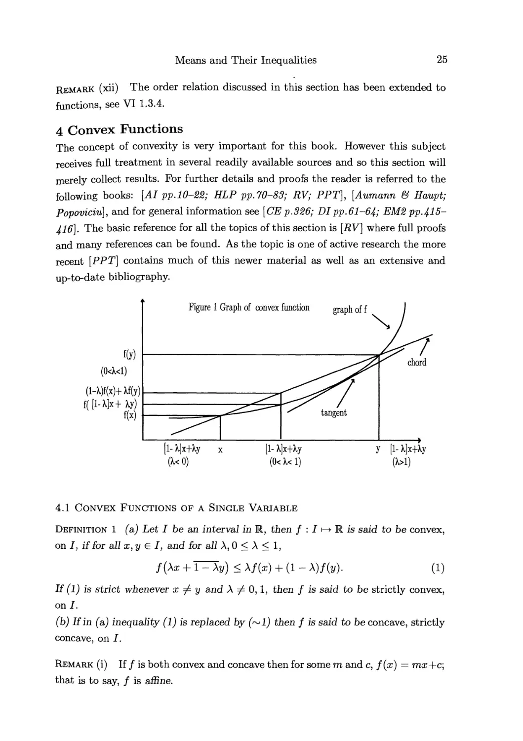
4.1 Convex Functions of Single Variable 25
4.2 Jensen's Inequality 30
4.3 The Jensen-Steffensen Inequality 37
4.4 Reverse and Converse Jensen Inequalities 43
4.5 Other Forms of Convexity 48
4.5.1 Mid-point Convexity 48
4.5.2 Log- convexity 48
4.5.3 A Function Convex with respect to Another Function 49
vii

4.6 Convex Functions of Several Variables 50
4.7 Higher Order Convexity 54
4.8 Schur Convexity 57
4.9 Matrix Convexity 58
CHAPTER II THE ARITHMETIC, GEOMETRIC
AND HARMONIC MEANS 60
1. Definitions and Simple Properties 60
1.1 The Arithmetic Mean 60
1.2 The Geometric and Harmonic Means 64
1.3 Some Interpretations and Applications 66
1.3.1 A Geometric Interpretation 66
1.3.2 Arithmetic and Harmonic Means in Terms of Errors 67
1.3.3 Averages in Statistics and Probability 67
1.3.4 Averages in Statics and Dynamics 68
1.3.5 Extracting Square Roots 68
1.3.6 Cesaro Means 69
1.3.7 Means in Fair Voting 70
1.3.8 Method of Least Squares 70
1.3.9 The Zeros of a Complex Polynomial 70
2. The Geometric Mean-Arithmetic Mean Inequality 71
2.1 Statement of the Theorem 71
2.2 Some Preliminary Results 72
2.2.1 (GA) with η = 2 and Equal Weights 72
2.2.2 (GA) with η = 2, the General Case 76
2.2.3 The Equal Weight Case Suffices 80
2.2.4 Cauchy's Backward Induction 81
2.3 Some Geometrical Interpretations 82
2.4 Proofs of the Geometric Mean-Arithmetic Mean Inequality 84
2.4.1 Proofs Published Prior to 1901. Proofs (i)-(vii) 85
2.4.2 Proofs Published Between 1901 and 1934. Proofs (viii)-(xvi) .. 89
2.4.3 Proofs Published Between 1935 and 1965. Proofs (xvii)-(xxxi) .. .92
2.4.4 Proofs Published Between 1966 and 1970.
Proofs (xxxii)-(xxxvii) 101
2.4.5 Proofs Published Between 1971 and 1988. Proofs (xxxviii)-(lxii) 104
2.4.6 Proofs Published After 1988. Proofs (lxiii)-(lxxiv) 114
2.4.7 Proofs Published In Journals Not Available to the Author 118
2.5 Applications of the Geometric Mean-Arithmetic Mean Inequality 119
2.5.1 Calculus Problems 119
2.5.2 Population Mathematics 120
2.5.3 Proving other Inequalities 120
2.5.4 Probabilistic Applications 124
3. Refinements of the Geometric Mean-Arithmetic Mean Inequality ... 125
3.1 The Inequalities of Rado and Popoviciu 125
3.2 Extensions of the Inequalities of Rado and Popoviciu 129
3.2.1 Means with Different Weights 129
3.2.2 Index Set Extensions 132
viii

3.3 A Limit Theorem of Everitt 133
3.4 Nanjundiah's Inequalities 136
3.5 Kober-Diananda Inequalities 141
3.6 Redheffer's Recurrent Inequalities 145
3.7 The Geometric Mean-Arithmetic Mean Inequality
with General Weights 148
3.8 Other Refinements of Geometric Mean-Arithmetic Mean Inequality 149
4. Converse Inequalities 154
4.1 Bounds for the Differences of the Means 154
4.2 Bounds for the Ratios of the Means 157
5. Some Miscellaneous Results 160
5.1 An Inductive Definition of the Arithmetic Mean 160
5.2 An Invariance Property 160
5.3 Cebisev's Inequality 161
5.4 A Result of Diananda 165
5.5 Intercalated Means 166
5.6 Zeros of a Polynomial and Its Derivative 170
5.7 Sanson's Inequality 170
5.8 The Pseudo Arithmetic Means and Pseudo Geometric Means ... 171
5.9 An Inequality Due to Mercer 174
CHAPTER III THE POWER MEANS 175
1. Definitions and Simple Properties 175
2. Sums of Powers 178
2.1 Holder's Inequality 178
2.2 Cauchy's Inequality 183
2.3 Power sums 185
2.4 Minkowski's Inequality 189
2.5 Refinements of the Holder, Cauchy and Minkowski Inequalities . 192
2.5.1 A Rado type Refinement 192
2.5.2 Index Set Extensions 193
2.5.3 An Extension of Kober-Diananda Type 194
2.5.4 A Continuum of Extensions 194
2.5.5 Beckenbach's Inequalities 196
2.5.6 Ostrowski's Inequality 198
2.5.7 Aczel-Lorentz Inequalities 198
2.5.8 Various Results 199
3. Inequalities Between the Power Means 202
3.1 The Power Mean Inequality 202
3.1.1 The Basic Result 203
3.1.2 Holder's Inequality Again 211
3.1.3 Minkowski's Inequality Again 213
3.1.4 Cebisev's Inequality 215
3.2 Refinements of the Power Mean Inequality 216
3.2.1 The Power Mean Inequality with General Weights 216
3.2.2 Different Weight Extension 216
3.2.3 Extensions of the Rado-Popoviciu Type 217
ix

3.2.4 Index Set Extensions 220
3.2.5 The Limit Theorem of Everitt 225
3.2.6 Nanjundiah's Inequalities 225
4. Converse Inequalities 229
4.1 Ratios of Power Means 230
4.2 Differences of Power Means 238
4.3 Converses of the Cauchy, Holder and Minkowski Inequalities 240
5. Other Means Defined Using Powers 245
5.1 Counter-Harmonic Means 245
5.2 Generalizations of the Counter-Harmonic Means 248
5.2.1 Gini Means 248
5.2.2 Bonferroni Means 251
5.2.3 Generalized Power Means 251
5.3 Mixed Means 253
6. Some Other Results 256
6.1 Means on the Move 256
6.2 Hlawka-type inequalities 258
6.3 p-Mean Convexity 260
6.4 Various Results 260
CHAPTER IV QUASI-ARITHMETIC MEANS 266
1. Definitions and Basic Properties 266
1.1 The Definition and Examples 266
1.2 Equivalent Quasi-arithmetic Means 271
2. Comparable Means and Functions 273
3. Results of Rado-Popoviciu Type 280
3.1 Some General Inequalities 280
3.2 Some Applications of the General Inequalities 282
4 Further Inequalities 285
4.1. Cakalov's Inequality 286
4.2 A Theorem of Godunova 288
4.3 A Problem of Oppenheim 290
4.4 Ky Fan's Inequality 294
4.5 Means on the Move 298
5. Generalizations of the Holder and Minkowski Inequalities 299
6. Converse Inequalities 307
7. Generalizations of the Quasi-arithmetic Means 310
7.1 A Mean of Bajraktarevic 310
7.2 Further Results 316
7.2.1 Deviation Means 316
7.2.2 Essential Inequalities 317
7.2.3 Conjugate Means 320
7.2.4 Sensitivity of Means 320
CHAPTER V SYMMETRIC POLYNOMIAL MEANS 321
1. Elementary Symmetric Polynomials and Their Means 321
2. The Fundamental Inequalities 324
3. Extensions of S(r;s) of Rado-Popoviciu Type 334
χ

4. The Inequalities of Marcus & Lopes 338
5. Complete Symmetric Polynomial Means; Whiteley Means 341
5.1 The Complete Symmetric Polynomial Means 341
5.2 The Whiteley Means 343
5.3 Some Forms of Whiteley 349
5.4 Elementary Symmetric Polynomial Means as Mixed Means 356
6. The Muirhead Means 357
7. Further Generalizations 364
7.1 The Hamy Means 364
7.2 The Hayashi Means 365
7.3 The Biplanar Means 366
7.4 The Hypergeometric Mean 366
CHAPTER VI OTHER TOPICS 368
1. Integral Means and Their Inequalities 368
1.1 Generalities 368
1.2. Basic Theorems 370
1.2.1 Jensen, Holder, Cauchy and Minkowski Inequalities 370
1.2.2 Mean Inequalities 373
1.3 Further Results 377
1.3.1 A General Result 377
1.3.2 Beckenbach's Inequality; Beckenbach-Lorentz Inequality .... 378
1.3.3 Converse Inequalities 380
1.3.4 RyfFs Inequality 380
1.3.5 Best Possible Inequalities 381
1.3.6 Other Results 382
2. Two Variable Means 384
2.1 The Generalized Logarithmic and Extended Means 385
2.1.1 The Generalized Logarithmic Means 385
2.1.2 Weighted Logarithmic Means of n-tuples 391
2.1.3 The Extended Means 393
2.1.4 Heronian, Centroidal and Neo-Pythagorean Means 399
2.1.5 Some Means of Haruki and Rassias 401
2.2 Mean Value Means 403
2.2.1 Lagrangian Means 403
2.2.2 Cauchy Means 405
2.3 Means and Graphs 406
2.3.1 Alignment Chart Means 406
2.3.2 Functionally Related Means 407
2.4 Taylor Remainder Means 409
2.5 Decomposition of Means 412
3. Compounding of Means 413
3.1 Compound means 413
3.2 The Arithmetico-geometric Mean and Variants 417
3.2.1 The Gaussian Iteration 417
3.2.2 Other Iterations 419
4. Some General Approaches to Means 420
xi

4.1 Level Surface Means 420
4.2 Corresponding Means 422
4.3 A Mean of Galvani 423
4.4 Admissible Means of Bauer 423
4.5 Segre Functions 425
4.6 Entropic Means 427
5. Mean Inequalities for Matrices 429
6. Axiomatization of Means 435
BIBLIOGRAPHY 439
Books 439
Papers 444
NAME INDEX 511
INDEX 525
xii

'Means and Their Inequalities"-Preface
There seems to be two types of books on inequalities. On the one hand there
are treatises that attempt to cover all or most aspects of the subject, and where
an attempt is made to give all results in their best possible form, together with
either a full proof or a sketch of the proof together with references to where a
full proof can be found. Such books, aimed at the professional pure and applied
mathematician, are rare. The first such, that brought some order to this untidy
field, is the classical "Inequalities" of Hardy, Littlewood L· Polya, published in
1934. Important as this outstanding work was and still is, it made no attempt
at completeness; rather it consisted of the total knowledge of three front rank
mathematicians in a field in which each had made fundamental contributions.
Extensive as this combined knowledge was there were inevitably certain lacunae;
some important results, such as Steffensen's inequality, were not mentioned at all;
the works of certain schools of mathematicians were omitted, and many important
ideas were not developed, appearing as exercises at the ends of chapters. The later
book "Inequalities" by Beckenbach L· Bellman, published in 1961, repairs many
of these omissions. However this last book is far from a complete coverage of the
field, either in depth or scope. A much more definitive work is the recent "Analytic
Inequalities" by Mitrinovic, (with the assistance of Vasic), published in 1970, a
work that is surprisingly complete considering the vast field covered.
On the other hand there are many works aimed at students, or non-mathematicians.
These introduce the reader to some particular section of the subject, giving a feel
for inequalities and enabling the student to progress to the more advanced and
detailed books mentioned above. Whereas the advanced books seem to exist only
in English, there are excellent elementary books in several languages: "Analytic
Inequalities" by Kazarinoff, "Geometric Inequalities" by Bottema, Djordjevic, Janic
&; Mitrinovic in English; "Nejednakosti" by Mitrinovic, "Sredine" by Mitrinovic
&: Vasic in Serbo-croatian, to mention just a few. Included in this group although
slightly different are some books that list all the inequalities of a certain type—a
sort of table of inequalities for reference. Several books by Mitrinovic are of this
type.
Due to the breadth of the field of inequalities, and the variety of applications,
none of the above mentioned books are complete on all of the topics that they
take up. Most inequalities depend on several parameters, and what is the most
natural domain for these parameters is not necessarily obvious, and usually it is
not the widest possible range in which the inequality holds. Thus the author, even
xin

the most meticulous, is forced to choose; and what is omitted from the conditions
of an inequality is often just what is needed for a particular application. What
appears to be needed are works that pick some fairly restricted area from the vast
subject of inequalities and treat it in depth. Such coherent parts of this discipline
exist. As Hardy, Littlewood & Polya showed, the subject of inequalities is not
just a collection of results. However, no one seems to have written a treatise on
some such limited but coherent area. The situation is different in the collection
of elementary books; several deal with certain fairly closely defined areas, such as
geometric inequalities, number theoretic inequalities, means.
It is the last mentioned area of means that is the topic of this book. Means are
basic to the whole subject of inequalities, and to many applications of inequalities
to other fields. To take one example: the basic geometric mean-arithmetic mean
inequality can be found lurking, often in an almost impenetrable disguise, behind
inequalities in every area. The idea of a mean is used extensively in probability
and statistics, in the summability of series and integrals, to mention just a few
of the many applications of the subject. The object of this book is to provide
as complete an account of the properties of means that occur in the theory of
inequalities as is within the authors' competences. The origin of this work is to
be found in the much more elementary "Sredine" mentioned above, which gives
an elementary account of this topic.
A full discussion will be given of the various means that occur in the current
literature of inequalities, together with a history of the origin of the various inequalities
connecting these means1. A complete catalogue of all important proofs of the
basic results will be given as these indicate the many possible interpretations and
applications that can be made. Also, all known inequalities involving means will
be discussed. As is the nature of things, some omissions and errors will be made:
it is hoped that any reader who notices any such will let the authors know, so that
later editions can be more complete and accurate.
An earlier version of this book was published in 1977 in Serbo-croatian under the
title " Sredine i sa Njima Povezane Nejednakosti". The present work is a complete
revision, and updating of that work.
The authors thank Dr J. E. Pecaric of the University of Belgrade Faculty of Civil
Engineering for his many suggestions and contributions.
Vancouver & Belgrade 1988
Although not mentioned in this preface the book was devoted to discrete mean inequalities and did
not discuss in any detail integral mean inequalities, matrix mean inequalities or mean inequalities in
general abstract spaces. This bias will be followed in this book except in Chapter VI.
XIV

PREFACE TO THE HANDBOOK
Since the appearance of Means and Their Inequalities the deaths of two of the
authors have occurred. The field of inequalities owes a great debt to Professor
Mitrinovic and his collaborator for many years, Professor Vasic. Over a lifetime
Professor Mitrinovic devoted himself to inequalities and to the promotion of the
field. His journal, Univerzitet и Beogradu Publikacije Elektrotehnickog Fakulteta.
Serija Matematika i Fizika, the "i Fizika' was dropped in the more recent issues,
has in all of its volumes, from the first in the early fifties, devoted most of its
space to inequalities. In addition his enthusiasm has resulted in a flowering of
the study both by his students, P. M. Vasic, J. E. Pecaric to mention the most
notable, and by many others. The uncertain situation in the former Yugoslavia
has lead to many of the researchers situated in that country moving to institutions
all over the world. There are now more journals devoted to inequalities, such as
the Journal for Inequalities and Applications and Mathematical Inequalities and
Applications, as well as many that devote a considerable portion of their pages to
inequalities, such as the Journal of Mathematical Analysis and Applications; in
addition mention must be made of the electronic Journal of Inequalities in Pure and
Applied Mathematics based on the website http://rgmia.vu.edu.au and under
the editorship of S. S. Dragomir. This website has in addition many monographs
devoted to inequalities as well as a data base of inequalities, and mathematicians
working in the field. Another welcome change has been the many contributions
from Asian mathematicians. While there have always been results from Japan, in
recent years there has been a considerable amount of work from China, Singapore,
Malaysia and elsewhere in that region.
It was taken for granted in the earlier Preface that anyone reading this book
would not only be interested in inequalities but would be aware of their many
applications. However it would not be out of place to emphasize this by quoting
from a recent paper; [Guo L· Qi).
"It is well known that the concepts of means and their inequalities not
only are basic and important concepts in mathematics, (for example, some
definitions of norms are often special means2), and have explicit geometric
More precisely "... certain means are related to norms and metrics." See III 2 4, 2 5.7 VI 2.2.1
XV

meanings3, but also have applications in electrostatics4, heat conduction
and chemistry5. Moreover, some applications to medicine6 have been given
recently."
Due to the extensive nature of the revision in the second edition and the large
amount of new material it has seemed advisable to alter the title but this handbook
could not have been prepared except for the basic work done by my late colleagues
and I only hope that it will meet the high standards that they set.
In addition I want to thank my wife Georgina Bullen who has carefully
proofread the non-mathematical parts of the manuscript, has suffered from computer
deprivation while I monopolized the screen, and without whose support and help
the book would have appeared much later and in a poorer form.
P. S. Bullen
Department of Mathematics
University of British Columbia
Vancouver ВС
Canada V6T 1Z2
bullen@math.ubc.ca
3 See II 1.1, 1.3.1; [Qi & Luo].
4 See[Polya & Szego 1951).
See[Walker, Lewis & McAdams], [Tettamanti, Sarkany, Kralik &:Stomfai; Tettamanti L· Stomfai]
6 See [Ding].
XVI

BASIC REFERENCES
There are some books on inequalities to which frequent reference will be made and
which will be given short designations.
[AI] Mitrinovic, D. S., with Vasic P. M. Analytic Inequalities, Springer-Verlag,
Berlin, 1970.
[BB] Beckenbach, E. F. & Bellman, R. Inequalities, Springer-Verlag, Berlin,
1961.
[HLP] Hardy, G. H., Littlewood, J. E. & Polya, G. Inequalities, Cambridge
University Press, Cambridge, 1934.
[MI] Bullen, P.S., Mitrinovic, D. S L· Vasic P. M. Means and Their Inequalities,
D.Reidel. Dordrecht, 1988. [The first edition of this handbook.]
[MO] Marshall, A. W. & Olkin, I. Inequalities: Theory of Majorization and Its
Applications, Academic Press, New York, 1979.
Many inequalities can be placed in a more general setting. We do not follow that
direction in this book but find the following an invaluable reference. Much of the
material is readily translated to our simpler less abstract setting.
[PPT] Pecaric, J. E., Proschan, F. & Tong, Y. L. Convex Functions, Partial
Orderings and Statistical Applications, Academic Press Inc., 1992.
There are two books that are referred to frequently in certain parts of the book
and for which we also introduce short designations.
[B2] Borwein, J. M. & Borwein, P. B. Pi and the AGM. A Study in
Analytic Number Theory and Computational Complexity, John Wiley and Sons, New
York, 1987.
[RV] Roberts, A. W. L· Varberg, D. E. Convex Functions, Academic Press, New
York-London, 1973.
In addition there are the two following references. The first is a ready source
of information on any inequality, and the second is in a sense a continuation of
[AI] and [BB] above, being a report on recent developments in various areas of
inequalities.
xvn

[DI] Bullen, P. S. A Dictionary of Inequalities, Addison-Wesley Longman,
London, 1998.7
[MPF] Mitrinovic, D. S., Pecaric, J. E. L· Fink, A. M. Classical and New
Inequalities in Analysis, D Reidel, Dordrecht, 1993.
There are many other books on inequalities and many books that contain
important and useful sections on inequalities. These are listed in Bibliography Books.
From time to time conferences devoted to inequalities have published their
proceedings. In particular, there are the proceedings of three symposia held in the
United States, and of seven international conferences held at Oberwolfach.
11(1965), 12 (1967), 13 (1969) Inequalities, Inequalities II, Inequalities III,
Proceedings of the First, Second and Third Symposia on Inequalities, 1965, 1967,
1969; Shisha, O., editor, Academic Press, New York, 1967, 1970, 1972.
GI1(1976), GI2 (1978), GI3 (1981), GI4 (1984), GI5 (1986), GI6 (1990), GI7 (1995)
General Inequalities Volumes 1-7, Proceedings of the First-Seventh International
Conferences on General Inequalities, Oberwolfach, 1976, 1978, 1981, 1984, 1986,
1990, 1995; Beckenbach, E. F., Walter, W., Bandle, C., Everitt, W. N., Losonczi,
L., [Eds.], International Series of Numerical Mathematics, 41, 47, 64, Birkhauser
Verlag, Basel, 1978, 1980, 1983, 1986,1987, 1992, 1997.
Individual papers in these proceedings, referred to in the text, are listed under the
various authors with above shortened references.
Finally there are two general references.
[EMI], [EM2], [EM3], [EM4], [EM5], [EM7], [EM8], [EM9],[EM10], [EMSuppI],
[EMSuppII], [EMSuppIII]; Hazelwinkel, M., [Ed.] Encyclopedia of Mathematics,
vol.1-10, suppl. I-III, Kluwer Academic Press, Dordrecht, 1988-2001.
[CE] Weisstein, E. W. CRC Concise Encyclopedia of Mathematics, Chapman &
Hall/CRC, Boca Raton, 1998.
Additions and corrections can be found at http://rgmia.vu.edu.au/monographs/bullen.html.
XV111

NOTATIONS
1 Referencing
Theorems, definitions, lemmas, corollaries are numbered consecutively in each
section; the same is true of formulae. Remarks and Examples are numbered, using
Roman numerals, consecutively in each subsection, and in each sub-subsection. In
the same chapter references list the section, (subsection, sub-section, in the case
of remarks and examples), followed by the detail: thus 3 Theorem 2, 4(6), or 1.2
Remark (6). Footnotes are numbered consecutively in each chapter and so are
referred to by number in that chapter: thus 1.3.1 Footnote 1. References to other
chapters are as above but just add the chapter number; thus I 3 Theorem 2(a),
II 4(6), IV 1.2 Remark (6), I 1.3.1 Footnote 1. Although there are references for
all names and all bibliography entries, in the case of a name occurring frequently,
for instance Cauchy, only the most important instances will be mentioned; further
names in titles of the basic references are usually not referenced, thus Hardy in
[HLP].
2 Bibliographic References
Some have been given a shortened form; see Basic References. Others are
standard, the name, followed by a year if there is ambiguity, or the year with an
additional letter, such as 1978a, if there is more than one any given year. Joint
authorship is referred to by using &, thus Mitrinovic L· Vasic.
3 Symbols for Some Important Inequalities
Certain inequalities are referred to by a symbol as they occur frequently.
(B) Bernoulli's inequality I 2.1 Theorem 1
(C) Cauchy's inequality III 2.2
(GA) Geometric-Arithmetic Mean inequality II 2.1 Theorem 1
(H) Holder's inequality III 2.1 Theorem 1
(HA) Harmonic- Arithmetic Mean Inequality II 2.1 Remark(i)
(J) Jensen 's inequality 14.2 Theorem 12
(M) Minkowski's inequality III 2.4 Theorem 9
(P) Popviciu's inequality II 3.1 Theorem 1
(R) Rado's inequality II 3.1 Theorem 1
(r;s) Power Mean inequality III 3.1.1 Theorem 1
S(r;s)... .Elementary Symmetric Polynomial Mean inequality V 2 Theorem 3(b)
xix

(Τ), (ΎΝ) Triangle inequality III 2.4 .
Integral analogues of these means, when they exist, will be written (J)-/, etc; see
VI 1.2.1, 1.2.2.; and (~B), etc. will denote the opposite inequalities; see 9 below.
4 Numbers, Sets and Set Functions
Z, Q,R, С are standard notations for the sets of integers, rational numbers, real
numbers, and complex numbers respectively. The set of extended real numbers,
R U {±oo}, is written R.
Less standard are the following:
Ν = {η; η e Z, andn > 0} = {0,1,2,...}, N* = N \ {0} = {1, 2,...},
R* =R\{0}, R+ = {x;x eRandrr > 0}, R^ = R+ \ {0} = {x;x eRandz >
0},
Q* = Q\{0}, Q+ = {x;xEQandx>0}, Ql = Q+\{0} = {x]xeQtmdx>
0}.
The non-empty subsets of N, or N*, are called index sets, the collection of these
is written X.
If ρ e R*, ρ 7^ 1, the conjugate index ofp, written ρ', is defined by
ρ 11
ρ' = -, equivalently —I—- = 1.
ρ - 1 Ρ Ρ
Note that
(p'Y = p> ρ > ι -£=> ρ' > ι, ρ > о and ρ' > ο ^^ ρ > ι, or ρ7 > ι.
A real function φ defined on sets, a set function, is said to be super-additive,
respectively log-super-additive, if for any two non-intersecting sets, I, J say, in its
domain
φ(Ι U J) > φ(Ι) + φ{3), respectively, φ(Ι U J) > φ{Ι)φ{3).
If these inequalities are reversed the function is said to be sub-additive,
respectively log-sub-additive. A set function / is said to be increasing if J С J =>>
/CO < /(«0> and if the reverse inequality holds it is said to be decreasing.
The image of a set A by a function f will be written f[A}; that is f[A] = {у; у =
/CO, χ e A}.
A set Ε is called a neighbourhood of a point χ if for some open interval ]o, b[ we
have ж Ε [α, 6[C J5.
5 Intervals
Intervals in R are written [a, b], closed; ]a,b[, open etc. In addition we have the
unbounded intervals [a, oo[, ] — oo, a], etc; and of course ] — oo, oo[= R, [—oo, oo] =
R, [0,oo[= R_|_, ]0, oo[= RUj_. The symbol (a, b) is reserved for 2-tuples, see the
о
next paragraph. If i" is any interval then i" denotes the open interval with the
same end-points as i".
xx

6 η-tuples
If di e R, C, 1 < i < n, then we write a for the, ordered, real, complex, n-tuple
(αϊ,..., αη) with these elements or entries; so if α is a real η-tuple α Ε Rn. The
usual vector notation is followed.
In addition the following conventions are used.
(i) For suitable functions /, g etc, /(α) = (/(αχ),..., /(an)), and g(a,b) =
(g(a\, bi),... ,#(αη, &n)) etc. This useful convention conflicts with the standard
notation for functions of several variables, /(a) = /(ai,..., an), but the context
will make clear which is being used.
So: a2 = (af,...,a^), ab = (aibi,..., anbn); but max a = maxi<Kna,, and
min a = mini<i<n &%·
(ii) a < b means that ai < bi, 1 < г < η. In addition m < a< Μ means that
m < di < M, 1 < г < n. The extensions to the other inequality signs is obvious.
In particular if a > 0, a > 0 etc, we say that the η-tuple is positive, non-negative
etc.
The set of non-negative η-tuples is written R™, and the set of positive n-tuples
(м;)п
(iii) An η-tuple all of whose elements are all zero except the г-th that is
equal to 1 is written e^. The η-tuples e^, 1 < г < n, form the standard basis of
Rn. As usual if η = 2,3 these basis vectors are written ег = г, е2 = j, е% = к.
(iv) e is the η-tuple each of whose entries is equal to 1 ; and 0, or just 0, is
the η-tuple each of whose entries is equal to 0.
(v) If 1 < г < η then o!i denotes the (n — l)-tuple obtained from α by
omitting the element a^.
(vi) a ~ b, α is proportional to 6, means that for some λ, μ G R, not both
zero, λα + /ib = 0; that is the two η-tuples are linearly dependent.
(vii) If α^ = c, 1 < г < η, we say that a is constant, or is a constant.
(viii) For Akan and see I 3.1. An η-tuple is called an arithmetic progression
if Δ1α^, 1 < к < η — 1, is constant, equivalently if Δ2α& = 0,1 < к < η — 2,
(ix) For а*Ь see I 3.2 Definition 4.
(x) For a-<b see I 3.3 Definition 11.
(xi) Given an η-tuple w. we will write Wk = Σ^=1^, 1 < г < η; and if
necessary Wo = 0· More generally if υ; is a sequence and / G I, an index set, see
4, we write Wj = Y,ieI Щ-
(xii) If / is a function of к variables, a and n-tuple, 1 < к < η, then
Σ&·./*(αΰ' · · · 5 aik) means that the summation is taken over all permutations of
к elements from the αϊ,... ,αη. In the case that к = η this will be written as
Σ!/(«)·
(xiii) The inner product of two η-tuples, a,b, written (а,Ь), is Σ™=1α$ι
if the η-tuples are real and Σ™=1 оцЬг if the η-tuples are complex. In both cases
Where appropriate the above notations will be used for sequences α = (αϊ, аг,...),
provided the relevant series converge.
xxi

7 Matrices
An πι χ η matrix is A = (a^·) i<i<m; the a^· are the entries and if they are real,
l<j<n
complex then A is said to be real, complex. The transpose of A is AT = (ац) i<i<m ;
l<j<n
A* = (aji)i<z<m is the conjugate transpose of A.
l<j<n
If A = AT then A is symmetric; if A = A* then A is Hermitian-, in these cases of
course m = η and the matrix is said to be square. The family of all η χ η Hermitian
matrices will be written Hn', the subset of positive definite η xn Hermitian matrices
is written 7Y+.
If А, В e Hn we write A < В if В —A is positive semi-definite, and A < В if В — A
is positive definite. This defines an order on Hn called the Loewner ordering.
A square matrix D with all non-diagonal elements zero is called a diagonal
matrix; if the diagonal elements are Q"ii = di, 1 < г < η, we write D = D(d) =
D(du ..., α^). li d = e the diagonal matrix is called a unit matrix, usually written
i", or In if it is important to show that it is an η χ η unit matrix8. The square
matrix all of whose entries are equal to 1 is written J, or if the order needs to be
noted Jn. A matrix of any order all of whose entries are zero, a zero matrix, will
be written O, the order being understood from the context.
If A E Hn with eigenvalues λ, then all of its eigenvalues real and A — U*D(X)U
where U is a unitary matrix, that is UU* = I; so for a unitary matrix Ό~ι = U*.
If A E Hn and / is a real-values function defined on an interval that contains the
eigenvalues of A we define the associated matrix function of order n, using the
same symbol, / : Hn i-> Hn by f{A) = UD(f(\))U*; see [MO p.462]. Further
(f(A)a,a) = ZL· \bi\2f(*i) where b = Ua.
8 Functions
A function of η variables / is said to be symmetric if its domain is symmetric and
if its value is not altered by a permutation of the variables. Precisely, if / : D >—► R
and (i) D С Шп, (ii) (al5..., αη) Ε D => (α^,..., α^η) Ε £) for every permutation
(г\,. .. ,гп) of (1,... ,n), (Hi) /(α^,... ,ain) = /(αϊ,... ,αη) for every permutation
(ii,..., in) of (1,. .., n), then / is said to be symmetric.
A related concept is that of an almost symmetric function: this is a function of
η variables and η parameters, defined on a symmetric domain, that is invariant
under the simultaneous permutation of the variables and the parameters.
Examples(i) The arithmetic mean with equal weights, /(α) = (αϊ Η han)/n,
is symmetric; the weighted arithmetic mean, /(a) = /(a;w;) = (w\a\ + · · · 4-
WnO"n)/(wi Η 4- гип), is almost symmetric; see II 1.1.
The Gamma or factorial function is denoted by ж!; that is
ж! = Г(ж4-1).
The identity function is written *,, and then the power functions ls,s eR*. That
is
l{x) = x; ls(x) = xs;
This conflicts with the use of I to denote an interval but in practice there will be no confusion.
ХХ11

the domain being clear from the context.
The maximum function is defined as usual by max{/, g]{x) = тах{/(ж),^(ж)}:
also,
ж+ = тах{ж, 0}; x~ = max{—x, 0}; χ = x+ — x~, |x| = x+ + x~.
By analogy if / is any real-valued function then /+ = max{/, 0} = max of; when
/ = /+-/-, 1/1 = /+ + /-.
The function that is equal to 1 on the set A and to zero off A, the indicator
function9 of A is written 1a- That is
The integral or integer part function [■] : R t—> Ζ is defined by:
[ж] = η, where η Ε Ζ is the unique integer such that η < χ < η + 1.
9 Various
Proofs begin with a square, D, on the left, and end with one on the right.
If (n) denotes an inequality then (~n) will denote the inequality obtained by
changing the inequality sign in (n); the opposite, inverse or reverse inequality.
A different concept is the converse or complementary inequality. Such inequalities
arise as follows: in general an inequality is of the form F > G or equivalently
F — G > 0. Usually both F, G are continuous functions and the inequality holds
on some non-compact set. If now we restrict the domain to a compact set we will
get that F — G attains a maximum on that set, F — G < Λ say. Another form
arises using the equivalent F/G > 1, giving on the compact set F/G < λ say.
The inequalities F — G < Λ, F/G < λ are converse inequalities for the original
inequality F > G.
If limx_,Xo f(x)/g(x) = 0 we say that / is little-oh of g as χ —ν xq , written f(x) —
о(^(ж)), χ —ν xq. In particular f{x) = o(l), χ —► xq means that limx^Xo f{x) = 0.
If there is some positive constant Μ such that for all χ in some neighbourhood
of xq \f(x)\ < Mg(x) we say that / is big-oh of д for χ as χ —ν xq , written
f{x) = 0[д(х)) χ -^ xq. In particular f(x) = O(l), x —► жо means that / is
bounded at xq. If f{x) = 0{g{x)) and g{x) = 0[f{x)) for x in a given set then
we say that f(x) and g(x) are of the same order of magnitude for χ in the given
set, written f{x) ~ g(x), χ —► xq.
Means are denoted throughout by Gothic letters: 21, <3,$)... etc.
Classes of functions are denoted throughout by calligraphic letters; thus С (I), the
space of functions continuous on /, Cn(7), the space of functions with continuous
nth order derivatives on /, etc.
This function is also called the characteristic function of A.
XX111

A LIST OF SYMBOLS
The following is a list of the symbols
used in the text.
N,N* xx
R*,R+,]R; xx
q*,q+,q; xx
X xx
p' xx
f[A] xx
[a, b], ]a, b[, etc xx
[a, oo[, ] — oo, a] xx
о
I xx
/(a),p(a,b) xxi
max a, min a xxi
a<b,m<a<M xxi
Щ, (R+)n xxi
e^hjjk xxi
e , 0 xxi
a^ xxi
a~b xxi
Δαη, Akan, Δαη, Akan xxi
a-kb xxi
b -< a xxi
Efc!/K>--->a*fc) ™
ЕШ ™
Wn,Wj xxi
(a, b) xxi
fe /], [a; /]n, [a0,. .., an; /] 54
a ^. 68
a,Wm 132
|a| 357
Un.Ui xxii
D(d) = D(du ... ,dn) xxii
I,In,J,Jn,0 xxii
xl xxii
l(x), is (x) xxii
ж+, x~, /+ xxiii
1a (x) xxiii
[x] xxiii
f+(Uo',v) 51
Ш 350
/* 381
f <g 381
D xxiii
(~ ·) xxiii
Яп(а), 2U(a; ш), ^fe ш) 60, 63
Sln(a*,l < г < n),2tn(ai,...,an) .61
«η-ι(α) 61
21/(a; w) 132
&m(a;w) 132
Щ&ш)Ж 136
^пЧ^ш),^"1 136
<(α), β;(a) etc 295
*n,a(a) 357
*[a,4 (/;/*) 374
2t(A,5;i),Sl(A,5) 429
2im(Ab...,Am;^) 432
®M(a) 424
C(I),Cn(I) xxiii
€n(a;w) 270
4Γ](α) 341
ckfc;^(g;a) 350
B£5(a;w) 229
£>(/) 316
XXIV

£η(α;£) 316
екг]Ы 321
ekfc;^(g;a) 350
£r's(a,b) 393
ё*\а,щ) 428
®п(а;ш), &п(а), #(а;ш) 65
07(а;ш) 132
Фт(а\щ) 132
0(a;w),<6 136
extern), <δ_1 136
<6%q(a;w) 249
0[a,b](/;M) 374
б(ЛБ;^),б(ДВ) 429
<6m(A1,...,Arn;w) 432
Hn,Ht xxii
Йп(а;ж),Йп(й),Й(а;ш) 65
Ъ[:](а]Ш) 245
(Ы)1\а) 364
%,.ь]СМ 374
Йе(а,&) 399
fi^iM) 400
S)(A,B;t),f)(A,B) 429
S)m(Au...,Am]w) 432
3{a,b) 167
3η(α;μ) 392
£(а,Ь) 167
£μ(α,6),£(α,6) 369
££(а,Ь),£~(а,Ь) 369,370
£[р](а,Ь) 385
£п(й),£п(а;ш) 391, 392
£n(a;w) 391
Ш1И(а;ш),Я«кг1(а), ^5
Ш^г](а;ш),9ЯИ(М) 175
mn(s,t;k;a) 254
Wln(a]w) 266
Щ,п{а',ш) 269
Ш?п'(а;^),Ш?п(а;;ша;) 310, 311
mn(а; а) 357
яИ[а,ч(/;/х) 373
^[в!ь](/;м) 374
Ш1[£М](а,Ь) 403
Ш1[^(а,Ь) 406
Ж <g> 9t(a, b),Wl®a 9t(a, b) 414
®?=1Ш1Й*](а;ш) 416
9t£](a;w) 226
04fc](a) 323
0(р(ж)),о(р(ж)), ж->ж0 xxin
Й(а,Ь) 169
Un(a]w) 175
0£в(а;ш) 229
Qkrl(a),qkr](a) 341
Qm](/;/x) 374
i2n+i(/;a;x) 7
7г(г, а), 7гп (г, а), 7г(г) 185, 186
7Z(r,a',w) 187
*H[/'n](a,b) 409
Фп\а,Ъ) 410
S(r,a),Sn(r,a),S(r) 185, 186
<S(r,a;w) 187
6n(a;w) 270
Sm{q.;w) 279
&:\a),sl\a) 322
Tn+i(/;a;x) 7
4M(a) 344
t[n^{a) 350
4Μ(α),»1Μ(α) 344
The Gothic alphabet: a, 21, b, 05, c, £, D,
m,OT,n,ai,o,D,p,q2,q,n,r,^,5,6,t,
T,u,il,d,QJ,m,2n,?,X,t),2},3,3.
The Greek alphabet: a, /?, 7, Γ, £, Δ, e,
ε, С, 77,0, θ, 6, /с, λ, Λ, μ, ζ/, ξ, Ξ, ω, π, Π,
ш, ρ, ρ, σ, Σ, τ, ι?, Τ, φ, Φ, ν?, χ, ^, Ψ.ω, Ω
XXV

AN INTRODUCTORY SURVEY
This book is aimed at a wide audience. For those in the field of inequalities the
table of contents, and the abstracts at the beginnings of chapters should suffice as
a guide to the material. However for others it may be useful to indicate the basic
material so as to allow the avoidance of the specialised sections.
The basic material can be found in Chapters I, II, III and VI while the remaining
chapters deal mainly with material that is more technical. However even in the
basic chapters material of less interest to the general reader occur. Such avoidable
sections are: I 3.1, 3.2, 4.5.3, 4.6, 4.8, 4.9; II 3.2-3.6, 3.8, 4, 5.4, 5.6-5.9; III 2.3,
2.5, 3.1.2-3.1.4, 3.2, 4, 5.2.3, 5.4,, 6.2-6.4; VI 1.3, 2.1.4, 2.4, 3.2.2, 4.3-4.6, 5.
The core of the book is the properties of various means. These means are listed
in the Index both separately, such as Arithmetic mean, and collectively, Means.
The simplest means are two variable means such as the classical arithmetic mean,
^(x -f y) and geometric mean, л/xy, and the less well known logarithmic mean,
(y - x)/(logy- logs); see II 1.1, 1.2. 5.5, VI 2, 3.
This leads to the question — what properties should a function f(x,y) have for
it to be considered as a mean? Clearly we require / to be continuous,
positive, defined for all positive values of both variables; a little less obvious are the
properties of symmetry, f(x,y) = f{y,x), reflexivity, f(x,x) — x, homogeneity,
f(\x,Xy) = \f{x,y), and monotonicity, χ < χ1 ,y < у' => f(x,y) < f{x',y')\
finally there is the crucial property of internality that justifies the very name of
mean, mm{x,y} < f{x,y) < max{x,y}.
Most of the means introduced are easily defined for η-tuples, η > 2, when these
various properties are suitably extended; see II 1.1 Theorem 2, 1.2 Theorem 6,
III Theorem 2(e) and VI 6. Of course there are many other properties of means
that have been identified as of interest; these are listed in the Index under Mean
Properties.
The inequalities between the various means defined form the core material of
the book. Again the two variable cases are the easiest II 2.2.1, 2.2.2, 5.5, VI 2,
3.1, 3.2.1. The fundamental result is the inequality between the arithmetic and
geometric means, (GA), discussed in detail in II 2.4 where well over 70 proofs
are given or mentioned; most are extremely elementary. The next basic result
generalizes this and is the inequality between the power means, (r;s), HI 3.1.1.
Integral forms of these results are also give; VI 1.2.2.
Prom Notations 9 we see that every inequality between means of η-tuples can be
regarded as saying a certain function of η is non-negative. For instance (GA) im-
xxvi

plies that R(n) — n(2in — <6n) > 0. A stronger property of this function of η would
be to show that it increases; stronger because -R(l) = 0; a similar discussion occurs
for related functions that are not less than 1, (2tn/^n)n > 1 for example. This
leads to the so called Rado-Popoviciu type extensions of the original inequality.
Such are discussed for (GA) in II 3.1; the analogous discussion for (r;s) in III 3.2
is much more technical as the simplicity of the (GA) case has been lost.
Finally many well-known inequalities arise from the discussion of mean inequalities—
in particular the inequalities of Cauchy, (C), Holder, (H), Minkowski, (M), Cebisev
and the triangle inequality, (T); see II 5.3, III 2.1, 2.2, 2.4.
xxvn

a

I INTRODUCTION
In this chapter we will collect some results and concepts used
in the main body of the text. There is no intention of being
exhaustive in any of the topics discussed and often the reader will
be referred to other sources for proofs and full details.
1 Properties of Polynomials
Simple properties of polynomials can be used to deduce some of the basic
inequalities to be discussed in this book. In addition certain simple inequalities,
needed at various places, are most easily deduced from the properties of some
special polynomials. These results are collected together in this section for ease of
reference.
Convention In this section, unless otherwise specified, all
polynomials will have real coefficients.
1.1 Some Basic Results The results given here are standard and proofs are
easily available in the literature; see for instance [CE pp.420,1573; DI p.70; EMS
p.59; EM8 p. 175), [Uspensky].
Theorem 1 A polynomial of degree η has η complex zeros, and if η is odd at least
one zero is real.
Theorem 2 [Descartes' Rule of Signs] A polynomial cannot have more positive
zeros than there are variations of signs in its sequence of coefficients.
Theorem 3 [Rolle's Theorem] If ρ is a polynomial then p' has at least one zero
between any two distinct real zeros of p.
Theorem 4 [Intermediate Value Theorem] A polynomial always has a zero between
any two numbers at which its values are of opposite sign.
Theorem 5 A zero of a polynomial is a zero of its derivative if and only if it is a
multiple zero.
1

2
Chapter I
The following result is basic to a variety of applications; see [BB p. 11; HLP ρρ.104~
105], [Milovanovic, Mitrinovic & Rassias pp.70-71; Newton], [Dunkel 1908/9;
Kellogg; Maclaurin; Sylvester]. The present form is that given in [HLP pp. 104~
105].
Theorem 6 If f(x,y) = Σ™=0 с%хг уп~г has, as a function ofy/x, all of its zeros
real then the same is true of all polynomials, not all of whose coefficients are zero,
derived from f by partial differentiations with respect to χ or у. Further if a zero
of one of these derived polynomials has multiplicity k,k > 1, then it is a zero of
multiplicity к -f 1 of the polynomial from which it was obtained by differentiation.
D The proof is immediate by repeated applications of Theorems 1,3,4 and 5.
D
Corollary 7 Ifn>2, and
Π Π / ч
p{x) = ς ^χί = Σ (\)άίχί w
is a polynomial of degree η with c0 ^ 0 and all zeros real, then if 1 < m < k+m < η
the polynomial q(x) = Σ™=0 (™)dfc+iX* has all of its zeros real.
D Let f{x, y) = YZ=Q (^)а{х'уп-\ We are given that d0 φ 0, so (0, у), у ф О,
is not a zero of /. Hence, by Theorem 6, (0,y),y φ 0, is not a multiple zero of
any derived polynomial. This implies that no two consecutive coefficients of / can
vanish.
Save for a numerical factor дп~ш f jдкхдп-к~шу is equal to Σ™=0 (7)c4+^w~*,
which by the previous remark does not have all of its coefficients zero. Hence the
result is an immediate consequence of Theorem 6. D
Remark (i) It follows from the above proof that if ρ is a polynomial of degree n,
as in (1), with cq φ 0, and if for some k, 2 < к < η — 1, c& = c^_i = 0, then ρ has
a complex, non-real, zero; [Wagner C].
Corollary 8 If η > 2, and ρ a polynomial of degree η given by (1) with c0 φ 0
and all of its zeros real, then for k,l < к <n — 1,
d\ >dfc_idfc+i, (2)
c\ >Cfc_iCfc+i. (3)
The inequalities (2) are strict unless all the zeros are equal.
D By Corollary 7 the roots of all the equations
dk-i + 2dkx 4- dk+ix2 = 0, 1 < к < η - 1, (4)

Means and Their Inequalities
3
are real; from this (2) is immediate.
Now from (2) and the definition of t4, 1 < к < η, see (1),
2 ^ (fc + l)(n-fc+l)
cfc > τ-;——ττ Cfc-iQc+i > cfc-icfc+i,
unless possibly either cj^-i = 0, or c^+i = 0; but then, by Remark (i), c& =£ О; and
so in all cases (3) is proved.
Finally, if for any к there is equality in (2) the associated quadratic equation (4)
has a double root, and so, by Theorem 6, the original polynomial ρ of (1), has a
single zero of multiplicity n. D
Remark (ii) Inequality (2) is sometimes called Newton's inequality and will
reappear later, II 2.4 proof (гж), V 2 Theorem 1; [DI p.192]. A direct proof can be
found in [Nowicki 2001]. A converse to this inequality has been given; [Whiteley
1969].
Remark (iii) The above implies that if for some k,l < к < n— 1, c2, < Cfc_iCfc+i,
then the above polynomial ρ has a non-real zero.
Remark (iv) By writing (2) in the form d2^ > <^_ι<2£+ι, l<r<k<n — 1,
multiplying, and assuming that cn = 1, we get the important inequalities, see V
2(6);
<С\ > <_r_i; (5)
similarly,
cn_r > cn_r_1. (6)
Example (i) A very important case of (1) occurs when — αϊ,...,— αη are the
real distinct zeros of p, when p(x) = П^=1(х 4- α&); then cn = 1 and Сп_& =
if Σΐ!αΰ ·-.aifc, 1 < fc < η; in particular cn_i = Σ^=1αΐ,θ3 = ΠΓ=ια*' see v
1(7).
1.2 Some Special Polynomials (a) [Dip.207], [Bullen 1996a; Cakalov 1963].
Define the polynomial pn,n > 1, by
pn(x) = xn+1 - (п+1)ж + п.
In particular then p\{x) = {x — l)2 > 0, ж =£ 1.
Clearly χ = 1 is a zero of both pn and of p^. So, by 1.1 Theorem 5, χ = 1 is a double
zero of pn. [This can also be seen from the identity pn(x) = (x~ l)2 Х]Г=о(п~^)жг·]
This, by 1.1 Theorem 2, implies that ж = 1 is the only positive zero of pn.

4
Chapter I
Since pn(0) = η > 0, and pn(n) = nn+1 — n2 > 0 if η > 1, we have by 1.1 Theorem
4, and the special case above that:
if x>0, x^l, then rrn+1 > (n + I) x - η. (7)
(b) [DI p.207]. Define the polynomial qn,n > 1, by
gn(x) = (x + n)n+1-(n + l)n+1x.
Then using an argument similar to that in (a), x = 1 is the only positive zero of
qn. Hence
if x>0, хф\, then [χ + n)n+1 > (η + l)n+1x. (8)
2 Elementary Inequalities
In this section we collect some important elementary inequalities.
2.1 Bernoulli's Inequality Inequality 1.2 (8) leads to one of the basic
elementary inequalities.
Take the (n 4- l)-th root of both sides in 1.2 (8) and put η 4-1 = -, and у = ж — 1
г
to get:
if 2/>-1,2/^0, then (1 + y)r < 1 + r^; (1)
This inequality (1), or (~1), can be shown to hold for arbitrary exponents r; [AI
p.34; HLP p.40], [Herman, Кисета & Simsa p.109].
Theorem 1 [Bernoulli's Inequality] If χ > — Ι, χ φ 0, and if 0 < а < 1 then
(1 4- x)a < 1 4- αχ- (Β)
if either а > 1 or а < 0; when of course χ Φ — 1, then (~ B) holds.
D (г) 0 < а < 1
Let f{x) = 1 4- αχ - (1 4- х)а, х > -1. Then /7(ж) = α(ΐ - (1 + ж)а-1)· Hence
/(0) = /'(0) = 0 and it is easy to see that this point is the minimum of /.
Alternatively we can look at f"{x) = a(l — a)(l 4- x)a~2, which shows that / is
strictly convex, see 4.1 below for a definition.
Either argument shows that f(x) > 0,ж φ 0, which is just (B).
(гг) a < 0 or a > 1
The argument in (г) shows that (~B) holds.

Means and Their Inequalities
5
(Hi) Alternatively we can show that the result for a < 0 follows from that for
a>0
If 1 + ax < 0 there is nothing to prove. So suppose that a < 0 and 1 4- ax > 0
and choose β so that β > 1 and 0 < -α/β < 1. Then from case (г) (1 + χ)~α/β <
a
1 - -qX, or
a
Hence (1 + x)a > (1 + ^ж)^ > 1 + ax, by case (гг). D
Remark (i) This important result is called Bernoulli's inequality, although the
original inequality of this name is (~B) in the case а = 2, 3,...; [СЕ p.Ill; DI pp.
28-29]. It is still the subject of study; see [MPF pp.65-81], [Alzer 1990a,1991c;
Mitrinovic L· Pecaric 1990a].
Remark (ii) (B) is equivalent to many of the fundamental inequalities to be
discussed; see for instance II 2.2.2 Remark (i), III 3.1.2 Theorem 6.
Remark (iii) The history of Bernoulli's inequality is discussed in [Mitrinovic L·
Pecaric 1993].
Remark (iv) Proofs of (B) that differ from the one above are given later: see
below 4.1 Example(iii), and II 2.2.2 Remark(i).
Remark (v) (B) can be extended to ПГ=(1 + Xi) > 1 + ΣΓ=ι ж*' — 1 < ж < 1,
χ φ 0; see [ΑΙ ρ.35; DI ρ.29; HLP ρ.60] and 3.3 Corollary 19(b). For further
generalizations see II 2.5.3 Theorem 22 and [Pecaric 1983a].
(B) is given a symmetric form in the following corollary.
Corollary 2 lfa,b>0,a^=b and 0 < α < 1 then
ааа-г(Ь -а)>Ъа-аа > аЪа-г(Ъ - а), (2)
т <аЪ+ (1 -а)а; (3)
а
if а > 1 or а < 0 then (~2) and (~3) hold.
□ Substitute x = 1 in (B) to give the left inequality in (2); interchange a
α
and b to get the right inequality. D

6
Chapter I
Remark (vi) A direct proof of (2) can be given using the mean-value theorem of
differentiation1; [Ruthing 1984}
Remark (vii) For a refinement of an integral form of (B) see [Alzer 1991c].
It is possible to obtain more precise inequalities; [HLP p.41]·
Theorem 3 If χ > 1, and 0 < r < 1, or if χ < 1 and r > 1 then
1 (T_1\2 rr — 1 1
£(! - ryJ^T- < (^ - !) - V" < 2(1 ~~ γ)χ(χ _ 1)2· (4)
If χ < 1 and 0 < r < 1 or if χ > 1 and r > 1 then (~4) holds .
D These inequalities follow using a calculus argument similar to that used to
prove (B). D
Corollary 4
(1 + x)r =1 4- rx + 0(x2), as ж -» 0; (5)
(1 + 0(r2))1/r =1 4- 0(r), as r -> 0. (6)
D These follow easily from (4); [note that if χ > 0, then жг = 1 -f O(r) as
r->0.]
D
Remark (viii) An alternative sharpening of (B) can be found in [Haber].
2.2 Inequalities Involving Some Elementary Functions (a) the
exponential Function [DI pp.81-83] If χ ^ e then
ex>xe. (7)
To see this note that у = x/e is a tangent to the curve у = log ж at the point
(e, 1). Hence by the strict concavity of the log function, see 4.1 Corollary 3 below,
χ
— > logic, ж/e, which is equivalent to (7).
e
Remark (i) The graphs of ex and xe touch at (e,ee). In general the graphs of
ax and xa, a > 0, cross at the two solutions of the equation ax = xa, χ = α, and
The mean-value theorem of differentiation, sometimes named after Lagrange, states: If f is
continuous on [a,b], differentiable on]a,b[ then there is a c, a<c<b, such that f'(c)= ъ^а ' t*-^
p. 1153]. We call such a point с a mean-value point of f. Further note that the mean-value theorem
of differentiation can be used to prove that: if /'>0 and every sub-interval contains a point at which
f'>0, in particular if /'>0 with f'(x)=0 at only a finite number of points, then / is strictly increasing.

Means and Their Inequalities
7
x = a, say. If a = e,a = a , if 1 < a < e then a > e, while if α > e, then
о
1 < α < e; for α < 1 take α = oo. If / = [a, a], or [a, a], then ax < xa if χ el and
a* > xa if ж £ J; [Bullen 2000; Qi Sz Debnath 2000b; Smirnov].
If χ φ 0 then
еж>1 + ж. (8)
This follows in several ways: (г) the strict convexity of the function ex implies by
4.1 Corollary 3 that at each point its graph lies above the tangent, and у = χ -f 1
is the tangent to the graph at χ = 0;
χ2
(гг) by Taylor's theorem2 since ex = 1 4- x 4- "тг^ f°r some j/ between 0 and x\
(%%%) note that f(x) = ex — 1 — χ has a unique maximum at χ = 0.
Remark (ii) Of course the Taylor's theorem argument can be used to prove that
xn
ex > 1 4- ж 4- ■ · ■ Η -, ж > 0. In particular, taking n = 2 and replacing χ by χ — 1
η!
we get ex~1/x > -(ж 4- l/ж), x > 1.
Another well-known fact is that
(l + i)n<e<(l + I)n+1, η EN*.
4 TV V TV
It can be shown that the left-hand side increases to e, and the right-hand side
decreases to e, as η —> oo; see II 2.5.3(£).
A simple deduction from these inequalities is a crude estimate for the factorial
function η!, η Ε Ν*; [Klambauer p.410].
nn nn+i
τ < n\ <
on—1
More generally, [Dip.81], [Wang С L 1989a], if χ φ 0,
;(1 + -Ρ<(1 + -)"<Λ neN',
which shows that limn_>oo (l Η—) = еж.
4 τν
(b) The Logarithmic Function [DI pp. 159-160} If ж > 0,# =£ 1 then
ж — 1
< log ж < χ - 1. (9)
Taylor's theorem states:if / has n,n>0, continuous derivatives on [a,b], and if /(n + 1) exists on
]a,b[ then /(χ)=Γη+ι(/;α;χ) + βη+ι(/;α;χ) where T^iC/jajx)-^^ /(^,(α) (x-a)fc is the Taylor
polynomial of order n+1 centred at a, and fiTt+i(/;a;x)=(n_114, J (ж—i)n/^ + 1) (i) at is the (n+l)-st
Taylor remainder centred at a; also for some c,a<c<b, Rn + i(f;a;x)=f^n+1^ (c) ^T^K^ · The
expression Tn^1+Rn + i is called the Taylor expansion of f. [EM9 pp.1355-136].

8 Chapter I
fx 1
The right-hand inequality is immediate because log χ = - at < χ—1; or because
Λ t
if f(x) = 1 — ж + log χ then / has a unique maximum at χ = 1. In addition a simple
change of variable changes (8) into the right-hand inequality in (9). The left-hand
inequality follows by a simple change of variable in the right-hand inequality.
Remark (iii) For another amusing way of proving (9) see 4.5.3 Example (iv).
A useful inequality is the following, [Wang С L 1989a}; if χ φ 1 then
log ж < n(x1/n - 1) < x1/n\ogx, η e N*,
which shows that Нп^-^ n(rc1/'n — 1) = log ж.
If χ > — 1 then
21x1 <|lOg(l+a0|<-JfL. (10)
2 + x bv y/l+x'
*2χ χ
Consider the functions f(x) = log(14-х) — 7: , and д(χ) = log(l 4-x) —
2 + a;'—^-^t*/ νΓΤΈ-
Then simple calculations show that /(0) = g(0) = 0 and gf < 0 < /;, which
implies (10).
Remark (iv) For other inequalities involving the logarithmic function see II 5.5
Corollary 13 and Remark (ii), and [Mitrinovic 1968b].
(c) The Binomial Function [DIpp. 35-37] Another useful inequality is the following.
Theorem 5 If either (a) x > 0 and 0<q<p,or(b)0<q<p and —q<x<0,
or (c) q < ρ < 0 and —p>x>0 then
(i + -)g<(i + -)p. (и)
q ρ
Inequality (~11) holds if either (d) q < 0 < ρ and q > χ > 0; or (e) q < 0 < ρ and
-ρ < χ < 0.
D For a simple proof by Bush see [AIp.365], [Bush]. D
This inequality is a generalization of (B); for a special case see 3.3 (20), and II
2.5.3(5).
In addition there is:
'n\ к
{l + x)n>l + nx + --.+ lkjx\ (12)
provided χ > 0,0 < к < n,n ^ I. Inequality (12) and the inequality in Remark
(ii) are special cases of Gerber's inequality, [DIpp.101-102], [Alio, Bullen, Pecaric
к Volenec 1998; Alzer 1990a; Gerber 1968].

Means and Their Inequalities
9
(d) The Circular and Hyperbolic Functions [DI pp. 131-132, 250-252]
Sin Ж 7Γ
cos ж < < 1, x φ 0; sin ж < χ < tan ж, 0 < χ < —; (13)
χ 2
sinn x
cosh ж > > 1, ж φ 0; tanha; < ж < втпж, ж > 0. (14)
ж
Remark (v) For an extension of the right-hand set of inequalities see II 5.5
Remark (vi). Further the left-hand side of the first set of inequalities in (14) can
be improved to (coshж/3)3, see VI 2.1.1 Remark (x).
(e) Maximum and Minimum Function Inequalities [DI pp.134] If Ql and k are real
η-tuples then
maxa -f minb < max(a -f b) < max a + maxb, (15)
maxaminb < maxab < maxamaxb. (16)
The right-hand inequalities are strict unless for some i, a* = maxa and bi = maxb.
Similar inequalities hold for sequences or infinite sets of real numbers but in that
case we usually write inf and sup for min and max respectively.
(f) A Simple Rational Function Let a, b > 0 and put
Дж) = - + -, ж>0.
α ж
Noting that fix) = —«(ж2 — ab) we see that / has a unique minimum at ж =
αχΔ
жо = Vab and that f(xo) = у о = 2у/Ь/а. In particular / is strictly convex, strictly
decreasing on the interval ]0,жо], and strictly increasing on the interval [жо,оо[.
Alternatively the equation fix) = у has two roots, Ж1,Ж2 say, and Ж1Ж2 = ab,
Ж1 + X2 = ay. So
χ b [b , ч
- + ->2W-, 17
а ж V а
with equality if and only if ж = yah]
further if ж > Ж3 > yab then
ж b Ж3 b , s
- + ->— + —, 18
а ж а жз
with equality if and only if ж = жз;
and finally if χγ < χ < X2 then

10
Chapter I
with equality on the left if and only if ж = xo, and on the right if and only if
X = Χι, ОГ X = X2-
Some special cases are of some interest.
(i) If a = b = 1 inequality (17) gives the familiar
x + ->2, x^l. (20)
χ
A direct proof follows immediately on noting that for χ =£ 1 (20) is equivalent to
(x - l)2 > 0, or by noting that (x - 1)(1 - l/x) > 0.
(ii) If α = — < 1, Ь = 1 then x0 = —^ < 1 So taking ж3 = 1 in (18) we get that if
χ > 1 then
аж-f-- > a-f-1, (21)
χ
with equality if and only if χ = 1. This is an inequality due to Chong, [Chong К
Μ 1983], A direct proof can be given as follows:
ax -\— =(a — l)x 4- (x Η—)
χ χ
>(α-1)χ + 2, by (20),
>α + 1.
For equality at the first step we need χ = 1, and then there is equality at the
second step.
Inequality (21) can be written in an equivalent form: put a = u/v, и > ν > 0
then
ux + ->u + v, (22)
χ
with equality if and only if χ = 1.
(iii) Given ra, M, 0 < m < Μ choose Χγ = га, Х2 = Μ and a = b = y/mM then
from (19)
ос у/^Ш [М fm _ ra + M
yfmM x Vra V^ VmM
with equality in the left inequality if and only if χ = y/mM, and in the right
inequality if and only if χ = m or χ = Μ.
Inequality (20) has been generalized by Korovkin; [Korovkin p.8].
Lemma 6 If x^ is a positive η-tuple, η > 2, then
ii + ^ + ... + Ξϋτ! + ^>η, (24)
X2 %3 xn Xl

Means and Their Inequalities
11
with equality if and only if χ is constant.
Π The proof is by induction, noting that the case η = 2 is just (20) with
α = b = X2 and x = x\- So assume (24) holds for integers less than n, and that
x = minx. Then the left-hand side of (24) is equal to
X\ %n—l . ί Xn — 1 Xn Xn —l\
X2 Xl V Xn Χγ Χγ )
>(n — 1) + ( n~ Η— ^—— J, by the induction hypothesis,
\ Xn X\ X\ J
{Xn ~ Xn— l)\Xn ~~ Xl) .
_n _j_ _ > n.
XlXn
The case of equality is immediate. D
Remark (vi) For further generalizations see II 2.4.5 Lemma 19 and II 2.5.3 (φ)
Theorem 25.
3 Properties of Sequences
3.1 Convexity and Bounded Variation of Sequences Let α = (αι,α,2,...)
be a real sequence and define the sequences Ака, к e N*, by recursion as follows:3
Αλαη = Δαη = an -an+b η e N*; Afcan = A(Afc-1an), neN*,A;>2.
Then it easily follows that
Afcan = ^(-lW . αη_μ, η Ε Ν*,
and that if 1 < j < k,
Δίβ» = Σ(<ί*ϊ-Τ2)Δ*α'+"-1· (2)
Convention Throughout this section we assume that:
~ ] = 1, and, if η > 2, that (П~ ) = 0·
(1)
\ 7. /
г=0
We will also use the notation Aka, where Δαη=-Δαη = αη+ι-αη, Akan=AyAk 1ατι), η€Ν*, fc>2
So Afcan = (-l)fcAan, fc,n€N*

12
Chapter I
Definition 1 (a) A sequence α is said to be к -convex, к e N*, if the sequence Aka
is non-negative.
(b) A sequence α is said to be of bounded k-variation, к е N*, if
£('+*-')i^i<~
i—i v '
Example (i) A sequence that is 1-convex is exactly a decreasing sequence; a 2-
convex sequence, usually called a convex sequence, has an — 2an+14-an+2 > 0, η >
1.
Example (ii) A sequence a is of 1-bounded variation, or just bounded variation,
if Σ£ι |α* — fli+i| < со. Clearly the sequence of partial sums of a series is of
bounded variation if and only if the series is absolutely convergent.
Remark (i) If / is a convex function, see 4.1 Definition 1, then an = f(n),n =
1,... is a convex sequence; more generally if / is /c-convex, see 4.7, then an =
(-l)nf(n),n= 1,... is /c-convex. [DI pp.6^-65, 191, EM2 p.419].
Remark (ii) If the sequence —a is convex, /c-convex we say that a is concave,
k-concave.
Remark (iii) The definition of a k-convex η-tuple, η > к, is immediate.
The partial sums of a series can be written as the difference of the partial sums of
two positive termed series, Bn = Y%=1 bn = Σ™=ι Κ ~ ΣΓ=ι Κ = pn - Nn; and
the series Σ bn is absolutely convergent if and only if both of the series Σ7=ι ^η
and Σ7=ι ^η converge. This can be expressed in terms of the present concepts as:
if a sequence is bounded then it is of bounded variation if and only if it can be
written as the difference of two bounded decreasing sequences. The main result
of this section, Theorem 3 below, is a generalization of this result due to Dawson,
[Dawson].
First we prove a basic lemma
Lemma 2 If α is a sequence that is bounded and k-convex, respectively of bounded
k-variation, к > 2, then:
(a) α is p-convex, respectively bounded p-variation, 1 < ρ < к — 1;
(b) Hm (n + J~lS)Ajan=0, 1 < j < к - 1;
7WOO \ j J
(c) У| . ., )Ajai =ai - Hm an, 1 < j < k.
Δ—' V j — 1 J n—>oo

Means and Their Inequalities
13
Ρ uy k = 2 and α is bounded and convex.
This implies that Δα is decreasing and so limn^oo Δαη exists. Further the
assumption that α is bounded implies that this limit is zero; hence Δα > 0.
This is (a) in this case.
Now
η n-l
αϊ ~ αη+1 = Σ Δα* = Σ ^2аг + ηΔαη, (3)
and noting that Δα > 0, Δ2α > 0, and that α is bounded, the series in (3)
converges, which implies (c).
Hence limn^oo an exists and is finite, which from (3) and the convergence of the
series shows that limn^oo nAan exists and is non-negative, and so is zero.
This gives (b) and completes the proof of this case.
(и): k = 2 and α is bounded and of bounded 2-variation.
From (3) the sequence nAan,n e N*, is bounded and hence Σί^ι |Δα^| converges,
which is (a) in this case.
Further limn^oo &n exists, and so from (3) limn_>oo nAan exists, A say, and assume
that Α φ 0. Then for some n0Gf,
2 A
i=no
1 Δα^+ι
Acii
oo
< Σ г\А<ц\
Δα,·
1 г=п0
oo
= £ г|ДЧ
< oo.
A
Hence TT (—-r^—) converges absolutely to some non-zero limit. This contradicts
г=по
the convergence of ΣΖι \^cii\, and so A = 0.
The lemma in this case now follows from (3).
(iii): к > 2 and α is bounded and /c-convex.
Since Δ^α = Δ2(Δ^~2α) the sequence Δ^~2α is convex and bounded. Hence (a),
in this case, follows by induction.
In particular α is convex and so (b) and (c) hold with ,7 = 1, and j = 1,2
respectively.
Suppose that I < jo < к and that (c) holds for j = jo- Then since
this implies ff'^0"1) Δ^'0+1α, < oo, and lim (П + j° ~ Λ Δ^0+1αη exists,
^ V ^0 J гь^оо \ jQ J
A say; assume that Α φ 0.

14
Since
Chapter I
'"+rv-(tc;*T2))^^(":*ry-
it follows that there is an no £ N* such that if η > no then
2n n\ jo J \ Jo-l J
oo / · ι · o\
This contradicts the convergence of ^ ( ■ ι ) ^°ai' so we ^ave (c) *n ^e
case к = Jq.
Hence A = 0; that is (b) holds with j = j0 and so, from (4) and (c) with j = j0,
V (г + *> - l) Дл+Ч = g Λ + Λ - 2λ дЛ+1 Ит
that is to say we have (c) with j = jo + 1.
This completes the proof of this case.
(iv): к > 2 and a is bounded and of bounded k-variation.
Afc-1an,n G N* converges to zero.
Then for some n0 Ε Ν* and A > 0 we have that
^Σ
vfc-l
&i+l
Δ*-1^
<
Σ
г + к - 2
fc-1
ΙΔ^α
1-
Δ^α
-г + 1
Δ*-1^
- ς С;*;2 V-i
Hence by arguing as in (гг),
lim Ак~1ап = A^Q.
n-+oo
Since a is of bounded /c-variation, and
(5)
f>2|A^| < Σ (* + * χ 2V«i| < oo,
we have that Ak~2a is of bounded 2-variation.
So, by the case к = 2, Ak~2a is of bounded variation; that is Υ^λ \A(Ak~2ai)\ =
Y^°Z1 |Δ^-1α^| < oo, which contradicts (5). Hence there is a strictly increasing

Means and Their Inequalities 15
sequence щ e N*,z Ε Ν*, such that lim ( )Ak~1ani = 0, which implies
that for some M,l*k_l J ΙΔ*"1^ | < M. Now,
П 7·—1
еГГлУ'-^е^У^Ч^-Г^'*·
<"£'с+ду°<|+«·
1—1 Ч '
Since α is of bounded /c-variation this last inequality implies that a is also of
bounded (k — l)-variation, and a simple induction completes the proof of (a) in
this case.
/ γ) . _L_ iji ) \
The two series in (4) with j0 = к -1 converge, and lim ( * Afc-1ani = 0;
г—юо у /С — 1 у
(η 4- к — 2\
)Afc~1an = 0, and (b) follows by induction,
/c — 1 /
Finally, from (4) with j0 = к - 1, JT Г + * ~ 2 J Δ4 = ]Γ Γ + * ~ 3 J Δ*"1^,
г—ι
and (c) follows by induction, and (5) is already proved when к = 2. D
We can now prove the main result of this section.
Theorem 3 If a is bounded then it is of bounded k-variation if and only if it is
the difference of two bounded k-convex sequences
D We may assume к > 1 as the case к = 1 is well known, see the comments
preceding Lemma 2.
(г) Assume that a= b — c, where b and с are bounded and /c-convex.
Then,
г—ι х ' i=i ч / г—ι ν /
by Lemma 2(c) with j = к.
(ή) Assume that α is bounded and of bounded /c-variation.
Then by Lemma 2(c) limn^oo an exists, A say.
Prom a simple extension of Lemma 2(c), Y~] ( , Afca^+n = an+i — A.
Now define
b"+i = E('t-^2)|A4+nl'neN'

16 Chapter I
Then b is bounded and
^ = Σ С t -Τ2) ιδ*—ι - Σ С1 -12) |дк—
HA'a^l + f^ + ^Wa
+n-l|
i+n-l\
\ К — Δ J
i—2
i=i ^ '
so, by an obvious induction,
Δ^6η = £ f "t * ~ Ϊ7 2) ΙΔ^+η-ιΙ > 0, 1 < j < λ;
ΐ=ι \ J '
showing that Ь is /c-convex.
Now define c = b — a when, using (2),we have for 1 < j < к that,
Ajcn=Ajbn -Ajan
This completes the proof. □
Remark (iv) More results on convex sequences can be found in the following
reference, where further references are given; [Pecaric, Mesihovic, Milovanovic &:
Stojanovic].
3.2 Log-convexity of Sequences
Definition 4 Given two real sequences α = (αο, αϊ,...) and b= (bo, bi, · ■ ·) ^ne
sequence c = a*b denned by
η
Cn=^2 arbn-r, П в N, (6)
r=0
or by the product of the formal power series
Σ °rxr = ί ΣατχΤ) (ΣbrxT I'
(7)

Means and Their Inequalities
17
is called the convolution of α and b.
Definition 5 (a) If 0 < а < со then the positive sequence c= (со, ci,...) is said
to be a-logarithmically convex, or just α-log-convex, if for η e N*,
f /α4-η-1\ /n-f 1 , .- ,
Cn+iCn-l, II OL ψ OO,
cl<<
Cn+iCn-i, it α = oo.
η
When а = 1 we will just say log-convex, and when а = со we will say weakly
log-convex.
(b) If inequality (~8) holds then we say that the sequence is a-log-
concave; or just log-concave if а = 1; if а = oo we say the sequence is strongly
log-concave. [DI p. 163].
Remark (i) In the convex case the smaller α the stronger the condition to be
satisfied, while in the concave case the larger α the stronger the condition.
Remark (ii) The sequence с is log-convex if and only if
c* <cn+1cn_b neN*; (9)
equivalently if and only if
-<-<··■< ^~ < .. · < Cm+n < · · ■, n, m £ N*; (10)
Co ci cm+i cm+n+i
in the case of log-concavity the inequalities (~9) and (~10) hold.
Example (i) The sequence α defined by
an = (-ψ(-α) = «(«+l)-(« + "-l)> n 6 N^ (11)
\ η ) n\
is o/-log-convex, respectively concave, if a' > a, respectively a' < a.
Example (ii) The sequence bn = —, η e N*, is 0-log-concave and so α-log-convex
for all α > 0.
Example (iii) The sequence cn = —, η £ Ν*, is weakly log-convex and so a-log-
convex for all a < oo.
Example (iv) Prom 1 Corollary 8 we see that if a polynomial has all of its roots
real then its coefficients are log-concave; in particular {(^), 0 < к < η} is log-
concave.

18
Chapter I
Remark (iii) It is useful to notice that с is α-log-convex, respectively concave, if
and only if с is log-convex, respectively concave, where for η e Ν* , cn = c/an if
0 < a < со, cn = ncn if a = 0, and Cn = n\cn if a = со; where an is defined in
(11).
The results of this section show that the property of log-concavity is preserved
under the operation of convolution. Not all the results are needed in the sequel
but are included for the sake of completeness.
Theorem 6 If a and b are log-convex, respectively log-concave, so is с where
°η = Σ
r=0
Οι'ρΟγι — γ>, Tl t
(12)
D (i)' α and b are log-convex; [Davenport L· Poly a].
The proof of inequalities (9) is by induction on n.
The case η = 1, c0C2 — c\ = a^ofo — b\) + bo(ao«2 —a?) > 0, follows from the
log-convexity of a and Ъ.
Now assume that (9) holds for all η, 1 < η < к — 1.
Then, noting that ( I — ( 1 + ( ) > we can write c^ = c'k_1 + 4'-i
where the sequences d, c" are defined using (12) with the sequences a/, b, and a, b"
respectively; where a' = a'0 = (αϊ, аг,...) , έ" = b[) = (bi, 62,...).
Hence,
cfc = (Cfc-l + Cfc_!) = Cfc_! + 2cfc_1Cfc_1 + Ск_г
<ck_2ck + 2л/ ck_2ckck_2ck 4- ck_2ck, by the induction hypothesis ,
<4-24 + 4-24' + 4-24 + 4-24, by (GA), see И 2.2.1 (2),
=Cfc_iCfc + i,
as had to be proved.
(гг): а and Ь are log-concave; [Wbiteley 1962b, 1965].
η—ι / _ ^n
Rewrite definition (12) as: cn = V^ (
So:
(ar_|_ibn_r_i -f arbn-r).
^n *-Vi — lQi + l
r ^
Σ
Lr=0
аГЬи
= A 4-В.
Σ
r=0
η —ι
n-1
Σ
L r=0
r
n-1
T" CLfOn — r J
CLr0ri — r
/ , ( ) («r+ibn-r 4- arb,
Lr=0
'n-r+lj

Means and Their Inequalities
19
where
A = 2^f (^s^r+s+l — br+sbs-i) ( ( _ 1 ) ( _i_ _ ι )an-r-s+l«n
r+s<~n+l
η \f n-1 \
s — 1/ \r 4- s — 1/
and Б is obtained from A by interchanging a and b.
The log-concavity of b shows that the first bracket in A is non-negative, (10);
further, since (r _^_ J ("l J) > (s ! x) (r+^ ^ the second bracket
in A exceeds ί _ , J ( , _ , ) {^n-r-s+iCLn-s - an-s+i^n-r+s), which is non-
negative by the log-concavity of a, (10).
A similar argument shows that В is non-negative and completes the proof. D
Remark (iv) It is not difficult to see that there is equality in inequalities (9) for c,
defined by (12), if and only if equality occurs in all the corresponding inequalities
for a and b.
Noting that if dn = cnxn, η e N, then с and d are a-log-concave together leads to
the following generalization of Theorem 6.
Corollary 7 If If a and b are log-convex, respectively log-concave, so is c{x,y)
where
cn{x,y) = Σ \Z\arbn_rxryn r,n βΝ,χ > 0, у > 0.
r=0 ^ '
(13)
Theorem 8 (a) If If α and b are log-concave, so is a-kb.
(b) If If a is a-log-convex, and b is (1 — a)-log-convex, 0 < a < 1,
then a-kb is log-convex.
D (a) [Menon 1969a] If с = а • b then,
П 71—1 71 + 1
cn ~ cn-lCn + l =( 2_^ ar^n-r) — ( 2_^ arbn-r-l) ( 2_^ arbn-r+l)
r=0 r=0 r=0
71—1 71 71 — 1 71
= (2^arbn_r)(^arbn_r) ~ ( /J arbn-r~i) ( /J arK-r+i)
r—0 r=0 r=0 r—0
71 71—1
+ anb0(2^arbn_r) - an+ib0(2_^arbn_r_i)
r—0 r—0
= A + В + С,

20 Chapter I
say, where
71 — 1 П П—1 П
A = ^2^2arak{bn-rbn-k -K-r-ibn-k-^-i) =ΣΣάτ>]<> say'
r=0 fc=l r=0 fc=l
n-1
5 = ^ arao(bn_rbn — bn_r_ibn+i),
r=0
η η—ι
С =апЬо ^^ arbn-r — αη+ι&ο ^, arbn_r_i
r=0 г—О
η
=апЬпа0Ьо + Ьо 2_^ bn-r (о,паг — an+iar_i).
Г=1
jB and C are easily seen to be non-negative by the log-concavity of a and b.
Since, in А, dr,r+i = 1 we get on combining dr-i^ and dfc_i>r that,
71
^ = Σ (dr-l,fc+dfc-l,r)
T-,fc=l
r<fc+l
71
r,k=l
r<fc + l
which is non-negative by (10).
(b) [Davenport &, Polya] Using (11), Example (i) and Remark (iii), and letting
β=1-α,
η η
Cn = у ^ CLrOn — r = / JO^rPn — r0jr^n — r· 1,14)
r=0 r=0
Simple calculations from (11) lead to:
fn\ (a + r - !)!(/? -f η - r - 1)!
aA"r"W n!(a-l)!(/?-l)!
"W (a - 1Ж/3 -1)!Уо ( } ^
Substituting in (14) and using the notation of (13)
^'(a-W-Dl/1^1-^'1^1-*^
<{а_щр_1у1 *Q_1(1 - i)'3" V^n-i(i, 1 - *)cn+1(i, 1 - i) di,
by Corollary 7 and (9).

Means and Their Inequalities
21
A simple application of (C)-|, see VI 1.2.1 Theorem 3(b), gives (9) and completes
the proof. □
Remark (v) In the proof of part (a) of this theorem С > 0, and so the inequalities
(9), for c, are strict. In part (b) however these inequalities can be equalities, and
are so if and only if all the inequalities for a, and for b are equalities.
Remark (vi) The results in (b) is best possible in that the analogue of (a) is in
general false; further the result does not hold in general if a = 1. The following
examples illustrate this.
Example (v) If α, β_ be two sequences defined as in (11); then α* β = a -f β and
so if α4-β > 1 the convolution is not log-convex but only c/~log-convex, a' > α+β.
Example (vi) Let an = —,bn = l,n e N*, then a is 0-log-convex, see Example
(ii), and b is log-convex; but a*b = с where cn = Σ™=11/r, η e N*, which is not
log-convex.
3.3 An Order Relation for Sequences
Definition 9 An η χ η matrix is S = (sij)i<ij<n with non-negative entries is
called doubly stochastic if
η η
2^ Sij = 1, 1 < г < η, and Yj Sij = 1, 1 < j < n. (15)
If in addition in any row or column all elements except one are zero the matrix
is called a permutation matrix; equivalently a doubly stochastic matrix is called a
permutation matrix if each row, and column, contains an element equal to 1.
[CE pp.1349,1743; EM9 p.9; MO p.19}
Example (i) If ^, q[ G R^ and qi -f q'i = 1, 1 < г < η, then the following matrices,
all η χ η except the Qi, are doubly stochastic:
/; ^J; Qi=(j. 41 ); Pi= Ι Ο Qi О |,1<г<п
Pn= [ Ο /η_2 Ο ] ; P = ]JPi
Definition 10 A real η-tuple b is called an average of the real η-tuple α if for
some doubly stochastic matrix S, b = aS.
Remark (i) To say that b is an average of α is a statement that does not depend
on the order of the elements in either of the η-tuples, and is a transitive relation

22
Chapter I
on the set of η-tuples; that is if a is an average of b, and b is an average of с then
α is an average of c.
Remark (ii) To say that b is an average of a is to say that each element of b is a
weighted arithmetic mean of the elements of a; see II 1(3).
Remark (iii) If b is an average of a and a is an average of b then b is a permutation
of a; conversely b is a permutation of α then b is an average of α and a is an average
of b.
Remark (iv) If 1 < m < η and b = (Ь(1),Ь(2)) where Ь(1) = (bb...,bm) and
k — (&т+ъ · · ·, bn) , with a = (а^\а^) defined analogously; then b^ an
average of gSl\ i = 1, 2, implies that Ь is an average of a.
Definition 11 (a) If а, Ь are decreasing real η-tuples we say that b precedes a,
b-< a, if:
(16)
Bk <Ak, 1 < к < п.
(b) Generally if a,b are real η-tuples we say that b -< α if when the two n-tuples
are arranged in decreasing order they satisfy (16).
Remark (v) This relation is an order relation on the set of decreasing real n-
tuples, and a pre-order on the set of real n-tuples.
Example (ii) If α is an η-tuple withai 4- ■ · ■ 4- an = 1, then (1/n,..., 1/n) -< a -<
(1, 0,..., 0); use (16) and (1/n,..., 1/n) = a( — J), see Example (i).
Example (iii) If с is a constant real η-tuple and b ·< a, respectively b is an average
of a, then b 4- с -< a 4- c, respectively b 4- с is an average of a 4- c.
Remark (vi) A full discussion of this concept can be found in [MO], and an
introductory survey is given in the article [Marshall L· Olkin 1981]; see also [DI
pp .198-199].
Lemma 12 b is an average of α if and only if it lies in the convex hull of the n!
points obtained by permuting the elements of а
D This follows from a theorem of Birkhoff; see [MO p. 19], [Marshall L· Olkin
1964]. [A definition of convex hull is given in 4.6 Definition 35(b) below]. D
Lemma 13 [Muirhead's lemma] If b -< α then b = 0T1T2 ■ · ·Γη_ι, where Ti is an
η χ η matrix of the form XI + (1 — X)Qi, where Qi is a permutation matrix that
differs from I in just two rows, or equivalently just two columns, 1 < i < η — 1.
D See [MO pp.21-22]. D

Means and Their Inequalities
23
Theorem 14 [Hardy, Littlewood L· Polya] A real η-tuple b is an average of α if
and only ifb -< a.
D See [HLP p. 49; MO p.22], [Rado]. D
Remark (vii) If (16) is replaced by
Bk < Ak, 1 < к < η, (17)
we say that b weakly precedes a, b -<w a; [MO pp.9-11].
A simple but useful idea is given in the following definition.
Definition 15 Two η-tuples a,b are said to be similarly ordered when,
(dj - ак){Ьа - bfc) > 0, 1 < j, к<щ (18)
if this inequality is always reversed then the η-tuples are said to be oppositely
ordered.
Remark (viii) Clearly α and b are similarly ordered if and only if a simultaneous
permutation of them both leads to decreasing η-tuples; and they are oppositely
ordered if and only if a simultaneous permutation leads to one increasing n-tuple
and one decreasing η-tuple; see [AIp.10; HLP p.43; MO pp.139-140].
A very simple but useful result is the following; see [DI pp.222-223; HLP pp.261-
262], [Herman, Kucera & Simsa pp.145-148], [Vince].
Theorem 16 if two η-tuples a and b are given except in arrangement then the
sum Σ aibi is greatest if they are similarly ordered and least if they are oppositely
ordered.
D It is sufficient to note that (djbj + акЬк) — (djbk + a^bj) = (clj — ak)(bj — b^);
for full details see the references above. D
Remark (ix) If any of the inequalities in (18) is strict then the resulting
inequalities in Theorem 16 are also strict; so there is equality if and only if either a or b
is constant.
Corollary 17 If o/ is a rearrangement of the positive η-tuple α then
±аЛ>п. (19)
г=1

24 Chapter I
Further the inequality is strict unless g/ = a.
D It is sufficient to remark that a and дГ1 are oppositely ordered and the
right-hand side of (19) is just Σ™=ι (α*—)· ^^е case °^ ecLuamT is immediate. D
Remark (x) This result of Chong Κ Μ, [Chong К М 1976с], has been generalized;
see [Ioanoviciu].
The following theorem is a simple application of these concepts due to Chong К
Μ; [Chong К М 1976с].
Theorem 18 ИЪ<а then Щ=1 bi > Щ=1α*·
D Suppose that b = λα 4- (1 — λ) α', where a/ is a permutation of a. Then,
Π Π / / \
пг-пН1-^)
η—-л " 1—1 ν '
к <
=χ;λ-Μ-λ)* Σ Πί
fc=0 l<2i<-<2fc<nj=i 2j
>Σλη-*(1-λ)*ί"), by Corollary 17,
к=0
The general case follows using Lemma 13. D
Corollary 19 (a) If χ > -1 then for n>2,
n-l
(20)
(Ъ) If either a^ > 0 or — 1 < a^ < 0, 0 < г < η then
η η
1 + £><П(1 + сц). (21)
г=1 г=1
D (a) Use Theorem 18 and the fact that:
(l 4- ж/п, 1 4- ж/п, •••,14- χ/η)
-< (1 4- ж/(п - 1), 1 4- х/(η - 1), ■ · ■, 1 4- χ/{η - 1), 1).
(b) Use Theorem 18 and the fact that (14-αχ,..., l4-an) -< (14-X]^ a», 1,..., l).
D
Remark (xi) (20) is a special case of 2.2(11).

Means and Their Inequalities
25
Remark (xii) The order relation discussed in this section has been extended to
functions, see VI 1.3.4.
4 Convex Functions
The concept of convexity is very important for this book. However this subject
receives full treatment in several readily available sources and so this section will
merely collect results. For further details and proofs the reader is referred to the
following books: [AI pp. 10-22; HLP pp.70-83; RV; PPT], [Aumann & Haupt;
Popoviciu], and for general information see [CE p.326; DIpp.61-64; EM2 pp. 415-
416]. The basic reference for all the topics of this section is [RV] where full proofs
and many references can be found. As the topic is one of active research the more
recent [PPT] contains much of this newer material as well as an extensive and
up-to-date bibliography.
f(y)
(0<λ<1)
(1-λ)ί(χ)+λ%)
ί([1-λ>+ λν)
Figure 1 Graph of convex function graph 0f f
[1- λ]χ+λγ χ
(λ<0)
[1- λ]χ+λγ
(0< λ< 1)
У [1-λ]χ+λγ
(λ>1)
4.1 Convex Functions of a Single Variable
Definition 1 (a) Let I be an interval in R, then f : 11—► R is said to be convex,
on J, if for all x,y e I, and for all λ, Ο < λ < 1,
f(\x +T=\y) < Xf(x) + (1 - A)/(y). (1)
If (1) is strict whenever χ ^ у and λ ^ 0,1, then f is said to be strictly convex,
on J.
(b) If in (a) inequality (1) is replaced by (~1) then f is said to be concave, strictly
concave, on J.
Remark (i) If / is both convex and concave then for some m and c, f{x) = тхЛ-с\
that is to say, / is аЖпе.

26 Chapter I
Remark (ii) The graph of a (strictly) convex, concave, function is also said to be
(strictly) convex, concave.
Remark (iii) The simple geometric interpretation of (1) is that the graph of /
lies below the chords of that graph; see Figure 1.
Remark (iv) If Xi, 1 < г < 3, are three points of J with x\ < x2 < хз, then (1)
is equivalent to:
xs — x\ хз — x\
or more symmetrically,
/Oi) + /Ы + /Ы > 0. ,2*ч
(xi - χ2){χι - x3) (x2 - ^з)(^2 - xi) {хз - ^ι)(χ3 ~ Χ2) ~
or even
1 xx f(xi)
1 X<2 ffa)
1 хз /(я*)
Lemma 2 If f is convex on I and if
> 0. (2**)
n(x,y) = f{y) f{x\x,yel,x^y
y-x
then η is increasing in both variables and strictly increasing if f is strictly convex.
Π Another way of writing (2) is: /(*l} ' /Ы < f^ ~ /(Жз). So, if
хг-х2 Х2-хз
^1,2/1,^2,2/2 e I with xi < yux2 < 2/2,
f(x2) - f(xi) < /(2/2) - /(2/3) ,3x
^2 ~ Ж1 ~ 2/2-2/1
The lemma is an immediate consequence of (3). D
Remark (v) In other words the slopes of chords to the graph of a convex function
increase to the right; further these slopes increase strictly if / is strictly convex.
This has some interesting implications.
Corollary 3 (a) At any point on the graph of a convex function where there is
a tangent the graph lies above the tangent.
(b) If f is convex on I but not strictly convex then it is afRne on some closed
sub-interval of I.
Remark (vi) The property (a) is illustrated in Figure 1.

Means and Their Inequalities
27
Remark (vii) The intervals where a convex, not strictly convex, function is affine
can be dense as the integral of the Cantor function4shows.
Theorem 4 Let f be convex on I then:
о
(a) f is Lipschitz on any closed interval in I;
/M f'± exist and are increasing on I and f'_ < /+; further if f is strictly convex
these derivatives are strictly increasing;
(c) f exists except on a countable set, on the complement of which it is continuous.
(d) If f and д are convex then so is λ/ + μ# if λ, μ > 0.
(e) If f and д are convex, increasing (decreasing) and non-negative then fg is also
convex.
if) If f is convex on I and g is convex in J, f[I] С J, g increasing, then д о / is
convex on I.
D See[RVpp.4-7,15-16}5 D
Remark (viii) If / is an affine function then (f) holds without the assumption
that д is increasing.
Corollary 5 (a) f is convex, respectively strictly convex, on ]a, b[ if and only if
for each xo, а < xo < b, there is an affine function S(x) = f(xo) + m(x — x0) such
that S(x) < f(x), а < χ <b, respectively S(x) < f(x), а < χ < b, χ ^ x0.
(b) If f is differentiable and strictly convex on an interval I and if for с е I we
have f'(c) = 0 then /(c) is the minimum value of f on I and this minimum is
unique
D (a) If / is convex, respectively strictly convex, take in S any value of m such
that m G [fL(xo),f+(xo)]·
Conversely suppose that such an S exists at xq and let xo = \x 4- (1 — X)y where
x, у e]a, b[, 0 < λ < 1. Then f(x0) = S(x0) = XS(x) + (1 - X)S(y) < Xf(x) + (1 -
X)f(y), showing that / is convex. The strictly convex case is similar.
(b) This is an immediate consequence of Theorem 4(b) and Corollary 3(a); see
[Tikhomirov, p. 117]. D
Remark (ix) The affine function S is called a support of f at xo; its graph is a
line of support for f at x0; [RV p.12].
4
The Cantor function is continuous, increases from 0 to 1, and is constant on the dense set of intervals
[1/3,2/3],[1/9,2/9],[7/9,8/9],..., where it takes the values 1/2,1/4,3/4,...; see [CE p.187; EM2 p.13;
Polya & Szego p.206]. A set, or a set of intervals, is dense if every neighbourhood of every point meets
the set, or the set of intervals; [CE p.416; EM3 pp.46,434].
A function / is Lipschitz if for some M>0 and all x,y, \f(y)— f(x)\<M\y—x\\ then Μ is called a
Lipschitz constant of the function; [CE p. 1091; EM5 p.532].

28
Chapter I
Theorem 6 (a) f : [a, b] ι—► R is (strictly) convex if and only if there is a (strictly)
increasing function д :]a, b[—► R and a c, α < с < b, such that for all α,α < χ < b,
f(x) = f(c) + JXg.
(b) If j" exists on]a,b[ then f is convex if and only if f" > 0; if every subinterval
contains a point where f" > 0 then f is strictly convex.
D See [RVpp.9-11]. D
Remark (x) For applications to inequalities the conditions of (b) usually
suffice; that is we are dealing with functions that are twice differentiable, with
second derivative positive on a dense set6— usually the complement of a finite
set; see [Bullen 1998]. It might be noted that, using the mean-value theorem
of differentiation7, we can, deduce from the last property that the chord slope
increases strictly; see Lemma 2.
Corollary 7 (a) If r > 1 or r < 0 and f(x)=xr,x>0, then f is strictly convex;
if 0 < r < 1, / is strictly concave. The exponential function is strictly convex and
the logarithmic function is strictly concave.
(b) If f G C2(a,6) with m = min//7,M = max/77 then both of the functions
WLx tyix
— f(x) and mf(x) —— are convex.
Δ Δ
D Simple applications of Theorem 6(b). D
Example (i) Other examples are: χ logo:, χ > 0 is strictly convex; if / is (strictly)
convex, twice differentiable on / and if / < 1 then 1/(1 — /) is also (strictly) convex
on /. These simple examples and those in Corollary 7(a) are used in many places
to prove various inequalities; [Abou-Tair & Sulaiman 1999].
Example (ii) The factorial function a:!, x > —1, is strictly convex but more is
true in this case; see 4.5.2 Example (i).
Example (iii) Prom Corollaries 7(a) and 3(a) we have: if χ > 0, χ ^ 1, then
xr <, [>], 1 -b r(x — 1), if 0 < r < 1, [r > 1, or r < 0]. This, with a simple change
of variable and notation is just 2.1 Theorem 1, that is (B), [(~B)] .
Remark (xi) Corollary 7(b) has been used to extend many of the inequalities
implied by convexity; [Andrica Sz Ra§a; Ra§a].
See Footnote 4
See Footnote 1.

Means and Their Inequalities 29
A simple property of convexity and concavity, that we will use later, is given in
the following lemma.
Lemma 8 [Kuang] If f : [0,1] н-> R is strictly increasing and either convex or
concave, then for all η > 1,
г=1 г=1 и
D The last inequality holds since / is strictly increasing.
Suppose then that / is convex and that 1 < г < η -\-1, then
>/( J, since / is strictly increasing and i < η 4-1.
Summing we get that
So
i Σ ((* -1)/(^) + (»-<+и/ф) + > > Σ K^U) - /d).
This on simplification gives the first inequality.
A similar argument, starting with -/( J -Ы 1 )/( ) leads
ь ь n + rln + 1/ V n + 1/ Vn + 1/
to the same inequality when / is concave. D
Remark (xii) This result is a special case of a slightly more general result;
[Kuang; Qi 2000a].
Another useful result is the following; see [DIpp. 122-123].
Theorem 9 [Hadamard-Hermite Inequality] If f : [a, b] \-+ R is convex and if
a < с < d<b, then

30
Chapter I
and
;Σ/(·+;γγϊ<>->)*ϊ^Γ'· w
Remark (xiii) Inequality (4) attributed Hadamard, and often called Hadamard's
inequality, is actually due to Hermite8; see [Mitrinovic Sz Lackovic] for an
interesting discussion of this. Recently much work has been done on generalizations of
this inequality; see[PPT p. 137], [Dragomir & Pearce], [Lackovic, Maksimovic L·
Vasic].
Remark (xiv) The left-hand side of (5) increases with n, having the right-hand
side as its limit; see [Nanjundiah 1946].
Finally mention should be made of the important connection between convexity
and the order relations of 3.3.
Theorem 10 (a) [Karamata] Ifa,beIn,Ian interval in R, then Ъ^а if and only
if for all functions f convex on I,
2=1 2=1
(b) [Tomic] If a,b e In, I an interval in R, then b -<w α if and only if for all
functions f convex and increasing on I,
2=1 2=1
D See [MO pp.108-109]. D
Corollary 11 If α and b are decreasing non-negative η-tuples such that
к к
2=1 2=1
then for all ρ, ρ > 0, αρ -<w ψ'.
D We can without loss in generality assume that the terms in the η-tuples are
all greater than 1. Then apply Theorem 10(b)with function f{x) = epx and the
η-tuples log a, log b. □
4.2 Jensen's Inequality One of the most important convex function
inequalities is Jensen's inequality; in fact it is almost no exaggeration to say that all
g
It is sometimes called the Hermite-Hadamard inequality

Means and Their Inequalities
31
known inequalities are particular cases of this famous result. It has been the
object of much research full details of which can be found in the various references;
[AIpp-10-Ц; CEp.953; DI рр.139-Щ; EM5 pp.23^-235; HLP pp.70-75; PPT
pp.p-57; RVp.89].
Theorem 12 [Jensen's Inequality] If I is an interval in R on which f is convex, if
η>^,2ϋΆ positive η-tuple, α an η-tuple with elements in I then:
( 1 n \ 1 n
f [w~n^Wia4 ^ ^τΣ^ί**)· (J)
If f is strictly convex then (J) is strict unless a is constant.
D It should first be remarked that the left-hand side of (J) is well defined since
the argument of / is the arithmetic mean of α with weight w_ and so its value is
between the max a, and mina, in particular it is in /; see II 1.1(2). Following later
usage we will refer to w_ as the η-tuple of weights.
(i) This proof, by Jensen, is by induction on η and the case η = 2 is just the
definition of convexity, 4.1 (1); see for instance [Hrimic 2001].
Suppose then that (J) holds for all /c, 2 < к < η — 1.
<y2-f(on) + -ψ^-f ( "^ ^2wiai J , by the case η = 2,
1 n
<—- 2_\wif(ai)^y ^ne induction hypothesis.
The case of equality is easily considered.
(w) A very simple inductive proof for the equal weight case has been given by
Aczel, [Aczel 1961a,b; Pecaric 1990c]. Assume that η > 2 and that the result is
known for all /c, 2 < к < п.
'(ϊ;Σ>) =/(5(^ΐ0" + ^Γ=Τ)έ0, + ^ϊΣα'))
by the case η = 2,
\ ч г=1 ' г=1 /
by the case n = 2, and the induction hypothesis.

32
Chapter I
On rearranging this gives
/(;Σ".)^Σ/κ>·
4 2 = 1 ' 2=1
{iii) A simple geometric induction can be given if we take as the definition of
strict convexity that f" > 0 and in every sub-interval there is a point where f" is
positive.; see 4.1 Theorem 6(b), Remark (x).
First we must prove (J) in the case η = 2; that is, show that 4.1 (1) holds strictly
ifa?^y,A^0,l.
With a slight change of notation we can rewrite (J) in this case as:
f(T=lx + sy) < (1 - s)f(x) + e/(y), 0 < s < 1, (J2)
with equality only if χ = у. То prove (J2) consider the following function obtained
from the difference between its two sides
D2(x,y; s) = D2(s) = (1 - s)f{x) + sf(y) - f(T=lx + ey)
where 0 < s < 1 and, without loss in generality, χ <y.
Then (J2) is equivalent to D2(s) > 0, 0 < 5 < 1.
Since Дг(0) = Дг(1) = 0 for some s0, 0 < s0 < 1, £>2(5ο) = 0; then 1 — sox + ^oy
is a mean-value point for / on [#,y]9. Further
Щ*) =/(y) - /(*) - (2/ - ^/'(T3^^ + *y)
D'i{s) = -{y-x)2f"(\-=-sx + sy)
By our assumption and Theorem 6(b), D is strictly concave and D'2 is strictly
decreasing. Hence So is unique, with D2 positive to the left of the mean-value
point, and negative to the right. Since then D2 is not constant we have that it is
positive except at 5 = 0,1, which proves (J2)5 and that / is convex in the sense of
4,1 Definition 1.
The case η = 3 of (J) can be written as,
f(l-s-tx + ay + tz)<(l-8- t)f(x) + sf(y) + f/(s), (J3)
where 0<s-H<1,0<s<1,1<£<1 with equality only if χ = у = ζ. To prove
(J3) we, by analogy with the above, consider the function,
D3(a?,y,*;M) = D3(a,t) = (l-8-t)f(x) + 8f(y)+tf(z)-f(l-8-tx+sy+tz)
9 See Footnote 1.

Means and Their Inequalities
33
where without loss in generality we have χ <y < z, and
0< s< 1, 0<f < 1, 0< s + ί < 1. Τ
Since D3 is continuous it attains both its maximum and its minimum on Τ and if
this occurs in the interior of Τ then it occurs at a turning point. Now
^D3(8,t)=f(y)-f(x)-f'(l-8-tx + 8y + tz)(y-x),
^D3(8,t)=f(z)-f(x)-f'(l-8-tX + 8y + tz)(z-x).
So for a turning point at (5, t) we must have that
m - fix) _ m - fix)
/'(l - s-tx + sy + tz) =
у — χ ζ — χ
By a 4.1 Lemma 2, (f(y) - f(x))/(y - x) < (f(z) - f(x))/(z - x). So D3 has no
turning points in Τ and attains its minimum on the boundary of T.
However on a side of Τ the problem reduces to the previous case; for instance
when t = 0, D3(x,y,z\ s,0) = D2{x,y\ s). Hence D3 attains its minimum value of
zero at the corners of T, the points (0,0), (0,1), (1,0), which proves (J3).
Now it is clear that this argument easily extends to the general case. D
Remark (i) Of course D2(s) is defined for all 5 £ R for which (1 — s)x -\- sy e I
and the argument given above shows that D'2 is strictly decreasing for all such 5.
This implies that D2 is negative outside [0,1]; that is
r = 0 if s = 0,1;
D2{s) I >0 if 0<s< 1;
I < 0 if 5 < 0 or 1 < 5.
So in the case η = 2, (J2) only holds for positive weights. If η > 3 the situation is
more interesting, see the Jensen-Steffensen inequality, see below 4.3 Theorem 20.
More precisely if η = 2 then (~ J2) holds if either s < 0 or s > 1, see Figure 1; in
the case η = 3 (~J3) will hold if either (i) 5 +1 > 1, t > 1, (ii) 5 +1 > l,i < 0,
(iii) 5 +1 < 0, t < 0, or (iv) 5 +1 < 0, t > 1.
Remark (ii) Proof (г), as well as other proofs, can be found in [PPT p.^S; RV
p. 189], [McShane; Mitrinovic L· Mitrovic; Pop; Zajta]. Proof (iii) is in [Bullen
1994b, 1998] See also [CE p.953; DIрр.129-Ц1; ЕМ5 pp.234-235].
Remark (iii) It is immediate that (J) is equivalent to (1) and so to convexity.
Remark (iv) Another form of (~J) can be found in III 2.1 Theorem 1 Proof (in).

34
Chapter I
A completely different proof of the equal weight case of (J) has been given in
the interesting paper by Wellstein; [Wellstein]. Given an с > 0 define Hn(c) as
Hn(c) = {a; a e Rn and Σ2=ι α* = nc}> further ^ Ρ *s an го-tuple define q and q'
by & = Pi/(Pi +Pi+i), 1 < i < n, g' = 1 - <?, where pn+1 = px. Using this notation
and that of 3.3 Example(i) we have the following result.
Theorem 13 If I is ал interval in R and if f : In Π Hn{c) н-> R is continuous at с
and for alH, 1 <i <n,f(a) > f{aPi) with equality if and only if α^+ι = a* £Ьел
Да) > /(се),
with equality if and only if α is constant.
D The proof depends on certain properties of doubly stochastic matrices. In
particular, again using the notation of 3.3 Example(i) and that in Notations 7,
lim Pk = - J. Details can be found in the reference. Π
к—юо П
Taking ρ = e and /(а) = Σ™=1 g(a>i), where g is convex this theorem gives a proof
of the equal weight case of (J).
As has been suggested (J) includes many of the classical inequalities as special
cases, and many other inequalities are often a much disguised form of (J); see [He
J K]. For instance we have the following.
Corollary 14 If w_ is a positive η-tuple then
2=1
D Use the concavity of the logarithmic function. D
The following interesting refinement of (J) has been given in [Vasic Sz Mijalkovic].
Let / G I, an index set, we extend the notation introduced earlier, Notations 6(xi),
by defining the following function on X\
Ffe /) = F(I) = Σ ™if(ai) ~ wif ( ^Γ Σ w^
iei \ I ш
Using this notation Theorem 12 can be expressed as follows.
If f is convex then F is non-negative, and if f strictly convex F is positive unless
α is constant.
In fact more is true, as the following theorem shows.

Means and Their Inequalities 35
Theorem 15 (a) If f is convex then F is super-additive as a function of I, that
jsif/1,/2Glwitii/in/i = 0,
F(/i) + F(/2)<F(/iU/2). (6)
If f is strictly convex then (6) is strict unless
(b) If f is convex then F is super-additive as a function of w_, that is if u, v_ are
η-tuples, then
F(m I) + F(v; I) < F(u + υ; I)
Q (a) As remarked above (J) implies that F(Ii U J2) > 0. In this inequality
replace a^ by bi where
bi= <
—- ^Wiui, if г G /i,
W7i r
11 ieh
—— ^Wiui, if г G /2-
Wl2 %eh
Then (6) is immediate and the case of equality follows from that for (J),
(b) See [Dragomir, Pecaric & Persson]. D
Since (6) gives a lower bound for F(I± U /2) that is in general positive it
extends (J). This is made more precise in the following corollary. In the case
Ik = {1,2,... ,/c}, 1 < к < η let us write F(Jfc) = i*fc(a;t/r,/)
Corollary 16 If f is convex then
Fnfam f) > Fn-i&w; /)>···> F2(a; w; /) > 0. (7)
In particular Fn(a;w_; f) > i^fe w; /), or more generally
Fnfam f) > хтахп iwifidi) + w0f(a0) - fa + w0)f y^.^S) J ' ^
D (7) is an immediate consequence of (6) and the rest follows noting that
F(In) is unchanged if the elements of a and w_ are simultaneously permuted. D
Remark (v) Further extensive study of the function F can be found in [Dragomir
&Goh 1997a].
Another very simple lower bound for Fn(a;w_;f) in the case of convex functions
with continuous second derivatives is given in the following theorem; [Mercer A
1998].

36 Chapter I
Theorem 17 If I is an interval in R on which f is convex, f e C2(I), η > 2, w_
a positive η-tuple with Wn = Ι, α an η-tuple with elements in I then for some
ξ, mina < ξ < max α,
Fn(&w,f) = ^„(а;ш;*2)/''(0 > °>
where l2 (x) = x2.
1 n
D Let а = У^ ι^α2· then, by Taylor's theorem, see 2.2 Footnote 2, for some
Ρ
ζί between α» and а, /(а<) = /(а) + (щ - a)f'(a) + |(а4 - а)2/"(&), 1 < г < п.
Multiplying by w4 and summing over i gives
Fn(a;w; f) =\ έ^ -a)2/"&)
2=1
1 n
=-(^ΐϋί(α2· - a)2)/"(£),mina<£<maxa, by the continuity of/",
2=1
D
Remark (vi) If in this theorem / is strictly convex then for some m > 0 we have
that /" > m so that
2=1 \ n i=l / 2=1
giving an improvement for (J).
Mitrinovic & Pecaric proved the following theorem; for a proof of a more general
version see [PPT pp. 90-91].
Theorem 18 Let f be convex on the interval I, with А, В and r 6l, r being in
an interval J such that if χ £ I then both of ((1 — X)x + Xr) A + (1 — X)(r — x)B
and X(r - x)A + (Xx + (1 - X)r)B are in I. If
g(x) = λ/((1 - X)x + Ar)A+(l - A)(r - x)£)
+ (1 - λ)/(A(r - χ)Α + (Ax + (1 - X)r)B),
then g is convex and if xy > 0 and \x\ < \y\ then g{x) < g{y).
Finally we give an extension of (J) due to Rooin, [Rooin 2001b].

Means and Their Inequalities
37
Theorem 19 Let I be an interval in R on which f is convex and ρ be a matrix of
аШпе functions, Pij(t) = (1 — 0a*j + *Aj» 1 < *».?" < ft, 0 < ί < 1, with
η η η η
(Xij, Pij > 0, 1 < i,j < η, and ^a^· = ^α»5· = J^ftj = J^fti = 1>
2=1 J=l 2=1 j = l
and for a given η-tuple a with elements in I we define
1 η η
η
2=1 J=l
Then F is convex on [0,1] and ifw_ is a positive η-tuple, t an η-tuple with elements
in [0,1]
j = l П 2=1 П 2=1 2=1
in particular
/(^ΐ>ί)^(*)^Σ/(*).ο<ί<ι,
j = l 2=1
j = l " U 2=1
Remark (vii) The last inequality is a discrete version of the Hadamard-Hermite
inequality, 4.1 Theorem 9.
4.3 The Jensen-Steffensen Inequality The inequality (J) is not generalized
if we allow the weights w_ to be non-negative, with of course Wn ^ 0. For if к
elements of w_ are zero, 0 < к < η then (J) becomes the same result but for an
(n — /c)-tuple; the case of equality when / is strictly convex has "aii elements of
α that have non-zero weights are equai" instead of " α is constant"; we then will
say that α is essentially constant as it is convenient to call the elements of α that
have non-zero weights the essential elements of α for the given weights
Also in the case η = 2 if we allow negative weights (J) does not hold, see 4.2
Remark (i). However if η > 3 real weights are possible as the following extension
of (J) due to Steffensen shows; see [DIр.Ц2], [Steffensen, 1919].
Theorem 20 [Jensen-Steffensen Inequality] If I is an interval in R on which f
is convex and if α is a monotonic η-tuple, η > 2, with elements in I and ifw_ is a
real η-tuple satisfying
Wa
Wn^0, and 0 < —j- < 1, 1 < i < n, (9)

38 Chapter I
then (J) holds; farther if f is strictly convex (J) is strict unless a is essentially
constant.
Remark (i) Condition (9) is equivalent to
щ- _ w.
Wn φ 0, and 0 < -?——- < 1, 1 < г < п.
In addition there is no loss in generality is assuming Wn > 0 when (9) is equivalent
to
0 < Wi < Wn, or to 0 < Wn - Wi < Wn, 1 < i < n.
D In this proof we will assume, without loss in generality by Remark (i), that
a is increasing.
As some of the weights may now be zero or negative it is not as obvious as in 4.2
1 n
Theorem 12 that the left-hand side of (J) is well defined. However —— Y^ гигаг· =
Wn 2=1
an + У^ —-Δα2· and so by (9), and the hypothesis on a, αχ < —- У^ гигаг· < an,
~1 wn Wn ^
2=1
1 n
in particular then —— V^ гигаг· £ I-
Wnt:
(г) The first proof is by induction on η so let us assume the result for all /c, 3 <
к < η, and assume without loss in generality that Wn > 0; this implies that
Wi,Wn > 0. Further if w_ > 0 the result reduces to (J) with a value of η the
number of non-zero elements in w_; so assume there is a /c, 1 < к < η, such that
u>i > 0,1 < г < k, and w^ < 0. Then:
г=1 \ i=i / i=k
\ г=1 / г=к
if( 1 vJ \ Wfc_!
+ ^/(afe) + -i- £ Wi/(ai). (11)
WnJy~K' ' Wn
2=fc + l
Now the coefficients Wk,Wk+ii · · · iwn satisfy condition (9) and so we can apply

Means and Their Inequalities
39
the induction hypothesis to the last two terms of (11) to get
Now the three coefficients Wk-i/Wn, —Wk-i/Wn, 1 also satisfy (9) and the result
follows by the case η = 3.
It remains to consider the case η = 3. In this case we can assume without loss
in generality that W3 > 0, ΐϋι,ι^ > 0,1^2 < 0 and a\ < a<i < аз; all other cases
either contradict (9) or reduce to (J) in the case η = 2.
Consider then (10) and (11) with к = 2; there is no need to apply (J) so they are
W2CL2 + ^3 a3
equal. Then, putting а = — , we get that
W3
3
1 V^ ft \ Wl (*< \ *( \\ 1 ^2/(^2) + ™зДаз)
щЪ^Ы = - w^i{a2)" /(αι)) + ϊ^
Wi
>-^(/(α2)-/(αι))+/(α), by(J).
1 3
Hence, putting a = —— ^ гигаг·
W*u*
т^ £>/Ы~/(а) > -|M/(a2) - /(а!)) + /(а) - /(a)
W8 ^ ' w ~ Wj
2=1
3
w1(a2 -αϊ)
W,
/(a) - /(a) /(a2) - /(αχ)
α·2 — οί
> 0, by 4.1 Lemma 2, since а2 < а < аз, and αϊ < а < аз.
This completes the proof of the case η = 3.
(гг) Proof (viii) of 4.2 Theorem 12, gives a particularly simple geometrical induction
of the Jensen-Steffensen inequality.
While -^2(5), using the notation of that proof, is positive precisely on the interval
]0,1[, see 4.2 Remark (i), the function D3(s,£) is positive on a region larger than
the interior of the triangle T. This is because D3 is continuous and positive on the
whole of Τ except for the corners.
Precisely D3 > 0 in the region bounded by the 0-level curve of D3 that passes
through the corners of T. The region bounded by the 0-level curve depends, in

40
Chapter I
general, on the values of x,y,z. Thus if χ = у it is the strip 0 < t < 1, while if
у = ζ it is the strip 0 < 5 + t < 1.
The question to be taken up is to find, if possible, a region larger than Τ that
does not depend on x,y,z, as Τ does not so depend, and on which Ds > 0. The
region we are looking for is 5 = f){(x,y,zy,x<y<z}{(s> *); Ds(x> У> ΖΊ 5> *) ^ °}· If T is
a proper subset of S then Jensen's inequality will hold for certain negative values
of the weights. This is just what Steffensen proved.
It follows from the above that S is a subset of the parallelogram common to the
two strips 0 < t < 1 and 0 < s -\-t < 1; that is the region:
0<s + t < 1, 0<t < 1. Ρ
Note that this parallelogram P, unlike the triangle T, is not symmetric with respect
to the variables s,t and so the condition χ < у < ζ used to prove Steffensen's
extension is necessary..
Since, as we have observed, D$ reduces to a D4 on each of the sides of Τ it
follows from the observations made about Di, 4.2 Remarks (i), that Ds < 0 on
the extensions of these sides; that is Ds(s,t) < 0 if (i) t = 0 and 5 < 0 or 5 > 1;
(ii) 5 = 0 and t < 0 or t > 1 (iii) 5 +1 = 1 and t < 0 or t > 1.
In addition considerations of the partial derivatives of D3 at the corners of Τ show
that Ds < 0 in the regions containing the external angles of T; that is the regions
bounded by two rays on which we have just seen that D3 is negative.
The tangent to the 0-level curve at the origin makes an angle Θ\ with the positive
s axis where tan* - ^3^(0,0) _ (у - x) (/'(с) - /'(*)) here ^
s axis where tanΘ, - ^^ ^ Q) - ^ _ χ) (/,((/) _ fl{x)), here as below
x < с < у, χ < d < ζ; as a result we have that — 1 < tan^ < 0. This implies that
the line s + t = 0 crosses the 0-level curve at the origin, being on the side of T
when 5 < 0.
Similarly the tangent to the 0-level curve at the (0,1) makes an angle #2 with the
(y _ x\ (f(c) - f(z))
positive s-axis where tan#2 = —7 ч / л// T4 л// чч,, and so — 1 < tan#2 < 0.
(z-x)(f'(d)-f'(z))
This implies that the line 5 + t = 0 crosses the 0-level curve at this point, being
above the curve when 5 < 0.
A similar discussion at the point (1,0) leads to an angle with a tangent that is
sometimes positive and sometimes negative depending on the values of ж, у, ζ, since
(у - x) if (с) - f(y))
there we have, with the obvious notation that tan#3 = —-. w p. T4 . .. ,
(z-x)(f'(d)-f'(y))
and so as is to be expected this corner is of no interest to us.
At the first two corners we have locally that Ds is positive on the sides of P.
We now show that in fact Ds is positive on these two sides of P.

Means and Their Inequalities
41
Put 0(5) = D3(s, 1) when ф'(з) = f(y) - f(x) - f'(sx + sy + z)(y - x) and
φη(β) = —f"(—sx -f- sy -f- z)(y — x)2. So φ is concave, zero at 5 = 0, with a unique
maximum at sq < 0, where — Sqx -f- s$y -f- ζ is a mean-value point of / on [ж, у].
Now consider 7(5) = 1)3(5, —5). A similar argument shows that 7 is concave, zero
at 5 = 0 with a unique maximum at s\ < 0 where χ -\- S\y — S\z is a mean-value
point of / on [y, 2]
So finally consider
£>3(-l,l) = /(*)-/(v)+/W
where h = ζ — y. Hence by the convexity of /, we get that Ds(—l,l) > 0.
So Ds is positive on the sides of Ρ except at the corners of Τ and so by the general
properties of Ds we have that Ds > 0 on P, being zero only at the corners of Τ ;
in addition Ds attains its maximum value on one of the sides of P.
In particular we have, on rewriting the inequalities that define P, that if χ < у < ζ
then (J3) holds, if
0<l-s-i<l, 0< 1-i < 1,
with equality only if χ = у = ζ. This is Steffensen's extension of Jensen's inequality
in the case η = 3.
Since, as we have seen, there is no Steffensen extension in the case η = 2, the
preceding result is the first step in an inductive proof of the Steffensen theorem.
As a result, to see how the induction proceeds we will consider the case η = 4.
Here the function to look at is,
D^(w,x,y,z)3,t,u) = DA(s,t,u) = (1-5 - t - u)f(w) + sf(x) + tf(y) + uf(z)
— f (l — 5 — t — uw + sx + ty + uz) ,
with w < χ < у < ζ and
0<s + t + u<l, 0<t + u<l, 0<и<1. S
As before the function D4 attains both its maximum and minimum values on S on
the boundary of S. Unlike the case of T, and its higher dimensional analogues, the
fundamental simplices, the restriction of D4 to a face of S does not immediately
reduce to a case of the Steffensen inequality for a lower value of n. However as we
will see, it is possible on each face to make this reduction in at most two steps.
There are six cases to consider:
(I) и = 0; (II) и = 1; (III) t+u = 0; (IV) t+u = 1; (V) 5+t+n = 0; (VI) s+t+u =
1.

42
Chapter I
Case (I) Here a simple reduction occurs: D±(w,x,y,z\s,t,0) = D^{w,x,y\s,t),
and 0 < 5 +1 < 1, 0 < t < 1. So on this face D4 > 0 by the case η = 3 .
Case (II) In this case 0 < — s — t < 1, 0 < — t < 1 and we have to show that
D±(w,x,y,z\s,t,l) > 0. Now,
(-e-i)/W+e/(a;) + i/(y) + /^)
=(-s - t)f(w) + (5 + *)/(*) - f/(я) + f/(y) + /(*),
>(-5 - t)f(w) + (5 + f)/(a) + /(-te + fy + 2:), by the case η = 3,
>/ (—5 — itu + s-bix + [—tx + ty + z]), by the case , η = 3,
=/ (-s-ίΐϋ + 5ж + ty + 2?) ,
which gives this case.
Case (III) Here 0 < s < 1, 0 < — t < 1 and we consider D4(w,x,y,z;s,t,—t).
Now
(1 - a)f(w) + β/φ + tf(y)-tf(z) > f(T=iw + еж) + f/(y) - f/(s), by (J2),
>/(l — SW + sx]+ty — tz), by the case η = 3,
=/(1 — 5 ги -f- 5Ж + ty — te).
So D±(w, x, у, ζ; s, ί, —ί) > 0.
Case (IV) Now 0 < —s < 1, 0 < ί < 1 and we must prove D±(w, x, y, z; s, t, 1 — t) >
0. Now,
-8f(w) + s/(z) + f/(y)+(l - *)/(*)
> - 5/H + 5Дя) + /(iy + T=f*)> by (J2),
>f(—sw + sx + [ty) + 1 — ί 2]), by the case η = 3,
which gives this case.
Case (V) Here 0 < -5 < 1, 0 < -5 - t < 1 and
/И + sf(x)+tf(y) + (-5 - t)/(2)
=/И + в/(я) - e/(y) + (β + *)/(y) + (s - t)f(z),
>f(w + sx — sy) + (5 + t)f(y) + (-5 - t)f(z), by the case η = 3,
>f([w + sx — sy] + s -\-1 у -\—5 — tz), by the case η = 3,
=/(w + sx - sy + ty + -5 -tz),
which shows that D^w, x, y, z\ s, t, —s — t) > 0.
Case (VI) Like Case (I) this case reduces directly to a case where η = 3 as
D±{w, x, y, 2; 1 — t — it, t, it) is just £>з(ж, у, г; t, u) and 0<£ + гл<1, 0<г/<1.

Means and Their Inequalities
43
These arguments can be extended to higher values of η
D
Remark (ii) The above inductive proof and the geometric proof are due to Bullen,
[Bullen 1970a, 1998]. The geometric proof shows that the domain of weights
defined by (9) is best possible.
Remark (iii) Note that as the domain defined by (9) is not invariant under
permutations of the order so that the condition that a be monotone is necessary;
see the comment in proof (ii).
Remark (iv) A different proof can be found in [MI] ; see also [PPT p. 57], [Lovera;
Magnus; Pecaric 1981b, 1984a, 1985a].
Remark (v) It was shown in the proof of the last theorem that condition (9) on
1 n
the weights implies that if α in increasing then —— y^wiCLi lies in the interval
[αι,αη]. The converse is also true as choosing for α the n-tuples (—1,0,... ,0),
(-1,-1,0,...,0), ...,(-1,-1,. ..,-1,0), (-1,-1,... ,-1) shows.
Remark (vi) For an application of the argument in proof (ii) see II 5.8 Remark
(v)·
4.4 Reverse and Converse Jensen Inequalities We have seen in 4.2
Remark (i) when (~ J2) or (~ J3) holds. Various reverse inequalities have been
proved for general n; we just mention two of these.
Theorem 21 [Reverse Jensen] If I is an interval in R on which f is convex, if
η > 2, w_ a real η-tuple, with Wn > 0, w\ > 0, Wi < 0,2 < г < η, α an η-tuple
1 n
with elements in I and with а = —— \^ Wiai Ξ I then (~J) holds. If f is strictly
Wn <=i
convex then (~J) is strict unless a is constant.
D This is a particular case of 4.2 Theorem 1; use the η-tuple (α, α2,..., an),
and weights (Wn, -w2, · · ·» ~wn)-
D
Remark (i) This is is given in [PPTp.83], [Vasic &; Pecaric 1979a]; these authors
have given similar reversals for 4.2 Theorem 15 and 4.2 Corollary 16. A special
case of this result is that of the inequality between the pseudo-arithmetic and
pseudo-geometric means discussed in II 5.8, and a related topic is the Aczel-Lorentz
inequality, III 2.5.7.

44
Chapter I
Theorem 22 [Reverse Jensen-Steffensen] Let a, /, n, be as in Theorem 21 with w_
a real η-tuple with Wn > 0. Then (~J) holds for all functions f convex on I and
for every monotonic α if and only if for some m, 1 < m < n, Wk < 0,1 < к < т
and Wn - Wk < 0, m < к < п.
D See [PPT pp.83-84], [Pecaric 1981a, 1984b]. D
The following upper bound for the right-hand side of (J) was proved in [Lah Sz
Ribaric] but the proof given is in [Beesack L· Pecaric]; see also [PPTp.98], [Pecaric
1990b].
Theorem 23 If f is convex on the interval I = [a, b] and α and η-tuple with
elements in I, and w_ a positive η-tuple, and ifa is as in Theorem 21 then
££щ/(в0<^/(а) + |^>). (12)
2=1
The right-hand side of (12) increases, respectively decreases, as a function of b,
respectively a. In addition if f is strictly convex, there is equality in (12) if and
only if α is constant.
D Prom 4.1 (2) we have that /(a*) < -^/(a) + y^/(b), 1 < i < n. This
clearly implies (12).
The case of equality is easily deduced and the monotonicity follows by writing the
right-hand side of (12) as Да) + (а - а)Щ^& or f(b) - (b - а)Щ^^-,
b — α b — а
and using 4.1 (3). D
It should be noted that (J) and Theorem 23 can be interpreted as follows,10 see
[Lob]:
Theorem 24 If f is convex on the interval I = [a,b], a an η-tuple with elements
in I, and w. a positive η-tuple then the centroid G of the points (aiy f(ai)) with
weights Wi, 1 < г < η, (α, a), lies above the graph of f and below the chord AB
where A — (a,f(a)),B = (b,f(b)); further if f is strictly convex and α is not
constant these inclusions are strict.
This simple geometric fact has been used by Mitrinovic & Vasic to obtain an
extension of (J); see [Mitrinovic L· Vasic 1975]. Interesting comments on the
history of this method of proof, the so-called centroid method, can be found in
an earlier paper, [Mitrinovic Sz Vasic 1974]; see also [MPF pp.681-695], [Aczel Sz
Fenyo 1948a; Beesack 1983; Beesack & Pecaric].
The centroid of the points alv..,afc is (a^—afc)/fc; the centroid of the points a1?...,afc with weights
u>i,...,u>fc, where Wj>0, l<j<k, is (wi^-]—Wkak)/Wk. In particular ~а=ур— У^™ Wif(a>i)·

Means and Their Inequalities
45
Theorem 25 [Converse Jensen Inequality] If I = [a,b], and if the function f is
positive, strictly convex and twice differentiable on Ι, α an η-tuple with elements
in I, n > 2, and w_ a positive η-tuple then
1 n / 1 n \
(13)
where if
Φ = (ίΤ\μ
f(b)-f(a) ^_bf(a)-af(b)
b — a ' b — a
then λ is the unique solution of the equation
D Noting by Theorem 4.1 Theorem 4(d) that if / is convex so is
(14)
=f(x)
Figure 2
g = λ/, λ > 0, choose λ so that the graph of g touches AB. Then AB lies below
the graph of g as also does the centroid G\ see Figure 2.
This gives (13), except for the determination of λ.
The equation of AB is у = μχ -f ν and this line is tangent to у = g(x) = Xf(x) if
Xf(x) = μχ Λ-ν and \f{x) = μ.
Solving these two equations for χ leads to the equation F(x) = 0 where F(x) =
μί(χ) — ί'{χ)(μχ Λ- ν). The graph of F cuts the axis in exactly one point in i"
since F(a)F(b) < 0, and F is strictly decreasing. Hence there is a unique λ that
is given by (14). D
Remark (ii) There is equality in (13) if and only if the point of contact of у — g{x)
with AB coincides with the centroid G. Now for G to lie on AB is is both necessary
and sufficient that there is an S С {1,2,..., η} such that di = b,i e S,a,i = a,i £
S. If then —- 2_jWi = θ there is equality if and only if f(b6 4- a(l — 0)) =
ίφ)θ+(1-θ)/(α).

46 Chapter I
Using the curves у = η -f f{x) Mitrinovic & Vasic have used the centroid method
to obtain the following converse inequality, [Mitrinovic &, Vasic 1975].
Theorem 26 Under the same conditions and notations as in Theorem 25
1 n / 1 n \
— £>i/(oi)<7 + /( ^гЕвдJ ' (15)
where 7 = μφ{μ) + ν — f ο φ(μ).
Remark (iii) Similar considerations to those in Remark (ii) can be used to obtain
the cases of equality in (15).
Remark (iv) A particularly simple application of this method is Docev's
inequality, II 4.2 Theorem 4.
Pecaric & Beesack have noted that Theorem 23 can be used to generalize Theorems
25 and 26.
Theorem 27 Let J, f,a,a,2L· be as in Theorem 23, and let J be an interval
containing the range of f, F : J2 1—> R increasing in the first variable, then
F(wnt^fM, /<*)) <-x {^(^/(«) + H^)' Л4
(16)
The right-hand side of (16) is an increasing function ofb, and a decreasing function
of a.
Remark (v) Theorems 25 and 26 can be obtained from Theorem 27 by taking
F(x,y) — x/y, x — У respectively.
The second proof of Jensen's inequality, 4.2 Theorem 12 proof (гг), gives a natural
proof of a converse of (J); [Bullen 1998].
Theorem 28 [Converse Jensen Inequality] If f : [a, b] i-> R is twice differentiable
with f" > 0 and if on every subinterval there is a a point where f" > 0 then
.. n 1 n
(17)
< (1 - i0)/(a) + tof(b) - f(T^>a + t0b),
where a, b are, respectively the smallest and the largest of the a^ with associated
non-zero Wi, and where 1 — ίο α + t(,b is the mean-value point for f on [a, b]. There
is equality in (17) only if either all the a is essentially constant or if all the w» are

Means and Their Inequalities
47
zero except those associated with α and b, and then these have weights 1 — to,t0
respectively.
D From 4.1 Theorem 6(b) / is strictly convex on [a, b). For the rest of the
proof we use the notations of 4.2 Theorem 12 proof (ii).
Clearly the argument in that proof shows that D2(s) attains a unique maximum
at s = so, so that D2(s) < D2(sQ) with equality only if s = sq. So if 0 < s < 1,
0 < (1 - s)f{x) + sf{y) - f(T^s~x + sy)
< (1 - s0)f(x) + s0f(y) - f(l-s0x + s0y)
with equality on the left, (J2), only if χ = у , or on the right, a converse of (J2),
if χ = у or if s = s0. Since D2{s) = f(y) - f{x) — (y — x)f'(l — sx + sy) and
Дг^о) = 0 we see that 1 — so x 4- so2/ is ^ne mean-value point of / on [a, b]. This
gives (17) in the case η = 2.
Similarly the argument in the same proof shows that Ds(s) attains its maximum
value on the boundary of T, and not at the corners where it attains its minimum
value, 0. As pointed out in that proof on each edge of Τ the problem reduces
to a case of η = 2. So from the above D3 has a local maximum on each edges
and the question is, which is the largest of the three? If 0 < s < 1 and we
consider^ as a function of χ then D'2{x) = (1 — s) (f(x) — /'(1 — sx -f sy)) ,
which is negative; while if we consider D2 as a function of у then D2(y) =
s {f'(y) — /'(1 — sx 4- sy)) , which is positive. Hence if χ' < χ < у < у' with
not both χ' = χ and у' = у then D2(x'}y';s) > D2(x,y;s), 0 < s < 1; in
particular the maximum value of D2{x'\ y'\ s) is larger than that of D2(x, y; s).
Hence the maximum of D3 occurs at (0, ίο) where 1 — to χ + t0z is the mean-value
point for /on [ж, ζ], since we have taken χ = min{x, ?y, 0}, ζ = тах{ж, у, ζ}; that
isifO<s<l,l<£<l,0<s + £<l then
(1 - s - t)f(x) 4- sf{y) 4- */(*) - f(l-s-tx + sy + tz)
<(1 - *о)/(*) + ίο/W - /(Τ^ϊο"χ + ίο*),
with equality only \ix = у = z, or s = Q,t = tQ. This gives (17) in the case η = 3.
Clearly the method extends readily to general n. D
Remark (vi) (J), as well as a converse of Giaccardi, [Giaccardi 1955], have been
used by several authors to obtain bounds for various functions; see for instance
[Afuwape L· Imoru; Keckic L· Vasic).
Remark (vii) For a different kind of converse to (J) due to Slater see [PPT pp. 63};
[Slater].

48
Chapter I
Remark (viii) Inequality (J) and its converse have been objects of much
recent study. Interesting generalizations can be found in [DI pp.139-142; MPF
pp. 1-20; PPT pp.43-106], [Pecaric], where there are further references and many
details, and in [Abou-Tair Sz Sulaiman 1998; Alzer 1991g; Barlow, Marshall Sz
Proschan; Dragomir 1989 a,b, 1991, 1992a, 1994a, 1995b; Dragomir L· Goh 1996;
Dragomir Sz Ionescu 1994; Dragomir Sz Milosevic 1992, 1994; Dragomir L· Toader;
Dragomirescu 1989, 1992a,b, 1994; Dragomirescu Sz Constantin 1990, 1991; Fu,
Bao, Zhang Ζ L· Zhang Y; Gatti 1956a; Imoru 1974a, 1975; Lin Y; Marshall L·
Proschan; Mitrinovic & Pecaric 1987; Mond Sz Pecaric 1993; Needham; Nishi;
Pecaric 1979, 1987c, 1990a, 1991a,b; Pecaric Sz Andrica; Pecaric L· Beesack 1986,
1987; Pecaric L· Dragomir 1989; Petrovic; Pittenger 1990; Rusmov; Schaumberger
L· Kabak 1989,1991; Sirotkina; Takahasi, Tsukuda, Tanahashi Sz Ogiwara; Vasic
Sz Pecaric 1979c; Vasic L· Stankovic 1973, 1976; Vincze I].
4.5 Other Forms of Convexity
4.5.1 Mid-point Convexity
Definition 29 If I is an interval in R then f : I \—> Ш is said to be mid-point
convex, or J-convex, on i" if for all x,y e. I,
Remark (i) Since (18) is easily seen to imply (1) for a dense subset of A it is
immediate that a continuous mid-point convex function is convex; the converse
is false, see [RV p.216]. However very mild restrictions on a mid-point convex
function do imply its convexity; see [RV p. 215].11
Theorem 30 If f is mid-point convex on I and bounded at one point of I then it
is convex.
4.5.2 Log-convexity
Definition 31 If I is an interval in Ш, then a function f : I \-+ R+ is said to be
log-convex or multiplicatively convex on / if logo/ is convex, or, equivalently if
for all x,y e I and all λ,0 < λ < 1,
f(Xx + T^~Xy)<fx(x)f1-x(y).
Example (i) The function x\,x > —1, is strictly log-con vex; see [Artin].
See Notations 9.

Means and Their Inequalities
49
Lemma 32 (a) A log-convex function is convex
(b) If f > 0 then f is log-convex if and only if g(x) = eaxf(x) is convex for all
ael.
D (a) This is an immediate consequence of 4.1 Theorem 4(f).
(h) See [Alp.19]. D
Example (ii) The converse of (a) is false as f{x) = ж3/2, χ > 0, shows.
Remark (i) See also [DIp.163; RVpp. 18-19], [Artin рр.7-Ц].
4.5.3 A Function Convex with respect to Another Function
Definition 33 if/ С I is an interval and f,g : J ι-» R are continuous, and g
strictly monotonic, J = g[I], also an interval, then f is said to be (strictly) convex
with respect to g if any of the following equivalent statements hold:
(a) f ° 9~X ls (strictly) convex;
(b) for some function к (strictly) convex on J, f = к о д;
(c) the curve χ = g(t), у = f(t), t £ I, is (strictly) convex.
Remark (i) Note that the curve in (c) is actually a graph; see 4.2 Remark (ii).
Remark (ii) This idea is a convenient way of expressing a property that occurs
naturally; see [HLP p.75], [Cargo 1965; Mikusinski].
Example (i) In this terminology / is log-convex if and only if log is convex with
respect to /_1; or in the terminology of the 4.5.2 Definition 31 we could say / is
convex with respect to д as д~г is /-convex.
Example (ii) / is convex if and only if it is convex with respect to a non-constant
affine function; see 4.1 Remark (viii).
Example (iii) / is convex with respect to д on I if and only if for all Xi, 1 < г < 3,
three points of I with x\ < x<i < xs,
1 д(хг) /(χι)
1 g(x2) f{x2)
1 д(хз) Джз)
>0.
This is a natural extension of 4.1 (2**).
Although the conditions for / to be convex with respect to g follow from conditions
for convexity the following condition has been obtained by Mikusinski, and in a
different way by Cargo.

50
Chapter I
Theorem 34 If g e C2(J), and f e C2(I), where I, J are as in Definition 33, and
if fid' are never zero then a sufficient condition for f to be convex with respect
to g is that
9' - /' '
Remark (iii) A geometric interpretation of this property is given in [Mikusinski].
If / is convex with respect to g on I = [a, b], g strictly increasing, and f{a) = g(a),
/(&) = g(b) then f{x) < g{x), a < χ < b\ see IV 2 Corollary 8. This extends the
property of convex functions in 4.1 Remark (iii); see also [RV pp.240-246].
Example (iv) It is easy to check that log ж is convex with respect to 1 — х~г and
using the previous remark this implies the left-hand side of 2.2 (9).
4.6 Convex Functions of Several Variables To extend the concept of
convex function to higher dimensions we need to make the nature of its domain
more precise.
Definition 35 (a) A set U С Rn, η > 1, is said to be convex if ae U and beU
implies that (1 - \)a + XbeU for all λ, 0 < λ < 1.
(b) If U С Rn, η > 1, then the convex hull of A is the smallest convex set that
contains A.
Example (i) If U is a finite set U = {al5... afe}, say, then the convex hull is the
set {χ; χ = Σί==1 Щ^, w_ > 0, Wk = 1}, the set of all convex combinations of the
points of U.
Example (ii) In Μ a set is convex if and only if it is an interval.
Example (iii) If / : i" i—* Ж then / is convex if and only if the set Ε С R2,
Ε = {(χ, у); х е I, у > f(x)} is convex. This set is called the epigraph of f,
and the definition easily extends to real-valued functions defined on subsets of
Mn, n> 2.
By replacing the interval i" in R by a convex set U in Mn, η > 2, and the points
x,y οϊ I by points u, y_ of U we can easily extend 4.1 Definition 1 to functions
/ : U -► R, and 4.5.2 Definition 31 to functions / : U -> R^; [DIp.63]. Jensen's
inequality, 4.2 Theorem 12, and Theorem 18 extend to this situation with the same
proofs, and 4.1 Theorem 4(a), (b) is valid in the following form; see [RV pp.93,
116-117]', and 4.5.1 Theorem 30 has a natural extension.

Means and Their Inequalities
51
Theorem 36 If f : U i—> R is convex on the open convex set U in Rn, η > 2, then
f is Lipschitz on every compact subset ofU and has urst order partial derivatives
almost everywhere that are continuous on the sets where they exist.
There is no single criterion for investigating the convexity of functions of several
variables. It is therefore useful to define some ideas that will help in special
situations, and to list several criteria for convexity.
Definition 37 (a) A set U in Rn is called a cone if и е U implies that for all
λ > 0, we have Xu e U.
(b) A function f denned on a cone is homogeneous of degree α if for all λ > 0 we
have f(Xu) = \af(u).
(c) If f is twice differentiable the matrix Η = (f"j)i<i,j<n is called the Hessian
matrix of f.
(d) The directional derivative of / at u0 in the direction ν is
when the limit exists.
Remark (i) A function / that is homogeneous of degree 1 is just said to be
homogeneous.
Remark (ii) If / is homogeneous of degree α and is differentiable then the partial
derivatives of / are homogeneous of degree а — 1 and we have the Euler's theorem
on homogeneous functions : uif[(u) 4- ■ · ■ 4- unf'n{u) = af(u).
Example (iv) The sets R™, (R^j_)n are cones.
Example (v) If / is differentiable at г^ then
f+{Uo;v) = V/(2Xo).v.
Theorem 38 A homogeneous function is convex on the cone U if and only if for
all u,v e U,
f(u + v)<f(u) + f(v), (19)
and is strictly convex if and only if (19) holds strictly for all u,v e U,u^v_.
Theorem 39 If f is convex on the open convex set U then f+(u0',u — u0) exists
and
/Ы>/Ы + ДК;м-м0)· (20)

52
Chapter I
If f is strictly convex and homogeneous then there is equality in (20) if and only
if и ~ Uq.
Conversely if f is differentiable on U and (20) holds, strictly, for all u0, и е U then
f is convex, strictly convex.
Theorem 40 (a) A function is convex if and only if its epigraph is a convex set.
(b) If f and д are convex, strictly convex, then so is af 4- β 9 for all α, β > 0.
(c) If fa, a e A, is a family of functions convex on U then f = suPq,^^ is convex
on {u; u^U, f(u) < oo}
(d) If f is convex and monotone in each variable on the parallelepiped rn<u< M,
and if each function qi, 1 < i < n, is convex if f increasing for the ith variable,
and concave if f is decreasing for the ith variable, and ifrrii<gi<Mi, 1 < г < η,
then /(<7i,... gn) is convex.
(e) If f is convex, strictly convex, and homogeneous of degree α, α > 1, and
positive except possibly at the origin then f1^ is convex, strictly convex, and
homogeneous.
(f) Suppose that f is a homogeneous function on a cone in the set {a; an > 0} and
convex as a function of {u\,..., nn_i, 1) then f is convex.
(g) Let f Ε C2(U), U an open convex set in M.n,n > 2. A function f is convex
on U if and only if the Hessian matrix Η of f is negative semi-definite; if Η is
positive definite on U then f is strictly convex.
Proofs of the Theorems 38-40 can be found in the standard references; [RV pp.
94-95, 98, 103, 117], [Rockafellar pp.23-27, 30, 32-^0, 213-2Ц], [Soloviov].
Remark (iii) It is easy to state an analogous result for concave, strictly concave,
functions.
( f" f" λ
Remark (iv) If η = 2 then Η = ( },} }2 ι and it is non-negative definite if
V /12 /22 /
and only if
/i'i > 0, [or/& > 0], and /ίΊ/& - /12 > 0; (21)
Η is positive definite if the inequalities (21) are strict; see [HLP pp.80-81).
The following examples are important for later applications.
Example (vi) Let w. £ (MiJ_)n and ρ > 1 then φ(α) = Σ™=1 що^ is strictly convex
on (R^_)n. This follows from the strict convexity of f{x) = xp, χ > 0, ρ > 1, and
Theorem 40 (b).
Example (vii) If ш and ρ are as in then previous example then 7(a) = φ1^ρ(α) =
convex on (IRl)n. This follows from Example (vi) and
Theorem 40 (e) since φ is homogeneous of degree p..

Means and Their Inequalities
53
Example (viii) If w_ is as in then previous examples then χ (α) = ΠΓ=ι ai
is concave on (M?J_)n, strictly if η > 1. The concavity is trivial if η = 1 so suppose
that we have concavity for η — 1 and write
П λ .W-n-i/W-n
х(а) = ^«(П«ГЛ-») -" ". (22)
i=l
Now g{x) = x(Wn/Wn\x > 0 is strictly concave, by the induction hypothesis
ΠΓ=ι ai " ^s concave5 and Мж) — xWn-l/,Wn is strictly concave. By
Theorem 40 (d) the second term on the right-hand side of (22) is strictly concave. So
using Theorem 40(f) χ is strictly concave on A; see also [Rockafellar pp. 27-28].
Example (ix) A further example of a concave function is p{g}^rn), where ρ is a
polynomial that is homogeneous of degree m; see III 2.1 Remark (iii).
Inequality (20) can be extended in the case of homogeneous convex functions to
the following inequality that is called the support inequality] [Soloviov].
Theorem 41 [Support Inequality] If f is a convex homogeneous function of the
cone U then for all u,v_e U,
f(u) > f'+(v;u); (23)
if f is strictly convex then there is equality in (23) if and only if и ~ v_.
D First note that
f(y_-l· \(u — v_)) >f(v 4- Xu) — f(Xv), by convexity,
=f{l + Xu) — Xfill), by homogeneity.
So
w, ч г f(v + X(u-v))-f(yd
/+teu-20=Ahm+ ,
> Ит f(v + Xu)-Xf(v)-f(vd
~ λ^0+ λ
=f+(v;u)-f(vd-
Then (23) follows from (20).
The case of equality follows from that in Theorem 39. D
Remark (v) If / is concave then (~23) holds. Further if / is differentiable then
(23) is just
f(u) > V/(u).u. (24)

54
Chapter I
4.7 Higher Order Convexity Let αΐ}0 < г < η, η > 0, be (n -f 1) distinct
points from the real interval i" then if / : i" \—> R the n-tii divided difference of f
at these points is 12
[a; /] = [a; /]n = [a0,..., an; /] = V *
~f ш №)
where w(x) = Ъ7п(я;а) = Щ=о(ж ~ a*)·
Remark (i) It is worth noting that
//(αο) /(αϊ)
det
[s;/]n =
V ι
/ «ο «Ϊ
/ „n—1 „n—1
det
V 1
see for instance [Popoviciu 1934a].
Example (i)
b;/]i
Ь;/Ь =
/(αο)
+
/(αι) ~ Дао)
αϊ - αο
/(«ι)
«г1
i J
«η
„n-1
+ ·
/(«2)
(25)
(α0 - αι)(α0 - α2) (αϊ - α2)(αχ - α0) (α2 - α0)(α2 - αϊ)
Remark (ii) The last expression shows that the left-hand side of 4.1(2*) is just
[жьж2,ж3;/]2.
Example (ii) If f{x) = xp,p = —1, 0,1, 2,... then
te/]n = {
( 0, ifp = 0, l...,n- 1;
1, ifp = n;
^ (a^a*1 ...akn"), if ρ = n +l,n + 2,...;
feoH Η^τι=ρ—™
(-1)"
i, αοαι ... an
See [Milne-Thomson pp.7-8].
Ίϊρ= -1.
12
Note that in this context a, is an (n + l)-tuple.

Means and Their Inequalities
55
Lemma 42 (a)
[α0,αι,α2;/ρ]2 = ρ(α0)[α0,αι,α2;/]2 4- [αϊ, α2;/]ι[α0, αϊ; c/]i 4- /(α3)[α0, αϊ, аз; р]2
(bj ifn> 1 then
^^[α;/]η = |ώ;/]η-ι - fe£;/]„-i (26)
D Simple calculations prove these identities. D
Remark (iii) If / and g have second order derivatives then on taking limits the
identity in (a) reduces to (fg)" = gf + 2/V 4- fg".
The definition of [dlq ,..., an; /] can be extended to allow for certain of the points to
coalesce, the so-called confluent divided difference, provided we assume sufficient
differentiability properties for / so as to allow the various limits to exist. If щ 4-1
of the elements of the η-tuple α are equal to a^, 0 < г < га, then
n0!...nm!anoa0...^n-amL
Example (iii) For instance it can easily be checked that
ΐα,α,Ο,Ο,/j- (ь_а)2
See [Milne-Thomson pp.12-19]; [Horwitz 1995].
Definition 43 If I is a real interval then f : I \-> Ш is said to be η-convex on i",
η > 0, if for all choices of (n 4-1) distinct points from I.
[α;/]η>0. (27)
If instead (~27) holds we say that f is η-concave on i". Further if (27), respectively
(~27)j is always strict we say that f is strictly η-convex, respectively strictly n-
concave.
Remark (iv) If η = 2 then, by Remark (ii), Definition 42 is equivalent to 4.1
Definition 1 so 2-convex functions are just convex functions. Also from Example
(i) 1-convex functions are just increasing functions; and, since [a;/]o = /(ao),
0-convex functions are just non-negative functions.

56
Chapter I
Theorem 44 (a) A function is both η-convex and η-concave if and only if it is a
polynomial of degree at most (n — 1).
(b) A function f is η-convex, η > 2 if and only if /(n~2) exists and is convex.
D A proof of this theorem together with many other details can be found in
[Aumann & Haupt pp.271-291]. □
Remark (v) In particular if / is η-convex, η > 2, and if 0 < к < η - 2 then /W
is (n — /c)-convex; f±~ exist, are increasing and /_ ~ < /+~ .
Lemma 45 (a) If f^ > 0 on the interval I then f is η-convex on I, and if every
subinterval of I contains a point where f^ > 0 then f if strictly η-convex on I.
(b) If f is η-convex, η > 2, and ifa,b are η-tuples with distinct elements and such
that a<b then
[α;/]η-ι < [kf]n-i\
when f is strictly η-convex this inequality is strict.
(c) If f is η-convex, η > 2, it is strictly η-convex unless on some sub-interval f is
a polynomial of degree at most (n — 1).
(d) If f is a polynomial of degree at least η and if f^ > 0, then f is strictly
n-convex.
(e) If for all h ^ 0 small enough and all χ, α < χ < b, we have for a bounded
function f that
[x,x + h,...,x + nh-J]n = ~ έ(-1)"""' (") f(x + ih) Ζ Ο,
then f is η-convex on ]a,b[. If the inequality is always strict then f is strictly
η-convex on ]a, b[.
D (a) This follows from Theorem 44(b) and the case η = 2, 4.1 Theorem 6(b);
[Bullen 1971a].
(b) This is a consequence of (26); see [Bullen 1971a].
(c) and (d) follow from (b) and Theorem 44(a); [Bullen Sz Mukhopadhyay p.314].
(e) Since / is bounded then it is continuous, [RV p.239], and for the rest see
[Popoviciu pp.48-49]. D
Example (iv) Using Lemma 45(a) we easily see that ex is strictly η-convex for
all n, and log ж is strictly η-convex if η is odd, and strictly η-concave if η is even,
Example (v) Similarly xr, χ > 0, is strictly η-convex if sign (ΠΓ=Γο (r ~ *)) ~ 1·
In particular this function is 3-convex ifr>2or0<r<l, and is strictly
3-concave if 1 < r < 2 or r < 0.

Means and Their Inequalities
57
Remark (vi) The property in (b) generalizes 4.1 (3).
Remark (vii) The property in (e) generalizes J-convexity, 4.5.1, and a function
with this property is said to be η-convex (J), or weakly n-convex. Part (e) extends
4.5.1 Theorem 30.
Remark (viii) An extensive study of higher order convexity can be found in
[Popoviciu]; see also [DI pp.190-191; PPT pp.15-17; RV pp.237-240].
4.8 Schur Convexity
Definition 46 A function f : In ь-» R, where I is an open interval in R+, is said
to be Schur convex on In if for all a,beln,
έ-!α=>/(6)</(α); (28)
if the inequality is always strict when b -< α and α is not a permutation ofb then
f is said to be strictly Schur convex on In.
Remark (i) If — / is Schur convex, strictly Schur convex, on In then / is said to
be Schur concave, strictly Schur concave on In.
Remark (ii) In proving Schur convexity we can often assume that η = 2. This
follows from 3.3 Lemma 13; see [MO p.58].
Lemma 47 (a) If f is Schur convex on In then it is symmetric.
(b) If fi, 1 < г < m, are all Schur convex on In and h : Rm i-> R is increasing in
each variable then h(fi,..., fm) is Schur convex on Iй.
(c) In particular with the assumptions in (b) min{/i,..., /m}, max{/i,..., fm},
and Πΐϋι fi are Schur convex on In.
(d) If f is Schur convex and increasing, in each variable, on In and if д :1и I is
convex then /(ρ(αι),..., д(ап)) is f is Schur convex on In
D All the proofs are straightforward; see [MO pp.60-63] D
Theorem 48 [Schur-Ostrowski] If f : In ь-» R, where I is an open interval in R+,
has continuous derivatives and is symmetric then f is Schur convex on In if and
only if for all г Ф j
(α. - aj)(fl(o) - ή (a)) > 0 for all а в Г
Π See [MO pp.56-57].
Π

58
Chapter I
Theorem 49 If f : In i-> R, where I is an open interval in R+, is symmetric and
convex then it is Schur convex.
D By Remark (ii) we can assume that η = 2 when for some λ, 0 < λ < 1
b\ = (1 — λ)αι + λα2, Ь2 = λα ι + (1 — λ)α2; see for instance 3.3 Lemma 13. So
/GO =/((1 ~ λΚ + λβ2, λ^ + (1 - λ)α2)
=/((1-λ)(α1,α2) + λ(α2,α1))
< (1 - λ)/(αι,α2) 4- λ/(α2,αι), by convexity.
=/(α), ЬУ symmetry.
Π
There is an extensive literature on this subject; see in particular [A I pp. 167-168;
BB ρ 32; DI pp.228-229; EM6 p.75; MO pp.5^-82; PPT pp.332-336).
4.9 Matrix Convexity If I is a interval in R then a function / : i" \-+ R is said
to be a increasing matrix function of order η if for all Α, Β Ε Τί^ with eigenvalues
in J and A < В we have that f(A) < f{B)13.
Remark (i) The usages decreasing matrix function and monotone function are
easily defined and if a function is monotone for all orders it is said to be operator
monotone.
Example (i) If f(x) = xp, 0 < ρ < 1 or g(x) = log χ then / and g are operator
increasing on R; see [DI p.182; MO pp.463-467; RV pp.259-262).
Remark (ii) The above definition can be made without the restriction to positive
definite matrices but the examples given above need positive semi-definiteness for
/, and positive definiteness for g.
If J is a interval in R then a function / : I i-> R is said to be a a convex matrix
function, of order n, if for all А, В e H^ with eigenvalues in I and all λ, 0 < λ < 1,
/(Γ^λ A + XB) < T=Xf(A) + Xf(B). (29)
Remark (iii) If the opposite inequality holds then the function is said to be a
concave matrix function, of order n. A function that is convex, concave, of all
orders is said to be operator convex, concave] [DI p.64; MO pp.467-474; RV
pp.259-262).
The various matrix concepts are defined in Notations 7

Means and Their Inequalities
59
Example (ii) If f(x) = x2,x \ 1/y/x then / is operator convex ; if f(x) = y/x
then / is operator concave.
Remark (iv) The comments in Remark (ii) apply here as well.
The topic of operator monotone and operator convex functions has a large
literature; in addition to the above references see [Furuta], [Ando 1979; Kubo L·
Ando).

II THE ARITHMETIC, GEOMETRIC
AND HARMONIC MEANS
This chapter is devoted to the properties and inequalities of the
classical arithmetic, geometric and harmonic means. In particular
the basic inequality between these means, the Geometric Mean-
Arithmetic Mean Inequality, is discussed at length with many
proofs being given Various refinements of this basis inequality
are then considered; in particular the Rado-Popoviciu type
inequalities and the Nanjundiah inequalities. Converse inequalities
are discussed as well as Cebisev's inequality Some simple
properties of the logarithmic and identric means are obtained
1 Definitions and Simple Properties
1.1 The Arithmetic Mean
Definition 1 If a = (αϊ,..., an) is a positive η-tuple then the arithmetic mean of
a is
oi ( ч αϊ Η f-an
%п(Ю = . (1)
η
This mean1 is the simplest mean and by far the most common; in fact for a non-
mathematician this is probably the only concept for averaging a set of numbers.
The arithmetic mean of two numbers a and b, (a -f b)/2, was known and used
by the Babylonians in 7000 B.C., [Wassell], and occurs in several contexts in the
works of the Pythagorean school, sixth-fifth century B.C. For instance in the idea
of the arithmetic proportion2 of two numbers, a, b, 0 < a < b, the number χ such
that χ — α : b — χ :: 1 : 1, when of course χ = (α -f b)/2.3 Aristotle, also in
the sixth century B.C., used the arithmetic mean but did not give it this name.
Another interpretation arises from the picturing of addition as the abutting of
two line segments. One then asks what line segment when abutted to itself will
More precisely called the arithmetic mean with equal weights; see Remark(x) below
2
The notion of a proportion, between four positive numbers, lengths, areas etc. is somewhat archaic
but has a long history, see[Euclid Book V, Heath vol 1.pp.84.-90, 384-391] If A,B,C,D are positive
numbers then A:B::C:D, read A is to В as С is to D, is equivalent to A/B=C/D
In this form the arithmetic mean is one of the ten neo-Pythagorean means; see VI 2.1 4 and 1 2
below.
60

Means and Their Inequalities
61
produce the same length as the abutting of two given line segments.The idea of
arithmetic mean is also found in the concept of centroid used by Heron, and earlier
by Archimedes in the third century B.C; [Heath vol.IIp.350].
In the notation introduced in Definition 1 the η-tuple may be replaced by some
specific formulation such as 2ln(ai,..., αη), or 2ln(oi, 1 < i < n). Further if η = 2
the suffix is omitted unless it is needed for clarity4; thus we will write 21 (a; w) etc.,
when η = 2. When there is no ambiguity either a, or the subscript n, or both may
be omitted.
Convention 1 If α is an η-tuple, η > 2, and if 1 < m < n, we
will write, whenever there is no ambiguity,
Convention 2 The various notations introduced above will
apply in various contexts throughout this work.
Clearly (1) does not depend on a being positive, and many of the properties of 21
can be deduced without this assumption, see below Remarks (v), (x), 1.3.3, 1.3.4,
1.3.9 and 2.4.5 Remark (v). In fact the whole discussion can take place in a very
general context, see for instance VI 5 and [Anderson L· Trapp].
However we have the following convention that will hold throughout the rest of
this book unless otherwise indicated.
Convention 3 All n-tuples and sequences will be positive
unless specifically stated otherwise; that is if α is an n-
tuple then unless otherwise stated, α e(R+)n.
The question of more general η-tuples will be discussed in various places later; for
a situation where the elements of α are complex see [Majo Torrent}.5
If the elements α are in Q then 2in(a) e Q, and because the above definition is
so elementary there is a certain point in using only the simplest tools to deduce
properties of this mean. Of course non-elementary proofs besides having an interest
in themselves suggest methods of generalization, and are often simpler than the
more elementary approaches.
Some elementary properties of 21 are listed in the following theorem; they are all
obtained by easy applications of simple properties of positive real numbers.
There are many means that are only defined when n=2, see VI 2, and dropping the suffix makes
comparisons easier to read. However the usage with n=2, or even n=l, is useful from time to time in
inductive arguments.
Convention 3 will not apply in Chapter IV.

62
Chapter II
Theorem 2 If h is a real η-tuple, α,α + h,b η-tuples, and if λ > 0 then:
(Ad) [Additivity]
2ln(a + b) = 2ln(a) + 2ln(6);
(As)m [id-Associativity]
2in(a) = 2tn(2tm,. ..2tm,am+i,... ,an), 1 < m < n;
(Όο,) [Continuity]
lim2ln(a + ft) =2tn(a);
(Ήο) [Homogeneity]
2in(Aa) = A2im(a), λ > 0;
(7л J [Internality]
mina < 2ln(a) < max a, (2)
with equality if and only if α is constant;
(Mo) [Monotonicity]
a<b => 2tn(a) <2tn(b),
with equality if and only if а = Ь;
fReJ [Reflexivity] If a is constant, (ц = a, 1 < г < η, tiien 2tn(a) = a;
fSyJ [Symmetry] 2tn(ai,.. . ,an) is not changed if the elements of α are permuted .
Remark (i) When m-associativity holds for all ra, 1 < m < n, as it does for the
arithmetic mean, we call it the property of substitution.
Remark (ii) Clearly it is inequality (2) that justifies the name of mean, see [B2
p. 230). While (2) will be called the property of internality the full property given
in (In) will be called strict internality.
Remark (iii) The word monotonic used in (Mo) is sometimes replaced by
monotone, or by isotone, see [B2 p.230). The concept can also be considered in a strict
form, strictly monotonic, etc.
Remark (iv) The properties listed in Theorem 2 are not independent. For
instance (In) is implied by (Mo) and (Re).
Remark (v) It is useful to note that these properties of the arithmetic means
hold if the гг-tuple α is allowed to be real.
Almost all the means we will discuss in this book satisfy some or all of these
conditions. The properties (Co), (Re) and (In) are so basic that we would consider

Means and Their Inequalities
63
them essential in any possible definition of a mean; the property (Ho) is a very
common property but does not always hold; for examples see IV. Others, such as
(Ad) are in some sense characteristic of the arithmetic mean; see VI 6.
Remark (vi) While (Ad) gives a simple relation between 2ln (a), 2ln (b) and 2ln (a+
b) it is much more difficult to obtain one between 2ln (a), 2ln (b) and 21η(αέ)> but
one is given later, see 5.3, and is known as Cebisev's inequality.
A very natural extension of Definition 1 is suggested when some of the elements of
α occur more than once or, from a practical point of view, if some are considered
more important than others.
Definition 3 Given two η-tuples a, w_, the weighted arithmetic mean of a with
weight, or weights, w_ is
wiaH \-wnan 1 ^A
«»te^ = Wl + ... + Wn = Wnywiai' (3)
It is easily checked that this more general mean has all the properties listed in
Theorem 2 except (Sy). Instead this more general mean has the following property:
( Sy*) [Almost Symmetry] 2infe W.) is not changed if the α and w_ are permuted
simultaneously.
Remark (vii) The name arithmetic mean will normally refer to (3), and if we wish
to specify (1) it will be referred to as the arithmetic mean with equal weights.
Remark (viii) Using this notation Jensen's inequality, I 4.2 (J), can be written
as:
/(Оп(а;ш)<Оп(/(а);ш). (4)
A refinement and strengthening of inequality in (2) is given in the following result
Lemma 4 (a) Ifa,b and w are η-tuples, then
min (ab-i) <^n(/f-) <шах(аГ1).
(b) IfWn = 1 and η > 2, then
max a — У1п(а', w_) > — у, \уаг ~ y/aj) ·
l<i<j<n
D (a) Let m = min (a b_1) and Μ = max (a b-1), then m < -^ < M, 1 < г <
n, or mwibi < diWi < Mwibi, 1 < г < η; summing over i gives the result.

64
Chapter II
(b) Let S(a) denote the difference between the left-hand side and the right-hand
side of the inequality in (b); we have to show that S(a) > 0. Put w — minw, and
assume without loss in generality that a is decreasing. Now,
η
/_] (y/αϊ — y/uj) ={n - l)2_\ai— ^ /_^ y/didj
l<i<j<n i=i l<i<j<n
η
<(n — 1) ^α^ — 2 X. min(ai,aj)
i=i l<i<j<n
η
= Y^{n + l-2i)ai.
η + 1 — 1%
So S(a) = ai - 2infe W.'), where w[ — wi -\ —w, 1 < i < n, and W'n =
1. Hence by (2) S(a) > 0 as was to be shown. D
Remark (ix) Result (a) is due to Cauchy, see [AI p.204), and analogous
inequalities can be given for the geometric and harmonic means defined in the next
section.
Remark (x) Part (b) is due to Alzer and can be extended to real η-tuples a;
[Alzer 1997d].
Remark (xi) Another generalization is given in [Bromwich pp.242, 4^^-420, 473-
474], [Bromwich].
Remark (xii) For an amusing discussion of weighted arithmetic means see [Falk
&Ваг-НПЫ}.
1.2 The Geometric and Harmonic Means Two other means of a very
elementary nature have been in use for a long time. Like the arithmetic mean they
arise naturally in many simple algebraic and geometric problems, some of which
are to be found in Euclid and in the work of the Pythagorean school. Thus in that
2ab a + b
school's theory of harmony study is made of the proportions a: -:: —-—: b; fur-
a + b 2
ther in Euclid we have the study of the proportions x — a: b—x:: a: x when χ = Vab,
the geometric mean of a and b, and χ — a : b — χ :: a : b when χ = 2ab/(a + b), the
harmonic mean; see also 1.1 Footnote 3. The name geometric is probably based
on the Greek picturing of multiplication of two numbers as the area of a
rectangle. One then asks what number multiplied by itself will produce a square of the
same area as the rectangle obtained by multiplying two given numbers; [Aumann
1935b].

Means and Their Inequalities
65
Definition 5 Given two η-tuples a, w_, the weighted geometric mean, respectively
harmonic mean, of α with weight, or weights, w is
0n(«;m) = (n«r)1/W". (5)
i=i
respectively
fin (a; w) = n n . (6)
Remark (i) The other variations of notation introduced for the arithmetic mean
will be used here, and with other means introduced later. Thus if w_ is constant
we get the means with equal weights, written Φη(α),ί)η(α); and note should be
made of 1.1 Conventions 1, 2 and 3.
Remark (ii) The replacement of the arithmetic means in inequality 1(4) by other
means has been used by some authors to define another form of convexity; thus we
would say that a function / : R+ ι—> R is convex relative to the geometric mean,
or just geometrically convex, if for all η-tuples α and w;
f(®n{a;w)) <®n(f(a)-w).
A function / is geometrically convex if and only if / о ехр is log-convex; [Jarczyk L·
Matkowski; Kominek L· Zgraja; Matkowski L· Ratz 1995a,b; Niculescu; Thielman;
Toader 1991b}; see also III 6.3 .
Remark (iii) The harmonic mean of two numbers with equal weights was
originally named the sub-contrary mean; it was renamed by Archytas and Hippasus;
see [Eves 1976; Heath vol.Ip.85}6.
The following simple identities should be noted.
Ыа;ш) = («„ (α"1; Μ))""1 or ^ ^^1; (7)
г=1
®n(g>]w) = exp (&n(bga;;u;)J, or log (<5п(а;ш)) = ^n(loga;u>). (8)
Because of the particular simplicity of (7) the properties of the harmonic mean
will often not be investigated in detail. In any case all of these means turn up
again later as special cases of the more general power means; see III 1.
Remark (iv) For other relations between the arithmetic and geometric means
with some geometric interpretations see [Jecklin 1962a; Usai 1940a}.
The frequency of the octaves being in the ratios 1,2,3... the harmonic mean of 1 and 2, namely 4/3,
gives the frequency of the fourth, that of 1 and 3, namely 3/2, gives the frequency the fifth etc. Further
8, the number of angles in a cube, is the harmonic mean of the number of edges, 12, and the number
of faces, 6. All good reasons for the name change; see [Heath vol.1 pp.75- 76, 85-86], [Wassell].

66
Chapter II
Theorem 6 The geometric and harmonic means have the properties of (Co),
(Ho), (Mo),(Re), (Sy*)} (Sy) in the case of equal weights, strict internality, and
(As)m for all m, the property of substitution. Further
{&n(a;w))r =<бп(аг;Ш), г е R.
(9)
(10)
Remark (v) A relation between 0η(α + έ;υ;) and (3n(a;w_) and &n{k;w) is more
difficult to obtain and is proved later, III 3.1.3 (10) and is sometimes called Holder's
inequality-, see also 1.1 Remark (vi).
Remark (vi) A particularly simple case of (9) is :
®n(a 1;w) = (&n(a]wY)
Remark (vii) While it is clear that the definition of the geometric mean requires
the η-tuple a to be positive, and the definition of the harmonic mean requires that
no element of α be zero extensions have been considered; [Asimov].
1.3 Some Interpretations and Applications
1.3.1 A Geometric Interpretation If 0 < a < b let ABC Ό be a trapezium
with AB, DC the parallel sides and AB — b, DC = а, К the intersection of AC
and BD, see Figure 1.
e/
c, /
л
уЛг
s\
/ \
Q
If
l XX
1
Ij
Figure 1
IJ, GH and EKF are parallel to AB; IJ bisects AD and ВС; GH divides ABCD
into two similar trapezia. Then IJ = Ща, b), GH = <3(a, b), EF — S)(a, b).
The above diagram suggests the following inequality that can be checked in a few
numerical cases by the reader;
a = min{a, b} < S)(a, b) < 0(a, b) < Ща, b) <b = max{a, b},
(и)

Means and Their Inequalities
67
with equality if and only if a = b. This is an important result, a case of the
geometric mean-arithmetic mean inequality; we will return to below in section 2.
Remark (i) That EF lies above I J, so that $)(a,b) < 2l(a, b), can be seen as
follows: consider what happens to EF as DC increases in length from 0 to a.
An extremely interesting series of applications of averages in graph theory and
combinatorics is to be found in [Wilf].
1.3.2 Arithmetic and Harmonic Means in Terms of Errors
Given two positive numbers a, b with a < b, and some number χ with a < χ < b,
if we guess у to be the value of χ then the error in making this guess is e = \y —x\,
while the relative error is ρ = \y — x\/x.
How should у be chosen so as to minimize the possible error, respectively relative
error? A classical theorem of Cebisev gives a method for such problems: choose
у so that the errors, respectively the relative errors, in the two extreme positions
are equal.
In the first case e = mina<y<i,таха<ж<{, {\y — x\ > occurs for the у such that
\у-а\ = \у- b\. That is у = (а + Ь)/2 = Sl(a, Ь).
In the second case ρ = тта<у<ь таха<х<ь < \y —x\/x > occurs for the у such that
\y - а\/а = \y- b\/b. That is у = 2аЬ/(а + Ъ)= й(а, Ь).
In words:
the approximation that yields the minimum for the greatest possible value of the
error, respectively the relative error, committed in approximating an unknown
quantity between two known positive bounds is the arithmetic mean, respectively,
harmonic mean, of these bounds.
Remark (i) This idea, first found in [Pdlya], has been investigated in detail; see
[Aissen 1968; Beckenbach 1950; Metcalf; Mon, Sheu L· Wang С L 1992a).
Remark (ii) A similar discussion for a different mean can be found in III 5.1
Remark (i).
Given η real numbers а = (αχ,..., αη) we can ask for the value of χ such that the
quantity Y^=i(di — x)2 is minimized. Using calculus, or the fact that a quadratic
attains its minimum at the mid-point of its zeros, we see that the required value
of χ is 2ln(fl)· If the numbers a^, 1 < г < η, are observations that are given weights
Щ, 1 < i < ft, then the best possible value for χ is Strifes)·
1.3.3 Averages in Statistics and Probability The use of averages in statistics
and probability is too well known to need elaboration; see for instance [Moroney
Chap.4), [Norris 1976], and an article by the Moroney in [Newman J. р.Ц57].

68
Chapter II
The Italian school of statisticians has made an extensive study of this subject as
the many articles in the Bibliography show; see [Barbensi; Bonferroni 1923-4; Gini
1940, 1949, 1952; Gini, Boldrini Galvani, & Venere; Gini Sz Galvani; Roghi], and
all the issues of the journal Metron founded by Gini, the most prolific member of
this school.
If we write α = 21η(α) then the variance of α is 2ln((a — ae)2); the square root of
this, the standard deviation more properly fits into the section on power means,
III 1 being in the notation defined there Qn(a — ae).
Another property of the arithmetic mean is as follows: the normal distribution
is the only probability distribution Ρ such that D(x) = ΠΓ=ι P(ai — x) nas its
maximum at 2ln(a) ; see [Renyi p.311} and for an extension see [Hosszu L· Vincze}.
In this application a need not be positive.
Gauss stated that the most probable value of a series of numerical observations
was their arithmetic mean and proofs of this from more basic hypotheses about
probability have been given by various authors; [Bemporad 1926, 1930; Broggi;
Schiaparelli 1868,1875, 1907; Schimmak; Tisserand]. The proof given in [Whittaker
& Robinson pp.215-217} was disputed by Zoch although his objections have in turn
been disputed, [Wertheimer; Zoch 1935, 1937}. While this statement of Gauss was
made as a postulate, the arithmetic mean of any number of observations tends to
the true value as the number of observations increases although this is a property
of many other means; [Whittaker & Robinson p.215}.
Other uses of these ideas are made below, see 2.5.4.
1.3.4 Averages in Statics and Dynamics If the η-tuple a denotes the coordinates
on a line of η particles whose masses are given by the η-tuple w, then 2tnfe w)
is the coordinate of the centre of mass; %1п(й2]Ш) is the square of the radius
of gyration of the system about the origin; the radius of gyration itself is more
properly considered as the power mean W[„](a;w) defined in III 1; see for instance
[Fowles, Chaps. 7,8}.
In this application a need not be positive, in fact if we allow the particles to be
situated in space a can be an η-tuple of vectors.
1.3.5 Extracting Square Roots A very ancient use of the arithmetic and
harmonic means is Heron's method of extracting square roots; [Heath vol.11 pp.323-
326}, [Chajoth; Pasche 1946, 1948}.
Suppose we wish to find the square root of the positive number x; choose any two
numbers a, b with 0 < a < b and ab = x. Putting a0 = a, b0 = b define inductively,
an = S)(an-i,bn-i), bn = 2t(an_i,6n_i), η e N*. It is easy to check that for all

Means and Their Inequalities
69
η e N,anbn = χ and, using (11), that an < αη+ι < bn+i < bn. η e N. Further
, . K-i ~ an-i ^ b-a
bn-an < < ■ · ■ < -^-, η Ε N.
So linin^oo an = linin-^oo bn = yfx.
This result can be expressed as follows: the iteration of the arithmetic and
harmonic means of two numbers converges to their compound mean, the geometric
mean.
The iteration of means and compound means are discussed in more detail later;
see VI 3.
Remark (i) Heron's method has been extended to roots of higher order; see VI
3.2.2 (e), [Georgakis; Nikolaev; Ory].
Remark (ii) A discussion of this topic and other simple concepts associated with
means can be found in [Bullen 1979; Carlson 1971].
Remark (iii) An iterative method for approximating higher order roots by using
geometric means, that is, in effect using square roots to obtain higher order roots,
has been given; see [Vythoulkas].
1.3.6 Cesaro Means The famous Cesaro means used to sum divergent series, in
particular Fourier series, are examples of arithmetic means; [Hardy 1949, p.96].
Thus, given a sequence a = (α0,αι,...) define Ak,k,j Ε Ν as follows:7 A® =
Α,+ι, j e Ν; Α) = Σΐ=ο А*"1» к 6 N*. Then the k-th Cesaro mean of the
sequence α is defined by
Ak
n + k
к
[Note that if α = ег then Akn = (П ~[ J.]
:ulations lead to,
^=7^rE(n"i!i"1)^=a-1^·
Simple calculations lead to,
1=0
к
a /a \ ~ /n — г -f- /c -f-1\
where A = (Ab .. .),w = ( ],0<г<п.
Remember that the sequence starts with ao so, with the notation of Notations 6(xi), An=S^Jl_ αι

70
Chapter II
By analogy we can use the geometric or harmonic means in a similar manner;
[Pizzetti 1940]. For instance: let G° = ay, j e N; G) = ΓΕ=ι <3*~\ ^N*, and
ίθί(α) = (σ*)1/^).
1.3.7 Means in Fair Voting A very interesting application of the three
elementary classical means has recently been made to the problem of the fair distribution
of seats in the U.S. House of Representatives amongst the fifty states. This
problem and this use of these means is discussed in [Sullivan], where other references
are given. After this paper the whole area of fair voting has received considerable
attention; see for instance [Balinski &; Young; Saari].
1.3.8 Method of Least Squares Given a set of data r^ = (щ,Уг), 1 < г < η, we
can ask for the best line ν = mu 4- с that fits this data in the sense that the sum
Y^=1(vi — тщ — с)2 is minimized. That is the squares of the vertical distances of
the data points from the line is minimized. This procedure goes under the name
of the method of least squares. A simple application of calculus shows that
Kn{uv) - Kn{u)Kn{v) %п{и2)%пЫ) ~ 2tnfe)2i
m= 2in(M2)-2in(n)2 ' °~ Мм2)-21пЫ2 '
where of course u— (ui,..., un), y_= (vi,..., vn). See [EM5 pp.376-380; Whit-
taker & Robinson pp.209-259], [Encke].
1.3.9 The Zeros of a Complex Polynomial The following are interesting results
on the zeros of a complex polynomial.
Theorem 7 If f(z) = ao 4- ■ · · 4- anzn is a complex polynomial of degree η, αη φ 0,
with zeros z_— (z±,..., zn) and ifV = (z[... . z'n_^) are the zeros of f then
2tnU)=2tn-i(l/)-
D Elementary algebra tells us that ζ\Λ l· zn = — (αη_ι/αη).
Since f{z) = αϊ 4- · · ■ 4- ηαηζη~1, we have by the same reasoning that z[ 4-
l· z!n_1= -((η-1)αη_ι/ηαη).
The result is now immediate. D
Theorem 8 If f(z) = ao 4- · · · 4- anzn is a complex polynomial of degree η, αη ^ 0,
with zeros z_= {z\)..., zn) then for each zero of f, z' say, there are non-negative
weights w_ such that z' = 2in (z_; w).
D The result is trivial if z' is also a zero of /, and in this case we have all
weights except one zero.

Means and Their Inequalities 71
Assume that this is not the case, z' is not a zero of /, f(z') ^ 0. Then:
п_.7Ч^У_у7" ι \ у *'-**
Solving for У gives the result with weights w^ = — —, 1 < к < η, and the
\z' - zk\2
weights are all positive in this case. D
This result is known as the Gauss-Lucas theorem and geometrically says: if the
zeros of / are the vertices of an n-gon then any zero of f lies inside this n-gon;
[Milovanovic, Mitrinovic & Rassias pp.179-183].
Remark (i) For a different result involving the zeros of / and f see 5.6 below.
Remark (ii) There are of course many other applications of the arithmetic mean
in the literature; [Dome; Jecklin 1971; Martins].
2 The Geometric Mean-Arithmetic Mean Inequality
2.1 The Statement of the Theorem Although the inequality between the
arithmetic and geometric means8 in its simplest form, 1.3.1(11), was probably
known in antiquity, the general result for weighted means of η numbers seems to
have first appeared in print in the nineteenth century, in the notes of Cauchy's
course given at the Ecole Royale, [Cauchy 1821, p.315], although certain results
of Newton are related to this inequality, see I 1.1 Remark(ii) and V 2 Remarks
(ii), (v).
Theorem 1 [The Geometric Mean-Arithmetic Mean Inequality] Given two n-tuples
a and w_ then
®n(a]w) <2in(a;^), (GA)
with equality if and only if α is constant.
This section is devoted to proofs of (GA); proofs giving sharper results that imply
(GA) will be given in later sections, or chapters.
Corollary 2 Given two η-tuples α and w_ then
Йп(а;ш) < ®п(а;ш) < 21п(а;ш), (1)
8
This result is named in various ways; the arithmetic-geometric mean inequality, the arithmetic mean-
geometric mean inequality, etc. We will usually refer to it as (GA)

72
Chapter II
with equality if and only if α is constant.
Π (г) Using the first identity in 1.2(7) and (GA) we have that
Йп(а;ш) = (&п(а-1;ш)) < (вп(а_1-,ш)) = ®п(а]Ш)-
(ii) Alternatively following Transon, [Transon], we can use the second identity in
1.2(7). This on rewriting and using (GA) gives:
l =gn(n?=1|Wfli, 1<^<п;ш)
<бп(а;ш) ΠΓ=ια*
>^η(ΠΓ=1,^^, 1<з<щш) ^ ι
The case of equality is also an easy deduction from that of Theorem 1. D
Remark (i) The apparently weaker inequality
fin (a; w) < Sln (a; ш), (НА)
implies (GA); see 2.4.3 Proof (xix).
Remark (ii) If we consider all the η-tuples with given harmonic and arithmetic
means we can ask for the range of possible values of their geometric means. In the
case of equal weights Post has shown that the extreme values are attained when
we choose the η-tuple to have only two values, and one of them is taken (n — 1)
times; [Post].
Remark (iii) For another form of (GA) see III 2.1 Remark (vii).
2.2 Some Preliminary Results Before proving 2.1 Theorem 1 we will consider
some results that help to simplify later work.
2.2.1 (GA) with η = 2 and Equal Weights We first consider (GA) in its
simplest form, 1(11), and give several proofs of this very elementary result; there
are no doubt many more.
Lemma 3 If α and b are positive real numbers then
V^<^, (2)
with equality if and only if а = Ъ.
Remark (i) First note the interesting fact that when η = 2 the geometric mean
is itself the geometric mean of the arithmetic and harmonic means; that is
&(а,Ъ) = у/Ща,Ъ)Я(а,Ъ).

Means and Their Inequalities
Using this we can write inequality (2) in any of the following forms:
0(a, b) < 2t(a, Ь), £(a, Ь) < 0(a, Ь), й(а, Ь) < 2t(a, Ь).
73
D (г) The result is immediate from the identity (a 4- b)2 = 4ab 4- (a — b)2.
This identity is illustrated by Figure 2, in which 0 < a < b.
a b
b
a
Figure 2
(гг) The result follows by noting that \Vb — y/a\ > 0 => α 4- b — 2л/аЬ > 0
(Hi) Since (2) is homogeneous9 there is no loss in generality in assuming ab = 1,
or equivalently that b = I/a when Lemma 3 is equivalent to: a -\— > 2 with
a
equality if and only if a = 1, which is just I 2.2 (20).
(iv) A variant of the the previous proof is to note that if ab = 1,0 < a < b, then
0 < a < 1 < b and so (b — 1)(1 — a) > 0; expanding this last inequality leads to
a + b> l + ab = 2.
(v) The first geometric proof is in [Heath vol.11 pp. 363-364; Pappus Book 3, p. 51}
and is illustrated by Figure 3.
The angles ADC, DEC
and DOF are right
angles
Figure 3
DO=l/2(b-a) °
An inequality P>Q is said to be homogeneous when the function P — Q is homogeneous.

74
Chapter II
Take any point D on the diameter AB of a semi-circle of centre 0, let AD =
a, DB = b. Construct the right angle ADC, then CD = y/ab, and CO = (a + b)/2.
The shortest distance from С to AB is the perpendicular distance so CD < CO
with equality if and only if D = О.
If DE is perpendicular to CO it is not difficult to check that С Ε = 2ab/(a Η- b) =
Д(а, Ь). So using a similar argument to the above some have proved that if a =£ Ь
then й(а,Ь) < 0(а,Ь); see [Ercolano 1972, 1973; Gallant; Garfunkel L· Plotkin;
Grattan-Guinness; Schild; Sullivan].
(ш) A similar proof can be found in [Ercolano 1972} but using Figure 4.
с
Figure 4
Angles CON, ONT, OTD
are right angles
Here AD = b,BD = a; and then OD = (a + b)/2,ND
TD = yfob.
(vii) Another geometric proof is given in Figure 5.
2ab/(a 4- b), and
Figure 5
Let ABCD be a square of side b, and let ABFE be a rectangle of sides α and b.
Then
area ABFE =area AGE + area ABFG
that is
<area AGE 4- area ABC;

Means and Their Inequalities
75
which is equivalent to (2). Further equality occurs only when ABC and ABFG
have the same area, that is if and only if a = b.
Figure 6
(3 21
(viii) The arithmetic mean of a and b is the common value of the co-ordinates of
the point where the level curve of f(x, y) = χ + у passing through the point (a, b)
meets the line у = χ. This simple observation, together with a similar one for the
geometric mean that is obtained when / is replaced by g(x, у) = ху gives a simple
proof of Lemma 3 base on the geometry of these curves.
Assume that 0 < a < b and let OGA, PGQ, PAQ be the curves у = x, xy =
ab, χ 4- у = a-\-b, respectively, see Figure 6. Then G = (Φ(α, b), 0(a, b)) and
A= (Ща,Ь),Ща,Ь)).
Since the function f(x) = abx~x, χ > 0, is convex, I 4.1 Corollary 7(a), the chord
PQ, that is the line χ 4- у = a 4- Ь, lies above the graph of /, I 4.1 Remark (Hi),
that is above xy = ab, and so the point G is to the left of the point A; that is
0(a,b) <2t(a,b).
Alternatively consider the fact that the two curves PAQ, PGQ only meet at Ρ
and Q, and that at Ρ the slope of the first is —1, and that of the second is —a/b.
Since — a/b > — 1, the curve PGQ lies to the left of PAQ between Ρ and Q.
(ix) The exponential function is strictly convex, I 4.1 Corollary 7(a), so by (J),
(χ 4- у ч exp χ 4- expу . Λ Ί. .r ι ι ·г ^
exp ( J < , with equality if and only it ж = у. Putting a =
ex,b = ey and noting that the exponential function is strictly increasing completes
this proof.
(x) A simple proof is given in [Hasto].
If 0 < a < b then putting u2 = b/a then и > 1 and
which is not less than 1 by I 2.2 (20).
(xi) See 5.5 Remark (ii); [Burk 1985, 1987].
%(q, b) _ Щ1,и)
&(а,Ъ) ~ 6(1,и) ~ 2vn
D
Remark (ii) Proofs (m), (w)and (ix) will be adapted to prove (GA); see 2.4.2

76
Chapter II
proof (жг), 2.4.3 proof (xxix), 2.4.2 proof (xvi).
Remark (iii) Proof (гг) which is in [Eves 1980 p. 14] can be elaborated to give a
further inequality; see VI 2.1.4 Theorem 22.
Remark (iv) Proof (x) is an elaboration of proof (iii) and proves a little more;
not only is 2l(a, b)/&(a, b) bigger than 1, but if a < b the ratio is increasing as a
function of b and decreasing as a function of a. A similar proof can be given by
considering the difference 21 (a, b) — Φ (a, b) — —G(u) where G(u) = 1 + 2u(u — 1).
2.2.2 (GA) with η = 2, the General Case We now consider (GA) in its next
simplest form, part (a) of the following lemma.
Lemma 4 (a) If a, b, a and β are positive real numbers with α -f β = 1 then
ааЪР < αα + pb, (3)
with equality if and only if а = b.
(b) If either а < 0 or а > 1 then (~3) holds, with the same case of equality.
D (a) We give eleven proofs of this result.
(г) Inequality (3) can be written as (—) < l + a(-— l), which follows from
b b
(B), I 2.1, on putting a/b = 1 4- x-
(ii) It follows from a simple case of 2.2.3 Lemma 5 below that we need only
consider a and β rational; the following proof using that assumption is given in
[Aiyar].
Let а = p/(p+q), β — q/(p+q),P,q £ N* and, assuming that 0 < α < Ь, subdivide
[α, b] into ρ 4- q equal sub-intervals, each of length (b — a)/(p 4- <?), by the points
Жг, 0 < 2 < ρ 4- <?, putting xq — a, xp+q = b. Then:
Xi -Xi-i = (b-a)/(p + q), 1 < г <p + q, Жг+ι = fe + ^+2)/2, 0 < i < p + q-2,
and so by (2)
a_ Χχ_ Жр+д-ι
Χι Ж2 &
Now put с = (α/χι,χι/χ2,... ,xq-i/xq), b= (xq/xq+i,... ,xp+g_i/b). Then from
the above and the internality of the geometric mean, 1.2 Theorem 6, 0q(c) <
0p(b); that is
φ1/9<φ1/Ρ·
Simple calculations show that xa = , which on substituting in the last
p + q
inequality gives the desired result.

Means and Their Inequalities
77
A similar proof can be given using Xi/xi-ι = (a/b)1^^^^ < г < ρ + q, and
y/XiXi+2 — Xi+i to obtain the sub-intervals,
(ш) The method of proof (viii) of Lemma 3 can be adapted to this more general
situation. The weighted arithmetic mean, respectively geometric mean, of a and
b is the common value of the co-ordinates of the point where the level curve of
f(x,y) = ax + Py, respectively g{x,y) = xay@, through P(a,b) meets the line
у = x.
Figure 7
0 21
Let OGA,PGQ,PAQ be у = х,хау(3 = ааЪ?,ах + py = aa + pb respectively,
where we assume that 0 < a < b, see Figure 7. Then G = 0(a, b; α, β), A =
2i(a, b;a,/?), and it is not difficult to check that PGQ is convex or that it is to
the left of PAQ at A, that is 0(a, b-,α,β) < 2i(a, b;a,β). In this case however
we must verify that the two curves meet as shown in a point Q(a',b'). Simple
calculations show that the two curves meet in points (x, y) where h{x) = 0, with
h{x) = αχχΙβ - {μα + fib)xa^ + paa^b. Clearly h(Q) > 0, h{a) = 0, and for large
x, h(x) > 0; further h has a unique negative minimum at χ = 21(α, b). So h has
two zeros a, a7, with a < 2l(a, b) < a'.
(iv) The strict convexity of the exponential function can be used as in proof (ix)
of Lemma 3; see [Mullin].
(v) Consider the function t{x) = αχΡ+βχ~α. Differentiation shows that if χ > 0
then t(x) > t(l) = 1. Substituting χ = a/b, gives (5), and the case of equality.

78
Chapter II
(vi) The method used in proof (vii) of Lemma 3 can be generalized.
Figure 8
Assume that ΑΒ,ΑΌ are the co-ordinate axes and that AGC is the curve у = xa^,
see Figure 8.. Then, as in the proof mentioned, if AB = b, AE = a,
area ABFE -area AGE + area ABFG
< area AGE 4- area, ABC;
(4)
or, by simple calculus
ab<cm1/Q + /?b1//3;
and a simple change of variable completes the proof.
Substituting a = l/ρ,β = 1 - 1/p = 1/У, in (4), where p' denotes the conjugate
index, see Notations 4, gives:
ι. ^ αΡ Ψ
ab<— + —,
Ρ Ρ'
(5)
a form of (3) used later; see III 2.1. Inequality (5) is sometimes called Young's
inequality, although it is really a very special case of that inequality, [AI pp.48-49;
MPF pp.379-389].
(vii) This is another proof of the case of rational weights; [Brown].
Let m, η be two positive integers and 0 < с < d, then
cm-l+cm-2d +
■ + dn
>
>
cn-dn сп-цсп-2^+ hd"-1 ndn~x ' ndn
On multiplying this gives: ndn(dm — cm) > mcTn(dn — cn). On rewriting this
inequality we get mcm+n + ndm+n > (m + n)cmdn. Now in this last inequality put
а = cm+n,b = dm+n to get (3) in the case of rational weights.
(viii) The restriction to rational weights in the previous proof can be removed,
see [Bullen 1997].

Means and Their Inequalities
79
Consider the distinct power functions φι(χ) = xu, 4>2{x) = xv] where и =£ ν,
и, ν > 1 and χ > 0 . Applying the mean-value theorem of differentiation, see I
2.1 Footnote 1, to both of these functions on the interval [c, d], с > 0, we get, on
cancelling the common factor d — c,
du - cu иеил~Х
dv - cv
ve0
for some ei, ег, with с < ei, e2 < d. Using the last condition and и =£ -у, η, -у > 1,
we get that
du -cu uc4'1 ucu
dv -cv vdv~1 ~vd»'
or on multiplying out vdv(du — cu) > ucu{dv — cv). We have assumed that и =£ ν
but it is easy to check that the last inequality remains valid when и = v. The
proof now proceeds as in proof (vii) with η, ν instead of га, п respectively.
If the Cauchy mean-value theorem10 is used we can take e± = e<i and then we
need only take u,v > 0, although given the fact that we only really use the ratios
u/(u + v), v/(u + v) the initial restriction, u, ν > 1, is unimportant.
(ix) The method used in proof (in) of (J), I 4.2 Theorem 12 , can be adapted to
give a proof of (3); [Bullen 1979, 1980].
Changing notation by putting χ = α, у = b, t = β, 1 — t = a, (3) becomes
G(t) = ж1-'?/ > A(t) = (l-t)x + ty, 0<t< 1. (6)
Further since the equality is trivial if χ = у we can, without loss in generality,
assume 0 < χ < у.
It is easy to see that both of the functions A and G strictly increase, from the
value χ when t = 0 to the value у when t = 1.
Simple calculations give: A'(t) = y—x, G'(t) = (\ogy — \ogx)G(t)] and A"(t) = 0,
G"(t) = (logy- log x)2G(t). Then clearly A' > 0 and G' > 0, which confirms the
above remark. Further however G" > 0 so G is strictly convex. Since A is linear
and A(0) = (3(0), A(l) = G(l), we see that the graph of A is a chord to the graph
of G] and G being strictly convex it has a graph that lies below this chord, which
is just (6).
An alternative method for this proof is given below in the discussion of (b).
The Cauchy, or extended, mean-value theorem states:if the functions f,g are continuous on [a,b]
and differentiable on ]a,b[, with g' never zero, then there is a point c, a<c<b, such that ^J_ Г =
4i4; [CE p.598].
g'(c) ' L ^ J

80
Chapter II
(χ) The following is a variant of proof (v); [Maligranda 1995]
If ρ > 1 and а, Ь > 0 consider the function
/(i) = ii-1/p/a+^i1/pb, ί >0,
Ρ Ρ'
where p' denotes the conjugate index. Simple calculations show that
f-(l + l/p')
/'(*) = —(Ы~а)>
PP
so that f(t) > /(α/Ь), with equality if and only if t = α/b, that is
αι/ρ&ι/ρ'< Vi/p'a + IiVPb,
with equality if and only if ί = α/Ь. Now putting t=\ ,- = a, — = /? in the last
inequality gives (3), and the inequality is strict unless a = b.
(xi) See also the proof of VI 5 Theorem 2 (a).
(b) We divide this part of the lemma into two cases.
Case (i) : a < 0
Put a' = αβ, b' = ЪР, a' = -α/β, β' = 1 - a' = Ι/β. Now apply (3) to a7, b', α', β'.
Case (ii): a > 1
In this case β < 0 so the previous argument can be easily adapted.
Alternatively we could use (B).
The proof (ix) of (a) gives both cases immediately. With the notation of that
proof write D(t) = A(t) - G(t), t e R. Then we have D(0) = £>(1) = 0, and
D"(t) < 0. Hence D(t) > 0, 0 < t < 1, and D(t) < 0, 0 > i,ori > 1. D
Remark (i) It follows from proof (i) of (a), and (b) that Lemma 4 and I 2.1
Theorem 1 are equivalent. In particular proofs (ii)—(vi) of (a) can be used to
give alternative proofs of (B).
2.2.3 The Equal Weight Case Suffices We now show that 2.1 Theorem 1 can
be deduced from its equal weight case.
Lemma 5 It is sufficient to prove Theorem 1 for the case of equal weights.
D Once Theorem 1 has been proved for constant w, simple arithmetic
arguments lead immediately to the case of rational weights; then (GA) for general real
w_ follows by a limit argument.
To complete the proof it must be shown that if α is not constant then (1) is strict.

Means and Their Inequalities
81
Suppose that not all of the weights are rational and write Wi = щ -f Vi, where
щ > 0 and Vi e Q+, 1 < г < η. By (GA), ^nfe^) < 2^nfe^); also since a is not
constant we have by Theorem 1 with rational weights, Фп(д;^) < 2ln(&;^)· So
,Un/Wn / NVn/Wn
/ \Un/Wn / \1
:(Яп(а;м)) («η(α; ν) J
<
<77r-2tnfe^) 4- 77^-2tnfe^), by (5),
=2ΐη(α;«;).
D
Remark (i) This result seems to appear for the first time in [HLP p. 18]; see also
[Herman, Кисета & Simsa рр.ЦЗ, 170-171]. Another proof is given later; see III
3.1.1 Remark (v). The result is generalized in 3.1 Lemma 2.
2.2.4 Cauchy's Backward Induction We now give a famous result of Cauchy,
[Cauchy 1821 p.315]. It enables the proof of Theorem 1 to be reduced to the
case of η-tuples with η belonging to some strictly increasing sequence, usually
η*; = 2fc, к e N*, and is part of Cauchy's proof of (GA), see below 2.4.1 proof (ii).
Lemma 6 If Theorem 1 has been proved for a particular positive integer then it
is valid for all smaller positive integers.
D By Lemma 5 it suffices to consider Theorem 1 in the case of equal weights
holds. Assume the result holds when η = m, that k£W,l<k<m and α a
positive /c-tuple. Define the m-tuple b by
h = ( di, if 1
0i \А=а*(а;щ), if /c
< i < k\
к < г < m.
By the hypothesis, Фт(Ь; w) < 2lm(b;w/); this inequality being strict unless b is
constant. -This inequality is easily seen to be,
or ($fc(a) < A = 2Ц(а), and there is equality if and only if α is constant. D
Remark (i) It follows from Lemma 6 that to prove (GA) it is sufficient to show
that if0<ni<ri2<·--, lim^oo n^ = oo then the assumption of the validity of
(GA) for n = Пк implies its validity for η = rifc+i.
We can formalize this as the Cauchy principle of mathematical induction; [Dubeau
1991b].

82
Chapter II
Theorem 7 IfnoE N* and V{n) is a statement about integers η > no such that:
(a) P(no) is valid;
(b) ifV(k) is valid for some к > η$ then there is an integer n^ > к such that
V(nk) is valid;
(c) ifV{k) is valid for any к > п$ then V{k — 1) is valid.
Then V(n) is valid for all η >uq.
2.3 Some Geometrical Interpretations Before turning to the proofs of
(GA) we give some particularly simple forms of that inequality that have
interesting geometrical applications.
Lemma 8 Theorem 1 is equivalent to either of the following.
(a) If α is an η-tuple such that ΠΓ=ι α* — 1 then Σ™=1 оц > η, with equality if and
only if α is constant;
(b) If α is an η-tuple such that Σ7=ι аг = ^ then ΠΓ=ι α* — (Vn) > with equality
if and only if α is constant.
D In both cases one implication is trivial.
Assume that (a) holds ; let α be any positive η-tuple; define b= (■^")···)"ί" ·
η η
Clearly Y\bi = 1, and so by (а) /__]Ьг > п. This by the definition of b is just
i = i i=i
% > (δ.
Assume that (b) holds ; let α be any positive n-tuple; define с = ( ——,..., —^-).
Vn2i nvx)
η η
Clearly /_^Q = 1, and so by (b) TTq < (l/n) . This by the definition of с is
just (3 < SI.
Thus either (a) or (b) is sufficient to imply (GA) in the case of equal weights,
which by Lemma 5 is sufficient to prove this lemma. D
Remark (i) The case η = 2 of Lemma 8(a) is just I 2.2 (20); for (b) see [Goursat].
Both results are classical and proofs can be found in many places; see for instance
[Chrystal pp.52-56], [Darboux 1887].
Both parts of this lemma have simple geometric interpretations.
Corollary 9 (a) Of all η-parallelepipeds of given volume the one with the least
perimeter is the n-cube.
(b) Of all η-parallelepipeds of given perimeter the one with the greatest volume is
the n-cube.
Corollary 10 Of all the partitions of the interval [0,1] into η sub-intervals, the

Means and Their Inequalities
83
partition into equal sub-intervals is the one for which the product of the intervals
is the greatest. See [Polyа 1954 P-129].
Lemma 11 (a) In the case of η = 3 (GA) is equivalent to the statement: of all the
triangles of given perimeter the equilateral triangle has the greatest area.
(b) In the case of η = 4 (GA) for Α-tuples of numbers the sum of any three of
which is greater than the fourth is equivalent to the statement: of all the concyclic
quadrilaterals of given perimeter the square has the greatest area.
D (a) Let а, Ь, с be the lengths of the sides of a triangle, s = (a 4- b 4- c)/2 its
semi-perimeter; then by a formula of Heron, [Heath vol.II pp. 321-323; Melzak
1983b pp. 1-3], its area is A = y/s(s — a)(s — b)(s — c). When the triangle is
equilateral this area is AQ = s2/Зл/З. By (GA) in the case η = 3 and equal
weights,
Л = ^(а-а)(а-Ь)(а-с))3/а<^(а-а) + (азЬ) + (а-с))3/2
with equality if and only if s — a = s — b = s — c, or a = b = с
Conversely if 01,02,03 are any three positive numbers define a, 6, с by a\ — s —
a,a,2 = s—b, as = s — c, where s, as above, is (a4-b4-c)/2 . Then simple calculations
show that s = a\ 4- 02 4- 03 so a = s — a\ = 0,2 4- 03, b = 03 4- a±, с = a\ 4- 02 are
positive and further a + b — c, b + c — a,c-fa- b are also positive, being 2аз, 2αι2α2
respectively, so that а, Ь, с are the sides of a triangle. Now using the inequalities
above
/Л\2/3 /Л0ч2/3
03(αι,α2,α3) = ^—/=J < ( "7=) = S/3 = ^з(<Н, «2, аз)
with equality if and only if a = b = c, or a\ = а2 = аз.
(b)Let а, Ь, с, d be the sides of a concyclic quadrilateral, s = (а4-Ь4-с4-а1)/2 its semi-
perimeter; then, by a formula of Brahmagupta, [Melzak 1983b pp.4-6], its area is
A = y/(s — a)(s — b)(s — c)(s — d). When the quadrilateral is a square this area
is Aq = s2/4. Noting that the 4-tuple a\ = s — a, a2 = s — Ь, аз = s — c, a4 = s — d
has the property required in the hypotheses— the sum of any three is greater than
the fourth— apply the equal weight (GA) in this special case to get
2 ((s - a) 4- (s - b) 4- (s - c) 4- (s - d\
^(s-a)(s-b)(s-c)(s-d))2<(

84
Chapter II
with equality if and only if s — a = s — b = s — c= s — d, or a = b = с = d.
Conversely if a\, a2, a^, (14 are any four positive numbers satisfying the hypothesis
that the sum of any three is greater than the fourth define, as in (а), а, Ь, c, d by
a\ = s — a,a2 = s — b,a,3 = s — c,a4 = s — d, where s, as above, is (a + Ь-f c + d)/2.
Then simple calculations show that 2s = a\ -f a2 4- as 4- &4 so 2a = 2s — 2ai = a2 4-
03-4-04 — αϊ > 0 and similarly b, с and d are positive. Further a+b+c—d = 2а^ > 0,
b + c-\- d— a = 2αι >0,c-fii-fa-6= 2a2, d -f a -f- Ь — с = 2аз so that а, Ь, с, d
are the sides of a coneyclic quadrilateral, see [Melzak 1983b pp.8-9). Now using
the inequalities above
04(αι,α2,α3,α4) = A1/2 < Ay2 = s/2 = 2s/4 = 214(>ι, α2,α3,α4),
with equality if and only if a = b = с = d, or a\ — a2 = аз = a±.
Noting that Lemma 5 shows that (GA) for equal weights and a given n-tuple
implies the general case for the same η-tuple completes the proof. D
Remark (ii) Extending this to a general concyclic n-gon seems difficult as there
seems to be no simple formula for the area of a concyclic n-gon, η > 5; see
[Robbins]. The need to phrase part (b) of this lemma in a manner different from
part (a) was communicated to me by Mowaffaq Hajja.
Remark (iii) For further discussions of the results in this section the reader
should consult the following: [Kazarinoff 1961a pp. 18-58; Kline p. 126), [Bioche;
Garver; Shisha; Usai 1940b].
2.4 Proofs of the Geometric Mean-Arithmetic Mean Inequality The
proofs will, as far as is known, be in the order of their appearance. Seventy four
proofs are given and there are undoubtedly as many more in the literature. A
survey of proofs given up to 1904 can be found in [Muirhead 1901/04) and a
survey of several proofs also occurs in [Colwell L· Gillett].
It is sufficient by Lemma 5 to give a proof for the equal weight case and many
proofs do this. Also, given 2.2.1 Lemma 3, or 2.2.2 Lemma 4, it is sufficient to give
the inductive step in any proof by induction; see also 2.2.4 Remark (i). Further for
a complete proof of the theorem it is clearly sufficient to prove that the inequality
is strict for non-constant n-tuples. In addition in an inductive proof we can also
assume that no two elements of the the η-tuple α are equal, for if two are equal
the inequality follows by the induction hypothesis; in fact we may assume that the
η-tuple is strictly increasing.
The proofs are divided into sections determined by the publication dates of the
four main references [HLP; BB; AI; MI), 1934, 1965, 1970 and 1988, respectively,

Means and Their Inequalities
85
preceded by the prehistoric proofs. A baker's dozen of proofs that are in journals
not seen by the author are listed for completeness in section 2.4.7.
2.4.1 Proofs Published Prior to 1901. Proofs (i)-(vii)
(i) Maclaurin circa 1729
This is by far the earliest proof and it appears to be due to Maclaurin who states
the result in the form of 2.3 Corollary 10.
D Suppose that 0 < a\ < a2 < · ■ · < an, a\ ^ an. If ai and an are replaced by
(αϊ 4- αη)/2 then 21 is unchanged, but using (2) it is easily see that 0 is increased.
If then a is varied so as to keep 21 fixed, and of such η-tuples gf is the one at
which 0 assumes its maximum value, the above argument shows that g/ must be
constant. Hence the maximum of 0 is attained when all the terms of α are equal,
and this maximum value is equal to 21. D
[Chrystal p.47}, [Grebe; Maclaurin].
Given the date of the proof it is not surprising that the existence of an gf at which
(3 attains its maximum was taken for granted. This missing step can be supplied
in either of the following ways, [HLP p. 19, footnote(a)].
(a) Use the fact that a continuous function, φ, defined on a compact set, K,
attains its maximum on that set. In this situation if χ = (ж1}... , жп),
Φ(x) — ( Τ7 χι) ; Κ = Ι χ; Χ{ > 0, 1 < г < η, and V_] x% = η% f·
i=i i=i
(b) After к steps in Maclaurin's proof let us denote the resulting n-tuple by
gSk\ and assume it is increasing. Then clearly
a(*) <a(*+D <...<a(W)<aW
Hence Нт^оо af, and lim^^oo a^ both exist, say with values a, A respectively. It
is not difficult to see that after η steps that maximum difference in the sequence
has been reduced by at least one half; that is
a(n) _ a(n) < a"~ai
and so lim^oo {an — (A ) = 0, or A — a. This argument is due to Hardy.
(й) Cauchy 1821
This elementary proof depends on a sophisticated induction argument, see 2.2.4
Lemma 6, and consists of proving (GA) for all integers η of the form 2fc, к £ Ν*.

86
Chapter II
D Assume the result is known for к = m and let a = (αϊ,..., α2™), b = (b\,..., b2m)
and с = (ci,..., c2m+i) = (a, b) = (αϊ,..., a2™, bi,..., b2m).
Now
62Tn+l(c) =7<52т(а)02т(Ь),
<y/2i2m(a)2i2m(b), by the induction hypothesis (7)
<2t(2t2m(a),2t2^(S)), by (GA) in case η = 2, Lemma 3, (8)
=2i2m + l(c).
Equality occurs at (7), by the induction hypothesis, if and only if a, and b are
constant, α and b respectively say; and then at (8) there is equality if and only if
a = b\ that is we get equality if and only if с is constant. D
[Cauchy 1821 p.315; Polya & Szego p.64], [Chajoth; Forder).
Remark (i) A variant of this proof can be found in [Boutroux]; Bellman has
given a particularly lucid version, [Bellman 1954].
(in) Liouville 1839
D Assume (GA) for all integers less than η and put α = (αϊ,..., αη_ι, ж), and
1еЬ/(х)=5^(о)-в^(о)· Then
. /77 — 1 γ·\Π —1
f'{x) = %nn-\a) - <δηηΖΐ(α) = (-—^(a) + -) - й5^(а).
This shows that f is increasing; further f vanishes when χ = χ', where χ' =
η6η_ι(α) — (η — 1)21η(α). Thus / has a unique minimum at x'', and the value of
this minimum is f(x') = (η—1)0^ΐ];(α)(21η_ι(α) — (δη_ι(α)), and by the induction
hypothesis f(x') > 0, .
Hence / > 0, which completes the proof except for the case of equality. In order
that f(x) =0 we need both that χ = x' and f(x') =0. By the induction hypothesis
f(x') = 0 if and only if αϊ = · ■ ■ = αη_ι = α, say; but then χ' = α and the proof
is complete. D
[Liouville].
Remark (ii) This early proof does not seem to have been noticed until it
appeared in the book by Mitrinovic & Vasic, [Mitrinovic & Vasic pp.28-29]. As a
result many other authors discovered it independently; see, for instance, [Buch;
Lawrence; Yosida]. Like proof (г) this is not an elementary proof. The method
can be used to obtain more precise results; see below 3.1 Theorem 1, and [Ruthing
1982].

Means and Their Inequalities 87
(iv) Thacker 1851.
This inductive proof is based on (~B).
K{a)=anAl + a2 + '"an + {l~n)ai)\
V na1 J
- αι (α2+η-ΪαηΤ~^ ЬУ l 2·2(11)' ΟΓ ЬУ
(~B), I 2.1 Theorem 1, with α = -^—,
71—1
>ai^n-ife) = ^nfe)5usmg the induction hypothesis.
Further, from I 2.1 Theorem 1 and the induction hypothesis this inequality is strict
unless a is constant. D
[Thacker].
(v) Hurwitz 1891
D If / is any function of η variables put Ρ(/(αι,..., an)) = ^/(a^, · ·· iain)·
So for instance:
if /(al5... , an) = axa2 · · · an then P(a1a2 · · -an) = nl^a^ · · · an) = n\<3n(an);
if /(ttl,..., an) = < then P«) = (n - 1)!« + < · · · + О = n!2in(an).
Define 0fc, 1 < /c < n — 1, by 0fc = P((a7~fc — a^~k)(a1 — α2)α3α± ■ · -α^+ι). Then,
as is easily seen, 0^ = P((a™_fc_1 4- · ■ ■ 4- a1^~k~1)(ai — α2)2α$α± · · -α^+ι), and so
if α is positive and not constant, фк > 0,1 < к < η — 1 while if α is constant then
0fc = 0,1 < к < η - 1. Also
0, = 2 ^Р(оГН1аа · · ■ ak) - P(an1~ka2 · · · ak+1)\
and so, summing over к we get Υ^ζΐ\ фк = 2(Ρ(α™) — Ρ(αι · · · αη)). Hence, from
the initial comments,
1 η—ι
2l„(fin) - 0n(a") = 5πγΣ^>0,
2(n!) £i
with equality if and only if a is constant. D
[Hurwitz 1891).
Remark (iii) This proof is interesting in that it is the first to give an exact value
for the difference %n(an) - ®n(an).
Remark (iv) In [BB p.8} it is pointed out that this proof contains the germ of
a technique that Hurwitz was to use later in his famous paper, [Hurwitz 1897],

88 Chapter II
on the generation of invariants by integration over groups. For further discussion
along these lines the reader is referred to the papers [Motzkin 1965a,b].
(vi) Crawford 1900
This is a variant of proof (г), more sophisticated but elementary.
D As in proof (г) let the η-tuple α be such that 0 < a\ < · · · < an, a\ =fi an
and define a/ by changing a\ to 5tn(a) = 21, and an to a\ 4- an — 21, the rest of the
a'i = ai. Then 2ln(a') = 21 and
η—ι
0£(α') =β^(ο) - Π *(* - «Ж*» " a)
>^n(«), the second term being positive by internality.
After at most (n — 1) repetitions of this process we arrive at a constant n-tuple
a", and this gives a proof of (GA). D
[Bnggs & Bryan p. 185; Hardy 1948 p.32; Polya 1954 V-Wl Sturm p.3],
[Crawford; Fletcher; Muirhead 1900/01, 1901/1904, 1906].
Remark (v) A similar proof has been constructed by defining a[ = 0n(o) = 0,
and an = a1a2/^6> The idea in this proof has been as a basis of a general method
of forming inequalities, [Keckic].
(vii) Chrystal 1900
D Again let the n-tuple a be increasing and non-constant, and assume (GA)
for all integers less than n.
αί / \ n_1oi / \ , an or / \ , «η-2ίη_ι(α)
2ίη(α) = 21η-ι(α) Η = Sin-1 (α) Η —. (9)
η η η
By internality an — 21η_ι(α) > 0 and so from the right-hand side of (9)
К(&) >К-Лй) + (an ~ Sln-i(a))SGli(a). by (~B),
=an%nn-_\{a)
>an6^lj;(a), by the induction hypothesis,
[Chrystal vol.II], [Muirhead 1901/04; Oberschelp; Popovic; Wigert].
Remark (vi) If the inductive hypothesis is used on the middle expression in (9)
then we get
oi*v W Λ* '~\ ι Дn-^n-l(д)^7г

Means and Their Inequalities 89
and the above argument again gives (GA); see [Weber pp.689-690), [Tweedie].
2.4.2 Proofs Published Between 1901 and 1934. Proofs (viii)-(xvi)
(viii) Muirhead 1900/1901
See V 6 Remark (iii).
(ix) Dougall 1905
Following ideas of Muirhead, Dougall made a study of various identities from which
(GA) becomes apparent. In particular he gives the following proof of (GA).
D With the notation of I 1.1(1) and Example (i) , if α is a non-constant n-tuple
the polynomial
has distinct roots so inequality I 1.1(4) is strict, that is
Л/г ^ jl/H-1 -, ^ ^
<C_r >dn/_r_11 1 <r<n.
In particular dn-1 > dQ, which is (GA). D
[Dougall].
Remark (i) In fact Dougall gives an exact formula for d™ — dn\ such a formula also
occurs in [Jolliffe; Muirhead, 1900/01]. A similar proof can be found in [Green].
(x) Polya 1910
D If α is a non-constant η-tuple define b by a^ = (1 4- M2ln(a; ш)> 1 < i < п.
Then b is not the zero η-tuple and Σ™=1 Wibi =0, and
®n (а; Ш) =%n (a; w) ®n (1 + b; w)
η
<2ίη(a; w) exp ( /^ги^ЬЛ, by inequality I 2.2(8),
=Stn(a;ti;).
D
[HLP p.103], [Alexanderson], [Lidstone; Wetzel].
Remark (ii) This proof is in [HLP] but is assigned this date by Alexanderson.
The equal weight case was rediscovered by Lidstone.
Remark (iii) An extension of the idea in this proof is given below in 2.4.5 proof
(xlii).

90 Chapter II
(xi) Dorrie 1921
D If α is a non-constant η-tuple, η > 3, and ΠΓ=ι ai = 1> tnen at least one
element is bigger than 1 and at least one is less than 1; assume аг < 1 < αι. Then
η η
22 °"i =α1 + α2 + ζ2 ai
i=l i=3
η
>1 4- αια2 4- Ύ2αΐ> see ^-1 Lemma 3 proof (iv),
i=3
>1 4- (n — 1) = η by the induction hypothesis,
and by 2.3 Lemma 8(a), this is equivalent to (GA). D
[Dome pp.37-39; Korovkin p.7], [Ehlers; Heymann; Kreis 1946].
(xii) Carr 1926
D The following is a simple inductive proof.
β»(α) = (вУ-^аГ2/"-1)17""^^:^'1-^)
<^;β^η-1(οχ-2/η-1 + ^|βη_ι(α), by (5), the case η = 2,
1 η — 2 η — 2
<7 7То0п(а) + τ ^2αη 4- -(5η_ι(α), by (5) again,
(η — Ι)2 [η — 2γ η — 1
1 η — 2 η — 2
<7 ττ?^η(α) 4- τ 7^αη Η 7&η-ι(α), by the induction hypothesis,
(η — iy (п — 2)г η — Ι
ώ^+Ι1-^)^·
(η-1)2 ην^ ' V (η-Ι)2
Simple calculations leads to 0η(α) < 51η(α). □
[Carr].
(жги) Steffensen 1930
We first have the following simple lemma.
Lemma 12 If a, b are increasing η-tuples and α < b, then (Y^=1a>i)(J2™=1bi)
is not decreased by interchanging dk and b^; further it is increased unless either
o>k =bk, or for all i ^ k,di = bi.
D This is immediate from the identity
η η
(Σαί + bk) (Σbi + ak)
ъфк г^к
ТЪ ТЪ ТЪ ТЪ
=(Σα0(Σ^) + (^-α,)(Σ^-Σ^)·
г^к г^к

Means and Their Inequalities 91
D
Using Lemma 12 we have the following proof of (GA).
D Suppose that a is non-constant increasing η-tuple, then
nn^{a) =(ai 4- · · · 4- αι)(α2 Η h α2) ... (αη Η l· αη)
<(αι 4- α2 Η h αη)(αι 4- α2 Η h α2) ... (αϊ 4- αη Η h αη).
by Lemma 12. The result follows by a repetition of this argument. D
[Steffensen 1930, 1931].
(xiv) Nagell 1932
D Assuming that α is a decreasing η-tuple define Δ = η(21η(α) — Φη(α)) and
A{ = a\'n - аУп, 1 < г < n. Then
-£*-^(j)((Gn:i)-Gn:i)£^)
+ Σ)(Σ<-*Π^))
j fc=l k=l /
У^ a^1-·7^71 (-) ( . 9 J Σ ^i' using induction on the terms of У)
J=2
J=2
>0
D
[iVagell; Solberg].
(ату) Hardy, Littlewood L· Polya 1934
D Suppose that (GA) has been proved for integers less than n, then
< Рп-1(а;ш) + цГап, by (5)
<—γ—21п-1(й;ш) 4- ^Γ^-αη, by the induction hypothesis,
=51п(а;ш),
The case of equality follow from 2.2.2 Lemma 4 and the induction hypothesis. D
[HLPp.38].

92
Chapter II
Remark (iv) A similar proof can be given starting with 5ln(a;u;)· The proof is
an adaption of a proof of (J); see I 4.2 Theorem 12 proof (г).
Remark (v) Other proofs of (J) and of the Jensen-Steffensen inequality can be
adapted to give a variant of this proof; see proof 2.4.5 (Hi) and [Magnus].
Remark (vi) Even in the case of equal weights appeal must be made to (5) rather
than (2). However in the equal weight case the appeal to (5) can be avoided by
using the the inequality 1.2 (8); see [Georgakis].
(xvi) Hardy, Littlewood L· Polya 1934
D Using the strict convexity of the exponential function we have:
®п(а]Ш) =exp (On(logа;ш)), ЬУ !·2(8)
<2ln(exp ο log a; w), by (J), see 1.1(4),
=2ln(a;u>).
D
[HLP p.78], [Barton; Flanders].
Remark (vii) A similar proof can be given using the strict concavity of the
logarithmic function, [Gentle 1977; Steffensen 1919].
2.4.3 Proofs Published Between 1935 and 1965. Proofs (xvii)-(xxxi)
(xvii) Bohr 1935
xv
D Consider the expansion of exy and in powers of y. Quite trivially no
k\
coefficient of the first expansion is less than the corresponding coefficient of the
second. It is then quite easy to see that the same is true of the expansions of
n (ЕР- Xi)kynk
the two functions exp (y V^ xA and -—г~\ ,N , both obtained as products of
ν /_^4 / (k\)n
functions of the above type.
Comparing the coefficients of ynk in the two equations we get that
Яп(зО > lf(nk)\\1/kn
0п(ж) - n\(k\)n
Now, using Stirling's formula in the form ml ~ т7Пе~тл/2пт, the right-hand side
tends to 1 as к —>> oo. D
[Bohr].
Remark (i) Bohr's proof does not give the case of equality, but the following
simple argument by Dinghas completes the proof; [Dinghas 1962/3]. Consider

Means and Their Inequalities
93
the non-negative function d(x) = 51п(ж) — ®n(x) then dd/dxi = (1 — <3n/xi)/n,
1 < г < п. Now assume that for a non-constant χ we have d(x) = 0. Choose
г so that Xi = minx, then dd/dxi is negative and so if X{ is increased slightly d
becomes negative, which is a contradiction.
(xviii) Dehn 1941
A particularly simple geometrical proof has been given by Dehn based on some
observations about angles and chords in a circle. In particular if the angles c^,
1 < г < η, are not all equal and from the centre of a circle cut off chords of lengths
Q>i, 1 < i < η respectively then %ln(a) is less than the length of the chord cut off
by the angle 2ln(<*); for full details the reader is referred to the reference.
[Dehn].
(xix) Walsh 1943
We first prove (HA).
Lemma 13 If a and w are η-tuples then
fin (а; Ш) < &n (a; ш), (НА)
or equivalently
i=i ' ^ i=i г '
(10)
with equality in either inequality if and only if α is constant.
D The proof is by induction, the case η = 1 being trivial. The left-hand side
of (10) is equal to
П—1 \ •Π—1 \
Σ^+ω«α«)(Σ^ + ^)
n_1 / \
>W%_1 4- wn ^2 wi ( — Η ~ J + wni ^ tne induction hypothesis,
\ CLi anJ
/2 ι On., ТЛ7 ι Λ.,2
>^_, + гшпИ^-х + w2n, by I 2.2 (20),
=W2
The case of equality is easily obtained. D
For another proof of (10) see III 2.2 Example(ii).
Now we proceed to Walsh's proof of the equal weight case of (GA) using (10).
D Assume that a is not constant.

94 Chapter II
It is easily seen that
η / n \ / n \
4ΣΣ(αΓ1-α?'1)(^-^)>ο.
2
j = i г=1
Hence
and by the induction hypothesis
η η
Σ aTx > (η -!) Πα*'* - fc -η'
ъ^к i^k
with at most one of these inequalities not being strict.
Adding these η inequalities and dividing by η gives
|>Γ'>(ίΗ(έέ}
Multiplying (11) and (12) gives
έ<>Κπ-)(Σ>)(έέ)
η
>n Y\ai, by the equal weight case of (10).
This completes the proof of the equal weight case of (GA), and the case of equality
is easily obtained from that in (10).
[Walsh].
(xx) Nanjundiah 1952
D For given η-tuples а, w_ define the η-tuples Ь, с as follows:
ТТЛ ТТЛ Wi/Wi
°% = —o>% ai-i, (H = , , 1 < г < n,
Щ Wi а™_г{1/Шг
where wq = 0 and ao = I.
Then by the symmetric form of (~B), I 2.1(3), с > Ь, with equality only if a is
constant. Easy calculations show that 21^(6; w) = a^ = (S>i(c; г/;), 1 < г < п. Hence,
using the monotonicity of the arithmetic mean,
21п(с;ш) - ®n(c]w) > 2ln(b;w) - 0n(c; w) = 0.

Means and Their Inequalities
95
This completes the proof since clearly we can define a from c, so с can be an
arbitrary η-tuple; the case of equality is immediate. D
[Nanjundiah 1952).
Remark (ii) This method is the basis of other important inequalities; see 3.1
Theorem proof (v) and 3.4.
(xxi) Jacobsthal 1952
This is a simple inductive proof that uses the polynomial in I 1.2(a); the same
method is used later for a stronger result; see 3.1 Theorem 1, proof (г).
D
> n~lV~ ( ( y n ~ . ) -f η — 1 ), by the induction hypothesis,
η V 0η-ι(α)/
Π
[Climescu; Jacobsthal].
(xxii) Devide 1956
D If α is a non-constant η-tuple define the η-tuple b by a^ 4- fy = 2ln(a), when
Вn = 0. The following identities are easily deduced.
Br{br+1 4- · · · 4- bn) = -Bl 1 < r < η - 1, (13)
and order α to obtain the following properties:
Bn=0; M2<0; Wr+i<0,2<r<n-l. (14)
This is possible since from (13) not all Brbj, r + 1 < j < n, can be positive.
The following identities can also be checked:
Brbr+1 = Ып(а) - Br\ar+1 - 2tn(a)i2tn(a) - Br+\ 1 < r < η - 1,
and so
n+i
5rbr+12i;_1(a) Д <n = Cr - Cr+1 1 < r < η - 1,
i=r+2

96 Chapter II
where
n+i
an+1 = 1, and Cr = 2ΐ;_1(α)(21η(α) - £r) Д a», 1 < r < η - 1.
i=r+i
Adding over these identities gives
n—1 n+i
r=i г=г+2
and the right-hand side is negative by (14). D
[Devide].
Remark (iii) This last identity should be compared with that in 2.4.1 proof (v).
Remark (iv) A η-tuple b is the same as χ used in 2.4.5 proof (xxxviii).
(xxiii) Blanusa 1956
If a is an increasing η-tuple then (GA) is equivalent to
η—ι г
(^(n-i)Aai)n>n"n(EAa«)' (15)
г=о i=o j—o
where Δαο = a\.
The case η = 1 of this inequality is trivial. So assume (15) holds as stated, with
η > 1.
Then, since
η—ι η η г
(^(η+1)(η-ί)Δαί)"^(η + 1)ηΔαί>ήη+1(η+1)η+1Π(^Δαί),
г=о г=о г=о .7=0
it suffices, for the induction, that is to show (l9) holds with η replaced by (n 4-1),
to prove that
η—ι η η ,
Γ^(η+1)(η-ζ)ΔαΛη^(η + 1)ηΔα^ < (^η^ + Ι-ήΑαΧ . (16)
г=о г=о г=о
Put β = ^^(п + 1)(п - ί)Δα,ί, η = Σ"=0 гЛа* and
n
a = a(j) = 2_](n ~^~ 1)п^аг — J7> 0 < J < n·

Means and Their Inequalities 97
Then noting that (a — j)(P 4- 7) > a/?, we get
a(j + 1)
Multiplying these inequalities gives
α(η)(/? + 7)η >α(0)/Γ,
which is (16). D
[Blanusa].
(xxiv) Bellman 1957
This proof uses the methods of dynamic programming.
D Consider the problem of maximizing ΠΓ=ι α* subject to the condition that
Y^i=1 аг = a; see above 2.3 Lemma 8(b). Let this maximum be g(n; a).
If we pick an > 0, it remains to obtain the a^ > 0,1 < г < η — 1, that maximize
ΠΓ^ι1 ai subject to the condition Y^I^ ai = а — an. Then g{l\ a) = a and if η > 2
д{ща) = maxo<an<a {&п9{п — l;a — an)}. Putting a^ = ab^, 1 < г < η, leads to
g(n; a) = ang{n; 1); and
(n _ 1 \n-i
g(n; 1) = 5(n - 1; 1) m^ {j/(l - у)""1} = ^—J 5(n - 1; 1).
Hence, using p(l;l) = 1 we get that д{щ a) = (α/η) , which completes the proof.
D
[MPF pp.697-708; BB p.6], [Bellman 1957; Mitmnovic & Vasic p.25], [Bellman
1957a,b; Dubeau 1990b,c; Iwamoto; Wang С L 1979a-d, 1980a, 1981a,b, 1982,
1984a).
(xxv) Mitrinovic 1958
D Let α be an (n+ l)-tuple and assume (GA) for integers less than n-f-1. Put
αη+ι + (η-1)%η+ι(α) / ™η-ι(Λ1,η
then by the induction hypothesis, A > G. Further
2ln+i(a) = ~ > \A42tn(tt), by the induction hypothesis,
>γ(76η(α), by the above observation, and the induction hypothesis,
l/2n
{КХ1(а)К+1^ш))

98 Chapter II
On rearranging this completes the proof. The case of equality is immediate. D
[Mitnnovic 1964 PP-S32 233].
(xxvi) Climescu 1958
D Put χ = a/b in I 1.2(7) to get:
nbn+1 + an+1 >{n + l)bna, (17)
with equality if and only if a = b. Now let α be an (n + l)-tuple, then
<^ГЧй) + ^«Ж,Ъу(17),
η Ι
< 21η(αη+1) Η τα^ίι"5 by the induction hypothesis,
~n-f-l w ; n+ 1 n+1' J JF
=2in+i(an+1).
The case of equality follows easily. D
[Climescu].
(xxvii) Newman 1960
This is a proof of 2.3 Lemma 8(a).
D Let α be a non-constant (n + l)-tuple with ΠΓ=ίι аг = 1· Since not all the
elements of α are equal, we may suppose without loss in generality that αη+ι φ 1.
Then ,
n+l η .j/
V^ di >n \\\o'i) + &n+i 5 by the induction hypothesis,
i=l i=l
Π
4- αη+ι
l/n
αη+1
>n +1, by (~B) with α = —l/n and 1 -\- χ = αη+ι
[Newman D J].
(xXViU) DlANANDA 1960
This is a modification of Cauchy's proof, 2.4.1 proof (гг).
D

Means and Their Inequalities
99
D
0„(a) = V^-i(«)«n/n_1®r2/n_1(«)
<|(e„_i(fi) + аУ"-1©^-27""1!»)), by 2.2.1 (2), (n = 2 equal weight (GA)),
<J(st„_i(a) + -^T + ^en(o)), by 2.2.2 (5), (n = 2 (GA)),
and the induction hypothesis,
which on simplification gives the result. D
[Diananda I960].
(xxix) Korovkin 1961
In Korovkin's book I 2.2 Lemma 6 is proved using (GA). We use the lemma to
give a proof of (GA) in the form of 2.3 Lemma 8(a).
D Let α be an η-tuple with ΠΓ=ι αΐ = 1 an<^ se^ xk = ΠΓ=&α*' 1 — ^ — n·
Then the left-hand side of I 2.2 (24) is just Σ™=1 cli and so by that inequality
ΣΓ=ι α* — n as na<^ ^° ^e Pr°ved. D
[Korovkin p.8].
(xxx) Mohr 1964
D Let α be a non-constant increasing η-tuple and first we introduce some
notation: a<°> = a; a^ = (a^)(1) = (a^\ .. ., al1}), where af} = 2in-i(a0,
where a^ is defined in Notations 6(v); and having defined gS°\ ... g^k~^ then
a(*) = f a(*-D
In other words the terms of a^ are the arithmetic means of the terms of a^-1^
taken (n — 1) at a time.
The following identities can easily be established:
2tn(a(/e)) = 2in(a^), к = 0, 1,...;
< 2tn(a(0)) + f""^, A; = 1,2,..., by internality.
(n — 1)K
Again by internality,
βη(α(*>) < 2ln(a(0)) + ^3^, к = 1,2,.... (18)

100
Chapter II
Now assume (GA) for all integers less than n, and we have immediately that
af^en-iife"-1»);)
= (вп(Д(*-Ц))П/П-1(в<*-1»)-1/("-1),* = 1,2>....
On multiplying these inequalities we obtain
<Sn(a{k)) > «„(a^-1»), fc=l,2,.... (19)
In addition since a\ =fi an,
®n(a{1)) > ©n(a(0)).
From (18) and (19),
Ma(m)) < Sl„(a(0)) + £luk> k=m,m + l,.... (20)
Using (18), choose a /c so that
β-(α(1)) - ^E^ > *»(Л
This last inequality and (20) with m = 1 completes the proof. D
[MoJhr 1964].
Remark (v) In fact this proves a little more:
0n(a(m))<2ln(a), m = 0,l,...
(xxxi) Beckenbach & Bellman 1965
This is another calculus proof of 2.3 Lemma 10(b).
D The object is to find the minimum of the function Σ™=1 αι on the compact
set {α;α>0, Π?=ια< = 1}·
Using the Lagrange multiplier11 approach, consider f(a) = ΠΓ=ι α* ~ ^ΣΓ=ια*>
when —— = TT en — λ, 1 < 7 < η.
bo it -— = · · · = —— we must have di = · · · = an.
oai oan
If / and g, are functions of η variables, and we wish to find the extrema of / subject to condition
<7=0 the auxiliary function f (x_,\) = f (x_) + Xg(x) of (n+1) variables is introduced and the problem
reduces to finding the turning points of /. The extra variable λ is called a Lagrange multiplier and
the procedure is called the method of Lagrange multipliers; [CE p. 1015; EM5 p. 336]

Means and Their Inequalities 101
This gives η as the unique minimum of Σ™=1 &% and proves 2.3 Lemma 10(b). D
[BB p.5], [Amir-Moez; Rodenberg].
2.4.4 Proofs Published Between 1966 and 1970. Proofs (xxxii)-(xxxvii)
(xxxii) Dzyadyk 1966
D The following two identities are given by Dzyadyk:
η6η(α)+αη+ι gn(q) /6n+i(a)Y
^®n+i(a)H Π~Μ ^ / ч 1; (21)
η 4-1 ww n + l^V ^n(a)
^(^-eniaj^^e^xiajpfc-if-^^), (22)
where pn is the polynomial of I 1.2(a) .
By I 1.2(6) the identity (21) implies that η6^^) + α^+1 > £>η+1(α) and, by
the induction hypothesis, the left-hand side of this expression is not greater than
—^-=——^— = 2ln+i(a). This proves (GA), and for equality we must have
ax = · · · = an, by the induction hypothesis, and 0n(a) = <Sn+i(a), by I 1.2(7).
This implies that a\ — · · · = αη+ι.
Identity (22), again using I 1.2(7), immediately implies (GA) and the case of
equality. D
[Dzyadyk].
(xxxiii) Guha 1967
Guha uses the following lemma to give a simple proof of (GA).
Lemma 14 If ρ > <? > 0, χ > у > 0 then
(px + y + a)(x + qy + a) > ((ρ + l)x + a) ((q + l)y + a),
with equality if and only if χ = у.
D This is an immediate consequence of the identity
(px + У 4- α)(χ + qy + a) - ((ρ + 1)ж + α) ((<? 4- 1)2/ 4- α) = (рж - ςτ2/)(α? - 2/).
D

102
Chapter II
D Repeatedly using Lemma 14 gives:
η factors
nStn(a)) = (αχ Λ V an) (аг Η h an)
n —2 factors
>(2αι 4- a3 h an)(2a2 4- a3 Η h an) (αϊ Η l· an) (αϊ Η l· an)
>
>nai(2a2 + a3 Η h an)(a2 4- 2a3 Η h an) (a2-\ h an_i 4- 2an)
η factors
D
> > (ηαι)... (nan) = nn6n(a)n.
The case of equality follows from that of the lemma.
[GuJha].
(xxxiv) Gaines 1967
The following result is well-known, [DIp.75].
Lemma 15 [Schur] If λ^,Ι < г < n, are the eigenvalues of the complex matrix
A = (α^)ι<*^<η then Y%=1 \\i\2 < E"j=i \αυ\2 with equality if and only if A* A =
AA\
D If
/ 0 αϊ 0
0 0 α2
0 *
0 0 0 ··· αη_ι
Van 0 0 ··· 0 /
the eigenvalues are all equal to Φη(α) and so by Lemma 15, Σ™=1 а2 > п<Зп(а2),
which is equivalent to (GA). D
[Gaines].
(xxxv) О'Shea 1968
О'Shea gives the following lemma.
Lemma 16 Let α be a non-constant decreasing η-tuple and if 1 < m < η define
an+m = an, 1 < m <n. Then
η m
(23)
further if 7П > 1 this inequality is strict.
D We first remark that if m < η the last term of the sum in (23) is negative.
Further if any term (23) is negative so is the succeeding term.

Means and Their Inequalities 103
To see this suppose that for some io < η and m < η, a™ — Y\T=1 aiQ+j < 0.
Then obviously io -{- m > n, but also since ax > · · · > an, ax > an we must
have that zo 4- m < 2n. This implies that aj0+m+1 = ai0+m+1_n. Hence since
n>z0 + l>z0 + l-fm — n,
Пт
Пга — rL· J-·
So
ra ra
a™+1 < a™ < ]^[aio+j < Д aio+1+j,
j=i j = i
or
ra
<+ι-Πα^ + 1+^'<0·
The proof of the lemma is by induction on m and it is obvious that (23) holds
with equality if m = 1.
Let r-th term be the first negative term when we can write (23) as
r—i m η m
Σ (a™ - J]ai+j) >Σ(Ι[ ai+> - aT)■ (24)
i=i j=i i=r j=i
where all the terms in both sums are non-negative.
Note that ar < di,i < r, ar > αι,ί > r with at least one of these inequalities being
strict.
Suppose that (24) holds for some ra, 1 < m < n, and multiply this inequality by
ar to get, using the above remark,
r — 1 m η m
Σai (< - Π а*+з) > Σai(Π ai+> - <)>
i=i j — i i—r j—i
which is just (23) with ra replaced by (m-f 1). This completes the proof of the
lemma. D
D To prove (GA) using Lemma 16 note that is just the case m = η of that
lemma. Π
[O'Shea].
(XXXVI) DlNGHAS 1968
In various papers Dinghas has obtained several identities from which (GA) follows.
Some are listed below; for proofs the reader is referred to the original papers.
(α) η(21η(α) - βη(α)) = £ (α,·Λ - ©г(а1Л)) Ρί-^ϊ*. β<-ι(αιΛ)),

104 Chapter II
where P0(x, y) = 1, Р^{х, у) = £}=2(j - \)х*-*у*~\ 3 < г < п.
(b) Я£(а) - &пп(а) = £ ίΠ^αΛ ^ - ^-^Рг^Ща),^^)),
where Pi-2 is as in (a).
(c) ok f \ = exp ( Σ ™^'(α* ~ а^)2-^(аг,^-,21п(а;^))У
,οο χ
where Wn = 1, and F{x, y, z) = ^ (χ + u){y + ^ + м) du.
(rf) n^~; =ехрГ^ги»(а» - 2ln(a;w))2 J(a*,2ln(a; w))),
where Wn = 1 and J(x, y) = I jz w ттт diz.
V Уо (1 + и){х + у + и)2
[Dinghas, 1943/44, 1948, 1953, 1962/63, 1963, 1966, 1968).
(xxxvii) Mitrinovic h Vasic 1968
This is a very simple proof of 2.3 Lemma 8(a) that can easily be modified to give
a direct proof of the general weight case.
D Let α be as in 2.3 Lemma 8(a), then by right-hand inequality in I 2.2(9),
η η η η
y^ log di - ^2 αΐ+n - °' °r Σαί -n ^ ^og (Πai)= n'
г=1 г=1 г=1 г=1
D
[Mitrinovic & Vasic 1968, p.27).
2.4.5 Proofs Published Between 1971 and 1988 Proofs (xxxviii)-(lxii)
(xxxviii) Yuzakov 1971
D Let α be a non-constant η-tuple with A = 2ln(a), and Xi = a^ — A, 1 < г < η,
when Х]^=1Жг = 0. Assume without loss in generality that X2 < 0 < x\\ then
αια2 = (A 4- x\){A 4- #2) < ^(^ 4- xi 4- #2)· Hence, assuming (GA) for positive
integers less than n,
/,Al , ч xi/(n-i) . (A4-X1 4-Χ2)4-α3Η 4-αη
А4-д?1+ж2аз...ап < = A
4 7 η — 1

Means and Their Inequalities 105
which, on using the above inequality
/αια2 \ΐ/(η-ι)
A> (——α3...αη)
which completes the proof of (GA). D
[Yiizakov].
Remark (i) Quantities similar to the χ>ϊ are used in 2.4.3 proof (xxii).
(xxxix) Segre
See VI 4.5 Example (Hi).
[Segre].
(xl) Chong Κ Μ 1976
This is based on a result of Chong Κ Μ I 3.3 Corollary 17.
rin ;
D Assume that Д ai = 1 and put a^ = τ-τη"7-1 = — , 1 < J < η — 1, and
i=l llj=i+iaj ci
an d
an = γψη — —· Then d is a rearrangement of c, and so by the I 3.3 Corollary
17,
i=i г=1 ^
[CJhongKM1976c].
(жй) Chong Κ Μ 1976
This proof is based on I 3.3 Theorem 18, and the following lemma of Chong Κ Μ.
Lemma 17 If a is an η-tuple and A = (2ln (a), 2ln (a),..., 2ln(a)) then A -< a.
D Assume, without loss in generality, that α is decreasing, when if 1 < к < η—I
к EIU+i ^ < (η - /с) £*_х <Ь, or
fc2tn(a) < Σα*' * - fe - n ~ L
Since of course n2ln(a) = 2^=1 a^, we get that A -< a. D
D Now by Lemma 17 and I 3.3 Theorem 18
η η
which is just (GA). Π
[Chong К М 1976с, 1979).
(xlii) Myers 1976
This is based on the idea in 2.4.2 proof (ж).

106 Chapter II
Lemma 18 If x_ is a real η-tuple with Σ™=1 x% = 0 then 1 > Πϋ=ι(1 + x^ w^n
equality if and only ifx_ is constant.
D If η = 2 then X2 = —x\ and so (1 4- #i)(l 4- £2) = 1 — x? < 1, with equality
if and only if xi = Ж2.
Now assume the lemma has been proved for all integers less than η, η > 2 and
that χ is not constant. Then not all a^, 1 < г < η, are zero, and assume without
loss in generality that xn-i <0 < xn. Then,
П Π—2
П(1 + ж») <(1+жп-1 + жп) JJ(1 4- ж»), since χη-ιχη < 0,
<1, by the induction hypothesis.
This completes the proof of the lemma. D
D Now let α be a non-constant η-tuple, with b defined as in 2.4.2 proof (ж),
that is di = (1 4- Ьг)21п(а), 1 < г < η, when, as in the earlier proof, Σ™=1 h = 0,
and not all of the terms of b are zero. Then
0n(a)=0n(l4-b)Sln(a)
<2tn(a), by Lemma 18.
D
[Myers].
Remark (ii) A simple proof Lemma 18 can be based on I 2.2(8). The same
η η
method will prove: У^ХгУг — 0 => 1 > TT(^ "^ Ж*)У% ^'£/ι equality if and only
i=i i=i
if χ is constant.
Chong Κ Μ 1976
D Let α be a non-constant η-tuple and assume without loss in generality that
a\ = mina < an = max a. Further assume that (GA) has been proved for integers
less than n. Then
КШ =Sln(a)St^i (αϊ 4-αη - On(a),a2,.. .,Οη-ι),
>2ln(a) (a\ 4- an — 2ln(&))a2 .. . an_i, by the induction hypothesis,
= (aian 4- (an - 2tn(a))(^n(a) ~ «i))«2 ·· · an-i > «ia2 .. .an,
which is (GA). D
[Chong· Κ Μ 1976b).
Remark (iii) Chong has given a similar proof using 0n(a); [Chong Κ Μ 1976a].

Means and Their Inequalities 107
(xliv) Bellman 1976
Bellman has given a proof of (GA) based on developing identities for 2l2fc (&) ~
<32k(a) and the use of 2.2.4 Remark (1).
D First note that
a\ + a\ = 2axa2 + (αϊ - α2)2, (25)
and so
a\ + a\ + aj 4- a\ = 2{αγα2 + аза4) 4- (αϊ - α2)2 4- (α3 - α4)2. (26)
Substituting α^ for αϊ, α2 for α2 etc. in (26) and using (25) we get
a\ 4- a2 4- a3 4- a\ = 4aia2a3a4 4- 2(aia2 - a3a4)2 4- (a2 - a2)2 4- (a2 - a|)2. (27)
Now add (27) to a similar identity using а5,аб,а7, ag and replace a\ by a\ etc, to
obtain a similar identity in eight variable with a\ 4- · · · 4-a§ on the left, 8aia2 ... ag
the first term on the right, and all the other terms on the right being non-negative.
In this way we obtain an identity of the form
2k 2k
У ai =2 1 I (Ц 4- non-negative terms,
from which (GA) for η-tuples with η = 2fc, /c = 1,2,... is immediate. D
[Bellman 1976].
(xlv) SCHAUMBERGER h KABAK 1977
This is a particularly simple inductive proof.
n+i
D Clearly ]T (a? - α^)(^ - αά) > 0. So,
i,j = l
П+1 П+1 П+1
«Σ«"+1^(Σ*Σ«»?)
J**
П+1 П+1
: ( 2_^ ain \\ aj) > by the induction hypothesis,
n+i
=n(n 4-1) Π aJ·
J=i
This gives (GA) and the case of equality is easily obtained. D
[Schaumberger L· Kabak 1977].

108 Chapter II
(xlvi) 197712
D We may suppose without loss in generality that βη(α;υ;) = e, and Wn = 1.
By I 2.2(7) we have a^ > eloga;, 1 < г < η, so
η η
21п(«;ш) = Σ^α* > elog ( Д «Г) = е = ^nfew).
The case of equality is easily obtained. D
(xlvii) Climescu 197713
D Assume, as we may, that the a is an (n-f- l)-tuple with nlLi* ai = 1. If then
we have proved (GA) for the integer η we have that
αϊ + · ■ · + αη > η(αι... αη)1/η (28)
Adding over n similar inequalities we obtain
n+i n+i v -, /_ n+i
kl/n
αϊ
+ ···+αη+1>^(Π^) η-Σ^1/η· (29)
Using the right-hand side of (35) as the left-hand side of (34) and repeating the
argument, and then iterating this we arrive after r steps at
n+i
αϊ Η h αη+1 > Σ α* r/n.
Letting r —► oo gives αϊ Η h αη+ι > η 4-1, which by 2.3 Lemma 8(b) completes
the proof. D
Remark (iv) Of course this proof does not give the case of equality.
(xlviii) Mijalkovic 1977 14
D Assume that 0n(a) = 1, and that (GA) is known for positive integers less
than n.
2C„(a)=^ + ^^Qln_1(a)
η η
>— Η Φη-ι(α), by the induction hypothesis,
η η
=^ + ^a;1/"-1 > 1, by 2.2.2 (5), (η = 2 (GA)). D
η η
12
I have no source for this proof other than [Ml\
13
I have no proper reference for this proof
14
This proof is unpublished.

Means and Their Inequalities
109
(xlix) SCHAUMBERGER 1978
The following is a very simple calculus proof.
D Put χ = an and f(x) = n0n(ai,..., an_i, x; w_) — wnx, and assume (GA) for
integers less than n. Then / has a unique maximum at χ = xq = (*5η_ι(α; w) and as
a result f{x) < f(xo). This inequality is Wn-i®n-i(a;w) > Wn&n(a]w) — wnan,
from which (GA) follows by the induction hypothesis. D
[Anderson D 1979a; Schaumberger 1978, 1990a].
(0 Landsberg 1978
The following interesting proof is based on the laws of thermodynamics. There
was some criticism of this method of proving mathematical theorems, criticism
that was itself objected to and the method extended; see the references and III
3.1.1 Theorem 1 proof (x)
D Let a,i, 1 < г < η, be the temperatures of η identical heat reservoirs each
having heat capacity c. Put the reservoirs in contact with each other and let them
come to an equilibrium temperature A, say.
The first law of thermodynamics, conservation of energy, tells us that A = 2ln(&)·
The second law of thermodynamics implies a gain of entropy, that is to say
en log(Α/<δη(α)) > 0. This implies that A = 2ln(a) > 0п(й); further there is
equality if and only if there is zero entropy gain, if and only if all the initial
temperatures are the same. D
[Abriata; Deakin L· Troup; Landsberg 1978,1980a,b,1985; Sidhu].
(li) Zemgalis 1979
This is a simple inductive proof of (GA) in the form of 2.3 Lemma 8(a).
D Assume (GA) has been proved for all integers /с, 1 < к < η, and that
Πΐ=ι аг = 1 where without loss in generality we can assume an = mina, an+i =
max a, when an < 1 < an+i. Then anan+i -f- 1 < an -f an+i, see 2.1 Lemma 3
proof(w).
Now:
η 4-1 =пбп+1(а) 4-1 = η(δη(αι,..., αη_ι, αηαη+ι) 4-1
<(αι 4- · · ■ 4- αη-ι 4- αηαη+ι) 4-1, by the induction hypothesis,
<αι 4- · · · 4- αη+ι; by the above remark.
The case of equality is immediate. D
[Herman, Kucera & Simsa pp.ЦЗ-144, 151], [Zemgalis].
(Hi) Bullen 1979

no
Chapter II
The proof (ix) of 2.2.2 Lemma 6, the η = 2, general weight case, can be extended
to give a geometrical inductive proof along the lines of a proof of (J), I 4.2 Theorem
12 proof (Hi). The induction is obvious from the following proof of the η = 3 case,
where the notation is that used in the quoted proofs of earlier theorems.
D Consider the function
D3(s,t) =Vl3(x,y,z;l -s-t,s,t)- 03(х,2/,г;1 -s-t,s,t),
definedonthetriangleT = {(s,£); 0 < s < 1, 0 < ί < 1, 0 < s + t < 1}. The proof
of (GA) in this case consists in showing that except at the corners of Γ, D3 > 0,
unless χ = у = z. We can assume, without loss in generality, that 0 < χ < у < z\
further, we can assume that 0 < χ < у < ζ; for if any two of x,y,z are equal
then D3 reduces to a case η = 2 of (GA) and is known to be positive unless the
remaining two are equal. Thus if у = ζ, and we put и = s 4-1
D3(s,t) = D(u) =Щх,у]1 - u,u) - &(x,y;l - u,u), 0 < и < 1; (30)
and D(u) > 0, и φ 0,1, see proof (ix) of 2.2.2 Lemma 6.
Being continuous the minimum value of D3 is attained somewhere on Г and if it
is at an interior point then it is at a point satisfying
-~ =(y - x) - ©3 bg(j//x) = 0,
^ =(*-*)-«3 log(z/a:)=0.
That is at some point (sch^o) such that
у — χ ζ — χ
1 ; = ι ] = 03(ж, y,z]l-s0- t0, s0, t0). (31)
log у — log χ log ζ — log χ
However the logarithmic function is strictly concave so since у < ζ the first ratio
in (31) is strictly less than the second15, I 4.1 Lemma 2; so there is no such point
(so, to), the minimum of D3 must occur on the boundary of T. However on a side
of T, D3 is of the form D in (30), and is then positive except at the end points of
the side. Hence D3(s,t) > 0 except at the corners of T.
In the general case suppose that we have (GA) for positive integers less than n. If
t = (ti,... ,in-i), Ш = (1 - Σ™=ι *>ί)> and Αι(έ) = %п(аж) - 0nfem), defined
on the simplex Τ = {£; 0 < w. ^ 1}· Then as before we can assume that α is a
strictly increasing η-tuple, for otherwise we are reduced to the case η — 1, and as
The quantities in the two ratios in (37) are the logarithmic means £(x,y), £(x,z); see 5.5, VI 2.1.1.

Means and Their Inequalities
111
before Dn must attain its minimum on a face of Τ where it is positive except at
the corners by the induction hypothesis. D
[Bullen 1979, 1980].
(liii) Cusmariu 1981
In trying to extend the geometric proof (v) of 2.2.1 Lemma 3 Cusmariu obtained
the following proof of (GA).
D Consider the following nxn matrices: i" the unit matrix, J the matrix with
entries all 1, and S the matrix whose elements α^+ι = 1,1 < г < η — 1, αη,ι = 1,
and the rest are zero. If now V = (I + S)/2 = (vij)i<i,j<n, then V is doubly
stochastic and so limm^00 Vm = — J. Alternatively this can be obtained directly.
Now if α is a non-constant η-tuple and for m £ N let V™ = (v\j)1<ij<n and
define
, η η (m)
i=i j=i
In particular /0 = 21п(д) and lim™^^ fm = <6n(a).
Further
fm=l(f(a,V™) + f(a,SV™))
>Vf^Vm)f(a,SVm), by 2.2.1 (2),((GA)with η = 2 and equal weights),
=f(a,Vm+1) = fm+i.
These facts imply (GA). D
[Cusmariu].
(Iw) VAN DER HOEK 1981
This is a simple inductive proof of 2.3 Lemma 8(a).
D Assume that Y[^=^ α* — 1 and put s = aJ/Д when ΠΓ=ι(δα*) ~ 1 an<^ so ^У
the induction hypothesis Y^=1(sdi) > n. Hence, by I 1.2(6),
n+i 1 η
Y^ai = -Y^(sai) + sn>-+sn>n + l. D
i=i i=i
[van der Hoek].
(Iv) Chong KM 1981
D Let α an η-tuple with αλ < an < an_x < · · · < a3 < a2, αλ =£ a2, and
for some r, 1 < r < η — 1, define и — α^ηα^7 ' v = аГ^Паг+1 · · · α\ίη-> x =
/α ι \ 1/n
( r J . Then η > -у and applying I 2.2 (22) we get that
. г-, ^ 1/n (n — l)/n . г-,
ar+i + Pr+i > a/ aj.+1 " + Pr,

112 Chapter II
where Pr = ajnaj^ ... a\[n', 1 < r < η — 1, and An = ax; this inequality is strict
when r = 1. Sum these inequalities over 1 < г < η — 1, to get
nSlnfe) >6n(a) +^a;/n4n_1
)/n
71 -i // -
>0n(a) + (n - 1) ( Y[ α\/ηα^~ι)/ηλ , by the induction hypothesis,
=n<5n(a).
This gives (GA). D
[Chong Κ Μ 1981].
(Ivi) Ruthing 1982
Ruthing has given several inductive proofs using the symmetric form of (B), the
inequalities I 2.1(2).
D All the proofs use the inductive hypothesis, 0n-i < 2ln-i, and an inequality
obtained from one or other of the inequalities I 2.1(2) by substituting a = η and
various expressions for a and b.
Thus using the left inequality with:
(a) a = α^(η-1}, b = ^/(η~1}(α), gives аЖп~А < K\ (b) a = aj/(n-1}, b =
<3n/(n-1)(a), gives <3n < i((n - 1)0η_ι + an);
and using the right inequality with:
(с) а — 21^_!(а), Ь = аУn, gives the inequality in (a); (d) a = 2ln_i, Ь = 2ln, also
gives the inequality in (a); (e) α = 6η(!\(α), Ь = αη , gives the inequality in (b);
(f) a = 0n_i(a), Ь = Φη(α) also gives the inequality in (b). D
[Ruthing 1982].
(Ivii) Wellstein 1982
Taking /(α) = ΠΓ=ι a* m * ^.2 Theorem 13 gives the equal weight case of (GA).
[Wellstein]
(Ivill) SCHAUMBERGER 1985
D Assume that Wn = 1. Then by the right-hand inequality of I 2.2(9),
^i>Wi + Wi ^(сц/вп) = ил + log(af/C), 1 < i < n.
Summing over г gives
^>^η + 1οδ((5η/((5η) = 1.
The case of equality is immediate. D
[Schaumberger 1985a, 1988].

Means and Their Inequalities 113
(lix) Soloviov 1986
D By I 4.6 Example (viii) χ (α) = ^n(a;w) is strictly concave on the cone
(R+)*, and, assuming that Wn = 1, Vx(e) = w.
(GA) now follows by an application of the support inequality, I 4.6 (~24), with
U. — <L-> 21 = й- П
[Soloviov].
(Ix) Teng 1987
This proof of the equal weight case depends on the following lemma that is another
generalization of I 2.2(20).
Lemma 19 The equal weight case of (GA) is equivalent to the inequality
η 1
(32)
with equality if and only if а = е.
D Given (GA) the left-hand side of (32) is greater than or equal to
/ η \ 1/(η + ι)
there is equality if and only if ax = · · · = an = =^ , that is, if and only if
IL=i ai
a-L = - · · = an = 1. Now given (32) and a positive real a we have that
n-i
Σαί , 1 ^
that is
n-i 1
Σα* + αηΗ^~~ -αη·
i=i IL=i α*
Taking a = (ΠΓ=ι агУ^п m ^ne ^as^ inequality gives (GA). The case of equality is
immediate. D
D As a result of Lemma 19 to prove (GA) we need to prove (32),which we do
using a short version of Teng's proof due to Hering; [Hering 1990].
The case η = 1 is just I 2.2(20) so suppose (32) holds for η, η > 1. Then
n+i ^ η ^ ι ^
> n+i +1 + (on+1 - i) (i - -4i—). (33)

114 Chapter II
by the induction hypothesis. Now either Π7=ι α* — 1 when at least one ai > 1,
or ΠΓ=ι аг < 1 when at least one a^ < 1. In either case we can, without loss in
generality, assume that this a^ is an+i- Hence the last term on the right-hand side
of (33) is non-negative and the proof of (32) is completed. D
[Teng].
(Ixi) Minassian 1988
This proof of the equal weight case is a mixture of induction and the use of calculus.
D Let n>2,a= (αϊ,... , αη_ι,χ), s = αχ -f «2 Η f-an_i, ρ = а\аъ ... αη_ι
and define /(ж) = nn(2l£(a) - 0£(а)),ж > °· Then
f(x) = (x + s)n - nnpx, f(x) = n(x + s)n_1 - n>, f"{x) = n(n - l)(x + s)n"2.
Hence / is seen to have a minimum at χ = xq = np1^71-1) — s, and simple
calculations give that f(xo) — nnp[s — (n — l);?1^71-1)). Now the induction hypothesis
is s > (n — l)^1/^-1) with equality if and only if a\ = · · · = αη_ι— a property
that clearly holds when n=2, 3. So by the induction hypothesis f(xo) > 0, with
equality if and only if χ = x0. D
[Minassian].
Remark (v) Minassian points out that this argument allows for consideration of
certain real α if (GA) is written in the form 21^(а;ги) > 0™(а;ги)·
(Mi) Yu 1988
D In the right-hand inequality of I 2.2 (9) put χ = ai/<6n(a;w_), and multiply
by Wi, 1 < i < n, and assume that Wn = 1.
This gives Wi log α^/Φη (α; w) < u^ — Wi, 1 < г < η. Adding over г gives (GA),
and the inequality is strict unless α is constant by I 2.2 (9). D
[Yu].
Remark (vi) This proof is similar to proof (Iviii).
2.4.6 Proofs Published After 1988. Proofs (Ixiii)-(lxxiv)
(IxUi) SCHAUMBERGER 1989
D Put χ = aie/<3n(a), 1 < г < η, in I 2.2 (7) and multiply to get
eV βη(α) ) >(еП^=1аЛе = епе
On simplifying this gives the equal weight case of (GA). The case of equality is
immediate from that of I 2.2 (7) . D
[Schaumberger 1989].

Means and Their Inequalities
115
(Ixiv) Ben-Tal, Charnes h Teboulle 1989.
See VI 4.6 Remark(vii).
[Ben-Tal, Charnes к Teboulle].
(Ixv) Alzer 1991.
See 5.5 where an interesting proof is given using Cebisev's inequality.
[Alzer 1991a].
(Ixvi) Schaumberger h Bencze 1993
Assume that we have the following inequality: if χ is an increasing non-negative
η-tuple then
Xn > #i(2£2 -£i)(3x3 - 2ж2)' * · (nxn -n- lxn-i), (34)
with equality if and only if χ is constant. Now, in this inequality, put α\= Χγ,α^ —
2ж2 — #ъ «з = Зжз — 2ж2 ... to get the equal weight case of (GA), together with
the case of equality.
To prove inequality (34) note that it is trivial if η = 1 and assume that it is valid
for some η > 1; then
xi(2x2 - Ж1)(3жз - 2ж2) ■ · -(nxn - η - 1жп_1)(п + lxn+i - nxn)
<x^{n + lxn+i — гсжп), by the induction hypothesis,
=<+1(^H:i=±i -n) < хЦ\, by I 1.2(7).
The case of equality follows from that of I 1.2(7).
An alternative proof of inequality (34) is given in 3.7 Example (i).
[Schaumberger L· Bencze 1993].
(Ixvii) Alzer 1996
D Assume Wn = 1 and that α is an increasing η-tuple. Then there is a /c,
1 < к < η, such that а^ < <бп{а',ш) < α&+ι· So
£g -1 - |>/>■ - o<<+|>/;w -«-)-
Since both sums on the right-hand side contain only non-negative terms we get
that the left-hand side is non-negative, which is (GA). Further the right-hand side
is zero if and only if a^ = (Sn, 1 < i < n, which gives the case of equality. D
[Alzer 1996a].

116 Chapter II
(Ixviii) Lucht 1995
D Let a,w_ be η-tuples, and assume that Wn = 1 and a is not constant; let
χ > 0, then by the right-hand inequality of I 2.2 (9) we have for each г, 1 < г < η,
di αϊ
Wi Wi> Wilog—;
X X
further this inequality is strict unless ai/x = 1. Adding and noting that at least
one αϊ/χ φ 1, we get
о* , \ л Фп(а;ш)
™n (α; Ш) > χ + χ l°g ·
Taking ж = (6n(a;w) gives (GA).
[Lucht].
Remark (i) This should be compared to 2.4.5 proofs (Iviii), (Ixii).
(Ixix) Usakov 1995
In an interesting paper Usakov developed a unified method of proving inequalities
based on the following simple lemma.
Lemma 20 Suppose that Μ С R and F : Μ ь^ R, where F(x) = Σ"=1 ft{x), then
η η
V inf fi{x) < infF(x), V sup ft(ж) > sup F(x)
^rcGM хем ΖΞίχΕΜ xeM
with equality in either inequality if and only if all the extrema occur at the same
value of x.
To prove (GA) assume let α and w_ be η-tuples with Wn = 1.
Let ft(x) = Wi(ii(x — log ж), 1 < ί < п,ж Ε Μ = R+ then ft has a minimum at
Xi = Ι/α*, 1 < г < n, giving £?=1 infxGM ft (x) = 14- log(0n(a; w)).
F(x) = %1п(а',ш)х — log ж which has a minimum at ж = 1/21п(а;ш) giving
inLceM F(x) = 1 4-log(2ln(a;u;)). Using the lemma we get (GA) together with
the case of equality.
[Sandor L· Szabo; Pecaric L· Varosonec; Usakov].
(hex) Hrimic 2000
D Let α be an η-tuple and define the η-tuple b by, b\ = —, b2 = —s ,...
..., bn = — " ' = 1. A simple application of I 3.3 Corollary 17 gives,
^ h 1 , h 1 , , h 1 αι , a2 , an
Лг bi bn_i βη(α) 0η(α) 0n(a)'
from which (GA) is immediate. D

Means and Their Inequalities
117
[Hrimic].
(IxXl) SCHAUMBERGER 2000
This is another proof that uses the the right-hand inequality I 2.2 (9); see also
2.4.4 proof (xxxvii), 2.4.5 proofs (Iviii), (Ixii) a,nd(lxviii).
D
η
> V^ log ( ) ), by the the right-hand inequality I 2.2 (9),
~ \On[a)J
"ь«П(г!1г)-а
D
[Schaumberger 2000].
(Ixxii) Gao Ρ 2001
D Assume without loss in generality that Wn = 1 and α is an increasing n-
i terms
tuple with αχ =fi an and write x_{ = (ж,..., χ, a,i+u ... an) and define the functions
Di(x) = 2ln(^;u>) - ®n(Xi',W.), ,0 < χ < αΐ+ι, 1 < г < п.
Then
D[{x) = Wi(l- 6n^;-M < o, by strict internality, 1.2 Theorem 6.
Hence Di is strictly decreasing and so
Α(αι) > АЮ = Α(α2) > Α(α8) = Α(α3) > · · ■ > Dn{an) = 0,
with at least one of these inequalities being strict; but D1(a1) > 0 is just (GA). D
[GaoP]. ^
(Ixxiii) Rooin 2001
D This proof proves the equal weight case of (GA) for rational η-tuples a. It
is then easy to see that we can assume this η-tuple consists of integers and even
that 2tn(a) = nk where к G N*, к > 2.
Now the set A = {α; α Ε (N*)n and Sin (a) = nk}, for a given positive integer к is
finite. Hence A contains an a/ for which the product of its elements is maximum;
that is
η η

118
Chapter II
Suppose that gf is not constant then there exist two elements of a/, without loss
in generality ax/ and a!,, such that a[ < к < α'2, which implies that a'2 — a[ > 2,
and a'2 — a[ — 1 > 0 . Now a" = (a[ -f 1, a!2 — 1, a'3,..., aJJ G A and
η
Π α? =K + l)(a'a - 1)α'3... <4 = {а[а'2 + а'2 - а[ - 1)а'3 ...а'п
i=i
η
>ικ
г=1
This is a contradiction and so α/ is constant. Hence a[ = · · · = a!n — к and this
implies (GA). D
Remark (ii) It is not immediate how to use this result to get (GA) for all positive
n-tuples.
[Room 2001c].
(Ixxiv) Hasto 2002
This proof by induction is an elaboration of 2.2.1 Theorem 3 proof (ж), in the form
suggested there in Remark (vi), and is related to Liouville's proof, 2.4.1 proof (Hi).
D Assume without loss in generality than a an η-tuple such that a\ < · · · < an.
Let χ = an and put f(x) = %ln(a;w_) - ^nfe^) when
Hence / is increasing if χ > 0n-ifew), in particular by the internality of the
geometric mean if ж > an-x. Hence f(x) > f(an-1) = 2tn-i(ani Ш*) ~ Φη-ι(^ή; Ш.')
where w_ is the η — 1-tuple (wi,..., wn-2, wn-i 4- wn). The result follows from the
induction hypothesis. D
[Hasto].
Remark (iii) As in the proof in 2.2.1 this gives a little more as it shows 2ln (a; w) —
®n (й.; ш) is increasing as a function of any term exceeding the geometric mean of
the remaining terms, and is decreasing as function of any term that is less than
the geometric mean of the remaining terms. A similar proof, that also gives a little
more, can be based on the ratio 21п(^;ш)/Фп(а;:ш)·
Remark (iv) Reference should be made to a slightly different use of the function
/ in proof (iii) of 3 .1 Theorem 1.
2.4.7 Proofs Published In Journals Not Available to the Author
These are listed in chronological order.

Means and Their Inequalities
119
[Schlomilch 1858a, 1859], see III 3.1.1 Remark (iv); [Unferdinger 1867; Tait 1867/69;
Schaumberger 1971, 1973, 1975a, 1985b, 1987, 1990b, 1991, 1995; Moldenhauer;
Pelczynski 1992].
2.5 Applications of the Geometric Mean-Arithmetic mean Inequality
We have already seen a simple but effective use of (GA) in Heron's method, 1.3.5
above. Another application was given by Kepler. He noted that an ellipse with
semi-axes α and b has the same area as a circle with radius y/ob. Hence from
the classical isoperimetric property the perimeter of the ellipse is bigger than the
circumference of that circle, 2π\/α6. Using (GA) Kepler gave π (α 4- b) as an
approximation for the perimeter of the ellipse16. We give some further uses below;
of course there are many more, see for instance [Monsky; Ness 1967).
Example (i) Determine all the polynomials xn-\-an-1xn~1-\ hao, with a\ = dbl,
0 < г < η — 1, having all real zeros. D Suppose that the zeros are Xi, 1 < г < η,
then Σ™=1 x^ = αη-ι ~ 2αη_2 = 1 zb 2 = 3, since the sum must be positive; further
ΠΓ=ι xi=ao = 1· Βν (GA) 1 < 3/n, so η < 3. It is now easy to look at the finite
number of possible polynomials particularly since when η = 3 the equality case of
(GA) implies that the zeros are all ±1, which gives αχ = — 1; [Boyd]. D
Example (ii) The proof of a surprising result due to Simons, [Simons], is based
on (GA). Let a be an η-tuple and α a real η-tuple all of whose terms are distinct
and define f{x) = ^гп=1а^, χ > 0. If д(х) = аха is chosen to give a good
approximation to f at the point χ = x0 in the sense that f(xo) = g(xo) and
f'(xo) = gf(xo) then f(x) > g(x) with equality if and only if χ = x0.
D The conditions imply that а = Y™=1 сцоцх^1 /f{xo) and а = f(xo)xQa-
Hence
f{x) = srn η ^i /(zo)>M( —) Джо), by (GA)
l^i=i aiX0 i=1KX0y
( X \ a
= ( —) Джо) = аха = g{x).
There is equality if and only if ((ж/ж0)а% 1 < г < η) is constant; that is if and
only if χ = xq. D
2.5.1 Calculus Problems Problems solved by elementary calculus can often be
solved using (GA), usually in its simplest forms 2.2.1(2) or 2.2.2(5); [Niven], [Boas
&; Klamkin; Frame; Lim].
The classical isoperimetric property is: of all convex closed curves of a given area the one with the
least perimeter is the circle. It is known that the perimeter of an ellipse cannot be expressed in terms
of elementary functions; [CE p.521; EM5 pp.206-207].

120
Chapter II
Example (i) Ншп_юо -γ/η = 1; [Room 2001a]. Assume that η > 3, then:
0 < Jfii - 1 = . n~l ~——j- < П~1 , by (GA),
n- 1 1
<
n(3n-l)/2n - ffi
Alternatively, [Sinnadurai 1961):
η — η terms
1 < η1/2" =(η«/2)1/"2 < 1 + -·· + 1+η^+-·· + ^, by (GA),
_П2 - П + Пу/П _ 1 _ 1 , J_ . ι , JL
This gives: 1 < n1'*1 = in1/2"1)2 < 1 + A=-
y/n
2.5.2 Population Mathematics An application to population mathematics,
[Anderson D 1979b], is based on estimating the lower bound for the positive root of
the equation
wi 4- W2X 4- · ■ · wnxn~1 — xk = 0, (35)
where υ; is positive and /c > η — 1 > 1. Using the results of I 1.1 it is easily seen
that this equation has exactly one positive root which we will assume is not equal
to 1, for in that case the discussion is trivial.
Equation (35) can be written as 0 = —- 2_^wiXl x — —-, using (GA) we easily
1=1
, n ν 1/Wn xk
get that 0 > ( ТТж^_1^г" J — ——. This leads to a lower bound for ж, namely
i=i
1 n
x > W%, where а = к — —- 2^ Wi+i-
Wn t=i
For further discussion the reader is referred to Anderson's paper.
2.5.3 Proving Other Inequalities This is of course one of the main applications
of (GA), and much of the rest of this book is evidence of this. Here we give a few
isolated examples of this use, many more can be found in [Herman, Kucera &
Sims a pp.151-166].
(a) It is possible to compare the geometric and arithmetic means with
different weights; [Bullen 1967; Dragomir L· Goh 1997a; Iwamoto; Mitrinovic L· Vasic
1966a,c; Wang С L 1979d].

Means and Their Inequalities 121
Theorem 21 If a,u,v_ are η-tuples then:
(a)
with equality if and only if avu-1 is constant;
(b)
K®n(a;u); \®n(a;v); \®η(α',1Α+ν)
D (a) It is easily seen that
which implies the result by (GA).
(b) This is an immediate consequence of the similar inequality associated with (J),
I 4.2 Theorem 15(b), applied to the negative log function. D
(β) The following theorem is in [Lupa§ Sz Mitrovic].
Theorem 22 If α is an η-tuple then
1 + 0η(α) <&n(e + o) <l + 2ln(a); (36)
1 + ^—гт <0n(e + a"1) < 1 +
6n(a) ~ ~ Йп(а)'
There is equality if and only if α is constant.
D By 1.2(7) and 1.2(10) it suffices to prove (36).
The right hand inequality is an immediate consequence of (GA) and the
observation that 2tn(e + a) = 1 + Sin (a).
For the left inequality consider,
η η
Π(ι+α*)=ι+Σ)Σ!(β<ι···ο
i=i m=i m
^+Е£)П!К'-^иу(СА),
ra=i ^ ' m
=1+е(;)(п^/"=(1^-й)"
771=1 ^ ' j = l
The case of equality follows from that of (GA).. D
Remark (i) Another proof of (36) has been given by Keckic, [Keckic].

122
Chapter II
Remark (ii) A part of this inequality has been generalized by Pecaric, see I 2.1
Remark(v), and similar but more general results can be found in some papers of
Kovacec and others; [Alzer 1990o; Kovacec 1981a,b; Mitrovic 1973; Pecaric 1983a].
In particular it is immediate from the above proof that the right-hand inequality
in (36) holds for weighted means. See also III 3.1.3 Remark (iv).
(7) The following inequality is in [Kalajdzic 1970].
Theorem 23 Let a,w be η-tuples with Wn = 1 and let b > 1, then:
^ ~ (n- 1)! ^
with equality if and only if α is constant.
D Let b = №- = (bai,..., ban), w. = (ги^,..., Win) and consider the sum on
the right-hand side of the above inequality
Y^[b(3n(a-w) <^|^(α;ώ)5 by (QA^
= Y^n(kw)
η
<Ymn(b-w) = (n-i)\^2ba\
The case of equality is immediate. D
(δ) (GA) can be used to give a simple proof of a special case of I 2.2(11); the case
when ρ = η -f l,q = Щ [Forder; Georgakis; Goodman; Melzak; Sinnadurai 1961].
l/(n+l)
(l(l + -)n) <-LT(l + (l + -) + ---+(l + -)Yby(GA),
χ
that is
X\n /„ X \n+l
(ι + -Γ<(ι + -^-)τ
4 η' ν η 4- 1
Remark (iii) This shows (l -\—) increases strictly with n, and a similar ar-
4 n/
gument can be used to show that (l Η ) strictly decreases with n; see I
2.2(a).
(б) Here we collect various results, without proofs.

Means and Their Inequalities 123
Theorem 24 (a) [Mijalkovic L· Keller; Lyons]
2tn(a;w) < <3n(a;au>).
(b) [Zaciu]
/gin(a)\a"Ca) Sw(o&)
(cj [Daykin & Schmeichel]
Ifan+k = dk, bk = Ak+n - Ak, 1 < к < η, then
η<δη(α) < 0П(Ь).
(d) [ΑΙ, ρ. 348]
lib?а > 0, 0 < j < к, and Afc+1a = 0 then
/га + η — 1
χ %m+n(a) V fc
Яп(й) /n-1
(е) [AI pp.208-209, 345-346], [Mitrinovic, Pecaric L· Volenec], [Klamkin
1968, 1976; Pecaric, Janic L· Klamkin 1981]
If α is an η-tuple define the η-tuples b,c by bk = Sin (a) — (n — l)afc, and
ck = , 1 < к < n; and assume that b is non-negative then
η — 1
0n® < ®n(a) < ®n(0)·
(f) [AI p.344], [Akerberg]
1 JL Ml/fc
fe=i
(g) [AI p.215], [Schaumberger 1975в]
IfO < a< b then
Remark (iv) The inequalities of (e) extend the results quoted from [AI].
Remark (v) The result in (g) has been extended; see below 4.1 Theorem 2.
(φ) The inequality I 2.2 (24) is a generalization of I 2.2 (20); another generalization
is the following; see [Janic L· Vasic].

124 Chapter II
Theorem 25 If χ is an η-tuple and ifl<m<n, then
Xl-\ l· Хш X2 Η l· £m+i Xn Η hXm-l ПШ
^m+1 Η l· Xn Xm+2 Η 1" Xn % Η l· Xn-1 Π - ΤΠ
D The left-hand side of this inequality is equal to
Xn ~ (жт+1 Η l· жп) Xn - (жт+2 Η hxi)
Xrn+l Η l· Жп Жт+2 Η l· Xl
^η ~ (Xm H hXn-l)
2-m "г * " " "τ Χη — 1
1
■ + ··■ + ■
П2Хп
>- г г — П,
(жт+1 Η l· Жп) Η l· [Xm Η l· Xn-1)
by (HA),
n2Xn nm
η
(η — m)Xn η — m'
D
2.5.4 Probabilistic Applications The mean, or expected value, of a random
variable X assuming the discrete value Xi with probability pi, 1 < г < η, is
E(X) = Σ?=ιΡΐχί· Hence we can write
Яп(&ш) = ЩХ); ®n(a;w) = exp(£(logX)); fin(a;w) = l/E{l/X).
Then (GA) can be expressed as
£7(log(l/Y)) > 0, where Υ = X/E(X);
the inequality between the geometric and harmonic means can be written as
£(log(l/Z)) > 0, where Ζ = (l/X)/E{l/X)
and (HA) can be written as
E{X)E{l/X) = E(l/Y) = E(l/Z) > 1.
The further discussion of these results is outside the scope of this book and
reference should be made to [Pearce }.

Means and Their Inequalities
125
3 Refinements of the Geometric Mean-Arithmetic Mean
Inequality
3.1 The Inequalities of Rado and Popoviciu There are many refinements
of (GA) and we first consider those that result from rewriting this inequality in
one of the forms
Ма;ш)-0п(а;ш) -° (*)
^nfe^)
>1 (2)
and then asking if the left-hand sides of (1) and (2) can be given more precise lower
bounds, in general, or for η-tuples satisfying certain conditions. The consideration
of this question often leads to still further proofs of (GA).
Theorem 1 If"α, υ; are η-tuples, η > 2 then
)). (R)
)1/Wn / ч 1/Wn_i
with equality in (R) if and only if an = Φη_ι(α; w), and in (P) if and only if
an = Stn_i(a;u;)·
D We give several proofs of these results.
(г) First we consider the case of equal weights and use a method due to Jacobsthal,
see 2.4.3 proof (xxi) of (GA); [Jacobsthal].
This is just (R), in the case of equal weights. Further, from I 1.2(7), there is
equality if and only if 0n(a) = 6η_ι(α), or equivalently if and only if an =
^n-i(fl).
Similarly,
21η(α)\η_721η-ι(α)
6η(α)/ ν^η-ι(α)
1 ι V ^ _ Λ\η**η-ι(β)
η \ Sin (α) // αη
Kfeis) ·*<->·

126
Chapter II
The case of equality follows from that of (~B).
(ii) Simple calculations show that (R) is equivalent to
™n Wn^1 . wn/WniiKWri^1/WTli ч ,Qs
W~an + -^Г-Яп-АО^т > a-n ' ^n-i (а;ш), (3)
which is a consequence of (GA).
A similar reduction gives a proof of (P).
(Hi) This is a modification of 2.4.1 proof (Hi) of (GA) and is due to Liouville;
[Liouville].
Let χ = an and /(ж) = Wn (2ln (α; υ;) — Фп(а;ш))· Differentiation shows that for
ж > 0, / has a single turning point, a minimum, at χ = x0 = ^n-ifew)- Simple
calculations show that /(жо) = Wn-i(2ln-i(a;w) — ^n-ifeu;))· Hence/(ж) >
f(xo), x φ xoj and this completes the proof of (R).
If instead we consider я(ж) = f J1 ~' ~~4 ) a similar discussion leads to (P).
V<3n(a;w)/ v y
(w) (R) is an immediate consequence of I 4.2(7) in the case f(x) = ex and the сц
there are replaced by loga^, 1 < г < п.
In a similar way we get (P) by putting f(x) = —logж.
(ν) The following ingenious proof is due to Nanjundiah who obtains (R) and (P)
simultaneously by appealing twice to (~B) in the form I 2.1(3); [Nanjundiah 1946].
* > %п(а;ш) 9Ln-i(a;w) = an
wn wn
*nVtem)
^(а;ш) Ч1'
> вп(а;ш) Фп-А&Ш)·
wn wn
(vi) A simple proof based on (B) has been given recently; [Redheffer Sz Voigt].
Rewrite (3) as
an > &п(а;ш) 6n-ifel, (4)
wn wn
and notice that this is just (~B) with 1 4- χ = &п(а]ш)/®п-1(а',ш) and a =
Wn/wn.
(vii) Proofs are easily obtained from the inequalities in (a) and (b) of 2.4.5 proof
(M)\ [Ruthing 1982]. D
Remark (i) Repeated application of (R) or (P) leads to (GA) together with the
case of equality; also repeated application of (R) gives a particular case of I 4.2(7);
Wn(Vln(a;w) - <3n(a;w)) > Wn-i(%b-i{&w) - <6n-i(Q;,w)) >■·
·■· > W2(%2(ar,w)-®2(a\w)) > W^few) - Ф^щ)) = 0.

Means and Their Inequalities
127
Remark (ii) (R) seems to occur for the first time in [HLP p. 61] where it is given,
in the equal weight case as an exercise and attributed to Rado. Known as Rado's
inequality it has been rediscovered many times; see [Bullen 1965, 1970b, 1971b;
Bullen L· Marcus; Cakalov 1946, 1963; Dinghas 1943/44; Ling; Popoviciu 1934b;
Stubben].
Remark (iii) (P) was proved first in the equal weight case by Popoviciu, [Popviciu
1934b], and is known as Popoviciu's inequality. It was implied in an earlier paper
but the author of that paper failed to notice what he had proved, [Simonart]. As
in the case of (R) this inequality has been rediscovered many times; see [Bullen
1965,1967,1968; Bullen L· Marcus; Dinghas 1943/44; Kestelman; Klamkin 1968;
Mitrinovic 1966; Mitrinovic L· Vasic 1966b, c].
Remark (iv) By adding the inequalities (4) we get another inequality also known
as Rado's inequality;
η
У^ u)kak > Wn<3n(a;w) - Wm<3m{a;w), 1 < m < n.
k=m-\-i
Remark (v) For an alternative formulation of proof (v) see below 3.4 Remark
(и).
A point of some logical interest is that the apparently stronger inequalities (R) and
(P) are equivalent to (GA) since, for instance, proof (гг) uses (GA) to prove both
(P) and (R). Moreover this proof can be used to obtain the following extension of
2.2.3 Lemma 5.
Lemma 2 It is sufficient to prove (GA), 2.1 Theorem 1, in the case of equal weights
and where in addition α has all terms except one equal.
D By 2.2.3 Lemma 5 it is sufficient to consider the case of equal weights, and
so since by Remark (i) (R) implies (GA), it is sufficient to prove (R) in the equal
weight case. That is, from (3), to prove that
^ + ^^^(α) > αΙ'»<ΰ£_-ϊ),η(α), (5)
with equality if and only if an = 0n_i(a).
Inequality (5) and the case of equality follows from the case of (GA) that satisfies
the conditions of this lemma.
D
Remark (vi) Since inequality (5) follows from 11.2(7) with χ = (αη/($„_! (α))
and η replaced by η — 1 we get yet another proof of (GA).

128 Chapter II
Corollary 3 If a,w_ are η-tuples, η > 2, then
2ln(a;w;)-<Sn(a;;w)>— max laiwi-{-aj'Wj-(wi + Wj)(a^iaJ3) w% Wj |,(6)
%п(а;ш) > ( max (maj+Wjaj 1 iV^" /7\
D By Remark (i) the left-hand side of (6) is not less than
W η Wn
This implies (6) since the η-tuples a, w_ can be simultaneously re-ordered to
maximize the right-hand side of (8) and leaving the left-hand side unaltered.
Inequality (7) is proved in a similar manner. D
Remark (vii) Inequalities (6), (7) give more precise right-hand sides to (1) and
(2); they are special cases of I 4.2(8). In the case of equal weights they are
particularly symmetric:
2in(a) - 0n(a) > -(л/maxa— ySa) ;
—f-^- > max < - + 7 ( h —) >
5η(α) \ι<ϋ'<ηΐ2 44aj ai;)
A Rado type inequality involving the arithmetic and harmonic means has been
proved; [Klamkin 1968].
Theorem 4 If α and w_ are η-tuples, η > 2, then
йп(а;ш) ν -6n-i(a;^)
with equality if and only if ап = л/%г-1 (д; ш)<Йп-1 (а; ш) ·
D
= r; τ ч + wn + Wn^n-i " + τ г
^И^_121тг_1(а;щ) 2 Ып-M'w)
> ~ / ч— + wn4-2wnWn_1W- -, by (GA) ,
fin-1 (а; ш) V fin-i(a;WJ
^п + ^п-ц τ г

Means and Their Inequalities
129
which implies (9). The case of equality follows from that for (GA). D
Remark (viii) Repeated application of (9) gives a proof of (HA), as well as
refinements of (HA) along the lines of Remark (i), inequality (7) and Remark (vii).
Remark (ix) Rado-like inequalities between the harmonic and geometric means
have been given by Alzer; [Alzer 1989d].
3.2 Extensions of the Inequalities of Rado and Popoviciu Various
authors have given extensions to inequalities (R) and (P). Interesting though these
may be they seem to have few applications. For this reason, and since most, if not
all, of these extensions can be deduced from a more general result to be given later,
full details will not be given in this section; [Bullen 1967, 1968, 1969a,b, 1970b,
1971b; Gavrea L· Gurzau 1986; Mitrinovic L· Vasic 1966a,b,c, 1967a,b, 1968a,b,c].
3.2.1 Means with Different Weights The most obvious extension is to allow
the means in (R) and (P) to have different weights. Unlike the situation for
2.5.3 Theorem 21(a) such results are not immediate consequences of the original
inequalities. A particularly fruitful method of discovering these extensions has
been used by Mitrinovic & Vasic, [AI p.90]. The proofs are based on proofs (ii)
and (Hi) of Theorem 1.
Some of these results are collected in the following theorem.
Theorem 5 (a) Let λ, μ £ Ш with Χμ > 0, and a,u,v_ be η-tuples, η > 2, with
Un > μηη. Then
Xv
VnZntev) -Un<6£(a;u) >
un
Vn^^n-i(a;v) (10)
- (Αμ)ϋ"/(ϋ"-^")-^-([/η -м«п)б1/хЛп"1)/(С/п"М"")(а;«)·
If Un < μηη then (~10) holds. In both cases there is equality if and only if
an = (A^)u»/(u»-'ltt»)0Uu"-l/(t/»-'1,1»)(o;u).
(b) Let λ,μ > 0, and a, u, v. n-tuples, η > 2, with 2lrl_1 (a; v) + > 0, Vn > μυη
Vn — l
then
(Kn(a;v) + \)Vn >
(K(a;u)){v"Un)/u" ~
XVn\v*-wn (11)
μμυ" \νη-μνη) (0£_1(a;u))(,",t'n-l)/ttn

130
Chapter II
IfVn < μνη then (~11) holds. In both cases there is equality if and only if
αη = μ9ίη(α;υ) -f λ.
(с) Let α, /3, λ e R with λ > 0, and a, u, y_ be η-tuples, η > 2, with β(α — β4η) > 0.
Ιί(α — βυ,η) > 0 then
(2in(a;iz) + A)Q
" £77 — > (12)
If а — βηη < 0 then (~12) holds. In both cases there is equality if and only if
(a - βΊΐη)νηαη = /3nn(K-i2tn-ife^.) + АУП).
D (а) (г) If λ = μ = 1 (10) reduces to
Vn%n{a:,v) -Un<3n(a;u) > K-i&n-ifev) -[/"„.^п-Да; u),
un un
and proof (Hi) of Theorem 1 suggests putting χ = an and f(x) equal to the
left-hand side of this last inequality.
The method of Mitrinovic & Vasic that leads to the general case consists of
introducing two extra parameters and putting χ = an and g\^(x) = g(x) equal to the
left-hand side of (10). Then
^^^-^η^-λμχ^-^/^^Γ^^^η)),
and so g'(x) = 0 if χ = ((А/х)^0£_ГЧа;ш))
Under the first set of hypotheses this is a minimum, whilst under the second set
it is a maximum.
The proof of both cases then proceeds as the proof (Hi) of Theorem 1.
(ii) The method of proof (гг) of Theorem 1 can also be used here.
However, unlike proof (г) above, this method gives no help in discovering the correct
form of the inequality to be proved. Simple manipulations show that (10) is
equivalent to
-γΓαη + {(Χμ) ηΚ-ι (йЛШ >ar?n \μ<δ*_ΐ η(α;η),
(13)
which is an immediate consequence of (GA).

Means and Their Inequalities 131
(b) The proof of (11), of which (P) is a special case, follows using either of the
methods used in (a). However it is of some interest to note that (b) is the same
as (a). Putting λ = —^r^^nfe^) — 21η(α; ν), μ = n n/3, (11) reduces to (10),
with λ, μ replaced by α, β respectively.
(с) As in (a) or (b) put X Οιγι and consider f(x) = — ■——. Then /
has a unique extremal at χ = β , which is a minimum if
vn α- βηη
the first hypothesis holds, and a maximum if the second holds. D
Remark (i) It might be noted that (13) shows that (10) is independent of v.
Example (i) We will see later, IV 3, that (R) and (P) are special cases of a more
general result. Here we note that the single inequality (10) also includes them
both by choosing special values of λ and μ. Take λ = μ = 1 and и = У_ = Ш then
(10) reduces to (R); taking λ = 2in(a;i^)/^nfeuz), and μ = l,u = y_ — Ш> (Ю)
reduces to (P).
Example (ii) If a = Vn, β = vn/un then (12) reduces to
{^n(^v) + x)Vri (^η-ι(α;^) + λ^-)
which is a multiplicative analogue of (10).
Remark (ii) Inequality (10) could be further extended by considering
9λ,μ^θ{χ) = 9{x) = Vn%n(a',w) - A0£(a;;u) - И£>£(а; v)
where χ = an and 9unVn = μνηυη.
Various choices of the parameters give results obtained independently by several
authors.
Example (Hi) Taking λ = μ = 1 inequality (10) reduces to a particularly simple
extension of (R) due to Mitrinovic, [Mitrinovic 1968c}:
—2ln(a; v) -6n(a;u) > -^Stn-^a; v) !iz:i0n_1(a;n).
vn un vn un
Example (iv) Taking λ = unVn/vnUn, Χμ = 1 in (10) gives the following
inequality that is another generalization of (R):
Vn(%n(a;v) - K"Un/UnVn(&^) > Vn-i(bn-i(a;v) - К"-Г lM"-'(ai3i)).

132 Chapter II
Remark (in) For further extensions see [Wang· С L 1979a,1984c].
3.2.2 Index Set Extensions Let a, w be sequences and I an index set, I € X, see
Notations 4, then extending the notations of Notations 6(xi) and I 4.2 Theorem
15, we write
%i(a,;w) = — 2^ВД; ® ι (aim) = \[[wiai)
Using this notation (GA), (R) and (P) can be expressed in the following form.
Theorem 6 Let a, w_ be sequences and define the following functions on the index
sets, I el,
p(I) = WI(M^m)-®i(a;w)), тг(7) = (^Щ) ^ ;
then both ρ and π are non-negative increasing functions.
The results of this section are concerned with obtaining more properties of the
functions ρ and тг; [Bullen 1965,1967; Everitt 1961; Mitrinovic к Vasic 1966b].
Theorem 7 The set function ρ is super-additive, and the set function π is log-
super additive.
Remark (i) The first part of this theorem is a special case of I 4.2 Theorem 15(a),
and both parts follow from more precise results which we now give.
If α is an (n + ra)-tuple, n, m e Ν*, α = (al5..., αη+πι), we will write
n-\-m n-\-m
α= (an+1,...an+m); 21т(а;ш) = -^=r- ^ wiai\ Wm = ^ w{; etc. (14)
Theorem 8 If a and w_ are (n + m)-tuples then
W
(a) Wn+m(2tn+m(a;^) - 0n+m(a;;w)) >
Wn{%n{ar,w) - <3n(am)) + Wm(^im(a;w) - <Зш{а;Ш))
®п+т(а;шу \®п(а',Ш/ \0w(a;w
There is equality in (a) if and only if <Sn(a;w) = ^mfe w); and there is equality
in (b) if and only if 2ln (a; w) = %ш (a; w) ·
D 3.1 Theorem 1 is a special case of this result, m = 1, and proof (ii) of that
theorem can be used to prove Theorem 8. Π

Means and Their Inequalities
133
Remark (ii) This result has been extended to allow for different weights in the
different means; [Bullen 1967; Mitrinovic Sz Vasic 1966b].
Remark (iii) The inequality in 2.5.3 Theorem 21 (b) also has index set extensions;
see [Dragomir L· Goh 1997a].
3.3 A Limit Theorem of Everitt Given a sequence α then the equal weight
case of (R) says that the sequence n(2tn(a) — Φη(α)), η Ξ Ν, is increasing. It
follows that limn^oo n(2tn(a) — Φη(α)) exists, in R, and it is natural to ask under
what conditions this limit is finite. Everitt gave a complete answer to this question,
and in this section we present his work; [Everitt 1967,1969].
Theorem 9 If α is a sequence then limn_>oo n{pin(a) — Φη(α)) is unite if and
only if: either (a) Σ™=1 α% converges, or (b) for some а > 0, Y^l^di —a)2
converges.
D The proof is given by considering the four possible types of behaviour of a:
(a) limn^oo an = 0; (β) limn_>oo an = a, a > 0;
(7) limsup^^ an = 00; (δ) 0 < liminfn^oo an < limsup^^ an < 00.
(a) Using 3.2.2 Theorem 6, and the notation defined there, if 1 < к < η,
η
Σ <Ь > η(<Άη(α) - βη(ο)) =ρ({1,..., η - 1, η}) > ρ({1,..., к, η})
ί=1
i=i i=i
Letting η —> oo, and then letting к —► сю we get that limn^oo n(2ln(a) — 6n(a)) =
Σϊι аь which completes the proof in this case.
(β) First remark that this hypothesis implies:
1 n
lim 2ln(a) — a, and lim — / (α^ — α)2 = 0.
n—voo n—юо П τ—-/
г=1
Now define r^· = a^ — 2lj(a); obviously Σ\=1τ^ = 0, and we investigate the
properties of the two quantities ^ τ2·, ^ r^·.
i=i i=i
Now:
i=i i=i i=i
к к
^ Σ7* = Σ (^ "«) + («- Slife))2» * < k < 3-

134 Chapter II
From this, and the preliminary remark, we make two deductions. First, letting
j —► oo, and then к —► сю, we get that
lim £>S = X>i-a)2; (15)
also,
1 j
lim -Vr?, = 0. (16)
Now, given б > 0 choose n0 such that if η > n0 then |an — a\ < e. If j > n0 then
no j i
г—ι г=гго + 1 г=1
Hence
Σ^· = °(Σ^).^~- (18)
i=i i~i
If we assume that Х^Да* — «)2 = сю, then using (15), (17) implies that
Σ4 = °(Σ0>^~· (19)
We now proceed to consider the proof of the theorem in this case.
βηω =*„ы ft О + вд)1/η=*»ω«ρ Й Σы* (ι + ^))
.зде^Аф^-^ + осы»)))
=<М»)еч> ( - Ι —(£,& + 0(£ы»))).
nV—/ г — χ ^ = 1
If then Σ~ι(α» - α)2 < oo then from (15) and (18)
м,)=адехр(4^|>4
or
η
(81η(α)-β„(α)) = ^^Στ^ + 0(1)>

Means and Their Inequalities 135
so limn^oo n(2tn(a) — Фп(й)) < oo.
If, on the other hand, Υ^Ι^α,ί — a)2 = oo, then from (15) and (19),
-l + o(l)
^^w^tw?^)·
η (α)
or
»(«ηω-β»ω) = ^Σ^
and so by (15) limn_>oo w(2ln(a) — Φη(α)) = °°-
(7) Assume, without loss in generality, that limn^oo сьп = oo, then by 3.2.2
Theorem 6
p({l,..., n}) > p({l, n}) =a1 + an- ^/axan,
and so limn^oo n{pin(a) — Φη(α)) = сю.
(δ) Let /? = liminfn^oo an, β = lim suprwoo an and e = (β — β)/3; further
suppose that 0 < an < λ, η e Ν*.
Now choose two sequences of integers p, g such that if г Ε Ν* then
Pi <qi < Ρ%+ι; αρί < β_ + e; aqi > β- е.
Then aPi -agi>e,iGN*, and so
р({Ръ0*}) =aPi +aqi - l^pi^i > jy (20)
So by 3.2.2 Theorems 6 and 7, and (20)
p({l, ■ · ·, 0*}) >p({Pi, 0i, ■ · · ,P», %})
>p({Pb 01, · ■ ■ ,P*-l, 0*-l}) + p({p», 0*})
* · 2
> Σρ({ρ*>0λ}) - τ;
fc=l
and so limn^oo w(2ln(a) ~~ 0η(α)) = oo. D
Remark (i) Everitt's original proof of case (7), [Everitt 1967], contained an error
that was pointed out by Diananda in his review of this paper, [Diananda 1969].
Diananda later supplied a correct proof; [Everitt 1969].
Remark (ii) It might be noted that this theorem gives some information on an
upper bound for 2ln(a) — 0n(a); this topic is taken up in more detail later; see 4
below.

136
Chapter II
A completely different limit is that given by the following result of Alzer, [Alzer
1994a]. Let fc = {l,2,...,fc}, k = 1,2,..., then
lim η^Γ7ΐτ ~ (n ~ !); ~
n-oo \ (5n(n) 'gn-xfn-l)/ 2'
The author has given other results for the means of this special sequence; [DI
p.18], [Alzer 1994b,c,d, 1995b].
3.4 Nanjundiah's Inequalities In this section we establish a very interesting
extension of (GA), inequality (31) below.
Given two sequences a, w_ let us write
Я(а;ш) = и = {Slifem), »2(а;щ), };
0(а;ш) = g. = {^1(а;ш), ^2fe ш), },
for the sequences of arithmetic and geometric means.
Regarding α ι-> 21, α ι-> 6. as two maps of sequences into sequences Nanjundiah's
ingenious idea was to define inverse mappings as follows:17
^Ча;ш) = -«η - ^α„-., e-^fijai) = t , , η e Ν*.
η—ι
These will be called, respectively, the sequences of inverse arithmetic and
geometric means of α with weight w, and we will use the above notation to write
3t_1few;) = a-1 = {Щ1(&ш),Щ1(а;ш) ...},
As usual in case of equal weights reference to the weights will be omitted in these
inverse means.
These inverse means have the elementary properties (Co), (Ho) and (Re) of the
original means; see 1.1 Theorem 2. In addition the obvious analogue of 1.2(8)
holds, the inverse arithmetic mean is (Ad) and the inverse geometric mean has the
property 1.1(9).
Lemma 10 (a) With the above notations
МЗГ1; ™) = а^ШЫ = 0п(£-1;ш) = ®пЧ&ш) = ап, п е Ν*.
(Ь) If η > 1,
®-Ча]Ш)>Ъ-\аЖ), (21)
17
Remember that Wo=0] see Notations 6(xi) See earlier 2.4.3 proof (xx), 3 1 Theorem 1 proof (v).

Means and Their Inequalities 137
with equality only if αη_ι = an.
(c) If η > 1 then
®п\йж) + ®п\кш)>®п\* + ки1), (22)
with equality only ifanbn-i = an_ibn.
D (a) Elementary.
(b) If we put a = Wn/wn then a > 1, and if further we put a = an, b = αη_ι, (21)
becomes (B) in the form I 2.1(2). Alternatively we can note that 21"1 and 0"1
are arithmetic and geometric means with general weights and use 3.7 Theorem 23.
(c) By the elementary properties noted above and (b) we have
β„ (a + b;w)
> a;1 (a/(a + b); w) + Я"1 (b/(a + b); w)
= Ш-\а/(а + Ь) + b/(a + b);w) = 1.
The case of equality follows from that of (b)
Remark (i) Clearly (a) justifies the name inverse mean given above.
D
Remark (ii) Inequality (21) is an analogue of (GA) for these means and can be
used to prove both (R) and (P). In fact proof (v) of 3.1 Theorem 1 is just two
applications of (21) with a replaced by И, and then by <3;
wn wn
Remark (Hi) Inequality (22) is an analogue of III 3.1.3(10), and will be used to
give a proof of that result, III 3.1.1 Theorem 8.
It is natural to consider what happens when the means in Lemma 10 (a) are
interchanged.
Lemma 11 Ifn> 1 and ifWnan, η £ Ν*, is strictly increasing, and Wn/wn, η Ε Ν*
is increasing then
вй1(3~1;ш)>Я£1(£-1;«>), (23)

138
Chapter II
with equality only if an_2 = an-i — αη·
D On writing out (23) we have to prove that
Wn _Wn-1
Wn Wn
Wn/wn
Wn-1/wri
(24)
W I aWri/Wn \ W iaWn~l/w
"n—1 / \^Π—2
Rewriting (24) with a simpler notation what we have to show is that
(т"(Г"1)СГ >^-(r-D^r, (25)
(«с-(«-1Г ~ cr b"~
and the conditions of the lemma imply the restrictions ra > (r — l)c, qc > (g — l)b,
r > 1, q > 1, and r > q.
The case q = 1, which occurs if η = 2, is an immediate consequence of (~J), I 4.2
Remark (i), and the convexity of xr, χ > 0, r > 1. So we now assume that q > 1.
Let us define β by re — (r — 1)/? = qc— (q — 1)6, when the left hand side of (25)
becomes
(ra — (r — l)c)
(rc-tr-l)/?)"-1'
which by (22) is greater than or equal to
(raY ((r - l)c)r
(26)
(27)
(re)-1 ((r _ i)/3)'-i *
Now by (GA) 0 = ^=4c+ ^—U > (с'-вьв-1)1/(г-1), or equivalent^
r — 1 r — 1 7
cr cq
Collecting (27), (26) and (25) we have proved (24).
For equality in the use of (GA) we need that b = c, when β = с. For equality
in the application of (22) we then need a — c. This completes the proof of the
lemma. D
Remark (iv) The reasons for the restrictions on a and w_ are clear from the
proof: (i) the left hand side of (23), or equivalently (24), needs Wnan to be strictly
increasing; (ii) for β to be an arithmetic mean the weights must be positive; and

Means and Their Inequalities 139
the condition Wn/wn strictly increasing ensures that r — q > 0. While if Wn/wn
is increasing then the case r = q means that β — h and the discussion is simpler.
Remark (v) When Lemma 11 is applied to different sequences a we must check
that the first condition holds for those sequences. In particular, in the case of
equal weights the first condition reduces to nan being strictly increasing and the
second is satisfied.
Theorem 12 If η > 1, and ifWn/wn, η e N*; is increasing then
,Яп(Й;ш)>/ ~ \*n-i(&;w)) ' (29)
with equality only if an = Φη_ι(α;υ;) = 2ln-i(i£;u;).
D Since Wn$ln(a; w) is strictly increasing we can apply Lemma 11 to 21 to get,
using Lemma 10(a),
In other words W^(2tn(0_1;w) - &~\^w)) is an increasing sequence.
This implies that
sinifi"1;^^^-1®^). (30)
In (30) replace a by (6 to get
which completes the proof since the cases of equality follow from those of Lemma
11. D
Corollary 13 If η > 1 then
6n(5l;^)>2ln(0;^), (31)
with equality only if α is constant.
D Rearrange , if necessary so that Wn/wn, η £ Ν* is increasing. This makes
/<3n(2l;w)\Wri
no difference to ( ™ '—г , which by (29) exceeds 1. D
Remark (vi) Theorem 12 is a Popoviciu type extension of (31) and we can also
prove a Rado type extension by a similar argument. All we have to do is to start
the proof of Theorem 12 by applying Lemma 11 to the sequence j6_. For this
however we need an extra lemma since it is not immediate that Wn<3n(a;w) is
strictly increasing.

140
Chapter II
Lemma 14 IfWnan is strictly increasing then so is WnQ5n(a;iii) provided Wn/wn
is increasing.
D Note that Wn<3n(a;w) = ®n(a;w), where
( WWi
1 n *"' if 1< t < n,
ΙαΓ if г = 1.
Then a^ = WidiPi, where
Wi-i/wi
ll if г = 1.
By hypothesis Wn/wn is increasing and so βη is increasing by I 1.2.2(11).
Hence an is strictly increasing and so therefore is WnGn(a; г/;). D
Theorem 15 If η > 1, Wnan, η £ W, strictly increasing, and Wn/wn, η e N*, is
increasing then
Wn (0п(а;щ) - Яп(Й;ш)) > Wn-ι (вп-1@;ш) - Яп-1(^;ш)),
witJh equality only if αη = 21η_ι(α; υ;) = Фп-гО&ш)·
Nanjundiah used the equal weight case of (31) to prove the important classical
inequality, Carleman's inequality. This inequality has been the object of much
research; for further information see [AI p. 131; DI рр.Ц-^5; EM2 p.25; HLP
pp.249-250], [Pecaric L· Stolarsky]. Other proofs of this inequality are given later,
see 3.6 Remark (i) and IV 4.2 Remark (ii).
Corollary 16 [Carleman's Inequality] If α is a non-null sequence then
η η
Яп (β(α)) < е21η(α), or £) «η(α) < е£) «г, η € Ν*;
if further Σ°11 а < oo then
oo oo
tJhe constant is best possible.

Means and Their Inequalities 141
η
D The equal weight case of (31) can be written as /^Φη(α) < ®n(l)>
i=i Vn!
where 0n(s) is the geometric mean of the first η terms of the sequence s = {αϊ, α\-\-
0,2, αϊ + ci2 + аз, · · ·}· However η/ \[гй < е, I 2.2, and so
η η
^0η(α) <e<3n(s) <e^ai-
г=1 г=1
The rest follows as in [ЯЬР]. D
Remark (vii) All the results of this section are stated in [Nanjundiah 1952], and
proved in the author's unpublished thesis that was communicated privately to the
author who then published Nanjundiah's proofs; [Bullen 1996b]. In the meantime,
based on numerical results, the equal weights case of (31) was conjectured. A proof
of this conjecture was given by Kedlaya, [Kedlaya 1994]. After the appearance
of this paper several other papers appeared, all apparently without knowing of
Nanjundiah's work. In these papers alternative proofs were given for Kedlaya's
result and also of the general inequality (31); further various extensions were made;
[Holland; Kedlaya 1999; Matsuda; Mond L· Pecaric 1996a,b; Pecaric 1995a], see
III 3.2.6, VI 5.
Remark (viii) These results can be regarded as mixed mean results; this topic is
taken up in III 5.3.
3.5 KOBER-DIANANDA INEQUALITIES Throughout this section α is an n-tuple
that is non-constant and non-negative, υ; is a positive η-tuple with Wn = 1.
Further we will use the following notations:
w = minw; W = maxu>;
Δη = 21η(α; w) - 0η(α; w); Dn = Sin (α) - #η(α);
Ση = Σ WiW5{y/oi- να")2; Sn = ^ (^/ο~-^α~)2.
i<i<j<n i<i<J<n
It is worthwhile noting some other forms for Ση and Sn.
1 η η η
i,J=i
1 η η η
i^^^-^)2-^-1)!^2 Σ ν^4· (33)
2
i,j=i i=i i<i<j<n

w
η —
1
1
Δη
<—-
<W:
<Ι.
142 Chapter II
Theorem 17 (V) With the above assumptions and notations
(34)
1-и;^Еп-«/ (35)
Cb^) There is equality on the left-hand sides of (34) and (35) only if either η = 2,
or η > 2 and the αι with minimum weight is not zero, and the rest of the a^ are
all zero.
(c) There is equality on the right-hand side of (35) only if either η = 2, or η > 2
and the a; with minimum weight is zero, and the rest of the α{ are all equal and
non-zero. The upper bound of (34) is in general not attained.
D (г) The left-hand side of (34)· Using (33) we see that,
Π П су П
Δη TSn=y^Wiai-wy~]ai-\ У] уЯ~а~ - <6n(a;w)
η—Ι έ—' ζ—' η —1 ^—' ν J
i=i i=i i<i<j<n
η су η
= Y](wi - w)a,i + Υ] y/^Oj-®n{a',m),
Ύϊ — 1
i—i i<i<j<n
where we have assumed without loss in generality that w\ = w.
Now the two sums in the last line contain terms involving the a^, 2 < г < η, and
the yfdidj, 1 < г < j < n, with weights that sum to 1; that is *%2™=2(щ — w) -f
(!*Ll2))(jHL) = i. Hence applying (GA) we find that these sums exceed
w
®п(а]Ш.), so that Δη -Sn > 0, which is equivalent to the left-hand side
η — 1
of (34).
Further by the case of equality in (GA) this inequality is strict, the a not being
constant, unless η = 2, or if η > 2, a\ =£ 0 and all the other a^, 2 < i < n, are
zero.
(гг) The left-hand side of (35). The proof in this case is similar to that of (г),
but using (32).
1 1 η η
Δη - Ση =- ( У^ WiWj,/a~aJ -w Υ^ιυ^αΔ - <бп{о±',ш)
1 — w 1 — w V ,^-—' v ^-^ /
*j=i г=1
1 η η
=——( ]P WjUij^ajaj + y^jwi(wi - w)aj) - 0п(а;ш),
where again, we have assumed without loss in generality that w = w\.

Means and Their Inequalities 143
As in (г) the sums form an arithmetic mean, and an application of (GA) shows
that Δη — Ση > 0, which is equivalent to the left-hand side of (35).
1 — w
The cases of equality follow as in (г) .
(Hi) The right-hand side of (35). Using (32) this is equivalent to proving
1 n
Φη = Φη(α) = - Σ wiWj(y/a~i- у/а]) - w(%l(a;w) - 0η(α; w)) > 0. (36)
The proof of (36) is by induction on η and since the case η = 1 is obvious
assume the result for all k, 1 < к < п. Assume, without loss in generality
that an = mina, put w = min{u>i,..., u>n_i}, and 7 = Φη-ι(α;2£')> where
Ш = (ϊ ,··■>! )· Then
Φη(7,7,...,7,αη) = (wn -w)(l - wn)j + wn(l - w - wn)an + WJ1~Wna™rι
-2wn(l -wn)y/ja^
and by (GA),
Φη(7,7,...,7,αη)>0. (37)
Now if a/ = (ai,... , αη-ι,21η-ι(α; w'))> and
1 n —1
Φη-ι(α') = 2 Σ ^jl^"^)2"!^ (%η-ι(α;υ/)~7),
then by the induction hypothesis
Φη_ι(α') >0. (38)
Further
<$>η(α)-Φη(Ί, 7, ■ · ·, 7, «η) - (1 - ^η)2Φη-ι(αΟ
η—ι
=(гу - ги + wn) ( ]Ρ ги»а» - (1 - wn)jj
η —ι
- 2υ;ηλ/α^ ^ ^ν7^ - ί1 - ™п)л/7) ·
ί=1
Now by (GA) both of the terms in the brackets are non-negative. Hence using
(37) and (38)
n—1 n—1
Φη(α) >юп(^м»а» ~ (X ~^n)7j - 2™n>/7( X] wiy/<H ~ i1 ~^n)y/lj,
i=i i=i
n — 1
=tw„ Σ MV^i - л/7)2 > О. (39)

144
Chapter II
This completes the proof.
Further there is equality in (39) if and only if a^ = · · · = an_x =7. Inequalities
(37) and (39) are equalities together if and only if w = wn, an = 0 and ai = · · · =
CLn-i > 0.
(iv) The right-hand side of (34)· We can write Sn = nDn+Fn where Fn = η2Φη,
and Φn is as above but with equal weights.
Hence by (39)
£s ;■ (40>
Further, assuming without loss in generality that wn = W,
D--^ = ^^W-w^ + ^(a;m)-en(a)>0,
by (GA). So
^ < nW. (41)
Combining (40) and (41) completes the proof of this case.
The final remark in (c) is shown by the following example. If we take η = 3
and wi = u>2 = 1/4, гУз = 1/2, then the upper bound of As/Ss occurs if either
αϊ = 0, α2 = (\/3 — 1)2аз, or а2 = 0, αχ = (\/3 — 1)2аз, when
If we put r = 2(1 Л—-=) what has to be shown is that
v3
(r - 2)a3 + (4^aia2- Kv^+ V^))^+(r - !)(ai + a2) - 7"л/а1а2 > 0. (42)
This holds, since the coefficient of аз is not positive, if and only if
(4^oT^ - г(л/аТ + χ/αϊ))2 - 4(r - 2) ((r - 1)(αι + a2) - гл/аТа!) < 0.
Since 3r2 — Ylr 4-8 = 0 this is equivalent to
ν^αια2(>/αι + л/а^) > 2λ/αια2, (43)
which is obviously true. For simultaneous equality in (42) and (43) we must have
that 2(r — 2)л/а3" = — ^α\α<ι 4- r{y/a{ 4- i/ai") and αϊ = 0, or a2 = 0, or a\ = a2,
and since not all of αϊ, α2, аз are equal this completes the proof. D

Means and Their Inequalities
145
Remark (i) The result (34) is due to Kober; Diananda proved (35) and gave
the above simplified proof of Kober's result; [Diananda 1963a,b; Kober]. A
multiplicative analogue of Theorem 16 has been given, where the differences An,Dn
are replaced by ratios; [Bullen 1967).
Remark (ii) Both Kober and Diananda gave consideration to the behaviour of
the ratios An/Sn, and Δη/Ση as α tends to a constant η-tuple; in particular if
the limit is not the zero η-tuple then Δη/Ση tends to 2.
Remark (iii) The following inequality can be found in [Beck 1969a}] see also
[Motzkin 1965b).
(mina)3 ^ Λ h2 ®п(а;ш) sr^ , x2
Remark (iv) Some of these inequalities are related to the mixed mean inequalities
of III 5.3; see [Mitrinovic L· Pecaric 1988b]. In particular the inequality Fn > 0,
see the equal weight case of (39), is equivalent to
(п-2)9Яп(1,0;1;а)+Ш1п(1,0;п;а) > ЯЯП(1,0; 2; а),
using the notation of III 5.3
Remark (v) The inequality (39), Φη > 0, or equivalently
1 n
2tn(a; WL) ~ ®п(а;ш) < γ- ^ WiWj(y/al - y/aj)
and the above inequality of Beck, are examples of converse inequalities, a topic
discussed in more detail later, see 4 below.
Remark (vi) Alzer has refined the right-hand side of (34); see [Alzer 1992a].
Remark (vii) Aczel, in his review of the above paper by Alzer, [ZbL, 0776.
26013], pointed out that the Kober-Diananda inequalities are helpful in
situations where the geometric mean is needed but the arithmetic mean is easier to
calculate; [Aczel 1991].
3.6 Redheffer's Recurrent Inequalities A very interesting general method
for obtaining inequalities is in [Redheffer 1967, 1981]. The method leads to certain
refinements of (GA) but has much wider applications.

146 Chapter II
Definition 18 Let /&, 1 < к < η, be intervals, and Д, g^ : Π£=ι ^ l~* ^> /^ ^ ^>
1 < /c < n, then
η η
Ι>Λ<Σ^ (44)
i=i i=i
is called a recursible or recurrent inequality if there exist functions Ffc : R и
R, 1 < к < η, such that
Ή:(μ)Λ-ι(α*,·· -,afc-i) = sup {μΛ(α*, ..., afc) - pfc(a*, ..., afc)},
where /o is denned to be 1.
A good motivation for this definition is given in the first reference.
Theorem 19 The recurrent inequality (44) holds for all α G ΠΓ=ι ^ if and only if
there exist 4^1, l<fc<n + l, £η+ι = 0, δι < 0, such that
Mfc = -^fc-1№) - tffc+i, 1 < /с < ?г;
where for each k, 1 < к <n, Fj^1(S) being any one of the solutions of -Ffc(/i) = δ.
D The proof is by induction on n; since the case η = 1 is obvious let us assume
the result for all k, 1 < к < п.
The inequality will hold for к = η if and only if it holds for the unfavourable
choices of an, assuming αϊ,..., αη_ι fixed.
Since the inequality is recurrent we get, using the induction hypothesis, the
relations of the theorem for /с, 1 < к < η — 2 and also
Fn^n) + /in- = F'l^Sn-!);
and defining δη = Fn(/in), completes the proof. D
As an application we give the following result.
Corollary 20 If β^ 1 < к < η 4- 1, are non-negative, βι < 1,/?η+ι = 0, and
λ^, 1 < к < η, positive then
η η
Σ>((λ*/?*)1Α -/?££) 0*(α) < £λ*α*. (45)
fc=i k=i
η η
D The inequality Υ^μ&0&(α) < У^^а^ is recurrent.
M^fc(a) - Afcafc = (/it - Afctfc)0fc_i(a),
To see this consider

Means and Their Inequalities 147
where tk = α&/($&_ι(α), к > 1. We then obtain that, к > 1,
I 0, if μ < 0;
and ί\(μ) = 0, μ < λχ, ίι(μ) = oo, μ > λχ.
Since ί&(μ) > 0 implies that 6k > 0, put 5k = {к — l)/?fc ~ to get that
where the /3fc,l</c<n — 1, are as stated. D
Corollary 21 If 2in(6) = 2ln(0i(a), 02(a),..., 6n(a)) then
^(ejexp^^^^eOnia), (46)
and
-2 U„(a) + 2ln(®)/~ β„(ο)' l j
with equality if and only if α is constant.
D Apply Corollary 20 with pk = ei(fc_1), t > 0, 1 < /c < n. By the mean-value
theorem of differentiation, see I 2.1 Footnote 1,
ΚβΙ'" - β\'+\) >-te\
so, taking λ^ = 1, 1 < к < η, (45) leads to
0η(α) < 21η(α)β-* + *An (0). (48)
The best choice of t is (βη(α/Λη(^)) - 1, which gives (46).
Now assume, without loss in generality that, α is increasing, and is not constant;
then 0 < 0i(a) < 02(a) < ■·· < 0n(a), and An(0) < 0n(a). So (47) follows
from (46) using the inequality in I 2.2 Remark (ii) and (20). D
Remark (i) Both of the inequalities (46) and (47) sharpen (GA). Since the
exponential term on the left-hand side of (46) is bigger than 1, (46) implies Carleman's
inequality, 3.4 Corollary 16; see also [Alzer 1993c].
Remark (ii) A direct proof of (48) is given in [Bullen 1969c] using methods
employed earlier in this chapter. Unfortunately the method requires that 0 < t < 2
and so does not give (46).

148
Chapter II
3.7 The Geometric Mean-Arithmetic Mean Inequality with General
Weights Clearly if all the weights are negative nothing new occurs since we
only use the positive ratios Wi/Wn, 1 < г < η. Further if we allow non-negative, or
non-positive, weights, with of course not all being zero, the effect is to reduce the
value of n, and to change the condition of equality from "a is constant" to "a is
essentially constant", see I 4.3. We will further talk of the arithmetic mean being
essentially internal meaning that in 1.1 (2) the minimum and maximum is taken
over the essential elements of a, with analogous usages for other properties. In the
case of (R), 3.1 Theorem 1, the extra generality means that either wn = 0 when
the inequality is trivial, or wn =fi 0 when as remarked above the result includes all
the cases 2 < к < η and the case of equality is unaltered.
However if both positive and negative weights occur (GA) can still hold; [Ayoub].
This is a consequence of 2.4.2 proof (xvi) which shows (GA) is just a special case
of (J). Hence applying the Jensen-StefFensen theorem, I 4.3 Theorem 20, instead
of (J) we get the following result.
Theorem 22 If η > 3, a and increasing η-tuple, and w a real η-tuple satisfying
Wo
Wn^0, and 0 < -1 < 1, 1 < i < η (49)
then
mina < $ln(a;w) < max a, mina < 0n(a; w) < max a. (50)
and (GA) holds with equality if and only if α is essentially constant.
D The proof of the left-hand inequalities in (50) is given in the preliminary
remarks in the proof of I 4.3 Theorem 20; the right-hand inequalities can then be
deduced in a similar manner, or by using 1.2 (8).
The proof of (GA) follows 2.4.2 proof (xvi), but now using the Jensen-Steffensen
theorem. D
Remark (i) All the methods used to prove I 4.3 Theorem 20 can be used to
obtain this result; the proofs are now simpler as this is a very special case of that
theorem.
When η = 2 the situation is different and very elementary but is worth stating for
reference; see also 2.2.2 Lemma 4(b).
Theorem 23 If η = 2, wiw2 < 0, W2 = 1, α a 2-tuple then (~GA) holds. More
precisely, if a\ < a2 and w2 < 0 then
Ща;ш) < ®(a;w) < mina (51)

Means and Their Inequalities
149
while if a\ < 0,2 and w\ < 0 then
®(a;w) > Ща',Ш) > max α. (52)
D This follows as a particular case of I 4.2 Remark(i) but we will give a simple
direct proof. Assume, without loss in generality, that Q<ai=x<a2 = y, and
wi = 1 — t, u>2 = t, t G R. Define the three functions:
A(t) = Ща;ш) = (1 - t)x + ty, G(*) = в(а;ш) = ж1-*?/*, D(t) = A{t) - G(t).
Now if t < 0 then G?(£) = х{у/х)ь < ж, which give the right-hand side of (51),
while if the 1 — t < 0, equivalently t > 1 then A(i) = (1 — t)(x — 2/) 4- 2/ > 2/, giving
the right-hand side of (52).
Now we easily see that D(0) = D(l) = 0 and D"(t) < 0. So D is strictly concave
and hence is negative outside the interval [0,1]. This completes the proof. D
Remark (ii) A particular case of arithmetic and geometric means with general
weights that do not satisfy (49) is discussed below in 5.8.
Example (i) A simple use of Theorem 23 is to prove inequality 2.4.6 (34); let χ
be an increasing η-tuple then
η η
χι Y[{kxk -к- lxfc-ι) <^i[] XkXk-ki~1} = xn-
k=2 k=2
3.8 Other Refinements of the Geometric Me an-Arithmetic Mean
Inequality There are many other refinements of (GA) of which we will mention
a few.
Theorem 24 [Siegel; Hunter J] If η > 2 and α a non-constant η-tuple then:
(a)
®п(Ь]Ш)®п(д;Ш) < ^n(а;Ш)> (53)
where b is the η-tuple defined by b^ = 1 -f (n — k)/(t + k — 1), 1 < к < n, and t is
the unique positive root of
йП(^Г" п (*-·,)·-(п-П <м>
k=i i<i<j<n i=i
®n(a; w) < ^(l + tn-l^l-i)"-1 2l„(а; ш), (55)

150 Chapter II
where 0 < t < 1, and t is a root of the equation
£ (ai-aj)2=t(n-l)(J2*i)2-
i<i<j<n i=i
Remark (i) Since for all k, 1 < к < η — 1, Ь& > 1 we have that 0n(b) > 1, (53)
is a refinement of (GA).
Remark (ii) Eliminating ΠΓ=ι ai fr°m (53) and (54 ) leads to the inequality
я*»-"(а)> π κ-^2π^ΓίΡ
i<i<j<n k=i ^ '
which in the case t — 0 is a refinement of a result of Schur; see [Schur 1918].
Remark (iii) The results in [Dinghas 1953) follow from (55).
Theorem 25 [Fink L· Jodheit 1976] If α is an increasing η-tuple then
0η(α)<21η(α;^), (56)
Wn
k<i
where Wi = —- Π (^ ~ (^ ~~ (— )* )j' 1 — ^— n' w^n equality if and only if
α is constant.
Remark (iv) The essence of this result is that the geometric mean with equal
weights is less than the arithmetic mean with certain smaller weights.
Remark (v) A general class of weights w for which (56) holds has been studied
in [Fink 1981].
Theorem 26 [Sierpinski's Inequality] If α is an η-tuple then
S)n(o) ^ /ЗДГ > (ЯпЩ"-1 j (57)
Sin (a) " \%n{a)J ~ V^n(a)
with equality if η = 1, 2, or η > 3 and α constant.
D The case η = 1 is trivial and for η = 2 see 2.2.1 Remark (i); so assume that
η > 2. A simple application of 1.2(7) shows that the left-hand inequality in (57)
implies the right-hand inequality, and so it is sufficient to prove that
"ОД-" (58)

Means and Their Inequalities 151
The proof is by induction, and let χ = αη, and then put the left-hand side of (58)
equal to g(ж), and / = log og
Simple calculations show that / has a unique minimum at the point χ — x' where
χΙ = (п-1)Ип(й)-Яп(о). since n > 2 we have by (HA) that x' > 0. So for
all χ =£ x',g(x) > g(xf). Simple calculations, and a further application of (HA)
show that q(x') > n~1 ~ ,η^ ~ and so the result follows from the induction
©r;(«)
hypothesis. D
Remark (vi) The result is in [Sierpinski]; this proof is from [Mitrinovic L· Vasic
1976], and clearly gives the following Rado type extension of (58):
К^ШЛяд ^ aCi(a)fin-i(q)
®n(«) - K-H&)
with equality if and only if α is constant.
Remark (vii) A simple proof giving the cases of equality can be found in [Alzer
1989a); the same author gives a generalization of (57), [Alzer 1989b, 1991b).
An extension to weighted means, when the weights are decreasing, can be found
in [Pecaric L· Wang; Wang С L 1979e). The following result generalizes these and
inequality (57); [Alzer, Ando L· Nakamura).
Theorem 27 If oLis a non-constant η-tuple, η > 2, and w_ is a decreasing n-tuple,
strictly if η = 2, define
fix) = (en(a1-x;w))Wn(^(a';w))W^4^n(axiw))Wn, ieK.
If a is increasing then f is strictly increasing on) — oo, 0], while if α is decreasing
f is strictly increasing on [0, oo[.
In particular we get the following generalization of (58).
Corollary 28 Ifa,w_ are decreasing n-tuples, n>3, then
effete)
with equality if and only if α is constant.
D Take χ = 0,1 in Theorem 27. D
Remark (viii) It is clear that it is sufficient to require that the η-tuples a, w be
similarly ordered; see I 3.3 Definition 15.

152
Chapter II
Remark (ix) The case, χ = r, r > 0, of Theorem 27 is given in III 6.4 Theorem
9.
Day kin & Eliezer have given a convex function whose value increases from one side
of (GA) to the other, thus providing many refinements of this inequality; [Daykin
Sz Eliezer 1967]. As these results follow from I 4.2 Theorem 18, we only give a
later result of Chong Κ Μ.
Theorem 29 [Chong Κ Μ 1977] If α is a non-constant η-tuple and
A{x) = %п(ахК~Х&ш);ш), 0 < χ < 1,
then A is strictly increasing.
Remark (x) This result generalizes (GA) since A(0) = £5n(a;w) and A(l) =
2ln(a;w).
This result has been extended in [Pecaric 1983-1984) where it is shown that
Φ η (x 2i-nfe Ш) 4- (1 — x)Q/, w)
2ln [x 2ln (a; w) 4- (1 — x)a; w)
is an increasing function: and Chong Κ Μ has given another simple function with
a similar property:
А/ ч ч \Wi/Wn
[[[х%г(а;ш) + (^ ~ x)ai)
i=i
Remark (xi) For further results of this type see III 2.5.4.
Theorem 30 [Wang С L 1980d] If α > Ο,β > 0, η > 0, α and w_ n-tuples with
Ql < y/l/β, and if f(x) = (βχ 4-7Ж_1)а then
)) < /(вп(а;ш)) < 21п(/(а);ш). (59)
D Since / is decreasing on [0,1/7/'β], see I 2.2(f), the first inequality in (59)
follows from (GA). Further д = f о ехр is convex so the other inequality follows
from (J) and 1.2(7). D
Remark (xii) The original proof of Wang used the ideas from linear programming
as well as Lagrange multipliers, see 2.4 Footnote 10; the above simple proof is due
to Pecaric.
Remark (xiii) Inequality (59) generalizes a result of Mitrinovic & Djokovic, see
[AI p. 282), and reduces to (GA) ifa = 7 = l,/? = 0.

Means and Their Inequalities
Theorem 31 [Room 200 1b] If
η η η η
(*ij, Pij > 0, 1 < г, j < η, and ^a»j = Σαν = Σ^' = Σ^' = 1'
then
153
J=i
J=i
λ Ι Π Σ (ί1 ~ t)aij+tPij)*3 < *п(й), 1 < ί < 1.
in particular
5η(α) <
Ν
Д ((1 - ί)α< + tan+1 - г) < On (α), 1 < ί < 1.
D
D These follow from I 4.2 Theorem 18 on taking f(x) = — log x.
A simple question that arises from (GA) is whether or not it is always true that
the geometric mean is nearer to the arithmetic mean than it is to the harmonic
mean. In the case of η = 2 and equal weights the answer is immediate since
Й(а, Ь) < 0(α, b) < Sl(a, Ь), and ϋ(α, b)Sl(a, Ь) = 02(a, 6)
easily imply that
(St(a, b)-0(a, b)) -(<8(a, Ь)-£(a, Ь)) = Sl(a, Ь)+й(а, &)-2^(Я(^Щм) > О,
or
χ < a(a)-g(a) < Я(а)
5(a)-Й(а) Я fe)'
However if n > 2 it is possible for both 0n(a) to be nearer to 5ln(a) and for 0n(a)
to be nearer to S)n(a); see [Scott]. The general situation is elucidated by the
following theorem of Pearce & Pecaric; [Pearce Sz Pecaric 2001], see also [Lord].
Theorem 32 If а > 0 and η > 2 and α is a non-constant η-tuple then
1 ^ S£(o) - β°(α) w_ 1λ/2Ι„(α)Α«
In particular
1 < 2ίη(α)-6η(α) < _ _2ln (a)
(60)
η - 1 ©„(a) - £n(a) £„(a)
D The case η = 2 can be handled as above so assume that η > 3.
ν (η—1)/η/^α/, ^1/n
0°(o)<(SG(fi)r
X^nfe)) > by Sierpinski's inequality, (58),
<u-is^(a) + ifl«(a), by(GA).

154
Chapter II
This, on rearranging, gives the first inequality in (60). The second inequality in
(60) follows by applying the first inequality to the η-tuple a-1. D
Further generalizations of (GA) can be found in many places in this book, and of
course turn up in the literature almost daily; see also [Alzer 1985, 1987b, 1989c,
1990c, 199Ы, 1992b; Chuan; Dragomir 1993, 1998; Hao 1990, 1993; Kritikos 1928;
Sandor 1990a; Wang WL 1994a,b].
4 Converse Inequalities
(GA) in either of the forms 3.1(1) or (2) can be regarded as giving lower bounds
to certain expressions. In general there are no interesting upper bounds unless the
η-tuples α are restricted to a compact, see Notations 9.
The topic of converse inequalities will be discussed fully for more general means in
a later section; see IV 6. Here a few simple results are given as their proofs differ
from those of the more general results.
4.1 Bounds for the Differences of the Means The basic result here is
found in [Mond к Shisha 1967a,b; Shisha &; Mond]; see also [Alzer 1990b; Bullen
1979, 1980 1994b; Dostor; Tang]
Theorem 1 Let a be a non-constant η-tuple with 0 < m < α < Μ, and гц and
η-tuple with Wn = 1 ; then
0 < 2lnfew) - ®n(a;UL) < θ Μ + (1 - θ)τη - Memx~\ (1)
where 0, 0 < θ < 1, is determined by
0(m, Μ; 1 - 0, 0) = £(rn, Μ). (2)
There is equality on the right-hand inequality of (1) if and only if for some index
set I, a subset of {1,... , n}, Wf = 6,ai = M,ieI,ai=m,i^L
D We give two proofs of this result.
(г) This theorem follows easily from proof (in) of 3.1 Theorem 1. The function /
defined there has a unique turning point, a minimum, and so if as here, its domain
is [m, M] the maximum of the function occurs at an end point, that is either at m
or at M.
Since this argument can be applied to an / that uses χ = a,i for any г, 1 < г < η, it
follows that the maximum of the difference in (1) must occur when for all г, сц = т
or αϊ = M. For such an η-tuple a, and some y, 0 < у < 1,
%n(a\W.) - ®п{а;ш) = 2/M + (1 - y)m - Myw}~y = g(y), say.

Means and Their Inequalities
155
Simple calculations show that g has its maximum at у = #, where θ is given by
(2), where £(ra, M) = (M — m)/(logM — logm), the logarithmic mean; see 2.4.5
Footnote 15, and 5.5 below.
(гг) The method used in proof (Hi) of (J), I 4.2 Theorem 12 can be adapted to
give an inductive proof.
In the case η = 2 define the difference function as in the proof of 3.7 Theorem
23, D2(x,y;t) = D2(t) = Я(ж, у; 1 - t,t) - <б(х,у; 1 - ί,ί), 0 < ί < 1, 0 < χ < у;
then D2(0) = Дг(1) = О and there is no loss in generality in the assumptions on
ж,2/. Simple calculations give D'2(t) = (y - x) - (logy -\ogx)<3(x,y; \-t,t) and
Dl2(t) = —(logy — log ж) <б2(х,у;1 — t,t). Hence D2 is strictly concave and so
positive unless t = 0 or t = 1.
Further D2 has a unique maximum at t = θ where Ό'2(θ) = 0, that is when
<32(x,y; 1 - θ, Θ) = £(ж,2/), which is just (2) in this case. That is 0 < D2(t) <
Ό2(θ), with equality on the left if and only if t = 1 or 0, and on the right if and
only if t = Θ. This gives both a proof of (GA), and of the above result for η = 2.
If we regard D2 as a function of χ then simple calculus show that it is a strictly
decreasing function, while as a function of у it is strictly increasing.
Hence if и < χ < у < ν, with not both χ = и and у — ν then D2(x,y;t) <
D2(u, v;t). In particular as a function of t the maximum of D2(x,y-, t) is strictly
less than the maximum of D2(u, v\t). This remark is used in the sequel.
We now consider the case η = 3. Define, for 0 < χ < у < ζ,
£>з(ж, у, ζ; s, t) = D3(s, t) = Sl3(z, 2/, z\ 1 - s - i, s, i) - 03(x, у, г; 1 - s - i, s, i),
and 0 < s < 1, 0 < t < 1, 0 0<s + t<l; that is (s, i) lies in the triangle T of I
3.2 Theorem 12. Note that ifs = 0, t = 0ors + t= l then D3 reduces to a case
of η = 2.
There is no loss of generality in the restriction on the numbers x,y,z since if all
are equal D$(s, t) = 0, and if two are equal D3 reduces to a case of η = 2.
Since D is continuous it attains its maximum and minimum on T, and if this is
an interior point we must have that
— =(y -x)-&2 (ж, 2/, г; 1 - s - ί, s,) (log у - log x) = 0,
—- =(z - ж) - 02 (я, 2/, г; 1 - s - *, 5, £) (log ζ - log x) = 0.
So at such a turning points £(ж, у) = £(ж, г) ί = 02 (ж, 2У, 2;; 1 — s —i, s,) j. However
£(x, 2/) < £(x, 2), see below 5.5 Theorem 10.

156
Chapter II
Hence the maximum and minimum of D3 occur on the boundary of T; but on
the boundary of T, as we have noted, D3 reduces to a D2, and we know that
D2 is positive except at the end points where it is zero. Further the discussion
of the η = 2 case shows that on each edge D3 has a local maximum and that
the largest of the three of these occurs on the edge s = 0, since on that side
the numbers χ. ζ are used. Further the maximum occurs when t = Θ, given by
&2(x,y;l -θ,θ) = £(ж,2:). This proves that
0 < D3(x,y, z;s,t) < D2(x,z;l - θ,θ),
proving (GA) in this case, and the above result.
The method clearly extends by induction to any value of n. D
The following results are of a different type.
Theorem 2 Let a,w_ be as in the previous theorem, then:
(a) [Cartwright L· Field]
-4 71 -4 Π
fc=i ,ГГ)
(b) [Mercer A]
fc=l fc=l
1 η 1 η
fc=l fe=l
Remark (i) The left-hand side in (a) with 2ln instead of <6n is the original result;
the stronger form, that has a similar proof, is due to Alzer; [Alzer 1997a].
Remark (ii) The equal weight case of (a) has been improved; [Rasa].
Remark (iii) The result in (b) is not comparable with that in (a) and is found
together with several other similar inequalities, in [Mercer A 1999)-. see also [Mercer
A 2000, 2001, 2002].
The proof of (b) depends on the following interesting mean-value theorem due to
Mercer.
Lemma 3 Ifa.w_ are as in the previous theorem, η > 2, and if f.g £ C2(m.M)
then for some y. m < у < Μ,
an(/(a);a) -/(ЯпОкаО) _ f"{y)
%г{д(а);ш)-д(Яп(а;ш)) д"(у)'

Means and Their Inequalities
157
provided the denominator on the left-hand side is never zero.
Remark (iv) For an extension of this result and of Theorem 2(b) see III 6.4
Theorem 8.
4.2 Bounds for the Ratios of the Means In the equal weight case a very
simple converse inequality has been given by Docev; the proof is based on the
centroid method, see I 4.4 Theorem 24; [Mitrinovic & Vasic pp.43-44], [Docev].
Theorem 4 Let a, M and m be as in Theorem 1, μ = M/m, then
ante) < (м-1)/^-1} ()
0n(a) elog/i ' l j
Further the right-hand side of (3) increases as a function of M, and decreases as
a function ofm.
D Since f(x) = — log ж, m < χ < Μ is strictly convex the centroid of the
points (а^Дсц), 1 < i < n, the point (21п(й;ш)> ~ log^nfe W.))i lies strictly
above the graph of / and below the chord t joining (m, f(m)) to (M, f(M)).
If then 7 is chosen so that the graph of д(χ) = η -\- f(x) is tangent to t it is
immediate that the centroid lies below the graph of g, that is — log0n(a;w;) <
7-log2ln(a;u0; or
2ί. (α)
< e7.
It remains then to calculate 7. Since i is a tangent to the graph of p, at (жо, Уо)
say,
1 log^ 2A)-Hogm -log μ
- 7 = ?A)-f-logXo, ~
жо m(/i — 1) xq — m πι(μ—1)
These easily show that e7 is the right-hand side of (3).
Further note that since / is strictly convex increasing Μ increases the slope of i,
while decreasing m decreases the slope of i\ see I 4.1 (3). This observation readily
implies the last part of the theorem. Π
Remark (i) Inequality (3) is referred to as Docev's inequality.
The following result also only considers the equal weight case; see [Loewner L·
Mann].
Theorem 5 If 0 < а < —Ц— < β < 2, 1 < г < η, then
SU (α)
< /Mgh» < (β/α)[«(/*-0/(/>-°)]0-n+i
-\<бп(а)) ~
1 + (β-α) [η{β - I)/{β - α)] - (η - !)(/? - 1)'

158
Chapter II
D We first find the minimum of f(x) = ΠΓ=ι(α + хг) m ^ne domain defined by
η
—α < —ρ < Xi < g, 1 < г < η; V^ a^ = c, ~^P < с < ng.
If η = 2 the minimum is at (—p, с 4- ρ) if cp < g, or at (g, с — g) if с — g > —p. In
either case, at most one of £1,2:2 is different from —ρ or g.
We now show that this is true in general.
Using Lagrange multipliers we se that the minimum occurs on the boundary and
so one of the elements of ж, xn say, is equal to —ρ or q. Assume that xn~q.
Now we have to find a point at which ΠΓ=ι (а+жг) nas its minimum in the domain
n—1
-a < -p < х± < g, 1 < i < η - 1; ^Xi = c- q, ~(n - l)p < с < (η - l)g.
The result now follows by an induction argument.
Now apply this to the case a — 2ln(a), x% — &* — 2ln(&)> when с = 0. From the above
2ln(&) — ^п(й) is maximized if / is minimized, and that occurs if at least (n — 1)
of the elements of χ are equal to either — p2ln(a) or to g2ln(a)· For simplicity put
%i(Ql) = 1 and let ^ = —Ρ, 1 <i <r, and Жг = #57" + 1<2<7" + 55 r + s = η — 1.
Then —p<xn = rp — sq < g, and so r < nq/{p+q) < r + 1. Now either nq/{p+q)
is not an integer when r = [nq/(p + g)], or it is an integer when it is equal to
either r or r + 1. In the latter case s = nq/(p + g), xn ρ so we could take
r = nq/(p + q).
In both cases therefore:
r = [ng/(p + g)], s = n-l- [nq/{p + g)], жп = (ρ + q)[nq/(ρ + q)] -nq + q,
and putting а = 1 — ρ, β = 1L -\- q simple rearrangements lead to the theorem. D
Theorem 6 [Dragomir] Ifa,w_ are two η-tuples then
fa - аз)2
max < -—7 f, ; f > < exp -—7 > WiWj-
D The proof uses the following inequality proved in [Dragomir, Dragomir L·
Pranesh; Dragomir & Goh 1996}; if Wn = 1,
0 - Σ ^ loS a« - loS ( Σ ™<α<) - Σ
WiWj
(^-Qj)2
i<i<j<n
D
A very simple converse inequality for the η = 2 case of (GA), in the form 2.2.2
(5), has been given by Zhuang, [Zhuang 1991].

Means and Their Inequalities 159
Theorem 7 If 0 < α < α < A, 0 < β <b < Β, ρ > 1 and p' the conjugate index
then
ap fcP'
— + -T < Kab, (4)
ρ ρ' ч
where
'qP/p + BP'/p' АР J ρ Λ-βν' J ρ'
К = max
aB ' Αβ
αΡ Ψ ι
Π The function f(a,b) = ( 1 -) /ab, a > 0, b > 0, attains its minimum,
ρ ρ' I
namely 1, inside the rectangle in the, hypotheses, when ap = Ψ ; this is just the
case η = 2 of (GA). Further this is the only turning point of /. So the maximum
on the given rectangle is on the boundary. It is then clear that this is at either
the point (a, B), or (Α, β). D
A completely different result has recently been given by Alzer, [Alzer 2001a]. To
state the theorem we need the following definitions. The digamma or psi function
is
Τ(χ)=φ(χ + 1) = (log ж!)'.
The derivatives of this function are called the the multigamma, or polygamma,
functions,
oo 1
*Ю{х) = (-1)Ык\'£ z>o;fc = i,2,..·;
see [DIpp. 71-72], where there are further references for these functions.
Theorem 8 If α and w are η-tuples, η > 2, Wn = 1, and if к G W, then
- Kk\(ot ( . \\» (5)
with equality if and only if α is constant.
The exponent on the left-hand side, k, cannot be replaced by any larger number.
ϋ The proof of (5) depends on showing that the function
/(*) = log (**№<*>(*:) |), z>0,
is strictly convex, when the result follows from (J).
For the rest if α is not constant and if (5) holds with exponent к replaced by а
then,
EL1^log|^^)(a,)|-log|^)(2in(a;^))|
a <
log %n (a; w) - log <3n (a; w)

160 Chapter II
which, on letting αγ —► oo and using an asymptotic property of the multigamma
function, log \ψ^(χ)\ ~ —/clogχ, χ —► oo, implies that a < k. D
Remark (ii) For another converse inequality due to Alzer see below, 5.7 Theorem
18.
5 Some Miscellaneous Results
In this section various properties of the elementary means of this chapter are
discussed. The various results are not related to one another nor, in general, to
the inequalities given earlier.
5.1 An Inductive Definition of the Arithmetic Mean We prove that the
equal weighted arithmetic mean of η-tuples can be defined from equal weighted
arithmetic means of (n — l)-tuples. This fact has been used extensively by Aumann
in his study of the axiomatics of means; see [Aumann 1933a,b].
Theorem 1 Let α be an η-tuple and define the η-tuples g^r\ rGf, recursively
as follows:
gS1) = the arithmetic means of the η possible (n — l)-tuples from a;
a(r) = the arithmetic means of the η possible (n — l)-tuples from a^r-1\ r > 2.
Then limr_^oo a[r) = 2ln(a), 1 < i < n.
D Assume for simplicity that for all г, а± < a^ · Then the result is immediate
from the following identities.
ΣΧ° =Έ^~1] =Έ«^> 2; αΜ - af> = °" ^ , г > 2.
D
Remark (i) This result has been extended; see [Kritikos 1949].
5.2 An Invariance Property Given a sequence a it is natural to ask which
of its properties are also properties of the sequences of means, 21, (3, defined in
3.4. We will only consider the sequence 21 in the equal weight case, and in several
instances the answers are immediate:
(a) if m < a < Μ then m < %_ < Μ since the arithmetic mean is internal, 1.1
Theorem 2 (I);
(b) if limn^oo an~ a then, by a well known result of Cauchy, limn_^oo 2ln(a) = a,
[Hardy p. 10}]

Means and Their Inequalities
161
(c) if a is increasing, strictly, so is 21, using internality of both the arithmetic mean
and the weighted arithmetic mean and the formula
η 1
2tn+i(a) = ^τγ^η(α) + ^γαη+ι·
This last case is generalized in the following theorem.
Theorem 2 (a) If α is k-convex so is 21·
(b) if α is bounded and of bounded k-variation so is 21.
D (a) Since α is /c-convex then Akan > 0, η e N*. Hence
ϊ-< (i - 1)! l ~
or equivalently
|^§д*вд > о,
which implies the result.
(b) By I 3.1 Theorem 3, a being bounded and of bounded k-variation implies that
α = b — c, where Ь, с are /c-convex. So by (a) 2in (b) and 2in (c) are bounded and
/c-convex. The result then follows since 2in(a) = 2ln(b) — 2ln(c). D
Remark (i) Part (a) of Theorem is due to Ozeki. Later Vasic, Keckic, Lack-
ovic & Mitrovic extended the case к = 2 to weighted means, finding necessary
and sufficient conditions on the weights for the result to hold; see also [Andrica,
Rasa L· Toader; Lackovic L· Simic; Mitrinovic, Lackovic L· Stankovic; Ozeki 1965;
Popoviciu 1968; Toader 1983; Vasic, Keckic, Lackovic L· Mitrovic].
The following slightly different result is due to Lupa§ and Sivakumar; [Lupas 1988].
Theorem 3 If α is a sequence such that mp < Apan < Mp, η = 0,1, 2,... then
-^-<A^n(a)<-^-n = 0,l,2,....
p+1 p+1
5.3 Cebisev'S Inequality We now consider the problem mentioned in 1.1
Remark (vi): to obtain a relation between 2in (a), 2in (b) and 2in(ab).
Theorem 4 (a) If a, b and w_ are η-tuples with α and b similarly ordered then,
Яп(а;ш)М&ш) < %n(ab;w), (1)

162
Chapter II
If a and b are oppositely ordered then (~1) holds.
In both cases there is equality if and only if either a, or b, is constant..
D (г) Suppose then that α and b are similarly ordered18.
η η η
i=i i=i i=i
η η
= 2_. (WiWjCLjbj — WiWjCLibj) = У. (^iwj^i^i ~~ WiWjCLjbi)
i,j=i ij=i
1 n
=— 2_. {^iWjajbj — WiWjdibj +WiWjdibi — WiWjdjbi)
1
2
У^ WiWj((li - CLj)(bi - bj) > 0, (2)
which is equivalent to (1).
Following I 3.3 Remark (viii) we can assume that both a and b are decreasing.
Then since (2) contains the term wiwn(ai — an)(bi — bn) we see that the sum can
be zero if and only if either a or b is constant.
(w) A simple proof of the equal weight case of (1) can be based on I 3.3 Theorem
16. Let bU) = (b[j)..., blj)) = (fy, bi+1,..., bn, bu ... bj^), 1 < j < n, putting
bo = bn. Since a and b are similarly ordered, Σ™=1 α,φί > Σ7=ι αΐ°ΐ\ 1 < 3 ^ η·
Adding over j of these leads immediately to the required result.
A similar proof can be given for (~ 1), when a and b are oppositely ordered. D
Inequality (1), in the equal weight case, is due to Cebisev, and is called Cebisev's
inequality; see [AI pp.36-37; DI pp.50-5; Hermite; HLP pp.43-44; PPT pp. 197-
198], [Herman, Kucera & Simsa pp.148-150, 159], [Cebisev 1883; Daykin;
Djokovic 1964; Jensen 1888]. A history of this inequality can be found in the
excellent expository paper [Mitrinovic L· Vasic 1974].
Generalizations are given in many places; see for instance [Pearce, Pecaric L· Sunde;
Pecaric 1985b; Pecaric & Dragomir 1990; Popoviciu 1959a; Toader 1996].
Remark (i) The requirement that the η-tuples be similarly ordered is sufficient
for (1) but it is not necessary; other sufficient conditions can be found in [Labutin
1947]. The problem of giving necessary and sufficient conditions for the validity
of Cebisev's inequality has been solved; see [Sasser L· Slater].
Nanjundiah has given a proof of (1) that yields a Rado type extension; [Bullen
1996b]. It is based on the use of Nanjundiah's inverse arithmetic means, see 3.4.

Means and Their Inequalities
163
Lemma 5 With the notation of 3.4 Lemma 10 and assuming that η > 1 and
(αη_ι, an), (bn_i, bn) are similarly ordered
witJh equality only if an = an_i, or bn = bn_i.
D This is an immediate consequence of the elementary computation
D
Theorem 6 If η > 1 and if α and b are both decreasing then
Wn(2in(a Ь; ш) - %nfe ^)^n(& ш)
>\¥п-г (Яп-1(аЬ;ш) - ^-1(а;ш)Яп-1(&ш)), (3)
with equality only if an = 2ln_i(a;w) or bn = 2ln_i(b;w).
D Since a and Ь are decreasing so are 2l(a; w) and 2t(b; w), 5.2 (c). So we can
apply Lemma 5 using these sequences to get
%пЧШшш)ЩЬ;&);ш)<К-1(Шш);ш)^1(Шш);ш)
=^п1ШаЫш);ш) by 3.4 Lemma 10 (a);
which is just (3). The case of equality follows from that of Lemma 5. D
A weaker result in the equal weight case, due to Janic, is that n2(2in(ab) —
2tn(a)2ln®) increases with n; [A I p.206], [Djokovic 1964]. The best result in
this direction is the following, due to Alzer; [Alzerl989e].
Theorem 7 If a, b are increasing η-tuples and w_ another η-tuple and к an integer
with 2 < к < η, and α\ < α,, bi < bk then
W2 W?
ш _n (On{ah шУ&п(α; w)Kn(Ь; w)) > _fe (21, (a b; w)^lk(a; w)9Lk(b; w)).
Remark (ii) The equal weight case of this result improves the quoted result of
Janic and the result of Nanjunduiah as it says that (n2/{n — l)(2in(a)2in(b) —
Sln(ab)) decreases with n.

164 Chapter II
Example (i) Suppose that 0,2 = · · · = an = b<i — · · · = an = 1 then
%n(Q b; w) -%n (a; w)%q(fe щ)
2tfc (u& ш) -2lfc fe ш)Я* (& ш)
= WnWfc2(wiaibi + Wn - wi) - ^2(ΐϋιαι + Wn - w^A + Wn - wi)
WfcW2(iuiaibi + Wfc - ил) - W2(tuiai + Wfc - iui)(iuibi + Wfc - ил) '
If now we let first a\ —> 1, and then let bi —> 1 the right-hand side has limit
Wi(Wn — wi)
ттД/ттГ г· This shows that the constant in the inequality in Theorem 7
W^Wk-W!)
cannot be improved.
Remark (iii) McLaughlin & Metcalf have studied inequality (1) from the point
of view of functions of an index set; see 3.2.2. They showed that under suitable
conditions the difference between the right-and left-hand sides, considered as a
function of index sets, is super-additive; [McLaughlin L· Metcalf 1968b].
Another result due to Alzer is the following lower bound for the difference between
the two sides in (1); [Alzer 1992c]
Theorem 8 If α and b are strictly increasing η-tuples and w_ another n-tuple,
η > 2, then
^η(αέ;^)-^η(α;^)^η(έ;^)>(21η(^2)-2ίη(^)) min {(а{-а^г)((^-bj^)}.
This inequality is strict unless for some positive α, β, a^ = а\ + (г — l)a, and
bi = h + (г - 1)β, 1 < г < η.
D Let cn = min<i}j<n {(щ - ^-^((bj - Ьу-ι)}. Then if г > j,
г г
{di- a,j)(bi -bj) = 2J (a*; - afc-i) z2 (Prn-bm-i)
k=j+i m=j + i
г
— z2 (ak -ak-l)(bm - bm-l)
k,m=j+i
i
> Σ cn = (i-j)2cn.
k,m=j + i
Now if Sn denotes the left-hand side of the identity (2), the above calculation
shows that
i,3 = i
2
Simple manipulations show that this is just the inequality to be proved. D

Means and Their Inequalities 165
Remark (iv) A related result can be found in [AI pp. 340-341]·
Writing (1) in the form
η η η
г=1 i=i i=i
and applying this to infinite sums leads to various interesting elementary
inequalities. For instance, [DIp.251]:
tan χ tan у < tan 1 tan xy if 0 < ж, у < 1, or 1 < ж, у < π/2;
arcsin χ arcsin у < - arcsin xy, if 0 < χ, у < 1.
Remark (ν) For an interesting application of Cebisev's inequality see below 5.5
Remark (vii).
The following definition allows us to generalize inequality (1).
Definition 9 Give two sequences a and w_ we say that α is monotonic in the
mean, increasing in the mean, respectively decreasing in the mean if the sequence
21ι(&; w), ^bfe w)·... is monotonic, increasing, respectively decreasing.
Theorem 10 If the m sequences g^k\ 1 < к < т are monotonic in the mean in
the same sense then
m m
k=l k=l
Remark (vi) In the case m = 2 this is due to Burkill & Mirsky, and a simple
proof of the general case has been given by Vasic L· Pecaric; see [Burkill Sz Mirsky;
Vasic L· Pecaric 1982a]. For further generalizations see [Daykin; Pecaric 1984c;
Sun X H; Vasic L· Pecaric 1982a].
Remark (vii) The concept of monotonic in the mean has been extended to
sequences k-convex in the mean; see [Toader 1983, 1985].
5.4 A Result of Diananda
Theorem 11 If α and w_ are η-tuples, к G N* and a>k, then

166
Chapter II
In particular if α > η — 1 then 1 < R < e. Further : (a) R = 1 if and only if all
the elements of α are integers, and (b) R tends to (1 + - ) if and only if each
element of α tends to (k + 1) from below.
Remark (i) This result of Diananda has been generalized by Kalajdic; [Dianada
1975, Kalajdzic 1973).
5.5 Intercalated Means Let α < b and as in proof (г'г) of 2.2.2 Lemma 4 let
us insert η arithmetic, η geometric and η harmonic means between α and b\ that
is define the η-tuples а, д and h as follows:
6V/(n+1) , аЪ
щ = аЛ -(b-α); 9i = а [ - ) ; /ι» = ; ; 1 < г < п.
71+1 W Ь_ ^ (6_α)
The following facts are easily verified:
21η(α)=21(α,δ); &п(д) = &{а, δ); f)n(h) = f}(a,b);
τ / \ τ «г / \ b — a
lim S)n{a) = lim 2ln(p)
lim S)n(g) = lim 2tn(ft) =
log Ь — log а'
log Ь — log a
n—>oo ' b — a
l/(b-a) у u l/(b-a)
/ba\>-/{0-a) /ab\
lim (5n(a) = e"1 -^ ; lim 0n(ft) = e -
The nine possible relations between these means are given in the following theorem.
Theorem 12
On (a) > 0n(a) > Йп(а) > Mg) > 6n(fl) > in(g) > МЮ > <3n(h) > S)n(h).
D Because of (GA) we need only prove that S)n(a) > 2tn(p) and S)n(g) >
2ln(h), and since the discussions are similar we just give a proof of the first.
Consider then
1 η 1 η
An& ="Eft = ή ΣβχΡ (losa + ^р[(1о%ь ~ 1οεα))
г=1 г=1
ι /•bgb
logb-loga7ioga
Ь — a
log Ь — log a

Means and Their Inequalities 167
Similarly, since S)n{a) = (δΐ^α-1)) , 1-2 (7), consider
™ / in lA -i 1 /"b ι , log b-log α
п^г b-aja b-a
again using I 4.1 (5). This completes the proof of the first inequality above and in
fact proves more, namely
Йп(й) > ]—г^т > An{9)·
log о - log a -
The similar proof of the second inequality also proves more, namely
log b-log а
ЙпЫ > г > An(h).
- о — a
Π
Remark (i) In fact I 4.1 Remark (xiv) shows that $)n(a) and S)n(g) decrease with
η while 2tn(p) and 2ln(/i) increase, to the limits given above.
Corollary 13
l/(b-a
a + b ^fb'V^0-^ b-a r-
> e 37 > л_и Ί„„„ > Vah (4)
2 \ αα / log b — log a
log b- log а /а^\1/(Ь-а) 2аЬ
ь-1 ν^α7 а + ^'
Remark (ii) Nanjundiah has pointed out that this last inequality is a considerable
improvement on the standard estimates for e and the logarithmic function, in
particular I 2.2(9). This is an implicit in a later proof of the same inequality by
Kralik which consists of substituting 1 + χ = b/a in I 2.2(10). [Nanjundiah 1946;
Kralik].
/hb\1^b~a^ b — a
The quantities e-1 ( — ) and -— are called respectively the iden-
\aa J log b — log a
trie and logarithmic means19 of а, Ь, written 3(a, b) and £(a, b); the definitions
are completed by putting 3(a, a) = £(a, a) = a.
Theorem 14 The means £(a, b) and 3(a, b) are strictly increasing as functions of
both α and b.
D This property of the logarithmic mean is a consequence of the strict
concavity of the logarithmic function and I 4.1 Remark(v). The same result and the
strict convexity of the function ж log ж, see I 4.1 Example(i), gives the property for
the identric mean. D
19
The logarithmic mean has occurred earlier in 2 4 5 Footnote 15 and 4 1.

168
Chapter II
Theorem 15 If a,b are positive numbers then
min{a, b} < £(a, b) < 3(a, b) < max{a, b}; (5)
more precisely
0(a, b) < £(a, b) < 3(a, b) < Sl(a, b). (6)
All these inequalities are strict unless а = b.
D (г) The outer inequalities in (5), the strict internality of the identric and
logarithmic means, follow from the proof of Theorem 14. Alternatively the results
are immediate from the mean-value theorem of differentiation, I 2.1 Footnote 1.
Assume that а < b then:
cv h\ /bg b-log αχ-1
£(α, b) = ( ) = с, lor some с, а < с < b;
\ b — α J
and
τ ~/ 7 4 blogb-aloga
log J(a, b) = —1-\ = log c, lor some c, a < с < b.
(ii) The rest of (5) and (6) is proved in (4). A different proof of the inner inequality
of (5) can be found in VI 2.1.1 Theorem 3; see also [Zaiming—Perez P].
We now give several proofs of the inequality for the logarithmic mean in (6),
<б(а,Ъ) <£(а,Ь) <21(а,Ь), (7)
and assume without loss in generality that а < b.
(Hi) (7) follows from the left inequalities in I 2.2(14) by putting χ = — log(b/a),
or by I 2.2(10) putting χ = b/α.
(ii) Consider the graph of f(x) = ex, log α < χ < logb. Then, using the convexity
of the exponential function and the Hadamard-Hermite inequality, I 4.1(4), we
easily obtain the following
/loga + logb\ n _ _ ч flogb хл exp log b 4- exp log α /Ί Ί Ί .
exP (о (bgb-loga)< / exdx< —±L_EL_(iogb_loga)5
V Z J ./log a Z
which is just (7).
(Hi) Comparing the area under the curve у = x~l■, α < χ < Ь, with the area
bounded by the lines χ = α, χ = b, the tangent to this curve at χ = (а + Ь)/2, у =
2/(а + b) and the X-axis gives the right-hand inequality in (7). Comparing the
area under the curve у = ж-1, л/а < χ < yb with the area bounded by the lines
χ = α,χ = b, the chord to this and the X-axis gives the left-hand inequality in
(7)·

Means and Their Inequalities 169
(iv) If t >0 then by (GA),
t2 + (a + b)t + ( °^- J > t2 + (a + b)i + ab > t2 + 2Vabt + ab,
and so
/»00 -| /»00 -ι /»00 -ι
I (t + (a + b)/2ydt<J0 (t + a)(t + b))dt<J0 (t + Vab)***'
which is just (7).
D
Remark (iii) Proofs (Hi) and (iv) are by Burk, [Burk 1985, 1987]] proof (iv)) is
due to Carlson, [Carlson 1972b]. Other proofs of parts of (6) have been given, see
for instance [College Math. J., 14 (1983), 353-356], [Perez Marco; Yang Υ 1987].
Remark (iv) In particular the above results show that these means are internal,
monotonic and it is easily seen that they are also homogeneous.
Remark (v) The result £(а,Ь) < Ща,Ь),а =£ b, occurs, heavily disguised, in
[Polya & Szego 1951 p.9 (5)]. In the same reference an even stronger inequality is
given
2 1
£(a, b) < -<3(a, b) + -Sl(a, b) < Ща, b), a^b;
ό ό
it is also heavily disguised; [Polya & Szego 1951 p.9 (6)]. A proof is given in VI
2.1.3 Remark (v).
Sandor, [Sandorl995a], has shown that if α φ b then:
-Ща,Ъ) <3(а,Ъ) <Ща,Ъ).
e
Remark (vi) The inequality used in proof (г), I 2.2(14), can be extended to
sinhrr . . . sinh2x
< tannrr < χ < sinn ж < —-—, χ > 0,
V sinh χ + cosh χ
when the same substitution, χ = - log(6/a), leads to
S)(a, b) < ®(a, b) < £(a, b) < Ща, b) < Q(a, b),
where jQ(a, b) = \/(a2 + b2)/2, the quadratic mean of a,b; see III 1. If in 1.3.1
Figure 1 the trapezium is divided into two equal areas by a line parallel to AB
then its length is Q(a, b).

170
Chapter II
Remark (vii) Proof (гг) of (7) gives another proof of (GA).
Alzer has used the Cebisev inequality, 5.3, together with the logarithmic mean to
give another proof of (GA); [Alzer 1991a).
D Let a,w_ be n-tuples with a increasing and Wn = 1, then, putting 21 =
2ln(a;w), 6 = 0n(a;w),
log^/2t) =-£кЖ' -г-п·
Adding these leads to
=έ^-(έ»Λ)(Σί(^)- w
By hypothesis a is increasing and so by Theorem 14 the n-tuple (£(а$, 21), 1 < г <
η) is also increasing. Hence by 5.3(1) the right-hand side of (8) is non-positive.
This gives (GA), and the case of equality follows from that of 5.3(1). D
Remark (viii) The logarithmic mean occurs in problems of heat flow; see [ Walker,
Lewis & McAdams]. Dodd has pointed out that if a collection of incomes has a
distribution between a and b that is proportional to their reciprocals then the
mean income is £(a,6); [Dodd 1941b]
Remark (ix) The topic of the identric and logarithmic means is taken up in more
detail later, see VI 2.1.1
5.6 Zeros of a Polynomial and Its Derivative
Theorem 16 Let ж be the η-tuple of the real distinct zeros of a real polynomial
of degree η arranged in increasing order, and let у be the (n — l)-tuple of the real
distinct zeros of its derivative, also in increasing order, then
Щ(х) >Щ-\{у)\ 2lj(ccn_j+i,...,a;n) > 2lj-i(2/n-j+i, · · · ,2/n-i), 2<3<n,
Further if f is a convex function on [x\, xn] and if A, 5 are denned by Ai =
Οη-ι(£·), Bj = 21п-2(^) 1 < г < η, 1 < j < η - 1, then
M/fe)) ^ *η-ι(/(]/)); Sin(/(4)) < Sln-i (/(£)).
Remark (i) See [AI pp.233-234], [Bray; Popoviciu 1944; Toda]; see also V 2
Remark (x), and for another amusing result involving polynomials see [Klamkin
L· Grosswald].
5.7 Nanson's Inequality

Means and Their Inequalities 171
Theorem 17 If a is a convex (2n + l)-tuple and if b = {α2,α4,... , α2η}, с =
{αι,α3,... ,α2η+ι} then
Sin® <Sln+1(c) (9)
wit-h equality if and only if α is an arithmetic progression.
D Since α is convex we have that Δ2αη > 0, I 3.1. So in particular for к =
1,2,...,n
k{n-k+ l)(a2fc_i - 2a2fc + a2fc+1) > 0,
fc(n - fc)(a2fc - 2a2fc+i + a2fc+2) > 0.
Adding these inequalities gives (9). The case of equality follows since Δ2αη = 0
implies that α is an arithmetic sequence. D
Remark (i) An equivalent result has been generalized by Adamovic h Pecaric;
see [AI pp.205-206; PPT pp.247-251), [Adamovic L· Pecaric; Andrica, Ra§a Sz
Toader; Milovanovic, Pecaric L· Toader; Nanson; Steinig].
Another result involving convex η-tuples has been given by Alzer, [Alzer 1990d]
Theorem 18 If α is an η-tuple with the (n + l)-tuple 0, αϊ,..., αη concave then
*η(α) < |βη(α),
and the constant is best possible.
5.8 The Pseudo Arithmetic means and Pseudo Geometric Means If
a, w_ are η-tuples then
W1 n Wri/Wl
, ^ η 1 V^ / \ al (лсл\
an{a;w) = —a1-~-}^wiai, Qn(a;w) = — ^j^; (10)
1 X i=2 lli=2 ai
are called the pseudo arithmetic mean, and pseudo geometric mean of α with
weight w, respectively.
Other forms of (10) are worth noting:
On few) = αϊ ^n-i^wj,
Wn/wi (11)
vn\-i—J , 4\(Wn_ι)/ωι '
а1=Оп(а|,;ш) = вп(аь;ш); (12)

172
Chapter II
where g$ and ab are defined as:
Оп(а;ш), ifi = l, ab fSnfew), ifi = l,
a^, if 2 < г < тг, г \ a^, if 2 < i < n.
Remark (i) Simple examples show that in general the quantities defined in (10)
do not satisfy internality, see 1.1. This explains the term pseudo mean. Indeed if
we assume that a\ = mina, then Оп(д;ш) > mina = a\ implies, using (11), that
ai > &n-i(&i; w'i)' which is false.
Remark (ii) This lack of internality is not surprising since these pseudo means
are cases of the arithmetic and geometric means with general weights that do not
satisfy 3.7 (49), a condition that is necessary and sufficient for internality, see I
4.3 Remark(v); precisely, On(a;w) = 2lnfe w')> &п(я^ш) = ®п(а',ш'), where
(Wn
if г = 1,
/ I w\
W; = < l
I w<j
if 2<г <п.
ν w\
Theorem 19 Ifa,ui are η-tuples then
an(a;w) < Qn(a;w), (13)
with equality if and only if α is constant.
D We give several proofs of this result,
(г) From (11) we have:
M«; w) <а^,т (01п_1(а'1;ш1)Г(И'"~1)Л1\ ЬУ (~GA). 3·7 Theorem 23,
^ Wn/wi (^ ( / / \\-{Wn~i)/wi , //ΊΑν
<a^ (en-iteiJWi)) , by (GA),
(ii) By (12) and (GA),
а!-21п(ай;ш) ><3п(ай;ш)
η
/ { ^Wl/Wn Τ-Γ Wi/Wn
this, on simplification is just the required inequality
(Hi) Simple calculations, from (12), give
Wn(pin(ab]w) - <5п(аЬ;ш)) = wi(0nfe ™) - ап(а;ш))· (14)

Means and Their Inequalities
173
This implies the result by (GA).
(iv) Since (13) is trivial if an(a;w) < 0 we can assume it to be positive and
apply the reverse Jensen inequality, I 4.4 Theorem 21, in a manner similar to the
standard use of (J) to prove (GA), see 2.4.2 ρτοοϊ(χνί).
In all proofs the case of equality is immediate. D
Remark (iii) The equal weight case of (13) is due to Iwamoto, Tomkins & Wang
but a full discussion of these pseudo means was given later by Alzer; [DI p.226],
[Alzer 1990q; Iwamoto, Tomkins L· Wang 1986a].
Remark (iv) Inequality (13) as proof (iv) makes obvious is an example of a
reverse inequality, another similar example of which is the Aczel-Lorentz inequality,
see III 2.5.7.
Remark (v) In the case η = 2 (13) is just a case of 3.7 Theorem 23. Further when
η = 3 the result follows from the discussion in the proof (гг) of I 4.3 Theorem 20.
It is shown there that the 0-level curve of D3(s, t) at the origin lies in the second
and fourth quadrants. Hence the region {(s, t) : s < 0, and£ < 0} lies outside this
level curve which implies that for such choices of s and t, (~J) holds.
Corollary 20 With the same conditions as in Theorem 19,
0nfe^) - αη(α;^) > дп_г(а;ш) - а^Да; w);
8п(а;ш) > Ап-1(о;щ)
An few) ~~ ап-Да;^)'
with equality, in both cases, if and only if a\ = an.
D The first inequality is an immediate consequence of (14) and (R).
The second inequality follows in a similar manner from (P) and the following
analogue of (14):
\®n(afi;w)) \an(a;w))
The cases of equality follow from those of 3.1 Theorem 1. D
Remark (vi) Clearly Corollary 20 gives Rado-Popoviciu type inequalities for
these pseudo means that are in a certain sense sharper than the original (R)
and (P).
Remark (vii) As for (R) and (P) Corollary 20 implies the original inequality (13)
and in fact can give better lower bounds, using the same idea as in 3.1 Corollary
3. In particular in the case of equal weights we get:
&пШ ~ 4n(a) > max ; ——^ > max
2<i<n a\ ' on(a) 2<i<n a\ — (a\ — a^)2

174 Chapter II
5.9 An Inequality Due to Mercer
Theorem 21 If a is a non-constant η-tuple such that m < α < Μ then
M + m-2ln a;w > —-, r.
D H0<m<t<M then obviously (t - m)(M - t) > 0 with equality if and
only if either t = m or t — M. Equivalently, see I 2.2(23):
Μ -bra — t > , with equality if and only if either t = m or t = M.
Put t = di, 1 < i < n, and then take the arithmetic mean of the left-hand sides
and the geometric means of the right-hand sides and the result is immediate using
(GA). D
This result can be found in [Mercer A 2002] and the substitutions m \—> га-1,
Μ κ-► Μ~γ,α ι—► α-1, lead to
М + га-21п(а;;ш) > .Ш > —γ. (15)
<3n(a;w) м-i + m-i _ (йп(а;ш))"
For a generalization see III 6.4 Remark (x).

Ill THE POWER MEANS
This chapter is devoted to the properties and inequalities of the
classical generalization of the arithmetic, geometric and harmonic
means, the power means. The inequalities obtained in the
previous chapter are extended to this scale of means. In addition some
results for sums of powers are obtained, the classical inequalities of
Minkowski, Cauchy and Holder, and some generalization of these
results. Various generalizations of the power mean family are also
discussed.
1 Definitions and Simple Properties
Definition 1 Let a,w_ be two η-tuples, r £ Ш, then the r-th power mean of a
with weight w is
[(^|>*)1/r. **·***>
#4r] (a; w) = I 0n(a;y, ifr = 0, f1)
max a, ifr = oo,
ν mina, ifr = —oo.
As in the previous chapter we will just write QJtj^ if the references are unambiguous,
9^n (й) will denote the equal weight case, ЯКУ* will be used if η = 2; see II 1.1
Conventions 1, 2, 3; and if I is an index set the notation fflf (a;w) is used in the
manner of Notations 6 (xi), I 4.2, II 3.2.2.
Since #41] = KnMn] = ®nMn1] = Йп the power means form a natural
extension of these elementary means. The case r = 2 is often called the quadratic
mean, of α with weight w_, and written £1п(й',ш)] the case η = 2 was introduced
in II 5.5. In addition the power means are sometimes called Holder means.
The following result shows that the r-th power mean, r £ R, is a mean in the sense
of II 1.1 Theorem 2 and II 12, Theorem 6, and that the special definitions given
for the cases r = 0, ±oo are reasonable.
Theorem 2 (a)IfreR then Tl[^](a;w) has the properties (Co), (Ho), (Mo),
(Re), (Sy*), (Sy) in the case of equal weights, and is strictly internal,
mina < 9Я^(а;гу) < max a, (2)
175

176
Chapter III
with equality if and only if α is constant.
(b)
\imm[;]{a;w) = &n{a;w).
(c)
lim 97ц^(а;гу) = max α; lim 971^(α;υ;) = mina.
r—>oo r—> — oo
D (a) Immediate
(b) We give several proofs of this result, and in all of them we assume that r e R*,
and without loss in generality that Wn = 1.
(i)[Paasche]
Hm loga^'feffi) = lim MEH^Q
r—►()
= lim ΣΓ=^Κα[ log аЛ> by 1Ήό ital>s Rul
η
= ^(w* bg а») = 2ln (log (а); w),
which gives the result by II 1.2 (8). The use of l'Hopital's Rule1 is easily justified.
(«)
1 n
log OHM (ο; ω) =- log (Σ Wial)
1 n
=- log (1 + r Y^{wi log Oj) + 0{r2)),
using the Taylor expansion of the exponential function. The result is now
immediate by I 2.2 (9), and II 1.2 (8).
(in) By the note in the proof of I 2.1 Corollary 4 a\ = 1 + b{, where hi = 0(r) as
r -> 0, 1 < г < n; and by I 2.1(5) aWiT = (1 + Ьг)^ = 1 + г^Ь» + 0(r2), as r -> 0.
Hence,
&n(a;w) = /nr=1q+bow<V/r
аякГ,(й;«г) νΣΓ-χ^σ + Μ/
(1 + 0(r2))1/r = 1 + 0(r), as r -» 0,
L'Hopital's Rule is:if f,g are real differentiable functions denned on the interval ]a,b[, bounded
or unbounded, with g' never zero and if, with c=a or c—6, either limx_»c /(a:)=limx_*c g(x)=0 or
limx_c \g(x)\=oo, then limx_>c Д||=Итх_»с /Ц > provided the right-hand side limits exists, unite
or infinite; [EM5 pp.407-408}

Means and Their Inequalities 177
from which (b) is immediate.
(iv) Assume r > 0, then as in (гг),
iogimLrIteM)=iiog(X>X)
^((Σ^Ο"1)- by I 2.2(9),
η r ι n
= ^2m— > ^Wilogai, asr -> 0,
= \og®n(a]w).
The opposite inequality follows from inequality (r;s) given below, 3.1.1.
The case r < 0 is handled similarly.
(c) Assume r e R+ and without loss in generality that max α = αη, then
(^)1/Гап<Ш^(аЖ)<ап,
which implies the first part of (c).
A similar proof can be given for the other part of (c).
A slightly different proof of the equal weight case is given below in 2.3. D
Remark (i) It follows from the internality that if α is a strictly increasing
sequence then so is dSv£(a\w),n e N*; see II 5.2 (c).
Remark (ii) More details of the behaviour of Wl$ as r —► 0, ±oo can be found
in [Gustin 1950; Shniad].
Remark (iii) Another proof of the equal weight case of (b) is given below, 3.1.1
Remark (xi).
The following simple identity is often useful.
If r, s e R*, t = s/r, b = ar,c= a* then
m^(a;w) = (m$(b-w))t/s = (SWM(su;))1/f (3)
in particular of course, taking r = s in the first identity,
Vt](a;w) = (2in(b;,w))1/S. (4)
Remark (iv) These extend the identities II 1.2 (7), (8).

178
Chapter III
THEOREM 3 If a,u,y_ are η-tuples with α increasing and Un = Vn, and if for
2<k<n,0<Vn- Vk^ <Un- U^ <Un = Vn, then for r e R*,
<rfe)<<r]feu).
Π Assume 0 < r < oo then
η η
^ща\ =αλυη + Χ)№-ι - г/п)А<_1
η η
>aiVn + X)(V5_i - Κ)Δ<_Χ = Σν,
— 1
D
Remark (ν) In particular if 0 < v_ < и with Un = Vn this reduces to a result of
Castellano; [Castellano 1948). The general result is due to Pecaric & Janic.
2 Sums of Powers
Before obtaining some deeper properties of the power means we study sums of
powers.
2.1 Holder's Inequality The following theorem, Holder's inequality, is basic
to all studies of power means and has many other applications.2
THEOREM 1 [Holder's Inequality] If α and b are two η-tuples and ρ > 1 then
Σ-α<(Σ«ΠΣΌ "■ да
i—\ г—ι i=i
Ifp<l,p^Q, then (~H) holds. In both cases there is equality if and only if
D [Case 1; ρ > 1] We give seven proofs of this basic result,
(г) Inequality (H) can be written as
By (GA), in the form of II 2.2.2 (5), the left-hand side of this inequality is not
greater than
V -—^ + -—% =i + - = l
2
ρ used in Theorem 1 and elsewhere is the index conjugate to p\ see Notations 4

Means and Their Inequalities 179
This completes the proof of (H) and the case of equality follows from that for
(GA).
(Й) Put a = ί/ρ,β = 1/ρ',α = ο</(Σ"=1 <%У'Р, Ь = &;/(Σ?=1 Щ)1/р' in II
2.2.2(4). Then summing over г gives (H) as in (г).
(iii) [Matkowski L· Ratz 1993] If h :]0,oo[i—► Ш is concave and if c, d are two
n-tuples then (~J) is equivalent to
η
h(Cn/Dn) > -λ-Y^dMa/di);
further if h is strictly concave then there is equality if and only if с ~ d; I 4.2
Theorem 12.
Taking h(t) = £1//p, ρ > 1, this inequality is
Q/p^/p'>Ectl/?41/p',
which after a simple change of variable is (H). The case of equality is immediate.
(iv) [Soloviov] Let 7(a) = ( Σ™=1 ap J then 7 is homogeneous and strictly convex
by I 4.6 Example (vii). Further 7^) = vP~l ( Y^L· νϊ) ~* * ■ Taking ν = Ь1/(р/_1),
and u = α the support inequality, I 4.6 (23), is just (H).
(v) A proof using II 2.4.6 Lemma 20 can be given; [Sandor &z Szabo; Usakov].
Using the notation of that lemma take fi(x) = α\χγΙν -f Щ x~l/v, χ e Μ = R^,
1 < г < η. So Σηί=1 inf^M fi(x) = KZti aibii where K = (p7p)1/p' + (p/p,)1/p-
Then
This by the quoted lemma completes the proof together with the case of equality.
(vi) There is an inductive proof in proof(zz) of Corollary 2 below.
(vii) See also 3.1.1 Remark (viii).
[Case 2; ρ < 0] Then 0 < p' < 1, see Notations 4; put r = —p/p' then r' = 1/p',
and r > 1.
Now put с = a~p ,d= ap ψ then,
by (H), Et^idi < (ΣΓ=1<)1/Γ(ΣΓ=1^')1/Γ'> which reduces to (~H).
[Case 3; 0 < ρ < 1] Apply the above argument to p' since now p' < 0. D
Remark (i) If υ; is some η-tuple it can be written asw = w}/pw}/v so (H) can
be given a weighted form
η η .. / η ι / '
(Σ^) (Σ^Ο · (ί)

180 Chapter III
Corollary 2 Let ri > 0, 1 < г \< m, and put l/pm = Y^LX V7"* and let
0>i = (au> · ■ · > агп), 1 <i <m, then
η m ч l/pm m η -. ,
Σ (ΕΚ) ) ^Π(Σθ) . (2)
with equality if and only if the η-tuples д£*, 1 < г < m, are pairwise dependent.
D We give two proofs of this generalization of (H).
(г) Proof (г) of Case 1 of Theorem 1 is easily extended to this more general
situation.
(ii) A proof of (2), and incidentally of (H), can be given by an induction argument.
If η = 2 then (H) reduces to
aibi +a2b2 < (a{ + ар2)1^(ь{ + ti£)1/p', (3)
which can be proved by one of the methods used to prove (H) in Theorem 1.
We can now proceed in one of two ways.
(г) Assume that (H) has been proved for all integers less than n, and that ρ >
0,q>0 and 1/p + 1/q = 1/r. Then
/ \r/p /n_1 \r/q
У^ arjbj <arnbrn + ( 2_\ aj ) ( 22i Щ) 'by the induction hypothesis,
*(Е«0Г"(ЕЧ)"'. *<»■
j=i j=i
This proves (H), which is (2) for general η and m = 2.
So now assume that (2) has been proved for all η and all ra, 2 < m < k. Then,
(Σ(Π«βΓ)"4Σ<;(Π«.,ΓΓ
^ (Σ °S) (Σ (Π a^j ) - bycase ^ =2 of (2),
and (2) follows by the induction hypothesis.
(ii) The order of the induction can be reversed. Inequality (3) gives (2) in the case
m = η = 2; keeping η = 2 assume the result for all integers less than ra. Then by
an induction on ra similar to that above and with Y^=11/n = 1
ra ra ra
1Ь+П^П«<+^)1/Г4· ω

Means and Their Inequalities
181
The rest of the induction follows easily, as also does the case of equality. D
Remark (ii) If m = 2 (2) can be written as
(Σ«Γϊ(έ"0"*(έ'·')""· μ
i—i i—i г —ι
where p, q > 0 and 1/p 4- 1/q = 1/r. It is easily seen that if either ρ < 0, or
q < 0 and if r > 0 then (~5) holds, while if r > 0 (5) holds. Finally if all three of
these parameters are negative then (~5) holds. This can be put in a symmetric
form as follows. Let a,b,c be three η-tuples such that abc = e and suppose that
1/p -f l/q 4- 1/V = 0, with all but one of p, g, r are positive, then
(Σ<)"(Σ<>0"(X4 ^ w
г—ι г=1 г—ι
if all but one of p, q, r are negative then (~6) holds.
This result can be extended torn, m > 3, η-tuples with all but one of the exponents
having the same sign; see [Aczel L· Beckenbach].
Remark (iii) Inequality (4) is of some independent interest. In particular it
shows, using I 4.6 Theorem 38, that if ρ : Rn ь-» R is a homogeneous polynomial
of degree m, and if /(a) = р{д}1ш) then / is concave, and of course homogeneous
of degree 1; see V 6 Theorem 3.
The extreme generality of (H) leads to many inequalities turning out to be special
cases in impenetrable disguises, as the next result illustrates; also see below, 2.5.4
Remark (iii).
Theorem 3 (a) If 0 < s < 1 then (H) is equivalent to
l-s
Σ°№-'< (Σ*) (Σ*)"· (7)
г=1
with equality if and only if а ~ b.
(b) [Liapunov's Inequality] If α and w_ are η-tuples and r > s > t > 0 then
η . η _ η _.
(Σ«**?)Γ~ <(Σ™*ίΒ0Γ~ί(Σ>*ίΒ<)β~· (8)
i=i i=i г=1
(c) [Radon's Inequality] If ρ > 1 then
(Σ3.ΛΓ "f""

182
Chapter III
with equality if and only ifa~b. If ρ < 1 then (~9) holds.
D (a) This is seen to be equivalent to (H) by simple change of variables.
(b) In (1) substitute ap = x\bp' = xr,p = (r -t)/(r -s),whenp' = (r-t)/(s-t).
(c) (H) implies (9) by a simple change of variable; [HLP p.61], [-Radon]. D
Remark (iv) Liapunov's inequality is a particular case of an inequality between
the Gini means, see below 5.2.1 Remark(iv); see also [AI p.54; DI p.157; MPF
p. 101; PPT ρ Λ17], [Allasia 1974-1975; Giaccardi 1956; Liapunov].
Remark (v) It has been observed by Maligranda that (7) was first proved by
Rogers by a use of (GA), [Maligranda 1998; Rogers]. As this gives Rogers a
priority he has suggested that (H) should be called the Rogers' inequality, or at
least the Rogers-Holder inequality.
Other forms of (H) are the following.
Theorem 4 (a) If ρ > 1 then
, l/p
(Σα0 = sup ^сцЬ»,
where the sup is over all b such that Σ™=1 Щ = 1; the sup is attained if and only
if а? ~ЬР'.
(b) If ρ > 1 and a,b are η-tuples with An = Bn = 1 then
with equality if and only if а ~ b.
Remark (vi) The first part of this theorem is an extremely useful way of
considering Theorem 1 and is the basis of a method of proof called quasi-linearization,
see [BBp.23; MPF pp.669-679].
Remark (vii) Many other inequalities can be considered this way; for instance
(GA): assuming without loss in generality that Wn = 1,
η
0п(а;г/;) = inf 2_\wiciai, where С = {с; 0п(с;:ш) = 1}.
~ г—ι
Remark (viii) Proofs of (H) can be found in many places; see [AI p. 50; BB p. 19;
HLP p.21], [Abou-Tair L· Sulaiman 2000; Avram L· Brown; Holder; Iwamoto; Liu

Means and Their Inequalities
183
& Wang; Lou; Matkowski 1991; Redheffer 1981; Vasic L· Keckic 1972; Wang С L
1977; You 1989a,b; Zorio].
2.2 Cauchy's Inequality If ρ = 2, when of course p' = 2, (H) reduces to
Π П 1 /9 n 1/9
Σ«α<(ςΟ (ΣΟ - (η
г=1 г—ι г—ι
known variously as Cauchy's inequality, the Cauchy-Schwarz inequality3, or the
Cauchy-Schwarz-Bunyakovskii inequality, see [Bunyakovskii\; we will refer to it
as (C). A discussion of the history of this inequality can be found in [Schreiber;
Zhang, Bao &: Fu]; an exhaustive survey of (C) and related inequalities can be
found in [Dragomir 2003].
Obviously any proof of (H) provides a proof of (C). However, the simple nature of
(C) allows for various direct proofs that show that 2.1 Theorem 1 holds for all real
η-tuples a,b when ρ = 2. For instance, either of the following identities implies
(C):
η η η η
Y^{aiX + bif = χ2 Σ α? + 2χ Σ aibi + Σ] $
г—ι ί=ι г—ι г—ι
(ΣΟ (ΣΟ - (ί>0 = \ Σ (**i - αΑ)2·
г=1 г—ι г—ι *J —1
The second identity is known as the Lagrange identity. For other proofs see
[1938a,b; Cannon; Dubeau 1990a,1991b; Eames; Sinnadurai 1963].
Remark (i) Of course (C) arises from (H) by taking p — p'. By taking r\ = · · · =
rm = m in (2) we get a simple extension of (C); [Kim S].
η m η
Σ^····α-,·<Π(Σθ1Λη·
3 = 1 г=1 j=i
Theorem 5 (Η) and (С) are equivalent.
D That (H) implies (C) is trivial and for the converse we show that (C) implies
the extension of (H) in 2.1 Corollary 2, (2).
The proof is in five steps and we assume in Corollary 2, without loss in generality,
that pm = 1.
3
This is K.Schwarz.

184
Chapter III
(г) т = 2 and τ γ — Г2 = 2: then Corollary 2 is just (C).
(гг) m = 2μ, μ £ Ν*, τ\ — · · · = Τ2μ = 2μ: the proof of this case of (2) is by
induction on μ, μ = 1 being (г). So suppose the result is known for integers
k,l <k < μ. Then
Σ!Παν = Σ^ (Π °ч) ( Π α^)
j —ι г—ι г^2/х-1+1
(η 2μ_1 \ 1/2 / η ·2· ч ι/^
Σ(Π4)) (Σ( Π 4)) ,μο,
j = i i—ι ' j = i г=г2^_1 + 1
2μ η j/2m
< JJ ( 2^ a?J ) ' ^y ^he induction hypothesis.
(iii) Now let m be any integer, r\ = · · · = rm = ra, and suppose 2μ > m. Define
o^·, 1 < г < 2μ, 1 < j < η, as follows:
(<V/ j if 1 < г < m, 1 < J < n,
(ffili^) , ifm<i<2M<j<n.
Then by (гг)
η m η 2μ
ΣΠα^=ΣΠα^
2μ П -, /ομ 771 Π Λ ,,
j=ri г=1 j—ι г—ι
г=1 j = i г=1 j=i
(w) Let m be any positive integer, r, G Q, 1 < i < m. Then for some integers
μ, μι, 1 < г < m, we have r^ = μι/μ, 1 < г < т. Define &ц = α^, 1 < г < га,
1 < j < w> then applying (гг'г) to the {a^} gives the result in this case.
(v) The general case of real r^, 1 < i < ra, follows by taking limits.
It remains to consider the case of equality. Let 1/r^ = qi + Pi, qi Ε Q, 1 < г < ra,

Means and Their Inequalities 185
then
η m η m
Гг(Яг+Рг)
ΣΕΚ=ΣΙΚ(
j = i i=i j—i г—ι
η πι η πι ρ
-Е(П«Г/(г") (П<Г/Р")
j=i г—ι г—ι
η πι ^ η τη ρ
^(ΣΓΚΓ^") (ΣΠ<Γ/Ρ") "· by the above,
πι η η πι ρ
^Π(Σα«Γ(ΣΠβίΓ/Ρη) "' by the above up to И,
г—ι j —ι j —ι г—ι
πι η πι η
^Π(Σ<ί)*Π(Σα«)'-ьу theabove-
m η
=Π(Σ<])'
г=1 j = i г=1 3=ι
πι η
ι l/^г
In using the above arguments up to (iv) we have strict inequality unless the n-
tuples a^, 1 < г < га, are pairwise dependent. This gives the case of strict
inequality in the general case, and Theorem 3 is proved. D
Example (i) Consider the part of an ellipse χ = (acos#, bsin#), 0 < θ < π/2,
where 0 < b < a. The distance, d, of the normal at the point χ from the origin is
given by d = |ж.£|/|£|, where t = (—asin#, bcos9). Simple calculations give that
d = (a2 - b2)/vVsin2#-f-b2cos2#. Now by (C)
Va2 sin2 θ + b2 cos2 θ = )/(a2 sin2 θ + Ь2 cos2 0) (cos2 0 + sin2 0) > (a+ 6) sin 0 cos 0.
with equality if and only if θ = 9q where tan#o — \/b/a. Hence the minimum
distance of a normal to the ellipse from the origin is (a — b), and it occurs when
θ = #o; [Klamkin L· McLenaghan].
Example (ii) (C) can be used to give a very simple proof of (HA) in the equivalent
form II 2.4.3(12); see [Batinetu].
Σ^)(έ?) * (Σ(^)1/2(?)1/2)2 = ^2;
2.3 Power Sums For an η-tuple α write
η
«Sn(r.o) = 53 of, r 6 К, 7гп(г,а) = ^(г.а), г 6 R*;

186
Chapter III
as usual reference to η and, or a, will be omitted if there is no resulting confusion.
We use (H) to obtain some properties of these quantities.
Since 1Z(r) = nl^rUJV^}{a) we have by 1 Theorem 2(c) that limr^007^(r) = max α
and limr^_007^(r) = mina; or just note that,
maxa < lZ(r) < nl'r max a, r > 0; nx'r mina < 1Z(r) < mina, r < 0.
This also shows that the equal weight case of 1 Theorem 2(c) can be deduced from
the limit values of ΊΖ{τ).
From the remark in the proof of I 2.1 Corollary 4 we have S(r) = n-f-O(r), r —+ 0.
Hence, \imr^o1Zn(r,a) = oo, if η > 1. The same result follows from the simple
observations,
nl'r minα < 1Z(r) < nl'r maxa, r > 0; nl^r maxa < !Z{r) < n1^ mina, r < 0.
Lemma б (а) ΊΖ is strictly decreasing; that is ifr<s then
TZ(s) = (f>s)l/S < (ΣοήΦ =K{r). (10)
(b) Both ofS,lZ are log-convex.
More precisely if 0 < λ < 1 and r,sGl then
«S((l - X)r + \s) < S^-x\r)Sx(s); (11)
with, if λ φ 0,1, equality in (11) if and only if α is constant;
if r, s > 0 then
n((l-\)r + \s) <n^-x)(r)nx(s). (11')
D (a) Assume that r > s and that S(s) = 1. Then for all г, 1 < i < n, we
have af < 1. So if s > 0, a\ > af, showing that 1 < <S(r), and so 1 < lZ{r)\ and if
s < 0, a\ < af, showing that 1 > <S(r), and so 1 < !Z{r).
This completes the proof in this special case so now assume that S(s) = σ, and
put, for all г, hi — di/a1^ = bi/7Z(s), when <S(s; b) = 1.
From the special case we then have that 7l{r\ b) > 1, which is just (10).
(b) First we consider S
±atX)r+Xs =Σ«)(1-λ)«)λ * (Σ<)(1_λ)(Σ«Ολ- ЬУ 2.1 (7).
The case of equality follows from that for 2.1 (7).

Means and Their Inequalities
187
Now we consider ΊΖ .
If !Z{r) > 1 then S(r) > 1 and so since \oglZ{r) = r_1 log<S(r) the result follows
from the convexity of log<S and f(r) = r-1, using I 4.1 Theorem 4(e).
If !Z{r) = ρ < 1 choose p', 0 < p' < ρ and let a[ = a,i/p'', 1 < г < η, when
7Z(a',r) = p/p' > 1 and so 7Z(a',r) is log-convex.
However log7£(a/,r) = \ogTZ(r) — log/97, so \og!Z(r) is convex.
D
Remark (i) The proof of (b) can be found in [Beckenbach 1946].
Remark (ii) If w. is an ττι-tuple with Wm = 1 a simple induction extends (11)
and (ll7) to
<S(%m(r;w),a) < 0m(<S(rba),...,<S(rm,a);w), (12)
7г(21т(г;^),а) < Фт(Щги а),..., ?г(гт, a);w). (127)
Ursell has made some interesting observations about (11) which we will now
discuss; see [Reznick; Ursell). Consider (11) in the special case obtained by putting
r = 0 and Xs = p,
S(p)<n1-^sSp/s(s). (13)
or equivalently ΊΖ(ρ) < n^p~^!Z(s).
Inequalities (10)—(13) are best possible in the sense that given n,r, s, A,p the
constants cannot be improved. However (10) and (13) are best possible in a
stronger sense. Given n,r, s,p, S(s) the values of S(r),S(p) are given by (10) and
(13). In the case of (13) equality implies that (7^(r)/7^(s))rs^1-r^ is equal to n,
in particular it is an integer. In other words, given n, r, s, λ and appropriate S(r)
and <S(s), we can still have strict inequality in (13) unless lZ(r)/lZ{s) has a special
value. The determination of the exact range of this left-hand side given the sums
on the right-hand side is completely determined by Ursell; see also [Pales 1990b]
and IV 7.2.2.
Remark (iii) The sums, S and ΊΖ, can be considered with weights; that is we
define S(r,a]w) = ΣΓ=ι WiCLi an<^ ^(r>^^0 = {Y17=iwiai) Г- ^ ls immediate
that Lemma 6(b) remains valid for these more general functions. Lemma 6(a) is
considered in [HLP p.29) and [Vasic L· Pecaric 1980a)] it is valid if w_ > e, while if
Wn < 1 the opposite inequality holds; see 3.1.1 Remark (ii). See also below IV 2
Theorem 13.
Remark (iv) If r > 1 then | Щг, а) - K(r, b) | < min Ι Σ^=1 \dk — bik ||5 where the
minimum is taken over all permutations {г1?..., in} of {1,..., n}. This answers

188 Chapter III
a question in [Mitrinovic Sz Adamovic]; some generalizations can be found in
[Milovanovic L· Milovanovic 1978; Pecaric Sz Beesack 1986].
Because of (HA) and Lemma 6(a) the following strengthens (12').
Lemma 7 If Wn = 1 then
^(imfc;i),a) <вт(7г(п,а),...7г(гт,а);ш), (14)
with equality if and only if either τι or α is constant.
D Raise the left-hand side of (14) to the power S) = S)n(a]w_) when we obtain,
П П П ft П / П ft ft\ Wj$)/rj
Σ-Ρ-ΣΟΚΟ snfeh-V"*) ·
by (2), since Y^j=1 Wj5)/rj = 1, and this implies (14). The cases of equality follow
from those of (2). D
Remark (v) By considering the case of constant a when (14) reduces to equality,
it is easily seen from (10) that (14) is best possible in the sense that йт(а;ш)
cannot be replaced by a smaller number.
Remark (vi) Inequality (14) is in [McLaughlin L· Metcalf 1968a], where it is also
pointed out that this inequality is best possible in another sense. The right-hand
side of (12) cannot be replaced by any function of the ΊΖ{τι), 1 < г < η, that is less
than or equal to the geometric mean but which is not the geometric mean itself.
Lemma 6(a) can be used to extend (H) and 2.1 (5) as follows.
Corollary 8 (a) Ifp, q > 0 and 1/p 4- 1/q > 1 then
Σ«λ<(Σ«0 (ΣΌ ·
(b) Ifp, q, r > 0 and 1/p + 1/q > 1/r then
i/r , » χΐ/ρ/ * χι/9
(Σμ»>'Γ <(Σ«0 '"(ΣΟ'
with equality if and only if 1/p + 1/q = 1/r and αρ ^ bq.
D (a) Put λ = 1/p +l/q> 1 and r = Xp > p\ then r' = Xq > q so
1/r/ ™ л1/г'
Σ>^(Σ°0 г(Еь0 .ьу (н),
i=i i=i i=i

Means and Their Inequalities
189
(b) This part is either (5), or reduces to (a) by a simple change of variable. D
Remark (vii) The properties of 7£(r), r < 0, and their applications to the various
results given above are easily obtained; see [HLP p. 28), [Vasic Sz Pecaric 1979b].
Remark (viii) In his very interesting paper Reznick, [Reznick], has considered
precise bounds for various products of power sums. Some of his simpler results
are that for real η-tuples α
η <S(a; l)<S(q; 3)
~8- <S(a;4) ~ '
<S(a; l)<S(a; 3)
<^vfc + f + o(n-n
<S(a;2)
Remark (ix) Given an η-tuple α inequalities of the form
η
Σ°?Α?<κ{<*,β,η№+β;
are considered in [Beesack 1969} ; in particular ifa>l,a-f-/?>l and α is positive
then К = 1; see [AIp.282].
2.4 Minkowski's Inequality A very important consequence of Holder's
inequality, 2.1 Theorem 1, is Minkowski's inequality.
THEOREM 9 [Minkowski's Inequality] Ifp>l then
φ*+>,y) "pi(|>?)"4|: Ч)1"-. <«)
if ρ < 1, ρ =£ 0, then (~M) holds. In both cases there is equality if and only if
D We give five proofs of this result.
(г) Consider the left-hand side of (M), and assume ρ > 1:
η η η
Σ(°<+ад* = Σ α·(α·+W"1+Σ w*+ад*-1
ί(Σ<Ό"'(Σ(«<+'<>'Γ""
+ (Σ^)1/Ρ(Σ(«ί+^)(Ρ")/Ρ> by (Η);
from which (M) follows.
If ρ < 1, p^O then (~M) follows by a similar argument from (~H).

190 Chapter III
The case of equality follows from that for 2.1 Theorem 1.
(гг) This proof uses quasi-linearization, see 2.1 Remark (vi) and [BB p.26]. Assume
that ρ > 1; the other case can be dealt with in a similar manner.
By the quasi-linearization form of (H), 2.1 Theorem 4(a), if L = {c; Σ™=1 с? = 1},
/ \ ι/ρ
then (Y%=i(ai + bi)p) = sup£GL Y^=1(a{ + 6»)с». Hence
П 1 /r> П П
(5^(oi + bi)A ^sup^OiCj + sup^bjCi, by I 2.2 (15)
= (Ea?)1/P + (Σ6?)17"' by 2>1 Theorem 4(a)·
(ш) [Konig; Maligranda 1995} With ρ > 1, £ > 0 and а, Ь > 0 consider the function
f(t) = t1-pap + (l-t)1~pVp.
Simple calculations show that f'(t) = (l-p)(t~pap - (1 - t)'pbp), and that / has
a minimum at t = a/(a -f b). In other words f(t) > f(a/(a 4- b)), with equality if
and only if t = a/(a 4- b), that is
(a 4- Ь)р < i1"^ 4- (1 - ί)ι~νΨ, (15)
with equality if and only if t = a/(a 4- b).
Now using (15)
f>+hr < ς {tl~p< + а - tf-^щ)
i=i i—i
\1/P
Hence the left-hand side is not greater than the minimum of the right-hand side
and the result follows by another application of (15). The case of equality is easily
obtained from that in (15).
(iv) [Matkowski 8z Ratz 1993} Use the same method as in proof (Hi) of (H), 2.1
Theorem 1, but now take h(t) = (14- t1/p)p, ρ > 1.
(v) [Soloviov} Let /(α) = ί Σ™=1 αΡ ) then / is strictly convex and homogeneous,
see I 4.6 Example (vii). So (M) is just I 4.6 (19). D
Remark (i) Of course basic properties of addition extends (M) in a trivial way
to the case ρ = 1.

Means and Their Inequalities 191
An important use of (M) is the proof of the triangle inequality, (T). If ρ > 1 then,
Φ loi - b^)1/P =QT|K -a) + (Ci - ы)\р)1/Р
<(Σ(Κ-^! + |^-Μ|)ρ)1/Ρ,
<(έ(|θί - c^)1/P + (£(|с, - ^\ή1/Ρ, by (M).
This inequality holds of course when ρ = 1 being a property of the absolute value.
So if pp(a,b) = [Σ™=1 \сц — bi\p ) , ρ > 1, then we have the triangle inequality,
£p(α, &) < Pp (a, c) + Pp (c, 6), (T)
the essential property for showing that pp is a metric on the space of η-tuples, or
equivalently that ||a||p = (Σ™=1 af) , ρ > 1, is a norm,
||α + 6||ρ<||α||ρ + ||έ||ρ. (TN)
Remark (ii) (M) was first used in the form (TN) by F. Riesz, and for this reason
Minkowski's inequality is sometimes called the Minkowski-Riesz inequality. For a
similar reason the Holder inequality is sometimes called the Holder-Riesz inequality
when written in the form
||αέ||ι<||α||ρ||6||ρ/;
see [MPF pp.473-513], [Maligranda 2001].
The following extension of (M) is analogous to the extension of (H) given in 2.1
Corollary 2.
Corollary 10 Иа{ = (α^,..., ain), 1 < г < m, and ρ > 1 then
(η m \ 1/p ran Λ ,
Σ(Σ-)*) *Σ(Σ·&Γ· («)
with equality if and only if the η-tuples а{, 1 < i < m, are pairwise dependent.
D Inequality (16), and so (M), can be proved by induction, as was the case for
(H), see 2.1 Corollary 2 proof (ii).
We start with the simplest case, the case m = η = 2 of (16):
((αϊ + hY + (α2 + Ъ2У)1/р < (of + 4Ϋ/ρ + (Ь? + Щ)1^.

192
Chapter III
This can be obtained from 2.1(3), the case η = 2 of (H), in the same way that
(M) was obtained from (H). Then, as with the inductive proof of 2.1 Corollary 2,
we can either fix m = 2 and give an inductive proof of (16) for all n, and then for
all m, or we can proceed the other way round; see [HLP p.38]. D
Remark (iii) Much work has been done on this inequality; see for instance
[Szilard; Zorio].
2.5 Refinements of the Holder, Cauchy and Minkowski Inequalities
The inequalities (H), (C) and (M) have been subjected to considerable
investigation, resulting in many refinements; some of these are taken up in this section.
2.5.1 A Rado type Refinement The simplest proof of (H), or of 2.1 Corollary
2, depends on (GA), and it is natural to ask if it is possible to refine (H) by using
(R); [Bullen 1974].
Theorem 11 With the hypotheses and notations of 2.1 Corollary 2 put
πγ=1(ς;=χ·)
then ifm>2
Sm(a) < Hm_!(a) Η , (17)
Pm Pm — i Τ
with equality if and only if for j — 1,. .., η
Π
Σ3=1 arnj \i=i Hj=i <V
D From (R)
μ/ν
1/Pn-1
^ / m Ί 77i \ . / m — 1 T m — 1 \
Putting
%'- -,j = l,...,n (18)
and summing the resulting inequalities over j leads to
Pm(l-Sm(a)) > pm-i(l -Hm_!(a)),
which is equivalent to (17).

Means and Their Inequalities 193
The case of equality follows from that for (R) given in II 3.1 Theorem 1. D
Remark (i) If m = 2 inequality (17) reduces to Нг(а) < 1, which is just (H).
Remark (ii) Repeated application of (17) leads to Sm(a) < 1, which is just
2.1(2).
Remark (iii) By terminating the process in (ii) one step earlier and allowing for
rearrangements of a^·, together with similar rearrangements of r\ the result in (ii)
can be improved as in II 3.1 Corollary 3.
Remark (iv) For a Rado type extension of (M) see 3.2.6 Corollary 26.
2.5.2 Index Set Extensions Define the following functions on the index sets X:
»«-(Ε<Γ(Σί)*-Ε·*
iei iei iei
μ/)=((Σ<)1/ρ+(Σ^)1/Ύ-Σκ+^.
^ iei iei J iei
The inequalities (H) and (M) show that if ρ > 1 then χ, μ > 0. In fact the
functions χ and μ are also increasing and super-additive as the following more
precise theorem shows; [Everitt 1961; McLaughlin L· Metcalf 1967a, 1968b,1970].
Theorem 12 Ifp> 1, I, J eX then
x(/)+x(J)<X(/UJ), (19)
/x(J) + /x(J)</x(JUJ). (20)
There is equality in (19) if and only if (J2ieI a?, Y.iej ai) ~ (Eie/6?'» Σ^ί),
and in (20) if and only if &iei *l Eiei Щ) ~ (Σί€ j *?, Σί€ j Щ) ·
D We first consider (19).
By 2.1 (3)
а^Ъ^' + α)Ι%ψ' < (αϊ + ^''(h + b2)^\
with equality if and only if (01,02) ~ (bi, 62)·
Substituting αϊ = Σ%εΐ аЬ а2 = E*GJaf' Ъ^ = Т^ге1Ъ1 > Ь2 = Еге j bf leaxis
immediately to (19), and the case of equality.
Now consider (20); by (~M),
((αϊ + h)1^ + (a2 + b2)1/p)P > (αϊ/ρ + α\'*)* + (b\/p + Ь^)*,

194 Chapter III
with equality if and only if (αϊ, аг) ~ (bi, Ьг)· The result, and the case of equality,
follow on putting αϊ = £-G/ a?, a2 = £iG/ Щ, Ьг = £iGJ a?, b2 = Σ^J *£· D
Remark (i) In the paper quoted above Everitt pointed out that the index set
function
(Σαη1/ρ+(Σ^)1/ρ-(Σκ+^)1/ρ
i£l iel iel
associated with (M) is not monotonic in either sense. In the second paper
mentioned above McLaughlin & Metcalf studied the function μ, as well as a certain
ratio associated with (M); see also [Dragomir 1995a; Vasic L· Pecaric 1983].
2.5.3 An Extension of Kober-Diananda Type With the notations of 2.1
Corollary 2 assume pm — 1 and define R — max1<i<rrir^, τ — min1<^<rn r,· and
\ 2
1 in ι n
«■■ΣΣ
Στη η л уг^т п ι '
\ 2
^ = όΣ Σ —
%' / "μ
г=1 \j,fc = i Г{Гк V ^г=1 αΰ' V 2^i=\ aik
Theorem 13 With the above notations
m η η m
ί1 - S) Π(Σ<ί)1/Γί * Σ ΕΚ * ma4°- α -^»)Π(Σ^)1/Ρ<}5
ran η m ТуГ m η
γ r lib ft II ΠΙ jy-
\ ΤΤίΎ^ r-^i/rt- ^-^t-t .. r„ /. л„
ДГт-пДАЦ-''
v ' г=1 j = \ j = i i=i i=i j = i
(1-^ιτ)Π(Σ^)1/^ΣΠ^^40'(1-τ1)Π(Σ<])1Μ}·
D The proof is based on the method used to obtain 2.1 Corollary 2 and
Theorem 1. Use inequalities II 3.5(34), (35) applied to a sequence b, make the
identification 2.5.1(18), and proceed as in the proof of 2.1 Corollary 2. D
Remark (i) The cases of equality are discussed by both Kober and Diananda;
Diananda gives a similar refinement of (M); [Kober; Diananda 1963a,b].
2.5.4 A Continuum of Extensions As has been remarked (C) is a particular
case of (H). In fact (H) can be used to prove much more. Let aij, r^, pm be as in
2.1 Corollary 2; then we have the following result.
Theorem 14 Ifre M* and w is an η-tuple define the function f as follows
m η m
/(-) = Π(Σ-^Γ/ΓΠ<Γ)1/η
i=i j = i k=i

Means and Their Inequalities
195
Then f is log-convex, increasing on [0, oo[, and decreasing on ]— oo,0], strictly
unless f is constant.
D If the m-tuples are not proportional then by 2.3 Lemma 6(b) and 2.3
Remargin)
η m
fc=i
j = i k=i k = i
is log-convex, 1 < г < т. Hence, I 4.1 Theorem 4(d),
bg f{x) = Σ —log gi(x),
is convex.
The rest of the proof is similar to that of I 4.2 Theorem 18; see [PPT pp.90,118],
[Mitrinovic L· Pecaric 1987]. D
Remark (i) Beside the paper just mentioned this result is discussed in [Daykin &:
Eliezer 1968; Eliezer L· Daykin; Eliezer L· Mond; Flor; Godunova L· Cebaevskaya;
Mon, Sheu & Wang 1992b]; see also IV 5 Example (xiv).
Remark (ii) The most interesting case of Theorem 13 occurs on putting г = pm
when /(0) is the left-hand side of a weighted form of 2.1(2), while f{pm) is the
right-hand side. Since /(0) < f(x) < /(pm), 0 < χ < pm, we get a continuum of
generalizations of 2.1(2), and so of (H): if 0 < χ < pm then
/ η m ч 1/ pm πι η πι πι η 1 ,
(Σ^(Πή,-Γ) *П(Е^""" П"£Г)1/р<*П (Σ-,4θ
\ j = i i=i ' i=i j = i k=i i=i 3 = 1
In this case the function / is a constant if the η-tuples a[*, 1 < г < т are
proportional.
Remark (Hi) The particular case, m = 2, η = Г2 = 2, of the result in the
previous remark is in [Callebaut] and is sometimes called CallebauVs inequality,
[PPT p. 118]: it0<x<y<l then
(E агЬг)2 < £ αί+·6ί-έ αί-6ί+· < jl· α]^^± ^^ <^±Ъ]
г=1 г=1 г=1 г=1 г=1 г=1 г=1
This result is an illustration of the comment that precedes 2.1 Theorem 3.
Callebaut proved one half of his inequality using (H) and remarked that the other half
was not apparently deducible from (H), and so gave another proof. However a
simple proof using (H) was given almost immediately, [McLaughlin L· Metcalf 1967b];
see also [Steiger].

196 Chapter III
Theorem 15 If 0 < ж < 1 then
,f
1=1 i,j = l
η η η η
< (j>? + 2x Σ α^) (Σ Ь< + 2χ Σ b*i)
D Using the identities
Σ^-=ι aibj = Σ?=ι αΐ Σ?=ι ^ -Σ?=ι α^> 2Σ?=) a^j = (Σ?=ι α0 -Σ?=ι α?>
and 2£)7Li b^· = (X)^=1bi) - Σ^=1^, and putting у = 1 - χ, (21) can be
i<4
written as
η η
(ζΣ^Σ^+^Σ^)2^ («(^α»)2+ϊ/Σα«2)(2;(ΣΜ2+2/Σδ«2)·
г=1 i=i i=i i=i i=i i=i i=i
On multiplying this out we obtain the equivalent inequality
η η η η η
*κΣ&Σ* - α> ΣΜ2+2/2((Σα')(Σδ2) - (Σ«α)2) > ο,
j=i i=i i=i i=i i=i i=i
which is an immediate consequence of (C). D
Remark (iv) If χ = 0 then (21) reduces to (C).
Remark (v) This result is due to S.S. Wagner, but the above simple proof is by
Flor; [MPF p.85], [Andreescu, Andrica &: Drimbe; Flor; Wagner S].
2.5.5 Beckenbach's Inequalities The first part of 2.1 Theorem 1 can be
interpreted as follows.
Given αϊ and b then (H) holds for all CL2,..., αη, with equality if and only if
аргЬрг' = ajb?' = а?Ь?\ 2 < г < η.
This has been generalized as follows in [Beckenbach 1966].
Theorem 16 Let α and b be η-tuples, ρ > 1, and 1 < m < n; define the n-tuple
α as follows:
di, if 1 < г < m,
0>i = <
^mJ г / 1 , ifm<i<n;
Σ,·=ι азЬэ

Means and Their Inequalities 197
then given αγ,..., am and b,
(ΣΓ=Χ)1/Ρ > (ΣΓ=1^)1/Ρ m,
for all am+i,... ,an.
If ρ < l,p ^ 0, (~22) holds. There is equality in both cases if and only if
di = di, m 4-1 < i < n.
D Assume that ρ > 1 and consider the left-hand side of (22) as function / of
the variables am+i,..., an. Then /j = Ρζλ,, m 4-1 < J < n, where
/■sr^n p\ — 1/p η η
(Li=i ai°i) i=i i=i
Since Ρ > 0 we have that the partial derivatives /' are zero if and only if the Qj
are zero; that is if and only if —3— = ηΐ=1 \ , m + l<j<n. Equivalently, if
"lb3 2^i=iaibi
and only if —3— = ^ 1—7-, m 4-1 < j < n; that is a,- = a,·, m 4-1 < j < n. It
is easily seen that this is a unique minimum of /. D
Remark (i) As we have seen above, the case m = 1 is just (H).
Remark (ii) A simple proof has been given in [Pecaric &; Beesack 1987a].
Another result of Beckenbach is the following.
Theorem 17 Suppose ρ > 1, а > 0, β > 0, j > 0, and α, Ь are non-negative
η-tuples; for m, 0 < m < n, define the (n — m)-tuple с by Ci = {otbi/β)ν /p, i =
m-fl,...,n. Then
β + ΐΈ^τη+,^ί β + ΊΣ^τη+ι^ί
with equality if and only ifdi = Ci, m 4-1 < i < n.
D
η η
β + Ί Σ aibi=a1'vtfa-1>v)+ Σ (71/ра0(71/гЧ)
i=m+i i=m+i
τι ■, ι η л ι '
<(α + 7 Σ αϊ) (α-ρ'/ρβρ'+Ί Σ bi) " > ЪУ (Н)'
i=m+i i=ra+i
i/p /? + 7LL+1te

198
Chapter III
The case of equality follows from that of (H). D
Remark (iii) A converse for this inequality has been given by Zhuang; [Zhuang
1993].
Remark (iv) All of these inequalities have been given considerable attention;
[Iwamoto к Wang; Wang С L 1977,1979b,d,1981a,1982,1983,1988b].
2.5.6 Ostrowski's Inequality This inequality is an extension of (C); [Ostrowski
p.289].
Theorem 18 Let α and b be η tuples such that α φ b and deune the η-tuple с
°У а. с = 0 and b.c= 1, then
s-^n 2 n n n
4^<(Σ«?)(Σ^2)-(Σ^)2,
with equality if and only if
b + kY^aj-ak^aibi 1<fc<n.
Remark (i) A proof can be found in [AI pp. 66-70], where several extensions
due to Ky Fan & Todd are also proved; [Fan L· Todd]; see also [Madevski; Mitrovic
1973]
Remark (ii) Beesack has pointed out that this result can be regarded as a special
case of a Bessel inequality for non-orthonormal vectors; [Beesack 1975]] see also
[Sikic L· Sikic]. It can also be regarded as an extension of 3.1.2 (7) in the case
r = q = 2,s = 1.
2.5.7 Aczel-Lorentz inequalities As was pointed out in 2.4 (M) is essential for
certain properties of norms on Rn. If a different norm is defined then we can ask
if similar properties hold. A so-called Lorentz norm4 is defined as
ΙΙ«ΐ£ = Κ-ΐ>ί)1/ρ,ρ>ΐ;
this is defined on the set Lp of positive η-tuples for which α\ > (Σ™=2 α?)1/?; [ΒΒ
pp.38-39]. Various inequalities using these expressions are then called Lorentz
inequalities, [Wang С L 1984a]. However the first such inequality was proved by
4 This is Н.А.Lorentz; see [EM6 p.46-47].

Means and Their Inequalities
199
Aczel, [Aczel 1956b], so such inequalities have also been called Aczel inequalities]
[DI pp. 16-17, PPT рр.Щ-126].
It turns out that the natural analogue in this situation is not (M) but (~M). As a
result of this the Lorentz triangle inequalities are analogous to (^T), (~Tjv), and
so the Lorentz norm is not a norm in the usual sense. The various Aczel-Lorentz
inequalities are examples of reverse inequalities similar to those in I 4.4.
THEOREM 19 (a) [Holder-Lorentz] If a,b are η-tuples in Lp, Lp> respectively,
where ρ > 1 then
aibi - X>fc > (a? -J2WPW' -Σ%')1/Ρ'- (23)
i=i i=i i=i
If 0 < ρ < 1 then (~23) holds; in either case there is equality if and only ifoP ~ bp .
(b) [Minkowski-Lorentz] Ifa,b are η-tuples in Lp, ρ > 1, then
((«i + hY - £> + ЪУ)1/Р > (a? - ΣαΓ)1/ρ + (Ь? - Σ^)1/Ρ· (24)
i=i i=i i=i
If 0 < ρ < 1 then (~24) holds, and in either case there is equality if and only if а
and b are dependent.
(c) [Beckenbach-Lorentz] Suppose ρ > 1, а > 0, β > 0, j > Q, and α, b are
non-negative η-tuples; for m, 0 < m < n, define the (n — m)-tuple с by Ci =
{abi/β)ν lv, % = m 4-1,. .., n. Further assume that a — 7 Y^i=m+i af > 0, and that
with equality if and only ifai = Ci,m + l < г < n.
Remark (i) The case ρ = 2 of (23), the "Cauchy" case, is the original result of
Aczel.
Remark (ii) The above results are given by Wang С L but other authors have
given different proof of certain results; [AI pp.57-59], [Mond &: Pecaric 1995b;
Popoviciu 1959a; Wang С L 1984a].
2.5.8 Various Results We first state an extension of (H) that is in [Mudholkar,
Freimer Sz Subbaiah]. First note, as is shown in Lemma 1 of the quoted paper,
that if b is a decreasing η-tuple, and m < n, then for some k, 0 < к < m — 1,
7ΓΓΊ - om_fc_!, Dm_fc < . (25;

200 Chapter III
Theorem 20 If а and b are decreasing η-tuples, ρ > 1, m < n, then
η m 1 / m—k — 1 D D 1 / /
Σ«Α<(Σ«?) (Σ ЬГЧ(Б"-+Д-ГГ') ■
i=i i=i i=i ^ '
where к is given by (25).
Remark (i) An extension of this result has been given in [Iwamoto, Tomkins &:
Wang 1986b], and a simpler proof of this extension, using Steffensen's inequality,
VI 1.3.6 Theorem 18, can be found in [Pearce Sz Pecaric 1995a].
The following result is in [Mikolas]; it reduces to (M) if pr = 1; see [AI p.369],
[Alzer 199П].
Theorem 21 Ifaj, 1 < j < n, are m-tuples and 0 < r < 1, 0 < pr < 1, then
m η η m
ΣίΣ^'^^ΣίΣ^')· (26)
If r > 1 and pr > 1 then (~26) holds.
The next result is a problem set by Klamkin, [Klamkin &: Hashway]. It is a
particular case of Callebaut's inequality, 2.5.4 Remark(iii).
Theorem 22 If α and b are η-tuples and if
η η
f(k) = (Σα*2~4")(Σα^2~")' ° < fc < «;
i=i i=i
then f is decreasing.
Remark (ii) The extreme inequality given by Theorem 22, /(0) > /(n), is just
(C)
The following is due to Abramovich; [Abramovich].
Theorem 23 If ρ > 1 and a,b,c are η-tuples with An = Cn = 1 and for some
m, 1 < m < n, di > Ci, cij < Cj, -^ > -^-, 1 < г < m, m + 1 < j < n, then
Oi Oj
Σι/ριΐ/ρ' < V^Ti/У i/p
where (d[i], · · · ^[n]) denotes a decreasing rearrangement of (d1}... dn).
Remark (iii) On putting b = с this theorem reduces to 2.1 Theorem 4(b).

Means and Their Inequalities 201
Theorem 24 If a, b, u, y_ are η-tuples with и < v_ then
η η η η η η
{^ща!})* (Y^Uitfy -^ща{Ъ{ < {Υν^Ί)* (ΥνφϊΫ -ΥνΐαΑ.
i=i i=i i=i i=i i=i i=i
Remark (iv) This extension of (C), due to Dragomir & Arslanagic has been
extended to (H) by Pecaric; [Dragomir L· Arslanagic 1991; Pecaric 1993].
The next result is in [Atanassov].
Theorem 25 Let α be an increasing η-tuple and k_ an increasing m-tuple of
positive integers then
TTi TL Ti
г=± j = i j = i
D The proof is by induction, using the inequality
η
AnBn < nYdjbi,
where a, b are increasing real η-tuples. D
Theorem 26 If α is an η-tuple such that a\ < 0,2/2 < ... < an/n and b is a
decreasing η-tuple then
г=1 г=1 i=i
where αο = 0. There is equality if and only if αι = mi, 1 < i < n, and b is
constant.
Remark (v) This result of Alzer has a proof that is quite long and complicated;
[Alzer 1992d, 1999b]. It generalizes the following variant of (C):
η η η
(]ГаЛ) <^Ьг^а^Ьг
i=l i=l i=l
The following is a very simple extension of (C) is due to Hovenier, [Hovenier 1994,
1995].

202 Chapter III
Theorem 27 If 0 < ra < η — 1, and a,b are η-tuples deune
ί ΣΓ=, «ibi + (EIUn+1 «г2)1/2(ЕГ=то+1 Ь?)1/2 if «г φ 0,
1(ΣΓ=1α?)1/2(ΣΓ=Λ2)1/2 ifm = 0.
Then am < am-i, 0 < m < η — 1.
D The proof uses the remark that if 1 < ra < η — 1 then αη_χ < am, because
У^ <Ц^ = ^2 aibi + X] аг^ < Х^ aA +
Π
Remark (vi) The inequality αη_ι < ao is just (C). A similar extension of (H)
has been made; [Abramovich, Mond Sz Pecaric 1995].
The next result is related to inequalities involving arithmetic means of powers
rather than power means, quantities that have played an important role in
statistics.
1 n
Theorem 28 If α is a real η-tuple and am = - ^a™, m e N*, and if оц = 0,
«2 = 1 then
η
i=l
η — 1 1
а4>1+аз; <*2m > «m-i+°™; а3 < -?==, аА<п-2-\ -а.
yjn — 1 η — 1
with equality in the last two inequalities if and only if a± = y/n — 1 and a^ =
-l/v/n^T, 2 < к <n.
The first result is in [Pearson], and given a different proof in [Chakrabarti; Wilkins];
these authors gave the bounds for the last two inequalities. The second inequality
is in [Lakshmanamurti]; see also [Madevski].
Remark (vii) There are of course many other references of interest of which we
mention the following: [MPF pp.83-189], [Abramovich L· Pecaric; Carroll, Cord-
ner L· Evelyn; Dragomir 1987,1988,1994b; Dragomir &; Arslanagic 1992; Dragomir,
Milosevic h Arslanagic; Dragomir L· Mond; Eliezer, Mond L· Pecaric; Liu; Mitri-
novic L· Pecaric 1990b; Pales 1990c; Persson; Yang X].
3 Inequalities Between the Power Means
3.1 The Power Mean Inequality

Means and Their Inequalities
203
3.1.1 The Basic Result The results of the previous section imply some relations
between the power means introduced in the first section. Here we give the basic
result, a fundamental generalization of (GA), called the power mean inequality.
We will refer to this inequality as (r;s), where —oo < r < s < oo. Some authors
refer to (r;s) as Jensen's inequality, see [HLP], [Beckenbach 1946; Cooper 1927a],
although this name is usually given to (J).
THEOREM 1 [Power Mean Inequality] Given two η-tuples a, w_ and r, s G R with
r < s then
алМ(&иО<яиМ(й;«г), (r;s)
with equality if and only if α is constant.
The first proof for arbitrary weights was given in 1879 by Besso, although the result
had been formulated in 1840 by Bienayme; [Besso; Bienayme]. In the case of equal
weights a proof was given in 1858 by Schlomilch for r and s positive integers or
reciprocals of positive integers, [Schlomilch 1858b]. Later, 1888, a proof of the
equal weight case for arbitrary r and s was given by Simon; [Simon]. In 1902
Pringsheim gave a proof for the case s = 1 and 0 < r < 1 that he attributed to
Liiroth and Jensen; [Jensen 1906; Pringsheim].
D If r = — oo, or s = oo, (r;s) is just the strict internality of the power means,
inequality 1(2).
Using 1(4) we readily see that (GA) implies (0;s), 0 < s < oo, and (r;0), —oo <
r < 0, and hence (r;s) when —oo <r<0<s<oo.
Further a simple use of the second identity in 1(3) shows that (r;s), —oo < r <
s < 0, follows from the case (r;s), 0 < r < s < oo .
Another use of the identity 1 (4) shows that we need only consider the two cases
(l;s), 1 < s < oo, and (r;l), 0 < r < 1.
Finally suppose that we have proved (l;s), 1 < s < oo and that 0 < r < 1;
then by (l;l/r) and 1(4) Ш[^/г]{аг;ш) > 21п(агш) = (Μ%\α;ν))τ, and by 1(4)
Я^п (лГ;ш) — (^п(^;ж))Г- These two equations give (l;r), showing that we need
only consider the case (l;s), 1 < s < oo.
Following these remarks we give several proofs of (r;s).
(г) Assume s > 1 and without loss in generality that Wn = 1.
η
Яп(й;«г) = ^(а|^)1/5Ч1_(1/8) < ®t\a;w), by (H),
i=i
proving (l;s).

204 Chapter III
(ii) Assume without loss in generality that 1 < a^, 1 < г < n, Wn = 1, and that a
is not constant and define
Дг) = отИ(а;Ш), Ф(г) = r2^, r e R*. (1)
Then
*М = Ё(^)'».ь8(^)Г; И
*'м = ,„,Γ Λί((Σ»'ί<)(Σ"'.°ί(1°8°<)')-(ΐ>«<ΐο8α,)!)<3)
VZ-^=i ^^i J ^ г=1 г=1 г=1 '
Hence, by (С), sign0' = signr, which implies that ф(г) >0,г ^0. This in turn
implies that f'(r) > 0, r Φ 0, from which (r;s) is immediate.
This proof can be given without appealing to (C), [Burrows Sz Talbot; Wahlund].
(in) Make the same assumptions as in proof (г).
Define the η-tuple b by b = ~—r. Then it is sufficient to prove that
Vri°\b;w)>l. (4)
From the definition of b, Σ™=1 Wibi = 1, so if we put Ьг = 1+Д, 1<г<п, then
ft >-l and ΣΓ=ι ^<ft = 0-
Hence, using (B),
η η
г=1 г=1
This immediately gives (4). See [Herman, Kucera & Simsa pp.167-168].
(iv)[Orts\ Assume that a is not constant.
(i) First assume that r, s G N*.
9Я[!](а;ш) < Ш[„](а]ш) follows by (C).
Now assume that m[£](a;w) < ЯЯ£+11(а; w), 1 < fc < m - 1. Then
v2m
(откт,(«;м)) m = (]>>αΓ) < (£>αΓ+1)(Σω<αΓ-1)> by (С),
г=1 г=1 г=1
= (2rtLm+ll(«;»))m+1 (ш1[Г-1](а;ш))т_1
< I Ж[™+1] (а; щП ί Ш1Г] (а; щ)) , by the induction hypothesii
This gives Wl^1 \a;w_) < Ш\™+1\а] w), and completes the proof for this case.

Means and Their Inequalities 205
(ii) Now suppose that r, s G Q, and that r = y/x, s = z/x where x,y,z G N*
and у < ζ; then
<(±m{a\iy)v,zr = т^,ш).
i=l
(iii) The general case of positive real r, s follows by taking limits, and as can
easily be verified strict inequality is obtained.
(υ) Assume that Wn = 1 and consider the extreme values of the function Y^=iWiCbi
as a function of a subject to the condition Σ2=± wiai — A we easily see that if
s > 1 then 2ln(&; w) < 9^n (й;ш)> while if s < 1 the opposite inequality holds.
(vi) We now give an inductive proof of the equal weight case of (l;s) that has been
attributed to Steinitz; see [Paasche]. In the case η = 2 assume that 0 < α < b
when we have to show that 2((a + b)/2) < as + bs, or
((a + b)/2)s -as <bs- ((a + b)/2)s (5)
This is immediate from the strict convexity of f{y) = ys, у > 0 and the property
of I 4.1 Lemma 2. Alternatively, putting β = (b — a)/2, (5) can be written as
{b-βγ-{b-2βγ <ь-{b-βγ
which follows by noting that the function g(y) = ys — (y — /3)s, у > β, is strictly
increasing, the last inequality being just g(b — β) < g(b).
Now let α be a non-constant η-tuple, η > 3, and without loss in generality assume
that max α = αη, mina = an_x when by the strict internality of the arithmetic
mean an_x < 2ln(a) < an- Now write A = 2ln(a), an_x =A — ^, an = A + A when
it is easily seen that (n - 1)A = Σ"_* <ц + (A - δ + Δ). Assuming (l;s) for all
(n — l)-tuples this last identity gives
П — 2
nAs = (n - 1)As + As < Σ at + (A - δ + Δ)' + A'·
However (A - δ + A)s + As < (A - S)s + (A + A)s since this inequality can be
written (A- δ + A)s - (A + As) < (Α- δ)3 - As which is a consequence either of
the strict convexity of the function / above, or of the strict monotonicity of the
function g above. This shows that nAs < Ση=1 af and completes the induction.

206
Chapter III
(vii) Cauchy's proof of (GA), II 2.4.1 (zz), can be adapted to give a proof for the
equal weight case of (r;s).
Suppose that η = 2m+1, and we assume the result for η = 2 and η = 2m, then
with a,b,c as in II 2.4.1 (zz),
S^io) =^Ш^М < (^^+^^)1/S, by the case η = 2,
<(№<»)' + №<*)'у'·, ^«„^
= Щ+1(а).
The proof for all η is completed by the method of II 2.2.4 Lemma 6.
(viii) The inequality to be proved is equivalent to
Ып(а]Щ)) < 2tn(«s;^), s > 1,
and so is an immediate consequence of (J), see II 1.1 Remark (xi), and the strict
convexity of the function xs, s > 1.
(ix) A simple proof can be given along the lines of Soloviov's proof of (GA), see
II 2.4.5 proof (lix). By I 4.6 Example (vii) the function 7(a) = (Σ£=ι wiai) is
strictly convex and homogeneous on (IR+)n. Now assume that Wn = 1 and then
Vx(e) = w, so (l;s) follows from the support inequality, I 4.6 (24); [Soloviov].
(x) If, in the thermodynamic proof of (GA), II 2.4.5 proof (£), the heat capacity is
allowed to be a function of the temperature then the argument there is readily
generalized to give a proof of (r;s) in the case 0<r<s = r + l; see [Landsberg 1980b;
Sidhu]. A similar idea occurs earlier in [Cashwell Sz Everett 1967,1968,1969].
(xi) Gao's proof of (GA), II 2.4.6 proof (Ixxii), can be adapted to give a proof
of (r;s) in the case (l;s) and (r;l), r / 0; [Gao]. Assume without loss in
generality that α is an increasing η-tuple with a\ ^ an and for ί G 1* let x_{ —
i terms
(ж,.. .,х,а»+1,...ап), and А (ж) = 21п(^;;ш) - ЯЯ^ж^ш), ,0<χ<αί+1, 1 <
г < п. Then
D[{x) = ^(l " (OTl"(f;m))1"t) < 0,by internality, 1(2).
Hence A is strictly increasing if t < 1, and strictly decreasing if t > 1, and so, as
in the quoted proof of (GA), Α (αϊ) > 0 if ί < 1, and Α (αϊ) < 0 if t > 1.
(xii) A very simple proof of the equal weight case with r = 1 and s an integer can
be found in [Brenner 1980].

Means and Their Inequalities
207
(xiii) A proof of the finite non-zero index case has been given by Qi; see VI 1.2.2
Remark(ix), [Qi, Mei, Xia &: Xu].
(xiv) A completely different proof is given by Segre, see VI 4.5 Example (iv);
[Segre].
(xv) Another proof can be found in VI 4.6 Remark(vii); [Ben-Tal, Charnes L·
Teboulle).
(xvi) See also 4.1 Remark (iv).
In all of these proofs the case of equality is easily discussed. D
Remark (i) Proof (гг) is in [Norris 1935); an alternative calculus proof can be
found in [Wang С L 1977]. A geometric version of the equal weight case of proof
(viii) has been given in [Gagan]. An alternative proof of the case when r and s
are integers can be found in [Ben-Chaim L· Rimer; Rimer L· Ben-Chaim].
Remark (ii) If0<r<s<oo and Wn < 1 then an easy deduction from (r;s)
is that 7Z(r,a]w) < 7Z{s,a;w); further if Wn < 1 this inequality is strict; see 2.3
Remark (iii) and 2.3 Lemma 6(b). It is easy to see that if this inequality holds for
all a then Wn < 1; see [HLP p.29).
Remark (iii) If s = 2r then (r;s) is equivalent to
(E«*<)2<Wn(f>af),
which follows from (C); and the case of equality also is given by that of (C). Of
course this is the basis of the first step in the induction in proof (iv) above.
Remark (iv) Using s = 2r = l/2m, m G N, (r;s) gives yet another proof of (GA);
[Schlomilch 1858a]. Assume α is not constant: then by (r;s) and 1 Theorem 2(b),
М«;ш) = 9Як1](а;ш) > #41/2]te^) > · · ■ > lim #42_m](a) - 0п(а;щ).
га—юо
Remark (ν) If (GA) has been proved, without the case of equality Paley used
an idea similar to that in the previous remark to complete the proof; see II 2.2.3
Lemma 5. Suppose then α is not constant, proceed as in Remark (iv):
*п(а;ш) > Ж[п/2]&Ш) = (2in(a1/2;^))2 > (β№/2; "θ)* = ®п(аж),
using the weaker form of (GA), obtained say by a limit argument from the rational
weight case.

208
Chapter III
Remark (vi) If r = 1, s = 2 the equal weight case of (r;s) is particularly easy to
prove.
η 2 n n
(Σ°0 = Σai+2Σ °<oi ^ Σα?+Σ (a«2+ai)> ъу (GA)>
i=i i=i i<i<j<n i=i i<i<j<n
η
=«Σαί·
ΐ=ι
See also [lies Sz Wilson].
Remark (vii) In II 2.2.1 Figure 3 the segment FD is Q(a, b), this is also the value
of segment CD in II 2.2.1 Figure 4. Hence these diagrams give proofs of the η = 2
case of (r;s) for the values r, s = — 1, 0,1, 2.
Remark (viii) If s = 1, r = 1/p < 1, w = cp ,aw_ = bp then (r;s) becomes
n ^ ι /^ n 1 /*,'
Σ^<(Σ»γ) (ЕЮ ·
i=l i=l i=l
that is (H). Since several proofs of (r;s) are independent of (H) they give further
proofs of (H).
-Remark (ix) Ifl<r<s<oo then (r;s) is pictured geometrically in
Figure 1, where 0 < αγ < · · · < αη, and the curve HL has equation χ = tr,y =
ts, αχ <t<an, and R and S have coordinates 1/Wn Σ™=1 ща>1, 1/Wn Σ™=1 wia?
respectively5, so G is the centroid of the points Pi...., Pn on the curve HL.
3
Q
S
s
1
4
x p
/ 1
V<-^-^
\y
К
G
Η
Ку
У
/
|РП
]
Jtv4)
*
Figure 1
See also VI 4.1 Example (iv)

Means and Their Inequalities 209
Remark (x) A proof of (r;s) in the case s = mr, m G N*, that uses Cebisev's
inequality is given in 3.1.4 Remark (i).
The inequality (r;s) with r = 1, s = 2 has been used to prove the following converse
of (T). If π/4 < θ < π/2, a - θ < arg zk < a + Θ, 1 < к < η, then
η 1 n
V2;
See [Janic, Keckic L· Vasic; Kocic L· Maksimovic; Vasic L· Keckic, 1971].
Burrows and Talbot have used proof (гг) of (r;s) to obtain another interesting
inequality. If / is as defined in that proof then f'{r) > 0, and substituting in (2)
bi = (аг//(0) > 1 ^ ^— n> leads to
1 n
— ^Wibilogbi > 0.
Wn .
г=1
That is: Qin(b]w) = 1 =>► 2ln(blogb\ w_) > 0; or equivalently
n / П \ l/Wn
y£wibi = wn =* (ПГЬ<) >ΐ·
г=1 г=1
There is equality if and only if b is constant; [Burrows L· Talbot].
The following result is due to Bronowski; [Bronowski]. If а > b > 1 and ifw. is a
real η-tuple with Wn = 0 then Σΐ=1 aWi > ΣΓ=ι ^-
Several proofs are given in the reference of which the following is the simplest. Let
r > 1 be defined by a = br when:
>(П(Ь№4)Ь") 1=1 , by (r-l;0),
η l/\^n bWi
> (J[ bWi^j i=1 = 1, since b > 1 and Wn = 0,
г=1
Remark (xi) Inequality (r;s) can be used to give a very simple proof of 1 Theorem
2(b) in the case of equal weights; [Schaumberger 1992]. Note first that if r φ 0
then Ж[-г](а; аг) = Ж[£{а). So if r > 0, we have by (r;s) that
<Зп(а;аг) > Ш^^д?) = Ш^(а) > 0η(α),

210
Chapter III
and the inequalities are reversed if r < 0. Letting r —► 0 in these inequalities gives
Umr_0OTW(o) = (5n(a).
The function ra(r) = ( QJtJP (α; υ;) ] is strictly log-convex unless a is constant, when
m is constant; see 2.3 Lemma 6(b), and 2.3 Remark(iii) The same result follows
by considering φ of (1) since, using (3), ф'{г)/г = (logom(r)) ; see [Beckenbach
1966; Norris 1935]. The log-convexity property is due to Liapunov. Popoviciu has
proved that log9JtJ^(a; υ;) is a convex function of 1/r, r > 0, and so 9Jt^ (a;w) is
a convex function of 1/r, r > 0. This last result was pointed out by Beesack, who
used it to give a simple proof of the following result due Hsu; see [Julia], [Beesack
1972; Hsu; Liapunov; Rahmail 1976].
Theorem 2 If0<r<s<t and α is not constant then
г < ш[*Ча;ш)-Ш[:](а;ш) < s(t-r)m
#4t] (a; w) ~ ®t] (а; w) r (* " s)'
and if 0 < r < oo,
t ^kr]fe^)-<~r]fe^) < ^n
ЯИ^1 (а; Ш) - βη (a; w) minш'
Remark (xii) The equal weight case of the second inequality was stated by Hsu
and given a proof by Rahmail; the general case can be found in [Pecaric L· Wang].
This result should be compared with 6.4 Theorem 8.
Remark (xiii) Further remarks and results on these convexity properties have
been made in [Beckenbach 1942; Shniad].
Inequality (r;s), together with 1 Theorem 2(c), has been used to approximate
roots of algebraic equations; [Netto pp.290-297], [Dunkel 1909/10]. Suppose for
simplicity that all the roots are positive and denote them, in increasing order,
by αι,...,αη. The numbers 9Я^(а), г е Z, form an increasing sequence with
Hindoo 9Jt£J = an, lmv^.oo OJt^ = ab
Now consider ( ( ) У^Кап°*2)г ) > r* Ε Ν*, we get an increasing sequence with
2
limit αη_ιαη; equivalently
/ \1/r
ηΧ]!(α<1αί2)Γ

Means and Their Inequalities
211
In general
/ pEKuu^Y \1/r
•-«»Ι(η-ρ+ΐ)Σί(Σ5=ι%) J
The values of the numerator in (6) are easy to obtain if we take r = 2,4,8,
This is done by forming equations whose roots are the sequences of those of the
original equation, and iterating this process. If the fc-th equation by this procedure
is xn + c\ x4*1 + ■ ■ ■ + Cn^x + ch = 0, and then the ratio in (6) is just
(fc) \ V2*
PCp
(η-ρ+1)4*Λ
In this way, by forming all such expressions, every root of the original equation
can be approximated simultaneously.
A different kind of generalization of Theorem 1 is the following result which
contains the equal weight (r;s) as a special case; see [Marshall, Olkin Sz Proschan].
Theorem 3 If α and b are η-tuples such that b is decreasing, but b/α is increasing
then ( Y™=1 a\ j Σ™=1 Щ) increases with r
Various rewritings of (r;s) can be found in [Kirn Υ 2000b].
3.1.2 Holder's Inequality Again In this section we will consider the inequality
a«if](fib;м) < an|?](а;ш)яикг](кж). (7)
Similar inequalities for power sums have been considered earlier; see 2.2 Remark
(i), 2.3 Corollary 8.
It is convenient to deal with various simple cases of this inequality and then state
a theorem that will cover the remaining more interesting situations.
As there is no loss in generality we will assume that q < r, q, r Ε Ш. Further since
(7) is an identity if both α and b are constant we assume that this is not the case.
(a) If either α or b is constant then (7) reduces to a case of (r;s). For instance, if
α is constant, when by the above assumption b is not constant, then (7) holds as
(s;q) if s < q, strictly if s < q, while (~7) holds if s > q, strictly if s > q.
(b) If q = r = oo then (7) holds by I 2.2 (16) and (r;s), strictly unless s = oo and
for some г, 1 < i < η, α^ = max a, bi = maxb. If q = r = —oo then (~7) holds by
(r;s), strictly unless s = oo and for some г, 1 < i < η, αι = mina, bi = minb.
(c) If q < r = oo then (7) holds strictly if s < q. If q = — oo < r then (~7) holds
strictly if r < s.

212
Chapter III
(d) If q = 0 then (7) holds for s = 0 and hence for all s < 0, strictly if s < 0 or if
s = 0 and r > 0.
(e) If r = 0 then (~7) holds for all s > 0, strictly if s > 0 or if s = 0 and g < 0.
(f) If q = r = s = 0 then (7) is an identity.
Theorem 4 If а, Ь and ш are η-tuples, ab not constant, then (7) holds if q, r,s £
R* and satisfy either (a) 0 < q < r and 1/q-{-1/r < l/s, or (b) q < 0 < r and
1/q + 1/V < l/s < 0. If qr < 0 < r and 1/q + 1/r > l/s > 0, or q < r < 0 and
1/g 4- 1/r > l/s then (~7) holds. The inequality is strict in both cases unless
l/9 + l/r = l/s and a9-br.
D Let - Η— = - then - Η— = 1 so t/q and t/r are conjugate indices.
q r t q r
In (a) £ > 0 and s < £ so
^](«Ь;ш) < Ш^(аЬ;Ш) =(21п((аЬ)';ш))1А, by(r;s) and 1 (4)
<^i?]fe^)<r]&^), by(H)
Similar arguments, using (H) or (~H), give the remaining cases.
The cases of equality follow from that for (r;s) and (H). D
Remark (i) The only case not obtained above is the case q = —r. Taking limits
suggests that the correct result is
minab < Wl[~r\a; w)Wt$(b\w) < maxab.
By the use of 2.1 Corollary 2 inequality (7) can be generalized.
Corollary 5 If η > 0, 1 < i < m, l/s > Y™=11/n and if a^\ 1 < г < m,w,
are η-tuples with Π2=ι -^ no^ cons^an^ then
m m
<s](nfl(i)^)<nKril(fi(i)^)),
with equality if and only if l/s = Y^=1 1/г{ an<^ {^) \ 1 < i < m are
proportional.
Remark (ii) See also IV 2 Theorem 12 for another way of stating this result.
It has been remarked earlier that certain of the basic inequalities are equivalent.
It is convenient to collect these equivalencies here.

Means and Their Inequalities
213
Theorem 6 (a) (B) 4=^ (GA): (b) (GA)=* (H): (c) (H) <=> (C):
(d) (H) <*=► (r;s): (e) (H) =» (M): (f) (M) =» (T);
(g) (T)=» (C); (h) (r;s), r, s > 0, =» (GA).
D (a) For the one implication see II 2.4.5 proof {lvi)\ for the other implication
let 0 < a < 1, then using (GA) we have:
(1 + x)a = (1 + ж)а11_а < α(1 + x) + (1 - α)1 = 1 + аж.
(b) 2.1 Theorem 1, proof (г). (с) 2.2 Theorem 5.
(d) 3.1.1 Theorem 1, proof (г) and 3.1.1 Remark (viii).
(e) 2.4 Theorem 9 proof (г). (f ) See 2.4
(g)(TN) with p = 2 is
N
X>i + bi)
2 <
Σ«? +
N
Έ*ι
which on squaring gives (C).
(h) Take s = 1 in (r;s) and let r —> 0.
D
Remark (iii) Better results are possible since for instance (GA) is equivalent to
(GA) with equal weights; (B) with 0 < a < 1 is equivalent to (B) with a > 1; etc.
This topic is discussed in [MPF pp. 191-209], [Infantozzi; Maligranda 2001].
3.1.3 Minkowski's Inequality Again
Theorem 7 (a) Let a, b and ш be η-tuples and suppose that 1 < r < oo, then
OTlrl (a + Ь; «г) < QJtM (a;Ж) + JWjT1 fe «г); (8)
witJh equality if and only if either (i) r = 1, or (iij 1 < r < oo and α ~ b, or
(iii) r = oo and for some г, 1 < г < η, max α = α^ and maxb = bi.
If r < 1 then (~8) holds.
(b) If a^ = (ali}..., amj) > 0, 1 < j < n, and a,^ = (a^,..., a^n) > 0, 1 < г <
га, и an m-tuple and v_ an η-tuple, and suppose r,s Gl, r < s, then,
*(^](^;.);^) < m^(m^\a{iy,v);u).
(9)
Π (a) If r φ 0 then this is just (M), 2.4 Theorem 9 and Remark (i).
Alternatively we can use I 4.6 Example (vii) which shows that M(a) = 9Л^(а;ш) :
(R* )n i-> Ш is strictly convex. The case r = 0 follows by taking limits.

214 Chapter III
However these methods fail to give the cases of equality when r = 0 so we give
two independent proofs of this case.
(г) By (GA) in a quasi-linearization form, see 2.1 Remark (vii), and assuming
without loss in generality that Wn = 1,
®n(a + k\w) = inf y^Wid(ai + bi), where С = {с; 0n(c; w) = 1}.
cec z—'
But infcec Σ^=ι wici(ai + Μ > infcec Σ)Γ=ι ^c*a* + infcec ZlLi ^c^, by I 2.2
(e)(~15) so we get
®n(a + k]w) >0n(a;w) + 0n(&;w)- (10)
the case r = 0 of (a).
More simply: with с = α or Ь and using (GA),
в"(^ш) ^6п(с/(а + Ь);ш)<^п(с/(а + Ь);^);
©η (α 4- о; w)
now add the two inequalities obtained by taking the two values of c.
The case of equality follows from that of (GA).
(гг) Since by I 4.6 Example (viii) the function χ(α) = 0п(&;ж) is strictly concave
(10) follows from II 4.6 (-19); see [Soloviov].
(b) Assume r, s G t, rs / 0, r < s, and without loss in generality that Um = Vn =
1 when (9) is
η m J mm ,
j = i i=i i=i i=i
or
η m ι πι η
(E(E«^;4)s/r) <Σ(Σ«;/ρ^)ρΛ;
but this is just 2.4(16).
The other cases are proved by taking limits. D
Remark (i) The cases of equality in (9) are discussed in [HLP p.31]. This
inequality is sometimes called Jessen's inequality, [MPF p. 108]; it has been much
generalized, see [Toader 1987b; Toader L· Dragomir].
Remark (ii) These results have been proved by many authors; see [BB p.26],
[Beckenbach 1942; Besso; Bienayme; Giaccardi 1955; Jessen 1931a; Liapunov;
Norris 1935; Schlomilch 1858b; Simon].
Remark (iii) Inequality (10) is sometimes called Holder's inequality.
A simple proof of (10) can be given using the inverse geometric means of Nanjun-
diah, II 3.4. The proof in fact gives a Rado-Popoviciu type extension of (10).

Means and Their Inequalities 215
Theorem 8 If η > 1 then
(®n(a;w) + <3n(b;w)\Wn < /gn-i(a;w) + gn-i(fcw)
with equality only if αη0η_ι(6; w) = bn0n_i(a;w;)
D By II 3.4 (22) and II 3.4 Lemma 10 (a)
which gives the above inequality.
The case of equality follows from that of II 3.4 Lemma 10 (c). D
Remark (iv) A simple proof of the right-hand inequality of II 2.5.3(36) can be
given using (10).
1 + 6п(а;ш) =®n(e;w) + <6n(a;w) < 6n(e-f-а;;ш), by (10),
<2in(e + a;w;), by (GA), = 1 + 2ln(a;w).
More can be proved by using (8) rather than (10), and appealing to (r;s) instead
of (GA). If 0<r < 1 then
1 +Ж[£]{а;ш) < ЯЯ|Г](е + а;ш) < 1 + Яп(а;ш).
Conversely, using the equal weight case of left-hand inequality of II 2.5.3(36) we
can prove the equal weight case of (10); [Dragomir, Comanescu L· Pearce].
^ = 1 + в„(а/й < 6n(e + а/Ь) = ^j^-
3.1.4 Cebisev's Inequality
We can extend Cebisev's inequality, II 5.3 (1), to power means.
Theorem 9 (a) If 0 < r < oo, and if a, b and w. are positive η-tuples with α and
b similarly ordered then,
m^(a;w)m^(b;w) < m^(ab;w), (11)
If a and b are oppositely ordered then (~11) holds.
(b) If —oo < r < 0, and if α and b oppositely [similarly], ordered, then (11) ,
УУ-П-

216
Chapter III
[(-11)}, holds.
There is equality in (11) when r = 0, and in all other cases there is equality if and
only if either a, or b is constant.
D The case r = 0 is trivial and is in any case pointed out in II 1.2 (9). If r ^ 0
then by 1(4) we need only consider the case r — 1. This however is just II 5.3
Theorem 4. D
Remark (i) If the η-tuples a^, 1 < к < m are similarly ordered and r > 0 then
from (11)
m m
fc=l fc=l
Now putting s = mr and a^ = · · · = oSm^ this inequality is just (r;s).
3.2 Refinements of the Power Mean Inequality
The inequality (r;s) has a similar form to (GA) and so it is natural to consider
extensions similar to those considered in II 3.
3.2.1 The Power Mean Inequality with General Weights As we have seen,
when r, s Ε Ш the inequality (r;s) is a particular case of (J), so we can use the
Jensen-Steffensen inequality, I 4.3, to extend II 3.7 Theorem 22 to allow general
weights in (r;s) that satisfy II 3.7 (49). In this more general situation however we
must take full note of the remarks in I 4.2 theorem 12 and I 4.3 Theorem 19 and
ensure that we are in the domains of the functions being used; that is we must
require that the sums Σ™=1 Wia\, Σ™=1 ^α| be positive. We will not pursue this
further but consider the case η = 2, that is the extension of II 3.7 Theorem 23.
Theorem 10 Ifn = 2, u>iu>2 < 0, W2 = 1 α a 2-tuple, r, s e M*, r < s, and if
wia[ -f ^2^2 > 0, wia{ 4- ^2^2 > 0 then (~r;s) holds.
Remark (i) If we assume that a\ < a2 this theorem can be put more simply since
then all we need is that wia{ 4- ^2^2 > 0, or w2 > ~αί/(α2 — αι)· Further we can
extend II 3.7 (51) and (52) as follows: if w2 < 0 then Wl[s]{a; w) < Ш[г]{а\ w) < au
while if ил < 0 then m[r](a;w) > Wl[s\a;w) > a2.
Remark (ii) This simple theorem is behind the interesting inequalities of Nan-
jundiah, see below 3.2.6.
3.2.2 Different Weight Extension

Means and Their Inequalities 217
Theorem 11 If а, и and v_ are η-tuples, and ifr,s e R*, r < s, define the
η-tuple w_ by 2us~r
m\r]{a.u)<^^mls]{a;vl
with equality if and only if aw_ is constant.
D Since
m[£\a;u) _ fm^(aw-us/^-^vr/{r-s))\ (fWfc](w;u)
ΐΣ^Ι^ίΣ^^'^ί^^'
the result is an immediate consequence of (r;s). D
Remark (i) See [Bullen 1967; Mitrinovic &: Vasic 1966a].
The following theorem is an application of this result;[Vasic L· Keckic 1971].
THEOREM 12 If z_is a complex η-tuple, w_ a positive η-tuple, and ifp> 1 then
fc=l fc=l
with equality if and only ifw. \z\p~x is constant, and z-^zj > 0, 1 < j, к < п.
A direct proof of this inequality using (H) can be found in [Bullen 1972].
3.2.3 Extensions of Rado-Popoviciu Type
An extension of (R) and (P) to power means is given by the following result.
Theorem 13 Assume that α and w. &re η-tuples, η > 2, and r,s Ε R, r =£ s.
(a) Ifr<s and λ = r or s but A^O, then
,λ / Μ Ν λ^
ИЦ(«ЩМ(а;«г)) -(Ш4г](а;«г))'
with equality when λ = s if and only if ап = Ш^_г(а;г^1), &nd when λ = r if and
only if an = 9Jt£! 1 (a; w).
(b) Ifr<Q<s then
f№teuu\W\ (nW-temiy*-1 f (13)
аякг)(а;ш)У WtLtem)

218 Chapter III
with equality, when s = 0, if and only if an = ^tjjl-^aju;), when r = Q, if and only
if ап = Шп_г(дг,т), and when r < 0 < s, if and only if both conditions hold.
D (a) The case r ^ 0, s = oo, when λ = r, or s ^ 0, r = — oo, when λ = s are
almost immediate.
As in 3.1 Theorem 1 we can if s =£ 0 use 1(4) to assume s — 1, or if r =fi 0 that
r = 1. Further if either s = 0, or r = 0, then (12) reduces to (R). So it suffices to
consider the cases (i) r = 1 < s < oo, and (ii) —oo <r<l = s,r^0.
Case (i) In this case if λ = s then (12) is equivalent to
η —ι η
W^^uW) +»rKan)S>Cs(Ew*e·) -
i=i i=i
and when λ = 1 to
^-i/s(i>«01/s > nc;/s(x><f/s+<-i/sko1/s.
i=i г—ι
An application of (B), or (H), confirms these inequalities and gives the cases of
equality.
Case (ii) To consider this case put χ = αη assume that λ = s = 1, and put
f(x) = Stn fe Ж) - ^1г](а;ш)· Then
«*>- (If *·-<*»+£*) - (^(*.<-)Г+^)"Г.
and
^"и^Д1 Wn+ wn[ χ > ) )■
So / has a unique minimum at χ = x0 = 9Jt£L x (а; ш) ·
As a result f(x) > f(xo) if χ φ жо> and simple calculations show that this is the
desired result.
(b) The cases of non-finite r and, or, s are straightforward. Further, if r, s e Ш
and either r or s is zero the result reduces to (P) by using 1(4). So we may assume

Means and Their Inequalities 219
that r,s el*. Then
, /9^femhw" w/l, (Wn_4 1 ^ wn sn
log(^R(^)) =4slogbrfc|>^+^g
by the concavity of the logarithmic function,
The case of equality follows since the logarithmic function is strictly concave. D
Remark (i) Another proof of one case of part (a) of this theorem is given below,
see 3.2.6 Theorem 24.
Remark (ii) The technique used in II 4.1 Theorem 1 proof (г) can be applied to
the proof of (a) case (ii) to obtain inequalities converse to (r;s). This will not be
done here as the whole topic will be taken up in 4 below.
Remark (Hi) Many similar results follow from more general theorems to be
proved later, see IV 3.2, and so we will not discuss them at this point; see [Bullen
1968; Mitrinovic L· Vasic 1966a,b,c],
A simple deduction from Theorem 13 is the following.
Corollary 14 If α and гц are η-tuples, n>2, and —oo <r<l<s<oo, r ^ s
then
Wn(<mW(a;w) - Tl^(a-w)) > Wn^(Tl[:Ua;w) - fB^l^w)), (14)
with equality when s = 1 if and only if αη = 9#£_ χ (α; w), when r = 1 if and only
if an = 3Jt£Li(a;w)j and when r < 1 < s if and only if both of these conditions
hold.
D Take λ = r = 1 and A = s = lin(12) and add the resulting inequalities.
The cases of equality are immediate. D
Remark (iv) Inequality (14) and its analogue (13) are the simplest extensions of
(R) and (P).

220 Chapter III
If we do not assume that r < 1 < s then (14) need not hold as the following
example of Diananda shows.
Example (i) Assume that 1 < r < s < oo, 0 < J < 1, wi = · · · = wn = 1, η > 3,
ax = · · · = an_3 = an = 1, an_2 = (1-f ^)1/s, an_x = (1 — £)1//δ. Then (14) reduces
to 1 + (n - 1)^1 x (a; w) > nQJlMfeu;) or equivalent^ 2ln(b) > mt|T](b), where
the η-tuple Ь = (fc,..., fc, 1), with к = (η - Ι)1/7, (η - 3 4- (1 4- £)r/s + (1 - £)r/s).
Since fc =£ 1 this is false by (r;s). If r < s < 1 repeat the above replacing s by r in
an_2, and in αη_ι.
3.2.4 Index Set Extensions We now prove a general theorem that implies many
extensions of the results in II 3.2.2 ; see [Mitrinovic L· Vasic 1968d].
Theorem 15 Let λ, μ > 0, λ 4- μ > 1, α, Ь, η, ν sequences, /ι, /2, Λ, «^2 index sets
with Ιι, Ji disjoint, I2, J2 disjoint, then
^ил*£ша (<1Л (й; М)) λΓ«U (6; «))"' (15)
If λ 4- μ > 1 (^15^) is strict; if λ + μ = 1 (^15^) is strict unless
и№№!(я4)*№£ыГ = ^^K|fe«))JrKi(^))^. (16)
If Χμ < 0, λ 4- μ = 1 then (~15) holds, with the same conditions for equality.
D This follows immediately from 2.3 Corollary 8(b) with η = 2 on putting
Λ = 1/p, μ = 1/У and a\ = Uh (9Л^(а; u))r, αξ = г/л(ОТ^(а;гг))г; and Ь?' =
^/2 (^й (& 2>))S > b2' = V>2 (9Я^ (6; v))S. The cases of equality are immediate. D
Remark (i) Since Theorem 15 is such an immediate consequence of a very simple
case of (H) any deduction from this theorem can also be obtained directly and
easily from (H).
Remark (ii) Inequality (15) is easily extended to allow for m pairs of disjoint
index sets.
Remark (Hi) Put \λ = I2 = Ι, 3γ = J2 = J, r = p, s = ρ', λ = 1/p, μ = 1/p' y
щ = 1 = Vi, г G N* then (15) becomes
(Σ«?Γ( Σ »Г)"^(Е°г)"'(Е'Г)"^(Е<.?)"'(ЕьГ)"''.
Since clearly
У^ CLibi = ^2 aibi + X] аЛ
/UJ / J
the last inequality implies the first part of 2.5.2 Theorem 12, and the case of
equality in that theorem is an easy consequence of that in 2.4 Corollary 10.

Means and Their Inequalities 221
Corollary 16 If I, J are disjoint index sets, a, u, v_ are sequences, r,s Gl, r <
0 < s, then
- Vr/(s-r) у m[s] fe ^ J yr/(s-r) у m[s] fe ^
The inequality is strict unless
Ui(m[f](g;u))r _Uj(m[?(g;u))r
Vi (Μψ(α;ν)Υ VJ (Mlf (α; v))s '
If rs > 0, r ^ s (~17) holds and is strict under the same conditions.
D This is an immediate consequence of Theorem 15, by taking α = 6, I\ =
h = I, Ji = J2 = J, λ = s/(s - r), μ = -r/(s - r). D
Remark (iv) Defining the following function on the index sets
4/)=er)iKr|yrVS/i!"r)
vr/(s-r) \(mW(a;v))s
then Corollary 16 says that ν is super-additive if rs < 0 and sub-additive if rs > 0.
Remark (v) Taking I = {1,2,..., η — 1}, J = {n} (17) becomes
with equality if and only if
(18)
\unVn-Jan (OT^feu))"'
Remark (vi) Inequalities of this type for power means seem to have been first
discussed by McLaughlin & Metcalf, and independently by Bullen; see [Bullen
1968; McLaughlin L· Metcalf 1967a,b,c].

222
Chapter III
Corollary 17 If I, J,a,u,n are as in Corollary 16 and r < 0 < s then
ι]
Ъ
Uiuj (Wi{?Oj{a;u)y\U'UJ fUi^^UJyV (Vj(W№(&1^ ' ^
Vruj V jrnW J(fi; v) > ) -\VA m[f (a; v) > ) γλ Ж1? (a; v)
(19)
Inequality (19) is strict unless %Rj(a]u) = %Rj (a;u).
D The right-hand side of (17), divided by Uiuj can be written in the form
Ui Ui (Ш1Р(а;и)у\ | U j lUj/mp{a;u
Utuj \ Vi \ mlf (a; v) > ) Uiv J \ Vj \ mlf (fi; „
which by (GA) is greater than or equal to
rUi/(s-r)Uiuj / <,r\, ч \ rUj/{s-r)Uiuj
Uj (Tl[P(a;u)y\ Uj (Щ*(а;и)\а
Ут\<тЫ(п-,л) / \Vr\
Vi Km[jS]{a',v)J J \VJ KWl[j\a;v)<
On taking suitable powers of this inequality (19) follows. D
Remark (vii) Taking J = {1,..., n}, J = {n 4- 1, ■ · ·, η + га}, η = ν, s = 1 and
then letting r —> 0—, (19) reduces to II 3.2.2 Theorem 8(b), together with the case
of equality, making Corollary 17 a generalization of that result.
Define the following function on the index sets, σ(Ι) = Wif№j(a;w), then the
following is an analogue of 2.5.2 Theorem 12; [Everitt 1963).
Corollary 18 If s > 1 and I, J are disjoint index sets then
σ(/ϋ J) >σ(/)+σ(7), (20)
with equality if and only if Τϊψ (or, w) = Tl[J](a;w). If s < 1 then (~ 20) holds
with the same case of equality If s = 1 then (20) is an identity
D The case s = 1 is trivial so suppose first that s > 1.
In Theorem 15 take Д = Д = J, Ji = J2 = </, r = 0, λ = 1 — μ, μ = 1/s, and
и = у_ = иг, the result is then immediate.
If s < 1, s =£ 0 there is a similar proof.
If s = 0 the right-hand side of (20) is
\ vviuj W/u j J
<WiOJidi{gr^Wjlw^ej{a:^ , by (GA),
=WiuJ<6IuJ(a-w).
The case of equality follows from that of (GA). D
The following generalizes II 3.2.2 Theorem 8 and the notation used is introduced
there; see [Bullen 1968; McLaughlin L· Metcalf 1967b, 1968b; Mitrinovic L· Vasic,
1968d).

Means and Their Inequalities 223
Theorem 19 If a,u and ν are (n + m)-tuples, A e 1, 0 < Xr^s-^Um < Un+1}
s/r > 1 then
Уп+тЫ:[т^у)Г -^шт{й.^у (21)
U m
'^(^(α;*))' -Щ^Ы;\а;и)У(ип+т-итХ^-^а)/г
+ (aJt1M)'4(5t1M)ii
and
^KU^))5 -A^Kfe^tf^)8 (22)
If 0 < s/r < 1 then (~ 21) and (~22) hold.
Equality occurs if s = Q, when no restriction need be placed on X, or if s =£ 0 if
иМ;](а;и) = (Хг/(г-8)ип^ш-ит)1/гт^(а;и).
Letting r —» 0 in (21), (21), gives inequalities that hold for all s, that are strict
except under the conditions obtained from the above conditions on letting r —» 0.
D Proof of (21) case (i) :r φ 0, s =£ 0. In this case (21) is equivalent
to
1 n+m jj n+m
1 V^ s Un+m / V~^ r\s/r
Vm i=i Um i=i
n+ra 1 n+m
V ^ \TTS
This, in turn, is equivalent to
+ = V VioJ - -±r( У щагЛ'/г.
Vm /-^ \TtsIt ^ '
m *=n+i MJm i=n+i
(У^ща1У,г(ип+т -um\r^f-s),r (23)
n-\-m n+m
ι=η+ι ΐ=ι
and this last inequality follows from the η = 2 case of (H), as does the case of
equality.

224 Chapter III
Proof of (21) case (ii):r^0, s = 0. Now (21) is equivalent to
Y^n_u^n^K_i{Un+m_UmX-l) + 1 + x-li
which reduces to an identity for all λ. Equivalently we could use (23).
Proof of (21) case (iii) :r = 0, s φ 0. Letting r —► 0 (21) becomes
%^KSU«;^))5 -4^Un+m{a-u)Y (24)
V m U m
V m U m '
+ (Ш[^(а;у)У -A-^e^feu))*·
But (24) is equivalent to
1 n-\-m jj ч л n TT
J_^Via?-%t-(en+m(a;«)) >^-^^-г(в«М) λ""/"»
1 n+m s _
+ ^~ Σ ^-^(«nfeu)) λ^/υ", (25)
or to
which is a special case of (GA). The case of equality follows from that of (GA).
Proof of (20) case (iv) r = 0, s = 0. This case is covered by the previous
case where the assumption s =fi 0 is not used.
Proof of (22)
In all four cases (22) holds under the same circumstances as (21); we see this as
follows in two important cases.
Case r^0,s^0. After some simplification (22) is seen to be equivalent to (21).
Case r = 0, s =fi 0. Letting r —> 0 (22) becomes:
K+mUl ,„.„\Y yUn+mf,* f„...\Y (WZ(&y)
\m^m{a,v)) -A^((3n+m(a;n))
Vrn V J Um V / у <Dm{a]V
> ^.(«шк-'teiO)' -л—^^(en(iEil))J (ψτ^
which after some simplification is seen to be equivalent to (25). D

Means and Their Inequalities
225
Remark (viii) It should be remarked that neither (21) nor (22) depend on v_.
Remark (ix) If we take λ = 1, u = ν then (22) shows that if s/r > 1 then
σ(Ι) = [/.((OTWfeu))8 - {m[p(a;u))s)
is super-additive, which generalizes II 3.2.2 Theorem 7.
Included as special cases of these results are the inequalities in II 3.2.1, in particular
those of Example (iii); and for further results see below 3.2.5 and IV 3.2.
3.2.5 The Limit Theorem of Everitt The result of II 3.3 is easily extended to
power means as was pointed out by [Everitt 1967,1969]. His results are included
in the following theorem, [Diananda 1973]
Theorem 20 If α is sequence and r, s are real numbers with —oo < r < 1 <
s < oo, r =£ s, then Итп_»оо η(9Jt|^(a) — 9JtJP(a)) is unite if and only if: either
(a) r = 1 and Σ™=1 αη converges , or (b) for some positive α, ]C^ULi(an — ol)2
converges.
The above limit exists because of 3.2.3 (14), but as we saw in 3.2.3 Example (i) the
limit need not exist if r and s do not straddle 1. However it could still happen that
Theorem 20 holds under these circumstances. A partial answer to this question
was given by Diananda.
THEOREM 21 If —oo < r < s < oo and the sequence α converges to the positive
number а then limn^oo n(Wl[£] (α) - Τ$ (a)) exists and is finite if and only if the
series Υ^=ι{αη — οι)2 converges.
In the same paper Diananda discusses the analogous Нтгг_>00(ЗЯ^(а)/ЗЯ^(а))п.
By 3.2.3 (13) this limit exists if —oo <r<0<s<oo, r^s, but not in general
if r and s do not straddle 0.
Theorem 22 If α is sequence and r, s satisfy —oo<r<0<s<oo,r^
s, then \1тп^^(т^](а)/тР(а))п is unite if and only if for some positive a,
^=1(an — a)2 converges. If lrnin^oo an = a, 0 < a < oo, the limit exists, finite,
under the same condition if —oo < r < s < oo.
3.2.6 Nanjundiah Inequalities
As might be expected the results of II 3.4 can be extended to power means. The
arguments being similar to the earlier ones will not always be given in detail.

226 Chapter III
If r G R, then the Nanjundiah inverse rth power mean, or just rth Nanjundiah
mean, of the sequence α with weight ш is:
U"1^), ifr = 0.
Of course 9l|^ (α; w) ~ 2l~γ (α; υ;), and we define the sequences of rth power means
Шгча; w), and inverse power means 21 (а;ш)> in a manner analogous to that
used in II 3.4 for the cases r = 0,1.
We easily extend II 3.4 Lemma 10 (a) and (b).
Lemma 23 (a) With the above notations
m[r](vx[r];w) = m[r](m[r]-w) = αη, η e n*.
(b) If η > 1 and r,sGl with r < s, and ifWnasn, η £ N is increasing, then
Steffi) >*М (а;ш), (26)
with equality if and only ifa^l_1 = asn.
D (a) Elementary.
(b) First note that 9lJ^(a;u;) = ^r\an-1,an\—Wn-1/wn,Wn/wn), and apply
3.2.1 Theorem 10, noting 3.2.1 Remark (i). D
We can now give a very simple extension of (R), a particular case of 3.2.3 Theorem
13 (a).
Theorem 24 Ifr,seR with r < s then
, ч (27)
> w^m^w))8 - Kite™))5),
with equality if and only if an = 9Jt£|_i(a; ш)-
D This follows as in proof (v) of II 3.1 Theorem 1, but using (26) and noting
that Wn(Wl[*]y, η G N, is increasing;
<sl Ш:]; ж) = an = этм (щгм; ш) > я!>] Ш:]; ш),
which is what we have to prove. The case of equality follows from that for Lemma
23(b). D
We can also give an analogue for (M), and use it to prove a Rado type extension
of (M).

Means and Their Inequalities
227
Theorem 25 If r > 1 and Wnan, Wnbn, η e N are increasing then
<r] (a + Ь; ш) > <rl (a; ш) + <r] (& щ); (28)
if r < 1 then (~28J holds.
D Assume that r > 1 and let
ttn , dn = \ , C^n = Wn{an + 6n)r,nn = AUn, η e N*.
on + bn an + 6n
Simple calculations then give:
т^шн^шш)=<r]fe30+<r](j;a)<8t-i(sg)+a-1(d;a)> by(26)
= а-1(с + 4;гг) = 1.
D
Corollary 26 If r > 1 then for η > 1,
^п((аг4г](а;ш) +^lr]fe^))r - (5Я1г](а + 6;ш))Г) (29)
D Replace а, Ь by 22м (а; ш), 22[r] (а; ш) respectively in (28). D
We now will generalize II 3.4 Lemma 11 and Corollary 13.
Lemma 27 If r, s e R, r < s then
*M (2I[s]; ш) > ^ln] (ffiW; Ш)■ (30)
D We can assume that r,sGl* since the other cases follow from II 3.4 Lemma
11. Further we will assume that r = 1, s > 1, when (30) is
Wn/Wn s _Wn-1 s Y^s _Wn~1fWn~1 s _Wn-1 s \
Ι &η Qjrr-, — Λ Ι Ι (λη — Λ &П — 2 I
Wn \Wn Wn J Wn νΐϋη_! Wn-i J
^(wn(wn wn-i γ Wn-./Wn-, wn-, y\1/s
\wn \wn wn / wn ^гУп-i гУп-ι ' /
or putting, an = a, an-i = b, an_2 = с and ρ = Wn/wn, q = Wn-i/wn-i,
p(pas - (p - 1)6*)1/S - (p - 1) fab' -(q- l)cs)1/s
/ \ l/s (31)
>(p(pa - (p - 1)6)* - (P - 1)(?6 - (9 - l)c)S) ·

228 Chapter III
Now if (p - 1)7 = (p — q)b + (q — l)c the right-hand side of (31) can be written
((p(po - (p - 1)6)s - (p - 1) {pb - (p - 1)7)S)1/S,
which by (28) is less than or equal to
p(pa° - (p - l)fos)1/s - (p - l)(p6s - (p - 1)7S)VS.
So we will have proved (31) if we show that
pbs-(p-l)7s>4bs-(<Z-l)cs;
equivalent ly
Vp — 1 ρ — 1 / ρ — 1 ρ—1
This however follows from (J) and the convexity of f(x) = xs. D
Theorem 28 Ifr,seR,r<s and η > 1 then
wn{m^\m^;w) -яяМ(Ш£М;ш)) > Wn^m^m^-w) -artLeLi@i[rl;M)).
D The proof follows that of II 3.4 Theorem 15, but using Lemma 27, rather
than II 3.4 Lemma 11. D
Corollary 29 If r, s e R, r < s and η > 1 then
msn№[r]; ш) < ®t] (ti[s] -ш), r<s. (32)
D Immediate consequence of Theorem 28. D
Remark (iii) The above results are stated in [Nanjundiah 1952] with some extra
conditions on the weights, and was proved in the author's unpublished thesis that
was communicated privately to the author who then published Nanjundiah's proof;
[Bullen 1996b]. A different proof given in [Rassias pp.27-37], [Mond L· Pecaric
1996a,c; Tarnavas Sz Tarnavas] is based on the lemma of Kedlaya, VI 5 Lemma
5(a); [Kedlaya 1994, 1999].
The following deduction from (32) was made by Nanjundiah.
COROLLARY 30 [Hardy's Inequality] If ρ > 1 and b is an η-tuple then
яикр1(Ш)<-^алМ®, or J2^(k)<(-P-YJ2^-

Means and Their Inequalities 229
D In the equal weight case of (32) take s = 1, r = 1/p and a = Ψ when we
get :
where the notation Si(p, b) is defined in 2.3. Now if we put w = (l, 2-1/p,.. . n~1//p),
and <S(p, b) = (Si(p,k), 1 < г < η), this becomes
i=l
Σ Я"® < n^W* Ш^ (S(p, b);w), ,
<v}-pWPSn{p,b), by internality, 1(2),
=i(i>-i/p)pi>?
ПР~ · 1
г—1 г—1
<(~ΓΣ>Ρ·
D
Remark (iv) This inequality has been the object of considerable research; for
further information see [AI p.131; DI pp.111-112; EM4 p.369; HLP pp.229-239].
4 Converse Inequalities
We extend the discussion of II 4 by considering the quantities
defined for all r, s £ Ш. Then the power mean inequality, (r;s), says that if r < s
then
Q;'s(a;^)>l; ^s(a;w)>Q.
with equality if and only if either r = s or a is constant. We are looking for upper
bounds for these quantities assuming that
0<ra<a<M<oo; (1)
upper bounds that depend only on Μ and m and that improve the trivial ones
^ > Q£s(«; Ш); М-т> Вг^(а;ш).

230
Chapter III
Various other forms of converse inequalities are possible; consider for instance 3.1.1
Figure 1. We have the simple inequalities RH < RG < RK and SI < SG < SL.
These imply that if 1 < r < s < со, a is not a constant and (1) holds, then
((%г^) <**w+MS™;-MrmS)1/r < *№)
\\MS -ms J K n w/ Ms-ms J n w
<™Ы / ч { (Ms -ms\ / frl, N\ * Mrms - Msmr \ 1/s
Such inequalities have been used, for instance in actuarial mathematics; see [Black-
well & Gir'Schick p.31], [Giaccardi 1955].
4.1 Ratios of Power Means
Theorem 1 (a) If r, s e R*, r < s then
1<г<п
(b) If r, s в R*, r < s and for some fc, 1 < к < η, Tt^\a;w) < ak < SOT^fe w),
then
Q%s(a;w)< ши^Йй).
l<«<n
D (a) it is easily seen that
l/s
(n -1)-1 Y?i=1(wn - «*)(ш£!_1&;«0)г)
(" -1)"1 ΣΓ=1(^η - ^(ялЦ^-.ш))
((η - i)-1^.^ " «Ό«1.(βί;«;))β) S
> mm Q^fe),
1<г<п
by (r;s), and by noting that (n — Ι)-1 Σ™=1(^η — ^) = 1·
(b) Assume, without loss in generality, that a is increasing, when the hypothesis
implies that
η
Wn{Tl^(a;w))s < £><α? + wk(Tl^(a;w))s,
г=1

Means and Their Inequalities
231
and so
Similarly
Hence
m^^ (w^k£^)1/s ■
^^^-{w^t^
1/r
i^k
and this completes the proof. D
Remark (i) This result is due to Gleser, who gives similar results obtained by
removing arbitrary sub-collections of a; [Gleser].
Remark (ii) Beckenbach, [Beckenbach 1964], has generalized Theorem 1 by
assuming that m < di < Μ only for г such that 0 < no < г < n; this result is proved
later, see IV 6 Corollary 3.
Theorem 2 Assume that r, s £ R* and that α is an η-tuple that is not constant.
If r is fixed, r > Q, there is a unique s = sq, Sq = r#, 0 < θ < 1, at which
(Qn'sfe^)) attains its unique minimum value; if r < 0 there is a unique such
So at which the unique maximum is attained.
D Assume, without loss in generality, that the non-constant α is increasing,
and put gr(s) = g(s) = log(Q^'s(a; w)) . Simple calculations give:
// ч rYZ=1Wial log a,i 1 ^A
9{s)= Σ^^Ι logwr|>^
(η η η
(Σ Wi<1i lQg2 tti) (Σ Wiui ) " (Σ WiaSi lQg °0'
■ - - - г=1 «=i i=i
If then r > 0, (C) gives that д" > 0 and so g' is strictly increasing. Further
^oo^W = 4^^) <о; м5'(8) = 4£^) >*
9'{r)
ΣΠ r
by (J), and the concavity of the logarithmic function.

232
Chapter III
These facts are sufficient to establish the result when r > 0; the case r < 0 is
similar. D
Remark (Hi) Some properties of gr,r > 0 are: there is a unique minimum at
s = so, 0 < so < r; gr(r) = 0; if ro < s < sf then gr(s) < gr{s').
Remark (iv) Since Q^'s(a; w;)Qnrfe Ш) = 1 we can easily state a similar theorem
with s fixed.
Remark (v) From the Remark (ii) if 0<r < s, (Q%s(a;w))rs > (Q£r(a;w))r =
1, which is equivalent to (r;s).
Remark (vi) Suppose that 1 < r < s then from the properties in Remark (ii),
applied to 9l: (Q^{a;w))a > (QFfaw))*, or
(su(a;uorr<5^^
ΣΠ r 1
i=i wiai
a result that, in the equal weight case, can be found in [Berkolaiko]. An
alternative proof has been given in [Mitrovic 1970). This is a particular case of the
fundamental inequality between the Gini means, 5.2.1(7).
Theorem 3 Assume that η > 2, α an η-tuple with 0 < m < α < Μ, w_ an
η-tuple with Wn = l,r,sER,r<s, and let β = M/m, then
5(a;w)<Tr's(p),
(2)
where
ΓΓ>3(β) = {
Further if
s-r β3
1/r
β3 - βτ Τ
1/8
ifrs φ 0,
β8 - βτ s ) \ s-r βτ -1
г.,.ОТ.л„г^).(^)"-«Р(^-1), „г.*.
rlogPY/r /1 log/?
ν·°(β)= lim
s—►()+
■~w-(^?) «*>■
/1 _ _log^_\
ifs = 0.
(3)
0(r,s) = <
s-rV/?r-l /?e-l/
ifrs^O,
ifr = 0, (4)

Means and Their Inequalities 233
then 0 < 0(r, s) < 1, and equality occurs in (2) if and only if for some set of indices
j} Wi = Θ, di = M,i e I and di = m,i <£ I.
D Let us define
rr's(/?) = sup{x; x = Q%s(a]w),Wn = 1,0 <m<a<M},
assuming, as will be shown, that this quantity does not depend on w.
Writing Λ = {α; 1 < a < β}, W = {w; Wn = 1}, also define
aeA
Then using the basic properties of Q%s,
Τ^(β) = sup Т^(р]Ш) = sup <&в(а;Ш). (5)
wGW aeA,w_£W
Clearly Tr,s(P) < β, and simple calculations establish the following identities:
Γ''°(β)=Γ-°>-'(β), (6)
(Γ^(β)Υ = Г^Ч/Г), 0<r< s< oo, (r°'s(/?))s = Г0'1^5), 0<s< oo, (7)
(rr's(/?))~r = Γ"1'-β/Γ(^-Γ), -oo < r < 0 < s < oo. (8)
Identity (6) shows that it is sufficient to evaluate Tr,s in the following three cases:
(a) 0 < r < oo; (β) r = 0, 0 < s < oo; (7) -00 <r<0<s<oo.
Further using (7) and (8) these three cases can be reduced respectively to a
consideration of: (г) Г1'*, t > 1; (гг) Г0'1; (ш) Г"1'*, 0 < t
(г) То evaluate Г1'*^) let us first consider Г1'*^,^)·
Since the set Л is compact there is a b £ Л such that
(г^,м))( = (Qi'fe))4 = ,£riWtt- (9)
(Σ<=ι "Ά)
η
For some /с, 1 < /c < n, put for s = 1 or t, Wk = w, 2_\wi^l = (1 — w)as. Then if
1 < χ < β, the function φ,
г=1
,, ч ftntifu и и и ^^t ^ж* 4-(1 --ш)а4
0(ж)= (Q^i,··· Α-ι,ζΑ+ι,..·,&η;^)) = 7 Γν*'
(гиж 4- (1 — w)a±)
has a maximum either at χ = 1 or at χ = β; this is immediate from a consideration
of φ'. Since /с, 1 < к < η, was arbitrary the point b of Λ given by (9) is such that

234 Chapter III
hi — 1 or /?, 1 < % < n. Write / for the set of indices for which the second
alternative occurs, of course / can be empty, and let у = Wj, when 0 < у < 1 and
(Г^Ш))' = /~" + ^t = Ф(У), say.
(l-y + yp)
By (5) (Γ^(β))τ = sup0<?/<1 ф(у), and simple calculations with ip' show that φ
has a maximum at yo, 0 < yo = #(1, t) < 1, where θ is defined by (4).
Hence i" is not empty and Γ1'*(/?) = ( ψ(θ(1, у)) ) , which is the value given by
(3).
The cases of equality are immediate from this argument.
This proves the theorem when either —oo<r<s<0or0<r<s<oo.
(гг) As in (г) there is a b e Л such that
г°»1(Аш) = 0^1(Ь;ш)
(exP ΣΓ=ι ™* loS Μ
For some к, 1 < к < η, put
Wk = W, jyi=i Wit
^ г^к
Then if 1 < χ < β the function φ,
Wk = w, jy!=i Wibi = (1 - w)ai, Σ^=1 ^ibgbi = (1 - w)ao.
г^к г^ак
., ч гуж4- (1 - ΐϋ)αι
0(ж) -
u> log ж 4- (1 — гу) log αο'
has a maximum either at χ — 1 or at χ = β. The argument then proceeds as in
(г), and gives the theorem when either —oo <r<s = 0or0 = r<s<oo.
(ггг) As in (г), or (гг), there is a b £ Л such that
(r-1-i(/3,«;))t = (E^)(E^^1)t.
i—i i=i
For some /с, 1 < /с < η, put
η η
wk=w1 ^Y^Wib* = (1-w)at and ^ги^"1 = (1 - w)a_i.
г=1 г=1
Then if 1 < χ < β the function φ,
φ(χ) = (wxb 4- (1 — ги)а*) (wrr-1 4- (1 — w)a-i)
has a maximum either at χ = 1 or at χ = β. The argument then proceeds as in
(г) and gives the remaining case of the theorem, —oo<r<0<s<oo. D

Means and Their Inequalities
235
Remark (vii) The above result is due to Specht, and was later rediscovered by
Cargo & Shisha who gave the cases of equality; [Cargo h Shisha 1962; Specht].
An alternative proof of Specht's result is in the paper by Beckenbach, [Beckenbach
1964). See also [Laohakosol Sz Ubolsri).
Another proof of Theorem 3 has been given by Goldmann, based on the following
inequality, that in the case r = s = 1 is due to Rennie, see [Goldman; Rennie
1963).
Lemma 4 If -oo < r < s < oo, rs <Q and 0 < m < α < Μ then
(Ms - ms)(m^]{a;w))r - (Mr - mr)(m^](a;w))s < Msmr - Mrms. (10)
If rs > 0 then (~W) holds.
D This lemma can be deduced from I 4.4 Theorem 23; see [Beesack Sz Pecaric;
Pecaric L· Beesack 1987b).
D
To deduce (2) from this lemma rewrite (10) as
r Mr -mr fm[n](a;w)\s s Ms - ms (OTl^1 (a; w) V Msmr - Mrms
s — r rmr \ m J s — r sms \ m J (s — r)mrms
and use (GA) to get
iMT -mr /Э745](а;ш)ч Л ~r^s~^ /Ms - ms /OT^fej^ ^ s/(s"r)
\ rmr V m J J \ sms V m /
Msmr - Mrms
{s — r)mrms
This, on rewriting, is (2).
Remark (viii) Theorem 3 in the special case r = 1, s > 1 was considered earlier;
see [Knopp 1935).
Other references are: [Mitnnovic & Vasic p. 78), [Cargo 1969; Diaz, Goldman L·
Metcalf; Diaz L· Metcalfl963; Lupas 1972; Marshall Sz Olkin 1964; Mond L· Shisha
1965; Newman Μ A; Rosenbloom; Shisha Sz Mond; Wang Sz Yang; Zhang Ζ Η).
The following more classical inequalities are special cases of Theorem 3; [Kan-
torovic; Schweitzer P).
THEOREM 5 (a) [Kantorovic's Inequality] If a, w_ are η-tuples, η > 2, with Wn = 1
and 0 < m < α < Μ, then
Е^ДЕ^-щ^-. (11)
2 = 1 / \ = S1 l /

236
Chapter III
with equality if for some index set I, Wj = 1/2, a^ = M, г £ I, and a^ = m,i fi I.
(b) [Schweitzer's Inequality] If α is an η-tuple, n>2, 0<ra<a< М, then
n2(M + m)2
i> ς^^^. (».
a,i) AMm
with equality if and only if there is an index set I containing n/2 elements, and
di = M, г Ε I, and a\ = га, г φ I; in particular (12) is strict if η is odd.
D (a) We give four proofs of this result.
(г) Put r = —1, s = 1 in Theorem 3.
(гг) [Henrici] Determine two η-tuples α, β as follows:
di = αιΜ 4- β%τη, α"1 = агМ~г 4- β%νη~γ, 1 < г < п.
It is easily seen that both of these η tuples are non-negative, and further
-1 = (a, + A)2 + aiP^M^J ; (13)
so in particular а 4- β < е.
Now let A = Σ™=1 iDiOti and Β = Σ™=1 ^ΐβΐ when
η
A + B = YjWi{ai+pi)<Wn = \. (14)
Hence the left-hand side of (11) is equal to
{AM + Bm^AM-1 + Вт-1) ={A + B)2 + AB ^M ~ ^
v ; AMm Шт
This completes the proof of (11). There is a equality if and only if A 4- В = 1
and, using the case of equality in (GA), A = B. From (14) the first condition
implies that a + β = e, which from (13) implies that for 1 < ί < η either oti = 0
or βί = 0; equivalently a; = Μ or m. So if / is the set of indices for which сц = Μ
the condition A = В implies that Wi = 1/2.
(in) [Ptak]
г=1 г=1 г=1 ν г=1
4(к+Ш *Ι2-2<23)-

Means and Their Inequalities 237
(iv) It is possible to deduce (11) from (12). We can without loss in generality
assume that that wi = vi/V,V,Vi e N*, 1 < i < n, Vn = V. Then simple
calculations show that (11) reduces to a case of (12).
(b) This is just a special case of (a). D
Remark (ix) Proof (гг) is based on a method used in [Polya & Szego 1972 p. 71}
to prove inequality (20) below.
Remark (x) The observation that (12) implies the more general (11) is due to
Henrici; see [Henrici].
Remark (xi) Theorem 3 has been used to obtain a matrix inequality that
generalizes Kantorovic's inequality; see [Mond 1965a] and VI 5.
Remark (xii) Kantorovic's inequality has been obtained in the form
21η(α)-ϋη(α) < (M-m)2
ΐη(α) ~~ 4Mra '
by Weiler, who then points out that because of (GA) the same inequality holds
with the harmonic mean replaced by the geometric mean; [Weiler].
A completely different type of converse inequality has been proved by Rahmail;
see [Pecaric 1983b; Rahmail 1978; Vasic L· Milovanovic].
Theorem 6 If 0 < r < s, w_ an η-tuple, α a monotonic, concave η-tuple, and
η = (0,1, 2,..., η — 1), η = (η — 1, η — 2,..., 1), then
^:\а-ш)<аШ^(а;Ш); (14)
where if α is increasing
а = т^(тш)/т[:](п;ш); (15)
while if α is decreasing,
a = m[°\n;w)/m[r\n;w).
If a is convex with a\ = 0 and 0 < s < r then (~14) holds with α given by (15).
Remark (xiii) The proof uses the monotonicity of the n-tuples -—г—, 1 < г < η,
and , 1 < г < η — 1.
η — г
Remark (xiv) The second part of the theorem has been generalized to /c-convex
η-tuples; see [Milovanovic L· Milovanovic 1979].
The following result is related to those in 2.5.4 and to II 3.8 Theorem 29.

238
Chapter III
THEOREM 7 If the η-tuples a, b, b/a are either all increasing, or all decreasing,
and ifr<s then f(x) = Q£s((l - x)b + χα; w), 0 < χ < 1, is decreasing. In
particular Q£s (b; w) > Q£s (a; ιυ) .
Remark (xv) In the special case r = 0, s = 1 and α constant this is due to
Pecaric; the general result was proved by Alzer; [Alzer 1990i; Pecaric 1984d].
4.2 Differences of Power Means
An upper bound for D)^s(a; w_) was given by Mond & Shisha, and is Theorem 10
below; [Mond L· Shisha 1967a,b; Rosenbloom; Shisha h Mond]
We first prove two lemmas.
Lemma 8 IfO<m<x<M and r < s deune f(x) = r(xr — axs — β) where
Mr-mr л Msmr-Mrms r, ч л
a = — , β = — , then fix) > 0, m < χ < Μ.
Ms - ras' H Ms -ms ' J v )
D Simple computations show that if we consider f(x), χ > 0, then f has a
unique zero. Since f(m) = f(M) = 0 all we need to show is that f'{m) > 0.
However putting у = Μ/га, f'{m) = rm?-1^ — asms~r) = rg{y)/{ys — 1) and so
sgn/'(ra) = sgn(rs)sgnp(y).
Noting that g(l) = 0 and g'(y) = rsyr-1{ys~r - 1) and that g'{y) > 0 if rs > 0,
g'{y) < 0 if rs < 0, completes the proof. D
Lemma 9 With the above notations deune the function h by
h(x)
on the interval J,
xxls -(αχ + β)1^, ifrs^O,
1/« f-к r ι \(x—ms)/(Ms—ms) .r _
x1/s -m(M/my ' \ ifr = 0,
fn/fl \(x-mr)/(Mr-mr) ц
{m{M/m) ' -xL/r, ifs = Q,
( [min{Ms,ms},max{Ms,ms}], if s φ 0,
~{[Mr,mr], ifs = 0.
Then there is a unique у eJ where h takes its maximum value. Further
( ((ΐ-θ)πι8 +6Ms)1/s - ((l-6>)mr + 6>Mr)1/r, if rs φ 0,
< ((\-θ)πι8 + ΘΜ8)1/8 -т}-вМв, if r = 0,
[ mx-QMQ - ((1 - в)тг + 9Mr)l/r, if s = 0,
h(y)
where
у —m°
Ms - ras'
у — mr
Mr - ras'
ifs^O,
ifs = 0.

Means and Their Inequalities
239
D Let us consider the case rs ^ 0.
о
Since h(ms) = h(Ms) = 0 and, by Lemma 8, h(x) > 0,ж Ε J, it is clear that for
о
at least one у £ J and h'{y) = 0.
Suppose that у is not unique; that is there are two points yi, 2/2> 2/i < У2, such that
h takes its maximum value at both.
Now if h'(x) = 0 then
h»{x) = l xV-\ax£ - -) + β{~ - 1)).
Since h"{yi) < 0, г = 1, 2, it follows from the above that for г = 1,2 we must have
that -(ayi( )+/?(--l)) < 0.
s s r' s '
Now for some x, yi < χ < У2 , h'{x) = 0 and this is a local minimum of h. However
from the expression for h" we see that h"{x) < 0. This is a contradiction, so у is
unique.
The cases r = 0, or s = 0, can be discussed in a similar manner, and the rest of
the lemma is a result of simple calculations. D
Theorem 10 Assume that η > 2, α an η-tuple with 0<m<a<M,w_an
η-tuple, r, 5 e R, r < s, and α, β, h, y, θ are as in Lemmas 8, 9 then
v>rris(u;m)<h(y) (16)
with equality if and only if for some index set I, Wj = θ,α,ΐ = M,i ζ Ι,α,ί = m,i fi
I.
D (i) rs ^ 0
Applying Lemma 8,
η η
and so
ЩЧ&;ш) < Vrf:\a;w) - (a(Tt\a;w)Y + β)1/Γ = h^Tl^^w))3), (17)
with equality if and only if for each г, 1 < i < η, α^ = m or M. This by Lemma
9 gives (16), with equality if and only if for each г, 1 < г < η, α^ = πι or M, and
Ση s
After simple computations this completes the proof in this case.

240
Chapter III
(ii) If instead of using Lemma 8 we note that if m < χ < Μ, q > 0 then, by the
strict concavity of the logarithmic function,
xq > Mq{x3-m3)/{M3-rn3)mq{M3-x3)/{M3-m3)^
with equality if and only if χ = Μ or πι, then we can obtain (16) in the case r = 0,
or s = 0.
This completes the proof. D
Remark (i) The case r = 1, s = 0 was considered earlier; see [Knopp 1935].
Remark (ii) In [Cargo Sz Shisha 1962] it is shown that the maximum of D)^s,
and also of Q^'s, occurs at a vertex of the η-cube; see also [Pecaric L· Mesihovic
1993].
Remark (iii) The methods used to obtain converses of (J), I 4.4 Theorem 28,
and (GA), II 4.1 Theorem 1 proof (ii) can also be used here; see [Bullen 1994a].
4.3 Converses of the Cauchy, Holder and Minkowski Inequalities
Converse inequalities for (C), (H) and (M) can be obtained as corollaries of the
results obtained in sections 4.1 and 4.2.
Theorem 11 Let b and с he η-tuples, peR, ρ > 1, 0 < m < Μ, β = M/m,
and suppose that, m < b1/p' /c1^ < M, then
(ΣΙ^Γ)1/Ρ(ΣΙ^')1/Ρ' < //р-/?Л/ ρ' γ/*, ρ γ" гш
(Σ?=Λ*) -ν ρ+ρ> )\ι-β-ν) \βρ-ι) ■ liej
1 / ρ' Ρ λ
Further if θ = ( —7 — — then equality occurs if and only if there
ρ -f ρ' V 1 — β-Ρ βΡ — 1 /
is a set of indices I such that, (1 — ^)Y^iejbiCi = O^^jbiCi and b/p c~ 'v =
M, г e I, = m, г φ Ι.
If 0 < ρ < 1 then (~18) holds.
D If ρ > 1 this is an immediate consequence of 4.1 Theorem 3 by putting
s = p, r = -ρ'', α = b1/p с'1/? and Wi = biCi/ Y%=1 bkck, 1 < г < п.
The other cases can be found in [Beesack Sz Pecaric; Vasic L· Pecaric 1983]. D
Remark (i) ltb<b<B,c<c<C then the right-hand side of (18) can
be replaced by the simpler (B/b) ip/c) ; see [Crstici, Dragomir L· Neagu].
Other results have been given in [Barnes 1970; Laohakosol L· Leerawat].
A particular case of (18) is the following result; [Watson; Greub L· Rheinboldt;
Masuyama 1982,1985].

Means and Their Inequalities
241
THEOREM 12 [Cassel's Inequality] Ifb,c,ui are η-tuples with 0 < mi < b < M\,
0 < Ш2 < с < M2, where mim2 < M\M2 then
i=i i = i i=i
Remark (ii) The case of constant w. can be written
and is called the Polya-Szego inequality; see [Polyа & Szego 1972 p.71). Clearly
(19) and (20) are equivalent.
Remark (iii) Inequality (20) is a special case of Kantorovic's inequality, 4.1 (11);
conversely, as Kantorovic pointed out, (11) follows from (20). For a generalization
of (20) see [Chen Υ L]
Remark (iv) All of the inequalities (11), (19) and (20) can be deduced from an
integral form of Schweitzer's inequality, VI 1.3.1(11); [Alp.60, Remark 2], [Makai].
An alternative proof of these results has been given by Diaz & Metcalf that is
based on the case ρ = 2 of the following theorem; [PPT p. 115], [Diaz &; Metcalf
1963 1964a, 1965; Mond L· Shisha 1967b; Shisha L· Mond].
Theorem 13 If w_,b and с are n- tuples, ρ > 1, and if 0 < m < c}fv'b~1/v < Μ
then
η η η
{Μ"' - тр')^ю^ + (тр'МРр'-Мр'трр')^ю^' < {Мрр'- трр') ^шД^,
г=1 г=1 i=i
(21)
with equality if and only if for all i, 1 < г < η, c/p b~ — m or Μ.
The same inequality holds if ρ < 0 but if 0 < ρ < 1 then (~21) holds.
D This is a consequence of I 4.4 Theorem 23; see [PPT pp. 1Ц-115]. D
Let us now see how inequality (20) follows by taking equal weights and ρ = 2 in
(21). Put m2 = m2/Mb M2 = M2/mi in this special case of (21) to get
Σ 2 , rn2M2 ^ 2 (M2 ™>2\x^h
i=i i=i i=i

242
Chapter III
V 777.1 Μι ) ί-J
V mi Mi J
i
ГП2М2
тгМг
η η
Σ*? Σ*
г=1 г=1
>
ΛΙ^^-ΛΙ
mi Μι ^ г ) ~
This on rewriting gives (20).
A converse of (M) can be deduced from the converse of (H) given in Theorem 11;
[Mond L· Shisha 1967b].
Theorem 14 Let b,c,m,M,P,6,p be denned as in Theorem 11 but now with
m < Ь1/р'(Ь + с)1/У, с^Р'^Ъ + с)1/*' < M; then
l/p
(ЕГ=1ьГГР + (Е1и
vVP
<E;
where Ε is the right-hand side of (18).
There is equality if and only if: (i) there is a set of indices, I, such that
(1 - 0) $>(b< + c^-1 = O^biibi + d)*-1,
iei φ
with {pi/{hi + Ci)) — Μ, or m according as i Ε I, or i <£ I;
and, (ii) there is a set of indices, J, such that
with (α/^ + α))1/ρ' =M, or m according asiEJ,ori<£J.
If either 0 < ρ < 1, or ρ <Q ,then (~24) holds.
D If ρ > 1 then by Theorem 11
η η η
^(Ьг+ъг =j2bi(-bi+c')p_1+Σ^(^ + c*)v~1
i=i i=i i=i
i=i i=i
+ Е-\±(*)1/р(£(Ь,+с>У)1/р',
which gives the result in this case.
The other cases have similar proofs.
(23)
D

Means and Their Inequalities 243
Theorem 15 Let b and с be η-tuples, ρ > 1, 0 < m < b1/pc1/p < M; then with
the notation of 4.2 Lemma 9,
with equality if and only if there is an index set, I, such that (1 — Θ) ^2ieI hci =
θ Σΐέΐ biCi, &яс/ bi c~ lv — M, or m, according as г £ I, or i <£ I,
D This follows from 4.2 Theorem 10 in a manner similar to the way in which
Theorem 11 follows from 4.1 Theorem 3. D
Remark (v) In the cases ρ = 1,2 converse inequalities of a different type have
been obtained by Benedetti who considers the maximum possible value when the
η-tuples have terms that are restricted to certain finite sets of values. However
it is beyond the scope of this work to consider the converses of (C), (H) and (M)
in more detail. The reader is referred to the standard works [ΑΙ; ΒΒ; PPT] for
further references in this area; see also [Dragomir L· Goh 1997b; Izumino; Izumino
& Tominaga; Toth].
Remark (vi) Converse inequalities have been based on the order relation of I 3.3;
see [Pecaric 1984a].
Remark (vii) A converse of the equal weight case of 3.1.3 (9) has been given by
Toyama; see [AIp.285], [Toyama].
ОТМ(ЯЛИ(%))) < (πιίηίτη,η})1/"^1^^'))·
This was given a simpler proof and extended to the weighted case in [Alzer &:
Ruscheweyh 2000].
Remark (viii) Leindler has proved that if 1 < p,q,r < oo, and if 1/p + 1/q =
1 + 1/r then
oo oo oo oo
( Σ <)1/ρ( Σ b,n)1/q< Σ ( Σ («-™)1/r;
n= — oo n= — oo n= — oo m= — oo
see [Leindler, 1972a,b,c, 1973a,b, 1976; Uhrin 1975].
The next result is a discrete form of a result of Zagier; [Alzer 1992e; Pecaric 1995b;
Zagier).

244 Chapter III
Theorem 16 Let d,b,c,d be sequences, a and b decreasing to zero, c,d< I and
let A = γ^χ α», Β = γ^Ζλ Ь», С = J^ Ci,D = ΣΖι di then
OO V^OO V^°° J L
l^ait)i- тах{С7,т '
i=i k J
In particular if a,b < 1
^ тах{А,Б}
D For any j > 1,
OO OO j
/ v a^Ci = Cdj + 2^(«г — CLj)Ci < Cdj + ^(^г — CLj)Ci,
i=i i=i i=i
SO
oo j
Dj V^diCi < jCdj + D 2_](ai ~~ аз) — max{C> D}Aj.
i = i i=i
Hence
OO
AbjDj ^2 аг°г ^ max{C, D}AjAbj.
which on summing over j gives the required result. D
Remark (ix) Obviously from (C),
OO OO OO
ΣαΑ<™η{Α,Β,(Σα*)1/4Σΰ)1/2}-
i=i i=i г=1
The following result is in [McLaughlin].
Theorem 17 Ifd,b are real 2n-tuples then
η 2η 2η η
(Х]а2^2г-1 -a2i-lb2i) < 2^а?Х^? ~~ (X]a*^) ·
г=1 г=1
An inequality that is a mixture of (H) and (M) has been proved in [Iusem, Isnard
L· Butnariu].
Theorem 18 Ifd and b are two η-tuples, ρ > 2, deune Ci = Щ~ , 1 < г < η, then
г=1 г=1 i=i г=1 i=i i = i

Means and Their Inequalities
245
If 1 < ρ < 2 the opposite inequality holds.
5 Other Means Defined Using Powers
There are many other generalizations of the classical arithmetic, geometric and
harmonic means besides the power means. Some generalizations are based on the
very close connection of the power means with the convexity of certain functions;
such generalizations are taken up in the next chapter. Other generalizations are
really only defined in the case η = 2 and these are considered in VI 2. Here we
study some generalizations that like the power means are based on the use powers,
logarithms and exponentials.
5.1 Counter-harmonic Means
Definition 1 If α and ш are η-tuples and r Ε Ш then the r-th counter-harmonic
mean of α with weight ш, is
С](а;ш)={
ΣΠ r
'-^ ifr е.
Wja-
r— ι '
Ση
max a, ifr — oo,
mina, ifr = —oo.
As with previous means we will just write S)^(a;w_) when η = 2, S)n if the
reference is unambiguous, S)%} (a) will denote the equal weight case, and if I is an
index set the notation S)[ (a;w) is used in the manner of I 4.2, II 3.2.2.
The following identities are easily obtained: !ry ' ^(a, b) = Φ(а, Ь), and
fin](a;w) = 2U(а;ш); ^L°](а;w) = Яп(а;ш);
Remark (i) The reader can easily check that i)JJ(a) is the point at which the
function Σ™-ι {(си ~ x)/x) takes its minimum value.
Theorem 2 (a) If 1 < r < oo then
$](аж)>Я$](а;ш), (2)
and if —oo < r < 1 then (~ 2) holds. Inequality(2) is strict unless r = l,oo or а
is constant.
(b) If —oo < r < 0 then the following stronger result holds:
^](a-w)<Tt-1](a;w). (3)

246 Chapter III
Inequality (3) is strict unless r = — oo, 0 or α is constant.
□ The cases r = ±oo are trivial so assume that rel; then
If 1 < r < oo then (r;s) and (4) imply (2), while if — oo < r < 1 (~2) is implied.
This completes the proof of (a).
Now assume that r < 0 then:
й1г1(«;ш) = (4-г+11(й-1;ш)Г1 < (©t^V1;™))-1, by(a),
= апкг"ч(а;ш)·
This gives (b), and the cases of equality are immediate. D
Remark (ii) Inequalities (2) and (3), together with 1 Theorem 2(c) justify the
cases r = ±oo of Definition 1; see [HLP p. 62].
Remark (iii) Inequality (2) in the equal weight case and with r = 2 is due to
Jacob; [Jacob].
Theorem 3 If α and w_ are n-tuples and if — oo < r < s < oo then
Ъ1;](а;ш)<Ъ[:](аЖ), (5)
with equality if and only if α is constant .
D (г) By 2.3 Lemma 6(b) and 2.3 Remark (iii), ra(r) = Σ™=1 Ίΐ)%α\ is strictly
log-convex if α is not constant; see also 3.1.1. So by I 4.1(3), if —oo < r < s < oo,
log om(r) — log om(r — 1) < log om(s) — log om(s — 1);
which is just (5) in this case. If either r = —oo or r = oo the result is immediate,
(гг) In the case that (s — r) Ε Ν the following proof has been given; see [Angelescu].
First note that m(r — l)x2 — 2m(r)x + m(r + 1) = Σ^=1 ^(ж — α^2α\~γ. Hence
this quadratic does not have any real zeros; so m2(r) < m(r + l)m(r — 1), which
implies (5) with s replaced by r + 1. D
It is easy to check that these means have the properties (Ho) and (Co), and (5)
shows that they are strictly internal. However counter-harmonic means do not
have the properties of (Mo) and substitution. Consider the following examples;
[Beckenbach 1950; Farnsworth L· Orr 1986].

Means and Their Inequalities 247
Example (i) If a = 1, b = 2, с = 3 then S)f (1,2,3) = 7/3, S)f](l,2) = 5/3 but
&ψ (5/3, 5/3, 3) = 131/57 φ 7/3
Example (ii) Consider h(x) = ϊ)ψ(χ, 1) = (l+x2)/(l + x) ; then h(0) = 1 = h(l)
and h has a minimum of 2(л/2 — 1) at ж = л/2 — 1.
Example (in) Consider χ(α) = йп fe) then
Vx(a) = —ЛггК"1 + (1 - Γ)α-2χ(α)),
and so ί)^ (α) is monotonic if 0 < r < 1.
Theorem 4 If 1 < r < 2 then
£lr] (a + 6; w) < fiM (a; ™) + S)$ (b; щ); (6)
if 0 < r < 1 then (~ 6) holds.
Inequality (6) is strict unless either r = 1 or a ^ b.
D The case r = 1 is trivial so assume r > 1; then by Radon's inequality, 2.1
(9), with η = 2, ρ = r we get that
((ΣΓ=1^<)1/Γ + (ΣΓ=1^)1/Γ)Γ
v y -<^](й;ш) + ^г1(Ь;ш).
)7
Then (6) follows using (M) on the numerator of the left-hand side, and (~ M) on
the denominator.
The case of equality follows from the cases of equality in the inequalities used in
the proof.
The proof when r < 1 is similar. D
Theorem 4 is trivial if r = ±oo but if2<r<oo, or — со < г <0 then
counterexamples show that the theorem may fail.
Example (iv) If 2 < r < oo take α = {1, e, e,..., e} and b = {1, e2, e2,..., e2} for
a suitable positive e.
Remark (iv) These means and their properties seem to be due to Beckenbach;
[Beckenbach 1950) where an alternative proof of (6) can be found. As a result (6)
is often called Beckenbach^ inequality; another inequality with the same name
is given above in 2.5.5; see also [BB p.27], [Bellman 1957b]. The above proof is

248
Chapter III
due to Danskin; [Danskin]. Other references are [Bagchi L· Maity; Bellman 1954;
Brenner & Mays; Castellano 1948; Lehmer; Wang W L & Wang Ρ F 1987].
5.2 Generalizations of the Counter-harmonic Means Various authors
have generalized the ratio in 5.1 (1) and while not obtaining such detailed results
have extended Theorem 3.
Mitrinovic & Vasic considered
Γ(χ)_ Т1[°](ах;ш)
showing that if r = s then F is increasing, or decreasing, according as rk > 0, or
rk < 0; if s < r then F has a unique maximum at χ = rk/'(r — s), whereas the
same point is the unique minimum if s > r. The methods of proof are those of
elementary calculus; [Mitrinovic &: Vasic 1966a]. The equal weight case with r = s
had been considered earlier; see [Izumi, Kobayashi L· Takahashi; Kobayashi].
Liu & Chen, [Liu L· Chen], have considered the ratio
«fete))*"1'
which if s = t = r and, r — 1 is substituted for r is just (1), in the case of r finite.
They then generalize (6) as follows.
Theorem 5 Ut > 1, and s>l>r then
£H(a-f b,ur,r, s;t) < £H(a, w;; r, s; £) 4- ЩЬ,Ш.',г, s;t).
while ift < 1, and s < 1 < r the opposite inequality holds.
Other authors have used ratios similar to those in the previous section to define
new means; [Castellano 1948; Dresher; Gini 1938; Gini L· Zappa; Godunova 1967;
Ku, Ku L· Zhang 1999; Pales 1981; Pompilj].
5.2.1 Gini Means Let α and w_ be η-tuples and for p,q £Ж define the Gini mean
of α with weight w_ by
ρ\1/ΣΓ-ιΐϋία?
Π η WiaK \ ^-ο-ι
Convention Since (3^q = Q5^p we will assume in this section
that ρ>q .

Means and Their Inequalities
249
The Gini means include both the power means and the counter-harmonic means
as special cases as the following simple identities show.
0£'°(а;ш) = a«M(o;te); в^-Ча-ш) = S$(a;w).
The means
&+1'(a,b) =#+1)(a,6) = br + a*r+ ,re R,
have been called Lehmer means] [Alzer 1988c; Lehmer]. When r = 1 the Lehmer
mean is called the contraharmonic mean6;
[2], ,s b2 + d2
0J'1(a>b)=UM(e,b) =
Ь + a '
Some properties of Gini means are given in the next theorem.
Theorem 6 (a)
птвГ(«;ш) = 0Г(«;ш);
p^q
lim 0^'9(a;w) = max α; lim 0^'9(a;w) = mina.
р—кх) q—> — oo
(b) Ifpi < P2, <?i < <?2 then
further if either pi ^ p<i or qi =^ 172 then inequality (7) is strict unless a, is constant.
(c) If ρ > 1 > q > 0 then
<ЗГ(а + &Ш) < ^'9(а;ш) + 0™(&*>). (8)
D (a) The first limit is a simple use, after taking logarithms, of l'Hopital's
Rule7.
As to the second:
log(д™ в»*&^) %^^(μΣ><) ~1οε(Σ>α?))
1 oo
= lim - \og(S^ Wid?),
p—юо Ό z—'
= log (max α), by 1 Theorem 2(c).
The contraharmonic mean is the solution χ of the proportion x — a:b—x::b:a and is a neo-Pythagorean
mean; see VI 2.1 4
7
See 1 Footnote 1.

250 Chapter III
The third limit is handled in a similar manner.
(b) It is easily seen that if ρ =fi q
logoerfe») = logom(p)-logow4
P- Q
where m is the function defined above in the proof of 5.1 Theorem 3, or in 3.1.1.
This function is log-convex and so (7) in the case pi =£ qi and p2 ¥" 42 is immediate
from a basic property of convex functions, I 4.1 Remark (v), and the fact that the
logarithmic function is strictly increasing; see [PPT pp.119-120]. The remaining
cases follow by taking limits.
(c) Assume that ρ > q > 0 and write the right-hand side of (8) as,
К'я(а;ш) + К'Чкш) = " w- „,,„_„, +
Now apply Radon's inequality, 2.1 (9), in the case η = 2, and ρ in that reference
taken as p/(p — q) to get
лм, ^^,nh ^ №Ча;ш) + ж%](Ъ;ш))р/{р-я)
_ иы(а;ш) +anh](fcjji))«/CP-«)
Now by (Μ), ρ > 1, and (~M), 0 < ς < 1,
OTl|fi (а; щ) + 9Jtjf1 (b; w) > SPtJT1 (o + fe щ)
απ[?] (a; m) + ®4?] (& ш) _ απί?] (α+& ω)'
Hence
The other cases of (8) are easily proved. D
Remark (i) The proof of (b) is due to Pecaric & Beesack; [PPT p. 119], [Pecaric
&Beesack 1986].
Remark (ii) The case pi = 1,<?ι = 0 of (7) has already been proved; see 4.1
Remark (v).
Remark (iii) Inequality (8) was first proved by Dresher and is sometimes referred
to as Dresner's inequality. The proof, which generalizes that of 5.1 (6), is due to
Danskin; [PPT pp. 120-121], [Danskin; Dresher]. A very detailed examination of

Means and Their Inequalities
251
the case η = 2 has been made in [Losonczi L· Pales 1996]. See also [B2 pp.233,
264], [Guljas, Pearce L· Pecaric]. An extension of (8) is given in IV 7.1 Corollary
5.
Remark (iv) Note that Liapunov's inequality, 2.1 (8), is just
^*(а;Ш)<в;'*(а;ш), 0<t<s<r.
Remark (v) These means have been generalized to allow for complex conjugate
ρ and q, [Pales 1989]. For another generalization see V 7.3.
Gini means have been studied in detail by many authors; see for instance [Aczel
& Daroczy; Allasia 1974-1975; Allasia & Sapelli; Brenner 1978; Clausing 1981;
Daroczy L· Losonczi; Daroczy L· Pales 1980; Farnsworth L· Orr 1986; Jecklin 1948b;
Jecklin L· Eisenring; Losonczi 1971a,c 1977; Pales 1981, 1983a, 1988c; Persson &
Sjostrand; Stolarsky 1996].
5.2.2 Bonferroni Means Another kind of generalization has been suggested by
Bonferroni, the Bonferroni means; [Bonferroni 1926, 1950].
Let α be an η-tuple and define
i/(p+g)
1
»£*(*) - τττ^ L· *?*■
n(n- 1) ^
3
L
with obvious extensions to *8£'9'г(а) etc.
Theorem 6 With the above notation ifh>0,q<p — h < p then
»Г(й) > ®rM+h(fi)·
D For a proof the reader is referred to the references. D
5.2.3 Generalised Power Means In a very interesting paper Ku, Ku & Zhang
have considered a very general extension of power means ; [Ku, Ku L· Zhang 1999].
Let ki, 1 < г < га, be distinct positive functions defined on the η-tuples a, and
write k_= (/ci,..., km). If ;ш, х_ are га-tuples, x_ allowed to be non-negative, and
such that Σ™-± WiXi = 1. If r £ R the r-th generalized power mean of α is :
fi№ntekm,x)=\ (S^^i(*i(fi))r)1/r. if ^°.
The generalized power means include power means, certain Gini means, in
particular the counter-harmonic means.

252 Chapter III
Example (i) Take ki(a) = сц and xi = W~x, 1 < г < η, when Л^ n(α; 4.; w_, ж) =
^n (й;ш)· In fac^, as we easily see,
ЛЙ,„(а;&ш,2) =Ш1Й(*1(а)."-.*т(о);Зйг)· (9)
Example (ii) More generally take ж^ = ^n г «, /сДа) = сц, 1 < г < η, when
we find that Я^"*1 (α; fc;ш,ж) = ®[ηΜ{α,ш),Р^Ч-
То obtain an extension of (r;s) here we need two further concepts.
Firstly we define an order on the set of ж; x_^> x_' <=> there is a го, 1 < го < ra,
such that
Xi >x'n 1 < г < г0, Яг0+1 < ж-0+ь
Xi < x'i, г0 -f 2 < г < га, if г0 4- 2 < га.
Secondly we define a condition of equality for the k: EQ(k,x >> ж', α) holds if and
only if
ra
У^ (/ci(a) — ki0(a)) = 0 <=>· α is constant.
г=1
Example (iii) If for some distinct г, j we have /сДа) = kj(a) <=> a is constant
then EQ(k,ai >> ж', а) holds for all distinct ж, ж', with ж >> ж'.
Example (iv) Particular cases of Example (iii) are given by: ki(a) = UJl%i](a;,w),
and ki(a) = (αη(ο))(η~Γι)/Γι(η"ι)(β„(ο))η(Γι_ι)/Γ'(η~ι)) for 1 < i < m, and where
0 < ri < · · · < rm <n.
Theorem 7 (a) Ifr,seR,r<s, then
&m,nfe & Ш,») < Я^ n(α; /с; w, ж),
with equality if and only if α is constant.
(b) If к is decreasing, that is /сДа) > &ΐ+ι(α), 1<г<га, r>0, and ж ^> ж' then
<n (ffi & Ш, S) > С (a; fc; ш, г') · (Ю)
If ж т^ ж' and ifEQ(k, ж ^> ж', α) is satisfied then (10) is strict unless α is constant.
D (a) This is immediate from (r;s) and (9).

Means and Their Inequalities 253
(b) (г) r = 0. Choose a β so that pkm > 1. Let го be the suffix given in ж > ж',
then since к is decreasing,
(pki)WiXi = (pki)Wi<(pki)Wiixi-x^ > (pki)WiX'^pkio)w^Xi-x^ 1 < i < i0.
Further Y™=x WiXi = ]Γ™ ι w^ = 1 and so ^=1 w^-x^ = 5Xi0+i ™»(я--ж»).
Using these facts we get that
го τη
Λ1η(α;Λ;ω,χ) = Π(№Γ"(α) Π (№)"iXi(«)
г=1 г=го + 1
>(^(о))^ш,("-1')Ц05к(Г!(а) Π GW'te)
i=i г=го + 1
г=1 г=го + 1
т io m
> Π (№)""(*ί-"")(α)Π(№),,"*1(α) J] (/^"""(α)
г=го + 1 г=1 г=го + 1
га
=/?ПСЖ%) =/?<„(a;fc;w>£')·
г=1
Equality holds if for г ^ г0, 1 < г < m, (/^^^"^(а) = (/ЗА^)"7*^*-^). Since
x^> χ' there is some г such that жг· =£ a^ and so the condition in the last sentence
implies that if г =£ г'о then /сДа) = /c^0 (α), and so by the condition EQ(k, x^>x',a),
we must have that a is constant.
(гг) г > 0
As the proof of this case is analogous to the one above it will be omitted. The
reader is referred to the reference for more details. D
Remark (i) Particular cases of inequality (10) are inequalities 5.1(2),(5) and
inequality 5.2.1 (7).
Example (v) Let m = 3 and ki(a) = 2ln(a), k2(a) = <$n(a), &з(a) = S)n(a) and
take r ^ 0 in (10). If χ > ж' then
(ΐϋιχι2ΐ;(α) + г^2ж2^п(а) + ^3ж3Йп(а))1/Г
> (^«(а) +w2x'2ern{a) + ™3«(θ))1/Γ-
The quantity here, #3 n [а;/с; ;ш, ж], can be considered as a two parameter family of
means lying between the extremes 2ln(a) and fin(a).
5.3 Mixed Means Let α be an η-tuple, к and integer, 1 < к < η, and denote
by щ ,. · ·, orK the κ,κ= (^), /c-tuples that can be formed from the elements of
a.

254
Chapter III
Definition 8 If s, t e Ш then the mixed mean of order s and t of a taken к at a
time is
Wln(s,t;k;a) = Я«М (Я^1 (o^), 1 < i < к). (11)
Example (i) The following special cases are immediate:
mn(s,t;l-a) = mn(s,s;k]a)=m^](a); mn(s,t]n-a) = Tl^(a).
Remark (i) An immediate consequence of (r;s) is that 9Яп(л £; &; &) is an
increasing function of both s and £.
The main results of this section are due to Carlson, Meany and Nelson; [Carlson
1970a,b; Carlson, Meany & Nelson 1971a,b].
Theorem 9 If -co < s < t < oo then
Wln(s,t',k- l;a) < 9Jln(s, t; k; a). (12)
If s > t then (~ 12) holds, and there is equality in both cases if and only if α is
constant.
D Denote by a·; , 1 < j < /c, the collection of (k — l)-tuples formed from the
elements of a\ '. Then each orh~ , 1 < h < к' = (fc^1), occurs (n — k + 1) times
in the collection of «L > 1 <J < /c,l <г</<с; note that (n-fc + 1).
Firstly
and so if s < t we have by (r;s) that
ш#(а*) >mf(т^а^),i<j<k). (is)
Hence, by (11), and using the above notation,
VJln(s, t; k;a) >9J4S] (τΐ[°] {m[tMj), 1 < J < *), 1 < » < «)
=апМ(ал111(а*-1),1<л<к')
=Wln(s,t; k — l;a).
If s > t the inequality (13) is reversed. The cases of equality are immediate. D
We now wish to obtain an inequality between different mixed means.

Means and Their Inequalities 255
Suppose that к + £ > η; then a\ and or- ' have m,m = m(i, j, k, £), elements in
common, m t^O, 1 <i<j <X= ("). For convenience we introduce the following
notations:
Lemma 10 lfk + £>n then
η =Я1®{тф 1 < г < к), 1<3<К (14)
σ· =Wl[*\aij,l < j < λ), 1<г<к. (15)
D We only give a proof of (14) as that for (15) is similar. Further if t = =too
the result is immediate and so we will assume that t is finite. Let us also assume
that t ^ 0.
Under these assumptions the sum on the right-hand side of (14) is a linear com-
(£)
bination of t-th powers of the elements of a- . Since the summation extends over
all the /c-tuples a\ the sum is unchanged if the elements of щ are permuted.
Hence the right-hand side is a multiple of ту, and by taking a constant it is seen
to be actually equal to Tj.
The case t = 0. can be handled in the same way. D
Theorem 11 If -co < s <t < oo and k + £> η then
mn{t,s;k;a) < OTn(s, t; £· a), (16)
with equality if and only if α is constant.
D We only consider the case where s, t are finite and non-zero as the other
cases are either trivial or similar. Using (11), Lemma 10, 3.1.3(9) and (r;s) the
following can be established.
Tln{t,s-k]a) = m[^](aul <i < к) =Ш[^] (Τϊψ(σί3,1 < j < λ), 1 < г < κ)
<τιψ (mfiny ι < j < λ), ι < г < κ)
=OT^(rj, 1 < j < λ) = mn{s, t- £;a).
This gives (16) and the case of equality follows from that of 3.1.3(9) and (r;s). D
Remark (ii) Taking k = £ = nwe see, from Example (i), that both (12) and (16)
include (r;s) as a special case.

256
Chapter III
Consider the following 2 χ η matrix
9Jln(s,i;l;a) Wln(s,t;2;a) ... Wln(s, t; n-\ 1; a) 93ΐη(Μ;^;α)
OTn(i,s;n;a) 0Jtn(i, s; η - 1; a) ... OTn(i, s; 2; a) OTn(i, s; 1; a)
where we assume that s < t and α is not constant. The inequalities (12) and (16)
can be summarized as saying: (i) the rows of Μ are strictly increasing to the right;
(ii) the columns, except the first and the last, strictly increase downwards; and of
course the entries in the first column both equal SDT^(a), while those in the last
column both equal 97t™(a).
Example (ii) Taking η = 3, t = 1, s = 0, к = 2, a = (а, Ь, c) in (16) gives the
inequality
Vab + Vbc+ л/са Ma + 6) (6 + c)(c + a) f
3 -V I ; (17)
a further discussion of this inequality, that can be compared with V 5.4(35), is in
[Carlson 1970a].
Example (iii) Another particular case of (16) is given when t = 1, s = 0, к =
η — 1,
*η(0η-ι(αί); 1<k<n)< ΜΟη-ιίαί); 1 < ^ < ^);
see [ΑΙρ.379], [Carlson 1970b].
Remark (iii) Further results can be found in II 3.5 Remark(iv), V 5.4 and other
mixed means are discussed in II 3.4, and 3.2.6 above; see also 6.2 Remark (i) and
[Acu; Mitrinovic Sz Pecaric 1988b; Ozeki 1973].
6 Some Other Results
In this section are a few results on power means that do not fit into the above
discussion. Still more results can be found in the references: [Jecklin 1963].
6.1 Means on the Move Hoehn and Niven proved a very interesting result,
called means on the move, that was generalized by Brenner and others; [Aczel L·
Pales; Brenner 1985; Bullen 1990; Hoehn Sz Niven].
If a, w_ are η-tuples, and r £ Ш then the result of Hoehn and Niven considers the
behaviour of ^щ} (α 4- te\ w) as t —► oo.
Theorem 1 With the above notation,
lim (#4r] (a + te; w) - 2in(a + te; w)) = 0; (1)
t—>oo '

Means and Their Inequalities
257
equivalently,
lim (ЯЯМ (α + te; w) - t) = 2in (а; ш) ■
D Let us first note that both of these limits exist.
If we put f(t) = UJv£ (a + te; w) — 2ln(a + ie; υ;) then a simple calculation and 1(2)
give mina — 2ln(a; w) < f(t) < max a — 21п(&;ш)5 so / is bounded.
Simple calculations show that if Mr (i) = QJtJ^ (a 4- ie; w) — 2ln (a + ie; υ;) then
Μ/ = (Mr_i/Mr)r~ and so /' = (Mr_i/Mr) - 1. Using this we have by
(r;s) that /' < 0.
So / is a bounded decreasing function, lini£_+oo f(t) exists and is in the interval
[min а — 2ln (α; υ;), max а — 2ln (α; υ;)].
If r ^ 0 then
η
ΜΓ(ί)-Μι(ί)= (i(^-1^^(i + ai/i)r)l/r-l-2in(a;^)) = 0(1/ί), ί -> oo.
by Taylor's theorem8. This completes the proof in this case.
If r = 0 then by (GA), 0 > MQ(t) - M^t) > M_i(i) - Mi(i), so the result follows
from the r^O case. D
Remark (i) It follows from the above argument that if r < 1 < s and if α is not
constant then M'T > M's. This is not in general true if r, s do not straddle 1; see
[Hoehn L· Niven].
Remark (ii) Generalizations of this result can be found in IV 4.5 and VI 4.3.
Another interpretation of this result is that translating the data values to larger
values pushes the power mean of the translated values closer to their arithmetic
mean. Alternatively the power mean of the translated values translated back
moves closer to the arithmetic mean of the original values; [Farnsworth Sz Orr
1988; Wang С L 1989b].
The idea in the last remark has been used to introduce a further generalization of
the power means; [Persson L· Sjostrand].
Definition 2 If α and w_ be η-tuples with Wn = 1, and t > 0 define
f ((ΣΓ=ι«'ί(β?+*),,/,)*/ρ-*)1/ί> if^°-
Ι (Σ?=1 Ща?)1'*, if ρ ^ 0, <? = 0.
See I 2.2 Footnote 2.

258
Chapter III
Theorem 3 With the above notations, and q^O
(а) т^(ат) = Ш^°(а-шУ,
t—ЮО
(с) 9Я[?'91;в(а;ш) < ОТ{?'*]*(а;ш), s < *.
D
(a) This is immediate.
(b)(t)p^o
^ i=i '
=ί1/'((Σω·(1 + ^+°(Γ2))),/,-1)1/' by I 2.1(5),
=*!/*((! + H^Bfi + 0(i-2))?/P - l)1/?
=i1/?((l/i)(f>af) f +0(r2))1/g, by I 2.1(5 ),
i=i
=0n^](a-w)+O(t~1), t -f oo.
(w) ρ = О
ше
^(а;иО=^(Ц(1 + ^Г-1)
1/9
=ti/,(l + ΣΓ^ια? + 0(r2) _ ^ by j 2Λ(5)ϊ
=^1?](а;ш) +0(t~1), t -> oo.
(c) We will only consider the case 0 < q < ρ as the other cases are similar. The
proof of Theorem 1 shows that if s < t then m%/q]{a* + s;w) < m%,q\aq + t)w).
Raising both sides of this inequality to the power \jq gives the result. D
6.2 Hlawka-type Inequalities One theme in this book has been the study
of sub-additivity or super-additivity of the difference between two sides of various
inequalities, the difference being regarded as a function on the index set; see I 4.2
Theorem 15, II 3.2.2 Theorem 7, above 2.5.2 Theorem 12, 3.2.4 Corollary 18, and
below IV 3.1 Theorem 1, Corollary 2. In an interesting paper Bur kill, [Burkill],
considered replacing the super-additivity of a function σ on the index sets by an

Means and Their Inequalities
259
inequality related to convexity, called H-positivity] [PPT p. 176-178]. Let I, J
and К be disjoint index sets the set function σ is Η-positive if:
σ(Ι U J U К) + σ(Ι) + a{J) + σ(Κ) > σ{1 UJ)-f σ(J U К) + σ{Κ U /); (2)
An inequality of type (2) was called by Burkill a Hlawka inequality, because of
the basic result for triples of η-tuples due to Hlawka:
|a + 6 + c| + |a| + |£| + |c| > \a + 6| + \b + c\ + |c + a| :
see [DI pp.125-127]. The general result for η-tuples ai5 1 < г < га,
Σΐ^ίΙ- Σ lfii + ail+ Σ la< + 0J+a*l + (-i)m_1l«i + ---aml>o
ϊ = 1 l<i<j'<m l<i<j<fc<ra
holds in general only if m = 1, trivial, m = 2, (M), or ra = 3, Hlawka's inequality;
[Jiang Sz Cheng].
In his paper Burkill proved several results of this type by considering :
(a) σ(Ι) = W/tf/few), and (b) σ(Ι) = И^(Ш#*](а; w)), where φ is a function
with φ" - (r - 1)0' > 0 ; in all cases J С {1, 2,3}.
In particular he obtained the following result.
Theorem 4 if α and w are 3-tuples, with W3 = 1 then:
0з(а;ш) + Яз(а;ш)
> (ил + w2)ar/(wi+waWa/(W1+Wa)
+ (w2 + ^3)аГ/("1+"2)% 3/("1+"2) + (ws + ^ι)α^3/("1+"2)αΓι/(ωι+"2).
If in addition r > Q and φ :R+^ R, with φ" - (r - 1)0' > 0 then:
> Οι +ы2)ф(Ш[2](а1,а2;'ш1,'Ш2)) (3)
+ (ΐϋ2 + ^з)0(Ш12г](а2,а3;г(;2,^з)) 4- (w3 + wi)0(OT2r](a3, αλ\ u>3, ил)).
The methods of proof were elementary and the paper caused much interest. In
particular if in the second case r = 1, when the mean is the arithmetic mean, the
condition on φ implies that it is convex. This simpler condition has been used to
obtain the same result, see [Baston 1976; Vasic &; Stankovic 1976], and [Pecaric
1986] for a different proof. It was Pecaric who noted that (3), with r = 1, implies
the following more general result; [PPT pp.171-180].

260
Chapter III
THEOREM 5 If φ : [α, b] ι—► R is convex, υ; ал η-tuple, a a real η-tuple with
α < си < b, 1 < г < η, and if 2 < к < η then,
Wn(^~^^ (4)
Inequality (3) with r = 1 is the case η = 3,/c = 2 of (4); further in the case
φ{χ) = \x\ (4) has been called Djokovic's inequality and is equivalent to the Hlawka
inequality; [Djokovic 1963; Takahasi, Takahashi L· Honda; Takahasi, Takahashi L·
Wada].
Remark (i) The above results imply certain inequalities for mixed means due to
Kober, II 3.5 Remark (iv), [Kober; Mesihovic; Ozeki 1973).
6.3 p-Mean Convexity The main results of this chapter can be, and have
been, derived from the properties of convex functions. It is possible to reverse this
process.
If — oo < ρ < oo, a, b > 0 define
mp(a,b)=i^lpi(a,b) if ab φ 0,
Ιθ if either a = 0 or b = 0.
We then say that / : Rn н-► [0, oo[ is p-теап convex if:
f(Xx + (1 - X)y) <mxp{f(x), f(y)),
for all x,y, and λ, 0 < λ < 1. There are obvious definitions of p-mean concavity,
p-mean log-convexity etc.; [Das Gupta; Uhrin 1975,1982,1984].
In particular Uhrin has proved the following theorem.
Theorem 6 If ρ -f q > 0, if f is p-mean concave, and д is q-mean concave then
the convolution f * g, f * g(u) = J^f(u — n)p(v)dv, is (p_1 -f- q~x + r)~1-mean
concave if— < < oo.
r p + q
Following the comments in II 1.2 Remark (ii) we can make a completely different
definition and say that a positive function is p-th mean convex, pet, on [a, b]9 if
for all x,y,a < x,y <b and λ, 0 < λ < 1,
f(\x + T^Xy) < m^{f(x),f(y);\, 1 - λ));
equivalently if ρ φ 0 this is just the statement that fp is convex; if the inequality
is reversed we say that / is p-th mean concave on [a, b]
6.4 Various Results
Here the terminology p-convex is more usual but when ρ is an integer this is confusing; see I 4.7.

Means and Their Inequalities
261
Theorem 7 (a) If α is an η-tuple and the η-tuple b is denned by b\ = αϊ, bi
(di 4- Oi_i)/2, 2 < i < n, then, with the notation of 4.1,
Q^(6)<2Q^(a).
(b) If η > 2 and α is an η-tuple of distinct entries then
where
^p,n —
2^-1 Elnj;1)/2(2^, if η is odd,
min{2p -1,1} Ση=ι№ - !)p> if ™ is even.
(c) Let f : [0, a] ^ Μ be (fc + l)-convex, with /(w)(°) = °> 1 < m < fc - 1, a a real
η-tuple with entries in [0, α], υ; an η-tuple then
f{Tt\a;w))<Vin{f(a);w).
(d) Let a be an m-tuple, г ЕШ, and denne the sequence recursively by
ап = 9ЯЙ (a<n-m, · · ·, αη-ι), n>m.
Then
lim an = <( V(w2+1),
mi an = < V ( 2 ) /
{ {<бш{а\,1 < t < m))w/(W2+1), if r = 0.
n—>oo
D (a) See [Math. Lapok, Problem F 1930, 50 (1975), 11-12].
(b) The case η = 2 is in [Mitrinovic, Newman L· Lehmer]; see also [AI p.34-0],
The case ρ > 1 was stated without proof in [Ozeiri 1968]] a proof was given in
[Mitrinovic L· Kalajdzic]. A proof for ρ < 1 is given in [jRusseii].
(c) This is a generalization, by Vasic, of a result of Markovic. A different proof has
been given by Pecaric who also shows that the same inequality holds if f{x1^k) is
convex on [0, ak]; [Keckic L· Lackovic; Markovic; Pecaric 1980a; Vasic 1968].
(d) See [Elem. Math. 29 (1974), 15-16]. D
Theorem 8 If η > 2 and w is an η-tuple, Wn — 1, α a reai η-tuple with
m < α < Μ, and ifr<s,t^ 0, then
1 |r(r-t))| < (iWLrl(a;m))r-(^]few))r < 1 |r(r-t))|
M(.-r) | e(r _ i) | - (2RW(a;«;))s - (»# (α; ω))' " m<-r) I s(r - i) I

262
Chapter III
Remark (i) This result is due to Mercer and the proof uses his mean-value
theorem, II 4.1 Lemma 3. If s = 2, r = 1 and t —> 0 the above inequalities reduce to
those of II 4.1 Theorem 2(b); [Mercer A 1999). Compare this result with the first
part of 3.1.1 Theorem 2.
The following is an extension of Sierpinski's inequality, II 3.8 (57); [Alzer, Ando
Sz Nakamura].
Theorem 9 Иа,ш are a decreasing η-tuples, η > 3, then ifr > 0,
(^1fem))w"-1(^r]feM))i""
with equality if and only if α is constant.
D This follows from II 3.8 Theorem 27 by taking χ — 0 and χ = r. D
Remark (ii) II 3.7 Corollary 28 is the case t = 1 of this theorem. As in that case
we note that it is sufficient to assume that the η-tuples α, w be similarly ordered,
see II 3.8 Remark (viii).
Remark (iii) Further interesting properties of the left-hand side of (5) can be
found in [Pecaric 1988; Pecaric L· Rasa 1993).
In the case of the special sequence y_ — {1,2,...} certain special results are
obtainable of which the most interesting is perhaps the following.
Theorem 10 If r > 0 and n>\ then
" <Jf<£L< ^^. („
D The left-hand inequality is obtained by using the function f(x) = xr in I
4.1 Lemma 8. The same lemma with f(x) = log ж gives the outer inequality; it
remains to prove the right-hand inequality.
The right-hand inequality is obtained if we show that vn — (Σ™=1 ir)/n(n!)r/n,
η = 1, 2,... is an increasing sequence. Now define the two decreasing n{n — 1)-
tuples, by:
(n — ]A
for 0 < к < η - 1, afc(n_!)+1 = a/c(n-i)+2 = ■ ■ ■ = a^n-^+n-i = , m/n '
and for 0 < к < η - 2, bfcn+i = bfcn+2 = ■ · ■ = bkn+n = г
((n-1))
Then vn > vn-i is equivalent to
n(n—ι) η(η—ι)
l/(n-l)·

Means and Their Inequalities
263
To see this it suffices, from I 4.1 Corollary 11, to prove that
га га
Y\bi < ТТсц, 1 < m < n{n — 1).
г—ι г—ι
Now when m = n(n — 1) both sides of this last inequality are equal, and equal to
1.
For some unique /c, j, 0 < к < η — 1, 1 < j < η — 1, m = /c(n — 1) + j and then
Πα ("Ο"'1 ("~*0'
Π г ((n _ Л _ ι),)""1 (n![fc(n-i)+4/n) ·
Note that m = k(n — 1) 4- j = kn 4- (j — /c); so there are two possibilities: (i)
j — к > 0. (ii) j — /c < 0, when we write m = (k — l)n + n -{- j — k.
Evaluating Πΐϋι ^ m these two cases and comparing with the above value of
Πΐϋι аг gives the result; for details see either the paper of Martins or that of
Alzer. D
Remark (iv) The outer inequality in (6) is called the Minc-Sathre inequality,
[DIp.85], [Mine &Sathre); the right-hand inequality is due to Martins, [Martins].
The final form above is due to Alzer, [Alzer 1993d; Chan, Gao L· Qi; Kuang; Qi
1999a, 2000a; Qi L· Debnath 2000a; Sandor 1995b].
Remark (v) Considered as bounds on the central ratio the extreme terms are
best possible as was pointed out by Alzer.
Remark (vi) Martins has pointed out that in the case of a^ = гг, г > 1, his
inequality improves the equal weight case of (P), being just
»η+ι(α) > Яп(й)
0n+i(u) 0η(α)"
This lead Alzer to further observe that the following improvement of (R) holds in
this special case:
2ln+i(a) ~ #η+ι(α) > Мй) ~ ^n(a)·
The following result concerning the factorial function due to Alzer; [Alzer 2000a].
Theorem 11 There are two positive numbers α, β, 0.01 < a < β < 11.3, such
that inequality
(artM(a;te))!<anW(a!;te)

264
Chapter III
holds for all positive η-tuples a, u>, with Wn = 1, if and only if а < r < β.
Whenever the inequality holds it is strict unless α in constant.
Remark (vii) For the exact definition of the two constants α, β the reader should
consult the reference.
Remark (viii) The case r = 1 is just (J) applied to the strictly convex factorial
function; I 4.1 Example(ii).
Remark (ix) In the case of harmonic and geometric means, when r is outside the
above interval [α, β], it is known that the inequality only holds for certain n-tuples
a; see the above reference.
A related factorial function inequality, also by Alzer, says that
й((х!)2,(^)2)>1.
This generalizes a well-known inequality of Gautschi where the harmonic mean is
replaced by the geometric mean, see [DI p.84], [Alzer 1997c, 2000b].
The following result is due to Mercer, [Mercer A 2002], generalizes II 5.9 (15).
Theorem 12 If a and w are η tuples with α not constant, m < α < Μ, and
Wn = 1 then, denning M^ = M® (M, m; a) = (m* + M* - (Wl[*](a; w))*) , t e
R, ifr,seR withr < s,
m < M[r]{M, M[s](M,m;a) <M
D Using the substitutions in 1(3) and 1(4) it suffices to consider the inequality
m;a), t > 1. Further we can, without loss in generality,
assume that a is increasing.
Let V = MM(M,m;a) - AfW(M, ra;a) then simple calculations show that:
dV/doi = ^(1-(^/М^)*_1),апаа|М^-а,|/ааг· = ±(ηΗαΙ~1(Μ^ψ-^/4ΐ),
according as aL > М^,а{ < M[il
Using these relations we can let the a-i < M^ tend to m and those a.L > Μ Μ tend
to Μ, to get for some positive W\, W2,W\ -f W<i = 1,
V > ((1 - Wi)mb + (1 - \¥2)Мг)1/г - ((1 - Wi)m + (1 - W2)M)\
and so V > 0 by (r;s). D
Remark (x) II 5.9 (15) is just ΜH (M, m;a) < M^ (M, m;a) < m\ a).

Means and Their Inequalities 265
Remark (xi) It is readily checked that limi_+_00 M^(M, m; a) = m, and that
Km М^(М,т; a) = Μ.
Finally we remark that if r G Μ then Wl%> (a), has the property of ra-associativity,
1 < m < n, see II 1.1. It has been proved that if two means, one defined on n-tuples
and the other on rrt-tuples means, have this property and if both homogeneous and
symmetric and one at least is an analytic function then the means are r-th power
power means for some τ G M; [Kuczma 1993).

IV QUASI-ARITHMETIC MEANS
The power means are defined using the convex, or concave, power,
logarithmic and exponential functions In this chapter means are
defined using arbitrary convex and concave functions by a natural
extension of the classical definitions and analogues of the basic
results of the earlier chapters are investigated. First however we
take up the problem of different convex functions defining the
same means; the case of equivalent means. The generalizations
(GA) and (r;s), their converses and the Rado-Popoviciu type
extensions are studied under the topic of comparable means. The
definition can be further extended although this leads to the
topics of functional equations and functional inequalities so is not
followed in detail.
1 Definitions and Basic Properties
1.1 The Definition and Examples The power means ^{a-w), r GR,
defined in the previous chapter can be looked at in the following way.
If r £ R and χ > 0 define
rhi \-iX^ if Г^0'
nX)~\\ogx, ifr = 0;
then
Ш1\^ш) = ф-4^-^1ф{а,)). (1)
This suggests the following definition; [DI pp.217- 218; HLP pp.65-70].
Definition 1 Let [m, M) be a closed interval in R, and Μ : [га, M] ь-+ R be a
continuous, strictly monotonic function; let α be a real η-tuple with m < α < Μ,
ui be a non-negative η-tuple with Wn φ 0; then the quasi-arithmetic Л4-теап of
α with weight w. is
OTn(a; w) = Μ'1 f-L ]Г илМ(аА . (2)
The function Μ is said to generate, to be a generator or to be a generating function
of the mean fXfln.
266

Means and Their Inequalities
267
In addition we will sometimes speak of the quasi-arithmetic mean, or just the
Л4-теап, of α with weight w_.
In the case of η = 2 the above definition has a simple geometric interpretation.
У=М(х)
M(a2)
w
M^)
Figure 1
9Jl(av& yWl.w2)
Remark (i) The functions used to define the quasi-arithmetic means will be
written Λ4, ΛΛ Τ etc1, and the corresponding means will then be 9Я, 9T, $ etc. Letters
such as 21, 0,й,П that already denote particular means will be avoided if there
is any possibility of ambiguity. These functions are finite except perhaps at the
end-points of their domains.
Remark (ii) The function M~x is continuous, strictly monotonic and defined on
the closed interval min { Л4 (ra), Λ4 (M)}, max bince we can
write Tln(a;w) = Μ'1 Ып{М(а)',уи)} the internality of the arithmetic mean, II
1.2 Theorem 6, implies that (Σ™=1 WiM{ai)/Wn) is in the domain of Л4-1, and
so the right-hand side of (2) is meaningful.
Remark (iii) As usual Шп(а) will indicate the mean with equal weights, and a,
and, or w_, may be omitted when there is no ambiguity; further 9Я/(а; w) will have
the meaning expected when i" is an index set; see Notations 6(xi), II 3.2.2, III
2.5.2.
Remark (iv) As will be seen below, 1.2 Remark (ii), there is no loss in generality
in assuming that M. is strictly increasing, although in particular examples this is
not always the case.
Remark (v) Note that in this chapter we do not assume that the η-tuple a is
Except in Figure 1 where Μ replaces Ad.

268
Chapter IV
positive2, just that m < a< M; a is always finite even if either ra, or M, is not .
Remark (vi) We also allow w to have zero elements. In general this allows the
statement of inequalities to include the case of all k, 1 < к < η, in the statement
of the к — η; then case of general к arises when w_ has η — к zero elements. So
there is a need to restate the cases of equality as the conditions need only apply
to those elements of a with non-zero weights, that is to the essential elements of
a; see I 4.3, II 3.7.
In the following discussions all the η-tuples a,w_, and the functions will be
assumed to satisfy the various conditions in Definition 1. However in applications to
particular cases and in the discussion of Rado-Popoviciu type results we will for
simplicity take w to be positive. In addition in the case where several means are
involved it is clear that the η-tuples a must be restricted to the intersection of the
various intervals [m, M] involved.
The following lemma states some simple properties of quasi-arithmetic means.
LEMMA 2 (a) The quasi-arithmetic M- mean has the properties: (Sy*), (Sy) in
the essentially equal weight case, essentially internal, essentially renexive, (Co)
and, if ЛЛ is increasing, (Mo).
1 n
(b) There is a unique a, min a < а < max a such that Л4(a) = -—- (\J WiM(ai)).
Furthermore unless a is essentially constant, some αι is less than a, ana some αι
is greater than a.
(c) If η > 2, a a fixed n-tuple and α is given with min a < а < max a, then there
is a non-negative η-tuple w_ with Wn = 1 such that 9Rn(a;w_) = a; further this w_
is unique if and only if η = 2.
(d) Ifu, v_ are non-negative η-tuples with Un =£ 0, Vn ^ 0 and ifu/Un < v_/Vn then
Шп(а;и) <Жп(а-у).
D All of (a) is trivial; the terminology in (a) is explained in II 3.7.
(b) This is immediate from Definition 1 and by noting that Y^=1 Wi{M.{a) —
M(ai)) = 0, which implies that unless all the terms of this expression are zero
some must be positive and some negative.
(c) This is an immediate consequence of the fact that, given a, Wln(a;w) is а
continuous function from the compact set of υ; to the closed interval [min a, max a].
(d) This is trivial. D
That is, Convention 3 of II 1 1 will not apply in this chapter.

Means and Their Inequalities
269
Remark (vii) This lemma justifies the use of the word mean and generalizes parts
of II 1.1 Theorem 2, II 1.2 Theorem 6 and III 1 Theorem 2.
Remark (viii) These means are discussed in detail in [HLP pp.65-101), [Mitri-
novic & Vasic pp. 104-113], [Aczel 1948а,1956а,1961а; Chisini 1929; de Finetti
1930,1931; Jecklm 1949a,b].
From the remarks preceding Definition 1 the power means form an example of a
scale of quasi-arithmetic means. Further examples of quasi-arithmetic means, and
scales of quasi-arithmetic means, are given in the following examples.
Example (i) [Burrows L· Talbot; Rennie 1991] If 7 > 0 and if [m, M] = 1 let
4 ' [x, if 7 = 1.
Then 9Лп(а;ш), written in this case OT7,nfe ш), is
^7,nfe^L) = {
^21п(а;ш), if 7=1.
Properties of these means are given below; see 2 Example(vi), 5 Example (iv).
Example (ii) If 7 > 0, 7 =£ 1, taking M{x) = y1/* gives another family of means,
called the radical means:
Шп(а;Ш) = (ΐο^Ι^^^Ί
Example (iii) If M{x) = xx, χ > e 1, we get the so-called basis-exponential
mean; if its value is μ then
Example "(iv) If Λ4(χ) = χγΙχ, χ > e"1, then in a similar manner we get the
basis-radical mean; if its value is ν then
ν
1
1^ = —^Гт,п^а·
Wn<
Remark (ix) The above means are some of the many introduced and used by
the Italian school of statisticians; see [Bonferroni 1923-4,1924-5,1927; Gini 1926;
Pizzetti 1939; Ricci].
The following results can be obtained.

270
Chapter IV
Theorem 3 If a is a positive η-tuple then
Σ(*η(α)Γ<±α?; ±a^ <±^n(a))^; 3*1^ (a) < I £>?«;
i=i i—i i—i i=i i=i
η η
^(OT[[](a))ai < ^ a», where r < тах{а^; а» < ш4г](а)}.
with equality if and only if α is constant.
D See [Pizetti 1939]. D
Example (v) Various trigonometric means have been studied; see in particular
[Bonferroni 1927; Jecklin 1953; Pratelli].
If 0 < а < π/2 Θη (α; υ;) = arcsin ί ^~ Σ™=1 гиг- sin а^),
£n (а; ш) = arccos ί ^ Σ"=1 Щ cos α» J;
if 0 < а < π/2, Χη (α; υ;) = arctan ί -ψ- Σ7=ι Wi ^an α*)>
and if 0 < а < π/2, <£Χη (α; w) = arccot ί ^- Y^i=± wi co^ a*) ■
The following result is due to Jecklin; [Jecklin 1953}; see 5 Example(xi); see also
2 Example(iii). No proof will be given as the theorem follows from more general
results given later.
Theorem 4 Let α be a positive non-constant η-tuple and write α, β, 7, δ for the
solutions in [0, π/2] of tan χ = 1/л/2, cot χ = 2x, cot χ = χ, tan ж = 2x, respectively
and e, φ for the solutions in ~Щ_ of cot χ = 1/л/2, tan ж = 2/χ respectively. Then:
S)n(a) < €%η(α) < ®n(a) < 6η(α) < Χη(α) < ^(α) < Πη(α), 0 < α < α;
Йп(а) < £Γη(α) < 0η(α) < 6η(α) < £η(α) < Χη(α) < Πη(α), &<α<β;
Йп(а) < ^η(α) < 0η(α) < ©η(α) < Μ«) < Οη(α) < £η(α), /? < α < 75
Йп(а) < ^Γη(α) < 6η(α) < 0η(α) < £η(α) < 0η(α) < Хп(й), 7 < α < е;
Йп(й) < ©η (й) < б^п(а) < 0η(α) < £η(α) < On (α) < £п(й), 7 < й < е;
©η(а) < #η(α) < ^η(α) < βη(α) < €η(α) < 0η(α) < Χη(α), 0 < α < <*;
©η (α) < Йп(й) < ^η(α) < £Γη(α) < £η(α) < Οη(α) < ^η(α), <* < α < π/2·
Remark (χ) A somewhat related mean is the following defined in [Ginalska]. Let
а > 1 then the exponential mean of α is: <£п(а) = ехр((ПГ=1loga^)1/71).
While it is not difficult to show that <£n (a) < 0n (a), the exponential and harmonic
means are not comparable.

Means and Their Inequalities
271
1.2 Equivalent Quasi-arithmetic Means It is natural to ask how far the
knowledge of the quasi-arithmetic .M-means determines the function Λ4; or, when
do two functions generate the same mean? Equivalently: if-for two functions Μ
and TV the quasi-arithmetic Л4-теап of a with weight w_ is always equal to the
quasi-arithmetic ЛЛ-теап of a with weight w, is Μ = ΝΊ
This is answered by the following result due to Knopp and Jessen; see [HLP
pp.66-68], [Jessen 1931b; Knopp 1929}] a more general result can be found in
[Bajraktarevic 1958).
THEOREM 5 in order that Tln(a;w) = У1п(а;уи_), for all η and all appropriate
η-tuples α in the common domain of Μ and λί and all non-negative w, Wn -φ 0,
it is necessary and sufficient that Λ4 = αλί -f β for some a,^Gl,a/0.
D Suppose first that the condition holds, then:
1 n
M(mn{a;w)) =--i^wiM{ai))
i=i
=od\f(mn(a]w)) +β = M(Vln(a;w)).
So, by 1.1 Lemma 2(b), 9Лп(й;ш) = 9Тп(й;ш)·
Now suppose that Ш2{а\п1) = У12(д/,и1) for all appropriate 2-tuples a and w_,
assuming, without loss in generality, that w\ -f w2 = 1. That is
Μ"1 (ΐϋιΛ^ί(αι) + w2M{a2)) = λί"1 (υ^Λ/Χαι) + w2N{a2)).
Putting φ = Μ οΛ/""-1, Xi = N{ai), г = 1,2, this is equivalent to saying that for all
(zi,z2),
</)(wiXi 4- ι^2χ2) = ίυ1φ(χ1) 4- ι^2φ(χ2).
Hence by a well known result, see [Aczel 1966 p.49], ф{х) — αχ Λ- β for some
α,β eR, a^O. Thus ΜοΜ"λ{χ) = ax 4- β, or Μ = αλί 4- β. □
Remark (i) This actually proves more: Μ = αλί4- β once 9ft2(a',w) = Ul2(a; w)
for all appropriate 2-tuples a and w_.
Remark (ii) An immediate consequence of this result is that Μ and — M. define
the same mean. Hence in 1.1 Definition 1 we can, without loss in generality, require
that Λ4 be strictly increasing.

272
Chapter IV
Example (i) Using this result it is possible to fit the geometric mean into the
family of power means in a neat manner. If r e R, define J^{x) = J^ tr~~1 dt;
that is
( xr -I r ,
r ι > ifr^O
I log ж, if r = 0.
Then for г = 0 the quasi-arithmetic .F^-mean is the geometric mean, and by
Theorem 5, for all other values of r it is just the r-th power mean.
A similar procedure can be used to fit the mean 9Jtijn into the 9Jt7jn family of
means; see 1.1 Example (i).
As a result of Theorem 5 it is possible to define a metric on the class of all
continuous strictly increasing functions ЛЛ on [m,M] normalized by Ai(m) =
т,Л4(М) = Μ. If Λ4 and λί are two such normalized functions let η e N* be
fixed and define
ρ(Μ,λί) = sup{£; t = |9Яп(а;ш) -*Яп(а;ш)|, Ш> 0,m < a < Μ}.
This metric defines a metric space that is homeomorphic to the one using the sup
norm; it is bounded but not totally bounded; see [Cargo L· Shisha 1969].
As we saw above, the power means are the basic quasi-arithmetic means; we now
show that they are the only homogeneous quasi-arithmetic means.
Theorem 6 Let M. :]0, oo[i—► Ш be continuous and strictly monotonic and suppose
that for all к > 0, and all positive η-tuples α and w_
DJln (fca; w) = кЖп (a; w). (3)
Then for some rGl and all positive η-tuples a and w_, Wln(a;w_) = Ш^/(а]ш)·
D Clearly the power means satisfy (3).
By Theorem 5 we can assume that M{1) = 0. By (3)
9#n fe W.) — к ~1 Wln (ka; w) = &n (a; w),
where JC(x) = M(kx).
By Theorem 5 there are a(fc), p(k) e R, a(k) φ 0, such that К = a(k)M + p(k).
Further since M(l) = 0 we have that p(k) = /C(l) = M(k).
Hence for all positive x, у
M{xy) = a(y)M(x) + M(y).
(4)

Means and Their Inequalities 273
Oi[X) — 1 Οί\ΊΙ ι — 1
Interchanging x,y and subtracting gives t ;, . = ; * ч , or (a — 1)1 Μ is a
Мух) М(у)
constant, с say.
Substituting this in (4) gives the following functional equation for M:
M{xy) = cM(x)M(y) + M(x) + M(y). (5)
There are two cases to consider: c = 0,c^0.
Case(i) c = Q
Then (5) reduces to
M(xy) = M(x) + M(y), (6)
of which the most general continuous solution is M(x) = A log χ; see [Aczel 1966
p.48]. So, by Theorem 5 3Κη(α;υ;) = 0п(а;;ш).
Case(ii) c^O
Putting λί = 1 + cM, (5) is equivalent to Af(xy) = Af(x)Af(y), of which the most
general continuous solution is Af(x) = xr\ see [Aczel 1966 p. 48)-
So M(x) = (xr - l)/с and by Theorem 5 UJln(q-w) = Wltf (a; w). D
Remark (iii) The above proof is a simplification of one due to Jessen, and can be
found in [HLPpp.68-69); [Ballantine; de Finetti 1930,1931; Jessen 1931a; Nagumo
1930; Poveda).
2 Comparable Means and Functions
We now turn our attention to generalizations of (r;s) that are valid for quasi-
arithmetic means. The result, Theorem 5 below, provides yet another proof of
(GA), as well as of (r;s); it seems to have first been proved by Jessen; [HLP
pp.69-70,75-76), [Dinghas 1968; Jecklin 1949a; Jessen 1931b).
Definition 1 The quasi-arithmetic M-mean and the quasi-arithmetic λί-mean
are said to be comparable when:
(a) the functions Μ and λί have the same domain;
(b) for all η and all appropriate η-tuples α and non-negative w, Wn =£ 0, either
mn{a;,w) <9Tn(a;w), (1)
or for all η and all appropriate η-tuples α and non-negative w, Wn =£ 0, (~1)
holds.
Remark (i) Thus (GA) says that the arithmetic and geometric means are
comparable, and (r;s) says that any two power means are comparable.

274
Chapter IV
Lemma 2 If Μ and N are continuous functions on [ra,M], and if N is strictly
monotonic and convex with respect to Μ then
М{Жп(а;щ)) <Кп(Я(а)-щ) (2)
for all η-tuples α such that m < α < Μ, and all non-negative η-tuples w. with
Wn t^ 0. If N is strictly convex with respect to Μ there is equality in (2) if and
only if α is essentially constant. If N is concave with respect to Μ (~2) holds.
D Putting b = Μ(α), φ = Ν ο M~l then φ is convex, see I 4.5.3, and (2)
reduces to 0(21η(έ; υ;)) < %п(Ф(Ь)',ш), which is just (J), I 4.2 Theorem 12.
The rest of the theorem follows from the cases of equality in (J), and from the fact
that if φ is concave then —φ is convex. D
Remark (ii) In particular cases some care is needed in choosing the domain
[m, M]. The function λί ο М~г has to be convex on [Л4(га), M(M)], so assuming
that Μ is increasing we must choose m and Μ so that M(m) and Λ4(Μ) lie in
the domain of convexity of Ν ο Mr1.
Remark (iii) This simple result has been rediscovered many times; see [Bonfer-
roni 1927; Bullen 1970b,1971b; Cargo 1965; Chimenti; Jecklin 1947; Lob; Shisha
L· Cargo; Watanabe).
The hypotheses Lemma 2 are weaker than those of Theorem 5 below so this
result can be used to deduce inequalities between means not obtainable from that
theorem.
Corollary 3 If 0 < r < s < oo, α an η-tuple with а > ((s -r)/(s + r))r , w_ a
positive η-tuple, then
!*» < y- _^_ f3)
1 + (^(«;м))5-^1 + «Г У>
with equality if and only if α is constant.
D If r t^ 0takeM(x) = xr, N(x) = 1/(1 + xs) thenA/O^M-1 is strictly convex
provided 0 < r < s and xslr > (s — r)/(s + r). The result is then immediate from
Lemma 2. If r = 0 the same argument applies taking M(x) = log ж. D
Example (i) When s = 1 and r = 0 (3) becomes
1 + 6η(α;υ;) 4^ 1 + α%'
N ' г=1
<> Τ^-,α>1; (4)

Means and Their Inequalities 275
and if a < 1 (~4) holds. The equal weight case of (4) is due to Henrici and so (4)
is known as HenricVs inequality.
In general inequality (4) cannot be improved by replacing the geometric mean by
an r-th power mean, r < 0. However the following related result has been proved
by Brenner & Alzer:
Wi
1-сц S
< —
- l-
> —
, - ι-
1 r η
-S)n(a]w)
if a < 1,
if a > 1;
also in this case the inequalities cannot be improved by using other power means
in the denominators .
See [AIp.212; DIpp.121-122], [Brenner L· Alzer; Bullen 1969a; Kalajdzic 1973;
Mitrinovic L· Vasic 1968c].
The proof of Corollary 3 depends on the strict convexity of the special function
Λ/Ό M~l defined there. If then we consider any function / such that 1/(1 + /) is
strictly convex on [m, M], (3) can be generalized as follows.
Corollary 4 If the function f is such that 1/(1 + /) is strictly convex on [m, M],
then
Wn < A U)j (
1 + /(Яп(а;щ)) -^1 + /Ы' ^ }
provided m < α < Μ, and there is equality if and only if α is constant.
Example (ii) Both Bonferroni and Giaccardi have used the strictly convex
function ЛЛ(х) = ж log ж, see I 4.1 Example (i), to deduce from Lemma 2 that
1 n
2ln (а; Ш) bg 2in (a; w) < — ^ w^i log a»;
Wn
[Bonferroni 1927; Giaccardi 1955].
Example (iii) Using a definition in 1.1 Example (v) Lemma 2 can be used to
prove that
%п(а',Ш) < 6nfel),
provided that 0 < α < π/2; [Lob].
We now give the main result of this section.

276
Chapter IV
Theorem 5 Let Μ and N he strictly monotonic functions on [m, Μ], Ν strictly
increasing, [respectively, decreasing], then for all η and all η-tuples a, m < a< M,
and all non-negative η-tuples ui, Wn φ 0,
^nfew) <У1п(а;Ш) (6)
if and only if Μ is convex, [respectively, concave], with respect to Λ4
If N is strictly convex,[respectively, concave], with respect to Μ there is equality
in (6) if and only if α is essentially constant.
If N is decreasing, [respectively, increasing], and N is convex, [respectively,
concave], with respect to M. then (~6) holds.
D This is an immediate consequence of Lemma 2.
D
Remark (iv) The cases of equality in Theorem 5, as well as conditions for (~6),
can be obtained by a similar discussion.
COROLLARY 6 The quasi-arithmetic ЛЛ-mean and quasi-arithmetic N-mean,
with Μ and J\f having a common domain, are comparable if and only if either Μ
is convex with respect to N, or N is convex with respect to M.
Example (iv) In particular if M~l is convex then Шп{а\и)) < 21η,(α; w), while if
M. is convex then UJln (a; w) > 2in (a; w).
Example (v) If M(x) = xr, Af(x) = xs, rs =£ 0, then AfoM~1(x) = xslr', which
is strictly convex if r < s, so (6) is a generalization of these cases of (r;s). The
cases when either r = 0 or s = 0 can be discussed similarly by taking Μ or N to
be log.
Example (vi) Similarly, for the means in 1.1 Example (i), taking Λ4(χ) = μχ,
Μ (χ) = νχ, μ, ν > 0, then Λ/Ό Λ4~1(χ) = ulog^ x which is strictly convex if ν > μ.
So under this condition we have that
with equality if and only if α is constant; this result is in [Bonferroni 1927; Pizzetti
1939].
Theorem 7 Let ΛΛ and N he strictly increasing functions on [m, M], and suppose
that for all 2-tuples α,πι<α< Μ, and all non-negative 2-tuples w_, W2 ^ 0,

Means and Their Inequalities
277
and
9^2 few) < 9^2 few) then for all η, η > 2, and all η-tuples а,т<а< Μ, and
all non-negative η-tuples w., Wn φ 0, inequality (6) holds.
D Suppose that (6) has been established for all n, 2 < η < к.
We can write 97ΐ*;_|_ι(α;υ;) = 9Я^(а;;ш), where
di, ii 1 < i < к — 1,
9Jl2(afc,afc+i; ; > ; Ь lf г = ^
r Wi, if 1 < г < к — 1,
w* = S
The hypothesis of the theorem implies that α< α* where
d;, if 1 < г < /c — 1,
^(afc^fc+r, ; , ; J, lb = /с;
So by monotonicity, 1 Lemma 2(a), and the induction hypothesis,
ЯЯ*+1(а;ш) = Wkfew) < Tth(a*;w) < Vth(a*',w) = 9^+1(а;;ш).
D
Corollary 8 Let ΛΛ,λί be strictly monotonic functions defined on [m,M] and
let Μ. = αλΛ + β,λί = jAi + 5, where a, /?, 7, £ are real numbers chosen so that
M{m) = ЛГ(т) = 0,M(M) = λί(Μ) = 1. Then inequality (6) holds if and only
if the graph of M. lies above the graph of N; equivalently if and only if for all
αι,α,2, m < αι,α,2 < M, and positive u>i, u>2 with w\ -f u>2 = 1,
WlM(ai) + W2M(02) - M{wiai+W202)
M(a2) - M(ai)
wiAf(ai) + w2N'(a2) - Af(wiai -\-w2a2)
<
ЛГ{а2)-ЛГ(а1
D By 1.2 Theorem 5 the means in (6) are given by Μ,λί, as well as by Μ,λί;
and by Theorem 7 it is sufficient to consider the case of η = 2. However in this
case the result is immediate using the geometric interpretation in Figure 1. Π
Other necessary and sufficient conditions for (6) have been given in [Mikusinski].
The first is that λί be less log-convex than Λ4 in the sense that for all distinct
oi,a2
Δ2Λ4(αι,α2) Α2λίΜ(α1,α2)
АМ{а1,а2) ~ ΔΛΓ(αι,α2) '

278
Chapter IV
where:
лллг,/ \ ka( \ ka( \ ь2кл( \ M(a1) + M(a2) Α,/αι+α2χ
AMF{aua2) = M(a2)-M{a1), A2M(aua2) = —κ—^ —L-M{ ).
Μ" Ν"
The second condition is given in I 4.5.3 Theorem 34 : —— > ——; see also \Cargo
Μ' Al'
1965].
A simple generalization of Theorem 5 is the following result.
Theorem 9 If N is strictly increasing then
/(а«п(а;ш)) <Яп(/(а);ш)
if and only if No f о М~х is convex; further if this last function is strictly convex
this inequality is strict unless α is essentially constant.
In particular
/(Яп(а;ш)) <М/(а);ш)
if and only if f is log-convex.
D The first part is immediate by applying (J) to the η-tuple Л4(а) using the
function N о / о М~г. The second part then follows on taking Uln = 0n, and
Жп = 2ln. D
Corollary 10 (a) If α and гц are positive η-tuples then
(2tnfe«i))a"M<6n(aa;i),
with equality if and only if α is constant.
(b) [Shannon's Inequality] If ρ and q are positive η-tuples with Pn = Qn = 1 then
η η
X^bgp* < 5^ft log ft.
D (a) Since ж log ж = logxx is strictly convex, see above Example (ii), this
result follows from the second part of Theorem 9.
(b) Take w = q,a = p/q in (a). A direct proof can also be given by noting that
the inequality is just
η
о < Y^Pi(q%/pi) iog(ft/p»),
which is an immediate consequence of (J) and the convexity of ж log ж. D
Remark (v) It is easy to see that Shannon's inequality holds with log replaced
by log6 for any base b > 1. The inequality is fundamental to the notion of entropy;
[MPF pp.635-650], [Rassias pp.127-164], [Mond L· Pecaric 2001].
The concept of comparability can easily be extended to functions; see [HLP pp.5-
6].

Means and Their Inequalities
279
Definition 11 If A is a subset of Rn then the functions /, g : A >-+ R are said to
be comparable if either for all а £ A, /(a) < g (a), or for all ae A, /(a) > ρ (a).
Example (vii) The quasi-arithmetic Л4-теап and the quasi-arithmetic ЛЛ-теап
are comparable if and only if the two functions of 2n variables
η η
are comparable.
Example (viii) The basic result III 3.1.3 Theorem 7(a) just says that for all r e R
the function Wl)fi (α 4- έ;ш) is comparable to the function 9JtJ^ (α; υ;) 4- ЯЯ^ (Ь; ш)·
On the other hand III 3.1.4 Theorem 9 shows that £Ш^ (ab;u;) is not in general
comparable to 9Jt£] (а; ш)9Яп] (& ш) ·
We сап rephrase III 3.1.2 Corollary 5 as a theorem concerning comparability.
Theorem 12 If η > 0, 0 < i < m, then the functions Wl[£o] (Π^ Q_{i); ш)
on the non-negative non-zero η-tuples α, υ;, are
comparable if and only if 1/tq > Σ™=1 Ι/π, when
га ra
ot^1 (П«м;ш) < nOTni](aw;«0. (7)
i=i г—ι
D Taking α& = (1,0,..., 0), 1 < г < т, in (7) implies that l/r0 > Σ™ χ !Λ"*·
The converse is immediate from III 3.1.2 Corollary 5 and (r;s). Π
Properties of analogous generalizations of the weighted power sums defined in III
2.3 Remark (iii) have been considered; see [Vasic L· Pecaric 1980a].
If α, υ; and M. are as in 1.1 Definition 1 define
η
SM(a;w) = M-1{J^wiM(ai)), (8)
г—ι
under the conditions: (i) w_ > l,(ii) Μ :]0, oo[i-»]0, oo[, (iii) either Итж_+оо Λ4(χ)
= ooor liniz^o Μ (χ) = oo.
Theorem 13 Sm &nd Sat are comparable if either (a) M and λί are strictly
monotonic in opposite senses, or (b) Μ and λί are strictly monotonic in the same
sense, and λΛ/λί is monotonic. If in case (a) M is increasing, or in case (b) ΛΛ/λί
is decreasing then

280
Chapter IV
D The proof is along the lines of [HLP Theorem 105, pp.84- 85]. D
Remark (vi) Further properties of these sums are given below in 5 Theorems 9
and 10.
3 Results of Rado-Popoviciu Type
Inequality 2(6) is, in a certain sense, an ultimate generalization of (GA), and it is
natural to ask if certain refinements of (GA), such as were discussed in II 3, have
extensions to quasi-arithmetic means. If so they should include as special cases
not only the results in II 3 but also those in III 3.2.
In this section such extensions are considered, and we also discuss certain particular
cases that could have been proved using the methods of the earlier chapters.
3.1 Some General Inequalities
Theorem 1 Let [m, M] be a closed interval in R, and Μ : [га, Μ] ι-> R be a
continuous, strictly monotonic function, and λί : [га, M] ^R be continuous and
convex with respect to Λ4; let α be a sequence, m < α < Μ, and w_ a positive
sequence. For all index sets I define
а(ЛГ,М;ш;1) = α(Ι) = WjM'(Wtj(α; w) ·
Then α is sub-additive, that is if I, J are two non-intersecting index sets then
a(lUJ) <a(J)+a(J). (1)
Further if Λί is strictly convex with respect to Μ inequality (1) is strict unless
N(ffli(gr,w) = ^(OJljfew;). IfAf is concave with respect to Μ then (~1) holds.
D This is an immediate consequence of (J), and the convexity of TV о M~1.U
Corollary 2 Let [m, M] be a closed interval in R, and M,Af,1C,£ : [m, Μ} f-> R
be a continuous, with Λ4 and /C strictly monotonic, Λί convex with respect to Λ4,
С concave with respect to 1С; let α be a sequence, m < α < Μ, and v_,w_ positive
sequences. For all index sets I define
β (I) = α(ΛΛ Μ; ν; Ι) - α(£, /С; w; /),
where α is as in Theorem 1. Then β is sub-additive, that is If I, J are two non-
intersecting index sets
p(IUJ)<p(I)+p(J). (2)

Means and Their Inequalities
281
If Μ is strictly convex with respect to Λ4, and С is strictly concave with respect to
/C then (2) is strict unless (a) Af(SDt/(a; v)) = λί(OJlj(a\ v)) &nd (b) £(Дг(а;ш)) =
£(£j(a;u;)). If λί is strictly convex with respect to Λ4, and if for some a, b Ε Ш,
С = αΚ, + b then equality occurs in (2) if and only if (a) holds; and if Μ = αΛ4 + Β
and С is strictly concave with respect to /C then equality occurs if and only if (b)
holds.
D This is a trivial consequence of Theorem 1. D
Remark (i) These results, that are almost trivial consequences of (J), include as
special cases many of the complicated inequalities discussed in II 3 and III 3.2;
[Bullen 1965,1970b,1971b; Mitrinovic Sz Vasic 1968d].
Remark (ii) If in Corollary 2 we take Λί concave with respect to ЛЛ and С convex
with respect to /C then (~2) holds and the cases of equality are easily stated.
As with (R) and (P) the simplest cases of the above result occurs when I =
{1,..., n} and J = {n 4- 1, · · ■, η 4- m}, η, га > 1. Then if as in II 3.2.2 we put
α = (αϊ,..., an+m) and α = (αη+ι,..., an+m), and use a natural extension of the
notation of II 3.2.2(14) we have the following deduction from Corollary 2.
Corollary 3 With the assumptions of Corollary 2, and the above notations,
Vn+mN(Wtn+m(o;iw)) - Wn+mC(&n,+m(g:,w)) (3)
< (vnAf(mn(a;w)) - WnC(^(a;w))^j + (vmN\Шш{а;, w) - W^/^fe; w))).
In particular
VnAf(Wln(a;w)) - WnC(&n(a;w)) (4)
< (yn-i^(S^-i(a;ty) - Wn-1C{Rn-i{mm)) + [ynM{an) - wnC{an)).
Remark (iii) The cases of equality in Corollary 3 are easy to state as conditions
(a) and (b) of Corollary 2 reduce to:
(a)7 ЛГ(Шп(а;у)) =M{mm(a;v))1 (Ъ)' Cfafaw)) =£(&„(&ш)).
The following general inequality extends the Mitrinovic & Vasic result that
contains extra parameters, II 3.2.1 Theorem 5; see [Bullen 1970b,1971b].
Theorem 4 Let a, v_, w, Л4, Λί, /С, С be as in Corollary 2, and let μ,ν еЖ, then
Шп(лГоМ-1^ХЯ1п(М(а);у) 4- μ) - С о КГ1 (Яп(/С(а); w) + ν)λ (5)
<И^n_Yл^oΛ4-1(λ,2ίrг_1(/C(a);7;)4-/i,) -Lor^Vi^jij + ^j

282 Chapter IV
where
VnwnMoAi-1oC(an) x,= WnVn^ /= Wn /= Wn
vnWn M{an) ' VnWn^ ' μ WnS* V Wn^V'
If Af is strictly convex with respect to Λ4, and С strictly concave with respect
to /C then (5) is strict unless (a) M(an) = \r?~^ %n-1 {Λ4(a); j;) + μ , and (b)
/C(an) = 5tn-i(/C(a);u;) + ^'·
D Since £ о /С-1 is concave,
= Ψη£ о /С"1 (^ (On-i(iC(a);m) + */') + ^Г*^))
> Wn-^o/C-^Sln-^/Cia);!!;) + ^') + wn£(an).
Since Af о М-1 is convex
WJV ο Μ'1 (mn(M{a)-v) + μ '
< Wn-i-Af о ЛГ1 (λΧ-! (Λ4(α); ν) + μ') + wn£(an).
Inequality (5) is now immediate, as are the cases of equality. D
Remark (iv) If λ = 1, μ = ν = Q, v_= гц, N = С then (5) reduces to a special
case of (4)—the simple case in which the last two terms on the right-hand side are
absent.
3.2 Some Applications of the General Inequalities We first state some
results of the type considered in II 3.2.2 and III 3.2.4 .
Theorem 5 (a) Ifr/t < 1 then μ(Ι) = W/ (ίΗΐψ (α; w))* is a sub-additive function
on the index sets.
(b) Ifr/t < 1 < s/u then и (I) = Vj (W$\a; v))* - WI(m[?[{a;,<w))u is a
subadditive function on the index sets.
(c) Ifr < 0 < s then p(I) = (Wl[f\a;v))Vl /(^s](a; w))Wl is a log-sub additive
function on the index sets.
D (a) In 3.1 Theorem 1 takeλί(χ) = χ\ M(x) = xr, r ^ 0,M(x) = logx, r = 0.
(b) In 3.1 Corollary 2 take Μ, λί as in (a), and C(x) = xu, JC(x) = xs.

Means and Their Inequalities 283
(c) In 3.1 Corollary 2 take M{x) = xr, JC(x) = xs and N{x) = C{x) = log ж. D
Using 3.1 Corollary 3 we now give generalizations of II 3.2.2 Theorem 8 and III 3.2.4
Theorem 19; the notation is defined in those references and is also used in 3.1
Corollary 3 above.
Theorem 6 (a) Ifr/t < 1 < s/u then
Wn+m{m[:lm(a;,w))u - yn+m(OTLrlmfelO)f
> Wn (<ЩМ fe Ш)Г- Vn (OT^l (a; t/))f+ Wm (ю£] (a; u,))tt- Vm (ю£] (a; tj))4,
with equality if and only if: either (i) r/t < 1 < s/u and 3JtJ^(a;i;) = 50Tm (a;?;),
and Ж\°](а;ш) = 9Я^(а;ш); or (ii) r/t<l = s/u and W$(a;v) = VR[£(a;v); or
(Hi) r/t=l< s/u and m\*](a;w) = OT^ (a;u>); or (iv) r/t=l = s/u.
In particular
Wn(9j4s1 (a; w))u - Vn[Ж^ (a; t/))' (6)
> Wn-^fm^faw))" - V^m^U (a;«))' + K< - «„<£),
with equality if and only if: either (i') r/t< \<s/t and 9Ett„l t (a; v) = 97t„L t (a; w) =
an; or (1/') r/t < 1 = s/ί and OTt^l^a; г/) = an; or ('iii '^) r/t = 1 < s/t and
9^LSl-i(s;w) = an; or (iv') r/t = 1 = s/i.
(b) Ifr < 0 < s thaa
(anLrLfes))Vn+m ~ Кг1(«;«)Г" (arCfe*))*" '
with equality if and only if: either (i) r < 0 < s and the conditions in (a)(i) hold;
or (ii) r < 0 = s and the condition in (a)(ii) hold; or (Hi) r = 0 < s and the
condition in (a) (Hi) hold ; or (iv) r = 0 = s.
In particular
(Mk'tor" > α.„-,„ ΚίΜΓ-1 (7)
with equality if and only if: either (i') r < 0 < s and the conditions in (a)(if)
hold; or (ii1) r < 0 = s and the condition in (a)(ii') holds; or (Hi1) r = 0 < s and
the condition in (a)(Hi1) holds; or (iv') r = 0 = s.
D These follow immediately from 3.1 Corollary 3 using the method in 3.2
Theorem 5. D
Remark (i) If v_ = w., τ = 0, s = и = t = 1 then (6) reduces to (R), and if
v_= w_, r = 0, s = 1 then (7) reduces to (P).

284
Chapter IV
Theorem 7 Let r e Ш, f : M+ \-+ R+ be such that 1/(1 + /) is strictly monotonic,
and either l/(l-\-f{x1^r)) is strictly convex when r =£ 0, or l/ (l+f(ex)) is strictly
convex when r = 0, and if for all index sets I, we deune
(Is = Yl y^ wi
X{) 1 + /(!^](α;*)) ^1 + /Ы
then: (a) χ is sub-additive; (b) in particular, using the notation of Theorem 6,
jr n+m
Vn+m V^ Щ
^ 1-
l + f^&v)) £? ! + /(*)
+
т~г п+т
* т.
ΣΓ
.i+/(*e<aii)) ,4ί,1+'<ο·ν'
witJb equality if and only ifuJv£(a;,v) = 9Rm (a\w); and,
Vn
■^ТТЖУ (8)
1 + /(ЯЯМ (α;υ)) ^ 1 + /Ы
^n - Wn I ^η-ι V^ _
1 + /(«η) V 1 + (/(2«ίί-ι(α;2)) £ί X + /(βί)
~ и
with equality if and only if ап = Шп_1{а;у).
D These results follow from 3.1 Corollaries 2 and 3 using M{x) = xr, r =£ 0,
Л4(х) = logx, r = 0, Щх) = K{x) = C-\x) = \ D
Remark (ii) It should be remarked that in particular cases the exact intervals in
which the functions l/(l 4- /{x1^)) and l/(l 4- f{ex)) are strictly convex need
not be R+ and this puts some restrictions on the η-tuple a.
Remark (iii) Repeated application of (8) leads to
η ΛΓ η
ST^ wi > Yn >p Wj - Vj
έί 1 + /(α0 - 1 + /(α<Γΐ(α;3θ) έί1+ /(*)'
with equality if and only if a is constant. If y_ = w, and f{x) = xs, 0 < r < s, (9)
reduces to Henrici's inequality, 2 Corollary 3. So (8) is a Rado type extension of
Henrici's inequality.
Remark (iv) If v_ = w_ various inequalities above are much neater, and the
corresponding functions of index sets are not only sub-additive but also decreasing.
We now consider some special cases of 3.1 Theorem 4.

Means and Their Inequalities 285
Theorem 8 (a) If -oo < r/t < 1 < s/u < oo, r ^ 0, then
wMm^(&w))u - (^)</гаГ'(т4г1 («;!>))') (ю)
> WnJ(TtUa;w))U - (^jVKLfei))'),
\ vnvvn—1 /
with equality if and only if either: (i) r/t < 1 < s/u and an = Tv^l^o/^w) =
(^~lWn)1/r^n~A^2l); or (ii) r/t = 1 < s/u and an = Wl^a-w); or (iii)
Wn-1vn/
r/t<l = s/u and an = (^~±Wn )1/г9Я|гг11(а; ν); or (iv) r/t = l = s/u.
(b)
\¥п{^(а;Ш) - {<6n{a;v))VnWn/VnWn) (11)
> шп_х{%п-Мш) - (®n-i(&;v))Vn-lWn/VTlWTl-1),
with equality if and only if ап = (0п(а;гО) n n п-1<Ш7г
(с) IfX>0 then
Wn(%n{a-w) - χΥ^<δη(α;ν)) (12)
with equality if and only if an = XVn'Vn~1^n-i(oL]2L)·
D (a) Take JC(x) = x\ C{x) = xu, M{x) = xr, λί(χ) = xs and μ = ν = 0 in
3.1 Theorem 4.
(b) Take JC(x) = C{x) = M{x) = x, M{x) = log ж and μ = ν = 0 in 3.1 Theorem
4.
(c) Take K{x) — C{x) = λί(χ) = —ж, M{x) = log ж and μ = ν = log λ in 3.1
Theorem 4. D
Remark (v) By taking M{x) = log ж the result in (a) can be extended to cover
the case r = 0; and similarly taking Af(x) = log ж the case s = 0 is obtained.
Remark (vi) Inequalities (11)—(12), as well as the extra cases mentioned in
Remark (v) can all be obtained from II 3.2.1 Theorem 5 by taking special values
of λ and μ.
4 Further Inequalities

286
Chapter IV
Much of this section could have been placed earlier in either Chapter II or Chapter
III but the use of quasi-arithmetic means simplifies many of the arguments.
4.1 Cakalov's Inequality The following special case of 3.1 Corollary 3 is a
simple generalization of (R).
Theorem 1 If Μ is denned on R^, η > 2 then in order that for all positive
η-tuples α and non-negative η-tuples u>, Wn ^ 0, we have the inequality
Wn(Kn(a;w)-Mn(a;w)) > Wn^(^n^(a',w) - mn(a;w)), (1)
it is necessary and sufficient that AA~X be convex. If AA~X is strictly convex then
(1) is strict unless αη = 9Jtn_i(a; u;)·
D Taking λί(χ) = /С (ж) = С (χ) = χ, and y_ = w in 3.1(4) gives (1); and the
case of equality follows using Remark (iii) of that section.
On the other hand with η = 2 in (1) we get, writing hi — λΛ{αι), г = 1,2,
WiM 1{bi)+U)2M 1(Ь2) .-ifWibi +W2b2 N
W\ 4" W2 ~~ \ Wi -{- W2 <
So if (1) holds for all positive а, ш then Μ 1 is convex. D
Remark (i) In the case of equal weights this result is due to Popoviciu, [Popoviciu
1959b, 1961a].
Remark (ii) If course if Μ = log then (1) is just (R).
Suppose now that not all of αϊ,..., αη_χ are equal, that is a/n is not constant, then
(1) can be written
&n (a; Ш) ~ Жп (α; w) Wn_x
That is to say the left-hand side is bounded below, as a function of a. Further this
lower bound is attained if and only if an = 9Jtn_!(a;u;)> and this is not possible
if maxa^ < an. In particular the lower bound is not attained for non-constant
increasing η-tuples. As a result we could ask if the lower bound could be improved
in that case. This problem was first considered by Cakalov, in the equal weight
case with Μ = log, when of course Шп{а\ w) = ^n(&); [DI p.4$], [Cakalov 1946].
Theorem 2 If Μ is strictly monotonic, w_ a positive η-tuple and α an increasing,
non-constant, positive η-tuple and if η > 2 then
W2 W2
" -{Zni&m) -9Яп(а;Ш)) > ш η~λ (Япм^ш) - Ж^а;щ)), (2)
Wn - ил ' ' Wn^1 - ил

Means and Their Inequalities
287
provided M. x is convex and 3-convex, or 3-concave, according as M. is increasing
or decreasing.
D We assume that M~x is convex, 3-convex and increasing; the other case
follows similarly.
Let D(a) be the difference between the left-hand side and right-hand side of (2)
and we have to show that D(a) > 0.
For simplicity we will write m = Λ4-1, and Dk(x) = D(a'), where a[ = cti, 1 <
г < к and o!i — x, к -f 1 < г < η, ak < χ < αη. Further let Bi(a') = Bi(x) = Bi =
%i{M(a/);w)) = М(Т1г(а'-ш)), l<i<n. Then for 1 < к < η - 1,
Bn = ^Bk + (1 - ^-М(х))9 Вп^ = тр^Вк + (1 - ^-М{х)У
Wn Wn ; Wn-гП Wn-i
Since m is 3-convex it is differentiable, I 4.7 Theorem 44(b), and simple calculations
give
Щх) =M'(x)(Wn^n - Wk) (m' о М(х) - m'{Bn))
— (m ο M(x) - m (Bn-!)) .
On rewriting this becomes
WnWn-x(Wn - wx)(Wn-x - iuJ V
+ Wk(Wn - wJfWn-! -Wk)(M(x) - Bk)[M(x),Bn,Bn-1-mf}\
As M~x is convex we have by I 4.1 Theorem 4 (b) that [M(x),Bn; m']i > 0;
M-1 is 3-convex so m! is convex, I 4.7 Theorem 44(b), and, by I 4.1 (2*) and I
4.7 Remark(ii), [M(x),Bn,Bn-i\m'}2 > 0; Μ is increasing, by hypothesis, and
differentiable since m is differentiable, so M! > 0.
Hence D'k(x) > 0, 1 < к < η — 1, ak < χ < an. This implies that
D(a) = Dn-1(an)>Dn-1(an-1) = Όη-2{αη-ι) > Dn-2(on-2) > ... > D1(a1) = 0
□
Remark (iii) This proof is an adaption of the proof (Ixxii) of (GA), II 2.4.6; see
also proof (xi) of (r;s), III 3.1.1 Theorem 1.
Since the means in (2) are almost symmetric, Theorem 2 can be stated as follows:

288 Chapter IV
Theorem 3 ИЛ4,ш are as in Theorem 2, and if α is non-constant with maxa^ <
an then
%iimw) -%Kn(a;w) > λη(2ίη_ι(α;^) -Wln-ii&w)), (3)
W2_1(Wn — wj)
where λη = ΎΎ™/ΎΎΤ— г, and where j is denned by dj = mina'
Remark (iv) It is easily seen that λη > Wn-i/Wn and so, for this restricted
class of sequences, (2) is more precise than (1). In general, unlike Wn_i/Wn, the
lower bound λη is not attained.
Example (i) If λη is replaced by a λ^ > λη there are η-tuples for which (3) would
then fail. To see this take Μ = log, αγ = 1 — e, e > 0, α<ι = ... = an = 1, when
Μα;^)-0η(α;^) = 1 - (wjWn) - (1 - e)^w"
Оп-1(а;ш) ~ 0n-i(a;w) 1 ~ (wjWn-J - (1 - e)"*/w» '
and ase-> 0+ the right-hand side tends to λη.
Example (ii) There is no corresponding result for (P). To see this consider the
following: αχ = ... = αη_2 = 1, αη_ι = an = χ and let μη > (η — l)/n when
,. an(a)/gn(a) n
hm j r-n- = 0.
η— (?ϊη_1(α)/βη_1(α))μη
This shows that the exponent (n — l)/n that occurs in (P) cannot be improved by
assuming that a is increasing; [Bullen 1969d; Diananda 1969].
4.2 A Theorem of Godunova The following simple theorem has many
interesting corollaries; see [Godunova 1965].
Theorem 4 Let Μ :]0, oo|W R be continuous, strictly increasing, with M~x
convex and Итх->оЛ4(х) — 0> or —oo; suppose further that α and b are two
positive sequences, and that for each n,n > 1, υ/η) is a positive η-tuple with
Wkn) = 1, and Σ™=]< w^bn <C,k>l. Then
oo oo
^2ЬпШп(а;Ш^)<С^ап. (4)
n=i n=i
1 n
If С = limn-^oo — V^ bn then the constant in (4) is best possible,
η f—'
k=i
D By 2 Example (iv), OTn(а;ш(п)) < Я„(о;ш(п)) = Σ*=ιω*")α*> η ^ L
Hence
n=i n=i fc = i k=i n=k
oo
<C V^ dk, by the above hypothesis.
fc = l

Means and Their Inequalities 289
Now let dk = 1, < к < га, = 0, к > га; then from (4)
1 m 1 oo -j m
с > - Σδ" + - Σ δ"·Μ_1 (Mi)wln)) ^ - Σ ь·.
η=ι η=ι η=ι
using the hypotheses on Λ4. This completes the proof. D
Corollary 5 The following inequalities hold for all positive sequences α and real
numbers p, q > 1.
n=i " fc=i n=i
CO ,ν·, .. П CO
<*) Σ(ν1(Π«·Γ)(-1,/η)<Σ-";
n=i ^n fc=i n=i
CO 71 , CO
w Σ(^τ^(^)(Σ8ίη^α,)ρ)<27ΓΣ<;
n=i k=i n=i
oo η со
П=1 fe=l П=1
со 1 1 η со „
<" Σ(^(;Σ-)*)<Σ^
71=1 fc = l П=1
со 1 η со
(/) Σ(^τϊ(-!Π^)1/η)<Σ«"·
n=i fc=i n=i
D These all result from Theorem 4. In (a), (c) and (e) α is replaced by ap,
and M(x) = x1^. Then: in (a) take wjj.n) = g Jg ~ ^, bfc = ^Ц-^, ra, fc > 1;
in (с) wi = sin— tan—-, bfc = ——-, n,fc > 1; in (e) w) = -, 6fc =
n2n «4-1 Kn
1 11
-, n, /c > 1, noticing that — < >^ — —, and use (5).
«4-1 к *-^ n(n 4-1)
n=k '
In (b), (d) and (f) take M{x) = log ж. Then: in (b) take w^n\b as in (a); in (d)
take uAn\b as in (c); in (f) take uAn\b as in (e).
(f) Same as (e) but with M{x) = log ж, and the sequence just α. Π
(η!)1/71
Remark (i) Since e λ < -———, see I 2.2(a), Corollary 5(f) implies Carleman's
inequality, II 3.4 Corollary 16; see [PPT p.231).
Remark (ii) Taking M(x) = x1^ or log ж, w^ = , ^ ^^ ? bfc = 1, n,« > 1,
„(η) _ Уа ^
(α 4- /?)n
where a,/? > 0, a 4- /? > 1, then an inequality of Knopp, a generalization of
Carleman's inequality, follows from Theorem 4; [Knopp 1930; Levin 1937].

290
Chapter IV
Remark (iii) Another proof of (4) that leads to many other examples has been
given; [Vasic L· Pecaric 1982b].
4.3 A Problem of Oppenheim In this section we consider the following
interesting question. If the quasi-arithmetic M-means of α and b are in a certain
order when can it be deduced that their quasi-arithmetic Μ-means are in the same
order?
The question was first studied, and solved, by Oppenheim for the arithmetic and
geometric means, in the case η = 3; [Oppenheim 1965,1968]. The extension to
general n, and in particular the important condition (6) below is essentially due,
to Godunova & Levin, [Godunova L· Levin 1970], who however failed to apply
their theorem, Theorem 6 below, to Oppenheim's problem. Another answer to the
general case is given in [Vasic 1972]; the discussion below follows that in [Bullen,
Vasic L· Stankovic].
Theorem 6 Let α and b be increasing positive η-tuples, η > 3, such that for
some m, 1 < m < n,
Q>i < b{, 1 < i < η — га; a^ >bi, η - m + 2 < г < η. (6)
Let w be another positive η-tuple, and M. : R+ иМав increasing concave function
with xM'{x) also increasing. If
Kn{Q;,w)<Vln(b;w), (7)
and if 0 < а < 1 ™~т then
2tn {M(o);w) - aM (2ln(a; w)) < 2ln (M(b); w) - aM (2ln(6; w)). (8)
If а = 0 we do not need to assume that xM!\x) is increasing. If Μ is strictly
increasing, M' strictly decreasing, and χλΛ'(χ) strictly increasing, a condition
that can be omitted if а = 0, then (8) is strict unless a = b.
D If 0 < λ < 1 and Cfc = (1 — λ)α^ 4- АЬ^, 1 < к < η, then c, like α and b, is an
increasing positive n-tuple.
Further define φ(Χ) = ^n{M(c);w) -aM(%n(c; w)), when (8) is just 0(0) < 0(1).
This last inequality will follow if we can prove that ф' > О.
Now
η η η
\νηφ'(λ) = Y^w^h - ai)M'(ck)~a(J2m{bi - α^Μ^—^υ^α). (9)

Means and Their Inequalities 291
If a = 0 the right-hand side of (9) reduces to its first term and since M! > 0 and,
from (7), Σ™=1 Wi(bi — di) > 0, we have that φ' > 0. So let us assume that a/0.
From the definition of c,
η η
Y^WiCi> Σ WiCi - Cn-m+i(Wn - Wn-m).
i=i i=n—m-\-i
Consider first the last term on the right-hand side of (9). Since Μ is concave M!
is decreasing, I 4.1 Theorem 4(b), and so, again using Σ™=1 щ(Ы — α;) > 0 :
Π 1 П П y-jy
*\J>2wi(Pi ~ ai))M' {цГ^™*0*) ^a(^2wi(Pi -^))Л4'(сп_т+1(1 ^Г^))
i=i n i=i i=i n
η ..
<a(y^Wi(bi -ai))M,(cn-m+1)- ш -
Kl^ J 1- ν1Ι^Λ
V Wn J
η
< 2_] щ{Ъ% — аг)Л4/(сп_т_(_1), by the monotonicity of xM'(x)(10)
Now we turn to the first term on the right-hand side of (9).
η n—m η
У^ Wi(bi - a,i)M'(ck) = Σ, wi(bi - a,i)M'(ck) - ^2 wi(ai ~ h)M'{ck)
i=i i=i i=n—m-\-i
n—m η
> ^ wi(bi ~ аг)Л4'(сп_т+1) - ^ m(ai - Ь;)Л4'(сп_т+1)
i=i i=n — m-\-i
η
= 2_,wi(bi — аг)Л4/(сп_т+1), by the monotonicity of M!. (11)
From (10) and (11) we see that φ' > 0. D
Remark (i) It is easily seen that (~8) holds if Μ is convex and decreasing, with
xM'{x) decreasing; and if Μ is convex, increasing and xM'{x) is increasing and
if (~7) holds so does (~8).
Corollary 7 Let η > 3, 1 < m < n, let a, b be two increasing positive n-tuples
that satisfy (6), and let w another positive η-tuple. If s e R and
тМ(а]Ш)<мЫ(Ъ]Ш), (12)
w
then if 0 < а < 1 ^^ and s > 0,
/TX^(b-w)\a
^W(a;M)

292
Chapter IV
and ifO<t<s,
{(т^\а;Ш)У-а(Ш^\аЖ))У/Ь < ((Ш#(Ь;иО)* - а(Ш^(Ь;щ))У/г. (14)
If (~ 12 J is assumed and if s < 0 (~13) holds , or if s < t < 0 then (~14) holds.
There is equality in (13), (14) if and only if а = b.
D This is immediate from Theorem 6, and Remark (i), by taking M{x)
variously as xr,\ogx,ex. D
Remark (ii) The case η = 3, m = 2, wi = u>2 = гиз, s = 1, α = 2/3 of (13)
is due to Oppenheim. By consideration of a special case Oppenheim pointed out
that if s = 0 the analogous inequality to (13) with 0n(a; w) replaced by $Ln(a\w)
does not hold in general. The correct form is given, as we have seen, by (14).
Example (i) In general (8) does not hold if a > 1 — Wn_m/Wn. Let η = 3,
wi = u>2 = гиз, 0 < αϊ < α2 < аз,0 < Ь\ < Ьч < b$ Then (6) implies that
оц < &i, Ьз < аз and а = 2/3. If s = 1 then (13) says that а1 + а2 + аз < 61 + 62 + 63
τ 4-u 4. л а1а2«з / &ι + 62 + 63 \ Q
implies that A = < 1. However if a\ = b\ — 1, a2 =
D1D2O3 \ai + a2 + a3 J
a — 1, аз = bs = 62 = a, a > 2, then
So if a > 2/3 and α is large enough we have that A > 1. This gives the
counterexample that is due to Oppenheim.
The weakest case of either Theorem 6, or Corollary 7, namely a = 0, gives an
answer to the problem of Oppenheim stated at the beginning of this section.
Corollary 8 Let Μ : R+ и R be strictly increasing .with M! decreasing.
Suppose further that a, b and w. are positive η-tuples, η > 3, with a, b increasing
and satisfying (6). Then
21п(а;ш) < %п&Ш) =*► Шп(а;щ) < Жп(Ь;Ш). (15)
If M' is strictly increasing there is equality on the right-hand side of (15) if and
only if а = b.
This corollary is clearly equivalent to the following:
Corollary 9 With the notations and conditions of Corollary 8, and ifAf : R+ >—>·
Ш is strictly increasing then
%i(a\w) <У1п&ш) => тп(ЛГ{а);щ) < Wln (λί {Ь); w). (16)

Means and Their Inequalities
293
Remark (iii) Using Remark (i) we see that Corollary 9 holds if we assume instead
that Μ is decreasing, and M! increasing; if instead we assume that M. and M!
are increasing then the inequality right-hand side of (15) is reversed.
Remark (iv) Bullen, Vasic & Stankovic have given a more general condition than
(6) for the validity of (15); but then (16) fails and so this more general result has
fewer applications.
Corollary 10 Let a,b and w be as in Corollary 8, and s,t el.
(a) Ift<s then:
©4s' (έ; ш) => a»4t]teш) < И? Cfc ш); (17)
(b) Ift> s then:
Ш^(Ь;Ш) < Ш^(а;щ) =► Ш^(Ь;ш) < m^(a;w). (18)
There is equality on the right-hand sides of (17), and (18) if and only if а = b.
D Immediate from Corollary 8 and Remark (iii), using M{x) = xr,logx or ,
ex.
D
Remark (v) The case η = 3, s = 1, t = 0, or s = 0, t = 1, w\ = u>2 = ws of (17)
and (18) are those originally discussed by Oppenheim in a very different manner.
Remark (vi) Since the larger α the stronger is inequality (8), Corollary 7 is more
precise than Corollary 10.
Corollary 11 Let α and b be positive η-tuples, not being rearrangements one
of the other, but such that their increasing rearrangements satisfy (6), and w_ be
another positive η-tuple. Further suppose that
mina < minb < maxb < max a,
then there is a unique sGl such that
(<m[t}{b-w) ift<s,
^l[n] (a; w) < > Ж[$ (b; w) if t > s,
[ = m^]lb;w) ift = s.
D This is an immediate from Corollary 10 and the continuity of 9Jtj^(c; w) as
a function of r. D

294
Chapter IV
Remark (vii) A generalization of Theorem 6 can be found in [Vasic &; Pecaric
1982b].
4.4 Ky Fan's Inequality The following important inequality is due to Levin-
son; [Bullen 1973b; Gavrea L· Gurzau 1987; Gavrea L· Ivan; Levinson 1964; Pecaric
1989-1990].
THEOREM 12 [Levinson's Inequality] Let I be an interval in R and Λ4 : i" ь-* R
be 3-convex, w_ a positive η-tuple, η > 2, α and b η-tuples with elements in I and
satisfying
max α < minb, αχ + b\ — · · · = ап + Ьп. (19)
Then
%n{M(a)]w) - M(9Ln(a;w)) < Vln(M(b);w) - M(Vln(b-w)). (20)
If Μ is strictly 3-convex then equality occurs in (20) if and only if a, or b, is
constant.
Conversely if for a continuous Λ4 : i" i—> Ш (20) holds, holds strictly, for all positive
2-tuples ш, and all non-constant 2-tuples α and b with elements in I satisfying
(19), with η = 2, then Μ is 3-convex, strictly 3-convex.
D In proving (20) we can assume without loss in generality that α is increasing,
when of course b is decreasing.
The proof is by induction on n. So first let us consider the case η — 2.
Note that if Xi £ i", 1 < i < 5, Xi > Жг+з, 0 < i < 2, the 3-convexity of M. implies
that
[X0,XI,X2]M)2 > [ЖЗ,Я4,Ж5;Л4]2, (21)
and (21) is strict if M. is strictly 3-convex; see I 4.7 Lemma 45 (b);
Putting x0 = bi,xi = ^2(b;w),X2 = &2,#3 = а2,Х4 = %>2(а',ш),хь = αϊ, and
given (19), (21) reduces to the η = 2 case of (20), with strict inequality if (21) is
strict.
Now assume the result for all η, 2 < η < m — 1.
%ш(М(а)]Ш) -Km(M(b);w)
= ^(Vi(^;w)-ViH®;u))) + ^(М(ат)-М(Ьт))
< ]^(м(^т-1(а;Ш))~М(Шт.1(Ь;и,)))+^{М(ат)-М(Ьт)),
by the induction hypothesis,
< Μ (%n (a; w)) - Μ (Slm(b; w)), by the case η = 2.

Means and Their Inequalities
295
The case where ЛЛ is strictly 3-convex, and the case of equality are easily obtained
from this proof.
Now assume that η = 2 and that (20) holds when a\ — x, b\ = χ + З/ι, a<i — b<i —
χ + 3/i/2, w2 = 2wi = 2. Then (20)reduces to
6h3[x + 3h,x + 2h,x + h,x;M]3 > 0. (22)
The hypotheses imply that (22) holds, or holds strictly, for all χ e I and h > 0,
small enough; so Λ4 is 3-convex, strictly 3-convex; see I 4.7 Lemma 45(e). D
Remark (i) If Μ is 3-concave (~20) holds,
Remark (ii) Inequality (20) is just the a = 1 case of inequality (8).
Remark (Hi) Pecaric has shown that (19) can be replaced by a\ — b\ — · · ■ =
an — bn; [Pecaric 1982].
Corollary 13 Let η > 2, and let α and b be positive η-tuples that satisfy (19),
w another positive η-tuple. If s > 0 and t < s or t > 2s; or s = 0 and t > 0; or
s < 0 and s > t > 2s then
((ш#]&иО)* - (т[:\аЖ)У)1/г < ((т^\ь]Ш)У - (τ$&ν)γ)1,\ (23)
while if s > 0
®пЫ;ш) < ш[:\а;ш) ,24)
Equality occurs in any of these inequalities if and only if a, or b, is constant.
D This follows from Theorem 12 and I 4.7 Examples (iv), (v). For (23): in
(20) take M{x) = xr, put r = s/t and replace α by as. For (24): in (20) take
M{x) = logrr, and replace α by as. D
Remark (iv) Corollary 13 is analogous to 4.3 Corollary 7.
A particular case of this last corollary is a famous inequality due to Ky Fan; [BB
p.5; DI p. 150]. Several independent proofs of this interesting result will be given.
The following notation is standard in the discussion of the Ky Fan: if α and w are
positive η-tuples, η > 2, with 0 < α < -, then we write
Я'п&Ш) =21η(1-αι,.·.,1-αη;:ω), &n(a;w) = 0п(1-<ц,..., 1-αη; w), (25)
with obvious extensions to other means.

296
Chapter IV
Theorem 14 [Ky Fan's Inequality] If a and w_ are positive η-tuples, η > 2, with
0 < α < - then
®п(тш) < %п(а;ш) (
with equality if and only if α is constant.
D (г) This is just a special case of (24); take s = 1 and αι + bi = · · · = ап-\-Ьп =
1.
(гг) Noting that f(x) = log ((1 —x)/x) is strictly convex on ]0, ^]; the result follows
from (J); [Chong К К 1998).
(ш) A very simple proof of the equal weight case can be based on the Cauchy
principle of mathematical induction, II 2.2.4 Theorem 7; [BB p. 5], [Dubeau 1991b].
Writing а = 21η(α), when 0 < а < |, then (26), in the equal weight case, is just
/ττ αί \1/n а /ч
When η = 2, and putting ρ = α\α<ι, (26) reduces to p(l — 2a) < a2(l — 2a). This
however is immediate by the η = 2 case of (GA), and the fact that 0 < α < \.
Now suppose that (27) holds for a particular value of η > 2 we first show that it
holds for 2n.
Let αϊ = 21η(αι,... ,αη),α2 = 21η(αη+1,... ,α2η),α = ^п(аь ... ,α2η) then
2η
νν -Йг α,· \V"
(ni^r-jmr^nni^)
г=1 V г=1 г=п+1
<л / ( 2^ ) ( =- ), by the induction hypothesis,
V Μ — αϊ/VI — аг/
<- =, by the case n=2.
1 — а
Now we show that if (27) holds for a value of η > 2 then it holds for η — 1.
Let α = 21η_1(α1,... αη-χ), then:
_ n-l
21η(α,αΐ5... ,αη_χ)
( = TT -—-— ) <- ™ ?_1? n ,by the induction hypothesis,
VI - α x± 1 - a*) 1 -2L(a, a,,... ,an_i)
1-a
This completes the induction, by II 2.2.4 Theorem 7.
(ш) [Sandor 1990b] Inequality (26) is an easy deduction from Henrici's inequality,
2(4). In 2(4) putting a^ = (1 — bi)/bi, 1 <i <n, gives (25) with a replaced by b.
(iv) Another proof, due to Segre, can be found in VI 4.5 Example(v); [Segre]. D
Among the many generalizations of (26) the following are worth noting.

Means and Their Inequalities 297
Theorem 15 If a and w_ are positive η-tuples, η > 2, with 0 < α < - then
Ъп(а',Ш) ^ <$nte^).
Ъ'п&ш) ~ unfaw)'
®n (α; Ш) - ®п (й; w) < 21η (α; ги) -
* --!_<*__!_<.
-<(а;ш);
1 1
*Ш «nte) - в;ы βη(ο) - a;(a) αη(α)'
with equality if and only if α is constant.
Remark (v) The first inequality is due to Wang & Wang, [Wang· Ρ F L· Wang
W L; Wang W L &; Wang Ρ F 1984), and as a result the combined inequality,
Ъп(д;ш) < ®п(а;ш) < %n(q;w)
is called the Ey Fan-Wang-Wang inequality.
Remark (vi) The second inequality, an additive analogue of the Ky Fan
inequality, is due to Alzer; [Alzer 1988a, 1990e, 1997b; McGregor 1996; Mercer P].
Remark (vii) The third inequality is due to Alzer, [Alzer 1990g]\ it generalizes
the equal weight case of an earlier result of Sandor, [Sandor 1991a}:
1 1 < 1 1
#nte™) ?)n(Q]w) %i'n{a;w) 21п(а;ш)'
Alzer, [Alzer 1995a], has also proved
1 1 < 1 1
S)fn(a;w) S)n(a;w) ®'n{a;,w) 0η(α;™)'
Reference should be made to VI 2.1.2 Theorem 13.
Extensions to all power means have also been obtained; [Wang· Ζ L· Chen; Wang-,
Li & Chen 1988].
Theorem 16 If a is an η-tuple, η > 2, with 0 < α < - and r, s еШ, г < s, then
artM(q) < a^i(a)
anilr'(a) - тГ(а)
or 9s
if and only if \r + si < 3 , and — > — ifr > 0, and r2r < s2s if s < 0.
r s
In addition we have various extensions of Rado-Popoviciu type due to Wang С L;
[Alzer 1990i; Kwon 1996; Wang С L 1980c, 1984b].

298 Chapter IV
Theorem 17 If a and w are positive η-tuples, η > 2, with 0 < α < - then
< Wn(i^(a;w)&n(a;w) - <(а;щ)0п(а;ш));
^ W-n-l /
νβη-ι(α;^)/<_ι(α;υΟ/ ~ \en(a;u;)/<(a;«z)y
Much research has been carried out on this inequality and many generalizations
have been given by several authors. There is an important survey article by Alzer
that contains interesting related results and a comprehensive bibliography, [Alzer
1995a]. Converse inequalities have also been proved and Alzer has given various
Ky Fan inequalities for the pseudo arithmetic and geometric means, see II 5.8;
[Alzer 1990q].
For further information see all the above references and also the following: [Alzer
1988b,1989f,g,h,i,1990f,h,j,k,m,1991e,1993a,b,1996b,1999a,2001b; Alzer, Rusche-
weyh Sz Salinas; Chan, Goldberg Sz Gonek; Chong К К 2000,2001; Dragomir
1992b; Dragomir Sz Ionescu 1990; El-Neweihi Sz Proschan; Farwig L· Zwick 1985;
Gao P; Jiang; Ku, Ku L· Zhang 1999; Lawrence L· Segalman; McGregor 1993a,b;
Mercer A 1996,1998, 2000; Neuman Sz Pecaric; Pecaric 1980b, 1981c; Pecaric Sz
Alzer; Pecaric Sz Rasa 2000; Pecaric Sz Zwick; Popoviciu 1961b; Vasic Sz Janic;
Wang С L 1988a; Wang С S; Wang W L 1999; Wang Sz Wu; Wang Z, Chen Sz Li;
Yang Sz Wang ; Yang Υ 1988; Zhang Ζ L; Zwick].
4.5 Means on the Move The results of III 6.1 have been extended to a certain
class of quasi-arithmetic means; see [Boas Sz Brenner; Gigante 1995a].
Theorem 18 IfM: R+ ι—► Ш and α and w_ are positive η-tuples then
lim (DJln (a 4- te; w) — t) = 2ln (a; w)
£—►00 '
provided Μ satisfies one of the two following sets of conditions.
(a) lim M{t) = lim Λ^"1^) = oo; lim 4ίττ = lim ^ A'ffl = 0,
ν M'(t + s) _. (AO'M .. . . . f
lim —, if . = lim , J ,\ . = 1, uniformly on compacts sets, ois:
t-oo M[t) t-oo М-г(р)
(b) lim M{t) = lim Л4_1(£) = 0; Μ has the other properties listed in (a), and
t—юо t—юо
^{Мм-щ8) = 1> (M-1Y(M(t)(i + e)) = (i + v)(iM-1)OM)(t),
where e, η —► 0, as t —► oo.

Means and Their Inequalities
299
Remark (i) It is easily checked that if M(x) = xr,r Φ 0, then Μ has these
properties.
Further extensions can be found in [Aczel, Losconzi &: Pales; Aczel &: Pales;
Brenner &: Carlson].
Theorem 19 Let Μ he a homogeneous function on positive η-tuples differentiable
at e, and such that if α is constant, α = (α,..., α), say, then Λ4(α) = α. If
дМ/дак{е) = Wk, 1 < к <n, then Wn = 1 and
lim (Μ (α + te) - t) = 2in (a; w). (28)
If Μ has continuous second order derivatives in the neighbourhood of e,
Л4(а + *е) = * + 21п(а;ш) + 0(1Д), t -> oo. (29)
D By Euler's theorem on homogeneous functions, see I 4.6 Remark (ii),
Σ/ϋ=ι ак~^—(а) = ЛЛ(а). Substituting а = e gives Wn = 1. In addition
lim (M(a + te) -t) = lim tiMCb^a + e) - l)
ί-юо ч ί-юо ч 7
Л4(е + sa) - Л4(е) ^д,/ч Έ.Έ . , ч
= hm —- — — = V.M(e).a, which is (28).
Finally if Μ if has continuous second order derivatives in the neighbourhood of e,
M{a-\- te) =tM(e + a/t), by homogeneity,
дм
дак
Л А А
Ш(е) + У^ак-—(e) + 0(t_1), by Taylor's theorem,
fc=l
which is (29). D
Remark (ii) An interesting application of this result to define scales of means is
in [Persson &; Sjostrand], see III 6.1.
5 Generalizations of the Holder and Minkowski Inequalities
In section 2 we discussed the comparability of means and obtained the inequality
2(6), a generalization of (r;s). It is natural to ask if the other inequalities between
the power means, III 3.1.2(7) and III 3.1.3(8), that are derived from (H) and (M),
have analogues for the more general means being considered here.
First we give a simple generalization of III 3.1.3 Theorem 7(b) and inequality III
3.1.3(9); [Aumann 1934; Jessen 1931a].

300
Chapter IV
Theorem 1 Let Λ4 and Μ be continuous strictly monotonic functions denned
on the same interval, then for all appropriate α^ = (a^,... ,ain), 1 < г < m,
ati) = (μ1ό,..., amj), 1 < j < n, and non-negative η-tuples и and v_,
^п{Шт{а^-и)-у) < mm^ln{a{i)-v)-u) (1)
if and only if the quasi-arithmetic Η-mean, where Η = λί ο Λ4_1, is a convex
function on the set of sequences on which it is denned.
D (1) is an easy consequence of the property of the function Η stated in the
theorem. D
Remark (i) A simple condition that implies that the function Η above satisfies
the required condition is given in Theorem 7 below.
We now consider a more general problem and to fix ideas suppose that we have
three functions /C : [/ci,^] »—> ]R, С : [Д,-^] »—► R, Л4 : [7711,7712] ι—► Ш. and the
associated quasi-arithmetic means: Яп(а;г/;), £п(к,ш), and 9ЯП (с; w) where υ; is a
positive η-tuple with Wn = 1.
We are interested in obtaining inequalities of the type
f(Ma;w)^n(b;w)) > mn(f(a,b);w) (2)
or its reverse, where / : [hi, fe] x [-^1,-^2] l_► [^1,^2] is a continuous function.
The most important examples of / are (i) f(x,y) = x 4- y, when inequality (2)
is said to be additive, and (ii) f(x,y) = xy, when inequality (2) is said to be
multiplicative. For instance the III 3.1.2(7) is multiplicative, while III 3.1.3(8) is
additive.
The extreme generality of (2) means that often different looking inequalities are in
some sense equivalent and it is worthwhile clearing up this point before proceeding
to the main theorem.
(A) A new inequality can be obtained from (2) by changing / as follows.
Let σ : [т^тг] ι—► [ji,J*2] be strictly monotonic and continuous and put д =
σο/, J — Mo σ_1, when (2) becomes
g(£n(a;w),£n(b]w)) >3n{g(a,b);w), (3)
if we assume σ to be increasing, or (~3) if we assume σ to be decreasing.
Example (i) In particular taking σ = Λ4, we have that J = 1, and (3) becomes
0(Яп(а;ш),£п(&ш)) > Яп(0(а,£);ш),
where д = Μ ο /.
(B) Instead of changing / we could change α and b as follows.

Means and Their Inequalities
301
Let к : [ki, k2] »—► [si, s2], λ : |Д, £2) 1—► [t\, t2] be strictly monotonic and
continuous, put a* = «(a), 6* = λ(6), and let ρ : [si, S2] x [£1, £2] l—* [mb m2] be denned
byg(s,t) = /(«-1(s),A-1(i)) and imaIIyput<S =/Co к"1, Г = £ολ_1, then (2j
becomes
р(©п(а*;ш),з:п(Ь*;ш)) > ягЦ$(^ь*;ш), (4)
or f~4J.
Example (ii) In particular taking к = /С, Χ = С then <S = Τ = 1 and (4) becomes
p(2in(a*;^),2in(6*;^)) > ^η(ρ(α*, 6*);^),
where g(s,t) = f(K-1(s)iС~Щ.
Definition 2 Inequalities derived from an inequality of type (2), or (~2), by
a finite number of applications of the procedures (A), and, or (B) are said to be
equivalent.
Remark (ii) This relation is an equivalence relation3.
Remark (iii) It is clear that both of the operations (A) and (B) take strict
inequalities into strict inequalities; so if the cases of equality are known for an
equality then they can be determined for the equivalent inequality.
Example (iii) It is not difficult to see that every multiplicative inequality is
equivalent to some additive inequality. Suppose that f(x, y) = xy and that the domains
of both /C and С are М+ when (2) is just
&n(a]w)£n(b;m) > Wtn(ab;w_)
Using (4) with κ = λ = log this becomes
6n(a» + Ъп(Ь*;Ш) > 11η(α* + Ь*;ш)
where α* = log α, b* = log b, S = /С о exp, Τ = С о exp, U = Μ о ехр.
Example (iv) Consider III 3.1.2(7) with q, r, s positive then, as in Example (iii),
putting 7i = eq, 72 = er, 73 = es we get the following equivalent inequality;
ЯТЦ,η (α*; w) + 9Я72,n (b*; w) > Ш17з,n(a* + b*; w), (5)
q
That is if we write (7)~(J) when the two inequalities (I),(J) are equivalent then: (i) (7)~(7),
(ii) (/)~(J)=KJ)~(/), (iu) (/)~(J) and (J)~(K)=KJ)~(K); see [CS p.559; EMS p402].

302
Chapter IV
provided 1/log71 4-1/log72 < 1/log73, 71,72,73 > 1; these means are defined in
1.1 Example (i). The case (a) of equality for III 3.1.2 (7) shows that in the case
of non-constant a*, b* there is equality in (5) if and only if 1/log71 -f 1/log72 =
1/log73, and от =Ъ ■
Example (v) The reader can easily check that the additive inequality III 3.1.3(8)
is equivalent to the multiplicative,
η η η
(exP$^iyt(logai)r)(exp^iui(logbi)r) > (exp^w;(loga^)r), r > 1.
i=l i~l i=l
Theorem 3 A necessary and sufficient condition for (2), respectively (~2), is
that the function
H{a,t) = M(f(K-1{8),£-1{t)j),
be concave, respectively convex.
D Use (A) as in Example (i) and then (B) as in Example (ii) to get the following
inequality equivalent to (2),
Я(Оп(а*;гу),Оп(Ь*;2^) > Ъп(Н{а\ b*);w)
which just says that Η is concave. D
Example (vi) Let f(x,y) = xy and M—\ then H(s,t) = KL~1{s)C~1{t). If Я is
concave then (2) gives the following generalization of III 3.1.2(7).
&n(a& w) < #nfe w)£n(fr;w). (6)
In particular if H(s, t) = s1^^^ then Η is concave if q, r > 1 and q_1 -f r-1 < 1;
if all these inequalities are reversed then Η is convex. In either case we get III
3.1.2(7) with s = 1. To get the general case take H(s,t) = sp/qtP/r, using ρ here
for the s used in 1113.1.2(7).
Example (vii) If H(s,t) = (s1^ + t^p)p then Η is concave if ρ > 1, see I 4.6
Theorem 40 (d), (e), and (2) reduces to (M).
/ log 73 log 73 \
Example (viii) Finally taking H(s,t) = expi logs 4- , logi) then Η
V log 7i log 72 /
is concave provided 1/log71 4- 1/log72 < 1/log73, see I 4.6 Theorem 40 (d), (e),
and then (2) reduces to (5).
It follows from the discussion of convex functions of two variables in I 4.6 that it
is often convenient to assume the existence of continuous first and second order
derivatives of functions being used, and not much generality is lost in so doing.

Means and Their Inequalities
303
Corollary 4 If Η is denned as in Theorem 3 and if H^ < 0, or Н!{2 < О, and
Н[\Н22 — Ηi2 > 0 then there is equality in (2) if and only if α and b are constant.
D Immediate using I 4.6 Remark (iv) and I 4.6 (21). D
Remark (iv) If the inequalities in Corollary 4 are not strict other cases of equality
are possible. More precision can be obtained but for details the reader is referred
to [Beck 1969b].
Example (ix) Consider the case considered in Example (vi) above, that is
#(s, t) = sp/qtP/r then:
H'A(s,t) = P-£ - l)s*/*-V/'; Я£(М) = ^ - l)s>'4*'r-2; Я&(М) =
2
P_sp/q-ltp/r-\ Hence
qr
(Н'АЩ2 - H['i)(s,t) = ^(1 -р/д-р/г)*гЫ*-1Н>'г-1.
Clearly iip/q > 0,p/r > 0 and p/q + p/r < 1 then H is concave, by I 4.6 Remark
(iv). If these inequalities are strict then by Corollary 4 there is equality if and
only if α and b are constant. Suppose however that p/q+p/r = 1, as in (H) when
ρ = 15 then we have to consider the quadratic form h^H^ -f 2hkH[f2 4- &2#22> and
2 2
in this case this is just 8р/<Цр/г— (h/s _ k/t)2, which is zero if h/s = k/t\ so
qr qr
then there is equality in (2) if aq ~ br.
Corollary 5 If f(x,y) = χ + у, when H(s,t) = M{KL-1{s) + £_1(0)> and
if Ε = Κ!/Κ!',¥ = C'/C",G = M'/M" and if all of these first and second
derivatives are positive then (2) holds if and only if
G(x + y)>E(x) + F(y). (7)
D In this case the conditions in I 4.6 Remark (iv) give
<^; ^-^<^; ^—T,^+ * )<
1 1 1 1 1 /
G(x + y) ~ ВД ; G(x + y) ~ F(y) ; G(x + y) V ВД ' F(v) > " E{x)F{y)'
which easily leads to the result. D
Remark (v) The functions /C, £, Μ determine the functions E,F,G respectively,
and the converse is true. For instance
K(x) = с exp(/ —T-rdtjdu, c> 0,
χ > a.
Example (x) If Ε = F = G then (7) just says that Ε is super-additive, which
is implied if E{x)/x is increasing. For instance if E(x) = ex, с > 0 then /С(ж) =
ж1+1/с for which the additive form of (2) becomes III 3.1.3(8), taking с = l/(r-1).

304
Chapter IV
Example (xi) If in the previous example we take Ε = tan then /C = — cos and
(2) leads to the inequality £п(а',ш) 4- £n(b;w) > £n(& 4- k; w_), if 0 < a,b< π/4;
the means being defined in 1.1 Example(v).
Example (xii) Another simple possibility is to take functions E, F, G constant;
Ε = б, F = φ, G = 7 say, with 7 > e + φ. Then JC(s) = xs,£(s) = ys,M{s) = zs
where χ = e1/6, у = e1^, ζ = e1/7. In this case (2) reduces to (5).
Corollary 6 Iff(x,y) =xy, whenH(s,t) = M{KL~1{s)C~1{t)), and if
К'(х) + х1С"{хУ v ' C'{x)+xC"{xY v ' M'{x) + xM"{xY
and ifK',C',M',A,B,C are all positive then (2) holds if and only if
C(xy)>A(x)+B(y).
D The proof is similar to that of Corollary 5; see [Beck 1970]. D
Remark (vi) As in Remark (v), a knowledge of the functions Л, Б, С determines
the functions /С, £, Л4 respectively, for instance
ВД = с^ ехр(^ ^dt)±du
Example (xiii) If the functions A, 5, С constants, A = α, Β = /3, С = 7, say,
with 7 > а 4- /5 then the multiplicative form of (2) becomes III 3.1.2(7), with
p = l/a,qr = l//?,r = I/7.
A different application of Theorem 3 is to determine conditions under which
9Rn(a;ui) is convex as a function of a.
Theorem 7 If Μ has a continuous second order derivative and if M' > 0, M" >
0, then Wln(a;w_) is convex as a function of α if and only ifM'/M" is concave.
D By continuity Wln (a; w) is convex if and only if and only if for all a, b,
TL
\~2~]Ш)- 2 ' (8)
see I 4.5.1, I 4.6. By Theorem 3 with К = С = Μ and f(x, у) = (ж + 2/)/2 this
holds if and only if H(s, t) = M[\M~1{s) 4- |Л4_1(£)) is concave.
An application of I 4.6 (21), shows that this is so if and only if
•М,("^~) If Μ'(χ) M'{y) ч
Λ4"(Ξ±") ~~ 2\Л4"(аО Λ4"(ΐ/)/'

Means and Their Inequalities
305
which completes the proof. D
Remark (vii) The main results above are due to Beck although less successful
attempts to obtain such results had been made earlier by Cooper; see [Beck 1970,
1975,1977; Cooper 1927b,1928].
Remark (viii) Inequality (8) is another generalization of (M), and Theorem 7
has been used by various authors to obtain other general inequalities.
Example (xiv) If a^,w_^ are defined using the notation in Theorem 1, each щ^
a positive η-tuple with Y^z=1 Wij = 1, 1 < г < га, then the function
m
S(x) = M(^uiTln(xa^i)\w(i)))i
where η is a positive га-tuple and M. satisfies the hypotheses of Theorem 7, is
convex and
m
This generalizes the result of Eliezer & Daykin mentioned in III 2.5.4 Remark (i);
see [Godunova L· Cebaevskaya; Godunova L· Levin 1968].
Inequality (6) generalizes (H) and this particular case of (6) is derived from two
inverse functions in either of the two following ways.
Let а > 0, and put k{x) = ха,£(х) = k~x{x) = ж1/" and then define 1С, С by
either
(i) JC(x) = xk{x), C{x) = x£(x), or (ii) /С(ж) = J^k, C(x) = JQ £.
In looking for more straight forward conditions for the validity of (6) than the
concavity of K~1{s)C~1{t) one might wonder if any other pairs of inverse functions
k, ί could be used as above. That this is not the case follows from the next theorem.
Theorem 8 Let к : R+ >—>· R+ be strictly increasing, with continuous second
derivative, and k(Q) = 0; let £ = к~г and define /C and С by
r-X rX
either (a) JC(x) = xk{x), C{x) = x£(x). or (b) KL{x) = / k,£(x)= / £.
Jo Jo
If (6) holds for all a,b then к is a power function and the inequality (6) is just (H).
D By Theorem 3 JC~1(s)C~1(t) is concave so from I 4.6 Remark (iv) we have,
(/C"1)" < 0, (C-1)" < 0 and for all x, у > 0,
((κ-η'ωμ-^'ίν))2 < 1С-\х)£-\у){{1С-1)'\х){с-1)'\у) (9)

306 Chapter IV
Assume now that (a) holds. Then : /С(/С_1(ж)) = /С-1 (х) к (/С-1 (ж)), from which
^~1(χ)) = /c=%)'Hence ^"1(χ) = '(*%))■ °r * = £(^c%)) and s°
/C-1(x)£-1(x)=x. (10)
Differentiating (10) twice gives
(/cr1)"/:-1 + 2(jc-1)\c-1Y + /cr1^-1)" = о (ii)
Applying (9) with χ = у we get from (11) that
((/c-1)"/:-1 + /c-1(£-1),/)2 = (2(/c-1),(£-1)/)2 < «r1/:-1^-1)"^"1)"
or ((/С"1)"/:-1 - /С-1(/:-1),/)2 < 0. Hence
(/c-1)"/:-1 = /cr1^-1)" = -(/c-1)'^-1)', (кг1)"/:-1 + (/c-1)'^-1)' = о,
or (/С-1)7/! г is constant. This by (10) implies that — — is constant or
/C i(x)
/C_1 is a power, from which the theorem follows.
If instead we assume that (b) holds then (9) becomes _.,, )mfn. < 1, where
apk'(a)i\p)
χ = /C(a),2/ = £(/?). Since t is the inverse of к this can be written, putting
Ί = c(0) *(<») < _^M_
/с(ж)
Since a, 7 are arbitrary this implies that ч is constant and so к is a power.D
ж А/(ж)
Remark (ix) The part (a) of this result is due to Cooper; see [HLP pp.82-83],
[Cooper 1928].
Some results have been obtained for the generalized weighted sums defined in 2(8)
Theorem 9 If Μ : R+ f-> R+ is convex, strictly monotonic, with M(Q) = 0 and
log oM. о ехр convex then
Зм(а + Ъ]ш) <SM(a-,w) + SM{k]w)'
This result, due to Milovanovic Sz Milovanovic, generalizes an equal weight case
of Mulholland; [AI p.57], [Milovanovic & Milovanovic 1979; Mulholland]; see also
[Pales 1999].

Means and Their Inequalities
307
Theorem 10 If Μ has continuous second derivative, is strictly monotonic and
convex and if M./M! is convex then <5^(α;υ;) is convex as a function of a.
This result is due to Vasic L· Pecaric, and generalizes a result of Hardy, Littlewood
& Polya; [HLP pp.85-88), [Vasic L· Pecaric 1980a].
6 Converse Inequalities
In this section the converse inequalities of III 4 are extended to quasi-arithmetic
means. Several authors have results of this kind, see for instance [Jzumi], but the
discussion below gives the very general results of Beck, [Beck 1969b).
Theorem 1 Let Μ and J\f be strictly monotonic functions denned on [m,M],
a sub-interval of R, TV increasing, λί strictly convex with respect to Λ4. Further
suppose that f : [m, Μ] χ [га, Μ] f—>· R is continuous, strictly increasing in the first
variable, strictly decreasing in the second, and with f{x,x) — C, m < χ < Μ.
Then for all appropriate η-tuples α and all non-negative η-tuples w_ with Wn = 1,
1(У1п{а;ш),Жп{а;ш))>С, (1)
there is equality if and only if α is essentially constant. In addition there is at least
one λ, 0 < λ < 1, such that
/(^nfe^),OTn(a;^))</(0T2(m,M;A,l-A),OT2(m,M;A,l-A)). (2)
If X is unique there is equality in (2) if and only if there is an index set I such that
Wj = λ, di = M, г e I, cti = m, г φ Ι.
D Inequality (1) is an immediate consequence of 2 Theorem 5 and the
properties of /.
Since m < а < Μ by 1.1 Lemma 2(c) there is a λ, 0 < λ < 1, such that a^ =
012(^71, M; Xi, 1 — Xi), 1 < i < n. So by simple calculations
Wn(a;w) =912(m,M;A, 1 - λ) where λ = 2in (λ; w). (3)
If a =m2(m,M;Xi,l - λ»), 1 < г < η, then Wln(c;w) =Wl2(m, Μ; λ, 1 - λ).
By 2 Theorem 5, с < α, and so by 1.1 Lemma 2(a) 9Яп(с;ш) ^ 9Rn(a]w_)] that is
Жп(а;ш) >Ж2(т,М;Х,1-Х). (4)
Using (3), (4) and the properties of / we get inequality (2), for some λ, 0 < λ < 1.
Now call the right-hand side of (2) φ(Χ), 0 < λ < 1; then this function is continuous
and by the first part φ > С, further 0(0) = 0(1) = С; so for some λ, 0 < λ < 1, φ

308
Chapter IV
takes its maximum value and this gives (2) for some λ, 0 < λ < 1, and completes
the proof except for the cases of equality.
For equality in (2) we need equality in (4), which requires that с = α, or that
Wl2(m,M-Xi,l-Xi) =У12{т,М;\г,1-\г), 1 < г < п. Since m ^ Μ the
hypothesis of strict convexity of λί with respect to Μ then implies that λ^ = 0, or 1, 1 <
г <n. This gives the cases of equality. D
Remark (i) Note the essential use of non-negative, as opposed to positive weights.
Example (i) The basic examples of / are χ — у and χ/у, when С = 0,1
respectively.
Example (ii) Taking f(x,y) = x/y, λί(χ) = xs, s ^ 0, = logrr, s = 0, M(x) =
xr? r 7^ 0, = log ж, r = 0, r < s, then the second part of Theorem 1 reduces to III
4.1 Theorem 3; while if we take f(x,y)=x — yit reduces to III 4.2 Theorem 10.
In HI 4.1 Remark (ii) an extension due to Beckenbach was mentioned. We show
that such an extension exists in the present general situation and state the
Beckenbach result as a corollary; [Beckenbach 1964]. For this extension we use the
following notation: If 0 < s < η let
α = (αχ,... ,αη) = (Ьь ..., ba, сь ..., cn_s) = (Ь,с),
w = (wb... ,wn) = (ni,...,ns,^i,... ,vn_s) = (u,v).
Theorem 2 Let Μ,λί and f be as in Theorem 1, b an s-tuple, m < а < M,
Ш — felO a non-negative η-tuple with Wn = 1, and put σ = 1 — Us = Vn-S. Then
for all appropriate c: (a) there is a y, m < у < Μ, such that
f{Kn(a;w),mn(a;w)) > /{^а+г(Ь,у;и^),Т18+1(Ь,у]и,а)); (5)
if у is unique then there is equality in (5) if and only if for all C{ with щ > 0 we
have that Ci = y;
(b) there is a λ, 0 < λ < σ such that
/(^(а;ш),^п(а;ш)) (б)
< /(^s+2(Ь, m, Μ; η, λ, 1 - λ), Ж3+2(6, m, Μ; и, λ, 1 - λ));
if λ is unique there is equality in (6) if there is an index set I such that Wi = λ
and di = M, i e I,di = m, г φ Ι.
Π (a) Put x = <Ttn_s(c;u>s+i/a,. ..,ΐϋη/σ); then 9ΐη(α;υ;) = 9ΐη (Ь, с; и, υ) =
^δ+ι&^;^σ)5 a trivial identity.

Means and Their Inequalities 309
If ζ = Wln-s(c',ws+1/a,... ,wn/a) then trivially, 9Rn(a',w) = Wls+1(b,z]u,a).
Prom the hypotheses and 2 Theorem 5 ζ < x, and so by 1 Lemma 2(b)
9ftn(a;w) = 9fts+i(fr, z\u,a) <Wls+1(b,x;u,a). (7)
Hence using the above identity , (7) and the hypotheses
/(^п(а;ш),9Лп(а;ш)) > f(Ws+1(b,x-,u,a),Wls+1(b,x]u, σ)),
and taking as у the values of χ for which the right-hand side of this last inequality
is a maximum, (5) follows.
The cases of equality are immediate,
(b) The proof is similar to the corresponding proof of Theorem 1. D
Remark (ii) Theorem 1, in particular (2), shows that in general the right-hand
side of (5) is an improvement on the obvious lower bound C.
Corollary 3 Let w_be a positive η-tuple, b a positive m-tuple, 1 < m < n; then
for all positive (n — m)-tuples с = (cm+i,..., cn), and any r, s, —oo < r < s < oo,
ЯЛМ (Ь,с;ш) _ m£\b,a;w)
where, except when r = —s = —oo, α is constant with each term equal to a,
minb, ifr = —oo < s < oo,
ΣΓ-.«'<*?ν/(ί"Γ) r
*-' -i , jf-oo < r < s < oo,
I max b, if —oo < r < s = oo;
if r = —s = — oo then a is arbitrary, subject to minb < а < maxb. There
is equality on (9) if and only if Ci = a, m + 1 < г < η, except in the case
r = — s = — oo, when there is equality if and only if minb < с < max b.
D Except in the cases that involve r = —oo, and, or s = oo, this is an
immediate consequence of Theorem 2(a) with f(x, y) = x/y, and ΛΛ,λί appropriate
power or logarithmic functions.
Consider as typical of the cases when one of r, s is infinite, the case r finite and
а \ max{£,c}
not zero, s = oo. Look at the function ф(с) = —τ-, . Simple computations
Щ^\Ь,с-щ)
show that if Cj < max{b,c} then φ^ < 0, while if Cj = max{b,c} then <//· > 0. So
(8) holds in this case with equality as stated.
If r = — s = —oo consider instead the function ф(с) = max{b, c}/min{b, c}. Prom
the definition of α in this case min{b, a} = min{b,max{b,a}} = maxb. Since in
any case min{b,c} < minb and max{b,c} > maxb, the result holds in this case
with equality as stated. □

310
Chapter IV
Corollary 4 Let 0 < τττ,ι < m2, w_ be a positive η-tuple with Wn = 1, b a
positive m-tuple, 0 < m < n. Then for any positive η — m-tuple c, τττ,ι < с < rri2,
and any r, s, —oo < r < s < oo, we have
жМ(Ъ,с;щ) < ^]+2fembm2;^a-a,g)
^Lr] (b, c; w) " 9я£]+2 (Ь, mi, m2; ν, σ - α, α)'
where v_ = (w1,..., wm), σ = 1 — Wm, and α = 0 if θ < 0, α = # if 0 < # < σ, and
а = σ if θ > σ, where: (i) if r, s are finite and rs ^ 0 then,
θ = _1_ (гЦТ^тЩ + ат:) _ Β{ΣΖι^4 + ση{)
s — г \ ra£ — m\ ml ~~ rni
(ii) ifr, s are unite and r = 0, or s = 0, θ is given by the appropriate limit of (10);
(Hi) ifr is unite, and s = oo, θ = 0; (iv) ifr = —oo and s is unite, θ = σ; (ν) if
r = —s = oo, θ = σ/2. Equality holds in (9) for unite r, s if and only if there is
an index set I with Wj = σ, q = m2,i £ I, Ci = πΐι, i £ i. If r = —oo , and s is
finite, [r unite and s = oo], there is equality if and only if the previous condition
holds and minb = 777,1, [maxb = 777,2]. If r = —s = 00 there is equality if and only
if min{/3, c} = 777,1 and max{/3, c} = 777,2 ·
D If r and s are finite this is a consequence of Theorem 2; the other cases can
be checked by inspection. D
7 Generalizations of the Quasi-arithmetic Means
As general as the definition of a quasi-arithmetic is, even more general means have
been defined and we consider some of these generalizations in this section. In
the end the extreme generality leads to topics in functional inequalities which are
beyond the scope of this book; see [Aczel].
7.1 A Mean of Bajraktarevic Let / be a closed interval in R, a^ e I, 1 < i <
η, ω_ — (ωι,.. -, ωη) an η-tuple of weight functions, where ωι : I 1—► R+, 1 < г < η,
and Μ : I 1—► R is strictly monotonic; then define
νΚη(α·ω) = Μ г' -— ; (1)
V 1^%=ιωΛα%) J
as with 1(2) the function Λ4 is said to generate, to be a generator of or to be a
generating function of this mean, the Bajraktarevic mean.
Example (i) If each ωι is constant, wi say, 1 < г < η, then (1) reduces to the
quasi-arithmetic A4-mean, 1(2).
(10)

Means and Their Inequalities 311
Example (ii) If ωι = Wi ω, W{ e R+, ω : i" \-+ R+, 1 < г < η, then (1) becomes
Example (iii) A special case of (2) is the Gini mean, Ф^'9(а; w) of III 5.2.1, that
is obtained by taking ω(χ) = xq, and M(x) = xp~q, or log ж, according as ρ > q,
or ρ = q.
These general means were first defined in [Bajraktarevic 1958,1963,1969; Daroczy
1964] where 2 Theorem 5 is extended to cover these generalizations.
The next theorem due to Losonczi extends 5 Theorem 3; see [Bullen 1973a; Loson-
czi 1971b].
THEOREM 1 Let fin(a; к), £nfe A) and ΤΧη(α\ ν) be three means as denned in (1),
with common interval I and the generating functions 1C,C,M being differentiable
and strictly monotonic, in particular Μ strictly increasing; and let, f : I2 i—> / be
differentiable. Then
/(£η(α;κ),£η(&λ)) >OTn(/(a,b);i/), (3)
if and only if for all u, v,s,t e I, and i, 1 < i < n,
Μ ο f(u, ν)- Mo f(s, t) \ (vj о f(u,v)
M'of(s,t) J\"n°f(s,t)J (4)
If the sign in (3) is reversed or replaced by equality the same is true of (4).
D (a) We first prove the necessity of (4). Given г, 1 < г < η, put СЦ = и, b{ = υ
and dk = s, bk = t, к =fi i ; then (3) becomes
(щ о f(u, ν)) (Μ ο f(u, υ) - Mo f (fin, £n))) (5)
η
< (.Μ ο/(£„,£„)-Λί ο/(s,t)) Σ Vk°f(a,t),
where fin,£*n denote respectively fin (α; κ), £n (b; λ) with the above choice of а,Ь .
Using the differentiability of Μ and / we have that
Moffat-Moffat) (6)
= (Mf о f(s,t) + €l) ((/{(M) + е2)(Лп - s) + (/£(M) + e3)(£n - *)),

312
Chapter IV
where 61, 62, 63 tend to zero as (Яп, £n) tends to (s, i).
If the definitions of λ^ and щ are extended by putting λ^ = λη, щ = vn, г > η, then
it is not difficult to show that limn_^oo &n = s, limn_^oo £n = t\ hence Итп_юо ei =
limn-^oo £2 = limn_^oo 63 = 0. In fact:
Using these values in (5) and (6) leads to (4).
(b) Now we consider the sufficiency of (4). Put и = щ, ν = bi, 1 < г < η,
s = Яп(а',к), t = £η(α; λ) in (4) and add the η inequalities obtained. This leads
to
M(mn(f(a,b);v)^ -Λ^ο/(^η(α;/ς),£η(α;λ))
^W(*n(a;«),£n(a;A))
<0,
which gives (3).
(c) Obviously the inequality sign in one of (3) or (4) can be reversed, or replaced
by equality, if it is so replaced in the other. Π
Remark (i) Let E{ = {(u,v,s,t); (4) holds with equality^ then, from the above
proof, there is equality in (3) if and only if (сц, Ьг,Яп{д/) к), £n(b; λ)) £ Е{, 1 < г <
п.
Remark (ii) Theorem 1 can be extended quite easily to the case of an / : Im \—► /.
Example (iv) If κ, λ, ν_ are equal and constant, see Example (i) above, (4) reduces
to
If we now assume that /С, £, Л4, f all have continuous second derivatives this last
inequality can be seen to be equivalent to H^h2 + 2Η"2ϊι1ϊ + Я|2/с2 < 0, for all h, k;
where Η is the function defined in 5 Theorem 3. This just says that this quadratic
form is positive semi-definite, equivalently Η is concave; see I 4.6 Theorem 40(g).
Theorem 1 can be used to obtain a condition under which these means are
comparable.

Means and Their Inequalities
313
Corollary 2 Let Яп(а\к) and Шп(а;к) be two means as defined in (1), with
common interval I and the generating functions Κ,,ΛΛ being differentiable and
strictly monotonic, in particular M. strictly increasing, then for all aeln
if for all u,s e I,
(M{u) - M(s)\ щ(и)
)\щ(и) < /JC(u)-JC(s)\kj(u) 1<-<
' vn(s) ~~ \ /C'(s) /«n(s)' ~ ~
V M'{s)
In particular: (a) ify_=K then the means 9Jtn(a; ι/), &η(α;ι/) are comparable if К
is increasing, respectively decreasing, and Л4 is convex, respectively concave, with
respect to /C; (b) if Μ = 1С and v\ — · · · = vn — ν, κ\ — ··- — κη = κ then the
means Шп(а; ν), 9Яп(а; к) are comparable if κ/ν is monotonic.
D The main statement is an immediate deduction from Theorem 1; just take
f(xi y) — x, and (b) is immediate.
As for (a) this follows from the fact if 1С is increasing and M. is convex with respect
to /C then {M{u) - M{s))/M'{s) < (JC(u) -/C(s))//C'(s); see I 4.1 Lemma 2 and
I 4.5.3 Definition 33(c). D
Remark (iii) The argument in Corollary 2 can easily be extended to show that
for anyF:/^/, 2ttn(F(a); v) < F(^n(a; к)) if and only if
F(u)-MoF(s)\vj(u) /K(u)-K(s)\ Kj(u)
Corollary 3 Let Яп(а;к) and Шп{дг,к) be two means as defined in (1), with
common interval I and differentiable strictly increasing generating functions, then
9Χη(α]ΐ/) = Яп(а;к) for all α e In if and only if 1С = (aM + P)/(jM + δ) and
Ki = €νι{ηΜ + δ), 1 < г < η, where the constants α, β, 7, δ e satisfy the conditions:
(i) e(72 + δ2){αη — β δ) =fi 0, and (ii) if 7 ^ 0 then —δ /η is not a value of Μ and
a/7 is not a value of 1С.
D Using Corollary 2 and the cases of equality in Theorem 1, with f(x,y) = x,
the above equality holds if and only if
(M(u)-M(s)\Vi(u) _ (1C(u)-1C(s)\Ki(u) ,,
\ M'{s) )un(s)~\ K'(8) )*η{8)'-%-η' [)
Fixing s = sq e I and putting m(u) = (M{u) — M(sq))/M!(s0), and k(u) =
(lC(u) — /C(so))//C/(so) it is easily seen that if u, s £ I \ {so} then
'm{u) — m(s)\ m(t) _ /k(u) — k(s)\ k(t)
ra'(s) J m(u) \ k'(s) J k(u)'

314
Chapter IV
Now fixing s = si 7^ so we get that K{u) = [aM{u) + β)/{ηΜ(η) + δ), и =£ so;
where the constants a, /3, 7, £ are determined from the values of Л4, Л41\ /C, KJ at
so, si. The formula holds at so as well, by continuity.
Further since /C is not constant a2 + β2 > 0 and αδ — fij =£ 0. If 7 =£ 0 then
K(n) — a/7 = (a£ — βη)/' (j2M(u) — £7), which implies the last condition in the
statement of the theorem.
Substituting for /C in (7) gives
\щ(и) J jM{u) + δ V 1/п(гг) / 7Λ^(ί) + δ' ~ ~ ' ^ '
this shows that the left-hand side is a constant, both as a function of г and as a
function of u. This completes this part of the proof.
The converse is easily verified. D
Corollary 4 With the notations and assumptions of Theorem 1 we have, for
all α,έ, Ξ In with α + be In, that Яп(а;к) + £η(& A) < Wln(a + b;v) if and only
if for all u,v,s,t e I,
'M(u + v) -M(s + t)\ fvi(u + v)\ , .
'JC(u)-JC(s)\ //ч(и)\ (C{u)-C{t)\ (\{y)_
/C'(s) J\Kn(s)J V £'(*) /Un(*),
D This is immediate on taking f(x, y) = χ + у in Theorem 1. D
Remark (iv) It might be noted that inequality (8) is unchanged if f κ, λ, y_ are
replaced by й, λ, Ρ, where for some suitable η-tuple w, h = (wiKi,..., wnKn),\ =
Οιλι,...,wnAn), £ = Oii/i,...,ΐϋηι/η).
A particular case of Corollary 4 gives, using Example (iii), the following property
of Gini means.
Corollary 5 If either ρ > q and max{l + q — p} < q < 1, or ρ < q and
max{g — ρ, l}<q<l + q — ρ then
®Рпд(а + Ъ;ш) < К'я&ш) + ®РпЯ(Ь;ш); (9)
if either p > q and q — ρ < min{l + q — p, 0}, or ρ < q and 0 < q < min{g — p, 1}
then (~9) holds.
D First let /С = С = Μ. and for some suitable η-tuple w_, and function ω,
к — \ = у_= mx). see Example (ii). Then (8) becomes
G{u + v,s + t)< G{u, s) + G(v, t) (10)

Means and Their Inequalities 315
where G(x,y) = ((M{x) - M(y))/M'(yj) (ш(х)/ш(у)).
In the case of Gini means we further have that M(x) = xp~q, or log ж, ω (χ) = xq,
and so G(x, y) = yg{x/y) where
/4 i—(*p-*9), ifp>9,
git) =<p-q
L*logi, iip = q.
It is easily checked that the convexity of g would imply (10), and that g"{t) > 0 if
t > 0 and p, q satisfy either of the first set of conditions.
The second set of conditions imply that g is concave and which in turn implies
(~10). This completes the proof. D
If we assume that I — R and that M"', ι/ exist then (10) can be solved in a manner
that is essentially unique.
Corollary 6 If Μ is a strictly increasing twice differentiable function on R
and if ω is a positive differentiable function on R then
Wn(a + b;wuj) < Mn(a;wu)+mn(b;wuj) (11)
for all real η-tuples a, b if and only if ω is constant and A4(t) = а + pt, for some
α, β £ R, β > 0; that is to say if and only if Шп(д/, wlu) = 2infe w)·
D As in Corollary 5, (11) holds if and only if (10) holds for all u, v,s,t e R. If
G(u + v,t)-G(v,t) G(u,0) - G(0,0)
и > 0 and s = 0, (10) can be written as —^ ^ у-^- < v ' ; K—L-L.
и и
Letting и tend to zero we get that G[(v,t) < G[(0,0). A similar argument with
и < 0 leads to the opposite inequality and so G[(u, v) = G[(0,0) = a, say.
In the same way we can show that G'2(u, v) = G2(0, 0) = β, say.
Hence, G(u, v) = au + βν, with a + β = 0, since G(u, u) = 0.
That is to say,
fM{x)-M{y)^
V M'(y) Juj{y) v y) y )
Putting у = 0 in (12) gives
Μ(χ) = Μ(0)+αω(0)Μ'(0)^-. (13)
LU\X)
On substituting this in (12) we get that
хш{у) - уш{х)
u{y) - уш'(у)
■■ a(x-y).

316
Chapter IV
Again putting у = 0, we get that a = 1; than putting у = 1, ω (χ) = Αχ + В.
Since и > 0 we have then that A = О, В > 0.
Hence from (13) M(x) = M(Q) + Л4'(0)ж = a + /to, /3 > 0, and the proof is
completed by using 1.2 Theorem 5. D
Remark (v) Although the main result in this section is due to Losonczi many
results involving particular means of this type had been obtained earlier by other
authors; see [Aczel L· Daroczy; Bajraktarevic 1951; Danskin; Daroczy 1971; Daroczy
L· Losonczi; Losonczi 1970,1971b; Pales 1987] as well as references in III 4.1, 4.2.
7.2 Further Results
7.2.1 Deviation Means Even more general means have been studied by various
authors; see [Daroczy 1972; Daroczy Sz Pales 1982; Losonczi 1973,1981; Pales
1982,1984,1988a,b; Smoliak]. We give some results concerning the deviation
means introduced by Losonczi; the symmetric means of Daroczy can be obtained
as special cases. Let I be a real interval and denote by T>(I) the set of functions
D : Ι2 ι—► R, satisfying:
(i) for all χ Ε /, D{x,·) : i" f—>· R is continuous and strictly increasing,
(ii) D(x,x) =0,xG/;
such functions are called deviation functions.
Let D_ = (Ζ>ι,..., Dn) where D{ e T>(I), 1 < i < n, and let αι £ i", 1 < г < η, then
К : у \-^ ΣΓ=ι Di(di,y) is strictly increasing and K(mina) < 0 < If (max a). So
the equation
η
Y^Di(ai,y) =0,
has a unique solution у such that mina < у < max a, called the a deviation mean,
or more precisely a D_-mean of a, written Dn(a; D).
Example (i) If Di = D, 1 < г < η, we obtain the symmetric mean of Daroczy-,
[Daroczy 1972].
Example (ii) If Di(x, у) = Шг{х)[М.{у) — M{x)), 1 < i < n, where Μ is
continuous and strictly increasing, we get the mean of Bajraktarevic, 9Κη(α;ω), defined
in 7.1 (1).
Let D_ = (D\,...) be a sequence of functions in V(I), and J2m = (D\,..., Dm),
m > 1; then D_ is called a reproducing sequence when for all α Ε Ik, к > 1, and
t e J, we have that: lim™^ m(Dfc+m(a^+w);Dfc+m) - t) = D(t) Y%=1 А(аг, t),

Means and Their Inequalities
317
m elements
where g,(k+rn) = (αϊ,... ak, t, t,..., t) and D is a non-positive function that
depends on D_. The set of all reproducing sequences will be written ΊΖ(Ι), and we
will write D*(x,y) = D(y)Di(x,y).
The following result, due to Losonczi, generalizes results in 7.1.
Theorem 7 Let I, h and I2 be intervals in R, f : Д χ Ι2 1—► i" a differentiable
function, С e 11(1), D_ e 11(h), Ε e ΊΙ(Ι2); then for all α e I?,b £ Ιξ,η> 1,
®n(f(a,b);Cn) < f(Vn(a;Dn),Vn(b;En)), (14)
if and only if for all u,s e h, and v,t e I2-
D*k(f(u,v)J(s,t))<Dt(u,s)f[(s,t) + D*k(v,t)ti(s,t), к > 1. (15)
If condition (15) is satisfied and if Δ^, к > 1, is the set of(u,v,s,t) for which there
is equality in (15) then there is equality in (14) if and only if for all k, 1 < к < η,
(ak,bk,®n(a',Dn),T>n(b',En)) e Ak.
Remark (i) The properties of "means on the move", see 4.5, have been
investigated for deviation means; [Pales 1991].
Deviation means have been even further generalized to quasi-deviation means
based on the concept of a quasi-deviation function, that is a function Ε : I2 \—> R
satisfying:
(i) for all (x, t) e I2, ugnE(x, t) = sign(x - t);
(ii) for all χ e I, E(x) ·) : i" f—>· R is continuous;
(in) for all x, у £ I, x < у, 11—► E(x, t)/E(y, t), χ < t < y, is strictly increasing.
If now aeln there is a unique solution of the equation
η
ΣΕ(αί,ί)=0,
i=l
called the quasi-deviation mean of α generated by E. Such means have been the
object of much study; see [Pales 1982,1983b,1988a,b).
7.2.2 Essential Inequalities In an interesting paper Pales, [Pales 1990b],
introduced the following concepts. Given к, к > 2, continuous, strictly increasing
functions M^ : i" = [m,M] \-+ R, 1 < г < к, with associated equal weighted
quasi-arithmetic means
σ^ΰΆ^,.,-Μ^) = {«; ^(^(а),...,!^»)),^/», η G Ν*};

318 Chapter IV
This set is called the space of means associated with the functions Л4^г\ 1 < i < k.
Its importance is that if for some continuous F : Ik \—► R an inequality that involves
all these means, say F(^l}(a),... ,т^](а)) > 0, a G In, η β Ν*, holds if and
only if
J4«)>o,ueaJ(a<1))...,im<*));
that is the only such inequalities are those that give a description of the space
σι{ΰκ£ , - · · >^n )· Inequalities of this type are called essential inequalities for
these means.
The basic theorem proved by Pales is the following; as the proof uses the Hahn-
Banach-Minkowski separation theorem it will be omitted.
Theorem 8 With the above notation and putting Μ. = αο + Σί=ι otiM.^ then
и e σ/(971^1),..., 9Л^}) if and only if for any choice of α* Ε R, 0 < г < к,
к
г=1
In the case of the power means the following can be obtained by using Theorem
8.
Theorem 9 (a)Ift<s<r and t < 0 < r then
aRl(m^\m^\m^) = {(u,v,w); o<u<v< w)}.
(b) IfO <t<s <r then
a4(ml\m[°\m[£) = {(ΐΛ,ν,ιυ); 0<u<v, Vs{r-t)/r{s-t)ut{s-r)/r{s-t) < w^y
(c) Ifr<s and I = [m, M] then
^(OTlT1,^1) = {(и, ν); m<u<v<M,andv < Wl[2s](m, Μ; λΓ(χ))},
where
Xr(x) = t
Mr-xr
nr ψ 0,
log Μ — log χ
log Μ — log m'
ifr = 0.
(a) The inclusion
a4{mfM:]M:]) Q {(«,«, ω); 0 < u < υ < w)},

Means and Their Inequalities
319
is immediate from (r;s). Now assume that rst =fi 0. Ii0<u<v<w, then by
Theorem 8 we must show that
ax* + βχ8 + ixr + δ > 0, χ > 0 =>► cm* + /?vs + 7^r + £ > 0. (16)
Divide the left-hand inequality in (16) by xl and then let χ —► 0 we see that α > 0,
dividing by xT and letting x-^oowe get that 7 > 0. So
au* + /3vs + 7^r 4- δ > au* + /3ns + 71/ + £ > 0,
by the left-hand inequality in (16).
The proofs of the other cases are similar.
(b) The proof is similar to that of (a) but uses Liapunov's inequality, III 2.1 (8),
in addition to (r;s).
(c) (z): aj(Tl^\m^) С {(u, ν); m<u<v<M, andv < Wl[2s](m, Μ; Ar(z))}.
If (u, ν) Ε ^/(ОТ^ЯЯ^) then m <u<v < Μ is immediate from (r;s). Further if
0 < A < 1 then Ж[2](ra, Μ; λ) < 9Я[>*](m, Μ; λ), which on substituting λ = Xr(x)
gives
χ <Wl[2s](m,M;\r(x)), m < χ < M. (17)
Now assume that rs ^ 0 and that и = Ш[^] (α), ν = ШТ^](α) , when from (17)
/ Mr — ar- ar- — rar \
signs(ai)s < signs!-— -ms + ττ Ms I, 1 < г < η.
& ν г; _ ь \Mr_mr Mr-mr /' ~ ~
Adding these gives υ < Wl2 (rn, M;Xr(x)).
The other cases are similar.
(гг): σΣ(Ж^,Ш[8]) Э {(и, υ); m<u<v < Μ, andv <^](т,МАг(ж))}.
Again assume that rs ^ 0, and that (u,v) is in the set on the right. By Theorem
8 we have to prove that
axr + βχ8 + 7 > 0, m < χ < Μ =^ aur + βν3 + ^ > 0. (18)
Take a convex combination of the inequalities obtained from the left-hand
inequality in (18) with χ = m,x = M, using as weights АГ(ж), 1 — Аг(ж), to get that
aur + /?(9K2S] (™,M; <V(z)))e + 7 > 0.
In addition, from (18), aur + /3us + 7 > 0. Take a convex combination of these
last two inequalities choosing the weights, 0,1 — 0, so that the resulting coefficient
of β is vs gives the right-hand inequality in (18).

320
Chapter IV
The other cases are similar. D
Remark (i) Part (c) can be used to obtain the converse inequality III 4.1 Theorem
3, and in particular Schweitzer's inequality, III 4.1 (12); [Pales 1990b].
7.2.3 Conjugate Means Let D be a symmetric, continuous and internal mean
of η-tuples with entries in the open interval i" and let φ be a continuous strictly
monotonic function on i" then the conjugate T>-mean, by φ, is defined by:
ψ \ η — 1
the definition in the case η = 2 is due to Daroczy, who solved the comparison
problem for two such means; [Daroczy 1999]. Later Daroczy & Pales showed which
of the conjugate arithmetic means are also quasi-arithmetic means and made the
above extension to η-tuples; [Daroczy L· Pales 2001a,b]. Their main results are
given in the following theorem.
Theorem 10 (a) Let φ and φ be continuous and strictly monotonic, φ increasing,
then
Ща)<Ща)
for all а £ I if and only if φ is convex with respect to φ.
(b) If η > 3 a conjugate arithmetic mean is a quasi-arithmetic mean if and only if
it is an arithmetic mean.
D The proofs of these results, and a discussion of the case η = 2 of (b), can
be found in the references. D
7.2.4 Sensitivity of Means Given two equal weighted quasi-arithmetic means
9Я, УХ defined for positive η-tuples, where Ш differentiable with positive partial
derivatives, we say that Ш has small sensitivity with respect to УХ if
ЩдЯП/дхи .. .,дЖ/дхп) < -.
η
THEOREM 11 The equal weighted quasi-arithmetic mean Ш has small sensitivity
with respect to the power mean QJtJp, r G R*, if and only if
Μ'" , ,{M"\2
F«2->(^)·
Μ v J\M'
equivalently if and only if \M' о A4~1\r is convex ifr > 0, concave ifr < 0.
D The proof can be found in [Dux &; Goda]. D
- end of Chapter IV -

V SYMMETRIC POLYNOMIAL MEANS
The elementary and complete symmetric polynomials have a
history that goes back to Newton at the beginning of the modern
mathematical era. They are used to define means that generalize
the geometric and arithmetic means in a completely different way
to the generalizations of Chapters III and IV. These new means
give extensions of the geometric mean-arithmetic mean inequality
In this chapter we study the properties of these means. In
addition generalizations of these means due to Whiteley and Muirhead
are discussed
1 Elementary Symmetric Polynomials and Their Means
lrrhe elementary symmetric polynomials2 arose naturally in the study of algebraic
equations, see for instance, [Milovanovic, Mitrinovic & Rassias pp. 7-8,52-58; Us-
pensky,1948, Chap.IX]. Consequently many of the results have been known for a
long time — the basic inequality, 2(1) below, being due to Newton and Campbell;
see [Newton], [Campbell]
The properties of these polynomials and the associated elementary symmetric
polynomial means3 have been studied in most of the basic references, [AI pp.95-
107; BB pp.33-35; CEpp.516-517; DIpp.76-71',243-244; EM9 pp.95-96,98; HLP
pp.44-64], and of course in various papers; in particular see [Bellman 1941; Brunn;
Fujisawa; Mardessich; Muirhead 1902/03] where many of the fundamental results
are often rediscovered.
Definition 1 Let α be an η-tuple, r and η are integers, 1 < r < n, then the rth
elementary symmetric polynomial of α is denned by
^]ω = ^Σ!(ΓΚ); α)
r ^3=1 ^
We revert now to Convention 3 of II 1; this convention was abandoned in the previous chapter
2
Also called eiemenfcary symmetric functions. We will prefer the word polynomial as the usage
symmetric function has a more general meaning in this book.
3
Again, these means are often called symmetric means but that usage has a more general meaning in
this book.
321

322 Chapter V
and the rth elementary symmetric polynomial mean of α is deuned by
[г], Л1/Г
^1Ш=1у^) · (2)
Example (i) It is easy to check that: eL (a) = αχ Η \-αη, ejT (a) = αια2 · ■ ■ an,
and βη (α) = αια2 + агаз + · · · + αη-χαη.
Example (ii) We have from Example (i):
©ίί1 (a) ^(a), 6kw](fl) = gn(fl), (3)
6»J(fl)=</ щ^Т) ·
Example (iii) If the polynomial cnxn + cn_1xn~1 + ■ · · + cxx + Co, cn =£ 0, has
zeros —αϊ,... , — an then
cnxn + cn-1xn~1 -\ \-c1x + c0 = cn(x + a1)(x + a2) ■ ■ · (ж + ап)
= cn {xn + eLl] (ajx^1 + ej?1 (о)хл"а + · · · + e™ (a)).
Hence
<£г](й) = —. l<r<n;
see I 1.1 Example (i).
Example (iv) A simple formula for the tangent of the sum of η numbers can be
given using the elementary symmetric polynomials; [Pietra].
tan I y^afe 1
l + Et^i-^^f^tana) '
A different definition of the rth elementary symmetric polynomial mean is often
given. In the references [AI p.95; HLP p.51 ) for instance, the definition is
яИ(а) = (6И(а))Г = ^. (4)
Example (v)
*» ,(ffl) = W or ^1^ = ^(й)- (5)

Means and Their Inequalities 323
The justification for (2) is that &£} has more of the properties of a mean than
does Bn ; for instance (3) above and Lemma 2(a) below. However some of the
algebraic properties are easier to state in terms of Sn , see for instance (10) below.
In addition s£ (a), like e£ (a), but unlike Θ^(α), is defined for all real a. For
these reasons, and also because sln is traditional we will continue to use it as well
авбМ.
When convenient the range of r in the above definitions can be extended as follows:
eN(a) = 6L0l(a)=s[°](a) = l;
eM (a) = ©И (a) = sM (a) = 0, r > n, r < 0.
Other notations such as eJT (a), ejjl^a) etc. will be used without further
explanation, see II 1.1 Convention 2, and II 3.2.2.
The ratios
^ЧЫ = -5#7,1<*<П,
*n J(a)
have been called Newton means; [Martens L· Nowicki; Nowicki 2001]. We see from
(6), Examples (ii), (v) that ^l](a) = 2tn(a), and 9^η1(α) = £η(α).
As is seen from Example (ii) the rth elementary symmetric polynomial mean
coincides with arithmetic and geometric means at the extreme values of r, r = 1
and r = n. So it would be reasonable to expect that (5^, 1 < r < n, is a scale of
comparable means between the geometric and arithmetic means. The justification
of this is given below in 2 Theorem 3(b), S(r;s).
It is important to note that the elementary symmetric polynomials can be
generated as follows, see Example (iii).
fc=i k=i fc=o ^ '
П(1 +акх) = ±еЫ(Фк = Σ (ПМ](а)хк-
k = i k = i k=o ^ '
(7)
k=
or, equivalently,
(8)
Remark (i) It is possible to define weighted elementary symmetric polynomial
means; if w_ is another n-tuple,
6W(a5ffl)=(^y/P. (9)
is called the rth elementary symmetric polynomial mean of α with weight w.
However as the properties of this weighted mean are not very satisfactory we will
not consider it in any detail; see [Bullen 1965].

324 Chapter V
Lemma 2 (a) The rth elementary symmetric polynomial mean, (5^ (a) has the
properties (Sy), (Ho), (Re), (Mo) and it is strictly internal,
mina < 6^(a) < max a,
with equality if and only if α is constant.
(b) If 1 < r < n- 1 then
ekr](a) = 41,(0)+anei:ri](a); sM(a) = ^^(a) + Г-апв^\а). (10)
The first part of this simple lemma extends results for means defined earlier; see
II 1.1 Theorem 2 and III 1 Theorem 2. In addition it helps to justify the use of
(5^(a) as the mean rather than Sn (a). The second part states some simple and
useful relations that are readily checked.
2 The Fundamental Inequalities
The following simple result is so basic that we will give several proofs.
Theorem 1 If α is an η-tuple and ifris an integer, 1 <r < η — 1, then
(ΒΜ(α))2>5[Γ-ΐ](α)4Γ+ΐ1(«); (1)
(eM(a))2 >е^(а)е^+1](а). (2)
Inequality (1) is strict unless α is constant.
D (г) We first prove (1) by induction on n.
If η = 2 then (1) reduces to the η = 2 case of (GA), see 1 (3) and (6), so suppose
that η > 2. and that (1), together with the case of equality has been proved for
all r and m where 1 < r < m — 1, 2 <m <n — 1.
Also assume that o/n is not constant. Ifl <r<n — 1, then by 1(10):
s!r4r+l] - (4rl)2 = ^{A + Ban + Gal), where
a =((„ - r)2 - i)5[:z?& - ((«- г-жю2,
5 =(n-r+l)(r + i)s^l + (n-r-l)(r-l)st74rXl] " 2r(n - г^Ч!,
By the induction hypothesis
γ°η —ι/ ^ ΰη-ι ΰη-ι ' V η — ι / ^ йп-гп-1 ' an-i ΰη-ι ^ an-i Λη— ι · \°)
This implies that A < -(sJ^L,)2, 5 < 25^5^1,, С < - (s^1)2; and so
(air]\2 <r г (*№ η Jr~^\2 (Λ\

Means and Their Inequalities 325
This proves (1) in this case.
Now suppose that g/n is constant, a\ = · · · = αη_ι = a ^ an, when (4) becomes
an equality since the inequalities (3) all become equalities in this case. But the
right-hand side of (4) can be written
-ά(*»2(41ί - *n)2=-~M-i])\- - «η)2 < ο,
(*]ω)2 * (г+;!1пЛ+1)^'1]^^+11^· (5)
which completes the proof.
(гг) (2) is an easy consequence of (1) which can be rewritten using 1(4) as
^ ^ (r + l)(n-r + l)
r(n — r)
Noting that the numerical factor on the right-hand side of (5) is greater than 1
establishes (2).
(ш) A direct proof (2) can also be given.
2 t—s r+s
A typical term in the expansion of εζ (a)en (en ) is ( TT a2,) ( TT a^);
k=i k=r — s + i
and this term has coefficient ( I — ( J which is negative.
(iv) Of course taking note of 1 Example (Hi) and 1(7) both (1) and (2) can be
deduced easily from I 1.1 Corollary 8; see [Campbell; Green; Nowicki 2001]. This
proof shows that these inequalities hold for real η-tuples a.
(v) The following identity is proved in [Dougall; Muirhead 1902/03].
1 ^ (2k\ (r, k)
(s[r]\ _s[r-i]s[r+i] = i y^
where (r, k) = Z)l Щ=*;-1 °% ) ( П^г-к αί ) (ar+fc -ar+k+i)2, the summation
being over all such products obtainable from 0,1,0,2,... ,an. This identity gives
another proof of (1).
(ш') Another identity due to Jolliffe, [Jolliffe], also gives an immediate proof of (1).
V(r-l)!(n-r-l)!/ Vn) n n )
(n-l)X)((oj-oi)C„_!lir.1)2
2!(n-3) v^// \/ s^ ^2
+ (r_!)(n_r_i) L·.((°* "α^α* "ae)c»-*,r-2)
3!(n — 5) v-4/·/· \f \r \^< \2
+ (r-l)(r-2)(n-r-2) ^ ((<Zi " aj',(afc " a£)(ap " °?) "
+ ···,
yn-6,i—3;

326
Chapter V
where Cn_2,r-i is the sum of the products of (r — 1) factors from the (n — 2) factors
differing from (jn —ctj), and the summation is over all possible terms of that type;
Сп_4)Г-2, СП_6)Г-3,... are defined similarly. D
Remark (i) In [Jecklin 1949c) there is another inequality similar to (5).
Remark (ii) Theorem 1, in the form of I 1.1 Corollary 8, was originally stated by
Newton without proof; [Newton pp.347-349]. The first proof was given in [Maclau-
rin]; later proofs can be found in [Angelescu; Bonnensen; Darboux 1902; Durand;
Fujisawa; Hamy; Ness 1964; PereVdik; Schlomilch 1858a; Sylvester]. Dunkel has
given a very full treatment of the whole topic, [Dunkel 1908/9, 1909/10]. Reference
should also be made to [Kellogg]. The inductive proof was discovered
independently by Dixon, Jolliffe and M. H. A. Newman, and is given in [HLP pp.53 54]-
Cubic extensions of these inequalities have been given; see [Rosset].
Corollary 2 (a) If 1 < r < s < n, then
βΙΓ-ι](α)βΜ(«) < e^(a)etl](o), and в^{а)в^{а) < *H(α)*ίΓι](й).
where the second inequality is strict unless α is constant.
(b)Ifl<r<n — l, and ejT~(α) > &n (a), respectively Sn (cl) > slT (a), then
eW(a) > eLr+l1 (a), respectively *M(a) > s^1 («)■
(c)Ifl<r + s<n then
4Τ+β](a) < еИ(a)<4f](«) and £+s](fi) < s(r](fi)sMfe)_
D (a) and (b) are immediate corollaries of (1) and (2) written as
skr] (a) ^skr-l](a) , el;\a) ekr"l](a)
> —γί , ana r , -, >
skr+ll(a) " slrl (a) ' ekr+ll(a) et\a) '
respectively. Then (c) follows from (a) by repeated application: for instance
eM(a)eW(fi) > e^(a)e^(a) >■■■> e^(a)e^r](a) = е[^(а).
a

Means and Their Inequalities 327
Remark (iii) Put a[l] = s[n\a)/s[£~l](a), 1 < к < п. Then by Corollary 2(a)
di > a^ > · · > Q>n , and if a is not constant these inequalities are strict.
Further Π£=ι ak = TYk=iak- Now iterate this procedure using a^.1 , 1 < /c < η
to get for each к a sequence aj, , m = 1, 2,... and /с, Итш_юо aj, — ^n(&); see
[Stieltjes].
Remark (iv) If eJT (a) < eJT (έ) then one can ask for what functions / is it true
that ejT (/(a)) < ejT (/(έ))? This question has been answered and in particular
this is the case if f{x) — xp, 0 < ρ < 1; see [Efroymson, Swartz Sz Wendroff].
We now establish the elementary symmetric polynomial mean inequality, S(r;s),
the basic result of this section, giving several proofs.
Theorem 3 Ifl<r<s<n then
(a)
<5](а)<<г]Ы;
(b)
е^(а)<е^(а\ S(r;s)
with equality, in either inequality, if and only if α is constant.
D (a) This is just a rewriting of (1) using the definition of Newton means given
in 1.
(b) (z) If 1< m < r then, from (1), (skw~l]skw+l])W < (*[™]) ™; multiplying all
of these over m gives
(*кг+1]) <(*!i]) or eir+li<eM, (6)
which clearly implies S(r;s). The case of equality is immediate,
(гг) It is of interest to see that S(r;s) can be proved from the weaker inequality (2).
The method of proof is similar to Crawford's proof of (GA), II 2.4.1 proof (m).
Suppose that 0 < аг < ··· < αη, аг ^ αη, and define a new η-tuple b by:
Ъг = е]г](а),Ък = ак, 2 < η < η - 1 and bn chosen so that 6^(6) = e[^](a),
or equivalently en (a) = eJT (έ)· If then we can prove that for any s > r,
©η 00 > ©If (α) the result follows as in the proof of (GA) mentioned above.
Let с = (α2, ·.., αη-ι) = (р2,..., bn-i) then by the definition of b,
e[[](a) =a1anel[,r22l(c) + (ax + an)ei[r2l](c) + е£!2(с),
ekr](a) = ekr]№) =ЬАе{ГГаа](с) + (Ь, + ^)е£га1](с) + е^2(с).
Hence,
(bibn - aian)ej[r22](c) = -(bi + bn - ai - an)e|[r2l](c), (7)

328
Chapter V
or
(he[::;](c) + е£:?(с)) bn = aianeJ[r22l(c) + («ι + an - h)e^](c).
Since by internality, 1 Lemma 2, an > b1 this last identity shows that bn > 0. Now
eW(b) - el?1 (a) =(Mn - а1ап)(е[г5Г22](с) + (Ь, Η- Ьп - a, - On)et'al](c)
The second factor is negative by Corollary 2(a). As to the first factor we have
from (7) that: sign^ + bn — ax — an)
= sign^an - ЪъЪп) = sign(b1(b1 + bn-a1- an) + axan - ЬхЬп)
= sign((b! - ai)(b± - an)) = -1.
This proves that e[n\b) > e[n\a), which is equivalent to 6^(έ) > β^α), and the
proof is complete.
(ш) A direct proof of inequality (6) has been given in [РегеГсИк]. For simplicity
let us use the notation: ek = ek (а), (ек)г = e\ = eki^a^), e^ = (e\)j, etc.
Let б > 0, and consider those a for which er = e, and find for which of these er+1
has a maximum value. We show that this is a unique maximum occurring when a
is constant, a say. Then if this is the case
Дел and e,+1<[er+1]max=(r;i)a^ = A^Jz_e^/r.
By 1 (2) this is (6) and because of the uniqueness of the maximum we also get the
case of equality.
Let u(a) = er+1 — X(er — e), when ди/дак — e% — Ае£_15 1 < к < п. For a
maximum we must have ди/дак = 0, 1 < к < η, so
λ= -γ4 1 </c<n. (8)
This implies that λ = v^nfe~1fer . The last identity shows that λ is a symmetric
Ση
function of a, and so in particular is invariant under interchange of any pair ai
and dj, 1 < г, j < n. Take /c = 1 in (8), and use 1(10) to get
Λ"4·Λ+α^2~5 + «^' У' " " '

Means and Their Inequalities
329
where А,В and С involve neither a\ nor a^. Interchanging a\ and a^, and using
the above noted symmetry of λ, we get that
A + akB A + a,B 2
¥Т^С = вТ^С> °r' («i-«*)(AC-B)=0. (9)
Hence, reordering α if necessary, there are two possibilities: either a is constant,
or for some г, 1 < г < η — 1, αχ =£ α-,, 2 < j < г + 1 and αχ = α,-, г + 2 < j < η.
Suppose the second case holds; then from (9) we have that if2</c<z + l then
l,fc 1>^с
AC - B2 = 0, or %r = Ц=^, 2 < к < г + 1. Hence
„l,fc l,fc
er_2
°Г—1 ^Г —2
A=-^V, 2<fc<i + l. (10)
^r—ι
Now repeat the above argument taking к — 2 in (10), and use 1(10) to get
e/J, +afcerL2
and so, since we are considering the second case ——r = r~17 , 3 < к < г + 1.
' ° 1,2,/e 1,2,К ' — —
ρ ρ
°Г—1 °Г —2
ei,2,...i+i
If г < η — г — 1 this process can be repeated until finally λ
τι — ι — ν
αΐ5 which by the symmetry of λ is a contradiction since a± =fi a2,. · -, сц+г-
r
Η r = η — m > η — i — 1 this process leads to
1,2,. ..,771 1,2,...,771 + 1 , 1,2,... ,771 + 1 *
°r —ι er—ι ι "-m+i^r—2
This is again a contradiction since ax =£ am+1.
Hence du/dak = 0, 1 < /c < n, implies that α is constant, α say. It remains to
prove that it is a maximum of er+i subject to er = e. Simple calculations show
that du = J2™=1(e + (λ — ai)elr_1)dai, and that
η η η
d2u =22e1r_1d2ai +^Д(^ — аг) }^егг,3_2аа^)ааг
n-i
r-2
a
1 (fa - 0 Σ d2ai + n(r - 1) Σ da*)2) < 0.
r(r — 1)
This completes the proof. □

330
Chapter V
Remark (v) The inequality S(r;s) is another extension of (GA) and proofs of
S(r;s) give further proofs of (GA). S(r;s) was first stated by Maclaurin; it was also
proved, probably independently, by Schlomilch and Dunkel. Proof (гг) above is in
[HLP p.53]. Muirhead states that Schlomilch gave precedence to Fort who had
given a proof in the eighteenth century; see [Brenner 1978; Dunkel 1909/10; Kreis
1948; Maclaurin; Muirhead 1900/01; Schlomilch 1858a].
Remark (vi) It was pointed out by Bauer and Alzer that using 1(3) and 1(5)
inequality S(l;n-1) is just Sierpinski's inequality, II 3.8 (58); [Alzer 1989b; Bauer
1986a].
Remark (vii) The second proof of (b) applies with no change to the weighted
mean defined in 1(9) provided the η-tuples α and w. are similarly ordered; see
[Bullen 1965].
Remark (viii) Inequality in Theorem 3(a) is a generalization of (HA).
In the case η = 3 S(r;s) can be given a simple geometric interpretation as follows.
COROLLARY 4 Let а\,ач, а3 be the sides of a parallelepiped, and A,B,C the sides
of a cube of the same perimeter, area and volume, respectively, then: A> В > С,
with equality if and only if the parallelepiped is a cube.
D This follows from S(r;s) because A = 6^ (α), Β = б j,21 (a), С = &ψ (а). D
Remark (ix) This last result can be extended to η-dimensions; see [Jecklin
1948a].
Remark (x) If ж, у, A are the η-tuples defined in II 5.6 Theorem 16, then it has
been proved that 0n(y) < 6^ (A) < 2ln(x); see the references given in that earlier
section.
As a corollary of S(r;s) we get a proof of an invariance property of the elementary
symmetric polynomial means ; see II 5.2 (c) for the same results for arithmetic
means.
COROLLARY 5 The sequences α and 6^ (a), (52 (й)> · · · increase, strictly, together.
D By 1(10) we have that s^+1 = —s%} 4 an+1s[[~^, or
equivalent ly
5[Г] л -sl'J =
r [r_4/ skrl \

Means and Their Inequalities 331
[r]
From S(r;r+1), (6), we easily then see that -^-r- < 6^ < Stn. Hence
an
UU-sW >^j4-1](an-*n)>0,
by the internality of the arithmetic mean.
Further if α is strictly increasing the above inequalities are strict. Π
The inequality S(r;s) implies that if 1 < r < η then 0n(a) < 6^(a) < 21(a), and
it is natural to ask if the outer means can be replaced by other by other power
means. Shi has shown that if 1 < r < η then for some ri, Г2, 0 < r\ <r<i < 1,
m^(a)<G^(a)<m^(a);
further if η = 3 then ri = 0 is best possible, and r<i = 2(1 — log 2/log 3) is best
possible; [Shi].
In addition we can ask for an r, r — г^(а), 0 < r < 1, such that ΰΤνζ} (а) = 6^J (а)?
Using Theorem 3 we easily see that 1 = r1(a) > · · · > rn(a) = 0. A lower bound
is readily obtained since if a = (1,0,..., 0) then rk(a) — 0, к > 2. On the other
hand it has been shown that if к > 3 then
r (a) < /;lQg(n/(n-l))
_ — log (n/(n — k))
Further this upper bound is sharp, being attained when a = (1,1,..., 1,0); [Kuczma
1992].
Mitrinovic has obtained the following interesting generalizations of inequality (2)
and Corollary 2(b); see [Mitrinovic 1967b,c,1968a]. [We write Ake[n~u] for Akc„
where cv = вп ]
Theorem 6 Let α he an η-tuple and r an integer, 1 < r < n, then
(A^eiT^)2 > (А/уе[гг-/у-1])(А/уе[гг-/у+1]), 0 < ν < r - 1. (11)
If in addition
{-1)ρΑρβ^-ν+ι] >0, 0<p<v<r, (12)
then
(-l)vAve^ >0. (13)
Π For (11) modify proof (iv) of Theorem 1 by applying I 1.1 Corollary 8 to
the polynomial (x — Ι)" ΠΓ=ι(χ + α*)' ηο^ηβ 1(7)·

332
Chapter V
Inequality (13) is proved by induction on v, noting that if ν — 1 the result is just
Corollary 2(b). So assume the result has been proved \ <v <k - \. From (11)
(Δ*-1^"*4"11)2 > (Δ*-4Γ~*])(Δ*~4Γ~*+21),
which by the induction process , (13) with ν = к — 1, is equivalent to
Afc-l Jr-fc+i] Ak-iJr-k+2]
Hypothesis (12), with ρ = ν — к is equivalent to
(-IJfc-Mfc-ie^-fc+a] > (-ijfc-Mfc-iej^-fc+i]. (15j
and the right-hand side of (15) is positive, by (14) with ρ = к — l,v = k. Hence
from (15) the right-hand side of (14) is greater than 1; this of course makes the left-
hand side of (14) greater than 1. Using this and (15), and reversing the argument
implies (13) with ν = к, and completes the induction. Π
Remark (xi) If ν = 0 (11) reduces to (2), and as we noted above if ν — 1 (13) is
just Corollary 2(b).
Remark (xii) Clearly similar results hold with Sn (a) replacing en (a)
Remark (xiii) By considering polynomials of the form Πj=i (x ~ aj) ΠΓ=ι (ж+αΌ
then I 1 Corollary 8 can be used to obtain even more general results; [Mitrinovic
1967a]. For instance applying 1 1 Corollary 8 to {χ — α) ΠΓ=ι(χ + αΌ we Set that
(е|Г1] - аекг-21)(екг+1] - ае[Г]) < (elT1 - ае!Г"1])2. That is, for every a
a2(e|r4rl - (екг_1])2) +«(4Г-ЧГ] " 4Γ"4Γ+ι]) + (£~4+ι] ~ №? < 0.
By (2) the coefficient of a2 is negative and so
(elT4rl " e!r4r+l1)2 < 4 (ekr~4rl " (eiT"1)2) (£~4+l] ~ (4Ψ) ■
Corollary 7 If (а) (-1)" A? e^I"^ Ю > 0, (b) (-Ι^Δ^ΓΓ^α'ι) > °> and
(c) (-Ι^Δ^Γ^α/ι) > 0 then
Δ4Γ-,"ι1(α)Δ4Γ-,'+,1(β) " (Δ^^-Ίία))2
< A4rrrl](ai)A4rrr+ll(fii) " (A^etr1^))2. (16)

Means and Their Inequalities 333
D Put ax—x and denote the left-hand side of (16) by f(x), when (16) becomes
f(x) < /(0). Simple calculations show that
/"(*) = 2(δ4ΓΓΓVi)A4rrVi) - (Δ4ΓΓΓΐ](α1))2) < 0. by (11).
Hence f'{x) < /'(0), so that the result will follow if we show that /'(О) < О.
Again, simple calculations show that
/'(0) = A^rrVjA-eLT+Vj - ДЧГГГ VjA'etTVj·
The hypotheses, together with (11) imply that
<(Δ4ΓΓ1"](αί))2(-1)"Δ4ΓΓΓ2](«ί)
<(-irA4rrr](a;)(A4rrr-1](ai))2,
which gives A^rrVjA'e^rVj < А^ЛОАЧ™1^)· Substi-
tuting this in /'(0) proves that /'(0) < 0 as was to be shown. D
Remark (xiv) Inequality (16) can be strengthened if a[ is replaced by α^,Ι <г < η,
and then taking the minimum over all i.
Corollary 8 If Ape[n~p] > 0, 0 < ρ < m, then Awekr~w+1] > 0.
D The case m = 0 is trivial and the case m = 1 is just Corollary 2(b).
Assume that Ape[n~p] > 0, 0 < ρ < ra - 1 implies that д™"^"™4"11 > 0 and we
prove that if also Ame[n~m] > 0 then Ame[Tw+1] > 0.
Prom (11) (A^eiT™^)2 > A^elT^A^eir™^, which by the induction
hypothesis is equivalent to
лт-ijr-m+i] Am-ijr-m]
^ (Λ l\
Дт-1е(г-т+2] ~ Am-ig^^1] " ^ '
The inequality Ame[n~m] > 0 is equivalent to Δτη~1βίΓ~τη1 > Aw-1ekr~w+lj, or by
the induction hypothesis to
^m-iJr-rn\
— Ρ-ΊΓ > 1- №
So, from (17) and (18), *£—— > 1, or А^еГ™^ > А^еГ^21,
which is just Amen~m+1] > 0, as had to be proved. This completes the induction.
D

334
Chapter V
3 Extensions of S(r;s) of Rado-Popoviciu Type
Since the basic inequality S(r;s) is a generalization of (GA) is natural to ask
whether generalizations of Rado or Popoviciu type are possible. A fairly complete
analogue of (P), II 3.1, due to Bullen, [Bullen 1965], is given below in Theorem
2, but extensions of (R) are much more incomplete. Unlike the similar extension
of (r;s), III 3.2.3, our present results cannot be deduced from a general result, as
in IV 3.2, but must be proved separately. However the techniques used are the
two basic ones used to prove II 3.1 Theorem 1— the use of elementary calculus,
and the use of the basic inequality, S(r;s) in this situation, on suitably chosen
sequences.
As in II 3.2.2 if a — (αϊ,... ,an+m) let us write a = (an+i,... ,an+m), and the put
Cjyi = Cm \Ql) ι 6tC.
The following simple lemma extends the identities 1(10).
Lemma 1 (a)
Σ*=οe™ ей, ifs < min{n, m},
En-\-m—s [n—t] ~[s—n-\-t] -r . r Ί
t=0 eln em J, if s > max{n,ra},
t=0eln em\ ifm<s<n.
(b) If 1 < s < η + m, и — max{s — n,0}, r = min{s,ra}, and if
η \ ( s
X(s. t) = -*—/ , \——, 0 < t < s.
s
then
t=u
D (a) follows immediately from 1(1), (7) or (8) , and using 1(4) it is easily
seen to imply (b). D
Remark (i) In particular if αη+ι = · ■ · = an_(_m = β then (1) reduces to
*lsL = ί>Μ)4τν, (2)
t=u
and if in addition a\ = · · ■ = an = a,
*181п = Еамк^, (з)

Means and Their Inequalities 335
Remark (ii) Identities 1(10) follow as particular cases of this lemma; take m = 1
and replace η by (n — 1).
We now prove the main result of this section.
THEOREM 2 Let a be an (n + m)-tuple, r and к integers with 1 < r < к <n-{-m,
and put и = max{r — n, 0}, ν = min{r, m}, w = max{/c — n, 0}, χ = min{/c, ra}.
(a) If ν < w and r — и < к — χ then
(b) Ifv>w then
~W\
eisuW -Utw' ' (6)
D (a) Rewrite (4) as L < R where
d rn+m/
By (1) and S(r;s)
t=u
> (J2^M^~u]){r~t)/{r~u)(^)t/v)k- (6)
t=u
This inequality is strict unless a\ — · · · = αη+τη. In certain cases this step is
vacuous; in particular ifr = l,/c = n-fra, when all the means in (4) are either
arithmetic or geometric means.
It follows from (3) that the last expression is the (kr)-th power of the rth
elementary symmetric polynomial mean of b where
1 \{sM)1/v ifn + l<i<n + m.
Hence by S(r;s) and (3) again
(4rL)fc > (ЕА(*;>*)(яГ»1)(*-*)/('-»)(5М)*/'')Г
t=W
X
= isir-u]y(k-x)/(r~u) i^iv]\wr/v /V^ w^ t\fs[r-u]\(x-t)/(r-u)s~[v]\(t-w)/v\r_

336
Chapter V
This inequality is strict unless θ£~^ = Ёт. If the previous application of
S(r;s) had not given a strict inequality, then neither can the present application.
However if, as noted above, the previous use had been vacuous, then strict
inequality could occur here. From this last expression we have that R > S, where
s = (ELW х(к,щ5£-и]){х-^(г-иН&*-ш)/УУ-
In a similar way using (1) and S(r;s),
(*i!L)p = (f>(M>iMiiS)P < (£ A(M)(4fc-*¥fc-t)/(^W)i/№)r,
t=w t=w
(7)
the inequality being strict unless a\ = · · · = an+m. So
(s[*]+my < ($-χ]η^]γ(Σ Kk,t)^ltx]){x-mr-x}(^]){t~w)/w)r,
which gives L < Τ where, Τ = (%%=*, λ(/ο,ί)(^~χ])(χ~*)/(^χ)(^])(^ω)/υ;)Γ·
But by S(r;s) and the hypotheses in (a) T < S, and this inequality is strict unless
ν = w and r — и = к — χ, or a\ — · · · = an + m. This completes the proof of (a),
(b) The proof is similar except that when S(r;s) is applied in (6) and (7) it is
applied to the second term only, that is to JsJJJ. □
Remark (iii) Although the cases of equality were not stated in the above theorem,
the proof is detailed enough for them to be obtained in any particular case.
Remark (iv) If r = l,k = η + m then (4) reduces to the equal weight case of II
3.2.2 Theorem 8(b); while if к = s 4-1, η = 1, m = q, r < s (5) reduces to
eH,fe, у" г r *ων (8)
a direct generalization of the equal weight case of (P).
Results similar to (8) can be obtained for the elementary symmetric polynomials;
see [Mitrinovic Sz Vasic 1968e].
Theorem 3 If α is an (n + l)-tuple, and if r, s are integers, 1 < r < s < n, and
ifQ<p<q then,
екг](й) N'W eif](a) У fq.

Means and Their Inequalities 337
(e[rL )p
D Suppose that 0 < ρ < q, and putting χ = an+1 , and f(x) = —?Φ^— then,
(4βίι)«
by 1 (10), f(x) = l" + " / and f'(x) = Щ^ A where
(eM+zeiT11)* (eLl)^
A =((p - ^xejT-11^-1' +P4f4r_1) " rfe^"1)
[s] [r—i] _ [r] [s —i]
1 (i-p)ekr-1,elf-1]
/ РМРИ />-ч >~1J\ \
So, using 2 Corollary 2(b), /' < 0 if χ > 0. hence /(αη+ι) < /(0), which is just
(9).
The case of ρ = q has a similar but easier proof. D
Theorem 4 (a) If α is an (n 4- 1)-tuple, and if s an integer, 1 < s < n, and if
0 <p < q, then,
(ЩтУ * ί^^"(4"%)Γ'|^- (ю)
V eh1 {а) / <?4 ек J(a)
(b) If α is an (η 4- 1)-tuple, and if s, /с, m integers, λ =£ 0, with:
1 < s < /c < n; l<ra<s<n if λ>0; or l</c<s<ra<n if λ<0. (11)
then
в&Ы-Ав&Ы eW(a)-Aekml(a)
e'sl(a) eifl(a)
If instead of (11) we have that l<m<s<k<nif\<0;orl<s<k<n,
l<s<m<nif\>0, then inequality (~12) holds.
(c) If α is an (n 4- l)-tuple, and if s an integer, 1 < s < η 4- 1, and if μ > 0 then
s —ι
(β^(α)+μ)* > V ~ ek5-1J(q),
^eLl(a) - (s-l)s-ie[r1](o) '
with equality if and only if an+i = ( μ 4- ejj1 — 5—r^-
s ~ 1 V e[n '
Remark (v) Ifp = s=l,g = n then (10) reduces to the equal weight case of
(P); while if s = η 4-1 in (13) this inequality becomes the equal weight case of the
result in II 3.2.1 Example (ii).
While Theorem 2 can be regarded as extending (P) to elementary symmetric
polynomial means no such complete extension of (R) is known. The following
result is a partial extension; [Mitrinovic Sz Vasic 1968b].

338 Chapter V
Theorem 5 If a is an (n 4- l)-tuple, and if r an integer, 1 < r < η + 1, and if
λ > 0 then
(n + l)(2in+1(a)-A6Lrl(a))> (14)
n(*n(a) - ХгПг-гЛп + 1){г-1)в1г1] _ n + l-r (6ξ(α)Γ \
witJh equality if and only if an+1 = (n+ l)(2tn_|_i — AS^J.
D Putting let /(ж) denote the left-hand side of (14). On
simplification, using 1(10), f(x) = n%n+x-(n- 1)λ (n + 1~TsP + -^-s^1^) .
\ n + 1 η 4- 1 /
ι ι _ И
So /(ж) is defined if χ > — ( J f ^ ,, and is easily seen to have a unique
minimum at x0 = ILI-Ia1^-1)©^ - П + 1 Г ^7" ■ On substituting,
f(xo) is the right-hand side of (14) and this completes the proof. D
Remark (vi) With r = η 4-1 (14) reduces to the equal weight case of II 3.2.1(10)
with μ = 1.
Remark (vii) It would be of interest to generalize (14) by replacing 2ln_|_i by
axis] .
©Jl^_1 m some way.
4 The Inequalities of Marcus & Lopes
In the case of power means and certain more general quasi-arithmetic means there
are inequalities connecting the values of these means at the η-tuples a, b and α 4- b;
see III 3.1.3 (8) and IV 5. We now consider such an inequality for elementary
symmetric polynomial means. The basic result is inequality (5) below due to Marcus
& Lopes; it is the corollary of a more general inequality (1), due to McLeod, and
independently Bullen & Marcus; see [Bullen Sz Marcus; Godunova 1967; Marcus
L· Lopes; McLeod; Yuan L· You].
Theorem 1 If α and b are η-tuples, r and s integers, 1 < r < s < n, then
^,y"j^LY'J^L)"\ (I)
Л \& + b)J \е!ГГ1(й)/ \е1ГГ1(Ь)
with equality if and only if either a~b, or r = s = 1.
D First assume that r=l, when we can clearly also assume that 2 < s < n,
and that a and b are not proportional. We give two proofs of this case.

Means and Their Inequalities 339
e[n] (a)
(i) Write gs(a) = 'n ~ , фа{а,Ь) = gs(a + b) - gs{a) - gs(b), and as usual
e[n \a)
An = Σ?=ι ai, Bn = £?=1 bi.
If s = 2 then 02 (а, Ь) = ^T1 г ™ г n > 0, which completes the proof in
2AnBn(An + Bn)
this case.
Now assume that s > 2. The following identities are easily demonstrated.
(a) eel?1 (fl) = Σ^«if-i1 &): (/?) ejf]Ы = «Д"" &) + еЦ^);
(7) (η - 8)eW(a) = £<£!,&); W s45](«) = А>екв1(й) - Eafe^1^).
From these we can deduce the following:
1 n / 2
·(α,β=«Μα4+Λ-ι(9ί) +
(<Ч + bi)2
bi+9s~i(ki) ai+bi+gs-^ + bi)
(3)
We are now in a position to complete the proof of this case, by induction on s.
By the induction hypothesis g 3-1(04 4-έί) > <7s-i(&0 + <7s-i(I^)> with equality if
and only if д/{ is proportional to b^. Then using (3), and the induction hypothesis,
<t>s(a,b) (4)
* ^ \(oi +pe-i(ai))(bi +pe-i(^))(ai + bi +pe-i(a<) + £s-i(^))/
Further if for at least one г, а^ is not proportional to b^ the first inequality in this
expression is strict and so φ3(α, b) > 0.
If on the other hand for all г there is a λ^ > 0 such that д/{ = \У{ then
(агд3-Ж) ~ bigs-Mi)? = (α* - λΛ)2^^),
which is positive since a is not proportional to b. So again ф8(а,Ъ) > 0. and the
proof of this case, r=l,l<s<n, is completed.
(гг) The inequality is immediate in this case from I 4.6 (~19) if we can show that
gs(a) is concave. This we show by induction on s and note that it is immediate if
s = 1. Now suppose gs-i(a) is concave and consider (2). The function x2/(x-\- y),
x, у e R+, is convex by I 4.6 Theorem 40 (g), increasing in χ and decreasing in y.
So, by (2), I 4.6 Theorem 40 (b) and (d), gs(a) is concave; [Soloviov].

340 Chapter V
Now suppose that r > 1. Then by (1) in the case r = 1,
eks~rl(a + b)/ Ш eks-jl(a + b)
l/r
^=V еГ,](й) eTJJ(6)
Then using (H) in the form III 2.1(4),
eV(a) \1,Г+{ βίίϋΟ Ч ^
The cases of equality are immediate from those for r = 1 and (H). D
Remark (i) Inequality (1) can be interpreted as saying that the function gSir(a) :
α ι-» , n_ ~ is concave; the case r = 1 was proved directly in proof (гг) above.
Remark (ii) In particular (1) shows that gSir(a) is an increasing function of ai
for each г, 1 < г < η. This however is easily proved directly. Using the identity
(β) above, and 2 Corollary 2(a),
дд3,Л&) = eif~r](a)ej1'I1ll(g;)-ei;1(a)ei;i1,-l](^)
^ (ek^fe))2
= etr'KR5:^) - ejfl^jelfir11^) 0
(вГг](а))2
Corollary 2 if α and Ь are η-tuples, r and integer, 1 < r < n, then
ekrl(fl + b)>6lrl(«) + ©kr1®- (5)
with equality if and only ifr = 1, or a~ b.
D (г) This is just the case s = r of Theorem 1.
(гг) Alternatively we can use the case r = 1 and the fact that the function gs(a) is
concave, see proof (гг) in Theorem 1. Clearly (sli (a)J — ( Щ=10г(^)) · So

Means and Their Inequalities 341
by I 4.6 Theorem 40(e) Un\a)) is concave and the result is just I 4.6 (~19);
[Soloviov]. D
Remark (iii) Proof (г) in Theorem 1, and Corollary 2, is that in [Bullen &;
Marcus; Marcus L· Lopes}; the proof in [McLeod] is entirely different. Proof (гг)
is due to Soloviov.
5 Complete Symmetric Polynomial Means; Whiteley Means
5.1 The Complete Symmetric Polynomial Means The definition of elr](a)
can be rewritten as:
4ρ](β) = Σ(ΙΝ)' d)
where the sum is taken over all (™) η-tuples (гх,..., in) with ij = 0 or 1, 1 < j < n,
and Σ"=ι 4 = r·
A natural generalization is the rth complete symmetric polynomial of a4, ч% {о),
(n -f- r — 1\
j non-negative integer n-tuples
(г15... ,гп) with Σ™=1 ij = r. In addition we define 4J(a) = 1; [AI pp. 105-106;
Dip.55; MPFp.165].
Example (i) It is easily checked that:
4г1] (α) = e£](α); c[? (α) = a\ -\ h a^ + αια2 Η l· an_ian;
[3l / \ Ч Ч Ч 9 9 9 9 9 9
сз (&) = a1 -{- a2 -l· a3 -{- oxo^ 4- а^з 4- o2as 4- &2αι 4- t^ai 4- α3θ2 4- 0,10,20,3
Associated with the rth complete symmetric polynomial is the rth complete
symmetric polynomial mean5 :
1/r
(3)
ОМ(а) = (qM(a))1^ = ((U%)
The complete symmetric polynomials can also be defined in a manner analogous
to 1(8):
Πα -α,*)-1 = Σ44ω** = Σ ( к" kw. (2)
г—ι к—о к=о ^ '
Lemma 1 If αϊ,..., αη are n distinct real numbers then
4rl(s) = fe^n+r-1]n-1. (4)
Also called complete symmetric function; see Footnote 2.
Also called the complete symmetric mean; see Footnote 3.

342
Chapter V
D If the rational function on the left-hand side of (2) is written in terms of its
partial fractions
i —ι i—ι
then evaluation of the coefficients Д· leads to (4); see I 4.7 Example (ii) and
[Milne- Thomson pp. 7-8]. D
Corollary 2 If к is even and if for у е R, Y*™0 i*4"^"1)^ > 0 where
b2rn > 0, then J2i^oCn (а)ЬгУг > 0 provided α is not constant. If к is odd the
same result holds provided α is non-negative and not constant
D From Lemma 1 if
ПУ) = Έ'Ζ <%+i](fi)W and f(x) = xn+k-i Σ·Γ„ biixyf
then F(y) = [a; /]n-i, and so to say that F is positive is equivalent to saying that
/ is strictly (n — l)-convex, see I 4.7.
Now /(η-1}(ζ) = (η - 1)}.хкТ,2г=о С^п-^ЩхуУ which is non-negative under
the above hypotheses. Since / is a polynomial of degree at least η we have from I
4.7 Lemma 45(d) that / is strictly (n — l)-convex, which completes the proof. D
Remark (i) This is a result of Popoviciu and is the basis of the first proof of the
next result that is analogous to S(r;s); [Popoviciu 1934a, 1972].
Theorem 3 If α is an η-tuple, r and s integers, with 1 < r < s then
й[:](а)<й)°\а), (5)
with equality if and only if α is constant.
D Using the method of proof (г) of 2 Theorem 3(b) it is sufficient to prove
that
(я1г1)2<я!гЧг+11, (6)
with equality if and only if α is constant; this is an analogue of 2(1).
We give two proofs of (6).
(0 Put m = 1 and к = (?)/(*^-1) in Corollary 2 then ^Lo {к+п-1")Ь^ =
(1 + у)2 > 0. So by that result
Σc["+i]teW = № + ^[n+1] + уЧ+2] > о,
with equality if and only if α is constant. Putting к = r — 1 implies (6).

Means and Their Inequalities 343
(ii) Let A = {(xlr .. ,xn-i); Жг > 0, 1 < г < η — Ι,Χι Η hxn-i < 1} and
Жтт, —- ι Χι " ^n—1· J-nen
ЦпЧа) = (ri - 1)\ / (a1x1-\ hanxn)rdxi .. .dxn-i,
and (6) follows by an application of (C)-J, see VI 1.2.1 Theorem 3(b). D
Remark (ii) This second proof is due to Schur; see [HLP p. 164].
Remark (iii) A completely different proof has been given by Neuman, who has
given the following interesting generalization of (6):
cfc+v]<{№])llV{<\tv'])lh\ (7)
where ρ > 1, ρ7 is the conjugate index, and u + v,up,vp' £ N*; putting ρ = 2, и =
(г - l)/2, ν = (г + 1)/2 in (7) gives (6); [Neuman 1985,1986; Neuman L· Pecaric
Η
The above integral for q£ (a) can be used to obtain the following extension of (6);
see [HLP ρ.164].
Theorem 4 И α is a real non-constant η-tuple then Σ™8=1(\η (α)χ j>xg is a
strictly positive quadratic form; and if α is a positive non-constant η-tuple then
Sr,s=i Яп 8+1]{а)хгх3 is strictly positive.
It is not known if the following inequality analogous to 4(1) is valid for the complete
symmetric polynomials:
<Jn-r](a + b)J ~ \c[rr](a)J VciTrl(6)
although the particular cases s = r, s = r -{- 1 have been proved by McLeod and
Baston respectively; in particular this gives an analogue for 4(5), see below 5.2
Remark (iv): [Baston 1976/7; McLeod].
An inequality between the elementary symmetric polynomial means and the
complete symmetric polynomial means is given below 6 Corollary 6.
For further results concerning the complete symmetric polynomials see the above
references and [Baston 1976,1978; DeTemple L· Robertson; Hunter D].
5.2 The Whiteley Means Identities (2) and 1(8) suggest the following
generalizations of the elementary and complete symmetric polynomials.

344
Chapter V
Let α be a real η-tuple, s e Ш, s =£ 0, к e Ν*, and define the sth function of degree
k, tts](a), by
1 + £>1M («)** =
П^+ЫхУ Hs>0,
fc=i inLf1"^)1 ife<0.
The WhiteJey meaas are defined as6
l/fc
(8)
ί / \
2ВкМ(й) =
if s > 0,
if s < 0.
(9)
An alternative definition of tn (a) is: £n ' (a) = Σ (Π£=ι -4/ajJ') > where
if s > 0,
λ* = <
(-1)г
if s < 0,
(10)
and the summation is over all non-negative integral η-tuples (ii,... in) such that
Remark (i) By analogy with Sn and Qn^ we will write wln'8] for (W[^s])k.
Example (i) If s = 1, and λο = Ι,λ^ = 0 otherwise, then from (10) we have
tn' = en , this is also immediate from (8).
[fc,-i]
J*l.
Example (ii) If s = — 1 then λ^ = 1 for all г, and so in J = Cn1; this is also
immediate from (8).
Example (iii) Simple calculations show that W^s\a) = 21п(й)> and
tt»l;
1 η η
^π((8-1)Σ°«? + 2βΣα*αί)
n(ns — 1)
Remark (ii) If s < 0 then the coefficients in tn 'sj are all positive; this is also the
case if s > 0 and either 0</c<s-f-l,s not an integer, or s is an integer and
0 < к < ns. This explains certain restrictions in the theorems given below.
Note that if s<0 then (-l)fc (nfcs) = (~nai'fc~1).

Means and Their Inequalities 345
We note that an expression for rn ,s* in terms of an integral can be obtained;
[BB p.36]. If s < 0 and \t\ is small enough then
1 f°°
i1 " ai)S = 1V / e-s(1-et)x-i_1 dx.
So
n -I />0O ЛОО П n
Π(1-α^)5 = - ττττη / ···/ exp(- Va^l - а^))Д х~5~Мх1 ■ · · dxn.
»=i Ц-5-1)1; ^0 Jo i=1 i=1
Hence
4M («) =
-ι /»oo /»oo n / n \ n
щ=гл)1г Уо ■' л(£ ад) ехрг £Ж1 νδxjs "ldri-da!-(ii)
In this section we extend various properties of the elementary and completely
symmetric polynomial means to the Whiteley means and in 5.3, by considering
even more general means, other properties will be extended.
First we note that the Whiteley means have the property of strict internality.
Lemma 5 If a is an η-tuple, к an integer, 1 < к <n,sGl,s^0, then
mina < W^,s\a) < max a,
with equality if and only if α is constant.
D This is immediate from (8) and (9). D
Before generalizing other properties of the elementary and completely symmetric
means we establish some lemmas of Whiteley; see [Whiteley 1962b].
Lemma 6 If 1 < г < n, then
Зщ +аг дсц ~Stn {-h S>U'
Ц^.^е^Ш.^^^ .<а
D If s < 0 we have from (8):
oo гч [fc,s]/ ч η σο
(1-αίΧ)Σ да хк = -зхЦ(1-акхУ = -8Х^ф^(а)хк.
к=0 г fc=l k=0
This gives the result in this case.
The proof for s > 0 is similar. D

346 Chapter V
Corollary 7
D Sum the results of Lemma 6 over г and the lemma follows easily from Euler's
theorem on homogeneous functions, see I 4.6 Remark(ii).
D
Lemma 8 If s < 0 then
2nlM1(a)<2uL2,sl(fi)·
If s > 1 this inequality is reversed and in both cases there is equality if and only
if α is constant.
D Prom Example (iii)
η2((20ίϊ··1(α))2 - (W^(a))A =^((» - 1)£>? -2$>a,·)
^ ' i—\ i<j
ns-1 ^V JJ
i<3
from which the result is immediate. D
The next result, the main result of this section, generalizes both S(r;s) and 5.1
Theorem 3.
Theorem 9 If a is a non-negative η-tuple, and s > Q, and if k,m are integers
with l<k<m<s-\-l when s is not an integer, and 1 < к < m < ns if s is an
integer and then
m[™>s\a)<m[^s]{a). (12)
If s < 0, (~12) holds. In both cases there is equality if α is constant.
It follows from the proof of 5.1 Theorem 3, and of proof (i) of 2 Theorem 3(b) that
it is sufficient to prove the following generalization of 2 (1) and 5.1(6); [Whiteley
1962 a).
Theorem 10 If α is a non-negative η-tuple, and s > 0, and if к an integer with
1 < к < s when s is not an integer, and 1 < к < ns if s is an integer and then
Kfc'sl(a))2 > ^-^(a^+^ta). (13)
If s < 0, (~13) holds. In both cases there is equality if α is constant.
D If η = 1 the result is immediate for all /с; if к = 1 the result reduces to
Lemma 8. The proof is completed by a double induction on к and n.

Means and Their Inequalities
347
Assume the result is known for all к and all n', n' < n, and all η and all к', к' < к
and put A = {a; a is a non-negative η-tuple and ton ~ ' (a) ton ' (a) = 1}·
Under the given hypotheses A is compact and so, on A, (ton (a)) must attain
its minimum if s > 0, its maximum, if s < 0. In either case call this value M.
By Euler's theorem on homogeneous functions, see I 4.6 Remark(ii),
^.(■Г-у^) . аюГ1,1(й)т,*«..1(й). 2k,
so that in A not all the partial derivatives of ton (a)ton ' (a) vanish together.
Let us first assume, that Μ is attained at a positive η-tuple, a0 in A say.
Apply Lagrange multiplier conditions, see II 2.4.3 Footnote 10, at this point:
0(юкм(о0))2 x0(tokfc-M(a>k*+M](fi0)) П1^.^
^° λ ад = o,i<*<n,
α [fe,s] r\ [k — l,s] r\ [fe+l,s]
Taking each of the identities in (14), multiplying by сц, adding and using Euler's
theorem on homogeneous functions gives λ = Μ.
We now obtain an upper bound for λ. Add the identities in (14) and use Corollary
7 to obtain
2kto^to^-1·^ = A((fc - l)roilfc+1's]Wlf_2's] + (*: - 1)№{?"М1юкМ)'
which on simplifying gives
[k + l,e] lk-2,,]
2к-\{к + 1) = \{к-1)П» 7" ■ (15)
Now as λ = Μ = (№kM])2Mfc"Mtokfc+Ml, puttingм = (»к*"1,в])2/(»5.*"2'в1»п,л1)
(15) becomes
2fc-A(fc + l) = ^—^. (16)
The inductive hypothesis is μ < 1, if s > 0, and μ > 1 if s < 0; substituting in
(16) leads to λ < 1, if s > 0, and λ > 1 if s < 0 which completes the induction. In
addition if λ = 1 then μ = 1 and the induction applies to the case of equality as
well.

348
Chapter V
Now consider the case when Μ is attained at point with only ρ non-zero
coordinates, ρ < n. This reduces to the previous case with η replaced by ρ and the proof
is complete. D
Remark (iii) From Examples (i) and (ii) it is immediate that (13) is a
generalization of 5.1 (6) and of 2(1). However here we need a to be non-negative, see the
comment in proof (iv) of 2 Theorem 1.
Example (iv) Consider for instance s = — 1, η = 2, к = 2, a\ = —α<ι = 1. Then
tt42'~1](a, -a) = a2 but m^'~1](a, -a) = ΐυί>3'~1](α, -a) = 0.
COROLLARY 11 If s > 0 and if к an integer with 1 < к < s when s is not an
integer, and 1 < к < ns if s is an integer and if α is a non-negative η-tuple then
(ίί?·ί1(α))2>(4*-1·ί](α))(4*+Μ(«));
the reverse inequality holds if s < 0.
D This an immediate consequence of Theorem 10, and the observation that
ns V ( > 1 if s>0,
fc-1
ns \ / ns
k + l)\k
I < 1 ifs<0.
D
Corollary 12 If s > 0 and ifk, m integers with 1 < к < m < s when s is not an
integer, and 1 < к < m < ns if s is an integer and if α is a non-negative n-tuple
then
the reverse inequality holds if s < 0.
D This follows from Corollary 11 just as 2(6) follows from 2(1). D
Whiteley has also extended 4 Corollary 2; [Whiteley 1962a].
Theorem 13 If s > 0 and if к is an integer, к < s 4-1 if s is not an integer, then
for non-negative η-tuples a,b,
W[^s\a + b)>wts\a)-l·W[^s](b). (17)

Means and Their Inequalities
349
Ifs<0(~18) holds, and the inequalities are strict unless к = 1 or α ~ b.
Π (г) Inequality (17) is equivalent to an analogous one in terms of tn (a)
which follows from (11), using a form of (M)-/, see VI 1.2.1 Theorem 3(c).
(гг) A direct proof following a method similar to that used to prove Theorem 10
is given in [Whiteley 1962a). However since the three cases, s negative, s positive
and not an integer, and s a positive integer, need separate treatments the proof is
rather long. A neater proof of a more general result is given in the next section.D
Remark (iv) If s = 1 then (17) reduces to 4(5), while if s = —1 we get Mcleod's
analogous result for the complete symmetric polynomial means: [McLeod].
U[:](a + b)<Q^(o)+Q^(b).
Remark (v) If s = —δ, where δ is a small positive number then tn'~ (α) =
ΣΓ=ι ai + °^2)- APP!ying (17) in this case and letting δ —»■ 0 we see that (17)
implies (M).
Remark (vi) Inequality (17) is equivalent to saying that the surface 2Π^'^(α) = 1
in the "positive quadrant " of Rn is convex if s > 0, and concave if s < 0.
Remark (vii) Other results can be obtained by noting that (13) says that №п
is a log-convex function of к .
5.3 Some Forms of Whiteley Let a^·, 1 < г < η, г = 1,2,..., be η sequences
of positive numbers and define inductively the η sequences of positive numbers
1 r
Pi,j, 1 < г < п,г= 1,2,..., by a^r = — JjAj-
' j=1
If α is a non-negative η-tuple, θ > 0 define the functions ghJ (a) of degree к by
OO П / OO \ПуОО
Σ^1(^* = <,Π(1 + Σα«.··(β*:Β)Ί = ίΙΙ(1+Σ(
k=0 г=1 ^ r=i ' г=1 ^ r=i
llj=lPi,j \, чГ
-^Ti—)(a^)
(18)
[Bullen 1975; Whiteley 1962b].
Example (i) The vn of the previous section are particular cases of gn ; in (18)
take Pi j = s-j'4-lifs>0 and Pij = -s 4- j - 1 if s < 0.
Example (ii) We can generalize the previous example by letting σ be a positive
or negative η-tuple, and taking β^ — σ^ — j 4- 1 if σ > 0 and β^ = —σι 4- j — 1
if σ < 0. In this case g\i ^ would be written t\i'~'. Clearly if o_ is constant, s say,

350
Chapter V
then tn — tnS. These particular functions of degree к can of course be defined
directly by writing:
~ r, , ΓΠ?=1(1+^)σ<, *<Ι>0,
fc=i (ilLt1-^' ίίσ<0.
The functions tn and their associated means were introduced by Gini, and
studied for statistical purposes by various authors, who in addition used these
functions to define various biplanar means; see 7.3. However because the main
interest was in finding suitable statistical means these authors seemed to have
introduced more means than they proved theorems about them; [Gini 1926; Gini Sz
Zappa; Pietra; Pizzetti 1939; Zappa 1939,1940]. Later these functions were studied
by Menon, who obtained most of their known properties; in particular he extended
5.2 Theorems 9 and 10 to this more general situation; [Menon 1969c,1970].
Certain restrictions have to be placed on к to ensure that the coefficients in tn
are positive; this is similar to the case see 5.2 Remark (ii). If σ < 0 then
no restrictions are needed, all к are permitted. When σ > 0, and miner is not an
integer then we require that 1 < к < 1 + miner. If miner is an integer then the
restrictions are more complicated to state, and for this reason this case has usually
been excluded from consideration; [Menon 1970,1971]. However the proofs only
require the coefficients mentioned above to be positive and so extend to this case
when it is known that the coefficients are in fact positive. Thus if σ is constant, s
say, then it is sufficient to have 1 < к < η, as we have seen.
Example (iii) Menon has made further extensions of the previous examples;
[Menon 1971]. If 0 < q < 1 then the q-binomial coefficients are defined by7:
ί Λ 1 - qs-i+1
11 l-o* '
1,
l>0.
if к > 0,
if к = 0,
if к < 0.
If then σ is a positive η-tuple define e„ (q;a), and c„ (q;a) as g„'(a) with a,r
given by ι and г respectively. In the above reference Menon has
Lr J L r J
extended Theorem 10 to this situation.
7 Note that limq_+i [£] = (£)·

Means and Their Inequalities 351
Example (iv) Menon also used the ^-binomial coefficients to generalize Sn (a) as
follows:
η
jr
Clearly: s[n\ (a) = sn(a); *n,]o (a) = e[i] (a).
Is
[k
Using this Menon proves
As we see in the proof of Corollary 15 below
is log-concave as a function of k.
5i,V](a)<il](a)<(^,(fi))2,
an inequality containing both 2(1) and 2(2) as special cases; [Hon; Menon 1972].
The original proof of 5.2 Theorem 13, [Whitely 1958], used 5.2 Corollary 11, or
5.2 Theorem 9, in a fundamental manner. Such results are not available in the
present more general situation. However as Whiteley pointed out slightly weaker
results will suffice; [Whiteley 1962b].
Let us consider the case s > 0; then inequalities (13) and (12) imply the following
weaker and simpler inequalities, with the restrictions on к and m given in Theorems
9 and 10;
(4M)2 > (nr) 'if-1''1 4?+1'e]; (*!4M)1/fc > (m!*M1/m- (19)
If s < 0 then the inequalities (~19) hold.
It is these results that will be extended, and which will then be used to obtain
Theorem 16 below, a theorem that contains 5.2 Theorem 13 as a special case.
If s > 0 then inequalities (19) imply the following still simpler and easier
inequalities:
(ί[Μ}2 > ί{ί-Μ] 4*+Μ. (ί{Μ)ΐ/* > (ίΚ.1)1/-. (20)
However if s < 0 we cannot deduce (~20); in fact as we will see below, (24), the
same inequalities, (20), are valid if s < — 1.
Theorem 14 (a) If α is a non-negative η-tuple and if in (18) for each г, 1 < г < η,
the sequences cxiT, r = 1,2,..
1 < i < n, j = 1, 2,..., then
j - 1
the sequences щг, r = 1, 2,... are log-concave, or equivalently Pij-i > —:—Pij,
(fllf1) ^ 9[tl] fliT11, к > 1; (flW)1^ > (ffiT1) /TO, 1 < Л < m. (21)

352
Chapter V
(b) If instead for each i, 1 < i < n, the sequences air, r = 1, 2,... are strongly
log-concave, or equivalently Pij-ι > Pij, 1 < г < ?г, j = 1, 2,.. ., then
(<a2 > (^±I) 9[tA ffjf+l1, к > 1; (9W)1/k > (5H)1M 1 < к < т. (22)
If the hypothesis is changed to weakly log-convex then inequalities (~22) hold.
D (a) In the case of positive sequences the left-hand inequality in (21) follows
by a simple induction from I 3.2 Theorem 8(a). If some of the αι are zero then
consideration of (18) shows that the inequality follows from the inequality for
smaller values of n.
The right-hand inequality in (21) follows from the left-hand inequality using the
arguments of 2 Theorem 3.
(b) This has the same proof as (a) except that now we use I 3.2 Theorem 6. D
Using the Remarks (iv) and (v) that follow I 3.2 Theorems 6 and 8 we can make
the following observations about the cases of equality in the above result.
(i) The left-hand inequality in (21) is strict unless a is zero, or if a^ = 0, г =fi j,
and a2jk = aj^-iOij^+i·
(ii) The right-hand inequality in (21) is strict unless a is zero, or if сц =
0,г ^ j, and α| = щ^-гЩ^+г, 1 < s < к.
(iii) The left-hand inequality in (22) is strict unless a is zero, or if a? · =
a^j-^ij+i, 1 < i < n, 1 < j < к 4-1.
(iv) The right-hand inequality in (22) is strict unless a is zero, or if щ =
0,г φ j and а2^к = ajjk-iOSj,k+i'
Corollary 15 If a is a positive η-tuple, σ a real n-tuple, 0 < q < 1, к a positive
integer then:
(4^(α))2 > *±1(ίί*-^(α)) (t[*+1^(o)), σ > 0; (23)
if σ < 0 then f~ 23) holds;
(4M(a))2 > (*к*-1523(о))(4*+1:а1(а)), 2 < "I; (24)
(ekfc;d(9;a))2 > (е^(«;а))(е£+1^(д;а)), σ > 0; (25)
(clf;2](9;a))2 > {&-^{q;a)){£+l^(.q-a)), σ > 1. (26)
D From Example (i) it is easily seen that Pij satisfies the condition in Theorem
14(b) if σ > 0, while if σ < —1 it satisfies the condition in Theorem 14(a). This

Means and Their Inequalities
353
by Theorem 14 implies inequalities (23) and (24); that they are strict follows from
the above discussion of the cases of equality.
Similarly using the definitions given above inequalities (25) and (26) follow from
and
s 4- r — 1
r
are log-concave
Theorem 14(a) if we show that the sequences
when s > 0.
We will only consider the first case, tho other can be handled in a similar manner.
Since
[б
s 1
_r — lj
Ί 2
Г s
[r + l_
(1
r.S — Г+1
)/(l-9r)
(l-9-r)/(l-9r+i)'
it suffices to show that f(x) = (1 — qs ж+1)/(1 — qx) is decreasing, 1 < χ < s 4- 1.
Now f{x) = bg^ (<f ~ж+1(1 - дж) 4-g*(l - qs~x+1))> which is negative since
0<q<l. D
Remark (i) Inequality (24) justifies the remarks made above about (20). Of
course inequalities stronger than (23) are known when σ is constant. All the
results in Corollary 15 are due to Menon, who also obtained similar results for
a type of function not being considered here that also generalizes rn ; [Menon
1969b,1970,1971]. In particular (25) implies the inequality of Menon quoted in
Example (iv).
We are now in a position to prove a generalization of 5.2 Theorem 13.
Theorem 16 If a and b are non-negative η-tuples, and if the sequences a^r,
,, 1 < i < n, are all strictly strongly log-concave, or equivalently if
Pij-i > ftj, 1 <i <n, j = 1,2,
(27)
then
\i/fc
l/fc
Л/к
(№(а + Ъ)ГК > (9Ш< + (<Л)Г/К, к > 1
(28)
If the hypothesis is changed to weakly log-convex then (~27) holds. In both cases
there is equality if and only if к = 1 or а~ b
Before starting the proof we make some preliminary remarks.
Remark (ii) The above discussion shows 5.2 Theorem 13 is a particular case
of this result. As a result, the following proof completes the discussion of that
theorem. The method of proof is similar to that used in 5.2 Theorem 10, as stated
in the discussion of that theorem. However Theorem 14 allows us to make a subtler

354
Chapter V
use of the Lagrange multiplier conditions. Further the use here of the more general
class of functions of degree /с, к £ Ν, allows us to differentiate and stay within this
class. As is easily seen, if gn is a function of degree /с, к > 1, then ддп /дат
is a function of degree к — 1; further if the coefficients of gn satisfy the above
hypotheses so do those of the partial derivatives ддп /даш, 1 < m < n.
Remark (Hi) It is easy to show that if a = (g/, α"), gf = (αϊ,... ,am), a" =
(am+i,... , an) then
<#](<0 = ^>№)яК(й")·
r=0
D The proof is by induction on k. If к = 1 there is nothing to prove as (28)
is trivial in this case. However to consider the cases of equality the induction
must start from к = 2. In that case squaring (28) twice leads to the equivalent
inequality 5^?,j=i /?i,i/?j,i(A,2/?j,2~A,ift',i)(^bj— djbi)2 < 0, which is an immediate
г > j
consequence of (27).
Now put A = {(a,b); a > 0,b > 0, and gn (a + b) = 1}. This set is a compact
subset in R2n. So the function (gn(a)) 4- (<7n (έ)) will attain its maximum
on A if (27) holds, and its minimum if (~27) holds. In either case call this value
M. It suffices, from considerations of homogeneity to prove in the first case that
Μ < 1, and in the second case that Μ > 1. Since both cases proceed similarly let
us consider the first case only.
Suppose that Μ is attained at a point (a, b) of A satisfying a{ > 0, i = zi,..., гП1,
and di = 0 otherwise; bj > 0, j = ji,...,zn2, and bj = 0 otherwise. We can
assume that 1 < щ, ri2 < n, since the cases when either, or both, of щ, η<ι is zero
are trivial.
The proof breaks into two cases:
(г): for some a, aqbq > 0;
(гг): for all г, aibi = 0; then in this case (zi,... ,гП1), (ji,... ,гП2) are distinct
subsets of (1,..., n); put a' = (a^,... ai ), У — (bj1, · ■ ■ bj ).
Proof of case(z).
Apply the Lagrange multiplier conditions, see II 2.4.3 Footnote 11, to the non-zero
variables сц, bj and proceed as in 5.2 Theorem 10 to obtain
W1(B)1/"-AJ|:(9i,'l(a + S)1", = o,j,,„...,fcI.
βο:0№))'" - а£-Ы,"(« + й)"' = о. * = *..■··,<»„
l-W'iB)"*-^
l/j ^I7j

Means and Their Inequalities 355
In other words,
(gW(a)f^/k Щ^ = X(9W(a + b)f-k)/k Ц£±М (29)
mk)f-^ &. = x{gw{u + b)f-k»k d-^^. (30)
Multiply (29) by сц, and (30) by bj, and add, г = zi,..., ini j = ji,..., jn2, and
use Euler's theorem on homogeneous functions, see I 4.6 Remark(ii), to get
(9[kW/k + (№(k))1/k = Ч9[кЧа + Ъ))1/к. (31)
Now take i = j = q in (29) and (30), raise both to the power l/(k — 1), and use
(31) to get
/dffnfe](a)xi/(fc-i) + /dffn](fr)xi/(fc-i) = Xk/(k-i) гд9п\а + k) ,i/(k-i)
^ daq ' ^ dbq ' ^ daq '
dg[n] (a)
By Remark (ii) —^—— is a function of degree (k — 1), satisfying (27). So the
OCLq
inductive hypothesis tells us that λ < 1; but by (31) Μ = λ, so Μ < 1 as had to
be proved.
Proof of case(zz) .
Using the notation introduced above (28) reduces to
(ffJfV+tf))1" > (9[кЧа'))1/к + (9[k](b'))1/k-
or, using Remark (iii),
£*№)$<*')) * №'))1A + Ш))1/к-
Raising this to the /cth power leads to the following inequality that has to be
proved.
E№)s£-p]oo ± Σ (f)(9[k}(a'))r/k(9[km{k'r)/k- (33)
r=0 r=0 ^ '
If 1 < r < /c — lwe have by the right-hand inequality (22) that gn\(g!) >
V yniK-}) , and g[k2 r](b') > (l~ V * ^equality (33) is then an
immediate consequence of these inequalities. D

356 Chapter V
Remark (iv) By applying Theorem 16 to the functions tn Theorem 12 can be
extended to such functions, as suggested in [Whiteley 1958, p.50].
5.4 Elementary Symmetric Polynomial Means as Mixed Means
Elementary symmetric polynomial means are particular cases of the mixed means
introduced in III 5.3: Θ^(α) = Шп(г,0',г;а). So we could compare, using a
matrix analogous to that in III 5.3, particular cases of III 5.3(12) with S(r;s) as
follows.
/ЯЯп(0,1;1;а) ЯЯп(0,1; 2; а) ... ЯЯп(0,1; η - 1; а) ЯЯп(0,1; η; α) \
ЯЯп(1,0;п;а) ЯЯП(1, 0;п - 1;а) ... ЯЯП(1, 0; 2; а) ЯЯП(1, 0; 1; а) .
V ©1П]Ы б1п-1]Ы ··. б1?](а) ©11](а)) У
Then by S(r;s) and III 5.3(12) the rows increase strictly to the right, and the
entries in the second row are strictly less than those in the first row, and strictly
greater than those in the last row, except for the first column all of whose entries
are 0n(a), and for the last column all of whose entries are 2ln(a) .
An immediate problem suggests itself— are there any further relations between
the elementary symmetric means in the last line and the mixed arithmetic and
geometric means in the first? Carlson, Meany & Nelson conjectured that if r-fra >
η then
SWn(r,0;r;a)<SDtn(0,l;m;a); (34)
[Carlson, Meany L· Nelson 1971b).
If this were proved to be correct the above matrix could be rewritten
/ЯЯп(1,0;п;а) ЯЯП(1, 0;n - 1;а) ... 9ЯП(1, 0; 2; а) 9ЯП(1, 0; 1; а) \
©Ιη](α) 6[Г1]Ы ··· ©12]Ы ©11](а)) .
\ЯЯп(0,1;1;а) 9ЯП(0,1; 2; а) ... 9ЯП(0,1; η - 1;а) 9ЯП(0,1; п; о) /
Now the rows again increase strictly to the right, but the columns strictly increase,
except of course the first and last.
The particular case η = 3 of (34), 9Я3(2,0; 2; а, Ь, с) < 9Я3(0,1; 2; а, Ь, с), was
proved in [Carison 1970a]. It is the following lemma that should be compared
with III 5.3(17).
Lemma 17 If a,b and с are positive numbers then
аЪ + Ъс+ са 3 (a + b)(b + c)(c + a) .

Means and Their Inequalities 357
D
(a 4- Ь)(Ь 4- с)(с 4- a) =(a 4- Ь 4- c)(ab 4- be 4- ca) — abc
= (a + b + c){ab + bc+ca)- ^ИХИО) ^УаТс
о
>-(a 4-6 4- c)(ab + bc + ca), by (GA),
3/2 ab + bc + ca
V 3 ' byS(r;s);
and this is just (35). D
More generally Kuczma has shown that:
Жп(2, 0; 2; a) < 9Jln(0, l;n - 1; a), and ЯЯп(п - 1,0; 2; a) < Ш1П(0,1; η - l;a).
Both of these inequalities include (35); [Kuczma 1994).
6 Muirhead Means
A very different generalization of the elementary symmetric polynomial means is
given as follows. Let α be a non-negative η-tuple, and write \a\ = a± 4- · · · 4- ctn\
then if a is an η-tuple we write
Π j=l
and define the Muirhead α-mean or just Muirhead mean of α as,
21η,α(α) = 2tn,(aiJ...>an)(a) = (nXnfea))1 ~; (2)
of course if \g\ = 1 then 21п,а(й) = mn (&;«)·
Remark (i) Clearly these means have the properties of (Co), (Ho), (Mo), (Re),
(Sy), and are strictly internal.
Convention Since the order of the elements of in α is
immaterial we will always take them to be decreasing.
, α<*\)β _|_ αβ})θί χ 1/α-\-β
Example (i) The following are easily checked. 2(.2,«,/?(&, b) = ( ) ;
2tn(a) = 2in,(i,o, . ,o)(a); 0n(a) = 2ln,(i/n, i/n,...,i/n)(a) = Stn,(i,...,i)(a);
r terms
ая{Г](й) = Я„,(г,о,..,о)(й), Γ?έ0; 6M(fi)=2l«,a(a), a = (ί~^7ΐ,0,... ,0).
Example (ii) Using 5.1 Example(i) we can readily see that
431 («) =^1(аз,(1,1,1)(й).5»з,(2,1,о) (а), Яз,(з,о,о) (fi); 1,6,3))
The main purpose of this section is to obtain conditions under which two different
Muirhead means are comparable. The answer, Muirhead's theorem, is in terms of
the order relation defined in I 3.3.

358 Chapter V
Theorem 1 [Muirhead's Theorem] Leta^, anda^ be non-identical non-negative
η-tuples, α an η-tuple; then mn(a; a^) and mn(a; a^) are comparable if and only
if one ofg?1' or a^ is an average of the other. More precisely
mn(a;a(1)) < mn(a;a(2)) 4=^ a(1) -< a(2\ (3)
or, a^ is an average of ο№\ Further the inequality in (3) is then strict unless а
is constant.
D (a) => Suppose that the inequality in (3) holds for all positive η-tuples a.
Choose a constant and equal to a, when the inequality becomes a'— I < a'- L
By considering large a and small a this implies that \a^\ = \а_(2Ц, that is the first
part of 13.3(16).
Now take a\ = · · · = a^ = α, α^+ι = -·· = αη = 1,1<&<η. Then the largest
power of a in mn(a; c^1)) is J2i=1 ot\ , whereas in mn(a; c^2)) it is Y^i=1 oq '. If
we now assume that a is large then the inequality implies the second part of I
3.3(16). Thuso^1) -<a{2).
(b) <=. We give two proofs of this implication.
(г) It is sufficient to note that φ(α) = ττιη(α;α) is both symmetric and convex and
apply 1 4.8 Theorem 49.
(гг) By I 3.3 Lemma 13, Muirhead's lemma, it is sufficient to consider the case
when o^1) = o№T and Τ — λ/4- (1 — λ)<2, where Q is a permutation matrix that
differs from / in just two rows. Without loss of generality we can assume that
41} = Xa^ 4- (1 - λ)<42), <41} = (1 - \)a?] 4- λ^2), a£] = ctf}, 3 < к < п.
Then
2(η!)(τπη(α;α^)-τπη(α;α(1)))
N^.TT "?\ ^ί2) ^2) , «ί2) «i2) <*P «P «21} «?\
i=3
^,ΤΤ "j0/ ^^/ «i2)-^2) , «i2)-42)
J=3
_ λ(«[2,-«?,)η(1-λ)(α(1ί,-α?)) _ (1-X)(a^-a^) X(a^-a^U
aii aii aii aii )
IX
Σ!Πβ«; («i^j0* (4(ι 2)-4(ι 2>)=
j=3
/ (1-λ)(α<2>-α<2>) _a(l-A)(a(2»-a<2))s > Q
The cases of equality are immediate. D

Means and Their Inequalities
359
Remark (ii) The second proof is essentially that in [Muirhead 1902/03]; see also
[AIp.167; DIpp.183-184; HLP рр.Ц-51; МО pp.87,110 111; PPT pp.361-364].
Remark (Hi) Since (1/n, 1/n,..., 1/n) -<; (1,0,..., 0) we see from Example (i)
that the above theorem gives another proof of (GA). It is worth giving the details.
Note first that (1/n,..., 1/n) = (1, 0,..., 0)-J, where J is the η χ η matrix all of
whose entries are equal to 1. Also, see I 4.3 Lemma 13, ~J = Πλ=ι ^ь
ί1"-1 ° ° \ 1/1 n-k\
Tk= 0 К 0 where K= - ( , , , Kfc<n-1.
V 0 0 J^k_J n-k + Лп-к I J ~ ~
Here Ij is the j χ j unit matrix or is absent if j = 0.
к terms
More directly let a^ be the η-tuple (n - k, 1,..., 1, 0,..., 0, 0), 0 < к < п. Then
n-2
Μαη)-0η(α") = Ε Μ«;α^) -mn(a;a^+1)))
A;=0
fc=0
>0;
where if /c = 0 there are no factors in ^! beyond the brackets; see [HLP p.50].
Corollary 2 (a) If α is an η-tuple and if a^ and aS2^ are distinct non-negative
η-tuples with a^ -< a^ then
^η,α(υ(α)<21η^(2)(α), (4)
with equality if and only if α is constant.
(b) [Schur] If α is a positive η-tuple and if α a non-negative η-tuple with |a| = 1
then
^n(a)<2tn,a(a)<2in(a), (5)
with equality if and only α is constant, or, on the left if 21п,а(й) = ^n(&), on the
right if 2ln,a(a) = 2ln(a)·
D (a) This is an immediate consequence of Theorem 1 and the definition of a
Muirhead mean.
(b) We give three proofs.
(г) By I 3.3 Example(ii) if |a| = 1 then (1/n, 1/n,..., 1/n) -< а -< (1, 0,..., 0),
and the result follows from (a) and Example (i); [HLP p.50].

360 Chapter V
(ii) A direct proof of (5) can be found in [Bartos L· Znam]. By (GA) we have, for
each permutation (z'i,..., in) that
η η
Πα? ^Σαοα3· (6)
Adding all these inequalities over all permutations give the right-hand inequality
in (5).
Again from (GA) and the definitions (1) and (2),
*«*(«)> (Π! Π <01/n,) = <Ms).
η j=l
giving the left-hand inequality in (5).
The cases of equality follow from those in (GA).
(Hi) Another proof, due to Segre, can be found in VI 4.5 Example (vi); [SegreJ.D
Remark (iv) Part (a) remains valid for all real η-tuples a^ and a^2\ such that
aW -«a<2> and \aW\ > 0.
The following interesting extension of Schur's result, (5), has been given; [Gel'man].
THEOREM 3 Let Fm be a symmetric polynomial of η variables, homogeneous of
degree m, and with non-negative coefficients. Then
(a) /(a) = Fmfa1/171) is concave, symmetric and homogeneous,(of degree 1);
(b) д(а) = \ogoFm(e™-) is convex,
(c)
&^4W))1/m^ml^- (7)
D (a) The concavity of / is given by III 2.1 Remark (iii), and the rest is
immediate.
(b) By (C),
fi^M) < V7(a)/G0·
Now replace α and b by e- and e-, respectively and take logarithms on both sides
of the last inequality.
(c) Consider first the right-hand side of (7), and put b = am.
1 n
Frn(a) = f(b) =- Σ f(hi · · ■, &n, &i ■ · ■, bi-i), by the symmetry of /,
i=i
<f(%n(L·),..., 2in®), by the concavity of /,
=On(6)/(e), ЬУ the homogeneity of /, = (Ш^(а))шFm(e).

Means and Their Inequalities 361
Now consider the left-hand side of (7) , and define b by a = exp(b/ra). Then, as
above, but using (b):
1 n
Fm(a) =g(b) = ~Σ f{bi,..., Ьп, Ъг,..., b;-i)
i=i
>^(Яп(Ь), · · · ,«n(iO) = bg (Fm(e^St-®>..., e**»®));
or, by the homogeneity of Fm, Fm(a) > Fm(e)e^® = Fw(e)(($n(a))m, which
completes the proof. D
Corollary 4 If 0 < ρ < 1 then
mn(a; a^) < Κ(α;α(2)))Ρ 4=^ a*1* -< pa{2\ (8)
D =>- This follows using the same argument as in (b) (г) of Theorem 1.
4= By Theorem 1, and (r;s) with r = p, s = 1,
™η(α;α(1)) < mn(a;pa(2)) < (mn(a; a(2)))P.
D
Remark (v) If we take a^1) = (r, 0,..., 0), a^2^ = (s, 0,..., 0), ρ = r/s, then the
inequality (8) is just (r;s).
Remark (vi) The proof of the necessity does not use the restriction on p, but
Remark (v) shows that if ρ > 1 then a^ -<; pa^ is not sufficient for the inequality
to hold.
Corollary 5 Let a, w_ he positive η-tuples then
Π(ί>»^ <Π(ί>«Λ *=* -(1)^«(2)·
г—ι к—ι г—ι /с—ι
D =>- This follows along the lines of Theorem 1.
<^= By 1 3.3 Theorem 14 a(1) -< ap"> implies that α(1) = a^S, where
S — (sij)i<i,j<n is a doubly stochastic matrix. Hence, by III 2.1 (2), (H),
fc = l fc —1 j —1 fc —1
and the result follows by multiplication. D

362
Chapter V
Corollary 6 If a is a positive η-tuple, r and integer, 1 < r < n, then
©Μ(α)<0Μ(α), (9)
with equality if and only if either r — 1 or α is constant.
D Let A = A^r\ be the set of η-tuples defined as the set
{«; QL > 0, decreasing, щ = 0, r -f 1 < г < η, щ an integer, 1 < г < r, \α\ = г}.
r terms
The A has η elements and in particular a0 = (1,..., 1, 0,..., 0) e A. Further if
a G A, a0 -< a, and so by Corollary 2(a) 2^^ (a) < 2tn,a(&)·
is an rth power mean of the {%in,a}aeA, see Example (ii); and, from
Example (i), 2ίη,α0(α) = β^(α); so the result is immediate by the internality of
the power means, III 1(2). D
Remark (vii) This result, which in the notation of 5.2 is W[^1] (a) < W[*~1] (a),
was stated without proof in [Zappa 1939]. In the same paper Zappa states a much
more general inequality using means derived from tn , see 5.3. This inequality
reduces, in the case of constant σ, s say, to W^ ,s* (a) < W^ '~s* (a). No proof was
given, although in the case of constant σ the proof of Corollary 6 can be used.
The following theorem generalizes 4 Corollary 2.
Theorem 7 Ifa,b, and α are positive η-tuples with 0 < |a| < 1, then
%η,α(α) + 2ίη,α(έ) < %η,*{α + Ъ). (10)
D
First we assume that 2in,^fe) — 21η,α(έ) — 1> when by homogeneity it suffices
to show that if 0 < λ < 1 then 21η,α(λα + 1 - ЛЬ) > 1.
ι n !
%η,α(λα + 1 - λ b) = (- Χ]! Π(λ% + 1 - λ^Γ) Ш
*(^(ΣΚλΠ^^' + α-^Π^^1)^1)^' byI112^w·
> (^(Е!АП«? + (1 - *) ΓΚ/Ρ = 1, by (r;s).
In general,
2tn,q(a + b)
21η,α(α) + Япй(Й
21η,α(λα' + 1-λ6')

Means and Their Inequalities 363
where a' = — r—; b = — —; λ = — , ™'~ ~ -ττ-. This shows that the
argument above is sufficient. D
By analogy with definition (2) Bartos L· Znam, [Bartos L· Znam], have defined,
for α with \a\ = 1, a geometric mean analogue of (2):
0η>α(α)= (Π!Σ^'α^
η j=i
and proved an inequality similar to (5).
Theorem 8 With the above notations,
®η(α)<<δη,«(α)<21η(α). (11)
D The left-hand inequality in (11) follows from (6) by multiplying all these
inequalities over all permutations. Also by (GA)
1 n
0η,α(α) < — Σ}·Σ<*όα4 = Яп(а),
η j=i
which gives the right-hand inequality and completes the proof. D
Remark (viii) In the same reference Bartos L· Znam have defined, for α with
Isl = 1.
71 71—1 71 71 — 1
«ш = (ΠΣ w-i)1/n; ^(a) = ΐΣΠ^ι;
j —ι г—о j=i г=о
where for к > η, α^ = α^_η. Using arguments similar to those in the previous
remark they have proved that
&n(a) < Sl£(a) < 2in(a), and 0n(a) < 0^(a) < 2in(a). (12)
However in this case some of the inequalities can become equalities even when a
is not constant.
Example (iii) Consider the case: сц = г, 1 < г < 3,α4 = 2, 2αχ = «2 = 2аз =
«4 = ^ when <Sf"(a) = 214(a) — 2; while with the same a with 2αι = a2 = as =
2a4 = 2, 1 < г < 3, a4 = 2 we get 2if(a) = 04(a) = >/2.
Example (iv) Letting a^ = г, 1 < г < η, αϊ = «2 = §,«* = 0, 3 < г < η in the
first inequality in (12) leads to:
22n /2n\ ^ (2n + 2)n
< <
n-f-1 \ rc / (n + l)
Μ

364 Chapter V
Remark (ix) A further quantity similar to one in Remark (viii) has been studied
in [Djokovic &;Mitrovic); see also [AIpp 284-285,3.6.46], [Mitnnovic & Djokovic],
[Mijalkovic Sz Mitrovic).
Remark (x) An interesting generalization of Muirhead means occurs in [Rado].
Other generalizations have been discussed; for instance we could consider:
mMfea) = ^f[aV > ^Ш = i^y^fe^))
ΤΞΓ
See [Beck 1977; Bekisev; Brenner 1978; Bering 1972,1973; Schonwald].
7 Further Generalizations
7.1 The Hamy Means The following slightly different means have been
considered by Hamy and others; see [Smith p.440, ex.38), [Нашу; Hara, Uchiyama L·
Takahasi; Ku, Ku L· Zhang 1997; Ness 1964).
Let α be an η-tuple and r an integer, 1 < r < n, then the Hamy mean of order r
of α is:
№а)кг)(а) = ^ЕКП^)1/Г-
\r) r j'=i
Since (ήα)η (α) = 0η(α), and (ήα)η (α) = 21п(а) the following result that contains
an analogue of S(r;s) shows that these means form yet another scale of comparable
means, between the geometric and arithmetic means.
Theorem 1 (a) Let α be an η-tuple and r an integer, 1 < r < n, then
6Lrl(a)<(i5a)M(s),
with equality if and only if either r = 1, or r = η or α is constant.
(b) Let α be an η-tuple and r and s integers, 1 < r < s < n, then
(Яа)1?](а)<(Яа)И(а),
with equality if and only if α is constant.
D (a) Immediate from (r;s).
(b) (г) The first proof is simple and direct and is that of Hamy.
If we assume that α is not constant it is sufficient to prove
Σ!(ΓΚ)1/(9+1) < (™-9)Σ!(ΠΚ)1/9· w
9+1 .7=1 Я J = i

Means and Their Inequalities 365
Consider a typical term in the left-hand side sum.
(a!a2...ag+1)1/(9+1)
= {(a2a3 ... a^)1'*^ ... α^)1/* ... (αχα2 ... α,)1/^)1/(9+1)
(а2аз · · - a<?+i)1/(? 4- (агаз · · · a<?+i)1/<? + ■ ■ ■ 4- (αια2 · · · a<?)1/<? b (QA^
94-1
Applying this argument to each term of the sum on the left-hand side of (1) we find
/ \ 1 q
that this sum is less than (д4-1)(д4-1)!( ) terms of the type τίΤΤ^ι)1^9·
\Q 4-1/ 9 4-1 aa
However there are only q\ ( ) different terms of this type, and by symmetry each
w
occurs equally often— that is (q -{- l)(n — q) times. This gives (1).
(гг) An alternative proof was given in [Dunkel 1909/10].
By (r;s), assuming that a is not constant,
((**№(*»' = (^ή)ΣκΠ«,)1/9) > (^η)ΣκΠ%)1/(9+1
\ 9+1
) ι
By S(r;s) applied to a1/^4"1), we have that
/i Я ч1/д / 1 9+1 \ l/(9+D
Combining these two inequalities we get the required result. D
The paper by Ku, Ku L· Zhang contains some interesting inequalities including
the fact that ((ίο)Ρ(α))Γ is log-concave.
7.2 The Hayashi Means Interchanging products and sums in 1(2) lead to the
means defined by Hayashi; [Hayashi].
^(9) = ΚΠΚΣ^))(;). *^<η.
Д")
Theorem 2 If 1 < r < s then
sii](a)<si?](a).
with equality if and only if α is constant.
D For a proof the reader is referred to the original paper. D

366 Chapter V
Since Ίν(α) = ®n(a) and Xj^(a) = 2ln(&) this is yet another generalization of
(GA).
7.3 The Biplanar Means Using the ideas of III 5.2.1 we can follow Gini and
others to define what they called the biplanar combinatorial (p,q) power mean
of order (c,d); here c, d are integers, 1 < c, d < n; see [Gini et al], [Castellano
1948,1950; Gatti 1956b,1957; Gini 1938; Zappa 1939].
Example (i) Clearly Ъ1^4 = 6^, and Q^'1^'1 = 0™.
The following simple theorem is in [Gini L· Zappa].
Theorem 3 With the above notations r&l;d+m]1'd is a decreasing function of d,
and *B^'c;1,d is a decreasing function of с
D The first part is an immediate consequence of 2 Remark (iii).
For the second part first note that «J^1·* = (Ul=d+i B^1'14-1)17^"^. So, by
the first part <B^'C;1' is a geometric mean of an increasing sequence.
Непсзе»^^»^1'0"1.
Further <B^c;1'd = (B^^^-^i/Cc-dJ^.c-i-.ii.dji-i/Cc-d) showing that <B*'C;M is
a geometric mean of the two means on the right-hand side. As we have just seen
it is not less than the first of these two means and so, by the internality of the
geometric mean, II 1.2 Theorem 5, it cannot exceed the second.
D
Remark (i) The proof of the second part of Theorem 3 shows that
ш1,с;1,с-1 < Ж1|С;М < fBl,c-l;l,dj
and it is easily deduced that if к > 0, с < d then b^+M.c-i < ^i.d <
Remark (ii) A similar extension that is related to the Gini means, III 5.2.1, has
been discussed in [Jecklin 1948b; Jecklin L· Eisenring].
7.4 The Hypergeometric Mean Let α and b be η-tuples, u/ an (n - l)-tuple;
let Ε be the set of y/ with the sum of the elements, Wn_i, less than 1. For each
u/ £ Ε let w_ = (υ;', 1 —Wn_i), so that Wn = 1. Then for ρ G R the hypergeometric
R-function is
R(p,b,a)= / (^гУг^О VP{b,m)au/\

Means and Their Inequalities 367
Р(к,Ш.) = nn U(h TTT n^i_1' *s ^ne weight function, and fEP(b,w) &w! = 1·
The hypergeometric R-function has a close connection with the theory of means.
A (homogeneous) hypergeometric mean of α is constructed as follows; see [Carlson
1965,1966].
If c> 0,
t(p,c,a,w) = ( (^(-№,α))ΐΛ\ if p^O,
L limp_>0 £{P, c; α, υ;), if ρ = 0.
The following result is in [Carlson L· Tobey).
Theorem 4 (a) limc^0 £(p, c; a, w) = OJlJf] (α; υ;).
(b) If α is not constant and ρ > 1, с > 0 then
€(р,с;а,11;)<аЯЙ,1(а;ш). (2)
(c) If α is not constant and ρ > 1 and с < с' then
£(p,c;a,w) < €(p,c';a,w). (3)
If ρ < 1 then inequalities (~2) and (~3) hold.
Remark (i) Carlson has pointed out that the Whiteley means are special cases
of the hypergeometric mean, and that the following generating relation is valid.
Π(ΐ -ίαο— = f;c(c+1)--n{c+n"1)jz(-n,ca,a)t".
Remark (ii) For further extensions see [Tobey].

VI OTHER TOPICS
This chapter will cover a variety of topics that do not fit into the
previous discussions. In particular there are two variable means,
means defined for pairs of numbers and which do not not readily
generalize to η-tuples. There is an elementary introduction to
integral means and to matrix analogues of mean inequalities The
topic of axiomatization of means is discussed but only briefly as
the topic leads away from the interest of this book into the theory
of functional equations and functional inequalities; [Aczel 1966].
1 Integral Means and Their Inequalities
1.1 Generalities The extension of the concept of a mean to functions by the
1 fb
use of integrals is a natural one. In most calculus texts the quantity / /
b~a Ja
is called the average, or arithmetic mean, of f on the interval [a,b], and this is
justified by noting that the approximating Riemann sums are the arithmetic means
of values of / at points distributed across [a, b]. In the usual notation,
1 n
^7^^/Ы(ж* -x%-i) = %п{а;ш), (1)
г—ι
where α^ = f(yi), m = (xi - Xi-i), 1 < г < n.
Further developments of this idea use concepts outside the scope of this book as
the natural setting is that of general measure spaces. However while most books
on measure theory discuss certain inequalities, in particular integral analogues of
(H), (J) and (M). they do not usually consider means.
If we restrict ourselves to real-valued functions on an interval the approach in
(1) can be used to extend (J). Then the definition of a quasi-arithmetic mean
is obtained by analogy with the discrete case, and this leads to the basic mean
inequalities. If the integrals used are of the Stieltjes type these integral results may
imply the discrete results as special cases. This method does not yield the cases
of equality, but these can be obtained under wide assumptions by the methods in
[HLP p. 151}] see also [Julia], [Mitrinovic L· Vasic 1968a), and 1.3.1 below.
368

Means and Their Inequalities
369
Remark (i) Another approach that incudes both the integral and discrete
inequalities as special cases is the use of time scales; see [Agarwal, Bohner L· Peterson].
More precisely: if μ : I = [a,b] ^ 1 is an increasing, left-continuous function1
with μ(Ι) = μ(6) — μ(α) > О2 then we say that / : [a, b] >—> Ж is μ-integrable on
[a, b] if there is an I G IR such that for all e > 0 there is a δ : [α, b] ^ R+ such that
for all J-fine partitions w = (ao, ai,.. . , an; yi,...,yn) such that
η
|]Γ/(1μ-ΐ| < б, where ^ /άμ = ]Γ /(^)(μ(α-0 - μία,.,)). (2)
τσ ш г—ι
Then I = Ι(/) is the μ-integral of f on I — [a, 6]. written I = Jf f άμ = Ja f άμ,
or/ab/(^)Mdx).3
The exact integral defined depends on what is meant by a J-fine partition; in all
cases α = ao < a\ < · · · < an = b\ if then [<ц-иаг] c]y\ -S(yi),yi-\-S(yi)[, 1 < г <
η the integral is the Lebesgue-Stieltjes integral, if in addition уг Ε [ατ-1}α-ι\, 1 <
г < η, it is the Perron-Stieltjes integral, and if in this case J is a constant, or just
continuous, the integral is the Riemann-Stieltjes integral.
Convention In the case μ(χ) = ж, а< х <b, when the measure is
Lebesgue measure, the integral is written /a/, or faf(x)dx,
and references to both μ and Stieltjes are omitted from
all associated notations.
If μ(Ι) = 1 then the measure is called a probability measure (on I).
For details see [Bartle; Lee & Vyborny] where it is shown that the ideas extend
easily to unbounded intervals.
Which form of integration used does not matter, and in the case of μ-almost
everywhere non-negative functions the more general Perron-Stieltjes integral is
equivalent to the Lebesgue-Stieltjes integral. Since in considering inequalities we
always require that / be μ-integrable and also that |/| be μ-integrable this will
mean that our μ-integrals will be Lebesgue-Stieltjes integrals4, and we write / Ε
£μ(α,6)
IfpeM; we write /e££(a,b) if \f\p e £μ(α, b) and £j>,b) = £μ(α,6). We
complete this definition by introducing the following quantities: the μ-essential
These restrictions are convenient but arc not necessary; see [Bartle pp 391 399] In fact much more
general measures can be considered; [Rudin pp.60 63], [Roselh L· Willem]
2
Note that this implies that 0<μ<οο. This corresponds to the assumption of non-negative weights in
previous chapters and is only waived for 1.2 1 Theorem 2 below.
3
It will be convenient to allow an integral to be infinite when the integrand is non-negative almost
everywhere; sec [Lieb & Loss ρ 15].
4
However more general integrals have been used even though the hypotheses arc shown to imply
Lebesgue integrability. sec [Ostaszcwski L· Sochacki]

370
Chapter VI
upper bound off = inf{/3; μ{χ\ f(x) > β} = θ}, and the μ-essential lower bound
of f — sup{/3; μ{χ] f(x) < β} = θ}; / is said to be μ-essentially bounded,
/б£°°(а, 6), if both of these quantities are finite.
In all these classes the functions are finite μ-almost everywhere.
As usual if ρ e Ш* then p' is the conjugate index of p; Notations 4. Further we
can, by considering the function 1//, allow ρ < 0, but we now must assume that
/ ψ 0 μ-almost everywhere
1 2 Basic Theorems
1.2.1 Jensen, Holder, Cauchy and Minkowski Inequalities The following
inequality is an integral analogue of (J), and will be referred to as ( J)-/. There
are many proofs in the standard literature; the one below is from [Lieb & Loss
pp.38-39]; see also [HLP pp. 150-151; PPT pp45-47].
THEOREM 1 [Jensen's Inequality] If f £ £μ(α,6), and if Φ is convex and μ-
integrable on some interval ]c,d[ containing the range of f then
<mf.'^ml·"^ (JH
If Φ is strictly convex then ( J)-J is strict unless f is μ-almost everywhere constant.
1 fb
D That A = ——- / / dμ is in the domain of Φ is a simple consequence of
β\* ) J а
obvious properties of integrals, and the fact that the domain of Φ is as stated.
Further since Φ is continuous the function Φ ο / is μ-measurable.
By I 4.1 Corollary 5 Φ has a support at A; that is for some constant m,
Ф{у) > Ф{А) + т(у -A),c<y<d (3)
From (3) we see that (Фо/)-(ж) < |Ф(Л)|Ч-|ш||Л|Ч-|т||/(х)|, so (Φο/)~ Ε£μ(α, b)
If right-hand side in (J)-/ is infinite the result is trivial so we can assume that
Φο/Ε£μ(α,6).
Now take у = f(x) in (3) to get
i°*M>-*(w)Lfd>')+m{,ix,-inL>i>'
(4)
which on integrating gives (J)-/.
If Φ is strictly convex then (3) is strict except when у — A. However if / is
not constant μ-almost everywhere then (4) must be strict on a set of positive
μ-measure, and so (J)-/ is strict. D

Means and Their Inequalities
371
Remark (i) The result also follows by applying (J) to the Riemann sums in (2),
and taking limits, as in the discussion of (1) but this does not give the case of
equality. An example of this procedure is given below in 1.3.1 Theorem 9.
Remark (ii) As was suggested in the preliminary remarks Theorem 1 can be
considered in more general settings; see [PPT pp.43-65), [Abramovich, Mond L·
Pecaric 1997; Beesack &: Pecaric; Roselli &: Willem].
Remark (iii) If Φ" 0 then ( J)-/ is strict unless is -almost everywhere
constant; see [HLP p.51).
An integral analogue of the Jensen-Steffensen inequality, I 4.3 Theorem 20, can
also be proved; [AIp.109;, MPFp.13]; [Boas 1970; Fink L· Jodeit 1990).
A measure , not necessarily non-negative, on [ ] is said to be end-positive if
([ ]) 0 and for all < < ([ ]) > 0 and ([ ]) > 0
This is a generalization of I 4.3 Remark(i).
THEOREM 2 [Jensen-Steffensen Inequality] If is an end-positive measure on
[ ), e £μ( ) is monotonic, and if Φ is convex and -integrable on some
interval containing the range of then ( J)-f holds.
THEOREM 3 (a) [Holder's Inequality] If 1 : [ ] \—► R are -almost
everywhere non-negative, with б£^( ), and Ε £Ρμ ( ), then e £μ( ),
and
if is not zero -almost everywhere there is equality if and only if for some Ε R
we have that p = p -almost everywhere.
(b) [Cauchy's Inequality] If : [ ] \—► R are -almost everywhere non-negative,
with e£2( ), then Ε£μ( ), and
if is not zero -almost everywhere there is equality if and only if for some e R
we have that = -almost everywhere.
(c) [Minkowski's Inequality] If 1, and if €£%( ) are -almost everywhere
non-negative, then ( -h )e£^( ), and

372 Chapter VI
if f is not zero μ-almost everywhere there is equality if and only if for some A e R
we have that f = Xg μ-almost everywhere.
D (a) Since the result is trivial if either / or g is μ-almost everywhere zero we
may suppose that both are μ-almost everywhere positive. Then we can use proof
(г) of III 2.1 Theorem 1 by considering,
fg _ / ρ \l/P/ gP γ/Ρ'
<
Ρ'
This implies that fg is /i-integrable, and integrating both sides gives (H)-/. The
case of equality follows from that of (GA).
(b) This is just the case ρ = ρ' = 2 of (a); the integral form of (C) is due to
Bunyakovskii, [Bunyakovskif\.
(c) The deduction of (M) from (H), III 2.4 Theorem 9 proof (г), can be adapted
using (H)-J\ D
Remark (iv) If ρ < 1 then we have (~H)-/, but the conditions of integrability
have to be restated; [HLP pp. 140-141].
Remark (v) Using (H)-/ it is easy to show that if-oo<r<s<oo then
/ e £^(a, b) implies that / Ε £τμ(α, Ь); again care must be taken when we allow
negative indices.
As in the case of (M) an important use of (M)-/ is the proof of the triangle
inequality; see III 2.4 (T). If f,g,he ££(a, b), ρ > 1 then,
(Ja\f-9\P d/i)1/P < ( J \f - h? άμ)1/P + ( JЬ\Н - g\P άμ) У*. (T)-
/
l/p
This is the essential property for showing that ||/||μ,ρ = ( Ja \f\pdμ) , ρ > 1, is
a norm, on the class of functions ££(a, b).6
Example (i) The following is a simple inequality for the factorial function is
application of (H)-/; [de la Vallee Poussin]. If ρ > 1, [0 < ρ < 1],
1 ί°° , , / ί°° \ !/ρ / Γ°° \ ι/ρ'
(-)!=/ e-^^dx <,[>], Π e-xxdxj Π е"ж dx\ = 1.
5
More precisely: a norm on the equivalence classes of μ-almost everywhere equal functions of £^(a,b);
[Lieb & Loss pp. 36-37; Rudin p.65]

Means and Their Inequalities
373
1.2.2 Mean Inequalities Suppose now that / : i" = [a, b] ι—► R, and that Μ is
a strictly monotonic function defined on an interval containing the range of /,
with Mo f e £μ(α, b) then the quasi-arithmetic M-mean, or just quasi-arithmetic
mean, of f on [a, b] with weight μ is:
OTM](/;M) = M-1(^7y^ Λίο/άμ); (5)
and when convenient we will define 9Jt[a,a](/; μ) = /(a)· There is no loss in
generality in assuming Μ to be strictly increasing; see IV 1.2 Remark (ii)
Remark (i) The various usages associated with IV 1.1 Definition 1 will be used
without further comments; in particular if μ is Lebesgue measure it is omitted
from the notation. In addition if μ (da;) = τη(χ)άχ we will write 9Я[а,ь](/; μ) =
ЯЯ[а,Ь](/;™).
Remark (ii) These means can be defined on more general measure spaces, in
particular for non-compact intervals, but that will not be pursued here; see most
of the references and in particular [Losonczi 1977]. In addition the Bajraktarevic
means, IV 7.1, have been studied in their integral form; [Gigante 1995b].
Remark (Hi) The quasi-arithmetic Л4-теап sometimes occurs with a different
notation; see [HLP p.158} where / : R i-> R, f^ dμ = 1, and 9Jl(/; μ) =
Μ-1(!Ζ0Μοίάμ). .
Using the methods of IV 2 Theorem 5 the following result follows from Theorem
1.
Theorem 4 Let Λ4 and λί be strictly monotonic functions on an interval that
contains the range of f : I = [a, b] \—► R, Λί strictly increasing, [respectively
decreasing], then for all f with Λ4 о /, TV о /e£M(a, b),
ш[аМи^)<щаМи·^) (6)
if and only if Λί is convex, [respectively concave], with respect to ΛΛ. Further if
Λί is strictly convex, [respectively, strictly concave], with respect to ΛΛ then (6) is
strict unless f is μ-almost everywhere constant.
If Λί is decreasing, [respectively, increasing], and Λί is convex, [respectively,
concave], with respect to Μ then (~6) holds.
Remark (iv) If {ΛίοΛΛ-1)" > 0 then (6) is strict unless / is μ-almost everywhere
constant; see 1.2.1 Remark (iii).

374
Chapter VI
Taking M(x) = xr, r e R*, assuming that / > 0 μ-almost everywhere, / > 0
μ-almost everywhere if r < 0, and / e £τμ(α, Ь), (5) defines the r-tii power mean
of/ on [a, b] with weight μ
<4(/^) = (^/βΓ<1μ)1/Ρ;
If r = 0 and logo/ ε £μ(α, Ь) then (5) defines the mean 9#L bi(/; μ). The case
r = 0 is also the limit of the general case on letting r —► 0; see[#I/P 136-139].
The particular cases r = —1,0,1, 2 are as expected called the harmonic, geometric,
arithmetic, and quadratic means of f on [a, b], with weight μ respectively, written:
fl[a,b](/;/*)= J'I/fd » 6кь](/;м) = ехр(—— у logo/d/x);
reference should be made to [ЖР pp. 136-137] for the exact interpretation of
^[a,b](/; μ)· Letting r -> ±oo we get
9Jt~? (/; μ) = μ-essential lower bound of / on [a, b];
^ abl (^' ^) ~ μ-essential upper bound of / on [a, b].
If μ is Lebesgue measure we drop it from the notations, in accordance with the
Convention in 1 above; this corresponds to the equal weight case for discrete means.
Remark (v) These means have most of the properties of the analogous discrete
means, as is easily seen. For instant the arithmetic mean has the appropriate
properties, (Re), (Ho), (Ad), listed in II 1.1 Theorem 2. The properties (In) and
(Mo) are given below in Theorem 6 (a), (b).
Remark (vi) Another useful property is the analogue of III 2.3 Lemma 6(b); the
function m(r) = rrif{r) = (ШТГ^/; μ))Γ, r G 1, is log-convex, strictly unless / is
/i-almost everywhere constant; [HLP рр.145-Ц6].
The following simple example of invariance property, see II 5.2, V 2 Corollary 5,
is often useful; see [AI p.9]
Theorem 5 If f is strictly increasing on [a, b] then 2l[Xj2/](/; μ), α < χ < у < b,
is strictly increasing in both χ and y.
D Suppose that α < χ < у < ζ < Ь, and let I = [x,y], J = [y,z],K = [x,z],
then simple calculations show that
Я[х,*](/;м) = ^%,„](/;μ) + ^fivMf^)-

Means and Their Inequalities
375
Thus the integral arithmetic mean on the left-hand side is also an arithmetic
mean of the two integral arithmetic means on the right-hand side. So the integral
arithmetic mean on the left lies between the two integral arithmetic means on the
right, and if / is non-negative and increasing we get from the internality of the
discrete arithmetic mean, that,
This implies the required result. D
Remark (vii) A simple corollary of this result is that integral power means have
the same property.
Theorem 6 (a) [In] If -oo < r < oo then
μ-essential lower bound of f < 9Л£bi(/; μ) < μ-essential lower bound of f. (7)
(b) [Mo] If f < g μ-almost everywhere then
Ч!ч^)^Ч!ы(^)·
(c)[(r;s)] If — oo < r < s < oo then,
Ч!ь](/;м)<Ч1ь](/^)' (T'>*H
(d) [(GA)]
й[а,ь](/;м) < в[а>ь](/;/х) <а[а>ь](/;/х), (GA)-/
In (a), (c) and (d) there is equality if and only iff is μ-almost everywhere constant.
D (a) and (b) follow from simple properties of the integral.
(c) (г) Taking particular functions for M. and Μ we get (r;s)-| for finite r and s
from (6); this is completely analogous to the discrete case, see IV 2 Example (v).
The other cases are included in (7).
(гг) Of course there are many independent proofs of (r;s)-|, —oo < r < s < oo.
Consider for instance the following; [Qi 1999b; Qi, Mei, Xia & Xu). Let I = [a, b]
and define, for t φ Ο, φ{ί) = log Ы[^ь] (/; μ)). Then
m _1оё(/аЬ/ММ)-1оё(М/)) = (log/ab/4M)-log(/abrdM)
rb
tJo V £ράμ J
by interchanging differentiation and integration, [McShane pp.216-217].

376 Chapter VI
By Theorem 6(b) the result follows if we can show that the integrand in the last
f fs\ogof άμ
integral, £(s) = ——^ , is increasing. Now, again interchanging differen-
Saf8^
tiation and integration,
which is non-negative by (C)-/. This shows that ζ is increasing and completes the
proof.
(d) Clearly (GA)-/ is a special case of (r; s)-/. D
Remark (viii) Inequality (7) can be generalized in a manner due to Cauchy, see
II 1.2 Lemma 4 (a).
*-*fr)*m$ ***&)■ (8)
These inequalities have been studied and generalized by several authors; [Kara-
mata; Polya & Szego 1972 pp. 80,90], [Godunova 1972; Karamata; Kwon & Shon;
Lukkassen; Lupa§ 1975,1978; Pecaric L· Savic; Sandor L· Toader; Winckler I860].
Remark (ix) The proof (гг) of (c) can be modified to give a proof of the discrete
version of (r;s).
An interesting inequality compares the geometric means of the arithmetic means
of the derivatives of two functions with the arithmetic mean of the derivative of
their geometric mean.
Theorem 7 Let f,g,h : [a, b) —► Ш\, with f increasing, g,h continuously differ-
entiable and g{a) = h{a),g(b) = h(b) then
в2(%1ь](р,;/),ам](л,;/))<а[а1ь](в,(р,л);/).
Remark (x) The case a = 0, b = 1, g(x) = x2p+1, h(x) = x2qJtl is due to Polya;
the generalization is by Alzer. Further generalizations in which the geometric
mean has been replaced by other means such as the Gini or Extended means, see
2.1.3 below, have also been given; [DIp.206]6, [Polya & Szego p.72], [Alzer 1990p;
Pearce & Pecaric 1998].
This reference has a mistake; the derivative is taken inside the square root, instead of outside

Means and Their Inequalities
377
Remark (xi) A study of the iteration of the arithmetic mean has been made
by Biickner; [Biickner]. Nanjundiah and Ky Fan type inequalities have also been
studied; [Rassias pp.27-50), [Cizmesija L· Pecaric; Kwon 1996).
An extremely important extension of the integral power means to analytic
functions is due to Hardy. If / is analytic in {z\ \z\ = \регв\ < 1} and ifO<p<l,0<
r < oo, then we define7
9Jt[rl(/;p)
exp(^J\og+\f(peie)\d9\, if r = 0,
1/r
^f_ \f(pei9)\rdej , if0<r<oo,
^Ρ-π<θ<π |/(Р^)|, if Г = OO.
These means clearly have all the properties of the power means above, having
analogues of (Η)-/, (Μ)-/, and (r;s)-|. In addition the following important theorem
can be proved.
Theorem 8 Ж[г] (/; ρ) is an increasing function of p, 0 < ρ < 1.
D The case r = oo follows from the maximum modulus theorem for analytic
functions; for the other cases see [Rudin p.330). D
These properties form the basis of an important area of mathematics known as
Hardy spaces; see [EM4, pp.366-369).
1.3 Further Results
1.3.1 A General Result A procedure whereby integral inequalities are deduced
from discrete inequalities can be stated in a fairly general way.
Theorem 9 Let φ : R3 \-+ Ш be continuous, J an interval, JCR,F,G: JnE;
jH" : J x J ι-» R, a,b η-tuples with elements in J, w_ an η-tuple, λ Ε R. If for all
such a, b, w_,
(η η η \
J2^F(ai),J2WiG№^WiH(ai'bi4 ^λ' (9)
i=i i—i г—ι /
then for all f,g: [a, b] i-> J with F о f,G о g,H(f,g) μ-integrable
ф( f Fo/dft / Οο9άμ, ί Я(/,fl)dμ) >λ. (10)
Using the notation of Notations 8; log+—max{log,0}.

378
Chapter VI
D If η > 0, and и e R3 then there is an ε > 0 such that if \u — v\ < ε, then
\Ф(и) -ψ(ν)\ <η·
Now there is a δ : [α, b] ι-» R+ such that for all o-fine partitions vj of [a, b],
£>ο/<Ιμ- / Fo/dJ<-^=, WGog^- f Gog
/d/i
<
V5'
ΣΗ(/,9)άμ- ί Η(/,9)άμ
<
л/5"
Hence
ν*
/" Fo/άμ, ί Οο9άμ, ί Η(/,9)άμ"
ч «/α «/α ν/α У
(η η η \
^ги»^(а»),^и;»С?(Ь»),^и;»Я(а»,Ь») Ι -τ/
г—ι г—ι i=i /
>λ-77,
which completes the proof. D
Remark (i) This result can be given several obvious variants and extensions to
functions φ of two variables, or of more than three variables.
Example (i) Taking ip{x,y,z) = x1^y1^''-z, F(x) = xp, G{x) = xp\ H(x,y) =
xy,X = 0, then (9) is (H) and (10) is (H)-/.
Example (ii) Taking ψ(χ,ν,ζ) = xy, F(x) = xp, G{x) = —,f = g and λ =
χ
((Μ + m)2)/4Mm, where 0 < m < f < Μ; then (~ 9) is the Kantorovic, or
Schweitzer, inequality, III 4.1 (11), (12), and (~10) is the integral analogue
i^X/V
<
(Af-f-m)2
AMm
(И)
Remark (ii) A completely different proof of (11), also a special case of a general
method, can be found in the interesting paper [Rennie 1963].
Remark (iii) A general integral approach to the Kantorovic inequality can be
found in [Clausing 1982]; see also [Diaz &; Metcalf 1964b; Lupas &; Hidaka].
1.3.2 Beckenbach's Inequality; Beckenbach-Lorentz Inequality Analogues
of these inequalities, III 2.5.5 Theorem 17 and III 2.5.7 Theorem 19 (c), have been
proved directly; [Mond L· Pecaric 1995b; Zhuang 1993].

Means and Their Inequalities 379
Theorem 10 Suppose ρ > 1, f e ££(a, b), with f μ-almost everywhere non-
negative, and д€С^ (a, b), with g μ-almost everywhere non-negative, а > 0, β >
0, 7 > 0, and deune h by h = {ад/βΥ^. Then
(a + 7f>dM)1/p > (α + 7/>Φ01/ρ
/? + 7/ab/pd/i β + ΊίΐΗ9άμ
with equality if and only if f = h, μ almost everywhere. IfO<p< 1 then (~12)
holds.
D Obviously /г G £J(a, &), and the right-hand side of (12) is just:
{<*№*''*(<*№/<*)>'+ Ί fig*'άμ)1/Ρ ( ,. , ή , ч-i/p'
V » 1 = U-v /vpP + 7 / gP άμ\ . (13)
(α/βγ/ρ(α(β/α)ρ'+ΊΙ°9Ρ'άμ) V Λ 7
Now:
β + Ί f ϊ9άμ<β + Ί(Ι Ράμ)1'^! 9ρ'άμ)1/Ρ , by (H)-/,
=α1/Ρ(/3α-1/ρ)+(7 Ζ* Ράμ)1,ν(η J g*'atf*
f fb \1/P/ ,, /"Ь , \1/P'
<{α + Ί J Γάμ) (οΓ*Ι*&> +7J д' άμ) , by (Η),
which by (13) completes the proof of (11).
The cases of equality follow from the cases of equality for (H)-/ and (H). D
Theorem 11 Let p, f,g,h, a, /?, 7 be as in the previous theorem . Further assume
that а--у /ab/pd/x>0 and α - Ί J* hp άμ > 0. Then
(α-7/>άμ)1/ρ ^ (a-7f>dM)1/p> (14)
β-ιίΙί9&μ β-ιΙαΗ9^μ
with equality if and only if f = h, μ almost everywhere.
D As in the proof of Theorem 10, h £ £ρμ{α, Ь), and we have that the right-hand
side of (14) is just (α-Ρ'/ΡβΡ' - 7 f*gp' άμ) Ρ .
By HI 2.5.7 Theorem 19(a), the Holder-Lorentz inequality, with η = 2, α^ = αλ/ρ,
«2 = {Ί$ΙΡάμ)1,Ρ, h = α-νΡβ, b2 = {η fig*' άμ)1,ν' we have
/ fb U/P/ ,, , fb , xl/p'
(α - 7у /P<1μ) [ο? Ι*β* - 7у 3Р άμ)
<P-l(J Γάμ)1/Ρ(Ι 9ρ'άμ)1/Ρ
<β-Ί Ι Ϊ9άμ, by (Η)-/.
J α

380
Chapter VI
As in Theorem 10 this completes the proof. D
1.3.3 Converse Inequalities Following the general remarks above converse
inequalities can be obtained from the discrete analogues but considerable work has
been done on direct approaches; [Alzer 199lh; Barnes 1969; Choi; D'Apuzzo &;
Sbordone; He L; Kwon 1995; Mond & Pecaric 1994; Nehari; Pecaric Sz Pearce;
Yang & Teng; Zhuang 1991).
The following converse of (J)-/ goes back to Knopp and should be compared to
I 4.4 Theorem 28; [Popoviciu pp.33-35), [Knopp 1935; Pecaric L· Beesack 1987b).
Theorem 12 Let Φ : [га, Μ] ι-» Ш be convex and strictly monotonic, and let
д : [0,1] ь+ [га, М) then
ί Фод-Ф([ д)<(1- *0)Ф(т) + ί0Φ(Μ) - Ф(Г^т + t0M),
Jo Jo
where 1 — ί0πι 4- toM is the mean-value point for Φ on [ra, Μ).
A particularly simple example of a converse Holder inequality is given in the next
theorem; [Zhuang 1993).
Theorem 13 Iff, д : [α, Ь] ^ R with 0 < mx < f < Mb 0 < ra2 < д < M2, with
fp and gp μ-integrable, ρ > 1, then
(| Γάμ)1/Ρ(Ι /dM)1/P <K J /fld/i, (15)
fmyp + Mj'/p' Ml/p + mi/p'\
where К = max < — , '—— >.
\ raiM2 M1m2 J
D
Κ ί fдάμ> ί (-fp + ^gp') d/i, by II 4.2 Theorem 7,
J α J α Ρ Ρ
= - [ Ράμ + — ί gv' άμ > the left-hand side of (15), by (GA).
Ρ J α Ρ J а
D
A converse of Beckenbach's inequality, 1.3.2 Theorem 10, has also been given by
Zhuang.
1.3.4 Ryff 's Inequality In a very interesting paper Ryff, [Ryff], has discussed
an integral analogue of Muirhead's theorem, V 6 Theorem 1, and of V 6 Corollary
2(a).

Means and Their Inequalities
381
For simplicity we consider real-valued functions on [0,1], and first we define an
integral analogue to the order -< defined in I 3.3; see [A I pp. 162-168; DI pp. 9,198;
HLP pp.276-279; MO p. 15; PPT pp.324-325].
If / and g are two decreasing functions we say the / -<; g when
//</%, 0<x<l, and [ f= f g. (16)
JO JO JO JO
In general / -<; g if (16) holds between the decreasing rearrangements of / and
g, where the decreasing rearrangement of a function /, written /*, is defined by
requiring: (i) /* is decreasing and right continuous, (ii) the sets {x\ f{x) > y} and
{x; f*(x) > y} have the same measure for all y.
Various of the results for the order defined in 1.3.3 have analogues in this situation;
in particular I 4.1 Theorem 10(a), and the following result of Ryff that is an
analogue of Muirhead's theorem.
THEOREM 14 [Ryff's Inequality] Let f,g be bounded and measurable on [0,1]. If
f -< g , and if и is a positive function with up integrable for all ρ еШ, then
J bg ( J u(y)№ dy) dx < J log ( J u{yY^ dy) dy. (17)
Conversely if (17) holds for all such и then f -< д.
Remark (i) The argument that (17) is the correct analogue of V 6(3) is given
in detail in the paper of Ryff. If the order of integration in (17) is reversed the
integrals may fail to exist.
Remark (ii) The question of the cases of equality in (17) remains open. Ryff
conjectures that there is equality if and only if either и is constant almost everywhere,
or/* =g\
1.3.5 Best Possible inequalities An inequality between two quantities P, Q of
the form Ρ < KQ is usually understood to be best possible when K, a constant
depending on the parameters in Ρ and Q, has been evaluated, and for no smaller
constant does the inequality hold in general. In interesting papers Fink and Jodheit
have suggested an alternative way of considering an inequality to be best possible;
[Fink 1994; Fink L· Jodheit 1984,1990).
This idea is best explained by the inequality of Karamata, I 4.1 Theorem 10(a):
ΣΓ=ι f(bi) ^ ΣΓ=ι /(αΌ f°r aU functions f convex on I if and only ifb -< a. Fink
pointed out that the following is also true: Σ™=1 f(pi) < Σ™=1 ί{ο>%) holds for all
a,b with b^ a if and only if f is convex; [Fink 1994),

382
Chapter VI
In other words Karamata's theorem not only characterizes the sequences for which
the inequality holds for all convex functions, but also it characterizes the class of
convex functions. We illustrate this idea further with two results, an integral
analogue of Cebisev's inequality, see II 5.3, and (J)-/.
We say that two functions defined on the interval [a, b] are similarly ordered when
(f(x)—f(y)) {g(x)—g(y)) > 0 f°r all ж, уе[а, b\] this is analogous to I 3.3 Definition
15.
In the next two theorems μ is a regular Borel measure8, and the notation in
Theorem 16 is that of 1.2.1 Theorem 1.
THEOREM 15 [Cebisev's Inequality] if f,g are piecewise continuous and non-
negative μ-almost everywhere on [a, b], then the inequality
pb nb pb pb
/ /pd/x / d/x > / /d/x / дάμ
Ja J a J a J a
holds for all similarly ordered pairs of functions f and д if and only if μ > 0.
Further this inequality holds for all μ > 0. if and only if the functions f and д ar

Bibliography

to the Course of Mathematical Instruction in the United States by Charles Davies,
A.S. Barnes & Co., New York, 1858; [see http://moa.umdl.umich.edu/].
Lieb Ε Η & Loss Μ Analysis, Graduate Studies in Mathematics, vol.14, American
Mathematical Society, 1997.
Littlewood J Ε L Theory of Functions, Oxford University Press, 1944.
Macdonald I G Symmetric Functions and Hall Polynomials. 2nd ed., Oxford
University Press, 1995.
Marshall A W & Olkin I Inequalities: Theory of Majorization and Its
Todhunter I Algebra for Beginners, Macmillan, London, 1869.
Uspensky F V Theory of Equations, McGraw-Hill Book Co. Ltd., New York,
1948.
Walker W H, Lewis W К & McAdams W Η Principles of Chemical Engineering,
3rd. ed., McGraw-Hill, New York, 1937.
Weber Η Lehrbuch der Algebra, 2nd ed., F. Vieweg, Braunschweig, 1898.
Weisstein Ε W CRC Concise Encyclopedia of Mathematics, Chapman Sz Hall/
CRC, Boca Raton, 1998.
Whittaker Ε Τ & Robinson G The Calculus of Observations; a Treatise on
Numerical Mathematics, Blackie, London. 1926.
Whittaker Ε Τ & Watson G N A Course in Modern Analysis, Cambridge
University Press, Cambridge, 1950.
PAPERS
Ablyalimov S В Generalized mean based on harmonic and geometric means,
Math. Mekh2, 2 (1967), 53-63.
Abou-Tair I A & Sulaiman, W Τ Notes on convex functions, Far East J. Math.
ScL, (1998), 69-76; [48].г
Abou-Tair, I A & Sulaiman, W Τ Inequalities via convex functions, Int. J. Math.
Math. ScL, 22 (1999), 534-546; [28].
Abou-Tair I A & Sulaiman, W Τ Simple methods for proving some major
inequalities, Far East J. Math. ScL, 2 (2000), 373-384; [182].
Abramovich S A note on generalizations of Holder inequalities via convex and
concave functions, J. Math. Anal. Appl.,152 (1990), 293-303; [200].
Abramovich S h Pecaric. J Ε Convex and concave functions and generalized
Holder inequalities, Soochow J. Math., 24 (1998), 261-272; [202].
Abramovich S, Mond В & Pecaric J Ε Sharpening of Holder's inequality, J.
Math. Anal. AppL, 196 (1995), 1131-1134; [202].
Abramovich S, Mond В & Pecaric J Ε Sharpening Jensen's inequality and a
majorization theorem, J. Math. Anal. AppL, 214 (1997), 721-728; [371].
Abriata J Ρ Comment on a thermodynamic proof of the inequality between the
arithmetic and geometric mean, Phys. Lett., A 71 (1979), 309-310; [109].
Acu D On a scheme of obtaining certain inequalities, Astra Math.,1 (1990),7-15;
[256].
Aczel J The notion of mean values, Norske Vid. Selsk. Forh.(Trondheim), 19
(1947), 83-86; [438].
Aczel J Un probeme de M.L.Fejer sur la construction de Leibniz, Bull. ScL Math.,
(2) 72 (1948a), 39-45 ; [269, 438].
Aczel J On mean values and operations defined for two variables, Norske Vid.
Selsk., Forh.(Trondheim), 20 (1948b), 37-40; [438].
Aczel J On mean values, Bull. Amer. Math. Soc, 54 (1948c), 392-400; [438].
Aczel J On some sequences defined by recurrence, Acta. ScL Math. (Szeged), 13
Journals reviewed in the Mathematical Reviews have titles abbreviated as in that journal
Numbers in square brackets refer to pages on which the reference is cited.
Alzer Η Inequalities for pseudo arithmetic and geometric means, GI6 (1990q),
5-16; [173, 298].
Alzer Η Another proof of the arithmetic mean-geometric mean inequality,
Internet. J. Math. Ed. Sci. Tech., 22 (1991a),143 -144; [115, 170].
Alzer Η A refinement of Sierpinski's inequality, Acta Math. Univ. Cominian.,
58/59 (1991b), 175-180; [151].
Alzer Η A refinement of Bernoulli's inequality, Int. J. Math. Educ. Sci. Tecnnol,
22 (1991c),1023-1024; [5, 6].
Alzer Η A note on the arithmetic mean-geometric mean inequality, Ann. Univ.
Sci. Budapest. Eotvos Sect. Math., 34 (1991d), 11-13; [154].
Alzer Η A short proof of Ky Fan's inequality, Arch. Math.(Brno), 27B (1991e),
199-200; [298].
Alzer Η Eine Ungleichung fur konvexe Punktionen, Mitt. Math. Ges. Hamb., 12
(1991g), 483-486; [48].
Alzer Η On an inequality of R. Bellman, Tamkang Math. J., 22 (1991h), 1887
191; [380].
Alzer Η A remark on an inequality of M. Mikolas, Ann. Univ. Sci. Budapest,
Eotvos, Sect. Math., 34 (1991i), 137-138; [200].
Alzer Η Refinement of an inequality of H. Kober, Period. Math. Hungar., 25
(1992a), 269-271; [145].
Alzer Η A sharpening of the arithmetic mean-geometric mean inequality, Utilitas
Math., 41(1992b), 249-252; [154].
Alzer Η A refinement of Tchebyschef 's inequality, Nieuw Arch. Wisk., 10 (1992c),
7-9; [164].
Alzer Η A refinement of the Cauchy-Schwarz inequality, J. Math. Anal. AppL, 168
(1992d), 596-604; [201].
Alzer Η On a converse Cauchy inequality of D. Zagier, Arch. Math., 58 (1992e),
157-159; [243].
Alzer Η Refinements of the arithmetic mean-geometric mean inequality by two-
parameter mean value families, Mathematics in Education, ed. Th. Rassias, Univ.
La Verne, (1992f), 139-142.
Alzer Η Refinements of Ky Fan's inequality, Proc. Amer. Math. Soc.,117 (1993a),
159-165; [298].
Alzer Η An inequality for arithmetic and harmonic means, JEquationes Math.,
46 (1993b), 257-263; [298].
Alzer Η On Carleman's inequality, Portugal Math., 50 (1993c), 331-334; [147].
Alzer Η On an inequality of H.Minc and L.Sathre, J. Math. Anal. AppL, 179
(1993d), 396-402; [263].
Alzer Η Bestmogliche Abschatzungen fur spezielle Mittelwerte, Zb. Rad. Prir.-
Mat. Fak., Univ. Novom Sadu, Ser. Mat., 23 (1993e), 331-346; [389].
Alzer Η Note on special arithmetic and geometric means, Comment. Math, Univ.
Carolin., 35 (1994a), 409-412; [136].
Alzer Η On some inequalities involving (n!)1/71, Rocky Mountain J. Math., 24
(1994b), 867-873; [136].
Alzer Η On some inequalities involving (n!)1/71, II, Period. Math. Hungar., 28
Anderson W N & Duffin R J Series and parallel addition of matrices, J. Math.
Anal. Appl, 26 (1969), 576-594; [432].
Anderson W N & Trapp G Ε The harmonic and geometric mean of vectors,
Linear and Multilinear Algebra, 22 (1987), 199-210; [61].
Ando Τ Concavity of certain maps on positive definite matrices and applications
to Hadamard products, Linear Algebra Appl, 26 (1979), 203-241; [59, 429, 430,
432].
Ando Τ On the arithmetic-geometric-harmonic mean inequalities for positive
definite matrices, Linear Algebra Appl, 52 (1983), 203-241; [429, 432].
Andreescu Τ D, Andrica D & Drimbe Μ Ο Pricipul trinomului in stabilrea unor
inegalitati, Gaz. Mat. (Bucharest), 90 (1985), 332-338; [196].
Andreoli G Aspetto gruppale e funzionale delle medie, Giorn. Mat. Battaglini,
5(85) (1957a), 12-30; [422].
Andreoli G Medie e loro processi iterativi, Giorn. Mat. Battaglini, 5(85) (1957b),
52-79; [417].
Andrica D & Ra§a I The Jensen inequality ; refinements and applications, Anal.
Numer. Theor. Approx., 14 (1985), 105-108; [28].
Andrica D, Ra§a I L· Toader, Gh On some inequalities involving convex
sequences, Anal. Numer. Theor. Approx., 13 (1985), 5-7; [161, 171].
Angelescu A Asupra unor medii, Gaz. Mat. Ser. A, 37 (1932), 244-247; [246,
326].
Anghelu^a Τη Ο clasa de neegalitati, §йЩа si Progres, 10 (1942),76-77.
Antoine, С Moyenne selon une loi de composition, Math. Sci. Hum., 151 (2000),
5-35; [438].
Ascoli G Sopra le disuguaglianze tra i valori medi, Boll. Mat., 18 (1922), 97-102.
Asimov D Geometric means in the complex plane, Tech. Eng. News, (1966), 34-
35; [66].
Atanassov Κ Τ A generalization of the Cauchy inequality, Internat. J. Math. Ed.
Sci. Tech., 27 (1996), 625-626; [201].
Aumann G Aufbau von Mittelwerten mehrerer Argumente, I, Math. Ann., 109
(1933a), 235-253; [160, 438].
Aumann G Konvexe Funktionen und die Induktion bei Ungleichungen, Bayer.
Akad. Wiss. Math. Natur. KL S.-B., (1933b), 403-415; [160, 438].
Aumann, G Grundlegung der Theorie der analytischen Mittelwerte, Bayer. Akad.
Wiss. Math. Natur. Kl. S.-B., (1934), 403-415; [299, 438].
Aumann G Aufbau von Mittelwerten mehrerer Argumente, II, (Analytische
Mittelwerte), Math. Ann., Ill (1935a), 713-730; [438].
Aumann G Ein geometrische Bemerkung zum arithmetischen und harmonischen
Mittel, Unterrichtsbl, 41 (1935b), 88; [64].
Aumann G Uber den Mischalgorithmus bei analytischen Mittelwerten, Math.
Zeit., 39 (1935c), 625-629; [419].
Aumann G Uber einen elementaren Zusammenhang zwischen Mittelwerten,
Streckenrechnung und Kegelschnitten, Tohoku Math. J., 42 (1936), 32-37; [405].
Aumann G Volkommene Funktionalmittel und gewisse Kegelschnitteigenschaften,
J. Reine Angew. Math., 176 (1937), 49-55; [405].
Aumann G Induction with inequalities involving non quasiarithmetic means, Gil
Bartos Ρ L· Znam S О symmetrickych a cyclickych priemeroch kladnych cisel,
Mat. Fyz. Casopis Sloven. Akad. Vied., 16 (1966), 291-298; [360, 363].
Baston V J On some Hlawka-type inequalities of Burkill, J. London Math. Soc,
(2)2 (1976), 402-404; [259, 342].
Baston V J Some inequalities involving the symmetric functions, Proc.
Edinburgh Math. Soc, (2)20 (1976/7), 199-204; [342].
Baston V J Two inequalities for the complete symmetric functions, Math. Proc.
Cambridge Philos. Soc, 84 (1978), 1-3; [342].
Batinetu D Μ On an inequality between weighted means and applications, Gaz.
Mat. (Bucharest), 87 (1982), 250-252; [185].
Bauer Η A class of means and related inequalities, Manuscripta Math., 55 (1986a),
199-212; [330, 423, 424).
Bauer Η Mittelwerte und Punktionalgleichungen, Bayer. Akad. Wiss. Math.-Nat.
KL, (1986b),1-9; [423].
Beck Ε Uber die Differenz zwischen dem arithmetischen und dem geometrischen
Mittel von η Zahlen, Math.-Phys. Semesterber., 16 (1969a), 117-123; [145].
Beck Ε Komplementare Ungleichungen bei vergleichbaren Mittelwerten, Monatsh.
Math., 73 (1969b), 289-308; [303, 307].
Beck Ε Uber Ungleichungen von der Form/ (Мф(ж, а), Му(у,а)) >Μξ (/(ж, у),а),
Univ. Beograd Publ. Elektrotehn. Fak. Ser. Mat. Fiz., No.320-No.328, (1970), 1-
14; [305]. м
Beck Ε Uber komplementare Ungleichungen mit drei Mittelen I, II, Monatsh.
Math., 80 (1975), 13-29; [305].
Beck Ε Uber Mittelwerte aus Potenzproduktsummen, Monatsh. Math., 83 (1977),
177-189; [305, 364].
Beckenbach Ε F Convexity properties of generalized mean value functions, Ann.
Math. Statist.,13 (1942), 88-90; [210, 214].
Beckenbach Ε F An inequality of Jensen, Amer. Math. Monthly, 53 (1946), 501-
505; [187, 203].
Beckenbach Ε F A class of mean value functions, Amer. Math. Monthly, 57
(1950), 1-6; [67, 246, 247].
Beckenbach Ε F On an inequality of Kantorovich, Amer. Math. Monthly,71
(1964), 606-619; [231, 235, 308].
Beckenbach Ε F On Holder 's inequality, J. Math. Anal. AppL, 15 (1966), 2-29;
[196, 210].
Beesack Ρ R On certain discrete inequalities involving partial sums, Canad. J.
Math., 21 (1969), 222 -231; [189].
Beesack Ρ R On weighted means of order r, Univ. Beograd Publ. Elektrotehn.
Fak. Ser. Mat. Fiz., No.381-No.409, (1972), 21-24; [210].
Beesack Ρ R On Bessel's inequality and Ostrowski's, Univ. Beograd Publ.
Elektrotehn. Fak. Ser. Mat. Fiz., No.489-No.541, (1975), 69-71; [198].
Beesack Ρ R On inequalities complementary to Jensen's, Canad. J. Math., 35
(1983), 324-338; [44].
Beesack Ρ R & Pecaric J Ε On Jessen's inequality for convex functions, J. Math.
Anal. AppL, 110 (1985), 536-552; [44, 235, 240, 370].
Beetle R D On the complete independence of Schimmack's postulates for the
Bohr Η The arithmetic and geometric means, J. London Math. Soc, 10 (1935),
114; [92].
Bonferroni С Ε La media esponenziale in matematica finanziaria, Annuario R.
1st. Sc. Econ. Comm. Ban, (1923- 4), 1-14; [68, 269].
Bonferroni С Ε Delia vita matematica come media esponenziale, Annuario R.
1st. Sc. Econ. Comm. Ban, (1924-5), 3-16; [269].
Bonferroni С Ε Sulle medie di potenze, Giorn. Econ. Riv. Stat., 66 (1926), 292-
296; [251].
Bonferroni С Ε Sulle medie dedotte da funzioni concave, Giorn. Mat. Finanz.,
1 (1927), 13-24; [269, 270, 274, 276].
Bonferroni С Ε Sulle medie multiple di potenze, Boll. On. Mat. Ital, (3)5 (1950),
267-270; [251].
Bonnensen Τ Inegalites entre des moyens arithmetiques,C R. Acad. Sci. Paris, 190
(1930), 714-716 ; [326].
Borchardt С W Uber das arithmetisch-geometrische Mittel, J. Reine Angew.
Math., 58 (1861), 127-134; [419].
Borchardt С W Uber das arithmetisch-geometrische Mittel aus vier Elementen,
Monatsber. Kongl. Akad. Wiss., (1876), 611-621; [419].
Borchardt С W Sur la moyenne aritmetico-geometrique entre quatre elements,
C. R. Acad. Sci. Paris, 84 (1877), 180; [419].
Borchardt С W Theorie des arithmetisch-geometrischen Mittels aus vier
Elementen, Abl. Konigl. Akad. Wiss. Berlin, (1878), 375-432; [419].
Borwein J Μ & Borwein Ρ Β The way of all means, Amer. Math. Monthly, 94
(1987), 519-522; [416].
Bos W Axiomatische Charakterisierung des arithmetischen Mittels, Math. Phys.
Semesterber., 18 (1971), 45-52; [438].
Bos W Zur Axiomatik des arithmetischen Mittels, Konstanz, (1972a); [438].
Bos W Mittelwertstrukturen, Math. Ann.,198 (1972b), 3317-333; [438].
Bos W Die Einbettung von Mittelwertstrukturen in Q-Vektorraume, Math. Zeit.,
128 (1972c), 207-216; [438].
Bos W Die Charakterisierung einer Mittelwertstruktur durch deren zweistellige
Mittelwertfunktionen, Arch. Math., 24 (1973), 397-401; [438].
Boutroux Μ Demonstration d'un theoreme de M.Cauchy, Nouv. Ann. Math., 1
(1842), 368-370; [86].
Boyarski! Ya A Means, Vest. Stat, 2 (1932), 32-66.
Boyd, D Inequalities for undergraduates, Notes Canad. Math. Congress, 7 (1974),
3-5; [119].
Bradley, A D Prismatoid, Prismoid, Generalized Prismoid,Amer.Ma£ii. Monthly,
86 (1979), 4867490; [399].
Brandli Η Uber arithmetisches,geometrisches und harmonisches Mittel, Mitt.
Natur. Gesell. Bern, (1840).
Bray, Η On the zeros of a polynomial and of its derivative, Amer. J. Math., 53
(1931), 804-872; [170].
Brenner J L A unified treatment and extension of some means of classical
analysis—1: Comparison theorems, J. Combin. Inform. System. Sci., 3 (1978),
Carlson В С & Tobey Μ D A property of the hyper geometric mean value, Proc.
Amer. Math. Soc, 19 (1968), 255-262; [367].
Carlson В С & Vuorinen Μ Problem 91-17, SI AM Review, 33(1991), 65; [390].
Carr A J Proof of the theorem that the AM of η quantities exceeds their GM,
Math. Gaz., 13 (1926/7), 244-245; [90].
Carroll J A, Cordner R L· Evelyn С J A A new extension of Holder's
inequality, Enseign. Math., II, 16 (1970, 69-71; [202].
Cartwright D I & Field Μ J A refinement of the arithmetic me an-geometric
mean inequality, Proc. Amer. Math. Soc, 71 (1978), 36-38; [156].
Cashwell Ε D & Everett С J The means of order t, and the laws of
thermodynamics, Amer. Math. Monthly, 74 (1967), 271-274; [206].
Cashwell Ε D L· Everett С J A general mean value theorem, Bull. Amer. Math.
Soc.,74 (1968), 1135-1138; [206].
Cashwell, Ε D L· Everett, С J The mean of a function x(u) relative to a
function w(f,i/), Amer. Math. Monthly, 76 (1969), 252-261; [206].
Castellano V Osservazione su alcune medie continue,Statistica (Bologna), 8
(1948), 3-6; [178, 248, 366].
Castellano V Studio delle medie ferme basali espresse dalla formula compressiva
del Gini, Atti. X Riunione Soc. Ital. Statistica, Roma, 1950; [366].
Cebisev On a series giving an upper bound for an integral by factoring the
integrand, Proc. Akad. Nauk., 57 (1883),No.4; [also in Collected Works, Moscow-
Leningrad, 1948, 157-159)]; [162].
Chajoth, Ζ Heronische Naherungsbniche, Jber.Deutsch.Math.-Verein., 42 (1932),
130-135; [68, 86].
Chakrabarti MCA note on skewness and kurtosis, Bull. Calcutta Math. Soc,
38 (1946), 133-136; [202].
Chan F, Goldberg D L· Gonek S On extensions of an inequality of Fan, Proc
Amer. Math. Soc, 42 (1974), 202-207; [298].
Chan Τ H, Gao Ρ L· Qi F On a generalization of Martins' inequality, Monatsh.
Math., (to appear); [263].
Chen Ji & Ни Во The identric mean and the power mean inequalities of Ky Fan
type, Facta Univ. Ser. Math. Inform., 4 (1989),15-18; [390].
Chen J ι & Wang Zhen On the lower bound of the logarithmic mean, J. Chengdu
Univ. Sci. Technol, #2 (1990), 100-102; [389].
Chen Ji & Wang Zhen Inequalities for the generalized Heron mean and power
means, J. Chengdu Univ. Natur. Sci., 12 (1993), 6-8; [401].
Chen Υ L A simpler proof of Kantorovich's inequality and of a generalization of
it, Math. Practice Theory, 1987, 78-79; [241].
Chimenti A Disuguaglianze tra medie associative, Publ. Fac Sci. Ing. Univ. Tri-
este,Ser. B, 7 (1947), 39-47; [274, 423].
Chisini О Sul concetto di media, Period. Mat., (4)9 (1929), 106-116; [269, 420,
437].
Chisini О Numeros indice et medias, Schola et Vita, 5 (1930), 181-190; [437].
Chisini О Alcuni teoremi sulle media, Scritt. Mat. in Onore de Filippo Sibiriani,
Bologna, 1957; [420].
Choi Κ Ρ A remark on the inverse of Holder's inequality, J. Math. Anal. Appl,
Cox D A Gauss and the arithmetic-geometric mean, Notices Amer. Math. Soc,
32 (1985), 147-156; [419].
Craiu V Valori medii, Gaz. Mat. Bucharest, 73 (1968), 258-267.
Crawford G Ε Elementary proof that the arithmetic mean of any number of
positive quantities is greater than the geometric mean, Proc. Edinburgh Math.
Soc.,18 (1899/1900), 2-4; [88].
Crstici B, Dragomir S S & Neagu Μ Une inegalite inverse pour l'inegalite
d'Holder, Proc. Sem. Math. Phys. Timisoara, (1987), 67-69; [240].
Cusmariu A A proof of the arithmetic-geometric mean inequality, Amer. Math.
Monthly,88 (1992),192-194; [111].
Czinder Ρ & Pales Ζ A general Minkowski-type inequality for two variable Gini
means, Publ. Math. Debrecen, 57 (2000), 1-2, 203-216; [396].
Danskin J Μ Dresner's inequality, Amer. Math. Monthly, 59 (1952), 687-688;
[248, 250, 316].
D'Apuzzo L & Sbordone С , Reverse Holder inequalities: a sharp result, Rend.
Mat. AppL, (7)10 (1990), 357-366; [380].
Darboux G Sur le maximum du produit de plusiers facteurs positifs dont la
somme est constante, Bull. Sci. Math., (2)11 (1887), 149-151; [82].
Darboux G Note relative а Г article precedent, Bull. Sci. Math., (2)26 (1902),
183-184; [326].
Daroczy Ζ Einige Ungleichungen iiber die mit Gewichtsfunktionen gebildeten
Mittelwerte, Monatsh. Math., 68 (1964), 102-112 ; [311].
Daroczy Ζ A general inequality for means, JEquationes Math., 7 (1971), 16-21;
[316].
Daroczy Ζ Uber eine Klasse von Mittelwerten, Publ. Math. Debrecen, 19 (1972),
211-217; [314, 316].
Daroczy Ζ On a class of means of two variables, Publ. Math. Debrecen, 55 (1999),
177-197; [320].
Daroczy Ζ & Losonczi L Uber den Vergleich von Mittelwerten, Publ. Math.
Debrecen,17 (1970), 289-297; [250, 316].
Daroczy Ζ & Pales, Ζ Multiplicative mean values and entropies, Coll. Math. Soc.
Janos Bolyai Functions, Series, Operators vols.I, II, Budapest, (1980), 343-359;
[251].
Daroczy Ζ & Pales Ζ On comparison of mean values, Publ. Math. Debrecen, 29
(1982), 107-115; [316].
Daroczy Ζ & Pales Ζ On means that are both quasi-arithmetic and conjugate
arithmetic, Acta Math. Hung., 90 (2001a), 271-282; [320].
Daroczy Ζ & Pales Ζ On a class of means of several variables, Math. Ineq. App.,
4 (2001b), 331-341; [320].
Das Gupta S S-unimodal function: related inequalities and statistical
applications, Sankhya, Ser.B, 38 (1976), 301-324; [260].
Davenport Η & Polya G On the product of two power series, Canad. J. Math.,
1 (1949), 1-5; [18, 20].
David L Theorie der Gauss'schen verallgemeinerten und speziellen arithmetisch
-geometrisch Mittels, Math.-Naturw. Berichte aus Ungarn, 25 (1907), 153-177;
complementary to those of Cauchy -Schwarz and Holder, J. Res. Nat. Bureau
Standards, Sect.B, 68B(1964), 147-149; [235].
Diaz J В & Metcalf F Τ Stronger forms of a class of inequalities of G.Polya-
G.Szego, and L.V.Kantorovich, Bull. Amer. Math. Soc, 69 (1963), 415-418; [235,
241].
Diaz J В & Metcalf F Τ Complementary inequalities. I. Inequalities
complementary to Cauchy's inequality for sums of real numbers, J. Math. Anal. Appl, 9
(1964a), 59-74; [241].
Diaz J В & Metcalf F Τ Complementary inequalities. II. Inequalities
complementary to Buniakowsky-Schwarz inequality for integrals, J. Math. Anal Appl, 9
(1964b), 278-293; [378].
Diaz J В & Metcalf F Τ Inequalities complementary to Cauchy 's inequality for
sums of real numbers, II (1965), 73 77; [241].
Dieulefait С Ε Sobre los valores medios, An. Soc. Cient. Argentina, 110 (1929),
387-392; [405].
Ding Υ Two classes of means and their applications, Math. Practice Theory, 25
(1995), 16-20; [xvi].
Dinghas A Uber eine algebraische Identitat zwischen dem arithmetischen und
geometrischen Mittel von η positiven Zahlen, Math. Zeit., 49 (1943/44), 563-564;
[104, 127].
Dinghas A Some identities between arithmetic means and other elementary
symmetric functions of η numbers, Math. Ann., 120 (1948), 154-157; [104].
Dinghas A Zur Abschatzung arithmetischer Mittel reeler Zahlen durch Differen-
zprodukte derselben, Rend. Circ. Mat. Palermo, (2)2 (1953), 177-202 ; [104, 150].
Dinghas A Zum Beweis der Ungleichung zwischen dem arithmetischen und den
geometrischen Mittel von η Zahlen, Math. Phys. Semester., 9 (1962/3), 157-163;
[92, 104].
Dinghas A Sur Abschatzung der Differenz zwischen dem arithmetischen und den
geometrischen Mittel von η positiven Zahlen, Norske Vid. Selsk. Forh. (Trond-
heim), 37 (1963), 22-27; [104].
Dinghas A Uber eine Integral identitat und ihre Anwendung auf Fragen der
Analysis, Norske Vid. Selske. Forh. (Trondheim), 39 (1966), 46-52; [104].
Dinghas A Superadditive Funktionale, Identitaten und Ungleichungen der ele-
mentaren Analysis, Math. Ann., 178 (1968), 315-334; [104, 273].
Djokovic D Ζ Generalizations of Hlawka's inequalities, Glas. Mat. Ser. II, 18
(1963), 169-175 ; [260].
Djokovic D Ζ On Tchebyshef's inequality, Mat. Vesnik, 1(16) (1964), 52; [162,
163].
Djokovic DU Mitrovic Ζ Μ Problem, Mat. Vesnik, 7(22) (1970), 561; [364].
Docev К Problem 95, Fiz.-Mat. Spis. Bulgar. Akad. Nauk., 9 (42) (1966), 54-55;
[157].
Dodd Ε L Frequency laws showing stability with reference to the geometric mean
and other means, Bull. Amer. Math. Soc, 38 (1932), 398-402; [385].
Dodd Ε L The complete independence of certain properties of means, Ann.of
Math., (2)35 (1934), 740-744; [438].
Dodd Ε L Some elementary means and their properties, Colorado Coll. PubL, 21
Dragomir S S On the arithmetic mean-geometric mean-harmonic mean
inequality, Austral. Math. Soc. Gaz., 27 (2000), 6-11.
Dragomir S S A survey of Cauchy-Buniakowsky-Schwarz type discrete
inequalities, J. Inequal. Pure Appl. Math., (2003), to appear ;http:/jipam.vu.edu.au; [183].
Dragomir S S L· Arslanagic S Ζ A refinement of Cauchy-Buniakowski-Schwarz
inequality, Rad. Mat., 7 (1991), 299-303; [201].
Dragomir S S L· Arslanagic S Ζ An improvement of the Cauchy-Buniakowsky-
Schwarz inequality, Mat. Bilt., 16 (1992), 77-80; [202].
Dragomir S S, Comanescu D & Pearce С Ε Μ On some mappings associated
with geometric and arithmetic means, Bull. Austral. Math. Soc, 55 (1997), 299-
309; [215].
Dragomir S S, Dragomir Ν Μ L· Pranesh К On an inequality for logarithms
and applications in information theory, Comput. Math. App., 38 (1999), 11-17;
[158].
Dragomir S S & Goh С J A counterpart of Jensen's discrete inequality for differ-
entiable convex mappings and applications in information theory, Math. Comput.
Modelling, 24 No. 2 (1996), 1-11; [48, 158].
Dragomir S S & Goh С J Some counterpart inequalities for a functional
associated with Jensen's inequality, J. Inequal. Appl., 1 (1997a), 311-325; [35, 120,
133].
Dragomir S S & Goh С J A counterpart of Holder's inequality, Mitt. Math. Ges.
Hamburg , 16 (1997b), 99-106; [243].
Dragomir S S L· Ionescu Ν Μ Some remarks on a converse of Ky Fan's inequality,
Studia Univ. Babes-Bolyai Math., 35 (1990), 21-24; [298].
Dragomir S S L· Ionescu Ν Μ Some converse of Jensen's inequality, Rev. Anal.
Numer. Theor. Approx., 23 (1994), 71-78; [48].
Dragomir S S L· Milosevic D A sequence of mappings connected with Jensen's
inequality and applications, Mat. Vesn., 44 (1992), 113-121; [48].
Dragomir S S L· Milosevic D Two mappings in connection with Jensen's
inequality, Zb. Rad., Prir.-Mat. Fak., Univ. Kragujevcu, 15 (1994), 65-73; [48].
Dragomir S S, Milosevic D Μ & Arslanagic S Ζ A Cauchy-Buniakowski-
Schwarz inequality for Lipschitzian functions, Zb. Rad. Prir.-Mat. Fak. Univ.
Kragujevac, 14 (1993), 25-28; [202].
Dragomir S S L· Mond В Some mappings associated with the
Cauchy-Buniakowski-Schwarz's inequality, Soochow J. Math., 21 1995, 413-426; [202].
Dragomir S S, Pecaric J L· Persson L Ε Properties of some functionals related
to Jensen's inequality, Acta Math. Hung., 60 (1996), 129-143; [35].
Dragomir S S L· Toader G A new improvement of Jensen's inequality, Zb. Rad.,
Prir.-Mat. Fak., Univ. Kragujevacu,U (1993), 29-31; [48].
Dragomirescu Μ Extensions of Jensen 's inequality I, Stud. Cere. Mat.,41 (1989),
473-480; [48].
Dragomirescu Μ Extensions of Jensen 's inequality, f{x\) + · · · + f{xn) >
nfUxi + · · · + xn)/n\ Rev. Roumaine Math. Pures Appl, 37 (1992a), 847-871;
[48].
Dragomirescu Μ Extensions of Jensen 's inequality III: On the inequality f(x) +
Eliezer С J & Mond В Generalizations of the Cauchy-Schwarz and Holder
inequalities, 13(1969), 97-101; [195].
Eliezer С J, Mond В & Pecaric J Ε Generalizations of the Cauchy-Schwarz and
Holder inequalities II, Bull. Calcutta Math. Soc, 85 (1993), 473-478; [202].
El-Neweihi Ε & Proschan F Unified treatment of some inequalities among ratios
of means, Proc Amer. Math. Soc, 81 (1981), 388 -390; [298].
Encke J F Uber die Begrundung der Methode der kleinste Quadrate, Abh. Berlin
Akad. Wiss., (1831), 6-13; [70].
Ercolano J L Geometric interpretations of some classical inequalities, Math.
Mag., 45 (1972), 226; [74].
Ercolano J L Remarks on the neglected mean, Math. Teacher, 66 (1973), 253-
255; [74].
Everett С & Metropolis N A generalization of the Gauss limit for iterated
means, Adv. in Math., 7 (1971), 197-300; [416].
Everitt W N On the Holder inequality, J. London Math. Soc, 86(1961), 145-158;
[132, 193].
Everitt W N On an inequality for the generalized arithmetic and geometric
means, Amer. Math. Monthly, 70 (1963), 251-255; [222].
Everitt W N On a limit problem associated with the arithmetic-geometric mean
inequality, J. London Math. Soc, 42 (1967), 712-718; [133, 135, 225].
Everitt W N Corrigendum: On a limit problem associated with the arithmetic
-geometric mean inequality, J. London Math. Soc, (2)1 (1969), 428-430; [133, 135,
225].
Falk F L· Bar-Hillel Μ Magic possibilities of the weighted average, Math.Mag.,
53 (1980), 106-107; [64].
Fan К & Todd J A determinantal inequality, J. London Math. Soc, 30 (1955),
58-64; [198].^
Farago Τ Uber das arithmetisch-geometrisch Mittel, Publ. Math. Debrecen, 2
(1951), 150-156; [419].
Farnsworth D & Orr R Gini means, Amer. Math. Monthly, 93 (1986), 603-607;
[246, 251].
Farnsworth D L· Orr R Transformation of power means and a new class of
means, J. Math. Anal. Appl, 129 (1988), 394-400; [257].
Farwig R & Ζ wick D Some divided difference inequalities for η-convex functions,
J. Math. Anal. Appl, 108 (1985), 430-437; [298].
Feng BQ& Tonge A Matrix versions of some refinements of the arithmetic-
geometric mean inequality, to appear; [432].
Fenyo I The inversion of an algorithm, Norske Vid. Sesk. Forh. (Trondheim), 19
(1947), 91794; [438].
Fenyo I Uber die theorie der Mittelwerte, Acta Sci. Math. (Szeged), 11 (1948),
239-245; [438].
Fenyo I The notion of mean-values of functions, Norske Vid. Selsk. Forh.
(Trondheim), 21 (1949a), 168-171; [438].
Fenyo I Uber den Mischalgorithmus der Mittelwerte, Acta Sci. Math. (Szeged),
13 (1949b), 36-42; [437].
Fink A M A weighted arithmetic-geometric means inequality, Univ. Beograd Publ.
Goursat Ε Sur le maximum d'un produit de plusiers facteurs positifs dont la
somme est constant, Nouv. Ann. Math., (3)6 (1887), 437-439; [82].
Grattan-Gi inness I A geometrical representation of the classical means of two
quantities, Math. Gaz., 85 (2001), 286-288; [74].
Grebe Ε W Uber die Vergleichung zwischen dem arithmetischen, dem geo-
metrischen und dem harmonischen Mittel, Z. Math.-Phys., 3 (1858), 297-298; [85].
Green S L The relation of the AM to the GM, Math. Gaz., 13 (1926/27), 334;
[89, 325].
Greub W & Rheinboldt W On a generalization of an inequality of L.V.Kan-
torovich, Proc. Amer. Math. Soc, 10 (1959), 407 -415; [240,435].
Guha U С Arithmetic mean-geometric mean inequality, Math. Gaz., 51 (1967),
145-146; [102].
Guldberg A Sur les valeurs moyens, C. R. Acad. Sci. Paris, 175 (1922), 1035-
1037.
Guljas B, Pearce CEM& Pecaric J Ε Some generalizations of the Beckenbach-
Dresher inequality, Houston J. Math., 22 (1996), 629-638; [251].
Guo Bai-Ni & Qi Feng Inequalities for generalized weighted mean values of
convex functions, Math. Ineq. App., 4 (2001), 195-207; [386, 395, 401].
Gustin W S Gaussian means, Amer. Math. Monthly, 54 (1947), 332-335; [416].
Gustin W S Asymptotic behaviour of mean value functions, Amer.Math.Monthly,
57 (1950), 541-544; [177].
Haber S An elementary inequality, Internat. J. Math. Sci., 2 (1979), 531-533;
[6].
Hamy Μ Sur le theoreme de la moyenne, Bull. Sci. Math., (2)14 (1890), 103-104;
[326, 364].
Hantzsche W & Wendt Η Zum arithmetischen, geometrischen und harmonisch
Mittel, Unterrichtsbl. Math. Naturw., 42 (1937), 22-25; [407].
Hao Ζ Note on the inequality of the arithmetic and geometric means, Pacific J.
Math., 143 (1990), 43-46; [154].
Hao Ζ A refinement of the arithmetic-geometric means inequality, J. Math.
Exposition, 13 (1993), 84-88; [154].
Hara T, Uchiyama Μ & Takahasi S-E A refinement of various mean inequalities,
J. Ineq. Appl, 2 (1998), 387-395; [364].
Haruki Η New characterizations of the arithmetic-geometric mean of Gauss and
other well known mean values, Publ. Math. Debrecen, 38 (1991), 323-332; [402,
403].
Haruki Η & Rassias Th New characterizations of some mean values, J. Math.
Anal. Appl, 202 (1996), 333-348; [402, 403].
Hasto Ρ A new weighted metric: the relative metric I, J. Math. Anal. Appl.,
(2002), -; [75, 118, 389].
Hayashi Τ Un theoreme relatif aux valeurs moyens, Nouv. Ann. Math., (4)5
(1905), 355-357; [365].
He J К Some thoughts on systems of inequalities and a proof, Heilongjiang
Shuizhuan Xuebao, 18 (1991), 63-64; [34].
He Li Holder's inequality, Hunan Jiaoyu Xueyuan Xuebao (Ziran Kexue), 7
(1965), 463-473; [435].
Hovenier J W Sharpening Cauchy's inequality, J. Math. Anal. Appl., 186 (1994),
156-160; [201].
Hovenier J W Erratum:"Sharpening Cauchy's inequality", J. Math. Anal. Appl,
190 (1995), 294; [201].
Howroyd Τ D Some existence theorems for functional equations in many
variables and the characterization of weighted quasi-arithmetic means, Mquationes
Math., 7 (1971), 1-15; [438].
Hrimic D The rearrangement inequality, Π in the Sky, Paciuc Inst. Math. Sci.,
December 2000, 21-23; [117].
Hrimic D Inequalities for convex functions. (Part 1), Π in the Sky, Paciuc Inst.
Math. Sci., December 2001, 20-24; [31].
Hsu N С Questions 1843, 1844, Math. Student, 23 (1955), 121; [210].
Hunter D В The positive definiteness of the complete symmetric functions of
even order, Math. Proc. Cambridge Philos. Soc, 82 (1977), 255-258; [342].
Hunter J A generalization of the inequality of the arithmetic geometric means,
Proc. Glasgow Math. Assoc, 2 (1956),149-158; [149].
Huntington Ε Sets of independent postulates for the arithmetic mean, the
geometric mean, the harmonic mean and the root-mean, Trans. Amer. Math. Soc,
29 (1927), 1-22; [436].
Hurwitz A Uber den Vergleich des arithmetischen und des geometrischen Mit-
tels, J. Reine Angew. Math., 108 (1891), 266-268. See also: Math. Werke II, Basel
(1933), 505- 507; [87].
Hurwitz A Uber die Erzeugung der Invarianten durch Integrationen, Nachr.
Gesell. Wiss. Gottingen Mat.-Phys. KL, (1897), 71-90. See also -.Math. Werke
BII, Base, (1933), 546-564; [87].
Iles К h Wilson L J A further neglected mean, Math,. Teacher, 70 (1977), 27-28;
[208].
Ilori S A An inequality for complete symmetric functions, Canad. Math. Bull,
21 (1978), 513-504; [352].
Imoru С О The Jensen-Steffensen inequality, Univ. Beograd Publ. Elektrotehn.
Fak. Ser. Mat. Fiz., No.461-No.497, (1974a),105.; [48].
Imoru С О On some inequalities for convex functions, Mat. Vestnik, (27)2 (1975),
265-269; [48].
Imoru С О The power mean and the logarithmic mean, Internat. J. Math. Sci.,
5 (1982), 337-343; [388].
Infantozzi С An introduction to relations among some inequalities, Notices Amer.
Math. Soc, 141 (1972), A819-A820; [213].
Ioanoviciu A Asupra unor inegalitata, Gaz. Mat. (Bucharest), Ser.A 82 (1977),
267-269; [24].
Ionescu Η Μ Valorii medii, Rev. Mat. Fiz., 4 (1953), 5-62.
Iusem A N, Isnard С A & Butnariu D A mixed Holder and Minkowski inequality,
Proc Amer. Math. Soc, 127 (1999), 2405-2415; [244].
Iwamoto S Dynamic programming approach to inequalities, J. Math. Anal. Appl,
58 (1977), 687-704; [97, 120, 182].
Iwamoto S, Tomkins RJ& Wang С L Some theorems on reverse inequalities, J.
Verein. Schweiz. Versich.-Math., 62 (1962b), 20-26.
Jecklin Η Uber Zusammenhange zwischen einfachen Funktionalgleichungen und
elementaren Mittelwerten, Mitt. Verein. Schweiz. Versich.-Math., 63 (1963), 19-
26; [256].
Jecklin Η Uber einfache und kombinatorische Potenzmittel,Mitt. Verein.Schweiz.
Versich.-Math., 66 (1966), 173-182.
Jecklin Η Diskussion einiger Naherungen der temporaren Verbindungsrente,
Mitt. Verein.
Schweiz. Versich.-Math., 71 (1971), 95-110; [71].
Jecklin Η Uber eine speziale algebraische Mittelwertbildung,Mitt. Verein.Schweiz.
Versich.-Math., 72 (1972), 159-169.
Jecklin Η & Eisenring Μ Die elementaren Mittelwerte, Mitt. Verein. Schweiz.
Versich.-Math., 47 (1947), 123-165; [251, 366].
Jensen J L W V Sur une generalisation d'une formule de Tchebycheff, Bull. Sci.
Math., (2)12 (1888),134-135; [162].
Jensen J L W V Sur les fonctions convexes et les inegalites entre les valeurs
moyennes, Acta Math., 30 (1906), 175-193; [203].
Jessen В Uber die verallgemeinerungen des arithmetischen Mittels, Acta Sci.
Math. (Szeged), 5 (1931a), 108-116 ; [214, 273, 299, 438].
Jessen В Bemaerkninger om konvekse Funktioner og Uligheder imellen Mid-
delvaedier I, II, Mat. Tidsskr., В (1931b), 17-28, 84-95; [271, 273, 403].
Jessen В Om Uligheder imellen Potensmiddelvaedier, Mat. Tiddskr., В 1-19;
[438].
Jessen В Uber eine allgemeine Ungleichung zwischen Mittelwerten, Acta Litt.
Acad. Sci. Univ. Hungary, 6 (1933b), 67-79; [437].
Jiang Τ Weighted Ky Fan inequality and its refinements, J. Math. Res.
Exposition, 17 (1997), 432-436; [298].
Jiang T& Cheng X On a problem of H. Freudenthal, Vietnam J. Math., 25
(1997), 271-273; [259].
Jolliffe A E An identity connected with a polynomial algebraic equation, J.
London Math. Soc, 8 (1933), 82 -85; [89, 325].
Kahlig Ρ & Matkowski J Decomposition of homogeneous means and
construction of some metric spaces, Math. Ineq. App., 1 (1998), 463-480; [413].
Kalajdzic G On an inequality, Univ. Beograd Publ. Elektrotehn. Fak. Ser. Mat.
Fiz., No.320-No.328, (1970), 47-50; [122].
Kalajdzic G Two elementary inequalities, Univ. Beograd Publ. Elektrotehn. Fak.
Ser. Mat. Fiz., No.412-No.460, (1973), 53-56; [166, 275].
Kammerer F Ein arithmetisch-geometrisches Mittel, Jber.Deutsch.Math.-Verein.,
34 (1925), 878-88; [419].
Kantorovic L V Functional analysis and applied mathematics, Успехи Мат.
Наук., (NS)3 (1948), 89-189. [See also: Nat. Bur. Standards Rep., No.1509 (1952)];
[235].
Karamata J О prvom stavu srednjih vrednosti odredjenih integrala, Gias. Srpske
Kraljevske Akad., CLIV (1933), 119-144; [376].
Keckic J D A method of forming inequalities, Math. Balkanica, 1 (1971), 140-
(1978), 84-90, 656; [393].
Leach Ε & Sholander Μ С Extended mean values II, J. Math. Anal. AppL, 92
(1983), 207-223; [386, 393, 396, 399].
Leach Ε & Sholander Μ С Multi-variable extended mean values, J. Math. Anal.
AppL, 104 (1984), 390-407; [393, 399, 406].
Lehmer D Η On the compounding of certain means, J. Math. Anal. AppL, 36
(1971), 183-200; [247, 249, 413, 416].
Leindler L On a certain converse of Holder's inequality, Linear Operators and
Approximation, Proc. Conf. Oberwolfach,1971; [384].
Leindler L On some inequalities concerning series of positive terms, Acta Sci.
Math. (Szeged), 33 (1972a), 11-14; [243].
Leindler L On a certain converse of Holder's inequality II, Acta Sci. Math.
(Szeged), 33 (1972b), 217-223; [243, 384].
Leindler L On a generalization of Bernoulli's inequality, Acta Sci. Math. (Szeged),
33 (1972c), 225-2309; [243].
Leindler L On some inequalities for series of positive terms, Math. Zeit., 128
(1973a), 107-110; [243, 384].
Leindler L Some remarks on inequalities of series of positive terms, Acta Sci.
Math. (Szeged), 35 (1973b), 107-110; [253].
Leindler L Generalizations of Holder's inequality, Acta Sci. Math. (Szeged), 38
(1976),107-112; [243].
Levin V Two remarks on van der Corput's generalization of Knopp's inequality,
Verh. Nederl. Akad. Wetensch. Afd. Natuurk. Sect.I, 40 (1937), 429-431; [289].
Levin V Notes on inequalities III. Inequalities involving the geometric means of
a non-negative-function, Rec. Math. Moscou, N.S., 4 (1938), 325-331.
Levinson N Generalization of an inequality Ky Fan, J. Math. Anal. AppL, 8
(1964), 133-134; [294].
Liapunov A Nouvelle forme du theoreme sur la limit de probabilite, Mem. Acad.
St. Petersbourg, VIII, 12 (1901), No.5, 1-24.; [182, 210, 214].
Lidstone G J The arithmetic and geometric mean, Math. Gaz., 16 (1932), 127;
[89].
Lim С Η Theorem of the means, Phys. Math. Sci. Soc. Singapore J., (1982), 46-53;
[119].
Lin Τ Ρ The power mean and the logarithmic mean, Amer. Math. Monthly, 81
(1974), 879-883; [389].
Lin Υ Generalizations of Jensen's inequalities, J. Fuzhou Univ. Nat. Sci. Ed., 22
(1994), 13-19; [48].
Ling G Geometric and arithmetic mean again, Math. Gaz., 69 (1985), 39-40;
[127].
Liouville J Sur la moyenne arithmetique et la moyenne geometrique de plusiers
quantites positives, J. Math. Pures AppL, 4 (1839), 493-494; [86,126].
Liu G L & Wang С L Holder inequality and its applications in Banach
algebras, Proc. 21st Manitoba Conf. Num. Math. L· Comput. 1991; Congr. Numer.,
86 (1992), 43-53; [182].
Liu Q Μ & Chen J On a generalization of Beckenbach's inequality, J. Chengdu
Univ. Sci. Tech., 124 (1990), 117-118; [247].
Lupa§ A On two inequalities of Karamata, Univ. Beograd Publ. Elektrotehn. Fak.
Ser. Mat. Fiz., No.602-No.633, (1978),119-123; [376].
Lupa§ A Problem E3095, Amer. Math. Monthly, 95 (1988), 52; [161].
Lupa§ A Inequalities between means and their applications, Astra Mat., 1, #5
(1990), 3-8.
Lupa§ A & Hidaka Η Problem 5666, Amer. Math. Monthly, 77 (1970), 411-412;
[378].
Lupa§ A & Mitrovic Ζ Problem 156, Mat. Vesnik, 21 (1969), 242; [121].
Lyons R Solution to problem E.2691, Amer. Math. Monthly, 86 (1979), 224 -225;
[123].
Maclaurin С A second letter to Martin Foulkes,Esq., concerning the roots of
equations with the demonstrations of other rules in algebra, Phil. Trans., 36 (1729),
59-96; [2, 85, 330].
Madevski Ζ Quelques consequences d'une inegalite d'Ostrowski, Univ. Beograd
Publ. Elektrotehn. Fak. Ser. Mat. Fiz., No.412-No.460, (1973), 167-170; [198,
202].
Magnus A Jensen's inequality revisited; a proof of Jensen's theorem by forward
induction, Normat, 28 (1980), 165,180; [43, 92].
Majo Torrent J Nota sobre la extension al campo complejo de la media arit-
meticay geometrica, Gac. Mat. Madrid, (1) (1956),195-198; [61].
Μακαι Ε On generalizations of an inequality due to Polya and Szego, Acta Math.
Akad. Sci. Hungar.,12 (1961), 189-191; [241].
Maligranda L A simple proof of the Holder and the Minkowski inequality, Amer.
Math. Monthly,m (1995), 256-259; [80,190].
Maligranda L Why Holder's inequality should be called Rogers' inequality, Math.
Ineq. Appl, 1 (1998), 69-73; [182].
Maligranda L Equivalence of the Holder-Rogers and Minkowski inequalities,
Math. Ineq. App., 4 (2001), 203-208; [191, 213].
Marcus Μ & Lopes L Inequalities for symmetric functions, Canad. J. Math., 9
(1957), 305-312; [338, 341].
Mardessich В Sulle relazione fra medie combinatorie e medie potenziate, Statis-
tica, (Bologna), 13 (1953), 77-85; [321].
Marichal J-L On an axiomatization of the quasi-arithmetic mean values without
the symmetry axiom, JEqationes Math., 59 (2000), 74-83; [438].
Markhasin A V A generalization of the inequality between the arithmetic and
geometric means, Акад. Наук СССР Сибирск. Отдел. Инст. Горн., (1971), 16-
19.
Markovic D I On an inequality of M. Petrovic, Bull. Soc. Math. Phys. Serbie, II
(1959), 45-53; [261].
Marshall A W & Olkin I Reversals of Lyapunov, Holder and Minkowski
inequalities and other extensions of the Kantorovich inequality, J. Math. Anal. Appl., 8
(1964), 503-514; [22, 235].
Marshall A W & Olkin I Inequalities via majorization—an introduction, GI3
(1981), 165-190; [22].
Marshall A W, Olkin I & Proschan F Monotonicity of ratios of means and
other applications of majorization, И (1965), 177-190; [211].
McLaughlin Η W & Metcalf F Τ Dependence of some classical inequalities on
the index set, 12 (1967a), 213-222; [193, 221].
McLaughlin Η W L· Metcalf F Τ Remark on a recent generalization of the
Cauchy-Schwarz inequality, J. Math. Anal. Appl, 12, (1967b), 522-523; [195, 221,
222].
McLaughlin Η W & Metcalf F Τ An inequality for generalized means, Pacific
J. Math., 222 (1967c), 303-311; [221].
McLaughlin Η W & Metcalf F Τ Several inequalities for sums, means and
integral norms, J. Math. Anal. Appl, 22 (1968a), 272-284; [188].
McLaughlin Η W & Metcalf F Τ The Minkowski and Tchebychef inequalities
as functions of the index set, Duke Math. J., 35 (1968b), 865-873; [164, 194, 222].
McLaughlin Η W & Metcalf F Τ Behaviour of the extended Holder inequality
with respect to the index set, J. London Math. Soc, (2)22 (1970), 121-124; [193].
McLeod J В On four inequalities in symmetric functions, Proc. Edinburgh Math.
Soc, 11 (1958/59), 211-219; [337, 341, 343, 349].
McShane Ε J Jensen's inequality, Bull. Amer. Math. Soc, 45 (1933), 521-527;
[33].
Melzak Ζ A On the exponential function, Amer. Math. Monthly, 82 (1975), 842-
844; [122].
Menon К V On the convolution of logarithmically concave sequences, Proc. Amer.
Math. Soc, 23 (1969a), 439-441 ; [19].
Menon К V Inequalities for generalised symmetric functions, Canad. Math. Bull,
12 (1969b), 615-623 ; [353].
Menon К V An inequality of Schur and an inequality of Newton, Proc. Amer.
Math. Soc, 22 (1969c), 441-449; [350].
Menon К V Symmetric forms, Canad. Math. Bull, 13(1970), 83-87 ; [350, 353].
Menon, К V A note on symmetric forms, Univ. Beograd Publ. Elektrotehn. Fak.
Ser. Mat. Fiz., No.357-No.380, (1971), 11-13; [350, 353].
Menon, К V An inequality for elementary symmetric functions, Canad. Math.
Bull, 15 (1972), 133-135; [351].
Mercer A McD A short proof of Ky Fan's arithmetic-geometric inequality, J.
Math. Anal. Appl, 204 (1996), 940-942; [298].
Mercer A McD An "error term" for the Ky Fan inequality, J. Math. Anal. Appl,
220 (1998), 774-777; [35, 298].
Mercer A McD Some new inequalities involving elementary mean values, J.
Math. Anal. Appl, 229 (1999), 677-681; [156, 262].
Mercer A McD Bounds for A — G, A — H, G — H, and a family of inequalities of
Ky Fan's type, using a general method, J. Math. Anal. Appl, 243 (2000), 163-173;
[156, 298].
Mercer A McD Improved upper and lower bounds for the difference of An — Gn,
Rocky Mountain J. Math., 31 (2001), 553-560; [156].
Mercer A McD A monotonicity property of power means, J. Ineq. Pure Appl.
Math, 3 (2002), article #40; http://jipam.vu.edu.au/v3n3/index.html; [156, 174,
264].
Mercer Ρ R A note on Alzer's refinement of an additive Ky Fan inequality, Math.
Ineq. App., 3 (2000), 147-148; [297].
17-19; [331].
Mitrinovic D S Problem 5626, Amer. Math. Monthly, 75 (1968b), 911-912; [8].
Mitrinovic D S Inequalities of R. Rado type for weighted means, Publ. Inst.
Math. Belgrade, (20)6 (1968c), 105-106; [131].
Mitrinovic D S & Adamovic D D Problem 109, Mat. Vesnik, (19)4 (1967), 453;
(20)5 (1968), 548-549; [188].
Mitrinovic D S, Bullen Ρ S & Vasic Ρ Μ Sredine i sa Njima Povezane Ne-
jednakosti, Univ. Beograd Publ. Elektrotehn. Fak. Ser. Mat. Fiz., No.600, (1977),
1-232.4
Mitrinovic D S, Djokovic DU Mitrovic Ζ Μ Problem 76, Mat. Vesnik, (22)7
(1970), 561.
Mitrinovic D S & Kalajdzic G On an inequality, Univ. Beograd Publ.
Elektrotehn. Fak. Ser. Mat. Fiz., No.678-No.715, (1980), 3-9; [261].
Mitrinovic D S L· Lackovic I B Hermite and convexity, JEquationes Math.,28
(1985), 229-232; [30].
Mitrinovic D S, Lackovic Ι Β & Stankovic Lj Addenda to the monograph
"Analytic Inequalities "II, Univ. Beograd Publ. Elektrotehn. Fak. Ser. Mat. Fiz.,
No.634-No.677, (1979), 1-24.; [161].
Mitrinovic D S & Mitrovic Ζ .Μ Problem 129, Mat. Vesnik, (21)6 (1966), 246;
Mitrinovic D S, Newman Μ & Lehmer J Problem Ε 2032, Amer. Math. Monthly,
74 (1967), 1134; 75 (1968), 1124; 76 (1969), 691-692; [261].
Mitrinovic D S & Pecaric J Ε Note on the Gauss-Winckler inequality, Anz.
Osterr. Akad. Wissen. Math.-Naturwissen. KL, Nr.6 (1986), 89-92; [383].
Mitrinovic D S & Pecaric J Ε Generalizations of the Jensen inequality, Sitzungs-
ber., Abt.II, Osterr. Akad. Wissen. Math.-Naturwissen,KL, 196 (1987), 21-26; [48,
195].
Mitrinovic D S & Pecaric J Ε On the Bellman generalization of Steffensen's
inequality III, J. Math. Anal. Appl, 135 (1988a), 342-345; [383].
Mitrinovic D S L· Pecaric J Ε Unified treatment of some inequalities for mixed
means, Osterr. Akad. Wiss. Math.-Natur. Kl. Sitzungsber. Abt.II,197 (1988b),
391-397; [145, 256].
Mitrinovic D S & Pecaric J Ε On Bernoulli's inequality, Facta Univ., Ser. Math.
Inf., 5 (1990a), 55-56; [5].
Mitrinovic D S L· Pecaric J Ε On an extension of Holder's inequality, Boll.
Unione Mat. Ital., VII.Ser.A4 (1990b), 405-408; [202].
Mitrinovic D S & Pecaric J Ε Bernoulli's inequality, Rend. Circ. Mat. Palermo,
42(2) (1993), 317-337; [5].
Mitrinovic D S h Vasic Ρ Μ Une classe d'inegalites, ou interviennent les moy-
ennes d'ordre arbitraire, Univ. Beograd Publ. Elektrotehn. Fak. Ser. Mat. Fiz.,
No.159-No.170, (1966a), 9-14; [120, 129, 216, 219, 248].
Mitrinovic D S L· Vasic Ρ Μ Nouvelles inegalites pur les moyennes d'ordre
arbitraire, Univ. Beograd Publ. Elektrotehn. Fak. Ser. Mat. Fiz., No.159-No.170,
(1966b), 1-8; [127, 129, 132, 133, 219].
An expanded English version of this is the first edition of the present work
Mond В A matrix inequality including that of Kantorovich, И (1965а), 191-197;
[237, 435].
Mond В A matrix version of Rennie's generalization of Kantorovich's inequality,
Proc Amer. Math. Soc.,16 (1965b), 1131; [435].
Mond В A matrix inequality including that of Kantorovich, J. Math. Anal.
Appi., 13 (1996), 49-52; [435].
Mond В & Pecaric J Ε Remarks on Jensen's inequality for operator convex
functions, Ann. Univ. Mariae Curie-Sklodowska Sect. A, 47 (1993), 96-103; [48, 432,
435].
Mond В & Pecaric J Ε Remark on a recent converse of Holder's inequality, J.
Math. Anal. Appl, 181 (1994), 280-281; [380].
Mond В & Pecaric J Ε Reverse forms of a convex matrix matrix inequality, Lin.
Alg. Appl, 220 (1995a), 359-364; [431, 435].
Mond В L· Pecaric A simple proof of the Beckenbach-Lorentz inequality, Bull.
Austral. Math. Soc, 51 (1995b), 471-420; [199, 378].
Mond В L· Pecaric Generalization of a matrix inequality of Ky Fan, J. Math.
Anal. Appl, 190 (1995c), 244-247; [435].
Mond В & Pecaric Generalized power means for matrix functions, Publ. Math.
Debrecen, (48) (1995d), 33-39; [435].
Mond В L· Pecaric J Ε A mixed means inequality, Bull. Austral. Math. Soc, 23
(1996a), 67-70; [141, 228].
Mond В & Pecaric J Ε Mixed means inequalities for positive linear operators,
Austral. Math. Soc. Gaz., 23 (1996b), 198-200; [141, 435].
Mond В & Pecaric J Ε A mixed means inequality, Austral. Math. Soc. Gaz., 23
(1996c), 449-454; [228].
Mond В & Pecaric J Ε A mixed arithmetic-mean-harmonic-mean matrix
inequality, Linear Algebra AppL, 237/238 (1996d), 449-454; [432].
Mond В & Pecaric Generalized power means for matrix functions II, Publ. Math.
Debrecen, 48 (1996e), 201-208; [435].
Mond В & Pecaric On some applications of the AG inequality in information
theory, RGMIA Res. Rep. Coll., 2 (2001), article #11; http://jipam.vu.edu.au/v2nl/
index.html; [278].
Mond В & Shisha О Ratios of means and applications, 11(1965), 191-197; [235].
Mond В & Shisha О Differences of means, Bull. Amer. Math. Soc, 73 (1967a),
328-333; [154, 238].
Mond В & Shisha О Differences and ratios of inequalities in Hubert space,
I2(1967b), 241-249; [154, 238, 242].
Monsky Ρ Simplifying the proof of Dirichlet's theorem, Amer. Math. Monthly,
100 (1993), 861-862; [119].
Morgan A de Principle of mean values, Seance of April 25, 1853, Cambridge
Philos. Soc, 9 (1866), 123-126.
Moskovitz D An alignment chart for various means, Amer. Math. Monthly, 40
(1933), 592-596; [406].
Motzkin, Τ S Algebraic inequalities, II (1965a), 199-204; [88].
Motzkin Τ S The arithmetic-geometric mean inequality, И (1965b), 205-224; [88,
Appi.,120 (1986), 315-320; [342].
Neuman Ε The weighted logarithmic mean, J. Math. Anal. Appi., 188 (1994),
885-900; [386, 392].
Neuman Ε & Pecaric J Ε Inequalities involving generalized symmetric means,
J. Math. Anal. Appi.,120 (1986), 315-320; [298, 342].
Neuman Ε & Sandor J On the Ky Fan inequality and related inequalities I, Math.
Ineq. App., 5 (2002), 49-56; [392].
Newman D J Arithmetic, geometric mean inequality, Amer. Math. Monthly, 67
(I960), 886; [98].
Newman Μ Kantorovich's inequality, J. Res. Nat. Bur. Standards, 64B I960),
33-34; [235].
Niculescu С Ρ Convexity according to the geometric mean, Math. Ineq. App., 3
(2000), 155-167; [65].
Nikolaev A N Extraction of square roots and cubic roots with the help of
calculators, Tashkent. Bull. Univ., 11 (1925), 65-74; [69].
Nishi A A proof of Jensen's "strict" inequality, int. J. Math. Educ. Sci. Technol.,
21 (1990), 800-801; [48].
Norris N Inequalities among averages, Amer. Math. Statist., 6 (1935), 27-29;
[210, 214].
Norris N Convexity properties of generalized mean value functions, Ann. Math.
Stat, 8 (1937), 118-120; [207].
Norris N General means and statistical theory, Amer.Statist., 30 (1976), 8-12;
[68].
Nowicki Τ On the arithmetic and harmonic means, Dynamical Systems, World
Sci. Publishing, Singapore 1998, 287-290; [414].
Nowicki Τ Sinks in Newton's means, Invent. Math., 144 (2001), 233-239; [3, 323,
325].
Oberschelp W Ein neuer elementaren Beweis fur die ungleichung zwischen dem
arithmetischen und dem geometrischen Mittel, Math.-Phys. Semesterber.(N.F), 18
(1971), 53-54; [88].
Oppenheim A On inequalities connecting arithmetic and geometric means of two
sets of three positive numbers, Math. Gaz., 49 (1965), 160-162; [290].
sets of three positive numbers, II, Univ. Beograd Publ. Elektrotehn. Fak. Ser. Mat.
Fiz., No.210-No.228, (1968), 21-24; [290].
Orts J Μ Iteration de funciones simetricas, Rev. Mat. Hisp.-Amer., (2)9 (1934),
1-6; [204].
Ory Η L'extraction des racines par la methode heronienne, Mathesis, 52 (1938),
229-246; [69, 420].
O'Shea S The arithmetic geometric mean inequality, Amer. Math. Monthly, 75
(1968), 1092-1093; [103].
Ostasiewicz S & Ostasiewicz W Means and their applications, Ann. Oper. Res.,
97 (2000), 337-355; [438].
Ostaszewski К & Sochacki J Gronwall's inequality and the Henstock integral,
J. Math. Anal. Appi, 128 (1987), 370-374; [369].
Ostle В & Terwilliger Η L A comparison of two means, Proc. Montana Acad.
Math. Soc Gaz., 27 (2000), 91-95; [124].
Pearce С Ε Μ & Pecaric J Ε On the ratio of logarithmic means, Anz. Osterreich.
Akad. Wiss. Math.-Natur. KL, 131 (1994), 39-44; [389].
Pearce С Ε Μ L· Pecaric J Ε On an extension of Holder's inequality, Bull.
Austral. Math. Soc, 51 (1995a), 453-458; [200].
Pearce С Ε Μ & Pecaric J Ε Some theorems of Jensen type for generalized
logarithmic means, Rev. Roumaine Math. Pures. AppL, 40 (1995b), 789-795; [389].
Pearce С Ε Μ & Pecaric J Ε A continuous analogue and an extension of Rado's
formula, Bull. Austral. Math. Soc, 53 (1996), 229 -233; [397].
Pearce С Ε Μ & Pecaric J Ε On some applications of integral power means,
Octogon Math. Mag., 5 (1997), 3-7; [387].
Pearce С Ε Μ L· Pecaric J Ε A generalization of Polya's inequality to Stolarsky
and Gini means, Math. Inequal. AppL, 1 (1998), 211-222; [376].
Pearce С Ε Μ & Pecaric J Ε More on the relative position of means I, Math.
Gaz., 85 (2001), 112-114; [153].
Pearce С Ε Μ, Pecaric J Ε & Simic V On weighted generalized logarithmic
mean, Houston J. Math., 24 (1998a), 459-465; [392, 395, 396].
Pearce С Ε Μ, Pecaric J Ε & Simic V Stolarsky means and Hadamard's
inequality, J. Math. Anal. AppL, 220 (1998b), 99-109; [397].
Pearce С Ε Μ, Pecaric J Ε & Simic V Functional Stolarsky means, Math. Ineq.
App., 2 (1999), 479-489; [395, 399, 405].
Pearce С Ε Μ, Pecaric J Ε & Sunde J On refinement of the Chebyshev and
Popoviciu inequalities, Math. Commun., 1 (1996), 121-126; [162].
Pearson К Mathematical contributions to the theory of evolution XIX: Second
supplement to a memoir on skew variation, Philos. Trans. Roy. Soc. London, Ser.A,
216 (1916), 432; [202].
Pecaric J Ε On the Jensen-Steffensen inequality, Univ. Beograd Publ. Elek-
trotehn. Fak. Ser. Mat. Fiz., No.634-No.677, (1979), 101-107; [48].
Pecaric J Ε Notes on some inequalities of P.M.Vasic, Publ. Inst. Math.(Belgrade),
(41)27 (1980a), 189-194; [261].
Pecaric J Ε On an inequality of N. Levinson, Univ. Beograd Publ. Elektrotehn.
Fak. Ser. Mat. Fiz., No.678-No.715, (1980b), 71-74; [298].
Pecaric J Ε Inverse of Jensen-Steffensen's inequality, Glas. Mat., (36)16 (1981a),
221-229; [44].
Pecaric J Ε A new proof of the Jensen-Steffensen inequality, Anal. Numer. Theor.
Approx., (46)23 (1981b), 73-77; [43].
Pecaric J Ε Note on an integral inequality of Ky Fan and G .G. Lorentz, Amer.
Math. Monthly, 88 (1981c), 275-276; [298].
Pecaric J Ε An inequality for 3-convex functions, J. Math. Anal. AppL, 90 (1982),
213-218; [295].
Pecaric J Ε On Bernoulli's inequality, Akad. Nauk. Umjet. Bosn. Hercegov. Rad.
Odelj. Prirod. Mat. Nauk., 22 (1983a), 61-65; [5, 122].
Pecaric J Ε Ο jednoj nejednakosti L. Berwalda i nekim primjenama, Aicad.
Nauk. Umjet. Bosn. Hercegov. Rad. Odelj. Prirod. Mat. Nauk., 22 (1983b), 123-
128; [237].
Pecaric J Ε On a generalization of the Chong Kong Ming theorem, Mat. Bilten
Pecaric J Ε & Beesack Ρ R Some Jessen-Beckenbach inequalities, Rocky
Mountain J. Math., 17 (1987a), 629-641; [48, 197].
Pecaric J Ε & Beesack Ρ R On Knopp's inequality for convex functions, Canad.
Math. Bull, 30 (1987b), 267-272; [235, 380].
Pecaric J Ε & Dragomir S A refinement of Jensen inequality and applications,
Studia Univ. Babe§-Bolyai Math., 34 (1989), 15-19; [48].
Pecaric J Ε & Dragomir S S Some remarks on Cebysev's inequality, Anal.
Numer. Theor. Approx., 19 (1990), 59-65; [162].
Pecaric J E, Janic R R & Klamkin Μ S Inequalities for polygons, Univ. Beograd
Publ. Elektrotehn. Fak. Ser. Mat. Fiz., No.716-No.734, (1981), 62-64; [123].
Pecaric J Ε & Mesihovic В A On some complementary inequalities, Makedon.
Akad. Nauk. Umet. OddeL Mat.-Tehn. Nauk., 14 (1993), 49-54; [240].
Pecaric J E, Mesihovic В A, Milovanovic IZ & Stojanovic N On some
inequalities for convex and V-convex sequences of higher order, II, Period. Math.
Hungar., 17 (1986), 313-320; [16].
Pecaric J L· Mond The arithmetic mean-the geometric mean and related matrix
inequalities, GI7 (1995), 77-91; [432].
Pecaric J Ε & Pearce С Ε Μ On an inverse to the Holder inequality, Internat.
J. Math., 20 (1997), 205-207; [380].
Pecaric J Ε & Ra§a I Inequalities for a class of means,Stud. Univ. Babe§-Bolyai,
Math., 38 (1993), 35-38; [262].
Pecaric J Ε & Ra§a I On an index set function, Southeast Asian Bull. Math.,
24 (2000), 431-434; [298].
Pecaric J Ε & Savic В О generalizacijama nekih rezultata J. Karamata i nekim
primjenama, Zb. Rad. VaKoV, 10 (1984), 245-268; [378, 383].
Pecaric J Ε &Simic V Stolarsky-Tobey mean in η variables, Math. Ineq. App.,
2 (1999), 325-341; [392].
Pecaric J Ε & Stolarsky К В Carleman's inequality: history and generalization,
Mquationes Math., 61 (2001), 49-62 ; [140].
Pecaric J Ε & Varosonec S A new proof of the arithmetic-the geometric mean
inequality, J. Math. Anal. Appl, 215 (1997), 577-578; [116].
Pecaric, J Ε & Wang С L An extension of a inequality of Sierpinski, Congr.
Numer., 61 (1988), 35-38; [151, 210].
Pecaric J Ε & Zwick D η-convexity and majorization, Rocky Mountain J. Math.,
19 (1989), 303-313; [298].
Peetre J & Persson L Ε General Beckenbach's inequality with applications,
Pitman Res. Notes Math. Ser., 211 (1989), 125-139.
Pelczynski A Another proof of the inequality between the means, Ann. Soc.
Math. Pol. Ser. II, Wiad. Mat., 29 (1992), 223-224; [119].
Perel'dik A L Generalizations of inequalities connecting the geometric and
arithmetic means of numbers, Byul. Sredneaziat. Gos. Univ., 22 (1937), 83-88; [326,
328].
Perez Marco R Solution of a problem of Zhang Zaiming, Amer. Math. Monthly,
95 (1988), 262-263; [169].
Persson L-E Generalizations of some classical inequalities, Nonlinear Analysis,
Function Spaces and Applications Vol.4. (Roudnice nad Labem, 1990), Teubner-
81-93; [286].5
Popoviciu Τ Asupra unor inequalitati intre medii, Acad. R. P. Romme Fil. Stud.
Cere. Mat., 11 (1961a), 343-355; [286].
Popoviciu Τ Sur un inegalite de N. Levinson, Mathematica (Cluj), (21)6 (1961b),
301-306; [298].
Popoviciu Τ A supra conservarii unor aluri ale sirurilor infinite reale prinanumite
transformar, Gaz. Mat. Ser.A, 63 (1968), 401-405; [161].
Popoviciu Τ Sur une inegalite entre des valeurs moyens, Univ. Beograd Publ.
Elektrotehn. Fak. Ser. Mat. Fiz., No.381.-No.409, (1972), 1-8; [342].
Porta Η & Stolarsky К В Means that minimize relative error, and an associated
integral equation, J. Math. Anal. Appl, 122 (1987), 95 -113; [405].
Post К A A note on means, Nieuw Arch. Wisk., IV ser.7 (1989), 117-11; [72].
Poveda Ramos G Medias cuasi-aritmeticas homogeneas, Bol. Mat. Bogota, 7
(1973), 101-112; [273].
Pratelli A Sulle medie trigonometriche, Atti. Prima Riun. Soc. Ital. Statist.,
Pisa, 1940, 99-104; [270].
Prekopa A Logarithmic concave measures with applications to stochastic pro-
gramming,Acta Sci. Math.(Szeged, 32 (1971), 301-316; [383].
Pringsheim A Zur Theorie der ganzen transcendental Punktionen, Bayer. Akad.
Wiss. Math.-Natur. Kl.S.-B., 32 (1902), 295-304; [203].
Ptak V The Kantorovich inequality, Amer. Math. Monthly, 102 (1995), 820-821;
[236].
Pusz W & Woronowicz S L Functional calculus for sesquilinear forms and the
purification map, Rep. Math. Phys., 8 (1975), 159-170; [429].
Qi С М Dual mean, logarithmic and Heronian dual mean of two positive
numbers, J. Suzhou Coll. Educ., 16 (1999), 82-85; [374].
Qi F Generalized weighted mean values with two parameters, Proc. Roy. Soc.
London, Ser.A 454 (1998a), 2723-2732; [395].
Qi F On a two-parameter family of nonhomogeneous mean values, Tamkang J.
Math., 29 (1998b), 155-163; [395].
Qi F A generalization of Alzer's inequality, J. Math. Anal. AppL, 240 (1999a),
294-297; [263].
Qi F Note on monotonicity of generalized weighted mean values, Proc. Roy. Soc.
Lond.. Ser. A Math. Phys. Eng. Sci., 455 (1999), 3259-3260; [374].
Qi F Generalizations of Alzer's and Kuang's inequality, Tamkang J. Math., 31
(2000a), 223-227; http://rgmia.vu.edu.au/v2n6.html; [29, 263].
Qi F Generalized abstract mean values, J. Ineq. Pure Appl. Math, 1 (2000b),
http://jipam.vu.edu.au/nlnl/013.99html; [395].
Qi F Logarithmic convexity of extended mean values, Proc. Amer. Math. Soc,
130(2001a), 1787-1796; [393].
Qi F Schur convexity of extended mean values, RGMIA Res. Rep. Coll., 4 (2001b),
article #4; http://rgmia.vu.edu.au/v4n4.html; [393].
Qi F Monotonicity results and inequalities for the Gamma and incomplete Gamma
functions, Math. Ineq. App., 5 (2002a), 61 -67; [396].
This paper is the same as the following except that it is in Russian and the following is in Roumanian.
Schaumberger Ν Τ New York State Math. Teachers' J., Spring (1985b); [115].
Schaumberger Ν Τ Pi Mu Epsilon J. , Fall (1987); [115].
Schaumberger Ν Τ A general form of the arithmetic-geometric mean inequality
via the mean value theorem, College Math. J., 19 (1988), 172-173; [112].
Schaumberger Ν Τ The AM-GM inequality via xxlx, College Math. J., 20 (1989),
320; [114].
Schaumberger Ν Τ The AM-GM inequality; a calculus approach, Pi Mu Epsilon
J, 9 (1990a), 111; [109].
Schaumberger Ν Τ Math, in College, (1990b); [115].
Schaumberger Ν Τ A coordinate approach to AM-GM inequality, Math. Mag.,
6 (1991), 273; [119].
Schaumberger Ν Τ Extending a familiar inequality, Pi Mu Epsilon J., 9 (1992),
384-385; [209].
Schaumberger Ν Τ The AM-GM inequality via one of its consequences, Pi Mu
Epsilon J., 10 (1995), 90-91; [119].
Schaumberger Ν Τ Mathematics without words, College Math. J., 31 (2000), 62;
[117].
Schaumberger NT& Bencze Μ A new proof of the arithmetic-geometric mean
inequality, Math.Mag., 66 (1993), 245 ; [115].
Schaumberger Ν Τ & Кавак В Another proof of the arithmetic-geometric mean
inequality, Pi Mu Epsilon J, 6 (1977), 352-354; [107].
Schaumberger Ν Τ & Кавак В Another proof of Jensen's inequality, College
Math. J., 20 (1989), 57-58; [48].
Schaumberger NT& Кавак В The weighted Jensen inequality, Pi Mu Epsilon
J., 9 (1991), 227-229; [48].
Scheibner W Uber Mittelwerte, Ber. Коп. Sachs. Gesell. Wiss. Math. Phys. Kl.,
Sitz. 12 Dez. 1873, 562-567.
Schering К Zur Theorie die Borchardtsen arithmetisch-geometrisch Mittels aus
vier Elementen, J. Rein. Angew. Math., 85 (1878), 115-170; [419].
Schiaparelli G Sul principio della media arithmetica nel calcolo dei resultati
delle osservazioni, Ins. Lombardo Accad. Sci. Lett. Rend., A(2)l (1868), 771-778;
Schiaparelli G Sur le principe de la moyenne arithmetique, Astronom. Nachr.,
86 (1875), 55-58; [68].
Schiaparelli G Come si possa giustificare l'uso della media arithmetica nel cal-
ceoli des risultati d'osservazione, Ins. Lombardo Accad. Sci. Lett. Rend., A(2)40
(1907), 752-764; also a shortened version in Astronom. Nachr., 176 (1907), 205-
212; [68, 436].
Schild A I Geometry of means, Math. Teacher, 67 (1974), 262-263; [74].
Schimmak R Der Satz vom arithmetischen Mittel in axiomatischer Begrundung,
Math. Ann., 68 (1909), 125-134; 304; [68, 436].
Schlesinger L Uber Arithmetisch Jugendarbeiten zum arithmetisch -geo-
metrischen mittel, Jber. Deutsch. Math. Verein, 20 (1911), 396-403.
Schlomilch О Uber die vergleichung zwischen dem arithmetischen, dem ge-
ometrischen und dem harmonischen Mittel, Z. Math. Phys., 3 (1858a), 187-189;
46 (1945), 302-312; [149].
Sierpinski W Sur une inegalite pour la moyenne arithmetique, geometrique et
harmonique, WarscL· Sitzungsber., 2 (1909), 354-357; [151].
Sikic Η & Sikic Τ A note on Ostrowski's inequality, Math. Ineq. Appl, 4 (2001),
297-299; [198].
Simon Η Uber eine ungleichungen, Z. Math. Phys. [Schlomich Z], 33 (1888), 56-
61; [203, 214].
Simonart F Sur certaines inegalites relatives aux moyennes d'une fonction, Ann.
Soc. Sci. Bruxelles, A52 (1932), 275-279; [127].
Simons S A novel inequality, Math. Gaz., 86 (2002), 99 -100; [119].
Sinnadurai J St.-C L An application of inequalities to means, Math. Gaz., 45
(1961), 330-331; [120, 122].
Sinnadurai J St.-C L A proof of Cauchy's inequality and a new generalization,
Math. Gaz., 47 (1963), 36-37; [183].
Sirotkina A A The discrete Jensen inequality for a function with an inflection,
Москов. Гос. Пед. Инст. Учен. Зап., 460 (1972), 102-105; [48].
Slater Μ L A companion inequality to Jensen's inequality, J. Approx. Theory,
32 (1981), 160-1166; [47].
Smirnov Ρ S Elementary proofs of some positive inequalities, Труд. Моск. Инст.
Инж. жел.-дор. Трансп., 230 (1966), 203-206; [7].
Smoliak S A On the determination of the mean, Докл. Акад. Наук СССР, 320
(1991), 1054-1057; [316].
Solberg, N Det aritmetiske og geometriske middetall, Nordisk Mat. Tidskr., 16
(1934), 58-59; [91].
Soloviov V Support functions and analytic inequalities, J. Math. Anal. Appl,
117 (1986), 23-41; [52, 53, 113, 179, 190, 206, 214, 338, 340].
Specht W Zur Theorie der elementaren Mittel, Math. Zeit., 74 (1960), 91-98;
Steffensen J F On certain inequality between mean values and their application
to actuarial problems, Skand. Aktuareitidskr., 1 (1918), 82-87; [382].
Steffensen J F On certain inequalities and methods of approximation, J. Inst.
Actuar., 51 (1919), 274-297; [37, 92].
Steffensen, J F Et Bevis for Staetningen om, at det geometriske Middeltal af
positive St0rrelser ikke er st0rre end det aritmetske, Mat. Tidskr., А (1930), 115-
116; [91].
Steffensen, J F The geometrical mean, J. Inst. Actuar., 62 (1931), 117-118; [91].
Steiger W L On a generalization of the Cauchy-Schwarz inequality, Amer. Math.
Monthly, (1976), 815-816; [195].
Steiner J Uber das grosste Produkt der Teiler oder Summander jeder Zahl, J.
Reine Angew. Math., 40 (1850), 280.
Steinig J Inequalities involving convex sequences, Elem. Math., 36 (1981), 58-64;
[171].
Sternberg W Einige Satze uber Mittelwerte, Leipzig. Ge. Wiss. Ber. Math.-Nat.
K1.0, 71 (1919), 277-285; [420].
Stieltjes Τ J Notiz uber einen elementaren Algorithmus, J. Reine Angew. Math.,
van de Riet R Ρ On the connection between the arithmetico-geometrical mean
and the complete elliptic integral of the first kind, Stichtung Math. Centrum
Amsterdam, Tech. Note, 36 (1964); [419].
van der Hoek J The arithmetic and geometric means, Math. Gaz., 64 (1981),
271-272; [111].
Vasic Ρ Sur une inegalite de M.Petrovic, Mat. Vesnik, 20(5) (1968), 473-478;
[261].
Vasic Ρ On inequalities connecting the arithmetic and geometric mean of η
positive quantities, Univ. Beograd Publ. Elektrotehn. Fak. Ser. Mat. Fiz., No.381-
No.409, (1972), 63-66; [290].
Vasic Ρ Μ L· Janic R R On an inequality of N.Levinson, Publ. Inst. Math.
(Belgrade), (24)10 (1960), 155-157; [298].
Vasic Ρ Μ & Kecki'c J D Some inequalities for complex numbers, Math. Balkan-
ica, 1 (1971), 282-286; [209, 217].
Vasic Ρ Μ h Kecki'c J D A note on some integral inequalities, Math. Balkanica,
2 (1972), 296-299; [183].
Vasic Ρ M, Keckic J D, Lackovic I B, & Mitrovic Ζ Some properties of
arithmetic means of real sequences, Mat. Vesnik, 9 (1972), 205-212; [161].
Vasic Ρ Μ & Mijalkovic Ζ Μ On an index function connected with Jensen
inequality, Univ. Beograd Publ. Elektrotehn. Fak. Ser. Mat. Fiz., No.544-No.576,
(1976), 110-112; [34].
Vasic Ρ Μ & Milovanovic I On the ratio of means, Univ. Beograd Publ.
Elektrotehn. Fak. Ser. Mat. Fiz., No.577-No.598, (1977), 33-37; [237].
Vasic Ρ Μ h Pecaric J Ε On the Jensen inequality, Univ. Beograd Publ.
Elektrotehn. Fak. Ser. Mat. Fiz., No.634-No.677, (1979a), 50-54; [43].
Vasic Ρ Μ & Pecaric J Ε On the Jensen inequality for monotone functions I, II
Ann. Univ.Timisoara Ser. §tinte Mat., 17 (1979b), 95-104: 18; [189].
Vasic Ρ Μ L· Pecaric J Ε On the Jensen inequality, Univ. Beograd Publ.
Elektrotehn. Fak. Ser. Mat. Fiz., No.634-No.677, (1979c), 50-54; [48].
Vasic Ρ Μ & Pecaric J Ε On the Jensen inequality for monotone functions III,
Ann. Univ.Timisoara Ser. §tmte Mat., 18 (1980a), 95-104; [187, 279, 307].
Vasic Ρ Μ L· Pecaric J Ε Notes on some inequalities for convex sequences and
/c-convex functions, Mat. Vesnik, 32 (1980b), 133-138.
Vasic Ρ Μ & Pecaric J Ε Comments on Chebyshev's inequality, Period. Math.
Hungar.,13 (1982a), 247-251; [165].
Vasic Ρ Μ & Pecaric J Ε Notes on some inequalities for convex functions, Mat.
Vesnik, 34 (1982b), 185-193; [290, 294].
Vasic Ρ Μ & Pecaric J Ε On the Holder inequality and some related inequalities,
Anal. Numer. Theor. Approx., 25 (1983), 95-103; [194, 240].
Vasic Ρ Μ L· Stankovic Lj R On some inequalities for convex and g-convex
functions, Univ. Beograd Publ. Elektrotehn. Fak. Ser. Mat. Fiz., No.412-No.460,
(1973), 11-16; [48].
Vasic Ρ Μ & Stankovic Lj R Some inequalities for convex functions, Math.
Balkanica, 44 (1976), 281-288; [40, 259].
Veinger N I On convergence of Borchardt's algorithm, Зап. Ленинград. Горн.
Инст. Плеханов., 43 (1964), 26-32; [420].