Graduate Texts in Mathematics
188
Editorial Board
S.Axler F.W. Gehring K.A. Ribet
Springer
New York
Berlin
Heidelberg
Barcelona
Budapest
Hong Kong
London
Milan
Paris
Singapore
Tokyo

Graduate Texts in Mathematics
1 Takeuti/Zaring. Introduction to
Axiomatic Set Theory. 2nd ed.
2 Oxtoby. Measure and Category. 2nd ed.
3 Schaefer. Topological Vector Spaces.
4 Hilton/Stammbach. A Course in
Homological Algebra. 2nd ed.
5 Mac Lane. Categories for the Working
Mathematician. 2nd ed.
6 Hughes/Piper. Projective Planes.
7 Serre. A Course in Arithmetic.
8 Takeuti/Zaring. Axiomatic Set Theory.
9 Humphreys. Introduction to Lie Algebras
and Representation Theory.
10 Cohen. A Course in Simple Homotopy
Theory.
11 Conway. Functions of One Complex
Variable I. 2nd ed.
12 Beals. Advanced Mathematical Analysis.
13 Anderson/Fuller. Rings and Categories
of Modules. 2nd ed.
14 Golubitsky/Guillemin. Stable Mappings
and Their Singularities.
15 Berberian. Lectures in Functional
Analysis and Operator Theory.
16 Winter. The Structure of Fields.
17 Rosenblatt. Random Processes. 2nd ed.
18 Halmos. Measure Theory.
19 Halmos. A Hubert Space Problem Book.
2nd ed.
20 Husemoller. Fibre Bundles. 3rd ed.
21 Humphreys. Linear Algebraic Groups.
22 Barnes/Mack. An Algebraic Introduction
to Mathematical Logic.
23 Greub. Linear Algebra. 4th ed.
24 Holmes. Geometric Functional Analysis
and Its Applications.
25 Hewitt/Stromberg. Real and Abstract
Analysis.
26 Manes. Algebraic Theories.
27 Kelley. General Topology.
28 Zariski/Samuel. Commutative Algebra.
Vol.1.
29 Zariski/Samuel. Commutative Algebra.
Vol.11.
30 Jacobson. Lectures in Abstract Algebra I.
Basic Concepts.
31 Jacobson. Lectures in Abstract Algebra
II. Linear Algebra.
32 Jacobson. Lectures in Abstract Algebra
III. Theory of Fields and Galois Theory.
33 Hirsch. Differential Topology.
34 Spitzer. Principles of Random Walk.
2nd ed.
35 Alexander/Wermer. Several Complex
Variables and Banach Algebras. 3rd ed.
36 Kelley/Namioka et al. Linear
Topological Spaces.
37 Monk. Mathematical Logic.
38 Grauert/Fritzsche. Several Complex
Variables.
39 Arveson. An Invitation to C*-Algebras.
40 Kemeny/Snell/Knapp. Denumerable
Markov Chains. 2nd ed.
41 Apostol. Modular Functions and
Dirichlet Series in Number Theory.
2nd ed.
42 Serre. Linear Representations of Finite
Groups.
43 Gillman/Jerison. Rings of Continuous
Functions.
44 Kendig. Elementary Algebraic Geometry.
45 Loeve. Probability Theory I. 4th ed.
46 Loeve. Probability Theory II. 4th ed.
47 Moise. Geometric Topology in
Dimensions 2 and 3.
48 Sachs/Wu. General Relativity for
Mathematicians.
49 Gruenberg/Weir. Linear Geometry.
2nd ed.
50 Edwards. Fermat's Last Theorem.
51 Klingenberg. A Course in Differential
Geometry.
52 Hartshorne. Algebraic Geometry.
53 Manin. A Course in Mathematical Logic.
54 Graver/Watkins. Combinatorics with
Emphasis on the Theory of Graphs.
55 Brown/Pearcy. Introduction to Operator
Theory I: Elements of Functional
Analysis.
56 Massey. Algebraic Topology: An
Introduction.
57 Crowell/Fox. Introduction to Knot
Theory.
58 Koblitz. p-adic Numbers, p-adic
Analysis, and Zeta-Functions. 2nd ed.
59 Lang. Cyclotomic Fields.
60 Arnold. Mathematical Methods in
Classical Mechanics. 2nd ed.
61 Whitehead. Elements of Homotopy
Theory.
(continued after index)

Robert Goldblatt
Lectures on the Hyperreals
An Introduction to Nonstandard Analysis
Springer

Robert Goldblatt
School of Mathematical and Computing Sciences
Victoria University
Wellington
New Zealand
Editorial Board
S. Axler F.W. Gehring K.A. Ribet
Mathematics Department Mathematics Department Mathematics Department
San Francisco State East Hall University of California
University University of Michigan at Berkeley
San Francisco, CA 94132 Ann Arbor, MI 48109 Berkeley, CA 94720-3840
USA USA USA
Mathematics Subject Classification (1991): 26E35, 03H05, 28E05
Library of Congress Cataloging-in-Publication Data
Goldblatt, Robert.
Lectures on the hyperreals : an introduction to nonstandard
analysis / Robert Goldblatt.
p. cm. — (Graduate texts in mathematics ; 188)
Includes bibliographical references and index.
ISBN 0-387-98464-X (hardcover : alk. paper)
1. Nonstandard mathematical analysis. I. Title. II. Series.
QA299.82.G65 1998
515—DC21 98-18388
Printed on acid-free paper.
© 1998 Springer-Verlag New York, Inc.
All rights reserved. This work may not be translated or copied in whole or in part without the
written permission of the publisher (Springer-Verlag New York, Inc., 175 Fifth Avenue, New
York, NY 10010, USA), except for brief excerpts in connection with reviews or scholarly
analysis. Use in connection with any form of information storage and retrieval, electronic
adaptation, computer software, or by similar or dissimilar methodology now known or
hereafter developed is forbidden.
The use of general descriptive names, trade names, trademarks, etc., in this publication, even
if the former are not especially identified, is not to be taken as a sign that such names, as
understood by the Trade Marks and Merchandise Marks Act, may accordingly be used freely
by anyone.
Production managed by Victoria Evarretta; manufacturing supervised by Jacqui Ashri.
Photocomposed pages prepared from the author's LATgX files.
Printed and bound by Maple-Vail Book Manufacturing Group, York^ PA.
Printed in the United States of America.
987654321
ISBN 0-387-98464-X Springer-Verlag New York Berlin Heidelberg SPIN 10659819

Preface
There are good reasons to believe that
nonstandard analysis, in some
version or other, will be the analysis of
the future.
Kurt Godel
This book is a compilation and development of lecture notes written for
a course on nonstandard analysis that I have now taught several times.
Students taking the course have typically received previous introductions
to standard real analysis and abstract algebra, but few have studied formal
logic. Most of the notes have been used several times in class and revised
in the light of that experience. The earlier chapters could be used as the
basis of a course at the upper undergraduate level, but the work as a
whole, including the later applications, may be more suited to a beginning
graduate course.
This preface describes my motivations and objectives in writing the book.
For the most part, these remarks are addressed to the potential instructor.
Mathematical understanding develops by a mysterious interplay between
intuitive insight and symbolic manipulation. Nonstandard analysis requires
an enhanced sensitivity to the particular symbolic form that is used to
express our intuitions, and so the subject poses some unique and challenging
pedagogical issues. The most fundamental of these is how to turn the
transfer principle into a working tool of mathematical practice. I have found it

vi Preface
unproductive to try to give a proof of this principle by introducing the
formal Tarskian semantics for first-order languages and working through
the proof of Los's theorem. That has the effect of making the subject seem
more difficult and can create an artifical barrier to understanding. But the
practical use of transfer is more readily explained informally, and typically
involves statements that are no more complicated than the "epsilon-delta"
statements used in standard analysis. My approach then has been to
illustrate transfer by many examples, with demonstrations of why those
examples work, leading eventually to a situation in which its formulation as a
general principle appears quite credible.
There is an obvious analogy with standard laws of thought, such as
induction. It would be an unwise teacher who attempted to introduce this
to the novice by deriving the principle of induction as a theorem from
the axioms of set theory. Of course one attempts to describe induction,
and explain how it is applied. Eventually after practice with examples the
student gets used to using it. So too with transfer.
It is sensible to use this approach in many areas of mathematics, for
instance beginning a course on standard analysis with a description of the
real number system Μ as a complete ordered field. The student already
has well-developed intuitions about real numbers, and the axioms serve to
summarise the essential information needed to proceed. It is rare these days
to find a text that begins by explicitly constructing Μ out of the rationale
via Dedekind cuts or Cauchy sequences, before embarking on the theory of
limits, convergence, continuity, etc.
On the other hand, it is not so clear that such a methodology is
adequate for the introduction of the hyperreal field *M itself. In view of the
controversial history of infinitesimals, and the student's lack of
familiarity with them, there is a plausibility problem about simply introducing *M
axiomatically as an ordered field that extends №., contains infinitesimals,
and has various other properties. I hope that such a descriptive approach
will eventually become the norm, but here I have opted to use the
foundational, or constructive, method of presenting an ultrapower construction of
the ordered field structure of *R, and of enlargements of elementary sets,
relations, and functions on M, leading to a development of the calculus,
analysis, and topology of functions of a single variable. At that point (Part
III) the exposition departs from some others by making an early
introduction of the notions of internal, external, and hyperfinite subsets of *M, and
internal functions from *M to *M, along with the notions of overflow,
underflow, and saturation. It is natural and helpful to develop these important
and radically new ideas in this simpler context, rather than waiting to
apply them to the more complex objects produced by constructions based on
superstructures.
As to the use of superstructures themselves, again I have taken a slightly
different tack and followed (in Part IV) a more axiomatic path by positing
the existence of a universe U containing all the entities (sets, tuples, rela-

Preface vii
tions, functions, sets of sets of functions, etc., etc.) that might be needed in
pursuing a particular piece of mathematical analysis. U is described by set-
theoretic closure properties (pairs, unions, powersets, transitive closures).
The role of the superstructure construction then becomes the foundational
one of showing that universes exist. Prom the point of view of
mathematical practice, enlargements of superstructures seem somewhat artificial (a
''gruesome formalism", according to one author), and the approach taken
here is intended to make it clearer as to what exactly is the ontology that
we need in order to apply nonstandard methods. Looking to the future,
if (one would like to say when) nonstandard analysis becomes as widely
recognised as its standard "shadow", so that a descriptive approach
without any need for ultrapowers is more amenable, then the kind of axiomatic
account developed here on the basis of universes would, I believe, provide
an effective and accessible style of exposition of the subject.
What does nonstandard analysis offer to our understanding of
mathematics? In writing these notes I have tried to convey that the answer
includes the following five features.
(1) New definitions of familiar concepts, often simpler and more
intuitively natural
Examples to be found here include the definitions of convergence,
boundedness, and Cauchy-ness of sequences; continuity, uniform
continuity, and differentiability of functions; topological notions of
interior, closure, and limit points; and compactness.
(2) New and insightful (often simpler) proofs of familiar theorems
In addition to many theorems of basic analysis about convergence and
limits of sequences and functions, intermediate and extreme values
and fixed points of continuous functions, critical points and inverses
of differentiable functions, the Bolzano-Weierstrass and Heine-Borel
theorems, the topology of sets of reals, etc., we will see nonstandard
proofs of Ramsey's theorem, the Stone representation theorem for
Boolean algebras, and the Hahn-Banach extension theorem on linear
functionals.
(3) New and insightful constructions of familiar objects
For instance, we will obtain integrals as hyperfinite sums; the reals
Μ themselves as a quotient of the hyperrationals *Q; other
completions, including the p-adic numbers and standard power series rings
as quotients of nonstandard objects; and Lebesgue measure on Μ by
a nonstandard counting process with infinitesimal weights.

Vlll
Preface
(4) New objects of mathematical interest
Here we will exhibit new kinds of number (limited, unlimited,
infinitesimal, appreciable); internal and external sets and functions;
shadows; halos; hyperfinite sets; nonstandard hulls; and Loeb
measures.
(5) Powerful new properties and principles of reasoning
These include transfer; internal versions of induction, the least
number principle and Dedekind completeness; overflow, underflow, and
other principles of permanence; Robinson's sequential lemma;
saturation; internal set definition; concurrence; enlargement; hyperfinite
approximation; and comprehensiveness.
In short, nonstandard analysis provides us with an enlarged view of the
mathematical landscape. It represents yet another stage in the emergence of
new number systems, which is a significant theme in mathematical history.
Its rich conceptual framework will be built on to reveal new systems and
new understandings, so its development will itself influence the course of
that history.

Contents
I Foundations 1
1 What Are the Hyperreals? 3
1.1 Infinitely Small and Large 3
1.2 Historical Background 4
1.3 What Is a Real Number? 11
1.4 Historical References 14
2 Large Sets 15
2.1 Infinitesimals as Variable Quantities 15
2.2 Largeness 16
2.3 Filters 18
2.4 Examples of Filters 18
2.5 Facts About Filters 19
2.6 Zorn's Lemma 19
2.7 Exercises on Filters 21
3 Ultrapower Construction of the Hyperreals 23
3-1 The Ring of Real-Valued Sequences 23
3.2 Equivalence Modulo an Ultrafilter 24
3.3 Exercises on Almost-Everywhere Agreement 24
3.4 A Suggestive Logical Notation 24
3.5 Exercises on Statement Values 25

χ Contents
3.6 The Ultrapower 25
3.7 Including the Reals in the Hyperreals 27
3.8 Infinitesimals and Unlimited Numbers 27
3.9 Enlarging Sets 28
3.10 Exercises on Enlargement 29
3.11 Extending Functions 30
3.12 Exercises on Extensions 30
3.13 Partial Functions and Hypersequences 31
3.14 Enlarging Relations 31
3.15 Exercises on Enlarged Relations 32
3.16 Is the Hyperreal System Unique? 33
4 The Transfer Principle 35
4.1 Transforming Statements 35
4.2 Relational Structures 38
4.3 The Language of a Relational Structure 38
4.4 *-Transforms 42
4.5 The Transfer Principle 44
4.6 Justifying Transfer 46
4.7 Extending Transfer 47
5 Hyperreals Great and Small 49
5.1 (Un)limited, Infinitesimal, and Appreciable Numbers ... 49
5.2 Arithmetic of Hyperreals 50
5.3 On the Use of "Finite" and "Infinite" 51
5.4 Halos, Galaxies, and Real Comparisons 52
5.5 Exercises on Halos and Galaxies 52
5.6 Shadows 53
5.7 Exercises on Infinite Closeness 54
5.8 Shadows and Completeness 54
5.9 Exercise on Dedekind Completeness 55
5.10 The Hypernaturals 56
5.11 Exercises on Hyperintegers and Primes 57
5.12 On the Existence of Infinitely Many Primes 57
II Basic Analysis 59
6 Convergence of Sequences and Series 61
6.1 Convergence 61
6.2 Monotone Convergence 62
6.3 Limits 63
6.4 Boundedness and Divergence 64
6.5 Cauchy Sequences 65
6.6 Cluster Points 66

Contents xi
6.7 Exercises on Limits and Cluster Points 66
6.8 Limits Superior and Inferior 67
6.9 Exercises on limsup and liminf 70
6.10 Series 71
6.11 Exercises on Convergence of Series 71
Continuous Functions 75
7.1 Cauchy's Account of Continuity 75
7.2 Continuity of the Sine Function 77
7.3 Limits of Functions 78
7.4 Exercises on Limits 78
7.5 The Intermediate Value Theorem 79
7.6 The Extreme Value Theorem 80
7.7 Uniform Continuity 81
7.8 Exercises on Uniform Continuity 82
7.9 Contraction Mappings and Fixed Points 82
7.10 A First Look at Permanence 84
7.11 Exercises on Permanence of Functions 85
7.12 Sequences of Functions 86
7.13 Continuity of a Uniform Limit 87
7.14 Continuity in the Extended Hypersequence 88
7.15 Was Cauchy Right? 90
Differentiation 91
8.1 The Derivative 91
8.2 Increments and Differentials 92
8.3 Rules for Derivatives 94
8.4 Chain Rule 94
8.5 Critical Point Theorem 95
8.6 Inverse Function Theorem 96
8.7 Partial Derivatives 97
8.8 Exercises on Partial Derivatives 100
8.9 Taylor Series 100
8.10 Incremental Approximation by Taylor's Formula 102
8.11 Extending the Incremental Equation 103
8.12 Exercises on Increments and Derivatives 104
The Riemann Integral 105
9.1 Riemann Sums 105
9.2 The Integral as the Shadow of Riemann Sums 108
9.3 Standard Properties of the Integral 110
9.4 Differentiating the Area Function Ill
9.5 Exercise on Average Function Values 112

xii Contents
10 Topology of the Reals 113
10.1 Interior, Closure, and Limit Points 113
10.2 Open and Closed Sets 115
10.3 Compactness 116
10.4 Compactness and (Uniform) Continuity 119
10.5 Topologies on the Hyperreals 120
III Internal and External Entities 123
11 Internal and External Sets 125
11.1 Internal Sets 125
11.2 Algebra of Internal Sets 127
11.3 Internal Least Number Principle and Induction 128
11.4 The Overflow Principle 129
11.5 Internal Order-Completeness 130
11.6 External Sets 131
11.7 Defining Internal Sets 133
11.8 The Underflow Principle 136
11.9 Internal Sets and Permanence 137
11.10 Saturation of Internal Sets 138
11.11 Saturation Creates Nonstandard Entities 140
11.12 The Size of an Internal Set 141
11.13 Closure of the Shadow of an Internal Set 142
11.14 Interval Topology and Hyper-Open Sets 143
12 Internal Functions and Hyperfinite Sets 147
12.1 Internal Functions 147
12.2 Exercises on Properties of Internal Functions 148
12.3 Hyperfinite Sets 149
12.4 Exercises on Hyperfiniteness 150
12.5 Counting a Hyperfinite Set 151
12.6 Hyperfinite Pigeonhole Principle 151
12.7 Integrals as Hyperfinite Sums 152
IV Nonstandard Frameworks 155
13 Universes and Frameworks 157
13.1 What Do We Need in the Mathematical World? 158
13.2 Pairs Are Enough 159
13.3 Actually, Sets Are Enough 160
13.4 Strong Transitivity 161
13.5 Universes 162
13.6 Superstructures 164

Contents xiii
13.7 The Language of a Universe 166
13.8 Nonstandard Frameworks 168
13.9 Standard Entities 170
13.10 Internal Entities 172
13.11 Closure Properties of Internal Sets 173
13.12 Transformed Power Sets 174
13.13 Exercises on Internal Sets and Functions 176
13.14 External Images Are External 176
13.15 Internal Set Definition Principle 177
13.16 Internal Function Definition Principle 178
13.17 Hyperfiniteness 178
13.18 Exercises on Hyperfinite Sets and Sizes 180
13.19 Hyperfinite Summation 180
13.20 Exercises on Hyperfinite Sums 181
14 The Existence of Nonstandard Entities 183
14.1 Enlargements 183
14.2 Concurrence and Hyperfinite Approximation 185
14.3 Enlargements as Ultrapowers 187
14.4 Exercises on the Ultrapower Construction 189
15 Permanence, Comprehensiveness, Saturation 191
15.1 Permanence Principles 191
15.2 Robinson's Sequential Lemma 193
15.3 Uniformly Converging Sequences of Functions 193
15.4 Comprehensiveness 195
15.5 Saturation 198
V Applications 201
16 Loeb Measure 203
16.1 Rings and Algebras 204
16.2 Measures 206
16.3 Outer Measures 208
16.4 Lebesgue Measure 210
16.5 Loeb Measures 210
16.6 μ-Approximability 212
16.7 Loeb Measure as Approximability 214
16.8 Lebesgue Measure via Loeb Measure 215
17 Ramsey Theory 221
17.1 Colourings and Monochromatic Sets 221
17.2 A Nonstandard Approach 223
17.3 Proving Ramsey's Theorem 224

xiv Contents
17.4 The Finite Ramsey Theorem 227
17.5 The Paris-Harrington Version 228
17.6 Reference 229
18 Completion by Enlargement 231
18.1 Completing the Rationale 231
18.2 Metric Space Completion 233
18.3 Nonstandard Hulls 234
18.4 p-adic Integers 237
18.5 p-adic Numbers 245
18.6 Power Series 249
18.7 Hyperfinite Expansions in Base ρ 255
18.8 Exercises 257
19 Hyperfinite Approximation 259
19.1 Colourings and Graphs 260
19.2 Boolean Algebras 262
19.3 Atomic Algebras 265
19.4 Hyperfinite Approximating Algebras 267
19.5 Exercises on Generation of Algebras 269
19.6 Connecting with the Stone Representation 269
19.7 Exercises on Filters and Lattices 272
19.8 Hyperfinite-Dimensional Vector Spaces 273
19.9 Exercises on (Hyper) Real Subspaces 275
19.10 The Hahn-Banach Theorem 275
19.11 Exercises on (Hyper) Linear Functionals 278
20 Books on Nonstandard Analysis 279
Index 283

Part I
Foundations

This page intentionally left blank

1
What Are the Hyperreals?
1.1 Infinitely Small and Large
A nonzero number ε is defined to be infinitely small, or infinitesimal, if
|ε| < £ for all η = 1,2,3,....
In this case the reciprocal ω = ^ will be infinitely large, or simply infinite,
meaning that
|ω| > η for all η = 1,2,3,
Conversely, if a number ω has this last property, then ^ will be a nonzero
infinitesimal.
However, in the real number system Μ there are no such things as nonzero
infinitesimals and infinitely large numbers. Our aim here is to study a larger
system, the hyperreals, which form an ordered field *M that contains Μ as
a subfield, but also contains infinitely large and small numbers according
to these definitions. The new entities in *M, and the relationship between
*M and M, provide an intuitively appealing alternative approach to real
analysis and topology, and indeed to many other branches of pure and
applied mathematics.

4 1. What Are the Hyperreals?
1.2 Historical Background
Our mathematical heritage owes much to the creative endeavours of people
who found it natural to think in terms of the infinite and the infinitesimal.
By examining the words with which they expressed their ideas we can
learn much about the origins of our twentieth-century perspective, even if
that perspective itself makes it difficult, perhaps impossible, to recapture
faithfully the "mind-set" of the past.
Archimedes
An old idea that has never lost its potency is to think of a geometric
object as made up of an "unlimited" number of "indivisible" elements.
Thus a curve might be regarded as a polygon with infinitely many sides
of infinitesimal length, a plane figure as made up of parallel straight line
segments viewed as strips of infinitesimal width, and a solid as composed
of infinitely thin plane laminas.
The formula A = \rG for the area of a circle in terms of its radius and
circumference was very likely discovered by regarding the circle as made
up of infinitely many segments consisting of isosceles triangles of height r
with infinitesimal bases, these bases collectively forming the circle itself. In
the third century вс, Archimedes gave a proof of this formula using the
method of exhaustion that had been developed by Eudoxus more than a
century earlier. This involved approximating the area arbitrarily closely by
regular polygons. From the modern point of view we would say that as the
number of sides increases, the sequence of areas of the polygons converges
to the area of the circle, but the Greek mathematicians did not develop
the idea of taking the limit of an infinite sequence. Instead, they used an
indirect reductio ad absurdum argument, showing that if the area was not
equal to A = \rC, then by taking polygons with sufficiently many sides a
contradiction would follow.
Archimedes applied this approach to give proofs of many formulae for
areas and volumes involving circles, parabolas, ellipses, spirals, spheres,
cylinders, and solids of revolution. He wrote a treatise called The Method
of Mechanical Theorems in which he explained how he discovered these
formulae. His method was to imagine geometrical figures as being connected
by a lever that is held in balance as the elements of one figure whose
magnitude (area or volume) and centre of gravity is known are weighed
against the elements of another whose magnitude is to be determined. These
elements are as above: line segments in the case of plane figures, with
length as the comparative "weight"; and plane laminas in the case of solids,
weighted according to area.1 Archimedes did not regard this procedure as
XA lucid illustration of the "Method" is given on pages 69-70 of the book

1.2 Historical Background 5
providing a proof, but said of a result obtained in this way that
this has not therefore been proved, but a certain impression has
been created that the conclusion is true.
The demonstration of its truth was then to be supplied by the method of
exhaustion. The lesson of history is that the way in which a mathematical
fact is discovered may be very different from the way that it is proven.
Indeed Archimedes' treatise, along with all knowledge of his "method",
was lost for many centuries and found again only in 1906.
Newton and Leibniz
In the latter part of the seventeenth century the differential and integral
calculus was discovered by Isaac Newton and Gottfried Leibniz,
independently. Leibniz created the notation dx for the difference in successive values
of a variable x, thinking of this difference as infinitely small or "less than
any assignable quantity". He also introduced the integral sign J, an
elongated "S" for "sum", and wrote the expression J ydx to mean the sum of
all the infinitely thin rectangles of size у χ dx. He expressed what we now
know as Leibniz's rule for the differential of a product xy in the form
dxy = xdy + y dx.
To demonstrate this he first observed that
dxy is the same thing as the difference between two successive
xy's; let one of these be xy, and the other χ + dx into у + dy.
Then calculating
dxy = (x + dx){y + dy) — xy
= xdy + ydx + dx dy,
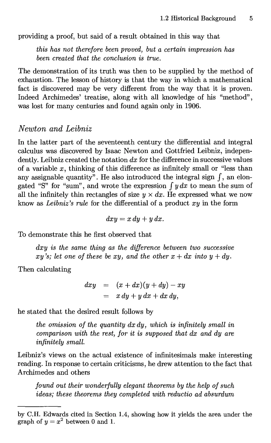
he stated that the desired result follows by
the omission of the quantity dx dy, which is infinitely small in
comparison with the rest, for it is supposed that dx and dy are
infinitely small.
Leibniz's views on the actual existence of infinitesimals make interesting
reading. In response to certain criticisms, he drew attention to the fact that
Archimedes and others
found out their wonderfully elegant theorems by the help of such
ideas; these theorems they completed with reductio ad absurdum
by C.H. Edwards cited in Section 1.4, showing how it yields the area under the
graph of у = χ2 between 0 and 1.

6 1. What Are the Hyperreals?
proofs, by which they at the same time provided rigorous
demonstrations and also concealed their methods,
and went on to write:
It will be sufficient if, when we speak of infinitely great (or more
strictly unlimited), or of infinitely small quantities (i.e., the very
least of those within our knowledge), it is understood that we
mean quantities that are indefinitely great or indefinitely small,
i.e., as great as you please, or as small as you please, so that
the error that one may assign may be less than a certain
assigned quantity ...by infinitely great and infinitely small we
understand something indefinitely great, or something indefinitely
small, so that each conducts itself as a sort of class, and not
merely as the last thing of a class . ..it will be sufficient
simply to make use of them as a tool that has advantages for the
purpose of calculation, just as the algebraists retain imaginary
roots with great profit.
Further indication of this attitude is found in the following passage from
an argument in one of his manuscripts:
If dx, ddx ... are by a certain fiction imagined to remain, even
when they become evanescent, as if they were infinitely small
quantities (and in this there is no danger, since the whole
matter can be always referred back to assignable
quantities), then ...
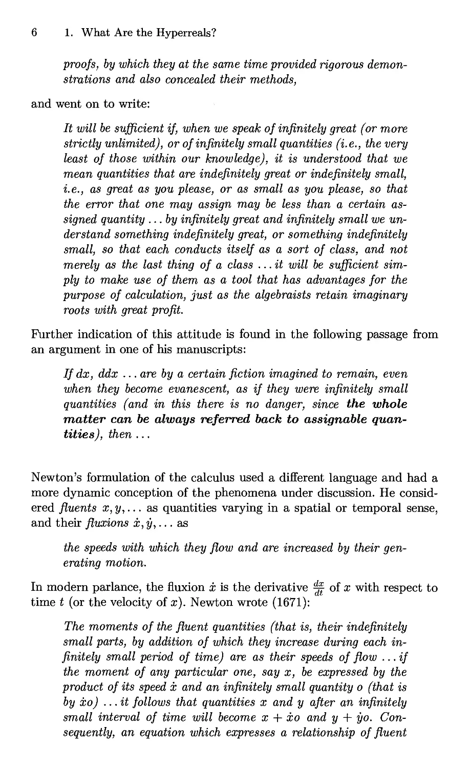
Newton's formulation of the calculus used a different language and had a
more dynamic conception of the phenomena under discussion. He
considered fluents x, y,... as quantities varying in a spatial or temporal sense,
and their fluxions x, y,... as
the speeds with which they flow and are increased by their
generating motion.
In modern parlance, the fluxion χ is the derivative ^ of χ with respect to
time t (or the velocity of a;). Newton wrote (1671):
The moments of the fluent quantities (that is, their indefinitely
small parts, by addition of which they increase during each
infinitely small period of time) are as their speeds of flow .. .if
the moment of any particular one, say x, be expressed by the
product of its speed χ and an infinitely small quantity о (that is
by xo) ...it follows that quantities χ and у after an infinitely
small interval of time will become χ + xo and у + уо.
Consequently, an equation which expresses a relationship of fluent

1.2 Historical Background 7
quantities without variance at all times will express that
relationship equally between χ + xo and у + yo as between χ and
y; and so χ + xo and у + уо may be substituted in place of the
latter quantities, χ and y, in the said equation.
In other words, if (x, y) is a point on the curve defined by an equation in
χ and y, then (x + xo, у + yo) is also on the curve. But this does not seem
right: surely (x + xo, у + yo) should lie on the tangent to the curve, the line
through (x,y) of slope y/x, rather than on the curve itself? Moreover, in
making the proposed substitution and carrying out algebraic calculations,
Newton permitted himself to divide by the infinitely small quantity о while
at the same time stating that
since о is supposed to be infinitely small so that it be able to
express the moments of quantities, terms which have it as a factor
will be equivalent to nothing in respect of others. I therefore cast
them out...
which seems to amount to equating о to zero.
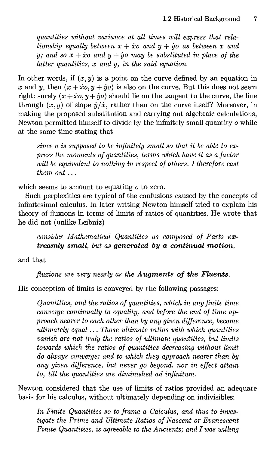
Such perplexities are typical of the confusions caused by the concepts of
infinitesimal calculus. In later writing Newton himself tried to explain his
theory of fluxions in terms of limits of ratios of quantities. He wrote that
he did not (unlike Leibniz)
consider Mathematical Quantities as composed of Parts ex-
trearrdy small, but as generated by a continual motion,
and that
fluxions are very nearly as the Augments of the Fluents.
His conception of limits is conveyed by the following passages:
Quantities, and the ratios of quantities, which in any finite time
converge continually to equality, and before the end of time
approach nearer to each other than by any given difference, become
ultimately equal... Those ultimate ratios with which quantities
vanish are not truly the ratios of ultimate quantities, but limits
towards which the ratios of quantities decreasing without limit
do always converge; and to which they approach nearer than by
any given difference, but never go beyond, nor in effect attain
to, till the quantities are diminished ad infinitum.
Newton considered that the use of limits of ratios provided an adequate
basis for his calculus, without ultimately depending on indivisibles:
In Finite Quantities so to frame a Calculus, and thus to
investigate the Prime and Ultimate Ratios of Nascent or Evanescent
Finite Quantities, is agreeable to the Ancients; and I was willing

8 1. What Are the Hyperreals?
to shew, that in the Method of Fluxions there's no need of
introducing Figures infinitely small into Geometry. For this Analysis
may be performed in any Figures whatsoever, whether finite or
infinitely small, so they are but imagined to be similar to the
Evanescent Figures ...
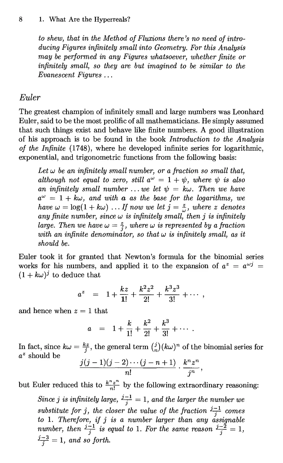
Euler
The greatest champion of infinitely small and large numbers was Leonhard
Euler, said to be the most prolific of all mathematicians. He simply assumed
that such things exist and behave like finite numbers. A good illustration
of his approach is to be found in the book Introduction to the Analysis
of the Infinite (1748), where he developed infinite series for logarithmic,
exponential, and trigonometric functions from the following basis:
Let ω be an infinitely small number, or a fraction so small that,
although not equal to zero, still αω = 1 + ψ, where ψ is also
an infinitely small number . ..we let ψ = ku. Then we have
αω = 1 + ku), and with a as the base for the logarithms, we
have ω = log(l + ku) ...If now we let j = J, where ζ denotes
any finite number, since ω is infinitely small, then j is infinitely
large. Then we have ω = 4, where ω is represented by a fraction
with an infinite denominator, so that ω is infinitely small, as it
should be.
Euler took it for granted that Newton's formula for the binomial series
works for his numbers, and applied it to the expansion of az = αω:> =
(1 + ku)i to deduce that
kz k2z2 k3z3
a = 1 + ΪΓ + -2Γ + -3Γ+··· >
and hence when ζ = 1 that
к к2 к3
a = 1 + Ϊ! + 2!+3!+····
In fact, since ku = ^, the general term (J)(faj)n of the binomial series for
az should be
j(j ~ l)(i - 2) · · · (j - η + 1) knzn
n\ ' jn '
but Euler reduced this to ^-f- by the following extraordinary reasoning:
Since j is infinitely large, ^y- = 1, and the larger the number we
substitute for j, the closer the value of the fraction ^^ comes
to 1. Therefore, if j is a number larger than any assignable
number, then ^^ is equal to 1. For the same reason i^ = 1,
^y^ = 1, and so forth.

1.2 Historical Background 9
His next step was a natural one:
Since we are free to choose the base a for the system of
logarithms, we now choose a in such a way that к = 1 ... we obtain
the value for
a = 2.71828182845904523536028.
When this base is chosen, the logarithms are called natural or
hyperbolic. The latter name is used since the quadrature of a
hyperbola can be expressed through these logarithms. For the
sake of brevity for this number 2.718281828459 · · · we will use
the symbol e ...
Whereas the modern view is that
e = lim [ 1 + -
n—>oo у п
Euler had obtained it by stipulating that e = (l + j) , and indeed e
(l + *У, for infinitely large j. In this way he "proved" that
jy *У *У
ez = 1 + H + ^ + ^!+··· -
η,Ζ ~,o ™4
log(l+a;) = χ-γ + -£-^- + ···>
and also showed that
cos a; = 1 +
x4 егх + е
sin a; = χ -j—-
2! 4! 2
x3 x5 егх — е~
3! 5! 2г
by using the equations coscj = 1, sincj = ω, and j = j — 1 = j — 2 = · · ·
with ω infinitely small and j infinitely large.
Euler's demonstration that the function ex is equal to its own derivative
employed the practice, which, as we saw, was adopted by Leibniz and
Newton, of "casting out" higher-order infinitesimals like dx dy, (dx)2, (dx)3, etc.
Applying his series expansion for the exponential function to edx he argued
that
d(ex)
=
=
=
=
x+dx _ χ
ex(edx - 1)
e x(dx + ^-
exdx.
(dx)3

10 1. What Are the Hyperreals?
Demise of Infinitesimals
The conceptual foundations of the calculus continued to be controversial
and to attract criticism, the most famous being that of Berkeley, who wrote
(1734) in opposition to the ideas of Newton and his followers:
And what are these fluxions ? The velocities of evanescent
increments? And what are these same evanescent increments? They
are neither finite quantities, nor quantities infinitely small, nor
yet nothing. May we not call them the ghosts of departed
quantities?
Eventually infinitesimals were expunged from analysis, along with the
dependence on intuitive geometric concepts and diagrams. The subject was
"arithmetised" by the explicit construction of the real numbers out of
the rational number system by the work of Dedekind, Cantor, and
others around 1872. Weierstrass provided the purely arithmetical formulation
of limits that we use today, defining lim^a f(x) = L to mean that
(Ve > 0) (36 > 0) such that 0 < \x - a\ < 6 implies \f(x) - L\ < ε.
Robinson
Three centuries after the seminal discoveries of Newton and Leibniz,
infinitesimals were restored with a vengeance by Abraham Robinson, who
wrote in the preface to his 1966 book Non-standard Analysis:
In the fall of 1960 it occurred to me that the concepts and
methods of contemporary Mathematical Logic are capable of
providing a suitable framework for the development of the Differential
and Integral Calculus by means of infinitely small and infinitely
large numbers.
The progress of symbolic logic in the twentieth century had produced an
exact formulation of the syntax of mathematical statements; an account
of what it is for a statement to be true of a mathematical system or
structure—i.e. for the structure to be a model of the statement; and
methods for obtaining models of prescribed statements. One such method comes
from the compactness theorem:
• If a set Σ of statements (of an appropriate kind) has the property
that each finite subset Σ' of Σ has a model (a structure of which all
members of Σ' are true), then there must be a single structure that
is a model of Σ itself.
Now suppose that we take I7r to consist of all appropriate statements true
of Μ (including the axioms for ordered fields amongst other things) together
with the infinitely many statements
0<ε, ε<1, ε<\, ε<\, ..., ε < ±, ....

1.3 What Is a Real Number? 11
Using the compactness theorem it can be deduced that £κ has a model
*M, which will be an ordered field in which the element ε is a positive
infinitesimal. Moreover, this model will satisfy the transfer principle:
• Any appropriately formulated statement is true of *M if and only if
it is true of M.
This is reminiscent of Leibniz's above-quoted remark that
the whole matter can be always referred back to assignable
quantities,
and might even suggest that there is no point in considering *M, since it
satisfies the same theorems as №.. But on the contrary, what it offers is a
new methodology for real analysis, because the availability of infinitesimals
allows for easier and more intuitively natural proofs in *E of some theorems
that can then immediately be inferred to hold of M. by transfer.
Of course for this to work, the theorems in question must be
"appropriately formulated", and explaining what this means is one of our major goals.
As we shall see, *R fails to satisfy Dedekind's completeness axiom
stipulating that any nonempty set with an upper bound must have a least upper
bound, so this is not the sort of assertion to which transfer applies. In order
to determine which statements are subject to it we will need the "concepts
and methods of contemporary Mathematical Logic" that were available to
Robinson, but not to Leibniz, nor indeed to those in the intervening period
who tried to work with infinitesimals or construct non-Archimedean
extensions of the real number system. Robinson's great achievement was to turn
the transfer principle into a working tool of mathematical reasoning. In
the last few decades it has been applied to many areas, including analysis,
topology, algebra, number theory, mathematical physics, probability and
stochastic processes, and mathematical economics.
To those unfamiliar with formal logic, the use of compactness may seem
like a kind of sleight of hand. A model of 17ц is produced, but we do not see
where it came from. However, the compactness theorem itself has a proof,
and one way to prove it is to use the notion of an ultraproduct, an algebraic
construction that takes all the assumed models of the finite subsets of Σ
and builds a model of Σ out of them. We can apply this construction
directly to the structure Ш. to build *lasa special kind of ultraproduct
called an ultrapower. This will be our first main task.
1.3 What Is a Real Number?
Consideration of this question provides motivation for the definition of the
hyperreal number system. Here are some standard answers.

12 1. What Are the Hyperreals?
(1) A real number is an infinite decimal expression, such as
y/2 = 1.4142135623731
that identifies y/2 as the sum of the infinite power series
4 14 2 1
1-1 1 1 1 μ μ . . .
10 102 103 104 105
(2) A real number is an element of a complete ordered field. Here
"complete", often called Dedekind complete, means that any nonempty
set with an upper bound must have a least upper bound. Any two
complete ordered fields are isomorphic, so this notion uniquely
characterises №..
(3) A real number is a Dedekind cut in the set Q of rational numbers: a
partition of Q into a pair (L, U) of nonempty disjoint subsets with
every element of L less than every element of U and L having no
largest member. Thus y/2 can be identified with the cut
L={qeQ:q2 < 2}, U = {q e Q : q2 > 2}.
The set of all Dedekind cuts of Q can be made into a complete ordered
field.
(4) A real number is an equivalence class of Cauchy sequences of
rational numbers. A sequence (г1,Г2,гз,... ) is Cauchy if its terms get
arbitrarily close to each other as we move along the sequence, i.e.,
lim \rn-rm\=0.
n,m—>oo
Thus y/2 is the limit of the rational Cauchy sequence
1, 1.4, 1.41, 1.414, 1.4142, 1.41421, 1.414213, ...
as well as being the limit of any of the subsequences of this sequence,
and of other rational sequences besides.
Two Cauchy sequences (n,r2,r3,... ) and (si,s2, S3,... ) are
equivalent if their corresponding terms approach each other arbitrarily
closely:
lim \rn - sn\ =0.
n—>oo
This defines an equivalence relation on the set of rational-valued
Cauchy sequences, and the resulting set of equivalence classes forms
a complete ordered field. Any two equivalent Cauchy sequences will
have the same limit, and so represent the same real number. For
example, y/2 corresponds to the equivalence class of the above sequence.

1.3 What Is a Real Number? 13
Answer (2) provides the basis for the axiomatic or descriptive approach
to the analysis of №.. The object of study is simply described as being a
complete ordered field, since all its properties derive from that fact. The
axioms for a complete ordered field are listed, and everything follows from
that. This is by far the favoured approach in introductory texts on real
analysis.
The constructive approach takes as given only the rational number
system and proceeds to construct M. explicitly. There are at least two ways
to do this, due respectively to Dedekind (answer (3)) and Cantor (answer
(4))·
It would be possible to develop an axiomatic approach to the hyperreals
*M by assuming that we are dealing with an ordered field containing Μ as
well as infinitesimals and satisfying the transfer principle "appropriately
formulated". However, in view of the controversial history of the notion
of infinitesimal, one could be forgiven for wondering whether this is an
exercise in fantasy, or whether there does exist a number system satisfying
the proposed axioms. The constructive approach is needed to resolve this
issue. We will be discussing a construction of *M out of Μ that is analogous
to Cantor's construction of Μ out of Q. Hyperreal numbers will arise as
equivalence classes of reaZ-valued sequences, and the challenge will be to
find an equivalence relation on such sequences that produces the desired
outcome.
To conclude this introduction to our subject, let us examine another
putative answer to the question "what is a real number?"—namely, that a
real number is a point on the number line:
Now, the intuitive geometric idea of a line is an ancient one, much older
than the notion of a set of points, let alone an infinite set. The identification
of a line with the set of points lying on that line is a perspective that belongs
to modern times. For Euclid a line was simply " length without breadth",
and his diagrams and arguments involved lines with a finite number of
points marked on them. By applying the field operations and taking limits
of converging sequences we can assign a point to each real number, but the
claim that this exhausts all the points on the line is just that: a claim. One
could seek to justify it by invoking a principle such as the one attributed
to Eudoxus and Archimedes that any two magnitudes are such that
the less can be multiplied so as to exceed the other.
This entails that for each real number r there is an integer n> r, and that
precludes there being any infinitely large or small numbers in M. But then
one could say that the Eudoxus-Archimedes principle is just a property
of those points on the line that correspond to "assignable" numbers. The

14 1. What Are the Hyperreals?
hyperreal point of view is that the geometric line is capable of sustaining
a much richer and more intricate number set than the real line.
1.4 Historical References
Amongst the numerous books available, the following are worth consulting
for more details on the historical background we have been discussing.
M. E. Baron and H. J. M. Bos. Newton and Leibniz. Open
University Press, 1974.
J. M. Child. The Early Mathematical Manuscripts of Leibniz. Open
Court Publishing Co., 1920.
E. J. Dijksterhuis. Archimedes. Princeton University Press, 1987.
С. Н. Edwards. The Historical Development of the Calculus. Springer,
1979.
Leonhard Euler. Introduction to the Analysis of the Infinite, Book
I, translated by John D. Blanton. Springer, 1988.

2
Large Sets
2.1 Infinitesimals as Variable Quantities
Cauchy (1789-1857) is regarded as one of the pioneers of the precision that
is characteristic of contemporary mathematics. He wrote:
My principal aim has been to reconcile rigor, which I have made
a law to myself in my Cours d'analyse, with the simplicity which
the direct consideration of infinitely small quantities produces.
His method was to consider infinitesimals as being variable quantities that
vanish:
When the successive numerical values of a variable decrease
indefinitely so as to be smaller than any given number, this
variable becomes what is called infinitesimal, or infinitely small
quantity One says that a variable quantity becomes
infinitely small when its value decreases numerically so as to
converge to the limit zero.
Even today there are textbooks containing statements to the effect that a
sequence satisfying
lim rn = 0
n—>oo
is an infinitesimal, while one satisfying
lim rn = oo

16 2. Large Sets
is an infinitely large magnitude. Can we then construct a number system in
which such sequences represent infinitely small and large numbers
respectively?
According to Cauchy, the sequence
1 I I I
x» 2' 3' 4'-- -
is an infinitesimal, as is
I I I I
2>4>6>8>
If these represent infinitely small numbers, perhaps we should regard the
second as being half the size of the first because it converges twice as
quickly? Similarly, the sequences
1,2,3,4,...,
2,4,6,8,...
both represent infinitely large magnitudes, and arguably the second is twice
as big as the first because it diverges to oo twice as quickly. On the other
hand, the distinct sequences
1,2,3,4,...,
2,2,3,4,...
will presumably represent the same infinite number.
These ideas are attractive because they suggest the possibility of using
infinitely small and large numbers as measures of rates of convergence. But
in the construction of real numbers out of Cauchy sequences (Section 1.3),
all sequences converging to zero are identified with the number zero itself,
while diverging sequences have no role to play at all. Clearly then we need
a very different kind of equivalence relation among sequences than the one
used in Cantor's construction of Μ from Q.
2.2 Largeness
Let r = (ri,r2,r3,... ) and s = {si,s2,s3,... ) be real-valued sequences.
We are going to say that r and s are equivalent if they agree at a "large"
number of places, i.e., if their agreement set
is large in some sense that is to be determined. Whatever "large" means,
there are some properties we will want it to have:
• N = {1,2,3,...} must be large, in order to ensure that any sequence
will be equivalent to itself.

2.2 Largeness 17
• Equivalence is to be a transitive relation, so if Ers and Est are large,
then Ert must be large. Since Ers Π Est С £rt, this suggests the
following requirement:
If A and В are large sets, and AnB C. C, then С is large.
In particular, this entails that if A and В are large, then so is their
intersection AnB, while if A is large, then so is any of its supersets
С 2 A.
• The empty set 0 is not large, or otherwise by the previous
requirement all subsets of N would be large, and so all sequences would be
equivalent.
Requiring Α Π Β to be large when A and В are large may seem restrictive,
but there are natural situations in which all three requirements are fulfilled.
One such is when a set А С N is declared to be large if it is cofinite,
i.e. its complement N — A is finite. This means that A contains "almost
all" or "ultimately all" members of N. Although this is a plausible notion
of largeness, it is not adequate to our needs. The number system we are
constructing is to be linearly ordered, and a natural way to do this, in
terms of our general approach, is to take the equivalence class of sequence
r to be less than that of s if the set
Lrs = {n:rn< sn)
is large. But consider the sequences
r = (1,0,1,0,1,0,...) ,
s = (0,1,0,1,0,1,...) .
Their agreement set is empty, so they determine distinct equivalence classes,
one of which should be less than the other. But Lrs (the even numbers) is
the complement of Lsr (the odds), so both are infinite and neither is
cofinite. Apparently our definition of largeness is going to require the following
condition:
• For any subset A of N, one of A and N — A is large.
The other requirements imply that A and N — A cannot both be large,
or else Α Π (Ν — A) = 0 would be. Thus the large sets are precisely the
complements of the ones that are not large. Either the even numbers form
a large set or the odd ones do, but they cannot both do so, so which is it
to be?
Can there in fact be such a notion of largeness, and if so, how do we
show it?

18 2. Large Sets
2.3 Filters
Let 7 be a nonempty set. The power set of I is the set
V(I) = {A : А С 1}
of all subsets of I. A filter on 7 is a nonempty collection Τ С Τ3 (7) of
subsets of / satisfying the following axioms:
• Intersections: if А, В £ J7, then AV\B £T.
• Supersets: ii AeJ7 and AC В С I, then В £ J7.
Thus to show В G .T7, it suffices to show
ΑιΠ···ΠΑηςβ,
for some η and some Ai,..., An £ J7.
A filter Τ contains the empty set 0 iff J7 = V(I). We say that Τ is proper
if 0 φ Τ. Every filter contains /, and in fact {/} is the smallest filter on I.
An ultrafilter is a proper filter that satisfies
• for any AC I, either A £ Τ or Ac £ J7, where Ac = I - A.
2.4 Examples of Filters
(1) J71 = {А С I: г £ A} is an ultrafilter, called the principal ultrafilter
generated by i. If I is finite, then every ultrafilter on I is of the form
J71 for some г £ I, and so is principal.
(2) Tco = {А С I: I — A is finite} is the cofinite, or Frechet, filter on I,
and is proper iff I is infinite. Tco is not an ultrafilter.
(3) If 0 φ Ή. С Р(/), then the ,/Шег generated by Ή, i.e., the smallest
filter on / including Л, is the collection
TH = {А С 7 : A D Βλ Π · · · Π Bn for some η and some B» 6 W}
(cf. Exercise 2.7(4)). For Η = 0 we put ^ = {/}.
If Η has a single member B, then J74 = {А С I: А Э B}, which is
called the principal filter generated by B. The ultrafilter J71 of
Example (1) is the special case of this when В = {г}.
(4) If {Tx : χ £ X} is a collection of filters on / that is linearly ordered by
set inclusion, in the sense that Tx С Ty or Ty С Tx for any x, у £ X,
then
[}хеХТх = {А:Зх£Х{А£Тх)}
is a filter on I.

2.6 Zorn's Lemma 19
2.5 Facts About Filters
(1) The filter axioms are equivalent to the requirement that
AnB eJ7 iff A,B EF.
(2) If Τ С V(I) satisfies the superset axiom, then Τ φ 0 iff/ G T. Hence
{1} С Τ for any filter T.
(3) An ultrafilter Τ satisfies
An Be J7 iff A e Τ and В e J",
iuBef iff ieforBef,
ylcef iff A £ J".
(4) Let .T7 be an ultrafilter and {Αι,... ,An} a finite collection of pairwise
disjoint (Ai Π Aj = 0) sets such that
AiU'-UAiGf.
Then Aj 6 .T7 for exactly one г such that 1 <i<n.
(5) If an ultrafilter contains a finite set, then it contains a one-element
set and is principal. Hence a nonrincipal ultrafilter must contain all
cofinite sets. This is a critical property used in the construction of
infinitesimals and infinitely large numbers (cf. Section 3.8).
(6) Τ is an ultrafilter on I iff it is a maximal proper filter on I, i.e., a
proper filter that cannot be extended to a larger proper filter on I
(cf. Exercise 2.7(5)).
(7) A collection Ή С V(I) has the finite intersection property, or ftp,
if the intersection of every nonempty finite subcollection of Ή is
nonempty, i.e.,
B1 Π · · · Π Βη φ 0
for any n and any B\,..., Bn e Ή.
Then the filter J74 is proper iff Ή has the fip.
(8) If Ή has the fip, then for any А С I, at least one of the sets Ή U {A}
and HU{4C} has the fip.
2.6 Zorn's Lemma
Fact 2.5(8) suggests a way to construct an ultrafilter: start with a set that
has the fip, e.g., {/}, and go through all the members A of V(I) in turn,

20 2. Large Sets
adding whichever of A and Ac preserves the fip. This presupposes that
there is such a thing as a listing of the members of V(I) that could be used
to "go through them all in turn".
Now, the assertion that any set can be listed in this way is one of many
mathematical statements that are equivalent to the axiom of choice, which
asserts that for any given collection of sets there exists a function whose
range of values selects a member from each set in the collection. The version
of the axiom of choice most used in algebra is Zorn's lemma:
If(P, <) is a partially ordered set in which every linearly ordered
subset (or "chain") has an upper bound in P, then Ρ contains
a <-maximal element.
(An element ρ of a partially ordered set is <-maximal if there is no element
q of Ρ that is greater than ρ in the sense that ρ < q and ρ ψ q.)
Here is an outline of how Zorn's lemma can be proven from the
assumption that the axiom of choice is true. Let / be a choice function defined
on the collection of all nonempty subsets of P. Thus for each such set X,
f(X) G X. Now begin with the element p0 = f(P)· If Po is maximal, we
have the desired conclusion. Otherwise, we use / to choose an element pi
that is greater thanp0, i-e·, Pi = f(X)> where X = {x e Ρ : Po < x] φ 0. If
Pi is maximal, again we are done. Otherwise we can choose pi with ρλ <pi-
If this process repeats denumerably many times, the pn's form a chain. By
the hypothesis of Zorn's lemma, this chain must then have an upper bound
ρω, giving
Po <Pi < ··· <Pn < ■·■ <Ρω-
If ρω is maximal, we are done; otherwise there exists ρω+ι > ρω, and so
on. Now, this whole construction cannot go on forever, because eventually
we will "run out of" elements of P. At some point we must finish with the
desired maximal element.
This argument shows what is going on behind the scenes when Zorn's
lemma is applied. Of course the part about running out of elements is
vague, and to make it precise we would need to introduce the theory of
infinite "ordinal" numbers and "well-orderings" in order to show that we
can generate a list of all the elements of P. In many applications,
appealing directly to Zorn's lemma itself allows us to avoid such machinery. For
example:
Theorem 2.6.1 Any collection of subsets of I that has the finite
intersection property can be extended to an ultrafilter on I.
Proof. If Ή has the fip, then the filter J^ generated by Τ is proper
(2.5(7)). Let Ρ be the collection of all proper filters on I that include Tu,
partially ordered by set inclusion C. Then every linearly ordered subset of
Ρ has an upper bound in P, since by 2.4(4) the union of this chain is in
P. Hence by Zorn's lemma Ρ has a maximal element, which is thereby a
maximal proper filter on I and thus an ultrafilter by 2.5(6). D

2.7 Exercises on Filters 21
Corollary 2.6.2 Any infinite set has a nonprincipal ultrafilter on it.
Proof. If / is infinite, the cofinite filter Tco is proper and has the finite
intersection property, and so is included in an ultrafilter T. But for any
i e I we have / - {г} б Тсо С J7, so {г} $ J7, whereas {г} 6 J*. Hence
Τ ψ T1. Thus Τ is nonprincipal. D
This result is the key fact we need to begin our construction of the hy-
perreal number system. We could have simply taken it as an assumption,
but there is insight to be gained in showing how it derives from more
general principles like Zorn's lemma. In fact, a deeper set-theoretic analysis
proves that there are as many nonprincipal ultrafilters on an infinite set I
as there possibly could be: an ultrafilter is a member of the double power
set V(V(I)), and there is a one-to-one correspondence between the set of
all nonprincipal ultrafilters on I and V(P(I)) itself.
2.7 Exercises on Filters
(1) If 0 φ А С I, there is an ultrafilter Τ on I with AeJ7.
(2) There exists a nonprincipal ultrafilter on N containing the set of even
numbers, and another containing the set of odd numbers.
(3) An ultrafilter on a finite set must be principal.
(4) For Η С V(I), let Tu be as defined in Example 2.4(3).
(i) Show that T4 is a filter that includes H, i.e., Η С Тп.
(ii) Show that J74 is included in any other filter that includes Τι.
(5) Let Τ be a proper filter on I.
(i) Show that T\J{AC} has the finite intersection property iff A £ T.
(ii) Use (i) to deduce that Τ is an ultrafilter iff it is a maximal
proper filter on I.

This page intentionally left blank

3
Ultrapower Construction of the
Hyperreals
3.1 The Ring of Real-Valued Sequences
Let N= {1,2,... }, and let MN be the set of all sequences of real numbers.
A typical member of MN has the form r = (г\,Г2,гз,... ), which may be
denoted more briefly as (rn : η G N) or just (rn).
For r = (rn) and s = (sn), put
r®s = (rn+sn:neN) ,
r © s = (rn · sn : η e N) .
Then (MN, φ, 0) is a commutative ring with zero 0 = (0,0,0,...) and unity
1 = (1,1,...), and additive inverses given by
—r = (—rn : η e N).
It is not, however, a field, since
(1,0,1,0,1,...)©(0,1,0,1,0,...)=0,
so the two sequences on the left of this equation are nonzero elements of
MN with a zero product; hence neither can have a multiplicative inverse.
Indeed, no sequence that has at least one zero term can have such an inverse
inMN.

24 3. Ultrapower Construction of the Hyperreals
3.2 Equivalence Modulo an Ultrafilter
Let Τ be a fixed nonprincipal ultrafilter on the set N (such exists by
Corollary 2.6.2). Τ will be used to construct a quotient ring of MN.
Define a relation ξ on MN by putting
(rn) = (sn) iff {neff:rn = sn} e T.
When this relation holds it may be said that the two sequences agree on a
large set, or agree almost everywhere modulo T, or agree at almost all n.
3.3 Exercises on Almost-E very where Agreement
(1) ξ is an equivalence relation on MN.
(2) ξ is a congruence on the ring (MN, Θ, ©), which means that if r = r'
and s = s', then
r(Bs = r'(Bs' and rQs^r'Qs'.
(3) (l,I,i,...)#(0,0,0,...>.
3.4 A Suggestive Logical Notation
It is suggestive to denote the agreement set {n e N : rn = sn} by [r = s],
rather than Ers as in Section 2.2. Thus
r = s iff [r = s]ef.
Then results like 3.3(1) and 3.3(2) can be handled by first proving
properties such as those in Section 3.5 below.
The set [r = s] may be thought of as the interpretation, or value, of the
statement "r = s", or as a measure of the extent to which "r = s" is true.
Normally we think of a statement as having one of two values: it is either
true or false. Here, instead of assigning truth values, we take the value of
a statement to be a subset of N. When [r = s] e T, it is sometimes said
that r = s almost everywhere (modulo J7).
This idea can be applied to other logical assertions, such as inequalities,
by defining
lr<s] = {neff:r„< sn},
lr>s] = {neff:r„> sn},
[r<s] = {neN:r„<4
and so on.

3.6 The Ultrapower 25
3.5 Exercises on Statement Values
(1) [r = s] Гф = t] С [r = t].
(2) [r = r'] Π [s = s'] С [r Θ s = r' Θ s'j Π [r © s = r' © s'].
(3) [r = r'] Π \a = s'\ Π [r < s] С [г' < β'].
(4) If r ξ r' and s = s', then [r < s] 6 J" iff [r' < s'j 6 J".
3.6 The Ultrapower
The equivalence class of a sequence r G MN under = will be denoted by [r].
Thus
[r] = {«el":rs s}.
The quotient set (set of equivalence classes) of MN by = is
*R = {[r] : r e KN}.
Define
[r] + [s] = [res] = [<rn + sn>],
[r]-[s] = [r©s] = [<r„-s„>].
and
[r] < [s] iff [r < s] e Τ iff {n£N:r„< sn} e T.
By 3.3(2) and 3.5(4) these notions are well-defined, which means that they
are independent of the equivalence class representatives chosen to define
them.
A simpler notation, which is attractive but puts some burden on the
reader, is to write [rn] for the equivalence class [{rn : η 6 Щ] of the sequence
whose nth term is rn. The definitions of addition and multiplication then
read
[rn] + [Sn] = [Гп + Sn] ,
[rn] ■ [Sn] = [Гп ■ Sn] .
Theorem 3.6.1 The structure {*R, +, ■, <) is an ordered field with zero [0]
and unity [1].
Proof. (Sketch) As a quotient ring of MN, *M is readily shown to be a
commutative ring with zero [0] and unity [1], and additive inverses given
by
-[(rn:neN)] = [(-rn:neN)},

26 3. Ultrapower Construction of the Hyperreals
or more briefly, — [rn] = [—rn]. To show that it has multiplicative inverses,
suppose [r] φ [0]. Then r ψ 0, i.e., {n e N : r„ = 0} ^ J, so as J is an
ultrafilter, J = {η Ε Ν : rn φ 0} e J7. Define a sequence s by putting
10 otherwise.
Then [r © s = 1] is equal to J, so [r © s = 1] G T, giving r © s = 1 and
hence
[r].[s] = [r©s] = [l]
in *M. But this means that [s] is the multiplicative inverse [r]_1 of [r].
To see that the ordering < on *M is linear, observe that N is the disjoint
union of the three sets
[r<s], [r = s], [s<rj,
so exactly one of the three belongs to Τ (by 2.5(4)), and so exactly one of
[r]<[s], [r] = [s], [s]<[r]
is true. It remains to show that the set {[r] : [0] < [r]} of "positive"
elements in *M is closed under addition and multiplication. This is left as
an exercise.
D
In the proof just given we were trying in effect to show that [r^]-1 = [r"1],
but were constrained by the fact that the real number r"1 may not exist for
some n. The reason why [r]_1 nonetheless exists is that r"1 exists for almost
all η (i.e., for all η in the set {n e N : rn φ 0} G T). This relationship
between *M and Μ characterises the definitions of the relations =, <, >,
etc. in *M, in the sense that
[rn] = [sn] iff rn = sn for almost all n,
[rn] < [sn] iff rn < sn for almost all n,
[rn] + [sn] = [tn] iff rn + sn = tn for almost all n,
[rn] ■ [s„] = [tn] iff rn ■ sn = tn for almost all n,
and so on. Let us call this relationship the almost-all criterion. As we will
see, it holds for many other properties and is the basis of the transfer
principle. Theorem 3.6.1 is itself a special case of transfer: *M is an ordered
field because Μ is. This is explained further in Section 4.5.
The ring MN is an example of what is known in algebra as a direct power
of M, a special case of the notion of direct product. An ω/irapower is a
quotient of a direct power that arises from the congruence relation defined
by an ultrafilter.

3.8 Infinitesimals and Unlimited Numbers 27
3.7 Including the Reals in the Hyperreals
We can identify a real number r G Μ with the constant sequence r =
(r,r,... ) and hence assign to it the *M-element
V=[r] = [<r,r,...>].
It can be shown that for r,s£l, we have
*(r + s) = *r + *s,
*(r · s) = V · *s,
*r <*s iff r < s,
*r = *s iff r = s.
Hence
Theorem 3.7.1 The map r н-> *r is an order-preserving field isomorphism
from Ш into *R. D
This result allows us to identify the real number r with *r whenever
convenient, and hence to regard Μ as a subfield of *R. In particular we may
identify [0] with 0 and [1] with 1.
3.8 Infinitesimals and Unlimited Numbers
Lets = (l,|,i,... ) = (i :neN). Then
[0 < ε] = {η e N : 0 < £} = N e T,
so [0] < [ε] in *R. But if r is any positive real number, then the set
[ε < r] = {n e N : i < r}
is cofinite (because ε converges to 0 in Ш !). Now, since Τ is nonprincipal,
it contains all cofinite sets (2.5(5)), so [ε < r] e Τ and therefore [ε] < *r
in *R. Thus [ε] is a positive infinitesimal.
Now let ω = (1,2,3,... ). Then for any rGl, the set
[r < ω] = {η e N : r < n}
is cofinite (by the Eudoxus-Archimedes principle!) and so belongs to T,
showing that *r < [ω] in *M. Thus [ω] is "infinitely large" compared to Μ in
*R, although we will prefer to use the adjective unlimited to describe such
entities. In fact ε · ω = 1, so [ω] = [ε]-1 and [ε] = [ω]-1.
The properties observed of [ε] and [ω] show that *M is a proper extension
of M, and hence a new structure. Even more directly, for any reR, the

28 3. Ultrapower Construction of the Hyperreals
set [r = ω] is either 0, or equal to {r} when r G N, so cannot belong to T,
implying V φ [ω]. Thus [ω] 6 *R - №..
This argument depends crucially on the fact that Τ is nonprincipal. If
Τ were principal, then there would be some fixed η 6 N such that
^ = Я={4СМ:п£А}.
But then each sequence s e MN would agree almost everywhere with the
sequence taking the constant value s„, and from this it would follow that
'R = {V : г £ 1}, and hence *M would be isomorphic to M. The details
of this are left as an exercise: the essential point is that use of a principal
ultrafilter to construct *K does not lead to anything new.
Our discussion of ε and ω shows in fact that if r is any real-valued
sequence converging to zero, then [r] is an infinitesimal in *M, while if r
diverges to oo, then [r] is unlimited in *R. Thus we have achieved the
objective proposed in Section 2.1 of building a number system with these
features.
Now that we have shown that there are infinitesimals in *M, we can begin
to apply the field operations to them to construct new numbers. What
happens for instance if we multiply or divide an infinitesimal by a positive
real number? Or by a negative real number? The general arithmetic of
hyperreals will be described in Chapter 5.
Exercise 3.8.1
Use only general properties of ordered fields to deduce from the fact that
[ε] is a positive infinitesimal the conclusion that [ε]-1 is greater than every
real number.
3.9 Enlarging Sets
A subset A of Ε can be "enlarged" to a subset *A of *M: for each relN,
put
[r] e*A iff {n 6 N : rn 6 A) 6 T.
Thus we are declaring, by the almost-all criterion, that [rn] is in *A iff rn
is in A for almost all n. Again it has to be checked that this is well-defined.
Invoking the [...] notation, put
[reiI = {neN:r„e A}.
Then
[r = r']n[re4]c[/e4
so
r = r' & (reAjeJ7 implies \r' 6 A\ e Τ

3.10 Exercises on Enlargement 29
as required. We have
[r] e *A iff freAje T.
Observe that if s 6 A, then [s 6 A] =Nef (where s = (s, s,... ) as
usual), so *s 6 *A Identifying s with *s, we may regard *A as a superset of
4 : i С '4. Elements of *A - A may be thought of as new "nonstandard",
or "ideal", members of A that live in *R.
For example, let A = N, and ω = (1,2,3,... ) as above. Then [ω 6 N] =
N e T, so [ω] e *N. [ω] is a "nonstandard natural number".
Theorem 3.9.1 Any infinite subset of Ш has nonstandard members.
Proof. Note first that this result must depend on Τ being nonprincipal,
because if Τ were principal, there would be no nonstandard elements of *M
at all.
Now, if А С Μ is infinite, then there is a sequence r of elements of A
whose terms are all distinct. Then [r 6 A\ = N e T, so [r] 6 *A. But for
each s £ A, {n : rn = s} is either 0 or a singleton, neither of which can
belong to Τ (2.5(5)), so [r] φ *s. Hence [r] e'A-A D
The converse of this theorem is also true (cf. the next exercise), so the
property of having nonstandard members exactly characterises the infinite
sets.
3.10 Exercises on Enlargement
(1) If A is finite, show that *A = A, and hence A has no nonstandard
members.
(2) А С В iff 'AC'S,
A = B iff *A = *B.
(3) *{A\JB) = MU*5,
*(AnB) = *Af)*B,
*(A -B) = *A- *B,
*0 = 0.
(4) Is it true that *((J~=1 An) = U~=1 *An ?
(5) Show that HACR, then *A Π Μ = Α.
(6) For α, b 6 К, let [α, 6] be the closed interval {a; e Μ : α < χ < b}.
Prove that *[o, b] = {x e *Ш : a < χ < b}.
(7) *Z is a subring of *R, i.e., *Z is closed under +, ·, — .

30 3. Ultrapower Construction of the Hyperreals
(8) If M+ = {x e M. : χ > 0}, show that *(R+) = {x 6 *K : χ > 0}, i.e.,
*(R+) = (*M)+.
3.11 Extending Functions
A function f :R->R extends to */ : *M -> *M as follows. First, for each
sequence r 6 KN, let / о r be the sequence (/(n), /(гг),... ). Then put
7(M) = [/or].
In other words,
7([(η,Γ2)...)]) = [(/(η),/(Γ2),...)],
or in the simplified notation,
7(Ы) = [/(rn)].
Now, in general,
[r = r'JC[/or = /or'J,
and so
r = r' implies f or = f or',
ensuring that */ is well-defined. Observe that */ obeys the almost-all
criterion:
7(M) = M iff lfor = s}er
iff {n e N : f(rn) = sn} Ε Τ
iff f(rn) = sn for almost all n.
For example, the sine function is extended to all of *M by
*sin([r]) = [(sin(ri),sin(r2),... )] = [sin(rn)] .
3.12 Exercises on Extensions
(1) Show that */ agrees with / on M: if r 6 K, then */(r) = f(r).
(2) If / is injective, so is */· What about surjectivity?
(3) For χ e *R, let
{x if χ > 0,
0 if χ = 0,
-x if χ < 0
be the usual definition of the absolute value function. Show that this
extends the definition of | · | on M: | [r] | = [(|ri|, |r2|,. ··)] = [ |rn| ].

3.14 Enlarging Relations 31
(4) Let xa be the characteristic function of a set А С №.. Show that
*(Xa) = X-A-
(5) Show how to define */ when / is a function of more than one
argument.
3.13 Partial Functions and Hypersequences
Let / : A —> Ш. be a function whose domain Л is a subset of Μ (e.g.,
f(x) = tana;). Then / extends to a function */ : *A —> *R whose domain is
the enlargement of A, i.e., dom*/ = *(dom/).
To define this extension, take rSKN with [r] € *A, so that
[r e a] = {n e N: rn e A} e T.
Let
= U{rn) if η e [re A] ,
Sn 10 if η £ [r e A}
(it is enough to define sn for almost all ή). Then put
7(H) = Is].
Essentially, we have defined
7(Ы) = [/(r„)]
as in Section 3.11, but with a modification to cater for the complication
that f(rn) may not be defined for some n. The construction works because
/(r„) exists for almost all η modulo T.
It is readily shown that if r € A, then */(*r) = *(/(r)), or identifying *r
with r etc., we have */(r) = /(r), so */ extends /. Therefore it would do
no harm to drop the * symbol and just use / for the extension as well, and
we will do so most of the time. It is a particularly natural practice for
the more common mathematical functions. For instance, the function sin a;
is now defined for all hyperreals χ £ *R.
An important case of this construction concerns sequences. A real-valued
sequence is just a function s : N —> R, and so the construction extends this
to a hypersequence s : *N —> *R. Hence the term sn is now defined even
when ne*N -N.
3.14 Enlarging Relations
Let Ρ be a fc-ary relation on R. Thus Ρ is a set of fc-tuples: a subset of M.k.
For given sequences r1,..., rk £KN, define
lP(r1,...,rk)} = {neN:P(r1n,...,r*)}.

32 3. Ultrapower Construction of the Hyperreals
Now Ρ can be enlarged to a fc-ary relation *P on *Ш, i.e., a subset of (*Ж)к.
For this we use the notation *P([r1],...,[rk]) to mean that the fc-tuple
([r1],..., [rk]) belongs to *P. The definition is:
*P([r1],...,[rk}) iff [Pfr1 r')]e;
iff P(rn,..., r£) for almost all n.
As always with a definition involving equivalence classes named by
particular elements, it must be shown that the notion is well-defined. In this case
we can prove
so that if r1 = s1 and ... and rk = sk and {Р(гг,... ,rfc)] e T, then
lP(s\...,sk)jeT.
When r1,... ,rk are real numbers,
P(r\...,rk) iff *P(V,...,*rfc),
showing that *P is an extension of P.
This definition of fc-ary *P encompasses the work of Sections 3.9-3.13 on
extensions of sets and functions. A subset A of R is just a unary relation
(k = 1), so the definition of *A is a special case of that of *P. When Ρ is
any of the relations =,<,>,< on R, then *P is the corresponding relation
that we defined on *R, because
[r] = [s] iff [r = e]e.F,
[r] < [s] iff [r < si e T,
and so on.
An m-ary function / : Шт —>■ Ш can be identified with its (m + l)-ary
graph
Graph/ = {{r1,...,rm,s):f(r\...,rm)=s}.
Then the extension of Graph/ to *R is just the graph of the extension
*/ : *Rm -> *R of / (Exercise 3.12(5)), i.e.,
*(Graph/) = Graph(7).
Moreover, Graph / is defined even when / is a partial function, and so that
case is covered as well.
3.15 Exercises on Enlarged Relations
(1) If Αχ,..., Ak are subsets of Ш, put Ρ = Αγ χ · · · χ Ak and apply the
definition of *P to show that
*(A1 x··· xAk) =*Ai x---x*Ak.

3.16 Is the Hyperreal System Unique? 33
In particular, explain why *(Kfc) = (*Щк, so that it is okay to write
*Rfc.
(2) Let domP denote the domain of a binary relation. If Ρ С R2, show
that *(domP) = dom*P.
(3) Generalise Exercise (2) to fc-ary relations. In particular, show that if
/ is a partial m-ary function, then the domain of */ is given by
dom7 = *(dom/) С *Rm.
3.16 Is the Hyperreal System Unique?
The construction of *R as a quotient ring of RN depends on the choice of
the nonprincipal ultrafilter Τ that determines the congruence =. But there
are many such ultrafilters on N, as many as there are subsets of P(N)—the
set of all nonprincipal ultrafilters on N is in bijective correspondence with
V(V(N)).
Now, it has been shown that under a certain set-theoretic assumption
called the continuum hypothesis the choice of Τ is irrelevant: all quotients of
RN with respect to nonprincipal ultrafilters on N are isomorphic as ordered
fields. To explain this assumption, let us say that a set A is smaller than set
B, and that В is larger than A, if there exists an injective function from A
to B, but none from В to A. A famous result of Cantor is that R is bigger
than N (and more generally that a set A is always smaller than its power
set V(A)). The continuum hypothesis asserts that there is no subset of R
that is smaller than R but bigger than N. This implies that R represents
the least "infinite size" greater than the size of N.
The continuum hypothesis is neither provable nor disprovable from the
generally accepted axioms of set theory, including the axiom of choice. Thus
we can say that if we take the continuum hypothesis as an axiom, then our
construction of *R produces a unique result. Without this assumption the
situation is undetermined.

This page intentionally left blank

4
The Transfer Principle
What properties are preserved in passing from Ш to *R? We have seen a
number of examples, and will now consider some more in order to illustrate
the powerful logical transfer principle that underlies them. To formulate
this principle we will need to develop a precise language in which to
describe transferable properties. Ultimately this will allow us to abandon the
ultrapower description of *R and ultrafilter calculations, in the same way
that the Dedekind completeness principle allows us to abandon the view of
real numbers as cuts or equivalence classes of Cauchy sequence of rationals.
Later it will be seen that the strength of nonstandard analysis lies in the
ability to transfer properties back from *E to R, providing a new technique
for exploring real analysis.
4.1 Transforming Statements
1. The Eudoxus-Archimedes Principle. The statement
Va; 3m (x < m and m € N)
is true when the variable χ ranges over R, but is no longer true when
χ ranges over *R (e.g., let χ = [(1,2,3,... )]). But if N is replaced by
its "^-transform" *N, the result is the statement
Ух Зт (x < m and m e *N),
which is true when χ ranges over all of *Ш.

36 4. The Transfer Principle
This example shows that in order to determine the truth value of
a sentence, we need to explain what values a quantified variable is
allowed to take. We can achieve this by using bounded quantifiers, a
notational device that displays the range of quantification explicitly.
Thus the first sentence can be conveniently written as
Va; e R3meN(a; < m),
which is simply true. Its ^-transform
Vze *R3me*N(x<m)
is also true. On the other hand,
Va; £*R3meN(a; < m)
is false.
2. Density of the Rationals. This is expressed by the true statement
Vx,у £Ш(х < у implies 3q e Q(x < q < y)).
The ^-transform
Ух, у e *Ш (x < у implies 3q e *Q (x < q < y))
is also true.
3. Finiteness. Let A = {τί, ... ,Гк} be a finite subset of R. Then the
statement
Vx £ A (x = Г\ Οΐ X = Г2 Οΐ ■ ■ ■ ОГ X = Гк)
is true, and so is its ^-transform
Va; 6 *A (x = *r\ or χ = *Г2 or · · · or χ = *Гк)-
Since we identify r^ with *rt in regarding Rasa subset of *M, this
implies that *A = A. Hence finite sets of standard numbers have no
nonstandard elements (Ex. 3.10(1)).
Question: why does this argument not work for infinite sets (Theorem
3.9.1)?
4. Finitary Set Operations. If А, В С Ш, then the statement
Va; e Ш (x € A U В iff χ e A or χ e B)
transforms to the true statement
Va; e *M (x e *(A U B) iff χ e *A or χ e *B),

4.1 Transforming Statements 37
which shows that *(Al> B) = *Al> *B. Similarly for the other results
of Exercise 3.10(3).
Question: why does the argument not work for unions of infinitely
many sets (3.10(4))?
5. Discreteness of N. If η € Ν, then the statement
Va;6N(n<a;<n+l implies x = norx = n+l)
transforms to
Ух e *N (*n < χ < *(n + 1) implies χ = *n or χ = *(n + 1)),
which again is true. Since η = *n and likewise *(n + 1) = η + 1,
this shows that there are no nonstandard members of *N occurring
between any standard natural numbers. Also, there are no members
of *N smaller than 1, i.e.,
Vxe*N(x>l);
hence any member of *N — N must be greater than all members of N,
and so is unlimited, i.e., infinitely large (Section 3.8).
6. Unbounded Sets of Reals. If we assume that there is an unlimited
N € *N, then we can deduce the Eudoxus-Archimedes principle in
the following way. If r is any real number, then r < N, since N is
unlimited, and so the statement
3n e*N(r < n)
is true. This is the ^-transform of the statement
3n e N(r < n),
and as we shall see, a statement must be true if its ^-transform is.
This shows that there is a positive integer greater than r.
More generally, this argument can be used to show that if the
enlargement *A of a set of reals has an unlimited member, then A itself
must be unbounded in R in the sense that for any real r there is a
member of A that is greater than r. In brief: if A has an unlimited
nonstandard member, then it has arbitrarily large standard members.
It appears from these examples that the ^-transform of a statement arises
by attaching the "*" prefix to symbols that name particular entities, but
not attaching it to variable symbols. The precise definition of ^-transform
will be laid out in Section 4.4.
Exercise 4.1.1
Verify the truth of the ^-transforms given in 1-5 above.

38 4. The Transfer Principle
4.2 Relational Structures
The examples just given used a semiformal logical symbolism to express
statements that were asserted to be true or false of the structures R and
*R. This symbolism will now be explicitly described.
A relational structure is a system of the form
§={S,Rel§,Fun§),
where S is a nonempty set, Relg is a collection of finitary relations on S, and
Fung is a collection of finitary functions on S (possibly including partial
functions). For instance, associated with any set S is the full structure
{S,Rels,Funs)
based on S, where Rels consists of all the finitary relations on S, and Funs
consists of all the finitary functions on S. Since sets are unary relations, a
full structure includes all subsets of S in Rels.
The full structure based on Ж will be denoted by 9Ί. Associated with it
is the structure
*9t = <*R, {*P:Pe RelR}, {*/:/€ FunR}>.
Thus *9Ί consists of the extensions *P and */ of all relations and functions
on Ш, as defined in Sections 3.9, 3.11, and 3.14. *9Ί is not, however, a full
structure, since there are relations on *R that are not of the form *P for
any Ρ € Relw
Exercise 4.2.1
Show that none of the sets N, Z, Q, R, and indeed no infinite subset of R,
can belong to ReUy\.
4.3 The Language of a Relational Structure
Associated with each relational structure § is a language £§ based on the
following alphabet:
• Logical Connectives:
Quantifier Symbols:
Λ
V
—ι
->
·*—>
V
3
and
or
not
implies
if and only if
for all
there exists

4.3 The Language of a Relational Structure 39
• Parentheses: (,),[,]
• Variables: A countable collection of symbols, for which we use letters
like x,y,z,xi,x', etc.
Terms of Cg
These are strings of symbols defined inductively by the following rules:
• Each variable is an £§-term.
• Each element s of S is an £§-term, called a constant.
• If / € Fung is an m-ary function, and τχ,... ,тт are £g-terms, then
f(n,..., rm) is an £§-term.
We will adopt the customary conventions of notation that depart from this
formal definition. For instance, we continue to use the usual "infix" notation
for binary operations, writing τχ +Τ2 or τχ ·Τ2 for /(τι, Τ2) when / is addition
or multiplication, etc. We will also retain such standard notations as 1/x,
—, χ , \х\ч β , etc.
What Does a Term Name?
A closed term is one that has no variables and therefore is made up of
constants and function symbols. Such a term is intended to name a particular
element of the structure §. But there are many opportunities in
mathematics to write down symbolic expressions that have no meaning because the
element they purport to name does not exist, as in
tan(7r/2).
(In ordinary language there is the similar phenomenon of syntactically well-
formed expressions that do not denote anything, such as Chomsky's famous
"green ideas".)
A closed term is undefined if it does not name anything. Here are the
rules that determine when, and what, a closed term names:
• The constant s names itself.
• If τι,..., rm name the elements S\,..., sm, respectively, and the m-
tuple (si,..., sm) is in the domain of /, then /(τι,..., тт) names the
element /(sb... ,sm).
• /(τι,..., тт) is undefined if one of τι,..., тт is undefined, or if they
are all defined but name an m-tuple that is not in the domain of /.

40 4. The Transfer Principle
Atomic Formulae of Cg
These are strings of the form
P(ri,...,rfe)
where Ρ € Relg is fc-ary, and the η are £§-terms. Such strings assert basic
relationships between elements of § and serve as the building blocks for
more complex expressions.
We also use conventional notation for atomic formulae where appropriate.
For binary relations (k = 2) there is the usual infix notation: Ρ(τι,τ2) is
written
П =т2
when Ρ is the identity relation {{a, b) € S χ S : a = b}, and as
П <т2
when Ρ = {{a,b) : a <b}. Similarly for η > τ2, τ\ < τ2, τ\ > τ2.
When к = 1 we have unary, or monadic, atomic formulae of the form
P{t), with Ρ being a subset of S. Such a formula expresses membership
of Ρ and so will usually be written in the form
те P.
Formulae
• Each atomic £§-formula is an £§-formula.
• If φ and ф are £§-formulae, then so are ψ Αφ, ψ У φ, -*ρ, φ —> ф,
φ <-» ф.
• If φ is an £§-formula, χ is any variable symbol, and Ρ £ Relg is
unary, i.e., Ρ is a subset of S, then
(Vz € Ρ) φ , (3χ£Ρ)φ
are £§-formulae. Here Ρ is the bound of the quantifier in question.
A formula is said to be defined if and only if all of its closed terms are
defined.
Parentheses will be inserted or deleted in formulae where convenient to
aid legibility. Various abbreviations and informalities will be used, such as
writing
x < У < ζ
for the formula (x < у)Л(у < ζ), or collapsing a string of similar quantifiers
with the same bound like
(Vz e P) (Vy e P) (V« e P)
to the form (Va;, y, ζ 6 Ρ).

4.3 The Language of a Relational Structure 41
Sentences
An occurrence of the variable χ within a formula φ is called bound if it is
located within a formula of the form (Va; € Ρ) ψ or (3a; € Ρ) φ that is part
of ψ. An occurrence that is not bound is free. Thus in
(x < 1) Λ (Va; eN)(i> j/),
the first occurrence of χ is free, while the others are bound, and the only
occurrence of у is free.
If a formula contains free variables, then it has no particular meaning
until we assign some values to those free variables. Thus the above formula
makes a true assertion if χ = у = 0, but if χ = 2, then it cannot be true
whatever the value of у is.
A sentence is a formula in which all variables are bound. The role of
each symbol in a sentence is determined. There are no free variables that
need to be assigned a value, and if the closed terms of the sentence are
all defined then it has a fixed meaning and makes a definite assertion. A
defined sentence is either true or false.
An atomic sentence is just an atomic formula P(ri,...,Tk) that is
a sentence. This means that the terms т\,...,Тк are all closed, i.e., the
formula has no variables at all.
Truth and Quantification
Suppose that there is only one variable, say x, that has any free occurrence
in a certain formula φ. Then we write y>(s) for the sentence that is obtained
by substituting the constant s in place of all free occurrences of χ in ψ. For
example, if ψ is
tan(—a;) = — tan(a;),
then φ(π/2) is the (undefined) atomic sentence
tan(-7r/2) = -tan(7r/2).
Now consider the truth of a defined sentence of the form (Va; € Ρ) φ. Here
only the variable χ can have any free occurrence in φ, so we can form
sentences of the type y(s). Intuitively, (Va; € Ρ) φ asserts that whatever φ
"says about a;" is true of each member of P, provided that this is defined,
and so it asserts that the sentence y>(s) is true for every element s of Ρ for
which it is defined. Thus
• (Va; € Ρ) ψ is true if and only if for all s in P, if the sentence y>(s)
is defined, then it is true.
For example, the following sentence is true:
(Va; e M.) [tan(-a;) = - tan(a;)].

42 4. The Transfer Principle
The corresponding analysis of the existential quantifier is
• (За; € Ρ) φ is true if and only if there is some s in Ρ for which y>(s)
is (defined and) true.
The standard meanings of the symbolic connectives Λ, V, -i, —>, <-»· are given
by the rules:
• φ Л ф is true if and only if φ is true and ф is true.
• ψ У ф is true if and only if ψ is true or ψ is true.
• -\φ is true if and only if φ is not true (i.e., is false).
• φ —> ф is true if and only if the truth of ψ implies that of ф (i.e.,
either φ is false or else ф is true).
• φ <-» ф is true if and only if φ —> ф and φ —> φ are true (i.e., φ and
ф are either both true or both false).
With all these rules, calculation of the truth value of a sentence is reduced
to the determination of the truth value of atomic sentences. For them we
have
• P{t\,. .., Tfc) is true if and only if the closed terms τχ,..., Tk are all
defined and the k-tuple of elements they name belongs to P.
This analysis of the meaning of "true" may appear to be making the
obvious seem complex and convoluted. But as was said in Section 1.2, it is
precisely this exact formulation of the syntax of mathematical statements,
with an associated account of their truth conditions, that makes the theory
of infinitesimals possible. We are able to distinguish exactly which
properties are transferable between Ш and *K because we can give an explicit
description of the sentences that express such properties.
4.4 *-Transforms
A formula in the language Cy\ of the real-number structure 9Ί has symbols
P, / for relations and functions of 9Ί. It can be turned into a formula of the
language £«$« of the hyperreal structure *9Ί by replacing Ρ by *P, and /
by */. Any constant r naming a real number is left as is, since we identify
r in 9Ί with *r in fs.
More precisely, we first define the ^-transform *τ of an £tK-term т. This is
obtained by replacing each function symbol / occurring in τ by */, leaving
the variables and constants of τ alone. Even more formally, we can give the
definition by induction on the formation of τ, using the following rules:
• If τ is a variable or an /^-constant, then *τ is just т.

4.4 *-Transforms 43
• If τ is /(η,..., тт), then *τ is */(
The ^-transform *<£> of an £fK-formula у> is obtained by
• replacing each term τ occurring in φ by *τ;
• replacing the relation symbol Ρ of any atomic formula occurring in
ψ by *P; and
• replacing the "bound" Ρ of any quantifier (Va; € P) or (За; € P)
occurring in ψ by *P.
Again we can spell this out by induction on the formation of ψ:
XP(ri,...,Tfc))
*(φ А ф)
*(φ V ф)
*{ψ -> ф)
*(Va; e Ρ) φ
*(3χ € Ρ) φ
*РСтъ...,*тк)
*φΛ*φ
*ψ4*φ
*ιρ <-»· *^)
(Va: e *P) V
(За; е *Р) *ψ.
We tend to drop the * symbol when referring to the transforms of some
of the more well-known relations like =, Φ, <, >, etc., and well-known
mathematical functions like sin, cos, log, ex, etc. For instance,
*(π < f{x + 1))
'(sine1 eQ)
(π < *f(x + 1)),
(sine^e^Q),
and so on. Even further, we noted in Section 3.13 that it would do no harm
to drop the * symbol in referring to the extension */ of any function /. If
this practice is adopted systematically, then the transform *τ of each term
τ will just be τ itself. Then atomic formulae like
T\ = τ2, η φ τ2, η < τ2, τι > τ2,
etc. that express basic equalities and inequalities will be left alone under
^-transformation, while a membership formula τ ς Ρ becomes τ e *P.
With all these conventions in place, the general procedure for "adding
the stars" reduces simply to replacing
P(Tb...,Tfc) by *P(Tb...,Tfc),
Vxe Ρ by Va; e *P,
3a; e Ρ by За; е *P.
To summarise all of this in words; the essence of ^-transformation is to

44 4. The Transfer Principle
(i) replace the bound Ρ of any quantifier by its enlargement *P; and
(ii) replace relations appearing in atomic formulae by their enlargements,
but only in the (unary) case of a membership formula (τ € Ρ), or for
relations of arity greater than one other than the common relations
=, φ, <, >, etc.
Exercise 4.4.1
Review the examples of Section 4.1, formalising them precisely in £<r, and
verify that they conform to our definition of ^-transform.
4.5 The Transfer Principle
The notion of an £<r sentence and its ^-transform provides an explanation
of the notion of an "appropriately formulated statement" as discussed in
Section 1.2, and hence provides a first answer to the question as to which
properties are subject to transfer between R and *R: any property
expressible by an /^-sentence is transferable. Formally, the transfer principle is
stated as follows:
• A defined C^-sentence ψ is true if and only if *φ is true.
As a first illustration of this, beyond the examples of Section 4.1, consider
the proof that *R is an ordered field (Theorem 3.6.1). Now, the fact that
R is an ordered field can be expressed in a finite number of /^-sentences,
like
(Ух,у eR)(x + y = y + x),
(Vxem.)(x-i = x),
(Ух, у е Ш) (х < у V χ = у V у < х),
and so on. By transfer we can immediately conclude that the ^-transforms
of these sentences are true, showing that *R is an ordered field. In
particular, to show that multiplicative inverses exist in *R, instead of making an
ultrapower construction of the inverses as in the proof of Theorem 3.6.1 we
simply observe that it is true that
(Vz e Щ [χ Φ ο -> (3y e Μ.) χ ■ у = l]
and conclude by transfer that
(Чх€*Щ[хфО->(Зу€*&)х-у=1].
For another example, consider the closed interval
[a,b] = {x £ R : a < χ < b}

4.5 The Transfer Principle 45
in the real line defined by points a, b € R. Then it is true that
(Va; eI)(ie[a,i]Ha<i< b),
so by transfer we see that the enlargement of [a, b] is the hyperreal interval
defined by a and b (Exercise 3.10(6)):
*[a,b] = {хе*Ш: a <x <b}.
Similarly, we can transfer to *R many familiar facts about standard
mathematical functions. Thus the following are true:
(Va; e *R) βίη(π - a;) = sin a;,
(Va; e *K) cosh a; + sinha; = ex,
(Va;, у e *M.+) log xy = log χ + log y.
All of the above examples involve taking a universally quantified С<я-
sentence of the form (Va;, y,... € Κ) φ and transforming it to an £«я
sentence (Vx,y,... € *R)*<p. They are instances of the following general
principle.
• Universal Transfer: if a property holds for all real numbers, then
it holds for all hyperreal numbers.
Of course the meaning of "property" has to be explained here, and that
is what the formal language £<χ was introduced for. To use
nonstandard analysis we need to develop the ability to show that a given
property can be expressed in a transferable form.
Dual to universal transfer is
• Existential Transfer: if there exists a hyperreal number satisfying
a certain property, then there exists a real number with this property.
For example, take a real-valued sequence s : N —* R for which we can
show (by some means) that the extended hypersequence *s : *N —> *R
never takes infinitely large values. Then existential transfer can be used to
conclude that the original sequence must be bounded in R. To see this, let
ijbea member of *N - N. By hypothesis it is true that
(Vne*N)(|*e(n)l<w).
Now, this sentence is not the ^-transform of an £tH-sentence, because it
contains the constant ω. But the constant can be removed in favour of an
existentially quantified variable, by observing that the sentence implies
(3y e *R)(Vn e*N) (!**(")I <v).

46 4. The Transfer Principle
which is now "appropriately formulated". Existential transfer then yields
that
(3yeR)(VneN)(|e(n)|<y),
which is the desired conclusion. Put informally, from the existence of a
hyperreal bound on *s we infer the existence of a real bound on s.
Typically, in order to show that a real number of a certain type exists, it
may be easier to show that a hyperreal of this type exists and then apply
existential transfer.
Exercise 4.5.1
Which of Exercises 3.10 can be proven using transfer?
4.6 Justifying Transfer
In constructing the ordered field *R we repeatedly used the criterion that a
particular property was to hold of hyperreals [r], [s],... iff the corresponding
property held of the real numbers rn, sn,... for almost all n. In fact, this
almost-all criterion works for any property expressible by an /^-formula,
and that ultimately is why the transfer principle holds.
To spell this out some further technical notation is needed. For a formula
ψ we write
φ(χι,...,χρ)
to indicate that the list x\,... ,xp includes all the variables that occur free
in the formula φ. Then
ip(si,...,sp)
is the sentence obtained by replacing each free occurrence of Xi in ψ by the
constant Si. For example, if φ(χ\,Χ2) is the formula
(3ye®)(xi + xl<y),
then φ(π, y/2) is the sentence
(3y e Q) (π2 + (V2)2 < y).
Now, if φ(χι,..., Xp) is a formula of £$н, and r1,..., rp e KN, put
[^(r1,...,rp)] = {neN:^(ri,...,rP)istrue}.
This extends the definitions of |r = s], [r < s], etc. to L^-formulae in
general. Then such statements as
[r] = [s] iff [r = e]e.F,
[r] < [s] iff [r < s] e T,
[r] e *A iff [r e A} e τ -
*P{[r\...,\rk\) iff [P(r\...,rfc)]e.F

4.7 Extending Transfer 47
(cf. Sections 3.6, 3.9, 3.14) are seen to be cases of the following fundamental
result.
For any C^-formula ψ(χι,...,xp) and any r1,... ,rp € RN, the
sentence *<p([r1],..., [rp]) is true if and only if <p(r\,..., r£) is
true for almost all η € N.
In other words,
ΜΙΛ-.., И) is true iff Mr1,... ,rp)j e T.
This result is known as Los's theorem, after the Polish mathematician who
first proved it in the early 1950s. It includes transfer as a special case,
because if ψ is a sentence, then it has no free variables, so that <£>(si,..., sp)
is just φ and likewise for *φ. Hence [^(r1,... ,rp)J is N if φ is true and 0
otherwise, independently of the sequences r-7. Since 0 ^ T, Los's theorem
in this case simply says
*φ is true iff ψ is true,
which is the transfer principle!
A proof of Los's theorem would proceed by induction on the formation
of the formula φ, considering first atomic formulae and then dealing with
inductive cases for the logical connectives and quantifiers. We will not enter
into those details here, but rely on the examples already discussed to lend
plausibility to the assertion of Los's theorem, and hence to transfer.
4.7 Extending Transfer
We defined general relational structures § and their languages £§, but
applied these ideas only to the language Cy\ in describing the transfer
principle. In fact, it is possible to use the ultrapower construction to build an
"enlargement" of any structure § and obtain a transfer principle for it. For
instance, by replacing R by С this would give us a way of embarking on
the nonstandard study of complex analysis.
It is important also to realise that the language Cy\, is limited by the
fact that its quantifiable variables can range only over elements of R, and
not over more complicated entities like subsets of R, sequences, real-valued
functions, etc. For example, the Dedekind completeness principle,
every subset of Ш. that is nonempty and bounded above has a
least upper bound,
cannot be formulated in Cy\ because the language does not allow quantifiers
of the type
Ух e V(R)

48 4. The Transfer Principle
that apply to a variable (x) whose range of values is the set of all subsets
of R.
Later on (Chapter 13), a language will be introduced that does have such
"higher-order" quantifiers and for which an appropriate transfer principle
exists. Before then we will see that £$н is still powerful enough to develop
a great deal of the standard theory of R, including the convergence of
sequences and series, differential and integral calculus, and the basic topology
of the real line. Indeed, for the next half-dozen chapters we will forget about
the ultrapower construction and explore all these topics using only the fact
that *R is an ordered field that
• has R as a subfield;
• includes unlimited numbers N € *N — N, hence infinitesimals (such
as jj); and
• satisfies the transfer principle.

5
Hyperreals Great and Small
Members of *Ш are called hyperreal numbers, while members of Ш are real
and sometimes called standard. *Q consists of hyperrationals, *Z of hyper-
integers, and *N of hyper naturals. That *Q consists precisely of quotients
τη/η of hyperintegers m,n £*Z follows by transfer of the sentence
Vxem[xeQ<r+3y,zeZ(z^0Ax = y/z)\.
It is now time to examine the basic arithmetical and algebraic structure of
TR, particularly in its relation to the structure of R.
•5.1 (Un)limited, Infinitesimal, and Appreciable
Numbers
A hyperreal number b is:
• limited if r < b < s for some r,s£l;
• positive unlimited if r < b for all rSl;
• negative unlimited if b < r for all rel;
• unlimited if it is positive or negative unlimited;
• positive infinitesimal if 0 < b < r for all positive r € K;
• negative infinitesimal if r < b < 0 for all negative r£l;

50 5. Hyperreals Great and Small
• infinitesimal if it is positive infinitesimal, negative infinitesimal, or 0.
• appreciable if it is limited but not infinitesimal, i.e., r < \b\ < s for
some r,s € Ш.+ .
Thus all real numbers, and all infinitesimals, are limited. The only
infinitesimal real is 0: all other reals are appreciable. An appreciable number is one
that is neither infinitely small nor infinitely big. Observe that b is
• limited iff |6| < η for some η € N;
• unlimited iff |6| > η for all neN;
• infinitesimal iff |6| < ^ for all η € Ν;
• appreciable iff — < |6| < η for some η € N.
We denote the set *N-N of unlimited hypernaturals by *Noo· Similarly, *R^
denotes the set of positive unlimited hyperreals, and *R^, the set of negative
unlimited numbers. This notation may be adapted to an arbitary subset
X of *R, putting Xoo = {x e X : χ is unlimited}, X+ = {x e X : χ > 0},
etc.
We will also use L for the set of all limited numbers, and I for the set of
infinitesimals.
5.2 Arithmetic of Hyperreals
Let ε, δ be infinitesimal, b, с appreciable, and Η, Κ unlimited. Then
• Sums:
ε + 6 is infinitesimal
b + ε is appreciable
b + с is limited (possibly infinitesimal)
Η + ε and Η + b are unlimited
• Opposites:
—ε is infinitesimal
—b is appreciable
—Η is unlimited
• Products:
ε ■ δ and ε ■ b are infinitesimal
b- cis appreciable
b ■ Η and Η ■ К are unlimited

5.3 On the Use of "Finite" and "Infinite" 51
• Reciprocals:
i is unlimited if ε φ Ο
I is appreciable
jj is infinitesimal
• Quotients:
f,jj, and jj are infinitesimal
| is appreciable (if с φ 0)
f, f-, and у are unlimited (ε,6 ^ о)
• Roots:
If ε > 0, y/ε is infinitesimal
If b > 0, \/b is appreciable
If Я > О, \/Я is unlimited
• Indeterminate Forms:
f > j(, ε ■ Η, Η + К
It follows from these rules that the set L of limited numbers and the set I
of infinitesimals are each a subring of *R. Also, the infinitesimals form an
ideal in the ring of limited numbers. What then is the associated quotient
ring L/I? Read on to Theorem 5.6.3.
With regard to nth roots, for fixed η € N the function χ н-» \fx is defined
for all positive reals, so extends to a function defined for all positive hyper-
reals. But we could also consider nth roots for unlimited n. The statement
(Vn e N) (Vz e R+) (3y e R) (yn = x)
asserts that any positive real has a real nth root for all η e N. Its transform
asserts that every hyperreal has a hyperreal nth root for all η e *N.
Exercise 5.2.1
For any positive hyperreal a, explain why the function χ н-* ах is defined
for all χ € *R. Use transfer to explore its properties.
5.3 On the Use of "Finite" and "Infinite"
The words "finite" and "infinite" are sometimes used for "limited" and
"unlimited", but this does not accord well with the philosophy of our
subject. A set is regarded as being finite if it has η elements for some η e N,
and therefore is in bijective correspondence with the set
{l,2,...,n} = {fceN: k<n}.

52 5. Hyperreals Great and Small
However, if N is an unlimited hypernatural, then the collection
{1,2,... ,N} = {k e *N ; к < N}
is set-theoretically infinite but, by transfer, has many properties enjoyed
by finite sets. Collections of this type are called hyperfinite, and will be
examined fully later. They are fundamental to the methodology of hyperreal
analysis.
There is also potential conflict with other traditional uses of the word
"infinite" in mathematics, such as in describing a series or an integral as
being infinite when it it is divergent or undefined, or in referring to the area
or volume or some more general measure of a set as being infinite when
this has nothing to do with unlimited hyperreals.
5.4 Halos, Galaxies, and Real Comparisons
• Hyperreal b is infinitely close to hyperreal c, denoted by b ~ c, if b — с
is infinitesimal. This defines an equivalence relation on *R, and the
halo of b is the ^-equivalence class
hal(b) = {cel:bc}.
• Hyperreals b, с are of limited distance apart, denoted by b ~ c, if b — с
is limited. The galaxy of b is the ^-equivalence class
gal(ft) = {c e *R : b ~ c}.
So, b is infinitesimal iff b ~ 0, and limited iff b ~ 0. Thus hal(0) = I, the
set of infinitesimals, while gal(0) = L, the set of limited hyperreals.
Abraham Robinson called hal(6) the "monad" of b and used the notation
μ(£>), which is quite common in the literature. The more evocative name
"halo" has been popularised by a French school of nonstandard analysis,
founded by George Reeb, which is also responsible for "shadow" (see
Section 5.6). The work of this school is described in the book listed as item 10
in the bibliography of Chapter 20.
5.5 Exercises on Halos and Galaxies
(1) Verify that ~ and ~ are equivalence relations.
(2) If b ~ χ < у ~ с with b and с real, show that b < с What if b and/or
с are not real?
(3) hal(6) = {b + e:£ehal(0)}.

5.6 Shadows 53
(4) gal(6) = {b + c:cegal(0)}.
(5) If χ ~ у and b is limited, prove that b-x ~b-y. Show that the result
can fail for unlimited b,
(6) Show that any galaxy contains members of *Z, of *Q — *Z, and of
*R- *Q.
i?eaZ Comparisons
Exercise (2) above embodies an important general principle, which we will
often use, about comparing the sizes of two real numbers b, с If b > c,
then the halos of the two numbers are disjoint, with everything in hal(6)
greater than everything in hal(c). Thus to show that b < с it is enough to
show that something in hal(6) is less than or equal to something in hal(c).
In particular, this will hold if there is some χ with either b ~ χ < с or
b < χ ~ c.
5.6 Shadows
Theorem 5.6.1 Every limited hyperreal b is infinitely close to exactly one
real number, called the shadow of b, denoted by sh(b).
Proof. Let A = {r £ Ш. : r < b}. Since b is limited, there exist real r,s
with r < b < s, so A is nonempty and bounded above in R by s. By the
completeness of R, it follows that A has a least upper bound csl.
To show b ~ c, take any positive real ε£ΐ. Since с is an upper bound of
A, we cannot have с + ε € A; hence b < с + ε. Also, if b < с — ε, then с — ε
would be an upper bound of A, contrary to the fact that с is the smallest
such upper bound. Hence b ^ с — ε. Altogether then, c — ε <b < c + ε, so
\b — c\ < ε. Since this holds for all positive real ε, b is infinitely close to c.
Finally, for uniqueness, if b ~ c' € K, then as 6 ~ c, we get с ~ с', and
so с = с', since both are real. D
Theorem 5.6.2 Ifb and с are limited and neN, then
(1) sh(6±c) = sh(6)±sh(c),
(2) sh(6 · c) = sh(6) · sh(c),
(3) sh(6/c) = sh(6)/sh(c) i/sh(c) φ 0 (i.e., if с is appreciable),
(4) sh(6") = sh(b)n,
(5) sh(|6|) = |sh(b)|,
(6) sh( Vb) = у/бЩ ifb>0,

54 5. Hyperreals Great and Small
(7) ifb<c then sh(b) < sh(c).
Proof. Exercise. D
We see from these last facts that the shadow map sh : b н-» sh(6) is an
order-preserving homomorphism from the ring L of limited numbers onto
K. The kernel of this homomorphism is the set {b e L : sh(6) ~ 0} of
infinitesimals, and the cosets of the kernel are the halos hal(6) for limited
b (cf. Exercise 5.5(3)). Thus we have an answer to our question about the
quotient of L by I:
Theorem 5.6.3 The quotient ring L/I is isomorphic to the real number
field Ш by the correspondence hal(6) н-» sh(6). Hence I is α maximal ideal
of the ring L. Π
The shadow sh(6) is often called the standard part of b.
5.7 Exercises on Infinite Closeness
(1) Show that if b,с are limited and b ~ b', с ~ c', then b± с ^ b' ±c',
b ■ с ~ b' ■ c', and b/c ~ b'/c' if с дк 0. Show that the last result can
fail when c^O.
(2) If ε is infinitesimal, show that
sin ε ~ 0,
cos ε ^ Ι,
tan ε ^ 0,
sin ε/ε ~ 1,
(cos ε — 1)/ε ~ 0
(use transfer of standard properties of trigonometric functions).
(3) Show that every hyperreal is infinitely close to some hyperrational
number.
(4) Show that R is isomorphic to the ring of limited hyperrationals *QnL
factored by its ideal *Q ΠI of hyperrational infinitesimals.
5.8 Shadows and Completeness
We saw in the proof of Theorem 5.6.1 that the existence of shadows of
limited numbers follows from the Dedekind completeness of R. In fact,
their existence turns out to be an alternative formulation of completeness,
as the next result shows.

5.9 Exercise on Dedekind Completeness 55
Theorem 5.8.1 The assertion "every limited hyperreal is infinitely close
to a real number" implies the completeness of Ш.
Proof. Let s : N —> R be a Cauchy sequence. Recall that this means that
its terms get arbitrarily close to each other as we move along the sequence.
In particular, there exists а к e N such that all terms of s beyond Sk are
within a distance of 1 of each other, i.e.,
Vm, η e N (m, η > к —> \sm — sn\ < 1)
is true. Hence the ^-transform of this sentence is also true, and applies to
the extended hypersequence (sn : η € *N) as defined in Section 3.13. In
particular, if we take TV to be an unlimited member of *N, then k,N > k,
so
kfc -sN\ < 1,
and therefore Sjv is limited. By the assertion quoted in the statement of
the theorem, it follows that sn — L for some LgK. We will show that the
original sequence s converges to the real number L,
If ε is any positive real number, then again, since s is Cauchy, there exists
je € N such that beyond SjE all terms are within ε of each other:
Vm,n e N(m,n > je —> \sm — sn\ < ε).
But now we can show that beyond Sje all terms are within ε of L. The
essential reason is that all such terms are within ε of sjv, which is itself
infinitely close to L. For if m € N with m> je, we have m,N> je, so by
transfer of the last sentence we get that sm is within ε of s^:
\sm ~ sN\ < ε.
Since sjv is infinitely close to L, this forces sm to be within ε of L. Indeed,
\sm — L\ < \sm — Sjv| + |sjv — Ц < ε + infinitesimal,
so as sm — L and ε are real, \sm — L\ < ε.
This establishes that all the terms Sj,Sj+i, sJ+2,... are within ε of L,
which is enough to prove that the sequence s converges to the real number
L. All told, we have demonstrated that every real Cauchy sequence is
convergent in R, a property that is equivalent to Dedekind completeness (cf.
Exercise 5.9 below). D
This result will be revisited in the next chapter (cf. Theorem 6.5.2 and the
remarks following it).
5.9 Exercise on Dedekind Completeness
For Theorem 5.8.1, instead of showing that Cauchy sequences converge we
can develop a direct proof that any subset Act with a real upper bound

56 5. Hyperreals Great and Small
has a least real upper bound. First, for each neN, let sn be the least к e Ζ
such that k/n is an upper bound of A. Then take an unlimited N € *Noo
and let L € К be infinitely close to sn/N.
(a) Verify that sn exists as defined for η € N.
(b) Show that s^/N is limited, so that such a real L exists under the
hypothesis of Theorem 5.8.1.
(c) Prove that L is a least upper bound of A in Ш.
Hint: consider (sjv — 1)/N.
5.10 The Hypernaturals
We now develop a more detailed description of *N. First, by transfer, *N is
seen to be closed under addition and multiplication. Next observe that the
only limited hypernaturals are the members of N. For if к е *N is limited,
then к < η for some η e N. But then by transfer of the sentence
yx£N(x<n^x=lVx = 2V---Vx = n)
it follows that к e {1,2,..., n}, so к е N.
Thus all members of *N - N are unlimited, and hence greater than all
members of N. Fixing К e *N - N, put
Ί{Κ) = {К} U {К ± η : η е Ν}.
Then all members of ί(Κ) are unlimited, and together form a "copy of Z"
under the ordering <. Moreover, it may be seen that
η{Κ) = {Η £*Ν:Κ~Η} = gai(K) Π *Ν,
the restriction to *N of the galaxy of K. The set *у(К) will be called a
*N-galaxy. We can also view N itself as a *N-galaxy, since N = gal(l) Π *Ν.
Thus we define η{Κ) = N when К е N. Then in general,
Ί{Κ) = 7(Я) iff K~H,
and the *N-galaxies may be ordered by putting
η{Κ) < 7(Я) iff Κ < Η
whenever Κ φ Η (i.e., whenever \K — Η\ is unlimited).
There is no greatest *N-galaxy, since η(Κ) < ί(2Κ). Also, there is no
smallest unlimited one: since one of К and К +1 is even (by transfer) and
j(K) = j(K + 1), we can assume that К is even and note that К/2 е *N,

5.12 On the Existence of Infinitely Many Primes 57
with η(Κ/2) < ί{Κ) and K/2 unlimited when К is. Finally, between any
two *N-galaxies there is a third, for if ~/(K) < 7(#), with Κ, Η both even,
then
Ί{Κ)<Ί{{Η + Κ)/2)<Ί{Η).
To sum up: the ordering < of *N consists of N followed by a densely ordered
set of *N-galaxies (copies of Z) with no first or last such galaxy.
5.11 Exercises on Hyperintegers and Primes
(1) Provide an analogous description of the order structure of the
hyperintegers *Z.
(2) Show that for any Μ e *N there is an N e *N that is divisible in
*N by all members of {1,2,..., M}. Hence show that there exists a
hypernatural number N that is divisible by every standard positive
integer.
(3) Develop a theory of prime factors in *N: if Π is the set of standard
prime numbers, with enlargement *П С *N, prove the following.
(a) *П consists precisely of those hypernaturals > 1 that have no
nontrivial factors in *N.
(b) Every hypernatural number > 1 has a "hyperprime" factor, i.e.,
is divisible by some member of *П.
(c) Two hypernaturals are equal if they have exactly the same
factors of the form pn with ρ e *Π and η e *N.
(d) A hypernatural number is divisible by every standard positive
integer iff it is divisible by pn for every standard prime ρ and
every η € N.
5.12 On the Existence of Infinitely Many Primes
The set Π of all standard prime numbers is infinite, a fact whose proof
is attributed to Euclid. Therefore, the enlargement *Π has nonstandard
members (by Theorem 3.9.1), so there are unlimited hypernatural numbers
that are prime in the sense of having no nontrivial factors in *N.
But by using ideas suggested in the above exercises, together with a
nonstandard adaptation of Euclid's own argument, we can show directly
that *Π has nonstandard members, thereby giving an alternative proof that
Π must be infinite, since if it were finite it would be equal to *Π.
Let TV be a hypernatural number that is divisible by every member of N
(Exercise 5.11(2)), and let ς be a member of *Π that divides ./V+l (Exercise

58 5. Hyperreals Great and Small
5.11.(3b)). Then q is our desired nonstandard prime. For if q € Π, then q
would divide N by assumption on N. But since it divides N + 1, it would
then divide the difference N + l — N= 1, which is false for a prime number.
Hence q cannot be standard.

Part II
Basic Analysis

This page intentionally left blank

6
Convergence of Sequences and
Series
A real-valued sequence (s„ : η G N) is a function s : N —> R, and so extends
to a hypersequence s : *N —> *K by the construction of Section 3.13. Hence
the term sn becomes defined for unlimited hypernaturals η G *Nqo (a fact
that was already used in Theorem 5.8.1), and in this case we say that sn
is an extended term of the sequence. The collection
{sn;ne *Noo}
of extended terms is the extended tail of s.
6.1 Convergence
In real analysis, (sn : η £ Ν) converges to the limit LeR when each open
interval (L — ε, L + ε) around L in R contains some standard tail of the
sequence, i.e., contains all the terms
from some point on (with this point depending on ε). Formally, this is
expressed by the statement
(Ve G M+) (3m£ G N) (Vn G N) (n > me -» |sn - L\ < ε),
which is intended to capture the idea that we can approximate L as closely
as we like by moving far enough along the sequence. It turns out that this
is equivalent to the requirement that if we go "infinitely far" along the
sequence, then we become infinitely close to L:

62 6. Convergence of Sequences and Series
Theorem 6.1.1 A real-valued sequence (sn : η G Ν) converges to L G M.
if and only if sn ~ L for all unlimited n.
Proof. Suppose (sn : η G Ν) converges to L, and fix an TV € *Noo· In order
to show that sjv — L we have to show that |sjv — L\ < ε for any positive
real ε. But given such an ε, the standard convergence condition implies
that there is an τηε G N such that the standard tail beyond sme is within
ε of L:
(Vn eN)(n>me-t |s„ - L\< ε).
Then by (universal) transfer this holds for the extended tail as well:
(Vn G *N) (n > m£ -» |en -L\< ε).
But in fact, Ν > τηε because N is unlimited and me is limited, and so this
last sentence implies |sjv — Ц < ε as desired.
For the converse, suppose sn ~ L for all unlimited n. We have to show
that any given interval (L — ε, L + ε) in M. contains some standard tail of
the sequence. The essence of the argument is to invoke the fact that the
eotiended tail is infinitely close to L, hence contained in *(L — ε, L + ε), and
then apply transfer.
To spell this out, fix an unlimited N e *Noo- Then for any η e *N,
if η > Ν, it follows thutt η is also unlimited, so sn ~ L and therefore
|s„ — L\ < ε. This shows that
(Vn g *N) (n > N -> \sn - L\ <e).
Hence the sentence
(3z G *N) (Vn G *N) (n > г -» |βη - L\ < ε)
is true. But this is the ^-transform of
(3z G N) (Vn G Ν) (η > ζ -» |βη - L| < ε),
so by (existential) transfer the latter holds true, giving the desired
conclusion. D
Thus convergence to L amounts to the requirement that the extended tail
of the sequence is contained in the halo of L. In this characterisation the
role of the standard tails is taken over by the extended tail, while the
standard open neighbourhoods (L — ε, L + ε) are replaced by the "infinitesimal
neighbourhood" hal(L).
6.2 Monotone Convergence
As a first application of this infinitesimal approach to convergence, here is
an interesting alternative proof of a fundamental result about the behaviour
of monotonic sequences.

6.3 Limits 63
Theorem 6.2.1 A real-valued sequence (sn : η G N) converges in Ш if
either
(1) it is bounded above in M. and nondecreasing: s\ < S2 < ■ ■ ■ ; or
(2) it is bounded below in M. and nonincreasing: Si > S2 > · ■ ■ ■
Proof. Consider case (1). Let sjv be an extended term. We will show that
sjv has a shadow, and that this shadow is a least upper bound of the set
{sn : η G N} in M.. Since a set can have only one least upper bound, this
implies that all extended terms have the same shadow, and so by Theorem
6.1.1 the original sequence converges to this shadow in M..
Now, by hypothesis there is a real number b that is an upper bound for
{sn : η G N}. Then the statement Si < sn < b holds for all η G N, so
it holds for all η G *N by universal transfer. In particular, Si < Sjv < b,
showing that Sjv is limited, so indeed has a shadow L.
Next we show that L is an upper bound of the real sequence. Since this
sequence is nondecreasing, by universal transfer we have
η < m —* sn < sm
for all n,m G *N. In particular, if η G N, then η < Ν, so sn < Sjv ^ L,
giving sn < L, as both numbers are real.
Finally, we show that L is the least upper bound in R. For if r is any
real upper bound of {sn : η G N}, then by transfer, sn < r for all η G *N,
so L ~ Sjv < r, giving L < r, as both are real. D
One significant use of this result in standard analysis is to prove that if
с is a real number between 0 and 1, then
lim cn = 0.
n—юо
To show this from the nonstandard perspective, note that if 0 < с < 1,
then the sequence (cn : η G N) is nonincreasing and bounded below, and
hence by Theorem 6.2.1 converges to some real number L. Thus if ./V is
unlimited, then both cN ~ L and cN+1 ~ L. But then
L ~ cN+1 = c-cN (by transfer of (Vn G N) cn+l = c-cn)
~ c-L (by Exercise 5.5(5), as с is real),
so we must have L ~ с · L. Hence L = с ■ L, as both numbers are real, so
as с ψ 1, it follows that L = 0 as desired.
6.3 Limits
It follows readily from Theorem 6.1.1 that a real-valued sequence has at
most one limit. For if (sn) converges to L and Μ in R, then taking an
unlimited n, we have sn ~ L and sn ~ M, so L ~ M, and therefore L = Μ
because L and Μ are real.

64 6. Convergence of Sequences and Series
Theorem 6.3.1 If lim^^oo sn = L and Ит^-юо tn = Μ in M., then
(1) lim^oo^ + tn) = L + M,
(2) limn_+00(csn) = cL, for any csi,
(3) limn^ooisntn) = LM,
(4) ]imn^O0{sn/tn) = L/M, ifM^O.
Proof. Use Exercise 5.7(1). D
6.4 Boundedness and Divergence
Theorem 6.4.1 A real-valued sequence (sn) is bounded in Ж if and only
if its extended terms are all limited.
Proof. To say that (sn:n£ N) is bounded in R means that it is contained
within some real interval [—b, b], or equivalently that its absolute values |s„|
have some real upper bound b:
(Vn G N) K| < b.
Then by universal transfer the extended sequence is contained in *[—b,b],
i.e., |s„| < b for all η G *N; hence sn is limited in general.
For the converse, if sn is limited for all unlimited η G *Moo > then it is
limited for all η G *N. Hence if r G *Κ^, is any positive unlimited hyperreal,
we observe that the entire extended sequence lies in the interval {x e *K :
—r < χ < r} and apply transfer. More formally, we have |s„| < r for all
η G *N, so the sentence
(3y g *R) (Vn e *H) \sn\ < у
is true. But then by existential transfer it follows that there is some real
number that is an upper bound to |sn| for all η G N. D
This proof can be refined to show the following:
• the real-valued sequence (sn) is bounded above in R, i.e., there is a
real upper bound to {sn : η G N}, if and only if it has no positive
unlimited extended terms;
• (sn) is bounded below in Ш, i.e., there is a real lower bound to {sn :
η G N}, if and only if it has no negative unlimited terms.
We say that (sn) diverges to infinity if for each real r there is some η G N
such that all terms of the standard tail sn, sn+i, sn+2, ■ ■ ■ are greater than
r. Correspondingly, (sn) diverges to minus infinity if for each real r there
is some η G N such that sm < r for all m> n.

6.5 Cauchy Sequences 65
Theorem 6.4.2 A real-valued sequence
(1) diverges to infinity if and only if all of its extended terms are positive
unlimited; and
(2) diverges to minus infinity if and only if all of its extended terms are
negative unlimited.
Proof. Exercise. □
6.5 Cauchy Sequences
The standard definition of a Cauchy sequence is one that satisfies
lim |sn - sm| = 0,
m,n—юо
meaning that the terms get arbitrarily close to each other as we move along
the sequence. Formally this is rendered by the sentence
(Ve G R+) (3j G N) (Vm, η g N) (та, η > j -» |sm - sn| < e).
Theorem 6.5.1 A real-valued sequence (sn) is Cauchy in M. if and only
if all its extended terms are infinitely close to each other, i.e., iff sm ~ sn
for all m,n G *Noo ·
Proof. Exercise. Π
Theorem 6.5.2 (Cauchy's Convergence Criterion). A real-valued
sequence converges in Ш if and only if it is Cauchy.
Proof. If (sn : η G N) is Cauchy, then it is bounded (standard result—why
is it true?). Thus taking an unlimited number та G *Nqo, we have that sm
is limited (Theorem 6.4.1) and so it has a shadow L G K. But all extended
terms of the sequence are infinitely close to each other (Theorem 6.5.1),
hence are infinitely close to sm, and therefore are infinitely close to L as
sm ~ L. This shows that the extended tail of the sequence is contained in
the halo of L, implying by Theorem 6.1.1 that (sn) converges to L G №..
Converse: exercise. D
Note that the assertion that Cauchy sequences converge is often taken as
an "axiom" for the real number system, and is equivalent to the Dedekind
completeness assertion that sets that are bounded above have least
upper bounds in Ш.. We used Dedekind completeness to prove the existence
of shadows (Theorem 5.6.1), which were then applied in Theorem 6.5.2
above. But we saw also in Theorem 5.8.1 that the existence of shadows in
turn implies convergence of Cauchy sequences (and existence of least upper
bounds in Exercise 5.9). The constructions in the proofs of Theorems 5.8.1
and 6.5.2 are essentially the same.

66 6. Convergence of Sequences and Series
6.6 Cluster Points
A real number L is a cluster point of the real-valued sequence (sn : η G N)
if each open interval (L — ε, L + ε) in R contains infinitely many terms of
the sequence. This is expressed by the sentence
(Ve G M.+) (Vm G N) (3n G N) (n > m Λ |βη - L| < ε). (i)
Prom this it can be shown that the original sequence has a subsequence
converging to L. Cluster points are also known as limit points of the
sequence.
Theorem 6.6.1 L G M. is a cluster point of the real-valued sequence (sn :
η G N) if and only if the sequence has an extended term infinitely close to
L, i.e., iff sn — L for some unlimited N.
Proof. Assume that (i) holds. Let ε be a positive infinitesimal and m G
*Noo· Then by transfer of (i), there is some η G *N with η > m, and hence
η is unlimited, and
\sn-L\ <ε~0.
Thus sn is an extended term infinitely close to L. (Indeed, the argument
shows that any interval of infinitesimal width around L contains terms
arbitrarily far along the extended tail.)
Conversely, suppose there is an unlimited N with sjv — L. To prove (i),
take any positive ε G M. and m G N. Then N > m and \sn — L\ < ε. This
shows that
(5n G *N) (n > m Λ |sn - L\ < ε).
Thus by existential transfer, |sn — L\ < ε for some η G N, with n> т. О
This characterisation shows that a shadow of an extended term is a cluster
point of a real sequence, and indeed that the cluster points are precisely
the shadows of those extended terms that have them, i.e., are limited. But
if the sequence is bounded, then all of its extended terms are limited and
so have shadows that must be cluster points. In particular, this gives a very
direct proof of a famous result:
Theorem 6.6.2 (Bolzano—Weierstrass) Every bounded sequence of real
numbers has a cluster point in R. D
6.7 Exercises on Limits and Cluster Points
(1) Let (sn) and (tn) be real-valued sequences with limits L, Μ
respectively. Show that if sn < tn for η G N, then L < M.

6.8 Limits Superior and Inferior 67
(2) If rn < sn < tn in R for all £ N, and lim,^,^ rn = lim^^oo tn, show
that (sn) converges to this same limit.
(3) If a sequence converges in Ш, show that it has exactly one cluster
point.
(4) Suppose that a real-valued sequence has a single cluster point. If the
sequence is bounded, must it be convergent? What if it is unbounded?
6.8 Limits Superior and Inferior
Let s = (sn : η £ Ν) be a bounded real-valued sequence. Even if the
sequence does not converge, its behaviour can be analysed into patterns
of regularity: the Bolzano-Weierstrass theorem guarantees that it has a
cluster point, and it may have many such cluster points with subsequences
converging to each of them. If Cs is the set of all cluster points of s, then
by the characterisation of Theorem 6.6.1 it can also be described as the set
of all shadows of the extended tail:
Cs = {sh(s„) : η is unlimited}.
Now, any real upper bound of the original sequence is an upper bound of
Cs, for if sn < b for all η £ N (with b £ M.), then for an unlimited η we
get sh(s„) ~ sn < b and hence sh(s„) < b, since both are real. Similarly,
any real lower bound of s is a lower bound of Cs. Since s is a bounded
sequence, it follows that the set Cs is bounded above and below in Ш, and
so has a real least upper bound, known as the limit superior of s, and a
real greatest lower bound, known as the limit inferior. The notations
limsups,! and liminfsra
n->oo n-+oo
are used for these two numbers.
Writing "sup" for the least upper bound (supremum) and "inf" for the
greatest lower bound (infimum), we have
limsupsra = sup{sh(s„) : η € *Noo},
n—юо
liminf sn = inf{sh(s„) : η £ *Noo}·
n—>oo
The symbols lim and lim are also used for lim sup and lim inf.
Exercise 6.8.1
Prove, by nonstandard reasoning, that both the limit superior and the limit
inferior are cluster points of the sequence s. D

68 6. Convergence of Sequences and Series
This exercise shows that lims and lims both belong to Cs, and hence are
the maximum and minimum elements of Cs respectively.
Theorem 6.8.2 A real number L is equal to lims if and only if
(1) sn < L or sn ~ L for all unlimited n; and
(2) sn ~ L for at least one unlimited n.
Proof The condition "s„ < L or sn ~ L" holds iff sh(s„) < L. Thus (1) is
equivalent to the assertion that L is an upper bound of Cs. But (2) asserts
that L is a cluster point, so (1) and (2) together assert precisely that L is
the maximum element of Cs, i.e., that L = lims. D
Formulation of the nonstandard characterisation of lim s corresponding to
Exercise 6.8.1 is left as a further exercise.
Theorem 6.8.3 A bounded real-valued sequence s converges to L G Ж if
and only if
limsups,! = liminf sn = L.
Proof. Since lims and lims are the maximum and minimum elements
of Cs, requiring that they both be equal to L amounts to requiring that
Cs = {L}. But that just means that the shadow of every extended term
is equal to L, which is equivalent to having s converge to L by Theorem
6.1.1. D
Theorem 6.8.4 If s is a bounded real-valued sequence with limit superior
lim, then for any positive real ε:
(1) some standard tail of s has all its terms smaller than lim + ε, i.e.,
sn < lim + ε for all but finitely many η £ Ν;
(2) lim — ε < sn for infinitely many η £ N.
Proof.
(1) If m G *N is unlimited, then sh(sm) < lim, so
~ sh(sm) < lim + ε,
showing that sm < lim + ε because sh(sm) and lim + ε are both real.
Thus all extended terms are smaller than lim + ε, and in particular,
this holds for all terms after sjv for any fixed unlimited N:
(Vm G *N) (та > N -> sm < lim + ε).
Existential transfer then provides an η G N such that all of
are smaller than lim + ε.

6.8 Limits Superior and Inferior 69
(2) lim is the shadow of some extended term sjv with N unlimited. Then
lim — ε < lim — Sjv, so lim — ε < s^. But now for any limited raeN
we have m < N and lim — ε < Sjv . Existential transfer then ensures
that there is a limited η with m < η and lim—ε < sn. This shows that
lim —ε < sn for arbitrarily large η £ Ν, giving the desired conclusion.
D
The two parts of the proof just given illustrate two fundamental principles
of nonstandard reasoning:
(a) If a property (in the above case sn < lim + ε) holds throughout the
extended tail of a sequence, then it holds throughout some standard
tail. More generally, if a certain property holds for all unlimited hy-
pernatural n, then it holds for all but finitely many (limited) η £ N.
(b) If a certain property (in the above case lim — ε < sn) holds for some
unlimited n, then it holds for arbitrarily large limited n.
Principle (a) was also at work in the proof of Theorem 6.1.1, where we saw
that if the extended tail lies between L — ε and L + ε, then so does some
standard tail. The principle itself is an instance of "underflow" (Section
11.8).
Principle (b) is manifest in the situation of Section 5.12: the existence
of a prime number bigger than some unlimited η implies the existence of
arbitrarily large standard primes.
Now, if a real sequence s is bounded in R, any standard tail sn, sn+i,...
is also bounded and hence has a least upper bound, which we denote by
Sn. Thus we are putting
Sn = sup sm.
τη>η
In general, Sn > Sn+\, so the sequence S = (Sn : η £ Ν) is nonincreasing.
Moreover, it is bounded below, for if b e R is a lower bound for s, then in
general b < sn < Sn. Thus by monotone convergence (Theorem 6.2.1), S
converges in Ш, and indeed its limit is the same as its greatest lower bound.
We will now see that this limit is also the limit superior.
Theorem 6.8.5 For any bounded real-valued sequence s,
lim sup sn = lim Sn = lim I sup sm ) .
„_oo n^oo п-юо \m>n J
Proof. First we show that
lim < Sm for all m £ N. (ii)
To see this, take an extended term s^ whose shadow is infinitely close to
the cluster point lim. Then if та G N, we have sn < Sm for all limited

70 6. Convergence of Sequences and Series
η > m, and hence for all hypernatural η > m by transfer. In particular,
sjv < Sm, so as lim ~ Sjv, this forces lim < Sm as required for (ii).
Now let L = ΙΐΓη^-,,οο Sn. Then L is the greatest lower bound of the
sequence S, and by (ii), lim is a lower bound for this sequence, so lim < L.
But if lim < L, we can choose a positive real ε with lim + ε < L, and
then by Theorem 6.8.4(1) there is some η e N such that the standard tail
sn: sn+i, sn+2,... is bounded above by lim + ε. This implies that the least
upper bound Sn of this tail is no bigger than lim + ε. However, that gives
Sn < lim + ε < L,
which contradicts the fact that L is a lower bound of S, and so L < Sn-
We are left with the conclusion that lim = L, as desired. D
The notion of limit superior can be defined for any real-valued sequence
s = (sn), bounded or not, by a consideration of cases in the following way.
(1) If s is not bounded above, put limsup?x_00 sn = +oo. In this case s
has at least one positive unlimited extended term (Section 6.4).
(2) If s is bounded above, hence has no positive unlimited extended
terms, then there are two subcases:
(i) s diverges to minus infinity. Then put limsup?x_O0 sn = — oo. In
this case all extended terms are negative unlimited (Theorem
6.4.2), so there are no limited extended terms and therefore no
cluster points.
(ii) s does not diverge to minus infinity. Then there is at least one
extended term that is not negative unlimited, and hence is limited
because there are no positive unlimited terms (as s is bounded
above). The shadow of this term is a cluster point of s. Thus
the set Cs of cluster points is nonempty and bounded above (by
any upper bound for s). Then we define limsup?x_00s?x to be
the least upper bound of Cs as previously.
6.9 Exercises on lim sup and lim inf
(1) Formulate the definition of the limit inferior of an arbitrary real-
valued sequence.
(2) Formulate and prove theorems about the limit inferior of a bounded
sequence that correspond to Theorems 6.8.4 and 6.8.5.
(3) If s is a bounded sequence, show that for each ε £ Ш+ there exists an
neN such that the standard tail sn, s„+i,s„+2,... is contained in
the interval (lim — ε,lim + ε).

6.11 Exercises on Convergence of Series 71
6.10 Series
A real infinite series Y^° Oj is convergent iff the sequence s = (sn : η G Ν)
of partial sums
sn = 0.1 Η \-an
is convergent. We write Y™ щ for sn, and YJ^ aj for sn—sm_i when n>m.
Extending s to a hypersequence {sn : η G *N), we get that sra and sm_i
are defined for all hyperintegers n, m, so the expressions Y™ сц and Y^ a%
become meaningful for all n,m G *N, and may be thought of as hyperfinite
sums when η is unlimited.
Applying our results on convergence of sequences to the sequence of
partial sums, we have:
• Σι° «i = Ь in Ε iff Σ™ a,i~L for all unlimited n.
• Σι° ai converges in R iff Y^ сц — 0 for all unlimited πι, η with
m < n.
The second of these is given by the Cauchy convergence criterion (Theorem
6.5.2), since ^α; ~ 0 iff sn ~ sm-i for unlimited m, n. Taking the
case m = η here, we get that if the series Y™ щ converges, then an ~ 0
whenever η is unlimited. This shows, by Theorem 6.1.1, that
• if Y™ щ converges, then lim^_00 a,- = 0.
Observe that for a convergent real series we have
Y™ ai = sh(Y™ai)
for any unlimited n.
A series Y™ щ always converges if it is absolutely convergent, which
means that the series Y^° \a,i\ of absolute values converges. The standard
proof of this uses the comparison test, which is itself illuminated by
nonstandard ideas (see Exercise (4) below).
6.11 Exercises on Convergence of Series
(1) Give an example of a series that diverges but has an infinitesimal for
all unlimited n.
(2) Give nonstandard proofs of the usual rules for arithmetically
combining convergent series:
YT a-i+YTbi = YT(ai + bi),
1 ai~Yl °i = Yl \ai-Oi),
ΣΟΟ /\—\00 \
! cai = c(Y1 ai).

72 6. Convergence of Sequences and Series
(3) Suppose that a^ > 0 for all г G N. Prove that Y^° Oj converges iff
Σ™ Oj is limited for all unlimited n, and that this holds iff J^™ o^ is
limited for some unlimited n.
(4) (Comparison Test) Let Y^f o^ and Y^° bi be two real series of non-
negative terms, with Y^° bi convergent. If Oj < bi for all г G Ν, use
result (3) to show that ΣΤ щ is convergent.
(5) Show that the comparison test holds under the weaker assumption
that an < bn for all unlimited η (hint: use the Cauchy convergence
criterion). Show that this weaker assumption is equivalent to
requiring that there be some limited к G N with an < bn for all η > к.
(6) Let ΣΤ ai and Σι° ^ De *w0 sei"ies °f positive terms such that the
sequence (a,-/6j : i G N) is convergent in M.. Show that for unlimited
m and n, Y^ ai is infinitesimal if and only if Y^ bi is infinitesimal.
Deduce that either both series converge, or both diverge.
(7) Let eel. Recall the identity
.2 η 1-ста+1
l + c + cf + --- + cn= — .
1-е
(a) Considering the case of unlimited n, show that the series ^^° сг
converges if \c\ < 1.
(b) Show that ^^ d is infinitesimal when m and η are unlimited,
either by applying result (a) or by making further use of the
above identity.
(8) (Ratio Test: Convergence) Suppose that
hmsup—:—j— < 1
in M. (i.e., the limit superior of the sequence of ratios is a real number
smaller than 1). Prove that the series ^^° ai is absolutely convergent,
by the following reasoning.
(a) Show that there exists a positive real с < 1 with |ara+i| < с \ап\
for all unlimited n.
(b) Hence show that there is some limited к G N such that \αη+ι \ <
c\an\ for all n> k.
(c) Deduce from (b) that in general,
\a.k+n\ < cn\ak\,
and hence

6.11 Exercises on Convergence of Series 73
(d) Use the last inequality and result 7(b) to conclude that Σι° щ
converges absolutely.
(9) (Ratio Test: Divergence) Suppose that
liminf^>l
г—oo | α^|
in Ш (i.e., the liminf is a real number greater than 1). Prove that the
series Y^° a^ diverges, as follows.
(a) Show that |ara+i| > \an\ for all unlimited n. Hence prove that
there is some limited к e N such that \an\ > |afc| > 0 for all
η > к.
(b) Deduce, by considering unlimited n, that Y^f щ cannot
converge.
(10) Apply the ratio test with aj = (хг/г\) to show that for any real
number x, the hyperreal xn/n\ is infinitesimal when η is unlimited.
(11) (Leibniz's Alternating Series Test) Suppose (α^ : г е N) is a real
sequence that is nonincreasing (i.e., αι > αί+1) and converges to 0.
Prove that the alternating series
Σ™ (-1)г+1аг· = αϊ -α2 +α3 -α4Η
converges by showing that in general
|E™(-i)i+4|<KI
and then considering the case of unlimited m.

This page intentionally left blank

7
Continuous Functions
Let / be an Ш-valued function defined on an open interval (a, 6) of Ш. In
passing to *M, we may regard / as being defined for all hyperreal χ between
a and b, since *(a, b) = {x £*Ш: a < χ < b}.
7.1 Cauchy's Account of Continuity
Informally, we describe the assertion
/ is continuous at a point с in the interval (a, b)
as meaning that f(x) stays "close to" /(c) whenever χ is "close to" с The
way Cauchy put it in 1821 was that
the function f(x) is continuous with respect to χ between the
given limits if between these limits an infinitely small increase
in the variable always produces an infinitely small increase in
the function.
Prom the enlarged perspective of *R, this account can be made precise:
Theorem 7.1.1 / is continuous at the real point с if and only if f(x) ~
/(c) for all χ e *K such that χ ~ c, i.e., iff
/(hal(c)) С hal(/(c)).
Proof. The standard definition is that / is continuous at с iff for each
open interval (/(c) — ε, /(c) + ε) around /(c) in M. there is a corresponding

76 7. Continuous Functions
open interval (c — 6, с + δ) around с that is mapped into (/(c) — ε, /(c) + ε)
by /. Since a < с < b, the number δ can be chosen small enough so that
the interval (c — δ, с + δ) is contained with (a, 6), ensuring that / is indeed
defined at all points that are within δ of с
Continuity at с is thus formally expressed by the sentence
(Ve G R+) (36 G R+) (Vic G R) (\x - c\ < δ -» \f{x) - /(c)| < ε), (i)
Now suppose χ ~ с implies /(ж) ~ /(c). To show that (i) holds, let ε
be a positive real number. Then we have to find a real δ small enough
to fulfill (i). First we show that this can be achieved if "small enough"
is replaced by "infinitely small", and then apply transfer. For if d is any
positive infinitesimal, then for any χ G *R, if \x — c\ < d, we have χ ~ c,
hence /(ж) — /(c) by assumption, so |/(ж)—/(c)| < ε, as ε is real. Replacing
d by an existentially quantified variable, this shows that the sentence
(36 G *R+) (Vic G *R) (\x - c\ < δ -► |/(ic) - /(c)| < ε)
is true. By existential transfer we then infer
{36 G R+) (Vic G R) (|ic - c| < δ -> |/(ic) - /(c)| < ε),
which is enough to complete the demonstration of (i).
Conversely, assume that (i) holds. Let ε be any positive real. Then by
(i) there is a positive δξΐ such that the sentence
(Ух G R) (\x - c\ < δ - I/Or) - /(c)| < ε)
is true, and hence by universal transfer we have
(Уж G *R) (\x - c\ < δ - |/(ж) - /(c)I < ε).
But now if χ ~ с in *R, then |ж — c| < δ, and so by this last sentence
\f(x) — /(c)| < ε. Since this holds for arbitrary ε G R+, it follows that
In other words, the halo hal(c) is mapped by / into the interval (/(c) —
ε,/(c) + ε) for any positive real ε, and hence is mapped into the halo
hal(/(c)). D
A close inspection of the first part of this proof reveals that in order to
establish the standard criterion for continuity at с it suffices to know that
f(x) ~ /(c) for all χ that are within some positive infinitesimal distance d
of с Thus we have this stronger conclusion:
Corollary 7.1.2 The following are equivalent.
(1) / is continuous at с G R.
(2) f(x) ~ /(c) whenever χ ~ с

7.2 Continuity of the Sine Function 77
(3) There is some positive d ~ 0 such that f(x) ~ /(c) whenever \x — c\ <
d. D
If Λ is a subset of the domain of function /, then / is continuous on the set
A if it is continuous at all points с that belong to A. Sometimes we would
like A to be something other than an open interval (a, 6), such as a half-
open or closed interval (a, b], [a, b), or [a, b], or a union of such sets. In this
case the definition of continuity is modified to specify that for each positive
ε there is a corresponding δ such that f(x) belongs to (/(c) - ε, /(c) + ε)
whenever a; is a point of A that belongs to (c — δ, с + δ). In other words,
the bounded quantification of χ in sentence (i) is restricted to the set A: f
is continuous at all points с in Λ if
(Vc G A) (Ve G M+) (3<5 G R+) (Vic G A) (\x - c\ < δ -* \f{x) - /(c)| < ε).
Reworking the proofs of Theorem 7.1.1 and Corollary 7.1.2, we obtain a
hyperreal characterisation of this refinement:
Theorem 7.1.3 The following are equivalent.
(1) / is continuous at с in A.
(2) f(x) ~ /(c) for all χ G *A with χ ~ с
(3) ГЛеге й some positive d ~ 0 suc/i ίΛαί /(ж) ~ /(c) /or αΠ a; G *A
шйЛ |ж — c| < ci.
It would be natural at this point to ask whether continuity of / on A
entails that the condition /(hal(c)) С hal(/(c)) must hold for all points
с G *A and not just the real ones. It turns out that this need not be so: it
is a stronger requirement, which, remarkably, is equivalent to the standard
notion of uniform continuity. We take this up in Section 7.7.
7.2 Continuity of the Sine Function
To illustrate the use of Theorem 7.1.1, let с be real and χ ~ с Then χ = c+ε
for an infinitesimal ε, and
sin ж—sine = sin(c + ε) — sin с
= sin с cos ε + cos с sin ε — sin с
= sinc(cos£ — 1) +coscsfr^
= an infinitesimal,
since cos ε ~ 1 and sin ε ~ 0 (Exercise 5.7(2)), while sine and cose are real.
Hence sin χ ~ sin c. This proves that the sine function is continuous at all
cGR

78 7. Continuous Functions
Note that in this proof we used the addition formula
sin(c + ε) = sin с cos ε + cos с sin ε.
This holds for all real numbers, and hence by transfer it holds for all hy-
perreals.
7.3 Limits of Functions
Continuity is often defined in terms of limits of functions. By similar
arguments to those of Section 7.1, one can establish that if c,L £ M. and / is
defined on А С 1, then
• 1шг,._с+ f(x) = L iff f(x) ~ L for all χ £ *A with χ ~ с and χ > с.
• lim.,._c- f(x) = L iff f(x) ~ L for all χ £ *A with χ ~ с and χ < с.
• Итя-к; f(x) = L iff f(x) ~ L for all χ £ *A with г: ~ с and ж ф с.
• Итж_с /(ж) = +оо iff f(x) £ *Ш^0 for all a; e *A with г: ~ с and
а; ф с.
• lim^c /(г;) = —оо iff f(x) £ ЧК^, for all г; е *А with г; ~ с and
г; ψ с,
• Ит^^+оо /(г;) = L iff /(a;) ~ L for all positive unlimited x £ *A (and
such χ exist).
• Птж__00 f(x) = L iff /(a;) ~ L for all negative unlimited χ £ *A
(and such χ exist).
7.4 Exercises on Limits
(1) Review the standard definitions of limits of functions, and derive the
above characterisations.
(2) Use these results to show the following standard facts:
• limx^c f(x) = L iff Итж^с+ f(x) = L and Итж^с- f(x) = L,
• If limI_c/(a;) and limx^,cg(x) exist, then
lim [f(x) + g(x)] = lim f{x) + lim g(x),
X—УС X—УС X—>C
lim [f(x)g{x)] = lim f(x) ■ lim g(x),
x—>c χ—>c χ—*c
lim[/(a:)/#(a:)] = lim f{x)/ lim g(x), if lim g(x) ψ 0.

7.5 The Intermediate Value Theorem 79
• / is continuous at с iff lim:t;_c f(x) = /(c).
(3) Use infinitesimals to discuss the continuity of the following functions:
Л(я)
/з(я)
Λ(ζ)
h{x)
{Ρ
{
{ί
{
π
if ж ^ О,
if χ = 0.
a; sin j if ж ^ 0,
0 if χ = 0.
if a; is rational,
0 if a; is irrational.
χ if a; is rational,
—x if χ is irrational.
if χ is irrational,
if a; = *? € Q in simplest form with η > 1.
7.5 The Intermediate Value Theorem
This fundamental result of standard real analysis states that
if the real function f is continuous on the closed interval [a, b]
in Ш, then for every real number d strictly between f(a) and
f(b) there exists a real с £ (α, 6) such that /(c) = d.
There is an intuitively appealing proof of this using infinitesimals. The basic
idea is to partition the interval [a, b] into subintervals of equal infinitesimal
width, and locate a subinterval whose end points have /-values on either
side of d. Then с will be the common shadow of these end points. In this
way we "pin down" the point at which the /-values pass through d.
We deal with the case f(a) < f{b), so that f(a) < d < fib). First, for
each (limited) η £ Ν, partition [a, b] into η equal subintervals of width
(6 — a)/n. Thus these intervals have end points pk = a + k(b — a)/n for
0 < к < п. Then let sn be the greatest partition point whose /-value is less
than d. Indeed, the set
{Pk ■ f(pk) < d}
is finite and nonempty (it contains p0 = a but not pn = b). Hence sn exists
as the maximum of this set, and is given by some pk with к < n.
Now, for а]] и EN we have
a<sn<b and f(sn) <d< f{sn + (b - a)/n),
and so by transfer, these conditions hold for all η e *N.
To obtain an infinitesimal-width partition, choose an unlimited hypemat-
ural N. Then sN is limited, as a < sN < b, so has a shadow с = sh^jv) e R

80 7. Continuous Functions
(by transfer, Sjv is a number of the form a + K(b — a) /N for some К е *N).
But (6 — a)/N is infinitesimal, so sjv and Sjv + (b — a)/N are both infinitely
close to с Since / is continuous at с and с is real, it follows (Theorem 7.1.1)
that /(sjv) and /(sjv + {b — a)/N) are both infinitely close to /(c). But
/(**)< <*</(*лг + (Ь-а)/ЛГ),
so d is also infinitely close to /(c). Since /(c) and d are both real, they
must then be equal. D
7.6 The Extreme Value Theorem
// the real function f is continuous on the closed interval [a,b]
in M., then f attains an absolute maximum and an absolute
minimum on [a,b], i.e., there exist real c,d € [a,b] such that
f{c)<f{x)<f{d)forallx£[a,b].
Proof. To obtain the asserted maximum we construct an infinitesimal-
width partition of [a,b], and show that there is a particular partition point
whose /-value is as big as any of the others. Then d will be the shadow
of this particular partition point. As with the intermediate value theorem,
the construction is first approximated by finite partitions with subintervals
of limited width -. In these cases there is always a partition point with
maximum /-value. Then transfer is applied.
For each limited η e N, partition [a,b] into η equal subintervals, with
end points a + k(b — a)/n for 0 < к < п. Then let sn e [a, b] be a partition
point at which / takes its largest value. In other words, for all integers к
such that 0 < к < η,
a,<sn<b and f(a + k(b — a)/n)<f(sn). (ii)
By transfer, (ii) holds for all η € *N and all hyperintegers к such that
0 < к < п.
Similarly to the intermediate value theorem, choose an unlimited hyper-
natural N and put d = sh(sjv) € Ш- Then by continuity
f(sN) * /(d). (Ш)
Now the "infinitesimal-width partition"
Ρ = {a + k{b - a)/N : к e *N and 0 < к < Ν}
has the important property that it provides infinitely close approximations
to all real numbers between a and b: the halo of each χ £ [a, b] contains
points from this partition. To show this, observe that if χ is an arbitrary
real number in [a,b], then for each η £ N there exists an integer к < η with
a + k(b — a)/n < χ < a + (k + 1)(6 — a)/n.

7.7 Uniform Continuity 81
Hence by transfer there exists a hyperinteger К < N such that χ lies in
the interval
[a + K{b - a)/N, a + {K+l){b- a)/N]
of infinitesimal width (6 — a)/N. Therefore χ ~ a + K(b — a)/N, so χ is
indeed infinitely close to a member of P. It follows by continuity of / at χ
that
f{x)~f{a + K{b-a)/N). (iv)
But the values of / on Ρ are dominated by /(sjv), as (ii) holds for all
η G *N, so
f(a + K(b-a)/N)<f(sN). (v)
Putting (iii), (iv), and (v) together gives
f(x) ~ f(a + K(b - a)/N) < f(sN) ~ /(d),
which implies f(x) < f{d), since f(x) and f(d) are real (Exercise 5.5(2)).
Thus / attains its maximum value at d.
The proof that / attains a minimum is similar. D
7.7 Uniform Continuity
If А С К and / : A —* M., then / is uniformly continuous on A if the
following sentence is true:
(Υε g K+) (36 g K+) (Vx,y G A) (\x -y\ < δ - \f(x) - f(y)\ < ε)
(compare this to the formal sentence just prior to Theorem 7.1.3).
Essentially, this says that for a given ε, the same δ for the continuity condition
works at all points of A.
Theorem 7.7.1 / is uniformly continuous on A if and only if χ ~ у
implies f(x) ~ f(y) for all hyperreals x,y G *A.
Proof. Exercise. D
Theorem 7.7.1 displays the distinction between uniform and ordinary
continuity in a more intuitive and readily comprehensible way than the standard
definitions do. For by Theorem 7.1.1, / is continuous on А С Ш iff χ ~ у
implies f(x) ~ f(y) for all x,y G *A with у standard. Thus uniform
continuity amounts to preservation of the "infinite closeness" relation ~ at all
hyperreal points in the enlargement *A of A, while continuity only requires
preservation of this relation at the real points.
Of course for some sets, these two requirements come to the same thing:
Theorem 7.7.2 If the real function f is continuous on the closed interval
[a,b] in Ш, then f is uniformly continuous on [a,b].

82 7. Continuous Functions
Proof. Take hyperreals x,y & *[a,b] with χ ~ y. Let с = sh(:r). Then
since a < χ < b and χ ~ c, we have с G [a, 6], and so / is continuous at
с Applying Theorem 7.1.1, we get /(ж) ~ /(c) and f(y) ~ /(c), whence
/(a;) ~ /(y)· Hence / is uniformly continuous by Theorem 7.7.1. D
7.8 Exercises on Uniform Continuity
(1) Explain why the argument just given fails for intervals (a,b), (a,b],
(α,+oo), (—oo,6), etc. that are not closed.
(2) Show that f(x) = 1/x is not uniformly continuous on (0,1).
(3) If / is uniformly continuous on Ж and (sn : η e N) is a Cauchy
sequence, show that (f(sn) '■ η € Ν) is a Cauchy sequence.
(4) Let the real function / be monotonic on [a,b], and suppose that for
all real r between f(a) and /(&) there exists a real с G [a, b] such that
/(c) = r. Prove that / is continuous on [a, b].
The property of closed intervals that makes Theorem 7.7.2 work will be
examined further in Section 10.4 when we study compactness from the
hyperreal perspective.
7.9 Contraction Mappings and Fixed Points
A function / : R —* M. is said to satisfy a Lipschitz condition if there is a
positive real constant с such that
\f{x)-M\<c\x-y\ (vi)
for all x,y G Ш.. Such a function is always continuous, indeed uniformly
continuous, as is readily explained by infinitesimal reasoning. First observe
that (vi) holds for all hyperreal x,y by transfer. But then if χ ~ y, we
have that c\x — y\ is infinitesimal, since с is real and \x — y\ ~ 0, so by (vi)
\f(x) — f{y)\ is infinitesimal, making f(x) ~ f(y). Hence / is uniformly
continuous by the characterisation of Theorem 7.7.1.
A contraction mapping is a Lipschitz function with constant с less than
1. Such a function acts on any two points to move them closer to each
other. It turns out that a contraction mapping has a fixed point: a point χ
satisfying f(x) = x. It certainly cannot have two such points, for if f(x) = χ
and f{y)=y, then
\x ~ У\ = I/(ж) - f{y)\ <c\x-y\,

7.9 Contraction Mappings and Fixed Points 83
and since с < 1, this is possible only if \x — y\ = 0 and hence χ = у.
Consider for example the contraction mapping / defined by
(what is the constant с here?). Its fixed point is the unique solution to
| + \ = x, namely χ = 1. Moreover, this fixed point can be approached by
starting at any real number χ and repeatedly applying / to generate the
sequence
*, /0O = f + ^. /(/(*)) = f + | /(/(/(*))) = f + |>····
The nth term of this sequence is
x_ _1_
2n 2та'
so the sequence does indeed converge to 1 regardless of what χ is (this can
also be effectively demonstrated visually by plotting a graph of the function
and the terms of the sequence).
Theorem 7.9.1 Any contraction mapping / : R —► R has a (unique) fixed
point.
Proof. Let с be the Lipschitz constant for /. Take any ieB, put so = x,
and inductively define
sn+i = f{sn)· (vii)
Observe that
|si-s2| < c|s0-si|,
|S2-S3| < φι -S2| < C2|S0 -Si I,
|s3-s4| < c\s2 - s3\ < c3 \s0 - si\,
and so on. In general, for η £ N we get
|sn-s„+i| <cn|s0-si|. (viii)
Hence
|so-sn| < |s0 -si| + |si ~s2\ + \s2 -S3Η r-|sn_i-sn|
< | so -si|+c|so -si|+c2|s0 -Si | Η he"""1 \s0 - si\
= Iso-siKl + c + ^ + .-'+c"-1)
1-е", ,
= -; s0-Si,
1-е

84 7. Continuous Functions
and therefore
|so-s„| < —— |s0-si| (ix)
for all η e N.
The standard proof of this theorem uses the more general formula
cm
km - Sn\ < —— |s0 -Si|
to prove that the sequence (sn : η £ Ν) is Cauchy, hence convergent, and
that its limit is a fixed point for /. Here we will instead extend to the
hypersequence (sn :e *N) and take the shadow of any term in the extended
tail.
Thus if η e *N is unlimited, then by transfer |s0 — sn\ is bounded by
the real right side of (ix), so sn is limited and has a shadow Lsl. Then
sn ~ L, and so as / is continuous, f{sn) ~ f{L). But f(sn) = sn+i by
transfer of (vii), and sn+\ ~ sn by transfer of (viii), since cn is infinitesimal
when с < 1 and η is unlimited, making \sn — sra+i| infinitesimal. Altogether
then we have
f(L) - f(sn) = sn+i ^sn~L,
giving f(L) ~ L. Since f(L) and L are real, it follows that they are equal,
so L is the desired fixed point. D
Notice that the fact that the sequence x, f(x),f{f(x)),- ■ ■ converges to a
fixed point of / now becomes a consequence of our proof, rather than being
part of the proof as in the standard argument. For we have shown that for
any unlimited n, the shadow sh(s„) exists and is a fixed point. Since there
can be only one fixed point, it follows that all extended terms have the same
shadow, and hence (Theorem 6.1.1) that the original sequence converges
to this shadow.
Theorem 7.9.1 is an instance of the Banach fixed point theorem, which
asserts the existence of a fixed point for a contraction mapping on any
"complete metric space". Essentially the same nonstandard analysis can
be used for the proof in that more general setting.
7.10 A First Look at Permanence
One of the distinctive features of nonstandard analysis is the presence of
so-called permanence principles, which assert that certain functions must
exist, or be defined, on a larger domain than that which is originally used
to define them. For instance, any real function / : A —* R automatically
extends to the enlargement *A of its real domain A.
In discussing continuity of a real function / at a real point c, we may
want (the extension of) / to be defined at points infinitely close to c. For

7.11 Exercises on Permanence of Functions 85
this it suffices that / be defined on some real neighbourhood (c —ε, c+ε) in
R, for then the domain of the extension of / includes the enlarged interval
*(c —ε, c + ε), which contains the halo hal(c) of с But the converse of this is
also true: if the extension of / is defined on hal(c), then / must be defined
on some real interval of the form (c — ε, с + ε), and hence on *(c — ε, с + ε).
In fact, for this last conclusion it can be shown that it suffices that /
be defined on some hyperreal interval (c — d, с + d) of infinitesimal radius
d. This is our first example of a permanence statement that is sometimes
called Cauchy's principle. It asserts that if a property holds for all points
within some infinitesimal distance of c, then it must actually hold for all
points within some real (hence appreciable) distance of с At present we
can show this for the transforms of properties expressible in the formal
language C<r. If φ(χ) is a formula of this language for which there is some
positive d ~ 0 such that
*φ(χ) is true for all hyperreal χ with с — d < χ < c + d,
then the sentence
{Зу е *ж+) (Vz e *&) (\x - c\ < у -» V)
is seen to be true by interpreting у as d. But then by existential transfer
there is some real ε > 0 such that
(Va; &R)(\x-c\ < ε-> φ),
so that φ is true throughout (c — ε, с + ε) in R. Hence by universal transfer
back to *R,
{Ух e *R) (\x - c\ <ε-> V),
showing that
*φ(χ) is true for all hyperreal χ with с — ε < χ < c + ε.
Note that in this argument с is a real number. Later it will be shown that
permanence works for any hyperreal number in place of c, and applies to
a much broader class of properties than those expressible in the language
Ah (cf. Theorems 11.9.1 and 15.1.1).
7.11 Exercises on Permanence of Functions
(1) If / is a real function and eel, verify in detail that f(x) is defined
for all χ ~ с if and only if f(x) is defined for all real χ in some open
interval (c — ε, с + ε) with real radius ε > 0.
(2) Let / be a real function that is defined on some open neighbourhood
of с € R. Show that if / is constant on hal(c), then it is constant on
some interval (c — ε, с + ε) CR.

86 7. Continuous Functions
(3) Let / be a real function that is continuous on some interval А С R. If
f(x) is real for all χ G *A, show with the help of the previous exercise
that / is constant on A.
7.12 Sequences of Functions
Let (/„ : η G N) be a sequence of functions /„ : A —* M. defined on some
subset A of Ш. The sequence is said to converge pointwise to the function
/ : A —> Ш if for each χ G A the Ш-valued sequence (/„(ж) : η G Ν)
converges to the number f(x). Symbolically, this asserts that
(Va: G A) lim fn(x) = f{x),
n—>oo
which is rendered in full by the sentence
(Va; G A) (Ve G R+) (3m G N) (Vn G N) (n > m -» |/n(ic) - /(ic)| < ε).
In this statement, the integer m that is asserted to exist depends on the
choice of χ G A as well as on ε. More strongly, we say that (/„ : η G N)
converges uniformly to the function / if m depends only on ε in the sense
that for a given ε, the same m works for all χ & A:
(Ve G R+) (3m G N) (Va; G A) (Vn G N) (n > m -» |/n(ic) - /(ic)| < ε).
Now, we know how to extend a sequence of numbers to a hypersequence
(Section 3.13), but at this point we would like to do the same for a sequence
of functions. For η G N, the function fn extends to a function with domain
*A, but we would like to define fn : *A —* *R also for unlimited n. To
achieve this we first identify the original sequence (fn : η G N) of functions
with the single function
F:Nx A->R
defined by putting F(n,x) = fn{x) for all η G N and χ £ A. This function
F has an extension
*F:*Nx*A^ *R,
which can then be used to define fn : *A —* *R by putting fn(x) = *F(n, x).
Thus we now have a hypersequence of functions (fn : η G *N) as desired.
For each standard integer η G N, the new construction of fn just
reproduces the extension of the original function fn, as defined in Section 3.13.
This follows by transfer of
(VxeA)(fn(x) = F(n,x)).
Moreover, for each χ G A, the real-number sequence s = (fn{x) '■ η G N)
has as its extension the hypersequence (fn(x) '■ η & *N). This follows by
transfer of
(Vn6N)(i(n) = F(n,i)).

7.13 Continuity of a Uniform Limit 87
In view of the characterisation of converging number sequences given by
Theorem 6.1.1, we can thus immediately infer
Theorem 7.12.1 The sequence (fn : η £ Ν) of real-valued functions
defined on A CM. converges pointwise to the function f : A —+ M. if and only
if for each χ £ A and each unlimited η £ *N, fn(x) — f{x)· Π
On the other hand, as the discussion in Section 7.7 might suggest, we have:
Theorem 7.12.2 (/„ : η £ Ν) converges uniformly to the function f :
A-»lif and only if for each χ £ *A and each unlimited η £ *N, fn{x) —
№■
Proof Exercise. Π
The ideas underlying this characterisation are well illustrated by the
behaviour of the sequence (/„ : η £ Ν) given by fn(x) = xn on A = [0,1].
This converges pointwise to the function / that is constantly zero on [0,1)
and has /(1) = 1. Thus when χ < 1, the sequence (xn : η £ Ν) converges
to 0, but as χ moves towards 1 the rate of convergence slows down, in the
sense that for a fixed ε £ Ш+, as χ approaches 1 we have to move further
and further along the sequence of powers of χ before reaching a point where
the terms are less than ε. Ultimately, when χ becomes infinitely close to 1
(but still less than 1), it takes "infinitely long" for xn to become infinitely
close to 0. Indeed, by transferring the statement of pointwise convergence
and taking ε to be a positive infinitesimal, it follows that there will be
some Μ £ *N such that for η > Μ we have xn < ε and hence xn ~ 0.
Now, this Μ will be unlimited, because when η is limited, χ ~ 1 implies
xn ~ 1. Hence {xn : η £ Ν} is contained entirely within the halo of 1.
But there is a permanence principle that concludes from this that there is
some unlimited N such that {xn : η < Ν} is contained in the halo of 1
(cf. Robinson's sequential lemma in Section 15.2). In particular, xN φ 0,
i.e., /jv(a;) φ f{x), showing that the condition of Theorem 7.12.2 is
violated, and therefore that the original standard sequence (/„ : η £ Ν) is not
uniformly convergent to /.
7.13 Continuity of a Uniform Limit
A sequence (/„ : η £ Ν) of continuous functions can converge pointwise
to a discontinuous function. We have just discussed the standard example:
take fn{x) =ϊ"οη4= [0,1]. Under uniform convergence this phenomenon
cannot occur. Here is a hyperreal approach to this classical result:
Theorem 7.13.1 If the functions (fn : η £ Ν) are all continuous on AC
R. and the sequence converges uniformly to the function f : A —> M., then
f is continuous on A.

88 7. Continuous Functions
Proof. Let с belong to A. To prove that / is continuous at c, we invoke
Theorem 7.1.3(2). If χ G *A with a; ~ c, we want /(ж) ~ /(c), i.e., |/(ж) -
/(c) | < ε for any positive real ε. The key to this is to analyse the inequality
\f(x) ~ M\ < \f(x) - fn(x)\ + \fn(x) - fn(c)\ + \fn(c) - /(c)|. (x)
On the right side, the middle term \fn(%) — fn{c)\ will be infinitesimal for
any η G N because χ ~ с and /„ is continuous at с By taking a large
enough n, the first and last terms on the right can be made small enough
that the sum of the three terms is less than ε.
To see how this works in detail, for a given ε G E+ we apply the definition
of uniform convergence to the number ε/4 to get that there is some integer
m G N such that
n> m implies |/„(ж) - f{x)\ < ε/4
for all η G N and all χ G A, and hence for all η G *N and all χ G *A by
universal transfer.
Now fix η as a standard integer, say by putting η = τη +1. Then for any
χ G *A with χ ~ с it follows, since ж, с G *A, that
Ι/η(*)-/(ζ)|, l/n(c)-/(c)|<e/4,
and so in (x) we get
|/(ж) - /(c)| < ε/4 + infinitesimal + ε/4 < ε
as desired. D
Note that this proof is a mixture of standard and nonstandard arguments:
it uses the hyperreal characterisation of continuity of fn and /, but the
standard definition of uniform convergence of (/„ : η G N) rather than the
characterisation given by Theorem 7.12.2.
In fact, we could invoke Theorem 7.12.2 to make the first and last terms
on the right of the inequality (x) become infinitesimal (instead of less than
ε/4), by choosing η to be unlimited. But then what happens to the middle
term |fn(x) — fn{c)\ when η is unlimited? Can we constrain it to still be
infinitesimal? We will take this up first as a separate question.
7.14 Continuity in the Extended Hypersequence
Given a sequence (/„ : η G N) of functions that are continuous on a set
А С Ш, it is natural to wonder about the continuity properties of the
extended terms /„ of the associated hypersequence (/„ : η G *N).
Now, when η is unlimited, then fn is a function from *A to *Ш, and
even when restricted to A it may take values that are not real, e.g., when

7.14 Continuity in the Extended Hypersequence 89
fn(x) = xn. Thus /„ may not be the extension of any M.-valued function,
and so we cannot apply the transfer argument of Theorem 7.1.1 directly.
However, we can demonstrate a continuity property of /„ that corresponds
to that of 7.1.3(3). Thus even though fn may not map the whole of the
halo of a point у into the halo of fn(y), it will do this to some sufficiently
small infinitesimal neighbourhood of y:
Theorem 7.14.1 If the functions (fn : η G N) are all continuous on AC
3., then for any η G *N and any у G *A there is a positive infinitesimal d
such that fn{x) — fn{y) for all χ G *A with \x — y\ < d.
Proof The fact that /„ is continuous on A for all η G N is expressed by
the sentence
(Vn g N) (Vy g A)
(Ve G K+) (36 G R+) (Vz G A){ \x - y\ < δ - \fn{x) - fn{y)\ < ε),
which states that "for all η G N and all у G A, fn is continuous at у in A".
Transfer this, take η G *N and у G *A, and let ε be a positive infinitesimal.
Then from the transferred sentence we get that there is some hyperreal
δ G *Ш+ such that \x - y\ < δ implies |/„(ж) - /n(y)| < ε for all χ G *A.
Hence for all such x,
\x-y\ <δ implies fn(x) ~ /n(y)
because ε is infinitesimal. Now replace δ by any positive infinitesimal d < δ,
and the desired conclusion follows. Π
This last result can now be used to give the suggested alternative proof
that uniform convergence preserves continuity (Theorem 7.13.1), a proof
that does use the hyperreal characterisation of uniform convergence given
by Theorem 7.12.2. As explained, the idea was to take the inequality
\f(x) - /(c)| < \f(x) - fn{x)\ + \fn(x) - fn(c)\ + \fn(c) - Дс)| (χ)
used in the proof of Theorem 7.13.1 and make the terms \f(x) — fn(x)\
and \fn(c) ~ /(c)| become infinitesimal, thereby forcing \f{x) — /(c)| to be
infinitesimal. To achieve this we must take η to be unlimited. In fact, the
inequality itself can be dispensed with in favour of a direct examination of
the infinitely close proximity of the terms involved.
To review this argument, let fn be continuous oniCR for all η G N,
and suppose (/„ : η G N) converges uniformly to / : A —> E. Take с G K,
with the object of showing that / is continuous at с Choose an unlimited
η G *N. Then by our new result, Theorem 7.14.1, there is some infinitesimal
ί > 0 such that
\x-c\ < d implies fn{x) ~ /n(c)

90 7. Continuous Functions
whenever χ e *A. But now if χ € *A and \x — c\ < d, we have fn(x) ^ f(x)
and /n(c) ~ /(c) by uniform convergence (Theorem 7.12.2) because η is
unlimited and x,c £ *A. Then
f(x)~fn(x)~fn(c)~f(c),
making f(x) ^ /(c).
All told, we have established that there is a positive d ~ 0 such that for
all a; e M,
|ж — c| < d implies /(ж) ~ /(c).
By Corollary 7.1.2(3) this guarantees that / is continuous at с
7.15 Was Cauchy Right?
The ideas discussed in this chapter are of central importance in analysis,
and have caused difficulty and controversy in the past. There is a famous
"theorem" of Cauchy (1821) stating:
If the different terms of the series
U0+Ui -\ l·Un+ Un+i -\
are functions of the same variable x, continuous with respect to
this variable in the neighbourhood of a particular value for which
the series is convergent, the sum s of the series is also, in the
neighbourhood of this particular value, a continuous function
ofx.
It has been widely held that this statement is in error, because it leaves
out the hypothesis of uniform convergence. But the development of
Robinson's nonstandard analysis has caused a reassessment of Cauchy's ideas,
producing the view that his theorem is correct if it is understood that he
intended to assert continuity of un{x) even for infinitely large n, and that
"neighbourhood of a particular value" refers to points infinitely close to
that value. The following articles explore this issue in depth:
John P. Cleave. Cauchy, Convergence, and Continuity. British J.
Phil. Sci., 22 (1971), 27-37.
Imre Lakatos. Cauchy and the Continuum: The Significance of
Non-Standard Analysis for the History and Philosophy of
Mathematics. In Mathematics, Science and Epistomology, Philosophical Papers
volume 2, edited by John Worrall and Gregory Currie. Cambridge
University Press, 1978, 43-60.

8
Differentiation
We come now to an examination—from the modern infinitesimal
perspective—of the cornerstone concept of the calculus.
8.1 The Derivative
Newton called the derivative the fluxion у of a fluent quantity y, thinking
of it as the "speed" with which the quantity flows. In more modern
parlance, the derivative of a function / at a real number χ is the real number
f'(x) that represents the rate of change of the function as it varies near x.
Alternatively, it is the slope of the tangent to the graph of / at x. Formally
it is defined as the number
Цш/0е + Д)-/0е) _
/ι-ю h
Theorem 8.1.1 If f is defined at χ e E, then the real number L € Ε is
the derivative of f at χ if and only if for every nonzero infinitesimal ε,
f(x + ε) is defined and
f(x + £)-f(x) ^L
ε
Proof Let g(h) = ^ + ^~^ and apply the characterisation of
" lim g(h) = L"

92 8. Differentiation
given in Section 7.3. D
Thus when / is differentiable (i.e., has a derivative) at x, we have
f(X)= sh(&tib^)
for all infinitesimal ε^Ο.
If (i) holds only for all positive infinitesimal ε, then L is the right-hand
derivative of / at x, defined classically as
Um f(X + h)-f(x)_
/1-+0+ h
Similarly, if (i) holds for all negative ε ^ 0, then L is the left-hand derivative
given by the limit as h —> 0~.
Exercise 8.1.2
Use the characterisation of Theorem 8.1.1 to prove that the derivative of
sina; is cos a; at real χ (cf. Section 7.2 and Exercise 5.7(2)).
8.2 Increments and Differentials
Let Ax denote an arbitrary nonzero infinitesimal representing a change or
increment in the value of variable x. The corresponding increment in the
value of the function f at χ is
Af = f(x + Ax)-f(x).
To be quite explicit we should denote this increment by Af(x,Ax), since
its value depends both on the value of χ and the choice of the infinitesimal
Ax. The more abbreviated notation is, however, convenient and suggestive.
If / is differentiable at χ € Ш, Theorem 8.1.1 implies that
so the Newton quotient -^ is limited. Hence as
" = £*.
it follows that the increment Af in / is infinitesimal. Thus f(x + Ax) ~
f(x) for all infinitesimal Ax, and this proves
Theorem 8.2.1 If f is differentiable at χ € R, then f is continuous at x.
Π

8.2 Increments and Differentials 93
The differential of f at χ corresponding to Δχ is defined to be
df = f'(x)Ax.
Thus whereas Af represents the increment of the "y-coordinate" along the
graph of / at x, df represents the increment along the tangent line to this
graph at x. Writing dx for Δχ, the definition of df yields
Now, since f'(x) is limited and Δχ is infinitesimal, it follows that df is
infinitesimal. Hence df and Z\/ are infinitely close to each other. In fact,
their difference is infinitely smaller than Δχ, for if
then ε is infinitesimal, because -^ ~ f'(x)> and
Af - df = Af - Γ(χ)Δχ = εΔχ,
which is also infinitesimal (being a product of infinitesimals). But
Δί - df εΔχ
Δχ Δχ
= ε~0,
and in this sense Z\/ — df is infinitesimal compared to Δχ (equivalently,
Af*df is unlimited). These relationships are summarised in
Theorem 8.2.2 (Incremental Equation) If f'(x) exists at real χ and
Δχ = dx is infinitesimal, then Δ$ and df are infinitesimal, and there is an
infinitesimal ε, dependent on χ and Δχ, such that
Δί = f'(x)Ax + εΔχ = df + εάχ,
and so
f(x + Δχ) = f(x) + f'(x)Ax + εΔχ.
a
This last equation elucidates the role of the derivative function /' as the
best linear approximation to the function f at x. For the graph of the linear
function
1(Δχ) = f(x) + Γ(χ)Δχ
gives the tangent to / at χ when the origin is translated to the point (x, 0),
and 1(Δχ) differs from f(x + Δχ) by the amount εΔχ, which we saw above
is itself infinitely smaller than Δχ when Δχ is infinitesimal, and in that
sense is "negligible".

94 8. Differentiation
8.3 Rules for Derivatives
If f and g are differentiable at χ € Ε, then so to are f + g, fg, and f/g,
provided that g(x) φ 0. Moreover,
(1) (f + g)'(x) = f(x)+g'(x),
(2) (fgY(x) = f(x)g(x)+f(x)g'(x),
(3)(f/gy(x) = f'{x)9{x)-f2{x)9'{x).
9{x)
Proof. We prove Leibniz's rule (2), and leave the others as exercises.
If Αχ φ 0 is infinitesimal, then, by Theorem 8.1.1, f(x + Δχ) and g(x +
Δχ) are both defined, and hence so is
(fg)(x + Δχ) = f(x + Δx)g(x + Δχ).
Then the increment of fg at χ corresponding to Δχ is
Δ{ί 9) = ί{χ + Δχ)9{χ + Δχ)-ϊ{χ)9{χ)
= {ί{χ) + Δί){9{χ)+Δ9)-ί{χ)9{χ)
= {Δί)9{χ) + ί{χ)Δ9 + ΔίΔ9
(compare this to Leibniz's reasoning as discussed in Section 1.2). It follows
that
* f'(x)g(x) + f(x)9'(x)+0,
since 2J — f'(x)i л! — 9'(x)> Af — 0 and all quantities involved are
limited.
Hence by Theorem 8.1.1, f'(x)g(x) + f(x)g'(x) is the derivative of fg
at χ. Ο
8.4 Chain Rule
If f is differentiable at χ € Ε, and g is differentiable at f(x), then go f is
differentiable at χ with derivative g'(f(x))f'(x).
Proof. Let Δχ be a nonzero infinitesimal. Then f(x + Δχ) is defined and
f(x + Δχ) c^ f(x), as we saw in Section 8.2. But g is defined at all points
infinitely close to f(x), since g'(f(x)) exists, so (g о f)(x + Δχ) = g(f(x +
Δχ)) is defined.

8.5 Critical Point Theorem 95
Now let
Af = f(x + Ax)-f(x),
Δ(9ο/) = g(f(x + Ax))-g(f(x))
be the increments of / and g о f at χ corresponding to Ax. Then Af is
infinitesimal, and
A(gof)=g(f(x) + Af)-g(f(x)),
which shows, crucially, that
A(g°f) is a^so the increment ofg at f(x) corresponding to Af.
In the full incremental notation, this reads
A(gof)(x,Ax) = Ag(f(x),Af).
By the incremental equation (Theorem 8.2.2) for g, it then follows that
there exists an infinitesimal ε such that
A(gof)=g'(f(x))Af + eAf.
Hence
Ax yKJK "Ax Ax
^ g'(f(x))f'(x) + o,
establishing that g'(f(x))f'(x) is the derivative of g о / at χ. Ο
8.5 Critical Point Theorem
Let f have a maximum or a minimum at χ on some real interval (a, b). If
f is differentiable at x, then f'(x) = 0.
Proof. Suppose / has a maximum at ж. By transfer,
f(x + Ax) < f(x)
for all infinitesimal Ax. Hence if ε is positive infinitesimal and δ is negative
infinitesimal,
Пх) ^ f±±A^m < о < ^+*)-/(*). m
and so as f'(x) is real, it must be equal to 0.
The case of / having a minimum at χ is similar. D
Using the critical point and extreme value theorems, the following
results can be successively derived about a function / that is continuous on
[a, b]Cl and differentiable on (a, b). The proofs do not require any further
reasoning about infinitesimals or limits.

96 8. Differentiation
Rolle's Theorem: if f(a) = f(b) = 0, then f'(x) = 0 for some χ G
(o,b).
Mean Value Theorem: for some χ G (a, 6),
№) = /w-/ω,
o— a
If/' is zero/positive/negative on (a, 6), then / is constant/increasing/
decreasing on [a, b].
8.6 Inverse Function Theorem
Let f be continuous and strictly monotone (increasing or decreasing) on
(a,b), and suppose g is the inverse function of f. If f is differ-entiable
at χ in (a,b), with f'(x) φ 0, then g is differentiable at у = f{x), with
g'(y) = l/f'(x).
Proof. Using the intermediate value theorem and monotonicity of / it can
be shown that g is defined on some real open interval around y. The result
g'{f{x)) = l/f'(x) would follow easily by the chain rule applied to the
equation g(f(x)) = x if we knew that g was differentiable at f(x). But
that is what we have to prove!
Now let Ay be a nonzero infinitesimal. We need to show that
g(y + Ay) ~ g(y) 1
Ay f'(xY
Now, if g(y + Ay) were not infinitely close to g(y), then there would be a
real number r strictly between them. But then, by monotonicity of /, f(r)
would be a real number strictly between у + Ay and y. Since у is real, this
would mean that у + Ay and у were an appreciable distance apart, which
is not so. Hence
Ax = g(y + Ay) - g(y)
is infinitesimal and is nonzero. (Thus the argument so far establishes that
g is continuous at y.) Observe that Ax is, by definition, the increment
Ag(y, Ay) of g at у corresponding to Ay.
Since g(y) = x, the last equation gives g(y + Ay) = χ + Ax, so
f(x + Ax) = f(g(y + Ay)) = y + Ay.
Hence
Ay = f(x + Ax)-f(x)
= Af, the increment of / at χ corresponding to Ax.

8.7 Partial Derivatives 97
Altogether we have
and
Af(x,Ax) _ Лу
Αχ Αχ
Ag(y, Ay) = Ax = Ax
Ay Ay Af'
Put more briefly, we have shown that
Ag _ 1
Ay Af/Ax'
To derive from this the conclusion g'(y) = l/f'(x) we invoke the
hypothesis that f'(x) φ 0 (which is essential: consider what happens at χ = 0
when f(x) = x3). Since sh(Af/Ax) = f'(x), it follows that Af/Ax is
appreciable. But then
sh['^ = si/ '
Af) \Af/Ax
1
sh(Af/Ax)
1
by 5.6.2(3)
Therefore,
Ag(y,Ay) Ax 1
Ay Ay f'(x)
Because Ay is an arbitrary nonzero infinitesimal, this establishes that the
real number l/f'(x) is the derivative of g at y, as desired. D
8.7 Partial Derivatives
Let ζ = f(x,y) be a real-valued function of two variables, with partial
derivatives denoted by fx and fy. At a real point (a,b), fx(a,b) is the
derivative of the function χ t—► f(x,b) at a, while fy(a,b) is the derivative
of у ι—> f(a,y) at b. Thus for nonzero infinitesimals Ax, Ay,
f , ,ч /(а + Ас,Ь)-/(а,Ь)
U(a,b) с — ,
f , ιλ „ f(a,b + Ay)-f(a,b)
fy(a,b) с — .
Points (xi,yi) and (#2,2/2) m the hyperreal plane *E2 are infinitely close
if both χι ~ X2 and у ι ~ 2/2, which is equivalent to requiring that their
Euclidean distance apart,
y/{x\ -Х2)2 + {У\ -У2)2,

98 8. Differentiation
be infinitesimal.
The function / is continuous at the real point (a, b) if (x,y) ~ (a, b)
implies f(x,y) — f(a, b) for all hyperreal x, y. For this to hold it is necessary
that / be defined on some open disk about (a, b) in the real plane.
We say that / is smooth at (a, b) if fx and fy both exist and are
continuous at (a, b).
The increment of / at a point (a, b) corresponding to Δχ, Ay is defined to
be
Af = f(a + Ax,b + Ay) - f(a,b),
while the total differential is
df = fx(a, b)Ax + fy(a,b)Ay.
The graph of ζ = f(x,y) is a surface in three-dimensional space, and Af
is the change in z-value on this surface in moving from the point (a, b) to
the point (a + Ax, b + Ay). The total differential df is the corresponding
change on the tangent plane to the surface at (a, b).
Theorem 8.7.1 (Incremental Equation for Two Variables) If f is
smooth at the real point (a, b) and Ax and Ay are infinitesimal, then
Af = df + ε Αχ + δ Ay
for some infinitesimals ε and δ.
Proof. The increment of / at (a, b) corresponding to Ax, Ay can be
written as
Af = [f(a + Ax,b + Ay) - f(a + Ax,b)] + [f(a + Ax,b) - f(a,b)}. (ii)
The second main summand of (ii) is the increment at a corresponding to
Ax of the one-variable function χ t—► f(x, b), whose derivative fx(a, b) is
assumed to exist. Applying the one-variable incremental equation (Theorem
8.2.2) thus gives
f(a + Ax, b) - f(a, b) = fx(a, b)Ax + ε Ax (iii)
for some infinitesimal ε.
Similarly, for the first summand we need to show that
f(a + Ax, b + Ay) - f(a + Ax, b) = fy(a, b)Ay + 6Ay (iv)
for some infinitesimal δ. Then combining (ii)—(iv) will give
&f = fx(a, b)Ax + fy(a, b)Ay + ε Ax + 6Ay,
which is the desired result.

8.7 Partial Derivatives 99
Now the left side of equation (iv) could be described as the increment in
the function у t-> /(α + Ax,y) at b corresponding to the infinitesimal Ay.
This is not a real function, because of the hyperreal parameter a + Δχ, so
the incremental equation 8.2.2 does not apply directly to it. To overcome
this we will examine the family of functions у >—> f(a + xo,y) for real xo,
and consider their increments corresponding to real increments yo in y.
This will give a statement about xo and yo to which we can apply transfer
and then replace xo and yo by Δχ and Ay.
The technical details of this are as follows. Since fx and fy are continuous
at (a, b), f must be defined on an open disk D around (a, b) of some real
radius r. Then if xo, yo are real numbers such that (a + xo, b + yo) G D,
the function у ι—► f(a + x0,y) is defined on the interval [b,b + yo] and is
subject to the one-variable mean value theorem. Hence there is some real Co
between b and b + yo such that the derivative of this one-variable function
at Co is given as
, , , λ f(a + x0,b + y0)- f(a + x0,b)
fy(a + x0,co) = Ь + у0-Ь '
and so
f(a + x0,b + y0) - f(a + x0,b) = fy(a + x0,c)y0. (v)
This obtains for all real x0, y0 such that (a + x0, b + y0) is within r of (a, b).
That is, for all such Xo,yo there exists Co G [b, b + y0] such that (v) holds.
Symbolically,
(V%y0eR)
(\/zo+2/o < r -> (3co G K) [b < c0 < 6 + yo and (v) holdsjj.
But (a + Δχ, b + Z\y) is within r of (a, b), since Δχ, Z\y are infinitesimal, so
by transfer there exists some hyperreal с between b and b + Z\y such that
f(a + Δχ, b + Ay) - f(a + Δχ, b) = fy(a + Δχ, с)Ay. (vi)
Then с ~ b, so (a + Ax, с) ~ (a, b), and hence by continuity of fy at (a, b),
fy(a + Ax,c) ~ fy(a,b).
Therefore the difference
^ = /!/(a + Z\a;,c) - fy(a,b)
is infinitesimal, with /y(a + Ax,c) = fy(a,b) + δ. Applying this to (vi)
yields (iv) and completes the proof. D

100 8. Differentiation
8.8 Exercises on Partial Derivatives
(1) Show that if / is smooth at (a, b), then it is continuous at (a, b).
(2) Let / be smooth at (a, b). Given infinitesimals Ax, Ay show that
the difference between Af and df is itself infinitely smaller than the
infinitesimal distance Al = \/Ax2 + Ay2 between (a, b) and (a +
Ax, b + Ay), in the sense that
4^ = 0. '
Al
8.9 Taylor Series
Let / be a real function and a a real number. The Taylor series of f at
iel, centred on a, is the series
f(a)+f\a)(x-a) + ^(x-af + ... + f-^(x-a)k + ---,
or more briefly, Σ™ 1~ы31(х ~ a)fe> where /(fe) is the kth derivative of /.
For this to be defined, / must be differentiable infinitely often at a, but even
if f(k\a) exists for all к G Ν, the series need not converge. Even if it does
converge, the sum need not be equal to f(x). A well-known example is the
function f(x) = e-1/*2 with /(0) = 0. This is so "flat" at the centre a = 0
that all its derivatives f(k\0) there are equal to 0. Hence the associated
Taylor series converges at all real x, but converges to f(x) only when χ = 0.
The partial sums of a Taylor series are the Taylor polynomials. The nth
polynomial is
Ρη(χ) = Eo^(*-«)fe
= /(«) + f'(a)(x -a) + Q&(x - a)2 + · · · + ^±(x - a)n.
Zi TV.
For any given x, the sequence (pn(x) '■ η € Ν) extends to a hypersequence,
so pn{x) is defined for all η € *N. Then from our earlier work on sequences
and series (Chapter 6) we see that
• the Taylor series for / at χ converges to a real number L if and only
if pn{x) — L for all unlimited n.
The difference between f(x) and pn{x) is the nth remainder at x:
Rn(x) = f(x)-Pn(x)- (vii)
If / is infinitely differentiable at a, then (vii) defines Rn(x) for all η G N.
The sequence (Rn(x) : η G N) then extends to a hypersequence, and by
transfer (vii) holds for all hypernatural n. Then:

8.9 Taylor Series 101
• the Taylor series for / at χ converges to f{x) if and only if Rn{x) is
infinitesimal for all unlimited n.
If the derivatives /(") exist for all η € N on some open interval J containing
a, then the sequence of functions (/(") : η G Ν) extends to a hypersequence
(/(") : η G *N) of functions defined on *J in the manner described in Section
7.12. Formally, we put F(n,x) = f^n\x) for η G N and χ G J and then by
extension get f^(x) = *F(n,x) for η G *N and χ G *J. Then results like
f(n)(a)
pn{x) - pn-M = —^{x ~ °)n
continue to hold for unlimited n, by transfer.
Now, the Lagrange form of the remainder stipulates that if / can be
differentiated n +1 times on some open interval containing a, then for each
χ in that interval there is some real number с between a and χ such that
f(n+l)(r\
Thus if / is infinitely differentiable on some open interval J containing a,
then for every η G N and every χ £ J we have
f(x) - pn(x) = 7(n + iy(z - a)n+1 (viii)
for some с between a and x. Hence by transfer, for every η G *N and χ G *J,
the Taylor formula (viii) holds for some hyperreal с between α and χ (с
may no longer be real). If we can show for a real χ that the right side of
(viii) is infinitesimal whenever η is unlimited, it will follow that the Taylor
series of / at χ converges to f(x).
Let us illustrate this with the case of the function f(x) = cos ж, analysing
its Maclaurin series, which is the Taylor series at the centre a = 0. For any
i£*l and η G *N we have
cos("+1> с n+1
(n + 1)!
for some с with \c\ < x. Now, if η G N and eel, then cos("+1)c is ±sinc
or ±cosc, and so in all cases lies between —1 and 1. This fact then holds
by transfer for any η G *N and с G *E, so cos^"+1^c is always limited. But
if χ G Ш and η is unlimited,
(n + 1)!
is infinitesimal (Exercise 6.11(10)). It follows in this case that Rn{x) is
infinitesimal, and therefore (cf. (vii)) f(x) ~ pn{x)- This shows that the
Maclaurin series for the cosine function converges to cos χ at all real x.

102 8. Differentiation
Exercise 8.9.1
Verify that the Maclaurin series for ex converges to ex at any χ e Ε by-
proving that the remainder Rn (x) is infinitesimal when η is unlimited.
8.10 Incremental Approximation by Taylor's
Formula
The incremental equation of Theorem 8.2.2 approximates the value f(x +
Δχ) by a linear function f(x) + f'(x)Ax of the increment Δχ, with an
error εΔχ that is infinitely smaller than Δχ. We will now see that there
are similar approximations by higher-order polynomials in Δχ (quadratics,
cubics, quartics, etc.).
Fix a real number χ and a positive integer η € N. Consider polynomials
centred at χ itself. If the nth derivative f^ exists on an open interval
J containing x, then the Taylor formula with Lagrange remainder (viii)
stipulates that for real numbers of the form χ + Δχ in J,
f(x + Ax) = ρη-ι(χ + Δχ) + Rn-i(x + Δχ)
for some с between χ and χ + Δχ. By transfer this holds whenever χ + Δχ
belongs to *J, and so it holds for any infinitesimal Δχ, in which case с a x.
Now (ix) can be modified to give
Hx + Δχ) = Σ;ίψ^ + /-М-^М^,
and if /Μ is continuous at x, then from с c± χ we infer f^(c) ~ f^n\x),
implying that the number
_f{nHc)-f{n)(x)
£ n\
is infinitesimal. Altogether:
Theorem 8.10.1 If the nth derivative /(") exists on an open interval
containing the real number x, and /(") is continuous at x, then for any
infinitesimal Δχ,
f(x + Δχ) = f(x) + f'(x)Ax + —^Δχ2 + ■■■ + ί~μίΔχη + εΔχη
ζ! η!
for some infinitesimal ε.
Π

8.11 Extending the Incremental Equation 103
In other words, the difference between f(x + Δχ) and the nth-order
polynomial
f{x) + f'(x)Ax + ^Ρ-Δχ2 + ■■■ + ^Ρ-Δχη
ζ! η!
in Δχ is the infinitesimal εΔχη, which is, as Leibniz would put it (Section
1.2), infinitely small in comparison with Δχη.
Exercise 8.10.2
There are forms for the Taylor remainder other than Lagrange's. One of
these is
Hn[X) (c-o)(n + l)! [ '
for some с between a and χ when /(™+1) exists between a and x.
Apply this form for Rn-i{x) to show that Theorem 8.10.1 holds without
the hypothesis of continuity of f(n\
8.11 Extending the Incremental Equation
The equation
f(x + Δχ) = f(x) + f'(x)Ax + εΔχ
holds for any real number χ at which / is differentiable. It is natural to ask
whether a similar formula holds for nonreal x, and it turns out that this is
intimately connected with the question of the continuity of the derivative
function /'.
Let us say that a hyperreal χ is well inside an interval (y, z) if у <
χ < ζ but χ is not infinitely close to either of the end points у and z.
Equivalently, this means that the halo of χ is included in the interval, so
that у < χ + Δχ < ζ for all infinitesimals Δχ.
Theorem 8.11.1 Let f be differentiable on an interval (a, b) in №.. Then
the derivative f is continuous on (a, b) if and only if for each hyperreal χ
that is well inside *(a, b) and each infinitesimal Δχ,
f(x + Δχ) = f(x) + ί'{χ)Δχ + εΔχ
for some infinitesimal ε.
Proof. Assume that the incremental equation holds at points well inside
*(a, b). To prove continuity of /', let с be a real point in (a, b) and suppose
χ ~ с We want f'(x) — f'(c).
Now, if Δ = (χ - с) ~ 0, then using Theorem 8.2.2 we get
f{x) = fie + Δ) = fie) + f'(c)A + εΔ

104 8. Differentiation
for some ε ~ 0. But χ is well inside *(a, b), since a < с < b and χ ~ c, so by
the assumed incremental equation at x, applied to the infinitesimal —A,
we have
/(c) = f{x + (-Δ)) = f(x) + f'(x)(-A) + ε'(-Δ)
for some ε' ~ 0. Combining these equations leads to
giving our desired conclusion f'(x) — /'(c).
The proof that continuity of /' implies the incremental equation at points
well inside *(a, b) is indicated in the following exercises, which also give an
example to show what can happen when continuity fails. D
8.12 Exercises on Increments and Derivatives
(1) Let / be differentiable and have /' continuous on (a, b) С Ε. Let χ
be well inside *(a, b) and Ax — 0.
(a) By an argument involving transfer of the standard mean value
theorem (Section 8.5), the shadow of ж, and the continuity of /',
prove that
_ f(x + Ax)-f(x)
S [X) ~ Ax
(b) Hence show that for some ε ~ 0,
f(x + Ax) = f(x) + f'(x)Ax + eAx. (x)
(2) Let
., . f a;2sin- if χ Φ 0,
'м=(о * ifz=0:
(a) Prove that /' exists at 0 but is not continuous there.
(b) Let χ = 1/(2πΝ) with N unlimited. Show that there is an
infinitesimal Ax such that equation (x) of Exercise (lb) fails for
any ε ~ 0.
In terms of Theorem 8.11.1, note that in Exercise (2), /' is continuous on
the interval (0,1) while the infinitesimal 1/(2πΝ) at which the incremental
equation fails is not well inside *(0,1).

9
The Riemann Integral
The definite integral Ja f(x)dx represents the area under the graph of the
function у = f(x) between χ = a and χ = b. The standard way to define
this is to partition the interval [a, b] into a finite number of subintervals,
approximate the desired area by sums of areas of rectangles based on these
subintervals, and then take the limit as the number of subintervals is
increased.
The hyperreal perspective suggests the alternative procedure of
partitioning [a, b] into subintervals of infinitesimal width, in line with
Leibniz's conception of the expression J у dx—with J as an elongated "S" for
"sum"—as meaning the sum of all the infinitely thin rectangles of size
у χ dx. In order to develop this approach we will first review the standard
definition of the integral that is associated with Riemann.
9.1 Riemann Sums
Let / be a function that is bounded on [a, b] in E. A partition of [a, b] is
a finite set Ρ = {xo,■..,xn} with a = xq < ■ ■ ■ < xn = b. Let Mi and
ттц be the least upper bound and greatest lower bound of / on [3^-1,24],
respectively, and Axi = Xi — Xi-i- Define the
• upper Riemann sum: U^if, Ρ) = Σ"=ι MiAxi]
• lower Riemann sum: Lba{f,P) = Y™=1miAxi;
• ordinary Riemann sum: Sb(f, Ρ) = Σ"=ι f(%i-i)Axi-

106 9. The Riemann Integral
If Μ and m are the least upper bound and greatest lower bound of / on
[a, b], then
m(b- a) < Lba(f,P) < Sba(f,P) < Ub(f,P) < M(b-a).
Also, by using refinements of partitions it is shown that any lower sum is
less than or equal to any upper sum:
Lba{f,P1)<Uba{f,P2).
We say that / is Riemann integrable on [a, b] with integral J f(x)dx if the
latter is a real number equal to the least upper bound of the lower sums
Lba{f, P) and also to the greatest lower bound of the upper sums Ub(f, P)
taken over all partitions Ρ of [a, b]. This holds iff
(1) Lba(/, P) < /ab f(x)dx < Ub(f, P) for all partitions P; and
(2) for any real ε > 0 there is a partition Ρ with Ub(f, P) - Lba(f, Ρ) < ε.
For a given positive real Δχ, let Рдх = {xo, ■ ■ ■, xn} be the partition
[a,Xi},...,[xn-2,xn-i}
of [a, b] into subintervals of equal width Δχ, together with a (possibly
smaller) last subinterval [xn-i, b]. This is given by taking η to be the least
integer such that a + ηΔχ > b, and xj. = a + ΙίΔχ for к < n. The partition
Рдх is uniquely determined by the number Δχ (observe that if Δχ >b — a,
then η = 1, and we just get Pax = {a, b}).
Now let υΙϋ,Δχ), Lba(f^x), Sb(f^x) be the upper, lower, and
ordinary Riemann sums for this partition. These quantities can be regarded
as functions of the real variable Δχ, defined on E+. Hence these functions
extend automatically to *E+. In particular, they are defined for all positive
infinitesimals, giving a hyperreal meaning to the notion of Riemann sums
for infinitesimal width partitions. For instance, we may informally think of
Sb(f, Δχ) as being the "sum"
/(χ0)Δχ + /(χι)Δχ -\ + /(χη-2)Δχ + /(ζ„_ι)(6 - χη-ι),
where η is the least hyperinteger such that a + ηΔχ > b. When Δχ is
infinitesimal, this η will be unlimited. (In Section 12.7 we will analyse this
informal view further, and express S^(f,Δχ) as a "hyperfinite sum" over
a "hyperfinite partition".)
The relationships
m(b -a)< Lba(f, Δχ) < Sba(f, Δχ) < Ub(f, Δχ) < M(b - a)
hold for all Δχ € E+, and hence by universal transfer hold for all positive
hyperreal Δχ, including positive infinitesimals. Similarly we have
ΐ}α{ί,Δχ)<υΙ{ί,Δν)
for all Δχ,Δν e *E+.

9.1 Riemann Sums 107
Theorem 9.1.1 If f is continuous on the real interval [a,b], then for any
positive infinitesimal Ax, Lba(f,Ax) ~ Ub(f,Ax).
Proof. The key to this is the fact that
Uba(f,Δχ) - Lba(f,Ax) = EILi(^ - пц)Ахг.
We will find an upper bound of the right side of this equation that has the
form
lf(c)-f(d)}(b-a),
where c, d are two numbers that are smaller than Ax. When Ax is
infinitesimal, the continuity of / then ensures that /(с) c± f(d), making our upper
bound infinitesimal.
By a method that is now becoming familiar, we first formalise the real
version of this construction, and then apply transfer. For positive real Ax,
let μ(Δχ) be the maximum of the numbers Mj — rrii for 1 < i < η in
the partition determined by Ax. Mi — rrii is the oscillation of / on the
ith interval, so μ(Δχ) is the largest oscillation on any subinterval of the
partition.
If μ(Δχ) = Mj - nij, let c(Ax) and d(Ax) be the points in [xj-i,x0-]
where Mj and m,j are attained. Existence of these points is guaranteed
by the extreme value theorem 7.6, because / is continuous on the closed
interval [ Jb A — \ j Jb A 1. Then
μ{Αχ) = ί^{Δχ))-ί{ά{Δχ)),
and
\c(Ax) - d(Ax)\ < Δχ. (i)
Hence
Uba(f,Ax)-Lba(f,Ax) = YZ^iMi-m^Axi
= μ(Δχ) ΣΓ=ι Δχί
= μ(Δχ)φ-α),
and so
Ub(f, Δχ) - Lba(f, Δχ) < [f(c(Ax)) - f(d(Ax))} (b - a). (ii)
Thus we have shown that for all real Δχ > 0 there exist c(Ax),d(Ax) €
a, b] such that (i) and (ii) hold. But then this transfers to *E. Choosing
Ax to be a positive infinitesimal, the transfer of (i) gives c(Ax) ~ d{Ax)
in *[a, b], so by taking their shadow we get a real r e [a, b] with
c(Ax) ~ r ~ d(Ax).

108 9. The Riemann Integral
Then by continuity of /,
f(c(Ax)) - f(r) * №Δχ)),
so f(c(Ax)) — f(d(Ax)) is infinitesimal (this is just a repetition of the
proof from Theorem 7.7.2 that / is uniformly continuous on [a, b\). Since
(b- a) is limited, transfer of (ii) then implies that Ub(f,Ax) - Lba(f,Ax)
is infinitesimal, as desired. D
Exercise 9.1.2 (Monotonic Functions)
Suppose that / is nondecreasing on [a, b] in the sense that f(x) < f(y)
whenever χ < у. Show that for Ax £ E+,
Ub(f,Δχ) - Lba(f,Ax) < Ax(f(b) - /(a)).
Similarly, if / is nonincreasing in the sense that f(x) > f(y) whenever
x < У, show that
Uba(f,Δχ) - Lba(f,Ax) < Ax(f(a) - /(b)).
A function is monotonic on [a, b] if it is either nondecreasing or else
nonincreasing. Prove that Theorem 9.1.1 holds for monotonic functions as well
as for continuous ones.
9.2 The Integral as the Shadow of Riemann Sums
It will now be shown that any continuous or monotonic function on a
closed interval in Ш is Riemann integrable (note that any such function is
bounded).
Let Ax\ and Ax2 be positive infinitesimals, with associated lower sums
L\,L<i and upper sums U\,Ui for a continuous or monotonic function /
on [a, b]. Then L\ < U\ and Li < U^. But since real upper sums dominate
all real lower sums, and this continues to be true in the hyperreal case by
transfer, we also have Li < U\ and L\ <Ui. Thus the possible relationships
are
Ll < Li < U2 < Uu
or
Li<L2<Ul< Ui,
or the corresponding statements with the subscripts interchanged. But
Li ~ U\ and Li ~ Ui by Theorem 9.1.1 or Exercise 9.1.2, so it follows
that in any case
Li ~ L2 ~ Ui ~ U2.

9.2 The Integral as the Shadow of Riemann Sums 109
Also, since the associated ordinary Riemann sums lie between their
corresponding upper and lower sums, these are also infinitely close:
Sba(f,AXl)~Sba(f,Ax2).
Altogether then, the Riemann sums determined by arbitrary positive
infinitesimals are all infinitely close to each other, and moreover are bounded
above and below by the real numbers m(b — a) and M(b — a), so are all
limited, and hence have the same shadow. Thus we may conveniently define
£f(x)dx = sh(Sb(f,Ax)) (iii)
for any positive infinitesimal Ax.
Now we show that this definition fulfills the characterising conditions (1)
and (2) of Section 9.1 for Riemann integrability. First observe that if Ρ is
any standard partition of [a, b], then taking an infinitesimal Ax yields
Lba(f,P) < Uba(f,Ax) с Jbaf(x)dx ~ Lba(f,Ax) < Ub(f,P),
and so as Lba(f,P) and Ub(f,P) are real,
Lba(f,P)<Ibaf(x)dx<Ub(f,P).
Secondly, given a positive ε € Ε then by Theorem 9.1.1 there exists a
hyperreal Ax (namely any positive infinitesimal) such that
Uba{f,Ax)-Lba{f,Ax)<e,
and so by existential transfer this holds for some real Ax.
This completes our proof using infinitesimals that a continuous or mono-
tonic function / is Riemann integrable on [a, b], with integral defined as in
(iii).
Notice that (iii) implies the standard characterisation of the integral as
a limit:
J*f(x)dx=limAx^Q+Sb(f,Ax).
Here Sb(f, Ax) was obtained formally as the extension of a standard
function. In Section 12.7 we will see how to obtain it by a more explicit
summation of terms f(x)Ax, with Ax infinitesimal, over a "hyperfinite" partition
of [a,b].
If a function / is Riemann integrable on [a,b], then in the standard
theory it is shown that the upper and lower sums approximate each other
arbitrarily closely, by showing that for any given ε € E+ there exists a
δ e E+ such that
(VAc € E+) (Ax < δ implies Ub(f, Ax) - Lba(f, Ax) < ε).
Transferring this and taking Ax to be infinitesimal, we get Ub(f,Ax) -
Lba(f,Ax) < ε. Since ε is an arbitrary member of E+ here, it follows that
Ub(f,Ax) and Lba(f, Ax) are infinitely close. Hence

110 9. The Riemann Integral
Ub(f, Δχ) ~ Lba(f,Δχ) for all positive infinitesimals Δχ.
But it was just this property that enabled us to obtain J f(x)dx by the
definition (iii). The property is therefore equivalent to Riemann integrabil-
ity of a bounded function / on [a, b].
Exercise 9.2.1
For each (standard) η G N, let Ub(f,n), Lba(f,n), Sba(f,n) be the upper,
lower, and ordinary Riemann sums for the partition determined by the
number Δχ = ^j2. Prove that if η G *N is unlimited, then
La(f,n)~Sba(f,n)~Uba(f,n).
Show how the definition and proof of existence for the Riemann integral
could be developed just using these functions of (hyper)natural numbers.
9.3 Standard Properties of the Integral
If / and g are integrable on [a, b] in E, then
• ta cf{x)dx = с /аЬ f(x)dx.
• /α /0е) + ^(X)dx = /α f(X)dx + la 9{x)dX-
• Iaf(X)dx = Jaf(X)dx + Jcf(X)dx ifa<C<6.
• fa f(x)dx < fa g(x)dx if f(x) < g(x) on [a, b].
• m(b - a) < /ab f(x)dx < M(b -a) if τη < f(x) < Μ on [a, b].
Here is a concise proof via infinitesimals of the third (juxtaposition)
property. If Δχ = (с - a)/n with η G Ν, then it is readily seen that
Sba(f, Δχ) = Sca(f, Δχ) + Sbc(f, Δχ). (iv)
Hence by transfer, this equation holds when Δχ = (с — a)/N with N
unlimited in *N. But then Δχ is infinitesimal, so applying the shadow map
to (iv) and invoking (iii) gives the result.
Exercise 9.3.1
Derive proofs in this vein for the other properties of the integral listed
above.

9.4 Differentiating the Area Function 111
9.4 Differentiating the Area Function
Integration and differentiation are processes springing from quite different
intuitive sources, but they are intimately related and, as every calculus
student knows, are in a sense inverses of each other: differentiating the integral
gives back the original integrand. This fundamental result is explained by
examining the area function F, defined by
F(x) = JxJ(t)dt
for χ e [a,b], where / is continuous on [a,b]. The key to the relationship
between differentiation and integration is the following fact.
Theorem 9.4.1 The function F(x) = J^f(t)dt is differentiable on [a,b],
and its derivative is f.
(This includes the right- and left-hand derivatives at the end points of the
interval.)
There is a very intuitive explanation of why this relationship should hold.
The increment
AF = F(x + Δχ) - F{x)
of F at χ corresponding to a positive infinitesimal Δχ is closely
approximated by the area of the rectangle of height f(x) and width Δχ, i.e, by
/(χ)Δχ. Thus the quotient ^ should be closely approximated by f(x)
itself.
Does "closely approximate" here mean ^ ~ f(x)? Well, observe that
Л-F is bounded above and below by ${χι)Δχ and ${χ2)Δχ, where χι and
X2 are points where / has its greatest and least values between χ and
χ + Δχ, so ^ lies between f(xi) and f{x2)· But x\ and x<i are infinitely
close to x, hence by continuity f(x\) and fix-i) are infinitely close to f(x),
and therefore so is 4^.
Δχ
We will now use transfer to legalise this intuitive approximation
argument. First, if Δχ is a positive real number less than b — x, then by
juxtaposition of the integrals,
F(x + Δχ) - F(x) = Jxx+Ax f(t)dt.
But on the interval [χ,χ + Δχ], f attains maximum and minimum values
at some points χ ι and X2, and so
f{x2)Ax < Jxx+Axf(t)dt < ί{χλ)Δχ.
Hence
„, ч Fix + Δχ) -F(x) rl ч
/Ы - Δχ " f{Xl)- (v)

112 9. The Riemann Integral
Thus for all real Δχ € (0,6 — x) there exist Χ\,χ·2 such that χ < Χ\,χ·2 <
χ+Δχ, and (v) is true. Hence by transfer, if Ax is any positive infinitesimal,
then there are hyperreal Х\,хъ € [χ,χ + Δχ] for which (v) holds. But now
χ ~ χ + Δχ, so £i ~ χ ~ X2, and hence by the continuity of / at x,
f(xi)~f(x)~ /(жг), from which (v) yields
F(x + Δχ) - F(x)
Δχ ~ПХ)·
Similarly, this conclusion can be derived for any negative infinitesimal Δχ.
It follows (Theorem 8.1.1) that f(x) is the derivative of F at x, proving
Theorem 9.4.1.
Theorem 9.4.2 Fundamental Theorem of Calculus. If a function G
has a continuous derivative f on [a, b], then Ц f(x)dx = G(b) - G(a).
Proof This follows from Theorem 9.4.1 by standard arguments that
require no ideas of limits or infinitesimals. For if F(x) = J" f(t)dt, then on
[a,b] we have (G(x) — F(x))' = f(x) — f(x) = 0, so there is a constant
с with G(x) - F(x) = с This implies G(b) - G{a) = F(b) - F(a). But
F(b)-F(a) = Jbaf(t)dt. О
9.5 Exercise on Average Function Values
Let / be continuous on [a, b] С Е. Define the "sample average" function
Av by putting, for each η e N,
Mn) = /(»„) + - + /(»„-!)
П
where Xi = a + i(b — a)/n.
Prove that if N e *N is unlimited, then
Av(N) ~ ^L- J f(x)dx
(i.e., the average value of / on [a, b] is given by the shadow of Av(N)).

10
Topology of the Reals
Abstract topology studies the the notions of nearness and proximity of
points by axiomatising the concept of an open neighbourhood of a point.
Intuitively, an open set is one with the property that if it contains a point
x, then it contains all points near x. In the hyperreal context we can make
this idea quite explicit by taking "near" to mean "infinitely close". As we
shall see, this leads to a very natural formulation and treatment of many
topological ideas.
10.1 Interior, Closure, and Limit Points
If А С Ε and r£l, then the following are standard definitions:
• r is an interior point of A if (r — e, r + ε) Ci for some real ε > 0.
The interior of A is the set A° of interior points of A.
• r is a closure point of A if (r — ε, r + ε) intersects A for every real
ε > 0. The {topological) closure of A is the set A of closure points of
A.
• r is a limit point of A if for every real ε > 0, (r — ε, r + ε) intersects A
in a point other than r. The set A1 of limit points of A is the derived
set of A.
It follows readily from these definitions that
A° CACA = AUA'.

114 10. Topology of the Reals
Now, r is an interior point of A if all points within some positive real
distance of r belong to A. Our discussion of permanence in Section 7.10
suggests that this property should be equivalent to requiring that all points
infinitely close to r should belong to *A. This is confirmed by the first part
of the next result.
Theorem 10.1.1 If A CM. and r eM.,
(1) r is interior to A if and only ifr~x implies χ G *A, i.e., iff hal(r) С
*A.
(2) r is a limit point of A if and only if there is an χ Φ r such that
r ~ χ G *A, i.e., iff hal(r) Π *Α contains a point other than r.
(3) r is a closure point of A if and only if r is infinitely close to some
χ G *A, i.e., iff hal(r) Π *Α is nonempty.
Proof.
(1) Let r G A°. Then (r - e,r + ε) Ci for some real ε > 0. Then the
sentence
(Vz еК)(|г-ж| <ε^ zg A) (i)
is true. But now if r ~ χ in *Ж, then \r - x\ < ε, so by universal
transfer of (i), χ G *A. This shows that hal(r) С *А. (An alternative
way of putting this is to observe that hal(r) С *(r - ε, r + ε) С *А.)
Conversely, if hal(r) С *А, then the sentence
(3ε G *E+) (Vjc G *R) (\r - x\ < ε -> χ G *A)
is seen to be true by interpreting ε as any positive infinitesimal. But
then by existential transfer there is some real ε > 0 for which (i)
holds, so (r — ε, r + ε) Ci and hence r G A°.
(2) If r G A', then the sentence
(νε G E+) (3x G R)(x ^гЛ\г-х\<гЛх€А) (ii)
is true. Now take ε to be a positive infinitesimal. Then by transfer of
(ii), there is a hyperreal χ Φ r with \r - x\ < ε, whence r ~ x, and
χ G *A.
Conversely, suppose there exists χ G hal(r) Π *A with χ φ r. Then if
ε > 0 is real, \r — x\ < ε, since r ~ x, and thus the sentence
(3x G *E) (x φ г Л \r - x\ < ε Λ χ G *A)
is true. By transfer then, there exists a real number distinct from r
that belongs to (r - ε, r + ε) Π A. This shows that r is a limit point
of A

10.2 Open and Closed Sets 115
(3) If r G A, then either r G A, in which case r G hal(r) Π *Α, or else
r G A', in which case hal(r) Π *Α φ 0, again by part (2).
Conversely, if there exists χ G hal(r) Π *A, then either χ = r, so r G
*AnE = A, or else ж ^ r, and so r G A' by (2). Thus reiUi'=I.
D
10.2 Open and Closed Sets
If А С Ε, then
• A is open if all its points are interior to it, i.e., A° = A.
• A is (topologically) closed if it contains all its closure points, i.e.,
A = A. Since A = A U A', this is equivalent to requiring that A
contain all its limit points, i.e., А' С A.
In view of Theorem 10.1.1, it follows that
• A is open if and only if for all r G A, if χ is infinitely close to r, then
• A is closed if and only if for all real r, if r is infinitely close to some
χ G *A, then r £ A.
Theorem 10.2.1
(1) A is open in Ε if and only if its complement Ac = Ε — A is closed in
E.
(2) The collection of open sets is closed under finite intersections and
arbitrary unions.
(3) The collection of topologically closed sets is closed under finite unions
and arbitrary intersections.
Proof.
(1) Observe that χ G *(AC) iff χ φ *Α, by transfer of
(Vz el)(ieicHi^ A).
Suppose Ac is closed. To show A is open, let χ ~ r G A. Then we
must show χ G *A.
Now, if χ G *(AC), then we would have r ~ a; G *(^4C), making r a
closure point of Ac, so as Ac is closed, r G Ac, contradicting r G A.
Thus we must have χ £ *(AC), implying χ G *A, as desired, by the
above observation.
The converse is similar, and given as an exercise.

116 10. Topology of the Reals
(2) Let Αι,..., An be open. If χ ~ r G A\ Π · · · Π Αη, then for each i,
i~r€ Ai, and so χ G Mj. Hence
χ G Μι Π · · · Π Μ„ = *(Αι Π · · · Π Α„).
This shows that ΑιΠ ■ ■ -Γ)Αη is open.
Now let {Ai : г G /} be a collection of open sets. If χ ~ r G Uie/ -^*>
then for some j, χ ~ r G A,·, so ж G *A,- С *(Це/ ^)· Hence Це/ Ai
is open.
(3) Exercise.
D
Theorem 10.2.2 For any real number r,
hal(r) = C\{*A '■ r £ A and A is open}.
Proof. We have already observed that ifrgiCR and A is open, then
hal(r) С *A. On the other hand, if χ £ hal(r), then χ φ. r, so there must
exist some real ε > 0 such that |r — ж| > ε. Put A = (r — ε, r + ε) СЕ.
Then r G A and A is open, but χ £ *A = {y G *E : \r - y\ < ε}.
Π
A topology on a set X is defined axiomatically to be a collection of subsets
of X that includes 0 and X and is closed under finite intersections and
arbitrary unions. The members of this collection are declared to be the open
sets, and their complements are called closed. In such a setting it is possible
to study any topological idea that can be characterised by properties of
open and closed sets, even in the absence of a notion of numerical distance
between points. For instance, the halo of a point r G X could be defined
by the equation of Theorem 10.2.2, leading to a nonnumerical account of
"infinite closeness" of points.
Exercise 10.2.3
Show that the proof of 10.2.1(2) does not work for infinite intersections by
showing that
•(n(-i.i))*rV(-*.*)·
10.3 Compactness
A set В С Ш is compact if every open cover of В has a finite subcover, i.e.,
if whenever В С \JieI Ai and each Ai is open in E, then there is a finite
J С I such that В С \JieJ At.

10.3 Compactness 117
This concept does not appear out of thin air. It emerged from studies
in the nineteenth century of bounded and closed intervals in the real line,
leading to a proof that such intervals are compact in the sense just
defined (Heine-Borel theorem). Since the definition refers only to open sets,
it becomes the appropriate one to use for an abstract topological space
where there is no notion of numerical distance to specify the notion of
boundedness.
Robinson's Compactness Criterion. В is a compact subset of Ε if
and only if every member of *B is infinitely close to some member of B,
i.e., iff
*B С (J hal(r).
rEB
Since the members of В are all real, the only such member that a given
χ e *B could be infinitely close to is its shadow. Thus another way to state
Robinson's criterion is
if χ £ *B, then χ is limited and sh(a;) € B.
This criterion gives an intuitively appealing and useful characterisation
of the notion of compactness. Constructions involving open covers are
replaced by elementary reasoning about hyperreal points. For instance:
• The open interval (0,1) С R is not compact, because if ε is a positive
infinitesimal, then ε € *(0,1) as 0 < ε < 1, but ε is not infinitely close
to any member of (0,1) because its shadow is 0 ^ (0,1).
• Any closed interval [a, b] С Ε is compact, because if a; € *[o, b], then
a < x < b, so χ is limited and its shadow r must also satisfy a <r <b.
Thus x~re [a,b].
• Any finite set is compact, because if В is finite, then *B = B, so each
member of *B is infinitely close to itself in B.
• If В С R is unbounded above, in the sense that
(Vz e R) (3y e B) (x < y),
then В cannot be compact: taking any unlimited χ e *R, by transfer
there exists у > χ with у е *В. Then у is unlimited, so cannot be
infinitely close to any member of B. Similarly, В cannot be compact
if it is unbounded below.
Altogether then, a compact set must be bounded above and below.
• If β is not closed, then В cannot be compact: it must have a closure
point r that does not belong to B. As a closure point, r is infinitely
close to some χ € *B. But then χ is not infinitely close to any member
of B, since sh(a;) = r £ B.

118 10. Topology of the Reals
Hence a compact set must be closed.
Proof of Robinson's Criterion.
We will show that Robinson's criterion fails if and only if the standard
definition of compactness fails.
If Robinson's criterion fails, there is a hyperreai b £ *B that is not
infinitely close to any member of B. Then for each r G B, b φ r, so there
must be a real er > 0 such that \b—r\ > er. Then {(r — er,r +er) : r G B}
is an open cover of B. But this cover can have no finite subcover. if, say,
ВС (η -εη,η +εΓι) U •••U(rn - еГп,гп +erJ,
then by properties of enlargements of sets (3.10),
*B C*(n -eri,ri +εΓι)υ···υ*(Γ„-εΓη,Γ„ + εΓη).
Since b G *B, it then follows that b G *(rj — εΓί,Γί+εΓί), and hence |£> —г*| <
εη for some i, contradicting the definition of eTi. Thus compactness fails
for B.
For the converse, suppose В is not compact, so that there is an open
cover С = {Ai : i G /} of В that has no finite subcover. Each r in В
belongs to Aj for some j G /, and hence r G (r — ε, r + ε) С Aj for some
ε G E+ because Aj is open. But then using the density of the rationale we
can find some rational numbers p, q with r G (p, q) С Aj. This shows that
there is an open cover С of В by intervals with rational end points, each of
which is included in a member of C. Because the rationale are countable,
there are only countably many intervals with rational end points, so we can
enumerate С and write
С = {(pn,9n):neN},
where {pn : η G N) and {qn : η G N) are sequences of rational numbers.
Now, С includes no finite subcovering of B, or else this would lead to a
finite subcover from C, since each member of С is included in a member of
С Thus for each к G N,
B£{puqi)U---U{pk,qk).
We can express this fact by the following true sentence:
(VJfe G N) (3a; G B) (Vn eN)[n<b -n(pn <x< qn)].
Now take an unlimited К G *N. Then by transfer there exists some hyper-
real i£*S such that the statement pn < χ < qn is false for all η G *N
with η < К. In particular, ри < ж < qn is false for all standard n. But now
ж cannot be infinitely close to any r Ε Β, because such a point r belongs
to {pn,qn) for some η G N, and so if ж ~ r, then ри < ж < <?„. Hence
Robinson's criterion fails, and the proof is complete. D

10.4 Compactness and (Uniform) Continuity 119
Robinson's criterion can be established for abstract compact topological
spaces (and leads to a beautifully simple proof of Tychonoff 's theorem that
the product of compact spaces is compact). In that context the reduction
to a countable cover via the density of Q in Ε is not generally applicable,
and instead a special principle of hyperreal analysis, known as enlargement
(cf. Chapter 14), is needed to establish the criterion.
Theorem 10.3.1 (Heine-Borel) A set В С Ε is compact if and only if
it is closed and bounded.
Proof. We have already seen that if В satisfies Robinson's criterion, then
it is closed and bounded (above and below).
Conversely, if В is closed and bounded, then there is some real b such
that
(Vz G B) (|z| < b).
Now, to prove Robinson's criterion, suppose χ G *B. Then by transfer,
|ж| < b G E. Hence χ is limited, and so has a shadow r € E. Then r ~
χ G *B, and so r G В because В is closed. Thus we have shown that χ is
infinitely close to the member r of B, proving that В is compact. D
Exercise 10.3.2
Use Robinson's criterion to prove that in Ε a closed subset of a compact
set is compact.
10.4 Compactness and (Uniform) Continuity
Compactness is an inherently topological notion, being preserved by
continuous transformations. Here is a simple hyperreal proof of that fact.
Theorem 10.4.1 The continuous image of a compact set is compact.
Proof. Let / be a continuous real function, and В a compact subset of Ε
included in the domain of /. Now, it is true, by definition of f(B), that
(Vi/ G /(B)) (3x € S) (i/ = f(x)).
Thus by transfer, if у G *(f(B)), then у = f(x) for some χ G *B. Since В
is compact, χ ~ r for some r G B. Then by continuity of /, f(x) ~ f{r),
i.e., у is infinitely close to f(r) G f(B). This shows by Robinson's criterion
that f{B) is compact. D
In Theorem 7.7.2 it was shown that a continuous function on a closed
interval [a, b] is uniformly continuous. We can now see that it is the compactness
of [a, b] that accounts for this phenomenon:

120 10. Topology of the Reals
Theorem 10.4.2 // / is continuous on a compact set SCI, then f is
uniformly continuous on B.
Proof. By Theorem 7.7.1 we have to show that for all x,y G *B,
x~y implies f{x) ~ f(y).
But Ίΐ x,y G *B, then by compactness i~reB and у ~ s G В for some
r, s. Thus if χ ~ i/, then r ~ s, and so r = s, as both are real. Hence by
continuity of / at r G B, f(x) ~ /(r) and /(j/) ~ /(r), whence f(x) ~ /(j/)
as desired. D
10.5 Topologies on the Hyperreals
There is no canonical way to extend the definitions of interior, closure,
and limit point—and hence the definitions of open and closed sets—to
general subsets of *E. These definitions depend on the concept of an open
neighbourhood (r — e,r + ε) of a point r, and one option would be to
allow r to be any member of *E but to continue to require that the radius
ε be a positive real number. Here (r — e,r + ε) is the hyperreal interval
{x £*Ш: r — ε < χ < r + ε}, and we call it a real-radius neighbourhood of
r when ε is a real number.
Thus a subset of *E will be called real-open if it is a union of real-
radius neighbourhoods. Examples of real-open sets include the sets of
limited numbers, unlimited numbers, positive (respectively negative) unlimited
numbers, appreciable numbers, positive (respectively negative) appreciable
numbers, and any galaxy (Section 5.4).
The class of real-open sets is closed under arbitrary unions, but is not
a topology on *E because it is not closed under finite intersections. For
instance, if (r — ε, r + ε) and (s — δ, s + δ) are real-radius neighbourhoods
that overlap in such a way that s — δ is infinitely close to r + ε, then the
intersection (s — δ, r + ε) has infinitesimal width and so does not contain
any real-radius neighbourhoods, hence is not real-open.
This suggests that the overlaps between real-radius neighbourhoods are
in some sense "too small". One way to remedy this is to modify the
neighbourhoods by removing those members that are infinitely close to the end
points, retaining those that are well inside the interval (as defined in
Section 8.11), thereby forcing any overlaps to be appreciable. To formalise this,
put
((r - ε, r + ε)) = {χ G *E : χ is well inside (r - ε, r + ε)}
= {zG *R :hal(z) С (r-ε,Γ+ε)}.
A set of the form ((r —ε, r+ε)) with real ε will be called an S-neighbourhood,
and an S-open set is one that is a union of S-neighbourhoods. The S-open
sets form the S-topology on *E, first introduced by Abraham Robinson.

10.5 Topologies on the Hyperreals 121
(The "S-" prefix here is for "standard" and is typically used when a
standard concept, or the nonstandard characterisation of some standard
concept, is applied more widely to nonstandard entities. In Theorem 11.14.4,
S-openness of a set В will be related to the notion of В being open when
it includes the halo of each of its points.)
Note that when ε £ R+, each point of ((r — ε, r + ε)) is of appreciable
distance from r —ε and fromr+ε. Alternatively, we can define ((r —ε,Γ+ε))
as consisting of those points χ whose distance from r is appreciably less than
ε, in the sense that
sh|r — x\ < ε,
i.e., ε — \r — x\ is appreciable. The intersection of two S-neighbourhoods
((r — ε, r + ε)) and ((s — δ, s + δ]) is S-open, because if t belongs to this
intersection, then
((f - 7, f + 7)) С ((r - ε, r + ε)) П ((s - Μ + 6)),
where 7 is any positive real number such that
7 < πηη{ε — sh|r —t\,6 — sh|s — f|}.
From this it follows that the intersection of S-open sets is S-open.
Exercise 10.5.1
Show that
(i) any S-open set is real-open;
(ii) each S-open set is a union of halos, but a union of halos need not be
S-open;
(ii) no real-radius neighbourhood can be S-open. D
Another topology on *E is obtained if neighbourhoods are allowed to have
any positive hyperreal (possibly infinitesimal) as radius. Thus any hyperreal
open interval (o, b) can be a neighbourhood, and we define a set А С *R
to be interval-open if it is a union of intervals (a, b) with a, b € *E. The
interval-open sets form the interval topology on *E. It is immediate that
all real-open sets are interval-open, but the converse is not true. There are
many hyperreal intervals (o, b) that are interval-open but not real-open, for
instance any having a ~ b. Also, any halo becomes interval-open but is not
real-open.
Consider furthermore the construction
f]{A : r € A and A is open}.
If "open" here means real-open (or S-open), then this gives the halo of r.
If it means interval-open, then the result is just {r}.
Any hyperreal interval (o, b) can be readily constructed as the
intersection of two real-radius neighbourhoods (in many ways). Therefore any

122 10. Topology of the Reals
topology that includes the real-radius neighbourhoods must include all hy-
perreal intervals, and hence all interval-open sets.
Exercise 10.5.2
Let A be an open subset of E.
(i) Show that *A is interval-open in *E.
(ii) Suppose A is the union of a sequence (An : η e N) of pairwise
disjoint open intervals in E, with the length of An being less than
^. Use transfer to show that some element of *A is infinitely close to
something not in *A. Deduce that *A is not S-open.
(iii) Show further that *A contains a point that does not belong to any
real-radius neighbourhood that is included in *A. Hence deduce the
stronger result that *A is not real-open.
The relationships between various topologies on *E will be explored further
in Section 11.14.

Part III
Internal and External
Entities

This page intentionally left blank

11
Internal and External Sets
In the construction of *E as an ultrapower in Chapter 3, each sequence of
points r = (rn : η G N) in Ε gives rise to the single point [r] of *E, which
we also denote by the more informative symbol [rn]. Equality of *E-points
is given by
[rn] = [sn] iff {n G N : rn = sn} G T.
This description works for other kinds of entities than points. We will now
see that a sequence of subsets of Ε determines a single subset of *E. In the
next chapter we will see that a sequence of functions on Ε determines a
single function on *E.
11.1 Internal Sets
Given a sequence (An : η G N) of subsets An С Ε, define a subset [An] С *Е
by specifying, for each [rn] G *E,
[r„] G [An] iff {n G N : rn G An} G T.
Of course it must be checked that this is a well-defined notion that does
not depend on how points are named, which means that if [rn] = [sn], then
{n G N : rn G An} G Τ iff {n G N : sn G Аи} G T.
This is a slight extension of the argument given in Section 3.9.
The subsets of *E that are produced by this construction are called internal.
Here are some examples:

126 11. Internal and External Sets
• If (An) is a constant sequence with An = А С Ε for all neN, then
the internal set [An] is just the enlargement *A of A defined in Section
3.9. Hence we may also denote *A as [A].
Thus the enlargement of any subset of Ε is an internal subset of *E.
In particular, we see that *N, *Z, and *Q and *E itself are all internal,
as is any finite subset 4C|, since in that case A = *A.
• More generally, any finite set X = {[rn],..., [r*]} of hyperreals is
internal, for then X = [An], where An = {r^,..., rn}.
• If о < b in *E, then the hyperreal open interval
(a, b) = {x G *E : a < χ < b}
is internal. Indeed, if a = [an] and b = [bn], then (a,b) is the
internal set defined by the sequence {(an,bn) : η G N) of real intervals
(an,bn) С Е. This follows because
[an] < [rn] < [bn] iff {n e N : an < rn < bn} G T.
Similarly, the hyperreal intervals (a, b], [a,b), [a,b], {iel:a<i}
are internal. Notice that if a is unlimited, then each of these intervals
is disjoint from E, so none of them can be the enlargement *A of a
set А С Ε, since *A always includes the (real) members of A.
• If N G *N, then the set
{k€*N:k<N} = {l,2,...,N}
is internal. If iV = [iVn], then this is the internal set [An], where
An = {к €N : k < Nn} = {l,2,...,Nn}
(since N G *N, we have {n : Nn G N} G T, so we may as well assume
Nntn for all η G N).
• If N = [Nn] G *N, then the set
{^:fcG*NU{0}andfc<Ar} = {o,l|,...,^,l}
is the internal set [An], where
These last two examples illustrate the notion of hyperfinite set, which will
be studied in the next chapter.

11.2 Algebra of Internal Sets 127
11.2 Algebra of Internal Sets
(1) The class of internal sets is closed under the standard finite set
operations Π, U, and —, with
[Ап]П[Вп] = [АпГ\Вп],
[An]U[Bn] = [AnUBn],
[An]-[Bn] = [An-Bn].
(2) [An\ С [Bn] iff {n G N : An С Bn} G T.
(3) [An] = [Bn] iff {n G N : An = Bn} G T.
(4) [AJ φ [Bn] iff {η€Ν:Αηφ Bn} G T.
Proof.
(1) Exercise.
(2) If [An] g [£?„], then there is some hyperreal [rn] G [An] - [Bn], so by
(1) we have
I = {n £N : rn & An - Bn} £ F.
But if
J = {n G N : Лп С Би},
then / С Jc, so Jc e f and hence J фТ.
Conversely, ιϊ J £ T, then Jc € T, so choosing rn & An — Bn for each
η € Jc and r„ arbitrary for η £ J, the argument reverses to give a
point [rn] G [An] - [Б„].
(3) This follows from (2) and closure properties of Τ (note that the result
is not a matter of the definition of [An] via T, since equality of [An]
and [Bn] is defined independently of Τ to mean "having the same
members").
(4) Exercise.
D
Part (3) above is important for what it says about the sequence (An : η G
N) that determines a certain internal set. We can replace this sequence by
another (Bn : η G N) without changing the resulting internal set, provided
that An = Bn for jF-almost all n. Thus we are free to alter An arbitrarily
when η is outside a set that belongs to T. For instance, if [An] is nonempty,
then as 0 = [0], we can assume that Αηφ% for every η G N (11.2(4)), while
if [An] is a subset of *N, then as *N = [N], we can assume that 4„CN for
every η (11.2(2)). Moreover, we can combine finitely many such conditions,
using the closure of Τ under finite intersections. So if [An] is a nonempty
subset of *N, we can assume that 0 Φ An С N for every η G N.

128 11. Internal and External Sets
Subsets of Internal Sets
The fact that the intersection of two internal sets is internal allows us to
prove now that
• if a set A of real numbers is internal, then so is every subset of A.
Proof Let X С A. Then *X is internal, so if A is internal, then so is
Α Π *Χ. But since АСШ,
АГ)*Х =АГ)*ХГ)Ш = АПХ
(cf. Ex. 3.10.5), so X = Α Π Χ is internal. D
This result will be used in Section 11.7 to show that actually the only
internal subsets of Ε are the finite ones.
11.3 Internal Least Number Principle and
Induction
A characteristic feature of N is that each of its nonempty subsets has a least
member (indeed this holds for any subset of Ζ that has a lower bound). The
same is not true, however, for *N: the set *N— N of unlimited hypernaturals
has no least member, for if N is unlimited, then so is N — 1 (why?). But
we do have
Theorem 11.3.1 Any nonempty internal subset of *N has a least
member.
Proof. Let [An] be a nonempty internal subset of *N. Then by the
observations above we can assume that for each η G Ν,
and so An has a least member rn. This defines a point [rn] G *E with
{fiSN:r„eA„} = Ne JF,
so [rn] G [An]. Moreover, if [sn] € [An], then
{n e N : sn e An} G Τ and {n G N : sn G An} С {η G N : rn < sn},
leading to the conclusion [rn] < [sn] in TEL Hence [An] indeed has a least
member, namely the hyperreal number [rn] determined by the sequence of
least members of the sets An.
Writing "minX" for the least element of a set X, this construction can
be expressed concisely by the equation
minf-An] = [min.An].

11.4 The Overflow Principle 129
D
Now, the least number principle for N is equivalent to the principle of
induction:
A subset of N that contains 1 and is closed under the successor
function пь»п+1 must be equal to N.
The corresponding assertion about subsets of *N is not in general true, and
can only be derived for internal sets:
Theorem 11.3.2 (Internal Induction) If X is an internal subset of
*N that contains 1 and is closed under the successor function η κ η + 1,
then Χ = *N.
Proof. Let Υ = *N - X. Then Υ is internal (11.2(1)), so if it is nonempty,
it has a least element n. Then η φ 1, as 1 G X, so η — 1 G *N. But now
η — 1 ^ Y, as η is least in Y, so η — 1 G X, and therefore η = (η — 1) +1 is
in X by closure under successor. This contradiction forces us to conclude
that Υ = 0, and so X = *N. D
11.4 The Overflow Principle
The set N cannot be internal, or else by internal induction it would be
equal to *N. Thus if an internal set X contains all members of N, then
since X cannot be equal to N, it must "overflow" into *N — N. Indeed,
we will see that X must contain the initial segment of *N up to some
unlimited hypernatural. In fact, a slightly stronger statement than this can
be demonstrated by assuming only that X contains "almost all" members
ofN:
Theorem 11.4.1 Let X be an internal subset of *N and к G N. IfneX
for all η G N with к < n, then there is an Unlimited К G *N with η £ X
for all η G *N with к <n < K.
Proof. If all unlimited hypernaturals are in X, then any unlimited К G *N
will do. Otherwise there are unlimited hypernaturals not in X. If we can
show that there is a least such unlimited number H, then all unlimited
numbers smaller than Η will be in X, giving the desired result.
To spell this out: if *N — X has unlimited members, then these must be
greater than k, and so the set
Υ = {η G *N : к < η G *N - X}
is nonempty. But Υ is internal, by the algebra of internal sets, since it is
equal to
(*N-{l,...,fc})n(*N-X).

130 11. Internal and External Sets
Hence Υ has a least element Η by the internal least number principle.
Then Η is a hypernatural that is greater than к but not in X, so it must
be the case that Η £ Ν, because of our hypothesis that all limited n> к
are in X. Thus Η is unlimited. Then Κ = Η — 1 is unlimited and meets
the requirements of the theorem: Η is the least hypernatural greater than
к that is not in X, so every η e *N with к < η < Η — 1 does belong to X.
D
Exercise 11.4.2
Show that overflow is equivalent to the following statement:
If an internal subset X of *N contains arbitrarily small
unlimited members, then it is unbounded in N, i.e., contains
arbitrarily large limited members.
(Hint: consider *N - Χ.) Ώ
The overflow principle implies that any cofmite subset of N is external: if
an internal ACN were cofmite, then it would contain {n € N : к < η}
for some к € Ν, so by overflow A would contain some unlimited number,
contradicting Л С N.
11.5 Internal Order-Completeness
The principle of order-completeness, attributed to Dedekind, asserts that
every nonempty subset of Ε with an upper bound in Ε must have a least
upper bound in E. The corresponding statement about *E is false. In fact,
Ε itself is a nonempty subset of *E that is bounded but has no least upper
bound. This is because the upper bounds of Ε in *E are precisely the
positive unlimited numbers, and there is no least positive unlimited number.
Just as for the least number principle, order-completeness is preserved
in passing from Ε to *E for internal sets:
Theorem 11.5.1 If a nonempty internal subset of *E is bounded above/
below, then it has a least upper/greatest lower bound in *E.
Proof. We treat the case of upper bounds. In effect, the point of the proof
is to show that the least upper bound of a bounded internal set [An] is the
hyperreal number determined by the sequence of least upper bounds of the
An s:
\ub[An] = [\иЪАп].
More precisely, it is enough to require that ^"-almost all An's have least
upper bounds to make this work.

11.6 External Sets 131
Suppose then that a nonempty internal set [An] has an upper bound [rn].
Write An < χ to mean that χ is an upper bound of An in E, and put
J={neN:i„< rn}.
We want J £ J7, li not, then Jc G J7. But if η G Jc, there exists some
an with r„ < an £ An. This leads to the conclusion [rn] < [an] G [An],
contradicting the fact that [rn] is an upper bound of [An].
It follows that J € J7. Since [An] φ 0, this then implies
J'={iieN:0^4<rn}ef.
Now, if η G J', then Аи is a nonempty subset of R bounded above (by rn),
and so by the order-completeness of E, An has a least upper bound sn G E.
Then if [bn] G [Л],
{n G N : Ьи G An} Π J' С {η g Ν : 6„ < sn},
leading to [bn] < [sn], and showing that [sn] is an upper bound of [An].
Finally, if [tn] is any other upper bound of [An], then {n : An < tn} G Τ
by the same argument as for [rn], and
{n £N : An < tn} П J' С {n £N : sn < tn},
so we get [sn] < [tn]. This shows that [sn] is indeed the least upper bound
of [An] in *E.
D
Exercise 11.5.2
Let X be an internal subset of *E. Prove the following.
(i) If X has arbitrarily large limited members, then it has a positive
unlimited member.
(ii) If X has only limited members, then there is some real r such that
X is included in the interval [—r, r] in *E.
(iii) If X has arbitrarily small positive unlimited members, then it has a
positive limited member.
(iv) If X has no limited members, then there is some unlimited b such
that X С {χ g *E : χ < -b or b < x}.
11.6 External Sets
A subset of *E is external if it is not internal. Many of the properties that
are special to the structure of *E define external sets:

132 11. Internal and External Sets
• Unlimited Hypernaturals. Since *N - N has no least member, the
internal least number principle (Theorem 11.3.1) implies that it cannot
be internal.
• Limited Hypernaturals. If N were internal, then by 11.2(1) so too
would be *N — N, which we have just seen to be false.
Alternatively, by the internal induction principle, Theorem 11.3.2, if
N were internal, it would be equal to *N.
• Real Numbers. Ε is external, for if it were internal, then so too would
beEn*N = N.
Alternatively, as noted at the beginning of Section 11.5, Ε is bounded
but has no least upper bound in *R, so must fail to be internal by the
internal order-completeness property, Theorem 11.5.1.
The fact that N is external will be used in the next section to show
that all infinite subsets of Ε are external.
• Limited Hyperreals. The set L of limited numbers is external for the
same reason Ε is: it is bounded above by all members of *E^, but
has no least upper bound. Since
L = f]{(-b,b) : Ъ is unlimited},
it follows that the intersection of an infinite family of internal sets
can fail to be internal.
Observe that if X is an internal set that includes L, then Χ φ L, and
so X must contain unlimited members (cf. (i) and (ii) of Exercise
11.5.2). In fact, by considering lower and upper bounds of 4R+ - X
and *E^, — X, respectively, we can show that if X is an internal set
with LCI, then [—b, b]C X for some unlimited b.
• Infinitesimals. The set I = hal(O) of infinitesimals is bounded above
(by any positive real), so if it were internal, it would have a least
upper bound b e *E. Such a b would have to be positive but less than
every positive real, forcing b ~ 0. But then b < 26 € I, so b cannot be
an upper bound of I after all.
By similar reasoning, any halo hal(r) is seen to be an external set, as
are its "left and right halves" {x > r : χ ~ r} and {x < r : χ ~ r}.
More strongly, this type of reasoning shows that if X is any internal
subset of I, then the least upper bound and greatest lower bound of
X must be infinitesimal, and so X С [—ε, ε] for some ε ~ 0.

11.7 Defining Internal Sets 133
Exercise 11.6.1
Show that the following form external sets:
the positive real numbers E+,
the integers Z,
the rational numbers Q,
the (positive/negative) unlimited hyperreals,
the appreciable numbers.
11.7 Defining Internal Sets
In proving the internal least number and order-completeness properties,
we reverted once more to ultrafilter calculations, so it is natural to ask
whether such results could be obtained instead by a logical transfer. The
assertion that a nonempty set A of natural numbers has a least element
can be expressed by the /^-sentence
[(За; G Щ(х G А) Л (Ух G Α){χ G Ν)] -» (За; G А)(Уу G А)(х < у).
This sentence transforms to
[(За: G *Щ(х G *A) Л (Va: G *Л)(а: € *N)] -» (За: G *i4)(Vj/ € *Л)(а: < у),
which asserts the least number principle for the enlarged set *A in *E. But
what we saw in Section 11.3 was that this transformed sentence is true
when *A is replaced by any internal set X С *N. The same observation
applies to the assertion
(3a: GK)(Vj/G A)(y < x) -*
(3a: G E) (Vj/ G A)(j/ < а;) Л (Vz G E) [(Vj/ G A)(j/ < z) -+ χ < ζ]
which expresses the order-completeness property that if A has an upper
bound, then it has a least upper bound. The transform of this last sentence
is also true when *A is replaced by any nonempty internal set X С *Е
(Theorem 11.5.1).
Let us write φ (A) to indicate that ψ is an /^-sentence containing the
set symbol A. Then *φ(Χ) denotes the sentence obtained by putting X in
place of *A in *φ. The examples just discussed suggest the following transfer
principle:
(f) If ψ(Α) is true whenever A is taken as an arbitrary subset of E, then
*φ(Χ) is true whenever X is taken as an arbitrary internal subset
of*R.

134 11. Internal and External Sets
To understand what is happening here we need to look more widely at
formulae that may have free variables. Let ψ(χ, у, A) be a formula with
free variables χ and у as well as the set symbol A; for example the formula
(VzeR)(x< z<y^> z£ A).
We can replace χ and у in *φ by elements of *R. Thus *</?([?*„], [sn], [An])
would be the sentence
(Vz G *R) {[rn] <z< [sn] ^zG [An]).
It can be shown that this sentence is true if and only if
{ii£N:VzeR(rn<z<sn^z£ An)} G T.
The general situation here is that
V([r ], [An]) is true (i)
if and only if
{n G Ν : ψ{τη, sn, An) is true} G T. (ii)
This fact can then be used to derive the transfer principle (f). But it also
leads to a new way of defining internal sets: holding the hyperreal [sn] and
the internal set [An] fixed, and allowing the value of χ to range over *E,
define
X = {b€*R: Mb, Ы, [An]) is true}.
Correspondingly, for each η G N put
Bn = {r €M.: ip(r,sn,An) is true}.
Then the equivalence of (i) and (ii) amounts to saying that for any hyperreal
[rn],
[rn] &X iff {neN:r„£B„}ef.
But this shows that X is the internal set [Bn] determined by the sequence
of real subsets {Bn : η G N).
Expressing this phenomenon in the most general form available at this
stage, we have the following statement.
11.7.1 Internal Set Definition Principle. Let
<p{xQ,X\,...,xn,Ai,...,Ak)
be an £<n-formula with free variables xo,...,xn and set symbols A\,..., Au.
Then for any hyperreals C\,..., cn and any internal sets X\,..., Xk,
{6G*E: Mb,ci,...,cn,X1,...,Xk)}

11.7 Defining Internal Sets 135
is an internal subset of *Ш. D
Note that this statement applies in particular to formulae that have only
number variables and no set symbols. It provides a ready means of
demonstrating that various sets are internal, including the examples from Section
11.1:
• Taking φ(χ0,χ\,... ,xn) as the formula (xo = X\ V ■ · · V xo = xn)
shows that any finite set
{сь...,сп} = {be *E: V(b,ci,...,cn)}
of hyperreals is internal.
• Taking ψ(χ0,χι,χ2) as (χι <xo < X2) yields that any open hyperreal
interval
(cbc2) = {be *E:ci <6<c2} = {6 e *M : *<p{b,cuc2)}
is internal.
We observed at the end of Section 11.4 that the overflow principle implies
that any cofinite subset of N is external. But much more strongly than
this, we can now use internal set definition to show (as promised earlier, in
Section 11.2) that
• every infinite set of real numbers is external.
In other words, if А С Е is internal, then A must be finite.
Proof: if such an A were infinite, then it would contain an infinite sequence,
i.e., there would be an injective function / : N —> A. Put X = {f{n) : η e
N}. Then X is internal, since it is a subset of the internal set A, and we
saw at the end of Section 11.2 that any subset of an internal set of real
numbers is internal.
Now, X is a bijective copy of N, so we should be able to show that N is
internal if X is, thereby getting a contradiction because we already know
that N is external. To make this work requires the internal set definition
principle, applied with φ(χ,Α) as the formula (x e Ν Λ f(x) e A). This
implies that the set
В={пе*Ш: *ψ{η,Χ)}
is internal. Observe that
в = {η e *N: *f(n) e X} = 7"1 (X).
However, as / is injective, */ : *N —> *A is an infective extension of /
(by transfer), from which it follows that В is just N itself, so we have the
contradiction. Π

136 11. Internal and External Sets
We will reconsider the internal set definition principle in a stronger
formulation in Section 13.15.
Exercise 11.7.1 Use the internal set definition principle to show that all
hyperreal intervals of the form
(c,d], [c,d), [c,d], {b£*R:c<b}, {b G *R : b < c}
etc. are internal, as are the sets
for all N G *N.
11.8 The Underflow Principle
This is the order-theoretic dual of the overflow principle of Theorem 11.4.1,
but its proof requires the additional reasoning power provided by the
internal set definition principle.
Theorem 11.8.1 Let X be an internal subset of *N, and let К G *N be
unlimited. If every unlimited hypernatural Η < К belongs to X, then there
is some к G N such that every limited η with к < η belongs to X.
Proof For Μ, Ν G *N with Μ < N, let
[Μ, Ν\ = {ζ£*Ν: Μ <z<N}
be the interval in *N between Μ and N. Our hypothesis is that \H, K\ С X
for all unlimited hypernatural Η < K. What we want to show is that
[fc,-K"J С X for some к G N. To put this more symbolically, we want to
show that the set
y={fcG*N: \k,K\ CI}
has a limited member.
Now, if Υ is internal, then by the internal least number principle it has a
least element k, and such а к must belong to N, because if it were unlimited,
then к — 1 would be unlimited, so by our hypothesis к — 1 would also be
in Υ but less than k.
It thus suffices to show that Υ is internal. But if φ(χ, у, A) is the formula
χ £NAx <y AVzeN(x < z<y ^ ζ e A),
expressing "z G N and \_x,y\ С A", then by the internal set definition
principle the set
{fcG*E: *φ{Ιζ,Κ,Χ)}
= {к G *N : к < К and Vz G *N(fc < ζ < К -у ζ G X)}
is internal. This set is just Y.
Π

11.9 Internal Sets and Permanence 137
Exercise 11.8.2
Show that underflow is equivalent to the following statement:
// an internal subset X of *N contains arbitrarily large limited
members, then it contains arbitrarily small unlimited members.
Deduce that if A is any infinite subset of N, then *A contains arbitrarily
small unlimited members.
11.9 Internal Sets and Permanence
In Section 7.10 it was shown that any property that is expressible by an
^-formula ψ(χ) and holds for all points infinitely close to a real number
с must in fact hold for all points within some real distance of c. In other
words, *φ cannot be true exactly of the members of the halo of c, and so
hal(c) cannot be defined by the transform of any /^-formula.
Now, the set В = {b € *E : V(6)} is internal, by the internal set
definition principle, so cannot be equal to hal(c) because the latter is external.
Viewed in this way, the result of Section 7.10 is seen to be a manifestation
of the fact that external sets are not internal.
Similar observations hold for the overflow and underflow principles, which
are related to the fact that an internal set cannot be equal to the external
set N, and the "spillover" results of Exercise 11.5.2 and Section 11.6, which
relate to the fact that an internal set cannot be equal to L. In general then,
we see that a permanence principle is typically a statement to the effect
that a property that defines an internal set cannot hold just of the members
of an external set like hal(r), Ν, Ν - {1,..., k}, *N - N, L, etc. If such an
internal property holds for all members of an external set E, then it must
continue to hold throughout a larger internal set strictly containing E.
Notice that universal transfer (Section 4.5) is a permanence assertion. It
states that if a certain kind of property holds for all members of the external
set Ш, then it must continue to hold throughout the internal extension *Ш.
Here now is a stronger version of the result of Section 7-10, which gives
:he promised extension to arbitrary hyperreal numbers. We will consider
an even stronger form of the result in Section 15.1.
Theorem 11.9.1 If X is an internal subset of *E that contains all points
that are infinitely close to b € *Ш, then there is a positive real ε such that
X contains all points that are within eofb.
Proof. Our hypothesis is that hal(6) С X. For к e *N, let (6 - \, b + |)
be the hyperreal interval
{zeH:\z-b\<\}.

138 11. Internal and External Sets
Now,
whenever к is unlimited, because in this case \ is infinitesimal, and so
(6-|,6+|)Chal(b)CX
by our hypothesis. Thus the set
Y={ke*N:(b-l,b+l)CX}
contains all unlimited members of *N. Hence by underflow we could
conclude that (6 — \,b + -i) С X for some к G N, and thereby complete the
proof by putting ε = |-, provided that Υ is internal. But applying internal
set definition with <p(x,y,A) as the formula
χ e Ν Λ (Vz G E) (\z - y\ < \ -> ζ G A)
(expressing ux G N and (y - ^, у + ^) С A") shows that the set
{fcGTR: *<p(k,b,X)} = {k€*ti: tfz €*R){\z-b\ < \ ^ ζ & X)}
is internal, and this set is just Υ. Π
11.10 Saturation of Internal Sets
The internal sets form a very special collection whose members are related
to each other in remarkable ways. For instance, it is impossible to
construct a nested sequence of internal sets whose intersection is empty. This
fact, which we now prove, is known as countable saturation. (The use of
"saturation" is explained at the beginning of the next section.)
Theorem 11.10.1 The intersection of a decreasing sequence
X1 ЭХ2 D ··· DXk D ···
of nonempty internal sets is always nonempty :
Proof This is a delicate analysis of the ultrapower construction, involving
a kind of diagonalisation argument, that is not easy to motivate intuitively.
For each к G N, let Xk = [A%\, so that Xk is the internal set defined by
the sequence (A^ : η G N) of subsets of E. Then by Section 11.2 the sets
{n G Ν : Α\φ 0} and {fieff'JjD Akn+1] belong to T. Hence if
Jk = {n£N:A1nD...DAkn^tt>},

11.10 Saturation of Internal Sets 139
then by closure of Τ under finite intersections it follows for each к G N that
Jk G T. Note that J1 D J2 D ■ ■ ■ .
We want to define a hyperreal [sn] that belongs to every Xk. This will
require that for each к we have sn G A\ for ^"-almost all n. We will arrange
this to work for almost all η > к, in the sense that
{n G N : к < η} Π Jk С {η G Ν : sn G A*}, (iii)
But the set {n G N : к < η} is cofinite in N, and so belongs to the
nonprincipal ultrafilter T. Since also Jk G T, (iii) then yields {n G N :
sn G A%} G J7, and therefore [sn] G Xfe as desired.
It thus remains to define sn fulfilling (iii). For η G J1 let
fcn = max{fc : к < η and η G Jfe}. (iv)
Then η G Jfen, so by the definition of Jkn we can choose some sn G A1^1,
and hence
япе^П-"ПЛ£\ (ν)
For η £ J1 let s„ be arbitrary. Now, to prove (iii), observe that if к < η
and η G Jfe, then by (iv), fc < fcn, and so by (v), sn G A\.
D
Countable saturation has some important consequences for the nature of
countable unions and intersections of internal sets:
Corollary 11.10.2 // {Xn : η G N} is a collection of internal sets and X
is internal, then:
(1) DneN-^™ Φ ® if {Xn · η G N} has the finite intersection property.
(2) If XC \Jn€NXn, then X С \Jn<kXn for some к G N.
(3) V f)n€NXn Q X, then [\n<kXn С X for some к G N.
(4) // UneN-^™ *s internal, then it is equal to \Jn<kXn for some к G N.
(5) // flneN-^™ *s internal, then it is equal to f)n<kXn for some к G N.
Proof.
(1) Let Yk =Х±П·· -Г\Хк. Then Y1 D Y2 D · · ·, and each Yk is internal
by 11.2(1). The finite intersection property implies that Yk φ 0, so
by the above theorem there is some hyperreal that belongs to every
Yk, and hence to every Xk.
(2) Suppose that for all к G Ν, Χ % \Jn<kXn and hence
Г)п<к(х-Хп) = х-(ип<кХп)Ф®-

140 11. Internal and External Sets
Then {X — Xn : η € Ν} is a collection of internal sets with the finite
intersection property, so by (1) there is some χ with
χ e fW* -xn) = x- (Un€N^n);
hence X g \Jn&iXn·
(3) Exercise.
(4) PutX = Un€N^nin(2).
(5) Similarly, from (3). D
Result (4) of Corollary 11.10.2 plays a crucial role in the nonstandard
approach to measure theory discussed in Chapter 16 (cf. example 6 of
Section 16.1 and example 3 of Section 16.2).
Exercise 11.10.3
Show that the union of a strictly decreasing, or strictly increasing, sequence
of internal sets is external.
What is the corresponding result about intersections of internal sets?
11.11 Saturation Creates Nonstandard Entities
The use of the term "saturation" is intended to convey that *E is "full
of elements". Countable saturation legislates into existence those elements
that can be characterised as belonging to the intersection of a decreasing
sequence of internal sets. For example, if we take Xn to be the hyperreal
interval (0,^), then (X n : η £ Ν) is a decreasing sequence of nonempty
internal sets. Its (nonempty) intersection Πη€Ν-^η ^s precisely the set of
positive infinitesimals.
Exercise 11.11.1
Use countable saturation to infer the existence of positive unlimited and
negative unlimited members of *E. D
Another interesting consequence of saturation is the property that
• every sequence of infinitesimals has an infinitesimal upper bound.
To see this, take (εη : η e Ν) with εη — 0 for all η € N. If Xn is the
internal hyperreal interval [εη, -), then the collection {Xn : η € Ν} has the
finite intersection property. For in general, if ε is the maximum element of
{еП1,...,£Пк}, then
ee[eni)i)n---n[enfc,^).
But any member of Пиеш-^и ^s an uPPer bound of the 5„'s that is smaller
than - for all η € Ν, and hence is infinitesimal.
η 7
Dually, we can use saturation to show that

11.12 The Size of an Internal Set 141
• every sequence (sn : η £ Ν) of unlimited hypernatural numbers has
an unlimited hypernatural lower bound,
by considering the internal intervals Xn = (n, sn]. In this case if χ belongs
to Г\пещХп, then a; is a positive unlimited lower bound of the s^'s. But
then (by transfer) we can take a member of *N between χ — 1 and χ to
get an unlimited hypernatural number that is less that sn for all η € N.
(Alternatively, put Xn = (n, sn] Π *Ν in this argument.)
Exercise 11.11.2
Show that the two properties
• every sequence of infinitesimals has an infinitesimal upper bound,
• every sequence of unlimited hypernatural numbers has an unlimited
hypernatural lower bound,
imply each other without using saturation. О
We will consider this property from another perspective at the end of
Section 15.4.
11.12 The Size of an Internal Set
Countable saturation implies that *R has so many elements that any big
internal set is very big. Such a set cannot be countably infinite:
• Every internal set is either finite or uncountable.
We already have an argument for this in the case of subsets of R: any
internal set of reals must be finite. In proving this in Section 11.7 we showed
in effect that an internal subset of R cannot be put in one-to-one
correspondence with N. But now we can demonstrate this for any internal set
whatsoever.
To see why this is so, let X = {xn : η € Ν} be a countable internal set.
We remove all the points from X in turn, by defining for each η the set
Xn = X — {χι,...,xn}, which is internal. But the l„'s form a decreasing
sequence, so if they were all nonempty, countable saturation would imply
that their intersection would be nonempty, which is false. We must therefore
conclude that there is an η for which Xn = 0 and so X = {χι,..., xn}.
This shows that any countable internal set must be finite. Hence an
infinite internal set must be uncountable.
This observation has an interesting bearing on the structure of the set *N
of hypernatural numbers (Section 5.10). If N is an unlimited hypernatural,
then the initial segment {1,2,..., N} of *N is internal, and is certainly
infinite, since it includes all of N, so is uncountable. It follows that there

142 11. Internal and External Sets
must be uncountably many unlimited members of *N that are less than
N. The set of all unlimited hypematurals is partitioned into *N-galaxies,
each of which looks like a copy of Z. If N is unlimited, then there are
uncountably many of these *N-galaxies between N and N.
11.13 Closure of the Shadow of an Internal Set
For any X С *R, let
sh(X) = {sh(a;) : χ € X and χ is limited}.
For example, if X is an interval (o, b) in *R, then if a, b are limited, sh(X) is
the closed interval [sh(o),sh(6)] in R, while if a is limited but b unlimited,
then sh(X) = [sh(o), +oo) С R, again a topologically closed subset of R.
Theorem 11.13.1 If X is internal, then sh(X) is closed.
Proof. Let r e R be a closure point of sh(X). We need to show that
r € sh(X), i.e., r is the shadow of some у € X.
Now, for each η € Ν, the hyperreal open interval (r — ^,r + ^) meets
sh(X) in some real point sn that must be the shadow of some xn € X.
Hence a;n~s„e(r-i,r+i),so the internal set
*n = Xn(r-i,r+£)
contains xn and is thereby nonempty . The ln's form a decreasing
sequence, so by countable saturation there is a point у in their
intersection. Then у € X and \y — r\ < ^ for all η € Ν, so у ~ г. Hence
r = sh(y) € sh(X).
This shows that sh(X) contains all its closure points and so is closed. D
Topological closure of the shadow of an internal set plays an important
role in the hyperreal "reconstruction" of Lebesgue measure. This will be
explained in Chapter 16 (cf. the proof of Theorem 16.8.2).
Exercise 11.13.2
Apply the internal set definition principle to show that if X is internal,
then for any hyperreal number r the set
{ne*N:Xn(r-i,r+i)^0}
is internal. Use this fact together with overflow to give an alternative proof
of Theorem 11.13.1 that does not appeal to countable saturation. D
The connection between countable saturation and overflow indicated by
this last exercise will emerge again in Chapter 15 (cf. the proof of Theorem
15.4.2).

11.14 Interval Topology and Hyper-Open Sets 143
11.14 Interval Topology and Hyper-Open Sets
In Section 10.5 we introduced the following notions:
• A set A of hyperreals is interval-open if each of its points belongs
to some hyperreal open interval (o, b) that is included in A. Thus
the interval-open sets are precisely those that are unions of hyperreal
open intervals. The class of interval-open sets is the interval topology
on*R.
• A real-open set, on the other hand, is one that is a union of hyperreal
open neighbourhoods (r - ε, r + ε) having real radius ε. Equivalently,
a real-open set is a union of hyperreal open intervals of appreciable
length. Each real-open set is interval-open, but not conversely: the
real-open sets are not a topology on *R, since they are not closed
under intersection.
• An S-open set is a union of S-neighbourhoods ((r — e,r + ε)) having
real radius ε, where
((r - ε, r + ε)) = {χ € *Ш : hal(a;) С (г - ε, г + ε)}.
The S-open sets form the S-topology on *R. Every S-open set is real-
open, but not conversely. Every S-open set is a union of halos, but
not conversely.
The example of the set
L = lUN(-n>n)
of limited numbers shows that while a real-open set is always a union of
internal sets (namely, open intervals), it may itself be external.
We now introduce a further class of subsets of *R: an internal set [An] will
be called hyper-open if
{n € N : An is open in Щ e T.
Each hyperreal interval (a,b) is hyper-open, as we saw in Section 11.1: if
α = [an] and b = [bn], then (o, b) is the internal set defined by the sequence
An : η € Ν), where An is the real interval (an, bn), which is indeed open
inR.
Lemma 11.14.1 Every hyper-open set is a union of hyperreal open
internals.
Proof. Let A = [An] be hyper-open. Take a point r = [rn] in A. Then we
ind that the set
J = {η &Ν : rn £ An and An is open in Щ

144 11. Internal and External Sets
belongs to the ultrafilter T. Our task is to show that r belongs to some
hyperreal interval (o, b) that is included in A.
Now, if η € J, then there is some real interval (an, 6n)CR with
rn £ (an,bn) С Ап.
Since J € T, this is enough to specify a as the hyperreal number [an] and
b as [bn]. Working with the properties of T, in a now familiar way, we can
then show that [an] < [rn] < [bn], and also that [sn] € [An] whenever
[an] < [sn] < [bn], so that
r € (a,b) С А
as desired. D
This lemma implies that every hyper-open set is interval-open. But there
are interval-open sets, like the set L of limited numbers, that are not hyper-
open, simply because they are external, whereas hyper-open sets are always
internal by definition. The example of L shows that the class of hyper-
open sets is not a topology, because it is not closed under infinite unions.
Instead, it is what is known as a base for the interval topology, because
every interval-open set is a union of hyper-open sets (open intervals).
Exercise 11.14.2
Show that the class of hyper-open sets is closed under finite unions. D
However, for internal sets, hyper-openness does prove to be equivalent to
interval-openness:
Exercise 11.14.3
If A = [An] is an internal set, let В = [Bn], where Bn is the interior of
An in R (cf. Section 10.1). Show that В is interval-open, and is in fact the
interior of A in the interval topology, i.e., В is the union of all interval-open
subsets of A.
Deduce from this that an internal set is interval-open iff it is hyper-open.
D
The classes of real-open sets and hyper-open sets are incomparable: L
is real-open (indeed S-open) but not hyper-open, while any infinitesimal-
length open interval is hyper-open but not real-open. This latter example
shows that even for internal sets the two classes remain distinguishable.
There is a characterisation of S-openness of internal sets that corresponds
to the nonstandard characterisation of openness of subsets of K, and
involves an interesting application of underflow:
Theorem 11.14.4 If В is an internal set, then В is S-open if and only if
it contains the halo of each of its points.
Proof. We have already observed that an S-open set is a union of halos.

11.14 Interval Topology and Hyper-Open Sets 145
Conversely, assume that hal(r) С В whenever r £ В. For such an r,
consider the set
X = {n e *N : (Vz e *R) (\r - x\ < £ -► χ e B)}.
Since В is internal, it follows by the internal set definition principle that
X is internal. Moreover, since hal(r) С В, it follows that X contains every
unlimited hypernatural n, because for such an n, \r — x\ < ^ implies χ €
hal(r). Hence by underflow, X must contain some standard η £ Ν, so В
includes the real-radius interval (r — ^,r + i). But then since ^ is real,
re((r-i,r+i))c(r-i,r+i)cs.
This shows that В is the union of S-neighbourhoods, and is thereby S-open.
α

This page intentionally left blank

12
Internal Functions and Hyperfinite
Sets
The method used to construct an internal subset of *R out of a sequence of
subsets of R will now be adapted to build hyperreal-valued functions out
of sequences of real-valued functions.
12.1 Internal Functions
Let {fn : η S N) be a sequence of functions /„ : An —> R, with domains An
included in R. Then a *R-valued function [/„] is defined on the internal set
[An] by putting
[/η]([Γη]) = [fn(rn)].
Observe that if [rn] £ [An], then the set J = {n £ N : rn £ An} belongs to
T, and for each η £ J, fn(rn) is defined. This is enough to make [/n]([?"n])
well-defined. We have
domt/n] = [dom/J.
Functions / : X —> *R that are obtained by this construction are called
internal. In the case that (fn) is a constant sequence, with fn = / : A —> R
for all n, then [/„] is just the function */ : *A —> *R extending /, as defined
in Section 3.13.
The following result shows that we only need to specify almost all of the
real functions /„ in order to determine the internal function [/„].
Theorem 12.1.1 Let {fn : η £ Ν) and {gn : η € Ν) be sequences of partial
functions from R to R. Then the internal functions [fn] and [gn] are equal

148 12. Internal Functions and Hyperfinite Sets
if and only if
{n G N : fn = gn} G J7.
Proof. Let J/s = {n G N : /„ = gn}, and suppose J/s G T. Now in
general, two functions are equal precisely when they have the same domain
and assign the same values to all members of that domain. Thus
Jfg С {п е N : domfn = dom^},
leading by 11.2(3) to the conclusion that the internal sets [dom/^] and
[dom^] are equal, i.e., domf/n] = dom[gn]. But for [rn] G domf/^],
J/s П {n G N : r„ G dom/n} С {η G N : fn(rn) = gn(rn)},
which leads to [/„]([rn]) = [д^КЫ)· Hence [/„] = [gn].
For the converse, suppose that Jfg φ Τ. Now, J? is a subset of the
union
{n G N : domfn Φ domg„} U {n G N : domfn =domgn but fn φ gn},
so either {n : domfn φ doing^} G T, whence domf/n] φ dom [gn] and so
[fn] Φ Ы, or else
J = {n G N : domfn = domgn but fn φ gn} G T.
But for η G J there exists some rn with fn(rn) Φ 9η{τη)· This leads to
1/п](Ы) Ф Ы(Ы), and so [/„] φ [gn]. □
12.2 Exercises on Properties of Internal Functions
(1) The image of an internal set under an internal function is internal:
if / = [fn] is an internal function, and A = [An] is any internal subset
of dom/, then the image set
f(A) = {/(a) : a G A}
is in fact the internal set [/η(4„)].
(2) The inverse image of an internal set under an internal function is
internal: if / = [/„] is an internal function, and В = [Bn] is an
internal set, then the inverse-image set
r1(B) = {aedomf:f(a)€B}
is the internal set [fn 1(Bn)].

12.3 Hyperfinite Sets 149
(3) The composition of'internal functions is internal: if / and g are
internal functions, with the range of / included in the domain of g, then
g о f is an internal function.
(4) An internal function [/„] is injective iff {n € N : /„ is injective} s Τ.
(5) The inverse of an internal function is internal: if [/„] is injective,
then [/n]-1 is the internal function [f^1] (which is well-defined by
the previous exercise and Theorem 12.1.1).
(6) If / and g are internal functions (with the same domain), then so are
the functions f + g, f ■ g, and c/ for any hyperreal с
(7) Let / be an internal function that takes only infinitesimal values:
f{x) ~ 0 whenever f{x) is defined. Show that the range {/(a;) : χ €
dom/} of / has an infinitesimal least upper bound.
(8) Give an alternative proof that every infinite subset of Ш. is
external (Section 11.7), by using Exercise 1 in place of the internal set
definition principle.
12.3 Hyperfinite Sets
If An is finite for (almost) all η € Ν, then [An] may nevertheless be infinite
(and then in fact uncountable!) but will have many properties that are
similar to those of finite sets. Thus an internal set A = [An] is called
hyperfinite if almost all A^s are finite, i.e., if
{n € N : An is finite} e T.
In that case, by 11.2(3) we may as well assume that all Are's are finite and
have finite integer size |An|. The internal cardinality (or size) of A is then
defined to be the hyperinteger
\А\ = [(\Ап\:пеЩ.
(More succinctly, | [An] \ = [\An\].) For example:
• Let AIl = {l,...,n}CN. The resulting hyperfinite set A includes N.
Being internal, it must therefore be an uncountable subset of *N. To
see that МСД observe that ifmgN, then the set {n £ N : m £ An}
is cofinite, being equal to {m,m + 1,...}, so belongs to T. Hence
*m e A.
• Refining the previous example, we see that if В is any countable
subset of R, then there exists a hyperfinite set A with В С А С *В.

150 12. Internal Functions and Hyperfinite Sets
For if В = {xn : η £ Ν}, let A = [An] where An = {χι,... ,xn}. In
this case the internal size of A is ω = [(1,2,3,...)].
Later we will see that the restriction to countability here can be
removed: any subset В of К has a "hyperfinite approximation" A
satisfying В CAC*B (cf. Sections 14.1 and 14.2).
• Any finite set of hyperreals is hyperfinite: as observed in Section 11.1,
if X = {[rn],..., [r£]} С *Ж, then X is the hyperfinite set [An], where
An = Vni ■ ■ ■ irni·
• If N = [Nn] e *N, then the set
{ke*N:k<N} = {l,2,...,N}
discussed in Section 11.1 is hyperfinite and has internal cardinality N,
since it is equal to [An], where An = {1,2,...,Nn} and \An\ = Nn.
• If N = [Nn] e *N, then the set
||:fce*ZandO<fc<Ar| = |o,l,^,...,^;l}
is hyperfinite of internal cardinality N + 1, since it is equal to [An],
where
ln ΓΝη'Νη>
Nn
• The last example is a special case of the fact that for any hyperreals
a, b, and any N £ *N, the uniform partition
la + к^Ь~а' : к е *Ъ and 0 < к < N
\ N ~ ~
is hyperfinite of internal cardinality N + 1.
12 A Exercises on Hyperfiniteness
(1) Any hyperfinite set has a greatest and a least element.
(2) The union and intersection of any two hyperfinite sets X and Υ are
hyperfinite, with
[X\JY\ = [Χ[ + [Υ[-[ΧΓ\Υ[.
(3) Any internal subset of a hyperfinite set is hyperfinite.

12.6 Hyperfinite Pigeonhole Principle 151
12.5 Counting a Hyperfinite Set
The above results are indicative of ways in which hyperfinite sets behave
like finite sets. More fundamentally, a finite set can be defined as one that
has η elements for some η € Ν, and so is in bijective correspondence with
the set {1,..., n}. Correspondingly, for hyperfinite sets we have
Theorem 12.5.1 An internal set A is hyperfinite with internal cardinality
N if and only if there is an internal bisection / : {1,..., N} —> A.
Proof. Let A = [An]. If A is hyperfinite with internal cardinality N =
[Nn], then we may suppose that for each η £ Ν, Αη is a finite set of
cardinality Nn. Thus there is a bijection fn:{l,...,Nn}—>An. Let / =
[/„]. Then / is an internal function with domain {1,..., N} that is injective
(12.2(4)) and has range A (12.2(1)).
Conversely, suppose that / = [fn] is an internal bijection from {1,..., N}
onto A. Then
[dom fn] = dom [fn] = {1,...,N} = [{1,..., Nn}],
so for JF-almost all n,
domfn = {l,...,Nn}. (i)
Also, as A is the image of {1,..., N} under [/„], Exercise 12.2(1) implies
that А = [/„({1,...,ЛГ„})], so
fn({l,...,Nn})=An (ii)
for JF-almost all n. Finally, by 12.2(4),
/„ is injective (iii)
for JF-almost all n. Then the set J of those η € N satisfying (i)-(iii) must
belong to T. But for η € J, An is finite of cardinality Nn. Hence A is
hyperfinite of internal cardinality N.
Π
An important feature of this result is that it gives a characterisation of
hyperfinite sets that makes no reference to the ultrafilter JF, but requires
only the hypematural numbers *N and the notion of an internal function.
This approach will be revisited in Section 13.17.
12.6 Hyperfinite Pigeonhole Principle
One classical way to distinguish the finite from the infinite is to characterise
the infinite sets as those that are equinumerous with a proper subset of

152 12. Internal Functions and Hyperfinite Sets
themselves. Thus A is infinite iff there is an injection /:Л->Л whose range
f(A) is a proper subset of A. Equivalently, A is finite iff every injection
/ : A —> A mapping A into itself is surjective, i.e., has f(A) = A (this
latter statement is known as the pigeonhole principle). Correspondingly,
we have the following characterisation of hyperfiniteness.
Theorem 12.6.1 An internal set A = [An] is hyperfinite if and only if
every injective internal function f whose domain includes A and has
f{A) С A must in fact have f{A) = A.
Proof Suppose A is hyperfinite. Let / = [/„] be an internal injective
function with А С dom / and f{A) С A. Then each of the following is true
for JF-almost all nEN:
An is finite,
An С dom/„,
fn{An) С Ап, cf. 12.2(1), 11.2(2)
/„ is injective.
Thus the set J of those η € N satisfying all of these conditions must belong
to T. But
J С {η e N : fn(An) = An}
by the standard pigeonhole principle, and so f(A) = [fn(An)] = [An] = A.
For the converse, suppose A is not hyperfinite. It follows that
J' = {n € N : An is infinite} e T.
But for each η € J' there is an injective function /„ : An —> An and some
rn € An — fn(An)- Let / = [/„]. This makes / an internal function with
domain A that is injective (12.2(4)) and has f(A) = [fn(An)] С A, while
[rn] eA- f(A) and so f{A) φ A. D
Here now is an example of a nonintemal function:
,, ч J 2n if η € Ν,
/W"\ η ifngN.
This function maps the internal set *N injectively into, but not onto, itself.
Hence by the hyperfinite pigeonhole principle (Theorem 12.6.1), / cannot
be internal.
12.7 Integrals as Hyperfinite Sums
The operation of forming the sum of finitely many numbers can be
extended to hyperfinitely many. More generally, we can define the sum over
a hyperfinite set of the values of an internal function.

12.7 Integrals as Hyperfinite Sums 153
To see this, if X is a finite set, let the symbol
Σχβχ 9(x)
denote the sum of the members of {g(x) : χ € X}. Then if A = [An] is
a hyperfinite set included in the domain of an internal function / = [/„],
define Σχ€Α f(x) to be the hyperreal number [rn] given by
rn = Liea„ fn{x)-
This makes sense because for JF-almost all η we have An a finite subset of
domfn. Thus
Σ^μη][№) = [ΣχεΑη fn(x)] ■
This operation has many of the properties familiar from finite summations:
if /, g are internal functions, А, В are hyperfinite sets, and с € *№, then:
• Σχ€Α°ί(χ) = c (Σ^α/(*))·
• ΣΧ€Α /ΟΌ + 9{χ) = Σχζα №) + Σχζα si*)-
• EseAuB fix) = ΣχβΑ ί(χ) + ΣχβΒ f(x) if A and B we disjoint.
• ΣΧ€Α Κχ) < Σχ£α 9(x) if f(x) < 9(χ) on A.
These are analogues of familiar properties of integrals (cf. Section 9.3). We
will now see that standard integrals can be realised as hyperfinite Riemann
sums over hyperfinite partitions.
Let / : [o, b] —> №. be an integrable function on the closed interval [o, b] С
№.. Take a positive infinitesimal Ax = [en]. Then for each η € N we may
assume that εη is a positive real number less than b — a. Let Pn U {6} be
the finite partition of [a,b] into subintervals of width εη. Thus if Pn is of
size Nn, we have the description
Pn = {a+ken:keZ and 0 < к < Nn}.
Let Ρ be the hyperfinite set [Pn], of internal size N = [Nn] € *N. Then in
fact,
Ρ = {a + kAx : к € *Z and 0 < к < Ν},
so PL) {b} is a hyperfinite partition of [o, b] into subintervals of infinitesimal
width Ax.
Now, the original function / lifts to the internal function [/„] : *[o, b] —>
*R determined by the constant sequence of functions fn = f- We continue
to use the symbol "/" for this extended function. Its domain includes P,
so the hyperfinite sum Σχ£Ρ f(x) is specified as the hyperreal number

154 12. Internal Functions and Hyperfinite Sets
Thus
Егер/(г)=[Ежерп/(г)]·
The ordinary Riemann sum for the real partition Pn U {b} was defined in
Section 9.1 as the number
Sba(f,en) = E,ep„ /ΟΦη = (Σι£ρ„ /(*)) en-
But the sequence of numbers {S^(f,en) : η € Ν) determines a hyperreal,
which by definition is the extension of the function S%(f, —) to the hyperreal
Ы = Δχ:
SS(/,Ac) = [SS(/,en)].
Thus we calculate
SbAf,Ax) = [(Егерп/(*)Ы
= [Е,ер„/И Ы
- (E.ep/W)Ar
= Егер /(я) Ас,
showing that the hyperreal number S^(f, Δχ), defined formally by the
extension process of Section 3.13, can be viewed as the (extended) ordinary
Riemann sum of the hyperfinite partition P.
Finally, from the analysis in Section 9.2 of the Riemann integral as a
shadow of Riemann sums we get that for any positive infinitesimal Δχ,
ь
f(x)dx = sh (Sba(f, Δχ)) = sh (ΣχβΡ Ι(χ)Δχ) .
Exercise 12.7.1
Verify that each member of the hyperfinite set Ρ has the form a + fc Ac for
some nonnegative hyperinteger к < N.
L

Part IV
Nonstandard Frameworks

This page intentionally left blank

13
Universes and Frameworks
The discussion of internal sets and functions in the previous two chapters
raises some fundamental conceptual issues:
• In proving internal versions of induction, the least number principle,
order-completeness, etc., we reverted once more to ultrafilter
calculations. Could we instead obtain these results by a logical transfer
principle, involving an extended version of the formal language of
Chapter 4? A limited extension of this kind is provided by the
statement (f) of Section 11.7, but perhaps this can be taken further by
using a more powerfully expressive language that would allow the
quantifiers V, 3 to range over collections of sets or functions rather
than just collections of numbers (cf. Section 4.7.)
# Now that we see how to identify certain subsets and functions in
*R as being internal, can we do the same for other more complex
entities? Are there internal topologies on Έ? Or internal measures?
If А с *Е is hyperfinite of internal cardinality IV, does it follow
that the power set of A is hyperfinite of cardinality 2N? Or is it the
collection of internal subsets of A that should be hyperfinite? This
would seem to require the notion of an internal function of the type
{1,...,2N}-+V(A).
It is time in fact to consider just how widely the methodology we have been
developing can be applied. To address this we will work with the entire set-
theoretic universe that can be erected on a set like R by forming sets of

158 13. Universes and Frameworks
sets, sets of sets of sets, etc., and then consider how this universe may
be "enlarged" to admit nonstandard entities, by analogy with the
enlargement of R to *R. Ultimately this will provide a framework that allows the
methodology of nonstandard analysis to be applied to any kind of
mathematical structure (function spaces, measure spaces, infinite-dimensional
Hilbert spaces, ...). It will also cause us to review what we have been
doing so far from a more abstract set-theoretic standpoint.
13.1 What Do We Need in the Mathematical
World?
In developing a mathematical theory, or analysing a particular structure,
access may be needed to a wide range of entities: sets, members of sets,
sequences, relations, functions, etc. We will posit the existence of a
"universe" U that contains all such entities that might be required. This will
have an associated formal language C\j whose sentences express properties
of the members of U. Then U will be enlarged to another universe *U that
contains certain new (nonstandard) entities whose behaviour can be used
to establish results about U by the use of transfer and other principles.
Here now is some more detailed discussion about the entities and closure
properties that U should have.
• Individuals. Although a real number might be viewed as a set of
Cauchy sequences, or a pair of sets of rationale (Section 1.3), when
studying real analysis we generally regard real numbers as
individuals, i.e., as "points" or entities that have no internal structure. The
same applies to the basic elements of any other structure that might
concern us, be they elements of an algebraic number field, complex
numbers, vectors in some Hilbert space, and so on.
The universe U will contain a set X of entities that are viewed as
individuals in this way. An element of X will be taken to have no
members within U. It will be assumed that R С X.
• Functions. If two sets A and В belong to U, then we may wish to
have all functions /:Л-»В available in U, along with the range of
/, the /-image /(С) С Б of any С С A, and the inverse image of any
subset of В under /. Moreover, the set BA of all functions from A to
В should itself be in U.
Also, we should be able to compose functions in U.
• Relations. An m-ary relation is a set of m-tuples (oi,..., am), and
is usually presented as a subset of some Cartesian product A\ χ
• · · χ Am, the latter being the set of all such m-tuples that have

13.2 Pairs Are Enough 159
Oi € Αχ,..., am € Am. Thus U should be closed under the formation
of tuples, and of Cartesian products and their subsets.
For binary relations (m = 2) the domain and range should be
available, and the operations of composing and inverting relations should
be possible within our universe.
• Set Operations. All the usual set operations of intersection Ail B,
union AuB, difference A — B, and power set V(A), when performed
on sets in U, should produce entities that belong to U. In fact, some
important constructions will require the union |JF and intersection
f]Y of any (possibly infinite) collection Υ € U to be available. Also,
if a set A belongs to U, then all subsets of A should too.
• Transitivity. If a set A is in U, we will want all members of A to
be present in U as well, i.e., A CU. This condition is usually called
transitivity of U, because it takes the form
a e A e U implies a € U.
This has an important bearing on the interpretation of a bounded
quantifier (Va; € A). We naturally read this as "for all χ in A", but
when used to express a property of an entity of U, there is a potential
issue as to whether this means "for all χ in A that belong to U", or
whether the variable χ is ranging over all members of A absolutely.
When U is transitive, this is not an issue: the members of A that
belong to U are simply all the members of A that there are. Transitivity
thus ensures that quantified variables always range over members of
U when given their natural interpretation.
Subset and Relation Closure
Transitivity of U together with closure under the power set operation will
guarantee that U has the property mentioned above of closure under subsets
of its members. For then if А С В € U, we get A € V{B) € U, and hence
A £ U by transitivity.
Then closure of U under Cartesian products will lead to closure under
relations between given sets in general. Thus if А, В are sets in U and
RC Ax B, then if Α χ Β € U, it follows that ЛёШЬу the argument just
given for subset closure.
13.2 Pairs Are Enough
The more we assume about the entities that exist and constructions that
can be performed within U, the more powerful will be this universe as a

160 13. Universes and Frameworks
tool for applications. On the other hand, for demonstrating properties of
U itself or showing that it exists (and *U does too), it is desirable to have
very few primitive concepts, so that we can minimize the number of cases
and the amount and complexity of work required in carrying out proofs.
Studies of the foundations of mathematics have shown that these
opposing tendencies can be effectively balanced by basing our conceptual
framework on set theory. To see this we will first show that apart from
purely set-theoretic operations, the other notions just described in Section
13.1 can be reduced to the construction of sets of ordered pairs:
• Functions. A function /:i-»B can be identified with the set of
pairs
{(a,b):b = f(a)},
which is a subset of the Cartesian product set Α χ В. Set-theoretically,
we define a function from A to В to be a set / of pairs satisfying
(i) if (a, b) € / then a € A and b e B;
(ii) if (o, b), (a, c) € f, then b = с (functionality);
(iii) for each a € A there exists b € В with (o, b) € / (the domain of
/ is A).
• m-Tuples. Given a construction for ordered pairs (2-tuples), the case
m > 2 can be handled by defining
(oi,...,om) = {(l,Oi),...,(m,om)}.
Thus an m-tuple becomes a set of ordered pairs (and actually is a
function with domain {1,..., m}).
Note: an alternative approach would be to inductively put
(oi,..., am+i) = ((αϊ, · · ·, im),um+i)j
so that an m-tuple beomes a pair of pairs of · · · of pairs. This works
just as well, but would be more complex set-theoretically than the
definition given.
• Relations. An m-ary relation is a set of m-tuples (oi,..., om), and
hence becomes a set of sets of ordered pairs. The Cartesian product
A\ χ · · · χ Am is a particular case of this, being the set of all such
m-tuples that have Oi € A\,..., am £ Am.
13.3 Actually, Sets Are Enough
But what is an ordered pair? Well, one of the most effective ways to explain
a mathematical concept is to give an account of when two instances of the

13.4 Strong Transitivity 161
concept are equal, and for ordered pairs the condition is that
(o, b) = (c, d) iff a = с and b = d.
In fact, this condition is all that is ever needed in handling pairs, and it
can be fulfilled by putting
{a, b) = {{a}, {a, b}}.
In this way pairs are represented as certain sets, and therefore so too are m-
tuples, relations, and functions. When it comes to the study of a particular
structure whose elements belong to some given set X, all the entities we
need can be obtained by applying set theory to X. This demonstrates the
power and elegance of set theory, and explains the sense in which it provides
a foundation for mathematics.
Exercise 13.3.1
(i) Verify that { {o}, {o, b} } — { {c}, {c, d} } iff a = с and b = d.
(ii) Show that for m > 2,
(αχ,... ,am) = (bi,... ,bm) iff ох = bi,... ,am = bm-
Product Closure
Closure of U under Cartesian products can now be derived set-theoretically
from transitivity and closure under unions and power sets. If А, В £ U and
(o, b) £ Ax B, then both {o} and {o, b} are subsets of AuB, i.e., members
of V(AUB). Hence
(o, b) = { {a}, {a, b} } € VV(A U B).
This shows that Ax В С VV(AUB), and so A x В е VW(AuB). Closure
under U and V and transitivity of U then give Α χ Β € U.
13.4 Strong Transitivity
Before giving the axioms for a universe, there is a further important
property to be explained, which we do with the following example.
If a binary relation R belongs to U, then its domain dom R should be
available in U as well. Now, if о 6 domi?, then there is some entity b
with (o, b) € R. According to our new definition of pairs, we then have the
"membership chain"
a e {o} € (a,b) ейёИ.

162 13. Universes and Frameworks
Transitivity of U will ensure that it is closed downwards under such
membership chains, giving a £ U. But this leads only to the conclusion that
dom R С U, whereas we want dom R GO. Is dom R perhaps too "big" to
be an element of U?
Now, if R itself were transitive, we would get a £ R, showing dom R С
йёИ, from which our desired conclusion would result by subset closure.
But of course R need not be transitive. On the other hand, it is reasonable
to suppose that R can be extended to a transitive set В that belongs to U
(i.e., R С В £ U). Then we can reason that domR С В £ U, leading to
dom R £ U, as desired, by subset closure.
The justification for this is that any set A has a transitive closure Tr(A),
whose members are precisely the members of members of · · · of members
of A. Tr(A) is the smallest transitive set that includes A: any transitive
set including A will include Tr(A). We are going to require that U be "big
enough" to have room for the transitive closure of any set A £U. For this
to hold it is enough that some transitive set including A belong to U. Thus
our requirement is
• Strong Transitivity: for any set A in U there exists a transitive
set В ell with ACBCV.
Note that the stipulation that BCUis superfluous if U is transitive, since
it then follows from Βεϋ. But the definition of strong transitivity itself
implies that U is transitive (since we get А С U when A £ Ό because
А С В С U), so this single statement captures all that is needed.
In a strongly transitive U we can assume that any set we are dealing
with is located within a large transitive set. This will be the "key to the
universe", as will become apparent.
13.5 Universes
In the light of the foregoing discussion, we now define a universe to be any
strongly transitive set U such that
• if a, b £ U, then {o, b} £ U;
• if A and В are sets in U, then Au В £V;
• if A is a set in U, then V{A) £ U.
Such a U will be called a universe over X if X is a set that belongs to U
(X £ U), and the members of X are regarded as individuals that are not
sets and have no members:
(Vz £ Χ) [χ φ 0 Λ (Vy £ U) (y i x)\.

13.5 Universes 163
It will always be assumed further that a universe contains at least one
set, and also contains the positive integers 1,2,... to ensure that m-tuple
formation can be carried out. In practice we will be using universes that
have KsU, with each member of №. being an individual, so these conditions
will hold.
Here now is a list of the main closure properties of such universes, many
of which have been indicated already. Uppercase letters A,B,Ai, etc. are
reserved for members of U that are sets.
Set Theory
• If a G U, then {o} G U.
• A\,..., Am G U implies Αχ U · · · U Am e U.
• U contains all its finite subsets: if А С U and A is finite, then A eV.
• А С В G U implies AeV.
• 0gU.
• If {Ai : i G /} С A G U, then \JieIAi G U. (Note: this uses strong
transitivity.)
• U is closed under unions of sets of sets: if В = {Ai : i G /} G U and
each Ai is a set, then \JB = \JieIAi e U.
• U is closed under arbitrary intersections: if {Ai : i £ 1} С U, then
f}ieIAi € U, whether or not the set {Ai : г € 1} itself belongs to U.
Relations and Functions
• If a, b € U, then (o, b) e U.
• If А, В e U and R С Α χ Β, then R e U.
• If ai,...,am e U (m > 2), then (oi,. ..,am) € U.
• U is closed under unitary relations: if Ai,..., Am £ U and R С
Αι χ · · · χ Am, then ДёИ.
• If R € U is a binary relation, then U contains the domain dom R, the
range rani?, the R-image -R'(C) of any С С domu, and the inverse
R~x, where
domR = {a: 3b({a,b) € R)},
rani? = {b:3a((a,b) G R)},

164 13. Universes and Frameworks
R\C) = {b:3aeC{{a,b)eR)},
R-1 = {{b,a):(a,b)eR}.
• If R, S £ U are binary relations, then U contains their composition
RoS = {(a,c) : 3b((a,b) € R and (b,c) € S)}.
• If / : A —> В is a function with A,BeU, then /gU. Moreover, for
any С С A and D С B,U contains the image
ПС) = {/(a) :aeC}
and the inverse image
f-1(D)={aeA:f(a)€D}.
• If А, В £ U, then the set BA of all functions from A to В belongs to
U.
• If {Ai : i e /} € U and / € U, then (Πί£/ Μ) € U.
13.6 Superstructures
It is time to demonstrate that there are such things as universes. Let X
be a set with KCX. The nth cumulative power set Un(X) of X is defined
inductively by
U0(X) = X,
Wn+l
(X) = U„(X)UP(U„(X)),
so that
U0(X) С Ui(X) С · · · С Un(X) С · · ·.
The superstructure over X is the union of all these cumulative power sets:
u(x) = 1Г=0и„(х).
The rank of an entity a is the least η such that a £ Un(X). The rank 0
entities (members of X) will be regarded as individuals:
(Ух e U0(X)) [χ φ 0 л (Vy e U(X)) (y i χ)].
All other members of U(X) (those with positive rank) are sets, and so U(X)
has just these two types of entity. We can show:
(1) Un+i(X)=XU7>(U„(X)).

13.6 Superstructures 165
(2) Un(X) € Un+i(X). Hence Un(X) € U(X), and in particular, X e
U(X).
(3) Un+i(X) is transitive. Indeed, a £ В £ Un+i(X) implies a £ Un(X).
(4) If a,6eUn(X), then {0,6} eUn+1(X).
(5) If ABeun(X),thenAu5sUn+1(X).
(6) A e Un(X) implies V{A) e ии+2(Х).
Prom (3) it follows that U(X) is strongly transitive, since every element of
U(X) belongs to some Un+i(X). Properties (4)-(6) then ensure that U(X)
is a universe, and by (2) it is a universe over X.
In fact, U(X) is the smallest universe containing X, in the sense that if
any universe U has X € U, then U(X) С U. Another description of this
superstructure over X is that it is the smallest transitive set that contains
X and is closed under binary unions A U В and power sets V{A).
Exercise 13.6.1
Verify results (1)^(6) above, and the observations that follow them. Show
further that if X С Y, then U(R) С U(X) С U(Y). Π
A universe is not closed under arbitrary subsets: if А С U, it need not
follow that A Gl] (e.g., consider A = U). In the case of a superstructure,
A will belong to U(X) iff there is an upper bound η € N on the ranks of
the members of A, i.e., iff А С ии(Х) for some n. All the entities typically
involved in studying the analysis of X can be obtained in U(X) using only
rather low ranks. If А, В € ии(Х), then any subset of Α χ Β, and in
particular any function from A to B, is in ии+2(Х). So constructing a
function between given sets increases the rank by at most 2. Using this, we
see that:
• A topology on X is a subset of ^(X), hence a subset of Ui(X), so
belongs to U2 (X) · Thus the set of all topologies on X is itself a member
ofU3(X).
• An R-valued measure on X is a function μ : Λ —> № with Λ a collection
of subsets of X, so Λ is of rank 2 and μ of rank 4. Thus the set of all
measures on X is also an element of U(X), of rank 5.
• A metric on X is a function d : Χ χ X —> №. of rank 5 (since Χ χ Χ has
rank 3). The set of all metrics on X has rank 6.
• The Riemann integral on a closed interval [o, b] can be viewed as a
function
fa:TZ[a,b]^№,

166 13. Universes and Frameworks
where lZ[a, b] is the set of integrable functions / : [o, b] —> R. Such an
/ is of rank 3, since [a,b] and №. have rank 1, so TZ[a, b] has rank 4
and therefore the integral J is an entity of rank 6.
13.7 The Language of a Universe
Given a denumerable list of variables, a language £u associated with the
universe U is generated as follows:
Cv-Terms
• Each variable is an jCu-term.
• Each member of U is a constant Сц-term.
• If τ\,..., тт are £u-terms (m > 2), then (τχ,..., тт) is an £u-term,
called a tuple.
• If r and σ are £u-terms, then τ(σ) is a function-value Cu-term.
Notice that our rules allow iterated formations of tuples of terms, such as
((τ,σ),τ, (ri,...,Tm>>.
A term with no variables is closed, and will name a particular entity of U
if it is defined (recall the discussion of undefined terms in Section 4.3.1).
The rules for determining when a closed tuple is defined, and what it
names, are as follows:
• If T\,..., тт name elements Oi,..., am, respectively, then (n,..., rm)
names the the m-tuple {a\,... ,am).
• (τι,..., Tm) is undefined if one of rx,..., rm is undefined.
For a closed function-value term, the rules are:
• If r names a function / and σ names an entity a that belongs to the
domain of /, then τ(σ) names the entity f(a).
• τ(σ) is undefined if one of r and σ is undefined, or if they are both
defined but r does not name a function, or if r names a function but
σ does not name a member of its domain.
The language С<л of Chapter 4 allowed formation of terms /(τι,... ,rm)
where / is an m-ary function. This is catered for here because of tuple
formation. Any finitary function on К belongs to U because К С X, so / is
a constant of Сц, and /(τι,..., rm) can be taken to be a simplified notation

13.7 The Language of a Universe 167
for the C\]-term f{(r\,..., rm)). More generally, we can write σ(τ\,..., тт)
for σ((τι,... ,тт)) when σ is an arbitrary C^-term (this is in line with
common practice: an m-ary function on a set A is just a one-placed function
on Am).
It follows that all jC^-terms are £u-terms.
Atomic £υ -Formulae
These have one of the forms
τ = σ,
τ e σ,
where r and σ are £u-terms. For example, if Ρ e U is a /c-ary relation,
then there are atomic formulae
(ri,...,Tfc> e P,
which may also be written Ρ(τ\,... ,ι\) as in the notation of Section 4.3,
or, in the case к = 2, using infix notation, as in τ\ < тг, т\ Ф тг, etc.
Since a function is a special kind of relation, symbols for functions may
occur in atomic formulae in two ways. For example, the two formulae
f(Ti,---,Tm)=a and ((n,... ,rm),a) e /
have the same intended meaning.
Formulae
• Each atomic £u-formula is an £u-formula.
• If ψ and φ are £u-formulae, then so are φ Αφ, ψ У φ, ->φ, φ —> ф,
φ *-* ф .
• If ψ is an £u-formula, then so are (Va; e τ)ψ and (Эх е τ)ψ, where r
is any jCu-term and χ is any variable symbol that does not occur in
r.
A sentence is, as usual, a formula in which every occurrence of a variable
is within the scope of a quantifier for that variable.
If φ is a formula in which only the variable χ occurs freely, and r is a
closed term denoting the set A e U, then the sentence (Va; e τ) φ asserts
that φ(α) is true for every a e A, while (За; е τ)ψ asserts that ψ(α) is true
for some such a. As explained in Section 13.1, transitivity of U ensures
that quantified variables always range over members of U when given their
natural interpretation.

168 13. Universes and Frameworks
As we will see later in applications of the language £u to mathematical
reasoning, the term r in a quantifier form (Ух е r) or (Эх е r) is usually
a variable or a constant.
Having observed above that the £u-terms include all £cK-terms, and that
Си allows the atomic formation P(n,... , τ*;), we can now conclude that
the £u-formulae include all jC^-formulae: any subset Ρ of К is in U, so the
formation rules of £u admit the bounded quantifier forms (Ух е Р) and
(За: e P).
13.8 Nonstandard Frameworks
Let U —> U' be a mapping between two universes, taking each a e U to an
element *a of U'. Then each £u-term r has an associated ^-transform *r,
which is the £u'-term obtained by replacing each constant symbol a by *a.
A constant a occurring in an £u-formula φ will do so as part of a term
r that appears either in an atomic formula or within one of the quantifier
forms (Ух e r) and (3x e r). Applying the replacement a i—> *a to all such
constants transforms φ into an £u'-formula *ψ. If φ is a sentence, then so
too is *φ.
A nonstandard framework for a set X comprises a universe U over X and
a map U —> U' satisfying:
• *a = a for all a e X.
• *0 = 0.
• Transfer: an £u-sentence ψ is true if and only if *<p is true.
Such a map will be called a universe embedding or transfer map. It preserves
many set-theoretic operations:
• a = b iff *a = *b. Hence а н-> *a is injective.
• a e В iff *a e *B.
• А С В iff *A С *β.
• If А С X, then AC'iC *X. In particular, X С *Х.
• *(A ПВ) = *АП *В.
• *(A U В) = *A U *Б.
• *(A -B) = *A- *B.
• *{αι,..., am} = {*αι,..., *am}. Thus *i = {*a:a€ A} if A is finite.

13.8 Nonstandard Frameworks 169
• All members of *X are individuals in U'.
• —> preserves transitivity: if A is a transitive set in U, then Μ is
transitive.
• *V(A) CV(*A).
• *{ai,...,am) = (*ai,...,*am).
• (au...,am) e Rifi (*ai,...,*am) e *R.
• If R e U is an m-ary relation, then so is *R.
• *(Ai x · · · x Am) = Μι χ · · · χ *Am. Hence *{Am) = (M)m for m e N.
• If R e U is a binary relation, then
*(domR) = dom*R,
*(ran R) = ran *R,
*(R-') = (*R)-\
*(R'(C)) = CR)'(*C) forCCdomii,
\R-\C)) = (-Д)-1^) for С С ran Д.
• ИД and 5 are binary relations, then *(Д о S) =*Ro *S.
• If a function f : A—> В belongs to U, then */ is a function from Μ to
*B, with *(/(a)) = *f(*a) for all a £ A. Also, / is injective/surjective
iff */ is.
To show that А С Μ С *X whenever iCX, observe that if А С X, then
Μ С *X, and if a e A, then α e X, and so α = *α e Μ. Also, by transfer
(using *0 = 0) we have
(Ух e *X) [χ Φ 0.л -.(Зу е ж) (у е ж)]
true, so if b e *X, then b is not the empty set and has no members, and
therefore is an individual.
For preservation of transitivity by —>, let A e U be transitive, i.e.,
(Ух е А) (Уу е х)у е A.
This transforms to
(Ух e M) (Уу ex) ye M,
showing that any set belonging to Μ is a subset of M, i.e., Μ is transitive
as desired.

170 13. Universes and Frameworks
The fact that *V{A) С V{*A) follows by transfer of
(Ух е V(A)) (Vy e x) (у е A).
This shows that if χ e *V(A), then у € ж implies у e Μ, and so ж С М,
whence ж е V(*A). The exact relationship between *V{A) and 7>(M) will
be revealed in Section 13.12.
Exercise 13.8.1
Verify all the other properties of the transfer map listed above. Π
If К С X, all of the standard operations and relations on Ж like +, —, x, |ж|,
sins, <, >, φ, etc. are entities in U, and so have corresponding entities *+,
*sina;, *ф, etc. for *K in U'. We will continue the practice of dropping the
*-prefix from such familiar notions when the intention is evident. However,
while this is harmless for functions and relations between individuals, when
entities of nonzero rank are involved, a transformed function */ need not
agree with / where their domains overlap, so more caution is needed. In
general, if a e dom/, then *f(*a) = *(f(a)), but even when *a = a this will
reduce to *f(a) = f(a) only when *(/(a)) is equal to f(a). For an example
showing that this need not hold, let / : Ж —> 'P(K) be defined by
f(r) = {x e Ж : χ > г}.
For a given r e ffi, transfer of the sentence
(Уж e Κ) (χ e f(r) ^x>r)
shows (since *r = r) that
7(0 = *(/(0) = Iх e *ж: χ > г}.
In particular, /(0) = K+, while */(0) = *K+.
Exercise 13.8.2
If φ(χ\,. ■. ,xm) is an £u-formula an(l A &U, show that
*{(au...,am) eAm :φ(αι,...,ατη)} =
{{b1,...,bm)€*Am:Mbi,---,bm)}.
Explain how various of the above results about preservation of properties
by —> can be derived from this general fact.
13.9 Standard Entities
The members of U' of the form *a with aEU, will be called standard. The
other members of U' are nonstandard. Any element α of X is thus standard,
since in that case a = *a.

13.9 Standard Entities 171
The question of the existence of nonstandard entities will be taken up
in earnest in the next chapter. For now we will just assume that U is a
universe over a set X that includes ffi, and that
• there exists an element η e *N — N.
Then - will be infinitesimal, and using transfer instead of ultrafilter
calculations we can derive in U' the arithmetical properties of limited, unlimited,
appreciable, etc. numbers as in Chapter 5, and then develop the theory of
convergence, continuity, differentiation, integration for K-valued sequences
and functions as in Chapters 6^9.
All standard members of *N belong to N, for if *a e *N, then by transfer
a e N, and so *a = a e N. Thus any member of *N—N must be nonstandard.
More generally, this argument shows that if А С X, then any member of
*A — A will be nonstandard.
We see then that standard sets *A may have nonstandard members. In
fact it turns out that *A has nonstandard members for every infinite set
A e U (cf. Section 13.14).
Examples of nonstandard sets are provided by initial segments of *N.
Consider the sentence
(Vn e N) (3V e -P(N)) (Ух е Ν) [x e V <-» χ < η],
which expresses "for all η e N, {1,... ,n} e 'P(N)". By transfer it follows
that for any N e *N, the subset {1,..., N} of *N belongs to the standard
set *V(N). If N e *N - N, then {1,..., N} cannot itself be a standard set.
For if *A is any standard subset of *N, then А С Ν, so either A is finite
and hence *A = A, or else A is unbounded in N, and hence by transfer *A
is unbounded in *N. In either case *A φ {1,..., ./V}.
For another illustration, let Int e U2(X) be the set of open subintervals
of the real line:
Int = {(a,b) CK:a,6eK}.
It follows by a transfer argument that
*(a, b) = {x e *ffi : a < χ < b},
so the standard set *(a, b) will have nonstandard elements. By transfer of
the statements
(VA e Int) (3a,b e К) (Ух е ffi) (x e A ^ a < χ < b),
(Уа,Ье К) (ЗА e Int) (Ух e Κ) (χ e A <-» a < χ < b),
we get
(УА e *Int) (3a, b e *R) A = {x e *Ж : a < χ < b},
(Vo, b e *R) (ЗА e *Int) A = {x e *ffi : a < χ < b},

172 13. Universes and Frameworks
so we see that the standard set *Int e U' consists precisely of the hyperreal
intervals (a, b) С *K for all a, b e *K. When one of a, b is nonstandard, the
corresponding interval is a nonstandard member of *Int.
Exercise 13.9.1 Characterise exactly the standard elements of *Int.
External Images of Infinite Sets
If *A has nonstandard members, then it is distinguishable from the set
imA = {*a:ae A},
which will be called the image of A. We have already observed that when A
is finite, then {*a : a e A} is equal to *A. If A is infinite, we will call 1ША the
external image of A. The reason for this name will be given in Theorem
13.14.1. 1ША is a subset of *A (since a & A implies *a e *A) that forms
a copy of A, in the sense that the transfer map аи*а gives a bijection
between A and imA. It turns out that imA is a proper subset of *A for any
infinite A e U (cf. Section 13.14).
Note that imN = N, imK = K, and in general iniA = A whenever А С X.
Theorem 13.9.2 imA is the set of all standard members of *A:
'1ША = {b e U' : b e Μ and 6 is standard}.
Hence *A and imA have the same standard elements.
Proof. The members of 1ША are standard by definition, and were noted
above to be members of *A.
Conversely, if b is a standard member of *A, then b = *a for some α£ϋ,
so then *a e *A and hence a £ АЪу transfer, showing b = *a e ™A D
Thus the nonstandard members of *A are precisely the members of *A—imA.
Exercise 13.9.3
Prove that standard sets are uniquely determined by their standard
members. In other words, if two standard sets have the same standard members,
then they are equal.
13.10 Internal Entities
In a nonstandard framework, an entity of U' is called internal if it belongs
to some standard set:
• a is internal if and only ifa£ *A for some A e U.
The set of all internal entities will be denoted by *U. Observe that
• every standard entity is internal,

13.11 Closure Properties of Internal Sets 173
because in general *a e *{a}, so the standard entity *a belongs to the
standard set *{a} and hence is itself internal. In other words, *a e *U for
all a e U.
Members of U' that are not internal are external. The question of the
existence of external entities will be clarified once we have explored the
world of internal entities a little further: in Theorem 13.14.1 it will be
shown that 1ША is an external subset of the standard set *A whenever A is
infinite.
Theorem 13.10.1 Any internal set belongs to a standard set that is
transitive. Hence *U is strongly transitive, and in particular, every member of
an internal set is internal.
Proof. Let A be internal, with A G *B for some В е U. By strong
transitivity of U there is a transitive Τ e U with В СТ. But as we have seen,
transitivity is preserved by the transfer map, so the standard set *T e *U
is transitive. Also, *B С *T, so A e T, establishing the first part of the
theorem. But then А С *T, and every member of *T is internal by
definition, so belongs to *U. Thus iCTC *U, completing the proof that *U is
strongly transitive.
The assertion that every member of an internal set is internal is now just
the statement that *U is transitive. Π
We have already seen in Section 13.9 some interesting examples of
nonstandard internal entities. Every initial segment {1,..., N} of the hypernaturals
*N is internal, since it belongs to *V(N), while any open hyperreal interval
{x e *K : a < χ < b} with a, b e *ffi is internal, since it belongs to *Int.
Also, any uniform partition
P«b = L + k^ :к&*Ъ&Ъ<к<ы\
with a,b e *ffi and N e *N is internal, since it belongs to *V(M) С V(*R)
and hence is an internal subset of *ffi. This follows by transfer of the
statement
(Vo, b e K) (Vn e N) (BP e V(R)) (Ух e ffi)
xeP<->(3keZ) (о<к<пЛх = а + А;^^)| .
13.11 Closure Properties of Internal Sets
• If A and В are internal sets, then so are ΑπΒ,ΑυΒ,Α— Β, and
A xB.
• The union and intersection of any internal collection of sets are
internal: if {Ai : г e 1} € *U and each Αι is a set, then \JieIAi and
f]ieIAi are internal. (Note: {Ai : г е /} С *U does not suffice here.)

174 13. Universes and Frameworks
• If αϊ,..., am are internal, then so are the finite set {αϊ,..., am} and
the m-tuple (αϊ,... ,am).
• If a binary relation R is internal, then so is its domain domii, its
range rani?, its inverse i?_1, and the image -R'(C) for any internal
С CdomR.
• If binary relations R, S are internal, then so is their composition RoS.
• If a function / is internal and α e dom/, then /(a) is internal.
Moreover, if С is an internal subset of dom/, then /'(C) is internal,
and if D is an internal subset of ran/ then f~1(D) is internal.
Here is the proof that the union of two internal sets is internal, i.e., *U is
closed under binary unions. The proof uses the closure of U under unions
together with strong transitivity of U to include any such union in a
transitive set.
So, let А, В e *U, with A e *C and В e *D. Now, in U there is a
transitive set Τ including CUD. Then A,BG *T. Since *T is also transitive
(cf. the proof of Theorem 13.10.1), A and В are then subsets of *T.
Now consider the sentence
(Vx,y e T) (Bz e V{T)) (Vu e T) [u e ζ <-> и e χ ν и е у],
which asserts the existence in V(T) of the union ζ = χ U у when χ, у e Τ
(and hence ж, у С Т). By transferring this sentence and applying it to
А, В e *T we see that there is some Ζ e *77(T) such that Ζ and A U В
contain exactly the same elements of T:
Ζ Π *Τ = (A U Б) Π *Τ.
Then Ζ e V(*T), so Ζ and A U В are subsets of T, i.e., aH members of Ζ
and A U -В are in *T. Therefore A U В is equal to the internal set Z.
Exercise 13.11.1
Verify all the other closure properties of *U listed above.
13.12 Transformed Power Sets
*U falls short of being a universe in its own right because it is not closed
under power sets. If it were, then V(*N) would be internal, i.e., V(*N) e *U.
By transitivity of *U this would imply that every subset of *N was in *U
too, and in particular N would be internal. However, this is incompatible
with the internal induction principle when *N — Ν φ 0, as will be seen in
this section.

13.12 Transformed Power Sets 175
Now, for any set A e U we have
'imV{A) = {*B:Be V(A)} С *V(A) С V(*A),
but these three sets derived from V(A) are not the same (for infinite A).
imV(A) is the collection of all standard subsets of *A, while *V{A) consists
of the internal subsets:
Theorem 13.12.1 *V{A) is the set of all internal subsets of* A, i.e.,
*V{A) = V{*A) П *U = {Б С Μ : В is internal}.
Proof. We have *V(A) С V{*A) in general. Moreover, if В е *V{A), then
В belongs to a standard entity, so В is internal.
For the converse, let В be an internal subset of *A. Then В е *C for
some CgU. Now, the sentence
(Ух e C) [(Уу e x)(y e A) -> χ e P(A)]
is true, since it asserts of any χ e С that if χ С Д then ж belongs to V{A).
By transfer it follows that for any χ e *C, if ж С *А, then χ belongs to
*V{A). But В e *C and В С М, i.e.,
(Vy e B)(y e M),
so we get В e +,P(A) as desired. Π
This result has an extremely significant consequence for statements that
quantify over power sets. Since the £u-sentence (Vх € 'Ρ(-^))φ transforms
to (Ух € *ν(Α))*φ, we now see from the characterisation of *V(A) that a
true jCu-statement of the form
for all subsets χ of Α, φ
gives rise to a true £u'-statement of the form
for all internal subsets χ of *A, *<p.
Consider for instance the least number principle
(Ух e V(N))[x ф$^(Эуех) (Уг ex)(y< ζ)].
This transforms to show that every nonempty internal subset of *N has a
least element, which is the internal least number principle of Section 11.3.
In a similar manner we can now derive the internal induction principle by
a transfer argument. Either of these principles can then be used to conclude
that if *N — Ν Φ 0, then N must be external, for the reasons explained in
Section 11.6.

176 13. Universes and Frameworks
13.13 Exercises on Internal Sets and Functions
(1) Derive in *U the principles of internal induction (Theorem 11.3.2)
and internal order-completeness (Theorem 11.5.1).
(2) Show that V(A) is in bijective correspondence with the set of all
functions / : A —> {0,1}. Adapt this to show that *V{A) is in bijective
correspondence with the set of all internal functions f :*A—> {0,1}.
(3) Extending the previous exercise, recall that BA denotes the set of all
functions from A to B. If А, В е U, show that *{BA) is the set of all
internal functions from *A to *B.
13.14 External Images Are External
Externality of N implies that of any set of the form imA with A infinite,
thereby justifying the name "external image", as the following result shows.
Theorem 13.14.1 The image 1ША of any infinite set A e U is external.
Proof. The method of proof was hinted at in Exercise 12.2(8), which is
itself the special case in which A is an infinite subset of Ж (cf. also Section
11.7).
In general, if A is infinite, then there is an injection / : N —> A. Put
X = {/(n) : η e N} С A. Then *X is internal (indeed standard), and so if
1ША were internal, then so too would be 1ША Π *Χ (Section 13.11). Observe
that
imA Π *X = {*a : a e A and *a ё *Х} = {*a:a&X}= imX.
Since the transform */ : *N —> *A is internal, this would then imply that the
inverse image of imX under */ is internal (Section 13.11). But by transfer
*/ is injective, and from this it can be shown that */-1(imX) is equal to
the external set N.
Therefore 1ША cannot be internal. D
Exercise 13.14.2
Verify that */-1(imX) = N in the proof just given. D
Since *A is internal, it follows from Theorem 13.14.1 that there are elements
in *A — imA By Theorem 13.9.2 these elements are nonstandard. All told
then, it has now been established that
• if *N has nonstandard elements, then so does *A for every infinite
set AeV.

13.15 Internal Set Definition Principle 177
Since imA is an external subset of *A, it belongs to V(*A) but not to *V{A).
Thus *V{A) is always a proper subset of V(*A) when A is infinite.
Exercise 13.14.3
Explain why *V{A) = V{*A) whenever A is finite.
13.15 Internal Set Definition Principle
In Section 11.7 we saw how internal subsets of *ffi could be defined from
properties expressible by (the transforms of) formulae from the language
C<r- We can now formulate and prove a much stronger version of this that
applies to formulae of the language £υ>. Such a formula may refer to much
more complex entities than are available in £κ, including entities of
arbitrarily high rank in the superstructure U(*X) over *X .
This new version of the internal set definition principle is as follows:
If <p(x) is an internal Сц/-formula (i.e., all of its constants are internal),
with χ the only free variable in φ, then for any internal set A, the set
{a e A : φ(α) is true}
is internal. In other words, if В = {a e U' : φ (a)} is a subset of U'
definable by an C\ji -formula with only internal constants, then for any internal
set Α, Α Π Β is internal.
Proof. Let C\,... ,cm be all the (internal) constants that occur in ψ.
Replace each constant Cj by a new variable ж* to get a formula φ(χ, Χι,..., xm)
that has no constants, hence is an £u-formula and is equal to its own *-
transform.
Now, the entities A, cx,..., cm all belong to some standard set *T that
is transitive (Theorem 13.10.1). But the sentence
(Vy,xi,...,xmeT)(3z e V(T))(Ух еТ)
x£z^[xeyA φ(χ, Χι,..., xm)\
is true, because it asserts the presence in V(T) of the set
2 = {ieT:iei/and φ(χ, xu..., xm)}.
Applying the transfer of this sentence to A, ch..., cm Ε *Τ, we una that
there is some internal set Ζ e *V(T) such that
Z = {ae*T:aeAandV>(a,c1,...,cm)}.
But А с *т by transitivity of *T, so Ζ is just the desired set f α e A : φ(α)}.
D

178 13. Universes and Frameworks
To illustrate this principle, let φ(χ) be the internal formula
(3* e *Z) (θ < к < Ν Α χ = a + k^-) .
Then {c e *ffi : <p(c)} is the internal partition Pffl discussed above.
13.16 Internal Function Definition Principle
Let f : A —> В be a function between internal sets A and B. Suppose that
there is an internal Cw -term т{х) with sole variable χ such that f {a) = τ{α)
for all a £ A. Then f is an internal function.
Proof. By the internal set definition principle, since Α χ Β is internal and
/ = {c e A x В : (Эх e A) (3y e B) (c = (x,y)Ay = t(x))}.
Π
We can illustrate this result by the internal partition example Pf^ once
more. Let τ(χ) be the internal term α + зг ^a . Then by the internal
function definition principle the function {0,1,...,JV} —> *ffi defined by r is
internal. The image of this function is thus internal, and is just P^b.
13.17 Hyperfiniteness
If A e U, let
VF{A) = {В С A : В is finite}
be the set of all finite subsets of A. Then Vf{A) e U. Under a transfer map
we have
*Vf(A)C*V(A)CV(*A),
so that each member of *Vf(A) is an internal subset of *A. But we should
not expect to have *VF(A) С VF(*A), unless A is finite. Consider for
instance the true £u-sentence
(Vn e N) (3V e Тр(Щ (Ух e Ν) [χ e V «-> χ < η],
which modifies the sentence of Section 13.9 to assert that for each natural
number η the set V = {1,... ,n} is actually in VF(N). By transfer, for
each η e *N, the initial segment
{l,...,n} = {x e*N: x<n}
of *N belongs to *Vf(N), and when η is unlimited this set includes N and
is infinite!

13.17 Hyperfiniteness 179
The members of *Vf(A) are called hyperfinite subsets of *A. Thus a hy-
perfinite set is one that belongs to *Vf(A) for some A e U. This notion
applies now to sets A of any rank, and is related by the following result to
our earlier study in Chapter 12 of the case A = M..
Theorem 13.17.1 A set В is hyperfinite if and only if there is an internal
bisection
/:{l,...,n}-B
for some η e *N.
Proof Let Φ(Υ, η, f, Ζ) be the conjunction of the following formulae with
free variables V, n, f, Z:
(Уже V)(xeNAx<n),
(VieN)(i<rm£ V),
(Vbef)(3xeV)(3yeZ)[b=(x,y)],
(Ух e V) (Vy,ze Z) [(x,y) efA(x,z)Gf^y = z],
(VxeV)(3yeZ)[{x,y)ef\,
(VyeZ)(3xeV)[{x,y)ef],
(Vx,ye V) (Vz e Ζ) [(χ,ζ) efA{y,z)ef->x = y].
Thus Ф(У,п,/, Ζ) asserts that V = {x e Ν : χ < η} and / is a function
from V onto Ζ that is injective. Hence if we define φ(η, f, Z) to be the
formula
{3ν&ν{Ν))Φ{ν,η,ί,Ζ),
then ψ asserts that / is a bijection between {1,..., n} and Z. Its transform
V makes exactly the same assertion, but replaces N by *N and so allows
the possibility that η e *N - N.
Now, if A e U, then the £u-sentence
(VZ e VF{A)) (3n e N) (3/ e V(N χ Α)) φ(η, f, Z)
is true. Hence by transfer, if В e * Vf {A), then there is some η e *N and
some / e *V(N χ A), i.e., some internal /C*P|x *A, such that / is a
bijection from {1,..., n} to B. Moreover, / is internal, as it belongs to the
standard set *V(N x A).
For the converse, suppose that there is an internal bijection /:У->В,
where V = {x e *N : χ < η} for some η e *N. Thus В is internal, being
the range of an internal function, and so В e *A for some A e U, which we
may take to be transitive, with *A transitive as well. Then В С *А, so / is
an internal subset of *N χ *Α, whence
/ e V(*N χ *Α) Π *U = V(*(N χ Α)) Π *U = *V(N χ A),

180 13. Universes and Frameworks
and *φ(η, f, B) holds.
Now consider the sentence
(VZ e A)([(3n e N) (3/ e V(N χ Α))φ(η,β,Ζ)] ->Ze VF(A)).
This sentence is true (using the fact that Ζ £ A implies Ζ С A), since it
asserts that if there is a bijection to Ζ from a set {1,... ,n} with η e N,
then Ζ is in Vf(A). Thus applying transfer and taking Ζ = В, we conclude
that В e *Р^(А), so that Б is a hyperfinite subset of *A. D
The number η in this theorem is the internal cardinality of the hyperfinite
set Β: η = \B\. The map Β ι—> \B\ is an internal function *Vf(A) —> *N, and
is the function that arises under the ^-embedding from the corresponding
function VF{A) ->N.
13.18 Exercises on Hyperfinite Sets and Sizes
(1) If there is an internal injection {1,..., n} —> {1,..., m}, then η < та.
If there is an internal bijection {1,..., n} —> {1,..., та}, then η = та.
(2) Let A be hyperfinite. Show that any internal set В С A is also
hyperfinite and has |Б| < \A\.
(3) Any hyperfinite subset of *K has a greatest and a least element.
(4) If A is hyperfinite, then so is the internal power set
Pj(A) = V{A) Π *U = {В С A : В is internal}.
Moreover, if \A\ - n, then \Vi(A)\ = 2n.
(5) A set В is hyperfinite iff there is a surjection f : {1,..., n} —> B, for
some η e *N, that is internal.
(6) Internal images of hyperfinite sets are hyperfinite: if / is internal and
В is hyperfinite, then f(B) is hyperfinite.
13.19 Hyperfinite Summation
In Section 12.7 the ultrapower construction was used to give meaning to the
symbol ΣχΕΒ f{x) when Б is a hyperfinite set and / an internal function.
In the context of a universe embedding U —> U', summation of hyperfinite
sets is obtained by applying transfer to the operation of summing finite
sets. The map Bi->^B from VfQ&) to К assigns to each finite set В С

13.20 Exercises on Hyperfinite Sums 181
Ж the sum of its members. This map transforms to an internal function
from *VF (Ж) to *ffi, thereby giving a (hyperreal) meaning to Σ В for every
hyperfinite set BCf.
Now, if / is an internal *K-valued function whose domain includes a
hyperfinite set B, then f(B) will be a hyperfinite subset of *ffi for which Σ
is defined. Thus we can specify
Σ*εΒ/0Ό = Σ/(£)·
13.20 Exercises on Hyperfinite Sums
(1) Explain why hyperfinite summation has the following properties: if
/, g are internal functions, В, С are hyperfinite sets, and с е *ffi, then
f(x)+g(x) =
• Zxesuc № = Zxes И*) + Zxec № ^ В П С = 0,
• Σχ€Β f(x) ^ Σχ€Β 9{x) if f(x) < 9(x) on В.
(2) Explain how and when it is possible to define indexed sums Σ"31*
with η unlimited.

This page intentionally left blank

14
The Existence of Nonstandard
Entities
How do we know that *Ж contains new entities in addition to the real
numbers? In the ultrapower construction of *K in Chapter 3, this was deduced
from the fact that the nonprincipal ultrafilter Τ contains no finite sets.
That allowed us to show that *A — A is nonempty whenever A is an infinite
subset of Ж.
If *Ж is the transform of Ж under a universe embedding, we may not be
able to conclude that *Ж φ Ж (for instance, the identity function on U is a
universe embedding U —> U making *Ж = Ж). The condition that *Ж - Ж
be nonempty will have to be added as a new requirement (as was done in
the previous chapter by assuming *N — Ν φ 0), or else derived from some
other principle.
In Section 11.11 it was shown that countable saturation guarantees the
existence of hyperreal numbers that are characterised by countably many
internal conditions. Saturation will be discussed further in Chapter 15. In
this chapter we look at another principle, known as "enlargement", which
is particularly convenient in the way it allows us to obtain nonstandard
entities. We will then see how enlargements can be constructed by forming
ultrapowers of superstructures.
14.1 Enlargements
Assume from now on that U is a universe over some set that includes Ж. U'
is called an enlargement of U if there exists a universe embedding U A U'
such that:

184 14. The Existence of Nonstandard Entities
if A £ U is a collection of sets with the finite intersection
property, then there exists an element b £ U' that belongs to *B for
every В £ A, i.e.,
b £ f]{*B : В £ A} = Π imA.
Enlargements have an abundance of nonstandard internal entities:
• Let A be the set of intervals (0, г) С Ж for all positive real r. Then
A £ U2OR) and A has the finite intersection property. If
беПГ(о,г):геК+},
then b is a positive infinitesimal member of *K. Indeed, in this case
p| 1ША is precisely the set of positive infinitesimals, and the
enlargement principle ensures that it is nonempty.
If we take A instead to consist of the intervals (—r,r) — {0}, then
p| 1ША is the set of all nonzero infinitesimals.
• For r e K+, let (r, 00) = {x £ К : r < x}. Then by transfer *(r, 00) =
{x £ *ffi : r < x}. The collection of intervals (r, 00) has the finite
intersection property, and any member of
П{*(г,оо):геМ+}
is a positive unlimited hyperreal.
• Let A £ U be an infinite set. Then the collection
{A - {a} : a £ A}
has the finite intersection property. Since *{A — {a}) = *A — {*a}, it
follows that in any enlargement of U there must be an entity b that
belongs to *A but is distinct from *a for all a £ A. Thus
b€*A-{*a:aeA} = *A- 'imA.
Such a b will be nonstandard, because if b = *a for some aSU, then
*a e *A, implying a e A (recall from Theorem 13.9.2 that imA is the
set of standard members of *A).
So we see that in an enlargement, any infinite standard set has
nonstandard members. In particular, if A is any infinite subset of К (e.g.,
A = N,Z,Q, etc.), then as A = imA, we deduce that A is a proper
subset of *A.
• If a e A, let Aa = {Z e VF{A) : a e Z} be the collection of
finite subsets of A that contain a. Then {Aa : a £ A} has the finite

14.2 Concurrence and Hyperfinite Approximation 185
intersection property, for if a\,... ,an ε A, put Ζ = {αϊ,..., an} to
get Ζ e Ααι Π · · · Π Ααη ■ But if
в е ППА.) -aeA},
then Б e *"Pf(^4), since in general *(Aa) С *VF(A), and 'α£ΰ for
each a £ АЪу transfer of the sentence
(VZeAa)(aeZ).
Thus Б is a hyperfinite subset of *A that contains {*a : a e A}, i.e.,
imA С Б С М.
The last example shows that enlargement is a stronger property than we
had considered hitherto, since we were previously only able to establish the
existence of such hyperfinite approximating sets in relation to countable
subsets of К (cf. Section 12.3).
We are left then with the question of whether enlargements themselves
exist. In fact, they can be obtained by applying the ultrapower construction
to the superstructure U(X), as will be explained below. The outcome is this:
Enlargement Theorem. For any set X there exists an enlargement of
U(X) that is of the form U(*X).
14.2 Concurrence and Hyperfinite Approximation
A binary relation R is called concurrent, or finitely satisfiable, if for any
finite subset {χι,..., xn} of the domain of R there exists an element у with
XiRy for all i between 1 and n.
If a concurrent relation R belongs to U, then an enlargement will contain
entities b with *x(*R)b for all χ e domii. This provides another language
for describing the above examples:
• Let R be the "greater than" relation on K+:
R = {(r, y) g K+ χ Κ+ : r > y}.
R is concurrent, and by transfer *R is the "greater than" relation on
*K+. If r(*R)b for all r e ffi+, then b is a positive infinitesimal.
• Let R be the "less than" relation on K+:
R = {(r, y) g K+ χ Κ+ : r < y}.
If r(*R)b for all r e ffi+, then b is a positive unlimited hyperreal.

186 14. The Existence of Nonstandard Entities
• Let R be the nonidentity relation on a set Л € U:
R={(a,y) eAxA:a^y}.
Then R is concurrent precisely when A is infinite, and *R is the
nonidentity relation on *A. If *a(*R)b for all a e A, then
b€*A-{*a:a€ A},
and so b is a nonstandard member of *A.
• Let R be the membership relation between A and Vf{A):
R={(a,Z):aeZeVF(A)}.
For any A e U, R is a concurrent relation in U. If *a(*R)B for all
а?Д then Б is a hyperfinite subset of *A that includes ™A
These notions yield alternative characterisations of the concept of
enlargement:
Theorem 14.2.1 If U A U' is α universe embedding, then the following
are equivalent.
(1) U' is an enlargement of U relative to —►.
(2) For any concurrent relation RgU there exists an entity b e U'. suc/i
fftaf *x(*R)b for all χ e dom Д.
(3) -For eacft sei 4 e ϋ fftere eaEsfs a hyperfinite subset В of *A that
contains all the standard entities of *A:
imA={*a:aeA}<ZBe *VF{A).
Proof First assume (1). If R is a binary relation in U, for each χ g dom R
let R[x] = {у е rani? : xRy}. Then if Д is concurrent, the collection
{R[x] : ж е domi?}
has the finite intersection property. Also, this collection is a subset of the
power set 'Р(гапД), so belongs to U. Hence by (1) there is a b e U' that
belongs to every *(Д[ж]). By transfer of (Vj/ e R[x\) (xRy) we then have
*x(*R)b for all χ e domii, establishing (2).
The proof that (2) implies (3) was indicated in the discussion of the last
example above.
To show that (3) implies (1), let A e U be a collection of sets with the
finite intersection property. Take a transitive TeU with AC.T. Then the
sentence
(vz e VF{A)) (Зу е Т) (Уг е z) (у е z)
is true. But assuming (3), there exists a hyperfinite В С *А containing
1ША. Then by transfer of this sentence, since В g *'Pp-(A), there exists
some b e *T with δ 6 ζ for all г e 5, and hence b e *C for all С е А
Therefore (1) holds. D

14.3 Enlargements as Ultrapowers 187
14.3 Enlargements as Ultrapowers
In Chapter 3 we constructed *R by starting with certain real-valued
sequences, i.e., functions r, s : N —> K, and identifying them when the set
[r = sJ = {neN:rn = sn}
on which they agree belongs to an ultrafilter Τ on N.
This method of construction can be applied much more widely by
allowing Τ to be an ultrafilter on a set I other than N. Then any two functions
with domain I can be identified if the subset of I on which they agree
belongs to T. The approach can be used to build enlargements of a
superstructure U(X), and we will now sketch out the way in which it works.
So, let I be an infinite set and Τ a nonprincipal ultrafilter on I. Then
U(X)7 is the set of all functions from I to U(X). For a e U(X), let a/ e
U(X)7 be the function with constant value a. For /, g e U(X)/, put
U = 9] = {iel:f(i) = 9(i)},
If eg] = {iel:f(i)eg(i)},
I/eaJ = lfeai] = {iei:f(i)ea},
[aef] = [o/e/] = {i6/:ae/(f)})
Zn = {/ e U(X)7: f/ e Un(X)J e T},
z = U{^n-.n>o}.
Ζ is then the union of the increasing chain Zq С Z\ С · · ·. The members
of Ζ may be viewed as functions of "bounded rank" in the sense that if
/ e Zn, then f(i) e Un(X) for ^-almost all i in /. In fact, such an / can
itself be assigned a rank, because
[/ e Un(X)J C{ie/: f(i) has rank 0} U · · · U {г e I: f(i) has rank n},
and the union on the right is made up of pairwise disjoint sets, so
{г e / : f(i) has rank k} e Τ
for exactly one к < n, allowing us to define / to be of rank k. Then
Zn — Zn-i consists of the functions of rank n, and the rank of the function
aj in Ζ is the same as the rank of the entity a in U(X).
For / e Z0, let [/] = {g e Z0 : [/ = g] e T}. Put
Υ ={[/]:/ € Z0}.
There is a map / ι—> [/] from Ζ to the superstructure U(Y) over Υ that
composes with the map α ι—> a/ of U(X) into Ζ to give a universe embedding.
The definition of [/] is by induction on the rank of /.

188 14. The Existence of Nonstandard Entities
For / e Z0, [/] has just been defined and is a member of U0(Y). Thus
for η > 0 we can make the inductive hypothesis that for all f £ Zn, [f] has
been defined and is a member of Un(Y). Then for g e Zn+i — Zn put
Ы = {[/}■■ f e Zn and [/ e g] e T}.
This specifies [g] as a subset of U„(Y), and hence a member of Un+i(Y),
and completes the inductive construction.
Now, for f,g £ Ζ it can be shown that
[f]G[g] iff {i G I: f(i) G g(i)} G Τ
and
[f] = [g] iff {ieI:f(i)=g(i)}GT.
For each a e U(X) define *a to be [a/] e U(Y). For aeX, aj is of rank 0,
i.e., a,[ e Z0, and we let a be identified with *a e Y. For a of rank η +1 we
find that
*a = {[/]:/ e Zn and [/ e o]-e T}.
Consequently,
*Un(X) = {[/]:[/eUn(X)le^}
= {[/]:/ has rank < n}.
In particular,
*x = {[/]: I/ e xj e T} = Y,
showing that U(Y) is just U(*X). Also, since [/ e 0J = 0,
*0 = { [/] : I/ € 01 € T} = 0.
To show that the transfer principle holds for this construction requires the
demonstration of a version of Los's theorem. This takes the following form.
For any Сщх)-/отти1а φ(χι,-.., xp) and any /i,..., fp e Z,
the sentence
V([/i], ···,[/„])
is true if and only if
{iel: (p(fi(i),..., fp(i)) is true} e T.
If the ultrafilter Τ is nonprincipal, then *K will have nonstandard members,
as shown in Sections 3.8 and 3.9. But to obtain U(*X) as an enlargement of
U(X) a special ultrafilter Τ has to be used. To define this, let I = 'Pp'(U(X)),
the set of all finite subsets of U(X). Each member of I belongs to U(X),
but I itself does not. For each a £ I, define
Ia = {b e / : а С b}.

14.4 Exercises on the Ultrapower Construction 189
Then if αϊ,..., an e I, putting b = αχ U · · · U an € I gives
b e Ιαι Π · · · Π Ian.
This shows that the collection {Ia : a £ 1} has the finite intersection
property, and so is included in some ultrafilter Τ on I (Theorem 2.6.1).
To show that the superstructure U(*X) associated with this particular Τ
is an enlargement, let A e U(X) be a collection of sets that has the finite
intersection property. For each b e I, b Π A is a finite subcollection of A,
so if 6 Π A is nonempty, it has nonempty intersection. In that case, let f(b)
be any member of this intersection. Hence
f(b)GC\(bnA)eV(UA).
If, however, b Π A = 0, let f(b) = 0. The resulting function / has bounded
rank, and so determines an element [/] of U(*X). It will suffice to show that
[f]er\{*B:B€A].
Now if В e A, then {B} e I, and so I{B} = {b e I : В eb} e T. But now
if В e b, then В ebnA, and so f(b) e B. This shows that
hey с {6 e 7: /(6) e £} = [/ e в],
giving [/ e -Bj e T, and therefore [/] e *B, as desired. This completes the
proof of the enlargement theorem.
An alternative proof that U(*X) is an enlargement can be given by
directly proving the hyperfinite approximation property that for any set
Л g U(X) there exists a B with
'imA<ZBe*VF(A). (i)
For such an A put g(b) = b Π A to define a function g : I —> Vf{A). Then
\g e VF(A)] = /ef,
making [g] e *Vf (A). But for a e A, we have α e δ Π A when α e ft, so
/w={iie/:aeiin4}=[ae 5J,
implying that *a e [5]. Thus putting Б = [д] fulfills (i).
14.4 Exercises on the Ultrapower Construction
(1) Verify the details of the ultrapower construction of enlargements.
(2) Suppose F £ Ζ is such that F(i) is a function for (almost all) г е I.
Show that [F] is a function satisfying
[F]([h]) = [k] iff {i:F(i)(M0) =*(*')} e;F.
(3) Is the ultrafilter used in the above construction nonprincipal?

This page intentionally left blank

15
Permanence, Comprehensiveness,
Saturation
Nonstandard analysis introduces a brave new world of mathematical
entities. It also has a number of distinctive structural features and principles
of reasoning that can be used to explore this world. Already in the context
of subsets of *K we have examined several of these principles: permanence,
internal induction, overflow, underflow, saturation. Now we will see that in
the context of a universe embedding U —> U' they occur in a much more
powerful form, since they apply to properties that may refer to any internal
entities in U'. We assume from now on that we are dealing with such an
embedding for which *N - N ^ 0.
15.1 Permanence Principles
Several times we have discussed situations in which a property of a certain
kind that holds on a particular type of set must continue to hold on some
larger set (cf. Sections 7.10 and 11.9). Here is a statement of how such
situations occur in U':
Theorem 15.1.1 Let <p(x) be an internal Cv-formula with only the
variable χ free. Then
(1) (Overflow) If there exists к e N such that φ{η) is true for all η e N
with к <n, then there exists К e *N - N such that φ(η) is true for
all η e *N with к <n< K.

192
15. Permanence, Comprehensiveness, Saturation
(2) (Underflow) If there exists К e *N — N such that φ(η) is true for all
η e *N — N with η < Κ, then there exists к e N such that ψ(η) is
true for all η e N with к < п.
(3) If ψ{α) is true for all hyperreals a that are infinitely close to some
b e *ffi, then φ(α) is true for all hyperreals a that are within some
positive real distance ofb.
(4) Ιίψ{α) is true for arbitrarily large (resp. small) a £ ffi, then it is true
for some positive (resp. negative) unlimited hyperreal a.
(5) If there exists rel such that φ(α) is true for all a e Ж with r < a,
then there exists a positive unlimited b e *ffi such that <p(a) is true for
all oil with r < a <b.
Proof.
(1) We adapt the proof of Theorem 11.4.1. Formula (k < χ) Α -^φ(χ) is
internal, and *N is internal, so by the version in Section 13.15 of the
internal set definition principle,
Υ = {η e *N : к < η and not φ(η)}
is an internal set. Now, if φ(η) is true for all *N — N, then any
К e *N—N gives the desired result (remember we assume *N—Ν ^ 0).
Otherwise Υ is nonempty, and so by the internal least number
principle has a least element H. Then Η is unlimited and К = Η — 1
gives the result.
(2) Adapt the proof of Theorem 11.8.1, using the internal formula
у < К Л (Уж G *N) (у < χ < К -> ψ(χ)).
(3) Adapt the proof of Theorem 11.9.1.
(4) Exercise, using internal order-completeness. Likewise for (5).
D
There are other permanence results in this vein, analogous to the ones
appearing in Exercise 11.5.2 and Section 11.6. Formulation and proofs of
these are left to the reader.
Exercise 15.1.2
Let / be an internal *K-valued function such that f{x) in limited for all χ
in some internal set А С dom /. Show that there is a standard η € N such
that |/(ж)| < η for all χ Ε A.

15.3 Uniformly Converging Sequences of Functions 193
15.2 Robinson's Sequential Lemma
Overflow has the following useful consequence:
Lemma 15.2.1 If s : *N —> *K is an internal hypersequence such that sn
is infinitesimal for all standard η G N, then there is an unlimited К G *N
such that sn is infinitesimal for all hypernatural n< K.
Proof. We cannot just apply overflow to {n G *N : sn ~ 0}, since we do
not know that this set is internal. Instead we use {n G *N : \sn\ < ^}.
Because s is internal, the formula
\x- s(x)\ < 1
is internal, and for each η G N, since sn — 0 we have η ■ sn ~ 0, and so
\n ■ sn\ < 1. Hence by overflow there is а К G *Noo such that if η < К, then
\n ■ sn\ < 1 and so \sn\ < -. But when such an η is unlimited, ^ — 0 and
so sn 2± 0. Π
The argument just given can be adapted to apply to an internal
hypersequence of the form s : {n G *N : η < Ν} —> *K with N unlimited, by using
the internal formula χ < N A \x ■ s(x)\ < 1.
Exercise 15.2.2
If с G *R and s : *N -► *R (or s : {n G *N : η < Ν} ^ *Ε) is an
internal hypersequence such sn~ с for all standard η G N, then there is an
unlimited К G *N such that sn~ с for all hypernatural η < Κ. D
Variations on the theme of Robinson's lemma can derived from other
permanence principles. For instance:
Theorem 15.2.3 // / is an internal *M.-valued function and f(x) is
infinitesimal for all limited hyperreals x, then there is an unlimited b such
that f(x) is infinitesimal for all χ G [—6, b] С *R.
Proof. As for the proof of Lemma 15.2.1, but using the internal formula
\x ■ f(x)\ < 1 and the fact that if an internal set includes L then it includes
[—6,6] for some unlimited 6 (Section 11.6). D
15.3 Uniformly Converging Sequences of
Functions
Robinson's sequential lemma (15.2.1) can be used to give an interesting
alternative proof of the following classical result that was already discussed
in Section 7.13:

194 15. Permanence, Comprehensiveness, Saturation
• If a sequence (fn : η G N) of continuous real-valued functions on the
closed interval [a, b] С R converges uniformly to a function g, then g
is continuous.
The sequence (/„ : η G N) is identifiable with a function of the type
/ : N -> K[a'b]
(cf. Section 7.12). This function belongs to U and transforms to
*/ : *N _> * (R[a,bl) .
But * (R[a'bl) is the set of all internal functions from *[o, b] to *K, so we get
*fn:*[a,b]^*R
for all η G *N. Thus the original sequence extends to an internal hyperse-
quence */ = {*fn : η G *N). For standard η and x, *fn(x) = fn{x)·
Now, uniform convergence of the fn's to g on [o, b] means that for each
ε G K+ there exists a к G N such that
(Vz G [a, b]) (Vn G N) [k < η -> \fn{x) - g(x)\ < ε].
Then by transfer it follows that \*fn{%) - *sOOI < ε whenever χ G *[a,b]
and к <п G *N. In particular, this will hold for any unlimited n, whatever
positive real ε is taken here. Therefore
*fn(x) ~ *g(x) for any η G *N - N and χ G *[o,6]. (i)
To prove that g is continuous at any real с G [a,b] we apply the theory of
Section 7.1 and show that if χ ~ с in *[o, 6], then *д(ж) — *з(с). But given
χ ~ c, then for η G N, *fn{x) — *fn(c) by continuity of /та. Thus
I7n(a;)-7n(c)|^0 for all η G N.
But the hypersequence {\*fn(x) — */n(c)| : η G *N) is internal (by the
internal function definition principle 13.16), and therefore by Robinson's
lemma (15.2.1) it follows that there is some unlimited К for which \*ίκ{χ) —
*ίκ(с) I =±0, and so
Ίκ(x) * Ίκ{ο).
Then by (i) we get that *fK(x) - *g(x), and */к(с) ~ *g(c), so *g(x) ~ *g(c)
follows as desired.
Exercise 15.3.1
Show that the condition (i) above is also sufficient for the sequence (fn :
η G N) of continuous real-valued functions on the closed interval [a,b] CI
to converge uniformly to the function g.

15.4 Comprehensiveness 195
15.4 Comprehensiveness
We know that a real-valued sequence (sn : η £ N) extends to a hyperreal-
valued function (sn : η £ *N) that is internal. But what about a hyperreal-
valued sequence N —> *K? Does this have an internal extension of the form
*N -> *R?
A universe embedding is called comprehensive if for each set A £ U and
each internal set В £ *U, any function / : A —> В extends to an internal
function +f : *A —> B, in the sense that +f(*a) = f(a) for all a £ A.
The embedding is called countably comprehensive if this condition holds
whenever A is countable. If it holds whenever A = N, we will call it
sequentially comprehensive. Since *a = a for о £ Ν, it follows that in a
sequentially comprehensive embedding, any sequence N —> *K does indeed
have an internal extension of the form *N —> *K. More generally, any
sequence (sn : η € N) of elements of any internal set В will extend to an
internal hypersequence {sn : η £ *N) of elements of B.
The ultrapower construction of Section 14.3 always produces a
comprehensive embedding of a superstructure U(X). The reason for this, which
involves some intricate details, is as follows. If В is internal, then it is equal
to [H], where Η £ Ζ is a function with some rank n, and we can suppose
that H(i) £ Un(X) for all i £ I. For each b £ В choose a function рь £ Ζ to
represent b, i.e., b = [рь]. In particular, for each a £ A we have f(a) £ B,
and so f(a) = [ρ/(α)] ε [Η]. Hence we can suppose Pf(a)(i) £ H(i) for all
i£l.
Now for each i £ I, define /, : A —> H(i) by putting fi(a) = Pf(a)(i) for
all aeA Then /, £ (Vn(X))A, so putting F(i) = fa makes F a function
on / of bounded rank, i.e., F £ Z. Let +/ = [F] £ U(*X).
Using the fact that each F(i) is a function from A to H(i), it can be
shown (with the help of Los's theorem) that the internal entity [F] is a
function from *A to [Η] = Β as desired. Its action on any [h] £ A (with
h(i) £ A for all i £ I) is given by [f]([/i]) = [k], where к is the function
k(i) = F(i){h(i)). Thus in general,
Hi) = fi(h(i)) = Pf(h(i)){i),
and so
+fW) = [(Pnhm(i):iei)].
But for о £ A, we have *a = [o/] where 0/(г) = о, and so
+/(*o)=+/([o/]) = [<P/(a,W)(0:ieJ>]
= [(Pf(a)(i):i£l)]
= [Pf(a)\ = /(a).
showing that +/ extends / in the manner required to prove
comprehensiveness of the embedding of U(X) into U(*X).

196 15. Permanence, Comprehensiveness, Saturation
Exercise 15.4.1
For / ι—> +/ defined as above, prove the following.
(i) If two functions f,g : A —> В differ only at finitely many elements
Oi,...,an of A, then +/ and +g differ only at *oi,..., *an.
(2) If / : A —> *C is the extension by * of some function h : A —> С in
U(X), i.e., f(a) = *(h(a)) for аеД then +/ is just the *-transform
*h : *A —* *C οϊ h. (Use a suitable choice of the representatives рь in
this case.) D
Theorem 15.4.2 For any universe embedding, the following are
equivalent.
(1) The embedding is countably comprehensive with *N — N φ 0.
(2) The embedding is sequentially comprehensive with *N - Ν φ 0.
(3) {Countable Saturation) Every decreasing sequence of nonempty
internal sets has nonempty intersection.
Proof. (2) follows as a special case from (1).
To show that (2) implies (3), let {An : η G N) be a sequence of nonempty
internal sets, with An Э An+\. Because A\ is internal, it is a subset of some
standard transitive set *T (Theorem 13.10.1). Put В = *V{T). Now, each
An is an internal subset of A\, hence of T, and so belongs to the internal
set B. Thus by sequential comprehensiveness the sequence {An : η G Ν)
extends to an internal hypersequence (An : η G *N) of elements of B.
By hypothesis, for each standard к G N we have
(Vn G *N) [n < к implies АпЭАкфЩ.
But this is an internal statement, so if *N — Ν φ 0, we can apply overflow
to conclude that it must hold for some unlimited k. Then for such a k we
have
0 φ Ak С f\n^An>
which establishes (3).
Finally, we derive (1) from (3). First, put An = {k G *N : η < к}. Then
for each η G N, An is internal by the internal set definition principle 13.15,
with An Э An+\. Hence by (3) there exists some К G Πί^η : η G Ν},
which entails К G *N - N, so *N - Ν φ 0.
Now to prove countable comprehensiveness. Let A = {an : η G N} be a
countable member of U, and / : A —> В with В internal. For each η G N let
An be the set of all internal functions from *A to В that have д(*ак) = f{a,k)
for all к < п. Then An Э An+\, and An can be shown to be nonempty and
internal. Hence by (3) there exists a g G f]{An : η G Щ. Such a g is an
internal function from *A to В that has g(*an) = f{an) for all η G N, so
g{*a) = f(a) for all о G A as desired.

15.4 Comprehensiveness 197
To see that An is internal, take a standard set *T with *A, В C*T. Let
ψη{9) be the statement
• g is a function from *A to В such that g(*a,i) = /(αϊ), · · · ,g(*an) =
f(On)·
For each particular η G N, <pn(g) is expressed by an internal formula. Also,
an internal function from *A to Б is a subset of *T χ *T = *(T χ Γ) and
hence belongs to the transformed power set *V(T x T). Thus
An = {9 e *V{T x Γ) : <pn(g) is true},
and this is internal by the internal set definition principle.
Lastly, An is shown to be nonempty by transfer of the property that
for any set Υ G V(T), and any χι,..., xn G Y, there is a g G V(A χ Τ)
that is a function from A to Υ such that g(ai) = Χι, ■ ■ ■, g(an) = xn. The
transferred property is applied with Υ = Β £ *V{T) and ж, = *α, to obtain
a function from *A to В that meets the definition of An. Π
The property expressed in Theorem 15.4.2(3) was derived in Section 11.10
for sequences of internal subsets of *K. Now we have seen that it holds for
any nested sequence of sets from *U. From what we have learned about
ultrapowers in this section it follows that the particular ultrapower
construction in Section 14.3 produces an enlargement that is comprehensive,
hence countably comprehensive, and so by Theorem 15.4.2 is countably
saturated. The argument of Section 11.12 then applies to show that any
infinite set in *U is uncountable.
An instance of this last property is the fact that an unlimited hypernatu-
ral number К has uncountably many hypernaturals greater than it, i.e., the
internal set {n G *N : Κ < η} is uncountable. Under countable saturation
we also have the result that К has uncountably many unlimited
hypernaturals less than it: the internal set {n G *N : η < К} is uncountable,
while its limited part N is countable. This result can instead be obtained
from the following theorem, due to Abraham Robinson, which we derived
using countable saturation in Section 11.11. Here now is Robinson's own
proof, which uses sequential comprehensiveness and indeed was his original
reason for introducing the comprehensiveness notion.
Theorem 15.4.3 In a sequentially comprehensive enlargement, if X is
any countable set of unlimited hypernaturals, then there is an unlimited
hypernatural К less than every member of X.
Proof. Write X — {sn : η G N) and extend this to an internal hyperse-
quence {sn : η G *N) by sequential comprehensiveness. Put
Υ = {к G *N : (Vn G *N) (n < к -> к < sn)}.
Then Υ is internal, as its defining formula is internal. Moreover, Υ contains
each standard к G N, since in that case Si,...,sfe are all in X, hence

198 15. Permanence, Comprehensiveness, Saturation
unlimited and so greater than k. By overflow, then, there is some unlimited
К in Υ. Then К < sn whenever η < K, which includes all η G N. Hence
К < χ whenever χ £ X. D
Yet another proof of this result can be obtained from Robinson's sequential
lemma, by the following construction. Given an internal hypersequence
s : *N —> *K, define the hypersequence s = (sn : η G *N) by putting
sn = min{sm : m < n}.
Note that {sm : m < n} is hyperfinite, being the image of {m G *N : m <
n} under the internal function s, so sn is indeed defined (13.18(3)). The
following exercise completes the proof.
Exercise 15.4.4
Show that s is internal. If sn G *Noo for all η G N, apply Robinson's
sequential lemma to the reciprocals of the sn's to obtain an unlimited
hypernatural number that is less than every member of {sn : η G N}.
15.5 Saturation
Countable saturation is itself equivalent to the assertion (cf. Corollary
11.10.2(1)):
• Every countable collection of internal sets with the finite intersection
property has nonempty intersection.
We should not, however, expect that the corresponding statement always
holds for uncountable collections of internal sets. For instance, the collection
{*M - {r} : r G *R}
of internal sets has empty intersection, but does have the finite intersection
property.
If к is a cardinal number, then an enlargement is called κ-saturated when
• any collection of fewer than к internal sets with the finite intersection
property has nonempty intersection.
(Consequently, "countably saturated" is the same as "Hi-saturated", where
Hi is the least uncountable cardinal.)
By using special kinds of ultrafilters it is possible to show that for any
cardinal к, any superstructure U(X) has a κ-saturated enlargement. In such
an enlargement *K must in fact be a set of size at least к (as indeed must
every infinite internal set!).
Some theorems of nonstandard analysis require κ-saturation for large к.
For instance, in the theory of topological spaces there is the property that

15.5 Saturation 199
the shadow of an internal set is topologically closed. This was demonstrated
for the topology of the real line in Section 11.13. For a general topological
space it requires κ-saturation with к larger than the number of open sets
in the topology.
Exercise 15.5.1
Show that κ-saturation is equivalent to the following statement:
If an internal relation R is concurrent on a subset A of its
domain that has cardinality less than к (A need not be internal),
then there is an entity b in the range of R such that aRb for all
a£ A.

This page intentionally left blank

Part V
Applications

This page intentionally left blank

16
Loeb Measure
Measure theory studies operations that assign magnitudes to sets, like
measuring the length of an interval, the area of a plane region, or the volume of
a solid; counting the number of elements in a set; calculating the
probability of an event in a sample space or the definite integral of some function
over a set; etc.
Now, the "measure spaces" on which such operations are defined are
typically closed under countable set unions, and this feature is fundamental
to the theory. But an internal collection of sets typicaJJy faiJs to be dosed in
this way. However, in 1973 Peter Loeb discovered that this very failure could
be exploited to give a new way of constructing standard measure spaces
out of nonstandard entities. λ This has led to some interesting applications,
particularly in probability theory and stochastic analysis. For instance, it
provides a representation of Brownian motion as a "random walk with
infinitesimal steps".
We will now develop Loeb's construction, elucidating the role played in
it by the nonstandard principles of countable saturation, sequential
comprehensiveness, and overflow. We will then apply it to show that Lebesgue
measure on the real line can be represented by a weighted counting measure
on hyperfinite sets, using infinitesimal weights.
But first, a review of some of the basic concepts of measure theory.
xSee example 6 of Section 16.1 and example 3 of Section 16.3.

204 16. Loeb Measure
16.1 Rings and Algebras
A ring of sets is a nonempty collection A of subsets of a set S that is closed
under set differences and unions:
• If А, В е A then Α- Β,ΑυΒ eA.
It follows that 0 e A, since A—A = 0, and that A is closed under symmetric
differences AAB and intersections AilB, since
AAB = {A-B)U{B-A), and
An В = A-{A-B).
An algebra is a ring A that has S £ A and hence (indeed equivalently) is
closed under complements Ac = S — A. If A is a ring, then Л U {S — A :
A e Л} is an algebra, the smallest one including A.
A σ-ring is a ring that is closed under countable unions:
• If An e A for all η G N, then \JneNAn Ε A.
The equation
Г)пепАп = Аг- (U„eN(^i - An))
shows that a σ-ring is also closed under countable intersections.
A σ-algebra is a σ-ring that is an algebra. The intersection of any family
of σ-algebras is a σ-algebra. Thus for any А С V{S) there is a smallest
σ-algebra S{A) that includes A. This S{A) is the σ-algebra generated by
A.
Here are some examples of these concepts:
(1) V(S) itself is a σ-algebra.
(2) If S is infinite, then
• the collection of all finite subsets of S is a ring that is not an
algebra;
• the collection of all finite or cofinite subsets of S is an algebra
that is not a σ-algebra;
• the collection of all countable subsets of S is a σ-ring that is not
an algebra when S is uncountable.
(3) Let Cm. be the collection of all subsets of К that are finite unions of
left-open intervals (o, b] = {x e К : о < χ < b} with a,b e К and
a < b. (Thus 0 = (о, о] е Сщ.) Сщ is ring in which each member is in
fact a disjoint union of left-open intervals (a, b]. Cm. is not an algebra,
and is not closed under countable unions: (0,1) is not in Cm, since each
member of Cm will have a greatest element, but (0,1) is the union of
the intervals (0,1 — £] for η e N.

16.1 Rings and Algebras 205
Cm. does, however, contain certain significant countable unions: for
instance (0,1] is the union of the pairwise disjoint intervals (^χγ, ^]·
Any reasonable notion of measure should thus assign to (0,1] the
infinite sum of the measures of the intervals (—rr, -1.
(4) Let Вт be the σ-algebra generated by Cm- Each open interval (o, b) in
К is in Вт, being the union of the countably many left-open intervals
(o, b - i] for η G N. Hence every open subset of К is in Вт, being the
union of countably many open intervals (take ones with rational end
points).
On the other hand, if a σ-algebra contains all open intervals, it must
contain any left-open (o, b] as the intersection of all (a,b + £) for
η G N. Thus Вт is also the σ-algebra generated by the open intervals,
as well as the σ-algebra generated by the open sets of K.
The members of Вт are called the Borel sets.
(5) Let S = {1,...,7V} with N an unlimited hypernatural. Then S is
hyperfinite, and the collection Vi(S) of all internal subsets of S is
an algebra (also hyperfinite) that by transfer of the finite case will
be closed under hyperfinite unions, i.e., unions of internal sequences
{An : η < К) for К £ *N. Vj(S) is not, however, a σ-algebra: it
contains each initial segment {1,... ,n} with η G N, but does not
contain their union because that is the external set N.
This same analysis applies to the algebra of internal subsets of any
nonstandard hyperfinite set S = {sn : η < Ν}.
(6) Let A be an algebra in some universe U. In any enlargement of U,
*A will be an algebra, by transfer, but in a countably saturated
enlargement *A will not in general be a σ-algebra, even if A is. To see
this, let (An : η e N) be a sequence of members of *A with union A.
Each An is internal, and if A were in A, it would also be internal and
hence by countable saturation would be equal to Unot^™ f°r some
к e N (cf. Corollary 11.10.2). Thus if Л is a genuinely infinite union
of the AnS, it cannot be in *A. This will happen, for example, if the
An's are strictly increasing (An С Ап+{) or pairwise disjoint.
For instance, in the case of the Borel algebra the internal sets *(—n, n)
belong to *Bm for all η G N, but their union is not in *Bm because it
is the external set of all limited hyperreals.
The closure condition that we do get for *A is that the sequence
(An : η e N) extends to an internal sequence {An : η e *N) whose
union can be shown by transfer to be in *A. In this sense *A is a
"hypers-algebra", but that is not the type of structure on which a
standard measure is defined.

206 16. Loeb Measure
This reasoning in fact shows that for any internal algebra of sets (not
just one of the form *A)
• the union of a countable sequence of sets can belong to the algebra
only if it is equal to the union of finitely many of its terms.
It is this feature upon which Loeb measure is founded.
16.2 Measures
Standard measure theory employs the extended real numbers
[-oo, +oo] = {-oo} U К U {+oo},
with —oo < r < +oo for r G K, r ± oo = ±oo, etc. We will usually put oo
for +0O, and also make use of the set [0, oo] = {r G К : r > 0} U {oo}.
Let Л be a ring of subsets of a set S, and μ a function from A to [0, oo]
that has μ(0) = 0. Then μ is called a measure if it satisfies:
(Ml) If {An : η G N) is a sequence of pairwise disjoint elements of A
whose union is in A, then
MUneiHn) = ЕпемМО4")·
This condition is called countable additivity. Note especially that it is not
required to hold for all (pairwise disjoint) sequences (An : η e Ν), but only
those whose union happens to belong to A (which is not guaranteed when
A is not a σ-algebra).
The function μ is called finitely additive if in place of Ml it satisfies
(M2) μ(Α U В) = μ(Α) + μ(Β) whenever А, В е A with А П В = 0.
Since a ring is closed under finite unions, M2 implies that
ΜΙΙ?=ι^) = ΣΓ=ι(^)
whenever A\,..., An is a finite sequence of pairwise disjoint members of
Α. Μ2 also implies that μ is monotonic:
• AC В implies μ(Α) < μ(Β), for all А, В е A;
as well as being subtractive:
• А С В and μ(Β) < oo implies μ(Β - A) = μ(Β) - μ(Α), for all
A,B eA.
Countable additivity implies the following important fact:

16.2 Measures 207
• If {An : η G N) is an increasing sequence of elements of A whose
union is in A, then
МЩгАг) = lim μ(Αη).
c n—>oo
An element A G A is called μ-finite if μ(Α) < oo, and μ-null if μ(Α) = 0.
The function μ itself is σ-finite if the set 5 is the union of countably many
μ-finite subsets.
For example:
/i\ if л г- а ^ ι a\ f l^li if A is finite,
(l)IfJ4c5)putMc(J4) = |^' ifj4isinfinite.
Then μ0 is a measure on V(S), the counting measure, which is σ-finite
iff S is countable. The restriction of μ0 to the ring of finite subsets of
S, or to the algebra of finite or cofinite sets, is also a measure.
(2) On the ring Cm of disjoint unions of left-open intervals (a,b], put
A((o, b\) = b — a and extend λ additively to all members of Cm · Then
λ proves to be a measure on Cm, and λ is σ-finite because К is the
union of the intervals (—n,n].
Here the symbol λ may be thought of as denoting "length", but it
also stands for "Lebesgue".
(3) Consider a countably saturated enlargement of a universe over a set
X that has [-oo, +oo] С X. Then the set
*[0, oo] = {x G *R : x > 0} U {oo}
is internal. Now let S be a hyperfinite set and Vi(S) the algebra of
all internal subsets of S. For each A eVi (S) put
(where \A\ is the internal cardinality of the hyperfinite set A). Then
μ is finitely additive in the sense of M2, because \A U B\ = \A\ + |Б|
when ΑΠ Β = 0 (but note that we are referring to + in *K rather than
K). Since |Л| < \S\ whenever А С S, μ takes limited values between
0 and 1, i.e., μ : Vj{S) -> *[0,1]. Putting
μL(A) = SЪ(μ(A))
then defines μι^ : Vj{S) —> [0,1] as a genuinely real-valued finitely
additive measure on Vi(S), with μι^(8) = 1·
But μ^ is in fact a measure, for the reason explained in example
6 of Section 16.1. If (An : η G N) is a sequence of pairwise disjoint

208 16. Loeb Measure
elements of Vi(S) whose union A belongs to Vi(S), then A must be
equal to \Jn<kAn for some k. But then when m > k, Am = 0, since
[jn<kAn and Am are disjoint, and so /^(Am) = 0. Hence
UneNAn = Аги---иАк> and
ЕггемМЛО = Vl{Ai) + · · · + μ^Μ),
from which it follows that μ/, satisfies Ml.
(4) Let A be an internal ring of subsets of some internal set S in a
countably saturated enlargement, and let μ : A —> *[0, oo] be a finitely
additive function. Adapting the construction of (3), put
/*4_ί δ!ι(μ(Α)), if μ (A) is limited,
^ ' \ oo, if μ(-Α) is unlimited or сю.
Then reasoning as in (3), we show that μι, : A —> [0, oo] is countably
additive, and so is a measure on the ring A.
(5) This last construction has (3) as a special case, and also covers other
natural extensions of (3) that involve hyperfinite summation. Let w :
S —> *K be an internal "weighting" function on a hyperfinite set S.
For each A e Vi(S) put
(recall the definition of hyperfinite sums in Section 13.19). Then μ™
is a "weighted counting function" that is finitely additive and induces
the measure μ^ on Vi(S).
In fact, every internal finitely additive function μ : Vi(S) —> *[0, oo]
arises in this way: put w(s) = μ({δ}). Example (3) itself is the special
case of a uniform weighting in which each point is assigned the same
weight w(s) = щ.
16.3 Outer Measures
We now review the classical procedure of Caratheodory for extending a
measure μ on a ring of sets Л to a measure on a σ-algebra including A.
If В is an arbitrary subset of the set S on which A is based, put
μ+(Β) = inf {Σ„€ν/*(Α0 -ΑηΕΑ, ВС ипеИп}.
Here the infimum is taken over all sequences (An : η G N) of elements
of A that cover B. The function μ+ : V(S) —> [0,oo] is called the outer
measure defined by μ (although it may not actually be a measure). It has
the following properties:

16.3 Outer Measures 209
• μ+ agrees with μ on A: if В G A, then μ+{Β) = μ(Β).
In particular, μ+(0) = 0.
• Monotonicity: if А С Б, then μ+(Α) < μ+(Β).
• Countable subadditivity: for any sequence (An) of subsets of S,
• For any В С S and any ε G K+ there is an increasing sequence
Αι С A2 С ■ ■ ■ of Л-elements that covers В and has
μ+(1)η^Αη)<μ+(Β)+ε.
A set Б С S is called μ+-measurable if it splits every set £ С S μ+-
additively, in the sense that
μ+(Ε) = μ+(Ε Π Β) + μ+(Ε - В).
For this to hold it is enough that
β+(Ε) > μ+(Ε Π Β) + μ+(Ε - В)
whenever μ+(Ε) < οο.
The class Α(μ) of all ^+-measurable sets has the following properties.
• Α{μ) is a σ-algebra.
• А С Α(μ), i.e., all members of A are ^+-measurable. Hence Α(μ)
includes the σ-algebra S(A) generated by A.
• All ^+-null sets belong to Α(μ) ■
• μ+ is a measure on Α(μ), and hence is a measure on S(A).
• If μ is σ-finite on A, and A is an algebra, then μ+ is the only extension
of μ to a measure on S(A) or on Α(μ)-
Because .4(μ) contains all μ+-ηιι11 sets, μ+ is a complete measure on it,
which means that
• ii ACB e Α(μ) and μ+(Β) = 0, then A e Α(μ).
This entails that
• if А, В е Л (μ) with AC В and μ+(Α) = μ+(Β), then any subset of
В — A belongs to Л (μ) (and is μ+-ηυ11), and hence any set С with
ACCCB belongs to Л (μ) and has μ+(0) = μ+{Α) = μ+{Β).

210 16. Loeb Measure
16.4 Lebesgue Measure
Lebesgue measure is defined by the outer measure λ+ constructed from
the measure λ on Cm that is determined by putting λ((ο, b]) = b — o. The
members of the σ-algebra Ce(A) are known as the Lebesgue measurable sets
and include all members of the σ-algebra Вт of Borel sets generated by Cm-
We will write X(B) for А+(Б) whenever В is Lebesgue measurable.
Some facts about Lebesgue measure that will be needed are:
(1) λ is the only measure on Вт that has λ((ο, b)) = b — o: any measure
on an algebra including Вт that agrees with λ on open intervals must
agree with λ on all Borel sets.
(2) For any Lebesgue measurable set В there exist Borel sets C, D with
С С В С D and X(D - С) = 0, hence \{B) = \{C) = \{D).
(3) A set Б С К is Lebesgue measurable if for each ε G R+ there is a
closed set C£ С В and an open set De 2 В such that \(De -Ce) < ε.
By using the axiom of choice it can be shown that there is a subset of К
that is not Lebesgue measurable.
16.5 Loeb Measures
Loeb measures are defined by applying the outer measure construction
to measures of the type μι, introduced in example 4 of Section 16.2. We
work from now on in a nonstandard framework that is countably saturated,
and hence sequentially comprehensive (Theorem 15.4.2). Let (S, Α, μ) be
any "measure space" consisting of an internal finitely additive function
μ : A —> *[0,oo] on an internal ring A of subsets of an internal set S.
Take μι, : A —> [0,oo] to be the measure defined in example 16.2(4), and
let μ\ be its associated outer measure on V(S). The members of the set
Α{μι) of μ^-measurable subsets of S will be called the Loeb measurable
sets determined by μ. We write μι,(Β) for μ^(-Β) whenever В is Loeb
measurable and refer to μι, as the Loeb measure and (S,A^l),IJ>l) as the
Loeb measure space determined by μ.
This definition of Loeb measure via the outer measure construction is
the way that the notion was first arrived at. By analysing its properties
we will see that Α(μ^ has a characterisation that would allow it and its
measure μ^ to be defined in a more direct way (cf. the comments at the
end of Section 16.7).
Lemma 16.5.1 If В is Loeb measurable with respect to μ, then
μ^Β) = inf {μζ,(Λ) : В С A G A}.

16.5 Loeb Measures 211
Proof. By monotonicity, μι^{Β) is a lower bound of the /xi,(j4)'s for В С
A G A. If ^l(B) = oo, then the result follows. If, however, μι^{Β) < oo,
to show that it is the greatest lower bound it suffices to show that for any
ε G R+ there is some set Αε G A with В С Αε and μι,{Αε) < μ^Β) + ε.
Now, for such an ε, by properties of outer measure there is an increasing
sequence A\ С А2 С · ■ ■ of Л-elements whose union includes Б and has
PidJneiAO </u(S)+e.
The sequence (An : η G N) extends by sequential comprehensiveness to an
internal sequence (Λη : η G *N) of elements of A. Then for each к G N we
have
(Vn G *N) (n < к implies An С Afe and μ{Αη) < μ^Β) + ε) (i)
(since μ(Αη) ~ μζ,(Α„) < μί(υ„£Ν^"))· But (0 ls an internal assertion,
since μ and the extended sequence are internal, while k, ε, and μ^Β) are
fixed internal entities (real numbers). Therefore by overflow (i) must be
true with some unlimited К G *N in place of k. For such a K we have
Ak G Л and An С Λκ for all η G N, so that
while μ(Α^) < μ^Β) +ε. Hence as //(Αχ) ~ μ^Ακ),
μ^Ακ) < μ^Β) + ε,
establishing that Αχ is the set Αε we are looking for.
D
Lemma 16.5.2 If В is Loeb measurable and μl-finite, then
μζ,(,Β) = sup {μζ,(-Α) : А С В and A G A}.
Proof. Given any ε G K+, we will show that there is some set Αε G A
such that Αε С В and μι,(Б) - ε < μ(Αε).
Since μ^Β) < oo, we know from Lemma 16.5.1 that there is some D G A
with BCD and μζ,(-Ο) < oo. The desired result is obtained by using
complementation relative to D. Firstly, D — В is Loeb measurable and
μζ,-finite, so by Lemma 16.5.1 there is a set С with D — В С С G Л and
/iL(C-)</iL(I>-S)+e.
We may assume С С D (since we could replace С by С П D here). Let
Αε = D — С G A. Then Λε С β, and С is the disjoint union of D — В and
Β - Αε, so
μί(Ό -Β) + μΣ(Β - Αε) = /ϋ((7) < /i£(D - Б) + ε,

212 16. Loeb Measure
implying that μι^{Β — Αε) < ε. Therefore
A»l(B) = Ml (At) + A»l(S - A) < ^l(As) + ε,
so μι,(-Β) - ε < μ(Α;) as desired. D
16.6 μ-Approximability
An arbitrary subset В of S is called μ-approximable if for every ε G K+
there exist "approximating" sets Ce,De £ A such that
CeCBCD£ and μ(£>ε - Ce) < ε.
Equivalently, for every ε G K+ there exist Ce,De £ A with Ce С В С De
and μι,(ΰε — (7ε) < ε. (The equivalence holds because μ(Α) ~ Hl{A) m
general.)
The notion of μ-approximability will provide an alternative
characterisation of Loeb measurability (Theorem 16.7.1). For this we need several
preliminary results.
Lemma 16.6.1 If В is Loeb measurable with μι,(Β) < oo, then В is μ-
approximable.
Proof. Given ε G K+, by Lemmas 16.5.1 and 16.5.2 there are CE,De G A
with CeCBCDe and μζ,(Α-) < йь(В) + § while μ^Β) < μ^Οε) + §.
Then
μί{Όε - Се) = μ^Όε) - μ^Β) + μ^Β) - μΏ{Οε) < ε.
D
The next lemma makes further appeal to sequential comprehensiveness and
overflow.
Lemma 16.6.2 // В is μ-approximable, then there is a set A £ A that is
"almost equal" to В in the sense that their symmetric difference AAB is
μ^-null.
Proof. Applying μ-approximability, construct a pair of sequences of A-
elements {Cn : η G N) and {Dn : η G N) with
■■■QCnCCn+1C.--CBC.-.CDn+1CDnC...
and μ/,(Ι)τι — Cn) < -. To see how this works at the inductive stage, given
С η and Dn, take C'n+1, D'n+1 £ A with
C'n+i Q В С D'n+1 and vL(D'n+1-C'n+l)<^

16.6 μ-Approximability 213
put Cn+i = CnU C'n+l and Dn+1 = Dn Π D'n+l.
By sequential comprehensiveness, these sequences extend to internal hy-
persequences {Cn : η G *N) and {Dn : η G *N) of Д-elements. Then for
each fceff,
(Vn G *N) (n<k implies CnCDkCDn). (ii)
This is an internal statement, so by overflow there is some unlimited К G *N
such that for all η G N,
CnQDKC Dn.
But then for any η G N,
£КДБ = (DK -B)U(B- DK) С (Dn - Cn),
and hence
μ+(ΌκΑΒ) <μ+(ΰη ~ Cn) < ^.
Thus μ+(ΰχΔΒ) = 0, and so Lemma 16.6.2 holds with A = DKeA. □
Note that we cannot arrange to get В С Dk in this argument, because
if we included "В С Dfe" in (ii), we would no longer have an internal
statement to which we could apply overflow.
Lemma 16.6.3 If В is μ-арргохгтаЫе, then В is Loeb measurable.
Proof. We have to show that any Ε С S is split /xj-additively by B, for
which it suffices that
μ+(Ε)>μ+(ΕηΒ)+μ+(Ε-Β).
Now, by Lemma 16.6.2 there is an A G A that is almost equal to B. The
desired inequality holds with A in place of B, since A is Loeb measurable,
and so as μ~1(ΒΑΑ) = 0, we can show it holds for В as well. Formally, let
С = (Ε Π В)-А,
D = (Ε Π Α)-Β,
G = E-(AUB),
Η = ЕПАПВ
(draw a Venn diagram!). Then С and D are included in BAA, so μ£((7) =
μ+(Ό) = 0. Thus
μ+(Ε Π Β) = μ+(0 U Я) < μ+(ϋ) + μ+(Η) = μ+(Η),
and similarly
μ+(Ε -Β)= μ+(ϋ U G) < μ+(Ό) + μ+(0) = μ+(0).

214 16. Loeb Measure
Hence
μ+(ΕηΒ)+μ+(Ε-Β) < μ+(#) +/i+(G)
< μ~£(ΕΓ)Α) + μ~1(Ε - A) by monotonicity
= μ!(Ε),
with the last step given by the μ^-measurability of A. D
Lemma 16.6.4 If μ~£(Β) < oo, then В is Loeb measurable with respect to
μ if and only if it is μ-approximable.
Proof By Lemmas 16.6.1 and 16.6.3. Π
16.7 Loeb Measure as Approximability
The work of the last section yields the following characterisation of Loeb
measurable sets.
Theorem 16.7.1 An arbitrary subset В of S is Loeb measurable with
respect to μ if and only if Β Π A is μ-approximable for all μ-finite A E A.
Proof. Let В be Loeb measurable. If A G A is //-finite, then Β Π A is Loeb
measurable, since the Loeb measurable sets are Π-closed, and /ij-finite
since В П А С A, so by Corollary 16.6.4 Β Π A is μ-approximable.
Conversely, let Β Π A be μ-approximable for all μ-finite A e A- To show
that В is Loeb measurable, we have to show that for any μ^-Αηϊίε ECS,
μ+(Ε)>μ+(ΕΠΒ)+μ+(Ε-Β). (iii)
But in such a case μ\ (EilB) < oo, so there must be a sequence {An : η G N)
of Л-elements that covers EilB with each An being μ-finite. Each BnAn is
then μ-approximable, by hypothesis, and so is Loeb measurable by Lemma
16.6.3. Hence if
А = 1)пеъ(ВПАп),
it follows that A is Loeb measurable, and so
μ+(Ε)>μ+(ΕΠΑ)+μί(Ε-Α). (iv)
But
EnA = EnQJneN(BnAn)) = EnB,
as the AnS cover ΕΠΒ. Then E — A = E — B, and hence (iii) follows from
(iv). D
The statement of Theorem 16.7.1 could be used to provide a direct
definition of the class «4(μι,) of Loeb measurable sets, with Lemma 16.5.1

16.8 Lebesgue Measure via Loeb Measure 215
providing the definition of the Loeb measure μ/, itself. But then we would
have work to do in proving that Α(μι) was a a-algebra including A, on
which μ/, was a complete measure.
16.8 Lebesgue Measure via Loeb Measure
Let N G *N be a fixed unlimited hypernatural number, and
S = {%:k£*Za,nd\k\<N2}
= {=± :l<k<N2}u{0}u{± : 1 < к < N2} .
S is a hyperfinite set, of internal cardinality 2JV2+1, forming a grid of points
spread across the hyperreal line between —N and N, with adjacent points
being of infinitesimal distance j^ apart. Each real number r is approximated
infinitely closely on either side by these grid points. This follows by transfer
of the statement
(VnGN) (|r|<n^(3fceZ) [|fc| <n2and (£ < r < *±!)]).
Now, let A = Vi (S) be the set of all internal subsets of S. A is an algebra,
is itself internal and hyperfinite, and all its members are hyperfinite. The
function μ : A —> *[0, oo) given by
is internal and finitely additive (and similar to example 16.2(3)). μ is a
weighted counting function in the sense of 16.2(5), determined by assigning
the infinitesimal weight -^ to each grid point. It induces the measure μ/,
on A having
μι (A) = / sh (^) ' if ^ is Jimited>
[ oo, otherwise.
Let (5, Α(μζ,)ι Ml) be the associated Loeb measure space as defined in
Section 16.5. Our first step is to show that the Lebesgue measure of any
real interval is obtainable by using μι, to count the weighted number of
grid points between the end points of the interval.
Theorem 16.8.1 For any a, b e К with a <b,
μι{{β e S : a < s < b}) = b- a.
Proof. Let A = {s e S : a < s < b}. Then A = S Π *(ο, 6), so A is internal
and belongs to Л, hence is Loeb measurable. Moreover, A is hyperfinite,
so has smallest and greatest elements, say s and t. Since о and b can be

216 16. Loeb Measure
approximated infinitely closely by members of S, we must then have а ~ s
and b ~ t. Also, we can put s = ^p and t = jfr for some K,L e *Z. Thus
^={^.^.···^} = {# :*<M<L},
which is hyperfinite of cardinality L—K, since the internal function f(x) =
^j^ is a bijection from {!,...,£, — ii} onto A. It follows that
and so μι, (A) = 6 — о as desired. D
Note that the proof of Theorem 16.8.1 shows readily that μ/, assigns
measure b — о as well to the sets
Sn*(a,b], Sn*[a,b), Sn*[a,b].
Thus if В is any finite interval in R, the Lebesgue measure of В is equal
to the Loeb measure of the set S Π *Β of grid points that are (possibly
nonstandard) members of B. One might wonder whether this equation
A(B)=/ii(Sn*B)
holds in general, but that suggestion is quickly dispelled by the case В = Q.
Every grid point is a hyperrational number, soSC*Q and hence μζ, (S Π
*Q) = μζ,(θ') = oo, while A(Q) = 0.
Rather than S Π *B, the appropriate set to represent В in S is the set of
grid points that approximate members of В infinitely closely. This is the
set
sh_1(S) = {s G S : s is infinitely close to some r e B}
= {s G S : s is limited and sh(s) G B},
which may be called the inverse shadow of B. The definition of sh_1(S)
uses a condition that is not internal, so the set itself cannot be guaranteed
to be internal, and more strongly may not be Loeb measurable, i.e., may
not belong to »4(μζ). One case in which it is not internal but nonetheless
is Loeb measurable occurs when В = К: since
sh_1(K) = {s e S : s is limited} = ЦгемО^П *(-n,n)),
while each set Sil *(—n, n) is an internal subset of S and so belongs to A, it
follows that sh_1(K) belongs to Л (μι,) by closure under countable unions.
But sh_1(K) cannot be internal, because it is bounded in *K but has no
least upper (or greatest lower) bound.
The general situation is this:

16.8 Lebesgue Measure via Loeb Measure 217
Theorem 16.8.2 A subset В of К is Lebesgue measurable if and only if
sh_1(S) is Loeb measurable. When this holds, the Lebesgue measure of В is
equal to the Loeb measure of the set of grid points infinitely close to points
ofB:
λ(Β) = μί(ΛΓ\Β)).
Proof Let Μ = {ВС R: sir1 (В) e Λ(μζ,)}· For В £ M, put
ν(Β)=μφΙι-1(Β)).
Our task is to show that Λ4 is the class Cr(A) of Lebesgue measurable sets,
and that ν is the Lebesgue measure λ.
By properties of inverse images of functions,
sh-1^) = 0,
ak~\A-B) = sh-^-sh-^B),
sh^OJneHn) = UneNsh"1^).
Since Λ(μζ,) contains 0 and is closed under set differences and countable
unions, these facts imply that Λ4 has the same closure properties. Since
sh_1(K) G .4(μζ,)> as was shown above, we also have К G Л4. Altogether
then Л4 is a σ-algebra, on which ν proves to be a measure.
At this point we need the the following lemma.
Lemma 16.8.3 Λ4 includes the Borel algebra Вт., and ν agrees with
Lebesgue measure on all Borel sets.
Proof. Each open interval (o, b) С К belongs to Λί, since sh_1((o, b)) is
the union of the sequence (An : η € Ν), where
But Вт. is the smallest σ-algebra containing all open intervals (o, b), so this
implies that Вт С М.. Also, by Theorem 16.8.1,
μ^Αη) = {b- ±) - {a+ ±) =b- a- I,
and hence as the An's form an increasing sequence,
и ((a, b)) = μι^ΐι"-1^, b)) = lim ць(Ап) =b-a.
n—>oo
Thus ν is a measure on Вт that agrees with λ on all open intervals. But
any such measure must agree with λ on all Borel sets (16.4(1)). D
Now, if Б С К is Lebesgue measurable, then (16.4(2)) there are Borel
sets C, D with С С В С D and X(C) = \(B) = \(D). Then
sh-^C) С sh-1^) С sh"1^),

218 16. Loeb Measure
and by Lemma 16.8.3, C,D G M, whence sh 1(C),sh X(D) G Λ(μζ,)> and
/iLish-^O) = v(C) = X(C) = \(D) = v{D) = /ibish-1^)).
Since μζ, is a complete measure on «4(μι,) (by the general theory of outer
measures), it follows that sh_1(S) G Α(μι,), and hence Β £ Λ4, with
i/(B) = ML(sh-1(5)) = ML(sh-1(C)) = X(C) = X(B).
This establishes that every Lebesgue measurable set is in M. (i.e., Cm.(X) Q
M) and that ν agrees with λ on all Lebesgue measurable sets.
It remains now to show that Λ4 С Се (λ), and for this we need the
result from Section 11.13 that the shadow of any internal subset of *K is
topologically closed as a subset of K, and so is a Borel set.
Let В £ ΛΊ, i.e., sh~1(B) G Λ{μ^· First we consider the case that
sh_1(S) is μ/,-fmite and show that В is Lebesgue measurable by the
criterion 16.4(3). But if μ^\Γ1(Β)) < oo, then by Lemma 16.6.1, sh_1(5) is
μ-approximable, so for any given ε G K+ there exist sets C, D £ Λ with
CCsh-'^CU and /iL(D)-/iL(C)<e.
Let Ce = sh(C) = {sh(s) : s G CnL}. Now, С is internal, being a member
of Л, and so by Theorem 11.13.1 Ce is closed, hence Borel, and therefore
Ce G Μ by Lemma 16.8.3. But since С С sh'1 (В), every member of С
has a shadow, so
С С ώ_1(ώ(ί7)) = sh-\Ce) G Λ(μι,)·
Hence
/*l(C) < μι^ΐι"1^)). (v)
Similarly, sh(S-D) is closed, and is disjoint from В because sh_1(S) С D.
Thus De = К - sh(6' - D) is open in K, hence Borel, and has В С D£.
Moreover, sh_1(D£) С D, and so
Mz,(sh-1(D£))<ML(D). (vi)
Thus we have Ce С В С De, with C£ closed, De open, and
λ(Ι)ε)-λ(α) = /iL(sh-1(De))-/iL(sh-1(C£)) by Lemma 16.8.3
< /iL(D) - μί(0) by (v) and (vi)
< ε.
According to 16.4(3), this is enough to ensure that В is Lebesgue
measurable.
For the general case, we use the fact that the set В of reals is the
countable union
Я = IUnGB П (-n,n)),

16.8 Lebesgue Measure via Loeb Measure 219
so that it is enough to show that each Β Π (—η, η) is Lebesgue measurable
in order to deduce that В itself is Lebesgue measurable.
Now, sh~ ((—η,η)) belongs to Α(μι,), since (—η,η) belongs to Λ4, and
so «4(μι,) contains the set
sh"1^) nsh_1((-n,n)) = sh-1(BП (-η,η)).
But this set is //^-finite, because
/iL(sh_1(B Π (-η,η))) < /^(sir^-n.n))) = 2n,
so the case just considered proves that Β Π (—η, η) is Lebesgue measurable.
This finishes the proof of Theorem 16.8.2, completing our demonstration
that the Lebesgue measure X(B) of a subset В of Ε can be obtained as the
Loeb measure /i/,(sh-1(S)).
D

This page intentionally left blank

17
Ramsey Theory
So far, the nonstandard methodology has been applied to calculus, analysis,
and topology. This is to be expected, since the notions of infinitely small
and large numbers, infinitely close approximation, limiting concepts, etc.
belong to those subjects. But there are other areas of mathematics that
can be illuminated by the methodology of enlargement, and we will look
at one such now: the combinatorics of infinite sets.
17.1 Colourings and Monochromatic Sets
Let C\,..., Cr be a finite sequence of pairwise disjoint sets and A a set
satisfying
А С d U · · · U Cr. (i)
If each of the sets Ci is finite, then so too is A. To put this another way:
• If A is infinite, then at least one of the C,-'s must be infinite.
This observation can be reformulated in the language of colourings. We
regard (i) as inducing a partition of the set A given by an assignment of
r different colours to the members of A. Then B%: = А П С, is the set of
elements of A that are assigned colour i. In these terms we have we have:
• For any colouring of an infinite set A using finitely many colours,
there must be an infinite subset В of A that is monochromatic, i.e.,
all members of В get the same colour.

222 17. Ramsey Theory
This is the simplest case of a powerful principle known as Ramsey's
theorem, which has significant combinatorial applications and which forms the
basis of a subject called Ramsey theory. To formulate the general case we
introduce the notation [A]k for the set of all fc-element subsets of A (where
fcGN):
[A]k = {BCA:\B\ = k}.
Notice that if В С A, then [B]k С [А]к. Given a finite colouring
[A]k С d U · · · U Cr
of the fc-element subsets of A, a set В С A is called monochromatic if all
its fc-element subsets get the same colour, i.e., [B)k С d for some i.
Ramsey's Theorem. If A is infinite, then for any Unite colouring of[A]k
there exists an infinite monochromatic subset of A.
Here is an illustration of the use of this principle.
Theorem 17.1.1 // (P, <) is an infinite partially ordered set, then Ρ
contains a sequence (pn : η G N) that is
(1) strictly increasing: p\ < P2 < ■ · · or
(2) strictly decreasing: pi > P2 > ■ ■ ■ or
(3) an antichain, i.e., pn andpm are incomparable under the ordering <
for all пфт.
Proof. Take a colouring
[P]2 = Cb U Cw
of the 2-element subsets of Ρ in which
Cb = {{p, q} :p<qor q < p}
and
Cw = [P]2 - Cb.
Thus Сь (the black sets) consists of pairs of elements that are comparable,
and Cw (white) consists of the incomparable pairs.
By Ramsey's theorem there is an infinite set Q С Р that is
monochromatic for this colouring. If [Q]2 С Cw, then any sequence of distinct points
in Q will be an antichain fulfilling (3). If, however, [Q]2 С Сь, then Q is
an infinite chain, from which we can extract a sequence satisfying (1) or
(2). Indeed, if Q is not well-ordered by <, then it must contain an infinite
decreasing sequence (2), and if it is well-ordered, then each of its nonempty
subsets has a least element, and we can use this fact to construct an
increasing sequence (1) inductively. D

17.2 A Nonstandard Approach 223
17.2 A Nonstandard Approach
The proof of Theorem 17.1.1 reveals nothing about the structure of the
poset (P,<), and leaves an air of mystery: we simply invoke this marvelous
new principle called Ramsey's theorem, and it delivers the set Q we need.
We do not see whether [Q]2 turned out to be black or white.
Here now is a nonstandard argument that does analyse the structure
of the partial ordering. We work in an enlargement of a universe U that
contains Ρ and < and in which members of Ρ are individuals. The extension
of the relation < to *P will also be denoted by <. It will be assumed that
Ρ has a least element 0 and a greatest element 1 (we can always add such
elements and then take them away at the end to get the desired result).
Let π be a nonstandard member of *P in this enlargement (recall from
Section 14.1 that infinite sets from U always have such members). Put
L = {p G Ρ : p< π},
U = {p€ Ρ :ρ>π}.
These sets are nonempty, since they contain 0 and 1 respectively. Several
cases are considered.
First, if L has no maximal member, then it must contain an increasing
sequence of the type (1) (p is maximal in L if there is no χ G L with ρ < χ).
Likewise, if U has no minimal member, it yields a decreasing sequence (2).
If neither of these cases holds, then L has a maximal element qi and U has
a minimal element qu. Since qi < π < qr, the statement
(By G *P) (qi<y< qu)
is then true, and so by transfer it follows that the set
Μ ={peP:qt<p<qu}
is nonempty, and contains an element ρχ. We will now inductively define
an antichain in Μ to complete the proof. The entity π belongs to *M and
is used to guide the construction of the antichain.
Assume that p\,... pn G Μ have been defined and are pairwise
incomparable. Now, Μ is disjoint from L, since all members of Μ are greater
than qi, which is maximal in L. Similarly, Μ is disjoint from U. But then
no member of Μ can be comparable with π, because an element of Ρ that
is comparable with π must belong to L or U. Hence the statement
(3ye*M)(pi£y£PlA---Apn£y£ pn)
is true (when у = π). By transfer it follows that there is some pn+i G Μ
that is incomparable with each ofpi,...,pn. This completes the inductive
step, showing that we can indeed obtain (pn : η G N) as an antichain in M.

224 17. Ramsey Theory
17.3 Proving Ramsey's Theorem
The essence of the inductive construction just given is that at each stage
the nonstandard element π of *M has the desired property (incomparability
with pi, ■■ ■ ,Pn), and so by existential transfer gives rise to a (standard)
element of Μ having the same property.
By an argument similar to this we can prove Ramsey's theorem itself,
using a nonstandard entity to guide the construction of a monochromatic set.
But first we observe that it is enough to obtain the result for 2-colourings,
because the rest can be done by standard induction. Fixing the
parameter k, assume inductively that any r-colouring of a set of the form [B]k
with В infinite has an infinite monochromatic subset of B. Then given an
r + 1-colouring
[AfQdU-UCr+i,
put Сь = C\ U ■ ■ ■ U Cr and Cw = Cr+i to turn it into a 2-colouring. If
the 2-colouring case holds, then it yields an infinite monochromatic set
В С A for this 2-colouring. If [B\k С Сь, then C\,...,Cr induce an r-
colouring on [B\k that by the induction hypothesis on r has an infinite
monochromatic set В' С В. Then В', being a subset of A, is an infinite
monochromatic set for the original (r-f l)-colouring of [A]k. If on the other
hand [B]k С Cw = Cr+i, then В itself is a monochromatic set for the
(r + l)-colouring.
Thus we are reduced to proving Ramsey's theorem for 2-colourings
[A]kCCbUCw
for infinite sets A. Now we proceed by induction on the parameter k. The
case к = 1 is just the special case described at the beginning: [A]1 can be
identified with A, via the correspondence {a} <-> a, and if А С Сь U Cw,
then one of Сь and Cw must be infinite. For the inductive case, assume that
Ramsey's theorem holds for any 2-colouring of any set of the form [D]k.
Let
[A]k+1CCbUCw (ii)
be a 2-colouring of [A]fe+1, with A infinite. Then the enlarged sets *Сь
and *CW give a 2-colouring of [M]fc+1, i.e., the partition of (k + l)-element
subsets of A into "black" and "white" extends to all (fc+l)-element subsets
of *A. To see this, observe that the fact that every (k + l)-element subset
of A belongs to [j4]fc+1 can be expressed by the sentence
(Vai,...,afe+i G A)
(f\i<i^j<k+i ai Φ aj) -> (3z e №+1) ζ = {αϊ,... ,afe+i},
where uz = {α,χ,..., α^+ι}" abbreviates the formula
αϊ G ζ A ■ ■ · Λ йк+ι G ζ A (\/x G ζ) (χ = αϊ V · ■ ■ V χ = α^+ι).

17.3 Proving Ramsey's Theorem 225
By transfer of this sentence it follows that every (k + l)-element subset of
*A belongs to *([A]k+1):
[*A]k+1 С *([A]k+1).
Exercise 17.3.1 Show that in fact, [*A]k+1 = *([A]k+1). Ώ
Now by transfer of (ii),
*([A]k+1)C*(CbUCw) = *CbU*Cw,
and *Сь and *CW are disjoint, by transfer of the fact that Съ Л Cw = 0.
Altogether then we get a 2-colouring
[*A]k+1 С *Cb U *CW
of the claimed type.
Because A is infinite, it includes a denumerable subset, so we may as well
assume NCA Now, let π G *N — N be an unlimited hypernatural number.
Then π G *A, and we use π to control the construction of an increasing
sequence s\ < S2 < ■ ■ ■ of standard positive integers with the property
that whenever n\ < ■ ■ ■ < nk+\, then
{sni ,...,snk, snk+1} G Cb iff { Sni, . . . , Snk , π} G *Cb. (iii)
This property asserts that each member of the sequence behaves in relation
to its predecessors just like π.
If such a sequence exists, then putting D = {sn : η G N} С А, а 2-
colouring
[D]k = C'bUC'w (iv)
of [D]k may be defined by
{sni, ■ ■ ■, snk} G C'b iff {s
Πι J ■ ■ ■ J $ПкI π} e *Cb, (v)
and C'w = [D]k — C'b. (Here we list the members of any fc-element subset of
D in increasing order.)
By the inductive assumption that Ramsey's theorem holds for k, it
follows that there is an infinite BCD that is monochromatic for the colouring
(iv). But then В will also be our desired monochromatic set for (ii). For if
[B]k С С'ь, then [Б]/с+1 С Cb, because if
\Sni, . . . , Snk , Snk + 1 } G [B\
(with ni < ■■ ■ < nk+ι), then
{sni,...,snk}e[B]kcci
and so by (v),

226 17. Ramsey Theory
and hence by (iii),
{sni,..., snk, snk+1 J- G G;,.
Similarly, if [B]k С C^,, then [f?]fc+1 С Cw, because (iii) and (v) also imply
|sni j · · · j snk / 6 Cw ш \snu ■ ■ ■ j Snk, Snk+l} G L>w.
It remains now to construct a sequence of standard integers satisfying (iii).
Choose si < · · · < Sfc arbitrarily. For η > к suppose inductively that
S\,..., sn have been defined in such a way that (iii) holds whenever ri\ <
■■■ < nk+\ < n. We have to define sn+i so that it behaves in relation to
its predecessors just like π. Thus s„+i must satisfy the condition
{«mv.V.Vi} 6 Cb (vi)
whenever Πχ < ■ ■ ■ < n^ < η and
{sni,...,snk,Tr}e*Cb. (vii)
Likewise, s„+i must satisfy the condition
{sni,..., snk, s„+i} ^ Cb (viii)
whenever щ < · ■ ■ < n^ < η and
{sni,...,snk,ir} i*Cb. (ix)
But there are only finitely many such conditions to be fulfilled, and so
our requirements can be expressed in a sentence of the formal language
associated with U.
To facilite this we will list the members of any (k+ l)-element subset of
{si,..., sn} in increasing order, so that such (k + l)-element subsets can
be identified with (k + l)-tuples (sni, ■ ■., snk+1) having щ < ■ ■ · < rik+i-
Now, let φ(χ) be the conjunction of all (atomic) formulae
such that (vii) holds and all formulae
(sni,..., snk ,x) ψ Сь
such that (ix) holds (where ni < · · · < щ < ri).
The transformed formula *φ(χ) is a conjunction of formulae of the form
{sni,..., snk, χ) e *Cb or (виц · · · j $пк 12") ^ *Сь· It makes an assertion
about χ that is true of the unlimited hypernatural number π, i.e., *φ{ττ) is
true. Since sn is standard, it follows that the sentence
(3a; G *N) (sn<xA *φ{χ))

17.4 The Finite Ramsey Theorem 227
is true. By existential transfer this implies that there is an sn+i G N with
sn < sn+i and (£>(s„+1) true. The definition of φ then ensures that (vi) and
(viii) hold according as (vii) and (ix) hold. Together with the induction
hypothesis on n, this guarantees that (iii) holds whenever щ < · · · <
nk+i < n+ 1.
This completes the construction of a sequence fulfilling (iii) in general,
and hence completes the proof of Ramsey's theorem.
17.4 The Finite Ramsey Theorem
If a set A is finite, then of course no colouring of [A]k can produce an infinite
monochromatic subset of A. But we can ask for a large monochromatic set,
by specifying in advance a minimum size for it. In this situation there
is a finitary version of Ramsey's theorem, which can be deduced in an
interesting way from the infinite version by further nonstandard reasoning.
In essence the new version says that if we specify the required size m for a
monochromatic subset of A, then such a monochromatic subset will exist
if the size η of A itself is great enough.
To simplify the formulation, we will confine the discussion of finite sets
to initial segments {1,... ,n} of N.
Finite Ramsey Theorem. For any given numbers k,r,m 6 N there
exists a number η G N such that the following holds:
ψ(η) : for any r-colouring
[{l,...,n}]k CdU-'-UCr
of [{1,..., n}]k there is a subset В of {1,..., n} that is
monochromatic, i.e., [B]k С d for some i, and has at least m elements, i.e.,
\B\ > m.
Proof. Fix the numbers k, r, m. Then the condition ψ(η) can be written
out as a formula of the language for U, with η as a variable. This formula
begins with the quantifier form
νσχ,.,.,σ,-εραΝ]*)
and has Б as a variable bound by the quantifier (3B e 7V(N)). The
transformed formula *ψ(τί) asserts that
for any r-colouring of [{1,... ,n}]k by sets in *P([N]fc) (i.e., by
internal subsets of [*Щк) there exists a hyperfinite subset of
{1,..., n} that is monochromatic and has at least m elements.

228 17. Ramsey Theory
Now, if η is interpreted as some unlimited hypernatural number N, then
the sentence *φ(Ν) is readily shown to be true by using the infinite Ramsey
theorem. To see this, observe that any r-colouring
[{i,...,iV}]fcc du--.ua
of [{1,... ,N}]k induces an r-colouring of [N]k, because N С {l,...,iV}.
But for the latter colouring we know that there is an infinite set D С N
that is monochromatic: [D]k С С,· for some i. Since D is infinite, we can
then take any m-element subset В of D to get [B]k С d and \B\ = m,
giving a B that fulfills the condition *ψ(Ν).
Thus by interpreting η as an unlimited hypernatural we establish that
(3ne*N)>(n).
By transfer it then follows that there is some η € N such that ψ (ή), and
so the finite Ramsey theorem is proved. Π
Exercise 17.4.1
Verify in detail that ψ(τί) can be written out as a formula of the language
forU.
17.5 The Paris-Harrington Version
The proof just given of the finite Ramsey theorem leaves room for its
conclusion to be strengthened, since the desired monochromatic set В was
chosen arbitrarily from the infinitely many m-element subsets of the
infinite monochromatic set D. This gives us scope to impose further properties
on B. For instance, consider the requirement
\B\ > mm(B)
that the size of В be at least as great as the smallest element of B. This is
sometimes expressed by saying that В is relatively large. From an infinite
set D С N we can select relatively large finite subsets of unbounded size:
given a lower bound m for \B\, choose any number j £ D that is at least
as big as m, and add to j another j — 1 elements of D that are bigger than
j to form а В having \B\ = min(5) = j >m.
Applying these observations to the above arguments leads to a proof that
for any given numbers k,r,m G N there exists a number η G
N such that for any r-colouring of [{1,... ,n}]k there exists a
relatively large subset В of {l,...,n} that is monochromatic
and has at least m elements.

17.6 Reference 229
This statement may appear to be a rather innocuous strengthening of the
finite Ramsey theorem, but in fact it is a remarkable one. It was shown
by Paris and Harrington that the statement cannot be proved in the first-
order axiom system of Peano arithmetic. This was the first mathematically
significant example of the Godel incompleteness phenomenon: a true
statement about the structure of the natural numbers that cannot be proven
from an appropriate set of axioms. Godel's own argument constructs such
sentences that are designed specifically to make his proof work and do
not have independent status. The Paris-Harrington version of Ramsey's
theorem, however, involves natural combinatorial ideas that arise quite
independently of considerations of the proof theory of statements about N.
17.6 Reference
The nonstandard approach to Ramsey theory presented in this chapter is
due to Joram Hirshfeld, and was presented in the following article:
Joram Hirshfeld. Nonstandard Combinatorics. Studia Log-
ica 47 (1980), 221-232.

This page intentionally left blank

18
Completion by Enlargement
There are many mathematical structures that are "incomplete" because
they lack certain elements, such as the limit of a Cauchy sequence, the sum
of infinite series, the least upper bound of a set of elements, a point "at
infinity", and so on. A variety of standard techniques exist for completing
such structures by adding the missing elements.
Now, the enlargement of a structure in a nonstandard framework is a
kind of completion, and we are going to explore ways in which
enlargements give an alternative approach to standard completions. Prom this
perspective there is some redundancy in the enlargement process because
in a sense it "saturates" a structure with all the elements one could ever
imagine adjoining to it. Some of these new elements are irrelevant to
completion, while others may be distinct but indistinguishable in terms of their
role in completing the original structure. Thus we need to factor out such
redundancy, and as we shall see, standard completions can typically be
obtained as quotients of certain kinds of enlargement.
18.1 Completing the Rationals
The set *Q of hyperrationals contains infinitely close approximations of all
real numbers. For if r G K, then by transfer
(Ух G *R) [r < χ -► (3q G *Q) (r < q < x)}.
So, putting χ = r + ε with ε a positive infinitesimal implies that there is
some q G *Q with r < q < r + ε and hence q ~ r. Thus q e*Q(lhal(r) and

232 18. Completion by Enlargement
r is the shadow of q.
There are two points to immediately note here:
• By this argument, for each χ G hal(r) there is a member of *Q between
χ and r, and these members are all equally good as infinitely close
hyperrational approximations to r.
• There are many members of *Q, namely all the unlimited ones, that
are "infinitely far away" and hence irrelevant to the issue of
approximating reals.
This suggests that we confine attention to the set
*Qlim = {x G *Q : χ is limited} = *Q Π L
of limited hyperrationals, and that we identify those that are in the same
halo. The way to make this work is to use the shadow map
sh : *Qlim -> К
introduced in Section 5.6. We have just seen in effect that this map is a
surjection from *Qlim to Ш: for each r G Ж there is an element q G *Qlim with
sh(q) = r. But *Qlim is closed under addition and multiplication, so forms
a subring of *Ж, and the shadow map preserves addition and multiplication
(Theorem 5.6.2) so is a ring homomorphism from *Qllm onto Ж. Thus by
the fundamental homomorphism theorem for rings, К is isomorphic to the
quotient ring of *Qhm factored by the kernel
{x G *Qlim : sh(a;) = 0}
of the shadow map. But this kernel is just the set
*Qinf = {x G *Q : x ~ 0} = *Q ΠI
of infinitesimal hyperrationals. So we have an isomorphism
*Qlim/*Qinf ^ К
(cf. Exercise 5.7(4)). The members of *Qlim/*Qinf are the cosets
Tf + i={? + i:?e*Qbt}
of elements χ G *Qlim. These are the same as the equivalence classes of *Qhm
under the relation ~ of infinite closeness, because the following conditions
are all equivalent:
χ ~ y,
sh(a;) = sh(t/),
sh(a; -y) = 0,
(x-y) G *Qinf,
*Qinf+:r = *Qini + y.

18.2 Metric Space Completion 233
Hence
*Qinf + χ = {y e *Qlim : χ ~ y) = hal(a;) Π *Q,
and *Qlim/*(Q)inf can also be described as the quotient set *Qlim/ ~. Its
isomorphism with К is given by the map *Qmf + χ н-> sh(:r).
This construction can be viewed as providing an alternative way of
building the reals out of the rationale. As it stands, we have assumed the
existence of К in the above analysis and used its Dedekind completeness in
obtaining the shadow map on which the discussion was based. But we could
try to prove directly that *Q1,m/*Qinf is a complete ordered field: since all
complete ordered fields are isomorphic, this would show that the
construction was independent of the choice of nonstandard framework in which *Q,
*Qhm, and *Qinf reside. The question of completeness of quotient structures
like *Qlim/*Qinf will be addressed in the next two sections. We will see that
there are many structures X for which *Xlim/ ~ is a "completion" of X.
18.2 Metric Space Completion
A metric on a set X is a function d : Χ χ X —► Ж- = Ж+ U {0} satisfying
the axioms
• d(x, y) = 0 iff χ = y;
• d(x,y) = d(y,x);
• d(x, y) < d(x, z) + d(z,y) (triangle inequality).
The pair (X, d) is a metric space, in which the number d(x, y) is to be
thought of as the distance from χ to y. The Euclidean metric on К is given
by d(x,y) = \x-y\.
When X carries a commutative ring structure, a metric sometimes comes
from a norm, which is a function χ н-> \\x\\ g Ж- satisfying
• ||a;|| = 0 iff ж = 0;
• ||a; · y\\ = \\x\\ ■ \\y\\;
• ||a; + y\\ < \\x\\ + \\y\\.
Then putting d(x, y) = ||a; — y\\ induces a metric on X. The absolute value
function | a; | is a norm on К that induces the Euclidean metric.
A sequence (xn ; η G N) in a metric space (X, d) is Cauchy if
(Ve G Ш+) (3ke G N) (Vm,η eN)[m,n> ke -+ d(xm,xn) < ε].

234 18. Completion by Enlargement
This is just like the definition of a Cauchy sequence in Ш, but with d in
place of the Euclidean metric on K. In fact, many of the ideas and results
about convergence etc. of sequences can be lifted to an abstract metric
space in this way. For instance, the sequence {xn : η G N) converges to χ
in(X,d)if
(Υε G K+) (3k£ G N) (Vn eN)[n>)t£^ d(xn,x) < ε].
Then the metric space can be defined to be complete if every Cauchy
sequence in the space converges to a point in the space.
A completion of a metric space (X, d) is another space (X', d') such that
• X С X' and d is the restriction of d! to X, i.e., (X, d) is a subspace of
(x'j(f);
• (X', d!) is complete;
• X is dense in X'.
The last condition means that any point x' in X' can be approximated
arbitrarily closely by points of X, i.e., there is a sequence (xn : η G N) of
points xn G X that converges to x'. For this it suffices that for each ε G Ш+
there is some i£eX with d'(x', χε) < ε. Thus К is a completion of Q under
the Euclidean metric.
It can be shown that any two completions of a metric space are isometric,
meaning that there is a bijection between them that preserves their metrics
and leaves the original space fixed. In this sense a completion of a metric
space is unique. In particular, К is the completion of Q.
18.3 Nonstandard Hulls
Consider a nonstandard framework for a set X that carries a metric d. We
will take this framework to be a sequentially comprehensive enlargement.
The extended function *d on *X is not a metric, because it takes values in
*R- rather than Ш-. But it does satisfy the axioms of a metric, by transfer,
and this is enough to ensure that we can define equivalence relations ~ and
~ of infinitesimal and limited proximity in *X. Put
χ ~ у iff *d(x, у) ~ 0,
χ ~ у iff *d(x, y) is limited,
for all x, у G *X. The equivalence classes under ~ are the halos
hal(x) = {y G *X : χ ~ y},
while the equivalence classes under ~ are the galaxies
gal(a;) = {y G *X : χ ~ y}.

18.3 Nonstandard Hulls 235
A member χ of *X is limited if it is of limited distance from some member
of X, i.e., if χ ~ у for some у G X. Let
*γ1Ιιη
= {x G *X : a; is limited}.
*Xlim proves to be a galaxy including X, and is sometimes called the
principal galaxy. At first sight it might be thought that the metric d could be
extended to *Xhm by taking the distance between limited points x, у to be
the real number sh(*d(:r, y)). But this number will be 0 whenever χ ~ y, so
the first axiom for a metric is not satisfied. What we must do therefore is
identify points that are infinitely close, by passing to the quotient set
X = (*Xlim/~) = {hal(z) : χ is limited}
(note that if ж € *ХИш, then Ъа1(х) С *Xlim, so *Xlim is partitioned by the
halos of its points). A metric is then defined on X by
d(hal(:r),hal(t/)) =sh(*d(x,y)).
This is well-defined, since if hal(a;) = hal(a;') and hal(t/) = hal(t/'), then
*d(x,y)~*d(x',y').
The pair (X, d) is called the nonstandard hull of (X, d). Observe that if
x, у are distinct members of X, then hal(a;) and hal(t/) are distinct (indeed,
they are disjoint), so the mapping χ н-> hal(a;) is an injection of X into X,
allowing us to identify X with a subset of its nonstandard hull. Moreover,
when i,jel,
d(x, y) = *d(x, y) = sh(*d(:r, y)) = d(hal(:r), hal(y)),
so under this identification (X, d) becomes a subspace of (X, d), and this is
what justifies us continuing to use the symbol "d" for the metric on X.
Theorem 18.3.1 The nonstandard hull (X, d) is complete.
Proof. Let (ha^a;^) : η G Ν) be a Cauchy sequence in X. The sequence
G Ν) of points in *Xhm extends to an internal hypersequence
\Χγΐ · Tl G *N) in *X, by sequential comprehensiveness. We will show that
(hal^n) : η G Ν) converges to Ьа1(хк) for some К G *Noo.
Now, for each η G N, by the Cauchy property there exists kn G N such
that for all standard m>kn,
1
d(hal(zm),hal(a;fe„)) < —,
and hence
*d(xm,xkJ < —. (i)

236 18. Completion by Enlargement
But the set {m G *N : *d(xm,хкп) < 1/(2η)} is internal, so by overflow we
conclude that there is some unlimited Kn G *N such that (i) holds for all
m €*N with kn<m< Kn.
Invoking sequential comprehensiveness again, there is some unlimited
К G *N that is smaller than every Kn (cf. Theorem 15.4.3). Then xK is
limited (e.g., *ά{χκ,Χΐα) < \ and xkl is limited), so Ъ.а1(хк) G X. To show
that (hal^n) : η G Ν) converges to hal(a;x) it is enough to show that for
each η G N we get
*d{xm,xK) < -
η
whenever m G N and kn < m. But for such m we have kn < m, К < Kn,
so by two applications of (i),
*d(xm,xK) < *d(xm,xkn) + *d(xkn,xK) < ^ + — = -·
D
The nonstandard hull X need not be a completion of (X, d). It may contain
points that cannot be approximated arbitrarily closely (in the real sense)
by points of X. To clarify this situation we introduce the concept of a point
χ G *X being approachable from X, meaning that for each ε G Ш+ there is
some (standard) χε in X such that *d{x,xe) < ε. Let
*Xap = {x G *X : χ is approachable from X} С *Xlim.
Now, if χ is approachable from X, then so is any point infinitely close to x,
i.e., hal(a;) С *ХаР. Thus
(*XaP/~) = {hal(a;) : χ G *Xap} С X,
and so *Xap/ ~ is a subspace of X in which X is dense, as follows readily
from the definition of "approachable". Moreover, in the completeness proof
of Theorem 18.3.1, if the points xn G *Xhm are all approachable from X,
then so is the point χχ· This implies that Cauchy sequences in *Xap/ ~
converge in *Xap/~, and so
Theorem 18.3.2 (*Xap/~,d) is a completion o/(X,d). □
A point χ G *X is near to X if it is infinitely close to some у G X, i.e., if χ
has the same halo as a (standard) point from X. Thus if a limited point χ
is not near to X, then its halo is distinct from the halos of all points of X,
so hal(a;) is a point of X that is not (identifiable with) a point of X.
All points near to X are approachable from X. If, conversely, every
member of *Xap is near to X, then
(*Xap/~) = {hal(:r)::r GX},
which is the set we identify with X itself. Thus:

18.4 p-adic Integers 237
Corollary 18.3.3 If in *X every point approachable from X is actually
near to X, then (X, d) is a complete metric space. Ώ
Exercise 18.3.4
Prove, conversely to Corollary 18.3.3, that if a metric space (X, d) is
complete, then in *X every point approachable from X is near to X. D
Consider for example a hyperrational χ G *Q that is infinitely close to
л/2 (recall that every real number is the shadow of some hyperrational).
Then χ is not near to Q, because it is not infinitely close to any standard
rational number, but χ is approachable from Q, since there is a sequence
in Q converging to \f2. This is a manifestation of the fact that Q is not
complete under the Euclidean metric.
A point near X is often called nearstandard, since it is infinitely close
to a standard point. (Points approachable from X are sometimes referred
to by the less evocative term pre-nearstandard.) The hyperrational χ just
considered as not being near to Q is, on the other hand, near to K, hence
nearstandard, because χ ~ у/2 £ Ш, This underlines the point that nearness
is always specified in relation to a particular set.
In the case of the rationale it turns out that
*QaP = *Qlim,
and so the nonstandard hull Q is equal to the completion *Qap/ ~ of Q
(which is isomorphic to R). This is because if χ G *Qlim, then the shadow
sh(a;) is a real number that can be approximated arbitrarily closely by
rational numbers. Therefore, χ can be approximated by rationale in this
way too and so is approachable from Q.
In Section 18.6 we will see an example, involving power series, of a metric
space (X, d) whose enlargement has limited points that are not
approachable from X. In that case the nonstandard hull X is strictly larger than the
completion *Xap/~.
18.4 p-adic Integers
Integers Modulo m
Recall that for x,y G Ζ, χ = y(mod m) means that χ is congruent to у
modulo m, i.e., the difference (x — y) is divisible by m, or equivalently, χ
and у have the same remainder upon division by m.
Z/m= {0, l,...,m- 1}
is the set of residues modulo m, i.e., remainders for division by m. Each
integer ζ is congruent modulo m to exactly one member of Z/m, which

238 18. Completion by Enlargement
will be denoted by ζ mod m. Z/m is itself a commutative ring under the
operations ®m and <g)TO of addition and multiplication modulo m.
p-adic Distance
Fix a prime number peN. Each positive integer ζ has an expansion in
base ρ of the form
ζ = z0 + zip + z2p2 Η l· znpn
with each z\ belonging to Z/p, i.e., 0 < z\ < p. Let
ai = z0 G Z/p,
a2 = z0 + zip eZ/p2,
a3 = z0 + zip + z2p2 eZ/p3,
an+1 = z0 + zlP+z2p2 + --- + znpn €Z/pn+1.
Consider the notion that the list α,χ, a2,..., αη+ι = ζ provides a sequence of
successively better approximations to z. This would require that successive
cii's get closer to each other, which is evidently not the case if the Euclidean
metric is used to measure proximity. But notice that
a2 = αϊ (mod p), as = ai2(mod ρ2), α± ξ a3(mod ρ ),...,
which suggests that we should view two numbers as being "close" if their
difference is divisible by a power of p: the higher the power of p, the closer
together are the numbers in question.
Now, every nonzero integer ζ € Ζ has a highest power of ρ dividing it,
i.e., there is a largest η > 0 such that ζ = 0(mod pn). In other words, z
can be written uniquely in the form
z=pny
with у an integer that does not have ρ as a factor. This unique η will be
denoted by op(n) and called the p-adic order of z. (It is also known as
the p-adic valuation of z, denoted by vp{z), and could equally naturally be
thought of as the p-adic "exponent" or "logarithm"—important concepts
often have more than one name.) Thus if Z- = N U {0}, we have
op : Ζ - {0} —> Z^
(sometimes op(0) is set equal to oo, but we will avoid this). The p-adic
order satisfies the laws
Op(zw) = op(z)+op(w),
op(z + w) > mm{Op(z),Op(w)}.

18.4 p-adic Integers 239
Now put
llp"\0 ifs = 0.
The function | \p is a norm on Ζ (sometimes called the p-adic absolute
value), and satisfies
k + to|p < max{|i;|p, |гу|р}.
It gives rise to the p-adic metric
dP(x,y) = \x-y\p-
Observe that \pn\p = p~n, so the sequence p,p2,p3,· ■■ converges to zero in
the sense of this p-adic size of its terms. Thus an expression like
2o + zip + z2p2 Η l· znpn Η ,
with 0 < Zi < p, can be seen as analogous to the decimal representation of
certain real numbers in the form
r0 + r1(i)+r2(i)2 + ..- + ril(i)ii + ···
with 0 < 74 < 10.
p-adic Integers
A p-adic integer is a sequence a = (an : η G N) such that for each η G N,
(1) an& Z/pn, and
(2) an+1 = a„(mod pn).
This implies that
(3) am = a„(mod pn) whenever m> η
(hence if am = 0, then an = 0 for all η <m).
The set Zp of all p-adic integers is a subset of the direct product
Ζ/ρ χ Ζ/ρ2 χ · · · χ Ζ/ρ™ χ · · ·
and inherits operations of addition and multiplication from this direct
product. Thus if a and b are p-adic integers, then
a + b = {an 0n bn : η e N),
ab = (an®nbn :neN),

240 18. Completion by Enlargement
where an (Bn bn and an ®n bn are the sum and product modulo n. Zp proves
to be an integral domain under these operations, and we now briefly review
its basic structure.
The divisibility relation | is defined in Zp just as it is in Z: for x, у G Zp,
x\y iff (3z 6 Zp) у = xz.
Each integer 2 e Ζ (positive or negative) can be identified with the p-adic
integer
az = {z mod ρ, ζ mod p2, ..., ζ mod pn, ...) .
For instance, —1 corresponds to the p-adic integer
<p-l,p?-l,...,pn-l,...> .
The map ζ н—> az is an injection of Ζ into Zp that preserves addition and
multiplication and allows us to identify Ζ with a subring of Zp.
A p-adic integer a has a multiplicative inverse in Zp iff αϊ ψ 0. When
αϊ φ 0, then in general an ψ 0(mod p) and an has an inverse bn in Z/pn, i.e.,
anbn = l(mod pn). Then (bn : η G N) is the inverse of a in Zp. Invertible
elements of Zp are called p-adic units, and can also be characterised as
those elements that divide 1 in Zp.
Let α be a unit. Then any factor of α is also a unit. But ρ itself is not a
unit, since it corresponds to the sequence αρ = (Ο,ρ,ρ,... ), so ρ is not а
factor of a, and therefore the only way to express α in the form pnb is to
put η = 0 and b = a.
On the other hand, if α is a nonunit, and nonzero, then taking the least
η > 0 such that an+\ φ 0, we have η > 1 and an = 0, so an+m = 0(mod pn)
for all m G N. Then
b = {an+i/pn modp, an+2/pn modp2, ...)
proves to be a unit of Zp with α = pnb.
This shows that the p-adic units are precisely those members of Zp that
are not divisible by p. The representation of any nonzero α in the form pnb
with b not divisible by ρ is unique, and this allows us to put op(a) = n.
Then defining \a\p = p~°p^ and |0|p = 0 gives a norm on Zp extending
the p-adic norm on Ζ and inducing the associated extended metric dp on
Zp. Note that α is a p-adic unit iff \a\p = 1.
Any p-adic integer α has
α ξ a„(mod pn)
in Zp, i.e., the difference a — an is equal to pnb for some b G Zp. This implies
op(a — an) > n, hence \a — an\p < p~n. Thus the sequence 01,02,03,...
converges to a in the p-adic metric, showing that Ζ is dense in the metric

18.4 p-adic Integers 241
space (Zp,dp). But in fact, using (1) and (2) it can be shown that a has
the form
(zq, z0 + ζχρ, zq + zip + z2p2, ...)
with 0 < zn < p, and so we can also write
a = zq + zip + z2p2 Η l· znpn -\ .
For instance, when ρ = 5,
-1 = (-lmod5, -1 mod 25, ..., -1 mod 5й, ...)
= (4, 24, 124, 624, ...)
= 4 + 4·5 + 4·52+4·53 + ···+4·5™ + ···.
The Nonstandard Analysis
Zp is complete under the p-adic metric dp, and is a completion of (Z, dp).
We are going to demonstrate this fact, not by appealing to any of the
convergence results just claimed for Zp, but by showing:
• (Zp, dp) is isometric to the nonstandard hull of (Z, dp).
• In (*Z, *dp), every limited point is approachable from Z.
This implies that the nonstandard hull of (Z, dp) is equal to the completion
of (Z, dp) based on approachable points, as given by Theorem 18.3.2.
The symbols | \p and op will continue to be used for the extension of
these functions from Ζ to the commutative ring *Z, as provided by the
nonstandard framework. In general, op(x) is a nonnegative hyperinteger,
i.e., Op takes values in the set *Z- = *NU {0}. The basic properties and
relationships of | |p and op are preserved by transfer. In particular,
, , 1
дЧ =:
for all nonzero hyperintegers x, so | |p takes hyperreal values in the set
{p~n : η G *Z-}. These values consist of positive infinitesimals (when η in
unlimited) and real numbers < 1 (when η is standard).
These functions can then be used to define the sets of limited and
infinitesimal elements in the p-adic sense as
*ziimp = {x ς *z : \x - z\p is limited for some ζ G Z},
*Zinf" = {x G *Z : \x\p ~ 0 in *R}.
Now, \x — 0\p = \x\p < 1 holds for all standard integers ieZ, and hence
for all hyperintegers χ G *Z by transfer. This means that every member
of *Z is p-adically limited, so *Zlim" = *Z and the nonstandard hull here

242 18. Completion by Enlargement
is just *Z/ ~ with the metric induced by the shadows of *dp. To explain
what the p-adic infinitesimals are, observe first that pN will be infinitesimal
whenever N is unlimited because then by transfer \pN\p = p~N £u 0. The
idea that a p-adically "small" number is one that is divisible by a "large"
power of ρ finds its ultimate expression in the following characterisation.
Theorem 18.4.1 For any nonzero hyperinteger χ G *Z, the following are
equivalent.
(1) ж G*Zin4
(2) Op (a;) is unlimited.
(3) χ is divisible by pn in *Z for all η G N.
(4) χ is divisible by pN for some unlimited N G *N.
Proof. \x\p is the reciprocal of p°p(x\ so is infinitesimal iff p°p^ is
unlimited, which holds iff op(x) is unlimited, as ρ is standard. Thus (1) and (2)
are equivalent.
Since the divisibility relation | is defined in Ζ by
x\y iff (3z eZ)j = xz,
it follows by transfer that x\y for hyperintegers in *Z iff у = χ ζ for some
ζ G *Z. Now, the statement
pn\x iff η < op(x) (ii)
holds for all χ G *Z and η G *Z-, again by transfer. Hence if (2) holds, then
for every η G N we have η < op(x), as op(a;) is unlimited, and so pn\x by
(ii). Thus (2) implies (3).
Next, observe that for each χ G *Z the set
{ne*N:pn\x}
is internal, by the internal set definition principle, so if (3) holds, this set
contains all members of N, and hence by overflow it contains some unlimited
N, establishing (4).
Finally, if pN\x with N unlimited, then (ii) gives N < op(x), so op(x) is
also unlimited. Thus (4) implies (2). D
This result shows that
*Zinf" = {pNq : N is unlimited and q G *Z}.
The main properties of congruence relations lift to *Z by transfer. In
particular, if m G N, then each χ G *Z is congruent modulo m to a unique
element r G Z/m, i.e., χ — r is divisible by m in *Z. We continue to denote
this unique element r by χ mod m. The map ihi mod m, which is a ring

18.4 p-adic Integers 243
homomorphism from Ζ onto Z/m, thereby lifts to a ring homomorphism
from *Z onto *(Z/m) = Z/m. This allows us to define a homomorphism
θρ ' Ζ —► Zp
by putting
θρ(χ) = {χ mod ρ, χ mod ρ2, ..., χ mod pn, ...) .
It is left as an instructive exercise to check that θρ(χ) G Zp, i.e.,
χ mod ри+1 ξ χ mod p™(mod ри),
and that θρ preserves addition and multiplication. Notice also that since
we identify the standard integer ζ with the p-adic integer
{z mod ρ, ζ mod p2, ..., ζ mod pn, ■■■) ,
it follows that θρ leaves all members of Ζ fixed. The kernel
{x G *Z : θρ(χ) = 0}
of θρ consists of those χ G *Z such that for all η G N we have a; mod pn = 0,
which means that pn divides x. By Theorem 18.4.1 this holds precisely when
\x\p ~ 0. Thus the kernel is exactly the set *Zinfp of p-adic infinitesimals,
which is therefore an ideal of the ring *Z. Then the coset
*Z!nf' +x= {pNq + x:N is unlimited and q G *Z}
is the set of all hyperintegers that are infinitely close to χ in the p-adic
metric, because \y — x\p is infinitesimal if and only if у — χ is of the form
pNq with N unlimited.
If we can show that θρ maps onto Zp, then by the homomorphism
theorem we will have a ring isomorphism
*Z/*Zinf" ё Zp.
To prove that θρ is onto Zp requires us to invoke the concurrence version of
enlargement (Theorem 14.2.1). If a = (an : η G N) G Zp, define a relation
Ra С Ν χ Ζ by putting
ni?aj/ iff у ξ an(modpn).
Ra has domain N and is concurrent: given integers n\,...,nk G N, take
any m G N with m > n\,...,пь- Then since am = a„(mod pn) whenever
m > η (condition (3) of the definition of p-adic integer), it follows that
ri\Raam,...,nkRaam. Hence as Ra is concurrent, there must be an χ G *Z
such that n(*Ra)x for all η G N. Transferring the definition of Ra then

244 18. Completion by Enlargement
shows that for all such η, χ = on(modpn), and hence ι mod pn = an.
Thus θρ(χ) = a, and the proof that θρ is onto is complete.
Note that in proving the concurrence of Ra here we can choose m such
that am > 0, so the proof shows that Ra is concurrent as a relation from
N to N, and hence will produce a positive χ (i.e., a member of *N) with
θρ(χ) = a. This fact will be used at the end of this chapter to derive a
description of p-adic integers as certain hyperfinite formal sums. Another
explanation of why such a positive χ can be found is that the hyperintegers
whose 0p-image is equal to a form a coset *Zmfp + y, and any coset must
contain positive elements. Indeed, for a given y, pN + у (which belongs to
*Zmfp + y) will be positive for large enough unlimited N.
Preserving the Metric
We have observed that the coset *Zmfp + χ is just the ~-equivalence class
halp(a;) = {y G *Z : \x - y\p ~ 0}
of χ in *Z. Hence
(*Z/~) = *Z/*Zinf» ^ Zp.
This bijection between the nonstandard hull *Z/ ~ and Zp is given by
halp(a;) ι—> θρ(χ). If we can show that it preserves the metrics, we will
have our desired demonstration that the nonstandard hull is isometric to
(Zp, dp). But the metric on *Z/~ is induced by the norm function
|halp(a;)|p = sh|a;|p,
so we want sh|a;|p = |0p(a;)|p, or equivalently, \x\p ~ |0p(o;)|p. There are two
cases:
(1) θρ(χ) = 0. Then χ G *Zinf" and \x\p ~ 0 = |0|p = \θρ(χ)\ρ.
(2) θρ(χ) ψ 0. Then by definition of θρ(χ) there must be some standard
η > 0 such that χ mod pn+1 ψ 0, and ορ(θρ(χ)) is the least such η by
definition of the p-adic norm on Zp. Now,
pn\x iff η < op(x)
for all η > 0 (cf. (ii) in the proof of Theorem 18.4.1), and op{x) is a
standard integer because \x\p φ 0, so op(x) is the least standard η for
which pn+1 \ x, i.e., the least standard η for which χ mod pn+1 φ 0.
Thus in this case op(x) = ορ(θρ(χ)) and \x\p = |0p(o;)|p.
Having now shown that the nonstandard hull of (Z, dp) is isometric to
(Zp, dp), it remains to show that this hull is a completion of (Z, dp) by

18.5 p-adic Numbers 245
showing that any point χ G *Z is approachable from Z. But for each η G N,
pn divides χ — (χ modpn), so
op(x - χ mod;/1) > η and \x — χ mod ри|р < p~n.
Then for any ε G K+, by choosing a standard η large enough that p~n < ε
we get the standard integer χ mod pn that is within ε of a; in the p-adic
metric. This shows that χ is approachable from Z. Thus
*4! *^lim„ _
Nearstandardness
To round out this discussion, consider the points in *Z that are near to Z.
If \x — z\p ~ 0, then pN divides χ — ζ for some unlimited N G *N. So the
nearstandard points of *Z are precisely those of the form χ = pNy + ζ with
N unlimited and ζ standard.
Since (Z, dp) is incomplete, there must be points in *Z that are
approachable from Ζ but not near to Ζ (Corollary 18.3.3). Indeed, if \x — z\p ~ 0
with ζ standard, then θρ(χ — ζ) = 0, and so θρ(χ) = θρ(ζ) = ζ. This shows
that the nearstandard points in *Z are just the #p-preimages of members
of Z. Any χ G *Z with θρ{χ) G (Zp - Z) fails to be near to Z.
18.5 p-adic Numbers
The ring Zp has a field of fractions
Qp = |^ : a, b G Zp and b φ θ|.
Members of Qp are called p-adic numbers, and equality between them is
given by
а с
— = — iff ad = be in Zp.
b d
The field operations are given by the familiar formulae from rational
arithmetic:
а с
b + d
а с
b"d
-(f)
/α\-ι
o-l
=
=
=
ad + bc
bd '
ac
bd'
(?)■
fb\
u ·

246 18. Completion by Enlargement
Thus Qp stands in the same relation to Zp that Q stands to Z. Moreover,
since ZCZp, it follows that QCQp.
The p-adic order function extends to Qp by putting
op(a/b) = op(a) - op(b).
This is well-defined, because if a/b = c/d, then op(a) — op(b) = op(c) —
op(d) by the "logarithmic" law op(ad) = op(a) + op(d) etc. Then we put
\x\p = p~°p(x) and dp(x,y) = |a; — y\p as before, but now for x, у G Qp. In
particular, this gives a p-adic order function and norm on Q. To analyse
this further, recall that nonzero j>-adic integers a, b can be written uniquely
in the form a = pnc and b = pmd with n, m > 0, c, d units in Zp, and ρ not
a factor of с or d. Then
Ь pmd d'
Here op(a/b) =n — m G Z, and c/d is a unit in Zp.
In general, then, any nonzero p-adic number has a representation in the
form pmb with m a standard integer and b a unit in Zp, and this
representation is unique (the case m > 0 giving the p-adic integers). Moreover, in
view of the representation in Section 18.4 of p-adic units as power series
with nonzero initial term, each p-adic number χ φ 0 is uniquely expressible
in the form
χ = pm(z0 + zip + z2p2+ --- + znpn + ---)
= zopm + zlPm+1 + z2pm+2 +■■■,
where m is the integer op(x), 0 < zn < p, and zq > 1. Since m can be
negative here, it follows that a p-adic number can be written in the general
form
z-kp~k Η h ζ-ιρ~λ + z0 + zip + z2p2 Η l· znpn -\ ,
with 0 < Zi < p, showing that it is the sum of a standard rational number
z-kP~k Η l· z-\p~x and a p-adic integer. Note the analogy with the fact
that any real number can be represented as an infinite decimal expression
г^Ш~к+---+Г-гШ-1+г0 + г1(^+г2(^)2... + гп(^п + ....
Under the metric dp, Qp is a completion of Q.
Limited p-adics
In a nonstandard framework, the functions op and | |p extend from Q to *Q
by the transfer map and continue to satisfy the usual properties, including
-Op(ж)
= Ρ
\x
Ρ
У\р

18.5 p-adic Numbers 247
for x, у G *Q. The sets of hyperrationals that are limited or infinitesimal
in the p-adic sense are given by
*Qiimp _ {a; G *q : |a; _ g|p js limited for some qeQ}
= {x 6 *Q : |a;|p is limited}
and
*Qmf„ = {a; g *Q . |з.|р ~ 0 in *Щ_
The p-adic order op(a;) of a nonzero hyperrational χ is itself a hyperinteger,
so falls under one of three cases:
(1) op(x) is limited, and hence is a standard integer. Then \x\p is a non-
negative real number, equal to 0 when χ = 0, and otherwise of the
form pm with meZ.
(2) op(x) is positive unlimited (i.e., in *Noo). Then p°"^ is positive
unlimited, and |a;|ρ is a positive infinitesimal: \x\p ~ 0.
(3) op(x) is negative unlimited. Then — op(x) G *Noo, and so \x\p is
positive unlimited.
This shows that χ can fail to be p-adically limited only when case (3)
occurs, so
*(Q)limp = {χ e *Q : Op(x) is not negative unlimited}
= {iE*Q:op(i)€ZU*N(B}.
This characterisation gives rise to a more useful one: p-adic limitedness of
a hyperrational depends on the size of the denominator, as the next result
indicates.
Theorem 18.5.1 Let y,z £ *Z. If \z\p is not infinitesimal, then y/z is
p-adically limited.
Proof. op(z) is a nonnegative hyperinteger, so if \z\p = р~°"(2) ф 0, then
op(z) must be limited, i.e., op(z) GNU {0}. But then since op(y) > 0,
oP(y/z) = op(y) - op{z)
cannot be negative unlimited. Hence as above, y/z 6 *Qhmp. D
The converse of this can fail. If \z\p ~ 0, then \y/z\p will still be limited if
\y\p <
η Ι ζ | ρ for some η G N (in which case \y\p is also infinitesimal). For
instance, this happens when у = 2pN and ζ = pN with N unlimited.
Now, we can express any hyperrational as a ratio of hyperintegers that
have no factors on common. It is the presence of unlimited powers pN of ρ
as factors that makes a hyperinteger p-adically infinitesimal, and it turns
out that the absence of common factors of this particular kind is enough
to give the converse to Theorem 18.5.1.

248 18. Completion by Enlargement
Theorem 18.5.2 Let y,z be hyperintegers that have no common factors
of the form pN with N G *Noo. If \y/z\p is limited, then \z\p is not
infinitesimal.
Proof. Suppose that \y/z\p is limited, but \z\p ~ 0. Then op(z) is positive
unlimited (Theorem 18.4.1), while op(y/z) — op{y) — op(z) is not negative
unlimited. But this can be so only if op(y) is also positive unlimited. Then
if N is the smaller of op(y) and op(z), we have N G *Noo and pN a factor
of both у and z. However, this contradicts the hypothesis. D
The Completion
We are going to show that Qp is a completion of Q under the p-adic metric
by exhibiting an isomorphism
*Qlimp/*Qinfi> g±Qp (Ш)
and demonstrating that all elements of *<Q)limp are approachable from Q.
For the isomorphism we need a homomorphism from *<Q)limp onto Qp. We
already have a homomorphism θρ : *Z —► Zp, and the relationships between
*Q and *Z and Qp and Zp suggest that we extend θρ to hyperrationals by
putting
p \y) ep{yy l ]
Of course for this to be defined we need вр(у) ф 0, but that is exactly
where limitedness comes in. We apply the definition (iv) only when x/y is in
reduced form, i.e., χ and у have no proper factors in common. In particular,
they have no common factors pN with N unlimited, so by Theorem 18.5.2
if x/y € *Q1!m", then \y\p φ 0, and so вр(у) ф 0. Thus (iv) is well-defined
for all members of *Qllmp.
The fact that θρ : *Z —* Zp preserves addition and multiplication and
maps *Z onto Zp can be used to show:
• 0+ is a ring homomorphism from *Qhmp onto Qp that extends θρ.
Thus to obtain the isomorphism (iii) we have only to show that *QInf" is
the kernel of 0+. But for x/y € *Qhmp in reduced form, \x/y\p = NP/|y|p
with \y\p φ 0, and hence \y\p is a standard real number. Therefore
|ж/у|р~0 iff |z|p~0 iff Θρ(χ) = 0 iff в+(х/у) = 0,
so indeed x/y belongs to *Qmf" iff it is in the kernel of Θ+.
Preserving the Metric
In order to show that the isomorphism (iii) preserves the metric of the space
*(Q)llmp/*(Q)mfp, and hence show that Qp is isomorphic to the nonstandard

18.6 Power Series 249
hull of (Q, dp), we need to show that sh|w|p = |0p4w)lp> or equivalently,
\v\p ~ \θρ{ν)\ρ, for all υ £ *Qlimp. As with the integer case in Section 18.4,
there are two parts to this:
(1) θ+{υ) = 0. Then υ £ *Qinfp and \v\p ~ 0 = |0|p = \θ+{υ)\ρ.
(2) θ+(ν) φ 0. Then in fact, |0^"(w)|p = |w|p, because if ν = x/y in
reduced form with x,y £ *Z, then вр{х),вр{у) φ 0, so |ж|р = |0p(a;)|p
and |y|p = |^P(y)|p by the integer case, and therefore
\Ф\р = Ш\у\р = К(*ЫШ\р = К№/Ш\р = К(х/у)\Р-
It remains now to prove that each υ £ *Qllm" is approachable from Q.
Again there are two parts:
(1) If θ+{ν) = 0, then \v — 0|p ~ 0, so υ is actually near to Q.
(2) If θ+(ν) φ 0, then as just shown, \v\v = Щ{у)\р. Since θ+{ν) is a
p-adic number, it is equal to pmb for some m £ Ζ and some b £ Zp
with ρ { i>, and so |b|p = 1. Now choose an χ £ *Z with θρ{χ) = b.
Then 0+ leaves pm fixed because it is a standard integer, and
θ+{ν - pmx) = 6+(ν) - 0+(proa;) = θ+(υ) - (ртЬ) = 0,
so \υ — pmx\p ~ 0.
But given any ε £ Ш+, since χ £ *Z is approachable from Ζ, there
must be a standard ζ £ Ζ such that
\χ-Αρ<-γ-
Then pm2 is a standard rational number that is p-adically within ε
of v, since
\V-Pmz\p < \v-pmx\p + \pmx-pmZ\p
= \v-pmx\p + \pm\p\x-z\p
< \v-pmx\p+p-m(epm)/2
< ε
because \v — pmx\p is infinitesimal.
18.6 Power Series
Polynomials
Let (R, +, —, ·,0,1) be a commutative ring. A polynomial in χ of degree η
over R is a "finite formal sum"
a0 + сцх + a>2X2 + · · · + anxn,

250 18. Completion by Enlargement
where ao,..., an are elements of R, called the coefficients of the polynomial.
Coefficient щ is of degree i. The leading coefficient is an, which is required
to be nonzero if η φ 0. The set of all polynomials in χ over R of all possible
degrees η e Z- is denoted by R[x].
When η = 0, a single element ao of R is regarded as a polynomial, and
has degree 0 (unless a0 = 0: the zero polynomial 0 will not be assigned a
degree). Thus we have R С R[x]. Members of R are constant polynomials.
Two polynomials are equal if they have the same degree and
corresponding coefficents (i.e., those of the same degree) are identical. Thus a
polynomial is uniquely determined by its list of coefficents, and this suggests
that a more explicit way to define a polynomial is to view it as a
sequence a = (ao,...,an,... ) of elements of R, or equivalently, a function
a : Z- —» R, that is ultimately zero in the sense that
(3n e Ϊ-) (Vm € N) (m > η -> am = 0).
The least such η is the degree of a. The inclusion of R in R[x] arises by
identifying each r € R with the sequence (r, 0,0,..., 0,... ).
The set R[x] of polynomials over R forms a commutative ring under the
operations
a + b = (a0+b0, ..., an+bn, ...) ,
—a = {—ao, ..., — an, ...) ,
ab = (aobo, a0bi + aib0, ..., aobn + aib„_i -\ \- anb0, ...) .
Power Series
A power series over R is an "infinite formal sum"
a = oq+ a\X + α-ιχ2 Λ + anxn -\
with coefficients from R. Thus we may simply say that a power series is
any sequence a = (ao,..., an,... ) of elements of R, or equivalently, any
function a : Z- —» R. The set of all power series over R will be denoted by
R{x]. It forms a ring under the operations defined as for R[x] and has R[x]
as a subring. Altogether now we have
R С R[x] С R{x].
If a power series a is nonzero, then it must have a nonzero coefficient. The
least η such that an φ 0 is called the order of a, denoted by o(a). Put
. . Γ 2-0W ifos^O,
ΙαΙ = \θ ife = 0.
Then d(a, b) = \a — b\ defines a metric on Д[ж]. Note that \a\ < 1 in general.

18.6 Power Series 251
A power series a as above determines the sequence
(kit ao+aix, do + aix + a2X2, ... , oo+ffliaH +anxn, ...
of partial sums, which are polynomials. The order of
a- (a0 + α,χχ -\ \-anxn)
is at least η + 1, and so
\a - (αο + αλχ -\ + anxn)\ < 2~n.
It follows that the sequence of partial sums converges to a in the metric
just defined. This implies that R[x] is dense in Д[ж]. In fact, Д[ж] is a
complete metric space, hence a completion of R[x], as we will now show by
invoking the nonstandard hull construction again.
Enlargement
Let *R[x] abbreviate the enlargement *(Д[ж]) of R[x] in a nonstandard
framework for R. Since members of R[x] are functions from Z- to R, the
members of *R[x] are internal functions from *Z- to *R (Exercise 13.13(3)),
or alternatively internal hypersequences a = (an : η £ *Z-). Since
polynomials are ultimately zero, so too are members of *Д[ж]. This is because
(3n £ l£) (Vm £ N) (m > η -> ат = 0)
is true for all a € R[x], so
(3n € *Ζδ) (Vm e *N) (m > η -» am = 0)
is true for all a £ *R[x]. But now the largest η for which an φ 0 may
be unlimited, so in general a member of *R[x] may be thought of as a
hyperfinite formal sum
a0 + a\X + a2x2 -\ + aNxN
with its degree N £ *N possibly being unlimited. The coefficients an can
be nonstandard here, even when η is standard. Thus a member of *R[x]
is an internal hyperpolynomial with coefficients from *R (note that *R is a
commutative ring, by transfer of the fact that R is).
*R[x] is not the same thing as (*Д)[ж]. The latter is the ring of (finite)
polynomials αο+αχχ+α2Χ2-\ \-anxn with coefficients from *Д. Of course
we can view a polynomial as a special case of a hyperpolynomial, and so
identify each member of (*Д)[ж] with a member of *Д[ж]. То be precise this
requires a use of transfer: for a fixed neZ-, the statement
(Voo,...,a„e R)(3b£R[x])
[ b0 = a0 A ■ ■ ■ A bn = an A (Vm £ N) (m > η —> bm = 0) ]

252 18. Completion by Enlargement
asserts (correctly) that for any list ao,...,an of elements of R there is a
polynomial b in R[x] having this list as its coefficients. By transfer then,
for any list ao,..., an of elements of *R (possibly including nonstandard
elements) there is a hyperpolynomial b in *R[x] with ao,..., an as its
coefficients.
In particular, *R[x] includes all members of *R as constant hyperpolyno-
mials. Also, if α € R[x], then a is regarded as being in *R[x] by identifying
it with its extension to *Z- having an = 0 for all unlimited n. The functions
o(a), \a\, a + b, ab all extend from R[x] to *Д[ж], preserving many of their
properties by transfer.
Theorem 18.6.1 a £ *R[x] is approachable from R[x] if and only if the
coefficient an belongs to R for all standard n.
Proof. Fix a standard η £ Z-. Then if two polynomials a,b £ R[x] are
closer than 2~n to each other (i.e., \a — b\< 2~n), the order of a — b must
be at least η + 1, so (a — b)n = 0 and hence an = bn. Thus the statement
\a-b\< 2~n -> an = bn
holds for all a, b £ R[x], and so by transfer holds for all a, b £ *R[x].
Now suppose that a is in *R[a;]ap, the set of all members of *R[x]
approachable from R[x]. Then for each standard η there must be some
polynomial b £ R[x] with \a — b\ < 2~n. From the previous paragraph it then
follows that an = bn £ R. Thus the coefficient an is in R for each standard
n.
Conversely, suppose a £ *R[x] has an £ R for all standard n. For each
such n, the polynomial
a \ n = oq+ a\X + α-ιχ2 Λ + anxn
belongs to R[x]. But a \ η is within 2~n of a, because the statement
\a-a\n\ <2~n
holds for all a £ R[x] (see above) so holds for all a £ *R[x] by transfer.
This shows that a is approachable from R[x]. О
At the end of Section 18.3 we promised to provide an example of a metric
space having limited entities that are not approachable. The theorem just
proved furnishes many examples. All members of *R[x] are limited, and
indeed satisfy \a\ < 1 by transfer. But if R is infinite then *R[x] will have
members that have some coefficents of standard degree that are
nonstandard, i.e., belong to *R — R. Such hyperpolynomials are not approachable
from R[x], as Theorem 18.6.1 shows.

18.6 Power Series 253
Infinitesimals
The infinitesimal members of *R[x] can be characterised as those internal
hyperpolynomials whose coefficients of standard degree all vanish:
Theorem 18.6.2 For any nonzero a £ *R[x], the following are equivalent.
(1) |a|cO.
(2) o(a) is unlimited.
(3) There is an unlimited N e *N such that an = 0 for all η < N.
(4) an = 0 for all standard n.
Proof In general, \a\ = 2_°(a) and o(a) is a nonnegative hyperinteger,
so \a\ will be appreciable iff o(a) is limited, or equivalently, \a\ will be
infinitesimal iff o(a) is unlimited. Thus (1) and (2) are equivalent.
Now, by transfer we have that for any nonzero a € *R[x],
(Vm e *Z-) [m < o{a) <-» (Vn e *Ъ~) (η < m -> an = 0)].
bYom this, (2) implies (3) by putting N — o{a). It is immediate that (3)
implies (4). Finally, if (4) holds, then the above transferred sentence ensures
that each standard m is smaller than o(a), so (2) follows. D
Corollary 18.6.3 In *R[x], two hyperpolynomials are infinitely close
precisely when their coefficients of standard degree are identical: a ~b if and
only if an = bn for all standard п. О
The Completion
Let θ : *R[x]ap —» Rfxj be the restriction map
a= (an:ne *Z-) ι—> (an : η e Z-),
i.e., θ(α) is the standard power series defined by putting θ{α)η = an for all
standard n. By Theorem 18.6.1, θ(α) is indeed a member of Rfx} whenever
a € *Д[ж]аР.
The map θ is a ring homomorphism. To see that it preserves addition,
notice that
(a + b)n = an+bn
holds for all η £ *Z- and all a, b e *R[x], by transfer, and this is more than
enough to guarantee
в(а + Ь)=в{а)+в(Ь).
For multiplication, observe that for any fixed standard n,
(ab)n = aQbn + aibn-i -\ l· anb0

254 18. Completion by Enlargement
for all a, b £ R[x], and hence for all a, b £ *i?[a;]. But this equation asserts
that (6(ab))n — (0(а)0(Ь))и. As this holds for all standard n, we conclude
that
0(ab) = 0(a)0(b).
Next we want to establish that 0 maps onto Rfx]. Given a power series
α £ R{x], then α is a function from Z- to R, and so it transforms to a
function *a : *Z- —> *R that has *o„ = an £ R for all standard n. In spite
of Theorem 18.6.1 we cannot conclude from this that θ(*α) = α, because we
do not know whether *a is in the domain *R[a;]ap of 0 at all. Indeed, *a will
not even be in *R[x] unless it is ultimately zero, and if all the coefficients
of a are nonzero, then we will have *am φ 0 for all m £ *Z- by transfer.
To overcome this, consider the statement
• for any function с £ Rz~ and any η £ Ζ- there is a polynomial
b £ R[x] that agrees with с up to n, i.e., cm = bm for all m <n.
Since this is manifestly true, so is its ^-transform. But *o is a standard,
hence internal, function from *Z- to *R, so belongs to *(i?z~). Therefore
if we take an unlimited N £ *N, by this ^-transform we deduce that there
is some b £ *R[x] that agrees with *a up to N. Hence b agrees with *a on
all standard n, so that bn — an £ R for all such n, implying both that
b £ *R[x]ap (Theorem 18.6.1) and 0(b) = a. Thus θ maps onto R{x].
From the definition of θ we have that
0(a) =0 iff an = 0 forallneZ^.
Theorem 18.6.2 then gives
0(a) = 0 iff \a\ ~ 0,
so the kernel of 0 is the set *R[a;]inf of infinitesimal elements of *R[x]. As
with previous cases, the cosets of the kernel are the equivalence classes
under the infinite closeness relation ~, and we conclude that RfxJ is
isomorphic to the corresponding quotient:
(ЩхГ/^^Rlxj.
It remains only to show that this isomorphism preserves metrics, in the
sense that sh|a| = |0(a)|, to conclude that the space Rfx] of power series
over R is isometric to the completion (*R[x]ap/ ~,d) of (R[x],d). This is
left as an exercise:
Exercise 18.6.4
If α is a nonzero member of *i?[a;]ap, show:
(1) If o(a) is limited, then \a\ = |0(a)|.
(2) If o(a) is unlimited, then \a\ ~ |0(a)|.

18.7 Hyperfinite Expansions in Base ρ 255
18.7 Hyperfinite Expansions in Base ρ
Any p-adic integer can be represented as an infinite sum
Σ™=ο ζηΡη = zo + zip + z2p2 -\ + znpn -\
with coefficients zn from Έ/ρ. In view of our discussion of power series in
the last section, this suggests that we could view it instead as a hyperfinite
sum.
To see how this works, recall that each standard positive integer ζ € N
has a unique expansion in base ρ of the form
ζ = z0 + zip + z2p2 -\ l· znpn
and so is represented in this base by the sequence (zi : 0 < i < n) of
numbers that are between 0 and ρ — 1. The representation gives a bijection
between N and the set Seq(p) of all finite sequences of elements of Ъ/р.
This bijection is provided by the operator
Σ ■ Seq(p) - N
taking (zi : 0 < i < n) to the number Σ?=ο ziPl- ^n a nonstandard
framework Σ wiU lift t° a bijection
Σ : *Seq(p) -> *N.
By appropriate transfer arguments we can see that *Seq(p) is the set of
all internal hyperfinite sequences of elements of *{Ъ/р) = Έ/ρ. A typical
member of *Seq(p) is an internal function of the form
(zi : i e *Z- and i < n),
with 0 < Zi < ρ and η possibly unlimited. The operator Σ takes this
hypersequence to an element of *N that we denote by Σ7=ο ζίΡ%· Every
member of *N is represented in this way as a hyperfinite sum determined
by a unique member of *Seq(p), and so has an expansion in base p.
Now, within Z-, if η < m, then the difference (Σ^ο ζ'Ρι) ~ (Σ7=ο ζ'Ρι)
is divisible by pn+1, so
ΣΖο Ы? = ΣΓ=ο ZiP^mod pn+l). (v)
By transfer, (v) holds for all n,m £ *Z- with η < m when these sums
are defined. This property can be used to analyse the relation of infinite
closeness of hyperintegers in terms of the behaviour of the coefficients of
their base ρ expansions.
Consider two hyperintegers that have base ρ expansions
i=0 ZiP> W = Σί=0 wiP

256 18. Completion by Enlargement
with Ν, Μ unlimited. If ζ and w are infinitely close in the p-adic metric,
i.e., \z — w\p ~ 0, then for any standard η > 0, pn+1 divides z — w (Theorem
18.4.1), so
But η < Ν,Μ, so applying result (v) gives
and likewise
Σ£ο «w* = ΣΓ=ο ^(mod ?и+1).
Consequently,
ΣΓ=0ν Ξ Er=o^i(mod^+1).
But then
ΣΓ=ο ^ = Er=o^(mod P-+1)
because both sums belong to Z/pn+1, and so the uniqueness of the base
ρ expansion of standard integers implies that z\ = tu» for i < n, and in
particular, zn = wn.
This argument can be worked in reverse, to establish the following
analogue of Corollary 18.6.3.
Theorem 18.7.1 Two positive hyperintegers are p-adically infinitely close
precisely when their base ρ expansions have identical coefficients of standard
degree:
Σ«=ο ziP% — Σ»=ο wiP% iff zi = wi for a^ standard i.
a
Now, we saw in Section 18.4 that if
a = z0 + zip + z2p2 -\ h znpn -\
is a p-adic integer, then there exists a positive hyperinteger χ with
a — θρ(χ) = (χ mod ρ, χ mod ρ2,..., χ mod pn, ...) .
Hence χ mod pn+1 = ζ0+ ζλρ + ζ2ρ2 Η + ζηρη for all η € Ζ-.
But χ has a base-p expansion
χ = xQ + χιρ -\ h xnPN
for some N e *Z-, and for each standard η > 0 we get by result (v) that
x = ΣΓ=ο XiP'(mod pn+1),
so
ΣΓ=0 xiP% = X mod РП+1 = ΣΓ=0 ZiP\

18.8 Exercises 257
and therefore x\ = щ for all i < n. Thus the p-adic integer a and the
hyperinteger χ have the same coefficients of standard degree in these base-
p expansions.
Of course for any given a £ Zp there will be more than one χ e *N
representing a in this way, i.e., having θρ(χ) = a, but all such x's will be
infinitely close in the p-adic metric. Altogether, this discussion shows that
we can view any p-adic integer as a hyperfinite base-p expansion
zq + zip -\ h zNpN
with 0 < Zi < p, provided that we identify any two such expansions that
differ only at coefficients of unlimited degree.
18.8 Exercises
(1) Write out in full the transfer arguments showing that members of
*Seq(p) are internal hyperfinite sequences of members οϊΈ/ρ (cf. the
proof of Theorem 13.17.1 for guidance).
(2) Complete the proof of Theorem 18.7.1 by showing that if two positive
hyperintegers have identical coefficients of standard degree in their
hyperfinite base ρ expansions, then they are p-adically infinitely close.

This page intentionally left blank

19
Hyperfinite Approximation
In some nonstandard frameworks there are infinite sets that can be
"approximated" by hyperfinite sets. From the discussion in Chapter 14 we
know that in an enlargement of a universe over a set A there will be a
hyperfinite set В with
ACBC*A.
This phenomenon suggests a new methodology for analysing infinite
structures by "lifting" a corresponding analysis that is known for finite ones.
The steps involved are as follows:
(1) Obtain information about finite structures by standard reasoning.
(2) Use transfer to lift this to hyperfinite structures, including the set В
above.
(3) Find some way of "pushing down" the results from В to the infinite
set A.
This procedure will now be illustrated with three applications: colouring of
graphs, representation of Boolean algebras, and the Hahn-Banach theorem
about extensions of linear functionals on vector spaces. For the first two
of these, the pushing-down step (3) is immediate. For the Hahn-Banach
theorem, however, it requires a little further nonstandard analysis in the
form of an appeal to the shadow map.

260 19. Hyperfinite Approximation
19.1 Colourings and Graphs
An r-colouring of a set G is a sequence C\,..., Cr of pairwise disjoint sets
satisfying
G С Ci U ■ · ■ U Cr.
Thus each member of G belongs to exactly one of the sets Cj. This situation
induces a partition of G, which we regard as being given by an assignment
of r different colours to the members of G. G Π Cj is the set of elements of
G that are assigned colour i (cf. Section 17.1).
Notice that the way we have defined this notion ensures that any r-
colouring of G is also an r-colouring of any subset of G.
In any nonstandard framework for G we will get
*G С *Ci U · · · U *Cr,
with *Ci Π *Cj = 0 whenever i φ j. Hence the enlarged sets *C\,..., *Cr
form an r-colouring of *G, which moreover agrees with the original colouring
when restricted to G.
A graph is a structure (G, E) comprising a nonempty set G with a binary
relation Ε on G that is irreflexive and symmetric:
{Vx£G){x,x)£E,
(Vx,y£G)((x,y) £ Ε ^ (y,x) £ E).
This is visualised as a collection of nodes, or vertices, labelled by the
members of G, with a line connecting the nodes labelled by χ and у whenever
(x, y) £ E. A pair (x, y) that belongs to Ε is called an edge with vertices χ
and y.
Any subset Η oiG defines the subgraph of (G, E) determined by retaining
just those edges whose vertices both belong to H. In other words, there is
a line connecting χ and у in this subgraph precisely when x,y £ Η and
{x,y)£E.
In a nonstandard framework for G the structure (*G, *E) is a graph,
since transfer ensures that *E is irreflexive and symmetric: Moreover, the
subgraph of this enlarged graph defined by G is just the original graph
{G,E), because
(x,y)£E iff {x,y)£*E
for each x, у £ G by transfer (note here that *{x,y) = (*x,*y) = (х>у)>
since χ and у are individuals in a nonstandard framework for G).
An r-colouring of a graph is an r-colouring of its set of nodes with the
additional property that the vertices of any edge have different colours, i.e.,

19.1 Colourings and Graphs 261
there is no line connecting two nodes of the same colour. This requires that
each of the statements
(Vz,y e G) ((x,y) eEAxed^yid)
must hold true for i = 1,..., r. An r-colouring of any graph is automatically
an r-colouring of any of its subgraphs.
Now, the assertion
"Ci,... ,Cr is an r-colouring of (G,E)"
can be expressed by a formula that we abbreviate as
Colour{Ci,...,Cr,G,E).
are all taken to be constants naming particular entities
in a universe over G, then this formula is a sentence whose *-transform
asserts that *C\,..., *Cr is an r-colouring of the enlarged graph {*G, *E). If,
however, we take C\,..., Cr to be variables, then we can form the sentence
(3<7b..., α e V{G)) Colourid, ...,Cr,G, E),
which states that there exists an r-colouring of (G, E). This can be modified
further to express the assertion that every finite subgraph of (G, E) has an
r-colouring: replace G by a variable Η and form
(Vtf e VF{G)) (3d,..., α e V{G)) Colourid, ...,Cr,H,E). (i)
Note that for (i) to be true it is required only that each finite subgraph
have its own r-colouring. The colourings of different finite subgraphs need
not agree with each other, so it is not obvious from (i) that the whole graph
(G, E) can itself be r-coloured. Nonetheless, it is true that
• if every finite subgraph of a graph has an r-colouring, then the graph
itself has an r-colouring.
A proof of this result will now be given by a simple application of the
hyperfinite approximation methodology. We work in an enlargement of a
universe over G, and observe first that by applying transfer to (i) we can
infer that each member of *Pf{G) defines a subgraph of {*G, *E) that has
an r-colouring. Thus the fact that every finite subgraph of (G, E) has an
r-colouring can be lifted to the conclusion that
every hyperfinite subgraph of (*G, *E) has an r-colouring.
But in the enlargement there is a hyperfinite approximant of G, i.e., a set
Я € *VF{G) with GCffC'G. Then the subgraph of (*G, *E) defined by
Η has an r-colouring, and it remains only to push this situation down to
(G, E) itself. But this is immediate, since (G, E) is a subgraph of the graph
defined by H, so the r-colouring of Η is also an r-colouring of (G, E).
Exercise 19.1.1
Write out explicitly the formula Colour{C\,... ,Cr,G,E).

262 19. Hyperfinite Approximation
19.2 Boolean Algebras
George Boole (1815-1864) was a pioneer of mathematical logic. He showed
that the study of logical connectives, and the validity of inferences, could
be carried out by a mathematical analysis of equations involving operations
that constitute what we now refer to as Boolean algebra.
To explain this, consider first the collection V(A) of all subsets of a set
A. This is closed under the binary operations Π and U of intersection and
union of sets, and under the unary operation — of complementation relative
to A. The structure
(V(A);n,U,-AA)
is the power set algebra of A. More generally, a field of sets is any nonempty
collection В of subsets of a set A (i.e., В С V(A)) that is closed under П,
U, and -. Then
(S;n,U,-,0,A)
is a subalgebra of the power set algebra of A.
These are concrete examples of the abstract notion of a Boolean algebra,
which can be defined as any structure
(Б;П,и,',0,1)
in which β is a nonempty set that contains elements 0 (the zero) and 1
(the unit) and carries binary operations Π and U and a unary operation '
such that the following equations hold for all x, y, ζ in B:
χ Г\ у = уГ\х,
χ \Л у = у U х,
χ Π (у Liz) = (χ Π у) U (χ Π ζ),
χ U (у Π ζ) = (χ U у) Π (x\Jz),
χ\1ί = χ,
χ U 0 = χ,
χ Π χ' = 0,
χ \J χ' = 1.
From these many other properties are deducible, including
x\lx = x,
xUx = x,
xn(yHz) = (xHy)nz,
xU(yUz) = (xUy)Uz,
xU(y\lx) = x,

19.2 Boolean Algebras 263
χ Π (у U χ)
(хПу)'
(χ U у)'
iUI
жПО
0'
1'
=
=
=
=
=
=
=
χ,
χ' U у',
χ' Π у',
1,
ο,
1,
ο,
χ Π у' = 0 iff хПу = χ.
The element а; П у is called the meet of a; and y, while a; U у is their join.
A relation < is defined in any Boolean algebra by
χ < у iff хГ\у = χ (iff xUy = у iff хГ\у = 0).
Then < proves to be a partial ordering (reflexive, transitive, antisymmetric)
in which the meet а; П у is the greatest lower bound of χ and y, and the
join χ U у is the least upper bound. In a field of sets, < is the relation С of
set inclusion.
Notice that in any nonstandard framework for B, the operations П, U, '
will extend to corresponding operations on *B, for which we continue to use
the same symbols. The Boolean algebra axioms hold for these operations by
transfer, and so *B becomes a Boolean algebra having β as a subalgebra.
Of singular importance is the two-element algebra based on the set {0,1},
in which 1 is identified with "true" and 0 with "false", and Π, U, ' are the
operations specified by the truth tables that give the usual meanings of the
logical connectives Λ, V, ->. This algebra is denoted by 2. It is isomorphic
to the power set algebra of any one-element set {a}, identifying 1 with
{a} and 0 with 0. The algebra 2 is a fundamental building block: from
the representation to be discussed below it can be shown that any Boolean
algebra is isomorphic to a subalgebra of an algebra that is constructed as
a direct product of copies of 2. This implies that any equation satisfied by
2 will be satisfied by every Boolean algebra.
Now, the properties of the set operations Π, U, — follow from their
definitions,
CHD = {x:xeC and χ £ D},
CUD = {x-.xeCorxeD},
-C = {x € A : not χ € C},
and hence depend on the meaning of the words and, or, not. Thus it is the
behaviour of these logical connectives that dictate that V (A) should be a
Boolean algebra, indicating a natural connection between the algebra of sets
and the algebra of connectives. This is further exemplified by a construction
that builds Boolean algebras out of formulae. Let Π he a, nonempty set,

264 19. Hyperfinite Approximation
whose members will be called sentence letters, and consider the class of
Π-formulae generated inductively from members of Π by the connectives
Λ, V, -i, —>, <-*. A Π-valuation is a function υ : Π —» {0,1} assigning a truth
value to each sentence letter. Any valuation extends in a unique way to all
formulae by the usual truth conditions:
ν(->φ) = 1
ν(φ Λψ) = 1
υ(ψ V ф) = 1
ν (φ —> φ) = 1
ν (φ +-* ψ) = 1
iff ν(φ) = 0,
iff ν (φ) = υ(φ) = 1,
iff υ (φ) = 1 or w(V>) = 1,
iff ν(φ) = 0 or ν(φ) = 1,
iff υ (φ) = ν (ф).
Α Π-formula is a tautology if it is assigned the value 1 by every Π-valuation.
Examples of tautologies are φ V -чр, φ —> φ, and φ Лф —> φ, where ф and
φ are any formulae. An inconsistent formula is one that always takes value
0, such as φ Α —>φ.
An equivalence relation ~ on the set of all 77-formulae is defined by
ψ ~ ф iff ψ <-* ф is a tautology
iff w(y?) = υ(φ) for all /Γ-valuations v.
The purpose of this relation is to identify formulae that are
indistinguishable by any truth-value assignment. Thus φ Α φ and φ Α φ, while being
distinct formulae, will belong to the same equivalence class.
The equivalence class of a formula φ will be denoted by [φ]. The set
Bn of all such equivalence classes becomes a Boolean algebra under the
operations
In this algebra we get
Μ
Ы
ve get
Μ < Μ
[φ] = 1
[φ] = 0
П[ф]
U [φ]
Ы
1
0
iff
iff
iff
= [ψ л ψ],
= [φνφ],
= ЬН.
= [ψ ν ->ψ],
= [ψΛ-χρ].
φ —* ф is a tautology.
φ is a tautology,
φ is inconsistent.
If Π is infinite, then so too is Bn, since no two sentence letters are
equivalent. On the other hand, if Π is finite, then the algebra Bn will be finite,
even though there are infinitely many Л-formulae. Indeed, if Π consists
of η sentence letters, then there are only 2n valuations Π —» {0,1} for

19.3 Atomic Algebras 265
distinguishing formulae. Each equivalence class can be identified with the
set of valuations {υ : ν(φ) = 1}, and there are no more than 22 such sets.
Further investigation establishes that Bn has exactly this number 22 of
members:
Exercise 19.2.1
Show that if Π is finite, then for any set V of 77-valuations there is a 77-
formula ψ such that in general, υ(φ) = 1 iff υ £ V. Hence verify in detail
that Bn has exactly 22 members if Π has n.
19.3 Atomic Algebras
We are going to prove (in Section 19.4) that any Boolean algebra has an
isomorphic representation as a field of sets. The key to this is the notion of
an "atom". To see what this means, observe that in the power set algebra
of a finite set each nonzero element of the algebra is itself a finite set and
so can be decomposed as the union/join
{αι}υ···υ{αη}
of finitely many singleton sets. These singletons themselves cannot be
further decomposed into smaller elements (so this is analogous to the
decomposition of integers into primes). One way to characterise the singletons is
by the fact that the only element smaller than them is 0.
In an abstract Boolean algebra we define an atom to be a nonzero element
that has no nonzero element smaller than itself in the partial ordering. This
can be symbolized by the formula atom(a, B), defined as
а ф О Л (Уж £ Β) {χ < а -> χ = О V χ = α),
which expresses "α is an atom of β". Note that reference to the ambient
algebra В is crucial here, since an atom of one algebra may fail to be an
atom within a larger algebra. This is the case with the atom {1,2} of the
field of sets
{0,{O},{1,2},{O,1,2}},
which is not an atom in ^({0,1, 2}).
Now let
Bx = {a £ В : atom(a, В) Л а < x}
be the set of atoms in В that are "below" x. Thus Βλ is the set of all atoms
of B, while Bq = 0. In general, it can be shown for any atom a that
a < хГ\у iff a < χ and a < y,
a < xUy iff a < χ οτ a < y,
a < x' iff ajtx,

266 19. Hyperfinite Approximation
implying that
Bxr\y = Bx Π By,
Bxuy = Bx U By,
Bxi = —Bx.
These conditions state that the map χ ι—> βχ is a homomorphism from β
into the power set algebra V{B1) of all subsets of the set of atoms of B.
A Boolean algebra is atomic if each of its nonzero elements has an atom
below it:
(Vz 6ΰ)[ϊ/0-»(3α€ Β) (atom(a, Β)Λα< χ)].
This means that
χ φ 0 implies Bx φ%,
which can be used to show that
χ фу implies Bx φ By,
and so altogether the map χ ι—> Bx is an injective homomorphism from В
into 'P(Bi). The image of В under this injection will be a subalgebra of
V(Bi) isomorphic to В itself. This establishes that
• any atomic Boolean algebra is isomorphic to a field of sets.
If В is finite, the injection χ ι—> Bx maps onto V(B\) (and so В has exactly
2й elements, where η is its number of atoms). This is because each nonzero
element {αϊ,... α^} of 'P(-Bi) is equal to Bx, where
ж = αϊ U · · · U dfc.
For infinite В the injection need not be onto, so we cannot conclude that
В is isomorphic to V(Bi). For example, if Π is countably infinite, then so
is the formula algebra Bn, and hence this algebra cannot be isomorphic
to any power set. The point is that there is no such thing as a countably
infinite power set: if A is finite, then so is V(A) (since ('P(A)I = 2lAl), while
if A is infinite, then V(A) is uncountable (by a famous diagonalisation
argument of Cantor, showing that there is no map from A onto V(A)).
This whole theory fails to apply to an algebra that is not atomic, i.e.,
has at least one element that lacks atoms below it. An extreme example
of this is provided by the formula algebra Bn whenever Π is infinite. This
has no atoms at all! For if [φ] is a nonzero element of Bn and Π is infinite,
we can choose a sentence letter ρ s Π that does not occur in φ. Then
Οφ[φΑρ]<[φ],

19.4 Hyperfinite Approximating Algebras 267
showing that [φ] is not an atom in Д7. We have [ι/)Λρ] < [φ] because
φ Α ρ —» φ is a tautology. As [φ] ф 0, there is a valuation ν with ν{φ) = 1.
Since ρ does not occur in φ, we can define a valuation v\ that agrees with
υ on the letters occurring in φ and has v\(p) = 1. Then ν\{φ) = ν(ψ) = 1,
so νι(φΑρ) = 1, showing [φ Α ρ] ф 0. Similarly, there is а ад with ν2(φ) = 1
but v2(p) = 0, so ν2(φ Ар) ф ν2(φ), implying [φ Ар] ф [φ].
On the other hand, the theory does always apply to a finite Boolean
algebra, since a finite one is always atomic. To see this, observe that if a
nonzero element a is not an atom, then there must be some nonzero αϊ
below it. If αϊ is not an atom, then there must be an a2 ф 0 with a2 < αϊ,
and so on. If this argument could be repeated infinitely often, it would
generate an infinite chain
■■■ < an < ■■■ < a2 < ai < a
of distinct elements of B. Thus if β is finite, the argument must stop at
some atom an below a.
To sum up:
• Every finite Boolean algebra is atomic and is isomorphic to the power
set algebra of its set of atoms.
19.4 Hyperfinite Approximating Algebras
The discussion of Boolean algebras so far has been entirely concerned with
their standard theory. We now bring in some nonstandard ideas to prove
that for any Boolean algebra В there is an atomic Boolean algebra B+ that
has β as a subalgebra. From the results described above we know that B+
is isomorphically embeddable into the power set algebra of its set of atoms,
and so β is likewise embeddable into that power set by the map
(1€В)н В+
that takes each member of В to the set of atoms of B+ that are below it.
Thus the representation of B+ as a field of sets immediately pushes down
to В itself. This establishes the fundamental representation result that
• every Boolean algebra is isomorphic to a field of sets.
Our desired algebra B+ is hyperfinite, and will be obtained as an
approximation to В in the sense that
В С В+ С *В (ii)
in a nonstandard framework for В. The essential reason why B+ turns
out to be atomic is that all finite Boolean algebras are atomic, and this
property is preserved by transfer to the hyperfinite B+.

268 19. Hyperfinite Approximation
We already know how to realise B+ as a hyperfinite set fulfilling (ii), but
now we want it to be a Boolean algebra. For this it suffices that it be closed
under the Boolean operations Π, U, and ', so that it is a subalgebra of the
Boolean algebra *B and hence is a Boolean algebra in its own right. There
is one more piece of standard theory that we need to make this work:
• Every finitely generated Boolean algebra is finite.
To explain this, let С be a subset of Boolean algebra B. Then there is a
smallest subalgebra of В that includes C. This is known as the subalgebra
generated by C. It may be defined in a "top-down" way as the intersection
of all subalgebras of В that include C, or given a "bottom-up" construction
by starting with the elements of С and repeatedly applying П, U, and ' until
a set of elements is produced that is closed under these operations. A finitely
generated algebra is one that is generated in this way by a finite set С
Now, if С = {£>i,..., bn}, then because of the particular equations
satisfied by Boolean algebras it can be shown that any member of the subalgebra
of В generated by С is equal to the join of finitely many elements of the
form
ь;п.-.пь?п...пь°,
where b° is either b% or b'v But there are at most 2n elements of this form
in B, and hence at most 22" joins of sets of such elements. In other words,
• a Boolean algebra with η generators has at most 22 elements
(cf. Exercise 19.5(2) below for an alternative proof of this).
Now let us work in a nonstandard framework for В that is an
enlargement. Define a binary relation RC. Β χ Vf(B) by letting
bRA iff b e A € VF{B) and A is a subalgebra of B.
Then R is concurrent, for if £>i,..., £>& £ B, and A is the subalgebra of В
generated by {i>i,..., i>fc}, then (as above) A is finite, and so biRA for all
1 < i < k. In particular, this shows (when к = 1) that the domain of R is
В itself.
It follows (Theorem 14.2.1) that in the enlargement there exists an entity
B+ such that b{*R)B+ for all b e B. This B+ is a hyperfinite subset of *B
including B, since by transfer *R С *B χ *Vf{B) and
b{*R)A ^beA
in general. Hence (ii) holds.
Next we show that B+ is a subalgebra of *B, and so is a Boolean algebra.
Every member of the range of R is a subalgebra of B, hence is closed under
the Boolean operations:
(VA e ran R) (\/x, у e B) (x,y e A ^ χ Π у e Α Α χ \J у e A A x' e A).

19.6 Connecting with the Stone Representation 269
By transfer it follows that every member of the range of *R is likewise
closed (recall that *(rani?) = ran(*R)). In particular, this applies to B+,
which is thereby a subalgebra of *B.
Finally, we want B+ to be atomic. But every member of the range of R
is a finite Boolean algebra, so is atomic:
(VA € rani?) (Vz ё4)[ж^0-»(3а6 A) (atom{a, Α)Λα< χ)],
where atom(a,A), as defined earlier, is the formula
α φ О Л (Уж € Α) (χ < a -> χ = О V χ = а).
Transfer of this asserts that all members of the range of *R, and in particular
B+, are atomic.
This completes the proof of the existence of a B+ with the desired
properties.
19.5 Exercises on Generation of Algebras
(1) Let С be a hyperfinite subset of *B. Prove that there exists a smallest
internal subalgebra of *B including C, and that this subalgebra is
hyperfinite.
(2) If В is a Boolean algebra with an η-element generating set, show
that there is a homomorphism from Bn onto В where Π is an n-
element set of sentence letters. Deduce from this that В has at most
22" elements (cf. Exercise 19.2.1).
19.6 Connecting with the Stone Representation
The fact that every Boolean algebra is isomorphic to a field of sets is known
as the Stone representation theorem after its discoverer, Marshall Stone.
The most commonly presented proof of this consists of an embedding of
the algebra into the power set of its set of ultrafilters.
Now, a filter of a Boolean algebra β is a nonempty set F С В satisfying
хГ\у G F iff χ € F and χ e F
for all x,y e F. Thus a filter on a set I, in the sense of Section 2.3, is the
same thing as a filter of the power set algebra V{I). A filter is proper if
0 ^ F, and is an ultrafilter if it is proper and has
χ eF or x' e F

270 19. Hyperfinite Approximation
for all χ € B. For example, if a € B, the principal filter
{x £ В : a < x}
of В generated by a is an ultrafilter of В if and only if α is an atom of
B. More generally, if α is an atom of any algebra B+ that has β as a
subalgebra, then the set
{у е В : a < у in B+}
is an ultrafilter of B. This is just the restriction to В of the principal
ultrafilter {y e B+ : a < y} of B+ generated by a. The restriction itself
need not have a generator in В (see below).
Any ultrafilter F satisfies
xUy e F iff χ e F от у e F,
x' € F iff χ £ F,
so if Ux is the set of ultrafilters of В that have a; as an element, then U\ is
the set of all ultrafilters of β, Uq =0, and
Uxiiy = Ux Π Uy,
Uxuy = Ux U Uy,
Ux' = — Ux.
This means that the map χ ι—> Ux is a homomorphism from β into V{Ui).
To make it injective it is enough to show that
χ t^-0 implies Ux φ%,
or in other words,
any nonzero element of a Boolean algebra belongs to an ultrafilter. (iii)
To prove this, we have to invoke Zorn's lemma to extend any proper filter
to a maximal one, and then observe that a maximal proper filter is the
same thing as an ultrafilter. This establishes the
Ultrafilter Theorem: any proper filter of a Boolean algebra
В can be extended to an ultrafilter of B.
By applying this theorem to the principal filter generated by a given nonzero
element, we obtain the desired result (iii) (cf. Section 2.6).
When the ultrafilter theorem is applied to power set algebras it
produces the ultrafilters needed to carry out the construction of ultrapowers
of superstructures as in Section 14.3. This construction then yields the
enlargement theorem, asserting the existence, for any set X, of an enlargement

19.6 Connecting with the Stone Representation 271
of a universe over X. Here we can turn the tables by assuming the existence
of enlargements and using them to give an explicit demonstration of the
ultrafilter theorem lying at the heart of Stone's theory.
We saw in the last section that if В is any Boolean algebra, then in a
suitable enlargement there is a hyperfinite and atomic Boolean algebra B+
having β as a subalgebra. Now, if F is a proper filter of B, we can extend
F to a maximal filter by showing that in B+ there is an atom that is below
all members of F, and then using this atom to define an ultrafilter of В in
the way described above.
There are two main steps in this procedure:
(1) Extend F to an internal proper filter F+ of B+.
(2) Show that in B+, every internal filter is principal.
To carry out (1), note that the enlargement *F of F will be a proper filter
of *B, by transfer of
(0 £ F) А (Vz, yeB)[xnyeF<->xeFAxeF].
Hence if we define F+ = *F Π Β+, then F+ will be a proper filter of B+.
Moreover, F+ is internal, being the intersection of two internal sets. Note
that FC'FnBC F+.
Result (2) holds in any hyperfinite Boolean algebra like B+, because
in a finite Boolean algebra any filter is principal: the filter {b\,..., bn} is
generated by the element i>i Π · · · Π bn. This fact transfers to show that any
internal subset of a hyperfinite Boolean algebra that is a filter must have
a generating element.
By (1) and (2), there is some element b £ B+ that generates F+ =
*FnB+:
F+ = {yeB+:b< y}.
Now, b φ 0, since F+ is proper, and B+ is atomic, so there is an atom a
in B+ with a < b. Then the set
G={y e В :а< у in B+}
is an ultrafilter of B, and G includes F because F С F+ С G. This
completes our nonstandard proof of the ultrafilter theorem.
The ultrafilter G is just the restriction to В of the principal ultrafilter
{y € B+ : a < у in B+}
of B+. G itself may be nonprincipal in B, for instance when F is the
principal filter of В generated by some χ φ 0 and there is no atom in В below
x. Thus we may think of a nonprincipal ultrafilter as a rather complicated
"ghost of a departed atom", just as a sequence of real numbers that
converges to 0 is a vestige in the standard world of a missing infinitesimal.

272 19. Hyperfinite Approximation
It would be incorrect to conclude on the basis of this discussion alone
that the ultrafilter theorem and the enlargement theorem are equivalent
as axiomatic principles. To construct an enlargement as an ultrapower, we
need to establish Los's theorem to verify the transfer principle, and the
proof of Los's theorem involves some form of choice principle in handling
the inductive case of the quantifiers. In fact, it has been shown that Los's
theorem and the ultrafilter theorem together are equivalent to the axiom
of choice, while the ultrafilter theorem by itself is weaker than the axiom
of choice. On the other hand, there are other model-theoretic techniques
for building enlargements that depend on principles no stronger than the
ultrafilter theorem—but that is outside of our present scope.
19.7 Exercises on Filters and Lattices
(1) Verify that G above is an ultrafilter of B.
(2) Write out in detail the transfer argument that every internal filter of
a hyperfinite Boolean algebra is principal.
(3) Work in an enlargement of a universe over a set /. Show that for any
nonprincipal ultrafilter J7 on I (in the sense of Chapter 2) there is an
element of *I that belongs to every member of T.
(4) (This is really a project rather than an exercise.) A lattice is an
algebra of the form (L; Π, U) with Π and U being binary operations
on the set L that are commutative and associative and satisfy the
idempotence laws
χΓ\χ = χ = xLlx
and the absorption laws
χ Π (χ U у) = χ = χ U (χ Π у).
A distributive lattice is one satisfying
x\l(y\Jz) = (χ Π у) U (χ Π ζ),
xU(yHz) = (χ U у) Π (χ U ζ).
These laws are satisfied by any set lattice, which is one of the form
(S, n,U) where S is a collection of subsets of some fixed set. Any
finitely generated distributed lattice is finite.
An element α of a lattice is called join-irreducible if
a = χ U у implies α = χ or α = у
for all χ, у £ L. By using join-irreducible elements in place of atoms,
adapt the analysis of Boolean algebras to give proofs by hyperfinite
approximation of the following facts.

19.8 Hyperfinite-Dimensional Vector Spaces 273
(a) Every distributive lattice is isomorphic to a set lattice.
(b) Every proper filter of a distributive lattice can be extended to a
proper filter G that is prime, meaning
χ U у £ G implies χ £ G or у £ G.
19.8 Hyperfinite-Dimensional Vector Spaces
Our study of Boolean algebras made use of a special feature: any Boolean
algebra В is locally finite, which means that its finitely generated subal-
gebras are finite. This implies that the finitely generated subalgebras are
atomic, a property that can then be transferred to the approximating
algebra B+. It also leads to the conclusion that B+ is hyperfinite.
A similar construction to this can be carried out for other kinds of
algebraic structure, even if they are not locally finite. By working with the
finitely generated subalgebras we can obtain an analogue of B+ that is hy-
perfinitely generated rather than hyperfinite. This is particularly relevant
to linear algebra, where the emphasis is on finite dimensionality rather
than actual finiteness. By making an enlargement it is possible to
approximate an infinite-dimensional vector space by one that is hyperfinite-
dimensional. This provides a methodology for transferring results about
finite-dimensional spaces to vector spaces in general.
We will assume familiarity with the general theory of vector spaces over
fields. Recall that a real vector space is an Abelian group (V, +, —, 0) with
a scalar multiplication map (λ, χ) ι—> \χ from Μ. χ V to V satisfying, for all
vectors x, у £ V and scalars λ, μ £ Μ.,
λ(χ + y) = λα; + Xy,
(λ + μ)χ = λα; + μχ,
λ(μχ) = (λμ)χ,
1χ = χ.
In a nonstandard framework for V the operations + and — lift to *V,
and scalar multiplication becomes a map of the form *R χ *V —» *V. The
vector space axioms are preserved by transfer, and so *V is a vector space
over the field *R, i.e., a hyperreal vector space. We can of course ignore the
nonstandard scalars and restrict scalar multiplication to a map from RxY
to *V, thereby viewing *V as a real vector space. It is important to recognise
that these two descriptions of *V, as a real space and as a hyperreal space,
are descriptions of spaces with different properties. For instance, *R itself
is a one-dimensional vector space over *R, but is m/imie-dimensional as a
vector space over M. (see Exercise 19.9.(2)).

274 19. Hyperfinite Approximation
A subspace of a real vector space V is a subset W С V that is closed
under vector addition and under multiplication by real scalars, and hence
contains all finite linear combinations
Σ" \Xi := λιΖι Η h Xnxn (iv)
for which x\,...,xn G W and λι,...,λη G Ш. W is of dimension n,
dim(W) = n, if there exists a sequence x\,...,xn of vectors in W (a
basis) such that each member of W can be written uniquely as the linear
combination Σ™ XiXi for some scalars Xi.
In a nonstandard framework the vector summation operator 5^" can be
defined for unlimited n, allowing the formation of hyperfinite sums and
linear combinations in *V. To achieve this we regard the symbol "5^" as
denoting a function whose domain is the set Seq(V) of finite sequences of
elements of V, and whose range is included in V. A member of Seq(V) is
itself a function into V from some initial segment {г G N : г < η} of N.
Thus by transfer, *Seq(V) is the set of all internal hyperfinite sequences
of elements of *V. A typical member of *Seq(V) is an internal function of
the form {xi : i < n) defined on some initial segment {г G *N : i < n} of
*N, with Xi G *V and η possibly unlimited. The operator Σ extends to a
function from *Seq(V) to *V, giving a meaning to the expression 5^" xt for
all internal hyperfinite sequences (xi : i < n).
Let Fin(V) be the set of all finite-dimensional subspaces of V. The
function dim : Fin(V) —* N assigns to each member of Fin(V) its dimension.
This extends to a function dim : *Fin(V) —► *N. By transfer, since
members of Fin(V) are closed under finite combinations with real scalars, a
typical member of *Fin(V) will be an internal subset of *V that is closed
under internal hyperfinite linear combinations with hyperreal scalars. If
W G *Fin(V) with dim(l¥) = η (possibly η G *Noo), then W is a
hyperreal subspace of *V, and there exists an internal sequence {xi : г < n) of
vectors in W that forms a "basis" in the sense that each member of W is
equal to 5^" \x% for a unique internal sequence {Xi : г < η) of hyperreal
numbers. Thus W is a hyperfinite-dimensional vector space over *Ш, with
hyperfinite dimension n.
Exercise 19.8.1
Write out the formal sentences whose transforms ensure that *Seq(V) and
*Fin(V) fulfill the descriptions just given of them. (The proof of Theorem
13.17.1 may provide some guidance.) D
The approximation of a general vector space by hyperfinite-dimensional
ones is given by the following result:
Theorem 19.8.2 If V is a real vector space, then in any enlargement of
a universe over V there is a hyperreal subspace V+ of *V with
V С V+ G *Fin(V).

19.10 The Hahn-Banach Theorem 275
Proof. Let R be the membership relation from V to Fin(V), i.e.,
xRW iff χ G W G Fm(7).
Then R is concurrent, for if xi,...,xn are vectors in V, and W is the
subspace they span (i.e., the set of all linear combinations 5^" XiXi with real
scalars), then W has dimension at most n, and so XiRW for all 1 < г < п.
This also shows that the domain of R is V.
Since *R С *V χ *Fm(V), it follows that in the enlargement there is
some V+ G *Fin(V) with x(*R)V+ for all хеУ, and hence V CV+. Π
19.9 Exercises on (Hyper) Real Subspaces
(1) Let {xi : г < η) be an internal hyperfmite sequence of elements of *V.
Show that there exists a W G *Fin(V) such that
(i) W is the smallest internal hyperreal subspace of *V that contains
(ii) each member of W is equal to Σ™ XtXi for some internal
sequence {Xi : i < n) of hyperreal numbers.
(2) Let r G *IR — R. Prove that r is not a root of any polynomial with
real coefficients. (Hint: a polynomial has finitely many roots.) Deduce
that the set {rn : η G N} of finite powers of r is linearly independent
over №., and therefore that *R is infinite-dimensional as a vector space
over R.
(3) Explain why the set L of limited hyperreals is an infinite-dimensional
real subspace of *K.
19.10 The Hahn-Banach Theorem
A function of the form / : V —> M. is called a functional on a real vector
space V. A linear functional is one that is additive, in the sense that
f{x+y) = f{x)+f{y) (v)
for all χ, υ G V, and homogeneous in the sense that
f{Xx) = Xf{x) (vi)
for all χ G V and λ G K. If / satisfies (vi) only for λ > 0, then it is positively
homogeneous, and if it satisfies
f{x + y)<f{x) + f{y)

276 19. Hyperfinite Approximation
in place of (v), then it is subadditive. Finally, a function / is dominated by
a function ρ if f(x) < p(x) for all χ in the domain of /.
Armed with these definitions we can state the following cornerstone result
from functional analysis.
Hahn-Banach Theorem: Let ρ be a positively homogeneous
and subadditive functional on a real vector space V, and f a
linear functional on a subspace W of V with f dominated by
p. Then there exists a linear functional gonV that extends f
and is still dominated by p.
They key idea for the proof is a construction that takes a vector χ G V — W
and extends / to the subspace generated by adjoining χ to W:
Lemma 19.10.1 Given the hypothesis of the Hahn-Banach theorem, if
χ G V — W, then there exists a linear functional h on a subspace of V
including W U {x} such that h extends f and is dominated by p.
Proof. We give only a sketch of the proof of this standard piece of linear
algebra. The subspace of V generated by WU{i} is the set
{y + Xx : у G W and λ G Щ.
A functional h is defined on this subspace by putting h(y + \x) = f(y) + \c,
where с is a real constant. Any such с will make h a linear functional
extending /, but с has to be chosen suitably to ensure that h is dominated
by p. It turns out that for this purpose с can any number bounded above
by the infimum of the numbers p(y + x) — f(y) and below by the supremum
of the numbers —p(—y — x) - f(y) as у ranges over W. Ώ
The nature of this result suggests that we can prove the Hahn-Banach
theorem by repeatedly applying the procedure of adjoining elements. Having
extended / to an h whose domain contains x, we then choose an x' £ dom h
and extend /itoa linear functional Ы that is dominated by ρ and defined
at x'. We continue this until we run out of elements of V to adjoin.
Recalling the discussion in Section 2.6, we see that this process involves
the axiom of choice in selecting x,x', etc. Alternatively, we could "well-
order" V — W into a linear list along which we iterate the construction
transfinitely often. This was precisely how Hahn and Banach
(independently) proved their theorem, and in fact, Banach expressed it very briefly.
Having explained the procedure that proves Lemma 19.10.1, he completed
his argument by simply stating,
It now suffices to well-order the set V — W, obtaining, by
successive extensions of f, following the procedure described above,
a functional g satisfying the conclusion of the theorem.
Modern treatments of the Hahn-Banach theorem use Zorn's lemma instead
to make a maximal extension of / and then show that its domain is the

19.10 The Hahn-Banach Theorem 277
whole of V. Here we will show that a proof can be developed in the language
of enlargements. The essential idea is to iterate the construction of Lemma
19.10.1 hyperfinitely often, adjoining enough elements to the domain of the
functional to include all of V.
By iterating the adjunctions finitely many times we can take any finite
sequence {χι : г < η) of elements of V and extend / to a linear functional
dominated by ρ whose domain includes the subspace generated by the a^'s.
Hence by applying transfer we can take any internal hyperfinite sequence
(xi : г < η) and extend / to the hyperfinite-dimensional subspace of *V
that it generates. In particular, this would allow us to lift / to the space
V+ G *Fin(V) including V that was obtained in Theorem 19.8.2, and then
push this extension down to V itself.
In fact, an even more direct approach is to incorporate into our present
situation the kind of concurrency argument used to derive V+. Given the
hypothesis of the Hahn-Banach theorem, define a binary relation R by
specifying that xRh if and only if
χ G V and h is a linear functional that extends / and is
dominated by ρ and whose domain is a subspace of V that includes
W U {χ}.
If χι,... ,xn G V (where η G N), then applying Lemma 19.10.1 at most η
times produces an h having XiRh for all 1 < г < п. So R is current and
has domain V. Working in an enlargement of a universe over V, we then
obtain an /+ such that x(*R)f+ for all χ G V. By transferring properties
of R we conclude that:
• /+ is a *R-valued function whose domain is a hyperreal subspace of
*V that includes V.
• f+ is hyperlinear, meaning that it is additive and is homogeneous for
hyperreal scalars: f(Xx) = Xf(x) whenever λ G *M..
• /+ extends /: f+(x) = f(x) for all χ G W.
• f+ is dominated by the extension of ρ to *V: f+(x) < p(x) for all
χ G dom/+.
At this stage we cannot simply restrict /+ to V to produce our desired
functional extension of /, because /+ may take nonstandard values on V.
However, these values are always at least limited, so we can take their
shadows. To see that this is so, note that in general,
-f+(x) = f+(-x)<P(-x),
whence
-p(-x) < f+{x) < p{x)

278 19. Hyperfinite Approximation
for all χ e dom/+. Therefore when χ G V, f+(x) is sandwiched between
the real numbers — p(—x) and p(x), so is limited and has a shadow. Putting
g(x) = sh(/+(z))
defines j:^-»lasa function that extends /. Then g is dominated by ρ
because g(x) ~ f+{x) < p(x), implying g{x) < p(x), since both g(x) and
p(x) are real. Finally, the shadow map sh : L —> № is a linear functional
that composes with the restriction of the hyperlinear /+ to V to make g
linear.
This completes our nonstandard proof of the Hahn-Banach theorem.
19.11 Exercises on (Hyper) Linear Functional
(1) Verify that sh : L —> № is a linear functional on the real vector space
L of limited hyperreal numbers.
(2) Write out in full the transfer arguments showing that /+ has the
properties listed above.
(3) (Due to W. A. J. Luxemburg) Given the hypothesis of the Hahn-
Banach theorem, let {fa : i G 1} be the set of all linear functionals
that extend /, are dominated by p, and are defined on a subspace of
V including W. For each χ €V, put Ax = {i G I: χ G dom/j}, and
let rx : I —> № be a function satisfying rx(i) = fi(x) for all i e Ax
(for definiteness rx can be equated to 0 outside of Ax).
(a) Show that {Ax : χ £V} has the finite intersection property.
(b) Let Τ be an ultrafilter on / including {Ax : χ G V}. Taking *R
to be the ultrapower of № by J7, define /# : V —> *R by putting
f*(x) = [rx]. Show that /# is hyperlinear.
(c) Use /# in place of /+ to prove that there is a linear functional
g on V that extends / and is dominated by p.
This gives a direct derivation of the Hahn-Banach theorem from the
ultrafilter theorem.

20
Books on Nonstandard Analysis
Many monographs about nonstandard analysis and its applications have
been published since the appearance in 1966 of Abraham Robinson's
immortal text on the subject he founded. Most of them are listed here
(Robinson's book is item 34).
There is also an extensive and growing body of articles in journals. The
book by J. E. Rubio (36) has a bibliography with more than 80 pages of
references to this literature.
The biography by Joseph Dauben (8) provides a comprehensive account
of the life and work of a remarkable figure in the history of mathematics.
1. Sergio Albeverio, Jens Erik Fenstad, Raphael H0egh-Krohn, and Tom
Lindstr0m. Nonstandard Methods in Stochastic Analysis and
Mathematical Physics. Academic Press, 1986.
2. Sergio A. Albeverio, Wilhelm A. J. Luxemburg, and Manfred P. H.
Wolff, editors. Advances in Analysis, Probability, and Mathematical
Physics: Contributions of Nonstandard Analysis. Kluwer Academic
Publishers, 1995.
3. Leif O. Arkeryd, Nigel J. Cutland, and C. Ward Henson, editors.
Nonstandard Analysis: Theory and Applications. Kluwer Academic
Publishers, 1997.
4. David Ballard. Foundational Aspects of "Nonstandard Mathematics.
American Mathematical Society, 1994.

280 20. Books on Nonstandard Analysis
5. Marek Capinski and Nigel J. Cutland. Nonstandard Methods for
Stochastic Fluid Mechanics. World Scientific, 1995.
6. Nigel J. Cutland, editor. Nonstandard Analysis and its Applications,
volume 10 of London Mathematical Society Student Texts. Cambridge
University Press, 1998.
7. Nigel J. Cutland, Vitor Neves, Franco Oliveira, and Jose Sousa-Pinto,
editors. Developments in Nonstandard Mathematics, volume 336 of
Pitman Research Notes in Mathematics Series. Longman, 1995.
8. Joseph Dauben. Abraham Robinson; The Creation of Nonstandard
Analysis: A Personal and Mathematical Odyssey. Princeton
University Press, 1995.
9. Martin Davis. Applied Nonstandard Analysis. John Wiley and Sons,
1977.
10. Francine Diener and Marc Diener, editors. Nonstandard Analysis in
Practice. Springer, 1995.
11. Francine Diener and Georges Reeb. Analyse Non Standard. Hermann,
Paris, 1989.
12. Marc Diener and Guy Wallet, editors. Mathematique Finitaires et
Analyse Non Standard. U. E. R. de Mathematiques de PUniversite
Paris VII, 1989 (in two volumes).
13. E. I. Gordon. Nonstandard Methods in Commutative Harmonic
Analysis, volume 164 of Translations of Mathematical Monographs.
American Mathematical Society, 1997.
14. James M. Henle and Eugene M. Kleinberg. Infinitesimal Calculus.
MIT Press, 1979.
15. R. F. Hoskins. Standard and Nonstandard Analysis. Ellis Horwood,
1990.
16. Albert E. Hurd, editor. Nonstandard Analysis-Recent Developments,
volume 983 of Lecture Notes in Mathematics. Springer, 1983.
17. Albert E. Hurd and Peter A. Loeb, editors. Victoria Symposium on
Nonstandard Analysis, volume 369 of Lecture Notes in Mathematics.
Springer, 1974.
18. Albert E. Hurd and Peter A. Loeb. An Introduction to Nonstandard
Real Analysis. Academic Press, 1985.

20. Books on Nonstandard Analysis 281
19. D. S. Jones. Introduction to Asymptotics: A Treatment Using
Nonstandard Analysis. World Scientific, 1997.
20. Vladimir Kanovei. A Course on Foundations of Nonstandard
Analysis. Institute for Studies in Theoretical Physics and Mathematics,
Tehran, Iran, 1994.
21. H. Jerome Keisler. Elementary Calculus. Prindle, Weber & Schmidt,
1976.
22. H. Jerome Keisler. Foundations of Infinitesimal Calculus. Prindle,
Weber к Schmidt, 1976.
23. H. Jerome Keisler. An Infinitesimal Approach to Stochastic
Analysis, volume 297 of Memoirs of the American Mathematical Society.
American Mathematical Society, 1984.
24. Fouad Koudjeti. Elements of External Calculus; with an application
to mathematical finance. Ph.D. thesis, Rijksuniversiteit Groningen,
1995. Published by Labyrint Publication, The Netherlands.
25. Anatoly G. Kusraev and Semen S. Kutateladze. Nonstandard
Methods of Analysis. Kluwer Academic Publishers, 1994.
26. A. H. Lightstone and Abraham Robinson. Nonarchimedean Fields
and Asymptotic Expansions. North-Holland, 1975.
27. Robert Lutz and Michel Goze. Nonstandard Analysis: A Practical
Guide with Applications, volume 881 of Lecture Notes in
Mathematics. Springer, 1981.
28. W. A. J. Luxemburg, editor. Applications of Model Theory to Algebra,
Analysis, and Probability. Holt, Rinehart and Winston, 1969.
29. W. A. J. Luxemburg and Abraham Robinson, editors. Contributions
to Non-standard Analysis, volume 69 of Studies in Logic and the
Foundations of Mathematics. North-Holland, 1972.
30. Moshe Machover and Joram Hirshfeld. Lectures on Non-standard
Analysis, volume 94 of Lecture Notes in Mathematics. Springer, 1969.
31. Edward Nelson. Radically Elementary Probability Theory. Princeton
University Press, 1987.
32. Salim Rashid. Economies With Many Agents: An Approach Using
Nonstandard Analysis. Johns Hopkins University Press, 1987.
33. Alain Robert. Nonstandard Analysis. Wiley, 1988.

282 20. Books on Nonstandard Analysis
34. Abraham Robinson. Non-standard Analysis. Princeton University
Press, revised edition, 1996. Originally published by North-Holland
1966.
35. Abraham Robinson. Selected Papers Volume 2: Nonstandard Analysis
and Philosophy. Edited by H. J. Keisler et al., North-Holland, 1979.
36. J. E. Rubio. Optimisation and Nonstandard Analysis. Dekker, 1994.
37. K. D. Stroyan and Jose Manuel Bayod. Foundations of Infinitesimal
Stochastic Analysis, volume 119 of Studies in Logic and the
Foundations of Mathematics. North-Holland, 1986.
38. K. D. Stroyan and W. A. J. Luxemburg. Introduction to the Theory
of Infinitesimals. Academic Press, 1976.
39. Curtis Tuckey. Nonstandard Methods in the Calculus of Variations,
volume 297 of Pitman Research Notes in Mathematics Series.
Longman, 1993.
40. Imme van den Berg. Nonstandard Asymptotic Analysis, volume 1249
of Lecture Notes in Mathematics. Springer, 1987.
41. Keith R. Wicks. Fractals and Hyperspaces, volume 1492 of Lecture
Notes in Mathematics. Springer, 1991.

Index
absolute convergence, 71
absolute value, 30
additive
countably, 206
finitely, 206
function, 275
agreement set, 16
algebra, 204
σ-, 204
almost all, 17, 24
almost everywhere modulo J7, 24
almost-all criterion, 26
antichain, 222
appreciable, 50
approachable point, 236
approximable, 212
Archimedes, 4
assignable quantities, 6, 11
atom, 265
atomic
Boolean algebra, 266
formula, 40, 167
sentence, 41
average function value, 112
axiom of choice, 20
and Los's theorem, 272
Banach fixed point theorem, 84
base ρ expansion, 238
hyper finite, 255
basis, 274
Berkeley, 10
best linear approximation, 93
Bolzano-Weierstrass theorem, 66
Boolean algebra, 262
atomic, 266
locally finite, 273
Borel sets, 205
bound variable, 41
bounded
quantifier, 36
sequence, 64
Cartesian product, 158
Cauchy, 15, 75, 90
Cauchy sequence, 12, 55, 65, 233
Cauchy's convergence criterion, 65
Cauchy's principle, 85
chain (in a partial ordering), 20
chain rule, 94

284 Index
closed set, 115, 116
closed term, 39, 166
closure
point, 113
(topological) of a set, 113
cluster point, 66
coefficient, 250
cofinite, 17
filter, 18
colouring, 221, 260
of a graph, 260
compact set, 116
compactness theorem, 10
comparison test, 72
complete measure, 209
complete metric space, 234
and approachability, 237
completion
of a metric space, 234
composition of relations, 164
comprehensive, 195
countably, 195
sequentially, 195
concurrent relation, 185
congruence modulo m, 237
constant polynomial, 250
constant term, 39, 166
continuous
at a point, 75, 76, 98
on a set, 77
uniformly, 81
continuum hypothesis, 33
contraction mapping, 82
convergence
absolute, 71
in a metric space, 234
of sequences, 61
of series, 71
pointwise, 86
uniform, 86
coset, 232, 243
countable additivity, 206
countable saturation, 138, 196
countably comprehensive, 195
counting measure, 207
critical point theorem, 95
cumulative power set, 164
Dedekind completeness, 11,12, 47,
55, 65, 130
internal, 130
Dedekind cut, 12
defined formula, 40
degree of a coefficient, 250
density
in a metric space, 234
of Q in R, 36
derivative, 91
left-hand, 92
partial, 97
right-hand, 92
derived set, 113
differential, 93
total, 98
dimension, 274
hyperfinite, 274
discreteness, 37
distributive lattice, 272
diverges to infinity, 64
domain, 163
dominated, 276
edge, 260
enlargement
as an ultrapower, 187
of a relation, 32
of a set, 28
of a universe, 183
enlargement theorem, 185
Euclidean metric, 233
Eudoxus-Archimedes principle, 13,
35
Euler, 8
existential transfer, 45
extended
tail, 61
term, 61
extended real numbers, 206
external
entity, 173

Index 285
image, 172, 176
set, 131
extreme value theorem, 80
field of fractions, 245
field of sets, 262
filter, 18
of a Boolean algebra, 269
cofinite, 18
Frechet, 18
generated, 18
maximal, 19
prime, 273
principal, 18, 270
proper, 18, 269
finite
μ-, 207
σ-, 207
finite intersection property (ftp),
19
finite Ramsey theorem, 227
finitely additive, 206
finitely generated, 268
finitely satisfiable relation, 185
fixed point, 82
fluent, 6, 91
fluxion, 6, 91
formula, 40, 167
atomic, 40, 167
defined, 40
inconsistent, 264
membership, 40, 43
Π-, 264
unary, 40
free variable, 41
full structure, 38
function, 160
function-value term, 166
functional, 275
linear, 275
fundamental theorem of calculus,
112
galaxy, 52, 234
*N-, 56
principal, 235
generated subalgebra, 268
ghost of a departed atom, 271
graph, 260
of a function, 32
Hahn-Banach theorem, 276
halo, 52, 234
Heine-Borel theorem, 119
homogeneous function, 275
positively, 275
hyper-open set, 143
hyperfinite, 52
approximant, 261
approximation, 150
dimension, 274
partition, 153
Riemann sum, 154
set, 149, 179
sum, 71, 152, 180
hyperfinitely generated, 273
hyperinteger, 49
hyperlinear, 277
hypematural, 49
hyperpolynomial, 251
hyperprime, 57
hyperrational, 49
hyperreal, 3, 49
vector space, 273
hypersequence, 31, 61
I, 50
image
external, 172, 176
inverse, 164
of a set, 172
under a function, 164
under a relation, 163
inconsistent formula, 264
increment, 92, 98
incremental equation, 93
and continuity of derivative,
103-104
for two variables, 98
generalised, 102

286 Index
individual, 158, 162
induction
internal, 129
infinitely close, 52
in the plane, 97
infinitely large, 3, 16
infinitesimal, 3, 15, 27, 50
p-adic, 242, 247
power series, 253
infix notation, 39, 167
integer
p-adic, 239
integers modulo m, 237
interior
of a set, 113
point, 113
intermediate value theorem, 79
internal
cardinality (size), 149, 180
entity, 172
function, 147
function definition principle,
178
induction, 129
least number principle, 128
set, 125
set definition principle, 134,
177
subsets of R, 128, 135
interval topology, 121
inverse
function theorem, 96
image, 164
relation, 163
shadow, 216
isometric, 234
join, 263
join-irreducible, 272
juxtaposition of integrals, 110
^-saturation, 198
L, 50
Los's theorem, 47, 188
and the axiom of choice, 272
Lagrange remainder, 101
language, 38
large set, 16, 24
lattice, 272
distributive, 272
set, 272
least number principle
internal, 128
Lebesgue measure, 207, 210
Leibniz's rule, 5, 94
limit
inferior, 67
of a function, 78
of a sequence, 61
superior, 67
uniqueness, 63
limit point
of a sequence, 66
of a set, 113
limited, 49, 235
p-adically, 241, 247
limited distance apart, 52
linear
combination, 274
functional, 275
Lipschitz condition, 82
locally finite, 273
Loeb, 203
measurable set, 210
measure, 210
measure space, 210
lower Riemann sum, 105
Maclaurin series, 101
maximal proper filter, 19
mean value theorem, 96
measurable set
Lebesgue, 210
Loeb, 210
μ+-, 209
measure, 206
complete, 209
counting, 207
Lebesgue, 207

Index 287
Loeb, 210
outer, 208
meet, 263
membership formula, 40, 43
method of exhaustion, 4
metric, 233
Euclidean, 233
p-adic, 239
metric space, 233
model, 10
monad, 52
monochromatic, 221, 222
monotonic, 108
μ-approximable, 212
μ-fmite, 207
μ-null, 207
/immeasurable, 209
N,23
*Noo, 50
near to X, 236
nearstandard, 237
pre-, 237
Newton, 6
Newton quotient, 92
node, 260
nondecreasing, 63, 108
nonincreasing, 63, 108
nonstandard
entity, 170
framework, 168
hull, 235
member, 29
natural number, 29
set, 171
norm, 233
p-adic, 239, 240, 246
null set, 207
number
appreciable, 50
extended real, 206
hyperinteger, 49
hypematural, 49
hyperprime, 57
hyperrational, 49
hyperreal, 49
infinitesimal, 50
limited, 49
p-adic, 245
real, 11
standard, 49
unlimited, 27, 49
open set, 115, 116
order
of a power series, 250
p-adic, 238, 240, 246
order-completeness, 130
ordered pair
definition of, 161
ordinary Riemann sum, 105
oscillation, 107
outer measure, 208
overflow, 129, 191
p-adic
infinitesimal, 242, 247
integer, 239
metric, 239
norm, 239, 240, 246
number, 245
order, 238, 240, 246
unit, 240
p-adically limited, 241, 247
Paris-Harrington theorem, 229
partial derivative, 97
partial sum, 71
partition, 105
permanence, 84, 137, 191
pigeonhole principle, 152
pointwise convergence, 86
polynomial, 249
constant, 250
hyper, 251
positively homogeneous, 275
power series, 250
power set, 18
algebra, 262
pre-nearstandard, 237
prime filter, 273

288 Index
principal
filter, 18, 270
galaxy, 235
ultrafilter, 18
proper filter, 18, 269
*Qinf, 232
*Qia{p, 247
*Qlim, 232
*(Q)lim*>, 247
QP, 245
Ш+, 30
m, 233
*R", 50
RN, 23
*R+, 50
*R, 3, 25
uniqueness of, 33
Ramsey's theorem, 222
finite, 227
range, 163
rank
of a function, 187
of an entity, 164
ratio test, 72
real comparisons, 53
real number, 11
real vector space, 273
real-open set, 120
real-radius neighbourhood, 120
reduced form, 248
relational structure, 38
relatively large set, 228
remainder, 100
Lagrange form, 101
Riemann integrable, 106
nonstandard criterion, 110
Riemann sum
hyperfinite, 154
lower, 105
ordinary, 105
upper, 105
ring
σ-, 204
of sets, 204
Robinson, 10
Robinson's
compactness criterion, 117
sequential lemma, 87, 193
Rolle's theorem, 96
S- as a prefix, 121
S-neighbourhood, 120
S-open set, 120
saturation, 140, 198
к-, 198
countable, 138, 196
scalar multiplication, 273
sentence, 41, 167
atomic, 41
sentence letters, 264
sequentially comprehensive, 195
series, 71
Maclaurin, 101
Taylor, 100
set lattice, 272
shadow, 53
inverse, 216
of a set, 142
shadow map, 54
σ-finite, 207
σ-algebra, 204
σ-ring, 204
sine, 30
continuity of, 77
derivative of, 92
smooth function, 98
standard
entity, 170
number, 49
part, 54
statement value, 24
Stone representation theorem, 269
strong transitivity, 162
subadditive function, 276
subalgebra
generated, 268
of power set algebra, 262
subgraph, 260

Index 289
subspace, 274
superstructure, 164
tautology, 264
Taylor
formula, 101
polynomial, 100
series, 100
term, 39, 166
closed, 39, 166
undefined, 39
topology, 116
interval, 121
S-, 120
total differential, 98
transfer, 168
map, 168
principle, 11, 44, 133
transform
♦-transform, 35-37,42-44,168
transitive closure, 162
transitivity, 159
strong, 162
triangle inequality, 233
truth values, 24
tuple, 160, 166
ultimately zero, 250
ultrafilter, 18, 269
principal, 18
ultrafilter theorem, 270
ultrapower, 26
unary
formula, 40
relation (subset), 32
undefined term, 39
underflow, 136, 192
uniform convergence, 86
uniform weighting, 208
uniformly continuous, 81
unit
of a Boolean algebra, 262
p-adic, 240
universal transfer, 45
universe, 162
embedding, 168
over X, 162
unlimited, 27, 49
upper Riemann sum, 105
valuation, 264
variable, 39, 166
bound, 41
free, 41
vector space
hyperfinite-dimensional, 274
hyperreal, 273
real, 273
vertex, 260
weighting function, 208
uniform, 208
well inside, 103, 120
well-defined, 25, 125
X, 235
*Xlim, 235
*XaP, 236
Z/m, 237
Zs, 238
*Zinf*, 241
*Znm", 241
Zp, 239
zero of a Boolean algebra, 262
Zorn's lemma, 20

This page intentionally left blank

Graduate Texts in Mathematics
62 Kargapolov/Merlzjakov. Fundamentals
of the Theory of Groups.
63 Bollobas. Graph Theory.
64 Edwards. Fourier Series. Vol. 1 2nd ed.
65 Wells. Differential Analysis on Complex
Manifolds. 2nd ed.
66 Waterhouse. Introduction to Affine
Group Schemes.
67 Serre. Local Fields.
68 Weidmann. Linear Operators in Hubert
Spaces.
69 Lang. Cyclotomic Fields II.
70 Massey. Singular Homology Theory.
71 Farkas/Kra. Riemann Surfaces. 2nd ed.
72 Stillwell. Classical Topology and
Combinatorial Group Theory. 2nd ed.
73 Hungerford. Algebra.
74 Davenport. Multiplicative Number
Theory. 2nd ed.
75 Hochschild. Basic Theory of Algebraic
Groups and Lie Algebras.
76 Iitaka. Algebraic Geometry.
77 Hecke. Lectures on the Theory of
Algebraic Numbers.
78 Burris/Sankappanavar. A Course in
Universal Algebra.
79 Walters. An Introduction to Ergodic
Theory.
80 Robinson. A Course in the Theory of
Groups. 2nd ed.
81 Forster. Lectures on Riemann Surfaces.
82 Bott/Tu. Differential Forms in Algebraic
Topology.
83 Washington. Introduction to Cyclotomic
Fields. 2nd ed.
84 Ireland/Rosen. A Classical Introduction
to Modern Number Theory. 2nd ed.
85 Edwards. Fourier Series. Vol. II. 2nd ed.
86 van Lint. Introduction to Coding Theory.
2nd ed.
87 Brown. Cohomology of Groups.
88 Pierce. Associative Algebras.
89 Lang. Introduction to Algebraic and
Abelian Functions. 2nd ed.
90 Br0ndsted. An Introduction to Convex
Polytopes.
91 Beardon. On the Geometry of Discrete
Groups.
92 Diestel. Sequences and Series in Banach
Spaces.
(continued from page ii)
93 Dubrovin/Fomenko/Novikov. Modern
Geometry—Methods and Applications.
Part I. 2nd ed.
94 Warner. Foundations of Differentiable
Manifolds and Lie Groups.
95 Shiryaev. Probability. 2nd ed.
96 Conway. A Course in Functional
Analysis. 2nd ed.
97 Koblttz. Introduction to Elliptic Curves
and Modular Forms. 2nd ed.
98 Brocker/Tom Dieck. Representations of
Compact Lie Groups.
99 Grove/Benson. Finite Reflection Groups.
2nd ed.
100 Berg/Christensen/Ressel. Harmonic
Analysis on Semigroups: Theory of
Positive Definite and Related Functions.
101 Edwards. Galois Theory.
102 Varadarajan. Lie Groups, Lie Algebras
and Their Representations.
103 Lang. Complex Analysis. 3rd ed.
104 Dubrovin/Fomenko/Novikov. Modern
Geometry—Methods and Applications.
Part II.
105 Lang. 5L2(R).
106 Silverman. The Arithmetic of Elliptic
Curves.
107 Olver. Applications of Lie Groups to
Differential Equations. 2nd ed.
108 Range. Holomorphic Functions and
Integral Representations in Several
Complex Variables.
109 Lehto. Univalent Functions and
Teichmuller Spaces.
110 Lang. Algebraic Number Theory.
111 Husemoller. Elliptic Curves.
112 Lang. Elliptic Functions.
113 Karatzas/Shreve. Brownian Motion and
Stochastic Calculus. 2nd ed.
114 Koblitz. A Course in Number Theory
and Cryptography. 2nd ed.
115 Berger/Gostiaux. Differential Geometry:
Manifolds, Curves, and Surfaces.
116 Kelley/Srimvasan. Measure and
Integral. Vol. I.
117 Serre. Algebraic Groups and Class
Fields.
118 Pedersen. Analysis Now.
119 Rotman. An Introduction to Algebraic
Topology.

120 Ziemer. Weakly Differentiable Functions:
Sobolev Spaces and Functions of
Bounded Variation.
121 Lang. Cyclotomic Fields I and II.
Combined 2nd ed.
122 Remmert. Theory of Complex Functions.
Readings in Mathematics
123 Ebbinghaus/Hermes et al. Numbers.
Readings in Mathematics
124 Dubrovin/Fomenkq/Novikov. Modern
Geometry—Methods and Applications.
Part III.
125 Berenstein/Gay. Complex Variables: An
Introduction.
126 Borel. Linear Algebraic Groups. 2nd ed.
127 Massey. A Basic Course in Algebraic
Topology.
128 Rauch. Partial Differential Equations.
129 Fulton/Harris. Representation Theory:
A First Course.
Readings in Mathematics
130 Dodson/Poston. Tensor Geometry.
131 Lam. A First Course in Noncommutative
Rings.
132 Beardon. Iteration of Rational Functions.
133 Harris. Algebraic Geometry: A First
Course.
134 Roman. Coding and Information Theory.
135 Roman. Advanced Linear Algebra.
136 Adkins/Weintraub. Algebra: An
Approach via Module Theory.
137 Axler/Bourdon/Ramey. Harmonic
Function Theory.
138 Cohen. A Course in Computational
Algebraic Number Theory.
139 Bredon. Topology and Geometry.
140 Aubin. Optima and Equilibria. An
Introduction to Nonlinear Analysis.
141 Becker/Weispfenning/Kredel. Grobner
Bases. A Computational Approach to
Commutative Algebra.
142 Lang. Real and Functional Analysis.
3rd ed.
143 Doob. Measure Theory.
144 Dennis/Farb. Noncommutative
Algebra.
145 VlCK. Homology Theory. An
Introduction to Algebraic Topology.
2nd ed.
146 Bridges. Computability: A
Mathematical Sketchbook.
147 Rosenberg. Algebraic K-Theory
and Its Applications.
148 Rotman. An Introduction to the
Theory of Groups. 4th ed.
149 Ratcliffe. Foundations of
Hyperbolic Manifolds.
150 Eisenbud. Commutative Algebra
with a View Toward Algebraic
Geometry.
151 Silverman. Advanced Topics in
the Arithmetic of Elliptic Curves.
152 Ziegler. Lectures on Polytopes.
153 Fulton. Algebraic Topology: A
First Course.
154 Brown/Pearcy. An Introduction to
Analysis.
155 KASSEL. Quantum Groups.
156 Kechris. Classical Descriptive Set
Theory.
157 Malliavin. Integration and
Probability.
158 Roman. Field Theory.
159 Conway. Functions of One
Complex Variable II.
160 Lang. Differential and Riemannian
Manifolds.
161 Borwein/Erdelyi. Polynomials and
Polynomial Inequalities.
162 Alperin/Bell. Groups and
Representations.
163 DIXON/MoRΉMER. Permutation
Groups.
164 Nathanson. Additive Number Theory:
The Classical Bases.
165 Nathanson. Additive Number Theory:
Inverse Problems and the Geometry of
Sumsets.
166 Sharpe. Differential Geometry: Cartan's
Generalization of Klein's Erlangen
Program.
167 Morandi. Field and Galois Theory.
168 Ewald. Combinatorial Convexity and
Algebraic Geometry.
169 Bhatia. Matrix Analysis.
170 Bredon. Sheaf Theory. 2nd ed.
171 Petersen. Riemannian Geometry.
172 Remmert. Classical Topics in Complex
Function Theory.
173 DlESTEL. Graph Theory.
174 Bridges. Foundations of Real and
Abstract Analysis.
175 Lickorish. An Introduction to Knot
Theory.
176 Lee. Riemannian Manifolds.
177 Newman. Analytic Number Theory.
178 Clarke/Ledyaev/Stern/Wolenski.
Nonsmooth Analysis and Control
Theory.
179 Douglas. Banach Algebra Techniques in
Operator Theory. 2nd ed.

180 Srivastava. A Course on Borel Sets.
181 Kress. Numerical Analysis.
182 Walter. Ordinary Differential
Equations.
183 Megginson. An Introduction to Banach
Space Theory.
184 Bollobas. Modern Graph Theory.
185 Cox/LiTTLE/O'Shea. Using Algebraic
Geometry.
186 Ramakrishnan/Valenza. Fourier
Analysis on Number Fields.
187 Harris/Morrison. Moduli of Curves.
188 Goldblatt. Lectures on the Hyperreals:
An Introduction to Nonstandard Analysis.
189 Lam. Lectures on Modules and Rings.