/


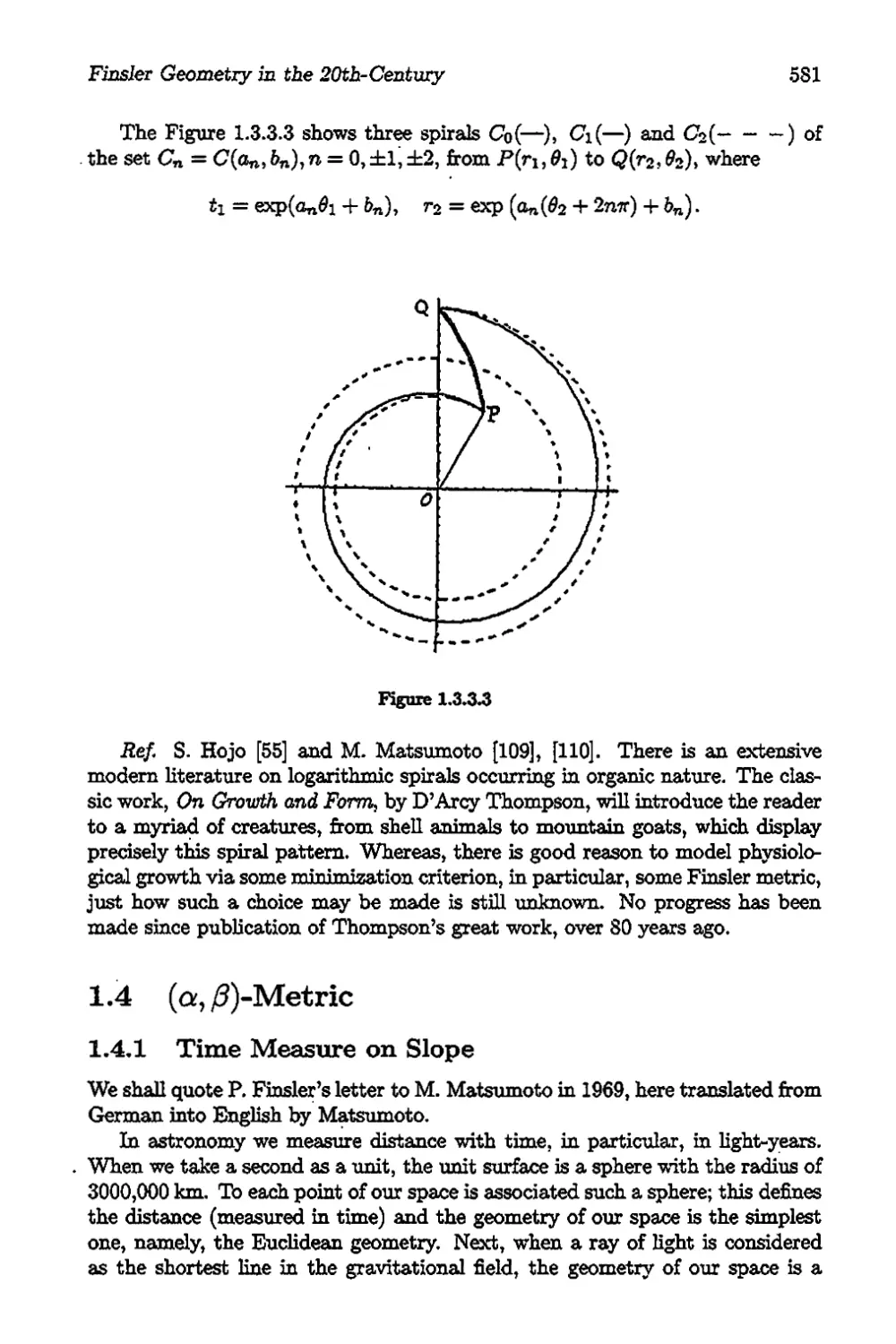
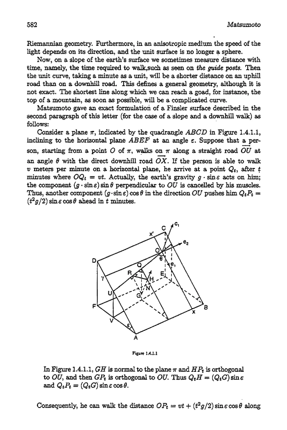
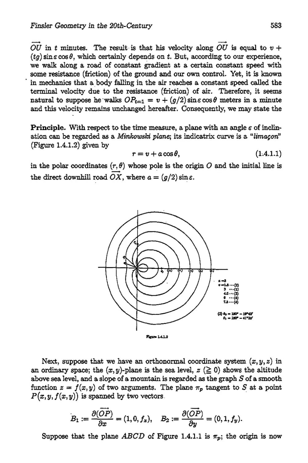


Author: Antonelli P.L.
Tags: mathematics geometry higher mathematics history of mathematics
ISBN: 1-4020-1555-0
Year: 2003


Text
Handbook of Finsler Geometry
Volume 1
Edited by
P. L. Antonelli
Department of Mathematical Sciences,
University of Alberta, Edmonton, Canada
KLUWER ACADEMIC PUBLISHERS
DORDRECHT / BOSTON I LONDON
A C.I.P. Catalogue record for this book is available from the Library of Congress.
ISBN 1-4020-1555-0 (Vol. 1)
ISBN 1-4020-1556-9 (VoL 2)
ISBN 1-4020-1557-7 (Set)
Published by Kluwer Academic Publishers,
P.O. Box 17.3300 AA Dordrecht. The Netherlands.
Sold and distributed in North, Central and South America
by Kluwer Academic Publishers.
101 Philip Drive, Norwcll. MA 02061. U.SA.
In all other countries, sold and distributed
by Kluwer Academic Publishers,
P.O. Box 322.3300 AH Dordrecht, The Netherlands.
Printed on acidfree paper
All Rights Reserved
© 2003 Kluwer Academic Publishers
No part of this work may be reproduced, stored in a retrieval system, or transmitted
in any form or by any means, electronic, mechanical, photocopying, microfilming, recording or
otherwise, without written permission from the Publisher, with the exception
of any material supplied specifically for the purpose of being entered
and executed on a computer system, for exclusive use by the purchaser of the work.
Printed in the Netherlands.
TABLE OF CONTENTS
Preface xv
Part 1 Complex Finsler Geometry 3
Tadaski Aikou
1 Kähler Fibrations 9
1.1 Fibrations 9
1.2 Local Treatments 10
1.3 Bott Connections 13
1.4 Kähler Fibration 18
2 Complex Finsler Bundles 23
2.1 Vector Bundles Over Complex Projective Space 23
2.2 Complex Finsler Metrics 27
2.3 Bott Connections of Finsler Vector Bundles 35
2.4 Negativity of Vector Bundles 39
2.5 Special Finsler Vector Bundles 48
3 Kobayashi Metrics . 59
3.1 Poincaré Metrics 59
3.2 Kobayashi Metric 62
3.3 Bounded Domains 65
3.4 Holomorphic Sectional Curvature and Schwarz Lemma . . 67
Part 2 KCC Theory of a System of Second Order Differential
Equations 83
P.L. Antonelli and L Bucataru
1 The Geometry of the Tangent Bundle 91
1.1 The Tangent Bundle 91
1.2 The Vertical Subbundle 93
1.3 The Almost Tangent Structure 94
1.4 Vertical and Complete Lifts 94
1.5 Homogeneity 95
2 Nonlinear Connections 97
2.1 Horizontal Distributions and Horizontal Lifts 97
2.2 Characterizations of a Nonlinear Connection 99
2.3 Curvature and Torsion for a Nonlinear Connection . . 102
2.4 Autoparallel Curves and Symmetries for a
Nonlinear Connection 103
2.5 Homogeneous Nonlinear Connection 107
v
vi
Anastasiei and Antonelli
3 Finsler Connections on the Tangent Bundle 109
3.1 The Berwald Connection Ill
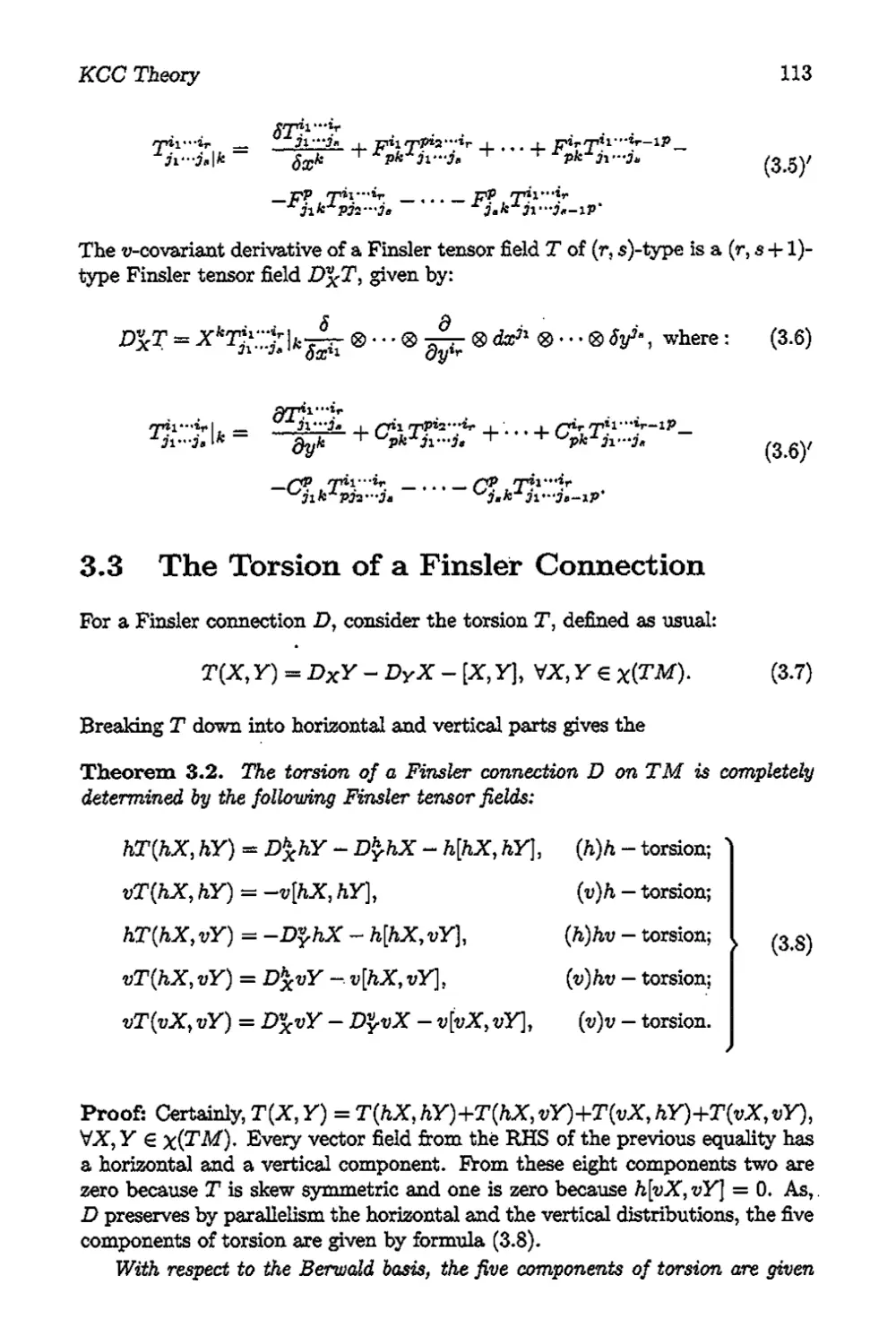
3.2 The h and i^Covariant Derivation of a Finsler
Connection 112
3.3 The Torsion of a Finsler Connection 113
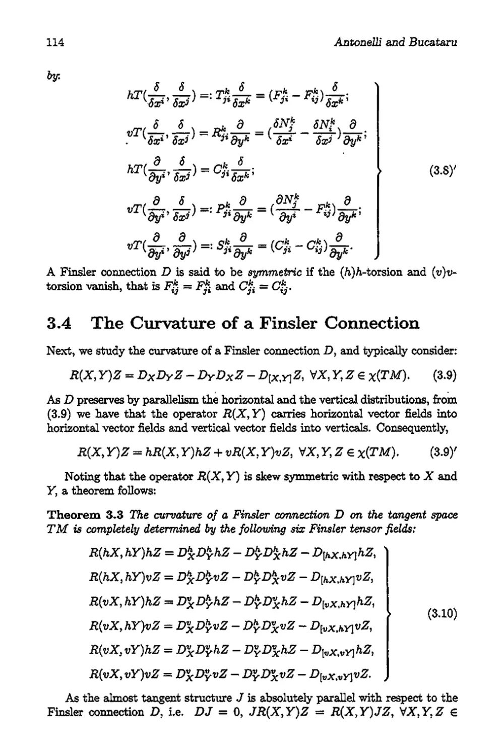
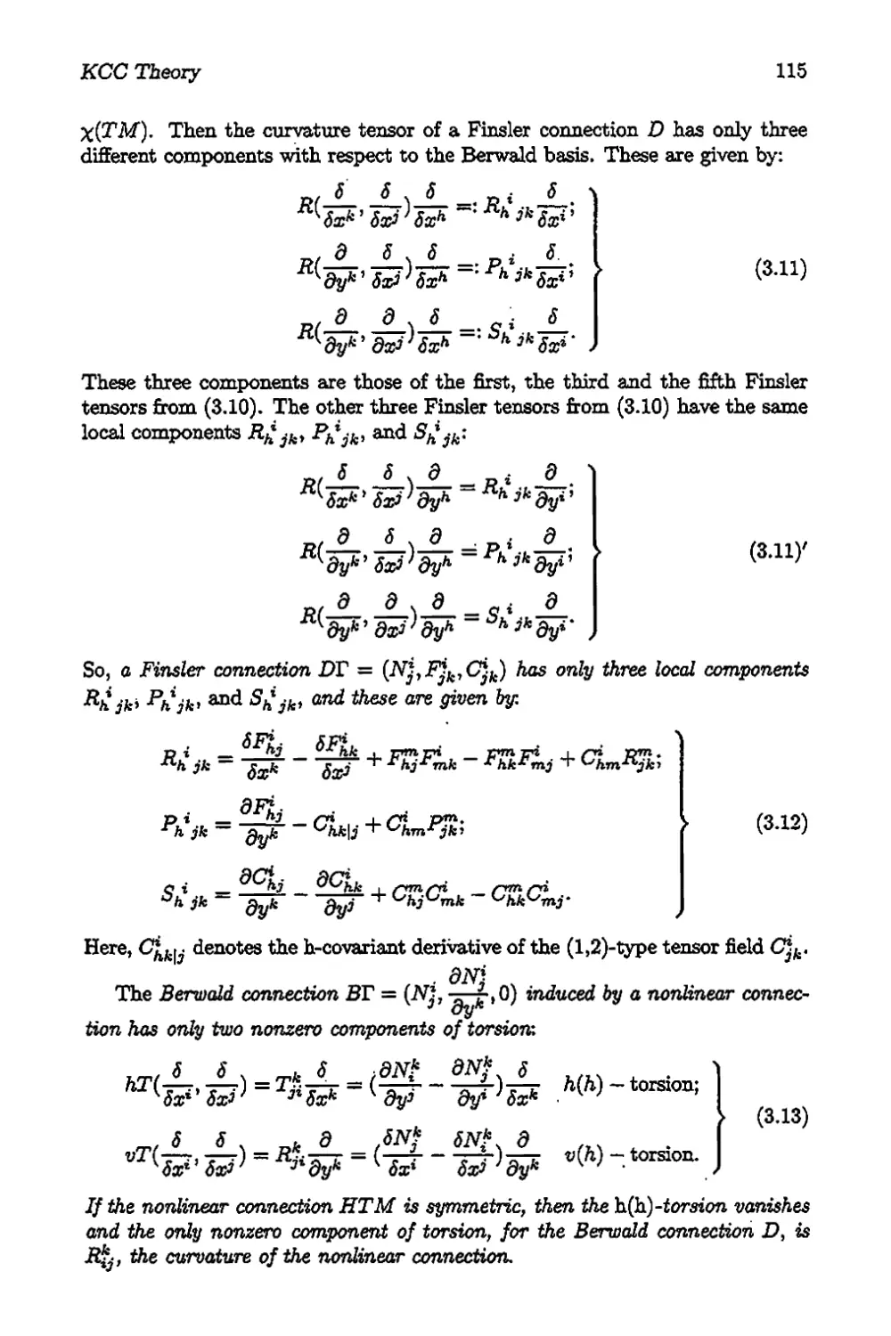
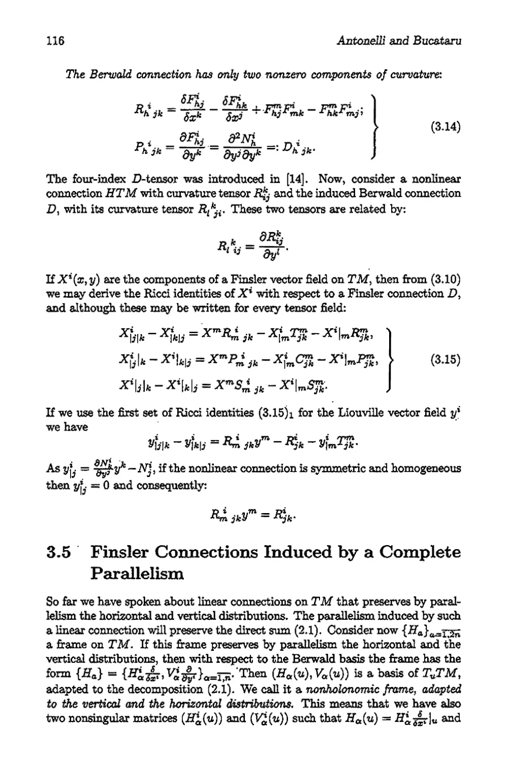
3.4 The Curvature of a Finsler Connection 114
3.5 Finsler Connections Induced by a Complete
Parallelism 116
3.6 The Cartan Structure Equations of a Finsler
Connection 118
3.7 Geodesics of a Finsler Connection 120
3.8 Homogeneous Berwald Connection 121
4 Second Order Differential Equations 123
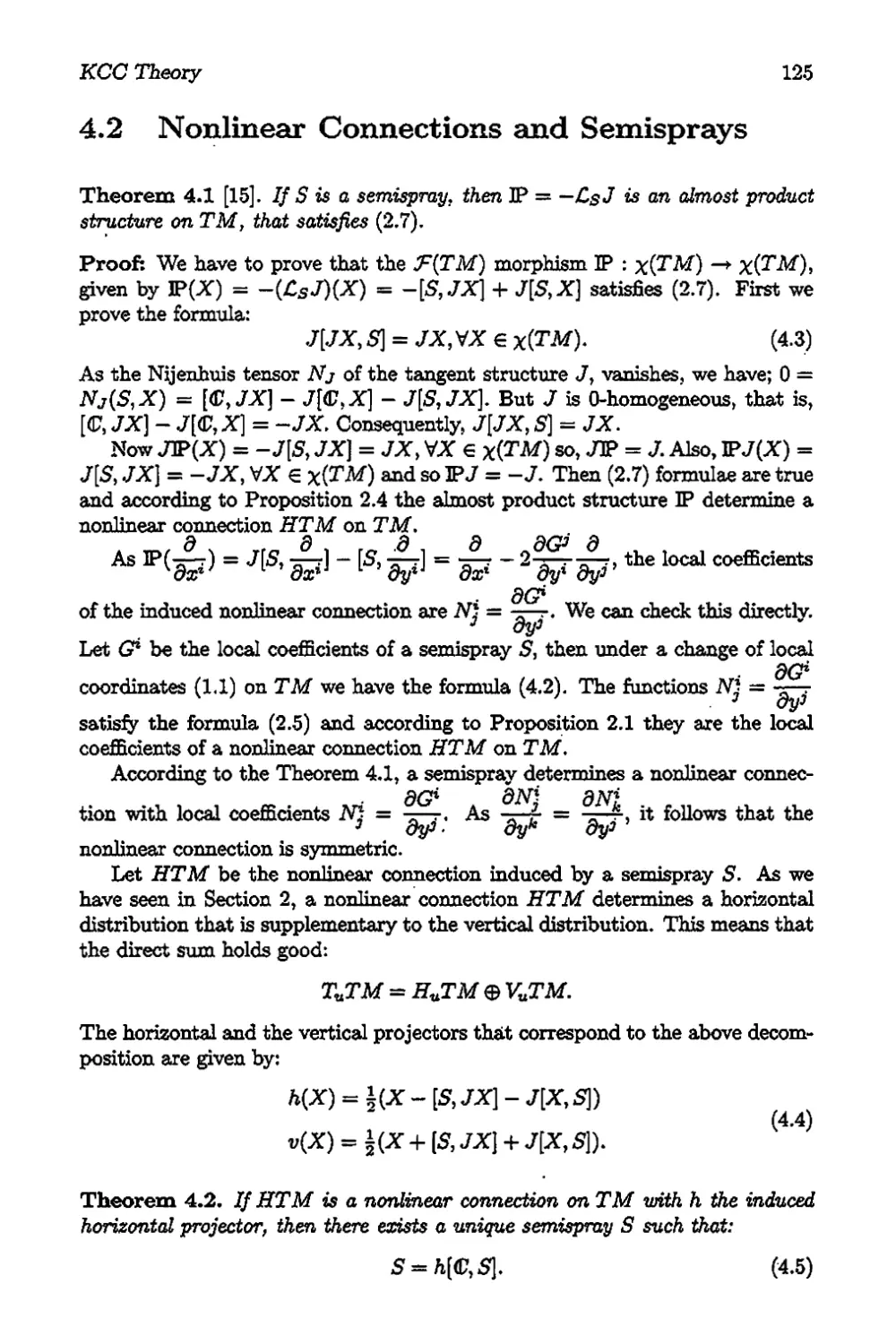
4.1 Semispray or Second Order Differential Vector Field . . 123
4.2 Nonlinear Connections and Semisprays 125
4.3 The Berwald Connection of a Semispray 127
4.4 The Jacobi Equations of a Semispray 129
4.5 Symmetries for a Semispray 131
4.6 Geometric Invariants in KCC-Theory 132
5 Homogeneous Systems of Second Order Differential
Equations 135
6 Time Dependent Systems of Second Order Differential
Equations 139
6.1 Sprays and Nonlinear Connections on Jets 139
6.2 Variational Equations 144
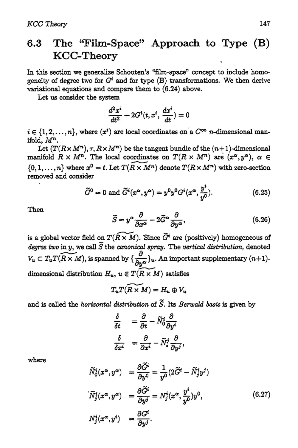
6.3 The “Film-Space” Approach to Type (B) KCC-Theory . 147
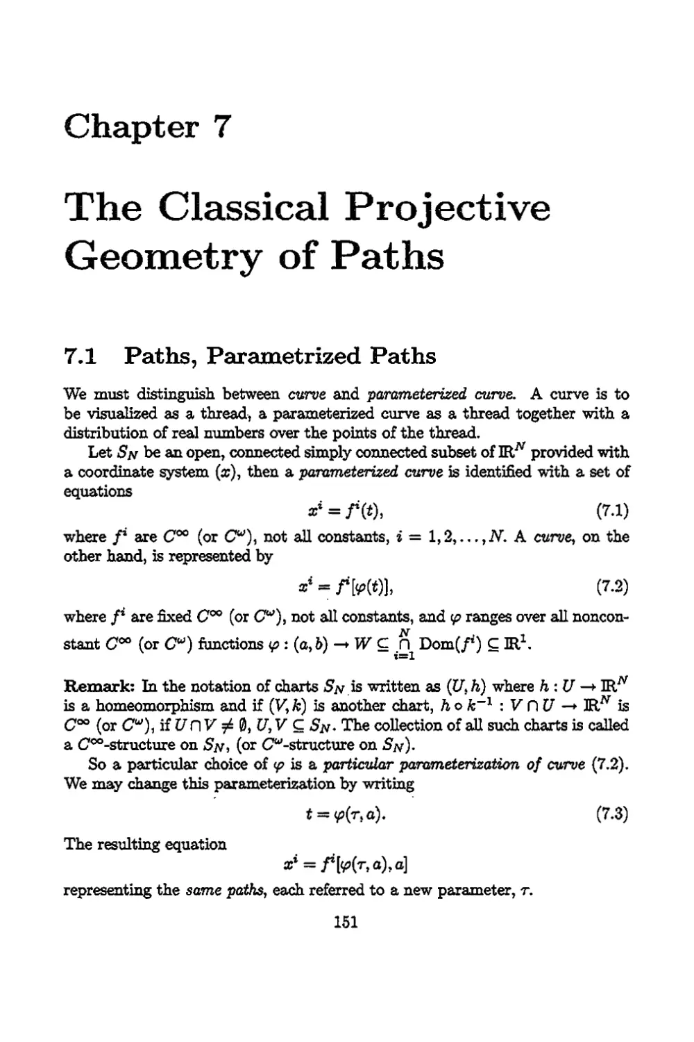
7 The Classical Projective Geometry of Paths 151
7.1 Paths, Parametrized Paths 151
7.2 The Various Geometries of Paths - Finite Equations . . 152
7.3 The Various Geometries of Paths - Differential Equations 153
7.4 Afhne Connections 155
7.5 The Fundamental Projective Invariants 158
7.6 The Projective Parameter and the
Normal Spray Connection 161
7.7 Projective Deviation 165
Part 3 Fundamentals of Finslerian Diffusion
with Applications 177
P.L, Antonelli and T.J. Zastawniak
1 Finsler Spaces 187
1.1 The Tangent and Cotangent Bundle 187
1.2 Fiber Bundles 189
1.3 Frame Bundles and Linear Connections . 191
1.4 Tensor Fields 192
1.5 Linear Connections 194
1.6 Torsion and Curvature of a Linear Connection .... 196
Table of Contents vii
1.7 Parallelism 197
1.8 The Levi-Cività Connection on a Riemannian Manifold 197
1.9 Geodesics, Stability and the Orthonormal Frame Bundle 199.
1.10 Finsler Space and Metric 200
1.11 Finsler Tensor Fields 202
1.12 Nonlinear Connections 202
1.13 Affine Connections on the Finsler Bundle 204
1.14 Finsler Connections 206
1.15 Torsions and Curvatures of a Finsler Connection . . . 208
1.16 Metrical Finsler Connections. The Cartan Connection . 210
2 Introduction to Stochastic Calculus on Manifolds 213
2.1 Preliminaries 213
2.2 Ito’s Stochastic Integral 216
2.3 Ito’s Processes. Ito Formula 219
2.4 Stratonovich Integrals 221
2.5 Stochastic Differential Equations on Manifolds .... 221
3 Stochastic Development on Finsler Spaces 227
3.1 Riemannian Stochastic Development 227
3.2 Rolling Finsler Manifolds Along Smooth Curves
and Diffusions 233
3.3 Finslerian Stochastic Development 242
3.4 Radial Behaviour 246
4 Volterra-Hamilton Systems of Finsler Type 249
4.1 Berwald Connections and Berwald Spaces 249
4.2 Volterra-Hamilton Systems and Ecology 253
4.3 Wagnerian Geometry and Volterra-Hamilton Systems . 254
4.4 Random Perturbations of Finslerian
Volterra-Hamilton Systems 260
4.5 Random Perturbations of Riemannian
Volterra-Hamilton Systems 262
4.6 Noise in Conformally Minkowski Systems 266
4.7 Canalization of Growth and Development with Noise , 267
4.8 Noisy Systems in Chemical Ecology and Epidemiology 271
4.9 Riemannian Nonlinear Filtering ...... 279
4.10 Conformal Signals and Geometry of Filters 285
4.11 Riemannian Filtering of Starfish Predation 289
5 Finslerian Diffusion and Curvature 295
5.1 Cartan’s Lemma in Berwald Spaces 296
5.2 Quadratic Dispersion 298
5.3 Finslerian Development and Curvature 299
5.4 Finslerian Filtering and Quadratic Dispersion 300
5.5 Entropy Production and Quadratic Dispersion .... 302
6 Diffusion on the Tangent and Indicatrix Bundles 319
6.1 Slit Tangent Bundle as Ri eman ni an Manifold 320
6.2 hv-Development as Riemannian Development with Drift 321
6.3 Indicatrized Finslerian Stochastic Development .... 323
vîii
Anastasiei and Antonelli
6.4 Indicatrized /^-Development Viewed as Riemannian . » 327
Appendix A Diffusion and Laplacian on the Base Space . . . . 335
A.1 Finslerian Isotropic Transport Process 336
A.2 Central Limit Theorem 338
A. 3 Laplacian, Harmonic Forms and Hodge Decomposition 340
Appendix B Two-Dimensional Constant Berwald Spaces .... 343
B. l Berwald’s Famous Theorem 343
B.2 Standard Coordinate Representation 344
B.3 B2(l) with Constant G^k 345
B.4 Class B2(2) with Constant 347
B.5 B2(r,s) with Constant Gjk 348
Part 4 Symplectic Transformation of the Geometry of
¿-Duality 359
D. Hrimiuc and ÏÏ. Shimada
1 The Geometry of TM and T*M 363
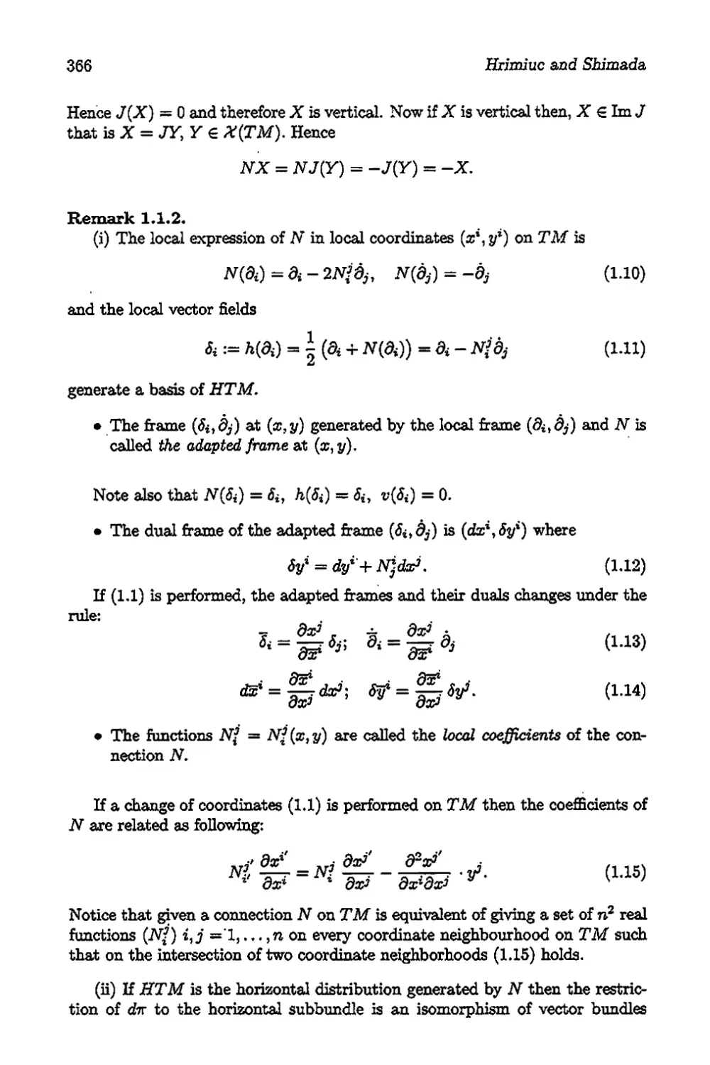
1.1 Connections on TM 363
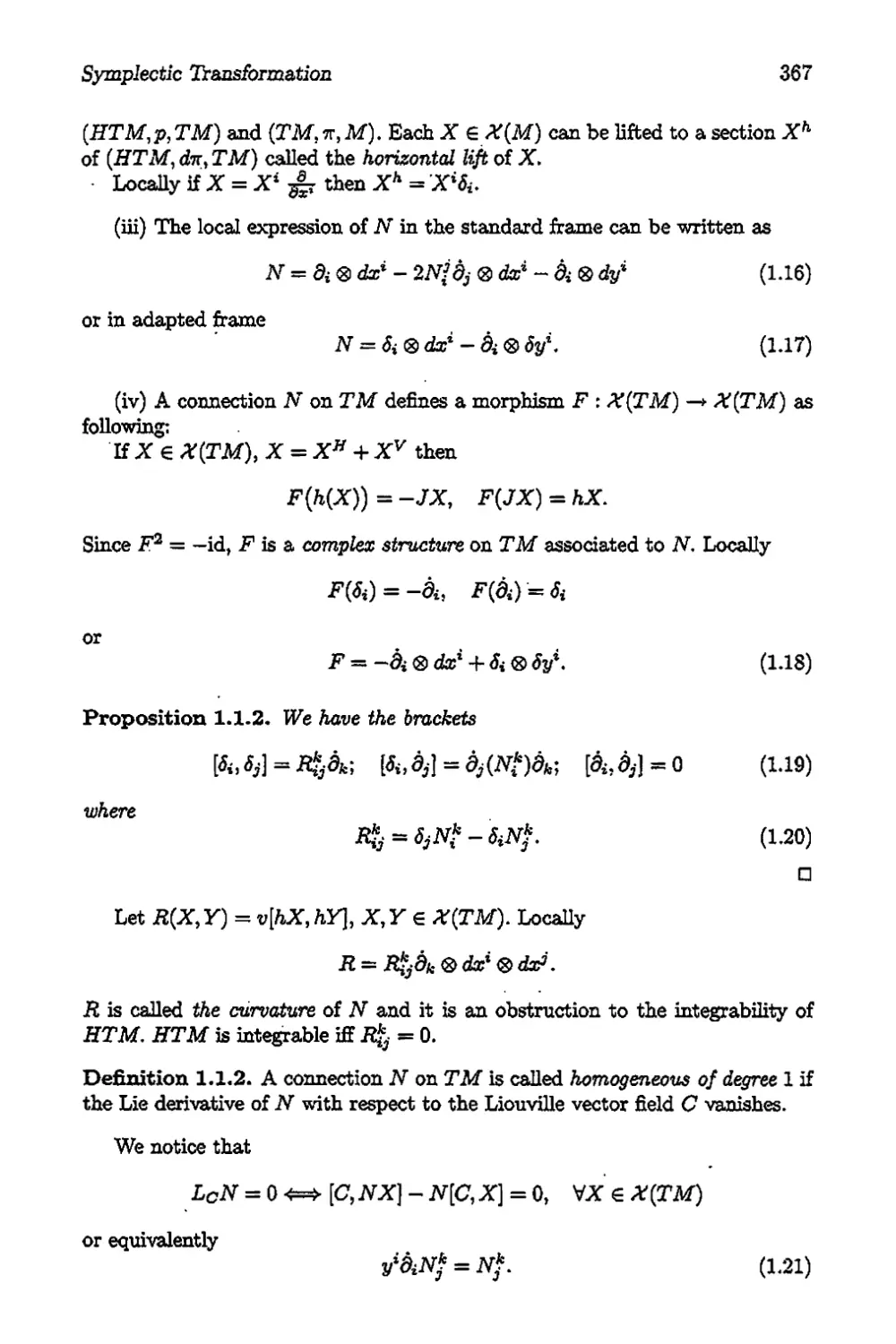
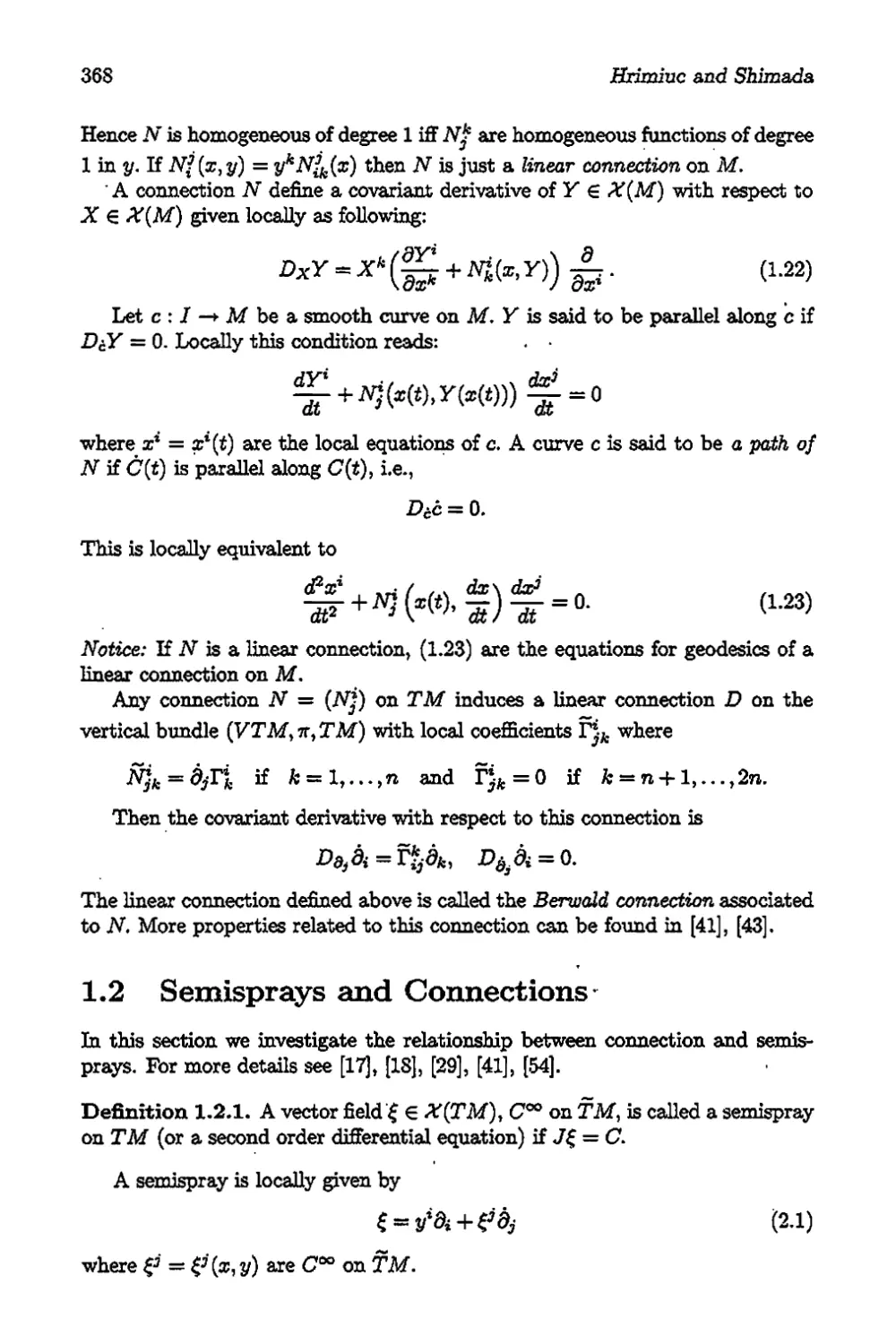
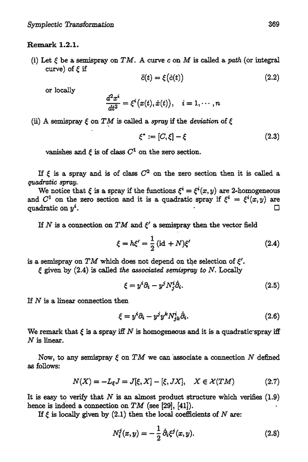
1.2 Semisprays and Connections 368
1.3 Linear Connections on TM 370
1.4 The Geometry of Cotangent Bundle 373
1.5 Linear Connections on T*M 376
1.6 Lagrange Manifolds 378
1.7 Hamilton Manifolds 381
2 Symplectic Transformations of the Differential Geometry
ofT*M 3S5
2.1 Connection-Pairs on Cotangent Bundle 385
2.2 Special Linear Connections on T*M 390
2.3 The Homogeneous Case 395
2.4 /-Related Connection-Pairs 398
2.5 /-Related ^-Connections 403
2.6 The Geometry of a Homogeneous
Contact Transformation 405
2.7 Examples 409
3 The Duality Between Lagrange and Hamilton Spaces .... 413
3.1 The Lagrange-Hamilton ¿-Duality 413
3.2 ¿-Dual Nonlinear Connections 417
3.3 ¿-Dual ¿-Connections 421
3.4 The Finsler-Cartan ¿-Duality 426
3.5 Berwald Connection for Cartan Spaces. Landsberg
and Berwald Spaces. Locally Minkowski Spaces . . . 431
3.6 Applications of the ¿-Duality 435
Table of Contents ix
Part 5 Holonomy Structures in Finsler Geometry 445
L. Kozma
1 Holonomy of Positively Homogeneous Connections . . . . . 453
1.1 Connections .of a Tangent Bundle . 453
1.2 Holonomy Group of a Positively Homogeneous Connection 454
1.3 Curvature and Holonomy Algebra of a Positively
Homogeneous Connection 455
1.4 Homogeneous Holonomy of Finsler Manifolds .... 458
1.5 Metrizability of Positively Homogeneous Connections . 458
2 Holonomies of Finsler V- Connections 463
2.1 A Topological Group and Its Lie Algebra 463
2.2 V-Connections 464
2.3 The V-Holonomy Group and V-Holonomy Algebra . . 465
3 Holonomies of the Finsler Vector Bundle 469
3.1 Linear Connections of the Finsler Vector Bundle . . . 469
3.2 Osculation of Finsler Pair Connections 470
3.3 ht^Holonomy Groups of the Finsler Vector Bundle . . 472
3.4 The Mixed Holonomy Groups 473
4 Holonomies of Special Finsler Manifolds 477
4.1 Berwald Manifolds 477
4.2 Landsberg Manifolds 481
Part 6 On the Gauss-Bormet-Chern Theorem in
Finsler Geometry 491
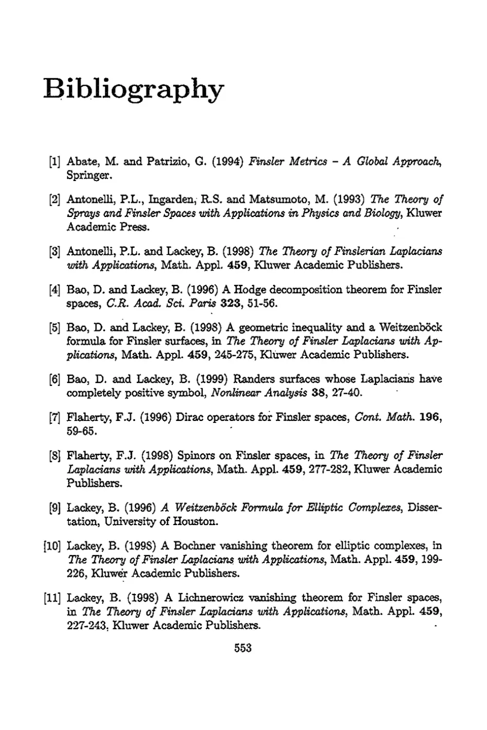
Brad Lackey
1 Topological Preliminary 497
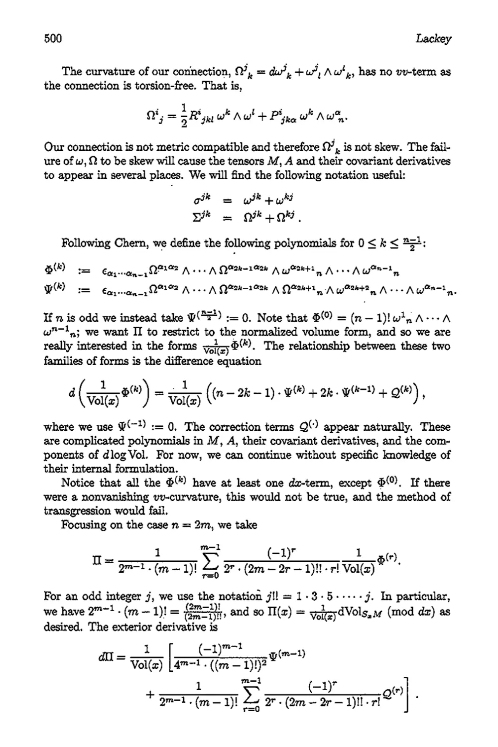
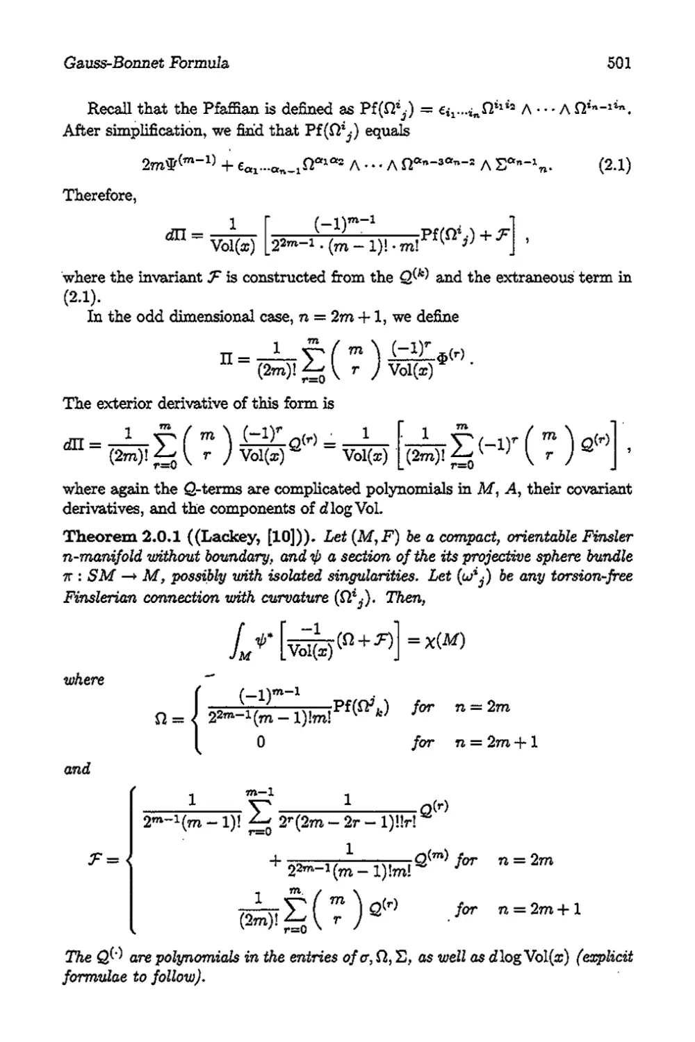
2 The Method of Transgression 499
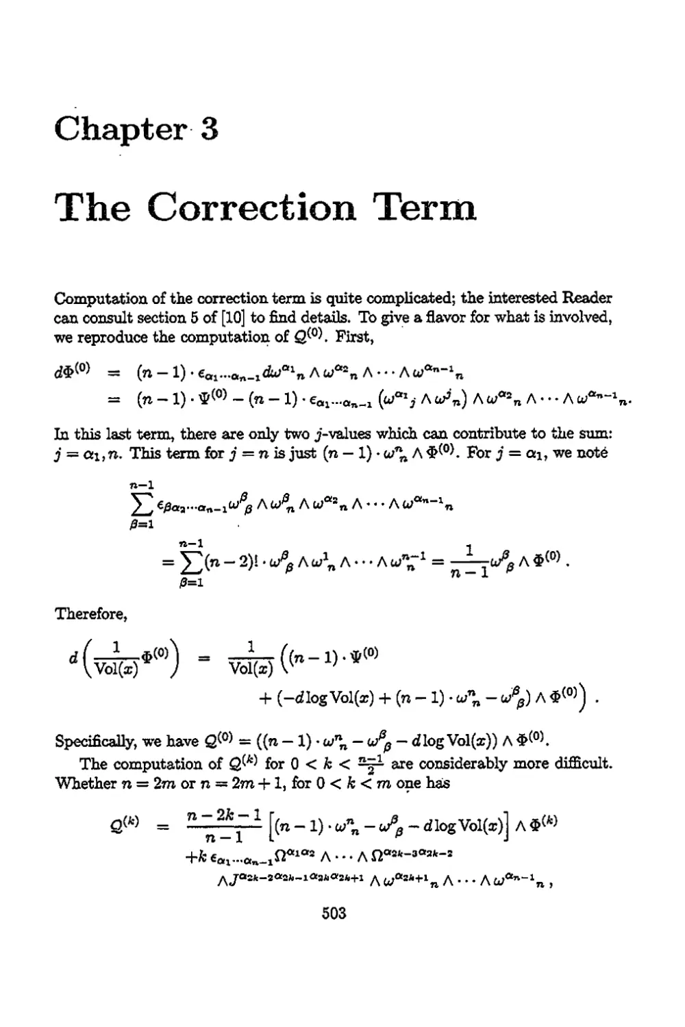
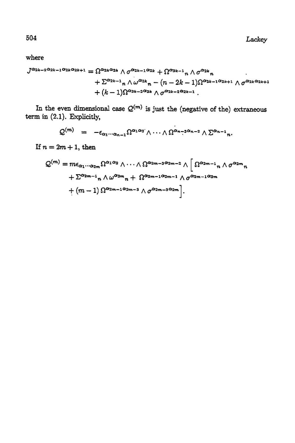
3 The Correction Term 503
4 Special Cases 505
4.1 Riemannian Geometry 505
4.2 The Chern Connection 505
4.3 A Special Family of Finsler Connections 506
Part 7 The Hodge Theory of Finsler-type Geometries 513
Brad Lackey
1 Elliptic Complexes 521
1.1 The Hodge-deRham Complex 521
1.2 Elliptic Complexes ■ 523
1.3 Elliptic Operators . 527
1.4 The Hodge Decomposition Theorem 531
2 The Weitzenbock Formula 533
2.1 Complete Positivity 534
2.2. Covariant Formalism 536
2.3 Existence and Uniqueness of a Connection 539
2.4 A Bochner Vanishing Theorem 541
X
Anastasiei and Antonelli
3 Complete Positivity of the Symbol 543
3.1 The Geometric Ratio 543
3.2 Computing the Geometric Ratio 545
3-3 An Example 547
Part 8 Finsler Geometry in the 20th-Century 557
M. Matsumoto
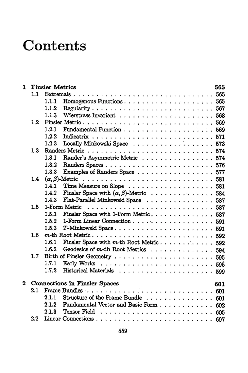
1 Finsler Metrics 565
1.1 Extremals 565
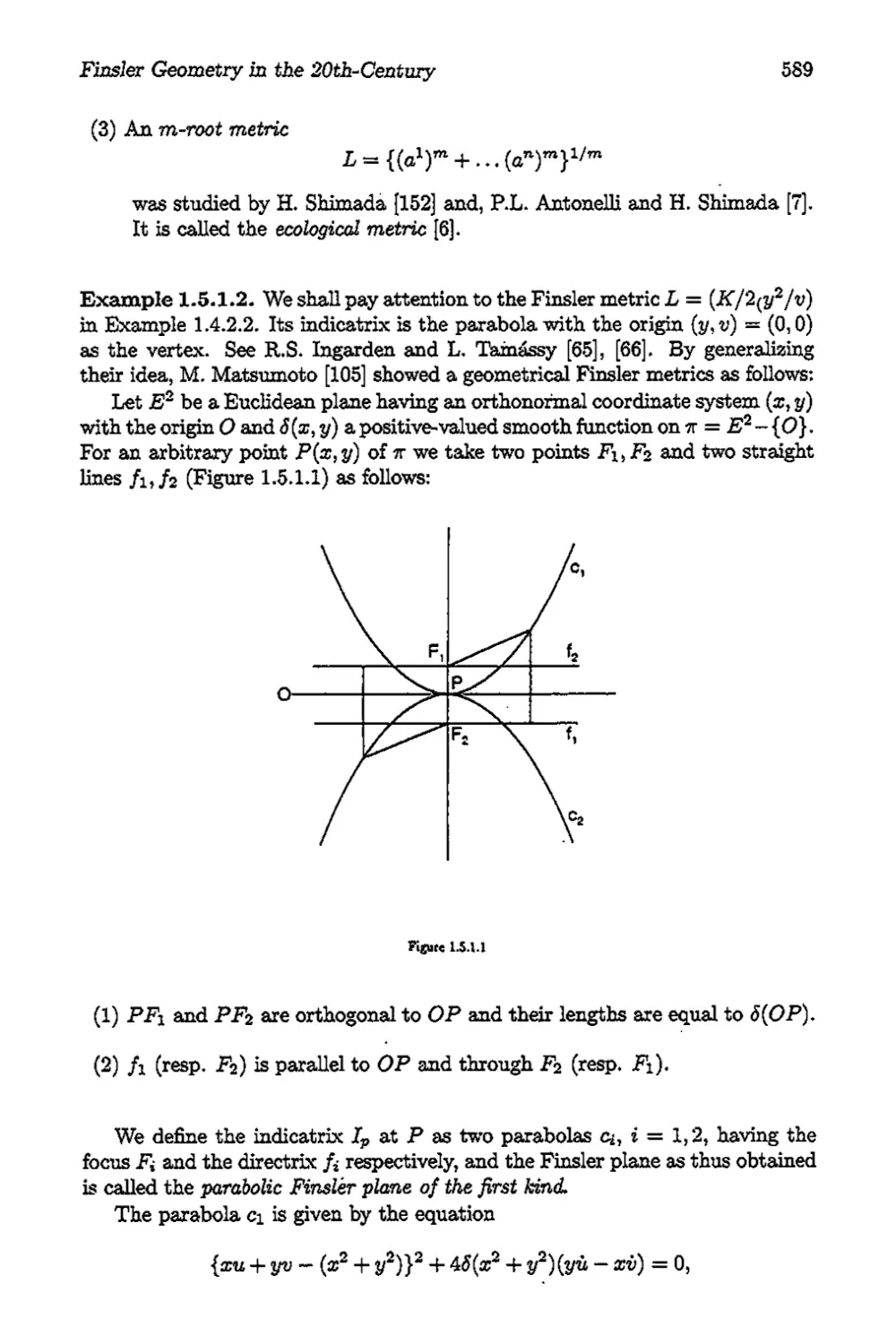
1.2 Finsler Metric ; 569
1.3 Randers Metric 574
1.4 (a,/3)-Metric 581
1.5 1-Form Metric 587
1.6 m-th Root Metric 592
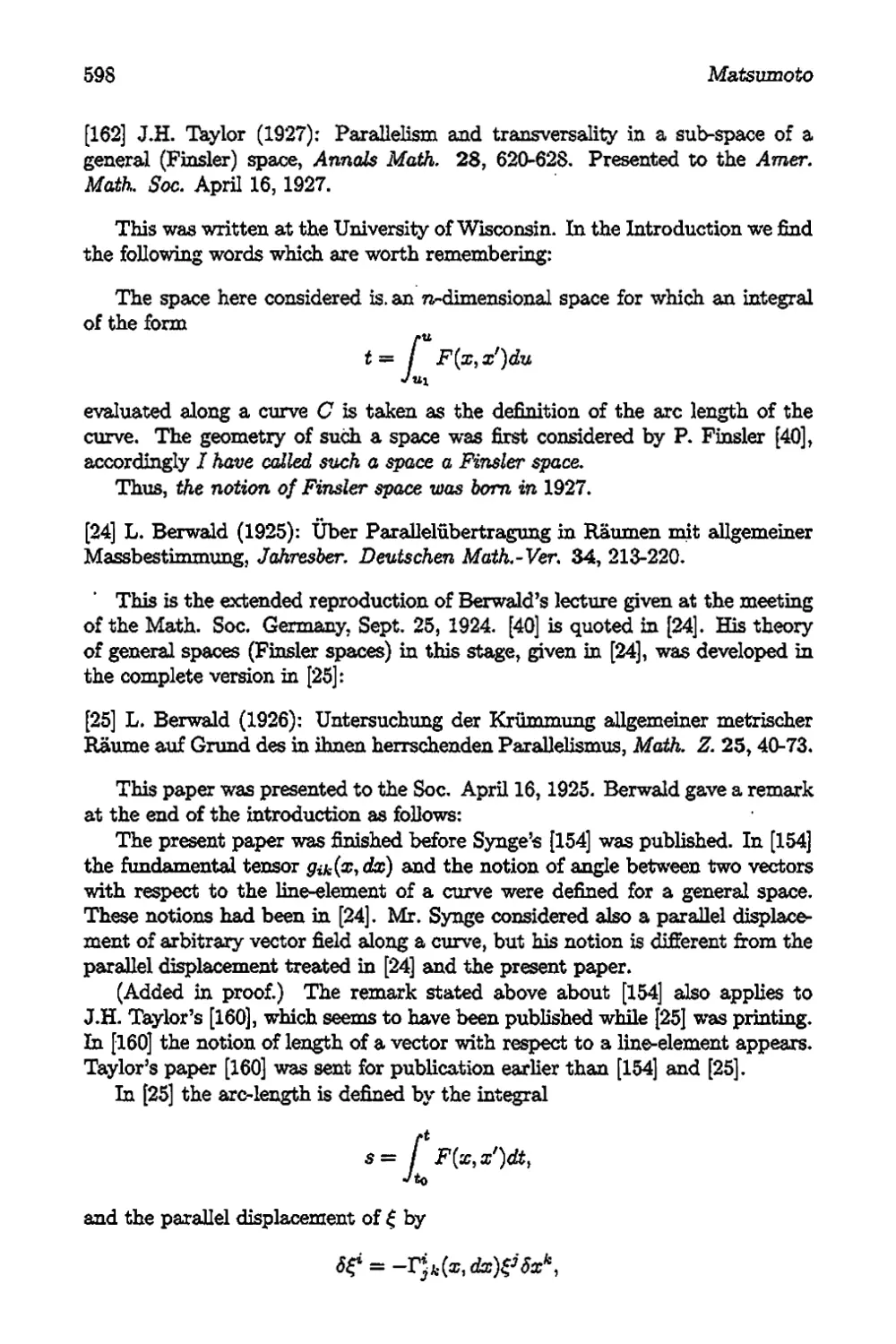
1.7 Birth of Finsler Geometry 595
2 Connections in Finsler Spaces 601
2.1 Frame Bundles 601
2.2 Linear Connections 607
2.3 Vectorial Frame Bundles 61S
2.4 The Theory of Pair Connections 628
2.5 Standard Finsler Connections 644
2.6 Special Finsler Connections 661
3 Important Finsler Spaces 677
3.1 Finsler Space of Dimension Two 677
3.2 Riemannian Space and Locally Minkowski Space . . . 709
3.3 Stretch Curvature and Landsberg Space 717
3.4 Berwald Space 723
3.5 Wagner Space 735
3.6 Scalar Curvature and Constant Curvature 741
3.7 Finsler Space of Dimension Three 753
3.8 Indicatrix and Homogeneous Extension 775
4 Conformal and Projective Change 783
4.1 Conformal Change 783
4.2 Conformally Flat Finsler Space 790
4.3 Conformal Change and Wagner Space 796
4.4 Projective Change 799
4.5 Douglas Space 814
4.6 Finsler Space with Rectilinear Extremals 827
5 Finsler Spaces with 1-Form Metric and with m-th Root Metric 839
5.1 Finsler Spaces with 1-Form Metric 839
5.2 Curvature of Two-Dimensional 1-Form Metric .... 847
5.3 Conformal Change of 1-Form Metric 854
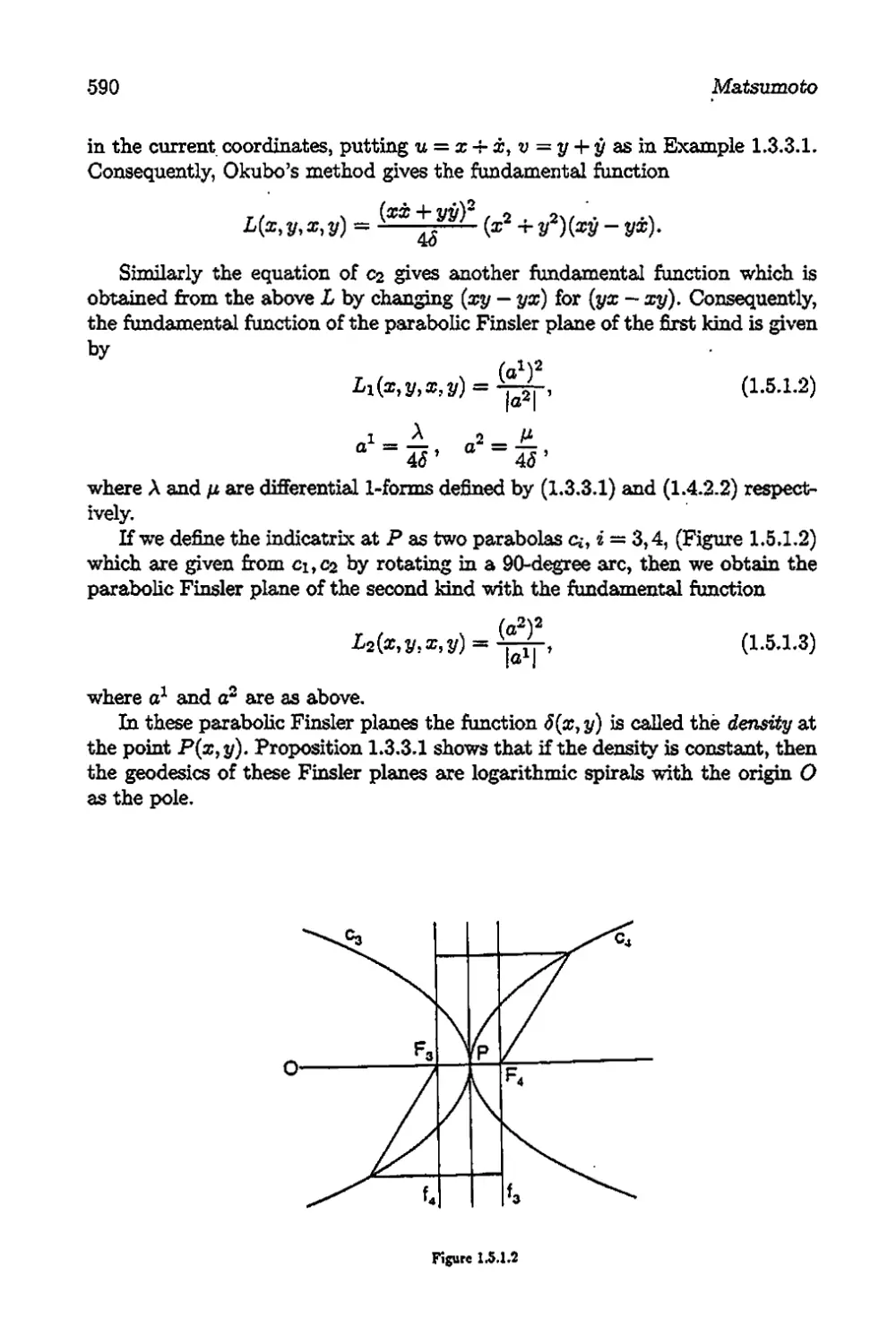
5.4 Finsler Space with m-th Root Metric 858
5.5 Stronger Non-Riemannian Finsler Space 867
5.6 Two-Dimensional m-th Root Metrics 874
5.7 Berwald Spaces of Cubic and Quartic Metrics .... 879
Table of Contents xi
6 Finsler Spaces with (a, ^-Metrics SS9
6.1 Fundamental Tensor of Space with (a, /3)-Metric . . . 889
6.2 C-Tensors of (a,/3)-Metrics 894
6.3 Connections for (a, /3)-Metrics 901
6.4 Douglas Space with (a, £)-Metric 913
6.5 Two-Dimensional Space with (a/?)-Metric 916
6.6 Strongly Non-Riemaanian (o/3)-Metric 924
6.7 Conformal Change of (a, ^-Metric 928
6.8 Projective Change of (a/3)-Metric 936
6.9 Randers Spaces of Constant Curvature 946
Part 9 The Geometry of Lagrange Spaces 969
Radu Miron, Mihai Anastasiei and Ioan Bucataru
0 Introduction 973
1 The Geometry of the Tangent Bundle 977
1.1 The Manifold TM 977
1.2 Semisprays on the Manifold TM 984
1.3 Nonlinear Connections 987
1.4 TV-Linear Connections 995
1.5 Semisprays, Nonlinear Connections and TV-Linear
Connections 1002
1.6 Parallelism. Structure Equations 1007
2 Lagrange Spaces 1013
2.1 The Notion of Lagrange Space 1013
2.2 Geometric Objects Induced on TM by a Lagrange Space 1017
2.3 Variational Problem and Euler-Lagrange Equations . . 1019
2.4 A Noether Theorem 1021
2.5 Canonical Semispray. Nonlinear Connection 1023
2.6 Geodesics in a Finsler Space 1025
2.7 Hamilton-Jacobi Equations 1028
2.8 The Almost Kâhlerian Model of a Lagrange Space Ln . 1030
2.9 Metrical TV-Linear Connections 1033
2.10 Almost Finslerian Lagrange Spaces 1038
2.11 Geometry of ç>Lagrangians 1042
2.12 Gravitational and Electromagnetic Fields 1045
2.13 Einstein Equations of Lagrange Spaces 1047
3 Subspaces in Lagrange Spaces 1053
3.1 Subspaces L in a Lagrange Space Ln 1053
3.2 Induced Nonlinear Connection 1056
3.3 The Gauss-Weingarten Formulae 1060
3.4 The Gauss-Codazzi Equations 1061
3.5 Totally Geodesic Subspaces 1062
3.6 Lagrange Subspace of Codimension One 1064
3.7 Subspaces in Finsler Spaces 1067
XU
Anastasiei and Antonelli
4 Generalized Lagrange Spaces 1073
4.1 The Notion of Generalized Lagrange Space 1074
4.2 Metrical ^-Connection in a GL-Space 1077
4.3 GL-Metrics Determining Nonlinear Connections . . . 10S0
4.4 GL-Metrics Provided by Deformations of
Finsler Metrics 10S5
4.5 Almost Hermitian Model of a Generalized
Lagrange Space 1091
5 Rheonomic Lagrange Geometry 1097
5.1 Semisprays on the Manifold TM x R 1097
5.2 Nonlinear Connections on E = TM x R 1099
5.3 Variational Problem 1101
5.4 Rheonomic Lagrange Spaces 1103
5.5 Canonical Nonlinear Connection 1104
5.6 An Almost Contact Structure on E 1105
5.7 TV-Linear Connection 1107
5.8 Parallelism. Structure Equations for
TV-Linear Connections 1108
5.9 Metrical TV-Linear Connection of a Rheonomic
Lagrange Space 1111
5.10 Rheonomic Finsler Spaces 1112
5.11 Examples of Time Dependent Lagrangians 1114
Part 10 Symbolic Finsler Geometry 1125
S.F. Rutz and R. Portugal
1 Computer Algebra for Finsler Geometry 1129
1.1 Introduction 1129
1.2 Computer Algebra 1130
1.3 Manipulation of Indices via Group Theory 1144
1.4 FINSLER Package 1150
Part 11 A Setting for Spray and Finsler Geometry 1183
J6zsef Szilasi
0 Introduction 1187
1 The Background: Vector Bundles and
Differential Operators 1191
A Manifolds . 1191
B Vector Bundles 1195
C Sections of Vector Bundles 1204
D Tangent Bundle and Tensor Fields 1208
E Differential Forms • 1218
F Covariant Derivatives 1226
2 Calculus of Vector-Valued Forms and Forms Along the
Tangent Bundle Projection 1237
A Vertical Bundle to a Vector Bundle 1237
B Nonlinear Connections in a Vector Bundle 1245
Table^of Contents xiii
C Tensors Along the Tangent Bundle Projection. Lifts . . 1258
D The Theory of A. Frolicher and A. Nijenhuis ...... 1272
E The Theory of E. Martínez, J. F. Cariñena and W. Sarlet 1298
F Covariant Derivative Operators Along the Tangent
Bundle Projection 1314
3 Applications to Second-Order Vector Fields and
Finsler Metrics 1347
A Horizontal Maps Generated by Second-Order Vector Fields 1347
B Linearization of Second-Order Vector Fields 1362
C Second-Order Vector Fields Generated by Finsler Metrics 1369
D Covariant Derivative Operators on a Finsler Manifold . . 1383
Appendix 1399
A.l Basic Conventions 1399
A.2 Topology 1400
A.3 The Euclidean n-Space R” 1401
A.4 Smoothness 1402
A.5 Modules and Exact Sequences 1403
A.6 Algebras and Derivations 1408
A.7 Graded Algebras and Derivations 1409
A.8 Tensor Álgebras Over a Module 1411
A.9 The Exterior Algebra 1415
A.10 Categories and Functors . 1419
PREFACE
It was over three years ago, at the annual meeting of the American Math¬
ematical Society in San Diego, California, that Dr. Paul Roos of Kluwer asked
me to poll Finsler geometers around the world as to their interest in writing
a HANDBOOK OF FINSLER GEOMETRY. The result of that query was a
resounding affirmation, and here at long last, is the final result.
You have in your hands,the most complete and authoritative exposition
of state-of-the-art Finsler geometry that is possible, today. Each of the eleven
parts is completely independent of the rest, and each has been written with
mathematics and science students in mind. These articles are accessible!
P.L. Antonelli
Edmonton, Alberta, Canada
June, 2003
xv
ACKNOWLEDGEMENTS
The editors would like to express their sincere thanks to Vivian Spak, who
typeset this book, and to Scott Berard, who kept our computers running.
xvii
PART 1
Complex Finsler Geometry
Tadashi Aikou
Contents
1 Kâhler Fibrations 9
1.1 Fibrations 9
1.2 Local Treatments 10
1.3 Bott Connections 13
1.3.1 Structure Tensors 14
1.3.2 Bott Connections 16
1.4 Kâhler Fibration 18
2 Complex Finsler Bundles 23
2.1 Vector Bundles Over Complex Projective
Space 23
2.2 Complex Finsler Metrics 27
2.2.1 Complete Circular Domains and Minkowski Functionals . 27
2.2.2 Complex Finsler Metrics on Cr and Kahler Metrics on Pr_1 30
2.2.3 Complex Finsler Metric on Vector Bundles 31
2.3 Bott Connections of Finsler Vector Bundles 35
2.4 Negativity of Vector Bundles 39
2.4.1 Positive Line Bundles and Ample Line Bundles 40
2.4.2 Negative Vector Bundles . . 43
2.4.3 Vanishing Theorems 45
2.5 Special Finsler Vector Bundles 48
2.5.1 Finsler Vector Bundles Modeled on a Complex
Minkowski Space 49
2.5.2 Flat Finsler Vector Bundles 50
2.5.3 Protectively Flat Finsler Vector Bundles 52
3 Kobayashi Metrics 59
3.1 Poincaré Metrics 59
3.2 Kobayashi Metric 62
3.3 Bounded Domains 65
3.4 Holomorphic Sectional Curvature and
Schwarz Lemma 67
3.4.1 Generalized Schwarz Lemma 68
3.4.2 Holomorphic Sectional Curvature by Curvature Tensor . . 71
5
Preface
In this short note, we shall discuss the geometry of Finsler vector bundle.
The geometry of Finsler bundles are treated as the geometry of fibred mani¬
folds. In fact, in the geometry of Finsler manifolds, each tangent space TXM
at x e M is considered as a Riemannian space TXM with a Riemannian metric
Sijfay), where x is fixed. This Riemannian metric is given by the Hessian
gij — ¿PF/dtfdyi of the fundamental function F — L2/2 of the Finsler met¬
ric. Since each tangent space TXM S has a natural flat structure, we can
consider (szfixed) as a so-called Hessian manifold. The tan¬
gent bundle 7T : TM —► M may be considered as a fibred manifold with each
fibre is a Hessian manifold such that Hessian structure depends smoothly on
the base point x € M» In this interpretation, a Landsberg space may be con¬
sidered as the fibred manifold 7m with isometric fibre, i.e., any local horizontal
mapping, which covers an arbitrary curve in the base space Af, is an isometry.
A Landsberg space is said to be a Berwald space if the local horizontal mapping
is defined by a linear connection on 7m- A Berwald space is said to be locally
Minkowski if the linear connection is flat, and thus a Finsler manifold is locally
Minkowski if and only if the fibred manifold 7m is locally trivial, i.e., it is locally
a Riemannian product of the base space M and a fibre.
In complex case, each tangent space TXM = C71 is considered as a Kahler
manifold with a Kahler metric for the fundamental func¬
tion F of the convex Finsler metric on a complex manifold. Since any Kähler
manifold is also a Hessian manifold, we also understand the geometry of com¬
plex Finsler manifold as a geometry of complex fibred manifold with each fibre
is Kahler manifold such that Kahler structure depends smoothly on the base
pint z € M, It is natural to generalize some special class of real Finsler metrics
to complex case. The purpose of the present note is to discuss some special
complex Finsler metrics.
Chapter 1
Kähler Fibrations
In this chapter, for applications to Finsler geometry, we shall investigate the
differential geometry of fibred complex manifold {Af, M, 7r} such that each fibre
is a Kahler manifold. We call such a fibred complex manifold a Kahler fibra¬
tion. Especially, we are concerned with Bott connections on the relative tangent
bundle TX/m>
1.1 Fibrations
Let X and M be connected complex manifolds with dime Af = n+r > dime M —
n. We assume that there exists a surjective holomorphic map % : Af —► M of
maximal rank.
Definition 1,1. We call % : Af —► M a fibration simply if the following condi¬
tions are satisfied.
(1) 7T : X —> M is a differentiable fibre bundle,
(2) every fibre 7r_;L(z) Xz (z € Af) is a connected complex submanifold of
X of dime X£ = r.
The complex manifold X is called the total space, M the base space and 7r the
projection.
We denote by Tx and Tm the holomorphic tangent bundles of X and M
respectively. Since the differential dir : Tx —* is surjective, we have the
fundamental sequence which is an exact sequence of vector bundles over X:
O^Vx-^Tx^ir*TM-*O, (1.1)
where Vx = ker{d7r : Tx —> is vertical subbundle of Tx- The exact
sequence
O - ® Vx -Û ®Tx-^ ® t-Tm -» O
9
10
Aikou
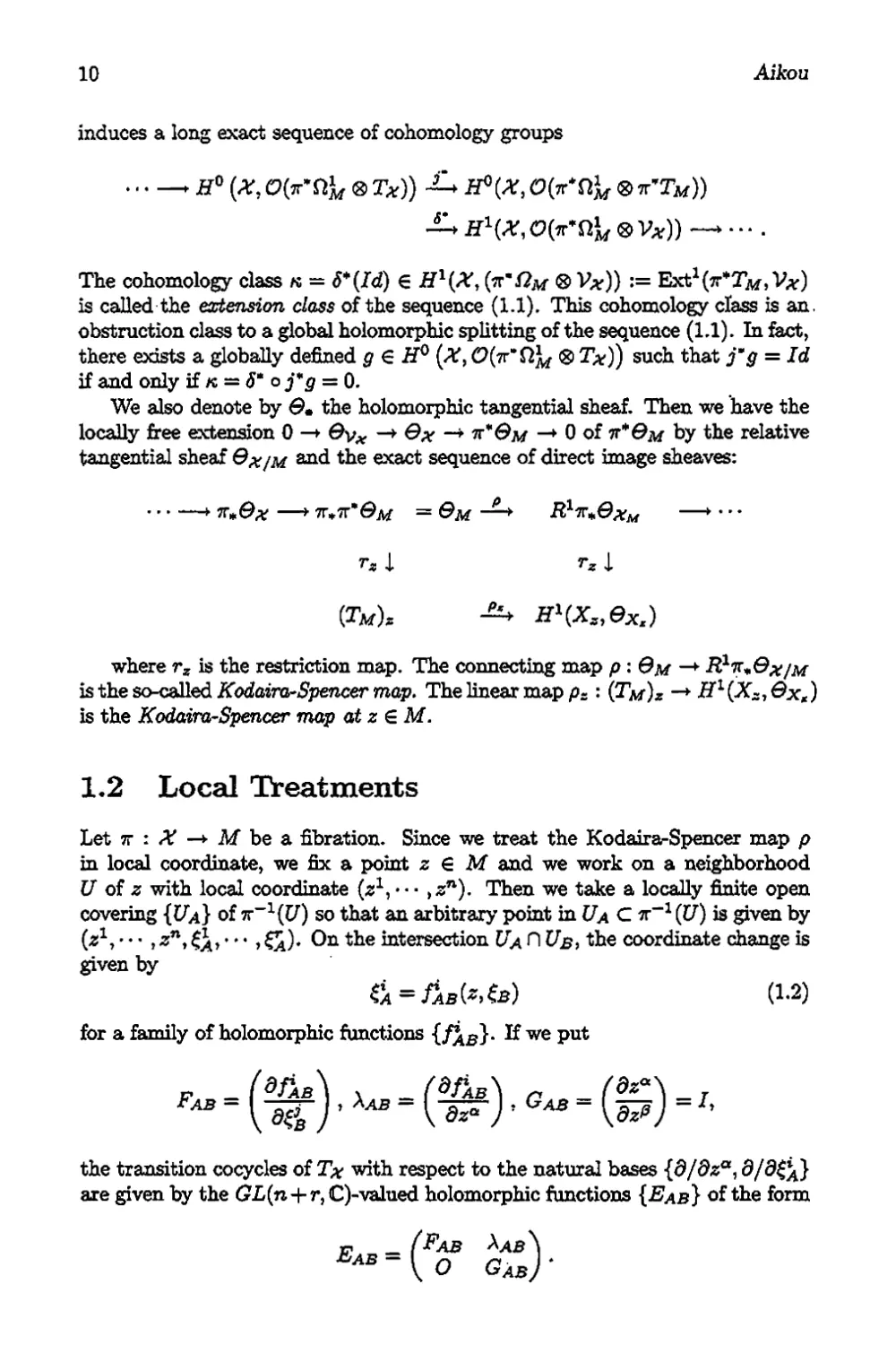
induces a long exact sequence of cohomology groups
>H°(X, ® Tat)) H°(X, ® %’T«))
H\X, 0(^(4 ® Vat)) —> • • • ■
The cohomology class k — 6*(Id) € (vr'iTw ® V*)) “ Ext1(«-*TM> Vx)
is called the extension class of the sequence (1-1). This cohomology class is an.
obstruction class to a global holomorphic splitting of the sequence (1.1). In fact,
there exists a globally defined g e HQ (Af, <9(7r*Q^ ® Tx)) such that j"g = Id
if and only if k = 5* o j*g = 0.
We also denote by 0» the holomorphic tangential sheaf. Then we have the
locally free extension 0 —► Gyx —> Ox -* —► 0 of it*Om by the relative
tangential sheaf Ox/m and the exact sequence of direct image sheaves:
> =3M -£-> R^Oxm —►' • •
7s i Tz J,
(TM), H\xs,ex,)
where rz is the restriction map. The connecting map p: Om —► Rfyv&x/M
is the so-called Kodaira-Spencer map. The linear map p~ : (Tm)z —> Hl (X-, 3x<)
is the Kodaira-Spencer map atztM.
1.2 Local Treatments
Let 7T : X —► Af be a fibration. Since we treat the Kodaira-Spencer map p
in local coordinate, we fix a point z G M and we work on a neighborhood
U of z with local coordinate (s1, • • ■ >sn). Then we take a locally finite open
covering {Ua} of Tr_1((7) so that an arbitrary point in Ua C tt“1 (C7) is given by
(21, • • • , zn, , ¿^). On the intersection Ua A Us, the coordinate change is
given by
(1.2)
for a family of holomorphic functions we Put
the transition cocycles of Tx with respect to the natural bases {d/dza,
are given by the GL(n + r, C)-valued holomorphic functions {j&ab} of the form
Complex Finsler Geometry
11
The vertical subbundle Vx is a holomorphic vector bundle over Af locally spanned
by and the structure cocycle of Vx is given by {Fab}. These cocycles
satisfy
Aac = FabAbc + AabGbc (1.3)
on Ua A Ub A Uc / 0- By this relation, the 1-cochain a = {«tab} € ®
Vx) defined by
satisfies aab + &bc + <tca = 0 whenever C7a A Ub n Uc / </>• Hence it defines
a cohomology class
« = [{^ab}] € H\X, ® Vx)) = Ext^Tw, VX),
which is the extension class of the sequence (1.1). The sequence splits holo¬
morphically if and only if the extension class « is trivial (cf. [14]). If we
have splittings : %*Tm|cJa —► on each Ua, the cocycle {hg —h^}
represents the extension class k. Because of dirx ° (^b — ^a) “ 0, we have
ha - ^a € her (cfrr^), and thus we may regard {Kb - ^a} as a O ® V^)-
valued 1-cocycle. By easy computations, we see that Iib — ^A = ^ab- The exist¬
ence of a global holomorphic splitting is equivalent to w = 0, i.e., the existence
of 0-cochain {Na G O ® V*)} satisfying
^ab = Na - Nb = ab- (1.4)
Then hA + Na (= hB + defines an element g € ZT° (<< (9(7t*Q^ ® 2»)
and satisfies j*g — Id.
For vv = £ v^z^d/dz* € r(U,^Af)? we define a holomorphic vector field
o-abM on Ua A Vb by
<tab{v) = € r(UA n US, ex/M).
Since (1.3) implies oab(v) + ascfa) + ^caM = 0 on Ua A Ub A Uc / the
collection {oab(^)} defines a cohomology class [<tab(v)] in H1(7r‘"1(U),
f°r Vu € By the direct limit of this corresponding
map
au : H*(U, eM) 9 v -> [aXB(v)J € H\*-\U), ex/M\^m),
we get the Kodaira-Spencer map a :== limacr: &m By restrict¬
ing a to each fibre Xx, we have Kodaira-Spencer map at z:
<r*: (Tm); Wk-w, ex/M\.-^)) = H\xs, ex,).
We denote by ® Vx) the sheaf of germs of smooth sections of the
bundle Since ®Vat) is fine, the cohomology class «is trivial
in C°°-categoiy. Hence there exists a 0-cochain .V » {TVa € 0 V^)}
satisfying (1.4) on Ua A Ub / If « = 0, we can assume that the 0-cochain N
is holomorphic. Since pab(v) = N&(v) — Na(v), we have
12
Aikou
Proposition 1-1. If the extension class k is trivial, the Kodaira-Spencer map
cr is trivial
For a 0-cochain N = {Na 6 ® V*)} satisfying (1.4), the extension
class k is given by [92V] in the Dolbeault cohomology 7r*Q^ ® Vx). We
shall express the 0-cochain 2V = {Na} in the form
(l.o)
on 7r_1(Z7). Then we define a Tx,-valued 9-closed form <pa by
where we put
(1.6)
Ri - J™'«
'
(1.7)
Then, from (1.4), we have
Proposition 1.2. Let N = {TVa} be an arbitrary representative of the extension
doss « of the sequence (1.1). The form represents az(d/dz°1') in Dolbeault
cohomology
Definition 1.2. A fibration tt : X —► M is said to be locally trivial if every
point z € M has a neighborhood U C M such that %“x(iZ) is bi-holomorphic
to U x X~.
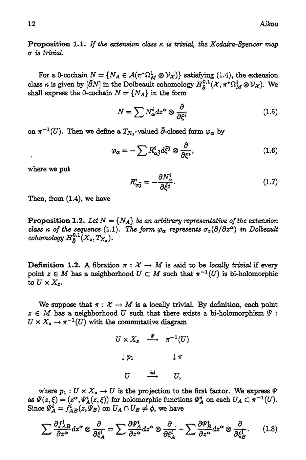
We suppose that 7r: X —* Ai is a locally trivial. By definition, each point
z e M has a neighborhood U such that there exists a bi-holomorphism & :
U x Xz —► 7T”1 (17) with the commutative diagram
U*XZ
I Pi J. it
u u,
where pi : U x Xs —> U is the projection to the first factor. We express S'
as #(3,f) = (za,^(z,i)) for holomorphic functions on each Ua C 1 (CZ).
Since ^a — £(b) on Ua H Ub / we have
Complex Finsler Geometry
13
Hence, if we define a O-cochain AT = {NA} by
(1-9)
then {JVa} defines a splitting h of (1.1). Since are holomorphic, h is holo¬
morphic, and so the extension class « is trivial.
Proposition 1.3. If a fibration tt : X —► M is locally trivial, the sequence (1.1)
splits holomorphically.
1.3 Bott Connections
To investigate the geometry of fibrations, we need a partial connection on
which is naturally defined from a connection of the sequence (1.1). A connection
of the fibration % is equivalent to single out a n-dimensional tangent subspace
called horizontal subspace at each point xeX, which is projected by dir on the
tangent space at the base point z — 7r(z) G M. For any O-cochain N = {Na €
4 ® V*)} satisfying (1.4), the local morphism Jia = Id — Na defines a
smooth splitting on each Ua- If the sheaf of splitting defines a globally
defined smooth splitting h, we call h a connection of the fibrations tt.
Definition 1.3. A connection h on a fibration % : X —> M is a smooth splitting
of the sequence (1.1), i.e., h : it'Tm —► Tv is a smooth bundle morphism
satisfying dir o h =: Id.
A connection h on a fibration ir : X —► M is given by a O-cochain N =
{Na} satisfying (1.4). Since ir : X —► M is a differentiable fibre bundle, we
may assume that every point z € M has a small neighborhood U such that
7T”1(CZ) is diffeomorphic to U x Xz. We denote by $ : U x Xz ir^(JJ) the
diffeomorphism, and we set = (z%l?x(2,s)) on eacb If we define a
O-cochain N by the same equation (1.10), then N defines a connection h of the
sequence (1.1).
Proposition 1.4. Any fibration ir: X —> M admits a connection h.
We suppose that a connection h is given by a O-cochain N. If we express N
as in (1.5), the horizontal lift of a vector field on M is defined by
(1-10)
14
Aikou
For a connection h : 7T*7m —> Tx on the sequence (1.1), the horizontal vector
bundle Hx is defined by Hx = h(ir*TM)> and it induces a smooth decomposition
Tx^x&Hx- (1.11)
By definition, Tix is a complex vector bundle over X locally spanned by {XQ}
(a = 1, • * • ,m), where Xa — h (d/dza) is the horizontal lift of {d/dz*} (a =
1,— ,n) in (1.11).
A connection h of the fibration tt is also defined by a splitting h of the exact
sequence
O —> Tr’n]^ —~
If we put V* — h (^vat) wbich is isomorphic to yAi, we get the dual splitting
(1.12)
The subbundle V* C is locally spanned by the forms {£’} (i = 1,• >• }r)
defined by
= h^) = de
According to the decomposition (1.13), the differential operator d : Ox —►
X(Q^) is decomposed as d = d° where <F : Ox X(V*) is the differential
operator along Vx and dh : Ox —► -4(^*HA/) is the one along the distribution
Hx* The operators d and d are also decomposed as d = dh+dv and S — dh+&u
respectively. We denote by X& the complex conjugate For any function F
on
and
‘"•-Efp, "-E^
for the dual frame fields of {d/d^ in local holomorphic coordin¬
ates (z0,^) on X,
1.3.1 Structure Tensors
The horizontal vector bundle ?ix C Tx is said to be integrable if it is stable
under the Lie bracket. We shall investigate the integrability conditions of a
connection h. We define the structure tensors JR^q and of Hx by
respectively, where we put
Complex Finsler Geometry
15
Definition 1.4. A connection h of a fibration 7r is said to be flat if ft is holo¬
morphic and integrable.
By this definition, we have
Proposition 1.5. A connection h of a fibration it is flat if and only if —
If we consider the following system of PDE
gj = -N^) (1.14)
with unknown ^’s, we have
Proposition 1.6. A fibration tt is locally trivial if and only if ir has a fiat
connection h.
Proof: We suppose that tt has a flat connection h. By the previous propos¬
ition, h is holomorphic and = 0 is satisfied. Then the PDE (1.15) has
holomorphic solutions {^} for every initial point (zo, <). Then ft# is an integ¬
rable holomorphic subbundle of T#, and it defines a holomorphic foliation whose
leaves are complex submanifolds of X transversal to the fibres. If we define a
holomorphic map # by #(z,£) ~ (Zj^^z,^)), the leaf through a point < € XZQ
is given by i<(z,<), and it defines a local triviality & : U x XZQ vr”1^) for a
sufficiently small U C M. The converse is trivial.
Q.E.D
We suppose that a connection h of the fibration n is flat. For the holomorphic
solution S'* satisfying ^(zq,?) = C, we have Then we may
consider the bi-holomorphic map # : (z“,£*) —> (za,C) = (za,^(z,$)) as a
coordinate change for a sufficiently small U. Then we have
Hence, if a fibration tt : X —► M admits a flat connection h if and only if there
exists a coordinate system U = {Î7, (z*,£*)} on X such that
With respect to such a covering U, we have IV* = 0 on each Ua € ZÏ, i.e.,
Na = 0. Then, from (1.4) we have a as = 0, i.e.,
on Ua ri U&.
16
Alkov
1.3.2 Bott Connections
Suppose that a smooth splitting h is given on the sequence (1.1). We introduce
the Bott connection on the vertical subbundle Vx-
Let X and Y be sections of Hx and Vat respectively. Then we put
JDxy=[X,y]v, (1.15)
where ( • )v : Tx —* Vx is the natural projection. By this definition, we can
easily show that DxY is O a-linear in X, and moreover it satisfies the Leibnitz
rule Dx{fY) = fDxY + (XfjY for all smooth function f on X, Then we get
a homomorphism D : >1(1^) —► X1^*) satisfying D (JY) = dhf 0 Y 4- fDY
for all section Y € A(VAf) and all smooth function f on Af. Such a morphism
D is called a partial connection m Vx-
Definition 1.5. The partial connection D of the vertical subbundle Vx is called
the Bott connection associated with the connection h.
We denote by — (wj) the connection form of D. For any Y — ^Yi (d/dÇ*)
we have
The forms wj are given by the horizontal 1-forms wj = with the
coefficients
dN*
= (1.16)
By definition (1.7) and (1.14), by direct calculations, we have
^ + £ wj A ^' = £•8^“ A dz& + £ A dz& + £^jd«° A&.
The form
r=£^®(^+£^)
is called the torsion form of D, From Proposition 1.5, we have
Proposition 1.7. A connection h of a fibration rr is flat if and only the torsion
form T of the Bott connection D associated with h vanishes identically.
The curvature form QD = (f2j) of D is defined by DoD (d/d£f) — £ (£/££*) 0
and is given by the End(V^)-valued horizontal 2-form
(1-17)
Complex Finsler Geometry
17-
Definition 1.6. A (partial) connection D is said to be flat if D o D = 0.
Then we have easily the following.
Proposition 1.8. Let h be a connection of a fibration x. The Bott connection
D associated with h is flat if and only if its curvature vanishes identically,
and moreover h satisfies dhcdh = 0.
We define a Vx 0 V£-valued horizontal (1, l)-fonn 3 — 0 $ 0
by
and a Vat 0 Vj-valued horizontal (1,0)-form # = 0 ®d/dÇ by
= (1-18)
where is defined by (1.7). We shall represent the curvature form in
terms of 3 and.
Proposition 1.9. The curvature L2D of the complex Bott connection D is given
by
QD = e_#/\$. (1.19)
Proof: Since = d(X&Nlf)ldzj + we have
sty+52 A = | E ~^fdzat A dzfi- (k2°)
Moreover, since X^a — d{X^N^)/d^ 4- we ^ave
- E A - £ 0 A (1.21)
Hence we have (1.20).
Q.E.D.
As an application of (1.20), we shall prove the following:
Proposition 1.10. A connection h of a fibration tt is flat if and only if its Bott
connection D is flat.
18
Aikou
Proof: We suppose that h is a flat connection of a fibration 7r. By Proposition
1.5, the connection h satisfies R^ = R^ — Rla- = 0. Then, from = 0,
(1.19) and (1.20), we get QD — 0.
Conversely, we suppose that D is flat. By Proposition 1.7, we have — 0
and dh o dh = 0. Since this second condition is equivalent to
we get $ — 0 from (1.20). Then, if we take a suitableHermitian metric (•, •)
on the vertical subbundle V^, we have ||#||2 = £0 A & = 0, and so we have
0 — 0. This means that R^ — 0. By using this and the equation R*a& = 0, we
get also dN^/dz^ =* 0. Consequently the coefficients N# are holomorphic, and
so h is holomorphic.
Q.E.D.
From the results in this section, we get
Theorem 1.1. Let h be a connection of a fibration 7r : A —► M. Then the
following conditions are equivalent mutually.
(1) h is fiat.
(2) ‘ There exists a coordinate system {C7, (^a,C)} 072 X such that
(3) The Bott connection D onV# associated with h is flat.
(4) The torsion form T of D associated with h vanishes identically.
1.4 Kähler Fibration
In this section, we shall consider the case where a fibration tt : X —► M is a
family of Kahler manifolds {XÄ, IIZ} (z e M) parameterized by the base space
M, here and in the sequel, we assume that the Kahler forms depend on
z G M smoothly.
Definition 1.7. A fibration % : X —» M is said to be a Kahler fibration if there
exists a locally öä-exact real (1, l)-fonn IIx such that its restriction Hx\xx *=
nx to each fibre X- = 7r_1(z) (z g M) is a Kähler form on Xz.
Complex Finsler Geometry
19
If 7T : X —► M is a Kahler fibration, then the real (1, l)-form fix induces
a Hermitian metric (♦, ♦) on V*. The Bott connection D on associated with a
connection h is said to be compatible with («, •) if it satisfies
dh{A, B) = {DA, B) + {A, DB) (1.22)
for A{VX).
We denote by g^ the metric tensor of the Hermitian metric (♦, •) on Vx
with respect to {0/5$*}. We also denote by (p^) the inverse matrix of (&j).
Since the Bott connection D is (l,0)-type, the connection form cu of P is given
by w*- * £^0^ “ E we Put = 2^%^“ 111 a
local coordinate, the compatibility condition (1.23) is equivalent to Xag^ -
= 0 which is written as
- ZXÿ - c1-23)
and thus we have
= = (1-24)
We shall show that the vertical subbundle Vx of an arbitrary Kahler fibration
f : X —> M admits a Bott connection D which is compatible with respect to
the metric induced on Vx- By definition, there exists a distinguished coordinate
system {CT^on tt“1 (Ï7) and R-valued smooth functions G on each Ua such that
wx = */-LddG on Ua and G|x, is the Kahler potential on Xz C\Ua> Each local
function G is pluri-subharmonic on Ua A Xz for each z g M. In terms of
distinguished coordinates (s*,^), the Kahler form IIz is given by the relative
(1, l)-form
where — d'G/d^dt?. We shall determine the Bott connection D which is
compatible with this Hermitian structure (-,♦). For this purpose, we determine
a connection h of tt. Since the coefficients I^a of D are given by (1.17), and
moreover, since dg&/d£? = dg^/dg, the compatibility condition (1.24) can be
written as
Proposition 1.11. The local functions
d2G
ds^dç-
(1.26)
define a connection h of the fibration it.
20
Aikou
Proof: Let {Ua} be a distinguished coordinate system on 7r^1(Cr). Then, in the
proof, to distinguish the quantities on a neighborhood Ua* we use the subscripts
A, B • * * in local computations. For the family of local functions {Ga} above,
since Gb—Ga is pluri-harmonic on Ua^Ub^ there exists a holomorphic function
<Pab on Ua A Ub </> satisfying Gb — Ga + <Pab + VaiL Then we have
^b = (dGA
d& d^J-
Differentiating by z“, we have
^b r^(&GA A
dzad?s d^B \dz^d^A dz<* 9AlmJ ’
and if we put
on Ua^Ubi we get the relation (14).
Q.E.D.
Remark 1.1. The coefficients defined by (1.27) and the components g$
are independent of the choice of potentials {<?} which represent the pseudo¬
metric Их- In fact, if we take another potentials {2/} adapted to the common
open covering {Ka} of vr-1 (£7), then G — H are pluri-harmonic. Then, by d§-
Poincare lemma, there exists a family of holomorphic functions {K} satisfying
G ~ H = К + X, and so we have
a2^ a2# a2^ а2я
a^a^ “ э^а^’ a^a^r a^a^*
Consequently the components g$ and functions are independent of the po¬
tentials of wx-
If we denote by D the Bott connection associated with the connection h of
(1.27), D is canonical in the following sense.
Proposition 1.12. Let {% : A —> M, IIx} &e a Kahler fibration. The Bott con¬
nection D defined by the connection h of (1.27) is compatible with the Hermitian
structure (•, •).
Proof: The coefficients (1.27) satisfy the equation (1.24). Then, since the
coefficients Tfa are given by T^a = dN^/d^ù we have (1.24). Hence D is
compatible with the Hermitian structure (♦,-).
Complex Finsler Geometry
21
Q.E.D.
We shall investigate the conditions for a Kahler fibration to be with isometric
fibres, i.e., the parallel displacement, which covers an arbitrary smooth curve
in the base space Af, is an isometry between the fibres. To this end, we shall
compute the Lie derivative
= 0, (1.27)
where the notation Lx» denotes the Lie derivation with respect to the horizontal
lift XH of a vector field X on the base M, and we use the notation g(Y
instead of (K, Z}. Then, since
the condition (1.28) is satisfied if and only if = 0 is satisfied. Hence the
horizontal mapping is an isometry between the fibres if and only if TiS = 0.
Proposition 1.13. The pseudo-Kahler manifold (X,J7) is a complex fibred
manifold with isometric fibres if and only if = 0, i.e,f <pa — 0.
As a special case of locally trivial fibrations, we shall investigate locally
trivial Kahler fibrations.
Definition 1.8. A Kahler fibration {% : X —► M, Л#} is said to be locally
trivial if every point zq e M has a sufficiently small neighborhood Z7 such that
each fibre (Х~,П~} (ztU) is holomorphically isometric to (X^, Л^).
We suppose that a Kahler fibration : X —* M, Л#} is locally trivial.
By definition, every point zq g M has a small neighborhood U С M and
a bi-holomorphism : U x Xo тг_1(Л) which makes the diagram (1.8)
commutative and induces a isometry between the fibres; We express the Kahler
form ПЯо on X^ by TZso — Since $7 induces an isometry from
(X~O,77ZO) to (Xz, Лг) for each z € Л, we can assume that the form Пх is
expressed by Л# = y/^lddG for local functions G = (ЙН1)*^ on each тг“1 (U).
The local real (1, l)-form y/^lddG defines a global (1, l)-form Л# and Пх\хл =
y/^Id^dvG is a Kahler form on X-. Since
9$(2о,С) = Й =X2>0)
and
дФт dG , .дФ1
2-^ dtf dzad^m ~dza'
22
Aikou
we have
on Tr“1(i7). Hence the connection h defined by these fonctions {N^} & Ûat, and
by Proposition 1.10, the Bott connection D is fiat. The converse is also true:
Theorem 1.2. A Kahler fibration ir is locally trivial if and only if its metrical
Bott connection D is flat.
Proof: We suppose that D is fiat. Then, by Proposition 1.10, the connection
h is also flat, and so by Proposition 1.6, the fibration 7r is locally trivial, i.e.,
there exist a bi-holomorphic map № tUx XZQ —> tt~ 1 (Ï7) for a sufficiently small
neighborhood U of zq e M. In fact, for the local solution W* of d^/dz* =
the map & is defined by ^(z.C) — (zaf^i(z1Ç)). Since {Xa} is the horizontal
lift, we have = 0. Moreover, since X& tangents to the leaf defined by ÿ,
we have
№ =
Consequently, the holomorphic map ÿ defines a holomorphic isometry îF- :
(XM for each z G U by
Q.E.D.
Chapter 2
Complex Finsler Bundles
La this chapter, we shall study the geometry of Finsler bundles as an application
of the geometry of Kahler fibrations. The fundamental tool in this chapter
is the Finsler connection, which is naturally defined as an extension of Bott
connections. We also see that our connection is also a natural generalization of
the so-called Rund connection of real Finsler geometry.
2.1 Vector Bundles Over Complex Projective
Space
Let Pr_1 the complex projective space of dimension r—1 (r > 2). Let^1,--- ,^)
the homogeneous coordinate system on Pr_1. On Uj = {[£] 6 IF-1 | & / 0},
we define a function Kj : Uj —► R by
On the intersection we have == Hence we have dd log Ki =
ddlogÆj, that is,
nFS = ^ÇÏaâiogKy
is a global real (1, l)-form on IP7*“1. By definition, IIfs satisfies (HIfs = 0- We
shall show that there exists a Hermitian metric on Pr“1 whose Kahler form is
just the form IIfs- In fact, if we put & — ^/s1 on Uit we see that IIfs is
given by
The Schwartz’s inequality implies the positive-definiteness of IIfs, an<l thus
Hfs defines a Kahler metric on P-1 which is called the Fubini-Study metric.
23
24
Aikou
The components of the metric are given by
Since H1 (P-1,©) = H~ (p-l,O) = 0, the exact sequence 0 Z —>
O O* —> 0 implies the exact sequence 0 —> Jff1(P’_x,<9*) №(P_X,Z)
—> 0. Then we have the isomorphism .
of abelian groups. Thus a holomorphic line bundle over F”1 is determined by
its Chem class. We shall list up some vector bundles over projective space P7""1
for later discussions.
Example 2.1. (Tangent bundle Tpr-i) Let p : <Cr\{0} —► F”1 be the
natural projection. We take an open covering U = {Uj} of F"1 defined by
Uj — {(i1 : • • •: C) € F“11 & 7^ 0}. We use the homogeneous coordinate
(i1, • • •, S’-) and set ? - g/g (i / j). Since
we have
(2.1)
and the holomorphic tangent bundle Tpr-i of F‘
is spanned by
with the relation (2.1). □
Example 2.2. (Hyperplane bundle) We use the notation in Example 2.1.
Let F^1, • • • be a homogeneous polynomial of degree 1. The set V(F) =
{£ € Cr\{0} [ F(f) = 0} is isomorphic to Cr\{0}. For the natural projection
p : Cr\{0} — F"1, we put HQ = p(V(F)). The hyperplane HQ * F“2 C F"1
is defined by the equation
Ri = ^.=0
on each Ui e U. Since on the intersection Utf\Uj, Ri/Rj = & /£? is non-vanishing
holomorphic function, {ft} defines a divisor. The, line bundle determined by
this divisor is called the hyperplane bundle over F“1. This line bundle is defined
by the cocycle
(2-2)
Complex Finsler Geometry
25
with the covering W. We denote this line bundle by H. All hyperplanes are
linearly equivalent to each other as divisors so that H is well-defined (In fact,
the line bundle H is defined by the cocycle defined by (2.2) which is inde¬
pendent of the polynomial F(£)).
On each Ly, we put gj = |2 ||£||2. Because of gi = |2^ on UiQUj 0,
{#} defines a n standard” Hermitian metric on H. The curvature form is given
by O = dd log ||f [|~, and its Chem form is given by
Thus ci(jy) = M is represented by the Kahler form 77fs of the Fubini-Study
metric on F_1.
A hyperplane 77q C F”1 defines a holomogy class in JHr2r_4(Pr"1,Z), and
its Poincare dual of Hq is given by ci(77) 6 772(F"X, Z) (cf. [27]). Since cx(77)
generates H2 (F-1,Z), every holomorphic line bundle S —> F”1 is a power of
77, i.e., S = H®171 for some m e %. For example, the canonical line bundle
K^-i = Ar"1T*r_1 is given by □
Example 2.3. (Tautological line bundle) Let L be the disjoint union of
lines in (T. For a line defined by vector £ € Cr\{0}, we define tt ; L —> F_1
by 7t(Zc) = p(£). In another way, L is defined by
L = {([^], V) € F“1 x Cr |£g V},
i.e., for [£] = e F“1 the fibre %"1([i]) is given by the line 1$ C Cr- We
show that 7T : L —> F“1 is a holomorphic line bundle. Since any point of L is
represented uniquely in the form
for (i1, “ • ,^r) € Cr\{0} and t € C, we have ?r“1(?7y) » {¿(f1, • * • ,£r) €
Cr I i € C,& 0} on Uj, Since t(£\ < ,C) x (£! : ••• : f) e Cx
where tj = is uniquely determined by the element of 7r 1(Uy). Then we
define a homeomorphism <pj : ?r_1(U}) —* Uj x C by
It is trivial that <pi is C-linear on fibres. On the intersection Uij = Ui n Z7y, if
tft1, • • •, C) € Tr“1(l7^) then, since tj = if* and ti == we have
This means that the coordinate change 1 is holomorphic, and thus %:£-*
F"1 is a holomorphic line bundle, which is called the tautological line bundle
26
Aikou
over Pr”1. The transition cocycle {¿(ij)} of L with respect to the covering {Uj}
of P7*“1 is given by
= | = (2-3)
□
From (2.3) we have
Proposition 2,1. The tautological line bundle L is the dual of the hyperplane
bundle i.e.,
L = H*=H~\ (2.4)
By this proposition, the fibre of H at [£] = lc 6 P* is given by l£ =
Hom(Ze,C), the space of linear functionals on 1$. Let f = 3 ^near
functional on Cr. For [£] = [i1, : • • * : Cl € F*1, the fibre 1$ of L over fc]
is given by 1$ = {(if1, • • * , tCj; i € C} C Cr. Then, if we denote by the
restriction of f to the line l^ we get a section erf of H by oy([f]) = f\i^ €
Thus any element of Hom(Cr, C) determines a global holomorphic section of H.
The converse is also true (cf. p. 86 of [70]).
Proposition 2.2. H’°(Pr’1,O(jH’)) is naturally identified with Hom (Cr, C).
The hyperplane bundle H has many global holomorphic sections, but the
tautological line bundle L has no non-zero holomorphic section. In fact, if we
suppose that L has a global section t, then, for every point [£] € Pr"1, r defines
a point (t1 ([$]),♦♦ - ,Tr([£])) € Cr which lies on the line Z$. By projecting to
the J-th component, we obtain a holomorphic function f$ : P1 —> C, that
is» P ((£]) = ([£])• Since Pr“1 is compact, and so Pr_1 has no non-constant
holomorphic function. Hence this function is constant. The functions f1, • * • , /**
defined in this way are constant. The constant point defined by these functions
should be the origin, since the point lying on all lines through the origin is the
origin itself. Hence L has no non-zero global holomorphic sections, (see [27],
[60])
Example 2.4. (Euler sequence) Let L be the tautological line bundle over
the complex projective space Pr“1. We recall the Euler sequence (cf. [71]):
0 —> L —* — 0. (2.5)
Because of H = £*, we have the exact sequence
0 —► Ijh-x -i. H®r X Tr-1 —+ 0,
Complex Finsler Geometry
27
where we put H®7' — H®- • (r-times). By Proposition 2.2, any holomorphic
section of H is naturally identified with a linear functional on Cr. We consider
a (1,0)-type vector field on Cr
where a1, • * • , aT are linear functionals on Cn. Since p*(a(Ai)) — for all
A € C, the definition p*(o-)([$]) = Mi)) is well-defined .The bundle morphism
P : -+ Tpr~i is defined by
PCa1,..- ,<Z) = d>(<7). (2.6)
Since each local coordinate Ç7 (1 < j < r) is considered as a section of H, the
morphism P is surjective. From (2.1) and the definition of P, if we denote the
section • ■ • ,f) € Z7°(F-\0(Hr)} by £, we have P(£) = 0. The trivial
line bundle lpr-i is spanned by the section 5. ’If we define a Hermitian metric
on jff®7*, we get the smooth orthogonal decomposition:
^ = 7^-1 ©lpr-i. (2.7)
Hence we have c (7pr-i) ♦ 1 = c (H®r\ where c ( - ) means the total Chern class.
Then, 22 cs ffir-1) = (1 + oi(£r))r, and so we have ci (T?r-i) — rci (H). □
2.2 Complex Finsler Metrics
2.2.1 Complete Circular Domains and Minkowski Func¬
tionals
Let V be a complex vector space. A complex Finsler metric on V is a norm || • ||
satisfying the following conditions:
(1) ||i|| > 0, and ||i|| = 0 if and only if £ = 0,
(2) ||ДСП = )A| ||e|| for € C and ё V,
(3) №1 is C~ on V\{0}.
The pair (V, || • ||) is called a complex Minkowski space. The unit ball 7? =
{i G C | ||i|| < 1} is called the indicatrix of || • ||. If we set /(£) = ||i(|2, then
f satisfies the following conditions:
1* /(i) > 0, and /(i) — 0 if and only if £ = 0,
2. /(Ai) = |A|2/(i) for VA e C and vf € V,
3. f is C°° on V\{0}.
28
Aikou
The function f is called a fundamental function of || • [|. A complex Finsler
metric is said to be convex if its fundamental function f is strongly pluri¬
subharmonic outside of the origin.
We fix a basis {$!>• • •> ,sr} of V and identify V with C7* with coordinate
system (f1,5C)- Then the strong pseudo-convexity of f is equivalent to
that its Levi form f = y/^ïddf is positive-definite, i.e., the complex Hessian
(A?) defined by
f
is positive-definite. We also need the following definition.
Definition 2.1. A domain T> in Cr satisfying the following conditions is called
a complete circular domain.
(1) If C € T> and A € C with |A| < 1, then A£ = (A?1, • • • ,AZT)
(2) If £ € D and A € C with |A| < 1, then A< € D.
In the sequel, we usually treat complete circular domains with smooth bound¬
aries. For such a bounded complete circular domain £>, its Minkowski functional
m?> is defined by
mo(e)“inf{| |tfiÉP,i>o},΀Cr. (2.9)
If we set
(2.10)
it is trivial that fa satisfies A>(A£) = |A|2/p(^) for all £ € Cr and A € C.
It is also true that $ G D if and only if A>(f) < 1, that is, the domain T> is
the indicatrix of the corresponding fundamental function fa Moreover, if T> is
strongly pseudo-convex, then
((A>)ij)>0, ((tog/p)#) > 0. (2.11)
A Minkowski norm whose fundamental function f satisfies these condition is
called a convex Finsler metric on Cr. There exists a one-to-one corresponding
between the set of complete circular and strongly pseudo-convex domains with
smooth boundaries and the set of convex Finsler metrics. The proof of the
following proposition is given in [55].
Proposition 2.3. Let Pi and T>2 be two complete circular domains in Cr with
smooth boundaries. Then. is biholomorphic to T>2 if and only if the Finsler
metric fa ofT>i is related to fa ofT>2 by fa = fa°A for some A G GL(r, C).
Complex Finsler Geometry
29
By using this proposition, the following characterization of Hermitian inner
product is obtained:
Proposition 2.4. ([55]) Let L> be a complete circular domain with smooth
boundary in Cr. The following statements are equivalent:
(1) T> is bzholomorphic to the unit ball B — {£ € Cr | £ |C|2 < 1}.*
I • I2
(2) the associated Finsler metric fa is of the form /p(i) = £
some A = (¿0 € GL^C),
(3) /© is smooth at the origin.
We shall give another characterization for Hermitian inner product. Let
G = {A & GL(r,C); | = Hill for v£ G V}
be the isometry group of || • ||. The continuity and the homogeneity of || • ||
imply that G is a compact Lie group(cf. [72], [70]), and so it is isomorphic
to a closed subgroup of U{r) “ GL(r,C) 0 G(2r). Since ||^|| ||£|| = 1 for
G S = &D and vp G G, G acts on the unit sphere S. The action is transitive
if and only if (V, [| • |[) is an inner product space. Then we have.
Proposition 2.5. Let (V, || • ||) be a complex Minkowski space. Then (V, ][ • ||)
is a Hermitian inner product space if and only if the isometry group G is iso¬
morphic to the Unitary group U(y).
Proof: Since G is compact, there exists a bi-invariant Haar measure dg. Then,
for an arbitrary Hermitian inner product (-,■)? we define a G-invariant inner
product < •, • > by
<i,’7>= [ (¡faffing-
Jg
The indicatrix Do of < •,• > is the open unit ball centered at the origin with
the isometric group Go — ^(r)- The group Go acts on the boundary dDo
transitively. We can assume without loss of generality that PriPo because
if it is necessary we multiply the inner product (♦, ♦) by a positive constant. Let
^o be a fixed point in D ADo- We suppose that G Z7(r). Then G also acts on
ODq transitively. For an arbitrary point r/ G d'Do, there exists a g 6 G satisfying
V = Then we have ||7/|| = ||^io|| “ ||fo || = 1* Hence p € from which we
have =< >.
Q.E.D.
30
Aikou
2.2.2 Complex Finsler Metrics on CT and Kahler Metrics
on F_1
Let / be the fundamental function of a convex Finsler metric. We shall show
that f induces a Kahler metric on the complex projective space F_1.
We denote by p : C*\{0} -+ P7-“1 the natural projection. The tangent bundle
Tpr-i is locally spanned by the vector fields {dp (д/d^)} with the relation (2.1).
For the hyperplane bundle H Pr_1, w’e identify the fibre Яде over [fj G Pr_1
with the set of homogeneous functions of order 1 on p^1 ([£]). Since the given
metric f on Cr is convex, we define a Hermitian metric (*, •) on by
for sections X = (X1, • •« , Xr) and Y = (У\ , Уг) of Яфг. With respect to
this Hermitian metric, the Euler sequence (2.5) implies the orthonormal decom-
position (2.7). By the relation (2.1), the bundle lpr-i is the trivial line bundle
locally spanned by 8 — (f1, ♦ - • , f7*) and, moreover we have (£, 8) = 1. Then any
section X G Яфг is decomposed as X = (X, 8}8 4- X for X = P(X) G Tpr-i.
Then it induces a Hermitian metric (*, on Tpr-i by
- (x,£) = (^logi) (X, Y).
For the homogeneous coordinate (f \ •, f7*) on Uj = {[f] G P7*-1 | f* / 0}, the
local function gj (f) := log /(f)—log |f* |2 on Uj satisfies V^lddgi = y/^lddgj —
yf=lddlog / on Ui П Uj. Hence the real (1, l)-form
Прг-i = J^lddgi = v^ia^log/ (2.13)
defines the Kahler metric (*, *)r-x* The functions {#} are called the Kahler
potentials of (», Especially, if the function / is given by /(f) =
(i.e., /(f) is the fundamental function of the flat metric ^d^^d^1 on C7*), the
induced Kahler metric on F_1 is the Fubini-Study metric. In the sequel of this
subsection, we shall show that the converse of this fact is also true.
Proposition 2.6. A Kahler metric Прг-i on the projective space P7'"1 defines
a convex Finsler metric on Cr which is unique up to a positive constant multiple.
If we denote by S the sheaf of germs of pluri-harmonic functions on Pr~1,
the exact sequence
o— X.Jt) . —> —* я°(Г— *,<$)—► /МОГ“1.*) —
5 i II
R СО
implies Я°(РГ_1,5) = R. Непсе any pluri-harmonic function on P7'“1 is con¬
stant.
Complex Finsler Geometry
31
Proof of Proposition 2.6: We express locally ZTpr-i = y/—lddgj on Uj for a
C00-function gj on Uj, Since gj — gL is pluri-harmonic, there exists a 1-cocycle
Kij e Z\Ui 0 Uj, Op— i) satisfying gj -gi~ Kij + Kij on Ui n Uj 0 $>, Then
{Kij} is a 1-cocycle on F“1, and since 2?1(Pr^1, Op—i) - 0, we may put
Kij — (Kj - log^) - (Ki -logf*) for a 0-cochain {Kj} on F“1. Hence we have
9i - {Kj + AT) + log |f I2 = 9i - {Ki + Kl) + log If I2
If we put
Wl)=exPto-(A<+^)}
on Uj, we have |^|2/j(KI) = l$*I2/»([$])• Thus we have a function f(£) —
ls5 l2/j(Kl) on Cr. It is clear thaty satisfies the condition (1) ~ (3). Moreover,
because of >/-iddlog/ = ^/-I^log/; — y/^lddgj > 0 and
V—lddf = (ddlog/ + ¿Hog/ A Slog/) ,
the function / defines a convex Finsler metric on Cr.
We suppose that we get another Finsler metric / from another Kahler po¬
tential {gj}. Then, since y/^lddgj = V—lddgj, the function log / - log/ is
pluri-harmonic function on F*“1. Hence it is a constant c. Consequently we
have / = ecf,
Q.E.D.
2.2.3 Complex Finsler Metric on Vector Bundles
Let 7Fe : E —► M be a holomorphic vector bundle over a complex manifold. If
rank(E) = 1, then any Finsler metric on E is reducible to a Hermitian metric,
and so we assume rank(E) = r > 2 in the sequel.
Definition 2.2. A complex Finsler metric on E is a smooth assignment to each
fibre Ez = 7r^1(^) of a norm [| • ||x. We call (E, || • ||) a complex Finsler vector
bundle.
We define a function fz : Ez JR by fz(£) = ||£||2 on each fibre E- Cr.
The function f- satisfies the following conditions:
1- /$(£) > 0 and /$(€) = 0 if and only if £ = 0,
2. /c(Ai) = |A|2A«)forvAeC,
3. f~ is smooth on E* = £!s\{0}.
32
Aikou
The function F : E —► R defined by F(;s,£) = /-(£) is called the fundamental
function of (£?, || • ||).
Conversely, if a function F : E —► R satisfying these condition is given
on E, then it defines a unique complex Finsler metric || * || on E. Thus, in the
sequel, we sometimes identify a complex Finsler metric || • || with its fundamental
function F,
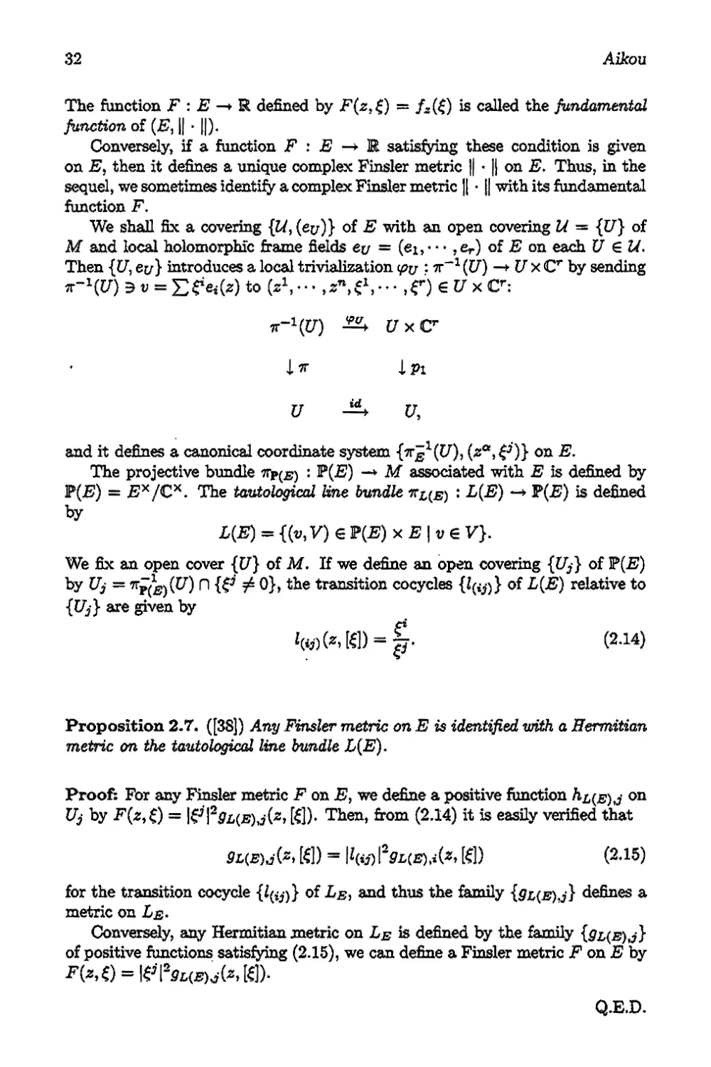
We shall fix a covering {Uy (ecj)} of E with an open covering U = {tZJ of
Af and local holomorphic frame fields ey = (ei,• • ♦ , er) of E on each U € U.
Then {Uy e&r} introduces a local trivialization tpy : tt^1 (U) -+ U x Cr by sending
v-\U) 9 v = £ to (A ’ • • , sn, i1, • • • , C) € U x e:
tt“1(CZ) CTxCr
i % i Pi
U Uy
and it defines a canonical coordinate system {vr^1(C7), (s*,^)} on E,
The projective bundle ^p(B) • P(F) -♦ M associated with E is defined by
!?(£?) = E*/C*. The tautological line bundle • ¿(-E) is defined
by
L(E) = {(yy V) € ]?(£) x E | v G V}.
We fix an open cover {U} of Ai. If we define an open covering {Uj} of P(F)
by Uj = A / 0}, the transition cocycles {l(ift} of L(E) relative to
{Uj} are given by
[£]) = (2.14)
Proposition 2.7. ([38]) Any Finsler metric onE is identified with a Hermitian
metric on the tautological line bundle L(E\
Proof: For any Finsler metric F on Ey we define a positive function on
Uj by F(zyÇ) = [£]). Then, from (2.14) it is easily verified that
9l(E) KI) = R(v) |20r(s)X*> KI) (2-15)
for the transition cocycle {¿(¿;)} of Le, and thus the family defines a
metric on Le-
Conversely, any Hermitian metric on Le is defined by the family
of positive functions satisfying (2.15), we can define a Finsler metric F on £ by
Q.E.D.
Complex Finsler Geometry
33
Definition 2.3. A complex Finsler metric F is said to be convex if F is convex
on each fibre Ez, i.e., the Levi form y/^lddf- is positive definite on Es,
Remark 2.1. We say F is strongly convex if its real Hessian on each fibre
E~ is positive-definite. The strong convexity implies the convexity. Instead of
convexity, we sometimes assume the strong convexity'. In fact, in real Finsler
geometry, we assume this strong convexity. An almost complex manifold (M, J)
with a strongly convex Finsler metric F has been investigated by Ichijyo[30],
and such a space (M, J, F) is called a Rizza manifold. □
It is easily shown that the definition of convexity is independent of the choice
of local trivialization {U, } of E. If we define a Hermitian matrix (F^j) by
- jgj. (2-16)
F is convex if and only if (F$) is positive definite.
Example 2.5. Let g be an arbitrary Hermitian inner product on E. With
respect to an open cover {&/, {gu)} we put g$ = gle^ e>), the function F : F —> R
defined by
(2.17)
defines a convex Finsler metric on E. We remark that this function F is smooth
on the whole of the total space E. □
If a convex Finsler metric F is given on E, we can define a Hermitian metric
{',•)$ on the vertical subbundle Vs by
(2.18)
By this definition, the metric F defines a Kahler metric IIs on each fibre Ez^Cr
by nz = V—ldSand the bundle tt : E M is a Kahler fibration with
the pseudo-Kahler metric ITs = y/^ldSF.
Any convex Finsler metric F defines a pseudo-Kahler metric on P(E). To
show this fact, we denote by H(E) = LIE)' the hyperplane bundle over P(F)
defined by the transition cocycles
KJ) ~ £i ~ (si)
(2.19)
The Euler sequence (2.5) is generalized to the sequence
0 —> L(E) —► *£(#)£ —► L(F) 0 > 0>
(2.20),
34
Aikou
and tensored by H(E) we have
0 1?(S) ® 7Tp^E -?-> Tp(e}/m —* 0,
where Ip(^) is the trivial line bundle over P(2?) spanned by the Euler vector
field i = (i1,1 jf) and the bundle morphism ? : H{E) ® Kp^E —> Vp(£) is
defined as follows. Any section a of H(E) is defined by a function cr : Es —> C
which is a linear functional on each fibre Es, and any section X of H E
is naturally identified with a section X = of V& satisfying the
homogeneity condition A£) — AX*(z,£) for all A G C*. Then we define
P(X) = dp^X\z,£)^
for the natural projection p : E* —► P(S).
If F is a convex Finsler metric on E, we can define a Hermitian metric (•, •)
on H(E) ® by
(X,Y}= r.,,1 f.y'-^rXiY3 = r^—r(x,Y\ (2.21)
\ / F(z,£)^d£d& F(z,£)\ ’ /e ' ’
for sections X = (X1, • ■ •, Xr) and Y = (Y1, • • •, Yr) of £T(F) ® Ac-
cording to the orthogonal decomposition H(E) ® ^p^E = lp(£) © the
map P is also defined by
P(X) = X- £ = X - 1 {x,£)s£.
For any sections X and Y of Ifys), we take sections X and Y of H(E)
such that P(X) = X and P(X) = Y. The induced Hermitian metric on Vp(£)
is defined by
i (x,Y)B - ± (2.22)
which is a Kahler metric IIS on each fibre P(FS) ~ Pr"'1 of the fibration 7rp(^.
Proposition 2.8. Let (EyF} be a convex Finsler vector bundle. Then the
bundle 7Tp(£) : P(F) —* M is a Kahler fibration with the pseudo-Kähler metric
^p(jE) — \/"~ldd log F.
We have obtained a Kahler fibration ^p(£) : P(2?) —► M with a pseudoKahler
metric %/^lddlogF from an arbitrary convex Finsler metric F, and it induce
a Hermitian metric as the restriction of to the bundle Vp^).
Conversely, from an arbitrary pseudo-Kähler metric 27?(e) of the projective
Complex Finster Geometry
35
bundle !?(£) or Hermitian metric (•, •}₽(£) on Vp(Jg)> it induces a convex Finsler
metric F on E, In fact, if we restrict to . any fibre IP(£7Z) = F*“1, we have a
Kahler metric Hs on IP(Es). Then, by Proposition 2.6, H. determines a convex
Finsler metric fz on Es Cr which is unique up to a positive constant multiple.
Since this Finsler metric fs depends on the base point z € M smoothly, we have
Proposition 2.9. If a pseudo-Kahler metric ITp(^) is given on the projective
bundle ]?(£) associated with Ef then defines a convex Finsler metric F
on E which is unique up the multiply of a positive function on M,
2.3 Bott Connections of Finsler Vector Bundles
Let (£7, F) be a convex Finsler vector bundle. Then we have two Kahler fibra¬
tions. One is the fibration ke : E —> M with the pseudo Kahler metric
IIe = V—lddF whose Kahler metric on each fibre Ez is defined by (2.18), and
another one is the fibration 7rp(s) ' P(£7) —► M with the pseudo-Kähler metric
17p(S) = V'^lddlogF whose Kahler metric on each fibre P(^) — F is defined
by (2.22), For local expression of complex Bott connection of these Kahler fibra¬
tion, it is convenient to treat the bundle (E, F) by considering (f1, • • • , $**) as
the homogeneous coordinate of the fibre
Let 7T : E -+ M be a holomorphic vector bundle over a complex manifold
with rank(£7) = r. Setting X — Ei the total space of the bundle, we obtain a
connection of the bundle tt : E —► M. Since each fibre of the fibration % is a
complex vector space, we denote by 5 the sheaf of germs of functions on the
total space E which are linear functionals along the fibres of 7r. Any connection
of the sequence
0 —> VE —► TE 7T*TM 0 (2.23)
is determined uniquely by the action of Ofe on the sheaf S.
Let U be an open set in M with local coordinate (z1, • • • , zn), and let =
(ei, - • ,er) be a local holomorphic frame field on U. Then the pair (t^ecz)
induces a coordinate (z1, • • • , zn, , f7*) on 7r"1(CZ), where (z1, zn) is
lifted from the base manifold M and (i1, • • ’ is the fibre coordinate. Then
a germ f of S is written in the form / = S on 7r”1(^)» and the action
on f is written as
=E^w • e+E/iW •
Since dfi € and € TQ;, there exists some functions {A^} on 71,-1 (tf)
satisfying
(2.24)
36
Aikou
By this definition, the functions satisfy the homogeneity condition:
Nl(z,À<)=ÀAX(^e) (2.25)
for all À G C, and, in generally, is not linear in the variable
If we take another open covering {(¡7, et/)} with the same open cover {¿7}
of M, there exists a holomorphic function Au :U —> GL(r, C) such that ëu =
eu Au* Let the coefficients of hs relative to the covering {(t7, e^)}, that is,
Here we note that (z“,^) with k the coordinate on tt”1^)
determined by (17, e^). Then, from (2.24), the relation (1.4) is written as
«)=E 4(z)^(S, ô - E <2-26)
Definition 2.4. A connection He of the bundle x : E —► M is called a non¬
linear connection of E. The functions are called the coefficients of h&. A
non-linear connection h& is said to be linear if the coefficients are linear
functionals along the fibres of ir.
Since the coefficients N^(z,£) are homogeneous of degree one with respect
to the variable £, hs is linear with respect to the variable £ if and only if
are holomorphic with respect to i.e., — 0.
We suppose that Ke is a linear connection of E. Let Xa be the horizontal
lift of d/dz°\ By definition, there exists some local functions Fya(~) satisfying
X^ = S ¿¿a (*)£*• By these functions the connection h : w*Tm -+Te is given
by
(2'27'
From the relation (2.26), the local 1-form wj = 520a(z)^Q defines the con¬
nection V : A(£7) —► Ax(£?) of (l,0)-type. Thus, if Ke is linear, then there
exists a connection wj = £TJa(z)dza on E such that and
the Bott connection DE associated with As is given by the bull-back connection
DE = 7r*V. Conversely, if a connection V : A(£) —* A1 (2?) is given by connec¬
tion forms wj — 2Fja(z)dza? then a connection hs • k*Tm —► 7b is defined
by (2.27) which is linear. Consequently we have
Proposition 2.10. Let h$ be a non-linear connection of a holomorphic vector
bundle 7T: E —► M. Then, the following conditions are mutually equivalent.
(1) hE is linear.
Complex Finsler Geometry
37
(2)^j = 0.
(3) There exists a connection V on E such that the Bott connection DE as¬
sociated with kg is given by the pull-back DE = tt* V.
Now we shall consider the Bott connection DE of the Kähler fibration tte :
E —> M with IÏ& — y/^lddF. In this case, from (1.27) the connection h& of
ke is defined by the coefficients
(2.28)
The derivation d^ = dfe + d$ associated with this non-linear connection is
defined by dfe = £ Xa0dza for the horizontal lift Xa of d/dz*. The coefficients
r%a of DE are defined by (1.17), and by the homogeneity of F, the coefficients
and satisfy the relations
(2.29)
This condition is equivalent to
£)*£ = 0.
(2.30)
Since {£,£) — F(z,£) and DE satisfies the metrical condition (1.23), we have
(2.31)
The following proposition is proved by direct calculations.
Proposition 2.11. ([6], [9]) Let DE be the Bott connection of(E, F) associated
with the non-linear connection Ke of (2.2S). Then we have
(1) d% o = 0, i.e., R^p = 0, and the torsion form T of D is given by
T* = £ R^dz* /\dzß + y^ R^dz* A A dz*. (2.32)
(2) + w A u) = 0, i.e., R^aß — 0 and the curvature form is given by
(2.33)
The components of QD is given by the form = £ Rt^dz* A dz0,
where the curvature tensor R*^ == — Xpr^* is expressed as
(2.34)
38
Aikou
by the identity (2.29), we have the relation
(2-35)
If the torsion form T of DB vanishes, then, by Proposition 2.10, there ex¬
ists a linear connection V such that DB — tt*V, and then (2.35) implies
Since R*a& — 0, the connection V and so DB is flat.
Conversely, if DB is flat, by Theorem 1.1 shows T — 0. Consequently we have
Theorem 2.1. Let DB be the Bott connection associated with the non-linear
connection He in (2.28). Then DE is flat if and only if its torsion form T
vanishes identically»
Next we shall consider the Bott connection of the vertical subbundle
Vp(s) of the fibration 7Fp^) : P(E) —► M. For this purpose, we shall define the
connection h?(E) of the fibration ttp(e)- We define a connection hp(^) of the
fibration %?(£) by
d$(B) = Y,dP ® d»“> (2.36)
for the projection p : —► P(£), where the vector fields
on T?(E) span locally the horizontal distribution Wp(s) = We shall
define a partial connection of T^e) as follows.
For any Ÿ € X(Tp(s)/M), there exists a section Y € A(H(E)®7fyB}E) such
that P(Y) = dp(Y) = Ÿ. If we denote by (»)y the natural projection from
TB to VB, we have \dp{Xa\Ÿ] = dp^.Y] and (dp[Xa, Y])y = P ([X*, Y]v).
Then we shall define
= P {DeY). (2.37)
Because of (2.31), (2.32) and
P (PSX) = PeX - 1 (DeX,£)b£,
the following proposition is proved by direct calculations.
Proposition 2.12. The partial connection satisfies
- ("M»+
/ord/X,Ÿ€X(TP(B)).
(2.3S)
Complex Finsler Geometry
39
The partial connection is just the Bott connection of the Kahler fibra¬
tion 7Tp(£) : P(E) —► M. The Bott connection DB is flat if and only if = 0
for certain local coordinate system. The flatness of is given as follows.
Proposition 2-13. The Bott connection Dv^ of the Kahler fibration %?(£) :
P(E) —* M is flat if and only if there exists a local coordinate system (z“^)
such that
= (2.39)
for some local function <?a(z) on eachU^U.
Proof: By Theorem 1.1, the Bott connection is flat if and only if ^p(£)
is flat and this is equivalent to the condition
«.-Es»*1-
By the definition (2.36) and, since kerdp is spanned by £, this condition is
equivalent to for some function satisfying the homogeneity
a(z, A^) — 0tt(z, Ç) for A € Cx. Then, we get
E « - E - E O’1) é (Sê) - «
because of the homogeneity of aa, and from this we get
which shows that a* is holomorphic with respect to the variable f. Since <ra
is homogeneous of degree zero with respect to <ra depends only on the base
point £ € M.
Q.E.D.
A convex Finsler metric whose non-linear connection is of the form (2.39)
will be discussed in a later section. We shall show that, if N& is of the form
(2.39), then there exists a local function <r(z) such that cra = dcr/dz01.
2.4 Negativity of Vector Bundles
In this section, we shall discuss the negativity (or ampleness) of holomorphic
vector bundles, and show a characterization of it by using complex Finsler geo¬
metry (see [21] and [38]).
40
Aikou
2.4,1 Positive Line Bundles and Ample Line Bundles
Let L be a holomorphic line bundle with a Hermitian metric g. Let
be an open covering of L with transition cocycle {guv}* If we put g(eu, ea) =
gu(z) on each ¿Z, the local function gu is smooth and positive, and moreover
it satisfies gv = gu\9uv\2 on U fl V. The Hermitian connection V of (L,^) is
given by the local (1,0)-form cvv = # log 0a and its curvature is given by
= dd log gu* The first Chern class ci(L) is represented by its Chem form
ci(L,0) = ^~~^Ric(g) for its Ricci curvature Ric(p).
2tt
Definition 2.5. A holomorphic line bundle L is said to be positive if its first
Chern class Ci(L) is represented by a positive real (1, l)-form.
By this definition, a holomorphic line bundle L is positive if and only if
L admits a Hermitian metric g whose curvature « Sd log g is positive-
definite. Then the form log g defines a Kahler metric on M. A complex
manifold M is said to be a Hodge manifold if there exists a positive line bundle
Example 2.6. Let H be the hyperplane bundle over a complex projective space
F1. From Example 2.2, we have
T 7T
and thus H is positive. □
Let 7T : L —> M be a holomorphic line bundle over a compact complex
manifold M. Since M is compact, dime #°(M, (P(L)) is finite. Let {so, • • *, sjv}
be a set of linear independent sections of L of the complex vector space of global
sections. The vector space spanned by these sections is called a linear system on
M. If the vector space consists of all global sections of L, it is called a complete
linear system on X. Then a rational map : M —► is defined by
V|L| (2) = M«): • • •: sk(«)], (2.40)
where we put ¥>(si) — /’) € U x C for a local trivialization : 7r“1(17) —.
U xC. This rational map is defined on the open set in M which is the comple¬
mentary to the common zero-set of the sections (Q <i < N). It is verified that
the rational map obtained from another basis {so? • • * is transformed
by an automorphism of
Complex Finsler Geometry
41
Definition 2.6. A line bundle L over M is said to be very ample if the rational
map ^i£| : M determined by its complete linear system |L| is an embed¬
ding. L is said to ample if there exists an integer m G Z such that L®m is very
ample.
Let L be a very ample line bundle over a compact complex manifold M, and
{so, • • ‘ > swj a basis of (9(L)) which defines an embedding : M —>
Pv. Under this imbedding, we can think of [so (s): • • •: sjv(s)] as a coordinate
system on the embedded M in P7^. We define an open covering {Vj} of M by
Vj = {z € M ] sj(z) 7^ 0}. With respect to this covering, the local trivialization
: 7r”1(^) —> V> x C of L is given by <£,($$) = The transition
cocycle [Ijk ' Vj A Vk —► C*} is given by
The transition cocycle {hjk} for the hyperplane bundle H is given by the
form (2.2) for the standard covering {llj} of Pn. Then, by definition, Vj =
{z € M | Sj/s) / 0} — H M). Hence we get
hjk ° V’l-DI =
and thus we have L —
Lemma 2.1, Let L be a very ample line bundle over a complex manifold. Then
L is isomorphic to the pull-back bundle of the hyperplane bundle H over
the target space PN ofy^.
The following well-known theorem shows that any Hodge manifold M is
algebraic, i.e., M is holomorphically embedded in a projective space P^.
Theorem 2.2. (Kodaira’s embedding theorem) Let L be a holomorphic
line bundle over a compact complex manifold. If L is positive, then it is ample,
i.e., there exists an integer no such that for all m> no the map : M —►
PA' is a holomorphic embedding.
Conversely, if L is ample, then there exists a basis {so, * • * , s/v} of HQ(M, C?(L®m))
such that | : M -+ PN defined by (2.40) is an embedding. By Lemma 2.1,
the line bundle L®™ is identified with (p*L0TTiiH. Thus there exists a Hermitian
metric g on L®m such that
ci(L^) = mci(L) =
^ïâaiogp(s) ,
42
Aikou
where g(z) is defined by g = 53 |/*G5)|*. Since H is positive, the (1, l)-form
y/^lSdlogg(z) is positive, and thus
ci(£) = i
m
^J-dd1ogg[z)
is positive. Consequently we get
Proposition 2.14. A holomorphic vector bundle L over a compact complex
manifold M is positive if and only if L ample.
Let E be a holomorphic vector bundle over a compact complex manifold M.
The Serre duality
and Dolbeault isomorphism = #g(M, t2p(E)) imply
H<(M,np(E)) * 2P”9(M,Pn“p(E*))*.
Putting p = q = 0, we have F°(M, (9(E)) * #n(M,
Now we suppose that M is a compact Riemann surface. Since dime M — 1,
we have
HQ(M, O(E)) ~ KX(M, PX(E’))* = 22X(M, O(E* ® KM))*
and dime0(E)) = dimcE^M, 0(E* ® Km)) for the canonical line
bundle Km = of M. The genus of M is defined by the integer
g := dime H1 (M, OM) = dime H* (M, O(KM)).
The degree of a line bundle L is defined by degE = / ci(£) 6 2, If we apply
Jm
the well-known Riemann-Roch theorem
O[L)) - dime EX(M, 0(2,)) = degL +1 - g
to the case of £ = KM, we have dime Hx(Af, O(Km)) = dime K°(Mi PX(K^)) =
dimc#°(M,0Af) = 1, since M is compact and thus Hq(M,Om) = C. Con¬
sequently we have deg Km = 2$ - 2, and the Euler characteristic x(M) is given
by
%(M)= [ ci(Tm) =-degKJtf = 2-2$.
Jm
Any compact Riemann surface M is determined completely by its genus $.
For example,
(1) if g = 0, then M is holomorphically isometric to the Riemannian sphere
Px=CU{oo},
Complex Finsler Geometry
43
(2) if g = 1, then M is holomorphically isometric to a torus C/A,
(3) if g > 1, then M is hyperbolic, that is, M admits a Kahler metric of
negative curvature.
In the case of g = 0, i.e., M =■ P1, then since ci(7\f) > 0, its tangent bundle
is positive (or equivalently ample). If g > 1, then its tangent bundle Tm is
negative since Ci(Tm) < 0.
In the case of dime M > 2, Hartshone’s conjecture:
• If the tangent bundle Tm is ample, then M is bi-holomorphic to the pro¬
jective space Pn
was solved affirmatively by Mori. It is natural to investigate complex mani¬
folds whose tangent bundles are negative. Kobayashi ([38]) has investigated this
problem by the method of complex Finsler geometry and shown the following:
♦ A holomorphic vector bundle : E M is negative if and only if E
admits a convex Finsler metric with negative curvature.
We shall discuss this problem in the next subsection.
2.4.2 Negative Vector Bundles
The interest in complex Finsler geometry arises from the characterization of
ample (or negative) vector bundles due to Kobayashi[38]. A holomorphic vector
bundle 7r : E -+ M over a compact complex manifold M is said to be ample
if its tautological line bundle L(E) —► P(E) is ample. A holomorphic vector
bundle 7T : E —> M over a compact complex manifold M is said to be negative
if its dual E* is ample. In this subsection, we shall investigate negative vector
bundles by differential geometric method.
Since the Chern class ci (£(£)) of L(E) is expressed by ddlogpj for
an arbitrary Finsler metric F on E, L(E) is negative if and only if
^^aaiogF<o (2.4i)
or equivalently this real (1, l)-form = x/^lddlogF defines a Kahler met¬
ric on the base manifold P(E). Kobayashi’s characterization is obtained by
analyzing the positivity of the form Hp(£). To investigate (2.41), the following
lemma is useful (cf. [9]).
Lemma 2.2. The curvature 3d log F o/(L(F),F) is given by
A (2.42)
where we put f07' curvature tensor of the Bott
connection DE.
44
Ajkou
We note that the curvature tensor Rifag is given by = -XpXaF^ +
^F^X^F^XaFii. We define a Hermitian form 'F = £ A on P(£)
by
K]) := F&t) £ ^3^. (2.43)
Then a convex Finsler metric is said to be negative curvature if # is negative,
i.e., < 0 for all (Xa) / 0. From (2.22), the second term in (2.42)
is negative definite, and thus we have Kobayashi’s theorem.
Theorem 2.3. ([38]) A holomorphic vector bundle E is negative if and only if
E admits a convex Finsler metric F with negative curvature
For a negative vector bundle E over M, we shall construct a convex Finsler
metric F with negative (cf. [8] and [79]). By definition the line bundle L(E)
is negative, and so L(E)* is ample. Hence there exists a sufficiently large m € 2
such that L := ¿(E)*®171 is very ample. By the definition of very ampleness, we
can take • , fN e if°(P(E), L) such that
<fif : P(S) 3 (z, [$]) [£]):•■•: fN(z, [£])) e P"
defines a holomorphic embedding ip/ : P(£) —► P77. Then, for the hyperplane
bundle H —► PN, from Lemma 2.1, we have L S Since PAr admits the
Fubini-Study metric, the first Chem form of H is given by
on Va = {[T1: •• •: Tw] € P");?“ * 0}. On Uj := H 0} C
P(l?), we put fb — {fj}, (6 = 0*• •, A*), where ff are holomorphic functions
on Uj. Then a canonical Hermitian metric of v>jH is defined by
a(z, [$])
. IWfl)l2 /
on tpj1 (Va) D Uj< Since H is ample and <pj is holomorphic embedding, we have
^^^log^jH.aCs, KJ) > 0.
The corresponding Hermitian metric gz on L is given by the functions
(2.44)
Complex Finsler Geometry
45
on each Uj. Since L — the corresponding Hermitian metric on L(E)
is given by the functions
on Uj. Since {#£(£) j} satisfies (2.15) on Ui fl Uj fa we may define a complex
Finsler metric F on E by
t) := I2gL(EU = <2’45)
Since F satisfies (2.41), we have
Proposition 2.15. Let E be a negative vector bundle over a compact complex
manifold M. For the holomorphic embedding tpf : P(£) —+ the function F
defined by (2.46) is a convex Finsler metric with negative curvature S'.
2.4.3 Vanishing Theorems
In this subsection, we shall investigate some vanishing theorems in complex
Finsler geometry. Let (F, F) be a convex Finsler vector bundle. For the Bott
connection DE of (F,F), we put
_R(Z) = ^2 «« ® dza A dz13
for *Z € A(Ve)‘ Then we have
Proposition 2.16. The Bott connection DE of (E,F) satisfies
d^{Z. Z)& = (DEZ, DeZ}b ~ {R[Z\ Z}E (2.46)
for all holomorphic section Z ofVE.
Proof: This equation is obtained from (1.23) and (2.33).
Q.E.D.
Let (F, F) be a convex Finsler vector bundle over a compact Hermitian
manifold (M, p), where g = 52 9^^° ® dz^. For the curvature tensor of
D, we put := 52 and call it the mean curvature of (F,F). Then
we shall define a Hermitian form K by
K(Z, W) := 52 Kt^Wi (2.47)
for *Z,W € A(Vj;). For any holomorphic section Q of E and the function
/«) ® F(z. £(z)), we have the following Weitzenbock-type formula.
46
Aikou
Proposition 2.17. Let (E,F) be a convex Finsler vector bundle over a Her¬
mitian manifold (M,g). For any holomorphic section Q of Ef the following
identity holds:
□/(2) = ||D^||2-K(C<), (2.48)
where we put
ll^r ==
Proof: Applying the formula (2.46) to the function f(z) = F(z,<(z)) =
«(«), C(*)>S»
0£ = -<*(0>0B + (P£<, DbQp)e, (2.49)
and by taking the ^-trace of the equation, we complete the proof.
Q.EJD.
For a holomorphic section £ of E, the equation (2.48) is written as
= -F(z,C(Sy)^z, [<(*)]) + £^(^(s))P*0Pf0.
If has at least one negative eigenvalue at every point of P(E), the complex
Hessian ddf has a positive eigenvalue at every pint of P(E). Hence we have
Kobayashi’s vanishing theorem.
Theorem 2.4. ([38]) Let (E,F) be a convex Finsler vector bundle over a com¬
pact complex manifold. If has at least one negative eigenvalue at every
point of P(£)> then there exists no non-zero holomorphic sections, that is.
HQ(M,O(E)) = 0.
Let C = C(s)$i be a non-vanishing holomorphic section of E over an open
set U. We say that a holomorphic section C — SC(^)s* is parallel with respect
to DB if it satisfies
+ = 0.
By the formula (2.48) we get the following Bochner-type vanishing theorem for
holomorphic sections:
Theorem 2.5. ([6]) Let {E, F) be a convex Finsler vector bundle over a compact
Hermitian manifold (M,p).
Complex Finsler Geometry
47
(1) If the mean curvature K is negative semi-definite on P(J5), then every
holomorphic section £ of E is parallel with respect to DB, that is, DB£ — 0,
and satisfies £) = 0.
(2) If K is negative definite on then E admits no nonzero holomorphic
section:
H°(M,O(E)) = 0.
Proof: Applying the maximum principle of E. Hopf (Theorem 1.10 of [39]) to
the formula (2.4S) implies our assertions.
Q.E.D.
bi the sequel of this sub-section, we shall show a vanishing theorem for
cohomology groups. Let (E, F) be a convex Finsler vector bundle over a compact
Kahler manifold where Um is its Kahler form. We assume that &
is semi-negative with rank > fc. Then the first Chern class Ci (£(£)) is semi¬
negative with rank > k + r — 1. Hence the bundle E is semi-negative of rank
> fc(cf. [39], p. 83). Then, Theorem 6.17 of [39] may be generalized as follows:
Theorem 2.6. ([8]) Let be a convex Finsler bundle o/rank(E) = r over
a complex manifold M.
. (1) The curvature & is semi-negative of rank >k if and only if the curvature
SdlogF of the corresponding Hermitian metric in L(E) is semi-negative
of rank > fc + r — 1.
(2) If the curvature W is semi-negative of rank > k, then E is semi-negative
of rank > k.
(3) If the curvature & is semi-negative of rank > k, then
Jf<7(M,Pi>(P)) = 0
for p + q<k — rt provided that M is compact Kahler.
Proof: The first and second are trivial from the definition of semi-negativity.
Hence we shall prove the third assertion. If we apply the Gigante’s vanishing
theorem(cf. [39], p. 69) to the Hermitian line bundle (L(E),F), we get
J7p(L(JE))) = 0
for P + Q < k + r — 2, where QP(L(E)) denotes the sheaf of E(E)-valued holo-
morphic P-forms. On the other hand, we know the following isomorphism(cf.
[39], p. 84):
E«(M, PP(E)) ~ f2n-”(E'))
« H"-’(P(E), i2”-₽((L(E))-))
~ E’+r-1(lP(E), ^^(¿(E))),
48
Aikou
where ~ and « denote the Sene duality and Le Potier isomorphism respectively.
This implies the third assertion.
Q.E.D.
As a special case, if S' is negative definite, Theorem 2.3 implies that E is
negative. Then Corollary 5.10 in [39] can be written as follows:
Corollary 2-1. Let E be a holomorphic vector bundle of rank r over a compact
complex manifold M of dimension n. If E admits a convex Finsler metric F
with negative №. then
QP(E)) = 0
for p + q <n — r.
In the case where E is a holomorphic line bundle, any Finsler metric on
E is a Hermitian metric, and so, Corollary 2.1 is a generalization of Nakano’s
vanishing theorem.
2.5 Special Finsler Vector Bundles
In this section, we shall investigate some special Finsler metrics on holomorphic
vector bundles as natural generalizations of the case of real Finsler geometry.
In real Finsler geometry, there exists three important notions of special Finsler
spaces, i.e., Landsberg spaces* Berwald spaces (or modeled on a Minkowski space)
and locally Minkowski spaces (or flat) ([16], [17], [51]). Let M be a smooth
manifold with a Finsler metric. Then the total space of its tangent bundle is
considered as a fibred manifold whose fibres are Hessian manifolds parameterized
smoothly by the base point in M, where a Riemannian manifold is said to be
Hessian if it is a flat manifold and the metric tensor is given by the Hessian
of a function in an affine coordinate system. A convex Finsler metric defines a
canonical horizontal subbundle of Tm, i.e., Cartan’s non-linear connection. A
Finsler manifold is said to be Landsberg if Tm is a fibred manifold with isometric
fibres, i.e., the parallel displacement along any smooth curve in the base space
M is an isometry between the fibres (cf. [4]). A Landsberg space is said to be
Berwald if the parallel displacement is linear. In this case, the Cartan’s non¬
linear connection is defined by the Riemannian connection of a Riemannian
metric on M (cf. [66]). A Berwald space is said to be locally Minkowski if the
non-linear connection is flat, i.e., the associated Riemannian metric is flat.
In complex case, we have no idea for the notion corresponding to Landsberg
spaces. As an analogy of real case, we suppose that the total space is a fibred
manifold with isometric fibres. Then, we have — 0 (cf. Proposition 1.13),
and the metric is modeled on a complex Minkowski space (cf. Proposition 2.10).
Thus, in this section, we shall investigate two special cases, the one is the case
where the metric is modeled on a complex Minkowski space and another one is
the case where the metric is flat.
Complex Finsler Geometry
49
2.5.1 Finsler Vector Bundles Modeled on a Complex
Minkowski Space
Ichijyô[29] has introduced the notion of Finsler manifolds modeled on a Minkowski
space. In this subsection, we shall generalize this notion to the case where the
metric is a convex Finsler metric on a holomorphic vector bundle.
Definition 2.7. A convex Finsler vector bundle (E, F) is said to be modeled
on a complex Minkowski space if its the non-linear connection hs in (2.2S) is
linear, equivalently, there exists a connection V on E such that Ds = it*V.
We suppose that (E,F) is modeled on a complex Minkowski space. By
Proposition 2.10, we have = 0, or equivalently, there exists a connection V
on E such that DE — V. Then, by Proposition 1.13, the parallel displacement
with respect to V is an isometry between the fibres, i.e., the Kahler metrics
(Ex, lddF-), and thus it is natural that the parallel displacement preserves
the Finsler metric F. We shall show that this connection V is the Hermitian
connection of a Hermitian metric gF on E. To show this, we need a lemma.
Let (E, F) be a convex Finsler vector bundle. For each z € M, the fibre E~
is a complex Minkowski space (Cr, /«)' with the norm ||s||2 = A(C)- We denote
by G the compact Lie group of isometries of the norm:
G = {g G GL(r, C); ||tf || = |]$||, € Ez}.
(2.50)
Let J be a complex structure on E, that is, J € End(E) satisfies J2 = —id. By
the idea due to Szabd ([66]), we have
Lemma 2.3. Suppose that E- admits a complex connection V on E which pre¬
serves the norm F invariant under the parallel displacement. Then there exists
a Hermitian metric gp on E such that V is compatible with gF.
Proof: Let H be the holonomy group of V with reference point z € M. Since
V preserves the Finsler structure F invariant, H is a subgroup of G. Then we
define an inner product •) on Ez by
'g
for an arbitrary inner product («, •) on Ez and a bi-invariant Haar measure dg
on G. Then we have
[ (.g(JO>g(Jy))dg= [ (J(g$,J(gri))dg = i {gi,grf}dg = &ri)s.
J G *G *G
Thus (-,‘)x is a Hermitian inner product on Ez. By definition, (•,-)• is G-
invariant and since H C <7, it is also H-invariant. Hence, by the help of parallel
displacement with respect to V, we can extend the inner product (•, •)- to a
50
Aikou
Hermitian metric gp on E. It is trivial V is compatible with respect to pF-
Q.E.D.
Suppose that (E, F) is modeled on a complex Minkowski space. Then, by
Lemma 2.3, there exists a Hermitian metric g? on E such that DE = is
compatible with pF, i.e.,
dgF^t ri) = 77) 4- 9f(£, V77)
for G A(E). Since DB is (l,0)-type, V is also (l,0)-type and so the
Hermitian connection of pF- Consequently we have a generalization of Szabd’s
theorem ([66]) to complex case.
Theorem 2.7. We assume that a convex Finsler vector bundle (F, F) is modeled
on a complex Minkowski space. Then there exists a Hermitian metric qf on E
such that V is the Hermitian connection of qf*
Concerning to Finsler metrics modeled On a complex Minkowski space, the
invariant group G defined by (2.50) is contained in the unitary group C7(r).
From Proposition 2.5, we have
Theorem 2.8. Suppose that a convex Finsler vector bundle (E,F) is modeled
on a complex Minkowski space. Then, if the invariant group G is isomorphic to
the unitary group U(r), then (E,F) is a Hermitian vector bundle.
2.5.2 Flat Finsler Vector Bundles
In this section, we shall define the flatness of a Finsler metric, and characterize
it by vanishing of the curvature 12s of complex Finsler connection DE of (B, F).
Definition 2.8. A complex Finsler metric F is said to be flat if there exists
an open cover {£/, (ea)} of E such that the fundamental function F relative to
{¿/»(ey)} is independent of the base point z € M, i.e., F$ — F^(£). Such an
open cover {ZY, (et/)} is said to be adapted.
If F is fiat, the coefficients in (2.2S) vanish in an adapted coordinate
system, and so the non-linear connection h& is fiat, and the Bott connection
DE associated with h$ is flat. Then the Kahler fibration ve : E M with
pseudo-Kahler metric y/^lddF is locally trivial.
Complex Finsler Geometry
51
Theorem 2-9, ([13]) A convex Finsler metric F is flat if and only if its complex
Bott connection DB is flat.
Proof: We suppose that DE is flat. Then» by Theorem 1.1, there exists a
coordinate system (z*, £*) on E such that = 0 with respect to this coordinate
system. In this case, from (2.28), we get (PF/dz^dtf — 0. Then we get
dz* ’
and thus' F is independent of the base point z G M. To complete the proof,
we shall show that such a coordinate system is adapted, i.e., such a coordinate
system is obtained from a change of local frame field eu &u on each U. If we
denote by (za, C) —► (za,l^(z,^)) the associated change of coordinate on C7,
from (2.26), the corresponding transformation of the coefficients of h$ is given
on each open set U. Since h$ is trivial, we may assume — 0, and so we have
iVj = №i/dza. Since N& is homogeneous of degree 1 relative to the valuable £
and !₽* are holomorphic, we have i.e., there exists a holomorphic function
Aj :U —> GL(r, C) such that = £ Ay (*)$*• The change of local frame field
is given by ej = 53eMy(s).
Q.E.D.
A flat Finsler metric F on E is a special class of Finsler metric modeled on a
complex Minkowski space. Since DB is given by the pull-back of the Hermitian
connection of the associated Hermitian metric if V£ is flat, the associated
Hermitian metric g? is also flat. Hence we have
Corollary 2.2. A convex Finsler vector bundle (E, F) is flat if and only if it is
modeled on a complex Minkowski space and, moreover its associated Hermitian
metric gp is flat.
Since any flat Hermitian metric is a flat Finsler metric, from Proposition
4.21 of [39], we have
Theorem 2.10. ([6]) Let E be a holomorphic vector bundle ofrank(E) = r.
The following conditions are equivalent.
1. 7r: E —> M is a locally trivial Kohler fibrations.
2. E admits a flat Hermitian metric.
52
Aikou
3. E is defined by a representation p: tfi(M) —► D’(r), i.e.} E MxpCr, where
is the fundamental group of M and M is the universal covering of
M.
2.5-3 Projectively Flat Finsler Vector Bundles
Let P be the GL(r, C)-principal bundle associated to E. We denote by PGL(r, C)
the projective linear group GL(r,C)/CIr} where Clr is the center of GL(r, C).
We denote by p : GL(r, C) —> PGL(ry C) the natural projection and by p! :
^Z(r,C) —* pgl{r.C) the Lie algebra homomorphism. Any connection V on
E with curvature Q induces a connection on the PGL(i\ C)-principal bundle
P = P/QIT, and the curvature of the induced connection is given by //(/?).
A vector bundle E is said to be projectively flat if P is provided with a fiat
structure, and so E is projectively if and only if E admits a connection whose
curvature Q is of the form Q = a 0 I for a complex 2-form a (cf. [39]). A
Hermitian metric g on E is said to be projectively flat if its curvature form is
also of this form. In [50], it is noticed that a Hermitian metric g on E is pro¬
jectively flat if and only if it is locally conformal-flat. In this section, we want
to investigate an analogy of Finsler geometry to Hermitian geometry.
Let (F, F) be a convex Finsler bundle. Then, by Proposition 2.8, the project¬
ive bundle 7Tp(j5) : P(F) —► M is a Kahler fibration, and the vertical subbundle
admits a Hermitian metric (•, ’)p(jE) defined by (2.22) in which each fibre
P(EZ) — F*“1 is a Kahler manifold with a Kahler metric
=
a2 log f
(2.51)
Corresponding to Definition 2.8, it is natural to define the projective flatness of
F as follows.
Definition 2.9. A complex Finsler metric F is said to be projectively flat if
there exists an open cover {14, (6^)} of E in which the Hermitian matrix G# is
a function of fibre point [£], i.e., G$ = <?#($).
Since each fibre P(F~) P1"”1 is compact and any pluri-harmonic function
on P(F^) is constant, by this definition and (2.51), F is projectively flat if and
only if logF(z, ¿) - depends only on fibre point i.e.,
= F(f) (2.52)
for some local function on each V € U> Hence the projective-flatness
is equivalent to the local conformal-flatness (cf. [10]). This equivalence in
Hermitian geometry is remarked in [50].
Complex Finsler Geometry
53
We also characterize the projective-flatness by the flatness of the projective
Bott connection Dp(E\ We assume that F is projectively flat, i.e., F satisfies
(2.52), Then, the definition (2.28) implies
(2.53)
i.e., TV = dcr{z) ® E which is of the form (2,39). Hence, by Proposition 2.13, the
projective Bott connection is flat.
Conversely we assume that is flat. By Proposition 2.13, the connection
hg is defined by in (2.39). Therefore the Bott connection DE is given by
and thus (F, F) is modeled on a complex Minkowski space. Then, by Theorem
2.7, there exists a Hermitian metric gp on E such that or — g^dgp. Hence we
have crc^z) = -tr^d^), i.e.,
_ 1 â log det (pf)
r dz*
If we put cr(^) = 1 log det (<7r) on each U € W, the metric F = e~a^F is flat
on {7, i.e., F is locally conformal-fiat. Therefore, corresponding to Theorem 2.9,
we have proved the following.
Theorem 2.11. A convex Finsler metric F is projectively flat if and only if its
projective Bott connection is flat.
Corresponding to Corollary 2.2, we have
Proposition 2.18. A convex Finsler metric F on E is projectively flat if and
only if (E, F) is modeled on a complex Minkowski space and its associated Her¬
mitian metric gp is projectively flat.
By this proposition, if a convex Finsler vector bundle (E, F) is projectively
fiat, then its associated Hermitian metric gp is also projectively flat, and so ac¬
cording to Proposition 2.8 in [39], the bundle E is projectively flat. Moreover P
is defined by a representation p : tti(M) —> FiZ(r), where PU(f) = U(r)
is the projective unitary group. This means that, if we consider the universal
covering space M as a %i(M)-principal bundle M —► Af, the bundle P is defined
by the representation p : iri(Af) —> PU(r). The flat structure of P is induced
by the natural flat structure of M —► M.
Conversely, any projectively flat Hermitian metric is also a projectively flat
Finsler metric. Hence we have(cf. Proposition 4.22 of [39])
54
Aikou
Theorem 2.12. The following conditions are equivalent:
1. : P(E) —> M is a locally trivial Kahler fibration.
2. E admits a projectively flat Hermitian metric.
3. The bundle P = P/Q*Ir is defined by a representation p : 7Ti(M) —► PU(r):
P*MxfiPU(r).
Example 2.7. (cf. [10]) Let M be a so-called Hopf manifold {Cn - 0}/Aa,
where A a is the group generated by the holomorphic transformations
(z1,— ,zn) (Az1,— ,Azn) on Cn - {0} for A e C, 0 < |A| < 1. Then M
admits a standard Hermitian metric, say Boothby metric
ds2 = -A y dz° ®dza = e-’osIM2 V dza ® da“.
Hall2
This metric is locally conformal Kahler-flat (cf. [69]), and thus it is also pro¬
tectively flat. Its Hermitian connection is given by
w = -5(log||z||2)®Z. (2.54)
The norm function defined by the metric above is -Fb(s,f) = e~108 H'H* ||£||2.
To obtain a projectively flat Finsler metric F, we shall modify Fo into the
form
F(z,i) = e-lo®»--«7(i) (2-55)
for an arbitrary convex Finsler metric /(£) on C71. Since F is also invariant by
the action of A^? it defines a convex Finsler metric on 7m. This Finsler metric is
of the form (2.52), and thus F is also projectively flat. We shall compute the non¬
linear connection in (2.28) to make sure. Because of F$ = *“los^a/<$(£)
and the definition (2.28), we obtain in the form (2.53):
fji _ dloghl|2-fi
1 “ dza * ’
and (1.17) implies that the connection coefficients of DTm are given by
h ■_ aiog||g||2H
“ dza f
Hence the connection form w of DTm is given by (2.54). The associated Her-
mitian metric gp is given by the Boothby metric. □
Let L be an arbitrary holomorphic line bundle over M with a Hermitian
metric pr. Since ]?(£ 0 E) = P(E) and L(L 0 F) = 0 L(£), we can
define a complex Finsler metric on the product bundle L 0 E. Let {Luv}
Complex Finsler Geometry
55
the transition functions of L with respect to an open covering {U, ¿a}- For
V£ = Etoto ® $Ui G A(L 0 E), we define its norm ||C||£0aB by
IlClkos — IltolL IlCalls = ot/WF(i,Cy),
where we put aa(^) — Pi Oto »to) and to = € A(U,E). Since ay =
aa|Lav|2 and Qj =» Lav£EavJ$r, t^b“8 definition is well defined. Hence
gi, • F — {ay • F} defines a Finsler metric on L 0 E, If {ay • F} defines a fiat
Finsler metric on L ® E, then F is locally conformal-flat, i.e., projectively flat.
. Now we shall consider the converse. We suppose that a holomorphic vector
bundle E admits a projectively flat Finsler metric. We shall investigate what
conditions imply that E 0 L admits a flat Finsler metric for a holomorphic line
bundle L.
A cohomology class c € №(M,1R) is said to be integral if c € J"E2(M,Z)
for the induced map J* : #2(Af,Z) —► if2(M,R) obtained from the inclusion
j : Z R. The following lemma is well-known (cf. Lemma 2.36 in [64]).
Lemma 2.4. Let £ be a closed real (1, on a complex manifold M. If
the de Rham class [£] G H2(M} R) is integral, then there exists a Hermitian line
bundle L over M with the curvature QL such that
For rank(E) — r of E, we say c is integral (mod r) if |c is integral. The first
Chern class ci(E) is integral (mod r) if and only if there exists a line bundle L
satisfying ci (L 0 E) = 0. Then we have
Theorem 2.13. Let E be a holomorphic vector bundle with rank(E) = r (> 2).
If L®E admits a flat Finsler metric for a holomorphic line bundle L, then E
admits a projectively flat Finsler metric.
Conversely, we suppose that E admits a projectively flat Finsler structure.
Ifci(E') is integral (modr), then there exists a holomorphic line bundle L such
that L®E admits a flat Finsler structure.
Proof: We shall prove the second part of the theorem. We suppose that E
admits a projectively flat Finsler structure F. Then, by Proposition 2.18, there
exists a Hermitian metric g? on E such that the curvature is given by =
0 Ie for the Ricci curvature p = dd log det pF of gp. The first Chern class
ci(E) is given by
If ci(E) is integral (mod r), then — ^ci(E) is integral, and so
by Lemma 2.4, there exists a Hermitian line bundle (L, g£) with curvature
56
Aikou
such that Px, = (57,). The complex Finsler metric defined by the function
p on the product bundle L ® E is fiat. In fact, since
I2l®e = 1 ® P + Pl ® 7s = -p 0 Ie p 01# = 0,
r r
the curvature vanishes identically:Hence L® E admits a fiat Finsler met¬
ric.
Q.E.D.
Proposition 2.19. Suppose that a holomorphic vector bundle E over a compact
Kahler manifold M admits a projectively flat Finsler metric. If ci (E) = 0, then
E admits a flat Finsler metric.
Proof: Since M is compact Kahler, the assumption ci(E) — 0 implies that
there exists a smooth real function f(z) on M such that --p = ddf(z). For
the trivial line bundle L = M x C with Hermitian metric g& = the product
bundle L®E admits a flat Finsler metric FL®E « e^F. Since L is trivial,
L®E~E. Hence e^F is a flat Finsler metric on E.
Q.E.D.
We shall investigate the condition for the projection 7tP(£;) : F(E) —* M
is a Kahler submersion with respect to a Kahler metric Um on M under the
assumption that the real (I, l)-form ZTp(s) is a Kahler metric on P(E).
Definition 2.10. ([72]) A holomorphic submersion 7r : X —► M is said to be
a Kahler submersion if X and M are Kahler manifolds, and % is a Rieman-
nian submersion, that is, is an isometry at each point for the orthogonal
complement Hx — (Va,)_L-
Watson[73] proved that, if 7r : X —► M is a Kahler submersion with the
horizontal subbundle ?ip(E) » then is integrable and totally
geodesic.
Now we suppose that a holomorphic vector bundle : E —> M admits a
convex Finsler metric F which defines a Kahler metric ZTp(£) — V^ïââlogF
on P(E). (By Theorem 2.3, if M is compact, this assumption is equivalent for
E to be negative.) Then, from (2.42)
dälogF = + A
Complex Finsler Geometry
57
defines a Kahler metric on P(£). The horizontal bundle 'Hp(e) = dp (7is) locally
spanned by {dp(XQ)} is the orthogonal complement of Vp(£) with respect to
i-e., ?fp(E) = (V?(.E)) •
Moreover we suppose that F is projectively flat. Then, by Proposition 2.18,
there exists an associated Hermitian metric gF on E which is also projectively
flat. We denote by Rap its Ricci curvature:
_ ^logdet^j?)
“ dzadz& *
Then the curvature R^a$ of DB is given by
and the curvature is given by
- p E^J
Since Jp^ is negative-definite, gF is a Hermitian metric with negative Ricci
curvature Rogiz). Then gF determines a Kahler metric g = (— on
M, and 7Tp(jb) : (P(E),7Zp(£j) —> (M,p) is a Kahler submersion.
Proposition 2.2Ö. Let F be a convex Finster metric which defines a Kahler
metric Æp(£) = lddlogF on ]?(£?). If F is projectively flat, then the base
space M is also a Kahler manifold and the projection kp(e) a Kahler submer¬
sion.
Conversely we suppose that H^E) ~ -/^lââlogF is a Kahler metric on
P(^) and the projection 7FP(£) is a Kahler submersion. Then &aß = —gaÿ(z) for
a Kahler metric Um = g^dz* A dz& on Af. By Watson’s theorem, the
horizontal subbundle Hp(E) is integrable, and thus R?a& is of the form R^ß =
Then we have
= IEFÄ^ = = A<&
Hence we have A^p = and Rï^ — -gapc\ Then (2.34) implies
- E^^F-
If (E, F) is modeled on a complex Minkowski space, i.e., R^ = 0, then we have
Rjctß
5S Aikou
and the associated Hermitian metric gp is also projectively fiat. From Pro¬
position 2.IS, the Finsler metric F is projectively flat. Consequently we have
Theorem 2.14. Let F be a convex Finsler metric such that (E, F) is modeled
on a complex Minkowski space. Assume that Zrpçs) = V—TddlogF defines a
Kahler metric on P(jE). Then the projection is a Kahler submersion if
and only id F is projectively flat.
Chapter 3
Kobayashi Metrics
In this section, we shall recall some properties of Kobayashi metric which is a
typical example of complex Finsler metrics. It is, well-known that, for a strongly
convex domain with a smooth boundary in Cn, its Kobayashi metric is a
strongly convex Finsler metric (cf. [47]).
3.1 Poincaré Metrics
First of all, we recall some facts on the Poincar6 metrics on the unit disc' A,
upper half plane IE and the punctured disc A*(cf. [45] and [22]).
Let M be a Riemann surface with a Kahler metric ds2 — 2g(z)dz ® dz. The
holomorphic sectional curvature Hg at (z, f) € Tm is given by
H3M =
1 d2
g(z) dzdz
(3.1)
Hence the sectional curvature of a Riemann surface is independent of the dir¬
ection £ and is just the Gaussian curvature Kg(z) of For the disc
A(r) {£ e C | |C| < r} of radius r > 0 in C71 centered at the origin, the Poincaré
metric pù(r) is defined by
SA(r)’22(r2-Kl^®^
(3.2)
Because of
a2 ( > \ = 2r2
g ^2 p - KI2)2/ (r2 - KI2)2 ’
we have Hg± (z, f) = —4, that is, the holomorphic sectional curvature Hg± is
negative constant. This shows that (A(r),pA(r)) is a hyperbolic manifold.
59
60
Aikou
Remark 3.1. On the unit disk A = A(l), if we define a holomorphic map
<p : A —► A(r) by ¥>(f) = then we have which shows that
<p : (A, g&) —► (A(r),£A{r)) is a holomorphic isometry. □
For any two pints £ and 77 in A, we take a C'1-class curve 7 : (0.1) —> A such
that 7(0) — £ and 7(1) =77. If we denote by ||*y(t) || the norm of tangent vector
7(t) with respect to g&, then its hyperbolic length La (7) is defined by
¿AW-/1 midt
Jo
(3.3)
The hyperbolic distance ¿^(£>77) between Ç and 77 is defined by
dù(Crç) = inf La (7),
(3.4)
where the infinimum is taken over for all C1 -class curves connecting £ and 77.
For. a holomorphic map <p : A —> A, the following lemma is well-known.
Proposition 3.1. (Schwarz-Pick Lemma) Let A be the unit disk with the
Poincare metric g&. Then every holomorphic map <p : A —> A is metric¬
decreasing <p*g& < g±:
19/(01 < 1
i-WOI2" 1-KP
(3.5)
for all Ç € A, and thus <p is distance-decreasing <p*d& < d&:
^(^(Ç),^))<dA(Cî7) (3.6)
for allCv e A.
Let Aut(A) be the group of automorphisms of A:
Aut(A) = |v(0 =
Then we have
Proposition 3.2. The Poincaré metric g^ on ïh is Aut(ty-invariant, that is}
<p*g& — g& for all ip € Aiit(A), and thus we have d±(ip(C),<p(7i) — ¿aÎC7?)*
Let 7(i) = r(t)^^ : (0,1) —► A be a C1-class curve connecting the
origin 7(0) = 0 and 7(1) = a. Then, because of
Complex Finsler Geometry
61
we have
¿a(0, Ct) = | log
and thus
(3-7)
l + l<*l
The equality holds if & = 0 and r(t) > 0. In this case such a curve is a shortest
curve between the origin and a, called a hyperbolic geodesic.
If we take an automorphism <p e Aut(ti) such that y>(f) = 0 and <^(77) =* a,
we have
dA(C»7) = di(0, a) = I log|^> r =
l-<7?
(3.8)
Then we can show that, for a sequence {2^} in A, the condition d&(zn,z) —>
0 (n —► 00) if and only if ► 0 (n —> 00), that is, d& and | • [ induce
the same topology on A. Moreover it is shown that the metric space (A, ¿a) is
complete. Since the holomorphic sectional curvature is negative constant —4,
we have
Proposition 3.3. The Poincaré disc (A, Pa) is a complete hyperbolic space.
Let El = {z € C| Im(.s) > 0} the upper half plane of C. Let <p : El —► A be a
bi-holomorphic mapping defined by
z + a
For the Poincar6 metric g± on A, we put g& — <p*g±. Then we have
5H -
1 l<fel2
4(Im(s))2
1
(l-l^)l2)2
The metric gu is also called the Poincar6 metric on EL The automorphism group
>4itt(E[) of BI is given by
Aut(H) = (a. b,c, d e R, ad - be = 1 | a PSL(2, R).
1 cz 4- d J
Then, it is easily shown that g& is Aut (El)-invariant. Moreover (El, g^) is Cauchy
complete and its holomorphic sectional curvature is also Bh = —4.
Now let : BI —► C a holomorphic mapping defined by ^(z) =
Since |^(z)| = |e~27ry| for z = x + (y > 0), we have 0 < |^(z)| < 1, and
thus is a holomorphic mapping from El on to the punctured disc A* = A\{0}.
62
Aikou
If we define an action of Z on H by z —> z+n (n G Z). Then we have JK/Z A*,
that is, : El —> A* is a universal covering map. Then there exists a Hermitian
metric 0a- on A* such that ip* g&s — g^, In fact, if we put w — e“2*v/zT~j then
we have
z =
(log |w| + v^largw),
and thus
W) »~j£log|w|.
1 dw
w ‘
dz =
Hence, if we put
~ (log |w|2)2 I"“ ’
we have = <7h- This metric g&* is also called the Poincard metric on A*.
We also see that (A*, <?£*) Is complete and its holomorphic sectional curvature
is Has = —4.
3.2 Kobayashi Metric
Let M be a complex manifold. A typical example of (pseudo) Finsler metric on
its holomorphic tangent bundle Tm is given by Kobayashi metric. We recall the
definition(cf. [22], [35], [41], [46]). We denote by A(r) C C the disk of radius
r > 0 centered at the origin.
Lemma 3.1. For any point p € M and any vector vP G T?tQM, there exists a
holomorphic map f : A(r) -+ M satisfying /(0) » p and
(3.9)
for sufficiently small r > 0.
Proof: Let p € U c M and denote by <p(z) — (z1, • • < , zm) a local coordinate
on Z7 such that z*(p) = 0 (i ® 1, • • • tm). We denote *vp G by vp =
X} sJ (d/d^)p f°r <* € C. Let : C -+ C”1 a holomorphic map defined by
^(A) = (A^1, • • •, A^™). If we take sufficiently small r > 0, we have ip (A(r)) C
Then, if we define a holomorphic map f : A(r) —> M by /(f) := y?“1 o
^ta(r)(C)i we have /(0) = p and it satisfies (3.9).
Q.E.D.
The norm of the vector G T0A(r) at the origin £ = 0 is given by
|[(d/^C)ollA(r) 555 r“1. We denote by Hom(A(r),M) thy space of holomorphic
maps from A(r) to M. The Kobayashi metric is defined as follows.
Complex Finsler Geometry
63
Definition 3.1. The Kobayashi metric kw : Tm —> R of a complex manifold
M is defined by
kM (p, v) := inf | 3f € Hom (A(r), JW), /(0) = p, /. (0) = vp
for v(p,t>p) G Tm, where the infinimum axe taken for all f 6 Hom(A(r),M)
satisfying /(0) — p and /* (0) = vp.
The Kobayashi metric kM is the maximum metric among the pseudo metrics
which satisfy the decreasing principal (cf. [41]). In fact, if H is a pseudo-metric
satisfying the decreasing principal, for the PoincarS metric pa(r) defined by
(3.2) on A(r)S we have f*H < g^ry Then, since for v(p,v) G 7m there exists
a holomorphic map f : A(r) —> M such that /(0) = p and A((®/^C))o = v, we
have
S(p,V)2 < gw ((Wo, (Wo) =
Thus we have H <
It is obvious that kM is absolutely homogeneous of degree 1, that is. for
vAgC:
fcM(p,A«) = |A|fcAf(p,v).
But kM is not the Finsler metric in our sense. It is known that kM is upper
semi-continuous, that is, for VX G Tm and ve > 0 there exists a neighborhood
U of X such that kM(Y) < kM(X) + e for all Y G U (cf. [41], [46]). This
metric is important notion on complex manifold, since the following Decreasing
Principal holds.
Theorem 3.1. ([41]) Let M and N be complex manifolds, and <p : N -* M a
holomorphic map. Then k^ > tp*kM holds, that is, for all X G 7\ we have
M*) > kM&*(XYL (3.10)
7/ 9?: TV —> M biholomorphic, then by = <p*kM>
Proof: For any vp G T*'QN, we take a map f G Hom(A(r),7V) satisfying
/(0) = p and (3.9). Then <p o f G Hom(A(r), M) satisfies (p o /(0) = y?(p) and
(p ° /)* (0) = ^*(^p). Hence we have
kM < i.
r
Since f is arbitrary, we have kw(yp) > kM(<p*(yP)). Hence we have (3.10). If <p
is bi-holomorphic, we apply (3.2) to y?”1, we have
kf/typ) = kN («;>))) < kM (V’.i®?)) >
and thus we have = <p*kM*
64
Aikou
Q.E.D.
By this theorem kM is Aut(M)-invariant, and so depends only on the
complex structure on M. In this sense, Kobayashi metric kM is an invariant
metric on M. By the Decreasing Principal, the following is also obtained.
Proposition 3.4. Let M and M be complex manifolds, and 7T : M —> M an
un-ramified covering map, Then we have k^ — kM*
For an arbitrary vector V on M, there exits a (1,0)-type vector X such that
V = X + X = 2ReX. Then we define kM(V) := 2kM(X). Let c : (0,1) —> M
be an arbitrary curve of C^-class on M. Then, the length L(c) with respect to
kM is defined by
Then for two point p, q € M, Kobayashi pseudo-distance d^(p, q) is defined by
pseudo-distance also satisfies the decreasing principal (cf. [41]):
<$(?,«) > (?(?)> ^(«))
for an arbitrary € Hol(N, M).
Definition 3.2. A complex manifold M is said to be Kobayashi hyperbolic if
the pseudo-distance is the distance in the strict sense.
There exists a criterion for Kobayashi-hyperbolicy.
Theorem 3.2. ([53]) A complex manifold M is Kobayashi-hyperbolic if and
only if there exists a positive junction c(z) and a continuous Finsler structure
F on Tm satisfying
(3.H)
for all e Tm-
Complex Piaster Geometry
3.3 Bounded Domains
65
In this section, we are concerned with completely circular domains in Cn. For
a completely circular domain V c Cn, its Minkowski functional mp is defined
by (2.9) and its fundamental function /p is defined by (2.10). If V = Cn,
then mp = 0. Hence, in the following, we always assume that T> is bounded.
Especially, if T> C Cn is bounded, then it will be proved that D is Kobayashi-
hyperbolic. The following is well-known.
Proposition 3.5. (cf. [35]) Let T> be a pseudo-convex and completely circular
domain in Cn. Then we have m^X) — fcp(0,X) for € (3b)o, ie., the
indicatrix of & at the origin coincides with the domain D.
Proof: We suppose mp(X) / 0. Then a holomorphic map (p : A —► T> is
defined by
Since <¿>(0) — 0 and y>'(0) = X/m^X), we have
M0,X) = inf {o > 0| y>(0) = 0, a^'(0) = X} = inf {^(X)} < m^X).
Hence we have k&(X) < m©(X).
Conversely, for ip e Hol(^T>) satisfying <^(0) = 0 and o<p'(0) = X (a > 0),
if we define (p € ifo^AjC71) by ^(A) ® A£(A), we have y?'(0) = £(0). Since
^?(A) € we get mp (^>(A)) = lAjm© (<£(A)) < 1, and thus we have
sup (mp o <p) = 1.
A—»SA
On the other hand, since T> is pseudo-convex,
d2 (mp o <p) (Pm-D 0<pl f dip™ \ n
dxox ~ dxldxm dx\dx )~
This shows that m© o <p is subharmonic, and thus from Maximum principal we
havempo^ < 1. Consequently we have mp(X) = mp (ay>'(0)) = ccm-o (£(0)) <
a. Then, by definition,
^(X) < inf {a > 0| p(0) = 0, c^'(0) = X} = fcp(0,X),
that is, m©(X) < &d(0,X),
Q.E.D.
We suppose that the automorphism group Aut(Z>) of T> acts on V transit¬
ively, that is, the domain D is homogeneous. Then for an arbitrary z 6 T> there
exists some e Aut(P) such that <p(z} = 0, and we have
fe(z,X) = k^(z)^(z)X} = to(0,^'(^)X) = 77lz>(/(5)X)
for an arbitrary X € TZT>.
66
Aikou
Example 3.1. (cf. [35]) The unit ball Bn of Cn is given by Bn —
{(z1, — , ;zn) € C1; ||z|| < 1}. The Kobayashi metric F^ of Bn is given by
11*11
-M2
2
l(s,*>l2 >
where (•. ■) is the standard Hermitian inner product on Cn. Especially (0, X) =
11*11- □'
For a pseudo-convex and complete circular domain 2? C C71, the following
representation of Fg is given by Suzuki[65]:
M0J)=W (3J2)
where R(X) is the radial of the disc D n lx, here lx is the complex line CX
in direction X through the origin. By using this formula, we shall show the
following proposition. The proof of it is also due to [65].
Proposition 3.6. A pseudo-convex and complete circular domain 2? c Cn is
Kobayashi-hyperbolic if and only if V is bounded.
Proof: We assume that 2? is not bounded. We take a sequence {zn} in 2> such
that lim ||zn|| = oo. Then, if we put Xn = zn/ ||zn ||, then we have
M0,*„)=£^-y,
since ||Xn || = 1. Since 2? is complete circular T> is defined by < 1. Then,
by Proposition 6.4, we have ||3n|| /R(zrf) — Zcp(0,^n) = mvfzn) < 1. Because
of R(Xn} = R(zn)t we have R(Xn) > ||zn||. Then we have
M°’x») = K(k)<liZii->0(n->oo)-
This shows that 2? is not hyperbolic. Hence, if V is hyperbolic, then 2? is
bounded.
Q.E.D.
Here we shall recall some facts due to Lempert[47], Let T> be a strongly
convex bounded domain with C^-class boundary (fc > 6). A holomorphic map
f : A —> T> is said to be extremal with respect to X e TPD if it satisfies the
following conditions:
Complex Finsler Geometry
67
(1) /(O)=p,
(2) there exists a real number A > 0 such that /'(0) — XX,
(3) for every holomorphic map g: A —> 2? such that $(0) = p and gf (0) = ¡¿X,
the inequality p>< A holds.
Then Lempert showed that for every X 6 TpP, there exists a unique extremal
holomorphic map Jx : A —* which is C*“4-class with respect to X. Then the
map
(A £ C\{0})
is extremal with respect to XX, and thus we have
Then the Kobayashi norm Zcp(p,AT) of X G Tp2?\{0} is given by fx(ty =
v/fcz>(p,X),i.e.,
kofaX) - i = inf | ¿(0) = p, g'(0) -rX,ge Hol(/X,ty
If 2? is a strongly convex domain with smooth boundary, then fcp(p, •): Tp2?\{0} -
1R is smooth and strongly convex. The indicatrix {X G TP7> | k&(p,X) < 1} C
TPD = Cn is not bi-holomorphic to the unit ball with respect to the standard
metric in Cn.
3.4 Holomorphic Sectional Curvature and
Schwarz Lemma
If the holomorphic sectional curvature Hs of a Hermitian manifold (M,g) is
bounded above by a negative constant — k < 0, then for every (z, f) G Tm we
have
> y/k ||£||^,
where ||f || is the Hermitian norm of £ relative to g. Hence, by Theorem 3.2,
such a Hermitian manifold is Kobayashi-hyperbolic.
Royden [57] defined the holomorphic sectional curvature Xf of a complex
Finsler manifold (M, F) as a natural generalization of Hermitian case. In this
section, we shall give a expression of Xf hi terms of the curvature tensor of the
Bott connection DTm gtlE^Tm over (Af, P) (cf. [3]).
68
Aikou
3.4.1 Generalized Schwarz Lemma
We suppose that a smooth Finsler metric F is given on a complex manifold. If
a holomorphic map <p : A(r) —► M is given, we can define a conformal metric
on the disk A(r) by
ds2 = çj’,F(CX®dC,
where we put /F(() = F(^(£),y?, (0)- The Gaussian curvature K#*? of ^*F
is given by (3.1):
(3.13)
v _ 2 32logv"jF
y*F ■
Then, we define the holomorphic sectional curvature of (M,F) at (z,£) € Tm
as follows.
Definition 3.3. The holomorphic sectional curvature /Cf(2,£) of F at (s,Ç) €
Tm is defined by
(3.14)
£f(*}%) := sup{K^p(0)},
where supremum is taken all holomorphic map ip : A —► M satisfying y>(0) = z
and ¥>W#C)o =
In the following, we shall denote by F^ the square of Kobayashi metric
that is, Fm = (&w)“. The following is the Schwarz Lemma for Finsler metrics:
Lemma 3.2. Let F be a smooth Finsler structure o/Tm. If the holomorphic
sectional curvature JCf is bounded by a negative constant —kf then we have
4F$ > kF
Proof: (cf. [53]) The proof is given by the same as the Hermitian case. For the
Poincae metric Pa(t) on A(r), we put
_ 2(^)(C)P - KI2)2
^^”r2/2(r2-|C|2)2 r2
The function is continuous on A(r) and /^(t) = 0 on dA(r). Hence there
exists some Co € A(r) such that log^Co) = sup log(0- Since (^*F)(C) /
C€A(r)
0, /¿r(C) is C°° near Hence, if we put C = x + y/^ly and Co = so + V—Uta,
since «
d2_ = 1 / a2 a2 \
d£<K 4 \&r2 + dy2 J
and Mr(C) attains the maximum at Co, we have
Complex Fiosler Geometry
69
logMr(c) log^rxc) (j,2 _ ^2)2
implies
(^1O6(^r)(<))0 ~ (^-ICbl2)2‘
On the other hand, from the assumption
(3.15)
2 a2log(y-F)(<)
<-fc
we have
*(<F)«o) < 2 (a^log^K))0 •
Hence, from (3.15) and (3.16) we have
(3.16)
^‘■F’)(Co)< (r2_|&|2)2>
that is, Atr(fo) < 1/A. Consequently, for all r such that 0 < r < 1 and for all
C e A(r), we have /¿r(C) < 1/&. For an arbitrary fixed £ e A(r),
& (0) < (r2 ^|2)2 (3-17)
implies < pA(r)- Hence kF(z, £) < 4/r2. By the definition of Icm* we have
kF(z^< 4F$(z,C).
Q.E.D.
This lemma and Theorem 3.2 implies
Theorem 3.3. ([38]) Let (M,F) be a complex Finsler manifold with the holo¬
morphic sectional curvature JCp which is bounded above by a negative constant
—k. Then M is Kobayashi-hyperbolic.
By this theorem, we have
Theorem 3.4. If M is a complex manifold with negative Tm? then M is
Kobayashi-hyperbolic.
70
Aikou
Now we shall show a characterization of Kobayashi metric due to [24] and
[541. Let F be a complex Finsler metric on M. A holomorphic map <p : A —*■ M
is said to be F-extremal for (z, € Tm if it satisfies y>(0) = z and
Proposition 3.7. Let (M, F) be a complex Finsler manifold. If its holomorphic
sectional curvature JCp is bounded above by negative constant —4 and there exists
a F-extremal for any (z, Ç) € Tm, then F coincides with the Kobayashi metric
Fm*
Proof: By assumption, for any (~,s) £ Tat, there exists a holomorphic map
(p : A —> M such that y?(0) = z and y?*(0)F(z,i) = Then, by the definition
of kjiif we have
= inf {)A|; ¥?(0) = a,A<p*(0) = C}
< |A|
hence we have Ffâ < F On the other hand, by K>k < -4 and Lemma 3.2, we
have F$ > F. Consequently we have F = F$.
Q.È.D.
Remark 3.2. The assumption of the existence for F-extremal can be replaced
by the existence of complex F-geodesic in the sense of Vesentini. A holomorphic
map <p : A —> M is said to be a complex F-geodesic if d&(a, b) = dw(^(a), ¥?(&))
for any a,b e A, where d& (resp. ¿m) is the distance defined by the Poincare
metric on A (resp. the Finsler metric on M). In fact, by the assumption on
JCf, we have F < F^, and
djtf(p,g)<inf [ y/Ftftffidt < [ y/Ftfttydt < f fcikrfr'(*))<&•
J q. J a I a
The decreasing property for kM implies g& > <p*F^, and so
J ^m(7 (t))dt < J — |r=t
dt ¿a (ct, 5).
Since d^a.b) == ¿Af(p,g) for a complex F-geodesic between p = p(d) and
q = <?(&), hence we have
Moreover, since > <p*F^ > ^>*F, we have g& « F. Consequently is an
isometric along the interval (a,&), from which we have Fj$ < F. □
Complex Finsler Geometry
71
3-4.2 Holomorphic Sectional Curvature by Curvature Tensor
The holomorphic sectional curvature £> is an important notion in Finsler geo¬
metry as shown in Theorem 3.3. We need a computational expression of
The holomorphic sectional curvature of a Hermitian manifold is expressed by
its curvature tensor. In the case of convex Finsler metric F at least of C3-class,
we also have the explicit expression of JCp by its curvature (cf. [1]. [3], [76]).
Let F be a convex Finsler metric on Tm with F^ = &F/d£d£?. The
canonical splitting Nj in this case is given by
Nj = E (3.18)
This splitting is called Chem’s non-linear connection in [1], which is exactly the
one defined by Rund[58] and Royden[57], The Bott connection DTm is given by
the (1,0)-form wj = 2 withl
For convenience in local computation, we shall introduce the normal coordin¬
ate system on complex Finsler manifold. A complex coordinate system is said
to be normal at P if it satisfies
1. ^(P) = ^,
2. r;fc(P) = o.
Proposition 3.8. For an arbitrary point Pq = (zo,£o) € Ты, we can always
choose a complex coordinate system {tt“1(Z7), (5.$)} around Po satisfying
ljfc(Po) + r4.(Po)=O (3.19)
Proof: For a given complex coordinate system {17, (2)} on M, we define a new
coordinate system {E7, (5)} around zq by
P = (? - 4) - 5 E ^(W - 4)(*‘ - 4)-
Then, we have (3,19) with respect to the new coordinate {17, (5)}.
Q.E.D.
A local coordinate (тг“'1(С7), (з4,О) around P € Tm said to be semi-normal
at P if the Bott connection DTm satisfies (3.19) at P. By Proposition 3.8, in a
complex Finsler manifold (M, F), for an arbitrary point P € Tm, there exists a
semi-normal coordinate around P.
72
Aikou
Remark 3.3. The Kahlerity of Hermitian manifolds will be generalized to
complex Finsler manifold. We remark that, in [3], we used the term Finsler-
Kahler manifold^ although in [1], it is called a strongly Finsler-Kahler manifold.
We define a fundamental form S by the horizontal (1, l)-form
By direct calculations, we see that dS = 0 if and only if F$ is a Kahler metric
on M, A convex Finsler metric on M is said to be Finsler-Kahler if it satisfies
dhE = 0. By direct calculations, we can show that a complex Finsler manifold
(M.F) is Finsler-Kahler if and only if DTm is symmetric, that is, Tjk = Tjj.
Since at each point P e 7m we can alway choose a semi-normal coordinate
around P, we have an intrinsic characterization of Finsler-Kahler manifold: A
complex Finsler manifold (M, F) is Finsler-Kahler if and only if around each
point P 6 7m there exists a complex coordinate system which is normal at P.
□
Now we shall investigate the holomorphic sectional curvature of Finsler man¬
ifolds. We define a function Hf by
_ 2 V" f'V _ ^~Fi3 \ eicjckct
~ f(z, e)2 ¿A2-' dzi dz^ds1 P'*'' •
From the last equality, we see that if is a Hermitian metric on 7m,
Hf is just the holomorphic sectional curvature Hg of (M, g) (cf. [SO]). We prove
the following theorem:
Theorem 3.5. ([3]) The holomorphic sectional curvature lCp(z,£) € (7m) -
coincides with the function HfM'
Proof: Since JCp(z,X£) = £f(z,£) and Hp(z,Xty — we may assume
F(s}£) = 1. In the following, we put <f>*F — E. Since we always choose a
coordinate ( on A satisfying (dE/d^)^Q — (dE/d^\=Q = 0, the sectional
curvature JCp(z,g) is defined by
Complex Finsler Geometry
73
By direct calculations, we have
=E +E (¿o+E ^) - &
where we put — (d2q?/âÇ2)çz=o. Form this equation, we have
HF{z,^ = K^F{z^) + 21 £ (X + E • <3-2°)
Hence Hp > K^f for all 92. If we take a semi-normal coordinate around the
point (z,£) e Tm and 92 : A —► M as a complex line y>(C) = (z1 + Ci1, • • • ,zn +
£$*) through the point, then the second term of (3.20) vanishes, and so the
sup {Kp.f} attains to the maximum J?f(z, £). Consequently we have Hp — ICf*
Q.E.D.
Remark 3.4. By the Hermitian form № defined by (2.43), the holomorphic
sectional curvature Kf is given by JCf = F(z,f)_1 s • Hence, by The¬
orem 3.3, if M is a compact complex manifold with negative Tm, then M is
Kobayashi-hyperbolic.
Let (M, F) be a complex Finsler manifold modeled on a complex Minkowski
space (V,/). Then, by Theorem 2.7, there exists a Hermitian metric gp on M
associated with F. In (V, /), the indicatrix T> = {£ € V; /($) < 1} is a bounded
and strongly pseudo convex domain. And so there exists a unique Euclidean
sphere S centered at the origin inscribed about the indicatrix T>, If necessary
by multiplication by constant, we may assume that S is the indicatrix of gF-
Let fM bo the function on Tm defined by fM = 2 for Since S is
inscribed about 2? we have
(3.21)
Moreover, if the sectional curvature ICp is bounded above by a negative constant
—k, Lemma 3.2 implies 4F$ > kfw- Consequently we have
Proposition 3.9. ([5]) Let (M, F) be a complex Finsler manifold modeled on a
complex Minkowski space. If the holomorphic sectional curvature JCp is bounded
above by a negative constant —k, the we have the following inequality:
4F$ — kfM kF.
(3.22)
74
Aikou
As an application of Proposition 3.7, we have a characterization of unit ball:
Theorem 3.6. ([8]) Let M be a simply, connected complete complex manifold
with a convex Finsler metric F. Suppose that (M,F) satisfies the following
conditions:
1. For each (z,£) € Tm, there exists an F-extremal.
2. Its holomorphic sectional curvature is negative constant —4.
3. (M, F) is modeled on a complex Minkowski space, and its associated hp is
Kahler.
Then (M,F) is holomorphically isometric to the unit ball with the standard
metric in Cn.
Proof: By the first and second condition, the given Finsler metric F coincides
with Kobayashi metric F^. Then (3.22) implies F = fM = F^. Hence, by
the third condition implies the manifold is a simply connected complete Kahler
manifold with negative constant curvature —4. By the well-known uniformiza-
tion theorem of Kahler manifolds(cf. [43]), (M, F) is holomorphically isometric
to the unit ball with the standard metric in Cn.
Q.E.D.
By Lempert [47], if T) is a strongly convex domain in Cn with smooth bound¬
ary, then its Kobayashi metric F% is a complete and strongly convex Finsler
metric. Since strong convexity implies convexity, the Kobayashi metric Fp
is a Finsler metric in our sense. Moreover F$ satisfies the first and second
assumption in the theorem above (see [1] and [24]). Hence we have
Proposition 3.10. ([8]) Let D be a strongly convex domain in Cn with smooth
boundary. The following statements are equivalent.
1. T> is biholomorphic to the unit ball in Cn.
2. (P, Fpf) is modeled on a complex Minkowski space, and its associated Her¬
mitian metric is Kahler.
Bibliography
[1] Abate, M. and Patrizio, G. (1994) Finsler metrics. A global approach,
Springer Lecture Notes 1591.
[2] Abate, M. and Patrizio, G. (1996) Finsler metrics of constant curvature and
the characterization of tube domains, in Finsler Geometry, Contemporary
Math. 196, 101-107.
[3] Aikou, T. (1991) On complex Finsler manifolds, Rep. Fac. Sei., Kagoshima
Univ. 24, 9-25.
[4] Aikou, T. (1993) Some remarks on the geometry of tangent bundles of
Finsler manifolds, Tensor, N.S., 52, 234-242.
[5] Aikou, T. (1995) Complex manifolds modeled on a complex Minkowski
space, J. Math. Kyoto Univ., 35, 83-111.
[6] Aikou, T. (1996) Some remarks on locally conformal complex Berwald
spaces, in Finsler Geometry, Contemporary Math. 196, 109-120.
[7] Aikou, T. (1997) Einstein-Finsler vector bundles, Publ. Math. Debrecen,
51, 363-384.
[8] Aikou, T. (1997) A note on infinitesimal deformations of complex Finsler
structures, Anal. St. a. Univ. “AL.I. CUZA” Iasi, Tomul XLIII, s. T. a,
Matemático, 295-305.
[9] Aikou, T. (199S) A partial connection on complex Finsler bundles and its
applications, Illinois J. Math., 42, 481-492.
[10] Aikou, T. (1999) Conformal flatness of complex Finsler structures, Publ.
Math. Debrecen, 54, 165-Í79.
[11] Aikou, T. (2000) Some remarks on the conformal equivalence of complex
Finsler structures, in Finslerian Geometry. A Meeting of Minds P. Anton¬
elli (ed.), Kluwer Acad. Publ., 35-52.
[12] Aikou, T. (2000) Some remarks on Finsler vector bundles, Publ. Math.
Debrecen, 57, 367-373.
75
76
[13]
[14]
[15]
[16]
[17]
[18]
[19]
[20]
[21]
[22]
[23]
[24]
[25]
[26]
[27]
[28]
[29]
[30]
Aikou
Aikou, T. (2002) Complex Bott connections of projective bundles and its
applications to complex Finsler geometry, Far East J. Math. Sd», 4,91-117.
Atiyah, M.F. (1956) Complex analytic connections in fibre bundles, Trans.
Amer» Math» Sd», 85,181-207.
Atiyah, M.F. and Bott, R. (1982) The Yang-Mills equations over Riemann
surfaces, Phil» Trans» Roy» Soc. London, A 308, 425-461.
Bao, D., Chem, S.S. and Shen, Z-M. (1996) Finsler Geometry, Contem¬
porary Math., 196.
Bao, D., Chem, S.S. and Shen, Z-M. (1999) An Introduction to Riemann-
Finsler Geometry, Springer.
Bland, J. and Kalka, M. (1996) Variations of holomorphic curvature for
Kahker Finsler metrics, in Finsler Geometry, Contemporary Math. 196,
121-132.
Chern, S.S. (1979) Complex Manifolds without Potential Theory, Springer.
Chem, S.S., Chen, W.H. and Lam, K.S. (1999) Lectures On Differential
Geometry, Series On University Mathematics, 1, World Scientific.
Cao. J.-G. and Pit-Mann Wong, Pit-Wann (2002) Geometry of projectiv-
ized vector bundle, preprint.
Dineen. S. (19S9). The Schwarz Lemma, Clarendon Press, Oxford.
Duchamp, T. and Kalka, M. (198S) Invariants of complex foliations and
the Monge-Ampdre equation, Michigan Math. J., 35, 91-115.
Faran, J. J. (1990) Hermitian Finsler metric and Kobayashi metric, J» Dif¬
ferential Geometry, 31, 601-625.
Faran, J.J. (1996) The equivalence problem for complex Finsler Hamilto¬
nians, in Finsler Geometry, Contemporary Math. 196, 133-144.
Fukui, M. (19S9) Complex Finsler manifolds, J. Math. Kyoto Univ., 29,
609-624.
Griffith, G. and Harris, J. (1978) Prindples of Algebraic Geometry, John
Wiley & Sons.
Hashiguchi, M. (1976) On conformal transformations of Finsler metrics, J.
Math. Kyoto Univ., 16, 25-50.
Ichijyo, Y. (1976) Finsler manifolds modeled on a Minkowski space, J.
Math. Kyoto Univ., 6, 639-652.
Ichijyo, Y. (1988) Finsler metrics on almost complex manifolds, Riv. Mat.
Unw. Parma, 14, 1-2S.
Complex Finsler Geometry
77
[31] Ichijyö, Y. (1988) Conformai curvature tensors of a generalized Finsler
metric, Tensor, N.S., 47, 171-178.
[32] Ichijyö, Y. (1991) Conformally flat Finsler structures, J. Math. Tokushima
Univ., 25, 13-25.
[33] Ichijyö, Y. (1994) Kaehlerian Finsler manifolds, J. Math. Tokushima Univ.,
28, 19-27.
[34] Ichijyö, Y. (1998) Kaehlerian Finsler manifolds of Chem type, preprint.
[35] Jarnicki, M. and Pflug, O. (1993). Invariant Distances and Metrics in Com¬
plex Analysis, Malter de Gruyter.
[36] Jost, J. (1991) Compact Riemann Surfaces, Universitext, Springer.
[37] Kikuchi, S. (1994) On the condition that a Finsler space be conformally
flat, Tensor, N.S., 55, 97-100.
[38] Kobayashi, S. (1975) Negative vector bundles and complex Finsler struc¬
tures, Nagoya Math. J., 57, 153-166.
[39] Kobayashi, S. (1987) Differential Geometry of Complex Vector Bundles,
Iwanami-Princeton Univ. Press.
[40] Kobayashi, S. (1996) Complex Finsler vector bundles, in Finsler Geometry,
Contemporary Math., 196, 145-153.
[41] Kobayashi, S. (1998) Hyperbolic Complex Spaces, Springer-Verlag.
[42] Kobayashi, S. and Wu, H.-H. (1970) On holomorphic sections on certain
Hermitian vector bundles, Math. Ann., 189, 1-4.
[43] Kobayashi, S. and Nomizu, K. (1963) Foundations of Differential Geometry,
II, John Wiley & Sons Inc., New York.
[44] Kodaira, K. (1986) Complex Manifolds and Deformation of Complex Struc¬
tures, Springer-Verlag.
[45] Krantz, S. (1990) Complex Analysis: The Geometric Viewpoint, The Math¬
ematical Association of America.
[46] Lang, S. (19S7) Introduction to Complex Hyperbolic Spaces Springer-Verlag.
[47] Lempert, L. (1981) La métrique de Kobayashi et la représentation des
domaines sur la boule, Bull. Soc. Math. France, 109, 427-474.
[48] Lübke, M. (1983) Stability of Einstein-Hermitian vector bundles,
Manuscripta Math., 42, 245-257.
[49] Manin, Y.I. (1997) Gauge field Theory and Complex Geometry, Springer,
Berlin.
78
Aikou
[50] Matsuo, K. (1996) On local conformal Hermitian-flatness of Hermitian
manifolds. Tokyo J. Math., 19, 499-515.
[51] Matsumoto, M. (1986) Foundations of Finsler Geometry and Special
Finsler Spaces, Kaiseisha Press, Otsu, Japan.
[52] Morrow, J. and Kodaira, K. (1971) Complex Manifolds, Holt, Reinhalt and
Winston, New York.
[53] Noguchi, J. (1990) Introduction to Hyperbolic Manifolds (in Japanese),
Sophia Kokyuroku in Mathematics No. 32. 1990.
[54] Y. Pang, M.Y. (1992) Finsler metrics with properties of the Kobayashi
metric of convex domains, Publications Matematiques, 36, 131-155.
[55] Patrizio, G. and Wang, P.-M. (1983) Stability of the Monge-Amperére Fo¬
liation, Math. Ann», 263, 13-29.
[56] Rizza, G.B. (1963) Strutture di Finsler di tipo quasi Hermitiano, Rw. Mat.
Univ. Parma, 4, 83-106.
[57] Royden, H.L. (1986) Complex Finsler metrics, Contemporary Math., 49.
261-271.
[5S] Rund, H. (1959) The Differential Geometry of Finsler Spaces, Springer-
Verlag.
[59] Rund, H. (1972) The curvature theory of direction-dependent connections
on complex manifolds, Tensor, N.S., 24,189-205.
[60] Smith, K.E., Kahnanpâa, L., Kekâlainen, P. and Traves, W. (2000) An
Introduction To Algebraic Geometry, Springer-Verlag.
[61] Schumacher, G. (1989) On the geometry of moduli spaces, Manuscripta
Math., 50, 229-267.
[62] Schumacher, G. (1989) The theory of Teichmüller spaces- A view towards
moduli spaces of Kahler manifolds, in Severed Complex Variables, VI,
Springer.
[63] Schumacher, G. (1993) The curvature of the Petersson-Weil metric on the
moduli space of Kahler-Einstein manifolds, in Complex Analysis and Geo¬
metry, V. Ancona and A. Silva (eds.), Plenum Press.
[64] Shifîmann, B. and Sommese, A.J. (1985) Vanishing Theorems on Complex
Manifolds, Birkhäuser, Boston.
[65] Suzuki, M. (1984) The intrinsic metrics on the circular domains in C*, Pac.
J. Math., 112, 249-256.
[66] Szabd, Z.I. (1981) Positive definite Berwald spaces, Tensor, N.S., 35.25-39.
Complex Finsler Geometry
79
[67] Thompson, A.C. (1996) Minkowski Geometry, Cambridge University Press.
[6S] Tondeur, P. (1988) Foliations on Riemannian Manifolds, Springer.
[69] Vaisman, I. (1982) Generalized Hopf manifolds, Geom. Dedicate, 13, 231-
255.
[70] Yang, K. (1991) Complex Algebraic Geometry: An Introduction to Curves
and Surfaces, Marcel Dekker, Inc.
[71] Zheng, F. (2000) Complex Differential Geometry, American Mathematical
Society and International Press.
[721 Wang, H.C. (1947) On Finsler spaces with completely integrable equations
of Killing, J. London Mat, Soc., 22, 5-9.
[73] Watson, B. (1976) Almost Hermitian submersions, J. Differential Geo¬
metry, 11, 147-165.
[74] Wells, R.O. (1979) Differential Analysis on Complex Manifolds, Springer,
GTM.
[75] Watt, C. (1996) Complex Sprays, Finsler Metrics and Horizontal Complex
Curves, Ph. D. Thesis, Trinity College Dublin.
[76] Watt, C. (1999) Horizontal complex curves and holomorphic curvature,
preprint.
[77] Watt, C. (1999) Complex sprays and complex curves, preprint.
[78] Wong, B. (1977) On the holomorphic curvature of some intrinsic metrics,
Proc. Amer. Math. Soc., 65, 57-61.
[79] Wong, B. (1984) A class of compact complex manifolds with negative tan¬
gent bundles, Math. Z., 185, 217-223.
[80] Wu, B. (1973) A remark on holomorphic sectional curvature, Indiana Univ.
Mate. J., 22, 1103-1108.
PART 2
KCC Theory of a System of Second Order
Differential Equations
P.L. Antonelli and I. Bucataru
Contents
1 The Geometry of the Tangent Bundle 91
1.1 The Tangent Bundle . 91
1.2 The Vertical Subbundle 93
1.3 The Almost Tangent Structure 94
1.4 Vertical and Complete Lifts 94
1.5 Homogeneity 95
2 Nonlinear Connections 97
2.1 Horizontal Distributions and Horizontal
Lifts 97
2.2 Characterizations of a Nonlinear Connection 99
2.3 Curvature and Torsion for a Nonlinear Connection 102
2.4 Autoparallel Curves and Symmetries for a Nonlinear Connection 103
2.5 Homogeneous Nonlinear Connection 107
3 Finsler Connections on the Tangent Bundle 109
3.1 The Berwald Connection Ill
3.2 The h and v-Covariant Derivation of a Finsler
Connection 112
3.3 The Torsion of a Finsler Connection 113
3.4 The Curvature of a Finsler Connection 114
3.5 Finsler Connections Induced by a Complete
Parallelism 116
3.6 The Cartan Structure Equations of a Finsler
Connection 118
3.7 Geodesics of a Finsler Connection 120
3.8 Homogeneous Berwald Connection 121
4 Second Order Differential Equations 123
. 4.1 Semispray or Second Order Differential Vector Field 123
4.2 Nonlinear Connections and Semisprays 125
4.3 The Berwald Connection of a Semispray 127
4.4 The Jacobi Equations of a Semispray 129
4.5 Symmetries for a Semispray 131
85
86
Antonelli and Bucataru
4.6 Geometric Invariants in KCC-Theory 132
5 Homogeneous Systems of Second Order
Differential Equations 135
6 Time Dependent Systems of Second Order
Differential Equations 139
6.1 Sprays and Nonlinear Connections on Jets . 139
6.2 Variational Equations 144
6.3 The “Film-Space” Approach to Type (B) KCC-Theory 147
7 The Classical Projective Geometry of Paths 151
7.1 Paths, Parametrized Paths 151
7.2 The Various Geometries of Paths -
Finite Equations . 152
7.3 The Various Geometries of Paths - Differential Equations .... 153
7.4 Affine Connections 155
7.5 The Fundamental Projective Invariants 158
7.6 The Projective Parameter and the Normal Spray Connection . . 161
7.7 Projective Deviation 165
KCC Theory
87
To the reader:
Here are two suggested approaches for reading this document. One (I) in¬
volves reading Chapter 7, last, while the other (H) has it first. The bridge
between (I) and (II) is Chapter 5. Thus, approach (I) including Chapter 5 is
completed by reading Chapter 7, last.
Approach (II) is to read Chapter 7, first, then read Chapter 5 to get an idea
of a global perspective.
Approach (II) is possible, for the most part, with only a calculus background.
It has been successfully used in teaching a one semester course at the senior
undergraduate level.
Introduction
The modem geometry of a system of second order differential equations (SODE)
was initiated in the 1920’s by Synge [26], Knebelman [16], Douglas [14] and the
geometric invariants of a SODE were obtained in the 1930’s by Kosambi [17],
Cartan [10], and Chem [11]. In their papers they considered a system of second
order differential equations
(l* tri1 « dsf,
-¿p + 2<7(t, $, —) = 0, * G {1,n} (1)
where (i, xz) are the local coordinates on a real (n-Fl)-dimensional fibred man¬
ifold 7T : M —> jR. The main problem they studied was to find the geometric
properties one can associate to the system (1) that are invariant under the
following groups of transformations:
{ £* = x^x*) OT
The problem is not completely solved and in the last decade, there have been a
lot of papers on the subject [12], [18], [20], [25]. On the other hand, properties
of (1) which are invariant under arbitrary (smooth) parameter transformation
on all solutions simultaneously, t — (pfra), where a = {ai,..-¡¿m} are a set
of parameters which suffice to distinguish the different solutions among them¬
selves, combined with arbitrary transformations, a = a(a), of these, are called
projective properties of (1). However, in this case, (1) is required to have Gi
independent oft and (positively) homogeneous of degree two in the dx/dt vari¬
ables. This is the setting for classical projective geometry of (1), pedagogically
described in Chapter 7. But, it is possible to extend these and other classical
results to systems occurring in engineering, biology and physics, etc. by use of
Schooten’s film space technique. We leave as an open problem for the reader
that of extending projective geometry to general SODE’s.
The geometry of the system (1) under the action of the group of transforma¬
tions (A) is called the KCC theory of type (A), while the geometry of the system
(1) under the group of transformations (B) is called the KCC theory of type
(B).
For a mechanical point of view the system (1) is called a dynamical system,
the manifold M is the space of configurations. From this point of view the main
89
90
Antonelli and Bucataru
problem is to find the symmetries of the system (1), that are the diffeomorphisms
of the space of configurations M that map solutions of (1) into solutions of (1)
and first integrals, i.e. functions which are constant on the solutions of (1).
In KCC theory of type (A), the system (1) lies on the tangent bundle of a
n-dimensional manifold Mn, while in KCC theory of type (B) the system (1) lies
on the first jet bundle of a n + 1-dimensional fibred manifold tf : Mn+1 —► R.
Chapter 1
The Geometry of the
Tangent Bundle
The KCC theory of type (A) we shall present here appears as a subgeometry of
the geometry of the tangent bundle. We start with a manifold M (the space of
configurations of a dynamical system), then construct the tangent and cotan¬
gent bundle and study some natural geometric objects like: the almost tangent
structure, the Liouville vector field, and the vertical distribution.
1.1 The Tangent Bundle
Let M be a real, n-dimensional manifold and A = {(C7a, Mati} be an atlas of
C°°-class on M. For every p 6 M, we denote by TPM and T£M the tangent and
cotangent spaces at p to M, respectively. The disjoint union TM =;
of tangent spaces to M is called the tangent bundle to M. Similarly, the disjoint
union of cotangent spaces to M is called the cotangent
bundle to M. For every local chart (£7, 0) on p € U C M we denote by
the local coordinates induced by 0, that is 0(p) = (^(p)) 6 jRn. We shall denote
this by 0 = (x*) or (CT,0 = (x*)). A local chart (CT, 0) at p € M induces an
isomorphism h^p : TPM —► 7?n, such that (h^p o o^“1)(v),
where (V, 0) it is another local chart at p e Af. In local coordinates, if 0 = (x£)
and V» = (£*), then (h^p o
We remark here that there is no canonical isomorphism between the tangent
space TPM at a point p G M and and between two tangent spaces TPM and
TqM at two points p and q to M. A connection provides one, as we shall see.
Denote by 7r: TM —► M the canonical projection, that is if v e TPM then
tt(v) = p, and we have 7r_1(p) = TPM, Vp 6 M. For a local chart (CT, 0) on M
we define & : %_1(C7) C TM -► 0(17) x Rn by $(y) = (0(7r(v)),h^ff(v)(v)). It
is easy to check that (7r"1(L7),$) is a local chart on TM and it is called the
induced local chart. The set of all induced local charts determines a differentiable
91
92
Antonelli and Bucataru
atlas of (7°°-class on TM. Consequently, we have that TM is a 2n-dimensional
manifold of C°°-class. By abuse of language the triple (TM, 7r, M) is called the
Tangent Bundle of the base manifold M, TM is the total space and % is the
canonical submersion.
Similarly, the cotangent space T”M carries a differentiable structure of C°°-
class, the triple (T*M,tt*,M) is called the cotangent bundle, and the canonical
submersion tt* : T*M M is defined by tt* (cu) = p if and only if w G T*M.
Throughout this work the summation convention on upper and lower re¬
peated indices is assumed.
Let (U, 0 = (x*)) be a local chart at p € M and h<t>,p : TPM —► the
induced isomorphism. If is the natural basis of B?, we denote by
Ip 388 h^p(ei). Then edited the natural basis of TPM. For
a vector v G TPM, we denote by (y*) the local coordinates with respect to the
natural basis, that is v = Ip* This is equivalent to h^p(v} = yiei. The local
coordinates determined by an induced local chart (tt- 1 (U), $) on TM are then
(xi,yi), because 4>(v) = (^(v^h^^v)) = (^(^(v)),^). So, an induced
local chart on TM will be denoted by = (æ*,^)). With respect
to the induced local coordinates, the canonical submersion has the expression
tt : (x^y*) w (x*).
The local coordinates on the cotangent space T*M are denoted by (xz,pi)
and the canonical submersion ; T*M —> M has the local expression 7r* :
(xSpi) >->• (x*).
If (IZ, <£ = (x1)) and = (51)) are local charts around p G M, the local
coordinates (x*) and (¿*) are related by 5* = x'fâ), with rank(^) — n. The
corresponding change of coordinates on TM, induced by = (x\ y'f)
and (7T-1(V), # = (£*,§*)) is given by:
(1.1)
We call (1.1) the change of coordinates formula on TM. As we have
that the Jacobian of is always positive (it is equal to det(|—)2), so TM
is an orientable manifold.
The change of local coordinates formula on T*M (the corresponding formula
of (1.1) on T*M) is:
®i = 2i(aS’), rank(fg-) = n, '
d&.
J
If u G TM, we denote by TUTM the tangent space at u to TM. This is
a 2n-dimensional vector space and the natural basis induced by a local chart
KCC Theory
93
(Tr_1(C7)}$ = (x1,^)) atuis {-z-yIu, ■£"T|uh=rç? After a change of coordinates
UX oyz
(1.1) on TM. the natural basis changes as follows:
d i _ r \ 9 \ t i 9 I
a?1“ " l“ + a®’ (uW“’
d i _ dit. . d .
ay*i“- dxi^dÿi^-
(1-2)
d d
A vector Xu € TUTM has the form Xu = ^(u) + y*(u)w*H-u with
ox1 ay1
respect to the natural basis. Under a change of coordinates (1.1) on TM, the
coordinates of a vector Xu e TUTM change as follows:
(1.3)
A vector field X on M is a differentiable section of the tangent bundle, that is
X : M —> TM, such that tt o X = Id m- Denote by x(M) the set of all vector
fields over M and by ¿F(M) the set of all real differentiable functions on M.
Then %(M) with the Lie bracket is a real Lie algebra of infinite dimension and
a module over the ring .F(M). Similarly, we denote by x(TM) and 5(TM) the
set of all vector fields on TM and the set of all real differentiable functions on
TM, respectively..
We may remark here that the tangent space TTM carries two natural pro¬
jections. One is the natural projection r of the tangent bundle (TTM,r,TM)
and the second one is the linear map tu induced by In local coordinates we
have:
r : (x,3/,X,y) e TTM i-> {x,y) € TM, and
tt* : (x,y,X,Y) € TTM » {x,X} € TM.
1.2 The Vertical Subbundle
Q
From the last formula of (1.2) we can see that span a n-dimensional
vector subspace VUTM of TUTM. We call it the vertical subspace and it determ¬
ines a n-dimensional, integrable distribution V : u € TM »-► VuTM C T^TM,
which is called the vertical distribution. If we denote by VTM — Utt€TAf KTM,
then VTM is a subbundle of the tangent bundle (TTM,r,TM) to TM. As
7r: TM —* M is a submersion it follows that : TUTM —► TV^M is an epi¬
morphism of linear spaces, for Vu € TM, where is the linear map induced
by 7T at u 6 TM. The kernel of is exactly the vertical subspace, that is
VuTM = Kerr^u,
Vu € TM.
94
Antonelli and Bucataru
We denote by xv(TM) the set of all vertical vector fields on TM. It is a
real subalgebra of %(TM).
Consider now T*TM the cotangent space of TM at it € TM and denote
by {dz* 1^, dyiI«} the natural cobasis. In other words, cfy*!«} is the dual
basis of ^7 luK ^l^ter a c^ianS€ local coordinates (1.1) on TM, the
dual basis changes as follows:
1
(1-4)
1.3 The Almost Tangent Structure
The almost tangent structure of the tangent bundle (or the vertical endomorph¬
ism) is defined as follows:
and
(1-5)
Using (1.2) and (1.4) one can check that J is globally defined on TM. For the
almost tangent structure J we have the properties:
1° J2 = 0;
2° Ker J= Im J=VTM.
The Nijenhuis tensor field of the almost tangent structure J is given by:
Nj(X, Y) = [JX, JY] - J[X, JY] - J[JX, Y],VX, Y € x(TM). (1.6)
A direct calculation shows that Nj = 0, that is, the almost tangent structure J
is integrable.
1.4 Vertical and Complete Lifts
For every u € TM, one defines the linear map lVtU : T%(U)M —> TUTM as
iv.vCXVC«))¿k«)) = I«- We can see that : TrwM -»
KTM is a linear isomorphism. It is called the vertical lift of the tangent bundle.
We may also think to the vertical lift lv as an 5'(M)-linear map between %(M)
and x(^M). In this case lv is defined as follows: for every vector field X —
€ X(-M% (lvX)(u) = ¿v>ti(X%(tt)). The vertical lift of a vector field
X € x(M) will be denoted also by Xv G x(TM).
KCC Theory
95
The complete lift Xc of a vector field X — X'-tt-t <= x(M) is defined as
follows: X
Xc = X*— J- A.
dxi 1 dx^dtf
(1.7)
Consider f 6 .F(M) a function on the base manifold M. Denote by fv = f o tt
and /c(x, y) — ^y1 the vertical and the complete lift, respectively. For the
vertical and the complete lifts we have the following properties:
1° (JX)'' = fvX*, (fX)c = fvXc 4- fcXv, VX € x(M), / 6 ^(M);
2° J(XC) = Xv, [Xv,yv] - 0, [Xv,yc] = [X,y}v, [Xc,yc] = [X,y]c.
A tensor field T of (r,s)-type on TM is said to be a Finsler tensor field (or a
distinguished tensor field, or a d-tensor field for short) if under a change of local
coordinates (1.1) on TM, its local components change as the local components
of a (r,s)-type tensor field on the base manifold.
1.5 Homogeneity
Denote by TM — TM \ {0} the tangent space with zero section removed. If
A € (0, 4-oo), we define hx : TM —> TM by Aa(z, y) = (x, Xy) and we call hx the
homothetic of ratio A. The set of all homothetics {hx, A € (0, +oo)} constitutes
a one-parameter group. The vector field that has this group as a one-parameter
group is called the LiouvUle vector field and in local coordinates it has the form
C = A function f € F(TM) is said to be homogeneous of degree r if
fohx — Xrf. There is a Euler type theorem for homogeneous functions, that uses
the Lionville vector field €: a function f € ^(TM) is homogeneous of degree r
if and only, if £cf — rft or equivalently, in local coordinates, ^y* = rf. Here,
is the Lie derivative in direction C.
We need also to define the homogeneity for a vector field X € So,
a vector field X 6 x(TM) is homogeneous of degree r ifXohx — Ar”1(h<x)»X.
A Euler type theorem says that X € x(TM} is homogeneous of degree r if and
only if £qX = (i— 1)X. In local coordinates a vector field X — X*
is homogeneous of degree r if and only if X*
d
As an example, we have that the Liouville vector field (D = yi^r7 is homo-
vy*
geneous of degree 1.
96
Antonelli and Bucataru
More generally, a tensor field T of (l,s)-type is homogeneous of degree r if
= (r — 1)T. As an example, we have that the almost tangent structure J
is a (1,1)-type tensor field homogeneous of degree 0. In order to prove this we
have to show that £^7= - J, that is equivalent to [C, JX] — J[(C, X] = —JX,
VX € xlTM)) and we can prove this by taking X e
If a function f € F(TM) is homogeneous of degree r, then there exist
the functions synimetric with respect to such that
/(z, y) = » • • y^, so f is a symmetric polynomial of degree r with
respect to y. If we want to avoid this particular cases, we have to assume that the
function f is of C°°-class on TM and continuous on the null section. A similar
remark holds also for tensor fields. Next, if we oxe^referring to a homogeneous
object this will be supposed to be of C°°-class on TM and continuous on the null
section.
If T is a (l,l)-type tensor field and X is a vector field then the Frolicker-
Nijenhuis bracket of T and X is a (l,l)-type tensor field [T,X], defined as
follows:
[T,X](y) = [T(y),X]-T[y,X].
The Frolicker-Nijenhuis bracket of two (l,l)-type tensors K and L is a vector
2-form [X, IS] and is defined as follows:
[A',L](X,y) = (K(X),L(y)] + [£(X),AT(y)] + (KoL)[X,y]+
(L o K) [X, y] - X[X, £(y)] - K[L(X), Y]-L[X, X(y)] - L[K(X), y].
In particular,
K](X,Y') = [X(X), X(y)l + K*[X, y] - K[X, K(y)] - A[K(X),y],
Njc ~ |[K, A] is called the Nijenhuis torsion of K. We already have seen that
Wj = j[J, J] = 0 and [J, <CJ = J.
Chapter 2
Nonlinear Connections
An important tool in the KCC-theory of type (A), as a subgeometry of the
geometry of the tangent bundle, is the notion of nonlinear connection. The
existence of a nonlinear connection on TM will allow us to extend some results
and geometrical objects from the vertical subbundle VTM to the tangent bundle
TTM.
In this section we shall give some equivalent definitions for a nonlinear con¬
nection and study the main geometrical objects induced by it. As we intend
to apply this theory to a dynamical system, we pay a special attention to the
autoparallel curves of a nonlinear connection and their symmetries. The case of
homogeneous nonlinear connection is also studied.
2.1 Horizontal Distributions and Horizontal
Lifts
Definition 2.1. A nonlinear connection on the tangent bundle TM is a sub¬
bundle (JHTM,rff,TM} of the tangent bundle ^TTM.r,TM} such that on
fibers we have
TUTM = HUTM © VUTM, Vtz € TM. (2.1)
A nonlinear connection HTM on TM induces a distribution H : u € TM w
HUTM C TUTM of constant rank n, provided M is connected. We call it the
horizontal distribution. From (2.1) we can see that the horizontal distribution
is supplementary to the vertical distribution.
For a nonlinear connection HTM we denote by h and v the horizontal and
the vertical projectors that correspond to (2.1), respectively. A vector field X E
x(TAf) is called horizontal if h(X) X and vertical if v(X) = X. We denote
by %h{TM} the ^r(TM)-module of horizontal vector fields.
As : TUTM —> T„.(U)M is an epimorphism, from (2.1) -we can see that
the restriction of to HUTM from HUTM to T^M is an isomorphism.
We denote by l^u : T^yM —► HUTM the inverse map of the above mentioned
97
Antonelli and Bucataru
isomorphism. We call lh.,u the horizontal lift induced by the given nonlinear
connection. The horizontal lift lh can be thought also as a 7*(M)-linear map
between x(M) and x(TM) and is defined as follow’s: if X = € x(M)
define lh(X)(u) = The horizontal lift of
a vector field X € x(M) will also be denoted by Xh €
The horizontal ¿ft 1^ induced by a nonlinear connection H and the vertical
lift lv are related by:
Jointly (2.2)
One can prove that if lh : x(M) —► x[TM) is a ^(M)-linear map such that (2.2)
holds then H : u 6 TM wHUTM = is a nonlinear connection on
W.
X/5 X
Denote by ^-r|u = We have that |u}i=T^ is a basis of
HUTM^ Vu 6 TM and under a change of coordinates (1.1) on TM we have
that:
tix* dxi ’
(2.3)
(2.4)
The set of functions (Arj) are defined on domains of induced local charts and
they are called the local coefficients of the nonlinear connection.
Proposition 2.1. To give a nonlinear connection HTM on the tangent bundle
TM it is equivalent to give a set of functions Nj on every domain of induced
local chart such that on intersections of such domains, they are related by:
(2.5)
Proof: The “if” part is a consequence of (2.3) and the action of the group of
coordinate transformations (1.1).
For the “only if” part we suppose that on every domain of induced local
chart we have a set of functions JVj such that on the intersection of any two
domains the corresponding functions Nj and Nfc are related by (2.5). Then we
&
may define as in (2.4). It is a straight forward calculation to check that •
fa? $
(2.3) is true and {—span a n-dimensional subspace HUTM of TUTM. As
|U! ■a“d*} linearly independent, thenHUTM and VUTM satisfy (2.1).
ox1 ay1
KCC Theory
99
Example 2.1. Let be the local coefficients of a symmetric linear con¬
nection on the base manifold M. Under a change of local coordinates on M we
have that: A ’
dxl d& dxk dx?dxq d& dxk *
If we denote by NJ(x,y) = 7jA(x)j/A and take into account the above law of
transformation, we find that N*(x,y) satisfy (2.5) so. they are the local coeffi¬
cients of a nonlinear connection.
2.2 Characterizations of a Nonlinear Connection
For a given nonlinear connection HTM^ we have a basis { |u} of TuTM
adapted to the decomposition (2.1). We call it the Berwald basis of the nonlinear
connection i
HUTM = € TUTM, ^(Xtt) = 0}.
The horizontal and the vertical projectors of the nonlinear connection can
be expressed with respect to the Berwald basis as follows:
v=-^®syi- <2'6)-
From (1.5) we can see that the almost tangent structure J acts on the Berwald
basis as follows:
Then for Vu € TM, Ju : HUTM —► VUTM is an isomorphism. The inverse map
of this isomorphism is denoted by 3V : VUTM —> HUTM. We may extend this
structure 3 to the whole TUTM by taking 3U := 3U a vu> This is equivalent to
We call the morphism 3 the adjoint structure. It has the properties:
1° 32 = 0, Im0 = Ker3 = HTM:
2° 3o J — h, J o3 = v and consequently Id = 3 o J + J o 3,
Conversely, we have:
Proposition 2.2. An FtJ'Myiinear morphism 3 : %(TM) —> x(TM) such that
32 = 0 and Id = 3°J+Jo3 determines a nonlinear connection HTM = Ker3.
100
Antonelli and Bucataru
Proof. Let «(¿) - A>and »(¿) = + d^ A.
»» + ■>'»(¿) - ® « >«" d^ + d A + Ai£, = «o
C{ = d'f and Al = —Dl. From 0 = 02(^“?) we that &i = —^Aj. Denote
by N? — A3if under a change of coordinates (1.1) on TM the set of functions
N? obey the transformation rule (2.5) so they are the local coefficients of a
d • d
nonlinear connection HTM. We have also that — N? ■=—r) = 0 and
Kdx* ’ d]p
d 0 • d
0(-z-^) = -5-7 and the statement is proved.
'dy*' dx* ldtf
Proposition 2.3. To give a nonlinear connection HTM on the tangent bundle
TM it is equivalent to give for every u € TM a linear map Ku : TUTM -+
TK(U)M such that Ku o Ju =
Proof: If we have a nonlinear connection HTM^ then we consider the structure
0 and we define Ku — tt*,« o 0U. As 0« o and tf*,u o we obtain
JCu O «Txt = 7T*jxa’
Conversely, let Ku : TUTM -* T^M be a linear map such that Ku o Ju —
7r+)tl. As is an epimorphism then Ku is so, Vu € TM. If we denote by
HUTM = KerKy, we have an «-dimensional distribution on TM. The vertical
distribution VUTM = KerJu is «-dimensional, too and from Ku oju — 7r*?tx we
have that HUTM A VUTM = 0 and then (2.1) it is satisfied.
The map we used in the above proposition is called the connection map and
appears for the first time in Dombrovsky’s paper, [13].
Now, let’s put all structures Ju, 0u, 7r*>u, Zv|W, Ku into a diagram:
VUTM
Ku
il>tU
K(u)M
Next we present two other structures, the almost product structure and the
almost complex structure whose existence is equivalent to the existence of a
nonlinear connection.
Proposition 2.4. To give a nonlinear connection HTM on the tangent bundle
TM it is equivalent to give a T(fTM)-linear morphism IP : x(TM) -+ x(^7Vf)
KCC Theory
101
such that:
JoF = J, IPo.7=-J.
(2-7)
Proof: If a nonlinear connection HTM is given, we define IP : x(TA7)
xfT.«) » F(i i + r - r- A. Th„ M „ lnle.
Conversely, let IP : x(TAf) —► x(TM) be a J7(TM)-linear morphism such
that (2.7) is true. Then in the natural basis, the morphism IP has the form
JP(tt7) = — 2AT/ and IP(-^r) = — It can be shown that under a
ax* ax* dy3 ay* dy*
change of induced local coordinates (1.1) on TM, the functions Nj satisfy the
formula (2.5) so they are the local coefficients of a nonlinear connection HTM.
The morphism IP defined in the “if” part of the above proof satisfies also
IP2 = Id, and consequently it is called the. almost product structure of the
nonlinear connection. It has the property that the distribution of eigenspaces
corresponding to +1 is the horizontal distribution and the distribution of ei¬
genspaces corresponding to —1 is the vertical distribution. With respect to the
Berwald basis of the nonlinear connection, the almost product structure JP has
the expressions
(2.S)
Proposition 2.5. To give a nonlinear connection HTM on the tangent bundle
TM it is equivalent to give a F(TM)-morphism IF : %(TM) —> xlTM), such
that:
1^ = —Id, andIFoJ + JoIF= Id. (2.9)
Proof: If we have a nonlinear connection HTM, we consider the adjoint struc¬
ture 0 and define F = 0—J. ThenF2 — 02-QoJ—JoO+J2 = -(h+v) = -Id.
Also, we have that F o J-f- Jo F = 0o J + Jo 0 = h + v = Id.
Conversely, consider a .7* (TM)-linear morphism F : x(TM) —> xC^M)
that (2.9) are true. If we define 0 = J+F we have that 02 = 0 and 0o J+Jo0 =
Id. According to Proposition 2.2, HTM — Ker0 is a nonlinear connection on
TM.
The structure F is called the almost complex structure of the nonlinear
connection and it has the following expression with respect to the Berwald
basis:
Let T be a tensor field of (r, s)-type on TM, so T is a ^(TMJ-linear morph¬
ism T : AX(TM) x • • • x A1 (TM) x x(TM) x • ♦ • x x(TM) J*(TM). As
for every 1-form cu € AX(TM) and every vector field X € xC^M) we have the
decomposition into a horizontal and a vertical component cu = huj + vw and
X — hX + vX, then T(7mji 4- wj,..., hur + vwr, hX^ + vXi,..., hXs + vX*) is a
sum of 2r+4' terms, each of them being a Finsler tensor field on TM. Then we
102
Antonelli and Bucataru
may define a Finsler tensor field of (r,s)-type as a tensor field that reduces to
only one term from those 2r_H possible terms, that is T(cui,u>r, Xi,XkS) =
T(£iw1,..-,£rwr,£1Xi,...,^Xtf), where si,...,€ {h,v}.
2.3
Curvature and Torsion for a Nonlinear Con¬
nection
If HTM is a nonlinear connection, according to Frobenius theorem, we have
that HTM is integrable if and only if %fe(TM) is a Lie subalgebra of x{TM).
$
As {7-7} are generators for %\TM), we have that HTM is integrable if and
8 8
only if [^-r, ^—7] € We have that:
(2.H)
±1=P‘± =6Nf_SNl
w’Jar h Sxi Sxi '
So, a nonlinear connection is integrable if and only if its curvature tensor Rjif
which is a Finsler tensor field of (l,2)-type, vanishes. The curvature tensor of
a nonlinear connection is defined as
(2.11)'
JZ=-№ = -i[A,A],
where h is the horizontal projector and № is the Nijenhuis tensor of h. We
have that:
R = R^dx* ftdx3 ®
3 dyk
For a nonlinear connection on TM we call the weak torsion of the nonlinear
connection, the vertical-valued 2-form:
t(X,Y) = J[AX,AY] - v[hX, JY] - v[JX,hY\.
(2.12)
With respect to the Berwald basis we have that the weak torsion has the form
* = ®® =: ® ® <2J2>'
We have immediately that Jot — 0 and t(JX, K) = t(X, JY) = t(JrX, JY) — 0.
A nonlinear connection is said to be symmetric if its weak torsion, t, vanishes,
. + . dNj dNl
that zs -¿—f- = -T—
dy^ dyi
The Nijenhuis tensors of the adjoint structure 0, the almost complex struc¬
ture, and the almost product structure are given by:
Ne = Njf = ijk^k ® ® + R№yk ® Sy1 ®
(2.13)
KCC Theory
103
Ntp = Qdx*®-^. (2.14)
From (2.14) we can see that a nonlinear connection HTM is integrable if and
only if the corresponding almost product structure TP is integrable, that is the
Nijenhuis tensor, Njp, vanishes.
From (2.13) we have that a symmetric nonlinear connection is integrable if
and only if the almost complex structure IF is integrable, which is equivalent to
the adjoint structure 0 being integrable.
2.4 Autoparallel Curves and Symmetries for a
Nonlinear Connection
Now let us consider the autoparallel curves of a nonlinear connection and their
symmetries. First we have to define the dynamical covariant derivative induced
by a nonlinear connection.
Definition 2.2. The dynamical covariant derivative induced by a nonlinear
connection HTM is V : xtM) —► VX = v(Xc), where v is the vertical
projector and Xc is the complete lift of X.
In local coordinates we have: if X — X*-^- g y(Af), then VX — VX*-^-,
dx' h dy*
where:
(2.15)
(2.16)
77ie dynamical covariant derivative has the properties:
1° V(X + Y) = VX + VY; V(/X) = feXv + f°VX-,
rux-x^t th» X‘ - x>± + vx‘A.
More generally, we may define the covariant derivative as V : ^(TAf)
XV(TM), by Vtx^y)^) - VX*^, where:
Q
We can see that if X = ■^i(aj)'S77t that is X is the vertical lift of a vector
oy
on Af, then the formula (2.16) reduces to (2.15). Denote now S = =
3 ' ■ 0 US' *
~ We have that S is a global vector field on TM. With this
notation, both formulae (2.15) and (2.16) can be written as follows:
VX^SiX^ + NJX* (2.17)
104
Antonelli and Bucataru
Definition 2.3. A smooth curve c : t e Z C IR h* c(t) = (x*(t)) G M is called
an autoparallel curve of the nonlinear connection HTM if its natural lift to TM,
C : t € I >-» c(i) = (**(*), € TM is a horizontal curve, which means that
the tangent vector field to c(t) is horizontal.
In local coordinates, a smooth curve c(i) = (^(t)) is an autoparallel curve
if and only if:
Using the dynamical covariant derivative, the invariant equivalent form of (2.18)
V(^)=0. (2.18)'
Consider now, c(t) = (x4(t)) a trajectory of (2.18), and let it vary into nearby
ones, according to
= (2.19)
where s denotes a scalar parameter with small value |e|, and ^(¿) are compon¬
ents of a contravariant vector field along the curve c. If we substitute (2.19)
into (2.18) and let € approach zero we get the so-called variational equations of
(2.18):
dt2 +<dyk dt ' dt dxi dtK
(2.20)
Theorem 2.1. For the variational equations (2.20), the equivalent invariant
form (the Jacobi equations) are given by:
+ + %k^k = 0. (2.21)
A vector field ^(¿) along a trajectory c(i) = (&*(*)) of (2.18) is called a Jacobi
vector field if it satisfies (2.21).
Proof: Along a trajectory of (2.18), we have that = S =:
So, the equations (2.20) are equivalent to
(2.22)
SW+^k++=°-
It is a straightforward calculation to check that (2.21) and (2.22) axe equivalent
if we take into account that VC = 5(C)+Njtf and V2C = S2^) + +
2NfyS(£?) + .
For every vector field on the base manifold X — X' -fg € x(M), we consider:
aj(n,y,X) =
k dX\Tk , 9XkKri , dN<vk , dNidXr
dxidxkV dxkNj + dxi dakX + dyr dxk
yk (2.23)
KCC Theory
105
The Lie derivative of NJ with respect to the complete lift Xc of a vector field
X = X*-^ € x(M) 0331 shown to be
+ (2.23)'
For every X e x(M) we have that aj(s,t/,X) = £x*NJ is a (l,l)-type Finsler
tensor field on TM. The variational equations (2.20), or the equivalent invariant
forms (2.21) or (2.22) can be written as follows, then:
<>;(»(«), $.5«))^=- »■' (2«)
Definition 2.4. A vector field X e x(M) is said to be a symmetry of a nonlinear
connection HTM, if £X°Y = [Xc,Z] € VZ s
As is a local basis for a nonlinear connection HTM on TM
we have that a vector field X G x№) is a symmetry of HTM if and only
if [Xc, ^-t] € xh(TM). Vi € [1, In local coordinates we have that
d d
v[Xc, = -a£(z,y,X)^j, where aJ(x,yyX) is defined by (2.23). Con¬
sequently we have that a vector field X € x( Af) is a symmetry of a nonlinear
connection HTM if and only if,
£x*NJ = 0. (2.25)
Theorem 2.2. A vector field X € ) is a symmetry of a nonlinear connec¬
tion HTM if and only if £x*№ — 0, where IP is the almost product structure
of the given nonlinear connection.
Proof: We have to prove that X € x(Af) is a symmetry of HTM if and only
if [Xc, IP(r)J - IP[XC, Y] = 0, VZ e x(TM), As £XeP(y) is ^(TM)-linear we
need to check this only for Y = and Y — -—-t.
dx1 dyl
Fory = wehavethat IXMP(A)]-P[X‘, ¿1 = (Id -I?)([X‘, ¿]) =
2v([Xc, ]). As X is a symmetry of HTM> we have that [Xc, is horizontal,
If y = A, [x. _ p[y, . _(Id + P)(|x., 2.n _
Conversely, consider £X<1P = 0. If Y € ^(TM), then [Xc,IP(y)] -
P[Xc,y] =x 0. But, IP(y) = y, so, (Id - IP)[Xc,y] == 0, that is v[Xc,y] = 0
and the theorem is proved.
106
Antonelli and Bucataru
Theorem 2.3. A vector field X € x(M) is a symmetry of a nonlinear connec¬
tion HTM if and only if £x'& — 0, 0 being the adjoint structure induced by
HTM.
Proof: We have that:
Then we obtain
[Xc, ?] = Cx.9 = £x.Nj-f^ ® W-
From these we have that £x^ = 0 if and only if = £x«ATJ = 0, that is X is
a symmetry of the given nonlinear connection.
Theorem 2.4. A vector field X € x(№) is a symmetry of a nonlinear connec¬
tion HTM if and only if = 0, IF being the almost complex structure of
HTM.
Proof: As IF — 6- J and £x<= J = 0, VX € %(M), we have that £x°G = £x«IF-
Theorem 2.5. Every symmetry of a nonlinear connection HTM is a Jacobi
vector field along any autoparallel curve of HTM.
Proof: A vector field X € x(M) is a symmetry of a nonlinear connection
HTM if and only if afo^y/x) = £xc^> = 0* Consequently we have that
aj(z, 2/, X)i/ — 0. The restriction of the last equation along an autoparallel
curve of HTM gives us the equations (2.24) which is an equivalent form of the
Jacobi equations (2.21).
If X e x(Af) is a vector field on the base manifold and is its local
one-parameter group of transformations, then the complete lift Xc has (&t) =
((&)*) as its local one parameter group of transformations. The vector field X
is a symmetry of a nonlinear connection HTM if and only if
c H^TM^u € TM.
Consider c an autoparallel curve of the nonlinear connection HTM. Then the
natural lift c of c to TM is a horizontal curve. This means that the tangent
vector field is a horizontal vector and is horizontal too. As
($tkc(*)(;f) = and $t Qc(t) is the natural lift of <^oc(t) we have
that the one-parameter group of transformations <f>t maps autoparallel curves
into autoparallel curves.
KCC Theory
107
2.5 Homogeneous Nonlinear Connection
If h\ : TM —► TM, h\(x,y) — (x,Xy) is the homothetic of ratio A, A e (0, oo),
then : TUTM T^^TM is an isomorphism of linear spaces, Vu €
TM. If for a nonlinear connection HTM, we have that
faMTM) C Hhx{u)TM,Vu € TM,
the nonlinear connection is said to be homogeneous. So, a nonlinear connection is
homogeneous if and only if Nfa, Xy) = XNfa, j/), that is the local coefficients of
the nonlinear connection are homogeneous functions of degree 1. Using the Euler
type theorem for homogeneous functions, we have that a nonlinear connection is
homogeneous if and only if^tyk = Nj. For homogeneous nonlinear connection
we assume that the local coefficients N* are of C°°-class on TM and continuous
on the null section. If the local coefficients NÎ- of a nonlinear connection are of
C°°-class on the whole TM, then Nj(x,y) = yjk(z)yk. In this particular case,
the connection is called linear. The functions 7jk(x) are the local coefficients of
a linear connection on the base manifold M as we have seen in Example 1.1.
Proposition 2.6. A nonlinear connection HTM is homogeneous if and only
if — 0. where C = is the LiouvUle vector field and IF is the almost
oy1
product structure.
Proof: In local coordinates we have that = (ATJ — ®
Thus, £clP = 0 if and only if ^¡kyk ~ Nj, that is, the nonlinear connection is
homogeneous.
The (l,l)-isflpe Finster tensor field CqffP is called the tension of the nonlinear
connection HTM.
Q
For a vector field X = & homogeneous nonlinear con¬
nection HTM, we define:
t . a2x£ ax* aw? di^dx?,
Q& Qyk + 9xi +
dN*3Xp d2N'p d2N* ax» 3
dyk dx$ dykfty? QypQyk Qr^a
(2.26)
The Lie derivative of the geometric object F%k(x, y) — with respect to the
complete lift Xc of a vector field X =» € x(M) *s given by:
rY pi + dX” , dXP F» dXi , ^Xi
£x'F]k - X {F]k) + ■*₽* Qxj + Fti> Qxk Fjk dalp + orf fat ■
(2.26)'
108
Antonelli and Bucataru
We have that for every vector field X G x(Af), 2/, X) is a (l,2)-type Finsler
tensor field and y,X)yk — afaiyiX'). So, a vector field X G %(M) is a
Jacobi vector field for HTM if and only if
A vector field X G x(M) is a symmetry of HTM if and.only ifGjjt(.x>y*X)yk =
afa,y,X)=0.
The Jacobi equations for a symmetric, homogeneous nonlinear connection
are now:
V2^+^^ = 0. (2.21)'
Chapter 3
Finsler Connections on the
Tangent Bundle
For a manifold M there is no canonical isomorphism between two tangent spaces
TPM and TqM at p, q € M. The existence of such isomorphism, which will be
called a parallel transport, is equivalent to the existence of a linear connection on
the manifold. If the tangent space TM is endowed with a nonlinear connection
HTM, then at every point u e TM we have the decomposition TUTM =
HUTM © VUTM. For two points u, v € TM we are interested to define a parallel
transport between TUTM and TVTM that preserves the above decomposition.
The linear connection that corresponds to such a parallel transport is called a
Finsler connection (or a TV-linear connection) on TM. We shall see that every
nonlinear connection HTM on TM determines a Finsler connection.
, So, a Finsler connection on TM is a special linear connection D on TM
that preserves by parallelism the horizontal and vertical distributions. We de¬
termine all components of curvature and torsion and give examples. The Cartan
Structure Equations of a Finsler connection are discussed and their integrability
conditions studied. •
Throughout this section a nonlinear connection HTM with local coefficients
NJ is fixed. Let h and v be the horizontal and vertical projectors induced by
HTM, Consider also the almost product structure IP, the adjoint structure 6
and the almost tangent structure IF induced by the nonlinear connection HTM,
Definition 3.1. A linear connection D (Koszul connection) on TM is called
a d-connection if it preserves by parallelism the horizontal distribution, that is
Dh = 0.
Proposition 3.1. A linear connection D on TM is a d-connection if and only
if one of the following conditions is true:
1° Dv = 0;
109
110
Antonelli and Bucataru
2° DJP = 0,
Proof: As Id = A + v we have that Dh = 0 and Dv = 0 are equivalent. Also,
from h = |(Id + IP) and v = |(Id - IP) we have that Dh = 0 and DIP = 0 are
equivalent.
As a d-connection preserves by parallelism the horizontal and the vertical
distributions we have that:
DXY = hDxhY + vDxvY,VX, Y € x(TM).
Proposition 3.2. For a d-connection D on TM the following conditions are
equivalent.
1° DJ = 0;
2* DO = 0;
3° DIF = 0.
Proof: As IF =s 0 — Jy it is enough to prove that two of the above three
conditions are equivalent. Suppose that DJ = 0 and let us prove that DO = 0.
As Dx0Y — GDXY is horizontal, we have that Dx0Y — 0DxY = h(Dx0Y —
0DxY) = 0J(Dx0Y - 0DxY) = 0DXJGY - 0JGDxY = 0DxvY - 0DxY =
0vDxY - 0DXY = 0DxY - 0DxY = 0, and then DO = 0.
Conversely, suppose that DO = 0. As D preserves the vertical distribution
we have that DXJY — JDXY is a vertical vector field. Consequently, DXJY —
JDXY = v(DxJY—JDxY) = J0(DxJY—JDxY) - JDX0JY-JOJDXY =
JDxhY - JDXY = JhDxY - JDXY = JDXY - JDXY = 0. So, we have
proved that DJ = 0.
Definition 3.2. A d-connection is called a Finsler connection (or a ïV-Iinear
connection) if one of the equivalent conditions of the Proposition 3.2. holds
good.
With respect to the Berwald basis a Finsler connection has the form:
~ 5xk ’ D~& dyi ~ Qyk ’
(3-1)
From (3.1) formula we can see that a Finsler connection D transports by par¬
allelism horizontal vectors into horizontals and vertical vectors into verticals.
Moreover, this parallelism acts on the same manner on horizontal and vertical
vectors.
The set of functions are called the local coefficients of a
Finsler connection D, Sometimes we refer to a Finsler connection D by the set
KCC Theory
111
Dr = Under a change of coordinates (1.1) on
TM, we have:
pk _ pi &xP &X<1 ^xk &xP ^x<1
ij q%i m Qfcj Qx^dx^ dx* d& ’
r* - — r‘ dxt> dx<>
ij dx‘ Md&d#'
So, the horizontal coefficients Fkj of a Finsler connection D on TM, have the
same rule of transformation as the local coefficients of a linear connection on
the base manifold M. The vertical coefficients are the components of a
(1,2)-type Finsler tensor field.
3.1 The Berwald Connection
The next theorem will give us our first example of a Finsler connection on TM.
Theorem 3.1. The map D : x(TM) x x(TM) —► %(TM), given by:
DXY = v[hX, vY] + hY] + 0Y] + G{hX, JY] (3.2)
is a Finsler connection on TM
We call it the Berwald connection of the nonlinear connection HTM.
Frooiz As all the operators involved in the right hand side of (3.2) are additive
we have that D is additive too, with respect to both arguments. To prove
that D/xY = fDxY, V/ 6 T’(TM), we have to use that vh — hv = Jv =
Gh — 0. Now let us prove that DxfY ~ X(f)Y + /DxY. From (3.2) we
have that DxfY = fDxY^(hXXf)v2(Y) + (vJf)(/)h2(Y) + (yX)(f)JG(Y) +
(hX)(/)^J(Y). As v2 = v, h2 = h, JG = v, and GJ = h we have that DxfY =
X(f)Y + fDxY. At this moment we have proved that D is a linear connection
on TM. As v J = J and Gv = G we have that DxvY = v[hX, vY] + GY] =
v{DxY)y that isDv = 0 and D preserves by parallelism the vertical distribution.
Consequently, D is a d-connection on TM.
Next, we have that DXGY = v[hX. vGY] + h[vX. hGY] + J[vX, 02Y]
+G[hX, JGY] = + 0[hX,uY] = 0(D*Y), because vG = 0, hO = G,
G2 — 0, and JG — v. So, DG = 0, and D is a Finsler connection.
With respect to the Berwald basis, the Berwald connection has the expres-
n li-
fa? “ 1 dyi dyk ~ dyi 8xk '
r. If S <5 1 A
Consequently, we have also
_ d _dNt d d .
dyi dyf dyk 3X1 Bv* dy3
112
Antonelli and Bucataru
We have then that the lnnal eneflfinients nf the Rerwald ennnectinn are PK =
In Example 2.1 we saw that if V is a linear connection on the base man¬
ifold Af, with local coefficients 7^(0;), then Nj(xyy) = 7jk(x)yk are the local
coefficients of a nonlinear connection HTM on TAf. The Berwald connection
that corresponds to this nonlinear connection HTM has the local coefficients
3.2 The h and v-Covariant Derivation of a Finsler
Connection
For a Finsler connection D on TM, there is associated a pair of operators:
h- and v-covariant derivation in the algebra of Finsler tensor fields. For each
X€xC™0,set:
DhxY = DmcY, D^f = (ftX)(/), VT e X(TM), V/ € F(TM). (3.3)
If we A1 (TM), define
(Dj^)(Y) = (ftX)(w(K)) ~ "(DxY'l, *Y € x(™). (3.3)'
So we may extend the action of the operator Dx to any Finsler tensor field by
asking that preserves the type of Finsler tensor fields, is IR-linear, satisfies
the Leibnitz rule with respect to tensor product and commutes with all contrac¬
tions. We shall keep the notation Dx for this operator on the algebra of Finsler
tensor fields. We call it the operator of h-covariant derivation.
In a similar way, for every vector field X € x(TM) set:
DVXY = DvXY, Dxf = (vX)(f), W € x(TM), V/ € JF(TAf). (3.4)
If or € A1 (TM), define
= (^V)(u/(y)) - o^R), Vy € X(™). (3.3)'
We extend the action of Dx to any Finsler tensor field in a similar way, as for
Dx. We obtain an operator on the algebra of Finsler tensor fields on TAf, this
will be denoted also by D* and will be called the v-covariant derivation.
If T is a Finsler tensor field of (r, s)-type with local components (a, y)}
then its h-covariant derivative is a (r, l)-type Finsler tensor field ¿>XT given
by:
№ = ® • • • ® ® dr* ® • • - ® V«, where: (3.5)
KCC Theory
113
(3.5)'
The v-covariant derivative of a Finsler tensor field T of (r, s)-type is a (r, s 4-1)-
type Finsler tensor field D^T, given by:
DVXT = where: (3.6)
(3-6)'
3.3 The Torsion of a Finsler Connection
For a Finsler connection D, consider the torsion T, defined as usual:
T(X, Y) = DXY - DYX - [X, Y], VX} Y € (3.7)
Breaking T down into horizontal and vertical parts gives the
Theorem 3.2. The torsion of a Finsler connection D on TM is completely
determined by the following Finsler tensor fields:
hT(hX, hY) =* D^hY - D$hX - h[hX, hY],
vT(hX,hY^ = -v[hX,hY],
hT(JhX,vY) = -D^hX - h[hX,vY],
vTfhX, vY) = D^vY -. v[fcX, vY],
(h)h — torsion;
(v)h — torsion;
— torsion;
(v)hv — torsion;
(3.8)
vT(yX> vY) = DxvY — DyvX - v[vX, vY], (v)v - torsion.
Proof: Certainly, T(X, Y) = T(hX, hY)+T(hX, vY)+T(uX, hY)+T(yX,vY),
¥X,Y € Every vector field from the RHS of the previous equality has
a horizontal and a vertical component. From these eight components two are
zero because T is skew symmetric and one is zero because h[i>X, vY] = 0. As,.
D preserves by parallelism the horizontal and the vertical distributions, the five
components of torsion are given by formula (3.8).
With respect to the Berwald basis, the five components of torsion are given
114
Antonelli and Bucataru
by.
A Finsler connection D is said to be symmetric if the (h)h-torsion and (v)v-
torsion vanish, that is and = C^.
(3.8)'
3.4 The Curvature of a Finsler Connection
Next, we study the curvature of a Finsler connection 7?, and typically consider:
R(X, Y)Z = DxDyZ - DyDxZ - D[x^ VX, Y, Z € (3.9)
As D preserves by parallelism the horizontal and the vertical distributions, from
(3.9) we have that the operator R(X,Y) carries horizontal vector fields into
horizontal vector fields and vertical vector fields into verticals. Consequently,
R(X> Y)Z =: hR(X> Y)hZ + vR(Xf Y)vZ, VX, Y,Ze X(TM). (3.9)'
Noting that the operator R(X, K) is skew symmetric with respect to X and
Y, a theorem follows:
Theorem 3.3 The curvature of a Finsler connection D on the tangent space
TM is completely determined by the following six Finsler tensor fields:
R{hX, hY)hZ = DxDyhZ - D^D^hZ - D^^hZ. '
RthX, hY)vZ = DxDyvZ - D^DxvZ - PpucjiyjvZ,
R(yX, hY)hZ » D^D^hZ - D$DvxhZ - D[vX.hY]hZ,
R(yX,hY)vZ = DxDyvZ - D^LfyvZ - D[vXthY}vZ,
R(vXs vY)hZ = DvxD^hZ - DyDxhZ - D^hZ,
R(yX, vY)vZ « D^D^vZ - D^DvxvZ - D^x^vZ. 4
(3.10)
As the almost tangent structure J is absolutely parallel with respect to the
Finsler connection 7X i.e. DJ = 0, JR{X,Y)Z = R(X>Y)JZ, WCYZ €
KCC Theory
115
X(TM), Then the curvature tensor of a Finsler connection D has only three
different components with respect to the Berwald basis. These are given by:
\ $ R' $ - '
^6xk,6^}6xh
k dyk ’ 6x3} 6xh ' h jk 6xi ’
рЛЛ±-.с^ ±
kdyk ’ дхз }6xh~' k jk 6xi *
(3.11)
These three components are those of the first, the third and the fifth Finsler
tensors from (3.10). The other three Finsler tensors from (3.10) have the same
local components Pffjk^ ^hjk*
p/ 0 0 \ — p *
{Sxk’ Sxi'dy11 ~ h jkdyi’
A.
' Qyk ’ Sri ' ~ h ik dyi ’
p/ & & \ & a i &
(dyk,dri)dyh kikdyi' J
(3.11)'
So, a Finsler connection DT = (Nj,Fjk,Cjk) has only three local components
Riijki Phjk< »“d i’fc* and these are siven
D i _ A J °”hk i pm ni r^m rri , i тут.
jk — faj~ + ^hj-^mk - “hk^mj + ^hm^jki
dFi-
pi "J ^y% i zM pm,
~ Qyk
Qi ^^hk i rrnrra гтт rd
&h, jk ^k “* Qyj ^hj'-'mk
(ЗД2)
Here, denotes the h-covariant derivative of the (l,2)-type tensor field Cjk.
The Berwald connection BT = (JVJ, -^pO) induced by a nonlinear connec¬
tion has only two nonzero components of torsion:
± Л=t*-_L = - dN*y 5
6x* ’ 5x3 ' зг fak ' Qyj Qyi ' fak
,T(± 5A_L
k 6xi' 6x3}~ 3* dyk k 6x* 6x3 } dyk
h(h) — torsion;
v(h) — torsion.
(3.13)
If the nonlinear connection HTM is symmetric, then the h(h)-torsion vanishes
and the only nonzero component of torsion, for the Berwald connection D, is
Rkj, the curvature of the nonlinear connection.
116
Antonelli and Bucataru
The Berwald connection has only two nonzero components of curvature:
(3.14)
The four-index B-tensor was introduced in [14]. Now, consider a nonlinear
connection HTM with curvature tensor and the induced Berwald connection
Z?, with its curvature tensor R^ These two tensors are related by:
If Xi{xyy) are the components of a Finsler vector field on TMb then from (3.10)
we may derive the Ricci identities of X* with respect to a Finsler connection Д
and although these may be written for every tensor field:
yi yi ym-D i yi 'pm Y’tl P™
Jk - xfmc% - ►
*U - jk - x*\ms%.
(3.15)
If we use the first set of Ricci identities (3.15)i for the Liouville vector field yf
we have
S'lyl* - J^li =
As Vy — the nonlinear connection is symmetric and homogeneous
then yfj =; 0 and consequently:
RÂjkym = ^k-
3.5 Finsler Connections Induced by a Complete
Parallelism
So far we have spoken about linear connections on TM that preserves by paral¬
lelism the horizontal and vertical distributions. The parallelism induced by such
a linear connection will preserve the direct sum (2.1). Consider now {#a}oc=T3^
a frame on TM. If this frame preserves by parallelism the horizontal and the
vertical distributions, then with respect to the Berwald basis the frame has the
form №} = {HXÀ.Kî^rh^-'Then Va(u)) is a basis of TUTM,
adapted to the decomposition (2.1). We call it a nonholonomic frame, adapted
to the vertical and the horizontal distributions. This means that we have also
two nonsingular matrices (B^(u)) and (V^(îî)) such that Ha(u) =* and
KCC Theory
117
V^(u) = Denote by (J7|*(ti)), and (V<Q(u)) the inverses of these two
matrices, that is:
ITaH? = ¿j; VjV/ = <5}; V?V£ = (3.16)
Next, consider only with nonholonomic frames for which V& — J (Ha), that is
This condition means that the frame Ha commutes with the almost
tangent structure J.
As a Finsler connection D preserves by parallelism the horizontal and the
vertical distributions, and the almost tangent structure J is absolutely parallel
with respect to it, i.e. DJ = 0, then:
(3.17)
DvaV^ = C^aVy.
The set of functions (Fp^C^) are called the nonholonomic coefficients of D
with respect to the nonholonomic frame (Ha, Va).
For a Finsler connection DV = and a nonholonomic frame
#i(u), the nonholonomic coefficients of D, and Fja are given by:
= = 1
► (3*18)
Theorem 3.4. There exists a unique Finsler connection D on TM such that
the given frame is h- and v-covariant constant. For this Finsler connection D
all components of curvature are zero.
Proof: The nonholonomic horizontal frame is h-covariant constant if for
all a € {1,n} we have » 0. This is equivalent to + F^H™ — 0.
Solving for we have
Similarly, the nonholonomic frame Ha is v-covariant constant if for all a G
{1,n} we have H^\j = 0. This is equivalent to + C^jH^ = 0. Solving
for
If we use the Ricci identities (3.15) for H}*, ~ ^fc,^ = 0,and
s£ kjHa = 0, Va e {1,n}. As is invertible, R^kj = kj = kj =
0.
The Finsler connection defined in Theorem 3*4. is called the Crystallographic
connection of the nonholonomic frame [6], [7] and this corresponds to the
complete parallelism on TM induced by the field of frames (if«, Va).
11S
Antonelli and Bucataru
3.6 The Cartan Structure Equations of a Finsler
Connection
5 0
Now denote by {Xa}a_Y^j the vector fields of the Berwald basis {^r,
induced by a nonlinear connection HTM and by the dual basis
{dx’.Jy*}. For a Finsler connection D, the connection 1-fonns (w£) which cor¬
respond to this basis are defined as follows:
w6a(X) = tF(DxXt), VX e
It is a straightforward calculation to check that the connection 1-forms are
given by wf = ( q J 0i ), where wj = Fjkdxk + Cjk8yk. For a vector field
w = waxaex(TM), 3
DVW = (V(W°) + Wbuf (V))XO, that is
0“(DvW) = (V).
Theorem 3.5. The Cartan’s first structure equations of a Finsler connection
D are given by:
—dxl'Aw}t = -&i, 1
-• r (3'19)
W) -¿y/‘Aa>l = -et, )
where the 2-forms of torsions 0° = (0l, 0*) are defined by:
0a(X,y) = i»a(T(X,y)), and are given by :
Q^^Tkdxi Adxk + Cjkdx? A<fyfc,
(3.20)
0* = A dxk + P^dx’ A 8yk + A 6yk.
Cartan’s second structure equations of a Finsler connection D are given by:
du}~w^ A4 = -iij, (3.21)
where Hie curvature 2-forms (flj) = q H*- ) ’ are
fl?(X,y) = io(J?(X,y)Xd), and 12/ are given by :
Qj = Adxh + P^&f A 8yh + Is^by” A 6yh. (3.22)
Proof: Note that 0°(X,y) = 0a(7(X,y)) = 0a(.Dxy)-0o(r>yX)-0a([X,y]) =
X(0«(y)) + ^(y)w£(X) - y(f*(X)) - eb(X)u>S (y) - 0°([X, yj) = dffa(X, Y) +
KCC Theory
119
(u?f A 0b)(X,Y). If we take 0® to be dx* and Syi) respectively, then we get the
Cartan’s first structure equations (3.19).
From Hg(X,y) = du;f(X,y) 4- (u£ Aa/J)(X,Z) we have
Cartan’s second structure equations (3.21).
The torsion two-forms 6^ contain the horizontal components of the torsion of
the Finsler connection D. We shall call them the horizontal torsion two-forms of
the Finsler connection D, For the Berwald connection D, the horizontal torsion
two-form 0* vanishes if and only if the nonlinear connection is symmetric. The
torsion two-forms 01 will be called the vertical torsion two-form.
Proposition 3.3. If for a Finsler connection D on TM the curvature 2-forms
Î2*- vanish, then there exists a nonholonomic frame (H^)such that the local coef¬
ficients of the connection D are given by:
(3.23)
Proof: If the curvature two-forms of D vanish, then the Cartan’s second struc¬
ture equations are:
dwf + a;* A = 0.
According to the general theory of linear connection, there exists a frame on
the tangent space TM, whose components with respect to the Berwald basis
are Hf{x,y), such that
¿Hf+ u£iff = 0. (3.24)
The parallelism induced by the Finsler connection D is path independent and
perfectly determined by the field of frames iff. As the Finsler connection pre¬
serves by parallelism the horizontal and the vertical distributions, then the
/ if j 0 \
frame iff has the form iff = I J I. We have also that the almost
tangent structure J is absolutely parallel with respect to the Finsler connec¬
tion D. This will imply that the frame if and the almost tangent structure J
commute. From this we have that H} = HÏ and the field of frames has the
form iff = ( ¡^’ 2f2 ■ The connection one-form of the Finsler connection
D is given by — iff ¿(if”1) J = — dH* (if“1) J. If we take into account the
particular form of the connection one-form cvf and the field of frames iff, we
have that = if/d(if“1)j = — dHl(if“1)*«. Consequently, the local coefficients
of D are given by (3.23).
The frame is said to be holonomie if there exist
dd>a
n functions <j>a on the base manifold M such that iff* = dz*-’ i.e. the one-form
rf* — Hfdxi is exact.
120
Antonelli and Bucataru
Proposition 3.4. A frame H^ is holonomic if and only if the horizontal torsion
two-form O\, defined by (3.20) i of the Crystallographic connection induced by
H\, both vanish.
Proof: From (3.20)i we have that 0* = 0 if and only if Tjk — 0 and cjfc = o,
where TL - FL -FJki and FL and CL are given by (3.23). But, CJk - 0 if and
J J J QH? dH**
only if H\ are functions of (x) only. So, TJk = 0 if and only if .
This is equivalent to H? being a gradient of n functions </>* on the base manifold
M.
Theorem 3.6. Consider D a Finsler connection on TM with local coefficients
(Fjk,CJk). The horizontal torsion two-forms 0* and the curvature two-forms £2}
vanish if and only if there are load coordinates on the base manifold such that
FJk = Cjk — 0, with respect to the induced coordinates on TM.
Proof: If the curvature two-forms of the Finsler connection 7?, vanishes
then from Proposition 3.3 there is a frame such that the local coefficients of
the Finsler connection D are given by (3.23). From Proposition 3.4, the frame
H? is holonomic, that is, there exist n functions such that Hf — Since,
are coordinate functions on M, with respect to the induced coordinates on
TM, the local coefficients of the Finsler connection D, vanish.
Applying Theorem 3.6 to the Berwald connection induced by a symmetric
nonlinear connection HTM, we have the following result:
Proposition 3.5. Let HTM be a symmetric nonlinear connection with local
coefficients Nj. There exists local coordinates (x*) on the base manifold M such
that with respect to the induced coordinates on TM, the functions NJ are func¬
tions of (s) only, if and only if the Berwald connection has zero curvature.
3.7 Geodesics of a Finsler Connection
Next we study the geodesics of a Finsler connection D. A smooth curve c:t €
I I-+ c(i) = (m^t),^^)) € TM is a geodesic of I? if D±c = 0, where c(i) —
i + 18 the tangent vector c- + c
is a geodesic of D if and only if:
. Erf , ri dxj 5^
dt2 jk dt dt ik dt dt ’
d , pi 6y^d^_ 5^
dt'' dt' ik dt dt dt dt
(3.25)
= 0.
KCC Theory
121
From these equations a horizontal curve is a geodesic of the Finsier connection
D if and only if
d2r'£ ~ dxj dap
dfi + *jk dt ~dT
dt
= 0.
We now consider smooth curves on M, c : t € I i-> c(i) = («*(<)) e M. We
say that c is a geodesic of a Finsier connection D, if its natural lift to TM.
c(t) — -T-) is a geodesic of D.
(tt
It follows that an autoparallel curve c(t) = (z’(i)) of a nonlinear connection
(Pxi ► dxj dxk
is a geodesic of a Finsier connection if and only if + Flk——— — 0.
at- J at at
If, for a Finsier connection D, the curvature two form Qi vanishes, then
6 J d
there exists a nonholonomic frame (Ha — H^——^Va — Hi-^) such that
% oxz oy1
its nonholonomic components vanish. If we denote by —rr — and
at at
fru<* fy?
-- = the nonholonomic components of the tangent vector c(t), then
at at
the smooth curve c is a geodesic of D if and only if
J
(3.25/
If in addition, the torsion two-form © and the curvature two-form 2*, of a given
Finsier connection P, both vanish, then around every point on the base manifold
M there exists local coordinates (s’) such that the equations of geodesics are
given by:
(3.25)"
3.8 Homogeneous Berwald Connection
Consider now a homogeneous nonlinear connection HTM, that is, the local
coefficients Nfa^y) of HTM are homogeneous functions of degree one with
respect to y. Recall here that for homogeneous functions we assume that the
functions are of C°° class on TM and continuous on the null section of the
tangent bundle TM. This is to avoid the particular case when a homogeneous
function of degree r is a polynomial function of degree r in y. Let D be the
Berwald connection associated to HTM. As Nj are homogeneous of degree one,
122
Antonelli and Bucataru
dN{
-^±yk = N^ that is, F%kyk = Ni
So the equations
= 0,
are equivalent. This means that the autoparallel curves of a homogeneous non¬
linear connection coincide with the geodesics of the induced Berwald connection,
Q
For this particular case, if X = X‘t-7 € x(M) then the (l,2)-type tensor
field a^k{x,y^X) given in (2.21) is the Lie derivative of Fjk with respect to the
complete lift Xc of X, that is:
Consequently, a vector field X € %(Af) is a symmetry of the nonlinear connec¬
tion HTM if and only if
Chapter 4
Second Order Differential
Equations
The geometric theory of a system of second order ordinary differential equations
(SODE) is named the KCC-theory after its initiators D.D.Kosambi, E.Cartan,
and S.S.Chem [17], [10], [11].
It is well known [15] that a SODE determines a nonlinear connection HTM
on TM and a Finsler connection D, namely the Berwald connection is induced
by HTM. The Cartan structure equations of the Berwald connection D will
give us the geometric invariants of the system. We also study the symmetries
of a SODE, by specializing the results we have found for the symmetries of the
induced nonlinear connection HTM.
4.1 Semispray or Second Order Differential Vec¬
tor Field
We start with a n-dimensional manifold M, that is the configuration space of
a dynamical system governed by a system of second order ordinary differential
equations:
•^r + 2i?(a;,— ) = 0. (4.1)
It is more accurate to say that each system (4.1) is defined over a local chart
on TM. So, we have a collection of systems (4.1) on local induced charts on
TM, that are compatible on the intersection of induced local charts. This
compatibility means that under a change (1.1) of local induced coordinates on
TM, the (LHS) of (4.1) is a Finsler vector field on TM. This is equivalent to
saying the functions ^(x, ^) transform according to:
123
(4.2)
124
Antonelli and Bucataru
0 0
Proposition 4.1. The vector field S = is globally defined
on TM if and only if the functions G2(x,y), defined on domains of induced local
charts, satisfy (4.2) under a change of local coordinates (1.1) on TM.
Proof: It is a straight forward calculation to check that under a change of
coordinates (1.1) on TM we have that
if and only if the functions G* and <7* are related by (4.2).
Definition 4.1. A vector field S G %(TM) is called a semispray, or a second
order vector field if JS = 47.
Proposition 4.2. A vector field S € xlfTM) is a semispray if and only if
on every domain of local charts on TM, there are functions Gi such that S —
The functions Gi (x,y) are called the local coefficients of the semispray. The
functions G* are supposed to be of C7°°-class on TM and continuous on the null
section.
Proof: A vector field S = Ai(x9y)^-r + Bi(x,y)^ on TM is a semispray if
ox* oy1
d d
and only if JS — Ai(x, y)-£-? = 47 — yi^^ If we take B* = -2(7* we have that
cfy uy*
d Ô
S is a semispray if and only if S = y'-x-? - ZG^x, j/)^-t.
ox“1 uy
Proposition 4.3. A vector field S G xfTM), that is,
a section on the tangent bundle (TTM, r, TM) is a semispray if and only if
S is a section of the bundle (TTM,n*,TM).
Proof: Let S — A*(z,3/)^r - 2Gi(x,y)^ a vector field on TM, As x, :
(¡r, y, X, Y) G TTM i-+ (x, X) € TM we have that S is a section of x, if and
only if tt+ o S — IdrAf * that is (z\ A* (a;, j/)) = (xi, y*) and the proof is finished.
Definition 4.2. A smooth curve c: t € I c(t) « («*($)) e M is said to be a
path of a semispray 5 if its complete lift c: t G I *-> c(t) = (s*(t), ^) 6 TM is
an integral curve of the vector field S.
d S
If S = “ 2<J*(z>^)^r then a smooth curve c on M is a path of S if
and only if c is a trajectory of (4.1). From Proposition 4.1 we have seen that
a collection of compatible systems (4.1) determine a semispray S with local
coefficients (7*.
KCC Theory
125
4.2 Nonlinear Connections and Semisprays
Theorem 4.1 [15]. If S is a semispray. then IP — —£sJ is an almost product
structure on TM, that satisfies (2.7).
Proof: We have to prove that the f(TM) morphism IP : x(TM) —>
given by JP(X) = —(£gJ)(X) = — [S, JX] 4- J[S, X] satisfies (2.7). First we
prove the formula:
J[JX, S] = JX, VX € x(TM).
(4.3)
As the Nijenhuis tensor Nj of the tangent structure J, vanishes, we have; 0 —
Nj(S,X) = [d7, JX] — J[d7.X] — J[S, JX]. But J is O-homogeneous, that is,
[C, JX] - J[(D, X] = - JX. Consequently, J[JX, S] = JX.
Now J1P(X) = -J[S, JX] = JX, VX G x(TM) so, .TIP = J. Also, IPJ(X) =
J [S' JX] = - JX, VX € x(^M) and so IP J = - J. Then (2.7) formulae are true
and according to Proposition 2.4 the almost product structure IP determine a
nonlinear connection HTM on TM.
of the induced nonlinear connection are Nj — We can check this directly.
Let G? be the local coefficients of a semispray S, then under a change of local
coordinates (1.1) on TM we have the formula (4.2). The functions Nj —
satisfy the formula (2.5) and according to Proposition 2.1 they are the local
coefficients of a nonlinear connection HTM on TM.
According to the Theorem 4.1, a semispray determines a nonlinear connec-
nonlinear connection is symmetric.
Let HTM be the nonlinear connection induced by a semispray S. As we
have seen in Section 2, a nonlinear connection HTM determines a horizontal
distribution that is supplementary to the vertical distribution. This means that
the direct sum holds good:
TUTM = HUTM © VUTM.
The horizontal and the vertical projectors that correspond to the above decom¬
position are given by:
h(X) = l(X-[S,JX]-J[XIS])
v(X) = |(X + [S, JX\ + J[X,S]).
(4.4)
Theorem 4.2. If HTM is a nonlinear connection on TM with h the induced
horizontal projector, then there exists a unique semispray S such that:
(4.5)
126
Antonelli and Bucataru
Proof: Let S' be an arbitrary semispray on TM and denote by S — hS'. Then
S is a semispray on TM, too. Indeed as Jh = J and J S' — C. then JS — C.
Furthermore, the semispray S does not depend on the semispray S'. That is,
if S* is another semispray on TM, then hS' = hS*. This is true because if S'
and S” are two semisprays on TM, then J (S' - S*) — 0 and their difference
S' — Sn is vertical. Consequently, hS' — hS”.
Now let’s prove that S = hS' = hS satisfies (4.5). FYom (4.3) if we take
X = St then J[JS, S] = JS and because JS — G, we have that J[C, S] — G — 0,
which is equivalent to J([(C, S] — S) — 0. Consequently, [C, S] — S is a vertical
vectorjield, so ~
If S is a semispray on TM such that (4.5) holds true we have that S' = [<C, S]
is a semispray and then S — h[(D, S] = hS' = S and the theorem is proved.
In local coordinates the semispray induced by a nonlinear connection HTM
with local coefficients Nfe.y) is given by:
that is, the local coefficients of the induced semispray are 2Gi(xi y) = NUx. yjy3.
. d d
For a semispray S = y'-^ ~ 2<rconsider the induced nonlinear con-
oxz ay1
nection HTM with local coefficients № = -r—r. We have the formula:
3 dy3
(4-6)
The Finsler vector field Pfay) = 2Gi(x^y') - Njfayjy3 — 2G*(x,y) -
is called the first invariant of the semispray.
Definition 4.3. A semispray S is said to be a spray if the first invariant £*
vanishes.
dG* ■
We have that a semispray S is a spray if and only if2G*(xty) = -^y3
oy3
which means that the functions G{(xf y) are homogeneous of degree two. This is
equivalent to say that S is a homogeneous vector field on TM. We may express
this by saying that a semispray S is a spray if and only if C^S — [C, S] = 0.
Proposition 4.4.
a) If S. is a semispray and HTM the induced nonlinear connection, then S is
a spray if and only if it coincides with the semispray induced by HT,M*
b) Let HTM be a symmetric nonlinear connection on TM and S the induced
semispray. The nonlinear connection induced by S coincides with the given
nonlinear connection HTM if and only if this is homogeneous.
KCC Theory
127
Proof:
a) Let G* be the local coefficients of the semispray S, Then the induced
nonlinear connection HTM has the local coefficients JVJ = The
.d'U3 . .
semispray S( induced by HTM has the local coefficients 2G/£ = Nfa =
3^72?. We have that S — S* if and only if Gn = that is equivalent to
OG*'
2Gi — 7-7^ and this means that S is a spray.
dy3
b) Let HTM be a symmetric nonlinear connection with A’J the local coeffi-
duced by HTM has the local coefficients — Njy?. Then the non-
. 3G*
linear connection induced by S has as local coefficients Nj = =
means exactly that the nonlinear connection HTM is homogeneous.
4.3 The Berwald Connection of a Semispray
From now on let S be a semispray with local coefficients G* and HTM the
dG^
induced nonlinear connection with local coefficients M Consider the
J ôy>
Berwald connection D induced by HTM. This is a Finsler connection with the
one-forms of the Berwald connection D are then given by
As the nonlinear connection is symmetric, the h(h)-torsion (3.13) of the Ber¬
wald connection D vanishes and consequently the Berwald connection D is
symmetric. The Berwald connection has only one component of torsion, the
v(h)-torsion, which is also the curvature of the nonlinear connection:
The horizontal two forms of torsion 6* of the Berwald connection vanish and
the vertical two-forms of torsion of the Berwald connection are given by:
Ada?.
128
Antonelli and Bucataru
The two nonzero components of curvature for the Berwald connection D are:
jç pii '
Di ■ h-j > rpm r^i tc*î .
-K'h.jk— fak fap +'Thj*mk
T)i _
h ~ dy*dyidyk' J
(4.8)
The curvature two forms of the Berwald connection are given by:
Qj- = A dxh + D/^dar* A Syh.
¿*
The Theorem 3.5 has the following particular form for the Berwald connection:
Theorem 4.1. TAe Carton's first structure equations of the Berwald connection
D are given by:
—dxh A = 0,
(4*9)
Au^ = A dxk.
The Cartan's second structure equations of the Berwald connection D are given
by:
dwj - A 4 = A dxh - DfuJaJ' A Sy11. (4.9)'
The above Cartan’s structure equations of the Berwald connection D are useful
to determine necessary and sufficient conditions in which the system of second
order differential equations (4.1) is linearizable in velocities.
Theorem 4.2. The Berwald connection of a semispray S has zero curvature
(is fiat) if and only if about every point p Q M there are local coordinates (x*)
in M such that with respect to the induced coordinates on TM, the local
coefficients of the semispray S have the form:
+ (4.10)
Proof: If there exist induced coordinates on TM such that the semispray S
has the local coefficients 2Gi(x,y) = Afa)y? 4- B*(x) then the local coefficients
ft-Qi
of the Berwald connection D vanish, that is Fh = = 9« Hom (4.S) we
cam see that the curvature components of D vanish so the Berwald connection
is flat.
Now let us assume that the curvature two forms QJ of the Berwald con¬
nection vanish. As the horizontal torsion two forms 0* are zero, according
to the Theorem 3.6 there are induced coordinates on TM with respect to
which the local coefficients of the Berwald connection vanish: Fjk = 0 and
KCC Theory
129
2C>(z, y) = A^x)^ + Bi(x).
Let us consider now the system (4.1) we start this section with:
According to the Theorem 4.2, this system is linearizable in velocities, that is
it takes the form: .
+ + = (4.11)
if and only if the curvature of the induced Berwald connection vanishes.
The systems (4.11) are used to describe models in biology, such systems are
known as Laird’s law in multidimensional growth, [4].
4.4 The Jacobi Equations of a Semispray
in Section 2. This covariant derivative was useful to determine an invariant form
(2.IS)' for the autoparallel curves of a nonlinear connection. We studied also the
variational equations of the autoparallel curves and we found an invariant form
(2.21) using this covariant derivative. Now we apply all these considerations for
the particular case when a semispray induces the nonlinear connection. This
way we can get information about the system (4.1).
If Xi(xf yj is a Finsler vector field on TM, we define its dynamical covariant
derivative by:
It can be easily proved that VX* is still a Finsler vector field. Then we can see
the dynamical covariant derivative as a map V : xv(TM) —► x^(TM), defined
by
Or we can view the dynamical covariant derivative as a map V : —*
Xv(TM)y defined by V(X*^r) — VX*-^. It can be seen that the first definition
can be derived from the second one by composition with the vertical lift.
Using the dynamical covariant derivative, the system of equations (4.1) takes
the form:
We may remark here that both sides of the equation (4.12) behave like a vector
field, so they are Finsler vector fields.
Let c(t) = (rr*(t)) be a trajectory of (4.1). If we perform a variation of this
trajectory into nearby ones according to
^(t)=xi(t) + sC(t),
130
Antonelli and. Bucataru
as we did for the autoparallel curves of a nonlinear connection, we get the
variational equations:
4.
dt2 ‘ dt
= 0.
(4.13)
Theorem 4.3. The variational equations (4.13) have an equivalent invariant
form (Jacobi equations)*.
V2f + + E&& = 0. (4.13)'
Here is the /¿-covariant derivative (with respect to the Berwald
connection) of the first invariant A vector field (C(t)) along a path c(t) of
the semispray S is called a Jacobi vector field if it satisfies (4.13).
Proof: Denote by:
i ^dy^ dyrdyl’
It can be proved that is a (l,l)*type Finsler tensor field. It has been intro¬
duced in [9], for the homogeneous case. This tensor field is called the second
invariant of the given SODE in [17], [10], and [11], or the Jacobi endomorphism
in [12]. It is easy to check that the equations (4.13) are equivalent to:
V2f + B^ = o. (4.15)
All we have to prove now is the following expression of the second invariant:
^ = ^+4. (4.16)
Let X£(rc, y) be an arbitrary Finsler vector field, and consider the vector field
X = Xi/? + 5(Xi)A
dx* x dy*
on TM. We have then:
[S,X] = (V2Xi + Bj^')^7.
If we consider the expression of S and X in the Berwald basis S = — £*
and X = respectively, then the bracket [5, X] can be expressed
as follows:
[S,X] = {V2X‘ + {%kyk +
If we compare the above two formulae and we take into account that X’(x, y) is
an arbitrary Finsler vector field, then the second invariant BJ can be expressed
as in (4.16).
131
KCC Theory
4.5 Symmetries for a Semispray
Definition 4.4.
1° A Lie symmetry of the semispray S is a vector field X on the base manifold
M such that [S, Xe] = 0, where Xe is the complete lift of X.
2° A dynamical symmetry of the semispray S' is a vector field X on TM such
that [S,X] = 0.
If X € is a Lie symmetry of S then Xe is a dynamical symmetry of S,
As for X e x(M) we have that Xe — 2Xh -r [S, Xv], then X is a Lie symmetry
of S if and oidy if
2[S, Xh] + [S, [S, Xv]] = 2£sXh + £S£SXV 0. (4.17)
Theorem 4.4.
1° A vector field X = X'fay) + Yt(xiy)^r is a dynamical symmetry of S
if and only if
Y1 = VX\ and V2X< + B]X^ = 0. (4.1S)
2° If X = X*(x,y)-£? + Yi(xiy)^ is a dynamical symmetry of the semispray
S and c(t) — (x’(i)) is a path of S, then the restriction of Xi(x,y) along
c(t) = (x*(t), ^(i)) is a Jacobi vector field for S.
Proof:
1° If we express the Lie bracket [S, X] using the Berwald basis, we have
[5,X) = (VX4 - y4)^ + (VT4 + BjX^. (4.18)'
So, X is a dynamical symmetry of S if and only if (4.18) is true.
2° If X’(x, y) axe the horizontal components of a dynamical symmetry X, then
V2X* 4- (J&jkyk + SfyXi = 0. The restriction of this along the curve c
gives us the equations (4.13)', and then X1 is a Jacobi vector field along
c.
The Jacobi equations (4.13)' are the invariant form of the variational equa¬
tions (4.13) using the dynamical covariant derivative. Also, in (4.18) we found
the invariant equations of dynamical symmetries (or Lie symmetries) in terms
of dynamical covariant derivative.
132
Antonelli and Bucataru
Ô
For a vector field X = £ x(M), we consider:
.. _ d2Xi j * , ^dX* kd&
a{x.y.X) -G dxj + 2dxjX +2dxkV dyl'
The Lie derivative of 2& with respect to the complete lift Xc of a vector field
X = № is defined as follows:
/) X* X*
« = X=(2Gi) - 2^ +
For every X € we have that a^x^X) — Cx^G*) is a Finsler vector
on TM.
Proposition 4.3.
a) A vector field X e x^M}. is a Lie symmetry for a semispray S if and only
if:
Lx<№(w)} = a^x.y.X) = 0. (4.19)
b) A vector field $*(i) along a trajectory c(t) = (z’(i)) of (4.1) is a Jacobi
vector field if and only if:
£i«(2(?(x) ^)) = ¿(z, = 0. (4.19)'
Proof: We have that for every X € x(M),
[S,X«1 = ¿frv.X)-^ = £x«(2<?i)^.
Then if we use the Theorem 4.4 for thé particular case of a complete lift of a
vector field X € x(M) we get the statements a) and b) of the Proposition.
4.6 Geometric Invariants in KCC-Theory
For a system (4.1) it is important to determine the geometric invariants under
the group of transformations x* = ÿ(arJ), rank(|^-) = n.
These geometric invariants where determined by Kosambi [17], Chem [11],
and Cartan [10] using the equivalence method. We want to prove now, that for
a given semispray, we can determine all these five geometric invariants using
KCC-Theory.
The first KCC-invariant is £* and it was defined in (4.6) as the vertical com¬
ponent of the semispray. The second invariant is B^, the Jacobi endomorphism,
defined in (4.14) and it has been used to study the Jacobi equations and the
symmetries of a semispray.
KCC Theory
133
The third, fourth and fifth invariants, as they were defined in KCC-papers,
[17], [11], [10] are:
.=
’ 3{dyk dyih
* dy' ’
dF]k &&
dyL dy^dykdyi '
Bijft
(4.20)
The Tensor D^kl is called the Douglas tensor*, and we already saw in (4.8) that
it is one of the nonzero components of the curvature of the Berwald connection.
Theorem 4.5.
1° The curvature R%k of the nonlinear connection N (or the (v)h-torsion of the
Berwald connection D) is the third invariant of the semispray S.
2° The Riemann-Christ off el curvature tensor R^kl of the Berwald connection
D is the fourth invariant of the semispray S.
Proof: We have to prove that Rjk = Bjk and = Bjki* First we prove that
R%k and R%kl satisfy (4.20)2, that is R^k — From (2.11) we have
** 6xi fap 1 dy1 dy1' fap ' dy1' faP '
A® = F^> we haTO that $ = ~ &($■) +
“ FtiFjp ~ Fiji- According to (4.16) we have
for the second invariant Bj, the expression Bj = R^y* + So, =
+ F^y1 + ^|fc. Then, g - = 22^. + + £f.|fc -4|j.
Using the Ricci identities (3.15) for the Berwald connection D and the first
invariant & we have that ¿¿It - = D\jk8\ and - 5*1^ =
As the Douglas tensor is symmetric we have that: - &|y|*.
Consequently, we have, = ^1^ - £*1^ ~ Rflkjyl ~ Rfkj. Finally,
we have that: = 3B}fc + (Bj^ + Rfa + Rj^)?/. Using the Bianchi
identity for the Berwald connection D, we have that R]^ + R^ + = 0, so
that Rfjk — j(-^ - and the theorem is proved.
1 Distinguished from the so-called Projective Douglas tensor.
Chapter 5
Homogeneous Systems of
Second Order
Differential Equations
In this section we study systems of second order differential equations:
(5.1)
where the functions G are homogeneous of degree two with respect to
As we have seen in Section 4, each system of (5.1) is defined on local charts on
TM and these systems are compatible on the intersections of domains of local
charts. The compatibility means that if <£*(£, y) and are defined on
7r“1(l7) and 7r_1(V) respectively, then on n V) we have:
2öi=£2ö,-ä5fe^fc-
(5.2)
From the above formula we can see that the required condition for the functions
Gi to be homogeneous of degree two with respect to is chart invariance- So,
if G are homogeneous of degree two, then G are also homogeneous of degree
two. Using the Euler theorem we have that the functions G are homogeneous
of degree two if and only if — 2G*.
If the systems (5.1) are given on each domain of local chart with the com¬
patibility conditions (5.2) then we may consider the vector field:
(5.3)
Then S is a globally defined vector field on TM and it is called a spray. As G
are homogeneous of degree two, are homogeneous of degree one, then S is a
135
136
Antonelli and Bucataru
vector field homogeneous of degree .two. This is equivalent to say that = S,
where — yi^ is the Liouville vector field.
The spray S induces a nonlinear connection HTM on TM with the local
coefficients Nj = and the horizontal and vertical projectors given by (4.4).
This nonlinear connection is symmetric and homogeneous because the local
coefficients N'j are homogeneous of degree one. This is equivalent, according
dN"1 I
to Euler’s theorem, to = Np We have seen in Section 2 that the ho¬
mogeneity of a nonlinear connection is equivalent with the homogeneity of the
induced almost product structure IP. According to the Proposition 2.6, this is
equivalent to £<pIP = 0.
For a spray S, we consider the induced nonlinear connection HTM with
g|r) the corresponding Berwald basis. FYom the homogeneity condition,
the first invariant — 2(7* — — 0 so we have that the spray S is a
horizontal vector field, that is:
(5.4)
Also the autoparallel curves of the nonlinear connection HTMy namely the
solutions of the system of second order differential equations:
(5.5)
coincide with the paths of the given spray 5.
Let D be the Berwald connection induced by HTM. Then the horizontal
coefficients Fjk = are homogeneous of degree zero. This means that
&& k dG*
dyidyk^ dyi
Then the equations (3.25) for the geodesics of the Berwald connection are now:
dV , drf dxk
= 0.
(5.6)
Consequently, we have that the geodesics of the Berwald connection D are
the same with the autoparallel curves of the nonlinear connection HTM and
coincide with the solutions of (5.1), the paths of the given spray S. The systems
of SODE (5.1), (5.5) or (5.6) are equivalent to:
(5.7)
Here V is the covariant derivative induced by the nonlinear connection HTM
or by the Berwald connection D:
VX* = S(A?) + N}X’ =
(5.8)
KCC Theory
137.
where is the /i-covariant derivation of X* with respect to the Berwald con¬
nection D.
Proposition 5.1. For a spray S, the second, the third and the fourth invariant
are related as follows:
■8} =^ikyk = ^ikymyk,
K* =RÀjkym-
Proof: The second formula (5.9) is a direct consequence of the Ricci identities
(3.15) and the homogeneity of the nonlinear connection HTM. This homogen¬
eity appears here in the form:
dN'-
Proposition 5.2.
a) The Jacobi equations of the system of SODE (5.7) have the form:
V=r+Si,^-?=O. !5-10)
b) A vector field X = e x(M) is a Lie symmetry for a spray S if and
only if:
V2X£ + R^ykXj = 0, (5.11)
or in the equivalent form:
Cx^) = W = 0. (5.11)'
Chapter 6
Time Dependent Systems of
Second Order
Differential Equations
In this section we shall develop a geometrical theory for a system of second
order differential equations:
+ (0.1)
More precisely, we shall study the geometric properties of this system under the
group of transformations:
This theory is called the KCC-theory of type (B).
6.1 Sprays and Nonlinear Connections on Jets
The system (6.1) lies on the first jet bundle of a n + 1-dimensional fibred man¬
ifold. It will be then expedient to develop our theory on a (n + l)-dimensional
manifold Mn+1 which is a fiber bundle over R with t as coordinate on R and
z1,..., xn as local coordinates on the n-dimensional fiber. This is a general¬
ization of Mn x R. Thus, given a bundle projection 7T : Mn+1 —► R, let
^1,0 ’ —► Mn+1 denote the induced bundle projection on the first jet bundle
Recall, that a point in the total space may be regarded as a tangent vector
of Mn+1 in the form dt+y'di, where yi are local coordinates on the fiber of
The vertical distribution is given by Ker (n^o)*, the kernel of the differential,
and is spanned by The natural basis on the tangent space Tp( Jxtt)
at a point p in the total space of J1^ is
139
140
Antonelli and Bucataru
Let us consider type (B) transformations
& rank(f£)=n.
Under change of coordinates (6.2) on Mn+1, the natural basis (^ |p, ^r|p) on
TpMn+\ p = (t,®1’) G Mn+1 transforms according to
£ = £ <?*l = A
dt §t+ dt dxv
d = dxi d
dxi ~ dx* dx*'
(6.3)
The induced change of coordinates in Jx7r is given by
t
= t
(6.4)-
It follows that GL(n,R) x R*) is an affine bundle, [22].
For u = (t)xiJyt) G the natural basis transforms according to
£ Ä£ + ^A + ^A
dt dt dt dx* dt 0yi
d _~dx? d dyi d
dxi ~ dxi dxi dxi dyi
d dxi d
dyl “ dxidyi'
(6.5)
We remark that the vertical distribution Vu :=» Ker(^1,0)*,-a C is n-
dimensional and integrable. The vertical endomorphism operator (or the almost
tangent structure) is the linear map
(6.6)
Definition 6.1. By a semispray on M”+1 we shall mean a vector field S G
%(J1^), the space of C°° sections of for which
dt(S) 1 and J(S) = 0.
KCC Theory
141
A semispray S may also be regarded as a section of the affine bundle
(J27r\7r2.i, In local coordinates S appears as
where Gi are called the local coefficients of the semispray S.
The local coefficients G* transform according to
dx? 2 0x3 V3 2 dt *
Definition 6.2. A nonlinear connection on J1 % is an (n 4- l)-dimensional
distribution JT which is supplementary to the vertical distribution
Tu © K, V u € J1^. (6.9)
We remark that restriction of (tti.oK.-u to Hu is an isomorphism onto the (n 4-
l)-dimensional vector space 0(ujAfn+1. In fact, the inverse linear map is
called the horizontal lift by the nonlinear connection H and is denoted lh,u :
GGrlioMMn+1 —> Hu, Also
with a € {0,1,, n}, x° = t and any u € J1^, defines the Berwald basis of
differential operators
(6.10)
Under type (B) transformations we see that
S S 6
St &+ dt fâ*
6 _ dx3 ô
Sxi dxi 5x$ ’
(6.11)
Note that for type (B) transformation |£(a:, y) is a covariant vector. This is, of
course, well known but was first pointed out by Berwald. We remark that the
set of functions (A7,2Vo) are defined in all local charts and this is part of our
definition of a C00 manifold. This set of pairs is called the set of local coefficients
of the nonlinear connection H on if and only if
(6.12)
142
Antonelli and Bucat&ru
Proposition 6.1.
0 d ■ d
a) Every semispray S — ~x~ 4- yl " 2G^ determines a nordinear connec-
dt dxz oyz
tion H with local coefficients
A/'"**
= N3 = 2^-^.
(6.13)
b) Every nonlinear connection H, with local coefficients (Nj, Nq) determines
a semispray S with local coefficients
2Gi = Njyj+N^
(6.13/
Moreover,
nection. then
is the Berwald basis adapted to the nonlinear con-
S =
(6.14)
Proof:
a) Let G^ be the local coefficients of a semispray S. Under a coordinate change
(6.4) Gi satisfy (6.8) so that
2
d&
"dx? yi
dt’
"dy? yi
a-# t_ a2#
~ dy? dx> dxr d&dxi* dx^dt
“ dyP dxi “dx? ’
because the last two terms sum to
dxf^dxi^ dt 9xP'
Hence, the first formula of (6.13) is verified. For the second formula of
KCC Theory
143
(6.13), consider
the last equality from (6.4). This establishes the second formula.
(b) One checks that under a change of coordinates (6.4) on the set of
functions 2G* = + Nq constitutes a semispray S given by (6.7). This
completes the proof.
As we can see from (6.14) a semispray S is always horizontal with respect
to the induced nonlinear connection H. This doesn’t happen for a time on
dependent semispray S, where the vertical component of S is the first invariant
which vanishes if and only if S is homogeneous.In KCC-theory of type (B) we
cannot define the homogeneity and the place of the first invariant & is taken
by the coefficients JVg.
We remark here that the integral curves of a semispray S (i.e. the so-called
paths) are jets of sections of t h or(t) = (t,s£(t), ^-) € J1^ for which the
tangent vector field d(t) satisfies d(t) = S(a(i)). In local coordinates, we have
(6.15)
Moreover, a section t 7(t) = (¿,^(i)) is an auioparallel for the nonlinear
connection (Nj, Nq) if and only if its first jet lies in the corresponding horizontal
distribution N. In local coordinates, this means
(6.15)'
Theorem 6.1. Lei S be a semispray induced from a nonlinear connection N.
The paths of S coincide with the autoparallels of N.
144
Antonelli and Bucataru
Proof: According to the equations (6.13) and (6.13)' we have that (1.15) and
(1.15)' are equivalent.
In Section 5 we saw that the paths of a spray S are the same with the auto¬
parallel curves of the induced nonlinear connection, but this is a consequence of
the homogeneity. Proposition 6.1. tells us that in KCC-theory of type (B) this
always happens.
Proposition 6.2. The horizontal distribution N is integrable if and only if
locally,
■Rjfc = 0 and = 0,
(6.16)
where
Sx* 8x1 Rlti
(6.17)
oi ^¿_ oi
St ~ R’°-
d 6 5 6
Proof: N is integrable if and only if the Lie brackets [—7,7-7] and ■=-?]
<5 6 °X d 6
belong to the horizontal distribution. But, =
and the result follows.
We remark that under a coordinate change (6.4)
Si _ ok dxP dx*
v - Qxi gxk
ryi _ Sm 1 Sr d®9 &xi
~R°ldxi 3xm + dt dxi dxT'
so that (6.16) are coordinate invariant conditions in J1^. It also follows that
the so-called “deviation tensor” or the second invariant of the system (6.1) is
given by
+ (6.18)
and it is a (1, l)-type Finsler tensor field.
We may compare (4.16) and (6.18) to see the difference between the second
invariant Bj in KCC-theory of type (A) and the second invariant in KCC-theory
of type (B).
6.2 Variational Equations
Let us first note that if f is a C00 real-valued function on Afn+1 then,
t_d_L+j?L
dt dt y dx*'
KCC Theory
145
while, if f is C°° on
dt
where a is a path of a semispray S. Secondly, the covariant derivative of a vector
field can be expressed as the vertical part, relative to a nonlinear connection, of
its complete lift. Let ns exploit this well-known fact as follows:
If X = is a vector field on Mn+1 its complete lift and
horizontal lift are given by
d • , s d dP d
On the other hand, if X = Vz(t, z) is a vector field on Mn+1 its complete
lift and horizontal lift are given by
vc \ d d
x
x"
Under a change of coordinates (6.2),
Since the covariant derivative of a vector field X on M is defined as:
VX
-^ = Xc-Xh = v(Xc)
at
we have in local coordinates:
™=^±=ff£+w+N<)±
dt dt dy* [dt+ ^dyi'
¡¡x^t,^
dt dt 9yi 1 dt 3 ,dyi’
d
if X = V’l(^aj)—Consequently, we have
(6.19)
(6.19)'
(6.20)
(6.20)!
(6.20)2
vxi _ dxi vxj
dt ~ dxi dt *
146
Antonelli and Bucataru
where X* is either or so that the covariant derivative of a
vector on Mn+1 is again a Finsler vector field under (6.2). Using this covariant
derivative, the equations (6.15) and (6.15)’ are equivalent to
(6.21)
Now we are interested to obtain the variational equations of (6.21). Consider
the path a(i) for a semispray 5, i.e. cr(t) = (tJxi(t)^ ^) € J1^, is a solution of
(6.1) and a variation of the form
t — t + T) and z*(t) = xl(t) + ^(t),
(6.22)
for |i7| small.
d
The variation vector field is X - -r- + ¿(t,^)-^-- E we evaluate the Lie
Qt OXZ
bracket
ro vci _ Ä + 2^ +
+2^? + ~Qyi dt +" dt ’dyv
we can determine the variation of (6.21):
^+,^+Ä + Ä-0
dt* +" dt + ~dx^ dyi di
(6.23).
The reader may compare this with the variational equations (4.13) in Section 4.
To obtain the normal form of (6.23) we must compute the Lie bracket [S', Xc]
in the Berwald basis (¿, A). We have S = Xc =
so that
dt dtf
[Ml -<f
+IS(^> +N^ + + +s5"’>^
Consequently, we have
Theorem 6.2. The variational equations (6.23) have the invariant form
+ (6.24)
The reader can compare (6.24) with (4.15) from Section 4.
KCC Theory
147
6.3 The “Film-Space” Approach to Type (B)
KCC-Theory
In this section we generalize Schouten’s “film-space” concept to include homo¬
geneity of degree two for & and for type (B) transformations. We then derive
variational equations and compare them to (6.24) above.
Let us consider the system
cPx* , i \
—) = 0
i 6 {1,2., n}, where (s’) are local coordinates on a C00 n-dimensional man¬
ifold, AT.
Let (T(7? x AP), r, R x AP) be the tangent bundle of the (n+l)-dimensional
manifold R x Mn. The local coordinates on T(R x AP) are (ra,/), a €
{0,1,... ,n} where a;0 = t. Let T(R x Afn) denote T(Rx AP) with zero-section
removed and consider
G° = 0 and &&*, ya) = <№&(??, ^).
(6.25)
Then
(6.26)
9 ar» 9
s~y d^~2G
is a global vector field on T(R x Af). Since Gi are (positively) homogeneous of
degree two in y, we call S the canonical spray. The vertical distribution, denoted
Vu C TUT(R x Af), is spanned by { An important supplementary (n-Fl)-
Oya
dimensional distribution u € T(R x Af) satisfies
TVT(R =
and is called the horizontal distribution of S. Its Beruiald basis is given by
where
6
dt °dyi
d’i
d d
N?-—
dxi 'df
6x*
^(3%y°)
_ d&
~ dyi'
(6.27)
148
Antonelli and Bucataru
Remark 6.1: If we consider transformations of type (B)
t
= S* (t, re*), rank(^) = n,
then the equation, y0 = 1, defines an immersed submanifold of T(R x M),
which is locally difieomorphic to the first jet bundle of the trivial bundle
projection % ; R x M —► R.
Remark 6.2: If we restrict Nj, ATj, along yQ = 1, we get Nj» N] where N£ s £*
in KCC-theory of type (A). We may remark here that 5* is not o Finsler vector
field in type (B) theory.
Define the curvature tensor of the nonlinear connection TV by
ja 5xa Sxi
Proposition 6.3. The nonlinear connection N is integrable if and only if
6 6 d
Proof: Since ■=—1 = RL-x—r, the Lie bracket is horizontal, i.e. in N, if
_ 6x3 6x<*1 3 dy'
and only if R%a — 0.
Consider the variation xa = xa of a path of the spray S, Its variational
vector field is X = £°— + £*-5—. The variational equations for (6,1) are thus
at oxa
d? + 9t~+ dx^ +~dyi dt +~dy° dt °
^ = 0
dt? U
Using
(6.28)
(6.29)
we rewrite (6.28) in the invariant form
V2f° V2P
-4- = 0 and—4- + Blf" = 0
*2 u dt- T "o'»
where B*, = R^y0 = + ^ay°, or equivalently,
(6.30)
(6.31)
KCC Theory
149
Theorem 6.3. Along the immersed manifold = 1 in T(R x M), the
variational equations (3.11) become,
which are identical with (6.24) for the variation (6.22), and R-kj' Rjo
^o-
Chapter 7
The Classical Projective
Geometry of Paths
7.1 Paths, Parametrized Paths
We must distinguish between curve and parameterized curve. A curve is to
be visualized as a thread, a parameterized curve as a thread together with a
distribution of real numbers over the points of the thread.
Let Sn be an open, connected simply connected subset of IRN provided with
a coordinate system (x), then a parameterized curve is identified with a set of
equations
** = /(*), (7.1)
where f are C°° (or Cw), not all constants, i = 1,2,..., N. A curve, on the
other hand, is represented by
¿-/w (7.2)
where are fixed C°° (or C^), not all constants, and tp ranges over all noncon¬
stant C°° (or C*) functions : (a, 5) —► W C .n Dom(/‘) C IR1.
Remark: In the notation of charts Sn is written as (U, h) where h : U —► IR77
is a homeomorphism and if (V,k) is another chart, hоk~l :VC\U—> ЖЛ is
C°° (or Cw), if V П V / 0, U, V C Sjv* The collection of all such charts is called
a C°°-structure on Sn, (or C^-structure on Sn).
So a particular choice of y? is a particular parameterization of curve (7.2).
We may change this parameterization by writing
t-ip^a). (7.3)
The resulting equation
representing the same paths, each referred to a new parameter, r.
151
152
Antonelli and Bucataru
7.2 The Various Geometries of Paths —
Finite Equations
By a system of paths in Sx we mean any system of curves definable by equations
? = /(t,a) ¿ =
of C°° (or Cw) curves with parameter t and a denotes a set of 2N - 2 (essential)
parameters ai, ¿2»•••? a27V-2, which vary from curve to curve, and such that the
following spray conditions hold:
a) there is a unique curve in the system passing through any two given points
in Sk, sufficiently close
b) there is a unique curve through any point p € Sn, with dxi/dt\i^o, being
(a direction at p) arbitrary.
Imagine a system of paths (i.e. a local spray) in S^, We require in addition
a reference system A with three components
(Ai) coordinate (ar)
(A2) a parameter t for each path
(A3) a set of parameters a ~ {ai,..., a^-2} to distinguish between the paths.
Once A has been selected, the system of paths is represented by the equation
(finite equation)
(7.4)
according to conditions given above.
For a given system of paths, the reference system A may be transformed as
follows:’
(Ti) transformation of coordinates in Saz (non-singular Jacobian),
(T2) simultaneous parameter transformation on all paths
i = ^(r,a),
(T3) By a transformation of parameters a:
a = a(a).
(7.5)
Suppose (Ti) i = 1,2,3 converts (7.4) into
=p\r,a).
KCC Theory
153
This is a representation of the same system of paths in a new reference system,
B. •
Remark: The condition (T3) does not effect the differential equations of the
paths:
w (’=$> ‘-1 N
The main theorem of J. Douglas (192S) is that (*) with each Hl is p-homogeneous
of degree two in p, is adequate to represent the most general system of paths
with thé spray conditions. We shall prove this below.
The Projective Geometry of a system of paths with spray conditions (i.e. a
local spray) is the theory of properties of (7.4) which are invariant under an
arbitrary transformation (T2) of the parameterization of the paths, combined
with an arbitrary transformation (T3) of the u’s.
The Affine Geometry of a local spray is the invariant theory of (7.4) under
coordinate transformations (regularX (Ti) combined with parameter transform¬
ations
t = ar + /3, (7.6)
simultaneously, along all the paths of (7.4), where c^/3 are arbitrary functions
(C°°) of the a’s. The relation (7.5) is called an affine parameter change.
Generally, if G is a group of coordinate transformations G C GL(IR, n) and
H is the additive group defined by (7.5). H is the so-called one dimensional
affine group. The corresponding (G, H) invariant theory of a spray is exactly
the classical affine connection theory. The case where H is reduced by a = 1,
is the classical metric connection theory. We will show, in fact, there exists a
(Finsler) metric function F(x, ^) which is constant along spray curves, in this
metric theory.
Remark: (GL(IR,n), (T2))-invariant theory is classical projective theory of
sprays, with Weyl curvature tensors, etc.
7.3 The Various Geometries of Paths — Differ¬
ential Equations
Case (A) Affine. Suppose we are given an affine space of paths
(*) + a) (7.7)a
This is a local spray, of course. Differentiating (7.7)a twice with respect to t we
get
Pi = = aX’ (a* + ft a)
(7.8).
154
Antonelli and Bucataru
and
= a2_f(at + /?, a). (7.9)a
Since there is a unique spray curve through each point in each direction, the 2n
equations (7.7)a, (7.8)a are solvable uniquely for the 2n unknowns a, at + 0,a,
as functions of x,p.
Claim: Substitution of these values in (7.9)* will result in a system of the form
- »'(»,»)• p.10).
To prove this note that if in (7.8)O each pi is replaced by Xp\ the resulting
equations can be written
Pi + a) (7.sya
and (7.7)O, (7.8)* are the same equations in a/X, ort + 0, a that (7.7)*, (7.8)*
are in a, at + 0, a. Hence, at + /?, a have the same values as before, while a
has X times the value it had before. Now because of the factor a2 in (7.9)* it
follows that the effect of multiplying each p by X is to multiply <P‘xi/dt?‘ by X2,
but this is the definition of homogeneity of 2nd degree, thus proving the claim.
Conversely, suppose given any system of o.d.e. of the form (7.10)*. Since
(7.10)* is invariant under t >-> at + /?, the integral curves are xi — /*(at + /?, a)
- i.e. an affine system of paths.
Case (B). Projective. The finite equations of a projective system of paths
are
*’ = /Wa),a] (7.7),
where 99 is an arbitrary function of its arguments (C00). Now embed the para¬
meterization a) into an affine space of paths by setting
S4 = r + 0,a), a) (7.8)6
(i.e. by writing at +0 in place of t). Differentiating (7.8), twice with respect to
t, we obtain
p* = a<p'f™ [<Xai + /3, a), a] (7.9)k
= a2(^W)2/<<"’[<p(at + ,5,a),a] +a2sp(")/<<'’[9P(at + J0,a),a]. (7.10)b
Now (7.8), and (7.9), give 2n equations in 2n unknowns a<p^\ <p(oct + £), a.
We can solve these locally for expressions in terms of xi and p\
If we omit for the moment the second term on the right of (7.10),, we have
the same elimination theory as in the affine case but with aif№\ a in place
of a, at + 0, a. It therefore follows that the first term can be written in the
form H^(x,p). Moreover, this form of H* is independent of the form of as a
KCC Theory
155
function of at+/3 and a, since , tp figure as whole symbols in the mechanics
of elimination. The functions are determined by the arbitrarily chosen initial
parameterization of the paths corresponding to <p(t, a) — t in (7.7)5.
Now the second term can be written as
i ^"Kat + M
¥?(')(at + /3, a)
since we can solve for the 2n unknowns a, at + a in terms of xi and p* in
(7.8)5, (7.9)5, we can substitute into (7.11)5 getting the expression
piQiX'p)' (7.12)5
where G is independent of index i, but depends on the form of 92 Le. on the
parameterization of the paths. In fact, G must be p-homogeneous of degree one.
For, as before, the effect of multiplying each pi by A > 0 is to multiply a by A
and leave at + /?, a fixed. Hence, the effect on G(a?,p), which is the 2nd factor
of (7.11)5 is multiplication by A.
We have shown that the projective system of paths has differential equation
where £T(ir,p) is actually an arbitrary Junction of its kind, varying with the
parameterization of the paths. Here is why: the two systems of o.d.e.s
represent the same spray in two different parameterizations. If t, r denote the
corresponding parameters on an arbitrary path, we have by (7.11)5
ag№ _ Pt/dr2 __ / dx\
<p№ dt/dr (i)\ ’ dr)
so that
dr -J H(x,dx)
di=Ae.M
(7.15)5
(7.16)»
along a path 7 of the system of paths. This shows that r is determined along
any path of the system 7 up to two arbitrary constants of integration, once
K (x, ) is chosen.
7.4 Affine Connections
A manifold S^n is affinely connected if, given any two points A and B and a
C°° curve AB (parameterized), starting at A and ending at B, there is a linear
map $ from tangent vectors at A to tangent vectors at B, i.e.
(7.17)
156
Antonelli and Bucataru
so that
^H^,AB) = A№,XB)+AW^) (7.18)
for any real scalars A, A'.
We say £b is obtained from ¿x by parallel translation along the curve AB
s
N = n
B
Figure A
Let us write
^=Fi(®,^,i) i = l,...,n = .W (7.19)
and see what affine connections arise from this infinitesimal definition. We
choose a parametrized curve AB, expressed as f = xi(t) and note that substi¬
tution of this into (7.19) will yield a 1st order ode in as functions of t. These
n equations can be solved uniquely with initial conditions t = to and C — Ci-
This will supply a unique tangent vector to the curve AB at any intermediate
point and we say is thereby parallel translated along AB. Furthermore, we
require linearity of jF* in f. Thus, (7.19) must read
Another natural requirement is that should be independent of the partic¬
ular parameter used for AB. If we replace t by y>(t) in (7.20) we get
from Hence, (7.21) is independent of «=> G) (m, g)
be ^-homogeneous of degree one, in .
Note: <ff (t) is assumed positive for all t. We can now write (7.21) as
(7.22)
or, equivalently,
(7.23)
KCC Theory
157
by homogeneity. Let us now define
or
Note that are of degree zero in so they are actually dependent on ratios
; no path parameters need by involved. By Euler’s theorem
(7-25)
We can further specialize $ by requiring to be symmetric in j, k i.e.
(7.26)
These are necessary and sufficient conditions for the existence, for each i 6
{1,..., n}, of a function ^)j suck that
(1/ 2 '(2)
(7.27)
Note that this existence is local onlyt but can be pasted together to provide
global description as in the early sections of this paper.
Theorem (J. Douglas). The most general symmetric (spray) connection defined
by odes (7.19) is
df = i 9^^^, (7.28)
2 (2)
where
1%==^^- (7-29)
which are the parametrized curves whose tangent vectors dx/dt (velocity) are
parallel under the connection (4.13): they are called the parametrized autopar¬
allels of the (spray) connection. From (7.25) taking g = we obtain from
Euler's theorem
dt2 (2) \ ’ dt )
(7.30)
as the differential equations of the autoparallels. We reserve the term geodesics
for the metric space of paths for which C* = 0. Geodesics are autoparallel curves
of the connection (7.29).
158
Antonelli and Bucataru
Remark A: In the case
^-7*^ = ^, ^ = 0,
is not —7*^, unless the Levi-Civit& symbols are independent of in which
case Tjfc == In general,
(*)
rfc = 7^++ -difyfa™.
The law of transformation of the connection coefficients r(x, i) are
dxa dxb ~ _ d&_ra _ d2^
dxi dxk dx* ik dx^dx*
(7-31)
or equivalently,
(Z.32)
Remark B: The Levi-Civita symbols do transform as an affine connection,
iff gij is independent of as can be seen directly from (*) since is x-
independent, iff is also.
To sum up, we have shown that affine spray curves are autoparallels of the
connection (7.2S) and (7.29). We shall call this connection the spray connection.
It is linear and affine iff IDJ^ — 0.
7.5 The Fundamental Projective Invariants
An arbitrary change of parameter on the paths is given by
H^IT+piH.
(2) (1)
(7.33)
Applying the operator | djdk to (7.33) we obtain
FL = 1% + &Hk+rk&i+Pi H 3k
(7-34)
where
Hj-.= \dhH and Hjk := dkHj
(ir 2 ft(i) (i/k
(7.35)
with Euler’s Theorem and (7.34) we obtain
r^=I^ + (n + l)Hfc.
(7.36)
Differentiation by p? yields
^ = ^ + («+1)^*
(7.37)a
KCC Theory
159
where
PH*
^jkt = Serjfc = djrk( = - dpjQ^dpf.
is the so-called Douglas Tensor.
Note that
(7.37)à
(7.38)
Thus, we see that the quantities
- r« - - ¡rniir:,- - p.39)
depend only on the paths themselves, regardless of their parametrization. ^jk
is called the fundamental protective invariant, m that every other projective
invariant is expressible in terms of and its partial derivatives. We also call
these quantities the projective connection after T.Y. Thomas.
By contraction of (7.32) we get
- dxb
^^(T^ + ftlogA) (7.40)
where A is det (f|) and
Exercise: ¿Mog A = > which is equivalent to d*A = db(d*xm).
Cofactor of daxm in A. (To see this last, expand â&A for fixed b and write out
righthand side for the case n — 2.)
Using the expression (7.39) for 7rj& and combining (7.31), (7.40) and the law
of transformation of H?ka we find
= ft d2^ dxl de d& de
dxi dxk ^ai> dxa dx^dxk dx? dxk dxk dxj
where 6 = log A. Applying di to (7.41) we obtain a tensor
(7.42)
160
Antonelli and Bucataru
since the last three terms in (7.41) do not depend on x. This is the so-called
Douglas projective tensor.
Define: A system of paths is protectively quadratic if 3 a parametrization of
the paths for which H1 are quadratic polynomials. We show this is equivalent
to
Claim: Differentiating (7.39) by pe we get
- jp(^ p^, (7.43)
where IP indicates the sum of three terms obtained by cyclic permutation of
j, kyL Hence, if = 0 in some parametrization of the paths, then = 0.
Conversely, suppose = 0. First, let fy act on (7.34) to get
dtT^ = d^k + + d^Hjk +PUhHjk
= irjkt + IP ’ (7.44)
Now if we choose a particular
H = - -Z— T^pk, (7.45)
(1) n +1 k 7
we obtain from (7.44)
= 0 = (7.46)
(i.e. there exists a parametrization of the paths for which = 0). This proves
the claim, since,
Remark: The complete obstruction to the existence of coordinate and projective
parameter change so that a given spray is quadratic is the vanishing of the
Douglas projective tensor,
KCÇ Theory
161
Corollary. If a spray is (projectively) quadratic in some coordinate system it
is in any coordinate system.
Proof: (ftj-w = 0) Hjy — 0? is true in every coordinate system, if it holds in
one, since it is a tensor.
7.6 The Projective Parameter and the Normal
Spray Connection
Given a local spray relative to coordinate (x) and parameter t :
we make a projective change t —► tx, defined by (7.45):
^=-^ïr^fc-
Thus, substitution into (7.44) results in the normal spray connection,
T* - rj. - 4^ -
where clearly,
(7-47)
(7.47)e
(7.47)d
r}fc = 7rjfc. (7.47)6
This normal spray connection T has for its coefficients precisely those of the
projective connection. The corresponding parameter for this projectively trans¬
formed spray is given by
at
and this normal spray has the equation
drxi _ * dxj dxk
dt% ~ *ik dt? dt? '
Remark: If P' is projectively related to a given T then (7.34) holds by definition
for some H. Hence (7.36) holds, i.e.
(i) }
= r;fc + (n + i)^.
Suppose both T and P' have the normality condition satisfied, i.e. P“fc = =
0. Then = PkHk — 0 and (7.34) implies Tjk = Tj*. This proves there is only
one connection projective to a given P such that normality holds. Also,
dt
— A-e
const.
162
Antonelli and Bucataru
so that the projective parameter tx of a normal connection t = tx is unique up
to a linear transformation, tf = At + B,
Remark: For a quadratic spray (Le. = 0) the values together with
determine completely. But, generally 0, so this is not so.
But, let us compute the effect of a regular coordinate transformation (x) —*
(z) on the projective parameter. Combining (7.36) and (7.40) we find
r«
ak~ dxk
(r26 + (n+l)Æ6 + ^logû)
(7.48)
soifrjj. = 0 = rjb. Then
1
n+ 1
so that
Therefore,
¿Mog A
afc(logA)ctafc
n+i
(7.49)
(7.50)
Conclusion. The projective parameter s = tx remains the same up to linear
transformation under coordinates transformation A = constant and only those.
Remark: (1) SL(IR, n) is a natural group of coordinate transformations for a
geometry that makes s — tx fundamental.
Theorem. Let F be a spray and consider the group (projective) of regular
coordinate transformations:
afê d-d*
ca2z* + d
with
D = det
d
ci
b1 ... bn~
/0
CA
7^ is a tensor relative to D and only these transformations.
Remark: Suppose — 0 and make a ^-transformation to This neces¬
sarily vanishes and the spray curves of the normal connection are straight lines
xi = azs + bz, i G {1.. .n} and in the new coordinate we have x* = a1 s 4- as
well. But, s is not necessarily s (up to a linear transformation) because
A=det(S)=-D* const-
KCC Theory
163
Proof; We see the types of transformation for which the coefficients of a pro¬
jective connection are components of a tensor. Obviously, we necessarily must
have from (7.41)
Px* ^dxa de dxa de
dx'dxi ~ dx* + dx* dx? ’
Let us differentiate this expression by d* to obtain
(7.51)
Interchanging j and k we have
0
dididkxa = {dj^kxa) • did+ dkxa ■ {djdifi)
0
+ M■ (djdkff).
It follows that
(*) dixa(dkdi9) + {dkdtx“} • djd = dkxa ■ {d^e) + ■ dke.
From (7.51) multiplication by dkf) yields
dke ■ did.jxa = • dke)+dimity ■ dke)
substitution into the RHS of (*) gives
RHS = dkX^dte) + dj^idiO ■ dk9) + dix0‘(dje)(dkff).
From (7.51) we have
didkXa = dkxa • did + 9iXa • dk6
so multiplying by dj9 yields
drf ■ didkxa = • {9i9 ■ dj9) + dixa(dk9 ■ djff).
Substituting into LHS (*) gives
LHS = djSPidkdiff) + dkdix* ■ dj9
= djxa(dkdiff) + dkxa(di9 ■ drf) + dixa(dk9 • 9,6)
164
Antonelli and Bucataru
noting the common term in LHS and RHS dixa(dj0 • dk0) we have LHS = RHS
is equivalent to
d^dkdiQ - dke • $0) = dkx^diO - d5e«dj).
This equation must hold for each value of a = 1,2,... > n. There are no summa¬
tions over indices and dx^/dx^ is regular so this is equivalent to
dkdiO - dke • diO = 0, (*)'
Noting that = (3/)2 has y = —¿nx + c as a solution let us try
e~e = akxk + d
where d are constants« Substitution into (7.51) we end up with
5J[(aAx*+d)g]+o<g=0.
Note: From (7.51)
e~9 • didjx* = -djX* • die~9 - dix^e-9
since die“9 = —dtf • e“9. But,
dj [(akxk + d) * 0^*] = dj [e~9 • dix*]
— e~9 • djdixa + (dje~9) * dixa, from above,
= —Qidjxa — <ijdiXa + (dje~9>) * dixa
11
= — ciidjxa
so
+ ¿0 * d»z“] + Oidjx* = 0
from which we see that
jl dxa
(akxk + d) 4- aix01 = c? = constants
and integrating we get
_a=
dj^x^ + d
w
Note: This last follows from
, , ,-dy , , dx + d
{ax + <i)-+dy = c^y=-^
I = elpW^ = e-T sfe <*» = |ao: + d|
KCC Theory
165
p(x) -
a
ax + d'
y' + p(x)y = Q(x)
f . v (az + d)c
[y(ax + d)] = = c
cm? 4- a
y(ax + d) = ex + d
_ cx + d
ax + d*
7.7 Projective Deviation
Given a local spray
+ 2Gl(x,x) =0 i — 1, • • * ti.
The quantities
^(x, x) = Gi ~ GÇ(x, ¿)iS (7.52)»
n 4" A
where GJ *= ¿jGiJ remain invariant under projective changes G* —> G* where
Gi = Gi + $(2?,±)ii (7.52)d
and #(ar, x) denotes the common value
— *r— • ('-52)‘
Of course, is p-homogeneous of degree one in x. We introduce the
notation
(7.53)
It is easy to see that
(7.54)»
and that
< = 0.
(7.54)*
Now considering
£* 4-2G*(s,s) _ № 4- 2CP(xix) (-* —
~ ” dt )
to undergo the projective change (7.52) 6 we get
s* 4- 2G* — 2$x* _ 4- 2G7 — 2$xi
xi x$
166
Antonelli and Bucataru
or
& H- 2G* & + 2G>
(7.54)c
In particular, let us choose $ = — in (7.52);,. Then (7.54)c is written
... x x + 27Tl ^+2ttJ
h\t) = — = r-—
xl xi
Introducing the canonical projective parameter
p = A-J¿W^dt + B
we can rewrite (7.54)d as
dp2
(7.54) j
(7.54) «
(7.54) ,
cPxi ■ ( dx\
Since {dPp/dt2)/dp/dt = h(t).
Now proceed with (7.54)j forming the variational equations in analogy to
the Finslerian case to attain the Projective Jacobi field equations (or Projective
Deviation Equations).
(7.55)«
where
Bfc, x) — 2dj^ — drrf-xr + 27r}r7rr -
(7..55)6
and
(7.55)e
is the equiprojective covariant derivative.
Note that
&rxr = 0
(7.55)«;
follows from p-homogeneity of degree two:
2(drTTi)±r - da^xsxT +
II.
= 2(âr7f')ir — 2Ôa7rtis +
2ir^xT - 7rXær
II II
27rj7T^ — 2^71^
= 0.
Remark: By the equiprojective geometry of sprays we mean the totality of
properties that remain unchanged under:
1) coordinate transformations with Jacobian equal to +1
2) parameter changes t* = i*(i) o)
KCC Theory
167
3) all regular transformation of 2n — 2 essential parameters by which the indi¬
vidual spray curves are identified.
Thus, the transformation of coordinates has the effect
2T = 2%^ - (dr^1) xrx*. (7.56)«
Note that differentiation of (7.56)a by x shows that 7r]w (= notation of
previous chapter) the so-called projective Douglas tensor is a tensor. (This is
even true with det(dtf/dx^) — +1 relaxed.) Equation (7.45) can now be written
as
= IDJfeg - + 3DJjr<% + IDJ^i’). (7.56)b
Now* define the equiprojective curvature scalar
B=^1 {2dr*r - (7.57)
Claim:
= -1=2^5. (7.58)
To establish this relation take 9* of to get
dk&j = - dr^kxr - + 2ir’-rJt9rr
+2^k-^j~4^k-
Contracting on k and i we have
=2^< - dj&i8-
+
= -a.^+7rjx-
But,
- ^2 d;B = - i -(dM -
= -[ar7rj -
which establishes the clam.
Now we define equiprojective torsion
&jk
(7.59)«
168
Antonelli and Bucata.ru
and the equiprojective curvature tensor
:= dhB}k = - dt&ty (7.59)*
Claim:
bU=°-
(7.59).
Proof: Use (7.59)*, (7.59)a together with (7.58) and note
didhBl - = ^ (- dkB) - a* (- diBj
= o.
Remark: The torsion and curvature equiprojective tensors are not tensors\
Why? Because (7.50) - the projective parameter p remains invariant (up to
linear transformation) if and only if A = const. Thus, if we start with the
(7.54)/ and proceed to obtain the deviation equation (7.55)O, it can only be
invariant under A = const. (A — +1 is equiprojective SL(n, IR)) so and all
others are at least tensors (i.e., equiprojective). It will happen that
some of these equiprojective tensors are actually tensors. For example, is a
tensor. There are others, as well.
Let us now evaluate in terms of GF(x, m) and their derivatives. To this
end we must substitute (7.52)a into (7.56)*. The result is using (7.54)a.
3 + TH ~ + nTi
+ TH “ 2d& ~ + + «71
Then, the equiprojective curvature scalar is seen to be
(7.60)
s-B + STi +
(7.61).
where
E := IB? = -i-z- (2^(7 - arG?ir + 2GlrGF - GyG?)-
n — 1 n — JL
(7.61)*
Now replace the factor of in RHS of (7.60) by its value from (7.61)a‘
Then differentiate (7.60) by dmi contract on i and m and notice that 1st degree
p-homogeneity of the 2nd parenthesis in (7.60) yields
“ 77x + nTT 3 (^ " W-
(7.62)«
KCC Theory
169
Denote the LHS of (7.62) by Wj, Then
wg = _ ©¿j - -L_ (e;t _ (7.62)*
does not change under projective turns of the spray <7*. Brom (7.62)a and (7.58)
we obtain
= + (7-62)c
which is also a projective invariant, and is 2nd degree homogeneous in ¿. We
have the identities
(i)wx = o, (2)w;-o, (3)ârwj = o (7.63)
which follows from (7.55)a, (7.57) and (7.58), using the 2nd degree homogeneous
of 5J and B in
Proof of (1):
B*rxr - BFrxr + \(drB)xrè = 0-5^4-1(2^ = 0.
Proof of (2):
BrT-Bn + \{drB)xT = (n-l)B-nB + B=0.
À
Proof of (3):
5*wg = dkB^ - + ^dkdjB}#- +
contracting on i and k to obtain
drwj = dr®- - i (drdjB)^ +1 fyB ■ n
= ^b - %b+i dr&B)xr + J d^B
Note: WJ = 0 for n = 2.
Sketch Proof: Use relation (7.55)^
Bixr = 0 and 9TB^k = 0 = l^jk
in (7.59)c.
170
Antonelli and Bucataru
Remark: We give a different proof later on.
Analogous to the formations of we form
and
Wijk-.= dhwjk.
Note that
= |(2w^' - dkwiih) = wi
because
dkWiÿ^-wi,
This last follows from (7.62)c and (7.55)d using
(7.64) a
(7-64)ft
(7.64) e
(7.64) «
(7.64) e
Claim:
(7.65)
Proof: (=>) is clear from (7.64)a and (7.64)*. To prove (<=) note that (7.64)c
and (7.64)a imply Wlhkxixh — so that Wj. => 0.
Theorem (H. Weyl).
= ^ + ¿1 № - W <7-66)
where Bij 8^z and fydjB = ^z^Bij.
Proof: Use (7.62)c, (7.64)a and (7.64)*.
Note:: 8^ is not the same as In fact, Bij — Bji — ~BZij- = 0 by (7.59)c.
In Riemannian geometry, we can write
= + (7.67)
using Riemannian curvature of the Levi-Civita connection.
Corollary. For n-dimension Riemannian manifolds, n > 3, = 0
constant curvature.
Proof: Constant curvature Rijkt = K(9jk9it - 9ji9ik) (if n > 3). Therefore,
VXjki=K(Sieg:ik-6ikgjt) and A, * = K(ngik-gjk) = (n~l)Kgjk. Substitution
leads to
+ Kfc - g^A = 0.
KCC Theory
Conversely, if W = 0, then
71 “ 1
By the skew symmetric identity
+ Rjw = 0,
we have
Rjk9i£ ~ KjZptA: + ^ik9jl “ №i£9jk = 0.
Transvection with gu yields
nRjfc - Mt + ^ikSj - ^9jk = o
n
where K :— Now plug this in above to get
R
(**) _ J) (9jk9i£ ~~ 9j£9ik) > 3)
Claim: must be constant [K = •
Remark: (**) holds for all 2-manifolds. The claim is false for n = 2.
Proof: It will suffice to show
R
Rjfc =» — gjkt n 3,
implies R = const.
The Bianchi Identity:
4” Rtj£j7l|fe 4“ ^¿J77lfc|Z = 0’
Transvection with gim yields
II
II
II
II
Rj4|fc
Now transvect with g^k to get
= 0
172
Antonelli and Bucataru
+
=0
pm
A£|?tx
+
II
But, RJ* = 5 so
;RI'-
and n / 2 => B — const.
Remark: For the case n = 2, we know that
■R1212 = [511522 - (5i2)2]K
and all others are zero’or ±Bi2i2 and K — is not constant in general.
This also explains why Weyl’s Tensor is identically zero for n = 2 i.e. =
0 for Riemannian geometry. In the more general spray case & — 0 for n = 2
also and W% = 0.
Bibliography
[1] Anastasiei, M. (1994) The geometry of time-dependent Lagrangians, Mathl.
Comput. Modelling, 20 (4-5), 67-81.
[2] Anastasiei, M. and Bucataru, I. (1997) Jacobi fields in generalized Lagrange
spaces, Rev. Roumaine Math, Pures Appl., 42 (9-10), 689-695.
[3] Antonelli, P.L., Auger, P. and Bradbury, R.H. (1998) Corals and starfish
waves on the Great Barrier Reef: Analytical trophodynamics and 2-patch
aggregation methods, Mathl, Comput. Modeling, 27 (4), 121-135.
[4] Antonelli, P.L. and Bradbury, R.H. (1996) Volterra-Hamilton Models in the
Ecology and Evolution of Colonial Organisms, World Scientific.
[5] Antonelli, P.L. and Bucataru, I. (2001) Volterra-Hamilton production mod¬
els with discounting: general theory and worked examples, Nonlinear Ana¬
lysis: Real World Applications, 2, 337-356.
[6] Antonelli, P.L. and Bucataru, I. (2001) On Holland’s frame for Randers
space and its applications in physics, Steps in Differential Geometry,
Kozma, L. (ed.) et al., Proceedings of the Colloquium on Differential Geo¬
metry, Debrecen, Hungary, July 25-30, 2000. Debrecen: Univ. Debrecen,
Institute of Mathematics and Informatics, 39-54.
[7] Antonelli, P.L. and Bucataru, I. (2001) Finsler connections in anholonomic
geometry of a Kropina space, Nonlinear Studies, 8 (1), 171-184.
[8] Antonelli, P.L., Ingarden, R.S. and Matsumoto, M. (1993) The Theory of
Sprays and Finsler Spaces with Applications in Physics and Biology, Kluwer
Academic Press, Dordrecht-Boston-London.
[9] Berwald, L. (1947) On systems of second order ODE’s whose integral curves
are topologically equivalent to the system of straight lines, Annals of Math¬
ematics, 48 (22), 193-215.
[10] Cartan, E. (1933) Observations sur le mémoir précédent, Math, Zeitschrift,
37, 619-622.
[11] Chem, S.S. (1939) Sur la géométrie d’un système d’equations differentialies
du second ordre, Bull. Sci. Math., 63, 206-212.
173
174
Antonelli and Bucataru
[12] Crampin, M., Martinez, E. and Sarlet, W. (1996) Linear connections for
systems of second-degree ordinary differential equations, Ann. Inst. Henri
Poincare, 65 (2), 223-249.
[13] Dombrowski,P. (1962) On the geometry of tangent bundle, J. Reine und
Angewande Math., 210, 73-88.
[14] Douglas, J. (1928) The general geometry of paths, Ann of Math., 29, 143-
169.
[15] Grifone, J. (1972) Structure presque-tangente et connexions I, II, Ann. Inst.
Henri Poincare, 22 (1), 287-334, 22, no. 3, 291-338.
[16] Knebelman, M.S. (1929) Colineations and Motions in generalized spaces,
Amer. J. Math., 51, 527-564.
[17] Kosambi, D.D. (1933) Parallelism and path-space, Math.Zeitschrift, 37,
608-618.
[18] Krupkova, O. (1997) The Geometry of Ordinary Variational Equations,
Springer.
[19] Kron, G. (1955) A physical interpretation of the Riemann-Christoffel
curvature (the distribution of dumping and synchronizing torques in os¬
cillatory transmission system), Tensor, N.S., 4, 150-172.
[20] Lackey, B. (1999) A model of trophodynamics, Nonlinear Analysis, 35 (1),
37-57. ’
[21] Matsumoto, M. (1986) Foundations of Finsler Geometry and Special
Finsler Spaces, Kaiseisha Press.
[22] Miron, R. and Anastasiei, M. (1994) The Geometry of Lagrange Spaces:
Theory and Applications, Kluwer Academic Press, Dordrecht-Boston-
London.
[23] Miron, R. and Anastasiei, M. (1997) Vector Bundles and Lagrange Spaces
with Applications to Relativity, Geometry Balkan Press.
[24] Schouten, J.A. (1951) Tensor Analysis for Physicists, Clarendon Press,
Oxford.
[25] Shen, Z. (2001) Differential Geometry of Spray and Finsler Spaces, Kluwer
Academic Publishers, Dordrecht.
[26] Synge, J.L. (1926) On the geometry of dynamics, Phil. Trans. Royal Soc.,
A 226, 31-106.
PART3
Fundamentals of Finslerian Diffusion
with Applications
P.L. Antonelli and T. J. Zastawniak
Contents
1 Finsler Spaces 187
1.1 The Tangent and Cotangent Bundle 187
1.2 Fiber Bundles 189
1.3 Frame Bundles and Linear Connections 191
1.4 Tensor Fields 192
1.5 Linear Connections 194
1.6 Torsion and Curvature of a Linear Connection 196
1.7 Parallelism 197
1.8 The Levi-Cività Connection on a Riemannian Manifold 197
1.9 Geodesics, Stability and the Orthonormal Frame Bundle 199
1.10 Finsler Space and Metric 200
1.11 Finsler Tensor Fields 202
1.12 Nonlinear Connections 202
1.13 Affine Connections on the Finsler Bundle 204
1.14 Finsler Connections 206
1.15 Torsions and Curvatures of a Finsler Connection 208
1.16 Metrical Finsler Connections. The Cartan Connection 210
2 Introduction to Stochastic Calculus on Manifolds 213
2.1 Preliminaries 213
2.2 Ito’s Stochastic Integral 216
2.3 Ito Processes. Itô Formula 219
2.4 Stratonovich Integrals 221
2.5 Stochastic Differential Equations on Manifolds 221
3 Stochastic Development on Finsler Spaces 227
3.1 Riemannian Stochastic Development 227
3.1.1 Deterministic Case 227
3.1.2 Stochastic Case 230
3.2 Rolling Finsler Manifolds Along Smooth
Curves and Diffusions 233
3.2.1 Deterministic Case 233
3.2.2 Stochastic h-Rolling of Finsler Spaces 237
3.2.3 Stochastic hv-Rolling of Finsler Spaces 239
179
180
Antonelli and Zastawniak
3.3 Finslerian Stochastic Development 242
3.4 Radial Behaviour 246
4 Volterra-Hamilton Systems of Finsler Type 249
4.1 Berwald Connections and Berwald Spaces 249
4.2 Volterra-Hamilton Systems and Ecology 253
4.3 Wagnerian Geometry and Volterra-Hamilton Systems 254
4.4 Random Perturbations of Finslerian
Volterra-Hamilton Systems . . . 260
4.5 Random Perturbations of Riemannian
Volterra-Hamilton Systems 262
4.6 Noise in Conformally Minkowski Systems 266
4.7 Canalization of Growth and Development with Noise 267
4.8 Noisy Systems in Chemical Ecology and Epidemiology 271
4.9 Riemannian Nonlinear Filtering 279
4.10 Conformal Signals and Geometry of Filters 285
4.11 Riemannian Filtering of Starfish Predation 289
5 Finslerian Diffusion and Curvature 295
5.1 Cartan’s Lemma in Berwald Spaces 296
5.2 Quadratic Dispersion 298
5.3 Finslerian Development and Curvature 299
5.4 Finslerian Filtering and Quadratic Dispersion 300
5.5 Entropy Production and Quadratic Dispersion 302
6 Diffusion on the Tangent and Indicatrix Bundles 319
6.1 Slit Tangent Bundle as Riemannian Manifold 320
6.2 /^-Development as Riemannian Development with Drift 321
6.3 Indicatrized Finslerian Stochastic Development 323
6.4 Indicatrized h-u-Development Viewed as Riemannian 327
A.l Finslerian Isotropic Transport Process 336
A.2 Central Limit Theorem 338
A. 3 Laplacian, Harmonic Forms and Hodge Decomposition 340
B. l Berwald’s Famous Theorem 343
B.2 Standard Coordinate Representation 344
B.3 B2(l) with Constant 345
B.4 Class B2(2) with Constant G^k 347
B.5 B2(r,s) with Constant 348
Introduction
The erratic motion of pollen grains and other tiny particles suspended in liquid
is known as Brownian motion, after its discoverer, Robert Brown, a botanist
who worked in 1828, in London. He turned over the problem of why this motion
occurred to physicists who were investigating kinetic theory and thermodynam¬
ics, at a time when the existence of molecules had yet to be established. In
1900, Henri Poincare lectured on this topic to the 1900 International Congress
of Physicists, in Paris [94]. At this time, Louis Bachelier, a thesis student of
Poincare, made a monumental breakthrough with his Theory of Stock Market
Fluctuations, which is still studied today, [36].
Norbert Wiener (1923), who was first to formulate a rigorous concept of
the Brownian path, is most often cited by mathematicians as the father of
the subject, while physicists will cite A. Einstein (1905) and M. Smoluchowski.
Both considered Markov diffusions and realized that Brownian behaviour could
be formulated in terms of parabolic 2ad order linear p.d.e.’s. Furthermore,
from this perspective, the covariance of changes in position could be allowed to
depend on the position itself, according to the invariant form of the diffusion
introduced by Kolmogorov in 1937, [64]. Thus, any time-homogeneous Markov
diffusion could be written in terms of the Laplacian, intrinsically given by the
symbol (covariance) of the p.d.e., plus a drift vector. The theory was further
advanced in 1949, when K. Yosida was able to study Brownian motion on a
3-sphere using semi-group methods, [99]. This linear operator approach was
fundamental to the Russian school of E.B. Dynkin and led to many interesting
theorems connecting geometry of the domain to properties of diffusions, [39].
Soon after in the 1940’s and 1950’s the subject of Stochastic Differential
Equations was developed by K. Ito and his school and was used extensively
in physics, engineering and finance, according to the method of “adding white
noise,” or simply, the noise ansatz. In this period, Ito and McKean’s book on
the Brownian path appeared, setting a high standard in the subject, [62]. Then
came McKean’s book on stochastic (Ito) integrals [75], the books of N. Ikeda
and S. Watenabe [59], and finally that of K.D. Elworthy [43]. They allowed
for a systematic study of Stochastic Riemannian Geometry, Such subjects as
Feynman-Kac solutions to PDE’s (Chapter 4) and the role of Riemann scalar
curvature, 1Z, in the Onsager-Machlup Theory (Chapter 5) could then be used in
applications in science and engineering, on problems such as filtering and large
deviations [12], [92]. Through the 60’s, 70’s and 80’s Stochastic Riemannian
181
182
Antonelli and Zastawniak
Geometry grew into a vast modem edifice because of the efforts of the ltd and
Dynkin schools. For up to date reviews see the papers of Mark Pinsky [S3], [84].
By the late 19S0’s, Stochastic Riemannian Geometry had been applied to
various subjects, for example, nonequilibrium thermodynamics, [49], [4S], and
Stochastic Nelson Mechanics, [82]. Yet the work of some of the contributors
of this book on coral reef ecology and chemical warfare in plants and marine
invertebrates [19], [16], [17], [3] marked a return to the biological world from
which Brownian motion had originally come. That reversion originated from
Peter Antonelli’s reading a paper of N. Nagasawa (19S0) on spatial patterns
in highly social and mobile monkey troops, [80], which prompted an interest
in Nelson’s stochastic (conservative diffusion) approach to Quantum Mechanics
and its application to invertebrate developmental models. Furthermore, it was
through the study of social interactions in ecology that the importance of Finsler
geometry was first realized, [8], [9], [7]. The breakthrough can be phrased in
terms of VolterrarHamilton systems, [14], [6].
Letting (X*, N*) denote the natural phase space coordinates in a local chart
of the tangent bundle TM, consider thé 2nd order system
(not summed)
-TihNiNk+rijN* + ei,
where all coefficients (possibly) depend on the n3 functions are
homogeneous of degree zero in the Nit1 and with smooth initial conditions
Xj, TVg, io- For almost twenty years this system has played a major role in math¬
ematical theories of ecology, evolution and development in colonial invertebrates
such as corals, starfish, bryozoans and other marine fauna, [7], [16], [17]. The
coordinates X* are Volterra’s production variables, whose constant per capita
rate of increase is fo, while the second part of the system is a description of how
different species or subpopulations of a colonial organism (i.e. castes) №* > 0,
grow (rj), interact (rjfc) and react (e*) to external influences. Generally, this
scheme must entail competition, symbiosis or parasitism, while predator effects
usually require additional equations coupled to 2 • The condition that rjftare
functions of ratios of JV*, mentioned above, signals the presence of so-called
social interactions, which are higher-order, density-dependent effects. Whereas
classical theory would have the n* merely constants, the theory of density
dependent social interactions, initiated by the great ecologist G.E. Hutchin¬
son in 1946, [56], [55], found experimental verification in subsequent work of
Wilbur, Hairston and others, [96], [95], [50]. In 1991, work with marine biolo¬
gist Roger Bradbury indicated that Hutchinson’s theory must be recast using
zero degree homogeneous interactions (i.e. the rjA.), in order to be consistent
with this data. Unfortunately, the mathematical approach that Hutchinson had
used in 1946 was intractable and his theory lay fallow for more than 40 years.
Thus, 1991 marks the birth of a mathematically accessible theory of Hutchinso-
nian social interactions, and also the realization that Finsler geometry describes
cost-effective growth and physiology in socially interacting colonial organisms
Finslerian Diffusion
183
like siphonophores, ants and other social insects, as well as many species of
(Acropora) corals. It also can be applied to the myxomatosis disease epidemic
model (Chapter 4).
In order to model environmental noise in the Volterra-Hamilton system ft
is not enough to merely add white noise to the second part, or population equar
tions. The fact can be simply illustrated with a coral colony. This grows mainly
due to the sun’s energy which induces photosynthesis in each coral polyp’s en-
dosymbiotic algae, allowing the whole colony to produce a calcium carbonate
exoskeleton. The coral colony is very sensitive to sunlight, so that random
fluctuations in cloud cover have a striking effect on a colony’s exoskeleton pro¬
duction (the X’s), causing erratic variations. The point of this example is that
both portions of 2 must be augmented with noise. The question is how to do
this. Somehow, the noise term added to the first part, or production equations,
must reflect the interactions through which the fluctuations are propagated,
for these interactions express the physiology which ultimately produces the cal¬
cium carbonate. Our answer to this is general enough to apply to all uses of
the VolterrarHamilton model, and not only the coral example.
The noise ansatz we use for the population equations, for the case of no social
interactions (i.e. q* do not depend on ratios of population sizes AP/1W), is
just the usual addition of white noise of constant variance. On the other hand,
a point in production space (X’s) will be displaced by a distance proportional to
the magnitude of the perturbation. But where does the concept “distance”, used
here, derive from? The answer is that gTowth and physiology are generally cost-
effective (or nearly so) so that it is natural to use an a priori given cost-functional
whose associated Euler-Lagrange equations will provide the coefficients FJfc (but
not generally the other terms) in the £ equations.
In the case of the Finsler cost-functional needed to obtain cost-effective social
interactions (the depend explicitly on ratios of AT*), the Finsler distance
function is used in our noise ansatz in place of a Riemannian one called for
in the absence of social interactions. Also, the noise added to the population
equations of is Minkowskian, rather than Euclidean or white. Thus, our
noise ansatz explains why all constructions take place on the tangent bundle
TM or one of its associated bundles. This is the natural setting for Finsler
geometry, as developed by R. Miron and his school, [78], [18]. It is here that we
develop Finslerian Diffusion Theory (Chapter 3) to be applied in Chapter 4 to
Volterra-Hamilton systems with noise for both the nonsocial (Riemannian) and
social (Finslerian) types. There is in that chapter a detailed discussion of
E. Nelson’s conservative diffusion theory, and filtering problems for Rieman¬
nian Volterra-Hamilton systems are discussed in detail, while the full power
of Finslerian Diffusion Theory on TM is brought to bear on the problem of
myxomatosis, the European Wild Rabbit disease.
In Chapter 5 we prove an Onsager-Machlup formula for a class of Finsler
spaces which arise in applications in the theory of evolution in biology, [29].
These are the so-called Berwald spaces with positive definite Finsler metric
tensor. Such formulas in the Riemannian case have involved the Riemannian
scalar curvature: for example, the term in the asymptotic sojourn time for¬
184
Antonelli and Zastawniak
mula for a Riemannian diffusion, [91], or in the nonequilibrium statistical ther¬
modynamics [49], [48]. Also, Riemannian scalar curvature often enters non¬
linear filtering theory, through the Zakai equations. In fact, this is shown to be
always true for 2-dimensional signals in Chapter 4.
Our Onsager-Machlup formula for positive definite Berwald spaces (the best
understood Finslerian spaces) applies to h-diffusions, only. We first formulate a
stochastic version of kinetic energy, called quadratic dispersion, which in normal
coordinates has the form
where £<<{•} is the conditional expectation given (a^, $/<,), where (a;,^) is a Fins¬
lerian h-difiusion. Expanding in powers of h, one obtains -$> as the coefficient of
the quadratic term. R is the Gauss-Berwald scalar curvature, which generalizes
the familiar Riemannian scalar curvature invariant to Finsler spaces.. This result
has not been generalized to more complicated Finsler spaces, largely because
our proof, like all known proofs of Onsager-Machlup formulas, depends on the
existence of normal coordinates and these exist only in Berwald spaces [38],
[14]. Yet, this class of Finsler spaces is important in applications, for example,
in coral reef ecology problems such as the crown-of-thoms starfish devastation
of the Great Barrier Reef, [19], [16], [17], [3]. An example of how theOnsager-
Machlop term enters a Finslerian filtering problem is given in Section 5.4. In
Section 5.5 its role in entropy production is examined in detail.
In Chapter 6 we answer the question of how the Finslerian Av-Brownian
motion is related to the Laplace-Beltrami operator on TM, provided with the
Riemannian metric defined by the Sasaki lift (i.e. diagonal lift) of the Finslerian
metric tensor, ^»y(x,^)< For the Finslerian Laplacian expressed in Riemannian
terms, one should always add to Laplace-Beltrami operators drift fields, coming
from two torsion tensors intrinsic to any Finsler geometry, not both of which
can be vanishing. The Finslerian Laplacian is, however, intrinsically defined by
Finslerian concepts extended to a probabilistic setting. The Laplace-Beltrami
operator on TM results only when gij is independent of y, which is exactly the
case when the drifts both vanish (i.e. Riemannian). That chapter also develops
the diffusion theory on the Indicatrfa Bundle of a Finsler manifold Af, in keeping
with the profound insights of E. Cartan, who viewed the subject as one taking
place on a sphere bundle associated with the tangent bundle, but with spheres
replaced by unit length vectors relative to the given Finslerian metric function.
The main result is again that Finslerian Diffusion on the Indicatrix Bundle
has the Laplace-Beltrami operator plus non-zero torsion-induced drift fields as
generator. The results of Chapter 6 are of importance for short-time asymptotics
of Finslerian Diffusions because they reduce the problem to a Riemannian one,
albeit with torsion-induced drifts, which is already well-understood. The main
obstacle would be the (ordinary) line integrals of these drifts, which enter the
asymptotic kernel, [79]. These would have to be numerically estimated is some
cases.
A. Milgram and P. Rosenbloom (1950) studied harmonic forms on a compact,
Finslerian Diffusion
185
oriented, Riemannian manifold without boundary, using heat kernel methods
from p.d.e. theory, [77].
In the Appendix A, we make a start on the Milgram-Rosenbloom program,
but for the more general case of Finslerian manifolds. The first requirement
is to construct a Finslerian Laplacian, Дд^, acting on p-forms. This operator
must live on M and not on TM, as do the generators of hv- and h-Brownian
motions. The construction proceeds by first introducing a Finslerian version of
a random walk and proving a Central Limit Theorem type result, which gives
rise to our Laplacian Ддз« This generalizes Mark Pinsky’s theory of isotropic
transport on a Riemannian manifold, [83]. Then, following arguments of D. Bao
and B. Lackey, [31], we show that each real de Rham cohomology class of M
has a representative form which is annihilated by Дди- For more information
on Finslerian Hodge Theory, the reader may consult The Theory of Finslerian
Laplacians and Applications, eds. P. Antonelli and B. Lackey, in Kluwer Aca¬
demic Press. Appendix В contains a complete proof of the classification of
locally constant Berwald spaces of dimension two. Such spaces play a major
role in applications throughout the text.
Acknowledgements. Thanks to Paule Antonelli and Joseph Modayil for proof
reading and to our friends Robert Elliott, Makoto Matsumoto, Robert Sey¬
mour, and Hideo Shimada who collaborated with us on various portions of the
theory we here record. Financial support was provided in part by NSERC.
The authors would also like to express their gratitude to Vivian Spak for her
excellent typesetting.
Chapter 1
Finsler Spaces
1.1 The Tangent and Cotangent Bundle
The Roman letter M will denote a smooth (i.e. C00) manifold of dimension n.
It will be assumed Hausdorff, connected and separable in the sense of having
a countable base for its topology. The smooth structure is a family ^(M) of
coordinate charts {(Ua,ha')} which form an open covering of M, and for which
all overlap maps
hp o h-1 : n Up) JET, (1.1)
are smooth (i.e. C°°), where each ha : Ua —► is a homeomorphism onto an
open set of Euclidean rt-space Rn. It is also required that F is mammal with
respect to the smoothness property of (1.1): if h^) has non-empty overlap
with an element of 5*, then it is itself in 5*.
A smooth (i.e. C°°) map f : M -> N, between smooth manifolds is a
continuous map for which the collection of functions
O f o h-1: ha(Ua) - kp{V0) (1.2)
are smooth, when (Ua,ha) € ^(M) and (Vp,kp) € F(N)- Note that is
open in and kp(Vp) is open in №.
A tangent vector A to M at a point p in M is a map which assigns to each
(lfa, ha) € 5*(M) for which p 6 an n-tuple A# of real numbers, such that if
(Up, hp) is another chart containing p, then
Ap = Ahpoh^^Aa, (1.3)
where J(hp o h^1) denotes the Jacobian of the overlap map evaluated at ha(p).
Here, Aa = (A*,..., A*) denotes the contravariant components of A relative to
the chart (I7a, ha). The collection of tangent vectors at p is denoted by TPM and
constitutes a real vector space of dimension n. It is called the tangent space at
p. Its operations are induced from component-wise addition and multiplication
by a real scalar. None of the concepts described above depend on particular
choices of coordinates.
187
18S
Antonelli and Zastawniak
For any tangent vector A at p E M and choice of chart around p, one can
uniquely write
*■=* (¿),- 0-0
(Summation on repeated upper and lower indices.) The dual vector space is
the so-called cotangent space at p and is denoted T*M. It has the dual basis
du\ i = 1,..., n given by
(¿,du^ = <5j (1.5)
where (,) denotes evaluation of the linear functional dv? on the vector (d/du*)
and Sj is the Kronecker delta or identity tensor. Elements of T*M may be
uniquely written as
B* = . (1.6)
The Bf are called the covariant components of the cotangent vector Ba =
..., B%) relative to the chart (Ua, ha). The transformation from one chart
to another is given by
= (1.7)
where Jj(h$ o h*1) is the (i, j)th entry in the Jacobian of (1.3) above.
The collection of all tangent vectors to M is denoted TM = Up€Af ?pM
while T*M = denotes the collection of all cotangent vectors to M.
These are called, the tangent bundle and cotangent bundle, respectively. They
are provided with a topology and smooth structure. First require the projection
map ?r: TM —► M defined by
tt(A)=p iff AeTpM
to be continuous, while also requiring the map
ha : %_1(EU -»Rn X Rn
(1-8)
given by
(ha{ir{A)\A^ = ha(A)
(1.8a)
to be a C°°
diffeomorphism. The requisite overlap maps are given by
fyj o h~x(p, A) = (hp o /£*(?), J(hfi a h^1) • a)
(1.9)
where p — ha(p) and the Jacobian is taken at p. Since hpoh~l are C°° maps
it follows that hp o h"1 are also smooth. Hence, the charts (tf”1^),^)
generate a smooth structure on TM. It is easy to see that TM is Hausdorff,
connected, separable and of dimension 2n and that the projection map 7T.is
smooth. A similar construction can be carried out for the cotangent bundle,
T*M, so that it too is a smooth 2n-manifold. Both these bundles are examples
of fiber bundles which we now briefly discuss. The basic reference is Steenrod’s
book, The Topology of Fibre Bundles.
Finslerian Diffusion
1S9
1.2 Fiber Bundles
Recall that a topological transformation group G acting on a space F is, firstly,
a topological group, meaning that G is a topological space for which the group
operations (01,02) 91 • 92 and 91 0J"1 taking G x G —> <? and G —> G,
respectively, are continuous. Secondly, G acts on F (from the left), if (pi • (02 *
/)) = . g2) • / for all pi,p2 € G and f € F. Here, (p, /) w p • f is the action
map G* F —> F. G is said to act freely, if I - f — f and p • f — f for some
f € F implies p — I. On the other hand, if I • f = f and p • / — f for all f € F
implies p — then G is said to act effectively. In this case, for any fixed p, the
map y —> p • y is a homeomorphism whose inverse is p —> p_1 > y. Therefore, G
is isomorphic to a group of homeomorphisms of F.
Often G is a Lie group, meaning that G is a smooth manifold and that the
two group operation maps are C°°, as well. A nice example of a Lie group
is, CL(R,n), the group of n x n real nonsingular matrices provided with the
topology it receives from being viewed as an open subset of It has two
connected components, these being determined by the continuity of the real-
valued determinant function defined on n).
A fiber bundle is a 5-tuple (B, tt, B, F, <7) where E, B, F, G are topological
spaces and tt : E —► B is a continuous map onto B with the following addi¬
tional requirements. There is an open covering of B, {VQ} so that there are
homeomorphisms
<f>a:VaxF-.ir-1(Vat)
(1.10)
for each Va and
f)=P for all P € Va
(1.10a)
and f e F.
Furthermore, there are continuous maps
haP : Va fl V? -> G
(1-11)
defined by homeomorphisms of F by
ha0(p) = fa^o^0,T>,
(1.11a)
with
¥>«,₽(/) = ¥>«(₽. /)>
(1.11&)
so that (1.11a) coincides with a unique element of G. The map of (1.11b)
is a map of F into 7r_1(p). Thus, G is a topological transformation group acting
(effectively) on F as a group of homeomorphisms.
The space E is called the total space of the fiber bundle, B, the base space, G,
the structural group and, F, the fiber space. The map 7r is called the projection
map of the fiber bundle. The special covering {KJ is called the trivializing
cover of the bundle. As stated above, the action of the structural group G on.
the fiber is always effective.
190
Antonelli and Zastawniak
One can show that
= Z
(1.12)
holds on the triple overlap V# n V$ A Vy. The properties (1.10), (1.10a) and
(1.12) characterize fiber bundles up to bundle equivalence. Two bundles with
the same base, fiber and structural group are said to be bundle equivalent if
their ^-functions are conjugate in G. That is to say, if for each pair (a, /3) there
is a continuous map A : Va 0 Vp —► G such that
M(p) = A 1(p) • ha0(p)\(p)
for all p 6 Va n Of course, A can be defined only when Va and Vp have
nonempty intersection.
If E, B, F, G are smooth manifolds and 7r is a smooth map of E onto B then
A and hap can be taken to be maps, as well. In this case, G acts as a group
of diffeomorphisms of the fiber manifold, F. Note that dim E = dim B+ dim F
and that % has maximal rank in the sense that its differential or Jacobian is a
surjective linear map of TPE to T„^B for each p € E.
In the special case where E is exactly B x F, the fiber bundle is said to be
a product bundle or that it is trivial. This must always be the case if G — {I},
as can be seen directly from the definitions. However, it can be shown for B a
Lie group, that the tangent bundle (a fiber bundle with GL(R, n) as structural
group) is trivial. It follows that T*G is trivial, as well, because G is orientable.
Here’s why. First, a manifold M is called orientable if its tangent bundle TM
is bundle equivalent to the same bundle, but with structural group GL(^,n)
replaced by SO(lR,n), the group of rotations. One says the structural group
GL(№, n) has been reduced to SO(R, n). Second, if M is orientable, then TM
and T*M are bundle equivalent. Last, observe that any Lie group is orientable
because its tangent bundle is actually reducible to {/}, because it is a product
bundle.
An important class of fiber bundles is the so-called principle bundles, which
have both fiber and group identical (F — G). Thus, G acts on itself effectively.
In fact, this action is free. As an example let us consider (S3, tt, S2,51, S1), the
so-called Hopf Bundle, where complex numbers of modulus one (i.e. S1) act by
multiplication on the unit quaternions (i.e. S3), the projection map tt is just
the quotient map of this action, which is without fixed points (i.e. free). The
base space B = S2, the unit 2-sphere, is just the quotient space. The fiber space
is S1 — F and the structural group G = S1 acts on F by left multiplication.
On the other hand, where K denotes the non-orientable, 2-
dimensional manifold known as the Klein bottle, is the total space of a bundle
with base space, S1 and fiber space, S1, but whose structural group, G, can
not be taken to be, S1. The reason being that, if it could, then the action of
S1 on F = S1 C K would be free with orbit space B — S1 which is impossible
because of non orientability of K. In fact, the group G can be reduced to 0(1),
the orthogonal group of dimension one, i.e. Z%, and the bundle is not principle.
Finslerian Diffusion
191
In the next section we discuss the most important principle bundle in dif¬
ferential geometry, namely, the frame bundle of a smooth manifold. We follow
A.I.M. rather closely, in this section.
1.3 Frame Bundles and Linear Connections
A frame z at p € M is a basis for TPM, that is, a set {za} a = 1,..., n of n
linearly independent tangent vectors at p. We let L denote the set of all frames
on M, and let tt: L —► M denote the projection ?r(z) = p, p being the origin of
the frame z. The set of all frames with origin p is just tf"1^), the fiber over p.
If is a chart on M and d/dx\ i = 1,... ,n, the basis for p € Ua,
then a frame z — evaluated at p is written z^d/dx^p. The subset
{7T“1 (Ua), c L is a chart on the (n2 4-n)-dimensional manifold L. The
fiber is an n2-dimensional submanifold with charts induced from those on L, i.e.
(zj). Define the free right action of GL(№, n) = G(n) on L by /3 : L x <?(n) —> L
with
/?(«. 9) = zg = (x*, zig*) (1.14)
and using the summation convention on repeated upper and lower indices. For
a fixed g e G(n), 0(z,g) = 0g(z) — zg G L, maps the fiber ^(p) into itself.
Therefore, M is the quotient space, L/G(n), of the free right action /3.
The 5-tuple (L,7T,M,<?(n),(?(n)) is a principle fiber bundle known as the
frame bundle on M.
TZL is the tangent space to L at z. There is a subvector space of tangent
vectors along the fiber containing z, LZ = {X G T~L|ci7r(X) = 0}. This is just
the kernel of the differential of 7r, the frame bundle projection. It is called the
vertical subspace of T-L.
Now fix z G L and note that z/3 : G(n) —► 7r“'1(p) given by the free right
action /3, has its differential, dzfi, mapping the tangent space, Te<7(n). onto L*.
That is, the linear map d«/3 maps the tangent space of G(n) at the identity e
onto the vertical subspace at z. The former is just the Lie algebra G(n) of G(n)
and consists of all n x n real matrices (Af) = A. Then d-fi(A) := Z(A)-. From
(3.1) we see that
Z(A) = zlA^d/dzl), A=(Ag), z=(xi>4)€L, (1.15)
since, dz/3(d/dg“)e = z* (d/dzj). This vertical vector field on L is called the
fundamental vector field corresponding to A.
What happens to Z(A) under the free right action? Consider the mapping
h G C(n) ghg~^ G G(n) for fixed g G G(n). .This is an inner automorphism
of G(n) and induces ad(p) : <?(n) —> G(n) of the Lie algebra, defined by
ad(p)A = (pJAJ^“1)^) and is called the adjoint representation of g € G(n),
Thus,
^/3(Z(A))=Z(ad(^1)A).
(1.16)
192
Antonelli and Zastawniak
Now, just as there are basic vector fields on L there are basic forms on L,
Let’s briefly describe these. Define the map
a ; x V -+ TPM (1.17)
by
a(z,v) = zv = z\y*(d/dx*) G TPM (1.17a)
with z — v — v*ea, where V is a real vector space of dimension n with
basis (ea), fixed once and for all. Now fix z € L and define the corresponding
induced map from (3.4)
za : v G V zv G TPM (1.18)
and its inverse
xOT1: Xi( A)₽ € TPM -+ z~xv e V. (1.18a)
Here, ((2“1)*) is the inverse matrix of (zj). We define the basic \-form by
9 = zoTY o cfrr = {(z“1)* cfcrl}ea (1,19)
from (1.18), (1.18a) and composition with the differential of the frame bundle
projection, Note that since the vertical subspace Lvz is the kernel of drr, we
must have, 9{X) = 0, for all vertical fields, i.e. X G Lt. Furthermore, since
(Z9)a_1 = ff_1Ga_1)-
we have
(1.20)
The relations (1.16) and (1.20), therefore settle the questions about action map
/3 and its effects.
1.4 Tensor Fields
Let V* denote the dual space of real vector space V of n dimensions. Thus,
V* is the set of all linear maps V -+ R with the basis ea, a = 1,... ,n, dual
to that of V, e&, i.e. such that, ea(e&) = Accordingly, e°(v) = va for vector
v = vaea G V.
Now we have the left action of G(n) on V defined by
< : (p, v) G G(n) xV-+gv = (g£vb)ea G V (1.21)
with g = (#£) and v = vaea.Thus, g acts on the basis (ea) by p(ea) ® (e^J).
This action is effective but not generally free.
Similarly to (1.21) we have
: {g, v+) G G(n) x V* gv* G V*
(1.22)
Finslerian Diffusion
193
given by
pv*(v) = v*(p“xv) for all v € V'
from (1.21) it follows that
gv' = t>6(5_1)«ea,
for v* = vaea. The mapping a defined in (1.17), (1.17a)) can be defined for V*
by
a’ : (z,v*) € ^_1(P) x V* zv* = e T*M (1.23)
with z = (s’, zla), = vaea and 7JJM denoting the dual space of the tangent
space TPM. Note that a* is characterized by
zv^zv) — v*(v).
(1.23a)
Now we can define the tensors of type (r,$) as the set Vf of all multilinear
mappings y x V* x • - x V* —► R provided with the basis (e^;;^r)
9 r
defined by
et-;.(ec,...,e‘i1...)=^...<5t.. (1.24)
This cumbersome notation is usually replaced with
XT = V y ® V* V* and
s r
4::. = ea®---®e6®...
The mapping £ and are also extended to (r, s)-tensors by
(1.4a)
(1-25)
given by
gvi(y,... ,«*,...) =w(p_1v p-1«’,...). (1.25a)
Thus, for example,
for g = (rf) and w = w^e^, € Vj.
If (t?) are chart coordinates around point p € M, a basis for TPM is [d/du^p.
while the dual basis for T*M is (du’)p according to (1.5). The tensor spaces
(TPM)g have bases d/dtf 0 • • ♦ ® du? ®.
By a tensor field T on M of type (r,s) we mean a ^-valued function, T,
on the frame bundle L defined as follows:
(1.26)
with
T.(y,Tp(zv,.. .,zv‘,...),
(1.26a)
194
Antonelli and Zastawniak
and 7r(z) = p, where, Tp is smooth as a function of u1 in a chart around p so
that it sends u€ M —>TU G (TUM)J. If we let be components of T in
coordinates («'*) then
fs = Th^)e?;;;, W = ^:r(u)4 • • • (z-1),- • • • • (1-266)
In fact,
T-.9 = (s-1)^ • • • Tt:::ai ■ ■ ■ (i.26c)
so that (1.25a) yields
Toi3s=g-'T. (L27)
We shall make good use of tensors from now on in our text. The first topic
to consider is of profound importance. It is the theory of Linear Connections
on Manifolds.
1.5 Linear Connections
In a smooth manifold TV a smooth map D *.u € N —> K G TUN where Vu is a
subspace of the tangent vector spaces TUN is called a distribution in N There
is a special distribution called the vertical distribution Lv : z G L —► Lvz € TZL
in the total space L of the frame bundle of M. It is identical to the kernel of the
basic 1-form 0 and is spanned at each point z e L by the fundamental vectors
Z(A).
A distribution T : z G L —► G TSL in the total space L of the frame
bundle is called a linear connection in L (or on M), if
1) TzL===r.©Z£
2) d^(Ts)=r^ geG(n).
The subspace Fz of TZL is called the horizontal subspace and X G F- are called
horizontal vector fields. A vector field on M induces by scalar multiplication
a smooth distribution of 1-dimensional subspaces, since it is a smooth map
u G M —► Tu € (TUM)?. Likewise, a 1-form induces via scalar multiplication a
1-dimensional distribution on T*M, since it is a smooth map u G M —> G
(TuM)q. The reader should note that on many occasions throughout this text,
distributions, tensor fields, connections etc. will be only locally defined.
By the lift with respect to F we mean a map ês : TPM T-, n(z) = p
such that
(1.28)
Note that F is invariant under the free right action, according to (2) above, and
is a complement of the vertical distribution.
For a given linear connection T we can define a G(n)-valued differential 1-
form, W, called the connection form of T, by
1) W(Z(A)) = A, A G G(n)
Finslerian Diffusion
195
2) = 0.
Thus, (1.16) and the definition of W imply
W o d/3g = ad(g~lyw. (1.29)
There is therefore, a one-to-one correspondence between linear connections F
and connection forms VZ
Consider the canonical coordinates in the frame bundle, namely, (uS^) :
W~ = (W^s)*) where
WS := + *£%<&*), (1.30)
where depend only on u\ These h? functions are the so-called connection
coefficients of T. Now, (2) in the definition of W leads to
(L31)
where X = Xi{d/dui)p G TPM. Thus, to each choice of v € V, the standard
fiber (Rn) of TM, we obtain a horizontal vector field, B(v), given by
B(v)s = 4(zv) = ~ (1.32)
with z = (ui, 3*), v = vaec.
This B(v) is called the basic vector field corresponding to v G V, Thus, (1.28)
gives
(1.33)
To sum up, a linear connection T yields a connection form, W, supplement¬
ary to the basic form 0, and the basic vector fields B(v) supplementary to the
fundamental vector field Z(A), satisfying
1) W(£(A)) - A, WW(vY) = 0
2) ¿(2(A)) =0, 0(B(v)) = t;. (1.34)
Now consider the V*-valued function T on L corresponding to a tensor field
T of type (r,s) as in (1.26) - (1.26c). The fundamental vector field Z(A) acts
on T so that
Z(A)(T) = -A-T, (1.35)
as follows from (1.26a) and (1.15). For instance, if (r,s) « (1,2) and w G
V/, A ■ w is just A%w£. - u&Ag - vl^Ai and d(z~x)?/^ =
In a similar manner we define covariant derivative of tensor field T of type
(r, s) to be VT, where on the frame bundle L,
V?(v) := B(v)(f).
(1.36)
196
Antonelli and Zastawniak
Thus, VT is a tensor of type (r, s + 1). For instance, for (r, s) = (1,1) we must
have
B(v2)(T(vi,v*)) =VT(vi,v2,v*)1 Vi,vs eV, v*<=V*. (1.37)
Then from (1.32) and (1.26c) we obtain the components of the covariant deriv¬
ative VT as
(VT)]k = dkTj + Trrrk - T^jk, (1.38)
which is also expressed as Tj.fc in classical notation.
1.6 Torsion and Curvature of a Linear Connec¬
tion
Recall that in the Lie algebra G(n) there is defined the Lie bracket, [Ai, As] :=
A1A2 — A2Ai. It is easy to see, then, that
[Z^^Z^-ZQAiMd) (1-39)
and
[£(A), B(t>)] = B(A • v) (1.39a)
where A * v is defined as in the example (1.35).
Now consider the Lie bracket of B(vi) and B(vs) and note
=B№,u2)) +Z(R(ux,^)) (1.40)
where T(vi, f2) G V and K(ui, ^2) € C(n) which can be identified with a tensor
of type (1,1). Since R o (33 = g~xR and T o = g^T from (1.16) and (1.34)
we are lead to tensor fields R of (l,3)-type and T(«i,V2) of (1,2)-type called the
V-curvature tensor and T-torsion tensor, respectively. Use of (1.32) give us for
curvature
(1) +r^rrA - 07*).
where (j/k} denotes the terms obtained from those proceeding by interchanging
indices j and k.
Likewise, for the torsion we have
(2) 3}fc = r’.fc-07fe).
Note that both (1) and (2) are local expressions, in a fixed chart on M.
Using the classical notation we can observe readily the Ried identity (for
contravariant vector fields)
Ai;ft;fc-(h/fe) = R)ZlfcAr-A’!r^. (1.41)
Finsleñan Diffusion
197
Similar expressions hold for other (r, s)-tensors. Using the Jacobi identity for
the Lie bracket of vector fields, applied to basic vector fields, we get
[ [Ufa), + (1,2,3) = 0, (1.42)
where (1,2,3) denotes the terms obtained from the first one by cyclic per¬
mutation. Substitution from (1.40) into this leads to the Bianchi identities by
splitting into horizontal and vertical parts, namely,
T* k + ^Tjk - H§k + (i,j, k) = 0 (1.43)
and
RfcVik + »Mrlife + (i> J, V = 0- (1-44)
1.7 Parallelism
If C : [0,1] —► £ is a smooth curve on the frame bundle, then 7T o (7 = <?, is a
smooth curve on M which is said to be covered by C. If the tangent vectors of C
are horizontal relative to a linear connection T, then C is called the horizontal
lift of C. In a local coordinate chart (t?) on M and the canonical coordinates
(tt\^l) in L, ?? is simply (t?(i)) whereas, C is (u*(t), z^tf) and (1.31) shows
dtf/dt - X\ dzi/dt = (u(i)) X*. (1.45)
A frame field along C on M is called parallel along C, if the smooth
curve t —► z(i) is horizontal. A vector field v(t) along (7 is called parallel along C,
if v(t) has constant components in a parallel frame field along C. It follows that
(1.45) gives a parallel frame field, and if v(i) = vl{t} — z* (t)va,
with constant then transvection with va gives
dv'/dt 4- («(*)) duk/dt = 0, (1.46)
as the equations for a parallel vector field. Generally, for a contravariant vector
field A* along (7 in Af, the absolute differential relative to T is defined as
DAi := dA? 4- A^k{u(t))duk, (1.47)
in a local chart (i?). Infinitesimal parallel displacement of a vector field A re¬
quires DA1 s= 0. Likewise, the absolute differential of a covariant vector field,
DAi :== dAi - (u(t)) duk. (1.48)
1.8 The Levi-Civita Connection on a Rieman-
nian Manifold
Suppose M is provided with a positive-definite tensor g of type (0,2), i.e. for
X, Y vector fields
g(X,Y)~g(Y,X), g(X,X)>0,
(1-49)
198
Antonelli and Zastawniak
with g(X, X) = 0, if and only if X — 0. In a local chart on M, (¿7, h) we can
OTlte g(X, Y) = gtfdi, Jdj) = g^rf, (1.49«)
where gij — gid^d/) and di — d/du\ This so-called Riemannian metric tensor,
gij, enables one to define arc lengths along any smooth curve, ul = ux(t), by
* - ft‘ <*, (1-50)
where du/dt is the velocity vector field of the curve. One is also able to define
angles between intersecting curves in M at the point p of intersection, as the
angle 0 defined by,
cos e =' g(Xp,Y>>) , (1.51)
■ yjgtmY^
where X? and Yp are the velocity fields of the two curves at intersection p.
Another important idea is that the Riemannian metric tensor allows us to
raise and lower indices of tensors. For instance,
H&mjk£ — (1.52)
define the purely covariant components of R and
(1-53)
defines the scalar curvature, R> and the Ricci curvature, R^. Of course,
so that ($v) in a particular local chart is the matrix inverse of (p^) in that
chart.
But, the role of the metric tensor is even more profound than the above,
because it can be used to construct a linear connection T which satisfies, via
the associated T-covariant derivative,
9ij;k := dkg-ij — grfTik — 9ri^jk — 0- (1.54)
This is the Ricci Condition. We say also that a connection T satisfying (1.54)
is metrical. The fundamental theorem of Riemannian geometry is simply that
there is exactly one linear metrical connection with T^k = 0, on a Riemannian
Manifold, (M,g). A connection with zero.torsion is called symmetric. This
unique symmetric metrical connection is called the Levi-Civit^ connection, after
its founder. It has the local coefficients (i.e. T’s)
ijk - 19U{pk9zi + &i9tk - di9ik)*
(1.55)
Finsleriân Diffusion
199
More generally, if we relax the symmetry condition on the connection T one can
show by direct calculation that
T'ijk — 9jr^ik ~~ 'Yijk “F Aijfcj
Aijk = q föijk (1.56)
Tijk — 9jrTik)
where 7yfc = Pjr7iA is given by (1.55).
Thus, if the torsion tensor Tjk is specified a priori there is a unique linear
connection T which is metrical, i.e. so that (1.54) holds.
1.9 Geodesics, Stability and the Orthonormal
Frame Bundle
It is often convenient to use a Riemannian metric on a given manifold M, as
they always exist. Therefore, there are a lot of linear connections, too, by the
results in Section 8 above. It is clear parallel displacement via the Levi-Civita
connection does indeed preserve the length of vectors in a Riemannian manifold,
because of its metricity. Similarly, the angle 0 between a pair of tangent vectors
at p is preserved; as follows from (1.51). Therefore, since g-ij = 1
is preserved under parallel transport, the covariant derivative of dxz/ds =
vanishes i.e. D(xz) — 0 or
dßx* dx^ dxk
The trajectories or solutions of (1.57) are called geodesics. In fact, (1.57) are
Euler-Lagrange equations for the (regular) variational problem
ds — 0,
(1.58)
with fixed endpoints and ds given by (1.50). The positive definiteness of g^
ensures that geodesics actually minimize length, locally. Let £*($; s) be a family
of geodesics with initial conditions 2^(0; s) and ¿*(0; e) = C(0î e), t » 1,2,..., n.
The #*($;£) are C°° relative to e. For |e| < 1 and each i,
xi(s\ e) = a*(s) + sV^(s) + s2(* • • )
from which it follows .that
1% (*(r, e)) = rjfc (®(s)) + diTjkeVe(s) + ^(- • • ).
Substituting into (1.59) and (1.60) into (1.57) we obtain
ds2 Edtr3kv & ¿g -£ljk ¿g ¿g +- ( )•
(1.59)
(1.60)
(1.61)
200
Antonelli and Zastawniak
Dividing by s and letting e —> 0, we obtain the deviation equations or Jacobi
field (V*) equations,
Direct calculations now show (1.62) can be written
P2V*
ds2
(1.62)
(1.62a)
which is the invariant form of the deviation equations. Here, JRJW are just the
coefficients given in (1) of Section 6. If 0 is a solution of (1.62), (1.62a) so that
initially V*(sq) is orthogonal to the velocity field of geodesic 7, then this is true
for all 5 > so.
Stability of geodesics, in the sense of Liapunov, can be decided by JR, Rij,
and JRjw. For example, if JR < 0, then geodesics are (locally) unstable while JR >
0 ensures stability, for the case n — 2. For higher dimensions one must require
the so-called sectional curvatures, defined below, all be positive for stability.
Just one of these being non-positive yields Liapunov instability. Let Xr :=
(d/duk) be n mutually orthogonal unit vectors at p € (U, h) on M. Thus,
(1.63)
and {Xi,..., Xn} is called an orthonormal frame at p. The sectional curvatures
K are determined by the set of all pairs (X^X^), by
K(r, s) = (1-64)
Just as the frame bundle L over M has been defined above using arbitrary
frames, one can restrict the frames to orthonormal frames defined by (1.63) for a
Riemannian manifold (M, g). However, G£(R,n) would be replaced by O(R, n),
the n-dimensional orthogonal group, in the construction. Alternatively, using
the fact that O(JR,n) is a compact Lie subgroup, which is also a deformation
retract of GL(JR,n), the bundle reduction theorem in Steenrod’s book (ibid.)
shows that the orthonormal frame bundle, thus constructed, is bundle equivalent
(in GL(R, n)) to L. We shall denote OM, for the orthonormal frame bundle over
Af in the rest of this text.
1.10 Finsler Space and Metric
Let M be an n-dimensional smooth, i.e. C°°, manifold.Then TM will denote
the tangent bundle over M with projection ttt : TM -+ Af, so that 7Tr(y) = a
if y € TMX, TMX being the tangent space at x G AT.
Given any smooth curve [a,&] <r(t) G M with velocity a(t) G
we define the length of cr by
b
1(a) = [ L(ff(i),a(i)) dt,
Finslerian. Diffusion
201
where L(xt y) is a scalar function defined for any x € M and y eTMXi which
can thus be regarded as a scalar field on TM, L : TM —► BL It is assumed that
L(x, y) satisfies the conditions below.
(LI) L(x, s/) is positively homogeneous of degree one in yf that is}
L(x, kyj = kL(x, y)
for any x € Mr y € TMXl and k> 0.
We observe that condition (LI) ensures that I(X) is independent of the para¬
meterization of X, as long as the change of parameterization preserves the
orientation of the curve.
(L2) L(X) y) is smooth at every x € X and y € TMX such that y 0.
Note that if L(x, y) is also differentiable at y = 0, then the homogeneity condi¬
tion (LI) implies that L(xy y) is linear in y.
Next, let us consider a local chart (z*) : M D U -* on a coordinate
neighbourhood U in M. For any x € U and y € TMX, we can write y = yidi>
where di = d/dx\ Then (¡e\j0 : TM D —► R2n is a local chart on TM.
We call the induced coordinates on TM.
Since, as a consequence of (LI), L2(æ, y) is homogeneous of degree two in y,
it can be written as L2(z, y) — gij(x, y)yzy^ in terms of the induced coordinates,
gij(x,y) being homogeneous of degree zero in y. If gÿ(x,y) is assumed to be
symmetric in £, J, then it is uniquely defined by this formula. By Euler’s theorem
on homogeneous functions, it is seen that
(1.65)
It follows immediately that g can be defined globally as a function from the
so-called slit tangent bundle TM, that is, TM with the zero section removed,
to the bundle T§M of tensors of rank (0,2) over M such that gfay) € T§MX
for any x € M and 0 / y € TMX.
In addition to (LI) and (L2), we assume that
(L3) gijtx.y) is a non-degenerate positive definite quadratic form for any x €
M and y € TMX such that y / 0.
The latter assumption is clearly a generalization of the positive definiteness
condition for the metric tensor in Riemannian geometry. It proves crucial for
the existence of a Brownian motion.
Definition 1.1. A Finsler space is a finite-dimensional smooth manifoldM
equipped with L : TM —► R such that conditions (LI), (L2), (L3) are satisfied.
The scalar function L is then called the Finsler metric function and g defined
by (1.65) is called the Finsler metric tensor.
202
Antonelli and Zastawniak
1.11 Finsler Tensor Fields
We have seen above that the Finsler metric tensor g is a smooth function from
the slit tangent bundle TM (that is, TM with the zero section removed) to the
bundle 2jM
of tensors of rank (0,2) on M such that p(x, y) € T§MX for any x € M
and 0 y e TMX. Similarly, the Finsler metric function L is a smooth scalar
function from TM to R. This observation gives rise to the following general
definition.
Definition 1.2. A Finsler tensor field A of rank (m,n) on TM is a smooth
function from the slit bundle TM to the tensor bundle T^M such that A(m, y) €
T£MX for any x G M and 0 / y
G TMX, that is, the following diagram
commutes:
A
TM
T^M
7T1 \
/ T2
M
Here 7ri and tto are the projections of the corresponding bundles over M.
The above definition should be compared with the standard definition of a
tensor field A on M as a smooth function from M to T^M such that A(x) G
T^Mx for any x GM, that is, a smooth section of the tensor bundle T^M:
A
M T^M
^2
By J^(TM) we shall denote the set of Finsler tensor fields of rank (m,n)
on TM. We shall write simply F = Fq(TM) for Finsler vector fields.We shall
denote by X£(M) the set of standard tensor fields of rank (m, n) on a manifold
M and write simply = Aq (M) for standard vector fields on M.
It follows that g : TM —► T$M defined by (1.65) is a Finsler tensor field in
J$(TM). It is called the Finsler metric tensor. By condition (L3) of the previ¬
ous section,the matrix (¿fa) representing g in local coordinates is non-singular.
Its inverse matrix (g^) determines another Finsler tensor field, which belongs
to ^(TM). One can use (¿p) and (¿fa) to raise and lower the indices of any
Finsler tensor field in the standard way.
As another example, we consider the so-called supporting element 7? € a
Finsler vector field defined by 7i(x,y) = y for any x € M and 0 y 6 TMX.
1.12 Nonlinear Connections
Let (a;*) be local coordinates on M with the associated induced coordinates
(x\ y*) on TM. We shall consider the tangent bundle TTM over TM refereed
to as the double tangent bundle. TTMX<U will denote the tangent space to TM
Finslerian Diffusion
203
at (x, y). We shall write di — d/dxi meaning the canonical vector fields on M,
and Tdi = d/dxi and Tdi = d/dyL for the induced vector fields on TM in local
coordinates.
Assigning di »-► one can readily obtain aglobally defined linear mapping
v from the space 5* of Finsler vector fields on TM to the space X of standard
vector fields on TM, defined locally by A'di *-> AfTdi, A1 being the local
components of a Finsler vector field A G 7. The vectors Td^ i =
span an n-dimensional subspace VTMx>y in TTMx,y for every (x,y) in the
corresponding coordinate neighbourhood, the subspace being independent of the
choice of local coordinates. The subspaces VTMx>y form the so-called vertical
distribution VTM over TM. The linear mapping v : T —► X is called the
vertical lift over TM.
Talking of Tdiy let us also mention that, applying this operator to any Finsler
field A of rank (m,n), we can get a new Finsler field of rank (m, n + 1) with
components
On the other hand, trying to use Tdi instead of Tdi as above, presents diffi¬
culties. The mapping di Tdi cannot be extended to a global linear mapping
from F to The subspaces spanned by Tdi;i = 1..., n depend on the choice
of local coordinates in M. And, lastly, Tdi applied to a Finsler tensor field does
not, in general, produce a Finsler tensor field, not even if the given tensor field is
a scalar Finsler field. The concept of a nonlinear connection as described below
provides a solution to these problems.
For any x € M and 0 / € TMX, VTMx,y is an n-dimensional subspace of
TTMXt3i. We can write TTMXt2/ = HTMx>y © VTMx,y, where HTMx>y is an
arbitrarily chosen n-dimensional subspace and © denotes the direct sum. The
distribution HTM over TM formed by all the subspaces HTMx>y is called a
horizontal distribution. We write TTM = HTM © VTM.
Definition 1-3. By a nonlinear connection over TM we mean any smooth
horizontal distribution HTM over TM.
For any (x^y) in a local coordinate neighbourhood on TM, there is exactly
one vector T bi in HTMXyV that projects onto Tdi. It can be written as
TSi - Tdi - Nf (x, y)Tfy.
We call N? (x, y) the nonlinear connection coefficients. The vectors Tbi span the
horizontal space HTMx>y. We say that Tbi and Tdi form the adapted frame.
We can now assign di !-► Tbi. This can be extended to a global linear
mapping : T7 —> called the horizontal lift over TM.
Corresponding to any nonlinear connection with coefficients Nj(x,y) is the
notion of parallelism along a curve a : [a, b] 911-* x(t) € M. We say that a curve
d : [a, &J 91 w (x(t), y(t)) € TM with 0 / y{t) e TMx(t) is a horizontal lift of a
if a is tangent to the horizontal distribution HTM, that is, dd{t)/dt € HTM^
for all t € [a, &]. In local coordinates this can be written as
dyi
dt
204
Antonelli and Zastawniak
1.13 Affine Connections on the Finsler Bundle
A modern approach to Finsler connections is to represent them as connections on
the Finsler bundle FMy a principal bundle over TM whose total space consists
of elements (x.j/,z), where x G M, 0 y G TMX, and z = (¿i,...,£n)Aare
linear frames in TMX, with the projection 7rp : FM 9 (x, z) i-> (s, y) e TM.
The structure group is GL(n), the group of non-singular linear transformations
g : Rn —► Rn with composition as the group operation. The right action of
GL(n) on FM is Rg(x,y,z) = (x,f/, zg), where (zg)j — zig^ with (#j) being the
matrix of g G GL(n) in the standard basis of Rn. Then TM can be identified
with the quotient space FM/GL{n).
Given a local chart (x*) : M O U —► on M, we define a local chart
(x*, y*, zj) : FM D jr^Sr^lT —► ]R2n+n* by writing y — y* di and Zj = zj d^ We
call (x*,y\ zj) the induced coordinates on FM. In this way the total space FM
can be equipped with the structure of a smooth manifold. The right action of
the structure group on FM is then a smooth mapping.
The Finsler bundle FM on which to introduce affine connections is used
with a view to developing the concept of parallelism for Finsler vector fields.
The slit bundle TM is the base space of FM because it is the domain of Finsler
fields. The fibres are linear frames in the tangent spaces to M because TM is
the range of Finsler vector fields. Once an affine connection on FM is specified,
it determines linear frames parallel along a curve a in TM. Then Finsler vector
fields parallel along a, and in fact Finsler tensor fields of any rank parallel along
<r, are defined as those whose components are constant in any parallel frame
along er.
We consider the tangent bundle TFM over FM. Given local coordinates
(x*) on M, we set Fdi = d/dx1^ Fdi — d/dy\ and F&1 = d/dz^ where (x\ y*, zj)
are the induced coordinates on FM. The vectors Fd^ span an n2-dimensional
subspace VFMU in TFMU for every u — (x, y, z) in the corresponding coordin¬
ate neighbourhood. The subspaces VFMU are independent of the choice of
local coordinates and form the so-called vertical distribution VFM over FM.
For any u G FM, we can choose a 2n-dimensional subspace HFMU such that
TFMU = HFMU © VFMU. By a horizontal distribution HFM over FM we
mean a distribution formed by such horizontal subspaces HFMU. We write
TFM = HFM®VFM.
Definition 1.4. By an affine connection over FM we mean any smooth hori¬
zontal distribution HFM over FM that is invariant under the right action of
GL(n), i.e.,
TR9(HFM) = HFM for any g G GL(n),
TRg : TFM —► TFM being the differential of Rg : FM —► FM.
For any u — (x, y, z) in a local coordinate neighbourhood on FM, there
is exactly one vector l(Tdi) in HFMU that projects onto Fdi and exactly one
Finslerian Diffusion
205
vector K^di) that projects onto Fd{. These vectors can be written as
l(Tdi) = (1.66)
l^di) = Fdi-C^x^dL (1.67)
We call r%j(x,y) and C^(x,y) the coefficients of the affine connection. That
they are independent of z follows from the invariance of HFM under the right
action of GL(n). The vectors l(Tdi) and where i =• 1,.. ..n, span the
horizontal space HFMU. On assigning Tdi >-> Z(Tft) and Tdi w l^dt), we can
extend I to a global linear mapping I: X —> X called the horizontal lift of the
affine connection HFM.
An affine connection on FM with coefficients T^k(x,y) and Cik(x,y) gives
rise to the notion of parallelism along a curve a : [a, 6] 9 t (x(t), y(t))
€ TM with x(t) G M and 0 0 y{t) G TMx(ty A curve & : [a, &] 9 t h
€ FM ^h z(t) being a linear frame in TMX^ is said to be a
horizontal lift of a if a is tangent to the horizontal distribution HFM, that is.
daffi/dt G HFMzty for every t € [a, 5]. In local coordinates this can be written
as
pi /_ kA ,A Lkdyi
We also say that the linear frame z(t) is parallel along a. Of a Finsler tensor field
A G F^(TM) we say that it is parallel along a if the components of A(a(t)) with
respect to a linear frame z(t) that is parallel along a are independent of t. For
instance» a Finsler vector field A G F is a parallel along a if A(a(t)) —
with o? = const. We define the so-called pull-back transformation along a by
Ts4 : TMX^ 9 »-> G TMX^, a4 G R
for any s,t G [a, 6], where z(t) is a linear frame parallel to a. The above
definitions are independent of the choice of the linear frame z(t) parallel along a.
A Finsler vector field A G F is a parallel along a if Ttf.tA(a(s)) = A(a(i)) for
any s, t G [a, 6]. In local coordinates the condition for A G F to be parallel along
<r(t) = (z(t),j/(t)) reads
= -rjk(x,y}Ak(x,y)^. - qk(z,y)A\x,y)^. (1.68)
An affine connection on FM determines the covariant derivative VzAeF
of a Finsler vector field A G F relative to a vector field Z G X. This covariant
derivative can be defined by taking any integral curve a of Z, that is, any curve
a : [a, 6] —► TM such that da/dt = Z o a, and setting
(VzX)(<r(t)) = Um (1-69)
for any t 6 (a, &). This defines at every point (x. y) of TM, since there is
always an integral curve of Z passing through (x,y). In local coordinates the
206
Antonelli and Zastawniak
expression for VgA reads
VZA = + rjfcA*) + Z& (^A* + Ak) ] di, (1.70)
where Z — ZiTdi + Z^Tdi and A = Aidi. The definition of VzA can be
extended in the standard way to Finsler tensor fields A e ^^(TM) of any rank
(m,n); cf. (1.73) and (1.74) in the next section.
It follows that the condition for a Finsler tensor field A € F£(TM) to be
parallel along a smooth curve a on TM can be expressed as (V^A) o a = 0,
where Z e X is any vector field on TM such that a is an integral curve of Z,
1.14 Finsler Connections
Formula (1.69) cannot be applied directly to define the covariant derivative of a
Finsier vector field A € F with respect to another Finsler vector field X E 5, for
there is no integral curve a on TM associated directly to X.. One can, however,
use a nonlinear connection over TM to lift X to a vector field in X, and then,
given an affine connection over FM, use the covariant derivative (1.69) of A
with respect to the lifted field. This leads to the following definition, which
combines the connections of the preceding two sections.
Definition 1.5. A Finsler connection on M is a pair consisting of a nonlinear
connection HTM over i*M and an affine connection HFM over FM.
Consider a Finsler connection on M whose nonlinear connection HTM has
coefficients jV/(x, y) and whose affine connection HFM has coefficients (x, y)
and C^(xyy) in local coordinates. Composing the horizontal and vertical lifts
h and v of the nonlinear connection HTM with the horizontal lift I of HFMt
we oh tain the linear mappings I * F —* X, which act as follows when
applied to fy:
loh(di) = l(Tii} = FSi-F^x,y)Z3lFdtk,
loV(di) = l(rd^) = Fdi-C^x>y)z3lFdlk, (1.71)
F6i = Fdi-NU^y)Fdj,
where
iy (», y} = ly(x, y) - N{ (x, y)Ckj (x, y). •
We call N^FijiCij the coefficients of the Finsler connection. It is customary
to refer to a Finsler connection simply by specifying the triple (Xf
Since either h or v can be used to lift a Finsler vector field X € F to a vector
field in X, there are two corresponding covariant derivatives of a Finsler vector
field A € F with respect to X defined by
VjrA = ^(X)A * ~
(1.72)
Finslerian Diffusion
207
These are called the horizontal and vertical covariant derivatives, respectively.
The covariant derivative on the right-hand sides in (1.72) is defined by (1.69).
It follows from (1.70) and (1.71) that
VhxA = X^S^ + Fi^di,
VJjA = Xi ^9^ + 0^) di
in local coordinates.
The definition of V^A and V^A can be extended in the standard way
to Finsler tensor fields A G ^(TM) of arbitrary rank (m,n). Denoting the
components of A in local coordinates by we set
n
(1-73)
_ pl
V=1 .
771
n
(1.74)
m=i
Then, for any X G the components of V^A and VVXA are an^
111 "tim7 respectively.
Let o*: [a, 6] G t -+ (x(t), ?/(t)) G TM with x(t) G M and 0 / y G TMX^ be a
curve in TM, To express the condition for a Finsler tensor field A G
to be parallel along a in terms of the Finsler connection, we take a vector
field Z G X for which a is an integral curve, that is, Z o a — da/dt^ and
consider the Finsler vector fields X, Y G T uniquely determined by the relation
Z = h{X} + v(K). It follows that
where
(1.75)
(1-76)
It also follows that VZA = V^-A + VyA. Then the condition (V^A) o j - 0
for A to be parallel along a can be written as
(V^A + V£A)c(7=;0.
(1.77)
In particular, for a Finsler vector field A G T7, the latter condition expressed in
local coordinates reads
208
Antonelli and Zastawniak
which is equivalent to (1.68) via (1.71) and (1.76).
As an example we consider the horizontal covariant derivative of the sup¬
porting element rj e 5*, a Finsler vector field defined in Sect. 1.11 by ??(a;, y) = y
for any x e M and 0 / € TMX. There is a Finsler tensor field D € (TAf)
called the deflection tensor such that = D(X) — D^X^di for any X €
It follows that
Dj(.x,y) = yi]j = F^k(xty)yk — N^(x,y)
in local coordinates. A Finsler connection is said to be deflection-free if D = 0.
From now on, when there is no risk of confusing vectors form different tan¬
gent bundles, we shall suppress the indices T and F attached to and d?.
1.15 Torsions and Curvatures of a Finsler Con¬
nection
We consider a Finsler connection with coefficients NJ, Fjki Cjk and designate the
horizontal and vertical covariant derivatives by j and | as in (1.73) and (1.74),
respectively. For any Finsler vector field A G 7, one can easily verify the Ricci
identities
= A^^^A^T^-A^R^ (1.78)
¿likÄb = A^P^^A^C^-A^P^ (1.79)
= A^S^-A^Sfi. (1.80)
The five Finsler tensor fields TyRtCyPyS € with components T^ki
R*jky Cjki Pjky S^k are called the torsions of the Finsler connection. We have
T(XyY) = 7JkXJYkdi for any X,Y € 7, and similar formulae for B(X,Y),
C(X, Y), P(X, Y), and S(X, Y).The components C^k of one of the torsion fields
turn out to be the same as the connection coefficients Cjk. The components of
the other four torsions are expressed in terms of the connection coefficients as
follows:
/pi _» Z?i
¿jk — ^jk^^kjt
= wn-Sktf,
sjk = cjk-c^
Pik .==
The three Finsler tensor fields R,PyS 6 ^¿(TM) with components R^kly P^kli
Sjkl are called the curvatures of the Finsler connection. We have R(A, Xy Y) =
R%klAi XkYldi for any A,X,Y € P, and similar formulae for P(A,X, Y) and
S(A, X, Y). The expressions for the curvature fields in terms of the connection
Finslerian Diffusion
209
coefficients read
= d^SiCij + CLFt? + (1.81)
sjkl = dkCij-ikCii +0^-0^.
It is customary to use the same letters R, P, S to designate both the curvature
fields and the corresponding three torsion fields. This abuse of notation is
unlikely to lead to ambiguity, as the curvature and torsion fields have different
rank.
Below we present an index-free description of the torsion and curvature fields
of a Finsler connection. For any Z,W € X such that Z = hX -I- vY and
W = hU + vV with X.YU.Ve P, we set
V^W = + vVhxV + vVyV e X.
We call V the lifted covariant derivative. We define the lifted torsion and
curvature tensors f G and R € Aj (TM) by
f(Z,W) = VzW-VwZ-[Z,W], (1.82)
R(Q,Z>W) « VzVwQ-VwVzQ-V[ZiW]Q (1.83)
for any Q, Z, W G X. Please note that formulae (1.82) and (1.82) cannot be writ¬
ten directly for Finsler vector fields without farther elaboration of the concept
of the Lie bracket [ •, • ] for such fields.
The one-to-one correspondence between vector fields A G X and pairs of
Finsler vector fields X, Y e 7 expressed by the relation A = hX + vY induces a
one-to-one correspondence between tensor fields in X™(TM') and 2Tn+n-tuples of
Finsler tensor fields in In the case of T G A^(TM) the corresponding
eight Finsler fields in Pj(TAf) are determined by
TQiX.hY) = hT(X,y) + vP(X,y),
-T(hX,vY) = My,X) + vP(y,X), f y
T(vX,hY) = hC(X,y) + vP(X,y), k }
T(vXyvY) = v5(X,y)
for any X,Y eP. It is seen that one of the eight Finsler fields on the right-hand
side of (1.84) is equal to zero, and the remaining ones are expressed in terms
of the Finsler torsion fields T, P, C.P^S G Pj (TM). In the case of the lifted
curvature field R G A3 (TM), the corresponding 16 Finsler fields in ^(TM)
are determined by
R(hA,hX,hY) = hR^X.Y), R(vA,hX,hY) = vR^A.X.Y),
—R(hAyhXyvY) = hP(A.Y,X), -R(vA,hXivY') = vP^^X),
R(hA,vX,hY) = hP(A,X,y), RlvA.vX.hY) « vP^X^Y),
R(hAivX,vY') = hS(AX,y), R^vA.vX.vY) = vS(A,X,Y) .
(1.85)
210
Antonelli and Zastawniak
for any A,X,Y G Eight of these 16 Finsler fields are seen to be zeros,
while the remaining eight are expressed in terms of the Finsler curvature fields
R,S,T € 5j(TM). Relations (1.84) and (1.85) can serve as definitions of the
Finsler torsion and curvature fields appearing on the right-hand sides.
1.16 Metrical Finsler Connections. The Cartan
Connection
The theory of Finsler connections presented in the preceding sections is de¬
veloped with no reference to the metric of a Finsler manifold. Here we shall be
concerned with Finsler connections compatible with the metric in the sense of
the definition below.
Definition 1.6. A metrical Finsler connection is one for which the Finsler
metric tensor g is parallel along any smooth curve on TM.
Given a smooth curve a on TM, we can choose two Finsler vector fields
X,Y e 7 such that a is an integral curve for Z = hX + vY eX. According
to (1.77), g is parallel along a if + Vyp) o a = 0. Since cr is arbitrary, it
follows that
V^5 = 0, V^p = 0 (1.86).
for any X € F. Conditions (1.86) are necessary and sufficient for a Finsler
connection to be metrical. It is said that a Finsler connection is h-metrical if
= 0 and v-metrical if = 0 for any X € F.
consider the submanifold OM of FM that consists of points u = (ar, j/, z) 6
FM such that x € M, 0 y € TM®, and z == (zi,..., Zn) is a linear frame
in TM® orthonormal relative to p(x,j/). This submanifold can be equipped
with the structure of a principal bundle over TM with projection ttq : OM 3
(x,i/,z) >-+ (ff,y) e TM and structure group O(ri) consisting of all orthogonal
transformations g : Rn —► R” with composition as the group operation. The
right action of O(n) on OM is Rg(x,y, z) = (s,3/,z0), where (zg)j — zig^, ($*♦)
being the matrix of g G O(n) in the standard basis of Rn. Then TM can be
identified with the quotient space 0M/0(n). We shall call OM the orthonormal
Finsler bundle.
Another equivalent condition for a Finsler connection to be metrical is that
HFMU c TOMU for every u 6 OM, (1.87)
where HFM is the corresponding horizontal distribution over FM and TOM
denotes the tangent bundle to OM.
To demonstrate the sufficiency of (1.86), we take a smooth curve c : [a, &] —>
TM and consider a horizontal lift cr: [a, 6] -* FM of a, so that a(t) G FM^
and d&(t)/dt G HFM&W for all t G as described in Sect. 1.13. This
determines a to within the initial condition a (a) 6 FMff^. We can choose
a(a) G OK(a). Then, by (1.87), it follows that a(t) G OM for all t G [a, 6].
Finslerian Diffusion
211
Hence» for all t G [a,&], the components of p(a(t)) in the frame ¿r(t) are equal
to i.e., constant. Thus, by definition, g is parallel along <t. which proves the
sufficiency of (1.87).
To verify the necessity of (1.87), we fix any u G OM and take an arbitrary
vector field Z G <V. Let a : [a, 6] —► TM be an integral curve of Z for which
u G and let 5- : [a, &] -* FM be the horizontal lift of a with a (a) *=
u G OM. Since g is parallel along a, it follows that <r(t) G OM for all t G [a, 6].
Thus (¿2% = d&(a)/dt G TOMu-> where I: X —> X is the horizontal lift defined
by (1.66) and (1.67). It foUows that (1.87) holds true, because every vector in
HFMu is of the form (ZZ)^ for some Z G X.
We note that condition (1.87) enables one to regard the affine part of a
metrical Finsler connection as an affine connection over the orthonormal Finsier
bundle OM, rather than over FM, the horizontal and vertical distributions
HOM and VOM over OM being defined by HOMu = HFMU and VOMU =
VFMU A TOMU for every u G OM. We then have TOM ® HOM © VOM. It
is easily verified that HOM is invariant under the right action of O(n). We call
the resulting connection the induced connection over OM. It will be referred
to frequently when dealing with metric Finsler connections later on.
It is also true that any affine (i.e. invariant under the right action of O(n))
connection HOM over OM can be extended to a metrical affine (i.e., satisfying
(1.87) and invariant under the right action of GL(n)) connection HFM over
FM. The reader may wish to check the details.
The principal example of a metrical Finsler connection has been introduced
by Cartan and called by him the Euclidean connection. Nowadays it is custom¬
ary to refer to it as the Cartan connection. It plays a similar role in Finsler
geometry as the Levi-CivitA connection in Biemannian geometry. Below the
Cartan connection is defined by a system of axioms due to Matsumoto.
Definition 1.7. The Carton connection is the unique Finsler connection that
(Cl) is h-metrical, V^g — 0 V X G
(C2) is ^metrical, V^g = 0 V X G
(C3) its torsion tensor T vanishes identically, T =. 0;
(C4) its torsion tensor S vanishes identically, S = 0;
(C5) its deflection tensor D vanishes identically, D — 0.
We shall denote the coefficients of the Cartan connection by
These coefficients can be computed from (C1)-(C5). Let us write (Cl) and (C2)
as
$k9ij = dk9ij — + &kj9n- (1.88)
Since, by (C3) and (C4), F}& = F^ and — CjH, we can find in much the
212
Antonelli and Zastawniak
same way as in the case of the Levi-Civita connection that ,
= ¿9* {SjSik-rSkgtj-Stg^, (1.89)
C}* = -^gil (djgik + ¿fcSy — &i9jk) • (1.90)
But = didjL2/2, and so (1.90) can be written simply as
c*fc = \gildi3jk. (1.91)
Since g^fay) is homogeneous of degree zero in it follows from (1.91) that
Cj*y* = O (1.92)
by Euler’s theorem on homogeneous functions. To determine Fjk and Nj, we
write (C4) as NJ = FJfcyfc. Note that the formula (1.S9) for involves Nj
via 6j = dj— NJ dj. We substitute this expression in (1.89), multiply by $/*, and
use (1.92) to get
NJ = Fjfe/ = 7Jfcyfc - CjfcNfj/, (1.93)
where
7^ = 5/ &9ik + &k9ij “ di9jk} * (1-94)
On multiplying (1.93) by and using (1.92) once more, we obtain =
7^3/^’ Thus, we finally find from (1.93) that
nJ = 7j*yfc - cJ^j/y”1. (1.95)
The coefficients NpF^CJ* are thus completely determined by (1.89), (1.91),
and (1.95) in terms of the metric tensor g^ and its derivatives. This also proves
the uniqueness of the Cartan connection.
Chapter 2
Introduction to Stochastic
Calculus on Manifolds
2.1 Preliminaries
The standard setting for stochastic calculus is a probability space (Q,P,P)
equipped with a filtration (Pt)t>o- Here Q is a set, P is a a-field on Q, that is,
a family of subsets of Q satisfying the conditions
(Fl) G P,
(F2) if A € P, then Q \ A G P,
(F3) if Ax,A2,then U~xA, G P,
and P : P —> R is a probability measure on P defined by the conditions
(Pl) P(A) > 0 for every AtF,
(P2) P(H) = 1,
(P3) if Ai, Ao, ... G T are disjoint sets, then P(U2i — £Xi ^(^)-
We shall always assume that the probability space is complete^ that is, if A C
B G P and P(B) = 0, then A G P
The sets A G P are called events and the elements cj G Q are called element¬
ary events. If a property holds for all cu G A\B, where A, B G P and P(B) = 0,
it is said to hold P-almost surely (P-a.s.) on A, In particular, if A ~ Q, then
we simply say that the property holds P-a.s.
A random variable with values in a topological space M is a function f :
Q —► M that is P-measurable, that is, such that ¿"X(B) e P for every B G B,
where B denotes the cr-field of Borel-measurable subsets of M. Given a family of
random variables ($)*€/ values in Af, we denote by a(^, i G I) the a-field
213
214
Antonelli and Zastawniak
generated by the family. It is defined as the smallest cr-field that contains all
the sets where i € I and B € B. It follows that c^i € /) C F. We
shall write cr(£) for the cr-field generated by a single random variable
We say that cr-fields 5i,.,. ,Fn c F are mutually independent if, for any
A1eFu...,AneFn,
P(Ai A Az A... O An) = P(Ai)P(A2) .. .P(A*).
Random variables are said to be mutually independent if the ^-fields
<r(^i), * • m are mutually independent. Sometimes it also is convenient to
say that a random variable £ is independent of a a-field Q whenever the a-fields
a(£) and Q are independent.
We denote the expectation of a random variable £ : ft —> by
provided the above integral exists. We say that f is integrable if E|£| < oo and
square-integrable if B]£|2 < oo, where | • | is the standard Euclidean norm in Rd.
Let Q be a cr-field on ft such that G c P and let £ : ft —► Rd be an integrable
random variable. A ^-measurable random variable with values in is called
the conditional expectation of£ given Q and denoted by E(f|S) if
fA^dP = f E(i\S)dP for all AeS.
The conditional expectation is unique to within equality P-a.s. and exists by
virtue of the Radon-Nikodym theorem. It has the following properties:
(El) £ w is a linear map,
(E2) 2?(£(C|0)=m
(E3) £(£ • 7}\S) = £ • E(r}\G) if $ is ^-measurable (where • denotes the scalar
product in Rd),
(E4) E(£\S) = P(<) if £ is independent of Q.
(E5) .E(P(f |£)|7f) = £($|7f) if H is a a-algebra on ft contained in Q.
A stochastic process with values in a topological space M is by definition
a function £ : ft x [0, oo) M such that £( •, t) is a random variable for any
t > 0. We shall often write £(*) instead of f , t). We can also consider stochastic
processes for which the interval [0, oo) is replaced by some other subset of R, for
example, a bounded interval or the set N of natural numbers. For any weft,
the function [0, oo) 9 t f (w, t)- € M is called a sample path of
By a filtration (^i)t>o we mean a family of a-fields, all of which are contained
in P, such that c Ft if s < t. In addition, we will always assume that all
the sets A € F with P(A) = 0 belong to Ft for every t > 0 and the filtration is
right-continuous, which means that Ft = Fs for every t > 0.
Finsleri&n Diffusion
215
We say that a stochastic process £ : ft x [0, oo) —► M is measurable if the
set {(w, i) : £(u>, t) € B} belongs to the product a-field F 0 5) for any B e 8.
We say that a stochastic process £ is adapted to the filtration (Ft)t>o if C(t)
is ^-measurable for every t > 0. Two stochastic processes £ and 7? are called
stochastically equivalent if £(t) = 7](t) F-a.s. for all t e [0, oo), in which case the
processes are also called modifications or versions of each other.
We say that a stochastic process £ : fl x [0, oo) —> M has the Markov property
if
E (/«(t))|a(m « < *)) = E (/(C(t))|a(i(a))) P-a.s. (2.1)
for any 0 < s < t and any bounded Borel-measurable function f : M —> R.
Let £ : £1 x [0, oo) —► Rd be a stochastic process adapted to the filtration
(Ft)t>o* It is called a martingale (to be precise, an (lFt)-martingale) if £(t) is
integrable for any t > 0 and
s(ew|p;)=^) p-a.s.
for any 0 < s < t.
A stopping time is a random variable r : Q -+ [0, oo] such that {r < ¿} 6 Ft
for every t € [0, oo]. For a stopping time r, we put
Fr — {A € F: A n {r < t} 6 Ft for every t € [0, oo]}.
It is easily seen that FT C F is a a-field on Q.If ( : Q x [0, oo) —> M is a
stochastic process, then : (u>,t) h* i(cu,t A r(w)) is said to be the process
stopped by r, Here A denotes the minimum of two real numbers.
Definition 2.1. A stochastic process w : Q x (0,oo) —► Rd adapted to the
filtration (Ft)t>o is called a (standard) Brownian motion (or Wiener process)
in Rd if the sample paths t w(i) are F-a.s. continuous, w(0) = 0 F-a.s., and
the increment w(t)—w(s) is independent of Ftf for any 0 < s < t and has normal
distribution such that
for any Borel set A C Rd, | • | being the standard Euclidean norm in
Since w(t) - w(s) is independent of F, it is independent of Fr for any
0 < r < $. It follows that w satisfies (2.1), that is, has the Markov property.
Definition 2.1 also implies that the components w1,..., wd of w are mutually
independent.
Another important consequence is that
S(w(i)|Z,) = w(s) (2.-3)
E((wi(t)-wi(s))(w?'(t)-wJ’(s))|j;) = t-s (2.4)
for any 0 < s < t. An alternative way of expressing (2.3) and (2.4) is to say
that w’(t) and wi(t)uF(t) — are martingales for any t, j — 1,... ,d. By a
216
Antonelli and Zastawniak
theorem of Lévy (see, for example, [37], Chap. 7 or [63], Chap. 3), conditions
(2.3) and (2.4) characterize Brownian motion.
More information on the notions mentioned in this section can be found, for
example, in [37], [62], [75], [46], [45], [30], [53], [59], or [63]. These books, and a
number of other books on stochastic processes and stochastic calculus, can also
be consulted for the proofs of the existence of a Brownian motion in and its
properties.
2.2 Ito’s Stochastic Integral
Integrals of the form Ç(s) duz(s), where Ç(i) is a stochastic process and w(t) a
Brownian motion, cannot be defined in the standard way as Lebesgue-Stieltjes
integrals along each sample path t >-> w(t), since the paths of a Brownian motion
are well known to be P-a.s. nowhere differentiable and to have infinite variation
on any finite interval [0, t]. The difficulty has been resolved by ltd [60], [61], who
gave an elegant definition of what is now known as Ito’s stochastic integral.
Here we shah present the definition of the stochastic integral withe respect
to a Brownian motion w(t) in Rd. The integrand £(t) will be a stochastic
process of a certain class specified below with values in the set (Rd)* of linear
transformations from to R. We shall write xy = xiy* for any x = (Xi) in
(Rd)* and y = (2/) in Rd. By | • | we shall designate either the absolute value
of a real number or the standard Euclidean norm in (Rd)*, depending on the
context. In the latter case |æ|2 = Ô^XiXj for any x = (xi) in (Rd)*.
Definition 2.2. The following spaces of processes are involved in the construc¬
tion of Ito’s stochastic integral:
a) The space of simple processes f : Q x [0,oo) —► (Rd)*. A simple pro¬
cess is by definition a stochastic process adapted to the filtration
bounded P-a.s., and such that there exists an increasing sequence of real
numbers 0 = fe<ti <..♦<<*<.♦. with t* —► oo as n -+ oo such that
£(i) = i (it) for any t G (ti-i, t»], (2.5)
where i = 1,2,... .
b) The space £2 of all measurable stochastic processes £ : Q x [0, oo) (R4)*
adapted to the filtration (Pt)t>o such that for every t > 0,
||Î^,,t = £jr‘|<(S)|2<iS<oo.
c) The space M2'c of continuous square-integrable martingales f : Q x [0, oo)
—► R, that is, martingales with P-a.s. continuous sample paths such that
for every t > 0,
= W)|2 < 00-
Finslerian Diffusion
217
d) The space P2 of all measurable stochastic processes £ : Q x [0, co) —> (Rd)*
adapted to the filtration such that for every t > 0,
t
j£(s)]2 ds < oo P-a.s.
e) The space of continuous local martingales f : Q x [0, oo) —»R, which
are defined as processes with P-a.s. continuous .sample paths such that
there exists a sequence rn of stopping times such that P{7n < t} —► 0 as
n oo for all t > 0, rn < Tn+i, and the stopped process £Tn (t) — ¿(i Arn)
is a martingale for each n,
The spaces £2 and M2,0 are equipped with the metrics
p& (i >»?) = 522_n i1 A -
n=l
oo
(2.6)
2 n (1A ||£ — yyll^c^) >
n=l
(2.7)
In P2 and we define the metrics
P?= (£>»?)
■I 1/2’
ds
(2.S)
1 A Sup
¿<=M
(2-9)
Remark 2.1. The choice of simple processes as ones with left-continuous sample
paths is not essential for the construction of Ito’s integral with respect to a
Brownian motion. Right-continuous sample paths are also admissible.
Remark 2.2. To be precise, processes <, rj € £2 should be identified if />¿2 (£, ij) =
0, and £2 should be regarded as a space of equivalence classes. Similar remarks
apply to P2, jVt2’c, and
Remark 2.3. A sequence Çn 6 P2 converges to f e P2 in the metric pps if and
only if f* |Çn(s) - ¿(s) |2 ds —> 0 in probability for every t > 0.
Remark 2.4. A sequence converges to in the metric
if and only if sup^o^j |sn(-$) - £(s) | —► 0 in probability for every t > 0, in which
case the sequence is said to converge in probability, uniformly on compact sets.
Theorem 2.1. a) Co is a dense subspace of the metric space £? with metric
b) The metric space M2'c with metric & complete»
21S
Antonelli and Zastawniak
c) £? is a dense subspace of the metric space P2 with metric p?z.
d) with metric pM^« is a complete metric space.
These results are now standard in stochastic calculus. For the proofs of a)
and b) we refer, for example, to [59] or [63]. The proof of c) can be found in
[45] or [70]. Assertion d) follows from Theorem 2.1,2 of [68].
We are now ready to construct the stochastic integral, first as a functional
A42*c, and then to extend it to a functional I : P2 —> For a
simple process f € £o defined by (2.5) we put
(/¿Xi) = £?(ti) [w(t A ii+1) - w(t A ti)] (2.10)
i=X)
for any t > 0. Note that there are only finitely many non-zero terms in the sum
for every t > 0. It is easily verified using (2.3) and (2.4) that for any £,ri e £q,
and 0 < s < t,
b((jo(*)|^) = (zow (2-n)
E(|(/e)(t)- (Ii)(s)|2|^) = (2.12)
It follows from (2.11) that If is a martingale for any f € £q. It is seen from
(2.10) that it has P-a.s. continuous sample paths, and from (2.12) that it is
square-integrable. Thus I : £o —► A42*c. Formula (2.10) implies that I is a
linear mapping. By taking the expectation of both sides of (2.12), we find that
= IKIU»,« for W < > 0, which yields pc^rj) = PM^sti for W
f, Tj € £o. This means that I is a linear isometry from the dense subspace £o of
¿2 to the complete space M2>c. Therefore it has a unique extension to a linear
isometry from £? to M2'c> which will be denoted by the same symbol I.
Definition 2.3. The linear isometry I: £2 —► M2'c is called the Ito stochastic
integral on £2. We shall often write jjf(s)dw(s) or just instead of
A simple argument shows that formulae (2.11) and (2.12) are true for any
i€£2.
We need the following lemma to define the stochastic integral as a functional
I :P2 —> Mby extending it from £2.
Lemma 2.2. The functional I: P2 ‘D £? —* M2 C is uniformly continu¬
ous with respect to the metrics ppz and pM^ induced on £? and Ai2,c from P2
and respectively.
Proof: The lemma is a simple consequence of the inequality
sup |(ze)(s)|>4<^+p( f[i(s)|2ds> J
(»€[0,4] J s UO J
Finslerian Diffusion
219
valid for every f G £2 and £,/2 > 0. The inequality is proved, for example, in
[70], Chap. 4 and [45], Chap. 4.
As a uniformly continuous functional from £2, which is a dense subspace
of P2 in the ppa metric, to the complete metric space JVi^, I has a unique
extension to a continuous functional from P2 to which we shall denote
by the same symbol I. It is readily verified that this extended functional is also
linear.
Definition 2.4. The extended linear functional I : P2 —► is called the
stochastic integral on P2. We shall often write /J f (s) dw(s) or J’j £ dw instead
of (If)(t) for any f G P2.
Note that when f G P2, the integral If will, in general, no longer satisfy
(2.11) or (2.12).
2.3 Ito Processes. Ito Formula
In stochastic calculus we frequently encounter processes f : ft x [0, oo)
the form
—> R of
f(t)-f(O) — / a(s)dw(s)+ / b(s)ds,
Jo Jo
(2-13)
where a: ft x [0, oo) —► (Rd)* and b : ft x [0, oo) —► R are measurable stochastic
processes adapted to the filtration (Ji)*>o such that
j |a($)|2ds < oo P-a.s.
(2.14)
[ ]&($)[ ds < oo P-a.s.
Jo
(2.15)
for all t > 0. This means that a is a process of class P2 defined in Sect. 2.2.
Similarly, we shall denote by Pi the class of all processes that satisfy the above
conditions for b.
Definition 2.5. We call a process f : ft x [0, oo) ~> R of the form (2.13), where
a G P2 and b G P1, an Ito process.
Note that every Ito process is measurable, adapted to the filtration (^i)t>o}
and has F-a.s. continuous sample paths. For example, each of the components
wi of a Brownian motion in Rd is an Ito process, and so is any deterministic
(that is, independent of a; G ft) 'real-valued process with absolutely continuous
paths. A multitude of other examples can be obtained with the aid of the Ito
formula below (Theorem 2.3).
It proves convenient to define the following stochastic integrals withe respect
to Ito processes.
220
Antonelli and Zastawniak
Definition 2.6. Let where i = 1,2,... be Itô processes such that
f (t) - C(0) = a\s) dw(s) 4- [* i>£(s) ds
with a* G P2 and 5* G P1, and let rj be a measurable process adapted to the
filtration (^t)t>o with P-a.s. continuous sample paths. We put
for any t > 0. Here {x, y) — ffixiyj is the ordinary Euclidean scalar product of
x = (a^) and y — (^¿) in (Rd)*.
The condition that r/ should have P-a.s. continuous paths can be relaxed.
For the integrals on the right-hand sides of (2.16) and (2.17) to exist it suffices
that 77a1 G P2, rjb1 G P1, and »/(a1, a2) G Pi.
The following Ito rules follow directly from (2.16)-(2.18):
a) / dwlduP = <FJi, b) [ dufdt — O, c) [ dtdt = O, (2.19)
Jo Jo JO
Here wl are the components of a Brownian motion in Rd.
Theorem 2.3 (Ito formula). Let ..., : Q x [0,00) —► R 5e Zto processes
and let f : Rn —> R be a function of class C2. We put £ = (£x,...,i*1). Then
f (£) is an Ito process and
/(£(<)) - /(?(0)) - jT $/«) + I f* (2-20)
for any i > 0. The integrals on the right-hand side of (2.20) exist, since dif(£)
and didjf(£) have P~a,s. continuous sample paths, dif and didjf being the
partial derivatives of f.
The proof of Ito’s formula can be found, for example, in [75], [46], [45], [59],
[63], and almost any other book on stochastic calculus.
It is customary to suppress the integral sign in equalities involving linear
combinations of stochastic integrals on both sides. For example, since /(£(t)) —
/(f(0)) = Jq d/(£)> the Ito formula (2.20) can be written as
#($) = dif®
(2.21)
This convention, referred to as the stochastic differential notation, will often be
used in the sequel. In this notation the Itô rules (2.19) will be written as
a) dw'dw^ = Ö^dt, b) dvfdt = 0, c) dtdt = 0.
Finslerian Diffusion
221
2.4 Stratonovich Integrals
The Ito formula (2.20) or (2.21) can be regarded as a stochastic analogue of
the change-of-variables rule in ordinary calculus. The second term on the right¬
hand side of (2.20) or (2.21) is a purely stochastic feature known as the stochastic
correction. Replacing the Ito integral by the Stratonovich integral defined below,
one can dispense with the correction term (more precisely, absorb it into the
integral). This is especially important when developing stochastic calculus on
manifolds to ensure the correct transformation properties. Another property
of Stratonovich integrals, which will also prove crucial to us, is their robust
behaviour under approximation by processes with piecewise smooth paths.
Definition 2.7. Let $ and ( be Ito processes. The Stratonovich integral is
defined by
ft ft i ft
Jo = Jo ^+2j0
or, in the stochastic differential notation,
The corollary below, which follows immediately from Theorem 2.3, states
the Ito formula in terms of the Stratonovich integral.
Corollary 2.4. If < = (i1,... ,$n), where are Ito processes, and
f : Rn —> R is of class C3, then
/(«(<)) - / (£(0)) = f dif® o df, (2.22)
Jo
or, equivalently, df(£) = di/(£) o d^.
Note that more smoothness is required of f in (2.22) than in (2.20). This is
necessary to ensure that £»/(£) is an Ito process.
2.5 Stochastic Differential Equations on Mani¬
folds
We begin this section with the definition of a strong solution of a stochastic
differential equation (SDE) in Rn. We confine ourselves to time-homogeneous
equations. Then we proceed to discussing SDEs on manifolds, in which case
the notion of a solution will be extended so as to include solutions that admit
explosions. «
Definition 2.8. Let w — (w1,..-,wd) be a Brownian motion in JRd and let
ai: Rn —► (Rd)* and b*: Rn —> R be Borel-measurable functions for i = 1,..., n.
222
Antonelli and Zastawniak
We say that £ = (S1,. *.,£*) : Q x [0,oc) —> Rrt, where are Ito
processes, is a strong solution of the SDE
df (t) = <?(£(*)) dw(t) + Fftty) dt (2.23)
ifaWeP3, &*(<(•)) ePSaad
C(i) - f (0) = f <?(£(«)) &»(«) + f b^(s)) ds P-:
Jq Jo
for any i = 1,..., n and t > 0.
Theorem 2.5. Suppose that a* and b* in Definition 2.8 satisfy the Lipschitz
and bounded growth conditions
< K\x-y\, 1^)1 <*(l + |s|), (2.24)
|^)-^)| < *|z-2/|, \b\x)\ <K(1 + |*|), (2.25)
for every x<y € Rn and some K > 0, and let 17 : Q—>Rn be an Po-measurable
random variable such that E|t7|2 < oo. Then there exists a unique (to within
equality P-a.s.) strong solution f of the SDE (2.23) with initial condition $(0) —
rj. Moreover, E|^(i)|2 < oo for every t > 0.
The proof of this standard result can be found, for example, in [70], [45],
[59], or [63].
Example 2.1. Let w be a one-dimensional Brownian motion and let a,b € R
be constants. It is easily verified that the unique solution to the SDE
d£(t) = a dw(t) — b£(t) dt
with initial condition f(0) = x G R is the Omstein-Uhlenbeck velocity process
£(t) = e“wa? + ae~bt [ e6ir dw(s).
jo
Example 2.2. The unique solution to the SDE d£(t) — £(t) dw(t) with initial
condition ¿(0) == 1, w being a one-dimensional Brownian motion, is the so-called
exponential martingale
$(t) = exp[w(t) -t/2].
According to Definition 2.8, a strong solution to a SDE must be defined
for all t > 0. This condition proves too stringent for SDEs on manifolds, in
which case one frequently encounters solutions that ‘explode’ (that is, escape to
infinity in finite time) with non-zero probability. Note that the standard global
Lipschitz and bounded growth conditions (2.24) and (2.25), which ensure- the
existence and uniqueness of a solution for all t > 0, do not readily generalize
to manifolds. As solutions of a SDE on a manifold M we must therefore admit
stochastic processes defined on a random interval [0,r), where r is a stopping
time.
Finslerian Diffusion
223
Definition 2.9. Let w = (w1,.. .,wd) be a Brownian motion in JR* and let
Ao, Ai,,.,, Ad GAf be vector fields on a finite-dimensional manifold M. A pro¬
cess £ : H x [0, r) —► M with r : Q [0, oo] a stopping time such that
a) 0 < r P-a,s.,
b) £(t) : Q D {i < r} —► M is Ji-measurable for every t > 0,
c) the sample paths [0,t) 9 t £(t) g M are P-a.s. continuous,
is called a solution of the SDE
= AotëW) dt + A^(t)) о dt?(t)
if for every f G Cq°(M) and t > 0,
/(«*))-жо))= f(Ao/)(i(S))^+ Лл/)«(а))
JO JO
(2.26)
о dwl(s)
(2.27)
P-a.s. on {t < t}, Oq°(M) being the set of smooth functions f : M —► JR with
compact support.
Remark 2.5. We shall often refer to the SDE (2.26) by writing it in local
coordinates as
(*) - 4(i(i)) dt + A&(t)) o
where Aj are the components of the vector fields A,.
The standard theorem on the existence and uniqueness of solutions of SDEs
on manifolds reads
Theorem 2.6. For any ^-measurable random variable 7}: О —> M there exists
a solution $ x [0,т) M to the SDE (2.26) with initial condition ¿(0) = 77
such that if f : Q x [0,r) —► M is another solution to (2.26) with ¿(0) = £(0)
P~a.s.f then
r>r and C = f on [0,t) P-a.s, (2.28)
The proof of Theorem 2.6 can be extracted from [59], [43], or [68].
Definition 2.10. A solution $ : П x [0, r) —> M to (2.26) that satisfies condition
(2.28) is called a maximed solution and the corresponding stopping time r is
called the explosion time of £.
The theorem below is concerned with the behaviour of a maximal solution
to a SDE near explosion time. It is a generalization of the well-known result for
ordinary differential equations and, in fact, justifies the term ‘explosion time?
Given a function f : [a, 6) —► M, we shall write Ит^ь/(¿) = 00 if for any
compact set К с M there is s G [a, 5) such that /(t) G M \ К for all t G [s, 5).
224
Antonelli and Zastawniak
Theorem 2.7. If £ : £7 x [0, r) —* M is a maximal solution to (2.26), then
P — oo or lim ¿(t) = oo j- = 1.
The proof of the above result follows, for example, from Theorem VII.6 of
[43].
An important consequence of Theorem 2.7 is that for any maximal solution
< : £7 x [0,r) —► M of (2.26) on a compact manifold M, r = oo P-a.s., that is,
there are no explosions.
The above definitions and theorems can readily be extended to the case
of initial conditions at s > 0. Given any s > 0 and x G M, we denote by
t >-* t) the maximal solution to the SDE (2.26) with initial condition
£($, x; s) == x. Let r($, x) be the corresponding explosion time.
„ Theorem 2.8. The system of maximal solutions £($, x; ♦) : Q x [s, r(s, a?)) —► M,
where s > 0 and x G M, has a version (for which we retain the same symbols
£(s, x; i) and t(s, x)) such that
a) i(s, f (r, x; $); t) = £(r, x; i) P-a.s. on {t< r(r, x)} for any Q <r < s <t;
b) M(s, t) = {x € M : t < r(s,x)} is an open subset ofM for every 0 < s <t
and £(s, ♦; t) : M(s, t) —> M is a C^-diffeomorphism onto an open subset
of M, P-a.s.;
c) £(s, z;t) is P-a.s. continuous as a function of (s,x,t), and so are its dif¬
ferentials of any order withe respect to x.
For the proof we refer the reader to Sect. VHI.2 of [43] and Sect. 4.8 of [68].
FYom now on we shall always use the version of £(s,x;t) described in The¬
orem 2.8 and refer to it as the stochastic flow on M associated to the SDE
(2.26).
An important consequence of Theorem 2.8 a) is that for any fixed r > 0 and
a? € M, £(r, x\ ’) satisfies the Markov property (2.1) for any s and t such that
r < s < t, P-a.s. on {t < r(r, a;)}.
Finally, we introduce the notion of the differential generator of $(s, x\ t). On
evaluating the Stratonovich integral in (2.27), we find that for any f G Cq°(M)
/ (£(s,a:;t)) -x = £ (^SijAiAjf + Al)f^^(s,x-,u)') du (2.29)
+ (A7) (€(«, x-,«)) dw(u)
P-a,s. on {t < r(s,x)}< We extend f(£(s9x*,t)) to a process defined for all
t > $ by setting it equal to zero if t > t(s,x). By Theorem 2.7, since f has
compact support, this yields a process with P-a.s. continuous trajectories. The
processes (Aif) (£(s,x;i)) and (^ijAiAjf + Acf) ($(s,z;t)) can be extended
Finslerian Diffusion
225
to any t > s in the same way We retain the same notation for the extended
processes. Then (2.29) becomes an equality satisfied F-a.s. on the whole set ft.
By taking the expectation of both sides of (2.29), we get
Ef(£(stX',t))-x = E
(i(s.x;tt)) du.
It follows that
(Df№) = Km x = Q&AiAif + Ao/) (x).
The operator D = AiA$ +Ao is called the differential generator of £($, x; t).
Chapter 3
Stochastic Development on
Finsler Spaces
3.1 Riemannian Stochastic Development
In this section M will be a d-dimensional Riemannian manifold with metric
tensor g(x)j x € M. The coefficients of the corresponding Levi-Civit& connection
V will be denoted by
'ijk = + &k9jn — &n9jk) • (3*1)
3.1.1 Deterministic Case
Let a; be an integral curve of a vector field X on M, that is,
dx . .
a’*»
A vector field Y on M is said to be parallel along x if
(Vxr)(x)=0. (3.2)
Putting y = K(z); we can write (3.2) in local coordinates as
The horizontal lift of a vector field X = X*di from M to TM is a vector
field h(X) on TM defined by
A(X)(®,v) = X*(x) (di - .
227
22S
Antonelli and. Zastawniak
An equivalent way of stating condition (3.2) is to say that is the horizontal
lift of X in the sense that,
= (3.4)
For a smooth curve (xfy) on TM such that (3.4) holds we say that y is a
horizontal lift of x to TM. Such a y is defined uniquely for each initial condition
3/(0.) € TMx(0). Equation (3.4) implies, in particular, that y(t) e TMX^ and
in local coordinates.
The mapping
9vhy(s,v;t) G TMX^
where y(s,v; ■) is the horizontal lift of x to TM such that y(s, s) — vy is called
the h-parallel transport along x. The following proposition means that is a
unitary mapping from TMX^ to TMX^.
Proposition 3.1. Let x be a smooth curve on M. If y and y are horizontal
lifts of x to TM, then
dij^y^ = const.
Proof: Differentiate gijfâÿÿ* with respect to t, use (3.3) to express and
and apply the metricity condition of the Levi-Cività connection
= dfcSij ~ dinYkj ~~ Snj^fik = 0 (3-6)
(which follows from (3.1)) to show that
(pv(®W) = o,
which proves the claim.
Let OM be the orthonormal frame bundle over M and X a vector field on
M. The horizontal lift of X to OM is a vector field l(X) on OM defined by
Z(X)(a:,z) = *’(*) (ft -^zfä) .
Let x be a smooth curve on M and (¡r, z) a smooth curve on OM. We shall call
z a horizontal lift of x to OM if
(3.7)
Finslerian Diffusion
229
Here A is a vector field on M such that a; is an integral curve of A, In local
coordinates equation (3.7) takes the form
<¿4
dt
(3.8)
where zi, ..., zj. are the vectors forming the frame z. An equivalent condition
is that each vector Zn is a horizontal lift of x to TM, that is,
^ = /l(A)(x,^n). (3.9)
for n = 1,..., d. However, this equivalence will no longer be valid in the case of
a Finsler manifold.
The lift from M to OM makes it possible to lift any smooth curve x from M
to any tensor bundle 7£M. Namely, for a smooth curve (a?,u) on T£M we say
that u is a horizontal lift of x to T£M if for any horizontal lift z of x to OM
the tensor u(t) has constant components in the frame z(t), This horizontal lift
u depends on the initial condition u(0) € but not on the choice of z.
Xt is clear that for TM ® T^M we obtain the same horizontal lift of x as that
defined by (3.4).
The parallel transport of tensors along x is defined by
where v;«) is the horizontal lift of x to T^M such that u(s, v; $) — v.
Let M and M be ¿-dimensional Riemannian manifolds. Suppose that they
start rolling against one another without slipping, the point of contact tracing
smooth curves x and x on M and M, respectively. We take horizontal lifts z
and z of x and x to OM and OM. The condition that no slipping is involved
means that the components of the velocity vector — in the frame z are the
same as those of in 5. This can be expressed by the differential equation
* dt * <ü ’
(3.10)
where < and Ç are the dual frames to z and z. If the initial conditions z(0), z(0)
and 5(0), ¿(0) are fixed, then this defines a one-to-one mapping between smooth
curves x and x on the two manifolds, which is known as (Riemannian) rolling,
A typical situation is when M = In this case z is constant and can be
chosen so that z^ = 4 (the canonical basis). Then equations (3.10) and (3.S)
reduce to
(3.11)
¿4
dt
(3.11a)
For any initial conditions x(0), z(0) the system (3.11) defines a smooth curve
(z, z) on OM called the (Riemannian) development of x. In particular, if x is
a straight line in then x will be a geodesic on M.
230
Antonelli and Zastawniak
3.1.2 Stochastic Case
Let M be a d-dimensional Riemannian manifold M. In the previous section we
considered the horizontal lift of a smooth curve from M to TM. This will now
be extended to the case -when the curve is replaced by a diffusion x on M. We
shall approximate the diffusion by a stochastic process with piecewise smooth
sample paths, take the deterministic [0,1] —► M, where V is a neighbourhood
of the diagonal {(z, x): x 6 M} in M x M, such that
(11) I fax fa = x for all t € [0,1],
(12) Z(®,a/,0) = x and /(x,a/,i) = s',
(13) d^Ifax'fa/dt™ = O fa™ fax')) for m = 1,2,3,
where dfax') is the distance between x and x' measured along the shortest
geodesic joining the two points.
There is a multitude of interpolation rules to choose from. A natural one,
which will be used in what follows, is the geodesic interpolation rule such that
t h I fa x\ t) is the shortest geodesic on M starting from x at t = 0 and arriving
at xl at t — 1, see [44].
In what follows x will be a diffusion on M satisfying by the SDE
dx = Ao(z)di + Am fa o dwm, (3.12)
where Ao?Ai,...,Ad are vector fields on M and w is a standard Brownian
motion in Let
7r: 0 — ¿o < <i <tz < •••
be a division of the time interval [0, oo] with diameter
M= sup [ti-ti-il.
We define a piecewise geodesic approximation of x by
for any t € ii] and ¿ = 1,2,... , The sample paths of xv are continuous
piecewise geodesic curves on M. Each curve of this kind can be lifted to TM
by taking the horizontal lift of each smooth segment and pasting the resulting
pieces together into a continuous piecewise smooth curve yv on TM. Each
smooth segment of y^ satisfies the differential equation
The following result is well known, see [44].
Finslerian Diffusion
231
Proposition 3.2. As |tt| —► 0 the approximation (x%, yn) tends in probability
uniformly with respect to t in any compact set to a diffusion (x,y) on TM
satisfying the SDE
dyl = Wj? ° dxk, (3.13)
This SDE can be expressed in coordinate-free form as
dy = h(AQ)(x, y)dt + у) о dw™. (3.14)
If (x, y) is a diffusion on TM satisfying (3.13), then у is called a horizontal
lift of x from M to TM.
Proposition 3.1 can be extended to diffusions as follows.
Proposition 3.3. Let x be a diffusion on M defined by (3.12). If у and у are
horizontal lifts of x to TMf then
9^(х)угУ^ = const P-a.s.
Proof: Compute the stochastic differential d (gij(x)yiyj>) with the aid of the
Ito formula, using (3.13) to express dyi and dip and applying the metricity
condition (3.6) of the Levi-Civit& connection to get
d (,9ц(¿)yiy>') = (dkgi^y1^ о dxk + дцу> о dy1 + д^у* о dy?
= {dkgij - ТадЛ» - УТ' ° dxk
= 0.
It follows that д^{х)угу^ is constant P-a.s.
By Theorem 2.6 the horizontal lift у of x to TM exists for any initial con¬
dition 2/(0) G TMa.(o) and it is unique in the sense that if у is also a horizontal
lift of s and P-a.s. 2/(0) = y(0), then P-a.s. y = y. Неге у and у are understood
as maximal solutions of the SDE (3.14). Moreover, Proposition 3.3 implies that
the length of у is constant P-a,s., so by Theorem 2.7 the explosion time of у
must be the same as that of x.
The mapping
JXr,t :TMX(9) Э v h+ y(s,v;t) 6 ТМхщ,
where ?/($, v; •) is the horizontal lift of x to TM such that y($, v; s) = v, is called
the stochastic parallel transport along x. Proposition 3.3 implies that Пч<д is
P-a.s. a unitary mapping from TMX^ to TMX^.
A diffusion x on M can also be lifted to the orthonormal frame bundle OM
in much the same way as a smooth function can. For a diffusion (x, z) on OM
we say that z = (zi,..., z*) is a horizontal lift of x if to OM if each TW-valued
diffusion Zm is a horizontal lift of x to TM, that is,
dzn = A(Ao)(x, Zn)dt + h{A^(x, z^} о dw™
232
Antonelli and Zastawniak
for each n = 1,..., d. An equivalent way of writing this condition is
dz = Z(Ao)(a;, z)dt + l{Am){xy zfo du™
or, in local coordinates,
¿4 = -7>fc(®)4 ° <&*■ (3.15)
These equations should be compared with (3.7), (3.S) and (3.9).
Theorems 2.6, 2.7 and Proposition 3.3 ensure that z exists and is unique
to within P-a.s. equality for any initial condition z(0) € OMX(0) that the
explosion time of z is the same as that of re.
We can also define stochastic versions of the horizontal lift of a diffusion to
any tensor bundle T£M and the parallel transport of tensors along a diffusion.
Namely, for a diffusion {x,u) on T^M we say that u is a horizontal lift of
a diffusion x from M to T^M if for any horizontal lift z of x to OM the
components of u{t) in the frame z{t) are F-a.s. constant. The stochastic parallel
transport of tensors from T%M along x is defined by
n»,t: W(>) => v I-» e TSMr(i),
where u(s, v, •) is the horizontal lift of a: to T%M with initial condition u(s, v, s) =
27.
Let M and M be d-dimensional Riemannian manifolds. The notion of
Riemannian rolling can be extended to the case of ‘rolling’ the manifolds along
diffusions x and x on M and M, respectively. Here we assume that x is given
by the SDE (3.12) with vector fields Ao, Ai,..., Ad and x by a similar SDE
with vector fields AotAi,..., Ad. We take z and z to be horizontal lifts of x
and x to OM and OM, respectively. Then the no-slipping condition (3.10) can
be generalized as follows:
o = (j o d^, (3.16)
where £ and Q are the dual frames to z and 5. If the initial conditions x(0), z(0)
and ¿(0), 5(0) are fixed, then the system of SDEs (3.16) defines a one-to-one
mapping between diffusions x and x on the two manifolds. This mapping is
called the {Riemannian) stochastic rolling. It is independent of the choice of z
and 5 as long as (3.16) is satisfied.
In particular, in the most typical situation when M = and x — w is a
Brownian motion in equations (3.16) and (3.15) reduce to
dx^z^odw”, (3.17)
¿4 = -4fc(a:)44l 0 (3.17a)
see (3.11). For any initial conditions x(0), z(0) the system of SDEs (3.17) defines
a unique (to within equality F-a.s.) diffusion (x, z) on OM, which is called the
{Riemannian) stochastic development
Finslerian Diffusion
233
It turns out that x has the Markov property (2.1) and the probability law
of x depends only on s(0), but not on 2(0), see [59], [43] or [44]. From (3.17)
we find that
dxl = z\dwrl + ^dz'ridwn
= z\dwn - ^kz&^dwmdwn
=
dx'dx3 = zinz^dwTLdwrri = g^dt,
since dwmdwn = 5Tnndt and = gij. Taking any smooth function f
from M to R and applying the Ito formula, we compute
d/(x) = (dif)dxi+ ^(didjf')dxidx^
= (difrtdw* +(didjf - ^dkf) dt.
It follows that the differential generator of x is
D = 5A = Iff« (a&f - rf3.(x)dkf),
where A the Laplace-Beltrami operator, A diffusion x on M with differential
generator 5 A is called a Brownian motion on Af.
3.2 Rolling Finsler Maniiolus Along Smooth
Curves and Diffusions
From now on M will be a d-dimensional Finsler manifold with metric func¬
tion L(ic,y), metric tensor gij(x,y) and the Cartan connection with coefficients
3.2.1 Deterministic Case
On a Finsler manifold the notion of parallelism along a curve splits into two
alternative concepts, namely, /¿-parallelism and hv-parallelism together with
the corresponding horizontal lifts, rolling and development. To begin with, we
shall introduce these concepts in the deterministic setting. This will then be
used to set up an approximation procedure, which gives rise to stochastic hr
and hv-horizontal lifts and rolling along a diffusion.
/¿-Rolling
Let X be a Finsler vector field on M. (In particular, X may be an ordinary
vector field on M.) We shall define the n-horizontol lift h(X) and the cor¬
responding n-horizontal lift of a smooth curve from M to TM. These will be
234
Antonelli and Zastawniak
determined by the nonlinear connection Nj- Namely, h(X) is a vector field on
TM defined by
h(X)(x,y) = Х'(х,у) (ft -N*(x,y)^) . (3.18)
Let x be an integral curve of a vector field X on M, that is = X, For a
smooth curve (x, y) on TM we say that у is an n-horizontol lift of x to TM if
^ = h(X)(x,y),
which in local coordinates takes the form
or, equivalently,
f = 0. (3.20)
This defines у uniquely for any initial condition 3,(0) € TMX^.
Proposition 3.4. If у is an n-horizontal lift of a smooth, curve x from M to
TM, then
L(x, y) — const.
Proof: First we compute
5il? 6i (gjky’y*}
= gik) yV + gjk (№} yk + ffifcSr’ (&£*)
= (Sigik - gjnF^ - SfaJTy) yiyk = 0,
since № « —N; = — (the Cartan connection is deflection-free) and
tiigjia = gjnFfk + gknFij (the Cartan connection is h-metrical). But diL2 =
2L5iL, so
6iL = 0.
Thus, by (3.20) we have
(x, у) = йДх, у) + 9iL(x, ») ^- = 0,
which proves the proposition,
Then-parallel transporting x is defined by
n£t:Э vm j/(s,v;t) €ТМлф9
where y(s, v; •) is the n-horizontal lift of з to TM -with initial condition у (s, v; s) =
v.
Finslerian Diffusion
235
The h-horizontal lift Z(X) of a Finsler vector field X to OM is a vector field
on the Finsler orthonormal frame bundle OM defined by
l(X)(x,y,z) = Х\х,у) (8¡ -F^z.y)^).
We say that a smooth curve z on OM is an h-horizontal lift of a smooth curve
x on M if
■£=l(X)(x,y,z),
where X is a vector field on M such that x is an integral curve of X and y is
an n-horizontal lift of x to TM. In local coordinates this differential equation
can be written as
(3.21)
where y satisfies (3.20). This defines z uniquely for any initial conditions z(0) €
OMe(Q) and j/(0) € rMx(o)<
The h-horizontal lift of any smooth curve x from M to T^M can be defined
as follows. Let (x, u) be a smooth curve on T£M such that for any h-horizontal
lift z of x to OM the components of u are constant in the frame z. Such a u is
defined uniquely for any initial conditions u(0) G T£MX(O) and y(ty € TMx(Qy
In particular, in TqM = TM the h-horizontal lift u satisfies the differential
equation
where y satisfies (3.20).
Because the Cartan connection is deflection-free, if y is an n-horizontal lift
of x, then it is also an hr-horizontal lift of x, but not the other way round. On
a Riemannian manifold both the n-horizontal lift and the h-horizontal lift of x
reduce to the differential equation (3.5), so they are the same.
Let M and M be two_ d-dimensional Finsler manifolds. We take smooth
curves x and x on M and M and their h-horizontal lifts z and z to OM and OM,
respectively. Thus, z satisfies (3.21), where y is a solution of (3.19).^Similarly,
z and y satisfy (3.21) and (3.19) with x,$/,Fjfc,Nj replaced by x,¿/,FJfc,
Ñj. We shall say that the manifolds h-roll against one another without slipping
if
dx? _ -¿dx*
dt “ Çj dt
where Q and C are the dual frames to z and 2, just like in the Riemannian case,
see (3.10). For initial conditions x(0),s/(0), z(0) and х(0),у(0), 2(0) this defines
a one-to-one mapping between smooth curves x and x on M and M, which will
be called the Finslerian h-rolling.
236
Antonelli and Zastawniak
Av-Rolling
The hv-horizontal lift l(Y) of a vector field Y = XiSi -5- Y*di on TM is a vector
field on the Pins!^ orthonormal frame bundle OM defined by
l(Y)(z,y,z) = X^yj^-F^y)^ (3.22)
H-Y^y^-C^.y)^),
see Sections 1.13 and 1.14. Let (z, y) be a smooth curve on TM and let (z, y, z)
be a smooth curve on OM. We say that z is an hv-horizontol lift of (z, y) if
^ = I(Y)(®,y,4.
where Y is a vector field on TM such that (z, y) is an integral curve of Y. In
local coordinates this differential equation can be written as follows:
^-P;.(«).<-c-rt(«)<. (3.23)
This defines z uniquely for any initial condition z(0) € OM^o^q)).
Now the Av-horizontal lift of any smooth curve (z, y) from TM to T^M can
be defined to be a smooth curve (z, u) on T^M such that for any Av-horizontal
lift z of y to OM the components of u are constant in the frame z. This definition
does not depend on the choice of z.
In particular, if u is a Av-horizontal lift of (z, y) to TqM = TM, than it
satisfies the differential equation
if = - Cjfe(^^f • (3.24)
When M is a Riemannian manifold, then y) = 0 and Fjfc(z,y) = ^k(x),
so the Av-horizontal lift of (z, y) reduces to the horizontal lift of z as defined in
Section 3.1.1.
Proposition 3.5. Let (z, y) be a smooth curve on TM. Suppose that u and v
are hv-horizontol lifts ofy to T^M = TM. Then
9ij (s, y)v№ — const.
Proof: Differentiate gijfayfuW with respect to t, use (3.24) to express and
and apply the A- and v-metricity conditions (1.88) of the Cartan connection
to show that
&9ijfay)v№ = 0,
which proves the proposition.
Finslerian Diffusion
237
Let M and M be two d-dimensional Finsler manifolds. We take smooth
curves (x, y) and (¿J/) on TM and TM, and let z and z be their ^horizontal
lifts to OM and OM, respectively. This means that z satisfies equation (3/23)
and z satisfies the same equation with x, y, Cj^ and Ô replaced by x,
and 5. We shall say that the manifolds hv-roll against one another without
slipping if
dt -V dt’
where Ç and Ç are the dual frames to z and z. Given the initial conditions
z(0),p(0),z(0) and z(0),ÿ(0),5(0) this defines a one-to-one mapping between
smooth curves (a?, y) and (5, y) on TM and TM, which will be called the Fins-
lerian hv-rolling.
3.2.2 Stochastic h-Rolling of Finsler Spaces
In Section 3.2.1 we discussed the n-horizontal and h-horizontal lifts in the de¬
terministic setting. One of the goals of the present section is to extend these
notions to the case of diffusions on a Finsler manifold. We shall proceed in a
similar manner as in Section 3.1.2, that is, we shall approximate diffusions by
processes with piecewise smooth sample paths and investigate the limit of the
corresponding lifts.
An interpolation rule on a Finsler manifold is defined by the same conditions
(I1)-(I3) as on a Riemannian manifold in Section 3.1.2. We shall use the geodesic
interpolation rule I on M such that t »-► I(æ, s', i) is the shortest geodesic with
Z(æ,ÿ,0) — x and 7(z, æ', 1) =* x'. Proposition (7.13) in [44] shows in detail
how to verify that conditions (II)—(13) are indeed satisfied in this case.
We take x to be a diffusion on a Finsler manifold M such that
dx = + An(z) o dwm, (3.25)
where Aq, Aj, ..., A¿ are vector fields on M, and w is a standard Brownian
motion in We define a piecewise geodesic approximation of x by
M*) = I (®(t»-i),«(*»),
for any t € [ti-i,and ¿ = 1,... ,n, where
% : 0 — íq < ti < to < * * *
is a division of [0, oo]. The sample paths of x* are continuous piecewise geodesic
curves on M. Each curve of this kind can be lifted to TM by taking the n-
horizontal .lift of each smooth segment and pasting the resulting pieces together
into a continuous piecewise smooth curve on TM. Each smooth piece of ’yn
satisfies the differential equation
238
Antonelli and Zastawniak
The standard theorem on approximating solutions of Stratonovich SDE’s, see
e.g. Theorem (7.24) in [44], implies the following result.
Theorem 3.6. As |7r| —> 0 the approximation (x^.y^) tends in probability um-
formly with respect tot in any compact set to a diffusion (¡r,y) onTM projecting
onto x and satisfying the SDE
dy1 = —NJ (a;, y) o dxk. (3.26)
This SDE can be expressed in coordinate-free form as
dy « h(Ao)(x, y)dt 4- h(Am)(x,y) o dwm, (3.27)
where h is defined by (3*18).
A diffusion (x^y) on TM such that y satisfies this SDE is called an n-
horizontal lift of x from M to TM.
For a diffusion (s, y) on TM we introduce the notation
Syi = dy1 + Nj(x,y) O dxh. (3.28)
Thus, for example, equation (3.26) can be written as (see (3.20))
6yi = 0. (3.29)
Proposition 3.7. If x is a diffusion on M and y is an n-horizontal lift of x to
TMf then
L(x, y) = const P-a.s.
Proof: It was shown in Proposition 3.4 that biL(x,y) = 0. Thus, computing
the stochastic differential of L(x, y), we obtain
dL(x, y) = diL(x, y)odxi 4- diL(x, y) o dyi
® 6iL(x, y)odaf + diL(x, y) o fry1 — 0.
by the ltd formula and (3.29). This proves that L(a;,y) = const P-a.s.
By Theorem 2.6 the n-horizontal lift y of x to TM exists for any initial
condition y(Q) 6 TMX(Q) and it is unique in the sense that if y is also a horizontal
lift of x and P-a.s. j/(0) = J(0). then P-a.s. y = y. Here y and y are understood
as maximal solutions of the SDE (3.27). Moreover, Proposition 3.7 implies that
the length L(xyy] of y is constant P-a.s., so by Theorem 2.7 the explosion time
of y must be the same as that of x.
Let (x> y,z) be a diffusion on the Finsler orthonormal frame bundle OM.
We say that z is an h-horizontal lift of x to OM if
d4 = -Fjfc(^y)Z> (3.30)
where y is an n-horizontal lift of x to TM. This SDE can be written in the
coordinate-free form
Finslerian Diffusion
239
dz - l(Ao')(x,yiz')dt-\-l{Arn){xiy,z) odwTni
where Ao,Ai,...,A„ are the vector fields defining x in (3.25). In this way
z is defined uniquely for any initial conditions y(G) G TMX^ and z(0) €
OM(x(0)13/(0))-
The h-horizontal lift of a diffusion x from M to T^M can be defined as a
diffusion (x, u) on T£M such that for any ¿-horizontal lift z of x to OM the
components of u are constant in the frame z. Such au is defined uniquely for
any initial conditions tt(O) G T^MX^ and y(0) € In particular, in
TqM = TM the ¿-horizontal lift u satisfies the SDE
<№ = -F}k(x,y)u3 o dx\
where y satisfies (3.26).
As in the deterministic case, if y is an n-horizontal lift of x, then it is also an
¿-horizontal lift of x, but not the other way round. This is because the Cartan
connection is deflection-free. On a Riemannian manifold the ^horizontal lift
and the ¿-horizontal lift of x both reduce to the SDE (3.13), so they are the
sama.
Let M and M be two d-dimensional Finsler manifolds. We take diffusions
x and x on M and M and their ¿-horizontal lifts z and z to OM and OM,
respectively. Thus, z satisfies (3.30), where y is a solution of (3.26) .^Similarly, z
and y satisfy (3.30) and (3.26) with x,7/,Fjfe,NJ replaced by x, J,FjA,Nj. We
shall say that the manifolds h-roll against one another without slipping if
(3.31)
where C and £ are the dual frames to z and z. Given the initial conditions
x(0),3/(0),z(0) and x(0),ÿ(0),z(0) this defines a one-to-one mapping between
diffusions x and x on M and M, which will be called the Finslerian stochastic
h-rolling.
3-2.3 Stochastic ¿^-Rolling of Finsler Spaces
To generalize the ¿v-horizontal lift we shall approximate a diffusion (x, yj on
TM (rather than on M, as in the previous section) by a process with continuous
piecewise smooth sample paths. To this end we need an interpolation rule
on TM rather than on M. Such an interpolation rule can be obtained by
introducing the so-called diagonal lift metric
G(x,y) - gij(xiy)dxl ® dx3 + gij(x>y)$yi ® Ôy3,
Since the Finsler metric tensor g is assumed to^be non-degenerate and positive
definite, this defines a Riemannian metric on TM with metric tensor G, Now
we are in a position to consider the geodesic interpolation rule J on TM such
that 1J((x,ÿ), (x'} s/),i) is a geodesic on the Riemannian manifold TM with
the diagonal lift metric G for any x, xz G M and y 6 TMXi y' G That
240
Antonelli and Zastawniak
this is indeed an interpolation rule follows directly from Proposition (7.13) in
Let (or, y), where y G TMX1 be a diffusion on TM satisfying the SDE
d(x, y) = Yq(x, y)dt + Ym(z, y) o dwm, (3.32)
where io, Yx,... ¡Yj are vector fields on TM. Writing Ym = Am$i + Bmdi for
m — 0,1,..., d. where the Am and Bm are Finsler vector fields on M, we can
express (3.32) in local coordinates as
&Y = A^(z.y)dt + A*n(xiy')odwm.
6y* = B^x^dt + B^x^odw™.
We define a piecewise geodesic approximation of (xt y) by
for any t G i, ii] and i = 1,..., n, and any division
7r:O = to<ii<*2<--- •
The sample paths of (x*, y^) are continuous piecewise geodesic curves on TM.
Now we can take the hv-horizontal lift of each sample path of (z^, y^ obtaining
a piecewise smooth process (xVi y„, z^) on the Finsler orthonormal frame bundle
OM. (To be precise» we lift each smooth segment of each piecewise smooth
path and then paste the lifted segments together to obtain continuous piecewise
smooth paths on OM.) Each smooth piece of the lifted process satisfies the
differential equation
From Theorem (7.24) in [44] we immediately obtain the following result.
Theorem 3.8. As |tt| —> 0 the approximation tends in probability
uniformly with respect to t in any compact set to a diffusion (x^ y, z) on OM
satisfying the SDE
dzn = ~Fjk (®> 3/)4 ° ^ - cjk(x> s/)4 ° svk- (3.33)
This SDE can be written in coordinate-free form as
dz — l(Y(f){x,y,z)dt 4- l(Ym)(xiyiz) o dwm, (3.34)
where I is the hv-horizontal lift (3.22).
We say that a diffusion z on OM satisfying (3.34) is an hv-horizontal lift of
(x,y). Theorem 2.6 implies that z exists and is unique for any initial condition
Finslerian Diffusion
241
¿(0) € OM(x(0),y(o))-Because the fibres of OM are compact, the explosion time
of z cannot be less than that of (x, y).
. In a similar way as in the previous sections we can define an hv-horizontal
lift of a diffusion (x, y) from TM to any tensor bundle T^M. For a diffusion
(x, u) on T£M we say that u is an hv-horizontal lift of (x, y) from Af to T^M
if for any fry-horizontal lift z of (x, y) to OM the components of u in the frame
z are P-a.s. constant. Such a diffusion u is defined uniquely (to within equality
P-a.s.) for any initial condition iz(0) and is independent of the choice
of z. I particular, if u is an hv-horizontal lift of (x, y) to TjM = TM, then it
satisfies the SDE
di? = -F}k (x, y)tf o dxk - C}k (x. y)uj o Syk. (3.35)
The stochastic hv-parallel transport of tensors from T£M along (x, y) is
defined by
: St’H u(s,v;t) € T£Mx(t),
where u(s,v; •) is the fry-horizontal lift of (x,y) to T^M with initial condition
u(s,v;s) = v.
Proposition 3.9. Let (x, y) be a diffusion on TM. Ifu and v are hv-horizontol
lifts of (x,s/) to TM. then
gijfayju'yi — const P-a.s.
Proof: Applying the Ito formula and using (3.35) to express du* and dtp, we
compute the stochastic differential
d ($ij (a?, 2/)uV) ® o dxk + (9^)uV o 6yk
+gijV^ o du* 4- gtju* o cfap
= (<Wy - PtnF",- - Sn.i-F^)uV o da?
+(.dk9ij - 9inCkj ~ 9njCki)uivi 0 ¿9* = °>
which is equal to zero because of the fr- and v-metricity conditions (1.88) of the
Cartan connection. It follows that P-a.s. gij(x^y)u*v^ = const, as required.
Let M and M be two d-dimensional Finsler manifolds. We take diffusions
(x. y) and (x, y) on TM and TM. Let z and z be their ^horizontal lifts to
OM and OM, respectively. This means that z satisfies the SDE (3.33) and z
satisfies the same equation with x,y,FJfc,Cjfc and 6 replaced by x}y,F^}Cjjj
and 5.
We shall say that the manifolds hv-roll against one another without slipping
if
Cj odx3 — QadxJ,
(3.36)
(3.37)
242
Antonelli and Zastawniak
where £ and £ are the dual frames to z and 5. Given the initial conditions
x(0),y(0),z(0) and ¿(0), ¿/(0),5(0) this defines a one-to-one mapping between
diffusions (x, y) and (z, y) on TM and TM, which will be called the Finslerian
stochastic hv-rolling.
3.3 Finslerian Stochastic Development
We shall apply the concepts introduced in Section 3.2 to roll a Finsler manifold
along a Brownian motion in a Euclidean space. Let M be a d-dimensional
Finsler manifold and let Rd with the ordinary Euclidean metric play the role
of another Finsler manifold. Then x can be identified with the tangent
space TRd. We denote by (w, v) a Brownian motion in Rd x that is. w and
v will be independent Brownian motions in JRd. According to the discussion in
the previous section, M can either be h-rolled along w or Av-rolled along (w, v).
This leads to two alternative approaches to Finslerian stochastic development.
In the case in hand equations (3.31), (3.29), (3.30) of Section 3.2.2 reduce to
dxl — z„ o dwn,
<5^0,
(3.38)
(3.38a)
(3.386)
Definition 3.1. A diffusion (z, 3/, z) on the Finsler orthonormal bundle OM
which is a maximal solution of the system of SDEs (3.38) is called a (Finslerian)
h-stocha$tic development.
On the other hand, equations (3.36), (3.37), (3.33) of Section 3.2.3 reduce to
dz4 = zj, o dwn,
fy* = z'n o dvn,
= -V^y^z^dw”1 - Cik(x,y)^m °dvm.
(3.39)
(3.39a)
(3.396)
Definition 3.2. A diffusion (z. y, z) on the Finsler orthonormal bundle OM
which is a maximal solution of the system of SDEs (3.39) is called a (Finslerian)
hv-stochastic development
For any initial conditions (z(0),y(0),^(0)) G OM both systems (3.3S) and
(3.39) have unique (to within equality P-a.s.) maximal solutions (z,y,s). In
general, the solutions are subject to explosions. The results of Section 3.4 will
imply that, in fact, only the x part of (z, 2/, z) can be subject to explosions. In
particular, this means that if M is a compact manifold, then (x,yy z) can never
develop explosions and is therefore defined for all t G [0,00).
Example 3.1 (Minkowski spaces). A Minkowski space M is by definition
a finite-dimensional normed vector space whose norm L(y) is smooth for all
y g M — M\ {0}. In this case the slit tangent bundle TM is trivial and can
Finslerian Diffusion
243
be identified with M x M. A Minkowski space is clearly a Finsler space with
metric function
MxM i-+ L(y) €. [0, oo).
It is easily seen that the Cartan connection coefficients N j and FJÆ are identic¬
ally equal to zero, so ¿i = dt, while CJfc(y) = ^9ü{y)^9jk(y) and the Finsler
metric tensor 9-ц(у) = depend only on y € TM = M, but not on
x e M. Here we assume in addition that 9ij(y) is non-degenerate and positive
definite.
In this case the system (3.38) of SDEs for the Л-stochastic development takes
the form
dx* ==
dy* = 0,
¿4 = o,
so y = const, and z = const P-a.s. and x is just a standard Euclidean Brownian
motion on M.
On the other hand, the system (3.39) of SDEs for the Tw-stochastic devel¬
opment reduces to
dx* = z^odw71,
dy1 = 4°^n,
¿4 =
The last two equations of this system are independent of x and have the same
form as the system of SDEs (3.17) for Riemannian stochastic development.
Therefore y is a Brownian motion on M regarded as a Riemannian manifold
with metric tensor py(y) and Levi-Cività connection
Example 3.2 (Berwald spaces). A Berwald space M can be defined as a
Finsler space such that = 0, where CJft are the vertical coefficients of
the Cartan connection. As a consequence, there exists a coordinate system in
which the horizontal coefficients of the Cartan connection are functions of
x e M only, that is, they are independent of y € TM, see [73]. In particular, it
follows that the nonlinear connection coefficients Nj are in fact linear functions
of y, that is, Nj(s,j/) (х)^Л in this coordinate system. Then the SDEs
(3.3S) for the Л-stochastic development take the form
dx% = Zn odwn,
W = 0,' (3.40)
The first and third equations in this system are independent of y. By a theorem
of Szabd [90], for any positive definite Berwald space M with compact smooth
244
Antonelli and Zastawniak
indicatrix there exists a Riemannian metric gij on M such that the Fjfc coin¬
cide with the Levi-Civita connection coefficients 7^ in this Riemannian metric
in the coordinate system in which the depend on x G M alone. Then the
first and third equations in (3.40) are just the SDEs (3.17) for the stochastic
development on M regarded as a Riemannian manifold with metric tensor
while the second equation in (ЗЛО) means that у is the Riemannian horizontal
lift of x. However, the initial conditions for (ЗЛО) corresponding to the Rieman¬
nian development and Finslerian h-development are different. Namely, in the
Riemannian case the initial fame з(0) must be orthonormal with respect to the
Riemannian metric while in the Finslerian case з(0) must be orthonormal
with respect to the Finsler metric gij.
The following results are concerned with the projection of an Л- or hv-
development (s, y. z) from OM to TM.
Theorem 3.10. If (x, y, z) is a Finslerian h-stochastic development^ then the
probability law of(x,y) is independent of the initial frame z(0). Moreover (®,y)
satisfies the Markov property and has the differential generator
D =x
Proof: Let (x,^,3) be a solution to the system of SDEs (3.3S) with initial
conditions (®(0),^(0),3(0)) e OM. Take any ¿(0) € Then there
exists h € O(Rd) such that ¿«(O) = ^3^(0). We put It is
easily seen that (m, 2/, 5) is a solution to (3.38) with wn replaced by w™ such
that w™ = and with initial conditions (s(0), j/(0),5(0)). But w is also
a Brownian motion on so it has the same probability law as w. It follows
that the probability law of (3, y) is independent on z(0). Because of this, since
(z, y, z) has the Markov property as a solution of the system of SDEs (3.38), it
follows (Xi y) also has the Markov property.
To compute the generator of (m5 y) we express the stochastic differential dx1
in (3.38) and dx'dx^ as
dx' = z'ndwn + ^dz„dwn
= zildwn-^Fik^kdt,
(kFdx? == = g^dt.
Next we evaluate the stochastic differential of any smooth function f on TM
Finsleri&n Diffusion
245
with the aid of the Ito formula:
d/(x,y) = (Sifydx* +
- - V&kf)dt + (SMdwn.
The differential generator | M is given by the expression multiplying dt above.
Theorem 3.11. If (x,y, z) is a Finslerian hv-stochastic development, then the.
probability law of(x,y) is independent of the initial frame s(0). Moreover, (x,y)
satisfies the Markov property and has the differential generator .
D = 5A'"’=l^(v?vi +
= (W - ^sk) + y* (didj - c£A) •
Proof: The proof is similar to that of Theorem 3.10. Let (or, y, z) be a solution
to the system of SDEs (3.39) with initial conditions (x(0),y(0),«(0)) € OM.
Take any 5(0) G Then there exists h e ¿(¿d) such that 5^(0) =
h™£m(0). We put 5n = h™Zm- It is easily seen that (x,y,z) is a solution
to (3.39) with initial conditions (x(0),3/(0),5(0)) and with wn,vn replaced by
wn,vn, where wm = h™wn and vm — h™vn. But (w,v) is also a Brownian
motion on x so it has the same probability law as (w,v). It follows
that the probability law of (x,y) is independent on z(0). Because of this, since
(s, y, z) has the Markov property as a solution of the system of SDEs (3.39), it
follows (z, y) also has the Markov property.
Next we evaluate the stochastic differentials dx* and 6y% in (3.39) and their
products
dxi = z^dwn + ^dz^dwn
= z^dvT - ^k^dwmdwn -
= z\dwn
(3.41)
Sy* ~ ¡sndv”' + X<izn^vn
£
= z\dvn - ±F$kz?nz^dwmdvn - ^Cijkzjtz^.dvmdvn
(3.41a)
= zidvn-^k^dt
dx'dx3 = Sy1 Sy3 — gl3dt
(3.415)
dx'Sy3 = Sy'dx? — 0.
(3.41c)
246
Antonelli and Zastawniak
We use these^ expressions to compute the stochastic differential of any smooth
function f : TM —* R with the aid of the Ito formula:
df(x,y) = {Sif'jdx1 +
+(<V)iy’ + |(W)<W +
• = ¿jW - ^Skf)dt+
+¿¡F&djf - c^dkf)dt+(ajXdv".
The differential generator | Ahv is given by the expressions multiplying di above.
Definition 3.3. A diffusion (x,y) on TM with generator jA^ (respectively,
I Afev) is called a Finslerian h-Brownian motion (/w-Brownian motion).
3.4 Radial Behaviour
By the radial behaviour of a diffusion (re, y) on TM we shall understand the
behaviour of L(x,y), where L is the Finsler metric function. We shall study
the radial behaviour of (re, y) for a stochastic ^-development or /^-development
(x, j/, 2?). One of the purposes of this study is to ensure that the y part of the
development cannot explode. Since the fibres of OM are compact, it is clear
that z cannot develop explosions either. Because of this, it is only the x part of
Finslerian development that may be subject to explosions.
We observe that an explosion of the y part could a priori occur in two ways,
namely, y could escape to infinity or to zero in the sense that L[x, y) —► oo or
£(x, y) —► 0 as t / r, where r < oo. If this were the case, it would be impossible
to extend the development beyond r. (In the latter case, when L(x,y) —> 0, this
is because Finslerian objects, for example, gtj(x,y) are, in general, undefined
for y — 0.) Therefore we have to ensure that y can neither escape to oo nor to
0 in finite time.
Theorem 3.12. a) If (z, y,z) is a Finslerian h-stochastic development, then
L(x, y) = const P-a.s.
b) If (x,y,z) is a Finslerian hv-stochastic development, then L(x,y) is a
Bessel process with index dirnM, that is,
dL2 (ar, y) — 2L(z, y)du + (dim M )dt,
where u is a standard Brownian motion in R. (On the Bessel process see [59],
Example 8.3. J
Finslerian Diffusion
247
Proof: In the proof of Proposition 3.4 it was verified that SiL2 = 0. Moreover,
diL- = di(gjkyiyk) = {digjk)yjyk+ ^^5^ (3.42)
= 2Cÿfc3/V+2yi = 2yi
by (1.92). Thus, by the Itô formula
dL2 (s, y) = 6iL2(x. y) o dxi + diL2(z, y) o fry*
= ftL2(z,S/)o<fyl
= diL2{xt y)dyz + ^idjL^x^drfty* + ^dibjL^X'y^y'&y*
= 2yiôyi + (x, yjdy^y^. (3.43)
Here we use the fact that dx'&yi = 0 for both the h- and /^-development.
a) Since fry* = 0 by (3.38a), it follows from (3.43) that dL2(x,y) = 0. This
means that L2(x,y) = const P-a.s,, which proves assertion a) of the theorem.
b) Because âyz « z^dvn - ^C^g^dt and = gijdt by (3.41a) and
(3.41b), it follows from (3.43) that
dL2(z, y) = (x, y)Syidyj
- 2yiZ^dvn + gij (x> y)gij (x, y)dt
= 2L(x, y)diL(x> y)z^dvn + (dim M) di,
since ÿiCjfc — 0 and 2yi — 2LdiL. Putting
= diL{x^ y)#n
and defining u to be an R-valued such that
du = Nndvn>
we can write
dL2(x, y) = 2L(x, y)du + (dimM) dt.
We claim that u is a standard Brownian motion in R. If this is so, then the
proof of b) is completed.
To verify the claim we shall apply the Lévy theorem (see, for example, [37]).
According to this theorem, it suffices to verify that u(t) and tr (t) -1 are mar¬
tingales. We observe that
L2NrnNnômn « ViV^ztt™ = yiVjg^ = L2,
which implies that NmNndmn = 1. It follows that u = f Nndvn is a square-
integrable martingale. By the Itô formula
du2 = 2uNndvn + NmNndmndt
== 2uNndvn + dt,
so tr — t is a martingale, which proves the claim.
248 Antonelli and Zastawniak
Remark 3.1. a) An interesting consequence of Theorem 3.12 a) is that if
(z, y, z) is a stochastic ^-development such that (z, y) starts from a point on
the indicatrix bundle
IM = {(z,y) € TM : L(x>y) =
then (z>2/) will P-a.s. remain on IM.
b) Theorem 3.12 b) means that if (z,j/,z) is a stochastic hv-development,
then L(z, y) exhibits the same behaviour as the radial part (wn)2of a
standard Brownian motion w in In particular, this means that P-a.s. L(z, y)
can neither escape to oo nor to 0 in finite time.
Chapter 4
Volterra-Hamilton Systems
of Finsler Type
4.1 Berwald Connections and Berwald Spaces
In this chapter on Volterra-Hamilton theory emphasis will be on the class of
Finsler connections known as Berwald connections, which arise locally from
the geodesic equations of the Finsler metric function L in that the torsion and
curvature tensors are intrinsically given by the equations of the geodesics them¬
selves. This connection is not generally metrical.
Thus, in a local chart we start with the L-geodesic equations
^-+2G<(a:,y) = 0, i = l,2,...,n, (4.1)
where G1 are positive homogeneous of degree two in y' = s being the
arc-length and &{x^y) — ijk^y)y^yki with
ijkM) = ^9a (dida + - di9jk}
being the Christoffel symbols of the metric tensor g# for L. The Berwald con¬
nection is given by
(^,^,^ = (^,^,0),
where Gj = djG* and G$k = dkG^ = djd^G1. Consequently, 2Gi = Gfâ —
G}kyW by Euler’s theorem on homogeneous functions. Note that the vertical
’connection is a tensor relative to admissible coordinate changes and that
for the Berwald connection it is always vanishing.
This connection has torsion tensors
^• = 0, Sjfc = O, ^k = B^k, 2^ = 0 (4.2)
249
250
Antonelli and Zastawnlak
where B'ojk := with
BU == -i- - (J/k). (4.3)
The deflection tensor for the Berwald connection vanishes identically in any
local chart:
■= t/Si = W + ^kyk = ~G} + = 0- (4.4)
The double short bar indicates horizontal covariant differentiation in terms of
the Berwald connection.
The corresponding S and P curvatures are
^=0, <4-5)
The Douglas tensor Dlh^k of the Berwald connection is actually the P curvature
of this connection and its vanishing is a necessary and sufficient condition for
& being a set of n quadratic forms in any coordinate system. This is a special
circumstance for a Finsler space. Namely, such a space is referred to as being a
Berwald space. Such spaces play an important role in VolterrarHamilton theory.
The importance of the Douglas tensor is highlighted by
Theorem 4.1. D}kl = 0 Cijk^ = 0 is independent of y. where
the short bar is the Cartan horizontal covariant derivative and C^k = &
the Cartan torsion tensor in pure covariant form [14].
The condition Cijk\i — 0 characterizing Berwald spaces means that Cijk is
a parallel tensor in the Cartan sense. In such spaces = 0 for Berwald
covariant differentiation [14].
Remark 4.1. Coordinates in which Berwald covariant differentiation reduces
to ordinary differentiation exist if and only Djki — 0 [38]. These are called
normal coordinates. There are spaces for which ~ 0 yet there are no normal
coordinates. These must be Landsberg spaces which are not Berwald.
A Finsler space is called locally Minkowski if there is a covering by local
charts in each of which the metric function L is independent of x.
Theorem 4.2. In a Berwald space Bjkl = 0 <=> = o the space is
locally Minkowski [14].
The reader will readily verify
Corollary 4.3. A Finsler space is locally Minkowski <=> = 0 and B^kl s 0
[14].
In the two-dimensional case we can compute Cijk in a simple form by us¬
ing the Berwald frame defined by I* := y'/Lfoy), giflzmf = 0, and
Finslerian Diffusion
251
gijm'm? — 1. This defines the frame to within the orientation of It- is easy
to see that gijVF — 1. Furthermore,
9ij 25 lilj “F TfiiTHj (4.6)
for the positive definite case [14]. Here k = gi$V and mi = gijm?. Then, using
Cijklk — 0, from homogeneity we obtain
LCijk “ 1772^771^771^, (4./)
where I(x,^) is a scalar function homogeneous of degree zero in y called the
principal scalar of the Finsler space. Obviously,
Corollary 4.4. A two-dimensional (positive definite) Finsler space is Rieman-
nian <==> I(x,y) = 0.
For the Cartan covariant derivative it is clear that g^i = 0, l*\j = 0, =
0, and L\j = 0, which implies
Corollary 4.5. Cijk\i = 0 <$=> Ip = 0 for the Cartan covariant derivative.
Theorem 4.6 (Berwald). = LKrn'tymk — btmj). This defines the
Gauss-Berwald curvature K(x,y) of a (positive definite) two-dimensional Finsler
space.
For a scalar field S(x,y) we obtain Berwald’s h-scalar derivatives (Sti,S,2)
and v-scalar derivatives (Sti,S«2) by setting
S|p = Sjli 4-Somi, S|i — S^li 4- (4.8)
where Sjp = diS — G^djS and S']» = diS. Note that if S(xy y) is positive
homogeneous of degree zero in y, then S;i = 0. Using this notation on S =
I(x,y) in Theorem 4.6, we see that
I,i,2- I2,x = -#I^ (4.9)
From Corollary 4.5 we know that a two-dimensional positive definite Finsler
space is Berwald iff I,i = 1,2 = 0. Therefore, ZCZo — 0, so that
Theorem 4.7 (Berwald). A positive definite Finsler space of two dimensions
is Berwald if and only if it is either locally Minkowski (If = 0) or I = const
(K / 0). Furthermore, there are three classes of spaces: (A) I2 < 4, (B) I2 = 4,
and (C) I2 > 4. The famous Berwald classification of the above cases is
(A) L2 - (/?2 4- 72)
(B) L2 = /32eW, (4.10)
(C)
where /3 and 7 are independent one-forms (that is, cross-sections of the cotan¬
gent bundle of the Finsler space) [14]. See Appendix B.
252
Antonelli and Zastawniak
We note that (A) has interest in our biological examples below. Antonelli’s
Berwald metric [4] in ecology is
L = ^1)2 4. (y2)2, (4.H)
where er is a smooth function of x and p is a constant called the perturbation
parameter. In Sect. 3.1 of [4] cr(x) — atx1 with constant ai and ao, while in
Sect. 3.6 of [4] ir(s) = OiX* + (x1)2 + (a2)2 with ft, fts, Æ
being constants. (C) also have biological applications.
Antonelli showed a relationship between I and p with
Theorem 4.8. A two-dimensional (positive definite) Finsler space with metric
junction (4.11) is of type (A) with I — 2p/ y/p? +1. Furthermore, the Berwald
connection coefficients are constants for f4.11) iff <r(z) is linear in x. Finally,
K = - (p2 +1) e-[2(’’2+1)''«+2>,“CTan(»,/»2)]/!k{r(a;), (4.12)
where A is the two-dimensional Euclidean Laplacian.
Let us prove (4.12). As in [14] (p. 128), the equation for the Landsberg angle
0 is
Ldi9 = rm (4.13)
can be integrated because
Ldjrm = - {li - Irm) mj (4.14)
follows from (4.7) and the properties of the Berwald frame (r,m*). F\irther-
more, The Bianchi identities become quite simply [14]
K-2 + IK + = 0. (4.15)
In the case K 0 the Berwald space must therefore satisfy (by Theorem 4.7)
K,2+IK = 0, (4.16)
which upon use of (4.13) becomes
d&K + IK = 0 (4.17)
(see [88], p. 256, and [14]). Now, in the case in which arctan^/jr) is omitted
the metric function (4.11) is Biemannian and it follows that ([2], p. 113)
£(®) = - (p2 +1)
Thus,
K(z,y) = R(x)e~n.
Since from (4.13) we find that
0 = y/pr +1 arctan
setting the arbitrary constant of integration equal to zero, we finally obtain
(4.12), as desired.
(4.1S)
(4-19)
(4.20)
Finslerian Diffusion
253
4.2 Volterra-Hamilton Systems and Ecology
Now we describe n-dimensional Volterra-Hamilton systems and give some ex¬
amples. The basic references here are [14] and [6]. Let us begin by writing (4.1)
in terms of an arbitrary path parameter i:
da? da*
dt dt
d2^4 _ z ..
-^■+2Gljk(x,x)
(4-21)
(i — (i1,..., xn), x* = ^). The length s of the trajectory in the Finsler metric
is called the production parameter and can be interpreted as the logarithm of
total size. In the case of unlimited or open growth s = Be** solves
drs ds
dP“<it
= 0,
(4.22)
allows (4.21) to be written as Volterra-HamÜton equations
< N'. . £ (4-23)
^-=.-G'jk(x,N)N^>Nk + XNt.
Here N* is interpreted as the number of individual production units of kind i
and the Volterra variables
xi(t) = Ni(r)dr + xi(Q') (4.24)
Jo
denote the total accumulation^ up to time t, of the ‘product’ of kind i.
In general, we replace the first equation by the Volterra production equation
— =k{^ z = l,...,n (4.25)
(where the parentheses cancel the summation convention on repeated upper and
lower indices), so that ki := is the per capita rate of increase of x4. Likewise,
the last term of the second equation of (4.23) is generally written as where
the 7] are constants. The second equation of (4.23) is the ecological equation.
The case when the Berwald connection coefficients are constants plays
an important role in the models of coral communities of n species, [14], [6]. Here
the coefficients define ecological interactions between these species in a manner
completely consistent with the original formulations of V. Volterra, the founder
of modern mathematical ecology. The reader is invited to consult any standard
text on ecology. We especially recommend G. E. Hutchinson’s famous book [56].
The case when the connection coefficients depend only on x4 naturally con¬
cerns the Finsler differential geometry of the associated Berwald space playing
an important role in chemical ecology. which these systems model [6]. Especially
254
Antonelli and Zastawniak
interesting is the problem of soft coral (Alcyonacea) encroachment on hard cor¬
als (Scleractinia) on reefs such as the Great Barrier Reef and Pandora Reef. It
is the soft coral which has evolved chemicals with which it can kill the reef build¬
ing hard corals. The variables xl represent amounts of chemicals in this case
and are allometrically related to soft coral biomass m (i.e. xi — logm + y%i
> 0). This expresses the fact that such chemicals are uniformly distributed
in soft coral tissues [6].
The same concepts have been used to model plant/herbivore interactions
in the terrestrial environment. In this case the xi measure so-called defensive
compounds which plants have evolved for protection by poisoning herbivores
which try to devour them [6]. In Sect. 4.7 we discuss, stochastic perturbations
of the Volterra-Hamilton system (4.23) with metric function (4.11).
4.3 Wagnerian Geometry and Volterra-Hamilton
Systems
A contravariant vector A? is T-parallel along a smooth curve C : x = x(t) on an
n-dimensional manifold with a linear connection F(z) iff locally
= (4.26)
'The connection can have non-zero torsion tensor := — and is defined
by the classical connection transformation law
d2x*
dxidxk
(4.27)
under a local diffeomorphism from (x1,..., xn) to (s1,..., xn). Note that no
reference to a metric tensor or function is necessary here.
A vector B* is T-parallel along C to A* iff
dßi 4.r> - dl°s*’
where B* — <X*)A* along C and <p(t) = etc dt.
Let us inquire into the conditions under which parallelism is the same for
two linear connections (possibly with torsion) T and T. It is a classical result
that this can happen iff
r|fc-rjfe + 2^ (4.29)
where is some covariant vector field [40]. It is not possible for both
connections to be torsion-free — 0, Tjk = 0) in this instance.
Theorem 4-9 (Schouten). A necessary and sufficient condition that parallel¬
ism be the same for two connections and where the first is torsion-free,
is that
(4.30)
Finsleriân Diffusion
255
The connection T^k is said to be semi-svmmetrically related to Tjk in this case.
Furthermore, the curvature tensors satisfy
(4.31)
If denotes the symmetrized connection, then
sfy = 5 +n,.) = rjfc +1 (fy>k+4^)
(4.32)
The reader will note that = B^kl iff = di^ for some smooth scalar
function ^(¿r).
Now consider the tangent field dxi/dt along C. f-parallelism of these vectors
along C means that
d?xi drf dxk dxi
di? di dt ~ $ dt
(4.33)
holds according to (4.23) and the fact that
(4.34)
can always be integrated to define a natural parameter s for T. Namely,
(4.35)
Choosing this parameter s for i, we obtain
and solutions of these define curves C which are called autoparallels of f.
Given a semi-symmetric change of T into f* given by a gradient the
T-autoparallels with natural parameter s will map in one-to-one correspondence
with those of f with natural parameter p given by
ds
The autoparallels of T can also be realized as solutions of
(4.37)
(4.38)
which are just the autoparallels of the torsion-free connection ST.
The trajectories of the F-connection are therefore preserved under a semi-
symmetric change or, from another point of view, are reparametrized in a way
very similar to a projective change of connection. We shall use the term semi-
projective transformation in the semi-symmetric case. It is important to keep
256
Antonelli and Zast&wniak
in mind the reparametrization perspective for these two concepts for they are
fundamental to various models we shall study.
The classical projective change of connection [40] is defined by
rjfcW = rjfc(w) + Sfa(x) + «Ui (®) (4.39)
with
(4.40)
as
Clearly, (4.32) above defines such a change with i&(x) —
Now let us consider a Finsler space with fundamental metric tensor g and
Finsler connection (iVj, Vjk) that satisfies the following four axioms of Hashigu-
chi;-
(Hl) It is h- and ^-metrical, i.e.
Svl* = 0 and py|*=0,
(H2) The deflection tensor D vanishes identically, i.e.
^=^-2^=0,
(H3) It is semi-symmetric, i.e.
= Fjk~ *lj =
for some specified covariant Finsler vector field ay (z, y),
(H4) The vertical torsion tensor vanishes identically, i.e.
^=^-^ = 0.
The connection is uniquely determined [51] and is called the Wagner connec¬
tion relative to a,(x,y). Note that Vfk « Cjk, the Cartan tensor. If ay = djff
for some smooth scalar function and if F^k is independent of y, the space is
called a Wagner space relative to a (sometimes, a-Wanner space). Fjk(x) is a
linear connection.
Note that any locally Minkowski space is a Wagner space relative to the zero
function. More generally, a Berwald space is a Wagner space relative to the zero
function.
Theorem 4.10 (Hashiguchi). If (N^,F^k(x),Cjk) is the Wagner connection
of a Wagner space with metric function L(x,y) and L = is a con¬
formally related metric. it is also a Wagner space equipped with connection
withTjk = T^+i&a-S&a.
Corollary 4.11. If L(x, y) is a locally Minkowski metric function, then any con¬
formally related metric L = e^L is a a- Wagner space with Wagner curvature
zero.
Finslerian Diffusion
257
Proof: Any Wagner space arising from another by a conformal change of
the metric function as above induces a semi-projective transformation of the
geodesics via the gradient djo(x), Consequently, by (4.31). Since
the Wagner connection for a locally Minkowski space can be expressed as (0,0. ),
it follows that Rjkl =0 and the corollary is proved.
Remark 4.2. The converse of Corollary 4.11 holds: A Wagner space with
— dicr(x) for which the Wagner curvature vanishes is necessarily conform¬
ally locally Minkowski with L = e^L [51].
We now turn to examples of 2-dimensional Wagner spaces. The basic refer¬
ence is [72].
Theorem 4.12 (Wagner). Let I and 9 denote the principal scalar and Lands¬
berg angle of a 2-dimensional Finsler space and suppose that d$I 0. This
space is a Wagner space iff del is a function of I. Furthermore, the vector field
Oi is given by
Remark 4.3. It is well known that I and 9 are conformal invariants [58].
For the 7nth-root metric function [23]
^y) = [(y1)’n + (y2r]1/m
(4.42)
we obtain
m - 2 1 - g”
2y/m — 1 v/g™
(4.43)
where z — y^/y1. Note that I may have the opposite sign if the Berwald frame
vector m* has reversed orientation. However, I2 is always uniquely defined.
Since the Landsberg angle is [23]
(4.44)
we see that
m(m - 2) (l + gm)2
9 4(m -1) zm
For m / 2 we obtain, therefore,
(4.45)
If we set m = 3, we obtain
ö9/ = -|-3/2,
(4.46)
258
Antonelli and Zastawniàk
which was originally obtained by Wagner for any cubic metric function
L(x,y}=[ai^}yW]l/3. (4.47)
Of course it is only the case when m is even that yields positive definite metric
tensors necessary for the stochastic theories developed herein.
For general 2-dimensional Finsler spaces we have the following result [28].
Theorem 4.13 (Antonelli, Zastawniak). For the Finsler metric junction
L = where L is locally Minkowskian, the Berwald- Gauss curvature is
expressed as
K — - (gFcij _j_ ImWaij - (del^n^rTijoiO-j^ , (4.48)
where andfh* ~ e“a^9n*, (P,™1) being the Berwald frame for
L and Oij(x) := didjtr(x).
The reader may compute (4.12) from (4.4S).
For L — with a(rr) =* o^x1 and L as in (4.42) we have [23]
~ _ m(m - 2) ftj - ai/aa)2 (zm +1)2 yxy2 .
A “ 4(in-l)2 L2 ' 1 }
If we start with a locally Minkowski metric L and perform a projective
change of connection via 4>(x), we arrive at reparametrized straight lines
+ (4.»>
where the new ‘tick’ of time or production measure is
p = A + bJ e2^^dTdt
along a trajectory 7.
This serves as a model of heterochrony, time-sequencing change in growth
and development for n-dimensional Gompertz growth
d2xi dx*
dt2 +*dt
= 0,
(4.51)
called Laird's law [6]. First, we pass to the total production parameter s so that
on 7
ds — L(x, dx) or L(x, dx/ds) = 1
and (4.51) becomes
(4.52)
Finslerian Diffusion
259
Then we arrive at (4.50) and finally pass back to real time t to obtain the
Volterra-Hamilton system
dx*
— = TV1
< dt. ’
(4.53)
where A is some constant.
A heterochronic change can be ‘reversible,’ as the above projective change
procedure can be reversed, but usually such time-sequencing changes occur be¬
cause of specific environmental influences. Thus, we need to have some descrip¬
tion of these dynamic external influences. As a first attempt we could try to add
to (4.50). But because we must require the heterochronic-
ally transformed system to be derivable from a Lagrangian, in feet a Finslerian
metric, we will set dp = L(x, dx) and try to determine X. Since L(x, dx/dp) = 1
along trajectories now, we observe that 0* = iFtj? — L2gtjdj<f> and that (4.50)
is therefore equivalent to
(4.54)
with
In other words., (4.54) are the geodesic equations of the Finsler metric e^L =
L. Thus, a heterochronic transformation will be a passage from (4.51) to
(4.55)
It is known that the external environmental influences cause the solution of
(4.51) to become curved. But we are not able to express this in the obvious way,
i.e. by using normal coordinates for L = e^Lat an arbitrary point. However, if
we use Wagnerian geometry, we can rewrite the geodesics of L as
dx^ dxk
dp dp
(4.56)
where
?L2 = = L2^ = L2?.
Now the left-hand side can be written in terms of ST, the symmetrized Wagner
connection, as
dx? dx*
dp dp
(4.57)
260
Antonelli and Zastawniak
At an arbitrary point we use normal coordinates x* for ST to obtain just
= (4.58)
for the geodesics through this point. Thus, (4.57) expresses a complete concept
of heterochrony, one that embodies a semi-projective (time-sequencing) change
of parameter along the Gompertz trajectories of (4.51) together with external
environmental causative influence C1. The reader can verify that Cl is ortho¬
gonal (relative to gy or gij) to the solutions of (4.57). Notice that we have not
claimed that is orthogonal to these geodesics. This is one reason why normal
coordinates for the symmetric linear connection not S^ve
correct description of how environmental influences cause the original straight
lines to become curved upon heterochronic transformation.
Remark 4.4. Normal coordinates exist for the Wagner connection of Wagner
space in the sense that ST in (4.57) can be viewed as a torsion-free linear
connection. Moreover, for the special case of the mth-root metric L defined by
(4.42) with
£ = e<r(x)L, <r(x) = aix\ ai,a2>0, (4.59)
the xi being log biomasses, one can exhibit a consistent interpretation of these
normal coordinates as multiples of true logarithms of biomasses. The reason
is that the heterochronic transformation of the straight lines of the ¿-space to
the geodesics of L as in (4.57) actually preserves a true straight line out of the
origin of the ¿-space. This is because <7* = 0 has exactly one solution, the ratio
yx/y2 = (ai/c^)1^17*”1)? so x1 = (ai/^)1^771“1^, and this is the image of
x1 = in ¿-space, so x1 = ax1 and x2 = bar for some constants
a, 5. This gives the consistency of interpretation.
The geodesics of (4.59) have interesting ecological meaning because the in¬
teraction coefficients are not constant (n > 3) but do not depend on x\ Such
spaces are called y-Berwald spaces [5].
4.4 Random Perturbations of Finslerian
Volterra-Hamilton Systems
We consider a general Volterra-Hamilton system of Finsler type
' = i
< <& V' (4-60)
.
using the total production parameter s. Here Ffa are the horizontal connection
coefficients of a Finsler connection 0% that is h~ and v-metrical
relative to a Finsler metric function ¿(x, yj with the corresponding metric tensor
Finslerian Diffusion
261
gij(x, y). As explained earlier in this chapter, the variables y* can be interpreted
as population numbers and the xz as the (log-) biomasses.
In the most general situation, random environmental and/or developmental
perturbations can occur in both the production and population equations. This
will be expressed by adding noise terms to the right-hand sides of both equations
in (4.60). In our model we take two independent standard (Euclidean) Brownian
motions t?(s) and w"(s) in perturbing the biomasses xx(s) and population
numbers yz(s\ respectively. We assume that this external noise <?($), w7(s) is
not affected by the behaviour of the Volterra-Hamilton system. However, the
response dxi(s\dyi(s) to the perturbations will, in general, depend not only on
the magnitude and direction of infinitesimal perturbations dvx(.$),dtox(s), but
also on state sT(s), y*(s) of the system.
But what are the responses as functions of d^x(s),dwx(s)? In
the present section we address this question by establishing a general rule for
noise addition in Volterra-Hamilton systems of Finsler type.
The metric plays a key role in expressing the responses in terms of perturb¬
ations. Loosely speaking,
the infinitesimal distance by which the state (z, y) of the Volterra-
Hamilton will be displaced must be proportional to the magnitude of
the perturbation dv^dw1
Since (z, y) € TM, a suitable metric on the tangent bundle TM is necessary
to measure this distance. A natural choice is the diagonal lift G(x, y) of the
Finsler metric tensor g(x. y) as described in Chap. 3. Thus, given the perturba¬
tions dvx, dwz with dtf dvi — dwidwj — tyds and dvzdwi — 0, the rule for noise
addition can be expressed by the condition that
the covariance matrix of x\ dyz must be equal to the metric of the
reciprocal tensor to G(x>y) in the natural frame dj times dsf that
is,
dxtdx^ dx'dy* _
_ [* gij -gik№k
_ dy'dx? dytdyi J " [ g* + gkiNlNl .
ds (4.61)
This can be achieved with the aid of hv-isometrical rolling (see Chap. 3). To
begin with, we consider a solution z(s).3/(s) to the deterministic system (4.60).
Then hv-rolling along this solution defines a smooth curve /¿(s),z/(s) in R2n
given by the system of differential equations
266
Antonelli and Zastawniak
where C* is given by (4.57). The second equation in (4.75) can clearly be under¬
stood as the geodesic equation (4.56) written in terms of Wagnerian geometry
and perturbed by noise.
4.6 Noise in Conformally Minkowski Systems
The metric function L of a conformally Minkowski space is defined by
X(a?} y) = « g Rn, y e R,
where = L(y) is homogeneous of degree one in y, i.e. it is the metric
function of an n dimensional Minkowski space. In fact, it is enough to require
L(a;,3/) to be locally Minkowski, i.e. L(xt y) — in .some system of coordin¬
ates z. Clearly, L(ar, y) defines the structure of a Finsler manifold on Rn called
a conformally Minkowski space.
The corresponding metric tensors
Sij = ^didjL2 and gij = ^&idjL2
are related by
= e2*(x)5yfe),
in analogy to the conformally flat case (4.70), which makes it possible to con¬
struct random perturbations in much the same way as in the 'examples in
Sect. 4.5. In particular, we refer to Example 4.2, which establishes a relationship
between random perturbations and the Wagner connection.
The Finsler space with metric L has the structure of a Wagner space with
the natural Wagner connection , where (see Sect. 4.3)
Fik^dk^ N1 = 9^, cjfc =
(The vertical connection coefficients are written without a bar because
they are conformal invariants.) The connection coefficients and Nj of the
Minkowski metric L(y) are of course identically equal to zero.
The geodesic equations can be written in terms of the Wagner connection
as (see (4.56)
<
f da;* .
¿¿=y’
w pi
ds C>
(4.76)
where
and
W dyi ,fridxj
ds ds i ds
(F - gi’gkmykymdj<l> - y^djt.
(4-77)
Finslerian Diffusion
267
Because the fibres of the tangent bundle axe no longer Euclidean, but have the
structure of a Riemannian manifold with metric function L{y), metric tensor
gij(y) and connection coefficients Cjk(y), it is necessary to modify the system
(4.75) of stochastic differential equations by introducing an auxiliary frame zj
orthonormal under gy*.
dxl = yzds + o dv*,
< 6y* — C^ds + o dvF, (4.78)
< dzj = -Ctklz‘jodyk.
This system combines the idea of isometrical rolling of a fibre regarded as •
a Riemannian manifold with metric tensor gij(y) and Levi-Civit4 coefficients
Cjfc(2/) with a stochastic perturbation of the form put forward in Example 4.2.
One can verify that
dxldx^ = e“2^^ dwds = e~2t^g^ds = g^ds,
dx'dyi = dx^dyi - N’k o da?) = -N^-^g^ds = -N^ds^
dy'dyi — (Sy* — Nko dxk)(Sy^ — o dxk) = e_2^(pv 4. g^ffyNfods
= (g* +gtaNiNi)ds,
which means that the rule of noise addition (4.61) is satisfied for the diagonal
lift <5(a?, y) of the of the metric tensor g(xf y).
The generator of a;(s), y(s) defined by (4.78) is easily seen to be
G = ¿3* faj - fa - + y^i + C^di. (4.79)
Remark 4.5.. An alternative way of introducing random perturbations in (4.76)
is to use the h-v-isometrical rolling with respect to the Wagner connection
{dx* = yzds + zj o dtf,
Sy* — C^ds + zj o dw\ (4.80)
dzj = o dxk - C^Zj o 6yk,
Here the auxiliary frames zj are orthonormal in the metric gtj (rather than gij,
as in (4.78). The Markov diffusion x^s^y^s) defined by (4.80) is equivalent to
that defined by (4.78) in the sense that it has the same generator (4.79).
4.7 Canalization of Growth and Development
with Noise
Consider a system governed by the Finsler Lagrangian (4.11), i.e.
L2(a;,y) = [(y1)2 + (y2)2] e2(J>3+i)<»(«)+2pMxtOa(91/v3)i
(4.81)
268
Antonelli and Zastawniak
where x = (s1, a?) and y — (p1,^2). The corresponding Euler-Lagrange equa¬
tions
+ (a2 - Qip)
= 0,
= 0
(fix1
da2
dx1 dx2
ds ds
+ 2(a2 + Ofip)
dx1 dx2
ds ds
(4.82)
describe the growth of a two-coral community of sclaractinian corals [3], [lo],
[13], [17]. According to the theorem on p. 209 of [14], the Finsler space with
Lagrangian (4.81) is a Berwald space with locally constant coefficients. In this
case there is a Riemannian metric
= Sij exp [2(aj - azp)^ + 2(a2 + aip)®2],
whose geodesic equations coincide with (4.82).
We employ the above system to construct a model of growth and develop¬
ment in the presence of noise and demonstrate that it gives rise to the canal¬
ization of biomasses around their ‘targeted’ values, a phenomenon discovered
experimentally by Medawar in his study of the growth of embryonic chicken
heart tissue [6].
The system will be subject to constant environmental influences (temperat¬
ure, etc.) expressed mathematically by introducing constants on the right-hand
sides of (4.82), which becomes
d2®1 _ _ dx1 dx2
-y^r + 2ofs -y—y—
ds- ds ds
(fix2 ( dx1 dx2
ds2 + ds ds
-r âi
+ &2
= -aôi,
= -Mi2,
(4.83)
where
&i = <21 — asP? «2 = Oi2 + aip, a > 0.
These constants can be obtained from the potential
V(x) = I exp (20«®*)
by computing the gradient, ad? = V*V := g^djV. In addition, we standardize
the external environmental influence by setting
a2 + - (1 + P2)(<2i + <*2) - I«
Our method of developmental noise and canalization rests on Nelson’s cel¬
ebrated conservative diffusion theory [81], [82]. Thus, we replace the-smooth
trajectory x(s) in (4.83) by a Markov diffiision £($) with generator of the form
Finsleriân Diffusion
269
where A := (g^g^dj) with g — det^y] is the Laplace-Beltrami oper¬
ator, v is the noise intensity, and b — b'di is a vector field refereed to as the
forward drift. We denote by p(s, x) the probability density of £(s) relative to the
volume form dVg^^dx^dar. Let u := |Vlnp be the so-called osmotic velocity
and v := b — u the current velocity.
Following Guerra and Morato [47] and [82], we define
The latter expression enables one to consider A as a functional of the drift field
b. In place of solutions x(s) to the deterministic system (4.83) we consider
diffusions C(s) that are critical pints for A under variations of the drift field b
such that the initial distribution p(0, x) is fixed, which we write briefly as
M(&) = 0.
This criticality conditions implies the Nelson-Newton law
(4.84)
In addition, we have the continuity equation
(4.85)
from which one can see that v*p is the probability current
We shall seek stationary solutions of (4.84), that is, those for which the
probability current vip vanishes everywhere. The latter implies that p and u
are both independent of s and (4.84) becomes
Therefore, there is a constant A such that
This can also be written as
(4.86)
where — y/p. Thus, the problem of finding stationary solutions of (4.S4) can
be reduced to the eigenvalue problem for the operator — A + V.
On applying the coordinate transformation
r = exp (¿hx1 4- c^2) , 0 — — dix2,
270
Antonelli and Zastawniak
the eigenvalue problem becomes
where
a - j.1 d
Apoiur- ^0+ r Qr + d&2i
which is just the eigenvalue problem for a harmonic oscillator in two dimensions.
As is well known, this problem has an increasing sequence of eigenvalues
An = VH*a(n-bl), n — 0,1,2,... .
The eigenfunction corresponding to the smallest eigenvalue Ao is
$0 = Coexp ,
where Co is a normalizing constant. For the second eigenvalue Ai there are two
independent eigenfunctions
^10 — Cio^exp
V>oi - Coiyexp
BÆ4
(-^4
where x = rcosO and y = rsin0 are the Cartesian coordinates. For the third
eigenvalue A2 there are three linearly independent eigenfunctions, and so on.
The corresponding densities p = -02 provide stationary solutions of (4.84), see
Figures 1-4.
In general, a stationary solution p has nodal lines p = 0, which split the
plane into disjoint domains. No sample path £($) of the corresponding Nelson
diffusion can ever cross any of these lines (i.e. the event has probability zero).
The diffusion £($) will therefore remain forever in one of these disjoint regions.
Moreover, its is a basic result of Nelson’s theory that the sample paths Ç(s) con¬
verge to the deterministic solutions of the Euler-Lagrange equations (4.S3) with
potential V, The confinement of £(s) in one of the regions bounded by nodal
lines can be interpreted as a mathematical manifestation of the canalization of
biomasses in the presence of developmental noise, in the sense of C.H. Wadding¬
ton [6].
Finslerian Diffusion
271
4.8 Noisy Systems in Chemical Ecology and Epi¬
demiology
Our goal is to introduce noise into the Berwald space with metric (4.81) and
into the geodesic dynamics of the Finsler metric L — • L, with L being
the 7nth~root Minkowski metric (4.42) We will do this in a way which results
in Markov Diffusions on TM, the slit tangent bundle over with M being
diffeomorphic to R2. Here, we interpret the noisy perturbation as due to external
environmental effect on the two subpopulations (n = 2). This is different in
spirit than that of Section 4.7, where Nelson’s conservative diffusion was used
to model developmental noise in the sense of C.H. Waddington. The geodesics
of the two metrics, therefore, have an interpretation consistent with Volterra-
Hamilton Theory as used in ecology [6]. For example, (4.81) has been used
to model corals of the Great Barrier Reef on the famous problem of starfish
devastation [3], while (4.42) has been used to model myxomatosis, the European
wild rabbit disease [22]., [20], [27], in which the rabbit flea is the disease vector.
In the absence of noise, the dynamics of either (4.81) or (4.42) is expressed
on TM by
dx* = yids, (4.87)
W = 0,
where бу* ® dy* + 2V^(o;,y)dsJ, TV* being the coefficients of the appropriate
nonlinear connection used in each of the cases. For (4.81) we use the Cartan
nonlinear connection while for (4.42) we use the Wagner nonlinear connection^
N} - dj&y**
The way noise enters the deterministic equations must depend on the current
state ir(s), y(s) of the two populations and on the geometry of the configuration
space (production space) in the neighborhood of s($). In Finslerian spaces,
this geometry depends on y(s), as well, but in a way that’s dictated by the
Finsler metric functions. First observe that any geodesic of either metric can be
obtained by /iv-rolling the Finsler space along a curve (7(s),t?(s)) in JR2 x R2,
where 7(5) = as+b is a straight line and rfa) — c is a constant. Here, a, 6, c are
points in R2 depending on the initial conditions in the equations for /iv-rolling.
We now perturb (7(a),??(s)) by the noise (w(s),^($)) to obtain the process
(7(s) + w(s), ??($) + v(s)) in R2 x R2, along which we ТмнгоИ the manifold using
the same initial conditions. Thus, we obtain the process (s(s), $/($), z(s)) on
OM, that solves the system of SDE’s.
dx* = Zj о dw? + y*dsy
бу* = + (4.8S)
о dxk - о Зук,
where (JVj, 7jk, Cjk) are the coefficients of the Cartan connection for the case of
(4.81) and those of the Wagner connection for the case of (4.42). For the former
272
Antonelli and Zastawniak
Figure 2. Density pu(x,y) and oodd Hues pufcy) -0-
Figure 1: Density /tofoy) and nodal lines posfc, y) =*0.
Figure 3: Density and nodal lines pufoy) = 0.
41 «2
Figure 4: Density y) and nodal lines pnfay) = 0.
Finslerian Diffusion
273
C* = 0, while for the Wagner case C* is given in (4.77). Note that Cjk = Cjk*
because the Cartan torsion tensor is a conformal invariant so they can each be
computed directly from the two Minkowski metrics associated with (4.81) and
(4.42)
The projected process (x(s),j/(s)) is a homogeneous Markov diffusion on
TM with generator
D = i5y(Mj - | - C$dk) + ädi + j6it (4.89)
where g^ = e2<rgij is the metric tensor of L in either (4.81) or (4.42)
Because yi(s) are interpreted as relative population sizes, the process
(x(s),p(s)) must be restricted to the region where both ^-coordinates are pos¬
itive, i.e. the process must start at a point (zo, 2/o) with yj > 0 for i = 1,2, and
will be considered up to the first moment r of hitting the set p1 jr = 0.
Let Gaßtpc, 0 = 1,2,3,4) be the Riemannian metric tensor on TM obtained
by the diagonal lift of gij (i>j — 1,2) and let
g = det (p^), G = det (Gap)
which means, p2 = G. Denote by p(s, x, y) the probability density of the process
with generator (4.89) stopped at time r, to bejn a region A C TM O {y1 >
0, y2 > 0} relative to the measure VGdxdy in TM, i.e.
p{(x(s),t/(s)) € A}= [ p{s,x,y)\/G{y)dady.
J A
The function p(s, x, y) satisfies the forward initial boundary value problem
lim p(s, x,y) = pa (x, y) (4.90)
„ =o>
where the initial density po(x,y) is supported on TM n {p1 >0,^0 > 0} and
D* is the adjoint of D relative to the measure VGdxdy.
Let us now proceed to solve (4.90) in each of the two cases, via the Feynman-
Kac formula. Let us consider (4.81) first. To this end, we compute D* to find
2?*/ = ©y - 2y^if - SgVviijf + g^C^f + Vf (4.91)
where use of Theorem 4.13 for the curvature K yields the Feynman-Kac poten¬
tial,
V = 2K + 21 — 4Imlj — 2I2
+ 4ylai - | I2/L2. (4.92)
274
Antonelli and Zastawniak
Here,
when is the h-curvature tensor of the Cartan connection. In the special
case we have here the main scalar = 2p/i/j? +T, is a constant function so
the last term in the expression for K in (4.48) vanishes.
We need now to introduce the auxiliary process (£(s), t?(s)) in TM which is
an Av-Brownian motion with additional horizontal and vertical drifts
fci = _2y*-4j%-, &T = ^C&.
Thus, (i(s),r?(s)) satisfies the system of SDEs
d£ = Zj o + &*(£, rj)ds
Sr? = zjodvi + 'b*(£,rj)ds
dzj = -F^rfizj od£k
(4.93)
(4.94)
We claim that £(£($),?;($)) is a Bessel process with index n = 2. The proof is
similar to the Bessel process result (Theorem 3.12 in Chapter 3), except that
drifts & and 6l must be taken into account. But, yk&(x,y) — 0 so the proof
of that result can be adapted to our case here. It follows that ??(s) cannot
have explosions, nor can the orthonormal frame z(t). In order to rule out the
possibility that £(s) might explode, we assume that cr(x) vanishes for [m| > B,
where B is a large enough real number. Biologically, this amounts merely to a
statement that the model is not applicable if biomass x exceed some a priori
given maximum.
With this support condition (4.94) reads
df* — s‘- o dw? — 2rfds
drf = z'j o dv^ + Q*(T})ds
« <fyk
where Since the right-hand sides of these SDEs are independent of
£ and neither t?(s) nor z(s) has explosions, f ($) cannot have explosions either.
We now denote by ¿^(s), ?7x>y(s) the solution of (4.94) with initial conditions
f(0) = re, ??(0) = 3/, z(0) = z. Note, incidentally, that the initial condition for
the frame z(s) can be omitted since (£($),??($)) is a Markov diffusion process
on its own. In addition, we denote by r^y the first hitting time at the surface
y^y1 = 0, by the process ^y{s). Then the solution to (4.90) can be written as
the so-called Feynmah-Kac formula
Finslerian Diffusion
275
There are a number of conclusions about the qualitative behaviour of p(s, x, y)
one can draw from this formula. For example, large positive curvature K will
cause p to increase locally, for the short time asymptotics, while just the op¬
posite will happen in regions which have large negative curvature. In models of
toxic soft corals competing for space against reef building hard corals [19], [6],
a = aixi +1 i/fx1)2 - pz1^2 and p in (4.81) has the interpretation of a morpho¬
logical adaptation in the hard coral species, to fend off the poisonous soft corals’
encroachment. If p > 0 is not too large, then K is negative so that over the
short-run the phase space transition density p(s, x, y) is relatively diminished.
This parameter is soft-coral encroachment, [ibid].
This is consistent with observations made on Pandora Reef on the Great
Barrier Reef of Australia, by Dr. P.W. Sammarco, [19], [6].
Now let us consider the rabbit/fiea model for myxomatosis using for the
basic deterministic model the geodesics of metric L in (4.42) with a certain
linear perturbation term to be described below. We must first, however, develop
a notation suitable to this fairly complicated model. An introduction to the
deterministic theory can be found in, [22], [27], [6].
Coevolution of the rabbit host and fiea parasite entails an uncertain environ¬
ment. Certainly, a portion of the parasite’s environment is the host population
undergoing random fluctuations. These noisy effects can be added in an intrinsic
manner directly from the deterministic dynamics, i.e. from the metric structure
of the physiological space, spanned by x(t) = (xp(i)TxH(t)) which denote the
(log) total caloric intake up to time t, for the parasite and host populations,
prescribed by their ecological interactions. The metric (4.42) is now written
and the deterministic equations are
with i,j, k G Ep - -spyF, EH = -enyH •
Here, r^A(ic,?/) are the Christoffel symbols for the Finsler metric (4.96) and
sp and £# are metabolic rates (greater for the parasite). The system (4.97) can
be written more explicitly as
(4.98)
Note that the linear terms will disappear under a transformation to a new time
parameter if £p = sh, only. Thus, (4.98) axe not generally geodesics. In any
276
Antonelli and Zastawniak
case» the metric remains biologically relevant, for it captures the ability of the
host/parasite co-evolved system to respond to external perturbations from the
environment. Namely, a state, which is represented by a point in the physiological
space, M, will be displaced a distance (in terms of the metric) proportional to
the magnitude of the perturbation. This is our noise ansatz.
The physiological manifold M with metric L has the structure of a Wagner
space with connection (ArJ, where F-k = 4>& and C*fc =
j g^tgjk- We shall see that the Wagner connection, although deflection-free and
h- and r-metrical relative to L, it has non-vanishing torsion
The equations (4.98) can be written in terms of the Wagner connection as follows
dx* — y*dt,
W = giiTjkgimykymdt +^dt,
(4.99)
where.
(4.100)
and the perturbed equations have the form
dx* = y*dt 4- du1
6yl = giiTj^lmykymdt + ^dt + dsi
(4.101)
where,
(4.102)
The noise terms du1 and ds* must transform like vectors and the Stratonovich
circle notation must be used to ensure that the stochastic .differential equation
(4.101) are covariant.
According to our general noise ansatz, the perturbation terms du1 and ds*
must be determined by the metric. Because the fibers of TM are non-Euclidean
for m > 3 (each fiber is isometrically isomorphic to a Minkowski space with
the mth root metric), the perturbations ds* added to the so-called population
equations are not simple white noises. In order to find the expressions for du*
and ds* in terms of L(z, y), we use hv-rolling of the Finsler space along a curve
as introduced in Chapter 3, but this time it will be controlled by the Wagner
connection. The result is (4.S8) with C* given by (4.77). Equivalently, we can
write
dx* = y*dt + Zj o duA,
Sy* = g^T^g^y^dt + FFdt + a*, o dtf,
dz] — -FkeSj o dxk - CiiZj o Hyk.
(4.103)
Finslerian Diffusion
277
Noting that
du1 = Zjo dw? = ZjdwJ -1“ ~ dZjdijji
= z}dw> -ir^z^’dt
= zjdwi - gM(x, y)T'kedt,
we conclude that
u^t) - u‘(0) - i i g:'k(x(s),y(s))7'jkds, (4.104)
70
is a martingale.
The Markov process (4.103) can now be shown to have generator (4.89) or
equivalently,
2> = Ig^SiSk-F^ + lg^dk-q^ (4.105)
+3/^ + gijT^gem fy^di + tfdi.
We can compute the adjoint operator to be
2>* = 2> + - 2E*di + V (4.106)
where
= -Sg^-W,
Bi = + (4.107)
& =
and
V = Qg^^i ~ ht^L2 + J2/2 L1 + 5j^ + 2s + (4.108)
where yp = y**, yH = — yH, € — | (ep 4-eh) is the average metabolic rate, and
£ — 1/sp — sr is the so-called efficiency of the system, [22], [6]. Here, 6 is the
Landsberg angle (4.44) and I the main scalar (4.43).
Once again we introduce an auxiliary process (X, Y) on TM defined by
dX1 = ZjoiW + A’dt,
6Y = 2}od^ + Bidt-2Eidt,
dZj = -F^od^-C^oiy*,
(4.109)
278
Antonelli and Zastawniak
where w and v are independent standard Brownian motions on R2 with respect
to a fixed probability measure P.
We denote by (Xx.y, Yx>y) the Markov diffusion on TM defined by (4.1Ô9)
with initial conditions X(0) = x, Y“(0) — y where (æ, y) 6 TM+ (all coordinates
of x, y are positive). Moreover, let Tx,y be the first hitting time for the boundary
£(TAf+) by the sample paths of (X^iZc.y)- Then the solution p(t,xty) to
(4.90) in the case at hand can be written as the Feynman-Kac formula
p(t,x,y) = js{x{rœ,ï>t}po(^lj,(t),yx,î,(t)) exp [j V(XX1JZ(s),yx,!,(a!))ds]},
° (4.110)
where E is the expectation relative to P and \ is the indicator function of a set.
We will now use (4.110) to obtain information about the myxomatosis epi¬
zootic. We demonstrate how to study the dependence on the average metabolic
rate s and the efficiency £ of the system. We will find strong relationships
between density dependence of the host/parasite system and Finsler geometric
quantities.
First, we extract the dependence of the Feynman-Kac potential V in (4.108)
on e and by use of the Cameron-Martin-Girsanov Theorem. We set
# = 2Çj£', duP^dw*, diï^dè-tfdt (4.111)
where Çj is the frame dual to Zj. Then the auxiliary diffusion (Xx>2Z, YXtV) defined
by (4.109) satisfies the following SDEs:
dXi = Z^odw^ + A^dt
SY* = Ziodvi+B'dt (4.112)
dÿ = -F'k{Z^dXk-CltZjoJYk,
where, by the Cameron-Martin-Girsanov Theorem, w, v are independent stand¬
ard Brownian motions on R2 with respect to P defined by
dP = exp ( Sirfdwi - i dP. (4.113)
The Feynman-Kac formula can now be written
p(t,®,y) = ¿{x{r..v>t}Po(Xx.j,(i),yx.v(t))exp S^duP
+| f MW + £ V(Xx>9(s), yx>9(«)>]}. (4.114)
The dependence on s and £ is now only in the exponent in (4.114) because
by (4.112) the probability law <£ [XXtinYx<y) relative to the new probability
measure P is independent of s and From (4.111) we compute
Si^duP -^Si^ijPdt = ig^odY1- 2gktEkBidt
+2gklEkEtdi - ^7lEkdt
(4.115)
Finslerian Diffusion
279
where = djA* + CjkAk is the vertical covariant derivative. Thus, substi¬
tution for and & from (4.107) and using the expression for V, it is possible
to write the entire exponent above in the form
* From this expression we can derive important consequences. Suppose ep »
sjf. Then s is large and $ is small so the above exponent is dominated by
■2 / ^u(X,Y){eYk +Ÿkl^{éYt ^Y1/^
which is negative when Yp and YH are both positive. This means the transition
density is degraded so that on average the process of myxomatosis is speeded
up, relatively speaking.
On the other hand, considering fixed values of sh and ep (or equivalently,
of e and f) if yH is small but yp « C > 0, where C is some constant, then
I2/2L~ and -Z^/2L“'both tend to +oo as y** —> 0 and yp —► C > 0. All the
remaining terms can be shown to be bounded, so that these two Finsler terms
involving the main scalar I will dominate the exponent. The result is increased
probability density for the transition into the vicinity of the y11 = 0 axis, as
one would expect in the myxomatosis epizootic when the rabbits have mostly
died off. Increased transition density into a neighborhood of y** = 0, also means
that the stochastic dynamics is slowed down, there. This slow down makes good
biological sense for the end of the epizootic. The major point here is that it is
due entirely to density-dependent (i.e. purely Finsler with m > 3) effects, for
when m = 2,1 = Iq — 0.
The above conclusions are consistent with the Lyapunov stability results for
the deterministic model, when ep ~ ejy, as follows from (4.49).
4.9 Riemaimian Nonlinear Filtering
The role of the scalar curvature, Tfc, in Graham’s formulation of path-integral
theories in quantum mechanics and in nonequilibrium statistical thermodynam¬
ics is well known and important [4S], [49]. Recent work by Takahashi and
Watanabe has made it possible for mathematicians to appreciate this, as well
[91]. However, it was Huzurbazzar and Rao who first brought scalar curvature
280
Antonelli and Zastawniak
into statistics via the maximum likelihood surface concept [57], [85]. This sec¬
tion may be viewed as an attempt to bridge a gap between these divergent
statistical theories. Here, it is demonstrated that enters nonlinear filtering
theory for the estimation of a signal process conditioned on information in the
observations process. Although we do not dwell on this here, it is interesting
to compare Fisher fs information matrix with the Ricci curvature tensor Rij,
defined in Section 4.10. The interested reader is invited to consult [1], [57], [85]
on these matters.
The scalar curvature enters filtering theory via explicit formulas for the
C00—densities of a large class of (adjoint) Zakai equations. This class is defined
in terms of the type of signal processes we allow. They are homogeneous Markov
diffusions whose noise terms are conformal, in the sense of differential geometry
explained in Section 4.10. The conformal restriction does not apply to the ob¬
servations processes which are taken to be homogeneous diffusions, also. In fact,
the conformal restriction is no restriction at all for two dimensioned Rieman-
nian signals. We do require that signal and observational noise are statistically
independent, however.
Generally, it is proved here that positive 'll increases the value of C°°—
densities for the signal estimates, while negative R does just the opposite. This
will be seen to appear explicitly in the measure-valued solutions of the nonlinear
Kushner equations, as well as in the C00—solutions of the adjoint Zakai equa-
tions. Important for our results is the previous work of Kunita [68] on the hy¬
poellipticity problem for stochastic partial differential equations, together with
that of Hormander [54]. Especially relevant to our approach is the backward
stochastic calculus for Stratonovich integration of SDEs. We believe, however,
that the present work is the first to bring scalar curvature into the theory of
stochastic differential equations and nonlinear filtering theory.
The Riemannian scalar curvature has significant application in mathematical
biology [2], [25], [1], [10], [26]. Especially interesting is its interpretation in the
growth and chemical ecological dynamics of sessile communities like forests and
coral reefs [2], where it can be used to estimate community vigor. Large neg¬
ative R—values indicate rapid growth potential and quick (chemical) responses
to predation or herbivory [11], [24]. Large positive 7?.—values indicate a relative
metabolic passivity [2]. Results of the present study applied to dynamics of
sessile organisms imply that signals from vigorous communities are more diffi¬
cult to estimate than for the less vigorous, all other things being equal. This
seems intuitively correct. However, more interesting is that under normalized
conditions this difficulty increases more than quadratically with the number of
species in the community.
In the last section we compute results for a much-studied model of starfish
predation on an n-species community of corals [11], [15], [13], [16].
First a brief review of nonlinear filtering following [42], [67]. In Section 4.10,
the necessary geometric definitions are given including the Levi-Cività connec¬
tion and the various curvature tensors leading to the Riemann scalar curvature
R. This invariant is given explicitly for the class of Riemannian geometries
known as locally conformally flat. All geometries, known to the authors, which
Finslerian Diffusion
281
arise in biological applications as above, are of this type. Thus, the coral/starfish
example uses this expression for 1Z to obtain the (7°°—density for the related Za-
kai equation, in Section 4.11. In Chapter 5 we shall consider Finslerian filtering
problems.
We suppose given, once and for all, a probability space (Q,P, P) and a
complete, right-continuous, filtration {Pi} of sub a—fields of P, for t € [0,T].
All processes considered will be Pt—adapted. There are two distinguished classes
of processes denoted generally {7G} and {Yi} and called signal and observation
processes, respectively. Write yt = <?{Xn ' s <t} for the a-field generated by
a given observation process Yt. Note that < Pt is usually proper inclusion.
Denote by
^ = ^1^) (4.116)
the least squares estimation of Xt conditioned on 34» and call Xt the mean
filter of the process Xt rel 34-
If Yt can be given in the form
Yt= f'hsds + Lt. (4.117)
Jq
where Yt = (Y/...., Y™), and where Lt = (Lj,..., L™), is an m dimensional
Wiener process (i.e., Brownian motion), then the process
vt = Yt- ^h3ds (4.118)
is a 34-“Brownian motion called the innovations process. This process will
be bounded and Pt—measurable t € [0,T] and represents information in the
observations yt concerning Xt.
In general below we shall be interested in a class of homogeneous strong
Markov processes of diffusion type Zt which are strong solutions of Ito type
vector stochastic differential equations like
dZt = k$ds + 6(Z3)dB^ (4.119)
where 5(Z) is nonsingular d x d matrix on IRd, bounded away from zero as
||5(Z)||e > s > o, z e JRd (4.120)
(Euclidean norm), and B# is a d—dimensional standard Brownian motion. Lipschitz
conditions are also invoked. Namely,
||£(Zt) - 5(Z;)||C < K\\Z-Z'\\*t (4.121)
for all t € [0,71] and K a constant, and where * denotes the supremum of norms
over i. Zt will have initial conditions independent of Po- We also require
^jTlIM2*) <00.
282
Antonelli and Zastawniak
(For the rest of Chapter 4 we suspend use of the summation convention on
repeated upper and lower indices.) We use the symbol & for the n—dimensional
signal process Xt governed by
d^t=X0(t,^dt + Y,Xi°d7ft,
(4.122)
where 77J are n separate Brownian motions and o denotes Stratonovich integra¬
tion. We often will suppose the observation process Yt is m—dimensional and
solves
dy„ = h^ds + £ ° dB>
(4.123)
for some initial condition independent of Fq and Jh» and it will be supposed that
sufficient smoothness and boundedness conditions are satisfied so that (4.122)
and (4.123) define diffusions equivalent to (4.119), so that we may pass back
and forth between Ito and Stratonovich theories, at will.
Let Bs be a standard Brownian motion. The filtration 5* is the least
complete a—field for which all random variables Bu — Bv : r < v < u < t
are measurable. If f (r), r € [0,i] is a continuous stochastic process which
is «7*—measurable for each r, then the Ito-Backwards integral is defined using
partitions A with f evaluated at right, instead of left, endpoints, i.e.
f{r)dBr = Hm
Of course, the Backward Stratonovich integral is defined similarly, but with
midpoint averaging, i.e.
f(r) o dBr = lta V ± + /(**))(Btk+l - BtJ.
”U 1.—fl z
We shall use Kunita’s method of solving forward sde and spde problems with
backward integrals and Feynman-Kac formulas [67].
Letting irt(dy, w) denote the conditional distribution of the signal given the
observation data we write
7Tt(dy,cd) = € ds/|3à)(<*>)
for w e Q and
JlR"
As in [42], one shows 7rt(/) satisfies the Kushner equation
Finslerian Diffusion
283
where
and
- n
A(s)f(x) - 5 £^(S)/(®) +X0(*j/(®)
(4.125)
is the infinitesimal generator of the diffusion signal process (4.122). Here we use
Hormander notation so that Xj are C£'2— vector fields1 on IRn with
*)(*)/(*)
Further,
D, = (Ol(s),...,Pm(s)),
where
n
W(«)=£il%w/(«);
(4.126)
£ = 1,..., m is defined by
dridBl-yi1.
(4.127)
Here absolute continuity of 7* is assumed relative Lebesgue measure on IRm
[42]. If we define the at-process by
at — exp [/0 i(y»)dYs')
|lJ'1(^)’r’(A*)l|eds]- <4-128>
Then,
*(/>*(/)«* (4.129)
solves the following Zakai equation (4.130) provided %*(/) solves the Kushner
equation (4.124). The Zakai equation is
pit/) = po(f)+£
+£ ["p^M^odY^, (4.130)
*=1Jo
where Mk(s) = Dk(s) + hk(s) and f € C£(IR”’). Also note that
’■•«-£$ (4-m)
1 Continuously differentiable in t and twice continuously differentiable in x and the first
derivatives aro bounded.
284
Antonelli and Zastawniak
so that 7Tt(/) may be recaptured from the measure solutions of the linear Zakai
equation. Note that the operator
1 m
I(4) = A(S)-i£M*2(3)
~ fc=l
(4.132)
is nontrivially elliptic [67]. If pt(dy) is a measure solution of (4.130) having a
(7°°—density it must satisfy the adjoint Zakai equation
dpt = L‘ (f)ptdi + MkPt °
k=l
(4.133)
where
1 n
i=l
(4.134)
x5 = -Xo + è(è^)xy,
j=l ¿=1
% = Ao+èè (È^xJ)2-È^*xo
" J=1 iz=l ¿=1
(4.135)
- n m n
J=1 fct=i Z—l
Mk = -Dk + hk,
(4.136)
(4.137)
and, finally,
(4.138)
i=l
The coefficients of the vector fields Xj and Dk are assumed bounded and con¬
tinuous, (71 in t, C4 in x, and C% in x.
We are interested in computing (7°°—densities for the (forward) stochastic
pde (4.130) which is in adjoint form. In order to do this we make use of the
backward Stratonovich calculus [67]. We will need to solve the backward equation
dt = -X0*(s,S)ds-
J=i
-¿Z>*(3,£)odB*, (4.139)
A=1
with terminal condition *tj(x) “ x, The unique solution passing through (x, t)
Finslerian Diffusion
285
is then written in terms of Stratonovich backward integrals as
= x + j xo (n &,t («)) dr
+ £ [ xi (’•i ?r.t («)) o drfr
5=1 J>
+ £ Dk(s,&,t)cdB*. (4.140)
A?=l
If we let z be a reaZ variatZe and write
ia,i(x,2,w) = s-expi^r/" hj(r,fr.t(x)) odB*
fc=iJa
+ f fto(n€,t(®))*-J, (4.141)
where Kq and are given in (4.136) and (4.138), then the C00—density for the
measure solution of the Zakai equation (4.130) must be
pt(x,w) = B:[po(So.t(®,w)) •$t0,t(a?>l,w)]. (4.142)
We will compute pt(®, w) for certain systems in the next section because it will
be shown that C°°—densities exist for these special systems.
4.10 Conformal Signals and Geometry of Filters
We consider signals of the form (4.122) for which Xo and X, = e^dj,
j = 1, ...,n, are Cw-vector fields (i.e. real analytic) with bounded first and
second partials. Also, we suppose
drftdBi - 0
for the noise functionals of the signal and observations process K- We require
Yt to be a homogeneous strong Markov process solving
dya = ha(x)ds + Sk(.ya) o dB*. (4.143)
Also, ha (®) = (hj (x),..., fe™(x)) are supposed Cu for all x G IRn. The operator
for the conformal signal process Zt is
A(s) = j £ e-*(ft(e-*ft)) + £^i-
— 1=1 1=1
Such a linear differential operator is said to be hypoelliptic in an open set
U C IRn+1 if every distributional function u in U is C°° in every open sub¬
set W C U in which A(s)u is C°° [54], p. 148. Thus, if A(s) is hypoelliptic with
286
Antonelli and Zastawniak
distributional solution u of A(s)u = 0, it follows that u can be modified on a
set of measure zero to be C00.
Noting that Mk = hk because of (4.143), it follows that the operator L(s)
of (4.132) is -elliptic, with scalar term
if A(s) is -elliptic. Also, the adjoint operator, L*(s), has h*k = hk from
(4.138) and
Ao = fto - £ diXi + 1 e-2* ¿[2(^)2 - (4-144)
i * j=l
follows directly from (4.136) and the form of A(s) above. It is clear that L*(s)
is elliptic, so by a theorem of Hormander the dimension of the Lie algebra
generated by {Xq — d/dt. Xj,..., Xn} is maximal and equal to n +1 [54], ibid.,
[67], p. 150. Since Cw, implies C°°, the result of Kunita ensures the existence
of a C00—density for the measure solution pt(/) of the Zakai equation (4.130).
Recall that Dk 0, here. This density is given by (4.141) and (4.142). Direct
substitution of hk for and (4.144) gives the density explicitly.
We wish to describe the Zakai (7°°-density geometrically. Therefore, we
digress into some background material on locally conformally flat Riemannian
spaces^ which is basic to the type of signal processes we use in our main results.
Let us rewrite the signal process (4.122) as
=)dxi = £ 4^) o drf + xidt.
fc—1
The corresponding infinitesimal generator for the Markov process solution & is
the elliptic operator
M i
-1
* r,k
(4.145)
■where
n
(4.146)
and
fc=l
chm = £(^-4
~ rJc
(4.147)
is the so-called Stratonovich termor Christoff el field [25], [1], [10],
Finslerian Diffusion
287
Both gij and its inverse g^ are second-order tensor fields on a Riemannian
space (lRn, g^) whose arc-length element is given by
ds2 - ^2^jdxz ® dx?
tj
(see [41] or [66]). A metric in the usual sense is obtained (1.50) by minimizing
£
over all C°°— curves 7 joining xo = 7(^0) to xi — 7(^1). This definition can be
shown independent of the particular parameter used. If xq and Xi are close
enough in this metric then the minimizing curve 7 is a solution to the geodesic
equations
fx 4. V'ri n
ds2 jk ds ' ds ’
it j, k = 1,..., n. Here, the Riemannian length of dx/ds, is unity, that is, d^/ds is
a unit vector, and the solution starts at xo and ends at Xi. The’ 3-index symbol
plays a fundamental role here, in that it defines Riemannian parallelism
on the one hand, and the Stratonovich term, or Christoffel field, on the other.
Given the Riemannian metric tensor g^, the Levi-Civitd connection is (1.55)
rJfc = | 22 + dj9kt - dtgjk). (4.148)
“ e-i
Note that all vanish if g^ = the identity matrix, but that a smooth
change of coordinates need not preserve this nullity because the T do not con¬
stitute a tensor. Nevertheless, the geodesic equations are invariant under the
transformation law of the connection T [41], [66], The quantities g^ and
and their first partial derivatives define the basic curvature notions of Rieman¬
nian geometry, and The most important of these is the (full)
Riemannian curvature tensor (see Section 1.6)
- ¿r^r-fc. (4.149)
r=l r=l
It is basic that Ufa = 0 for all i,j, k,£, if and only if g^ is transformable to
the Euclidean metric tensor «5«. But, this is only a local statement It holds for
S1 x JR1, the ordinary straight cylinder, for example.
The next most important curvature is the so-called Ried curvature
«=1
(4.150)
288
Antonelli and Zastawniak
This tensor is powerful enough to distinguish (locally) between all 2- or 3-
dimensional Riemannian spaces, as is [41], [66]. Finally, the Riemann
scalar curvature,
(4-151)
j,k
is good enough to distinguish all (2-dimensional) Riemann surfaces, locally. All
such surfaces are locally conformally flat, in that it is possible to use the Cauchy-
Riemann equations to prove the existence of so-called isothermal coordinates u1
and vr so that
= e+2^3ij, « ¿(u1, w2)
[66]. The Riemann scalar curvature is then
7£=-2e~2*(^ + ^).
Note that there is always lurking behind Ryu,Rih, and a sign convention.
It is simply a matter of how one arranges the minus signs in (4.149). In [41],
the sign convention is opposite to that used here, for example. This carries over
systematically to Rjk and R.
In general, n-dimensional Riemannian spaces for which
ga = e^Sij (4.152)
holds in some coordinate patch are called locally conformally flat spaces. Their
Levi-Civit& connections are then given (see [2]) as
1^=1^=^, igtj
i^j (4.153)
r*fc = 0,
The Riemann scalar curvature is given by
* = -(n- l)e-2*£>(^) + (n - 2)O,^)2) (4.154)
j
(see [41]).
Returning to (4.144) and the conformal signal Xo, Xj — use of
(4.154) allows us to write
ha = ho - +1 {(n + 2)llgrad^ll2 + }, (4.155)
Ugrad^H2 = ]Te_2*(a^)2
where
(4.156)
Finslerian Diffusion
2S9
is the Riemannian norm of the Riemannian gradient of </>,
grades £ff^0=e-2W).
(4.157)
It now follows that the function of (4.141) is
4 [(n + 2)||grad9<+
dr
+52J °^r}>
(4.158)
3
where solves (4.139) with £tit — xt and 0. It is clear that for conformal
signals, regarding H as an independent variable, if His generally positive, $
has a relatively larger value, while if JR is negative generally, # has a relatively
smaller value. This carries over to the C00—density of the Zakai equation.
Furthermore, because
Pt(f) = [ /{¿)pt(x)dx
and
JlR«
solve the Kushner equation, this behaviour carries over to the estimation problem
for any suitably smooth f, providing at = Pt(l) is independent of JR.
The estimation of /(&) conditioned on observational data from Yt, is larger
ifHis generally positive, and is smaller if H is generally negative, providing
Pt(l) is independent ofH.
Remark 4.6. Because any Riemannian metric on a 2-dimensional surface is
locally conformally fiat, all two-dimensional signals of the form (4.122) can be
considered to be conformal signals. This firmly establishes the role of H in the
associated Zakai and Kushner equations for the nonlinear filtering problems of
signal dimension two.
4.11 Riemannian Filtering of Starfish Predation
We follow [26] in this section (but consult [11], [20], [22] also). Let IR”+ denote
the subspace of !Rn defined by all x* > 0. Define the metric
290
Antonelli and Zastawniak
where all > 0 are constants. Extend this metric to all of IRn by modification
with C°°-bump functions as follows. Let C denote a unit size collar of the
boundary of Define
on
on IRn-IR^+,
where
0
btf) =
1
0 < xi < 1
for xi < 0
for xi > 1,
and all i. Note dib^x*) > 0 for 0 < xi < 1 and all orders of derivatives are
bounded. Thus, gij =• — e2t^6ij = g^ on IR"+ — and is the fiat metric
outside IR"+. Clearly, then e~$, &(e~*), . djke~^ are all bounded in JR”.
It is necessary to discuss the hypoellipticity of
(4.159)
on IRn in order to ensure the existence of a C00-density for the Zakai equation
for the conformal signal (4.161) and observations process (4.163), below. The
operator j4(s) is clearly elliptic on IR£+ and, by a well-known theorem, supports
a C00—fundamental solution, (i.e., is hypoelliptic). A(.s) agrees with A(s) on
I&++ — <0, defined in terms of g^ in the same way as ^4(s) is defined in terms of
g^, But, X(s) is O'—elliptic. By Hormander’s theorem, this analyticity implies
the Lie algebra generated by {Xq — d/dt, Xj_,... ,Xn} has maximal rank equal
to n+1, on IR++ — C [54], p. 149, [67], p. 150. Outside R”+, A(s) has Euclidean
symbol and again its associated Lie algebra has rank n + 1. We claim this is
true in the collar C, as well. The argument applied to our special case is due to
Hormander [54], p. 149. He shows that if A(s) is not of maximal rank at x e <P,
then the Frobenius theorem can be used to show that X(s) is not hypoelliptic.
But we know* that <A(s)u = 0 has a C00—solution which is in fact a density on
IRn. Thus, A(s) has maximal rank everywhere.
Now, using a theorem of Kunita [67], p. 153, the C°°—vector fields Xo, Xx,...
Xni with Dk = 0, k = 1,... ,m, and the maximal rank Lie algebra condition
implies the associated Zakai equation has a C°°—density for its measures solu¬
tion. The L(s) operator (4.132) for this problem is A($) — | £4X1 Mt (s)
will be further described.
Because we are interested in g^ only for biological reasons we may use g^ <t>
instead of g^ </> in what follows. Consequently, it is the behaviour in IEt++
w*hich mainly concerns us in this example. The Levi-Civita connection is
Finslerian Diffusion
291
given by (4.153) to be
Ta = Oi,
rk = r^ = a>>
rjy = -ait
(4.160)
i% = o,
(see [2])-
The signal process to be considered is defined initially only on 1R" + x IR£+
by
dx*
= N$dt + e~^drft
= [ - r]k№Nk + XiNi- dt + drji,
(4.161)
where Xi > 0 and di > 0 are 2n fixed constants and F is defined on IR^. 2
Extension to all of EV* x IRrt is done by regarding the tangent bundle TIR"
as identical to IR* x JR”, with the base space spanned by x1,... ,xn and the
canonical fiber spanned by N1,.2Vn. We define a Riemannian metric tensor
on TTRn as ds2 = e+2^ In this way TIRn becomes the
product Riemannian manifold (JRn,gij) x (IRn, fy). Replacing <j> by in (4.161)
yields the extended ¿¿—process, ¿¿. Note that ¿t is not a conformal signal, strictly
speaking, rather it is an extended conformed signal.
The scalar curvature 11 of the product metric is numerically identical with
that for the p# factor alone because the canonical fiber ]Rn of TIRn is fiat
EucEdeaa. Therefore, the curvature for ¿¿,7^, is
7*c = -(n-l)(n-2)e-«[f>)2].
1=1
(4.162)
Note that |7£c| | 0, as ||x||c T oo for x G IR*+, and that 72$ becomes more
negative with increasing n. In fact, it does so at least quadraticcdly keeping
constant as n varies. Finally, note that for n = 2, 7£$ = 0.
Now the observations process to be considered here is
(dYt ==) dFt = ^(M, Ft)Ftdt 4- ’
where >
^ = ■^ = -£ + 7^ + ^^ t
(4.163)
and £, 7, S'i are positive constants.3 We are supposing difdW = 0 for all i. Here,
m = 1, Pi s 0, so Mi = hi = t/i. Therefore,
| Mfc(s) = j and L(s) = A(s) - i ^2.
is to be modified by multiplication with a C™ bump function so that it is zero for large
enough jF—values, likewise for 7 in (4.163).
is modified by multiplication with C°° bump function so it is zero for large enough
^-values; likewise for 7 in (4.163).
292
Antonelli and Zastawniak
The adjoint Zakai equation is
dpt - - i tfjptdt + (& • pjo dWt
as follows from (4.132), (4.133), (4.137), (4.138). Note that integration may be
taken to be of Ito type. The C00—density pt (x,tu) may now be constructed as in
(4.142) using (4.133). Thus, for the extended conformal signal (4.161) we have
Xo given by
Xi = 2V\ i = l,...,n
Xj+n = -£rjkN*Nk + XiNi-6iNiF,
jjc
and the divergence of Xq is given by Si=i = S?=i(^o+n/dN*), because
we suppose a? and N* are independent variables. We leave it to the interested
reader to compute this divergence in more detail from (4.153) and the definition
of 0. The functional can be explicitly written as
= z-expf [ (4.164)
J* i=i
+| ((n + 2) E *’2 W)2 + )] (n tr.i)dr
f '^^r^dr+/ ^(r> &,*(«)) °dw’r}.
In the region of biological interest, IRJ+ x JR^+, the positive quantity
£7 e-25^^2 becomes e-2^ • £Xi(a»)2> an<^ IPven by (4.162). Also, &
solves the backward Stratonovich SDE in Hn x IRn,
dZ = -X0*(s,£)<fe -
>1
as follows from (4.139). Xq is computed from (4.135) replacing n with 2n and
defining Xj in the obvious way from the product metric “square root*.
Note that, since the Tj/s in (4.161) are constants [see (4.160)], so that the
second equation (4.161) is independent of x. It follows, in particular, that N
and F are independent of the curvature 7^, which by (4.162) is a function of x
only. Hence, the At—process in (4.163) is also independent of It now follows
that ott = pt(l) [see (4.128), (4.129)] is independent of and so, as indicated
in the discussion following (4.158), we can conclude that the Kushner measure
ih(f) = Pt(/)/pe(l) (4.165)
increases with increasing distance from the origin in IR++ x IR++, because
becomes less negative with distance. Also, 7^ decreases at least guadratically
FinsleriâJi Diffusion 293
with other things being equal (see the discussion following (4.162)). Interpret¬
ation of this is straightforward. Namely, the “difficulty” in estimating the state
(a:1, A7*)? i = 1,2,... ,n, of the community increases with the negativeness of 7^.
Because — He is a measure of vigor in production [2], [26], the more vigorous
communities are harder to estimate, regardless of the fixed observations process
used to obtain information, all other things being equal.
In the next chapter we develop a stochastic notion of vigor appropriate for
a large class of Finslerian h—diffusions and use it in Finslerian filtering. The
technicalities are based on quadratic dispersion.
Chapter 5
Finslerian Diffusion and
Curvature
As in the well-known Riemannian case, one would expect Finslerian diffusion to
be closely related to the curvature of the manifold. In the present chapter we
establish such a relationship for Finslerian h-development. A major difficulty is
that all methods of relating curvature and diffusion involve normal coordinates,
which, unfortunately do not exist for all Finsler manifolds. This is because the
exponential map from TMX to M can, in general, develop a singularity at the
origin. Because of this, we restrict ourselves to Berwald spaces, a class of Finsler
spaces which can be characterized by the existence of normal coordinates at each
point x eM [38].
The main tool used to relate diffusion and curvature on a Riemannian man¬
ifold is the Cartan lemma, which provides an expansion of the metric tensor
gij in normal coordinates in terms of the curvature tensor Rjkl and its covari¬
ant derivatives. Because no analogue of the Cartan lemma for Finsler spaces
has been known so far, our first task will be to extend the result to Finsler
spacs of Berwald type. This is done in Section 5.1. Then, in Section 5.2 we
define the quadratic dispersion of a diffusion and establish a stochastic version
of the Taylor formula. In Section 5.3 the quadratic dispersion of Finslerian
¿-development will be related to the curvature through the Onsager-Machlup
term where R is the Cartan scalar curvature. (Equal to the Berwald scalar
curvature K in the case of Berwald spaces.) The results of the present chapter
were first announced by the authors in [29].
In the case of ¿^-development the relationship with curvature can be studied
on the basis of a result established in Chapter 6, which makes it possible to
regard ¿‘v-development as a Riemannian development (with some additional
drift) on TM equipped with a certain Riemannian metric, see Theorem 6.4.
Because the curvature of this Riemannian metric can be expressed in terms of
the Finslerian curvature tensors, we will be able to reduce the problem to the
well-known case of diffusion on a Riemannian manifold. The details will be
295
296
Antonelli and Zastawniak
presented in Chapter 6. In Section 5.4, we show quadratic dispersion enters
a Finsler filtering problem. In the long Section 5.5 its relationship to entropy
production is examined.
5.1 Cartan’s Lemma in Berwald Spaces
Throughout this chapter we assume that M is a Berwald space with metric
function L(x,y). For the definition and the main properties of Berwald spaces,
see Section 4,1.
We denote by expx the exponential map from a neighbourhood of 0 e TMX
to a neighbourhood of x G M. Namely, for any x € M and y G TMX we consider
the geodesic y; t\ starting from x with velocity y at t = 0, that is,
-
¿v 1 ri
dp +F*
Xd^drf
) dt dt
(5-1)
with
v(.x,y;0) =z,
d
dt
n(x,y',t) = y,
(5-2)
t=0
and we put
exps
y = r){x,y,l),
provided exists for t — 1. When M is a Berwald space, expx is a
diffeomorphism from a neighbourhood of 0 G TMX to a neighbourhood of a: €
M. The inverse map exp“1 form neighbourhood of x G M to a neighbourhood
of 0 G TMX defines the normal coordinates at x, which will be denoted by NC®
for brevity.
For the definition of the Berwald connection coefficients and G^k appear¬
ing in the lemma below, see Section 4.1.
Lemma 5.1. Let M be a Berwald space. Then for any x GM and any y G TMX
(a) Nj(x,y) = Gj(x,y) = 0 in NCX,
(b) F*fc(x,v) = Gfcw) = 0 in NCI(
(c) Sigjkfay) = 0 in NCX,
(d) Sidjf(z,y) = dj5if{x,y) in NC® for any smooth function f : TM —> R,
(e) V) + y) + y) = 0 in NC,-
Proof; In normal coordinates equation (5.1) becomes
$£ = 0 inNCx
(5.3)
Finslerian Diffusion
297
for any geodesic passing through x. For any y e TMX we can take a geodesic
such that (5.2) holds. Putting t — 0 in (5.2) and (5.3), we find that
(Tix, y) = F)fc(x, 2/)^^ = 0 in NCx
for any y G TMX. Differentiating this with respect to y^ we immediately
obtain (a) and (b), since Nj = Gj = djGi and Fjfc = G^k = djG^ = djdkGi in
a Berwald space. Next, (c) follows from (b) because of the h-metricity condition
ôiffjk = F^m* + F^jm, and (d) obviously follows form (a).
To prove (e) we differentiate both sides of the geodesic equation (5.1) with
respect to t to get
d2??™ dr? dqk
dt2 dt dt
drtf dqk
di2 dt
= 0.
But in normal coordinates (5.3) holds for any geodesic passing through x, so
the above reduces to
dqm drp dqk
dt dt dt
— 0 in NCX.
Taking 7] to be a geodesic satisfying (5.2), we obtain
SmFijk(.x,y)ymyiyk = 0 inNCs (5.4)
for any y € TMX. Because, by (d) and (b),
OnSmFjk (s, V) =* y) = 0 in NCX
for all y € it follows that SmFjk is in fact independent of y. Thus,
differentiating (5.4) three times with respect to y, we obtain (e).
Now we are in a position to extend the Cartan lemma to Finsler spaces of
Berwald type.
Lemma 5,2. Let M be a Berwald space. Then for any x^M and y G TMX
(a) g^g^ShSkgij = j-R in NCS,
in NC«.
Here R is the Cartan scalar curvature (equal to the Berwald scalar curvature K
in the case of Berwald spaces.) and F£ = ^F’^.
Proof: Contracting the indices in (e) of Lemma 5.1, we obtain
0x2^'+^ inNCx.
298
Antonelli and Zastawniak
Moreover,
R = K - ghkg^Khijk
= g^F^-bF* in NCX.
Adding both sides of these equalities, we obtain (a). Subtracting the second
equality twice from the first one gives (b).
Remark 5.1. The Cartan lemma on Riemannian manifolds involves fewer con¬
traction of indices, so the full curvature tensor features there. This is also
possible in the case of Berwald spaces, but the proof is more involved and the
above is just what is needed for our purposes.
5.2 Quadratic Dispersion
The definition below is motivated by the notion of kinetic energy U =
of a smooth trajectory x on a Riemannian manifold as used in
classical mechanics. The kinetic energy U can also be defined by
Z4W*)) = [expX(1t)a;(i+/i)]3
= h2U + o(h2).
The latter definition can readily be extended to diffusions.
Let M be a Berwald space and let (z, y) be a diffusion on TM with generator
D.
Definition 5.1. The quadratic dispersion of (®,y) is defined by
Wh(a;(t), y(t)) = {[exp"^x(t + ft)] [exp^x(t + ft)]*},
for t,h > 0, where Et = E{* |«(t),y(t)} is the conditional expectation given
In normal coordinates this expression takes the form
%(a:(i),g(i)) = ^9ij(x(t\y(f))Ei{xi(t + h')xi + (5-5)
Proposition 5.3. Let M be a Berwald space and let (x, y) be a diffusion on
TM with generator D and initial conditions x(0) — xq, 2/(0) = yv. Then
Uh{xQ,yo) = ^3v(®o,yo)£(a:i:c’)l o (5.6)
6 y°»W0
h2 |
(®°> „,0 + in NCro-
’ V“W0
Finslerian Diffusion
299
Proof: For any smooth function f we have
<t+h
Etf(x(t + h),y(t + h')) = + / EtDf(x(s),y(s))ds
t
= y(t)) + hDf(x(t), y(i)) + o(A)
Applying the same formula to the integrand above, we obtain the following
stochastic version of the Taylor formula (note that D here is a second-order
operator):
- y(i)) + hDf(x(t), y(t)) + —DDf(x(f), y(t)) + o(A2).
Now, for any fixed zq e M and ya € TMXQ we take
/(x,y) = ®v mNCS(>.
Then, by (5.5) and (5.7), we obtain (5.6).
5.3 Finslerian Development and Curvature
In this section we establish a relationship between curvature and one kind of
Finslerian development, namely, the h-development on a Finsler manifold of
Berwald type. It is remarkable that this relationship involves the term ~ of
Onsager-Machlup type, where R is the Cartan scalar curvature (equal to the
Gauss-Berwald scalar curvature K in a Berwald space).
Theorem 5.4. Let M be a Berwald space and let {x^y^z) be a stochastic h-
development with initial condition (xo^yo^zo) € OM. Then
(5.8)
Proof: In what follows the arguments (zo, ya) will be omitted for brevity. By
Theorem 3.10 the generator of (z, y) is
so we can apply Proposition 5.3 with D First, we evaluate
ДА(®^’) = gV -
300
Antonelli and Zastawniak
The last two terms vanish in NCXo by Lemma 5.1 (b), so
gijAft(a;V)I = gyffV = dimM in NCX0,
which, by (5.6) gives the first term in (5.8). To find the second term we compute
pvAfcAh(x^)|_o
^g™^^ -5^
-^g^SmSngn-S^
R 2R = R
3 + 3 3
in NCœo
In this computation we discard all terms which vanish in the normal coordinates
by virtue of Lemma 5.1 (b) and the fact that a;l|x=sx0 — 0 in NCXo, and then we
apply Lemma 5.2 (a) and (b). By (5.6) it gives the second term in (5.8).
We observe that even though (5.8) has been proved in normal coordinates,
it is in fact independent of the choice of local coordinates.
The interpretation of the coefficient of the h2-term in the quadratic disper¬
sion formula as the negative of vigor, —V, has its roots in [2] for the deterministic
case and in [12], on filtering, and [21] on entropy-production. Its deep role in
filtering any 2-dimensional signal is presented here in detail in the last part of
Chapter 4. In the next section, we consider a 2-dimensional example of Finsler
filtering and the role of quadratic dispersion.
5.4 Finslerian Filtering and Quadratic Disper¬
sion
Consider a 2-dimensional Volterra-Hamilton system of Berwald type
=\i)Ni-TijhWNiNk
(5-9)
where are the Berwald connection coefficients of the metric
L2(æ, y) = [(y1)2 + (y2)2] exp [2(p2 + l)<r(m) + 2p arctan ^5]
= Z2 • exp[2(p2 + 1)<t(o;)].
(5.10)
Finslerian Diffusion
301
The extended dynamical equations for our filtering problem are
= AiN1 — 2r}2^№ — — T22(№)2 — iiFN1
= Aa^-srljW2-^^1)2-^^2)2-^^2
= ßF^+N^+^-sF. (5.11)
Here Xit 6iy s are positive constants and
1$ = -didjB^k
(5.12)
Bhk =^L2-gkk-i/V
with a* == dk<r. The Minkowski metric tensor is
r. _ ^(,y1+py2')-y1i 4
t (y\)2 + (y2)2 J
(5.13)
P12(y)
$21 (S') = [1 “
^pTan-1 4
(y1)2 + (y2)21
The Berwald coefficients are explicitly, given as
r« =^ = -4. (i ¿3),
= Fji ~ &3 (* 7^ J),
with
5i = dicr- (02<T)p}
52 = ^2<r + (dia)p,
as in (4.82). We will now assume a is linear m Therefore, di<r — &i, i = 1,2
are constants, taken positive throughout this section. It follows that the vigor, V,
vanishes because of Theorem (4.8). However, following the method of Section 4.7
on Stochastic Nelson Mechanics, we use the addition of noise ansatz
dXf = N}dt + e*™ -difi
& : (5.14)
dN} = [-V^N* + A(i)JV* - S^N^dt + dr,i
for the signal process and an observation process of the form (4.163) with n = 2
and ¿i = = Pi i.e.
(dYt =) dFt = Ft)Ftdt + dWt
(5.15)
ht= V = -e + 7-ft + ßFt(Nt + N?)-
302
Antonelli and Zastawniak
This is allowed only because the Finsler geodesic equations (4.S2) for the metric
(5.10) are precisely those of the Riemannian metric
lr = Ife1)2 + (p2)2] exp [251> (5.16)
with a — ?i3;1+a2X2, £i — ai — c^p, ^2 — ao+^ïp* Naturally, the Riemannian
scalar curvature vanishes for this metric, so the Riemannian and Finslerian
quadratic dispersions agree.
The filtering problem is solved by the expression (4.164) for the Zakai equa¬
tion (4.130) with n = 2 and ■£> IR^ = 0. Also, 7rt(/) given by (4.165). However,
the h—diffusion for this filtering problem can be chosen Riemannian because the
Berwald connection coefficients are constants. To see that this is true, suppose
there exists a scalar function so that
01 — po^
1+P2’’
0's + po*i
1+ p2 ■
Integrability of (5.17) implies
Ao- = didia + = 0,
(5.18)
so that a(®) must be harmonic. Therefore, the Riemannian metric, L 2
[(p1)2 + (p2)2]e2^*\ whose geodesics are
+ /(®) G/1)3 + - /(xXj/2)2 = o
(5.19)
7&T - S&Ky1)2 + 2/WpV + ff(»)(v2)2 - o
with
01 — po>2
1+P2 ’
S(x) =
O~2 +PO~1
1+P2
/(®) =
must have vanishing curvature. This follows directly from Theorem (4.S) with
p — 0 and replacing ¿r(x).
Therefore, if a(x) is taken to be a quadratic polynomial, for example, the
above trick can not be used to solve the filtering problem. In the same way,
filtering the myxomatosis model dynamics which involves the mth—root metric
will not yield to this method, except for the m = 2 case, [20], [22]. Both these
filtering problems, then, are open at the time of this writing.
5.5 Entropy Production and Quadratic Disper¬
sion
Let M be an orientable n—dimensional C°° —manifold without boundary (e.g.,
lRn). Associated to a Riemannian geometry on Af, is the Riemannian volume
form (or invariant measure), dp, defined by
djjfx) — yfg (x)dx
(5.20)
Finslerian Diffusion
303
where y/g (x) = (det (pii(z)))1^2 in local co-ordinates x = {**}, and where dx
denotes the standard Lebesgue measure on !Rn.
The function y/g (a;) does not define an invariant scalar function on M. In
fact, its transformation law is
J9 (£) =
(5.21)
where | J(s,2i)| is the determinant of the Jacobian matrix of the transformation
x w x of local co-ordinates. However, if we are given a second Riemannian
geometry g^ (defining the same orientation as gij), then it is clear from the
universal relation (5.21) that the ratio
(5.22)
does define a C°° invariant scalar function on M, Furthermore, <•> is strictly
positive everywhere.
Let (tt, v)gf denote the £2—inner products defined by the invariant measures
dp, dp' for the geometries gij and 5^, respectively (5.20). Here, u and v are
suitable scalar functions on M which are square integrable with respect to both
measures (e.g., C°° functions with compact support, or which decay to zero
rapidly enough at infinity).
If IL : Cr(M) -+ Cr~fc(M) is a linear operator on Cr-scalar functions on
M (r > k > 0), denote by IL+, respectively £*, the Lo—adjoints of IL with
respect to dp and dp'] i.e.,
(ILtz;v)5 = (u;IL+‘u)5 and (ILu;v)^ = (wIL*?;)^
for any pair u, v for which both inner products exist. We then have
IL* (fai) — $L+ (u)
(5.23)
(5.24)
for any u e Cr(M), where is given by (5.22).
To establish (5.24), let v € <7°°(Af) have compact support. Then the inner
products in (5.23) exist for any u € &(№). From (5.20) and (5.22), we have
that dp = <j>dpf, whence,
(5.25)
Thus
(v; IL* (¿u))^ = (IL v; 4ni}3>
= \JUUU, tpUJgt
= (W.IL+u).;
= (v;^IL+^
by (5.23)
by (5.25)
by' (5.23)
by (5.25).
Since v is arbitrary, (5.24) now follows from the non-degeneracy of the inner
product.
304
Antonelli and Zastawniak
We apply (5.24) to the case L = © = © + V, where V is a continuous
potential function on M, and © is a diffusion operator of the form,
lD = i ù.g + h.
(5.24a)
Associated to such an operator are two forward diffusion equations
(5.26)
where it, v are scalar functions on M x (0, oo) which are C2 in the space variables
and C1 in the time variable. The relation (5.24) allows us to establish a relation
between solutions of the two equations (5.26). Thus, we have
Proposition 5.5. Let v be a solution of the first equation (5.26) with initial
distribution vq = limjio'Ut- Then u = is a solution of the second equation
(5.26) with initial distribution uq =
To use Proposition 5.5, we need to compute the adjoint ID+ in terms of
invariants involving the geometry. To this end, we recall the definition of
the Riemannian divergence of a contravariant vector field X;
(5.27)
in any local co-ordinate system.
Now recall (5.24a) that D - | A5 4- H V, where A5 is the invariant
Laplacian for the ^-geometry, and h is a contravariant vector field on M. We
may regard h as a first order differential operator on (r > 1); h = h'di.
We then have
= -h- divph. (5.2S)
To establish (5.2S), we have that, for suitable test functions u and v,
{h(u); v)3 + {u',h(v) -I- v div3h)g
= {h(u)v + uh(v) + uv div? h}dp
&vg(uvh)dfj, using (5.27).
Supposing u to have compact support, this integral is zero by the divergence
theorem and (5.28) now follows.
Recalling that is self-adjoint in the ^—geometry, (5.28) now shows that
If ]D = i A^ + h + V, then ©+ = i As-h-divsh + V. (5.29)
Note that (5.29) implies that © is self-adjoint if and only if h = 0.
From (5.25), taking u to be the constant function 1, we obtain, D’(^) —
• ©(1), and from (5.29), © +(1) = V — div5fc. Thus, we have shown
Finslerian Diffusion
305
Proposition 5.6. Let <l> be as in (5.22), and suppose that V — div^h = 0.
Then ID *(0) = 0; i.e., <p is a C°°-stationary density for the forward diffusion
operator ID * = ID* + V.
Note in particular, that Proposition 5.6 holds if V = div^h — 0. As is
well known, the requirement that h be divergence free means that h preserves .
volumes in the -geometry. The more general statement of Proposition 5.6
can now be interpreted as stating that a sufficient condition for the existence
of a stationary density is that any tendency of the (covariant) drift vector h
to compress or expand volumes, should be compensated by the existence of a
balancing gradient field. _
We resume the task of computing ID * in terms of invariants of the gij —geometry.
From (5.28), we have
= divs-fc + V.
À
(5.30)
To compute div^/h, we note the formula
div5(V>X) =s -0 divffX + X(^),
(5.31)
where X is a C1 contravariant vector field on M (regarded as a first order
differential operator), and is a C1—scalar function. Using the fact that y/g =
V/77 (5.22), (5.27), and (5.31), we find that
(5.32)
Now let (X; Y)g denote the Riemannian inner product for vector fields X
and y, i.e.,
(X;y)5=P^y>,
(5.33)
and let |X|S = {X : X)J^2, denote the associate Riemannian norm. Finally, for
a C1 -scalar function, let grad^ denote the Riemannian gradient of
(5.34)
We may write the second term of (5.31) as
XW = (*; grad^),.
From (5.30), we must compute AJ. We have
A; = Ai7-2gradi7(£n^)+r5(0),
(5.35)
(5.36)
where the vector field grad^n </>) is regarded as a first order differential oper¬
ator, and £g (</>) is the invariant scalar function
(5.37)
306
Antonelli and Zastawniak
To establish (5.36). recall that Ag(u) — divpgradÿ(u). Thus
Д;(и) =^Д+(1и) (from (5.24))
= ^Д9(1«)
since A^ is self-adjoint in the ^—geometry.
Now, use of (5.31), (5.35) and the relation grad^(^) = grad^u+w grad^,
shows that, for any C2 —scalar function
A5^M = Ф&ди + 2(gradffi£; grad^w) + uA^v.
Applying this with = l/ф, and noting that (l/ф) grad?0 = grad5(£n ф), we
find that
Д;(«) = Д9и - 2(gcaÂs(e^)-,giaÂau)a + {2|grad9(b $j2 - 1 &дф}и.
Finally, we note, using (5.31) and (5.35), that
дя(&1 ф) = 1 Ь.дф - [grads(£n ¿)2|j.
(5.36) and (5.37) now follow.
To summarize, from (5.30), (5.32), and (5.36), we have shown
Proposition 5.7. Lei ID == | Aff + h. Then
Ю- = 1д, - (h + grad,(Ai ф)) + {I£а(ф) + h(ÙL ф) - div9(ft)},
where ф is given by (5.22), £д(ф) by (5.37), and ID* is the adjoint of ID with
respect to the metric gl^.
Another useful expression for ID* is now easily derived from Proposition 5.7,
namely
ID* fa) = divj- {| ф gradfffa-fa) - uh}. (5.3S)
To see this, express div^ in terms of divff using (5.32), then expand the right¬
hand side of (5.38) using (5.31) and (5.35), and compare the resulting expression
with that given in Proposition 5.7.
Finally, it is worth noting that nothing in the discussion of this section
depends on any properties of the metric other than its volume from dp\ It
therefore suffices just to postulate the existence of such a volume form (defining
the same orientation as d/z), rather than a full Riemannian geometry. The
essential point is that the forward diffusion equation has ID* as above, if the
Chapman-Kolmogorov equations for the process {Xt} are defined with respect
to the measure dp!.
We return to the case M == IRn, and take to be the standard Euclidean
metric. Thus, for a diffusion operator ID given by (5.24a), ID* refers to the
formal Euclidean adjoint
Finslerian Diffusion
307
Given an initial distribution tto on lRn, we consider solutions u(x,t) to the
forward diffusion equation (ID* — (d/£t))u = 0 with limeio^GM) — uq(x).
(Here, as above, ID * = ID’ 4- V for some potential function V.) We suppose
u(x, i) is C2 in x and C1 in t for t > 0. Under certain additional boundedness
and smoothness conditions, an explicit expression for u(x,t) can be given in
terms of a functional integral; e.gM [67], part I, Sect. 5. However, we will not
make use of such expressions here, and we merely suppose that such solutions
exist and are sufficiently well-behaved.
Generally, we are interested in non-negative solutions which remain positive
somewhere (and hence on some non-empty open set) throughout their evolution.
Thus, we rule out solutions which decay to zero after a finite time. In order to
normalize such a solution to form a probability density, we must find conditions
under which
Nt = i u(x,t)dx (5.39)
is finite. Note that our assumptions on the positivity of u(x, t) imply that Nt > 0
for all t > 0.
We shall consider the finiteness of (5.39) by making assumptions concerning
the Riemannian geometry associated to the operator ID. To do this, it is
convenient to use Proposition 5.5 to express the solution u{x, t) in the form
u(x, t) = v(x, t)<j)(x), (5.40)
where v(x,t) is a solution of (ID+ - (d/dtf)(v) = 0, with limtiovfot) =
0~1(e)wo(e). Here, = ^/g (x) is given by (5.22) with g^ the standard
Euclidean metric (so that g^x) = 6% in standard co-ordinates). Since <j> is
strictly positive everywhere, the assumptions concerning the positivity of u(x, t)
are equivalent to similar assumptions for v(x,t).
The reason for preferring (5.40) is that we shall assume that 0(e) has strong
convergence properties. In particular, we want to assume that IRn has finite
volume in the g±j geometry. But we shall require rather more than this. To
state what is needed to justify the formal manipulations which follow, we first
define two notions of domination for (Lebesgue measurable) functions on IRn,
both of which imply that Such functions are integrable with respect to the
measure dp>(x) = 0(e)dx, given suitable assumptions on the gtj metric.
First, we shall say that a function f(x) is polynomially dominated (p.d.) if
|/(®)[ <<7(l + |«|ft) ' (5.41)
for some positive constant C, and non-negative integer k.
The notion of p.d. is independent of the metric gtj, but we shall also need
a (weaker) notion of domination which is geared to the specific metric we are
considering. Thus, we shall say that f(x) is allowably dominated (a.d.) if
|y(x)| < <7(1 + (5.42)
with C and k as in (5.41) and 0 < a < 1. The idea is that |/(e)| should be
allowed to grow very fast as |e| —► oo, but not quite as fast as 0_1(e).
308
Antonelli and Zastawniak
In terms of these notions of domination, we shall make specific assumptions
concerning the metric gij and the solutions t>(z,i). Thus, for the metric, we
assume
(i)
(H)
(in)
(iv)
Each is p.d.
gll (x) and its first partial derivatives are a.d.
£n <6 and its first and second order partial
derivatives are p.d. (5.43)
0(e) < e"some positive constants K and a,
and for all sufficiently large |a?|.
Note that (iv) implies that 0(x) —► 0 as |x| f oo. Also, (i) implies that the
gij(x) are fairly tame at infinity, while (ii) implies that g^(x) can be much
wilder as |x| T oo (but not as wild as 0_1). From (iv), we have 0“"(e) > 1 for
all positive a and sufficiently large |z|. Hence, (5.42) implies (5.41), so that a.d.
is weaker than p.d.
We collect together the technical properties we shall use, which follow from
the assumptions (5.43).
Lemma 5.8. (i) If f(x) is a.d. then f € L1(IRn;dju).
(ii) If f(x) is p.d. and g(x) is a.d., then f(x)g(x) is a.d.
(iii) If f(x) and its first partial derivatives are p.d., then ]gradff/| is a.d.
(iv) If X is a vector field on IR" such that [X| is a.d., and f(x) is as in (iii),
then X(J) is a.d.
(v) If |X] and div X are a-d., then so is div5 X.
(vi) If f(x) and its first and second order partial derivatives are p.d., then &gf
is a.d.
Proof:
(i) follows from (5.42), (5.43)(iv) and the fact that
for a, X(1 — a) > 0; and k a non-negative integer.
(ii) is obvious.
(iii) First observe that a vector field X has the property that |X| is a.d. if and
only if each component X* is a.d. Now grad* f is a sum of a.d. functions
by (5.43) (ii) and hence is a.d.
Finslerian Diffusion
309
(iv) |X(/)[ = |(X;grad f)\ < |X| • |grad f|, and this is the product of an a.d.
function and a p.d function, so the result follows by Lemma 5.8(ii).
(v) |div5 XJ = ¡div X + X(tn ¿)| < |div X] + |X(^n ¿)|, by (5.32).
The first term is a.d. by hypothesis, while the second term is a.d. by
(5.43) (iii) and Lemma 5.8(iv),
(vi) A/ = div^grad/) = div grad/ + (grad5/)(^n <j>) by (5.32). The
second term is a.d by (5.43) (iii) and Lemma 5.8(iii).
For the first term, we have
div grad/ =
The result now follows from (5.43)(ii) and the fact that djf and didjf are
p,d., and Lemma 5.8(ii).
For the solution v^t) of (5.40) we shall assume that v(z,t) and its first
and second order (space) partial derivatives are p.d. Note, in particular, that
this implies that |grad5vt[ and Agvt are a.d. (by Lemma 5.8(iii) and (vi)). We
shall also suppose that |fe[ and div h are a.d., and that V is measurable and
a.d. Note that this implies that h(yt) and (V - div^h)vt are a.d. (by Lemma
5.8(ii) and (iv)). It now follows, from (5.29), that = dvt/dt is a.d., and
hence is L* with respect to dp (Lemma 5.8(i)).
It follows from (5.40) and the preceding discussion that 0 < Nt < oo. Thus,
the probability density .
p(xf t) = u(x, t)/Nt (5.44)
exists. Note, however, that p(x, t) does not in general satisfy the forward dif¬
fusion equation (ID * — d/dt)p = 0. In fact, assuming that Nt is differentiable
(which will be justified below), we have
(5.45)
The additional term on the right-hand side of (5.45) can be obtained by replacing
V by the (time-dependent) potential V - (d/di)(^n iVt), and so it acts as an
additional force acting to counterbalance any loss or gain of “total mass” in
time. Note that, if total biomass is conserved in time; i.e., if Nt — No for all
t > 0, then (5.45) reduces to the original diffusion equation, and almost all
properties of u(x, t) are inherited by p(®, t).
To see what is required for ^conservation of mass” recall that our assump¬
tions imply that dv(xyt)/dt « ID + (v(x, ¿)) is a.d. Hence, by Lemma 5.8(i), the
differentiation under the integral sign is justified in the computation
310
Antonelli and Zastawniak
Here {f)t denotes the expected value of the function /(2?) with respect to the
measure v(x, t)dp,(x) = u(x, t)dx. Note that, our assumptions on V and h imply
that both ID + (v(x,t)) and V(x)^(ir,t) are a.d., so that both right-hand integ¬
rals exist. Of course, (5.46) also shows that Nt is differentiable, and so justifies
(5.45).
We would now like to apply (5.3S), and conclude from the (Euclidean) diver¬
gence theorem, that the first integral on the right-hand side of (5.46) vanishes.
Clearly, we must have fairly stringent boundary conditions “at infinity” for this
to be justified. Assuming such conditions for the moment, (5.46) then integrates
to give
Nt = NQ + f\v}ads. (5.47)
Jo
This shows that the accumulation or loss in time is due entirely to the potential
V (provided there are no sources or sinks “at infinity”). In particular, ifV = 0,
then Nt — Nq for all t, and we have “conservation of total biomass.” Another
notable case is when V — E, a non-zero constant, and we then have Nt —
so that total biomass grows or decays exponentially.
To see what conditions are required for (5.47) to hold, we apply the diver¬
gence theorem to (5.38) and use (5.40) to obtain
f ID *(«(□;, t))dx = | Um /" (v; ¿grad9(vt))dÄÄ
J]R,n * «Too JSr
-Um [ (y;<puth)dAR, (5.48)
•»Too J$R
where Sr is the (Euclidean) sphere of radius jR, centre 0, in IRn, dA& the
induced Euclidean measure on Sr, and v the outward pointing unit normal.
Now note that, for any vector field X on Hn, we have
\js (v;j>X)dAR\<V(S)Rn~
Tsup {|X(jR»)|^(Bv)},
vGS
where S is the unit sphere in JRn, and V (S) its Euclidean volume. Thus,
/ div (^X)cte = 0 if ¿(z)|X|n~1|X(ir)| -► 0 as |X| T oo. (5.49)
JlRn
In particular, this is true if |X(x)| is a.d. (see (5.42) and (5.43)(iv)).
From (5.48) and (5.49), we conclude that (5.46) holds if [v*7i| and [grad^vj
are a.d. But this is implied by our assumptions on and h. Hence, with
our stated assumptions, (5. 47) holds. □
We shall retain our previous assumptions, but now also suppose that V = 0,
so that Nt = No for all t, and the probability density (5.44) is a stationary
solution of the forward diffusion equation (5.45). Consider the (information)
Finslerian Diffusion
311
entropy
St = - i in (p(z, t)}p(xrt)dx
JJR,n
= - [ &(p(a:,t))g(a:,i)<iM(a:), (5.50)
JlRn
where q(x,t) = v(z,t)/Nb> and p(pit) = 0(«)g(ir,t).
It is usual to take (p £np)(x,t) = 0 if p(x,i) » 0 for some (re,t). However,
if we allow pt to have finite zeros, certain additional complications arise in the
arguments which follow. Although this can to some extent be overcome by
additional assumptions, it seems best, to retain reasonable simplicity and avoid
too many side issues, to assume that pt is strictly positive on IRn for all t > 0.,
Again, to justify the formal manipulations which follow, we shall need to
assume not only , that qty but also that in qt is reasonably well behaved “at
infinity”. Specifically, we must ensure that |ingt| does not grow “too fast” if
qt —> 0 in some direction. The easiest way to ensure this is to suppose that in qt
and its first and second order (space) partial derivatives are p.d.
We also note the following useful fact
1/ /(x) is a.d., then so are f£n</> and f in|/|. (5.51)
That f tn is a.d. follows from (5.43) (iii) and Lemma 5.8(ii). For f in we
note first that (5.42) and (5.43) (iii), Lemma 5.8(ii) imply that
(l/l^|/|)(x) <JD(l + Wi>-₽.
But, from the fact that y in y > —1/e for any y > 0, we have that |/| in|/| is
bounded below, and so (5.51) follows.
The existence of the integral (5.50) follows from the estimate
|<?t in p*| = 1^ in qt 4- qt </>\ < lit in it | + |it in <j>\,
and the fact that all these functions are assumed p.d. (and hence a.d.).
We now wish to compute dSt/dt. Differentiating (5.50) formally, we obtain
f (s-52)
To justify the differentiation under the integral sign, it is enough to show that
each of the three terms in the integrand are a.d. Now, as noted previously, our
assumptions imply that ID+(&) = dqt/dt is a.d. Hence, (dqt/dt) in is a.d. by
(5.51), while (dqt/dt) tn qt is a.d. by Lemma 5.8(ii) and our assumption that
in qt is p.d.
We proceed with the formal analysis of (5.52), Noting that we have shown
previously that
Ld^d^L^ =°’
312
Antonelli and Zastawniak
(5.52) reduces to
= _^RTl = - J TD*(pt)£apt-dx. (5.53)
To compute the latter integral, we first use (5.3S) to obtain the formula
Thus, it follows from (5,49) that is (u grad^v — v grad^w) — twfc] wa.cL then
(5.55)
We wish to apply the above with u = ¿n pt = ¿n Qt + -fa 0, and v — qt, The
vector field inside the { } in (5.54) then becomes
Recalling that we are assuming that qtf £n qt and In </> are p.d. and that |h|
is a.d., it follows from Lemma 5.8 (ii), that [(# £n qt + g*€n </>)h\ is a.d. Again,
(5.43) (iii) together with Lemma 5.S(ii) and (iii) imply that qt |gradff(^n ^)| is a.d.
Also, frgrad^ngt) = grad^gt is a,d. by Lemma 5.8(iii), while |gradp(gt).£n^|
is a.d, by Lemma 5.8(iii) and (5.43)(iii). Finally, |grad5(gt)^n gt| is a.d. by the
Lemma 5,8(iii) and the assumption that ¿n qt is p.d. We conclude that (5.56)
is a.d., and we have therefore obtained the relation (5.55) with u = In pt and
v = qt> Hence (5.53) reduces to
- = -[ Pt^Pt)dX.
at jjRn
(5.57)
Now note, from (5.24a) that
D(inp) = A?(ûip)+À(£ip)
= 5 (iA,(p)-| gradin p)|=} + ih(p)
= H>(p) - 11 gradinp)ß.
Thus, (5.57) reduces to
(5.58)
It remains to compute the first integral in (5.58). To this end, take v =
u = pt ~ <j>qt in (5.54) to obtain
PtlD *(1) — ID (pt) = — div [<l>qt{h+ gradin 0)}].
Finslerian Diffusion
313
Our assumptions that qt is p.d. and ]h| is a.d. imply that |gth| is a.d. Also,
(5.43) (iii) and Lemma 5.8(iii) and (ii) imply that |gtgrad5(£n 0)| is a.d. Hence,
we may apply (5.55) to conclude that
(5.59)
But, from Proposition 5.7, ID*(1) — | £$(<£) + h(€n <j>) — div5ft = | £</0) -
divh (by (5.32)). Thus, combining (5.58) and (5.59), we have proved
Theorem 5.9. Let the metric gij satisfy the assumptions (5.43), and let ID =
j A5 +h for some C1 vector field h with |&| and div h a.d. Suppose that p(x, t) =
$(z)q(x, t) is a strictly positive solution of the forward diffusion equation (ID * —
(d/dtf)p = 0, and suppose that q(x, t), £n g(a?, i) and their first and second order
(space) partial derivatives are p.d. Then the rate of change on entropy (5.50),
is given by
| <|grad9(&ipi)||)fl -
where Mg(h) = |£p(^) — divh, and Cg^) given by (5.37).
It is now straightforward to interpret Theorem 5.9. The expression Mg(h)
splits into two parts, | £$(<£) which is an invariant of the diffusion geometry
only, and div h, which is an invariant of the drift only. (In particular, if h
preserves Euclidean volumes, then Mg(h) = | £^(0) is independent of h.) From
the formula in Theorem 5.9 , we conclude that if Mg.(h) < 0 everywhere, dSt/dt
is always positive so that entropy always increases with time. Further, the more
negative, JAg{h\ the faster St increases. However, if Mg(h) > 0 everywhere,
then it is possible for entropy to decrease with time (at the very least, it increases
less rapidly than it would if the geometry and drift had no influence other than
through the density pt itself). Further, the more positive Mg(h) is, the closer
the system is to one for which the entropy will decrease over some time interval.
Thus, in the positive case, we see that it is possible for the degree of uncertainty
about the state of the system at time t (given some initial density po) to decrease
with i, so that the system progresses to a state of greater order or canalization,
all this, of course, is in the absence of external forces (V = 0). □
Now recall Example 4.1 or (4.152) that a metric on IRn is conformally
flat if there is a smooth function -0 such that
(5.60)
in standard co-ordinates. We shall compute the invariant £5($) of (5.37) for
•such a metric.
We have
¿(z) = V5 (z) =
(5.61)
314
Antonelli and Zastawniak
and the Christofiel symbols are easily computed to be
ri = ^ = -rv if i*j
r:7. =rv=ö^ if
= 0 otherwise.
(5.62)
We shall compute £g in terms of theRiemannian scalar curvature. 7Z. To
this end, note that
R = S% (5.63)
where Ri, is the Ricci tensor (4.150), is given by
= dkr§ - rrj^. + I*afc(& V5) - didi(£n Vg). (5.64)
Use of (5.61), (5.62), (5.63), and (5.64) now yield
R = -(n - l)e“2* ¿{2(^3^) + (n - 2)(0^)2}. (5.65)
i=:l
Using (5.61), and (5.62) we find that
A,(& <f>) = ne~^ ¿(AM + (n - 2 W)2}
i-1
and
|grads£n <j>\2 = n2e~^ ^(ftv)2. (5.66)
i=l
Combining (5.65), (5.66) and using (5.37), we find an invariant closely related
to quadratic dispersion (5.8)
| {(n + 2) Igrad^l2 + ^}. (5.67)
Thus, we see that, in view of Theorem 5.9 and the remarks following, the rate of
production of entropy for a conformally flat metric, and hence the possibility for
the production of order, is strongly influenced by the sign of Riemannian scalar
curvature 1Z. Thus (on the surfaces Igrad^l^ — constant), £g(</>) is smaller in
regions where 7Z is negative, and larger in regions where H is positive. To obtain
a negative rate of change of entropy, we require £g(<j>) to be large and positive.
Thus, for fixed drift vector h, the more positive 7Z is, the smaller the rate of
entropy production, whereas, the more negative 1Z is, the greater the entropy
production per unit time.
It is interesting to compare the above remarks with results on filtering
(4.15S), where the formula (5.67) occurs explicitly. There it is shown that,
for a given signal process, the estimation problem becomes more difficult as 1Z
becomes more negative. In particular, in relation to the chemical ecology of
Finslerian Diffusion
315
communities of sessile organisms, the negative of the quadratic dispersion, V,
is a measure of community vigour, so that the more vigorous communities are
harder to estimate (with a’ given observations process). Regarding entropy as
a measure of the degree of uncertainty, we see that the amount of uncertainty
inherent in a community increases faster for more vigorous communities, and
so, from this point of view, it is not surprising that it becomes more difficult to
estimate (i.e., less information is obtained from a given observation). Thus, the
approach in Section 5.4 and that given here, reinforce each other in this context
and show* the profound role of quadratic 'dispersion in these problems.
To further justify the above discussion, we must consider when our metrics
(5.60) satisfy the assumptions of Theorem 5.9, i.e., satisfy the conditions (5.43).
Observe first that the conditions on 0 and <p (5.43(iii) and (iv)) imply
that must satisfy
-C|s|fc < ^(z) < -A'|z|<r as [z| T oo, (5.68)
for some positive constants C, K, a and non-negative integer k. In particular, we
must have gij{x) —► 0 as |x| f oo, and so the gij{x) are bounded Hence, (5.6S)
implies that (5.43 (i)) is satisfied.
Next, observe that dkffl) = — 2(dk^)gij- Thus, to conform with (5.43 (iii))
we must require that be p.d., and hence by Lemma 5.8(ii), £*(0V>) is a.d.
if and only if is a.d. But (5.60) and (5.61) imply that
= (5.69)
and so g^ is a.d. provided n > 2. Thus, all hypotheses (5.43) are satisfied
provided (5.68) holds and each dkfyfi is p.d., if n > 2.
For n = 2, we cannot use Theorem 5.9 as it stands. The essential point about
a.d. functions used is that such functions belong to ZA(IRn;dp). To retain this
property, and obtain a formula for dSt/di like that in Theorem 5.9, we must
impose very strict domination conditions on the solutions q(x,t) of the diffusion
equation (ID + — d/dt)q = 0, to compensate for the lack of a good constraint on
the g^. Thus, we can recover the results of Theorem 5.9, if we assume thatln qt
is p.d. (as before) and that qt and its first and second order partial derivatives
are dominated by
C(1 + 1*1* W) (5.70)
for some s > 0. The proof is essentially the same. The point is that the product
of gv with a function dominated by (5.70) is a.d.
Note that solutions q(x,t) dominated by (5.70) tend to zero as ]x| T oo, so
that the result for n — 2 applies to a very much more restricted class of solutions
than the result for n> 2. O
Recall that, from Proposition 5.6, 0 is a stationary density for the diffusion
operator ID * if V = i.e., ifID = |A£?+Zi+ div5h. For a conformally flat
metric (5.60), this density is given by (5.61). We shall be particularly interested
in the case in which (5.60) is a Gaussian metric; i.e., a metric for which
^(¿r) - i (x - p)u4(z - /¿)* + c
(5.71)
316
Antonelli and Zastawniak
for some m € Rn, constant c, and positive definite, symmetric matrix A == (%•)
(here, * denotes transpose). Such metrics are of interest in connection with the
chemical ecology.
For a Gaussian metric, the normalized stationary probability density pÿt =
ÿ/VÇ(IRn), is the given by the n-variate Gaussian distribution with mean /x and
covariance matrix nA,
' (det A)1/2exp { - (x - ¿)A(x - //)•}. (5.72)
We shall consider the entropy of (5.72) in terms of the ^temperature-like” para¬
meter
T = (det A)"1/n,
(5.73)
i.e,, T is the reciprocal of the geometric mean of the eigenvalues of A. By analogy
with classical thermodynamics, we shall refer to T as the absolute temperature
of the Gaussian metric defined by (5.71). We shall show that, for fixed n, the
entropy is a function ofT alone.
Performing an orientation preserving orthogonal transformation of coordin¬
ates, if necessary, we may suppose that A = diag (Ai,..., An), and then, via
(5.73), (5.72) reduces to the product
(5.74)
so, the entropy S is given by
The integral is easily computed to be
| V2%/nAi • yfa/nXj = (27rT/n)n/2,
using (5.73). Thus, we obtain an expression for S as a function of T,
(5.75)
Note that S is an increasing function ofT. Thus, large temperatures means
more disorder, while small temperatures mean more order.
Finslerian Diffusion
317
Also of interest is the variation of S with n for fixed T, Replacing n by a
continuous positive variable u, we find that S(u) has a maximum value of T
at u = 2ttT, and S(u) increases as u increases from 0 to 27rT, and decreases
as u increases beyond 27rT. In fact, S(u) = 0 when u — ?7rTe, and becomes
negative as u increases beyond this point. It follows that, if n > 27rT, the more
species there are living in a community at a given temperature, the more orderly
the system is. Furthermore, this effect is enhanced if the temperature decreases
as more species are added, and is diluted otherwise. This type of result, with
identical parities, was proved for the vigour V in the filtering sections.
Remark 5.2. We note finally, that using the formulas (5.66), we may compute
the invariant £ff(0) for the Gaussian metric (5.71). We find
£,(«) = ne-W{2\(z - g)A|2 + TY (A)},
where Tr(A) = trace of A. It is clear then, that £ff(<£) depends on all the
eigenvalues of A separately, and is not a simple function of T alone. Note also
that
>ne-^®>IY(A)>0
for all x, since A is positive definite. Thus, from the discussion after the proof
of Theorem 5.9, we see that the rate of entropy production is strictly smaller
for a Gaussian metric than for a metric with non-positive £g(0) but comparable
density at some given time t
Chapter 6
Diffusion on the Tangent
and Indicatrix Bundles
Finslerian diffusion has been constructed in Chapter 3 by extending the notion
of stochastic development from Riemannian manifolds to Finsler manifolds. In
the present chapter we shall study Finslerian diffusion as a process on the slit
tangent bundle TM and the indicatrix bundle IM of a Finsler manifold M.
In Section 6.1 it is demonstrated that the Finslerian hu-Brownian motion in¬
troduced in Chapter 3 is equivalent to Riemannian Brownian motion with drift
on the slit tangent bundle TM equipped with a suitable Riemannian metric,
the so-called Sasaki lift or diagonal lift of the Finsler metric. In Section 6.3 an
alternative approach to Finslerian diffusion will be developed with TM replaced
by the indicatrix bundle IM, in line with the view that Finslerian objects de¬
pend in fact only on the direction of a tangent vector to M because of their
homogeneity in y e TM. This leads to the definition of an indicatrized Finsler
hv-Brownian motion. Similarly as in the case of 7w-Brownian motion on TM,
in Section 6.4 it is demonstrated that the indicatrized Tiv-Brownian motion is
equivalent to a Riemannian Brownian motion with drift on the indicatrix bundle
IM equipped with the diagonal lift metric. The drift on TM and the drift on
IM can both be expressed in terms of the torsion tensors P and C of the Cartan
connection.
Throughout this chapter we shall assume that M is an n-dimensional Finsler
manifold with metric function £, positive definite metric tensor and the
Cartan connection (NJ,FjA, Cjfc). Given a local coordinate system (a?) on M,
we take the induced coordinates (a®, yt) on TM and consider the adapted frame
on TM, where
Here di — d/dxi and d^ == d/dy1. For ease of notation, in the present chapter
we shall write in place of the symbol di used throughout the rest of this
319
320
Antonelli and Zastawniak
book. The dual frame to will be denoted by 6y\ where
6yl = dy* + Nj (x, y)dx3.
6.1 Slit Tangent Bundle as Riemannian Mani¬
fold
The goal of the present section is to demonstrate that Finslerian /tu-Brownian
motion as defined in Chapter 3 by means of Finslerian stochastic development
can also be regarded as Riemannian Brownian motion with a suitable drift on
the slit tangent bundle TM equipped with the so-called diagonal lift metric,
which turns TM into a Riemannian manifold. The drift can be expressed in
terms of the torsion tensors Pik and Cjk of the Cartan connection.
Definition 6.1. The diagonal lift metric on TM is defined by
G(x,y) = gi,(x,y)dxi ® do?’ + (a;,y)Sy‘ ® 6y>,
where g is the Finsler metric tensor.
If g is positive definite, then so is G. Equipped with, the metric tensor G, the
slit tangent bundle TM becomes a Riemannian manifold. We shall also need
the following connection on TM.
Definition 6.2. The connection V on TM such that
= rfyji* +
+.
= r(i)üA +
r^)0W = <%dw
is called the horizontal lift of the Cartan connection to TM.
The above formulae define the coefficients etc. of V in the
adapted frame 6k* fyjt) on TM in terms of F^ and C-. Namely,
pfc — pi*2) _
1 1 (i)Ü)
Proposition 6.1. V is a metrical connection with respect to the Riemannian
metric G on TM, that is,
VG = 0.
Finslerian Diffusion
321
Proof: The proposition follows immediately from the definitions of V and G,
and the fact that the Cartan connection is h- and v—metrical.
Even though V is a metrical connection, it differs from the Levi-Cività con¬
nection in that it has non-vanishing torsion, which is computed in the next
proposition.
Proposition 6-2. In the adapted frame d(i) the torsion tensor T of V can
be expressed as follows:
TWa)
= T*6k
+
4%) = Rikdw,
= T^6k
4-
= -c&k-P*dw,
Wi)
= T^,5k
4-
= +c&k+p$dw,
= TfawSk
4-
T^dw = 0.
where
(6-1)
are the coefficients of the three non-vanishing torsion tensors R, P, C of the
Cartan connection in the adapted frame
Proof: The formulae follow by direct computation from the formulae for the
coefficients V in Definition 6.2 and the general definition
T{X, y) = - VyX - [X, y]
of the torsion tensor.
6.2 /^-Development as Riemannian Development
with Drift
According to Propositions 6.1 and 6.2 the horizontal lift V of the Cartan con¬
nection is a metrical connection with torsion on TM regarded as a Riemannian
manifold with the diagonal lift metric G. The following theorem extends the
results of Section 3.1.2 to the case when the Levi-Cività connection on a
Riemannian manifold is replaced by a metrical connection FJ^ with torsion.
Theorem 6.3. Let M be an n-dimensional Riemannian manifold with metric
tensor gij and let F^ be the coefficients of a metrical connection with torsion
tensor
rrti ■ ■ Tit ini
322
Antonelli and Zastawniak
Then for any diffusion (Xy Z) on the orthonormal frame bundle OM satisfying
the system of SDEs
dX{ = (6.2)
dZ^ =
X is a diffusion on M with generator
n = - r^fc) = 1a+B, (6.3)
where
WWHfc)
is the Laplace-Beltrami operator and B a vector field on M such that
B^^T^di. (6.4)
This is to say. X is a Riemannian Brownian motion on M with drift B given
by (6.4). Note that Frame fields (Z^) are denoted as upper case Roman letters
in this chapter.
Proof: This result is well known. For the proof we refer, for example, to [59].
We are now in a position to present the main result of this section, accord¬
ing to which Finslerian Av-Brownian motion can be regarded as Riemannian
Brownian motion with drift on TM.
Theorem 6.4. A diffusion (X,Y)on TM is a Finslerian hv-Brownian motion
if and only if it is a Riemannian Brownian motion with drift
* = (s-5)
on the slit tangent bundle TM regarded as a Riemannian manifold with the
horizontal lift metric G of Definition 6.1. Here and Cjk are the coefficients
(6.1) of the torsion tensors P and C of the Cartan connection in the adapted
frame 6i, 9(f).
Proof: It suffices to demonstrate that the generator D of Riemannian Brownian
motion on TM with drift (6.5) is the same as that of the Finslerian Av-Brownian
motion. To this end we apply Theorem 6.3 to the case of TM with the diagonal
lift metric G and the horizontal lift V of the Cartan connection to TM. The
drift B in Theorem 6.3 can be written as
Finslerian Diffusion
323
This follows immediately from Proposition 6.2. Now, expressing the generator
D = + B
in Theorem 6.3 in terms of the adapted frame 6i, 6^ and applying the formulae
for the connection coefficients of V given in Definition 6.2, we find that
D = - C^w).
This is the generator of Finslerian /w-Brownian motion, see Theorem 3.11.
6.3 Indicatrized Finslerian Stochastic Develop¬
ment
In the present section we adopt the point of view that Finslerian objects should
depend only on the direction of a tangent vector y € TM, the dependence on
the length of y being completely determined by the homogeneity conditions. In
line with this point of view we reformulate the theory of Finslerian diffusion,
using the indicatrix bundle IM with fibres
IMX = {y GTMX : I(M) = 1J
in place of the slit tangent bundle TM.
While the system (3.39) of SDEs defines Finslerian hv-stochastic develop¬
ment in terms of ‘rolling’ along a Brownian motion (W, V) on the ‘tangent
bundle’ Rn x over we shall introduce ‘rolling’ along Brownian motion
(W, U) on the ‘sphere bundle’ R” x Sn“T over Rn, where
S’1-1 = {¡r € F : = 1}
is the unit sphere in Rra. Thus, we now assume that W is a standard Brownian
motion on Rn and U is a Riemannian Brownian motion on the unit sphere
S’1“1 C Rn such that U and W are independent.
We consider the unit sphere 5n_1 c Rn as a Riemannian manifold with
metric induced from Rn. By definition, a Riemannian Brownian motion U on
S71"1 is an Sn"1-valued diffusion with generator D = |A, where A is the
Laplace-Beltrami operator on Sn_1, which, as is well known, can be written as
A = - x^didj - (n -
where x* are the canonical Cartesian coordinates on Rn and di = d/dx1, Even
though expressed in terms of the operators di on Rn, the above expression
defines an operator on Sn_1, since, for any smooth functions /i,/s : —> R,
if fx = f2 on S71’1, then A/i ~ A/i on S”"1.
To construct a concrete specimen of Riemannian Brownian motion U on
Sn~l, one can employ the system (3.17) of SDEs for Riemannian stochastic de¬
velopment. However, for our purposes, it proves more convenient to use another
324
Antonelli and Zastawniak
representation of Brownian motion on S^1 due to Stroock [89] (see also [59],
Section IIL2). Namely, let
for any 0 / x € Rn and let V be a standard Brownian motion on Rn. Then the
solution U to the SDE
dJ7£=A}(i7)odVJ‘ (6.6)
with initial condition 17(0) € S*1"1 is a Brownian motion on 5n_1. It is easily
verified that
dCT = -i(n-l)irdt, (6.7)
dtTdZP = (S”'-UWjdt.
Definition 6.3. Let (X, Y, Z) be a solution to the system
dXi =
SYi = Z]odUj (6.8)
dZj = -Fii(X,r)2,jodXfc-Ci.i(X,Y)2,jo<5yfc
of SDEs, where
SY1 = dY1 + N}(X, Z) o dXj
and where W is a standard Brownian motion on and U a Riemannian
Brownian motion on the unit sphere 5n_1 C Rn such that U and W are in¬
dependent, with initial conditions X(0) = a?o € M, Z(0) = yo € IMXo, and
£(0) — 2o, a frame in TMXo orthonormal with respect to the quadratic form
0(®Ch3fo) such that y*(0) « IP (0)£j(0). Then (X, Z, Z) is called the indicatrized
Finslerian hv-development.
As compared to Definition 3.2, we have used a Riemannian motion U on
the unit sphere S”"1 in place of a Euclidean Browmian motion in Rn, and we
introduced the initial condition Zi(0) — £P(0)Zj(0). As the theorem below
demonstrates, the resulting process (X, y, Z) is restricted to a subbundle of the
orthonormal Finsler bundle OTM.
Definition 6-4. The orthonormal Finsler bundle OIM c OTM over IM C
TM is, by definition, a subbundle of OTM induced by the projection 7r :
OTM TM, that is, OIM = n~l(IM).
Theorem 6.5. The indicatrized Finslerian hv-development (X, Y,Z) is a diffu¬
sion on the orthonormal Finsler bundle OIM over IM, and (X, Y) is a diffusion
on IM with generator
0 = + i(i?y (6.9)
Finslerian Diffusion
325
Remark 6.1. Even though the generator D given by (6.9) is expressed in terms
of the adapted frame on TM it can be regarded as an operator over IM
in the sense that if /1, /2 : TM —> R are smooth functions such that /1 = /2
on IM, then D/i = D/o on IM, This property of D can be verified by direct
computation, but it also follows from the proof of Theorem 6.5 as well as from
assertion b) of Theorem 6.9
Lemma 6.6. Under the assumptions of Theorem 6.5.
a) Yi = U’Z} P-a.s.,
b) = P-a.s.,
c) L(X,Y) = l P-a.s..
Proof: a) Given the solution (X, Y, Z) to (6.S) with the initial conditions de¬
scribed in Theorem 6.5, we consider the SDE
dAi = —F|,z (X, Y)Al o dXk - (X, Y)Al o 6Yk + 2} o dUj. (6.10)
Since Cjk^y)yk — 0 the Cartan connection is deflection-free, i.e.,
FJfc(a;, y)yk = NJ (x, y), it follows from the second equation in (6.7) that Ai — Yi
is a solution to (6.10). By the Ito formula, d(tPZj) = IF o dZ] + Zj o dW.
Substituting for dZj from the third equation in (6.8), we find that A* — IPZ*
is also a solution to (6.10). But, by assumption, Y£(0) = CP(O)Zj(O), which, by
uniqueness, means that Y* = IFZij, as required.
b) The proof of assertion b) is exactly the same as that of (Prop. 3.9) above.
c) By the Ito formula,
dL2(X, Y) = 5iL2(X, Y) o dXi + 0(i)L2(X, Y) o JY\
Since the Cartan connection is deflection-free, it follows that <5«L2(m, y) = 0. We
also have d^L2{x,y) — 2gij(x,y)y?. Thus, by the second equation in (6.7) and
assertions a) and b) of the present lemma,
dL2(X,Y) = 2^(X,Y)Yio6Y^
- 2gij[XiY)UkZikZjodUt
= 26kiUkodUl
~ 2d(6kiUkUl) — 0,
for 17 is a Brownian motion on the unit sphere, i.e., 5kiUkUl = 1. Because, by
assumption, L(X(0), Y(0)) = 1, it follows that L(X, Y) = 1, as required.
Proof:[Proof of Theorem 6.2.1]As a consequence of assertions b) and c) of
Lemma 6.6, (X, Y,Z) is a diffusion on the orthonormal Finsler bundle 01M
over IM with projection (X, Y) onto IM.
326
Antonelli and Zastawniak
Let us now compute the stochastic differentials dX* and from (6.7):
dX* - ZjdWi -^(X.YyZ^dV^dW^
5Yi = Z^KF - \-Fikl{XiY)Z^ZlidWmdUi
-^(X^Z^Z^dU^.
But dWmdWi — S^dt by the Ito rules, and dUmdW2 = dW™dU3 — 0 because
U and IV are independent. Without loss of generality, we can assume that U is
the representation of Brownian motion on the unit sphere S^1 C Rn defined
by (6.6), which means that w’e can use formulae (6.7) for dlP and dJJ^dW, It
follows that
dX* = Z^dW^ -^^(X^Z^Z^dt
= ZidWi - ±gki(X, Y^X, Y)dt,
SY* = Ztei-SuUWydV*
2>
= Zj (Si - SuUWydV* -Ifn-l^dt
—g^Y^X^dt,
since Z^Z^S”* = 5W(X,y) by assertion b) of Lemma 6.6, Y* — U^Zj by
assertion a) of Lemma 6.6, and = 0. It also follows that
dX*dX> - ZiZ{dWkdWl = ZiZtS^dt = gij(X,Y)dt,
SY'SY^ = ZikZi<ttJkdUl = Zj.Z{ (Skt - UkU‘ydt
= (ffy(x,y)-yiy^<it1
dXW = ZiZ]dWkdUl = 0,
STTdX’ = Zlzi^dW1 = 0,
Finslerian Diffusion
327
Thus, for any smooth function f : TM —► R,
df(X, Y) = 6if(X, Y) o dXi + ¿to/(X, Y) o 5Yi
$if(Xy Y)dXi + S(i)/(X, Y)^T
+ Y^dX'dXi + ^Sid^ftX, Y)dXi3Y’
+ ¿d^ftXWrdXi +
= Sif(X,Y)ZidWi + d{i)f(X,Y)Zi(& - SkiU’U^dV11
+ t^(X, Y^S^X, Y) - F*.(x, Y)Skf(X,Y))
+ |(?'(x,y) -y’y>)(5way)/(x,y) - c^{x,Y)d(k)f(x,Y))
-|(n-i)yfcaw/(x,y)]dt.
As a consequence, (X, Y) is a diffusion with generator D given by the expression
in square brackets multiplying dt above. Since, by assertion c) of Lemina 6.6,
L(X, Y) = 1, that is, (X, Y) 6 ZAf, it follows from the above calculation that
D is an operator on IM in the sense of Remark 6.1.
Definition 6.5. The solution (X, Y, Z) to (6.S) with the initial conditions in
Theorem 6.5 will be called an indicatrized Finslerian hv-stochastic development.
Definition 6.6. A diffusion (X, Y) on IM with generator D given by (6.9) will
be called an indicatrized Finslerian hv-Brownian motion.
We have just proved that if (X, Y, Z) is an indicatrized ^stochastic devel¬
opment, then (X, Y) is an indicatrized hv-Brownian motion. In the next section
we shall demonstrate that an indicatrized hv-Brownian motion can also be rep-
resented as a Riemannian Brownian motion with drift on the indicatrix bundle
IM equipped with the Riemannian metric induced from TM.
6.4 Indicatrized /^-Development Viewed as Rieman¬
nian
As in the previous section, we assume that M is an n-dimensional Finsler man¬
ifold with metric function L, positive definite metric tensor and the Cartan
connection (Nj, F^3 CJA). We shall use the standard summation convention on
upper and lower indices supplemented with the rule that there is no summation
with respect to n = dim M. We also assume that Latin indices t, J, Zc, Z, m run
from 1 to n, while Greek indices x, A, /z run from 1 to n — 1.
We consider the indicatrix bundle IM C TM as a Riemannian manifold
equipped with the metric G induced by the diagonal lift metric G defined on
TM by Definition 6.1. We shall prove the following theorem.
328
Antonelli and Zastawniak
Theorem 6-7. A diffusion (X, Y) on IM is an indicatrized hv-Brownian mo¬
tion if and only if it is a Riemannian Brownian motion with drift B on the
indicatrix bundle IM equipped with the Riemannian metric G.. The drift is ex¬
pressed as
in terms of the torsion tensors and Cjk of the Cartan connection and the
adapted frame
Remark 6.2« The vector field B on TM defined in Theorem 6.7 is tangent to
IM. which means that it can also be regarded as a vector field on IM. This can
be verified by direct computation, but it also follows from the proof of assertion
a) of Theorem 6.9 below.
Theorem 6.7 will be proved at the end of the present section. Right now, let
us introduce the notation and state some facts concerning the indicatrix bundle
IM to be used in the remainder of this section.
Let (xk) be local coordinates on M and let {xk,yk) be the induced coordin¬
ates on TM. The vector fields
= 9w = a/ay\ sk = dk-Njk(x,y)d(J)
on TM are defined as before. We also choose another system (xk,yk) of local
coordinates on TM defined by
$*(», y) = iFfay) = y*/L(x, y), y^x, y) = L(x, y),
subject to the condition d(n)L(x, y) / 0. Since y / 0 and y)=yk/L for
any k, reshuffling the indices if necessary, one can always ensure that the latter
condition is satisfied in a neighbourhood of any given point in TM. Then, by
the implicit function theorem, (xk$*) are well defined local coordinates in a
neighbourhood of the given point. Also, the indicatrix bundle IM is given by
the equation y^^y) = 1 and $\y*) are local coordinates on IM.
Using the identities
d(k)L{x,y) = y*/£(a;,y),
dkLfay) - 'fok{x,y)/L(x>y),
where = 7jfc(®»y)yil^> one finds that
_ n - n
93? l’ &$ ' 9$ ’ 9x‘~ yn'
dy* _ SML 9yn _ dyk _
dyx x ’ dy* yn' 9yn L'
(6.12)
We define the vector fields 9*. = d/9xk and 9(k) = on TM. From (6.12)
it follows that
dk = dk - (7o&/l/n)^(n), 5(X) = L5(X) - (Lyx/j/n)5(n), 3(n) = WIL)9($.
Finslerian Diffusion
329
Clearly, the vector fields dk and d^ are tangent to IM.
Proposition 6.8.
a) The vector fields 6k — dk - are tangent to IM\
b) The vector field â(n) = d/dy* is perpendicular to IM in the diagonal lift
metric G.
Proof: The proof depends on the condition = 7^(2;, y) satisfied
by the nonlinear part of the Cartan connection.
To prove assertion a), it suffices to express as a linear combination of dk
and We get
Sk = dk — N*0(0
= & - (Nè/L)3w + [(7g*/»n) - (N^/ïn) - NJ№(n)
= &-(Nè/L)ôw.
To prove assertion b), we shall demonstrate that is perpendicular to
each of the vectors 6k, d^ tangent to IM, which clearly form a basis in TIM.
But,
G(M(n)) = G(6k, (?/L)^(i)) == 0,
G{d^,d^) — G(Ld(rf — (i®x/yn)d(n)i ü/7£)d(i))
= y^ -
■ “ 3/x ~ y* — 0,
as required.
We set dxk = dxk and 6yk = (d^/dy^y1, where 6yl — dyl + N!m(xfy)dxm.
Then 6yk is the dual frame to 6k, Moreover, 6y* is the dual frame
to the frame 6k, d(x) on IM.
Let G be the diagonal lift metric on TM. We set
Then, by Proposition 6.8 b), the metric tensor G on TM and the induced metric
tensor G on IM can be written, respectively, as
G = gkidZk ® ¿S' + 9(x)(x)Sy>‘ ® Sy* + g(n^n')Syn ® ¿y",
G = gkidxk Qdz1 + 9{>t)(X)Sy*c ® 5j/\
(6.13)
(6.14)
330
Antonelli and Zastawniak
From (6,13) and (6,14) it follows that the dual tensors G# and to G and G
can be expressed as
G* = sklSk ®6t+ g^d{x) ® dw = gW)d<n) ® 0(n), (6.15)
G* = gkiSk ®5t + J(xW(x) 0 dw,
where g*1 and ¡ft® axe, respectively, the inverse matrices to gki and 5(fe)(z}-
By transforming the formulae for the horizontal lift connection V (Defini¬
tion 6.2) on TM into the frame and projecting the resulting expressions
orthogonally onto TIM, we obtain jbhe following formulae for the induced con¬
nection V on IM (cf. [98]), where V is called the K-connection):
=
=
öj,™ \>kdy>~ + &y>Fkl)
KJ
=
=
äFCfciötn
=
=
d^dy1
dy™ dy^dy^ dy* dyx
(6.16)
Since V is a metrical connection on TM with respect to the metric tensor G, it
follows that V is a metric connection on IM with respect to the induced metric
tensor G. In general, the induced connection V has a non-vanishing torsion
tensor T, which can be obtained by transformingthe formulae of Proposition 6.2
for the torsion tensor T of V into the frame 8k, and projecting the resulting
Finslerian Diffusion
331
expressions orthogonally onto TIM. This procedure yields
f(«U0 = r^6m+T^d{lt}
(6.17)
^(^(x),^)) — + r(xj(A>^W
= 0
We are now in a position to consider the Riemannian stochastic development
defined by (6.2) in the case of IM equipped with the Riemannian metric G and
metric connection V. By Theorem 6.3, the projection (X, Y) of this Riemannian
stochastic development from the orthonormal frame bundle 01M onto IM is a
Riemannian Brownian motion with drift B on IM.
Theorem 6.9. Let (X, K) be the above Riemannian Brownian motion with drift
B on IM. Then
a) B can be expressed by the formula in Theorem 6.7,
b) (X, Z) is an indicatrized Finslerian Jw-Brownian motion.
Proof: To prove assertion a), we compute the drift B using formula (6.4) from
Theorem 6.3 in thejsase of the indicatrix bundle IM with metric tensor G and
metric connection V. By (6.15) and (6.17), we have
B = (6.18)
332
Antonelli and Zastawniak
The last equality holds, since
by1 dy* _ _ by* dy*
by* dyj ~ dyk dyj dyn dyj
(6.19)
= gij -y^/L2
Because y) is homogeneous of degree one in y, it follows by the Euler
theorem that ^^)N^(t,2/) = Nj^y), which implies that
yly^m = №№ - FCJ = y^in ~ y^in = 0.
We also have ymClmL(x,y) = 0. Since L(x,y) = 1 on IM, the formula for B
therefore follows from (6.18).
To prove assertion b), we compute the generator D of (X, Y) using formula
(6.3) from Theorem 6.3 in the case of the indicatrix bundle IM with metric
tensor G and metric connection V. Writing the first equality in (6.3) in terms of
the frame 5*, by (6.15), (6.16), (6.19), (6.20), and the identity yiC^ix, y) =
0, we have
D = - fs^n - rtfdw)
+ j$MW(W(A) - r£)Wim - f$waM)
- - FB« + wt
(Py* 3^ a 3j/fc dy1 dy* dym _,i a \
dy*dy* dyi dy?a(m) dy* dy‘ dy* dy? ^'kl0<‘mu
= - F$Sm) + - Cß0(m))
To evaluate the last term in the above formula, we compute the following second-
order partial derivative, the result being equal to zero, since L(xty) = J* is
independent of ^A:
o
d2L2(x,y) nd fdyi \
yi)
~dy*dy*yi+“dyxdy*9i:i'
Finslerian Diffusion
333
Thus,
dyi dtf
&yx dyx9ij
-(n-l).
Since L{x, y) — 1 on ZM, it follows that D is given by formula (6.9), i.e., (X, V)
is an indicatrized Finslerian Au-Brownian motion.
Proof: [Proof of Theorem 6.2.1]If follows from Theorem 6.9 that the generator
D of an indicatrized Av-Brownian motion given by (6.9) is equal to + B,
where A is the Laplace-Beltrami operator on IM equipped with the Riemannian
metric G and where B is the vector field in IM defined by (6.11). This proves
Theorem 6.7.
Appendix A
Diffusion and Laplacian on
the Base Space
Our aim in this appendix is to present a construction of the Laplace operator
on the base space M of a Finsler manifold rather than on TM or IM, as in the
main body of the book. The operator will be applied to define harmonic forms
and to obtain a Hodge decomposition theorem for Finsler spaces. The vehicle
we employ in our construction is diffusion theory, in particular, a result which
can be understood as the Central Limit Theorem for geodesic random walks.
This extends Pinsky’s results on isotropic random walks and their, limit on a
Riemannian manifold [83], [84]. Diffusion theory makes it possible to resolve
the well-known difficulties inherent in studying harmonic forms on a Finsler
manifold. The Laplacian emerging from diffusion on the base space M provides
a natural definition of harmonic forms as those that realize heat equilibria.
We shall denote our Laplacian by Aaz to distinguish it from that proposed
by Bao and Lackey in their ground-breaking paper [31]. We shall refer to the
latter as the BL-Laplacian and denote it by A bl« It was constructed by consid¬
ering the indicatrix bundle IM as a Riemannian manifold with the diagonal lift
metric G (for the definition, see Chapter 6), which gives rise to a Hodge star *
on IM and thus an inner product
of differential forms 77, 9 on IM. This can also be regarded as an inner product
of differential forms tj, 9 on M, since any such form can be identified with a form
on IM (depending only on x G M). Taking to be the exterior differential
on M and the adjoint to ¿m in the sense that
= {ri,dMe}'
for any differential forms 77,9 on M, the BL-Laplacian Abl on M can be defined
by
Abl = + djwdjf •
335
336
Antonelli and Zastawniak
Because an inner product has been introduced on the elliptic complex of differ¬
ential forms on M, a Hodge decomposition theorem follows by a general result
about elliptic complexes in Wells [93], Chap, 4, Theorem 5.2.
Is any of the two Laplacians Abl and Aaz more natural than the other? Or
could perhaps yet another candidate on which to base Finslerian Hodge Theory
be revealed? After all, as far as the Hodge decomposition theorem is concerned,
it only matters that there should be a well-defined inner product on differential
forms, which leaves plenty of room for choice. Our Laplacian Aaz emerging
from diffusion theory appears to be the most natural one in that the resulting
harmonic forms realize heat equilibria, that is, they are invariant under the
heat flow generated by diffusion on M. This completes the first step of the
Milgram-Rosenbloom program for Finsler Hodge theory.
The construction of Aaz will proceed as follows. First we shall introduce a
geodesic random walk on a Finsler manifold M extending Pinsky’s concept of
an isotropic random walk on a Riemannian manifold [S3], [84]. Then a limit
will be taken under suitable scaling as in the Central Limit Theorem, producing
a diffusion generator on M, which is obviously a second-order operator. The
quadratic form of this operator will give rise to an inner product of differential
forms on M, leading eventually to the definition of our Laplacian Aaz m a
similar way as for Abl above. Harmonic forms are then introduced and a Hodge
decomposition obtained again by a general result about elliptic complexes in
[93].
Throughout this appendix M will be a without boundary compact Finsler
manifold with smooth metric function L : TM —> R positive definite metric
tensor g : TM —► ToM. This ensures that for each x e M the indicatrix IMX
is a smooth compact submanifold in TM. In addition, we shall assume that L
homogeneous in y, that is,
= |A|L(x,y),
and not just positive homogeneous.
A.l Finslerian Isotropic Transport Process
To define this process we first introduce the geodesic flow on a Finsler manifold.
This is a deterministic motion &(x,y) obtained by following the unit speed
geodesic with initial position £o(z, — x € M and initial velocity ¿o(z, j/) =*
y € IMX. It satisfies the geodesic equation
=0,
where are the Finslerian formal Christoffel symbols (1.55). If we put
= №(*,»),&(*»»))
for any function f e then I^i-t = and
u(t,x,y) = (2?/) (x,y)
Finslerian Diffusion
337
satisfies the p.d.e. dtu — Zu, where the first-order operator
Z = y*di -'^k{x,y)yiyi.di = y*5i
is known as the geodesic flow field or the canonical horizontal vector field on
IM. It is the infinitesimal operator of the semigroup T?tt> 0.
Next, for any x € M we consider the indicatrix IMX as a submanifold of
IM with the diagonal lift metric G induced from IM. This means simply that
gij(x,y) considered as a function of y with x fixed is taken as a metric tensor
on TMX and then it is restricted to IMX c TMX. The indicatrix IM® equipped
with this metric is a compact Riemannian manifold. We denote by wx the
volume measure of IMX in this metric and assume that it is normalized so that
/ = 1.
JIMK
The canonical projection operator II: C°°(IM) —► C^tM} is then defined by
(II/)O) = [ f(x,y)tox(y).
JIM*
Let us take a sequence of independent random variables ei, • • * with ex¬
ponential distribution
> 0 = i > 0,
on some probability space (Q, S, P). Then tn = ei 4 F en are the jump times
of a Poisson process with unit rate. We also put to = 0 for convenience.
The isotropic transport process can be defined by induction. For any given
starting point x GM and starting velocity y 6 IMX we put xo = x and yo — y.
Assuming that Xi 6 M and yi G IMX. have been constructed for i — 0,.,., n-1,
we put
«n = íe„(®n-l,í/n-l)
and require that the conditional distribution of yn € ZMX. given ex,... , en and
yi,...,yn-i should be uniform on IMXn under the normalized volume measure
wXn, that is,
■E{/(sn>yn)|ei,. • - ,en,yi,... ,yn-i} = (n/)(®„)
for any f G C°°(JMXn). Finally, we put
Xt — ^t—tn (pm yn) and = Xt for t G [tn? ín+i)j n == 0,1,2,,.. .
In this way we obtain a Markov process (Xt,Yt) on the indicatrix bundle IM
defined for all t > 0, called the isotropic transport process. The sample paths
of Xt áre continuous piecewise geodesic with jumps of the tangent vector Yt at
the jump times tn of the Poisson process.
The infinitesimal operator L of (Xt, Yi) can be computed by observing that -
on {t < ei}, which has probability e“\ the process moves along the original
338
Antonelli and Zastawniak
geodesic y), and on {t > ei}, which has probability 1—e *, a new direction
Vi is chosen according to the measure wXl at time ti. For any f G C^fJM) we
f(Xt,YJ = Шх,уШх,у)) = f(x,y) + t(Zf)(x,y) + o(t)
on {t < ei} and
f(Xt,Yt) = /(xljifl)+o(l)
(Щ)(х^ = (П/)(®)+о(1)
on {t > ei}. Using the fact that E{f(xi,yi)|ei} = (Hf)(xi), we obtain
Ef(Xt,Yt) = [ f(Xt,Yt)dP+ [ f(Xt,Yt)dP
= e_ + t(Zf)(x,y)] + [ №i,yi)dP4-o(t)
= ^[f(x,y) + t(Zf)(x,y)}+ [ (Hf)(X1)dP + o(t)
= e-t[/(x,?/) + t(Z/)(^j/)] + (1 - е-‘)(П/)(х) +o(t)
= f(x,y)+t[(Zf)(x,y) + (П/)(®) - f(x,y)] + o(i).
It follows that
Ь/ = Шп1(/оТ^/) = Я/ + П/-/.
Here Tt is the semigroup of (X£, Y£),
(Ttf)(x,y) = Ef(Xt,Yt)
for any f 6
A.2 Central Limit Theorem
We shall scale the isotropic transport process in such a way that the mean time
and distance travelled between consecutive jumps of direction will be a2 and
e, respectively, where a > 0. In other words, the scaled process X® will be
piecewise geodesic with speed 1/s and jumps of direction at the jump times of a
Poisson process with rate 1/e2. The velocity part of the process will be defined
by Yf == eXf to ensure that the joint process (Xf, Yf) lives on the unit-radius
indicatrix bundle IM. The infinitesimal operator of the scaled process (Xf, Yf)
is then found to be
Г = (1/£)2 + (1/е2)(П-1).
We claim that Xf tends weakly to a diffusion process on M as a 1 0.
First we observe that П2 = П and 1ЮТ — 0. The latter equality depends
on the fact that any linear function of у on IMX has integral zero with respect
to the normalized volume measure wx. This will be so if the indicatrix IMX
Finslerian Diffusion
339
is symmetric about the origin in the tangent space TMX, which is the case if
the Finsler metric function L is homogeneous in y (rather than just positive
homogeneous). Using these two equalities, we obtain the identity
27(1 + sZ + e2Z2)n = n^2n + eZ3H.
This implies the following lemma.
Lemma A.L For any f G C^M) put
fc = (1 + eZ + s2Z2)/ 6
Then
= f and lim 27/' = TLZ2f.
The operator HZ2 on the right-hand side is the generator of a diffusion Xt
on M. The theory of convergence of semigroups, in particular, the limit theorem
for semigroups in application to random evolution proved by Kurtz in [69] can
now be applied to show that
lime^7 = e‘nz7
eXO J
for all f G which, in turn, implies that X* converges weakly to Xt in
the sense that
Um£{/(Xf)}-E{/(Xt)}
for every f e C(M'). All technical assumptions leading to these results are
trivially satisfied if M is compact.
The diffusion generator IIZ2 can be expressed as
(ILZ2/) (x) = [ yLy> (didj - (x, j/)5fc) f(x) dux (y)
for any f G C°°(M).
This limiting argument is based Pinsky’s approach to isotropic transport
and diffusion on Riemannian manifolds, see [S3], [84], where further technical
details can also be found. In particular, if M is a Riemannian manifold, then
g*(x) = (dimM) [ y^d^^y)
JIM*
and
A = (dimM)nZ2,
the Laplace-Beltrami operator, so Xt/aim m is a Brownian motion on M. This
has been extended above to the case of Finsler manifolds.
340
Antonelli and Zastawniak
A.3 Laplacian, Harmonic Forms and Hodge De¬
composition
The diffusion generator ILZ2 is a second-order differential operator with leading
quadratic form
Jimx
which is clearly non-degenerate and positive definite. When M is Riemannian,
it reduces to the metric tensor g^(x) = (dim M) H^(x). Similarly, we define
= i ..y'+yb dwx(sz),
Jim*
which can be written briefly as
[ //Ml1)
. Jim*
for multi-indices I and J. Because
- [ (yTu/)2 dwx(y) > 0 (Al)
Jim*
for any p-form u / 0, it follows that HIJ(x) defines an inner product on the
exterior algebra AgM, namely,
(#) = [ m9jHIJjHdx,
Jm
where
Vh= Vg^(.y), V9= J&rt.atj')-
Jim* v
It is easily seen that \/H is a tensor density of weight 1 and H1J is a contravari¬
ant tensor of rank 2p on M, so the product (t?|0) is well defined. It follows from
(A.l)) that HIJ is invertible as a map from p-forms to p-forms. The inverse
will be denoted by Hu =
We denote by d the exterior differential on M and by 6 the codifferential
defined to be the adjoint to d in the above inner product,
(<M*) = W*)
for any 7) e A^M and 0 € APM.
Definition A.l. The AZ-Laplacian on the base manifold M is then defined by
Aaz = Sd + d6.
Finslerian Diffusion
341
Proposition A.2. Let M be a without boundary compact Finsler manifold with
smooth metric Junction L(x^y) homogeneous (rather than just positive homo¬
geneous) in y and such that the Finsler metric tensor metric tensor gij(xfy) is
positive definite. Then
&AZn = Q<^dr/ = &? = 0 (A.2)
for any ri € №M:
Proof. Indeed, if Aaz*? = 0, then
0 « (AAz7?W - {SdrM) + (¿fyW = (dr)\drfj + ,
so dr) — St) = 0. □
Definition A. 2. A form rj € APM satisfying either side of the equivalence
(A. 22) will be called harmonic and the space of such forms will be denoted by
№M.
Finally, we are in a position to state the following Hodge decomposition
theorem based on our Laplacian A az-
Theorem A.3. Let M be a Finsler manifold satisfying the assumptions of
Proposition A.2, with harmonic junctions defined by means of the AZ-Laplacian
£±AZ’ Then
(a) Each cohomology class HPM contains a unique harmonic representative.
(b) is finite dimensional, its dimension being equal to the pth Betti
number of M.
(c) APM = © dAf^M © 5Ap+1M, the three spaces on the right-hand
side being mutually orthogonal in L$.
Proof. The proof is exactly the same as in Bao and Lackey’s paper [31]. It
follows directly from the general result about elliptic complexes in Wells [93],
Chap. 4, Theorem 5.2, or can be proved by the elegant and simple argument
presented in [31]. Rather than repeating this word-by-word, we refer the reader
to the sources. □
Appendix B
Two-Dimensional Constant
Berwald Spaces
B.l Berwald’s Famous Theorem
We consider an ^-dimensional Finsler space F" = (AT, L(x, j/)) : (x1) local
coordinates and (jf) tangent vectors; therefore,
F = L2/2, gi^didjF, (g^) = (gii)-1,
7jh = 9"{dk9rj + dj9rk — dTgik)/2,
2i? = 3ii{yr^rF') - djF} = ^ky>yk,
Gj = Gjfc=^Gj, 2Gi = G‘*^fe,
dx
with the geodesics: + 2G*(x, —) = 0.
Fn is called a Berwald space, if G^k depend on x — (zl) alone. We shall
find all the Finsler spaces with constant Gjk from the set of Berwald spaces of
dimension n — 2»
Fn is called a Locally Minkowski space, if L depends on y — (yl) alone for
some choice of x — (z*). Then of F71 vanish, hence a locally Minkowski
space is, of course, a kind of Berwald space.
We have the following celebrated theorem on two-dimensional Berwald spaces
which are not locally Minkowski.
All the two-dimensional Berwald spaces which are not locally Minkowski are
divided into the following three classes according to the magnitude of the main
scalar J:
(1) B2(1):Z2<4,
L = ^/(a1)2 + (a2)2 exp {J tan“1 (a1/«2)},
J = W4- P,
343
344
Antonelli and Zastawniak
(2) B2(2) : I2 = 4,
L = [a1] exp (ecr/a1),. f = //2-il,
(3) B2(r,s) : I2 > 4,
L= |(a1)r(a2)4'|, r + s = l,
where aa(x,y) = a“(x)yx + o^{x)y2y a — 1,2, are independent 1-forms. This
is the celebrated Theorem of Berwald, [74].
Theorem B.l. 2Gi(xiy) of the spaces belonging to B2(l), B2(2) and
B~(r, s) are written in the form
XTfay) = {rjfc(®) +Tijk(x,y)}yiyk,
where we put
rjk(x) = ti-dka?, (&l) = (a?r1,
rjk(x) = rjA - rl,., T*jk =
Putting d ~ det (a*) / 0 and A* = dsaf — djag, we have
(1) *2(1) ■
/no
T2
<00
= (A«6o)(^)/<i2(l + J2),
^-(A^Xa^y^l+J2),
bi = a1 + Ja2, b^ — a2 — Ja1,
(2) B2(2); {
= (Aaca)(a$c0')/cft,
= -(Aaca)(afcj3)/d2,
d = a1 — ea2, cz = sa1,
(3) B2(r,s):
— —T^saza1 + raJa2)/rscP,
= T(sa2ax + raja^/rsd2,
T — rAx a2 + sA2«?.
B-2 Standard Coordinate Representation
Let l/a(x) and l/b(x) be integrating factors of a1 and a2, respectively. That is,
we have the functions x1 (x) and x2(x) such that
a1 (x, dx) = a} (x)dx1 + ai>(x)dx2 — a(x)dxx,
a2(x,dx) = a2(x)dxx + c&(x}dx2 — &(x)dx2.
Finslerian Diffusion
345
The pair (s1,#2) may be regarded as a new local coordinate system, because
the Jacobian dtx1, ®2)/^(a;1, x2) — d/ab does not vanish. Such a coordinate
system is called a standard coordinate system of a two-dimensional Finsler space
with 1-form metric. It is noted that for a standard (a;1,®2) coordinate system,
(far1, kx2) with non-zero constant fa k is also standard.
We shall write the expression of Gjk(x) of Finsler spaces belonging to the
classes B2(l), B2(2) and B2(r, s) respectively, in a standard coordinate system:
(®,y) s (s1,^2) and (i,y) = (j/1,?/2).
(1) B2(l) :
a6(l + J2)©2! = bax(l + J2) - <7a(aj, + Jbx),
<z(l + J^)Gi2 = 05, + Jbx,
a2(l + J2)G^ = 6(Jos-l>a),
d2(i + J2)G?1 = -a(ns + J&a)1
b(l + J2)G212 = bx- Jay,
+ J2)G^2 = ods(l + J2) - Jb{Joy - bx),
(2) J52(2) : The surviving (i.e. non-zero) G^k are
<?n = Ox/<¡ + soy/b ~ b*/b,
(^^-(a/bXoy/b-ebx/b),
G?2 = eoy/b,
(B.2)
(3) B2(r, a) : The surviving are
G11 = (ryl* + sBx)/r,
A= log |a[,
G22 — “i"
B = log |6|.
(B.3)
B.3 B2(l) with Constant G^k
We shall find the Finsler spaces belonging to B2(l) which have constant Gj-fc in
a standard coordinate system.
From the equations (B.l), we have generally
a2G^ + b2Gl2 = a2Gj2 + b2Gh = 0. (B.4)
Now, assume that all the G^k are constant. Then (B.4) leads us to the
following two cases:
(1°) G%2 or Gji / 0. Then c = b/a is constant.
(2°) G?2 = = 0. Then G1^ = G|2 - 0.
346
Antonelli and Zastawniak
First, we deal with the case (1°). Since (x,cy) may be regarded as the new
standard coordinate system (x:y), we may take c = 1. Consequently, (B.l)
reduces to
<31 = GÎ2 = ~^2 = (*« - + *^2)> (B
^12“ ^22 = = Gfy + *7ax)/a(l + J2),
which imply
(Z®/d — ^11 “h *7^22» Cfy/& = ^22 *7^11*
Thus ax/a = ai and Oy/a — 02 must be constant, hence we have a = exp (giîd+
a2y + Go) with another constant ao>
Proposition B.2. A Finsler space which belongs to B2(l) and has constant
Gjk in standard coordinates is such that
L(x, VW y) = \/x2 + y2 exp {ais 4- a2y + ao + J ^^(x/ÿ)},
where ai, a2 and ao are constant and the dots denote d/ds. Also,
G11 — C12 ” ~^*22 ~ (ai — *7^2)/(l + *72) ~ ci,
^22 = ^12 ~ “^11 = (a2 + *7ûl)/(l + <7“) = C2,
and the geodesics are
x + c\d? + 2c2xy — cry2 — 0,
y - c2x2 + 2crxy + c2y2 = 0,
or
y" = <0/')2 + 1}(*2 ~ ciî/'), yf - dy/dx.
Remark B.3. It is obvious that a$ may be reduced to zero by the homothetic
transformation. Thus we obtain P.L. Antonelli's metric where oti = 0^/(1 + J2),
[3], [4].
The case (2°) leads us only to locally Minkowski spaces. In fact, =
(712 = 0 yield Oy — bx = 0, hence a = 0(2:) and b — b(y). Then
= Oxja ==• Cl, (?22 = — &1,
hence we have a = exp (ai® + ao) and & — exp (biy+bo) with constant ao and
ba. If arbr 0, then we put
ai5 == exp (aix + ao), brÿ = exp (fay + &0).
If ai = 0, then we put x = (exp ao)x, then it is easy to show that £ does not
contain either x or y.
Finslerian Diffusion
347
B.4 Class B2(2) with Constant G^k
From (2) we can solve for aXi ay, bx and by as follows:
de — gGJi + sbGrii) Oy ~ sbCf^i
bx = b&G&a -r G?2), by = b((%2 + £bG212/a).
Or, w*e put b — ca and obtain
Ox/a — Gi! + £cG2i, a^/a = ecG^t
c^G^-G^, cy/c = (^.
Suppose that all the G$k be constant. Putting
Cl = G*2 ^11» c2 — ^22,
(B.6)
(B.7)
(B.S)
two equations of (B.7) yield c = exp (ciz + C2p + co) with another constant cq.
Similarly as in Section B.3. co may be taken co = 0. Hence
c = exp (cis + C2j/).
(B.9)
Next, if we put A = log |a|, the remaining two equations of (B.7) are written
as
Ax = Gii + ¿v - «*>12, (B.10)
which imply cyGl1 = CxG?3, that is,
c2G?i=dGi2) (B.ll)
which is a necessary condition for our assumption. Then (B.10) yields
A = Gi1x + sGi1 J cdx +f(y)—sGlz J cdy + g(x).
Therefore, we have
(1°) ci / 0 : A = Gixa; + £Gh(c/ci) + co,
where co is another constant.
(2°) ci — cs = 0 : A = (Gfi + scG^x + ecG^y + co,
where cq is a constant. On the other hand, we have c = exp co; this constant c
may be taken as c = 1 because a = eA and b = ceÂ, as in Section B.3.
Proposition B.3. A Finsler space which belongs to B2(2) and has constant
G*jk in standard coordinates is such that
348
Antonelli and Zastawniak
(1°) L = |i| exp (A + ecy/x), A = G^x + eG?, (c/ci),
c = exp (d®4- dy), ci = G{2 - Gii 0, (B .
C2 = G22, C1G12 = dGll,
with the geodesics:
Ci# 4- (coco — cj)#2 = 0, co — Giu
Ciy 4- cq#(ci# 4- c2y) + czyfax 4- ci£) « 0,
or
yft 4- c2(s/)2 + (c? + coc2)y'/ci 4- co = 0.
(2°) L = |#| exp (A + ey/x), A = (Gjx 4- ¿Ch)* 4- eG^y,
(?12 = <^11 = Cl, G%2 = °>
with the geodesics: x 4- cj#2 = 0, y 4- coir 4- 2ci#y = 0, or
y" + cxyf + c2 = 0, c2 = Ch-
B.5 B2(r, s) with Constant G^k
Assume that G^k are constant in (B.3). Then we have
rA 4- sB — rcix 4- sc2y 4- Co,
Cl — <?i1} C2 = G^t CQ = COnst.
Hence, we have
|arb*| = exp (rcix 4- sc2y 4- co).
Proposition B.4. A Finsler space which belongs to B2(r,s) and has constant
G^k in a standard coordinate system is such that
L = |#7y,| exp (rci® 4- sc2y + co),
ci-Ch, c2 = G22,
with the geodesics:
¿4-ci#2=0, y4-c2y2=0,
or
y" - -c2(^)2 + cis/'.
Bibliography
[1] Antonelli, P.L. (1979) The geometry of random drift. V. Axiomatic de¬
rivation of the WFK diffusion from a variational principle, Adv. in Appl.
Probab., 11, 502-509.
[2] Antonelli, P.L. (ed.) (1985) Mathematical Essays on Growth and the
Emergence of Form, University of Alberta Press, Edmonton, Canada.
[3] Antonelli, P.L. (1990) Applied Volterra-Hamilton systems of Finsler type:
Increased species diversity as a non-chemical defense for corals against the
crown-of-thorns, Lecture Notes in Biomathematics (R.H. Bradbury, ed.),
88, pp. 220-235.
[4] Antonelli, P.L. (1991) Finslerian Volterra-Hamilton systems in ecology,
Tensor (N.S.), 50, 22-31.
[5] Antonelli, P.L. (1993) On y-Berwald connections and Hutchinson’s ecology
of social interactions, Tensor (N.S.), 52, 27-36.
[6] Antonelli, P.L. and Bradbury, R. (1996) Volterra-Hamilton models in the
ecology and evolution of colonial organisms, Series in Mathematical Bio¬
logy and Medicine, Word Scientific Press, Singapore.
[7] Antonelli, P.L., Bradbury, R., Krivan, V. and Shimada, H. (1993) A dy¬
namical theory of heterochrony: Time-sequencing changes in ecology, de¬
velopment and evolution, J. Biol. Systems, 1, 451-487.
[8] Antonelli, P.L., Bradbury, R. and Lin, X. (1991) A higher-order predator¬
prey interaction with application to observed starfish waves and cycles,
Ecol. Modelling, 58, 323-332.
[9] Antonelli, P.L., Bradbury, R. and Lin, X. (1992) On Hutchinson’s com¬
petition equations and their homogenization: A higher-order principle of
competitive exclusion, Ecol. Modelling, 60, 309-320.
[10] Antonelli, P.L., Chapin, J. and Voorhees, B. (1980) The geometry of ran¬
dom drift. VI. A random selection diffusion model, Adv. in Appl. Probab.,
12, 50-58.
349
350
Antonelli and Zastawniak
[11] Antonelli, P.L. and Elliott, R.J. (1986) Nonlinear filtering theory for
coral/starfish and plant/herbivore interactions, Stochastic Anal, AppL, 4,
1-23.
[12] Antonelli, P.L., Elliott, R.J. and Seymour, R.M. (1987) Nonlinear filtering
and Riemannian scalar curvature (R), Adv. in AppL Math., 8, 237-253.
[13] Antonelli, P.L., Fuller, K.D. and Kazarinoff, N. (1987) A study of large
amplitude periodic solutions in a model for starfish predation on coral,
IMA J, Math. AppL Med, BioL, 4, 207-214.
[14] Antonelli, P.L., Ingarden, R.S. and Matsumoto, M. (1993) The Theory
of Sprays and Finsler Spaces with Applications in Physics and Biology,
Kluwer Academic Publishers, Dordrecht-Boston-London.
[15] Antonelli, P.L. and Kazarinoff, N. (1984) Starfish predation of growing
coral reef community, J. Theor. BioL, 107, 667-684.
[16] Antonelli, P.L,, Kazarinoff, N.D., Reichelt, R.E., Bradbury, R.H. and
Moran, P.J. (1988) A diffusion-reaction transport model for large-scale
waves in crown-of-thorns starfish outbreaks on the Great Barrier Reef,
IMA J, Math. AppL Med. BioL, 6, 81-89.
[17] Antonelli, P.L, and Lin, X. (1990) Bifurcation analysis of a coral-starfish
model, Mathl. and Comput. Modelling, 13, 35-44.
[18] Antonelli, P.L. and Miron, R. (eds.) (1996) Lagrange and Finsler Geo¬
metry. Applications to Physics and Biology, Kluwer Academic Press,
Dordrecht.
[19] Antonelli, P.L. and Sammarco, P. (1992) Allelochemic interactions on Pan¬
dora Reef and The Great Barrier Reef: Stabilizing weak chaos in produc¬
tion, Open Systems and Information Dynamics, 1, 207-215.
[20] Antonelli, P.L. and Seymour, R.M. (1987) Nonlinear filtering of Myxo¬
matosis based on hormonal control of flea reproduction by the rabbit,
Stoch. Anal, and AppL, 5, 245-265.
[21] Antonelli,. P.L. and Seymour, R.M. (1987) Entropy production in
stochastic Riemannian geometries with applications to chemical ecology,
Adv. in AppL Math., 8, 254-280.
[22] Antonelli, P.L. and Seymour, R.M. (1988) A model of Myxomatosis based
on hormonal control of rabbit-flea reproduction, IMA J. Math. AppL Med. r
BioL, 5, 65-80.
[23] Antonelli, P.L. and Shimada, H. (1991) On 1-form Finsler connections
with constant coefficients, Tensor, N.S., 50, 263-275.
Finslerian Diffusion
351
[24] Antonelli, P.L. and Skowronski, J.N. (1988) Identification of states and
parameters in a model of starfish predation on corals, Math. Comput.
Modelling, 10, 17-25.
[25] Antonelli, P.L. and Strobeck, C. (1977) The geometry of random drift. I.
Stochastic distance and diffusion, Adv. in Appl Probab., 9, 238-249.
[26] Antonelli, P.L. and Voorhees, B. (1983) Nonlinear growth mechanics. L
Volterra-Hamilton systems, Bull. Math. Biol., 45, 103-116.
[27] Antonelli, P.L. and Zastawniak, T.J. (1994) Density-dependent
host/parasite systems of Rothschild type and Finslerian diffusion, Math.
Comput. Modelling, 20, no. 4-5, 117-129.
[28] Antonelli, P.L. and Zastawniak, T.J. (1996) Curvature and production
stability in Volterra-Hamilton systems of Finsler type, Open Systems and
Information Dynamics, 3.
[29] Antonelli, P.L. and Zastawniak^ T.J. (1997) Stochastic Finsler geometry
in the theory of evolution by symbiosis, Dynamics of Continuous, Discrete
and Impulsive Systems, 3, no. 1, 1-18.
[30] Arnold, L. (1974) Stochastic differential equations: Theory and applica¬
tions, Interscience, New York-London.
[31] Bao, D. and Lackey, B. (1996) A Hodge decomposition theorem for Finsler
spaces, C.R. Acad. Sd.} Paris, Ser. 1 323, 51-56.
[32] Cartan, M.E. (1934) Les espaces de Finsler, Actualités, 79, Hermann,
Paris, 2nd edition, 1971.
[33] Cartan, M.E. (1939) Les Problèmes d’Equivalence, (Paris), Paris,, pp. 113-
136.
[34] Chem, S.S. (1943) On the Euclidean connections in a Finsler space, Proc.
Nat. Acad. Sd. U.S.A., 29, 33-37.
[35] Chem, S.S. (1948) Local equivalence and Euclidean connections in Finsler
spaces, Sd. Rep. Nat. Tsing Hua Univ., Ser. A, 5, 95-121.
[36] Cootner, P.H. (ed.) (1964) The Random Character of Stock Market Prices,
MIT Press, Cambridge, Mass.
[37] Doob, J.L. (1953) Stochastic Processes, John Wiley and Sons, New York.
[38] Douglas, J. (1927/28) The general geometry of paths, Ann. of Math., 29,
143-169.
[39] Dynkin, E.B. (1965) Markov Processes, Springer-Verlag, Berlin.
[40] Eisenhart, L.P. (1927) Non-Riemannian geometry, AMS Colloq. Publ., 8,
American Mathematical Society.
352
Antonelli and Zastewniak
[41] Eisenhart, L.P. (1949) Riemannian Geometry, Princeton Univ. Press,
Princeton, NJ.
[42] Elliott, R.J. (1982) Stochastic Calculus and Applications, Springer-Verlag,
New York.
[43] Elworthy, K.D. (1982) Stochastic differential equations on manifolds, Lon¬
don Mathematical Society Lecture Notes Series, Cambridge University
Press, Cambridge.
[44] Emery, M. (1989) Stochastic Calculus in Manifolds, Springer-Verlag,
Berlin-Heidelberg-New York.
[45] Friedman, A. (1975) Stochastic Differential Equations and Applications,
Academic Press, New York-San Francisco-London.
[46] Gihman, I.I. and Skorohod, A.V. (1972) Stochastic Differential Equations,
Springer-Verlag, Berlin-Heidelberg-New York.
. [47] Guerra, F. and Morato, L.M. (1983) Quantization of dynamical systems
and stochastic control theory, Phys. Rev. D, 27, 1774-1786.
[48] Graham, R. (1977) Covariant formulation of non-equilibrium statistical
thermodynamics, Z. Phys. B, 26, 397-405.
[49] Graham, R. (1977) Path integral formulation of general diffusion pro¬
cesses, Z. Phys. B , 26, 281-290.
[50] Hairston, N., Allan, J., Colwell, R., Futuyma, D., Howell, J., Lubin, M.,
Mathias, J. and Vandermeer, J. (1969) The relationship between species
diversity and stability: and experimental approach with protozoa and
bacteria, Ecology, 49, 1091-1101.
[51] Hashiguchi, M. (1975) On Wagner’s generalized Berwald spaces, .7. Korean
Math. Soc., 12, 51-61.
[52] Hashiguchi, M. (1986) Some topics on Finsler geometry, Conferenze del
Seminario di Matemática dell’Universit& di Bari, 210,1-26.
[53] Hida, T. (1980) Brownian Motion, Springer-Verlag, Berlin-Heidelberg-
New York.
[54] Hórmander, L. (1969) Hypoelliptic second order differential operators,
Acta Math., 119,147-171.
[55] Hutchinson, G.E. (1947) A -note on the theory of competition between
social species, Ecology, 28, 319-321.
[56] Hutchinson, G.E. (1978) An Introduction to Population Biology, Yale Uni¬
versity Press, New Haven, Conn.
Finslerian Diffusion
353
[57] Huzurbazzar, V.S. (1949) On a property of distributions admitting suffi¬
cient statistics, Biometrika, 71-74.
[58] Ichijyo, Y. (1976) Finsler manifolds modeled on a Minkowski space, J.
Math. Kyoto Univ., 16, 639-652.
[59] Ikeda, N. and Watanabe, S. (1989) Stochastic Differential Equations and
Diffusion Processes, Second ed., North-Holland, Amsterdam-Oxford-New
York.
[60] Ito, K. (1987) Differential equations determining Markov processes, Selec¬
ted Papers (Berlin), Springer-Verlag, Berlin.
[61] Ito, K. (1944) Stochastic integral, Proc. Imp. Acad. Tokyo, 20, 519-524.
[62] Ito, K. and McKean, H.P. Jr., (1964) Diffusion Processes and their Sample
Paths, Academic Press, New York.
[63] Karatzas, I. and Shreve, S.E. (198S) Brownian Motion and Stochastic
Calculus, Springer-Verlag, New York-Berlin-Heidelberg.
[64] Kolmogorov, N. (1937) Zur Umkehrbarkeit der statistischen Naturgesetze,
Math. Ann., 113, 766-772.
[65] Kopp, P.E. (1984) Martingales and Stochastic Integrals, Cambridge Uni¬
versity Press, Cambridge.
[66] Kreyszig, E. (1968) Introduction to differential geometry and Riemannian
geometry, Math. Expositions, 16, Univ. Toronto Press.
[67] Kunita, H. (1983) Stochastic partial differential equations connected with
nonlinear filtering, in Nonlinear Filtering and Stochastic Control, Lecture
Notes in Math., 972, Springer-Verlag, New York/Berlin, 101-169.
[68] Kunita, H. (1990) Stochastic Flows and Stochastic Differential Equations,
Cambridge University Press, Cambridge.
[69] Kurtz, T.C. (1973) A limit theorem for perturbed operator semigroups
with applications to random evolutions, J. Functional Analysis. 12, 55-
67.
[70] Liptser, R.S. and Shiryayev, A.N. (1977) Statistics of Random Processes,
Springer-Verlag, New York.
[71] Matsumoto, M. (1966) A Finsler connection with many torsions, Tensor,
N.S., 17, 217-226.
[72] Matsumoto, M. (1982) On Wagner’s generalized Berwald space of dimen- '
sion 2, Tensor, N.S., 36, 303-311.
[73] Matsumoto, M. (1986) Foundations of Finsler Geometry and Special
Finsler Spaces, Kasheisha Press, Otsu, Japan.
354
Antonelli and Zastawniak
[74] Matsumoto, M. (1994) Geodesics of two-dimensional Finsler spaces, Math.
Comput. Modelling, 20, no. 4-5, 1-23.
[75] McKean, H.P. Jr. (1969) Stochastic Integrals, Academic Press, New York-
London.
[76] Medawar, P.B. (1940) The growth, growth energy, and aging of chicken’s
heart. Proc. Royal Soc. London, B129, 332-355.
[77] Milgram, A.N. and Rosenbloom, P.C. (1951) Harmonic forms and heat
conduction in closed Riemannian manifolds, Proc. N.A.S., 37, ISO-184.
[78] Miron, R. and Anastasiei, M. (1994) The Geometry of Lagrange Spaces:
Theory and Applications, Kluwer Academic Press, Dordrecht.
[79] Molchanov, S.A, (1975) Diffusion processes and Riemannian geometry,
Russian Math. Surveys, 30:1, 1-63.
[80] Nagasawa, M. (1980) Segregation of a population in an environment,
J. Math. Biol., 9, 213-235.
[81] Nelson, E. (1967) Dynamical Theories of Brownian Motion, Princeton
University Press, Princeton, New Jersey.
[82] Nelson, E. (19S5) Quantum Fluctuations, Princeton University Press,
Princeton, New Jersey,
[83] Pinsky, M. (1978) Stochastic Riemannian Geometry, (A.T. Bharucha-
Reid, ed.), Academic Press, New York, pp. 199-235.
[84] Pinsky, M. (1992) Inverse Questions in Stochastic Differential Geometry,
(Berlin-New York) (L. Chen, K. Choi, K. Hu., and J.H. Lou, eds.), Walter
de Gruyter & Co., Berlin-New York, pp. 3-28.
[85] Rao, B.R. (1960) A formula for the curvature of the likelihood surface of a
sample drawn from a distribution admitting sufficient statistics, Biomet-
riba, 47, 203—20S.
[86] Riemann, B. (1S92) Uber die Hypothesen, welsche der Geometrie zu
Grande liegen, Habilitationsvortrag, Geom. Math. Werke (Leipzig),
Leipzig. Reproduced by Dover Publications, 1953, pp. 272-288.
[87] Rogers, L.C.G. and Williams, D. (1990) Diffusions. Markov Processes and
Martingales. Ito Calculus, John Wiley and Sons, Chichester-New York.
[8S] Rund, H. (1959) The Differential Geometry of Finsler Spaces, Springer-
Verlag, Berlin-Gottingen-Heidelberg.
[89] Stroock, D.W. (1971) On the growth of stochastic integrals, Z. Wahr.
verv. Gebiete, 18, 340-344.
Finslerian Diffusion
355
[90] Szabd, Z.I. (1881) Positive definite Berwald spaces. (Structure theorems
on Berwald spaces), Tensor (N.S.), 35, 25-39.
[91} Takahashi, Y. and Watanabe, S. (19S1) The probability functionals
(Onsager-Machlup functions) of diffusion processes. Lecture Notes in
Math., 851, Springer-Verlag.
[92] Varadhan, S.R.S. (1984) Large Deviations and Applications. SIAM Pub¬
lications, Philadelphia.
[93] Wells, R.O. (1980) Differential Analysis on Complex Manifolds, Springer-
Verlag, Berlin-New-York.
[94] Wick, D. (1995) The Infamous Boundary: Seven Decades of Controversy
in Quantum Physics, Birkhäuser, Boston.
[95] Wilbur, H. (1971) Competition, predation and the structure of the
AbystomarRana Sylvatica community, Ecology, 53, 3-21.
[96] Wilbur, H. (1971) The ecological relationship of the salamander Abystoma
Laterale to its all-female gynogenetic associate, Evolution, 25,168-179.
[97] Williams, D. (1979) Diffusions, Markov Processes and Martingales.
Foundations, John Wiley and Sons, Chichester.
[98] Yasuda, H. and Fukui, M. (1980) On the curvature of the indicatrix bundle
over a Finsler space, Ann. Rep. Asahikawa Med. Coll., 2, 1-21.
[99] Yoshida, K. (1949) Brownian motion on the surface of the 3-sphere, Ann.
Math. Stat., 20, 292-290.
PART 4
Symplectic Transformation of the Geometry of
T*M; ^-Duality
D. Hrimiuc and H. Shimada
Contents
1 The Geometry of TM and T*M 363
1.1 Connections on TM 363
1.2 Semisprays and Connections 36S
1.3 Linear Connections on TM 370
1.4 The Geometry of Cotangent Bundle 373
1.5 Linear Connections on T*M 376
1.6 Lagrange Manifolds 378
1.7 Hamilton Manifolds 381
2 Symplectic Transformations of the Differential Geometry of
385
2.1 Connection-Pairs on Cotangent Bundle ...... 385
2.2 Special Linear Connections on T*M 390
2.3 The Homogeneous Case 395
2.4 /-Related Connection-Pairs 398
2.5 /-Related 0 -Connections 403
2.6 The Geometry of a Homogeneous Contact Transformation .... 405
2.7 Examples 409
3 The Duality Between Lagrange and Hamilton Spaces 413
3.1 The Lagrange-Hamilton ¿-Duality 413
3.2 ¿-Dual Nonlinear Connections 417
3.3 ¿-Dual d-Connections 421
3.4 The Finsler-Cartan ¿-Duality 426
3.5 Berwald Connection for Cartan Spaces.
Landsberg and Berwald Spaces. Locally
Minkowski Spaces 431
3.6 Applications of the ¿-Duality 435
361
Chapter 1
The Geometry of TM
and T'M
Introduction
The study of the geometry of Lagrange and Hamilton manifolds, by using the
ideas from Finsler spaces, was initiated by IL Miron [34], [38] and then developed
by many other authors. The basic concept used in these geometries is the
nonlinear connection that generates simplifications of many geometrical objects
and also yields other new geometrical structures.
1.1 Connections on TM
This paragraph is a short description of the geometry of tangent bundle related
to the concept of nonlinear connection.
Let M be a C°°-differentiable manifold, n-dimensional and vr: TM —> M
its tangent bundle. If (x*) is a local system of coordinates on a domain of chart
(U, on M, the induced system of coordinates on 7r_1({7) in TM is (z\ ya).
We put di := da := d/dya to denote a local frame of TM generated
by (a:*,*/*). We may keep the notation for the standard frame of TXM,
x — (x1).
A change of coordinates on TM is given by
5i=5i(x1,...Ix")J = rank(g)=n. (1.1)
(The range for all indices is {1,2,.,. ,n}.)
Let dvr : TTM -+ TM be the differential of tt and VTM =s Ker(dr) the
vertical bundle, which is a subbundle of (TTM, dvr, TM). Since 7r is a submersion
363
364
Hrimiuc and Shim&da
we remark that the vertical bundle is in fact the bundle of tangent spaces tangent
to the fibres induced by tf.
A vector field X € X(TM) is locally written as
and the vertical distribution u —> VUTM = Ker dvr (u) is locally spanned by
hence it is integrable.
Let x € -M and y G TXM. We can define a linear map TXM —> VyTM as
follows: each u G TXM is mapped into the vertical vector uv, the tangent vector
to the curve t —> y + tu, at t — 0. This map
u € TXM. uv 6 VyTM
is called the vertical lift.
Now every vector field X G X(M) can be lifted to a vertical vector field Xv
on TM such that
X’(j/) = (X(ir(j/))1', y^TM.
Locally if
X = Xif^ then Xv = Xidi. (1.2)
Now we can introduce a linear map J : X(TM) —> X(TM) defined as
J(X) = O(X)f, X € X(TM).
J is locally given by
J(a) = ^ J(&)=0
or
J = di ® da? (1.3)
J is called the canonical almost tangent structure of TM. The following
properties are immediate:
J2 = 0, Ker J = Im J = VTM. ' (1.4)
Let TM be the tangent space on M with the null cross-section removed.
Definition 1.1.1. A nonlinear connection (shortly connection) on TM is an
almost product structure .V on TM (i.e. N2 = id), smooth on TM, such that
VTM= Ker(id + 2V).
Remark 1.1.1.
(i) If N is a connection on TM then HTM — Ker (id — N) is a subbundle
over TM (or a distribution on TM) supplementary to the vertical bundle (or
vertical distribution). Hence
TTM = HTM ®VTM.
(1-5)
Symplectic Transformation
365
HTM is called the horizontal subbundle (distribution) associated-to N.
Each X € X(TM) can be written as
x = xH+xv
where Xa and Xv are sections in the horizontal and respectively vertical sub-
bundle.
• XH and Xv are called the horizontal and respectively the vertical com¬
ponent of X. •
• If Xv = 0 then X is called a horizontal vector field, while if XH = 0 then
X is called a vertical vector field.
An important example of a vertical vector field is the Liouville vector field
C. It is defined as following: for each y € C(y) = yv € VyTM. Locally we
have
0 = ^ (1.6)
(ii) A connection N on TM generates two morphisms (projectors)
h,v : X(TM) X(TM)
h(X)=XH, v(X)=Xv, XeX(TM).
We have
A=l(id+2\T), u = i(id-JV). (1.7)
and
Ker h = hn v = VTM, Im h = Ker v = HTM. (1.8)
Proposition 1.1.1. An almost product structure N on TM smooth on TM is
a connection if
NJ — —J and JN = J. (1.9)
Proof: Let N be an almost product structure on TM. Then for each X €
X(TM) by using (1.4) and (1.8), we have .
JN(X) = J(X - 2v(X)) = J(X)
and
NJ(X) = J(X) - 2«(J(X)) = J(X) - 2J(X) = -J(X).
Conversely, let N be an almost product structure on TM such that NJ.= — J
and JN = J.
If N(X) = -X,X€ X(TM) then
JN(X) = J(X) « -J(X).
366
Hrimiuc and Shimada
Hence J(X) = 0 and therefore X is vertical. Now if X is vertical then, X € Im J
that is X = JY, Y G *(TM). Hence
NX = NJ(Y) = - J(Y) = -X.
Remark 1.1.2.
(i) The local expression of A’ in local coordinates (re*, y') on TM is
N{di) = 2N&, (1.10)
and the local vector fields
Si := A(di) = 1 (di + N(di)) =&i- N{dj (1.11)
generate a basis of HTM.
• The frame at (x,y) generated by the local frame (<%,<%) and TV is
called the adapted frame at (x, y).
Note also that A^,) = h(5i) — 6^ v(5<) = 0.
• The dual frame of the adapted frame dj) is (dz\ Sy') where
Sy^dtf + Ntdx*. (1.12)
If (1.1) is performed, the adapted frames and their duals changes under the
rule:
^=SSyi- (L14)
• The functions N? = N?(x,y) are called the local coefficients of the con¬
nection N.
If a change of coordinates (1.1) is performed on TM then the coefficients of
N are related as following:
v dxi i dxi dx^xi
(1-15)
Notice that given a connection N on TM is equivalent of giving a set of n2 real
functions (N?) =T,... ,n on every coordinate neighbourhood on TM such
that on the intersection of two coordinate neighborhoods (1.15) holds.
(ii) If HTM is the horizontal distribution generated by N then the restric¬
tion of ¿7T to the horizontal subbundle is an isomorphism of vector bundles
Symplectic Transformation
367
(HTM^p, TM) and (TM, %, M). Each X € X(M) can be lifted to a section Xh
of (HTM, d7r, TM) called the horizontal lift of X,
Locally if X = X1 £ then Xh = X^i.
(iii) The local expression of A' in the standard frame can be written as
= di ® dx* - 2N?dj todat-di® dyi (1.16)
or in adapted frame
N = 6i®dxi-di®dyi. (1.17)
(iv) A connection N on TM defines a morphism F : X(TM) —> X(TM) as
following:
If X € X(TM), X = X* + Xv then
F(h(X)) = - JX, F(JX) = hX.
Since F2 — — id, F is a complex structure on TM associated to N. Locally
F№) = -a, F(di)^6i
or
F — —di ®dxl + 6i® dy\ (1.18)
Proposition 1.1.2. We have the brackets
[6^]=^-, [di,dj]^0 (1.19)
where
= SjN? - 5iNj. (1.20)
□
Let R(X,Y) = v[hX,hY], X,Y e X(TM). Locally
R — R^jdk 0 dx1 0
R is called the curvature of and it is an obstruction to the integrability of
HTM. HTM is integrable iff R^ — 0.
Definition 1.1.2. A connection N on TM is called homogeneous of degree 1 if
the Lie derivative of N with respect to the Liouville vector field C vanishes.
We notice that
LcN = 0 [C, JVX] - jV[C, X] = 0, VX € X(TM)
or equivalently
y^iNf = Nf. (1.21)
368
Hrimiuc and Shimada
Hence A’ is homogeneous of degree 1 iff N!f are homogeneous functions of degree
1 in y. If Nl[x,y) = ykNlk(x) then N is just a linear connection on M.
’ A connection A’ define a covariant derivative of Y € X (M) with respect to
X € #(M) given locally as following:
p-22’
Let c : I —► M be a smooth curve on M. Y is said to be parallel along c if
D±Y = 0. Locally this condition reads:
where xi = xl(t) are the local equations of c. A curve c is said to be a path of
A if C(t) is parallel along C(i), i.e.,
D^c = 0.
This is locally equivalent to
Notice: If N is a linear connection, (1.23) are the equations for geodesics of a
linear connection on M.
Any connection A = (AJ) on TM induces a linear connection D on the
vertical bundle (VTM,7r,TM) with local coefficients where
& = l,...,n and 1^=0 if k = n +1,...y2n.
Then the covariant derivative with respect to this connection is
Dg.di^dk, Ds.di = 0.
The linear connection defined above is called the Berwald connection associated
to N. More properties related to this connection can be found in [41], [43].
1.2 Semisprays and Connections
In this section we investigate the relationship between connection and semis-
prays. For more details see [17], [18], [29], [41], [54].
Definition 1.2.1. A vector field £ € X(TM\ C°° on TM, is called a semispray
on TM (or a second order differential equation) if = C.
A semispray is locally given by
where f7 — y) are C°° on TM.
(2.1)
Symplectic Transformation
369
Remark 1.2.1.
(i) Let be a semispray on TM. A curve c on M is called a path (or integral
curve) of f if
c(i) = i(c(t)) (2-2)
or locally
(ii) A semispray £ on TM is called a spray if the deviation of £
r-icci-e (2*3)
vanishes and f is of class C1 on the zero section.
If is a spray and is of class C2 on the zero section then it is called a
quadratic spray.
We notice that $ is a spray if the functions = ^(x, y) are 2-homogeneous
and C1 on the zero section and it is a quadratic spray if are
quadratic on y\ - □
If TV is a connection on TM and g a semispray then the vector field
4 = ft£' = l(id+^' (2.4)
is a semispray on TM which does not depend on the selection of f
£ given by (2.4) is called the associated semispray to N. Locally
i = (2.5)
If N is a linear connection then
$ = (2.6)
We remark that $ is a spray iff TV is homogeneous and it is a quadratic'spray iff
N is linear.
Now, to any semispray £ on TM we can associate a connection N defined
as follows:
N(X) = J = X] - [£, JX], X € X(TM) (2.7)
It is easy to verify that N is an almost product structure which verifies (1.9)
hence is indeed a connection on TM (see [29], [41]).
If f is locally given by (2.1) then the local coefficients of N are:
(«» y) = - | (®, v)-
(2.S)
370
Hrimiuc and Shimada
If i is quadratic then N is a linear connection on M and its coefficients are
= = Nir (2.9)
If TV is the connection associated to £ then the associated semispray to N
is Thus, the associated semispray associated to N is just £ iff £* = 0,
that is N is homogeneous.
On the other hand if £ is a spray and W is defined by (2.7) then
This equation shows that any homogeneous connection and its associated spray
have the same paths.
1.3 Linear Connections on TM
In this section we consider a connection ¿V on TM previously given.
The approach of the geometry of the tangent bundle TM endowed with a
connection TV can be considerably simplified. Because of decomposition (1.5)
we can introduce the algebra of a special tensor field called d-tensor field (or
TV-tensor field). This algebra is locally generated by (1,over the ring
5(TM).
For instance a vector field X e TV(TM) is locally written as
X = + (3.1)
and a one form w on TM is given locally as follows
w = Widx1 +
(3.2)
The tangent vector to a curve c : / —► TM, c(t) = (ar(t), y(t)) is locally given by
dx*
"dt
(3.3)
Notice that if
dt dt
+ N?(x(t),y(t)') = 0,
tel
(3.4)
then c is called a horizontal curve.
Let F be the almost complex structure on TM induced by N as in (1.18).
Definition 1.3.1. Let V be a linear connection on TM.
(i) We say that V is a N-connection (or a d-connectiori) if VjV « 0.
(n) We say that V is a normal N-connection (or a normal d-connection) if
VN = 0, VF = 0.
Symplectic Transformation
371
Remark 1.3.1.
(i) A linear connection V on TM is a ^connection iff preserves by parallelism
the vertical and the horizontal distribution generated by N on TM.
(ii) A JV-connection V is normal iff V J = 0.
□
A N-connection on TM induces two types of covariant derivatives.
(i) an À-covariant derivative, given by
Vxy := V^Y, X, y € X(TM)
(3.5)
(ii) a -v-covariant derivative, defined as follows
V$Y :== VxvK X, Y € X(TM)
where Xs and Xv are the horizontal and vertical projections of X.
(3-6)
A ¿-connection V on TM can be characterized by a quadruple of local
coefficients (£jfc(*,y), L^x,y), C\a(z,s/), C*bc&, y)) given by
Ôa$j = = O^bc^a»
For a normal JV-connection,
Lfk = and O4*, = S^C^.
(3-7)
(3.8)
(3.9)
For a change of coordinates given by (1.1), the coefficients obey the
classical law of change for the coefficients of a linear connection while C^ja, Cabc
are (1,2) ¿-tensor fields.
For instance, if we have the ¿’tensor field
K = K^6i ®da®dxi® 5j/6
its h-covariant derivative is
(3.10)
:= = Kfyk6i ® da 0 dx3 0 Syb, where
Tfia f jfia ri Tfla , ra rfic rt 7c Tria,
Ajb\k — OkJijb + ¿'¿k^jb + ¿'ck^jb “ hjkJ^tb ~ ^bk-Kjc)
and similar its v-covariant derivative:
(3.U)
*$|c = - Cli6K% - C^Kft.
(3.12)
372
Hrimiuc and Shiznada
The torsion tensor field T of V is defined as usual
T(X,Y) = VXY - VyX - [X,y], X.Y e X(TM).
In the adapted basis we put
R{^kt ^j) = T1 jk$i "I" 'T<l'jkd(i
r(^,^) = Pi^+P°A
T(£C)$fr) = S^bc^i ~F S&bc&a
We have
T*jk ~ Ljk — ■L/Cj, Tajfc — R?jk> P*jb = jb9
S'bc s^c =0,
(3.13)
ft, =* R*^ R?jk - tkN? - 6jNS (3.14)
is the torsion tensor field of N — (Nf).
The curvature of a ^connection on TM,
R(X, Y)Z = VxVyZ - VYVxZ - V[xr]2, X, y, Z e *(TM)
is written in the adapted basis with only six non-vanishing components
= P/wih P(<fre>£&)9& “ R^* kt^a
P(^Cj &k)$j = Rj*kc$ii R(dci $k)db — Rbakc^a
p(4, = s^i, R(dd, de)db = sbacdda.
By a simple computation we get
= II +WA)+^^k, (3.15)
W,C)
Rbajk = II + Сльс^к, (3.16)
(5Л)
Rj ко. — ^лЦк “ C*je|A + C*jt>pbkat (3*17)
Rbakc = ^c^bk ~ C*bc\k + СамР^ka (3.1S)
Sfbc = Ц + Скзь&кс, (3.19)
(СЛ)
Sb* cd = П {^‘bc + C'bcC'td, (3.20)
(c,d)
where TJ {• • *} indicates interchange of j and k for the terms in the brackets
(M)
and subtraction.
Symplectic Transformation
373
For normal JV-connection we get only three curvature tensors: RfSjk^Pj'ka,
Sfab*
Let us consider the metric tensor on TM
G = gij(x,y)dxi ® dtf ^gab^v^y* 0 5yb. (3.21)
The following result is well known:
Theorem 1.3.1., If a nonlinear connection N = (Nf) is fixed, there exists
only one normal N-connection DT — (L^k,Cabc) which satisfies the following
properties:
(i) 9ij\k = 0 — metrical) (ii) ^|c = 0 (v-metrical)
(Hi) T^ = 0 (iv) 5^ = 0.
The coefficients of this normal ^connection are given by
£jk = q + fikgjh, ~ ^h9jk)i (3.22)
— 2 d^^bddc + dcPbd ~ ddSbc)- (3.23)
This connection will be called canonical
A systematic presentation of the geometry of TM (from above point of view)
is given in the monograph of Miron and Anastasiei [41]. Also, see [42], [43].
1.4 The Geometry of Cotangent Bundle
The geometry of cotangent bundle 7r* : T*M —► M can be developed similar
as for the tangent bundle. However, the geometry of T*M cannot be obtained
from that of TM by simple dualization because the geometrical structures of
T*M, TT'M, and TM, TTM are different.
If (x') is a local system of coordinates on a domain of chart (C7, <p) on M
then the induced coordinates of a point u € tt*^1(L7) c T*M, 7r*(u) = x will
be denoted by (rr*,Pi) (the range for all indices is {1,2, • - ,n}). If (f^tPi) are
the local coordinates on T*M induced by another local chart, we have
(4-1)
We denote di :=
dx^
x —
Pi =
374
Hrimiuc and Shimada
According to (4.1) the local fields of frames (${,&) and (&,&) on T’M are
related by:
(4-2)
(4-3)
s*-
For the dual frame (dz\dpi\ we have the transformation
da?
d3f = —
dx3 02xk dx3 h
dFdpi+pkd?d&dJdx •
Let VT*M = Ker(d7r*) the vertical bundle, which is a subbundle of
(TT*M, d7T\ TM).
The vertical distribution u -+• Kerd7r*(u) is locally spanned by S’, hence is
integrable.
Definition 1.4.1. A nonlinear connection (or connection) on T*M is an almost
product structure N* on smooth on such that VT*M = Ker(id +
N*).
Remark 1.4.1.
(i) If N' is a connection on T*M then HT*M = Ker (id — JV*) is the horizontal
subbundle associated to 2V* and
(4-4)
Each X 6 /¥(Z*M) can be written as
X = XH + XV
where XH and Xv are sections in the horizontal and respectively vertical sub¬
bundle.
If XH = 0 then X is called a vertical vector field and if Xv — 0 it is called
a horizontal vector field
The vector field C* given locally by
(4.5)
is a vertical vector field called Lionville vector field
. (ii) A connection TV* on T*M induces two projectors
h\v* : X(T*M) X(T*M)
h* (X) = XH, v* (X) = Xv. X e * (T*M)
Symplectic Transformation
375
such that
ft‘ = i(id+lV*), v* = |(id-^)
(4-6)
and
Kerb* = Imv* - VT*M; Imh* = Kero* = HT”M.
(4-7)
Locally, we have
^(ft) = di + 2^°, jV*(da) = -da
(4-8)
and the local vector fields
5- := hT {di) - i {di +’ (^)) = di +
(4.9)
generate a basis of HT*M~
• The frame ($■ ,0*) is called the adapted frame at fop).
We also have
v“W)=0.
• The dual frame of the adapted frame (£*, 5°) is (dz\ $*pft) where
rpa^dpa-Ni^dx*. (4.10)
With respect to (4.1) the transformation formula for the
coefficients = ^(a?,p) is
dxh dxh
dx1 dx3
Nhk(x,p) +ph
d2xh
d&dx3'
(4.11)
Conversely, if on the domain of each local chart of T*M there exist n2 differen¬
tiable functions Nij(x,p), i, j — 1, • • • ,n satisfying (4.9) on overlaps, then there
exists a unique connection N* on T’M whose coefficients are JVy(x,p).
Also, if (4.1) is performed then
=
dx*
dx3
(4.12)
• jV* can be locally expressed in the standard frame as
- Ar’ = di ® dx' + 2Nijd3 0 dx' — d* 0 dpi
(4-14)
or in the adapted frame
(4.15)
376
Hrimiuc and Shimada
(iv) A connection TV* on T*M defines an almost symplectic structure
w dx1/\6*Pi> (4.16)
We remark that if =; Nji (i.e. TV* is symmetric) then
or — dx1 A dpi = —d0
where 0 = pidxi is the canonical 1-form of T*Ttf and thus w is just the
canonical symplectic form of T*M.
(v) We have the brackets
[¿?,#] = -#(№*)$*; = 0 (4.17)
where
(4.18)
is the curvature of TV*.
HT*M is integrable iff Rijk = 0*
(vi) A connection TV* on T*M is called homogeneous if the Lie derivative of
TV* with respect to the Liouville vector field C* vanishes.
Locally this is equivalent to
Pi^Njk = Njk. (4.19)
1.5 Linear Connections on T*M
The algebra of d-tensor fields on T*M can be introduced in a similar way as
for the tangent bundle, with respect to the horizontal and vertical distribution.
This algebra is generated by (1,^3*) over the ring Jr(T*M).
For instance the tangent vector to a curve c : I C IR —► T*TVf, c(i) ==
(®(t),p(t)), t € I is written as follows:
dt \dt J \dtj dt 1 dt
where
S’Pi dpt t ,.^daP
We say that c is horizontal if (~“)V = 0- Hence c is horizontal if and only if,
locally
~ Nii= °-
Suppose that we have fixed a connection TV* on T*M.
(5.1)
Definition 1.5.1. Let V be a linear connection on T*M.
Symplectic Transformation
377
(i) We say that V is a N*-connection (or a ¿-connection) if VTV* — 0.
(“) We say that V_is a normal N*-connection (or a normal ¿-connection) if
V7V* = 0 and Vu = 0.
Similar as for tangent bundle we get an ft- and v-covariant derivative, asso¬
ciated to a TV*-connection. Also, we can characterize a TV*-connection by a quad¬
ruple of local coefficients DN* — ((ar, p), Hgk (x, p), Vy* (x. p), V*b (x, p)) where
we have put: _ _
(5.2)
= -ve^,
For a normal jV*-connection we obtain:
Hgk = S?8iH>k, V? = (5.3)
For a ¿-tensor field
K = ® 3d ® (fa? ® 8*pa
we get the h-covariant derivative
Aj6||* — ^k^jb “T H-ikAjb T MckKjb - ^jk^tb - ^bk^jc V>A)
and the v-covariant derivative
J$||c = + Vf'Kfi + V\CK^ - - VkjeKiS>.
We also have the torsion tensors (similar to those in Section 1.3).
T*jk = &jk - T^k = Rajk, T*,-“ = Vy.
A? = Hbaj - d»Nja, S* = V* - Va*
hCre AOJ-fc = - S*kNja
and six kinds of curvature tensors (see Section 1.3)
R^k = II {Wk+H&rtk}
(W)
= II ~ RcJkV^,
(M)
- vy n* + V^TV,
>«*c = + vafc||A - K6<f?dfcc,
S?“* = U {ddV^c + VkieVikd},
(d»c)
(5.5)
(5-6)
(5.7)
(5-8)
(5-9)
(5.10)
(5-11)
(5-12)
378
Hrimiuc and Shimada
Sabcd = H + VacdVeae}. (5.13)
(M)
For a normal N*-connection we get
Wjk = -T&w, Pj\a = -fyf, s1^ = -^d- (5.14)
Let us consider the metric tensor on T*M
G{x,p} = 9i^ (¡xtp)dx2 ^dx3 + Jph(xJ>)6*p* 0 6*pt.
The following result can be proved [35], [43].
Theorem 1.5.1. If a connection N* — (Nia) is fixed on T*M, there exists only
one normal N*-connection DN* = V^) having the following properties:
(i) ^IIA: =0 (h—metrical) (ii) ^[1° = 0 (y-metrical)
(iii) 7^ = 0 (iv) 3^ = 0.
The coefficients of this d-connection are given by:
Hik = | - ^gifc), (5.10)
. V*1“ = -1 gad(aV= +d°3u- W). (5.16)
This connection will be called canonical.
1.6 Lagrange Manifolds
Some generalizations of Finsler geometry have been proposed in the last three
decades by relaxing the definition of Finsler metric. The Lagrange manifolds
introduced by J. Kern [27] and developed by R. Miron in [34], [39], [41] represent
a first direction. In a Lagrange geometry the metric tensor is obtained by taking
the Hessian with respect to the tangential coordinates of a smooth function L
defined on the tangent bundle. The function is called a regular Lagrangian,
provided the Hessian is nondegenerate, so no other conditions are envisaged.
Many aspects of theory of Finsler manifolds apply equally well to Lagrange
Manifolds. However a lot of problems may be totally different, especially those
concerning the geometry of M. For instance, because of lack of the homogeneity
condition, the length of a smooth curve on M, if defined as usual for Finsler
manifolds will depend on the parametrization of thecurve.
Let M be a smooth differentiable manifold and TM the slit tangent bundle
i;e. the tangent space with the null cross-section removed.
Definition 1.6.1. A regular Lagrangian on M is a continuous function L :
TM -+ IR of class C°° on TM such that the matrix with the entries
3ij(x,y) = 6idjL(x.y)
(6.1)
Symplectic Transfonnation
379
is nondegenerate on TM.
A Lagrange manifold is a pair (M, L) where M is a smooth manifold and L
is a regular Lagrangian.
Examples.
1. Any Finsler space F* = (M,F(x,y)) is a Lagrange manifold. Here
L(z,3/) s= ^F^x^y), positively homogeneous of degree two with respect
to y and the matrix with the entries (6.1) is nondegenerate.
2. (M? L) with
L=ir2(a;,ii) + 6i(x)S/i + c(x) (6.2)
where F is the fundamental function of a Finsler space, bi = bi(x) are the
components of a covector field and c — c(x) is a smooth function on M is
a Lagrange manifold. □
For any smooth path 7 : [0,1] —► M the action integral may be considered
I(7)= /1i(7(i),7(i))di- (6-3)
Jo
A geodesic of a Lagrange manifold (M, L) is an extremal curve of (6,3).
The extremal curves with fixed endpoints are solutions of the Euler-Lagrange
equations
d /â£\ _ dL _ _ da?
dt xdx1) dx* " ’ X ~~ dt
(6.4)
where (a?(t)) is a local, coordinate expression of 7.
This system is equivalent to
Gi{x,y) = gi’(ykdjdkL-djL), i = l,...,n. (6.6)
Now, as in Finsler manifolds, we can derive from (6.5) a connection having the
following local coefficients
Nj = ^djGi(x,y). (6.7)
This connection is called the canonical connection (nonlinear) of the Lagrange
manifold (M, L) and will be considered in the next.
On a Lagrange manifold we can consider the canonical 1-form
= diLdx*
(6.8)
380
Hrimiuc and Shimada
which is globally defined on M. The exterior differential of is the canonical
closed two form
wl = d$L — didjLdxL A drr7 + didjLda? A dyi
which is a symplectic structure on TM.
Remark 1.6-1. Let E — yzdiL — L be the energy functional associated to L.
The vector field $ solution of the equation
ix<*>L ~ dE
is a semispray (see [28]) locally
e = y^i + fdi, è = - îfdidkL)
where t? = gV(djL — ykdjdkL) = —G\ The local coefficients of connection (2.7)
associated to £ are according to (2.8)
Mj&y) = -^d£(x,y) =
that is (6.7).
Proposition 1.6.1. In adapted coordinates
= 9ij^yz I\dxP. (6.9)
Proof: From (6.8) we have
= d$L — + 5i(âj£)dxx) A da?.
Now using (6.7) we obtain
ôidjL = $jdiL
hence
Wl = gijty* A da? 4* i - iy $£))<£? A da?
2
= 9ijtyl Adsb7.
Proposition 1.6.2. For a Lagrange manifold the following properties
hold:
(i) 3hkRhij + gihl&jk + gjhRhki = 0.
(Ü) fij9ik $i9jk = 9ih.dkNj
(6.10)
(6.11)
Symplectic Transformation
381
Proof: Since 6yl = dy1 + Njdrf by taking the exterior differential we obtain
d($/) = I A <tofc + A fat.
Now since
0 — d?u?L = d@L
we get by using (6.9)
^k9ijd^k + dkgij&Uk) A fry1 A
+ gij (1 R}kfa? A fa* + dkNfaf A fa?) A fa? = 0.
from which (i) and (ii) can be easily derived.
If (M, L) is a Lagrange manifold, on TM a metric tensor can be defined as
following:
G(x, y) = gij(x, y)dx' 0 cfe* + g*b(xz y)6ya 0 6yb
where gij(x.y) are given by (6.1).
The vertical and horizontal distributions are orthogonal with respect to G.
Moreover, there exists only one normal N-connection that verifies (i) - (iv)
of Theorem 1.3.1. The coefficients of this connection are given by (3.22) and
(3.23).
1.7 Hamilton Manifolds
The geometry of cotangent bundle endowed with a Hamiltonian was investigated
by R. Miron in [38], [40], [43] developing concepts and finding results which
have similarities to those of a Lagrange space. In [23], [24], [43] D. Hrimiuc
and H. Shimada derived the geometry of a Hamilton manifold from that of a
Lagrange manifold using the Legendre duality. _
Let M be a smooth differentiable manifold and TM* the slit cotangent
bundle.
Definition 1.7.1. A regular Hamiltonian on M is a continuous function
H : T*M —► R smooth on T*M such that the matrix with the entries
(7.1)
is everywhere nondegenerate on T*M.
A Hamilton manifold is a pair (M, H) where M is a smooth manifold and
J? is a regular Hamiltonian.
382
Hrimiuc and Shimada
Examples.
1. Let
H = 17V (x)pi₽i + V (z)pi + c(x) (7.2)
where 7^(2;) are the components of a Riemannian metric on M, bz(x) are
the components of a smooth vector field on M and C = c(z) is a smooth
function on M.
2. A Cartan manifold is a pair (M, F) where F : T*M —> R is continuous,
smooth on positively 1-homogeneous with respect to p and such that
g^(xtp) « | d'&F“ is nondegenerate» These spaces were introduced by
R. Miron [36], [37], [38]» A Cartan manifold is a Hamilton manifold with
tf=|F2. □
Let (Af, H) be a Hamiltonian manifold. If 9 = dpi A dx* is the canonical
symplectic structure of T*AT we can find an unique vector field X# € #(T*Af)
such that
iX/i9 = -dH. (7.3)
The integral curves of Xu are the solutions of the Hamilton-Jacobi equations:
d± = QH dpi=_dH
dt dpi' dt dxi * Z< '
On a Hamilton manifold we can consider a connection (nonlinear) whose local
coefficients are given by
NV = | (dkgi;dkH- dkga&H)
“ 1 (7.5)
- (gik&djH+gjk&diH).
This connection is called thecanoniccd connection of the Hamilton space (M, H).
It was obtained by R. Miron [40] and it is the Legendre dual of (6.7). This
connection will be obtained in Section 3.2 as a result of ¿-duality.
Proposition 1.7.1. The canonical connection of the Hamilton space (Af, H)
has the following properties
(i) Rijk + Rjki H“ Rkij — 0 (7-6)
(ii) Nij = Nji (symmetric connection)» (7.7)
The above properties are the dual of (6.10) and (6.11) and will be justified
in Section 3.2.
Symplectic Transformation 383
We also mention that the tensor field given by (7.1) generate a metric on
G'(.x,p) = g^(x,y)dxiè>d^+g’ab{x,p)S‘pa^6,pb. (7.8)
With respect to this metrical structure the distributions VT*M and HT'M
are orthogonal. There is a unique normal ;V*-connection on T*M that verifies
(i) - (iv) of Theorem 1.5.1. The coefficients of this connection are given by
(5.15) and (5.16).
Chapter 2
Symplectic Transformations
of the Differential
Geometry of T*M
It is well-known that symplectic transformations preserve the form of the Hamilton
equations. However, the natural metric tensor (kinetic energy matrix) is not
generally invariant nor is its associated differential geometry. In this chapter
we address precisely the question of how the geometry of the cotangent bundle
changes under symplectic transformation. As a special case, we also consider the
homogeneous contact transformations. This chapter follows closely the subject
as developed in [4], [5], [43].
2.1 Connection-Pairs on Cotangent Bundle
Let M be a n-dimensional C°°-differentiable manifold and тг* : T*M —> M
the cotangent bundle. As we have seen (Section 1.4) a nonlinear connection
on is a supplementary distribution HT'M of the vertical distribution
VT*M = Ker d(%*) or an almost product structure N on T’M such that
VT*M = Ker (id +2V).
If f € Diff (T’M) and N is a connection on the push-forward of N by
f generally fails to be a connection. Because of this, we will now define a new
geometrical structure which nevertheless is an extension of the above definition
for connections.
Definition 2.1.1. A^connection-pair ф on T*M is an almost product structure
on T*Af smooth on T'M such that Ker (id — ф) is supplementary to VT*Af.
HT*M — Ker (id — ф) will be called the horizontal bundle and WT*M =
Ker (id + ф) the oblique bundle.
Remark 2.1.1. If ф is a connection-pair on T*M, then a unique connection N
3S5
386
Hrimiuc axid Shinxada
can be associated to it, such that Ker (id — 2V) = Ker (id — 0), therefore <f> — N
on Ker (id - 0). Conversely, if a connection N is given on T*Af, we can get a
conn ection-pair on T*M by taking a complementary subbundle of Ker (id — N).
Let 0 be a connection-pair on and N the associated connection. We
will denote by h and v the projections induced by N :
h=|(id+N), W=i(id-JV)
(1-1)
and by h', w those induced by <p
h'= 5 (id +0)» w= 1 (id -$•
(1-2)
The local expression of N is given by
N(di) = di + 2Ni^, N(&) =
(1-3)
and the local vector fields:
% := h{di) = I (di 4- A^)) =di+ Ni^
(1-4)
provide us with a frame for HT*M at (x,p).
We also obtain:
^)=x(d?)=sr, m)=^-
(1-5)
On the other hand,
<^(ai) = -ai+2irii;.
(1.6)
Indeed, from <!>(&) = we get
+ VkFk} +
and now (1.6) follows easily.
The local vector fields
£ := w(^) = | (6»‘ - ^)) = & - ITJS*j
(1-7)
form a basis for WT*M at (x,p) and
= —F.
(1-8)
Therefore, ($£,#) is a frame for 7T*M at (s,p), adapted to the connection¬
pair,
The dual of this adapted frame is (¿>*z%£*pi) where
Fx* = d'pi = dpi - NjiCW.
(1-9)
Symplectic Transformation
387
(1.10)
(1.11)
Using the notation above we have the following local expression of <j> and its
associated connection N :
^=5? 0<Tpi} TV = £* - & ®rPi.
With respect to natural frame, <j> has the local form
<№i) = $ - '2NijWk)dk + 2(M* - Ni^N^d*,
= 2nifc& + (2TT’Njk - 31)0*.
From (1.4) and (1.7) we get:
Proposition 2.1.1. The adapted basis (£*,£*) and its dual (6*x\0*pi) trans¬
form under a change of coordinates on T*M as follows:
5$ = fyzV;, 8e = dix1'?, (1.12)
¿V' = S'p« = di^tfpi. . (1.13)
Proposition 2.1.2. If a change of coordinates is performed on T*M> then the
coefficients of the connection-pair </> obey the following rules of transformation
Ni'j'(x\pf) - dx^xidj^Nij{x1p) +pkdi'dj'xk, (1.14)
ir^(x',p') = dixi'djx’'lF(x,p'). (1.15)
Remarks 2.1.2. (i) In spite of being an object on T*M, T& follows the same
rule of transformation as a tensor of type (1,1) on M, therefore are the
components of a d-tensor field.
(ii) If M is paracompact, there exists a connection-pair on T*M if and only
if, on the domain of each chart on T'M there exists 2n2-difierentiable functions
Nij and IF5 satisfying (1.14) and (1.15) with respect to the transformation of
coordinates on T"M.
(iii) Explicit examples of connection-pair on T*M. Let 7 = (7^) a Rieman-
nian metric on M and { ?,} the Christofiel symbols of g. We can define on every
domain of a chart
I. ’ •
Na = { J?*, ii* = -.7, -.
1
(1.16)
These are the local components of a connection pair [50].
More generally, if (M, H) is a Hamilton manifold, we can take Nij as the
coefficients of the canonical nonlinear connection and = d'&H.
Proposition 2.1.3. We have the brackets:
№,5)]= Rij£TI.tk3*k+Rijk3kt
(1-17)
38S
Hrimiuc and Shiznada
[$M;j = (¿‘IP* 4- ¡PRiorf* + #N¡¿1!*)% (1.18)
+ (&Nik + TPtRiik')6k,
[6\&]= Rykrk + №T&NTk - H?TSiNrk)6k, (1.19)
where
Rijk= FiNjk-rjNik, (1.20)
= ii-tfk _ £nj7= + (ITW„ - TPr5iNn>)U‘>k. (1.21)
Let us put
= *+*'.
where [0, <j>] denotes the Nijenhuis bracket of </> and R, JR! are given by
R(X, Y) = w[h% h'Y], R'(X, Y) = h'[wX, wY].
We call R the curvature and Rf the cocurvature of the connection-pair <j>. R and
R! are obstructions to the integrability of HT*M and WT’M, respectively.
Locally we have:
R = R^S* 0 Fz* 0 R! = R*’k6*k 0 FPi 0 5*Pj. (1.22)
HT*M and WT*M are integrable iScftis integrable, or equivalently, R — R! — Q.
Definition 2.1.2. A connection-pair <f> on T*M is called symmetric if Nij = Nji
and IT' = n>\
Let 0 — pidz1 be the canonical one form of T*M and w = d0 the canonical
symplectic 2-fonn.
The Definition 2.1.2 above is invariant because of
Proposition 2.1.4. A connection-pair </> is symmetric if and only if
= -cu. (1.23)
Proof: w has the local expression
oj = dpi Adz1.
We obviously have From
5t) = -W(d;, - 0,
’ we get
ir^nji + iri,tfr(№r-^) = 0i Nsr = Nrs.
We obtain therefore, № « IF* and Nij === Nji.
Corollary 2.1.1. The following statements are equivalent
Symplectic Transformation
389
(i) 0 is symmetric.
(ii) WT*M and HT*M are Lagrangian (every subbundle is both isotropic and
coisotropic with respect to w).
Proof: If 0 is symmetric, using the proposition above we get =
0, = 0 and on account of dim WT*M = dim HT'M = j dïmTT*M
it follows that HT*M and VT*M are Lagrangian.
Now, if conversely HT* M and VT*M are Lagrangian, using again the pro¬
position above, we get that 0 is symmetric.
Remark 2.1.3. A connection-pair <6 on T*M induces two almost symplectic
forms, globally defined on :
of == a dx\ of' = ô*pi A Î’a:4. (1-24)
$ is symmetric iff u; .= of = a/'.
Its associated connection N is symmetric (that is My = Nji, or equivalently
N*oj = —a;) iff w = a/.
Let C = pièf be the LiouvUle vector field, globally defined on T*M. We
denote by T*M the slit cotangent bundle, that is, the cotangent bundle with
zero section removed.
Définition 2.1.3. A connection-pair on T*M is called homogeneous if the Lie
derivative of <f> with respect to C vanishes, that is
2^0 = 0. (1.25)
The following, characterize the property of homogeneity for connection-pairs
in terms of homogeneity of its connectors.
Proposition 2.1.5. A connection-pair $ is homogeneous iff N# and ITJ are
1-homogeneous, respectively, —1-homogeneous, with respect to p.
Proof: From L^<f> = 0 and (1.5) we get
But,
@J>l] = (-Nkh+pidiNkk)dk
and from (1.6)
¿(^) ==-£* +211^;.
Therefore,
(-Nkh + Pi&Nkh)#1 + (Nkh -Pid^n^ = 0
390
Hrimiuc and Shimada
and thus Nij are 1-homogeneous.
We also must have:
4- £*] = 0,
but using the 1-homogeneity of Nij above, we get
5k] = (-n^ - 5k
and thus
that is, 11** is -1-homogeneous relative to p.
2.2 Special Linear Connections on T*M
Let 0 be a fixed symmetrical connection-pair on T*M and
TT'M = HT'M © WT*M,
the splitting generated by it. HT*M is the horizontal bundle and WT*M is the
oblique bundle.
Every vector field X € X(T*M) has two components with respect to the
above splitting
X==Xh'+Xw (2.1)
where Xh' = hf(X) is the horizontal component and Xw = w(X) is the oblique
component of X.
We can also introduce some special tensor fields, called ^-tensor fields as
objects in the algebra spanned by {1, <5*, £*} over the ring of of smooth
real valued functions on T*M. For instance
K = K$St®5i® S'xk®8*ph (2.2)
is a (2,2) ^-tensor field. For a change of coordinates given on T*M the com-
ponents of a ^-tensor are transformed in exactly the same way as a tensor on
M, in spite of Pi dependence, thus K is a ¿-tensor field.
Definition 2.2.1. Let V be a linear connection of T*M and a connection¬
pair. We say that V is a ^-connection if
V</> = 0 and Vcj — 0. (2.3)
It can easily be proved that V0 = 0 is equivalent to Vw = 0 or VZ&' = 0.
This definition extends to a general setting, the definition of so called Finsler
connection for Cartan space.
A ^-connection can be characterized locally by a pair of coefficients (Hjki Vjk)
such that
va;^ = ^5 VS'F = -HikV,
v*.? = = v?k6*.
Syraplectic Transformation
391
Proposition 2.2.1. Under a change of coordinates on T*M the coefficients of
a (¡¡-connection V change as follows:
Hj,k, - diZ*'dj'xidk'ZkHjk + (2.5)
V^tj = dix1'dk>xkVkj ^dkx%l5h{dk>xk), (2.6)
Remark 2.2.1.
(i) (2.6) is equivalent to
v£j' = atx^d^d^v^+T^dh^dk'^did^'. (2.7)
(ii) A ^-connection can be characterized by a couple of coefficients (Hjk> Vÿ*)
which obey the transformation law of (2.5) and (2.6), if a change of co¬
ordinates on T*M, is performed. □
A ^-connection on T*M induces two types of covariant derivative:
(a) the h-covariant derivative
v£y := Vxv Y V X,y € X(T’M) (2.8)
(b) the w-covariant derivative
V^r := Vx-y V X y € X(T* M). (2.9)
If K is the ^-tensor field of (2.2) , then the local expressions of its h -and w-covariant
derivative have the following form:
® & ® ® S*Pi.,
= Kf-, ® # ® 5‘a/ ® FPif,
where,
xf |& - rkK$ + HikK%, + - HerkK%, (2.10)
= 6kK$ + VjkK$ + Vf'“^ - VfkK%, - VpK%. (2.11)
Let C = piU1 the Liouville vector field on T*M.
Definition 2.2.2. A (^»-connection V on T*M is of Cartan type if = 0
and = id.
392
Hrimiuc and Shimada
Proposition 2.2.2. A ¿-connection is of Carton type iff
pi}j = 0 Hkpk -Nij = Q (2.12)
= %*=> V^Pk + I&Nu = 0. (2.13)
Remark 2.2.2. (i) If (2.12) is verified, we say that V is h-deflection free and
if (2.13) is true then V will be called v-deflection free,
(ii) When ITJ — 0, ÿ is just the connection N which arises as usual. We
o
will denote this JV'-'Connection by V.
Locally, we have
vs.d' = -H}k&>, = v?8;. 1
Theorem 2.2.1. Let ft be a connection-pair and N its associated connection,
o
Then a N-connection V induces a ¿-connection V on T*M, given by:
VXY = w(Vxi™) + h'(yxYh'), X, Y 6 (2.15)
The local connectors of V are the following:
V?' =vV-ltâi&. (2.16)
Proof: V from (2.14) is clearly a linear connection. Let us find the local form
of this connection.
We have
v,/; = h'(yS;8ï) =
Vj.55 = w(Vi(.<P) = w(Vj- (& - IP’£))
= w( - - W)J; -
= h'(V^6k - tf*H^) = (VfS*k - T^H^k,
= w(Vi4^) = w(V* (# - IP‘*^) - ITWi.(# - IP*i£))
' = w((nisn’iÆjz + IT^XIF*) - IJ^vr - ^(IV*))^
+(-v*+ML)sm)
»-(vË-n^HL)*”1.
Symplectic Transformation
393
Therefore, V is a ^-connection and also (2.16) are verified. □
Let V be a ^-connection and
T(X, K) == - VyX - [X, y], (2.17)
its torsion.
Locally, with respect to the frame , ¿*), we have
= T^+fyfci*,
Ttf, Sj) = (2.1S)
T(&,6i) -s*krk+sgsk,
Where T* = H*j-H*i+Rijetfk-, Tijk = Rijk,
Ff (¿¿II** + T^R^IL™ +
I»kj =Hij-(&N.ik+TLieRjek')t <2"19)
5« = yii _ Vii _ - r&iiNrk).
o
Proposition 2.2.3. The torsion connectors of V and V are related as follows:
=T^-Rjitntk, Tijk = fijk,
O fci
PF = P< -(5mik+'lPtRjemn.mk + ^Njentk),
o. (2-20)
P*kj = F*W-H^№,
S% = Sÿ + (W№fc - K’t&Nek).
However, V has an extra torsion tensor S^k — R'^ which does not occur
o
when IPJ = 0. It is clear that V is /i-deflection free iff V is h-deflection free.
The following result gives the relations between v-deflection free tensors:
o
Proposition 2.2.4. Assume that V is h-deflection free. Then V is v-deflection
o
free iff V is v-deflection free»
Proof:
ttl* = s* <=*■ v?kPj °
= -nw№ VikPj - n«^
= -nw№ 4=> VikPj = 0
■*"*P<|* = $*
394
Hrimiuc and Shimada
(here J denote the v-covariant derivative induced by V).
The curvature tensor of a ^-connection V,
R{X, Y)Z = VyZ - Vy VXZ - V(x,y]Z
has three essential components.
We have:
*(^W. = #jU&
R{SktSk)g;
¡W =-R$kh6i,
R(ik,6^ =-p;№,
R(ih,6k)6i * * =-S?hS’,
(2.21)
where
= II {5^ + H£H>mh} - Rhki(rfmjrjm + V"),
(W
- Ji(^) + H‘jkV? - H'akVfh
- (i^nw + + 3^11^)^ - + TL^R^V^
= II {^(^*) + V^V?} - 8!»% - (UM^ - WNuM
3
(2.22)
where U {• • •} indicates interchange of i and k for the terms in the brackets
O.fc)
and subtraction.
Let us consider the diagonal lift metric tensor on T*M
G = ga (x.p)^®4 ® <5*^ + gi3(x,p)S*pi ® 5'Pj, (2.23)
where jy is a symmetric nondegenerate d-tensor field.
Theorem 2.2.2. Let $ be a fused connection pair on T’M. Then there exists
only one ¿-connection such that the following properties are verified:
(i) 9ijfk =0, (ii) =0,
(iii) T]k =0, (iv) Sf =0.
The coefficients of this ¿-connection are the following:
Hij = | (2.24)-
Vik = " j 9im(Sj$mk + - WA) - i gim(gajB^k + gakB^ + gm"Bk3),
(2.25)
Symplectic Transformation
395
where
A*k ^.Rk^-, S'? := n.’er&Nri - n^Nri. (2.26)
Proof: (i) is written in the following from:
$k9ij = Htkdrnj + i^jkQiTn, (2.2/)
and by using the same technique used to find the Christoffel symbols for Rieman-
nian manifolds, and the first of (2.19), we get (2.24); similarly for (ii), but using
o
the last equation of (2.19). In particular, the N-connection V has the coeffi¬
cients
hi = 5 g^i'iSmi + S]gim -¡M (2.28)
hk = -~gim&gmk + dkgim-dmgik) (2.29)
and verifies (i) - (iv); this connection is metrical with respect to
G = gij(x9p)daf + g^(x,p)6*pi 0 5*pj. (2.30)
a o
Theorem 2.2.3. Let V be the G-metrical connection above, and V its- induced
(^-connection (2.15). Then V is G-metrical
Proof: We must show only that V is v-metrical. By virtue of (2.16) we have:
Sy I* = 8kgij - Vfkgtj - V-kgu
= &aij - TL^ga - (Vf* - T^H^gti - (Vjk - nk>Hj.)ga
= d^ga - vikga - vfgu - n^g« - han ~ Hfa«)
ok 0.
= 5yl =0.
o
Remark 2.2.3. This ^-connection, induced by V, is the appropriate one for
studying the geometry of T*M endowed with the metric tensor (2.23). Eisenhart
[14] and also Yano-Davies [56] used a similar connection.
2.3 The Homogeneous Case
We specialize, here, the results of previous sections in the particular case when
ff*(x,p)= (3.1)
and J? is a real smooth function, 2-homogeneous in p», and such that the tensor
(gV(a?,p)) is everywhere nondegenerate on T*M. Spaces endowed with such kind
396
Hrimiuc and Shimada
of functions are called Cartan. manifolds [37], [43]. Among nonlinear connections
on these spaces the Cartan nonlinear connection is without doubt important.
This connection has the following coefficients:
(3-2)
where we have put, as usual,
7,>- := l9kh(.digi>.j + d,gih - dhgij), 7y := 7kjPn,
7it> ••= TijPkP*, Pi :=
Note that N is deflection free, [35], [43].
However, the geometry of Cartan manifolds as given in [23], [40], is dra¬
matically changed under a diffeomorphism which is not fiber-preserving. In this
case, the geometrical approach described in the previous section is the correct
one to use.
Theorem 2.3.1. Let be a homogeneous connection-pair on T*M, such that
Pilft = 0. If V is the ^-connection given by (2.24), (2.25) and g^ are those of
(3.1), then
(i) V is h-deflection free iff
Nij — P™ (RimtH?9Qsj ■+■ 9»i)' (3.3)
(ii) If V is h-deflection free, then Vfkpk — 0.
(Hi) 7/V is h-deflection free, then V is also v-deflection free.
Proof: (i) By definition V is h-deflection free iff = HkjPk* From (3.1) we
see that
yijk = Qigjk (3.4)
is completely symmetric and because g*k is 0-homogeneous we get
Pi&g* = P&g* - P&g* = 0,
and also
jfrga = -p* gaging1™ = -Pidkgtmgjm = 0. (3.5)
Taking into account that = 0 and using the above identities, from (2.24)
transvecting by p*, we get:
Nij = 7& “ - ipn*(^m£n^i + ÆiWn^).
Symplectite Transformation
397
Transvecting again by pf, we obtain N{q = 7^ and thus
Nfj = 4-^wn^),
that is, (3.3) holds true.
To prove (ii) we need the following:
Lemma. IfV is h-deflection free, then Rijtp* = 0.
Proof: Because V is ¿-metrical and ¿-deflection free and H = g^PiPj we get
5^H — 0, that is,
diH=-NijdjH. (3.6)
Therefore,
R,ktPe = (6tNM - = [(&№, - dkNa) + (N'i&Nu - N^N^H
= ds(NkiOeH') - dkINted'H) - NM*H + N^dk&H
+ Nsi&tNu&H) - N/'i&yU&H) - NM^H + NkM^H
- -d'dkH+dkd,H - Nkidt&H+Naidh&H - N^&dkH+
= 0.
Let us now prove (ii). We have
Pk^9mk = ¿’W**) - ypkd1^
= i - B?3N,k)gmk
= | &dmH - | | 'K>aN3tdtdmH -gjm + Ii?),N3igtm
= - i | iP3dm(NatdlH)
¿1 ¿1
Thus,
pfci^m& -Pk5mgik = | - n"“^^)p£ + (IP’g™* - II”VZ)^,
and by using the above lemma we get,
Pk^g^-Pki"1^ = | (BT^Nrs - nro’W,)i>a + (IP'g™* - n"Vz)AU
On the other hand,
g™Bk/Pk =
398
Hrimiuc and Shimada
and
Pk9*V ~ | - TPrr*NrJp*.
From the last four equalities, by again using (3.5) and pilf J = 0, we finally get,
v?kpk = 0.
(ill) From the last of Eq. (2.19) we get
V?kPi = VkiPi + (lW*№i - nfcs S’Nsifa - -IL^N^
and thus V is ^-deflection. free.
Remark 2.3.1. (i) The condition pilft = 0 was used by Yano-Davies [56] and
Yano-Muto [57] and it holds when WT*M is the image of the vertical subbundle
through a TV-regular homogeneous contact transformation (see the next section).
In fact, in this case the Liouville vector field C = pi& belongs to WT*M.
(ii) Eq. (3.3 ) shows how to select the connection TV such that (2.24), (2.25)
hold and the connection is of Cartan type.
2.4 /-Related Connection-Pairs
Let 0 be a connection-pair on T'M and WT*M —► T’M, HT*M -+ T*M,
the oblique and horizontal bundles. We denote by W its associated connection
(nonlinear).
Definition 2.4.1. f 6 Diff (T*M) is called TV-regular if the restriction of
(%/)♦ := d(7rf) to HT'M
(tt/% : HT*M -> TM
is a diffeomorphism.
If f has the local expression f(x,p) « (z(z,p),p(z,p)), then it is TV-regular
iff (tt/),(^), i 6 l,n are linearly independent, that is, the matrix with entries
e* := = diXk + Nij&x* (4.1)
has maximal rank.
Theorem 2.4.1. Let </> be a connection-pair onT'M and f € Diff (T*M). The
following statements are equivalent
(i) <£ = is a connection-pair
(ii) f is N-regular.
Proof: <f> is clearly an almost product structure on T*M and it is a connection¬
pair iff Ker (id - is transversal to VT* M, or equivalently, tt* : Ker (id — 0) —►
TM is an isomorphism. But this last condition is equivalent to (ii) because
(Ker (id - 0)) = Ker (id - 0).
Symplectic Transformation
399
Definition 2.4.2. The connection-pair <j> given by (i) _above is called the pushr
forward of (/> by /. The connection N associated to ÿ will also be called the
push-forward of N byf.
Also we will say that and are f-related.
Theorem 2.4.2. The coefficients of two f-related connection-pairs </> and <f> are
connected by the following equations:
<$7^=^, (4.2)
(&pk - = IP 6* - (4.3)
Proof: From 0/» — f*<t> and (1.5) we get: </>/*(¿7) = that is A(<7) G
HT*M := Ker (id — </>). On the other hand,
= (<5‘^)(^-^) + Wpfc)>
Therefore,
AW) G HT*M dtfk = 5l^NZk,
that is (4.2).
Now, let us prove (4.3). We have
¿AW) = -/.(£) A(^) G WT'M := Ker (id +?).
But,
7*(ji) = (^fc)% + №)èfc
= ÿ&fâ - Nkt^ + H*^)) + + n*%)
= (5*®* - $^iNiaTïsk + SipiT£,k'irk + (^pfc - S&N'kft.
Thus /.(£) € WT'M iff
<Fx* - + ^psîffc = 0.
By using (4.2) we get (4.3).
Corollary 2.4.1._jÇf №j^*) are adapted frames at (x,p) and (x.p)
induced by ÿ and 0 respectively, then:
(4.4)
400
Hrimiuc and Shimada
(4.5)
where
(4.6)
The regularity of 0j follows from (4.5) but is also a consequence of
Proposition 2.4.1. (i) / is N-regulariff f"1 is ~N-regular.
If f G Diff(T“M) is N-regular, then
(u) (£?$*)$>') = <5?; and
(Hi) (^pfc - &&Nhk)(Shpj -
Proof: We have
W?)) = ^a-1^) = (¿?®*)(&®%*
and (i), (ii) follow.
To prove (iii) we use the following equalities:
r = tW) = (^ -
=
Generally, if N is a connection on T*M the push-forward of N is not a
connection. Some consequences of Theorem 2.4.2 are the following.
Proposition 2.4.2. Let N be a connection on T*M and f 6 Diff(T*M)
N-regular. Then <t> = f^NfT1 is a connection-pair; the connectors of the con¬
nection N associated to <j> are given by (4.2) while has the following form:
IT = (¡MN* - &pk)dka?. (4.7)
Proposition 2.4.3. The push-forward of a connection-pair <f> by a N-regular
diffeomorphism is a connection if and only if
IP = faFfaj. (4.8)
Corollary 2.4.2. The push-forward of a connection N by a N-regular diffeo¬
morphism is also a connection iff f is fiber preserving (that is. locally. f(x,p) —
(x(x),p(x,p)j.
Now we will study when the push-forward of symmetric connection-pair by
f is also symmetric.
Symplectic Transformation
401
Theorem 2.4.3« Let ф be a symmetric connection pair on T*M and ф the
push-forward о/фЬуа N-regular diffeomorphism f. The following statements
are equivalent:
(i) ф is symmetric
(ii) HT*M and WT*M are f*и-Lagrangian.
Proof: ф is symmetric if and only if HT*M and WT*M are both Lagrangian.
Therefore, we must have:
^(2 ¿5) (¿i j ) = 0, = 0.
By using (4.4) and (4.5) these conditions are equivalent to
/М*Лф=0 and
therefore HT*M and WT*M are isotropic and thus Lagrangian with respect
to /*oz. The converse statement is immediate.
Corollary 2.4.3. ф is a symmetric connection pair iff
(4.9)
6кр^ = Ькр^. (4.10)
Proof: We have:
Гы = = (S^PiS*sk + S'pJ'p,') A (ffiTS-x* + Г&Грг).
By using Theorem 4.3 we get the equalities above.
Note: N is symmetric iff (4.9) is verified.
Theorem 2.4.4. Let f be a N-regular symplectomorphism. Then ф is symmet¬
ric iff ф is symmetric.
Proof: ф is symmetric iff HT*M and WT*M are /*o>-Lagrangian, that is
w-Lagrangian which is equivalent to ф being symmetric.
To summarize the results above we can state the following:
Theorem 2.4.5. Let f 6 Diff (T’M), N-regular, such that (<?,£*) »
Then each pair of the next statements implies the third:
(i) f is a symplectomorphism
(ii) ф is symmetric
402
Hrizmuc and Shimada
(iii) is symmetric.
Remark 2.4.1. (i) The condition /*o>(d'\<5J) = is equivalent to
(4.U)
and it is obviously verified when f is a symplectomorphism.
(ii) If f is a TV-regular symplectomorphism then
© WT'M) = A(2ÏT*M) © MWT'M). ’
Proposition 2.4.4. Let f be a N -regular symplectomorphism ofT*M.
Then ~
^4 = ^ (4.12)
Proof: It follows from
using (4.4) and (4.5).
Note: Under the conditions of the above result and Proposition 2.4.1 we have:
Q} = + N^x1 = iTpj - Nsj&x*, (4.13)
and its reciprocal,
9} = - Nkjd^ = djx* + Nk&x*. (4.14)
Proposition 2.4.5. If f € Diff (T*M) is a N-regular symplectomorphism and
(S*xijrpi') is the dual offâ,#) then
/.(i*®i) = ê}T^; f.(S*pi) = efffy. (4.15)
Proof: L ~
/.(Fx4)^) = = S'x^S*}
=
and first equality (4.15) follows. A similar proof holds for the second.
Let us now study the connection between curvature tensors Rf and Rf of N
and TV.
Proposition 2.4.6. Let <j> be a connection-pair and <j> its push-forward by a
N-regular symplectomorphism. If R and R are the curvature tensors of N and
N then:
&jk = Rtm(4.16)
Symplectic Transformation
403
RiikT^ = ^(C) - + tiffl&RHjr*. (4.17)
Proof: From (1,17) we get:
Ç] = Rin&j"1 + Ri3kntkwTm.
On the other hand,
/♦MJ = [^,^i
= - *$(0^ + ^iW”1+
and the relations above follow immediately.
Corollary 2.4.4. If ST™ = 0 then
Rii^ - riJ(C) - «7^(0- (4.18)
2.5 /-Related </> -Connections
Let us now investigate the behaviour of geometrical objects described in Sec¬
tion 2.2 under symplectomorphisms.
If is a connection-pair on T*Af and f : T*M —► T*M is a ^regular
symplectomorphism, then the symmetry of the connection-pair <t> — MfT1 is
preserved and also
/.№*) . /.(*) =
/.(<5*^) = x^, f.(6'pi) - e{s*pj,
where
= 3 and =
We can construct a new geometry on T*M, generated by f, by pushing
forward all geometrical objects described in Section 2.2, thereby extending to a
more general setting, the results of [16], [50], [56].
For instance, if K is the tensor field, locally given by (2.2), then we can
consider its push-forward:
where
(5.1)
404
Hrimiuc and Shimada
In particular, the push-forward of G from (2.23) has the following local form:
G = g^T ® T x3' + ® T pjt (5.2)
where
^0/ = ^. (5.3)
If V is a linear connection on T*M, we define its push-forward by f as
follows:
VYY:=fjyxY\ X = ? = A(n (5.4)
V is clearly a linear connection on T*M.
Proposition 2.5.1.
(i) V is a ^connection iff V is a ^-connection.
(ii) V is G-metrical iff V is G-metrical.
Proof: (i)
V0 = 0 v^(y) = 0(vxy))
= (Mf^)f.^xY) V<t> = 0.
On the other hand,
Vg/ = V/^ = A(Vw)
because f is symplectomorphism and thus
Vcj = 0 Vu> = 0.
(ii) This follows from
VG^A(VG).
Proposition 2.5.2. The coefficients of V are related to those of V by the
following relations:
K = (5.5)
V? = 0^,0^' + . (5.6)
Similar theorems to those of Section 2.2 (Theorem 2,2.2 and 2.2.3) hold when
V is replaced by V and G by 3.
Symplectic Transformation
405
2.6 The Geometry of a Homogeneous Contact
Transformation
In this section we will restrict our considerations to the slit tangent bundle T*M
instead of T*M. _
Let 0 be the canonical one form of locally given by
0 = pi da?1.
(6.1)
Definition 2.6.1. A diffeomorphism f :T”M —> T*M is called a homogeneous
contact transformation (h.c.t.) if 0 is invariant under /, that is
pe = e.
(6-2)
Proposition 2.6.1. If f is a h.c.t. then f*ÇS) == C.
Proof: We use the property of the Liouville vector field C — p>d\ as the only
one such that i^d0 = 0 where V denotes the interior product of C and d0. We
have
i^WX) = <w(/.(c),x) = de(MC), /.(r1).^))
= (/•<#) (5, = d(f*e)d5, (f-z),x)
= ae(c, (f~l),x) = i^e((f-^x)
= e((f~1).x) = (f~1)’e(x) = e(x)
for every X G X(T*M).
Note: The set of h.c.t. is clearly a subgroup of the group of symplectomorphisms
off*M.
Corollary 2.6.1. If f fap) = (fc fap),9 fap)) is the local expression o/ah.c.t.
then x = xfap) and p — pfap) are homogeneous of degree 0 and 1 with respect
to p.
Proof:
/. (C) = c Pid&dk + P&PJ& =
<=* pi&x*=o, pid^pk = Pt •
Remark 2.6.1.
(i) See also [14] for another proof of this result.
(ii) A h.c.t. is a symplectomorphism, therefore we must have:
^¿a? * — d pi, dipk — dkPi,
(6.3)
406
Hrimiuc and Shimada
If x = x(z,p), p = p(x,p) are homogeneous of degree 0 and 1 with respect
to p, Eq. (6.3) are also sufficient conditions for f(x,p) = (x,p) to be a
h.c.t.
In [14] it is proved that f is a h.c.t. then
di^djPk - dj&diPk = o,
d^&Pk-d^djp^fy (6.4)
which in fact results from (6.3).
(iii) If Jo € Diff (M) then the cotangent map induced by /o is a h.c.t. In fact,
if x — x(x) is the local form of fo then,
f(x, p) = (x (ar), p(x, p)), pk = Pi^kX*.
In this case f is called an extended point transformation.
It can easily proved that every fibre preserving map which is also a
h.c.t. is an extended point transformation (see also [50]).
(iv) The reason to use the word “contact” in the name of this transforma¬
tion is given by the property of preserving the tangency of some special
submanifolds of T*M. (See [50].)
Proposition 2.6.2. Let $ be a connection-pair, N its associate connection and
f a TV-regular h.c.t.
(i) </> is homogeneous <&=> <j> is homogeneous
(ii) If V is a (^-connection ojy is the ^-connection defined by (5.4), then V is
h(v)-deflection free iff V is h(y)-deflection free.
Proof: Straightforward consequence of Definition 2.2.2 and Proposition 2.6.1
Let H : T*M —> JR be a 2-homogeneous regular Hamiltonian and H the
push-forward of H by /,
H = Hof~\ (6.5)
H is also 2-homogeneous Hamiltonian, but the matrix with entries
(6.6)
c c
may not be regular. Assume also that f is N-regular, where N is given by (3.2).
Symplectic Transformation,
407
Using the homogeneity property of f we get
Pi = Pk&Pi = Pkt&Pi - d^N^) = efpk.
Therefore,
Pi-^iPk and Pfc = ^Pi. (6.7)
Let be the metric tensor (5.2). The push-forward of G is given by (2.23),
where
= (6.8)
We have
= PiPj^Xfffc,l(®,p) = PfcPfc5fcft(x,p).
Therefore,
(6.9)
Of course, we also have
H= i^iPj,
but gij may happen.
In fact, the metric tensor induced by f is g* and not g^ in general.
The tensor J*5 is 0-homogeneous with respect to p± and nondegenerate, but
it may lack the property
^gV = îÿgV
w’hich assures that following Section 2.5, the geometry, as in Section 2.3, can be
derived from it.
Therefore, it is from g^ that we can derive the geometry described in Sec¬
tion 2.2.
Now let us find the relationship between g^ and g*.
Proposition 2.6.3. (i) ikH = o f-1
(Ü) = r’ + - (M - ^№fc)^)pfc.
Proofs (i) tkH = dsH&'x" + d’H&p,.
But 5$H = 0 ==> d3H = —Nat&H = —NstpP and by using (3.2) we get,
because of homogeneity of ffy,
9,H = -y°a0 = -Naipi. (6.10)
Therefore,
+p>tkp,
= piffipi - (7y - £
= Pi (&Pi - nJFx*'} =
408
Hrimiuc and Shimada
where we also have used (4.13). '
Therefore, we get (i).
Now,
3&h = +s^dkHd^x^ + &H(dm0il&vm+amij^pro).
Using Eq. (6.10) we obtain
dmdkH - -dmNkipe ~ NktdmdeH
and this equality transforms into (ii) after a straightforward calculation.
Note: The relation (ii) above is just (3.19) combined with (3.20) of [15], if we
start with a Riemannian metric g* ~ 7^(x).
Remark 2.6.2. g* - - {de^ - tf^Nek)#^ = 0. By
using (6.4) we see that this equality is equivalent to
pedh&ie = Aid,lxk and p^dM-S^N^ Aides*,
for some functions AJ..
But from these equalities we get
4 = «Wl - <FmdmNta + Nevj^p*
(see also [15], (3.26)).
Also note,
gti =gV holds t
-ftg^p^Q
^g^p, =pk = gkjPj-
As a consequence of the discussion above and results of previous sections,
we have the following summary:
coo
(a) If we start with a Cartan manifold (M,tf), we get the triple (2V,V, (7)
o c o
given by (3.2), (2.28), (2.29) and (2.30) V is a ^connection, G-metrical,
o o . .
of Cartan type and the torsion tensors Tfj, S± vanish.
(b) TaJking a TV-regular h.c.t. we get a new triple (<£, V, <7). Here </> is a homo¬
geneous connection-pair those coefficients are given by (4.2) and (4.7); V
is the ^connection of Theorem 2.2 (in (2.24) and (2.25) gij and are
substituted by g^, J* and 6*, by J*, ?) and G is given by (5.2). This lin¬
ear connection is G-metrical and of Cartan type. Also, the torsion tensors
and 5^ vanish. In fact, T*- and S% are contact transformation (as
(5.1))ofT^aadSi<
Symplectic Transformation
409
We get a new function H as in (6,5) which may not be a regular Hamilto¬
nian,
Also,
S*^ = 0 and Hpp =23-1*7 = 2^ (6.11)
where f denotes the ^covariant derivative with respect to V.
(c) If — gt then Ji is a regular Hamiltonian and Theorem (3.1) is valid
(baring all the coefficients). A simple consequence, for the deflection-free
case, is :
n = N iff (5iTOZn<X +^n^)r> = 0. (6.12)
The relation (6.11) can be also written by using Proposition 2.4.6 and
(5.3) in terms of similar objects derived from H. (Rimt and g9j are contact
transformations of RimJ. and gsf).
When (6.12) is verified, by virtue of Theorem 2.2.1, Proposition 2.2.2
c o o o
and Theorem 2.2.3 we can pass to the triple when V' is a
C_ Q
.V-connection, G-metrical, hr and ^-deflection free, but generally fails to
o. ’
have vanishing torsion tensor T^k, Sj. Therefore, it does not coincide with
the Cartan linear connection for the Hamilton manifold (M,H) [23], [40].
If f is an extended point transformation, then n = 0, N = N and the
push-forward of the geometry of Cartan manifold (M, H) is just the geometry
of (M, H) so this geometry is invariant.
2.7 Examples
We now construct a connection-pair on T*IR2 which is horizontally flat, but with
complicated IT*. In fact, we construct a homogeneous contact transformation
between (T*IR2, H), where = 0 and "Ny 0, and (T*IR2, if), where IT* / 0
and Tij = 0. Here, 1H » | (P2 4- P?) is the Euclidean Hamiltonian in T*IR2,
spanned by (Q1, Q2,Pi,P2), and gij = fit
Select, once and for all, a Finsler metric function A = ACg1,^2,?!,^) and
the metric = e“2^*1 • (¿£d*A2) and set
where,
iX«1,«2, Q1. <Q2) = Ate1»«2)«!?1 + fetfrflQ2 = A
is defined in terms of C°° functions /i, /2 and A, some constant. Noting that
Pid<Ql — Pidqz = 0,
410
Hrimiuc and Shimada
we have the possibility of constructing the desired contact transformation
(Q \Pi) i-► (g\pi) and its inverse, locally. But, two side conditions will be
necessary for this.
Firstly,
det' = det(|^)/0,
must hold in some chart (Z7,h). Then
has a unique solution in (Z7, A),
<Ci = ^(pi.ps.«1,«2)-
Of course,
Pi-AAfcW),
so that the transformation is determined by fa and djfa.
It is also required that the transformation by N-regular. In this case, = 0,
so this condition is merely
Now, the push-forward of g^ — is required to be (by results of Section 8.6)
g* = ^(JH o $ = I (5^ A2) •
A
where,
= -jWl)2 + (/2)2].
We have supposed that g2) is known and defined in a chart (Ï7, h).
Secondly, we must now select /¿(g1,#2) so that the N-regularity condition
holds, locally.
Set 1R « — (ps A) + (pi A) 92, to denote this linear operator and assume
A isjndependent of g1, g2. Thus, X is a Minkowski metric function in the chart
Note that d?1 « - l/det/IR(A) and Q2 = - l/det/IR(A).
Proposition. Under the condition det/ 0 in N-regularity holds for
A Minkowski <=> 9i(¿n det/) [(IRA) QR o - (IRA) • (H o %)(/2)] -
92(£n det/)[(R/2)(lRo91))(A) - (1RA)(IRo91)(A)L^ [(!Ro91)(A)]
x[(IRo92)(A)]-[(1Ro91)(a)][(1Ro^)(A)] in (p,h).
Corollary. Zn addition, assume fz — c * ._where c > 0 is a sufficiently
small constant. Then N-regularity holds in (V,h) <$=> Hess (A) 0 in (V,h)
Symplectic Transformation
411
_ o o
(Hessian determinant) and ft = y/e2* — (eg2)2 . Here. V C B C U (B is
interior of closed 2-disk).'
Proof: A short calculation shows that the condition of the proposition reduces
to the non-zero Hessian condition. An easy continuityjargument shows that
fi above is well-defined in some closed 2-disk in (i/,h). Merely note m <
> i2) < M holds in any closed disk B C (U, h) and take the radius r = ^em
so that c ♦q2 < in this. B (radius = r). Now choose a smaller chart V in the
interior of B. This completes the proof.
_Also note that by linear adjustment, we can always suppose that d> (center
of B) == 0 in IR2. We can now state the
Theorem. If <j> has a non-degenerate critical point x in (U, h) of IR2, then
N-regularity holds in some neighborhood of x.
Consequently, (T*IR2,H) is homogeneous contact equivalent to (T*IR2}H)
where = kg^Pipj = le~2*(&$X2)piPj. Moreover, IT-7 is by (4.7) not zero
generally and is completely determined by = 0, Nij = 0 and this transform¬
ation.
Similar results are possible even if has no nondegenerate critical points.
For example, if <j> = a#*, a» constants, the conclusion of the theorem above
holds. It can be reformulated as
Theorem. Any 2-dimensional constant Wagner space is the Legendre-dual of
the homogeneous contact transformation of the fiat Cartan space (T*IR2, H)
with non-trivial oblique distribution II.
Similar reformulations can be made of the main theorem on ^regularity,
as well, using the known result that Wagner spaces with vanishing Ti-curvature
must have local metric functions of the form • A. These have been found to
be of fundamental importance in the ecology and evolution of colonial marine
invertebrates.
Chapter 3
The Duality Between
Lagrange and Hamilton
Spaces
In this chapter we develop the concept of duality between Lagrange and
Hamilton spaces (particularly between Finsler and Cartan spaces) and a new
technique in the study of the geometry of these spaces. We will apply this tech¬
nique to study the geometry of Kropina spaces (especially the geometric objects
derived from the Cartan Connection) via the geometry of Ränders spaces.
These spaces are already used in many applications.
3.1 The Lagrange-Hamilton ^-Duality
Let L be a regular Lagrangian on a domain D C TM and let H be a regular
Hamiltonian on a domain P* C T’M.
Hence, the matrices with entries
and
gab(x,y) := dadi>L(x,y)
g^fap) d* & H(x,p)
(i-i)
(1-2)
are everywhere nondegenerate on D and respectively P‘.
If L € ^(P) is a differentiable map, we can consider the fiber derivative of
Ly locally given by
V(.^,y) = (xi,daL(x,y)>) '(1.3)
which will be called the Legendre transformation.
It is easily seen that L is a regular Lagrangian if and only if <p is a local
diffeomorphism.
413
414
Hrimiuc and Shimada
In the same manner if H € ^(D*) the fiber derivative is given locally by
= (x\ ^H{x,p)) (1.4)
which is a local diffeomorphism if and only if H is regular.
Let us consider a regular Lagrangian L. Then p is a diffeomorphism between
the open sets U CD and iZ* C T*M. We can define in this case the function:
H: K(x,p) = pal/a _ (1 5)
where y =» fea) is the solution of the equations pa = daL(z3 y).
Also, if H is a regular Hamiltonian on M, $ is a diffeomorphism between
same open sets CZ* c D* and U G TM and we can consider the function
L:U —► jR, L(xt y) = paya - p), (1.6)
where p = (pa) is the solution of the equations
p* = ^tf(s,p).
It is easily verified that H and L given by (1.5) and (1.6) are regular.
The Hamiltonian given by (1.5) will be called the Legendre transformation
of the Lagrangian L (also L given by (1.6) will be called the Legendre transfor¬
mation of the Hamiltonian H.
Examples.
1. If L is zn-homogeneous, m / 1, regular Lagrangian, then locally,
H(x,p) — (m — l)L(x,y), pa = daL(x,y).
2. If L(x, y) = ^Oij (x)ylyi + ¿¿Ji1 + c then its Legendre transformation is the
Hamiltonian
£■(«,₽) - ^aV(x)piPj - ttpi + d
where b* := and d := btb* — c.
In the following , we will restrict our attention to the diffeomorphisms
<p : U —► IT and : tZ* —> CZ (1.7)
(where is the Legendre transformation associated to the Hamiltonian given
in (1.6)).
We remark that U and CZ* are open sets in TM and respectively T*M and
generally are not domains of charts.
The following relations can be checked directly
Symplectic Transformation
415
930^ = 1^,, ^0^ = 1 [j (1.8)
9iH(xtp) - -diL(x,y); didaL(xty) = -di^’H(x,p)g*l>(x,p') (1.9)
5«*(®,!/)<?*6c(^p)=i: (1.10)
where pa = daL(x,y), ya = 9aB'(x,p).
Using the diffeomorphism tp (or we can pull-back or push-forward the
geometric structures from U to C7* or from U* to U.
A) if f 6 5*(U) we consider the pull-back of f by (or push-forward by p)
r-.= fo^ = fo<p-\ reW). (1.11)
Also, if f € F(U‘), we get /> € F(U)
f° •- fo<p = fotp-1. (1.12)
We have the following properties:
(i) (A/ + pg)* = A/* + MT, w = /‘S’; VA,p € Si,Vf,g € F(U),
(ii) (A/ + pg)0 = A/0 + pg°, \fg)° = f°g°; VA)/t e € ^(¡7‘),
(iii) (/‘)° = /, (I?0)* = g, f e F(U),g e F(u*),
(iv) (gab)‘— g*“*, (fta)’^.
B) If X € X(U) the push-forward of X by <p (or pull-back by ^) is
X* e *(17*)
X‘ ¡=T<poXo<p-1=Ti>~1oXoi>. (1.13)
(T<p is the tangent map of <p.)
Also, if X e X(U*) we can consider the push-forward of X by t/> (or pull¬
back by <p), X° € *(17)
X°-.= Ttl>oXotl>~l:=T<p-1oXo<p
The following relations are easily checked:
(i) (fX + gYY~FX-+g*Y-, Vf,g £?(?),VX,Y € X(U),
(ii) (fX + gY)° = f°X° + g°Y°, Vf,g 6 F(U*),VX,Y € *(17’),
r«n =ix*>y,i> vx>y e x^>
w ix,y]0 = [X0,y°], VX,y G*(17*),
(iv)' (X*)° = X, (K0)’ = Y, Xe X(U), Y € X(U').
(1.14)
416
Hrimiuc and Shimada
C) If 0 € X* (U) the push-forward of 0 by y? (or pull-back by VO is
0* € X*(£7*)
0* — (Ttpy* o 0 o «p”1 = (2V1)* o 0 o (1-15)
and if 0 € X* (£7*) we can consider
0° = (T^)* o 0 o -0"1 =: (TV1)’ o 0 o <p (1.16)
where (Tip)* denotes the cotangent map of <p. We have similar properties
as (i), (ii), (iv) above.
D) Generally if K e 77(£7) is a tensor field on U we can define similar the
push-forward of K by <p, K* G 77 (£7*) and, for K € 77 (C7*) we get
X* € 77(£7). We have
(X ® T)* =K*®T\ (K' ® T')° = X'° ® T'°. (1.17)
Let V be a linear connection on U, We define a linear connection V* on £7*
as follows:
:= (Vx»y°)*, X,Y e X(U*). (1.18)
Also, if V is a linear connection on U* we get a linear connection V° on ¡7.
V&K := (Vx-r-)°, X,YG X(U). (1.19)
It is easily checked, using the above examples, that V* and V° are indeed
linear connections on £7* and £7.
For the torsion and curvature tensors of V* we have
. T*(X, y) = [T(X°, y°)]*, VX, Y e X(£7’)> (1.20)
R\X,Y)Z = [K(X0,y°)Z°r, VX,y,Z G X(£7*). (1.21)
Generally, if K € 77(£7) and X* G 77(£7*) is its push-forward by then
V*X* = (VX)*. (1.22)
Definition 3.1,1. We will say that f and /* (or f and J0) X and X* (or X
and X°), K and K' (or K and X°), V and V* (or V and V°) are dual by the
Legendre transformation or are ¿-dual.
In the next section we will look for geometric objects on £7 and £7* which
are ¿-dual. These geometric objects will be obtained easily each one from the
other.
417
Symplectic Transformation
3.2 £-Dual Nonlinear Connections
Let N and N be two connections on the open sets U C TM and U* C
and KZ7, HZ7* the induced horizontal subbundles.
Definition 3,2.1. We say that N and TV are £-dudl if
Ty(HU) = HU*. (2.1)
Let (Nf) and (Ma) be the coefficients of N and N.
Theorem 3.2.1. The following statements are equivalent:
(i) N and N are £-dual;
(ii) = -N*fT* - d&H or N^ = -Nfa + di9aL-,
(iii) N = Tip o N o Tip-1 (i. e. N = <p*N).
(iv) SitT = -Nf*;
MM = <;
(vi) Str = VfertU).
Proof: N and N are £-dual«^=f-Tv>(fi’Z7) = HU*-^Tip(8i) e HMU',
Vi € 1, n. We must have
TiptSi) = = ai(d}- + N^).
On the other hand,
T<p(Si) = T<p(di - Nfda) = T<p(di) - NtT<p(da)
= di + didbL^> - N?dttdbLdb = di + (didbL - Nfgab')db.
Therefore, we get
4 = and N?a = -Ntgab + d^L
(or, equivalent, N*‘ = —Nag'ba—didftH) and we have proved that (i) (ii).
Now we have
dtf” =* di^r + Nibfyf = d&H + Nit&d'H «= Nag'^ + d^H
SiP°a = diP° - N?dbP° = didaL - NfdtdaL = -Nfa» + didaL
Str = №/)* <=► {difr + (daf)-d&H+N^dhfY^H
=* (difY-Nrtdkfr-
Using these relations we get the proof.
The ¿-dual of the nonlinear connection N will be denoted by Ar*. (Similarly,
the ¿-dual of N will be denoted by TV0.)
418
Hnmiuc and Shbnada
Corollary 3.2.1. If N = (Nf) and A* = (№») are two £-dual nonlinear
connections we have
(These properties are characteristic for two £-dual nonlinear connections, too J
Proposition 3.2.1. The following equalities hold good:
(d^y^dx1-,
¿v- = g^(àbf)-t dif = (dif)*+d&H&fy.
Corollary 3.2.2. Let N = (Nf)^V* = (A^) be two £-dual nordinear connec¬
tions. The following assertions hold:
(i) If X = X*6i + then X* = + g*bXa'db and
(Xs)* = (%*)*, (Xy)* = (X’)y.
(ii) If w = Wiada? A 5ya then — (wia)*p*abdx® A
(iii) If K => ® da ® d& ® tyb then
X* = (K^)*O*Wi< ®dc®dxi® 5*pd.
Remark 3.2.1. We have There¬
fore the components of the £-dual of K in (x,p) are obtained from the com¬
ponents K'fb of K in (x,y), = daL{xyy\ unchanging the horizontal part
and raising and lowering of indices for vertical part by using g^
Examples.
1. The £-dual of the metric tensor gab has the components g***.
2. If Ccte = then C‘*»° = ~&lg*bc.
If = ¿gadddSbc then = —g^g'^.
3. If <5 is the Kronecker delta, with components 6^ then the components of
its dual <5* are as follows:
= = <Z**.
Let c(t) — (x(i), y(t)), t G IC 2R be a differentiable curve on U. The tangent
vector can be written as follows:
c(t) =
(2-2)
5ya
We say that c is a horizontal curve if -7- = 0.
at
Symplectic Transformation
419
A similar definition holds for differentiable curves on 17*.
Proposition 3.2.2. (JV,JV) is a pair of £-dudl nonlinear connections if and
only if the £-dual of every horizontal curve is also a horizontal curve.
Proof: Let c(t) = (x(t),y(t)), c*(t) = (x(t),p(t)), tele JR two ¿-dual curves,
therefore ya(f) — d^H^t^p^t)). We have:
^-0 «aS.H^ + ^a^ + i,.^_o
<=► g*ba~ + (didaH + N^^-=o
at at
^■ + ^dkdbH + g’abN^=0.
Let suppose that N and .V are ¿-dual nonlinear connections. Using The-
orem2.1, (ii), and the above relation we get = 0. Conversely, from -y- — 0,
at at
= 0 we obtain easily that N and N are ¿-dual.
at
Example. For a Lagrange manifold the geodesics are extremals of the action
integral of L and coincide with the integral curves of the semispray
XL = yidi-2Gada, (2.3)
where
Ga = ¿s“ - dbZ). (2.4)
This semispray generates a notable nonlinear connection, called canonical, whose
coefficients are given by
N^dyGa (2.5)
(see Section 1.6, Ch. 1).
Using (ii) from Theorem 3.2.1, we get the coefficients Nia of its ¿-dual
nonlinear connection:
^ = -diGiffba + &idkL
and after a straightforward computation we obtain
Ki = ^gljdkH - d^H) --(g^ff+g;kj*d)H). (2.6)
We remark that is expressed here only using the Hamiltonian. This is the
canonical nonlinear connection of the Hamilton manifold (M, H) obtained in
[40].
We also remark that the canonical nonlinear connection (2.6) is symmetrical,
that means
Tij = Nij — ffji — 0. (2.7)
420
Hrimiuc and Shimada
Taking the ¿-dual of (2.7) we get the “symmetry” condition for (N?)
Nfai ~ N?9ij - djdiL - didjL . (2.S)
((2.8) can be also checked directly and thus (2.7) may be obtained as a con¬
sequence of (2.S)).
Now, let us fix the nonlinear connection given by (2.5) and (2.6) on U and
respectively ¿7*.
The canonical two form
u) = dxa A 6”pa
is just the canonical symplectic form of T*M.
The Hamilton vector field Xh can be obtained from the condition:
ixHw = dH ix^dx* A 6*pi) = fr-Hdx* + dm^Pi.
Consequently,
Xh = (2.9)
The integral curves of Xh are solutions of Hamilton-Jacobi equations
^ = 9% ^=-$2 (2-10)
(equivalently with ~ ).
ctt etc
The ¿-dual of Xh is just X^ the Lagrange vector field from (2.3).
In adapted frames (2.3) one reads
XL^yi5i + ^Nf-2Ga)da
and we remark that X& is horizontal iff Ga is 2-homogeneous. An integral curve
of Xl verifies the Euler-Lagrange equations:
i - * - "?<’«>• <2-n>
which are ¿-dual of (2.10).
The ¿-dual of the canonical one form, 0 = pidx1 is the canonical 1-form of
the Lagrange manifold
0 = diLdrf (2.12)
and the ¿-dual of w is the canonical 2-form of (M, L)
= g^dx1 A fry*.
Proposition 3.2.3.
(i) If N and N are £-dual then
(2.13)
Symplectic Transformation
421
(ii) = o,
(Hi). (d-Nn,)0 = gae(Si9el> - gM9cN^.
Proof:
(i) [¿;, ii] = &,5fc]’ = (#,*&)* = Rajkd°.
(ii) We use the symmetry of the tensor ¿kgjk in all indices.
(iii) [d5, On the other hand,
[<M]0 = ^da^] = -gbadaN& - ^(g^da
and then we will get (iii).
Proposition 3.2.4. Let N and N be two ¿-dual nonlinear connections. Then
(i) Nv = Nji N^gid - Nfaj = djdiL - d^L,
(ii) = d’Nji ^=> gih.dkNf - gjk9kN? = - Si9]k,
(iii) g^N* - g^N* = - 6i9'k 9^ = 9^.
Proof: (i) follows from Theorem 3.2.1, (ii), and (ii), (iii) are direct consequences
of (iii) of Proposition 3.2.3.
3.3 £-Dual ¿-Connections
Let (N, TV*) be a pair of ¿-dual nonlinear connections. Then ¿-dual of the
almost product structure TV = da®$ya on C7 is AT* = 8>®dxi~da®6*pa.
Let V be a linear connection on U and V* its ¿-dual on C/*, given by (1.18).
Proposition 3.3.1. V is a d-connection if and only if V* is a d*-connection.
Proof: We use V*N* (Vtf)*.
Theorem 3.3.1. Let CT(N) = (L^,L^,C*jc, C%c) te a N-connection on U,
and CT (TV*) = Va^) be a d-connection on U*. Then CT(N)
and CT(N*} are ¿-dual if and only if the following relations hold:
(i) (Hjk)°^Ljk
(H) (H^^g^gv'-g^Lfo
(iii)
(iv) (V^)° = g^g^ld^gea) -gafCfed].
422
Hrimiuc and Shimada
Remark 3.3.1. We see that is obtained very simple from Ljk and V'j0, as
the ¿-dual of that is
On the other hand,
V* = -C*be-g*adddg*bc
and therefore <=s- = —g^g’1” 4=* = ^9^.
Corollary 3.3.1.
(i) v**=VHw, V*y = Vv*.
(ii) Let K* be a d*-tensor on U*f the C-dual of the d-tensor K on U, K* [*
*
and K* |c its h- and v-covariant derivative with respect toV\T:- K|fe,
Tf K\e. Then
K**k = T\ k*]c = t'*.
A consequence of (1.20) and (1.21) is the following result:
Proposition 3.3.2. Let V and V* be two C-dual d-connections, Then, the
torsion and curvature tensors of^v* are C-dual of torsion and curvature tensors
ofV,
Remark 3.3.2. The proposition above states that the torsion and curvature
tensors of V* can be obtained from those of V by lowering or raising vertical
indices, using gat>.
As we have seen (Theorem 3.3.1), the ¿-dual of a normal N-connection
generally is not a normal iV*-connection.
Proposition 3.3.3. Let CT(N) = (2^., C0^) be a normal N-connection on U
and CT*(7V*) » Ve) its C-dual, Then
RSk^a^g^-g^M, (3.1)
(3.2)
Conversely, if the coefficients ofV (the C-dual ofV) verify (3.1) and (3.2)
then V is a normal N-connection.
Proof: Let F* — —g^d* 0 dz* + g*^* ® ô*pa be the ¿-dual of thé almost
complex structure
F = —di ® dz* — fa 0 6y\
Symplectic Transformation
423
Then the N-connection V is normal if and only if
Vr = 0 <=> V’F = 0 <=> (3.1) and (3.2).
□
On the tangent bundle we have the metrical structure
G = gtjdx1, ®dx? + g^ya ® &yb- (3.3)
The ¿-dual of this metric tensor is
<7* = g^dx* ®<&+ g'*bFpa 0 Fpb. (3.4)
Therefore we are in the position to apply Theorem 1.5.1 and Theorem 3.3.1
and so we will get the canonical d-connection of the Lagrange and Hamilton
manifolds (here restricted to U and [/*).
Theorem 3.3.2. The £-dual of the canonical N-connection of a Lagrange ma¬
nifold is just the canonical N*-connection of its associated Hamilton manifold,
(Only in this case = C*6®.)
Proof: Using Theorem 1.3.1 and Theorem 3.3.1, (i) we get
= yh^9hk + 5kgjh - 6hgjk),
and using Theorem 3.2.1 we obtain
+6’k9'jh - 5wjk).
Also, making use of Theorem 3.3.1, (iv) and Theorem 1.5.1, we have
Va* = + dV* - Pg'^ = = 0*<y
and from (ii) and (ii) of Theorem 3.3.1 we obtain
Theorem 3.3.3. Let V* be the £-dudl of a normal N-connection CT(N) =
(LjA,Ca^c) on ¡7. Then we have:
(») = Hik iffV* « h-metncal (g*j ¡fc = 0,p^> |* = 0);
(ii) = V* iff V* is v-metrical ¡c = 0,^ |c = 0).
424
Hrimiuc and Shimada
Proof: (i) The /¿-metrical condition for V* and (3.1) can be rewritten in the
following forms:
9^k + = 6^ ( i* = 0)
9cb^k + 9lcPbk = $k9ab ( 9db I* = 0)
9ha^bk + 9bi^h.k = ^k9bh'
If Hjk = from the last equality we get the first two and from the last
condition and the first we get Hjk = Hjk. By a similar argument we can prove
(ii).
Consequently, we can conclude finally:
Theorem 3.3.4. The class of normal N-connections which is preserved by
^-duality is only the class of normal metrical N-connections.
Let u>£ be the canonical symplectic form of (M,L) given by (2.13). The
following result is a consequence of the above theorems:
Theorem 3.3.5.
(i) If V is a normal N-connection onU c TM, then
~ 0 ■4=^ VC? = 0.
(ii) If V is a normal N*-connection onU* C T*M then
VF* = 0 VG* = 0.
Proof: (i) Let V* be the ¿-dual of V. Then VG = 0 V*G* V* is
normal <=> V*cu = 0 <=> Vljl = 0.
(ii) We use a similar argument.
□
Let us stand out some problems connected with the deflection tensor field.
The h-deflection tensor field of a ¿-connection V, on the tangent bundle can
be defined as follows:
D : X(U) —► X(U), D(X) =
where C is the Liouville vector field.
Locally we have:
C — y*da, D = Daida^dxi,
Dai = y^L^-Nf.
(3.5)
Symplectic Transformation
425
The deflection tensor field of a jV-connection V, on the cotangent bundle,
P(X) = V*C where C is the Liouville vector field on T’Af, C — has the
local form
P — DaifF ® dx’, Dai — Pa||i — Nia “ f^aiPb-
(3.6)
Also we can consider the v-deflection tensor field
d(x) = v%c, d=dabdb ® 6ya, dab = yfa = 5? + cfceayc
(3.7)
and its correspondent for cotangent bundle
d(x) = v£c, d = &bdb ® s-Pa, &b=pbIIa = - vbMpe.
(3.8)
Using the ¿-duality we see that generally, the ¿-duals of D and d are
different by D and respectively d.
We have
D*(X) = V^C*
(3.9)
where <7* is the £-dual of the Liouville vector field,
C* = y>, yl-^g^h
(3.10)
and locally
D* = ® dx*, D'ai = or
%=y:î«=^:-^y;.
(3.11)
The ¿-dual of d is d* = 0 <5po where
d-%=^*ae(dcc)-=2/0’|ö.
(3.12)
The following result holds:
Proposition 3.3.4. C* — C if and only if L{x^y) = ip2(a:,y) +ti(sc) where F
is 1-homogeneous and u is à scalar field. In this case D = D* and d =« d*.
Proof: C* = (?■-<=>. g^yblK — pa ^=> yadadt>L — dbL <=> 9aL is 1-homoge-
Remark 3.3.3. As we have seen from the last two sections there exists many
geometrical objects (nonlinear connections, linear connections, metrical struc¬
tures and so on) which can be transfered by using ¿-duality from U to CZ* and
also from CZ* to U.
Now let suppose we have a regular Hamiltonian defined on a domain D* C
T*M. The Legendre transformation : [Z* —> U is a diffeomorphism between
some open subsets U*,U of P* and TM, Taking the Lagrangian L{x^y) =
palP—H(¡r, p), pa* = tFHix^p) we can construct a Lagrange geometry restricted
to U and then we pull-back by V’ the geometrical objects on U, to tZ*. These
will depend only by Hamiltonian, therefore we will be able to extend them on
the whole domain D’.
426
Hnmiuc and Shimada
3.4 The Finsler-Cartan ^-Duality
In this section we will give an idea for the study of the geometry of a Cartan
space using the ¿-duality and the geometry of its associated Finsler space.
Let if be a 2 positively homogeneous Hamiltonian on a domain of T*M,
: U* —► U the Legendre transformation and
L^y^p^-H^p), y^ =diH(xtp) (4.1)
its associate Lagrangian'.
We remark, using the 2 positively homogeneous property of 7?, that
L(x,y) = H(x,p). (4.2)
Proposition 3.4.1. The Lagrangian given by (4.1) is a 2 positively homogenous
Lagrangian.
Proof. Let us put
/(X.P) := y* = 9i(x,y) := p? = ¿Ofay).
We know that /* is 1 positively homogeneous, then
9i(x, Ay) - 9i(xrXfi(x,p))=9i(tx,fj(x,Xp)) = Ap? = X9i(x,y)
and thus gi is 1 positively homogeneous so, L is 2 positively homogeneous.
Therefore, using the theory made in the previous sections we may carry some
geometry of Finsler spaces on 2-homogeneous Hamilton manifolds.
Remark 3.4.1. For 2 positively homogeneous Hamiltonian we have
Pi=yi or Pi=Vi (4.3)
PW == S^P* = 9ijVi = Vi (4.4)
pi~g-Hp.=g*iiy>=y», (4.5)
Among the nonlinear connections of a Finsler space one has the most interest.
It is the Cartan nonlinear connection
^Wo-CWoo (4.6)
where 7’^ = ^yi'“(diyW: + dk9jh - dh9,k), CPjk = ^g^dhSjk, ¥00 = 7jfcSr'y*>
7jo = ^k»*-
Theorem 3.4.1. The £-dval of the Cartan nonlinear connection (4.6) is
(4.7)
Symplectic Transformation
427
where we have put
7$ = ^9'kh(diS*hj + dj9;h - dh9^, 1$ - 7y%,
7*o° = 7*^^ and Vkij =
Proof: We have (№j)° = -Nigkj + didjL and making use of (4.2) we get
Mi MY + \9M,yryrda9ii - ^9lj (4.8)
where A? := d^H.
On the other hand,
2(7y»r)* — + (d?9ij)* ~~ (dj9ir)* (&i9jr + &r9ij “ fy9ir}~
So, we will have
2(7iir)*r = ~Pk^ + jT (Mr ~ ^№*9*)*}
i'WTy')’ = -prfhF + y*sy^9lr ~
= -Pfc7^ +y’ay*rd9g"„.
Then (4.S) becomes
Mi =pfc7yfc. - |^7«W- +y*rMr)
+ \da9ijya{y*Td»9'„ + Akg'‘ba).
But we can write:
V*rMr = 9'TkPkdi9jr = ~Pkg*kr9jK9ltdi9’ht
' = -9^9'^) = ~9*jhdi^H = -Afaj
and substituting it in the above equality we get (4.7).
Among Finsler connections, the Cartan connection is without doubt very
important.
The following result is also well known [30].
Theorem 3.4.2. On a Finsler space there exists only one Finsler connection
which verifies the following axioms (Matsumoto's axioms)
Cl) 9ij\k = 0 (h-metrical); C^) g. j = 0 (v^metrical);
v fc
428
Hrimiuc and Shimada
C3) = —Ar£ + y^k = 0; Q) T^ - 0; C5) S^k = 0.
The coefficients of this Finsler connection are:
Fjk = ^9ih^j9hk + $k9jh - ¿h9jk) (4.9)
& jk == ~^9^^h9jk (4.10)
and the nonlinear connection is given by (4.6).
The Finsler connection given by (4.9), (4.6), (4.10) is the Cartan connection
of the Finsler space F* = (M, F).
Using the results of the previous sections we can state the ¿-dual of The¬
orem 3.4.2 for the Cartan space C71 = (M, F).
Theorem 3.4.3. On a Cartan space (M, F) there exists only one normal N-
connection CT — (AT) = (#Jfc, VFk) which satisfies the following axioms:
C£) s’yil* = 0; Q) ÿ^ll* = 0; Q) ¿u = -Nik +PiH^ = 0;
<3)2^ = 0; C6Wfc = 0.
It is the £-dual of the Cartan connection above. That is:
Hjk = ¿g-^g'kk + w - rhg& (4-n)
= (4.12)
and the nonlinear connection is given by (4.7).
Proof: The connection given by (4.11), (4.12) and (4.7), verifies CJ)-££). For
this connection T^k — Sijk = S*ijk and Âa = IFik (Proposition 3.3.4).
This connection is unique. Indeed, if there exists another one, taking the
¿-dual of it we will get two Finsler connections (restricted to an open set) which
satisfy Matsumoto’s axioms.
The AT*-connection of Theorem 3.4.3 is just the Cartan connection of the
Cartan space C71 — (Af,F). We remark that conditions C^-CJ) are all the
¿-duals of Ci)-<7b).
Consequently, all properties of the Cartan connection from Finsler spaces
can be transfered on the Cartan spaces only by using the ¿-duality.
Remark 3.4.2. When we look for a ¿-dual of a AT-tensor field we must pay
attention to the vertical indices; in this section (and sometimes in the other
sections) for the sake of simplicity we have omitted to use indices a, 6, c, d, e, f
to stand out the vertical part.
Symplectic Transformation
429
Let c*(i) = (z(t),p(t)), t € I C JR a differentiable curve on Z>*. c* will be
called h-path (with respect to Cartan connection CT*) if it is horizontal and
drxi i idx dp\ dx^ dxk
dt2 + ^k\dt'
(<=^(t)c(t) = 0).
Theorem 3.4.4. The ¿-duals ofh-paths ofCT^(N*') = (Hjki VPk) are h-paths
Proof: It follows from Proposition 3.2.2 and Theorem 3.3.1, (i).
Corollary 3.4.1. Let c*(t) = (x(t),p(t)) be an integral curve of the Hamilton
vector field (2.9). then c“(t) is an h-path of CT*.
Proof: c*(i) = (x(t),p(t)) is an integral curve of X& iff its dual c(i) —
(æ(i), j/(t)) is an integral curve of and therefore an Æ-path so its C-dual c*
will be also an h-path.
□
The next results will give us an interesting field where the C-dual theory
can be applied.
As we know a Randers space is a Finsler space where the metric has the
following form
F(z,y)=a + /3 (4.13)
(Randers metric) and a Kropina space is a Finsler space with the fundamental
function
F(x,y) = c?/0 (4.14)
(Kropina metric) where a = \/aij{x)yiyi is a Riemannian metric and 0 —
bitx'jy* is a differential 1-form.
We can also consider Cartan spaces having the metric functions of the fol¬
lowing forms
F(x,p) = yja^pipj + b*pi or (4.15)
F(x,p) = (4.16)
trpi
and we will again call these spaces Randers and, respectively, Kropina spaces
on the cotangent bundle T*M.
Theorem 3.4.5. Let (M,F) be a Randers space and b = (a^d*^)1/2 the
Riemannian length of bi. Then
(i) If b2 = 1, the ¿-dual of (M,F) is a Kropina space on T*M with
H(x,p) =
(4.17)
430
Hrimiuc and Shhnada
(ii) If b2 / 1, the C-duoI of (M, F) is a Handers space on T*M with
H(x,p) = | ^/aVpiPj i&p^ , (4.18)
wAere -aH = _2_ov + 5* = —^v-
(in (4.18) ” corresponds tob2 < 1 and “+” corresponds tob2 > 1).
Proof: We put a2 = y,#*, b' = aPbj, @ = biÿi, /3* = b'pi, p* = a^pj, a*2 =
PiPi = aypipj.
We have
F-a + 0, p< = = (« + /?) (J+ fe) =-F’(§ + &i)-
Contracting in (4.19) by pz and bz we get:
a*2=-p(?+j8*)’^=f (ê+à2)’
(4-19)
(4.20)
Therefore»
(4.21)
JT*2
(i) If b2 = 1, from (4.21) we obtain /3* = — and using (4.20), we get
a
f,, a*2 atfpiPi
rM>
(n) If Ô2 / 1, from (4.20) and (4.21) we have:
l«-2 = £ + /r;/3‘ = f + F(62-l)
and by substitution
- ia- - (»’ - 1)F - f ~ (f + ' .
From this last relation we obtain (4.18).
Theorem 3.4.6. The £-dual of a Kropina space is a Randers space on T*M
with the Hamiltonian
#(*,?) = | (^fa&PiPj ±
av = = ±b\
4 2
where
(4.22)
Symplectic Transformation
431
(Here "+ * corresponds to /3 > 0 and to ¡3 < 0.)
Proof: We use the same notations as in. the proof of Theorem 3.4.5. We have
Pi = FdiF=^(2yi~Fbi). (4.23)
Contracting by pi and then by b* we get:
■ a*2 = y (2F - IT), f = ^(2/3 - Fb2). (4.24)
Using these relations, after a simple computation, we obtain (4.22).
We must have b2 0 for regularity of a*. But, the regularity condition for
the Kropina metric leads to b2 0.
Remark 3.4.3« Using the Theorem 3.4.6, we can derive the geometrical pro¬
perties of Kropina spaces, very simply, from those of Handers spaces, by using
¿-duality.
We will explain this more precisely in the next section.
3.5 Berwald Connection for Cartan Spaces.
Landsberg and Berwald Spaces. Locally
Minkowski Spaces
Berwald connection BT — (dkNij,Nij,0) of Cartan space (here Nq are given
by (4.6)) is not the ¿-dualof Berwald connection of its associated Finsler space
like Cartan connection. There exist some important distinctions here, which are
consequences of the nonexistence of a spray and thus, the nonlinear connection
cannot be obtained as a partial derivative of a spray.
Theorem 3.5.1. On Cartan space (M,F) there exists only one Finsler con¬
nection with the following properties:
BJ) ^=o, b2‘) 5y=o,
Bl) = 6Jg-k -
Bl) Pak = Q, Bl) V?* = 0.
Proof: It is easily checked that the connection BP = (dkNij,Nij,0) with Nij
given by (4.6) satisfies all B{)—B£). Indeed, let us take the local diffeomorphism
: U* - U and consider W = (N])> the ¿-dual of N = N = (Wj) is
'Cartan nonlinear connection of the associated Finsler space (M, F). We have
F1Ji = ^F=№F)*=0.
B4) and are obvious and BJ) is equivalent to = djNf (see (2.8)).
432
Hrimiuc and Shimada
Let us prove the uniqueness of the Finsler connection which satisfies BJ) -
BJ). If ST = (Hik,N^V/k) is another connection, then it must have the
following form:
Br=(dkNij)Nij,0).
Taking the lift of this connection on ¿7*, we get a normal ¿-connection (d'Nij, dk Nij,
0, 0), and ((dfc JVij)0, dkify 0, gkh dh9ij\ is the ¿-dual of this connection, where
(jV£) is the ¿-dual of (№y).
This ¿-connection provides a Finsler connection of U
Br==(^,j\y,o)
which has the following properties:
FK = 0, Pj-O, P^-0, cr^ = o.
These conditions are sufficient to assure the uniqueness of Finsler connection of
U. Now, we can easily prove the uniqueness.
□
Let us put
©A :=aw^.
Berwald connection for Cartan spaces has the following, generally nonvan¬
ishing curvature tensors:
- II G^j + G^Gfk}
and a torsion tensor Ajfe =
Proposition 3.5.1. The following relations hold good:
(i) Hfi*jk = (ii) PiHhjk ~ ~"Rhjk'
Proposition 3.5.2. Let (M,F) &e a Cartan space and Shzjkt Hhfjk the
/¿-curvature tensors of BY and of Berwald connection of its (locally) associated
Finsler spacCf respectively. Then we have in £7*
Swk = - 2Vih*Rsjki (5.2)
where (HihjkY means that the value of Hihjk calculated in (rc,p), y* =
¿^(^p). (Hhijk =9isSh*jk, Hihjk = dhsKfjk)-
Let us denote by the h-covariant derivative with respect to Berwald
connection
BY=(diNijiNij,Q).
(/¿-curvature),
(5-1)
(hv-curvature)
Symplectic Transformation
433
Theorem 3.5.2. Let CT and BT be the Cartan and Berwald connections of
respectively. Then
(i)GÀ=fi}fc-^[10, (ii)S*tf^ = -2Vfc%. (5.3)
Proof: (i) Let us restrict our considerations to the open sets U\U such that
Legendre transformation : U* —> U is a diffeomorphism.
If we consider the ¿-dual of Cartan connection CT, CT =
we have in U
P9^C*W ([30], page 114).
Taking the ¿-dual of this relation, we get
ft? = ft?||0 - &Nit = V^uo,
where VSJfc||0 = K?ny>\ pA = g*hTPr-
(ii) We have
> = Îi+ Gékg*^ +
= <Tij||fc - = -2Vfc>.
Definition 3.5.1. A Cartan space is called a Landsberg space if V**||q = 0. It
is called a Berwald space if W*||ji = 0 = g*uVFk = — ? ¿V**, =
Using the ¿-duality between Cartan and Finsler spaces, we can easily prove:
Proposition 315.3. A Cartan space is a Landsberg (Berwald) space if and only
if every associated Finsler space is locally Landsberg (Berwald) space.
The following theorems characterize Cartan spaces which are Landsberg and
Berwald spaces.
Theorem 3.5.3. A Cartan space is a Landsberg space if and only if one of the
following conditions holds:
(a) H^k = Ô/fe, (b) P?/ = 0, (c) = 0.
Proof: Using the ¿-duality, we get W*||0 — 0 4=> (c) <=> (b). Then (a) 4=^
(b) follows from (5.3).
Theorem 5.4. A Cartan space is a Berwald space if and only if one of the
following conditions is true:
(a) <5/^ = 0,
434
Hrimiuc and Shimada
(b) BY is a linear connection (that is Gfk are functions of position only),
(c) are functions of position only.
Proof: Obviously (a) <=> (b). Now let us prove
vijA|[A = O<=^(5Afc = o.
The associated Finsler space (17, F) is Berwald space because of Cijk\h = 0
(¿-dual of W*||* — 0), therefore the coefficients of Cartan connection are
functions of position only. From
= F]k(x,y), y* =
we obtain also that are functions of position only.
Now’, using (5.3) and again V^kno = 0, we get (a).
Conversely, we obtain Gjlkh = 0, and (5.3) yields
Taking the ¿-dual of this equation, we obtain
dh$jk - jJc||o) = 0 or Ffkh - & jHO-h = 0,
where F/kh is the Tw-curvature tensor of the Rund connection of (U, F). From
this relation we obtain Cijk\h ~ following the same way as in [30], page 161,
and by ¿-dualization we get V**fc||h = 0.
Finally, from the above considerations we can easily prove (a) <=* (c).
Definition 3.5.2. A Cartan space (M, F) is called locally Minkowski space if
there exists a covering of coordinate neighborhoods in which depends on Pk
only.
Proposition 3.5.4. A Cartan space (M, F) is a locally Minkowski space if and
only if every locally associated Finsler space is locally Minkowski space.
The following result characterizes the Cartan spaces which are locally Minkowski
spaces.
Theorem 3.5.5. A Cartan space is locally Minkowski space if and only if one
of the following conditions holds:
(i)S^* = 0, 6^ = 0, (¡1)^ = 0, V^||fc = 0.
Proof: If (M,F) is locally Minkowski space, then Ny = 0 and Slg^k — 0»
Therefore (i) and (ii) hold.
Symplectic Transformation
435
If (ii) is true, using the ¿-duality we can easily prove that (M, F) is locally
Minkowski space (see also [47]).
If (i) is true, Gh'jk = 0 yields that (M, F) is Berwald space and thus
Vijk\\h = 0.
On the other hand, 8hzjk = 0 and from (ii) and Proposition 3.5.1, it follows
Rhjk = 0. • _
In the same time Gf^ = Hjk holds and therefore, we get RtSjk = S^jk — 0
from (5.1).
Definition 3.5.3. a) Cartan space (M, F) is said to be of scalar curvature if
there exists a scalar function K = K(x,p) such that
Hkijkp^XhXk = K{jg*hjg;k - gUg^p^XW (5.4)
for every (x,p) G D* and X — (X’) € TXM.
b) A Cartan space (M,F) of scalar curvature is said to be of constant
curvature K if the scalar function from a) is constant
From Proposition 3.5.1, (ii) and (5.4) we easily obtain that (M, F) is of
constant curvature K if and only if RijkP^ ~ K F2^, where h*ik — g^—^Pipk
is the angular metric tensor of Cartan spaces.
Theorem 3.5.6 (i) A Cartan space is of scalar curvature K(xtp) if and only
if every associated Finsler space is of scalar curvature y1 = é*H(æ,p).
(ii) A Cartan space is of constant curvature K if and only if every associated
Finsler space is of constant curvature K.
Proof: Contracting (7.2) by p’,p*,X\Xfc, we get
8hijkpi^xhxk = -(XiwYp'pWx*
or
&WaWXkXh = -(HihjkyitfXhXk'}\ (5.5)
(Here the ¿-dual of X = X^x)^ is X° — X*(a?)5i.) But a Finsler space
is said to be of scalar curvature K(X,y) if Hi^jky^X^^X1^ = K^g^k —
9ik9hj')yiyjXhXit and if K(x,y) — const., it is said to be of constant K (see
[30], page 167).
Now, using (5.5), we obtain the proof.
Remark 3.5.1. We can get some similar results as in Proposition 3.5.3, Pro¬
position 3.5.4 and Theorem 3.5.6 for a Finsler space, considering Cartan spaces,
locally associated to it. Therefore, some nice results in Finsler space can be
obtained as the ¿-dual of those from Cartan spaces.
3.6 Applications of the ¿-Duality
In this section, we shall give some applications of the ¿-duality between Finsler
and Cartan spaces.
436
Hrimiuc and Shimada
In terms of the Cartan connection a Landsberg space is a Finsler space such
that the hv-curvature tensor P^jk ~ 0 [30].
A Cartan space is called Landsberg if P’Vj* = 0. Using the ¿-duality it is
clear that a Finsler space is a Landsberg space iff its ¿-dual is a Landsberg one.
In [53] (see also [31], [28]) was proved that a Randers space is a Landsberg
space iff &ia = 0 (here stands for covariant derivative with respect to Levi-
Civita connection of the Riemannian manifold (M,o^)).
For Kropina spaces we have a “dual” of the above result:
Theorem 3.6.1. A Kropina space is a Landsberg space if and only if
bitk = bifk - bkfi + aikfibj, fta*/,. (6.1)
Proof: The Randers metric
F&,p) = y/o^PtPj ± Fpi
is a Landsberg metric iff
(here “H” stands for covariant derivative with respect to the Levi-CiviU con¬
nection of the Riemannian manifold (Af, a^)).
Hence, we have the following equivalent statements:
The Kropina space is Landsberg <=> its ¿-dual is Landsberg
But {*&} - {!k} - - ajko^f«}, where fk := dfc(log6) and
{ {jfc} are the coefficients of the Levi-Civit& connection of dijt respectively
&ij (a>ij = prOij therefore dij and Oij are conformal metrics).
So we get
bi-k = bifk - bkfi + Oikfjbj, fj := a3*fi
which was obtained in [5], [28], [31] by a different argument.
We can obtain other properties of Kropina spaces from those of Randers by
using the ¿-duality.
Theorem 3.6.2. i) Kropina space is a Berwald space if and only if
^7kbi — bifk — bkfi H- Q'ikfibj.
(6.2)
Symplectic Transformation
437
ii) Kropina space is locally Minkowski space if and only if the condition (6.2)
above holds and also
Rihjk — J J {aiikfij + Oijfhk + fmQ‘ikQ'hj}> (6.3)
UM
where /* := ¿^(logd), f* :® aikfky fij = ^ifj+fifj> Vk stands for the covariant
Q
derivative with respect to Levi-Cività connection of (M,a»j) and Rihjk is the
Riemannian curvature tensor.
First of all we need the following
Lemma 3.6.1. Let (M,F) be Carton space with Renders metric
F(x,p) = yja^pipj + tfpi.
Then
(i) (M, F} is a Berwald space if and only if V^bi — 0,
(ii) (M, F} is Minkowski space if and only if — 0, Rfjk = 0,
(6-4)
_ o
where Vfc stands for Levi-Cività connection of (M^j) and R is Riemannian
curvature tensor.
Proof: The proof of this Lemma follows step by step the ideas of Kikuchi [28].
For example, here, to obtain that (M, F) is Berwald space on the condition
— 0, we use Theorem 3.4.3 and prove that the Cartan connection of this
space is CT = ( {j^}, {j]ç} where are the coefficients of the
Levi-Cività connection of ôÿ.
Proof of the Theorem 3.6.2: We take the ¿-dual of the Kropina metric
(4.14) and we get the Hamiltonian (4.18). We have
âij = = e2<T%-, a := log2 - logô.
Therefore, Riemannian manifolds (M,a^) and (Af,ô#) are conformal and the
coefficients of Levi-Cività connections are related as follows:
The condition (6.4) is written as (6.2).
Also, for the conformal metrics, we have
o o
Rikjk = Rihjk - sjffik + - OikCrej)
+(i*ay - tfatk)amn<7m<Tn-
438
Hrimiuc and Shimada
For our position cri == -fa crij = -'Vifj - fifj — —fij and using the above
equality, we get (6.3). Finally, we apply the results of the previous section.
Remark 3.6.1. (i) The results of Theorem 3.6.1 were obtained by Kikuchi [27]
in a different form and also by Matsumoto ([31], [32]) in this form, by using of
totally different ideas (see also Shibata [52]).
(ii) A Finsler space with a Kropina metric is Berwald space if and only if (6.2)
is true. Indeed, it is easily checked that the Cartan space with Randers metric
(4.15) is a Berwald space if and only if Va&i = 0 (see [53], [5S] for Finsler spaces
with Randers metric). Therefore, we follow the same idea as in Theorem 6.1.
Let us now give another example of using of ¿-duality. If (M, F) is Finsler
space with
P(x,y) = + • • • + On(®)(yn)m}1/’"
(m-th toot metric [3],), its ¿-dual is Cartan space having fundamental function
F(x,p) = [
(P1/ + --- +
1
(ante)/“*
1
(atCr)/-1
where | = 1.
In particular, if ai(a;) = • ■ • = a* (a) = ^(®) — + • ♦ ♦ +
(<l>i = const.), we get the ecological metric of Antonelli ([3], [20]):
F(x, y) = e^W)"1 + * • * + (j,"r
and its ¿-dual is
F(x,y) = + • • • + (p„/}^.
The geodesics of (M, F), parameterized by the arclength, are just the ecological
equations (see [3]). The ¿-duals of these equations have a simpler form:
<6'5’
(Hamilton equations), where H = % F2. The solutions of (6.5) are h-paths of
(M,F) [20].
Bibliography
[1] Abate, M., Patrizio, G. (1994) Finster Metrics. A Global Approach with Ap¬
plications to Geometric Function Theory, Springer-Verlag, L.N. in Math¬
ematics 1591.
[2] Anastasiei, M. and Antonelli, P.L. (1996) The Differential Geometry of
Lagrangians which Generate Sprays, Kluwer Acad. Publ. FTPH, no. 76,
15-34.
[3] Antonelli, P.L., Ingarden, R.S. and Matsumoto, M. (1993) The Theory of
Sprays and Finster Spaces with Applications in Physics and Biology, Kluwer
Acad. Publ. FTPH 58.
[4] Antonelli, P.L. and Hrimiuc, D. (1999) Symplectic Transformations of the
Differential Geometry of T*Af, Nonlinear Analysis, 36, 529-557.
[5] Antonelli, P.L. and Hrimiuc, D. (1997) On the geometry of a homogen¬
eous contact transformation, Revue Roumaine de Mathématiques Pure et
Appliquées, 9-10, 697-705.
[6] Antonelli, P.L. and Bucataru, I. (2001) Finsler connections in an homologic
geometry of a Kropina space, Nonlinear Stud. 8(1), 171-1S4.
[7] Antonelli, P.L. and Miron, R. (eds.) (1996) Lagrange and Finsler Geometry.
Applications to Physics and Biology, Kluwer Acad. Publ., Dordrecht,
FTPH no. 76.
[8] Antonelli, P.L. (ed.) (2000) Finslerian Geometries. A Meeting of Minds,
Kluwer Acad. Publ./ FTPH 1909.
[9] Asanov, G.S. (1985) Finsler Geometry, Relativity and Gauge Theories,
D. Reidel Publ. Co., Dordrecht.
[10] Bao, D., Chem, S.S. and Zhen, Z. (2000) An introduction to Riemannian-
Finsler geometry, Graduate' Texts in Mathematics 200, Springer-Verlag.
[11] Bejancu, A. (1990) Finsler Geometry and Applications, Ellis Harwood Ltd.
[12] Davies, E.T, (1953) On the invariant theory of contact transformations,
Math. Zeits 57, 415-427.
439
440
Hrimiuc and Shimada
[13] Doyle, T.C. (1941) Tensor decomposition with applications to the contact
and couple groups, Ann. Math. 42, 698-721.
[14] Eisenhart, L.P. (1929) Contact transformations, Ann. Math. 30(2), 211-
249.
[15] Eisenhart, L.P. (1936) Finsler spaces derived from Riemannian spaces by
contact transformations, Ann. Math. 37, 747-765.
[16] Eisenhart, L.P. and Knebelman, M.S. (1936) Invariant theory of homogen¬
eous contact transformations, Ann. Math. 37, 747-765.
[17] Grifone, J. (1972) Structures presque-tangentes et connexions, I, An. Inst.
Fourier Grenoble 22, 287-334.
[18] Grifone, J. (1972) Structures presque-tangentes et connexions, II, An. Inst.
Fourier Grenoble 23, 291-33S.
[19] Hashiguchi, M. (1976) On conformal transformations of Finsler metrics, J.
Math. Kyoto Univ. 16, 25-50.
[20] Hrimiuc, D. (1994) Hamilton Geometry, Pergamon Press, Math. Comput.
Modelling 20 (415), 57-65.
[21] Hrimiuc, D. (1990) On the geometry of an infinite dimensional Hamilton
space, Tensor N.S. 49, 238-249.
[22] Hrimiuc, D. (1988) The generalized Legendre transformation, Proc, of Nat.
Seminar on Lagrange Space, Bra§ov, 167-171.
[23] Hrimiuc, D. and Shimada, H. (1996) On the ¿-duality between Lagrange
and Hamilton manifolds, Nonlinear World, 3, 613-641.
[24] Hrimiuc, D. and Shimada, H. (1997) On some special problems concerning
the ¿-duality between Finsler and Cartan spaces, Tensor N.S., 58, 48-61.
[25] Ichijyo, Y. (1976) Finsler manifolds modeled on a Minkowski space, J.
Math. Kyoto Univ. 16, 639-652.
[26] Ichijyo, Y. (198S) On the Finsler group and an almost symplectic structure
on a tangent bundle, J. Math. Kyoto Univ. 28, 153-163.
[27] Kern, J. (1974) Lagrange geometry, Arch. Math.. 25, 438-443.
[28] Kikuchi, S. (1979) On the condition that a space with (a,/?)-metric be
locally Minkowsian, Tensor N.S. 33, 242-246.
[29] de Leon, S. and Rodriguez, P.R. (19S9) Methods of Differential Geometry
in Analytical Mechanics, North-Holland, 73-124.
[30] Matsumoto, M. (1986) Foundations of Finsler Geometry and Special
Finsler Spaces, Kaiseisha Press, Otsu.
Symplectic Transformation
441
[31] Matsumoto, M. (1992) Theory of Finsler spaces with (a,/^-metric, Rep.
Math. Phys., 31, 43-83.
[32] Matsumoto, M. (1991) A special class of locally Minkowski space with
(a, /?)-metric and conformally fiat Kropina spaces, Tensor N.S. 50, 202-
207.
[33] Matsumoto, M. and Shimada, H. (1978) On Finsler spaces with 1-form
metric, Tensor N.S. 32, 161-169.
[34] Miron, R. (1968) A Lagrangian theory of relativity, An. St. Unru.
uAU,Cuza", Iasi, S.Ia., Mat., 32, 37-62.
[35] Miron, R. (1989) Hamilton geometry, An. St. Univ. “AU. Cuza", Iasi, S.Ia.,
Mat., 35.
[36] Miron, R. (1987) Cartan spaces in a new point of view by considering them
as duals of Finsler spaces, Tensor N.S., 46, 330-334.
[37] Miron, R. (198S) The geometry of Cartan spaces, Prog, of Math., India 22
(1/2), 1’38.
[38] Miron, R. (1988) Sur la g&untrie des espaces Hamilton, C.R. Acad. Sd.
Paris, Ser. 1, 306 (4), 195-198.
[39] . Miron, R. (1994) Lagrange geometry, Math. Comput. Modelling 20 (4/5),
25-40.
[40] Miron, R. (1987) Hamilton geometry, Univ. Timisoara. Sem. Mecanica,
3, p.54.
[41] Miron, R. and Anastasiei, M. (1997) Vector Bundles and Lagrange Spaces
with Applications to Relativity, Geometry Balkan Press, Bucure§ti, no. 1.
[42] Miron, R. and Anastasiei, M. (1994) The Geometry of Lagrange Spaces:
Theory and Applications, Kluwer Acad. Publ., FTPH 59.
[43] Miron, R., Hrimiuc, D., Shimada, H. and Sabau, V.S. (2001) The Geometry
of Hamilton and Lagrange Spaces, Kluwer Acad. Publ., FTPH 118.
[44] Miron, R., Ianus, S. and Anastasiei, M. (1989) The geometry of the dual
of a vector bundle, Publ. de I’lnst. Math. 46(60), 145-162.
[45] Muto, Y. (1938) On the connections in the manifolds admitting homogen¬
eous contact transformations, Proc. Phys. Math. Soc. of Japan 20,451-457.
[46] Muto, Y. and Yano, K. (1939) Sur les transformations de contact et les
espaces de Finsler, Tohoku Math. J. 45, 293-307.
[47] Okada, T. (1982) Minkowskian product of Finsler spaces and the Berwald
connections, J. Math. Kyoto Univ. 22, 323-332.
442
Hrimiuc and Shimada
[48] Randers, G. (1941) On a symmetric metric in the four space of general
relativity, Phys. Rev. 59, 195-199.
[49] Rund, H. The differential geometry of Finsler spaces, Grundlehr. Math.
Wiss.. Springer-Verlag, Berlin 101.
[50] Sasaki, S. (1962) Homogeneous contact transformations, Tohoku Math. J.,
14, 369-397.
[51] Sasaki, S. (1958) On the differential geometry of tangent bundles of
Riemannian manifolds, Tohoku Math. J.} 10, 338-354.
[52] Shibata, C. (1978) On Finsler space with Kropina metric, Rep. on Math.
Phys. 13, 117-128.
[53] Shibata, H., Shimada, H., Azuma, M. and Yasuda, H. (1977) On Finsler
spaces with Randers metric, Tensor N.S. 31, 219-226.
[54] Szilasi, J. (1998) Notable Finsler connections on a Finsler. manifold, Lec-
tureas Matemáticas 19, 7-34.
[55] Vaisman, I. (2002) Lagrange geometry on tangent manifolds, preprint.
[56] Yano, K. and Davies, E.T. (1954) Contact tensor calculus, Ann. Math. Pur.
Appl., 37, 1-36.
[57] Yano, K. and Muto, Y. Homogeneous contact manifolds and almost Finsler
manifolds, Kodai Math. Sem. Rep., 21, 16-45.
[58] Yasuda, H. and Shimada, H. (1977) On Randers spaces of scalar curvature,
Rep. on Math. Phys. 11, 347-360.
PARTS
Holonomy Structures in Finsler Geometry
L. Kozina
Contents
1 Holonomy of Positively Homogeneous Connections 453
1.1 Connections of a Tangent Bundle 453
1.2 Holonomy Group of a Positively Homogeneous Connection .... 454
1.3 Curvature and Holonomy Algebra of a Positively Homogeneous
Connection 455
1.4 Homogeneous Holonomy of Finsler
Manifolds 457
1.5 Metrizability of Positively Homogeneous
Connections 458
2 Holonomies of Finsler V—Connections 463
2.1 A Topological Group and Its Lie Algebra 463
2.2 V-Connections 464
2.3 The V-Holonomy Group and V-Holonomy Algebra 465
3 Holonomies of the Finsler Vector Bundle 469
3.1 Linear Connections of the Finsler Vector
Bundle 469
3.2 Osculation of Finsler Pair Connections 470
3.3 hv-Holonomy Groups of the Finsler Vector Bundle 472
3.4 The Mixed Holonomy Groups 473
3.4.1 Invariant distributions of parallel transport 474
3.4.2 Decomposition and reducibility of mixed holonomies . . . 475
4 Holonomies of Special Finsler Manifolds 477
4.1 Berwald Manifolds 477
4.1.1 The characterization of the Berwald connections 478
4.1.2 The generalized de Rham’s decomposition theory 479
4.2 Landsberg Manifolds 481
447
Introduction
In this report we intend to collect results concerning the holonomy concept in
Finsler geometry. The presentation is based mostly on the works [9, 15, 28,
29, 30, 34, 36, 43]. Other papers dealing with the holonomies of Finslerian
structures are listed in the References. Most of the statements herein will be
given with proofs.
In Riemannian geometry the holonomy groups, which consist, roughly speak¬
ing, of all parallel translations along loops at a point, measure the non-flatness of
the structure. They are compact Lie subgroups of the Orthogonal linear groups,
and their Lie algebras are spanned by P^-i o R(P^(ti),Pv(v)) involving the
curvature mappings Ru,v for all vectors u and v and the parallel translations P#
along curves In the Finslerian setting one can use several generalizations of
the Levi-Civiti parallel translation, and consequently, several types of holonomy
groups can be derived in a Finsler manifold. It is not clear, as yet, which is the
most adequate.
One approach is to work on the base manifold, and then the connections of
the tangent bundle are fundamental tools. Since, in a general Finsler manifold
there does not exist a metrical and linear connection, one of the assumptions
should be weakened. So we arrive at the notion of positively homogeneous con¬
nection, also called a nonlinear connection in the literature. A detailed study
on the holonomy group of positively homogeneous connections was initiated by
W. Barthel in [9]. These are, however, not linear groups. They are subgroups of
an infinite dimensional diffeomorphism group of positively homogeneous trans¬
formations. For a Finsler manifold, the holonomy group of the canonical pos¬
itively homogeneous connection is a subgroup of the norm-preserving posit¬
ively homogeneous diffeomorphism group. This is described in the main part of
Chapter 1. In the last part of the chapter the metrizability problem of positively
homogeneous connections is discussed, citing the works [28] and [34].
Another approach in connection theory of Finsler manifolds is when linear
connections are considered in the Finsler vector bundle (called the support ele¬
ment bundle, in the classical literature), which can be a pull back bundle over
the tangent space, the vertical bundle, or the second tangent bundle. In this
case the covariant derivation has the usual property, but all quantities depend
on the tangent vectors (classically, on the support elements). This is motivated
by the fact that the metrical fundamental tensor of a Finsler manifold is defined
on the space of support elements. Chapter 2 presents the holonomy theory of
449
450
Kozina
V-connections which is directly associated to the positively homogeneous con¬
nections, based upon the work of T. Okada ([36]). This study applies the theory
of principal bundles and principal connections.
In Chapter 4 several types of holonomies are introduced and studied in the
Finsler vector bundle. We apply here our method of osculation when a Finsler
pair connection is approximated by a linear connection along a fixed vector field
([28]). This construction is similar to that of M. Matsumoto ([33]) called Y-
linear connection. The osculation is used to establish a relationship between the
holonomies of the Finsler vector bundle and those of positively homogeneous
connections in the base manifolds. The mixed holonomy groups of Grangier
([IS]) seems to be too restrictive, for the reducibility of the mixed holonomy
group implies the reduction of the Finsler manifold to a Riemannian structure.
The last chapter is devoted to special Finsler manifolds. The first class,
Berwald manifolds admit linear metrical connections, and it enables one to
apply the sophisticated theory of linear holonomy. Szab<5 ([43]) utilized this for
classification of all positive definite Berwald spaces. In the case of the more
general class of Finsler manifolds, called Landsberg manifolds, the holonomy
group is a finite dimensional Lie group but not a linear group. This result is
based upon a theorem of Ichijyo ([23]).
Now we recall, more precisely, some classical results about the holonomies of
Riemannian manifolds. This part is quoted mainly from Bryant’s work ([12]).
Let M be a connected and simply connected manifold, and let g be a Rieman¬
nian metric on M. Associated to g is the notion of parallel transport along
curves. Thus, for each (piecewise C1) curve <p : [0,1] —► M, there is associated a
linear mapping P^ : —> T^M, called parallel transport along which
is an isometry of vector spaces and which satisfies the conditions P$ — and
=» Pps 0 where is the path defined by <p(t) — ^(1 — t) and <£>2<Pi is
defined only when <£i(l) = 9^(0) and, in this case, is given by the formula
<P2<P1 W =
<P2(2t- 1)
for 0 < t <
for i < t < 1.
2
These properties imply that, for any x 6 Mt the set of linear transformations
of the form P^ where p(0) — <p(l) = x is a subgroup Hol* C O(TXM) and that,
for any other point y € M, we have Hol^ = P^HolxFp where <p : [0,1] —► M
satisfies 9?(0) = x and ^(1) — y, Assuming that Af is simply connected, Hol* is
a connected and closed subgroup of SO(T®M).
Theorem 0.0.1. (Ambrose and Singer, 1953, [6]). The holonomy algebra
is spanned by all elements of the form P^-i o ¿(P^u), Pv(v)) involving the
curvature mappings RuyV for all vectors fields u and v at x and the parallel
translations P^ along curves <p(Q) — x.
Theorem 0.0.2. (de Rham, 1952, [40]). If there is a splitting TXM = Vi 6 V2
which remains invariant under all the action o/Holx, then the metric g is locally
Holonomy Structures in Finsler Geometry
451
a product metric in the following sense: The metric g can be written as a sum
of the form g = 51+52 m such a way that, for every point y<zM there exists a
neighborhood U of y, a coordinate chart (31,2:2) : U —► x and metrics
gi on so that gi = (&).
In this reducible case the holonomy group Hol® is a direct product of the
form Hol* x Hol£ where Holj. C SO(Vi). Moreover, for each of the factor groups
Ho4? there is a submanifold Mi C M so that TxMi = Vi and so that Holj, is
the holonomy of the Riemannian metric gi on Mi.
From this discussion it follows that, in order to know which subgroups of
SO(n) can occur as holonomy groups of simply connected Riemannian mani¬
folds, it is enough to find the ones which, in addition, act irreducibly on &n.
Using a great deal of machinery from the theory of representations of Lie groups,
M. Berger [10] determined a relatively short list of possibilities for irreducible
Riemannian holonomy groups. See also the works of Alekseevski, Brown and
Gray ([5], [11]).
Theorem 0.0.3. (Berger, 1955, [10]). Suppose that g is a Riemannian metric
on a connected and simply connected n-manifold M and that the holonomy group
Holx acts irreducibly on TXM for some (and hence every) x G M. Then either
(M,g) is locally isometric to an irreducible Riemannian symmetric space or else
there is an isometry b : TXM —► so that H = ¿Holz6_1 is one of the subgroups
of SO (n) in the following table.
Subgroup
Conditions
Geometrical Type
SO(n)
U(m)
SU(m)
Sp(m)Sp(l)
Sp(m)
G2
Spia(7)
any n
n — 2m>2
n — 2m > 2
n = 4m > 4
n = 4m > 4
n = 7
n = S
generic metric
Kahler
Ricci-flat Kahler
Quaternionic Kahler
Hyperkahler
Associative
Cayley
Chapter 1
Holonomy of Positively
Homogeneous Connections
In this chapter we give first the basic notions of connection theory: horizontal
map and subspaces, parallelism and covariant derivation. Our main goal is to
define and study the holonomy group of a positively homogeneous connection.
This was done by W. Barthel ([9]). We present his main results, especially the
partial extension of the Ambrose-Singer theorem which relates the curvature
structure and the holonomy algebra of a positively homogeneous connection.
The last section concerns the role of the holonomies in the metrizability problem
for a positively homogeneous connection.
1.1 Connections of a Tangent Bundle
By a connection of tm we mean a splitting H: 7f*(ta/) —> ttm of the short
exact sequence
0 —> Vtm ?TAf 0
where div: ttm —► is given by c?7t(A) = (7rTjw(A),d7r(A)) for A G TTM.
H is also called a horizontal map, and its images HZTM — ImP|^jxrirU)Ai are
the horizontal subspaces which are complementary to the vertical subspaces:
TTAi = Vtat G Pnf, The projections v and h adapted to this direct decom¬
position will be called the vertical and horizontal projections, respectively. Let
ip: I —► M a curve in the base space. A vector field Y € X(M) is called parallel
along <p if dY (ip) are horizontal vectors, where ip denotes the tangent curve of
tp. This means that H(Y o<p,(p) = dY(cp). From elementary calculus it follows
that for a given curve <p and a vector z in T^(o)M there exists — at least locally
— a vector field Y which is parallel along ip and z = Y(y>(0)).
Y(y?(t)) is called the parallel translation of z along ip, and denoted by
z). The covariant derivation V: X(M) xX(M) —► X(M) is given as Vx Y =
453
454
Kozina
a(v(dZ(X))) for all X, Y -G X(M) where a « pr2 o : Vtm —► tm. It is plain
that Y(t) is parallel along <p if and only if V0Z(t) = 0.
Denote ¡¿t : TM —> TM the multiplication by t € R in the fibres of tm’• It is
said that a horizontal map satisfies the positively homogeneity condition when
holds for all z € TM, v G TM and t € R. If the differentiability of If is not
assumed at the zero vectors of tm, and H satisfies the positively homogeneity
condition, we speak of a positively homogeneous connection (nonlinear connec¬
tion). When H satisfies the positively homogeneity condition and differentiable
anywhere, then we get a linear connection. Homogeneous connections arise
naturally in Finsler geometry. In fact, in general it is not possible to introduce
a linear connection in tm compatible (metrical) with the Finslerian metric, only
a positively homogeneous one.
In what follows we consider a manifold M of class C7*, and a positively,
homogeneous connection on it.
Definition 1.1.1. Let tp : [0,1] —+ M be an oriented curve, and 0 : Z —* TM a
curve in TM over <p. $ is called a parallel vector field along y? is 0 is horizontal,
i.e. its tangent vectors 0 belong to the horizontal subspaces. Then, we say that
0(1) is the parallel transport of 0(0) along 9?.
In [9] Barthel showed that for any curve <p : [0,1] -+ M and zq G Tv^M
there exists a unique parallel vector field 0 : Z —► TM along the entire curve
<p with initial vector zq — 0(0). Then the mapping zo 0(1) is called the
parallel transport Pv : Tv(o)M —► T^M along <p- The parallel transport P^
of a positively homogeneous connection is a bijective positively homogeneous
map: P^tz) = iPv(z).
Considering a local coordinate system (z,y) on tt~ 1 (U), a positively homo¬
geneous connection has 2-index parameters, by which the horizontal subspaces
HZTM can be generated:
These local parameters are positively 1-homogeneous: Nl{xyty) = tN^(xyy).
Then, the covariant derivations of a vector field Y = Yi^7 G X(7r“x(ZZ) in the
direction u = ul~ € TPM is given as follows:
^Y=ui
1.2 Holonomy Group of a Positively Homogen¬
eous Connection
The holonomy group for positively homogeneous connections is defined as usual
for linear connections: It is the group at the point x generated by the par¬
allel translations along all loops at x. This is not a subgroup of the linear
Holonomy Structures in Finsler Geometry
455
group but gives a subgroup of the group of all invertible positively homogen¬
eous differentiable map of the fibre. In general it is neither infinite dimensional
diffeomorphism group nor Lie group. In the last chapter we show a class of
special Finsler manifolds where the holonomy groups of its canonical positively
homogeneous connection are compact Lie groups (see Theorem 4.2.4).
The holonomy groups of the positively homogeneous connection H, denoted
by Hol£ at x € M is given as follows:
Hol£ = : TXM -+ TXM | <p: [0,1] M,^(0) =?(1) = x}
It was defined and investigated in details by W. Barthel ([9] ,1963). The holonomy
groups at different points of a connected manifold are isomorphic, since they
have the usual relationship:
where joins the points and xq.
We consider all positively homogenous mappings of the tangent fibre TXM:
: ZL-M TXM | $ is positively homogeneous: &(Xv) = A#(v), A > 0}
This has a natural structure of Banach vector space where the norm is given by
11M = sup
uj^Q,z^Q
(it is independent from an arbitrarily chosen norm |.| in TXM).
The parallel transports along all loops at x € M are bijective positively
homogeneous mappings of the tangent fibre, therefore Hol£ is not a linear group
except in the case of Berwald spaces (see Chapter 5), however, it is a subgroup
of the locally Banach topological group consisting of positively homogeneous
bijective (7°° mappings on TXM \ {0}.
1.3 Curvature and Holonomy Algebra of a Pos¬
itively Homogeneous Connection
For two positively homogeneous mappings A, B : TXM —► TXM their Lie bracket
[A, B] : TXM -+ TXM is defined as follows:
(AB](v) = dBv(A(y)) -dAv(B(vï).
The covariant derivative of a field A : M —> SS(M) of positively homogeneous
mappings is defined at any v € TXM:
(yvA)(u)
where U e X(M) is a parallel vector field with starting vector u = tZ(7r(v))
in the direction v: VvU = 0. Then VvX : TXM -*• TXM is also positively
homogeneous.
456
Kozina
In local coordinates, with the notations v = , u — and A(tt) —
Al(u)^r we obtain easily
(V0A)(u) = ? - ^x,u)N{(x,u) + Nik(x,Ak(u)^
Proposition 1.3.1. Let 93 (M) be two fields of positively homo¬
geneous mappings, and f € C°°(M). Then it holds for any v € M:
(1) Vv(fA) = v(/)A + /VvA,
(2) Vv[A,B] = [VvB, A] + [B,V„A].
For the proof we refer to [9] (Satz 10).
The curvature of a positively homogeneous connection is the mapping X(M) x
X(M) X(M) defined as follows:
R(X9Y)Z = a(vz[X^Y^
where X^,vz,ot denote the horizontal lift of X € 3C(M) to Z, the vertical
projection at Z, and the natural projection VTM —► TM identifying the tangent
space of the tangent vector fibre with the fibre itself.
Clearly, R is linear and skew-symmetric in X and Yf but not linear in Z,
only positively homogeneous in general. It local expression the curvature is
given as follows:
«^¿^¿>(«*¿1 “ z> - V
Proposition 1.3.2. (Ricci identity). Let <p : (-a, a) x (—a, a) —> M be a surface
element with <p(0,0) = x, di^(0,0) — u, $2^(0,0) — v, and A : (—a, a) x
(—a, a) —> 93 (M) a field of positively homogeneous mappings over the surface
element <p. Then
Vv V«A(0,0) - VwA(0,0) == [A(0,0), R(u, v)]
holds.
See the proof in [9] (Satz 12).
Definition 1.3.3. Let t£1} = Tid(Hol*) C and for k > 1: ¿*+1) =
Then
is called the holonomy algebra of the positively homogeneous connection.
It is easy to see that fjolg. is a subspace of 93x, and t* C f)ol£ C . Further¬
more, the holonomy algebra l)o£, equipped with the Lie bracket of positively
homogeneous mappings above, provides a Lie algebra structure.
Holonomy Structures in Finsler Geometry
457
Proposition 1.3.4. (Barthel, 1963, [9]). For any two non-zero vectors u.v e
TXM the mapping
Ru,v : z € TXM —> j?(u, v)z e TXM
satisfies: Rw € .
Proof: Consider a surface element of class C°°
¥: (-a, a) x (-a, a) M>, (a, <p(a, p)
lying entirely in a normal neighborhood of the point x e M. Suppose y?(0,0) =
x, and u = di<p(0,0), v = ft>^(0,0). Denote the parameter lines by a<p : t €
[0,/?] -+ M;t i—► and : * € [0, a] —> w ¥>(<,/?). Then the
composition of parallel translations:
C(a,£) == P~£ o p~£ o P^ o P^
belongs to Hol£. Now it can be seen that C(a,£) depends smoothly on a and
/?. Fixing a, we obtain a curve Ca in Hol£. Its tangent vector at 0 gives
an element in t* for any a € (—a, a). Differentiating again, the tangent of
at a = 0 gives an element in t~. Lengthy but routine calculation shows that
Qcr^(O) — Riv^v), (See for details [9].) □
Theorem 1.3.5. (Barthel, 1963, [9]). For an arbitrary Ui,tt2, • • • G TXM let us
construct the mappings
h^....uli-TxM^TsM
by induction:
&) “ R(Ui)U2)
b) k > 2. Consider Xi(t),... ,Xk-i(t) parallel vector fields along <p(t) with
Xi (0) = t*i, • • • > 1 (0) = Ufc-i. Let
Then the vector space rx spanned by all mappings h^1tt,tUh gives a Lie subalgebra
of the holonomy algebra
For the proof we refer to [9].
1.4 Homogeneous Holonomy of Finsler
Manifolds
A function L: TM —> Ris called a Finsler fundamental function in a tangent
bundle tm if
45S
Kozma
1. L(u)>0
2. L{Xu) = XL(u) VA € R+w € TM
3. L2 is smooth except on the zero section
4. Pv(®,3/) = ' 18 P°sitive definit€ for any (X'V) °-
A manifold M endowed with a Finsler fundamental function L is said to be
a Finsler manifold.
The last assumption implies that the indicatrix
ir-{z€TxM = 7r“1(a;) | L(z) = 1}
at each point x G M is convex (see [41]). The indicatrix bundle 3tm =
(ITM, if, M, S’71-1) is formed with the indicatrices Ix as fibres. Roughly speak¬
ing, a Finsler fundamental function Lp at p G M gives a positively homogeneous
norm in the tangent space TPM,
There is a canonical positively homogeneous connection [8], called here as
Barthel connection given as follows
• y) = 'ilj{x,y)yk - ^r(.x,y)^(.x,y)^(x,y)ykyl
where (7^(s,yf) are the Christofiel symbols of gij(x,y) with respect to x. In a
coordinate-free manner, this connection was constructed by Grifone ([19]), see
also in [45]. In that terminology the fundamental lemma of Finsler geometry
states that in a Finsler manifold there exists a unique conservative (i.e. metrical),
homogeneous and torsion free connection.
For a Finsler manifold (M, L) the parallel translation of the Barthel posit¬
ively homogeneous connection HB preserves the length of vectors, i.e. the pos¬
itively homogeneous holonomy group Hol£ is a subgroup of the norm-preserving
positively homogeneous bijective transformations
{$: TXM -► TXM | pos.hom., L o 0 = L, C^onT^M \ {0}}
1.5 Metrizability of Positively Homogeneous
Connections
Definition 1.5.1. A positively homogeneous connection is called metrizMe if
there is a Finsler fundamental function such that the length of translated vectors
along any curve remains constant.
By formulae, the metrizability of a positively homogeneous connection means
that
L o Fp — const.
Holonomy Structures in Finsler Geometry
459
Furthermore, using the covariant derivation of L, it is equivalent to the condi¬
tion:
VjtL
dxk kdyi
= o.
We remark that this notion is weaker than that of a variational spray (or
variational connection). See [25].
It is known that if a linear connection has a relatively compact holonomy
group then it is the Levi Civita connection of some Riemannian connection.
In the positively homogeneous case the Barthel connection plays the same role
instead of the Levi Civita connection.
Theorem 1.5.2. (Kozma, 2000, [30]) . If the holonomy groups of positively
homogeneous connection given on an arcwise connected manifold are compact
Lie groups then the connection is metrizable.
Proof: We use the method of Z.I. Szabd given for the linear case ([43]).
In the first step we construct an invariant norm at the point x € M using
the Haar biinvariant measure of the holonomy group: choose an arbitrary norm
and take the average of all translations of the specified vector:
£(*) = f L0(h(z»d^h).
AeHoL
It is easy to check that we get an invariant positively homogeneous norm at x:
W)) = [ „ 5 Lo(h(h(z)))d/x(h) = f L^h(z))dKh) = L(zy
JheHol* Jh=hheB.ola
In the second step we extend this norm to the whole manifold:
where y?-joins t(z) and x. We show that this extension is independent of the
choice of the joining curve. If r also joins ?r(z) and x, then r<p is a loop at
x € M, so PT$ € Holx, therefore
£(*(*)) = L(PT(P9(Pv(z)M = L(PT^Pv(z)m = I(F„(z)),
for L is invariant with respect to Holx. □
The question of metrizability has been investigated in several aspects. Namely,
a spray (a path space) is called metrizable if the paths of the spray are just the
geodesics of some metric space (Riemannian or Finsler space). Then the spray
is called variational. On the other hand, a positively homogeneous connection
is called metrizable if there is a Finsler fundamental function such that the con¬
nection is metric, i.e. length-preserving [34]. We adopt here this notion. It is
open whether the spray of the connection is variational in this case.
460
Kozina
The next two results were proved by Matsumoto and Tamassy ([34]).
A vector y G TXM is called an eigenvector of the holonomy group Hol*, if
there exists a mapping h G Hol* such that h(y) “ Xy, (A > 0), and A is called
an eigenvalue of Hol*. If H is metrizable, we see L(x, h(y)) = Lfay), that is
L(ir}A3/) — L(xfy), which implies A = 1 by the homogeneity assumption of L.
Therefore for the metrizability of a positively homogeneous connection H it is
necessary that its holonomy groups has no eigenvalue which is not equal to one.
We denote the ray through the vector y 6 M by and the set of rays at
a point x € M by The holonomy group Hol* acts on TxAf, and on
T*M/R+ as well. For any y G the set P<?(y} C TM means here all the
vectors of all the horizontal lifts of curves starting from x G M.
Theorem 1.5-3. (Matsumoto and Tamassy, 1980, [34]). If the holonomy group
of a two dimensioned positively homogeneous connection H on a connected dif¬
ferentiable manifold has no eigenvalue which is not equal to one and it is trans¬
itive on then H is metrizable in a unique way within homothetic
transformations.
Proof: The transitivity of the holonomy group means Hol*(?/o^+) — TXM/W~.
Therefore Holx(2/o)ri2/IR+ 0 0 for any y G TXM. But Hol*(j/o)nj/R4' cannot con¬
sists of more than one vector, for this would mean the existence of an eigenvalue
which is not equal to one. Then we define a function L on M as follows: Let L be
positive and constant on each P^y). If £ £ P<p(ya) then y £ Hol* (2/0), however
according to the transitivity of the holonomy group n Hol* (2/0) / 0, and
there exists a unique A > 0 such that Xy G Hol* (2/0 )< On the other hand the ho¬
mogeneity of the positively homogeneous connection implies P^Xy) = XP^y).
Therefore, if we define L(P^(yo)) = co > 0 and require positively homogeneity
of L : LtP^Xyf) = XL(P<p(y)), then L is well defined, positively homogen¬
eous and positive on M. Moreover, Pp(y) — c holds for any y G M, thus the
space is metrizable. If the value L(xo, 2/0) is changed for an other value, it gives
rise to a homothetic transformation of L, and these prove the assertion of the
theorem. □
Theorem 1.5.4. (Matsumoto and Tamassy, 1980, [34]). If a positively homo¬
geneous connection H of a 2-dimensional connected manifold is metrizable and
there exists an arc E of fix vectors ofTXoM/R+, then H is metrizable in many
ways.
Proof: Let L be a metric function on M. Then L(P^(?/o)) is constant for every
2/o? and L[x$,y) = 1 is an indicatrix curve 1* at zq. Let us deform I in TXQM
into another differentiable curve J* such that I* is met by any ray s/R+ in exactly
one vector again, and such that I remains unaltered at the intersection with the
rays belonging to the complementary arc S — (T*0M/R+) \ E of E. We define
an L* on T*0M such tha£L*(2/) - 1 if y G I* and ¿’(At/) = XL* (2/) (A> 0),
and we extend L* over M such that L* is positively homogeneous on M and
L* is constant on every P<p(yfi Thus L* is well defined on M, it is positive, and
Holonomy Structures in Finsler Geometry
461
the last two conditions are compatible since S consists of fix vectors and since
Z* coincides with I on S. Then H is metrizable with respect to L. Thus L* is
a new metric function on M different of L. Since the above deformation may
be performed in many different ways, so we get many metrizations of H, □
Chapter 2
Holonomies of Finsler
V—Connections
This chapter sketches the principal bundle approach of holonomy structures
for Finsler connections, based on the work of T. Okada ([36]). First a special
topological group and its Lie algebra are defined whose subgroups and subspaces
may represent the holonomy groups and algebras of special type of Finslerian
connections, called V-connections. These connections are closely related to
positively homogeneous connections of a Finsler manifold, for this relationship
see [32, §8].
2.1 A Topological Group and Its Lie Algebra
Let Vn be a vector space of dimension n except the zero vector and GL(n, R)
be the general linear group of dimension n, We shall denote by G the set of all
<7°° mappings a : Vn GL(n,R) which satisfy the following conditions:
(1) a(t>) is positively homogeneous of degree 0 with respect to v € Vn, i.e. for
any positive number A, a(Av) = a(u).
(2) For any v € Vn, a(t/)t/ = v has a unique solution t/ € Vn, i.e. the
mapping a(*)* : Vn —► Vn is injective.
Then the set G becomes a local Eréchet topological group, whose group structure
and distance are defined as follows:
(1) The multiplication aob for a,b € G is defined by (ao&)(v) — a(6(v)v)6(b’).
(2) The unit element e of G is defined as a mapping whose values are con¬
stantly the unit matrix.
(3) The inverse element a“1 of a e G is defined by a“1^) = a(v')”1, where
= v.
463
464
Kozma
(4) The distance d(a, ft) of a, b € G is defined by
d(a, 6) = ||a — 6||,
where put
W- = .up IDWcWI, P» =
H==i
|p| = ¿i + i2 + * * • + In¬
Next we shall define the Lie algebra fl of G> which can be naturally defined
by virtue of the Lie algebra gl(n, R) as follows:
Let flI(n,R) be the Lie algebra of GL(n,R). The Lie algebra $ of the group
G is a linear set spanned by all C°° mappings X : V* —> gl(n, R) which are
positively homogeneous of degree 0. The bracket operation ins is defined by
[A o B]j(v) = Ai(«)B|(V) - Bfc)Afr) + (dAj/dvk)(y)Bk(v>‘
- (^/avfc)(v)4(v)^
for any A, B € fl.
It is easily seen that, by defining the distance in fl similar to (4) above, then
fl becomes a Fréchet space and G is an open subset of g with respect to this
distance.
2.2 V-Connections
Here we sketch the theory of V-connections, for further details see [32].
Let M be a C°° manifold of dimension n and L(M) be the linear frame
bundle over M,
Definition 2.2.1. A V-connection Vv on M is a family of C°° distributions
rM in L(Af) parameterized by v € Vn} which satisfies the following conditions:
(1) The tangent space L(M)Z to L(M) at z € L(M) is the direct sum of the
tangent space L(M)J to the fiber at z and rlv\ i.e. L(M)- = L(M)J+rLvL
(2) holds for any g € GL(n,R), where Rg is the right translar
tion of the frame bundle.
(3) rW is positively homogeneous of degree 0 with respect to v, i.e.
holds for any positive number A.
Holonomy Structures in Finsler Geometry
465
Let Mz be the tangent space to M at x E M and 4^ • be
the operation of the horizontal lift with respect to fM. The basic vector field
corresponding to u E V is defined by (<zu). We denote the differential
mapping of the left transformation L- : GL(n, R) —► L(M); g *-> zg, by the same
symbol Lz. Then, for A E LZ(A) is called the fundamental vector field
corresponding to A, In terms of the canonical local coordinates (sa,zf) of
z E L(M), these vector fields are written as
BM(«) = ¿zftd/dx“ - Fdba(x°,z^zjd/dz^ LX(A) = A]z?d/dz^
where v = (v*), u — (i?) and A — (Aj).
2.3 The V—Holonomy Group and V—Holonomy
Algebra
Let x be an arbitrary point of the manifold M and be a piecewise C°° closed
curve at x, If we denote by (z) the result of the parallel displacement along
<p with respect to I'M, starting from the point z of the fiber on x} then there
is a mapping a{z, ♦) : Vn —► GL(n,R), identified with an element of the group
G defined in Section 2.1, such that P^(z) = z • o^(z,v). It is easy to show
that ay(zg,g~lv) — ^”1av>(z,v)5 holds for any g E GL(n,R). By the composed
parallel displacement with respect to I'M, corresponding to the continued by
another closed curve we obtain from z the point z • a^^Zy v), where (z, *)
is the multiplication of a^z, *) and a^Zy *) in the group G> Similarly, by the
parallel displacement along the inverse closed curve <p of the </>, we obtain from
z the point z • a”x(z, v), where a“x(z, *) is the inverse element of a^(z, *) in the
group G. Therefore, the set Hol]f of the av(z, *) corresponding to all piecewise
C°° closed curves <p at x E M is a subgroup of the group G.
Definition 2.3.1. The subgroup HolY of G as above given is called the V-
holonomy group at z with respect to the V-connection Tv.
As Hol^ = ad(g x) o Hol]f holds for any g E GL(n, R), Hol^ is isomorphic
with HolY. Accordingly they are called the holonomy group HolY with reference
point x = tt(z), where 7r is the projection of the bundle L(M). For two distinct
points x and xf of the connected manifold M, the group Hol^ is isomorphic with
Holy/, hence they are briefly called the V-holonomy group of M with respect
to
If a mapping K : (—1,1) x Vn —► fl((n,R); (t, v) »->■ Kt(v)y is (7°° differenti¬
able and positively homogeneous of degree 0 with respect to v, then Kt is called
a C°° curve in jj. The tangent vector K to a (7°° curve Kt at K$ is defined by
K(v) = ^|t=s0A?(t)(v). Then lim|| = 0 holds, where the notation
|| || is defined in Section 2.1. That is, K — |t==0AV holds in the sense of the
convergence with respect to the distance of the Lie algebra £j.
466
Kozma
Theorem 2.3.2. (Okada, 1973, [36]). LetT* be the set of all tangent vectors at
e to every C00 curve through e in the V-holonomy group Hol^, and let Tf*1 be
the set of all tangent vectors to Tf. Every 7? (p = 1,2,...) and fjoL —
are the linear subsets of the Fr£chet space g, and T} C FjoL C t\ (closure of
Tf). Moreover, fjoL is a Lie subalgebra of g.
Proof: The proof is divided into three steps.
(a) Let us first prove that Ti is a linear subset of g. Suppose A,B G 75,
then there exist C°° curves at, bt in Hols, such that oq — bn = e, A = ■% |t=sOat
and B = ¿|t=06t. It is observed that atobt and a^t for any real number k are
also C°° curves in Hol-, satisfying
— I
dt u~o
(at O &t)
d 1
zr = A + B,
Ut 11—0
Al
dt I t=o
Ofct« kA,
from which A + B € Tl and kA € are obtained.
(b) By induction, we show that every and F)oL are the linear subset of
g. Assume that TJ fc a linear subset of g. Take A, B € TZ“1, then there exist
<7°° curves At,Bt € T? such that A « and B = By
assumption At + Bt and kA* are also the C°° curves in T? and
(At + Bt) = A + B( ¿1 (fcAt) = feA.
dt\t=G dt\t-c
Therefore we obtain A + B € 7'?4’1 and kA € Tp+\ As T$ c Tf-1 is obvious,
faL is also the linear subset of g.
Since lim|| - a|| = 0 holds for any C°° curve At € T}, we obtain
7? c 7L1, where T3 is the closure of_7j with respect to the norm in g. Similarly,
7^_1 c 7J holds. Assume 7J C T*, then 7T+1 C 7L1 is shown from the last
result.
(c) To prove that Fjolz is a Lie a subalgebra of g, we show by induction that
[7J,7J] C Let a3, bt be two C°° curves in Hz such that ao =; bo —
A = sl,=0a* andB = iliio6*- Kwe-Put K„{v) = K|t==0(aaoi>toa71)(v), then
we obtain
K,{v) =
= a.«1(v)f)S(a71(v)v)~1ai,(v)
+ {(daa/dvjffl-1 (t>)w)B(a71 (v)v)ajx (v)®}a7l (®),
which implies that K3 is a C°° curve in T* and Kq — B. Since
Holonomy Structures in Finsler Geometry
467
[X o Bj is an element of 7?. Therefore we obtain [7? o 7L1] c 7?. Suppose 4t
be a C°° curve in T? and B G 7^» then A = |t=0 At belongs to 7?"1. Now, if
[At o B] G T?p is assumed, then we obtain [A o B] € 7?p+1, because
_ sl1.«{x‘WBW - B«'4‘W + - ^(«W«.)»}
= A(v)B(v) - B(v)A(u) + ^(v)B(v)v - j^(y)A(y)v = [Ao B](v).
That is, if \Tf o 7J] C T:p is assumed, then we obtain [77+1 o TZ] C T?p+1.
Similarly we obtain pH’"1'1 o 7*4*1] C Consequently, we proved that
frz o ijJ c t)x. □
Definition 2.3.3. The Lie subalgebra i)oL of 9 in Theorem 2.3.2 is called the
V-holonomy algebra at 3.
As fjoL^ — od(p_1) o fjo[z holds for any g G GL(n,lR), i)oLp is isomorphic
with FjoL. Therefore they are called the holonomy algebra reference
point x = r-(z).
Chapter 3
Holonomies of the Finsler
Vector Bundle
The Finsler vector bundle 7t*(tm) is an analogue of the Finsler principal bundle
used in M. Matsumoto’s theory for Finsler connections ([32]). Since the metrical
I y)
fundamental tensor gij^y) = - QyiQ^j ' defined on TM, (^homogeneous,
the arena for Finslerian connection theory is here the pull back bundle
It is easily seen that the Finsler vector bundle is canonically isomorphic to the
vertical bundle Vtm< The first section describes the linear connections of the
Finsler vector bundle, the second one offers an osculation method which helps to
associate a linear connection of the base manifold to any Finsler pair connection
if a fixed vector field is given. This osculation enables us to find relationships
between the holonomies of the Finsler vector bundle and the holonomy of the
osculating linear connections on the base manifold. Section 4.3 gives the notion
of (h,v)-holonomy group where the loops are considered in TM, composed from
horizontal and vertical curves. The mixed holonomy group of Diaz and Grangier
is slightly different, but its reducibility has a strong implication, namely, the
reducibility of the mixed holonomy implies that the structure is Riemannian.
3.1 Linear Connections of the Finsler Vector
Bundle
Following the ideas of M. Matsumoto given for principal bundles and principal
connections, we use a vector bundle approach here. Thus the pull back bundle
— (TM xm TMyTMjpriiF) is called now a Finsler vector bundle.
Definition 3.1.1. A pair (HF, jff) is called a Finsler pair connection where
HF is a connection of tt*(tm)» and H is a positively homogeneous connection
of We speak of a linear Finsler pair connection, when HF satisfies the
469
470
Kozina
corresponding homogeneity condition, too:
for all t G R, Z G TM xm TM^ U G where is the multiplication
by t G R in the fibres of 7t*(tm). In the linear case the pair is denoted by
Definition 3.1.2. For a Finsler manifold (M,L) a Finsler pair connection
(KF, H) is called h-metrical if for any ^-horizontal curve : I —* TM (i.e. —
(*" ° ^)) the parallel translation with respect to HF preserves the length
of Finsler vector fields:
V parallel S e X(S o ip) = const..
It can be expressed in the form
dL(fi’/'(Z,Wr)) = 0
VZ G TMW g HTM.
QT
^g = 0
V X €
where g is the Riemannian metric in the Finsler vector bundle induced by L;
g..(X y) -
On a Finsler manifold there are known several important Finsler pair con¬
nection such as of Cartan, Berwald, Rund, etc. See for details [32] or [45].
We shall also refer to torsion and curvature tensors. For their definitions and
properties see also e.g. [32, pp. 72-74.], or [45, page 39].
3.2 Osculation of Finsler Pair Connections
Let us consider a Finsler pair connection (HF, H) of the Finsler vector bundle
’’■'(■’’m)- Let Y 6 X(Af) be a fixed vector field on M. Then the map
.ffy
defined as
HY(ztv) :=
is a horizontal map for tm , i.e. a connection in tm> where the map fly: TM —>
TM Xm TM is given as fry (z) = (Y (%(£)), s).
This connection HY is called as an osculating connection of (tfF, H) along
Y 6 X(Af) [28]. It is easy to show that if HF is a linear connection in tt* (tm),
then any osculating connection HYalong Y G X(M) is linear as well.
In order to investigate relationships between the structures at different levels
we define a lift and a projection of some sections.
Let Z G X(M) be an arbitrary vector field of tm. The section ZT of tt* (tm)
defined as ZT(z) = (z, Z(7r(s))) for all z G TM is called as a lift of Z. Let now
Holonomy Structures in Finsler Geometry
471
Y G X(Af) be a fixed, and E € Secir*(rM) an arbitrary section. Then the map
Sy = pr2 o S o Y is called as a projection of S along Y G X(M).
The following theorem states that the parallelism of sections is hereditary
through lifting and projecting of sections with respect to osculation [28].
Theorem 3.2.1. a) If S € Secir*(rM) is parallel along Y op with respect to
HF, then Sy is parallel along p as well with respect to Hy.
b) If Z 6 X(Af) is parallel along p with respect to HY, then Z^ G Secit*{rM)
is parallel along Y op with respect to HF.
Proof: a) First calculate dEy (£). Using the relation S o Y = fly o Sy and the
parallelism of S along Y o p, we obtain
dSy (<£) = dpr2(dS(dy (<£))) — dpr2(dS(y o ^?)) —
= dpr2(HF(E o Y o p, (Y o ¥>)•)) = o sp), dYfcp))) =
Considering that Y is parallel along p we can continue as follows
= O p), H(Y o v», 0))) = HY(Si- O V,<p).
This proves the part a).
Before we prove part b) note the following simple corollary. If Z € X(M) is
parallel along p with respect to HY and S € Sec7r*(rw) is parallel along Yop
with respect to HF> furthermore there exists such a to € I that Sy(^(to)) =
Z(^(to))> then Sy op = Z op in some neighborhood of to.
b) Let S G Sec7r*(Tjvf) be such a section that is parallel along Y o p with
respect to HF, and starts from fly (Z(^(0))). We state that Z' oYop — T^oYop.
This will give our assertion b), for the parallelism of a section depends only on
the value along the curve. In fact, using the previous corollary Sy o p = Z o p,
and considering some simple properties of lifting and sinking we get
Z^ o Y o p = fly O z Op fly O Sy o p = S O y o p.
This theorem shows us that the notion of osculation could be defined in
terms of parallelism. Namely, starting from a parallelism structure PF of the
Finsler vector bundle fixing a vector field Y G X(M), an osculation
parallelism structure PY can be defined as follows:
P% ^przoP^ofiy
It can be verified that this type of osculation means the same as the previous one.
A similar argument is valid for covariant derivations under the next theorem [28]:
Theorem 3.2.2. Denote VF and Vy the covariant derivations belonging to HF
and HY, respectively. Then for any X G X(M), Z € X(Af) and S G Sec^ir^)
472
K'ozma
(^dr(x)S)y —
hold.
An analogous relationship is valid for curvature structures through oscula¬
tion. In [28] there are given the relationships for horizontal and vertical projec¬
tions.
We regard now the metrical aspects of this osculation method.
Theorem 3.2.3. If a Finsler pair connection (£fF, H) is h-metrical with respect
to a Riemannian metric g in induced by L, then the osculating linear
connection along an absolute parallel vector field Y is metrical with respect to
the osculating Riemannian metric gY = go fiy.
Conversely, if the (v)h-torsion tensor R} — 0, and for any absolute parallel
vector field Y the osculating linear connection HY is metrical with respect to
the osculating Riemannian metric gY, then HF is h-metrical.
Proof: Take a parallel vector field Z € X(M) with respect to HY along a curve
<p in M. It is to be shown that the square of the length gY(Z o Z o is a
constant function. By Theorem 3.2,1 Z^ € Sec7T*(rAi) is parallel along Y o <p
with respect to HF^ and by the assumption Y o is a horizontal curve in TM,
therefore L?(Z^ oYoip) = g(2fi oYo<p,Z^ oy oy>) is constant. By the definition
of gY and using the relationship fiy o Z — Z^ oY we have
py(Z O (faZoip) = g($Y o'Zo<py/3yoZ<>p) = gift oY oip,Z^ oY o<p),
which was to be proved.
Conversely, for any (V} W) where V e TM x m TM, W e HTM there exists
an absolute parallel vector field Y such that (V, W) = (/3y(z), dy(u)) where
£ = przty'hv = d7r(W). Then
dL(FfF(V,W)) =
= dLodfiyo dpr2 o H*\/3y(z), dr(v)) =
= d(L o/3y)o Hy(z, v) = dLY o HY (z, v) - 0,
where LY (z) = gY(&z). □
3-3 Holonomy Groups of the Finsler Vector
Bundle
Given a Finsler 'pair connection for tm, several types of holonomy
groups can be considered. Naturally, there are holonomy groups of HF at the
level of the Finsler vector bundle 7t*(tm), denoted by Hoe at z e TM generated
by parallel translation of HF along arbitrary loops in TM at z € TM. Holf is
linear group and contained in Gl(ri).
Holonomy Structures in Finsler Geometry
473
We define now the notion of ht>holonomy groups of (2ZF,i7) as follows:
Consider a loop cp at x € M and its horizontal lift 0 starting from z e TM:
tto 0 = ^, 0(0) = z. 0 is not necessarily a loop. Join 0(1) and 0(0) with a
vertical straight line r in TXM. The parallel translations of HF along composite
loops 0 * r generate the hv-holonomy group Hol^at z G TM.
Combine now our method of osculation with the notion of holonomy. We
can prove the following
Proposition 3.3.1. Let us denote by Hol^ the holonomy group atx e M of the
osculating linear connection HY of a linear Finsler pair connection (HF,H).
Then there is an injection
Ho£-Hol$(x).
Specially, ifYe X(M) is an absolute parallel vector field of H, then Hol^ is
mapped into the hv-holonomy group Holy^.
Proof: The injection is given as follows: Take a h G Hol^ generated by the
loop 9? at x. Consider now the loop Y o <p at y(z), It determines an element
hF of Hol$(x). It is well defined, for if (p generates the same h as <p, then Y o (p
does as Y o <p. By Theorem 3.2.1 we have
pY pY > k pF pJ7
*tp * Yo^p ~
Therefore this map is an injection.
For an absolute parallel vector field Y, the loop Y o <p is a closed horizontal
curve, so hF — PFO(f, is contained in Holy^. □
3.4 The Mixed Holonomy Groups
In [18] G. Grangier gave a similar notion of holonomy group Hol™, called
as mixed holonomy group. He used the Cartan connection and there the
second part of parallel translation was substituted by the canonical isomorph¬
ism {*} x i5} x TXM> which does not depend on HF. Then
Hol™ £ Holf. The main result of [18] is that the reducibility of the mixed
holonomy group implies that the Finsler space is Riemannian and de Rham
decomposition arises.
Definition 3.4.1. For all € M we consider the transformations t : v x
—► w x between the fibers of the Finsler vector bundle tt*(tm)
which is induced by the Finsler parallel transport P$ of the Cartan connection
along any continuous and piecewise differentiable curve 0 joining v and w. These
mappings are called of the first kind. The transformations of the second kind
are defined only for vectors v and w in the same fiber: 7r(v) = flr(w) « x.
t: v x TXM —► v x TXM> t(v, u)•—> (w, u).
474
Kozina
For any v € M, an automorphism of the fiber v x T^M is called a mixed
transformation if it has the form t — f2 o 5 o ti, where if (respectively, 12)
is a transformation of the first kind with starting point v (respectively, with
endpoint v), and s is a finite composition of transformations of first and second
kind, having each starting point equal to the end point of the preceding one.
All mixed transformations at v form a group Hol™ called the mixed holonomy
group at v.
If only null-homotopic.curves are allowed then we get the restricted mixed
o
holonomy group HolJ*. Naturally it is a subgroup of HolJ1. Moreover, the
following reduction theorem is valid.
Theorem 3.4.2. (Diaz and Grangier, 1976, [15]).
o
(1) -if n > 2, then HolJ1 is a Lie group.
(2) If n > 3, then Hol^/HolJ1 is isomorphic to Holf/Holf, and Hol^1 is a
o
Lie group f HolJ1 is its connected Lie subgroup containing the identity.
Proof: (1) For two vectors v, w G M in the same fiber TXM, denote the canon¬
ical (affine) parallel transport by ¿(v,w), and the Finslerian parallel transport
of the Caxtan connection by P? along a curve $ : I —► TXM joining v and
w in TXM. Then by ¿(v, w) o P£ is an element of the restricted mixed holonomy
o
group HolJ*.
(2) In dimension > 3, every punctured space TXM is simply connected,
therefore we can define a mapping
F: Hol^/Hol? -»• Holf/ffol£
0 °C-
which maps a class i modulo Hol™ to the class t(^) modulo Hol£ of the parallel
transport relative to VF along the curve p associated to t F is really an
isomorphism. The last step comes in a classical way. □
o
The tensorial characterization of the Lie algebra of HolJ1 is still open.
3.4.1 Invariant distributions of parallel transport
Theorem 3.4.3. (Diaz and Grangier, 1976, [15]), Let a vector subbundle (dis¬
tribution) D of the Finsler vector bundle be invariant with respect to the
parallel transport of'V*'. Then the following assertions are equivalent:
(1) T> is invariant with respect to the parallel translations of the Cartan con¬
nection
(2) For every x € M there exists a subspace Ex C TXM such that Ex =
pr2(Ds).
Holonomy Structures in Finsler Geometry
475
(3) For every pair E, 0 G 5ес7г+(тм) vhth S € SecV it follows that T(E, 6) €
Sect).
(4) T) is invariant with respect to the parallel translations of the Berwald con¬
nection
In the proof we use the following observation.
Lemma 3.4.4. Let T> be a vector subbundle of the Finsler vector bundle (гм).
Then the following are equivalent:
(i) D is invariant with respect to a linear connection VF.
(ii) For all Y G £(M) E G SecD implies VyS G SecD.
Proof: (1) <=> (2) Let x G M and u, v be a pair of nonzero tangent vectors in
TXM. Using the notation of the previous theorem we have £(v,u) о P§ g G™.
The invariance with respect to Hol£ implies £(v, u) о P£(Dv) =s Duy and so
£(u,v)(Pv) = P$(DV) — Pv. Therefore pr2(Pt*) = pr2(Pv)- The converse is
trivial.
(2) (3) For every pair S,0 G SecTr*(rAf) we have
T(S, e) = 2J[i(e), я(Е)]+v£e)s.
Since T> is invariant with respect to the parallel transport ofVF7 S € V im¬
plies G SecP. If for a Finsler vector field S G XF(M) = Зестт^т/и)
one denotes by s(S) the restriction of ¿(E) to the tangent fiber ТЖМ, it is
easy to see that ®(б?тг[г(0),Я(Е)]) = V®^x(S). Therefore (ii) implies that
¿7г[г(0),Я(Е)] G SecP for any E G SecP. So J3) holds. Conversely, for any
X, Y G X(TxM) one can construct E, 0 6 XF(Af) with X = ¿(S), Y = ¿(0),
and so that if X G Px, then S G SecP. It follows, in virtue if the assumption
(iii), that <йф(0),Я(Е)] G P, and consequently V^-У G Dx*
(3) «<=> (4) The relation T(E, 0) V^S - VF@)E and the assumption
of invariance at parallel transport with respect to D imply that the assertion
(3) is equivalent to the following: S G SecP implies G SecP for all
0 G SecTT^Tjtf). Then it follows that S G SecP implies PyS G SecP for all
Y G X(M) which is equivalent to (4). □
3.4.2 Decomposition and reducibility of mixed holonomies
The main result of [18] is that the reducibility of the mixed holonomy group
implies that the Finsler space is Riemannian and de Rham decomposition arises.
Let P* be a nontrivial subspace of v x T^yM which is invariant with respect
to НоЦр. Then Pj is invariant with respect to Hol^, too. Denote by D% the
orthogonal supplementary subspaces of Pj in v x and translate parallel
both of the subspaces with respect to The two distributions w k —
476
Kozma
1,2 are orthogonal. Furthermore, both are invariant with respect to the mixed
holonomy groups. It is evident for P1, and the following argument proves this for
7?2: Since l?Hs invariant with respect to Hol171, Q G 2?1 implies T(Q, G) G P1 for
all G € XF(M). Thus for any S G Z>2 we have #((Q, G), E) = 0j= 0), ft),
consequently, Sei?2 implies T(S, G) G T? for any G € XF(M). Condition (3)
of the previous theorem gives the assertion required. In virtue of condition (2)
of the previous theorem, for any x € M there exist the subspaces Vk C TXM
such that for all v G txM the relation Vk = pr2(Pj) holds (k = 1,2).
Both distributions x Vk are C°°-integrable. In fact, both are invol-
utive: Let X,Y G X(M) be two vector fields with values in Vk. Then we
construct the Finslerian vector fields S,G as follows: S(v) = (t>,X(îr(v))),
G(v) = (v, r(*(v))). Since d?r[tf(S),ir(0)] = DW(S)G - PW(e)S is in D*, and
dn[H('E),H(&)] ■= we obtain [X,Y] 6 Vk.
By Frobenius theorem for all x € M there exist two maximal integral sub¬
manifolds Mi and Ms of M subordinated to the distributions V1 and V2, and
a neighborhood U of x such that U — U1 x Ï72, Uk C M*, and for all y G U
Vk = dtjb(TyÀ.(M*)) holds, where ¿* : Mfc —► M is the injection, yk is the
component of y in Uk, k = 1,2.
It can be proved, further, that denoting the restriction of the energy function
E := L2 to Mfc: Ek Ek(Xk) = E(dbk(Xk)f Xk G TMk, for any
vector field X on U we have the decomposition X = cUi(Xx) + dt2(-^2) and
E(X) — ^(X1) + £2(X2). Therefore the manifold is Riemannian. In fact,
fixing a nonzero vector X2 G TU2,
E^u^X1) = EMdt^X1) + <M%2)) - £21ip(X2)
holds, and so the fact that is C°° on M implies that El [¿jx is C°° on TU1.
Such neighborhoods cover the entire M, so M is a Riemannian manifold. The
argument above proved the following result:
Theorem 3.4.5. (Diaz and Grangier, 1976, [15]).
(1) Let (M,L) be a Finsler manifold. If there exists a vector v G M such
that the mixed holonomy group Hol^ is reducible, then the manifold is
Riemannian. If additionally, M is simply connected, and complete, then
M is decomposable in the sense of de Rham.
(2) Non-Riemannian Finsler manifolds are irreducible (with respect to the
mixed holonomy groups.)
Chapter 4
Holonomies of Special
Finsler Manifolds
In this chapter we present some results on two special classes of Finsler man¬
ifolds. The first one, the class of Berwald manifolds is characterized by the
assumption that the canonical Berwald (Barthel) homogeneous connection is a
linear connection of the base manifold. Then, as Szabd has shown ([43]), the
space is also Riemann metrizable, therefore the method of Riemanniah holonomy
can be applied for Berwald manifolds. In Section 5.1 the main classification res¬
ults of Szabd’s work [43] is described. The second section deals with Landsberg
manifolds. This class is much larger than the class of Berwald spaces, neverthe¬
less its geometric behavior is fairly understood. Based upon the property that
the parallel transport between the tangent fibres is a Riemannian isometry, we
can show that the homogeneous holonomy group is a compact Lie group in the
case of Landsberg manifolds.
4.1 Berwald Manifolds
This section is an outline of Szabd >s work ([43]). We summarize its main results
without proofs.
Let (M, £) be a Finsler space, where M is a connected differentiable manifold
of dimension n and L(x, y), is the fundamental function of the space defined on
the manifold M of non-zero tangent vectors. The study is restricted here only to
the case when L is positive and the fundamental tensor — \didjLr is positive
definite. The connection coefficients G*jk of the Berwald connection are
defined by
Gi = l9ik(lfdkdrL2-dkLii), <% = №, Gjfe=4'Gl-.
If V/c stands for the covariant derivative with respect to the Berwald connec¬
tion, then VfcL = 0, = 0 hold, where — diL. from these identities it
477
478
Kozma
follows that the parallel displacement along the curves of M derived from the
Berwald connection keeps the length of the vectors invariant, where the length
of a vector X 6 TP(M) is defined by |X| = Lp(Xyj. This property is for the
Berwald connection of the space characteristic. (We note that the homogeneous
connection G^ is also called Barthel connection, see 1.4.)
A Finsler space is called a Berwald space if the Berwald connection of the
space is a linear connection on the manifold Af, that is, the coefficients Gjk are
functions of the position (x*) only. Several characterization are found in [32].
In what follows we shall denote a Berwald space by the triple (M,L,V),
where V is the linear connection of the given Berwald space.
It is clear that a Riemann space (Af, g) or a locally Minkowskian space is
a Berwald space as well. The last type of Finsler spaces can be defined also
as Berwald spaces (M, L, V) for which the curvature tensor R of the linear
connection V vanishes.
4,1.1 The characterization of the Berwald connections
A linear connection V of a manifold Af is called Riemann metrizable if a
Riemann space (Af, <?) exists such that V is the Riemannian connection of the
space (M.g). V is called Berwald, respectively, strictly Berwald metrizable,
if a Berwald space, respectively, a non-Riemannian Berwald space of the form
(Af, L, V) exists, that is, the given V is the Berwald connection of the space
(M,L).
The first basic observation is the following
Theorem 4.1.1. (Szabd, 1981, [43]) . Let be a Berwald space. Then
the connection V is also Riemann metrizable.
The proof of this theorem was adapted for Theorem 1.5.2. The following
main theorem characterizes the linear connections, which are strictly Berwald
metrizable.
Theorem 4.1.2. (Szabd, 1981, [43]) . Let V be a torsion free linear connec¬
tion on a connected manifold M whose curvature tensor R does not vanishes
everywhere. The V is strictly Berwald metrizable if and only if the following
two conditions are satisfied: 1) V is Riemann metrizable; 2) V is either locally
reducible or it is a locally irreducible, locally symmetric connection of rank > 2.
The necessity of condition 1) follows from Theorem 4.1.1, and the necessity
of condition 2) follows from a theorem of Simons [42]. The sufficiency is simple
in the reducible case, namely an invariant norm Lp can be given at a point
p G Af as follows
= 7|X|2 + yjAbF + |X112^ + - • • + W7
for any natural number s, and X — Xo+XiH hXfc is decomposed with respect
to the decomposition TPM — Vo+Vi + * • •+Vk, corresponding to the reducibility
Holonomy Structures in Finsler Geometry
479
of the holonomy group HolP. (See Ambrose-Singer [6].) The indicatrix of this
norm is clearly not an ellipse. Then, with the help of the parallel translation Lp
can be naturally extended to a fundamental function L on the whole manifold
(just as was done in the proof of Theorem 1.5.2). The sufficiency of the locally
irreducible case is the most difficult part of the proof. It extensively uses the
theory of symmetric Lie algebras. See the original work of Szabo [43].
4.1.2 The generalized de Rham’s decomposition theory
Let V, respectively, V be linear connections on the manifolds M, respectively.
M. For every point p € Af x Af the tangent space TP(M x M) of the manifold
M x M can be decomposed into the direct sum TP(M x Af) — Tp ф Tp such
that 7г*(Тр) 0, and 7г»(Тр) = 0, where the mappings 7f : M x M —► M,
5r: Af x Af —* M are the natural projections. If X is a vector field on M, then
let 7f*(X) denote the unique vector field on Af x Af for which тг*7г*(Х) = X and
5гФ7г*(Х) = 0. Next, тг*(Х) is similarly obtained for a vector field X G X(Af).
The linear connection V x V on M x Af denotes the Descartes product of V
and V, that is,
V x V^X7f*r = тГwhere X, Y G X(Af)j~
V x = 0, where X G X(Af), Y G X(Af);
V x = 0, where X G X(M), Y G £(M);
V x V^x^Y = 7Г*VxK, where X, Y G X(M).
Definition 4.1.3. The Berwald space (Af, L, V) is said to be the Descartes
product of the Berwald spaces (AfJT, V) and (Af, Z, V) if the following condi¬
tions are satisfied: 1) Af — ~M x Af; 2) V => V x V;. 3) Lp(n*X) = ¿^(Х),
where~X G Тад(М) and Lp(?r*X) - ¿^^(X), where X G T^(M), p G
Mx M,
Note that this Descartes product is the regular one with respect to the
product of the manifolds and the linear connections, however, it is not the usual
one regarding the metric. In fact, the Finsler fundamental functions on the
factor manifolds should be extended onto the product manifold such that it
must be parallel with respect to the product of the linear connections. Such
a product of the metric can be controlled at an arbitrarily fixed point, since
at that point the Finsler fundamental functions on the factor tangent spaces
should be extended onto the whole product tangent space such that it is invari¬
ant with respect to the holonomy group on the product manifold. Then this
Finsler fundamental function extends onto the whole manifold by parallel dis¬
placement. The Finsler fundamental function after Theorem 4.1.2 shows that
this product metric is not uniquely determined even in that case when all the
factor metrics are Riemannian ones. Just the usual Descartes product gives in
this case a Riemannian metric. All the other product metrics are appropriate
non-Riemannian Berwald metrics.
480
Kozina
Let (M, L, V) and (Af, L, V) be two Berwald spaces. Consider the Finsler
space (M x M^L x L) defined by
(Z x L)„(X) = +
p € Af x Af, X e TP{M x M), This Finsler space is also a Berwald space, and
it is the Descartes product of the spaces (M, L, V) and (M, L, V) in the above
sense. Furthermore, we jaote again that there exist infinitely many Berwald
spaces of the form (Af x M, L, V x V) which can be considered as the Descartes
product of two given Berwald spaces (Af,L, V) and (Af, L, V). For instance, if
for every natural number k we define the fundamental function by
WQ = -^y(Z x £)2(X) +
p G M x M, X € TP(M x Af), then the (Berwald) space (Af x M, V x V)
is the Descartes product of the spaces (Af, L, V) and (Af, £, V).
It is plain that in a Berwald space (M x Af, L, V x V) (which, can be de¬
composed to the Descartes products of the spaces (AT, L, V) and (M, L, V)) the
submanifolds of the form (a, M) and (M, 6), a G Af, b G M, are totally geodesic.
The Descartes product of more than two Berwald spaces can be defined by
induction.
We say that a Berwald space (Af, £, V) is locally decomposable to a Descartes
product, if every point p G Af has a neighborhood U such that the restriction
of the given Berwald space on U (denoted by (Lf, £, V)) can be decomposed to
a Descartes product of Berwald spaces.
Definition 4.1.4. A Berwald space (Af, L, V) is said to be locally, respectively,
globally symmetric, if the linear connection V is locally, respectively, globally
symmetric. In this case the rank of the space is defined by the rank of V. The
space (Af, L, V) is called complete, if V is complete, i.e., if every geodesic can
be extended to a geodesic xt defined for all —oo < t < oo.*
The next theorems have been obtained in [43].
Theorem 4.1.5. (Szabd, 1981, [43]) . A connected Berwald space
must be one of the following four types: 1) (Af, L, V) is a Riemannian space
2) (Af, L, V) is a locally Minkowskian space, 3) (M, L, V) is a locally irredu¬
cible and locally symmetric non-Riemannian Berwald space of rank r > 2. 4)
(Af, L, V) is locally reducible, and in this case (Af, L, V) can be locally decom¬
posed to a Descartes product of Riemannian spaces, locally Minkowskian spaces
and locally irreducible, locally symmetric non-Riemannian Berwald spaces of
rank r > 2.
Corollary 4.1.6. A Berwald space of dimension 2 is either a Riemannian space
or a locally Minkowskian space.
Holonomy Structures in Finsler Geometry
481
Corollary 4.1.7. A Berwald space (M,L,V) of dimension 3 must be one of
the following types: 1) (M, £, V) is a Riemannian space; 2) (A7, L, 57) is a
locally Minkowski space; 3) (M, L, V) can be decomposed locally to the Descartes
product of a 1-dimensional and a 2-dimensional Riemannian space.
Theorem 4.1.8. (Generalized de Rham’s decomposition theorem). A connec¬
ted simply connected complete Berwald space (M, L, V) can be decomposed to
the Descartes product of a Minkowski space (Mq,I№), simply connected com¬
plete irreducible Riemannian spaces and simply connected complete irreducible
globally symmetric non-Riemannian Berwald spaces of rank > 2. Such a de¬
composition is unique up to an order.
It is clear from Theorem 4.1.5 that the prototypes of Berwald spaces are the
Riemannian spaces, locally Minkowski spaces and locally irreducible globally
symmetric non-Riemannian Berwald spaces. Other Berwald spaces can be loc¬
ally described with the Descartes product of these spaces. Hence it is important
to determine all locally irreducible globally symmetric non-Riemannian Berwald
spaces. These are exactly the homogeneous spaces of the form (G/H,L, V),
where any possible G/H is listed in Cartan’s lists (see in Szabd’s work ([43]),
or in Helgason’s book [21, page 516—518]), and V is such a G-invariant lin¬
ear connection on G/H as before. The non-Riemannian fundamental function
L metrizes the connection V as a non-Riemannian Berwald space. There ex¬
ists infinitely many such non-Riemannian fundamental functions (see Theorem
4.1.2). For any such Berwald space (G/H, L, V) the elements of G act on G/H
as isometries of the space, that is, the function L is G-invariant. Conversely, for
every G-invariant Finslerian fundamental function L, the Finsler space (G/H, L)
is a Berwald space with the Berwald connection V.
4.2 Landsberg Manifolds
In the literature, a Finsler space is called Landsberg if its canonical Berwald
connection is v-metrical. Here, in the definition of Landsberg spaces we use the
Berwaldian Finsler pair connection constructed from an arbitrary homogenous
connection 27 in First we show a global process for introducing the Berwal¬
dian Finsler connection in the vertical bundle Vtm which canonical isomorphic
tO 7T*(7m).
Let H: TM xm TM —► TTM be a horizontal map for rw, and v € TM a
fixed tangent vector, x — Denote 27v: TXM —► TTM the map arising
from H by fixing v : Hv(z) =* H(z, v), where z 6 TXM. To define a connection
for Vtm we are to give a map HB: VTM XtmTTM —► T(VTM). Taking into
account that TTM = HTM © VTM, HB is enough to define for vertical and
horizontal vectors, and then to extend it linearly for all TTM.
First let Z € VTM and U € VTM. Then we choose HB(Z, 17) as an ele¬
ment of the induced vertical subspaces such that ditv(HB(Z, U)) — U. Such an
element uniquely exists. Secondly let U € HTM be a horizontal vector, and
v — dv(U). Then the horizontal map for the Berwald connection is given as
482
Kozina
follows:
HB{Z,U) = sodHv{Z),
where s: TTTM —> TTTM means the canonical involution for TM. Thus we
really get a horizontal map, for Im = V(Ttm)- The connection in Vtm
determined by HB is just the Berwold’s connection, for a short computation
shows that its local components are
F<* = QN* q CS — 0
It is obvious that the Berwald connection in Vtm is linear, for it was defined
by a differential map. It is also easy to prove (see [44]), that H satisfies the
homogeneity condition if and only if the Finsler pair connection (H3,#) is
deflection free.
As mentioned, here we give a slightly more general definition of Landsberg
spaces than usual. Instead of a Finsler fundamental function L, we suppose
that a Riemannian metric g is given in the Finsler vector bundle 7r*(rjvf).
Definition 4.2.1. Let (rw»p) be a Finslerian vector bundle, H a positively
homogeneous connection and g a Riemannian metric in the Finsler vector bundle
H) is called a Landsbergian vector bundle if the Berwaldian
Finsler pair connection (H3, H) is h-metrical.
Applying the above construction of the Berwaldian connection HB the as¬
sumption can be expressed as
dL°sodHv = Q vtTM,
where ¿2(u) = Using the covariant derivation of HB it is equivalent to
Vug = 0 for any horizontal U.
We have the classical notion of Landsberg space if g is derived from a Finsler
d2L^
fundamental function L: gij(x,y) = ? and H is the Barthel positively
oyvoy3
homogeneous connection given in Section 1.4 is used: H — HB. A series Miff*
conditions is known for Landsberg spaces [32, p. 162].
Consider now the parallel translation with respect to H. Due to'[9] it exists
for entire curve <p: I —► M. Therefore the parallel translation : TPM —► TgM
is a positively homogeneous bijective map if <p joins p € M and q € M. Secondly,
a fibre TPM at a point can be regarded as a Riemannian space by g(p, z) fixing
the point p. We can prove now the next
Theorem 4.2.2. (Ichijyo, 1983, [23]; Kozma, 1996, [29]). (rM,p, H) is a Lands¬
bergian vector bundle if and only if the parallel translation of the positively ho¬
mogeneous connection is an isometry between the fibres as Riemannian spaces
for any curve.
Proof: Consider the parallel translation Pv^: —► T^M between the
points ¥>(0) and <p(t). Pv,(t) is an isometry if dPv(t): T(TV(^M)
Holonomy Structures in Finsler Geometry
483
is. a linear isometry, te. VZ G T^T^yM) — V-TM (TM XmTM)~
g(Z,Z) = g(dP^(Z),dPv^(Z)).
Denoting p(Z,Z) = L*(Z), the condition means that L* o dP^ty = const. Note
that the generalization of the equality of mixed partial derivatives for the case
F: R x M -+ IV is described in the following manner:
s o dF(y) — (dF(v))‘
where $: TTN —► TTN is the canonical involution for N, and the dot and d
denote the differentials with respect to R and M, respectively. Using this for
the case F(t,z) — Ptfi(t)(z): TVM —► TM we get
(L* o dP^Y - dL* o (dP^t)y = dr o s o dP^ty
Applying the relationship P^ = Hv between the parallel translation and the
horizontal map, we continue further as
= dL*oscdHv = 0
because of the Landsberg property. □
This theorem was proved by Y. Ichijyo in [22] by another method. As corol¬
lary we obtain a result of [7]:
Corollary 4.2.3. For a Landsberg space the volume junction of the indicatrices
is constant.
There are a lot of interesting results concerning Landsberg spaces [16, 27,
52, 53]. Specially, Landsberg spaces are characterized by the condition that
the indicatrix I? at any point p € M is a totally geodesic submanifold of the
total space ITM of the indicatrix bundle. In [1] T. Aikou proved that the
Landsberg property is equivalent to that the tangent fibres are totally geodesic
submanifolds of TM with respect to the Sasaki metric of TM,
In the case of Landsberg spaces we can prove using the previous result that
the holonomy group is a compact Lie group.
Theorem 4.2.4. (Kozma, 2000, [30]). The holonomy group of a Landsberg
manifold is a compact Lie group.
Proof: Theorem 4.2.2 means that the holonomy group is a closed subgroup of
the isometry group of the fibre considered as Riemannian space. On the other
hand the indicatrix remains invariant when the holonomies are applied. Take
the restriction of the holonomies on the indicatrix. Now the indicatrix at a point
x is a compact Riemannian space, therefore its isometry group is a compact Lie
group [26]. Thus the holonomy group is a closed subgroup of the compact Lie
isometry group, consequently itself is a compact Lie group, too. □
484 Kozma
Acknowledgement
The author is very much indebted to Professor Peter L. Antonelli for his en¬
couragement, and Professor Zoltán I. Szabd for his advice.
Bibliography
[1] Aikou, T. (1993) Some remarks on the geometry of tangent bundle of
Finsler manifolds, Tensor, N. S, 52, 234-242.
[2] Akbar-Zadeh, H. (1963) Les espaces de Finster et certaines de leurs
généralisations, Ann. Sei. École Norm. Sup. (3), 80, 1-79.
[3] Akbar-Zadeh, H.. (1954) Sur la réductibilité d’une variété fmslérienne, C.
R. Acad. Sei. Paris, 239,945-947.
[4] Albu, A.C. and Opri§, D. (1982) Holonomy groups of continuous connec¬
tions. Finster continuous connections, Tensor (N.S.), 39, 105-112.
[5] Alekseevskiï, D. V. (1968) Riemannian spaces with unusual holonomy
groups (Russian), Funkcional. Anal, i Prilozen 2, no. 2, 1-10.
[6] Ambrose, W. and Singer, I.M. (1953) A theorem on holonomy, Trans.
Amer. Math. Soc., 75, 428-443.
[7] Bao, D. and Shen, Z. (1994) On the volume of unit tangent spheres in a
Finster manifold, Results in Mathematics, 26, 1-17.
[8] Barthel, W. (1953) Über eine Parallelverschiebung mit Längeninvarianz in
lokal-Minkowskishen Räumen I,II, Arch. Math., 44, 346-365.
[9] Barthel, W. (1963) Nichtlineare Zusammenhänge und deren Holonomie-
gruppen, J. Reine Angew. Math., 212, 120-149.
[10] Berger, M. (1955) Sur les groupes d’holonomie homoge'ne des variétés a{
connexion affine et des variétés riemanniennes, Bull. Soc. Math. France 83,
279-330.
[11] Brown, R.B. and Gray, A. (1972) Riemannian manifolds with holonomy
group Spin (9), Differential Geometry (in honor of Kentaro Yano), Kinok-
uniya, Tokyo, 41-59.
[12] Bryant, R.L. (1995) An introduction to Lie groups and symplectic geo¬
metry, in Geometry and Quantum Field Theory (Park City, UT, 1991),
Amer. Math. Soc., Providence, RI, 5-181.
485
486
Kozma
[13] Casciaro, B. and Dragomir, S. (1984) On the reducible Finsler spaces with
a vanishing Rjk torsion tensor field, In: Proceedings of the Romanian-
Japanese Colloquium on Finsler geometry (Ia§i/Bra§0Vf 1984), Bra§ov, 41-
60.
[14] Dragomir, S. (1982) On the holonomy groups of a connection in the induced
Finsler bundle, In: The Proceedings of the National Seminar on Finsler
Spaces (Bra$ov, 1982), Soc. Stiin^e Mat. R.S. Romania, Bucharest, 83-97.
[15] Diaz, J.G. and Grangier, G. (1976) Courbure et holonomie des variétés
Finsleriennes, Tensor, N S., 30,95-109.
[16] Dragomir, S. and Capursi, M. (1987) On the topology of Landsberg spaces,
Riv. Mat. Univ. Parma, 13 (4), 305-313.
[17] Eguchi, K. and Ichijyô, Y. (1969) General projective connections and
Finsler metric, J. Math. Tokushima Univ., 3. 1-20.
[IS] Grangier, G. (1973) Sur Pholonomie des variétés finslériennes, C. R. Acad.
Sci. Paris Sér. A-B, 276 , A289-A292.
[19] Grifone, J. (1972) Structure presque tangente et connexions I, H, Ann. Inst.
Fourier, Grenoble, 22 (1), 287-334; 22 (2), 291-338.
[20] Heil, E. and Laugwitz, D. (1974) Finsler spaces with similarity are
Minkowski spaces, Tensor (N.S.), 28, 59-62.
[21] Helgason, S. (1978) Differential Geometry. Lie Groups, and Symmetric
Spaces, Academic Press.
[22] Ichijyô, Y. (1978) On special Finsler connections with the vanishing tv¬
curvature tensor, Tensor (N.S.), 32 (2), 149-155.
[23] Ichijyô, Y. (1983) On holonomy mappings associated with a nonlinear con¬
nection, J. Math. Tokushima Univ., 17, 1-9.
[24] Joyce, D.D. (2000) Compact Manifolds with Special Holonomy, Oxford
Univ. Press, Oxford.
[25] Klein, J. and Voutier, A. (1968) Formes extérieures génératrices de sprays,
Ann. Inst. Fourier (Grenoble) 18 (1), 241-260.
[26] Kobayashi, S. (1972) Transformation Groups in Differential Geometry,
Springer-Verlag, Berlin, Heidelberg, New York.
[27] Kovâcs, Z. (1996) On construction of Landsbergian characteristic subal¬
gebra, Lagrange and Finsler Geometry, 99-111, Fund. Theories Phys., 76,
Kluwer Acad. Publ., Dordrecht.
[28] Kozma, L. (1989) On osculation of Finsler type connections, Acta Math.
Hung., 53 (3-4), 389-397.
Holonomy Structures in Finsler Geometry
487
[29] Kozma, L. (1996) On Landsberg spaces and holonomy of Finsler manifolds,
Contemporary Mathematics, 196, AMS, 177-185.
[30] Kozma, L. (2000) On holonomy groups of Landsberg manifolds, Tensor,
N.S. 62, 87-90.
[31] Laugwitz, D. (1956) Geometrische Behandlung eines inversen Problems der
Variationsrechnung, Ann. Univ. Sarav., 5, 235-244.
[32] Matsumoto, M. (1986) Foundations of Finsler Geometry and Special
Finsler Spaces, Kaishesha Press,.
[33] Matsumoto, M. (1990) Contributions of prescribed supporting element and
the Cartan Y-connection, Tensor, N. 5. 49, 9-17.
[34] Matsumoto, M. and Tamdssy, L. (1981) Scalar and gradient vector
fields of Finsler spaces and holonomy groups of nonlinear connection,
Demonst. Math., 13 (1980), 551-564. 14, 529.
[35] Misra, R.B. and Pande, K.S. (1970) On the Finsler space admitting a
holonomy group, Ann. Mat. Рига Appk, 85 (4), 327-346.
[36] Okada, T. (1975) The holonomy group of Finsler connections I. The
holonomy group of the V-connection, Tensor, N. S., 27 (1973), 229-239;
29, 314.
[37] Ötsuki, T. (1957) Note on homotopies of some curves in tangent bundles,
Math. J. Okayama Univ., 7, 191-194.
[38] Ötsuki, T. (1957) Theory of affine connections of the space of tangent
directions of a differentiable manifold, I, П, Ш, Math. J. Okayama Univ.,
7, 1-74, 95-122.
[39] Radivoiovici, M.S. (1986) Holonomy groups and Finsler metric connection,
Bull. Math. Soc. Sd. Math. R. S. Roumanie (N.S.), 30 (78) (2) ,163-165,
[40] de Rham, G. (1952) Sur la reductibilitd d*un espace de Riemann, Comment.
Math. Helv., 26, 328-344.
[41] Rund, H. (1959) The differential geometry of Finsler spaces, Grundlehr.
Math. Wiss., 101, Springer.
[42] Simons, J. (1962) On transitivity of holonomy systems, Ann. of Math., 76,
213-234.
[43] Szabd, Z.I. (1981) Positive definite Berwald spaces, Tensor, N.S., 35,25-39.
[44] Szilasi, J. and Kozma, L. (1984) Remarks on Finsler type connections,
Proc. Nat.Sem. on Finsler Spaces, Brasov, 307-320.
488
Kozma
[45] Szilasi, J. and Vincze, C. (2000) A new look ai Finsler connections and
special Finsler manifolds, Acta Math. Acad. Paed. Nyzregyhdziensis, 16,
33-63,
[46] Teleman, C. (1959) Généralisation du groupe fondamental d’un espace to¬
pologique, C. R. Acad. S ci. Paris, 248, 2845-2846.
[47] Teleman, C. (1959) Généralisation du groupe fondamental d’un variété
différentiable, C. R. Acad. Sci. Paris, 248, 2930-2932.
[48] Teleman, C. (1960) Généralisation du groupe fondamental, Ann. Sci. Ecole
Nom. Sup. , 77 (3), 195-234.
[49] Vasil'eva, M.V. (1979) The holonomy groups of an n-dimensional Finsler
space, In Geometry of Imbedded Manifolds (Russian), Moskov. Gos. Ped.
Inst., Moscow, 14-21.
[50] Vasil'eva, M.V. (1980) Finsler spaces with the degenerate holonomy group
of Rund, In Geometry of Imbedded Manifolds, Moskov. Gos. .Ped. Inst.,
Moscow, 16-22.
[51] Wagner, V. (1943) Les espaces de Finsler à deux dimensions à groupes
d’holonomie finis et continus, C. R. (Doklady) Acad. Sci. URSS (N.S.),
39,210-212.
[52] Yasuda, H. (1979) On the indicatrices of a Finsler space, Tensor, N. S.,
33, 213-221.
[53] Yasuda, H. (1980) On Landsberg spaces, Tensor, N. S., 34, 77-84.
Institute of Mathematics and Informatics, University of Debrecen,
H-4010 Debrecen, P O Box 12, Hungary, E-mail: kozma@math.klte.hu
PART 6
On the Gauss-Bonnet-Chem Theorem in Finsler
Geometry
Brad Lackey
Contents
1 Topological Preliminary 497
2 The Method of Transgression 499
3 The Correction Term 503
4 Special Cases 505
4.1 Riemannian Geometry 505
4.2 The Chern Connection 505
4.3 A Special Family of Finsler Connections 506
493
494
Lackey
When coupled to the Hopf-Poincard index theorem, the Gauss-Bonnet for¬
mula is firmly planted at the crossroads of the researches which form the dis¬
cipline of global differential geometry. Leading away from this central position
are the paradigms of invariant theory, index theory, obstruction theory, and
K-theory; as well, it has inspired innumerable other individual results.
There are two (not entirely distinct) views of the Gauss-Bonnet formula.
Historically, the formula gives the relationship between curvature and “angular
excess”. The notion of angular excess for a geodesic triangle on a surface is self-
evident; as one moves to more general figures in higher dimension, angular excess
becomes burdened by increasingly opaque definitions. Perhaps the ultimate
result along these lines is Theorem II by Allendoerfer and Weil, [2], which states
that for a Riemannian polyhedron P of dimension n, whose boundary consists
of polyhedra Pa, we have
(-I)V(P) = [ *«) <fo(C) + £ [ [ d<)
JP « JP* ’/r(C)
where £'(£) is the Pfaffian of the Riemaimian curvature suitable normalized, r(£)
is a subset of the unit sphere at < often called the “exterior” or “outer” angle
of Pa at Ci the form d£|Pa) is a measure of the curvature of Pa analogous
to the geodesic curvature of a curve on a surface, dv is the Riemannian volume
form, and is the “interior Euler characteristic” (computed the same way at
the Euler characteristic, but only using the interior faces of a triangulation).
The modern view of the Gauss-Bonnet formula is that the curvature of a
Riemannian manifold reflects the topology of the space. Perhaps the ultimate
result along these lines is Theorem I of Allendoerfer and Weil, [2], which states
that for a compact and oriented Riemannian manifold without boundary, we
have
x(M)= [ *(C)dv(C).
JM
The proof of Theorem I of Allendoerfer and Weil follows immediately from
Theorem n, with some straight forward combinatorics. The proof of Theorem
II, however, is immensely complicated and involves an equally complicated res¬
ult of Weyl, computing volume of tubular neighborhoods of a Riemannian cell
embedded in Euclidean space; this can be found as Lemma 6 in [2]. As no non-
Riemannian Finsler space can be isometrically embedded into a Euclidean space
(or generally even into a fixed norm linear space), any hope of extending the
Gauss-Bonnet theorem to Finsler spaces using the techniques of Allendoerfer
and Weil is hopeless.
Fortunately, the paper of Allendoerfer and Weil was not the final word in the
history of the Gauss-Bonnet formula. The next year, Chern proved the Gauss-
Bonnet formula of Allendoerfer and Weil using what we now call the “method
of transgression”, [8]. This method is so powerful, it has its own field of study in
invariant theory, called Chern-Weil theory. Moreover, the technique is so simple
that most authors now call the Gauss-Bonnet formula the “Gauss-Bonnet-Chem
theorem.”
Gauss-Bonnet Formula
495
The method of transgression has set the standard for the generalization
of the Gauss-Bonnet formula to Finsler manifolds. Let us briefly examine the
philosophy behind the technique. The goal of any theorem in Chem-Weil theory
is to represent a characteristic class of some vector bundle over a manifold by
some geometrically significant object. The Euler class is the subject of the
Gauss-Bonnet-Chem theorem. For a Riemannian manifold, the geometrically
significant object is the Pfaffian of the Riemannian curvature form.
Proof of the Gauss-Bonnet formula for a Riemannian goes as follows: (1)
take a unit vector field with possibly isolated singularities; (2) extract small balls
about these singularities - then the remainder of the manifold is in some sense
trivial, (3) realize the Pfaffian is the derivative of a form, the geodesic curvature,
which is only defined on the total space of the sphere bundle; (4) apply Stokes’
theorem and one is left with the integral of this geodesic curvature along the
surface of each of these carved out balls; finally, (5) pull-back to the manifold
using the unit vector field, and as the radius of a ball tends to zero, this can be
none other than the index of the vector field at the singularity (multiplied by
the volume of the sphere).
Extending the formula to Finsler spaces is entirely natural; while the method
of transgression for a Riemannian manifold requires the lifting of the curvature
to the sphere bundle, for a Finsler space the curvature form is already a form
on the sphere bundle. Lichnerowicz,
[11], extended the Gauss-Bonnet formula to a very restricted class of Finsler
spaces, now called Cartan-Berwald spaces, by applying the method of trans¬
gression to the Pfaffian of the Cartan curvature. But, only in the case of these
Cartan-Berwald spaces does this yield a geodesic curvature that measures the
index of the vector field at a singularity. That is, only on a Cartan-Berwald
space can this Pfaffian represent the Euler class.
The method of transgression can be operated in reverse. Beginning with a
candidate for the geodesic curvature, one can exterior differentiate to find an
analogue for the Pfaffian of the curvature. This approach is taking by Shen,
using Cartan’s connection, in the unpublished work, [13].
Bao and Chem, [3], discovered that the Chem connection offers much better
success, but with a price. The Chem connection is not metric compatible, hence
the Pfaffian of the curvature is not closed. But, they showed that with a suitable
correction term, one gets a geodesic curvature form restricting to a multiple of
the volume form on the fibres. Yet, the volume of the fibres is not generally
constant on Finsler manifolds, hence one gets a weighted sum of indices of the
unit vector field - each index weighted by the volume of the fibre above the
singularity. At this point it is not clear that the integral is independent of the
section taken. Bao and Chem restrict to the case where the volume of the
fibres is constant, hence with suitable normalization, the corrected curvature
polynomial does represent the Euler class, [3, Theorem 3].
Lackey, [10], made a simple modification to the technique of Bao and Chem.
Normalizing by the typically nonconstant volume of the fibre before applying
the method of transgression, one finds a correction term that indeed sums with
the normalized Pfaffian of the Chem curvature form to represent the Euler class
496
Lackey
for any Finsler space. Unfortunately, the correction term involves the derivative
of the volume function. However, in said work, Lackey considers a general
torsion-free connection on a Finsler space, and shows that by proper choice
of metric-incompatibility one can absorb these extrinsic terms. This gives a
correction term that is a polynomial in the curvature and connection forms
alone, however the connection is somewhat more complicated than the Chem
connection.
Chapter 1
Topological Preliminary
Let M be a smooth, compact and orientable manifold without boundary. Let
e e Kn(M,Z) be its Euler class. Let x : SM —► M be the (projective) sphere
bundle. Our goal is to represent the pull-back, ?r*e € Hn(SM, Z), by differential
forms of geometric content. That is, we search for closed forms 2 € Qn(SM)
such that for any section : M —► SM, possibly with isolated singularities,
Jm
where x(M) is the Euler characteristic of M.
If {a,*} are the singularities of -0, then by the Hopf-Poincar6 theorem,
%(M) = ^mdex,^)
As we are taking the limit as e —> 0, we may take any form K € On^1(SM) and
have
as long as II = (mod dx).
But, UMis the boundary of M \ Bc(a?^) (with the wrong orienta¬
tion). So, by applying Stokes’ theorem,
xW = -^lim [ m
498
Lackey
The final term in this string of equalities is very misleading. The integrand,
^*dH, is not defined at the singularities of ip. This equality states, more pre¬
cisely, that the negative of the Euler characteristic is the residue of ^*dll relative
to M.
For a Riemannian manifold, we have dlL = 7r*n where Q is the suitably
normalized Pfaffian of the Riemannian curvature form, and II is its geodesic
curvature form, [8]. In this case, 2 — wherever -0 is defined, and therefore
the integrand can be smoothly extended across the singularities of & This has
little bearing on the residues however, as the extension will no longer be exact
in general. This last statement is a loose paraphrasing of the main result of
Allendoefer and Eells, [1], stating that the derived cohomology of the differen¬
tial graded module of differential forms with singularities is isomorphic to the
deRham cohomology.
In fact, for a Riemannian manifold, it may be more enlightening to say
that the (suitably normalized) Pfaffian of the Riemannian curvature form is
exact modulo a zero manifold, and that its residue relative to M less any such
zero manifold is the Euler characteristic. This is precisely the approach taken
by Eells, [9], which includes not only the representation of the Euler class by
curvature forms, but also the Stiefel-Whitney classes.
Chapter 2
The Method of
Transgression
The technique of Bao and Chem, extended by Lackey, is to apply the method of
transgression as if our Finsler space were Riemannian; the necessary correction
term will automatically be generated in the process. As a technique, the method
of transgression is a difference equation in exterior differential forms; therefore
we will need the structure equations of our Finsler connection.
As usual, let F be a Finsler norm, and w71 = the Hilbert form.
Here and later, we use (z, y) as an adapted homogeneous coordinate system of
7T: SM —> M. Let {uP} = {wa,a;n} be an orthonormal coframe of tt*TM over
some open domain of SM. We are only considering torsion-free connections, so
the first structure equations read:
A A wn
dwn = A wa - cdnn A wn.
Notice the use of left-invariant forms, rather the right-invariant ones preferred
by Bao and Chem. It is easy to verify that is a vertical coframe of SM,
see [7], for instance. These forms transform in the same way as {wa}. By
declaration, we may take to be an orthonormal coframe of SM
(the interested reader may want to compare this to the Sasaki lift).
The pure depart of A •»• A a/1“1« generates a volume form on each
fibre of SM, For a Riemannian manifold, the volume of each fibre is constant:
the volume of the Euclidean sphere S’1”1. In many Finsler spaces, for instance
Landsberg spaces, the volume is also constant, although it need not be this
value, [6]. We will denote Vol‘(x) for the volume of SXM with this metric.
The metric-incompatibility of our connection is given by the structure equa¬
tion:
WjA + - Mjki
where Aijk *= f Cartan tensor.
499
500
Lackey
The curvature of our connection, = du?k + u?^ A u?A, has no vy-term as
the connection is torsion-free. That is,
«S- = Aw‘ + -F% wft A <.
Our connection is not metric compatible and therefore is not skew. The fail¬
ure of w, Q to be skew will cause the tensors M, A and their covariant derivatives
to appear in several places. We will find the following notation useful:
<r>k = uik+uki
Y,jk
= Q.jk+Qkj.
Following Chem, we define the following polynomials for 0 < k <
$<fc> := A • • ■ A №*-*“** A A • • • A
■- eax-an-xH“1®2 A • • • A ft“2*-»"»* A n“2*+*n A wQ2*+2„ A • • • A
If n is odd we instead take ) ;= 0. Note that = (n — 1)! wxn A • • • A
wn_1n; we want II to restrict to the normalized volume form, and so we are
really interested in the forms The relationship between these two
families of forms is the difference equation
“ (dw - w (<” - “ - ■ *w+“ ■ +a“’) •
where we use yA“1) := 0. The correction terms appear naturally. These
are complicated polynomials in M, A, their covariant derivatives, and the com¬
ponents of d log Vol. For now, we can continue without specific knowledge of
their internal formulation.
Notice that all the have at least one dir-term, except <I><°\ If there
were a nonvanishing yy-curvature, this would not be true, and the method of
transgression would fail.
Focusing on the case n = 2m, we take
(-1)’
n = 1 V 1
2m_1. (m _ 1)! 2^ 2r • (2m - 2r - 1)1! • r! Vol(z)
For an odd integer j, we use the notation j!l — 1 »3 * 5 j. In particular,
we have 2—1 • (m -1)! = ^5$, and so 11(3?) = ^dVols.M (mod fa) as
desired. The exterior derivative is
i)
411 Vol(®) L4’»-1-((m-l)!)2
- m—1
(-If
- m—a
1 v
2m-i. (m _ i)i 2r • (2m - 2r - 1)!! • r! ~
Gauss-Bonnet Formula
501
Recall that the Pfaffian is defined as Pf(O®j) — €<1..»iwn£1<a A • • - A Qjn-lin.
After simplification, we find that Pf(Q^) equals
+ €ai...ttn_in0'1“2 A • • • A A S“""1«. (2.1)
Therefore,
•Pf(n^.)+5-] ,
1
dll -
Vol(x) |_221TO_1 • (m — 1)! • m!
where the invariant F is constructed from the 2^ and the extraneous term in
(2.1).
In the odd dimensional case, n — 2m +1, we define
The exterior derivative of this form is
where again the 2-terms are complicated polynomials in M, A, their covariant
derivatives, and the components of d log Vol.
Theorem 2.0.1 ((Lackey, [10])). Let (M,F) be a compact, orientable Finsler
n-manifold without boundary, and ip a section of the its projective sphere bundle
% : SM —► Af, possibly with isolated singularities. Let (w^) be any torsion-free
Finslerian connection with curvature Then,
= x(M)
where
and
for n — 2m
for n = 2m + 1
Q - <
0
n = 2m
n = 2m + 1
The are polynomials in the entries of cr, Q, S, as well as dlog Vol(x) (explicit
formulae to follow).
Chapter 3
The Correction Term
Computation of the correction term is quite complicated; the interested Reader
can consult section 5 of [10] to find details. To give a flavor for what is involved,
we reproduce the computation of First,
d$<°) = (n — 1) • eai...an_1dw“1n A w“2n A • ■ • A wa"_1n
— (n -1) • i(0) - (n - 1) • e(J1...an_1 (w“13 A aP’n) A w“!n A • • • A
In this last term, there are only two j-values which can contribute to the sum:
j = O!i,n. This term for j = n is just (n - 1) - A3><°\ For j = ai, we note
n-1
52 €0«a-«n-iA W^n A w“’n A • • • A w“"-',
/3=1
=52(n “ 2)! • A wln a • • •A w"»1 = A $(0) •
3=1
Therefore,
Vol(s) C” ‘$(0)
+ (-¿log Vol (x) + (n - 1) • wnn - wfy A .
Specifically, we have — ((n — 1) • wnn - — ¿log Vol(x)) A
The computation of for 0 < k < are considerably more difficult.
Whether n = 2m or n — 2m +1, for 0 < k < m one has
q« n ~ ~1 [(„ -1) • u>nn -w^- dlog Vol(z)j A
+fc A • • • A
Ajas«:-saa).-i<»a*«s*+i A w“=*+in A • • • A W8"-1, ,
503
504
Lackey
where
jttaA-s^k-xorsfeaat+i _ A ^aat-iaafe Qa2^^ A <Ta~kn
+ E*2^1* AiJ^n — (n — 2k — l)^2*-1®2^1 A aa2Je“afc+1
+ (k — l)Qa2fc-2aa* A <T®2Af-2Qafc-x .
In the even dimensional case Q,^ is just the (negative of the) extraneous
term in (2.1). Explicitly,
Sw = -e1I1...(1,.lfiaiOSA-Afi<'’T3a“-=AS#»-lll.
If n = 2m +1, then
qW = meai..,a2mnO!1Of2 A • • • A Q^m-aaam-s A [ A a«s™n
_|_ A LJOf2mn + A 0-a2™-1^2™
+ (m - 1) A
Chapter 4
Special Cases
4.1 Riemannian Geometry
The Christoffel-Levi-Civita connection of a Riemannian manifold is character¬
ized by M = A = 0. So, we have and <r5fc vanishing as well. Moreover,
Vol(a;) = Vol(Sn“1). Therefore, = 0 for all k, and hence 5* = 0. We
recover the classical Gauss-Bonnet-Chem theorem for Riemannian manifolds,
as a result.
Theorem 4,1.1 ((Chem, [8])). Let (M,p) be a compact, orientable Rieman¬
nian n~ manifold without boundary. Then, if is the Christoffel-Levi-Civita
connection with curvature (f^)?
where
n = 2m
0 for n = 2m +1
4.2 The Chem Connection
If u4 / 0, then F is properly Finslerian. The choice Mijk — 0 determines the
Chem connection of F; the connection forms and curvatures live d priori only
on SM.
Theorem 4.2.1. Let (Af, F) be a compact, orientable Finslerian n—manifold
without boundary, and a section of the its projective sphere bundle 7r: SM —►
M, possibly with isolated singularities. Let ) be the Chem connection with
curvature Then,
505
506
Lackey
where
for n = 2m
for n = 2m + 1
and
for n = 2m +1.
1
(2m)I
We have Q<°> = -dlog Vo!(x) A for 0 < k < we have
+fciat...a„_in“’“2 A-'-Ail“2»-’“»*-2 A
- (n. - 2k - A a0,2*a2’,+1
+ (k - A or“»-»“»*-»] A w“:k+'„ A • • • A Wa*-ln ;
and, if n — 2m 4-1 we have
QW = 7n€O1...aainirxtts A •1 • A na2m'3“3m“a A (1*^-1 A
+ (m - 1) Qa2m-ia2m-3 A ^„1-3*2™]
Proof: We need only indicate two things. First, as Aabn — 0 for all a, b we have
aan = 0 and Son = 0 for all a. The former is immediate, while the latter requires
some computation (or see exercise 2.5.4 in [4]). Second, as we
have A = 0.
If the volume of the indicatrix is constant, then d log Vol(x) vanishes, recov¬
ering the formulae in Bao and Chem, [3].
4.3 A Special Family of Finsler Connections
The Gauss-Bonnet formula strives to represent the Euler class in terms of geo¬
metrically significant objects. One could argue that this requires the integrand
of the formula to consist of polynomials only in the connection forms, curvature
forms, and covariant derivatives thereof. Our most general formula fails in this
regard, as the correction terms contain explicit reference to d log Vol (z).
But, the only place where d log Vol (z) explicitly appears in any of the Q poly¬
nomials is within the term (n — 1) wnn — — dlog Vol(z) I. If the connection
Gauss-Bonnet Formula
507
forms are such that this term vanishes, then the integrand of the Gauss-Bonnet
formula will consist solely of polynomials in the connection forms, curvature
forms, and covariant derivatives thereof. This is what was proposed in Lackey,
[10].
For the following, write := — for the Hilbert form and fy* gjk — tjtk
for the angular metric tensor. Take constants a, b with a + b = 1, consider the
connection with metric incompatibility given by
Mjkt fa1 = -J— ((a • tjik - b ■ hjk) ■ dlog Vol(z))
71 1
For any fixed a, b, such connections have three important properties:
1. It is constructed solely from the Finsler metric.
2. If the volume of the indicatrix is constant then we have the Chera con¬
nection.
3. The correction term F is a polynomial in the connection and curvature
coefficients.
Bibliography
[1] Allendoerfer, C.B. and Eells, J. Jr. (1957/8) On the cohomology of smooth
manifolds, Comm. Math. Helv. 32, 165-179.
[2] Allendoerfer, C.B. and Weil, A. (1943) The Gauss-Bonnet theorem for
Riemannian polyhedra, Trans. Amer. Math. Soc. 53, 101-129.
[3] Bao, D. and Chem, S.S. (1996) A note on the Gauss-Bonnet theorem for
Finsler spaces, Ann. Math. 143, 233-252.
[4] Bao, D., Chem, S.S. and Shen, Z. (2000) An Introduction to Riemann-
Finsler Geometry, Springer-Verlag.
[5] Bao, D. and Lackey, B. (1996) A Hodge decomposition theorem for Finsler
spaces, C.R. Acad. Sei. Paris 323, 51-56.
[6] Bao, D. and Shen, Z. (1994) On the volume of unit tangent spheres in a
Finsler manifold, Results in Math. 26, 1-17.
[7] Chem, S.S. (1943) On the Euclidean connections in a Finsler space, Proc.
Natl. Acad. Sei. USA 29, 38-43.
[8] Chern, S.S. (1944) A simple intrinsic proof of the Gauss-Bonnet formula
for closed Riemannian manifolds, Ann. Math. 45, 747-752.
[9] Eells, J. Jr. (1959) A generalization of the Gauss-Bonnet theorem, Trans.
Amer. Math. Soc. 92, 142-153.
[10] Lackey, B. (2002) On the Gauss-Bonnet formula in Riemann-Finsler geo¬
metry, Bull. London Math. Soc. 34.
[11] Lichnerowicz, A. (1949) Quelques théorèmes de géométrie différentielle
globale’, Comm. Math. Helv. 22, 271-301.
[12] Shen, Z. (1994) On a connection in Finsler geometry, Houston J. Math. 20,
591-602.
[13] Shen, Z. (1996) A Gauss-Bonnet-Chem formula for Finsler
manifolds, preprint, available through the author’s homepage,
http: //www.math.iupui.edu/~zshen/.
509
PART 7
The Hodge Theory of Finsler-type Geometries
Brad Lackey
Contents
1 Elliptic Complexes 521
1.1 The Hodge-deRham Complex 521
1.1.1 Exterior derivative 522
1.1.2 DeRham’s Cohomology 523
1.2 Elliptic Complexes 523
1.2.1 Linear Differential Operators 523
1.2.2 The Laplacian 525
1.3 Elliptic Operators 527
1.3.1 Sobolev Norms 527
1.3.2 Elliptic Operators 529
1.4 The Hodge Decomposition Theorem 531
2 The Weitzenbock Formula 533
2.1 Complete Positivity 534
2.2 Covariant Formalism 536
2.2.1 Torsion on an Elliptic Complex 536
2.2.2 The Adjoint Operator 538
2.2.3 The Weitzenbock Formula 538
2.3 Existence and Uniqueness of a Connection 539
2.4 A Bochner Vanishing Theorem 541
3 Complete Positivity of the Symbol 543
3.1 The Geometric Ratio 543
3.2 Computing the Geometric Ratio 545
3.3 An Example 547
515
Preface
The notion of the Laplace operator in Finsler geometry saw rapid development
in the 1990’s. Since this is not the topic of this article, we refer the reader to
the comprehensive collection of works in this subject, [3]. Rather, this report
concerns “Hodge Theory”, which we interpret to mean results derived from the
isomorphism between cohomology and the space of harmonic forms. Most of the
works given, and cited, in [3] deal only with the Laplace-Beltrami operator on
functions, and hence properly belong to the subject entitled, “Potential Theory.”
The most general Hodge Decomposition Theorem holds in the context of an
elliptic complex of partial differential operators (of a fixed order) between vector
bundles equipped with metrics; at present day, this result is considered classical,
and reader can find it in the more analytical books on differential geometry -
for instance Warner, [12], or Wells, [13]. We will examine this general setting
in some detail in the first chapter. In fact, this general setting for the Hodge
theorem encompasses Finsler geometry, at least in the context of positive definite
metrics defined on the whole of the sphere bundle.
At the suggestion of Chem, Bao and Lackey examined the problem of how
to formulate the Hodge theorem for Finsler spaces. After some time, they
realized that the general Hodge Decomposition Theorem as stated above would
apply, if one could generate a metric on each grade of differential forms using
the Finsler structure. They accomplished this by: (1) pulling back the forms
to the sphere bundle; (2) using the natural inner product there, albeit with a
normalized volume; and, (3) with a partition of unity argument produced the
metric tensors. This yielded the Hodge theorem for Finsler spaces, [4]. We will
examine this technique in the middle of the first chapter.
This construction created a difficulty seemingly missed by all the classical
authors. In the general Hodge theorem, no assumptions are made about the
leading order symbol of the Laplacian - indeed, none are needed beyond ellipti¬
city. Yet, when producing a Weitzenbock formula, by which we mean a covariant
expression for the Laplacian, all previous works immediately assume this symbol
is the tensor product of a Riemannian metric with the identity operator. This
is indeed the case for the classical elliptic complexes on a Riemannian manifold.
However, for a Finsler space, this is dramatically not the case.
The moral of the construction by Bao and Lackey is that for a Finsler space,
the Hodge-deRham complex (that is, the exterior algebra with the exterior de¬
rivative) should be treated as a general elliptic complex, as there is no additional
517
518
Lackey
structure preserved by the induced metrics. Specifically, the Hodge-deRham
complex of a Riemannian manifold carries a representation of the Clifford al¬
gebra, while that of a Finsler space does not. Therefore, the creation of a
Weitzenbock formula for a general elliptic complex was needed, but none exis¬
ted. The generation of a general Weitzenbock formula is the topic of the second
chapter.
One of the main problems in constructing a Weitzenbock formula is that
one needs connections on the vector bundles making up the elliptic complex.
Since these bundles have metrics, is it reasonable to consider metric compatible
connections; but, mere metricity is insufficient to specify a unique connection. If
one takes any metric covariant derivative, one can generate a covariant formula
for the Laplacian. Typically this formula will include terms involving the second
and first covariant derivative of the section.
Lackey postulated, in [9], that the vanishing of the first order covariant de¬
rivative term is a good condition to place on the connection. This condition,
after a long computation, reduces to a linear system involving the unknown com¬
ponents of a metric connection. In fact, this system is well-posed and therefore
existence and uniqueness of the connection are tied together. The system has a
unique solution if and only if the symbol of the Laplacian satisfies an additional
positivity condition - beyond ellipticity - that we will call “complete” positivity.
The initial analysis of complete positivity for the symbol of the Laplacian
appeared, in [10], with the hope that all Laplacians have completely positive
symbol. However, this was soon discovered not to be the case. Bao and Lackey,
in [5], restricted to the case of a Finsler surface; they produced the “geomet¬
ric ratio,” which is bounded between | and 3 precisely when symbol of the
Laplacian is completely positive. Then, in [6], by examining the geometric ratio
for a Randers surface, they produce examples of Finsler spaces for which these
bounds fail. These explicit constructions form the third chapter.
We would like to conclude with citing some other topics that fall under
the title of Finslerian Hodge Theory, but are incomplete or too tangential to
include here. The Hodge-DeRham complex is one of four of the classical elliptic
complexes of Riemannian geometry; the others being the signature complex, the
spin complex, and the ^-complex.
The signature complex requires the introduction of the Hodge star. For
Riemannian manifolds, this object is entirely natural, and compatible with the
Clifford algebra structure on the exterior algebra. In [9] (or see [11]), Lackey
proposed the extension of the Hodge star to the Finsler case through the equa¬
tion (0, 0) — J where the inner product was that given by Bao and Lackey
in [4]. This definition seems satisfactory as the induced spaces of self-dual and
anti-self-dual forms are well behaved. Unfortunately, the Hodge-deRham oper¬
ator (that is, the Dirac operator on forms) is not as well behaved, and forms
that are harmonic to this complex are not typically harmonic in the usual sense
(Lackey calls these forms “signature forms”). Nonetheless, the Weitzenbock
formula follows from generality, and the analogue of Lichnerowicz’s vanishing
theorem follows: the self-dual curvature is positive, the signature is nonpositive;
and if the anti-self-dual curvature is positive, then the signature is nonnegative.
Hodge Theory
519
A notion of the spin complex for a Finsler space is far from clear. The
representation of the Clifford algebra given by a Riemannian geometry is a key
element in the formulation of the spin bundles; at present there is no replacement
for this construction on a Finsler space. Yet, Flaherty has proposed two natural
versions of spin structures on the sphere bundle of’a Finsler space. In [7], he
introduces “vertical spinors” on odd dimensional Finsler manifolds. The base
manifold plays the role of a parameter space for a family of spin structures on
its tangent spheres. The notion of “horizontal spinor” is introduced in [8], more
in the spirit of this work. Yet, the fibre-wise dependence of the spinors and
ensuing Dirac operator is quite evident, linking the theory to the geometry of
the sphere bundle rather than that of the manifold itself.
Perhaps the most beautiful study in geometry - outside the Gauss-Bonnet
theorem - is the Hodge theory of the ^-complex on Kahler manifolds. Oddly
enough, the task of extending this to Finsler spaces has never been taken up,
despite that there appears to be no immediate complications. The construction
of the ¿-complex requires no geometry (in the same way as the Hodge-deRham
complex for real manifolds). The Hermitian structure on the projectived tangent
space of a complex Finsler space is well known, see Abate and Patrizio for a
complete treatment [1]. Although there are many candidates for the Kahler
condition on a Finsler space, none are too complicated to analyze in this context,
again see [1].
Chapter 1
Elliptic Complexes
The elliptic complex supports a bridge between algebraic topology and differen¬
tial analysis. On one side, cochain complexes are the basic elements in homolo¬
gical algebra; the cohomology of these complexes is one of the most fundamental
measurements of nontriviality. On the other side, elliptic operators - although
defined by local information - carry some global nature of their domain in their
kernel and index. The elliptic complex is the object built from these two no¬
tions: a cochain complex where the connecting maps are differential operators
carrying some notion of ellipticity.
1.1 The Hodge-deRham Complex
The prototypical elliptic complex is the Hodge-deRham complex: the space of
differential forms together with the exterior derivative. The general theory of
elliptic complexes is a straight forward generalization of this complex.
Throughout the following, M is a smooth manifold of dimension n. Depend¬
ing on desired context, M can be quite general. We will demand our manifold
be compact, oriented, and without boundary; yet, each of these conditions may
be dropped with appropriate assumptions placed upon our forms. If we wish to
allow for noncompact manifolds, we need to consider forms which are square-
integrable. For non-orientable manifolds, we must work with twisted differential
forms, and volume measures. If we wish our manifolds to have boundary, we
need to stipulate what sort of boundary conditions our forms will satisfy.
For p > 1, we write QP(M) for the space of smooth p-forms on M. As usual,
we take Q°(M) to be thé space of all smooth functions. We will often have
cause to examine the components of a differential form. Let be a local
frame field of M - that is, the are locally defined tangent vector fields, which
at every point of their domain form a basis of the tangent space. Let
be the dual coframe field. Then, over the domain of the frame field, any p-form
521
522
Lackey
G € HP(M) can be written
= 12 0h--i,W WÙ|SA--- A w*|x
In the final term, the summation convention demands that each of the indices
¿1, * * * ,ip are summed over all possible values; this means that we' must take
as totally skew in its indices, which means that each terms is counted
pl-times in the sum.
Because of the heavy use of components of multilinear objects, we will find
a multi-index convention very useful. We will follow the rules:
• A multi-index is an ordered tuple of indices I = (zj, • • • ,zp) where each
index may take any value in its appropriate range.
• The degree of the multi-index I = (i1? ■ • • ,ip) is p, and is denoted |Z|.
• The concatenation of two multi-indices is denoted (IJ) and is a multi¬
index of degree ]I] + [ J|.
• The summation convention is used when a multi-index appears in a term,
one up and one down, then summation over all possible values of the
multi-index is implied.
For instance, := A - • • A The expression above for the
p-form in multi-index notation, then reads
1.1.1 Exterior derivative
The exterior derivative can be defined in terms of invariant axioms, but these
are just restatements of the coordinate formula:
A dz’1 A • • - A dzX
p! drf
This formula is easy to remember, but not wholly accurate. In order to use the
summation convention, we demanded that the coefficient be totally skew in all
its indices, which dQ^.^/dx^ is certainly not (unless p = 0). In order to make
the formula for the exterior derivative conform to our conventions, we need to
introduce the e-tensor:
01 î * • • j jp) an even permutation of (&i, • ♦ •, kp)
Ok • • ,jp) an odd permutation of (¿1, • • • ,kp)
otherwise
Hodge Theory
523
The form dx3 A dx*1 A • • • A dxtp is already totally-skew, owing to the wedge
product. Therefore,
dx3 A dx'1 A - • - A dx'? =
1
(p+ 1)!
We use this equation to correctly rewrite the above formula for the exterior
derivative:
d6 =
_1 dOj^ • 1
pl (p-hl)I
dx31 A • • • A dx***1
A €bJ) 1
p! J dx? (p +1)!
dxJ.
1.1.2 DeRham’s Cohomology
Clearly, d(dO) = 0: the coefficient involves which vanishes when skew-
symmetrized in j <-► k. This shows that the exterior differential forms with the
exterior derivative form a cochain complex:
0 -f n°(M) ^(M) fin(M) -> 0.
We use the usual notation for cocycles/closed forms and coboundaries/exact
forms:
Zp = ker(d : 2P(M) -> ^(M)) = {0 6 iF(M) : d0 = 0},
Bp = im(d: - Qp(M)) = {0 6 2P(M) : 0 = #}.
Now, Bp C as a vector subspace; the p-th deRham cohomology of M is the
quotient space /P(M) = Z* /BP >
1.2 Elliptic Complexes
The elliptic complex is the most straight forward generalization of the Hodge-
deRham complex. To keep close contact with our main example, we will insist
on using covector bundles (although this will have no bearing on the subject
until -we consider covariant derivatives). We will also use the term “form” for
a global section of one the covector bundles, and even use an index convention
that mimics the multi-indices above.
1.2.1 Linear Differential Operators
Much as the exterior derivative can be defined invariantly, the notion of a linear
partial differential operator can be formulated without coordinates. But, this
would require us to introduce the notation of a jet bundle, which is too far afield.
Let V and W be covector bundles over a smooth manifold M, and denote their
space of global sections by T(V) and r(W), A linear partial differential operator
524
Lackey
L : r(V) —* T(Uf) is a linear map that in any coordinate system (x?) of M, and
coframes (fr4) and (ez) of V and W respectively, L has the form
(W);= £
|S|<i
Here, the sum indicates that all multi-indices S whose degree is at most £ are
allowed; for a multi-index S = (si, • • • one means
ai*1
dxs dx^ ‘ • • dx*h '
Under change of coordinates and change of coframe, one finds two basic
invariants for a partial differential operator. The first is its order: the least I
such that at least one coefficient (.A5)/4^) is non-zero for |S| = L Second is
its symbol (sometimes called “principal” or “leading order” symbol). If (pj) is
the induced coordinates of T*M by the coordinate system (a-7), then the object
(vL)jA(x,p) = £ (^,s)/(a:)ps
|S|=£
is invariant under change of coordinate. As well, this object transforms prop¬
erly under change of coframe (when changing coframe, any term containing a
derivative of a change of coframe matrix will have on 6 strictly less than £ deriv¬
atives, and so not appear as a term in the above formula). Therefore, we have
<rL(x9p) : Vx —► Wx a linear map. Alternatively, if we write p : T*M \ {0} —► M
for the projection, then <?L : p*V —> p*W is a vector bundle homomorphism.
Note that we exclude p — 0, as the symbol is always trivial there.
Definition 1.2.1. The symbol of a linear partial differential operator L, is the
bundle morphism oL.
Note that this definition is non-traditional in two ways: many authors in¬
clude coefficients of the lower order terms, and/or would include a factor of i&.
The coefficient of the lower order terms are invariants in some sense, but they
are not bundle morphisms; moreover, they play on a minor role in the theory
and are therefore easier to consider separately. The only reason to include the
factor of i* is to have the map L w crL preserve adjoints - that is, after endow¬
ing V and W with metrics, one can compute L*, which is a partial differential
operator whose symbol we might wish to satisfy <r(L*) = (crL) . This is not the
case, as we have defined the symbol. We have a(L*) = (—l)i(aL)t. We will
ultimately restrict to the case I — 1, at which point it is easier merely to track
the negative sign rather than complexify.
Definition 1.2.2. Let be a collection of covector bundles over a com¬
pact and orientable manifold M, without boundary. A complex over this col¬
lection is a selection of linear differential operators, all of order
> IXY”-1) rev”) r(Vp+1) ->•••,
Hodge Theory
525
such that cP = 0. A complex is said to be elliptic if the sequence induced by
the symbol map over \ {0},
is an exact sequence.
1.2-2 The Laplacian
Let us consider some additional structure on our elliptic complex. We insist
1. the manifold M is oriented with volume form y/G dx, and
2. each covector bundle Vp is equipped with a metric tensor Gp.
Note that “y/G dxn is strictly notation; we do not intend to place a metric on
M from which the volume form is derived (although one could always to this in
principle, there is no unique choice of such a metric). Moreover, the metrics Gp
are selected arbitrarily with respect to the volume form on M and each other.
In fact, it is not clear how there could be any relationships between these in
general.
The purpose of introducing these structures is to endow each space of section
with an inner product:
(9,^= / G^^VGdx.
With this done, the connecting maps of the elliptic complex act between inner
product spaces. So, we may compute their adjoints. In this context, the adjoint
of a linear partial differential operator is again a partial differential operator
of the same order. In general, the formula is quite complicated, so we will not
reproduce it here. We will consider the adjoint of first order operators in detail,
later.
The adjoint of the connecting map d: r(Vrp) —► r(V’iH_1) is a partial differ¬
ential operator d* : IXV7^1) —> r(yp). Without introducing an more notation,
we will also write the adjoint of d: r(Vp_1) —► r(yp) as d* : T(VP) —> r(VT”1).
Definition 1.2.3. The Laplacian of an elliptic complex at degree p is the linear
partial differential operator A *= dd* + d*d: T(VP) r(Vp).
Clearly, if the connecting maps are of order <£, then the Laplacian is of order
2^, and its symbol is given by
<rA = <r(dd* + d*d) = (-l/(<7d(ad)* + (ad)‘ad).
Example [(Bao-Lackey)] This example is the main thesis of this article, and
is a straightforward generalization of the construction of Bao and Lackey, [4].
Consider a geometric framework that involves a fibre bundle tt : E —► M, and
526
Lackey
a metric g defined on We shall suppose that the fibres of E are com¬
pact, and naturally equipped with volume forms» C®, that have been normalized:
Js« C« = n = dhn(^) and n + d = dim(.E).
Finsler geometry naturally arises in this framework: E = SM, g is the
fundamental tensor, and C# is the normalized fibre volume generated by the
angular metric, see [4]. Therefore, we will call the construct above a Finsler-
type geometry.
Note that there is a natural volume form on E induced by this structure:
y/gdx AC®» This formula is misleading as stated, as the form G is defined on
the fibre Ex, not on the space E. However, any lift of C® (for instance by using
a nonlinear connection) will satisfy C® « C® modulo da-terms. Therefore, the
expression y/g dx A C® is independent of how we lift to E.
In general, forms on E will not have an inner product structure. However,
horizontal forms - that is, those having only da-terms - do. For 0» 0 6 QP(M),
we define
At first, it does not appear that we have the desired framework: a volume form
on M and metrics on each grade of exterior differential forms. So we simplify
the above expression.
Let {/?a} be a partition of unity subordinate to a trivialization of E, and let
/i,/2€Q°(M). Then
/1/2 y/gdx A Cx
/1/2 Í [ Pay/gÇxjdx1
where we have introduced the tensor density on M,
^(S)= Í Vs
* Ea
This is the canonical volume form for our manifold.
This argument carries over to p-forms identically. Namely,
Hodge Theory
527
where the matrix on p-forms is given by the tensor on M,
(1.1)
In multi-index notation the inner product on p-forms is,
{9,4>}p=~, f e^jGIJVGdx.
y Di Ins
Pl Jm
Suppose the metric g depends only on x - that is, it is the pull-back of a
Riemannian metric from M to E. As the volume of each fibre of E is one,
we have VG = y/g and Gw*"*™? — ghii ...gWP recovering the traditional
Riemannian construction.
Yet in the properly Finslerian case, • • • G™», in general.
There may exist general comparisons between the metrics of different degrees
of forms, but these relationships are far from clear. In order to continue the
analysis of the Hodge-deRham complex for Finsler-type type geometries, we
must allow for arbitrary selection of a metric on each degree of form, which
means we may as well study a general elliptic complex whose connecting maps
are first order operators.
1.3 Elliptic Operators
Our goal will involve a detailed study of the Laplacian of an elliptic complex. In
any elliptic complex, the Laplacian is an elliptic operator, hence we may apply
the regularity results from this general theory. Since this brand of analysis is
tangential to our presentation, we expose some of the constructions used, but
refer the reader to say Warner, [12], or Wells, [13], for a more detailed treatment.
1.3.1 Sobolev Norms
Let M be a smooth and compact n-manifold without boundary, oriented with
volume form VGdx; and, let V be a vector bundle over M of rank d. Let {pa} be
a partition of unity subordinate to a covering of M by coordinate charts which
locally trivialize V and If G F(V*), then pQ$ is supported in a coordinate
chart. Thus we can view as a vector valued function on Rn with support
in the compact set dom(pa). That is, we may interpret pa$ € C£°(lRn,Cd). So
we may express p^ in terms of its Fourier transform
PaV’W = (27r) ? f pa^(p)eix'p dp.
(1-2)
For fixed x, we have is canonically isomorphic to itself, the term x • p
is just the natural pairing between vectors and covectors. Hence the p-variables
describe points in 7^Rn.
We still have in place the identification between our neighborhood in M and
an open set in the pull-back of which is an isomorphism between T*Rn and
528
Lackey
T*M. We may as well take the p’s as coordinates of T*M. For concreteness let
us write out, for one time only, what the proper expression should be for (1.2)
including all the dependence on coordinates. Say : (7 —> is the coordinate
chart in question. Then (1.2) would, and perhaps should, read
Pa<Kx) = (2ff)-* [ <Fadp.
Jt’M
We have written as if this function does not depend on x. In some
sense it does not - the value is independent of x - however it is only defined for
x e dom(pa). Since our partition of unity is locally finite, to any x € M there
are only finitely many Pa$(p) defined. If we set po^(p) = 0 when x £ dom(pCK),
then it makes perfect sense to speak of the function ^(p) = SaPaV'Cp)- This
function is piece-wise constant in x for any fixed p.
Summing over cu gives us the expression
$(x) - (2?r)“'*' [ $(p)eix‘pdp,
where we have suppressed the use of the coordinate charts </>a. The object $ is
a section of the bundle p*V we get by pulling back V over p: T*M —► M. This
section depends on the coordinate systems used.
We define the sth Sobolev norm as
Ml= [ i II^(p)IIx(i + ||?||2)^Wg<*c
where the norm ||$(p) ||a is that induced by pulling back the Hermitian inner
product from V to p* V. Similarly, ||p|| is computed in a local coordinate system
by pulling back the Euclidean norm from by our coordinate charts. We
require no metric structure on T’M, and suppose none. Although this Sobolev
norm depends on the choice of partition of unity and coordinate cover, one can
show that changing the partition and cover yields an equivalent norm.
Definition 1.3.1. The sth Sobolev space, W*(V), is the topological vector
space obtained by the completion of T(V) in || • ||s.
Theorem 1.3.2 ((Sobolev embedding)). For s > [§] + k 4- 1, we have
w*(v)-+rfc(y).
Here, r*(V) is the fc-fold continuously differentiable sections of V.
Theorem 1.3.3 ((Rellich compactness)). Fort < s, W*(V) *-»- W*(V)
completely continuously.
Another important estimate is as follows.
Proposition 1.3.4. Let r < s < t and e > 0 be given. Then there exists a
constant k > 0 such that ||^||* < + fc||^||? for all e W*(V).
We will write W~(V) = W*(V) and W-~(V) = UieK V^(V).
Hodge Theory
529
1.3.2 Elliptic Operators
Let us return to our differential operator L : r(V) —► F(W), which in a coordin¬
ate system (^*) of M, has the form
If we apply this operator to the Fourier integral (1.2), we get
|S|<£ v
Using the Sobolev norms, we get the following inequality.
t
In the last step, we used Rellich’s lemma. Thus, L : W*+€(V) —► WS(W) is
bounded.
Definition 1.3.5. A differential operator, L : r(V) —► F(W), is elliptic if its
symbol map crL: p*V -* p*W is a vector bundle isomorphism.
Recall that when dealing with the symbol map, we use p: T*M \ {0} —> M,
With the zero section removed, ellipticity can be restated as crL(p) is invertible
for every nonzero p 6 T*M. Clearly, an operator can only be elliptic if the
vector bundles on which it lives are of the same rank. With the additional
assumption of ellipticity, we may prove a reverse inequality to the one above.
The following is the key regularity estimate for elliptic operators, often called
the elliptic or Garding’s inequality, and so we reproduce the proof of this from
[12].-
Proposition 1.3.6. Let L : T(V) —> F(W) be an elliptic operator of order
Then
Ms+z<C-([|£V-||, + MW.
(1-3)
530
Lackey
Proof: Let us denote by L the differential operator which consists only of the
¿-th order terms of L. Thus <rL — crL. As aL is an isomorphism and as M is
compact, there exists a constant c > 0 so that
]|<7L(a:,p)£||2 > c||£||2
for all x € M, ||p|| = 1, and £ € p’V*. But aL is homogeneous of degree I in p
so that
ll<« > clhrilill“
Now,
(IlK+llO = [ [ >Z< + H||2] (i + IIpII2)*^^
> [ i kpimis+n<] a+iMiw/Gtto
> K [ [ 11^111(1+ i|p||3)s+Z^<to
Jm Jt-m
=
where K > 0 is constant. Thus,
IMI2+Z < K' ■ (li^ii2 + |K) < k" ■ (ii^H, + imi,)2 .
But we have, ||L^|b <_ ||L^IU + IIC& ~ ¿Mb IPMb + rIMb+*-i f°r 803316
constant r > 0 since L — L is a differential operator of order I — 1. By the
estimate above, we get for each small e,
MUi < ^hii^+^ik < (eiMi^+fcii^n-)2
for some constant k. So inserting all this into the above,
IMUr < c- (||L^||S + er||^||H7 + Mil’ll») •
We choose € < jlj, subtract the ||^||«+z term to the left side of this inequality,
and set our constant C appropriately to get the desired result.
Corollary 1.3.7. Let L be elliptic, and Lip — £ with f € VP’(W). If ip e
then ip e VP+£(V).
Proof: Let -0 € V7_00(V), that is G W^V) for some t € R. If t > s, then
ll^ll^ < c ■ (lirvriu + |MW = c • (Hill, + IMI,).
Hence ip € Wtf+£(V) as desired.
If t < s then we have .
So Iterating, we eventually find that t + > s for some integer
n, so we return to the case above.
Hodge Theory
531
Corollary 1.3.8. Let L be elliptic and LiJ) — 0. Then $ 6 r(V).
Proof: We have i/) G W°°(V) from above,and W°°(V) — Tfc(V) for all k by
the Sobolev embedding theorem. Thus ij) G r(V).
Corollary 1.3.9. The kernel of an elliptic operator. L, is finite dimensional.
Proof: For ij) G ker(£) and s — 0, inequality (1.3) reads
Mk<o- Mo-
So, any orthonormal basis of ker(£) is bounded in W£(V). Yet by Rellich’s
lemma, WZ(V) <-> W°(V) completely continuously. Therefore, any orthonormal
has a Cauchy subsequence in W°(y)3 which can only occur if it is finite.
1.4 The Hodge Decomposition Theorem
The following is the general Hodge decomposition theorem for elliptic complexes.
The proof we give is a simple modification of that in [4].
Theorem 1.4.1. Let (yp,Gp)pGZ be a collection ofRiemannian covector bundles
over a compact and orientable manifold M without boundary, oriented manifold
with volume form VG dx. Let
—► nv”-1) nv*) 4 riv^1) -* • • •
be an elliptic complex of linear differential operators of order H. and define A =
d*d 4- dd* to be the associated Laplacians. Then the following hold.
(a) HP(M) is finite dimensional;
(b) JF>(M) ~ ker(A : r(V*) -+ r(V*));
(c) r(yp) — im d © im d* © ker A where the summands are orthogonal.
Proof: Let us write — ker(* : — (V^) —> — (W)) (usually called the har¬
monic p-forms). We claim that is a finite dimensional space of smooth
forms. This will follow immediately by corollaries 1.3.8 and 1.3.9 once we es¬
tablish that A is elliptic. Fix a nonzero £ G T*M. For ease of reading, let us
denote
A = <r(d: r^”1) — r(V*))(i)
B = <r(d:r(Vi>)->r(V3>+1))(i)
for the two symbols. One can easily see that aA(f) — AA* + B*B. As we are
working with an elliptic complex, we have that im A = ker B. Now,
V? — im A © (imA)1 — im A © (ker B)x = imA©imB*.
532
Lackey
On im A, ker A* = (im A)-1 and ker B = im A imply that AA* is injective
and B*B vanishes. Identically, on im B*, we have AA* vanishes and B*B is
injective. Therefore <rA($) is injective, and hence an isomorphism, as desired.
As we now know that H'S is finite dimensional, (a) follows immediately from
(b). To prove (b), let us take 0 E Zp and consider the element 0 + Bp £ Bp
as an affine subset of r(V’J>). If we take closures in W°(VP), then & + Bp is a
closed and convex subset of the Hilbert space Zp, Therefore, this set contains a
unique element of least norm, fa We claim that 3q is in fact harmonic. To this
end, let ip e r(V'J’“1). Then by construction, the function /(e) — ||0o + ed0||2
has a unique minimum at € = 0. Yet,
/(e) = |IM2 + 2^0,#) + ||#||2.
In order to have a minimum at e = 0, we must have 0 = (fa dip) = (d*faip).
Yet, 0 € IX?*"1) is arbitrary, and IXV*"1) is dense in W°(yp_1). Thus,
d*$Q = 0. We already know that d$o = 0, therefore We note that the
map 0 + Bp 0Q is well defined, linear, and injective, by construction. To see
surjectivity, just note that if #o is harmonic, then 0q 4- Bp i—► fa Therefore, (b)
is established.
Finally for (c), note that A is self-adjoint, hence ker A = (im A)-1. Thus,
(ker A)-1 — im A. Yet, we have seen that ker A is finite dimensional, so im A
has finite codimension and is therefore closed. Hence, W°(VP) = TtfV' ® im ■. If
we take a 6 € P(VP) then this decomposition give an rj e H'S and £ € W°(VP)
such that
0 = Tj + A£.
Yet, as both 0,7? are smooth, so is A£. Thus, by corollary 1.3.8, £ is smooth as
well. Therefore 0 = d(d*£) + d*(d£) + 77 where and are smooth. Finally,
noting that im d = (ker d“)±> we see that these three terms are orthogonal and
live in the appropriate Rummands-
Chapter 2
The Weitzenbôck Formula
Let M be a compact and oriented manifold without boundary, with volume
form y/G dx, As usual, the volume is completely general. Suppose also that
we are given a collection of Riemannian covector bundles (Vp,Gyp€z> and an
elliptic complex,
—<■ rev”-1) 4 r(v”) 4 r(v₽+1) ->••••
where the connecting maps are now first order partial differential operators.
Our goal is to derive a general covariant formula for the Laplacian on any
grade of this elliptic complex. The covariant derivatives on each of the vector
bundles Vp have yet to be determined. Yet, we will need the assistance of a
covariant derivative on M. As M is a volume space, the natural conditions are
that the affine connection be torsion^free and volume compatible: Vy/G dx = 0.
In other words, we have taken a torsion-free Sl(n)-structure on M. In the end,
this connection will have no bearing on the Weitzenbock formula^
As each vector bundle Vp has a metric, it makes sense to require the co¬
variant derivative of Vp be metric compatible: = 0. This does not
uniquely determine the connection; there is no notion of “torsion-free” on an
arbitrary vector bundle. Therefore, we will need to use the structure within
elliptic complex itself to determine the connection precisely.
Unnecessary in the previous chapter, we must now take extreme care as
to the geometric nature of our objects, so let us consider a connecting map
d: r(Vp) -+ r(Vp+1). For 0 G r(Vp), this map will have the local structure
+s>’
or with indices inserted,
<d^^^+SR!9t.
533
534
Lackey
The symbol term, 5: ► -(W ), has£‘(§) e )§®
7§M. That is, B' (§) is a vector-valued matrix on M. We see that such an object
carries both the geometric character of the bundle and the manifold.
A slightly more complicated object to consider is the symbol of the Laplacian.
Since we are now dealing with a elliptic complex of first order operators, cA(p)
is a homogeneous quadratic in the components of p. Moreover, the ellipticity
guarantees that <rA(p) is invertible when p 0 (in fact, it is easy to see that it
is positive definite). A natural construction is to take two covectors £,0 € T*M
and polarize the symbol:
aA(C, ip) - (<?&(£ + i>)~ aMC “ ’W) •
This object is a symmetric bilinear form on T*M with values in End(Vp). To
achieve our Weitzenbock formula, we will need a notion of positivity stronger
than ellipticity. This “complete positivity” was introduced in [10].
2.1 Complete Positivity
Let (V, G) be a finite dimensional real vector space with an inner product G, and
let W be another finite dimensional real vector space. These play the roles of the
fibre of Vp and T*M, respectively, in the above. Now let S € VZ*® W*®L(V) be
a matrix-valued tensor. Assume that for all £, 0 6 Wf we have S(f, 0) = S(0, £)
and that , £) is a positive definite Asymmetric matrix, whenever £ / 0. This
tensor is much like the symbol of the Laplacian.
Definition 2.1.1. A symbol, S, as above is completely positive if, for any n
and collection of n linearly independent vectors, {£*} € W, we have $3) is
positive definite as an element of Mn(L(V)) = L(V™). Here, Vn has the usual
norm, || (vtt) ||2 = Sa G(v<*’v«)-
Note that for n = 1, this is just the usual definition of positivity for the
Laplacian. We call this extended notion “completely positive” in analogy with
the situation in operator space theory. As a principle submatrix of a positive
definite matrix is positive definite, it clearly suffices just to consider the case
n — dim(W) in which case {£«} forms a basis of W. One can also easily verify
that when S is completely positive for a particular basis of W, then it is for all
bases of W. Therefore, complete positivity is a property of S alone.
Let us define an bilinear pairing on W ® V by
(£ ® v, 0 ® w)s — G(Vi S(£, 0)w)
for elementary tensors, and extending bilinearly. Clearly, from the bilinearity
of both S and G, this pairing is well defined.
Lemma 2.1.2. (•, -)s is an inner product if and only if'Eis completely positive.
Hodge Theory
535
Proof: Bilinearity is built into the definition. Symmetry is also clear:
(C ® vt 0 w)s = G(v, S($, ip)w) « v)
= G(w, £(-0, £)v) = ® w, $ ® v)e.
In order to prove positive definiteness, let us take 22a ®^a € W® V. Without
loss of generality, we may assume that the ¿a ax® linearly independent (otherwise
we reduce the expression to this case). Then
J £a ® Va > ® Vj(?)s = £(?(««, > 0
a 0 a0
as £(£*,&) is positive definite, and = 0 if and only if
va = Q.
Conversely, if E is not completely positive, then for some choice of ^Vq
(not all zero),
< 0,
a/3
and so (22« ® 22,3 ® v#)s < 0, as well. Therefore, this bilinear form is
not positive definite, so not an inner product.
Proposition 2-1.3. Suppose E is completely positive. Then, for €
Ty®L(V), the formula
^9B,t9C) = ^)C)
extends bilinearly to an inner product on W ® L(V).
Proof: Again, bilinearity and symmetry are clear, we need only show positivity.
To this end, let 22a 6» ® Ba G W ® L(V) be such that the £* are linearly
independent. Now note that ^QpB^(£ai&)Bp is a symmetric element of
L(V). Let v be an eigenvector (of unit length) of this matrix with corresponding
eigenvalue X. Then
A =
«0
= ^G(Bav,^,^)B0v)
a0
= |]5>a®B«v|ll:>0.
a
As the eigenvectors are complete, the spectrum of 22a/? non"
negative. Thus TrcQ^p &)Bp) > 0. If equality holds, then all the ei¬
genvalues of this matrix must vanish; that is 22«/? &)B$ ~ 0- But ^om
above, we see that for any v € V, || 22O -Basils = 0* Thus 22a = 0
in VK® V; but the £a are linearly independent, so Bav = 0 for all a. Therefore,
Ba = 0, as required.
536
Lackey
2.2 Covariant Formalism
We will find several occasions where we will need to “covariantly integrate by
parts.” An immediate consequence of the divergence theorem is the following
Lemma 2.2.1. Let M be a compact and oriented manifold without boundary,
with volume form y/Gdx. Given any connection that satisfies s= d* log y/G,
the following formula holds for any global vector fields:
Jm
This “volume compatibility” in the lemma above is precisely the statement
Va/5 dx = 0. We suppose throughout that our manifold is equipped with
such a connection. This choice of connection will play no role in the final result,
as we will see.
2.2.1 Torsion on an Elliptic Complex
We will analyze our elliptic complex at the p-th grade:
► r(Vp-1) r(V”) 4 ny**1) ->•••,
To avoid unnecessary notational difficulties, we use the following coordinate
formulae:
d = M'^i+B-) : r(V”-1)^r(V’),
d= (B'^i +5+) : r(V₽)^r(V”+1).
Fix a connection on Vp. Write the connection coefficient matrices are in a
coordinate neighborhood of M as Since we have chosen covector bundles,
tradition has the covariant derivative given by
We can express the maps d using the covariant derivative
d& =
= B'V10 + (B’w('/)+S+)0.
We have defined = B^w, + S+.
V 1
Hodge Theory
537
( oo)
Identically, we define +5“, in which case dtp — X’ V]0+
T,+ .6. Yet this term is related to the connection on V’p_1. We define the
V“00'
other torsion term of by the relation
d^ = Vi(X^)+^.
From this, we easily compute T .
Proposition 2.2.2. For all 6 G r(Vp) and</> € r(V'p_1). the following formulae
hold:
where
• 7^=8^ +<$+,
. TQ = -5|4l + wj^1 “ «4^ log v^ + S-.
We see that a connection induces two types of what we call torsions: 7^.
Note that although the covariant derivative on M was used to compute T“, it
does not enter into the definition of the torsions.
Example Returning to the Hodge-deRham complex, consider a connection
on V1 = T*M. This can be considered as an affine connection on M; upon
expressing (wy)** = 7*^, we have
rr+9 J* J - — (J -J
V >11-11« “ e €li-lk7 II “ e V ll-lk 7 Ikll-; •
That is, when it is possible to interpret our vector-bundle connection as an
affine connection on the manifold, our notation of torsion coincides with the
usual notion. Incidentally,
Cr-), =7llm -a,iog^.
So our other “torsion” measures the failure of the connection to be volume¬
compatible.
538
Lackey
2.2.2 The Adjoint Operator
Now we wish to compute a covariant formula for d*-: —* V?. To avoid
clutter, we will use indices for the metric and forms of Vp, and
R, S. T, • • • for those of Vp+1. Consider,
fa, g^r + (Ttys'VGdx
= - [ V,(GRSiMB\)s'}e1VGda:+ [ G^R^Cjs'eiVGdx.
Jm v 7 Jm V
We introduce the transpose,
MSJ Gji.
Using this notation, we rewrite the above expressions as
= fM GIJ [-V,- + ((Tty^ty 6jVG dx,
where we have used metric compatibility of the connection: = 0. There¬
fore,
^ = ^•((51)^)+^)^.
2.2.3 The Weitzenbock Formula
Our present goal is to compute a covariant form for the Laplace operator, A =
d*d + dd\ Before we delve into this, some notation is in order. Let us write
(5l)uBy +4<(Xl*)u = a-111 +a-W,
where
= i((Bl)uBll + (B,l)uB,+Xl(X»)u+X,l(Xl)u) ,
aA'fe = 1 ((5l)u5“ - (Bl')u5' + A* (.A11 )u - X11 (4')u) •
The notation for a A serves a dual role: it is the symmetric part of Su5+jL4u,
and it is the symbol of the Laplacian, considered as a matrix valued symmetric
bilinear form.
The two terms comprising the Laplacian are
^ = -vz (^(¿I'rvu^+Vy -7;-)(Al)uV|t?+7^)(^-))ui.
77 7 7(2.1)
and
-V,- +(^))L'5IV|0 + (V)
7 (2.2)
d*de ~ -Vy
Hodge Theory
539.
Putting these two. together and taking the symmetric and skew-part where
appropriate, we discover the most general Weitzenbock formula on an elliptic
complex,
V'J
Ad = -V^o-A^Vfc) (2.3)
+ [v*(*a*)+<4i(V/))u - Vz)(Ai)u + CZ£))uBl - (£|)UV/)] v3-d
:1
4“
V'' V' ' ' V
- V/ ((S1)“^)
+V,>(VU + (39)U7??] “■
Example Returning to Finsler-type geometries, the metric G^lfcl",-7j>fcp is given
by formula (1,1), and the exterior derivative by
We identify (Bl)jcJ = ^ne can a^JSO compute the symbol of the Lapla¬
cian, see [4],
+GC^GBK .
If the Finsler space is Riemannian, then this expression reduces to But
note that times the Kronecker-e is just the identity on p-forms-
2.3 Existence and Uniqueness of a Connection
We have derived a general Weitzenbock formula in (2,3). Yet, this expression is
mostly worthless. A “good” Weitzenbock formula would have no linear term in
V0. In other words, using formula (2.3), among the metric compatible connec¬
tions on Vp, we search for one for which
Vfc(aA'*) + - X-)(A’)U + (7^))u5l - (B'W) = /.
At this point, it is not clear what sort of equation this is for the unknown
components of the connection (we have already assumed the connection is
metric-compatible). Our present goal is to rewrite this equation in a fashion
that makes this dependence clear.
We will need to introduce some notation representing the metric-compatibility
of our connection; to be consistent with the literature, we adopt the same rather
540
Lackey
distasteful notation in Lackey, [10]. In index-free notation, the metric compat¬
ibility condition reads:
0 = = (dkGjG'1 -
We write Pk — so that
Pfc=ww+(WW)‘.
Notice,
3fc(L‘) = dk{GLG-1) = GLdk{G-1) + (dkL'f + (dkG)LG-1
= PkL' + ldkltf-L'Pk,
and (Pitf = Pk for all k,
When dealing with, the metric Gp on Vp let us write P^ = (dj-GyC”1.
Re-expressing the equation
• Vfc(a^*) + ^(^))u-7;-)(Xl)u + (^))uBl - (Bl)u7J+) = /
v V V v
in terms of the skew-symmetric part of the connection, is
quite a chore, and fortunately a wholly straightforward one. We discover that
the equation above expands to
crA^c^ - (o-A^w^y = (S+)uBl - (Bl)uS+ +XI(S")U -S-(Xl)u
+i [(^(4>)u+xllM')u) pfcw-pj?
+ - Al(-4“)u +v4ii(^I)u)
+(5l)udj|B“- (B»)ud||5l + - (5hjB“)uBI
+(3M')(.4II)U - Xll(^|Xl)u - X'iM1)0 + (MM1)“
-(bI)ljp||'/+°o)bI| + (Bii)up||'/+oo)Bi
+^P1pr°O)(.4|l)u -Xl^v'~OO)(Xl)lJ] .
If r is the rank of Vp as a vector bundle, then the above statement is n *
linear equations in the components of - for which consist precisely
of n • ’-(r~ ■ unknowns. Another point of interest is that the dependence on the
manifold connection T has completely disappeared. Moreover, it is the only the
symbol of the Laplacian that determines the solvability of this equation. Let us
define the right side of the above previous expression as CL
Lemma 2.3.1. Suppose the symbol of the Laplacian is completely positive. Then
there exists a unique solution to
- (aA'^y =£l
(2-4)
541
Hodge Theory
among ¿A<s collection of skew-symmetric matrix-valued forms dxk
Proof: As this is a well-posed linear system, we need only show that the left
side of (2.4) is injective. That is, we show the only solution to
<г^кш^ - = 0, (2.5)
is d/p) = 0. We multiply (2.5) from the left with wjp^ and take the trace, giving
0 = Tec + (тД^ЦЮ)*)
= -2 TrG ((ы^/аД*^).
But from proposition 2.1.3, this trace is a norm, hence = 0, as required.
Therefore, we have proven the main theorem of this chapter:
Theorem 2.3.2 ((Lackey, [9])). Let M be a compact oriented manifold with
volume form у/G dxf and Г be any torsion-free connection on M such that
= ¿¿log^/G. Take any elliptic complex of first order differential operators
on Riemannian covector bundles, (fVp,Gp),d), whose Laplacian A — d*d+dd*
has completely positive symbol. Then there exists a unique metric compatible
connection on each Vpf such that for 0 € Г(УР)
A0 - VJGrA^V^) + H&>0 ,
where R^ is the curvature endomorphism ofa№>:.
rW = ±atiktljk + fakatik + lv, + T^(A>)‘)
+ (т+у&) +т^(Тад)‘ + (aft)^ •
2.4 A Bochner Vanishing Theorem
Recall that the Hodge Decomposition Theorem shows that the cohomology of an
elliptic complex is isomorphic to its space of harmonic forms, Continuing the
assumptions and notation of Theorem 2.3.2, we have the following fundamental
inequality.
Lemma 2.4.1. Let 0 € Then {0,H^0} < 0 with equality holding if and
only if V0 — 0.
Proof: From the Weitzenbock formula, we have,
= {'7,е,а^к'7к9) + {9>'В.^&).
542
Lackey
If 0 6 then
{e, R^e) = -(v^, <r^k v*0).
But, as the symbol of the Laplacian is assumed completely positive, this second
term is negative definite. That is, (0, < 0 with (0, R<p)0) = 0 if and only
if (Vj0,aAi?fcVfc0) = 0 if and only if V0 = 0.
With the lemma proven, we are able to extend Bochner’s Vanishing Theorem
as follows»
Theorem 2-4.2 ((Lackey, [9])). Given the situation as in corollary 2.3,2. if
R(*) is positive semidefinite then all harmonic forms are covariantly constant.
IfRW is in fact positive definite, then = f.
Proof: If R^ is positive semidefinite, then from the fundamental inequality,
(0. R^0) = 0 for all harmonic forms. Hence again by the lemma, all harmonic
forms are covariantly constant. If R^ is positive definite, then (0,R^0) = 0
implies 0 = 0. Hence — /.
Chapter 3
Complete Positivity of the
Symbol
As we have just seen, the complete positivity of the symbol of the Laplacian
plays a crucial role, not only in the existence and uniqueness of the connection,
but also in the generalization of Bochner’s Vanishing Theorem. We wish to
examine the necessity of including this positivity assumption.
In any of the classical elliptic complexes of Riemannian geometry, the sym¬
bol of the Laplacian is = gij 0 Id. This is clearly completely positive.
Therefore, to look for examples where complete positivity may fail require we
go beyond Riemannian geometry. This chapter focuses on the symbol of the
Laplacian of the Hodge-deRhain complex on a Finsler surface, and can found
in the two paper by Bao and Lackey, [5, 6].
3.1 The Geometric Ratio
The geometric ratio arises from a direct computation of the complete positivity
condition for the Laplacian on one-forms. To be complete, we show that the sym¬
bol of the Laplacian on functions and two-forms is always completely positive
for surfaces. Hence, the bounds on the geometric ratio given are both necessary
and sufficient conditions for all the constructions of the previous chapter for
Finsler surfaces.
Zero-Forms
On functions, D°(M), the symbol of A is always completely positive. Virtually
by definition, In words, as we are dealing with a rank one vector
bundle, the symbol of the Laplacian is a 1 x 1-matrix valued bilinear form;
therefore, ellipticity and complete positivity are equivalent concepts.
543
■544
Lackey
Two-Forms
The same argument works for the complete .positivity of crA on 2-forms. Let
us give a direct verification nonetheless. It is convenient to raise one index and
express
Here, I, Jy K, L are 2-form indices, hence can take the values (12) or (21). Ln
particular, we have
aAij(12)(12)
= G<12)W + Gf(21)b,fr)
Recall that we have defined
G(yx«)= 1 /■
v G Js*m
so that
/^11(12X12) aA12(12X12) \ / C22 _Gm\
^21(12X12) aA22(12)(12) ) ~ U^S ) ' _G12 J ,
where we introduce the first important object
[ det($y)7$&.
v<? Js,m
Complete positivity of <rA - at the 2-form level - is now apparent.
One-Forms
It remains to address the issue for 1-forms. Again, it is more convenient to raise
one index, and express
To make the following expressions more legible, let us punctuate o-A’j7j =
aA^A Our matrix
aA[n](ii] ^[linw] ^[111(21]
aA[12Hul <tA112)1121 irAl12U21l
CTAPliM g-aMPu]
o-a^I12! crAt22!^)
o-AMl22! \
ffAi12H22l
o-AP^22]
ctAI22)!22] /
Hodge Theory
545
is
/ GUGU
GUG12
GUG12
G12G12-re \
GirG12
G11G22 - 2«
G12G12 + e
g22g12
gug12
G12G12 + e
G11G22 - 2e
g22g12
1
\ G12G12 + e
GKG12
GMG12
g22g22 J
where
€ := - (det f g* -J det 5“)
(3.1)
and we introduce the second important object
det/5“ := det(^) = G11 G22 - (G12)2,
Recall, G^ := -jg Is.mS’3 VH justifying the notation.
The symbol of the Laplacian on one-forms is completely positive if and only
if the above matrix is positive definite. This is true if and only if all the principal
sub-determinants are positive. We reproduce the following table from [5]:
size
principal sub-determinant
1x1
2x2
3x3
(G11 )2
(G11)2 /det^
I (£U )2 [/<tetps + det/^] [3/det^ - det Jps]
4x4
X[/det^ + det/^]2 [3/det^-det/<fl [3det/p# -/detp*]
The lxl and 2x2 sub-determinants are clearly positive. The 3x3 and
4 x 4 are if and only if we have the following inequality involving the “geometric
ratio”:
1 /det g»
3 det/g»
Equivalently:
1 det j gl
3 < /detg«
<3.
One of these inequalities is automatic: by convexity of the determinant, / det g^ <
det/^. The other inequality, however, is not always true, as we will soon see.
Incidentally, the geometric ratio of a Riemannian metric is 1.
3.2 Computing the Geometric Ratio
In this section, we examine the algorithm by Bao and Lackey, [6], which can
be used to compute the geometric ratio systematically. The idea is, in local
546
Lackey
coordinates, express the Finsler function in polar coordinates r, 0 for the y
variables:
y1 — r cos fa y2 =r sin<£.
As we are interested only in the punctured plane, r > 0 and 0 < <j> < 2%. Since
F is positively homogeneous of degree one in 0,
F(x, y) = r • F(x\ cos <£, sin <£) =: r • e^x;co8
where
f (x; cos 0, sin faj := log[F(x; cos fa sin <£)].
As in [6], we adopt the abbreviations
J ‘ dfa d<?'
Straightforward computations lead to the components of the fundamental
tensor:
9u =
012 =
022 —
1 + f2 + ~f - f sin 2$ - (f2 + 5/) cos2^j
f cos2<£ - (f2 +sin2^ e2/,
l + /2 + |/ + / sin2^+ + cos2<£
(3-2)
(3-3)
(3.4)
Hence,
det(py) = (1 + f3 + /) e4/,
Vs = Vl + ^ + Ze^. .
The volume form dG, the volume Vol (a;), and the normalized volume form £
of SXM are, respectively,
de =
= Vi+/2+7<^,
Vol(x) =
= Jl + P+fd#,
C =
Next, we have
Hodge Theory
.547
Using this and glx = ) > et cetera, we have
Q11 = Jo27fg22e~2/
Jo’Ci+^+Z)«2'^ ’
G12 __ -f£* 9i2<j~2fd</>
Jo’(i+/2+7)e2/^ ’
q22 _ Jo"gne~2/
Finally, the numerator and the denominator of our geometric ratio are, re¬
spectively,
detjp* = det(G^),
/det^ =
The geometric ratio, ^/g* is therefore,
(/o2’ 322 ® 2/ (Jo2’ 91! e 25 #) - (J,2* gi2 e_2/
[JT (1 + J2 + 7) df] (ft* e-2/ <#)
3.3 An Example
Let us consider a Handers surface
F(s,y) := yV + bi(x) y\
As usual, we define b* := bj, whose length with respect to a# is
B~ yjoij w.
For our Finsler structure to be strictly convex (and nonnegative), we must take
B < 1 - see [2].
Fix any point xo € M. If B = 0 at x0, then the geometric ratio is 1 (as the
space is Riemannian at this point). So we will assume B / 0 at xo.
Let {ei, ea} be an orthonormal basis of TX0M with respect to dx* ® dx3
and let (a*) coordinate system about xo such that:
a
dx1
Xo
= ei,
Therefore, at x<^ we have
F{x0,y) = vW+W + By1,
548
Lackey
or in terms of the polar coordinates r, 0 of the previous section
F(x0, y) = r • (1 + B cos 0).
Now, to compute the geometric ratio at our point xo, we have
f = log(l 4-Bcos0),
giving
f =
f =
—Bsin0
1 + Bcos0’
-B(B4-cos0)
(1 + Bcos0)2 ’
/2 + i/ =
l + ? + i/ =
-B(cos04-Bcos20)
. 2(1 + Bcos¿)2 ’
2 4“ B“ 4" 3B cos 0
2(1 + Bcos0)2 ’
1+?+/ =
1
1 + Bcos0’
The components of the fundamental tensor are:
Ph — 1 + B2 4- 3Bcos0 — Bcos3 0,
$12 = Bsin30,
$22 = 1 + B COS3 <f>.
and,
y/g — (1 4-Bcos0)3/2.
Then, ¿0, Vol(zo), and Cr, satisfy
as = ■7-. 1
vi 4- Bcos0
v*-> -
c = 1
x Vol(ito) -\/l 4- Bcos0
(3.6)
(3.7)
The volume Vol(xo) is related to the following complete elliptic integral of
the first kind:
dfi,
^/1 ~ fc2sin2p
Substituting 0 = 2/z, and with some manipulation, (3,7) becomes
Hodge Theory
549
Fortunately, we will not need to know this value explicitly.
Next, we find the miraculous formula
27T
Vol(zo)’
(3.8)
Although this is completely trivial to derive, only the combination y/G • Volfco)
enters into the computation of the geometric ratio. Thus, the above elliptic
integral above plays absolutely no role in the geometric ratio. All the terms
necessary to compute the geometric ratio are:
1 f2* 1 H-Bcos3^
2tt Jo (1 + Bcos^)2^’
1 f2?r l + B2 + 3Bcos^-Bcos3^
2TrJ0 (1 + Bcos^)2 ’
J_ f2” —Bsin3<p
2% Jo (1 + Bcos0)2^
and
1 /*2?r 1 1
/ det^ = — f (i + Bcos^J^-
We must still compute det / detfG^’).
First.
<?12 = 0,
because the integrand is odd about <j> = ir. The remaining antiderivatives are
tedious, but straight forward. The important results are:
1 f2* 1
2?r Jo (l+Bcos^)2^
1 f2* cos<ft
2% Jo (l+.Bcos^)2^
1 [2v cos3
2irJ0 (1 + Bcos^)2^
Therefore,
G11 =
G22 =
In particular, the numerator of ou
1
(1-B2)v'l-B2’
—B
(l-B^Vl-B2’
2 - 3B2 - 2(1 - B2)V1 - B2
B3(l - B2)V1 - B2
r geometric ratio is
det f =
4 (1 - VI - B2)2
B4 VI - B2
550
Lackey
We have already determined its denominator:
/detpB =
1
(1 - B2)V1-B2 ’
The geometric ratio is therefore
(3-9)
Figure 3.1: From [6]. The geometric ratio as a function of B. The ratio is larger
than | if and only i£ B <BO& 0.9139497.
In order to obey the geometric inequality, we must constrain B so that
the ratio is strictly larger than Setting the formula above equal to j and
rationalizing, we see that the cut-off value Ba satisfies
I2(i-yr^)2 (i-b2)=b^.
This gives
Bo = ^v/(5-v^)(6+v^)-
Numerically, Bo w 0.9139497. The geometric inequality is satisfied at xo if and
only if the Riemannian length B of the drift vector at xo is constrained by
0 $ B < Ba := ^y(5-5/3)(6 + A/3). (3.10)
This irrational number works for every Randers surface since when
B < Ba < 1 the Finsler function is defined globally on TM, strictly positive on
TM \ 0, and will have positive definite fundamental tensor.
We finish with the concrete example provide in [6]. Let M be the torus of
revolution T2 in Euclidean space obtained by revolving the circle (x—R)2+z2 =
Hodge Theory
551
r2 (which lies in the xz-plane) around the z-axis. Here, both r and R are
constants, with 0 < r < R. A global coordinate system on T2 has angle f
which goes around the z-axis, and angle 9? which parametrizes each (meridian)
cross-sectional circle of radius r. We define a Randers surface with the following
data:
• The underlying Riemannian metric is the one induced by the Euclidean
scalar product. Explicitly,
(R + rcos^)2d? ® + r2d<p ® .
« The underlying 1-fonn is
where e is some constant to be stipulated below.
computation gives B = •j> + yCoay T and so
In particular:
• If we set c < (R - r) y (5 - \/3)(6 + V3), then the resulting Randers
surface’s Laplacian has completely positive symbol.
• If we set e > (R + r) ¿y(o-^(6 + \/3), then the Laplacian of the
resulting Randers surface does not have completely positive symbol at any
point.
• If e is between these two values, then the symbol of the Laplacian will be
completely positive in a proper subset of the surface, but not so elsewhere^
Bibliography
[1] Abate, M. and Patrizio, G. (1994) Finsler Metrics - A Global Approach,
Springer,
[2] Antonelli, P.L., Ingarden, R.S. and Matsumoto, M. (1993) The Theory of
Sprays and Finsler Spaces with Applications in Physics and Biology, Kluwer
Academic Press.
[3] Antonelli, P.L. and Lackey, B. (1998) The Theory of Finslerian Laplacians
with Applications, Math. Appl. 459, Kluwer Academic Publishers.
[4] Bao, D. and Lackey, B. (1996) A Hodge decomposition theorem for Finsler
spaces, C.R. Acad. Sd. Paris 323, 51-56.
[5] Bao, D. and Lackey, B. (1998) A geometric inequality and a Weitzenbock
formula for Finsler surfaces, in The Theory of Finsler Laplacians with Ap¬
plications, Math. Appl. 459, 245-275, Kluwer Academic Publishers.
[6] Bao, D. and Lackey, B, (1999) Handers surfaces whose Laplacians have
completely positive symbol, Nonlinear Analysis 38, 27-40.
[7] Flaherty, F.J. (1996) Dirac operators for Finsler spaces, Cont. Math. 196,
59-65.
[S] Flaherty, F.J. (1998) Spinors on Finsler spaces, in The Theory of Finsler
Laplacians with Applications. Math. Appl. 459, 277-282, Kluwer Academic
Publishers.
[9] Lackey, B. (1996) A Weitzenbock Formula for Elliptic Complexes, Disser¬
tation, University of Houston.
[10] Lackey, B. (1998) A Bochner vanishing theorem for elliptic complexes, in
The Theory of Finsler Laplacians, with Applications, Math. Appl. 459,199-
226, Kluwer Academic Publishers.
[11] Lackey, B. (1998) A Lichnerowicz vanishing theorem for Finsler spaces,
in The Theory of Finsler Laplacians with Applications, Math. Appl. 459,
227-243, Kluwer Academic Publishers.
553
554
Lackey
[12] Warner, F.W. (1983) Foundations of Differentiable Manifolds and Lie
Groups, Springer.
[13] Wells, R.O. Jr. (19S0) Differential Analysis of Complex Manifolds,
Springer.
PART 8
Finsler Geometry in the 20th-Century
M. Matsumoto
Contents
1 Finsier Metrics 565
1.1 Extremals 565
1.1.1 Homogenous Functions 565
1.1.2 Regularity 567
1.1.3 Wierstrass Invariant 568
1.2 Finsier Metric ; . 569
1.2.1 Fundamental Function 569
1.2.2 Indicatrix 571
1.2.3 Locally Minkowski Space 573
1.3 Randers Metric 574
1.3.1 Rander’s Asymmetric Metric 574
1.3.2 Randers Spaces 576
1.3.3 Examples of Randers Space 577
1.4 (a, /3)-Metric 581
1.4.1 Time Measure on Slope 581
1.4.2 Finsier Space with (a,/^-Metric 584
1.4.3 Flat-Parallel Minkowski Space 587
1.5 1-Form Metric 587
1.5.1 Finsier Space with 1-Form Metric 587
1.5.2 1-Form Linear Connection . . . . 591
1.5.3 T-Minkowski Space 591
1.6 m-th Root Metric 592
1.6.1 Finsier Space with m-th Root Metric 592
1.6.2 Geodesics of m-th Root Metrics 594
1.7 Birth of Finsier Geometry 595
1.7.1 Early Works 595
1.7.2 Historical Materials 599
2 Connections in Finsier Spaces 601
2.1 Frame Bundles 601
2.1.1 Structure of the Frame Bundle 601
2.1.2 Fundamental Vector and Basic Form 602
2.1.3 Tensor Field 605
2.2 Linear Connections 607
559
560
Matsumoto
2.2.1 Connection Coefficients 607
2.2.2 Covariant Differentiation 609
2.2.3 Torsion and Curvature. 611
2.2.4 Ricci Formula and Bianchi Identities 614
2.2.5 Parallelism and the Leci-Cività Connection 616
2.3 Vectorial Frame Bundles 618
2.3.1 Tangent Bundles 618
2.3.2 Vectorial Frame Bundles 620
2.3.3 Distributions in Vectorial Frame Bundles 624
2.4 The Theory of Pair Connections 628
2.4.1 Pair Connections 628
2.4.2 H and V-Covariant Derivatives 631
2.4.3 Torsions and Curvatures of Pair Connection 633
2.4.4 Bianchi Identities of Pair Connections 635
2.4.5 D-and ¿/-Conditions 638
2.4.6 Parallel Displacement 640
2.4.7 Homogeneity of Pair Connection 641
2.5 Standard Finsler Connections ’ 644
2.5.1 Typical Vertical Connections . . 644
2.5.2 Cartan Connection 646
2.5.3 U- and P1-Processes 650
2.5.4 Chern-Rund Connections 654
2.5.5 Berwald Connection 656
2.5.6 Hashigughi Connection 659
2.6 Special Finsler Connections 661
2.6.1 Induced Finsler Structure 661
2.6.2 Induced Finsler Connection 664
2.6.3 Induction of Standard Connections 667
2.6.4 Vector Relative Connection 670
2.6.5 Barthel Connection 672
2.6.6 Cartan Y-Connection 674
3 Important Finsler Spaces 677
3.1 Finsler Space of Dimension Two 677
3.1.1 Berwald Frame and Main Scalar 677
3.1.2 Landsberg Angle and Length of Indicatrix 680
3.1.3 Torsions and Curvatures 684
3.1.4 Two-Dimensional Finsler Space with J(æ) 689
3.1.5 Equations of Geodesics in Two-Dimensional Space .... 693
3.1.6 From Geodesics to the Metric, I 696
3.1.7 From Geodesics to the Metric, II 701
3.2 Riemannian Space and Locally Minkowski Space 709
3.2.1 Deicke’s Theorem 709
3.2.2 BrickelTs Theorem 712,
3.2.3 Szabo’s Theorem 714
3.2.4 Locally Minkowski Space 715
Finsler Geometry in the 20th-Century
561
3.3 Stretch Curvature and Landsberg Space 717
3.3.1 Stretch and Shrink 717
3.3.2 Stretch Curvature Tensor 718
3.3.3 Landsberg Space 720
3.4 Berwald Space 723
3.4.1 Characteristics of Berwald Space 723
3.4.2 Two-Dimensional Berwald Space 726
3.4.3 Я-Curvature Dependent on Position Alone 728
3.4.4 C-Reducibility 732
3.5 Wagner Space 735
3.5.1 Generalized Berwald Space 735
3.5.2 Wagner Space 737
3.5.3 Wagner Space of Dimension Two 739
3.6 Scalar Curvature and Constant Curvature 741
3.6.1 Finsler Space of Scalar Curvature . 741
3.6.2 Stretch Curvature of Space of Scalar Curvature 743
3.6.3 Numata’s and Shibata’s Theorems 745
3.6.4 Isotropy 747
3.6.5 Ricci Tensor 750
3.7 Finsler Space of Dimension Three 753
3.7.1 Modr Frame and Connection Vectors 753
3.7.2 Ricci Identities 759
3.7.3 Main Scalars 761
3.7.4 Curvatures 763
3.7.5 Three-Dimensional Bianchi Identities 768
3.7.6 Semi-C-Reducibility 770
3.8 Indicatrix and Homogeneous Extension. . • 775
3.8.1 Indicatrix as Riemannian Hypersurface 775
3.8.2 Indicatory Tensor and Homogeneous Extension 777
3.8.3 Indicatorization 780
4 Conformal and Projective Change 783
4.1 Conformal Change 783
4.1.1 Geometrical Meaning of Conformal Change 783
4.1.2 Conformal Changes of Landsberg and Berwald Spaces . . 785
4.1.3 Conformally Closed Berwald Space 787
4.2 Conformally Flat Finsler Space 790
4.2.1 Conformally Invariant HMO-Connection 790
4.2.2 Conformally Berwald and Conformally Flat
Spaces 793
4.2.3 Conformally Flat Space of Dimension Two 794
4.3 Conformal Change and Wagner Space 796
4.3.1 One-Sided Projective Change 796
4.3.2 4.3.2. Conformal Change of Wagner Space 798
4.4 Projective Change 799
4.4.1 Relation Between two Gi 799
562
Matsumoto
4.4.2 Metrics in Projective Relation 800
4.4.3 Douglas Projective Tensor 802
4.4.4 Weyl Projective Tensor 804
4.4.5 Projective Connection 807
4.4.6 Projective Invariants Q’s 809
4.5 Douglas Space 814
4.5.1 Equations of Geodesics of Remarkable Form . 814
4.5.2 Characteristics of Douglas Space 816
4.5.3 Douglas and Landsberg Space 818
4.5.4 Special Douglas Space 821
4.5.5 Geodesic of Two-Dimensional (a, £)-Metric 823
4.6 Finsler Space with Rectilinear Extremals 827
4.6.1 Projective Flatness 827
4.6.2 Finsler Space with Rectilinear Extremals 830
4.6.3 Rectilinear Coordinate System 833
4.6.4 Berwald Space with Rectilinear Extremals 837
5 Finsler Spaces with 1-Form Metric 839
5.1 Finsler Spaces with 1-Form Metric 839
5.1.1 1-Form Finsler Connection 839
5.1.2 Cartan Connection of Space with 1-Form Metric 843
5.1.3 Two-Dimensional 1-Form Metric 844
5.2 Curvature of Two-Dimensional 1-Form
Metric 847
5.2.1 Scalar Curvature of 1-Form Metric 847
5.2.2 1-Form Metric with Constant Main Scalar 848
5.2.3 Locally Minkowski Space with 1-Form Metric 852
5.3 Conformal Change of 1-Form Metric 854
5.3.1 1-Form Cartan C-Connection 854
5.3.2 Conformal T-Flatness 856
5.4 Finsler Space with m-th Root Metric 858
5.4.1 Basic Tensors of m-th Root Metric 858
5.4.2 Cartan Connection of m-th Root Metric 859
5.4.3 Christoffel Symbols of m-th Order 862
5.4.4 Berwald Connection of m-th Root Metric 865
5.5 Stronger Non-Riemannian Finsler Space 867
5.5.1 Existence of Orthonormal Frames 867
5.5.2 T-Tensors of Cubic and Quartic Metrics 870
5.5.3 Strongly Non-Riemannian Cubic and Quartic
Metrics 872
5.6 Two-Dimensional m-th Root Metrics 874
‘5.6.1 Main Scalar of m-th Root Metric 874'
5.6.2 Main Scalar of Cubic Metric 875
5.6.3 Main Scalar of Quartic Metric 877
5.7 Berwald Spaces of Cubic and Quartic
Metrics 879
Finsler Geometry in the 20th-Century 563
5.7.1 Berwald Spaces of Dimension Two With Cubic and Quartic
Metrics . ; • 879
5.7.2 Berwald Space of Three-Dimensional Cubic
Metric 882
6 Finsler Spaces with (a, ^-Metrics 889
6.1 Fundamental Tensor of Space with (a,/3)-Metric 889
6.1.1 Components of Fundamental Tensor 889
6.1.2 Regularity of (a, ^-Metrics ’. .890
6.1.3 Irregular (<*/?)-Metrics 893
6.2 C-Tensors of (ce,/?)-Metrics 894
6.2.1 Generalizations of C-Reducibility 894
6.2.2 Semi-C-Reducibility of (a, /3)-Metrics . 895
6.2.3 C-Reducible Finsler Spaces 897
6.3 Connections for (a, ^-Metrics ; . . . 901
6.3.1 Berwald Connections of (a, ^-Metrics 901
6.3.2 Berwald Spaces with.(a/3)-Metrics 903
6.3.3 Locally Minkowski Space with (a,/3)-Metric 906
6.3.4 Equations of Geodesic of (a,/?)-Metric 907
6.3.5 Generalized Berwald Space with (a, /?)-Metric 910
6.4 Douglas Space with (a,/3)-Metric 913
6.4.1 Condition for Douglas Space 913
6.4.2 Kropina Space of Douglas Type 914
6.5 Two-Dimensional Space with (a/?)-Metric 916
6.5.1 Relation Between Berwald Frames 916
6.5.2 Main Scalar-of (a,/?)-Metric 918
6.5.3 Two-Dimensional Landsberg Space with (a. /3)-Metric . . 920
6.6 Strongly Non-Riemannian (a^)-Metric 924
6.6.1 Riemannian Space with (a, £)-Metric 924
6.6.2 Essential Vector Fields p and Y 926
6.7 Conformal Change of (a,/?)-Metric 928
6.7.1 Conformal Change of Pair (q, /3) 928
6.7.2 IÆ-Connection 930
6.7.3 Randers and Kropina Spaces Conformal to Berwald Space 931
6.7.4 Conformal Flatness of (a, /?)-Metric 934
6.8 Projective Change of (a,/?)-Metric 936
6.8.1 /3-Change‘of (a,/?)-Metric 936
6.8.2 Protectively Related (a, /3)-Metrics 938
6.8.3 Protectively Flat Randers and Kropina Spaces 940
6.8.4 Projectively Flat Kropina Space 942
6.9 Randers Spaces of Constant Curvature 946
6.9.1 The First Condition ♦ 946
6.9.2 The Second Condition 950
6.9.3 The Form of °R 952
6.9.4 RCG Space and RCT Space 952
564
Matsumoto
Editors Notes:
Throughout this text we make use of the symbol [AIM] to indicate reference to
[6] which was an important book, on which the present work is strongly based.
Chapter 1
Finsler Metrics
1.1 Extremals
1.1.1 Homogenous Functions
Let TJ be an open region of the real number space IRn = {(tf1,.. . ?arn)} of n
dimensions. We shall consider a real-valued function
fix1, ...,xn,y1,...,yn) = f(x,y): U x IR" ->■ IR1
of 2n arguments (a*) and (y*), i == 1,... ,n, which is assumed to be of class C2
for x in U and for y unrestricted.
Next, let C be a curve [a, 6] —► U in U of the form
x1' = x*(t), a t £ b,
where xi(t) are assumed to be of class C1 in [a, 5]. Such a curve having the fixed
endpoints x(a), x(b) is called admissible.
Now we shall consider the integral
x = dx/dt,
along these admissible curves and the variational problem in parametric form.
Then it is well-known that each segment of class C1 of a curve C which affords
a minimum to J(C) must satisfy the Euler equation
dt dxi
= 0.
(l.l.l.l)
From the point of view of our geometrical problems it is natural to require
that the admissible curves be regarded as oriented curves with increasing para¬
meter t and that the integral J(C) is independent of the choice of such para¬
meters. Thus, we deal with a change t = ^(r), t e [c,d] C IR1, of parameter
565
566
Matsumoto
having d$/dr > 0 and suppose
where a = 4>(c) and b =
If we differentiate this with respect to d and pay attention to the arbitrariness
of the endpoint x(b), then we get
'(*■ f )©-'(•■£)•
In particular, we can take the parameter change t — pr with a fixed positive
number p and obtain
/(x’Sp=/(a:’(S)p)- (tLi-3)
Definition 1.1.1.1. A function ^(u1,... >un) = g(u) of n arguments u — (t?)
is called positively homogeneous of degree r in u (for brevity, (r) p-homogeneous
in u), if the equation
g(pu) = prg(u) (1.1.1.4)
is satisfied for any positive number p.
Thus, (1.1.1.3) shows that the integrand /(x^y) must be (1) p-homogeneous
in y. Conversely, it is obvious that (1.1.1.3) implies (1.1.1.2). Thus, we have the
Caratheodory Theorem:
Proposition 1.1.1.1. The integral J(C) is independent of the choice of para¬
meter along the oriented curve C, if and only if the function /(x, y) is
(l)p-homogeneous in Y.
Remark: EYom ftx.py) == /(a, y)p we have fi(x,py) =■ /¿(or, y)p, where /¡(x, y) =
d/(x, p)/ftr*. Hence the derivatives /¿(x, y) are still (1) p-homogeneous in y.
Let us continue to consider an (r) p-homogeneous function g(u) in u. Differ¬
entiate (1.1.1.4) with respect to p and put p = 1. Then we have
(^)wi = r5W. (1.1.1.5)
Conversely, (1.1.1.5) implies
regarding g(pu) as a function h(p) of an argument p, the above shows
d(h(p)/pr)/dp = 0, and hence we have h(p) = prh(l), which is (1.1.1.4). Con¬
sequently, we obtain the Euler Theorem on homogeneous functions as follows:
Fmsler Geometry in the 20th-Century
567
Theorem 1.1.1.1. A function g{u) of class Cl is {r) p-homogeneous, if and
only if it satisfies the condition (1.1.1.5).
Further, differentiating (1,1.1.5) by v?, we have
Therefore, Theorem 1.1:1.1 shows
Proposition 1.1.1.2 If a function g{u) of class C2 is (r) p-homogeneous in u,
then dg/duz is (r — l)p~homogeneous inu.
Finally, (1.1.1.4) yields hm g{pu) = 0 for r > 0, while Um g(pu) = g{u) for
r = 0. Therefore we have
Proposition 1.1.1.3. If an (r)p-homogeneous function g{u) in u is continuous
atu = 0, then
(1) r > 0 : p(0) = 0, (2) r = 0 : g{u) is constant»
1.1.2 Regularity
We considered the Eider equation (1.1.1.1) on the assumption that f{z, y) be of
class C2 and (l)p-homogeneous in y. Putting fa = df/dy1 and faj = dfa/dy3,
we have
Since fa are (0) p-homogeneous in p, we have fajy* = 0. Hence the rank of matrix
{faj) must be less than n and we can not rewrite the differential equations Ei{C)
of second degree in the so-called normal form. Next, since we get Ei{C)tf = 0
from {dfa/dxtyy* — df/dxi, these n equations are not independent.
Now we shall rewrite (1.1.1.1) in terms of the function
(1.1.2.1)
which is (2) p-homogeneous in p, so that
where we put Ft = dF/dy\ Taking the normalized parameter r of C, defined
by
568
Matsumoto
clearly we have dr/dt = f(x>x) and f(x,x(dt/drf) = f(x,dxfdr) = 1 from the
homogeneity. Hence Ei(C) = dFi/dr - dF/dx1 — 0, y = dx/dr, and, if. we put
g2p
<1L2'2>
we obtain
a(C) - ri(g) + { (g> - g) - 0, (1.1-2.3)
where y — dx/dr.
Therefore, if det(Fij) does not vanish, then Ei(C) are n independent equa¬
tions and can be rewritten in the normal form.
Definition 1.1.2.1. If det(F^) does not vanish, then the variational problem
in parametric form is called regular.
1.1.3 Wierstrass Invariant
We treat the equations of extremals in the two-dimensional case as an example.
Denote the function f(x,y\ x =* (a;*), y = (p*) as f(x,yypyq) wherep — x and
q — y, and partial derivatives of f by subscripts. Then the Euler equations
(l.l.l.l) are
These are not independent, as shown above.
Since f is (l)p-homogeneous in (p, q) and fp and fg are (0) p-homogeneous
in (p,q) by Proposition 1.1.1.2, Theorem l.l.l.l shows
/ppp + fpqq — fqpP + fqqQ — 0»
which imply the existence of a function W(oj,p,p,g) given by
fp? _ _ _ Zw _ xir
42 PQ & '
called the Weierstross invariant Further, since fx and fv are still
(l)p-homogeneous in (p,g), Theorem l.l.l.l yields
fxpP + fx^q = fxi fypP + fygq “ fy
Substituting these in (1.1.3.1), it is seen that either extremal equation is reduced
to the single equation
fxq- fyp + (pq- qp)W = 0, (1.1.3.2)
called the Weierstross form of the Euler equation.
It is remarked that W(x,p,p, q) is (—3) p-homogeneous inp(q).
Finsler Geometry in the 20th-Century
569
1.2 Finsler Metric
1.2.1 Fundamental Function
We consider an n-dimensional smooth manifold AP. Let Af* = TxMn be the
tangent (vector) space at a point x of Mn and TMn its tangent (vector) bundle.
The projection map 7rr : TAP —► AP is defined by irT(y) = x for y e Mx. For
a local coordinate system {Uy (a*)} in a coordinate neighborhood U of Mn a
tangent vector y at a point x = (x4) is written as yi{d/dxz}x, and hence we
get a local coordinate system (tc), (z*, j/1)} in the coordinate neighborhood
tt71(17) of TMn, called a canonical coordinate system of TMn. Thus TMn is
regarded as a 2n-dimensional smooth manifold.
Let {C7, (a?)} and (if, (a7*)} be two coordinate systems of AP having the
put Xi = dx1,/dxi and for the inverse JCr « dxi/dxf. Then the following rela¬
tions are obtained between the corresponding canonical coordinate coordinates
(aj\F) and (x^F).:
(1.2.1.1)
For instance, according to the classicjd definition a tensor field T of (l,2)-type
in AP is a collection on n3 smooth functions T^k (s), called the components of T,
in each coordinate neighborhood U such that in the region UC\U its components
Tjk(x) and T^(x) satisfy the transformation law
Trat(,X)=T^k(x)XriXi^.
(1.2.1.2)
We shall extend the notion of tensor field to a collection of smooth functions
in each canonical coordinate neighborhood which satisfy the
transformation law (1.2.1.2). Such a tensor field is called a vectorial tensor field.
Ci. §2.3.2. (In [AIM] [6] this is called a spray tensor field.)
For instance, the equations (1.2.1.1) shows that the collection (j/*), as func¬
tions of (x,y), is a vectorial tensor field of (l,0)-type, called the supporting
element.
Differentiation of (1.2.1.2) by yq gives
(1.2.1.3)
This shows that the partial derivatives by yi of the components of a vectorial
tensor field of (r, s)-type constitute a vectorial tensor field of (r, s + l)-type.
Assume that a vectorial scalar field y) is given in Mn. Then we define
the notion of length of a curve. Let xi =■ xl(t), a t b, be the equations
of a segment of a curve C in a coordinate neighborhood U. The length, s of the
segment is given by the integral
(1.2.1.4)
570
Matsumoto
The manifold Mn equipped with such a notion of length is called an n-dimensional
Finsler space with the fundamental function L(x,y) (or metric function, or Lag¬
rangian) and denote by F7* = (Mn,L(x,y)'), if L fulfills the conditions below
(Finsler 1918; also Rund, 1959; Laugwitz, 1965; Asanov, 1985; Matsumoto,
1986).
For our differential-geometric purpose we must assume the differentiability
for L(x,y) with respect to the arguments хг and y*. Unless otherwise stated,
wTe shall assume that L(x, y) is of class (7°° (or (7°°) in x and, in accordance
with our manifold Mn being of class (or C°°). Farther, according to the
discussions in §1.1.1, we shall stipulate the following four properties:
(1) The length of any oriented curve does not depend on the choice of para¬
meter. That is, the fundamental function L (x, y) is (1) p-homogeneous in y.
(2) The length integral (1.2.1.4) gives rise to the regular variational problem.
That is, the Finslerian spray tensor field (<7^), defined by
Q~F r2
= F=y, (1.2.1.5)
has non-zero determinant.
The differentiation symbols di = d/dxi and di = d/dy* are used throughout.
We shall denote by the inverse of the matrix (5^). The tensor field g is
called the fundamental tensor or metric tensor. Its components gij[x,y) and
g^(x, y) are (O)p-homogeneous in у and we have
yi = = diF = L(diL), (1.2.1.6)
y)s/V = 2F(x, y) = L2(x, у). (1.2.1.7)
If gij(z,y) be continuous at у = 0, then Proposition 1.1.1.3 shows that
gij are functions of position x alone and (1.2.1.7) is reduced to a Riemannian
metric L\x,y) — gij^y^. This, together with the homogeneity, leads us to
the following assumption:
(3) In each tangent space Mx we have a region M* such that L(x,y) is dif¬
ferentiable in y\ where M* does not contain у = 0 and is a positively
conical region, that is, consists of non-zero tangent vectors у G M* for
which py G M* for any p > 0. Thus M* = U M* is the domain D of
definition of L.
An important special case is TM\{0}.
If we put t =5 yxlL(x,y), then (1.2.1.7) shows gij{x,y}tl^ = 1, that is, the
Finslerian vector field I = (£*) has unit length with respect to the fundamental
tensor g. However, owing to the existence of the Finsler metric L{x,y), it will
Finsler Geometry m the 20th-Century
571
be convenient to introduce the absolute length |y| of a tangent vector y* as the
value of L(xt y). If L(x, y) is positive, then we have
from the homogeneity, and thus I = (¿*), called the normalized supporting ele¬
ment, has the unit absolute length. This leads us to the fourth assumption:
(4) The fundamental function L(x, y) is positive-vcdued for any y belonging to
the positively conical region MJ,
This positivity assumption is desirable, because the integral (1,2.1.4) gives
the length of the curve. Further, the positive definiteness of gij(x,y)v*vi
desirable owing to (1.2.1.7) and |v|y = is called the length of v
relative to y. But, it is well-known that the Riemannian metric appearing in
the theory of general relativity for instance is not positive definite and, as will be
seen later on, the positive definiteness of gij(x, y)v1^ gives rise to the exclusion
of some interesting examples of Finsler metrics. Likewise, we do not require the
symmetry property of L : L(x,y) — L(x, — y).
Consequently, throughout the following, we shall be concerned with Finsler ,
metrics satisfying the four assumptions above, and these will be sufficient for
our purposes.
(1.2.1.6) can be written as yi/L = gijt? = fyL. Thus,
¿i = Vi/L = diL.
(1.2.1.8)
1.2.2 Indicatrix
The extremal of the length integral (1.2.1.4) is called a geodesic of the space.
From (1.1.2,3) it follows that a geodesic is a curve given by the differential
equations
(1.2.2.1)
where s is the normalized parameter, that is, the arc-length, and
(1.2.2.2)
which are quite important quantities in Finsler geometry.
We now introduce the Christoffel symbols 7^(2:, y) constructed from gij (s, y)
with respect to x :
(1.2.2.3)
Then we get
Z&fay) = 7oo = 'YjkVW-
(1.2.2.4)
572
Matsumoto
Throughout this book the index 0 is used to show transvection by yl. For
instance, (1.2.1.6) and (1.2.1.7) may be written as yi— gw and L2 — poo-
On the other hand, we have the Christoffel symbols constructed from p^ (x, p)
with respect to y which give rise to the C-tensor:
Cjikfay^gihCljk
_ (dkgij + fygik - digjk)
2 (1.2.2.5)
2 *
It is easy to show that Cjik are symmetric in i, j and k and satisfy Cijkfx, y)yk —
CijQ = 0 by Theorem 1.1.1.1.
Each tangent space Mx may be regarded as an n- dimensional Riemannian
space with the.Riemannian metric
gij(xiy)dyldyj where x=(xT) is fixed.
Then, are the Christoffel symbols of Mx which are constructed from the
Riemannian metric above. This is a very special type of Riemannian space,
since lijk of a general Riemannian space are not symmetric in all indices.
As has been seen, for y with L(xyy) > 0 we have
<L2'2'6>
The set Ix — {y G Mx\L(xyy) = 1} is called the indicatrix at the point x, It
is a hypersurface of Mx and may be written in parametric form yi = p^u*),
a = l,...,n — 1. Ix has the induced Riemannian metric
SaßW = 3ij (®, B* = (1.2.2,7)
Differentiate L(xyy(u)} = 1 by ua. On account of (1.2.2.6) we get
ABX-0, (1.2.2.S)
which implies that £» are covariant components of the normal vector of Ix. If we
introduce the angular metric tensor
hijfay) =9ij=L(didjL\ (1.2.2.9)
then (1.2.2.7) may be written as
Saß («) = fey (s, y(u)) B^B£. (1.1.1.7')
Thus the Riemannian metric gaß of Ix may be regarded as the induced one from
the angular metric tensor h.
Finsler Geometry in the 20th-Century
.573
Since djL is (0)p-homogeneous in y, (1.2.2.9) shows hijix.y^y1 = 0, so that
the rank r of the matrix (hy) must be less than n. If r is less than n — 1}
then (1.2.2.9) implies a contradiction to the regularity: rank of (pij) equals n.
Therefore we have
Proposition 1.2.2.1. The components hij of the angular metric tensor h con¬
stitute the matrix of rank n — 1. A non-trivial solution (v*) of the system of
algebraic equations
7^ = 0, i = l,...,n,
must be proportional to y1.
Consider the Taylor expansion of the function L2(x, I) at a point ¿o of lx *
L*(x,t) = L2(x,£0) + [SiX2]^ - 4)
where [... ] denotes that £ = 4) is assumed in the expression. From the homo¬
geneity of L we have
[ftLVo = 2I2CMo), [¿Wo = &*21-
Hence the expansion is reduced to L2(x,£) = gi$(x&)£W +... and the homo¬
geneity yields
i2(x,i/) = +... ; (1.2.2.10)
For yc e Ix the set Ix(yo) = {y^ijfayoWyi = 1} is called the the osculating
indicatrix at y^ Therefore it follows that the indicatrix Ix is osculating with
the osculating indicatrix Ix(^o) at each point yo-
Ix(sfo) is a quadratic hypersurface with the origin y = 0 as its centre. If
the space F71 is Riemannian, then the indicatrix coincides with its osculating
indicatrix at every point.
1.2.3 Locally Minkowski Space
We are concerned with the fundamental tensor gij(x,y) of an n-dimensional
Finsler space F71 = (AP, L(z, 3/)) and the two extreme cases: g^ depends on x
alone and on y alone.
The dependence on x alone is nothing but a characterization of Riemannian
metric and Cij* — 0 from (1.2.2.5). Since Cij* are components of the C-tensor,
the dependence on x alone does not depend on the choice of coordinate system.
On the other hand, the dependence on y alone is characterized by dkpij = 0.
Then (1.2.1.7) shows that g^ depend on j/ alone, if and only if L depends on
y alone. But dzL and d^gy do not constitute tensor fields and hence we must
state as follows:
Definition 1.2-3.1. A Finsler space Fn w (Afn, £(x, y)) is called a locally
Minkowski space, if Mn is covered by coordinate neighborhoods in each of which
574
Matsumoto
L does not depend on the arguments (z£). Such coordinates (x1) are called
adapted.
It is well-known that a real vector space V is called a Minkowski (Banach)
space, if a Minkowski (Banach) norm is defined on V. A Minkowski (Banach)
norm M of a point v of V is a real-valued function with the following properties:
(1) |(v|| 0, and ||v|| = 0 if and only if v == 0,
(2) ||®1+V2|| S ||vi|| + IM>
(3) ||pv|| = p||v|| for any p > 0.
If V is n-dimensional and we put v = viei in a base (e^), i = 1,.. . ,n, of V,
then the norm ||v|| is represented as a real-valued function ||v|| = /(v*) of n
arguments v\
Consequently, the tangent space Mx at a point x of a Finsler space F71 »
(Mn,L(x,y)) can be regarded as a Minkowski space with the norm function
L(x,y), though, rigorously speaking, L(x,y) must also satisfy the first two of
the three conditions above.
If L does not depend on x = (xl) in an adapted coordinate system (U, (z*)),
then (CZ, L(j/)) may be regarded as a domain of a Minkowski space.
We shall consider locally Minkowski space again in §3.1.3, where some
coordinate-free characterizations of such space will be given.
1.3 Randers Metric
1.3.1 Rander’s Asymmetric Metric
We quote at length the first two sections of G. Randers’ (1941) original paper:
1. Introduction. In the geometry of affinely connected spaces the metrical
and the affine properties are completely independent. The characteristics of the
space described by the curvature tensor are derived from the definition of parallel
displacement, or covariant derivation. Only when we want to compare vectors
of different directions, the need for a metric arises. We are, however, quite free
in the choice of metric. That is, we can choose at will measuring units in every
direction at each point of the space. The locus of the end points of all the unit
lengths radiating from a certain point zq. is called the indicatrix. In Euclidean
geometry this locus is a (hyper-) sphere around zo- In Riemannian geometry
the indicatrix is a quadratic surface around xq with coefficients equal to the
fundamental tensor g^, which already exists at each point by the definition of
the Riemannian parallel displacement.
There would be nothing to prevent the choice of another tensor, h^, to define
the metric. As far as the application to physical space-time goes, however,
there is no indication of the need for a new tensor, because there is no need
for twenty independent potentials. However, the Riemannian metric has one
Finsler Geometry in the 20th-Century
575
property which does not seem quite appropriate for the application to physical
space-time, and that is the perfect symmetry between opposite directions, for
any coordinate interval. Perhaps the most characteristic property of the physical
world is the unidirection of time-like intervals. Since there is no obvious reason
why this asymmetry should disappear in the mathematical description it is of
interest to consider the possibility of a metric with asymmetrical properties.
2. The eccentric metric. It is known that many reasons speak for the neces¬
sity of a quadratic indicatrix. The only way of introducing an asymmetry while
retaining the quadratic indicatrix, is to displace the center of the indicatrix.
In other words, we adopt as indicatrix an eccentric quadratic (hyper-) surface.
This involves the definition of a vector at each point of the space, determining
the displacement of the center of the indicatrix. The formula for the length ds
of a line-element dx* must necessarily be homogeneous of first degree in dx*.
The simplest “eccentric*’ line-element possessing this property, and of course
being invariant, is
ds = k^dx* + (g^dx^dary2, (1.3.1.1)
where is the fundamental tensor of the Riemannian affine connection, and
is a covariant vector determining the displacement of the center of the indicatrix.
If a space of Riemannian affine connection is given, we are, as mentioned earlier,
completely free in our choice of metric, and consequently free in our choice of
the vector This vector, therefore, does not describe any properties of the
Riemannian space considered, but only the properties cf the units chosen for
measuring intervals. To change from one vector field k^ to another, only means
to change from one system of asymmetrical units to another. By each of the
measuring systems we can determine certain paths in the space, defined by the
condition
6 i ds = 0. (1.3.1.2)
We may now divide the variety of arbitrary vector fields k^ into classes giving
the same paths (1.3.1.2). If we only allow changes of units within each class, the
vector k^ has attained a certain significance besides describing the units chosen,
namely it defines a set of paths. The only change of kp which will not affect the
path by (1.3.1.2) is the addition of a gradient vector,
X = + (1-3.1.3)
The change (1.3.1.3) will according to (1.3.1.1) result in the addition of a
total differential dt/> to ds. Hence
ds^ds+fj^dx* (1.3.1.4)
and this addition does not affect Bq. (1.3.1.2). The change of units corres¬
ponding to the transformation (1.3.1.3) will be called a k transformation. The
fundamental difference from the gauge-transformation of Weyl should be no¬
ticed. Weyl’s transformation is change on units at different points, while the k
transformation is a change of units in different directions at the same point.
576
Matsumoto
1.3.2 Randers Spaces
Definition 1.3.2.1. In an rz-dimensional smooth manifold Mn a Finsler metric
r(z5^) = a(x,y) + p(x,y)
is called a Randers metric^ where a(s, y) is a Riemannian metric {aijtx^y1^}1^2
in Mn and /3(a;, y) is a differential 1-form bitxjy* in Mn. In the following we
shall admit even a so-called pseudo-Riemannian indefinite metric Oi(x,y). The
Finsler space F71 — (Mn, L = a + /3) with a Randers metric is called a Randers
space.
We first consider a geodesic. Let r be the Riemannian length, that is, dr =
a(a;,d2:) and put yi = da?/dr. Then a geodesic as given as (l.l.l.l);
S(C) = {if>
Sa-I , fd(^) _ W_\ = 0
dxi J 1 dr dxi J
From a2 = aijtxjy'yi we have
da _ akiy* da 2°°fc
dyk ~~ a ’ dxk ~~ a ’
where 7^(3?) — Ofr7i* are Christoffel symbols constructed from %■. Then we
a a
have the above first {• • ♦} as in the form of (1.1.2.7):
The second {♦ ■ •} is easily written as 2Jio where we have put
Therefore, we have differential equations of geodesics in the form
(1.3.2.1)
(1.3.2.2)
where we put Fj (a?) = a^Frj and (air) is the inverse of the matrix (%•)• It is
obvious from (1.3.2.1) that the k transformation does not affect the equations
(1.3.2.2), as Randers mentioned.
We are concerned with the problem of positivity of a Randers metric, on the
assumption of positive definiteness of a. Suppose that L is positive:
{ay(s)yV}1/2 > ~bi(x)y\ Vy‘^0.
If we take y* = —S’ (= — airbr) in the above, then we have
{a^btb^2 > btB1.
Finsler Geometry in the 20th-Century
577
If we denote by b the length of the vector bi with respect to a, then the above
shows b > b2, that is, 1 > b.
Conversely, if 1 > b holds, then the well-known inequality
|ayBV| < W * 0
gives
IWI < w?}1/2,
which implies L = a + p > 0, 0.
Next, suppose again that L is positive for Vi/ / 0. Then L(x, y) x L(x, — y) >
0, which is written as
~ (W)2 = (ay - mW > o.
Hence dij — fybj is positive definite.
Conversely, if —bify is positive definite, then we get L(x, y) x L(x, —y) > 0.
Since L(x,y) -I- L(x, —yj — 2a(x, y) > 0, both L(x, y) and L(e, —y) are positive.
Therefore we have
Theorem 1.3.2.1. A Randers metric L = a + fi is positive-valued for any y, if
and only if (1) the length of bi with respect to a is less than 1, or (2) Oij — bibj
is positive definite, provided that o? is positive definite.
If we put Yi = Oiryr and kij = Oij - (Yi/a)(Yj/oi) (the angular metric tensor
of the Riemannian a), then the fundamental tensor gij(x,y) of the Randers
space is written in the form
+ + + (1.3.2.3)
and it will be shown in §6.1 that
det (ffy) = + det (ay). (1.3.2.4)
Consequently, the Randers metric is regular, provided that L is non-zero.
1.3,3 Examples of Randers Space
We consider the equation L(x, y) = 1 of the indicatrix Ix at a point x of a
Finsler space F* = (Mn, ¿(s,y)).
Definition 1.3.3.1. Let f(x,y) — 0 be the equation of the indicatrix Ix.
Then the fundamental function L(x, y) of F™ is given as an implicit function
satisfying f(x,y/L) = 0. The method of getting L from — 0 is called
Okubo’s method.
In fact if we put L = 1 in f(x, y/L) = 0, then we get the equation f(x, y) — 0
of Ix< This L is homogeneous of degree one in y because f(x, (py)/(pL)} = 0
578
Matsumoto
for any non-zero p. We must, of course, choose L from f(x, y/L} = 0 which
satisfies the conditions for the fundamental function.
This method has been communicated from K. Okubo to the author.
Example 1.3.3.1. We shall show a geometrical example of a Randers metric
of dimension two. Let E2 be a Euclidean plane with an orthonormal coordinate
system (x,y). At an arbitrary point P(x,?/) of it = E2 — {0} we define the
indicatrix curve Ip (Fig. 1.3.3.1) such that Tp is a circle with the center O = (0,0)
and radius e OP, where e(x, y) is a positive-valued function. Then Ip is
given by the equation
(1) u2 4- v2 — (14- e)(x2 + ?/2),
in the current coordinates Since the tangent space of E2 at P can be
identified with E2 itself, we may put u = x 4- x and v = y.+ y* Then (1) is
written as
(2) e(x2 4- y2) - 2(xx 4- yy) - (±2 + ÿ2) = 0.
Now we apply Okubo’s method to (2): Replacing (x,ÿ) by (x/L^y/L) we get
(3) e(x2 4- y*)L2 ~ 2{xx 4- yy)L - (±2 4- y2) = 0.
This algebraic equation for L has two solutions, one is positive and the other
negative. We choose the positive solution
where we put
(1.3.3.1)
Thus, we obtain a Randers surface (tt, L) where the Randers metric L is given
Finsler Geometry in the 20th-Century
579
by (4).
From A (as, y, da, dy) = ¿(log y/x2 + y2) it follows that, provided that e =
const., Fij defined by (1.3.2.1) vanishes and (1.3.2.2) shows that this Randers
space has the same geodesics as that of the Riemannian space (7r, ^P2 + A2)
(but is not Riemannian)! Of. 6.9.
Example 1.3.3.2. We shall give another example of Randers metric in tt. At
a point P(z, y) we define the indicatrix Ip (Fig. 1.3.3.2) such that Ip is a conic
section with the focus P, the directrix g through O and orthogonal to OP, and
eccentricity e(x,y). Then Ip is given by the equation
(1)
y/(u -x)2 + (v - ^)2 =
e(xu + yv)
\/x2 + y2 ’
in the current coordinates (-u,v). It is noted that in case e > 1, Ip is assumed
to be on the positive side of xu + yv. Putting u — x + x and v = y + y, we get
from (1)
(2) y/(x2 4- y2)(x2 4- y2) — e(x2 + y2 + xx + yy).
Then Okubo’s method leads us to the fundamental function
(3)
where p and A are given by (1.3.3.1). Thus we obtain a two-dimensional Randers
space (tf, L) with the L above. It is obvious that this Randers space has the
580
Matsumoto
same geodesics as that of the Riemannian space (?r,p/e).
We are again concerned with geodesics of the Randers planes given in the
two Examples above. Let us deal with them in the polar coordinates (r, 0) where
x = rcos0 and y — rsin0. Putting (u,v) — (r,0), (1.1.3.2) gives the equation
of geodesic:
L„ - LBu + (uv + w) = 0. (1.3.3.2)
Proposition 1.3.3.1. Assume that the fundamental function L(r,fyu,v) is
written as f(01r/r') which is p-homogeneous function f (21,22) ¿n (21,22). Then
the geodesics are logarithmic spirals r = aeM with constants a and 6, provided
that f has non-zero second derivatives.
Proof: Denoting /a = df/dza, a — 1,2, we have
Iu = 7> i« = o, ¿».-/22/r3, in> = -A2(J).
Hence (1.3.3.2) in this case is written as
fl2UV2 + (vik — UV)f22 — 0.
The homogeneity gives /21V -F fyfa/r) — 0 and, in consequence, the above is
reduced to u/u = rjr + v/v, provided that uvfa 0. Then two integrations
lead us easily to the equations of logarithmic spirals.
In terms of (r, 0) we get (1.3.3.1) in the form
(a) P2 =(£)* +(¿A (b) A=£. (1.3.3.3)
Therefore we have
Corollary I.3.3.I. If e is a constant, then the geodesics of the Randers planes
given in Example 1.3.3.1 and 1.3.3.2 are logarithmic spirals with the origin
0(0,0) as the pole.
Finster Geometry in the 20th-Century
581
The Figure I.3.3.3 shows three spirals Cq(—), Ci(—) and ) of
the set Cn = C(an,6n),n = 0,:±:l,±2, fromP(ri,0i) to Q(r2»fe)» where
ti = exp(on^i + bn), r2 = exp (on(02 + 2n?r) 4- bn).
Figure 1.3.3.3
Ref S. Ho jo [55] and M. Matsumoto [109], [110]. There is an extensive
modem literature on logarithmic spirals occurring in organic nature. The clas¬
sic work, On Growth and Form, by D’Arcy Thompson, will introduce the reader
to a myriad of creatures, from shell animals to mountain goats, which display
precisely this spiral pattern. Whereas, there is good reason to model physiolo¬
gical growth via some minimization criterion, in particular, some Finsler metric,
just how such a choice may be made is still unknown. No progress has been
made since publication of Thompson’s great work, over 80 years ago.
1.4 (a, /3)-Metric
1.4.1 Time Measure on Slope
We shall quote P. Finsler’s letter to M. Matsumoto in 1969, here translated from
German into English by Matsumoto.
In astronomy we measure distance with time, in particular, in light-years.
When we take a second as a unit, the unit surface is a sphere with the radius of
3000,000 km. To each point of our space is associated such a sphere; this defines
the distance (measured in time) and the geometry of our space is the simplest
one, namely, the Euclidean geometry. Next, when a ray of light is considered
as the shortest line in the gravitational field, the geometry of our space is a
582
Matsumoto
Riemannian geometry. Furthermore, in an anisotropic medium the speed of the
light depends on its direction, and the unit surface is no longer a sphere.
Now, on a slope of the earth’s surface we sometimes measure distance with
time, namely, the time required to walk,such as seen on the guide posts. Then
the unit curve, taking a minute as a unit, will be a shorter distance on an uphill
road than on a downhill road. This defines a general geometry, although it is
not exact. The shortest line along which we can reach a goad, for instance, the
top of a mountain, as soon as possible, will be a complicated curve.
Matsumoto gave an exact formulation of a Finsler surface described in the
second paragraph of this letter (for the case of a slope and a downhill walk) as
follows:
Consider a plane tt, indicated by the quadrangle AB CD in Figure 1.4.1.1,
inclining to the horizontal plane ABEF at an angle e. Suppose that a per-
son, starting from a point 0 of 7r, walks on 7r along a straight road OU at
an angle 3 with the direct downhill road OX. If the person is able to walk
v meters per minute on a horizontal plane, he arrive at a point Qt, after t
minutes where OQt = vt. Actually, the earth’s gravity g • sine acts on him;
the component (g ■ sine) sin6 perpendicular to OU is cancelled by his muscles.
Thus, another component (g-sine) cos 3 in the direction OU pushes him QtPt =
(i23/2) sine cos 0 ahead in t minutes.
D
F
B
A
Figure 1.4,1,1
In Figure 1.4.1.1, GH is normal to the plane 7r and HPt is orthogonal
to OU, and then GPt is orthogonal to OU. Thus QtH = (QtG) sine
and QtPt = (Q*G) sine cos 0.
Consequently, he can walk the distance OPt = vt + (^/2) sine cos 0 along
Finster Geometry in the 20th-Century
5S3
OU in t minutes. The result is that his velocity along OU is equal to v +
(tg) sins cos 3, which certainly depends on t. But, according to our experience,
we walk along a road of constant gradient at a certain constant speed with
some resistance (friction) of the ground and our own control. Yet, it is known
in mechanics that a body falling in the air reaches a constant speed called the
terminal velocity due to the resistance (friction) of air. Therefore, it seems
natural to suppose he walks OPt^i = v + (p/2) sins cos 0 meters in a minute
and this velocity remains unchanged hereafter. Consequently, we may state the
Principle. With respect to the time measure, a plane with an angle e of inclin¬
ation can be regarded as a Minkowski plane; its indicatrix curve is a “limaQon”
(Figure 1.4.1.2) given by
r = v + acos0, (1.4.1.1)
in the polar coordinates (r, 0) whose pole is the origin O and the initial line is
the direct downhill road OX. where a = (g/2) sins.
Next, suppose that we have an orthonormal coordinate system (x,y7z) in
an ordinary space; the (a?, y)-plane is the sea level, z (^ 0) shows the altitude
above sea level, and a slope of a mountain is regarded as the graph S of a smooth
function z = f(x,y) of two arguments. The plane 7rp tangent to S at a point
Pfay, ffay)) is spanned by two vectors.
Bi :=
d(OP)
dx
= (i,o,A),
= (0,1, A).
Suppose that the plane ABCD of Figure 1.4.1.1 is the origin is now
584
Matsumoto
the point P. Let ei and ez be unit vectors on OX and OY of Figure 1.4.1.1.
respectively, that is, ei is the direct downhill vector and e2 the horizontal vector
on 7TP. Then we have
^1 “ fyi fx 4" Zy )i = fzi 0),
where we have put p_1 = 1 + f£ + f~ and ç”1 = y]fl + fy •
Next, any vector on ttp is written as a linear combination xei +yez, and the
limaçon (1.4.1.1) is written in form
x2+y~ = v\Z®2 + ÿ2 4- ax. (1.4.1.2)
Since (a?, y) may be regarded as a local coordinate system of the two-dimensional
manifold S, any vector of np is written as xBi 4- yBz. Thus we have xei 4-ÿes =
¿Bi 4- yBz, w’hich implies
* = - (<ify)y, y = + (qZxJît
Therefore we get xfx 4- yfv = —xpjq and
s2 4-ÿ2 + (i/x + ÿfy)2 = x2 + y2.
We consider a = (p/2) sine. Since the unit normal vector £3 of S is equal to
p(—fx9 —fyj 1), we have cose = p, sins = y/l—p2 — p/q and a = pg/2q. Then
ax = -(g/2)(xfx +ÿ/y). Finally (1.4.1.2) is written as
i2 + ÿ2 + (xfx + ÿfy)2 = vy]x2+ÿ- + (ifx + ÿfyf* - (I) (xfx + ÿfy),
and Okubo’s method leads us to the fundamental function
£(x’y’i,ÿ) = w = 2 ’ (L4-1-3)
a2 = ®2 + V2 + (xfx + ÿfy)2, 0 = ifx + ÿfy. (1.4.1.4)
Consequently, a slope of a mountain can be regarded as a two-dimensional
Finsler space with the fundamental function (1.4.1.3). Note that a2 of (1.4.1.4)
is the induced Riemannian metric of S as a surface in an ordinary 3-space.
Ref M. Matsumoto [97], §16; [100]. T. Aikou, M. Hashiguchi and K. Yamau-
chi [3].
1.4.2 Finsler Space with (a,/?)-Metric
Generalizing the Randers metric and the slope metric, we can state the
Finsler Geometry in the 20th-Century
5S5
Definition 1.4.2.1. The fundamental function L of a Finsler space F* =
(M,£) is called an (a,/3)-metric, if L is a (1) p-homogeneous function of two
arguments
o(®. y) = {ay (®)yV}1/2, V) = bit^y*,
where a is a Riemannian fundamental function and ß a differential 1-form. The
space Pn = (M, a) is called the associated Riemannian space and the covariant
vector field bi the associated vector field.
Ref. M. Matsumoto [86], [106].
In the following we shall denote by 7}k(z) the Christoffel symbols constructed
from that is, the connection coefficients of the Levi-Civitä connection of
Rn, and by the comma (,) the covariant differentiation with respect to this
connection.
Example 1.4.2.1. We are again concerned with the plane — E2 — {0}
and orthonormal coordinate system- (x,p) on it. At an arbitrary point (P(x,y)
of 7Г the norm ||PP|| from P to a point R(u,v) is to be defined by ||PP|| =
PR/OH (Figure 1.4.2.1), where PR is the Euclidean length and OH is the
one of perpendicular to PR. From the area of ДОРР we have OH = \yu —
xv\/y/(u — x)2 + (v — y)2. Then, if we put и = x + x and v = у+ y, then we
get ||PP|| = (x2 + y2}/yx — Consequently, we have the Finsler metric
2
L(x,y,i,y) = , (1.4.2.1)
where p is defined by (1.3.3.1) and
(xy - yx)
(x2+y2) *
(1.4.2.2)
So, we obtain an (a,/?)-metric L = or/ß where a = p and ß = |/x|. Since we
have p/x, y, dx, dy) — d(Arctan(p/a;)), we get
д = 0,
(1.4.2.2')
similar to (1.3.3.3). Thus, Proposition 1.3.3.1 shows any geodesic of (?r,L) with
L given by (1.4.2.1) is a logarithmic spiral with 0 as the pole.
The indicatrix of this Finsler plane consists of two circles which contact
the line OP at P and have the diameter equal to the length of OP, because we
have OH = PQ which implies ||OQ|| = 1.
586
Matsumoto
Ref. W. Wrona [171].
Figure 1.4.2.1
Generalizing the above (a, /?)-metric we have a class of interesting (a, ^-metrics
defined as follows:
Definition I.4.2.2. The (a, ^-metric L ==• a2//? is called a Kropina metric
and L = am+1/3~m (m / 0, —1) a generalized m-Kropina metric.
Ref. V.K. Kropina ([79],VKK2); M. Matsumoto [86]; C. Shibata [148].
Example 1.4.2.2. R.S. Ingarden [6] exhibited a Finsler space in his theory of
thermodynamics as follows:
Let X be a manifold of thermodynamical states of dimension n and x —
(x1,,.., xn) a coordinate system in it. We introduce X* = R1 x X and
= (/2 = 0,1,...,«),
y* •- (y**) = (y°,!/)> y° '■= V = di/du, y := dz/du,
where u is a parameter. The Finsler space Fn+1 — (X*,D,L) is defined as
follows: D is defined by v > 0 for each x € X and L : D —#• R1 is given by
. := 1
I dx,idxf^ fx'=z 2v
Finsler Geometry in the 20th-Century
5S7
Where S(z,z/) is the relative entropy (information gain between states x and
a/). F*14-1 is said to be thermodynamic geometry or thermodynamic space-time
with thermodynamic time t = x° and thermodynamic time-direction component
v^=yQ = dt/du.
This metric can be written in the form
dt
which may be regarded as a special case of a Kropina metric. For more detail
on the mathematical theory of this metric, see C. Shibata [148].
In case of the canonical distribution of an ideal gas we have n = 1 and
L(t,x,v,y) =
(W
V
for a certain constant K. It may be called a parabolic Finsler plane.
Note: this metric ds of X* is unusual as a Kropina metric, because this
a2 = gij(x)dx%dx? is a Riemannian metric of the n-dimensional X, but not of
the whole (n + l)-dimensional X’.
1.4.3 Flat-Parallel Minkowski Space
We now introduce a special class of Finsler spaces F71 = with
(a, £)-metric. Assume that the associated Riemannian space — (m,a) is
locally flat, that is, has vanishing curvature tensor. Then it is well-known that
there exists a covering by local coordinate systems {U, (z*)} of M, called adapted
coordinate systems, in each of which the fundamental tensor &ij has constant
components, so that all the Christoffel symbols 7^ in Rn vanish. Further as¬
sume that the associated vector field bi is parallel in R”, that is, the covariant
derivatives vanish. This means that all the components bi are constant in
the adapted coordinate systems (a;*). Consequently, both a and /3 are functions
of y* alone and Fn is locally Minkowski, independent on the form of the func¬
tion L(a,£). Therefore, we get a special class of locally Minkowski spaces with
(a, /?)-metric as follows:
Definition 1.4.3.1- A Finsler space with (a, /?)-metric is called flat-parallel
Minkowski, if the associated Riemannian space is locally fiat and the associated
vector field bi is parallel in jR*.
1.5 1-Form Metric
1.5.1 Finsler Space with 1-Form Metric
An n-dimensional smooth manifold M is called completely parallelizable, if there
exist n smooth vector fields ba, a = 1,... ,n, which are linearly independent at
every point. Let b# be components of ba in a local coordinate system. Then the
Matsumoto
det(b^) does not vanish and, in consequence, we have n linearly independent
covariant vector fields a®, whose components constitute the inverse matrix (af)
of (b^). Thus, we get n linearly independent differential 1-forms =
a?(x)dx\
The converse is also true; n linearly independent differential 1-forms
dx) = af(x)dxi induce n linearly independent contravariant vector fields
whose components constitute the inverse matrix (b^) of (a^).
Definition 1.5.1.1. Assume that an n-dimensional smooth manifold M.admits
n linearly differential 1-forms aa(x,dx) = a?(x)dx\ a — l,...,n. A Finsler
metric L(a?) is called a 1-form metric, if L(a?) is a (1) ^homogeneous function
of n arguments
Thus, each tangent space Mx of a Finsler space F71 = (M, L(aa)) with 1-
form metric may be regarded as congruent to the Minkowski space Vn with the
norm L(va).
Ref. M. Matsumoto and H. Shimada [126]. Y. Ichijyo [57] have defined the
notion of {V, H}-manifold based on the Minkowski norm and linear Lie groups
leaving the norm invariant. His {V, manifold is essentially same as a Finsler
space with 1-form metric.
If we put F = L2/2 and denote by the subscripts a, . of F the partial
derivatives with respect to a?, aP,..., then we have the fundamental tensor
and the C-tensor Cijk of a Finsler space with 1-form metric as follows:
= (1.5.1.1)
Thus, det(Ftt0) 0 must be assumed.
Example 1.5.1.1. Some special 1-form metrics have appeared from the stand¬
point of mathematics, physics and biology as follows:
(1) Berwald-Mo&r metric.
£(®,y) = (yV...»n)1/n,
defined in a local coordinate neighborhood, given by A. Moor [130]. Its
generalization
¿(a;^) = (a1a2...an)1/n
was given by G.S. Asanov [8].
(2) A special Randers metric
L = {(a1)2 + • • • + (a**)2}1/2 + fca1
was given by Y. Ichijyo [57], where k is a constant.
Finsler Geometry m the 20th-Century
589
(3) An m-root metric
was studied by H. Shimada [152] and, P.L. Antonelli and H. Shimada [7].
It is called the ecological metric [6].
Example 1.5-1.2. We shall pay attention to the Finsler metric L = (K/2(y2/v)
in Example 1.4.2.2. Its indicatrix is the parabola with the origin (y, v) = (0,0)
as the vertex. See R.S. Ingarden and L. Tainassy [65], [66]. By generalizing
their idea, M. Matsumoto [105] showed a geometrical Finsler metrics as follows:
Let E2 be a Euclidean plane having an orthonormal coordinate system (xy y)
with the origin O and <5 (a, y) a positive^ valued smooth function on tt = E2 ~ {(?}.
For an arbitrary point P(x,y) of tt we take two points Fi, Fs and two straight
lines A» A (Figure 1.5.1.1) as follows:
(1) PFi and PP2 are orthogonal to OP and their lengths are equal to <5(OP).
(2) A (resp. Fo) is parallel to OP and through Fo (resp. Fi).
We define the indicatrix I? at P as two parabolas c*, i = 1,2, having the
focus Fi and the directrix A respectively, and the Finsler plane as thus obtained
is called the parabolic Finsler plane of the first kind.
The parabola ci is given by the equation
{xu + yv - (x2 + J/2)}2 + 4$(or 4- y2)(yu - xv) = 0,
590
Matsumoto
in the current coordinates, putting u = x + x, v = y + y as in Example 1.3.3.1.
Consequently, Okubo’s method gives the fundamental function
L(x,y,x,y} - (x2 -i- y2)(xy - yx).
Similarly the equation of C2 gives another fundamental function which is
obtained from the above L by changing {xy - yx) for {yx — xy). Consequently,
the fundamental function of the parabolic Finsler plane of the first kind is given
by 12’
Lx{x,y,x,y) = (1.5.1.2)
where A and /x are differential 1-forms defined by (1.3.3.1) and (1.4.2.2) respect¬
ively.
If we define the indicatrix at P as two parabolas c;, i =* 3,4, (Figure 1.5.1.2)
which are given from ci,cs by rotating in a 90-degree arc, then we obtain the
parabolic Finsler plane of the second kind with the fundamental function
L2(x,y,x,y)-^^-, (1.5.1.3)
where a1 and a2 are as above.
In these parabolic Finsler planes the function ${x, y) is called the density at
the point P(x, y). Proposition 1.3.3.1 shows that if the density is constant, then
the geodesics of these Finsler planes are logarithmic spirals with the origin O
as the pole.
Figure 1.5.1.2
Finsler Geometry in the 20th-Century
591
1.5.2 1-Form Linear Connection
We shall consider a Finsler space F* — (Af, L(a®)) with 1-form metric. Then
the equations
(1.5.2.1)
determine the quantities T^(x) uniquely as
= b\dka?(x). (1.5.2.2)
It is obvious from (1.5.2.1) that these £}*(:&) constitute a linear connection T1
with respect to which both n covariant vectors aa and n contravariant vectors
ba are parallel. This connection T1 is called the 1-form linear connection.
We are concerned with a geodesic of F*. From (1.5.2 J) we have for F = L2/2
djF = F«agr§, d,F (= %) = Faa?,
difyF = + Fjfyjal = SjA-rSi + ykV^i,
and (1.2.2.2) gives
2Gj = PjaFqq + yk^jQ ~ 3/&Fqj?.
The 1-form linear connection F1 has the torsion tensor Tjk = rj* - TJj given
by
(1.5.2.3)
♦ and hence we obtain
2^(3?, y) = FJo + Too, (1.5.2.4)
(1.5.2.4) where T]k = girgj9Tfk.
Therefore we have the equations of geodesic in the form
g+{rJ1W+Ii^)}(£)(£)-o. (X.5.2.6)
1.5.3 T-Minkowski Space
It follows from (1.5.2.3) that the 1-form linear connection T1 is without torsion,
if and only if we have dkaf = djak, a = 1,..., n, that is, all the covariant vector
fields a® are locally gradient, that is, we have locally n functions x* satisfying
dyr* = a®. Then (x®) may be regarded as a local coordinate system because of
det(a^) / 0, in which y* — = a®. Consequently, the metric L(a®) can
be written as L{ya\ Thus the space is a kind of locally Minkowski space.
Definition 1.5.3.1. A Finsler space F” = (M,L(a®)) with 1-form is called
T-Minkowski, if all the covariant vector fields (a®) are locally gradient vector
fields, that is, all the 1-forms a® = af (x)dx{ are differentials of functions locally.
Example 1.5.3.1. We are again concerned with the parabolic Finsler planes
with the 1-form metric L(ax,a2) in Example 1.5.1.2. We have the components
a® as
a\ ~xz, ai = yz, a% = -yz, = xzf
592
Matsumoto
where z 1 — 4$(z2 + у2), and
b{ = 4Sx, bj = 46y, bl = -4Sy, Й = 4&c.
Hence the 1-form linear connection Г1 is given by
where r2 = or + y2. Consequently we get the torsion tensor of Г1 :
Therefore the planes are T-Minkowski, if and only if the density 6 is constant.
1.6 m-th Root Metric
1.6.1 Finsler Space with m-th Root Metric
We consider an n-dimensional Finsler space F71 = (M, L) with such a metric
L(z< y) that
Lm = ahi..jt(x)yhyi ...yk, (1.6.1.1)
where are components of an m-th covariant symmetric tensor, that is,
Lm is an invariant homogeneous polynomial in y* of zn-th degree.
Definition 1.6.1.1. The Finsler metric L given by (1.6.1.1) is called an m-th
root metric.
In the case m = 2 the metric L is Riemannian, and in the cases m — 3 and
4 these metrics are called cubic and quartic, respectively.
Example 1.6.1.1. We have two well-known cubic metrics:
n =2,
71 — 3,
W = {уг)3 + (У2)3,
(L2)3 = (y1)3 + (y2)3 + (У3)3 - Wy3-
These metrics have been considered by P. Humbert [56] as generalizations of
Euclidean metrics.
Example I.6.I.2. In his quartic metric theory of gravity, I.W. Roxburgh [142]
has payed special attention to the strongly spherically symmetric metric
ds4 =* Adt4 + Bdtrdsr + Cdx4,
where <hs2 = cfe2+dy2+dz2 and A, B, C are functions of the Newtonian potential
U = m/r, r2 = x2 + y2 + z2. For the later use, we shall reduce it to a two-
dimensional quartic metric
£4 = Co(yx)4 + 6c2(yx)2 (ÿ2)2 + c4(y2)4,
Finsler Geometry in the 20th-Century
593
with the coefficients Ci(æ), i — 0,2,4.
Now we are concerned with F71 = with m-th root metric L,
given by (1.6.1.1). Differentiating (1.6.1.1) by y* and then we obtain
...yk,
m(m — l)Lm"2^ + = m(m - 1)0^..^(x)^*... yh.
Consequently, we get
(a) €¿ = 0», (b) hij = (m-“l)(av - o»^), (1.6.1.2)
where we put
From (1.6.1.2) it follows that the fundamental tensor gij = hij +&i£j is given by
9ij = (^ - l)aij - (m - tydidj.
(1.6.1.4)
Definition 1.6.1.2. A Domain D of a Finsler space with m-th root metric is
called regular^ if the matrix (a^) is non-sirujular at every point of D.
Example 1.6.1.3. We deal with the cubic metrics Li and L? of Example
I.6.I.I.
which imply det(a^) = yxy2/L~, Hence Li is regular, if y^y2 / 0.
which imply det (a#) = -L3/4 “ “(y14-^4-y3){(y2-y3)2 + (y3-j/1)2 + (i/1 -
JZ2)2}/S. Hence ¿2 is regular in the domain where y14- y2 4- y3 / 0.
We shall restrict our consideration of Finsler spaces with m-th root metric
to a regular domain in the sense above.
Let (aij ) be the inverse of the matrix (uty). (1.6.1.4) leads to
where p is a scalar and a1 = aîrar. The condition gucg^ “ on p yields
= {(m -1) - m - 2)a2},
(1.6.1.5)
594
Matsumoto
where a2 — an?. Then & — g^tj — gijaj is written as ? = (l/(m-l) -f-pcrja’.
Multiplying by ¿i = a», we get 1 = (l/(m - 1) + pa2)a2. This together with
(1.6.1.5) yields a2 — 1 and p = (m - 2)/(m -1). Thus we get
(»)* = «*, (b) g* = . (1.6.1.6)
Ref. This terminology was introduced by R.S. Ingarden [147] in his Ph.D.
Thesis, where he was the first to realize the importance of Finsler ideas on
Randers’ work.
J.M. Wegener [168] has first considered Finsler spaces with cubic metric of
dimension two and three. According to his paper [169], the paper above was
written as the third part of his thesis on Finsler spaces in March 1935 to the
German University in Prague, the referee being L. Berwald.
In 1979, M. Matsumoto and S. Numata considered the theory of cubic met¬
rics and H. Shimada [152] immediately extended their theory to the theory of
m-th root metrics.
Recently, M. Matsumoto and K. Okubo [123] and Matsumoto [113] have
developed systematically the theory of m-th root metrics which was founded
by Wegener and Shimada. They indicated in 1996 an interesting metric of a
three-dimensional Berwald space conformal to the metric L2 of Example 1.6.1.1
which Wegener failed to find.
1.6.2 Geodesics of m-th Root Metrics
Now we consider a generalization of Christofiel symbols Tj/c = g^r{ik,r} of a
Riemannian metric L2 — gik(x)yiyk given by (2.2.5.3) to m-th root metrics.
The are defined by
2{i&, r} — dkgir 4* diQkr drgik* (1.6.2.1)
We deal with, for instance, a cubic metric Lz = ahi^x^y^ and put
= dfiOijp 4" di<ty* 4" djGhip **
with a number N3, which we shall determine conveniently such that N2 = 2
holds. Then we get
№[{pM, j} 4- (pv\ h} 4- {pjh, ¿J] = Sdpahij 4- dhdijP 4- ditty* 4-
= 4dpahij 4-
If we decide N3 = 4, then we get
dpdhij « {phi, j} + {pij, h} -I- {pjh, 3} - {hij, p}, (1.6.2.2)
► 4{hij,p} = d№ijp 4- ditty* 4* djafaip — dpCL^ij. (1.6.2.3)
Similarly, if we treat of a quartic metric L4 == ahijk&yhy'yiy16, then it is
observed that
6{hiyfc,p} = dhdiji* 4* •" + dkdhijp dpQhijki
Finsler Geometry in the 20th-Century
595
leads to
dpOhijk - {phij, *} + ••• + {pkhij, j} - 2{hijk,p}.
Thus it is conjectured that
2(7x1 — dh.On.,.jkp 4" • • ♦ + &kQ>hi...jp dpQ‘hi.,.jk) (1.6.2.4)
will be suitable definition and then we get
dpthi^k = [phi.. J, £} + ••• + {pkhi..., J}
—(m — 2'){hi...jk,p}.
(1.6.2.5)
For a cubic metric, we have from (1.2.2.2)
2Gi = 2Gr(2ari — a^Oi)
Multiplying by a* = r. we get 2arGr = (däaPqT')ypygyrysi and hence
Consequently, we obtain
(1.6.2.6)
Finally the equations of geodesic (1.2.2.1) can be written as
It is remarkable that the {pgr, 2} do not contain dx*/ds.
1.7 Birth of Finsler Geometry
1.7.1 Early Works
[40] Paul Finsler (1951): Uber Kurven und Flachen in allgemeinen Räumen,
Dissertation, Göttingen, 1918. Verlag Birkhäuser, Basel.
P. Finsler (1894-1970) entered in the University of Göttingen in 1913. The
director of his thesis [40] was Prof. C. Carathéodory. It was emphasized later by
Finsler that his thesis was written under the influence of Carathéodory’snotion
of geometrization of the theory of variations.
After some preliminaries, the arc-length of a curve x = a?(i) is defined by
the integral
596
Matsumoto
corresponding to our (1.2.1.4). That is, our L(x,y) is Finsler’s In his
thesis Finsler considered only “curves and surfaces of a generalized space, not
of a Euclidean space”.
[23] Ludwig Berwald (1919/20): Ueber die erste Krümmung der Kurven bei
allgemeiner Massbestimmung, Lotos Prag 67/68, 52-56.
L. Berwald (1883-1942) entered in the University of München in 1902. He
became a full professor of the German University of Prague in 1922. When he
wrote [23] in Prague, 1920, he was a lecturer still.
In [23] he considered the theory of curves in a generalized space in the sense
of Finsler. [40] was quoted in [23].
[154] John Lighten Synge (1925): A generalization of the Riemannian line¬
element, Trans. Amer. Math. Soc. 27, 61-67.
This was written when J.L. Synge was in the University of Toronto and
began with the statement as follows:
In a manifold of N dimensions and coordinate system xi, let P(a;i) and
Qtz1 + dxl) be two points with infinitesimal coordinate differences. Our fundar
mental postulate is as follows:
Postulate. The points P and Q define an invariant infinitesimal line-element
ds, expressible as a function of z1, s2,..., xN, dx^dx2,...,
Obviously ds must be homogeneous of the first degree in the differentials,
and we write
(1.1) ds? = Fix1,. ..,2^; dxl,...,dxN),
where F is homogeneous of the second degree in the differentials. We shall in
general write
(1.2) F(^,...,xJV;e1,...,^)=F(a:;i).
The further essential postulate in the differential geometry of Riemann is
(1.3) F(x; dx) = gijtfafdx?.
where gij are functions of the coordinates only. In the present paper, I wish to
develop the more obvious deductions from (1.1), without assuming (1.3).
Finsler [40] was quoted in [154]. The fundamental tensor fa is defined by
, _ 1 PFfax)
/ij 2 dxidtf ’
It is noted that Synge’s F differs with Finsler’s F: In our symbol Synge’s F is
equal to L2.
Finsler Geometry in the 20th-Century
597
On account of (1.2.2.4), the equations (1.2.2.1) of geodesics are written in
the form
which coincides with Synge’s (3.5), while the parallel displacement defined by
Synge is
X* + C^XW +^kxiik = 0.
It seems rather strange that 5* is contained in the above.
[160] James Henry Taylor (1925): A generalization of Levi-Civit&’s parallelism
and the Frenet formulas, Trans. Amer. Math. Soc. 27, 246-264.
[161] J.H. Taylor (1925): Reduction of Euler’s equations to a canonical form,
Bull. Amer. Math. Soc. 31, 257-262.
[161] begins with the statement as follows:.
As a by-product of the preparation of an earlier paper by the author, [160],
(Dissertation, University of Chicago, 1924), two useful methods of solving for the
second derivatives in Euler’s equations associated with the problem of minimiz¬
ing an integral were discovered. In this paper, these two methods are presented
in detail.
Taylor’s length integral is written as
Thus Taylor’s F, which coincides with Finsler’s F, was quoted in [160]. He intro¬
duced the function f = F2/2 and the fundamental tensor is = d2f
Taylor’s parallelism is the same with Synge’s, containing the second deriv¬
atives of the curve along which a vector is displaced.
[154] was presented to the American Math. Society, Dec. 30, 1924 and pub¬
lished in voL‘27, 61-67. On the other hand, [160] was presented to the Society,
April 19, 1924 and published in the same vol. 27, 246-264. Thus “presented”
and “published” are reversed for these papers and this resulted, in a loss to
Taylor. Hence Taylor was forced to write a note as follows:
I regret to say that adequate reference has not here been made to the paper,
[154]. When I returned the proof sheets of my paper, I was aware that Mr. Synge
had written a paper on the same general subject, but the scanty and indirect
account I had of his paper did not indicate much overlapping. It was only upon
publication of Mr. Synge’s paper that an adequate account of his results became
available to me.
The same remarks apply to §4 of my paper [161].
598
Matsumoto
[162] J.H. Taylor (1927): Parallelism and transversality in a sub-space of a
general (Finsler) space, Annals Math. 28, 620-628. Presented to the Amer.
Math. Soc. April 16, 1927.
This was written at the University of Wisconsin. In the Introduction we find
the following words which are worth remembering:
The space here considered is. an n-dimensional space for which an integral
of the form
evaluated along a curve C is taken as the definition of the arc length of the
curve. The geometry of sudi a space was first considered by P. Finsler [40],
accordingly I have called such a space a Finsler space.
Thus, the notion of Finsler space was bom in 1927.
[24] L. Berwald (1925): Über Parallelübertragung in Räumen mit allgemeiner
Massbestimmung, Jahresber. Deutschen Math.-Ver. 34, 213-220.
This is the extended reproduction of Berwald’s lecture given at the meeting
of the Math. Soc. Germany, Sept. 25, 1924. [40] is quoted in [24]. His theory
of general spaces (Finsler spaces) in this stage, given in [24], was developed in
the complete version in [25]:
[25] L. Berwald (1926): Untersuchung der Krümmung allgemeiner metrischer
Räume auf Grund des in ihnen herrschenden Parallelismus, Math. Z. 25,40-73.
This paper was presented to the Soc. April 16,1925. Berwald gave a remark
at the end of the introduction as follows:
The present paper was finished before Synge’s [154] was published. In [154]
the fundamental tensor gik^dx) and the notion of angle between two vectors
with respect to the line-element of a curve were defined for a general space.
These notions had been in [24]. Mr. Synge considered also a parallel displace¬
ment of arbitrary vector field along a curve, but his notion is different from the
parallel displacement treated in [24] and the present paper.
(Added in proof.) The remark stated above about [154] also applies to
J.H. Taylor’s [160], which seems to have been published while [25] was printing.
In [160] the notion of length of a vector with respect to a line-element appears.
Taylor’s paper [160] was sent for publication earlier than [154] and [25].
In [25] the arc-length is defined by the integral
4
and the parallel displacement of £ by
Finsler Geometry in the 20th-Century
599
with the coefficients
(xdx}--
( > - ddxjg,k ■
What complicated symbols were used! The functions are defined by the
equations of geodesics
x'H « s'),
= 2(9*, in our symbols. The problem of how to determine <£* from F(x, dx)
was treated in No. 9, but in very complicated discussions because of
det^F/ddx^dx^) = 0. As a consequence, [25] is hard to read; (compare with
[161]). Finally, the covariant derivatives of is defined by
in his complicated symbols, owing to 'which a theory of curvature could be
considered by Berwald.
1.7.2 Historical Materials
M. Matsumoto [115]: A history of Finsler geometry, Proceedings of the 33rd
Symposium on Finsler geometry, Oct. 21-24, Lake Yamanaka, 71-97.
. This was originally written as Appendix of Matsumoto’s monograph (1986).
A revised one will be published in Tensor N.S.
M. Pinl [138]: In memory of Ludwig Berwald, Scripta Math., 27, 193-203.
This is English translation of “Casopis pro pSstonvanf matematiky, roc. 92
(1967), Praha, 229-239”.
We have Berwald’s important posthumous paper:
[31] L. Berwald (1947): Ueber Finslersche und Cartansche Geometrie IV, Ann.
Math. 48, 755-781.
With Editor’s footnote:
Excerpt from a letter from Dr. Henry Loewig, dated May 11,1946: “In 1939,
Berwald lost his post as a professor of mathematics at the German University
of Prague because he was regarded as a “non-aryan”. On the 26th of October,*
1941, he was deported to Lodz (Litzmannstadt) Ghetto. Since he did not return
after the end of the war, we must suppose that he is not alive any longer.”
The author was told in 1971 by Prof. H. Takeno, The University of Hiroshima,
the address of Dr. H. Loewig: At that time he was a professor of at the Uni¬
versity of Alberta, Edmonton, Canada. The author send a letter to Loewig
immediately and got his answer:
Thank you for your letter dated October 25 about L. Berwald. You are
asking me to tell you details of Berwald’s life. You will find such details in
the paper “In Memory of Ludwig Berwald” by Max Pinl, published in the
600
Matsumoto
Scripta Mathematica, Vol. 27, pp.‘193-203. This paper also contains a list of
his publications.
Professor Loewig continues: After this paper has been published I discovered
one serious mistake and two misprints in it and pointed this out to the author.
I am enclosing a copy of my correction.
Professor Max PinTs address runs as follows: Stammheimer Str. 34-35, 5
Köln-Riehl 60, Federal Republic of Germany. I am writing a letter to him to
send you a reprint of his paper “In Memory of Ludwig Berwald”.
One of Loewig’s correction:
Berwald became a full professor in 1927.
[159] L. Tamässy (1970): Ottö Varga in memoriam 1909-1969, Publ. Math»
Debrecen 17, 19-26.
We find some interesting lines in [159] as follows:
After a year O. Varga left the Vienna Polytechnic for Prague’s old Charles
University. On concluding his university studies, he obtained his doctorate and
his habilitation at a quite young age, in 1933 and in 1937, respectively.
Under the influence of his eminent teacher at Prague University, Professor L. Ber¬
wald, the interests of Ott6 Varga soon turned towards differential geometry, in
particular towards Finsler geometry, then in its early development.
We remember two papers. Both of which are abstracts from their theses.
Referee: Prof. Berwald. These are interesting in relation to Berwald and Varga:
[163] 0. Varga (1936): Beiträge zur Theorie der Finslerschen Räume und der
affinzusammenhängenden Raume von Linienelementen, Lotos Prag 84, 1-4.
[169] J.M. Wegener (1936): Untersuchung über Finslersche Raume, Lotos Prag
84, 4-7.
The papers [169] consists of three sections as follows:
I. Two- and three-dimensional Finsler spaces,
II. Hypersurfaces as transversal surfaces of a family of extremals,
Ut. Two- and three-dimensional Finsler spaces with a fundamental function
L = yy3aiuxfiz'kxf*.
Chapter 2
Connections in Finsler
Spaces
2.1 Frame Bundles
2.1.1 Structure of the Frame Bundle
We consider a smooth manifold M of dimension n. Let Mx be the tangent vector
space of M at a point x. A frame z at x is by definition a base of Mx as a vector
space, that is, a set (za), a = 1,..., n, of n linearly independent vectors at x.
Let L be the set of all frames at all points of M. We shall define the mapping
%£ : L —► M, called the projection such that itl(z) — x is the origin of z. The
set of all frames with the origin x is written as tt^1 (x) and called the fibre over
x.
We are concerned with a local coordinate system {CZ, (a?)} in a coordinate
neighborhood U of M. Every tangent vector za of a frame z = (za) at x = (x*) €
U is written as
which gives a local coordinate system {^^(tZ), of L, called the ca¬
nonical coordinate system of L induced from {CZ, (a;*)}. As a consequence, L is
regarded as an (n2 +n)-dimensional smooth manifold and then a fibre over x is
an n2-dimensional closed submanifold of L with the coordinates (5*).
Let GL(n, R\ simply written as G(n) throughout the following, be the gen¬
eral real linear group which consists of all non-singular real n-matrices g — (<?£).
G(n) is a group having the multiplication
r : (5, h) e G(ri) xG(n) -+gh= tfhfi € G(n),
where
9 = (9$)>
601
602
Matsumoto
For an n-dimensional real vector space V with a fixed base (ea) we have the
left action of G(ri) on V as follows:
i : (g, ®) € G(n) x V -r gv = (pf e V, (2.1.1.1)
where
9 - (9b), v = ^aea:
This action is effective: If gv = v for all v, then g = I (identity), but is not free:
There exists g / I such that gv = v for some v. For a fixed g 6 G(n) we have
the mapping
g£ : v € V gv € V. (2.1.1.2)
We define the action of G(n) on L as follows:
0: («, p) € L x G(n) -♦ zg = (x*, ^p*) € L, (2.1.1.3)
where
z=(xi,zi), g = (g>).
This action is free: zg~ z necessarily implies g = I because of det (x£) / 0. For
a fixed g € G(n) we have the mapping
0s-.z = (x1, zl)eL-^zg= (a?, zjp£) e L. (2.1.1.4)
This is called the right-translation of L by g € G?(n). The fibre (x) ~ {zg, g €
Gr(n)} for a fixed point z of this fibre. Consequently, the manifold M may be
regarded as the quotient space L/G{ri).
Thus we obtain a collection ¿(Af) = {£,757,, M, G(n)} with the action /3 of
C?(n) of L. It is easy to show that L(Af) satisfies the conditions of a smooth
principal bundle.
Definition 2.I.I.I. The principal bundle — {L, M, G(n)} is called
the frame bundle of a manifold M. L and M are called the total space and the
base manifold respectively, and <7(n) the structure group, as well as the fiber»
2.1.2 Fundamental Vector and Basic Form
Let L~ be the tangent vector space at a point z of the total space L of the frame
bundle L(Af). L~ has a subspace Lvz = {X 6 (X) = 0}, the kernel of the
differential %£ of the projection %£,.
L” is called the vertical subspace of Lx and X € LZ is vertical.
If we fix a point z — (z*,z*) of L and x = then we get from /3 the
mapping
z0-g& G(n) —»zg — (x*,z^) e^(x). (2.1.2.1)
Finsler Geometry in the 20th-Century
603
Consequently the differential -fi' gives the mapping of the tangent vector space
G(n)c of G(n) at the unit e onto LZ. Since <?(n)e may be identified with the Lie
algebra G'(n) which consists of all real n-matrices A ~ (Af), we get a tangent
vector field Z(A) of L which is defined at a point z by
Z(A)S = (2.1.2.2)
Definition 2.1.2.1. The tangent vector field Z(A) of the total space L of
the frame bundle £(M) is called the fundamental vector field, corresponding to
A € G'(n).
Z(A) is vertical. In fact, (2.1.2.1) gives
(2.1.2.3)
where
Hence (2.1.2.2) yields for A = (4*)
2(A).
(2.1.2.4)
Since the matrix (^) is non-singular, z*A$ = X£ has the unique solution (j4J)
for any X%, and hence each vertical subspace L* is spanned by n2 fundamental
vectors.
The mapping h G G(n) —► ghg^1 G G(n) for a g G <?(n) induces the mapping
ad(g) of G(n)' onto itself, defined by
A = « -> ad(g)A = (tfAfo-1®.
ad(g) is called the adjoint representation of p.
Proposition 2.1.2.1. A right translation /3g ads on a fundamental vector field
Z{A} as
^(Z(A)) = Z(ad(<7-1^).
In fact (2.1.1.3) gives
^.fA A A (A tfL
Ps Yd#’dsU A’ dziJ
(2.1.2.5)
Then (2.1.2.4) shows
604
Matsumoto
Next we define a mapping
a : (2, v) G x V -* zv = z^va € Ma?, . (2.1.2.6)
where z = (®*, x£), v — vaea.
For a fixed v eV we get the mapping
av: z € —► zv € Mx.
It is easy to show (zg)v — z(gv), that is,
a# 0 Pg = (2.1.2.7)
For a fixed z G Tr£1(®) we get the mapping
za : v G V —► zv G Mx.
Then (z$)v = z(gv) leads to
(2.1.2.8)
The inverse za”x : X G Mx —► z~xX G V is important:
;<T': X = X’ e Mx -f z~*X = e V. (2.1.2.9)
Definition 2.1.2.2. The V-valued differential 1-form
6 = zOT1 o
on the total space L is called the basic form on £.
It is obvious that 6 vanishes on vertical vectors. From (2.1.2.9) we get
= (z-^X^,
which implies
^ = {(2_1)?^}ea- (2.1.2.10)
Proposition 2.1.2.2. The basic form 0 satisfies
9*Va = SFl9.
In feet, we observe for X = X'd/dx' + X^d/Qx^
tgaT^X) = = p_1{ia“1(X)}.
Finsler Geometry in the 20th-Century
605
2.1-3 Tensor Field
We deal with an n-dimensional real vector space V with a fixed base (ea). Let
V* be the dual space of V, that is, the set of all linear mappings V —► R. It has
the dual base (ea) such that ea(e&) = , or ea(v) = va for v — vaea. Similarly
to i of (2.1.1 J) we have a mapping on V* as
c : (g,v*) G G(n) x V* -+ gv* = G V*,
(2.1,3d)
where
v* — t>aea.
9 = (9b),
This can be defined by the relation
= v*(iTx®)>
(2J.3.2)
for any v e V.
Corresponding to a of (2d,2.6) we can define
<2* : (xf, v*) e x F —> zv* — € (Mr)*,
(2.1.3.3)
where
a = 7ri,(z), « = (^,2*),
This can be defined by the relation
v* = vaea.
(^*)(zv) = v*(v),
(2d.3.4)
for any v eV. For a fixed v* we have the mapping
This satisfies zg(v*) = z(pv*), that is,
(2J.3.5)
aj. o/?s =ajtr-
Generalizing these V and V* we obtain the tensor space VJ of (r, s)-type
which consists of all multilinear mappings
R.
The mappings f and f also are generalized to
(2.1.3.6)
606
Matsumoto
Example 2.1.3.1. We consider : (g,w) € G(n) x Vf, For vjf « vioea,
vj = ^2aea, v = vaeo and g = ($J) we have
?w(vj, V2,«) = w(s_1 vj, vj, p_1 v),
where we have from (2.1.3.1) and (2.1.1.1)
g_M = Vlbffae°. ff“1« -
If we put w = w^e^, then
w(ff~1v;,g-1V2,g-1v) = wtc('uirgS)(v2sg’){(g-1)fgt}.
Consequently we obtain
Now we shall be concerned with a manifold M and its tangent vector space
Mr. Let {U, (a;*)} be a coordinate system where Ulz. Then Mr has the natural
base (d/dx^x. The dual base is written as (dx1-)^ Thus we get the notion of
the tensor spaces (Mr) J of.(r,s)-type with the base
• ; -
The components of a tensor field T with respect to the base above are called
the components of T with respect to (x*).
We consider a tensor field T of (2,l)-type, for instance:
For the later use in Finsler geometry, T is regarded as a mapping
T -.zeL-tT^vf, (2.1.3.7)
Ts(vl,V2,v) = T^zv^zv^Zv),
where x = ^(2). If we put Tx = T^‘{z)e.^b, then the above is written as
T?(z) = T^^z-^z-^. (2.1.3.8)
Or we can write in the form
We observe for a T € V^1
Tza(v*,v) = Tx((zg)v*, (zg)vj = Tx{z(gv^,z(<gv))
= T.(gv*,gv) = g~lfx(y*,v).
(2.1.3.8T)
Finsler Geometry in the 20th-Century
607
Thus, in general we get
T opg = g~1T. (2.L3.9)
Proposition 2.I.3.I. A tensor field T of fas)-type on a smooth manifold M
is regarded as a M*-valued function T on the total space L of the frame bundle
L(M) satisfying (2.1.3.9),
We have to show the inverse. Let T be a VT'-valued function on L satisfying
(2.1.3.9). We define by the right-hand side of (2.1.3.8’). These seem to be
functions on L. But (2.1.3.9) shows T^(zg) = T^fa), so that are constant
on every fibre and hence are functions on the base space M.
T is called the tensor function of (r,s)-type on L. Compare (2.1.3.9) with
Proposition 2.1.2.2.
2.2 Linear Connections
2.2.1 Connection Coefficients
An r-dimensional distribution 2? of a smooth manifold N is by definition a
correspondence x € N -+ Dx c Nx where Dx is a closed subspace of constant
dimension r.
For instance, in the total space L of the frame bundle L(M) of an n-dimensional
manifold M we have the vertical distribution Lv : z 6 L Lz, which is of di¬
mension n2, the kernel of the basic form 8 and spanned by the fundamental
vectors Z(A)z.
Definition 2.2.1.1. A distribution T : z € L —* P- c Ls of the total space
L of the frame bundle (M) is called a linear connection in L or on M, if the
following two conditions are satisfied:
(1) Ls = Pz ® Lz (direct sum),
(2) №)=r„,
at every point z of L and any g of G(n). Tz is called the horizontal subspace of
Ls and X e Pz is horizontal.
If a linear connection T is given, then we can write
X = + eLz, Xh€Vz, XveLvz,
uniquely. Xh and Xv is called the horizontal and vertical parts respectively. We
have ?r£(X) = ^(X^). Conversely, we can define
4 : X € Mr -> £z(X) € Ts, x = tt(z),
7r£o4(X) = X.
60S
Matsumoto
lz is called the lift with respect to T From the condition (2) we have
$»4=4,. (2.2.1.1)
Definition 2.2.1.2. For a linear connection T we have a C?(n)'-valued differ¬
ential 1-form w on L by
(1) w(2(A))=A, (2) w(rs) = 0.
w is called the connection form.
From Proposition 2.1.2.1 we have
u;o^(Z(A)) = ^(^(ad^“1^)) = ad^“1)^.
On the other hand, for X € T. we have fi'g(X) e Vzg and hence w(/?'(X)) = 0.
Consequently we have
. ° = ad^“1)^. (2.2.1.2)
The following proposition is essential for a linear connection.
Proposition 2.2.1.1. A linear connection F gives the connection form w by
(1) above and (2.2.1.2). Conversely, if a -valued differential 1-form cv
satisfies these conditions, then (2) above defined the linear connection T whose
connection form is w.
We shall write the connection form w in a canonical coordinate system
(^,4). Put
W?(«) = + Wb&tyil!*..
Then (2.1.2.4) gives the condition cu(Z(j4)) » A in the form
wg?(^) = A°1
for y any A**, which implies w^z^ — Thus we get
<CW - (s-1)?«- (2.2.1.4)
Next, for Xz = Xi{d/dxi)z + Xl(d/dz^z, we have from (2.1.2.5)
= xi(ft/dxi)zg + xM/dz[)za,
and hence
o ^(xs) « w^i(zg)Xi +
On the other hand, (2.2.1.3) leads to
= (9-1)ae{w^)Xi + w^(z)Xie}g^
Finsler Geometry in the 20th-Century
609
On account of arbitrariness of (X*, X*) the above leads to
(1) = (ff_1)?«Si(^,
(2) wg(zg)g% =
(2) is only a consequence of (2.2.1.4). (1) is rewritten as
^gYaiv^zg^zg)-1^ =
The left-hand side obtains from the right-hand side by changing z for zg. There¬
fore
have the same values at z and zg, and hence these are functions of (s’) alone.
Finally, we obtain the expression of wz = (irf(z)) as
"№) = + №(x)d^}. (2.2.1.5)
The local functions rj.y(x) are called the connection coefficients of T.
2.2.2 Covariant Differentiation
Suppose that a linear connection T is given on a smooth manifold Af. We treat
a tangent vector field X of M. From rcfL o£z(Xx) = Xx it follows that 4(Xx) is
written in the form
Then u;(^(Xx) j = 0 and (2.2.1.5) lead to Xj + z^Tj^X* = 0. Consequently we
have
Definition 2.2.2.1. For a given linear connection T and v 6 V we have a
horizontal vector field B(v), which is given at a point z 6 L by
B(v)- =* zv = <*(z, v).
This is called a basic vector field, corresponding to v G V.
From (2.1.2.6) and (2.2.2.1) we get
(2.2.2.2)
V = Z = (x\zî).
Since zîya = X* has the unique solution v°, we have
610
Matsumoto
Proposition 2.2.2.1. Given a linear connection T in the total space L of L(M)
we have the direct sum
As = e Lvz.
The horizontal subspace F- is spanned by the basic vectors B(v)z and the vertical
subspace by the fundamental vectors Z[A]z.
Equations (2.2.1.1) and (2.1.1.7) lead to
' = /% o iz(zv) = €xi(zp(ff_1v)),
which shows
&sB(y) = B^v). (2.2.2.3)
For the basic form 3 we have
0(B(v)z) — -a”1 O7r£(^-(zv)) = -a”1 (,a(v)) = v.
Consequently the pair (3,w) is the dual of (^(?l),B(v)) in the following sense:
<W))=0, 0(B(v))=v,
w(Z(^L)) = A, w(B(v)) = 0. k 7
We should recall here Propositions 2.1.2.1, 2.1.2.2, and equations (2.2.1.2) and
(2.2.2.3).
Since Z(A) and B(v) are tangent vector fields in L, these operate on a tensor
function T. First we shall see the operation of Z(A) :
Z(A)T = —A*T. (2.2.2.5)
Here the operation of G(n)' on ® defined, for instance, as
A-w- (Atvite - WfrA* - w£iAe)e^, (2.2.2.6)
' 4 = (Ag)€G(n)', w = <4=€V21.
For instance, taking Tx = T* (z)e£ € Vi1, from (2.1.2.4), (2.1.3.S) and paying
attention to
we have
On the other hand, the operation of B(v) is closely related to the linear
connection F.
Finsler Geometry in the 20th-Century
611
Definition 2.2.2.2. Given a linear connection T on M, the covariant derivative
VT of a tensor field T on M is defined by
VT(v) = B(v)T9
where T and VT are tensor functions, corresponding to the tensor fields T and
VT respectively»
We deal with a tensor field T — Tf(x)(d/dxh)<8dxi of (l,l)-type for brevity.
Then we have
f==(r*)$(x)44
Equation (2.2.2.2) yields
B(v)f = + r&z? - I$T£)e*
where di = d/dx\ Hence, if we put
T^d^+T^-Ttr^
(2.2.2.7)
then we obtain
VT(v) =
(2.2.2.S)
Consequently (2.1.3.8) leads to
(2.2.2.9)
2.2.3 Torsion and Curvature
We deal with the Lie brackets of tangent vector fields on the total space L. In
general, for two tangent vector fields X — Xi{d/dxi') and Y — Yi[d/dxi) on a
coordinate neighborhood U of a smooth manifold N, the Lie bracket [X, Y] is
defined as the tangent vector field
[X, yj = (xW - ~.
It is easy to show that for functions f and g on U we have
[/X, pY] = /<?[*, Y] + {f • X(i)}Y - {p • Y(f)}X. (2.2.3.1)
Now we are concerned with the Lie brackets of tangent vector fields on the
total space L of the frame bundle L(M) equipped with a linear connection T.
First we shall show
. [Z(A\ Z(B)] = Z([A, B]) + Z(Z(AjB) “ Z(Z(B)A). (2.2.3.2)
This is not related to T. The bracket [A, B] is such that
A = (AJ), B = =
612
Matsumoto
We put (2.1.2.4) at z = as
Z(A) = A$Zb,
Then it is easy to show
[Zb,Zt\ = 5bZi-S*Zb.
Thus (2.2.3.2) will be shown by (2.2.3.1).
Next we are concerned with ¿(A) and B(v)> On account of (2.2.2.2J we put
B(v) = vaBa, Ba = z\Bi. (2.2.3.3)
First we consider [Z(A), B(v)]. We have [Zb, Be] = 6bBa and [^(A),B(t>)J =
[ASZb,veBe]. Then (2.2.3.1) implies
[Z(A), B(»)] = B(A • v) + B(Z(A)v) - Z(B(v)A), (2.2.3.4)
where A • v has been defined by (2.2.2.6).
Secondly (2.2.3.1) yields
=
= z^Bi.Bj] + zM^Bj -
We can easily show Bi(z%) = —and
where the symbol (i/j) denotes the interchange of indices i,j of the preceding
terms. Consequently we obtain
[Be,B6] = i&Bc + .R^(
/pc _ nri -¿(-—Ixc rpk r>k pfc
¿ab ±ij'i'a,zb\z Jkj k ji>
Finally we consider [B(t>i), B(v2)]. Since this can be written as [V^B*, v^B^j
we get
= B(f(vi,«2)) +Z(R(v1,v-i)')
(2.2.3.S)
+ B(B(vi)V2) - B(B(V2)1>1),
Finsler Geometry in the 20th-Century
613
where
f(v!,®2)=^c^ea€V ’
= (^vM) e G(n)'. ’
The equation (2.2.3.5) is called the structure equation of the linear connection.
If vi and vi are constant, then (2.2.3.5) is reduced to
(2.2.3.7)
We have to show that T and R in (2.2.3.7) are tensor functions of (1,2) and
(l,3)-type, respectively.
From (2,2.2.4) it follows that for fixed Vi and v2
0[B(vi),B(v2)] =fz(vi,v2)-
Then Proposition 2.1.2.2 shows
B{v2)]i =
By (2.2.2.3) the left-hand side is rewritten as
The right-hand side is equal to Thus we get
and for v* € V* we have
Txg{v’, vi, va) = v' @zg(vi, «2))
= V*(ÿ-1fs(ffVl,PV2))
= ($«•)(?! (ffVl,S«2))
which shows the tensor property of T by (2.1.3.9).
Next we consider R. (2.2.2,4) gives
w[B(vi),B(v2)k = BS(V1,V2).
Then (2.2.1.2) leads to
cjo^[B(vi),B(v2)]- == od(p“'1u;[B(vi),B(^)]^.
614
Matsumoto
The equations (2.2.2.3) and (2.2.3.5) lead the left-hand side to
w[B(p_1vi), B(g~ -g = R^g^v^g'^),
and the right-hand side is equal to ad(g~1Rz(y\1V2\ Hence we have
= ad(ff_1)^3(vi, v2). (2.2.3.8)
2i(vi,V2) = (■^04^1^2) 6 G(n)' is naturally regarded as R € V31 as follows: For
u* € V* and vo € V we define
B(u-,«0,^1, V2) = R(vi, V2)(u’,«o) p 9)
= R^at'UdVgvi V%.
Then we observe
<»i(ff_1)-R(Vl,«2)(«‘>Vo) = {(S_1)e-R?a(>ffc}“<rfo1Jxw2
= R((vi,V2)(gu,,gvQ)').
Consequently (2.2.3.8) yields
vo, vi, V2) = ¿^(vi, v2)(ti*, vo)
= V0)
= Rz (gu*, $ v0, pvi, ¿Vo),
which gives Rzg =» g^Ra, the tensor property of R.
The tensor fields T and R, corresponding to the tensor functions T and R,
are called the torsion tensor and the curvature tensor of the linear connection
T under consideration.
2.2.4 Ricci Formula and Bianchi Identities
Let K be a tensor function corresponding to a tensor field Given a Jinear
connection T, we get the covariant derivative VK of K by VJf = B(v)K. We
shall find the commutation formula of covariant differentiation. Considering
(B(vi), B(v2)]K, (2.2.3.5) and (2.2.2J5) yield
V(VK(v!))v2 - V(Vtf(v2)vi) = B(vi,vs) • K - VK(f(vi,v2)). (2.2.4.1)
We are concerned with a tensor field K of (l,l)-type, for instance. On
account of (2.2.2.6), the above may be written in the form
Tfh vsh tst nh rs-h ryr r^h rpr fn n 4 a\
This gives the law of commutation of covariant differentiations, called the Ricci
formula.
Finsler Geometry in the 20th-Century
615
Next we have the Jacobi identity
[[*, + [M*] + [i^ X], Y] = 0
for three tangent vector fields Xi Y, Z on a smooth manifold. For the case of
the total space L of the frame bundle L(Af) with a linear connection T, we have
such identities of four type:
[[Z(Ai), Z(A2)], Z(As)] + (1,2,3) = 0. (2.2.4.3)
[[Z(Ai),Z(A2)),.B(v)] + [[Z(A2),B(V)], 2(40] + [[B(v), Z(A)], Z(A2)] =0,
[(B(vi), B(t>3)], Z(A)] + [[B(«2), Z(A)], BM] + [(Z(A), B(Vl)], Bfa)] = 0,
[[B(vi), B(v2)], B(t*)] + (1,2,3) = 0,
where A’s G G(n)f and v’s G V are fixed and the symbol (1,2,3) denotes the
cyclic permutation of subscripts 1,2,3.
These identities are reduced to trivial identities except the last. We shall
prove this fact.
From (2.2.3.2) it follows that the first is only reduced to the trivial identity
[[Ai, A2]. A3] = 0.
On account of (2.2.3.4), the second is reduced to
[Ai, A2p v = Ai • (A2 -v)-A2' (Ai ■ v),
which is trivial from the definition of [Ai, A2] and (2.2.2.6).
Next, on account of (2.2.3.4) and (2.2.3.5), the third is written as
[B(T(V1,-U2)) +Z(R(v1,v2)),Z(A)] -= 0.
This is divided in the horizontal and vertical parts as follows:
•Z(A)T(vi, ®s) + A • T(«1, V2) + T(A • «2, vi) - T(A • vi, t>2) = 0,
~ ~ ~ ~ (2.2.4.4J
Z(A)jR(vi,V2) - [B(vi,V2),A] +B(A-V2,Vi) -^(A-Vi,V2) — 0.
We have
^(A)f(vi,^) = (Z(A)f}(vi,V2) = “(A • f)(vi,f2)
= -(A^, - f‘ AJ - 2%A>'^a € V,
and it is observed that
”2e<‘ = A ' ^(vl>®2)> ^cg-AfVl^a ~ T(A • Vl, V2).
Hence the first of (2.2.4.4) is satisfied. Similarly the second of (2.2.2.4) is satis¬
fied, if we pay attention to
= -(A-5)(U1,V2)
= -<A&bIg - j^Ag'- <SAJ - 6 <?(n)',
616
Matsumoto
and
-(4%, - %/BAfr>№ = [Kfa, %), A].
Similarly to the case above, the fourth of (2.2.4.3) is equivalent to the fol¬
lowing two identities:
VT(wi,®2,t>3) +T(y3,T(vi,v2y) - B(v3,«i,«2) + (1,2,3) = 0,
VH(vi, vs, V3) + + (1,2,3) — 0.
Here we have
VT («1,-02, V3) = B(«3)f («1,«2) =
and (2.2.3.9) shows
B(«3, V1,V2) = € v.
Consequently (2.2.4.5) are written in the components with respect to (s*) as
Tij,k + “ -ftfeij + (»> J> *) = 0, (2 2 4 6)
R*ij,k + ^ikr^tj + (M> — 0-
These are called the Bianchi identities of the torsion tensor and the curvature
tensor respectively.
2.2.5 Parallelism and the Leci-Civita Connection
We consider the frame bundle L(M) with linear connection T. Let (7° : I =
{t|0 t 1} —► L be a smooth curve. Then we get a smooth curve
C = o C° : I -► M.
C is called the projection of (7° and conversely (7° is said to cover the vector
tangent to C°. If it is horizontal at every point of C°, then C° is said to be
horizontal.
Definition 2.2.5.1. A curve C° — {z(t)} of L is called a lift of a curve C =
{a;(t)} of M if (7° is horizontal and covers <7. Then the frame z(t) is called to
be parallel along C,
We discuss the lift (7° = {a1 (t), z*a (t)} by using a canonical coordinate system
(x\ zj). {x*(t)} is the projection C of (7°. The vector field tangent to (7° is given
by
/dxl\ d fdz*\ d
(df) a? + Cdr) ajp
Finsler Geometry in the 20th-Century
617
Then (2.2.2.1) shows that C° is a lift of C, if and only if dx'/dt = Xi and
dz^/dt = -z£T£/(o:(i))X< Therefore we obtain
f+«,«<)) (^)=<>. (2.2.5.1)
as the differential equations satisfied by parallel frame field along a curve {^(¿)}.
Definition 2.2.5.2. A vector field given along a curve C of M is called parallel
along C, if it has constant components with respect to a frame field which is
parallel along C.
It will be clear from (2.2.5.1) that this notion of parallelism does not depend
on the choice of the parallel frame field. In fact, if z(t) is parallel along C and
Xi = z*ya with constant v’s, then (2.2.5.1) gives rise to
T + X‘W‘C) = 0' (2.2.S.2)
which are differential equations of parallel vector field {Xi(t)} along {^(t)}.
Let a tangent vector field X — Xid/dxi be defined on the base manifold M.
Then X is parallel along a curve C = {z*(t)}, if and only if
where (Xj) are components of the covariant derivative VX of X. Thus Xj = 0
is the condition for X to be parallel along any curve.
Generalizing this notion to a tensor field of any type, we are led to
Definition 2.2.5.3. A tensor field T on the base manifold M is called parallel,
if the covariant derivative of T vanishes identically.
Now we are concerned with a Riemannian manifold (M,p) with the funda¬
mental tensor g — (^j(x)) : ds2 = gijdz'dx?. The covariant derivative Vg with
respect to a linear connection T has the components
5»j,A = &k9ij “ ^ijk —
Definition 2.2.5.4. We shall introduce a new symbol
= Aijkh. + Ajkih “ Afcijhi
for a set of quantities Aijkh- To construct from Aijkh is called the
Christoffel process.
Applying the Christoffel process to we get
618
Matsumoto
where Tijk = 9^rT[k. Therefore, if we impose the conditions gt^k = 0 and
Tfk = 0, then we obtain
rik = | 9^ (dk9ir + dtSkr - dTgjk^ • (2.2.5.3)
Thus the linear connection T is uniquely determined from the Riemannian metric
9-
Definition 2.2.5.5. Let (M,g) be a Riemannian manifold with the funda¬
mental tensor g. A linear connection (2.2.5.6) is uniquely determined by the
following two axioms is called the Levi-Civitd connection:
W)Vg = 0, (2)T = 0.
As it is well-known, the Levi-Civitd connection is decisively dominant in the
differential geometry of Riemannian spaces. In particular, the parallel displace¬
ment of tangent vectors does not change the length or angle:
dktgaXW') = = o.
2.3 Vectorial Frame Bundles
2.3.1 Tangent Bundles
Let Mx be the tangent vector space at a point x of an n-dimensional smooth
manifold M and T the set of all tangent vectors at all points of M. The mapping
kt :yeT—>xeMis called the projection of T where x is the origin of y.
(®) = Mr is called the fibre over x.
Let {^(rr2)} be a local.coordinate system of M. Then a point y € Mr?
x — (s*), is written as yt(d/dxi)x, and hence we get a local coordinate sys¬
tem (^,2/*)} of T, called a canonical coordinate system of T. As a
consequence, T is a 2?i-dimensional smooth manifold. (See [6] for more detail.)
If we take a frame z = (x1, z*) G 7t£1(3;), then on account of the mapping a
defined by (2.1.2.6) a point y G vr?1^) is written as zv, v € V. Thus every fibre
ttJ1^) is isomorphic to the vector space V.
Definition 2.3.1.1. The collection T(M) = (T, kt, M, V, G(n)) is called the it
tangent bundle over M. T, M and V are called the total space, the base manifold
and the standard fibre respectively, while G(n) is the group of the tangent bundle.
G(n) acts on V as i of (2.1.1.1) and on the total space L of the frame bundle
L(M) as of (2.1.1.3). Thus we get the mapping
77: ((«, v),5) € (I x V) x G(n) e L X V, (2.3.1.1)
= £(*>$)> g~'v = ttg \v).
Finsler Geometry in the 20th-Century
619
Hence we obtain the quotient space (L x V)/G(n) with respect to 77. A point
of (L x V)/G(ri) may be written as zv because of (2.1.2.7) and (2.1.2.8). Con¬
sequently the total space T of T(M) may be regarded as this quotient space.
Therefore, T(M) is a so-called associated bundle of the frame bundle L(M) with
the standard fibre.
The subspace Tjj = {X £ Ty|7Ty(X) = 0} of the tangent vector space Ty
at a point y £ T is called the vertical subspace and X £ is called vertical
Since 7Ty is constant on a fibre 7Ty1(x),7^ is the tangent vector space of this
fibre. In a canonical coordinate system (z\ a vertical vector X is written as
W/d^.
Next we deal with
za : v £ V —► zv £ ttJ1^), x = 7tl(z).
Since the base (ee) of V is regarded as fixed, we have the global coordinate
system (va) of V where v = vaea, and the natural based (d/dvay)u of the tangent
vector space Vu at a point u of V.
Definition 2.3.1.2. The tangent vector space Vu of V at a point u can be
identified with V by the mapping
: w = w°ea - w„ = * e Vu.
w is called the paraHei vector field on V, corresponding to w £ V.
The differential za' of zot gives the mapping Vu Tsu, Since tvt °z a is
constant, we have
Hence zo'(X) is vertical. Thus we get the mapping
tal o Iu : w € V ->■ z'awa € (Tzv.)v, (2.3.1.2)
w = waea, z = (xi,zia)..
Definition 2.3.1.3. The mapping : Mx —► is defined as follows: X £ Mx
is regarded as a point X G 7r^x(o;) and hence we get -o_x(X) = z~xX = v £V
for z £ 7r£x(z). Then ¿J(X) — -offy). Also, tyX) is called the vertical lift of
X.
The vertical lift does not depend on the choice of z £ ir£x(o;). In fact, we
can easily verify by (2.1,2.8) and
3g(w) = gw.
In coordinate systems we have
(2.3.1.3)
620
Matsumoto
which shows
<2-3-L4>
2.3.2 Vectorial Frame Bundles
We consider the frame bundle L(M) and the tangent bundle T(M) over M.
Then the projection ttt • T M induces from L(M) another principal bundle
over T, usually written as x£(T(M)).
№
F(M) > L(M)
1
> M
Figure 2.3.2.1
Definition 2.3.2.1. The induced bundle (£(Af)) is called the vectorial frame
bundle of M and denoted by F(M) = {F,fix,T,<J(n)}.
We exhibit the structure of F(M). The base space T of F(M) is the total
space of the tangent bundle T(M). The total space F of F(M) is defined as
F = {(SG 2) e T X i|’Tr(y) = W2,(2)}.
That is, a point u — (j/, z) € F is a pair of a tangent vector y eT and a frame
z € L at a same point x e M. Thus we have a canonical coordinate system
of F, where (a1,#*) and (a?*,^) are canonical coordinates of y and z
respectively, induced from a local coordinate system {U, (z*)} of M.
The projection : u = (y, G F —► y G T and we get another mapping
7T2 : u — (y, z) G F —► z G L, called the induced mapping. We have the relation
(Figure 2.3.2.1):
7TT O 7T1 = TT£ o 7T3. (2.3.2.1)
The subspace F£ = {-¥ e Fu|Tri (X) = 0} of a tangent vector space Fu is called
the vertical subspace and X G F£ is called vertical.
Similarly to /? and /3ff in the case of L(M), we define the action of G{ri) on
F as follows:
p: (it = (y,z),g) € F x <?(n) -f ug = (y,zg) e F,
(2.3.2.2)
Finsler Geometry in the 20th-Century
621
where zg — /3{z} g). Then we get the right translation of F by g:
ps:u - (y, z) €.F —*ug = (y, zg) 6 F (2-3.2.3)
Hence we hâve the obvious relations:
(a) 7T1 O pg = m, (b) 7T2 O pg = /3g o 7T2. (2.3/14)
On the other hand, we get firom p
vp : 9 £ ^(n) —+ ug € F>
which gives rise to a fundamental vector field F (A) of F(M) : Similarly to
(2.1.2.2) and (2.1.2.4), we define
r(A)„ = B//(A) = 4^(^)w, A=(A?). (2.3.2.5)
The vertical subspace F£ is spanned by n2 fundamental vectors. Similarly to
Proposition 2.1.2.2, we can easily show
p^(F(A))=F(ad(5-1)A). (2.3.2.6)
Let us recall the basic form 9 of L(Af), given by Definition 2.I.2.2. It induces
in F(M) a V’Valued 1-form
Qh =z 0 o= za 1 o 7Tj, o Tri = 1 o ir'T o Trj,
(2.3.2.7)
called the h-basic form. It is observed that
r Of/g = 6 Offs = e O^j
= g~l0o'Ki2 —g^0h.
Thus we have
9hop'g^g-10h, (2.3.2.8)
Prom (2.1.2.11) we get
0h = (z-^dx^. (2.3.2.9)
Now we are concerned with a tensor field appearing in Finsler geometry. The
components in a coordinate system (a?) are functions of position (a;*) as well
as direction (y*) in general. Thus a Finslerian vector field of an n-dimensional
manifold M has n components which are, however, functions of 2n variables
(x1,!/4). To rationalize such strange fact, we shall recall the notion of tensor
function in §2.1.3.
Definition 2.3.2.2. A vectorial tensor field T of (r, s)-type on a manifold M is
a V/-valued function on the total space F of the vectorial frame bundle F(M)
which satisfies
Topg^g^T,
622
Matsumoto
for any g € G(ri).
Let us deal with a vectorial tensor field T of (l,l)~type, for instance. T is
written as T = Tfe^ e Vi1 in the base (e*) of VJ. The condition for T is
K(ug) =
Then we get
which shows that
T^u) = ztt(u)(z~l}t, (2.3.2.10)
are equal to Tj(ug). Hence Tj are functions on the base space T of the vectorial
frame bundle F(M), and thus we get the so-called components Tj^y) of T in
the coordinates (s*).
Owing to (2.3.2.5), the essential equation (2.2.2.o) is easily generalized to
vectorial tensor field T :
F(A)T = -A-T. (2.3.2.11)
We omitted to put (~) on a vectorial tensor field, and shall omit “vectorial”
of vectorial tensor field in the almost all cases in the following. A tensor function
T, corresponding to an ordinary tensor field T, may be regarded as a vectorial
tensor field, because T o tto satisfies
(T O 7T2) O pg = T O O 7T2 = ^“1(T O 7F2)-
Definition 2.3.2.3. A vectorial tensor field e : u = (y, z) € F -* z~Ty € V is
called the supporting element
This e is certainly a vectorial tensor field of (1,0) -type. Because we have
s(y,z) = yaea, ya = (2.3.2.12)
Thus the components of s in (□:’) are nothing but
Proposition 2.3.2.1. The mapping
I = fabc): = (y,z) e F -> (z.z"1^) e L x V,
yields an isomorphism of the total space F of F(M) with the product LxV.
Because we have the inverse Z”1 of I as
I-1: (z,v) € L x V - (zv, z) e F. (2.3.2.13)
Theorem 2.3.2.1. A tangent vector X € Fu, u = (y,z), is uniquely given by
each one of the pair (X-^Xz) or the pair (X2.X3) as follows:
Finsler Geometry in the 20th-Century
623
(a) Xi =5 ttj (X) and X2 = ^(X) such that
X = Gfli-VCXi - <X2)), V = s(u).
(b) X¡ and Xz = ¿(X) such that
X = (r1)'(X2>X3).
Proof: (2) is obvious from Proposition 2.3.2.I. We shall show (1). It is enough
to prove that
From Tn = a o I we have
7FÍ = a' o it2 + got o ¿r', v = e. (2.3.2.14)
Hence we get Xi = a¿(X2) 4- -¿/(Xa).
Corollary 2.3.2-1. A tangent vector X 6 FL vanishes, if
(1) 7rl(X)=^(X) = 0, or
(2) %l(X)=e'(X)=0.
We shall apply (a) of Theorem 2.3.2.1 to a fundamental vector field F(A).
X1=w'1(F(A))=0, X2 = tt'(F(A))=Z(A).
To find X3, we consider a V-valued function <j>: x = (x¿) £ TV —► ^®(a;)ea € V
on a manifold TV. The differential <// is
4>'(X)~x\d^} (A)*, v = ^).
Hence we have
¿'(X)=IV(X(¿)). (2.3.2.15)
See Definition 2.3.I.2.
Consequently (2.3.2.11) yields
e' (F(A)) = Iv (F(A)e) = Iv(-A • e) = -A • £■
There we obtain
F(X) = (r1)'(¿(A), -ÁT). (2.3.2.16)
624
Matsumoto
2.3.3 Distributions in Vectorial Frame Bundles
We shall give two distributions of F(M) as follows:
Definition 2.3.3.1. In the tangent vector space Fu of the total space F of the
vectorial frame bundle F(M),
(1) the subspace F£ = {X e FU|^(X) = 0} is called the induced-vertical
subspace.
(2) the subspace F£ = {X € o %i(X) = 0} is called the quasi-vertical
subspace.
(2.3.2.1) gives immediately the inclusion relations
F^CF^.
Definition 2.3.3.2. A tangent vector field Y(v) = (Z_1)'(Otv), v € V, on the
total space F, is called the induced-fundamental vector field.
From (b) of Theorem 2.3.2.1 it follows that the equations
(a) T^y(v) = 0, (b) £/y(v) = v, (2.3.3.1)
characterize y(v), and hence y(v)u € F*. Since any X € F^ can be written in
the form (I“1)'(0, X3), X3 € K(u)> the induced-vertical subspace is spanned at
every point by the induced-fundamental vectors.
Proposition 2.3.3.1. An induced-fundamental vector field Y(v) satisfies
(1) 7rir(v) = .a'(v)= at u = (y, z).
(2) Y(v)s = v,
(3) p;y(«) = y(5-^).
.Proof: (1) is shown by (2.3.2.14) and Definition 2.3.I.3. Next we have (2) from
(b) of (2.3.3.1) and (2.3.2.14). We consider (3). By (2.3.2.4) and (2.3.3.1) we
have
A{p'syW} =03° = 0,
and by the tensor property of s and (2.3.1.3) we have
«'{/’P'M} = (s_1e)'y(v) = Hi'®«'1'!’) = 9~*v-
Hence (2.3.3.1) shows (3).
Proposition 2-3.3.2 We have the direct sum
Finsler Geometry in the 20th-Century
625
Proof; We first consider X € F£FiF^ Xi = ^(X) = 0 and X% = ^(X) = 0.
Hence Corollary 2.3.2.1 leads to X — 0.
Next we deal with X e F£, u = (j/,z), that is, TtrfaiCX’)) = 0, which
shows 7r|(X) e Hence we have vG V such that ttJ/X) = -a'(v), and
Z = X — y(y) is vertical on account of (1) of Proposition 2.3.3.I. Therefore we
obtain X = K(v) + Z, Z(v) € F* and Z G F%.
Consequently F£ is spanned by induced-fundamental vectors Y(v)u and fun¬
damental vectors F(A)U.
We shall write Y(y) in a canonical coordinate system (zi,yi,zia). First we
have
Z_1 : (z = v = («“)) -u = (xi,yi = 4«°, 4)-
Hence the differential (I-1)' is
{^k> a!*-} -* <va(w) + A}5
(Z-1)' :
Consequently Y{v) » (7 1/(0,v) is written as
y W» = 4«“ > U=(y,z). (2.3.3.2)
Since an induced-vertical vector X satisfies 713 (X) == 0 and 7r2 : y\ z%) =
(x\ z*), we have X = X*(d/dy') and (2-3.3.2) implies X = y(v), v = (3"'1)®Xiea.
From (2.3.3.2) it is obvious that
I^(^i),y(v2)] = 0, (2.3.3.3)
and (2.3.2.5) gives
iww = [4^ (^), 4^(3^)]
Consequently (2.3.3.2) and (2.2,2.6) lead to
(2.3.3.4)
Definition 2.3.3.3. A horizontal connection Vh in the vectorial frame bundle
F(M) is a distribution ueF^F^cFv satisfying
(1) Fu - r£ e F<, (direct sum), (2) p'(r£) =
Give a horizontal connection rA, Proposition 2.3.3.2 yields the decomposition
of every tangent vector space Fu of F as
Fu=r£©z£®J£, (direct sum).
(2.3.3.5)
626
Matsumoto
Then, by the projection tti : F —> T we get the decomposition of every tangent
vector space of T as follows: Ty = fli(Fj) (Fj). (1) of Proposition 2.3.3 J
gives 7Ti(jF£) = Ty at u = (?/, z)< Therefore we obtain the direct sum
T9 = *i(r£) © T^, u = (y, z). (2.3.3.6)
The condition (2) shows that ^(Fj) does not depend on the choice of u G
More generally that (2.3.3.6) we put
Definition 2.3.3.4. A spray connection N in the tangent bundle T(M) is a
distribution y G T —> Nv C TVi satisfying
Ty=Ny® (direct sum)1.
X G Ny is called horizontal with respect to N.
By the symbol we denote the vertical component of X € Ty with
respect to N
Definition 2.3.3.5. With respect to a spray connection N a V-valued 1-form
0V is defined on the total space F of F(M) as
(a’% = I-1 o (-a-1)' o vN °
where u = (y, z) and v = z~xy. 3V is called the v-basic form with respect to N.
By xot o Iv(u) = ly{zu), ueV<we have another expression of 0^ as
(^')u = xa~1o(^)~1ovjvo7ri, u= (y,z). (2.3.3.7)
Since (2.1.2.9) gives isa_1 = g^oT1, (2.3.3.7) shows
(2.3.3.S)
To write 3V in a canonical coordinate system, we put
0* = (0*)*ea, (0V)‘ = 0tW + 0^)d2/i + 0?bdzJ.
Given a vertical vector X = X*(O/dzl) 6 FJ, we have (0V)°X = 3fbXi = 0,
which implies 3fb — 0. Next, given an induced-vertical vector X = Xi(d/dyi) G
Ft. we have (0*)aX = 3^ and (2.3.3.7) gives (0V)°X = Hence
0*) = (z“1)®. Finally, we treat (2.3.3.8) similarly to the case of the connection
form in §2.2.1. Then we get
e?(«S) = GTX)^(«).
which shows that N? = zjflf are functions of (a;’, if’) alone. Therefore we obtain
fl* = (0*)aeo, (ev)a = (z-1)? (dy* + Wjdxi). (2.3.3.9)
Finsler Geometry in the 20th-Century
627
The locally defined functions Nfa.y) are called the coefficients of the spray
connection N.
We deal with a horizontal vector X — Xi{d/dxi)y + X® (d/dy^y € Ny.
Owing to vw(X) = 0, (2.3.3.9) yields X& + N^X? = 0. and hence we have
P-3-3-1»)
Definition 2.3.3.6 A vertical connection Fv in the vectorial frame bundle F(M)
is a distribution u e F —* T£ C F£, satisfying
(1) F<=r*®FZ (direct sum), (2) ¿(1^) = T^.
From Proposition 2.3.3.2 and (3) or Proposition 2.3.3.1 it follows that the
induced-vertical distribution ueF->Fj;CFf[$z kind of a vertical connection.
Definition 2.3.3.7. The induced vertical distribution F* is called the flat
vertical connection.
F* is actually flat, because F* is spanned by the induced-fundamental vector
fields y(v) and we have (2.3.3.3),
The conditions for rv are quite similar to those for a linear connection. In
fact, I” is a connection in the principal bundle
{F^.TTi.Tr^C^.GCn)},
with the base space and the total space
F(x) = {ti e F|ttt o 7Ti (ti) = æ}, x 6 M.
Its right-translation by g € G(n) is pg itself. The tangent vector space F(x)u is
nothing but FJ.
Proposition 2.3.3.3. We put F(x) as above. A vertical connection Tv is such
that the restriction rv|F(x) is a connection in the principal bundle
Denote the lift with respect to Fv by : X € 7r71(m)2/ —► £^(X) € F£,
u = (y, z). Similarly to Definition 2.2.2.1, we have a basic vector field
= % q sa'(v) = % o %(zv), (2.3.3.11)
where is the vertical lift. This satisfies
In fact, (2.3.1.3) and (2.1.2.S) show
Pg ° 0 »<*'(?) = ^g°
= ^g°=ga'(S~1v)
(2.3.3.12)
628
Matsumoto
We consider the expression of Bv(v) in a canonical coordinate system. Since
(1) of Proposition 2.3.3.1 and (2.3.3.11) show that Y(v) - Bv(v) is vertical, we
may put
K(v) = Bv(y) + F(i7(v)), (2.3.3.13)
where Î7(v) G (7(n)'. Then (c) of Proposition 2.3.3.1, (2.3.3.12) and (2.3.2.6)
yield
4(m.) =y(ff-1v)us
which gives Îf(ÿ_1u) = od(s~1)Z7(v), similarly to (2.2.3.S). Hence, if we put
U(u',v0,v) = U(v)(u*,v0) = U&wfr,
u* « voea, vo = Vq ea, v — vaea,
then we obtain the Vÿ-valued functions Ugc satisfying the tensor property:
Uug - S_1UU and having the components
The tensor U is called the vertical tensor field of Tv. From (2.3.2.5) and (2.3.3.13)
we obtain
(2.3.3-14)
Finally we shall recall the flat vertical connection F*.
Proposition 2.3.3.4. The induced-fundamental vector fields Y(y) are v-basic
vector fields of the flat vertical connection F*. Its vertical tensor field U vanishes
identically,
2.4 The Theory of Pair Connections
2.4.1 Pair Connections
We have prepared for defining the connections which are needed to develop the
differential geometry of Finsler spaces. Now we shall state the fundamental
notion of the connection as follows;
Definition 2.4.1.1. A pair connection (T\rv) on a smooth manifold M is
a horizontal connection FÂ and a vertical connection Fv in the vectorial frame
bundle F(M).
For a given horizontal connection we have the direct sum decomposition
FU = I*®F%,
Finsler Geometry in the 20th-Century
629
as in Definition 2.3.3.3, and for a given vertical connection P we have the direct
sum decomposition
*2 = ^,
as in Definition 2.3.3.6. Consequently, for a given pair connection (P,P) we
have the direct sum decomposition
F„=r^®r:@2^. (2.4.1.1)
Then the sum
ru = r£@q;, (2.4.1.2)
gives rise to a connection V : u e F —>TU E Fu in the vectorial frame bundle
F(M). In fact, (b) of Definitions 2.3.3.3 and 2.3.3.6 give
= (2.4.1.3)
Next, the horizontal connection Th gives rise to a spray connection N by
(2.2.3.6):
(a) Ty = Ny e TJ, (b) = <(r£). (2.4.1.4)
Let £u: X eTy-> £V(X) € ru be the lift with respect to F. Then (2.2.4.2) and
(2.4.1.4) show
(a) W) = I* (b) 4(7J) ~ TS. (2.4.1.5)
Thus we obtain the pair (T, N) from the pair connection (P,P).
Now we shall consider the inverse direction: Suppose that a pair (T, 2V) of a
connection T in the vectorial frame bundle F(M) and a spray connection N in
the tangent bundle T(M) be given. We denote by the lift with respect to T
and define P and P by (2.4.1.5). These are horizontal and vertical connections
respectively. Because we have
(a) Fu = T, e (b) Ty = Ny® T£, (2.4.1.6)
from which we get (2.4.1.1). Further o — ¿ug yields p^(F£) = and
p^FJ) — T^. Consequently we get the pair connection (P,P).
The correspondence above of (P,P) and (V,N) is obviously one-to-one.
Therefore we can state
Theorem 2.4.1.1. Defining a pair connection (P; ,P) in F(M) is equivalent
to defining a pair (F, 2V) of a connection T in F(M) and a spray connection N
in The correspondence between them is given by
(P;, P) - T = P e P, = <(P),
(r, JV) -> = ¿(2V), P = £(P).
We consider a smooth manifold Af equipped with a pair connection (P, P)
or equivalently the pair (F, 2V). We have the basic vector field B^v) of P by
630
Matsumoto
(2.3.3.11), which is now called v-bosic vector field. Tv is spanned by v-basic
vector fields at every point of F. (2.3.3.11) implies
Bv(v)u = 4 o ?y(zv). (2.4.1.7)
Let us define another basic vector field Bh(y) as
Bk(v)u = 4 ° ^(^), u = (y, (2.4.1.8)
where two lifts appear:
ev:Mx^Ny, 4:T9 = ^©7;^rS®ri.
Bk(v) is called the h-basic vector field. It is obvious that Vk is spanned by these
vectors at every point of F. We have the equation (2.3.3.12) for B^v) and also
(2.4.1.9)
because we have
p'x(Bh(v)u) =tu3 °4((~s)(i' Xv})-Bk(g xv)„s.
We have the h-basic form Qh defined by (2.3.2.7) and the v-basic form Gv
defined by Definition 2.3.3.5 with respect to N.. Further we introduce the con¬
nection form <jj of T. This is a C?(n)'-valued 1-form given by
(a) w(F(A)) = A, (b) w(r) = 0. (2.4.1.10)
Similarly to the case of a linear connection, we have the equation satisfied by
w :
w op' = (2.4.1.11)
We shall write w in a canonical coordinate system. We put
w = wf ) c> = <ífci + Víb(í)dyi + Wm «fee-
We are concerned with (2.4.1.9) and (2.4.1.11). then we get first wgf(-u) =
and
r$* = (^^XkW. uik -
are functions of (x*\ y*) alone. Consequently we obtain
“’?(«) = + ^(rjfcdr* + Ujkdyk)}.
Now, (b) of (2.4.1.10) leads to
(2.4.1.12)
rtt 9
(2.4.1.13)
Finsler Geometry in the 20th-Century
631
Then (b) of (2.4.1.5) shows
er=-
Since rj is spanned by Bv(v), we understand that Ufa are just the vertical
tensor field which appears in (2.3.3,14).
We consider Bh(v) = zv — ziaya'(d/dxi'} and (2.3.3.10) leads to
Therefore (2.4.1,13) gives
_4F*(2j)}, (2.4.1.14)
where *we put
F^-U^. (2.4.1.15)
The triad (Bh(v), Bv(v), B(j4)) of tangent vector fields on F is the dual of
(r\r<',w) of differential 1-forms on F in the following sense:
ek(Bh(v}') =v,
F>(Bh(v'j) =Q,
W(BA(«))=0,
^(B’(v)) = 0,
^(B”(v)) =V>
= 0,
Ôh(F(Aj)=0,
r(F(A))~0,
u(F(A)) = A.
(2.4.1.16)
These are easily shown by their definitions. We have the set of functions
(Fjk>Nj,Ufac) of variables («*,?*) : These are called the connection coefficients
of the pair connection, although (CTJA) are still components of the vertical tensor
field. It is remarked that we have the relation (2,2.4,13). According to it, it
seems that Fjk are more essential than 1%. The latter are not connection coef¬
ficients.
2.4.2 H and V-Covariant Derivatives
Similarly to the case of a linear connection, we define the notions of covariant
differentiations of a tensor fields with respect to a pair connection (rA,rv) as
follows:
Definition 2.4.2.I. The h and v-covariant derivatives VhT, VVT of a tensor
field T are given respectively by
VhT(y) = B^vjr, WT(v) = BV(T).
First we have to show their tensor property. Let T be of (l,l)-type, that is
Tvp(iT,ui) = Tutgv^gvr), t? € V*> vi € V.
632
Matsumoto
Then we have
By (2.4.1.9) we have
= ^-8ft(sv)u{Tui;(«*,vi)} = a pg}
= Bh(gv)u{Tu{gu*,gvTy} =
= p-l(VAT)„(«*,v1,«),
which implies VftT ° Pg — g~1'VllT, the tensor property of V&T.
We consider the components of covariant derivatives in a canonical coordin¬
ate system. Let T be, again, of (l,l)-type. Then (2.3.2,10) and (2,4.1,14) lead
to
VfcT(v) = 4v»{* - z^F*(—)}
where we put
6i = di-Nrdr. (2.4.2.1)
Thus we get
= [(z-^z&t* - *«Q^]eg
= + ziF^(z-^k(S-^
-zlF^z-^Me^
= zlv^z-'faWiT? + - T*F&e*.
Consequently, we obtain
VhT(v) = T^-,e v°eb, Tk;c = (z-1)^ zizi, (2.4.2.2)
Th = Stf + TTFh _ r^pr,
6i is called the 6-operator which is defined with respect to the spray connection
N.
Similarly we obtain the v-covariant derivatives on account of (2.3.3.12) and
(2.3.2.10) as follows:
VvT(v)=Ti“:cVce») T^c= (*" W 44 (2.4.2.3)
T? fy? + TTty - T^.
Finsler Geometry in the 20th-Century
633
Definition 2.4.2.2. For a tensor field T the O-covariant derivative is given by
V°T(t>) = Y(v)T.
According to Proposition 2.3.3.4, V0T(t>) is the v-covariant derivative in
the pair connection (r\ F*) with the flat vertical connection. Then (2.3.3.13)
together with (2.3.2.11) gives
V'TCv) = V°T(v) + Ufa) * T. (2.4.2.4)
(2.3.3.2) yields immediately
V°T(v) = Tb -c v'et TS-C = z[zi, (2.4.2.5)
7*.,= 3,3*.
We deal with the covariant derivatives of the supporting element e. Since (2)
of Proposition 2.3.3.1 gives
VM*)=^ A'M’ (2.4.2.6)
and (2.3.3.13) gives
Vefa) - v + Ufa) • e, + j/%, (2.4.2.7)
it may be better to write Ufa) • £ in the form Ufa v).
Definition 2.4.2.3. The deflection tensor field D of a pair connection (P\rv)
is given by Dfa) = V*e(v).
Owing to (2.4.2.2) the components of the deflection tensor D are given by
(2.4.2.8)
2.4.3 Torsions and Curvatures of Pair Connection
We consider the Lie brackets of basic vector fields on the total space F of the
vectorial frame bundle F(M) with a pair connection r\rv), and introduce the
torsions and curvatures, as in §2.2.3.
If we put
then we have h and v-basic vector fields Bhfa)y B^fa) in the forms z^vaBj,
zfaaB? respectively. Thus, for constant vj and v% eV (2.2.3.1) leads to
634
Matsumoto
Bt(v2)] and [Bv(ui)rBv(v2)] are written in the similar forms. We have
= ^ + «i^SJ.
A+F«B;>
Bi(&a) = B?(ziva) = -¡faW*,
where we have put
= 6iNi - (»/A Pij = fyN? ~ ffi, (2.4.3.1)
RkMj = Kfo + U^, Kfa = 6^ + F&F*- - (i/j), (2.4.3.2)
Phii = Jty " Ufc* +U^, = d^..- (2.4.3.3)
= &^i + U^Uk - (i/j). (2.4.3.4)
Then we obtain
(a) [Bh(vi)JB'l(îi2)] =Bh(T(v1,V2))+Bv(R1(vuv2)) (2.4.3.5)
+F(R2(v1,Vz)),
(b) [Ba(vi),B*(v2)] = Bfc(J7(«1)V2)) +B’'(Pl(vi,v2)) + F(P2(vltV2))
(c) [B*'(vi),Bt'(v2)] = ^(S^v^vz)) + F(S2(v1,v2)),
where the components of R1, P1, R2, p2 and & are R^P*, R^., P^ and
as defined above and that of T and S1 are V
^=^~-FfcP Sjfc = U}fc-^. (2.4.3.6)
It is remarked that U is the vertical tensor field of T<
The equations (2.4.2.S) is called the
called as follows:
T ... (h) h-torsion tensor,
U ..»(h) hv-torsion tensor,
S1 ... (v) v-torsion tensor,
R2 ... h-curuature tensor,
P2 ... hv-curvature tensor,
structure équations and T,..., S2 are
R1 ... (v) h-torsion tensor,
P1 ... (v) hv-torsion tensor,
S2 ... v-curvature tensor.
Finsler Geometry in the 20th-Century
635
Remark: In §§2.4.3 and 2.4.4 the following abbreviation symbols are used:
(i/J), (1/2), A(i2]: interchange of 1,2 (¿, J) and subtraction,
(i, &)> (1>2? 3), S(i23), S(ijfc) : cyclic permutation of 1,2,3 (i, J, fc) and sum¬
mation.
The structure equations give rise to the commutation formulae of h and
ü-covariant differentiations. We apply them to a tensor field K and obtain
(a) Vk{V^(«2)}-(l/2)
= VaA'(T(vi,v2)) + VK(B1(vi,«2)) -^(«1,%) -K
(b) Va{V“A(^)} - 5T{V^Cvi)}^)
= +V"A'(P1(vi,v2))-P^vJ-K,
(c) ViVKWXvi) - (1/2) = V^S1^)) - S®(vi, va) • A.,
(2.4.3.7)
2.4.4 Bianchi Identities of Pair Connections
We are concerned with the Jacobi identity
[X, [y, Z]\ + [y, [Z,X]] + [Z, [X, yj] = 0,
satisfied by the Lie brackets. Applying this identity to the h and t^basic vector
fields, we get the following four classes of identities: We shall write, for instance,
Bh(y2) as J?2 f°r brevity.
+(1,2,3) =0,
[B£, [B2, BJJ] + [B2, [*3, #]] + [BJ, [Bi, B2fcl] = 0,
[Bi,[B?,Bj]] + [B?,[BS,Bfl] + [Bj,[Bi,Bi]J =0,
[B?,[^,BJJ]+(1,2,3) =0.
636
Matsumoto
For instance, we shall deal with the first class in detail. (1) of (2.4.2 Ji) leads
to
[в^,вл(т(2,з))] + [в^в^л^з))]
+ ^^(^(2,3))]+(1,2,3) = 0,
where T(2,3) = *уз) and so on are used for brevity. On account of (2.4.2.S)
together with (2.2.3.1) we have
[Bf, Bh (T(2,3))] = Bh (T(l, T(2,3)).+ Bv (Я1 (1, T(2,3))
+ ^{#(1, T(2,3))} + Bft{Vft (T(2,3)) («х)},
[В£,В*(Я1(2,3))] = Bk(U(l,Rx(2,3))) + BV(P1(1, R42,3)))
+ P{P2(l,B1(2,3))} + B’{Vh(B1(2,3))(v1)},
[Bi,F(B2(2,3))] = -Bh(R?(2,3) -V1) + F{Vft(B2(2,3))(vi)}.
To get the last equation, we used
[Р(А),ВЛ(«)] = Bh (A • v) + Bft(P(A>) - F(Bk(y)A),
which is easily verified by (2.2.3.1).
Consequently, the identity of the first class is divided in Г\ Tv and F^-components
as follows:
■ E(123){T(l,T(2,3))+VftT(l,2,3) + ?7(l,B1(2,3)) -A2(l,2,3)} =0,'
+ P1(1,B1(2,3)) + VW(1,2,3)} = 0, >
Ъ^){#(1,Т(2,3')) + P2(1,B1(2,3)) + VhR?(l,2,3)} = 0„
(2.4.4.1)
where we used the notation
VfcT(l, 2,3) = Vh (T(vi, V2)) (t<s), ^(l, 2,3) = Я2 («2, Vj-VL
In terms of the components these identities (2,4.3.1) are written in the forms
+ T^,k +!% - R^k} = 0,'
S(Wfc) = 0, >
+ FtirRjk + =
(a)
(b)
(c)
(2.4.4.2)
Finsler Geometry in the 20th-Century
637
Next, we consider the second class. In a similar way to the above we obtain
V’TXl, 2,3) - £7(T(1,2),3) + A(12]{T(1, £7(2,3))
+ Vfc£7(2,3,1) +17(1, Px(2,3)) - P2(l,2,3)} = 0,
V* P1 (1,2,3) - P1 (T(l, 2), 3) + S1 (3, P1 (1,2)) - P2(3,1,2)
+ A[12]{Pl(l,£7(2,3)) + P1(1,P1(2,3)) - VfcPx(2,3,l)} =0,
VVP2(1,2,3) — P2 (T(l, 2), 3) + S2 (3, P^l, 2))
+ A[12]{P2(1, £7(2,3)) + P2(1,P1(2,3)) + V^W)} = 0.
In terms of the components, these are written as
(a) T^.k-U^ + ^{T^UTk
+ E7^ + £7^.-pAfc} = 0,
(b) P*j 'fc ~ ~ Pktj (■>444)
+ A[y]{P££7ft + P&.P& + P^} = 0,
(c) Rtij+ SikrRij
+ A(tf]{P&r£7fc + PiirPjk + -fjyfc;»} =
Next we consider the third class, which gives
£7(3, S1 (1,2))—£2(3,1,2)
+ A[12I {£7(£7(3,2), 1) - V"£7(3,2,1)} = 0,
VS1 (1,2,3) + P1 (3, S1 (1,2)) + A[12] {P1 (£7(3,2), 1)
- S1 (1, Px(3,2)) - V’P1^ 2,1) + P2(l,3,2)} = 0,
VhS2 (1,2,3) + P2 (3, Sl (1,2))
+ A[i2] {P2 (£7(3,2), 1) - S2 (1, P\3,2)) - V’P2(3,2,1)} = 0.
(2.4.4.5)
The first of (2.4.4.5) is nothing but the equation (2.4.2.4) in terms of the
v-covariant differentiation. On the other hand, the second and third are written
638
Matsumoto
in terms of components as follows:
(a) S^+^ + A^P^
-S^-P^!i + ^} = 0)
(2.4.4.6)
0») S^ + P^
+ ^{P^U^ - - Pehkj;i} = 0.
Finally the fourth class yields only two identities as follows:
S(!23) {s1 (1, Sx(2,3)) + VS1 (1,2,3) - S2(l, 2,3) = 0,
S(123) W, Sl(2,3)) + V’Ss(l,2,3)J = 0.
In terms of components they are written as
(a) S(y*){S^+^:ft-S^} = 0,
(b) £(yfc){St^fc + S^:fc} = 0.
These are quite similar to (2.2.4.6) of a linear connection.
All of these identities satisfied by torsion tensors and curvature tensors are
called the Bianchi identities for torsion tensors and curvature tensors of the pair
connection.
2.4.5 P-and [/-Conditions
We define a mapping for a fixed v eV
7rv = o^ o 772 : u = (y.z) € F —> zv eT.
By the supporting element e : u= (y^z) e F —► z^y € V we get
t = av o tto. v = e, (2.4.5.1)
Then (2.3.2.13) can be written as
fli = t' + o s'.
We apply this mapping to the h and v-basic vector fields Bh(v) and B^(u).
Since (2.3.2.15) leads to
sfBh(v) = VAs(v), ?Bv(u) = V^v),
in the symbol given by Definition 2.3.1.2, we obtain
(1) r^Bh(v} =r'B/l(v) + 5a'(V/l£(v)).
(2) 7rJBv^) = T,Bv(v) + 2a'(Vv£(v)).
(S.4.5.2)
Finsler Geometry in the 20th-Century
639
Remark: In a canonical coordinate system we have
r : y\4) - (?, 41?), t? = (s'W-
d d \ (d n ,
„ ’ dy*’ dzi) 0>V
Consequently (2.2.4.12) and (2.3.3.14) give
rtsW - sM(gjr).
Now we are concerned with (a) of (2.4.5.2). According to Definition 2.4.213,
it is written as
^Bh(v) = t'B^v) + -a' (D(v)). (2.4.5.3)
Consequently, according to (2.4.1.4) we get
Proposition 2.4.5.1. We consider a pair connection (r\ Tv) and equivalent
pair (r, 2V). Then r,{rh) coincides with the spray connection N, if and only if
= 0, that is, the deflection tensor field D vanishes identically.
Definition 2.4.5.1. If the deflection tensor field D vanishes identically, then
the pair connection is said to satisfy the D-condition,
From (2.4.2.S) it follows that the D-condition is written locally as
yrFrj = N].
(2.4.S.4)
Next we deal with (b) of (2.4.S.2). From (2.3.3.11) its left-hand side is equal
to -¿/(v). On the other hand we have (2.4.2.7). Thus (b) of (2.4.S.2) is written
in the form
r'Bv(v) = --¿(Ufa v)).
(2.4.5.S)
Proposition 2.4.5.2. /(T*) vanishes, if and only ifVve = 6, that is, vertical
tensor field U satisfies U (s, v) = 0 for any v EV,
Definition 2.4.5.2. If the vertical tensor field U of a pair connection satis¬
fies U(s,v) — 0 for any v E V, then the pair connection is said to satisfy the
U-condition,
From (2.4.2.7) it follows that the D-condition is written locally as
iTC^O.
(2.4.O.6)
Now we deal with a pair connection satisfying both the D and D-conditions.
Applying the Ricci identities (2.4.2.7) to K « e, we have the following remark¬
able fact:
640
Matsumoto
Theorem 2.4.5.1. For a pair connection satisfying the D- and U-conditions,
the torsion tensors of (v)- type are obtained from the curvature tensors as fol-
lOWS: 7 0 7 0
-H (vi,v2) = v2), P (vi,v2) = P2(e,vi,t^),
*S,1(vi,V2) — S2(e, vi,v2).
In terms of the components the above are written in the forms
Then (b) of the Bianchi identities (2.4.4.2), (2.4.4.4) follow from (c), and (a) of
(2.4.4.6), (2.4.4.S) follows from (b).
2.4.6 Parallel Displacement
Let <7* be a smooth curve: I = {t|0 t < 1} —► F in the total space F of the
vectorial frame bundle F(M). Then we get the curve C — o C* in the total
space T of the tangent bundle T(M). C* is said to cover C.
Similarly, let C : I T be a smooth curve in T. Then we get the curve
Co = ttt o (7 in the base manifold M. C is said to cover Co.
Given a pair connection (r\r*) or equivalently the pair (T, N), if a curve
C* of F is tangent to T at every point, then C* is called V-horizontal. Similarly,
if a curve C of T is tangent to N at every point, then C is called N-horizontal.
If a curve C" of F covers a curve C of T and is T-horizontal, then C* is called
a F-lift of C. Similarly, if a curve C of T covers a curve Co and is ^horizontal,
then C is called a N-lift of Cq.
Let C* — ^¿(t)) be aT-lift of C = (s*(T),j/’(t)). Then (2.4.4.13)
shows
^l=Xi *£ = X®
dt ’ di ’
^--z^Xi + UijXW}.
Hence we obtain the differential equations of the T-lift as
^ + <4{rU«)(^) +^(«10 -«■ (2-4-61)
Next, let C = (x* (t),y*(t)) be a N-lift of Co = . Similarly to the
above we obtain the differential equations of the N-lift by (2.3.3.10) as follows:
(2A6-2)
Definition 2.4.6.I. Let C* = («(<)>y(t),2(t)) be a T-lift of a curve C —
(x(t), j/(t)) of T. Then the frame field z{t) along the curve Co = (s(i)) of AT is
called parallel along Co vhth respect to the vector field y(t) given along Co-
Finsler Geometry in the 20th-Century
641
Hence (2.4.6.1) gives the differential equations of such a parallel frame field
a(t).
We deal with two special two cases as follows: Fist, suppose that the curve
C of T is JV-lift of Cq. Then, substituting from (2.4.6.2) and paying attention
to (2.4.1.5), we have
(a) ^ + ^(®-y)^ = 0, (2.4.6.3)
(b) =
Secondly, suppose that C is vertical, that is, x(t) = zo is fixed, then (2.4.6.1)
is reduced to
+ z*U'kj(x0, y) = 0. (2.4.G.4)
In the case (2.4.6.3), the curve C* = (#(t),y(t), s(t)) is tangent to the hori¬
zontal connection while in the case (2.4.6.4), the curve C* = (azo, y(t), z(t))
is tangent to the vertical connection F.
Definition 2.4.6.2. Let v(t) be a vector field given along a curve Cq — (a?(t))
of the base space Af. If v(t) has constant components with respect to a parallel
frame field z(t) along Co with respect to a vector field j/(t), then v(t) is called
parallel along Cq with respect to y(t\
Hence v(t) — vi(t)d/dxi, vl(t) = z*(i)va with constant and (2.4.6.1)
gives the differential equations of such v(t) :
+ U^y) = 0. (2.4.C.5)
It is specially interesting when y(t) is a JV’-lijft of Cq. Then (2.4.6.3) yields
(a) + = (2.4.6.6)
09
2.4.7 Homogeneity of Pair Connection
We define a transformation of T as
hp : y e T py € T, for p € K+.
This induces a transformation of F by
u =($/,£) e F pu = (py,s) € F,
which is called a homogeneous transformation of F by p. We have
642
Matsumoto
(a) 7F1 o Hp = hp o %!J (b) TT2 o Hp — 7T2, (2.47.1)
as the characteristic properties of Hp.
ks it has been stated in §1.1, a real-valued function f(xyy) on T is called
(r) p-homogeneous in y\-if fohp=prf holds for any positive number p.
Definition 2.4.7.I.
(1) A vector-valued function f on F is called (r) p-homogeneous, if f°Hp = prf
holds for any p > 0,
(2) a tangent vector field X of F is called (r) p-hoomgeneous, if Hp(X) = prX
holds for any p > 0,
(3) a vector-valued 1-form a on F is called (r) p-homogeneous, if ao Hp = pT a
holds for any p > 0,
(4) a distribution D on F is called p-homogeneous, if Hp(D) = D holds for any
p>0,
(5) a distribution D on T is called p-homogeneous, if hp(D) « D holds for any
p>0.
In canonical coordinate systems (æ*, y*) of T and (a:*, z*) of F, we have
hptây*) = (x^py*), Hp{x\y\z\) =
Hence we have
(a) hfp(di,di) = {diypdi), (2.47.2)
(b) ^(ft,ft,^) = (âi,pÔi,^)î
where df — d/dz&-
Proposition 2.4.7.1.
(1) The supporting element £ is (1) p-homogeneous,
(2) a fondamental vector field F(A) is (0) p-homogeneous,
(3) the h-basic form № is (0) p-homogeneous,
(4) a induced-fundamental vector field Y (v) is (1) p-homogeneous.
Proof: (1) (2.3.2.12) gives e(pu) — ps(u).
(2) (2.3.2.5) gives
HtfWj = 0 = ^{A) = F^.
Finsler Geometry in the 20th-Century
643
(3) (2.3.2.7) and (2) of (2.4.7.1) yield
(4) (2.2.3.1) shows
«3 °H'p(Y(v')) = ’I2(yW) = °>
s' off'(y(v)) =ps'(Y(v)') = pv.
Hence we have H£(y(a)) = Y(pv) = pY(y).
Now we are concerned with the homogeneity of a pair connection.
Definition 2.4.7.2. A pair connection (r\ Tv) is called p-homogeneous, if both
Th and rv are p-homogeneous distributions.
Theorem 2.4.7.1. A pair connection (F\TV) is p-homogeneous, if and only if
one of the following three conditions holds:
(1) both T = + Fv and N — ^(P*') are p-homogeneous,
(2) anyh and v-basic vector fields Bh(v) andB^iy) are(O) and (1) p-homogeneous
respectively. Then the vertical tensor field U is (-1) p-homogeneous.
(3) The connection form w and v-basic form are (0) and (1) p-homogeneous,
respectively.
Proof: (1) if both I* and Fw are p-homogeneous, then T = + Tv is ob¬
viously p-homogeneous and (1) of (2.4.7.1) gives hp(N) — N. Conversely, the
p-homogeneity of (F, JV) implies
h'P * *y = H'po£u = ^po h'p. (2.4.7.3)
Hence we have
HJ(T*) = O 4(^) = ip* o h^Nv) = ¿Mv) = r^,
and similarly = P' because of h'p(rT') = Tv.
■ (2) (2.4.1.7) and (2.4.7.3) give
H'p o £u o£y(zv) = ip» o o £y(zv) = £₽« o £w(«v) = BA(v)pu.
On the other hand, (2.3.3.13) yields
H'p(Y(v)v) =PY(y)pv = p{Bv(y)pu +
• =j3J(b«(w)„)+h;(f(d-wj),
which together with (b) of Proposition 2.4.7.1 leads to
= pB^v)^, U(v)pu =p-'U(v)„.
644
Matsumoto
The latter shows that U is (-1) p-homogeneous. (3) is shown by the duality
(2.4.1.16).
Next, (2.2.4,12) and (2.3.3.14) yield
W/W = pNfa), F*(pu) = F*(u).
Therefore we have
Corollary 2.4.7.1. A pair connection (r\v) is p-homogeneous, if and only if
the connection coefficients are (0), (1) and (-1) p-homogeneous
functions respectively.
Definition 2.4.7.3. A pair connection (T\ P) is said to satisfy the Us-condition,
if y(s) is v-horizontal, that is, Yfa 6 P.
From (2.3.3.2) we have y(s)u = yid/dyi at u = (s*,?/1,^). We have a
relation between the homogeneity and ¿/o-condition. In fact, from the trans¬
formation Hp we get a curve
Hu : p G -* pu € K for a fixed u G F.
From Hi : (d/dp)p y^d/dy^ we get
Consequently we have
Proposition 2.4.7.2. A pair connection (T\P) satisfies the ^-condition, if
and only if Hi(d/dp} is v-horizontal at p = 1.
From (2.3.3.13) and CZ(s)(u’,u) =« Ufa\v,£) we have
Theorem 2.4.7.2. A pair connection (T\P) satisfies the Uz-condition, if and
only if the vertical tensor field U satisfies Ufa e) = 0 for any v G V.
Thus the fact
= (2.4.7.4)
is the Ui-condition. Recall the ¿/-condition: tfU^fa y) = 0 in §2.4.5.
2.5 Standard Finsler Connections
2.5.1 Typical Vertical Connections
We consider an n-dimensional Finsler space F* = (M,L(x,y)) with the fun-
damental function Lfay). We shall construct a pair connection in F* from
Lfay) with the object of studying differential-geometric properties. Such a
pair connection is called a Finsler connection of P.
Finsler Geometry in the 20th-Century
645
As it has been observed in §2.2.5, a Riemannian space has the Levi-Civita
connection which is the most reasonable from all the viewpoints. On the other
hand, we have had some Finsler connections from the author’s standpoint and
his purpose. The present section is devoted to giving Finsler connections useful
for various purposes.
As it has been mentioned in §1.2.2, the tangent space Mx at a point x of M
is regarded as a Riemannian space with the Riemannian metric
P'vfaoi x$ = (a?o) being the coordinate of x.
Consequently it is natural to introduce in Mx the Levi-Civit& connection ^x
constructed from gij(xQ9y) with respect to (y*). According to (1.2.2.5), the
connection coefficients of yx are nothing but the components C^x^y) of the
C-tensor.
Therefore Definition 2.2.5.5 leads to
Proposition 2.5.1.1. Assume that the vertical connection Vv of a Finsler
connection FT satisfies
(1) v-metrical: Vvg — 0, (2) (v) v-torsion S1 — 0.
Then the components Ujk of the vertical tensor field U are uniquely determined
as the components Cjk of the C-tensor.
' In this case FT satisfies the U and ¿Zn-conditions, that is,
jA^ = C^ = 0, (2.5.1.1)
which are consequences from the (0) p-homogeneity of (x, y). Further we have
the v-curvature tensor S2 of the form
(2.5.1.2)
because we have (2.4.3.4) and
gktdjChi = djChti—
. where the first term is symmetric in i,j.
On the other hand, we pay attention to the fact that are components of
the vertical tensor field C7. Thus the vanishing of does not depend on the
coordinate system. Further Proposition 2.3.3.4 leads us to
Proposition 2.5.1.2. We have the Finsler connection FT = (r\r*) whose
vertical connection T0 is the fiat vertical connection F\
(1) The vertical tensor field U vanishes,
(2) the v-covariant differentiation is nothing but the partial differentiation by
y\
646
Matsumoto
(3) the (v) v-torsion tensorS1 and the v-curvature tensorS2 vanish identically.
It seems that (F\ F*) is a very convenient connection, but Definition 2.4.2.2
shows
V’Sy = V°iy=2C'yfe. (2.5.1.3)
2-5.2 Cartan Connection
We consider the horizontal connection of a Finsler connection (r\rv), and
pay attention to the axioms of the Levi-Civit& connection:
(1) ^metrical: Vhg == 0, (2) (h) h-torsion T — 0.
But (2-2.4.12) shows that the axioms (1) and (2) do not uniquely determine
rA, because we have many unknown functions, not only F%ki but also N%. Con¬
sequently we pay attention to the deflection tensor D whose components are
given by (2.4.2.S). Therefore, adding to (1) and (2) we have
(3) deflection tensor D = 0, that is, = 0.
Thus we shall consider a Finsler connection satisfying (1), (2) and (3).
First, on account of (2.4.2.2), (1) is written in the form
Then, similar to the case of the Levi-Civita connection, the Christoffel process
(Definition 2.2.S.4) leads immediately to the beautiful form
^ik = 1^9ir + $i9kr - Sr9ik)>
But we have unknown functions Nj yet in the ¿-operator. In terms of the
^-operator the above is
rewritten as
&ijk ~ 'Yijk CijrNrk OkjrNJ + CikrNj-) (2.5.2.1)
where 7y* ® 1/2 (dig^ + - dy&fc). Transvecting with yi (2.5.2.1) yields
Foja = 70jffc ^kjr^Q‘ (2.5.2.2)
Here and throughout the following, the subscript 0 denotes the multiplication
by and summation (i.e. transvection with y*).
Further, transvecting the above yields FOjo — 7ojo,, that is,
^00 ~ T&p
Since the condition (3) gives F$k - from (2.4.2.8), the above shows 2Vg = 7^
and hence (2.5.2.2) is written as 2V£ — 7^ — Oj/yoo- Thus, the spray connection
has been determined. Then (2.5.2.1) gives the definite form of
Finsler Geometry in the 20th-Century
647
We recall G* given by (1.2.2.4). Then it is easy to show that
N] = Gj- (= - Cj^So, (2.5.2.3)
where are the Christoffel symbols constructed from ^(x, y) with respect to
x\
Therefore we have
Definition 2.5.2.1. Let Fn = (M, L(x,y)) be a Finsler space with the fun¬
damental function L(x,y) and g = the fundamental tensor. The Cartan
connection CV = (r\rv)‘of Fn is a Finsler connection which is uniquely de¬
termined by the system of axioms:
(1) h-metrical : Vàp = 0,
(2) (h) h-torsion T = 0,
(3) deflection tensor D — 0,,
(4) v-metrical : = 0,
(5) (v) v-torsion S1 — 0.
The horizontal connection Th is determined as Fy* (= gjrF^) of (2.5.2.1)
and Nj of (2.5.2.3). The vertical connection T* is determined by the Christoffel
symbols constructed from Pv(x,y) with respect to that is, the components
Cjk of the C-tensor.
Ref, E. Cartan [35]. The system of axioms (1),...,(5) as above was first
given by M. Matsumoto [85], and was discussed in detail by T. Aikou and
M. Hashiguchi [2].
The h and v-covariant differentiations with respect to the Cartan connection
GT are denoted by (j, |) respectively throughout the following. The commuta¬
tion formula (2.4.3.8) of these differentiations are written as
(a) K^k - (j/k) = «¡fy - K№ijk - K^k, ■ (2.S.2.4)
(b) = K?P?jk - K*PTik - K^jk -
(c) - 0*) = - K$srjk.
Since CT satisfies the D- and ¿/-conditions, Theorem 2.4.5.1 shows
(a)^ = ^.fc! (b) P& = P0%. . (2.5.2.S)
The components of the torsion and curvature tensors of CT are specially
given by
(a) =
(2.5.2.6)
648
Matsumoto
(b)
(c) +
(d) P*k = F$k-C^+CtrPrk,
(e) S^ = CrfcC^-(JA),
where the tensors K^k and Fhk are defined as
(a) K*k = SkF* + ]%F* - (j/k), (2.5.2.7)
(b) *& = M-
It is noted that the tensor K is defined similarly to the form of the curvature
“tensor R^k of the Levi-Civit& connection.
Applying (2.5.2.4) to the fundamental tensor we get the identities satis¬
fied by the covariant components Rhijk = 9irP^jk and Phijk = dirPhjk ‘
vs (a) Rhijfe “ —‘P'ihjki (b) Pfrijk — ~Pihjk’ (2.5.2.3)
Now we are concerned with the Bianchi identities of CT. First (2,4,4.2) are
written as
(a) SWfc){^.fc-C^fc} = 0, (2.S.2.9)
(b) S(W{^ + ^} = 0,
(c) s(W<t+4^} = o.
As it has been remarked at the end of §2.4.,5 that (b) is a consequence of (c).
Next, (2.4.4,4) are written as
(a) AM{C^ + C^-^ft} = 0, (2.5.2.10)
(b) + R^CFjk + P^k} = 0
(c) |* + + Ali31 {P*kli + R^CJk + P&%} = 0.
(b) is also a consequence of (c).
Next, (2.4.4.6) are written as
(a) Wli + P&j + P&qk} = 0, (2.5.2.11)
(b) S*jlk + Afo-]{P^b- + ~ S^} = 0.
Finally (2.4.4.S) are reduced to
(a) S(W{S<%} = 0,
(2.5.2.12)
Finsler Geometry in the 20th-Century
649
(b) S(W{^I4=O.
Now, if we rewrite (a) of (2,5.2.9) in the covariant components, then we get
by (2.5.2.S)
^(ijk){Rhijk + Cjk-ftrj*} = 0,
where Rijk = girRjk — Roijk- By transvecting with we have
S(W{^fc} = 0. (2.5.2.13)
We deal with (a) of (2.5.2.10). If we write it in the covariant components
Phijk = 9vrPhjk and Pijk = girPjk ~ Poijk> then
{Qij/ett •+ ^hi^rjk 4" Phijk} = 0*
Applying the Christofiel process with respect to (h, i,j), the above yields
Phijk — Cjkiih Cjkhn 4“ ChjPrik ~~ C'ijPrhk'
Transvecting with yh and then 3A we have P^k — CjkitQ—CijPrOk and P^k — 0.
Consequently we obtain the interesting forms of Pijk and Phijk as follows:
(a) Pijk = Cijki0, (2.5.2.14)
(b) Phijk = A^]’{CJ^Crt/ciO Crjkhii}*
(b) of (2.5.2.14) shows the following identities:
(a) B(w>){P^} = 0, (2.5.2.15)
(b) {Phijk} =
(c) — SjwjiO,
(d) PhiQk — PhijO — 0.
We shall return to (a) of (2.5.2.11). In terms of covariant components it is
written as ~
4" Pihkj 4" PhriC'kj} = 0»
Apply again the Christofiel process in (7m, j). Then we obtain
Phijk — 4- PikrCjh} (9 5 2 16)
= 4- PhjrCik}.
Thus we .have the interesting equations on Phijk and Pijk as (b) of (2.5.2.5) and
(2.5:2.16). Finally we shall list some important formulae for the later use:
(a) 1^0, fc£ = 0, 4^0, (2.5.2.17)
(b) L\i = £i, 4b = kt,
650
Matsumoto
where hij — gij — is the angular metric tensor (1.2.2.9)
(a) hijlk = 0, (2.5.2.18)
(c) \,.fc = 2Cijk - .
Example 2.5.2.1. We shall show a little application of the Cartan connection.
We have the notion of concurrent vector field; it is defined by in
a Riemannian space with the Levi-Civita connection. In a Finsler space with
the Cartan connection was defined by S. Tachibana [158] as follows: A tangent
vector field X*(s) is called concurrent, if
(1)X< = -^ (2) X^,=0.
From X1 = Xi(x) and (2) we have X*|j = 0.
Here we shall define it as follows: A contravariant vector field Xi(x,3/) is
called concurrent, if
(a) X£ = -(5J, (b) X^O.
The condition (a) implies that a concurrent X* does not vanish at each point.
We pay attention to the Ricci identities (2.5.2.4). These yield immediately
(a) X’X,* == 0, (b) X%k + = 0, . (c) X%A = 0. (2.5.2.19)
(b) and (b) of (2.5.2.S) give XrXzPrijk == 0. Hence (b) leads to (2) above and
then (c) is satisfied by (e) of (2.5.2.6).
Next we observe
Xi I, = 0 = djXi + XrC< = d^X\
x-iiy = ^xq, - djXi+xrc£ - ^x-
Therefore both Xi and X» are functions of position alone.
Proposition 2.5.2.1. A concurrent vector field X* of a Finsler space with the
Cartan connection is defined by
Then both X2 and Xi = giTXr are functions of position (¡s’) alone and satisfy
XiCik = 0 and (2.5.2.19).
2.5.3 U- and P1-Processes
We are concerned with two Finsler connections FT and ‘FT on a manifold
M. Let and (Bh(y)f B°(v)) be respective h and v-basic vector
fields.
Finsler Geometry in the 20th-Century
651
From (2.4.1.S) we have - Bh(y)) — 0. Hence 'BE(v) - Bh(y)
is quasi-vertical by Definition 2.3.3.1 and Definition 2.3.3.6 shows the existence
of Dh(v) e V and AA(v) € G(nf such that
fBK(v) Bh(y) + Bv(DA(v)) + F(Ah(v)). (2.5.3.1)
From (2.3.2.6) and (2.3.3.12) and (2.4.1.9) we can prove that Dh and Ah are
tensor fields of (1,1) and (1.2)-type, respectively.
Applying (2.5.3.1) to the supporting element £ and paying attention to Defin¬
ition 2.4.2.3, (2.4.2.7) and (2.3.2.11), we .have
'D(v) = D(v) + Dh(v) + U&D\v)} - Ah(s,v). (2.5.3.2)
Next, (2.3.3.11) shows 7r£ (z('Bv(v) -B^(v)) = 0 and hence we have Av(v) 6
G(n)' such that
'^(v) = Bv(v) + F(A°(t>)).
(2.5.3.3)
A” is a tensor field of (l,2)-type and (2.3.3.13) shows
Y(v) = 'B”(v) + Fftr(v)) = Bv(v) + F(?(v)),
(2.5.3.4)
which implies
• 'U(v) = U(y)-Av(y).
(2.5.3.5)
Thus Av is simply given by (2.5.3.5).
Definition 2.5.3.1. (A\ Av^Dh) is called the set of the difference tensors of
FT from 'FT.
Further we construct [/B/l(u)/Bv(v)] by substituting (2.5.3.1) and (2.5.3.3).
Then, comparing Fà and I* components, we get .
'P^vi, va) + Dâ(,ÎZ(vi,v2)) = F1^!,^) + Sl(Dh(vi),V2)
- V^MXva) - Av(va) ♦
+ Ah(vl)^-F(Av(v2))DA(v1).
By paying attention to
= D*(A*(vi,v3)) - A’(P*(vi),V2),
from (2.2.2.6), the above is written as
'P1 (Vi > V2) = p1 (yi,vz) + s1 v2) + Aft(v2, Vi) g.
' We first pay attention to the horizontal connections.
Proposition 2.5.3.1. The Finsler connection 'FT has the same horizontal
connection with a Finsler connection FT, if an d only if the difference tensors
of FT are {Ah,AviDh) = (0,Av,0).
652
Matsumoto
We shall denote by FT (Ph) the set of Finsler connections having the same
rh. Thus, for FT, 'FT G Fr (1^) we have 'Bh(y) = Bh(y) and (2.5.3.4) shows
they have the common Bv (v) + F (U(v)) which is equal to Y(y). These common
fBh(y) — Bh(y),
'B’'(v) = B’’(t,) + P(UW) ( = r(v)), (2'5‘3a)
give a unique Finsler connection, because it is obtained from FT e FT•(I*) by
the difference tensors (A\ Av, Dh) = (0, U, 0).
Definition 2.5.3.2. The Finsler connection 'FT which is obtained from FT G
FT (rA) by the difference tensors (Ah, Dh) = (0, ¿7,0) is called the Finsler
-connection. The process of constructing it from FT is called the U -process.
By constructing the structure equations of the Finsler connection from
(2.5.3.7), we obtain its tensors as follows:
= 'T = T, 'C7 = 0, ■'R1=R1i 'P^P1,
'S1 = 0, 'S2=0,
=P2(«1,«2) + VAiZ(v2,V1) - UtPXv!,»!)) (2.5.3.8)
= P(vi,t>2),
= P2(«i,«2) - = KiyuVï),
where F and K are defined by (2.4.3.3) and (2.4.3.2), respectively. The most
remarkable point is, of course, '[7 = 0.
Next, we are concerned with the spray connection N. Equations (2.5.3.1)
and (2.4.1.4) show
Proposition 2.5.3.2. A Finsler connection 'FT has the common spray con¬
nection N with a Finsler connection FT\ if and only if the difference tensors
= (A\Av,0).
If we put Dh — 0 in (2.5.3.6), then we get
^(va.vi) = 'P1^,^) - P^vi, V2).
Using the Kronecker’s S : 6(v) = v, the above may be written as Ah(y) =
'P^u.J) - P^M)- Thus (2.5.3.1) gives
N(v) = B\v)-F(P\v,6)')>
Y(v) = Bv(y)+F(U(y)), k“' ' '
are common to all the Finsler connections having the same spray connection N.
This set of Finsler connections is denoted by FT (77). There exists the Finsler
connection whose (Bh (v), Bv (v)) are (N(v),y(v)) : Its difference tensors (j4h,Av,DÂ)
from a FT € FT(N) are given by (A^(v), A* (v), Dh(vfi = (-Px(v, <5), U(y), 0).
Finsler Geometry in the 20th-Century
653
Definition 2.5.3.3. A Finsler connection obtained from a FT € FT(JV) by the
difference tensors (A*(v),A*(v),D*(v)) = ( — Px(v>^)i^(v)jO) is called the
Finsler N-connection.
Since we have defined the (/-process. we shall here pay attention to -P1 (v, <J)
only and put
Definition 2.5.3.4. To construct the Finsler connection *FT from a FT e
FT(N) by the difference tensors (A*(v), Av(v),Dh(v)) = ( — P1^, 5), 0,0) is
called the Pl-process.
Let (*Bh(u), *Bv(v)) be the h and v-basic vector fields of *FT above. Then
we have
= Bh(v) - FfP^v,¿)), *B*(v) = Bv(v). (2.5.3.10)
By (2.5.3.2) and constructing the structure equations of *FT, we obtain the
torsions and curvatures of *FT as follows.
*D(v) = D(v) + Px(v,s), U, *BX = Px,
*T(vi, V2) = T(vi, v2) - A^P1^)},
+Px = 0, *BX=SX, *S2 = 52,
•P2(vi,^) =P2(v1,t;2) + P1(tr(v1,v2),^ I-(2-5*3‘n)
*P2(vi,v2) = P2(vi, V2) +P1(T(vi,V2),<5)
+ A[12] {P1 fa, P1 (vi, ty + V^P1^!, <5, v2)}.
From the above it follows that a remarkable property of • FT is *P1 — 0.
To construct the Finsler //-connection, we must construct first the *FT by
the P1-process and next the '* FT by the (/-process :
'(‘^(e)) = *Bh(v) = Bh(y) - = 2V(t>),
'(*Bv(v)) = *Bv(v)+F(*U(y)') = B’(v) + F(U(v)) = K(v).
On the other hand, the first is the tZ-process and next the P1 -process :
* (Bk(yï) = 'Bh(y) - F(Pl(v,3)) = Bh(v) - F(Px(v, 5)) = N(v),
*('B“(v)) = 'Bv(v) = Bv(v) + F(I7M) = Y(v).
Therefore we have
Theorem 2JL3.1. The Finsl&r N-connection can be constructed from a FT €
FT (7/) by the P1-process and next the U-process, or equivalently by the U-process
and next the P1-process.
654
Matsumoto
2.5.4 Chern-Rund Connections
Let be the connection coefficients of the Cartan connection CT
given by Definition 2.5.2.1.
Definition 2.5.4.1. The Finsler connection CRT which is obtained from CT
by the ^/-process is called the Chem-Rund connection.
Thus the connection coefficients of CRT are (Fjk,65,0) and the covariant
differentiations are denoted by Equation (2.5.3.8) gives the deflection tensor
D = 0 and torsion and curvatures of CRT :
7 = 0, ¡7 = 0, Sl = Û,
P2 — F, R2 = K, S2 = 0,
and P1 and P1 coincide with that of CT.
The Ricci commutation formulae (2.4.3.8) are reduced to
(a) ~ 07*) = ^jk-- K?Krjk - K&RTjk, (2.5.4.1)
(b) K^k - = KÏF& - K!iFrk - K^k,
(2.5.3.8) yields
(a) K^k=R^jk-C^ (3.5.4.2)
(b) ^k = P^ + c^~c^k.
Since CRT satisfied the D- and ^-conditions, Theorem 2.4.5.1 shows
(a) yiK^k = R^k, (b) ^ = 7*, (2.5.4.3)
which are also obvious from (2.S.4.2).
We are concerned with the Bianchi identities of CRT. The first class (2.4.4.2)
is written as
(a) E(w{K^} = 0, (2.3.4.4)
(b) {Æy,fc + PirKjk} =
(c) S(W{K?y*+F^} = 0.
The second class (2.4.4.4) is written as
(a) F^-F^O,
(b) R^.k - 4- {Pfa + P^k} = 0,
(c) Kfa.k + + F&Prk} = 0.
(2.5.4.S)
Finsler Geometry in the 20th-Century
655
The third class (2.4.4.6) is reduced to
(a) Ate-j{F^-P^}x=0, (2.5.4.6)
(b) F^-F^O.
(a) of (2.5.4.3) and (b) of (2.S.4.6) are obvious from (2) or (2.5.2.7).
CRT is, of course, ¿-metrical, but not v-metrical : gtj.k — 2Cijk* Then,
applying (2.5.4.1) to we have
(a) K^k + Kihjk + = 0, (2.5.4.7)
(b) Fhijk H“ Rihjk “1“ 2@hirPjk = ZCftiktj^
where K^k = 9irK£jk and Fhijk =
Ref In H. Rund [145], R2 and K of our notation appear on p. 101 and p. 97.
In his paper [143], Rund introduced the connection coefficients Pjk by means of
which a parallel displacement of a vector field Xi is given by
d*Xx = —PjkXidzk (in his notation),
Fjt = 7jt - Cjr7*o-
According to his opinion, the idea to introduce the above parallelism is Minkowskian,
while Cartan’s is Euclidean. A. Kawaguchi, the reviewer of Rund [143] in Math.
Rev., wrote:
Although the ideas and methods in this paper are interesting and may be a
contribution to the theory of Finsler spaces, the introduction of the last one of
the four conditions for seems to the reviewer to be incomplete, because the
covariant differential Dgy has never been defined, although the author, defined
that of a tensor aij(x) whose components depend only on the position xi but
not on the direction y\
In Rund [144] he modified the above and obtained new connection coef¬
ficients Pfi. See p. 59 of Rund [145]. These, however, coincide with F*k. of CT,
as indicated by the reviewers E.T. Davies in Math. Rev, and A. Deicke-W. Siiss
in Zentralblatt.
On the other hand, in 194S S.-S. Chem [36] has introduced a remarkable
connection in Finsler geometry by means of some connection 1-forms. In 1994
M. Anastasiei [5] wrote:
That connection remained outside of the mainstream of the development
of Finsler geometry in the next decades. It was only briefly treated in the
monograph by H. Rund [145], and not at all in that of M. Matsumoto [97]. Chem
came back to his connection in 1992, in a paper with D. Bao, its extraordinary
usefulness in treating global problems in Finsler geometry was shown.
Anastasiei then shows that Chem’s connection coincides with the Rund con¬
nection. Since this Finsler connection was first introduced by Chern, it is quite
natural that it bear his name. However, Chem has rather graciously suggested
that it be called the Chem-Rund connection.
656
Matsumoto
Although the name “the Rund connection” has been a current word since
around 1980, we use the name “the Chem-Rund connection” in the present
monograph. But we have some confusion of symbols. In D. Bao, S.-S. Chem.
and Z. Shen [20] the Chem-Rund connection is throughly used. See p. 39, their
and Bjitf of p. 52, (3.3.2) are nothing but Kjk^ and of our (2.5.2.7)*
2.5-5 Berwald Connection
Here, starting from the Cartan connection CT, we get a Finsler N-connection
introduced by Definition 2.5.3.3 as follows:
Definition 2.5.5.1. The Finsler ^connection BT constructed from the Cartan
connection CT is called the Berwald connection.
According to Definition 2.3.5.3, the Berwald connection BP is obtained
from CT by the difference tensors ( - JPa(v, 5), 0(v), 0), or from CRP by the
P1-process. The h and v-basic vector fields Bh(v)iBv(y) are equal to N(y) and
Y(y) respectively, given by (2.5.3.9). From (2.4.1.15) and (2.2.2.5) we have
Hence, if we put
~ Gj (¿) - ZiG§ (^) }, (2.5.5.1)
then we have BP =* (G!^ where
G^Ft + P^. (2.5.5.2)
In this equation, it is noted that the (v) hv-torsion P1 = (P£) of CT is sym¬
metric in i>j.
From (2) of (2.5.2.6) we are led to the relation
Then, from (2.5.2.3) we have the very simple expression of the connection coef¬
ficients of BP as
Proposition 2.5.5.1. The connection coefficients (Fjk1 Ujk1 Nj) of the Berwald
connection BP are.given by (Gjfc,O,G£) where
^ = 9^, G^k=9kG}.
(2.5.5.3)
Finsler Geometry in the 20th-Century
657
Since BP is obtained from CRT by the /^-process, the relations (2.5.3.11)
give the torsion and curvature tensors of BP in terms of CRT : the surviving
torsion tensor is only (a) of (2.5.2.6):
= (2.5.5.4)
The ^-curvature tensor S2 vanishes obviously and the h and hv-curvature
tensors are written as
(a) h-curvature H : H*k = K*k + Aw{P*lk + P^P/^}, (2.3.5.5)
(b) hv-curvature G : G$jk = F§k + J* fc.
The h and v-covariant differentiations with respect to BY are denoted by
(;, •) throughout the following. Then the Ricci commutation formulae are writ¬
ten as
(a) K^k - (j/k) = KTH\k - K?Hrjk - K&fy, (2.5.5.6)
(b) K^.k - = K^G^k - K'Gfa,
(c) K?M-(J/*)=O.
We have simple forms of the curvature tensors H and G as follows:
(a) H*k = 5kG% + (%G*k - {j/k} = (2.S.5.7)
(b) G^k=9kG^.
The former is given by (2.4.3.2) and (2.5.3.4). The latter is given by (2.5.2.7),
(2.5.5.5) and (2.3.5.2) as
G^k = dk(F$+P& = dkG^.
Now we are concerned with the Bianchi identities. They are reduced to only
the following
(a) = (2.5.5.S)
(b) S(yA){^} = 0,
(c) S(W{^;fc+G^fc} = 0,
(d) Stij'k + ^[v]{Gtjk'ii } = °>
and = R!^ which has been given by (a) of-(2.5.5.7).
The Berwald connection BP is not ^-metrical : g^k = 2C^. It is also not
/^metrical, because (2.S.5.2) easily yields
9ijik = —ZPijk = —ZCijw
(2.5.Ô.9)
658
Matsumoto
We apply (b) of (2.5.5.6) toyi = giryr-
iij'k ~yi<ktj — ~yr@ijk'
Since we have
Vi>j = (Stryr)',j = -2Pir>^r = 0,
yi-kij ~ {Si^y ~ 9ikij = %Pikj>
we obtain the relation between the (v) /w-torsion tensor P1 of CT and the
Av-curvature tensor G of BP as
H%k ~ ^yrGijk' (2.5.5.10)
It is remarked that we have the identities
y'Gijk = ^Gijk = ^Gijk = 0- (2.5.5.11)
Also (b) of (2.5.5.7) shows that G^k are symmetric in the subscripts..
We have (a) of (2.5.5.5); the relation between R2 of CRT and that of BP.
Further, from (a) of (2.5.4.3) and (a) of (2.5.5.5) we get
Rhijk = Rhijk “ C'hirRjk 4" + PhjrPik}' (2.5.5.12)
Hence (2.5.2.S) leads to
Rhijk Rihjk — (Rhijk PhkrRij 4“ (2.5.5.13)
We are interested in constructing the Berwald connection from the axiomat¬
ical standpoint, just as the Cartan connection.
Theorem 2.5.5.1. The Berwald connection BP = (Gj&,0, Gj) is a Unique
Finsler connection satisfying the system of axioms as follows:
(1) L-metricol: — 0,
(2) (h) h-torsion T = 0,
(3) (v) hv-torsion P1 = 0,
(4) deflection tensor D = 0,
(5) vertical tensor IT = 0.
Proof: We must first show (1): L\i = 0. In CT we have
9&k = o, vij = 0, (¿2),fc « (ffijliV).* - o,
and hence = 0:
Ai = diX-(drL)GT = £;<=0.
Finaler Geometry in the 20th-Century
659
Now we shall find the Finsler connection (Fjk,Ujk = 0,Nj) satisfying (1) -
(4). Putting F = L2/2, we have from (1)
OiF = LdiL = L(NTdrL) = yrNr,
y^diF = y^yrNT) = (g^NT + yrdjNT)y\
By means of (2) - (4) we observe .
yryidjNr = yTNT = djF.
Therefore (1.2.2.2) gives
Gi = i (y'djdrF - %F) = 1
which implies & = 1/2 N^yr and
Gj = № = 1 1 Nj = Nj.
Finally (3) implies Fjk = djNfc = G^.
Ref. Theorem 2.5.5.1 was given by T. Okada [135]. The detailed discussion
of Okada’s system of axioms was given by T. Aikou and M. Hashiguchi [2].
2-5.6 Hashigughi Connection
As it has been shown, from the Cartan connection CT we obtained the Chem-
Rund connection CRT by the ¿/-process and next the Berwald connection BT
by the pi-process. Further we have Theorem 2.5,3.1. Thus the diagram shown
by Figure 2.5.6.1 holds and we get the following remarkable connection:
CT ——> CRT
jp1
1 1
HV ► BY
u
Figure 2.5.6.1
Definition 2.5.6.1. The Finsler connection HV constructed from the Cartan
connection CT by the Px-process is called the Hashiguchi connection.
Consequently (2.5.3.10) and (2.5,3.11) give all the information on the
Hashiguchi connection HT :
660
Matsumoto
The connection coefficients of NT are (Fjk+Pjk, Cjki Gj) where (J^fc, Cjk, GJ)
are those of CT. Hence (2.5.5.2) shows
Kr»(Gj*,Cjk,Gj). (2.5.6.1)
Next(2.5.3.11) gives *D = 0 because of D = 0 and Pjkyk - 0 of CT, and
further
'P = 0, *T = 0, ‘R1 = R1 : *^ = (7:0}*,
*Px = 0, ‘S^O, *SZ = S2-. (2.5.1.2),
*p~ : ’j^fc = +j$|k, (2-5’6‘2)
*R? : + J$|fc}.
On the other hand, BV is obtained from HT by the ¿/-process. Consequently
(2.5.3.8) gives
S'th. ♦ p/i i xt/x .
^ijk — *ijk + ?
rrh * ph sih nr
**ijk
(2.5.6.3)
Proposition 2.5.6.1. The four Finsler connections ST, GT, CRT and HT has
the common spray connection N = (GJ) and their (v) h-torsion tensor H1 —
(*&).
R$k = 5kGj - (j/k), 6k = dk- Gidr,
is regarded as the curvature tensor of N.
We shall show that R1 may be regarded as the curvature tensor of N. On
account of (2.3.3.10), N is locally spanned by n tangent vector fields
If N is integrable, that is, there exists an n-dimensional subspace S : yz = ^(m)
of the 2n-dimensional total space T of the tangent bundle T(Af) such that Xf)
are tangent to S, then the tangent vectors of S must be
Hence we have
dtf = -Gl(x,y(x)).
Conversely, if this system of differential equations are completely integrable,
then we have a subspace S : y^ziy^yo) which are solutions of the system and
S is an integral manifold of N\
The integrability of the system is given by
- (i/k) =Rik = 0..
Finsler Geometry in the 20th-Century
661
Thus R1 may be called the curvature of N,
We have (a) of (2.5.3.7) and further show
= (2.5.6.4)
(b)^ = (l/3){^-(j/fc)}.
First we have from (a) of (2.5.3.7)
H^k = R^k. (2.5.6.5)
This is also obvious because BV satisfied the D and {/-conditions, so that The¬
orem 2.4.5.1 gives (2.5.3.5). Then (a) of (2.5.5.8J yields
Rik = SjOk~SkOi- (3.5.6.6)
Now, on account of (a) of (2.5.3.7) we have
= Rjk + y^ = ^ + Hfrk.
Then (2.3.6.6) leads to (b) of (2.3.6.4).
Theorem 2.5.6.1. Let FT — (FJ^., a Finsler connection and
(;,:) the h and v-covariant differentiations with respect to FT. Then the Finsler
connection *FT = (*Fik,*Ujk,N$) is h and v-metricd^ where
*Fik = F}k + ¡Fgri-,k /2, = U*jk + girgrj -.k /2.
The proof is easily obtained by the direct calculation. The method above to
obtain the metrical Finsler connection is called the Kawaguchi process.
Corollary 2.5.6.1. The metrical Finsler connections obtained from KT, CRT
and FT by the Kawaguchi process coincide with the Cartan connection CT.
This is obvious from (2.3.5.2) and (2.3.5.9).
Ref, The notion of the Hashiguchi connection was communicated by
M. Hashiguchi to the author in 1969. The Kawaguchi process was given by
A. Kawaguchi [69].
2.6 Special Finsler Connections
2.6-1 Induced Finsler Structure
We-consider an n-dimensionai Finsler space F71 — (AP, L(a,y)) with the-fun¬
damental function L(x, y) and a hypersurface AP”1 of AP which is given by
the parametric equations
AP 1 : x* — a = 1,... ,n - 1.
662
Matsumoto
The matrix consisting of the projection operators — dxi/duCi is assumed to
be of rank n — 1. Then = (B*) is regarded as n - 1 linearly independent
vectors tangent to Mn-1 and any vector X1 tangent to Mn~l is expressed in the
form X* = , where X* are components of this vector in the coordinate
system (uft) of M””1.
• To introduce a Finsler structure in M71“1, the supporting element yi at a
point of (tia) of Mn^ is to be taken as tangent to Hence we may write
(2.6.1.1)
This (va) is thought of as the supporting element in Af*“1 at the point(ua).
Denote yi of (2.6.1.1) by Then
v.) - L(x(u),y(u,v)) (2.6.1.2)
gives rise to the fundamental function of. Mn”\ induced from the one of the
ambient space. Thus we obtain the (n — l)-dimensional Finsler space F71“1 =
called the Finslerian hypersurface of F".
In the following, we shall use the notation
Also, dp = d/du? and dp = d/dv^ are written from (2.6.1.1) as
— Bp&t + Bçpdi, dp = Bpd.
From the induced metric L* we get
c _ à L a a- &<dpL*) r a
— UclIj*, gap — » Oa'fy — 2 1
of Fn_1. Paying attention to dpB^ = 0, (2.6.1.2) yields
= C^^CiikB^B3^. (2.6.1.4)
At each point (ua) of Mn 1 we get the unit normal vector J5’(u, v) with
respect to v — (va), defined by
(a) gij^u^y^v^B^^B3 - 0,
(2.6.15)
(b) gii(x(iu),y(u,v))BiB^ = 1.
The normal vector Bi obviously depends on the supporting element y(u, v) and
hence it should be said that we have the normal cone generated by Bi at the
point (ua).
From (2.6.1.1) we have y} — girB^vQ and then (a) of (2.6.1.5) gives yiBi — 0.
This together with (2.6.1.4) show's that the angular metric tensor h# = g^ —£z£2
satisfies
hi^B^h^ h^B^B3 =ti, hi^Bi = l.
(2.6.1.6)
Finsler Geometry in the 20th-Century
663
The matrix (B^, B*) is non-singular as it is easily verified from (2.6.1,5) and
we have its inverse matrix (B?,Bi):
= 5i,
BiB? = 0,
and further
B’.B® + B’Bj = <5J. (2.6.1.8)
We use the relations Bf = g^gijB^ and Bi gijBi,
Let us deal with a tensor field X — y)) of Mn, for instance. We get
the projection Xa^ = XijkB^B^B^ on Mn_1 of X and further
Xa=XijkB^Bk, x = xijkBiB^Bk.
Then we have the relations among them as follows:
(a) XiikB^B^Xa^Bl+X^Bk, (2.6.1.9)
(b) XijkB* = X^Bf + XaB,,
(c) XijkBiBk = XaB? + XBt.
To show them, we pay attention to the first terms of the right-hand sides of
(2.6.1.9): For instance, on account of (2.6.1.8) we observe
X^B? = (X^B* B$Bfc)B?
= XihfcB*($-BJBft)Bfe
= ^fcBi-XaBJ.
Thus (b) is shown.
Now, from the C-tensorC^jt and the vertical tensor Uijk of F71 we define
MaP --- CijkB^Bk, Ma = c^b*. 6 x
Ug = B30UjkBfBk, Ug = B3gUjkBiBk. '
Differentiation (2.6.1.5) by we have
2Maja + gijB*adpB3 = 0, M? + gijB^dpBi = 0.
Hence we get
fyB’ - —2M£Bj - MpB*, (2.6.1-11)
which shows the dependence of the normal vector BJ on the supporting element
v*. Next we get on account of (2.6.1.9)
dpB? = dg^G^B3,) = (-20^ + 2ga''CijkB$)B>l
= -2C^B* + 2^(C^jBf + M^Bi) = 2M$Bi.
664
Matsumoto
Similarly we have the following two equation:
fyB? - d?Bi = MpBi. (2.6.1.12)
Therefore we have the frame B*) and its dual (Bf f Bi). Among B^. B?
and Bit the three, except the first, depend on va as it is shown by (2.6.1.11)
and (2.6.1.12).
2.6.2 Induced Finsler Connection
Now we are concerned with a Finsler space F1” = (Mn, L(z, ?/)) equipped with a
Finsler connection FT = (FJfc, Nj). To define the notion of induced Finsler
connection in a hypersurface Mn_1, we first consider the absolute differentials
Dyi of the supporting element y* and DX* of a Finslerian vector field X*(x,y),
defined by
Dy* - dy* + Nj(x, y)dx3,
DXi=dXi + {Tijk(x,yjda;k + Untidy*}.
These come from (2,4.6.2) and (2.4.6.1) respectively. From the infinitesimal
viewpoint: Du* = 0 and DX* = 0 imply the parallel displacements of y* and
X*, respectively.
Definition 2.6.2.1. The induced Finsler connection IFF of a hypersurface
Mn_1 of a Finsler space Fn — (Mn,L(xjy)) with a Finsler connection FT
is a Finsler connection such that, in the infinitesimal viewpoint, the parallel
displacement with respect to IFF is obtained from that with respect to FT by
the projection on Mn_1 : That is, Dva — BftDyi and DXa — B“DXZ where
y* = Biva and Xi = BÎX*.
Remark: We have the Finsler hypersurface F^1*1 = (Mn_1,L*(u,v)) with
the induced Finsler metric L* in the last section, so that F^-1 has a Finsler
connection FT* which is defined from L*. FT* is called the intrinsic Finsler
connection. Thus F™-1 has two Finsler connections, one is the induced connec¬
tion IFF and the other is the intrinsic Finsler connection. However, as it will
be seen, they do not coincide with each other in general.
Let us denote the connection coefficients of IFF by (Fj^U^Nf). Then,
on account of (2.6.1.1), the condition Dva == B^Dy* is written as
dva + Ngdu0 = BfiB^dul3 + + NjB’pdu13'),
which implies
Nf = BfÇB^ + JVjs£). (2.6.2.1)
Similarly the condition DX“ = BfDX* yields two equations as follows:
= B?{B^ + BÿyjkBk +
(2.Ô.2.2)
(2.6.2.3)
Finsler Geometry in the 20th-Century
665
If we put
= + (2.6.2.4)
then this together with (2.6.2.1) gives
B^ + = N^B^ + H7B\ (2.6.2.5)
the normal component of Bq^+NJB^ is called the normal curvature vector.
Consequently, (2.6.2.2) and (2.4.1.15) lead to
= Bf{B^ + B^B* + l^B%)}. (2.6.2.6)
Theorem 2.6.2.I. The induced Finsler connection I FT = (Fgyi Nfj) of a
hypersurface of a Finsler space with a Finsler connection FT — (F}k, U^Nj)
is given by (2.6.2.6), (2.6.2.3) and (2.6.2.1).
The (h) h and (v) v-torsion tensors T*,SJ of I FT are given from (2.6,2.6)
and (2.6.2.3) as follows:
T,: = B?B%rjkBk + - U“H0,
: S?py = Bf$ikBpBk,
where U? is defined by (2.6.1.10).
Next, if we put
= Bi{B^ + B^kBk + lPjkBkHy)},
then this together with (2.6.2.6) leads to
B^ + B’^B* + i&B%) = + H^B*.
This is regarded as the so-called Gauss equation in the theory of hypersurface
of a Riemannian space. is called the second fundamental h-tensor of F71-1.
It is, however, remarked that is not a symmetric tensor in general.
Next, differentiating (2.6.2.5) by v& and substituting from (2.6.2.9), we have
B^ + = (dpN« - 2M^Hy)Bi + (d0H^ - MpHJB*.
Hence, this together with (2.6.2.9) yields the (v) /intorsion P,1 and the other
as follows:
Pi ■ P^u = B?I^BkB^ + (2M£ - UfiHy, (2.6.2.10)
-Hfr = B^B^ + (Mp - U0)Hy, (2.6.2.11)
where U’s are defined by (2.6.1.10).
Prom (2.6.2.6) we get
= B^B^ + ^kBk 4- UikBkHJ}.
(2.6.2.7)
(2.6.2.S)
(2.6.2.9)
666
Matsumoto
This together with (2.6.2,1) yields the deflection tensor D* as follows:.
D, : DZ, = + UlkBkH^, (2.6.2.12)
We need the h and ^-covariant differentiations with respect to the induced
Finsler connection IFT. First we introduce the relative h-covariant derivative.
For a tensor Yffi such as with Latin and Greek indices, we define it by
xri®, X„via i vka T?i via 7?k
YiP »7 - ¿ky - ^*¿7 (2 6 2 13v
i •c'a isia jnd '
+ rj7?2\y7 - YjS
where ¿7 » — N$d$ is the ¿-differentiation with respect to the induced spray
connection (NJ) and are mixed connection coefficients given by
JF^ = (2.6.2.14)
which has appeared in the left-hand side of (2.6,2,9). The relative v-covariant
derivative is defined by
y~ia . — A yia .t y karri -yiarrk
*j/3 .7 — CfyYj0 + Y^ Ufy - Yk^Ujy
i‘V^TTQ viarrS
T XjpUfry
where are also the mixed connection coefficients given by
üir=lw
From (2.6.1.3) we have
Sfi = Biff8i + BiH0di.
Hence, for Y*, for instance, we get
1?7 = Yffi + Y?jBiH^
yi = YiBi.
■'f lgDT
For the projection operators Bj we have
(2.6.2.15)
(2.6.2.16)
(2.6.2.17)
(2.6.2.1S)
23^7 = 1^, Bß^ = U^rBi,
(2.6.2.19)
where Upy = is to be called the second fundamental v-tensor,
corresponding to ZT^.
We are now concerned with the metrical conditions. From (2.6.1.2), (2.6.2.17)
and paying attention to B'ti = 0, we have L.-a = £aL, in the form
L..a=L;iBi.
Next, from (2.6.1.4), (2.6.2.18) and (2.6.2.19) we get
9<xßrt ~ (SijtkBk + 9i)-.kBkH^B^Bp.
(2.6.2.20)
(2.6.2.21)
Similarly we have
9aß,.'t — 9ij-kB^tBgBk.
(2.6.2.22)
Finsler Geometry in the 20th-Century
667
2.6.3 Induction of Standard Connections
We consider the induced Finsler connections of a hypersurface F71"1 =
in a Finsler space Fn = (MTOfL(æ,ÿ)) which are constructed
from the standard Finsler connections BT, CT, CRT and BT.
Let us first consider the Cartan connection CT and the induced Finsler con¬
nection ICT. We are concerned with the system of axioms in Definition 2.5.2.1.
Since gij.tk = gijih = 0 in CT, (2.6.2.21) and (2.6.2,22) give gaßn - gaß.k = 0
in CT, (2.6.2.21) and (2.6.2.22) give gaß-y « gapn = 0 in ICT. Next (2.6.2,12)
and Ujk = Cjk give D* = 0. Also (2.6.2.7) leads to = 0, but T* does not
vanish. In fact, we have
Proposition 2.6.3.1. The induced Cartan connection ICT of a hypersurface
of a Finsler space with the Cartan connection CT is such that
(1) h-metricfd,
(2) (h) h-torsionT^ = M£B7 - M“Bß,
(3) deflection D* = 0,
(4) v-metrical,
(5) (v) v-torsion Si — 0,
where Mßy =; gay^ß — ^B^B^Cijk and Hß is the normal curvature vector.
Remark: Since IL does not vanish in general, ICT is not the Cartan connec¬
tion CTm, in general, which is the intrinsic Cartan connection constructed from
L*(w,v).
From (2.6.2.S) and (2.6.2,4) we have
Hßo — Hß = MßH$.
By multiplying by v7, (2.6.2.11) together with the above leads to
dßHs = 2Hß + MßH<). (2.6.3.1)
Now consider the condition T* = 0 : MjfHy = M*Hß. Assume that Hß / 0.
Then we have ha satisfying Mf = hFHß. The symmetry of Mßa implies the
existence of ha (= gaßh^} — hHa, and hence Mßa « hHßH^. From Moa = 0
we get hH$ — 0. h = 0 implies Mßa = 0. Bb = 0 together with (2.6.3.1) shows
Bß == 0, contradiction. Consequently we have
Theorem 2.6.3.1. The induced Cartan connection ICV of a hypersurface S
of a Finsler space with the Cartan connection CT coincides with the intrinsic
Cartan connection CT* constructed from the induced Finsler metric L*. if and
only if S satisfies
(1) Maß = 0, or (2)Ba —0.
668
Matsumoto
Ref O. Varga [164], [166]. M. Matsumoto [96].
Now we are concerned with the Chem-Rund connection CRT and the in¬
duced connection I CRT. The vertical tensor U vanishes and hence (2.6.2,3)
implies U* — 0. Fjk and Gj of CRT coincide with those of CT and are determ¬
ined by “^metrical”, T1 = D = 0. Thus (2.6.2.12) shows D. — 0 and (2.6.2.7)
gives T* ® 0. (2.6.2.22) gives ga^ = Therefore we have
Proposition- 2.6.3.2. The induced Chem-Rund connection ICRT of a hyper¬
surface of a Finsler space with the Chem-Rund connection CRT is such that
(1) “ 21^afiR'r
(2) (h) h-torsion T* == 0,
(3) deflection D* — 0,
(4) vertical tensor 17* = 0.
Thus, the important h-metrical condition does not hold by ICRT. Since
Paj3;7 “ 0 and (2) - (4) determine CRT, we have
Theorem 2.6.3.2. The induced Chem-Rund connection ICRT coincides with
the intrinsic Chem-Rund connection CRT* constructed from the induced Finsler
metric L* if and only if
(1) Ma/? = 0, or (2) B* = 0.
Next, we deal with the induced Berwald connection IBT of a hypersurface.
The Berwald connection BT is determined by the system of axioms stated in
Theorem 2.5.5.1. First L*;o! = 0 holds by (2.6.3.20), T* — 0 by (2.6.2.7), £>* = 0
by (2.6.2.12). Next Pj are given by (2.6.2.10). Consequently we have
Proposition 2.6.3.3. The induced Berwald connection IBT of a hypersurface
of a Finsler space with the Berwald connection BV is such that
(1) L*-metrical,
(2) (h) h-torsionT* — 0.
(3) deflection D* = 0,
(4) (v) hv-torsion
(5) vertical tensor 17* = 0.
Note that the most remarkable fact, P} = 0, of the Berwald connection,
does not hold.
Theorem 2.6.3.3. The induced Berwald connection IBT of a hypersurface
coincides with the intrinsic Berwald connection constructed from the induced
Finsler metric £*, if and only if
Finsler Geometry in the 20th-Century
669
(1) . or (2) Ha=0.
Finally we consider the induced Hashiguchi connection IHT of a hypersur¬
face. If we pay attention to Ujk = for HF, then (2.6.2.7) gives —
MpHy — Also (2.6.2.10) gives P* as in the case in I BY. Therefore we
have
Proposition 2.6.3-4. The induced Hashiguchi connection IHT of a hypersur¬
face of a Finsler space with the Hashiguchi connection HF is such that
(1) L.-metrical,
(2) (h) h-torsion Tfa = M$Hy - M°H0i
(3) deflection D* — 0,
(4) (v) hv-torsion
(5) vertical tensor U* = C-tensor.
Theorem 2.6.3.4 The induced Hashiguchi connection IHT of a hypersurface
coincides with the intrinsic Hashiguchi connection HT* constructed from the
induced Finsler metric, if and only if
(1) M^ = 0, or (2) Ha = 0.
Now, we consider the notions of path of a Finsler space F71 and that of a
Finsler hypersurface F1"1, In a Finsler space F* with a Finsler connection FT,
a curve C = (s’(i)) of the base manifold M is a path with respect to FT, if
the tangent vector field (j/* ® dx'/dt) otC is parallel with respect to the spray
connection N, that is,
Dy1 — dy* + N](x, y)dx? - 0.
A path in F”“1 is also defined by Dv* = 0.
We have Dv01 — BfDy* in Definition 2.6.2.1. On the other hand,
BiDyi = Bi{B^dvP + BfaP + N}B^du0)
= Bi(Bi0 + NjB^)d^.
Hence (2.6.2.4) shows BiDy' — HpdvP. Hence we have
Dy1 = DvaBia + HaduaB\ (2.6.3.2)
Definition 2.6.3.1. A hypersurface F"_1 with the induced Finsler connection
IFF of a Finsler space F" with a Finsler connection FT is called a hyperplane,
if each path of the ambient space Fn on Fn^1 is a path of F71-1.
That is, D^dx'/dt) — 0 implies D(dua/dt) = 0 necessarily. Thus (2.6.3.2)
shows Ha — 0 always.
670
Matsumoto
Theorem 2.6.3.5. A hypersurface F*1“1 with the induced Finsler connection
IFF is a hyperplane, if and only if the normal curvature vector Ha vanishes
identically.
Ref. The definition of hyperplane as above is the Definition 1 of a hyperplane
of the first kind of M. Matsumoto [96). In this paper we have the definitions of
ftj/pezpZanes of two other kinds.
2.6.4 Vector Relative Connection
We consider a Finsler space F71 — (M, L(z, y)) with a Finsler connection FT =
(r\ru) = (I\2V). Suppose that M admits locally a non-zero tangent vector
field Y = (y£(ir)). Y(x) is regarded as a cross-section of the tangent bundle
Y :x e M -* y (x) € T. Hence we get the mapping
Tf: z € L -> (y(x), z) eF, x = kl(z).
This satisfies
(a) 7ri o = y o 7TX,, 7f2 ° t? = identity, (2.6.4.1)
(b) i7o^ = P5oi?, 'n°z0 = rj(z)P>
In the respective canonical coordinate systems (s*, z\) and (a?*, y\ z^) of T
and F, we have
^>4) = (»Sv4 ~
> 5^) = (^F + W{w)' 3^)’
and the dual rf of the differential rf is given by
rT(dx\dy\d£) = (^,(^^^,¿4). (2.64.2)
Now we deal with the connection form with respect to T and the v-basic
form with respect to I*, given by (2.4.1.12) and (2.3.3.9) respectively. From
them we obtain the differential forms
^-^(u), *(**)= 77*(0*)>
on L. From (2.4.1.12) and (2.6.4.2) we have *cu = *^{d/dg^\ with
X“= +
*rjk(x) = + U*h(x,Y^}dkYh.
From (2.4.1.11) and (2.6.4.1) we have
Ws = ad^~x)*u, *u(Z(A)) = A.
(2.6.4,3)
Finsler Geometry in the 20th-Century
671
Thus -*w is certainly a connection form on L from Proposition 2.2.1.1 and hence
we obtain the linear connection *T(Y) whose connection form is +cv. That is,
the horizontal subspace *TZ « {X € Lz|*w(X) =0}.
On the other hand, we have ’(0V) = 0°ea with
6a = + Nj(xyY(x)). (2.6.4.4)
It is easy to show that o and hence the coefficients Yj
constitute a tensor field. Or, directly we have
= Yi-Ni{xX) + Y*F№,Y}
= Yf + D}{x,Y)y
where the last term is the deflection tensor. Therefore Yj(x) is a tensor field.
The connection coefficients *Tjfc of (2.6.4.3) can be rewritten on account of
(2.4.1.15) in the form
*Vijk^rjk(x,Y) + U;r(x,Y')Y^. (2.Ô.4.5)
Definition 2.6.4.1. The linear connection *T(Y) with the connection form *o>
is called the connection associated to the Finsler connection FT by a tangent
vector field Y(x). The tensor *Y — (Y^(x)) is called the v-basic Y-tensor field.
Definition 2.6.4.2. Given a vectorial tensor field T : F —► we have a
tensor field *T = T o rç. This is called the Y-tensor field associated to T by
Ytf).
The condition *T o fi'g = g~uT for a tensor field is easily verified. In the
components Tfa,y)> for instance, of (l,l)-type, we have *Tfa) — Tj (x, Y(x)).
We denote by (,) the covariant differentiation with respect to T. For a
tensor field *T above, we have from (2.6.4.4)
d^ = [dkii+dr^-N^)]Y,
where • ]y shows that we put y — Y(x) in [♦ • • ]. Hence we may write *2^(œ) =
s/)]y. It is easy to show
%k = [^+^]Y.. (2.C.4.6)
We shall find the torsion tensor and the curvature tensor of the
connection *r(Y). First (2.6.4.S) gives directly
‘Tjk = Tjk{x, Y) + U^x, Y)Yk - U^x, Y)Yf, (2.6.4.7)
where T and U are torsion tensors of FT and Y£ are components of the v-basic
V-tensor field T
672
Matsumoto
To find the curvature tensor ’ R, we first get
dkY} - (j/k) = [r*>+ {(/£ + 2^)17 - (j/fc)}]y,
which gives
V/k - OA)' = + {4y7 - (i/fe) } + Wy* ] Y• (2-6-4-8)
where R, P and S are torsion tensors of FT.
Next we have for a Y-tensor field *Xi = Xz{x^ Y}
+ yi r Yi J- Y* Vr i Y* V7"
+ XtrYr/k+Xfr:sYrY^Y.
Consequently, we have
*X^k - (j/k) = [(xifc - (j/fc)) + {(X’,r - X^)Y£ - (j/k)}
+{x^-(r/s)}YJYi
+^fe"07fc)}]y-
Therefore the Ricci identities (2.2.4.2) and (2.4.3.S), together with (2.6.4.7) and
(2.6.4.S) yield
*&hjk = + {P^YZ - (j/k)} + SiraYTYk>]y, (2.S.4.9)
where R, P and S are curvature tensors of FT and * Y = (1J) is the v-basic
Y’tensor.
Proposition 2.6.4.1. The torsion tensor *T and the curvature tensor *R of the
connection associate to a Finsler connection FT by Y(x) are given by (2.6.4.T)
and (2.6.4.9) respectively.
2.6.5 Barthel Connection
We continue the theory of vector relative connections. Thus, assume that the
underlying smooth manifold M of a Finsler space F” = (M, L(®, y)} admits a
non-zero smooth tangent vector field Y(x) and define the notion of Y-tensor
field *T =s TqT} associated to a tensor field T of M by Y(x):
Definition 2.6.5.1. The Y-tensor field *g(z) = (gijfaY)) associated to
the fundamental tensor field *g(x>y) * Finsler space Fn =
by Y(x) is called the Y-Riemannian metric and the space (M,* g)
is the Y-Riemannian manifold.
On account of (2.6.4.6) we have
Filler Geometry in the 20th-Century
673
Proposition 2.6.5.1. If a Finsler connection FT of Fn is h and v-metrical,
then the connection *r(y) associated to FT by Y(x) is metrical with respect to
the Y-Riemannian metric *g.
We have considered the Cartan connection CT which is h and v-metrical.
Thus the connection *r(Z) associated to CF by Y(xf is metrical with respect
to *g.
Definition 2.6.5.2. The connection *r(y) associated to the Cartan connection
CT by Y(x) is called the Barthel connection induced by K(æ) and denoted by
Theorem 2.6.5.1. The Barthel connection *BFfY) induced byY(x) is metrical
with respect to the Y -Riemannian metric *g and has the torsion tensor
“Tjk{x) = CjT(x,Y)Yk —
Therefore *BT(y) is not the Levi-Ci vit à connection of the y-Riemannian
manifold (M, *p) in general.
We observe the absolute differential Du* of a vector field v* with respect to
the Barthel connection *Br(y) :
Dv* = dvi + ■j'Tijkdxk. (2.6.5.1)
This is linear in In fact, on account of (2.5.2.1), (2.5.2.3) and (2.6.4.5), we
have
^jk = - CjrGl ~ + CjkrG^ + Cpfly, (2.6.S.2)
Gj = froj “ Cjr7ooly-
In particular, as to the vector field y(s) itself, we have Y^Cj^x^Y) = 0,
and hence
Proposition 2.6.5.2. The absolute differential DY of the vector field Y(x)
with respect to the Barthel connection *BT(Y') induced byY(x) is given by
DY* = dY*+Y^^k(x,Y)-C*kr(x,Yyf0j(x,Y)}dxk.
The coefficients which is inside of {• • *} is not linear in Y, though it can be
simply constructed from *<?.
Ref The origin of the notion of linear connection T(y) was R.S. Ingarden
[61], in which we find DY1 = 0 of Proposition 2.6.5.2, as it was given by Barthel
[21]. This DYi = 0 was again published in 1994, and further revised by In¬
garden, Matsumoto and Taméssy [64]. See Ingarden and Matsumoto [63].
674
Matsumoto
2.6.6 Cartan Y-Connection
The problem of the Barthel connection raises the new question: How to get
the Levi-Cività connection with respect to the K-Riemannian metric 'g as the
connection associated to a Finsler connection FT by a given vector held Y(z)7
Thus, we have to pay attention to (2.6.4.7). As *T vanishes, if and only if
we have
This leads us to
Theorem 2.6.6.1. In a domain D of the underlying manifold M of a Finsler
space F* = (M,L(æ,y)) which admits a non-zero vector field Y(x), a Finsler
connection is uniquely determined by the system of axioms as follows:
(1) h-metrical : Vhg — 0,
(2) (h)h-torsionTiT^
(3) deflection tensor D — 0,
(4) v-metrical : = 0,
(5) (v) v-torsionS1 = 0,
where Lq (z, y) = L(x, y)/L(®, Y(s)) and Yf(x) = diYi + Nj (x, Y(x)).
Why the Lq7 It is desirable on account of Corollary 2.4.7.1 that T^k(xty)
is (0) p-homogeneous. Since we have Ujk = Cjk by (4) and (5) and Yj, do
not depend on y*, (UjrY£ ~ V^YJ) are (-1) p-homogeneous. So this gap of
homogeneity can be avoided by putting Lq and that Lq(x,Y) = 1 in [T^Jy.
Now we shall give the proof of Theorem 2-6.6.1. Let us recall the theory in
§2.5.2. First, we have
= Fjk + Fjik.
If we put Tijk = gjTTfk and
Atjk = t (2A61)
then the Christoffel process leads to
Fijk = 'Yijk ■“* CijrNk + OikrNj + Aijk. (2.6.6.2)
Transvecting by yi and next by yki we have
Ftyk = CijrNç 4- AojA, Fojo = 70j0 + Aojo*
Since we get Nj = from the condition (3), we get = Too+-Aqq and hence
Nj = - c?rT5o) + (4/ - cjM. (2.6.6.3)
Finsler Geometry in the 20th-Century
675
So Nj is determined and (2.6.Ô.2) gives Fjk.
We sum up with
Theorem 2.6,6.2. A Finsler connection is uniquely determined in a Finsler
space F™ = (M, L(x, y)) by the system of axioms as follows:
(1) h-metrical,
(2) (h) h-torsion T is given,
(3) deflection tensor D = 0,
(4) v-metrical.
(5) (v) v-torsion S1 0.
The connection coefficients (Fjk,Ujki Nj) of the connection above are given by
(2.6.d2), (2.6.6.3) and UJk = C]k.
In the case of Theorem 2.6.6.1, we have
Aijk « L0(CikrYf - CikrYT), Xjo = 0. (2.Ô.6.4)
which leads to
Wj(^2/)=7j,-C?r(75o-W).
Since yor = {daYT)Ya + N$(x, Y) and NÇ(x, Y) = 7oo(*> Y). Consequently we
obtain
Nfe, K) = -fax, y) + Cjr(z,y)(^y’-)y\ (2.Ô.6.5)
Therefore we have
Definition 2.6-6.1. The Finsler connection, determined by the system of ax¬
ioms in Theorem 2.6.6.1, is called the Cartan Y-connection and denoted by
CTT. Its connection coefficients ÇFjkiUjk)N^) are given by (2.6.6.2J, (2.6.6.S)
and Ujk = C^.
Thus, we have the main result:
Theorem 2.6.6.3. The connection *T(Y) associated to the Cartan Y-connection
CYL byY(x) is the Levi-Cività connection *7(Y) of the Riemannian Y -manifold
In conclusion, we obtain (1) the Barthel connection *BT(y) associated to
the Cartan connection CT by à^(rc)5 and (2) the Levi-Cività connection *7(K)
associated to the Cartan ^-connection CYT by Y(x).
(1) cT-*Br(y), (2) oyr->*7Cn.
It seems that the original CT is simpler than CTT, while the result *7(K) is
certainly simpler than *BT(y).
676
Matsumoto
Example 2.6.6-1. We consider the Barthel connection *ST(y) induced from a
concurrent vector field Y^x), which is treated in Example 2.5.2.I. Then (2.6.4.4)
gives in CT
yj = 9jY* + YrF^(x,Y) = Y$ = -<5j,
and hence (2.6.4.3) leads to
*T*jk(x) = Fjk(x,Y)— Cjk(x,Y).
Thus the torsion *7^. = 0, and hence Theorem 2.6.5.1 shows that the Barthel
connection is just the Levi-Civita connection of the Y -Riemannian space. Fur¬
ther we observe
Yfa =djYi + Yr^rirj^djYi + Yr^j-C^
as it has been shown in Example 2.5.2.1. Therefore Y(x) is really a concurrent
vector field of the Y -Riemannian space.
We shall find the curvature tensor *7? of the y-Riemannian space. From
(2.6.4.9) *R is of the form
- Pfa) + S^Jy,
and (2.5.2.15) leads to
Further (b) of (2.5.2.19) yields
TTP^k(x,Y) + Cjk(x,Y) = Pjk(x,Y) + C}k(x,Y) = 0,
and hence Cjkl0(x,Y) — —Cjk(x,Y) from (a) of (2.5.2.14). Consequently, we
*Shjk>o(.x> = ■'4-b*] io]y
= -2Sijk(xyY).
Therefore we obtain the final form of *R?fljk as
^fc(*) = [^fc-sU]y-
Chapter 3
Important Finsler Spaces
3.1 Finsler Space of Dimension Two
3.1.1 Berwald Frame and Main Scalar
We shall deal with Finsler spaces of dimension two in the characteristic way.
First we define the orthonormal frame field.
According to Proposition 1.2.2.1, the components hij of the angular metric
tensor h of a two-dimensional Finsler space F2 constitute the matrix (hy) of
rank one, and hence
det (^) ~ hnh22 - (h12)2 = 0. (3.1.1.4)
If hu = /i22 « 0, then (3.1.1.1) gives hu = 0, that is, contradiction hij — 0.
Thus, we may assume hij / 0 and take the.sign s — ±1 of hu. Then shn =
(mi)2 gives a non-zero mi uniquely up to the sign. Next, ehi2 — mim2 gives
m2 and (3.1.1.1) leads to sä22 = (m2)2. Consequently we have (mi,m2) and
the sign s, satisfying
hij » emimj, i,j = 1,2. (3.1.1,2)
Since we have g% = fytj 4- hij from (1.2.2.9), gij is written as
gij = ¿i£j -b smimj. (3.1.1,3)
The sign e is called the signature of F2. From hijtf = 0 it follows that
(3.1.1.2) gives rrij^ = 0. Hence m* — g^rrtj constitutes the orthogonal frame
(¿*,m’), called the Berwald frame, and now we get the co-frame (£ifmi). The
equation (3.1.1.3) gives gijrn? = £mi{rn,jm^, which implies
rrijm? =s e. (3.1.1.4)
Hence (¿Sm*) is a orthonormal frame. (3.1.1.3) yields
% = rtj + sm>, gij = W + emW. (3.1.1.5)
677
678
Matsumoto
If we put
h = — £2mx), k = e/(£i?7i2 — ¿2^1),
then the sets of equations (Fmi = 0, rr^mj = s) and (W = 0,
yield respectively
mim' = e)
(mi, m2) = h(—¿2,^1), (mx,m2) = ¿(—¿2,^i)>
(3.1.1.6)
and (3.1.1.4) shows hk = e. Then (3.1.1.3) leads to
g — ( = det(p.^)) == e/k2 = eh2 = h/k.
(3.1.1.7)
Farther, we obtain
(m1,m2')/h =
(3.1.1.8)
We denote di by (.¿) and find and Differentiating Lp = yi by y\ we
get and (3.1.1.5) leads to Lfy = em'mj. Also, differentiating
L.i = by y^ we get L.i,j =hij/L — and (3.1.1,2) leads to Lti.j — smimj.
Consequently, we have
Lfy = L^.j « emimj. (3.1.1.9)
Next, we deal with the C-tensor Cijk- From CijkVi == Gijktf = Cijkyk = 0
we can put
LCijk = Irnimjrnk* (3.1.1.10)
The scalar I as thus defined is (0) p-homogeneous and called the main scalar of
F2.
Remark: We wrote above uehn = (mi)2 gives uniquely within the sign?
In fact, the orientation of rm is not determined by (3.1.1.2). If we take the
inverse orientation of m<, then (3.1.1.10) shows that the sign of I is changes. In
the following it will be seen that I2 is more essential than I itself.
Differentiating fyn1 = 0 and gijrrfmj = e by yk, (3.1.1.9) and (3.1.1,10)
lead to
(Lm^)€i = -mic, = -Im^
= 0 is obvious from the homogeneity of m’, and hence the above gives
Lm*k = —(& + From &mi = 0 and rr^mi = e we have similarly
I/mi,k = — (¿i slmi}mk. Therefore, we obtain
Lrn^ = Lmi.j = — (£ — (3.1.1.11)
The equations (3.1.1.9) and (3.1.1.11) lead to
L(^mj - £jmi) k = el(£imj — ^rn^mk-
(3.1.1.12)
Finsler Geometry in the 20th-Century
679
Now, let S(x,y) be a (r) p-homogeneous scalar. Then = rS, and hence
S.i, may be written as
LS.i - rS£i + S-pMi.
Then as thus defined, is a (r) p-homogeneous scalar.
Throughout the following we shall deal with homogeneous scalars in yz of
degree 0. Consequently, we have the above in the form
LS.i = S.2mi. (3.1.1.13)
Example 3.1.1.1. We treat of a tangent vector field of the underlying
manifold M2 of a Finsler space F2. Let us put
vx(a?) = v1? +
Both v1 — vz&i and v2 — €vlmi are (0) p-homogeneous. By (3.1.1.19), (3.1.1.11)
and (3.1.1.13) we have
LdjV* = Q = v1\2 + v1£mzmj + tr j2 rnjm' — v2(t +
which implies
v;2 = tr, v22 == —£(vx — Iv2).
This is obviously necessary and sufficient for to be functions of position alone»
Similarly, a covariant vector field Wi = wi^ + wqjth is Wi(x), if and only if
W1;2 = W2, W2;2 = —e(wi + Iwq).
These conditions show that if one ofv1 andv2, or one of wj and W2 vanishes,
then the other vanishes also.
From (3.1.1.3) and (3.1.1.5) it follows that g = det(p^) is written as
g — s(£im2 — ^rai)2» V9 = elf1™2 — ^m1)2.
On the other hand, we have in the general dimensional case
9-i = = (2C/jhW* = 2Cig,
where Ci = g^Cijk = Then it follows from (3.1.1.10) that
Lg.i — 2eglmi.
(3.1.1.14)
(3.1.1.15)
(3.1.1.16)
Example 3.1.1.2. In the two-dimensional case a tensor field T = (ti<7) of
(0,2)-type can be written as
Tij = + TWiTOj + Tztrmtj + Tnmimj.
It is easy to show* that det (T^) « (TnTaa - Ti2T2i)(fimj - tyni)2, and hence
(3.1.1.14) gives
det (Tij) = £g(TnT22 - Ï12T21).
680
Matsumoto
Similarly, we get
det (T*) = (TnT22 - 7I2721).
If Tij is skew-symmetric, then Tn = T22 = 0 and T2i = — Ti2. Hence
may be written as
Tij — T(£i7Jlj ¿jTTtijy
with a scalar T,
Example 3.1.1.3. If a two-dimensional Finsler space F2 admits a concurrent
vector field, then F2 is a Riemannian space.
In fact, Example 2.5.2.1 and (3.1.1.10) give X'(Imimjmk) = 0, which im¬
plies I = 0 or — 0. The latter leads to Xi = 0 on account of Ex¬
ample 3.1.1.1, a contradiction.
3.1.2 Landsberg Angle and Length of Indicatrix
From (1.2.1.8) it follows that the first vector I of the Berwald frame (€,m) is
given by = d{L. On the other hand, we consider the differential equation
LdiO = mit (3.1.2.1)
From (3.1.1.11) we have
L2djd{0 = —tjtni — (€$ —
which is symmetric in i.j. Hence (3.1.2.1) is completely integrable and hence
it gives a function 0(z, y) with the parameters (a;1) • 0 is called the Landsberg
angle. Since the Jacobian
d(Lt 6) _ (€i7n2 - €2?ni)
W,i/2)” L ^u’
from (3.1.1.14), the pair (L,0) may be regarded as a coordinate system in the
tangent space (M2)x and called the Landsberg polar coordinate system.
Remark: We consider a Euclidean plane with the orthonormal coordinate sys¬
tem (x9 y). A polar coordinate system (p, is given by z = pcos<£, y = psin<£.
Then we get
This corresponds to (3.1.2.1).
For a scalar S{x,y} we have from (3.1.2.1)
4*00
Finsler Geometry in the 20th-Century
681
(3.1.2.2)
Thus (3.1.1.3) gives
g = («№)-*■
Assume that S be (0) p-homogeneous, and we get
W ^ = <7
dL °’ de s-2'
From §1.2.1 and (1.2.2.5) it follows that a tangent space Mx of a Finsler space
E* = (M, L(xy p)) is regarded as a Riemannian space with the metric ds2 =
gij(x^y)dyidy^t The components Cjk of the C-tensor are Christoffel symbols of
Mx. Consequently, the v-covariant derivative in CT :
is the covariant derivative o/X1 in the Riemannian space Mx.
We restrict our consideration to the two-dimensional case and use the Lands¬
berg polar coordinate system (L, 9) — (pa), a = 1,2. Then we have
<fe2 = 9^a^b, gab = gy (|^) (|p).
Since the Jacobian matrix d(y1ty2)/d(L19) is the inverse of d(Li9)/d(y1^y2),
we get
dL e’ de
Therefore, we have
Pn
P12
922
= (ifc)
= S'v(^r) =gi^{Lm?} =0,
~ 9ij (^0 = ^rnx)(LmP) = sL2.
Thus in the Landsberg polar coordinate system, we get
dx2 = di2+eL2<W2.
(3.1.2.3)
Now we consider the theory of curves in the Riemannian space having
the positive signature e = +1. Let y* = ^(s) be the equation of a curve C and
(t’,7?) the unit tangent and normal vectors of C respectively. Then
f= Kn\ (3.1.2.4)
where K 0 is the curvature of C. In the Berwald frame (A m) we put
t' — F cos a + n? sin a, nz = smoi-^vn^ cos a. (3.L2.5)
682
Matsumoto
Along C we have dLfds = L,^ and dfi/ds = 6,iti) so that (3.1.2.5) gives
dL
— = cos a.
ds
dti _ sin a
ds~ L
(3.1.2.6)
On account of (3.1.1.9) and (3.1.1.11) we get similarly
d& _ m*sina dm* _ (€* + Im^sina
~ds ~ L 9 L ‘
Hence we have
zsin2a\^ < zsinax, _ , . , fdot\ z
=-(—X+(—)(cosa - Is^m + fe)n •
Therefore, on account of (3.1.1.10) we have (3.1.2.4) in the form
dot since
ds L
(3.1.2.7)
Proposition 3.1.2.1. In the Landsberg polar coordinate system (L,0) of M2,
we have the complete system of differential equations (3.1.2.6) and (3.1.2.7) of a
curve of M2, where I and K are the main scalar and the curvature of the curve
respectively.
In the following we apply the theory above to the indicatrix C : y* = y*(s)
where L(yi(s)) » 1 (§1.2.2). Then (3.1.2.6) and (3.1.2.7) are reduced to
da
cos a = 0, ~ =z since, — + since = K.
ds ds
Thus we obtain,
a —
p s-1' *->■
Further, we use the polar coordinate system (p, (f>) of M; :
y1 = pcos0, y2 — psunj).
We shall write ds of <7 in terms of dtj>. C is given by L(pcos0,psin^) =
pL(cos 0, sin 0) = 1. Putting
#(0) = L(cos <£, sin <£),
we have p = 1/«£>(<£). Hence we have
C : y1 — cos0/£, y2 = sin</>/&.
If we put
= £.i(cos0?sm<£),
Finsler Geometry in the 20th-Century
683
then the homogeneity implies #1 cos# + #2 sin# — Thus, along C we have
dy1 {-#sin# —cos#(—#isin#+^gcos#)}
d# ~ &
_ {—$ sin^ + (& — $2 sin#) sin 0 — #2 COS2 #}
- $2
= _*2
£2 ’
Similarly, we get dj^/d# — #i/&2 so that we obtain
= $“4{pn($2)2 - 2^1*2 + 522(4?l)2}<ty2.
Since = -¿¿(cos#, sin#) and (pn,-912,922} = g^22,912,9X1}, we get ds2 =
(p/#4)d#2. Therefore we proved
Theorem 3.1.2.1. In the two-dimensional Riemannian space M2 with ds2 =
tfijOr^d^dy2 , the indicatrix of M2 is a curve of curvature K = 1 and its arc¬
length s is equal to the Landsberg angle 0 upto an additive constant, ds for the
indicatriz is written as
L = L(xi,z2;y1,y2'), (jAs/2) = (cos&sM)-
The Euclidean angle a has the domain 0 a 27r, but the domain of the
Landsberg angle 9 is not necessarily equal to 2%, as it will be shown by the
following examples.
Example 3.1.2.1. We are concerned with a Renders space F2 with L — a+/3,
where the Riemannian metric a2 = aij(x}dxidx^ is assumed to be positive-
definite. On account of Theorem 1.3.2.1, the length B = y/a&bibj of bi with
respect to a is less than 1, if and only if 9ij(x)y}yiy^ is positive-valued. Thus
B < 1. From (1.3.2.4) we have
zZ\3
9 = (-) det (°v)-
Let (y^y2} be an isothermal coordinate system: a(x>y} = a(x} y/(3/1)2 + (y2)2
with some positive function a(x), that is, Oij — a26ij. Hence, in (jz1,^/2) =•
(cos#,sin#) we get
684
Matsumoto
Therefore the total length Li of the indicatrix is equal to
WéW+GrW}1/2
?w/2
= 2 / {(1 + 6cos<£)-1/2 + (1 — b cos^)-1/2}^
Jo
where b — + (&s)2/a. The value of this elliptic integral is more than 2ir,
because
(l + a;)_1/2 + (l-a;)_1/2 >2, 0 < x < 1.
Ref. M. Matsumoto [93] , and K. Okubo [137].
Example 3.1.2.2. On a Euclidean plane with a orthonormal coordinate system
(jz1, jz2), we consider the Minkowski metric
i=(!y1lJ, + |y2lp)1/p,
which-is a p-th root metric (§1.6.1). In the first quadrant we have
9n = (iZ1)'-2«!^ + (p - l)(sz W2"2*,
512 = (2 - P)(y1y2)p^2^2~2pi
922 = (y2)p~2{(y2)p + (p - l)(2/x)p}L2_2p.
Thus, we have (p- l)(y1?/2)p_2L4“2p and g^d^dy^ is positive-definite, if
and only if p > 1. In (51, jz2) — (cos<£, sin 0) we get
yfg _ •'/jT— 1 (cos sin 0)fr/2)~x
L2 (cos? <p + sin* 0)
Putting T = tan<£, the total length L\ of the indicatrix is equal to
r a ! T f°° 4ttVP“ Ï
{(ThF)?
Thus we have Li 2tt and the equality holds only ifp = 2.
3.1-3 Torsions and Curvatures
We treat first a two-dimensional Finsler space F2 with the Cartan connection
CT. Let S be a scalar and we put
Sii — S,i 4-5,2 LS|i = Sîi £i + S;2 m». (3.1.3.1)
The coefficients (5,i, 5,2 ) and (S*i, S;z ) are called the h and v-scalar derivatives
of 5, respectively. Since we have
Sii = diS-(drS)Gri, S\i = diS.
Finsler Geometry, in the 20th-Century
685
the same results hold in the Berwald connection BP. Thus we get
S, 1 = S^, S,2 =
S;i = LSk?, S.2 = sLSkmi
Throughout the following, our discussions will be restricted to (0) p-homogeneous
scalars. Then we get S;i = 0 and (3.1.1.13) holds. We consider the covariant
derivatives of the Berwald frame (&m). In CT we have = 0 and g^k — 0»
and hence = 0. Thus
^7 — 0,
— 0, miij = 0.
Next, we obtain, for instance,
+ mr(IrnrTnlmj)'
Hence (3.1.1.9) and (3.1.1.11) lead to
Llz\j = Llj\j = erriim^
Lm'lj = —rmy, Lmi\j = —fhmj.
(3.1.3.3)
(3.1.3.4)
Brom (3.1.3.4) we get
LtyiTTij — 0.
(3.1.3.5)
To consider the covariant derivatives in the Berwald connection Br, we first
treat Cijkih' Brom (3.1.1.10), (3.1.3.1), (3.1.3.3) and (2.5.2.14) we get
(a) LCijk,h = (Ijth +
(3.1.3.6)
(b) Ctffcio « Cijw = Pijk - I^rriiTnym.k.
Thus (2.5.S.9) leads to
= 2Zfi77lt772j‘77lA,
(3.1.3.7)
where (;) is the h-covariant differentiation in BT.
Now we deal with L£* = yx. From L.ti = 0 and = 0 we get — 0. Next
A = girF and (3.1.3.7) lead to = 0.
Next, differentiating — 0 and .gtfmhmf = e, (3.1.3.7) leads to = 0
and — I,i mj. Thus we get ® From rrti = girml we get
rrivj —
Consequently, we obtain
— 0j — 0?
— si a m*mj9 = —el^mirrij.
(3.1.3.8)
Brom (3.1.3.8) we have
(¿¿m, - = sI^iTrij -
(3.1.3.9)
686
Matsumoto
Now we shall consider the torsions and curvatures, by treating commutation
formulae of covariant differentiations» First of all, we have
Theorem 3.1.3.1. In the two-dimensional case, the v-curvature tensor S2 of
the Cartan connection vanishes identically.
This remarkable fact is obvious from (3.1.1.10) and (5) of (2.S.2.6).
Now, we have from (3.1.3.2) that
5,1 = 5^,
5,1,2 ~
S,2 — eSijm?)
5,2.1 = (^5|j^)lfr
Then, from (2.Ô.2.4) it follows that
5,1,2 ~~ 5,2,1 = .
The h-curvature tensor Rhijk of CT is skew-symmetric in (h,ï) and (j,A), and ■
hence Proposition 3.1.1.2 shows the existence of a (0) p-homogeneous scalar R
such that
(a) Rfoijk — £i<fàh){fjrnk — £/¡.771^),
(b) Rtfk ~ y^Rhijk = eLRmi{fjm,k fck'mj)*
R is called the scalar curvature or the Gauss curvature of Berwald. Then we
get 5,1,2 “■ 5,2,1 ~ -RS*.
Next, for a (0) p-homogeneous scalar S we have
5,ia = sL(Sn&)\jTn? = sLSii\^mj + 5,2
5;2,i = (£¿5^).^ = eLS\jdrn?r.
Hence (2.S.2.4) leads to
5fX;2 - 5;2,i - + 5 2
= -sLS|r^^+S,2.
The first term of the right-hand side vanishes from (3.1.3.6).
Next we have
5,2î2 — = LS^rrfrn? - e5,i,
5;2>2 = e{eLS\jm?\irr^ = LS^tm'rn?.
Hence we get from (2.S.2.4)
5,2:2 - 5;2,2 = £(5,i|j - 5|^)mW - sS 1
= L(^SirCT. - S^rrtmi - s5,i
= -eI5,2 - eZjS.2 - s5,i.
Finsler Geometry in the 20th-Century
687
Therefore we obtain the commutation formulae*.
(a) S,i,2 — 5,2.1 ~
(b) S,1;2 - 5*2.1 = 5t2?
(c) St2-2 — S^2t2. “ “£(5,1 + IS,2 + ■f,15;2).
Next, (3.1.3.6) and (2.5.2.16) yield
LPhijk = 7,i (4^ -
(3.1.3.10)
(3.1.3.11)
As a consequence, it is seen that P/iijk is symmetric in J, k.
Finally we deal with Chij\k-
L(LChij)\h = LtkChij +
On the other hand, (3.1.1.10) and (3.1.3.4) lead to
= L^Imhrriimj^k
= 4" £iC>hkj “F fcjC'hik)'
Hence, if we define
Thijk = ^Chij |fc 4- ¿kChij 4- ¿jChik 4- tiChjk 4- ¿hCijk t (3.1.3.12)
then in the two-dimensional case we get
LThijk = i&mhrntmjmk*
(3.1.3.13)
The tensor T^ijk is called the T-tensor. It is completely symmetric in the general
dimensional case. Because we have
according to the definition of the above shows Ctajl* —
Proposition 3.1.3.1. The main scalar I is a function of position alone, if and
only if the T-tensor vanishes identically.
In fact, I = I(x) is I|i = 0, so that (3.1.3.2) show’s I.3 = 0.
Ref The T-tensor was introduced by H. Kawaguchi [71]. Simultaneously
M. Matsumoto [87] found it in the two-dimensional case.
Now we are concerned with the Bianchi identities (2.3.2.9) - (2.5.2.12) of
CT. Among them, the first three and the last two identities are clearly reduced
688
Matsumoto
to trivial identities in the two-dimensional case, (a) of (2.5.2.10) is essentially
rewritten’in the form (2.5.2.16). (b) of (2.5.2.10) and (a) of (2.5.2.11) are con¬
sequences of (c) of (2.5.2.10) and (b) of (2.5.2.11) respectively. Thus, we have
to consider only two. (c) of (2.5.2.10) and (b) of (2.5.2.11).
(b) of (2.5.2.11) is reduced to
The first term is symmetric in i, j from (3.1.1.10) and (3.1.3.11). Next (3.1.3.1)
gives from (3.1.3.4) and (3.1.3.5)
I'~Rmhkj h =
which is also symmetric in i, j. Therefore, this identity is also trivial.
Now (c) of (2.5.2.10) is written in the form
LÄynhtjIfc + {RmhirfLCjfc') + LPfrihir^jk I'Prnhjkii ~ (VZ)} ~
From (3.1.3.10), (3.1.3.11) and (3.1.3.5) we have
IsRmhij\k
Rmhir(LCjk) ~~ (VJ)
LPmhirPjk ~ (*/Î)
~o,
I'Rmhjkii ~ {i/j)
= Zti,i(€mT7Z7i,
Therefore, this identity is written in the form
sR’2 + RI + /, i,i = 0.
(3.1.3.14)
Summarizing the above, we have
Proposition 3.1.3.2. In the two-dimensional case, the torsion and curvature
tensors of the Cartan connection CT are written as
= eLRm^tjmk - Cjk = L^Im^m^
Pl:Pjk - ^lrr^mjmk,
R2 : ^hjk = ¿Whin* - &mh) (fyn* -
P2 : ^hjk = (.^m1 - S2 = Q.
The main scalar I and the scalar curvature R are in the relation (3.1.3.14). The
scalar derivatives satisfy the Ried identities (3.1.3.10).
Finster Geometry in the 20th-Century
689
We now consider the Berwald connection BY and its h and /incurvature
tensors H and G. From (2.5.3.7), we have R^k = and hence (3.1,3.10)
gives immediately
Hkhij = £{R(^kmh - ¿Wk) + R^mkmhy^imj - tyroi). (3.1.3.15)
Thus HkMj consists of the skew-symmetric and symmetric parts in k, h.
Next (2.5.S.2) and (2.5.5.T) give
Giijk — &kFhj + ?hj-k'
From (2.5.2.7) and (2.5-2.6) it follows that the first terms above is equal to
Phjk = Phjk + “ ChrPjk'
The second term is written as
P^\k - p^clk + PijCL +
Since the term LCihTP^k of the first and the similar three terms of the second
are of the same form we have
Consequently, we get
= {-21,1 + ( A1j2 + (3.1.3.16)
We now consider the h-curvature tensor K of the Chern-Rund connection
CRT. (2.5.2.6) gives
jzi z?® "or
— ^hjk - ^hr^jk-
Therefore, we obtain
K^k « {sR^m* - Fmh) — Rlmhm^^jmk - ¿rfrij). (3.1.3.17)
Proposition 3.1.3.3. In the two-dimensional case, (1) the h and hv-curvature
tensors of the Berwald connection BY are written as (3.1.3.15) and (3.1.3.16),
and (2) the h-curvature tensor of the Chern-Rund connection CRT is written
as (3.1.3.17).
3.1.4 Two-Dimensional Finsler Space with I(x)
The present section is devoted to the consideration of two-dimensional Finsler
spaces with the main scalar I -which depends on a position x alone, that is,
/52 = 0.
First, we put
2v^ff
(3.1.4.1)
690
Matsumoto
which is (2)p’homogeneous. Now put D — log# and denote by subscripts of
B and D the derivatives by yi. Then Di == Bi/B is (-l)p-homogeneous and
(3.1.1.15) leads to
LDX (3.1.4.2)
The purpose of the following is to find the expression of Bijk in terms of I. From
Bi = BDi we get
Bij = B(DiDj +
Bijk — B[DiDjDk 4- {DiDjk 4- (i, J. k)} 4- Dijk]*
We shall use the following simple symbols for brevity:
£ij ^i^jt
(*»)«
— £imj 4- tjMi, rriij = miTtij
£ijk — £i£j£ki
(££m)ijk
(£mm)ijk = Zirrijmk + (i, j, ty,
. ™ijk
— mimjmk-
Then (3.1.1.9) and (3.1.1.11) lead to
Ltij.k = E(trn)ijmk> Lrrnj.k = {-(¿m)ij 4- Zsimijjmki
L(£m)ij,k - 4- el(tm)ij 4- Zem^mk.
Now, from (3.1.4.2) we obtain
L2Dij = -2£ij 4- €l(bn)ij 4- (2s - el;2
and hence
= B{2£y ~ s/(^)v + e(2 -1^}.
Consequently, Example 3.1.1.2 and (3.1.4.1) show
4det(B^) =: 4e - -I2. (3.1.4.3)
Next we have
L3Dijk = 4^-fc - 2eI(Um)ijk - 2(2s - el;2 -12)
4" (61 “ 2s/2 — 4ZZ;2 ~ sLt2\2)^ijk’
Since is (0) p-homogeneous. we have Bijkft — Bijk^ — Bijk^ o
and hence Bijk are proportional to mijk> Therefore B^k = 0, if and only if
Bijk^rr^m^ — 0. We get
LDirrt = -I, tfDijTrf'm? = 2s - eZ;2— A
tfDijkmWm* = 6sl - 2I2 - 4eZI.2 -1;2;2.
Thus,
rfBijkmWm* = -B[en,2 4- (3.1.4.4)
Finsler Geometry in the 20th-Century
691
Therefore (3.1.4.3) and (3.1.4.4) show
Proposition 3.1.4.1. If the moan scalar I is a function of position x alone,
then Bijk = 0 and 4det(Bv) = 4e — Z2.
It is obvious that B^k = 0 if and only if B is a quadratic form in y* :
2B = éy(x)»V-
Then Bij =
We shall classify the spaces under consideration in the four classes as follows:
(i)S = l, /*>4,
25 = j371
(ii) £ = 1, I2 = 4,
2B = 02,
(iii) e = 1, I2 < 4,
2B = ^2 + 72,
(iv) s = -1, 2B = 0-y,
where /3 — Pi(&)y* and 7 = Qi(x)yi are 1-forms in y*, independent to each other:
Pi<to-P2<h. ^0.
(i) : 2bij = piqj +pjqi and 4 det (5^) « -(pigs -P2$i)2 = 4 - Z2. Putting
r2 = Z2 - 4, we get r = p\qz - P2Qi-
(ii) : bij - piPj. We put r == p^ -pzqi.
(iii) : bij - piPj 4- qiqj and 4det(dy) = 4(pi$2 -P2£i)2 = 4 - Z2. Putting
4r2 = 4 — Z2, we have r = pi$2 — p^qi*
(iv) : bij = piqj +pjqi and 4 det (5^) = -(pigs -P2$i)2 = -(4 + Z2). Putting
r2 = Z2 + 4, then we have r = piq2 —pzqi*
In all the cases we have r » piq$ — p2Qi- Now (3.1.1.11) and (3.1.2.1) lead to
di log y/eg — sl(x)di0. By integration, we get y/eg = j(x)exp(eI0) with some
function j(x). Thus (3.1.4.1) gives
L2 = (2JB) exp(sZ0). (3.1.4.5)
We shall find 0, To do so, we take (£,7) as the variables instead of (y1,^2).
From the elements (dB/dy\ d^/dy*) = (p^ qt) of the Jacobian r = dffi^/dty^y2}
we get the inverse Jacobian ^(yx,y^)/^(/?, 7) of the elements
/V _ /ft -ft \
\dp ’ dp)~\r 1 r )’
dy1 Qy2} _ / _pz pi
&y ’ dy) ~ \ r’r
692
Matsumoto
Consequently, (3.1.2.1) gives
— = (—A -i- (dy2'\
00 \0yiJ\00J't\0ys)\00)
_ (miqs - nt2gi)
rL
We have (3.1.1.6) and (3.1.1.7): (mi, m2) = h(—Z2^1), hr = eg. Thus, we may
put h = y/sg. Consequently,
M ... fh'X -. ri ^7 7
00 \rL)q' rL2 2tB‘
Similarly we obtain
7 W = P
dp~ 2rB' &y~ 2rB ’
(i) and (iv): {dO/dp,dO/&y} = (—l/r/3, 1/ry) and integration leads to
<-(-w
with some function «(x). Consequently (3.1.4.5) yields
*=w?r
By including g(x) and k(x) in P and 7, we finally get L2 = P*f(l /P)1^ •
(ii) : (dO/dP, dO/dy) — (—^/rP2, 1/rP} and integration leads to
L3 = i02 exp { (g) + «},
with some «(x). By including y(x), «(x) and r(x) in P and 7, we have finally,
L2 = p2exp(Iy/p).
(iii) : (dO/dP, dO/dy) s= (— 7/rQ32+72), P/r(p2+y2)) and hence integration
gives
0=(1) Aretan (2)+k,
with some w(x). By including j,« and r in p and 7, we obtain
L3 - (02 + t2) exp { (1) Aretan }.
In this case, we have 4r2 — 4 — I2. We rewrite 2r as r and then L2 = (J32 +-
72) exp{(2Z/r) Arctan (7//?)}, r = y/^ — T2.
Theorem 3.1.4.1. Two-dimensional Finsler spaces having the main scalar I =
I(x), that is, the vanishing T-tensor, are classified the four classes as follows:
Finsler Geometry in the 20th-Century
693
(i) £ = .1, I2 > 4 : Zr = r =
(ii) s = 1. Z2 = 4 : L2 = /32 exp(l7//3),
(iii) £ = 1, Z2 < 4; £2 _ (yj2 +<y2) exp{(2Z/r) Arctan (7/^), r = V4 — Z2,
(iv) e = — 1; L2 = r = VZ2 + 4,
where /3 and y are independent 1-forms in y\
In (i) and (iv) both of L2 may be written in the form
L2 = F-?, s + t =
where s and t are such that
(i) s < 0 < is
(iv) 0 < s < t, st
(3.1.4.6)
(3.1.4.7)
Ref. L. Berwald [26], [30]. It seems that the case (iv) was first considered
by G.S. Asanov [10].
According to Theorem 3.1.4.1, the four forms of L2 can be defined, provided
that /3 does not vanish Therefore,
Corollary 3.1.4.1. If a two-dimensional Finsler space has the main scalar
I = I(x) and its fundamental function L can be defined in any non-zero yi)
then the space must be a Riemannian space.
In fact, only “(iii), I = 0” is possible.
3.1.5 Equations of Geodesics in Two-Dimensional Space
We have had the equations of geodesic in the general form
(3.1.5.1)
with the parameter s = arc-length, where &(x,y) are defined by
In the two-dimensional case, we have (3.1.5.1) in a single equation (1.1.3.2),
called the Weierstrass form:
hxq ~~ fsyp 4" (p^ qpfW — 0,
(3.1.5.2)
694
Matsumoto
where (s*) = (x,y)> (y*) = (dx*/ds) = (p, g) and W is the Weierstrass fonction:
?" pq p
Now, let us write (3.1.5.2) in terms of y1 = dy/dx and y" = d?y/dx2. To do
so, we define the associated fundamental function A(x, y, z) as
A(x, y,z) = L(x,y,l,z),
£(*> W>P> 9) = A(x, y, ^p, (3.1.5.3)
where the parameter t is assumed to be p — dxjdt > 0. Then (3.1.5.2) can be
written as '
Azzy" d-A^tf + Axz-Aj, = 0, z = y', (3.1.5.4)
which is called of the Rashevsky form.
We consider (3.1.5.1) again.. From pq — qp = p3p" and (3.1.5.1), that is,
p = — 2G1, q = — 2G2, we obtain the equation of geodesic in the form
y" = {G1 (x, y; p,q)q- G2 (x, y, p, q)p}.
Since G^ix.y^p.q) are (2)p-homogeneous in (p,ç), we get ^{x^p.q) —
p^G^X) y, 1, j/). Thus the above is rewritten as
y" = 2{G\x,y, 1, VW - G2(x, y, 1,3/)}. (3.1.5.5)
Proposition 3.1.5.1. In the two-dimensional case we have the equations of
geodesics as follows:
(1) (3.1.5.2), (p,q) = (dx/ds, dy/ds).
(2) (3.1.5.4), with (3.1.5.3),
(3) (3.1.5.5), y = dy/dx. y" = &y/dx2.
We shall deal with the functions Gi(x>y\p, q) in detail. If we put Li = diL
and Lty = diL. then
Zf}» = Li — L{r]Gri = 0,
From these equations we obtain
La (=W) = ^r(T,
_ hr* Grl .
£«ü) = £ *■ •
(3.1.5.6)
Finsler Geometry in the 20th-Century
695
The latter gives
- (7) - - (^) № -
Hence we have
M (= ¿1(2) - ¿2(1)) === - mi^2) 1
and then (3.1.1.6) leads to M = {sh/L2)mryiG^. Thus we get 2mrGrr =
eML2/h. This and (3.1.5.6) yield the following expression of 2G* in the Berwald
frame (1, m):
2Gi = Lo£i+(^)mi.
By (3.1.1.7) and (3.1.1.8) this is rewritten in the form
Finally, we have from the definition of W and (3.1.1.6)
W,32 = i?₽ = ^=(J)(»ni)2
= (J>2(*2)2
W
This together with (3.1.1.7) gives
WL3 = g. (3.1.5.7)
Consequently we have
Proposition 3.1.5.2. In the two-dimensional case the functions G* appearing
in the equations of geodesics (3.1.5.1) are given by
2LG1 = Lop - 2L& = Loq+ (^)LP,
where Lq = Lxp 4- Lyq, M = Lxq — Lyp and W is the Weiersbrass function.
Ref. M. Matsumoto [111]. The following example is also given in that paper.
Example 3.1.5.1. We consider a two-dimensional fundamental function
r / > _ iVQ\ (*2P + xyq + y2^ \
L(x,y,p,q) = ).
696
Matsumoto
We get
Lq = 2xypg + (x2 + y2)q2 + ~Xy^ + ,
2LG1 = -x2p\
2LG2 = (^)(p= + ^)(2p+ +^.
On account of (3.1.5 .5) we obtain the differential equation of a geodesic as
sw" + (i/)2 + i = o>
and integration leads to the finite equation
. (x~a)2+y2 = ft2,
where a and b (> 0) are arbitrary constants.
3.1.6 From Geodesics to the Metric, I
Suppose that a two-parameter family of curves
O'(a, b) :y- ffa а, &), (3.1.6.1)
be given in the (ir,3/)-plane, or in a coordinate domain of a local coordinate
system (z, y) of a smooth manifold M of dimension two. Our problem is: to
find the Finsler metric L(s,y;i,y) the geodesics of which are given by C{abb).
Here we pay attention to the equation of geodesic of the Rashevsky form
(3.1.5.4);
A(C) — Assy/f + АухУ* + Asch — Ay — 0, Z — yf.
Now our problem is to find A{xyy^z) such that A(C) = 0 is satisfied by у of
(3.1.6.1). From (3.1.6.1) we have
(a) z (= У) = /z(x; a, 6), (b) z' = fxx{x\ а, Ь). (3.1.6.2)
Solving the parameters (u,b) from (3.1.6.1) and (a) of (3.1.6.2), we obtain
a - a{x.y.z), b — fiix^z). (3.1.6.3)
Hence (b) of (3.1.6.2) is rewritten in the form
/ = fxx(x\ a, p} = u(x. y, z).
Next, differentiating the identity
Л(С) = Azzu + AyZz + Axz — Ay — 0
(3.1.6.4)
Finsler Geometry in the 20th-Century
697
by z and putting B = Az£, we obtain
Bx + ByZ + B£u + Bu£ = 0.
(3.1.6.5)
To solve (3.1.6.5) for B, we shall recall a theorem on partial differential
equations as follows:
Let B), i = 1,..., n, and R(x, B) be given functions of xi and B. We
shall find the general solution of a first order quasi-linear differential equation
To do so, we construct the auxiliary equations
and find n independent solutions fi(x,B) — Cj, c’s being constants. Then the
given equation (a) shows the existence of a functional relation among ft, that
is, ^(/i,..., /„) = 0 gives the general solution for an arbitrary function <1*.
Now we return to our problem. The auxiliary equations (b) of (3.1.6.5) are
written as
From the first two equations dy/dx = z and dzjdx = u we get the solutions
(3.1.6.1) and (a) of (3.1.6.2), that is, (3.1.6.3). Next dx — —dB/Buz yields the
third solution B = c/CZ(z; a, 5), c = const, where
iT(z;a,6) = exp< / u£(x.
Consequently (3.1.6.5) shows the existence of a functional relation among a = a,
b — 0 and c = B V where V is defined by
V(x,y,z') = U(x;a,0).
Therefore, this functional relation may be written in the form
(3.1.6.7)
where H is an arbitrary function of (a,/3).
Then, if we construct
(3.1.6.8)
we obtain A^y^z) in the form
A(x, y, z) - A* (x, y, z) + zD(x, y) + C(x, y),
(3.1.6.9)
698
Matsumoto
where D and C can be arbitrarily chosen, but this A must satisfy A(C) = 0
(3.1.6.10)
It is easy to verify that the right-hand side of (3.1.6.10) is independent of z.
Therefore we have
Theorem 3.1*6.1. The associated fundamental function A(x, z) whose geodesics
are given by (3.1.6.1) is (3.1.6.9), where
(1) -4*(s,3/,3) is given by (3.1.6.8), and Cfay) and D(x,y) are arbitrarily
chosen such that (3.1.6.10) holds.
(2) B(x,yiz') in (3.1.6.8) is found as follows:
(i) Wefinda(x,y,z) andß(x,y,z) o/(3.1.6.3)/rom (3.1.6.1) and(a) of (3.1.6.2),
(ii) U(x;a9b) is (3.1.6.6), Vfoy,*) — U(x;a90) and B is (3.1.6.7), where H
may be arbitrarily chosen.
Example 3.1.6.1. We consider the family of straight lines y » ax + b as
(3.1.6.1). Then we have
Ci = x, ß = y- zx> u = 0, U ~ 1 = V.
Hence B = Hfay ~ zx). According to the formula
we have
If we put H? = ÖH /dfy then we get
Hence Dx — Cy = 0, which implies the existence of a function E(x, y)
satisfying C = Ex and D = Ey. Therefore we have
Finsler Geometry in the 20th-Century
699
Thus (3.1.5.3) leads to
Theorem 3.1.6.2. Let F2 be a two-dimensional Finsler space with the funda¬
mental function L{xy y\x, y) whose geodesics are given asy = ax + b. Then L is
written in the coordinates (x, y) as
L(x,y;x,
y) = x [ (z - t)H(i, y - tx)dt + Exx -I- Eyy,
Jo
where H and E are arbitrarily chosen.
Remark: It is obvious that H and E as above must be chosen such that L
satisfies the conditions of a Finsler metric.
Example 3.1.6.2. We consider the family of spirals r = exp(a0 + 5) in the
polar coordinates (r,0). If we put x — 0 and y « logr, then the spirals are
written as y — + b. Therefore the result of Example 3.1.6.1 can be applicable
to this case without any modification.
Example 3.1.6.3. To find a surface of revolution having the minimum area
leads to the variational problem of the integral
= J y>/l + (y/)s dx, y g 0,
and the extremals for it are catenaries
:y = a cosh
We shall apply Theorem 3.1.6.1 to this C(a, &). Then
y
a = —=== ,
ï/ï + «2
(1+32)
u = -,
V
p = x - a log (z + Vl + z2 ),
U = cosh V = 1 + z2.
Thus B « -ff (a,/?)/(! + z2). Here, let us chose « a. Then we have
and Dx — Cy = 0. If we chose C — D = 0,, then we obtain the original integrand
A(x, y, z) = j/\/l + z*.
Example 3.1.6.4. We are concerned with the well-known linear differential
equation
y" + P(x)yf + Q(x)y = R(x).
(3.1.6.11)
700
Matsumoto
Let tz(z) and t>(x) be independent solutions of the homogeneous
. y" + P(x)yf + Q(x)y = 0,
and w(x) an arbitrary solution of (3.1.6.11), Then the general solution of
(3.1.6.11) can be written in the form
y = au(x) + bv(%) + w(x), (3.1.6.12)
with two arbitrary constants (a, 6). Recall that u(rr) and v(x) are independent,
if and only if Wo = ui/ — vu' / 0.
Now our problem is to find a Finsler metric whose geodesics can be written
as (3.1.6.11). Thus we apply Theorem 3.1.6.1 to (3.1.6.12):
z (= 2/0 = ud + bvf + w'.
Hence we obtain
_ (y'y -vz + B) (u'y - uz + j4)
a~ Wo ’ P~ Wo
where we put A = uw' — wu', B — yw' — wv'. Next we have
= — a(Puf + Qu) — b(Pif 4- Qv) + (R — Fu/ — Qw)
= —Pz -Qy + Rf
which is obvious from (3.1.6.11). Thus
U(x; a, b) — exp ( - j Pdxj = y(x, y, z),
and B(x, y, z) — H(a, /3) Pdx). Let us chose H = 1; we get
B{x,y. z) = exp (y Fete), A^(x,y, z) = exp ( j Pdzj.
Therefore we have
A(x, y, z) = (y) exp ( y P<fa) + C(x, y) + D(x, y)z<
where C and D must satisfy
Dx — Cy = exp (Jpdx)(Qy-R).
Then we may take D = 0 and C = exp(J Pdx)(Ry — Qtf2/2). Finally we obtain
the fundamental function
L(x,y,p,q) = exp^f Pdxj + +Exp + Eyq.
Finsler Geometry in the 20th-Century
701
If we take E = 0, then this L is a kind of Kropina metric. See Defini¬
tion 1.4.2.2 and Example 4.6.3.I.
Ref. The problem treated in the present section is the so-called inverse
problem of variational calculus. Theorem 3.1.6.1 has been seen in Darboux
(Leçons sur la théorie des surfaces, III, Nos. 604, 605). M. Matsumoto [101].
3.1.7 From Geodesics to the Metric, II
The present section is devoted to a related inverse problem of variational cal¬
culus: namely, when the family of curves C(ayb) is given by the parametric
form
C(a, 5): x — 0(t; a, &), y = ipfa a, 6). (3.1.7.1)
Throughout the present section we use the symbols = d<p/dt and ip — dip/dt.
To deal with homogeneous functions, we introduce the auxiliary parameter
c (> 0) such that
x = <P(ct; 0,6), y — ip(ct*, a. &). (3.1.7.2)
This yields p » dx/dt = ¿c, q = dy/dt = ipc. Hence we have
2 = 0(rf; a, b), - = a, &). (3.1.7.3)
c c
We get four equations (3.1.7.2) and (3.1.7.3). FYom three equations among
these equations we solve (a, 6, ct) as functions of x. y and one of (p/c, g/c), and
substitute into the remaining equation.
For instance, we now suppose that from
p ♦
x = <£(ci;a, 6), y = ^(c£;a,&), - = 0(ci;a,&)
c
we can solve a, 5, ct as
a = tt*(®,y,2) b = ct = r’(x,y,^y
Then the remaining equation is written in the form
£ = V(x,y,^,
Now we solve c from (3.1.7.6) and obtain
c = y(x,y,p,q).
Consequently, we obtain
a = a* (®, ÿ, ^) = a(x, y,p, q),
(®,y, = 0(x,y,p, «),
(3.1.7.4)
(3.1.7.5)
(3.1.7.6)
(3.1.7.6')
(3.1.7.7)
t =
7
= r(x,y,p,q).
702
Matsumoto
We have to pay attention to the homogeneity of q, 7 and t in (p, q). In
fact, for a positive number k we have from (3.1,7.6)
(feg)
(Ac)
and (3.1.7.6’) implies kc = ^(x^y^kp^kq). Hence 7 is (1) p-homogeneous in
(p, q), Then (3.1.7.7) shows that a, 0 and r are (0), (0) and (-1) p-homogeneous,
respectively.
Next, from (3.1.7.3) we get the following functions P and Q :
P = = P(x, y,p,q),
q = ^(tt; a, 0)72 = Q(x, y,p, q).
(3.1.7.8)
It is obvious that P and Q are (2) p-homogeneous in (p, g).
Now our problem is to find £(z, y;p, g) such that the equation (3.1.5.2) of a
geodesic in the Weierstrass form
W(C)=Lx^£w + PW = 0, R = pQ-qP,
becomes the identity [W] = 0 in (x, p, p, q). It is remarked that R is (3) p-homogeneous
in (p,g), while W is (-3) p-homogeneous.
Let us differentiate [W] = 0 by p and g. For instance, differentiating by p,
we have
From Lpp — Wq2 and Lpq — —Wpq, we have
£*7*7 - Lypp = -(Wxp + Wyq)q.
Further, on account of the homogeneity of P, Q, R and W, we have
Ppp + Pq<l = 2P, Q?P + Qg<l =2Q,
RpP + Rrf = 3P, Wpp+WQg = -3W.
From these relations it is shown that [W]p and [W% can be written as [W]p =
-g[W]o and [W]g = p[W]o where we put
[Wjo = W*p + Wyq •+ WpP + WqQ + (Pp 4- <?g) W.
Consequently, instead of the two equations (W][ = [W]ç = 0, we have the single
quasilinear differential equation [W]o = 0.
Now we apply again the theorem, which was used to solve (3.1.6.5), to [W]o =
0. The auxiliary equations are now written as
dx _ dy _ dp _ dq __ dW
Finsler Geometry in the 20th-Century
703
If we put the above to be equal to dt, then
«-Ç. a-* *-£,
p q F Q
give the four solutions. Introducing the fourth integration constant to» these
solutions are written as
x = <£(c(t + to); a, &), U= + to); a, &),
2 ~$(c(t + toy,a,b), | =^(c(t +to); <*,&)• (3.1.7.9)
The remaining equation dt = —dW/(Pp + Q9)W is written as
dW . .
— = {Pp(^,^,c^,c^) + Q9(^,^,c0,c^)}di.
Thus» owing to the homogeneity of P and Q, if we put u — c(t + to) and define.
TT, II, U by
V,P, 5) == P? + Qq, n(u; a, b) = tt(^ ^), (3.1.7.10)
U (u; a, b) = exp { J II(u; a, b)du J,
then we get the fifth solution
W(c(t + t0);a,&) = ^, (3.1.7.11)
with the fifth integration constant d.
From (3.1.7.9) and (3.1.7.11) we solve for a, &, c,to and d, and then obtain
a = a, & = /3, c = 7j io = r - i, d = W V,
where V is defined as
Vfay,P,<fi = (3.1.7.12)
It is noted that V is (0) p-homogeneous in (p, q).
Consequently, the differential equation [VK]o = 0 shows the existence of a
functional relation among a, £,7, r—t, and WV. It must be, however, remarked
that in our problem the following two conditions of W should be requested for
the relation:
(i) W does not contain t explicitly and hence the relation may be written as
WV^aM
(ii) W is (-3) p-homogeneous in (p,$).
704
Matsumoto
Since and 7 are (0), (0), (0) and (1) p-homogeneous, respectively, for a
positive number k we have
H* (a, P'k-f') -W (x, y, kp, kq)V (x, y, kp, kq)
= {?^^}V(x,y,p,<l).
If we put k = 1/7 and Jf*(a,/3,1) = then we finally obtain
W{x,y,p,q) = ^^-, (3.1.7.13)
where H is, of course, arbitrarily chosen.
From Lpp — Wg3 and Lqq = Wp3 we may put
L*1 = ej(J‘wdp)dp, L‘2=p?f(Jwdq)dq, (3.1.7.14)
where the integrations must be done such that , i — 1,2, are (1) p-homogeneous.
Remark: If we were to take 3nr 4- 2xy, for instance, then we would get
4- 2xy)dx - x3 + x2y 4- c(p),
where the function c(y) of y could be arbitrarily chosen, so that the above is not
necessarily homogeneous in (x, p). We will show how to obtain the homogeneous
function of degree r +1 by the integration of a homogeneous function of degree
r as follows:
Suppose that f(x,y) is a given function homogeneous of degree r in (x,p).
From f(x, y) = yTf(x/y, 1) we have
If we put h{z) — f f(zy l)dz, then h(z) is homogeneous of degree 0, so g(x, y) =
yr+1h(x/y) is obviously homogeneous of degree r 4-1.
Now, for instance, we obtain L in the form
L = LJ 4- pC*(a?, y, q) 4- P*(a?, y, g).
Since C* and Z>* must be (0) and (1) p-homogeneous in q respectively, we may
put C* = C(x,y) and P* = gP(a?,p). Therefore we obtain
L(x.y;p,q) = L#i (a, y;p, q) 4- pC(x,y) 4- qD(x> p), ¿ = 1,2. (3.1.7.15)-
Finally, substituting the above in [W] = 0, we get the condition for C and
D as
Cy - Dx = (Lt)xq - (L;)w + RW. . (3.1.7.16)
Finster Geometry in the 20th-Century
705
It is remarked that the right-hand side of the above does not depend on (p, g),
as easily verified by making use of (Li)XJW7 — pgWx, (£*)ypp = g2^, etc.
Theorem 3.1.7.1. The fundamental function L(x^y:p,q) whose geodesics are
given by the parametric equations (3.1.7.1) is obtained in the form (3.1.7.15),
where L^i — 1,2, are given by (3.1.7.14) and C(x, y) and D(x, y) are arbitrarily
chosen such that (3.1.7.16.) are satisfied. W(x,y;p,q) in (3.1.7.14) is found as
follows:
(i) a*,ß* and 7* of (3.1.7.5) are given from (3.1.7.4), for instance, and y of
(3.1.7.6’). from (3.1.7.6).
(ii) a.ß and i are defined by (3.1.7.7), and P and Q by (3.1.7.8).
(iii) II and U are given by (3.1.7.10), and V by (3.1.7.12).
(iv) W is given by (3.1.7.13) where H is an arbitrary Junction.
Example 3.1.7.1. We shall deal with the well-known Brachistochrone prob¬
lem, that is, to determine for a heavy particle, the curve of steepest descent
between two given points in a vertical plane. This leads to the two-dimensional
Riemannian space with the metric
y, p> 1} = ’ y>Q’
vy
and the curves are its geodesics, called cycloids:
x = a(t — sint) +5, y = a(l— cost).
We shall apply Theorem 3.1.7.1 to this family of cycloids. We start from
three equations:
x = ^(ct; a, b) = a{ct — sin(ci)} + 5,
y — iKct; a, b) = a{l — cos(ct)},
| = ^(ct; a,b) = a sin(ct),
because the remaining equation p/c =. a{l — cos(ct)} has the same right-hand
side as the second equation. Then a*, and so on of (3.1.7.7), are given by
. _ {(g/^ + y2}
2y
ß“ =x-^a*r* + ~,
c
(3.1.7.7)
= Arctan
r 2y(g/c) 1
L{(g/c)2-y2}J‘
706
Matsumoto
Since the remaining equation p/c = y yields c (= 7) = p/p, we have
r = (2) Arctan {(^}-
Then we get
sin(r7) =5^7
cos(r7)
2sin(ct)
~ {1—cos (ci)} ’
n
U = {l~cos(ct)}3, V ={5^sy}2.
Consequently we obtain W = H(a,/?){(p2 + g2)22/3/4p7)}.
Since this W can be -written as W = H^ff^cry/p3), we may replace
by the new H(a, /3\ according to the arbitrariness of H. Finally we
obtain
W = H(a,^).
On the other hand, the original Riemannian metric L gives W = (p2 +
42)“3/2/, and hence this W is obtained from the above W where H is chosen
as H = (2a)"3/2.
Example 3.1-7.2. We consider the family of semicircles (X — a)2 + j/2 = &2,
y > 0, which has been treated in Example 3.1.5.1. Instead of this equation, we
treat its parametric form
ic = a + 6cost, p = 6sint,
and apply Theorem 3.I.7.I. Then, from three equations
x = a + 6cos(ct), p = &sin(c£), -=5cos(c£),
we get
a = x—-,
c
Then we have
&=; v^ + Gz/c)2, ct =. Arctan
V = v'y2 + («/c)2, r* = Arctan (^j) >
and the remaining equation is p/c — —y. Then 7 = —p/y and
a = a: + 7’ ^=g)Vp2+?2, r= (|) Arctan (?).
Finsler Geometry in the 20th-Century
707
Next we obtain
P (=-bcPcosfcty = Q ( = -&<?sin(ct)) =-y.
Hexice we have
U = SinUj
7Г
COXU
sin-u ’
Since this W can be written in the form H(a,0)0y2/p?, we may write W as
p3
If we choose H = 1/g3, then we get W = (p2 + r)"3/2^ corresponding
to the well-known L = y/p2 + q2/y> that is, the family of the semicircles are
geodesics of the Riemanniah metric ds2 = (dor + dy^/y2 of constant curvature
-1.
In Example 3.1.5 J we had W = <loty2/p\
Example 3.1.7.3. We are concerned with the family of parabolas
by =(x-a)2, y,b>0,
on the semiplane JR2 having the vertex (a, 0). This can be written in the para¬
metric form
t2
Then we apply Theorem 3.I.7.I.
(ci)2
x « 4>(ct;a, &) - a + ci, p = ^(ct; a, b) = ——.
c ’ c b *
From the three equations except p/c = 1, we get
a* = x -
2V
(g/c)’
(9/c) ’
and the remaining equation p/c — 1 gives c = p = 7. Hence, we get
708
Matsumoto
So we obtain
p =o, Q=g, ir = *, n=£,
u = exp{if(j)du} =u2, V = (^®)2.
Consequently, we have
H(q,0) H(q,0)
0yp? '
Thus we use £$ of (3.1.7.14):
Let us choose #(a,/3) — fi*. We obtain
. r* . .7»—l_.2zi—1 ^-2 —27» - Z 1 1
h2—y P T > n r1» 2 ’
In particular, we treat of the case n — 0. Then C and D may be chosen to be
zero and we get
This is of the type (i) of Theorem 3.1.4.1. Applying Proposition 3.1.5.2, we
obtain
G1'=0, G2 = -^-.
4y
Next, we treat the exceptional case n = 1, that is, H = 0. We have
Hdq}<*9 = 4yp2(log |p| - log |ff|) = 4yp2 log | ^ |,
where the term log |p| is added for the homogeneity of Thus we get
£;==4plog[^|.
Since R = p<rf'2y and W = 4/pç2, (3.1.7.16) gives Cy — Dx — 2/y, and hence
we choose C = 0 and D — — 2xjy. Therefore, we obtain
(b) L = 2plog|*|+.^.
It is easy to show that the Finsler spaces with the metric (a) and (b) have
the same geodesics and there are given by
W'-(/)2 = o,
Finsler Geometry in the 20th-Century
709
which is the differential equation defining the family of parabolas we considered.
Further, Gi of the metric (b), denoted by *<?*, are a little complicated, but
it is easy to show that
.G^G + Py*, F=—,
p
where G* are of the metric (a). That is, (a) is projective to (b). See §4.4.2.
Ref M. Matsumoto [100], [108], [110].
3.2 Riemannian Space and Locally Minkowski
Space
3.2.1 Deicke’s Theorem
Let F™ = (Ai, £(æ,ÿ)) be a Riemaxmian space with a Riemaimian metric
Then (1.2.1.5) is written as
F=y = did, F =
Thus (1.2.2.5) lead immediately to Cijk = 0.
Conversely, we have
n _ r* __
U - Uijk - —~ 2 ’
which implies that F is a quadratic form in (#*) and hence L(x, y) is a Rieman-
nian metric. Therefore we have
Theorem 3.2.1.1. Among Finsler spaces, the class of all the Riemannian
spaces is characterized by the vanishing of the C-tensor.
The condition C^k = 0 means that the vertical connection Fv of the Cartan
connection CT is flat, that is, P = F* of Definition 2.3.3-7.
There will be many authors having bitter experiences such that on some
desirable and interesting conditions the Finsler space under consideration all
too soon has been reduced to a Riemannian space. Almost all of such simple
results must have not been published. The following is a typical example of
such results which are not worth writing.
Proposition 3.2.1.1. If the C-tensor is v-recurrent, i.e.f there exits a vector
field Xi{x^y) such that the v-covariant derivative ChijU of Chij with respect to
CT is of the form Chij\k — ChijXk, then the space is Riemannian.
710
Matsumoto
Proof: From Chij‘Uh' = 0 and the assumption, we have
= o = - cikj = -c*,,
which shows that the space is Riemannian.
We have, however, three important theorems which assert the space to be
reduced to a Riemannian space. These are never all too soon> but quite astonish¬
ing theorems. Because the proofs of them exceed the contents of our treatment,
we shall show only an outline of the proofs.
Theorem 3.2.1.2. If the torsion vector At = LCi, Ci = CJ., of a Finsler
space F71 = (M, X(z, y)) vanishes identically, then the space F” is Riemannian,
provided that L be positive-valued and C4 differentiable for any non-zero y*.
Ref This theorem was first proved by A. Deicke [37] by applying affine dif¬
ferential geometry, and F. Brickell [32] gave another proof based on an inequality
between geometric and arithmetic means and E. Hopf’s maximum principle for
elliptic differential operators.
The importance of the class of Finsler spaces with A{ = 0 had been noticed
by many authors. For instance, W. Barthel [21], B. Su [153], J. Wegener [169].
In 1934 E. Cartan spent about three pages of his monograph to treat such
spaces and showed a close relation between them and his hyperareal spaces.
In [129] A. Modr discussed a duality of such Finsler spaces and Cartan spaces
(hyperareal spaces) with A1 = 0. L. Berwald already stated ([31], p. 769): Any
two-dimensional Finsler spaces with Ai = 0 is Riemannian [from (3.1.1.10)],
although it seems that he had noticed it when he introduced the main scalar in
1927 [26].
A geometrical meaning of Ci is as follows: We are concerned with g =
det(gijf Then
& Vg = (2J5 ')gjk9i3ik = Vg^Cjki = y/gCi,
which implies
Ci = &(log Jg). (3.2.1.1)
As a consequence, g is a function of position alone, if and only if Ai = 0. Thus,
in a space with Ai = 0, the concept of the volume-element y/gdsi... dxn can
be delined, as in a Riemannian space.
We shall sketch the proof of Theorem 3.2.1.2, given by Brickell. Denote by
Rn the n-dimensional number space of points (y*) and by Rfi the space R* with
the point (0) removed. We consider the fundamental function L = L(xq, y) with
x* = x^ fixed as a function on Rq. Suppose that L is
(a) positive,
(b) differentiable of class C4,
Finsler Geometry in the 20th-Century
711
(c) (l)p-homogeneous.
Then the matrix g of elements g*j = dtdj(L2/2) is positive definite, as Deicke
has showed.
Lemma 1. Let ycty be two points in jSJ. Then Trg^1(yo)g(y') n.
Next we introduce the elliptic differential operator
A = gijdidj,
where g'i denotes the element of the matrix g_1.
Lemma 2. The matrix Ag is positive definite.
Then Aghh § 0 for each h. Since g^h is (O)p-homogeneous, it attains a
maximy-m on Thus E. Hopf’s theorem shows that g^h is constant on .
Lemma 2 now implies that Aghk = 0 for all h, k and, as before, Hopf’s theorem
shows that ghk is constant on Eft.
Now we describe E. Hopf’s theorem. In a number space U = (x*) of dimen¬
sion > 2, we consider an elliptic differential operator
th<9
dx^dxk dx* *
where and h£(x) are continuous functions on U, and the matrix (g^k) is
supposed to be positive definite. Then
Theorem (E.Hopf). If a function # of class <? on U satisfies E(&) 0, and
if® attains a maximum on U, then $ must be constant If E($) 0 and if<&
attains a minimum on J7, then $ must be constant.
Proposition 3.2.1.2. Let F™ — (M, L(x, 3/)) be a Finsler space with the fun¬
damental function
L(x, y) = cix^y2... yn')1/n,
where c(x) is an arbitrary positive-valued function. The torsion vector A* ofF71
vanishes identically.
Proof: The fundamental tensor is given by
s“~^ HT'
where i and j are not summation indices. The
det(^) = c2"^—l)”_1n_n,
which does not contain y1,. ..,yn.
712
Matsumoto
Ref, Soon after Deicke’s paper, [37] was published, A. Modr published a
paper [130] as a supplementary note to a paper [129] and showed the interesting
example stated as Proposition 3.2.1.2 which is due to L. Berwald. His example
is not a counterexample of Theorem 3.2.1.2, but asserts the necessity of the
assumptions of L in this theorem.
3.2.2 BrickelFs Theorem
We shall turn our attention to the second important theorem. The fundamental
function L(x, y) of Finsler spaces treated in this theorem must satisfy the four
assumptions as follows:
Fl. L(x,y) is defined and positive for all non-zero y\.
F2. L(x, — y) = y), called the symmetry.
F3. The fundamental tensor g is positive-definite.
F4. L(x,y) is differentiable at any non-zero y*.
Theorem 3.2.2.1. If the v-curvature tensorS2 — (Slhjk) of the Cartan connec¬
tion CT of an n (> 2)-dimensioned Finsler space F71 = (M,£(z,3/)) vanishes
identically, then Fn is a Riemannian space, provided that L satisfy the assump¬
tions (F1-F4).
As it has been shown in Theorem 3.1.3.1, any two-dimensional Finsler space
has S2 = 0. Next, in the case of general dimension, S2 is the curvature tensor
of the tangent space with the Riemannian metric gij(xoiy)dyzdy^, as in §2.5.1.
Ref This theorem was proved by F. Brickell [33], and R. Schneider [147]
gave another proof from an isoperimetric inequality.
A. Lichnerowicz [S3] showed a generalization of the Gauss-Bonnet formula
in a Riemannian space to a class of Finsler spaces, called the Berwald space by
him, which are characterized by S2 = 0 of CT. (We do not, however, use the
name “Berwald space” for such a Finsler space. Of. §3.4.1.)
In [70] A. Kawaguchi concluded that a Finsler space with S2 — 0 is Rieman¬
nian, although it seems that his viewpoint is rather intuitive. D. Laugwitz [S2]
showed that S2 vanishes for any two-dimensional Finsler space and stated in
1965 the conjecture that a Finsler space ofnfe 3) dimensions with S2 = 0 will
be Riemannian,
Now we shall sketch BrickelFs proof. First the four lemmas are given as
follows:
(1) Let f(y) be a real-valued function of class C1 on Rfi, where R$ denotes
Rn with the origin removed. f(y) is (O)p-homogeneous, if and only if
(W=0- :
Finsler Geometry in the 20th-Century
713
(2) Let f(y) be real-valued function of class C1 on Rft and fyf are
(O)p-homogeneous. Then f =s g + c, where g is (l)p-homogeneous and c is
a constant.
(3) Let Hq be a Riemannian space defined on RJ with a positive-definite
Riemannian metric gij(y)dyidyj where gij = d{dj(L2/2). We also give
R” and Rq the Euclidean metric (efy1)2 H F (dyn)2 and denotes these
spaces by EF and Eq respectively. Suppose that Hq has zero curvature
and n > 3. Then there is an isometry y —► Y(y) = (Y'£(y)) of Hq onto
Eq which is differentiable of class C3, (Inhomogeneous and such that Y*
satisfy Y^djdkY^ = 0.
(4) Suppose that L2 is (2)-homogeneous. Then the isometry Y given in (3) is
(l)-homogeneous.
(1) and (2) are rather trivial, and proof of (3) is based on the well-known
isometric immersion of Hq into Eq.
Next, the Laplace operator A on E* is considered.
(5) Suppose that Y* are real-valued functions on Eft of class C2, (l)-homogeneous
and satisfy Y* AY* = 0. Then they are homogeneous linear functions.
Finally the functions Yx of (3) are considered. From (4) it is seen that they
are (l)p-homogeneous and thus satisfy the hypotheses of (5). Therefore, they
are homogeneous linear functions. Consequently the proof is complete.
It should be emphasized that the most essential point of the above proof is to
show the linearity of Y*. In fact, (Y’) is then regarded as an induced coordinate
system of the tangent space. See yr — X^yi of (1.2.1.1).
It is noticed by careful examination of Brickell’s proof that the condition
(F2) is not made full use. He wrote a note on Theorem 3 of a paper [34] and
pointed to the question of whether the symmetry condition imposed on £ is
necessary. It is known that it can be omitted that the real vector space V has
dimension 3 and L is analytic^ as H.F. Munzer showed.
However, it should be remarked that the conditions (Fl, F4) can not be
removed. This is confirmed by an interesting example due to S. Kikuchi [73] as
follows:
Proposition 3.2.2.I. Let = (M,£(z,£)), n = 2k 4- r be a Finsler space of
n dimensions with a fundamental function
L(p,y)z- = {£1(1, y\y2)}2 + • • • + {Lk(x, y2*"1, y2*)}2
n
+ zL
p,g=2Jf+l
714
Matsumoto
where La(z;S/2a”1)3/2a), a = 1,..., k, are {\)p-homogeneous functions in j/2®"1
and y2a, and gpq are functions ofxz alone- The v-curvature tensor S2 and T of
this space vanishes identically.
This is obvious because of the fact that S2 vanishes for the two-dimensional
case. This L can not be defined at a point (y*) = (0,0, y3,..., yn).
3.2.3 Szabo’s Theorem
The notion of the T-tensor has been introduced in §3.1.3 dealing with the
torsions and curvatures of two-dimensional Finsler spaces. It was found by
H. Kawaguchi and M. Matsumoto almost simultaneously.
H. Kawaguchi [71] considered Finsler spaces with the vanishing Zw-curvature
tensor P2 of CT (Landsberg spaces in §3.3.2), and showed that if a Finsler space
F71 is conformal to a Minkowski space with the vanishing T-tensor, then F71 is
a Landsberg space. He (1978) proved that a Finsler space F", n > 2, with
T = 0 is such that the indicatrix at each point x of F71 is a locally symmetric
Riemannian space under the metric induced from the metric of Fn.
On the other hand, M. Matsumoto [87] considered a generalization of the
transformation theory of Finsler spaces and showed that a two-dimensional
Finsler space F2 admits the strictly isometric V-rotations of the maximal order
I, if and only if the T-tensor vanishes identically. He [89] studied the Finsler
spaces’of dimension three with T = 0 and Bp = g~L^L2/2 (cf. (3.1.4.1)) of
quadratic form of yii and then gave a conjecture: There may exist no non-
Riemannian Finsler space of dimension more than two with T = 0, provided
that the metric satisfies some of the four „assumptions given in §3.2.2.
M. Hashiguchi [47] showed the close relations between conformal changes of
metric and the T-tensor. See §4.1.2. He proved: The Ziv-curvature tensor P2
is invariant under any conformal changes, if and only if the T-tensor vanishes
identically.
A Landsberg space remains to be a Landsberg space by any conformal
changes, if and only if the T-tensor vanishes.
In 1981 Z. Szabd [157] proved M. Matsumoto’s conjectures:
Theorem 3.2.3.1. If for a Finsler space F7* with positive definite metric tensor
field gijy the tensor field T vanishes, then the space is Riemannian.
Here we shall show another proof given by S. Kikuchi [75]. His and Szabd’s
proofs are both with the aide of Deicke’s Theorem 3.2.1.2 at the final stage, and
therefore L must be C^-differentiable for any non-zero 3/, in particular.
Z. Szabd recognized n = 2 as an exceptional case as in Deicke’s Theorem,
but we have showed Corollary 3.I.4.I.
From (3.1.3.12) and T = 0 we have
Ty’/s BCj |A: + 4” &kCj ~ 0,
T = Tjkg*k = LCj\kgjk = 1(0^ - CrC&g^ = 0.
Finsler Geometry in the 20th-Century
715
(3.2J.1) shows Cj — djcr, a = log y/g. Therefore we have
a is (O)p-homogeneous. Now E. Hopfs Theorem is applied and o is reduced to
constant, that is, Cj = 0. Thus, according to Deicke’s Theorem, our space must
be Riemaxmian.
The proof above leads to
Corollary 3.2.3.1. If Fn, n > 2, has T = ghig^kThijk = 0, then F71 is a
Riemannian space, provided that the metric is positive definite and C4-differentiable
for any non-zero y1.
3.2.4 Locally Minkowski Space
We have given the definition of locally Minkowski space in §1.2.3. The man¬
ifold M of a locally Minkowski space F™ = (M, L) is covered by coordinate
neighborhoods in each of which L does not depend on the arguments (x*). Such
coordinates (a:1) are called adapted.
Since L is independent of (x1), G* vanish identically from (1.2.2.2). Con¬
versely, if G1 = 0 hold, then we have
which implies diL =s 0. So we have the
Proposition 3.2.4.I. A Finsler space F71 = (M, L) is a locally Minkowski
space, if and only if M is covered by coordinate neighborhoods in each of which
Gi vanishes identically. Such a coordinate system is adapted.
We have the transformation law of connection coefficients G^k for a coordin¬
ate change (x*) -+ (xa):
GfaXt = G^X^Xck + dkX^ X“ = dixa. (3.2.4.1)
Let (xa) be an adapted coordinate system. Then = 0 and we get the system
of differential equations for (x a, X *)
Six* = X dkX$ = G^Xf, (3.2.4.2)
Here Gjk are independent of yi, Because — &d@bc = 0 and ^bcd 8X6
components of the Tw-curvature tensor of BT, so that we have G^k = 0, which
is nothing but dkGij = 0.
The integrability condition of (3.2.4.2) is
^ + ^rfc-(VA) = 0,
the left-hand side of the above are components of the ¿-curvature tensor Hjkh
of BT. Thus we obtain
716
Matsumoto
Theorem 3.2.4.1. A Finsler space if locally Minkowski, if and only if the h and
hv-curvature tensors H and G of the Berwald connection BT vanish identically.
Corollary 3.2.4.1. Let F™ = (M, L) be a locally Minkowski space. Then the
system (3.2.4.2) of differential equations for gives an adapted coordin¬
ate system (xa).
If (a;2) of (3.2.4.2) is also an adapted coordinate system, then Cjk vanish
also, and hence we have d&X J = 0. The converse is also obvious. Therefore we
have
Corollary 3.2.4.2. In a locally Minkowski space, the transformation between
two adapted coordinate systems is affine.
If we consider'Finsler spaces with CT or CRT connections then the locally
Minkowski, property is stated as follows:
Theorem 3.2.4.2. j4 Finsler space is locally Minkowski, if and only if
(1) R2 = ^7hC = 0 in the Cartan connection,
(2) K = F = 0, or K = —0 in the Chern-Rund connection.
Proof: In an adapted coordinate system we have L = £(jf), so that
Gi = 0, = 0. Thus (2.5.2.1) gives F*k =* 0 and (2.5.2.T) shows K = F = 0
and R2 = 0.
; Chijlk = dkChij = 9kd^^ - 0.
Conversely, K = F = 0 show Fjk = Fjk(x) and
d^+F^-i-O.
This implies we have a coordinate system in which — 0, and hence Nj — 0.
Thus (2.5.2.1) shows gij ~9ij(y), so that L2 — gzjViyj — L2(y), which implies
that this (a?*) is adapted.
K = F = 0 immediately yield Chi^k = dkChij = 0. Conversely, VhC = 0
implies P2 = 0 and F = 0 from (d) of (2.5.2.6).
Ref. Corollary 3.2.4.2 has been known since the early period of Finsler
geometry, because O. Vargo [165] mentioned it. So far as the author knows, the
proof was first published by E. Heil [54]. Corollary 3.2.4.1 has been given by
S. Bacsd and M. Matsumoto [15].
Theorems 3.2.4.1 and 3.2.4.2 were mentioned by L. Berwald [27] and by
E. Cartan [35], but neither provided any proof. It seems that the proofs of
them were first shown by H. Rund in his monograph.
In Theorem 3.2.4.1, H and G are h and Jw-curvature tensors of BF, and
in Theorem 3.2.4.2, K and F are also h and hv-cxirvature tensors of CRT, but
Finsler Geometry in the 20th-Century
717
the hv-curvature tensor P2 of CT does not play any role in this theorem. The
condition VhC = 0 is stronger than P2 — 0, as it is shown by (2.5.2.14), but it
is natural to conjecture:
If a Finsler space satisfies R2 — P2 =0, then the space is locally
Minkowski, provided that the metric satisfies some of the four assump¬
tions given in §3.2.2?
This is an unsolved problem.
3.3 Stretch Curvature and Landsberg Space
3.3.1 Stretch and Shrink
We consider a Finsler space F™ = (M, L(x, t/)) equipped with a Finsler connec¬
tion FT = Ujk)> 113 denote the fundamental tensor by gij and the
h and v-covariant differentiations with respect to FT by (; >:) respectively.
We are concerned with an infinitesimal circuit of M which consists of four
points P(x), Q(x+dix), R(x+dix+d2(x+dix)), S(x+dzx), and a vector field
v = (^) which is given along the circuit and transformed parallel with respect
to a parallel supporting element y, Thus (2.4.6.6) yields
dvi + v^da? - 0, dyi + Njdrf = 0.
(3.3.1.1)
Then, for a function /(az, £/), we have
df = + (djfldy* =
(3.3.1.2)
where di is the ¿-operator (2.4.2.1).
We deal with the fundamental tensor ghi:
dgtn - (Sjghijdxl = (ghi.j + griF^ + ghTFij)dx?.
For the covariant components vi = of v
dot = + gijdv^ = faij* + grjF&v1 dxk.
Thus, for the length V of we have
dV2 = dtviK1) = ghi.jVhvlc№.
718
Matsumoto
Consequently we obtain along PQR
djdiV2 = d2(ffhiyvAvidi«’)
= SkiShi^daX^v'diX3' - gri.tj(vrF^kd2Xh')vidix:i
- 9hr-jvh(vr Fikd*xk)d,.x? + ghi-jV^dzdix?
= (Skghi-.i - gn-.iFkk - Sferu-f?fe)«'lv’di®,d2®*
+ ghiijVhv*d2dix?
= (ghi-j-'k + ghi^FJky^d^dax^
+ g^v^dad-L^.
Therefore, if we put
(d2di - did2)V2 = -1 Ehijk^v^d^dsxi - dzaPdiz**),
then we obtain
(3.3.1.3)
where T is the (h)h-torsion tensor of FT.
Thus the “stretch and shrink” of the length of parallel vector field along a
circuit is given by the tensor S.
3.3.2 Stretch Curvature Tensor
It is obvious from (3.3.1.3) that if the Finsler connection FT is /¿-metrical, then
the length of parallel vector field along a circuit is invariant, though its direction
may be changed. Consequently, if we are concerned with the Cartan connection
CT or the Chem-Rund connection CRT, then (3.3.1.3) is of no interest.
On the other hand, the Berwald connection BT = (Cj^GpO) and the
Hashiguchi connection HT » are not /¿-metrical and have the
common (Gjki (?}) and hence the common S.
Definition 3.3.2.1. We consider a Finsler space F71 with the Berwald connec¬
tion or the Hashiguchi connection. The tensor S given by (3.3.1.3) is called the
stretch curvature tensor of F*.
Then, from (2.5.5.6) it follows that the stretch curvature tensor S is written
(3.3.2.1)
where Hhijk = 9irHhjk- Equation (2.5.6.3) gives another expression of S :
^hijk — Rhijk 4" *Rihjk‘
(3.3.2.2)
Finsler Geometry in the 20th-Century
719
It is interesting to get the expression of S in the Cartan connection CT.
From (2.3.2.2), using (2.S.6.2) and (2.5.2.S), we obtain
^hijk = Phik\j)‘ (3.3.2.3)
If we pay attention to the relation between Fjk of CT and Gjk of BT, then
(3.3.2.3) is rewritten in the form
^hijk = Phiktf)* (3.3.2 *4)
This leads us to the more interesting expression of S. (2.5.5.8.d) and (2.5.5.7,a)
give
Rtyfik + Gtjk,i ~ &eik;j ~ Oj
which implies
yh^j.i.k + yhOij^i - yh.G&k.j = 0,
and (2.5.5.10) leads to
yhRtyt.k ~fyjk',i + = 0.
Hence (3.3.2.4) yields
^hijk = yr-HJfc.fc.i » (3.3.2.5)
Proposition 3.3.2.1. The stretch curvature tensor S is written as
(3.3.2.1) in BF, (3.3.2.2) in BT,
(3.3.2.3) in CT, and (3.3.2.5).
Ref. The notion of the stretch curvature was introduced by L. Berwald [24],
but it had been buried in oblivion, until C. Shibata [149] brought it before the
public. Though the tensor S is certainly significant in a Finsler space equipped
with nonmetrical connection, we have very interesting expression (3.3.2.5) of S
from the standpoint of Proposition 2.5.6.1.
Now we consider a two-dimensional Finsler space and find the expression of
the stretch curvature tensor S. Since (3.1.3.6) gives
Phijtk — (I.i.iA + f^^k^rnhTnimjy
(3.3.2.3) implies
^hijk ~ ¿kTrij)* (3.3.2.6)
From (3.1.3.14) and (3.3.2.6) we have
Proposition 3.3.2.1. If the scalar curvature R of a two-dimensional Finsler
space vanishes, then its stretch curvature tensor vanishes.
720
Matsumoto
Next (3.1.1.13), (3.1.1.4) and (3.1.1.16) show
L(R2gfi — 2Rg(R.t2 + eRI)mi — -2sRgItljmi‘
Thus we get
L(R Vlsi ).i = -i Visi Äi,i»nv
(3.3.2.7)
This and (3.3.2.6) yield
Theorem 3.3.2.1. In a two-dimensional Finsler space F2, Fi/lFl depends on
a position alone, if and only if F2 has vanishing stretch curvature tensor.
Ref Therefore the total curvature
can be defined only in a two-dimensional Finsler space with £ = 0, as L. Berwald
indicated [25], p. 65-66. See D. Bao and S.S. Chem [19], p. 238.
From (3.1.3.14) it follows that l,i ,i = 0 is equivalent to sR;2 -hRZ = 0, which
can be written on account of (3.1.2.2) as
^dlog|fl|\
k 96 )'
(3.3.2.8)
If the T-tensor vanishes, then (3.1.2.2) and (3.1.3.13) show dl/dQ = 0. Therefore
we obtain
Theorem 3.3.2.2. Let F2 be a two-dimensional Finsler space with vanishing
stretch curvature tensor.
(1) Its main scalar I is given by the scalar curvature R as (3.3.2.8) where 0 is
the Landsberg angle.
(2) If its T-tensor vanishes identically, then the scalar curvature R is written
as R = exp(A0 + p) where A and p are functions of position.
Remark: All two-dimensional Finsler spaces with zero T-tensor are given by
Theorem 3.I.4.I.
3.3.3 Landsberg Space
The present section we consider the hv-curvature tensor P2 of a Finsler space
with the Cartan connection.
Definition 3.3.3.1. A Finsler space F71 is called a Landsberg space, if its
Tiv-curvature tensor P2 of the Cartan connection CT vanishes identically.
Thus (2.5.2.S) shows that the (v)hv-torsion tensor P1 of a Landsberg space
vanishes identically, and the inverse holds on account of (2.5.2-16).
Finsler Geometry in the 20th-Century
721
We have the following expression of P1 :
(3.3.3.1)
where 6r — dr — G^ds and (; ) is the h-covariant differentiation in BI\ ’
Next we have (2.5.5.9). On the other hand, (2.5.5.10) shows that a Landsberg
space is characterized by yrG^ ~ 0*
Further (2.5.S.2) shows G^k for a Landsberg space. Next (2.5.2.14)
shows that Chij»k is symmetric for a Landsberg space and the inverse is true
from Chij,0 = Chinjyr = 0. Therefore we have
Theorem 3.3.3.1. A Finsler space is a Landsberg space, if and only if one of
the following holds:
(1) In the Cartan connection CT,
(a) the (y)hv-torsion tensor P1 = 0
(b) = 0,
(c) Chijik is symmetric.
(2) In the Berwald connection BY,
(a) BT is h-metrical,
(b) Cijktf = 0,
(c) the hv-curvature tensor G satisfies yrG^k — 0.
(3) (a) CT = HT,
(b) CRT = BP.
Proposition 2.5.5.T and (2.5.5.T, b) show that G^ is symmetric in the
subscripts and satisfies (2.5.5.10). Thus, in a Landsberg space the covariant
Ghijk = 9iTGrhjk satisfies
y Ghijk — y^Ghijk — if Ghijk — ykGhijk — 0.
For a Landsberg space we deal with the /¿^-curvature tensors F and G of
CRT and BT, respectively. Expressions (2.5.2.6,d) and (2.5.5\5) show
722
Matsumoto
Theorem 3.3.3.2. A Finsler space is a Landsberg space, if and only if
(1) F*k = in CRT, (2) Gfo = in BT.
From (3.3.2.3) we have
Proposition 3.3.3.1. In a Landsberg space the stretch curvature tensor S
vanishes identically.
Ref We first find the name “Landsberg space” in L. Berwald’s early papers
[24], [27]. He payed attention to (2.5.S.9) and mentioned that a Finsler space is
called a Landsberg space when Br is /i-metrical.
Now, concerned with two-dimensional Landsberg spaces, we see that (3.1.3.11),
or (3.1,3.16) shows
Proposition 3.3.3.2. A two-dimensional Finsler space is a Landsberg space,
if and only if the main scalar I satisfies = 0, that is, V*Z(c) = 0.
We shall recall the notion of concurrent vector field. Then (b) of (2,5.2.19)
gives immediately
Proposition 3.3.3.3. If a Landsberg space admits a concurrent vector field,
then it is reduced to a Riemannian space.
According to Proposition 3.3.3.1, the condition “vanishing stretch curvature”
is weaker than the condition “Landsberg space”. We shall discuss another
weaker condition. It is obvious from (3.1.3.6) and (3.1.3.11) that every two-
dimensional Finsler space satisfies
Pijk = Fhijk = XhOijk — XiChjfri
where A = A(x. y) is a scalar and Xh = X^x, y) a covariant tensor.
Theorem 3.3.3.3. We consider a Finsler space F71 satisfying
(1) Pijk = ACyifc, and (2) Phijk = Pfcikj-
Then Fn is a Landsberg space, or has vanishing v-curvature tensor S2 of CT.
Proof: (2.5.2.15) shows that (2) is equivalent to
(2’) ShijktQ = 0.
On the other hand, by differentiating h-covariantly (2.5,2.6, e) and substituting
from (1), we get
ShijkiQ ~ 2AShijTj.
Thus, if S2 does not vanish, then F71 is a Landsberg space.
Finsler Geometry in the 20th-Century
723
Corollary 3.3.3.1. 1/ the hv-curvature tensor P2 of the Carton connection CT
of a Finsler space Fn can be written in the form
Pfrijk — XfoCijk ~~
then F71 is a Landsberg space or has vanishing v-curvature tensor S2 of CT.
This follows because this condition leads to the symmetry Phijk = Phikj
and yhPhijk — yKXh.Cijk> that is, Pijk = the second condition of The¬
orem 3.3.3.3.
Ref. The theorem above was proved by M. Hashiguchi [45]. A Finsler space
satisfying the condition (1) is called *P-Finsler by H. Izumi [68]..
3.4 Berwald Space
3.4.1 Characteristics of Berwald Space
We have the important functions GP^y) which appear in the equations of
geodesic (1.2.2.1) and are (2)p-homogeneous. From them we construct as (2.5.2.3),
(2.5.5.3) and (2.5.S.7):
&jk = G^-d^dkG*.
From (2.5.5.2) and (1.2.2.4) we have
Gjkt^y^y11 = Fjk(3>>y)y:’vk = = 7oo(a:>y)>
where 7^(2:, y) are Christoffel symbols constructed from the fundamental tensor
with respect to xi as (1.2.2.3). For a Riemannian space, we have
We have the equations of geodesic as
in BT and PT, and
in CT and CRT.
Definition 3.4.1.1. A Finsler space is called a Berwald space, if G^k are
functions of position alone, that is, the Berwald connection BF is linear.
Though G^k are not components of a tensor field, it is obvious that a Berwald
space is characterized by the tensorial equations dh.Gjk — ^hjk “ 0 where
724
Matsumoto
G^ = 0 means that GL(x, y) are homogeneous polynomials in of degree two.
Consequently,
Theorem 3.4.1.1. A Finsler space is a Berwald space, if and only if one of
the following holds:
(1) G'fay) are quadratic polynomials in y\
(2) the hv-curvature tensor G of the Berwald connection BV vanishes -Identic-
ally.
Thus (2) of Theorem 3.3.3.1 shows
Proposition 3.4-1.1. If a Finsler space is a Berwald space, then it is a Lands¬
berg space.
Now consider (2.3.5.5):
Since for a Berwald space this gives F = 0 because of G = 0 and Pl = 0 from
Proposition 3.4.1.1. That is, Fjk are functions of position alone from (2.5.2.T).
Conversely, if F =* 0, then (2-5.4.3) shows P1 = 0 and the above implies <7 = 0.
Therefore,
Theorem 3.4.1.2. A Berwald space is characterized by either one of the fol-
(1) Fjk are functions of position alone, that is, the h-connection of CT or CRT
is linear,
(2) the hv-curvature tensor F of CRT vanishes identically.
We shall state one more characterization of a Berwald space. For a Berwald
space we have F = P1 = 0, and hence (2.5.2.16) implies P2 = 0. Hence (2.S.4.2,
b) gives =s 0. Conversely, VhC = 0 implies P2 = 0 from (2.5.2.14) and
P1 — 0 from (2.5.2.5). Thus F = 0 from (2.5.4.2, b). Consequently we have
Theorem 3.4.1.3. A Finsler space is a Berwald space, if and only if the
C-tensor satisfied ^hC = 0 in GT.
Thus a Landsberg space and a Berwald space are characterized by
Landsberg: VaC(s) = 0, Berwald: VhC = 0.
Ref. When L. Berwald [25] proposed the notion of a Berwald space, he called
it “affinely connected space”. V. Wagner was the first to use “Berwald space”.
See the footnote of p. 81 of H. Rund [145].
Finsler Geometry in the 20th-Century
725
To show a remarkable example of a Berwald space, we first pay attention to
one of the commutation formulae (2.4.3.8):
ijfe 'k'3 ¿rjk X-trUjk
Hence the Finsler connection FT under consideration is such that the h and
^covariant differentiations commute with each other, if and only if
Curvature Pfo - F*k - U^j + U^k = 0,
(h)hv-torsion U*k = 0,
(v)fa;-torsion Pjk = dkNj - Fgy = 0.
Thus the conditions are written as
t& = 0, F$k(=dkF&=Q, F^d^.
From U = 0 it follows that the v-covariant differentiation (:) coincides with the
partial differentiation (•) by p*. Further, for the
deflection tensor P} = y^F^j - Nj = yhdhNj - Nj>
Hence, if the spray connection of FT is (1) p-homogeneous, then D vanishes.
Therefore,
Theorem 3.4.1.4. The h and v-covariant differentiations with respect to a
Finsler connection FT = (Fjfc, commute with each other if and only if
t^ = o, ^fe = jjfc(«) = w
Further, if Nj are (1) p-homogeneous, then the deflection tensor D vanishes.
For such a connection FT we observe that
= ~9ij№ =
Hence = 0 implies g^ = 0. On the other hand, we have
&k = SijtkÿV, if yifc (= Dk) = 0.
Therefore,
Theorem 3.4.1.5. If the h and v-covariant differentiations with respect to a
Finsler connection FT commute with each other and FT is L-metrical, then FT
is h-metrical. Further, if the spray connection of FT is (1) p-homogeneous, and
FT is h-metricoL, then FT is L-metrical.
Example 3.4.1.1. Let F* — (M, L(a, fty be a Finsler space with (a, /?)-metric,
and R? « (Àf,a) the associated Riemannian space (§1.4.2). We denote by 7 =
726
Matsumoto
('/Jfci®)) Levi-Cività connection of Rn and by *7 = (7^,7^ 0) the induced
Finsler connection. *7 satisfies all the conditions stated in Theorem 3.4.1.4 and
7j0 are (Inhomogeneous. Since 7 satisfies ct;» = 0. we have
Thus, if bi(x) is parallel in Fn, then *7 if ¿-metrical. According to Theorem 3.4.1.5.,
*7 is ^-metrical and obviously satisfies (1), (2) and (3) of Definition 2.5.2.I. Con¬
sequently, 7^(2) must coincide with Fjk of CT and (1) of Theorem 3.4.1.2 leads
to
Theorem 3.4.1.6. Let Fn =- (M,£(a,/?)) be a Finsler space with (a,ff)-metric
where /3 = bi(x)yt. If bi(x) is parallel in the associated Riemannian space R* —
(M,a), then F* is a Berwald space.
Ref M. Hashiguchi and Y. Ichijyo [50] Example 2. % being parallel" is,
of course, a sufficient condition for the F” to be a Berwald space. See Defini¬
tion 6.3.2.1.
Theorem 3.2.4.2 on a locally Minkowski space can be now expressed in other
words:
Theorem 3.4.1.7. A Finsler space is locally Minkowski, if and only if either
one of the following three are satisfied:
(1) it is a Berwald space with R2 — 0,
(2) it is a Berwald space with-R1 — 0,
(3) it is a Berwald space with H = 0,
where R2 and H are the h-curvature tensors of CT and BT, respectively, and
R1 the (v) h-torsion tensor of CT.
Proof: (2) (2.5.2.S) leads to R1 = 0 from R2 = 0. Conversely, R1 = 0 gives
R2 = K from (2.5.4.2) and H — 0 from (2.5.5.7,a), and = 0 leads to
H — K from (2.5.5.5,a). (3) is obvious from Theorem 3.2.4.1.
3.4.2 Two-Dimensional Berwald Space
According to (3.1.3.6) and Theorem 3.4.1.3 we have
Proposition 3.4.2.1. A Finsler space of dimension two is a Berwald space, if
and only if the main scalar I satisfies Iti = 0, that is,
Ai = As = 0
in the notation of (3.1.3.2).
Finsier Geometry in the 20th-Century
727
Then, from (3,1,3,10) we have RI& = 0. If the scalar curvature R vanishes,
then the space is locally Minkowski because of Theorem 3-2.4.2. If I# — 0? then
Proposition 3.4.2.1 implies I = const, thus
Theorem 3.4.2.1. All two-dimensional Berwald spaces are classified as follows:
(1)
72 = 0,
I const..
(2)
fl = 0,
I — const.
(3)
I — const.
Berwald spaces belonging to (1) or (2) are locally Minkowski, while those belong¬
ing to (3) are not so.
We have Theorem 3.1.4.1 which lists the Finsier spaces with € = Z(s). Con¬
sequently, two-dimensional Berwald spaces belonging to (2) and (3) are given
as follows:
Theorem 3.4.2.2. Two-dimensional Berwald spaces with the constant main
scalar I are classified as follows:
(1) e = l, I2 >4: L2=ßy(-y/ßy/\ t =
(2) e = 1, J2 = 4: L2 = ß2 exp(fy/ß),
(3) e = 1, I2 < 4 : L2 = (/J2 + y2) exp{(2//r) Arctan^/W,
r=>/4 —J2,
(4). £ = -1: L2 = r = VI2+ 4.
where /3 and j are independent 1-forms in y*.
Theorem 3.4.2,3. If a two-dimensional Finsier space F2 is a Landsberg space
and has the vanishing T-tensor, then F2 is a Berwald space with the constant
main scalar I.
Proof: Proposition 3.3.3.2 shows that F2 has 14 = 0 and (3.1.3.13) shows
¿2 = 0. Then, applying (3.1.3.10, b) to I, we have <2 — 0- Thus the proof is
complete.
Remark: As the Theorem above, it is known that a Landsberg space is re¬
duced to a Berwald space, if it satisfies some additional conditions. See The¬
orems 4.2.3.3, 4.5.3.1, 5.1.3.2, fi.4.4.2, 6.2.3.2, 6.5,3.1 and 6.5.3.2, and Corol¬
lary 3.7.6,1. Those are called the Reduction Theorems of Landsberg space. As
a consequence, we have an open problem: Find an explicit fundamental metric
function of Landsberg space which is not of Berwald space. See M. Matsumoto
[112].