/


Author: Baez J. Muniain J.P.
Tags: physics quantum physics gravity theory of gravity
ISBN: 9810217293
Year: 1994

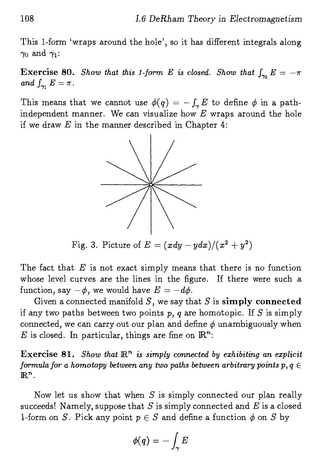
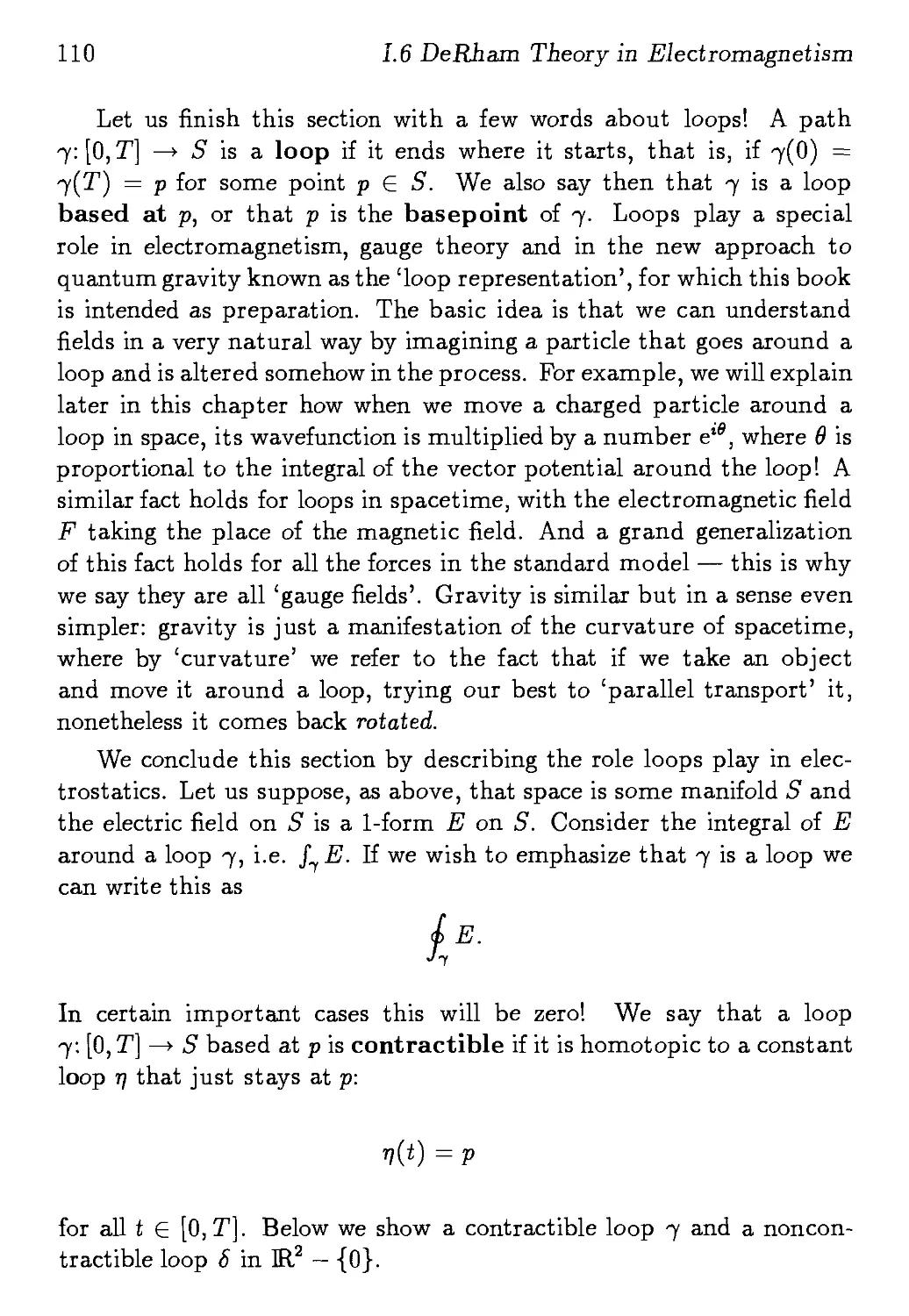
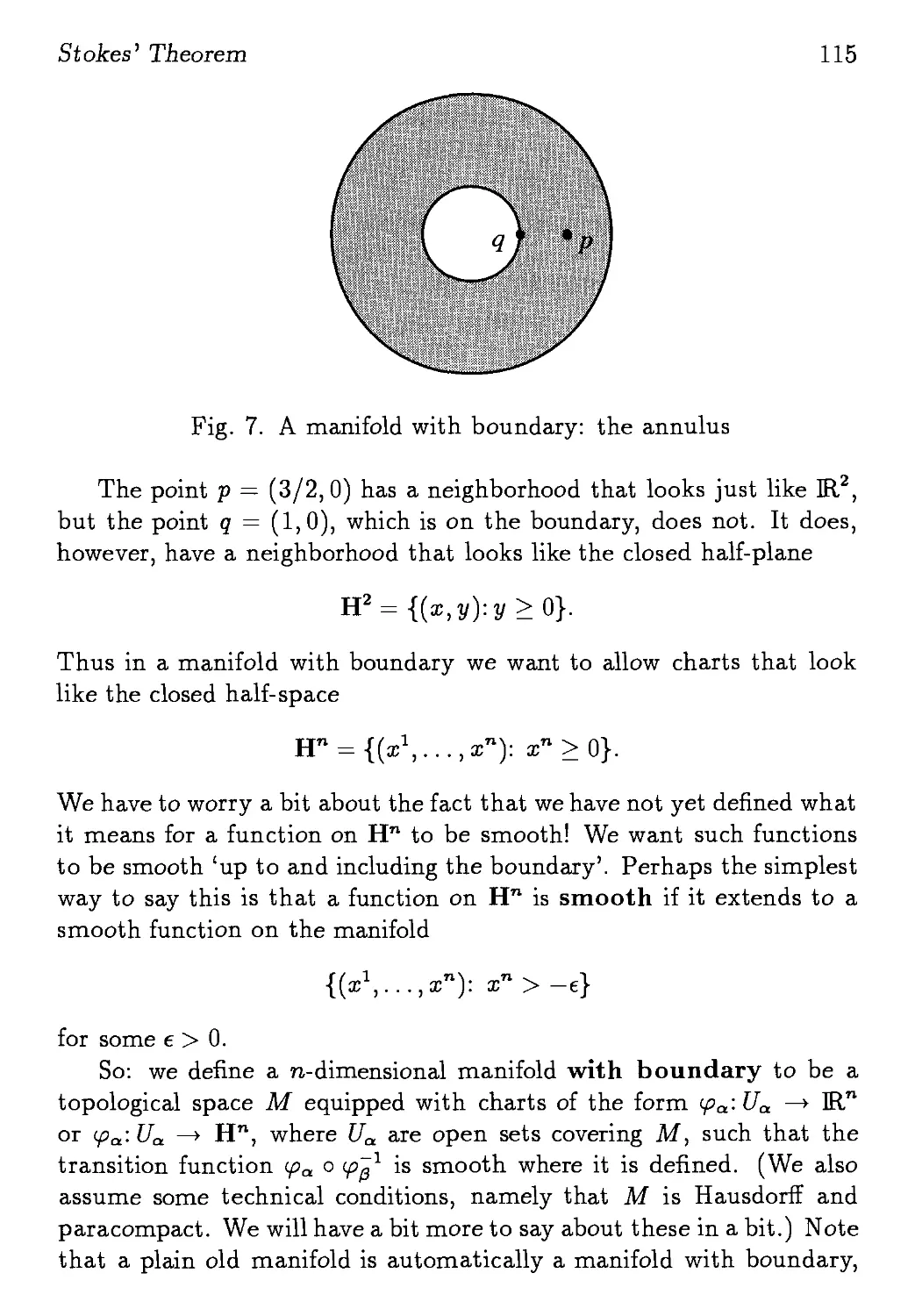
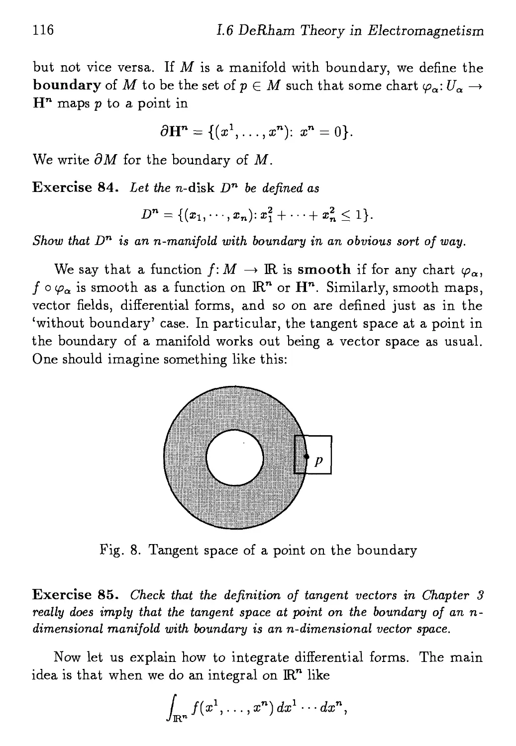
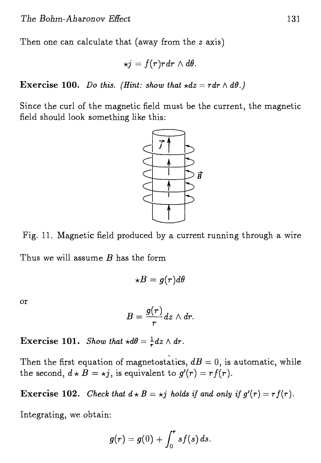
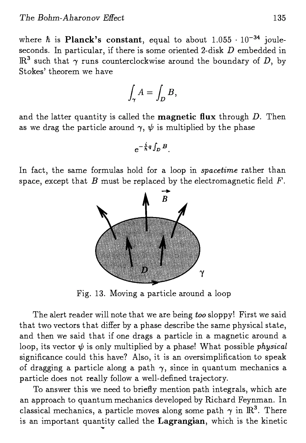
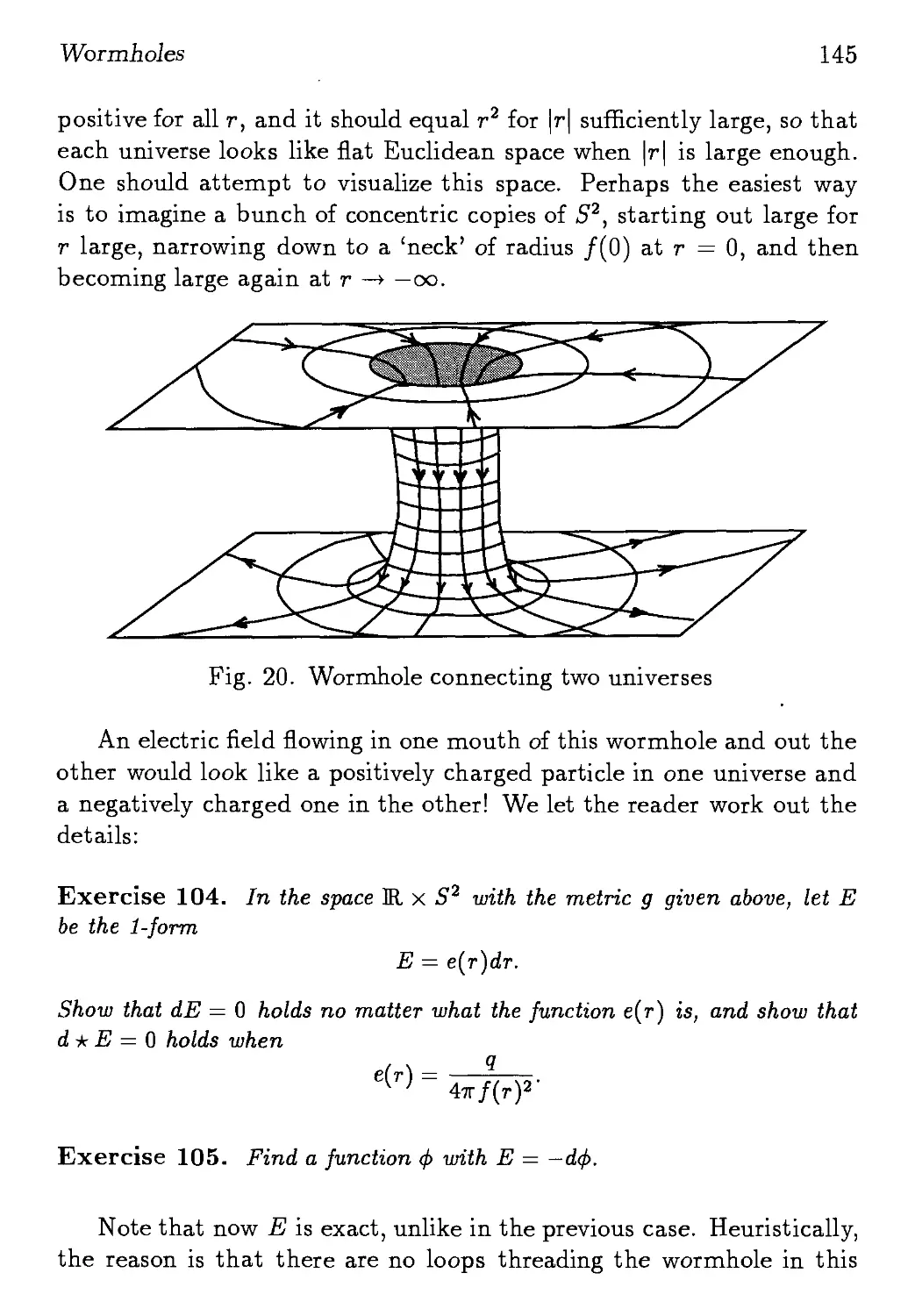
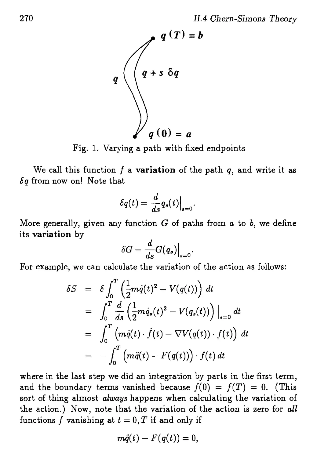
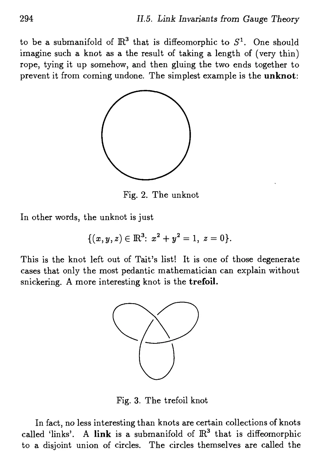
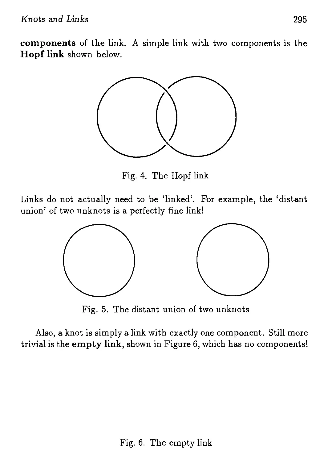
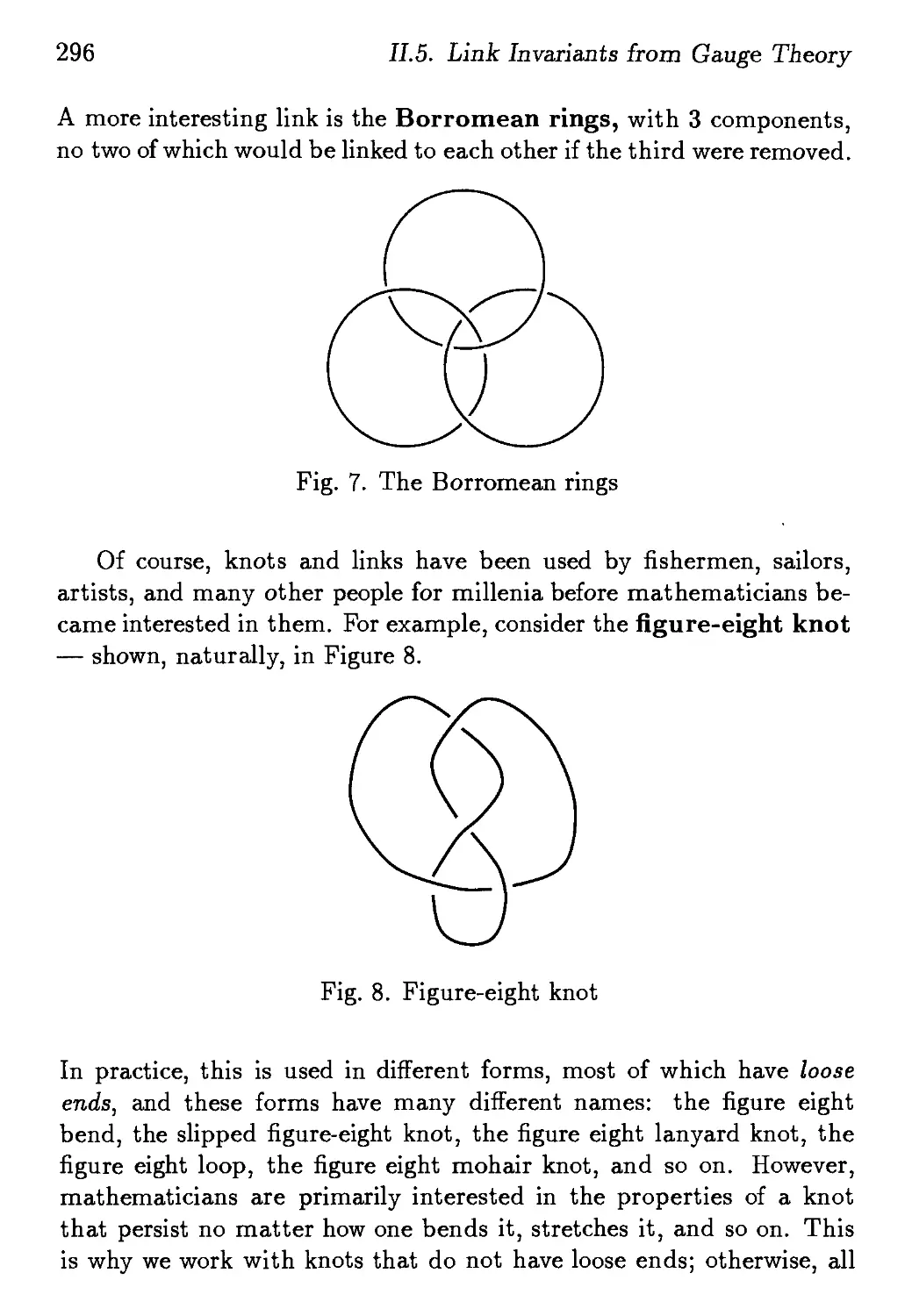
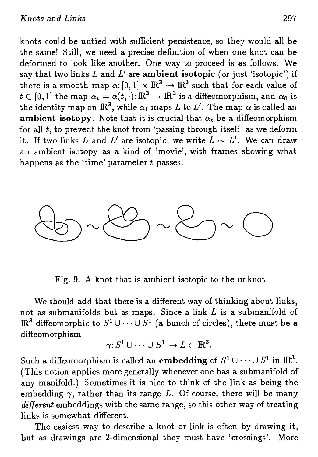
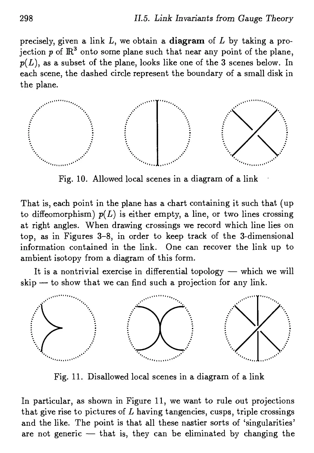
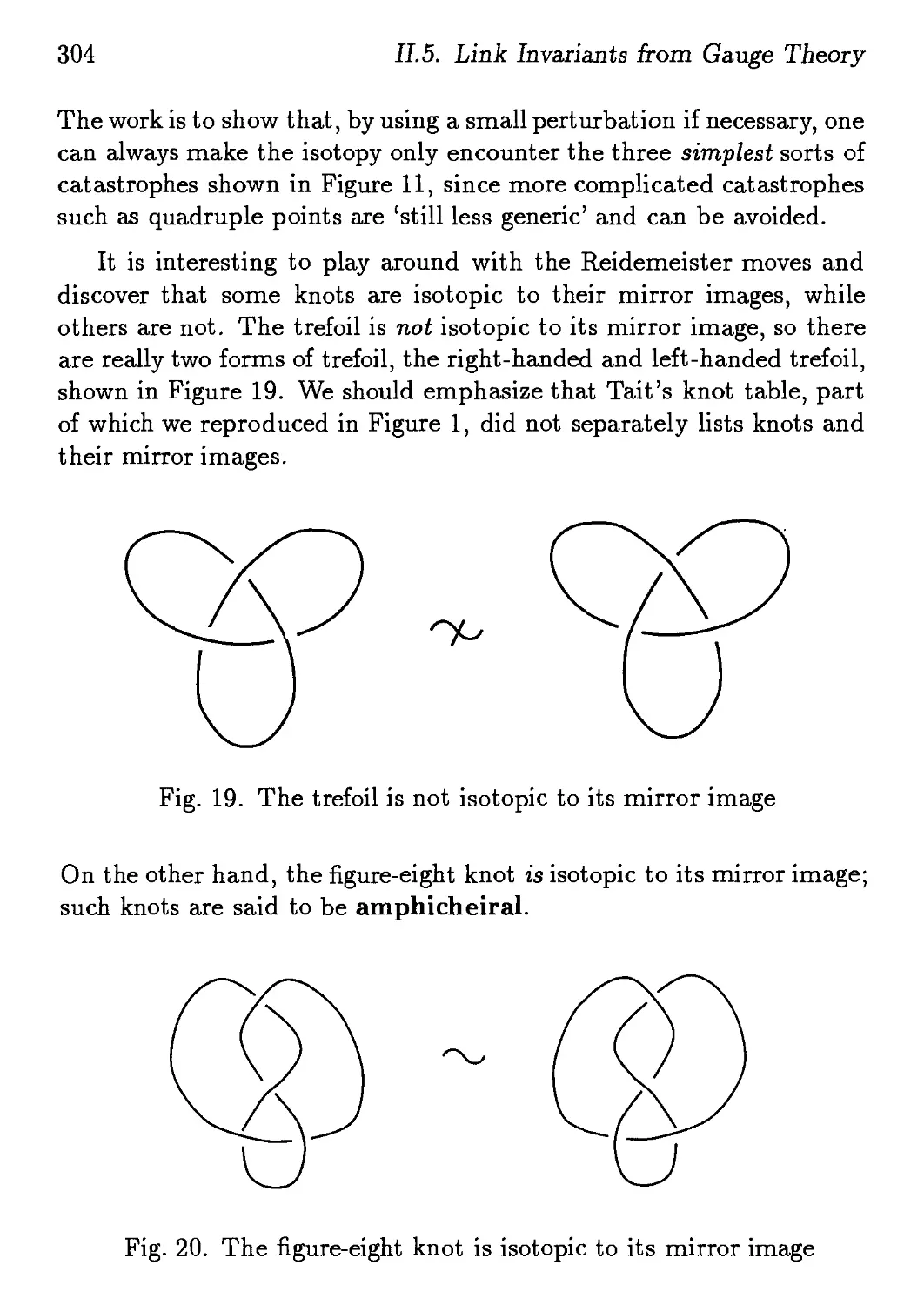
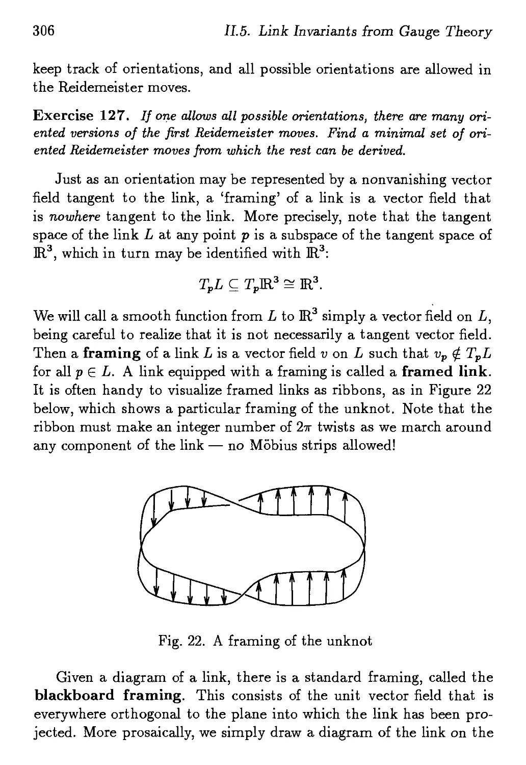
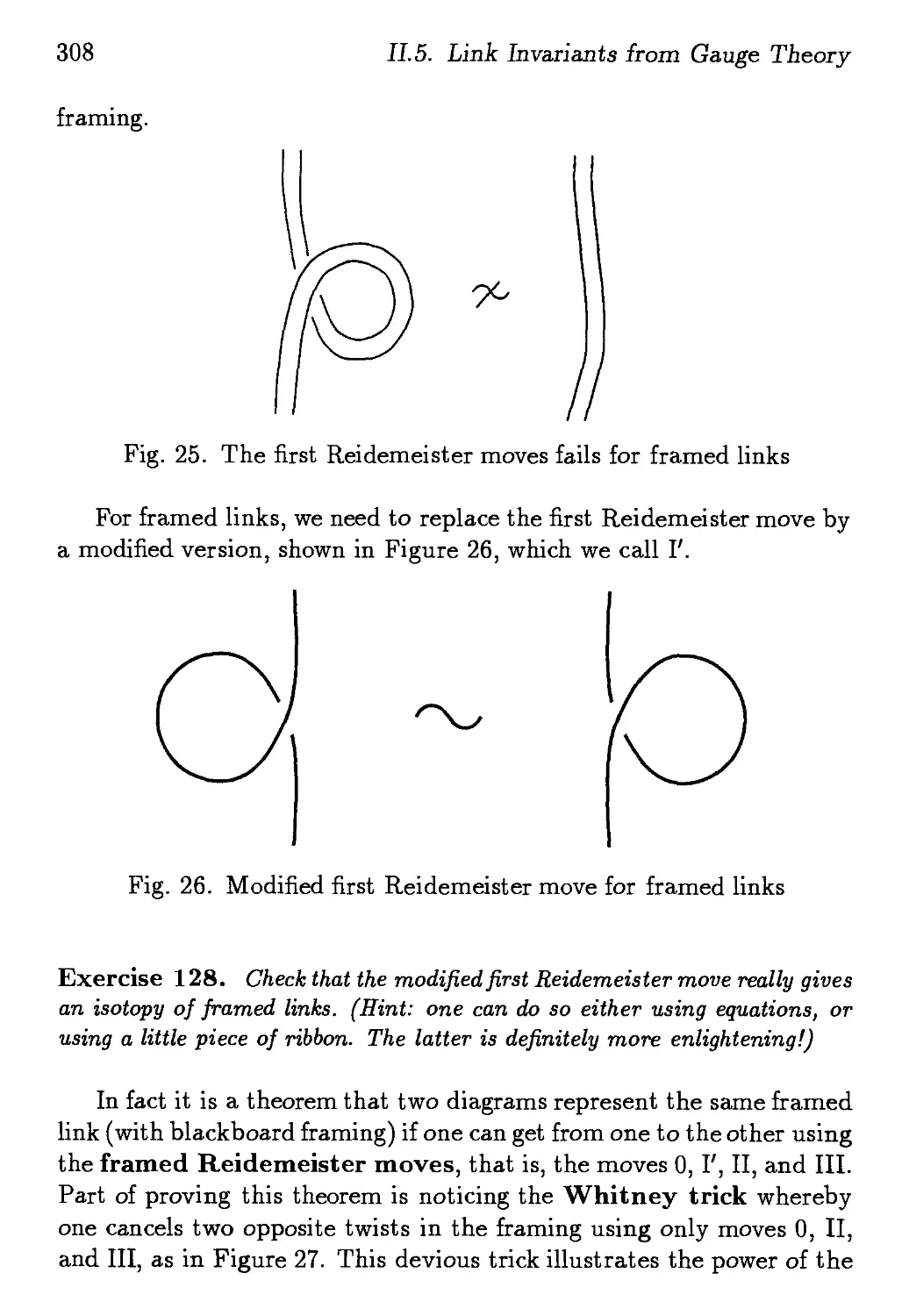
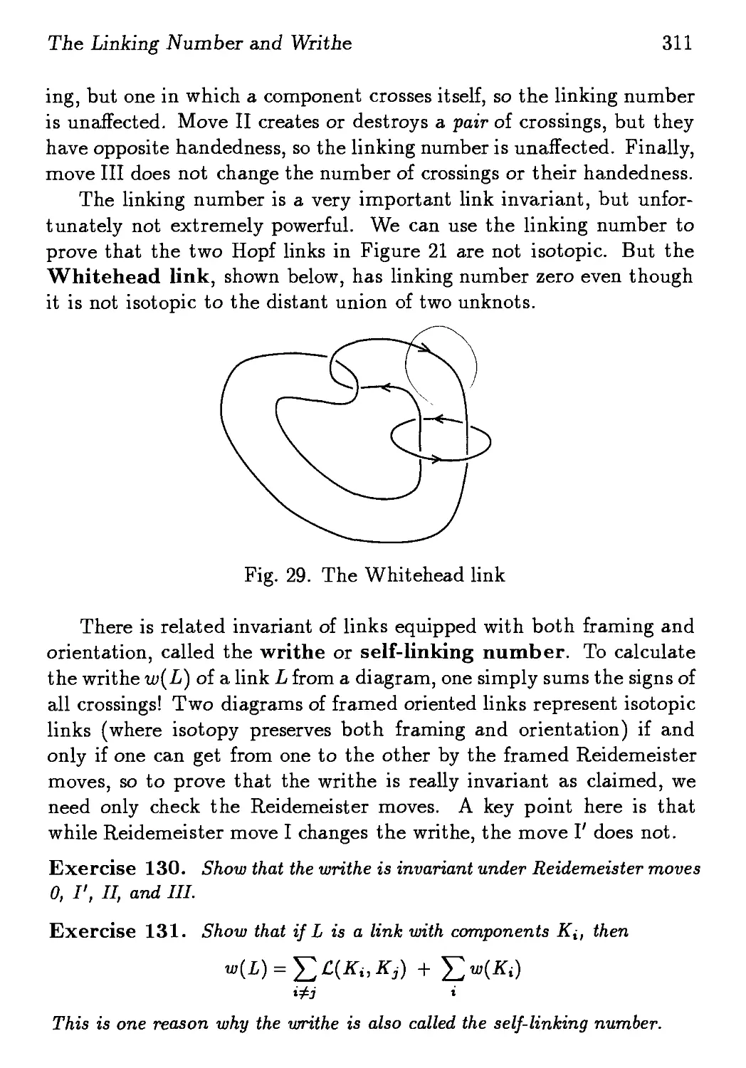
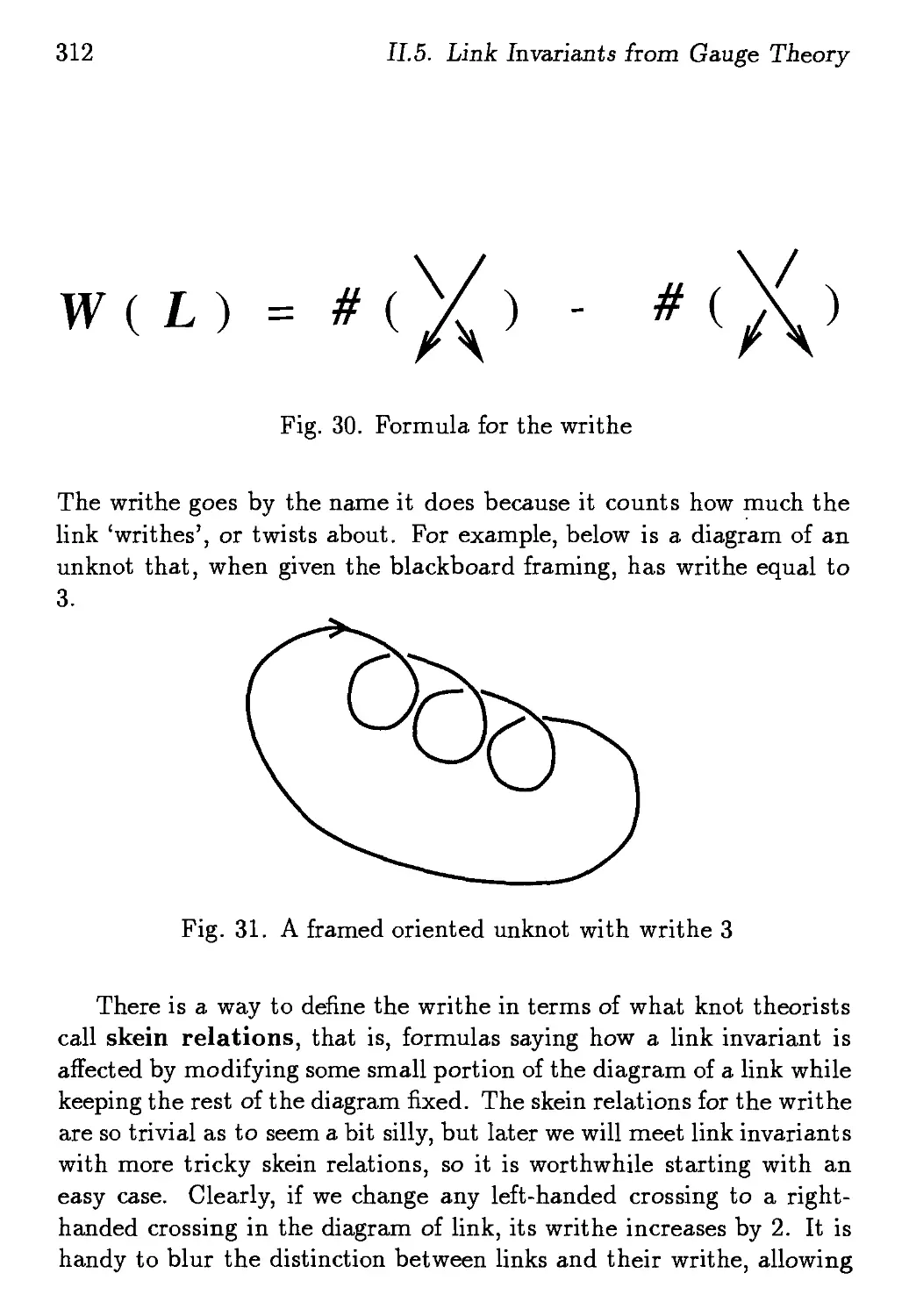
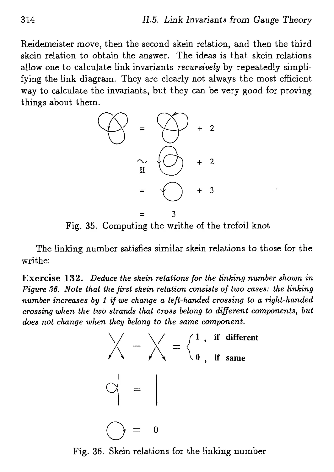
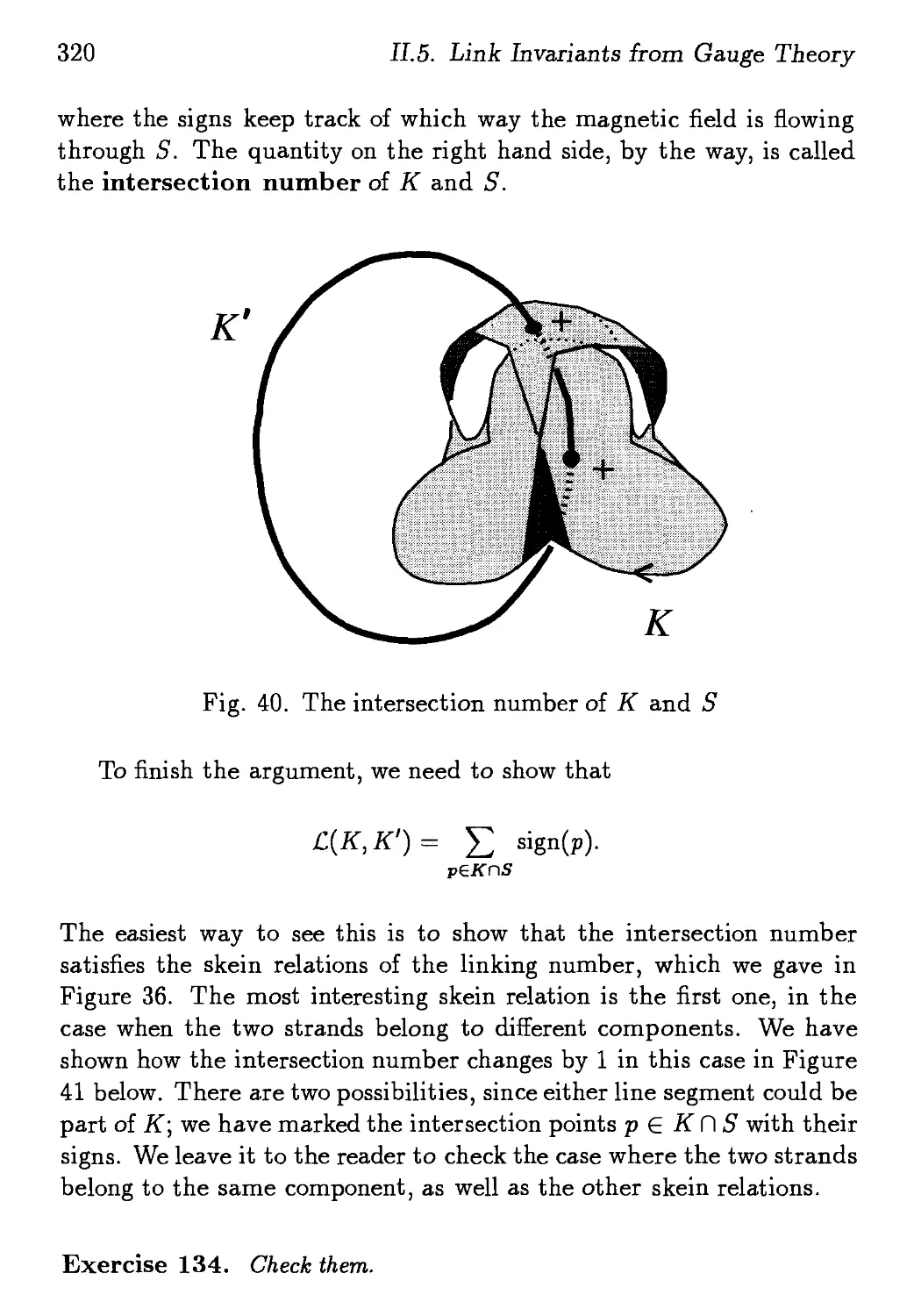
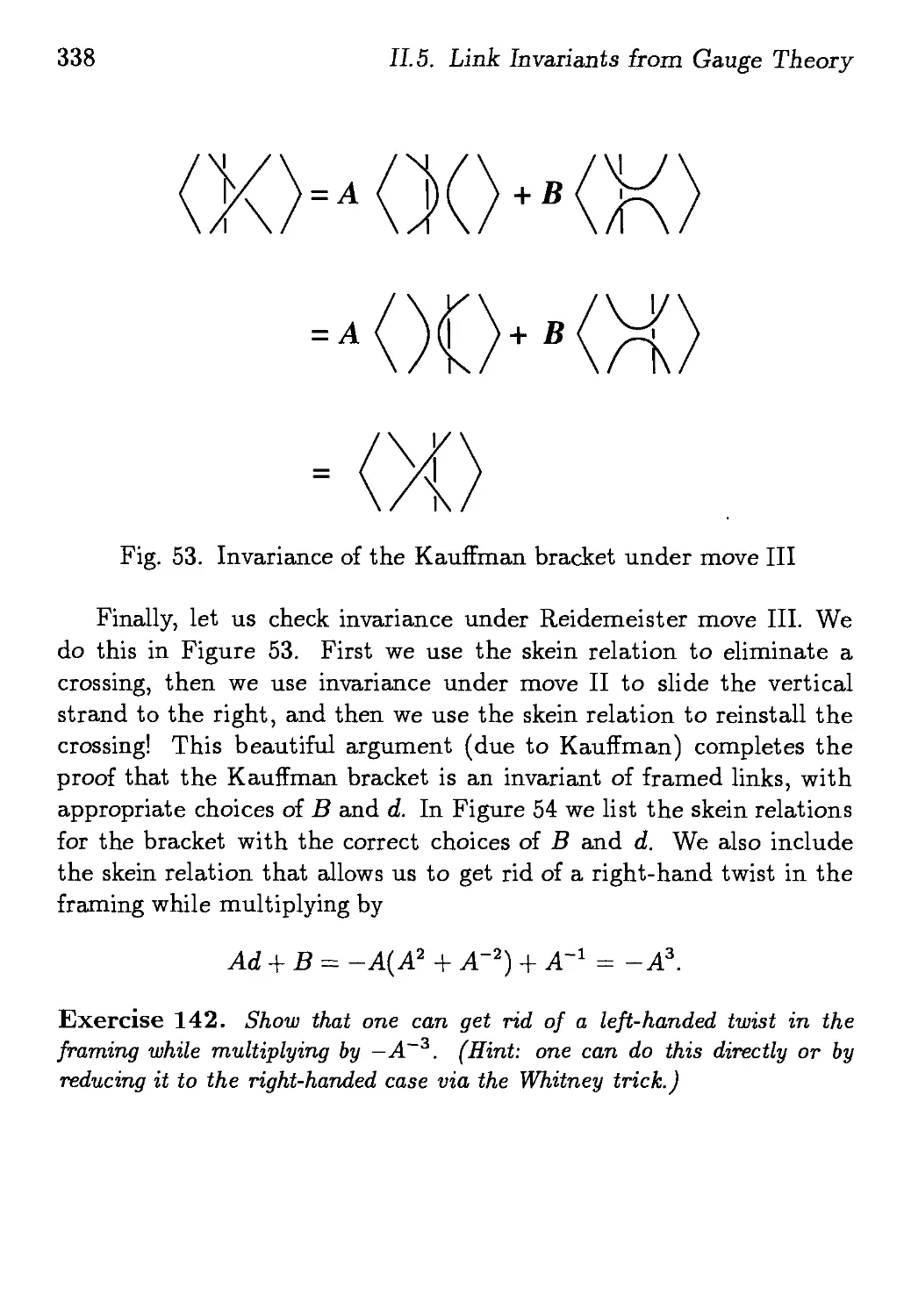
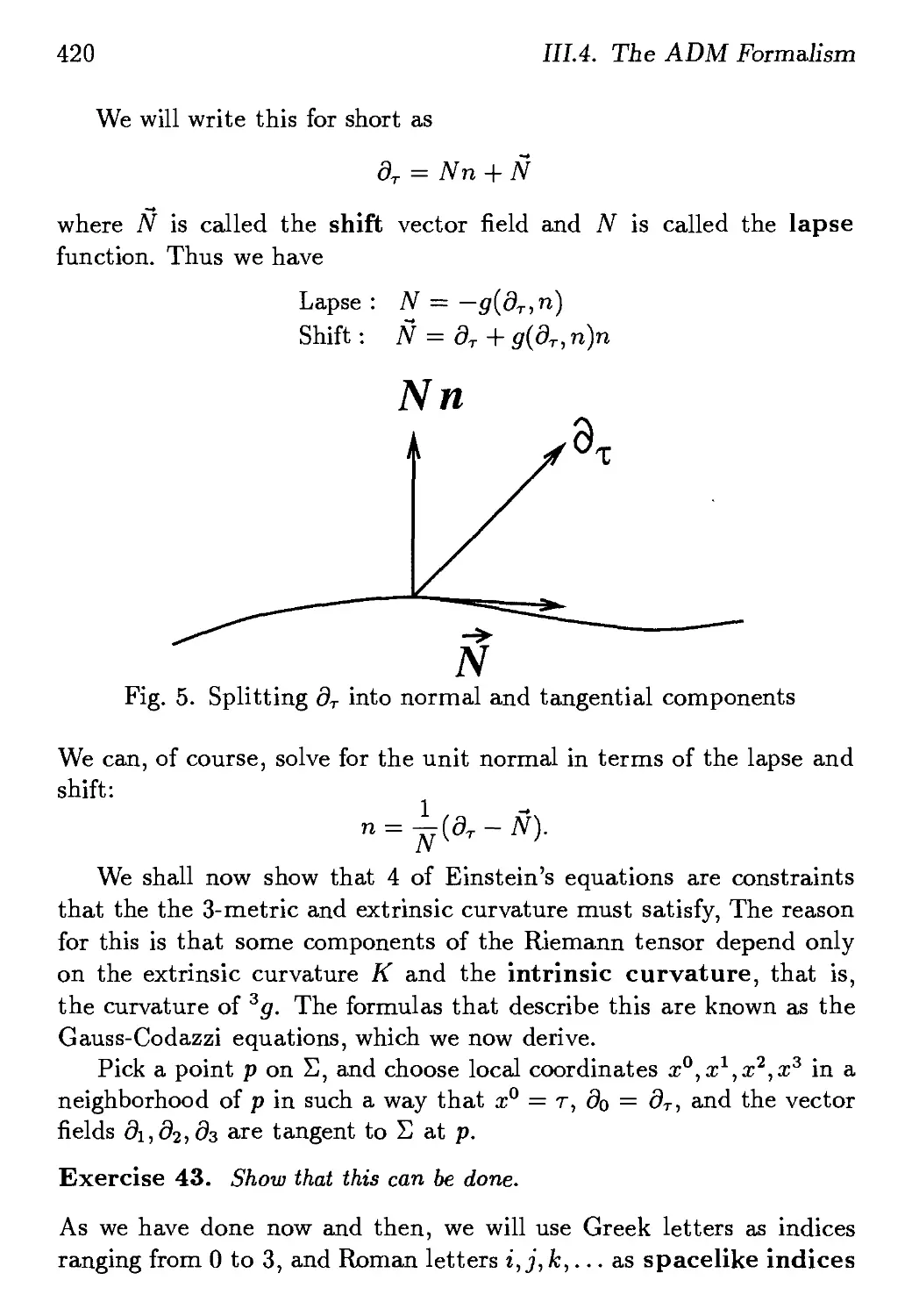
Text
KBE Series on Knots and Everything — Vol. 4
GAUGE FIELDS,
KNOTS AND GRAVITY
Johrt|Baez
Department of Mathematics
University of California
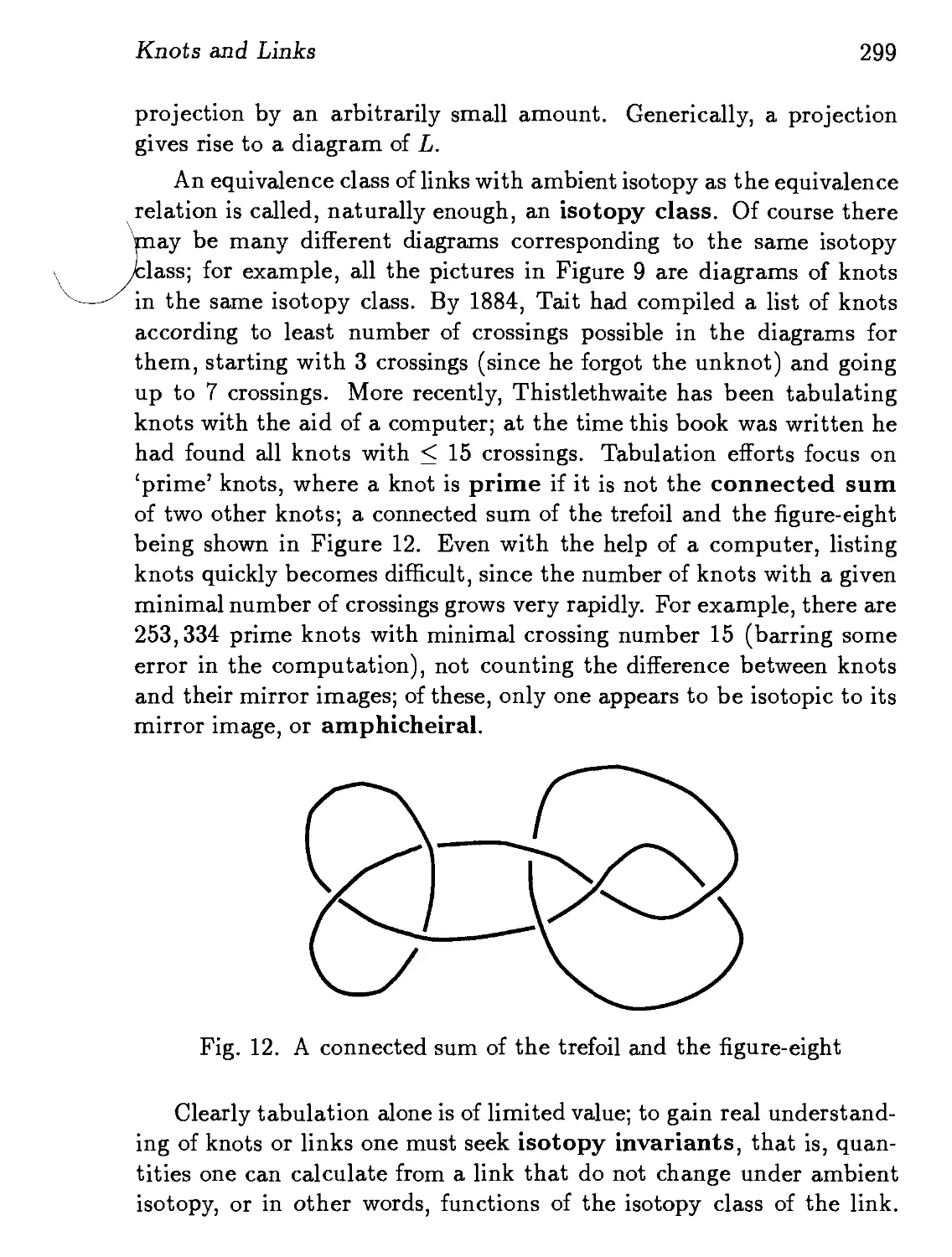
Riverside
Javier P. Muniain
Department of Physics
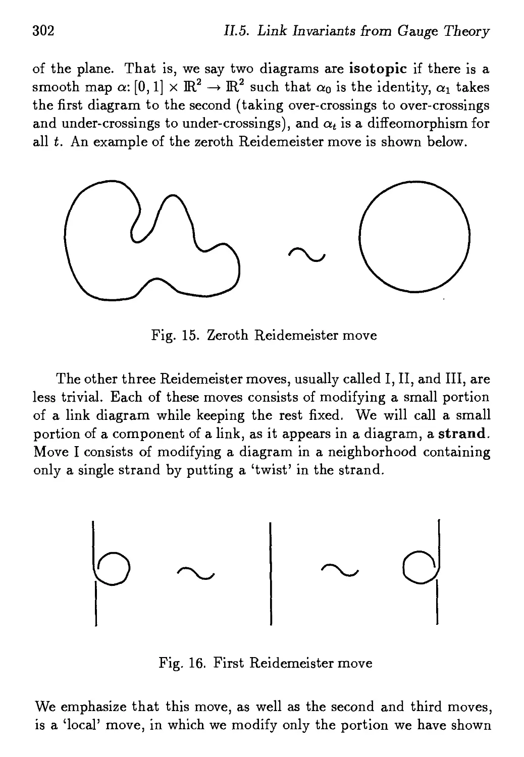
University of California
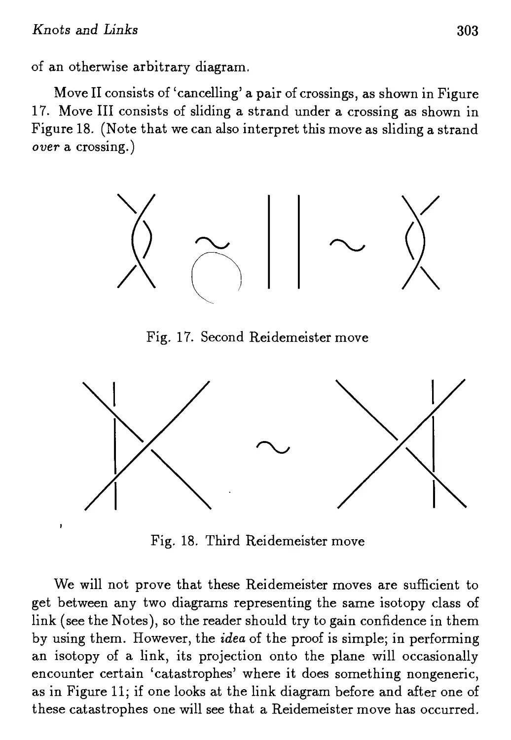
Riverside
№* World Scientific
™b Singapore • New Jersey • London • Hong Kong
Published by
World Scientific
P О Box 128, Fai
USA office: Suite rB, 1060 Main Street, River Edge, NJ 07661
UK office: 73 Lynton Mead, Totteridge, London N20 8DH
Library of Congress Cataloging-in-Publication Data
Baez, JohnC, 1961-
Gauge fields, knots, and gravity / John С Baez and Javier P.
Muniain.
p. cm. — (Series on knots and everything ; vol. 4)
Includes index.
ISBN 9810217293 -- ISBN 9810220340 (pbk)
1. Gauge fields (Physics) 2. Quantum gravity. 3. Knot theory.
4. General relativity (Physics) 5. Electromagnetism. I. Muniain,
Javier P. II. Title. III. Series: К & E series on knots and
everything ; vol. 4.
QC793 3.F5B33 1994
530.1'4-dc20 94-3438
CIP
Copyright © 1994 by World Scientific Publishing Co. Pte. Ltd.
All rights reserved. This book, or parts thereof, may not be reproduced in any form or by any means,
electronic or mechanical, including photocopying, recording or any information storage and
retrieval system now known or to be invented without written permission from the Publisher.
For photocopying of material in this volume, please pay a copying fee through the Copyright
Clearance Center, Inc., 27 Congress Street, Salem, MA 01970, USA.
Printed in Singapore by Uto-Print
To Our Parents
Preface
Two of the most exciting developments of 20th century physics were
general relativity and quantum theory, the latter culminating in the
'standard model' of particle interactions. General relativity treats grav-
gravity, while the standard model treats the rest of the forces of nature.
Unfortunately, the two theories have not yet been assembled into a
single coherent picture of the world. In particular, we do not have
a working theory of gravity that takes quantum theory into account.
Attempting to 'quantize gravity' has led to many fascinating develop-
developments in mathematics and physics, but it remains a challenge for the
21st century.
The early 1980s were a time of tremendous optimism concerning
string theory. This theory was very ambitious, taking as its guiding
philosophy the idea that gravity could be quantized only by unifying it
with all the other forces. As the theory became immersed in ever more
complicated technical issues without any sign of an immediate payoff in
testable experimental predictions, some of this enthusiasm diminished
among physicists. Ironically, at the same time, mathematicians found
string theory an ever more fertile source of new ideas. A particularly
appealing development to mathematicians was the discovery by Ed-
Edward Witten in the late 1980s that Chern-Simons theory — a quantum
field theory in 3 dimensions that arose as a spin-off of string theory
— was intimately related to the invariants of knots and links that had
recently been discovered by Vaughan Jones and others. Quantum field
theory and 3-dimensional topology have become firmly bound together
ever since, although there is much that remains mysterious about the
relationship.
While less popular than string theory, a seemingly very different ap-
vn
vim /'/<•/,и <¦
proach to quantum gravity also made" dramatic progress in the IMNOv
Abhay Ashtekar, Carlo Rovelli, Leo Srnolin and others discovered liovv
to rewrite general relativity in terms of 'new variables' so that it nmrc
closely resembled the other forces of nature, allowing them to apply
a new set of techniques to the problem of quantizing gravity. Tin"
philosophy of these researchers was far more conservative than that,
of the string theorists. Instead of attempting a 'theory of everything'
describing all forces and all particles, they attempted to understand
quantum gravity on its own, following as closely as possible tin" tradi-
traditional guiding principles of both general relativity and quantum theory.
Interestingly, they too were led to the study of knots and links. Indeed,
their approach is often known as the 'loop representation' of quantum
gravity. Furthermore, quantum gravity in 4 dimensions turned out to
be closely related to Chern-Simons theory in 3 dimensions. Again,
there is much that remains mysterious about this. For example, one
wonders why Chern-Simons theory shows up so prominently both in
string theory and the loop representation of quantum gravity. Perhaps
these two approaches are not as different as they seem!
It is the goal of this text to provide an elementary introduction to
some of these developments. We hope that both physicists who wish
to learn more differential geometry and topology, and mathematicians
who wish to learn more gauge theory and general relativity, williind this
book a useful place to begin. The main prerequisites are some familiar-
familiarity with electromagnetism, special relativity, linear algebra, and vector
calculus, together with some of that undefinable commodity known as
'mathematical sophistication'.
The book is divided into three parts that treat electromagnetism,
gauge theory, and general relativity, respectively. Part I of this book
introduces the language of modern differential geometry, and shows
how Maxwell's equations can be drastically simplified using this lan-
language. We stress the coordinate-free approach and the relevance of
global topological considerations in understanding such things as the
Bohm-Aharonov effect, wormholes, and magnetic monopoles. Part II
introduces the mathematics of gauge theory — fiber bundles, connec-
connections and curvature — and then introduces the Yang-Mills equation,
Chern classes, and Chern-Simons classes. It also includes a brief intro-
introduction to knot theory and its relation to Chern-Simons theory. Part
Preface
IX
III introduces the basic concepts of Riemannian and semi-Riemannian
geometry and then concentrates on topics in general relativity of spe-
special importance to quantum gravity: the Einstein-Hilbert and Palatini
formulations of the action principle for gravity, the ADM formalism,
and canonical quantization. Here we emphasize tensor computations
written in the notation used in general relativity. We conclude this part
with a sketch of Ashtekar's 'new variables' and the way Chern-Simons
theory provides a solution to the Wheeler-DeWitt equation (the basic
equation of canonical quantum gravity).
While we attempt to explain everything 'from scratch' in a self-
contained manner, we really hope to lure the reader into further study
of differential geometry, topology, gauge theory, general relativity and
quantum gravity. For this reason, we provide copious notes at the end
of each part, listing our favorite reading material on all these subjects.
Indeed, the reader who wishes to understand any of these subjects in
depth may find it useful to read some of these references in parallel
with our book. This is especially true because we have left out many
relevant topics in order to keep the book coherent, elementary, and
reasonable in size. For example, we have not discussed fermions (or
mathematically speaking, spinors) in any detail. Nor have we treated
principal bundles. Also, we have not done justice to the experimental
aspects of particle physics and general relativity, focusing instead upon
their common conceptual foundation in gauge theory. The reader will
thus have to turn to other texts to learn about such matters.
One really cannot learn physics or mathematics except by doing
it. For this reason, this text contains over 300 exercises. Of course,
far more exercises are assigned in texts than are actually done by the
readers. At the very least, we urge the reader to read and ponder the
exercises, the results of which are often used later on. The text also
includes 130 illustrations, since we wish to emphasize the geometrical
and topological aspects of modern physics. Terms appear in boldface
when they are defined, and all such definitions are referred to in the
index.
This book is based on the notes of a seminar on knot theory and
quantum gravity taught by J.B. at U, C. Riverside during the school
year 1992-1993. The seminar concluded with a conference on the sub-
subject, the proceedings of which will appear in a volume entitled Knots
X I'rrftu-r
and Quantum Gravity.
We would like to thank Louis Kauffman for inviting us to write this
book, and also Chris Lee and Ms. H. M. Ho of World Scientific for
helping us at every stage of the writing and publication process. We
also wish to express our thanks to Edward Heflin and Dardo D. Piriz
for reading parts of the manuscript and to Carl Yao for helping us with
some MgXcomplications. Scott Singer of the Academic Computing
Graphics and Visual Imaging Lab of the U. C. Riverside deserves special
thanks and recognition for helping us to create the book cover. Some
of the graphics used for the design of the cover were generated with
Mathematical by Wolfram Research, Inc.; these were kindly given to us
by Joe Grohens of WRI.
J.B. is indebted to many mathematicians and physicists for useful
discussions and correspondence, but he would particularly like to thank
Abhay Ashtekar, whose work has done so much to unify the study of
gauge fields, knots and gravity. He would also like to thank the readers
of the USENET physics and mathematics newsgroups, who helped in
many ways with the preparation of this book. He dedicates this book
to his parents, Peter and Phyllis Baez, with profound thanks for their
love. He also gives thanks and love to his mathematical muse, Lisa
Raphals.
J.M. dedicates this book to his parents, Luis and Crescencia Perez
de Muniain у Mohedano, for their many years of continued love and
support. He is grateful to Eleanor Anderson for being a patient and
inspiring companion during the long and hard hours taken to complete
this book. He also acknowledges Jose Wudka for many discussions on
quantum field theory.
Contents
Preface vii
I Electromagnetism
1 Maxwell's Equations
2 Manifolds
3 Vector Fields
4 Differential Forms
5 Rewriting Maxwell's Equations
6 DeRham Theory in Electromagnetism
Notes to Part I
II Gauge Fields
1 Symmetry
2 Bundles and Connections
3 Curvature and the Yang-Mills Equation
4 Chern-Simons Theorv
1
3
15
23
39
69
103
153
159
161
199
243
267
XI
xii
5 Link Invariants from Gauge Theory 291
Notes to Part II 353
III Gravity 363
1 Semi-Riemannian Geometry 365
2 Einstein's Equation 387
3 Lagrangians for General Relativity 397
4 The ADM Formalism 413
5 The New Variables 437
Notes to Part III 451
Index 457
Gauge Fields, Knots, and Gravity
Part I
Elect romagnet ism
Chapter 1
Maxwell's Equations
Our whole progress up to this point may be described as a gradual develop-
development of the doctrine of relativity of all physical phenomena. Position we
must evidently acknowledge to be relative, for we cannot describe the posi-
position of a body in any terms which do not express relation. The ordinary
language about motion and rest does not so completely exclude the notion of
their being measured absolutely, but the reason of this is, that in our ordi-
ordinary language we tacitly assume that the earth is at rest.... There are no
landmarks in space; one portion of space is exactly like every other portion,
so that we cannot tell where we are. We are, as it were, on an unruffled
sea, without stars, compass, sounding, wind or tide, and we cannot tell in
what direction we are going. We have no log which we can case out to take
a dead reckoning by; we may compute our rate of motion with respect to the
neighboring bodies, but we do not know how these bodies may be moving in
space. - James Clerk Maxwell, 1876.
Starting with Maxwell's beautiful theory of electromagnetism, and
inspired by it, physicists have made tremendous progress in under-
understanding the basic forces and particles constituting the physical world.
Maxwell showed that two seemingly very different forces, the electric
and magnetic forces, were simply two aspects of the 'electromagnetic
field' . In so doing, he was also able to explain light as a phenomenon
in which ripples in the electric field create ripples in the magnetic field,
which in turn create new ripples in the electric field, and so on. Shock-
Shockingly, however, Maxwell's theory also predicted that light emitted by a
moving body would travel no faster than light from a stationary body.
4 I.I Maxwell's Equations
Eventually this led Lorentz, Poincare and especially Einstein to realize
that our ideas about space and time had to be radically revised. That
the motion of a body can only be measured relative to another body
had been understood to some extent since Galileo. Taken in conjunc-
conjunction with Maxwell's theory, however, this principle forced the recogni-
recognition that in addition to the rotational symmetries of space there must
be symmetries that mingle the space and time coordinates. These new
symmetries also mix the electric and magnetic fields, charge and cur-
current, energy and momentum, and so on, revealing the world to be much
more coherent and tightly-knit than had previously been suspected.
There are, of course, forces in nature besides electromagnetism, the
most obvious of which is gravity. Indeed, it was the simplicity of gravity
that gave rise the first conquests of modern physics: Kepler's laws of
planetary motion, and then Newton's laws unifying celestial mechanics
with the mechanics of falling bodies. However, reconciling the sim-
simplicity of gravity with relativity theory was no easy task! In seeking
equations for gravity consistent with his theory of special relativity,
Einstein naturally sought to copy the model of Maxwell's equations.
However, the result was not merely a theory in which ripples of some
field propagate through spacetime, but a theory in which the geometry
of spacetime itself ripples and bends. Einstein's equations say, roughly,
that energy and momentum affect the metric of spacetime (whereby
we measure time and distance) much as charges and currents affect
the electromagnetic field. This served to heighten hopes that much or
perhaps even all of physics is fundamentally geometrical in character.
There were, however, severe challenges to these hopes. Attempts by
Einstein, Weyl, Kaluza and Klein to further unify our description of the
forces of nature using ideas from geometry were largely unsuccessful.
The reason is that the careful study of atoms, nuclei and subatomic
particles revealed a wealth of phenomena that do not fit easily into any
simple scheme. Each time technology permitted the study of smaller
distance scales (or equivalently, higher energies), new puzzles arose. In
part, the reason is that physics at small distance scales is completely
dominated by the principles of quantum theory. The naive notion that
a particle is a point tracing out a path in spacetime, or that a field
assigns a number or vector to each point of spacetime, proved to be
wholly inadequate, for one cannot measure the position and velocity
Maxwell's Equations 5
of a particle simultaneously with arbitrary accuracy, nor the value of a
field and its time derivative. Indeed, it turned out that the distinction
between a particle and field was somewhat arbitrary. Much of 20th cen-
century physics has centered around the task of making sense of microworld
and developing a framework with which one can understand subatomic
particles and the forces between them in the light of quantum theory.
Our current picture, called the standard model, involves three forces:
electromagnetism and the weak and strong nuclear forces. These are
all 'gauge fields', meaning that they are described by equations closely
modelled after Maxwell's equations. These equations describe quantum
fields, so the forces can be regarded as carried by particles: the elec-
electromagnetic force is carried by the photon, the weak force is carried by
the W and Z particles, and the strong force is carried by gluons. There
are also charged particles that interact with these force-carrying par-
particles. By 'charge' here we mean not only the electric charge but also
its analogs for the other forces. There are two main kinds of charged
particles, quarks (which feel the strong force) and leptons (which do
not). All of these charged particles have corresponding antiparticles of
the same mass and opposite charge.
Somewhat mysteriously, the charged particles come in three fami-
families or 'generations'. The first generation consists of two leptons, the
electron e and the electron neutrino ue, and two quarks, the up and
down, or и and d. Most of the matter we see everyday is made out
of these first-generation particles. For example, according to the stan-
standard model the proton is a composite of two up quarks and one down,
while the neutron is two downs and an up. There is a second genera-
generation of quarks and leptons, the muon /x and muon neutrino u^, and the
charmed and strange quarks c, s. For the most part these are heavier
than the corresponding particles in the first generation, although all
the neutrinos appear to be massless or nearly so. For example, the
muon is about 207 times as massive as the electron, but almost iden-
identical in every other respect. Then there is a third, still more massive
generation, containing the tau т and tau neutrino vT, and the top and
bottom quarks t and b. For many years the top quark was merely con-
conjectured to exist, but just as this book went to press, experimentalists
announced that it may finally have been found.
Finally, there is a very odd charged particle in the standard model,
6 LI Maxwell's Equations
the Higgs particle, which is neither a quark nor a lepton. This has not
been observed either, and is hypothesized to exist primarily to explain
the relation between the elecromagnetic and weak forces.
Even more puzzling than all the complexities of the standard model,
however, is the question of where gravity fits into the picture! Einstein's
equations describing gravity do not take quantum theory into account,
and it has proved very difficult to 'quantize' them. We thus have not
one picture of the world, but two: the standard model, in which all
forces except gravity are described in accordance with quantum the-
theory, and general relativity, in which gravity alone is described, not in
accordance with quantum theory. Unfortunately it seems difficult to
obtain guidance from experiment; simple considerations of dimensional
analysis suggest that quantum gravity effects may become significant
at distance scales comparable to the Planck length,
lp = (Й/с/с3I/2,
where h is Planck's constant, к is Newton's gravitational constant, and
с is the speed of light. The Planck length is about 1.616 • 10~35 meters,
far below the length scales we can probe with particle accelerators.
Recent developments, however, hint that gravity may be closer
to the gauge theories of the standard model than had been thought.
Fascinatingly, the relationship also involves the study of knots in 3-
dimensional space. While this work is in its early stages, and may
not succeed as a theory of physics, the new mathematics involved is
so beautiful that it is difficult to resist becoming excited. Unfortu-
Unfortunately, understanding these new ideas depends on a thorough mastery
of quantum field theory, general relativity, geometry, topology, and al-
algebra. Indeed, it is almost certain that nobody is sufficiently prepared
to understand these ideas fully! The reader should therefore not expect
to understand them when done with this book. Our goal in this book
is simply to start fairly near the beginning of the story and bring the
reader far enough along to see the frontiers of current research in dim
outline.
We must begin by reviewing some geometry. These days, when
mathematicians speak of geometry they are usually referring not to
Euclidean geometry but to the many modern generalizations that fall
Maxwell's Equations 7
under the heading of 'differential geometry'. The first theory of physics
to explicitly use differential geometry was Einstein's general relativity,
in which gravity is explained as the curvature of spacetime. The gauge
theories of the standard model are of a very similar geometrical charac-
character (although quantized). But there is also a lot of differential geometry
lurking in Maxwell's equations, which after all were the inspiration for
both general relativity and gauge theory. So, just as a good way to
master auto repair is to take apart an old car and put in a new engine
so that it runs better, we will begin by taking apart Maxwell's equations
and putting them back together using modern differential geometry.
In their classic form, Maxwell's equations describe the behavior of
two vector fields, the electric field E and the magnetic field B.
These fields are defined throughout space, which is taken to be Ш.3.
However, they are also functions of time, a real-valued parameter t.
The electric and magnetic fields depend on the electric charge density
p, which is a time-dependent function on space, and also on the electric
current density J*, which is time-dependent vector field on space. (For
the mathematicians, let us note that unless otherwise specified, func-
functions are assumed to be real-valued, and functions and vector fields on
Ш." are assumed to be smooth, that is, infinitely differentiable.)
In units where the speed of light is equal to 1, Maxwell's equa-
equations are:
= 0
= 0
= P
= 3-
There are a number of interesting things about these equations that
are worth understanding. First, there is the little fact that we can only
determine the direction of the magnetic field experimentally if we know
the difference between right and left. This is easiest to see from the
Lorentz force law, which says that the force on a charged particle
with charge q and velocity v is
F = q (Ё + v x B).
хЁ
xB
V
+
V
—
в
дВ
~~dt
¦ Ё
дЁ
~dt
8 I.I Maxwell's Equations
To measure E, we need only measure the force F on a static particle
and divide by q. To figure out B, we can measure the force on charged
particles with a variety of velocities. However, recall that the definition
of the cross product involves a completely arbitrary right-hand rule!
We typically define
v x В = (vyBz — vzBy,vzBx —vxBz,vxBy — vyBx).
However, this is just a convention; we could have set
v x В = (vzBy — vyBz, vxBz — vzBxvyBx — vxBy),
j
and all the mathematics of cross products would work just as well.
If we used this 'left-handed cross product' when figuring out В from
measurements of F for various velocities v, we would get an answer
for В with the opposite of the usual sign! It may seem odd that В
depends on an arbitrary convention this way. In fact, this turns out
to be an important clue as to the mathematical structure of Maxwell's
equations.
Secondly, Maxwell's equations naturally come in two pairs. The
pair that does not involve the electric charge and current densities
V-5 = 0 V x ??+ — = 0,
at
looks very much like the pair that does:
дЁ
V-E = p V x Я - — = j*.
at
Note the funny minus sign in the second pair. The symmetry is clear-
clearest in the vacuum Maxwell equations, where the charge and current
densities vanish:
= 0,
at
V x 5-—- = 0.
at
Maxwell's Equations 9
Then the transformation
Вь^Ё, Ё ^-В
takes the first pair of equations to the second and vice versa! This
symmetry is called duality and is a clue that the electric and magnetic
fields are part of a unified whole, the electromagnetic field. Indeed, if
we introduce a complex-valued vector field
? = E + iB,
duality amounts to the transformation
? и-> — i?,
and the vacuum Maxwell equations boil down to two equations for ?:
V-? = 0, Vx? = i4
ot
This trick has very practical applications. For example, one can use it
to find solutions that correspond to plane waves moving along at the
speed of light, which in the units we are using equals 1.
Exercise 1. Let к be a vector in Ж.3 and let ш = \k\. Fix E ? (C3 with
к ¦ E = 0 and к х Е = iwE. Show that
?{t, x) = Ё е-И-М
satisfies the vacuum Maxwell equations.
The symmetry between E and В does not, however, extend to the
non-vacuum Maxwell equations. We can consider making p and J*com-
J*complex, and writing down:
V-? = p, Vx? = i(+j).
However, this amounts to introducing magnetic charge and current den-
density, since if we split p and J*into real and imaginary parts, we see that
10 I.I Maxwell's Equations
the imaginary parts play the role of magnetic charge and current den-
densities:
P = Pe+ ipm,
3 = Je +ij"m.
We get
Vxit? =
WE = pe VxB- — =?e.
at
These equations are quite charming, but unfortunately no magnetic
charges — so called magnetic monopoles — have been observed!
(We will have a bit more to say about this in Chapter 6.) We could
simply keep these equations and say that p and J* are real-valued on
the basis of experimental evidence. But it is a mathematical as well
as a physical challenge to find a better way of understanding this phe-
phenomenon. It turns out that the formalism of gauge theory makes it
seem quite natural.
Finally, there is the connection between Maxwell's equations and
special relativity. The main idea of special relativity is that in addition
to the symmetries of space (translations and rotations) and time (trans-
(translations) there are equally important symmetries mixing space and time,
the Lorentz transformations. The idea is that if you and I are both un-
accelerated, so that my velocity with respect to you is constant, the
coordinates I will naturally use, in which I am at rest, will differ from
yours, in which you are at rest. If your coordinate system is (t,x,y, z)
and I am moving with velocity v in the x direction with respect to you,
for example, the coordinates in which I am at rest are given by
t' = (cosh </>)i — (sinh ф)х
x = —(sinh </>)i + (cosh ф)х
у' = у
z' =
where ф is a convenient quantity called the rapidity, defined so that
tanh ф = v. Note the close resemblance to the formula for rotations in
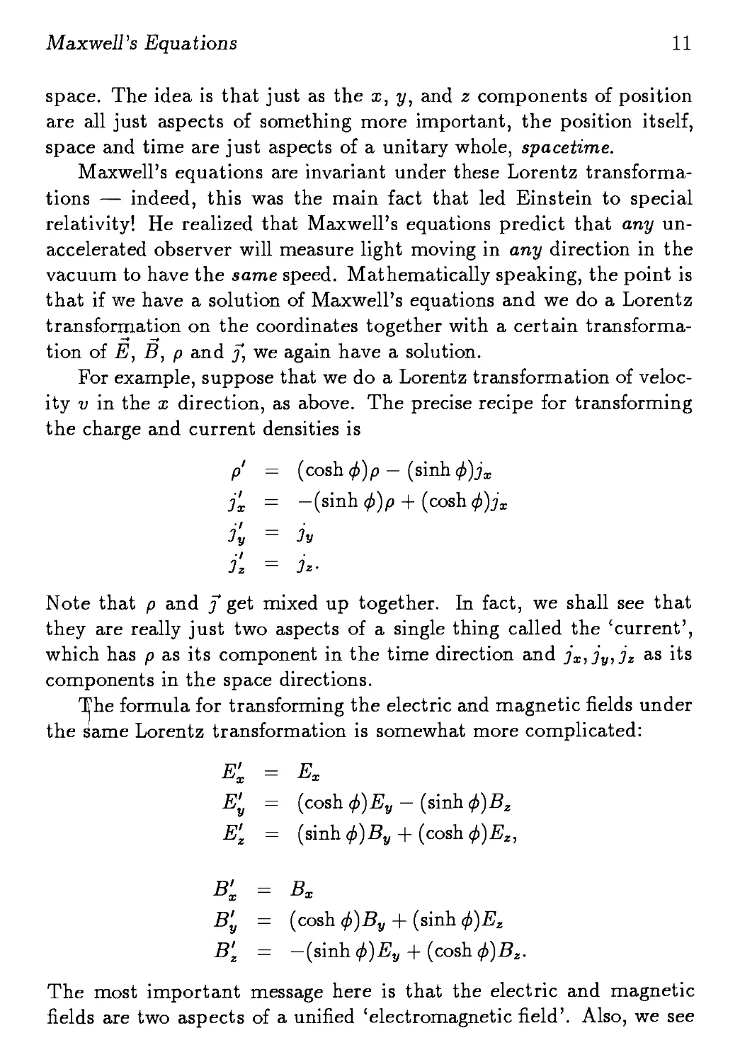
Maxwell's Equations 11
space. The idea is that just as the x, y, and z components of position
are all just aspects of something more important, the position itself,
space and time are just aspects of a unitary whole, spacetime.
Maxwell's equations are invariant under these Lorentz transforma-
transformations — indeed, this was the main fact that led Einstein to special
relativity! He realized that Maxwell's equations predict that any un-
accelerated observer will measure light moving in any direction in the
vacuum to have the same speed. Mathematically speaking, the point is
that if we have a solution of Maxwell's equations and we do a Lorentz
transformation on the coordinates together with a certain transforma-
transformation of E, В, p and f, we again have a solution.
For example, suppose that we do a Lorentz transformation of veloc-
velocity v in the x direction, as above. The precise recipe for transforming
the charge and current densities is
p = (cosh ф)р — (sinh ф)]х
j'x = —(sinh ф)р + (cosh (f)jx
j'y = 3v
?. = 3*.
Note that p and f get mixed up together. In fact, we shall see that
they are really just two aspects of a single thing called the 'current',
which has p as its component in the time direction and jx,jy,jz as its
components in the space directions.
The formula for transforming the electric and magnetic fields under
the Same Lorentz transformation is somewhat more complicated:
К = Ex
E'y = (cosh ф)Еу - (sinh ф)Вг
E'z = (sinh ф)Ву + (cosh ф)Ег,
B'x = Bx
By = (cosh ф)Ву + (sinh ф)Ег
B'z = -(sinh ф)Еу + (cosh ф)Вг.
The most important message here is that the electric and magnetic
fields are two aspects of a unified 'electromagnetic field'. Also, we see
12 I.I Maxwell's Equations
that the electromagnetic field is more complicated in character than
the current, since it has six independent components that transform in
a more subtle manner. It turns out to be a '2-form'.
When we have rewritten Maxwell's equations using the language
of differential geometry, all the things we have just discussed will be
much clearer — at least if we succeed in explaining things well. The
key step, which is somewhat shocking to the uninitiated, is to work
as much as possible in a manner that does not require a choice of
coordinates. After all, as far as we can tell, the world was not drawn
on graph paper. Coordinates are merely something we introduce for
our own convenience, and the laws of physics should not care which
coordinates we happen to use. If we postpone introducing coordinates
until it is actually necessary, we will not have to do anything to show
that Maxwell's equations are invariant under Lorentz transformations;
it will be manifest.
Just for fun, let us write down the new version of Maxwell's equa-
equations right away. We will explain what they mean quite a bit later, so
do not worry if they are fairly cryptic. They are:
dF = 0
-kd-kF = J.
Here F is the 'electromagnetic field' and J is the 'current', while the d
and * operators are slick ways of summarizing all the curls, divergences
and time derivatives that appear in the old-fashioned version. The
equation dF = 0 is equivalent to the first pair of Maxwell's equations,
while the equation -kd-k F = J is equivalent to the second pair. The
'funny minus sign' in the second pair will turn out to be a natural
consequence of how the * operator works.
If the reader is too pragmatic to get excited by the terse beauty
of this new-fangled version of Maxwell's equations, let us emphasize
that this way of writing them is a warm-up for understanding gauge
theory, and allows us to study Maxwell's equations and gauge theory on
curved spacetimes, as one needs to in general relativity. Indeed, we will
start by developing enough differential geometry to do a fair amount of
physics on general spacetimes. Then we will come back to Maxwell's
equations. We warn the reader that the next few sections are not really
Maxwell's Equations 13
a solid course in differential geometry. Whenever something is at all
tricky to prove we will skip it! The easygoing reader can take some
facts on faith; the careful reader may want to get ahold of a good book
on differential geometry to help fill in these details. Some suggestions
on books appear in the notes at the end of Part I.
Chapter 2
Manifolds
We therefore reach this result: In the general theory of relativity, space
and iime cannot be defined in such a way that differences of the spatial co-
coordinates can be directly measured by the unit measuring-rod, or differences
in the time co-ordinate by a standard clock.
The method hitherto employed for laying co-ordinates into the space-
time continuum in a definite manner thus breaks down, and there seems to
be no other way which would allow us to adapt systems of co-ordinates to
the four-dimensional universe so that we might expect from their application
a particularly simple formulation of the laws of nature. So there is nothing
for it but to regard all imaginable systems of co-ordinates, on principle, as
equally suitable for the description of nature. This comes to requiring that:
The general laws of nature are to be expressed by equations which hold
good for all systems of co-ordinates, that is, are co-variant with respect to
any substitutions whatever (generally covariant). — Albert Einstein
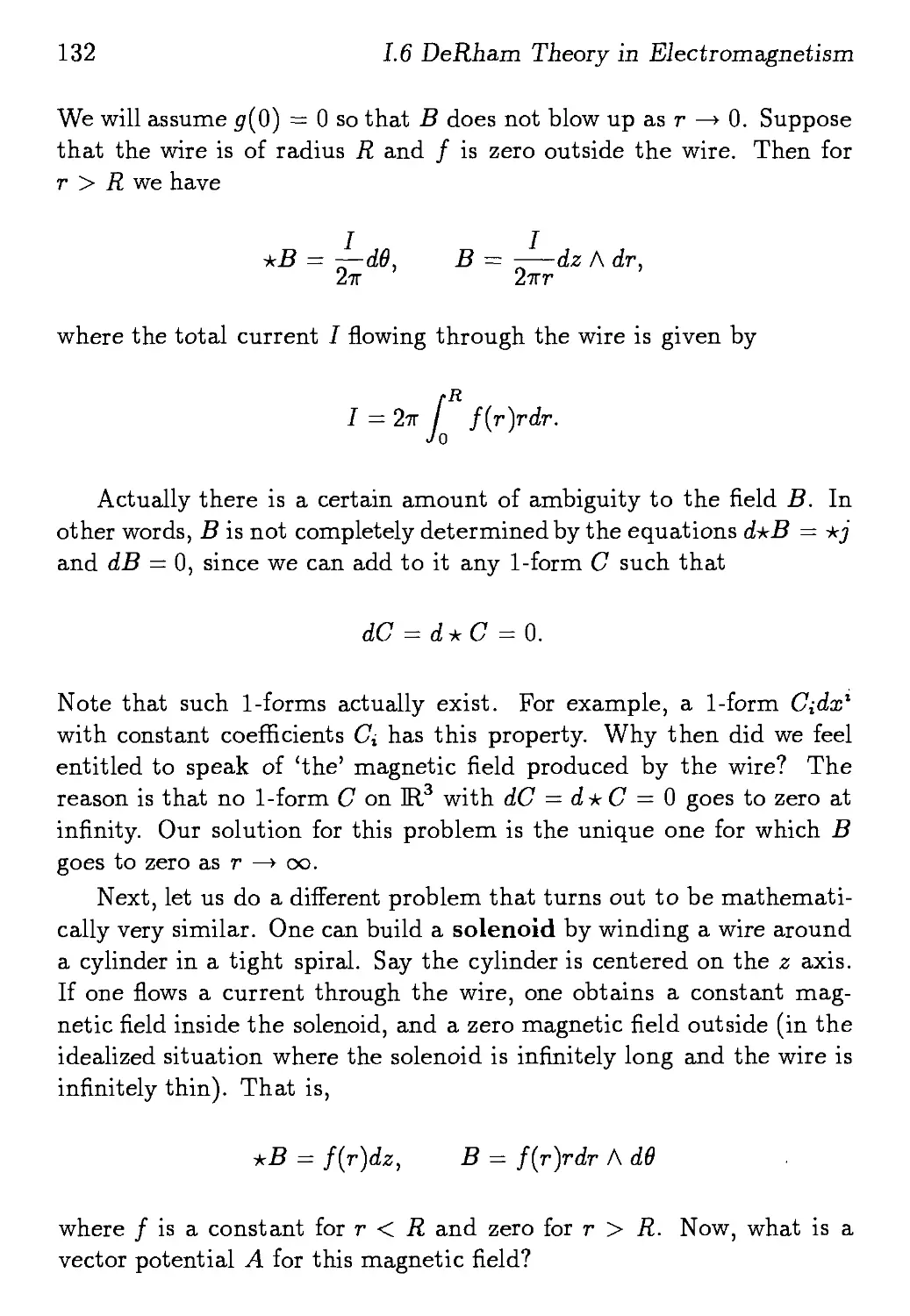
In order to do modern physics we need to be able to handle spaces
and spacetimes that are more general than good old ]Rn. The kinds
of spaces we will be concerned with are those that look locally like
]Rn, but perhaps not globally. Such a space is called an n-dimensional
'manifold'. For example, the sphere
x2 + y2 + z2 = 1,
looks locally like the plane Ш.2, which is why some people thought the
Earth was flat. These days we call this sphere S2 — the 2-sphere — to
indicate that it is a 2-dimensional manifold. Similarly, while the space
15
16 1.2 Manifolds
we live in looks locally like Ш,3, we have no way yet of ruling out the
possibility that it is really S3, the 3-sphere:
w2 + x2 + y2 + z2 = 1,
and indeed, in many models of cosmology space is a 3-sphere. In such a
universe one could, if one had time, sail around the cosmos in a space-
spaceship just as Magellan circumnavigated the globe. More generally, it is
even possible that spacetime has more than 4 dimensions, as is assumed
in so-called 'Kaluza-Klein theories'. For a while, string theorists seemed
quite sure that the universe must either be 10 or 26-dimensional! More
pragmatically, there is a lot of interest in low-dimensional physics, such
as the behavior of electrons on thin films and wires. Also, classical
mechanics uses 'phase spaces' that may have very many dimensions.
These are some of the physical reasons why it is good to generalize
vector calculus so that it works nicely on any manifold. On the other
hand, mathematicians have many reasons of their own for dealing with
manifolds. For example, the set of solutions of an equation is often a
manifold (see the equation for the 3-sphere above).
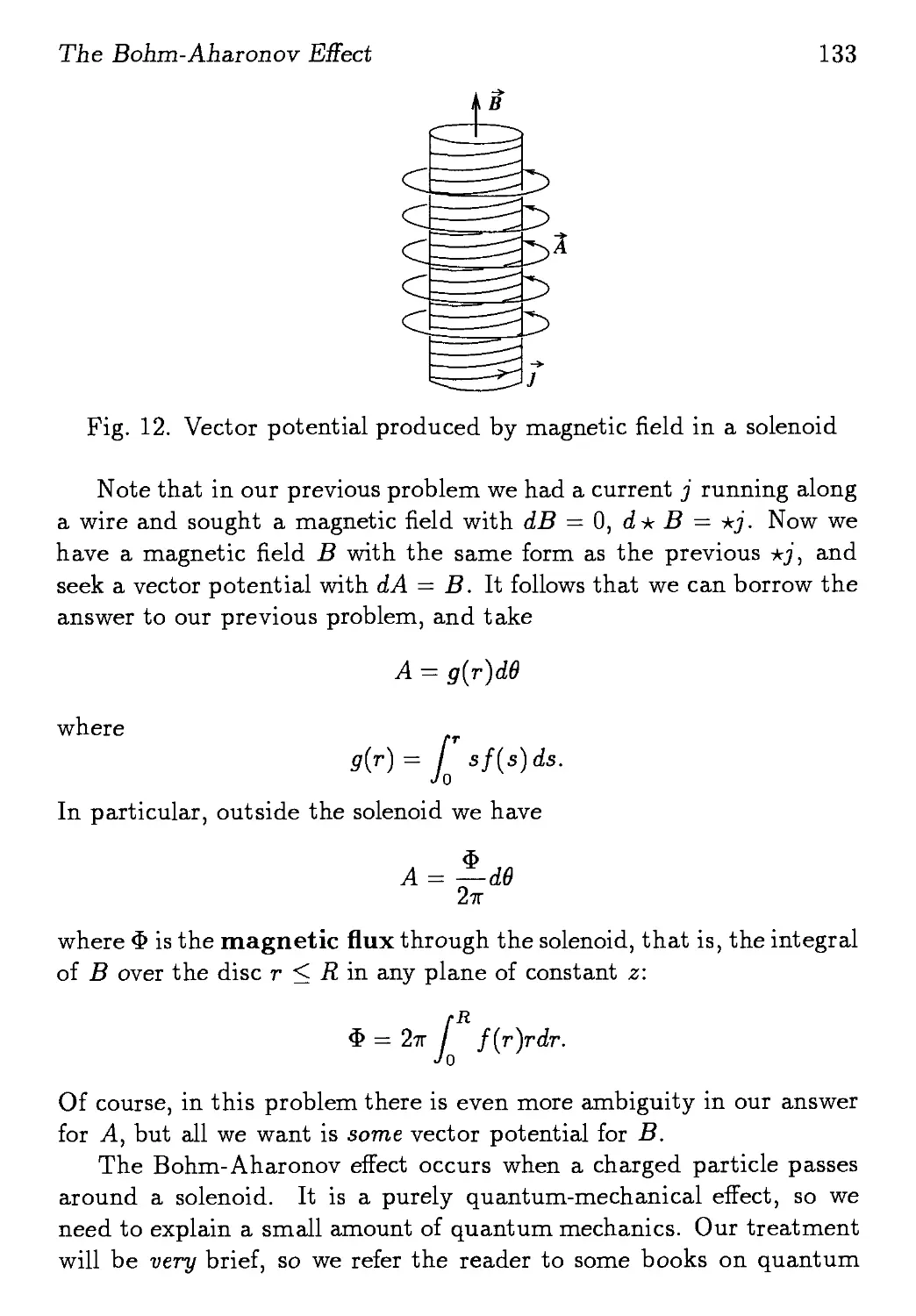
We now head towards a precise definition of a manifold. First of
all, we remind the reader that a topological space is a set X together
with a family of subsets of X, called the open sets, required to satisfy
the conditions:
1) The empty set and X itself are open,
2) If U, V С X are open, so is U П V,
3) If the sets Ua С X are open, so is the union \J Ua.
The collection of sets taken to be open is called the topology of X.
An open set containing a point x ? X is called a neighborhood of x.
The complement of an open set is called closed.
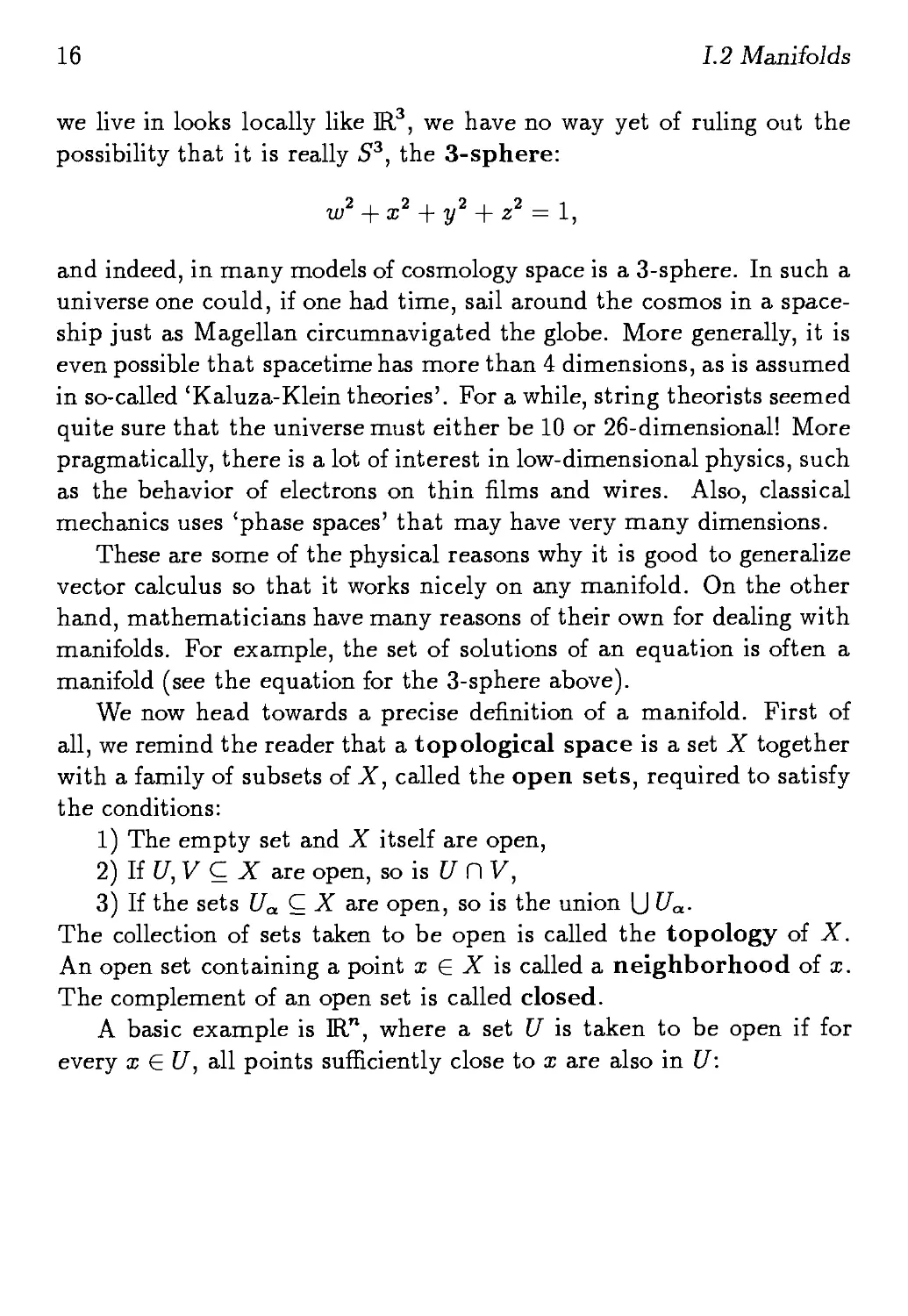
A basic example is Ш.", where a set U is taken to be open if for
every x ? U, all points sufficiently close to x are also in U:
Manifolds
17
U
Fig. 1. An open set in Ш.2
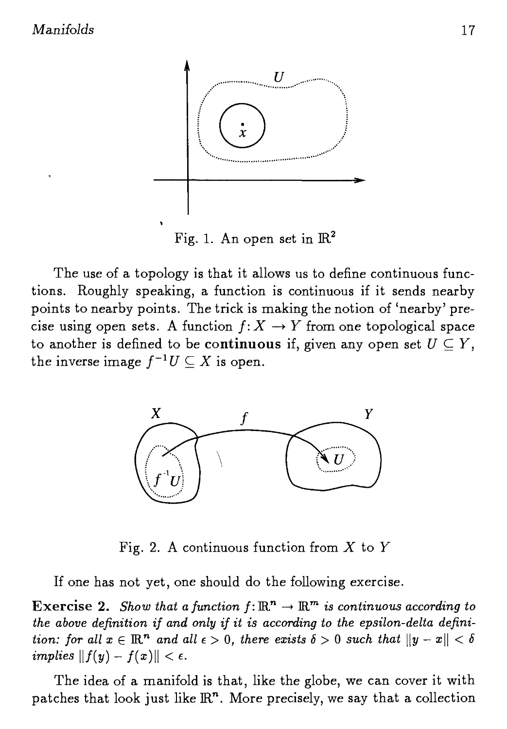
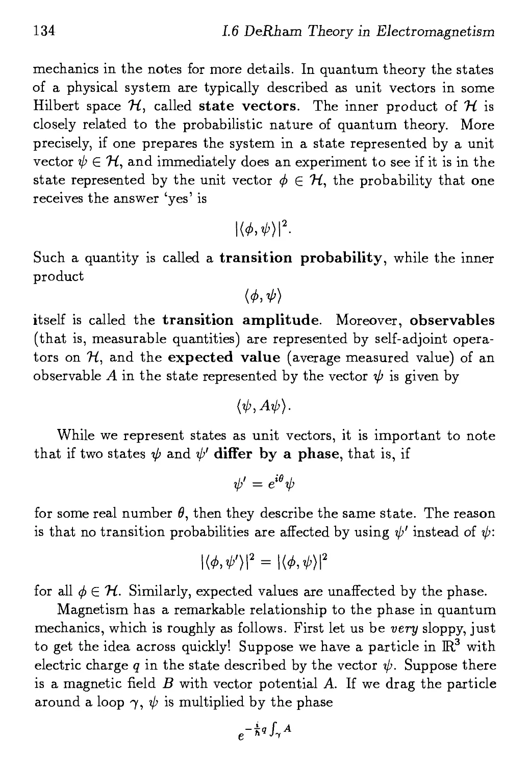
The use of a topology is that it allows us to define continuous func-
functions. Roughly speaking, a function is continuous if it sends nearby
points to nearby points. The trick is making the notion of 'nearby' pre-
precise using open sets. A function f:X—*Y from one topological space
to another is defined to be continuous if, given any open set U С Y,
the inverse image f~1U С X is open.
Fig. 2. A continuous function from X to Y
If one has not yet, one should do the following exercise.
Exercise 2. Show that a function /:Ш,П -+ Ж is continuous according to
the above definition if and only if it is according to the epsilon-delta defini-
definition: for all x ? Ш,™ and all e > 0, there exists 6 > 0 such that \\y — x\\ < 6
implies ||/(y)-/(z)|| < e.
The idea of a manifold is that, like the globe, we can cover it with
patches that look just like Ш.". More precisely, we say that a collection
18
1.2 Manifolds
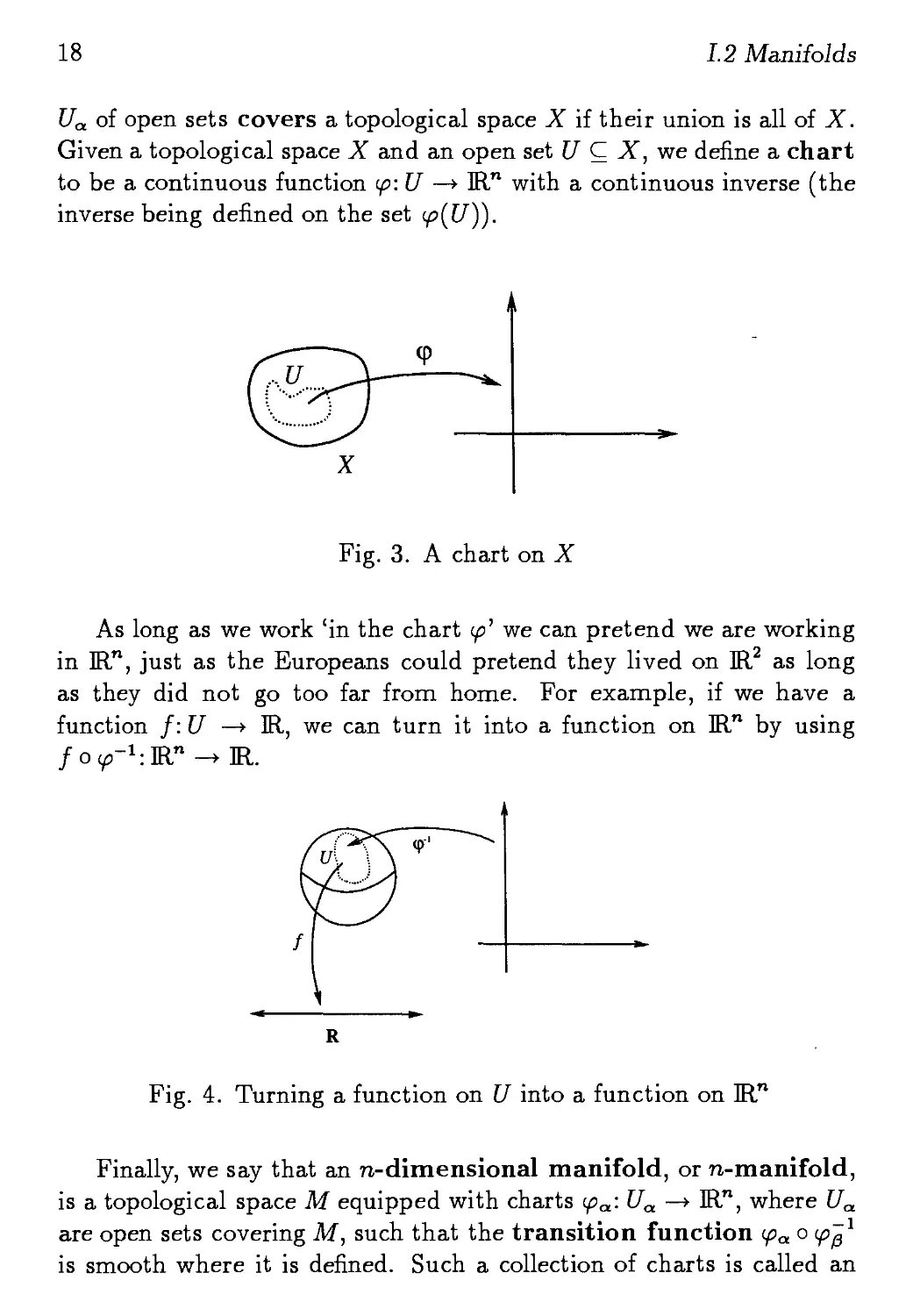
Ua of open sets covers a topological space X if their union is all of X.
Given a topological space X and an open set U С X, we define a chart
to be a continuous function (p:U—+ Ш." with a continuous inverse (the
inverse being defined on the set
Fig. 3. A chart on X
As long as we work 'in the chart ip' we can pretend we are working
in Ш.", just as the Europeans could pretend they lived on Ш.2 as long
as they did not go too far from home. For example, if we have a
function f:U—* Ш., we can turn it into a function on ]Rn by using
Fig. 4. Turning a function on U into a function on ]Rn
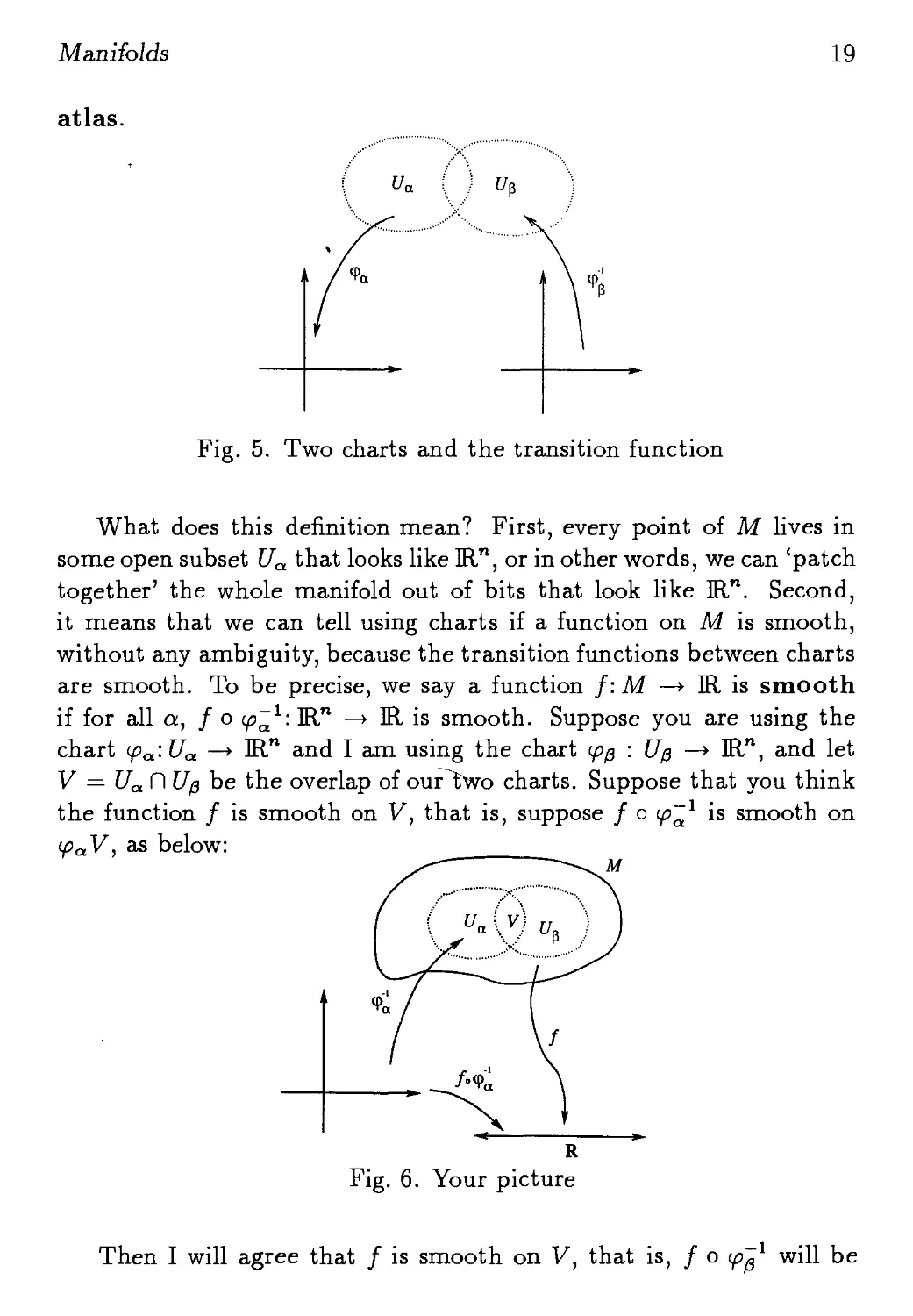
Finally, we say that an n-dimensional manifold, or n-manifold,
is a topological space M equipped with charts ipa'-Ua —> Ш.", where Ua
are open sets covering M, such that the transition function tpa о ip^1
is smooth where it is defined. Such a collection of charts is called an
Manifolds
atlas.
19
Fig. 5. Two charts and the transition function
What does this definition mean? First, every point of M lives in
some open subset Ua that looks like Ш.", or in other words, we can 'patch
together' the whole manifold out of bits that look like Ш.". Second,
it means that we can tell using charts if a function on M is smooth,
without any ambiguity, because the transition functions between charts
are smooth. To be precise, we say a function /: M —* Ш. is smooth
if for all a, / о уз: Ш." —> IR. is smooth. Suppose you are using the
chart <pa'-Ua —> IRn and I am using the chart ipp : Up —* Ш.п, and let
V = Ua П Up be the overlap of our^Ewo charts. Suppose that you think
the function / is smooth on V, that is, suppose / о уз is smooth on
(paV, as below:
Fig. 6. Your picture
Then I will agree that / is smooth on V, that is, / о tp^ will be
20
1.2 Manifolds
smooth on ippV too:
Fig. 7. My picture
Why? Because we can express my function in terms of your function
and the transition function:
Strictly speaking, the sort of manifold we have defined here is called
a smooth manifold. There are also, for example, topological mani-
manifolds, where the transition functions are only required to be continuous.
For us, 'manifold' will always mean 'smooth manifold'. Also, we will
always assume our manifolds are 'Hausdorff' and 'paracompact'. These
are topological properties that we prefer to avoid explaining here, which
are satisfied by all but the most bizarre and useless examples.
In the following exercises we describe some examples of manifolds,
leaving the reader to check that they really are manifolds.
Exercise 3. Given a topological space X and a subset S С X, define the
induced topology on S to be the topology in which the open sets are of the
form UnS, where U is open in X. Let Sn, the n-sphere, be the unit sphere
in Жп+1 :
n+1
Sn = {x
Show that Sn С Htn+1 with its induced topology is a manifold.
Exercise 4. Show that if M is a manifold and U is an open subset of M,
then U with its induced topology is a manifold.
Manifolds 21
Exercise 5. Given topological spaces X and Y, we giveXxY the product
topology in which a set is open if and only if it is a union of sets of the
form U X V, where U is open in X and V is open in Y. Show that if M is
an m-dimensional manifold and N is an n-dimensional manifold, M X N is
an (m + n)-dimensional manifold.
Exercise 6. Given topological spaces X and Y, we give XUY the disjoint
union topology in which a set is open if and only if it is the union of
an open subset of X and an open subset of Y. Show that if M and N
are n-dimensional manifolds the disjoint union M U N is an n-dimensional
manifold.
There are many different questions one can ask about a manifold,
but one of the most basic is whether it extends indefinitely in all di-
directions like ]R3 or is 'compact' like S3. There is a way to make this
precise which proves to be very important in mathematics. Namely, a
topological space X is said to be compact if for every cover of X by
open sets Ua there is a finite collection Uai, ¦ ¦ ¦, Uan that covers X. For
manifolds, there is an equivalent definition: a manifold M is compact
if and only if every sequence in M has a convergent subsequence. A
basic theorem says that a subset of Ш." is compact if and only if it is
closed and fits inside a ball of sufficiently large radius.
The study of manifolds is a fascinating business in its own right.
However, since our goal is to do physics on manifolds, let us turn to the
basic types of fields that live on manifolds: vector fields and differential
forms.
Chapter 3
Vector Fields
And it is a noteworthy fact that ignorant men have long been in advance
of the learned about vectors. Ignorant people, like Faraday, naturally think
in vectors. They may know nothing of their formal manipulation, but if they
think about vectors, they think of them as vectors, that is, directed magni-
magnitudes. No ignorant man could or would think about the three components
of a vector separately, and disconnected from one another. That is a device
of learned mathematicians, to enable them to evade vectors. The device is
often useful, especially for calculating purposes, but for general purposes of
reasoning the manipulation of the scalar components instead of the vector
itself is entirely wrong. — Oliver Heaviside
Heaviside was one of the first advocates of modern vector analysis,
as well as a very saxcastic fellow. In the quote above, he was making
the point that the great physicist Faraday did not need to worry about
coordinates, because Faraday had a direct physical understanding of
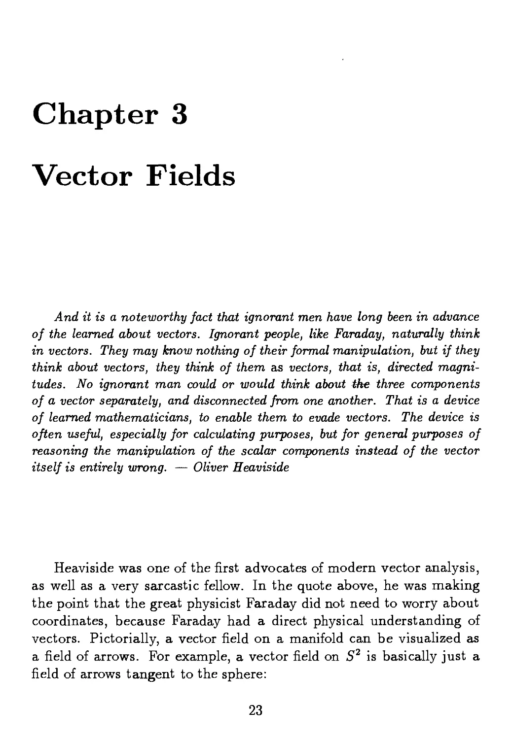
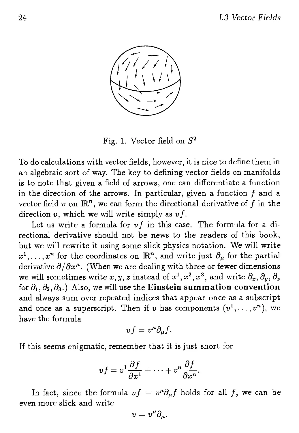
vectors. Pictorially, a vector field on a manifold can be visualized as
a field of arrows. For example, a vector field on S2 is basically just a
field of arrows tangent to the sphere:
23
24 1.3 Vector Fields
Fig. 1. Vector field on S2
To do calculations with vector fields, however, it is nice to define them in
an algebraic sort of way. The key to defining vector fields on manifolds
is to note that given a field of arrows, one can differentiate a function
in the direction of the arrows. In particular, given a function / and a
vector field v on ]Rn, we can form the directional derivative of / in the
direction v, which we will write simply as vf.
Let us write a formula for vf in this case. The formula for a di-
directional derivative should not be news to the readers of this book,
but we will rewrite it using some slick physics notation. We will write
x1,... ,xn for the coordinates on IRn, and write just 8^ for the partial
derivative д/дх^. (When we are dealing with three or fewer dimensions
we will sometimes write x, y, z instead of a;1, x2, x3, and write дх, 8y, 8Z
for 8^,82,83.) Also, we will use the Einstein summation convention
and always, sum over repeated indices that appear once as a subscript
and once as a superscript. Then if v has components (y1,... ,vn), we
have the formula
vf = v"dj.
If this seems enigmatic, remember that it is just short for
In fact, since the formula vf = v^d^f holds for all /, we can be
even more slick and write
v =
Vector Fields 25
What does this mean, though? The sight of the partial derivatives дц
sitting there with nothing to differentiate is only slightly unnerving;
we can always put a function / to the right of them whenever we
want. Much odder is that we are saying the vector field v is the linear
combination of these partial derivatives. What we are doing might
be regarded as rather sloppy, since we are identifying two different,
although related, things: the vector field v, and the operator v^d^ that
takes a directional derivative in the direction of v. In fact, this 'sloppy'
attitude turns out to be extremely convenient, and next we will go even
further and use it to define vector fields on manifolds. It is important
to realize that in mathematics it is often crucial to think about familiar
objects in a new way in order to generalize them to a new situation.
Now let us define vector fields on a manifold M. Following the phi-
philosophy outlined above, these will be entities whose sole ambition in life
is to differentiate functions. First a bit of jargon. The set of smooth
(real-valued) functions on a manifold M is written C°°{M), where the
C°° is short for 'having infinitely many continuous derivatives'. Note
that C°°(M) is an algebra over the real numbers, meaning that it is
closed under (pointwise) addition and multiplication, as well as multi-
multiplication by real numbers, and the following batch of rules holds:
f+9 = 9+f
f(gh) = (fg)h ^
= f9 + fh
= fh+gh
1/ = /
= (*/*)/
= a/ + ag
where f,g,h G C°°(M) and a,/3 G Ш.. Of course it is a commutative
algebra, that is, fg = gf.
Now, a vector field v on M is defined to be a function from C°°(M)
to C°°(M) satisfying the following properties:
26 1.3 Vector Fields
«(/ + $) = v(f)+v(g)
v(af) = av(f)
v(fg) = v{f)g + Mg),
for all f,g ? C°°{M) and a G Ш.. Here we have isolated all the basic
rules a directional derivative operator should satisfy. The first two
simply amount to linearity, and it is the third one, the product rule or
Leibniz law, that really captures the essence of differentiation.
This definition may seem painfully abstract. We will see in a bit
that it really is just a way of talking about a field of arrows on M.
For now, note the main good feature of this definition: it does not rely
on any choice of coordinates on M! A basic philosophy of modern
physics is that the universe does not come equipped with a coordi-
coordinate system. While coordinate systems are necessary for doing specific
concrete calculations, the choice of the coordinate system to use is a
matter of convenience, and there is often no 'best' coordinate system.
One should strive to write the laws of physics in a manifestly coordinate-
independent manner, so one can see what they are really saying and
not get distracted by things that might depend on the coordinates.
Let Vect(M) denote the set of all vector fields on M. We leave it to
the reader to check that one can add vector fields and multiply them
by functions on M as follows. Given v,w G Vect(M), we define v + w
by
and given v ? Vect(M) and g ? C°°(M), we define gv by
Exercise 7. Show that v + w and gw ? Vect(M).
Exercise 8. Show that the following rules for all d,i» ? Vect(M) and
f,g?C°°(M):
f(v + w) = fv + fw
{f+9)v = fv + gv
{fg)v = f{gv)
lv = v.
Tangent Vectors 27
(Here '1' denotes the constant function equal to 1 on all of M.) Mathemat-
Mathematically, we summarize these rules by saying that Vect(M) is a module over
It turns out that the vector fields {d^} on ]Rn span Vect(]Rn) as
a module over C°°(M). In other words, every vector field on Ш,™ is a
linear combination of the form
for some functions v^ ? C°°(JRP). It is also true that the vector fields
{d^} on Ш." are linearly independent
Exercise 9. Show that if v^d^, = 0, that is, v^d^f = 0 for all f e
С°°(Ш.П), we must have v» = 0 for all fi.
This implies that every vector field v on Ш." has a unique representation
as a linear combination v^d^; we say that the vector fields {d^} form
a basis of Vect(IRn). The functions v1* are called the components of
the vector field v.
Tangent Vectors
Often is is nice to think of a vector field on M as really assigning an
'arrow' to each point of M. This kind of arrow is called a tangent vector.
For example, we may think of a tangent vector at a point p ? S2 as a
vector in the plane tangent to p:
Fig. 2. Tangent vector
28 1.3 Vector Fields
To get a precise definition of a tangent vector at p ? M, note that a
tangent vector should let us take directional derivatives at the point p.
For example, given a vector field v on M, we can take the derivative v(f)
of any function / ? C°°(M), and then evaluate the function v(f) at p.
We can think of the result, u(/)(p), as being the result of differentiating
/ in the direction lvp at the point p. In other words, we can define
vp:C°°(M) ->]R
by
and think of vp as a tangent vector at p. We call vp the value of v at p.
Note that vp has three basic properties, which follow from the defi-
definition of a vector field:
vP(f + g) = vp(f) + vp(g)
Vp(af) = avp(f)
Henceforth, we will simply define a tangent vector at p ? M to be
a function from C°°(M) to Ш. satisfying these three properties. Let
TpM, the tangent space at p, denote the set of all tangent vectors at
p ? M.
It now follows rigorously from our definitions that for each p ? M,
a vector field v ? Vect(M) determines a tangent vector vp ? TpM. One
can also show, though it takes a bit of work, that every tangent vector
at p is of the form vp for some vector field or other. A related fact,
which is much easier to show, is the following:
Exercise 10. Let v, w ? Vect(M). Show that v = w if and only ifvp = wp
for all p G M.
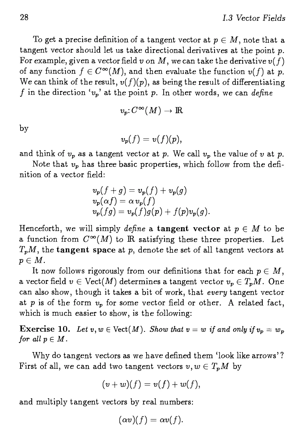
Why do tangent vectors as we have defined them 'look like arrows' ?
First of all, we can add two tangent vectors v,w ? TpM by
(v + w)(f)=v(f) + w(f),
and multiply tangent vectors by real numbers:
(av)(f) = av(f).
Tangent Vectors 29
(Now we are using the letters v,w to denote tangent vectors, not vector
fields!) With addition and multiplication defined this way, the tangent
space is really a vector space. For example, in Figure 2 we have drawn
a tangent space to look like a little plane. The tangent vectors can be
thought of as arrows living in this vector space.
Exercise 11. Show that TpM is a vector space over the real numbers.
Another reason why tangent vectors really look like arrows is that
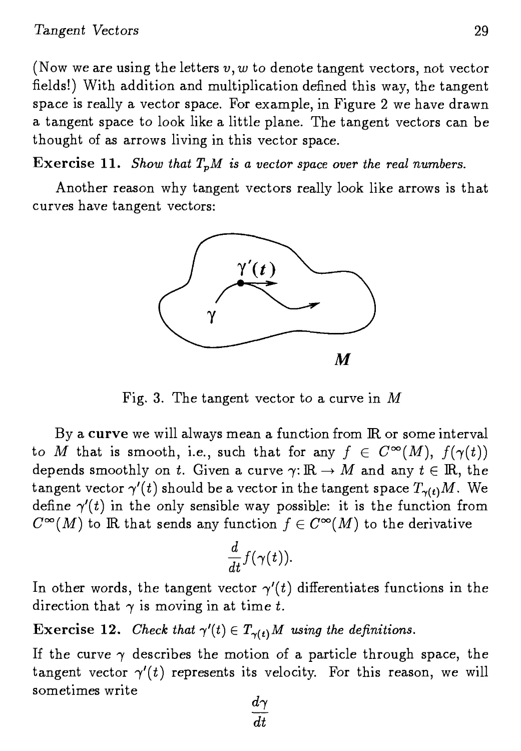
curves have tangent vectors:
Fig. 3. The tangent vector to a curve in M
By a curve we will always mean a function from IR or some interval
to M that is smooth, i.e., such that for any / G C°°(M), /G(J))
depends smoothly on t. Given a curve 7: Ш. —> M and any <G E, the
tangent vector 7'(i) should be a vector in the tangent space T7(t)M. We
define 7'(i) in the only sensible way possible: it is the function from
C°°{M) to IR that sends any function / E C°°(M) to the derivative
In other words, the tangent vector *y'(t) differentiates functions in the
direction that 7 is moving in at time t.
Exercise 12. Check that j'(t) G T^it\M using the definitions.
If the curve 7 describes the motion of a particle through space, the
tangent vector "f'(t) represents its velocity. For this reason, we will
sometimes write
d7
dt
30
1.3 Vector Fields
for 7'(i), especially when we are not particularly concerned with which
value of t we are talking about.
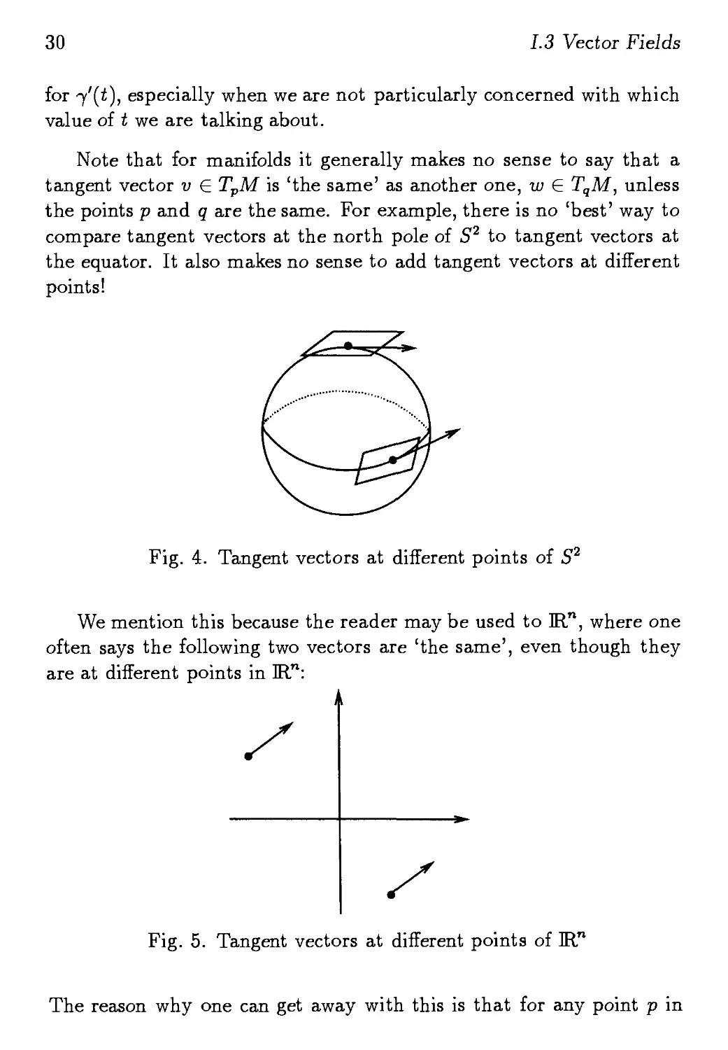
Note that for manifolds it generally makes no sense to say that a
tangent vector v ? TpM is 'the same' as another one, w ? TqM, unless
the points p and q are the same. For example, there is no 'best' way to
compare tangent vectors at the north pole of S2 to tangent vectors at
the equator. It also makes no sense to add tangent vectors at different
points!
Fig. 4. Tangent vectors at different points of S2
We mention this because the reader may be used to ]Rn, where one
often says the following two vectors are 'the same', even though they
are at different points in IRn:
Fig. 5. Tangent vectors at different points of ]Rn
The reason why one can get away with this is that for any point p in
Covariant Versus Contravariant 31
]Rn, the tangent vectors
form a basis. This allows one to relate tangent vectors at different
points of ]Rn — one can sloppily say that the vector
and the vector
v = v*(djp e TplRn
to = w^djg E TqWLn
q
are 'the same' if v^ = w^, even though v and го are not literally equal.
Later we will get a deeper understanding of this issue, which requires
a theory of 'parallel transport', the process of dragging a vector at one
point of a manifold over to another point. This turns out to be a crucial
idea in physics, and in fact the root of gauge theory!
Covariant Versus Contravariant
A lot of modern mathematics and physics requires keeping track of
which things in life are covariant, and which things are contravariant.
Let us begin to explain these ideas by comparing functions and tangent
vectors. Say we have a function ф: M —> N from one manifold to
another. If we have a real-valued function on N, say /: N —> IR, we
can get a real-valued function on M by composing it with /.
M
R
Fig. 6. Pulling back / from N to M
32 1.3 Vector Fields
We call this process pulling back / from N to M by ф. We define
and call ф*f the pullback of / by ф. The point is that while ф goes
'forwards' from M to N, the pullback operation ф* goes 'backwards',
taking functions on N to functions on M. We say that real-valued
functions on a manifold are contravariant because of this perverse
backwards behavior.
Exercise 13. Let ф:Ш, -+ Ж be given by ф(?) — e*. Let x be the usual
coordinate function on Ж. Show that ф*х = ex.
Exercise 14. Let ф:Ш.2 -+ Ж2 be rotation counterclockwise by an angle в.
Let x,y be the usual coordinate functions on Ж2. Show that
ф*х — (cos в)х — (sm в)у
ф*у = (sm6)x + (cos6)y.
By the way, we say that ф: M —> AT is smooth if / G C°°(N)
implies that </>*/ G C°°(M). Henceforth we will assume functions from
manifolds to manifolds are smooth unless otherwise stated, and we will
often call such functions maps.
Exercise 15. Show that this definition of smoothness is consistent with
the previous definitions of smooth functions f: M —» Ж and smooth curves
7:Ж-> М.
Using our new jargon, we have: given any map
ф: N -> M,
pulling back by ф is an operation
ф*:С°°(М) -^C
Tangent vectors, on the other hand, are covariant: a tangent vector
v G TpM and a smooth function ф: M —> N gives a tangent vector
ф*у е Tj,(p)N, called the pushforward of v by ф. This is defined by
Covariant Versus Contravariant 33
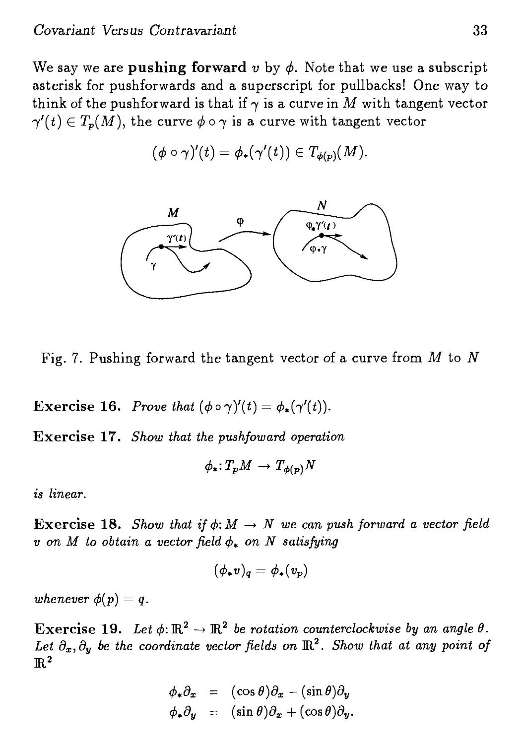
We say we are pushing forward v by ф. Note that we use a subscript
asterisk for pushforwards and a superscript for pullbacks! One way to
think of the pushforward is that if 7 is a curve in M with tangent vector
7'(i) G Tp{M), the curve 0 о 7 is a curve with tangent vector
м
Fig. 7. Pushing forward the tangent vector of a curve from M to N
Exercise 16. Prove that (^7)'(<) =
Exercise 17. Show that the pushfoward operation
ф.:ТрМ - Тф{р)Н
is linear.
Exercise 18. Show that if ф: M —> N we can push forward a vector field
v on M to obtain a vector field ф* on N satisfying
whenever ф(р) = q.
Exercise 19. Let ф:Ш? -» Ж2 be rotation counterclockwise by an angle в.
Let дх,ду be the coordinate vector fields on Ж2. Show that at any point of
Ж2
ф,дх = (c
ф,ду = (sm6)dx + {cos6)dy.
34 1.3 Vector Fields
It is traditional in mathematics, by the way, to write pushforwards
and other covariant things with lowered asterisks, and to write pull-
backs and other contravariant things with raised asterisks. It might
help as a mnemonic to remember that the tangent vectors d^ are writ-
written with the fi downstairs, and are covariant. In the next chapter we
will discuss things similar to tangent vectors, but which are contravari-
contravariant! These things will have their indices upstairs. We warn the reader,
however, that while the vector field dy. is covariant and has its indices
downstairs, physicists often think of a vector field v as being its compo-
components v^. These have their indices upstairs, so physicists say that the
v* are contravariant! This is one of those little differences that makes
communication between the two subjects a bit more difficult.
Flows and the Lie Bracket
One sort of vector field that comes up in physics is the velocity vector
field of a fluid, such as water. Imagine that the velocity vector field v
is constant as a function of time, so that each molecule of water traces
out a curve ^{t) as time passes, with the tangent vector of 7 equal to
the value of v at the point j(t):
= v
-f(t)
for all t. If the curve starts at some point p G M, that is 7@) = p, we
call 7 the integral curve through p of the vector field v:
11
Fig. 8. Integral curve through p of the vector field v
Flows and the Lie Bracket 35
Calculating the integral curves of a vector field amounts to solving
a first-order differential equation. One has to be careful, because the
solution might 'shoot off to infinity' in a finite amount of time:
Exercise 20. Let v be the vector field x2dx + ydy on Ш,2. Calculate the
integral curves j(t) and see which ones are defined for all t.
We say that the vector field v is integrable if all the integral curves
are defined for all t.
Suppose v is an integrable vector field on M, which we think of as
the velocity vector field of some water. If we keep track of how all the
molecules of water are moving along, we have something called a 'flow'.
Let </>t(p) be the integral curve of v through the point p G M. For each
time t, the map
c/>t:M -» M
turns out to be smooth, by a result on the smooth dependence of so-
solutions of differential equations on the initial conditions. Water that
was at p at time zero will be at </>t(p) by time t, so we call the family
of maps {</>t} the flow generated by v. The defining equation for the
flow is (rewriting our equation for 7):
Exercise 21. Show that ф0 is the identity map id: X —> X, and that for
all s,t G Ж we have ^0^, = 4>t+s-
There is an important way to get new vector fields from old ones
that is related to the concept of flows. This is called the Lie bracket or
commutator of vector fields. Given v,w G Vect(M), the Lie bracket
[v, го] is defined by
[v,w](f) = v(w(f))-w(v(f)),
for all / G C°°{M), or, for short,
[г>,го] = г>го — гог>.
36
1.3 Vector Fields
Let us show that the Lie bracket defined in this way actually is a vector
field on the manifold M. It is easy to prove linearity, so the crucial thing
is the Leibniz rule: if и = [v,w], we have
= (vw - wv)(fg)
= v[w(f)g + fw(g)} - w[v(f)g + fv{g)}
= vw(f) g + f vw{g) - wv(f) g - f wv(g)
Here we used the Leibniz law twice and then used the definition of the
Lie brackets.
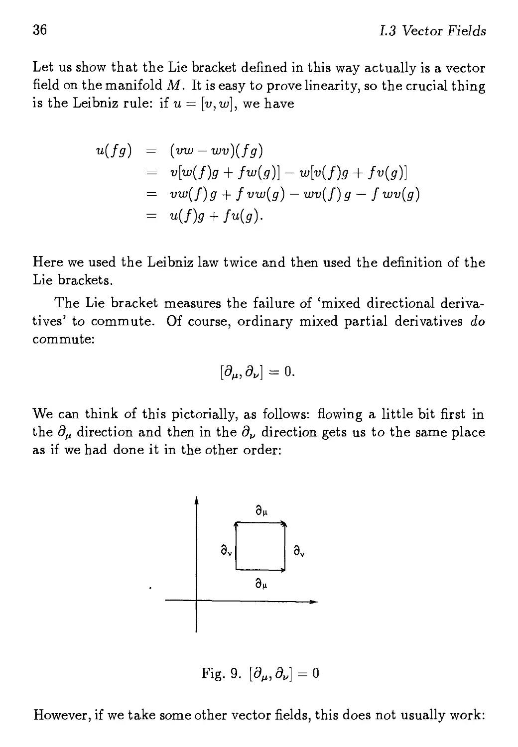
The Lie bracket measures the failure of 'mixed directional deriva-
derivatives' to commute. Of course, ordinary mixed partial derivatives do
commute:
We can think of this pictorially, as follows: flowing a little bit first in
the 8^ direction and then in the dv direction gets us to the same place
as if we had done it in the other order:
Fig. 9.
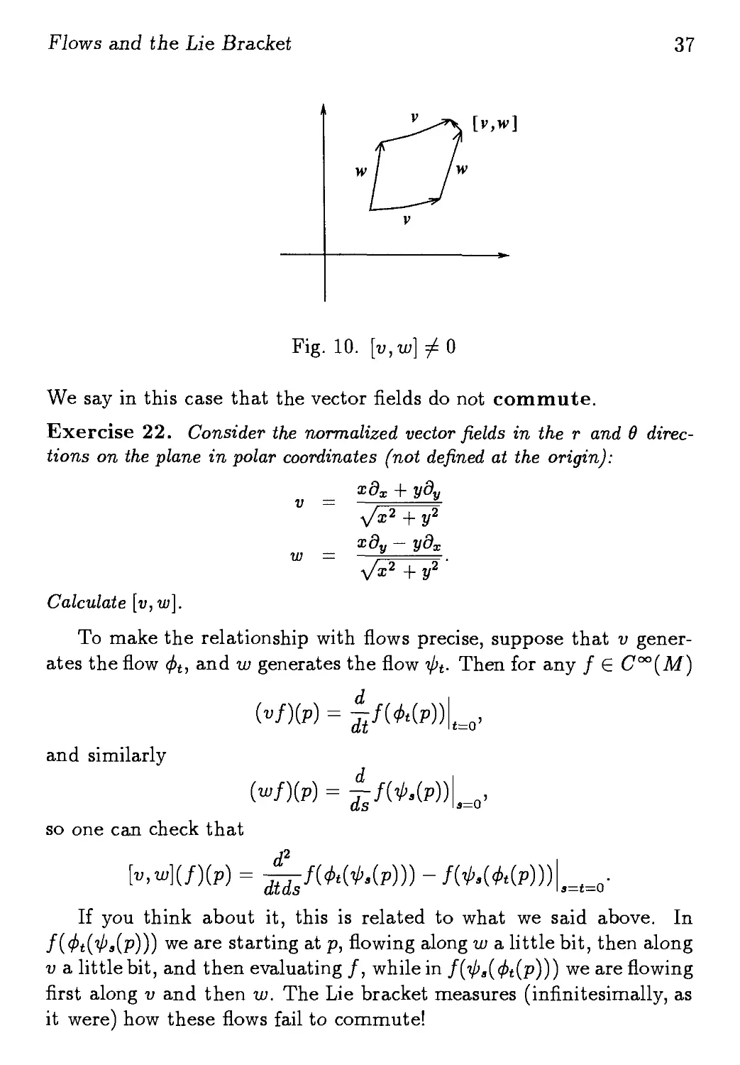
However, if we take some other vector fields, this does not usually work:
Flows and the Lie Bracket
37
[v,w]
Fig. 10. [v,w]^0
We say in this case that the vector fields do not commute.
Exercise 22. Consider the normalized vector fields in the r and в direc-
directions on the plane in polar coordinates (not defined at the origin):
хдх + уду
v =
w =
/x2 + у2
ду - удх
Calculate \v,w\.
To make the relationship with flows precise, suppose that v gener-
generates the flow </>t, and го generates the flow г/»4. Then for any / G C°°(M)
Ы)(р) = ^
t=o'
and similarly
so one can check that
d2
s=t=O
If you think about it, this is related to what we said above. In
т/)а(р))) we are starting at p, flowing along го a little bit, then along
v a little bit, and then evaluating /, while in /(^«(^(p))) we are flowing
first along v and then го. The Lie bracket measures (infinitesimally, as
it were) how these flows fail to commute!
38 13 Vector Fields
Exercise 23. Check the equation above.
The Lie bracket of vector fields satisfies some identities which we
will come back to in Part II. For now, we simply let the reader prove
them:
Exercise 24. Show that for all vector fields u,v,w on a manifold, and all
real numbers a and /3, we have:
1) [v,w]= -[w,v].
2) [u,av + fiw] = a[u,v} + fi[u,w].
3) The Jacobi identity: [u, [v, w]] + [v, [w, u]] + [w, [u, v]] = 0.
Chapter 4
Differential Forms
As a herald it's my duty
to explain those forms of beauty. — Goethe, Faust.
1-forms
The electric field, the magnetic field, the electromagnetic field on space-
time, the current — all these are examples of differential forms. The
gradient, the curl, and the divergence can all be thought of as different
aspects of single operator d that acts on differential forms. The funda-
fundamental theorem of calculus, Stokes' theorem, and Gauss' theorem are
all special cases of a single theorem about differential forms. So while
they are somewhat abstract, differential forms are a powerful unifying
notion.
We begin with 1-forms. Our goal is to generalize the concept of
the gradient of a function to functions on arbitrary manifolds. What
we will do is to make up, for each smooth function / on M, an object
called df that is supposed to be like the usual gradient V/ defined on
M™. Remember that the directional derivative of a function / in the
on M™ in the direction v is just the dot product of V/ with v:
V/ • v = vf.
In other words, the gradient of / is a thing that keeps track of the
directional derivatives of / in all directions. We want our 'df to do the
same job on any manifold M.
39
40 1.4 Differentia/ Forms
The gradient of a function on M™ is a vector field, so one might want
to say that df should be a vector field. The problem is the dot product
in the formula above. On M™ there is a well-established way to take the
dot product of tangent vectors, but manifolds do not come pre-equipped
with a way to do this. Geometers call a way of taking dot products of
tangent vectors a 'metric'. In fact, we will see that in general relativity
the gravitational field is described by the metric on spacetime. Far from
there being a single 'best' metric on a manifold, there are typically lots
that satisfy Einstein's equations of general relativity. This makes it nice
to avoid using a particular metric unless we actually need to. Therefore
we will not think of df as a vector field, but as something else, a '1-form'.
The trick is to realize what V/ is doing in the formula V/ • v = vf.
For each vector field v that we choose, this formula spits out a function
vf, the directional derivative of / in the direction v. In other words,
what really matters is the operator
v t—> V/ • v,
or, what is the same thing,
v и-> vf.
Let us isolate the essential properties of this map. There is really
only one: linearity! This means that
V/ • (v + w) = V/ ¦ v + V/ ¦ w
for any vector fields v and w, and
V/ ¦ (gv) = 5(V/ • v)
where g is any smooth function on M™. Since we can pull out any
function g G Coo(IRTl) in the above formula, not just constants, math-
mathematicians say that
v и-> V/ • v
is linear over С°°(Шп) — not just linear over the real numbers.
So, abstracting a bit, we define a 1-form on any manifold M to be
a map from Vect(M) to C°°(M) that is linear over C°°(M). In other
1-forms 41
words, if we feed a vector field v to a 1-form ш, it spits out a function
uj{v) in a way satisfying
w{y + w) = w(v) + w(w),
tu(gv) — gw(y).
We use fi!(M) to denote the space of all 1-forms on a manifold M.
Later on we will talk about 2-forms, 3-forms, and so on.
The basic example of a 1-form is this: for any smooth function /
on M there is a 1-form df defined by
df{y) = vf.
(Think of this as a slick way to write V/ • v = vf.) To show that df is
really a 1-form, we just need to check linearity:
df (y + w) = (v + w)f = vf +wf = df(y) + df(w),
and
We call the 1-form df the differential of /, or the exterior derivative
of /.
Just as we can add vector fields or multiply them by functions, we
can do the same for 1-forms. We can add two 1-forms ш and ft and get
a 1-form w + ft by defining
and we can multiply a 1-form ш by a smooth function / and get a
1-form fw by defining
(fu)(v) = fU(v).
Exercise 25. Show that u> + /i and fw are really 1-forms, i.e., show lin-
linearity over C°°(M).
Exercise 26. Show that П!(М) is a module overC°°(M) (see the defini-
definition in Exercise 8.)
42 1.4 Differential Forms
The map d:C°°(M) —> fi!(M) that sends each function / to its
differential df is also called the differential, or exterior derivative. It is
interesting in its own right, and has the following nice properties:
Exercise 27. Show that
d{af) = adf
(f + g)dh = fdh + gdh
d{fg)= fdg + gdf,
for any f,g,h? C°°(M) and any a ? H.
The first three properties in the exercise above are just forms of
linearity, but the last one is a version of the product rule, or Leibniz
law:
d{fg) = fdg + gdf.
It is the Leibniz law that makes the exterior derivative really act like
a derivative, so if you only want to do part of Exercise 27 check that
the Leibniz law holds! It is worth mentioning, by the way, that when
Leibniz was inventing calculus he first guessed that d(fg) = df dg, and
only got it right the next day.
In fact, the reader has seen differentials before, in calculus. They
start out as part of the expressions for differentiation
dy
dx
and integration
' f(x)di
1
but soon take on a mysterious life of their own, as in
dsmx = cosxdx\
We bet you remember wondering what the heck these differentials really
are! In physics one thinks of dx as an 'infinitesimal change in position',
and so on — but this is mystifying in its own right. Early in the
history of calculus, the philosopher Berkeley complained about these
1 -forms 43
infinitesimals, writing "They are neither finite quantities, nor quanti-
quantities infinitely small, nor yet nothing. May we not call them ghosts of
departed quantities?" More recently, people have worked out an al-
alternative approach to the real numbers, called 'nonstandard analysis',
that includes a logically satisfactory theory of infinitesimals — puny
numbers that are greater than zero but less than any 'standard' real
number. Most people these days, however, prefer to think of differen-
differentials as 1-forms.
Let us show that d sin x = cos x dx is really true as an equation
concerning 1-forms on the real line. We need to show that no matter
what vector field we feed these two 1-forms, they spit out the same
thing. This is not hard. Any vector field v on Ж is of the form v =
f(x)dx, so on one hand we have
(dsin x)(v) — v sinx — f(x}dx sin x — f{x) cos a;,
and on the other hand:
(cos x dx)(v) = (cos x) v(x) = f(x) cos x dxx = f(x) cos x.
This is in fact just a special case of the following:
Exercise 28. Suppose /(x1,..., xn) is a function on Ш.п Show that
df = d^f dx".
This means that on M™ the exterior derivative of a function is really
just a different way of thinking about its gradient, since in old-fashioned
language we had
To do the exercise above one needs to use the fact that the vector
fields {d^} form a basis of vector fields on M™. In fact, this implies that
the 1-forms {dx^} form a basis of 1-forms on M™. The key is that
dx\dv) = dvx» = 6»
where the Kronecker delta 8? equals 1 if /i = v and 0 otherwise. Now
suppose we have a 1-form w on M™. Then we can define some functions
44 1.4 Differentia/ Forms
and we claim that
w = w^dx^.
This will imply that the 1-forms {dx^} span the 1-forms on Ж™. To
show that w equals w^dx^, we just need to feed both of them a vector
field and show that they spit out the same function! Feed them v =
vvdv, for example. Then on the one hand
u(v) = w(vvdv) = vvw{dv) = vvwv,
while on the other hand,
using the fact that dx»(dv) = 6?.
We leave it to the reader to finish the proof that the 1-forms {dx^1}
form a basis of П^Ж"):
Exercise 29. Show that the 1-forms {dx**} are linearly independent, i.e.,
if
w = uj^dx*1 = 0
then all the functions и)^ are zero.
Cotangent Vectors
Just as a vector field on M gives a tangent vector at each point of M, a
1-form on M gives a kind of vector at each point of M called a 'cotan-
'cotangent vector'. Given a manifold M and a point p ? M, a cotangent
vector w at p is defined to be a linear map from the tangent space
TpM to Ж. Let T*M denote the space of all cotangent vectors at p.
For example, if we have a 1-form ш on M, we can define a cotangent
vector u)p ? T*M by saying that for any vector field v on M,
Here the right-hand side stands for the function w(v) evaluated at the
point p.
Cotangent Vectors
45
Exercise 30. For the mathematically inclined: show that the u>p is really
well-defined by the formula above. That is, show that u>(v)(p) really depends
only on vp, not on the values of v at other points. Also, show that a 1-form
is determined by its values at points. In other words, if u>, v are two 1-forms
on M with u>p = Up for every point p ? M, then u> = v.
Fig. 1. A picture of the cotangent vector (df)p
How can we visualize a cotangent vector? A tangent vector is like
a little arrow; it points somewhere. A cotangent vector does not. A
nice heuristic way to visualize a cotangent vector is as a little stack
of parallel hyperplanes. For example, if we have a function / on a
manifold M, we can visualize df at a point p ? M2 by drawing the level
curves of / right near p, which look like a little stack of parallel lines.
The picture in Figure 1 is two-dimensional, so level surfaces are just
contour lines, and hyperplanes are just lines.
The bigger df is, the more tightly packed the hyperplanes are. When
we take a tangent vector v ? TpM, the number df{y) basically just
counts how many little hyperplanes in the stack df the vector v crosses.
In Figure 2 we show a situation where df(v) = 3. By definition, of
course, the number df{y) is just the directional derivative v(f)\
46
1.4 Differential Forms
У I
Fig. 2. df(v) = 3
Actually we must be a bit careful about thinking about df(v) in
terms of pictures, because it could be negative! If we think of the
little stack of hyperplanes as 'contour lines', we should really count the
number of them v crosses with a plus sign if v is pointing 'uphill' and
a minus sign if it is pointing 'downhill'.
У
Fig. 3. df(-v) = -3
If this way of thinking of 1-forms is confusing, feel free to ignore it —
but people with a strong taste for visualization may find it very handy.
Now let us explain precisely what we mean by 1-forms being dual
to vector fields. First of all, given any vector space V, the dual vector
space V* is defined to be the space of all linear functionals w: V —» JR.
In particular, the cotangent space T*M is the dual of the tangent space
TPM. More generally, if we have a linear map from one vector space to
Cotangent Vectors 47
another,
f:V^W,
we automatically get a map from W* to V*, the dual of /, written
/•: W* -» V*
and defined by
Thus the dual of a vector space is a contravariant sort of beast: linear
maps between vector spaces give rise to maps between their duals that
go 'backwards'.
Exercise 31. Show that the dual of the identity map on a vector space V
is the identity map on V*. Suppose that we have linear maps f:V^>W and
g:W -> X. Show that (gf)* = f*g*.
This means that cotangent vectors are contravariant. In other
words, suppose we have a map ф: M —> N from one manifold to another
with ф{р) — q. We saw in the last section that there is a linear map
ф.:ТрМ -» TqN.
This gives a dual map, which we write as ф*, going the other way:
ф*:Т*И -^Т*М.
If a; is a cotangent vector at ф(х), we call ф*ш the pullback of ш
by ф. Explicitly, if v G TpM and w ? TqN, we have
(ф*ш){у) = ш(ф*у).
We can also do this 'pulling back' globally. That is, given a 1-form ш
on N, we get a 1-form ф*ш on M defined by
(ф*и)р = ф\шч)
where ф{р) = q.
Exercise 32. Show that the pullback of 1-forms defined by the formula
above really exists and is unique.
48 1.4 Differential Forms
Recall from the previous section that we can also pull back functions
on N to functions on M when we have a map ф: M —> N. There is
a marvelous formula saying that the exterior derivative is compatible
with pullbacks. Namely, given a function f on N and a map ф: М —> N,
we have
Mathematicians summarize this by saying that the exterior derivative
is natural. For example, if ф: Ж™ —» Ж™ is a diffeomorphism repre-
representing some change of coordinates, the above formula implies that we
can compute d of a function on Ж" either before or after changing co-
coordinates, and get the same answer. (We discuss this a bit more in the
next section.) So naturality can be regarded as a grand generalization
of coordinate-independence.
To prove the above equation we just need to show that both sides,
which are 1-forms on M, give the same cotangent vector at every point
p in M:
This, in turn, means that
for all v G TPM. To prove this, work out the left hand side using all
the definitions and show it equals the right hand side:
To make this more concrete it might be good to work out some exam-
examples:
Exercise 33. Let ф: Ж -> Ж be given by ф(г) = sini. Let dx be the usual
1-form on Ж. Show that ф^х = cos t dt.
Exercise 34. Let ф: Ж2 —> И2 denote rotation counterclockwise by the
angle в. Let dx, dy be the usual basis of 1-forms on Ж2. Show that
ф*dx = cos в dx - sin в dy
ф*dy = sin в dx + cos в dy.
Change of Coordinates 49
The formula
is a very good reason why the differential of a function has to be a 1-form
instead of a vector field. Both functions and 1-forms are contravariant,
so if ф: M —> N and / €E C°°(N), both sides above are 1-forms on N. If
one tried to make the differential of a function be a vector field, there
would be no way to write down a sensible formula like this, since vector
fields are covariant. (Try it!)
Change of Coordinates
Indeed, from childhood we have become familiar with the appearance of phys-
physical equations in non-Cartesian systems, such as polar coordinates, and in
non-inertial systems, such as rotating coordinates. — Steven Weinberg
The introduction of numbers as coordinates [...] is an act of violence whose
only practical vindication is the special calculatory manageability of the or-
ordinary number continuum with its four basic operations. — Hermann Weyl
So far we have been avoiding coordinates as much as possible. The
reason, of course, is that the world does not come equipped with co-
coordinates! As far as we can tell, coordinates are something we impose
upon the world when we want to talk about where things are. They
are extremely useful, and in many applications quite essential. Unfor-
Unfortunately, different people might pick different coordinates! So it is good
to know how the components of a vector field or 1-form depend on the
coordinates used.
First let us describe how one can use coordinates locally on any
manifold to work with vector fields and differential forms. We described
the basic idea back in Chapter 2: given an n-dimensional manifold M,
a chart is a diffeomorphism ip from an open set U in M to M™. This
allows us to do turn calculations on U into calculations on M™.
For example, we can use ip to pull back the coordinate functions
x>* from Ж" to U. Instead of calling these functions ip*x* as one really
should, we usually call them simply x^. This is not too confusing as long
as we know we are 'working in the chart' <p: U —> M™. The functions
50 1.4 Differential Forms
x>* on U are known as local coordinates on U. Any function on U
can be written as a function /(a;1,. .., xn) of these local coordinates.
Similarly, the coordinate vector fields d^ are a basis of vector fields
on Ж™, and we may push these forwards by со to a basis of vector
fields on U. As with the local coordinates, people usually denote these
vector fields simply as d^. These are called the coordinate vector
fields associated to the local coordinates x^ on U. One thus writes any
vector field v on U as
v = v^d^.
In the same way, the coordinate 1-forms dx^ are a basis of 1-forms on
Ж™, which we may pull back to U by со, obtaining a basis of 1-forms on
U. These are called the coordinate 1-forms associated to the local
coordinates x^. These are written simply as dx>*. Note that our use
of x^ and dx^ to denote functions and 1-forms on U, while sloppy, is
consistent:
Exercise 35. Show that the coordinate 1-forms dx** really are the differ-
differentials of the local coordinates Xм on U.
We can write any 1-form ш on U as
из — cu^dx^.
We should emphasize that it is bad to think of vector fields v от
1-forms w as being their components v>* от w^. Instead, we should think
of them as having components, which depend on the basis used. For
example, the usual coordinate functions x1,..., xn on Ж" give a basis
{дц} for Vect(IRTl). Given any vector field v on Ж", I can write it
uniquely as
v = ь^дц,
where the v^ are functions on Ж". But suppose you chose some other
coordinates on Ж" — that is, some functions x'1,.. . ,x'n on Ж" such
that {d'v} was another basis for Уес^Ж"). Then you would write
v = v'vd'v.
The vector field v is the same in both cases — it is blissfully unaware
of which coordinates we mere mortals are using. But its components
Change of Coordinates 51
depend on a coordinate system, and for us to talk to each other, we
need to know how your components, v'v, are expressed in terms of mine,
First, since your vector fields form a basis, we can express mine as
linear combinations of yours:
д — Tvd'
where the T? are a matrix of functions on IR". It is not too hard to
figure out these functions. Just apply both sides of the equation, which
are vector fields, to the coordinate function а;'л:
The partial derivative d'vx'x is just the Kronecker delta 6*, so actually
we just have
d^x'x = T*.
We can write this out somewhat more impressively as follows:
This implies that
Then, to express the components v'** in terms of the components
v**, start with the fact that v'^d'^ = v^d^, and use the equation above
to get
Equating coefficients, we get
,„_ dx^_ ^
~ dx»V '
Now we can talk to each other! In short, to translate from my com-
components to yours, I simply multiply by a matrix of partial derivatives
corresponding to the change of coordinates.
1-forms work the same way, and we leave them as an important
exercise for the reader:
52 1.4 Differential Forms
Exercise 36. In the situation above, show that
Show that for any 1-form ш on И™, writing
ш =
your components ui'v are related to my components ш^ by
There is an interesting distinction between 'active' or 'passive' co-
coordinate transformations. A passive coordinate transformation is a
change of coordinate functions (on M™, or on a chart), which is what
we have just been considering. We are not moving points of our space
around, just changing the functions we use to describe them. An active
coordinate transformation is just another name for a diffeomorphism
ф: M -> M;
it moves the points of M around. We can push vector fields forwards
by a diffeomorphism, and pull functions and 1-forms back. It is nice to
know how these look in the special case of IR" (or a chart). Not surpris-
surprisingly, the formulas look similar to the formulas for passive coordinate
transformations that we have just derived!
There is, however, something a bit tricky about this business. The
simplest example of this trickiness occurs when people in certain places
switch from standard time to daylight saving time in the spring. The
mnemonic formula is 'spring forward, fall back'. This is supposed to
remind you to set your clock forward in the spring and back in the fall.
The hard part is remembering what setting a clock 'forward' means! Is
one supposed to move the hour hand to a later time, so one has to wake
up earlier than one otherwise would? Or is one supposed to move the
hour hand to an earlier time, so one can stay in bed later? Note that
it takes a clock and a point in time to give a number that we call the
'time' t. More generally, it takes a coordinate system together with a
point in spacetime to give a number. Changing the coordinate system
Change of Coordinates 53
one way has a similar effect to moving points of spacetime around the
opposite way.
Let us now consider the effect a map ф: IRm —> M™ has on coordinate
vector fields and 1-forms. If n = m and ф is a diffeomorphism, this is
an 'active coordinate transformation', but it is actually easier to keep
things straight if we work in the general case. Write xl,...,xm for
the coordinates on Mm, and x'1,... , x'n for the coordinates on M™.
First note that we can pull back the coordinate functions x'v on M™ to
functions ф*хш on Mm using ф. The definition is that
= х~(ф(р))
for any point p in Mm. In what follows, we will be sloppy and write
dx'v
when we really mean
dx»v
The reason we do this is simply that everyone does it, and the reader
will have to get used to it.
Now consider the coordinate vector field d^ on IRm. We can push
d^ forward by ф, and we claim that
To see this, just apply both sides to any coordinate function x'x on IR"
and show that we get the same answer. The left hand side gives
дх
'х
where in the last step we are being sloppy in the way described above.
The right hand side gives
ftiv a n/
- — 6A
~ dx*v
dx'x
54 1.4 Differential Forms
which is the same.
Finally, consider a coordinate 1-form dx'v. We can pull this back by
ф. We claim that
Exercise 37. Show this.
With these basic formulas in hand, you should be able to transform
between coordinates both actively and passively!
To conclude, we should note that sometimes it is nice to be more
general and work with a basis eM of vector fields on a chart that are not
the coordinate vector fields. These are easy to come by:
Exercise 38. Let
where dv are the coordinate vector fields associated to local coordinates on an
open set U, and T? are functions on U. Show that the vector fields eM are a
basis of vector fields on U if and only if for each p G U the matrix T?(p) is
invertible.
If we have such a basis, we automatically get a dual basis of 1-forms
/" on U such that
the Kronecker delta.
Exercise 39. Use the previous exercise to show that the dual basis exists
and is unique.
We can write any vector field v on U as a linear combination
v = v^e^
where v1,... ,vn are functions on U, called the components of v in
the basis eM. Similarly, we can write any 1-form ш on U as a linear
combination
и = W/if.
We will use these more general bases quite a bit in the next chapter,
when we discuss the notion of a 'metric'. This is like an inner product,
p-forms 55
and it will be handy to work with 'orthonormal' bases of vector fields
and 1-forms on a chart. We leave it to the reader to work out how
the components of a vector field or 1-form change when we perform an
arbitrary change of basis:
Exercise 40. Let eM be a basis of vector fields on U and let /M be the dual
basis of 1-forms. Let
he another basis of vector fields, and let /'** be the corresponding dual basis
of 1-forms. Show that
f'M _ (rn-l\IJ.fV
Show that if v = vMeM = v'^e'^, then
and that if w = cu^f» = u'J'» then
p- forms
By the geometrical product of two vectors, we mean the surface content of
the parallelogram determined by these vectors; we however fix the position of
the plane in which the parallelogram lies. We refer to two surface areas as
geometrically equal only when they are equal in content and lie in parallel
planes. By the geometrical product of three vectors we mean the solid (a
parallelepiped) formed from them. — Hermann Grassman
If you ever seriously wondered how to take cross products in 4 di-
dimensions, you were well on your way to reinventing differential forms.
In fact, if you ever wondered why the definition of cross products re-
requires a 'right-hand rule', you were getting close. (This rule is especially
irksome to those who happen to be left-handed.) Differential forms al-
allow one to generalize cross products to any number of dimensions, and
it turns out that if one does things correctly, no right-hand rule is neces-
necessary! Interestingly, though, it turns out to be better to define the cross
product not for tangent vectors (or vector fields) but for cotangent vec-
vectors (or 1-forms). If we do this, we get an extra bonus. Namely, we can
56 1.4 Differential Forms
show that the gradient, curl, and divergence are all different versions
of the same thing, and see how to define them on arbitrary manifolds.
Let us plunge right in. Let V be a vector space. We want to be able
to multiply two vectors in V somehow, and we want the basic property
of the cross product, the antisymmetry,
v X w = ~w X v,
to hold. But we will call this generalized sort of cross product the
'wedge product' (or 'exterior product') and write it with а Л. We
proceed in an abstract, algebraic sort of way. Namely, we will define a
bigger vector space AV, in fact an algebra, so that the wedge product
of any number of vectors in V will lie in this algebra. First we will give
the definition as a mathematician would: the exterior algebra over
V, denoted AV, is the algebra generated by V with the relations
v A w = —w A v
for all v,w ? V. What does this mean? Roughly, it means that we
start with the vectors in V together with an element 1, and then form
an algebra by taking all linear combinations of formal products of the
form v\ A • • ¦ Л vp, where V{ ? V\ the only relations we impose upon
these linear combinations are those in the definition of an algebra (as
defined above in Chapter 3) together with the 'anticommutative' rule
v A w — —w A v.
For example, say V is 3-dimensional. Then everything in AV is a
linear combination of wedge products of elements of V. Suppose V has
a basis dy, dy, dz. (We write the basis this way because in a bit we will
want V to be a space of cotangent vectors.) Then for starters we have
1 ? AV
and
dx,dy, dz ? AV,
along with all linear combinations of these. But we can also take the
wedge product of any two elements v, w ? V and get an element of AV.
If
v = vxdx + Vydy + vzdz
w = wxdy + Wydy + wzdz
p-forms 57
then we have
v A w = (vxdx + Vydy + vzdz) A (wxdy + wydy + wzdz)
(yxwy — vywx)dx A dу + [yywz — vzwy)dy A dz + (г^го,. — vxwz)dz A dx,
where all we did is use the definition of an algebra together with the
'anticommutative' rule. Notice that this looks a whole lot like the
formula for the cross product! If we have a third element of V, say
и = uxdx + Uydy + uzdz,
we can get another element of AV, namely и Av Aw. This triple wedge
product is closely related to the 'triple product' of three vectors in Ж ,
й ¦ (у х w). We can also take wedge products of four or more vectors,
but if V is 3-dimensional, this is always zero;
Exercise 41. Show that
I ux uv uz \
и A v A w = det I vx vy vz I dx A dy A dz.
\ wx wy wz j
Compare this to й • (v X w).
Exercise 42. Show that if a,b,c,d are four vectors in a 3-dimensional
space then a Ab А с A d = 0.
Exercise 43. Describe AV if V is 1-dimensional, 2-dimensional, or
4-dimensional.
In general, for any vector space V, we define AVV to be the subspace
of AV consisting of linear combinations of p-fold products of vectors in
V, e.g.
V\ A ¦ ¦ ¦ A vp.
Elements of AV that lie in APV are said to have degree p. For example,
Л1^ is just V itself, while A°V is by convention defined to be Ж, since
numbers can be regarded as wedge products of no vectors. Copying the
example above, one can show the following:
58 1.4 Differential Forms
Exercise 44. Let V be an n-dimensional vector space. Show that AFV is
empty for p > n, and that for 0 < p < n the dimension of APV isn\/p\(n—p)\
Recall that a vector space V is a direct sum of subspaces L\,...,Ln
if every vector v ? V can be uniquely expressed as уг + • • ¦ + vn, where
V{ ? L{. In this situation, we may think of vectors in L as n-tuples
(г>1,... ,vn) where V{ ? L{. Alternatively, given vector spaces Vi,..., Vn,
the direct sum Vi 0 • ¦ • 0 Vn, sometimes written
is defined as the vector space of all та-tuples (v\,.. . ,vn) with V{ ? V{,
where addition and scalar multiplication are defined componentwise.
The exterior algebra is an example of such a direct sum:
Exercise 45. Show that AV is the direct sum of the subspaces APV:
and that the dimension of AV is 2" if V is n-dimensional.
There is something very special about the exterior algebra in 3 di-
dimensions! The wedge product of two vectors in V lies in A2V. Only in
dimension 3 is the dimension of A2V equal to that of V itself. So only
in 3 dimensions can we pretend, if we so desire, that the wedge product
of two vectors is again a vector! The way to do this (as we will see
in Chapter 5) is to define a linear map called the 'star operator' that
turns elements of A2(V) into AV. When V has the basis dx, dy, dz, the
star operator is given by
*: dx
*:dy
•k: dz
Л
Л
Л
dy н
dz н
dx н
-> dz
-> dx
-> dy.
The cross product really amounts to taking the wedge product and
then applying the star operator. Note, however, that our definition of
p-forms 59
the star operator incorporates a right-hand rule. We could just as well
have defined *: A2V —> V by
*: dy A dx t—> dz
-k: dz A dy t—> dx
•k: dx A dz н-> dy
which would amount to a left-hand rule. In short, the 'right-hand rule'
nonsense enters when we unnaturally try to make the product of two
elements of V to come out to an element of V, instead of A2V. This
is noted in some physics books, where they say that the cross product
of two vectors is a 'pseudovector' or 'axial vector', rather than a true
vector. We prefer to say that the wedge product of 2 vectors lies in
A2V — this is true in all dimensions.
Exterior algebra is an interesting subject in itself, but we do not just
want to generalize the cross product of vectors; we want to generalize
the cross product of vector fields. Actually, as already mentioned, it is
much better to take products of 1-forms! We will do this by copying
our construction of AV, with the smooth functions C°°(M) on some
manifold M taking the place of the real numbers, and the 1-forms
O1(Af) taking the place of the vector space V. Namely, we define the
differential forms on M, denoted 0(M), to be the algebra generated
by 01(M) with the relations
ш A /i = —/i Л ш
{от all o),(ie 0!(M). To be precise, we should emphasize that we form
п(М) as an algebra 'over C°°{M)\ This means, first of all, that п(М)
consists of linear combinations of wedge products of 1-forms with func-
functions as coefficients. We allow all locally finite linear combinations,
that is, those for which every point p in M has a neighborhood where
only finitely many terms are nonzero. Secondly, it means that 0(M)
satisfies the rules of an algebra with functions taking the place of num-
numbers. Maybe we should say again what all these rules are. We have, for
all w,/i,z/ G fi(M) and f,g G C°°(M),
w + /i = /x + и, ш + (/i + u) — (w + /i) + v, ш A (/i Л и) = (w A /i) Л и,
60 1.4 Differential Forms
We define the 0-forms, fi°(M), to be the functions themselves, and
define the wedge product of a function with a differential form to be
the ordinary product: /Лш = feu. We define the product of a number
с and a differential form ш to be the product of the constant function
с G O°(M) and и. Elements that are linear combinations of products
of p 1-forms are called p-forms, and we write the space of p-forms on
M as fiP(M). We have
П(М) = 0Пр(М).
p
For example, suppose M = IR". The 0-forms on Ж" are just functions,
like
The 1-forms all look like
where the coefficients ш^ are functions. It is easy to check that the
2-forms all look like
- w^vdx^ A dxv
where we have put in a factor of | because dx^ A dxv ~ —dxv A dx^.
Also for this reason, we may as well assume that lj^v = — uVil. Then on
IR3, for example, we have
w = w12dx1 A dx2 + LJ2zdx2 A dx3 + w3idx3 A dx1.
Similarly, the 3-forms look like
— w^xdx^ Л dxv A dxx,
and we may as well assume that шм„д is totally antisymmetric (that is,
switches sign when we switch any two indices). On M3 we get
dx1 A dx2 A dx3.
p-forms 61
There are no nonzero 4-forms, 5-forms, etc., on M3. In general, there
are no nonzero p-forms on an та-dimensional manifold if p > n.
We leave it for the reader to show some important facts about dif-
differential forms in the following exercises.
Exercise 46. Given a vector space V, show that AV is a graded commu-
commutative or supercommutative algebra, that is, if w ? APV and /i ? AqV,
then
шЛц= (-1)р>Лш.
Show that for any manifold M, fi(M) is graded commutative.
Exercise 47. Show that differential forms are contravariant. That is,
show that if ф: M —> N is a map from the manifold M to the manifold
N, there is a unique pullback map
ф*:п{И)^ U{M)
agreeing with the usual pullback on 0-forms (functions) and 1-forms, and
satisfying
ф*(аш) = аф*ш
ф*(ш + ц) = ф*ш + ф*/г
f(o)A/i) = ф*ш Л ф*{1
for all u>,fj,(E fl(N) and a ? И.
Exercise 48. Compare how 1-forms and 2-forms on Ш.3 transform under
parity. That is, let P: Ш? -> Ш.3 be the map
P(x,y,z) = (-x,-y,-z),
known as the 'parity transformation'. Note that P maps right-handed bases
to left-handed bases and vice versa. Compute ф*{ш) when w is the 1-form
, and when it is the 2-form ^uj^dx1* Л dxv.
In physics, the electric field E is called a vector, while the magnetic
field В is called an axial vector, because E changes sign under parity
transformation, while В does not. In Chapter 5 we will see that it is
best to think of the electric field as a 1-form on space, and the magnetic
field as a 2-form. In other words, while we may be used to thinking of
62 1.4 Differential Forms
E = (Ех,Еу,Ег) and В = (Bx,By,Bz) as vector fields, it is better to
use
E = Exdx + Eydy + Ezdz
and
В = Bxdy Adz + Bydz A dx + Bzdx A dy.
By the above exercise, this means that they transform differently under
parity.
If the reader is frustrated because exterior algebras and differen-
differential forms seem difficult to visualize, we suggest taking a peek ahead
to Figures 3 and 4 of Chapter 5. Grassman, the inventor of the ex-
exterior algebra, visualized a wedge product v\ A ¦ ¦ ¦ A vv as an oriented
parallelepiped with sides given by the vectors г>1(... , vp. One must be
careful, however, because the wedge product of 1-forms corresponds to
a parallelepiped in the cotangent space.
The Exterior Derivative
We know from the first section of this chapter that the differential is a
nice way to generalize the good old 'gradient' to manifolds. As we saw,
the differential of a function, or 0-form, is a 1-form. Now we will show
how to take the differential of a p-form and get a (p + l)-form:
d:№(M) -» 0p+1(M).
This will let us generalize the gradient, the curl and the divergence in
one fell swoop, and see that they are secretly all the same thing. The
big clue is that the curl of a gradient is zero:
V x (V/) = 0
This suggests that we make d satisfy d(df) — 0 for any function /.
Another clue is that the various product rules
V x (fv) = Vfxv + fVxv
V-(/w) = V/-W + /V-W
V • (v x w) = (V • v)w — i»V • w
Tie Exterior Derivative 63
should all be special cases of some sort of Leibniz law for differential
forms. Since the differential forms are graded commutative, it turns
out that we need a graded version of the Leibniz law.
After scratching our head for a while, we define the exterior deriva-
derivative, or differential, to be the unique set of maps
d:up(M) -> 0p+1(M)
such that the following properties hold:
1) d:O,°(M) —> 01(M) agrees with our previous definition.
2) d(w + /i) = duj + dfi and d(cu>) = cdu> for all w, /i ? 0(M) and
c? Ж.
3) d(<jJAfi) = dco A fi + (-1)pcj A dfi {от all cu ? пр(М) and /x ? п(М).
4) d(dw) = 0 for all и ? fi(M).
To show that these properties uniquely determine the exterior deriva-
derivative, one just needs the fact that any 1-form is a locally finite linear
combination of those of the form df (with functions as coefficients).
This fact is easy to see on IR", and can be shown in general using
charts. Then to calculate d of any differential form, say
fdg Л dh,
we just use rules 1) - 4):
d{fdg Л dh) = df A (dg A dh) + f A d{dg A dh)
= df Adg Adh + fd(dg) A dh - fdg A d{dh)
¦= df Adg A dh.
To show that d with these properties is actually well-defined, it suffices
(by the black magic of algebra) to show that this way of calculating d
is compatible with the relations in the definition of differential forms.
The most important one of these is the anticommutative law
ш A /i = —/i Л ш
{от 1-forms. For d to be well-defined, it had better be true that calcu-
calculating d(w A /i) gives the same answer as d{—/i A cj). This is where the
64 1.4 Differentia! Forms
graded Leibniz law is necessary: when ш and /i are 1-forms, we have
d(—fj,Acj) — —d(fiAcj)
— —dfi A w + /x Л duj,
= —dj A d/x + du> Л /i
= d(w Л /i).
Let us calculate the exterior derivative of 1-forms and 2-forms on
Ж3. Taking any 1-form
из — cuxdx + cjydy + LJzdz,
we get
dcj = du)x A dx + dcjy A dy + dujz A dz,
hence by the rule for d of a function and a little extra work
dw = (душг — dzWy)dy Adz + ^zUx — dxwz)dz Adx + (dxwy — dyUxjdx Ady.
In other words, the exterior derivative of a 1-form on Ж3 is essentially
just the curl! We need right-hand to define the curl, however, while the
exterior derivative involves no right-hand rule. This is because d oi a
1-form is a 2-form; the right-hand rule only comes in when one tries to
pretend that this 2-form is a 1-form, using the star operator as follows:
•kdui = (dywz — dzwy)dx + (dzwx — dxwz)dy + (dxwy — dyujx)dz.
And, as noted, this pretense is only possible in 3 dimensions, while we
can take d oi a 1-form in any dimension:
Exercise 49. Show that on Жп the exterior derivative of any 1-form is
given by
д^а-х" A dx".
Next, taking a 2-form on IR3:
lj = LJxydx A dу + ijJyZdy A dz + wzxdz A dx
Tie Exterior Derivative 65
we get
dw = du)xy A dx A dy + dwyz A dy A dz + dujzx Adz A dx
= dzwxydz Л d x A dу + dxcuyzdx A dy A d z + dywzxdy Adz A dx
= (dzwxy + д^уг + dywzx)dx A dy A dz.
Thus the exterior derivative of a 2-form on IR3 is just the divergence
in disguise. In short, the exterior derivative has as special cases the
following familiar operators;
о Gradient d: fi°(IR3) -» fi^IR3)
о Curl 33
О Divergence d: O2(IR3) -» 03(M3)
In fact, there is a simple formula for the exterior derivative of any
differential form on IR". Let / stand for a multi-index, that is, a
p-tuple (ii,... ,гр) of distinct integers between 1 and n. Let dx1 stand
for the p-form
dxix Л • • • Л dxip
on M™. Then any p-form on IR" can be expressed as
ш =
where following the Einstein summation convention we sum over all
multi-indices /. We have
du> = dcor Л dx1
by the Leibniz law, since d(dxT) = 0 (as can easily be checked). More
concretely, using the formula for d of a function, we have
du> = (d^wi) dx** A dx1.
Using this formula it is easy to derive an amazing identity:
d(du) =0
66 1.4 Differential Forms
{от any differential form on IR". Just compute:
d(du) = d(d^idx» A dx1)
11 Л dx'1 A dx
and note that on the one hand
by the equality of mixed partials, but on the other hand
dxv Ndx» = -dx» Ndxv
by the anticommutative law. With a little thought one can see this
means that d{diuS) is equal to the negative of itself, so it is zero. This
rule is so important that people often write it as
d2u = 0
or even just
d2 = 0.
On IR3, d acts like the gradient on 0-forms, the curl on 1-forms and
the divergence on 2-forms, so the identity d2 = 0 contains within it the
identities
V x (V/) = 0
and
V-(V x v) = 0.
But this identity is better, since it applies to differential forms in any
dimension. In fact it applies to any manifold! Here is an easy proof
that does not use coordinates. By definition, any p-form on a manifold
is a linear combination — with constant coefficients — of p-forms like
w = fodfi Л ¦ ¦ ¦ Л dfp.
So it suffices to prove the identity for p-forms of this sort. We have
<L) = df0 A dfx A ¦ ¦ ¦ A dfp
Tie Exterior Derivative 67
by the Leibniz law and the fact that d(df) = 0 for any function. Using
the Leibniz law and d(df) = 0 again, we obtain
d(dw) = 0.
It turns out that the identity d2 = 0 and its generalizations have
profound consequences for physics, starting with Maxwell's equations.
It is also the basis of a very important connection between geometry
and topology, called deRham theory. We will explore these in Chapter
6. When we do, it is important to remember that this identity is just
a way of saying that partial derivatives commute! As so often the case,
the simplest facts in mathematics lie at the root of some of the most
sophisticated developments.
We will wrap up this section by showing that the exterior derivative
is natural. We already discussed this for functions in Section 4; it
simply meant that d commutes with pullbacks. In fact, this is true for
differential forms of any degree. In other words, for any map ф: M —> N
between manifolds, and any differential form u> ? fip(M), we have
The proof is easy. By Exercise 47, ф* is real-linear, so it suffices to treat
the case where
<*> = fodfi Л ¦ ¦ ¦ Л dfp.
We then have, using Exercise 47 again together with the naturality of
d on functions,
= ф\df0AdflA¦¦¦Adfp)
= фЧ/ол---лфЧ/р
= dф*fo^¦¦¦^dф*fp
*f0 a dф*f1 л ¦ ¦ ¦ л d<pfp)
*f0 А фЧ/г Л ¦ ¦ ¦ Л фЧ/р)
as desired.
Chapter 5
Rewriting Maxwell's
Equations
Hence space of itself, and time of itself, will sink into mere shadows, and
only a union of the two shall survive. — Hermann Minkowski
The First Pair of Equations
We now have developed enough differential geometry to generalize the
first pair of Maxwell equations,
VB = 0
Vx?+— = 0,
ot
to any manifold. We claim that they have a very beautiful form as a
single equation in terms of differential forms.
Before giving away the answer, let us consider a special case: the
static case. Then we just have two equations for vector fields on space,
Ж3:
V-5 = 0, Vx? = 0
In the language of differential forms, the divergence becomes the exte-
exterior derivative on 2-forms on IR3. Thus, instead of treating the magnetic
field as a vector field В = (Bx,By, Bz) we will treat it as the 2-form
В = Bxdy Adz + Bydz A dx + Bzdx A dy.
69
70
1.5 Rewriting Maxwell's Equations
Similarly, the curl becomes the exterior derivative on 1-forms on IR3, so
instead of treating the electric field as a vector field E = (Ex,Ey, Ez)
we will treat it as the 1-form
E = Exdx + Eydy + Ezdz.
The first pair of static Maxwell's equations then become
dE = 0, dB = 0.
Next consider the general, time-dependent case. Now we must think
of the electric and magnetic fields as living on spacetime. We begin by
working on Minkowski spacetime, IR4, using the standard coordinate
system, which we will number as (х°,хг,х2,х3). We will often write
t instead of a;0 for the time coordinate, and x,y,z for the space coor-
coordinates (a;1, a;2, a;3). The electric and magnetic fields are 1-forms and
2-forms on IR4, namely
and
E = Exdx + Eydy + Ezdz
В = Bxdy A dz + Bydz A dx + Bzdx A dy
We can combine both fields into a unified electromagnetic field F, a
2-form on IR4, as follows:
F = В + E A dt.
If we want to look at all the components,
Adx",
'-\>
we can write them out as a matrix:
" iiv —
0 ~EX -Ey -Ez \
Ex 0
Ey —Bz
\EZ By
Bz -By
о вх
-вх о J
Tie First Pair of Equations 71
The beauty of this way of unifying the electric and magnetic fields is
that the first pair of Maxwell equations become simply
dF = 0.
To see this, first note that
dF = d(B + E Adt) = dB + dE Adt
Then split up the exterior derivative operator into a spacelike part and
a timelike part. Recall that for any differential form ш we have
du> = dpUii dx^ A dx1,
where / ranges over all multi-indices and /i = 0,1,2,3. We can thus
write du> as a sum of the spacelike part
dsco = diU>i dxl A dx
where i ranges over the 'spacelike' indices 1,2,3, and the timelike part
dt A dtu> — dou>r dx° Adx1.
Then we have
dF = dB + dE A dt
= dsB + dtA dtB + {dsE + dt A dtE) A dt
= dsB + (dtB + dsE) A dt
Note that the first term has no dt in it while the second one does. Also
note that the second one vanishes only if the expression in parentheses
does. It follows that dF = 0 is equivalent to the pair of equations
dsB = 0,
= 0.
These are just the first pair of Maxwell equations in slightly newfangled
notation!
72
1.5 Rewriting Maxwell's Equations
Fig. 1. Splitting spacetime into space and time
One advantage of the differential form language is its generality. We
can take our spacetime to be any manifold M, of any dimension, and
define the electromagnetic field to be a 2-form F on M. The first pair
of Maxwell equations says just that
dF = 0.
Sometimes — but not always — we can split spacetime up into space
and time, that is, write M as Ш.Х S for some manifold S we call 'space'.
If so, we can write t for the usual coordinate on Ш., and split F into an
electric and magnetic field:
Exercise 50. Show that any 2-form F on Ш. x 5 can be uniquely expressed
as В + Е Л dt in such a way that for any local coordinates xl on S we have
E = Eidx* and В = ^Bijdx* Л dxi
We can also split the exterior derivative into spacelike and timelike
parts as before:
Exercise 51. Show that for any form ш onlxS there is a unique way
to write dui = dt Л dfUJ + dsu such that for any local coordinates xl on S,
writing t — x°, we have
d$u = дц/Ji dxl Л dxl',
dt Л dfU — doui dx° A dx .
When we split spacetime up into space and time, dF = 0 becomes
equivalent to the pair of equations
dsB = 0, dtB + dsE = 0.
The Metric 73
In the static case, when dtE = dtB = 0, we can forget about the t
coordinate entirely and treat E and В as forms on space satisfying the
static equations
dsB = 0, dsE = 0.
Note that the electric and magnetic fields are only defined after we
choose a way of splitting spacetime into space and time! If someone
hands us a manifold M, it may be diffeomorphic to Ш. x S in many
different ways, or in no way at all. In special relativity one learns
that different inertial frames (corresponding to observers moving at
constant velocity) will give different splittings of spacetime into Ш. х Ш.3,
which are related by Lorentz transformations. This means that the
electric and magnetic fields will get mixed up when we do a Lorentz
transformation, as described in Chapter 1. More drastically, we could
split spacetime into space and time in a wiggly way as in Figure 1
above. This may seem perverse, but there is usually no 'best' way
to split spacetime into space and time, particularly in the context of
general relativity.
The Metric
In the Space and Time marriage we have the greatest Boy meets Girl story
of the age. To our great-grandchildren this will be as poetical as the ancient
Greek marriage of Cupid and Psyche seems to us. — Lawrence Durrell,
Balthazar
The first pair of Maxwell equations does not involve measuring dis-
distances in spacetime. That is why they are 'generally covariant', i.e.,
one can pull back a solution by any diffeomorphism, no matter how
much it stretches or distorts spacetime, and get another solution. This
is not the case for the second pair, which require for their formulation
a way of measuring distances and times. The key idea of relativity
is that distances and time intervals are two aspects of a single con-
concept, the 'spacetime interval'. Mathematically, spacetime intervals are
calculated using a 'metric' on spacetime.
In ordinary Euclidean Ш.3 we measure distances and angles using
74 1.5 Rewriting Maxwell's Equations
the dot product of vectors:
v ¦ w = vlwl + v2w2 + v3w3,
and the norm defined using the dot product:
lull2 = v ¦ v.
In Minkowski spacetime we measure 'intervals' using a generalization
of the dot product. In units where the speed of light, c, is equal to 1,
this is given by
v ¦ w = —v°w° + vlw1 + v2w2 + v3w3.
If x G V has x ¦ x > 0, x is called spacelike, since it points more in the
space directions than the time direction. If x is spacelike, the square
root of x ¦ x represents the length of a straight ruler that stretched from
the origin to x. If x has x ¦ x < 0 we call it timelike, since it points
more in the time direction than in the space directions. The velocity
of a particle moving slower than the speed of light is timelike. If x is
timelike, the square root of x ¦ x measures the time a clock would tick off
as it moved from the origin to a; in a straight line. If x ¦ x = 0, x is called
null or lightlike, since it points just as much in the time direction as
in the space directions. We should add that sometimes people use the
negative of our Minkowski metric and reverse the definitions of spacelike
and timelike. This is just a matter of convention — but we will always
follow the above convention!
The notion of a metric generalizes these concepts. A semi-
Riemannian metric (or just 'metric') on a vector space У is a map
g:V xV ^JR,
that is bilinear, or linear in each slot:
g(cv+v',w) = cg(v,w) + g(v',w)
g(v,cw+w') = g(v,w) + cg(v,w'),
symmetric:
g(v,w) = g(w,v),
The Metric 75
and nondegenerate: if g(y,w) = 0 for all w ?V, then v = 0. We say
that v G V is spacelike, timelike or null depending on whether g(v,v)
is positive, negative or zero. If g(v,w) = 0, we say that v and w are
orthogonal. Note that null vectors are orthogonal to themselves!
Given a metric on V, we can always find an orthonormal basis for
V, that is, a basis {e^} such that д(е^, ev) is 0 if \l ф i/, and ±1 if fi = v.
The number of +l's and —l's is independent of the orthonormal basis,
and if the number of +l's is p and the number of —l's is q, we say the
metric has signature (p, q). For example, Minkowski spacetime has
signature C,1), with the Minkowski metric given by
rj(v,w) = —v°w° + v1w1 + v2w2 + v3w3.
So far we have been talking about spacetimes that are vector spaces.
Now let M be a manifold and consider a situation where the metric
depends on where one is. A metric g on M assigns to each point
p G M a metric gp on the tangent space TPM, in a smoothly varying
way. By 'smoothly varying' we mean that if г? and w are smooth vector
fields on M, the inner product gp(yp,wp) is a smooth function on M.
By the way, we usually write this function simply as g(y,w).
One can show that the smoothness condition implies that the sig-
signature of gp is constant on any connected component of M. We are
really only interested in cases where the signature is constant on all of
M. If the signature of g is (n,0), where dimM = n, we say that g
is a Riemannian metric, while if the signature is (n — 1,1), we say
that g is Lorentzian. By a semi-Riemannian manifold we mean
a manifold equipped with a metric, and similarly for a Riemannian
manifold and a Lorentzian manifold.
In relativity, spacetime is a Lorentzian manifold, which in the real
world appears to be 4-dimensional, although other cases are certainly
interesting. The easiest way to get ahold of a 4-dimensional Lorentzian
manifold is to take a 3-dimensional manifold S, 'space', with a Rieman-
Riemannian metric 3<7, and let M, 'spacetime', be given by IR X S. Then we
can define a Lorentzian metric
9 = ~dt2 + 3g
on M as follows. Let хг (г = 1,2,3) be local coordinates on an open
subset U С S, and let t or a;0 denote the coordinate on Ш., that is,
76 1.5 Rewriting Maxwell's Equations
'time'. Then x*1 (/i = 0,1,2,3) are local coordinates on Ш. x U С M,
and we can define the metric д to be that with components
0\
(-1
0
0
I 0
0
0
This represents a special sort of static spacetime, in which space has
a metric that is independent of time.
The most basic use of a Lorentzian metric is to measure distances
and times. For example, if a path 7: [0,1] —> M is spacelike, that is, if
its tangent vector is everywhere spacelike, we define its arclength to
be
JQ
If 7 is timelike, we define the proper time along 7 — that is, the time
ticked off by a clock moving along 7 — to be
Jo v
We will mainly be interested in some more sophisticated applica-
applications of the metric, however. The most fundamental of these is 'raising
and lowering indices', that is, converting between tangent and cotan-
cotangent vectors. If У is a vector space equipped with a metric g, there is
a natural way to turn an element v ? V into an element of V*, namely
the linear functional g(y, •) which eats another element of V and spits
out a number.
Exercise 52. Use the nondegeneracy of the metric to show that the map
from V to V* given by
v (->5(u,-)
is an isomorphism, that is, one-to-one and onto.
It follows that if M is a semi-Riemannian manifold the metric de-
defines an isomorphism between each tangent space TPM and the corre-
corresponding cotangent space T*M. We can picture this as follows: if the
tangent vector и is a little arrow, the cotangent vector u> = g(v,-) is
The Metric
77
a stack of hyperplanes perpendicular to v, as in Figure 2. The reason
for this is that ш vanishes on vectors orthogonal to v. The key point is
that one needs the metric to know what 'orthogonal' means!
Fig. 2. Tangent vector v and cotangent vector g(v, ¦)
Similarly, we can convert between vector fields and 1-forms on M.
By using the metric on space, for example, we can think of the electric
field as a vector field instead of a 1-form. We need to do this in order
to think of the electric field as 'pointing' in some direction.
Suppose Mis a semi-Riemannian manifold. Now that we can visu-
visualize 1-forms on M as fields of little arrows, there is a nice way for us
to visualize p-forms for higher p as well. We can draw a wedge product
wAfi of two cotangent vectors at p as a little parallelogram, as in Figure
3. So we can visualize a 2-form on M as field of such 'area elements'.
Similarly, we can draw a wedge product ш A \l A v of three cotangent
vectors at p as a little parallelepiped, as in Figure 4, and visualize a
3-form as a field of these 'volume elements' — and so on for higher
p- forms.
CO
Fig. 3. Picture of w A \l G A2T*M
78
1.5 Rewriting Maxwell's Equations
Fig. 4. Picture of ш А ц A v G A3T*M
We should not take these pictures too seriously. For example, if we
drew
and
(dx + dy) A (dy + dz)
(dy + dz) A {dz — dx)
this way, we would get different-looking parallelograms, even though
they are equal as elements of A2T^IR3. However, there is a lot about
these parallelograms that is the same. First, they lie in the same plane
V С Ш.3. Second, they have the same area. And third, the pairs
(dx + dy, dy + dz), (dy + dz, dz — dx) are bases for V that have the same
orientation, in the usual sense of right-handed versus left-handed bases.
This is true in general, which is why we think of u> Л \l G A2T*M as an
'area element'. Similar statements are true for wedge products of more
cotangent vectors. On the other hand, it is worth noting that there
are usually plenty of elements of AlT*M that are not wedge products
of i cotangent vectors — we need to consider linear combinations, too.
Still, with a little care one can get some good insights about differential
forms using these pictures, as we will see.
Now let us say some things about how the metric looks in the lan-
language of indices. Let us work in a chart, and let eM be a basis of vector
fields. Then we can define the components of the metric as follows:
The Metric 79
If M is n-dimensional, g^ is an n X n matrix. The nondegeneracy
condition implies this matrix is invertible, so let g^v denote the inverse
matrix. Then we have the following handy formulas, which explain why
the process of converting between vector fields and 1-forms using the
metric is called raising and lowering indices:
Exercise 53. Let v = v^e^ be a vector field on a chart. Show that the
corresponding 1-form g(v,-) is equal to vvfv, where /" is the dual basis of
1-forms and
Exercise 54. Let ш = u^f*1 be a 1-form on a chart. Show that the corre-
corresponding vector field is equal to uvev, where
Exercise 55. Let r\ be the Minkowski metric on Ш.4 as defined above. Show
that its components in the standard basis are
(-1 0 0
0 10 0
0 0 10
0 0 0b
In general, if we have any quantity with some indices, such as
ЛО.Р--1
we can lower or raise any index with the metric and its inverse, using
the Einstein summation convention. E.g., we can lower a and get
or raise ? and get
If we have a lot indices floating around it is important to keep track
of their order when we raise and lower them; otherwise things get con-
confusing. Note that we can even raise and lower indices on the metric
itself:
80 1.5 Rewriting Maxwell's Equations
Exercise 56. Show that g? is equal to the Kronecker delta 6?, that is, 1 if
(i = v and 0 otherwise. Note that here the order of indices does not matter,
since g^v = gVfi.
We finish off this section by showing how to extend the idea of a
metric to differential forms. Let M be a semi-Riemannian manifold.
Recall that if г; and w are vector fields on M, g(y,w) is a function on
M whose value at p is gp(vp,wp). This is bilinear,
g(fv+v',w) = fg(v,w)+g(v',w), g(v,fw + w') = fg(v,w)+g(v,w'),
where now / is any function on M. It is also symmetric:
g(v,w) = g(w,v),
and nondegenerate :
VtuGV g(v,w) = 0 => v = 0.
We can define something with the same properties that works for 1-
forms on M using the fact that the metric allows us to turn 1-forms
into vector fields. Given two 1-forms ш and fi, we call the resulting
function (u),[i), the inner product of a; and fi. In terms of indices, if
g(v,w) = gaPvawp,
then for any 1-forms ш and \l we have
Next, we define the inner product of p-forms. The inner product
of two p-forms Ш and fi on M will be a function (ш, pi) on M, and it
is required to be bilinear, so it suffices to define it for p-forms that are
wedge products of 1-forms. Say e1,..., ev and f1,..., fp are 1-forms
on M. Then we define
where the right-hand side denotes the determinant of the p x p matrix
of inner products g(el, /J).
The Metric 81
Exercise 57. Show that the inner product of p-forms is nondegenerate by
supposing that (e1,. .., en) is any orthonormal basis ofl-forms in some chart,
with
where e(i) = ±1. Show the p-fold wedge products
e*1 Л ¦ ¦ ¦ Л eip
form an orthonormal basis of p-forms with
{eil А---Аег",еч А ¦¦¦Ле1") = e(ii) ¦ ¦ ¦ e(ip).
Exercise 58. Let E = Exdx + Eydy + Ezdz he a 1-form on Ш.3 with its
Euclidean metric. Show that
(E,E)=El + E2y + E2z.
Similarly, let
В = Bxdy Adz+ Bydz A dx + Bzdx Л dy
be a 2-form. Show that
(B,B) = Bl + B2y + Bl
In physics, the quantity
\((E,E)+(B,B))
is called the energy density of the electromagnetic field. The quantity
is called the Lagrangian for the vacuum Maxwell's equations, which we
discuss more in Chapter 4 of Part II, in greater generality.
Exercise 59. In K.4 let F he the 2-form given by F = В + Е Л dt, where
E and В are given by the formulas above. Using the Minkowski metric on
Ш.4, calculate -^(F,F) and relate it to the Lagrangian above.
82 1.5 Rewriting Maxwell's Equations
The Volume Form
Since a metric allows us to measure distances on a manifold, it should
allow us to measure volumes as well, and thus allow us to do integrals.
This is in fact the case. We will postpone the study of integration on
manifolds to Chapter 6, but we will define a basic ingredient of it here,
the 'volume form'. This concept is needed to write down Maxwell's
equations in differential form language. It turns out that a closely
related concept is that of an 'orientation', that is, a globally well-defined
way to tell the difference between left and right.
Given an n-dimensional vector space V with two bases {e^}, {Д,},
there is always a unique linear transformation T: V —> V taking one
basis to the other:
Те» = /„.
This is necessarily invertible, so its determinant is nonzero. Let us
say that {e^} and {/^} have the same orientation if detT > 0, and
the opposite orientation if det T < 0. For example, any right-handed
basis in Ш. has the same orientation as the usual right-handed basis
(ei,e2,e3):
ex =A,0,0), e2 = @,1,0), e3 = @,0,1),
while any left-handed basis, like (—ex, —e2, — e3), has the opposite ori-
orientation.
Exercise 60. Show that any even permutation of a given basis has the
same orientation, while any odd permutation has the opposite orientation.
Let us define an orientation on У to be a choice of an equivalence
class of bases of V, where two bases are deemed equivalent if they have
the same orientation. E.g., on Ш.3 there is the right-handed orientation,
which contains the basis (ei,e2,e3) and all other bases with the same
orientation, and the left-handed orientation. There are always only two
orientations on V.
There is another way to think about orientations. Suppose V is an
n-dimensional vector space with basis {e^}. Then
e\ Л • • • Л еп
The Volume Form 83
is a nonzero element of AnV which we call the volume element asso-
associated to the basis {e^}. We can picture it as a little parallepiped in n
dimensions.
Let us see how the volume element depends on a change of basis.
Note that any element u> G AnV can be written as
cei Л • • • Л еп,
for some constant c, since a wedge product that contains any e^ twice
automatically vanishes. Suppose {fv} is another basis of V and let T?
be the matrix with
fu = Т„%.
Then
= (detT)ei Л ¦¦¦ Л еп
since in the first line one is really summing over all expressions of the
form
where a is a permutation and sign(cr) is its sign, which comes in from
the anticommutativity of the wedge product. Thus two bases have
the same orientation if the corresponding volume elements differ by a
positive scalar multiple. Or, if we like, we can think of an orientation
as being a choice of a volume form modulo positive scalar multiples.
Now let us turn from vector spaces to manifolds in general. As
usual, let M be an n-dimensional manifold. We define a volume form
lo on M to be a nowhere vanishing n-form. Thus for each point p ? M,
u>p is a volume element on T*M. The standard volume form on IRn is
ш = dx1 Л • • • Л dxn.
As we will see, when we do a multiple integral like
/ / dxdydz
we are really integrating the 3-form fdx Л dy Л dz.
84
1.5 Rewriting Maxwell's Equations
We say M is orientable if there exists a volume form on M. By an
orientation on M we mean a choice of an equivalence class of volume
forms on M, where two volume forms ш and a/ are equivalent if a/ = fu;
for some positive function /. Any volume form that is in the chosen
equivalence class is said to be positively oriented; otherwise it is said
to be negatively oriented. In particular, the standard orientation
on IRn is the equivalence class containing the volume form dx1 Л- • -t\dxn.
If we have an orientation on M, we can decide unambiguously
whether any basis e>* of a cotangent space T*M is right-handed or
left-handed, as follows. Just pick a volume form ш in the equivalence
class, write e1 Л ¦ • ¦ Ле" as a constant times ш, and check to see whether
the constant is positive or negative. This is the precise sense in which
an orientation gives a global definition of right vs. left. Since a basis
of the tangent space gives a dual basis of the cotangent space, we can
also define right-handed and left-handed bases of the tangent space.
The classic example of a nonorientable manifold is the Mobius strip:
Fig. 5. The Mobius strip is nonorientable
As the figure indicates, there is no way to define the notion of a
right-handed basis of T*M for the Mobius strip in a smoothly varying
way. Using a Riemannian metric we can identify T*M with the tangent
space TPM. We have drawn a 'right-handed' basis of TPM at one point,
and show how if one drags it smoothly around a noncontractible loop
it become 'left-handed'. If space was nonorientable, we might take a
long journey in a spaceship around a noncontractible loop and come
back home as a mirror-image version of ourselves. (However, we would
not feel reflected; we would think everything else had been reflected.)
The Volume Form 85
A manifold equipped with an orientation is said to be oriented.
One can also think of an oriented manifold as one having 'oriented
charts' as follows:
Exercise 61. Let M be an oriented manifold. Show that we can cover M
with oriented charts (pa: Ua —* Ш.", that is, charts such that the basis dx^
of cotangent vectors on Ш.", pulled back to Ua by (pa, is positively oriented.
Exercise 62. Given a diffeomorphism ф: M —> N from one oriented man-
manifold to another, we say that ф is orientation-preserving if the pullback of
any right-handed basis of a cotangent space in N is a right-handed basis of
a cotangent space in M. Show that if we can cover M with charts such that
the transition functions ipao ip^1 are orientation-preserving, we can make
M into an oriented manifold by using the charts to transfer the standard
orientation on Ш." to an orientation on M.
Now suppose that M is an oriented n-dimensional manifold with
metric g. There is a canonical volume form on M which we can con-
construct as follows. First, cover M with oriented charts (pa: Ua —> Ш.". In
any chart set
and define
vol= у|det g^v\ dx1 Л¦¦ ¦ Л dxn.
Clearly this is a volume form on U. What we need to show is that given
any overlapping chart ip': U' —> Ш.", and defining
then the volume form
vol' = J\ det g' \ dxn Л ¦ ¦ ¦ Л dx'n,
agrees with vol on the overlap U П U'. This will imply the existence
of a volume form on all of M, defined by this sort of formula, and
independent of choice of chart.
On the overlap we have
dx'v =
86 1.5 Rewriting Maxwell's Equations
where the matrix-valued function T is given by
rpu _ UX
" dx*'
Thus we have
dxn Л ¦ ¦ ¦ Л dx'n = (det T)dxl Л ¦ ¦ ¦ Л dxn,
so to show vol = vol' we need to show
To see this, note that
or, taking determinants,
det 5^ = (det T)~2 det g
Since both charts are oriented, detT > 0, so
as desired.
We call vol the volume form on M associated to the metric g. People
often write the volume form as J\ detgl^a;. In the Lorentzian case,
this is just
vol = у — det g dP'x,
since the determinant of д^„ is negative. In general relativity, people
often write the volume form as simply \f^g d^x, using g to stand for
the determinant of g^.
In Chapter 6 we will describe integration theory on an oriented
manifold, and show how to integrate functions on an oriented semi-
Riemannian manifold M. The basic idea is that when we integrate a
function / over M, we are really doing the integral
/ /vol,
Jm
The Hodge Star Operator 87
that is, integrating the n-form /vol. Right now our main goal is to
describe the second pair of Maxwell equations in differential form lan-
language. For this, we need the volume form to define something called
the Hodge star operator. The following fact will come in handy:
Exercise 63. LetM be an oriented n-dimensional semi-Riemannian man-
manifold and let {e^} be an oriented orthonormal basis of cotangent vectors at
some point p ? M. Show that
ei Л • • • Л en = volp,
where vol is the volume form associated to the metric on M, and volp is its
value at p.
The Hodge Star Operator
The Hodge star operator is the key to understanding the 'duality' sym-
symmetry of the vacuum Maxwell equations, as described in Chapter 1.
This symmetry is the reason why the second pair of Maxwell equa-
equations look similar (but not quite the same) as the first pair. Think
about these equations in ordinary Minkowski space. In old-fashioned
notation, they are:
VB = 0
- dB
Vx?+— = 0
ot
V-E = p
In differential form notation, the first pair becomes:
dsB = 0
dtB + dsE = 0,
where В is a 2-form on space and E is a l-form on space (both functions
of time). The funny thing is that the second pair seems to have the
roles of E and В reversed (modulo the minus sign). This would amount
88
15 Rewriting Maxwell's Equations
to treating E as a 2-form and 5asa 1-form! The Hodge star operator
saves the day, since it converts 1-forms on 3-dimensional space into
2-forms, and vice versa. However, it does so at a price: it requires a
choice of metric and also a choice of orientation.
How does the Hodge star operator do this? Here is where our way
of drawing differential forms comes in handy. At any point p in a 3-
dimensional Riemannian manifold M, the Hodge star operator maps
a 1-form v, which we draw as a little arrow, into a 2-form из Л /x that
corresponds to an area element that is orthogonal to u, as follows:
*v = со Л \x.
со
Fig. 6. The Hodge star of v is из А /х
Conversely, it maps из A /x to v. In general, in n dimensions the
Hodge star operator maps p-forms to (n — p)-forms in a very similar
way, taking each little 'p-dimensional area element' to an orthogonal
'(n — p)-dimensional area element'.
The precise definition of the Hodge star operator uses the inner
product of differential forms. Let M be an n-dimensional oriented
semi-Riemannian manifold. Then the inner product of two p forms из
and /x on M is a function (из, /х) on M. We define the Hodge star
operator
•:
to be the unique linear map from p-forms to (n — p)-forms such that
for alia;,/x ? ftp(M),
из Л */х = (из, /х) vol
Note that both sides of the equation are n-forms. We often call */x the
dual of /x.
The Hodge Star Operator 89
It might not be obvious from this definition that the Hodge star
operator really exists, or how to compute it! For this, it is nice to
have a formula for it. Suppose that e1,..., en are a positively oriented
orthonormal basis of 1-forms on some chart. Thus
if /x ф v, and
where e(/x) = ±1. Then we claim that for any distinct 1 < zi,..., ip <
n,
•(e*1 Л • • • Л ег") = ±ег"+1 Л • • • Л eIn
where {ip+i,... ,гп} consists of the integers from 1 ton not included in
{ii,... ,ip}:
The sign ± is given by
sign(zb..., гп)б(г1)---б(гр),
where sign(zi,.. ., гп) denotes the sign of the permutation taking A,.. ., n
to (zi,.. .,гп).
Exercise 64. Show that if we define the Hodge star operator in a chart
using this formula, it satisfies the property ш Л */х = (o>,/x)vol. Use the
result from Exercise 63.
The formula for the Hodge star operator might seem complicated,
so consider an example. Take dx,dy,dz as a basis of 1-forms on IR
with its usual Euclidean metric and orientation. Then we have
•kdx = dy Л dz, -kdy = dz Л dx, -kdz = dx A dy,
and conversely
*dx A dy — dz, *dy A dz = dx, -kdz A dx = dy.
90 1.5 Rewriting Maxwell's Equations
If one interprets the definition correctly, one also can work out what the
Hodge star operator does to the 0-form (or function) 1 and the volume
form dx Л dy A dz:
•1 = dx Л dy Л dz, -kdx Л dy Л dz = 1.
Since Hodge star operator on IR3 lets us turn 1-forms into 2-forms
and vice versa, it sheds some new light on familiar operations like the
cross product, curl and divergence. Given two 1-forms ш and /x on IR3,
their wedge product is a 2-form, and is perfectly well-defined without
reference to a metric and orientation. But if we allow ourselves to use a
metric and orientation, we can take the Hodge star of ш Л v and obtain
a 1-form! If
ш = u>idxl, v = Uidx1,
then using the standard metric and orientation we get
•(о; Л и) — (шуи2 - u2vy)dx + (ш2их - uxu2)dy + (шхиу - uyux)dz.
This is basically just the cross product! The reader may wonder why
we have done all this work to get back to concepts that everyone knows
from basic vector calculus. Part of the point is that we now can work
in spacetimes of arbitrary dimension, with arbitrary metrics and orien-
orientations. But it is also nice to see just where the metric and orientation
are needed in the definition of the cross product in IR3: only when we
want to take a 2-form and convert it into a 1-form are they necessary.
Moreover, if a» is a 1-form on IR3, dui is a 2-form, but -kdui is a 1-
form again, and if we use the standard metric and orientation this is
basically just the curl of ш:
Exercise 65. Calculate *du; when ш is a 1-form on Ш.3.
Similarly, if a; is a 1-form on IR3, d-кш is a 3-form, but -kd-кш is a 0-form,
or function, and this basically amounts to taking the divergence of ш:
Exercise 66. Calculate -kd-кш when ш is a 1-form on Ш.3.
We encourage the reader to do the following exercises, too:
The Second Pair of Equations 91
Exercise 67. Give Ш.4 the Minkowski metric and the orientation in which
(dt,dx,dy,dz) is positively oriented. Calculate the Hodge star operator on
all wedge products of dx1* 's. Show that on p-forms
Exercise 68. Let M be an oriented semi-Riemannian manifold of dimen-
dimension n and signature (s,n — s). Show that on p-forms
¦к2 ~ (-
Exercise 69. Let M be an oriented semi-Riemannian manifold of dimen-
dimension n and signature (s,n — s). Let eM be an orthonormal basis of 1-forms
on some chart. Define the Levi-Civita symbol for 1 < ij < n by
_ j sign(i!,..., in) all ij distinct
6n..in - | о otherwise
Show that for any p-form
ш= —ш^...1реч Л ¦••Ле1'
we have
The Second Pair of Equations
We now use the Hodge star operator to write the second pair of Maxwell
equations in terms of differential forms. The key thing to understand
is the effect of taking the dual *F of the electromagnetic field F.
First consider the case where M is Minkowski spacetime with its
usual coordinates ccM. We will sometimes write t for the time coordinate
x°. Then we can split F into electric and magnetic fields,
F = В + Е Л dt,
where В is a time-dependent 2-form on space and E is a time-dependent
1-form on space. If one likes components, we have F = ^F^dx1* A dxv
92
where
1.5 Rewriting Maxwell's Equations
— ?jx — Ely
0 Bz
-Bz 0
B,, —B~
-ЕЛ
вх
о
Now introduce the Minkowski metric on spacetime:
¦q(v,w) = -v°w° + v1w1 +v2w2 +v3w3.
This allows us to define the Hodge star operator. A little calculation
using Exercise 67 shows that
/0 Bx By Bz \
-Bx 0 Ez -Ey
-By -Ez 0 Ex
\—Bz Ey —Ex 0
In other words, taking the dual of F amounts to doing the replacements
This is the main difference between the first pair of Maxwell equations
— which in old-fashioned form are
and the second pair:
at
r dt J
The other difference between the first and second pairs is that the
latter contain p and j. To speak of these in the language of differential
forms, we use the fact that the metric allows us to turn vector fields
into 1-forms. Thus we can turn the good old current density
f=j1d1+j2d2+j3d3
into the 1-form
j =
1 + j2dx2 + j3dx3
The Second Pair of Equations 93
Similarly, we can combine the current density and the electric charge
density p in a single vector field on Minkowski spacetime:
J = pdo + j1d1+j3d3+j3d3,
and by using the Minkowski metric, we can turn this vector field into
a 1-form
J = j — pdt
which we call the current.
Now we claim that just as the first pair of Maxwell equations are
really
dF = 0,
the second pair are really
*d*F = J.
This is not so surprising, because at least on Minkowski space, the
second pair of Maxwell equations
-. дЁ
ЧЕ = р, VxB
can be rewritten as
*sds *s E - p,
—dtE +
where •$ denotes the Hodge star operator on 'space', that is, IR3 with
its usual Euclidean metric.
Exercise 70. Check this result.
These look very similar to the version of the first pair of Maxwell equa-
equations in which we have split spacetime into space and time:
dsB = 0,
= 0.
The difference really amounts to using the Hodge star operator twice.
94 1.5 Rewriting Maxwell's Equations
More generally, start by assuming that spacetime M is any manifold.
Then the electromagnetic field F is a 2-form on M the current J is a
1-form on M, and the first Maxwell equation is dF = 0. We must
assume M is semi-Riemannian and oriented to write down the second
pair of Maxwell's equations, that is, -kd-k F = J. To introduce electric
and magnetic fields we must assume M = Ш X S, where S is space,
and write F = В + Е Л dt. Similarly we write J = j — pdt. Then the
first Maxwell equation splits into
dsB = 0, dtB + dsE - 0.
Suppose also that space is 3-dimensional and that the metric on M is a
static one of the form д = — dt2+ Зд where 3g is a Riemannian metric on
space, S. Let *s denote the Hodge star operator on (time-dependent)
differential forms on S. Then
*F = *SE - *SB Л dt
so
d-kF = -ksdtE /\ dt + ds *s E - ds *s В /\ dt
and
-kd-k F = —dtE ~-ksds-ksEAdt + *5 ds -ks B.
Setting -kd-kF = J and equating like terms, we obtain
-kSds *s E — p, —dtE + *sds *s В = j,
as desired.
Exercise 71. Check the calculations above.
It is interesting to note that in the static Maxwell equations,
where E and В are independent of t, there is a pair involving only E:
dE = 0, *s ds-ks E = p,
and a pair involving only B:
dB = 0, -ksds-ks В = 0.
The Second Pair of Equations 95
This makes it clear that only when the electric and magnetic fields are
time-dependent do they affect each other. Historically, it was Faraday
who first discovered in 1831 that a changing magnetic field causes a
nonzero curl in the electric field. He is responsible for the
dB
term in the equations of electromagnetism. Maxwell's brilliant con-
contribution to the equations came when he hypothesized in 1861 that a
changing electric field causes a nonzero curl in the magnetic field. In
other words, he guessed there should be a
dE_
term, too. It is only when both of these effects are taken into account
that we get electromagnetic radiation, in which ripples in E cause rip-
ripples in В and vice versa, causing waves that move through space.
Interestingly enough, the reason Maxwell made his hypothesis was
not an experiment, but a problem with the equations of electromag-
electromagnetism as they stood at the time. This was the problem of charge con-
conservation. Not only is the total electric charge of the world constant,
the only way charge can get from one place to another is by moving
through the intervening regions. This is called a 'local conservation
law'. Mathematically, one can formulate it in Minkowski spacetime by
saying that any increase or decrease in the charge density at any point
is solely due to the divergence of the current density. In old-fashioned
language one expresses this by the continuity equation
Maxwell realized that the дЕ/dt term would make the continuity equa-
equation an automatic consequence of the laws of electromagnetism! This
can be seen by starting with
96 1.5 Rewriting Maxwell's Equations
taking the divergence of both sides to obtain
and then interchanging the order of the derivatives on the left hand
side and using the fact that
In fact, the continuity equation can expressed more elegantly in
differential form language as
d* J = 0,
and this law is a simple consequence of Maxwell's equations in their
most general modern form. Starting with -kd-k F = J and taking the
dual of both sides we obtain d* F = ± • J, where the sign depends
on the value of *2 on 1-forms (see Exercise 68). Taking the exterior
derivative of both sides and using d2 — 0, we get d* J = 0. In terms of
components, this equation is written 9MJM = 0.
This is a good example of how the identity d2 = 0 has power-
powerful physical consequences. When we get to gauge theories we will see
that Maxwell's equations are a special case of the Yang-Mills equa-
equations, which describe not only electromagnetism but also the strong
and weak nuclear forces. A generalization of the identity d2 — 0, the
Bianchi identity, implies conservation of 'charge' in all of these theories
— although these theories have different kinds of 'charge'. Similarly,
we will see when we get to general relativity that due to the Bianchi
identity, Einstein's equations for gravity automatically imply local con-
conservation of energy and momentum! So what we are seeing here is only
the tip of the iceberg.
It is also interesting to consider the vacuum Maxwell equations,
that is, the case J = 0:
These are preserved by duality:
The Second Pair of Equations 97
Recall that when spacetime M is of the form E x 5, so that F =
В + E A dt, we have -kF — *sE — *sB A dt, so duality amounts to:
В н-> *SE, E н-> -*SB,
or when S = Ш3,
В^Ё, Е н-> -В
in old-fashioned language.
In 4 dimensions something very interesting happens, since then the
dual of a 2-form is a 2-form. Note from Exercise 67 that if M is a
Lorentzian 4-dimensional manifold, the operator
has
*2 = -1,
while if M is Riemannian, we have
In the Riemannian case things are very nice: we say F 6 П2(М) is
self-dual if*F = F, and anti-self-dual if *F = -F. Since *2 = 1, it
is not surprising that the Hodge star operator has eigenvalues ±1. That
is, we can write any F 6 П2(М) as a sum of self-dual and anti-self-dual
parts:
Exercise 72. Show this is true if we take
In the Lorentzian case things are not quite as nice, since *2 = — 1
implies its eigenvalues are ±г. This means that we should really con-
consider complex-valued differential forms on M. If we do that, we can
write any F G П2(М) as
F = F+ + F_
where
*F+ = ±iF+.
98 1.5 Rewriting Maxwell's Equations
Exercise 73. Show that this result is true.
Let us bend words a bit and say in this case too that F+ is self-dual
and F- is anti-self-dual.
In either the Riemannian or Lorentzian case, if we have a self-dual
(or anti-self-dual) 2-form F satisfying the first pair of vacuum Maxwell
equations:
dF = 0,
it automatically satisfies the second pair:
Of course, in the Lorentzian case F will need to be complex-valued,
which is not very sensible physically. However, since Maxwell's equa-
equations are linear, we can always take the real part (or imaginary part)
of a solution and get a real-valued solution.
The trick of turning two pairs of vacuum Maxwell equations into
one turns out to be the tip of another iceberg. First, the Hodge star
operator and the exterior derivative interact with each other in a very
nice way that has a lot to do with topology. This leads to a subject
called Hodge theory. Self-duality is also important in the Yang-Mills
equations. These are a lot harder to solve than Maxwell's equations,
because they are nonlinear, but using self-duality one can find some
solutions in the Riemannian case. These self-dual (or anti-self-dual)
solutions are called 'instantons', because they start out small near t =
— oo, get big for a little while, and then get small again near t = +oo.
Instantons are of importance both in the physics of the strong force
and in studying the topology of 4-dimensional manifolds.
Self-duality also turns out to be important for the Einstein equa-
equations. This was emphasized by Penrose, who used a method called
'twistors' to find self-dual solutions to the Einstein equations. Self-
duality of a somewhat different sort is also crucial in Ashtekar's refor-
reformulation of general relativity, which we discuss in Chapter 5 of Part
III.
We can get a bit of the flavor of this business by using self-duality to
find some solutions of the vacuum Maxwell's equations on Minkowski
space. These solutions represent light moving around through empty
The Second Pair of Equations 99
space! If we write
F = В + Е Л dt
we have
*F - -kSE - -kSB Л dt,
so F will be self-dual if
*SE = iB, *SB = -iE.
Exercise 74. Show that these equations are equivalent, and both hold if at
every time t we have
E = Eidx1 + E2dx2 + E3dx3,
В — —i(E\dx2 Л dx3 + cyclic permutations).
Let us assume F is self-dual and that E is a plane wave, that is,
of the form
E{x) = Еегк»х"
where E = Ejdx3 is a constant complex-valued 1-form on IR3 and
к G (IR4)* is a fixed covector, called the energy-momentum. Recall
that the covector к eats the vector x G IR4 corresponding to a point
in Minkowski space and spits out a number k{x) in a linear way: in
coordinates this is just
k(x) — k^x^.
By self-duality, we have
B{x) = Beik"x"
where В = —i-ks E. Thus the first Maxwell equation, d$B — 0, implies
that
В Л dse*"lM = 0
at all points x. Let us write 3k for kjdx3, the spatial part of the energy-
momentum, called the momentum of the plane wave. Then
dseik»x" = e*" 3k,
so the first Maxwell equation holds precisely when
вл3ьо.
100 1.5 Rewriting Maxwell's Equations
Expressing В in terms of E, this equation is equivalent to
*SE Л 3k = 0,
or, by the definition of the Hodge star operator,
(E,3k) = 0.
This says that the electric field must be orthogonal to the momentum
of the plane wave.
Similarly, the second Maxwell equation, dtB + dsE = 0, says that
Зк Л E = A;0B.
Exercise 75. Check the above result.
This equation is really just a fancy way of saying that the cross product
of the electric field and the momentum is proportional to the magnetic
field. The number k0 is called the frequency of the plane wave. Writ-
Writing В in terms of E, we obtain an equation E must satisfy:
Exercise 76. Show this equation implies к^к1* = 0. Thus the energy-
momentum of light is light-like!
If we solve the first pair of vacuum Maxwell's equations this way,
duality automatically implies we have solved the second pair. A simple
example of a solution is
к = dt — dx, E = dy — idz.
Note that 3k and E are really orthogonal, and also
Зк Л E = —dx Л dy + idx Л dz = — ik0 *s E,
as required.
It is enlightening to express this solution in old-fashioned language.
It gives:
E = @, е*(<-*), -ге^*-*)), В = @, -г^*~х\ -е1^).
Tiie Second Pair of Equations 101
Exercise 77. Check the above result.
Of course, to get an honest, real solution of Maxwell's equations we can
take the real part:
Ё = @, cos(i - x), sin(i - ж)), В = @, sin(t - ж), - cos(t - ж)).
In other words, the plane wave moves in the x direction at the speed
of light, with the electric and magnetic fields orthogonal to each other
rotating counterclockwise in the yz plane. A plane wave in which E
and В rotate counterclockwise when viewed as the wave moves towards
one is said to be left circularly polarized. As it turns out, all the
self-dual plane wave solutions of Maxwell's equations are left circularly
polarized. To get right circularly polarized plane waves, we need the
anti-self-dual plane wave solutions. General plane wave solutions will
be linear combinations of self-dual and anti-self-dual ones.
One thing we see here is a close connection between the Hodge
star operator and chirality, or handedness. In a more sophisticated
quantum-field theoretic picture of light, we may think of it as made of
photons that spin either clockwise or counterclockwise about their axis
of motion. Light has no preferred chirality. However, a different sort of
massless particle, the neutrino, does have a preferred chirality — one
of the puzzles of nature.
Exercise 78. Prove that all self-dual and anti-self-dual plane wave solu-
solutions are left and right circularly polarized, respectively.
Exercise 79. Let P: Щ4 —> Щ4 be parity transformation, that is,
P(t,x,y,z) = (t,-x,-y,-z).
Show that if F is a self-dual solution of Maxwell's equations, the pullback
P*F is an anti-self-dual solution, and vice versa.
Chapter 6
DeRham Theory in
Electromagnetism
/ received your paper, and thank you very much for it. I do not say I venture
to thank you for what you have said about "Lines of Force", because I know
you have done it for the interests of philosophical truth; but you must suppose
it is work grateful to me, and gives me much encouragement to think on. I
was at first almost frightened when I saw such mathematical force made to
bear upon the subject, and then wondered to see that the subject stood it so
well. — Michael Faraday, to James Clerk^Maxwell
Closed and Exact 1-forms
As we have seen, the first pair of Maxwell equations simply say that
electromagnetic field F has dF = 0. In the static case, they say that
the electric field has dE = 0 and the magnetic field В has dB = 0.
Equations of this sort are especially charming because they are 'gen-
'generally covariant', that is, independent of any fixed choice of metric or
other geometrical structure on spacetime. This implies that they are
preserved by any diffeomorphism. In other words, if u> is a form on a
manifold M satisfying the equation dw = 0, the pullback of ш under any
diffeomorphism of M again satisfies this equation. Since a diffeomor-
diffeomorphism is a kind of change of coordinates, this means that the first pair of
Maxwell equations is invariant, not just under Lorentz transformations,
rotations, and translations, but under all coordinate transformations.
103
104 1.6 DeRham Theory in Electromagnetism
Now let us try to solve these equations. It is easy to come up
with lots of solutions, because d2 = 0. If F is d of something, it
automatically satisfies dF = 0, and similarly for E and В in the static
case. This simple observation is the basis of a surprisingly large amount
of mathematics and physics. It leads to a very interesting question: can
one get all the solutions of the first pair of Maxwell equations this way?
The branch of mathematics that answers this sort of question is called
deRham cohomology.
Let us first introduce some standard terminology. In general, if the
exterior derivative of a differential form is zero, we say the differential
form is closed. On the other hand, a differential form that is the
exterior derivative of some other differential form is called exact. The
equation d2 = 0 may thus be expressed in words by saying 'all exact
forms are closed'. For example, if the electric field E is d of some
function on space, we will automatically have dE — 0. In physics one
calls a function (or 0-form) ф with
E = -йф
a scalar potential for E\ the minus sign is just a convention. Sim-
Similarly, if the magnetic field В is d of some 1-form on space, we will
automatically have dB = 0. One calls a 1-form A with
B = dA
a vector potential for B. Also, if the electromagnetic field F satisfies
F = dA
for some 1-form A on spacetime, we automatically have dF = 0, and
we call A a vector potential for F.
Now let us study when a closed 1-form is exact. Say we have a
manifold S, with a 1-form E on it satisfying dE = 0. Can we cook up
a function ф on S with E = — 6,ф1 Let us try and see what, if anything,
prevents us. We will attempt to find such a function ф by integrating
the 1-form E along paths in S. Technically, a path 7 in S is a piecewise
smooth map from 7: [0, T] —> S, but in this section we will be lazy and
only work with smooth paths. If 7 is a path, 7*(i) is a tangent vector
Closed and Exact 1-forms 105
at the point 7(i), and applying the cotangent vector -E7(t) at the same
point we get a number; then we integrate this from 0 to T. We write
this as
[e= /
J-t JO
Our plan will be to define ф as follows: fix any point p G S and for any
q G S let
= - / E
j1
where 7 is some path from p to q. The reader may be familiar with
this strategy in the special case when S = IR3; this is how one writes a
curl-free vector field as the gradient of a function.
There are a number of potential problems with this plan. First,
there might not be any path from p to q\ It is rather odd to imagine in
terms of physics, but mathematically there is nothing to stop S from
being made of several pieces, or 'components', with no paths from one
to another. For example, S might be the disjoint union of two copies
of IR3 — two separate universes, as it were — and there would be no
path from one to the other. We will have to rule out this case. If there
is a path between any two points in S, we say that S is connected (or
more precisely, arc-connected). If not, a maximal connected subset
of S is called a connected component. Henceforth in our quest to
solve dE — 0 we will assume S is connected. (If not, it would be easy
to apply our technique to each connected component separately.)
The next problem, which is more serious, is that the integral /7 E
will in general depend on the details of the path 7, not just its endpoints
<y@) = p and 7(T) = q. We want to see what conditions are necessary
to rule out this problem. First, let us see how the integral changes
when we smoothly vary the path 7. In other words, suppose that we
have a smoothly varying family of paths from p to q labelled by some
parameter s G [0,T]. We can describe all these by a function 7(s,i).
For each s, 7(s, •) is a smooth path with 7(s, 0) = p and 7(s, T) = q,
and "f(s,t) should depend smoothly on s as well as t.
106
1.6 DeRham Theory in Electroma,gnetism
Fig. 1. A smoothly varying family of paths from p to q
To see how
J.=
)dt
depends on s, let us differentiate it with respect to s. To do compu-
computations we can assume we are working in a coordinate chart on S - if
not, break up the integral into pieces that each fit in a chart. Using
coordinates to describe the pairing of the 1-form E and the tangent
vector 7', we have
J 0
Thus
dt
dt
using the product rule, then integration by parts, and then the chain
rule. Recalling that
dE =
we obtain
dt.
Closed and Exact 1-forms
107
Thus I, is independent of s when dE = 0. This shows that Is will
be the same for two different paths as long as we can find a smoothly
varying family of paths interpolating between them.
In math jargon, we say two paths 7о,7:ь [0, T] —> S from p to q are
homotopic if there exists a smooth function 7: [0,1] X [0,T] —> S such
that 7(s, •) is a path from p to q for each s, and
We call the function 7 a homotopy between 70 and 71. In this ter-
terminology, what we have shown is that a closed 1-form has the same
integral along any two homotopic paths.
There still may be a problem with defining
<f>(q)=-J E
where 7 is any path from p to q. Perhaps not all paths from p to q are
homotopic! A nice example is the plane with the origin removed: this
is a manifold, and the two paths from ( — 1,0) to A,0) shown below are
not homotopic:
Fig. 2. Two paths that are not homotopic in IR — {0}
It is pretty obvious that there is no way to smoothly deform the
path 70 to the path 71 without getting snagged on the hole at the
origin. Of course, being 'obvious' does not count as a proof! However,
we can really prove this fact by finding a closed 1-form that has different
integrals along the two paths. It is not hard: try
_ xdy - ydx
108
1.6 DeRham Theory in .Eiectromagnetism
This 1-form 'wraps around the hole', so it has different integrals along
70 and 71:
Exercise 80. Show that this 1-form E is closed. Show that J E = -ж
and J E = 7Г.
This means that we cannot use (j>(q) = — / E to define ф in a path-
independent manner. We can visualize how E wraps around the hole
if we draw E in the manner described in Chapter 4:
Fig. 3. Picture of E = (xdy - ydx)/(x2 + y2)
The fact that E is not exact simply means that there is no function
whose level curves are the lines in the figure. If there were such a
function, say —ф, we would have E = —dф.
Given a connected manifold S, we say that S is simply connected
if any two paths between two points p, q are homotopic. If S is simply
connected, we can carry out our plan and define ф unambiguously when
E is closed. In particular, things are fine on IRn:
Exercise 81. Show that Ш." is simply connected by exhibiting an explicit
formula for a homotopy between any two paths between arbitrary points p,q ?
ntn.
Now let us show that when S is simply connected our plan really
succeeds! Namely, suppose that S is simply connected and E is a closed
1-form on S. Pick any point p E S and define a function ф on S by
= - E
Closed and Exact 1-forms 109
where 7 is any path from p to q 6 S. Let us show that
E = -<1ф.
To show that these 1-forms agree at some point q, it suffices to show
that they agree when applied to any tangent vector v 6 TqS. By the
definition of с1ф, this means we need to show
E{v) = -ь{ф).
To do this, pick a path 7: [0, 2] —> S with 7@) = p and 7A) = q, and
such that 7'A) = v, as shown below. Then we have
E{v) =
using the fact that the derivative of ^>G(s)) with respect to s is the
same as the derivative of ф in the direction 7*(s) = v.
Y@) =p
Fig. 4. Proof that E =-Ц
To summarize, we have shown that on a simply connected manifold,
every closed 1-form is exact. In this case, we can always find a scalar
potential for the electric field. Later, we will show how to generalize
this result to p-forms for higher p. For 2-forms, this will let us un-
understand when we can find a vector potential for the magnetic field or
electromagnetic field.
110 1.6 DeRham Theory in Electromagnetism
Let us finish this section with a few words about loops! A path
7: [0,T] —> S is a loop if it ends where it starts, that is, if 7@) =
7(T) = p for some point p G S. We also say then that 7 is a loop
based at p, or that p is the basepoint of 7. Loops play a special
role in electromagnetism, gauge theory and in the new approach to
quantum gravity known as the 'loop representation', for which this book
is intended as preparation. The basic idea is that we can understand
fields in a very natural way by imagining a particle that goes around a
loop and is altered somehow in the process. For example, we will explain
later in this chapter how when we move a charged particle around a
loop in space, its wavefunction is multiplied by a number егв, where в is
proportional to the integral of the vector potential around the loop! A
similar fact holds for loops in spacetime, with the electromagnetic field
F taking the place of the magnetic field. And a grand generalization
of this fact holds for all the forces in the standard model — this is why
we say they are all 'gauge fields'. Gravity is similar but in a sense even
simpler: gravity is just a manifestation of the curvature of spacetime,
where by 'curvature' we refer to the fact that if we take an object
and move it around a loop, trying our best to 'parallel transport' it,
nonetheless it comes back rotated.
We conclude this section by describing the role loops play in elec-
electrostatics. Let us suppose, as above, that space is some manifold S and
the electric field on 5 is a 1-form E on S. Consider the integral of E
around a loop 7, i.e. J^E. If we wish to emphasize that 7 is a loop we
can write this as
E.
In certain important cases this will be zero! We say that a loop
7: [0, T] —> S based at p is contractible if it is homotopic to a constant
loop 77 that just stays at p:
v(t) = v
for all t G [0,T]. Below we show a contractible loop 7 and a noncon-
tractible loop 6 in IR2 — {0}.
Closed and Exact 1-forms
111
Fig. 5. A contractible loop 7 and a noncontractible loop 8
By the result established earlier, if dE = 0 then we must have / E = 0
if 7 is contractible, since the integral of E around a constant loop is
zero. In particular, if S is simply connected, j^E = 0 for all loops if
dE = 0. This is definitely not true when S is not simply connected; for
example, our friend the 1-form
E =
xdy — ydx
x2 +y2
on IR2 — {0} gives an integral of 2тг around the loop 6 shown above.
More generally, it gives 2тг times the winding number of the loop,
that is, the number of times the loop goes around the origin, counted
with a plus sign when it goes around counterclockwise, and with a
minus sign when it goes around clockwise.
There is a converse, too, that allows us to rephrase the electrostatic
equation dE = 0 purely in terms of integrals around loops. This con-
converse is a consequence of Stokes' theorem relating the curl of a vector
field to its integral around a loop bounding a surface. Let us pick a
chart giving coordinates x^ about some point p G S, and consider the
integral of E around a square loop 7 in the x^-xv plane:
112
1.6 DeRham Theory in Electromagnetism
Fig. 6. The integral of E around a small square
Suppose this square is given by
{0 < в" < e, 0 < xv < e}.
dx'dx"
Then by Green's theorem,
f F Г Г (Я F Я
Jj Jo Jo
and in the limit as e —> 0 this is equal to
e2 (д^Е„ - dvE,i) = e
evaluated at p, plus terms of order e3. So if ЦЕ vanishes for all con-
tractible loops in S, then dE = 0.
In short, a 1-form E is closed if and only if /7 E = 0 for all con-
tractible loops 7. Similarly, it follows from things we have already
shown that E is exact if and only if /7 E = 0 for all loops. In the next
sections we will generalize this result to p-forms. For this, we will need
to generalize Stokes' theorem.
Exercise 82. Show that a 1-form E is exact if and only if J E = 0 for
all loops 7. (Hint: if ш is not exact, show that there are two smooth paths
7,7' from some point x ? M to some point у ? M such that J ш ф J , ш.
Use these paths to form a loop, perhaps only piecewise smooth.)
Exercise 83. For any manifold M, show the manifold S^xM is not simply
connected by finding a 1-form on it that is closed but not exact.
Stokes' Theorem 113
Stokes' Theorem
The objects which we shall study are called exterior differential forms. These
are the things which occur under integral signs. — Harley Flanders
We have been so busy showing what differential forms have to do
with Maxwell's equations that we have neglected to properly emphasize
that differential forms are just things that one integrates! This is a
terrible omission, which we now correct. We will see that n-forms can
be integrated over n-manifolds, or more generally n-manifolds with a
'boundary', and that the concepts of exterior derivative and boundary
are tied together by the modern version of Stokes' theorem.
The modern version of Stokes' theorem is beautiful because it shows
that a number of important theorems of calculus are really all aspects of
the same thing. Let us give rough statements of these to point out how
similar they are. First, there is the fundamental theorem of calculus.
This says that if one has a function /: [a, b] —> IR, then
f\x)dx = f{b) - /(a).
It relates the integral of the derivative of / over the closed interval [a, b]
to the values of / on the 'boundary', that is, the endpoints. Second,
there is the good old version of Stokes' theorem. This says that if one
has a 2-dimensional surface S in IR3 whose boundary dS is traced out
by a loop 7: [0, T] —> IR3, and A is a vector field on IR3, then
f(VxA)-n= [A,
JS J-4
where ft is the unit normal to S. Again, this relates the integral of the
derivative of A over S to the integral of A over the boundary dS. Third,
there is Gauss' theorem. This says that if one has a 3-dimensional
region R С IR3 with smooth boundary dR, and A is a vector field
defined on R, then
./ VA= / A-n
JR JdR
where n is the outwards-pointing unit normal to dR. This too relates
the integral of the derivative of A over R to the integral of A over the
114 1.6 DeRham Theory in Electromagnetism
boundary dR. In physics, we call JaR A ¦ n the flux of A through the
surface dR.
Now that we know about differential forms, it is clear that in the
fundamental theorem of calculus we are starting with a function, or
0-form, /, forming the l-form df — f'(x)dx, and integrating it over a
closed interval. A closed interval is not quite a manifold, since the two
endpoints do not have neighborhood that looks like IR, but we will see
that it is a 1-dimensional 'manifold with boundary'. We have also seen
that the curl really amounts to d of a l-form. Thus in Stokes' theorem
we are really taking d of a l-form, obtaining a 2-form, and integrating
it over a 2-dimensional manifold with boundary, S. We have also seen
that the divergence in IR3 is really d of a 2-form. So in Gauss' theorem
we are really taking d of a 2-form, obtaining a 3-form, and integrating
it over a 3-dimensional manifold with boundary, R.
Roughly speaking, the general Stokes' theorem says that under cer-
certain conditions, if M is a n + 1-dimensional manifold with boundary
and w is an n-form on M, then
duj — / ш.
M JdM
We will not prove this theorem, but we will make sense of all the pieces
involved. To do this, we will define a manifold with boundary, and
then explain how to integrate differential forms over manifolds with
boundary. We refer the reader to the notes at the end of Part I for
books that prove the theorem — it is not really all that hard!
The concept of a manifold with boundary is a simple generalization
of that of an ordinary manifold. A simple example would be the annulus
{(х,у)ЕШ2: 1<х2+у2 <2}.
Stokes' Theorem
Fig. 7. A manifold with boundary: the annulus
The point p - C/2,0) has a neighborhood that looks just like IR2,
but the point q = A,0), which is on the boundary, does not. It does,
however, have a neighborhood that looks like the closed half-plane
Thus in a manifold with boundary we want to allow charts that look
like the closed half-space
We have to worry a bit about the fact that we have not yet defined what
it means for a function on Hn to be smooth! We want such functions
to be smooth 'up to and including the boundary'. Perhaps the simplest
way to say this is that a function on Hn is smooth if it extends to a
smooth function on the manifold
{{x\...,xn): xn>-e}
for some e > 0.
So: we define a n-dimensional manifold with boundary to be a
topological space M equipped with charts of the form (pa:Ua —> IR"
or (pa: Ua —> H", where Ua are open sets covering M, such that the
transition function tpa о tp^1 is smooth where it is defined. (We also
assume some technical conditions, namely that M is Hausdorff and
paracompact. We will have a bit more to say about these in a bit.) Note
that a plain old manifold is automatically a manifold with boundary,
116
1.6 DeRham Theory in Electromagnetism
but not vice versa. If M is a manifold with boundary, we define the
boundary of M to be the set of p e M such that some chart ipa: Ua ->
H" maps p to a point in
We write dM for the boundary of M.
Exercise 84. Let the n-disk Dn be defined as
Show that Dn is an n-manifold with boundary in an obvious sort of way.
We say that a function /: M —> IR is smooth if for any chart ipa,
f о ipa is smooth as a function on IRn or Hn. Similarly, smooth maps,
vector fields, differential forms, and so on are denned just as in the
'without boundary' case. In particular, the tangent space at a point in
the boundary of a manifold works out being a vector space as usual.
One should imagine something like this:
Fig. 8. Tangent space of a point on the boundary
Exercise 85. Check that the definition of tangent vectors in Chapter 3
really does imply that the tangent space at point on the boundary of an n-
dimensional manifold with boundary is an n-dimensional vector space.
Now let us explain how to integrate differential forms. The main
idea is that when we do an integral on IR" like
/(ж1,... ,xn)dxl ¦¦¦dxn,
Stokes' Theorem 117
we should think of it as integrating the n-form
fdx1 Л•••Л dxn,
not the function /. The reason is that when we change coordinates,
an n-form picks up exactly the right factor of the determinant of the
Jacobian of the coordinate transformation that we need in the change
of variables formula for multiple integrals.
More precisely, suppose ш is any n-form on IR". We can write
(jj = fdx1 Л • • • Л dxn,
so let us define
I u= I fdxl---dxn,
JTRn JTRn
assuming the integral on the right side converges. Now let us see
whether this definition is coordinate-independent. Suppose that x'11
are another set of coordinate functions on IR", and write
ш = fdx'1 ¦ ¦ ¦ dx'n
for some other function /'. We saw in the section on the volume form
in Chapter 5 that
dxn Л • • • Л dx'n = (det T) dx1 A ¦ ¦ ¦ A dxn
where
is the Jacobian of the coordinate transformation from the unprimed to
the primed coordinates. Thus
/=(detT)/'.
This implies
/ fdx1---dxn=f f (detT)dx1 ¦¦¦dx",
but by the change of variables formula for multiple integrals we have
/' \(detT)\dx1---dxn= [ f'dxn---dx'n.
JTRn
118 1.6 DeRham Theory in Electromagnetism
Thus we do indeed have coordinate-independence,
f'dxn---dx'n,
if det T > 0. Recall from Chapter 5 that when det T > 0, the volume
forms dx1 Л • • • Л dxn and dxn Л • • • Л dx'n define the same orientation.
Now let M be an oriented manifold with boundary, and let uj be an
n-form on M. The obvious way to define
м
is to break the integral up into a sum of integrals over charts. So
let {(fa} be an atlas of charts for M, with either с/эа: Ua —> K-" or
(fa'- Ua —> H". We can assume that all these charts are oriented. (See
the section on the volume form in Chapter 5.) As it turns out, we can
always find a collection of smooth functions {fa} on M such that:
1. fa is zero outside Ua-
2. Any point p G M has an open set containing it on which only
finitely many of the functions fa are nonzero.
3. For any p G M,
These functions {fa} are called a partition of unity. This technical
result uses the fact that M is 'paracompact and Hausdorff' — see the
references in the notes for details — but this is the case in all reasonable
examples, and we have been implicitly assuming this hypothesis all
along.
Using this device we have
4 V r
where fa0J vanishes outside Ua- We may thus write
/au = gaix1,..., x^dx1 Л • • • Л dxn
Stokes' Theorem 119
where x* are the local coordinates on Ua associated to the chart tpa>
and the function ga vanishes outside Ua. We then define
/
M
" = ? fga{x\...,xn)dx1A---Adx
a J
whenever the integrals and sum on the right hand side converge abso-
absolutely. Using the fact that all the charts are oriented, one can show
that this definition of JM w is independent of the choices we have made.
Exercise 86. For the mathematically inclined reader: prove that f^u is
independent of the choice of charts and partition of unity.
The other thing to note is that if M is an oriented manifold with
boundary, the boundary dM is an oriented manifold in a natural way.
Take an atlas of charts for M and only consider those charts (pa: Ua —>
Hn that map to the half-space Hn. Let Va = Ua П дМ, so that Va is
an open subset of dM, and let фа denote the restriction of (pa to Va.
Then
<фа: Va -> ИГ
is continuous with a continuous inverse, and the transition functions
"фа ° ipp1 are smooth and orientation-preserving. Thus {V'a} form a
collection of charts for dM, making it into an (n — l)-manifold, and it
becomes an oriented manifold by Exercise 62.
Exercise 87. Show that dDn = S", where the n-disk Dn is defined as
in Exercise 84-
Now we can state Stokes' theorem again, and everything in it
should make sense. Namely, let M be a compact oriented n-manifold
with boundary and let w be an (n — l)-form on M. Then
JM Jdl
lM JdM
Alternatively, we can drop the hypothesis that M be compact if we
assume that ш vanishes outside of some compact set.
The simplest example is the following:
120 1.6 DeRhain Theory in Electromagnet ism
Exercise 88. Let M = [0,1]. Show that Stokes' theorem in this case is
equivalent to the fundamental theorem of calculus:
f1f'(x)dx=f(l)-f@).
Jo
Exercise 89. Let M = [0,oo), which is not compact. Show that without
the assumption that f vanishes outside a compact set, Stokes' theorem may
not apply. (Hint: in this case Stokes' theorem says /g f'(x) dx = —f(Q).)
For fancier examples, it is nice to consider 'submanifolds'. Given
a subset 5 of a n-manifold M, we say that 5 is a A:-dimensional sub-
submanifold of M if for each point p G S there is an open set U of M
and a chart tp: U —> IR" such that
snu = ip-1mk.
In other words, just as M looks locally like IR", S locally looks like a
A:-dimensional hyperplane in IR", as below:
M
Fig. 9. A submanifold 5 С М
Exercise 90. Show that any submanifold is a manifold in its own right in
a natural way.
Exercise 91. Show that S" is a compact submanifold о/Ш.".
Exercise 92. Show that any open subset of a manifold is a submanifold.
Stokes' Theorem 121
There is a similar definition for 5 to be a submanifold with
boundary of an n-manifold M; here for some points p G S,
snu = ч>-1пк.
If TV is a manifold (possibly with boundary) and ф: N —> M is a smooth
map such that ф(N) is a submanifold of M (possibly with boundary),
we say ф is an embedding of N in M, and we say N is embedded
in M. Applying our generalized Stokes' theorem to such submanifolds
of IRn for n equal to 2 or 3, we get several classic theorems of vector
calculus: the original version of Stokes' theorem, as well as Green's and
Gauss' theorems.
Exercise 93. Show that if S is а к-dimensional submanifold with boundary
of M, then S is a manifold with boundary in a natural way. Moreover, show
that dS is а (к — 1)-dimensional submanifold of M.
Exercise 94. Show that Dn is a submanifold о/Ш." in this sense.
Exercise 95. Suppose that S С Ш.2 is a 2-dimensional compact orientable
submanifold with boundary. Work out what Stokes' theorem says when ap-
applied to a 1-form on S. This is sometimes called Green's theorem.
Exercise 96. Suppose that S С Ш.3 is a 2-dimensional compact orientable
submanifold with boundary. Show Stokes' theorem applied to S boils down
to the classic Stokes' theorem.
Exercise 97. Suppose that S С Ш-3 is a 3-dimensional compact orientable
submanifold with boundary. Show Stokes' theorem applied to S is equivalent
to Gauss' theorem, also known as the divergence theorem.
Next, we will apply Stokes' theorem to the problem of closed versus
exact forms.
122 1.6 DeRham Theory in Electromagnetism
DeRham Cohomology
The boundary of a boundary is zero. — John Archibald Wheeler
All exact forms are closed but not vice versa. The study of this 'vice
versa' is called deRham cohomology, after the inventor of differential
forms. In the previous section we saw that the closed 1-forms on a
manifold are automatically exact if a certain topological condition held,
namely that the manifold was simply connected. If a manifold is not
simply connected, it has some sort of 'holes' in it: think of the example
IR2 — {0}, or more generally the plane with some finite set of points
removed. One might call these '1-holes' (this is not standard termi-
terminology!) because they prevent closed 1-forms that 'wrap around them'
from being exact. They also deserve that name because they prevent
certain 1-dimensional objects, namely paths, from being homotopic.
There are, however, various sorts of holes besides 1-holes. For ex-
example, the space Ш.3 — {0} clearly has some sort of 'hole' in it. However,
this space is simply connected; it is easy to visualize how any two paths
in the space are homotopic by a homotopy that 'dodges the hole'. So
this hole is not a 1-hole. In fact, this hole deserves to be called a
'2-hole', because it prevents certain 2-dimensional surfaces from being
deformed into one another, namely the upper and lower hemispheres of
the unit sphere:
Fig. 10. Two surfaces that are not homotopic in IR3 — {0}
Cohomology is basically the study of holes by algebraic methods. Hav-
Having holes is a topological property of a space, that is, a property pre-
DeRham Cohomology 123
served by all continuous mappings with continuous inverses, so coho-
cohomology theory is a branch of algebraic topology. We will barely scratch
the surfaces of this subject, which is becoming ever more important in
physics, but we provide a list of basic references in the Notes at the end
of Part I.
The 'pth deRham cohomology' of a manifold M is a vector space,
written HP(M), whose dimension is the number of 'p-holes' in M. To
define this vector space, first write ZP(M) for the set of closed p-forms
on M. This is a vector space, since the sum of closed forms, or any
number times a closed form, is again closed. Similarly, let us write
BP(M) for the vector space of exact p-forms. The exact p-forms are a
subspace of the closed p-forms:
BP{M) С ZP(M)
so the most natural way to see how many closed forms there are that
are not exact is to take the quotient space
HP(M) = BP(M)/ZP(M),
called the pth deRham cohomology group of M. This is really
a vector space, not just a group (every vector space is a group under
addition), but the term group is used because other sorts of cohomology
theories only give groups.
It might not hurt to remind the reader what this quotient space
business really means. An element of HP(M) is an equivalence class
of closed p-forms, where two closed forms a;, a/ are equivalent if they
differ by an exact p-form, or in other words, if there is a (p — l)-form
/x such that
w — w' = dp.
As part of the jargon of cohomology theory, when ш and w' are equiv-
equivalent in this way we say they are cohomologous, and we call the
equivalence class of w its cohomology class:
[w] = {cj1: 3/x w — w' = dyi].
The simplest case of these definitions is H°. Let M be a manifold.
When is a 0-form on M closed? Recall that the O-forms on M are just
124 1.6 DeRham Theory in Electromagnetism
functions. In local coordinates,
df = dj dx»
for any function / on M. Thus a 0-form / is closed if and only if all
its first partial derivatives vanish, that is, if it is locally constant. A
function can be locally constant but not constant if M is not connected.
For example, suppose M has connected components Мг,..., Mk. Then
the most general locally constant function on M is one that takes the
constant value c, on the ith component. When is a 0-form on M exact?
When it is d of a ( —l)-form, presumably, but there are no ( —l)-forms!
Thus by convention we say that the space of exact 0-forms is the trivial
vector space {0} consisting only of the zero function. We thus have
#°(M) = Z°{M)/B°(M) = Z°(M)/{0} ^ Z°{M),
or in words, the Oth deRham cohomology of M is isomorphic to the
space of locally constant functions on M. This is a vector space whose
dimension is the number of connected components of M. Thus H°(M)
conveys some very basic information about the topology of M. In
particular, H°(M) = {0} if and only if M is connected.
Similarly, as we have said before in other ways, Нг(М) = {0} if and
only if M is simply connected, since then every closed 1-form is exact.
But how do we calculate Hl{M) when it is not zero? There are lots of
ways, but going into these would require a long digression on algebraic
topology. Here we will only describe how to show a given closed 1-form
is not exact. This is a step in the right direction, since if we can find
a set of closed 1-forms cj1,. .. ,wd on M such that no nontrivial linear
combination of them is exact:
then we know that Нг(М) is at least d-dimensional.
The trick is to use Stokes' theorem. Suppose S С М is a circle
embedded in M. If w G пг(М) equals df for some function /, then
Stokes' theorem implies
fu=fdf=[ / = 0
Js Js Jas
DeRham Cohomology 125
because dS is the empty set! So if we can find a circle 5CJII with
ш
we automatically know that w is not exact. In fact, we saw this a
different way in the first section of this chapter: there we showed that
if the integral of w around any loop is nonzero, w is not exact.
In fact, this trick can be substantially generalized. Suppose w =
dfi is an exact p-form on M. Then for every compact p-dimensional
manifold S and map ф: S —> M, we have
Jas
since S has no boundary. In particular, if S С М is any compact
orientable submanifold, we have
ш = 0.
s
There is, in fact, a remarkable converse: if /s ф*ш = О for every
map ф: S —> M of a p-dimensional manifold S to M, then w is exact.
For p — 1 this fact is only a slight refinement of Exercise 82, but it is
considerably trickier when p > 1. We will not prove this fact, referring
the reader instead to the notes.
This fact gives us a new outlook on exact differential forms: they
are the ones whose integrals are zero! In the following sections we
apply this idea to electromagnetism. We leave the reader with a few
handy facts presented as exercises, and the following pretty formula
that explains the quote by Wheeler at the beginning of this section:
0 = / d2uj = f duj= f w = 0
JM JdM JddM
since dM has no boundary.
Exercise 98. Show that the pullback of a closed form is closed and the
pullback of an exact form is exact.
126 1.6 DeRham Theory in Electromagnetism
Exercise 99. Show that given any map ф: M —> M' there is a linear map
from HP(M') to H?(M) given by
[ш] Н-» [ф*ш]
where ш is any closed p-form on M'. Call this linear map
ф*:Нр(М')-^ HF{M).
Show that if ф: M' —> M" is another map, then
= ф*ф*.
Gauge Freedom
Just as one can get solutions for one of the two equations of electrostat-
electrostatics more cheaply if the electric field comes from a scalar potential, one
can simplify work in magnetostatics if the magnetic field comes from a
vector potential. Remember that the equations of magnetostatics are
dB = 0, *d*B=j
where the magnetic field В is a 2-form on space and the current density
j is a 1-form. If В is exact:
B = dA,
the first equation is automatically true, and the second one reduces to
the following equation for the 1-form A:
•kd * dA = j.
Given the magnetic field B, a 1-form A is called a vector potential
for B. We say 'a' vector potential rather than 'the' vector potential
because A is not uniquely determined, since we can add any closed
1-form to A without changing dA. In particular, we can change A to
A + df for any function / without changing B. This way of changing
A is called a gauge transformation. Our freedom in choosing A is
called gauge freedom.
Gauge Freedom 127
As we have noted, the same remarks hold in the spacetime context
for the electromagnetic field F. Maxwell's equations say that this 2-
form satisfies
dF = 0, *d*F = J.
We say A is a vector potential for F if dA = F; if this is the case,
Maxwell's equations reduce to
•kd * d A — J.
It can be handy to use the gauge freedom to make the vector poten-
potential satisfy various extra conditions. Choosing such a condition is called
choosing a gauge. Many physicists have gauges named after them,
the most well-known being Coulomb gauge, Lorentz gauge, Feynman
gauge and Landau gauge. We do not want to get very deep into this
issue, but, particularly for mathematicians (who tend to be scared of
this for some reason), we want to give an example.
The simplest gauge is temporal gauge. Suppose we are working on
a spacetime of the form IR x S, where S is 'space', and IR x S is given
the Lorentzian metric dt2 — 3g, where 3g is a Riemannian metric on S
and t, 'time', is the coordinate on IR. Differentiation with respect to
t can be thought of as a vector field dt on IR x S. If the 1-form A on
IR x S satisfies
A{dt) = 0,
we say A is in temporal gauge. For example, in Minkowski spacetime,
IR4, any 1-form A can be written as
A = Aodt + Atdx + A2dy + A3dz,
and temporal gauge is simply the condition that Ao = 0. To keep our
notation simple, let us define
Ao = A(dt)
for any spacetime of form IR x S, so that A is in temporal gauge if
Given any exact 2-form F on IR x S, we can find some A in temporal
gauge such that dA = F. To see this, start with A, not necessarily in
128 1.6 DeRham Theory in Electromagnetism
temporal gauge, such that dA = F. Let / be the function on IR x S
such that for any point (t,p) ? IR x S,
/(*,?)= / A0{s,p)ds.
Jo
Let
A' = A - df.
We claim that dA' = F and that A' is in temporal gauge. For the
former, simply note that
dA1 = d(A - df) = dA = F.
For the latter, note that
A'0(t,p) = A0(t,P)-(df(dt))(t,p)
= A0{t,p)-(dtf){t,p)
ft
= A0(t,p) -dt A0(s,p)ds
Jo
= 0.
Let us see what Maxwell's equations on IR x S look like when the
vector potential A is in temporal gauge. Since Ao = 0, we can think
of A as just a 1-form on S that is a function of time. Moreover, since
F = В + E A dt and
F = dA = dt A dtA + dsA,
we have
E = -dtA, В = dsA.
We will rewrite Maxwell's equations in terms of the Cauchy data
{A, E) on a spacelike surface {i} x S. The first pair of Maxwell equa-
equations, namely
dsB = 0, dtB + dsE = 0,
become tautologies in terms of A:
4^ = 0, dtdsA-dsdtA = 0,
Gauge Freedom 129
while the second pair, namely
¦kSds *s E = p, -dtE + *sds *s В = j,
become two equations about the Cauchy data. The first equation, the
Gauss law, is a constraint that the Cauchy data (A, E) must satisfy
at any given time:
¦ksds *s E = p.
The second equation, together with the fact dtA = —E, can be sum-
summarized as an evolutionary equation that says how the Cauchy data
change with time:
dt{A, E) = (-?, *sds *s dsA - j).
If we are good at differential equations, we can use the evolutionary
equation to determine (A,E) at any later (or earlier) time provided we
know it at time t. Typically one starts with t = 0.
It is worth noting that as long as the continuity equation
dtp + *sds*s j = 0
holds (recall that this expresses local conservation of electric charge),
the Gauss law at t = 0 together with the evolutionary equation imply
the Gauss law at later times. We say that the Gauss law is 'preserved
by time evolution'. The basic idea of the proof is that the evolutionary
equation and continuity equation at any time t imply that
dt{*sds *s E - p) = 0,
so if the Gauss law holds at time t it will continue to hold later. To see
this, just compute:
dt{*sds *s E - p) = -kSds *s dtE - dtp
= *sds *s {*sds *s dsA - j) - dtp
= -*s ds *s j - dtp
= 0
using the facts that *| = ±1 and ds = 0.
130 1.6 DeRham Theory in Electroma.gnetism
One other thing to note is that if we have an exact 2-form F on
Ex5, the 1-form A in temporal gauge such that F = dA is not
unique. In other words, there is still some gauge freedom. The reason
is that if w is any fixed closed 1-form on space, A' = A + w will again
be a 1-form onlx5 that is in temporal gauge and has dA' = F. In
particular, we can take w = df for some function / on space. Getting
rid of this remaining gauge freedom, if for some reason we want to, is
more work.
The Bohm-Aharonov Effect
The Bohm-Aharonov effect is important because it dramatizes the im-
importance of the vector potential in electromagnetism, especially in the
context of quantum mechanics, and also shows how funny things can
happen in regions of space that are not simply connected. It also has
technological applications, as we shall see.
First let us do a little problem in magnetostatics that we will need
the answer to later: determining the magnetic field produced by a
current running through an infinitely long cylindrical wire. Suppose
the wire runs along the z axis. We will use cylindrical coordinates
(г, в, z) on IR3. Here we should note that г is a smooth function on IR3,
so dz is a 1-form defined on all IR3, but r is smooth only away from
the z axis, that is, r = 0, so dr is defined only away from this line.
Moreover, the 'coordinate' в, in addition to being ill-defined on the z
axis, is really only defined modulo 2тт. Nonetheless, it is customary to
define a 1-form ld6\ which we can do in rectangular coordinates by
xdy - ydx
x2 +y2
The calculation in Exercise 80 shows that 'd6' is closed, but we have
seen that it is not exact, so the name ld6} is very misleading. We will
bow to tradition and call it d6, however.
Now, suppose the current is cylindrically symmetric and flows in
the z direction, so that
3 = f(r)dz.
The Bohm-Aharonov Effect
131
Then one can calculate that (away from the z axis)
*7 = f(r)rdr Л d6.
Exercise 100. Do this. (Hint: show that -kdz = rdr Л dd.)
Since the curl of the magnetic field must be the current, the magnetic
field should look something like this:
с
с
с.
Fig. 11. Magnetic field produced by a current running through a wire
Thus we will assume В has the form
*B = g(r)d6
or
Exercise 101. Show that -kd9 = \dz Л dr.
Then the first equation of magnetostatics, dB = 0, is automatic, while
the second, d-k В = *j, is equivalent to g'(r) = rf(r).
Exercise 102. Check that d-k В — *j holds if and only if g'(r) = rf(r).
Integrating, we obtain:
Г sf{s)ds.
Jo
132 1.6 DeRham Theory in Electroma.gnetism
We will assume ^г(О) = 0 so that В does not blow up as г —> 0. Suppose
that the wire is of radius R and / is zero outside the wire. Then for
r > R we have
*B = —d6, В = dz A dr,
2-7Г 27ГГ
where the total current / flowing through the wire is given by
I = 2тг / f(r)rdr.
Jo
Actually there is a certain amount of ambiguity to the field B. In
other words, В is not completely determined by the equations d*B = -kj
and dB = 0, since we can add to it any 1-form С such that
dC = d*C = 0.
Note that such 1-forms actually exist. For example, a 1-form C{dxl
with constant coefficients Ci has this property. Why then did we feel
entitled to speak of 'the' magnetic field produced by the wire? The
reason is that no 1-form С on IR3 with dC = d-kC = 0 goes to zero at
infinity. Our solution for this problem is the unique one for which В
goes to zero as r —> oo.
Next, let us do a different problem that turns out to be mathemati-
mathematically very similar. One can build a solenoid by winding a wire around
a cylinder in a tight spiral. Say the cylinder is centered on the z axis.
If one flows a current through the wire, one obtains a constant mag-
magnetic field inside the solenoid, and a zero magnetic field outside (in the
idealized situation where the solenoid is infinitely long and the wire is
infinitely thin). That is,
*B = f(r)dz, В = f{r)rdr Л d6
where / is a constant for r < R and zero for r > R. Now, what is a
vector potential A for this magnetic field?
The Bohm-Aharonov Effect
133
Fig. 12. Vector potential produced by magnetic field in a solenoid
Note that in our previous problem we had a current j running along
a wire and sought a magnetic field with dB = 0, d* В = *j. Now we
have a magnetic field В with the same form as the previous *j, and
seek a vector potential with dA = В. It follows that we can borrow the
answer to our previous problem, and take
A = g(r)d6
where
g(r) = / sf(s)ds.
Jo
In particular, outside the solenoid we have
Ф .„
A =
where Ф is the magnetic flux through the solenoid, that is, the integral
of В over the disc r < R in any plane of constant z:
Ф
rR
= 2тг / f(r)rdr.
Jo
Of course, in this problem there is even more ambiguity in our answer
for A, but all we want is some vector potential for B.
The Bohm-Aharonov effect occurs when a charged particle passes
around a solenoid. It is a purely quantum-mechanical effect, so we
need to explain a small amount of quantum mechanics. Our treatment
will be very brief, so we refer the reader to some books on quantum
134 1.6 DeRham Theory in Electromagnetism
mechanics in the notes for more details. In quantum theory the states
of a physical system are typically described as unit vectors in some
Hilbert space 7i, called state vectors. The inner product of 7i is
closely related to the probabilistic nature of quantum theory. More
precisely, if one prepares the system in a state represented by a unit
vector ф ? "H, and immediately does an experiment to see if it is in the
state represented by the unit vector ф ? 7i, the probability that one
receives the answer 'yes' is
\(Ф,Ф)\2-
Such a quantity is called a transition probability, while the inner
product
(Ф,Ф)
itself is called the transition amplitude. Moreover, observables
(that is, measurable quantities) are represented by self-adjoint opera-
operators on 7i, and the expected value (average measured value) of an
observable A in the state represented by the vector ф is given by
(ф,Аф).
While we represent states as unit vectors, it is important to note
that if two states ф and ф' differ by a phase, that is, if
ф' = ёвф
for some real number в, then they describe the same state. The reason
is that no transition probabilities are affected by using ф' instead of ф:
for all ф ? 7i. Similarly, expected values are unaffected by the phase.
Magnetism has a remarkable relationship to the phase in quantum
mechanics, which is roughly as follows. First let us be very sloppy, just
to get the idea across quickly! Suppose we have a particle in IR3 with
electric charge q in the state described by the vector ф. Suppose there
is a magnetic field В with vector potential A. If we drag the particle
around a loop 7, ф is multiplied by the phase
A
1
The Bohm-Aharonov Effect 135
where h is Planck's constant, equal to about 1.055 • 10~34 joule-
seconds. In particular, if there is some oriented 2-disk D embedded in
IR such that 7 runs counterclockwise around the boundary of D, by
Stokes' theorem we have
J
Jy
А= В,
¦у JD
and the latter quantity is called the magnetic flux through D. Then
as we drag the particle around 7, ф is multiplied by the phase
In fact, the same formulas hold for a loop in spacetime rather than
space, except that В must be replaced by the electromagnetic field F.
В
Y
Fig. 13. Moving a particle around a loop
The alert reader will note that we are being too sloppy! First we said
that two vectors that differ by a phase describe the same physical state,
and then we said that if one drags a particle in a magnetic around a
loop, its vector ф is only multiplied by a phase! What possible physical
significance could this have? Also, it is an oversimplification to speak
of dragging a particle along a path 7, since in quantum mechanics a
particle does not really follow a well-defined trajectory.
To answer this we need to briefly mention path integrals, which are
an approach to quantum mechanics developed by Richard Feynman. In
classical mechanics, a particle moves along some path 7 in IR3. There
is an important quantity called the Lagrangian, which is the kinetic
136 1.6 DeRhenn Theory in Electromagnetism
energy minus the potential energy, and is a function of time that can
be calculated from the particle's position and velocity:
The exact formula for the Lagrangian depends on the forces acting
upon the particle. If we consider the particle's path only from time 0
to time T and integrate the Lagrangian over this interval of time, we
get a quantity called the action,
5G)= / L.
Jo
The amazing thing about the action is that in classical mechanics, a
particle going from some point p at time 0 to some point q at time T
will always follow a path 7 that is a critical point for the action. That
is, if we change the path a little bit to a new path from p to q, the action
will be unaffected to first order. Often the path simply minimizes the
action, as if nature were lazy, but this is not always the case. We will
derive the basic equation of classical mechanics, F = ma, from this
'action principle' in Chapter 4 of Part II.
In quantum mechanics the action also plays an important role. Here
the state of the particle is described by a vector in a Hilbert which in
the simplest case is just L2(IR3), the space of all complex functions on
IR3 such that
\ф(х)\2 d3x < 00
!\
This space has the inner product
We call a state vector ф ? L2(IR3) a wavefunction. Given the wave-
function ф G .L2(IR3), we can think of ф(х) as being the amplitude
density for the particle to be at the point x ? IR3, or |^(a:)|2 as the
probability density, meaning that the probability for it being in some
set U С IR3 is
The Bohm-Aharonov Effect 137
Now suppose that we have a quantum-mechanical particle that
starts out in the state ф at t = 0 and we wish to compute its state
ф at some other time T. Suppose first that there is no magnetic field.
Let
V = {T. [0,T] -» Ж3: 7@) = a, 7(T) = b}
denote the space of all paths that start at the point a at time 0 and
end at the point b at time T. Then
ф(Ъ) = J
IV
where V-y is some sort of mysterious 'Lebesgue measure' on the space
V. In other words, we can think of the particle as taking all paths from
a to b, weighted by the phase factor
One can show that as h —> 0, this phase factor oscillates very rapidly
except near the paths that are critical points of the action, cancelling
out in such a way that only the classical path contributes.
We emphasize, however, that doing these integrals over V, or path
integrals, is highly nontrivial, primarily because the 'Lebesgue mea-
measure' ?>7 is not really a measure according to the standard mathemati-
mathematical definition. Figuring out what ?>7 really means and how to compute
with it is a serious challenge! There are much easier ways to make quan-
quantum mechanics rigorous than via path integrals — for rigor, it is easier
to use the 'Hamiltonian' approach. Path integrals are especially useful,
however, for qualitative insight into quantum theory and for practical
perturbative calculations. While many mathematicians have torn out
their hair trying to provide a rigorous foundation for path integrals,
with only partial success, physicists sail right along using them very
effectively.
Next let us suppose that, in addition to whatever forces were already
acting on our particle, there is also a magnetic field В on IR3 with vector
potential A. For simplicity let us consider the case when A and В are
independent of time. Then the path-integral formula for the state ф at
time T should be modified as follows:
ф(Ъ) =
138 1.6 DeRham Theory in Electromagnetism
In other words, the phase factor is multiplied by the additional phase
A
Alternatively we can say that the Lagrangian L is replaced by the
Lagrangian
L -
In particular, if we are interested in the case when а = b, so that the
path 7 is a loop based at a, the extra phase factor is just
or if 7 bounds the disk D,
This phase factor does have physical effects, since it can differ for dif-
different loops 7, producing constructive or destructive interference in the
path integral.
All this about path integrals and the magnetic field applies equally
well to any manifold S we wish to use as 'space', not just IR3. The
Bohm-Aharonov effect is an interesting phenomenon that occurs when
5* is not simply connected. For example, suppose we have a cylindrical
solenoid of radius 1/2 centered on the z-axis, as in Figure 12. If the
solenoid completely excludes the electron, we might as well take space
to be the manifold
S = Ж3 - {r < 1/2},
which is not simply connected. The magnetic field vanishes in S, but
the vector potential does not. Now suppose that we send an electron
from the point а = (—1,0,0) to the point b = A,0,0) in S. Since this
is quantum mechanics, the electron can take any path in S from a to
b:
The Bohm-Ahasonov Effect
139
Fig. 14. Bohm-Aharonov effect: two paths from a to b
However, due to the vector potential, the electron can pick up a
different phase depending on which path it takes from a to b. This
gives rise to interference, which is the Bohm-Aharonov effect. In short,
in quantum mechanics the vector potential can affect the wavefunction
in significant ways even in regions where the magnetic field is zero!
To see this more precisely, first note that when the magnetic flux
flowing through the solenoid is Ф, the vector potential is (up to gauge
freedom)
Ф
A = —d6
2tt
so the phase factor
equals exp(— iq$ j2K).ioi the path 70 shown in Figure 14, while it equals
ехр(гдФ/2й) for the path 71. By adjusting Ф to the appropriate value
we can arrange for this phase factor to be i for the path 70 and —г
for 71. Similarly, by symmetry, every path from a to b has a reflected
version for which the phase factor has the opposite sign! On the other
hand, by symmetry, the standard action 5* will be the same for these
two reflected paths. Thus
L
vanishes, where now
: 7@) = a, 7(T) = b}.
140 1.6 DeRham Theory in Electromagnet ism
In other words, for the right value of Ф there is complete destructive
interference: an electron starting at a will never go to b\ This effect
has been observed and is in fact the basis for the technology of SQUIDs
— superconducting quantum interference devices — which are used to
accurately measure magnetic flux.
It is crucial here that the space S is not simply connected: this is
what allows integrals of a closed form along different paths from a to b
to give different answers. While one may object that space is still really
IR3, which is simply connected — and this is true — the point is that
the Bohm-Aharonov effect is most easily understood using a model in
which space is not simply connected.
Wormholes
A more detailed scrutiny of a surface might disclose that what we had con-
considered an elementary piece in reality has tiny handles attached to it which
change the connectivity character of the piece, and that a microscope of
ever greater magnification would reveal ever new topological complications
of this type, ad infinitum. The Riemann point of view allows, also for
real space, topological conditions entirely different from those realized by Eu-
Euclidean space. — Hermann Weyl.
Wormholes and monopoles live at the speculative end of theoretical
physics, uneasily close to science fiction. They have never been ob-
observed, nor even firmly predicted from some well-established physical
theory. They are, however, quite fun to think about, and very nice
illustrations of deRham theory. We urge the reader to take this section
and the next in that spirit.
A 'wormhole' is a kind of 'handle' in space that makes it non-simply-
connected. This is easiest to visualize in 2 dimensions. In 2 dimensions,
we can get a wormhole by taking IR2, cutting out two disks, and gluing
on a handle, that is, a cylinder [0,1] x S1:
Wormholes
141
Fig. 15. A wormhole
Alternatively, we can start with the torus T2, which is the 2-
manifold that looks like the surface of a doughnut, i.e., 51 x 51, and
remove a point. Suitable stretching reveals this to be the same as the
plane with a handle attached:
Fig. 16. Making a wormhole from a torus
This viewpoint makes it easy to prove that our wormhole is indeed a
manifold; first one proves that the circle S1 is a manifold, then that
S1 x S1 is a manifold, and then that removing a point from a manifold
142 1.6 DeRhenn Theory in Electromagnetism
leaves a manifold. All of these were exercises in Chapter 1. One can also
develop a very useful rigorous theory of cutting and pasting manifolds,
called 'surgery theory', but we will not do this here.
Wormholes also make mathematical sense when space has 3 or more
dimensions. One can either start with IRn, cut out two disks Dn, and
glue on a handle [0,1] x 5", or start with the n-torus Tn, that
is, the product of n circles, and remove a point. Note that we can
give this manifold a metric for which the handle forms a very good
shortcut between two otherwise distant points! Whether such metrics
are physically possible is another matter, of course.
An interesting idea, advocated by the relativist John A. Wheeler, is
that the 'mouths' of wormholes can act somewhat like charged particles.
Electric field lines can flow in one mouth and out the other, so that one
mouth looks like a negatively charged particle and the other looks like
a positively charged one, with equal and opposite charge. If we had
a theory that could describe the interaction of the wormhole metric
and the electric field (or other gauge fields) flowing through it, we
might be able to see that such wormholes would have various stable
states, corresponding to the different generations of particles. We could
even imagine calculating their masses. Unfortunately, all this is just
a dream at present, because to treat phenomena accurately at very
small distance scales requires quantum theory, and we have no quantum
theory of gravity of the sort required to treat the dynamics of the
wormhole metric. In fact, in standard general relativity, which ignores
quantum effects, wormholes tend to 'pinch off' very rapidly. In what
follows we will completely ignore this problem and simply treat the
wormhole metric as a given. We will also completely ignore quantum
theory and consider only the classical Maxwell equations that we have
been discussing so far.
First, recall that if we think of S1 as the unit circle in the IR2, there
is a closed but not exact 1-form on it that goes by the misleading name
d6. Consider Tn, the n-dimensional torus. Using the fact that it is the
product of n copies of S1, we obtain n closed but not exact 1-forms on
Tn which we call d0j,..., <Wn.
Exercise 103. Work out the details. (Hint - define maps p;: Tn —> 51
corresponding to projection down to the ith coordinate, where 1 < i < n, and
Wormholes
let dOi = p*d6.)
143
Now consider the 1-form E = d6i. If we draw this using the method
described in Chapter 5, it looks like Figure 17, at least in the 2-
dimensional case.
Fig. 17. Electric field on a torus — 1-form picture
Alternatively, we can use a metric to convert E into a vector field. Then
it looks as follows:
Fig. 18. Electric field on a torus — vector field picture
The arrows show how the 'electric field lines' wrap around the torus.
Finally, if we remove one point from Tn and do some stretching, we
obtain our wormhole and an electric field E on it that is closed but still
not exact, since its integral around a loop threading the wormhole is
nonzero. This is shown in Figure 19. Each mouth of the wormhole will
appear somewhat like a charged particle, and the two ends will appear
to have equal and opposite charge, since electric field lines are flowing
144 1.6 DeRham Theory in Electromagnetism
in one end and out the other.
Fig. 19. Electric field on a wormhole — vector field picture
Now let us concentrate on the 3-dimensional case. We have been
rather sketchy so far, since we have not specified metrics on our spaces,
and the full equations of vacuum electrostatics
dE = d*E = 0
require a metric. The equations actually work out more easily if we
work with a slightly different kind of wormhole, namely one connect-
connecting two different 'universes', as in Figure 20. Here we have drawn the
2-dimensional case, which is the manifold 1R x S1 — that is, just a cylin-
cylinder, but with a funny metric on it. In 3 dimensions the corresponding
space is IR x 52, with a metric of the form
д = dr2 + f{rJ{d<j>2 + Sin2 <j>d62)
By this, we simply mean that with respect to the coordinate basis of
vector fields дг,дф,дв, we have
The reason for this sort of notation will become clearer in Part III.
Here we are working in a modified version of spherical coordinates in
which the coordinate r ? IR ranges from 0 to +oo in this 'universe' and
from 0 down to — oo in the other 'universe'. The function / should be
Wormholes
145
positive for all r, and it should equal r2 for \r\ sufficiently large, so that
each universe looks like flat Euclidean space when \r\ is large enough.
One should attempt to visualize this space. Perhaps the easiest way
is to imagine a bunch of concentric copies of S2, starting out large for
r large, narrowing down to a 'neck' of radius /@) at r = 0, and then
becoming large again at г —* —oo.
Fig. 20. Wormhole connecting two universes
An electric field flowing in one mouth of this wormhole and out the
other would look like a positively charged particle in one universe and
a negatively charged one in the other! We let the reader work out the
details:
Exercise 104. In the space Ix52 with the metric g given above, let E
be the 1-form
E = e(r)dr.
Show that dE = 0 holds no matter what the function e(r) is, and show that
d * E = 0 holds when
Exercise 105. Find a function ф with E = -d(f>.
Note that now E is exact, unlike in the previous case. Heuristically,
the reason is that there are no loops threading the wormhole in this
146 1.6 DeRham Theory in Electromagnetism
case. In fact, one can show that IR x S2 is simply connected, so every
closed 1-form is automatically exact. Second, we have
E = qdr
47rr2
for IrI large, so the usual inverse square law holds with the constant
q playing the role of the electric charge of the wormhole. Third, the
integral of *E over any 2-sphere centered about the mouth of the worm-
hole equals q. To do this integral, we need to pick an orientation for
S2. The two choices of orientation correspond to the two volume forms
±r2 sin 6 d6 A dcf), and we pick the standard choice, the one with the
plus sign.
Exercise 106. Let S2 denote any of the 2-spheres of the form {r} X S2 С
Ш. X S2, equipped with the above volume form. Show that
/,
*E = q.
It should actually be no surprise that the integral of *E over a surface
should measure the flow of the electric field through that surface. For
recall that if we use the metric to forget the distinction between vectors
and covectors, the * operator in 3 dimensions can be thought of as
turning a vector into a little area element orthogonal to it, as in Figure
6 of Chapter 5. Thus the integral of *E over a surface is just a slick way
of talking about the integral of the normal component of the electric
field over that surface.
It is indeed quite natural to call
*E
the charge of the wormhole. For suppose that instead of a wormhole
we simply had an electric charge density p in a region R of Euclidean
IR3 with boundary dR = S2. Then by Maxwell's equations and Stokes'
theorem,
/ *E = / d-k E = I -kp = / pdxdydz
Js2 Jr Jr Jr
where the final integral of the charge density over R is what we normally
call the total electric charge of the region.
Wormholes 147
Now for a riddle: since electric field lines are flowing in one mouth
of the wormhole and out the other, we would expect that one mouth
would look positively charged and the other negatively charged. But
in Exercise 106 we saw that the integral of *E over any 2-sphere of
constant г gave the answer q. What integral gives the answer — qi
We will give the reader a clue: we must give S2 an orientation in
order to integrate over it. For the integral at hand, the standard orien-
orientation, given by the volume form r2 sin в d6 Л d(f> on the unit 2-sphere,
gives the answer q. The opposite orientation, given by —r2 sin 6d6 Л d<f>,
gives the answer —q. The amount of electric field flowing in one mouth
is the same as that flowing out the other mouth, and it is the orien-
orientation of the 2-sphere that keeps track of this distinction between 'in'
and 'out'.
Exercise 107. With this clue, work out a careful answer to the riddle.
It is also worth thinking about these integrals in terms of coho-
mology. The 2-form *E is closed, but since its integral over certain
2-spheres is nonzero it must not be exact. The fact that 1R x S2 has
closed 2-forms on it that are not exact implies that Н2(Ш, х S2) is
nonzero. Actually, using some algebraic topology one can show that
while the space 1R x S2 has H1 = 0, it has H2 = IR. In 3 dimensions,
a space must have nonzero H2 in order for there to be a surface S
with fs*E ф 0 when p = 0. This phenomenon is what Wheeler called
'charge without charge'.
Exercise 108. Describe how this result generalizes to spaces of other di-
dimensions.
Let us return to our wormhole and restrict our attention to one of
the two 'universes', namely, the region г > 0. It is easy to see that this
region, which is the manifold @, oo) x S2, is diffeomorphic to IR3 — {0}.
That is because in this region we can pretend that г, в, and ф are the
usual spherical coordinates on IR3 — {0}. It follows that we can work
with Cartesian coordinates related to these spherical coordinates by
the usual formulas. Just for fun, let us calculate *E in terms of these
Cartesian coordinates on the part of the г > 0 region where /(r) = r.
As usual,
г = \Jx2 + y2 + z2,
148 1.6 DeRham Theory in Electromagnetism
so
dr dr dr ,
dr = —dx + -r-dy + —dz
ox dy dz
xdx + ydy +
Since /(r) = r, the metric looks like the usual Euclidean metric on IR3,
so the usual formulas for the Hodge star operator apply, and
*E = qdT
4-тгг2
q * (xdx + ydy + zdz)
q[xdy A dz + 2/<?z Л dx + г^х Л
In fact, we can define a 2-form
xdy A dz + ycfe Л dx + г^х Л dy
uj =
on IR3 — {0}, which blows up as r —> 0. One can, if one likes, check
directly that u; is closed:
Exercise 109. Show using Cartesian coordinates that ш is closed on
Ш,3 - {0}.
Since the integral of ш over the unit sphere is nonzero, it is not exact.
This implies that #2(IR3 — {0}) is nonzero. Using some algebraic topol-
topology, one can show that it is 1-dimensional; in other words, ш forms a
basis for the closed 2-forms modulo exact 2-forms.
Clearly this 2-form ш is the natural analog in one higher dimension
of the 1-form on IR2 — {0} that we discussed in the first section of this
chapter, namely
xdy — ydx
ш =
This generalizes to all dimensions:
Monopoles 149
Exercise 110. Generalize these examples and find an (n — l)-form on
Жп - {0} that is closed but not exact. Conclude that ffn~1(]Rn - {0}) is
nonzero.
In fact, Hn~l of IRn — {0} is 1-dimensional. This makes precise the idea
that IRn — {0} has a single hole in it, which is an '(n — l)-hole', since
we can wrap an (n — l)-sphere around it as in Figure 10.
Monopoles
I think it's a peculiarity of myself that I like to play about with equations,
just looking for beautiful mathematical relations which maybe don't have any
physical meaning at all. Sometimes they do. — Paul Dirac
Just as we saw in the previous section a situation where the electric
field is closed but not exact, so there is no scalar potential, there are
situations, at least mathematically speaking, where the magnetic field
is closed but not exact, so there is no vector potential. In physics, this
sort of situation goes by the name of a magnetic monopole. Let us first
give an example of this situation, and then talk a bit about the physics
of it.
In fact, it is very easy for us to get a solution of the equations of
magnetostatics in a vacuum:
dB = 0, d*B = 0
where В is not exact, because in the previous section we found a solu-
solution of the equations of electrostatics in a vacuum:
where *E was not exact. We simply need to take В = *E — in other
words, duality comes to the rescue!
Namely, suppose space is given by IRx S2, as in Figure 20, with the
metric
g = dr2 + f{rJ{d<j>2 + Sin2 <j>d62)
as in the previous section. Then taking
p _ , mdr
4тг/(гJ'
150 1.6 DeRham Theory in Electromagnetism
we know from the previous section that В satisfies the equations of
vacuum magnetostatics but is not d of any vector potential. The same
thing applies if we consider only the region r > 0, which gives the
space IR3 — {0}. We call this kind of field configuration a magnetic
monopole, since if we do the integral
В =т
over a sphere of any radius about S2, we get the magnetic charge m,
unlike in ordinary IR3, where the equation dB = 0 implies that В is
exact, hence
f В = 0
for any embedded 2-sphere.
Exercise 111. Check this. (Hint: show that В = (т/4тг) sin(/>d0 Л d<f>.)
Monopoles were first seriously studied by Paul Dirac. They have
not been repeatably detected, but certain 'grand unified theories' pre-
predict their existence. Perhaps the most interesting thing about them is
Dirac's original argument that if one monopole existed, it would imply
that the electric charge of all particles must be an integral multiple
of a certain fundamental unit. All free particles have charges that are
an integer multiple of the electron charge. However, quarks, which ac-
according to the standard model are 'confined' components of the proton,
neutron and other hadrons (particles interacting via the strong force),
have charges that are multiples of 1/3 the electron charge. Nonetheless,
it appears that all particles do have charges that are integer multiples
of some basic charge. It would be nice to find some reason for this fact.
How does Dirac's argument go? Recall the relationship between
magnetic fields and the phase. Namely (and we are being sloppy again),
if we drag a particle with electric charge q around a loop -y that bounds
a 2-disk D embedded in space, its wavefunction is multiplied by a phase
If there is a vector potential A with dA = B, this phase is clearly
independent of the disk D we pick, since
В = f A.
Monopoles 151
But in the present situation there may be an ambiguity, since there is
no vector potential. For example, say 7 is a loop that goes around the
equator of the unit sphere:
Y
Fig. 21. Transporting a charged particle around a monopole
Then we can calculate the phase in two different ways! We can use
the disk Di, the northern hemisphere, or D2, the southern hemisphere.
By insisting that these two ways give the same answer, we will derive
Dirac's result.
We have to be a bit careful about orientations. The standard orien-
orientation of the northern hemisphere is the right one to use when comput-
computing fDi B, since that is the one compatible with the orientation on 7.
(See the section on Stokes' theorem; the simple way to think about it is
that we need the orientation such that 7 runs counterclockwise around
the disk.) Then
m rl2 f2* ,.
= — / / smSdO AdS=
4tt jo Jo
m
giving a phase of exp(— iqm/2h). On the other hand, we need to use
the opposite orientation on the southern hemisphere, so we get
f 771 f" f2lr ТП
Jd2 4тг Л/2 Уо 2
giving a phase of ехр(гдгтг/2Й.). For these to be equal we need
152 1.6 DeRham Theory in Electromagnetism
or in other words, q must be an integer multiple of 2-к%/т. Now
Planck's original constant h was defined so that % = /г./2тг, so we have
the result that
q = Nh/m
for some integer N.
Thus, a fixed monopole charge forces quantization upon the electric
charge; but we can equally well think of it the other way around. A
more symmetrical way of putting it is that for any particle of electric
charge q and any monopole of magnetic charge m we must have the
relation
qm = Nh.
Indeed, if you compare the previous section on wormholes to the present
section, it is clear that if particles were mouths of wormholes, there
would be a complete symmetry between electrically charged particles
and magnetic monopoles! This is, of course, nothing but duality.
However, whether or not we ever find magnetic monopoles, it is
pretty clear that for some reason there is not much symmetry between
electric and magnetic charge; the former is common while the latter,
if it exists at all, is very rare. The version of Maxwell's equations in
terms of F emphasizes the symmetry between magnetic and electric
fields, and in 4 dimensions we can easily introduce a magnetic current
Jm by analogy with the usual electric current Je:
On the other hand, the standard version in terms of the vector potential
A with dA = F makes dF = 0 a tautology and rules out the possibility
of a magnetic current. Indeed, it is a generalization of the latter version,
the so-called Yang-Mills equation, that describes the weak and strong
forces as well as electromagnetism. However, as we shall see, there is
room for monopoles even in the Yang-Mills equations if we work with
'nontrivial vector bundles'. But that is the subject of the next part!
Notes to Part I
1. Maxwell's equations
Maxwell's prescient remark appears in his book Matter and Motion, the
first edition of which appeared in 1876, but which has been reprinted by
Dover, New York, 1952. We found this quote in Genesis of Relativity by
Loyd S. Swenson, Jr., Burt Franklin, New York, 1979, which is a short,
readable history of how special relativity was born out of electromagnetism.
Another interesting history of electromagnetism is A History of the Theories
of Aether and Electricity by E. T. Whittaker, Tomash, New York, 1987. A
detailed consideration of the prehistory of relativity theory can be found in
Absolute or Relative Motion? by Julian B. Barbour, Cambridge U. Press,
Cambridge, 1989. This will be of special interest to anyone interested in the
philosophical aspects of relativity.
One of the best ways to get a gut feeling for Maxwell's equations is to
read the second volume of The Feynman Lectures on Physics, by Richard P.
Feynman, Robert B. Leighton and Matthew Sands, Addison-Wesley, Red-
Redwood City, 1989. The canonical text on electromagnetism, where everything
is worked out in detail, is John David Jackson's Classical Electrodynamics,
Wiley, New York, 1975.
2. Manifolds
The quote by Einstein is from 'Die Grundlage der allgemeinen Relativitats-
theorie', which appeared in Annalen der Physik in 1916. It is reprinted
in The Principle of Relativity, translated by W. Perrett and G. B. Jeffery,
Dover, New York, 1923.
Topology is the study of topological spaces and continuous maps be-
between them. The canonical text is General Topology by John L. Kelley, Van
Nostrand, New York, 1955.
153
154 Notes to Part I
Differential topology is the study of smooth manifolds and smooth maps
between them. A good friendly introduction is Differential Topology by
Victor Guillemin and Alan Pollack, Prentice-Hall, Englewood Cliffs, 1974.
As a reference work, Differential Topology by Morris W. Hirsch, Springer-
Verlag, New York, 1976, is good to have on hand.
Differential geometry is closely related, but tends to emphasize various
structures one can build up on smooth manifolds. Some we will be dis-
discussing are vector bundles, connections, and metrics. There are many good
books on this subject. Two of our favorites are Frank W. Warner's Foun-
Foundations of Differentiable Manifolds and Lie Groups, Springer-Verlag, New
York, 1983, and Lectures on Differential Geometry by Shlomo Sternberg,
Chelsea, New York, 1983. The canonical reference work is Foundations of
Differential Geometry, two volumes by Shoshichi Kobayashi and Katsumi
Nomizu, Interscience, New York, 1963-69.
For people interested in physics, an excellent overview of vast amounts
of differential geometry and other mathematics, with applications to physics
described, is Analysis, Manifolds, and Physics, by Yvonne Choquet-Bruhat,
Cecile DeWitt-Morette, and Margaret Dillard-Bleick, North Holland, New
York, 1982. A second part, by Choquet-Bruhat and Cecile DeWitt-Morette,
appeared in 1989, with the same publisher. This covers many examples and
somewhat more advanced topics. It is good to keep these books by ones
bedside until one learns everything in them.
If the texts above are too intimidating, it might be a good idea to try
A Course in Mathematics for Students of Physics, two volumes by Paul
Bamberg and Shlomo Sternberg, Cambridge University, Cambridge, 1988-
1990. This is an excellent gentle introduction to the mathematics modern
physicists need.
3. Vector Fields
The quote is from Oliver Heaviside's Electromagnetic Theory, published in
1893, but we found it in Michael J. Crowe's A History of Vector Analy-
Analysis, University of Notre Dame, Notre Dame, 1967. Heaviside was a fiery
polemicist in favor of notation for vectors similar to that used in current un-
undergraduate mathematics and physics courses. This notation was very close
to that developed by Gibbs, and around the turn of the twentieth century
there was a battle between this notation and the quaternionic notation de-
developed by Hamilton and advocated by Tait. Vector fields are a basic aspect
of differential geometry and are treated in all the texts listed in the notes
Notes to Part I 155
for Chapter 2.
4. Differential Forms
The quote from Goethe's Faust was translated by George Madison Priest.
The quote from Bishop Berkeley is from 'The Analyst: A Discourse Ad-
Addressed to an Infidel Mathematician', written in 1734, part of which is
reprinted in Volume 1 of James R. Newman's The World of Mathematics,
Simon and Schuster, New York, 1956. The quote from Grassman is from
his Theorie der Ebbe und Flut, in which he applied his ideas on linear alge-
algebra to physics; we found it in A History of Vector Analysis, as cited above.
Grassman's works were regarded as very difficult in his day, and his devel-
development of exterior algebra went almost unread, but Gibbs later cited it as
influencing his ideas on vectors. The quote from Weinberg is from his book
Gravitation and Cosmology, Wiley, New York, 1972. His book approaches
general relativity in a pragmatic fashion that downplays differential geome-
geometry, indeed, he states that "the passage of time has taught us not to expect
that the strong, weak, and electromagnetic interactions can be understood
in geometrical terms, and too great an emphasis on geometry can only ob-
obscure the deep connections between gravitation and the rest of physics."
Our own attitude is in direct contradiction to this, and is represented by the
quote from Weyl's Philosophy of Mathematics and Natural Science, which
appeared in 1949, and has been reprinted by Atheneum, New York, 1963.
There are many ways to become acquainted with differential forms. A
highly readable introduction is Differential Forms with Applications to the
Physical Sciences by Harley Flanders, Dover, New York, 1989. They are also
treated in most of the texts on differential topology and differential geometry
listed in the notes for Chapter 2.
5. Rewriting Maxwell's Equations
The quote from Minkowski is from his 1908 address to the 80th Assembly
of German Natural Scientists and Physicians, titled 'Space and Time'; it is
reprinted in English translation in The Principle of Relativity, Dover, 1923.
6. DeRham Theory in Electromagnetism
The quote by Faraday appears in C. N. Yang's Selected Papers, where Yang
warns experimentalists not to be intimidated by theorists; see the notes to
156 Notes to Part I
Chapter 1 of Part II. The quote by Wheeler appears in Gravitation, as cited
in the notes to Chapter 2 of Part III. The quote by Dirac is from Abraham
Pais' essay 'Playing with equations, the Dirac way', in Paul Adrien Mau-
Maurice Dirac, eds. Behram N. Kursunoglu and Eugene P. Wigner, Cambridge
U. Press, Cambridge, 1987. The quote by Weyl is from his Philosophy of
Mathematics and the Natural Sciences, trans. Olaf Helmer, Princeton U.
Press, New Jersey, 1949.
DeRham cohomology can only be fully appreciated if one knows some
other homology and cohomology theories. A homology theory associates
to a space X a chain complex Cv, that is, a sequence of vector spaces
(or more generally groups) together with linear maps (or homomorphisms)
dp\Cp —> Cp-i satisfying dp-idp = 0. The pth homology of the chain
complex is then
kereL
Typically this contains topological information about the space X. The
first homology theory one should learn about is probably singular homology,
which is based on maps from simplices or cubes into the space X. This
is discussed in many books on algebraic topology; for example, William
Massey's Singular Homology Theory, Springer-Verlag, New York, 1980. The
canonical text on algebraic topology is Edwin Spanier's Algebraic Topology,
Springer-Verlag, New York, 1981. This may be slightly terrifying to the
uninitiated.
Given any homology theory one can get a cohomology theory, that is,
something that associates to X a cochain complex Cp, which consists of
vector spaces with linear maps dp:Cp —> Cp+1 satisfying dp+idp = 0. The
pth cohomology of the cochain complex is then
DeRham's theorem says that under certain conditions the singular cohomol-
cohomology of a manifold agrees with its deRham cohomology, and it is the basis
of many applications of algebraic topology to geometry and physics. This
is proved in the books by Flanders and Warner cited above. For a deeper
look at how differential forms are used in topology see Differential Forms
in Algebraic Topology by Raoul Bott and Loring W. Tu, Springer-Verlag,
New York, 1982. For a grand tour of geometry and algebraic topology, try
the 3-volume text, Modern Geometry - Methods and Applications, by B. A.
Notes to Part I 157
Dubrovin, A. T. Fomenko, and S. P. Novikov, Springer-Verlag, New York,
1990.
Stokes' theorem is proved in any good book on differential forms, such
as the books by Flanders, Choquet-Bruhat et al, Guillemin and Pollack, or
Warner, mentioned above. A nice book that treats Stokes' theorem in an
elementary fashion and in great detail is Calculus on Manifolds by Micheal
Spivak, Benjamin, New York, 1965.
The fact that a form on M is exact only if its pullback by all maps
ф: S —>¦ M integrate to zero is really a statement about cobordism theory
with real coefficients. Cobordism theory is a cohomology theory which is
based on maps from manifolds into a topological space. This is treated
nicely in Volume III of the book by Dubrovin, Fomenko, and Novikov cited
above.
Our favorite introduction to quantum mechanics is the third volume The
Feynman Lectures on Physics, by Richard P. Feynman, Robert B. Leighton
and Matthew Sands, Addison-Wesley, Redwood City, 1989. This needs to
be supplemented by texts that work out lots of problems in detail; a very
thorough introduction to quantum mechanics is A. Galindo and P. Pascual's
Quantum Mechanics, in two volumes, Springer-Verlag, New York, 1990-1991.
For more on the path-integral approach to quantum mechanics, R. P. Feyn-
Feynman and A. R. Hibbs' Quantum Mechanics and Path Integrals, McGraw-Hill,
New York, 1965, is an excellent place to start. A detailed rigorous treat-
treatment of path integrals in quantum mechanics can be found in Barry Simon's
Functional Integration and Quantum Physics. This requires a fair amount
of competence in analysis; a good place to acquire such competence and see
its relevance to physics is the 4-volume series Methods of Modern Mathe-
Mathematical Physics by Michael Reed and Barry Simon, Academic Press, New
York, 1980.
It is also good to spend some time pondering the mathematical and
conceptual foundations of quantum theory; for this, Josef M. Jauch's Foun-
Foundations of Quantum Mechanics, Addison-Wesley, Reading, 1968, is a nice
place to start. However, we urge the reader not to get too entangled in the
endless debate about the philosophy of quantum mechanics until he or she
is rather competent at using it to solve physics problems!
A brief introduction to SQUIDs appears in Chapter 21 of Feynman's first
volume, but more can be found in the books on superconductivity cited in
the notes for Chapter 5 of Part II. A nice place to start learning about recent
work on wormholes is 'Wormholes in spacetime and their use for interstellar
travel: a tool for teaching general relativity', by Michael S. Morris and Kip
158 Notes to Part J
S. Thorne, Am. J. Phys. 56 A988), 395-412.
A good introduction to the Dirac theory of monopoles can be found
in 'Magnetic monopoles, fiber bundles and gauge fields', by C. N. Yang,
reprinted in his Selected Papers, as cited in the notes to Chapter 2 of Part
II. To understand the role monopoles play in grand unified theories one
must become well acquainted with gauge theory. Monopoles also play a
significant role as part of pure mathematics; see for example The Geometry
and Dynamics of Magnetic Monopoles by Michael Atiyah and Nigel Hitchin,
Princeton U. Press, Princeton, 1988, as well as the book by JafFe and Taubes
cited in the notes for Chapter 5 of Part II.
Part II
Gauge Fields
Chapter 1
Symmetry
Einstein in his lifetime had toiled incessantly to construct a "complete sys-
system of theoretical physics." He searched for "the concepts and fundamental
principles" that would allow for a grand synthesis of the structure of the
physical world. Central to this synthesis are the forces, or interactions, that
hold matter together, that produce the multitude of reactions that constitute
natural phenomena.
I believe we are today still very far from this grand synthesis that Einstein
dreamed about. But we do have one of its key elements: the principle that
symmetry dictates interactions, first used by Einstein himself. — C. N.
Yang
Lie Groups
Group theory is the study of symmetry. For mathematicians, symmetry
is worth studying simply for the sake of its beauty, but symmetry is
also very important in physics, because it allows us to at least partially
understand situations that would otherwise be too complicated. Gauge
theories are among the most beautiful, symmetrical laws of physics we
know, and our current theories of electromagnetism, the strong and
weak forces, and gravity are all gauge theories. The first three forces
are described by a kind of gauge theory called Yang-Mills theory, a
generalization of Maxwell's equations, which we describe in this part.
Gravity, the odd man out, is described by a rather different sort of
gauge theory, general relativity, which is the topic of Part III of this
161
162 ILL Symmetry-
book. In this section we give a brief introduction to group theory,
emphasizing the aspects used in gauge theory.
What is a group? A good example is the group of all rotations in
3-dimensional space. Given any two rotations, we can compose them —
do one after another — to obtain a third. Composition is associative,
but not commutative. Why? Take a book and lay it on the table facing
towards one. Rotate it 90 degrees clockwise about the x axis, then 90
degrees clockwise around the у axis. Alternatively, rotate it 90 degrees
clockwise about the у axis and then 90 degrees clockwise about the x
axis! The results are not the same. Note also that there is a particularly
boring rotation, the 'identity', which consists of rotating not at all. If
we compose the identity with any rotation we get that rotation back
again. Moreover, any given rotation has an 'inverse' rotation such that
if we compose the rotation with its inverse we get the identity. For
example, the inverse of rotating 90 degrees clockwise about some axis
consists of rotating 90 degrees counterclockwise about that axis.
Abstracting these properties, we define a group G to be a set
equipped with a binary operation ¦: G X G —> G, often called the prod-
product, an operation -1: G —> G, called the inverse, and a special element
1 ? G, called the identity, such that for all g, h, к ? G we have
l)(g-h)-k = g-(h-k).
We usually leave out the ¦ and write the product of g and h simply
by gh. However, there are some groups where the product is called
'addition'. In these groups we write the product as g + h, the identity
as 0, and the inverse of g as —g. For example, the real or complex
numbers form a group with addition as the product.
Many of the groups useful in physics are matrix groups, that is,
sets of matrices closed under matrix multiplication and inverse, and
containing the identity matrix. For example, the group of all invertible
n X n matrices with real entries is called the general linear group
GL(ra, IR). Similarly, the group of all invertible nxn matrices with com-
complex entries is denoted GL(n, (D). A subgroup of a group is a subset
closed under multiplication and inverse, and containing the identity, so
Lie Groups 163
we may say that a matrix group is a subgroup of GL(ra, IR) or GL(ra, С ).
Of course, GL(ra, IR) is a subgroup of GL(ra, ©).
Some other important matrix groups are as follows. The special
linear group is the set of matrices with determinant 1; we write
SL(ra, IR) for the n X n real matrices with determinant 1, and SL(ra, (D)
for the n x n complex matrices with determinant 1. We can think
of SL(ra,IR) as the group of all volume-preserving linear transforma-
transformations of IRn, since the Jacobian of a linear transformation is simply its
determinant.
Just as it is interesting to consider groups of linear transformations
that preserve volume, it is interesting to consider groups that preserve
distances and angles — that is, the metric. If p and q are nonnegative
integers with p + q = n, let g be a metric on IRn of signature (p, q), for
example,
g(v,w) = vl wl + • • • + vpwp - vp+lii?+l vp+qxvp+q.
We define the orthogonal group 0(p, q) to be the set of n X n real
matrices T that preserve g, that is, such that
g(Tv,Tw) = g(v,w)
for all v,w G IRn. The special orthogonal group, SO(p, g), is set
of matrices in 0(p, q) that also have determinant 1. If p = n, so that
g is the usual Euclidean metric, we simply call these groups O(ra) and
SO(ra). Thus S0C) is the official name for the group of all rotations in
3-dimensional Euclidean space. Note that parity, the linear transfor-
transformation
P:(x,y,z) i-> (-x,-y,-z)
of IR3, lies in 0C) but not S0C), because it has determinant —1.
The group S0C,1) does for Minkowski spacetime more or less what
S0C) does for Euclidean space. It is called the Lorentz group. (More
generally, we can think of any group S0(ra, 1) as a Lorentz group.) We
prefer to think of it as the group of 4 X 4 matrices preserving the
standard Minkowski metric
rj(v,w) — -»V + v1w1 + v2w2 + v3w3.
It contains the spatial rotations in an obvious way, but also contains
the Lorentz transformations that mix up space and time coordinates:
164 ILL Symmetry
Exercise 1. Show that S0C,1) contains the Lorentz transform mixing up
the t and x coordinates:
( cosh ф - sinh ф 0 0 \
- sinh ф cosh ф О О
0 0 10
v 0 0 0 1,
as well as Lorentz transformations mixing up t and y, or t and z coordinates.
Exercise 2. Show that S0C,1) contains neither parity,
nor time-reversal,
T:(t,x,y,z)^ (-t,x,y,z),
but that these lie in 0C,1). Show that the product PT lies in S0C,1).
A very important Lie group in particle physics is the Poincare group.
This is the group of symmetries of Minkowski space, that is, the group
of all diffeomorphisms of Minkowski space that preserve spacetime in-
intervals. It turns out that any such diffeomorphism is a product of a
translation, a Lorentz transformation, and possibly parity and/or time
reversal.
The orthogonal groups have complex analogs. The most important
is U(n), the unitary group, consisting of all unitary n X n complex
matrices, that is, those that preserve the usual inner product on Cn
given by
(v,w) =
n
Finally, SU(n), the special unitary group, denotes the subgroup of
U(ra) consisting of matrices that have determinant 1. Of course, one
should check the following:
Exercise 3. Show that SL(n,ffi.), SL(n,<D), O(p,q), SO(p,q), U(n) and
SU(n) are really matrix groups, that is, that they are closed under matrix
multiplication, inverses, and contain the identity matrix.
Lie Groups 165
The matrix groups we have listed above happen to be submanifolds
of the the vector space of n X n matrices. Moreover, the product and
inverse operations can be shown to be smooth maps, using the explicit
formulas for them. Groups of this type turn out to be the most im-
important ones in physics. We say a group G is a Lie group if it is a
manifold, and the product and inverse operations ¦: G X G —> G and
~l:G —> G are smooth maps. These are named after Sophus Lie, who
began their study in the 1880s; however, the modern definition came
much later.
Exercise 4. Show that the groups GL(ra, M), GL(ra, <C), SL(ra, M), SL(ra, <C)
O(p, Я), SO(p, q), U(ra) and SU(ra) are Lie groups. (Hint: the hardest part
is to show that they are submanifolds of the space of matrices.)
Exercise 5. Given a Lie group G, define its identity component Go to
be the connected component containing the identity element. Show that the
identity component of any Lie group is a subgroup, and a Lie group in its
own right.
Exercise 6. Show that every element of 0C) is either a rotation about
some axis or a rotation about some axis followed by a reflection through
some plane. Show that the former class of elements are all in the identity
component of 0C), while the latter are not. Conclude that the identity
component of 0C) is S0C).
Exercise 7. Show that there is no path from the identity to the element
PT in S0C,1). Show that S0C,1) has two connected components. The
identity component is written S0oC,1); we warn the reader that sometimes
this group is called the Lorentz group. We prefer to call it the connected
Lorentz group.
Just as the notion of a vector space would be of little use without
the notion of a linear map, and the notion of a manifold would be
worthless without the notion of a smooth map, playing around with
groups requires the idea of a 'homomorphism'. Given two groups G
and H, we say a function p: G —> H is a homomorphism if
p(gh) =
As it turns out, this automatically implies some other good things.
166 П.]. Symmetry
Exercise 8. Show that if p:G —> H is a homomorphism of groups, then
p(l)=l
and
Pig-1) = p(g)-\
(Hint: first prove that a group only has one element with the properties of
the identity element, and for each group element g there is only one element
with the properties of g~l.)
A homomorphism that is one-to-one and onto is called an isomor-
isomorphism. Generally speaking one can get away with being sloppy and
regarding isomorphic groups as 'the same'. For example:
Exercise 9. A 1 x 1 matrix is just a number, so show that
U(l)= {eie: в ЕЩ.
In physics, an element of U(l) is called a phase. Show that U(l) is isomor-
isomorphic to SOB), with an isomorphism being given by
ie ( cos в sinfl
(Hint: rotations of the 2-dimensional real vector space Ж2 are the same as
rotations of the complex plane, (C .)
We have said that groups describe symmetries, and given one ex-
example: SOC) describes the rotational symmetries of 3-dimensional Eu-
Euclidean space. In other words, S0C) 'acts' on IR3, meaning that any
element of S0C) defines a linear transformation of IR3. More generally,
we say a group G acts on a vector space V if there is a map p from G
to linear transformations of V such that
p(gh)v = p(g)p(h)v
for all v G V. We also say that p is a representation of G on V.
A representation is really just a special kind of homomorphism. If
we define the general linear group GL(V) to be the group of all
Lie Groups 167
invertible linear transformations of V, a representation of G on V is
nothing but a homomorphism
p:G ->GL(V).
Henceforth, when G is a Lie group, we will restrict attention to repre-
representations p:G—> GL(V) where V is finite-dimensional and p is smooth
as a map between manifolds, so that we can apply the tools of differ-
differential geometry.
The beautiful fact, which will take a while to fully explain, is that
different Lie groups give different equations, called Yang-Mills equa-
equations, which describe various forces in the standard model. The group
is called the 'symmetry group' or 'gauge group' of the force in ques-
question. As we will see, electromagnetism has U(l) as its gauge group.
In other words, the Yang-Mills equations with gauge group U(l) are
simply Maxwell's equations. What makes this case so special is that
U(l) is commutative, or 'abelian' — where we say that a group G is
abelian if
gh = hg
for all g,h ? G. The Yang-Mills equations are linear precisely when
the gauge group is abelian! In the standard model the strong nuclear
force has as its gauge group the group SUC), which is nonabelian. This
makes the strong force behave in a nonlinear manner that is far more
subtle than electromagnetism. Furthermore, for any two groups G and
H there is a way to cook up a group G X H called the 'direct product'
of G and H, and in the standard model the electromagnetic and weak
forces are treated in a unified manner, with the so-called electroweak
force having gauge group SUB) X U(l). This group is also nonabelian.
Exercise 10. Given groups G and H, let G x H denote the set of ordered
pairs (g,h) with g ? G, h ? H. Show that G X H becomes a group with
product
(g,h)(g',h') = (gg',hh'),
identity element
1 = A,1),
and inverse
168 ILL Symmetry
The group G X H is called the direct product or direct sum of G and
H, depending on who you talk to. (When called the direct sum, it is written
G@H.) Show that if G and H are Lie groups so isGx H. Show that Gx H
is abelian if and only if G and H are abelian.
The gauge group of the entire standard model is SUC) X SUB) X
U(l). This is a rather funny group, so there has been much work on
grand unified theories or 'GUTs', in which this group is treated as
a subgroup of a nicer group. The simplest choice is SUE). Gravity
is not described by quite the same sort of 'gauge theory' as the other
forces, but as we will see, there is a sense in which it can be construed
as a theory with gauge group S00C,1) or SLB, ©).
In the standard model every particle has a charge, and by this we
mean not only the usual electric charge but also charges that determine
how the particle interacts with the weak and strong nuclear forces. (The
strong force charge is usually called 'color'.) The wonderful connection
between group theory and charge is that the charge of a particle really
just amounts to a choice of a representation for the gauge group in ques-
question. This is one of many reasons why group representations have been
extensively studied and, for some groups, completely classified. The
Notes contain some basic references on Lie groups and their represen-
representations; here we will only scratch the surface of this beautiful subject,
concentrating on the simplest examples, namely U(l) and SUB).
In order to classify group representations we need to know two rep-
representations are essentially 'the same'. In other words, we need a notion
of 'equivalence' of representations. Say we have two representations
/r.G-»GL(V), p':G -
Then we say they are equivalent if there is a one-to-one and onto
linear map T: V -> V with
p{g)T = Tp'(g)
for all g e G.
The next thing to do is find some representations! Of course, since
every matrix group is already sitting inside GL{V), where V is IRn
or Cn, matrix groups come pre-equipped with a special representation
Lie Groups 169
called the fundamental representation. However, a group typically
has lots of different representations. There are, for example, various
ways to get new representations from old ones. The simplest is called
taking a 'direct sum'. Let G be a group and let p be a representation
of G on V and p' be a representation of G on V. Let p © p', the direct
sum of the representations p and p', be the representation of G on the
direct sum V © V given by
for all v G V, v' G V. (Recall that the direct sum У © У is the space
of all pairs (v,v') with v eV,v' e V.)
Exercise 11. Show that direct sum of representations is really a represen-
representation.
A subtler way to form new representations is by taking the 'tensor
product' of old ones. First let us recall the notion of the tensor product
of vector spaces. A quick and dirty way to define it is as follows. Let
V and V' be vector spaces. Pick a basis {ei\ for V and a basis {e'j} for
V. Then the tensor product V (8> V is the vector space whose basis
is given by all expressions of the form ei (g) e'. Thus, the dimension
of V <S> V is the dimension of V times the dimension of V. Given
v = v1e1 G V and v' = v'-'e'j G V, we define the tensor product of v and
v', written v (8) v', by
The problem with this definition is that it depends on an arbitrary
choice of basis for V and V. The remedy is to realize that the tensor
product has a certain basis-independent 'universal property'. Namely,
given any bilinear function
/: V X V -> W
to some other vector space W — that is, a function /(•,•) that is linear
in each slot — there is a unique linear function
F:V®V -> W
such that
f(y,v') = F(v®v').
170 III. Symmetry
Exercise 12. Prove that the above is true.
The slick definition of tensor product of V and V is that it is any vector
space having this universal property.
Now suppose that p is a representation of G on V and p' is a rep-
representation of G on V¦ Then the tensor product p (g) p' of the repre-
representations p and p' is the representation of G on V ® V given by
Exercise 13. Show that this is well-defined and indeed a representation.
The direct sum and tensor product are both recipes for making
big representations out of smaller ones. Alternatively, one can look
for a small representation in a big one. Namely, suppose that p is a
representation of a group G on the vector space V. Suppose that V is
an invariant subspace of V, that is, if v G V then p(g)v G V for all
jGG. Then we can define a representation p' of G on V by setting
p\g)v = p(g)v
for all v G V. We call p' a subrepresentation of p.
Exercise 14. Given two representations p and p' of G, show that p and
p' are both subrepresentations of p © p'.
A representation p of a group G on a vector space V always has the
subspaces {0} and V itself as invariant subspaces. If p has no other in-
invariant subspaces we say it is irreducible. Irreducible representations
are like the elementary building blocks from which one can build up
other representations. More precisely, if G is compact, every represen-
representation of G is equivalent to a direct sum of irreducible ones. In fact, the
gauge groups appearing in physics are usually compact — with general
relativity being an exception! — and elementary particles typically do
correspond to irreducible representations of these groups.
To get a little feeling for this sort of thing, let us take a good look at
the groups U(l) and SUB). We begin with U(l), which is just the unit
circle in the complex plane with multiplication as the group operation.
Note that for any integer n, U(l) has a representation pn on С given
by
pn(eie)v = einev.
Lie Groups 171
Exercise 15. Check that this is indeed a representation.
It is clear that the representations pn are irreducible, since the vector
space (D has no subspaces other than {0} and the whole space. In fact,
any irreducible representation of U(l) (on a complex vector space) is
equivalent to one of these representations pn. To see this, one first notes
the following:
Exercise 16. Show that any complex 1-dimensional representation o/U(l)
is equivalent to one of the representations pn.
Then one can use a basic result called Schur's lemma. This says
that if we have an irreducible representation p:G —> GL(V), any linear
operator T: V —> V that commutes with all the operators p(g) must be
a scalar multiple of the identity operator. Now, if G is abelian, any p(g)
commutes with all the rest, so in an irreducible representation p of G all
the operators p(g) must be multiples of the identity. This implies that
every subspace of V is invariant, so the only way p can be irreducible
is by being 1-dimensional. In short, every irreducible representation of
an abelian group is 1-dimensional. The previous exercise thus means
that any irreducible representation of U(l) is equivalent to one of the
representations pn. Since U(l) is compact, this means that all finite-
dimensional representations of U(l) can be built up as direct sums of
the representations pn.
We have mentioned that the group U(l) is the gauge group for elec-
tromagnetism. In fact, this is the correct attitude only if we assume
in advance that the electric charge of any particle is a multiple of a
certain unit charge q. Then a particle with charge equal to nq trans-
transforms according to the representation pn of U(l)! In fact, we have
already seen a bit of this in Chapter 6 of Part I. There we saw that
there is a deep relationship between electromagnetism and the phase of
a quantum particle. Namely, if we move a quantum particle of charge
nq around a loop 7 in spacetime, its wavefunction is multiplied by a
certain phase, or element of U(l), namely
-inq ? A
e h J-t
where A is the vector potential. We can work in units where q = К = 1,
and then, thinking of
-i ? A
e jt
172 ILL Symmetry
as an element of U(l), the above phase is just
The point of gauge theory is to generalize these ideas to groups G that
are more interesting than U(l). There will be a thing generalizing the
vector potential, called a 'connection', and if we integrate the connec-
connection around a loop in a certain way we will get an element g G G called
the 'holonomy'. If we have a particle corresponding to some represen-
representation p of G, moving it around the loop corresponds to applying the
linear transformation p(g) to its wavefunction.
To complete our picture of U(l) and its representations, we should
mention how tensor products of representations of U(l) behave:
Exercise 17. Show that the tensor product of the representations pn and
pm is equivalent to the representation pn+m-
Physically, if we have two particles corresponding to two different rep-
representations of a group, a 'bound state' in which the two particles are
held together by attractive forces corresponds to the tensor product of
the two representations. The previous exercise simply means that the
electric charge of such a bound state is the sum of the charges of the
constituents!
Now let us get a good picture of SUB) and its representations.
Recall that SUB) consists of all 2 X 2 unitary complex matrices with
determinant 1. We will show that just as U(l) is really the circle in
disguise, the group SUB) is really the 3-sphere! First, define the Pauli
matrices as follows:
i о J ' CT" - (, i о J' a* - ^ о -l
The matrices ax, ay, and crz are also called сг\, а2, and «73. Together with
the identity matrix, sometimes called a0 in this context, these form a
basis for the 2x2 hermitian matrices.
Exercise 18. Show that any 2x2 matrix may be uniquely expressed as a
linear combination of Pauli matrices a0,..., <7з with complex coefficients, and
that the matrix is hermitian if and only if these coefficients are real. Show
that the matrix is traceless, that is, its trace (sum of diagonal entries) is
zero, if and only if the coefficient of ctq vanishes.
Lie Groups 173
They also satisfy some very nice algebraic relations:
Exercise 19. For i = 1,2,3 show that
°\ = 1,
and show that if {i,j, k) is a cyclic permutation of A, 2, 3) then
Note that if we let
/ = — у—1 O"i, J = —V—1 <72, К = —y/—l <73
the exercise above implies:
P = J2=K2= _^
JJ = - JJ = A", JA" = -A" J = /, KI= -IK = J.
The algebra
M = {a + bI + cJ + dK: a, b,c,de Щ,
with the multiplication rules given above is called the quaternions,
and it was invented by Hamilton when he was trying to generalize the
complex numbers to create algebras of higher dimension. For a while
they were popular as an approach to what we now handle with vectors.
(In particular, the relation to the vector cross product should be clear!)
They fell out of favor around 1900, when Gibbs' vector notation took
over, but in the age of quantum mechanics they were reinvented by
Pauli to explain 'spin', that is, the intrinsic angular momentum of the
electron and other particles. The word 'spin' comes from the relation-
relationship with rotations in 3-dimensional space, which we will clarify in a
bit.
The relation between the quaternions (or Pauli matrices) and SUB)
is as follows:
SUB) = {a + bI + cJ + dK: a, b, c, d G Ш, a2 + b2 + c2 + d2 = 1}
In other words, SUB) is just S3, the unit sphere in the quaternions!
174 III. Symmetry
Exercise 20. Show that the determinant ofthe2x2 matrix a+bl+cJ+dK
is a2 + b2 + c2 + d2. Show that if a, b, c, d are real and a2 + b2 + c2 + d2 — 1,
this matrix is unitary. Conclude that SUB) is the unit sphere in Ш.
Now let us turn to the representation theory of SUB). This group
has one irreducible representation (up to equivalence) of each dimen-
dimension. We will construct them, which is easy to do, but we will not
prove that they are irreducible, nor that they are all of the irreducible
representations. (Any good book on representation theory will do this;
see the Notes.) In physics, these representations are called the spin-0
representation, the spin-1/2 representation, the spin-1 representation,
and so on, with the spin-j representation having dimension 2j + 1.
Let us denote the spin-j representation by Uj, and define it as fol-
follows. Let Tij be the space of polynomial functions on C2 that are
homogeneous of degree 2j. In other words, if we write a vector in С2 as
a pair of complex numbers (x, y), an element of Tij is just a polynomial
in x and у that is a linear combination of polynomials
where the total degree p + q is 2j. Note that Tij has dimension 2j + 1,
since it has a basis given by
T2j T2j-1,, „2J-2 2 2j
x , x y, x у , . .., у .
Now, for any g G SUB), let Uj(g) be the linear transformation of Tij
given by
for all / G 7~Cj and v G C2- It is easy to check that this is really a
representation: Uj{\) is the identity, and for any g,h G SUB) we have
for all / G Tij, v G ©2- (Note that the annoying inverses are really
needed to make things work!)
This definition is clever, but it takes a bit of work to see its signifi-
significance. To start, the reader should do the following exercises:
Lie Groups 175
Exercise 21. Show that the spin-0 representation of SUB) is equivalent
to the trivial representation in which every element of the group acts on (C
as the identity.
Exercise 22. Show that the spin-1/2 representation o/SUB) is equivalent
the fundamental representation, in which every element g ? SUB) acts on
ft2 by matrix multiplication.
Exercise 23. Show that for any representation p of a group G on a vector
space V there is a dual or contragredient representation p* of G on V*,
given by
for all v eV, f e V*. Show that that all the representations Uj of SUB)
are equivalent to their duals.
However, it is the spin-1 representation, which is 3-dimensional,
that is the most closely related to the familiar geometry of rotations in
3-dimensional space. This relationship is based on the existence of a
beautiful two-to-one homomorphism
which we will describe shortly. If we take its existence on faith for a
moment, and note that S0C) is a subgroup of GLC, С), we can think of
p as a, homomorphism from SUB) to GLC, ©), that is, a 3-dimensional
complex representation of SUB). This turns out to be equivalent to
the spin-1 representation.
In fact, the homomorphism
is the reason why physicists became so interested in SUB) in the first
place! They started out being interested in rotations in IR3; the study of
SUB) was eventually forced on them. We can construct this homomor-
homomorphism as follows. Let V be the space of hermitian 2x2 matrices. We
can identify this space with IR3, since by Exercise 18 any such matrix
is of the form
T = TVi + TV2 + T3a3
176 II.1. Symmetry
with real coefficients T\ Now if T G V and g G SUB), we have
trigTg-1) = tr(T) = 0
and
so gTg~l is again in V. Let us write
p(g)T = gTg~1.
We claim ^ is a representation of SUB) on V; to check this, simply
note that
p(g)p(h)T = ghTh~lg~l = p(gh)T
and
p(l)T = IT I =T.
In other words, we have a homomorphism p: SUB) —» GL(V). If we
identify V with IR3 using the basis of Pauli matrices, we can think of
this as a homomorphism
^:SUB)^ GLC,IR).
In fact, we claim p maps SUB) into 0C). To show this, we just need
to show that the transformation p(g) preserves the lengths of vectors in
V. Note that Exercise 20 implies that det T is just minus the Euclidean
length of the vector (T^T^T3) G IR3. Since
det(^)T) = detigTg-1) = det(S) det^det^) = det(T),
it follows that p(g) is length-preserving.
The only thing left to show is that p(g) actually lies, not just in
0C), but in S0C). One approach is to calculate the determinant of
P(g) by brute force and show that it equals 1. There is, however, a
more enlightening way to see this using some topology, as follows. We
will not make this argument rigorous, but it is not too hard. Begin by
pondering how S0C) sits in 0C). The determinant of any element of
0C) is either 1 or —1. By Exercise 6, every element of 0C) is either
a rotation or a rotation followed by a reflection. The former have
Lie Groups 177
determinant 1 and the latter have determinant — 1; each kind forms
a single connected component of 0C). Thus S0C) is the connected
component of 0C) that contains the identity element — the so-called
identity component of 0C).
On the other hand, since SUB) is just S3 as a manifold, SUB) is
connected. The map p: SUB) —» S0C) is continuous, and it maps the
identity to the identity, so it must map all of SUB) to the identity
component of 0C). Thus
^:SUB) ->S0C),
as we wanted to show.
The interesting thing is that while p is not an isomorphism, it is
close — it is two-to-one and onto, or what one calls a double cover.
Certainly p is at least two-to-one, for we always have p(g) = p(—g):
p(-g)T = (-з)Т(-з)-1 = gTg-1 = p(g)T.
In fact, p is exactly two-to-one. Suppose p(g) = p[h). Then
Now the only way we can have p(gh~l) = 1 is if gh~l commutes with
all matrices T ? V, but this can only happen if gh~l is a scalar multiple
of the identity:
Exercise 24. Show that if S is a 2 X 2 matrix commuting with all 2 X 2
traceless hermitian matrices, S is a scalar multiple of the identity matrix.
(Оле approach is to suppose S commutes with the Pauli matrices <j\, 02, cr2
and derive equations its matrix entries must satisfy.)
However, the only scalar multiples of the identity that lie in SUB) are
±1, so we must have h = ±g. Thus p is two-to-one. We will see that p
is onto in the next section.
Exercise 25. Using the fact that GLC,]R) is a subgroup o/GLC,(C), we
can think of p as a homomorphism from SUB) to GLC,(C), or in other
words, a representation o/SUB) on (C3. Show that this is equivalent to the
spin-1 representation o/SUB).
178 III. Symmetry
The physical implications of the double cover p are profound. In
quantum theory the states of a physical system are typically described
as unit vectors in some Hilbert space 7i. As we mentioned in Chapter
6 of Part I, the inner product of 7i is used to calculate probabilities
in quantum theory; if one prepares the system in the state represented
by the unit vector ф and does an experiment to see if it is in the state
represented by ф, the probability one gets the answer 'yes' is
In the simplest situations in which group G acts as symmetries of the
system, there is a unitary representation p of G on 7~Ct that is, a
representation for which p(g) is unitary for all g ? G. The idea is that
each group element g E G corresponds to some sort of operation on the
states of the system, given by
For example, if G = S0C) and the system is a particle of some sort, the
operators p(g) describe what happens when one rotates the particle in
space. The point of requiring p(g) to be unitary is that then it preserves
transition amplitudes:
ШФ,рШ) = №>*)¦
The point of requiring p to be a representation is that, for example,
first rotating the particle by some amount h ? S0C) and then rotating
it by some amount g ? S0C) should have the same effect as rotating
it by the amount gh:
P{9)p(h) = p(gh).
However, there is a further subtlety. For many purposes, the vector
ф ? 7i is indistinguishable from any other vector е*вф differing from ф
by a phase e*e ? U(l). This is because the transition probabilities are
insensitive to the phase:
Indeed, the probability that if the system is prepared in the state ф
then it will be detected in the state е*вф is equal to 1:
Lie Groups 179
What this means is that states are not really the same as unit vectors
in 7i; instead, they are equivalence classes of unit vectors
[ф] = {e'"V: в е Щ-
Note, however, that even if ф and ф' differ from a phase, it will not
usually be true that ф + ф and ф' + ф differ by a phase, so in path-
integral calculations phases are very significant — see the section on
the Bohm-Aharonov effect in Chapter 6 of Part I.
Because state vectors differing only by a phase are the same for
certain purposes, it turns out that symmetries need not correspond
to unitary representations; they can correspond to projective unitary
representations, in which the rules of a representation hold only 'up to
phases':
p(g)p(h) =
Here в is a fixed real number, while the cocycle ete^9'h^ is any function
of g and h.
Exercise 26. Show that the cocycle automatically satisfies the cocycle
condition
eie(g,h)eie(gh,k) _ eie(g,hk)ei9(h,k)
Now, for the same reasons, one can change a projective representa-
representation p to another one p' by throwing in an extra phase without changing
the physics:
p\g) =
One then has
p'(g)p'(h) = J"MpX
where
в1 = e
в'(д, h) = в(д, h) + v(g) + <p(h) - <p(gh).
Clearly by a suitable choice of the function ip one can make p'(l) = 1,
but one cannot always obtain в\д,К) = 0 for all g, h G G. If no
180 ILL Symmetry
choice of ip makes в'(д, h) = 0 for all g, h, we say the cocycle e*e(Si^ is
essential. What this means is that it is impossible to 'straighten out'
the projective representation p into an actual representation.
Essential cocycles turn up quite often in quantum physics, and per-
perhaps the most important example arises when one is studying how par-
particles transform under rotations in 3-dimensional space. As we will see,
the spin-j representation of SUB) gives rise to a unitary representation
of SOC) when j is an integer 0,1, 2,... — the so-called bosonic case
— but only a projective unitary representation when j is a 'half-integer'
1/2,3/2,5/2,... — the fermionic case. In fact, this gives a complete
list of the irreducible projective unitary representations of SOC) (where
irreducibility is defined for projective representations just as for honest
ones). Every particle in nature transforms under rotations according to
one of these projective representations, and the 'bosons' (named after
Bose) are utterly unlike the 'fermions' (named after Fermi). In partic-
particular, all the quarks and leptons in the standard model are fermions of
spin 1/2, while the force-carrying particles, or gauge fields (the pho-
photons, W, Zt and gluons) are bosons of spin 1. For this reason, the
force-carrying particles are usually called 'gauge bosons'.
The difference between bosons and fermions is a spinoff of the double
cover
>SOC).
Recall that this maps both 1 and —1 to the identity of SOC). Now,
an element of the spin-j representation space Tij is a homogeneous
polynomial / of degree 2j on С2. This implies that
so
0i(-l) = (-!JJ-
Thus when j is an integer, Uj also maps both 1 and —1 to the identity,
while when j is a half-integer it does not. This gives rise to a vast
difference between the bosonic and fermionic cases.
First consider the bosonic case. Here Uj(—1) = 1, so that
Uj(g) = Ujf-g)
Lie Groups 181
for all g G SUB). Since ^( —1) = 1, we also have
р(я) = р(-я)
for all g G SUB). This allows us to define a a unitary representation Vj
of S0C) as follows. For each h G S0C), pick g G SUB) with p{g) = h
— we can do this, since p is onto. Then define
V,(h) = U3{g).
Note that this is independent of our choice of g with p(g) = h\ If we
chose g with p(g) = h, we could also have chosen —g. We say that
both g and — g cover h. But Uj(g) = Uj(—g), so the definition of Vj is
unaffected by the choice. Note also that Vj is really a representation.
If we have elements h,h' G S0C), we can pick g,g' G SUB) covering
them, and it follows that p(gg') = hh', and
Vj(hh') = Щдд') = UjWfa') = Щд)Щд')
as desired. It is easy to see that V}A) = 1, too.
The fermionic case is trickier; here we cannot construct a unitary
representation of S0C) as in the bosonic case, but only a projective
one. We define the projective unitary representation Vj of S0C) as
follows. As before, for each h G S0C), pick an element g G SUB)
covering h, and set
Vj(h) = Uj(g).
Also, if we choose such an element g, we could equally well have cho-
chosen —g, but this time, Vj{K) is not independent of our choice, since
Uj(-l) = -1, hence
Still, we go ahead and randomly make a choice. Then, if h, h' G S0C),
we have chosen gt g' G SUB) with p(g) = h and p(g') = h'. This implies
p(gg') = hh', that is, gg' covers hh'. However, — gg' also covers hh',
and we might have picked either gg' or — gg' as our choice of element
covering hh'. So all we can say is that
Vj(hh') = Uj(±gg') = ±Uj{g)U,{g') = ±Vj(h)Vj(h').
182 III. Symmetry
In other words, Vj is a projective representation, with a cocycle that
equals ±1. One might object that perhaps making the choices intelli-
intelligently would get rid of this irritating cocycle! In other words, one might
hope the cocycle is inessential (in the technical sense). Unfortunately,
this cocycle is essential.
Exercise 27. Show this. (Hint: show that if the cocycle were inessential
we would have Uj( — 1) — 1, which is not true for j a half-integer.)
Of course, if one dislikes projective representations, one can instead
work directly with the representations Uj. This is what physicists usu-
usually do. The price one pays is that one must work not with the rotation
group S0C) but with its double cover SUB). However, one quickly
adapts, because the group SUB) is mathematically simpler. This is an
instance of a very general phenomenon. The group S0C) is not simply
connected, but its double cover SUB) is, because it is diffeomorphic to
S3, which has no noncontractible loops in it. For a simply connected
Lie group all cocycles are inessential. Given any Lie group G, there is
a simply-connected 'covering group' G equipped with an onto homo-
morphism p: G —> G. Given a projective representation U of G, the
projective representation U о p can always be straightened out to an
honest representation of G, and we can work with that.
Sadly, we must part from the theory of Lie groups now, but not
before noting the marvelous fact that everything we have just done
generalizes from rotations in Euclidean IR3 to Lorentz transformations.
In particular, it turns out that SLB, С) is a double cover of the identity
component of the Lorentz group, S0oC,1). We leave the reader to show
this in a series of exercises. The fact that such a basic group, SLB, С ),
is so closely related to the structure of spacetime, can only serve as a
challenge to our understanding of physics. Is this a coincidence or a
clue have still not fully understood?
Exercise 28. Suppose that x ? Ш.4. Show that хцхц as computed using
the Minkowski metric,
= -x% + x$ + xl + x\,
is equal to minus the determinant of the matrix x^u^ (which is to be under-
understood using the Einstein summation convention).
Lie Algebras 183
Exercise 29. Let M denote the space of 2x2 hermitian complex matrices,
a 4-dimensional real vector space with basis given by the Pauli matrices ац,
fj. = 0,1, 2, 3. Let p be the representation of SLB, (C) on M by
Using the identification M with Minkowski space given by
Ж4 -> M
x и-» хцац,
show using the previous exercise that p preserves the Minkowski metric and
hence defines a homomorphism
)^ 0C,1).
Exercise 30. Show that the range of p: SLB, <C) -> 0C,1) UesinSO0C,1)
Exercise 31. Show that p is two-to-one. Infactfp is also onto, so SLB, (C)
is a double cover of the connected Lorentz group SOoC,1).
Exercise 32. Investigate the finite-dimensional representations o/SLB, (C)
and SOC,1), copying the techniques used above for SUB) and SOC).
Lie Algebras
Lie algebras are a very powerful tool for studying Lie groups. Recall
that a Lie group is a manifold that is also a group, such that the group
operations are smooth. It turns out that the group structure is almost
completely determined by its behavior near the identity. This, in turn,
can be described in terms of an operation on the tangent space of the
Lie group, called the 'Lie bracket'.
To be more precise, suppose that G is a Lie group. We define the
Lie algebra of G, often written g, to be the tangent space of the iden-
identity element of G. This is a vector space with the same dimension as
G. A good way to think of Lie algebra elements is as tangent vec-
vectors to paths in G that start at the identity. An example of this is
the physicists' notion of an 'infinitesimal rotation'. If we let 7 be the
184 III. Symmetry
path in S0C) such that 7(i) corresponds to a rotation by the angle t
(counterclockwise) about the z axis:
cos t — sin t 0
7(t) = | sint cost 0
0 0 1
Then the tangent vector to 7 as it passes through the identity can be
calculated by differentiating the components of 7(?) and setting t = 0:
0-10
7@) = I 1 0 0
0 0 0
If we do this for rotations about the x and у axes as well, we get three
matrices:
0 0 0 \ / 0 0 1 \ /0—10
Jx= I 0 0 -1 , Jy=\ 0 0 0 , Jz= 1 0 0
010/ V-100/ V ° 0 °
These are all in the Lie algebra of SOC), written soC).
The point of these matrices in the Lie algebra, which describe 'in-
'infinitesimal rotations', is that we can obtain matrices describing actual
finite rotations by exponentiating them. The exponential of an n x n
complex matrix T is defined by the obvious sort of power series
гп2
p
exp(T) = 1 + T + — + — + •••.
Exercise 33. For analysts: show that this sum converges.
To get the matrix describing a rotation by the angle t around the
z axis, for example, we just need to calculate the exponential exp(i Jz).
To work this out note that
J2 =
Lie Algebras 185
so that Jl = —Jz, J* = —Jl, and so on. Thus
= 1 + sin t Jz + A - cos t) Jl
cos t — sin t 0
sin t cos i 0
0 0 1
which is a counterclockwise rotation by the angle t about the z axis.
More generally:
Exercise 34. Show that the matrix describing a counterclockwise rotation
of angle t about the unit vector n = (nx,ny,nz) ? Ж3 is given by
expt(nxJx + nvJy + nzjz).
We have already noted earlier that a rotation about the x axis usu-
usually does not commute with a rotation about the у axis. This manifests
itself 'infinitesimally' in the failure of the matrices Jx and Jy to com-
commute. Suppose, for example, that we rotate by the angle s around the
x axis, then t around the у axis. This is typically not the same as
rotating by t around the у axis and then 5 around the x axis. Thus
typically
expEja.)exp(iJy) ф exp(iJy)exp(sJa:).
We can visualize this noncommutativity abstractly as follows:
h
g
Fig. 1. Noncommutativity: gh ф hg
186 II.l. Symmetry
If we consider the difference
and expand it as power series in s and ?, keeping only the lowest-order
terms, we obtain
st(JxJy — JyJx) + higher order terms in s and t.
Exercise 35. Check this!
Note the important fact that the first-order terms vanish. Moreover,
we did not use any special properties of Jx or Jy to have this happen!
Also note that that the second-order term measures how much Jx and
Jy fail to commute. In general, given two n x n matrices S and T,
or any elements of any algebra, we define their commutator or Lie
bracket, written [S,T], by
[S, T} = ST - TS.
In other words, the noncommutativity of the group is reflected on the
'infinitesimal' level by the noncommutativity of the Lie algebra. We
will explain this in more detail shortly. For now, we simply urge the
reader to calculate some of these commutators.
Exercise 36. Show that
/2 _ т2 _ т2 _ i
Jx — Jy — J z — l
and
[Jxi ** y\ = "zj L У) z\ — "xi L zj xj — у
Note the resemblance to vector cross products and quaternions, but also the
differences.
Now let us turn to the problem of describing the Lie algebras of some
of the famous matrix groups we introduced in the previous section. Let
us start by figuring out what the Lie algebra 5o{n) of the group SO(n)
looks like, for any n. Let 7 be a path in SO(n) with 7@) = 1. Then
for any vectors v, w 6 IRn,
(-y(t)v,-y(t)w) = (v,w)
Lie Algebras 187
for all t, where (•, •) is the Euclidean inner product. Differentiating this
relationship and setting t — 0 we get
(г;,7'@)го) + G'@>;,го) = 0.
If we think of 7 as a path in the space of n x n matrices, so that
T = 7'@) is an n x n matrix, this implies that the matrix entries T,y
satisfy
Тц + Tit = 0
for all i,j. In this situation we say that T is skew-adjoint. In short,
elements of so(n) must be skew-adjoint.
Conversely, if T is a skew-adjoint real n X n matrix, let
It is not too hard to show that j(t) is really a smooth path in the space
of n x n matrices. Moreover, by a power series computation we obtain
V(') = E4«
n=o аъ
71=1
It follows that for any v,w G Ш." we have
-
= G(*)„, T-y(t)w)
= 0
where in the last step we use the skew-adjointness of T. It follows that
7(?) preserves inner products for all t, that is, 7B) is a path in O(n).
Now, when ? = 0, 7B) is the identity matrix, so its determinant is
1. Moreover, the determinant of 7B) must vary continuously with i,
but determinant of a matrix in O(n) must be either 1 or — 1, so the
determinant of 7B) must equal 1 for all t. Thus 7B) is actually a path
in S0(n). This implies that its tangent vector at the identity,
7@) = T,
188 III. Symmetry
lies in so(n). Thus we have shown that so(n) consists precisely of the
skew-adjoint n x n real matrices.
The methods we have used to see this allow us to determine the Lie
algebras of the other matrix groups discussed in the previous section.
We urge the reader to do the following exercises, or at least to learn
the answers by heart:
Exercise 37. Suppose T is any n x n complex matrix. Show that
exp((s+ t)T) = exp(sT)exp(tfT)
by a power series calculation. (Hint: use the binomial theorem.) Show that
for a fixed T, exp(iT) is a smooth function from t ? Ж to the nxn matrices.
Show that exp(iT) is the identity when t = 0 and that
Exercise 38. Show that the Lie algebra gl(n, (C) of GL(n, (C) consists of
all nxn complex matrices. Show that the Lie algebra д[(п,Ж) o/GL(n, Ж)
consists of all n X n real matrices.
Exercise 39. Show that for any matrix T,
det(exp(T)) = e^T\
(Hint: first show it for diagonalizable matrices, then use the fact that these
are dense in the space of all matrices.) Use this to show that the Lie algebra
sl(n, (C) o/SL(n, (C) consists of all nxn traceless complex matrices, while the
Lie algebra sl(n, Ж) of SL(n, Ж) consists of all nxn traceless real matrices.
Exercise 40. Let g be a metric of signature (p,q) on Ж", where p + q =
n. Show that the Lie algebra so(p,q) of SO(p,q) consists of all n x n real
matrices T with
g(Tv,w)=-g{v,Tw)
for all v,w € Ж". Show that the dimension of 50(p, q), hence that of
SO(p, q), is n{n — l)/2. Determine an explicit basis of the Lorentz Lie alge-
algebra, 50C,1).
Lie Algebras 189
Exercise 41. Show that the Lie algebra u(n) o/U(n) consists of all skew-
adjoint complex n x n matrices, that is, matrices T with
In particular, show that u(l) consists of the purely imaginary complex num-
numbers:
U(l) = {ix: x e Ж}.
Show that the Lie algebra Slt(n) of SU(n) consists of all traceless skew-adjoint
complex n X n matrices.
Though we will not prove it here, it is important to know that any
Lie group G, not just the matrix groups we have considered here, has
an exponential map. This is a (smooth) map
exp:q —> G
uniquely determined by the following properties:
1) exp(O) is the identity element of G.
2) exp(scc) ex-p(tx) = exp((s + t)x) for all x ? 7 and s, t ? 1R.
3) — expficc) = x.
By these properties and the inverse function theorem, one can show
that exp maps any sufficiently small open set containing 0 ? g onto
an open set containing the identity of G. Using some topology, it
follows that any element of the identity component of G is the product
of elements of the form exp(cc). (In fact, for a compact group every
element in the identity component is of the form exp(cc).) This makes
is plausible that in some sense most of the structure of a Lie group is
encoded in that of its Lie algebra. That is indeed true, and in what
follows we will explain how — leaving out all the difficult steps! (See
the Notes for references.)
Since the Lie algebra is a tangent space of the Lie group, it is natural
to obtain operations on the Lie algebra from those on the group by
differentiation. Consider first the operation of taking inverses. If one
considers a path 7 in G with 7@) = 1, the inverse operation in G gives
190 ILL Symmetry
a new path "/(t)^1. We can relate the derivative of *y(t) at t = 0 to that
of 7(i)-1, and the result is
t=o
Exercise 42. Show this for G a matrix Lie group by differentiating
= 1
with respect to t, using the product rule.
A more concise way of saying this is that the differential of the inverse
map -1: G —> G at the identity of G is the linear map
0^0
x i—> — x
In short, inverses in G correspond to negatives in g. Similarly, the
differential of the product map ¦: G x G —> G at the identity element
of G x G is just the linear map
0©0 -» 0
(x,y) ь-> x+y.
That is, multiplication in G corresponds to addition in g. The reader
should check this fact, at least for matrix Lie groups:
Exercise 43. If G is a matrix Lie group and 7,77 are paths in G with
7@) = 77@) = 1, show that
di
Conclude that the differential of :G X G -> G at A,1) G G X G is the
addition map from дфд to g.
These facts are nice, but they do not really show how the interesting
aspects of a Lie group are encoded in its Lie algebra! For that, we must
turn to the Lie bracket, or commutator. We have already seen in a
special case that the Lie bracket in g is related to the group commutator
Lie Algebras 191
in G. Here it is convenient to consider curves exp(to) and exp(sitf) in
G, where v,w ? q. As we saw earlier in the special case of 50C), if G
is a matrix Lie group then
exp(sv) exp(tw) — exp(fro) exp(sv) = st[v,w] + higher order terms,
so that
d2
^^ ((
dsdi
~ exip(tw) exp(sv)) \^
In fact, given any Lie group G, not necessarily a matrix group, one
can define a Lie bracket operation on its Lie algebra 0. In this case,
however, it makes no sense to subtract two group elements, so one needs
to be more clever; we explain this below.
In the case of matrix Lie groups, where the Lie algebra again con-
consists of matrices and the Lie bracket [г;,го] is simply the commutator
vw — wv, it is easy to check the following identities:
1) [v,w] = — [w,v] for all v,w G 0.
2) [u, av + /Згу] = a[u, v] -\-/3[u,w] for allu, v,w G 0 and scalars a,/3.
3) The Jacobi identity: [u, [v,w]} + [v, [w,u]} + [w, [u,v]} = 0 for
all u,v,w G 0.
Exercise 44. Check these. Note that in 2), the term 'scalars' means real
numbers if Q is a real vector space, but complex numbers if 0 is a complex
vector space.
In fact, we can quite abstractly define a Lie algebra to be any
vector space 0 equipped with a map [•,•]: 0 x 0 —> 0 such that the
identities 1) - 3) hold. Just as with Lie groups, there is a notion of
homomorphism from one Lie algebra to another; it is simply a linear
map / from the Lie algebra 0 to the Lie algebra f) such that
for all v,w G 0. When / is one-to-one and onto, it is called an isomor-
isomorphism; two isomorphic Lie algebras can be regarded as the same for
most practical purposes. Perhaps the most important example of a Lie
algebra isomorphism is the following:
192 III. Symmetry
Exercise 45. Show that the Lie algebras suB) and soC) are isomorphic
as follows. First show that SltB) has as a basis the quaternions I, J, К, or
in other words, the matrices -icrj,-г<72)-г<73. Then show that the linear
map /:SUB) —> soC) given by
is a Lie algebra isomorphism.
As we shall see, this isomorphism is the 'infinitesimal' version of the
homomorphism p: SUB) —> SOC) discussed in the previous section.
The astute reader will note that everything we are doing is very
reminiscent of Chapter 3 of Part I, where we introduced the Lie bracket
of vector fields. The space Vect(M) of all vector fields on the manifold
M is indeed a Lie algebra, where we define the Lie bracket by
[v,w)(f) = v(w(f))-w(v(f)).
It is, however, an infinite-dimensional Lie algebra, unlike the ones we
have just been considering. The reader should also compare Figure 1
of this chapter to Figure 10 of Chapter 3, Part I. The resemblance is
no coincidence! Of course, nothing in mathematics ever is, but here it
is worthwhile to make the connection explicit.
We have been paying a lot of attention to the tangent space of the
identity of a Lie group, but a Lie group is so symmetrical that every
tangent space looks just like every other one. Let us make that more
precise. Fixing any element g of a Lie group G, there is a map from G
to itself given by
h i—> gh,
called left multiplication by g, and written Lg: G —> G. Since this
map has an inverse, namely left multiplication by д~г, it is a diffeomor-
phism. This means that we can push forward any vector field on G by
w
(?e),:Vect(G) -» Vect(G).
We say that a vector field v on G is left-invariant if (Lg)*v = v for all
g G G. Since the pushforward (?3)« is linear, the left-invariant vector
fields on G form a vector subspace of Vect(G). More interestingly,
they form a Lie subalgebra, that is, a subspace closed under the Lie
bracket:
Lie Algebras 193
Exercise 46. Let M be any manifold and v,w ? Vect(M). Let ф be a
diffeomorphism of M. Show that
<t>t[v,w]= [ф,у,ф,ы].
Conclude that if v,w are two left-invariant vector fields on a Lie group, so
is [v,w].
The wonderful thing is that the space of left-invariant vector fields
on G is isomorphic to the Lie algebra g of G. First, given any vector
Di ? g — which is just a tangent vector at 1 ? G — we can obtain a
left-invariant vector field as follows:
One can show that vg depends smoothly on G, so there is really a vector
field v on G whose value at any point g ? G is vg. Moreover, the vector
field v is left-invariant! To see this, we need to show that for any g ? G
{Lg)*v = v,
or in other words, for any h ? G,
(Lg)tvh = vLgh,
that is,
(Lg)tvh = vgh.
To see this, we just use the definition of v:
{Lg)*vh = (Lg),(Lh),vi
= vgh-
Note that in the next-to-last step we have used the fact that LgLh =
Lgh, which is easy to check. Conversely, given any left-invariant vector
field v on G, we can take its value at the identity of G, obtaining a vector
in g. Thus the space of left-invariant vector fields G is isomorphic as a
vector space to g.
194 ILL Symmetry
Now we have a way to endow g with a Lie bracket even when G is
not a matrix group: simply use the above isomorphism to transfer the
Lie bracket of left-invariant vector fields on G over to g. Of course, we
should check that when G happens to be a matrix group this definition
agrees with our previous one. We leave this to the reader:
Exercise 47. Let G be a matrix Lie group. Let v be a left-invariant vector
field on G and v\ ? g its value at the identity. Let ф^. G —> G be given by
Show that <^>t is the flow generated by v, that is, that
for all g ? G.
Exercise 48. Let G be a matrix Lie group andQ its Lie algebra. Let u\,v\,
and Wi = [ui,vi] be elements of g, and let u,v, and w be the corresponding
left-invariant vector fields on G. Show that [u, v] = w, so that g and the left-
invariant vector fields on G are isomorphic as Lie algebras. (Hint: use the
previous exercise, and if necessary, review the material on flows in Chapter
3 of Part I.)
Henceforth, we will allow ourselves to define the Lie algebra g of a Lie
group G as either the tangent space of G at the identity, or as the space
of left-invariant vector fields on G.
There is much more to say about the relationship between Lie
groups and Lie algebras, but we will only touch upon a few more basic
points before turning to the real subject of Part II, gauge theory. It
is crucial to note that just as every Lie group has a Lie algebra, every
homomorphism p:G —> H between Lie groups determines a correspond-
corresponding homomorphism dp: g —> f) between their Lie algebras. This simply
amounts to pushing forward tangent vectors at the identity of G:
Exercise 49. Show that this is a Lie algebra homomorphism.
Lie Algebras 195
For example, suppose p: SUB) —> 50C) is the two-to-one homo-
homomorphism of the previous section. Let us get our hands dirty and work
out the corresponding homomorphism dp: suB) —> soC) explicitly, and
show
dpi-iaj/2) = Jj
In the process, we will show that p is really onto, as claimed.
First we will work out the exponential
gt = ехр(-**оз/2) G SUB),
then we work out p(fft) G S0C), and finally we will differentiate with
respect to t and set t = 0 to get dp(—ia3/2) ? soC), which we claim is
the 3x3 matrix J3. Rolling up our sleeves, we first note that since
0
we have
/ е-'/2 О
_
9t ~ { 0
Now let us work out p(gt)- To do this, we need to work out each
P(9t)<rj = 9t^j9Tl j = 1,2,3,
as a linear combination of all three J's, and summarize the results as
a 3 X 3 matrix. We have
е-*/2 О WO l\( e^2 0
0 e«/2 )[г q )[ 0 e-*
О е~й
ей О
= cos t<Ti + sin i<72
Similarly — now the reader will need to lend a hand — we have
p{9t)<T2 = ~ sin tai + cos ta2,
Exercise 50. Do these calculations.
196 III. Symmetry
Thus, if we express p(gt) as a linear transformation of the space spanned
by the <jj, and write it as a matrix in the (Tj basis, we have
cos t — sin t 0
p(gt) = | sini cost 0
0 0 1
In other words, p takes gt = exp(—ita3) to a rotation of angle t about
the z axis. With more work, one can do the following:
Exercise 51. Show that p(exp(—itai/2) is a rotation of angle t about the
x axis, and p(exp(-ii<72/2) is a rotation of angle t about the у axis.
There are, of course, more conceptual and less computational ways to
establish these results, but it is occaisionally good to check that matrix
multiplication really works as advertised.
As an immediate consequence we see that p is onto, since any rota-
rotation in S0C) can be obtained as a product of rotations about the x, y,
and z axes. Moreover, we can differentiate these formulas with respect
to t and set t = 0 to see that
dpi-iaj/2) = J,
31
as desired. It is thus a consequence of Exercise 45 that dp is a Lie
algebra isomorphism, although this also follows from the fact that it
is a homomorphism (by general theory) and one-to-one and onto (by
inspection).
At this point it is worth mentioning some very powerful theorems
relating Lie groups and Lie algebras. Not only does every Lie group
G determine a Lie algebra g, but for every Lie algebra g there is a Lie
group G having g as its Lie algebra. The Lie group G is not unique,
but there is a unique such G (up to isomorphism) that is connected
and simply connected. All other connected Lie groups having g as
Lie algebra are covered by G, meaning that there is a Lie algebra
homomorphism p from G onto them such that dp is an isomorphism.
For example, if g = suB) = soC), both SUB) and SOC) are connected
Lie groups with Lie algebra g; SUB) is also simply connected, and
covers S0C).
Lie Algebras 197
We conclude this chapter by describing how Lie group representa-
representations determine Lie algebra representations and vice versa. Recall that
a representation of a Lie group G on V is nothing but a homomorphism
p: G —> Gh{V). Similarly, we define a representation of a Lie algebra
g on a vector space У to be a Lie algebra homomorphism /: g —> Ql(V),
where Ql(V) is the Lie algebra of all linear operators on V, with the
usual commutator. From our earlier results, if we have a representa-
representation p: G —> GL(F) we can differentiate it to obtain a representation
dp: g —> Ql(V). A deeper result says that if we start with a representa-
representation /:g —> gt(F), we can 'exponentiate' it and obtain a representation
p: G —> GL(V) with dp = f, given that G is simply connected.
The relation between Lie group and Lie algebra representations is
very important in physics. For example, suppose we have a quantum
system described by a Hilbert space 7i. As we have seen, if this symme-
symmetry possesses symmetry under rotations in 3-dimensional space, there
is a unitary representation U of SUB) on 7i. This gives rise to a rep-
representation dll of suB) on Ti. We can define dll(ix) = idll(x) for any
x G suB), and then the operator dU[az/2) on Ti called the angular
momentum about the z axis. What this means is that for any state
vector ф G TC, the expected value — or average observed value — of
the z-component of the system's angular momentum about that axis is
given by
In a similar manner, the angular momentum about some unit vector
v G Ш. corresponds to the operator
dU{viai/2).
Other symmetry groups give other observables in a similar manner:
translation in space gives momentum, translation in time gives energy,
and so on.
Exercise 52. Show that in the spin-1/2 representation of SUB), the ex-
expected value of the angular momentum about the z axis in the so-called spin-
up state,
198 III. Symmetry
is 1/2, while in the spin-down state,
it is —1/2. Similarly, compute the expected value of the angular momentum
about the у and z axes in these states.
The relation between Lie group and Lie algebra representations is
also very useful in classifying Lie group representations, basically be-
because vector spaces are easier to deal with than manifolds. The 20th
century has seen a tremendous amount of work on Lie algebra rep-
representation theory, starting with Lie, Killing, Cartan, and Weyl, and
continued by Wigner, Harish-Chandra, and many other researchers.
Most of the work has gone into the study of semisimple Lie algebras,
that is, those such that every element is a linear combination of the Lie
brackets of other elements. This includes many of the cases of greatest
interest in physics; for example, s[(n, Ш,), s[(n, (D), so(p, q), and su(n)
are all semisimple (except for a few low-dimensional cases that are easy
to handle separately). This theory is part of the toolkit of every good
mathematician or theoretical physicist, but we will not go into it further
here, instead referring the reader to the Notes.
Exercise 53. Show that з[(п,Ж), sl(n, (C), 50(p, q), andsu(n) are semisim-
semisimple, except for certain low-dimensional cases, which you should determine.
Exercise 54. Show that if g and f) are Lie algebras, so is the direct sum
g © f), with bracket given by
Show that if G and H are Lie groups with Lie algebras g and f), the Lie
algebra ofGxH is isomorphic to g©f). Show that ifg and f) are semisimple,
so is 0Ф f)
Chapter 2
Bundles and Connections
Maxwell's equations and the principles of quantum mechanics led to the idea
of gauge invariance. Attempt to generalize this idea, motivated by physi-
physical concepts of phases, symmetry, and conservation laws, led to the theory
of non-Abelian gauge fields. That non-Abelian gauge fields are conceptually
identical to ideas in the beautiful theory of fiber bundles, developed by mathe-
mathematicians without reference to the physical world, was a great marvel to me.
In 1975 I discussed my feelings with Chern, and said "this is both thrilling
and puzzling, since you mathematicians dreamed up these concepts out of
nowhere." He immediately protested: "No, no. These concepts were not
dreamed up. They were natural and real." — C. N. Yang
Bundles
In Part I we dealt with the electromagnetic field, which is a 2-form
on the spacetime manifold M. Gauge theory deals with more general
fields on spacetime, so we need to say what these more general fields
are. This requires the language of vector bundles. The simplest sort of
'field' on a manifold M is a function
f:M -» V
from M to some fixed vector space V. However, the case of electro-
magnetism already shows that this conception of fields is inadequate;
a 2-form cannot generally be regarded as a function from M to some
vector space V, except when working locally in a chart. A vector field is
199
200
11.2. Bundles and Connections
a simpler example. A vector field v on M assigns to each point p G M a
vector — but not a vector in a fixed vector space, rather, a vector vp in
the tangent space TPM. This has tremendous consequences. It means
that we cannot easily compare the values of a vector field at different
points in M, since they live in different spaces (see Figure 4 in Chapter
3 of Part I). This, in turn, means that we cannot naively differentiate
a vector field the same way as we do a function, since derivatives in-
involve comparing values at different points. Gauge theory is all about
this sort of situation, where rather than a fixed vector space, we have
a 'bundle' of vector spaces, one for each point in M. In gauge theory,
fields are 'sections' of vector bundles, which assign to each point in
spacetime a vector in the vector space for that point. To write down
differential equations in gauge theory, like the Yang-Mills equations, we
need a mechanism whereby we can compare vectors in these different
vector spaces. This is called a 'connection'. The connection is a field
in its own right, and the Yang-Mills equations are particularly elegant
because they are equations for the connection itself! This is the sub-
subject of the next chapter. We must begin with the definition of a vector
bundle.
M P
Fig. 1. A bundle iv.E^M
First, a bundle is a structure consisting of a manifold E, a manifold
M, and an onto map -к: E -> M. A simple bundle is shown in Figure
1, where M is the real line, E is the plane Ш, х Ш., and 7r: E —> M is
the standard projection from the plane down to the x axis. In general,
the manifold E is called the total space, the manifold M is called
the base space, and 7Г is called the projection map. For each point
Bundles 201
p G M, the space
Ep = {q G E: 7r(g) = p}
is called the fiber over p. In Figure 1 we have indicated a point p in
the base space and the fiber over p, which is literally sitting right over
it. Note that the total space E is the union of all the fibers:
E = U Ev
рем
This is why we speak of a 'bundle' of fibers. Sometimes we will call
such a bundle 1/к: Е —> M\ and sometimes we will be lazy and simply
call the bundle lE\ If we want to remind the reader about the base
space, we will say that we have E is bundle a over M.
In the cases we are interested in, M is physical space or spacetime,
and each fiber Ep is a vector space. The tangent bundle of a manifold
M is a good example. Here, the total space, denoted by TM, is simply
the union of all the tangent spaces of M:
TM = U TPM.
рем
The projection ir:TM —> M maps each tangent vector v G TPM to
the point p G M. The fiber over any point p G M is thus the tangent
space TPM. However, we must give TM the structure of a manifold
in such a way that 7Г is a smooth map. There is a standard good way
of doing this, which we leave as an exercise to the reader. The idea
is as follows: if M is an n-manifold, it locally looks like Ш,71, and the
tangent space at each point looks like Ш,71. To specify a point in TM is
the same as specifying a point p in M together with a vector v G TpM.
Thus, locally TM looks like IRn x IRn. Thus we should make TM into
a manifold of dimension 2n.
Exercise 55. Given a manifold M, define charts for TM starting from
charts tpa: Ua —* I" for M as follows. Let Va be the subset of TM given by
Va = {v ? TM: tv(v) ? Ua}.
Show that every point in TM lies in some set Va. Define maps фа: Va —>
I" x I" by
202 П.2. Bundles and Connections
where we think of (^a),», which is really a tangent vector to I", as a vector
in Ж™. Give TM the topology in which open sets are the unions of sets of
the form О С Va such that -фа(О) С Ж" X Ж" is open. Check that фа are
charts, so that TM is a manifold. Check that r: TM —> M is smooth.
In general there is no need for all the fibers of a bundle to look
alike. However, for the bundles we will be interested in, they do. In
particular, given manifolds M and F, the trivial bundle over M with
standard fiber F is simply the Cartesian product E = M x F, with
the projection map given by
*(P» f)=P
for all (p, /) ? M X F. The example in Figure 1 is a trivial bundle. In
the trivial bundle E = M X F, the fiber over p is
Ep = {p} x F
Thus, not only are all the fibers diffeomorphic to the standard fiber F,
there is an obvious 'best' — or in math jargon, 'canonical' — diffeo-
morphism between each fiber and F, sending (p, /) ? Ep to / ? F.
This property is special to trivial bundles.
While trivial bundles are a very narrow class of bundles, the most
interesting bundles are those that are locally trivial. Roughly speaking,
a locally trivial bundle is one that looks trivial if we examine it over a
small enough neighborhood of any point of the base space. Globally,
however, it may have 'twists'. For example, the cylinder is a trivial
bundle over S1 with standard fiber Ш,, while the Mobius strip is not
a trivial bundle, as we can see in Figure 2. Nonetheless, if we look
at the piece of a Mobius strip that sits over a small portion of S1, it
looks just like the cylinder. Topologically speaking, only if we take a
trip all the way around the circle do we notice the twist in the Mobius
strip. To make the concept of a 'locally trivial' precise, we will need
to introduce the notion of 'isomorphic' bundles and the notion of the
'restriction' of a bundle to a submanifold of the base space. Having
done so, we will say that a bundle is locally trivial if each point in the
base space has a neighborhood for which the restriction of the bundle
to that neighborhood is isomorphic to a trivial bundle.
Bundles
203
Fig. 2. The Mobius strip as a nontrivial bundle over S1
Suppose, then, that we have two bundles, 7r: E —> M and n': E' —> M'.
A morphism from the first to the second is a map ф: E —> E' together
with a map ф: M —> M' such that ф maps each fiber ^p into the fiber
?
Ц,
E?p}
M
M'
Fig. 3. A bundle morphism
We say this morphism is an isomorphism if ф and ф are both diffeo-
morphisms.
Exercise 56. Given bundles ty: E —> M and 7г': E' —> M', s/гош i/iai i/ie
maps ~ф:Е —> ?' and ф: M -^ M' are a bundle morphism if and only if
к' оф = фо7г. This condition is shown in Figure 4, where we have drawn the
total spaces E and E' over the corresponding base spaces M and M'. Show
that ф uniquely determines ф.
Since ф:Е^у E' uniquely determines ф: M —> M' when we have a
bundle morphism, we feel free to call ф the bundle morphism.
204
11.2. Bundles and Connections
E
E
к
Ф
л'I
M M
Fig. 4. The condition ж' оф = ф о ж
The best example of a bundle morphism comes from the pushfor-
ward of tangent vectors. If ф: M —> M' is any map between manifolds,
we can use it to push forward tangent vectors from the tangent space
TPM to the tangent space
ф,:ТрМ ^
Since TM is just the union of the tangent space TPM, and similarly for
TM', we really have a map
ф.:ТМ ^TM'
One can check that фф is smooth. It follows that ф+: TM —> TM' is a
bundle morphism.
Exercise 57. Check that ф* is smooth when we make the tangent bundle
into a manifold as in the previous exercise.
Exercise 58. Show that iffy. M —> M' is a diffeomorphism, then ф+: TM —>
TM' is a bundle isomorphism.
Given a bundle 7r: E —> M and a submanifold S С М, we define its
restriction to S1 as follows. Take as the total space
take S as the base space, and use 7Г (restricted to E\s) as the projection.
See Figure 5 for a picture of the Mobius strip, which is a bundle over the
Vector Bundles
205
circle, and its restriction to a small open set. Note that its restriction
to a small open set looks just like the trivial bundle with standard fiber
IR. In general, we say a bundle 7r: E —> M is locally trivial with
standard fiber F if for each point pgM, there is a neighborhood U
of p and a bundle isomorphism
ф:Е\и^ U x F
sending each fiber Ep to the fiber {p} x F. We call ф a local trivial-
trivialization. A section of E\u is called a section of E over U. The idea of
a local trivialization of a bundle is very much like the idea of a chart on
a manifold: it allows us to assume locally that the situation is a simple,
standard one.
Exercise 59. Show that for any manifold M, the tangent bundle 7г: ТМ —>
M is locally trivial.
Exercise 60. Describe a bundle that is not locally trivial.
Fig. 5. The Mobius strip as a locally trivial bundle
Vector Bundles
Now we are finally ready to define a vector bundle, which is the kind
of bundle we are really interested in! An n-dimensional real vector
bundle is a locally trivial bundle 7r: E —> M such that each fiber Ep is
206 11.2. Bundles and Connections
a n-dimensional vector space. Furthermore, we require that, for each
point p ? M, there is a neighborhood U of p and a local trivialization
ф:Е\и -» U x ИГ
that maps each fiber Ep to the fiber {p} x ПГ linearly. In short, we
require the the trivialization to be fiberwise linear. We can simi-
similarly define a complex vector bundle, with Ю" taking the role of
ПГ above. The real and complex cases are very similar, so in various
definitions below we will only mention the real case, with the implicit
understanding that the complex case goes the same way.
Exercise 61. Check that the tangent bundle of a manifold is a vector bun-
bundle.
Exercise 62. A 1-dimensional bundle is called a (real or complex) line
bundle. Check that the Mobius strip is a real line bundle if we regard the
standard fiber as being Ж.
Note that while each fiber of a vector bundle is isomorphic to ПГ (or
Ю"), there need not be a canonical isomorphism. The tangent bundle
of S2 is a good example. You might wish to identify the tangent space
to the north pole with Ш, in one way, but I, viewing the sphere from a
different angle, might prefer to do so in some other way — and neither
of us would be 'right'. This is of extreme importance in physics, where
we use bundles to describe fields! It means that, just as the laws of
physics should be expressed in a way that looks equally nice in any
local coordinate system on spacetime, they should look equally nice in
any local trivialization of whatever vector bundles are involved. We
will try to make this principle, the principle of 'gauge invariance', more
and more clear as we proceed.
Along with our definition of vector bundles we should give a defini-
definition of the sort of maps between vector bundles that we are interested
in. Suppose that 7r: E —> M and 7г': E' —> M' are vector bundles. Then
a vector bundle morphism from the first to the second is a bundle
morphism ф: E —> E' whose restriction to each fiber Ep of E is linear.
Exercise 63. Show that if a vector bundle morphism is a diffeomorphism,
its inverse is a vector bundle morphism.
Vector Bundles
207
We said at the beginning of this section that fields in physics are
often described as 'sections' of vector bundles. Let us now define this
term precisely. A section of a bundle 7r: E —> M is a function s: M —>
E such that for any p ? M,
s(p) e Ep.
In other words, the section assigns to each point in the base space a
vector in the fiber over that point. Another way of saying this is that
7Г о s is the identity map. We can draw a section as follows:
M P
Fig. 6. A section s of a bundle 7r: E —> M
Note that if E = M x F is a trivial bundle with standard fiber F, a
section of E is really just a complicated way of talking about a function
from M to F\ In other words, if we have a section s: M —> E, there is
function /: M —> F such that
Conversely, if we have a function /: M —> V, the formula above defines
a section. Indeed, the bundle we have shown in Figure 6 is trivial, so
the picture of the section s is really just the graph of a function. The
concept of a section becomes really useful when considering nontrivial
bundles. For example, a vector field on M is nothing other than a
section of the tangent bundle of M.
Exercise 64. Show that a section of the tangent bundle is a vector field.
A section of a nontrivial vector bundle, namely the Mobius strip, ap-
appears in Figure 7.
208
II.2. Bundles and Connections
Fig. 7. A section of a nontrivial bundle
Suppose E is a vector bundle over M. We can add sections of E and
multiply them by functions on M as follows. If s and s' are sections of
E, and / ? C°°(M), we define the section s + s' by
and define the section fs by
(/•)(p) = KpHp)-
We denote the set of all sections of E by T(E). We can summarize the
properties of addition and multiplication by functions as follows:
Exercise 65. Show that T(E) is a module over C°°(M).
When we do computations with vector bundles, it is very handy to
work with a 'basis of sections'. Given a vector bundle E, we say that
the sections ex,..., en of E form a basis of sections of E if any section
s G Г(.Е) can be written uniquely as a sum
s = sle,-
(using the Einstein summation convention), where Si ? C°°(M). Un-
Unfortunately, a vector bundle has a basis of sections if and only if it is
isomorphic to a trivial bundle! To see this, note that a basis of sections
determines a vector bundle isomorphism
ф:М хШп ^у Е
Vector Bundle Constructions 209
by
where p ? M, v ? IRn. Conversely, if we have a vector bundle isomor-
isomorphism ф: M x IRn —> i2, we can use it to transfer the obvious basis of
sections for M X IRn to a basis of sections for E. Luckily, the definition
of a vector bundle says that every vector bundle is locally isomorphic
to a trivial bundle. In local computations, therefore, we can always
work with a basis of sections over some neighborhood of any point in
the base space.
Exercise 66. Show that every section of the Mobius strip (viewed as real
line bundle over S1) vanishes somewhere. Conclude that the Mobius strip
has no basis of sections, hence is not trivial.
Vector Bundle Constructions
Now let us describe a few ways to get new vector bundles from old
ones. The basic thing to keep in mind is that any natural operation
on vector spaces can also be done with vector bundles. (Indeed, a
vector space is really just a vector bundle with base space equal to a
single point!) For example, just as we can define duals, direct sums, and
tensor products of vector spaces, we can define them for vector bundles.
Starting with the tangent bundle, these constructions will allow us to
define the 'cotangent bundle' and various 'tensor bundles' that are very
important in general relativity.
First, given a vector bundle E over M, we can define the dual
vector bundle E* over M as follows. Each fiber Ep is a vector space,
and thus has a dual space E* We define the total space E* to be the
union of the spaces E* for all p ? M, and let the projection 7r: E* —> M
map each E* to the corresponding point p. Thus the fiber over p ? M
is E*. The only thing to check is that we can make E* into a manifold
so that there is local trivialization of E* that is fiberwise linear. One
can do this starting with the manifold structure and local trivialization
of E.
Exercise 67. Check the above statement. Also, show that given a basis of
sections ei of a vector bundle E, there is a unique dual basis e1 of sections
210 11.2. Bundles and Connections
of E* such that for each point p G M, el(p) is the basis of E* dual to the
basis ei[p) of Ep.
Exercise 68. Show that if s is a section of a vector bundle E over M and
A is a section of E*, there is a smooth function A(s) on M given by
X(s)(p)=X(p)(s(p))
for all p G M. Show that A(s) depends С °° {М)-linearly on A and s.
A good example of a dual bundle is the cotangent bundle T*M
of a manifold. Here the fiber T*M is just the cotangent space at p as
we have earlier denned it! Furthermore, a section of T*M is nothing
but a 1-form on M.
Exercise 69. Show that a section of the cotangent bundle is the same as
a 1-form.
Similarly, given two vector bundles E and E' over M, we can define
the direct sum vector bundle E © E' over M. This bundle has fiber
over p equal to the vector space ЕрфЕр. Likewise, the tensor product
vector bundle E®E' over M has fiber over p equal to Ep®E'p. Again,
one can check that these are really vector bundles.
Exercise 70. Check this fact.
Exercise 71. Suppose that E and E' are vector bundles over M, s is a
section of E, and s' is a section of E'. Show that there is a unique section
(s, s') of E ф E' such that for each point p G M, (s, s')(p) = {s(p), s'(p)).
Show that there is a unique section s®s' of E®E' such that for eachp G M,
(s ® s')(p) = s(p)
Exercise 72. Suppose that E and E' are vector bundles over M. Show
that any section of E®E' can be written, not necessarily uniquely, as a locally
finite sum of sections of the form s ® s', where s G Г(.Е) and s' G T(E').
Given a vector bundle E over M, we can also define an 'exterior
algebra bundle' Л.Е over M. We show the reader how to do this in
Exercise 73. This construction is another way of thinking about dif-
differential forms: starting with the tangent bundle TM, one forms its
dual, the cotangent bundle T*M, and then the exterior algebra bundle
of that, AT*M, called the form bundle; a differential form on M is
just a section of the form bundle.
Vector Bundle Constructions 211
Exercise 73. Suppose that E is a vector bundle over M. Define the ex-
exterior algebra bundle AE over M to have total space equal to the union
of the vector spaces AEp and projection map -к sending AEp to p. Show how
to make KE into a manifold such that -к: AE —> M is a vector bundle.
Exercise 74. Show that AE is the direct sum of bundles АгЕ,
n
AE = 0 Л*Я
i=0
where n is the dimension of the fibers of E, and the vector bundle AlE has
fiber over p ? M given by АгЕр. Show that sections of A°E are in natural
one-to-one correspondence with functions on M and sections of Л1 Е are in
natural one-to-one correspondence with sections of E.
Exercise 75. Show that for any sections o>,// of AE there is a section ш/\рь
given by
(w Л fi)(p) = w(p) Л fi(p).
Show that the sections of AE form an algebra. Show that that the sections
of AlE form a subspace of the sections of AE, and that the sections of AlE
are all locally finite sums of wedge products of sections of E.
Exercise 76. Show that sections of АгТ*М are in natural one-to-one cor-
correspondence with i-forms on M.
Another very important way to construct vector bundles is by gluing
together trivial vector bundles. This is where the group theory we
discussed in the previous chapter comes in. Before we describe the
general construction let us describe it with a simple example. We can
make the Mobius strip bundle over 51 (see Figure 2) by gluing together
trivial line bundles over three open sets U\, U2,U3 that cover the circle:
212
II.2. Bundles and Connections
Fig. 8. Building the Mobius strip out of trivial bundles
We get the 'twist' as follows: if p G U\ П U2, then we glue the point
(p, v) G U\ X IR to the point (p, — v) ? f/2 X E. The minus sign here is
a special case of a 'transition function'.
In general, let M be a manifold and {Ua} a cover of M by open sets.
Let У be a vector space and let p be a representation of some group G
on V. We will glue together the trivial bundles Ua X V to get a vector
bundle 7г: E —> M using transition functions да/з'- Ua П Up —> G. To
get E, we start with the disjoint union
\JUaxV,
a
and then we regard any two points (p, v) ? UaxV and (p, г/') gf/^xV
as equal — in math jargon, we 'identify' them — if
To save space (and time), we will usually just write this as
v = gapv'.
However, this procedure will only give a vector bundle if the transi-
transition functions satisfy a couple of consistency conditions. Suppose that
p G Ua. Then by the above recipe we have to identity (p, v) G Ua X V
with (p,gaav) G Ua X V. However, we do not want to identify two
different points in the same trivial bundle Ua x V, so we require
Ясс =1 ОП Ua.
Vector Bundle Constructions 213
There is also a more subtle condition along these lines if p ? Uaf]U/3r\Uy.
In this case we will identify
{P,v)e uaxv
with
(P,9yav) eUyxV,
which we identify with
which in turn we identify with
,av) eUaxV.
Again, so that we do not identify two different points in G„ х У, we
will require the со cycle condition:
9<xt39l3-y9-tct = 1 ОП Ua П Щ П Uy.
The reader can easily think up many more consistency conditions of
this general sort, but the wonderful thing is that they all follow from
these two.
Exercise 77. Show that these conditions imply ga@ = gZ\. Show that for
any sequences ax,. .., an and Pi,..., Cm with a\ = Pi, an = am, they imply
Let us write [p, v]a for the point of E corresponding to (p, v) ?
Ua X V. (The bracket here has nothing to do with a Lie bracket!)
Because of the identifications we have made, we have [p, v]a = [p, gpav]/3-
We define the projection 7г: Е —> V by
=P-
The fiber Ep is thus the set of all points in E of the form [p, v]a.
Now, one can show that if the consistency conditions on the transi-
transition functions hold, 7r: E —> M is really a vector bundle.
214 II.2. Bundles and Connections
Exercise 78. Prove that if gaa = 1 and дарЯруЯ-уа = 1 where defined,
7г: E —> M is a vector bundle. (Hint: first show how to give each fiber Ep
the structure of a vector space, and then show that E is trivial over each set
Ua, with a fiberwise linear local trivialization.)
We call this sort of vector bundle a G-bundle. The group G is called
the gauge group of the bundle and V is called the standard fiber.
In gauge theory, fields are described by sections of G-bundles, with
different choices of the gauge group being used for different forces, as
mentioned in Chapter 1.
The trivial bundles UaxV give rise to local trivializations of E, say
Ф*. E\Ua ^UaxV,
given by
Фа\рМа = (P,f)
for p G Ua, v G V. To compare two of these trivializations on the
overlap Ua П Up we use the transition function gap\ in other words,
Фаофр1 = р{да/з)
on any fiber {p} x V with p G Ua П Up. The idea is that I can do local
calculations over Ua by working in Ua X V using the trivialization фа,
while you do local calculations over Up by working in Up X V, but to-
compare notes about what is going on in the overlap, we need to use
the transition function gap.
Since each fiber Ep really 'looks like V, but not canonically, and G
has a representation p on V, it makes sense to ask if a linear transfor-
transformation T: Ep —> Ep is of the form p(g) — but not to ask which g G G\
More precisely, suppose p G Ua. Then we say T lives in G if it is of
the form
[?,«]<*>-> \p,gv]a
for some g G G. The point is that this definition is independent of the
choice of a. For suppose p G Up as well: then
\p,v]a = \p,gpav]p
since we have identified them, and similarly
Gauge Transformations 215
so T is also given on Ua П Up by
\p,90av}0 ^ \p,g
or in other words
where we have made the change of variables v' = ^at), g' =
The same thing holds for the Lie algebra of G. Namely, we say
T: Ep —> Ep lives in g if it is of the form
\p,v]a^ \p,dp(x)v]a
for some i?g.
Exercise 79. Show that if the above condition holds, and p 6 Ua П Up,
then T is also of the form
\p,v% (-» [p,dp(x')v%
for some t'gg.
Gauge Transformations
The conservation of isotopic spin is identical with the requirement of invari-
ance of all interactions under isotopic spin rotation. This means that when
electromagnetic interactions can be neglected, as we shall hereafter assume
to be the case, the orientation of the isotopic spin is of no physical signifi-
significance. The differentiation between a neutron and a proton is then a purely
arbitrary process. As usually conceived, however, once one chooses what to
call a proton, and what to call a neutron, at one space-time point, one is
then not free to make any choices at other space-time points.
It seems that this is not consistent with the localized field concept that
underlies the usual physical theories. In the present paper we wish to explore
the possibility of requiring all interactions to be invariant under independent
rotations of the isotopic spin at all space-time points, so that the relative
orientation of the isotopic spin becomes a physically meaningless quantity....
— C. N. Yang and R. L. Mills
Having introduced vector bundles, it is now time to introduce the
natural groups of symmetries of vector bundles. The most basic kind
216 11.2. Bundles and Connections
of symmetry is called a 'gauge transformation'. Yang and Mills became
interested in finding equations that were invariant under gauge trans-
transformations when they were thinking about the physics of 'hadrons' —
particles that interact via the strong force.
The most common hadrons in everyday matter are neutrons and
protons. These two particles, which are the constituents of atomic
nuclei, are in a funny way both very similar and quite different. Both
are fermions with spin 1/2. The mass of the proton is about 1836
times that of the electron, while the mass of the neutron is about 1839
times the electron mass. The proton is positively charged, while the
neutron is neutral, so they interact very differently with respect to
the electromagnetic force, but they interact in a very similar way with
respect to the strong nuclear force. The proton appears to be absolutely
stable, despite careful experiments seeking to observe proton decay. An
isolated neutron is not stable; it has a mean lifetime of about 15 minutes
and decays into a proton, an electron and an electron anti-neutrino, in
what is called 'beta-decay'. In the 1930s Heisenberg introduced the
concept of 'isospin' to try to account for some of these facts. The idea
was that, if we could ignore all interactions apart from the strong force,
we could treat the proton and neutron as two states of single particle,
the 'nucleon'. By analogy with spin, Heisenberg described the internal
degrees of freedom of a nucleon by a unit vector in (D2, with the proton
being arbitrarily assigned the 'isospin-up' state
and the neutron being the down state
0
n=
One says, for short, that the nucleon is an isospin doublet. More-
Moreover, he described the symmetry between protons and neutrons by the
spin-1/2 representation of SUB). This kind of symmetry hypothesis
provides a useful guiding principle, because it limits ones search for the
correct laws governing the strong force to those admitting an SUB)
symmetry in which the nucleon transforms in this way.
Gauge Transformations 217
Of course, such a hypothesis has to be tested empirically. For ex-
example, in Heisenberg's time it was believed that the strong force was
carried by particles called pions. There are three pions, positive, neg-
negative and neutral in their electric charge, written iv*1 and 7Г°, and, like
the proton and neutron, these are very similar to each other. The 7r+
and 7Г~ have a mass about 140 times that of the electron, while the
7Г0 has mass 135 times the electron mass. All are unstable and decay
quite rapidly. The тг~ has a half-life of about 2.6 X 10~8 seconds and
almost always decays into a muon (fi~) and muon antineutrino (г^),
while the 7r+, its antiparticle, has the same half-life but decays into an
antimuon (ц+) and muon neutrino (v^). The 7Г° has a half-life of about
8 X 10~17 seconds and almost always decays into a pair of photons.
Ignoring the rather violent differences in half-lives and decay modes,
which we can suppose are due to interactions other than the strong
force, we can hypothesize that all three pions are states of a single par-
particle, the pion, which transforms according to the spin-1 representation
of SUB), making the following assignments:
"•¦(!)-"¦(!
In other words, the pions form an isospin triplet.
So far we have only been thinking of the internal degrees of freedom
of the nucleon or pion, rather than their motion in spacetime, but
to describe actual physical processes we need to treat the nucleon as,
roughly speaking, a field
V>:IR4 ^<D2
on Minkowski spacetime, and the pion as a field
The idea is then to write down nonlinear wave equations describing the
behavior of these fields, making sure that if we act on any solution by
an element of SUB) as follows:
ф\х) = дф(х), ф'(х)=дф(х),
218 11.2. Bundles and Connections
we again obtain a solution. Here g G SUB) acts on N(x) and 7r(a;)
according to the spin-1/2 and spin-1 representations, respectively, so a
more explicit formula would be
Ф'{х) = иф(д)ф(х), ф\х) = и1(д)ф(х)
where Uj is the spin-j representation described in Chapter 1. The
simplest example of such a nonlinear equation would be the following
equation for a self-interacting pion field:
where фlфi denotes the inner product in (D3 and Л > 0 is a real number,
the 'coupling constant', which adjusts the strength of the nonlinear
term.
Exercise 80. Check that if ф:Ж.4 —> С3 is a solution of this equation, so
is и\{д)ф for any g G SUB).
Actually, we have written down this equation just to give the slight-
slightest flavor of the real physics, and we should immediately emphasize that
we are simplifying things a lot. A more realistic model would involve
both the nucleon and the pion fields, with a nonlinear term describing
a nucleon-pion interaction. Moreover, we have neglected the fact that
the nucleon has ordinary spin as well as isospin, so that it is really a
'spinor field'. Even worse, particles are really described, not by a 'clas-
'classical field theory', but by a quantum field theory in which N and 7Г are
replaced by operators. Quantum field theory is an enormous subject
which this book merely skirts; for introductory references on it, see the
notes at the end of Part II.
The great idea of Yang and Mills was to look for equations possess-
possessing much more symmetry, namely, symmetries under transformations
of the form
ф'(х)=д(х)ф(х), ф'(х)=д(х)ф(х),
where
g: Ж4 -» SUB)
Gauge Transformations 219
is any SUB)-valued function on spacetime. This is called a 'gauge trans-
transformation'. It is much more difficult to invent equations possessing so
much symmetry, but they succeeded by copying Maxwell's equations!
Their work led to an SUB) 'gauge theory' of protons, neutrons, pi-
ons and other hadrons. Various groups of hadrons could be classified
into multiplets, families corresponding to different representations of
SUB), and many qualitative and approximate quantitative properties
were explained.
At about the same time, Gell-Mann realized that more patterns in
the data about hadrons could be explained if one thought of SUB) as
a subgroup of SUC): various multiplets could be lumped together into
still larger families. A stunning triumph of this approach was Gell-
Mann's prediction of the existence and properties of the fi particle, a
hadron about 3272 times as massive as the electron. Gell-Mann also
originated the notion of elementary constituents of the hadrons, trans-
transforming according to the fundamental C-dimensional) representation
of SUC). These were called the up, down, and strange quarks, since
the former two form an isospin doublet, while the first evidence for the
third was the anomalously long decay of certain 'strange' particles. At
first it was not at all clear if the quarks were really particles or sim-
simply mathematical conveniences, because they were never observed in
isolation.
Eventually a good theory of the strong force predicting 'quark con-
confinement' was devised to account for the fact that quarks are never seen
alone. In a very curious twist, the key idea here was 'color' symme-
symmetry, a gauge symmetry with gauge group SUC), utterly unrelated to
the SUC) symmetry between the various 'flavors' of quarks — a mixed
metaphor referring to up, down, and strange. Recall that the symme-
symmetry between up and down was never proposed as anything more than
an approximation suitable when the electromagnetic field could be ne-
neglected. Indeed, in the quark theory, the up has charge 2/3, while the
down has charge —1/3. In addition, the strange quark is considerably
more massive than the up or down, so SUC) flavor symmetry is only
a rough approximation. On the other hand SUC) color symmetry is
intended as an exact symmetry. The gauge theory associated to this
symmetry is called quantum chromodynamics. Later, other flavors of
quarks were discovered — the charm and bottom quarks — and for
220 II.2. Bundles and Connections
reasons too subtle to go into here, a further, the top quark is expected
as well. But the SUC) theory of the strong force is still regarded as
correct, and is part of the standard model. Similarly, the electroweak
force is described by a SUB)xU(l) gauge theory in the standard model.
There is, of course, far more to the standard model than we can treat
in this book, and the reader is urged to read the Notes for some good
introductory references to this wonderful theory of particles and forces.
While the standard model is unlikely to be the last word on physics —
in particular, it does not treat gravity — it is likely to be a useful basis
for future developments.
In the rest of this section, we will make the notion of a gauge trans-
transformation precise for general vector bundles. Suppose we have a vector
bundle 7r: E —> M. A gauge transformation is essentially just a one-to-
one and onto linear transformation of the fiber Ep which varies smoothly
with the point p ? M. However, if E is a G-bundle, as denned in the
previous section, we will demand that the linear transformation lives
in G.
Given a vector space V, the linear functions from V to itself are
sometimes called endomorphisms by those who wish to show off their
Greek, and the set of all endomorphisms of V is denoted End(F). This
is a vector space in its own right, where we define
(aT)(v) = aT(v)
and
for any scalar a, any S,T ? End(V), and any v E V. Note that End(F)
is also an algebra, with the product denned by
(ST)(v) = S(T(v)).
For example, End(IRn) is simply the algebra of n x n real matrices,
while End((Dn) is the algebra of n X n complex matrices, with matrix
multiplication as the product.
In general, if we take a basis ei of V and let eJ denote the dual basis
of V*, a convenient basis of End(V) is given by the elements e*-, where
ej
Gauge Transformations 221
8 denoting the Kronecker delta. When V is Ш." and e,- is the standard
basis, the matrices e*- are called matrix units. In this case, e*- is the
matrix with a 1 in the ith row and jth column and all other entries
zero.
Note that there is an isomorphism
V ® V* ~ End(F)
taking the element v ® / ? V ® V* to the linear function given by
x h-? f(x)v
for all x G V. In terms of bases, this isomorphism is given by
e*.
In fact, there is no harm in defining End(V) to be V ® V*. The advan-
advantage is that, since we already know about duals and tensor products of
vector bundles, this immediately lets us generalize from vector spaces
to vector bundles. Thus: given a vector bundle E over a manifold
M, let End(^), the endomorphism bundle of E, denote the bundle
E ® E*. This name is a good one, since sections of End(^) really do
determine vector bundle morphisms from E to itself, as follows. The
fiber of End(^) over any point pG Mis just the same as End(?^p), the
endomorphisms of Ep. As a result, any section T of End(^) defines a
map from E to itself sending v ? Ep to T(p)v ? Ep, which is a vector
bundle morphism.
As a result, any section T of End(^) acts on any section s of E
pointwise, giving a new section Ts of E, as follows:
(Ts)(p) = T(p)s(p).
Thus T determines a function
T:V{E) -» T(E),
where Г(^) is the set of all sections of E. This function is C°°(M)-
linear, i.e.,
ту,) = fT(s)
222 II.2. Bundles and Connections
for all functions / and sections s of E. With some work, one can show
that all C°°(M)-linear maps
T:T(E) -»Г(Я)
correspond to sections of End(^) in this way.
Exercise 81. Show this. (Hint: use a local trivialization and the 'partition
of unity' trick described in Chapter 6 of Part I to reduce this to the case of
a trivial bundle.)
Now suppose that 7r: E —> M is a G-bundle, where G is some Lie
group. Remember that this means there is an open cover {Ua} of M
such that E is built by gluing together trivial bundles Ua X V, where V
is a vector space on which G has a representation p. Suppose also that
T ? End(^). We saw at the end of the previous section that there is a
well-defined notion of T(p) ? End(_Ep) living in the gauge group G от
the Lie algebra g. If T(p) lives in g for all p ? M, we say simply that T
lives in g . If T(p) lives in G for all p ? M, we say that T is a gauge
transformation. The set of all gauge transformations, which we call
Q, is actually a group, with products and inverses given by
(gh)(p) = g(p)h(p),
Exercise 82. Show that the product or inverse of gauge transformations
is a gauge transformation, and that the identity is a gauge transformation.
Beware: sometimes physicists call this group the 'gauge group', while
others reserve that term for G.
The principle of gauge theory is that fields should be sections of G-
bundles, and that the laws of physics should be differential equations
such that if the section s is a solution, so is gs for any g ? Q. Such
differential equations are said to be gauge invariant. For example, in
the isospin theory, the pion field is a section of an SUB)-bundle with
standard fiber given by the spin-1 representation of SUB). It is not so
easy to write down differential equations that are gauge invariant! The
problem is that the derivatives of gs can be very different than those
of s, since g(p) depends on the point p. It took Yang and Mills quite
a while to figure out the trick. However, the trick had already been
figured out by mathematicians — it goes by the name of a 'connection'.
Connections 223
Connections
It should be clear by now that differentiating a section of a vector
bundle is a nontrivial affair. The usual derivative of a function on the
real line, for example:
df _ Hm f[x + e) - f(x)
dx e-»o e
involves subtracting the value of / at two different points, x and x-\-e. A
section of a bundle, however, assigns to each point in the base a vector in
the fiber over that point. There is no canonical way to add or subtract
vectors in different fibers. As a consequence, there is usually not a
single 'best' way to differentiate sections of a vector bundle; instead,
there are many different ways. A way to differentiate sections is called
a 'connection'.
To be precise, let E be a vector bundle over the manifold M. Recall
that V{E) denotes the space of sections of E. A connection D on M
assigns to each vector field v on M a function Dv from T(E) to T(E)
satisfying the following properties:
Dv(as) = aDvs
Dv(s + t) = Dvs + Dvt
Dv+Ws = Dvs + Dws
Dfvs = fDvs
for all и, го G Vect(M),s,t? V{E), f G C°°(M) and all scalars a. (Here
'scalars' are real or complex numbers depending on whether E is a real
or complex vector bundle.) Note that this definition is very similar
to the definition of a vector field! In particular, the third property,
the Leibniz law, is what makes Dv act like differentiation. Given any
section s and vector field г;, we call Dvs the covariant derivative of
s in the direction v.
This definition of a connection may seem abstract, so let us see what
it amounts to in terms of local coordinates and a local basis of sections
of the bundle E. Let хц be coordinates on an open set U С М, let d^
224 II.2. Bundles and Connections
be the corresponding basis of coordinate vector fields, and let в{ be a
basis of sections of E over U. We use the abbreviation
= D
,.
Note that for any fi,j we can express D^ej uniquely as a linear combi-
combination of the sections e^, with functions on U as the coefficients. Thus
we can define functions A1^ on U by
These functions are called the components of the vector potential;
in a bit, we will give a more coordinate-independent description of the
vector potential. The point of the vector potential is that we can use
it to work out the covariant derivative Dvs of any section s of E over
U, in the direction of any vector field v on U. Namely, we have
Dv s = Dvpd,js
where in the third step we used the Leibniz law, and in the fourth we
switched the names of the indices г and j in the second term. Alter-
Alternatively, if we define functions (D^sI by D^s = (D^sYei, the above
equation gives
(D^sf = d^s1 + A^j.
Physicists often use this sort of notation, except that they usually just
write D^s1 instead of (D^sI. This is a bit confusing, because we are not
taking the covariant derivative of the function sl (which is undefined,
after all); instead, we are taking the covariant derivative of s, and then
looking at one of its components in the basis e^. Be forewarned!
Let us figure out the geometrical meaning of the vector potential.
In other words, let us try to think of it, not as a big batch of functions
A1^ labeled by indices fi,i,j and depending on local coordinates and a
local trivialization of the bundle E, but as a section of some bundle.
Connections 225
To do this, we should figure out what job the vector potential actually
does in the formulas above. We started with a vector field v and a
section s of E over U, and when we calculated Dvs, we got a term of
the form
which is a new section of E over U. Note that this expression is linear
in both v and s; in particular, it is linear over C°°(U), meaning that if
we multiply either v or s by a function the expression is multiplied by
that function, since no derivatives appear in it. So the real role of the
vector potential is to eat a vector field and a section of E over U and
spit out a new section of E over U in a C°°(f/)-linear way.
Pondering along these lines, one is led to think of the vector po-
potential as an End(i2)-valued 1-form on U, that is, a section of the
bundle
End(E\u) ® T*U.
The reason is that if we define the vector potential A this way:
A = A'^ ej ®J® dx»,
the 1-form part eats any vector field v on U and spits out a section of
End(E) over U,
A(v) = A^e^e^dx^v)
which in turn eats any section s of E over U and spits out
A{v)s = ^«"(e,-® е*)«
= л'>"*4-
which is the section of E over U that we are interested in. In these
terms, we have
{DvSy = vs' + {A(v)s)\
It is sometime nice to suppress the internal indices i,j, and so on,
which are associated to the basis of sections e,-, and write the vector
potential in terms of components
226 11.2. Bundles and Connections
Each of the components A^ is a section of End(-E) over U. The reader
should be wondering about the precise relationship between the 'vector
potential' we are talking about here and the electromagnetic vector po-
potential discussed in Part I. A simple way of thinking about gauge theory
is that it generalizes electromagnetism by letting the vector potential
be, not merely a 1-form with components A^, but a matrix-valued 1-
form with components A3^. Of course, we need a local trivialization of
End(i2) to define the components A3^, so a more invariant way to think
of the vector potential is as an End(i2)-valued 1-form with components
A..
One advantage of thinking about the vector potential as an End(i2)-
valued 1-form is that we can do so, not just locally over some open set
U, but globally, throughout M. Let us describe how. Suppose that A
is an End(i2)-valued 1-form. By Exercise 72, we can write
where Ti are sections of End(^) and Ш{ are 1-forms on M. Thus for
any vector field v on M we can define the section A(v) of End(i2) by
Exercise 83. Check that A(v) is well-defined, i.e., independent of how we
write A as a sum X] ^i ® шг ¦
This section A(v) acts on any section s of E to give a new section A(v)s.
Now, we claim that if D° is any connection on E, so is D = D° + A,
by which we mean the connection such that
Dvs = D°s + A(v)s.
Moreover, we claim that any connection D can be written as D°-\-A. In
short, once we have chosen a single connection, we can write all others
as that one plus some vector potential. This is why when people are
being sloppy they do not worry much about the difference between a
connection and a vector potential, particularly when there is an obvious
'best' connection D° around. Indeed, this was the case back when we
Connections 227
were working using local coordinates and a local trivialization of E.
There, we were implicitly making use of the connection
D°vs = v{Si)ej
to write any connection D as D° + A:
Dvs = («(«*)+ 4Iw.t;'
= D°vs + A(v)s.
This connection D° is called the standard flat connection on Е\ц.
The standard flat connection depends on the choice of local trivializa-
trivialization of E; it is not canonical.
Let us sketch the proofs of the above claims. First we need to check
that if D° is a connection on E and A is an End(E)-valued 1-form,
D = D° + A is also a connection on E. The only nontrivial part of
checking this is the Leibniz law:
Dv(fs) = D°(fs) + A(v)(fs)
= v(f)s + fDv{s).
Second, we need to check that if D is any other connection on E, we
have D = D° + A for some End(i2)-valued 1-form A. The main thing is
to show that A = D — D° really has the property that A(v)s depends
С°°(М)-1теаг1у on v and s. Linearity in v is obvious, since Dvs and
D°s depend linearly on v. Linearity in s is a bit less obvious, but not
hard to show:
Dv(fs) - D°v(fs) = v(f)s + fDvs-v(f)s-fD°vs
= f{Dv.-LP.)
for any function / on M. Then, using the fact that A(v)s has these
linearity properties, we can cook up the desired End(i2)-valued 1-form
A. For example, for any local coordinates хц and local basis of sections
e,- of E, we can define
A = A'^ej ® ei (
where
228 II.2. Bundles and Connections
Exercise 84. Work out the details of the proof we have sketched here.
When our vector bundle E has some extra structure, the connections
that are compatible with this structure (in some sense or other) become
especially important. In general relativity, for example, the crucial
vector bundle is the tangent bundle of spacetime. Since spacetime has
a metric on it which allows one to measure lengths of tangent vectors,
the most important connections for physics are those that 'preserve'
the metric — in a sense that we define in Chapter 1 of Part III. In
Yang-Mills theory, on the other hand, the vector bundles at hand are
always G-bundles, where G is the gauge group of the theory. Here the
physically relevant connections are those whose vector potentials look
locally like a g-valued 1-form. To make this more precise, we will use
the notion of a section of End(_E)p that lives in g. Suppose that E is a
G-bundle with standard fiber given by some vector space V on which
G has a representation p. Then there are local trivializations
such that the transition functions фа о ф^1 are of the form р(да/з) for
some G-valued function да/з on the overlap. Now suppose that D is
a connection on E. Over any one of the Ua we can write D as the
standard flat connection D° plus a vector potential A. We say that D
is a G-connection if in local coordinates the components Ац ? End(i2)
live in g. This definition may appear to depend on the local coordinates
хц used to define the components End(i2), but it does not really: if we
change to new coordinates хш, we get new components A'v given by
, _ ox
v~ dx» "'
which will live in g if the original components Ац did.
Just as we can apply a gauge transformation to a section of a G-
bundle, we can apply it to a G-connection. Let D be a G-connection
on E and let g G Q be a gauge transformation. Then we claim that
there is a new G-connection D' on E such that
D'v(gs) = gDvs
Connections 229
for all vector fields v on M and sections s of E. The explicit formula
for D' is
D'v(s) = gD^g-1,),
so we just need to check that D' is a G-connection. We check that D'
satisfies the Leibniz law, leaving the rest to the reader. Suppose / is
any function on M. Then
D'v(f>) =
= v(f)s + fD'vs.
Exercise 85. Check that D' has the rest of the properties of a connection.
Exercise 86. Using a local trivialization of E over Ua С M write the G-
connection D as the standard flat connection plus a vector potential: D =
D° + A. Show that the vector potential A' for D' is given in local coordinates
by _
Show that since Ац lives in Q, so does А'ц. (Hint: show that if A^ lives in g
and g G G, then gAllg~1 lives in g. Also show that if g 6 Q, ддцд~1 lives in
g.) Conclude that D' is a G-connection.
If the G-connection ТУ is obtained from the G-connection D by a
gauge transformation, we say that D and ТУ are gauge-equivalent.
In gauge theory, two connections are regarded as describing the same
physical field if they are gauge-equivalent. Sometimes people denote
the space of all G-connections on a G-bundle as Л, and write AjQ
for the space of gauge equivalence classes of connections, also known
as the space of connections modulo gauge transformations. The
geometry of AjQ plays a crucial role in gauge theory.
Let us see what gauge transformations do to connections in the case
G = U(l), that is, the case of electromagnetism. For simplicity, let us
assume E is a trivial complex line bundle over M. In other words,
we assume E = M x <D, so that the fiber Ep over any point p ? M
equals (D. A connection D on E can then be described by its vector
230 II.2, Bundles and Connections
potential A, which is an End(i2)-valued 1-form, but since End((D) = (D
(more precisely, they are canonically isomorphic) this is the same as
a complex-valued 1-form. Note that E becomes a U(l)-bundle if we
think of its standard fiber, С , as the fundamental representation of the
group U(l). If the connection D is a U(l)-connection, the components
Ац of the vector potential must live in u(l). Since
u(l) = {ix: x в Ш},
this means that the components Ац are purely imaginary functions, or
in other words, A equals г times a real-valued 1-form. This may puzzle
the reader, since in Part I we said that the vector potential was a real-
valued 1-form! The point is that the vector potential we are dealing
with here is really equal to г times the one used in Part I. This actually
turns out to be rather handy, but one has to be careful to keep things
straight.
Now suppose we apply a gauge transformation g to the vector po-
potential A. Since E is trivial we can think of g as a U(l)-valued function,
and by Exercise 86 we obtain
Since U(l) is abelian, this simplifies to
and if we can write
for some imaginary-valued function /, we have gdllg~1 = дц/, hence
от simply
A1 = A + df.
In other words, in this special case, applying a gauge transformation
to A simply amounts to adding the exact 1-form df. This was the
definition of a gauge transformation in electromagnetism that we gave
in Part I.
Holonomy 231
We will not go too much deeper into the study of gauge freedom
for G-connections, but leave off with a useful exercise. If we have a
G-bundle over a spacetime M that we can split into a product Ш. X S of
space and time, we can define the notion of a G-connection in 'temporal
gauge', just as in electromagnetism, and we can show that any G-
connection is gauge equivalent to one in temporal gauge:
Exercise 87. Suppose that E is a trivial G-bundle over the spacetime Ж х
S, where S is any manifold. Given an F,nd(E)-valued 1-form A on M, let
Ao — A(dt), where t is the usual time coordinate on Ш. x S. We say that a
G-connection D on E is in temporal gauge if D = D° + A where Ao = 0.
Modify the argument given in the section on gauge freedom in Chapter 6 of
Part I to show that any G-connection on E is gauge-equivalent to one in
temporal gauge.
Holonomy
A connection on a vector bundle actually plays two closely related roles.
First, as we have seen, it allows us to differentiate sections. Second, it
allows us to perform 'parallel transport'. As we have described, there
is no canonical way to compare vectors lying in the fibers of a vector
bundle over two different points p and q. If we pick a connection and a
path 7 from p to q, however, there is a canonical way to drag a vector
in the fiber over p along the path 7, winding up with a vector in the
fiber over q. Except in certain special circumstances, the result will
depend on the path 7.
A good example is the tangent bundle of the sphere, TS2. As we
shall see in Part III, the usual Riemannian metric on S2 determines a
connection on its tangent bundle. Not worrying about the formula for
this connection for now, let us simply describe what happens when we
use it to parallel transport a vector tangent to the north pole down to
the south pole. There are, of course, many paths from the north pole to
the south pole. In Figure 9 we have chosen one of these and shown how
a particular vector tangent to the north pole is parallel transported to
the south pole. Note that this corresponds to what one would do if,
standing at the north pole with a big arrow in ones hands, one were told
to carry it to the south pole while keeping it tangent to the sphere and
232 11.2. Bundles and Connections
keeping its direction as constant as possible each step of the way, never
rotating it unnecessarily. Of course, keeping it tangent to the sphere
and never letting it change direction are contradictory if we think of the
vector as a vector in Ш.3, but we are thinking of it as a tangent vector
to S2, and the orders for the traveler are simply to keep its direction
as constant as possible each step of the way.
q
Fig. 9. Parallel translating a tangent vector along a path
In Figure 10 we show the result of parallel transporting the same
vector to the south pole along a different path. Note that the result
is different! Alternatively, we can parallel transport a vector around
a loop that begins and ends at the north pole, as shown in Figure 11;
typically, it does not wind up where it began. Parallel transport around
a loop defines a linear map from a given fiber of a vector bundle to itself,
called the 'holonomy' of the connection around the loop.
P
q
Fig. 10. Parallel translating a tangent vector along another path
Holonomy 233
Ч
Fig. 11. Parallel translating a tangent vector around a loop
The notion of holonomy plays a basic role in gauge theories of
physics. An example that we have already seen in electromagnetism
is the phase a charged particle's wavefunction is multiplied by when
the particle is moved around a loop. The phase is an element of the
group U(l), the gauge group of electromagnetism. Recently there has
been a lot of work on formulating gauge theories completely (or as much
as possible) in terms of holonomies around loops. This approach, called
the 'loop representation' of a gauge theory, has been used in quantum
chromodynamics starting in the late 1970s. In 1990, Rovelli and Smolin
published a paper in which they used Ashtekar's formulation of general
relativity as an SLB, (D) gauge theory to construct a loop represen-
representation of quantum gravity. We hope this book will help prepare the
reader to understand their paper and its many interesting spinoffs!
Let us make the concept of parallel translation precise. Let E be a
vector bundle over M equipped with a connection D. Let 7: [0, T] —> M
be a smooth path from the point p to the point q, and suppose that
for t ? [0, T], u(i) is a vector in the fiber of E over 7B). We want
to write an equation saying that u(t) is 'parallel transported' along 7.
This should somehow say that the covariant derivative of u(t) in the
direction 7 is going, namely 7;(^)> 1S ecLual to zero. Formally we can
write this as
Dy@«(<) = 0.
The problem is that so far we only know how to define the covariant
derivative of a section of E denned on some open set, while и lives only
on the curve 7. However, if we use a local trivialization
E\u^U xV
234 II.2. Bundles and Connections
of E over a neighborhood U of ^y(t), we can think of sections s of E as
V-valued functions and think of the connection D as the standard flat
connection plus a vector potential A:
D^s = d^s + A^s
where Ац is an End(F)-valued function. Thus, by analogy, we define
the covariant derivative
Dyl{t)u{t) = -u(t)
Exercise 88. Show that Dy^u(t) defined in this manner is actually in-
independent of the choice of local trivialization.
We then say that u(t) is parallel transported (or parallel trans-
translated) along 7 if D7/(t)u(i) = 0 for all t.
In fact, starting with any vector и ? Ep, we can parallel translate
it along 7, that is, we can find u(t) ? -Ey(t) such that
u@) = u, D7'(o«(*) = 0.
To see this, it suffices to work locally and show that we can solve the
differential equation
This follows from the basic existence result on linear differential equa-
equations, but it is also very nice to have an explicit formula for the solution.
This is easiest to describe if we assume the whole curve 7 lies in an open
set over which we have trivialized E; otherwise, we can cut 7 up into
pieces, each of which lies in such an open set, and treat them separately.
Rewriting the equation as
ju{t) = -AG'(*)M*),
we see that the solution, if it exists, satisfies
u(t) = u- [
JO
Holonomy 235
Of course, we cannot say yet that we have 'solved for' u(i) in this
equation, since the quantity to be solved for also appears in the right
hand side. Nonetheless, we can use a sneaky recursive trick to really
solve for u(t). Simply plug the left hand side into the right hand side!
If we do it once we get:
u(t) = u- [tAA'(t1))udt1+ f Г
Jo Jo Jo
If we do it again, we get
u(t) = u- /' AA'(t1))udt1
Jo
Jo Jo
Jo Jo Jo
It seems that we are getting nowhere fast! However, if we repeat this
process infinitely many times we get a formula for u{t) as the following
infinite sum:
u{t) = ?) ((-1)
t>h >•••><„>o
The wonderful thing is that this sum actually converges to the right
answer! This is a little exercise in analysis:
Exercise 89. Put a norm on the vector space V and give End(V) the norm
\\T\\= sup ||Tu||.
IHI=i
Let
K= sup '
Show that the nth term in the sum above has norm < tnKn\\u\\/n\, so that
the sum converges. Show using similar estimates that v(t) is differentiable
(in fact, smooth), and that u@) = и and ?u(t) = -A(j'(t))u(t).
236 II.2. Bundles and Connections
Physicists have a nice way of thinking about this sum. Let us define
the path-ordered product
PA{1\t1))---A{i{tn))
to be the product with the factors permuted
so that the larger values of t{ appear first:
> *«r(n)-
The integral
/ AA'(t1)).--A(i(tn))dtn---dt1
/
Jt>ti>->U>0
is equal to
- f PA{i{tl))---A{1\tn))dtn--.dtl,
Til Jti€[O,t]
от, for short,
Thus if we define the path-ordered exponential by
we have
Note that the path-ordered exponential reduces to the ordinary ex-
exponential in various cases. If A(j'(t)) is independent of t, so that it
equals a fixed element A ? End(F), our original differential equation
has constant coefficients:
ju[t) = ~Au(t)
Holonomy 237
and the solution is the ordinary exponential
u{t) = e~tAu,
defined by the power series
Also, if the A(j'(t)) for different values of t commute, the path-ordering
process has no effect:
P AG'(t!)) • • • A{i{tn)) = Afr'fa)) • • • ЛG'(*п)),
so we have
u{t) = e ¦'т и.
This occurs whenever the gauge group is abelian. Indeed, we saw a
similar expression in Chapter 6 of Part I, namely
which describes the phase acquired by a charged particle as it moves
along a path through a magnetic field. In our new setup, the U(l)-
connection A automatically includes the factor of i that we had to write
down explicitly in Part I. Also, the factor of q/h we saw in Part I is now
being set equal to 1 by an appropriate choice of units. More precisely,
if choose units so that q/h = 1 for q the fundamental unit of charge in
nature, then the wavefunction of a particle with this charge will be a
section of a U(l)-bundle with standard fiber given by the fundamental
representation of U(l). Similarly, the wavefunction of a particle of n
times this charge will correspond to a section of a U(l)-bundle with
standard fiber given by the representation pn of U(l).
Suppose now that 7: [0, T] —> M is a smooth path from p to q in
the manifold M and E is a vector bundle with connection D. Given
и G Ep, let #G, D)u denote the result of parallel transporting и to
q along the path 7. Since the differential equation defining parallel
transport is linear, the map
H{1,D):Ev^Eq
238 11.2. Bundles and Connections
is linear. We call this the holonomy along the path 7. More generally,
if 7 is piecewise smooth, we can find the points at which it is not
smooth, break it up into maximal smooth pieces ji:[ti,ti+i] —> M,
where 1 < i < n, and define the holonomy by
In other words, we parallel translate a vector along a piecewise smooth
path by parallel translating it along one piece at a time.
This leads us to the notion of the 'product' of paths. Suppose that
we have a path a in M from p to q, and a path /3 in M from q to
r. We say that a and /3 are composable, since we can 'compose' or
stick them together to get a path /3a from p to r, as in Figure 12.
Note the unfortunate fact that we have decided to call this path /3a
instead of the seemingly more sensible name a/3. This is because we
wish to be compatible with the traditional notation for composites of
functions, where g о / denotes the result of first doing / and then g.
Some people have gotten so annoyed by this business that they have
proposed writing the composite of functions the other way around. We
will stick with the traditional way.
Fig. 12. The product of paths a and /3
More precisely, if we have a path a: [0, S] —> M and /3: [0, T] —> M
with /3@) = a(S) we define the product
/3a: [0, S + T] -* M
by
(/3a)(t) =
_ J a(t) if 0 < t < S
/3(t- S) iiS <t<S + T
Holonomy 239
Note that even if a and /3 are smooth, /3a need only be piecewise
smooth; this is the main reason for working with piecewise smooth
paths. The parametrization that we have chosen for /3a is somewhat
arbitrary, but luckily the holonomy along a path does not depend upon
its parametrization:
Exercise 90. Let a:[0,T] —> M be a piecewise smooth path and let
f: [0, S] -» [0, T] be any piecewise smooth function with /(О) = 0, f(S) = T.
Let /3 be the reparametrized path given by /3(t) = a(f(t)). Show that for any
connection D on a vector bundle -к: E —> M, H(a, D) = Я(/3, D).
The notion of a product of paths is nice because it is not hard to
show that if a and /3 are composable paths,
H(/3a,D) = H(/3,D)H(a,D).
Also, for any path a: [0, T] —> M from p to q there is an inverse path
a~x from q to p given by
and one can show that
Moreover, for any point p we can define the identity loop lp: [0,1] —>
M which is the path that simply stays at p:
i,(t) = o.
If a is a path from p to q we do not have identities like lqa = a,
alp = a, or аГха = lp, but we do have
H(lqa,D) = H(a,D)
H(alp,D) = H(a,D)
HAP,D) = 1.
Exercise 91. Check these identities.
240 11.2. Bundles and Connections
The holonomy H(j,D) is affected in a very simple way when we
apply a gauge transformation g to the connection D. This is easy to
see in a local trivialization. Suppose that u(t) ? ^(t) satisfies the
parallel transport equation
If A is the vector potential of D, this equation says
or
where we write just AM for A,JL{'y{t)). Now apply a gauge transformation
g to u(i), defining w(t) by
We can differentiate w and obtain
jtw{t) = {i9b{t)))u{t) + аШ) iu{t)
Since gg is constant, we have
so
where A' is the vector potential obtained from A by the gauge trans-
transformation g:
A'=gAltg-1+gdllg-1.
Holonomy 241
Thus w(t) satisfies the parallel transport equation
D'y>[t)w(t) = 0
where D' is the result of applying the gauge transformation g to D.
Since the holonomy #G, D) is the linear map sending u@) to u(T), and
similarly H{-y,D') sends w@) = g(-y@))u@) to w(T) = g(~f(T))w(T),
it follows that
tf G, D') = g(>y(T)) ЯG, D)g{>y{0)r1 •
This is the formula for how holonomies transform under gauge trans-
transformations.
Exercise 92. Check that this formula holds even when the path 7 does not
stay within an open set over which we have trivialized the G-bundle E, by
breaking up 7 into smaller paths.
Something very special happens when we consider the holonomy
around a loop. If 7 is loop based at p G M, the holonomy ^G, D) is a
linear map from Ep to itself. In other words,
tfG,Z>)eEnd(?)p.
In this case, when we apply a gauge transformation g to D, we have
so if we take the trace of ^G,!)), we obtain a number that does not
change under gauge transformations:
tr(#G,Z>')) = tv(g(p)HA,D)g(p)-1)
We therefore say that tr(ifG, D)) is gauge invariant.
Recall that two connections are regarded as physically the same if
they differ by a gauge transformation. Physically observable quantities
in a gauge theory should not change under gauge transformations. For
this reason, gauge-invariant quantities are very precious in physics, and
242 II.2, Bundles and Connections
the trace of the holonomy around a loop has a special name; we call it
a Wilson loop and write it as
These are named after Kenneth Wilson, who introduced them in the
context of statistical mechanics. In the case of a U(l) gauge theory
the Wilson loop is simply the phase acquired by a charged particle as
it moves around 7 in the vector potential corresponding to the U(l)
connection D. As we saw in Chapter 6 of Part I, it is this sort of phase
that gives rise to interference effects like the Bohm-Aharonov effect.
In general, we can think of the Wilson loop as measuring the self-
interference of a particle moving in a loop through the gauge field. The
marvelous thing about a G-connection is that its holonomy around any
loop lives in the gauge group G. However, unless G is abelian, the
holonomy around the loop changes when we change the connection by
a gauge transformation. (See the formula above for how the holonomy
transforms under gauge transformations.) We take the trace of the
holonomy and form the Wilson loop in order to extract some gauge-
invariant information out of the holonomy.
Exercise 93. Show that if D is a G-connection on a G-bundle and 7 is a
loop, the holonomy #G, D) lives in G. (Hint: first work in a local trivial-
ization and use the fact that Q is the tangent space of the identity element
ofG.)
We cannot resist noting at this point that Wilson loops are the way
knots become involved in recent work on quantum gravity and other
field theories. We will discuss this a bit more in Chapter 5. First,
however, we need to talk about the grand generalization of Maxwell's
equations that arises when we generalize the vector potential to an
arbitrary G-connection as we have. This is the Yang-Mills equation.
Chapter 3
Curvature and the
Yang-Mills Equation
What Mills and I were doing in 1954 was generalizing Maxwell's theory.
We knew of no geometrical meaning of Maxwell's theory, and we were not
looking in that direction. To a physicist, gauge potential is a concept rooted
in our description of the electromagnetic field. Connection is a geometrical
concept which I only learned around 1970. — C. N. Yang
Curvature
Suppose that .E is a vector bundle over M with connection D. The 'cur-
'curvature' of a connection D measures the failure of covariant derivatives
to commute, or if you like, the failure of equality of mixed 'covariant
partial derivatives'. Given two vector fields v and w on M, we define
the curvature F(v,w) to be the operator on sections of E given by
F(v,w)s = DvDws — DwDvs — D[ViW]S.
The first two terms are a rather obvious way to measure the failure
of the derivatives Dv and Dw to commute, but the third term calls for
some comment. The point is that even in the best of situations, when E
is a trivial bundle and D is the standard flat connection, the covariant
derivatives may not commute, solely because the vector fields v and w
may have nonvanishing Lie bracket. (See the end of Chapter 3 in Part
243
244 II.3 Curvature and the Yang-Mills Equation
I where we discuss this.) The term —!)[„„,] is meant to correct for this
effect. For example, in the case of the standard flat connection on a
trivial bundle with fiber V, where a section is really just a function
/: M —> V, we have
F(v,w)s = vwf — wvf — [v, w]f = 0
thanks to the third term. A connection with vanishing curvature, that
is, one with F(v,w)s = 0 for all vector fields v and w and sections s,
is said to be flat. We have just seen that the standard flat connection
on a trivial bundle is really flat.
We can think of the curvature F(y,w) as an entity in its own right,
the operator upon sections given by
F(v,w) = DVDW - DWDV - D[VtW],
от if one wants to be still more terse,
F(v,w) = [DV,DW] - D[v>w].
The simplest property of the curvature is that it is antisymmetric:
F(v,w) = —F(w,v).
A subtler but very important property is that it is also linear over
C°°(M) in each argument:
F(fv,w)s = F(v, fw)s = F(v,w)(fs) = fF(v,w)s
for all functions / and vector fields v,w. Sometimes people express
this property by saying that the curvature is a 'tensor', which we make
clearer later. This property is rather remarkable, because one might
expect derivatives of / or s to show up.
First let us show that F(v,fw) = fF(v,w). By definition,
F(v,fw) = DvDfw - DfwDv - D[vfw].
Now, the Lie bracket of vector fields satisfies
[v,fw] = f[v,w] + v(f)w.
Curvature 245
Exercise 94. Check the above identity.
Thus we have
F(v, fw) = DvDfw — DfwDv — -0/[„,„,]+„(/)и.
= DvfDw - fDwDv - fD[vM - v{f)Dw
= fDvDw + v(f)Dw - fDwDv - fD[ViW] - v(f)Dw
= fF{v,w).
Note that the third term in the definition of the curvature is crucial
here! To see that F(fv,w) = fF{y, w), we just use the previous calcu-
calculation and the antisymmetry of F:
F(fv,w) = -F(w,fv) = -fF(w,v) = fF(v,w).
Finally to show that F(v,w)fs = fF(v,w)s, we calculate:
F(v,w)(fs) = DvDw(fs) - DwDv(fs) - D[ViW](fs)
= Dv(fDws + w(f)s) - Dw{fDvs + v(f)s) -
fD[VtW]s-([v,w](f))s
= fDvDws + v(f)Dws + w(f)Dvs + v(w(f))s -
. fDwDvs - w(f)Dvs - v(f)Dws - w(v(f))s -
fD[v<w]s-([v,w](f))s
= f[Dv, Dw]s — fD[ViW]S
= fF(v,w)s.
This last result shows that for any fixed v and w, F(v,w) defines a
C°°(M)-linear map from V(E) to itself. By a result of the previous
chapter, this means that F(v,w) corresponds to a section of End(.E).
Le us think a bit about the curvature in terms of local coordinates
Xм on some open set U С М. Define F^ to be the section of End(.E)
given by
Fp, = F(d» dv).
Note that since [9M, dv] = 0, we also have
Fta, = [Dtl,Dv].
246 II.3 Curvature and the Yang-Mills Equation.
By the linearity properties of the curvature, we can write F(y,w) for
any vector fields v, w on U as
If we also have a local basis of sections e{ for E over U, we can
define the components A3^ of the vector potential by
The covariant derivative of any section s of E over U is then given by
We can use these facts to work out a formula for the curvature in terms
of the vector potential:
or relabeling indices
Since the sections ej ® el form a local basis of sections for End(.E),
we can also write
for some set of functions F^, the 'components' of the curvature. In
particular,
pp. — pi ...
so the result of the previous paragraph gives
Fyvi — dvAvi ~ диА^ + A^A^ — А^кА^.
This ugly formula can be very useful for certain calculations, but like a
fire extinguisher, it should be pulled out only in an emergency. Physi-
Physicists often suppress the internal indices i,j, к associated to the basis of
Curvature
247
sections of E over U. This allows them to write the following prettier
formula for the curvature in terms of the vector potential:
Fp, = dpA,, - dvAp + [AM, Av].
Lest the reader think that curvature is a rather abstract thing, de-
defined using either sophisticated mathematics or masses of indices, we
hasten to explain what it has to do with parallel transport. We have
already seen that parallel transporting a vector from one point to an-
another yields a result that depends on the path taken — see Figures
9 and 10 in the previous chapter. In fact, this effect is often due to
curvature. Let us work in local coordinates with a given point p ? M
as the origin. Take a vector v E Ep and parallel transport it around
a small square in the xM-x" plane whose sides are both of 'length' e in
this coordinate system:
Fig. 1. The holonomy around a small square
The result is a vector v' ? Ev slightly different from v. In fact, up
to terms of order e2,
v — v = t^F^v,
or in other words, if 7 denotes the loop going around the square,
In short, the curvature really measures the holonomy around 'infinites-
'infinitesimal loops'!
Exercise 95. Prove this formula for the holonomy around a small square.
(Hint: use the path-ordered ej^onential formula for parallel transport and
keep only terms of order e2 or less.)
248
II.3 Curvature and the Yang-Mills Equation
This result makes it not too surprising that if the connection D is
flat — that is, if its curvature vanishes — the holonomies along any two
homotopic paths from some point p to another point q are the same.
Exercise 96. Show this. (Hint: choose a homotopy 7, between two paths
70 and 71 from p to q, express the parallel transport map -ffGs, D) using the
path-ordered exponential, and show
if D is flat.
This implies that if M is simply connected and D is flat, the holon-
omy around any loop in M is the identity. If M is not simply connected,
there may be nontrivial holonomies even when D is flat. The simplest
example is the Mobius strip — see Figure 2.
Exercise 97. Show that every connection on a vector bundle тг: E
is flat if M is 1-dimensional.
M
Fig. 2. Nontrivial holonomy around a noncontractible loop
The calculus of connections and curvature can be clarified using
End(.E)-valued differential forms, that is, sections of the bundle
End(?) ® KT*M
or its restriction to some open set in M. We saw already in Chapter 2
that if we work in an open set U С М where we have introduced local
coordinates and a local trivialization of E, we can write any connection
Curvature 249
D as D° + A, where D° is the standard flat connection and the vector
potential A is an End(j?)-valued 1-form. We then have
A = Ац ® dxM
where each AM is a section of ~End(E\u)-
Similarly, there is a nice way to view the curvature of the connection
D on E as an End(j?)-valued 2-form F. As we have already seen, for
any vector fields v and w, F(v,w) is a section of End(.E), so that
working with coordinates on an open set U, the 'components'
are sections of End(.E) over U. We can then define the curvature
2-form F, an End(.E)-valued 2-form, by
F = iF^dx» A dxv.
The factor of 1/2 is introduced for the same reasons as in Chapter 4 of
Part I, namely to correct for the double-counting that occurs because
F^ = -Fvll1 dx» Л dxv = -dxv Л dz".
Now, while our definition of the curvature 2-form F involves co-
coordinates, it is actually coordinate-independent and defined on all of
M. The most elegant way to see this, and to really understand the
meaning of F, involves a generalization of the usual exterior derivative
called the 'covariant exterior derivative'. This reduces to the usual ex-
exterior derivative d in the special case of the standard flat connection
on a trivial line bundle, where sections are just functions on M. As we
have seen, one of the most important properties of the usual exterior
derivative is that d2 = 0. It turns out that the square of the exterior
covariant derivative is not zero; in fact, it is proportional to F. This
makes sense, because the reason why d2 vanishes is that partial deriva-
derivatives dft commute, and the curvature measures the failure of 'covariant
partials' DM to commute.
Suppose that E is a vector bundle over a manifold M equipped with
a connection D. We define a ^-valued p-form to be a section of
E <g> APT*M.
250 II.3 Curvature and the Yang-Mills Equation
An E-valued 0-form is really nothing but a section of E. Moreover,
just as a 1-form on M is just a C°°(M)-linear function from Vect(M)
to C°°(M), a ^-valued 1-form is really nothing but a C°°(M)-linear
function from Vect(M) to V(E).
Exercise 98. Use Exercise 72 to show that any E-valued differential form
can be written — not necessarily uniquely — as a sum of those of the form
s ® u>, where s is a section of E and ш is an ordinary differential form on
M.
Exercise 99. Using the previous exercise, show that there is a unique way
to define the wedge product of an E-valued form and an ordinary form such
that the wedge of the E-valued form s ®w and the ordinary form fj, is given
by
(s ® u>) Л fi — s ® (u> Л fi).
and such that the wedge product depends C°°(M)-linearly on each factor.
We define the exterior covariant derivative do of ^-valued dif-
differential forms as follows. First, we define dp of a section s of E to be
the ^-valued 1-form dos such that
v) = Dvs
for any vector field v on M. This is just a generalization of the old
formula
df(v) = v(f).
Alternatively, in local coordinates xM on some open set U С М, we
have
Exercise 100. Check that these definitions are equivalent.
To define do on arbitrary ^-valued differential forms, it suffices, by
Exercise 98, to define it on those of the form s ® ш where s is a section
of E and ш is an ordinary differential form. We do this as follows:
(g) ш) = djys Л ш + s ® dw,
Curvature 251
where wedge product dps Л ш is defined as in Exercise 99. Strictly
speaking, we should check that dp is well-defined, since an .E-valued
form may be written as a sum of those of the form s ® ш in many
different ways. A concrete way to take care of this is to obtain an
unambiguous formula for dp in local coordinates xM on an open set U.
In this situation there is a basis of differential forms dx1, where I ranges
over multi-indices. Then we can write any .E-valued differential form
on U uniquely as
s/ (g) dx1,
for some sections s/ of E\u- We then obtain
do^siQdx1) = dDsj A dx1 + s7 ® d(dxT)
= (D^sx <g> dV) Л dx1
= D^si <g) dx» Л dx1.
This is just a generalization of the following formula for the exterior
derivative:
d(uIdxI) = {д^ил) dx» A dx1.
Now let us show that d^ is proportional to the curvature of D. For
this, we need to define the wedge product of an End(j?)-valued form
and an .E-valued form, as follows. By linearity it suffices to consider
the product of T ® ш with s ® /i, where Г is a section of End(.E), s is
a section of E, and ш, \i are ordinary differential forms. We define
(T <g> ш) A (s <g> p) = T(s) <g> (ш A p).
Exercise 101. Check that the definition above extends uniquely to a wedge
product of arbitrary End(E)-valued forms and E-valued forms that is C°°(M)
linear in each argument.
Now we claim that
for any .E-valued form tj. Working in local coordinates, we write 77 =
1 for some sections s/, and compute:
d2Dr) = dD(DvsI ® dxv A dx1)
Л dxv A dx1
252 II. 3 Curvature and the Yang-Mills Equation
-
= FAr,,
[Dp, A,]s7 <g> dx» Л dx" Л dx1
„F^sj <g> dx» A dxv Л dx1
where in the third line we used the antisymmetry of the wedge product.
Not only does this formula show how curvature arises naturally from
trying to generalize differential calculus to arbitrary bundles, it also
proves that the curvature 2-form F is defined independent of any choice
of coordinates — since do is!
To wrap up this section, let us see what happens to the curvature
when E is a G-bundle and the connection D is a G-connection. We
can then work in a local trivialization of E we then have D = D° + A
where D° is the standard flat connection and the components AM of the
vector potential live in g. Since
F^ = дцА„ - д„Ац + [AM, Av]
and the bracket of two sections of End(.E) that live in g again lives
in 7 (since g is a Lie algebra) it follows that the components of F^
live in g. If G = U(l) and the standard fiber of E is the fundamental
representation of U(l) on С, this means that in a local trivialization we
can think of F as i times a real-valued 2-form. Since U(l) is abelian,
we have
in this case. Apart from the factor of i that is now included in the
definition of A and F, this is just the formula for the electromagnetic
field in terms of the vector potential! It is for this reason that the
curvature plays a role in gauge theory that generalizes the role of the
electromagnetic field in Maxwell's equations.
In the next section, we will see that the first pair of Maxwell equa-
equations, which are simply a tautology in terms of the vector potential, are
a special case of a tautology called the Bianchi identity. In the section
after that, we will see how Yang and Mills generalized the second pair
of Maxwell equations to obtain the Yang-Mills equation.
The Bianchi Identity 253
The Bianchi identity
The Bianchi identity has many forms and many applications. For ex-
example, we will see that in electromagnet ism it is simply the equation
dF = 0, which implies conservation of charge, while in general rel-
relativity it is equivalent to (local) conservation of energy and momen-
momentum. Perhaps the simplest way to start is by thinking of it as a special
case of the Jacobi identity. Recall that for any three linear operators
X, У, Z: V —> V on a vector space V the Jacobi identity holds:
[X, [Y, Z}} + [Y, [Z, X}} + [Z, [X, Y}} = 0.
Exercise 102. Check this identity.
In particular, if u, v, and w are vector fields on M, the Bianchi iden-
identity simply says that
[Д,, [Dv, Dw)\ + [Dv, [Dw, Du]] + [Dw, [Du, Dv]] = 0.
Thi# may not seem to have much to do with the curvature. Suppose,
however that we take u, v, and w to be the coordinate vector fields
dft, dv, d\. Using the fact that [DM, Dv] = F^, we obtain another form
of the Bianchi identity:
[Dp,FvX] + [Dv,FxA + [Dx,F^\ = 0.
In short, the Bianchi identity says that a certain combination of
derivatives of the curvature vanishes. It takes more work to see the
real meaning of this combination of derivatives. In order to do this, and
also to familiarize the reader with various commonly used notations in
gauge theory, we will derive the Bianchi identity in two other ways.
For these, we need to define an exterior covariant derivative for
End(.E)-valued differential forms — this will let us see the Bianchi
identity in its most beautiful form. We could define do just as we did
for E, if only we had a connection on End(.E). Thus we will describe
a recipe for getting a connection on End(.E) from the connection D on
E. The subject of getting new connections from old ones is actually
interesting in its own right. Let us start with the connection D on a
vector bundle E over M. Then there is a unique connection on the dual
254 II.3. Curvature and the Yang-Mills Equation
vector bundle E*, which we could call D*, such that for any vector field
v on M and sections s E V(E), A E Г(?*),
v(X(s)) = (D:\){s) + XDv(s).
(Think of this as a version of the product rule, or Leibniz law.) To
obtain this, we simply define D* on E* by
Exercise 103. Check that D* is a connection on E*.
Next, suppose that we also have a connection D' on another vector
bundle E' over M. Then there is a connection on the vector bundle
E ф E', which we could call D ф D', such that, for any vector field v
and sections s E Г(?), a' E T(E'),
Exercise 104. Check that D ф D' is a connection.
Similarly, there is a connection on E ® E', which we could call D ® D'',
such that
(D ® D')v(s ® a') = (Д,а) ® a' + s ® (^5')-
(Again, this is a form of the Leibniz law.)
Exercise 105. Check that D ® D' is a connection.
Since End(.E) = E ® E*, we can get a connection on End(.E) from
a connection on E using the above constructions. Abusing language a
bit, we will use D to denote both a connection on E and the resulting
connection on End(E) — the context should make things clear. More
explicitly, we have the following formula for the connection on End(.E):
Exercise 106. Starting with a connection D on E, and using the above
constructions to define a connection D on End(?l), show that
= Dv{Ts)-T{Dvs)
for all vector fields v on M, sections T of End(?'), and sections s of E.
The Bianchi Identity 255
Now that we have a connection D on End(.E), we can use it to define
the exterior covariant derivative do of End(i?)-valued differential forms.
In these terms, we claim that the Bianchi identity takes the elegant
form
dDF = 0.
This is really just a generalization of the first pair of Maxwell's equa-
equations, dF = 0, which are an identity if we assume F = dA. The nontriv-
ial Yang-Mills equations, which we discuss in the next chapter, are the
generalization of the second pair of Maxwell's equations, *d* F = J.
To get ahead of ourselves a little bit, these are simply
*dD* F = J\
So Yang-Mills theory is very much like electromagnetism.
To derive the above form of the Bianchi identity, we need a fact
about the covariant exterior derivative of a wedge product:
Exercise 107. Show that if D is a connection on E, ш is an End(E)-
valued p-form, and fj, is an E-valued form, we have
(w Л fj.) = djyu Л fi+ (—l)pw Л d?)fj,.
(Hint: do the calculation in Ickal coordinates.)
Now let us look at the action of d?D on any .E-valued form ту on M.
On the one hand,
dDV = dD(cPDr)) = dD{F Arj) = dDF A t] -I- F Л dDrj,
but on the other hand,
Since this is true for any ту, we must have the Bianchi identity,
dDF = 0.
To see that this really is just the Bianchi identity, the reader should
work out djjF in local coordinates:
256 П.З. Curvature and the Yang-Mills Equation
Exercise 108. Writing
F = ^
Л dxu
in local coordinates, show from the definition of do on End(E)-valued 1-
forms that
dDF = jj
+ DvFXll +
dx» Л dx" A dx\
Thus the vanishing of djjF is equivalent to the equation
D^FvX + DvFxp + DXF^ = 0.
Using Exercise 106, this is equivalent to
[?>„, [DV1 Dx}} + [Dv, [Dx, ?>M]] + [X>A, [D», Dv\] = 0,
which is a version of the Bianchi identity that we have already seen.
У
q
Fig. 3. A cube in xM-a;'/-xA space
The reader may think the Bianchi identity is a pretty formula but
still wonder about its geometrical significance! For this, let us briefly
mention what Bianchi identity is really saying about holonomies. We
have already seen that, working in local coordinates, the holonomy of
the connection D around a square loop 7 of size e in the x^-x" plane
is, to second order in e,
1 - 62FMJ/.
With more work along these lines, one can show that the Bianchi iden-
identity really concerns the holonomies around faces of a cube in х*-хи-хх
The Bianchi Identity
257
space. On the cube above we have marked three paths 7; from one
vertex, p, to the opposite vertex, q.
Starting with this result, and working a bit more, one can show
that the holonomies around the three loops shown in Figure 4 are, up
to third order in e,
Уг
Fig. 4. Proof of the Bianchi identity
If we compose these three loops, using file facts about holonomies
that we described in the previous chapter we get
ЯGГ17з7з~17272~17ь^) = H{lr,D) = 1.
On the other hand, up to third order in e we have
Thus we obtain the Bianchi identity ,
in a form we have just seen.
258 II.3. Curvature and the Yang-Mills Equation
Exercise 109. Prove the above formulas for the holomies around 7^*73,
73~172, and 72~17i- (Hint: use the path-ordered exponential and keep only
terms of order e3 or less.)
Before we finish this section, we would like to derive the Bianchi
identity one more time in a slightly different way. This makes use of
some more of the algebra of E-valued and End(?)-valued forms, which
we present as a series of exercises below. The point is that one can
define the wedge product of End(.E)-valued forms in an obvious sort of
way, as well as a kind of commutator of such forms.
Exercise 110. Show that there is a unique way to define the wedge product
of two End(E)-valued forms such that the wedge of the End(E)-valued forms
S ® w and T ® fi is given by
and such that the wedge product depends C°°(M)-linearly on each factor.
Exercise 111. Show that if D is a connection on E, ш is an End(E)-
valued p-form, and ц is an End(E)-valued form, we have
dD(w Л (jl) = dr>u A fj,+ (-l)pw Л dDfj,.
Exercise 112. Given an End(E)-valued p-form w and an End(E)-valued
q-form fi, define the graded commutator by
[u,fi\ = uAfj,- (-l)P4fiAui.
(The factor of (— l)p' is to correct for the antisymmetry of the wedge product
of ordinary differential forms.) Show that
Also show the graded Jacobi identity: i/w,//,7/ are End(E)-valuedp-, q-,
and r-forms, respectively, then
Show that if A is an End(E)-valued form, we need not have А Л А = 0, but
we do have [A, A] = 0 and [A, A A A] = 0.
The Bianchi Identity 259
Now let us assume that the bundle E admits a flat connection D°.
This is true for all trivial bundles, so it is always true if we work locally.
Let us write
d =
for the exterior covariant derivative of E-valued or End(.E)-valued forms
with respect to the connection D°. This abuse of notation is somewhat
reasonable, since, as D° is flat, this d satisfies
d? = 0
just as the exterior derivative of ordinary differential forms does. Given
any other connection D on E, we can write it as D° + A, where A is
an End(.E)-valued 1-form. We claim that then
dDu = duo -f А Л ш,
for any E-valued form ш, while
for any End(j?)-valued form tj. To show the first, work in local coor-
coordinates and write ш = ui ® dx1 where the ш/ are sections of E, and
note: *
dot*} = DyUi (g) dx11 Л dx1
= doj ¦+¦ А Л ш
For the second, work in local coordinates and write the End(j?)-valued
p-form 7/ as rji ® dx1, where ш\ are sections of End(.E):
dr>j] = [D^tji] <g> dx*1 Л dx1
= [Z>° + Л„, ту/] ® dx" Л dx1
= drf + А Л ту - (—1)РТ7 Л А
= cfy + [А, ту]
using the definition of the graded commutator.
260 II.3. Curvature and the Yang-Mills Equation
Now, we have already seen that if ш is any ^-valued form we have
d2Du} = F Л ш
where F is the curvature of D. We can also compute
А Лш)
= d2u> + А Л du + d(A Лш) + АлАЛш
= А Л du + dA Л u> — AAdw + А Л АЛш
= (dA + АЛА) Ли.
This strongly suggests that
F = dA + А Л А.
Indeed, this is true; it is simply a compressed form of our earlier formula
In this context we can prove the Bianchi identity
dDF = 0
by the following nice computation:
dDF = dF + [A,F]
= d(dA + AAA) + [A,(dA+AA A)}
= [dA,A] + [A,dA]
= 0
using the identities in Exercise 112. This approach is particularly handy
in studying Chern-Simons theory, as we will do in the next chapter.
Chem-Simons theory is a gauge theory defined for trivial vector bun-
bundles, so we can use this formalism globally, not just locally.
The Yang-Mills Equation 261
The Yang-Mills Equation
Recall Maxwell's equations:
dF = 0, *d*F = J.
In the key case when the electromagnetic field is the exterior derivative
of a vector potential
F = dA
the first equation becomes a tautology, so all the physics is concentrated
in the second. As we have seen, the tautologous half of Maxwell's
equations has a far-reaching generalization, the Bianchi identity: for
any connection D we have
dDF = 0.
To generalize the other half of Maxwell's equations we need to define a
Hodge star operator for endomorphism-valued differential forms.
To do this, let тг: E —» M be a vector bundle over an oriented semi-
Riemannian manifold M. Then let the Hodge star operator* acting
on End(.E)-valued differential forms to be the unique C°°(M)-linear
operator such that for any section T of End(.E) and any differential
form ш,
•(T®w) = T®*w.
On the right side, • represents the Hodge star operator on ordinary
differential forms. Then for any End(.E)-valued 1-form J on M, called
the current, the Yang-Mills equation is
*dD • F = J.
In particular, when E is a trivial U(l) bundle with standard fiber given
by the fundamental representation of U(l), the Yang-Mills equation
reduces to Maxwell's equation *d* F = J.
To see the Bianchi identity and the Yang-Mills equation in a more
concrete physical form, let us split spacetime into space and time. Let
M be a 4-dimensional static spacetime of the form E x 5. Then M
has a metric of the form
д = -dt2 + Зд
262 II.3 Curvature and the Yang-Mills Equation
as in Chapter 5 of Part I. We can write
F = В + Е Л dt
where B, the Yang-Mills version of the magnetic field, is an End(.E)-
valued 2-form on space, while the electric field E is an End(.E)-valued
1-form on space. (We will have to live with the annoying fact that E
stands both for the bundle and the electric field!) Similarly we write
J = j — pdt
where j is an End(.E)-valued 1-form on space and p is a section of
End(.E), both depending on t. We can split the exterior covariant
derivative into space and time parts:
= dt Л Dtu> +
Then the Bianchi identity becomes
dDF = dsB + dtA {DtB + dsE) = 0,
hence
dsB = 0, DtB + dsE = 0.
Let *5 denote the Hodge star operator on End(j?)-valued forms on S.
Then
and the Yang-Mills equation becomes
*d* F = —DtE — *sds *s E Л dt + *sds *s В = j — pdt,
hence
*sds*s E = p, -DtE + *sds*s В = j.
Let us show that the Yang-Mills equation is gauge-invariant, that
is, that if D is any connection satisfying the Yang-Mills equation, so
is any gauge transformation of D. To show this, we need to figure out
how the curvature transforms under gauge transformations. So fix a
The Yang-Mills Equation 263
connection D on E, let д be a gauge transformation, and let D' be the
gauge transform of D by g, defined by
D'vs=gDv(g-1s).
Let F be the curvature of D and let F' be the curvature of D'. Then
*"(«,«)* = D'uD'vs - D'vD'us - D'Ms
= gDuDv{g-xs) - gDvDu{g-ls) - gD'^g-1 s)
or simply
F' =
where we axe taking the product of the sections g,g~l of End(.E) with
the End(.E)-valued form F. (This is a special case of the wedge product
of End(.E)-valued forms, thinking of g as an End(.E)-valued 0-form.) In
local coordinates, this means simply that
We can then show directly using local coordinates that
*dD • F = J => -kdD, *F' = J'
where J' = gJg~l- Suppose that -kdp • F = J, and^recall that
*dD • F = -[Dp, Fv\] ® •(dxM Л*(dxv Л dxx)),
where on the right hand side J9M denotes the covariant derivative on
sections of E, not on sections of End(.E). (This notation may be a bit
confusing here, so we advise the reader to review the relevant parts of
the previous section.) It follows that
1 л
•kdi)i -k F = -[D , Fvy\ ® *(dx'1 Л -k{dxv Л dx ))
= -[gD^g ,gFv\g ] ®*(dxM A-k(dxv Л dx ))
2
' A*(dxv A dxx))
= J'.
264 II.3 Curvature and the Yang-Mills Equation
Let us take advantage of the gauge-invariance to write the Yang-
Mills equations in an even more explicit form on Minkowski space.
Every vector bundle over ]Rn is trivial, so we will take advantage of
this and write any connection D as the standard flat connection plus a
vector potential, or in component form,
A* = дц + Ар.
Moreover, by Exercise 87 we can work in temporal gauge, so that Ao = 0
and
A = dt, Dt = di + Ai
for i = 1,2,3. Then the Yang-Mills electric and magnetic fields are
given by
E = Eidx\ В = -ei3kBidxj Л dxk,
where
and
If we think of A as an End(.E)-valued l-form on space (depending on
time), the Bianchi identity becomes
i + [A\ Bt] = 0, dtB{ + &h(djEk + [Aj, Ek]) = 0,
and the Yang-Mills equation becomes
[A\ EJ = p, -ЪЕ< + eijk(d3Bk + [A3; Bk]) = j\
Note that the only real difference between these and Maxwell's equa-
equations are the nonlinear terms that arise when the commutators do not
vanish. There is thus a direct link between the nonabelian nature of
the gauge group and the nonlinear nature of the corresponding gauge
theory. Note that, as with Maxwell's equations, the Yang-Mills equa-
equation consists of one constraint on the Cauchy data (A, E), called the
Gauss law, together with three evolutionary equations.
In what follows we let the reader work out the transformation prop-
properties of exterior covariant derivatives, and use this to prove the gauge
invariance of the Yang-Mills equations in a somewhat more conceptual
manner.
The Yang-Mills Equation 265
Exercise 113. Let-к: E —> M be a vector bundle with a connection D, and
let D' be the gauge transform of D given by D'vs = gDv(g~1s). Show that
the exterior covariant derivative of E-valued forms transforms as follows: if
T) is any E-valued form, then
dD,j] = gdD(g-1v).
Exercise 114. Using the same notation as in the previous exercise, show
that the covariant derivative of any section T o/End(.Z?) transforms as fol-
follows:
D'VT = Ad(g)Dv(Ad(g-1)T),
where Ad(g)T = дТд'1.
Exercise 115. Show that the exterior covariant derivative of any End(.Z?)-
valued form j] transforms as follows:
dD,v = Ad{g)dD(Ad{g-1)V)
where Ad(g)r] = grjg'1.
To see the gauge invariance of the Yang-Mills equations, we now note
that
so
•kdD • F = J => *dDi *F' = J'.
Chapter 4
Chern-Simons Theory
On a manifold it is necessary to use covariant differentiation; curvature
measures its noncommutativity. Its combination as a characteristic form
measures the nontriviality of the underlying bundle. This train of ideas is
so simple and natural that its importance can hardly be exaggerated. —
Shiing-shen Chern
The Action Principle
In the previous chapter we came to the Yang-Mills equation by follow-
following an analogy with Maxwell's equations. In modern physics, however,
one rarely starts with differential equations for fields; rather, one de-
derives them from a 'Lagrangian'. The advantages of this approach are
that symmetries and other important properties of the equations can
easily seen by looking at the Lagrangian, and, more importantly, the
Lagrangian gives one information on how to 'quantize' the theory. We
emphasize that everything we have been doing so far in Part II is classi-
classical field theory, where a field is simply a section of a bundle! At the end
of this section, we will touch upon the uses of Lagrangians in quantum
field theory. This is a vast subject of its own.
Action principles arose in physics with Fermat's discovery that light
tended to take the path of least time. More generally, classical systems
often tend to follow a path that minimizes a quantity called the action,
which is the integral of a quantity called the Lagrangian. In fact, the
common term 'principle of least action' is a bit of a misnomer, since
267
268 ПА Chem-Simons Theory
the action is not always minimized. For example, light bouncing off a
mirror does not take the path of least time, but merely a path such
that small variations do not change the action to first order. Thus we
prefer to speak simply of an action principle.
Let us begin by illustrating this principle for the motion of a classical
point particle. Recall Newton's law of motion,
F = ma.
Here we are studying the motion of a particle in IR" as time passes;
for each time t ? IR, the particle has some position q(t) ? IRn. The
velocity of the particle is given by
v = q(t),
where, following Newton, we use a dot to denote differentiation with
respect to t. Similarly, acceleration of the particle is
a = q{t).
The mass of the particle is simply a positive constant m. In the sim-
simplest case, the force F on the particle is a vector that depends only
on the particle's position; that is, F is a fixed vector field on IRn, and
Newton's law says
mq{t) = F(q(t)).
As it turns out, the force is often the gradient of some function on
IRn. For reasons we will soon explain, it is handy to include a minus
sign, and call the function V on IRn with
F=-VV
the potential energy. The potential energy of the particle at time t
is V{q{t)). We can also define a quantity called the kinetic energy T
by
meaning that the kinetic energy of the particle at time t is ^mq(tJ.
The main point of these quantities is that their sum, the total energy
or Hamiltonian,
H = T + V
The Action Principle 269
is conserved:
dH _ dT dV
dt dt dt
= mq\t) ¦ q{t) - F{q{t)) ¦ q{t)
= 0.
However, it is also profitable to introduce a quantity called the La-
grangian, the difference of the kinetic and potential energy:
L = T-V.
The particle's path can be determined by the action principle, which
says that the path must be a critical point of the action, which is the
integral over time of the Lagrangian. More precisely, suppose q: [0, T] —»
IRn is any path. Then we define the action S(q) by
Ldt
S(q) = f
Jo
dt-
Now suppose q is a path that begins at some point a and ends at some
point b:
q@) = a, q(T) = b.
We can vary the path q to a nearby path with the same endpoints
by taking any function /:[0,T] -» IRn with /@) = /(Г) = 0, and
considering
?.(*) = ?(*) + */(*)
for some small value of s ? JR..
270 ПА Chern-Simons Theory
q(T) =b
g(O) = a
Fig. 1. Varying a path with fixed endpoints
We call this function / a variation of the path q, and write it as
Sq from now on! Note that
More generally, given any function G of paths from a to b, we define
its variation by
i
For example, we can calculate the variation of the action as follows:
fit) - VV{q{t)) ¦ f{t)) dt
= -J*(mq(t)-F(q(t)j)-f(t)dt
where in the last step we did an integration by parts in the first term,
and the boundary terms vanished because /@) = f(T) = 0. (This
sort of thing almost always happens when calculating the variation of
the action.) Now, note that the variation of the action is zero for all
functions / vanishing at t = 0, T if and only if
mq(t) - F(q(t)) = 0,
The Action Principle 271
that is,
F = ma\
In other words, Newton's law is equivalent to demanding
SS = 0
for all variations / that vanish at the endpoints t = 0, T.
Let us repeat the calculation of SS is a more terse sort of way, to
show how physicists usually do it:
SS = S i{\mq2-V{q))dt
= I\mq ¦ Sq - VV(g) • Sq) dt
= - j{mq+VV{q))-Sqdt.
More generally, the Lagrangian could be any function of the particle's
position and velocity,
L = L{q{t),q{t)),
and we obtain
SS = S I Lit
= S I
where we are using the Einstein summation convention. It follows that
SS = 0 for all variations Sq vanishing at the endpoints if and only if
the Euler-Lagrange equations
dL_ _ ±дЬ_
dqi ~ dt dq{
hold for i — 1,... ,n.
At this point we should interject a remark about the 'calculus of
variations' we are using here. We are taking a quick and dirty approach
272 II.4 Chern-Simons Theory
to the subject, but to delve into it more deeply one should take a more
sophisticated approach. In particular, one should think of the space of
all (smooth) paths from a to b,
V = {q:[0,T}-+mn:q@)=a, q(T) = b}
as a kind of 'infinite-dimensional manifold'. In fact, one can develop a
very nice theory of infinite-dimensional manifolds and make this precise.
We have defined the variation of any function G on "P by
SG=~
where the variation Sq = f is a fixed function vanishing at the endpoints
of [0,T]. With this definition, SG is just the directional derivative of
G in the direction /. However, it is better to define SG to be the
differential dG, which summarizes all the directional derivatives of G.
Then SG is a 1-form on V. The action principle then says that a particle
always travels along paths that are 'critical points' of the action, that
is, points of V at which the 1-form SS vanishes. The only reason we will
not take this more sophisticated approach to the calculus of variations is
that we do not want to take the time to develop the theory of differential
forms on infinite-dimensional manifolds! We urge the reader to read
some of the references in the Notes that explore this subject.
Now let us show how to derive the Yang-Mills equation — hence,
as a special case, Maxwell's equations — from a Lagrangian. Recall
that to set up the Yang-Mills equation, we need a vector bundle E
over a semi-Riemannian oriented manifold M. Suppose that M is n-
dimensional. Then the Yang-Mills Lagrangian will be an га-form that
we integrate over M to get the action.
To define the Yang-Mills Lagrangian, we need to define the 'trace'
of an End(.E)-valued form. Recall that the trace of a matrix is the sum
of its diagonal entries. Thus if we have a real vector space V and pick
a basis for V, we can write elements of End(V) as matrices and define
their trace this way. Actually, however, the trace is an invariant notion
that is independent of the choice of basis. A definition of the trace that
makes this clear is as follows. As we saw in the previous chapter, we
have End(V) = V ® V* — an isomorphism that does not depend on
The Action Principle 273
any choice of basis — so the pairing between V and V* defines a linear
map
tr:End(F) -» IR
To see that this is really the usual trace, pick a basis e,- of V and let e7
be a dual basis of V. Writing T ? End(F) as
Г = Tj et ® e',
we have
tr(T) = Г^е.) = Т$ = Т:,
the sum of the diagonal entries! (Similar remarks apply if V is a com-
complex vector space.)
This implies that if we have a section T of End(.E), we can define
a function tr(T) on the base manifold M whose value at p ? M is the
trace of the endomorphism T{jp) of the fiber Ep:
tr(T)(p) = tr(T(p)).
We can similarly define the trace of an End(.E)-valued form, which is
an ordinary differential form. If Г is a section of End(.E) and a; is a
differential form, we define
Now we can write down the Yang-Mills Lagrangian: if D is a
connection on E, this is the n-form given by
Cym = -
where F is the curvature of D. Note that by the definition of the Hodge
star operator, we can write this in local coordinates as
274 ПА Chern-Simons Theory
If we integrate Сум over M, we obtain the Yang-Mills action
1 t
2 Jm
This integral may not converge if M is not compact, so we will assume
for the moment that M is compact. In Exercise 120 we show how to
remove this assumption. We warn the reader, by the way, that it is
customary to put a minus sign in front of the Yang-Mills action, so
that it comes out positive when we D is a G-connection and the gauge
group G is compact.
We want to show that the Yang-Mills equations are equivalent to
the action principle
SSYM = 0.
First we need to make clear what this equation means! The Yang-Mills
action depends on a connection D, but we can fix a connection D° on
E and write
D = D° + A,
where the vector potential A is an End(.E)-valued 1-form. This allows
us to think of the Yang-Mills action as a function on the vector space
of End(.E)-valued 1-forms:
1 t
2 jm
We can then consider varying the vector potential by adding to it s
times any End(.E)-valued 1-form 5A:
As = A + sSA.
The variation of any function G of A is then defined by
and when we write SG = 0, we mean that this variation vanishes for
all variations 6A.
To calculate the variation of the Yang-Mills action, we need to see
how F varies when we vary A. We have already seen that if D° is flat,
the curvature F of D is given by
F = dA + А Л А,
The Action Principle 275
where d is short for the exterior covariant derivative dn° ¦ However, as
we shall see, not every vector bundle admits a flat connection, so we
need a formula for F that applies when D° is not flat. Note that when
D° is not flat, the square of dpo does not vanish, so it is somewhat
dangerous to write dDo as d — but being hardy souls, we will risk it!
We then have
d2u> = Fo А ш
for any E-valued form ш, where Fo is the curvature of D°. Similarly,
we have
?Du> = F А ш,
but also
+ А Аш)
= d(dw + AAu>) + AA(dcu + АЛи>)
so, while we have not quite proved it, it is pretty clear that
F = Fo + dA + A A A.
Exercise 116. Check this by a calculation using local coordinates and a
local trivialization of E.
This allows us to calculate the variation of F:
d (F
ds ,=o
= dSA + SAAA + AASA
= dSA + [A,SA]
= dD6A.
Here [¦, •] is the graded commutator introduced in the previous chapter.
The result is quite simple and beautiful: the variation of the curvature
equals the exterior covariant derivative of the variation of the vector
potential!
276 ПА Chern-Simons Theory
Now let us compute the variation of the Yang-Mills action. For this,
we will use a few properties of the trace of End(j?)-valued forms, which
we let the reader work out:
Exercise 117. Suppose тг: E —> M is a vector bundle. Show that if u> is a
Fiiid(E)-valued p-form and ц is an Find(E)-valued q-form, then
tr(w Ац) = ( —l)P4tr(/i Л w).
We call this the graded cyclic property of the trace, as it generalizes the
usual cyclic property of the trace, namely that ti(ST) = tr(TS) for any two
nx n matrices S,T. Show that this implies
Exercise 118. Now let D be a connection on E. Show that if w is an
~End(E)-valued p-form then
tT(djyu}) = dtr(w).
Exercise 119. Now suppose that M is oriented and n-dimensional. Sup-
Suppose that ш is an Find(E)-valued p-form and ц is an Find(E)-valued q-form
on M. Using Exercise 118, show that if M is compact and p + q = n — 1,
then
f tT{dDu> Л ц) = {-l)p+l f tv{ujAdDn).
JM JM
Show that if M has a semi-Riemannian metric and p + q = n, then
/ trfw Л */i) = / tr(/*A*o>).
JM JM
With these identities in hand, computing the variation of the Yang-
Mills action is a snap, at least if we assume M is compact:
SSym = -6 I
2 Jm
= - f tr(SF A *F + F A *6F)
2 J M
= f trFFA*F)
The Action Principle 277
by Exercise 119; so using the formula for SF together with Exercise 119
again,
SSym = I te{dD6A A *F) = f ttFA AdD* F).
J м J м
The integrand vanishes for an arbitary variation 8A if and only if the
Yang-Mills equation
dD • F = 0
holds!
Exercise 120. Show how to derive the Yang-Mills equation from an action
principle when M is not compact. (Hint: In this case note that, while the
integral in Sym{A) тпау not converge, if we define
= / 6CYM{A)
Jm
we get an integral that converges when 6A vanishes outside some compact
subset of M. Restricting ourselves to variations of this kind, we can show
SSym{A) = 0 if and only if the Yang-Mills equations hold.)
Exercise 121. Derive Maxwell's equations directly from the action
F A*F
where F = dA, A being a 1-form on the oriented semi-Riemannian manifold
M. (This is easier than the full-fledged Yang-Mills case and sort of fun in
its own right.) Show that when M = Ж x S with the metric dt2 — 3g,
-F A*F =
in this case (see Exercise 58 of Part I). Generalize this to a formula for the
Yang-Mills Lagrangian in terms of the Yang-Mills analogs of the electric and
magnetic fields.
Now suppose that E is a G-bundle and we are restricting our atten-
attention to G-connections. Since the solutions of the Yang-Mills equation
are precisely the critical points of the action, the gauge-invariance of
the Yang-Mills equations will follow from the gauge-invariance of the
278 ПА Chern-Simons Theory
Lagrangian. Of course, we have already shown the gauge-invariance of
the Yang-Mills equations directly, but it is nice to see how to prove
invariance properties starting with the Lagrangian. It is very easy in
this case; if A' is the transform of the vector potential A by the gauge
transformation g, the curvature F' of A' is related to that of A by
F' = gFg~\
so
Cym{A') = ^
= CYM{A)
using the graded cyclic property of the trace proved in Exercise 117.
In addition to its gauge invariance, the Yang-Mills equation has
other symmetries that follow from symmetries of the Lagrangian. A
nice way to think of these symmetries is in terms of bundle automor-
automorphisms, that is, bundle isomorphisms tp:E—>E mapping E to itself.
Any bundle automorphism gives rise to a diffeomorphism ф: M —» M
of spacetime such that фок — irotp, where тг: E —» M is the projection.
It turns out that a bundle automorphism -ф preserves the Yang-Mills
equation whenever the corresponding diffeomorphism ф of spacetime
preserves the metric, so that it preserves the Hodge star operator up to
a sign. For example, the Yang-Mills equation for a trivial bundle over
Minkowski space is invariant under the Poincare group.
In physics it is always worth looking for laws that have as much
symmetry as possible. In the next sections we will discuss some La-
grangians that are invariant under almost all bundle automorphisms.
These give rather boring equations when we find critical points of the
action, so that the classical field theories with these Lagrangians are
not very interesting. However, these Lagrangians are interesting in
quantum field theory and also in topology.
Chern Classes 279
Chern Classes
The Yang-Mills equation depends on the metric on spacetime, since the
Yang-Mills action
= ± f
Z J
M
involves the Hodge star operator. This metric is what physicists would
call a 'fixed background structure', since it plays a crucial role, but
rather than being a solution of some equations, it is simply postulated
to have a particular form, such as the Minkowski metric on IR4. Starting
with Einstein's theories of special and general relativity, the philosophy
of much modern physics has been that such fixed background structures
are undesirable. Of course, this philosophy may or may not turn out
to be correct. For more discussion, see the references in the Notes —
but remember that the last word on the laws of physics belongs to
Nature. In any event, as we shall see in Part III, the theory of general
relativity puts an end to thinking of the metric as a a fixed background
structure by saying that any metric is allowed as long as it satisfies
Einstein's equation. There is a more naive approach worth thinking
about, however. We could attempt to write down an action for a gauge
theory that does not involve the metric at all!
For example, in 4 dimensions we could try the action
S{A) = f ti(F Л F)
J м
as an alternative to the Yang-Mills action. It is worth noting that
this action is proportional to the Yang-Mills action when A is self-
dual, that is, when F — *F. When A is self-dual (or anti-self-dual),
the Bianchi identity (IaF = 0 automatically implies the Yang-Mills
equation oU * F = 0. Thus our new action is closely related to Yang-
Mills theory and self-duality. In fact, a vast amount of physics and
mathematics arises as spinoffs of this fact! Self-dual solutions of the
Yang-Mills equation are called instantons, and instantons are crucial
in quantum chromodynamics, as well as the profound work of Donald-
Donaldson and others on differential topology in 4 dimensions. For more on
these topics we refer the reader to the Notes.
280 ПА Chern-Simons Theory
More generally, if our spacetime M is 2n-dimensional, we could take
as an action
S(A)=
[
j м
where the nth Chern form tr(Fn) is the trace of the n-fold wedge
product:
tr(FA---AF).
n factors
Unfortunately, this Lagrangian gives completely trivial equations —
i.e., every vector potential is a critical point for this action! To see this,
simply compute, copying what we did for the Yang-Mills case:
SS = S f tr(Fn)
J м
= n f trFF AF"-1)
Jm
= nj ti{dD8A/\Fn-x)
= n f
Jm
Jm
Finally, use the Bianchi identity and the Leibniz law to note that
dDFn~l = dDFAFn-2 + FAdDFAFn-3 + ---
= 0,
so SS = 0 for all A.
We can turn this sad defeat into a victory of another sort, however,
if we realize that SS = 0 is simply saying that S(A) is independent of
A, so it depends only on the bundle тг: E —» M. In other words, there
is an invariant of bundles E over an oriented manifold M given by
where F is the curvature of any connection on E.
In fact, there is much more invariant information in the Chern forms
than in the integral above. To see this, first of all note that the Chern
Chern Classes 281
forms are all closed:
dti(Fk) = ti(dDFk)
= tv(dDF A Fk~x + F A dDF A Fk~2 + ¦ • ¦)
= 0,
where we have used Exercise 118 and the Bianchi identity. This means
that the Aith Chern form defines a cohomology class in H2k(M) (see
Chapter 6 of Part I). Now, the Chern form itself depends on the con-
connection A, but its cohomology class does not — that is, if we change
A, the Chern form changes by an exact form. To see this, note that
8ix{Fk) = ti(SFk)
= ti(SF A Fk~x + F ASF A Fk~2 + ¦¦¦ + Fk~l Л 5F)
= ktriSFAF1*-1)
= kix{dD8AAFk-1)
= к dti(SA Л F*-1),
using the graded cyclic property of the trace and the Bianchi identity,
among other things. Now suppose A' is any other vector potential with
curvature F'. Setting
SA = A' -A, As = A + sSA,
and letting Fs be the curvature of As, the difference of Chern forms
ix(F'k) - tr(Ffc) = С ~ix{Fk)ds
Jo ds
= kf dtT(SAAFk-l)ds
= kd(f\i(SAAFk-l)ds)
is exact, as desired.
We thus can define the Aith Chern class Ck(E) of the vector bundle
E over M to be the cohomology class of tr(Ffc), where F is the curvature
of any connection on E. These invariants are a very important tool for
282 II.4 Chern-Simons Theory
classifying vector bundles, and show up all throughout mathematics
and physics. Using a more topological definition of the Chern classes,
one can show that when properly normalized, their integrals over any
compact oriented manifold mapped into M are integers. We thus say
that they are integral cohomology classes. To be precise, if E is a
complex vector bundle,
is an integral class. This means, for example, that when M is compact
and oriented,
(/)
is an integer.
As we will see, the integrality of the Chern classes turns out to be
very important in Chern-Simons theory. It also has a nice application
to monopoles, as follows. We have seen that the magnetic field В is a
2-form on space. As we saw in Chapter 6 of Part I, there are solutions
of the equations of vacuum magnetostatics on IR3 — {0},
dB = d*B = 0,
having arbitrary magnetic flux through the unit sphere about the origin:
В = m.
f
Js
s2
We can think of this sort of solution as representing a monopole with
magnetic charge m. However, if В = dA for some 1-form A, the mag-
magnetic flux must vanish! To see this, divide S2 into northern and southern
hemispheres D\ and Di- Both of these have the equator as boundary,
but they induce opposite orientations on the equator. Thus, if we use
7 to denote a loop going around the equator counterclockwise when
viewed from the north pole, Stokes' theorem gives
/ B= f B+ f B= [ A- [ A = 0.
7s2 /d1 Jd* J-f J-f
It might seem, therefore, that we cannot have magnetic monopoles
of this sort when the magnetic field comes from a vector potential.
Chern Classes 283
However, we can obtain monopoles if we generalize electromagnetism
slightly. As we saw in the previous chapter, the Yang-Mills equations
reduce to Maxwell's equations in the case of U(l)-connections on a U(l)
bundle E with standard fiber given by the fundamental representation,
as long as E is trivial. What if E is not trivial? Then the Yang-Mills
equations for U(l)-connections on E look locally just like Maxwell's
equations, since E is still locally trivial. Globally, however, interesting
topological effects can occur. In particular, if A is the vector potential
for a U(l)-connection on such a bundle over Ш.3 — {0}, and F is the cur-
curvature of A, tr(F) equals i times a real-valued 2-form on IR3 — {0}. Call
this 2-form B, since when E is trivial this 2-form is just the magnetic
field. By the integrality of the first Chern class, we must have
В = 2-kN
for some integer JV. In other words, the magnetic charge is quantized!
In fact, by choosing appropriate bundles we can obtain monopoles of
any magnetic charge m = 2irN this way.
How does this result compare to what we said in Chapter 5 of Part
I about monopoles and charge quantization? To make a comparison,
recall that we are now working in units where q/h = 1, where q repre-
represents the fundamental unit of charge. Putting these constants back in
explicitly, the result we have just obtained is that qm/h = 2-kN, or
qm = Nh,
which is just the same as what we obtained before! It may seem myste-
mysterious that we obtained the same result by two seemingly very different
arguments. Actually, with some work and cleverness one can turn the
argument for charge quantization in Chapter 6 of Part I into a proof of
the integrality of the first Chern class for a U(l)-connection. We leave
this as a challenge to the reader.
Exercise 122. Show that if E is a ~U(l)-bundle over M with standard fiber
given by the fundamental representation o/U(l), the first Chern class of E
is integral.
284 II.4 Chern-Simons Theory
The Chern-Simons Form
Let тг: E —» M be a trivial vector bundle over M, and let D be a
connection on E. Write
D = D° + A
where D° is the standard flat connection and the vector potential A is
an End(.E)-valued 1-form. Then we can write
= du) + А Л ш
for any ^-valued form to, where we use the abbreviation
and similarly
ofy + [A, 77]
for any End(.E)-valued form ш.
We have already seen that the second Chern form,
tr(F Л F),
is closed. In the present context, it is actually exact! This is easy to see
abstractly. First, if we take A = 0, then F = 0, so that tr(F Л F) = 0
in this case. Second, we have proven that changing A simply changes
tr(F Л F) by an exact form. So tr(F Л F) must be exact for all A.
However, the proof that changing the vector'potential changes the
Chern form by an exact form actually gives an explicit 3-form whose
exterior derivative is tr(F Л F). Namely, let As = sA and let
F, = sdA + s2A Л А
be the curvature of As. Repeating the steps of the proof in this special
case, we get
Г1 d
tr(FAF) = f —tv(FsAFs)d
Jo ds
r\ dF
= 2/ tv(^A
Jo ds
The Chern-Simons Form 285
= 2d / tr(A A F,) ds
Jo
/•1
= 2d I tx(sA AdA + s2A A A A A) ds
Jo
2
= dtr(A A dA + -A A A A A),
о
where in the final step we did the integral over s.
We call the 3-form
2
tr(AAdA+ -AAAAA)
о
the Chern-Simons form. It is nice to check directly that its exterior
derivative is the second Chern form. Using Exercise 118 and the graded
cyclic property of the trace we have
2
dtr(A A dA + -A A A A A) = tr(cL4 Л dA + 2A A A A dA),
О
but
tr(A AAAAAA) = 0
by the graded cyclic property, so
2
dtr(AAdA+ -A A A A A) = tr(cL4 Л dA + 2A A A A dA)
= tr((<L4 + A A A) A (dA + A A A))
= ti(FAF).
In fact, Chern-Simons forms exist much more generally. We are
mainly interested in the 4-dimensional case because, as we shall see, it
is related to knot theory and quantum gravity.
Exercise 123. Let E be a trivial bundle over the manifold M and let
D= D° + A,
where D° is the standard flat connection and A is any vector potential. Gen-
Generalize the above construction and obtain an explicit formula for the kth
Chern-Simons form, a form whose exterior derivative is tr(Fk), where F
is the curvature of D.
286 IIA Chern-Simons Theory
Another way to think about the Chern-Simons form is as a 'bound-
'boundary term' that shows up when we integrate the second Chern form over
a 4-dimensional spacetime of the form
M = [0,1] x S.
We can think of M as a piece of the spacetime IR x S. Suppose that S
(hence M) is oriented, so that we can do integrals over it, and let E be
a trivial vector bundle over M. If F is the curvature of a connection on
E, we can form the integral of the second Chern form over M. Since
the second Chern form is the exterior derivative of the Chern-Simons
form, by Stokes' theorem this integral is equal to the integral of the
Chern-Simons form over dM, that is, the surfaces t = 0 and t = 1.
Actually, we can use this idea to compute the Chern-Simons form.
This is easiest if we assume the vector potential A for D is in temporal
gauge. Thus for each time t, A is really just an End(j?)-valued form At
on {t} x S. Splitting d into space and time parts, we have
F = dA + AAA
= dsAt + dt Л dtAt + At Л At
It follows that
/ tr(F Л F) = 2 / tr(cft Л dtAt Л dsAt + dt Л dtAt AAtA A),
Jm J м
where we have left out terms involving dt Л dt or a 4-form on S, since
they vanish, and we have grouped together terms that are equal by the
graded cyclic property of the trace. With a bit more work, this yields
/ tr(F Л F) = / tr (dt Л dt{At Л dsAt + -At Л At Л At))
Jm Jm \ о J
= J dt (J tr(At Л dsAt + -At Л Л Л At)\ dt.
Doing the t integral, we find
/ tr(F Л F) = f ti(At Л dsAt + -At Л At Л A
/ ti(F Л F) = ScsiAJ - Scs(A0)
jm
or
The Chern-Simons Form 287
where the Chern-Simons action Scs(A) of the vector potential A on
the space S is given by
f 2
Scs(A) = / tr(A Л dsA + -А Л А Л А).
Js 3
We speak of the Chern-Simons 'action' because it can be used as
the action for a field theory in 3 dimensions, called Chern-Simons
theory. Classically, this theory is not very interesting, because the
Euler-Lagrange equations
SScs = 0
say simply that A must be flat. To see this, we compute the variation
of the action. In what follows we will simply write d for ds.
We find
SSCS = S f tr(A Л dA + -А Л А Л А)
JS о
= 2 [ tr((cL4 + АЛА) Л 6 A)
which only vanishes for all variations 6A if
However, the quantum version of Chern-Simons theory is very interest-
interesting, as we shall see in the next chapter.
The special thing about Chern-Simons theory is that the Chern-
Simons action is invariant under all orientation-preserving diffeomor-
phisms of S, and it is also almost gauge-invariant. The diffeomorphism-
invariance is easy to see; since we have defined integration in a coordi-
coordinate invariant manner we always have
when a; is a differential form and ф is an orientation-preserving diffeo-
morphism, so in particular
Scs(A) =
288
II.4 Chern-Simons Theory
where we can pull back the End(.E)-valued 1-form A in an obvious
manner when E is trivial.
Now suppose that E is a trivial G-bundle, and restrict our atten-
attention to G-connections. The Chern-Simons action is not quite gauge-
invariant, but it is invariant under gauge transformations g that are
connected to the identity, meaning that there is a smooth 1-param-
eter family of gauge transformations gs, s ? [0,1] such that go = 1 and
<7i = g. In physics these are often called small gauge transformations.
Consider such a 1-parameter family of gauge transformations gs.
Let As denote the gauge-transformed vector potential
A. = g.AgJ1 + g.digj1).
Then we claim
^-sScs(As) = 0.
With no loss of generality, it suffices to show this for 5 = 0. As a
preliminary for this, let us write T for the section of End(.E) given by
т d
ds
Noting that
we also have
Then note that
s=0
-1
91
-1
±-i
ds
s=0
ds
s=0
= [T,A]-dT.
This formula expresses how the vector potential transforms under 'in-
'infinitesimal gauge transformations'. Using it together with Stokes' the-
theorem and the graded cyclic property of the trace, we obtain
d " " 41 = 2 I ti(\T,A]AdA + AAAA([T,A]-dT)).
Tie Chern-Simons Form 289
Exercise 124. Check the above calculation.
Next, note that
[tr(AAAA[T,A]) = O
Js
by the graded cyclic property of the trace, so
~SCS(AS) _ = 2 / tx{[T,A\AdA-AAAAdT)
as &—^ j s
as
= f tr(T AAAdA- A AT AdA- A A A A dT)
J S
= f ti(d(A AT A A))
J S
= fdtx(AATAA)
Js
= 0
by Stokes' theorem.
The Chern-Simons action is not invariant under large gauge trans-
transformations, that is, those that are not connected to the identity. How-
However, under large gauge transformations it always changes by an integer
multiple of 8тг2. This is a consequence of the integrality of the second
Chern class. Let us just give a rough sketch of the argument. Suppose
that A and A' are two connections on E that differ by a large gauge
transformation g. Let A, be a 1-parameter family of connections on E
given by
A, = A + s(A' - A),
so that Ao = A and A\ = A'. We can also think of As as defining a
connection A in temporal gauge on [0,1] x S. In fact, since A\ differs
from Ao only by the gauge transformation g, we can glue the two ends
of [0,1] x S together and get a vector bundle E over S1 x S with a
connection on it, say A. (Here we are thinking of S1 as the interval
[0,1] with its two ends identified.) On the one hand, we know by the
integrality of the second Chern class that
/ tr(F Л F) = 8tt2N
for some integer N. On the other hand, we have
/ tr(F Л F) = f tr(F AF) = ScsiAj - SCS(AO)
Js^-xS ./[0,1] xS
290 ПА Chem-Simons Theory
by our earlier result describing the Chem-Simons action as a boundary
term. It follows that Scs(A') differs from Scs(A) by an integer multiple
of 8тг2. As we shall see at the end of the next chapter, this turns out
to be good enough to develop a gauge-invariant quantum version of
Chern-Simons theory!
Chapter 5
Link Invariants from Gauge
Theory
I was led to the consideration of the form of knots by Sir W. Thomson's
Theory of Vortex Atoms, and consequently the point of view which, at least at
first, I adopted was that of classifying knots by the number of their crossings.
~ P. G. Tait
Knots and Links
Now we will turn to another theme of this book: knot theory. The goal
of knot theory — simply put, to classify all knots — has its origins in the
physics of the late 1800's. At this time, atoms were a mystery. Why
should there be these apparently indestructible particles of so many
different types, able to combine into molecules as they do, producing
all the wonders of chemistry? At the time, the most beautiful equations
in all physics were Maxwell's new equations for electromagnetism, so
perhaps it was natural to attempt to explain atoms purely in terms
of electromagnetism, even though we now know this was doomed to
failure. In the late 1800's, electromagnetic waves were widely thought
to be vibrations of a medium known as the 'luminiferous ether'. The
rest frame of the ether was thought to provide a notion of absolute
rest. Only later, due to the experiments of Michelson and Morley, did
it become clear that motion with respect to this ether was undetectable.
291
292 II.5. Link Invariants from Gauge Theory
In special relativity, the ether hypothesis was dropped along with the
notion of absolute rest.
This was a difficult conceptual step: waves without something wav-
waving! Previously, there had always been a desire to understand elec-
tromagnetism using mechanical analogies. Maxwell, for example, had
spent some time seeking to understand Faraday's electric and magnetic
field lines in terms of "fine tubes of variable section carrying an incom-
incompressible fluid." One reason for this was that the equations of vacuum
electrostatics
V-? = 0, Vx? = 0,
are also the equations for the flow of an incompressible frictionless fluid
with no viscosity and no 'vorticity', or curl:
where v is the velocity field. More generally, in the situation where the
vorticity V x v is not zero, Hermann von Helmholtz showed in 1858
that the vortex lines — that is, the lines of V x v — move in the di-
direction of v as if they had an existence of their own. These vortex lines
cannot have ends, but they can form loops. In 1867 the mathemati-
mathematician P. G. Tait (a follower of Hamilton and champion of quaternions)
devised an ingenious way to demonstrate this fact by cutting a circu-
circular hole in a box, filling the box with smoke, and pressing the air out
of the hole to form smoke rings. He showed these to his friend the
physicist William Thomson (perhaps better known by his other name,
Lord Kelvin). Kelvin soon noticed the analogy with electromagnetism
and proposed a theory in which atoms were vortices in the ether! He
also hypothesized that different kinds of atoms might correspond to
differently knotted vortices! Tait began trying to list knots according
to their numbers of crossings when drawn on the plane in the most
efficient possible way. The very beginning of Tait's list is shown below.
(In this table we do not distinguish between knots and their mirror
images — more on that in a bit.)
Knots and Links 293
Fig. 1. Knots with < 5 crossings, as listed by Tait
The beauty of the vortex atom theory was that it seemed to relate
the continuous world of fluid flow, or Maxwell's equations, to the dis-
discrete collection of different kinds of atoms. A main difficulty with the
theory was the remarkable stability of atoms. By 1905 Kelvin admitted,
"After many years of failure to prove that the motion in the ordinary
Helmholtz circular ring is stable, I came to the conclusion that it is
essentially unstable, and that its fate must be to become dissipated
as now described." Indeed, the stability of atoms was one of the puz-
puzzles that gave birth to quantum mechanics. Once it was discovered that
atoms consisted of electrons revolving about a central nucleus, the chal-
challenge was to explain why the electrons did not spiral into the nucleus,
radiating energy in the form of light. Eventually Bohr had the courage
to simply postulate that the electrons were confined to certain discrete
energy levels or 'orbitals', which was later seen to be a consequence of
Schrodinger's equation.
With the acceptance of special relativity, 'ether' became a synonym
for a concept designed to explain something that needed no explanation,
and with quantum mechanics, Kelvin's vortex theory of atoms was
largely forgotten. Knot theory had taken on a life of its own though, in
part because of some conjectures Tait had made but could not prove.
These conjectures were only proven in the late 1980's, as a spinoff of an
amazing set of new developments connecting knot theory and physics.
To proceed, we will need to define knots more carefully. To math-
mathematicians, a knot is a particular way the circle, S1, can sit inside or-
ordinary space, Ш.3. One way to make this precise is by defining a knot
294
II.5. Link Invariants from Gauge Theory
to be a submanifold of Ш.3 that is diffeomorphic to 51. One should
imagine such a knot as a the result of taking a length of (very thin)
rope, tying it up somehow, and then gluing the two ends together to
prevent it from coming undone. The simplest example is the unknot:
Fig. 2. The unknot
In other words, the unknot is just
This is the knot left out of Tait's list! It is one of those degenerate
cases that only the most pedantic mathematician can explain without
snickering. A more interesting knot is the trefoil.
Fig. 3. The trefoil knot
In fact, no less interesting than knots are certain collections of knots
called 'links'. A link is a submanifold of Ш,3 that is diffeomorphic
to a disjoint union of circles. The circles themselves are called the
Knots and Links
295
components of the link. A simple link with two components is the
Hopf link shown below.
Fig. 4. The Hopf link
Links do not actually need to be 'linked'. For example, the 'distant
union' of two unknots is a perfectly fine link!
Fig. 5. The distant union of two unknots
Also, a knot is simply a link with exactly one component. Still more
trivial is the empty link, shown in Figure 6, which has no components!
Fig. 6. The empty link
296
II.5. Link Invariants from Gauge Theory
A more interesting link is the Borromean rings, with 3 components,
no two of which would be linked to each other if the third were removed.
Fig. 7. The Borromean rings
Of course, knots and links have been used by fishermen, sailors,
artists, and many other people for millenia before mathematicians be-
became interested in them. For example, consider the figure-eight knot
— shown, naturally, in Figure 8.
Fig. 8. Figure-eight knot
In practice, this is used in different forms, most of which have loose
ends, and these forms have many different names: the figure eight
bend, the slipped figure-eight knot, the figure eight lanyard knot, the
figure eight loop, the figure eight mohair knot, and so on. However,
mathematicians are primarily interested in the properties of a knot
that persist no matter how one bends it, stretches it, and so on. This
is why we work with knots that do not have loose ends; otherwise, all
Knots and Links 297
knots could be untied with sufficient persistence, so they would all be
the same! Still, we need a precise definition of when one knot can be
deformed to look like another. One way to proceed is as follows. We
say that two links L and L' are ambient isotopic (or just 'isotopic') if
there is a smooth map a: [0,1] x Ш.3 —» ]R3 such that for each value of
t 6 [0,1] the map at = a(t, •): Ш.3 —» Ш.3 is a diffeomorphism, and a0 is
the identity map on Ш.3, while «i maps L to V. The map a is called an
ambient isotopy. Note that it is crucial that at be a diffeomorphism
for all t, to prevent the knot from 'passing through itself as we deform
it. If two links L and L' are isotopic, we write L ~ V'. We can draw
an ambient isotopy as a kind of 'movie', with frames showing what
happens as the 'time' parameter t passes.
Fig. 9. A knot that is ambient isotopic to the unknot
We should add that there is a different way of thinking about links,
not as submanifolds but as maps. Since a link I is a submanifold of
]R3 diffeomorphic to S1 U • • • U S1 (a bunch of circles), there must be a
diffeomorphism
7:51U---U51 ^Lcl3.
Such a diffeomorphism is called an embedding of S1 U • • • U S1 in ]R3.
(This notion applies more generally whenever one has a submanifold of
any manifold.) Sometimes it is nice to think of the link as being the
embedding 7, rather than its range L. Of course, there will be many
different embeddings with the same range, so this other way of treating
links is somewhat different.
The easiest way to describe a knot or link is often by drawing it,
but as drawings are 2-dimensional they must have 'crossings'. More
298
II.5. Link Invariants from Gauge Theory
precisely, given a link L, we obtain a diagram of L by taking a pro-
projection p of Ш.3 onto some plane such that near any point of the plane,
p(L), as a subset of the plane, looks like one of the 3 scenes below. In
each scene, the dashed circle represent the boundary of a small disk in
the plane.
Fig. 10. Allowed local scenes in a diagram of a link
That is, each point in the plane has a chart containing it such that (up
to diffeomorphism) p(L) is either empty, a line, or two lines crossing
at right angles. When drawing crossings we record which line lies on
top, as in Figures 3-8, in order to keep track of the 3-dimensional
information contained in the link. One can recover the link up to
ambient isotopy from a diagram of this form.
It is a nontrivial exercise in differential topology — which we will
skip — to show that we can find such a projection for any link.
00
Fig. 11. Disallowed local scenes in a diagram of a link
In particular, as shown in Figure 11, we want to rule out projections
that give rise to pictures of L having tangencies, cusps, triple crossings
and the like. The point is that all these nastier sorts of 'singularities'
are not generic — that is, they can be eliminated by changing the
Knots and Links
299
projection by an arbitrarily small amount. Generically, a projection
gives rise to a diagram of L.
An equivalence class of links with ambient isotopy as the equivalence
relation is called, naturally enough, an isotopy class. Of course there
Way be many different diagrams corresponding to the same isotopy
yfclass; for example, all the pictures in Figure 9 are diagrams of knots
—-^ in the same isotopy class. By 1884, Tait had compiled a list of knots
according to least number of crossings possible in the diagrams for
them, starting with 3 crossings (since he forgot the unknot) and going
up to 7 crossings. More recently, Thistlethwaite has been tabulating
knots with the aid of a computer; at the time this book was written he
had found all knots with < 15 crossings. Tabulation efforts focus on
'prime' knots, where a knot is prime if it is not the connected sum
of two other knots; a connected sum of the trefoil and the figure-eight
being shown in Figure 12. Even with the help of a computer, listing
knots quickly becomes difficult, since the number of knots with a given
minimal number of crossings grows very rapidly. For example, there are
253,334 prime knots with minimal crossing number 15 (barring some
error in the computation), not counting the difference between knots
and their mirror images; of these, only one appears to be isotopic to its
mirror image, or amphicheiral.
Fig. 12. A connected sum of the trefoil and the figure-eight
Clearly tabulation alone is of limited value; to gain real understand-
understanding of knots or links one must seek isotopy invariants, that is, quan-
quantities one can calculate from a link that do not change under ambient
isotopy, or in other words, functions of the isotopy class of the link.
300
II.5. Link Invariants from Gauge Theory
Indeed, in practice one needs to use such invariants when tabulating
knots, to make sure one has not counted certain knots twice. A famous
example, the Perko pair, was listed as two different knots by the knot
tabulator Little, and was only revealed to be two diagrams of the same
knot in the 1970s by Perko!
(y
Fig. 13. The Perko pair
In listing knots Tait noticed some interesting patterns, which he
formalized as conjectures. Let us call a diagram of a link alternating
if, as we walk around any component, its crossings alternate between
over and under. For example, the diagram of the trefoil in Figure 3
is alternating, as is that of the Hopf link in Figure 4. The simplest of
Tait's conjectures was that if a link has any alternating diagram, the
diagram of the link that has the fewest possible crossings is an alter-
alternating diagram. He also conjectured that any two alternating diagrams
of the same link have the same number of crossings as long as neither
diagram has a removable (or nugatory) crossing as shown in Figure
14. In this figure, the gray blobs denote an arbitrary mess of stuff.
Knots and Links
301
Fig. 14. Nugatory crossing in a link diagram
While, Kelvin/s theory of atoms as knotted electric field lines is only
of historicai-interest now, there is an important kernel of insight in it.
As we will see in the next section, electromagnetism does have an in-
interesting connection to knot theory. As early as 1833, Gauss used elec-
electromagnetism to obtain a very important invariant of links called the
'linking number'. In fact, Gauss' result can be most elegantly derived
in terms of U(l) Chern-Simons theory, rather than Maxwell's equa-
equations. A massive generalization of Gauss' result was found by Witten,
who showed that Chern-Simons theory gives a a link invariant for each
choice of compact gauge group and each choice of (finite-dimensional)
representation. The simplest nonabelian example is the 'Jones polyno-
polynomial', which comes from the spin-| representation of SUB). In a case
of true poetic justice, this invariant turned out to play a crucial role in
proving the Tait conjectures. It also appears naturally in the study of
quantum gravity. In fact, the 'loop representation' of quantum gravity
bears a mild resemblance to Kelvin's old theory of vortex atoms! We
discuss the relation between knots and quantum gravity a bit more at
the end of Part III.
For now let us start with a very basic question. We noted that
there are many different diagrams that represent the same isotopy class
of links. When do two different diagrams represent the same isotopy
class? This question has a beautiful answer. Two diagrams repre-
represent the same isotopy class if and only if one can get from the first to
the second by a sequence of maneuvers known as the Reidemeister
moves. The zeroth Reidemeister move consists simply of an isotopy
302
II.5. Link Invariants from Gauge Theory
of the plane. That is, we say two diagrams are isotopic if there is a
smooth map a: [0,1] X Ш.2 —» Ш.2 such that clq is the identity, «i takes
the first diagram to the second (taking over-crossings to over-crossings
and under-crossings to under-crossings), and at is a diffeomorphism for
all t. An example of the zeroth Reidemeister move is shown below.
Fig. 15. Zeroth Reidemeister move
The other three Reidemeister moves, usually called I, II, and III, are
less trivial. Each of these moves consists of modifying a small portion
of a link diagram while keeping the rest fixed. We will call a small
portion of a component of a link, as it appears in a diagram, a strand.
Move I consists of modifying a diagram in a neighborhood containing
only a single strand by putting a 'twist' in the strand.
b
d
Fig. 16. First Reidemeister move
We emphasize that this move, as well as the second and third moves,
is a 'local' move, in which we modify only the portion we have shown
Knots and Links
303
of an otherwise arbitrary diagram.
Move II consists of 'cancelling' a pair of crossings, as shown in Figure
17. Move III consists of sliding a strand under a crossing as shown in
Figure 18. (Note that we can also interpret this move as sliding a strand
over a crossing.)
Fig. 17. Second Reidemeister move
Fig. 18. Third Reidemeister move
We will not prove that these Reidemeister moves are sufficient to
get between any two diagrams representing the same isotopy class of
link (see the Notes), so the reader should try to gain confidence in them
by using them. However, the idea of the proof is simple; in performing
an isotopy of a link, its projection onto the plane will occasionally
encounter certain 'catastrophes' where it does something nongeneric,
as in Figure 11; if one looks at the link diagram before and after one of
these catastrophes one will see that a Reidemeister move has occurred.
304
II.5. Link Invariants from Gauge Theory
The work is to show that, by using a small perturbation if necessary, one
can always make the isotopy only encounter the three simplest sorts of
catastrophes shown in Figure 11, since more complicated catastrophes
such as quadruple points are 'still less generic' and can be avoided.
It is interesting to play around with the Reidemeister moves and
discover that some knots are isotopic to their mirror images, while
others are not. The trefoil is not isotopic to its mirror image, so there
are really two forms of trefoil, the right-handed and left-handed trefoil,
shown in Figure 19. We should emphasize that Tait's knot table, part
of which we reproduced in Figure 1, did not separately lists knots and
their mirror images.
Fig. 19. The trefoil is not isotopic to its mirror image
On the other hand, the figure-eight knot is isotopic to its mirror image;
such knots are said to be amphicheiral.
Fig. 20. The figure-eight knot is isotopic to its mirror image
Knots and Links 305
Exercise 125. Find a sequence of Reidemeister moves taking the figure-
eight knot to its mirror image — see Figure 20.
Exercise 126. Show using Reidemeister moves that the Perko pair con-
consists of two isotopic knots. (Hint: it might help to make a model with string.)
One nice way to get ahold of link invariants is to give a recipe for
calculating a number from a diagram of a link, and then prove that
this number is unchanged by the Reidemeister moves. The simplest
example is the linking number. However, for this example, and others
to come, it is necessary to consideHlnfcs equipped with extra structures:
so-called 'oriented' and 'framed'[links. \
Since a link is a manifold (a submanifold of Ш.3) it makes sense to
give it an orientation; a link with ah orientation is called an oriented
link. Two oriented links are said to be isotopic if there is an ambient
isotopy taking one to the other and also taking the orientation of the
first to the orientation of the second. We can represent the orientation
of a link by a nowhere vanishing vector field tangent to the link. All
that matters about this vector field is which way it points, not its
magnitude, so there are 2n ways to give a link with n components an
orientation. In the figure below we give the Hopf link an orientation in
two different ways:
Fig. 21. Two orientations for the Hopf link
As we shall soon show, these two different oriented links are not iso-
isotopic. There are Reidemeister moves for oriented links, and they are
just the same as the basic Reidemeister moves, except that we must
306
II.5. Link Invariants from Gauge Theory
keep track of orientations, and all possible orientations are allowed in
the Reidemeister moves.
Exercise 127. If one allows all possible orientations, there are many ori-
oriented versions of the first Reidemeister moves. Find a minimal set of ori-
oriented Reidemeister moves from which the rest can be derived.
Just as an orientation may be represented by a nonvanishing vector
field tangent to the link, a 'framing' of a link is a vector field that
is nowhere tangent to the link. More precisely, note that the tangent
space of the link L at any point p is a subspace of the tangent space of
Ш, , which in turn may be identified with Ш, :
TPL С ТРИ3 * Ш3.
We will call a smooth function from L to Ш.3 simply a vector field on L,
being careful to realize that it is not necessarily a tangent vector field.
Then a framing of a link L is a vector field v on L such that vp (fc TPL
for all p G L. A link equipped with a framing is called a framed link.
It is often handy to visualize framed links as ribbons, as in Figure 22
below, which shows a particular framing of the unknot. Note that the
ribbon must make an integer number of 2тг twists as we march around
any component of the link — no Mobius strips allowed!
Fig. 22. A framing of the unknot
Given a diagram of a link, there is a standard framing, called the
blackboard framing. This consists of the unit vector field that is
everywhere orthogonal to the plane into which the link has been pro-
projected. More prosaically, we simply draw a diagram of the link on the
Knots and Links
307
blackboard, and imagine the framing to be pointing perpendicular to
the blackboard, into the classroom.
Fig. 23. The blackboard framing
We say two framed links are isotopic if there is an ambient isotopy
taking the first link to the second and also taking the framing of the
first to the framing of the second. Thus, for example, in Figure 24
below we show two ways of making the unknot into a framed link that
are not isotopic as framed links. In fact, there are infinitely many ways,
corresponding to the different numbers of twists in the framing.
Fig. 24. Two framings of the unknot
Given two diagrams of framed links (with the blackboard framing),
when are they isotopic? The key thing to note is that the first Reide-
meister move no longer holds, since it introduces an extra twist in the
308
framing.
П. 5. Link Invariants from Gauge Theory
Fig. 25. The first Reidemeister moves fails for framed links
For framed links, we need to replace the first Reidemeister move by
a modified version, shown in Figure 26, which we call I'.
Fig. 26. Modified first Reidemeister move for framed links
Exercise 128. Check that the modified first Reidemeister move really gives
an isotopy of framed links. (Hint: one can do so either using equations, or
using a little piece of ribbon. The latter is definitely more enlightening!)
In fact it is a theorem that two diagrams represent the same framed
link (with blackboard framing) if one can get from one to the other using
the framed Reidemeister moves, that is, the moves 0, I', II, and III.
Part of proving this theorem is noticing the Whitney trick whereby
one cancels two opposite twists in the framing using only moves 0, II,
and III, as in Figure 27. This devious trick illustrates the power of the
Knots and Links
309
Reidemeister moves! By the way, if one can get from one link diagram
to another using only moves 0, II, and III, one says they are regular
isotopic. This is an equivalence relation on link diagrams, not on links
— we mention it here only because it is frequently discussed.
II
Fig. 27. The Whitney trick
Exercise 129. Show using the framed Reidemeister moves that the figure-
eight knot and its mirror image in Figure 20 are regular isotopic, hence
isotopic as framed knots, giving both the blackboard framing. (Hint: this
takes work, and it uses the Whitney trick.)
The reader may find the idea of a framed link rather artificial. Ac-
Actually, it corresponds quite nicely to what one can do with an actual
piece of rope, since a rope, not being infinitesimally thin, remembers
when it has been twisted. For very similar reasons, we will later see that
framings arise naturally when considering 'regularized' Wilson loops in
quantum field theory. Moreover, as we shall see when studying the
Jones polynomial, one can sometimes get invariants of links without
framing from invariants of framed links.
310 П. 5. Link Invariants from Gauge Theory
The Linking Number and Writhe
Thus, if two vortex-rings were once created in a perfect fluid, passing through
each other like links of a chain, they never could come into collision, or
break each other, they would form an indestructible atom; every variety of
combinations might exist. — Lord Kelvin
The simplest link invariants — apart from the number of compo-
components — are the linking number and the writhe. As we shall see, these
are closely related to electromagnetism, while certain subtler link in-
invariants correspond to subtler gauge theories. We will define the linking
number for oriented links with 2 components, as follows. Given a di-
diagram of an oriented link, we can distinguish between right-handed
and left-handed crossings as in Figure 28 below. Note that it takes
an orientation to make this distinction invariant under the zeroth Rei-
demeister move! We define the sign of a crossing to be +1 if it is
right-handed and —1 if it is left-handed.
Right-handed Left-handed
Fig. 28. Right-handed and left-handed crossings
We define the linking number as half the sum of the signs of all
crossings where different components of the link cross each other. For
example, the two differently oriented Hopf links in Figure 21 have link-
linking numbers 1 and — 1, respectively.
It is easy to show that the linking number is an isotopy invariant of
oriented links using the Reidemeister moves. Move 0 does not change
right-handed crossings into left-handed crossings, or vice versa, so it
preserves the linking number. Move I creates or destroys a single cross-
The Linking Number and Writhe 311
ing, but one in which a component crosses itself, so the linking number
is unaffected. Move II creates or destroys a pair of crossings, but they
have opposite handedness, so the linking number is unaffected. Finally,
move III does not change the number of crossings or their handedness.
The linking number is a very important link invariant, but unfor-
unfortunately not extremely powerful. We can use the linking number to
prove that the two Hopf links in Figure 21 are not isotopic. But the
Whitehead link, shown below, has linking number zero even though
it is not isotopic to the distant union of two unknots.
Fig. 29. The Whitehead link
There is related invariant of links equipped with both framing and
orientation, called the writhe or self-linking number. To calculate
the writhe w(L) of a link L from a diagram, one simply sums the signs of
all crossings! Two diagrams of framed oriented links represent isotopic
links (where isotopy preserves both framing and orientation) if and
only if one can get from one to the other by the framed Reidemeister
moves, so to prove that the writhe is really invariant as claimed, we
need only check the Reidemeister moves. A key point here is that
while Reidemeister move I changes the writhe, the move I' does not.
Exercise 130. Show that the writhe is invariant under Reidemeister moves
0, Г, II, and III.
Exercise 131. Show that if L is a link with components Ki, then
This is one reason why the writhe is also called the self-linking number.
312 JJ.5. Link Invariants from Gauge Theory
W ( L) = #
Fig. 30. Formula for the writhe
The writhe goes by the name it does because it counts how much the
link 'writhes', or twists about. For example, below is a diagram of an
unknot that, when given the blackboard framing, has writhe equal to
3.
Fig. 31. A framed oriented unknot with writhe 3
There is a way to define the writhe in terms of what knot theorists
call skein relations, that is, formulas saying how a link invariant is
affected by modifying some small portion of the diagram of a link while
keeping the rest of the diagram fixed. The skein relations for the writhe
are so trivial as to seem a bit silly, but later we will meet link invariants
with more tricky skein relations, so it is worthwhile starting with an
easy case. Clearly, if we change any left-handed crossing to a right-
handed crossing in the diagram of link, its writhe increases by 2. It is
handy to blur the distinction between links and their writhe, allowing
The Linking Number and Writhe
us to write this skein relation simply as below.
313
= 2
Fig. 32. First skein relation for Hie writhe
Similarly, if we eliminate a right-handed twist «.s below, the writhe
decreases by 1.
Fig. 33. Second skein relation for the writhe
Finally, if our link diagram contains a circle embedded in the plane,
we can get rid of it without changing the writhe. We can write this
symbolically as follows:
r\
Fig. 34. Third skein relation for the writhe
We can use the skein relations to calculate the writhe of the trefoil
knot as in Figure 35. We apply the first skein relation, then the second
314 II.5. Link Invariants from Gauge Theory
Reidemeister move, then the second skein relation, and then the third
skein relation to obtain the answer. The ideas is that skein relations
allow one to calculate link invariants recursively by repeatedly simpli-
simplifying the link diagram. They are clearly not always the most efficient
way to calculate the invariants, but they can be very good for proving
things about them.
l yw + 2
И У1 +2
+ 3
3
Fig. 35. Computing the writhe of the trefoil knot
The linking number satisfies similar skein relations to those for the
writhe:
Exercise 132. Deduce the skein relations for the linking number shown in
Figure 36. Note that the first skein relation consists of two cases: the linking
number increases by 1 if we change a left-handed crossing to a right-handed
crossing when the two strands that cross belong to different components, but
does not change when they belong to the same component.
\/ \/ j\ , if different
/\ /\ VO , if same
ol =
O= °
Fig. 36. Skein relations for the linking number
The Linking Number and Writhe 315
Now let us explain what the linking number has to do with electro-
magnetism. Actually there are a number of relationships; the first one
was discovered by Gauss. Consider an oriented link with two compo-
components. Think of each component as a wire. Let an electrical current
of unit strength flow around one of the wires, in the direction given
by the orientation. The current will produce a magnetic field. Do a
line integral of the magnetic field around the other wire. The resulting
number is the linking number!
Let us make this a bit more precise using differential forms. Let
us call the two components of our link К and K'L since each one is a
knot. Replace the knot К by a wire of finite thickness -/- that is, an
embedded solid torus Sl X D2 that does not bump into the knot K'.
Let a unit current j flow around this solid torus in the direction given
by the orientation of K.
s
Fig. 37. The Gauss integral formula for the linking number
The magnetic field В must satisfy
d*B = *j, dB-0,
since we are assuming there are no electric fields around. Note that
the 'line integral of the magnetic field around K'' is too sloppy a way
of talking when we are working with differential forms; since knots are
1-dimensional manifolds, we can integrate 1-forms over them, but В is
a 2-form. Luckily we can use the Hodge star operator to turn В into a
1-form. We then claim that the Gauss integral
/,
316 JJ.5. Link Invariants from Gauge Theory
equals C(K,K'), the linking number of the link with components К
and K'.
Something even better is true, too. The equation dB = 0 is actually
utterly irrelevant to the problem at hand. Any 2-form В with d*B = *j
will give the same value for the Gauss integral. In other words, we can
add to В any 1-form С with d -к С = 0 without changing the value
of JK, B. Proving this fact uses a bit of deRham theory. Since Ш.3 is
simply connected, the fact that d -к С = 0 implies that -kC = df for
some function /. It then follows by Stokes' theorem that
/ C= f df= j / = 0
Jk' Jk1 JdK'
since K' has no boundary. Thus such a 1-form С contributes nothing
to the Gauss integral.
At this point the reader should review some things we said in the
section on the Bohm-Aharonov effect in Chapter 6 of Part I. There we
saw how the equations d • В = -kj and dA = В were related by the
change of variables *B —> A, -kj —> B. This gives us a second rela-
relationship between electromagnetism and the linking number. Namely,
suppose we have a link with two components К and K'. Thicken up К
to obtain an embedded solid torus T that does not bump into K', and
let В be a flux tube running around T that contains unit magnetic
flux. In other words, using the coordinates (i, г, в) on T = S1 X D2,
where t goes around the 51 direction, let
В = f(r, в) rdr A dB
where / = 0 for r > 1, and
/ Г f(r,e)rdr Ad6 = 1
Jo Jo
Let A be a vector potential for В, that is, a 1-form with
Note that such an A always exists, because В is closed and Н2(Ж3) = О.
Then we claim that
The Linking Number and Writhe 317
Of course, we have not proved this result yet, but the reader should see
from what we have said that this result is equivalent to Gauss' original
formula.
The flux tube version of the formula for the linking number is math-
mathematically more elegant than Gauss' version, since it does not involve
the Hodge * operator, and thus requires no metric on space. It may
seem more abstract, since wires are easier to visualize than flux tubes.
However, flux tubes do exist in nature. Superconductive materials —
which have essentially zero electrical resistance due to oaantum effects
— tend to exclude magnetic fields; if one puts a so-cal/ed typfe II super-
superconductor in a magnetic field whose strength exceeds \he 'lovfei critical
field', it penetrates, but only through small tubes, also called 'vortex
lines'. The magnetic flux flowing along each these vortex lines is pre-
precisely
Ф = —
2?
where q is the electron charge, h is Planck's constant, and we work in
units where the speed of light is 1, as always. The reason is that the
electrons in superconductors form 'Cooper pairs' with charge 2q, and
for the wavefunction of these pairs to be preserved by parallel transport
around the flux tube, we must have
e h J-i =e * Jd = e л = 1
where 7 is a loop winding once around the flux tube, and D is a disk
bounded by 7. Of course, this does not explain why the flux is exactly
one of these basic flux units h/2q, which is a consequence of the detailed
energetics of the superconductor.
We cannot resist adding that superfluids such as liquid helium, char-
characterized by near-zero viscosity, are mathematically analogous to su-
superconductors in many respects. Just as superconductors tend to have
V x A = 0, superfluids tend to have V X v = 0, where v is the fluid
flow velocity. However, under certain circumstances V X v is nonzero
along vortex lines having quantized angular momentum! These may
be thought of as the quantum analogs of the smoke rings produced by
Tait. To see them outside the laboratory, one should look at the core
of a neutron star, such the pulsar in the Crab Nebula. These cores
318 II.5. Link Invariants from Gauge Theory
are made of an extremely dense superfluid consisting mostly of neu-
neutrons. The angular momentum of the core is completely contained in
vortex lines, which form a hexagonal array. In the Crab nebula they
are probably spaced about 0.0025 centimeters apart. For more on su-
superconductors and superfluids, the reader is urged to the references in
the Notes!
Let us now sketch an argument for the claim made above that JK, A
is the linking number of К and K'. This argument will be neither very
rigorous nor very efficient, but it illuminates a number of interesting
points. (For a rigorous proof, see the references in the Notes.) Note,
by the way, that JK, A looks as though it depends on a choice of an
embedded solid torus T having К as its core, as well as a choice of
vector potential A for B, where В is defined by the formula above. But
given that this integral equals the linking number, these choices must
be immaterial!
Fig. 38. The pancake proof
First, we need to use a remarkable fact: the knot K' is always the
boundary of a surface S С М3, that is, a 2-dimensional submanifold
with boundary. This can easily be seen by the 'pancake proof shown in
Figure 38. Draw a diagram of K' and think of it as a stack of pancakes.
Connect the pancakes with twisting ramps and one has a surface S
having the knot as boundary! In fact, this surface is orientable, and an
orientation on K' determines an orientation on it.
Exercise 133. By examining the pancake proof, show that S is orientable.
The Linking Number and Writhe
319
Show that if K' is oriented there is a unique orientation on S compatible with
the orientation on the K' in the sense explained in Chapter 6 of Part I —
see also Figure 39.
The surface S is called a Seifert surface for K'.
Fig. 39. Orientation on S compatible with orientation on K' = dS
Now, draw a diagram of the link and use the pancake proof to
construct a Seifert surface S for K'. By deforming S slightly if nec-
necessary, we can assume that К intersects S transversely in finitely
many points, that is, К is never tangent to S. We can give each point
pG К П S a sign, say sign(p) = ±1, as follows. Pick a right-handed
basis e!,e2 of TPS. The coordinate vector field dt on К gives TPK a
basis. Then let sign(p) = +1 if the basis e!,e2,9t is positively oriented
relative to the standard orientation of IR3 and let sign(p) = —1 if it is
negatively oriented. Now by Stokes' theorem, the integral of A around
K' is the magnetic flux through S:
I A-f
Jk' Js
B.
Since the magnetic field В has a unit flux around the embedded torus
T, the magnetic flux through S is a sum of contributions over the points
P,
B= 72 sign(p).
320 II.5. Link Invariants from Gauge Theory
where the signs keep track of which way the magnetic field is flowing
through S. The quantity on the right hand side, by the way, is called
the intersection number of К and S.
К
Fig. 40. The intersection number of К and S
To finish the argument, we need to show that
C(K,K')= ? sign(p).
The easiest way to see this is to show that the intersection number
satisfies the skein relations of the linking number, which we gave in
Figure 36. The most interesting skein relation is the first one, in the
case when the two strands belong to different components. We have
shown how the intersection number changes by 1 in this case in Figure
41 below. There are two possibilities, since either line segment could be
part of K; we have marked the intersection points p 6 К П S with their
signs. We leave it to the reader to check the case where the two strands
belong to the same component, as well as the other skein relations.
Exercise 134. Check them.
The Linking Number and Writhe
321
К К К' К
К К' К К'
_ V =1
Fig. 41. Checking the first skein relation for the linking number
The Gauss formula for the linking number can be generalized to
treat the writhe. Unlike the linking number, the writhe depends on a
framing. The point is that while we can get an embedded solid torus by
thickening up a knot, there are different ways to do so, and to choose a
way so we need to choose a framing for the knot. The idea is that the
framing tells us how many times the embedding of the solid torus in
IR3 'twists' as one goes around the knot. More precisely, we can get an
embedded solid torus from a framed oriented knot as follows. Think of
the knot as an embedding
7:
M3
on
and let v be the framing of K, that is, a vector field on К that is
nowhere tangent to K. Give Sl x D2 the coordinates (t,r,Q), where t
goes around the S1 direction and has 0 < t < 2тг. We can think of S1
as a subset of 51 x D2, namely the subset {r = 0}. We can also use
Cartesian coordinates (x,y) on D2, so that there is a vector field д.
Sl x D2. Then one can show that there is an embedding
7: S1 x D2 -> M3
of the solid torus in IR3 with the properties listed below:
1) 7 restricted to S1 = {r = 0} is equal to 7.
322 II.5. Link Invariants from Gauge Theory
If these hold, we say that the knot 7 is the core of the embedded
solid torus corresponding to 7. The embedding 7 is not at all unique.
However, one can show that it is unique up to isotopy: that is, given any
two embeddings satisfying 1) and 2) above, there is a ambient isotopy
carrying one to the other. In fact, the ambient isotopy classes of framed
oriented links are in one-to-one correspondence to the ambient isotopy
classes of embedded collections of solid tori in IR3, where the tori are
required not to intersect. (For proofs of these facts, see the reference
in the Notes.)
Now suppose L is a framed oriented link with components K{. We
can thicken all the components to nonintersecting embedded solid tori
Ti С IR3 as in the previous paragraph. It will be handy sometimes to
write 7^ for the actual embedding
7,: S1 x D2 -> IR3
corresponding to Ti. We can use 7^ to transfer the coordinates (t,r,6)
from 51 x D2 to Ti. For each solid torus Ti choose a magnetic flux tube
Bi as we did in the proof of Gauss' formula for the linking number.
Thus Bi is a 2-form vanishing outside Ti and given by
Bi = f(r, e)rdr A dB
in Ti, where the function / has
/ Г f(r,6)rdr AdB=l.
Jo Jo
Let the total magnetic field be the sum of these flux tubes:
5 = ? Bi.
If we choose a vector potential Ai for Bi, so that dAi = Bi, the sum
has dA = B. Then we claim that the writhe of L is given by
w(L) = f AAB.
4 ; Jtr*
The Linking Number and Writhe 323
Before we sketch the proof of this fact, note the relationship to
Chern-Simons theory! In general, the Chern-Simons action is given by
Scs(A) = J tr(A Л dA + ^A A A A A),
but in the case of electromagnetism, taking the trace is ^unnecessary
and A A A = 0, so one has
Scs(A) = J AAdA = J AAB.
Now let us outline how one can prove the integral formula for the
writhe. First, note that
f А А В = V f
V f
where both г and j range over all the components of the link L. If
г ф jy we have
/ AlABj= f А{А f(r)rdr A dB
Jtr3 Jtj
in terms of the coordinates (t,r, в) on Tj. If we write
А{ = (Ai)tdt + (Ai)Tdr + (
on Tj, this reduces to
/ А, Л Bj = f (AAtdt A f(r)rdr A d6
Jtr3 jtj
= Г Г rWtf(r)
Jo Jo Jo
Now, the integral
/ {Ai)tdt
Jo
is just the integral of Ai over the knot a: Sl —> IR3 given by
324 П.5. Link Invariants from Gauge Theory
By Gauss' formula this is just the linking number of Ki and the knot
a, which equals the linking number of Ki and Kj. We thus have
/ AibBj = Г f1 Г{Ax)tf{r)r dtdrdd
Jtr3 Jo Jo Jo
- ГI
Jo Jo
when i ф j.
This argument breaks down when i = j, since Gauss' formula only
applies when we have two distinct knots that are components of a link.
The i = j case is crucial; until we deal with it, all we can conclude is
that
Luckily, from Exercise 131 we have
so to finish the proof that
w(L) = f АЛВ,
K ' Jtr*
all we need to show is that
w(Ki) = f А, Л Bi.
This formula for the writhe of the knot Ki in terms of the magnetic
flux tube Bi and its vector potential Ai is a kind of generalization of
Gauss' formula to the case of self-linking.
In sketching the proof of this formula, we might as well drop the
subscript i, since no knots except Ki are involved. Thus, we want to
show that
The Linking Number and Writhe
325
where К is any framed oriented knot, T is an embedded solid torus
having К as its core, В is the magnetic flux tube running around T,
and dA = B.
Exercise 135. Check that this integral does not depend on which vector
potential A we choose such that dA= B. s -ч
We use the following trick: we cover D2 with lots of embedded
disks Da, and use this to subdivide T into lots of thinner solid tori Ta
as follows:
Fig. 42. Subdividing an embedded torus
We call these thinner tori cables. Let Ka denote the core of the
cable Ta. If а ф /3, we have
For example, if we took a framed oriented unknot К with writhe 1,
thickened it up to a solid torus T, and looked at two cables in T, we
would see something like this:
Fig. 43. Writhe as the linking of cables
326 П.5. Link Invariants from Gauge Theory
The cores of these two cables have linking number 1.
Using a partition of unity we can write the function / on D2 as a
sum of functions fa, where fa is zero outside Da. We can then write
В = ?Д*, where
Ba = fa rdr A dO
is a flux tube running around the cable Ta. If we choose vector poten-
potentials Aa such that Ba = dAa, then A = ?Aa has dA = B. Then
Itr3 ^ Jtr3
When а ф /3, our previous results imply
/ AaABp = (/ fardrAde)(f f0rdrAde)C(Ka,Kp)
= (f fardrAde)([ fprdr A d9) w(K).
Jd2 Jd2
Exercise 136. Check this computation.
The terms with a = /3 are still a nuisance, but the point is that if
we subdivide T into a large number of cables, say n, there will be n2
terms in the sum over a and /3, but only n terms for which a = /3.
Using some analysis, one can arrange things so that as n —>¦ oo, the
terms with a = /3 go to zero, so that
lim V / AaABp = lim V / Aa A Bp
in J iTt Я w iTl
= [ AAB
Jtr3
and also
lim 2^{ I fardr A d6)( I fprdr A
„Hm, XX / 2 /« rdr л d^)( / 2 /a rdr л
{j Jrdr Ade){J Jrdr Add) = 1.
The Jones Polynomial
As a result, one obtains
/ А А В = lim V /
Jtr* "->°° *r?B Jtr
327
Л
= lim
im ?)(/ 3 f<*rdr A d6)([ Jprdr А йв) w{
as desired! In short, the mysterious 'self-linking' terms with а = /3
go to zero in the limit as n —» oo, and the writhe of К is completely
accounted for by the terms
AaAB0
with аф /3.
The Jones Polynomial
The linking number is, in fact, just the tip of a very interesting iceberg.
First of all, there is a famous link invariant known as the Alexander-
Conway polynomial. This is an isotopy invariant of oriented links;
it is a polynomial in one variable, say z. It is customary to write the
Alexander-Conway polynomial of a link L as Vl(-z). The easiest way
to define this polynomial is by its skein relations:
mmmu -л
Fig. 44. Skein relations for the Alexander-Conway polynomial
328 П. 5. Link Invariants from Gauge Theory
The first relation relates the polynomial for three different link di-
diagrams having either a right-handed crossing, a left-handed crossing,
or no crossing in some region, but otherwise the same. The second
relation says that a unknot that is not linked to any other components
can be removed if one multiplies the polynomial by 1, and also that
the polynomial applied to the unknot equals 1. (Note that we are us-
using multiplication in this skein relation where we used addition in the
corresponding skein relation for the writhe.) We illustrate these rules
for calculating the Alexander-Conway polynomial of the Hopf link in
Figure 45.
+ Z
1 + z
Fig. 45. The Alexander-Conway polynomial of the Hopf link
If the reader has not seen the Alexander-Conway polynomial be-
before, it should be utterly mysterious why the skein relations uniquely
define the polynomial of any link diagram. For all one knows, after
all, different ways of applying the skein relations might give different
answers. It should also be mysterious why the polynomial is invariant
under the Reidemeister moves! We will not explain these mysteries;
to do so would be too much of a digression. (See the reference in the
Notes.) Instead, we simply want to note that the resemblance of these
skein relations to those for the linking number are no coincidence. The
reader can show the following using the skein relations:
Exercise 137. Write
i=0
The Jones Polynomial 329
Show that ao is 1 if L has exactly one component, and 0 otherwise. Show
that ai is the linking number of L if L has exactly two components, and 0
otherwise. -- ^
Exercise 138. Given an oriented link L, let L* denote its mirror imt(ge~.
Show that Vl(z) = ^L*(z)- Thus the Alexander polynomial is unable to
distinguish between links and their mirror images. \
We should also say that the Alexander-Conway polynomial is a 'clas-
'classical' invariant of links, meaning that it was discovered by Alexander
in 1923 when algebraic topology was first being developed, and that
it is best understood in these terms, in particular, in terms of homol-
ogy theory. Alexander only noted the skein relations in passing, and
the polynomial was given its present normalization and simple-looking
definition in terms of skein relations by Conway in 1970.
In a paper that appeared in 1985, Vaughan Jones described a re-
remarkable new link invariant, now called the Jones polynomial. He was
not even working on knot theory at the time! He was working on oper-
operator theory — closely related to some aspects of quantum field theory
— and came across the application to knots more or less by accident.
The remarkable thing was that this new invariant could also be defined
using very simple skein relations; however, it could not be explained in
terms of existing ideas in algebraic topology. One sign of this is that it
very easily distinguishes between certain knots and their mirror images
— something that was traditionally a bit tricky.
This development led to an amazing burst of activity. People in-
invented new link invariants and tried to understand them. The new
invariants were closely related to physics in many ways, only a few of
which we will discuss. Work on these new invariants is not done yet!
There is much we do understand about them, and much that we do not.
One thing that is quite clear by now is that knot theory and gauge the-
theory are very closely connected. Just as the linking number turns out to
be related to a U(l) gauge theory (electromagnetism), it was shown by
Witten that the new link invariants are related to gauge theories with
other, nonabelian gauge groups. In fact, there is one new link invariant
for each finite-dimensional representation of each semisimple Lie group.
The Jones polynomial is the simplest of all these invariants, because it
is associated to the spin-| representation of SUB).
330 II.5. Link Invariants from Gauge Theory
To keep life simple, we will concentrate on the Jones polynomial
and only make passing reference to some of the other new link invari-
invariants. Moreover, we will take advantage of Kauffman's work and give
his very simple construction of the Jones polynomial. This proceeds as
follows: first one defines an invariant of framed links called the 'Kauff-
man bracket', and then one uses this together with the writhe to define
the Jones polynomial, which is an invariant of oriented links.
Let L be the diagram of an oriented link. The Kauffman bracket of
L, written (L), will start out being function of three variables, A, B,
and d. Later we will see that by making a special choice for В and d,
namely
the Kauffman bracket will be invariant under the framed Reidemeister
moves.
The invariants we discussed in the previous section were defined as
sums over crossings of L. The Kauffman bracket is given by a subtler
sum, called a 'state sum'. A state a of L assigns to each crossing p of
L a number ap that is either А от В. Thus a link with n vertices has
2" possible states.
Next, given any state a of L, go to each crossing p of L, and view
it from some angle so that it looks like this:
Fig. 46. Correct view for computing the Kauffman bracket
If ap = A, replace the crossing by two roughly vertical arcs that do not
cross each other, while if av = B, replace it by two roughly horizontal
arcs that do not cross each other:
The Jones Polynomial 331
Fig. 47. Eliminating crossings according to whether crp is А от В
Exercise 139. Check that this process is really well-defined, that is, there
is no ambiguity about what to do!
The result is a new link diagram having no crossings whatsoever; thus
it consists of a finite set of circles (topologically speaking) embedded in
the plane. The number of circles is called the loop number of a and
is written as ||cr||.
The Kauffman bracket is then defined by a sum over all states, or
state sum, as follows:
(L)= ? dNI Ц *p.
states <7 crossings p
Let us illustrate this with the Hopf link. The Hopf link, as diagrammed
in Figure 48, has 2 vertices, hence 4 possible states, which we have
shown.
332 II.5. Link Invariants from Gauge Theory
в
Fig. 48. Computing the KaufFman bracket of the Hopf link
For each state we have eliminated the crossings according to the rule
in Figure 47 and worked out the loop number. We obtain the following
sum over 4 states:
(L) = d2A2 + dAB + dAB + d2.
Before we check that the KaufFman bracket really is an invariant
of framed links — with the appropriate choices of В and d — let us
comment on the formula for it, which may seem arbitrary and puzzling.
KaufFman was led to it in part by analogies with statistical mechan-
mechanics. Suppose we have a physical system that can be in finitely many
states s, each state having some energy E(s). Then in equilibrium, the
probability that the system will be in any state s is proportional to
е-РЩ>)
c )
where
T being the temperature and к being a constant known as Boltzmann's
constant. Thus, the probability of being in a given state diminishes
exponentially with the energy of that state, with the exponential de-
decreasing most rapidly at low temperatures. Of course, the probabilities
should sum to 1, so the actual probability of being in a given state s is
The Jones Polynomial 333
where the partition function Z@) is given by
states л
However, far from being merely a boring normalization factor, the par-
partition function turns out to contain a large amount of information about
the system. For example:
Exercise 140. Show that
This is the expected value of the energy of the system at temperature T,
usually written E.
Exercise 141. Show that
This quantity, which measures the change in expected energy with change in
temperature, is called the specific heat of the system at temperature T.
In the statistical mechanics of crystals one obtains partition func-
functions very similar to the state sum formula for the Kauffman bracket.
Imagine, for example, a crystalline magnet, which is a lattice of atoms,
each having an electron whose spin can point either up or down. Thus
a state s of such a system assigns to each point in the lattice, or site,
a spin sp. The energy E(s) of the state typically consists of two parts:
a sum over sites p of some energy E(sp) depending only on the spin at
p, and an 'interaction energy' Eint(s) due to the interaction of spins at
different sites. That is,
E(s) = Еш(з) + ? E(sp).
sites p
The
partition
function
ад
is
=
thus
states з
? e~pE
states з
Ь-М П
sites p
334 П.5. Link Invariants from Gauge Theory
Note how this resembles the formula for the Kauffman bracket,
(L)= ? dIMI Ц CTp.
states <j crossings p
One can think of the crossings of the knot as analogous to sites, and
two allowed values A and В of ap as corresponding to the values of
exp(—/3-B(sp)) when the spin sp is up and down, respectively. The
quantity w^", which is more global in nature (as it depends on the loop
number), is analogous to the term depending on the interaction energy.
In fact, this analogy is a deep one. One can use ideas from knot
theory to exactly solve certain problems in two-dimensional statistical
mechanics; conversely, one can apply techniques from statistical me-
mechanics to gain information about knot theory! This is a fascinating
and active subject, but we will have to leave off here and direct the
interested reader to the Notes.
Now we return to the problem of proving that under appropriate
conditions the Kauffman bracket is an invariant of framed links. To do
so, it is very useful to note that it satisfies some skein relations. These
are shown below:
i
= d
= A ( ) + В
Fig. 49. Skein relations for the Kauffman bracket
The first relation is due to the product over crossings in the formula
The Jones Polynomial \ 335
for the Kauffman bracket,
(L)= ? dIMI П *„
states <7 crossings p
together with how one uses the two choices <тр = А, В to decide how
to eliminate the intersection when calculating the loop number, as in
Figure 47. The second relation means that the presence of an embedded
circle in a link diagram has the effect of multiplying the value of the
Kauffman bracket by d. The reason for this is that the embedded
circle contributes nothing to the product over crossings (since it has no
crossings), but it contributes 1 to the loop number \\a\\ no matter what
the state a is. We call d the loop value of the Kauffman bracket. These
skein relations should be supplemented by the rule that the Kauffman
bracket of the empty link is 1 (by convention).
¦AY )+B
Fig. 50. The Kauffman bracket of the Hopf link using skein relations
In Figure 50 we calculate the Kauffman bracket of the Hopf link
using the skein relations. Compare this calculation to that appearing
in Figure 48 and the text that follows. It should become clear that the
skein relations are simply a handy way of working out the state sum a
bit at time.
We should emphasize that while the writhe is an additive link
invariant, meaning that the writhe of a disjoint union L U L' satisfies
336
II.5. Link Invariants from Gauge Theory
w(L U L') = w(L) + w(L'), the Kauffman bracket is multiplicative,
meaning that (L U L') = (L) (?'). Thus in Figure 34 we indicated that
an unlinked unknot adds zero to the writhe, while in Figure 49 we mean
that an unlinked unknot multiplies the Kauffman bracket by d.
Now let us check invariance of the Kauffman bracket under the
framed Reidemeister moves 0, I', II and III. Recall that move 0 simply
consists of an isotopy of the plane. The formula for the Kauffman
bracket makes it clear that (L) only depends on the link diagram L up
to isotopies of the plane, not the actual geometry of the diagram, so
we have invariance under move 0. We check invariance under move I'
in the figure below.
О
+ В
+ B
= Ad
= (Ad+B)
= л(\о) + в
'p
Fig. 51. Invariance of the Kauffman bracket under move I'
Here we get rid of the twist by first using the skein relation that
eliminates crossings, and then the one that eliminates embedded cir-
circles. We see that a right-handed twist of either type has the effect of
multiplying the Kauffman bracket by the same factor, Ad + B.
The Jones Polynomial 337
Likewise, we check invariance under move II in the following figure^
using the rule for right-handed twists that we just derived. f
Fig. 52. Invariance of the Kauffman bracket under move II
+[A2+B (Ad + B)] (V
We see that an unwanted factor of AB appears, as does a bad term
that vanishes only if
A2 + B(Ad+B) = 0.
The factor of AB goes away if we set
B = A-1.
This means that
A2 + B(Ad + B) = A2 + A~2 + d,
so that the bad term vanishes if we also set
d = -\A2 + A~2).
Henceforth we will choose В and d in this manner.
338 II. 5. Link Invariants from Gauge Theory
= A
= A
Fig. 53. Invariance of the Kauffman bracket under move III
Finally, let us check invariance under Reidemeister move III. We
do this in Figure 53. First we use the skein relation to eliminate a
crossing, then we use invariance under move II to slide the vertical
strand to the right, and then we use the skein relation to reinstall the
crossing! This beautiful argument (due to Kauffman) completes the
proof that the Kauffman bracket is an invariant of framed links, with
appropriate choices of В and d. In Figure 54 we list the skein relations
for the bracket with the correct choices of В and d. We also include
the skein relation that allows us to get rid of a right-hand twist in the
framing while multiplying by
Ad + В = -A(A2 + A~2) + A'1 = -A3.
Exercise 142. Show that one can get rid of a left-handed twist in the
framing while multiplying by — A~3. (Hint: one can do this directly or by
reducing it to the right-handed case via the Whitney trick.)
The Jones Polynomial
339
V
\
= A
-XX
= -A"
= -A"
О
Fig. 54. Skein relations for the KaufFman bracket link invariant
For practice with the skein relations, try the following:
Exercise 143. Show that the Kauffman bracket of the trefoil knot shown
in Figure 3 equals -(A2 + A~2)(-A5 - A~3 + A~7). Show that the Kauff-
Kauffman bracket of the unknot (with an arbitrary choice of framing) is — (A2 +
A~2)(—A3)w, w being its writhe. Conclude that the trefoil is not isotopic to
the unknot. I.e., the trefoil knot is really knotted!
Exercise 144. Calculate the Kauffman bracket of the mirror image of the
previous trefoil knot. Conclude that the trefoil is not isotopic to its mirror
image.
Exercise 145. Show that for any framed HnkL, the mirror image L* has
(L*)(A) =
Exercise 146. Calculate (К) for the figure-eight knot К shown in Figure
8. Check that (K)(A) = (Jf)(A~1), which is consistent with the above ex-
exercise and the fact, shown in Exercise 119, that К is regular-isotopic to its
mirror image.
It should be clear from these exercises that there is a profound relation
between the KaufFman bracket and chirality, or handedness. This is
340 II. 5. Link Invariants from Gauge Theory
of course built into its definition, either in terms of the state sum or
the skein relations. We will, however, see a deeper explanation of this
fact in the next section: the KaufFman bracket is associated to Chern-
Simons theory, which has intrinsic chirality-dependence.
Now let us turn to the Jones polynomial. Again, this is an invariant
of oriented links. We will first define it for links equipped with both a
framing and an orientation, and then prove that it is independent of
the framing. The definition is simple: let L be a framed oriented link;
then the Jones polynomial VL(A) is given by
VL(A) = (-А-3Г^(ЩА)
where w(L) is the writhe of L. This is clearly an invariant of framed
oriented links, since both the writhe and KaufFman bracket are; all we
need to show is that it is invariant under Reidemeister move I. This
follows from the skein relations for the KaufFman bracket in Figure 54;
the point is that the framing-dependence of the KaufFman bracket is
precisely cancelled by the factor of (—A~3)W(L\
One can easily derive skein relations for the Jones polynomial from
those for the writhe and the KaufFman bracket. These are written below
in terms of the variable q = A4 which is commonly used in this context.
Exercise 147. Derive the skein relations far the Jones polynomial.
= (я2- я2)
= 1
Fig. 55. Skein relations for the Jones polynomial
Chem-Simons Theory 341
С hern-Simons Theory
Finally, let us sketch the relationship between some of the link invari-
invariants we have described and Chern-Simons theory. This relationship
was first worked out by Witten in a paper that appeared in 1989, and
subsequently there has been a flood of work relating quantum field the-
theory and topology in 3 dimensions. As we shall show in Chapter III,
these results are also relevant to quantum gravity in 4 dimensions!
To begin with, we must say a bit about the Lagrangian, or path-
integral, approach to quantum field theory. We warn the reader that
this is a large subject which is rather famous for its subtleties. We
already mentioned the path-integral approach to quantum mechanics in
Chapter 6 of Part I; the basic idea was that transition amplitudes could
be computed as integrals over the space of paths using the 'measure'
where S is the action and ТУ) is 'Lebesgue measure' on the space of
paths. As we have noted, these 'measures' are difficult to define in a
rigorous way, so the path integral is merely a heuristic device until one
puts in a lot of work to figure out how to compute it approximately, or
prove theorems about it! We will not go into these issues in any detail,
instead referring the reader to the Notes for Chapter 3 of this part for
more information on path integrals.
It is easiest to describe path integrals in field theory in the case
where the spacetime M is a Riemannian manifold: one recovers results
for the physically more realistic Lorentzian spacetimes by a process
known as 'Wick rotation', which in simple cases essentially amounts to
making a substitution t —¦» it. Consider Yang-Mills theory, for example.
Let E be a G-bundle over the oriented Riemannian manifold M; if A
denotes the vector potential for a connection on E, the Yang-Mills
action is given by
= l f ti(FA*F).
In classical field theory, we were interested in solutions of the Yang-Mills
equation, and we have seen that they are given by critical points of the
342 II.5. Link Invariants from Gauge Theory
action. In quantum field theory one uses the action to compute the
'vacuum expectation values' of observables, that is, their average mea-
measured values in the vacuum state. (Various tricks allow one to express
many physically interesting quantities as vacuum expectation values.)
Mathematically, we may think of an observable in this formalism as
a gauge-invariant function on the space Л of all G-connections on E.
The vacuum expectation value of the observable /, denoted by (/),
is then given by
(A minus sign one often sees here has been absorbed into our defini-
definition of Sym(A).) Here VA denotes 'Lebesgue measure' on Л, and the
normalization constant Z is given by
Z=
= I e*
Ja
and is called the partition function, in analogy to statistical mechan-
mechanics. In fact, the analogy between path integrals in quantum field theory
and state sums in statistical mechanics has been very fruitful both for
physics and pure mathematics.
We should note that since an observable in the path-integral ap-
approach to gauge theory / is a gauge-invariant function on Л, one often
thinks of it as a function on the space A/Q of connections modulo gauge
transformations. One then writes
A/Q
where VA now denotes the 'measure' on A/6 obtained from pushing
forward Lebesgue measure on A by the map A —*¦ A/Q that sends each
connection to its gauge equivalence class, and A now denotes a gauge
equivalence class of connections.
The simplest observables in gauge theory are the Wilson loops:
given a loop 7 in M, the Wilson loop W(j, A) is the trace of the
holonomy around 7 of the connection having vector potential A. We
can think of WG, A) as a function on A, which we write as 1^G) for
Chern-Simons Theory 343
short, and its vacuum expectation value is given by
(W(j)) = \ f W{-),A)e*SYMWVA.
Z JA
Alternatively, since W(j) is gauge-invariant, we can think of it as a
function on A/G and write
(W(j)) = \ f W(j, A) ets™W VA_
¦" Ja/g
Since Yang-Mills theory involves the metric on M, the vacuum expec-
expectation value of a Wilson loop in Yang-Mills theory depends not just on
the topology of the loop (e.g. its ambient isotopy class, if it is a knot),
but also on its actual geometry.
Kenneth Wilson introduced Wilson loops in a paper published in
1974, in order to study the issue of 'confinement' in quantum chromo-
dynamics. 'Confinement' is the name for the fact that one never sees
free quarks or other objects of nonzero color except at extremely high
temperatures. Instead, all one sees is hadrons, which are color-neutral
collections of quarks: either mesons, which are quark-antiquark pairs,
or baryons, which consist of three quarks bound together. For exam-
example, the pions are mesons, while the proton and neutron are baryons.
Naively, one hopes to explain confinement for mesons by showing that
there is force binding its two constituent quarks that does not diminish
with distance. This would be equivalent to saying that the energy of
the pair of quarks is proportional to their distance. Now, with some
work one can transform this statement into a statement about vacuum
expectations of Wilson loops! We will skip the heuristic derivation and
just state the result: confinement is equivalent to the fact that for a rect-
rectangular loop 7, the expectation value (^G)) decreases approximately
as an exponential function of the area of the rectangle. (We turn the
reader to the Notes for more details.) A vast amount of work using an-
analytical methods and computer calculations has gone into checking that
(VFG)) really does satisfy this area law in quantum chromodynamics.
While the numerical evidence seems convincing, a rigorous proof of this
fact — or even a rigorous formulation of the theory! — is still lacking.
The path-integral approach is, at least in principle, applicable to
any field theory for which one has a Lagrangian. If one has a La-
grangian for a gauge theory, one can write down a formula analogous
344 II.5. Link Invariants from Gauge Theory
to those above for the vacuum expectation values of Wilson loops in
the theory. In his 1989 paper, Witten attempted to understand the
new link invariants in a systematic way by relating them to the vac-
vacuum expectation values of Wilson loops in Chern-Simons theory. Using
the invariance of the Chern-Simons action under orientation-preserving
diffeomorphisms, these vacuum expectation values should be isotopy in-
invariants! For expository purposes, we will first sketch this idea in its
beautiful simplicity as if the path integral presented no problems. Then
we will mention some of the problems and briefly describe some ways
people have dealt with them. For the details of this fascinating busi-
business, which is still not completely understood, we will have to refer the
reader to the Notes.
One beautiful feature of the Chern-Simons construction of link in-
invariants is that it works on manifolds other than IR . The basic def-
definitions of knot theory are the same for links in arbitrary manifolds:
a link in a manifold S is simply a submanifold of S diffeomorphic to
a collection of circles, two links L,L' are said to be ambient isotopic
if there is a smooth one-parameter family at of diffeomorphisms of S
with a0 equal to the identity and ax mapping L to L', and so on. For
some purposes it is best to work on a compact oriented 3-dimensional
manifold. Now IR3 itself is not compact, but for the purposes of knot
theory one can replace Ш,3 by S3 by adding a 'point at infinity'. Any
link in Ш,3 can then be regarded as a link in 53, and two links in IR3
are isotopic as links in S3 if and only if they are isotopic as links in IR3.
Thus isotopy classes of links in S3 are in one-to-one correspondence
with those in IR3. The same is true for links with orientation and/or
framing.
So, let S be a compact oriented 3-dimensional manifold, and let E be
a trivial G-bundle over S with standard fiber given by the vector space
V on which G has a representation p. Let Л denote the space of all
G-connections on E. We can write any connection as a flat connection
plus a vector potential since E is trivial, so we will simply think of the
connection as being the vector potential. Now, as we have seen, the
Chern-Simons action
Г 2
Scs(A) = / tT(A A dA + -A A A A A)
J S о
Chern-Simons Theory 345
is invariant under orientation-preserving diffeomorphisms and also gauge
invariant up to integer multiples of 8тг2. It follows that the exponential
where к is an integer called the level, is invariant under gauge transfor-
transformations, so one can use this quantity in path integrals for Chern-Simons
theory just as one would use
in Yang-Mills theory.
Suppose, for example, that L is an oriented link with components
given by the loops 71,... ,7„. The vacuum expectation value
is given by
where the partition function Z(S) is given by
t>A.
Of course, one must use ingenuity to work with these formal expressions
involving the 'Lebesgue measure' T>A. With some optimism, however
— and mathematical physics is a discipline that requires endless opti-
optimism — one might expect that T>A is diffeomorphism invariant, hence
that the vacuum expectation value is invariant under all orientation-
preserving diffeomorphisms of S. If this were the case, it would be an
isotopy invariant of the link L.
The problem is thus to make enough sense of the path integral to be
able to compute it, at least in some cases. This has been done rather
thoroughly when G is compact, and to a lesser extent for certain non-
compact semisimple groups. However, there are two significant caveats
involved. First, it turns out that we can make sense of the path in-
integral only if we equip L with a framing. This appears to be due to
346 II.5. Link Invariants from Gauge Theory
the need for 'regularization'. In quantum field theory, vacuum expec-
expectation values of products of fields are frequently rather singular. For
this reason, the fields need to be 'regularized' or 'smeared', that is,
multiplied by a function on spacetime and then integrated, before one
multiplies them. Physically, this corresponds to the fact that we never
measure the value of a field at a single point, but only integrals thereof,
as our probes have finite size. Similarly, it appears that the path inte-
integral above is ill-defined unless we do something such as thickening each
loop to a solid torus, as we did when discussing the writhe and elec-
tromagnetism, and using this to 'smear' the Wilson loop. Recall that
a framing of a loop 7: 51 —> S gives us a way, unique up to ambient
isotopy, to thicken it to an embedded solid torus 7: S1 x D2 —> S. This
embedded solid torus defines a family of loops jp in S, one for each
point p G D2. In equations, we have
for all t G S1. Thus if we pick a function / on D2 with / / = 1, we can
define the smeared Wilson loop
where vol is the usual volume form on the disk. It appears that only
products of these smeared Wilson loops (or something along these lines)
have truly well-defined vacuum expectation values in Chern-Simons
theory.
The second caveat is that making sense of the 'measure'
requires a choice of framing of S, that is, an equivalence class of trivial-
izations of the tangent bundle of S. If S is connected, any two framings
differ by an integer number of 'twists' of a certain sort. If we change
the framing by adding a twist, the definition of the 'measure' above
can change by a phase factor. The reason for this is quite subtle and
beyond the scope of this text! Let us simply note that when trying to
make sense of path integrals, ambiguities that can only be resolved by
additional information are rather frequent.
Chern-Simons Theory 347
In any event, having chosen a framing for S, the idea is to obtain
an invariant С of framed oriented links in S as follows: given a framed
link L with components ji} thicken the ji to embedded tori using the
framings, and set
C(L) = / W(;y1,A)---W(;yn,A)e^Sc^A> VA.
Ja
(Here we have not bothered dividing by the partition function.) It turns
out that one can make sense of this formula at least whenever G is the
direct sum of a simply-connected compact Lie group and copies of U(l)
(and probably in other cases too). Thus one obtains a link invariant for
every finite-dimensional representation of a group of this sort! Consider
for example the case of S3, which has a standard framing. When p is the
fundamental representation of the group U(l), the invariant we obtain
is simply a constant to the writhe of L:
C(L) = e*~W/*.
When p is the fundamental, or spin-|, representation of SUB), C(L) is
the Kauffman bracket evaluated at A = q1/4, where
From this point of view, the wonderful ability of the Kauffman bracket
to detect the chirality of links is due to the fact that the Chern-Simons
action is not preserved by diffeomorphisms that reverse orientation!
For other representations we get other interesting link invariants. For
example, from the fundamental representation of SU(n) one gets a gen-
generalization of the Kauffman bracket or Jones polynomial known as the
HOMFLY polynomial, named after some of its discovers (Hoste, Oc-
neanu, Millet, Freyd, Lickorish and Yetter), while from the fundamen-
fundamental representation of SO(n) one gets another invariant known as the
Kauffman polynomial. All these invariants satisfy simple skein rela-
relations. From more complicated representations one gets invariants that
do not have such simple skein relations.
Now let us say a bit about how these results may be obtained. We
will simply sketch a few approaches and provide more thorough refer-
references in the Notes. Perhaps the most obvious approach would be to
348 II.5. Link Invariants from Gauge Theory
figure out the nature of the 'Lebesgue measure' T>A to the extent that
one could calculate path integrals from first principles and compute the
link invariants this way. Thanks to recent work on the loop represen-
representation of quantum gravity — an approach based on Wilson loops — a
reasonable candidate for this 'Lebesgue measure' has emerged. This is
actually a 'generalized measure' with respect to which products of Wil-
Wilson loops have well-defined integrals even without regularization (see
the Notes). However, the exponential of the Chern-Simons action is
probably not integrable with respect to this generalized measure, ex-
except maybe in certain cases. Our evidence for this is primarily the funny
framing-dependence of the path integrals. It may thus be necessary to
interpret the whole expression
e?s°*W VA
as a generalized measure of some sort, rather than trying to make sense
of the parts separately; this is rather common in quantum field theory.
In any event, while this sort of 'direct' approach to the path integral is
worth pursuing, it has not yet been carried out.
An alternative approach is to calculate the path integral 'pertur-
batively' using Feynman diagrams. This is a very common technique
in quantum field theory. The only path integrals that people axe very
good at doing are those in which the action is quadratic in the fields
and their derivatives, because there are explicit formulas for the inte-
integrals involving Gaussians, and one can simply use those formulas with-
without worrying about the nuances of infinite-dimensional integration. In
Chern-Simons theory the action becomes quadratic whenever the gauge
group is abelian, which makes the A A A A A term vanish. For example,
when G = U(l) and p is the fundamental representation,
which is really the explanation for all the expressions involving / А А В
in the section before last. When the gauge group is not abelian, the
Chern-Simons action is not quadratic, so a good idea is to write the
action as a quadratic paxt plus a cubic part that is proportional to some
sort of 'coupling constant', and then to work everything out as a Taylor
Chern-Simons Theory 349
series in this coupling constant. For example, if one rescales the vector
potential A by writing С = к1'2A, one has
^Scs(A) = -i- / tr(C Л Л? + ^/2C Л С Л С)
Аж Аж JS 3
which expresses the action as a part quadratic in С plus a part cubic
in С that is proportional to кг1/2. One can then attempt to compute
the link invariant as a Taylor series in fc/2, whose terms are multiple
integrals over S. Feynman developed a wonderful technique for keeping
track of such integrals using diagrams, now called Feynman diagrams!
See the cover of the book for an example — drawn in a rather more
flamboyant style than is strictly necessary! In Chern-Simons theory,
these diagrams consist of wiggly lines that connect various points of
the link; these wiggly lines represent the field C, and vertices where
three wiggly lines meet axe allowed, corresponding to the С Л С Л С
'interaction' term. Physically, these have a simple interpretation: we
think of the link as a collection of loops traced out by particles moving
around in the manifold S, and the wiggly lines represent the gauge
bosons emitted and absorbed by these paxticles.
A difficulty with this perturbative approach is that, unless it is done
carefully, it does not recover the curious shift к —> к + 2 occuring in the
definition of q above. Some perturbative calculations give the wrong
answer, namely
— I IN
q = e * (wrong!)
after which one must make the shift к —> к -\- 2 on an ad hoc basis. We
should note that it is typical in perturbative gauge theory to replace
the integral over A. with an integral over the space A.\Q of connections
modulo gauge transformations, using the gauge invariance of the in-
integrand. Doing this in practice involves introducing additional 'ghost'
fields into the Lagrangian, using a technique originally due to Faddeev
and Popov but refined by Becchi, Rouet, Stora and Tyutin into what
is now known as the BRST formalism.
A different sort of perturbative approach consists of trying to recover
the skein relations by a perturbative calculation, rather than evaluating
the invariant on a particular link. This approach depends on some
beautiful formulas relating the change in the Wilson loop W(j, A) as
350 II.5. Link Invariants from Gauge Theory-
one varies 7 or Л to the curvature of A, formulas which also play a
key role in the loop representation of quantum gravity. However, this
approach also has difficulty accounting for the к —> к + 2 shift.
The original nonperturbative approach is that appearing in Witten's
paper on quantum field theory and the Jones polynomial. This relies
upon the relation between Chern-Simons theory and a quantum field
theory in 2 dimensions known as the Wess-Zumino-Witten (or WZW)
model. This is a conformal field theory, that is, a quantum field theory
defined on a Riemann surface (an n-holed torus equipped with geo-
geometrical structure locally isomorphic to that of the complex plane).
Conformal field theory is an extensive discipline in its own right, origi-
originating in string theory.
There are also a variety of nonperturbative approaches that make
Witten's argument more rigorous and completely avoid path integrals.
These tend to use mathematical machinery associated to conformal
field theory. For example, the approach followed by Atiyah, Hitchin
and others makes extensive use of Riemann surface theory to define
the link invariants. An alternative style of approach due to Crane,
Kohno, Reshetikhin, Turaev and others makes use of marvelous math-
mathematical structures known as 'quantum groups'. These are not groups,
but instead algebraic structures generalizing groups that are in one-to-
one correspondence with the semisimple Lie algebras, but also depend
on a parameter q. (In the case of SUB), this parameter is related to the
level к by the formula above.) In the limit as q —> 1, quantum groups
reduce to ordinary Lie groups, but for q ф 1 they are closely related to
knot theory, since their axioms are closely related to the Reidemeister
moves. This approach lays bare the algebraic aspects of 3-dimensional
topology in a most intriguing way. Generalizations of all of these ap-
approaches to cover gauge theories in higher dimensions — particularly
the 4-dimensional spacetime we know and love — are being eagerly
sought.
Clearly there is much more to say about these topics, but we wish
instead to move on and discuss general relativity. The reader who
wishes to leaxn more about the marvelous interplay between gauge fields
and knots will have to turn to the references in the Notes. But we
have not yet said all we mean to about Chern-Simons theory and the
Kauffman bracket polynomial — as we shall see, they also have some
Chern-Simons Theory 351
relevance to treating gravity as a quantum field theory!
Notes to Part II
1. Symmetry
The quote from Yang is from his commentary to his paper 'Einstein's im-
impact on theoretical physics', reprinted in his Selected Papers, 1945-1980,
with Commentary, W. H. Freedman and Company, San Francisco, 1983.
An excellent series of talks on the concept of symmetry appears in Her-
Hermann Weyl's classic Symmetry, Princeton U. Press, New Jersey, 1980. For
a quick tour of Lie groups, Lie algebras, and their applications to physics,
try Robert Hermann's Lie Groups for Physicists, Benjamin Cummings, New
York, 1966. A more thorough explanation of Lie theory, which also covers
many of the basics about Riemannian manifolds, is Differential Geometry,
Lie Groups, and Symmetric Spaces by Sigurdur Helgason, Academic Press,
New York, 1978. (Symmetric spaces are certain very nice manifolds that can
be expressed as quotients G/H of Lie groups.) A nice text that puts more
emphasis on representation theory is Lie Groups, Lie Algebras, and Their
Representations by V. S. Varadarajan, Prentice-Hall, New Jersey, 1974. To
start learning the deeper aspects of the representation theory of semisim-
ple Lie groups, try Anthony Knapp's Representation Theory of Semisimple
Groups, an Overview Based on Examples, Princeton University, New Jersey,
1986. To really appreciate the wide-ranging applications of groups and their
fundamental role in quantum theory, read Unitary Group Representations
in Physics, Probability, and Number Theory by George Mackey, Addison-
Wesley, Massachusetts, 1989.
The theory of essential versus inessential cocycles is really part of a sub-
subject called group cohomology. This is a cohomology theory that applies to
groups rather than spaces! For an introduction, try An Introduction to Ho-
mological Algebra by Joseph J. Rotman, Academic Press, New York, 1979.
Homological algebra is abstract but it clarifies a diversity of phenomena.
Cocycles also show up as 'anomalies' when one tries to quantize gauge theo-
353
354 JVotes to Part II
ries. For more on anomalies, try Current Algebra, and Anomalies, eds. Sam
B. Treiman, Roman Jackiw, Bruno Zumino, and Edward Witten, Princeton
University Press, New Jersey, 1985.
2. Bundles and Connections
The quote by Yang is from his review article 'Magnetic monopoles, fiber
bundles, and gauge fields', reprinted in his Selected Papers, cited above.
The quote by Yang and Mills is from their paper, 'Conservation of isotopic
spin and isotopic gauge invariance', Phys. Rev. 96 A954) 191-195, in which
they presented the Yang-Mills equations, and which is reprinted in the same
volume.
The standard model is a summary of a vast amount of research on the
fundamental laws of physics, and some knowledge of the history of the quest
for these laws is necessary to fully appreciate it. Also, a historical introduc-
introduction is easier to start with than a quantum field theory text full of nasty
equations! We recommend Inward Bound: of Matter and Forces in the
Physical World, by Abraham Pais, Clarendon Press, New York, 1986, and
From X-Rays to Quarks: Modern Physicists and Their Discoveries by Emilio
Segre, W. H. Freeman, San Francisco, 1980, for a general overview of the
physics of this century. The latter volume is a sequel to Segre's From Falling
Bodies to Radio Waves: Classical Physicists and Their Discoveries, W. H.
Freeman, New York, 1984, which is good for the reader wanting to start a
bit earlier in the story. For the history of quarks in particular, a nice book is
Constructing Quarks: A Sociological History of Particle Physics by Andrew
Pickering, U. of Chicago Press, Chicago, 1984 — a book which is carefully
neutral on the topic of whether quarks really exist, but which contains a lot
of good physics!
For a more technical introduction to the standard model, try Quarks,
Leptons and Gauge Fields by Kerson Huang, World Scientific, Singapore,
1982. This assumes some familiarity with quantum field theory (see the notes
for the next chapter), but it is very lucid, particularly on the topological
issues involved. Two excellent books that really get into the experimental
results underlying the standard model are Particle Physics and Introduction
to Field Theory by T. D. Lee, Harwood, New York, 1988, and Leptons and
Quarks, by L. B. Okun, North-Holland, New York, 1982.
Vector bundles, connections and so on play a fundamental role in differ-
differential geometry and topology, so many of the references listed in the notes
to Chapter 2 of Part I discuss these topics, and the reader should consult
Notes to Part II 355
these. Also try Connections, Curvature, and Cohomology by Werner Greub,
Stephen Halperin, and Ray Vanstone, published by Academic Press, New
York, 1972-1976, which is a 3-volume series that explores the relations be-
between connections, topology, and Lie group theory.
A very good advanced book on bundles is Dale Husemoller's Fibre Bun-
Bundles, Springer-Verlag, New York, 1975. This contains a good introduction
to if-theory, which is a cohomology theory constructed using bundles. The
idea is that given a topological space X, we can form a group K°(X) by
considering all formal differences E — F of vector bundles over X, modulo
the equivalence relation
for some vector bundle G, and with the group operations being (in additive
notation)
(E-F) + {E' - F') = {E® F') - (?' ф F), -(E - F) = F-E.
(This is analogous to how one may construct the integers as differences of
natural numbers.) With some more work one can construct a group called
K1(X), and then one has for a compact manifold M
K°(M)®? ^0Я2р(М), K\M)®C ^0Я2р+1(М),
p>0 p>0
where HP(M) is the deRham cohomology of M. A good book devoted to K-
theory is Max Karoubi's K-theory: An Introduction, Springer-Verlag, New
York, 1978.
Much of the most interesting work on Wilson loops appears in the physics
literature. As early as 1962, S. Mandelstam used the concept to study elec-
tromagnetism, but the name 'Wilson loop' goes back to Kenneth G. Wil-
Wilson's paper 'Confinement of quarks', Phys. Rev. D10 A974) 2445-2449. For
a thorough review of the physics and mathematics of Wilson loops, try Re-
nate Loll's paper 'Quantum chromodynamics and gravity as theories on loop
space', to appear.
3. Curvature and the Yang-Mills Equation
The quote by Yang is from an interview of him by D. Z. Zhang, 'C. N. Yang
and contemporary mathematics', Mathematical Intelligencer, 14 A993) 13-
21.
356 Notes to Part II
Curvature is discussed along with connections in the references for Chap-
Chapter 2. A solid understanding of the physics of the Yang-Mills equations re-
requires some preparation in quantum field theory, which in turn requires some
quantum mechanics — see the notes to Chapter 6 of Part I for this.
A good book that bridges the gap between quantum mechanics and quan-
quantum field theory is J. J. Sakurai's Advanced Quantum Mechanics, Addison-
Wesley, Redwood City, 1992. Another is Relativistic Quantum Mechanics
by James D. Bjorken and Sidney D. Drell, McGraw-Hill, New York, 1964.
To get going on quantum field theory proper, Bjorken and Drell's classic
Relativistic Quantum Fields, McGraw-Hill, New York, 1965, is still worth
reading (despite the the lack of any treatment of gauge theories other than
quantum electrodynamics). A good introduction along more modern lines is
Quantum Field Theory by Lewis H. Rider, Cambridge U. Press, Cambridge,
1985.
A good place to begin studying the physics of the Yang-Mills equations
is Kerson Huang's book Quarks, Leptons, and Gauge Fields, cited in the
notes for Chapter 2. A bit more advanced but still very readable is Gauge
Theory of Elementary Particle Physics by Ta-Pei Cheng and Ling-Fong Li,
Oxford University Press, Oxford, 1984. It is also worth looking at Gauge
Theories of Strong and Electroweak Interactions by Peter Becher, Manfred
Bohm and Hans Joos, Wiley, New York, 1984, or for more emphasis on
the experimental data, Ал Introduction to Gauge Theories and the 'New
Physics' by Elliot Leader and Enrico Predazzi, Cambridge U. Press, Cam-
Cambridge, 1982. Still more advanced texts include J. Leite Lopes' Gauge Field
Theories, an Introduction, Pergamon, New York, 1981. For more on the
strong force, try The QCD Vacuum, Hadrons and the Superdense Matter,
by E. V. Shuryak, World Scientific, Singapore, 1998, and F. J. Yndurain's
Quantum Chromodynamics: An Introduction to the Theory of Quarks and
Gluons, Springer-Verlag, New York, 1983. The former has a lot on confine-
confinement and instantons, and also a well-organized bibliography of important
papers on gauge theory. For a nice introduction to the electroweak force, try
Gauge Theories of Weak Interactions by J. C. Taylor, Cambridge U. Press,
Cambridge, 1976. For a survey of the role of 'anomalies' in gauge field the-
theory, try the book edited by Treiman et ai, as cited in the notes to Chapter
1.
None of the texts above is at all mathematically rigorous. The mathe-
mathematically inclined reader is likely to wonder whether quantum field theory
is really a theory or only a mirage, due to the many dubious manipulations
used. In fact, as of the writing of this book there was still no rigorous con-
Notes to Part II 357
struction of an interacting quantum field theory in 4-dimensional spacetime,
despite decades of hard work on the subject! There is, however, a lot that
has been rigorously shown concerning field theory. This work falls into two
broad schools: 'axiomatic field theory' proves results about quantum fields
starting from physically reasonable postulates, while 'constructive field the-
theory' attempts to rigorously construct models meeting these axioms. For
an introduction to quantum electrodynamics that pays attention to issues
of rigor, try G. Scharf's Finite Quantum Electrodynamics, Springer-Verlag,
New York, 1989. For some excellent tours of rigorous field theory, each em-
emphasizing different aspects of the vast territory, try PCT, Spin and Statis-
Statistics, and All That by R. F. Streater and A. S. Wightman, Addison-Wesley,
Reading, 1989, Introduction to Axiomatic Quantum Field Theory, by N. N.
Bogolubov, A. A. Logunov and I. T. Todorov, Benjamin, Reading, 1975,
and Local Quantum Physics: Fields, Particles, Algebras by Rudolf Haag,
Springer-Verlag, New York, 1992. For constructive quantum field theory
from the Lagrangian viewpoint, try Quantum Physics: A Functional Inte-
Integral Point of View by James Glimm and Arthur Jaffe, Springer-Verlag, New
York, 1981; for the Hamiltonian viewpoint, try Introduction to Algebraic
and Constructive Quantum Field Theory, by John C. Baez, Irving E. Segal,
and Zhengfang Zhou, Princeton U. Press, New Jersey, 1992.
For the mathematics of curvature and the Yang-Mills equations, one
should study the differential geometry books cited in the notes for the pre-
previous chapter and Chapter 2 of Part I, particularly those by Sternberg,
Kobayashi and Nomizu, and Choquet-Bruhat et al. Or, for mathematics
aimed at physicists, one can try Topology and Geometry for Physicists by
Charles Nash and Siddhartha Sen, Academic Press, New York, 1983. A
good treatment of the exterior covariant derivative, as well as a lot of other
differential geometry, is Differential Geometric Structures by Walter Poor,
McGraw-Hill, New York, 1981.
For a wide-ranging, sophisticated but readable tour of gauge fields, mod-
modern quantum field theory and topology, we strongly recommend Charles
Nash's Differential Topology and Quantum Field Theory, Academic Press,
New York, 1991.
4. С hern-Simons Theory
The quote by Chern is from Volume II of his Selected Papers, Springer-
Verlag, New York, 1989.
As we have indicated, the calculus of variations springs out of classical
358 Notes to Part II
mechanics, and a good understanding of the physics is necessary to appre-
appreciate the mathematics. If ones classical mechanics is rusty, one might start
with a physics treatment such as Herbert Goldstein's Classicai Mechanics,
Addison-Wesley, Reading, 1980. It is also worth learning some more mathe-
mathematically sophisticated approaches; here it is good to begin with Mathemat-
Mathematical Methods of Classical Mechanics by V. I. Arnol'd, Springer-Verlag, New
York, 1989, and then study Foundations of Mechanics by Ralph Abraham
and Jerrold E. Marsden, Benjamin/Cummings, Reading, 1978.
For a discussion of 'fixed background structures' in physics, see for ex-
example the essay 'Space and time in the quantum universe' by Lee Smolin,
pp. 228-291 of the volume Conceptual Problems of Quantum Gravity cited
in the notes to Chapter 6 of Part III. This essay also has many other useful
references.
For proof of the integrality of the Chern classes, and an excellent intro-
introduction to characteristic classes from the topological viewpoint, try Char-
Characteristic Classes by John W. Milnor and James D. Stasheff, Princeton U.
Press. For a quick introduction to Chern-Simons classes, try the second
volume of Choquet-Bruhat et al (see the notes for Chapter 2 of Part I).
For insight into how Chern-Simons classes show up in physics, see the book
edited by Treiman et ai, as cited above in the notes to Chapter 1. More
references on Chern-Simons theory appear in the notes for the next chapter.
For an introduction to instantons, try Solitons and Instantons by R.
Rajaraman, North-Holland, New York, 1987. For their uses in the standard
model, see the texts by Kerson Huang and E. V. Shuryak cited in the notes
for Chapters 2 and 3. For an introduction to their applications to topology,
try the book by Charles Nash cited in the notes for Chapter 3. A more
thorough introduction to the relation between topology and the Yang-Mills
equations in 4 dimensions, with an emphasis on the self-dual solutions, is
Instantons and Four-Manifolds, by Daniel S. Freed and Karen K. Uhlenbeck,
Springer-Verlag, 1984. A still more detailed and demanding text along these
lines is The Geometry of Four-Manifolds by Simon K. Donaldson and P. B.
Kronheimer, Oxford U. Press, Oxford, 1990.
Notes to Part II 359
5. Link Invariants from Gauge Theory
The quote by Tait is taken from Life and Scientific Work of Peter Guthrie
Tait, by Caxgill G. Knott (we kid you not!), Cambridge U. Press, Cambridge,
1911. Tait's On Knots was reprinted by Amphion Press, Washington D.C.,
in 1993. The quote by Maxwell is from his 1855 paper 'On Faraday's Lines
of Force', which appears in The Scientific Papers of James Clerk Maxwell,
ed. W. D. Niven, Dover, New York, 1966. The paper by Helmholtz on
vortex lines is 'Uber Integrale, der hydrodynamischen Gleichungen, welche
den Wirbelbewegungen entsprechen', Jour. Reine Angewandte Mathematik
55 A858), 25-55. The quote by Kelvin at the beginning of the chapter
appears as a footnote in his paper 'Deep-Water Ship-Waves' in Proc. Roy.
Soc. Edinburgh, 25 A905), 562-587, while the quote appearing in the section
on the linking number and writhe is from a letter of his to Helmholtz in 1867,
quoted in 'Thomson, Maxwell and the universal ether in Victorian physics'
by Daniel M. Siegel, in Conceptions of Ether, ed. G. N. Cantor and M. J. S.
Hodge, Cambridge U. Press, Cambridge, 1981. For more on the history of
ether, see the book by E. T. Whittaker cited in the notes for Chapter 1 of
Part I. A nice introduction to the theory of vortex lines in fluid flow appears
in the second volume of Feynman's lectures on physics, referred to in the
notes for Chapter 1 of Part I.
For compendia of knots, try George Russell Shaw's Knots — Useful and
Ornamental, Houghton Mifflin, Boston, 1924, or Clifford W. Ashley's The
Ashley Book of Knots, Doubleday, Garden City, 1944. If you have always
been unable to tie knots, try John Cassidy's The Klutz Book of Knots, Klutz
Press, Palo Alto, 1985.
Good introductions to knot theory include Dale Rolfsen's Knots and
Links, Publish or Perish, Berkeley, 1976, Gerhard Burde and Heiner Zi-
eschang's Knots, W. De Gruyeter, New York, 1985, Siegfried Moran's The
Mathematical Theory of Knots and BraJds: an Introduction, North-Holland,
New York, 1983, and Louis H. Kauffman's On Knots, Princeton U. Press,
Princeton, 1987. For braids, which are intimately related to knots and links,
try Braids, Links, and Mapping Class Groups by Joan S. Birman, Prince-
Princeton U. Press, Princeton, 1974. Kauffman's book contains a proof that the
Alexander polynomial is a knot invariant which uses only the skein relations,
as well as the standard proof using homology theory, which is conceptually
somewhat simpler. It also discusses Seifert surfaces.
Two books stand out when it comes to the relationship between knot
theory and physics. Louis H. Kauffman's Knots and Physics, World Scien-
360 Notes to Part II
tific, Singapore, 1991, is delightfully easy to read, loaded with pictures, and
concentrates on the use of knot diagrams, state sums, and representations of
the category of tangles to define and study the new knot polynomials, in par-
particular the Kauffman bracket. Michael Atiyah's The Geometry and Physics
of Knots, Cambridge U. Press, Cambridge, 1990, assumes a fair amount of
mathematical sophistication and concentrates on Chern-Simons theory.
The recent burst of activity on knot theory and physics was triggered by
Vaughan F. R. Jones' discovery of what is now called the Jones polynomial,
published in 'A polynomial invariant of knots and links', Bull. Amer. Math.
Soc. 12 A985), 103-111. His work deals primarily with certain operator al-
algebras known as factors, and a good introduction to it can be found in his
slim book, Subfactors and Knots, American Mathematical Society, Provi-
Providence, 1991. The connection between knot theory and Chern-Simons theory
was made in Edward Witten's paper 'Quantum field theory and the Jones
polynomial', Comm. Math. Phys. 121 A989), 351-399.
The papers by Jones and Witten cited above both appear in the reprint
collection New Developments in the Theory of Knots, ed. Toshitake Kohno,
World Scientific, Singapore, 1990. This is an excellent source of information
about the knot revolution of the late 1980s. It also contains Kunio Mura-
sugi's proof of the Tait conjectures, which first appeared in 'Jones polyno-
polynomials and classical conjectures in knot theory', Topology 26 A987) 187-194.
Another reprint volume, which concentrates on the statistical mechanics as-
aspects, is Braid Group, Knot Theory, and Statistical Mechanics, eds. C. N.
Yang and M. L. Ge, World Scientific, Singapore, 1989. The conference pro-
proceedings Knots, Topology and Qu&ntum Field Theories, ed. L. Lusanna,
World Scientific, Singapore, 1989, contains some nice papers on knot theory
and quantum gravity. The volume Proceedings of the Conference on Quan-
Quantum Topology, ed. David Yetter, World Scientific, Singapore, 1994, goes into
many more recent developments in knot theory, Chern-Simons theory, and
the like.
For a readable introduction to superconductors and the quantization of
magnetic flux, try Fundamentals of Superconductivity by Vladimir Z. Kresin
and Stuart A. Wolf, Plenum Press, New York, 1990; for more detail, espe-
especially on vortices, try Foundations of Applied Superconductivity by Terry P.
Orlando and Kevin A. Delin, Addison-Wesley, Reading, 1991. For a much
more mathematical approach to vortices and the Landau-Ginzburg equation
(a phenomenological U(l) gauge theory describing superconductivity), try
Vortices and Monopoles: Structure of Static Gauge Theories by Arthur Jaffe
and Clifford Taubes, Birkhauser, Boston, 1980.
JVotes to Part II 361
For a nice proof of Gauss' formula for the linking number using differen-
differential forms, see Differential Forms in Algebraic Topology, cited in the notes
to Chapter 6 of Part I. For a proof that ambient isotopy classes of embed-
embedded solid tori are in one-to-one correspondence to ambient isotopy classes
of framed oriented links, and applications of this fact to gauge theory, see
'Link invariants, holonomy algebras and functional integration', by J. Baez,
to appear in Jour. Fund. Anal..
For quantum groups try A Guide to Quantum Groups, by Vyjanathi
Chari and Andrew Pressley, Cambridge U. Press, Cambridge, 1994. For var-
various approaches to making Witten's work on Chern-Simons theory rigorous,
see for example Louis Crane's paper '2-d physics and 3-d topology', Comm.
Math. Phys. 135 A991), 615-640, Nikolai Reshetikhin and Vladimir Turaev's
paper 'Invariants of 3-manifolds via link-polynomials and quantum groups',
Invent. Math. 103 A991), 547-597, Toshitake Kohno's paper Topological
invariants for 3-manifolds using representations of mapping class groups I',
Topology 31 A992) 203-230, Dror Bar-Natan's paper 'On the Vassiliev knot
invariants', to appear, and Scott Axelrod and Isadore Singer's paper 'Chern-
Simons perturbation theory', to appear. (Also see the books by Atiyah and
Kauffman cited above, which contain further references.)
The relationship between Chern-Simons theory and quantum gravity in
3 dimensions was noted by Edward Witten in '2+1 dimensional gravity as
an exactly soluble system', Nud. Phys. B311 A988) 46-78, and a rigorous
construction of this theory using quantum groups was provided by Vladimir
Turaev and Oleg Viro in 'State sum invariants of 3-manifolds and quan-
quantum 6j-symbols', Topology 31 A992), 865-902. For an elementary approach
to the Turaev-Viro theory based on the Kauffman bracket invariant, try
the book by Louis Kauffman and Sostenes Lins, Temperley-Lieb Recou-
pling Theory and Invariants of 3-manifolds, Princeton U. Press, New Jersey,
1994. For further discussion of the relationship to the loop representation of
quantum gravity, see 'The basis of the Ponzano-Regge-Turaev-Viro-Ooguri
quantum gravity model is the loop representation basis' by Carlo Rovelli, to
appear.
Part III
Gravity
Chapter 1
Semi-Riemannian Geometry
Riemann has shown that as there are different kinds of lines and surfaces,
so there are different kinds of space of three dimensions; and that we can
only find out by experience to which of these kinds the space in which we live
belongs. I hold in fact
A) That small portions of space are in fact of a nature analogous to little
hills on a surface which is on the average flat; namely, that the ordinary laws
of geometry are not valid for them.
B) That this property of being curved or distorted is continually being
passed on from one portion of space to another after the manner of a wave.
C) That this variation of the curvature of space is what really happens
in that phenomenon which we call the motion of matter, whether ponderable
or etherial.
D) That in the physical world nothing else takes place but this variation,
subject (possibly) to the law of continuity. — William Clifford, 1876.
Tensors
Part of the beauty of Einstein's theory of gravity is that it lives up to
Clifford's dream, and explains gravity in purely geometrical terms as
the curvature of spacetime. As we have tried to explain, Yang-Mills
fields are geometrical in essence, since a connection is really just a rule
for parallel translation, and the Yang-Mills field F, being just the cur-
curvature of a connection, measures the dependence of parallel translation
on the path taken between two points. General relativity is even more
365
366 III.l Semi-Riemannian Geometry
geometrical, since it concerns, not just any old bundle, but the tan-
tangent bundle! The basic ingredient of general relativity is the metric on
spacetime, but this metric defines a connection on the tangent bundle,
and thus a curvature, and this curvature — the Riemann tensor — is
the real star of the show. To understand the Riemann tensor we need
to talk about 'tensor bundles' a bit.
Let M be an n-dimensional manifold. Recall that starting with the
tangent bundle TM we can take its dual and get the cotangent bundle
T*M. Sections of TM are vector fields; sections of T*M are 1-forms.
If we are working with local coordinates asM on an open set U С М, we
have a basis of vector fields d^ and a dual basis of 1-forms dx^. More
generally, any basis of vector fields e^ on an open set of U gives a dual
basis e^ of 1-forms.
We define the bundle of (r, s) tensors to be the tensor product of
r copies of the tangent bundle and s copies of the cotangent bundle:
TM ® • • • ® TM® T*M ® • • • ® r*Af
We call a section X of this bundle an (r, s) tensor field , or just an
(r, s)-tensor for short. We define @, 0) tensors to be simply functions
on M; physicists also call these scalar fields.
By Exercise 72 in Part II, any (r, s) tensor field is a linear combi-
combination of ones that look like
where vi,..., vr are vector fields and lji, ... ,ljs are vector fields. (Note:
the subscripts here do not denote components; we are using them only
to list the vector fields Vi and 1-forms uij.) Thus for defining and proving
things it is often enough to consider tensor fields of this type. Alterna-
Alternatively, in local coordinates, we have a basis of (r, s) tensor fields given
by
drt?i • • • C?i Я C
where the indices a.i,/3j run independently over 1,.. ., n. Thus if we
have any (r, s) tensor field X, we can write
X = X%;:? dai ® • • • ® dar
Tensors 367
in local coordinates, where the functions X^'"^ are the components
of the tensor. We can also do the same thing using any basis e^ of
vector fields and dual basis e^ of 1-forms.
Another way to think of an (r, s) tensor field X is a kind of machine
that accepts r 1-forms u>i,... ,wr and s vector fields v\,... ,v3 as input,
and outputs a function on M, in a manner that is C°°(M)-linear in
each input. This works as follows in local coordinates:
For example, we can think of a semi-Riemannian metric g as a @,2)
tensor, because we feed it two vector fields v,w and get a function
g(v,w), and it is С°°(М)-1теаг:
g(y + v',w) = g(y,w) + g(v',w)
g(v,w + w') = g(v,w)+g(v,w')
g(fv,w) = g(v,fw) = fg(v,w)
where v,v',w,w' g Vect(M) and / S C°°(M). In local coordinates, we
have
9 =
where
It is common, however, to be sloppy and leave out the ® symbol here.
Thus, in spherical coordinates (ф,в) on S2, the standard metric has
д(дф,дф) = 1, д(дв,дв) = *т2ф, д(дв,дф) = 0,
so we should write it as
2
g = <1ф®<1ф + sin2
but instead we just write
g = <1ф2 + sin2 ф de2.
Another important example of a tensor is a differential form! A
p-form is really just another way of thinking about a completely anti-
antisymmetric @,p) tensor. This is because we can identify the p-form
ш = —u}ai...apdxai Л • • • Л dxap,
368 III.l Semi-Riemannian Geometry
where we assume the coefficients wai...ap switch sign when we inter-
interchange any two indices, with the @,p) tensor
—,ua,...avdxai ® • • • ® dxa".
pi
In other words, for any vector space we can think of APV as a subspace
of the p-fold tensor product V ® • • • ® V, so we can think of the p-form
bundle AP(T*M) as a sub-bundle of the bundle of @,p)-tensors.
There are a number of basic operations on tensors that are fre-
frequently used in general relativity. First, since we can take the tensor
product of a section of a vector bundle E and a section of a vector
bundle E' to get a section of E ® E', we can take tensor products of
tensor fields. In particular, the tensor product of an (r, s) tensor field
and an (r', s') tensor field Y is a (r + s, r' + s') tensor field X ® Y. The
components of X ® Y are given by
Second, since we can pair a vector field and a 1-form to get a func-
function, if we start with an (r, s) tensor field X we can get an {r — 1, s — 1)
tensor field Y in many ways. For example, if we have the (r, s) tensor
field
X = Vi <g) ¦ ¦ ¦ ® Vr <g) LL>i ® • • • ® Шя,
we can pair, or contract, the zth vector field with the jth 1-form to
get the (r — l,s — 1) tensor field
Y — LOj(vi) Vi ® • • • Vi ¦ ¦ • ® VT ® UJ\ ® ¦ ¦ ¦ UJj ¦ ¦ ¦ ® Ш„,
where the " on top of Vi and cjj means that those factors are left out.
In terms of components, we can describe this process as follows: we
obtain Y from X by by contracting one of the upper indices with one
of the lower ones. Namely, if the same index fi shows up as both the
zth superscript and the jth subscript of the components of the tensor
A", the components of Y are given by
where we use the Einstein summation convention to sum over \l from
1 to n.
Tensors 369
Exercise 1. Show that this follows.
There are a few things we should say at this point about working
with tensors. Contracted (repeated) indices are also called dummy
indices and can be labeled with any letters we want, as long as we use
the same one for both indices. For example, in a bit we will be talking
a lot about the Riemann curvature tensor, which is a A, 3)-tensor with
components Rap-,6- (We write the components this way to emphasize
the fact that the index a comes 'first'.) We can contract this to get
something called the Ricci tensor, a @,2)-tensor given by
Rpy = R pay.
But we could equally well write
= R"pa--,
since a was a dummy index.
Another powerful technique we can use when we work with tensors is
raising and lowering of indices using a semi-Riemannian metric. We
have already described this in Chapter 5 of Part I, where we introduced
not only the metric, with components gap, but also the inner product
on 1-forms, with components ga^, which satisfies
where 8 is the Kronecker delta. The inner product on 1-forms is a B,0)-
tensor since it accepts two 1-forms as input and gives us a function, their
inner product. For example, starting with the Ricci tensor above we
can get a 'different version' of it, a A, l)-tensor, by raising an index:
Щ = g^Rp-y-
We can then contract this to get a @,0)-tensor or function, the Ricci
scalar:
R = Raa.
The trick to keep from screwing up while doing index gymnastics
is to look at both sides of the equation and check that we have the
370 III.l Semi-Riemannian Geometry
same indices appearing as superscripts and subscripts on both sides,
not counting dummy indices. In the equation
Щ = g
we have on the left hand side a as a superscript and /3 as a subscript. On
the right hand side we have the contracted (dummy) indices 7, which
we can cancel in our minds, as well as an a on top and a /3 on bottom.
This is thus a sensible equation, while something like R" = ga"fR/3y
would mean one has made a mistake somewhere.
Just to whet the reader's appetite, and to provide a nice example
of tensor equation, we will write down Einstein's equation for general
relativity:
—g^R = о7г к! pV.
Here TpV is called the stress-energy tensor, which describes the flow of
energy and momentum through a given point in spacetime, and к is
Newton's gravitational constant, about 6.67 • 10~n newton-meter2
per kilogram2. This is the constant appearing in Newton's inverse
square force law for gravity.
Some readers may be mildly appalled by the 'debauch of indices',
to use Cartan's famous phrase, in the equations above. Things will
get worse! It is important to understand a few things about all these
indices. First and most importantly, there are so many operations on
tensors that any notation able to describe all these operations is bound
to be a bit messy, and the index notation is in fact the simplest one
known that handles all these operations. Secondly, while we appear to
be introducing coordinate-dependence when writing the components of
a tensor, such as gap, rather than the tensor itself, such as g, there is
a way of thinking that avoids this conclusion. Namely, we can think of
the superscripts and subscripts as abstract indices whose sole purpose
is to tell us what kind of tensor we are dealing with and to efficiently
describe the process of contraction. Most people in general relativity
have adopted this view, and part of why we will not flinch from using
index-ridden notation is to get the reader used to how relativists think.
For more about this, see the Notes.
The Levi-Civita Connection 371
The Levi-Civita Connection
In general relativity the basic 'field' is the metric, which lets us mea-
measure distances and angles. However, general relativity is also a bit
like Yang-Mills theory and other gauge theories, since the metric gives
rise to a connection on the tangent bundle, the Levi-Civita connec-
connection. In other words, a metric on spacetime allows us to parallel trans-
translate tangent vectors in a unique 'best' way. What do we mean by
'best'? It turns out that there are two conditions that make the Levi-
Civita condition best: it is metric preserving and torsion free. The
condition that it be metric preserving is simple: it just says that a
tangent vector does not change length when we parallel translate it.
Fig. 1. A metric-preserving connection
The condition that the Levi-Civita connection is torsion free is sub-
subtler. Basically, it means that a tangent vector does not rotate when
we parallel translate it. It takes some work to make this condition pre-
precise, though! After all, how can we tell if the vector rotates except by
comparing it to the original vector by parallel translation? The trick
is as follows. Work in local coordinates so that we can freely identify
vectors with points, as in IRn. Consider a small square of size e in the
x^-xv plane. We can take the vector ed^ and parallel translate it in the
dv direction to the tip of edv, obtaining a vector v shown in Figure 2
below. Alternatively, we can parallel translate edv in the d^ direction to
the tip of едц, obtaining a vector u. The condition that the connection
be torsion free says that the tips of v and и touch — up to terms of
order e3. The idea is that neither и nor v has rotated. Interestingly,
372 III.l Semi-Riemannian Geometry
this condition will then hold in any coordinate system.
Fig. 2. A torsion free connection
Unfortunately, the standard definitions of 'metric preserving' and
'torsion free' hide these simple ideas a bit, because they speak in terms
of the connection itself, rather than in terms of parallel translation.
They go as follows. Suppose M is a manifold with semi-Riemannian
metric g, and let D be a connection on the tangent bundle TM. The
connection D allows us to take the derivative of a vector field v on M
in the direction of a vector field u, obtaining a new vector field Duv, in
such a way that the usual rules for a connection hold. We say that D
is metric preserving if for all u,v,w 6 Vect(M)
ug(y,w) = g(Duv, w) + g(v, Duw).
If D were not metric preserving we would have a third term involving
the derivative of g. We will show later that D being metric preserving
in this sense implies that parallel translation preserves the lengths of
vectors. We say D is torsion free if for all u,v,w 6 Vect(M)
[v,w] = S/Vw — Vwv.
Note that since the Lie bracket [v,w] and the expression S/Vw — S/Wv
are both antisymmetric and involve derivatives of v and w, it is not
unreasonable to hope that they are equal.
Now let us prove a wonderful result: for any metric g, there is
precisely one connection on TM that is metric-preserving and torsion-
free. This is the so-called Levi-Civita connection, and it is denoted
by V.
The Levi-Civita Connection 373
Exercise 2. The tangent bundle ofM," is trivial, with a basis of sections
being given by the coordinate vector fields da; thus it has a standard flat
connection D° as described in Chapter 2 of Part II. Show that this is the
Levi-Civita connection for the standard metric of signature (p,q) on Жп,
g = dx2 + --- + dx2p- dx2p+1 dx2p+q.
In particular, this applies to Euclidean Жп or Minkowski spacetime. More
generally, show it is true for any metric on Жп such that the components
gap with respect to the coordinate vector fields are constant.
Suppose V is a metric-preserving, torsion-free connection on TM.
Let us work in local coordinates, and write
Va = Ve...
Then since V is metric preserving,
da 5/3-y = da g(dp, dy) = g(Va d0, dy) + g(d0, Va dy).
Similarly, by permuting indices as shown below we obtain:
III :
Now, since the connection is torsion free and the coordinate vector fields
commute, we have
so Vadp = Vpda. Together with the symmetry property of the metric,
this implies that the terms above labeled b and e are equal, and similarly
that с and / are equal. If we add and subtract the equations above to
get I+II—III, the b and e terms cancel, as do с and /, and we get
374 III.l Semi-Riemannian Geometry
Since two vector fields can only have the same inner products with all
the coordinate vector fields dy if they are equal, this formula determines
the covariant derivatives Vadp, which means that V is unique.
To show that V exists, we should use the formula above to get
an explicit formula for the Levi-Civita connection. Recall that when
we had a connection D on a vector bundle E and worked in local
coordinates with a local basis of sections ei of E, we could define the
components of the vector potential A as follows:
As a special case, we can define Christoffel symbols for the Levi-
Civita connection by
Vad0 = Т^рд-,,
and then the covariant derivatives of any vector field w in the direction
v are given by
Vvw = va(daWe + Т^)др.
Rewriting the formula in the previous paragraph as
dagp-y + dpgya - d^gaP = 2g(Tsa0ds, dj = 2Tsa0 g(ds, dj = 2gSyTsa0
and raising the index 7, we get a formula for the Christoffel symbols:
Exercise 3. Show that for the Levi-Civita connection V, the Christoffel
symbols are given by
Exercise 4. More generally, suppose we are working with an arbitrary ba-
basis of vector fields ea, satisfying
Defining
and
show that
The Levi-Civita Connection 375
It is often handy to use a comma for partial derivatives, for example:
Using this notation, the above formula becomes a bit easier to remem-
remember if we juggle indices a bit and write it as:
Гс/3-y = ~(<7a/3,-Y + 9-ya,P — <7/3-Y,a + Са/З-у + Sa/3 ~~ C/3-ya)-
Exercise 5. Show that in a basis of coordinate vector fields we have
¦рос рек
1 /3-у — l -Y/3
while in an orthonormal basis, e.g. one in which g(ea,ep) is zero if а. ф C
and ±1 if a — /3, we have
Exercise 6. Compute the Christoffel symbols on S2 in spherical coordi-
coordinates, with the standard metric
d<t>2 + sin2 4>d92.
Do the same for the spacetime Ш.4 using spherical coordinates on space, with
the metric
g = -f{rfdt2 + f{r)-2dr2 + r2(dcf>2 + Sin2 ф d62)
(Up to a change of coordinates, this is basically a spacetime version of the
wormhole metric considered in Chapter 6 of Part I.)
Now that we have the Levi-Civita connection on the tangent bundle
TM, we automatically get connections on all the (r, s) tensor bundles
using the recipes of Chapter 2, Part II. We call all these connections V
too. If we have an (r, s) tensor field X, we can use the aforementioned
recipes to work out the components of V^X, that is,
376 III.l Semi-Riemannicin Geometry
in terms of partial derivatives of the components of X and Christoffel
symbols. One gets, for example,
(+) for vector indices
( —) for covector indices
in the case of a B,2) tensor field.
Exercise 7. Prove that this sort of formula holds for arbitrary (r, s)-tensors
We should note that
is usually sloppily written as
or sometimes as
where the semicolon denotes covariant differentiation just as a comma
denotes a partial derivative (see Exercise 4).
Recall that an (r, s) tensor field X can be thought of as a machine
that eats r 1-forms and s vector fields and spits out a function in a
C°°(M)-linear manner. Since VVX depends C°°(M)-linearly on the
vector field v as well, we can define an (r,s + 1) tensor field VX, the
covariant derivative of X, by
VX(ll>i, . .. ,wr,v,vi,... ,v3) = (Vr
In local coordinates we have
VX =
One can show that this covariant derivative has a bunch of nice prop-
properties, and in fact is uniquely determined by these properties:
Exercise 8. Show that the covariant derivative V satisfies linearity
V(cJT) = cVX, V(X + X') = VX + VX'
The Levi-Civita Connection 377
(where с is a scalar), the generalized Leibniz law
VM(JT ® X') = V^X ® X' + X ® VMJT',
compatibility with contraction: if Y is obtained from X by contracting
indices as follows,
then
, гое define the covariant derivative of a @,0)-tensor to be its differential,
V/ = d/,
and define it to agree with the Levi-Civita connection on A,0)-tensors. Show
that V is uniquely determined by the above properties.
As an example of a little calculation involving the Levi-Civita con-
connection, let us show that Vagp-f = 0. Since the Levi-Civita connection
is metric preserving,
Thus
= dag fa - Kpg^ - T^gpy. = 0.
378 III.l Semi-Riemannian Geometry
Geodesies
The theory described here originates from the conviction that the proportion-
proportionality between the inertial and gravitational mass of a body is an exact law of
nature that must be expressed as a foundation principle of theoretical physics.
— Albert Einstein and Marcel Grossman
Einstein's explanation of the force of gravity was inspired by the
observation that it is impossible to tell the difference between being in
a gravitational field and being in an accelerated reference frame using
only a local experiment. If, for example, one were in an elevator in a
space station, as the elevator accelerated upwards one would be pushed
down to the floor just as if one were standing in an elevator at rest in
the earth's gravitational field. Another way of putting this is that while
in Newtonian gravity mass plays two logically distinct roles — inertial
mass measures the force required to accelerate a body a certain amount,
while gravitational mass measures the force a gravitational field creates
on a body — the ratio of inertial to gravitational mass appears to be
the same for all objects (and is set to 1 in standard units).
Einstein's explanation of gravity says, first of all, that gravity is
not really a force! In other words, the natural state of motion is free
fall, and it takes a force to create a deviation from free fall. To put it
dramatically but quite correctly, there is not really a force of gravity
pulling us down as we stand on the floor; instead, the electromagnetic
repulsion of the molecules on the floor are pushing our feet up\ (It is
amusing to get into the habit of feeling things this way.) Geometrically
speaking, free fall traces out a path in spacetime that is as straight
as possible at every step of the way, a so-called 'geodesic'. It is only
the curvature of spacetime that makes these geodesies look different
from straight lines in Minkowski spacetime. For this reason, the very
notion of a 'gravitational field', as some sort of force field a la Newton,
is misleading and not really appropriate to general relativity. There is
only the metric, which, as we now show, determines the notion of a
geodesic via the Levi-Civita connection.
We already know about parallel transport from our study of gauge
theories. Suppose we have a path 7 in M and at each point 7B) a
Geodesies 379
tangent vector г>(?). If we translate the definition from gauge theory:
{t)
(see Chapter 2 of Part II) into the language of general relativity, we get
the following formula in coordinates for the covariant derivative of
v{t) along 7:
In particular, v{t) is parallel transported along 7 if
= О,
and the path 7 is a geodesic if the tangent vector j'(t) is parallel
translated along 7, that is,
D-y'{t)l'(t) = 0.
In coordinates, this reads
dt2 vX dt dt
The path of a particle in free fall satisfies this equation.
Exercise 9. Show that the great circles on the sphere S2 are geodesies with
respect to its standard metric.
Geodesies are the closest thing there are to straight lines on a semi-
Riemannian manifold. If M is Riemannian, we can define the length
of a path 7: [0, T] —> M to be the integral
We can then define the distance between two points to be the minimum
(or more precisely, the greatest lower bound) of the lengths of all paths
from one to the other. One can show that any two sufficiently nearby
points have a unique path between them minimizing the distance, and
380 III.l Semi-Riemannia,n Geometry
that this is a geodesic. In the semi-Riemannian case we need to consider
timelike geodesies separately since then the quantity in the square root
is negative.
We will not go further in the study of parallel transport and geodesies
except to show that the metric-preserving property of the Levi-Civita
connection implies that the length of a vector does not change when
one parallel transports it. More generally, if 7 is a path and v{?),w{t)
are two vectors parallel transported along 7, we claim
To see this, note that from
ug(y,w) = g(yuv,w) + g(u,Vuw)
we expect
jt9(v(t), w(t)) = g(yy(t)v(t), w(t)) + g(v(t), Vy(t)™(t)) = 0.
One can confirm this with an explicit computation.
Exercise 10. Do the computation.
The Riemann Tensor
General relativity is all about curved spacetime. We now have all the
tools in place to explain exactly what it means for spacetime to be
curved. In general relativity, spacetime is a Lorentzian manifold. More
generally, any semi-Riemannian manifold M has a 'best' connection on
its tangent bundle — the Levi-Civita connection, V — and we define
the Riemann curvature tensor to be the curvature of this connec-
connection. Just as it is traditional to write the 'vector potential' for gravity
as Г^, rather than A, it is traditional to write the Riemann curvature
as Rapys rather than F. Thus, given vector fields u,v,w on M, we have
R(u,v)w = (VUV« - V«VU - V[u,v])w,
The Riemann Tensor 381
or if we pick a local basis of vector fields ea, we have the components
Rap-f6 given as follows:
We can also think of the Riemann curvature as a machine that accepts
a 1-form ц and three vector fields u, v, w on M and returns the function
fi(R(u,v)w).
By the general theory of curvature, fj,(R(u,v)w) depends C°°(.M)-lmearl
on u,v,w and Ц, so the Riemann curvature is a A,3) tensor field.
The physical, or geometrical, significance of the Riemann curvature
is simple: working in coordinates, if we take the tangent vector ds and
parallel translate it around a square of size e in the x^-x plane, it comes
back slightly 'rotated' if spacetime is curved. The change is given, up
to second order in e, by
—6
This follows from a result of Chapter 3 in Part II.
As a sort of stretching exercise for the serious index gymnastics
to follow, let us calculate the components of the Riemann curvature
in terms of the Christoffel symbols. Together with the formulas in
Exercises 3 and 4, this lets one calculate the Riemann curvature of any
metric. Part of the trick is knowing when a basis of coordinate vector
fields makes the calculations easier, and when an orthonormal basis is
better. We will only work out Rap~,6 in the case of a coordinate basis,
leaving the general case to the reader. We begin as follows:
since [dp, dy] = 0. Then we use the definition Уадр = Г^Э^, repeatedly:
With a little reshuffling and relabeling of dummy indices, we get
382 III.l Semi-Riemannian Geometry
It is important to realize that we have not done anything new here:
this is simply a horribly ugly way of writing our earlier result, good for
the curvature of any connection, that
or, even more elegantly,
F= dA+[A,A].
All the formalisms we developed in Part II still apply, and are very
useful.
Something special we can do with the Riemann tensor is to contract
it and get other tensors. By this process we get the Ricci tensor,
Raff = R~* a-y{3
and the Ricci scalar or scalar curvature,
As we shall see, if we multiply this by the volume form associated to
the metric, we get the Lagrangian for general relativity. Another very
important tensor is the Einstein tensor
Gaff = Raff — ~Rga0-
This is the tensor that appears in one side of Einstein's equation for
general relativity.
Exercise 11. Calculate the Riemann tensor, the Ricci tensor, the Ricci
scalar and Einstein tensor for the standard metric on S2, starting vnth the
results of Exercise 6. Do the same for the spacetime metric
g = -f{rJdt2 + f{r)-2dr2 + r\d<S>2 + Sin2 (f>de2).
This takes some work, but in the next chapter you can use these computations
to work out the metric describing a black hole!
Riemann Tensor Symmetries 383
Symmetries of the Riemann Tensor
There are some important identities satisfied by the Riemann tensor
which we need to understand to appreciate Einstein's equation. These
identities also imply identities for the Ricci tensor and scalar.
Some of the symmetries of the Riemann tensor are easiest to state
if we lower one index as follows:
RafryS = 9 ex A R 0-yS-
It is important to note that upon lowering the index we put it first.
We warn the reader that different people have different conventions for
this and all other matters concerning the Riemann tensor! The virtue
of the above convention is that
Ra/3-yS — З(ес
where ea is the basis of vector fields used to define the components.
Exercise 12. Show that Rap-yS — <7(ea, R{e@, е^)е$).
The three basic symmetries of the Riemann tensor are:
*• '• RaP-yS = ~Rsp-/a
3dA n
The square brackets in the third relation mean that we are to antisym-
metrize, that is sum over all the possible permutations of the indices
enclosed by the brackets, multiplying each term in the sum by the sign
of the permutation (+1 for an even permutation and —1 for an odd
one), and then divide by n! if n indices are enclosed by the brackets.
This is standard general relativity notation, as are round brackets for
symmetrization, where we leave out the signs.
Exercise 13. Write the relation Rx^s^ — 0 in an explicit form, and sim-
simplify it using other symmetries.
Let us start by proving relation 1. Note that this is equivalent to
384 III.l Semi-Riemannian Geometry
where ea is the basis of vector fields we are using to define components
of tensors. This is a consequence of the fact that
R(v,w) = —R{w,v)
for any vector fields v,w; we saw in Chapter 3 of Part II that the
curvature of any connection has this property.
Similarly, relation 2 is equivalent to
and can be expressed in a coordinate-free manner as
g(u, R(v, w)z) = -g(z, R(v, w)u)
for any vector fields u,v,w,z. By linearity it suffices to show this for
coordinate vector fields, in which case [v,w] = 0. To do this, first note
that since the connection is metric preserving,
vw(g(u,z)) - v(
= sCV.V^u, z)
g(Vvu, Vwz) + g(u, VvVwz)
and similarly
wv(g{u, z)) = g(VwVvu, z)+g(Vwu, Vvz)+g(Vwu, Vvz)+g(u, Vw
Subtracting these and using the symmetry of the metric, we get
(yw - wv)(g(u, z)) = g([Vv, Vw]u, z) + g(u, [V«, Vjz),
or, using the definition of the Riemann tensor and the fact that [v,w]
vanishes,
0 = g(R(v,w)u, z) + g(u, R(v, w)z)
which gives the desired result.
Relation 3 is, by Exercise 13, equivalent to
R p-,6 + R -ysp + R sp~f = 0,
Riemann Tensor Symmetries 385
or
R(ep, e^)es + R(ey, es)el3 + R{es, e@)ey = 0.
In coordinate-free form, it simply says that
R{u, v)w + R(v, w)u + R(w, u)v = 0
for all vector fields u,v,w. By linearity it suffices to show this when
u,v,w are coordinate vector fields, in which case all their Lie brackets
vanish and
R(u,v)w + R{y,w)u + R{w,u)v =
VuVvw - VvVuw + V^u - VwVvu + VMV,,« - VuVwv.
Using the fact that the connection is torsion free, the above equals
Vu[v,w] + Vv[w,u] + Vw[u,v],
which is zero since the Lie brackets vanish.
One can show that relations 1-3 are essentially all the symmetries
possessed by the Riemann tensor. There are, however, nice symmetries
that are simply algebraic consequences of these basic ones. As they are
useful but not fundamental, we leave them as exercises.
Exercise 14. Show that relations 1-3 imply Rap-fS — R-ySa/з and R[ap~fS] —
0.
Now let us consider the Ricci tensor Ra@. Using Exercise 14, we see
that it is symmetric:
Rps = R^p-ys = g
This also implies the symmetry of the Einstein tensor:
Gaff = Gffa,
where recall that Gap = Ra@ — ^Rga@. Another handy identity allows
us to express the Ricci tensor in terms of the Einstein tensor in all
dimensions other than 2. Raising an index and contracting,
Gl R
where n is the dimension of spacetime, so
R G R G +
Rgap Gap +
2, 2, — n
386 III.l Semi-Riemannian Geometry
Exercise 15. Show that all the @,2) tensors that can be constructed from
the Riemann tensor by raising indices and contraction are proportional to
the Ricci tensor.
Exercise 16. Show that in 2 dimensions
Ra/3 = r-Rffa/3
so that Gap — 0. Show that in 3 dimensions
(
90-yRcxS ~ 9cxSR0-y г(
Chapter 2
Einstein's Equation
The sought for generalization will surely be of the form T^v — kT^v, where
к is a constant and T^v is a contravariant tensor of the second rank that
arises out of the fundamental tensor g^» through differential operations. —
Albert Einstein and Marcel Grossman
The Stress-Energy Tensor
Einstein's equation says how spacetime is curved by the presence of
matter, or more generally, anything possessing energy or momentum.
The wonderful thing about this equation is that it is the simplest one
relating curvature and energy-momentum for which the law of local
conservation of energy-momentum is an automatic consequence! This
is analogous to Maxwell's equation
*d*F = J
which automatically implies local conservation of electric charge:
d-kJ = 0.
In the case of Maxwell's equation, the key to local conservation of
electric charge is the identity d2 = 0. In the case of Einstein's equation,
the key is its natural generalization, the Bianchi identity.
In relativistic physics, the flow of energy and momentum through
a given point of spacetime is summarized by the stress-energy ten-
tensor, which is a @,2) tensor with components written T^v. Suppose
387
388 Ш.2. Einstein's Equation
that spacetime is split into time and space by IR x S, and pick local
coordinates x°,x1,... ,xn~l where x° = t is the time coordinate and
x1, i = l,...,n — 1 are the space coordinates. Then Г00 represents
the energy density, the components T*° represent the flow of energy
in the di direction, TOj represents the density of the jth component
of momentum, and TtJ represents the flow of the jth component of
momentum in the 9,- direction. This tensor (at least in the theories we
are interested in) is symmetric:
T — T
On curved spacetime, the law of local conservation of energy-
momentum is written
V 1 м„ — U,
where the left hand side is short for дмАУлТм„. We say that Тм„ is
divergence-free. To understand the physical meaning of this condi-
condition, we should compare the situation with electromagnetism. As we
mentioned, the current 1-form J satisfies d*J = 0, but one can show
that for any 1-form J,
so we can also express this as Vм JM = 0.
Exercise 17. Show that for any 1-form J on a Lorentzian manifold,
¦kd-kJ =
In Minkowski spacetime, where the Levi-Civita connection is just the
standard flat connection, this reduces to
a" j, = o,
or the 'continuity equation'
which says that any divergence in the current density must give a corre-
corresponding change in the charge density. Similarly, in Minkowski space-
time the equation VMTM1, = 0 gives four equations: for v = 0, we get
The Bianchi Identity 389
conservation of energy
00 dTi0
dT00 dT
+
while for j = 1, 2, 3 we obtain conservation of momentum
gT0j grpij ^
~dT + ~9^~ = °"
Different kinds of fields have different stress-energy tensors. This
subject has some tricky aspects, and we refer the reader to the Notes
for references. As an example, though, the Yang-Mills field has
We leave it to the reader to check that this is divergence-free, and move
on to the other side of Einstein's equation.
Exercise 18. Show that the Yang-Mills equations imply V^T^ = 0 with
Tfa, defined as above. Work out the components ofT^ in terms of the Yang-
Mills electric and magnetic fields, and compare Too to the quantity discussed
in Exercise 58 of Part I, keeping track of the fact that the vector potential of
a U A) -connection is an imaginary-valued 1-form.
The Bianchi Identity
It is to be emphasized that the (generally covariant) laws of conservation are
deduced from the field equations of gravitation, in combination with the postu-
postulate of general covariance (relativity) alone, without using the field equations
for material phenomena. — Albert Einstein
To get equations for gravity that are consistent with conservation
of energy it is natural to try something of the form
n _ т
where C^ is a symmetric divergence-free tensor that depends only on
the curvature of spacetime, that is, the Riemann tensor. As we shall
390 III.2. Einstein's Equation
show, the simplest choice is the Einstein tensor G^v (up to a con-
constant factor). By analogy with Maxwell's equations and the Yang-Mills
equations, we expect to get something divergence-free using the Bianchi
identity, so we should look at various versions of the Bianchi identity
for the Riemann curvature. Most of these are just special cases of the
versions discussed in Chapter 3 of Part II, to which we refer the reader.
The simplest form to remember is that for any vector fields u,v,w
on spacetime,
[Vu, [Vw, VJ] + [Vw, [Vw, VJ] + [Vw, [Vu, V.]] = 0,
which is just the Jacobi identity. From this it follows that
[ve, R[a0, a,)] + [v* ад, да)} + [v,, ад,, дь)] = о.
It is also illuminating to regard the curvature as an End(TM)-valued
2-form, say TZ. This is just another way of talking about a (l,3)-tensor
IFp-tS with IFp-tS = —К*-у0б- In these terms, the above version of the
Bianchi identity becomes simply
dvll = 0
where dxj is the exterior covariant derivative coming from the Levi-
Civita connection.
There is yet another version of the Bianchi identity that is very
useful in general relativity. This relies upon the fact that the exterior
derivative of a p-form,
d(u)IdxI) = (duU^dx» A dx1,
is also equal to
(V^w/)^ Л dx1
where V is the Levi-Civita connection. If we use V^ this way to define
the exterior derivative of ordinary differential forms, and thence to de-
define ^v on End(TM)-valued differential forms, working out the Bianchi
identity d^V, — 0 in local coordinates gives
= 0.
The Bianchi Identity 391
Exercise 19. Check these claims.
Now let us get 'boiled-down' versions of the Bianchi identity by
contracting indices. If we contract once we get
V[ai2a^]5 = 0.
If we explicitly write out the antisymmetrization, we get
S/aR*fryS + V' pB^-yaS + V-yifa^ = 0
or
S/aK^fryS + V' pR^-yaS — V-yif^ai = 0,
which by the definition of the Ricci tensor and a little index juggling is
just
= 0.
We can boil down the Bianchi identity still further. First, using the
symmetries of the Riemann tensor, we have
VxRs-rpa + VpR-fS — У-yRps = 0.
Then, raising the index /3 and contracting it with S, we get
V-уД = 0
or relabelling dummy indices and dividing by 2,
VR^ - \v^R = 0
which we can also write as
Va(Ara - l-gyaR) = 0
since Vag-,a — 0, as shown earlier. The tensor in parentheses is just
the Einstein tensor. In other words, we have shown that
= 0.
392 III.2. Einstein's Equation
The Einstein tensor is thus the simplest divergence-free symmet-
symmetric @,2)-tensor that depends only on the curvature of spacetime, so
Einstein's equation for general relativity,
automatically implies local conservation of energy and momentum! The
vacuum Einstein equation is the special case when T^ = 0. This says
simply that the Einstein tensor vanishes, but except in dimension 2
this is equivalent to the vanishing of the Ricci tensor, as we saw in the
previous chapter. So except in 2-dimensional spacetime, the vacuum
Einstein equation simply says that the metric is Ricci flat, that is,
Jtbfiv =0.
At this point the reader should get a good book on general relativity
and look at a bunch of solutions of Einstein's equation to see what it
says about our world! The first solution to be studied is a spherically
symmetric static vacuum solution, the Schwarzschild solution, which
represents the gravitational field of a point mass.
Exercise 20. Starting vrith the metric
g = -f(rJdt2 + f(r)-2dr2 + г\йф2 + sin2 ф d02),
use the results of Exercise 11 to show that Einstein's equation implies the
differential equation for f,
This has the solution
f(rJ=l~2-f,
which describes (in units where к = 1) the metric produced by a point particle
of mass M.
In fact, this solution is singular and describes a black hole! Still, it is
a good enough approximation to the gravitational field of the sun for
Einstein to have correctly used it to explain a mysterious small amount
of precession in the orbit of Mercury, and to predict the bending of
The Bianchi Identity 393
starlight as it passed by the sun. (Both of these are simply matters of
computing geodesies in the Schwarzschild metric.)
However, there is another sort of divergence-free symmetric @,2)-
tensor that we can cook up starting from the metric, namely, the metric
itself! We have already seen that
so we could, if we wanted, modify Einstein's equation by adding a term
proportional to the metric, as follows:
The parameter Л is called the cosmological constant, because Ein-
Einstein introduced it when he noticed that his original equation predicted
an expanding universe — obvious nonsense! Then Hubble's study of
galactic redshifts led people to conclude that the universe is indeed
expanding, and Einstein rejected the cosmological term, calling it the
"biggest blunder of my life." Pushing it over to the right hand side of
the equation, the cosmological term can be interpreted as the stress-
energy tensor of the vacuum. There has continued to be interest in
the cosmological term, for a variety of reasons; we will eventually see
that Chern-Simons theory gives a solution to the quantized version of
Einstein's equations with cosmological constant. (From this solution
one can also construct solutions with zero cosmological constant.)
There is, of course, much more to say about all these matters, but
let us wrap up this chapter by saying a bit about the dimension of
spacetime. Nobody knows why spacetime is 4-dimensional, mainly be-
because nobody knows what an answer to this question would amount
to. Quite possibly it is a meaningless question. Still, it is interesting
to ponder the things that are special about 4 dimensions. Earlier we
have seen that Maxwell's equations and the Yang-Mills equation are
special in 4 dimensions, because in that dimension F and -kF are both
2-forms, so that duality becomes a powerful tool. Later we will see that
self-duality is important in Einstein's equations as well, and possibly
the key to developing a quantum theory of gravity. On the other hand,
general relativity is not a very interesting theory in dimensions less
than 4. To see this, we need only count the independent components
of the Riemann and Ricci tensors, as follows.
394 111.2. Einstein's Equation
One can show that the symmetries of the Riemann tensor R*^5
reduces number of independent components from n4, where n is the
dimension of spacetime, down to
n\n2 - 1)
12
Exercise 21. Show this.
In particular, in dimension 1 the Riemann tensor has no independent
components, because every connection on a 1-dimensional manifold is
flat. In dimension 2 the Riemann tensor has just one independent
component, which is proportional to the Ricci scalar R. Thus the
curvature of a 2-manifold is completely described by a function on the
manifold that at each point says how much it is 'positively curved', like
a sphere, or 'negatively curved', like a saddle. In dimension 3 there are
6 independent components, and in dimension 4 there are 20.
As for the Ricci tensor R^, since it is symmetric one would expect
that it has
n(n + 1)
2
independent components. This is true except in dimension 1, where
of course it must vanish, and in dimension 2, where it has only one
independent component, since by Exercise 15 we have R^^ = \Rgap
in dimension 2. In dimension 3, the Ricci tensor has 6 independent
components, which is just as many as the Riemann tensor. In dimension
4 it has 10 independent components.
It follows that in dimensions 1 and 2 the vacuum Einstein equation
is automatically true for any metric, while in dimension 3 the vacuum
Einstein equation implies that the Riemann tensor vanishes — i.e.,
spacetime is flat! Only in dimension 4 do things get interesting: there
are, in fact, lots of non-flat solutions of the vacuum Einstein equations,
some of which represent gravitational waves. A simple example is as
follows:
Exercise 22. Suppose the metric on Ш.4 has the form
g = L{uJ(e2^uUx2 + e'^^dy2) - dudv
The Bianchi Identity 395
where и = t — z, v = t + z. Show that the vacuum Einstein equations hold
when
\ du
Study linear approximations to this equation when L is near 1 and /3 is small;
note that L — 1, /3 = 0 gives the Minkowski metric. Show that solutions of
the linearized equations represent propagating ripples in the metric.
Chapter 3
Lagrangians for General
Relativity
Whenever any action occurs in nature, the quantity of action employed by
this change is the least possible. — Pierre de Maupertuis, 1Ц6
The Einstein-Hilbert Action
In this chapter we will derive Einstein's equations from an action prin-
principle, just as we derived the Yang-Mills equations from an action prin-
principle in Chapter 3 of Part II. In the case of the Yang-Mills equations
we treated the spacetime metric as a fixed background structure, the
presence of which allowed us to define the Hodge star operator and then
the Yang-Mills Lagrangian, which is quadratic in the curvature F. The
Lagrangian for Einstein's equations is somewhat different. First, in
this case the only basic field is the metric, which we are now treating
as a dynamical variable. Second, the Lagrangian we will use is linear
in the curvature: this simpler possibility is available because gravity
is 'all about the tangent bundle', while Yang-Mills theory concerns an
arbitrary vector bundle. We will discuss two ways of formulating an
action principle for gravity in this chapter, the Einstein-Hilbert action
and the Palatini action. The first approach emphasizes the importance
of the metric, while the second emphasizes the connection.
Suppose that M is an oriented manifold, 'spacetime', with a semi-
397
398 III.3. Lagrangieuis for Genera! ReJativity
Riemannian metric д on it. The Lagrangian for general relativity, dis-
discovered by Hilbert five days before Einstein independently found it, is
simply
Л vol
where R is the Ricci scalar curvature of д and vol is the volume form
associated to д. The Einstein-Hilbert action is thus
S(g) — / Л vol.
Jm
If M is not compact this integral may not converge, but we will see
that as in the Yang-Mills case, the variation of S will still make sense
if the variation of the metric vanishes outside of a compact set.
To emphasize the dependence of the volume form on the metric one
can also write the Einstein-Hilbert action in local coordinates as
For a Lorentzian metric we have | det g\ = — det g. We warn the reader
that people often do not bother writing the 'det' in this formula.
Let us compute the variation of the Einstein-Hilbert action in the
Lorentzian case (other signatures are just as easy, but it is simpler to
be specific). Suppose g is a Lorentzian metric and 6g is any symmetric
@,2)-tensor that vanishes outside a compact set. If s € И is small,
g + sSg will still be a Lorentzian metric, so as s varies, g + s8g is a
path of metrics through g. This allows us to define the variation of the
action as
6S(g) = ±
and we can define the variation of any quantity depending on g in a
similar manner. We have
6S = f 6(Rvol) = f FR)vol + R6vol.
Jm J m
To continue this calculation, we must compute the variations of R and
the volume form. Let us do the volume form first, as it is a bit easier.
We need a little fact about linear algebra:
The Einstein-Hilbert Action 399
Exercise 23. Show that for any matrix A, det(l + sA) is equal to 1 +
str(^) up to terms of order s2. (Hint: first consider the case where A is
diagonalizable, and then use the fact that such matrices are dense in the
space of all matrices.)
Using the above exercise, it follows that for any two matrices A and B,
d I d
ds '5=0 ds
so
Alternatively, since ga®gap equals n in n dimensions, its variation is
Thus we can write
6(detg) = -(det g)ga06gaf).
This implies that
SyJ- det g = - - yf- det g ga0 6gaP,
hence
which is the formula we will need.
Now, to compute 6R we need to go back and compute the variation
of the Christoffel symbols, the Riemann tensor, and the Ricci tensor!
This takes some work, and we will only outline the computations, leav-
leaving the reader to fill in the details. First, recall how we defined the
Christoffel symbols:
From this, one can compute the variation
^- V, 69fh).
400 III.3. Lagrangians for General Relativity
Exercise 24. Compute the variation of the Christoffel symbols.
Similarly, starting from the definition of the Riemann tensor
one can show that
Exercise 25. Compute the variation of the Riemann tensor. (Hint: one
can do this from scratch or by showing that it is a special case of the formula
SF = do^A given in Chapter 4 of Part II.)
We thus have
= V
and if we use the formula for the variation of the Christoffel symbols,
this gives
SRc* = \{g^VvVpSg^ + gnVJJJg,* - <Г"У7(V^ Sgar, + VaSgfh,)).
Exercise 26. Check this formula for the variation of the Ricci tensor.
Finally, for the variation of the Ricci scalar, we obtain
6R = 6{д°*Я#)
= Ra0 6gat> + VV^g** Sga0) - V
or simply
6R = ^
where the 1-form w is given by
Exercise 27. Check this computation of the variation of the Ricci scalar.
The Einstein-Hilbert Action 401
Now we are ready to derive Einstein's equation from the Einstein-
Hilbert action. We have:
SS = / FR) vol+ R6vol
Jm
= f {Ra06ga0 + Vau>a - \r9ol0 6даC) vol
Ignoring the second term for a moment, this is just
m л
which is zero for all variations 6ga& vanishing outside a compact set
precisely when Einstein's equation holds:
Ra/3 — Х^а/З = О.
What about that second term, however? Well, in Exercise 17 the dili-
diligent reader showed that for any 1-form ш we have
Vawa = — * d-кш,
so the term involving w is just
— / vol A-kd-кш = ± / d-k ш Л *vol = ±/ d*u = 0
Jm Jm Jm
by Stokes' theorem, where the ± sign comes from the fact that *2 =
±1. In physics terminology, we say that an expression like Vawa is a
total divergence. It is worth noting that when M has a boundary,
this term does not equal zero; in fact it leads to interesting physics.
For example, in the study of 'asymptotically Minkowskian' solutions
of general relativity one can attach an ideal 'boundary at infinity' to
spacetime, and this extra term then becomes crucial for understanding
the dynamics of the theory (we refer the reader to the Notes for more).
It may seem odd to derive Einstein's equation this way, but there
are many spinoffs of this point of view. In general, the initial-value
or 'Hamiltonian' approach to classical and quantum field theories is
closely intertwined with the variational or Lagrangian approach, and
402 III.3. Lagrangians for General Relativity
they must be studied together. One immediate bonus for having com-
computed all those variations is that we now know the 'linearized' version
of the vacuum Einstein equations. That is, if one considers a metric
д solving the vacuum Einstein equation — the simplest example being
the Minkowski metric — one can consider a perturbation д + eh and
demand that this new metric also be a solution up to first order in e.
Since д was a solution, its Ricci tensor vanishes, and by the formula for
8Rap, the Ricci tensor of д + eh is
plus terms of higher order in e. For this to vanish, h must satisfy the
linearized vacuum Einstein equation
Vah0r,) = 0.
This is what people often use to study the propagation of small ripples
in the Minkowski metric, or gravitational waves. These have yet
not been observed directly, but there is a project underway to detect
them. Most people believe in the existence of gravitational waves, in
part because general relativity has been confirmed in other ways, and in
part because of some beautiful indirect evidence: Russell A. Hulse and
Joseph H. Taylor won the Nobel prize in 1993 for careful observations
of a binary pulsar that turned out to be gradually spiralling down
precisely as one would predict by using general relativity to compute
the gravitational radiation emitted.
Some rough insight into quantum gravity can be obtained by consid-
considering the linearized Einstein equation on Minkowski space: the quan-
quantum theory thereof turns out to be the theory of a spin-2 massless
particle, the graviton. From the viewpoint of standard quantum field
theory it is natural to first study the linearized equations and then in-
incorporate the nonlinear terms as 'interactions'. However, this violates
the spirit of general relativity, since it privileges the particular solution
being perturbed about (Minkowski space), which plays the role of a
'background geometry'. This violation is punished by intractable in-
infinities — one says the theory is nonrenormalizable — and these days
the most interesting work on quantum gravity is 'nonperturbative'.
The Palatini Action 403
Exercise 28. Work out the linearized Einstein equation more explicitly in
the case where g is the Minkowski metric. Use a plane wave ansatz to find
solutions.
Exercise 29. Derive Einstein's equations from the Einstein-Hilbert action
when the metric has arbitrary signature. Derive the equations for Yang-Mills
fields coupled to gravity from the Lagrangian R vol + |tr(.F Л *F) by varying
both the metric and the Yang-Mills vector potential A.
Exercise 30. Show that one can pull back @, s) tensors in a manner simi-
similar to how one pulls back differential forms. If g is a semi-Riemannian metric
on M and ф: M —> M is a diffeomorphism, show that the Einstein-Hilbert
Lagrangian of ф*д equals the pullback of the Einstein-Hilbert Lagrangian of
g. Use this to show that if g satisfies Einstein's equation, so does ф*д, so
that Einstein's equation is diffeomorphism-invariant.
The Palatini Action
The Palatini action for general relativity is simply the Einstein-Hilbert
action
S{g)= f Rvol
J м
rewritten so that it is not a function of the metric, but instead a function
of a connection and a 'frame field'. For us, its main importance will be
as a warmup for our discussion of Ashtekar's 'new variables' for general
relativity in Chapter 5, but it is certainly beautiful and useful in its
own right.
We begin by defining the concept of a 'frame field'. Suppose that M
is an oriented n-dimensional manifold diffeomorphic to IR". Physically,
we can think of M as a small open subset of spacetime (since every
manifold can be covered with charts diffeomorphic to 1R"). Since the
tangent bundle of IR" is trivial, so is TM. A trivialization of TM,
recall, is a vector bundle isomorphism
e:M X И" ^TM
sending each fiber {p} X И" of the trivial bundle M X ]R" to the cor-
corresponding tangent space TPM. A trivialization of TM is also called
404
III.3. Lagrangians for General Relativity
a frame field, since for each p it sends the standard basis of И" to a
basis of tangent vectors at p, or frame:
Fig. 1. A frame field on the torus
If M is 3-dimensional, a frame field on M is also called a triad or
dreibein, depending on whether one prefers Greek or German; if M is
4-dimensional, a frame field on it is called a tetrad or vierbein.
The idea of the Palatini formalism is to do a lot of work on the
trivial bundle M X IR", which serves as a kind of substitute for the
tangent bundle. We can pass back and forth between M X IR" and TM
by using the frame field e and its inverse,
e~l:TM -» Mx ПГ.
We need to develop some notation to do this efficiently. To keep things
specific, let us suppose that we are in the n-dimensional Lorentzian case
(other cases work similarly). A section of M X IR" is just an Unvalued
function on M, so there is a natural basis of sections ?o,. ¦ ¦ ,?n given
by
Ш = A,0,0,...)
?(p) = @,1,0,...)
6(p) = @,0,1,...)
and so on, and we can write any section s as
s =
where we use Einstein summation to sum over /. In this game, Ш.™ is
often called the internal space. To keep from getting mixed up, we will
The Palatini Action 405
use upper-case Latin letters I,J,... for internal indices associated to
the basis of sections ?j, and use lower-case Greek letters for spacetime
indices associated to the coordinate vector fields d^ on a chart.
We can think of the frame field e: M x И" —> TM as defining a
map from sections of M X IR" to vector fields on M, which we also call
e. Applying this map to the sections ?/, we get a basis of vector fields
e(?i) on M, and in a chart we can write these as
where the components e™ are functions on M. In relativity it is typical
to abbreviate e(?7) as just e/, so we will do this. Also, since either the
coefficients ej or the vector fields ej = e(?/) are enough to determine
the frame field e, it is common to call either of these things the frame
field.
Now the real key to the Palatini formalism is that M X IR™, as
a kind of 'imitation tangent bundle', has one thing the real tangent
bundle lacks, namely a canonical inner product. In other words, given
two sections s and s' of M X IR", we can define their inner product
V(s,s') by
r)(s,s') =r)ijsIs'J
where rjjj is copied after the Minkowski metric:
/-1 0 0 0\
0 10 0
о о ¦¦¦ о
0 0 0 1/
and is called the internal metric. We can raise and lower internal
indices with rju and its inverse rjIJ, just as we raise and lower spacetime
indices using a metric. Of course, what we are really doing thereby is
mapping IR" to its dual (or vice versa) using the internal metric.
Now suppose that M has a Lorentzian metric g on it. This means
that we can take inner products of vector fields on M by
We say that the frame field e is orthonormal if the vector fields ej are
orthonormal, that is,
g{ei,ej) = rju.
406 III.3. Lagrangians for General Relativity
If the frame field is orthonormal, the metric д on M is nicely related
to the internal metric 77, as follows:
g(e(s),e(s'))=r,(s,s')
for any sections s, s' of M X IR". To see this, we just compute:
9(e(s),e(s')) = 5(e(S76),e(SJ6))
= sIsJg(eI,eJ)
Exercise 31. Conversely, show that if g(e(s),e(s')) = r)(s,s') for all sec-
sections s,s' of M X Ш-", i/ien g(e/, ej) = r/ij.
In the Palatini formalism we work with orthonormal frame fields
rather than metrics on M. If the frame e is orthonormal, the result
above implies that the metric on M is given in terms of the inverse
frame field by
g{v,v') - 77(e~1u,e~1u').
Conversely, since we are assuming M is diffeomorphic to IR" (which we
can always arrange by taking M to be a small open subset of spacetime),
one can show that every metric g admits some orthonormal frame field.
The formula above for the metric in terms of an orthonormal frame
may look a bit abstract, but for computations one can use the following
formulas. Suppose that e is an orthonormal frame field. Then
Starting with this, by suitable index gymnastics one can show
cl la
bJ = e<xeJ-
Exercise 32. Prove this identity.
The Palatini Action 407
It follows that the inverse frame field is given by the following formula:
since if v = e(s) for some section s of M X IR4, this formula gives
= s
as it should. From this, we can derive a formula for the metric g in
terms of the coframe field e? (also known as a cotriad or cotetrad
in dimensions 3 and 4):
Besides the frame field, the other ingredient in the Palatini formal-
formalism is a connection on the trivial bundle M X IR". By analogy with the
definition of a metric-preserving connection, we say a connection D on
this bundle is a Lorentz connection if
vrj{s, s') = rj(Dvs, s') + rj(s, Dvs').
This is the same as being an SO(n, l)-connection in the sense of gauge
theory. Note that it makes no sense to ask if a connection on M X ]R"
is torsion free! There is thus no 'Levi-Civita connection' on M X IR".
However, there is a specially nice Lorentz connection, the standard flat
connection D°, given by
D°vs = v(s%.
We can write any connection D as D° + A for some vector potential A,
which is an End(H")-valued 1-form on M:
We write the curvature of the connection D as F, or using indices,
F"fi = d«A\3 - дРА« + [A., Ap}IJ.
It is easy to recognize a Lorentz connection by looking at its vector
potential:
408 III.3. Lagrangians for General Relativity
Exercise 33. Show that a connection D on M x Ш." is a Lorentz connec-
connection precisely when Aj/ = —AJJ, which is just a way of saying that A^ lives
in the Lorentz Lie algebraso(n, 1).
Exercise 34. Show that if A is a Lorentz connection then FH = -Fl? =
ji
Suppose now that we have both a frame field e and a Lorentz connec-
connection D. We can use the frame field to transfer the Lorentz connection
from the trivial bundle M x 1R" to the tangent bundle TM. When we
do this, we obtain a connection V on TM given by
where the coefficients Г^« are defined by
We will call V the imitation Levi-Civita connection and call the
Г^д the imitation Christoffel symbols. Note that the imitation
Christoffel symbols are obtained by converting internal indices in the
vector potential A to spacetime indices, using the frame field and
coframe field. Similarly, we can define an imitation Riemann tensor
by
an imitation Ricci tensor by
and an imitation Ricci scalar by
Exercise 35. Show that the imitation Riemann tensor is the curvature of
the imitation Levi-Civita connection.
We are now ready to describe the Palatini action! It is basically
the Einstein-Hilbert action in disguise, but we emphasize again that,
unlike the Einstein-Hilbert action, it is not a function of a metric on
The Palatini Action 409
M. Instead is a function of a frame field e and a Lorentz connection A.
In the Palatini approach, the metric on M is not a fundamental field;
instead, it is a function of the frame field given by
e
The Palatini action is given by
S(A,e)= I eje'l^vol.
J м
Here the volume form is given by the usual formula in terms of g, but
now g is a function of the frame field!
Now we shall show that the Palatini action gives Einstein's equa-
equations. More precisely, if we vary S with respect to both A and e, the
equation 6S = 0 will imply that the metric ga$ = rfue^e^ satisfies the
vacuum Einstein equation. We begin by computing the variation with
respect to the frame field, that is, computing 6S assuming 6A = 0. As
in the previous section
but now
so
,IJ
Svol = -r,IJga0 e5(
or expressing g in terms of e and doing some index gymnastics,
Svol = -e*(Se?)vol.
Exercise 36. Perform the gymnastics required to derive the above formula.
This lets us compute the variation of the action as follows:
SS =
= 2 Jm (fF» - \el^LF«L) (ОД vol
410 III.3. Lagiangians for Genera! Relativity
where we used the result of Exercise 34. Expressing this in terms of
the imitation Ricci tensor and scalar, we obtain
*S = 2 / (Д* - \RaafiWJJj (Sef) vol.
jm z.
Exercise 37. Check this result.
It follows that SS = 0 for an arbitrary variation of the frame field
precisely when
~ 1 ~
Rap - -Rgap = 0.
This looks a lot like Einstein's equation, and it is Einstein's equation
when the imitation Riemann tensor is equal to the Riemann tensor of
g\ By Exercise 35, this will hold when V = V.
Next let us vary the Lorentz connection. In other words, let us
compute 6S assuming Se = 0. We will show that in this case 6S = 0
precisely when V = V. Combined with the results of the previous
paragraph, this means that SS = 0 for all variations of the connection
frame field and connection precisely when V equals the Levi-Civita
connection of g and g satisfies the vacuum Einstein equation.
Note that the Palatini Lagrangian is given by
ej е% Fl% vol = Rvol.
It follows that when 8e = 0, we have
SS = I FR) vol
= I
JM
I
JM
Copying a formula from the previous section, we have 6Rxaap = 2V[a
hence
If we write
we have
W _ -p-y i га
a/3 — L a/3 T °a/3>
The Palatini Action 411
since 6T^0 =0. A computation then gives
Exercise 38. Check this result .
The first term above is a total divergence and contributes nothing to
the integral over M. With some work, the remaining terms can be
shown to vanish if and only if C^p = 0, in other words, V = V.
Exercise 39. Do the work necessary to prove the claim above.
This completes the derivation of Einstein's equation from the Palatini
action. We present an alternative, more conceptual derivation in the
following exercises:
Exercise 40. Suppose D is a Lorentz connection and V the corresponding
imitation Levi-Civita connection. Show that V is metric preserving, and
conclude that V = Vi/ and only if V is torsion free.
Exercise 41. The inverse frame field e~l: TM -> M x Ш." can be thought
of as an JR.n-valued 1-form. Using the Lorentz connection D to define exte-
exterior covariant derivatives of Ш.п -valued forms, show that V is torsion free if
and only ifdoe'1 = 0.
Exercise 42. Express the Palatini action S in terms of the Ш."-valued 1-
form e and the End(IRn)-valued 2-form F, the curvature of D. Using the
formula SF — dnSA and Stokes' theorem, show that when we vary A, SS = 0
implies doe~l =0. As a consequence, if SS = 0 for both variations in the
frame field and variations in the connection, V = V and Rap — \Rgap — 0,
hence Rap - \Rgap = 0.
Chapter 4
The ADM Formalism
World-wide instants are not natural cleavage planes of time ... they are
imaginary partitions which we find it convenient to adopt .... There is a
difference between simplicity and familiarity. A pig may be most familiar to
us in the form of rashers, but the unstratified pig is a simpler object to the
biologist who wishes to understand how the animal functions. — Sir Arthur
Eddington.
While Einstein's equation is very beautiful, it takes a lot of work to
extract the physics it contains. In this section we will describe how to
think of Einstein's equation as a rule that tells the geometry of space
how to evolve as time passes. Thus we will consider the case of a
Lorentzian manifold M diffeomorphic to E X 5, where the manifold S
represents 'space' and i ? E represents 'time'. Of course, the partic-
particular slicing of spacetime into 'instants of time' is an arbitrary choice,
rather than something intrinsic to the world. In other words, if some-
someone simply hands us the spacetime M, there are lots of ways to pick a
diffeomorphism
ф:М -^UxS.
These give different ways to define a time coordinate r on M. namely
the pullback by ф of the standard time coordinate t on ]R X S:
т = фЧ.
Different people could pick different time coordinates on M this way,
so we should make sure that anything we do applies equally well to any
413
414
III A. The ADM Formalism
one of them. Let us say that a submanifold E С M is a slice of M if it
equals {r = constant} for some time coordinate r. In the figure below
we show a few different slices of a 2-dimensional cylindrical spacetime
JRxS1:
Fig. 1. Slices of the spacetime И х S1
In what follows we will concentrate on the case of a 4-dimensional
spacetime. In this case Einstein's equation is really 10 different equa-
equations, since there are 10 independent components in the Einstein tensor.
We will rewrite these equations in terms of the metric on the slice S,
or '3-metric,' which we write as 3g, and the 'extrinsic curvature' К
of the slice S, which describes the curvature of the way it sits in M.
As we shall see in the next chapter, the extrinsic curvature can also
be thought of as representing the time derivative of the 3-metric. We
can think of Cg, K) as Cauchy data for the metric, just as earlier we
thought of the vector potential on space and the electric field as Cauchy
data for electromagnetism or the Yang-Mills field. We will see that of
Einstein's 10 equations, 4 are constraint equations that the Cauchy
data must satisfy, while 6 are evolutionary equations saying how the
3-metric changes with time. This is called the Arnowitt-Deser-Misner,
or ADM, formulation of Einstein's equation.
Extrinsic Curvature
Let S be a slice of the spacetime IR X S. We will assume that E is
spacelike, that is, when we restrict the metric g on M to S, we get a
Extrinsic Curvature 415
Riemannian metric on S, meaning that
g(v,v) >0
for all nonzero v 6 TPS. We denote this metric on S by 3g, and call
it the 3-metric. In this situation we can find a field of timelike unit
vectors n normal to S:
g(n,n) = -l and
g(n,v) = 0.
Fig. 2. A field of timelike vectors normal to a spacelike slice
There are actually two choices of a normal vector field n, since we can
switch the sign of n. One can think of these two choices as pointing
in the 'future' and 'past' directions, as long as one remembers that the
physics problem does not know which is the future and which is the
past. We may simply pick a choice of n and think of it as pointing
towards the future!
Now, given any vector v 6 TPM we can decompose it into a compo-
component tangent to E and a normal component proportional to n:
v = —g(v, п)п + (v + g(v, n)n)
The signs here may seem odd, but they are a consequence of the fact
that g{n,n) = —1. We can check, for example, that the normal com-
component of n is really n with this definition:
-g(n,n)n = n,
416
III.4. The ADM Formalism
and that the tangent component of any vector field v is is really or-
orthogonal to n:
g(v + g(y,n)n,n) = g{v,n) + g(y,n)g(n,n) = 0.
- g(v,n)n
v,n)n
Fig. 3. Decomposing a vector into tangent and normal components
In particular, given any vector fields u, v on S, we can split Vuv
into normal and tangent parts:
Vuv = -g(Vuv, n)n + (Vuv + g(Vuv, n)n).
We write the first term as
—g(yuv,n)n = K(u,v)n,
where K(u,v) is called the extrinsic curvature. This measures how
much the surface S is curved in the way it sits in M, because it says
how much a vector tangent to S will fail to be tangent if we parallel
translate it a bit using the Levi-Civita connection V on M. We should
note that the difference between extrinsic and intrinsic properties is
basic to differential geometry. For example, consider a cylinder in И3.
If we restrict the usual Euclidean metric on IR to the cylinder we get
a flat metric on the cylinder — as we can see by simply unrolling it —
but the extrinsic curvature is not zero.
We write the second term as
Extrinsic Curvature 417
because it turns out to be just the Levi-Civita connection on S associ-
associated to the metric 3g. Let us prove this fact! First let us show that it
is a connection. As usual, the only nontrivial part is the Leibniz law:
3Vv(fw) = v(f)w + fVw,
for any u,v € Vect(S) and / € C°°(S). To prove this we simply use
the definition of 3V and the fact that g(n,w) = 0:
= v(f)w + fVvw + g(n, v(f)w)n + g(n, fVvw)n
= v(f)w +fVvw + fg(n,Vvw)n
Next, let us show that 3V is metric preserving. Letting u,v,w €
Vect(S), we check:
ug(v,w) =
= g(K(u, v)n + 3Vuv, w) + g(v, K(u, w)n
since g(n,w) = g{v,ri) = 0. Finally, let us show that 3V is torsion-free.
This follows from the fact that K{u, v) = K(y, u) for all u, v € Vect(A/),
which we prove in a bit:
3Vuv-3Vvu = Vuv- K(u,v)n- Vvu + K(v,u)n
= [u,v]
since V itself is torsion free.
The basic properties of the extrinsic curvature are that it is a tensor
and that it is symmetric. Recall that by K{u, v) being a tensor we mean
that it depends C°°(S)-linearly on the vector fields и and v, so that for
any u,»we have
K(u,v) = Kijtfvi
418 III 4. The ADM Formalism
in local coordinates, where
Кц = K(di,dj).
To see that K(u, v) is C°°(S)-lmear in и we merely note that
K(fu,v) = -g(Vfuv,n) = -g(fVuv,n) = ~fg(Vuv,n) = fK(u,v)
for all / € C°°(S). To show that it is C°°(S)-linear in v takes only a
bit more work:
K(u,fv) = -g(VJv,n)
= ~fK{u,v)
using the fact that g(y, n) = 0.
To see the symmetry property K(u,v) = K(v,u), it thus suffices to
show that Kij = Kji, which we do using the fact that V is torsion free:
= 0.
It is worth knowing about another definition of the extrinsic curva-
curvature, namely
K(u,v) = g(yun,v).
This agrees with the earlier definition because V is metric preserving:
0 = ug(n, v) = g(Vuv, n) + g(n, Vuv).
This other definition gives us another way to think about K{u,v): it
measures how much the unit normal n rotates in the direction v when
we parallel translate it in the direction u.
The Gauss-Codazzi Equations
419
n
n
n
Fig. 4. Rotation of the unit normal n in the v direction
The Gauss-Codazzi Equations
In this section we will show that in 4-dimensional spacetime, 4 of Ein-
Einstein's equations are constraints on the 3-metric and extrinsic curva-
curvature. The remaining 6 describe how the 3-metric changes with time.
Of course, there are lots of different ways to split spacetime into space
and time, hence lots of different ways to push a given spacelike slice
'forwards in time'. We cannot expect Einstein's equations to tell us
how the extrinsic curvature and 3-metric will change with time until
we explicitly say how we are pushing the spacelike slice forwards in
time! This is expressed by the 'lapse' and 'shift', as follows.
Let us pick a particular way of splitting time into space and time,
that is, a diffeomorphism
ф: M -»¦ И x S.
This gives us a time coordinate т = ф*1 on M and thus a particular way
of getting slices {r = s}. It also gives us a particular vector field dT on
M, namely the pushforward by ф~1 of the vector field dt on И х S. This
vector field points 'forwards in time', but it is not necessarily orthogonal
to the slices {r = s}{ Let us concentrate on a particular slice S, say the
'time-zero' slice {r = 0}, and assume it is spacelike. We can split dT
into a component that is normal to S and a component that is tangent
to E:
дт = -д(дт,п)п + (дт +д(дт,п)п)
420
III.4. The ADM Formalism
We will write this for short as
dT = Nn + N
where N is called the shift vector field and ./V is called the lapse
function. Thus we have
Lapse : N = —g(dT,n)
Shift: N = dT + g(dT,n)n
Fig. 5. Splitting dT into normal and tangential components
We can, of course, solve for the unit normal in terms of the lapse and
shift:
We shall now show that 4 of Einstein's equations are constraints
that the the 3-metric and extrinsic curvature must satisfy, The reason
for this is that some components of the Riemann tensor depend only
on the extrinsic curvature К and the intrinsic curvature, that is,
the curvature of 3g. The formulas that describe this are known as the
Gauss-Codazzi equations, which we now derive.
Pick a point p on S, and choose local coordinates a;0,^1,^2,^3 in a
neighborhood of p in such a way that x° = т, до = дт, and the vector
fields С?1,С?2,5з are tangent to S at p.
Exercise 43. Show that this can be done.
As we have done now and then, we will use Greek letters as indices
ranging from 0 to 3, and Roman letters i, j, A;,... as spacelike indices
The Gauss-Codazzi Equations 421
ranging from 1 to 3. We will write the Christoffel symbols of the con-
connection 3V on our slice S as 3Г*д., and write the Riemann tensor of 3g
ЯЧ 3 Ft™ ¦¦,
as it ,jk-
We will compute the components Raijk in terms of Кц and 3Rm;jk.
To do this we need to compute
Wi,dj)dk = ViVjdk - VjVidk.
Let us calculate the first term and then get the second term by switching
i and j. The main fact we will use is that Vuv = K(u, v)n + 3Vuv for
any vector fields u, v on S, which implies
We will also need to use the fact that K(u,v) = g(Vun,v), which
implies
V{n = K?dm.
Using these, the first term becomes:
= Kjktin + KjkV{ n + zTJkidm + 3Г™к 4{дт
= K]Ki n + K]kK?dm + 3Г^,5т + 3r™k(Kim n + Xm
= (Kjkti + zTfkKim)n + KjkK?dm + Cr^it- + 3Г^3Г?
Subtracting the second term, which has i and j switched, we get
i, dj)dk = {Kik,{ - KikJ + 3rjkKim - 3TTkKjm)n +
{KjkK™ - KikKf)dm +
{ ljk,i~ lik,j+ ljk Lit —
Now note that the first line on the right hand side is just
CViKjk - 3VjKik)n,
while the third is just
422 III.4. The ADM Formalism
Thus we have the Gauss-Codazzi equations:
R(di, dj)dk = {zViKjk - 3VjKik)n + CR?jk + KjkK? - KikK?)dm.
To understand these equations, let us assume that do = n, that is,
that the lapse is 1 and the shift is 0. This will make the formulas a
little simpler; we will say at the end of this section what happens in
general. In this situation, if we apply the 1-form dx° both sides of the
Gauss-Codazzi equations we get the Gauss equation:
л ijk = 3V{Kjk — VjKik.
Alternatively, if we apply the 1-form dxm to both sides, we get the
Codazzi equation:
r>m 3 тут , rr ту-т, rs jv-m
ti ijk = ti ijk + AjfcA,- — h.ikl\j .
Note that the Codazzi equation implies that the intrinsic curvature
3Rmijk equals part of the Riemann tensor of M, namely R^ijk, when
the extrinsic curvature of S vanishes.
Now let us rewrite the 4 of Einstein's equations that involve G°a
using the Gauss-Codazzi equations. Recall that the Einstein tensor
looks like GMI/ = i?MI/ — \g^vR, where R^ = Raма„ and R = R^ =
Ra/3ap- Using the symmetries of the Riemann tensor that we derived
in Chapter 1, we have
na na T> a Ti a
-**' pxxv — ¦" cx\iv — ¦"/xi/ a — -*t'/x vex)
or
T> n a
By raising the fi index using the metric, we get
We thus have
Gl
If we work this out for the case ц = v = 0, we get (in 4 dimensions)
The Gauss-Codazzi Equations 423
Exercise 44. Check this result; note that a lot of terms in the formula for
Gq cancel due to the symmetries of the Riemann tensor.
If we apply the Codazzi equation, we obtain
-G°o =
Now we claim that the terms involving К are equal to — ^{
KijK'i), while if we use 3R to denote the Ricci scalar curvature of 3g,
3131 = 13R
Exercise 45. Check the above claims.
Using these facts, we obtain
or, if we think of К as a matrix, simply
It follows that Einstein's equation Gq = 8ttkTq is a constraint relating
the extrinsic curvature of any spacelike slice to its scalar curvature!
The three Einstein equations G° = 0 are also constraints. Take the
case i = l, for example. Starting with
G» = R^ua - \s^aP.
we set fj. = 0 and v = 1; now the second term will not contribute. We
obtain
/-iO rfia r?0 a dO O.dO 1i_dO 2,dO 3
1*1 = Л la = Д „1 = It 01 +Л и +Л21 +«31 ,
424 III.4. The ADM Formalism
where the first two terms vanish due to the symmetries of the Riemann
tensor. Therefore
/Ы) _ pO 2 I pO 3
(jj — It 21 +Я 31
Using the Gauss equation we get
This works the same way for all the other G?, so we have
In other words, the 3 Einstein equations G° = %-KK.Tf are constraints
on the extrinsic curvature of any spacelike slice!
It is not much harder to show that similar results hold when we
drop the assumption that do = n. We urge the reader to do this:
Exercise 46. Show using the Gauss-Codazzi equations that for any choice
of lapse and shift,
G^nv = -±CR+(trKJ - tr(K2)),
and if the vectors di, 82,83 are tangent to S at the point in question,
The 6 remaining Einstein equations Gij = 0 are dynamical equa-
equations describing the time evolution of 3g. These are the equations which
involve the second time derivatives of the metric. We will say more
about them in the next section!
Canonical Quantization
We have touched upon one approach to quantum theory, the path-
integral or Lagrangian approach. There is a complementary approach,
the 'canonical' or 'Hamiltonian' approach, which is equally important.
Canonical Quantization 425
In this section, we briefly describe the idea of canonical quantization
in the simple case of the quantum mechanics of a particle in Щ™, and
then sketch how it is applied to quantum gravity. As we shall see,
this approach to quantum gravity is closely connected to the ADM
formalism.
Consider a classical particle in Щ™, as we did in Chapter 4 of Part
II. We call Ш,™ the configuration space of the particle, since as time
t passes it traces out a path q(t) in this space. Its path satisfies the
Euler-Lagrange equations
dqi ~ A dqi'
where the Lagrangian L(q, q) is a function of the position and velocity.
In the simplest case of a particle with mass m in a potential V,
L = \mq2 - V(q)
and the Euler-Lagrange equations give
mq = -VV{q),
which is just F = та.
There is a general recipe for starting with a Lagrangian and obtain-
obtaining a formula for the Hamiltonian, or energy. First, we start with the
Lagrangian and define the momentum p, conjugate to the position
coordinate q' by
dL
In the case of a particle in a potential, this gives the usual formula
for momentum, p = mq. In general, if we are able to solve for the
velocity q in terms of the position and momentum we can define the
Hamiltonian by
H{p,q) =p-q- L{q,q).
For the particle in a potential, this equals p2/2m + V(q), as expected.
In what follows, we assume we can solve for q in this way. However, this
will not hold in general relativity, because that theory has constraints.
426 IIIA. The ADM Formalism
In general relativity, the 3-metric plays the role of 'position', and the
time derivative of the 3-metric can be expressed in terms of its conjugate
momentum together with the lapse and shift.
The position and momentum taken together give a point (q, p) in the
phase space IR2n. In a more general approach to classical mechanics,
the configuration space can be any manifold M, and the velocity is
a tangent vector to M, while the momentum is a cotangent vector.
(This is why we write the components p; with subscripts.) The phase
space is then the cotangent bundle of the configuration space, and the
state of a classical system is represented by a point in the phase space.
The idea of the Hamiltonian approach is to convert the Euler-Lagrange
equations into equations describing how the state evolves in time. To
do this in the case of a particle in IR™, we simply compute dH in two
different ways: on the one hand,
dH=w,Pi+^q'
but on the other hand,
dH = p'idq1 + q'dpi - — dq% - — dq%
Oq% oq%
+ q'dpt - — —. dql - p{ dql
where we have used the definition of momentum and the Euler-Lagrange
equations. Equating these two formulas for dH, we get Hamilton's
equations:
, дН , ОН
An elegant way to think of Hamilton's equations involves the for-
formalism of 'Poisson brackets'. Note that the momentum coordinates p,-,
the position coordinates q\ and the Hamiltonian can all be thought
of as functions on phase space. Indeed, in classical mechanics any ob-
observable may be regarded as a function on phase space. One can define
a Lie bracket on the algebra of functions on phase space, the so-called
Canonical Quantization 427
Poisson bracket, by
XJ'9i dpidq' dtfdpi'
using the Einstein summation convention as usual.
Exercise 47. Check that {•,•} satisfies the Lie algebra axioms as well as
the Leibniz law {/, gh} = {f,g}h + g{f, h}.
In terms of Poisson brackets, Hamilton's equations become
Note that in going from the Lagrangian to the Hamiltonian approach,
we have exchanged n 2nd-order differential equations for 2n first-order
equations. More generally, if / is any observable, we have
) - 5?' + ?*
OH Of дН df
dpi dq' dq' dpi
= {я,/},
or / = {H,f} for short. In other words, the rate of change of an
observable is determined by its Poisson bracket with the Hamiltonian.
We say that the Hamiltonian generates time evolution.
Turning to the Hamiltonian approach in quantum mechanics, re-
recall from Chapter 6 of Part I that the Hilbert space of states for a
quantum particle on IRn is given by L2(JRn). To quantize the particle,
the idea is to replace observables that are functions on phase space
with observables that are self-adjoint operators on L2(IRn), in such a
way that Poisson brackets go over to commutators. In other words, to
each important function / on phase space we would like to associate a
self-adjoint opera.tor / on L2(IRn), in such a way that if
then
[f,g] = -i
428 III.4. The ADM Formalism
The factor of i is required for the operator к to be self-adjoint; also,
there is really a factor of h in the right hand side of the last equation,
but we will use units in which it equals 1. Unfortunately, it is typical in
quantization that many problems and subtleties to arise. In particular,
it is impossible to assign operators to all observables in such a way that
the above relation holds. Thus one should think of this prescription as
an ideal to strive towards, rather than a simple recipe to follow. If one
succeeds in assigning operators to observables in a satisfactory way,
including the Hamiltonian, one then describes the time evolution of
observables by setting
so that, in analogy with classical mechanics, we have
jtf, = i[fj,\.
Again we say that time evolution is 'generated' by the Hamiltonian.
A simple example of this quantization procedure is the free parti-
particle, by which we mean a particle on IR™ in the potential V = 0. The
most fundamental observables are the momentum, position, and the
Poisson brackets of these are given by
If we define operators on L2(JRn) by
(х) = х*ф(х),
we will obtain analogous relations for the commutators — the so-called
canonical commutation relations:
\Pj, Qk] = -»**, [ft, Pk] = [qj, Qk] = 0.
Since classically we have
Я =p2/2m,
we define the Hamiltonian for the quantum free particle by
Я = p2/2m,
and use this to define the dynamics of the theory.
Canonical Quantization 429
Exercise 48. Compute the commutator of H withp3 andqj, and compare
it with the Poisson brackets of H with p> and qj.
Suppose now that we attempt to apply this recipe to general rela-
relativity! This is quite complicated, so to make the essential ideas stand
out clearly we will skip all the long calculations and just present the
main results, all the time working by analogy with the case of a particle
in IR™. There are many subtleties and problematic issues that we will
ignore, so for more details, we urge the reader to the references in the
Notes.
To keep life simple, we will only consider the vacuum Einstein equa-
equation. We assume that our spacetime M is diffeomorphic to IRx S, where
S is a 3-dimensional manifold, and we fix a spacelike slice E. The ana-
analog of the 'position' q in this case is the 3-metric, and the analog of the
configuration space Ш,™ is the space Met(S) of all Riemannian metrics
on S. We say that Met(S) is the configuration space for gravity.
More flamboyantly, Met(S) is also known as superspace. To empha-
emphasize the analogy with the position of a particle, it is typical to write the
3-metric as g,j rather than 3<7,j, and we will do this. We will also write
simply q for the determinant of %¦
To define the momentum conjugate to the 3-metric we will write
the Einstein-Hilbert Lagrangian in terms of % and <j,j. Of course, to
define time derivatives we need to proceed as in the previous section by
fixing a diffeomorphism between M and Ш, x S, thus obtaining a time
coordinate r and vector field dT. We take S = {r = 0}, and work in
local coordinates such that do = dT, and such that di, C?2, дз are tangent
to S. If we do this, it turns out that <j,-j is closely related to the extrinsic
curvature! Namely, one can show that
The Lagrangian is given by R(— det gI^2 d4x, but we will factor out
the form dAx and instead work with the function
C = RyJ- detg.
In terms of the 3-metric and lapse function this is given by
С = q1/2 NR,
430 Ш.4. The ADM Formalism
and if one expresses R in terms of the 3-metric and extrinsic curvature,
discarding terms that give total divergences (since these would integrate
out to zero, at least when E is compact), one obtains
С = ql'2N{zR + %v{K2) - (trA-J).
From this version of the Lagrangian and the relation between Кц
and qtj one can obtain the momentum conjugate to %:
and it works out to be
Then one can work out the Hamiltonian — or more precisely, Hamil-
Hamiltonian density — by the formula
The integral of this quantity over S is the Hamiltonian for general
relativity
H= [ H<Px,
in the case of a compact space S. (In the noncompact case one cannot
throw out total divergences as we have been doing.) If one computes
H, discarding total divergences again, one obtains
П = q1/2(NC + TO)
where
= ~3R+q-i(tr(p2)-1-tr(pJ)
and
The fact that the Hamiltonian involves terms proportional to the
lapse and shift should not be surprising, since the role of the Hamil-
Hamiltonian is to generate time evolution, and in general relativity we need
Canonical Quantization 431
to specify the lapse and shift to know the meaning of time evolution!
There is, however, something much more surprising to be seen here. If
we express the quantities С and C,- in terms of the extrinsic curvature
using our formula for p'-7, we find that
С = -2G^n^nv
and
d = -2См,-п".
Exercise 49. Check these equations using Exercise \6.
This implies that the Hamiltonian density for general relativity must
vanish by the vacuum Einstein equation! In other words, Einstein's
equation imply
Я = 0.
This fact seems rather puzzling at first. A theory with Hamiltonian
equal to zero might seem to be completely trivial, yet the dynamics of
general relativity is very interesting. How can this be?
The key is that the equations
С = С,; = О
axe precisely the 4 Einstein equations that axe constraints on the initial
data. We said the configuration space of general relativity is Met(S).
It is natural then to expect that the phase space is the space of all pairs
(g,j,p'J), or the cotangent bundle T*Met(E). However, not all points
of this phase space represent allowed states! The Einstein equations
that are constraints must be satisfied, and this restriction picks out a
subspace of the phase space called the physical phase space:
The Hamiltonian vanishes on this subspace. However, as we shall see,
Hamilton's equations still give nontrivial dynamics.
To formulate Hamilton's equations, we can formally define the Pois-
son bracket of two functions on phase space by
do df da , ,/, .,
432 III A. The ADM Formalism
Here the derivatives on the right are called functional derivatives.
These can be a bit confusing at first, but they are really just another
way of thinking about the concept of 'variation' we have been using.
Suppose, for example, that / is a function on Met(S). Then we write
df
dqij{x)
for the function on Met(E), if it exists, such that
for every symmetric @,2) tensor field h. If we wrote h as 5g, we would
also write the right-hand side of this equation as Sf. The case of func-
functions on T*(Met(S)) is similar. We can use the formula for the Poisson
brackets to compute the brackets of the рц and q*', obtaining formulas
analogous to those for the particle in IRn:
We can also obtain the evolutionary part of Einstein's equations by
this means. These are really just the equations G,j = 0 in disguise,
which are equations for the second time derivative of the 3-metric, but
rewritten so as to give twice as many first-order equations. In brief,
they are just
%
However, one can also work out the brackets explicitly, obtaining the
rather terrifying equations
l 23V[t- Nfl,
Ц^)+МЧ^{раьраЬ -\{paaf)
-2Nq-1/2(pia pi - ^paapij) + 91/2(V'V^'iV - q'i 3Va3VaN)
apij) - 2pa[i 3VaNi]
Canonical Quantization 433
which we present solely to impress the reader. The point is that, even
on the physical phase space X where H = 0, the time evolution given
by Hamilton's equations is nontrivial.
Recall that the lapse and shift measure how much time evolution
pushes the slice ? in the normal direction and the tangent direction,
respectively. In particular, if we set the shift equal to zero, the Hamil-
Hamiltonian for general relativity is equal to
C(N)= f NCq1/2d3x,
and it generates time evolution in a manner that corresponds to pushing
? forwards in the normal direction. On the other hand, if we set the
lapse equal to zero, the Hamiltonian becomes
C{N)= f N'd
which generates a funny sort of 'time evolution' that pushes ? in a di-
direction tangent to itself. More precisely, this quantity generates trans-
transformations of X corresponding to the flow on ? generated by N. This
flow is a 1-parameter family of diffeomorphisms of ?. For this reason,
C(N) or d is called the diffeomorphism constraint, while C(N) or
С is called the Hamiltonian constraint. It is actually no coincidence
that С and C, play a dual role as both constraints and terms in the
Hamiltonian. This is, in fact, a crucial special feature of field theories
with no fixed background structures!
It is interesting to see the Poisson brackets of the Hamiltonian and
diffeomorphism constraints. The formulas are nicer if we use the inte-
integrated versions C(N) and C(N); one obtains:
{C(N),C(N)} = C(NN')
{C{N),C{N')} =
where ./V N' is simply the derivative of the function N' in the direc-
direction ./V, and (Nd'N' — N'dlN)d; is the result of converting the 1-form
NdN' — N'dN into a vector field by raising indices. The relations
above are known as the Dirac algebra. Note that the constraints are
434 Ш.4. The ADM Formalism
closed under taking Poisson brackets; that is, the bracket of any two
constraints is again a constraint.
Now let us see what happens if we try to quantize gravity using the
Hamiltonian approach. At this point, we warn the reader that quan-
quantum gravity is still poorly understood, and that we will be sketching a
program that people hoped would lead to a theory of quantum gravity,
but which is ridden with difficulties. First we need to define a Hilbert
space for the theory. The natural choice is to use L2 of the configuration
space. However, Met(E) is infinite-dimensional, so it is unclear what
a square-integrable function on this space would be! This is a com-
common problem when doing canonical quantization of a field theory, and
there are occasionally ways around it, so rather than giving up we will
pretend we know how to make sense of L2(Met(E)). Next, we need to
find operators corresponding to 3-metric and its conjugate momentum.
By analogy with the case of the particle in IR™, we take the operator
corresponding to the 3-metric to be
where g 6 Met(E) is a 3-metric and x is any point of E. Similarly, we
define the momentum operator to be the functional derivative
These operators satisfy the canonical commutation relations
[*ij(s),ЫУ)] = ~i(&i S{ + Si 8{) 5V\x,y)
[f'(*),f'B/)] = 0
[Qii(x),qu(y)] = 0
Next let us try to quantize the Hamiltonian. For this, we take
the formulas for the Hamiltonian and diffeomorphism constraints and
replace <j,j and p'-7 wherever they appear with the operators fcj and p'-7,
to obtain quantum versions С and G,- of the constraints as operators
on L2(Met(E)). To do this, we must confront operator ordering
problems: since g,j and p'-7 do not commute, different ways of writing
down the classical formulas for the constraints yield different operators!
Canonical Quantization 435
A 'good' operator ordering would make the quantum constraints satisfy
commutation relations analogous to the classical ones:
[C(N),C(N')] = -iC(NN')
[C(N),C(N')] = -i
Unfortunately, this seems well-nigh impossible to achieve. Particularly
problematic is the fact that the constraints involve q1/2, the square root
of the determinant of the metric. Operator-ordering problems are noto-
notoriously tricky when one deals with operators that are not polynomials
in the basic position and momentum operators.
Suppose, nonetheless, that we succeeded in obtaining operators С
and C; that we were happy with. We could then write down the Hamil-
tonian for the quantum theory as
H = I' {NC+NiCi)qll2(fx.
Classically, the Hamiltonian vanishes on the physical phase space X
because of the 4 Einstein equations that serve as constraints. How are
we to deal with these constraints in the quantum theory? The subject
of constraints in quantum theory is a profoundly vexed and complicated
one, but there is an approach due to Dirac which goes as follows (in
a very simplified form). We say that a vector ф ? L2(Met(S)) is a
physical state if it satisfies the constraints in their quantum form:
бЙ = 0
for all JV, ./V. Alternatively, we may require that the Wheeler-DeWitt
equation
Нф = 0,
hold for all choices of lapse and shift.
At this point, the program of canonical quantization runs into dif-
difficulties too severe to ignore. There are many subtle technical issues
we cannot go into, but we should note three basic problems that are
absolutely devastating. First, nobody has ever found any solutions of
the Wheeler-DeWitt equation posed in this form! Certain expressions
436 Ш.4. The ADM Formalism
can be written down that appear to be solutions at a formal level, but
it is very difficult to make sense of them.
Second, if one were to find physical states, they would span some
vector space, the physical state space,
nphys = {ф: VJV, N С{Щф = С{Ё)ф = 0}.
There is, however, no reason to expect the physically relevant inner
product on Uphys to agree with the inner product in L2(Met(S)) (which,
as we noted, is not easy to define in the first place). This is called the
inner product problem. It appears that one should determine the
correct inner product by requiring that observables come out to be
self-adjoint operators. Unfortunately, this leads us into the jaws of the
third problem! The Hamiltonian vanishes on Hphys, so any operator
A on Uphys automatically commutes with the Hamiltonian, It follows
that such operators correspond to observables that do not change with
time:
jtAt = i[H,At]=0.
Where has the dynamics of the theory gone? It turns out that the states
in Uphys do not describes states of quantum gravity at a particular time
the way the pair Cg, K) does in classical gravity, rather, they describe
states for all time, or more precisely, just that information about the
state that is invariant under all spacetime diffeomorphisms. This is
the famous problem of time in quantum gravity. We are not used
to doing physics in a manifestly diffeomorphism-invariant way, so we
do not know any candidate observables that should be represented as
operators on Ирнуа-
These problems held up progress in canonical quantum gravity for
many years. Indeed, the inner product problem and the problem of
time are just as frustrating as ever, so there may well be something
fundamentally misguided about the whole project. However, there is
new hope in canonical quantum gravity these days, because some so-
solutions of the Wheeler-DeWitt equation have been found in terms of
the 'new variables' for general relativity, and also in terms of the 'loop
representation'. In the next chapter, we briefly sketch how this works.
As we shall see, knot theory makes an interesting appearance here!
Chapter 5
The New Variables
Electromagnetism is, as we have seen, a gauge field. That gravitation is a
gauge field is universally accepted, although exactly how it is a gauge field is
a matter still to be clarified. — C. N. Yang
As we saw in the last chapter, the dynamics of general relativity is
generated by constraints. That is, the 6 Einstein equations describing
time evolution can be obtained by calculating the Poisson brackets of
the 3-metric and its conjugate momentum with a Hamiltonian that is
a linear combination of constraints: quantities that must vanish on the
physical phase space by the other 4 Einstein equations. While there
are profound conceptual problems associated with quantizing gravity
(and, we may hope, unifying it with the other forces), many of the
technical problems in canonical quantum gravity revolve around these
constraints. In the early 1980s, Abhay Ashtekar and others developed
'new variables' to describe general relativity, in terms of which the con-
constraints radically simplify. This eases the otherwise intractable factor-
ordering problems one runs into when one tries to turn the constraints
into operators in the process of canonical quantization. These new vari-
variables also bring the mathematical structure of general relativity much
closer to that of Yang-Mills theory. As a result, one can apply tech-
techniques from gauge theory to quantum gravity. In particular, as we
shall see, one can use Chern-Simons theory to obtain a solution of the
Wheeler-DeWitt equation,
437
438 Ш.5. The New Variables
in the case of quantum gravity with a nonzero cosmological constant.
The physical significance — if any — of this 'Chern-Simons state' is
still under investigation, as are its mathematical properties, but at least
now we have a solution to study!
We have alluded already to the 'loop representation' of a gauge the-
theory, in which the key observables are Wilson loops. Using the new
variables, Lee Smolin and Carlo Rovelli were able to devise a loop rep-
representation of quantum gravity in the late 1980s. In this representation,
states of quantum gravity correspond to isotopy invariants of 'gener-
'generalized links', that is, collections of loops (not necessarily embedded)
in space. This has led to the discovery of intriguing relationships be-
between quantum gravity and knot theory. The Chern-Simons state, for
example, corresponds to the Kauffman bracket link invariant. It ap-
appears that these ideas can be used to construct many more solutions of
the Wheeler-DeWitt equation, as well. It seems, therefore, that gauge
fields, knots and gravity are different facets of a single subject! Re-
Research on these topics is extremely active, and the reader will need to
study the references in the notes, as well as the stream of new papers
on the subject, in order to learn the state of the art. By the same
token, the reader should take with a grain of salt anything we write
about quantum gravity (as opposed to, for example, the new variables
in classical general relativity), since today's conventional wisdom could
easily be overthrown tomorrow.
As Yang noted in the quotation above, while general relativity is
clearly a gauge theory in some sense, the precise relation between gen-
general relativity and other gauge theories is not a simple matter. Certainly
the notions of connection and curvature are crucial in general relativity,
but in the original Einstein-Hilbert formulation they are derived from
a more basic entity: the metric. For many years people have tried to
invent formulations of general relativity in which the connection plays
a more fundamental role and the metric is de-emphasized.
In the Palatini formalism, for example, the metric is a secondary
concept, the basic fields being a Lorentz connection on the 'imitation
tangent bundle' M x ПГ and a frame field e: M x ПГ -> TM. It
is interesting to see what happens when one attempts to canonically
quantize gravity using the Palatini formalism. Since there are more
variables one expects more constraints. Indeed, one finds that in ad-
The New Variables 439
dition to the Hamiltonian and diffeomorphism constraints, there is a
Gauss law constraint analogous to that in electromagnetism and Yang-
Mills theory. The form of these constraints is much simpler than in the
Einstein-Hilbert approach we discussed in the last chapter. In partic-
particular, one can write the constraints so that they are polynomials (and
spatial derivatives thereof) in terms of fields satisfying the canonical
commutation relations. Unfortunately, the constraints are not closed
under Poisson brackets. This complicates the quantization of the the-
theory in such a way that the Palatini formalism is little better than the
Einstein-Hilbert one for the purposes of quantum gravity.
The 'new variables' can be thought of as a modification of the Pala-
Palatini formalism that avoids this problem. The main idea is to take
advantage of the special features of 4-dimensional spacetime and work
with the 'self-dual part' of the Lorentz connection. Let us explain this
notion! In what follows we will speak as physicists and not worry about
the difference between a connection and its vector potential.
As with Maxwell's equations, using self-duality in gravity when the
metric is Lorentzian requires working with complex-valued fields. Thus
we define the complexified tangent bundle of M, written <D TM, to
be the vector bundle whose fiber at each point p ? M is the vector space
<D ® TPM consisting of complex linear combinations of tangent vectors.
There is also an 'imitation' complexified tangent bundle, namely the
trivial bundle M x <D 4, A complex frame field is then a vector bundle
isomorphism e: M x <D4 —> <CTM.
We define the internal metric 77 on M x <D4 by the same formula
as for M x Щ4, This allows us to raise and lower internal indices,
A connection A on M x (D4 is an End((D4)-valued 1-form on M, Its
components are written A^j, where a is a spacetime index and /, J are
internal indices. Alternatively, we can raise an index and think of the
connection as having components A™. We say that Л is a Lorentz
connection if Aj/ = —A^1. Because of this antisymmetry property,
we can think of a Lorentz connection as a A2(D4-valued 1-form. Recall
that the Hodge star operator maps 2-forms to 2-forms in 4 dimensions,
which is the basis of duality symmetry. There is an analogous internal
Hodge star operator mapping A2(D4 to itself: denoting it by *, it is
440 III.5. The New Variables
given by
*Г" = \eIJKLTKL
for any quantity with two antisymmetric raised internal indices, by
analogy with the formula for the usual Hodge star operator (see Exer-
Exercise 69 in Chapter 5 of Part I), In particular, we can define the internal
Hodge dual of a Lorentz connection by
and we can write any Lorentz connection Л as a sum of self-dual and
anti-self-dual parts:
A = +A + -A, *±A = ±i ±A
Explicitly, we have
M = {А т i * A)/2.
In the self-dual formulation of general relativity, one of the two basic
fields is a self-dual Lorentz connection, that is, a Lorentz connection
+A on M x <D4 with
* +A = i +A.
The other basic field is a complex frame field e: M x <D4 —> <CTM. The
action in the self-dual formulation is built using the curvature of the
self-dual Lorentz connection, which is written +F and given by
2 %3 lJ + [+Л,, +A0}IJ.
As in the Palatini formalism, one can use the frame field to define a
metric g on M by
where the coefficients e? are defined using the inverse frame field:
However, because the frame field is complex, the metric g is now com-
complex. The self-dual action is given by
SSD(+A,e)= f e^
The New Variables 441
where, as in the Palatini formalism, the volume form is given by
vol = J— det g d4x,
g being defined in terms of e as above.
Before discussing the equations one gets from the self-dual action,
we should say a bit more about self-duality. One can define the internal
Hodge dual of the curvature of a connection on M x C4 as follows:
J. t j r~,WT
and one says the curvature is self-dual if
*F = iF.
It turns out, quite pleasantly, that the curvature of a self-dual Lorentz
connection is self-dual! One can check this fact directly with a compu-
computation:
Exercise 50. Check by a computation in local coordinates that the curva-
curvature of a self-dual Lorentz connection on M x <C4 is self-dual.
However, this fact is so important the we should explain the deep
underlying reason for it. Given a real Lie algebra g — one which is a
vector space over the real numbers — we can make the vector space
g ® <D into a Lie algebra by defining, for any x, у ? g and a, /5 ? <D,
[x <g> a, у <g> /5] = [x, y] <g> a/5.
The Lie algebra g <g> С is called the complexification of g. Now, every
complex Lie algebra can be thought of as a real Lie algebra if we ignore
our ability to multiply its elements by imaginary numbers. If g came
from a complex Lie algebra in this manner, it turns out that g ® <D is
isomorphic to the direct sum of two copies of g, which we can think of
as 'right-handed' and 'left-handed' copies:
Exercise 51. Show that the complexification of a real Lie algebra g is a
complex Lie algebra. If g comes from a complex Lie algebra as described
above, show that
g± = {x &> 1 ± ix &> i: x 6 g}
are Lie subalgebras of g (g> <C that are isomorphic as Lie algebras to g, and
that g ® <C is the direct sum of the Lie algebras g±.
442 III. 5. The New Variables
Now, a Lorentz connection on M x <D4 is basically just an soC,1) (g>
(D-valued 1-form, However, in Exercise 31 of Part II, the hard-working
reader showed that SLB, (D) was a double cover of S0oC,1), This
implies that Lie algebras soC,1) and slB, <D) are isomorphic. It fol-
follows that soC,l) ® (D is isomorphic to slB, (D) ® <D. As a conse-
consequence, soC,l) ® (D is a direct sum of two Lie subalgebras isomor-
isomorphic to slB, <D), called the 'self-dual' and 'anti-self-dual' parts. The
self-dual part of a Lorentz connection is simply the part having compo-
components in the self-dual Lie subalgebra. Since a Lie subalgebra is closed
under taking brackets, if the connection +A is self-dual, then so is its
curvature +F. From this point of view, it is the existence of the dou-
double cover /j:SLB,(D) —> S00C,1) that makes self-duality so useful in
4-dimensional gravity! The splitting of A2(D4 into self-dual and anti-
self-dual parts corresponds to the splitting of soC,1) ® <D into two Lie
subalgebras isomorphic to slB, (D ),
Now let us see what happens when one computes the variation of
the self-dual action and demands that
SSSD = 0.
Since the action is similar to the Palatini action, the computation pro-
proceeds in a similar manner. One obtains two equations. First, by varying
the self-dual connection, one obtains an equation saying that +A is the
self-dual part of a Lorentz connection A on M x <D4 for which the
corresponding imitation Christoffel symbols
equal the Christoffel symbols of the metric g. This implies that the
self-dual part of the Riemann tensor of g,
is related to +F by the frame field as follows:
Second, by varying the frame field, one obtains a self-dual analog of
Einstein's equation;
+R = 0
The New Variables 443
where
+Ra0 = +RxaX0, +R = +Raa.
However, using symmetries of the Riemann tensor, this analog of Ein-
Einstein's equation is equivalent to the vacuum Einstein equation!
Exercise 52. Check the computations above and show that +Ra0-^+Rga0 =
0 implies the vacuum Einstein equation Ra@ = 0.
Note, however, that we have recovered the vacuum Einstein equa-
equation for complex metrics on the spacetime M, To obtain ordinary gen-
general relativity, we need to impose reality conditions on the complex
frame field that make g real-valued. Dealing with the reality conditions
requires extra work, both in the classical and in the quantum theory.
There are a number of strategies for handling them — indeed, this is a
somewhat controversial aspect of the theory — but we will not go into
these here. Instead, let us sketch the Hamiltonian formalism that goes
along with the self-dual action.
Let ? be a spacelike slice of the manifold Их S, and for simplicity let
us work in coordinates such that do is normal to ?, while 5; is tangent
to ? for the spacelike indices. Given a self-dual Lorentz connection
+ AIaJ on M x <D4, we can restrict it to a connection A\J on ? x <D4. (It
is customary to leave out the plus sign here,) This connection A\ still
satisfies
A\J = -Af1, *A = iA,
so we will still call it a self-dual Lorentz connection. Since slB,(D)
has a basis in terms of Pauli matrices, we can also write this self-dual
Lorentz connection as — |A"cra, where we use letters such as a,b,c, to
denote indices running from 1 to 3, associated to the Pauli matrices.
We raise and lower these indices using the Kronecker deltas 8аъ and 6ab.
The configuration space for the 'new variables' formulation of gen-
general relativity is the space Л of all self-dual Lorentz connections on
E X (D4. In other words, the field playing the role analogous to the
'position' in classical mechanics is now the self-dual Lorentz connection
A" on space, rather than the 3-metric, The momentum conjugate to
A" turns out to be
К = яг/4
444 Ш.5. The New Variables
where q is the determinant of the 3-metric, and we have the Poisson
bracket relations;
{ЁЦх),Ё1(у)} = О
{A?(x),A)(y)} = О
In terms of the new variables, the Hamiltonian and diffeomorphism
constraints are given by
С = €abcEiElFijc
Cj = EkaF«k,
where Ffj, an soC)®(D -valued 2-form, is the curvature of the connection
A on E. We write the Hamiltonian constraint with a tilde because it is
densitized, that is, it equals qll2 times that of the one in the previous
chapter. Also, we have suppressed some constant factors which clutter
things up. There is also a Gauss law constraint given by
Ga = DiEi,
where D is the connection corresponding to the vector potential A.
While we will not go into the details, it is absolutely crucial that
these constraints are closed under taking Poisson brackets. It is also
important to note the relationship between general relativity and Yang-
Mills theory that follows from the above facts. The field E*a plays the
part of the electric field in Yang-Mills theory, while F* plays the part
of the magnetic field. The Gauss law Ga = 0 for gravity in the new
variables format is identical to that for the Yang-Mills equations, but
the Hamiltonian and diffeomorphism constraints are new, as is the fact
that time evolution is generated by constraints.
Now let us turn to the quantization of gravity in the 'new variables'
formalism. In the quantum theory we would expect states to be vectors
in the space L2(A) of all square-integrable functions on A. Of course,
until we have a working theory of the 'Lebesgue measure' T>A on A, this
L2 space is purely formal. Thus we will ignore the condition of square-
integrability for now and think of states as arbitrary functions ф on
The New Variables 445
A. To quantize, we replace the classical 'position' and 'momentum'
variables A% and E^ by the operators
and
which have commutation relations
[М('),А%У)] = О
analogous to the classical Poisson bracket relations. With these oper-
operators in hand we can then make the Hamiltonian, difFeomorphism and
Gauss law constraints into operators. There are a number of operator
orderings to choose from, but a convenient choice is the following:
С = zabcEiEZFljc
Cj =
Ga =
= EkaFfk
where
While there is some controversy about this, owing in part to the formal
nature of mathematics involved, it seems that these operators satisfy
commutation relations analogous to the Poisson brackets of the clas-
classical constraints. As in the previous chapter, we define the physical
state space Tiphys to be the space of functions ф on A that satisfy the
constraints in quantum form. In other words:
nphys = {ф: Сф = С^ф = даф = 0}.
The problem, then, is to find functions ф in 'Hphya.
What do the constraint equations mean? The difFeomorphism con-
constraint generates flows on the slice E, so
Cjrl> = 0
446 Ш.5. The New Variables
is really saying that ф(А) = 'ф(А') whenever A' is obtained from A
by applying a diffeomorphism that is connected to the identity by a
flow. Similarly, the Gauss law constraint turns out to generate gauge
transformations, so that
says that ф(А) — ф(А') whenever A' is obtained from Л by a small
gauge transformation. How about the Hamiltonian constraint? This is
the one that really encodes the ^-dimensional diffeomorphism invari-
ance of general relativity, and all the dynamics of the theory lurk within
it. Precisely for this reason, it is difficult to find explicit functions -ф
on Л for which
holds.
Now, finally, we come to the fascinating relationship between Chern-
Simons theory and quantum gravity! The point is that Chern-Simons
theory gives rise to a solution of all three constraint equations, if we
work with a version of quantum gravity in which the cosmological
constant, Л, is nonzero. If the cosmological constant Л is nonzero,
the Gauss law and diffeomorphism constraints are unchanged, but the
Hamiltonian constraint becomes
С = zabcEiEiFijc - ^eij
о
We define the Chern-Simons state ^cs to be the following function
on A:
where as in Part II,
Scs[A) = / tr(AAdA+-AAAAA).
We claim that 4>Cs lies in the physical state space for quantum gravity
with cosmological constant:
= 0.
The New Variables 447
Two of these three equations are obvious! Since the Gauss law con-
constraint generates gauge transformations, and the Chern-Simons action
is invariant under small gauge transformations, we have
Ga4cS = 0.
Since the difFeomorphism constraint generates difFeomorphisms of S,
and the Chern-Simons action is preserved by difFeomorphisms that are
connected to thp identity, we also have
Cj9cs = 0.
The fact that C^cs = 0 is not so obvious. Why should the Chern-
Simons state, a creature of 3 dimensions, satisfy an equation that ex-
expresses 4-dimensional difFeomorphism invariance? The ultimate expla-
explanation for this puzzle appears to be the relation between the Chern-
Simons class and the 2nd Chern class, which lives in 4 dimensions. We
will not go into this, however; instead, we simply offer a direct argument
to show that C^cs - 0.
For this, recall that in Chapter 4 of Part II we showed that
SScs = 2 I tr(F ASA).
In coordinate notation we have F = ^Fijdx1 A dx^, or putting in the
internal indices,
F = —F^jdcdxl A dx1.
4
1 - 'd_ j к
Similarly, we have
Since tr(crc0d) — 28cd, it follows that in index notation
8A=--8Adkaddxk.
In functional derivative notation, the above equation is written
^Scs(A) = -\<"kFijc.
448 III. 5. The New Variables
It follows that
9 *
As a consequence,
д
so
What is the physical meaning of the Chern-Simons state? This
is still unclear, but a clue is provided by the work of Kodama, who
first wrote down this state. Kodama's work indicates that the Chern-
Simons state is a quantized version of 'anti-deSitter space', a simple
solution of the vacuum Einstein equations with nonzero cosmological
constant. However, the extent to which the Chern-Simons state is phys-
physically realistic is still controversial. In particular, to better understand
the dynamics of the Chern-Simons state, more work on the problem of
time in quantum gravity is needed.
Recall from Chapter 5 of Part II that — at least formally — every
'measure' on Л that is invariant under diffeomorphisms connected to
the identity gives rise to a link invariant. Thus, in terms of the new
variables, states of quantum gravity should yield invariants of links,
as well as collections of loops that are not necessarily embedded. In
particular, the 'measure'
corresponds to the Kauffman bracket link invariant! This hints at a
relationship between knot theory and quantum gravity that we are cur-
currently only beginning to fathom. The 'loop representation' of quantum
gravity proposed by Rovelli and Smolin exploits this relationship by ex-
expressing the Hamiltonian constraint as a constraint that an invariant of
The New Variables 449
generalized links must satisfy in order to come from a state of quantum
gravity. At a formal level, this allows them to construct many solutions
of the Wheeler-DeWitt equation starting from the simplest invariants
of links, those which equal 1 on a given isotopy class of link and 0 on
the rest. On the other hand, starting with the Chern-Simons state,
Brugmann, Gambini, Pullin and others have been constructing solu-
solutions of the Wheeler-DeWitt equation from link invariants such as the
coefficients of the Alexander-Conway polynomial. As with the Chern-
Simons state, the physical significance of all these states is a matter
of debate, and the mathematics involved has not been made rigorous.
Nonetheless, a tantalizing picture has emerged in which links serve as
flux tubes of area in the theory of quantum gravity, the area of a sur-
surface being given by the number of such tubes that pierce it times ip/2,
where ip is the Planck length. If something like this were the case,
the relation between gauge fields, knots, and gravity would be a truly
profound one.
Unfortunately, we must leave at this point, just when things are
getting really interesting! The reader can continue to follow the story
in some of the references provided in the Notes. We conclude with one
more exercise, as a challenge, and one more quotation, for inspiration.
Exercise 53. Construct a theory of physics reconciling gravity and quan-
quantum theory. (Hint: you may have to develop new mathematical tools.) De-
Design and conduct experiments to test the theory.
Notes to Part III
1. Semi-Riemannian Geometry
The quote by William Clifford is from the abstract of his paper for the the
Cambridge Philosophical Society, 'On the space theory of matter', written
in 1876, and reprinted in Volume 1 of The World of Mathematics by James
Newman, Simon and Schuster, New York, 1956. The quote by Einstein
and Grossman is from their 1913 paper, 'Entwerf einer verallgemeinerten
Relativitatstheorie und einer Theorie der Gravitation', in Zeit. Math. Phys.
62, 225-261, translated in Misner, Thorne and Wheeler's Gravitation (see
below).
Most of the books on differential geometry listed in the notes to Chapter
2 of Part I discuss Riemannian or semi-Riemannian geometry; in particu-
particular, Choquet-Bruhat, DeWitt-Morette and Dillard-Bleick's book is a good
overview. For a good book precisely on this one subject, we recommend
Semi-Riemannian geometry: with Applications to Relativity by Barrett
O'Neill, Academic Press, New York, 1983.
2. Einstein's Equation
The quote by Einstein and Grossman is from the 1913 paper cited above,
while the quote by Einstein is from his 1916 paper 'Hamiltonsches Princip
and allgemeine Relativitatstheorie', Sitzungberichte der Preussichen Akad.
Wissenschaften, which was reprinted in translation in The Principle of Rel-
Relativity, cited in the notes for Chapter 2 of Volume I.
A gentle introduction to the ideas of general relativity is Robert M.
Wald's Space, Time, and Gravity: the Theory of the Big Bang and Black
Holes, U. of Chicago Press, Chicago, 1977. To dig in a bit deeper but still
not get overwhelmed by the details, try Hans Adolph Buchdahl's Seven-
Seventeen Simple Lectures on General Relativity Theory, Wiley, New York, 1981,
451
452 Notes to Part III
or Essential Relativity; Special, General, and Cosmological, by Wolfgang
Rindler, Springer-Verlag, New York, 1979.
Eventually, however, one must get thoroughly immersed in the wonderful
complexities of relativity, and for this there are two more books that stand
out in our opinion. Splendidly original and eccentric, Gravitation by Charles
W. Misner, Kip S. Thorne and John Archibald Wheeler, published by W. H.
Freeman, San Francisco, 1973, was one of the first thorough treatments of
general relativity to embrace modern coordinate-free notation. It has been
suggested that the title is an allusion to the book's large mass: a wide variety
of topics are covered in detail, for a grand total of 1279 pages. While some
love and others hate this book, everybody interested in general relativity,
especially quantum gravity, should have a copy. A more compact and up-
to-date treatment is Robert M. Wald's General .Relativity, U. of Chicago
Press, Chicago, 1984, which is especially notable for good introductions to
the ADM formalism, the singularity theorems and Hawking radiation. Wald
gives a good description of the philosophy of abstract index notation.
It is worth noting that while energy and momentum are locally conserved,
meaning that V^T^,, = 0, conservation of 'total' energy or momentum —
meaning the existence of quantities given by integrals over space that do
not change with the passage of time — is more problematic. As we note in
Chapter 4, one obvious candidate for the total energy, namely the Hamil-
tonian for general relativity, vanishes thanks to Einstein's equations in the
case of a universe with compact spacelike slices. See the books above for
more on this interesting subject.
3. Lagrangians for General Relativity
The quote due to Maupertuis is from his 1746 paper 'Recherche des loix du
mouvement', Acad. R. Sti. Berlin, and was taken in translation from Misner,
Thorne and Wheeler's Gravitation, cited in the notes to Chapter 2.
Our version of the Palatini formalism is a relatively modern one; in
the original one, the metric and a connection on the tangent bundle were
taken as independent fields. A good introduction to the Einstein-Hilbert
and Palatini actions appears in Gravitation, cited above; the treatment in
Wald's General Rela,tivity (also cited above) is also worth reading, as is that
in Ashtekar's Lectures on Non-perturba,tive Canonical Gravity, cited in the
notes to Chapter 5. Peter Peldan's paper 'Actions for gravity, with gener-
generalizations: a review', to appear in Class. Qua,nt. Grav. sometime in 1994,
presents a thorough discussion of various Lagrangians for general relativity.
Notes to Part III AM
4. The ADM Formalism
The quote from Eddington is from The Nature of the Physical World, chap-
chapter III, 'Time'. By the way, 'rashers' are essentially the same as bacon.
Wald's General Relativity has a good introduction to the ADM formalism
and the initial-value problem for general relativity, that is, the problem of
constructing solutions from Cauchy data. Gravitation, while less detailed, is
also worth reading for physical insight. Another good source for this subject
and many other aspects of relativity, especially the singularity theorems, is
The Large Scale Structure of Space-Time, by S. W. Hawking and G. F. R.
Ellis, Cambridge U. Press, Cambridge, 1973.
The original paper by R. Arnowitt, S. Deser and C. S. Misner is still very
much worth reading; it is 'The dynamics of general relativity', in Gravitation:
an Introduction to Current Research, ed. Louis Witten, Wiley, New York,
1962, pp. 227-265. Since then there has been a lot of rigorous mathematical
work on the ADM formalism, some of which is reviewed in A. Fischer and J.
E. Marsden's paper 'The initial value problem and the dynamical formulation
of general relativity', in General Relativity, an Einstein Centenary Survey
ed. S. W. Hawking and W. Israel, Cambridge U. Press, Cambridge, 1979,
pp. 138-211.
For the Hamiltonian approach to classical mechanics and classical field
theory, see any of the texts on classical mechanics cited in the notes to Chap-
Chapter 4 of Part II. Most of the texts on quantum mechanics and quantum field
theory cited in the notes to Chapter 6 of Part I and Chapter 3 of part II
discuss canonical quantization. In addition to a general knowledge of these
subjects, work in gauge theory and quantum gravity requires an especially
good understanding of the role played by constraints. Constraints are men-
mentioned in passing in most of the quantum field theory books cited above, but
for a deeper study of them, the place to start is still P. A. M. Dirac's Lec-
Lectures on quantum mechanics, Yeshiva University, New York, 1964. For more
modern ideas, try Marc Henneaux and Claudio Teitelboim's Quantization
of Gauge Systems, Princeton U. Press, New Jersey, 1992, and the references
therein.
A good place to start reading about canonical quantum gravity is the
original series of papers by Bryce S. DeWitt, 'Quantum theory of gravity,
I-III', Phys. Rev. 160 A967), 1113-1148, 162 A967) 1195-1239, 1239-1256.
Discussions of canonical quantum gravity and other approaches to quantum
gravity can also be found in Quantum Gravity: An Oxford Symposium, eds.
Chris J. Isham, Roger Penrose, and Dennis W. Sciama, Oxford U. Press,
454 Notes to Part III
Oxford, 1975, and Quantum Gravity 2: A Second Oxford Symposium, with
the same editors, Oxford U. Press, Oxford, 1981. For modern (circa 1990)
work on canonical quantum gravity, the best place to start is with the two
books by Ashtekar cited below.
5. The New Variables
Ashtekar and collaborators have already written a couple of excellent books
summarizing the state of the art concerning canonical quantum gravity, par-
particularly the new variables and the loop representation. In a sense, our book
should be regarded as preparation for these. The first, New Perspectives
in Canonical Gravity, lecture notes by Abhay Ashtekar and invited contrib-
contributors, was published in 1988 by Bibliopolis, Napoli, Italy. It is available
through the American Institute of Physics. Errata have been published as
Syracuse University preprint by Joseph D. Romano and Ranjeet S. Tate, but
are also available from the Center for Gravitational Physics and Geometry at
Pennsylvania State University. The second, Abhay Ashtekar's Lectures on
Non-perturbative Canonical Gravity, prepared in collaboration with Ranjeet
Tate, was published in 1991 by World Scientific, Singapore.
The loop representation of quantum gravity was initiated in Lee Smolin
and Carlo Rovelli's paper 'Loop representation for quantum general relativ-
relativity', Nucl. Phys. B331 A990), 80-152, and this is still a good place to begin
the serious study of it. A very good review article on the loop representation
is 'Recent developments in nonperturbative quantum gravity' by Lee Smolin,
in Quantum Gravity and Cosmology: Proceedings of the XXIIth GIFT In-
International Seminar on Theoretical Physics, ed. Juan Perez-Mercader et al,
World Scientific, Singapore 1992. There are more nice review articles in
Conceptual Problems of Qu&ntum Gra,vity, edited by Abhay Ashtekar and
John Stachel, Birkhauser, Boston, 1991; this book also treats broader issues
such as the problem of time. For a review of recent work that emphasizes the
relationship to knot theory, try Knots and Quantum Gravity, ed. John Baez,
Oxford U. Press, Oxford, 1994, which is the proceedings of a conference held
in 1993. The volume Knots, Topology and Quantum Field Theories, cited
in the notes to Chapter 5 of Part II, also has some articles on knots and
quantum gravity.
H. Kodama's paper on the Chern-Simons state is 'Holomorphic wave-
function of the universe,' Phys. Rev. D42 A990), 2548-2565. For more on
this state, see Jorge Pullin's review paper 'Knot theory and quantum grav-
gravity in loop space: a primer', to appear in Proceedings of the Vth Mexican
Notes to Part III 455
School of Particles and Fields, ed. J. L. Lucio, World Scientific, Singapore,
and the references therein.
The quotation from Maxwell is from his article 'Faraday', and it appears
in his Scientific Papers, cited in the notes to Chapter 5 of Part II. We found
it in Yang's Selected Papers, as cited in the notes to Chapter 1 of Part II.
Index
abelian, 167
acceleration, 268
action, 136, 166, 267, 269, 398
action principle, 136, 267, 269
additive link invariant, 335
ADM formalism, 414, 425
Alexander-Conw ay polynomial, 327,
328
algebra, 25
commutative, 25
graded commutative, 61
super commutative, 61
alternating link diagram, 300
ambient isotopy, 297, 344
amphicheiral knot, 299, 304
angular momentum, 197
anti-deSitter space, 448
anti-self-duality, 97, 440, 442
antisymmetrization, 383
arc-connectedness, 105
arclength, 76
atlas, 19
baryon, 343
base space, 200
basepoint, 110
basis of sections, 208
beta-decay, 216
Bianchi identity, 253, 255, 257,
390
bilinear map, 74
nondegenerate, 75
symmetric, 74
blackboard framing, 306, 307
Bohm-Aharonov effect, 139
Borromean rings, 296
boson, 180
boundary, 116
bundle, 200
locally trivial, 202, 205
trivial, 202
cable, 325
canonical commutation relations,
428, 434
canonical quantization, 424
Cauchy data, 128, 129, 264, 414
charge density, 7
chart, 18, 115
oriented, 85
Chern class, 281
Chern form, 280
Chern-Simons action, 287
Chern-Simons form, 285
Chern-Simons state, 438, 446
Chern-Simons theory, 287
Christoffel symbols, 374
imitation, 408
closed form, 104
closed set, 16
457
458
Index
cocycle, 179
essential, 180
cocycle condition, 179, 213
Codazzi equation, 422
coframe field, 407
cohomologous forms, 123
cohomology class, 123
integral, 282
color, 168, 219
commutativity, 37
commutator, 35, 186, 427
compactness, 21
components, 27, 54, 295, 367
configuration space, 425, 426, 429
connected component, 105
connected Lorentz group, 165
connected sum, 299
connected to the identity, 288
connectedness, 105
connection, 200, 223
flat, 227, 244
Lorentz, 407, 439, 443
modulo gauge transformations,
229, 342, 349
self-dual, 440, 443
constraint, 129
continuity, 17
continuity equation, 95, 388
contractible loop, 112
contraction, 368
contravariance, 32, 47
coordinate 1-forms, 50
coordinate transformation
active, 52, 53
passive, 52
coordinate vector fields, 50
core, 322
cosmological constant, 393, 438,
446
cotangent bundle, 210
cotangent vector, 44, 45, 47, 77
cotetrad, 407
cotriad, 407
covariance, 32
covariant derivative, 223, 234, 376
379
covariant exterior derivative, 249
cover, 18, 181, 196
curl, 65
current, 93, 131, 261
current density, 7
curvature, 243
self-dual, 441
curvature 2-form, 249
curve, 29
degree, 57
densitized tensor field, 444
deRham cohomology, 123
diagram, 298
diffeomorphism constraint, 433
differential, 41, 42, 63
differential form, 59
^-valued, 249
p-form, 60
1-form, 40-44
closed, 104
End(?)-valued, 248
exact, 104
Dirac algebra, 433
direct product, 168
direct sum, 58, 168, 169, 198
direct sum vector bundle, 210
disjoint union topology, 21
Index
459
disk Dn, 116
distance, 379
divergence, 65
divergence-free tensor, 388
double cover, 177, 178
doublet, 216
dreibein, 404
dual basis, 54, 209
dual form, 88
dual linear map, 47
dual vector bundle, 209
dual vector space, 46
duality, 9, 149
^-valued differential form, 249
Einstein summation convention,
24, 79
Einstein tensor, 382
Einstein's equation, 370, 387, 392,
393
linearized, 402
vacuum, 392
Einstein-Hilbert action, 398
electric field, 7, 104
gravitational, 444
Yang-Mills, 262, 264
electromagnetic field, 3, 12
electron, 5, 216
electroweak force, 167
embedding, 121, 297
empty link, 295
End(?)-valued 1-form, 225
End(?)-valued differential form,
248
endomorphism, 220
endomorphism bundle, 221
energy, 389
energy density, 81, 388
energy-momentum, 99
Euler-Lagrange equations, 271,
425
evolutionary equation, 129
exact form, 104
expected value, 134
exponential, 184
exponential map, 189
exterior algebra, 56, 59
exterior algebra bundle, 211
exterior covariant derivative, 250
exterior derivative, 41, 42, 48,
63-65
exterior product, 56
extrinsic curvature, 416
fermion, 180
fiber, 201, 206
fiberwise linearity, 206
figure-eight knot, 296
flavor, 219
flow, 35
flux,114, 133
flux tube, 316, 449
force, 268
form bundle, 210
frame, 404
frame field, 404
complex, 439
framed link, 306
framed Reidemeister moves, 308
framing, 306, 346
free particle, 428
frequency of a plane wave, 100
functional derivative, 432
G-bundle, 214
460
Index
G-connection, 228
gauge boson, 180
gauge choice, 127
gauge equivalence, 229
gauge field, 5
gauge freedom, 126
gauge group, 214
gauge invariance, 206, 222, 241
gauge transformation, 126, 222
large, 289
small, 288, 446
gauge-invariant, 262
Gauss equation, 422
Gauss integral, 315
Gauss law, 129, 264, 439, 444
Gauss-Codazzi equations, 422
general linear group, 162, 166
geodesic, 379
gluon, 5
graded commutator, 258
graded cyclic property, 276
graded Jacobi identity, 258
gradient, 39, 40, 65
grand unified theory, 168
gravitational constant, 370
gravitational waves, 394, 402
graviton, 402
group, 162
hadron, 150, 216, 219, 343
Hamilton's equations, 426
Hamiltonian, 268, 425, 426, 430
generating time evolution, 427,
428
Hamiltonian constraint, 433
Higgs boson, 6
Hodge star operator, 87, 88, 261
internal, 439
holonomy, 238, 247
homomorphism, 165, 191
homotopy, 107
Hopflink, 295, 305
identity, 162
identity component, 165, 177
identity loop, 239
indices
abstract, 370
dummy, 369
internal, 225, 246, 405
raising and lowering, 76, 79,
369
spacelike, 420
spacetime, 405
induced topology, 20
inner product, 80
inner product problem, 436
instanton, 98, 279
integral curve, 34
internal metric, 405
internal space, 404
intersection number, 320
intrinsic curvature, 420
invariant subspace, 170
inverse, 162
inverse path, 239
isomorphism, 166, 191, 203
isospin, 216
isotopic, 302
isotopy class, 299
isotopy invariant, 299
Jacobi identity, 38, 191
Jones polynomial, 340
Index
461
Kauffman bracket, 335
kinetic energy, 268
knot, 293
Kronecker delta, 43
Lagrangian, 135, 269, 341, 425
lapse function, 420
left circularly polarized wave, 101
left multiplication, 192
left-handed basis, 84
left-handed crossing, 310
Leibniz law, 26
length, 379
lepton, 5
level, 345
Levi-Civita connection, 372
imitation, 408
Levi-Civita symbol, 91
Lie algebra, 183, 191
semisimple, 198
Lie bracket, 35, 186
Lie group, 165
Lie subalgebra, 192
lightlike vector, 74
line bundle, 206
linearity over C°°, 40
link, 294, 344
linking number, 310, 314
living in g, 215, 222
living in G, 214
local coordinates, 50
local trivialization, 205
locally constant function, 124
locally finite linear combination,
59
loop, 110
contractible, 110, 111
loop number, 331
loop representation, 438
loop value, 335
Lorentz force law, 7
Lorentz group, 163
Lorentz transformation, 10
Lorentzian metric, 75
magnetic charge, 150
magnetic field, 7, 69, 131
gravitational, 444
Yang-Mills, 262, 264
magnetic flux, 133, 135
magnetic monopole, 10, 150
manifold, 18
Lorentzian, 75
orientable, 84
oriented, 85
Riemannian, 75
semi-Riemannian, 75
smooth, 20
topological, 20
with boundary, 115
map, 32
mass, 268
matrix groups, 162, 163, 165
matrix units, 221
Maxwell's equations, 3, 7, 69,
72, 92, 93
static, 69, 70, 94
vacuum, 8, 96
meson, 343
metric, 73, 75
metric-preserving connection, 372
Minkowski metric, 75
module, 27
Mobius strip, 84, 202, 203, 212
462
Index
momentum, 99, 388, 389
conjugate, 425
monopole, 150
morphism, 203, 221
multi-index, 65
multiplet, 219
multiplicative link invariant, 336
muon, 5, 217
naturality, 48, 67
negative orientation, 84
neighborhood, 16
neutrino, 5, 216, 217
neutron, 5, 216
new variables, 437
Newton's law, 271
nondegeneracy, 80
nonorientability, 84
nucleon, 216, 217
nugatory crossing, 300, 301
null vector, 74, 75
observable, 134, 426
one-form, see differential form
open set, 16, 17
operator ordering problems, 434,
445
orientation, 82, 84
orientation-preserving map, 85
oriented link, 305
orthogonal group, 163
orthonormal basis, 75
p-form, see differential form
Palatini action, 408, 409
Palatini formalism, 404-406
pancake proof, 318
parallel translation, 234
parallel transport, 231, 234, 379
parity, 61
partition function, 333, 342
partition of unity, 118
path, 104
path integral, 135, 137, 341
path-ordered exponential, 236
path-ordered product, 236
paths
composable, 238
product of, 238
Pauli matrices, 172
Perko pair, 300
phase, 134, 166
phase space, 426
physical, 431
photon, 5
physical state, 435
physical state space, 436, 445
pion, 217
Planck length, 6, 449
Planck's constant, 135, 152
plane wave, 99
frequency, 100
Poincare group, 164
Poisson bracket, 427
position, 268
positive orientation, 84
potential energy, 268
prime knot, 299
problem of time, 436
product, 162
product topology, 21
projection map, 200
proper time, 76
proton, 5, 216
pullback, 31, 32, 47, 53, 61
Index
463
pushforward, 32, 33
quantum chromodynamics, 219
quantum group, 350
quark, 5, 219, 220
quaternions, 173
rapidity, 10
reality conditions, 443
regular isotopy, 309
Reidemeistermove, 301-303, 308,
336-338
representation
contragredient, 175
dual, 175
equivalent, 168
fundamental, 169
irreducible, 170
of a group, 166
of a Lie algebra, 197
projective, 179
trivial, 175
restriction, 204
Ricci flat metric, 392
Ricci scalar, 382
imitation, 408
Ricci tensor, 382
imitation, 408
Riemann curvature tensor, 380
Riemann tensor
imitation, 408
Riemannian metric, 75
right-handed basis, 84
right-handed crossing, 310
scalar curvature, 382
scalar field, 366
scalar potential, 104
Schur's lemma, 171
section, 200, 207, 208
over a set, 205
Seifert surface, 319
self-dual action, 440
self-duality, 97, 279, 440-442
self-linking number, 311
semi-Riemannian manifold, 75
semi-Riemannian metric, 74
shift vector field, 420
sign, 310
signature, 75
simply connected, 108
site, 333
skein relations, 312
for Alexander-Conway poly-
polynomial, 327
for Jones polynomial, 340
for linking number, 314
for writhe, 313
skew-adjoint, 187, 189
slice, 414
smearing, 346
smooth function, 19, 115, 116
smooth manifold, 20
smooth map, 32
smoothness, 7
solenoid, 132
spacelike slice, 414
spacelike vector, 74, 75
spacetime, 72
splitting, 72
spacetime interval, 73, 74
special linear group, 163
special orthogonal group, 163
special unitary group, 164
specific heat, 333
464
Index
sphere Sn, 15, 16, 20
spin-down state, 198, 216
spin-up state, 197, 216
standard fiber, 202, 205, 214
standard flat connection, 227
standard model, 5
standard orientation, 84
star operator, 58
state, 330
state sum, 331
state vector, 134
static spacetime, 76
Stokes' theorem, 119
strand, 302
stress-energy tensor, 387
strong force, 167
subgroup, 162
submanifold, 120
with boundary, 121
subrepresentation, 170
superconductivity, 317
superfluidity, 317
superspace, 429
symmetrization, 383
tangent bundle, 201
complexified, 439
tangent space, 28, 116
tangent vector, 27, 28, 30, 77
to a curve, 29
tau particle, 5
temporal gauge, 127, 231
tensor, 366
tensor field, 366
tensor product, 169, 170
tensor product vector bundle, 210
tetrad, 404
three-metric, 415
time coordinate, 413
time-reversal, 164
timelike vector, 74, 75
topological space, 16
topology, 16
torsion-free connection, 372
torus Tn, 141, 142
total divergence, 401
total space, 200
trace, 172, 272
traceless matrix, 172
transition amplitude, 134
transition function, 18, 19, 212
transition probability, 134
transversality, 319
trefoil knot, 294, 314
triad, 404
triplet, 217
unitary group, 164
unitary matrix, 164
unitary representation, 178
unknot, 294, 312
vacuum expectation value, 342
variation, 270, 271, 274, 432
vector bundle
complex, 206
real, 205
vector bundle morphism, 206
vector field, 24, 25
integrable, 35
left-invariant, 192
vector fields
basis of, 27
linearly independent, 27
Index 465
spanning, 27
vector potential, 104, 126, 224,
225
velocity, 268, 426
vierbein, 404
volume element, 83
volume form, 83, 85
associated to a metric, 86
vortex lines, 292, 317
vorticity, 292
W boson, 5
wavefunction, 136
wedge product, 56
Wheeler-DeWitt equation, 435,
437
Whitehead link, 311
Whitney trick, 308
Wilson loop, 242, 342, 343, 438
winding number, 111
wormhole, 141
writhe, 311, 312, 314
Yang-Mills action, 274, 279
Yang-Mills equation, 261, 262,
277, 278
Yang-Mills Lagrangian, 273
Z boson, 5