SPRINGER BRIEFS IN PHYSICS

Mariana Graña
Hagen Triendl

String Theory
Compactifications

123

SpringerBriefs in Physics
Editorial Board
Egor Babaev, Amherst, Massachusetts, USA
Malcolm Bremer, University of Bristol, Bristol, UK
Xavier Calmet, University of Sussex, Brighton, UK
Francesca Di Lodovico, Queen Mary University of London, London, UK
Pablo D. Esquinazi, University of Leipzig, Leipzig, Germany
Maarten Hoogerland, Universiy of Auckland, Auckland, New Zealand
Eric Le Ru, Victoria University of Wellington, Kelburn, New Zealand
Hans-Joachim Lewerenz, California Institute of Technology, Pasadena, USA
James Overduin, Towson University, Towson, USA
Vesselin Petkov, Concordia University, Montreal, Canada
Charles H.-T. Wang, University of Aberdeen, Aberdeen, UK
Andrew Whitaker, Queen’s University Belfast, Belfast, UK
Stefan Theisen, Max-Planck-Institut für Gravitationsphys, Golm, Germany

More information about this series at http://www.springer.com/series/8902

Mariana Graña Hagen Triendl
•

String Theory
Compactifications

123

Hagen Triendl
Imperial College London
London
UK

Mariana Graña
Institut de Physique Théorique
CEA/Saclay
Gif-sur-Yvette Cedex
France

ISSN 2191-5423
SpringerBriefs in Physics
ISBN 978-3-319-54315-4
DOI 10.1007/978-3-319-54316-1

ISSN 2191-5431

(electronic)

ISBN 978-3-319-54316-1

(eBook)

Library of Congress Control Number: 2017932091
© The Author(s) 2017
This work is subject to copyright. All rights are reserved by the Publisher, whether the whole or part
of the material is concerned, specifically the rights of translation, reprinting, reuse of illustrations,
recitation, broadcasting, reproduction on microfilms or in any other physical way, and transmission
or information storage and retrieval, electronic adaptation, computer software, or by similar or dissimilar
methodology now known or hereafter developed.
The use of general descriptive names, registered names, trademarks, service marks, etc. in this
publication does not imply, even in the absence of a specific statement, that such names are exempt from
the relevant protective laws and regulations and therefore free for general use.
The publisher, the authors and the editors are safe to assume that the advice and information in this
book are believed to be true and accurate at the date of publication. Neither the publisher nor the
authors or the editors give a warranty, express or implied, with respect to the material contained herein or
for any errors or omissions that may have been made. The publisher remains neutral with regard to
jurisdictional claims in published maps and institutional affiliations.
Printed on acid-free paper
This Springer imprint is published by Springer Nature
The registered company is Springer International Publishing AG
The registered company address is: Gewerbestrasse 11, 6330 Cham, Switzerland

Contents

String Theory Compactifications . . . . . . . . . . . . . . . . . . . . . . . . . . . . . . . .
1
Lecture 1: Introduction to String Theory . . . . . . . . . . . . . . . . . . . . . . .
1.1
Bosonic Strings . . . . . . . . . . . . . . . . . . . . . . . . . . . . . . . . . . . . .
1.2
Superstrings . . . . . . . . . . . . . . . . . . . . . . . . . . . . . . . . . . . . . . .
2
Lecture 2: Compactifications on Tori . . . . . . . . . . . . . . . . . . . . . . . . . .
2.1
Kaluza-Klein Compactifications
on S1 (in Field Theory) . . . . . . . . . . . . . . . . . . . . . . . . . . . . . . .
2.2
Compactifications of the Bosonic String on S1 . . . . . . . . . . . . .
2.3
Toroidal String Compactifications . . . . . . . . . . . . . . . . . . . . . . .
3
Lecture 3: Calabi-Yau Compactifications . . . . . . . . . . . . . . . . . . . . . . .
3.1
The Geometry of Calabi-Yau Manifolds . . . . . . . . . . . . . . . . . .
3.2
Effective Theory for Compactifications of Type II Theories
on CY3 . . . . . . . . . . . . . . . . . . . . . . . . . . . . . . . . . . . . . . . . . . .
4
Lecture 4: Fluxes and Generalized Geometry . . . . . . . . . . . . . . . . . . . .
4.1
Charges and Fluxes . . . . . . . . . . . . . . . . . . . . . . . . . . . . . . . . . .
4.2
Generalized Geometry. . . . . . . . . . . . . . . . . . . . . . . . . . . . . . . .
4.3
Flux Compactifications and Generalized Complex
Geometry . . . . . . . . . . . . . . . . . . . . . . . . . . . . . . . . . . . . . . . . .
5
Lecture 5: 4D Effective Actions . . . . . . . . . . . . . . . . . . . . . . . . . . . . . .
5.1
Compactifications on Twisted Tori and N ¼ 8 Gauged
Supergravity . . . . . . . . . . . . . . . . . . . . . . . . . . . . . . . . . . . . . . .
5.2
Compactifications on Generalized Complex Geometries
and N ¼ 2 Gauged Supergravity . . . . . . . . . . . . . . . . . . . . . . . .
5.3
Exceptional Generalized Geometry . . . . . . . . . . . . . . . . . . . . . .

1
3
3
9
14
15
16
18
20
22
30
34
34
39
45
46
46
51
58

v

vi

6

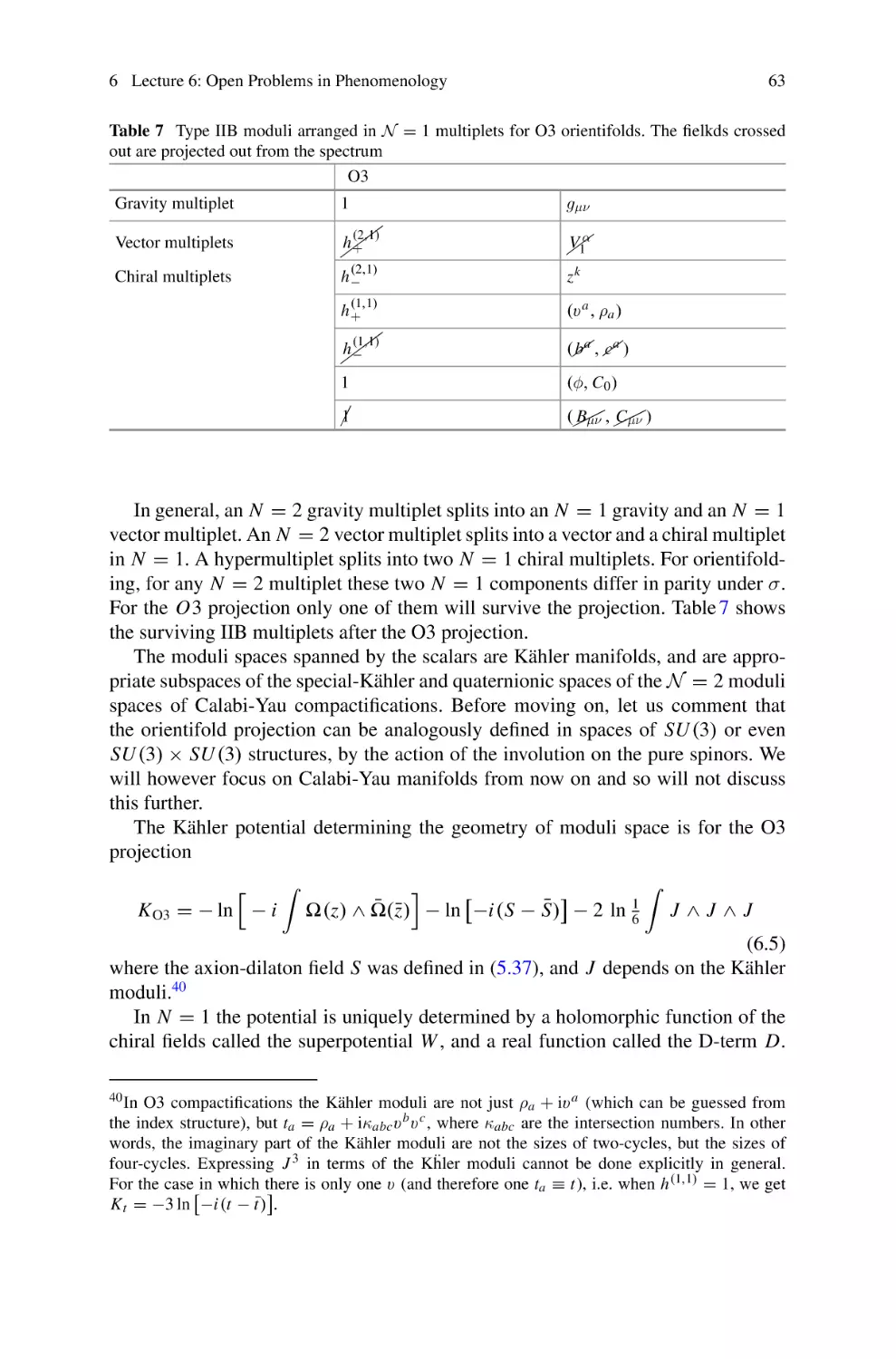
Lecture 6: Open Problems in Phenomenology . . . . . . . . . .
6.1
Calabi-Yau Orientifold Reductions . . . . . . . . . . . . .
6.2
Moduli Stabilization in Type IIB . . . . . . . . . . . . . .
6.3
Moduli Stabilization Including Non Perturbative
Effects and de Sitter Vacua . . . . . . . . . . . . . . . . . . .
References . . . . . . . . . . . . . . . . . . . . . . . . . . . . . . . . . . . . . . . . .

Contents

.........
.........
.........

60
62
64

.........
.........

68
73

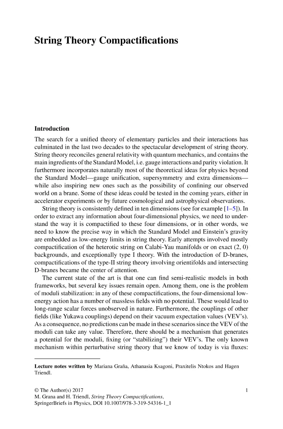
Abstract

String theory is consistently defined in ten dimensions, six of which should be
curled up in some small internal compact manifold. The procedure of linking this
manifold to four-dimensional physics is called string compactification, and in these
lectures, we will review it quite extensively. We will start with a very brief introduction to string theory; in particular, we will work out its massless spectrum and
show how the condition on the number of dimensions arises. We will then dwell on
the different possible internal manifolds, starting from the simplest to the most
relevant phenomenologically. We will show that these are most elegantly described
by an extension of ordinary Riemannian geometry termed generalized geometry,
first introduced by Hitchin. We shall finish by discussing (partially) open problems
in string phenomenology, such as the embedding of the Standard Model and
obtaining de Sitter solutions.

vii

String Theory Compactifications

Introduction
The search for a unified theory of elementary particles and their interactions has
culminated in the last two decades to the spectacular development of string theory.
String theory reconciles general relativity with quantum mechanics, and contains the
main ingredients of the Standard Model, i.e. gauge interactions and parity violation. It
furthermore incorporates naturally most of the theoretical ideas for physics beyond
the Standard Model—gauge unification, supersymmetry and extra dimensions—
while also inspiring new ones such as the possibility of confining our observed
world on a brane. Some of these ideas could be tested in the coming years, either in
accelerator experiments or by future cosmological and astrophysical observations.
String theory is consistently defined in ten dimensions (see for example [1–5]). In
order to extract any information about four-dimensional physics, we need to understand the way it is compactified to these four dimensions, or in other words, we
need to know the precise way in which the Standard Model and Einstein’s gravity
are embedded as low-energy limits in string theory. Early attempts involved mostly
compactification of the heterotic string on Calabi-Yau manifolds or on exact (2, 0)
backgrounds, and exceptionally type I theory. With the introduction of D-branes,
compactifications of the type-II string theory involving orientifolds and intersecting
D-branes became the center of attention.
The current state of the art is that one can find semi-realistic models in both
frameworks, but several key issues remain open. Among them, one is the problem
of moduli stabilization: in any of these compactifications, the four-dimensional lowenergy action has a number of massless fields with no potential. These would lead to
long-range scalar forces unobserved in nature. Furthermore, the couplings of other
fields (like Yukawa couplings) depend on their vacuum expectation values (VEV’s).
As a consequence, no predictions can be made in these scenarios since the VEV of the
moduli can take any value. Therefore, there should be a mechanism that generates
a potential for the moduli, fixing (or “stabilizing”) their VEV’s. The only known
mechanism within perturbative string theory that we know of today is via fluxes:
Lecture notes written by Mariana Graña, Athanasia Ksagoni, Praxitelis Ntokos and Hagen
Triendl.
© The Author(s) 2017
M. Grana and H. Triendl, String Theory Compactifications,
SpringerBriefs in Physics, DOI 10.1007/978-3-319-54316-1_1

1

2

String Theory Compactifications

turning on fluxes for some of the field strengths available in the theory (these are
generalizations of the electromagnetic field to ten dimensions) generates a non trivial
potential for the moduli, which stabilize at their minima. The new “problem” that
arises is that fluxes back-react on the geometry, and whatever manifold was allowed
in the absence of fluxes, will generically be forbidden in their presence.
Much of what we know about stabilisation of moduli is done in two different
contexts: in Calabi-Yau compactifications under a certain combination of three-form
fluxes whose back-reaction on the geometry just makes them conformal CalabiYau manifolds, and in the context of parallelizable manifolds, otherwise known
as “twisted tori”. In the former, fluxes stabilize the moduli corresponding to the
complex structure of the manifold, as well as the dilaton. To stabilize the other
moduli, stringy corrections are invoked. The result is that one can stabilize all moduli
in a regime of parameters where the approximations can be somehow trusted, but
it is very hard to rigorously prove that the corrections not taken into account do
not destabilize the full system. In the latter, one takes advantage of the fact that,
similarly to tori, there is a trivial structure group. However, the vectors that are
globally defined obey some non-trivial algebra, and therefore compactness is ensured
by having twisted identifications. What makes these manifolds amenable to the study
of moduli stabilisation is the possibility of analyzing them as if they were a torus
subject to twists, or in other words a torus in the presence of “geometric fluxes”, which
combined to the electromagnetic fluxes can give rise to solutions to the equations
of motion. One can then use the bases of cycles of the tori, and see which ones
of them get a fixed size (or gets “stabilized”), due to a balance of forces between
the gravitational and the electromagnetic ones. It turns out that even in this simple
situations, it is impossible to stabilize all moduli in a Minkowski vacuum without the
addition of other “non-geometric” fluxes, which arise in some cases as duals to the
known fluxes, but whose generic string theory interpretation is still under discussion.
In the last years the framework of generalized complex geometry has turned out
to be an excellent tool to study flux backgrounds in more detail, in particular going
away from the simplest cases of parallelizable manifolds. In these lectures, we review
these tools and discuss the allowed manifolds in the presence of fluxes.
Generalized complex geometry is interesting from a mathematical viewpoint on
its own, as it incorporates complex and symplectic geometry into a larger framework
[6–8], and thereby finds a common language for the two sectors of geometric scalars
that typically arise in compactifications. It does so by introducing a new bundle
structure that covariantizes symmetries of string compactifications, T-duality among
others. In particular, mirror symmetry between the type II string theories appears
naturally in this setup.
These lectures shall give a brief introduction into generalized geometry and its
appearance in string theory. For more comprehensive reviews and lecture notes, see
for instance [9, 10], while introductions to string theory and D-branes can for example
be found in [1–5].

1 Lecture 1: Introduction to String Theory

3

1 Lecture 1: Introduction to String Theory
In this section we give a basic introduction to string theory, focusing on its low
energy effective description. We start with the bosonic string, work out the massless
spectrum, and introduce the low energy effective action governing its dynamics. We
then continue with the superstring, showing the corresponding massless spectrum
and action. More details can be found in [1–4].

1.1 Bosonic Strings
String theory is a quantum theory of one-dimensional objects (strings) moving in a Ddimensional spacetime. Strings sweep a two dimensional surface, the “worldsheet”,
labeled by the coordinates σ along the string (0 ≤ σ ≤ π for an open string and
0 ≤ σ ≤ 2π for a closed string with 0 and 2π identified), and τ .
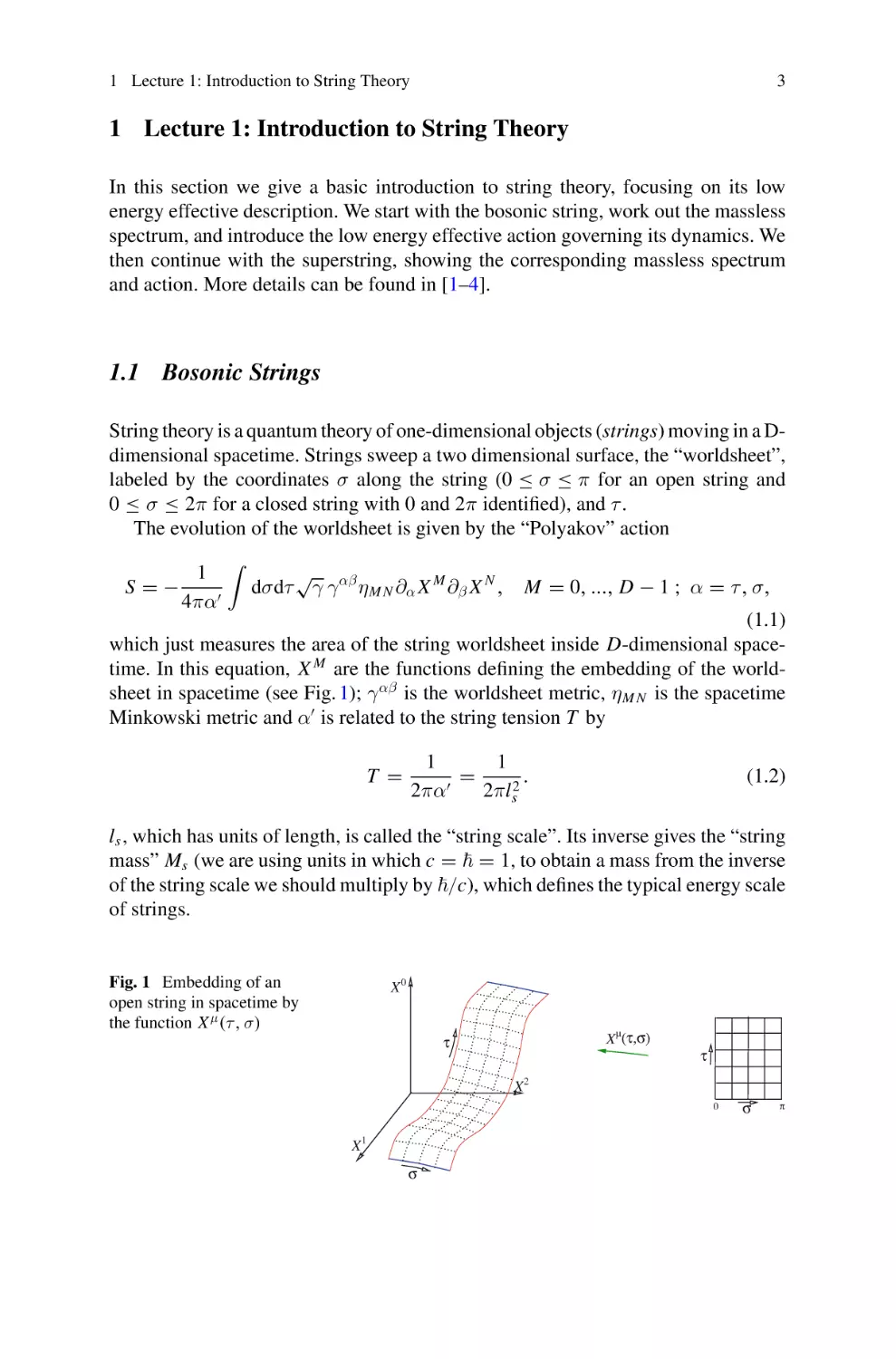
The evolution of the worldsheet is given by the “Polyakov” action
S=−

1
4πα



√
dσdτ γ γ αβ η M N ∂α X M ∂β X N ,

M = 0, ..., D − 1 ; α = τ , σ,

(1.1)
which just measures the area of the string worldsheet inside D-dimensional spacetime. In this equation, X M are the functions defining the embedding of the worldsheet in spacetime (see Fig. 1); γ αβ is the worldsheet metric, η M N is the spacetime
Minkowski metric and α is related to the string tension T by
T =

1
1
=
.
2πα
2πls2

(1.2)

ls , which has units of length, is called the “string scale”. Its inverse gives the “string
mass” Ms (we are using units in which c =  = 1, to obtain a mass from the inverse
of the string scale we should multiply by /c), which defines the typical energy scale
of strings.

Fig. 1 Embedding of an
open string in spacetime by
the function X μ (τ , σ)

X0
X μ(τ,σ)

τ
X

τ

2
0

X1
σ

σ

π

4

String Theory Compactifications

Varying the action (1.1) with respect to X M we get the following equations of
motion
 2

∂
∂2
−
(1.3)
X M (τ , σ) = 0.
∂σ 2
∂τ 2
By introducing left- and right-moving worldsheet coordinates σ ± = τ ± σ, the above
equation can be rewritten as
∂ ∂
X M (τ , σ) = 0,
∂σ + ∂σ −

(1.4)

which means that the embedding vector X M is the sum of left- and right-moving
degrees of freedom, i.e.
X M (τ , σ) = X RM (σ − ) + X LM (σ + ).

(1.5)

We will concentrate on closed strings from now on, and discuss very briefly the
open string at the end of this section. Imposing the closed string boundary conditions X M (τ , 0) = X M (τ , 2π), X M (τ , 0) = X M (τ , 2π) (with prime indicating a
derivative along σ) we get the following mode decomposition
X M (τ , σ) = X RM (σ − ) + X LM (σ + )

  1/2 
1 M −2inσ−
α
1 M
 M −
αn e
= x +α p σ +i
2
2
n
n=0
  1/2 
1 M −2inσ+
α
1
α̃n e
X LM (σ + ) = x M + α p M σ + + i
,
2
2
n
n=0
X RM (σ − )

(1.6)

where x M and p M are the centre of mass position and momentum, respectively. We
can see that the mode expansion for the closed string is that of a pair of independent
M
=
left- and right- moving traveling waves. To ensure a real solution we impose α−n
M ∗
M
M ∗
(αn ) and α̃−n = (α̃n ) .
Varying (1.1) with respect to the worldsheet metric γαβ gives the extra constrains
that the energy-momentum tensor is vanishing
T

αβ

2π δS
1
≡ −√
=− 
γ δγαβ
α



1 αβ
α M β
λ M ρ
∂ X ∂ X M − γ γλρ ∂ X ∂ X M = 0. (1.7)
2

This enforces the additional conditions
η M N ∂σ+ X LM ∂σ+ X LN = η M N ∂σ− X RM ∂σ− X RN = 0.

(1.8)

The system governed by the action (1.1) can be quantized in a canonical way in
terms of left- and right-moving oscillators, resulting in the following commutators

1 Lecture 1: Introduction to String Theory

5

[αnP , αmQ ] = [α̃nP , α̃mQ ] = nδn+m η P Q , [x P , p Q ] = iη P Q .

(1.9)

M
M
, α̃−n
with n > 0
We can therefore interpret αnM , α̃nM as creation operators and α−n
as annihilation operators, which create or annihilate a left or right moving excitation
at level n.1 Each mode carries an energy proportional to the level. The mass (energy)
of a state is obtained using the operator

2
M = 
α
2

∞



α−n · αn + α̃−n · α̃n − 2

(1.10)

n=1

where the −2 comes from normal ordering the operators (corresponding to the zero
point energy of all the oscillators). The classical conditions (1.8) in the quantum
theory become the vanishing of the so-called Virasoro operators on the physical
spectrum. We will not go into more details here (these can be found, for example, in
[1–3]) but only mention the most important of these contraints, the level-matching
condition that says that the operator

∞
1 
L̂ 0 =
α−n · αn − α̃−n · α̃n
2 n=1

(1.11)

vanishes on the physical states. Thus, we have to impose N = Ñ , where N , Ñ are
the total sums of oscillator levels excited on the left and on the right, respectively.
The massless states have therefore one left-moving and one right-moving excitation,
namely
(1.12)
|ξ M N ≡ ξ M ξ˜N α1M α̃1N |0
and a center of mass momentum k M , k · k = 0. It is not hard to check that the norm
of the state is positive only if ξ, ξ˜ are space-like vectors. The classical conditions
(1.8) impose ξ · k = ξ˜ · k = 0, i.e., the polarization vectors have to be orthogonal to
the center of mass momentum. Choosing a frame where k = (k, k, 0, ..., 0), we get
that ξ M , ξ˜M belong to the D − 2-dimensional space parametrized by the coordinates
2, ..., D − 1. The states are therefore classified by their SO(D − 2) representations.
The tensor ξ M N ≡ ξ M ξ˜N decomposes into
ξ M N = ξ sM N + ξt η M N + ξ aM N ,

(1.13)

where we have defined
ξt ≡

1 Note

1 MN
1
1
η ξ M N , ξ sM N = (ξ M N + ξ N M − 2ξt η M N ), ξ aM N = (ξ M N − ξ N M )
D
2
2
(1.14)

that the convention used here for creation (positive modes) and annihilation operators (negative modes) is opposite to the one used most often (for example in [2]).

6

String Theory Compactifications

The state corresponding to the polarization ξ M N is a massless state of spin 2: the
graviton. The state corresponding to the scalar ξt is the dilaton, while the one given
by an antisymmetric tensor is called the B-field.
The ground state of Hilbert space |0 has a negative mass square (it is − α4 ).
The appearance of this tachyon means that the bosonic string is unstable and will
condensate to the true vacuum of the theory. We will see in the discussion of the
superstring below how to remove the tachyon from the spectrum to obtain a wellbehaved theory (this cannot be done for the bosonic string).
Strings moving in a curved background can be studied by modifying the action
(1.1) by the following “σ-model” action [11]
S=−

1
4πα



√
dσdτ γ γ αβ G M N (X )∂α X M ∂β X N ,

M = 0, ..., D − 1 ; α = τ , σ

(1.15)
This action looks like (1.1) but it now has field dependent couplings given by the
spacetime metric G M N (X ). The curved background can be seen as a coherent state
of gravitons in the following sense: If we consider a small deviation from flat space,
G M N = η M N + h M N (X ), with h small, and expand the path integral [12]

Z=

D X Dγe−S =




D X Dγe−S0 1 +

1
4πα




√
dσdτ γ γ αβ h M N ∂α X M ∂β X N + ... ,

(1.16)
we find that the additional terms correspond to inserting a graviton emission vertex
operator with h M N ∝ ξ sM N . Thus, a background metric is generated by a condensate
(or coherent state) of strings with certain excitations. It is natural to try and further
generalize the σ-model action (1.15) to include coherent states of the B-field and the
dilaton. The natural reparametrization-invariant σ-model action is
1
S=−
4πα



√ 
dσdτ γ γ αβ g M N (X ) + iαβ B M N (X ) ∂α X M ∂β X N + α R .

(1.17)
The power of α in the last term should be there in order to get the right dimensions.
Note that α in this action behaves like : the action is large in the limit α → 0,
which makes it a good limit to expand around.
Something remarkable happens with the dilaton . Since it appears multiplied by
the Euler density, it couples to the Euler number of the worldsheet
χ=

1
4π


d 2 σ(−γ)1/2 R.

(1.18)

In the path integral (1.16) the resulting amplitudes are weighted by a factor e−χ .
On a 2-dimensional surface with h handles, b boundaries and c cross-caps, the Euler
number is χ = 2 − 2h − b − c. An emission and reabsorption of a closed string
amounts to adding an extra handle on the worldsheet (see Fig. 2), and therefore
results in δχ = −2. Therefore, relative to the tree level closed string diagram, the
amplitudes are weighted by e2 . At the same time, this diagram has two powers of

1 Lecture 1: Introduction to String Theory
Fig. 2 Worldsheet topology
change due to the emission
and absorption of a closed
string. The second diagram
has two powers of the string
coupling gs with respect to
the first one

7

δχ=-2

the closed string coupling constant gs2 . This means that the closed string coupling
is not a free parameter, but it is given by the VEV of one of the background fields:
gs = e<> . Therefore, the only
√free parameter in the theory is the string tension (1.2),
or the string energy scale (1/ α ). However, without the introduction of fluxes the
VEV of the dilaton is undetermined, as the action does not contain a potential term
for it. This is actually the main motivation for considering backgrounds with fluxes,
as the latter generate a potential whose minimum determines the dilaton VEV.
Although the σ-model action (1.17) is invariant under Weyl transformations2 at
the classical level, it is not automatically Weyl invariant in the quantum theory, and
therefore the theory as it is is not consistent. Weyl invariance (also called conformal
invariance) can be translated as a tracelessness condition on the energy momentum
tensor (1.7). The expectation value of the trace of the energy momentum is given by
[13]
T αα = −

1 G αβ
i B αβ
1 
M
N
β g ∂α X M ∂β X N −  β M
N  ∂α X ∂β X − β R.
2α M N
2α
2

(1.19)

where we have defined


1
PQ
G
 R
H
+ O(α2 ),
βM
=
α
+
2∇
∇

−
H
MN
M N
MPQ N
N
4


B
 −1∇P H
P H
+ O(α2 ),
=
α
+
∇
βM
P
M
N
P
M
N
N
2


D − 26
1 2
M − 1 H
M N P + O(α2 ),
β  = α
−

+
∇
∇
H
∇
M
M
N
P
6α
2
24

(1.20)

and HM P Q is the field strength of B P Q , i.e. HM P Q = ∂[M B P Q] . We have written
the one-loop contribution, while contributions from higher loops give higher orders
in α and therefore in derivatives. By setting these beta-functions to zero, we obtain
spacetime equations for the fields. Therefore, Weyl invariance at one loop (in α ) gives
the spacetime equation of motion for the massless closed fields. The first equation
in (1.20) resembles Einstein’s equation, and we can see that a gradient of the dilaton
as well as H-flux carry energy-momentum. The second equation is the equation of
motion for the B-field, and it is the antisymmetric tensor generalization of Maxwell’s
equation. The third equation is the dilaton equation of motion. The first term in this
last equation is striking: if the spacetime dimension D is not 26, then the dilaton or
2A

Weyl transformation is γαβ → eω γαβ .

8

String Theory Compactifications

√
the B-field must have large gradients, of the order 1/ α . If we do not allow for
this, then the spacetime dimension must be 26.3 The equations of motion (1.20) can
actually be derived from the following spacetime action
S=

1
2κ20



d D X (−G)1/2 e−2 R + 4∇ M ∇ M  −

1
HM N P H M N P − 2(D − 26)3α + O(α ) .
12

(1.21)

Summarizing, we have found that the massless closed string spectrum contains the
graviton, a scalar and an antisymmetric two-form. Demanding Weyl invariance of the
the worldsheet action, we have obtained their equations of motion. The equation for
the metric resembles Einstein’s equation, with the gradient of the other fields acting
as sources. The B-field obeys a Maxwell-type equation, while from the equation of
motion for the dilaton we have fixed the spacetime dimension to be 26.
One first remark is that the massless closed string spectrum does not contain a regular (one-form) gauge field. There is however a gauge field in the spectrum of massless
open strings. The solution to the (worldsheet) equations of motion (1.3) imposing
Neumann boundary conditions at σ = 0, π (i.e. ∂σ X M (τ , 0) = ∂σ X M (τ , π) = 0)
gives the following mode decomposition
X M (τ , σ) = x M + 2α p M τ + i(2α )1/2

1
αnM e−inτ cos(nσ).
n
n=0

(1.22)

The mass operator is given by cf. (1.10)
1
M = 
α
2

∞



αn · α−n − 1 .

(1.23)

n=1

The massless states are therefore given by
|ξ M ≡ ξ M α1M |0

(1.24)

which is a gauge field A M . The σ-model action for the gauge field is boundary action

∂M

dτ A M ∂τ X M

(1.25)

Its equation of motion can be derived from the spacetime action
1
S=−
4

= (D

− 26)/α ),

d D X e− FM N F M N + O(α ),

(1.26)

D = 26, like the “linear dilaton” [14] (an exact solution with  = VM X M ,
but we will not discuss them here.

3 There are solutions with

|V |2



1 Lecture 1: Introduction to String Theory

9

where F = d A. This is the Yang-Mills action, with a field dependent coupling constant go = e</2> which is the square root of the closed string coupling constant
gs .
Similarly, one can replace some of the Neumann boundary conditions by Dirichlet
boundary conditions, restraining the endpoint of the open string to p + 1-dimensional
surface, a so-called D p-brane (D for Dirichlet) [15]. The sigma-model action then
depends on a p + 1 dim. vector plus D − p − 1 scalars on the boundary of the open
string, similar to (1.25). It turns out that similar to the closed string, the VEV of
these scalars determines the position of the D p-brane. In other words, the dynamics
of the open string corresponds to the dynamics of the D p-brane, which therefore is
a dynamical object.

1.2 Superstrings
So far we have found a graviton, a gauge field, a scalar and a two-form in the massless
spectrum of open and closed strings. None of these is a fermion like the electron, or
the quarks. In order to have fermions in the spectrum, we should introduce fermions in
the worldsheet. We therefore introduce superpartners of X M (i.e., the field related to
˜ M . Each of them is a MajoranaX M by a supersymmetry transformation):  M and 
Weyl spinor on the worldsheet, which has only one component (times D − 2 for the
˜ M is
index M). The combined action (1.1) for X M and  M , 
S=

1
4π


d2 σ η M N
M

1
¯ N +
˜ M ∂¯ 
˜N
∂ X M ∂¯ X N +  M ∂
α

(1.27)

where we have used the Euclidean worldsheet by sending τ → iτ , and the derivatives
are with respect to the holomorphic coordinate z = eτ −iσ . The equations of motion
˜ admit two possible boundary conditions, denoted “Ramond” (R) and
for  and 
“Neveu-Schwarz” (NS)
R:

 M (τ , 0) =  M (τ , 2π)

NS :

 M (τ , 0) = − M (τ , 2π)

(1.28)

and similarly for ψ̃. When expanding in modes as in (1.6), the first type of boundary
condition (R) will give rise to an expansion in integer modes, while the second type
(NS) gives an expansion in half-integer modes. The (anti-)commutation relation for
the modes are
(1.29)
{ψrM , ψsN } = {ψ̃rM , ψ̃sN } = η M N δr +s .
In a similar fashion as for the bosonic string, in the superstring conformal anomaly
cancellation imposes a fixed dimension for spacetime: D = 10.
The quantized states have masses

10

String Theory Compactifications

1
M = 
α
2

∞


αn · α−n +




r ψr · ψ−r − a + same with tilde ,

(1.30)

r

n=1

where the normal ordering constant a is zero for Ramond modes, and 1/2 for NS
modes. Furthermore, the level-matching condition says that physical states vanish
under the action of the operator
L̃ 0 =

∞

n=1

αn · α−n +




r ψr · ψ−r − a − same with tilde .

(1.31)

r

The massless states are therefore
R − R : ξ M N ψ0M ψ̃0N |0 ,
N
M
NS − NS : ξ M N ψ1/2
|0 ,
ψ̃1/2

M
NS − R :ξ M N ψ1/2
ψ̃0N |0 ,
N
R − NS :ξ M N ψ0M ψ̃1/2
|0 .

(1.32)

In the same way as for the bosonic string, the polarizations ξ M have to be orthogonal to
the center of mass momentum k, and are therefore classified by SO(8) representations.
Let us now first discuss the left-moving states. We combine them with the rightmoving states afterwards. Let us start with the Ramond states. Since 0 obeys a
Clifford algebra, we can form raising and lowering operators d±i = √12 (ψ02i ± ψ02i+1 ),
with i = 1, . . . , 4. The Ramond ground states form a representation of this algebra
labeled by s:
1
1
1
1
(1.33)
R : ψ0M |0 → |s = | ± , ± , ± , ±
2
2
2
2
where ± 21 are the chiralities in the four 2-dimensional planes.4 The state ψ0M |0 is
therefore a spacetime fermion, in the representation 16. The 16 reduces into 8s ⊕ 8c .
In order to get spacetime supersymmetry, we need only 8 physical fermions (to be
the superpartners of the 8 X M ). We therefore would like to project out half of the
fermions. This is consistently done by an operation called
4 “GSO” projection (named
si = 0 (mod 2). One can
after Gliozzi, Scherk, and Olive [16]), which requires i=1
view the GSO projection as the projection to the (Majorana-)Weyl spinor subspace
of definite chirality.
Let us now turn to the NS states. From the above definition one can see that the
GSO projector anti-commutes with single creation and annihilation operators. This
means that the GSO projection either projects out the (tachyonic) vacuum state |0
or the massless state
M
|0 ,
(1.34)
N S : ψ1/2
which forms a vector in 10-dimensional spacetime. This means that we can choose
the GSO projection such that there is no tachyon in the superstring spectrum while
4 The

RR massless state ξ M N ψ0M ψ̃0N |0 should therefore be undesrtood as |s ⊗ |s̃ .

1 Lecture 1: Introduction to String Theory

11

we keep the massless NS states. As we will see, the latter is actually identical to the
massless left-moving sector of the bosonic string.
Note that in transverse eight-dimensional spacetime the irreducible spin 1/2 and
spin 1 representations have the same number of degrees of freedom: 8. We label the
spinors of positive and negative chirality by 8s and 8c , respectively, while the vector
representation is called 8v . Actually, there is a discrete symmetry interchanging the
three of them. This is called “triality” (for the trio 8s , 8c , 8v ), and plays a very
important role in string theory.
We are ready to build the whole closed superstring massless spectrum. In the R-R
sector, we have the product of two spinorial 8 representations, one for the left and
one for the right movers. We can take the same GSO projection for the left movers as
for the right movers, but we could as well take opposite projections. The first choice
leads to the so-called type IIB superstring (which is chiral, since we chose the same
chiralities on the left and on the right), while the other choice leads to the type IIA
superstring. Decomposing the products into irreducible representations we get
type IIB R − R : 8s ⊗ 8s = 1 ⊕ 28 ⊕ 35+ = C0 ⊕ C2 ⊕ C4+
type IIA R − R : 8s ⊗ 8c = 8v ⊕ 56t = C1 ⊕ C3 .

(1.35)

In this equation, we have defined Cn to be an n-form, called a R-R potential. In
type IIB there are even-degree R-R potentials (with C4 satisfying a duality condition
dC4 = ∗dC4 ). In type IIA, the R-R potentials are odd.
From the NS-R and R-NS sectors we find the fermionic states
type IIB NS − R : 8v ⊗ 8s = 8s ⊕ 56s = λ1 ⊕  1 M ,
R − NS : 8s ⊗ 8v = 8s ⊕ 56s = λ2 ⊕  2 M ,
type IIA NS − R : 8v ⊗ 8c = 8c ⊕ 56c = λ1 ⊕  1 M ,
R − NS : 8s ⊗ 8v = 8s ⊕ 56s = λ2 ⊕  2 M .

(1.36)

The fermions in the 8 representation λ A (A = 1, 2) are called the dilatini, and the
ones in the 56,  A,M are the gravitini. The name “type II” refers to the fact that there
are two gravitini.
Finally, in the NS-NS sector we get
N S − N S : type IIA and IIB 8v ⊗ 8v = 1 ⊕ 28 ⊕ 35 =  ⊕ B2 ⊕ GMN (1.37)
This sector is common to both theories and it has the same matter content the as
the massless bosonic string: a scalar, the dilaton; a symmetric traceless tensor, the
graviton; and a two-form, the B-field.
In the open strings, from the R and NS sectors we get respectively a fermion and a
gauge field A M , whose spacetime action is the supersymmetrized version of (1.26),
i.e. the action for an Abelian (U(1)) gauge field and fermionic matter. The discussion
of Chan-Paton factors, D-branes etc. carries over from the discussion for the bosonic
superstring.

12

String Theory Compactifications

Note the magic that has happened: We started with worldsheet fermions and
worldsheet supersymmetry and we ended up with massless spacetime fermions,
spacetime bosons and (two) spacetime supersymmetries. This is known as the NSR
formulation
of superstrings. The spectrum of massive states has masses of order
√
1/ α . At energies much lower than the string scale, these states can be neglected
and one can just consider the massless spectrum, which forms the field content of
the type II supergravities in ten dimensions.5 When we discuss compactifications we
will work in this limit.
Type IIA and IIB are not two independent theories, but they are related by a
symmetry called T-duality (for a review see [17]). This symmetry is inherent to 1dimensional objects: if we compactify one direction on an S 1 of radius R, the center
of mass momentum for the string along that direction will be quantized, in units of
1/R. On the other hand, there are “winding states”, namely states with boundary
conditions X M (τ , 2π) = X M (τ , 0) + 2πm R. A string with n units of momentum,
m units of winding and N , Ñ total number of oscillators on the left and on the right
has a total mass given by cf. Eq. (1.10)
M2 =

n2
m2 R2
2
+
+  (N + Ñ − 2)
R2
α2
α

(1.38)

This formula is symmetric under the exchange of n and m (or in other words winding
and momentum states) if we also exchange R with α /R! This means that large and
small radius of compactification are dual, on one side the momentum modes are
light, and winding modes are heavy, while on the T-dual picture winding modes
will be light, and momentum would be the heavy modes. The exchange between
winding and momentum amounts to exchanging X LM + X RM with X LM − X RM , and in
the superstring ψ M with ψ̄ M . This exchanges representations 8s with 8c and therefore
the GSO projections, or in other words type IIA with IIB!
T-duality has also another important consequence for type II string theories: Since
T-duality maps type IIA and IIB theory into each other, the composition of two Tdualities on different circles maps the theory non-trivially into itself and therefore
provides a symmetry of type II string theory on an n-dimensional torus. These symmetries combine with the translational and rotational symmetries of such a torus into
the discrete symmetry group O(n, n, Z), the so-called T-duality group.
At the classical level, the massless superstring spectrum is symmetric even under
continuous transformations in the group O(8, 8). Apart from Lorentz-transformations
in Gl(8) that act equally on left- and right-moving excitations, this group incorporates
rotations between left- and right-movers. More precisely, both left- and right-movers
admit a Clifford algebra for O(8) on their own. Together, they combine into the
Clifford algebra of O(8, 8). Both the R-R and NS-NS sector form irreducible representations of this group: The R-R fields combine into an O(8, 8) spinor, while
5 Note

that the discussion of Weyl anomalies of the superstring is analogous to the one in (1.20) for
the bosonic string. The vanishing of the beta functions correspond to the equations of motion of
type IIA and IIB supergravity in ten dimensions.

1 Lecture 1: Introduction to String Theory

13

the metric and the B-field form a symmetric tensor, the O(8, 8) metric. The dilaton
remains a singlet under O(8, 8).
The group O(8, 8) is not only a classical symmetry of the massless fields, but is
also locally a symmetry of their field equations in ten dimensions.6 This means that
we can make the corresponding type II supergravity and its field equations covariant
under this group. The program to understand geometry in this covariant language
is called generalized complex geometry and will be discussed in more detail in the
next section. Generalized complex geometry turns out to be extremely helpful for
understanding more complicated backgrounds of string theory, as we will see in
Lecture 4.
Under T-duality, the Neumann boundary conditions along the T-dualized directions for the open string are switched to Dirichlet boundary conditions, or the other
way around. This means that under T-duality, a D p-brane changes its dimension and
becomes a D( p ± 1)-brane.
There is an analogous action to (1.21) for D p-branes, which is called the BornInfeld action (1.39)


(1.39)
S D B I = −T p d p+1 ξe− det(G ab + Bab + 2πα Fab )
(where T p = 8π 7 α7/2 (4π 2 α )− p/2 supplemented by the Chern-Simons term depending on RR potentials



SC S = iT p

e2πα F ∧ C

(1.40)

p+1

where C is the sum of the RR potentials, and the integral picks only the p + 1rank forms. In these expressions, the background fields should be pulled-back to the
D-brane world-volume. For example, the pulled-back metric is
G ab (ξ) =

∂XM ∂XN
G M N (X )
∂ξ a ∂ξ b

(1.41)

With N D-branes on top of each other, the open strings transform in adjoint
representations of U(N). The excitations along the brane represent a U(N) gauge
field and gaugino, while excitations orthogonal to the brane are bosons and fermions
in the adjoint representation of U(N). The DBI action can actually be generalized
to the case of a non-Abelian gauge group. With stacks of D-branes intersecting
at angles, or D-branes placed at special singularities, the U(N) symmetry can for
instance be broken to the gauge group of the Standard Model of particle physics,
namely SU (3) × SU (2) × U (1) (see for example [18] for a review).
In summary, we have seen that string theory relies on supersymmetry (the spectrum of the purely bosonic string has a tachyon, which signals an instability). We
6 The

symmetry group of the supergravity theory is in fact O(10, 10) and thus larger, but the
orthogonality of the oscillators reduces the symmetry on the spectrum to O(8, 8), cf. the paragraph
below (1.12).

14

String Theory Compactifications

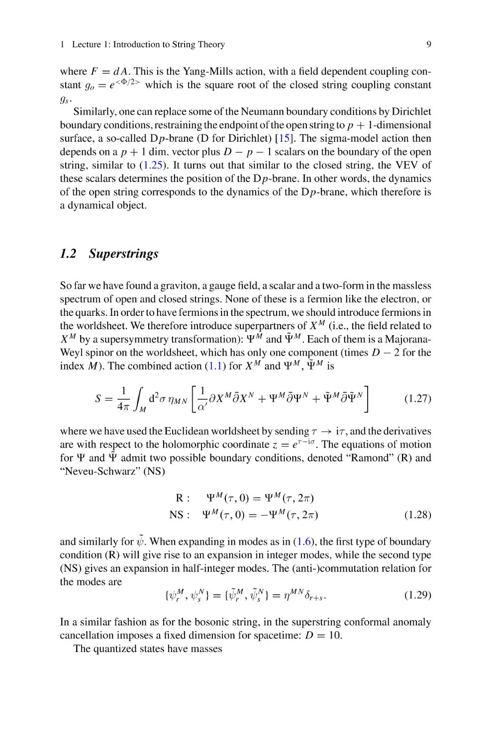
M-theory

Fig. 3 String theories as
limits of one theory

Type IIA

E8 × E8 heterotic

Type IIB

SO (32) heterotic

Type I

showed that in the massless spectrum of string theory there is a graviton, and there
are also gauge fields and fermions in representations that can be that of the Standard
Model of particle physics. As well as type IIA and type IIB, there are other string “theories”, consisting, for example, of a mixture of the bosonic string on the left movers
and the superstring on the right movers. These other “theories” are connected as well
to type IIA and type IIB by dualities. There might therefore be a single string theory
and various corners of it, or various low energy versions. One can move from one
corner to another by varying the VEVs of scalar fields (in a similar fashion as the
string coupling constant, or the radius of a circle). The space of VEVs of massless
scalar fields is called moduli space, which is shown in Fig. 3.

2 Lecture 2: Compactifications on Tori
Compactification is a very old idea in physics. It originates back in 1921 when
Theodor Kaluza tried to unify gravity with electromagnetism with the assumption
of an extra dimension.7 This additional dimension should be finite in order not to be
observed (Klein 1926). Although the original Kaluza-Klein idea did not work out, the
concept of compactification became again popular more than half a century later in the
framework of string theory. As we saw in the previous chapter, consistent superstring
theories can live only in a 10-dimensional spacetime. The compactification scheme
then goes as follows: The 10-dimensional spacetime is divided into an external noncompact spacetime M10−d and an internal compact space Md , so that it reads
M10 = M10−d × Md .

7 To

(2.1)

be historically fair, the first person to introduce an extra dimension to unify gravity with
electromagnetism was Gunnar Nordström in 1914.

2 Lecture 2: Compactifications on Tori

15

The physically interesting case is of course d = 6. The compactification scale is
Mc = 1/R (R the typical length scale associated with the internal space) and is
considered much smaller than the string scale Ms = 1/ls . We will work at energies
E  Mc  Ms .

2.1 Kaluza-Klein Compactifications on S1 (in Field Theory)
Example 1 As a warm-up, we consider a real massless scalar field living in five
dimensions x M = (x μ , x 4 ), μ = 0, 1, 2, 3 with a product structure
ds 2 = gμν (x μ )d x μ d x ν + (d x 4 )2

(2.2)

and the fifth dimension compactified x 4 ∼
= x 4 + 2π R. Then, the five-dimensional
field can be expanded in Fourier modes
(x M ) =



φn (x μ )einx

4

/R

(2.3)

n∈Z

and the 5D equation of motion ∇ M ∇ M  = 0 splits into
(∇μ ∇ μ − n 2 /R 2 )φn = 0

(2.4)

where the field φ0 is real and the fields φn , n ≥ 1 are complex. We see that the fourdimensional field theory describes particles which have masses integer multiples of
the compactification scale Mc = 1/R. Hence, it is safe to ignore the massive modes
(the so-called Kaluza-Klein tower) if we work at energies E  Mc .
Example 2 The next example we are going to consider is a five-dimensional Einstein gravity with the fifth dimension compactified as previously. The metric can be
parametrized as follows
ds 2 = G M N d x M d x N = gμν d x μ d x ν + g44 (d x 4 + Aμ d x μ )2

(2.5)

The above metric is invariant under five-dimensional general coordinate transformations x M → x M (x N ). Adopting a four-dimensional point of view for our geometry,
i.e. restricting ourselves only to transformations x μ → x μ (x ν ) splits the original
metric into
• a scalar field G 44 = g44 = e2σ
• a vector field G μ4 = e2σ Aμ
• a metric G μν = gμν + e2σ Aμ Aν

16

String Theory Compactifications

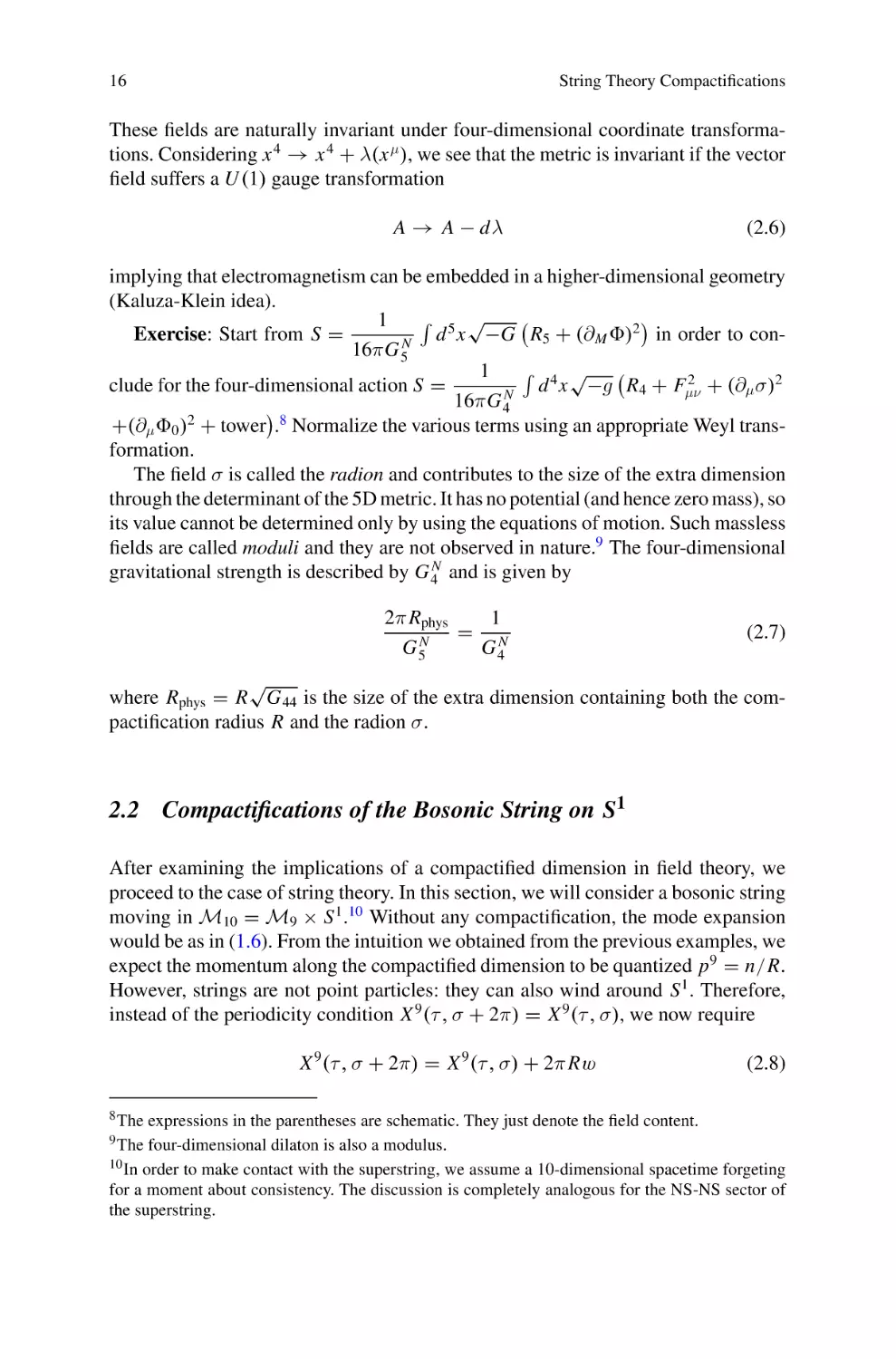
These fields are naturally invariant under four-dimensional coordinate transformations. Considering x 4 → x 4 + λ(x μ ), we see that the metric is invariant if the vector
field suffers a U (1) gauge transformation
A → A − dλ

(2.6)

implying that electromagnetism can be embedded in a higher-dimensional geometry
(Kaluza-Klein idea).
 5 √
1
d x −G R5 + (∂ M )2 in order to conExercise: Start from S =
N
16πG 5
 4 √
1
2
clude for the four-dimensional action S =
d x −g R4 + Fμν
+ (∂μ σ)2
N
16πG 4
+(∂μ 0 )2 + tower .8 Normalize the various terms using an appropriate Weyl transformation.
The field σ is called the radion and contributes to the size of the extra dimension
through the determinant of the 5D metric. It has no potential (and hence zero mass), so
its value cannot be determined only by using the equations of motion. Such massless
fields are called moduli and they are not observed in nature.9 The four-dimensional
gravitational strength is described by G 4N and is given by
2π Rphys
1
= N
N
G5
G4

(2.7)

√
where Rphys = R G 44 is the size of the extra dimension containing both the compactification radius R and the radion σ.

2.2 Compactifications of the Bosonic String on S1
After examining the implications of a compactified dimension in field theory, we
proceed to the case of string theory. In this section, we will consider a bosonic string
moving in M10 = M9 × S 1 .10 Without any compactification, the mode expansion
would be as in (1.6). From the intuition we obtained from the previous examples, we
expect the momentum along the compactified dimension to be quantized p 9 = n/R.
However, strings are not point particles: they can also wind around S 1 . Therefore,
instead of the periodicity condition X 9 (τ , σ + 2π) = X 9 (τ , σ), we now require
X 9 (τ , σ + 2π) = X 9 (τ , σ) + 2π Rw
8 The

(2.8)

expressions in the parentheses are schematic. They just denote the field content.
four-dimensional dilaton is also a modulus.
10 In order to make contact with the superstring, we assume a 10-dimensional spacetime forgeting
for a moment about consistency. The discussion is completely analogous for the NS-NS sector of
the superstring.
9 The

2 Lecture 2: Compactifications on Tori

17

where w is an integer called the winding number. Then, the mode expansion takes
the form

 
αn
+ w R σ + + oscillators
(2.9)
X 9L (σ + ) =
R
 

αn
(2.10)
X 9R (σ − ) =
− w R σ − + oscillators
R
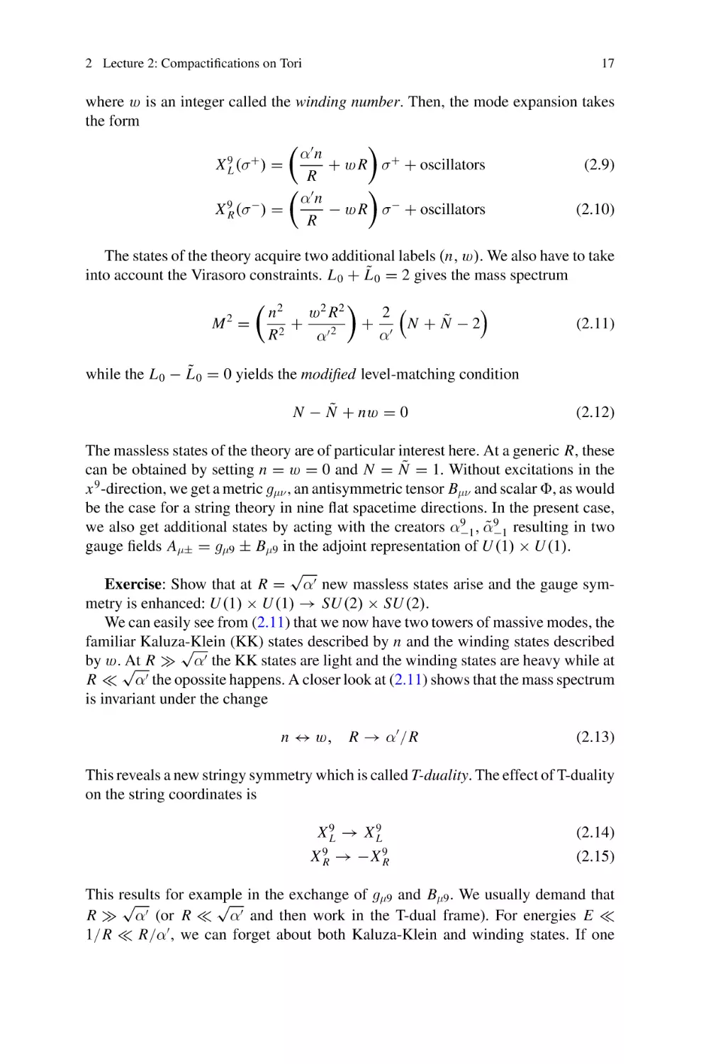
The states of the theory acquire two additional labels (n, w). We also have to take
into account the Virasoro constraints. L 0 + L̃ 0 = 2 gives the mass spectrum

M =
2

n2
w2 R 2
+
R2
α 2


+


2 
N
+
Ñ
−
2
α

(2.11)

while the L 0 − L̃ 0 = 0 yields the modified level-matching condition
N − Ñ + nw = 0

(2.12)

The massless states of the theory are of particular interest here. At a generic R, these
can be obtained by setting n = w = 0 and N = Ñ = 1. Without excitations in the
x 9 -direction, we get a metric gμν , an antisymmetric tensor Bμν and scalar , as would
be the case for a string theory in nine flat spacetime directions. In the present case,
9
9
, α̃−1
resulting in two
we also get additional states by acting with the creators α−1
gauge fields Aμ± = gμ9 ± Bμ9 in the adjoint representation of U (1) × U (1).
√
Exercise: Show that at R = α new massless states arise and the gauge symmetry is enhanced: U (1) × U (1) → SU (2) × SU (2).
We can easily see from (2.11) that we now have two towers of massive modes, the
familiar Kaluza-Klein
(KK) states described by n and the winding states described
√
by w. √
At R  α the KK states are light and the winding states are heavy while at
R  α the opossite happens. A closer look at (2.11) shows that the mass spectrum
is invariant under the change
n ↔ w,

R → α /R

(2.13)

This reveals a new stringy symmetry which is called T-duality. The effect of T-duality
on the string coordinates is
X 9L → X 9L
X 9R → −X 9R

(2.14)
(2.15)

This results
for example
√
√ in the exchange of gμ9 and Bμ9 . We usually demand that

R  α (or R  α and then work in the T-dual frame). For energies E 
1/R  R/α , we can forget about both Kaluza-Klein and winding states. If one

18

String Theory Compactifications

considers the superstring, the above analysis also holds for the NS sector. In the
R sector T-duality has another feature: It changes the chirality of the spinor that is
preserved by the GSO-projection. Therefore, T-duality exchanges type IIA and type
IIB.

2.3 Toroidal String Compactifications
Up to now, the compactifications we have considered were on a single circle. However, in order to have some hope to describe the real world, we should compactify
on higher-dimensional manifolds in order to end up with 4 noncompact dimensions.
So, as a next step let us try
(2.16)
M10 = M10−d × T d
where T d is the d-dimensional torus defined by the identification
xm ∼
= x m + 2π R m , m = 1, . . . , d

(2.17)

Generically, the massive states have at least one of the (wm , n m ) non-zero. In this
case, it is convenient to collect all the KK and winding numbers in a 2d vector
N M = (w m , n m )

(2.18)

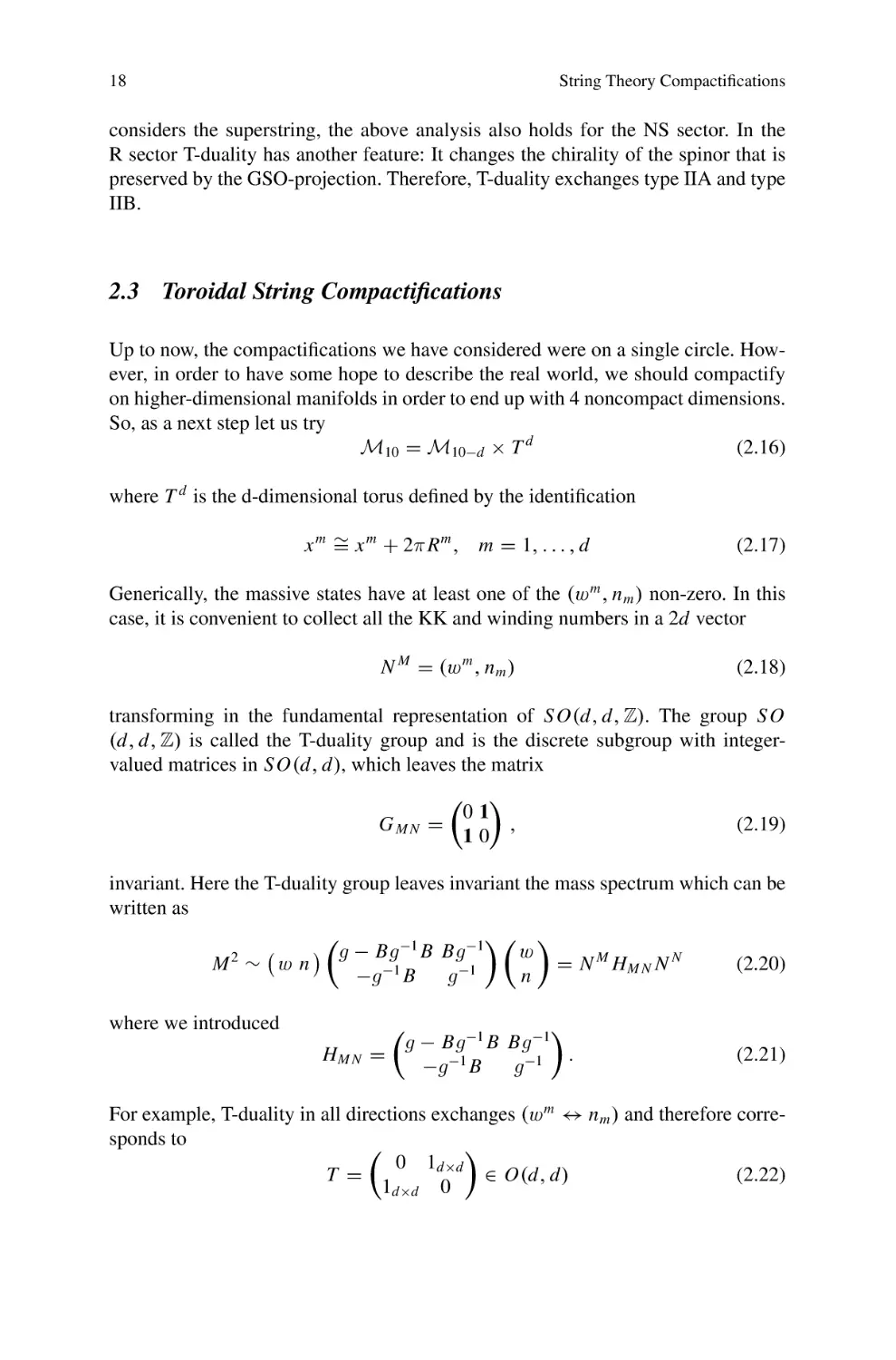
transforming in the fundamental representation of S O(d, d, Z). The group S O
(d, d, Z) is called the T-duality group and is the discrete subgroup with integervalued matrices in S O(d, d), which leaves the matrix
GMN =

 
01
,
10

(2.19)

invariant. Here the T-duality group leaves invariant the mass spectrum which can be
written as
 

w
g − Bg −1 B Bg −1
= N M HM N N N
(2.20)
M2 ∼ w n
−g −1 B
g −1
n
where we introduced
HM N =



g − Bg −1 B Bg −1
.
−g −1 B
g −1

(2.21)

For example, T-duality in all directions exchanges (w m ↔ n m ) and therefore corresponds to


0 1d×d
∈ O(d, d)
(2.22)
T =
1d×d 0

2 Lecture 2: Compactifications on Tori

19

Also the level matching condition can be written in a S O(d, d, Z)-covariant way as
N − Ñ + N M G M N N N = 0.

(2.23)

In general, the T-duality group S O(d, d, Z) is generated by
• discrete (d-dimensional) rotations that map the torus (or the lattice defining the
torus) non-trivially onto itself,
• discrete “boosts”, that correspond to pairs of T-dualities on two circles on the torus
and
• shifts of the B-field by an integer amount of a two-dimensional volume form on
the torus (a large gauge transformation).
We procceed now to the massless states, arising from two oscillation modes. The
following table describes the dimensional reduction of the massless bosonic spectrum
in the NSNS sector on T d . As an illustrative example we take d = 2, namely the
compactification is performed on a 2-dimensional torus.
Fields in 10-dim. theory Fields in (10-d)-theory
Metric g M N
gμν → 1 metric
gμm → d vectors
gmn → d(d + 1)/2 scalars
Kalb-Ramond B M N
Bμν → 1 Tensor
Bμm → d vectors
Bmn → d(d − 1)/2 scalars
Dilaton 
 → 1 scalar

Example for d = 2
1 metric
2 vectors
3 scalars
1 Tensor
2 vectors
1 scalar
1 scalar

Exercise: consider the full massless spectrum of the superstring and complete the
above table with the new states. Show that all these states are organized in multiplets
of N = 8 4-dimensional supergravity.
In the case of T 2 , parametrized by the coordinates x 8 and x 9 , from the 4 massless
scalars g88 , g89 , g99 and B89 , we can form 2 complex scalars ρ and τ . The first is
defined by
(2.24)
ρ = B89 + ivol(T 2 )
and is called the Kähler modulus. The complex structure modulus τ is then defined
through its appearance in the T 2 -metric as
ds22 =

Imρ
Imρ
|d x 8 + τ d x 9 |2 ≡
dzd z̄
Imτ
Imτ

(2.25)



Imρ
1 Reτ
.
Imτ Reτ |τ |2

(2.26)

or in matrix form
g2 =

Exercise:
take Imρ = 1 and prove that we can write g2 = ∂τ ∂τ̄ K where K =

¯ and  = d x 8 + τ d x 9 .
−log i  ∧ 

20

String Theory Compactifications

S L(2, R) × S L(2, R)
.
U (1) × U (1)
However, there are discrete symmetries (like T-duality) that give equivalent backgrounds. A coordinate transformation X → L X , where X = (x 8 , x 9 ) and L ∈
S L(2, Z) gives the same physics, and transforms τ by fractional linear transformations. Therefore the inequivalent (in the sense of corresponding to different backgrounds) values of τ live in the coset
S L(2, R)
.
U (1) × S L(2, Z)
Similarly, the Kähler modulus enjoys the same symmetries, as on one hand shifting
the B-field by an integer number (i.e. ρ → ρ + N ) does not change the physics, and
on the other it is not hard to check that T-duality on T 2 acts by ρ → −1/ρ. These
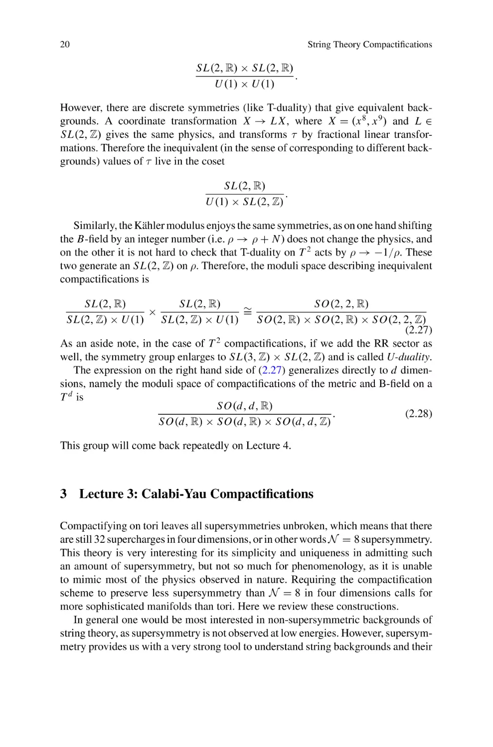
two generate an S L(2, Z) on ρ. Therefore, the moduli space describing inequivalent
compactifications is
S L(2, R)
S L(2, R)
S O(2, 2, R)
∼
×
=
S L(2, Z) × U (1)
S L(2, Z) × U (1)
S O(2, R) × S O(2, R) × S O(2, 2, Z)
(2.27)
As an aside note, in the case of T 2 compactifications, if we add the RR sector as
well, the symmetry group enlarges to S L(3, Z) × S L(2, Z) and is called U-duality.
The expression on the right hand side of (2.27) generalizes directly to d dimensions, namely the moduli space of compactifications of the metric and B-field on a
T d is
S O(d, d, R)
.
(2.28)
S O(d, R) × S O(d, R) × S O(d, d, Z)
This group will come back repeatedly on Lecture 4.

3 Lecture 3: Calabi-Yau Compactifications
Compactifying on tori leaves all supersymmetries unbroken, which means that there
are still 32 supercharges in four dimensions, or in other words N = 8 supersymmetry.
This theory is very interesting for its simplicity and uniqueness in admitting such
an amount of supersymmetry, but not so much for phenomenology, as it is unable
to mimic most of the physics observed in nature. Requiring the compactification
scheme to preserve less supersymmetry than N = 8 in four dimensions calls for
more sophisticated manifolds than tori. Here we review these constructions.
In general one would be most interested in non-supersymmetric backgrounds of
string theory, as supersymmetry is not observed at low energies. However, supersymmetry provides us with a very strong tool to understand string backgrounds and their

3 Lecture 3: Calabi-Yau Compactifications

21

corrections. Therefore, in general those models are preferred where supersymmetry
is broken at scales comparably low to the compactification scale.
Obviously, not just any manifold can be picked as internal space. For starters,
for the 10-dimensional spacetime to be a product space M10 = M4 × M6 , the first
equation of motion in (1.20) (or rather its version in the superstring, whose NSNS
piece looks like that in (1.20), but also has contributions from the RR fields) tells us
that in the absence of flux the manifolds must be Ricci-flat, i.e.
Rmn = 0.

(3.1)

In the following we want to find a four-dimensional vacuum, in other words a
solution where M4 is four-dimensional Minkowski spacetime and all fields have an
expectation value invariant under the Poincar’e group.11 This means that the vacuum
expectation value of any field except scalar fields is zero, while scalar expectation
values must be constant.
Supersymmetry imposes an additional constraint: a supersymmetric vacuum
where only bosonic fields have non-vanishing vacuum expectation values should
obey < Q  χ >=< δ χ >= 0, where Q is the supersymmetry generator,  is the
supersymmetry parameter and χ is any fermionic field.12 In type II theories, the
A
, A = 1, 2 and two dilatini λ A . In the superfermionic fields are two gravitini ψ M
gravity approximation, the bosonic part of the supersymmetry transformation of the
gravitini is
1
1  (10)
F/n  M Pn  ,
(3.2)
δψ M = ∇ M  + H
/ M P + eφ
4
16
n
where M = 0, ..., 9, ψ M stands for the column vector

ψM =

ψ 1M
ψ 2M


,

(3.3)

containing the two Majorana-Weyl spinors of the same chirality in type IIB, and of
opposite chirality in IIA, and similarly for , the 2 × 2 matrices P and Pn are differ(n/2)
ent in IIA and IIB: for IIA P = 11 and Pn = 11 σ 1 , while for IIB P = −σ 3 ,
even and Pn = iσ 2 for n+1
odd. A slash means a contraction
Pn = σ 1 for n+1
2
2
with gamma matrices in the form F/n = n!1 FP1 ...PN  P1 ...PN , and HM ≡ 21 HM N P  N P .
When no fluxes are present, demanding zero VEV for the gravitino variation (3.2)
requires the existence of a covariantly constant spinor on the 10-dimensional manifold, i.e. ∇ M  = 0. Spliting the supersymmetry spinors into four-dimensional and
six-dimensional spinors in the form
11 More generally also de Sitter and anti de Sitter and their corresponding symmetry groups can be
chosen as vacuum state.
12 The same should be true for bosonic fields, but their supersymmetry transformation is proportional
to fermionic fields whose vacuum expectation value has to vanish in order to preserve Lorentz
symmetry in four dimensions.

22

String Theory Compactifications
i
i
1 = ξ1+
⊗ η+
+ h.c.,
i
i
2 = ξ2+
⊗ η∓
+ h.c.,

(3.4)

where i = 1, .., N (N ≤ 4) will indicate the number of preserved supersymmetries in four-dimensions, the subindices denote chirality in four and six dimensions,
and upper (lower) sign is for type IIA (type IIB), each four and six-dimensional
pieces must be covariantly constant. In particular if the four-dimensional space is
Minkowski, then the four-dimensional spinor is just constant. The six-dimensional
space is then required to have a covariantly constant spinor, i.e. there should exist at
least one spinor on the compactification manifold η such that
∇m η = 0.

(3.5)

This puts a strong requirement on the internal geometries. Such manifolds are called
“Calabi-Yau” (CY).13 It is not hard to show that (3.5) implies that the manifold is
Ricci-flat, but the converse is not necessarily true. For each covariantly constant
spinor on the internal manifold, we recover two four-dimensional supersymmetry
parameters. In this case we find two four-dimensional supersymmetry parameters ξ1
and ξ2 , and therefore the four-dimensional supersymmetry preserved is N = 2. We
will now dwell into the properties of Calabi-Yau manifolds. Excellent, comprehensible lecture notes on the subject of Calabi-Yau manifolds are [19].

3.1 The Geometry of Calabi-Yau Manifolds
As we said, the internal manifold in the compactification scheme is required to
have a covariantly constant spinor. This puts both an algebraic (topological) and a
differential condition on the structure of the manifold.
The algebraic condition is that there should exist an everywhere non-vanishing
Weyl spinor. More precisely, this means that at each point contained in the overlap of
two patches, the spinor should be identical in both patches. Therefore, the transition
functions (which form a representation of Spin(6) ∼
= SU (4)) should respect this
property. In other word they can rotate the other three spinors among themselves, but
should leave this spinor invariant. This results in a reduction of the group of transition
functions, the structure group, to SU (3).
The differential condition is the integrability of the spinor, which is expressed as
∇m η = 0. This imposes stronger constraints on the manifold, namely that it should
have SU (3) holonomy. The holonomy group is defined as the group of transformations suffered by vectors or spinors when they are parallel transported with the
Levi-Civita connection around a closed loop. In order to understand what holonomy
is, we will examine the following illustrative example.
13 In

the strict sense, Calabi-Yau’s are manifolds that have only one covariantly constant spinor.

3 Lecture 3: Calabi-Yau Compactifications

23

Fig. 4 A vector parallel
transported around the closed
loop in R2 /Z 6 comes back to
itself up to a Z 6 rotation

It is obvious that two-dimensional flat space R2 has trivial holonomy (only the
identity element), as it has trivial connection. However, if we consider R2 /Z6 (where
points are identified if the angle they form with the origin is 60◦ ), the holonomy
group reduces to Z6 , i.e. vectors parallel transported around closed loops (in the Z6
sense) can be rotated in multiples of 2π/6. This is illustrated in Fig. 4.
An alternative (and equivalent) definition of CY manifolds is that these are Kähler
(i.e. complex and symplectic) manifolds with c1 = 0. Let us define these in turn, and
then see how this definition relates to the one of SU (3) holonomy.

3.1.1

Complex Manifolds

Almost complex manifolds of even dimension d = 2n are those where one can define
a real map I from the tangent space to itself such that
I 2 = −1.
This map is called the almost complex structure, as having n (+i) eigenvalues and n
(−i) eigenvalues, allows to define holomorphic and antiholomorphic vectors. Let us
see how this works with a very simple example in d = 2, with the almost complex
structure given by


0 1
.
I =
−1 0
The eigenvectors are then given by
∂
∂
∂
,
+i 2 ≡
∂x 1
∂x
∂z

∂
∂
∂
.
−i 2 ≡
∂x 1
∂x
∂ z̄

Given an almost complex structure for the tangent space, one can define the projectors
P± =

1
(1 ∓ i I )
2

which project onto the holomorphic and anti-holomorphic bundles.

24

String Theory Compactifications

There are a few equivalent ways of defining integrability of an almost complex
structure. Here we use the one that is easily generalized to generalized almost complex
structures that will appear in the next lecture. We say that I is integrable if and only
if
(3.6)
P− [P+ v, P+ w] = 0,
i.e. the Lie bracket14 of two holomorphic vectors has to be holomorphic as well. The
adjective “integrable” is used because if (and only if) I is integrable, there are complex
coordinates z i (i = 1, .., n) such that (dz)i = d(z i ) give a set of holomorphic oneforms. In other words, the holomorphic one-forms dz can be integrated globally to
find the coordinates z. An integrable almost complex structure is called a complex
structure (with the corresponding manifold being called complex manifold).
On an almost complex manifold, any n-form A
A=

1
Am ...m d x m 1 ∧ . . . ∧ d x m n ,
n! 1 n

can be decomposed into its holomorphic and anti-holomorphic components, as:
A p,q =

1
Ai ...i j¯ ...j¯ dz i1 ∧ . . . ∧ dz i p ∧ d z̄ j¯1 ∧ . . . ∧ d z̄ j¯q ,
p!q! 1 p i q

(3.7)

where p + q = n. If the manifold is even complex, the exterior derivative
dA =

1
∂[m Am ...m ] d x m 1 ∧ . . . ∧ d x m n+1 ,
n! 1 2 n+1

(3.8)

can be split into a holomorphic and an antiholomorphic pieces, namely d = ∂ + ∂¯
where
∂ : ( p, q) → ( p + 1, q),
∂¯ : ( p, q) → ( p, q + 1).
Complex manifolds look locally like Cn , and have holonomy G L(n, C) (or a subgroup thereof), since parallel transport preserves the complex structure (or in other
words it preserves holomorphicity).

3.1.2

Symplectic Manifolds

A 2n-dimensional manifold is symplectic if there is a globally-defined nowhere
vanishing two-form J such that
d J = 0,
(3.9)
14 The

definition of Lie bracket is as follows:
[v, w]n = (v m ∂m w n − w m ∂m v n )∂n .

3 Lecture 3: Calabi-Yau Compactifications

25

and if J is non-degenerate, i.e. if the top-form J n is nowhere vanishing. This defines
a symplectic product
< v, w > J ≡ J (v, w) = v m Jmn w n

(3.10)

Similarly to complex coordinates z i for complex manifolds, in symplectic manifolds
one can define Darboux coordinates (x i , y i ) such that
J=

n


d x i ∧ dy i

(3.11)

i=1

A symplectic manifold has holonomy Sp(2n) (or a subgroup thereof), as parallel
transport preserves J .

3.1.3

Kähler Manifolds

Kähler manifolds are complex and symplectic manifolds for which the complex and
symplectic structures are compatible. This means that J is (1, 1) in terms of I , i.e.
J = Ji j¯ dz i ∧ d z̄ j¯ .

(3.12)

This also implies that the complex and symplectic groups intersect in U (3), i.e. G L
(n, C) ∩ Sp(2n) = U (3), and the holonomy of the manifold must be contained in
this U (3).
The complex structure I and the symplectic two-form J together define the metric
g via
gmn = Jmp I p n .
This metric can be derived from a real scalar function K called the Kähler potential,
namely15
Ji j¯ = igij = i∂i ∂¯ j̄ K
We are almost there on our way to Calabi-Yau manifolds. Only the last requirement, c1 = 0, remains to be explained. To understand what it means, we need to
introduce the notion of cohomology classes.

15 Note

that the Kähler potential is not uniquely defined, but a so-called Kähler transformation
K → K + f (z) + f¯(z̄) leaves the metric invariant. Moreover, the Kähler potential is only locally
defined if J is not an exact two-form. In particular, on any compact manifold K is only locally
defined.

26

3.1.4

String Theory Compactifications

Cohomology Classes

The exterior derivative given in (3.8) is a nilpotent operator (of order two), i.e. d 2 = 0,
and as such it allows to define cohomology classes, as will be explained now. Let us
make the following definitions:
• Closed p-forms A p are p-forms such that d A p = 0. Let us call C p (M) the space
of closed p-forms.
• Exact p-forms B p are such that B p = dC p−1 for some globally defined ( p − 1)form C p−1 .16 Let us call Z p (M) the space of exact forms.
Then the p-th de Rham cohomology H p is defined by
H p (M) = C p (M)/Z p (M).
The elements of H p are equivalence classes of closed forms and are called cohomology classes. Two forms A p and à p are in the same cohomology class (A  Ã) if
A p = Ã p + dC p−1 for some ( p − 1)-form C p−1 . Note that though both the closed
and exact forms form vector spaces of infinite dimension, the dimension of the H p
are finite and define the Betti numbers b p , i.e.
dim H p (M) = b p .

(3.13)

These are topological invariants, i.e. independent of the metric that we define on
the manifold. If the manifold is orientable (and compact), Betti numbers have the
property17
b p = bd− p .
On complex manifolds one can define cohomology classes for ( p, q) forms. Furthermore, one can define another cohomology called the Dolbeault cohomology,
which is analogous to the de Rham cohomology but with the exterior derivative d
replaced by the holomorphic derivative ∂. On Kähler manifolds, the de Rham and
the Dolbeault cohomology theories coincide, namely
p,q

Hd

p,q

= H∂

p,q

= H∂¯ .

(3.14)

The dimensions of these cohomology classes are denoted by the Hodge numbers
h p,q and satisfy the following properties

16 Note

that (as stated by the Poincar’e Lemma) all closed forms are locally exact, i.e. exact in a
patch. Here by exact we mean globally exact, i.e. exact on the whole manifold.
17 This fact follows from the properties of the Hodge star operator that we will define in (3.28). This
property is not true for non-orientable manifolds: since the manifold is non-orientable, the volume
form is not well-defined and we have bd = 0, while of course b0 is larger than zero and counts the
number of connected components.

3 Lecture 3: Calabi-Yau Compactifications
p


27

h k, p−k = b p ,

h p,q = h q, p = h n− p,n−q .

(3.15)

k=0

It is customary to arrange these numbers in the following diamond (we give the
example for six-dimensional manifolds)
h 0,0
h 1,0
h 2,0
h 3,0

h 0,1
h 1,1

h 2,1
h 3,1

h 0,2
h 1,2

h 2,2
h 3,2

h 0,3

(3.16)

h 1,3
h 2,3

h 3,3
Using (3.15) one can see that the diamond is symmetric under reflections through the
horizontal and vertical axes. Furthermore, h 0,0 simply counts the connected components so that for connected manifolds one finds h 0,0 = h 3,3 = 1.
A particularly important cohomology class is the one in which the Ricci two-form
lives. The latter is defined as
R ≡ Rmnpq J pq d x m ∧ d x n .
This form is closed on Kähler manifolds, dR = 0, and therefore allows to define a
cohomology class, the first Chern class18
c1 =

3.1.5

1
[R].
2π

(3.17)

Calabi-Yau Manifolds

On Calabi-Yau manifold the holonomy is SU (3). Equivalently, CY manifolds are
Kähler manifolds on which the first Chern class is trivial (c1 = 0), or in other words
R = d A for some globally defined one-form A. Calabi conjectured, and Yau proved
that these manifolds always admit a Ricci-flat metric (i.e. there is always a metric
for which A = 0).
The Hodge diamond (3.16) is quite simple for CY manifolds. First there is h 1,0 = 0
and h 2,0 = 0, with the former equation saying that all closed one-forms are exact (or
“trivial in cohomology”). Furthermore, one finds h 3,0 = 1. A representative of this
cohomology class is called the holomorphic three-form ,

18 There

are also higher Chern classes constructed out of the curvature tensor, but we will not use
or introduce them.

28

String Theory Compactifications

=

1
i jk dz i ∧ dz j ∧ dz k .
6

(3.18)

Equivalently to the complex structure I , this form tells us what the complex coodinates are.19 If the complex structure is integrable then d = ξ ∧  for some one-form
ξ. For a Calabi-Yau there is ξ = 0 so that d = 0.
Using the properties (3.15), the Hodge diamond of a CY manifold is then simply
of the form
1
0
0
0
h 1,1
0
(3.19)
h 2,1
1
1
h 2,1
0
0
h 1,1
0
0
1
and is therefore completely determined by two independent topological numbers h 1,1
and h 2,1 .
It is customary to denote the elements in H 1,1 as ωa , a = 1, ..., h 1,1 , and those of
2,2
H as ω̃ a . They can be chosen such that

ωa ∧ ω̃ b = δab ,

(3.20)

while for the real 3-forms we use α K , β K , K = 0, .., h 2,1 (note that since these forms
are real, they belong to H 2,1 ⊕ H 1,2 , or H 3,0 ⊕ H 0,3 ). They can also be chosen to
satisfy

α K ∧ β L = δ KL .

(3.21)

One can also choose a basis of complex forms, which are purely in H 2,1 . These forms
are called χk . Table 1 summarizes all this.
Going back to the covariantly constant spinor, we find that J and  can be written
as bilinears of the spinor, namely
†
γmn η±
Jmn = ∓ 2i η±

†
mnp = −2i η−
γmnp η+ .

(3.22)

Taking η+ to be the Clifford vacuum, i.e. such that it annihilated by gamma matrices
with holomorphic indices (γ i η+ = 0), it is not hard to see that Jmn is a (1, 1)-form
with respect to this complex structure, while  is a (3, 0)-form.
be more precise,  defines a complex structure, but the opposite is not necessarily true. Only
when the U (1) piece of the U (3) holonomy of Kähler manifolds is trivial (i.e. when the holonomy
is reduced to SU (3)), one has such a closed (3, 0)-form  globally defined. This statement is
equivalent to the requirement c1 = 0.
19 To

3 Lecture 3: Calabi-Yau Compactifications

29

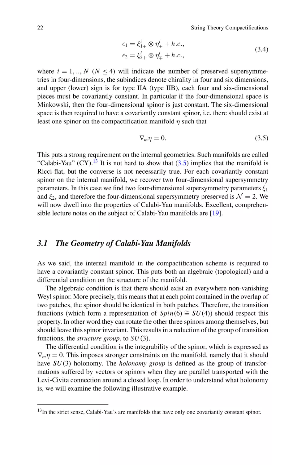
Table 1 Basis of harmonic forms in a Calabi–Yau manifold
Cohomology group
Basis
H (1,1)
H (0,0) ⊕ H (1,1)
H 3,3 ⊕ H (2,2)
H (2,1)
H (3)

3.1.6

wa
w A = (1, wa )
w̃ A = (vol, w̃a )
χk
(α K , β K )

a = 1, .., h (1,1)
A = 0, .., h (1,1)
A = 0, .., h (1,1)
k = 1, .., h (2,1)
K = 0, .., h (2,1)

Examples of Calabi-Yau Manifolds

It is time to give someexamples of Calabi-Yau manifolds. In two dimensions, the
only CY manifold is the torus. In four dimensions, there is T 4 , which in the strict
definition of Calabi-Yau n-folds to exactly have SU (n) (and not smaller) holonomy is
not a Calabi-Yau. The only ‘exactly’ SU (2) holonomy manifold in four dimensions
is called K 3. To be more precise, K 3 is not a single manifold, but a class of manifolds,
which are all diffeomorphic to one another and all have the same Betti numbers b1 = 0
and b2 = 22. This class is a 58-parameter family of K 3, where these 58 parameters
each deform the metric and correspond to moduli in the lower-dimensional theory.
One can describe K 3 as the resolution of the singular space T 4 /Z2 , where Z2 acts by
inverting all four directions on the torus. This involution has 16 singularities which
must be blown up into two-spheres to make the manifold smooth. These two-spheres
each define non-trivial homology classes, so that together with the six two-cycles
on T 4 /Z2 we find 22 non-trivial homology classes, giving b2 = 22. On the other
hand, all one-cycles are projected out by the Z2 so that K 3 has b1 = 0, similar to
Calabi-Yau threefolds.
In six dimensions, there are many Calabi-Yau manifolds known and their number could possibly be infinite. There are various ways of constructing Calabi-Yau
manifolds. In the following we will give an example by constructing a family of
Calabi-Yau three-folds by taking the zeros of certain polynomials in the complex
projective space CP 4 . The Complex projective space CP n+1 is the space that results
from taking Cn+2 \ {0} and identifying points if they are related by a complex scaling,
i.e.
(3.23)
(z 1 , ...., z n+2 ) ∼ λ(z 1 , ...., z n+2 ), for λ ∈ C∗ .
To visualize this, we can think of the real projective space RP 1 , in which two points
in R2 {0} are identified if they are related by a real rescaling, i.e. if they lie on a line.
We can take a representative of this line as a point that is at unit distance from the
origin. The set of inequivalent points therefore lie on the circle of unit radius, hence
P1 ∼
= S 1 .20
20 The

inequivalent points actually lie on half of the circle, as one half is identified with the other,
so technically P1 ∼
= S 1 /Z2 , but this is just isomorphic to S 1 , since Z2 is just a rotation by 180◦ .

30

String Theory Compactifications

The complex projective spaces CP n+1 are Kähler manifolds, but not Calabi-Yau.
But the n-dimensional subspace defined by
G(z 1 , ..., z n+2 ) = 0,

(3.24)

where G is a holomorphic homogeneous polynomial of degree n + 2 (i.e. G(λz 1 ,
..., λz n+2 ) = λn+2 G(z 1 , ..., z n+2 )), is a Calabi-Yau n-fold.
For example, for n = 3, the “quintic CY” is the family of subspaces in CP 4
defined as the zero set of holomorphic homogeneous polynomial G of degree five,
for instance by
4

G=
(z a )5 .
(3.25)
a=1

It has b2 = 1 and b3 = 204, where the former is the two-cycle inherited by CP 4 and
the latter correspond to the number of changes in the coefficients in the polynomial G.
It can be shown that the manifolds just described have SU (n) holonomy and
therefore admit a Ricci-flat metric. However, the explicit metric is not known, not
even for the only (complex) two-dimensional Calabi-Yau manifold K 3. However,
we can go a far way along without knowing the metric explicitly, as we will see in
the following.

3.2 Effective Theory for Compactifications
of Type II Theories on CY3
In the following we want to discuss how Calabi-Yau compactifications of type II
string theory can be effectively described at low energies. By decoupling all modes
with a mass at least of the order of the compactification scale, one can in general find
an effective action. In the particular case when the internal manifold is Calabi–Yau
and no fluxes are turned on, the four-dimensional effective action is well known: It
corresponds to an N = 2 ungauged supergravity whose matter content is completely
determined by the Hodge numbers h (1,1) and h (2,1) , depending on which type II theory
we look at.
This effective action arises from expanding all 10-dimensional fields in a basis
of “massless” forms, i.e. in the higher dimensional equivalent to the zero mode
n = 0 of the S 1 compactification. One can show that the operator whose eigenvalues
correspond to four-dimensional masses is21
 = d d † + d † d,

(3.26)

√
can be shown for example by splitting the term
−G H 2 in the Lagrangian into external
and internal components, and integrating by parts the contribution from the internal piece.

21 This

3 Lecture 3: Calabi-Yau Compactifications

31

where d is the exterior derivative and d † is its “adjoint”, given by
d † ≡ (−1)dp+ p+1 ∗ d∗

(3.27)

where p is the degree of the form that is acting on, d the dimension of the space, and
∗ is the Hodge star operator, which on a p form acts as
(∗A)m p+1 ...m d− p =

1
m ,...,m d− p m 1 ,...,m p Am 1 ,...,m p
p! p+1

(3.28)

√
and m 1 ...m d is the volume density, with values ± g (and whose indices are raised
with the inverse metric). Forms which satisfy d † A = 0 are called coclosed.
It is easy to see that
• d : p → p+1
• d† : p → p − 1
• : p→ p
The operator  replaces then the Laplacian that appears in S 1 compactifications.22
Harmonic forms are those that satisfy A = 0. It is not hard to show that a form is
harmonic exactly if it is both closed and coclosed
 A = 0 ⇔ (d A = 0 and d † A = 0).

(3.29)

The so-called Hodge theorem states that any p-form D p can be decomposed
uniquely into an harmonic, a (globally) exact, and a coexact piece, i.e.
D p = A p + d B p−1 + d † C p+1 where  A p = 0.

(3.30)

This is called the Hodge decomposition. If D p is closed, then C p+1 = 0, and D p is
in the same cohomology class as A p . This means that each cohomology class has
exactly one harmonic form, which we can take to be a representative of it. Therefore
the space of harmonic p-forms is isomorphic to the p-th cohomology. The forms in
Table 1 can therefore be chosen to be harmonic forms, and will in the following be
used to expand all the 10-dimensional fields in, in order to obtain the four-dimensional
low-energy action. We will now show how this works.
We start with the NSNS sector. The dilaton is “expanded” in the only scalar
harmonic form w0 , which we can identify with the constant 1. As there are no
harmonic one-forms on a CY in which one could expand the mixed components of
the B-field, it can have only purely external or internal components. The former is
expanded in the only internal scalar 1, while the latter is expanded in the basis wa
(this makes sense, as B is a gauge field, i.e. B  B + dλ, which is precisely the
definition of a cohomology class). As for the metric, the four-dimensional massless
22 For scalar fields, ∇ 2

the curvature.

and  coincide, while for higher order p-forms they differ by terms involving

32

String Theory Compactifications

fields correspond to deformations that respect the Calabi-Yau condition. It is not hard
to see that the deformations δgi j¯ correspond to deformations of the fundamental form
J2 , which is closed and coclosed (∗J = J 2 , so d † J = 0), and therefore expanded in
the basis of h (1,1) harmonic forms. δgi j correspond on the contrary to deformations
of the complex structure, which are in one-to-one correspondence with the harmonic
(2, 1)-forms. We have therefore the following expansions for the deformations of the
fields in the NS sector:
φ(x, y) = φ(x) ,



gi j¯ (x, y) = iv (x)(ωa )i j¯ (y),
a

¯

(χ̄k )i k̄l¯ k̄l
δgi j (x, y) = i z̄ (x)
||2
k


j

(y), (3.31)

B2 (x, y) = B2 (x) + ba (x)ωa (y),
where x parameterizes the external coordinates, while y parameterize the internal
ones. Here, all x-dependent fields are massless scalars in the four-dimensional theory,
so-called “moduli”.23 In the NSNS sector we get a total of 2 (h (1,1) + h (2,1) + 1)
moduli.24
In the RR sector, we perform the following expansions
C1 (x, y) = C10 (x),
C3 (x, y) = C1a (x) ωa (y) + ξ K (x)α K (y) − ξ˜K (x)β K (y)

(3.32)

for type IIA, and
C0 (x, y) = C0 (x),
C2 (x, y) = C2 (x) + ca (x)ωa (y) ,
C4 (x, y) = V1K (x) α K (y) + ρa (x)ω̃ a (y)

(3.33)

for type IIB. In the expansion of C4 we have used the self duality of F5(10) , which
connects the terms expanded in α K to the ones that would be expanded in in the
forms β K , and similarly for ρa , which are dual to h (1,1) tensors D2 coming from
expanding in the basis ωa .
These moduli arrange into the N = 2 multiplets shown in Tables 2 and 3.
Inserting the expansions (3.31), (3.32) in the 10-dimensional type IIA action,
and (3.31), (3.33) in the IIB one and integrating over the Calabi-Yau, one obtains a
standard four-dimensional N = 2 ungauged supergravity action whose forms is

23 The

terminology “modulus” is sometimes used also to denote the (unfixed) VEV of the scalar
field.
24 Note that the z k (x) are complex scalar fields and therefore have two degrees of freedom. Moreover,
the field B2 (x) is a four-dimensional tensor field, which however can be dualized into a fourdimensional scalar field.

3 Lecture 3: Calabi-Yau Compactifications

33

Table 2 Type IIA massless fields arranged in N = 2 multiplets
Gravity multiplet
1
Vector multiplets
h (1,1)
Hypermultiplets
h (2,1)
Tensor multiplet
1

(gμν , C10 )
(C1a , v a , ba )
(z k , ξ k , ξ̃k )
(B2 , φ, ξ 0 , ξ̃0 )

Table 3 Type IIB massless fields arranged in N = 2 multiplets
Gravity multiplet
1
Vector multiplets
h (2,1)
Hypermultiplets
h (1,1)
Tensor multiplet
1

(gμν , V10 )
(V1k , z k )
(v a , ba , ca , ρa )
(B2 , C2 , φ, C0 )

(4)
SIIA


=
M4

− 21 R ∗ 1 + 21 ReN AB F A ∧ F B + 21 ImN AB F A ∧ ∗F B

(3.34)

−G ab dt a ∧ ∗d t¯b − h uv dq u ∧ ∗dq v ,
for type IIA, and
(4)
SIIB


=
M4

− 21 R ∗ 1 + 21 ReM K L F K ∧ F L + 21 ImM K L F K ∧ ∗F L
−G kl dz k ∧ ∗d z̄ l − h pq d q̃ p ∧ ∗d q̃ q .

(3.35)

Let us explain these expressions. In the gauge kinetic part, the field strengths are F A =
dC1A = (dC10 , dC1a ) in the IIA action (3.34), and F K = d V1A = (d V10 , d V1k ) in the
IIB action (3.35). The gauge kinetic coupling matrices N and M depend only on the
scalars in the respective vector multiplets. In IIA, these are the complex combination
of Kähler and B-field deformations t a , called complexified Kähler deformations, and
defined
(3.36)
B + i J = (ba + iv a ) ωa ≡ t a ωa .
In IIB, the scalars in the vector multiplet moduli space are the complex structure
deformations z k , or the periods, defined as

ZK =

 ∧ βK .

(3.37)

The scalars in the vector multiplets span a special Kähler manifold of complex
dimension h 1,1 and h 2,1 in IIA and IIB respectively, whose metric G ab and G kl will
be given shortly. The scalars in the hypermultiplets span a quaternionic manifold (a
manifold that looks locally like copies of the quaternions) whose coordinates are q u ,
u = 0, ..., h (2,1) and u = 0, ..., h (1,1) for IIA and IIB respectively.

34

String Theory Compactifications

The Kähler potential in the vector multiplet moduli space in IIA, which is spanned
by the complexified Kähler deformations t a , is given by
K = − ln

4 
3


J∧J∧J ,

(3.38)

In type IIB, the scalars in the vector multiplet moduli space are the complex
structure deformations z k . They span again a Kähler manifold, with Kähler potential
given by
 

¯ .
K = − ln i  ∧ 
(3.39)
These spaces are “special Kähler”, which means that the Kähler potentials can
be derived from a holomorphic function called the prepotential. The matrices M
and N in the four-dimensional effective actions (3.34) and (3.34) are obtained from
derivatives of these prepotentials. For the interested reader, more details are given in
[9], and references therein.

4 Lecture 4: Fluxes and Generalized Geometry
4.1 Charges and Fluxes
4.1.1

Homology

Similar to the concept of cohomology classes for differential forms, which we introduced in Sect. 3.1.4, there is a similar characterization for submanifolds. The role
of the exterior derivative on forms is played in this case by the boundary operator
δ, that maps a p-dimensional submanifold to its ( p − 1)-dimensional boundary. As
a submanifold that is itself a boundary cannot have any boundary, the operator δ is
nilpotent and obeys
(4.1)
δ 2 = {}.
Closed submanifolds (called cycles) are defined as those manifolds that have no
boundary, while an exact submanifold is a boundary of another submanifold of one
dimension higher. Moreover, we can define addition and subtraction on submanifolds:
The sum C p + C˜ p of two p-dimensional submanifolds C p and C˜ p is the union of the
two, respecting the orientation of both, while the difference C p − C˜ p is the union of C p
and C˜ p , but with the orientation of C˜ p inverted. Homology classes are now defined as
equivalence classes of closed p-dimensional submanifolds, where two submanifolds
C p and C˜ p are equivalent (or “homologous”) if the difference C p − C˜ p = δD( p+1) is
a boundary. Therefore, homology is defined as

4 Lecture 4: Fluxes and Generalized Geometry

35

Fig. 5 The cycles C p and C˜ p together are homologous to D p

Hp =

{C p |δC p = {}}
.
{δD( p+1) }

(4.2)

An illustration of equivalent cycles is given in Fig. 5, where the sum of the cycles C p
and C˜ p is homologous to D p .
There is a canonical pairing between a p-form α p and p-dimensional submanifold
C p , given by integrating α p over C p , i.e.

(C p , α p ) =

Cp

αp.

(4.3)

This scalar product also relates the exterior derivative d and the boundary operator
δ as dual operators, by Stokes theorem



Cp

dα p−1 =

δC p

α p−1 .

(4.4)

Using Stokes theorem, it is easy to see that the scalar product is well-defined on
H p (M) × H p (M), as ([C], [α]) is independent of the respective representatives.
Furthermore, it gives an invertible b p × b p matrix. This means that homology and
cohomology are in fact dual spaces to each other, and they are therefore isomorphic
to one another, i.e.
(4.5)
H p (M) ∼
= Hd− p (M),

36

String Theory Compactifications

by the identification




Cp

4.1.2

αp =

Cd− p ∧ α p .

(4.6)

M

D-Branes as Dirac Monopoles

In the following we want to discuss the field configuration sourced by a D-brane. This
field configuration resembles just a higher-dimensional realization of the magnetic
monopole configuration in electrodynamics that was first discussed by Dirac.
D-branes are charged objects. From (1.40) we see that a D p-brane electrically
sources the field C p+1 or, equivalently, magnetically sources C10− p−3 . If we consider
now a D p-brane in flat 10-dimensional spacetime, it will fill out p + 1 dimensions
and create in the 9 − p other directions a non-trivial field configuration for C10− p−3
so that for any (8 − p)-sphere S 8− p surrounding the D p-brane we find

S 8− p

F8− p = T p ,

(4.7)

where F8− p is the field strength of C7− p . If C7− p would be globally defined, then
from Stokes theorem (4.4) we would find that



F8− p =
dC7− p =
C7− p = 0,
(4.8)
S 8− p

δS 8− p

S 8− p

as the sphere has no boundary, therefore being in conflict with (4.7). Therefore, the
gauge field C7− p is only locally defined, i.e. in the northern and southern hemisphere
8− p
8− p
D(N ) and D(S) of S 8− p . These two gauge fields must then be related by a gauge
transformation, thus
(N )
(S)
(4.9)
d(C7−
p − C 7− p ) = 0.
Locally, we can again write
(N )
(S)
C7−
p − C 7− p = d6− p .

This means that we can reduce



(N )
F8− p =
dC7− p +
8− p

S 8− p


=

D(N )

7− p

D(N )

(N )
d6−
p +



8− p

(S)
dC7−
p

7− p

d(S)
6− p ,

D(S)



D(S)

7− p

=

7− p

S 7− p

(4.10)

(N )
(S)
(C7−
p − C 7− p )

(4.11)

where S 7− p is the equator of S 8− p and D(N ) and D(S) its corresponding hemispheres.
This reduction can be continued in an inductive way so that we end up with

4 Lecture 4: Fluxes and Generalized Geometry

37




S 8− p

F8− p =

S1

dλ = T p ,

(4.12)

φ
. Effectively, the field strength F8− p defines a non-trivial
where we have λ = T p 2π
8− p 8− p 25
(S ). If we now forget about the D p-brane and the
cohomology class in H
ambient space and focus on the field strength configuration on the sphere, we see
that it can be non-trivial. This field strength configuration is called a flux.
This solution tells us a number of things. For cycles that belong to non-trivial
homology classes, the field strength can have a non-vanishing flux on it. This flux
through non-trivial cycles is measured by the cohomology class of the form field
strength on M. In general all form fields of string theory, being harmonic according
to their EOM, can admit such a flux. Fluxes have an important consequence: as the
cohomology class of the field strength is non-trivial, the field strength can never
become zero everywhere on the compactification manifold. Therefore, the supersymmetric solutions to (3.2) will not be Calabi-Yau any more. Next we will briefly
discuss the geometry of these solutions before introducing new tools to deal with
them.

4.1.3

Compactifications with Flux

As we have seen in Lecture 3, compactifications on Calabi-Yau manifolds have
great mathematical sophistication but suffer from various phenomenological problems. First of all, the supersymmetry preserved in four dimensions is N = 2, which
does not allow for chiral interactions like that mediated by the electro-weak force.
Supersymmetric extensions of the standard model can therefore have at most N = 1
supersymmetry. Besides, compactifications on Calabi-Yau manifolds have a number
of moduli (massless fields with no potential), like the complex structure or the Kähler
deformations of the metric [20]. The magnitude of four dimensional masses and interactions depends on the vacuum expectation value of these moduli, which can take
any value. Furthermore, massless fields lead to a long range fifth force unobserved
so far in nature. Therefore, there should be some mechanism creating a potential for
these scalar fields, such that their vacuum expectation value is fixed or “stabilized”.
The only mechanism within perturbative string theory creating a potential for the
fields that we know of today is to turn on fluxes for the field strengths Fn , H3 . String
theory in non-trivial backgrounds with fluxes, known as flux compactifications, has
a number of novel features that make them particularly interesting. First of all, fluxes
break supersymmetry partially or completely in a stable way, leading to N = 1 (and
thus phenomenologically viable) backgrounds. Second, some or all of the moduli of
traditional compactifications get fixed, thus limiting the arbitrariness of the vacuum.
Besides, fluxes allow for a non-trivial warp factor A(y) in the 10-dimensional metric
ds 2 = e2 A(y) gμν d x μ d x ν + gmn (y)dy m dy n ,
25 Since

S 8− p is orientable, we know that b8− p = 1 and therefore H 8− p (S 8− p ) ∼
= R.

(4.13)

38

String Theory Compactifications

which could be responsible for the observed hierarchy between the Planck and the
electroweak scale.26
For general fluxes, the equations of motion and even the supersymmetry conditions
(3.2) are much more difficult to solve. As we saw in Lecture 3, in the absence of fluxes,
supersymmetry requires a covariantly constant spinor on the internal manifold. This
condition actually splits into two parts, first the existence of such a spinor (i.e., the
existence of a non-vanishing globally well defined section on the spinor bundle over
T ), and second the condition that it is covariantly constant. A generic spinor such as
the supercurrent can be decomposed in the same way as the supersymmetry parameters, Eq. (3.4). The first condition implies then the existence of two four-dimensional
supersymmetry parameters and thus an effective N = 2 four-dimensional action,
while the second implies that this action has an N = 2 Minkowski vacuum. As far
as the internal manifold is concerned, the first condition is a topological requirement
on the manifold, while the second one is a differential condition on the metric, or
rather, on its connection. In general however, Eq. (3.2) will only have a solution with
a spinor that is not covariantly constant, in other words ∇η = 0. Therefore, we can
only impose the first condition for compactifications with fluxes.
A globally well defined non-vanishing spinor exists only on manifolds that have a
reduced structure group [21]. Here, the structure group of a manifold is the group of
linear transformations G ⊂ G L(d) that is needed to glue together objects in different
patches. In particular, the vielbein (i.e. the set of d independent sections in the frame
bundle) transforms under the structure group when going from one patch to another.
Therefore the manifold has G-structure if the frame bundle admits a subbundle with
fiber group G.
A Riemannian manifold of dimension d has automatically structure group S O(d).
All vector, tensor and spinor representations can therefore be decomposed in representations of S O(d). If the manifold has reduced structure group G, then every
representation can be further decomposed in representations of G. For example,
Weyl spinors have four complex components in six dimensions, and the structure
group acts via its double cover SU (4) ∼
= S O(6). If we know that one spinor η is
globally defined, it does not need to transform under the structure group. Therefore,
the structure group must actually be contained in SU (3) ⊂ SU (4).
As in the Calabi-Yau case, we can construct a real two-form J and a complex
three-form  from η. For a Calabi-Yau, η was covariantly constant and therefore
J and  where closed forms. Therefore Calabi-Yau manifolds are both symplectic
and complex (and has additionally c1 = 0). For general flux compactifications, this
is not true any more, and both J and  can have a non-trivial exterior derivative.
Moreover, there is another generalization that did not play a role in the absence
of fluxes. In (3.4) we assumed that we could expand both 10-dimensional supersymmetry parameters i in terms of the same internal spinor η. As long as η must be
covariantly constant, this is indeed the most general ansatz. In the presence of R-R
fluxes however the symmetry between left- and right-movers can be broken and the
26 Non-trivial fluxes also appear in most string backgrounds with field theory duals, and they therefore play an important role in the present understanding of holography.

4 Lecture 4: Fluxes and Generalized Geometry

39

most general ansatz for a compactification with minimal supersymmetry is
1
1 = ξ1+ ⊗ η+
+ h.c.,
2
2 = ξ2+ ⊗ η∓
+ h.c.,

(4.14)

where in general η 1 and η 2 might coincide at some points on the internal manifold, but
differ at generic points. In order to describe such backgrounds in a more natural way,
we need to introduce new tools. Next we will introduce the mathematical formalism of
generalized geometry and show that flux compactifications are naturally described
in this language. We will see that general flux backgrounds can be understood as
complex or symplectic manifolds in a generalized sense.

4.2 Generalized Geometry
As we have just discussed, for general flux compactifications the supersymmetry
condition (3.2) is difficult to solve. In order to do so, we will use a formalism that
geometrically covariantizes the symmetries of string theory and that is called generalized complex geometry. Generalized complex geometry was first proposed by
Hitchin and his students in [6, 7] in order to describe complex and symplectic geometry in a unifying formalism, before being utilized to describe flux compactifications
of string theory [22, 23]. In this section we introduce the mathematical formalism
and discuss its relevance in string theory in the subsequent section.
First let us review what are the additional symmetries that we have in string
theory, compared to a conventional point particle theory. In Lecture 2 we discussed
compactifications of string theory on tori. One of the major results was that the
full string spectrum was invariant under the group S O(d, d, Z). Momentum and
winding formed a S O(d, d, Z) vector N M , see (2.18), and the mass spectrum was
given in terms of a metric HM N for this vector, cf. (2.21). Moreover, the massless
spectrum on the torus was even symmetric under the continuous group S O(d, d),
as the massless scalar fields arrange in the metric HM N and span the moduli space
(2.28). Here, the two copies of S O(d) in the denominator are actually two copies
of the internal Lorentz group. These two Lorentz groups are acting on left- and
right-movers individually. String theory on a torus is therefore highly symmetric.
The torus is however a very special background and we cannot expect any of the
symmetries discussed to carry over to a general compactification manifold. However,
locally (i.e. in a patch) any manifold looks like a torus, up to second derivatives like
the curvature. Therefore, we expect for any manifold to locally (i.e. over a point)
find the symmetry group S O(d, d). Generalized geometry is the formalism that
covariantizes S O(d, d) by defining a geometry that transforms covariantly under it.
The procedure of making S O(d, d) manifestly covariant can be viewed analogously to general relativity. There the Lorentz group (in Euclidean signature) S O(d)
is a local symmetry over each point, though globally the space admits no symmetries.

40

String Theory Compactifications

The symmetry is realized as a symmetry of the tangent space T p M over each point
p. The tangent space admits a G L(d) action, with S O(d) being the subgroup that
leaves the metric invariant. The metric itself therefore forms the coset G L(d)/S O(d)
over each point of the space.
In generalized geometry we follow this procedure in exactly the same way, but now
for the group S O(d, d) and for two copies of the Lorentz group, i.e. S O(d) × S O(d).
The construction is based on the generalized tangent bundle.

4.2.1

The Generalized Tangent Bundle

Usual complex geometry deals with the tangent bundle of a manifold T , whose
sections are vector fields X , and separately, with the cotangent bundle T ∗ , whose
sections are 1-forms ζ. In generalized complex geometry the tangent and cotangent
bundle are joined as a single bundle, T ⊕ T ∗ . Its sections are the sum of a vector
field plus a one-form X + ζ. The bundle T ⊕ T ∗ transforms under a more general
group of transformations. While diffeomorphisms act on the tangent and cotangent
bundle independently, there are more general transformations that mix both components. However, all these tranformations should preserve the canonical pairing of
tangent and cotangent space, represented by the split-signature metric (2.19). The
transformations that preserve this metric are O(n, n), where n is the dimension of
the manifold. In the following we will concentrate on manifolds of dimension n = 6.
Of particular interest is the nilpotent subgroup of O(6, 6) defined by the generator

B=


0 0
,
B0

(4.15)

with B an antisymmetric 6 × 6 matrix, or equivalently a two-form. This transformation is used to patch the generalized tangent bundle. To be more precise the
generalized tangent bundle E is a particular extension of T by T ∗
π

0 −→ T ∗ M −→ E −→ T M −→ 0.

(4.16)

In going from one coordinate patch Uα to another Uβ , we do not only patch vectors
and one-forms by a diffeomorphism-induced Gl(6)-matrix a(αβ) , but also use such
two-form shifts b(αβ) to fiber T ∗ over T . In total, the patching reads


−T
x(α) + ξ(α) = a(αβ) · x(β) + a(αβ)
ξ(β) − ιa(αβ) x(β) b(αβ) ,

(4.17)

where a −T = (a −1 )T . In fact, for consistency the two-form shift must satisfy b(αβ) =
−d(αβ) , where (αβ) are required to satisfy
(αβ) + (βγ) + (γα) = g(αβγ) dg(αβγ)

(4.18)

4 Lecture 4: Fluxes and Generalized Geometry

41

on any triple intersection Uα ∩ Uβ ∩ Uγ and gαβγ := eiα is a U (1) element. This is
analogous to the patching of a U (1) bundle, except that the transition “functions” are
one-forms, (αβ) . Formally it is called the “connective structure” of a gerbe. This is
exactly the structure that we encountered already in Sect. 4.1.2 when we described
the field configuration for flux through the sphere. Therefore, this gerbe structure
reflects exactly the presence of flux for H3 .

4.2.2

Generalized Complex Geometry

The standard machinery of complex geometry can be generalized to this evendimensional bundle. One can construct a generalized almost complex structure J ,
which is a map from E to itself that squares to −I2d (d is real the dimension of the
manifold). This is analogous to an almost complex structure Im n , which is a bundle
map from T to itself that squares to −Id . As for an almost complex structure, J must
also satisfy the hermiticity condition J t GJ = G, with respect to the natural metric
G on T ⊕ T ∗ defined in (2.19).
Usual complex structures I are naturally embedded into generalized ones J : take
J to be


I 0
,
(4.19)
J1 ≡
0 −I t
with Im n a regular almost complex structure (i.e. I 2 = −Id ). This J satisfies the
desired properties, namely J 2 = −I2d , J t GJ = G. Another example of generalized almost complex structure can be built using a non degenerate two-form Jmn ,

J2 ≡

0 −J −1
J 0


.

(4.20)

Given an almost complex structure Im n , one can build holomorphic and antiholomorphic projectors π± = 21 (Id ± iI ). Correspondingly, projectors can be built out of
a generalized almost complex structure, ± = 21 (I2d ± iJ ). There is an integrability
condition for generalized almost complex structures, analogous to the integrability
condition for usual almost complex structures. For the usual complex structures, integrability, namely the vanishing of the Nijenhuis tensor, can be written as the condition
π∓ [π± X, π± Y ] = 0, i.e. the Lie bracket of two holomorphic vectors should again
be holomorphic. For generalized almost complex structures, integrability condition
reads exactly the same, with π and X replaced respectively by  and X + ζ, and
the Lie bracket replaced by the Courant bracket on T M ⊕ T ∗ M, which is defined as
follows
1
[X + ζ, Y + η]C = [X, Y ] + L X η − LY ζ − d(ι X η − ιY ζ).
2

(4.21)

42

String Theory Compactifications

The Courant bracket does not satisfy Jacobi identity in general, but it does on the
i—eigenspaces of J . In case these conditions are fulfilled, we can drop the “almost”
and speak of generalized complex structures.
For the two examples of generalized almost complex structure given above, J1
and J2 , integrability condition turns into a condition on their building blocks, Im n
and Jmn . Integrability of J1 enforces I to be an integrable almost complex structure
on T , and hence I is a complex structure, or equivalently the manifold is complex.
For J2 , which was built from a two-form Jmn , integrability imposes d J = 0, thus
making J into a symplectic form, and the manifold a symplectic one.
These two examples are not exhaustive, and the most general generalized complex
structure is partially complex, partially symplectic. Explicitly, a generalized complex
manifold is locally equivalent to the product Ck × (Rd−2k , J ), where J = dx 2k+1 ∧
dx 2k+2 + · · · + dx d−1 ∧ dx d is the standard symplectic structure and k ≤ d/2 is
called rank, which can be constant or even vary over the manifold (jump by two at
certain special points or planes).
On this generalized tangent bundle E we can also define a positive definite metric
H. On T ⊕ T ∗ a standard choice would be to combine the ordinary metric g and
its inverse in a block-diagonal metric. However, this metric can be rotated by some
two-form shift B as given in (4.15). Indeed it turns out that locally a generalized
metric on the gerbe E can always be written in the form (2.21). If we have now a
pair of commuting generalized almost complex structures Ji , i = 1, 2, we can define
from this a generalized metric via
H = GJ1 J2 .

(4.22)

Commutation and Hermiticity of the Ji ensures that H is indeed a generalized metric.
There is an algebraic one-to-one correspondence between generalized almost
complex J structures and (lines of) pure spinors of Clifford(6, 6) .27 It maps
the +i eigenspace of J to the annihilator space of the spinor . In string theory,
the picture of generalized almost complex structures emerges naturally from the
worldsheet point of view [24], while that of pure spinors arises on the spacetime
side, as we discuss in Sect. 4.1.3.
One can build Clifford(6, 6)Weyl pure spinors by tensoring Clifford(6) Weyl
spinors (which are automatically pure), namely
2†
1
⊗ η±
.
± = η+

(4.23)

Using Fierz identities, this tensor product can be written in terms of bilinears of the
spinors by
6
1  1 2†
2†
1
η γi ...i η 1 γ ik ...i1
η+
⊗ η±
=
(4.24)
4 k=0 k! ± 1 k +

27 A

spinor is said to be pure if its anihilator space is maximal (i.e. 6-dimensional in this case).

4 Lecture 4: Fluxes and Generalized Geometry

43

A Clifford(6, 6) spinor can also be mapped to a formal sum of forms via the Clifford
map
 1 (k) i ...i
i
k
Ci1 ...ik γαβ
k!
k

←→

 1 (k)
Ci1 ...ik dx ii ∧ . . . ∧ dx ik .
k!
k

(4.25)

The tensor products in (4.23) are then identified with sums of regular forms. From
now on, we will use ± to denote just the forms. The subindices plus and minus in
± denote the Spin(6, 6) chirality: positive corresponds to an even form, and negative
to an odd form. Irreducible Spin(6, 6) representations are actually “Majorana-Weyl”,
namely they are of definite parity (“Weyl”) and real (“Majorana”). The usual spinor
bilinear form ψ t · χ is then related to the Mukai pairing "·, · on forms by
(ψ t · χ)  = "ψ, χ =


(−)[ p/2] ψ p ∧ χ6− p ,

(4.26)

p

where the subscripts denote the degree of the component forms and [ p/2] takes the
integer part of p/2.
The B-transform (4.15) on spinors amounts to the exponential action
± → e−B ± ≡ ±D

(4.27)

where on the polyform associated to the spinor, the action is e−B  = (1 − B ∧
+ 21 B ∧ B ∧ +...). We will refer to  as naked pure spinor, while  D will be
called dressed pure spinor. The former lives in the spinor bundle over T ⊕ T ∗ , the
latter lives in the spinor bundle over E.
For the particular case η 1 = η 2 ≡ η, the pure spinors in (4.23) reduce to
+ = e−iJ ,

− = −i,

(4.28)

i.e. the symplectic and the complex structure on the manifold (the relation between
J and  and the spinor η is given in (3.22)).
Under the one-to-one correspondence between spinors and generalized almost
complex structures we have
i
− = −  ↔ J1
8
1 −iJ
+ = e
↔ J2
8

(4.29)

where J1 and J2 are defined in (4.19) and (4.20). These spinors are of special
type: they correspond to a purely complex or purely symplectic generalized almost
complex structure. In a more general case, such as the one obatined by doing tensor
products of two different Clifford(6) spinors, one obtains pure spinors which are a
mixture of a complex and a symplectic structure. For example, if the two Clifford(6)

44

String Theory Compactifications

spinors are orthogonal, they define a complex vector (i.e., one can write η 2 = (v +
iv  )m γ m η 1 , and the corresponding pure spinors would read
i

2†
1
⊗ η+
= − ω ∧ e−iv∧v ,
+ = η+
8
1
2†
1
− = η+
⊗ η−
= − e−i j ∧ (v + iv  ).
8

(4.30)

These are given in terms of the local SU(2) structure defined by (η 1 , η 2 ): j and ω
are the (1, 1) and (2, 0)-forms on the local four dimensional space orthogonal to v
and v  . + describes therefore a generalized almost complex structure “of rank 2”
(i.e., of complex type in two dimensions), while the rank of − is one. In the most
generic case, the rank of the pure spinors need not be constant over the manifold, but
can be point-dependent, and jump across the manifold.
Integrability condition for the generalized complex structure corresponds on the
pure spinor side to the condition
J is integrable ⇔ ∃ vector v and 1-form ζ such that d = (v+ζ∧)
A generalized Calabi-Yau [6] is a manifold on which a closed pure spinor exists:
Generalized Calabi-Yau ⇔ ∃ pure such that d = 0
From the previous property, a generalized Calabi-Yau has obviously an integrable
generalized complex structure. Examples of Generalized Calabi-Yau manifolds are
symplectic manifolds and complex manifolds with trivial torsion class W5 (i.e. if ∃ f
such that  = e− f  is closed). More generally, if the integrable pure spinor has rank
k, then the manifold looks locally like Ck × (Rd−2k , J ), as we mentioned before.
As an alternative to the use of the generalized tangent bundle E, one can just use
T ⊕ T ∗ and twist the differential d by a closed three-form H such that the differential
becomes d − H ∧. Similar, the Courant bracket is then modified to
[X + ζ, Y + η] H = [X + ζ, Y + η]C + ι X ιY H,

(4.31)

and with it the integrability condition. In terms of “integrability” of the pure spinors
, adding H amounts to twisting the differential condititions for integrability and
for generalized Calabi-Yau. More precisely,
“twisted” generalized Calabi-Yau ⇔ ∃ pure, and H closed s.t. (d − H ∧) = 0
Alternatively, a twisted generalized Calabi-Yau can be defined by the existence of a
pure spinor  D on the generalized tangent bundle E such that d D = 0.

4 Lecture 4: Fluxes and Generalized Geometry

45

4.3 Flux Compactifications and Generalized
Complex Geometry
As we reviewed in the previous sections, as a result of demanding δm = δλ =
0, supersymmetry imposes differential conditions on the internal spinor η. These
differential conditions turn into differential conditions for the pure Clifford(6, 6)
spinors ± , defined in (4.23). We quote the results of Ref. [23], skipping the technical
details of the derivation. N = 1 supersymmetry on warped Minkowski 4D vacua
requires
e−2 A+φ (d + H ∧)(e2 A−φ + ) = 0 ,
e

−2 A+φ

(d + H ∧)(e

2 A−φ

(4.32)

i
¯ − + eφ+A ∗ FIIA +
− ) = d A ∧ 
16

for type IIA, and
¯+−
e−2 A+φ (d − H ∧)(e2 A−φ + ) = d A ∧ 

i φ+A
e
∗ FIIB −
16

e−2 A+φ (d − H ∧)(e2 A−φ − ) = 0 ,

(4.33)

for type IIB, and the algebraic constrain
|+ | = |− | = e A

(4.34)

In these equations
FIIA ± = F0 ± F2 + F4 ± F6 ,

FIIB ± = F1 ± F3 + F5 .

(4.35)

These F are purely internal forms, that is related to the total 10-dimensional RR field
strength by
(4.36)
F (10) = F + vol4 ∧ λ(∗F),
where ∗ the six-dimensional Hodge dual, we have used the self-duality property of
the 10-dimensional RR fields
Fn(10) = (−1)Int[n/2]

(10)
F10−n
,

(4.37)

and λ is
λ(An ) = (−1)Int[n/2] An .

(4.38)

According to the definitions given in the previous section, Eqs. (4.32) and (4.33)
tell us that all N = 1 vacua on manifolds with SU(3) × SU(3) structure on T ⊕ T ∗ are
twisted Generalized Calabi-Yau’s, which we discussed in Sect. 4.2. We can also see

46

String Theory Compactifications

from (4.32), (4.33) that RR fluxes act as an obstruction for the integrability of the
second pure spinor.
Specializing to the pure SU(3) structure case, i.e. for ± given by Eq.(4.28), and
looking at (4.29), we see that the Generalized Calabi-Yau manifold is complex28
in IIB and (twisted) symplectic in IIA. For the general SU(3) × SU(3) case, N = 1
vacua can be realized in hybrid complex–symplectic manifolds, i.e. manifolds with
k complex dimensions and 6 − 2k (real) symplectic ones. In particular, given the
chiralities of the preserved Clifford(6, 6) spinors, the rank k must be even in IIA and
odd in IIB (equal respectively to 0 and 3 in the pure SU(3) case).
A final comment is that N = 2 vacua with NS fluxes only, where shown to satisfy
˜ ± = ± , FIIA = FIIB = A = 0 [25].
Eqs. (4.32) and (4.33) for 

5 Lecture 5: 4D Effective Actions for Compactifications on
Manifolds of Reduced Structure
In Lectures 2 and 3 we reviewed compactifications on tori and on Calabi-Yau manifolds, and their corresponding four-dimensional low energy actions. In this lecture
we will see how this changes when the corresponding compactification manifolds
do not have reduced holonomy (like tori, which have trivial holonomy, or CalabiYau manifolds, which have SU(3) holonomy), but reduced structure. We start by
reviewing the case of trivial structure, which corresponds to the so-called “twisted
tori”, that give rise to four-dimensional N = 8 gauged supergravity, and then move
on to compactifications on manifolds of SU (3) structure, or more generally, as we
explained in the previous lecture, on manifolds of SU (3) × SU (3) structure. These
give effective actions in four-dimensions which have the form of N = 2 gauged
supergravity.

5.1 Compactifications on Twisted Tori and N = 8 Gauged
Supergravity
5.1.1

Twisted Tori

Let us start with a Lie group G of dimension d viewed as a manifold (also called
a group manifold).29 From the Maurer–Cartan equations, G has a set of d globally
defined one forms ea that satisfy
in Eq.(4.33) does not “twist” the (usual) complex structure, as (d − H ∧) = 0 implies in
particular d = 0.
29 A Lie group is a continuous group that can also be understood as a manifold, i.e. there are charts
and a tangent bundle. The tangent space at the neutral element of the group and the commutation
relations of its tangent vectors define the Lie algebra.
28 H

5 Lecture 5: 4D Effective Actions …

47

dea =

1 a b
f bc e ∧ ec ,
2

(5.1)

with the f a bc being constant. Such a basis is obviously very useful: it can reduce
many differential problems to algebraic ones. One can also define a basis of vectors
êa dual to the ea (i.e. "êa , eb = δa b ). This basis obeys
[êb , êc ] = f a bc êa .

(5.2)

This shows that the constants f a bc are indeed the structure constants of the group G.
Conversely, if we are looking for a manifold M with a basis ea of globally defined
one-forms, we are providing a global section to the frame bundle, hence trivializing
it. The cotangent and tangent bundle will therefore be topologically trivial. Such
manifolds are called parallelizable. One can of course always expand dea in the basis
of two-forms eb ∧ ec , which would give us (5.1), but in general the f a bc will not
be constant. If they are constant, the manifold is homogeneous. Imposing d 2 ea = 0
results in
(5.3)
f a [bc f e d]a = 0,
i.e. the f a bc satisfy Jacobi identities, and are therefore structure constants of a real
Lie algebra G. The vectors êa , when exponentiated, give then an action of G over
M. One can see that this action is transitive (it sends any point into any other) and
hence M = G/ , where  is a discrete subgroup.
Let us show the simplest example of this type of manifolds, which will explain
the name “twisted torus”, the so-called Heisenberg algebra. The structure constants
in the form language of (5.1) are:
de1 = 0 ;

de2 = 0 ;

de3 = N e1 ∧ e2 .

(5.4)

One can see this is a torus fibration over a circle (N e1 ∧ e2 being the curvature of
the fibration). To see this more clearly, let us choose a gauge where
e1 = d x 1 ;

e2 = d x 2 ;

e3 = d x 3 + N x 1 e2 .

(5.5)

We can compactify G by making the identifications (x 1 , x 2 , x 3 )  (x 1 , x 2 + a, x 3 ) 
(x 1 , x 2 , x 3 + b), with a, b integer, but cannot do the same for x 1 , because the one
form e3 would not be single-valued. For that, we need to “twist” the identification by
(x 1 , x 2 , x 3 )  (x 1 + c, x 2 , x 3 − N c x 2 ). This means that when moving once around
in the x 1 plane, the x 2 -x 3 torus is tilted N times in such a way that it gets identified
with itself again (i.e. the tilt maps the lattice that defines the torus non-trivially onto
itself). In this way, the resulting G/  turns out to be a T 2 fibration over S 1 whose
c1 = N , and hence topologically distinct from T 3 . Such a quotient of a nilpotent
group by a discrete subgroup is called a nilmanifold or sometimes more loosely a
“twisted torus”, as such a fibration twists some torus directions over others. The
structure constants are often referred to in the literature of flux compactifications as

48

String Theory Compactifications

“metric fluxes”. Some twisted tori are T-dual to regular tori with NS 3-form fluxes,
as we will see. For instance, the manifold given in this example T-dual to a T 3 with
N units of H flux.
Another example of a parallelizable group manifold is S 3 , which is identical with
the group SU (2). The structure constants in this case are f a bc = abc . The globallydefined one-forms ea are obtained by demanding that they behave in a natural way
under the pull-back of the group action. If the ea are constant under the group action
from the left, they are called left-invariant forms. In this case the group SU (2) can
act from the left or from the right onto σa ea , where σa are the Pauli matrices. If the
forms are left-invariant, they obey
g −1 dg = σa ea .

(5.6)

Note that, beyond semi-simple groups, which are always compact, it is in general a
non-trivial problem which non-compact Lie groups can be made compact by dividing
by a lattice . In the following, we will always assume that we have such a  at our
disposal, in other words that the manifold is compact.

5.1.2

Reductions on Twisted Tori

Reductions on twisted tori work very similar to torus compactifications, doing the
replacement d x m → em . For instance, the metric for a twisted torus is of the form
ds 2 = gμν d x μ d x ν + Mmn (x) em + Am (x) en + An (x) ,

(5.7)

where
• gμν is the four-dimensional metric,
μ
• Am = Am
μ d x are the four-dimensional Kaluza-Klein (KK) vector fields and
• Mmn is an arbitrary symmetric matrix whose coefficients are four-dimensional
scalar fields.
As for the torus compactification, the internal metric spans the space SGl(6)
. However,
O(6)
there will also be some differences. As the one-forms em are not closed any more,
m
.
the curvature tensor contains additional terms that are linear and quadratic in f np
As the 10-dimensional Ricci scalar appears in the action, these additional terms will
appear as additional couplings in four dimensions. It turns out that these couplings
can be associated with gaugings and potential terms. The reduction however is rather
involved and we therefore will not go into details. The situation can be seen more
clearly from the expansion of the form fields, as the following exercise shows.
Exercise: Expand B2 and C in em , em ∧ en etc. and show that H3 and F contain
covariant derivatives for the 4d fields. For instance, the NS-NS two-form is expanded
as
B ∼ Bμν d x μ ∧ d x ν + Bμm d x μ ∧ em + bmn em ∧ en

5 Lecture 5: 4D Effective Actions …

49

then the 3-form flux H contains Dμ bmn d x μ ∧ em ∧ en , with the covariant derivative
given by
p
.
(5.8)
Dμ bmn = ∂μ bmn + Bμ p f mn
Therefore the four-dimensional scalars will now be gauged under the fourdimensional vector fields. It turns out that all modifications from the torus reduction
can be summarized by gauging certain scalars under the vector fields, parameterized
p
by the f mn .
Note that we can also incorporate fluxes in the reduction, by writing the form field
strengths H3 and F as harmonic piece plus the exterior derivative of the potential, in
the fashion of (3.30). The flux numbers h mnp = H3 (êm , ên , ê p ) (and their analogues
for F) also appear as gaugings in the four-dimensional supergravity.
Apart from multiplet numbers and moduli space data, gaugings are the only free
parameters of supergravity (for N ≥ 2).30 These gaugings lead to a non-trivial potential for the scalars that is helpful for moduli stabilization and spontaneous supersymmetry breaking (also to N = 1). We will give more details on these topics in
Lecture 6.
In the special case that type II theories are reduced on twisted tori, the resulting
action is an N = 8 gauged supergravity. In Sect. 5.2 we will discuss more general
reductions to N = 2 gauged supergravity, which allows for more freedom and therefore for more interesting theories from the point of view of phenomenology.
In general one has to be careful with reductions on twisted tori. There is usually no
mass gap between the masses induced by the gaugings and the masses of the KaluzaKlein modes. Consequently, the derived action does not contain the light modes of
the theory, compared to heavy Kaluza-Klein modes. In particular, the gaugings give
not only extra masses to scalars in the action, also the masses of modes in the massive
towers can change due to these gaugings and some modes can even become massless.
Therefore the theory is not an effective action in the Wilsonian sense. This makes
the action only partly useful for understanding low-energy effects. Furthermore, the
vacuum of the supergravity action might appear to be non-supersymmetric though
it is supersymmetric in the full 10-dimensional theory. The four-dimensional action
is usually rather interesting as a consistent truncation: Solutions to its equations of
motion are always solutions to the (rather complicated) 10-dimensional equations
of motion. Therefore, the four-dimensional action is useful to generate classical
solutions for 10-dimensional string theory.

5.1.3

T-Duality, Non-geometric Fluxes and T-Folds

One of the new phenomena of string theory for a torus background was T-duality,
relating torus compactifications with large and small radii. An interesting question
is what happens to fluxes and the structure constants under T-duality. Let us discuss
30 For N = 1 supergravity, the only additional parameter is the holomorphic superpotential that also
contributes to the scalar potential.

50

String Theory Compactifications

this for a simple example: A three-dimensional torus with H3 flux on it. In other
words, h 123 is nonzero. If we now perform T-duality, we can read off from (2.21) the
transformation behavior of H3 and gmn . It turns out that the T-dual geometry has no
flux in H3 . However, some of the torus directions are fibred over the others. A closer
look reveals that the geometry T-dual (on x 3 ) to a torus with H3 -flux is the twisted
torus with f 3 12 being equal to the flux number h 123 of the original torus. This is the
example we already discussed in Sect. 5.1.1.
A natural question to ask is now which geometry we find if we perform another
T-duality, but now along x 2 . From (2.21) we find again an answer, though it is
more puzzling than before: The resulting background has no well-defined metric any
more. In other words, when one encircles once the x 1 direction, not only transforms
the x 2 –x 3 torus non-trivially onto itself, but (among other transformations) it also
transforms its volume up to two T-dualities. Though this is not a valid background
for point-particles, it is a well-defined background for propagating strings, as their
spectrum remains invariant under these changes. This is reflected by the fact that the
metric (and the B-field) are individually not well-defined any more, but the matrix
HM N in (2.21) is. It remains a difficult task to find a valid global description of such
backgrounds that grasps all its features. String worldsheet computations suggest that
such backgrounds render the string coordinates non-commutative.
In principle one could imagine even performing a third T-duality, this time in the
x 1 direction. Not much is known about these backgrounds, but there exist arguments
that such backgrounds would even locally not be well-defined for a point particle, and
worldsheet reasonings suggest that string coordinates would become non-associative.
In total, we find the following chain of dualities
h 123 ↔ f 3 12 ↔ Q 23 1 ↔ R 123 .




(5.9)

non-geometric flux
123
Both numbers Q 23
are called “non-geometric fluxes”. It still remains an
1 and R
open problem to fully describe backgrounds with these features. A first step into this
direction is the idea of T-folds.
Similarly to generalized geometry, T-folds covariantize more string symmetries,
in this case S O(n, n, Z). More particularly, one takes two tori of opposite signature

T̃ 6 ,
T 6 × 

momentum

(5.10)

winding

that should reflect the dual coordinates to momentum and winding modes of the
string. This covariantizes T-duality: Performing a T-duality corresponds in this language to exchanges of circles between T 6 and T̃ 6 .
However, similar to twisted tori, we can also twist these T-folds. In other words,
we define one-forms
 a
e
,
(5.11)
EA =
ẽa

5 Lecture 5: 4D Effective Actions …

51

such that
d E A = F A BC E B ∧ E C .

(5.12)

If we decompose the 2n-dimensional structure constants F A BC , we can write
them as
a b
c
abc
e ∧ ec + Q ab
ẽb ∧ ẽc 0,
dea = f bc
c ẽb ∧ e + R

d ẽa =

Q abc ẽb

∧ ẽc +

c b
f ab
e

∧ ẽc + Habc e ∧ e
b

(5.13)

c

A
One can show that these FBC
just become the structure constants of the supergravity
gauge group which is a subgroup of S O(6, 6).
On a first glimpse, this seems to be able to describe non-geometric fluxes, as
it puts all fluxes on an equal footing. However, this is only formal. Strings should
see only six of the twelve coordinates, but in order to reproduce all components
of the 2n-dimensional structure constants, the exterior derivative must necessarily
depend on all twelve coordinates. Furthermore, this formalism can formally describe
non-geometric generalizations of twisted tori, but it is difficult to generalize this
idea to non-parallelizable manifolds (with less than N = 8 supersymmetry). Some
attempts towards this direction are collectively termed “doubled geometry”. Also
there basic problems arise that make it unclear how to generalize the formalism
beyond twisted tori. Effectively, one can conclude that T-folds are defined “bottomA
, one postulates
up”. As the gauged supergravity is well-understood for general FBC
a 10-dimensional origin by formally defining a T-fold. It remains however unclear
how to understand string dynamics in such backgrounds, including string corrections
to the classical action.

5.2 Compactifications on Generalized Complex Geometries
and N = 2 Gauged Supergravity
Let us now get to reductions within generalized geometry, in particular reductions
that lead to N = 2 rather than N = 8 gauged supergravity. This follows very much
the procedure of reductions for Calabi-Yau manifolds: we expand all fields in some
set of forms, with the coefficients being four-dimensional fields. In this case we
expand the pure spinors + and − in a set of even and odd forms, respectively.
These are given by
A
I
(5.14)
+ = (ω A , ω̃ ),
− = (α I , β ),
which we require to form symplectic vectors under the Mukai pairing (4.26). In other
words, the Mukai pairing pulls back to non-degenerate symplectic forms S+ and S−
on + and − , respectively, where the pullback is given by
S± = "

±,

T
±

.

(5.15)

52

String Theory Compactifications

In general we can choose the vectors ± such that S± is of the standard form, i.e. so
that


0 I
.
(5.16)
S± =
−I 0
In general now the modes in ± are not closed. We have seen in the case of twisted
tori that the non-closure of forms led to gaugings in the four-dimensional theory.
This will also happen in this case. Before we do so however, we first discuss how
10-dimensional fields assemble in four-dimensional N = 2 supergravity multiplets
in general, and we will come back in Sect. 5.2.2 to the conditions required on these
forms.

5.2.1

Group Theory and Multiplets

In this section we discuss the group-theoretical properties of massless type II supergravity fields in a generalized geometry background. In particular we show how the
fields assemble in N = 2-like multiplets.
Let us start by decomposing even and odd forms in terms of SU (3) × SU (3)
representations. Here, even forms are given by tensoring spinors of opposite chirality
while odd forms are formed by tensoring spinors of the same chirality. In other words,
even T ∗ M decomposes under S O(6, 6) → S O(6) × S O(6) → SU (3) × SU (3) as
32+ → (4, 4̄) ⊕ (4̄, 4) → 2(1, 1) ⊕ (3, 1) ⊕ (3̄, 1) ⊕ (1, 3) ⊕ (1, 3̄) ⊕ (3̄, 3) ⊕ (3, 3̄),

(5.17)

while odd T ∗ M is given by
32− → (4, 4) ⊕ (4̄, 4̄) → 2(1, 1) ⊕ (3, 1) ⊕ (3̄, 1) ⊕ (1, 3) ⊕ (1, 3̄) ⊕ (3, 3) ⊕ (3̄, 3̄).

(5.18)

We can collect all these representations in a ‘generalized diamond’ in Table 4, which
resembles very much the Hodge diamond of Calabi-Yau compactifications. Note
however that each entry in the diamond contains poly-forms, i.e. sums of forms of
different degree. For example + , which is a singlet under both SU (3) structures,
belong to U1,1̄ .
Now let us see how these reprentations link to four-dimensional supergravity
multiplets.
In Lecture 4 we have seen that a pair of compatible pure spinors define an
SU (3) × SU (3). Here, the two SU (3) structures correspond to the two internal
spinors η1 and η2 . The interpretation in terms of string theory is that left-movers
actually see the supersymmetry defined by η1 while right-movers the one of η2 .
Following this point of view, we can decompose the 10-dimensional string modes
in terms of four-dimensional fields times some SU (3) × SU (3) representations.
Therefore, we consider the decomposition of 10-dimensional string modes under
S O(8) → S O(2) × SU (3) × SU (3), where S O(8) is the Lorentz group acting on
transversal excitations. In order to do so let us first recall the decomposition of the two

5 Lecture 5: 4D Effective Actions …

53

Table 4 Generalized SU(3) × SU(3) diamond
U1,1̄
U3̄,1̄
U3,1̄
U1̄,1̄

U1,3
U3̄,3

U3,3
U1̄,3

U1,3̄
U3̄,3̄

U3,3̄
U1̄,3̄

U1,1
U3̄,1

U3,1
U1̄,1

8-dimensional inequivalent Majorana-Weyl representations 8S and 8C and the vector
representation 8V of S O(8) under S O(8) → S O(2) × S O(6) → S O(2) × SU (3).
One has
8S → 4 1 ⊕ 4̄− 1 → 1 1 ⊕ 1− 1 ⊕ 3 1 ⊕ 3̄− 1 ,
2

2

2

2

2

2

8C → 4− 1 ⊕ 4̄ 1 → 1 1 ⊕ 1− 1 ⊕ 3− 1 ⊕ 3̄ 1 ,
2

2

2

2

2

(5.19)

2

8V → 11 ⊕ 1−1 ⊕ 60 → 11 ⊕ 1−1 ⊕ 30 ⊕ 3̄0 .
where the subscript denotes the helicity of SO(2).
Let us start with the decomposition of the fermions which arise in the (NS,R)
and (R,NS) sector. More precisly, in type IIA the two gravitinos together with the
two dilatinos are in the (8S , 8V ) and (8V , 8C ) of SO(8) L × SO(8) R while in type IIB
they come in the (8S , 8V ) and (8V , 8S ) representations. The decomposition of these
representations under SO(8) L × SO(8) R → SO(2) × SU(3) L × SU(3) R yields31
(8S , 8V ) →(1, 1)± 3 ,± 1 ⊕ (3, 1) 3 ,− 1 ⊕ (3̄, 1)− 3 , 1 ⊕ (1, 3)± 1 ⊕ (1, 3̄)± 1
2

2

2

2

2 2

2

2

⊕ (3, 3) 1 ⊕ (3̄, 3)− 1 ⊕ (3, 3̄) 1 ⊕ (3̄, 3̄)− 1 ,
2

2

2

2

(8V , 8S ) →(1, 1)± 3 ,± 1 ⊕ (3, 1)± 1 ⊕ (3̄, 1)± 1 ⊕ (1, 3) 3 ,− 1 ⊕ (1, 3̄)− 3 , 1
2

2

2

⊕ (3, 3) ⊕ (3̄, 3) ⊕ (3, 3̄)
1
2

1
2

2

− 21

⊕ (3̄, 3̄)

2

− 21

2

2 2

,

(5.20)

(8V , 8C ) →(1, 1)± 3 ,± 1 ⊕ (3, 1)± 1 ⊕ (3̄, 1)± 1 ⊕ (1, 3)− 3 , 1 ⊕ (1, 3̄) 3 ,− 1
2

2

2

2

2 2

2

2

⊕ (3, 3)− 1 ⊕ (3̄, 3)− 1 ⊕ (3, 3̄) 1 ⊕ (3̄, 3̄) 1 .
2

2

2

2

We see that the gravitini (the ± 23 representations) assemble both in type IIA and
in type IIB into two singlet and two triplet representations. As will be confirmed
below, the singlet representation includes the N = 2 gravitational multiplet, while the
triplet representations consist of N = 2 gravitino multiplets. As the N = 2 gravitino
multiplets will be massive for generic SU (3) × SU (3)-structure compactifications,
we see that the triplet representations will consist of only massive multiplets, and will

31 The

SO(2) factors for left- and right-movers in four-dimensional spacetime are identified.

54

String Theory Compactifications

be ignored in the mode expansion. In other words, we project out all SU (3) × SU (3)
triplets. This will ensure to lead to a ‘standard’ gauged N = 2 supergravity.
After this projection both type II theories have two gravitinos and two Weyl
fermions (dilatinos) in the (1, 1) representations. They reside in the gravitational
multiplet and the ‘universal’ tensor multiplet respectively. Furthermore, Eq. (5.20)
shows that there is a pair of Weyl fermions in the representations (3, 3) ⊕ (3̄, 3̄) and a
pair in the (3̄, 3) ⊕ (3, 3̄). These fermions are members of vector- or hypermultiplets
depending on which type II theory is being considered.
The bosonic fields in the NS sector can be similarly decomposed under
SU(3) × SU(3). It is convenient to use the combination E M N = g M N + B M N of the
metric and the B-field since from a string theoretical point it is a tensor product
of a left and a right NS-mode excitation. As a consequence it decomposes under
SU(3) × SU(3) as
E μν : (1, 1)±2 ⊕ (1, 1)T ,
E μm : (1, 3)±1 ⊕ (1, 3̄)±1 ,
E mμ : (3, 1)±1 ⊕ (3̄, 1)±1 ,

(5.21)

E mn : (3, 3)0 ⊕ (3̄, 3̄)0 ⊕ (3̄, 3)0 ⊕ (3, 3̄)0 ,
where T denotes the antisymmetric tensor. Projecting out the triplet representations
leaves only E μν and E mn in the spectrum. From a four-dimensional point of view
E μν corresponds to the graviton and an antisymmetric tensor while E mn represent
scalar fields. The latter can be viewed as parameterizing the deformations of the
SU(3) × SU(3) structure or equivalently as deformations of the pure spinors ± .
More precisely, keeping the normalization of the pure spinors fixed, δ+ transforms
¯ + , δ
¯ − transform in the
in the (3̄, 3), while δ− transforms in the (3̄, 3̄) (and δ 
complex conjugate representations, (3, 3̄) and (3, 3) respectively).
Finally we decompose the fields in the RR-sector. Here the bosonic fields arise
from the decomposition of (8 S , 8C ) for type IIA and (8 S , 8 S ) for type IIB. One finds
(after projecting out the triplets)
IIA :

(8 S , 8C ) → (1, 1)±1,0 ⊕ (3, 3)0 ⊕ (3̄, 3̄)0 ⊕ (3, 3̄)1 ⊕ (3̄, 3)−1 ,

IIB :

(8 S , 8 S ) → (1, 1)±1,0 ⊕ (3, 3)1 ⊕ (3̄, 3̄)−1 ⊕ (3, 3̄)0 ⊕ (3̄, 3)0 .

(5.22)

In type IIA the RR sector contains gauge potentials of odd degree. The decomposition
(5.22) naturally groups these into vectors (helicity ±1) and scalars (helicity 0) from
a four-dimensional point of view. This leads us to define
C0− = A(0,1) + A(0,3) + A(0,5)  (1, 1)0 ⊕ (3, 3)0 ⊕ (3̄, 3̄)0 ,
C1+ = A(1,0) + A(1,2) + A(1,4) + A(1,6)  (1, 1)±1 ⊕ (3, 3̄)1 ⊕ (3̄, 3)−1 ,

(5.23)

5 Lecture 5: 4D Effective Actions …
Table 5 N = 2 multiplets in type IIA
Multiplet
SU(3) × SU(3) rep.
Gravity multiplet
Tensor multiplet
Vector multiplets
Hypermultiplets

(1, 1)
(1, 1)
(3, 3̄)
(3, 3)

Table 6 N = 2 multiplets in type IIB
Multiplet
SU(3) × SU(3) rep.
Gravity multiplet
Tensor multiplet
Vector multiplets
Hypermultiplets

(1, 1)
(1, 1)
(3, 3)
(3, 3̄)

55

Bosonic field content
gμν , C1+
Bμν , φ, C0−
C1+ , δ+
δ− , C0−

Bosonic field content
gμν , C1−
Bμν , φ, C0+
C1− , δ−
δ+ , C0+

where A( p,q) is a ‘four-dimensional’ p-form and a ‘six-dimensional’ q-form.32 C0−
contains ‘four-dimensional’ scalar degrees of freedom and is a sum of odd ‘sixdimensional’ forms while C1+ contains ‘four-dimensional’ vectors and is a sum even
‘six-dimensional’ forms.
In type IIB the situation is exactly reversed. Here we define
C0+ = A(0,0) + A(0,2) + A(0,4) + A(0,6)  (1, 1)0 ⊕ (3, 3̄)0 ⊕ (3̄, 3)0 ,
C1− = A(1,1) + A(1,3) + A(1,5)  (1, 1)1 ⊕ (3, 3)1 ⊕ (3̄, 3̄)−1 .

(5.24)

As expected all these fields combine into N = 2 multiplets, as shown in Tables 5
and 6.
We see that the fields arrange nicely and symmetrically into multiplets of a given
Spin(6, 6) chirality. From these tables it should be clear that SU(3) × SU(3) structure
is the relevant one for N = 2 effective actions coming from type II theories.

5.2.2

Dimensional Reduction and Consistent Truncations

Now let us come to the reduction ansatz. As already anticipated, we expand the
10-dimensional fields in the modes + and − , given in (5.14). In order to find a
consistent theory in four dimensions, we have to make a few assumptions, beyond ±
forming symplectic vectors. In particular, we want to ensure that the four-dimensional
equations of motion imply the 10-dimensional ones. This is called a consistent trun32 There is an ambiguity in the representation of the scalar degrees of freedom arising in the RRsector. They can be equally well written as a four-dimensional two-form. On the other hand, A+
1
includes both the vector and dual vector degrees of freedom.

56

String Theory Compactifications

cation. We already mentioned that there should be no triplets of SU (3) × SU (3)
inside ± . Moreover, the forms in ± should form a closed set under the exterior
derivative d and under the Hodge star. The former implies
dα I = p IA ω A + e I A ω̃ A ,

dβ I = q I A ω A + m IA ω̃ A ,

dω A = m IA α I − e I A β I ,

d ω̃ A = −q I A α I + p IA β I ,

where p IA , e I A , q I A , m IA are constant coefficients. In terms of
turns into
d H + = S+ QT (S− )−1
dH − = Q +,


where
Q=

pI A eI B
qJA mJ B

+

and

−

(5.25)

−

Eq. (5.25)
(5.26)


.

(5.27)

Note that in both equations of (5.26) the same matrix Q has to appear in order
to ensure consistency of partial integration, i.e. M 6 " + , d − = M 6 "d + , − .
Furthermore d 2 = 0 implies two additional quadratic constraints
QS+ QT = 0 = QT (S− )−1 Q.

(5.28)

The matrix Q determines the four-dimensional gaugings. The quadratic constraints
will turn into the quadratic constraints of gauged N = 2 supergravity.
Exercise: Expand the R-R fields C in + and − and show that the field strength
F = dC contains covariant derivatives for the scalars C0 that couple them to the
vectors C1 via the charge matrix Q.
Now let us expand + and − in + and − , respectively. This gives
+ = Z A ω A + G A ω̃ A ,

− = X I α I + F I β I .

(5.29)

We therefore see that both ± form holomorphic symplectic vectors. This is exactly
the structure of special-Kähler geometry. Special-Kähler manifolds are Kähler manifolds that admit a symplectic holomorphic vector Z A such that the Kähler potential
reads
(5.30)
K + = −log(i( Z̄ A G A − Z A Ḡ A )).
This means that

¯ ± ).
K ± = −log(i"± , 

(5.31)

In most cases, one can locally choose the Z A to be homogeneous coordinates and
find a holomorphic function G such that
GA =

∂G
.
∂Z A

(5.32)

5 Lecture 5: 4D Effective Actions …

57

One can furthermore show that G is homogeneous of degree two, i.e. for Z A → λZ A
we find G → λ2 G with λ ∈ C∗ .
For a single SU (3) structure, i.e. for + = 18 e−(B+iJ ) , − = − 8i e−B , the Kähler
potentials are given respectively by the familiar expressions
+

e−K =

1
48

J ∧ J ∧ J,

−

e−K =

i

64

¯
∧ .

(5.33)



Note
that B drops from these expressions (which is easy to see since e−B ψ, e−B χ =

ψ, e B e−B χ = "χ, ψ ).
It turns out that the Kähler potential coincides with the Hitchin functional of a real
pure spinor. Let us review this connection. Working at a fixed point in the manifold,
one starts with a real stable Spin(6, 6) spinor, or its associated form χ± . Such form is
stable if it lies in an open orbit of Spin(6, 6). One can construct a Spin(6, 6) invariant
six-form, known as the Hitchin function H (χ± ), which is homogeneous of degree
two as a function of χ± . One can get a second real form by derivation of the Hitchin
function: χ̂± (χ) := −∂ H (χ± )/∂χ± . This form χ̂± has the same parity as χ± , and
can be used to define the complex spinors ± = χ± + iχ̂± . Hitchin showed that the
complex spinors built in this form are pure. Since H is homogeneous of degree two
in χ± , we have



1
¯± .
(5.34)
H (± ) = χ± , χ̂± = i ± , 
2
There is a symplectic structure on the space of stable spinors given by the Mukai
pairing and a complex structure corresponding to the complex spinor ± . Both
complex and symplectic structures are integrable, and therefore the space of stable
forms (or pure spinors) is Kähler, or rather it is rigid special-Kähler. Quotenting this
space by the C∗ action ± → λ± for λ ∈ C∗ (i.e., modding out by rescalings of
the pure spinor), gives a space with a the Kähler potential K related to the Hitchin
function by


±
¯± ,
(5.35)
e−K = H (± ) = i ± , 
which defines a local special-Kähler metric.
Now let us turn to the R-R fields. As already discussed, from the expansion of
C we find a symplectic vector of vector fields C1± and a symplectic vector of scalar
fields C0∓ (in type IIA/IIB). The former combines with the scalars from ± into vector
multiplets, while the latter combine with ∓ , the dilaton φ and the four-dimensional
tensor Bμν into hypermultiplets. The space of hypermultiplet scalars therefore forms
a fibration over ∓ , which is usually denoted as the “c-map”. This c-map maps
the special-Kähler space of ∓ to a quaternion-Kähler space, whose geometry is
completely determined by the Kähler potential K ∓ .

58

String Theory Compactifications

The resulting N = 2 supergravity is gauged, with gauging parameters Q. These
gaugings introduce non-trivial couplings between vector and hypermultiplets.33 Furthermore, it leads to a potential that can break (part of) supersymmetry.
Let us close this section by remarking that there is a symmetry between type IIA
and type IIB that just corresponds to the exchange of S O(6, 6) spinor chiralities. In
other words,
+ ↔ −
F+ ↔ F− .

(5.36)

This symmetry between type IIA and type IIB is believed to hold even at the quantum
level and is denoted by mirror symmetry. We see that in the framework of generalized
geometry, this symmetry is manifest.

5.3 Exceptional Generalized Geometry
Generalized geometry is manifest under symmetries that are common to both type
II and heterotic (and even bosonic) string theories, this means those symmetries that
transform NS-NS sector and R-R sector (or the gauge sector) individually without
mixing them. This means that each individual string symmetry should actually have
further symmetries, depending on its extension to a supersymmetric (and anomalyfree) theory. As we could already understand the T-duality group S O(d, d, Z) and
its continuous partner S O(d, d) from its appearance in torus compactifications, also
the full symmetry group of type II reductions can be anticipated in this case: If we
compactify type II string theory on a d-dimensional torus, we find the U-duality
group E d+1(d+1) (Z), and the moduli space is given by the coset space E d+1(d+1) /K ,
where K is the maximal compact subgroup of E d+1(d+1) . Let us first introduce these
groups before we define a geometric theory in which these symmetries are manifestly
covariant.

5.3.1

Exceptional Lie Groups and String Dualities

The group E n(n) is a non-compact version of the Lie group E n that belongs to the
exceptional cases in the classification of simple Lie algebras and Lie groups. Here,
simple Lie groups are all compact non-Abelian Lie groups that cannot be decomposed
into a product of two groups. Among the simple Lie groups are the infinite series
S O(n), Sp(n) and SU (n), but there are also exceptional cases that are denoted by

33 Remember

plets.

that ungauged N = 2 supergravity has no couplings between vector and hypermulti-

5 Lecture 5: 4D Effective Actions …

59

G 2 , F4 and E n , with n = 6, 7, 8.34 As complex groups, this list is even exhaustive,
but there are various real Lie groups related to each of them. As S O(n, n) is a
non-compact version of S O(2n) (which are both defined by certain real forms of
S O(2n, C)), the group E n(n) is a non-compact version of E n . The maximal compact
subgroups of E n(n) are U Sp(8), SU (8) and S O(16) for n = 6, 7, 8, respectively.35
Similar to the T-duality group S O(d, d, Z), the discrete subgroup E d+1(d+1) (Z)
of E d+1(d+1) can be understood as the subgroup that maps integer quantum number
of string states to integer quantum numbers.36 Let us discuss the simplest case, which
is E 2(2) ∼
= S L(2, Z), which is usually denoted as the S-duality group, and exists in
type IIB even in the ten dimensional theory. It acts on the axiodilaton
S = C0 + ie−φ ,

(5.37)

with C0 being the axionic scalar from the R-R sector and φ being the dilaton, by
S→

aS + b
,
cS + d

(5.38)

where a, b, c and d are integers obeying ad − bc = 1 and thereby defining a matrix
in S L(2, Z). This group is spanned by large gauge transformations C0 → C0 + 1
and a strong-weak duality, that for vanishing axion reads eφ → e−φ , which maps
strongly and weakly coupled theory to each other.
An important feature of E d+1(d+1) is for d ≤ 5 that it admits a maximal subgroup
R+ × S O(d, d). The second factor can be easily identified with the continuous Tduality group of generalized geometry, while the first one acts on the four-dimensional
dilaton φ. The group E 7(7) that is relevant for compactifications to four dimensions
even has the maximal subgroup S L(2, R) × S O(6, 6), where the first factor is the
continuous S-duality group acting on the four-dimensional axiodilaton37 b + ie−φ ,
where b is the axion that is dual to B2 in four dimensions. Therefore the group
S L(2, R) × S O(6, 6) is the one that acts on NS-NS and R-R sector individually. On
top of these transformations, E d+1(d+1) consists of large gauge transformations for
the R-R form fields and of string dualities that mix the NS-NS and R-R sectors.

can define the groups E n also for n ≤ 5, but in these cases they always coincide with
other, regular Lie groups, for instance E 3 ∼
= SU (2) × SU (3), E 4 ∼
= SU (5) and E 5 ∼
= S O(10).
Generalizations for n > 8 are known (and interesting for string theory), but fall into the more general
class of Kac-Moody algebras, which can be understood as infinite-dimensional generalizations of
Lie groups.
35 Here, U Sp(8) is a compact symplectic group that is also often denoted by Sp(4).
36 Depending on d, the interpretation of E
d+1(d+1) (Z) is however less obvious, as for instance E 8(8)
(and also E 8 ) does not admit a representation in terms of matrices.
37 The dilaton in 10 − d dimensions consists of the 10-dimensional dilaton and the internal volume
of the compactification manifold.
34 One

60

5.3.2

String Theory Compactifications

Embedding Generalized Geometry into E7

Similar to generalized geometry, we can define a formalism that makes the E 7(7) symmetry manifest for general type II compactifications to four dimensions by identifying
the correct extension of the generalized tangent bundle. By using the representation
theory for the subgroup S L(2, R) × S O(6, 6) ⊂ E 7(7) , one can identify this bundle
locally as38
F ∼ T M ⊕ T ∗ M ⊕ 5 T M ⊕ 5 T ∗ M ⊕ even T ∗ M.

(5.39)

As in generalized geometry, globally F should be viewed as a fibration of these factors
over each other, defined in terms of a gerbe structure that corresponds to the fluxes
for F and H . Similar to generalized geometry and T-folds, where T M and T ∗ M
corresponded to momentum and winding modes for the string, one can associate
certain charged string objects to each of the components above. So corresponds the
last term even T ∗ M for instance to D-branes wrapping even cycles in the internal
geometry. Furthermore, F has dimension 56, which is exactly the dimension of the
fundamental representation of E 7(7) .
The discussion of generalized geometry carries over from E to F. Most importantly, the pure spinor + and the vectors Cμ from the R-R sector can both be
embedded into the last component even T ∗ M in (5.39), giving the vector multiplets of N = 2 supergravity. In particular, the vector multiplet scalars can be assembled in a vector L in the complex fundamental representation. The pure spinor −
and the R-R scalars C however do not fit into F. They are embedded into three
K a , a = 1, 2, 3, in the adjoint representation of E 7(7) which has dimension 133.
Together they form an SU (2) subalgebra in the Lie algebra of E 7(7) and define
a quaternion-Kähler manifold. The incorporation of the R-R fields to form out of
S L(2, R) × S O(6, 6) the group E 7(7) exactly corresponds to the c-map construction in supergravity, cf. Sect. 5.2.2. It turns out that the supersymmetry conditions
for vacua can be stated in a very simple way in terms of “integrability conditions”,
schematically as
D K L = 0.
(5.40)
DL K a = 0 ,

6 Lecture 6: Open Problems in Phenomenology
In this lecture we will explain the basic idea and address the current status of moduli
stabilization and de Sitter vacua in string theory.
We will first consider moduli stabilization in the context of Calabi-Yau compactifications with NS-NS and R-R flux. We already pointed out that the introduction of
fluxes leads to gaugings in the four-dimensional action and that these give rise to a
38 The following expressions are for type IIA. For type IIB, just exchange all chiralities as discussed
at the end of Sect. 5.2.2.

6 Lecture 6: Open Problems in Phenomenology

61

potential. We will focus here on the form of this potential, in particular on its explicit
dependence on moduli.
As we explained in Sect. 4.1.3, NS-NS flux is expanded in a basis for the odd
cohomology, namely
(6.1)
H = m K αK − eK β K .
Upon reduction on Calabi-Yau manifolds, the kinetic term for H in the 10dimensional action gives rise to a potential

H ∧ ∗H −→ V ∼ (e K + M K M m M )(ImM) K L (e L + M̄ L N m N )

(6.2)

where M was introduced in (3.35) and depends on the complex structure moduli.
This can be understood since the Hodge star in the 10-dimensional action introduces
a dependence on the metric, and furthermore since it is acting on a 3-form, it only
depends on the complex structure part of it. The NS-NS fluxes e, m create therefore a
non-trivial potential for the complex structure moduli, which can acquaint therefore a
preferred vacuum expectation value, or in other words these moduli are “stabilized”.
Similarly, R-R fluxes in type IIB, being odd as well, give rise to a potential for
complex structure moduli, while in IIA they create a potential for Kähler moduli.
In general compactifications on manifolds of SU (3) structure, the NS-NS H flux units combine with those coming from the non-closure of the form basis (a.k.a.
“metric fluxes”) to build matrices m IA , e AI , where m 0I is the H -flux. Upon reduction
of (6.2), we get extra terms in the potential, since
H = d B + Hflux ,

(6.3)

where Hflux is the piece we have just discussed, and39
B = ba ωa ⇒ d B = ba (m aI α I + e I a β I ) ,

(6.4)

where we have used (5.25). Inserting this into (6.2) we get a potential for the axions
ba that depends on the complex structure moduli.
All the different pieces of the potential should assemble such that the latter comes
from the Killing prepotentials (or moment maps), as dictated by N = 2 supersymmetry (remember that the deformations in N = 2 cannot be arbitrary, but are completely determined by the gaugings. The latter create a potential which is uniquely
determined by the moment maps corresponding to the gaugings). However, for phenomenological applications we are not so much interested in compactifications with
N = 2 supersymmetry, but rather on those with N = 1. The latter can be obtained
as a projection on the former by an “orientifold action”.

39 Here and in the following, we neglect any dependence on four-dimensional spacetime coordinates

and focus on the potential terms.

62

String Theory Compactifications

6.1 Calabi-Yau Orientifold Reductions
Orientifolding amounts to keeping states that are invariant under the action of an
involutive symmetry σ (i.e. such that σ 2 = 1), that leaves the metric invariant, combined with the world-sheet parity action  p that exchanges left- and right-movers.
For consistency, certain orientifold actions have furthermore to be combined with
(−1) FL , the fermionic index on the left-moving sector. The latter is +1 for NS-NS
states, and −1 for R-R ones. Since  p exchanges left- and right-movers, it acts as
+1 on the metric and as −1 on the B-field (remember the former has a symmetric
combination of a left- and a right-mover, while for the latter they are antisymmetric).
The action on the R-R states alternates sign, for type IIB for instance it is +1 for C2
and −1 for C0 , C4 .
On Calabi-Yau compactifications in type IIB, such a orientifold projection is
consistent if the involution σ is holomorphic (i.e. σ ∗  = ± and σ ∗ J = J ), while
in type IIA it has to be anti-holomorphic (σ In m = −In m ), which acts on the three¯ where θ is some phase, while σ ∗ J = −J . The different
form  as σ ∗  = e2iθ ,
signs lead to fixed points (or rather fixed planes) of different dimensionality. These
planes are called “orientifold planes”. We will only discuss projections with fixed
planes that span the four-dimensional space-time but are point-like inside the CalabiYau, i.e. where the involution σ consists of inverting all the internal coordinates close
to the fixed plane. These fixed planes are called O3-planes (the notations is as in D p branes, denoting only the spatial directions wrapped by the plane) and exist only in
type IIB.
Besides projecting out half of the supersymmetries (which one can understand
as the left- and right-moving supersymmetries get related by  p ), orientifold planes
have negative D-brane charge and tension. They are therefore a necessary ingredient
in a compactification, where tadpole cancelation requires all charges and masses of
spacetime-filling objects to add up to zero (in other words, if there is a source of
charge or mass on a compact manifold, there should be a sink for it somewhere else).
The massless states that survive the orientifold projection are those that are even
under the combined action of (−1) FL  p σ for an O3 projection. For example, the
B-field is odd under (−1) FL  p (as it is odd under  p and it has FL = 0). This implies
that in the presence of any O-plane, the only components of B that survive are those
that are odd under σ.
The space of harmonic p-forms, H p , splits into two eigenspaces under the action
of σ with eigenvalues plus and minus one. From the massless modes of the B-field
given in Table 2, ba and B2 , only a subset of ba , namely those multiplying a twoform in H−(1,1) , survive. The same is true for v a , the Kähler deformations of the
metric. Opposite to this, the vector C1a , which is in the same N = 2 multiplet as
the complexified Kähler deformations and comes from C3 , should be expanded in
harmonic forms in H+(1,1) The case of O3-planes is particularly simple, as even forms
are even under σ, while odd forms are odd. Therefore, certain fields like for instance
ba are projected out.

6 Lecture 6: Open Problems in Phenomenology

63

Table 7 Type IIB moduli arranged in N = 1 multiplets for O3 orientifolds. The fielkds crossed
out are projected out from the spectrum
O3
Gravity multiplet

1

gμν

Vector multiplets

(2,1)
h +


α
V
1


Chiral multiplets

h−

zk

(1,1)
h+

(v a , ρa )

(1,1)
h −


(
ba , 
ca )

1

(φ, C0 )


1

(
B
C
μν , 
μν )

(2,1)

In general, an N = 2 gravity multiplet splits into an N = 1 gravity and an N = 1
vector multiplet. An N = 2 vector multiplet splits into a vector and a chiral multiplet
in N = 1. A hypermultiplet splits into two N = 1 chiral multiplets. For orientifolding, for any N = 2 multiplet these two N = 1 components differ in parity under σ.
For the O3 projection only one of them will survive the projection. Table 7 shows
the surviving IIB multiplets after the O3 projection.
The moduli spaces spanned by the scalars are Kähler manifolds, and are appropriate subspaces of the special-Kähler and quaternionic spaces of the N = 2 moduli
spaces of Calabi-Yau compactifications. Before moving on, let us comment that
the orientifold projection can be analogously defined in spaces of SU (3) or even
SU (3) × SU (3) structures, by the action of the involution on the pure spinors. We
will however focus on Calabi-Yau manifolds from now on and so will not discuss
this further.
The Kähler potential determining the geometry of moduli space is for the O3
projection


K O3 = − ln − i






1
¯
(z) ∧ (z̄) − ln −i(S − S̄) − 2 ln 6
J∧J∧J

(6.5)
where the axion-dilaton field S was defined in (5.37), and J depends on the Kähler
moduli.40
In N = 1 the potential is uniquely determined by a holomorphic function of the
chiral fields called the superpotential W , and a real function called the D-term D.
O3 compactifications the Kähler moduli are not just ρa + iv a (which can be guessed from
the index structure), but ta = ρa + iκabc v b v c , where κabc are the intersection numbers. In other
words, the imaginary part of the Kähler moduli are not the sizes of two-cycles, but the sizes of
four-cycles. Expressing J 3 in terms of the Kḧler moduli cannot be done explicitly in general.
For the casein which there is only one v (and therefore one ta ≡ t), i.e. when h (1,1) = 1, we get
K t = −3 ln −i(t − t¯) .

40 In

64

String Theory Compactifications

The latter is zero for Calabi-Yau compatifications with O3 planes, so we will not
discuss it. The superpotential (together with the Kähler potential defining the moduli
space metric) determines the potential by
¯

V = e K K I J D I W D J¯ W̄ − 3|W |2 ,

(6.6)

¯

where K is the Kähler potential, K I J is the inverse of the metric in moduli space,
and we have defined the Kähler covariant derivatives as
DI W = ∂I W + W ∂I K .

(6.7)

A solution to the equations of motion satisfies ∂ I V = 0, while a supersymmetric
solution should additionally satisfy D I W = 0. On the contrary, a supersymmetric
vacuum with D I W = 0 for all I automatically satisfies ∂ I V = 0.
The Kähler potential for the chiral multiplets in type IIB O3 compactifications
coming from N = 2 hypermultiplets, i.e. the last term in Eq. (6.5), satisfies a very
important property, namely
(6.8)
∂ta K ∂t¯b K K ta t¯b = 3.
This is a no-scale type condition. This condition (6.8) implies that the positive contribution to the potential (6.6) offsets the negative one −3|W |2 , and we therefore get
V ≥ 0. This equality can be easily checked in the simple case of one Kähler modulus
(see footnote 40). Note that Kähler potentials are independent of the axions due to
their shift symmetry.
The type IIB superpotential for compactifications on Calabi-Yau O3 generated by
the fluxes is

(6.9)
W O3/O7 = G 3 ∧  , where G 3 = F3 − iS H3
This superpotential depends on the complex structure moduli through , and on the
axiodilaton, by the definition of G 3 . On the contrary, the Kähler moduli t do not
appear in the superpotential. Therefore, Dt a W = W ∂t a K , and the no-scale property
of the Kähler potential means that the potential is positive semi-definite. In particular,
it is zero (i.e. Minkowski) for supersymmetric vacua, for which Dt a W = 0 implies
W = 0. The potential has therefore the form illustrated in Fig. 6.
In the following section we will show how moduli stabilisation works on tori, as
this is far more intuitive than general Calabi-Yau manifolds, but we will work on an
N = 1 subset of the torus moduli.

6.2 Moduli Stabilization in Type IIB
In this section we discuss moduli stabilization in compactifications of type IIB, where
we start from the example of tori, since they are far more intuitive, and one can get

6 Lecture 6: Open Problems in Phenomenology

65

the hands dirty and work on them explicitly. We will present one of the first examples
discussed in the literature, that of Kachru-Schulz-Trivedi (KST) [26], consisting of
N = 1 compactifications on a T 6 /Z2 orientifold with NS-NS flux H3 and R-R flux
F3 .
The moduli for O3 compactifications in Calabi-Yau manifolds are given in Table 7.
In the case of a torus, we have to take into account that the structure group is trivial. This implies that besides h (2,1) = 9, h (1,1) = 9, we have to consider also the
cohomologies h (1,0) = h (2,0) = h (3,1) = h (3,2) = 3 and their conjugates (h (0,1) = 3,
etc.).
The explicit solution is constructed as follows. First, let x i , y i , i = 1, 2, 3 be six
real coordinates on the torus, with periodicities x i ≡ x i + 1, y i ≡ y i + 1, and take
the holomorphic 1-forms to be
dz i = d x i + τ i j dy j .

(6.10)

The matrix τ i j specifies the complex structure. The holomorphic 3-form is
 = dz 1 ∧ dz 2 ∧ dz 3 .

(6.11)

The basis (α K , β L ) from Eq. (3.21), where K = 0, .., 9 is taken to be
α0 = d x 1 ∧ d x 2 ∧ d x 3 ,
1
αi j = ilm d x l ∧ d x m ∧ dy j ,
2
1
β i j = −  jlm dy l ∧ dy m ∧ d x j
2
β 0 = dy 1 ∧ dy 2 ∧ dy 3 .

(6.12)

The holomorphic 3-form  in (6.11) is given in this basis by
 = α0 + αi j τ i j − β i j (cofτ )i j + β 0 (det τ ),

Fig. 6 Potential for
Calabi-Yau O3
compactifications with fluxes

(6.13)

66

String Theory Compactifications

where
(cofτ )i j ≡ (det τ )τ −1,T =

1
ikm  j pq τ kp τ mq .
2

(6.14)

The NS-NS three-form fluxes along these three-cycles are denoted e0 , ei j , m 0 and
m i j (see Eq. 6.1), and similarly for the R-R fluxes, adding a subindex “RR”.
For the given setup, the superpotential (6.9) is
ij

W = (m 0RR − Sm 0 ) det τ − (m RR − Sm i j )(cofτ )i j − (ei j RR − Sei j )τ i j − (e0 RR − Se0 ).

(6.15)
The supersymmetry conditions reduce to eleven (complex) equations, namely
Dt a W = 0 ⇔ W = 0 ,

∂S W = 0 ,

∂τ i j W = 0

(6.16)

The equations resulting from here are eleven complex coupled non-linear equations
for ten complex variables, namely the axiodilaton and the nine complex structure
moduli τ i j . They depend on twenty flux parameters. Generically, these cannot be
solved and supersymmetry is broken, or even more drastic, for a given set of fluxes
there might be no solution at all to the equations of motion.41
ij

Exercise: Show that for (ei j , m i j , ei j RR , m RR ) = (e, m, eRR , m RR ) δi j , the complex structure matrix that solves (6.16) should be proportional to the identity
τ i j = τ δ i j . This means that the torus factorizes as T 6 = T 2 × T 2 × T 2 with respect
to the complex structure. Show that τ is the root of a third degree polynomial equation where the coefficients are given by the fluxes. Taking for example the set of
ij
fluxes (e0 , ei j , m i j , m 0 , e0 RR , ei j RR , m RR , m 0RR ) = (2, −2δi j , −2δ i j , −4, 2, 0, 0, 2),
2πi
show that the complex structure and the dilaton are fixed at S = 21 τ = e 3 .
Note that the coupling constant gs in this example
√ is fixed at a value where perturbative corrections are important, namely gs = 1/ 3. It is possible however to chose
fluxes such that gs is fixed in the perturbative regime.
Exercise: Show that for the solution just found, the complex 3-form flux is
imaginary-self dual, i.e.
(6.17)
∗ G 3 = iG 3 .
The result of these exercises should be surprising: we just found a solution with
fluxes on a torus, though we initially said that fluxes back-react on the geometry, and
tori (or more generally Calabi-Yau manifolds) are no longer solutions to the equations
of motion. The solution found lies actually in a very particular class of solutions where
the back-reaction on the geometry is minimal. The internal manifolds are conformal
SU (3), one should additionally impose the three-form
flux G 3 to be primitive, i.e. J2 ∧ G 3 = 0. These are six real equations for the nine Kähler moduli
v a , which means that generically, and differently from the Calabi-Yau case, only three of them
remain unfixed.
41 Since the structure group is trivial and not

6 Lecture 6: Open Problems in Phenomenology

67

Calabi-Yau, where the conformal factor is the inverse of the warp factor introduced
in (4.13), i.e. the 10-dimensional metric is of the form
ds 2 = e2 A ημν d x μ d x ν + e−2 A g̃mn (y)dy m dy n ,

(6.18)

where g̃ is the metric on a Calabi-Yau manifold, and A depends on the internal
coordinates. In the effective action, such warp factor is taken to be constant (we
are expanding in the harmonic forms of the Calabi-Yau manifold, which for a scalar
function corresponds to a constant), but uplifting the solution back to 10-dimensions,
one can see that it has to be a non-trivial function of the coordinates. The solution
has also RR five-form flux associated to the variation of this warp factor, namely
1 (10)
F
4 5

= d A ∧ vol4 + ∗6 d A ,

(6.19)

and from the equation of motion for F5 , A (or rather e−4 A ) satisfies a Laplace equation
with sources, where the sources are D3-branes (if any), the O3 planes and the threeform fluxes.
Exercise: Show that this solution satisfies the N = 1 Eqs. (4.33).
Going back to the problem of moduli stabilization, this class of solutions are noscale, i.e. dilaton and complex structure moduli are stabilized, but Kähler moduli are
not. There are further (or different) steps to stabilize the rest of the moduli, e.g.
• Use fluxes in type IIA on T 6 , where one can have supersymmetric Ad S vacua
where all moduli except a few axions are stabilized. This cannot be done however
on a Calabi-Yau threefold.
• Add “geometric fluxes” (i.e. go to SU (3) structure manifolds) and different orientifold projections. The problem there is that one does not know the basis of
forms which one should keep in the spectrum, except in the case of twisted tori.
Furthermore, solutions have typically still some moduli unfixed.
• Add “non-geometric” fluxes. The solution in four-dimensional gauged supergravity indicates that all moduli can be stabilized in this context, but then it is not clear
whether this four-dimensional gauged supergravity is still a valid description.
• Stay within the class described in this section, but take into account the α’ and gs
corrections to the action.
We will not review explicitly the works done around the first three possibilities,
but we just give some of the tools needed, in particular the superpotential, which is
nicely encoded in the language of generalized complex geometry. Taking the IIB/O3
superpotential (6.9) and following the mirror symmetry rules (5.36), we get exactly
the RR contribution to the IIA superpotential on Calabi-Yau, namely
WIIA,RR = "F+ , ei J .

(6.20)

This can be easily generalized to manifolds of SU (3) × SU (3) structure by replacing
ei J by + . The NS-NS contribution to (6.9) does not transform as naively expected
from the exchange of pure spinors, as the NS-NS flux contribution in type IIA is

68

String Theory Compactifications

still of the form H ∧ . One may wonder then what is the mirror counterpart of this
term, that should depend on the Kähler moduli. The answer should not come as a
total surprise: the mirror of NS-NS flux is purely in the geometry, i.e. is “geometric
flux”. The best way to see it it to write
H ∧  = "dRe(+D ), −D

(6.21)

where ±D are the B-field dressed pure spinors, defined in (4.27). We can now follow
the mirror symmetry rules, and we get that the mirror of H ∧  is d ∧ J . The full
IIA and IIB superpotentials, where S O(6, 6) symmetry and mirror symmetry are
manifest, are

WIIA = "+ , d Re(eiθ e−φ − ) + i "+ , F+ ,

(6.22)
WIIB = "− , d Re(eiθ e−φ + ) + i "− , F− ,
where θ is a phase that depends on the type of orientifold projection (θ = 0 for O3
projection).
We will now discuss the last item in the above list of possible ways to achieve
moduli stabilisation, namely taking into account the corrections to the low-energy
action.

6.3 Moduli Stabilization Including Non Perturbative Effects
and de Sitter Vacua
We saw in the previous sections that fluxes are usually not enough to stabilize all
moduli. In particular, we reviewed in the previous section that in type IIB compactifications on Calabi-Yau orientifolds fluxes stabilize the complex structure moduli and
the dilaton, but leave the Kähler moduli unfixed. There are nevertheless perturbative
and non-perturbative corrections to the tree-level Kähler potential and superpotential
considered in previous sections that can help in stabilizing the remaining moduli.
In this section we discuss these corrections, concentrating on their effect on moduli
stabilization, and whether they lead to de Sitter vacua. We will mainly focus on type
IIB compactifications on Calabi-Yau orientifolds. Nothing is known so far about
corrections on more general manifolds of SU (3) structure.
Corrections to the low-energy effective supergravity action are governed by the
Planck scale, which in string theory is given by M P8 = g2 (α1  )4 . In the low-energy limit,
s

the dimensionless parameter lRP , where R is a characteristic length of the solution,
controls the corrections. The corrections can then be understood as a double series
expansion in gs and α . There are perturbative and non-perturbative corrections to
the supergravity action. The non-perturbative arise ones from world-sheet or brane

6 Lecture 6: Open Problems in Phenomenology

69

instantons. A world-sheet or a p-brane wrapping a topologically non-trivial spacelike 2-cycle or p-cycle on the internal manifold gives instanton corrections which
V ol( )
are suppressed by e− 2πα . This will be the main effect stabilizing the Kähler moduli.
Let us discuss the perturbative corrections in the case of N = 1 compactifications, concentrating on compactifications of IIB on Calabi-Yau orientifolds. The
10-dimensional supergravity action is corrected by a series of α terms, coming from
higher-derivative terms in the action:
S = S(0) + α3 S(3) + · · · + αn S(n) + · · · .

(6.23)

In addition to higher-derivative corrections contributing to (6.23), there are string
loop corrections to the action, suppressed by powers of gs . String loop corrections
to the bulk effective action appear at order α3 , so their effects are subsumed in the
expansion (6.23), as a further gs expansion of each term.
The term S(3) contains R4 corrections to the action (where R is the Ricci scalar),
as well as R − F p terms mixing flux and curvature, whose form is not yet known.
These higher-order terms lead to corrections to the four-dimensional Kähler potentials and superpotentials. The N = 1 Kähler potential receives corrections at every
order in perturbation theory, while the superpotential receives non-perturbative corrections only. Considering leading α corrections, the Kähler potential and superpotential can be written
K = K 0 + K p + K np
W = W0 + Wnp .

(6.24)

where K p comes from the corrections discussed above, K np comes mainly from fundamental string worldsheet instantons, and Wnp comes from non-perturbative effects
of string theory such as D-brane instantons (or similarly, from gaugino condensation
on D-branes).
In type IIB on Calabi-Yau O3 orientifolds, the R4 corrections to the 10dimensional action correct the last piece of the Kähler potential (6.5) in the form

K = −2 ln

1
6

J ∧ J ∧ J − i α3

kχ
(S − S̄)3/2

,

(6.25)

where k is some real positive number and χ is the Euler characteristic of the CalabiYau. We notice immediately that there is no longer a separation between the moduli
space for the dilaton and that of the Kähler moduli. Furthermore, the perturbative
correction breaks the no-scale structure of the potential. In other words Eq. (6.8)
is no longer true, and therefore the Kähler moduli appear explicitly in the potential
and not just as an overall multiplicative volume factor e K any more. Fluxes on an
α’-corrected moduli space have therefore the capability of stabilizing Kähler moduli.
As for corrections to the superpotential, these have two origins: gaugino condensation and D-brane instantons. We will briefly discuss the latter, coming from

70

String Theory Compactifications

Euclidean D3 branes wrapping four-cycles in the Calabi-Yau. Their contribution to
the superpotential is
a
(6.26)
Wnp = An e−2πn ta ,
where n a is the wrapping number on the cycle whose volume is measured by the imaginary part of the Kähler modulus ta and An are one-loop determinants that depend
on the expectation values of the complex structure moduli.42 The non-perturbative
superpotential depends therefore on Kähler moduli, which were absent in the flux
induced GVW superpotential (6.9). Taking into account this non-perturbative correction to the superpotential can lead to Calabi-Yau O3 compactifications with all
moduli stabilized. Using these corrections, there are two types of moduli stabilization
scenarios widely used these days, the so-called “KKLT-type” and the “large volume”
scenarios.
Considering the non-perturbative corrections to the superpotential, all moduli
can be stabilized in type IIB compactifications on Calabi-Yau orientifolds. The idea
was first put up by Kachru, Kallosh, Linde and Trivedi (KKLT) [27], where it was
argued that besides having all moduli stabilized in this type of compactifications, it
is possible to obtain de Sitter vacua by adding a small number of anti-D3-branes. If
in these setups W0  1 holds in suitable units, then the tree level superpotential can
have similar magnitude as the non-perturbative superpotential, leading to
2
2
∼ VWnp  VK p ∼ Wnp
Kp,
W0 ∼ Wnp ⇒ Wnp

(6.27)

and K p can safely be ignored.
KKLT study IIB flux compactifications on Calabi-Yau O3 orientifolds with h (2,1)
arbitrary, and h (1,1) = 1, i.e. with any number of complex structure moduli but with
only a single Kähler modulus t. A single instanton leads to a total superpotential of
the form (6.24), namely
(6.28)
W = W0 + Be−2πt
where W0 is the contribution coming from the fluxes. Setting the axion ρ = 0, a
supersymmetric minimum satisfying Dt W = 0 is attained at
Imt ≡ σcr = 21 Vcr2/3 ,



4π
σcr ,
W0 = −Be−2πσcr 1 +
3

(6.29)

where V is the overall volume. The volume, stabilized at Vcr = (2σcr )3/2 , can take
reasonably large values for sufficiently small |W0 |. Inserting this in the potential, we
get that the minimum leads to an AdS vacuum
Vmin = −3(e K |W |2 )min = −

42 The

2π 2 B 2 e−4πσcr
.
3σcr

explicit form of the coefficients An is often difficult to determine.

(6.30)

6 Lecture 6: Open Problems in Phenomenology

71

A few comments are in order. First, note that we need W0 = 0 for the complete
stabilization to work. In the previous section, when we discussed the supersymmetry
conditions, we set D I W0 = 0, as well as W0 = 0. Looking at the Eqs. D I W = 0,
we see however that if we do not consider
derivatives
along the Kähler moduli, the


supersymmetry conditions are just Ḡ 3 ∧  = G 3 ∧ χk = 0, or in other words,
the complex three-form flux G 3 must be imaginary self-dual (see Eq. 6.17), which
means that G 3 is has a (2, 1) component that is primitive and an additional (0, 3)
component. If we consider a (0, 3) piece in G 3 , the superpotential does not vanish. If
we had just the flux superpotential, this will break supersymmetry, as DTα W0 = 0.
However, KKLT have shown that taking into account the non-perturbative corrections
to the superpotential, (0, 3) pieces of the three-form flux can lead to supersymmetric
(AdS) vacua. This piece has to be fine-tuned, though, to give e K |W0 |2  1, otherwise
there is no large radius minimum of the potential.
KKLT further argued that the negative AdS potential can be uplifted to a positive
value by adding a small number of anti-D3-branes at the bottom of one of the warped
throats, where the warp factor e2 A is very small and which are typically supported by
the presence of flux. The potential energy of such D3-brane should be proportional
to e4 A at the location of the brane and inversely proportional to the square of the
volume. Adding a small number n of D3-branes, there is an extra contribution to the
potential of the previous section, given by
VD3 =

D
D
=
,
3
σ
(ImT )3

(6.31)

where the coefficient D is proportional to n and e4 A at the position of the branes.
Adding this to the previous potential, we get
V =

Aπe−2πσ
σ2






2π
D
Ae−2πσ 1 +
σ + W0 + 3 .
3
σ

(6.32)

There are two extrema of the potential, a local minimum at positive energy and a
maximum separating the de Sitter minimum from the vanishing potential at infinity.
By fine-tuning D, it is easy to get very small positive energy, at large values of σ,
i.e. at large volume.
Note that the de Sitter vacuum just obtained is metastable, as there is a runaway
behavior to infinite volume. This is expected for many reasons. On one hand, it has
become clear on entropy grounds that de Sitter space cannot be a stable state in any
theory of quantum gravity. On the other hand, the runaway behavior is a standard
feature of all string theories, i.e. a positive vacuum energy in a space with extra
dimensions implies an unstable universe towards decompactification. KKLT showed
nevertheless that the lifetime of the dS vacuum is large in Planck times (which can
be much greater than the age of our universe).
There are several critiques to the KKLT procedure, to be discussed shortly. These
critiques do not affect the main results, but they do affect the detailed physics and
therefore tell us that KKLT should be taken only as a toy model of complete moduli

72

String Theory Compactifications

stabilization in compactifications of IIB Calabi-Yau orientifolds. The first critique
is that the procedure of obtaining an effective potential for light moduli via nonperturbative corrections after integrating out moduli that are assumed to be heavy at
the classical level is in general not correct. In some cases, this two-step procedure can
fail, giving rise to tachyonic directions. One should instead minimize the full potential, which has additional terms (mixing the light and heavy modes). This is a highly
involved procedure, which has not been carried out in the explicit examples, where
a full stabilization had been worked out in the framework of KKLT in the literature.
Another critique is that the corrections to the Kähler potential, both perturbative and
non-perturbative in nature, have not been taken into account. As reviewed, the α
corrections to the Kähler potential are subleading whenever W0 ∼ Wnp . Otherwise,
the perturbative corrections to the Kähler potential dominate, and one should include
them in order to analyze the details of the potential. At large volumes, the vacuum
expectation value of the GVW superpotential, cf. Eq. (6.9), is indeed larger than the
non-perturbative one, and perturbative α corrections start to take over. Taking into
account the known α correction to the Kähler potential (6.25), it was shown that
there is a large-volume minimum which for sufficiently small values of W0 coexists
with the KKLT minimum. Finally, some arguments show that in order to stabilize
the Kähler moduli at strictly positive radii, one needs a sufficient number of distinct
four cycles, which excludes the case of internal manifolds with h (1,1) = 1, as in the
toy model of KKLT.
Let us note again that due to the critiques discussed in the previous section, KKLT
is a toy model for getting de Sitter vacua in IIB compactifications. Differently from
the case of AdS vacua, no explicit models with dS vacua were constructed so far. On
top of the difficulties already discussed in stabilizing all moduli in a controlled way,
there is an extra fine tuning needed in order to make the constant D sufficiently small
and to get at the same time a long lived vacuum. More severe arguments resulting from
studying the back-reaction of anti-D3-branes on the geometry suggest the possibility
that such a metastable vacuum does not even exist.
In the second scenario usually termed large volume stabilization, explicit examples
of type IIB orientifold compactifications were constructed with all moduli stabilized
on some particular Calabi-Yau manifolds. In these setups, one uses both Kähler
and superpotential corrections. At least two Kähler moduli are needed, and they are
stabilized such that one takes large values (tl ) while the other one takes small values
(ts ). The zeroth order Kähler potential written in terms of these moduli is of the form
(see footnote 40)

K = −2 ln

1
6



3/2
J ∧ J ∧ J ∼ −2 ln tl − ts3/2 .

(6.33)

We can therefore picture the small cycles as holes, since they subtract in the formula for the volume. Manifolds with these property are referred to as “swiss cheese”
Calabi-Yau. In these scenarios, which need additionally h (2,1) > h (1,1) > 1 to have
negative Euler characteristic (the α’ correction to the Kähler potential is proportional to it), all moduli can be stabilised in a non-supersymmetric AdS vacuum at

1.6 Lecture 6: Open Problems in Phenomenology

73

exponentially large volume. It has recently been shown that with a certain amount
of fine-tuning, one can get also de Sitter vacua this way. In these scenarios, moduli
stabilization also works as a two-step procedure (first stabilizing dilaton and complex structure moduli, and in a second step stabilizing Kähler moduli), so the same
critiques as in the KKLT scenario regarding this apply (though here we do not need
|W0 |  1).

References
1. M.B. Green, J.H. Schwarz, E. Witten, Superstring Theory, vol. I, II (Cambridge University
Press, 1987)
2. J. Polchinski, String Theory, vol. I, II (Cambridge University Press, 1998)
3. C.V. Johnson, D-Branes (Cambridge University Press, 2003). C.V. Johnson, D-Brane Primer.
arXiv:hep-th/0007170
4. B. Zwiebach, A First Course in String Theory (Cambridge University Press, 2004)
5. K. Becker, M. Becker, J.H. Schwarz, String Theory and M-Theory
6. N. Hitchin, Generalized Calabi–Yau manifolds. arXiv:math.DG/0209099
7. M. Gualtieri, Generalized Complex Geometry, DPhil thesis (Oxford University, 2004).
arXiv:math.DG/0401221
8. F. Witt, Special metric structures and closed forms, DPhil thesis (Oxford University, 2004).
arXiv:math.DG/0502443
9. M. Grana, Flux compactifications in string theory: a comprehensive review. Phys. Rep. 423,
91 (2006). arXiv:hep-th/0509003
10. M.R. Douglas, S. Kachru, Flux compactification. Rev. Mod. Phys. 79, 733 (2007).
arXiv:hep-th/0610102. R. Blumenhagen, B. Kors, D. Lust, S. Stieberger, Four-dimensional
string compactifications with D-branes, orientifolds and fluxes. Phys. Rept. 445, 1 (2007).
arXiv:hep-th/0610327. H. Samtleben, Lectures on gauged supergravity and flux compactifications. Class. Quant. Grav. 25, 214002 (2008). arXiv:0808.4076 [hep-th]. P. Koerber, Lectures on
generalized complex geometry for physicists. Fortsch. Phys. 59, 169 (2011). arXiv:1006.1536
[hep-th]
11. C.G. Callan Jr., E.J. Martinec, M.J. Perry, D. Friedan, Strings in background fields. Nucl. Phys.
B 262, 593 (1985)
12. A.M. Polyakov, Quantum geometry of bosonic strings. Phys. Lett. B 103, 207 (1981)
13. D. Friedan, E.J. Martinec, S.H. Shenker, Conformal invariance, supersymmetry and string
theory. Nucl. Phys. B 271, 93 (1986)
14. A. Chodos, C.B. Thorn, Making the massless string massive. Nucl. Phys. B 72, 509 (1974).
R.C. Myers, New dimensions for old strings. Phys. Lett. B 199, 371 (1987)
15. J. Polchinski, Dirichlet branes and ramond-ramond charges. Phys. Rev. Lett. 75, 4724 (1995).
arXiv:hep-th/9510017
16. F. Gliozzi, J. Scherk, D.I. Olive, Supersymmetry, supergravity theories and the dual spinor
model. Nucl. Phys. B 122, 253 (1977)
17. A. Giveon, M. Porrati, E. Rabinovici, Target space duality in string theory. Phys. Rept. 244, 77
(1994). arXiv:hep-th/9401139
18. D. Lust, Intersecting brane worlds: a path to the standard model? Class. Quant. Grav. 21, S1399
(2004). arXiv:hep-th/0401156
19. P. Candelas, Introduction to Complex Manifolds (Lectures at the 1987 Trieste Spring School)
20. P. Candelas, X. de la Ossa, Moduli space of Calabi-Yau manifolds. Nucl. Phys. B 355, 455
(1991)
21. S. Salamon, Riemannian Geometry and Holonomy Groups. Pitman Research Notes in Mathematics, vol. 201 (Longman, Harlow, 1989). D. Joyce, Compact Manifolds with Special
Holonomy (Oxford University Press, Oxford, 2000)

74

String Theory Compactifications

22. M. Graña, R. Minasian, M. Petrini, A. Tomasiello, Supersymmetric backgrounds from generalized Calabi-Yau manifolds. JHEP 0408, 046 (2004). arXiv:hep-th/0406137
23. M. Grãna, R. Minasian, M. Petrini, A. Tomasiello, Generalized structures of N = 1 vacua.
arXiv:hep-th/0505212
24. U. Lindstrom, R. Minasian, A. Tomasiello, M. Zabzine, Generalized complex manifolds and
supersymmetry. Commun. Math. Phys. 257, 235 (2005). arXiv:hep-th/0405085. U. Lindstrom,
M. Rocek, R. von Unge, M. Zabzine, Generalized Kaehler geometry and manifest N = (2,
2) supersymmetric nonlinear sigma-models. arXiv:hep-th/0411186. M. Zabzine, Hamiltonian
perspective on generalized complex structure. arXiv:hep-th/0502137
25. C. Jeschek, F. Witt, Generalised G(2)-structures and type IIB superstrings. JHEP 0503, 053
(2005). arXiv:arXiv:hep-th/0412280
26. S. Kachru, M.B. Schulz, S. Trivedi, Moduli stabilization from fluxes in a simple IIB orientifold.
JHEP 0310, 007 (2003). arXiv:hep-th/0201028
27. S. Kachru, R. Kallosh, A. Linde, S.P. Trivedi, De Sitter vacua in string theory. Phys. Rev. D
68, 046005 (2003). arXiv:hep-th/0301240