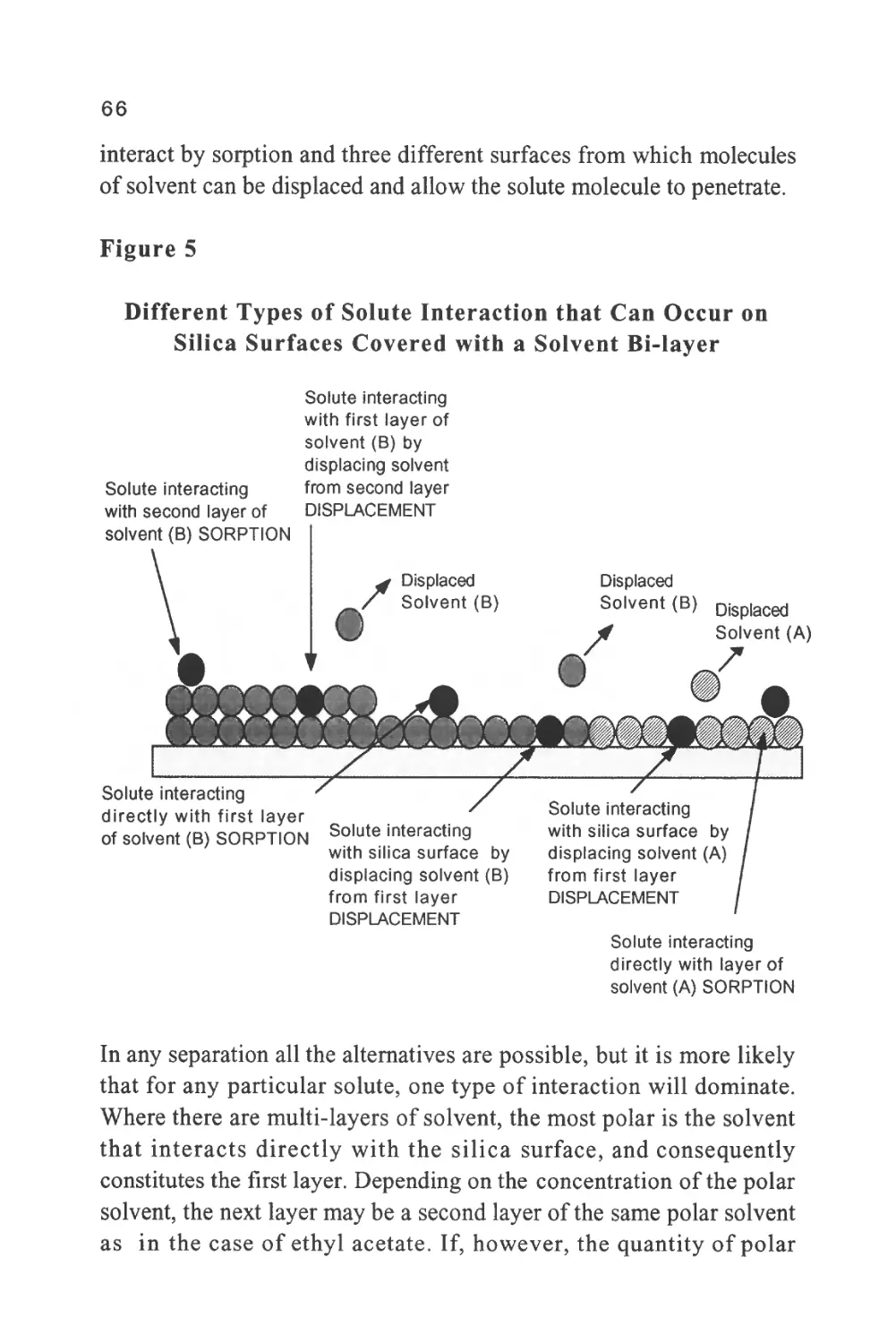
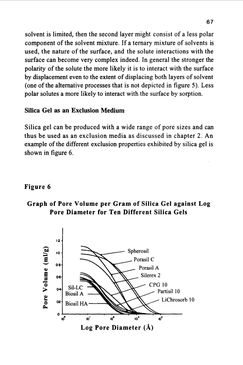
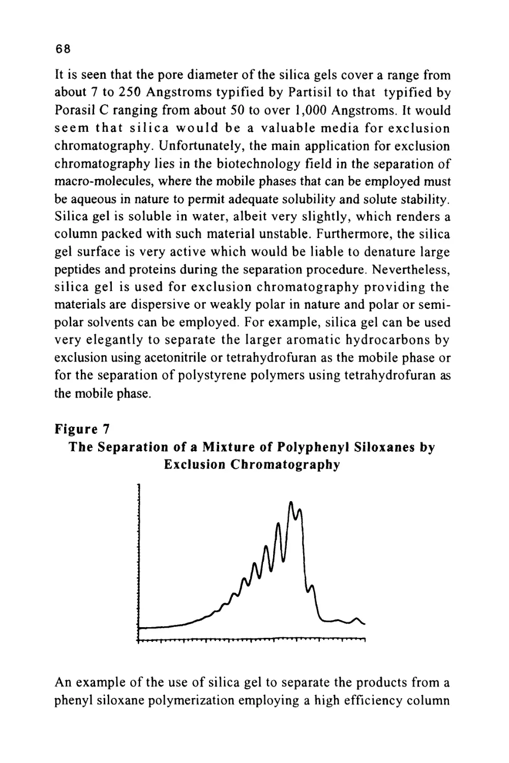
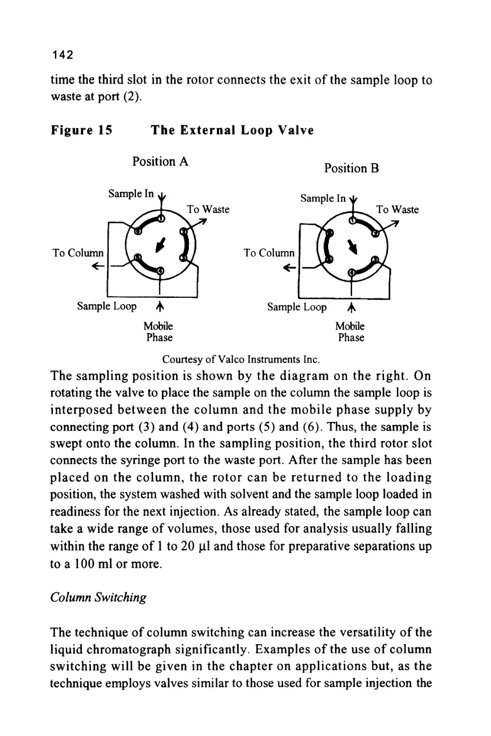
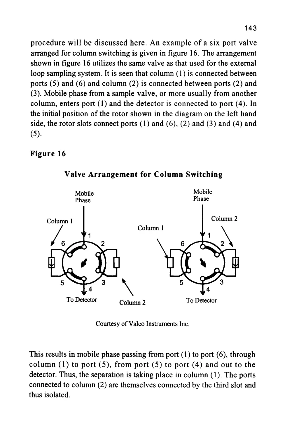
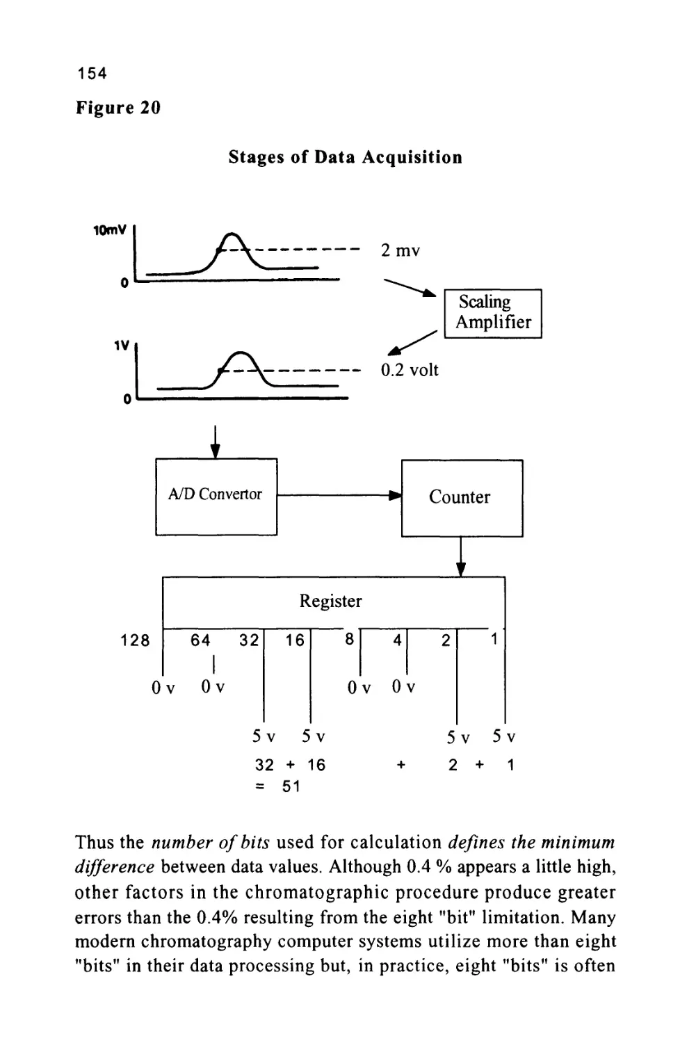
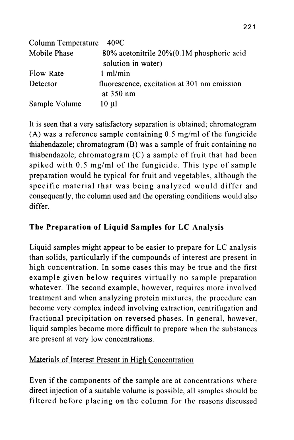
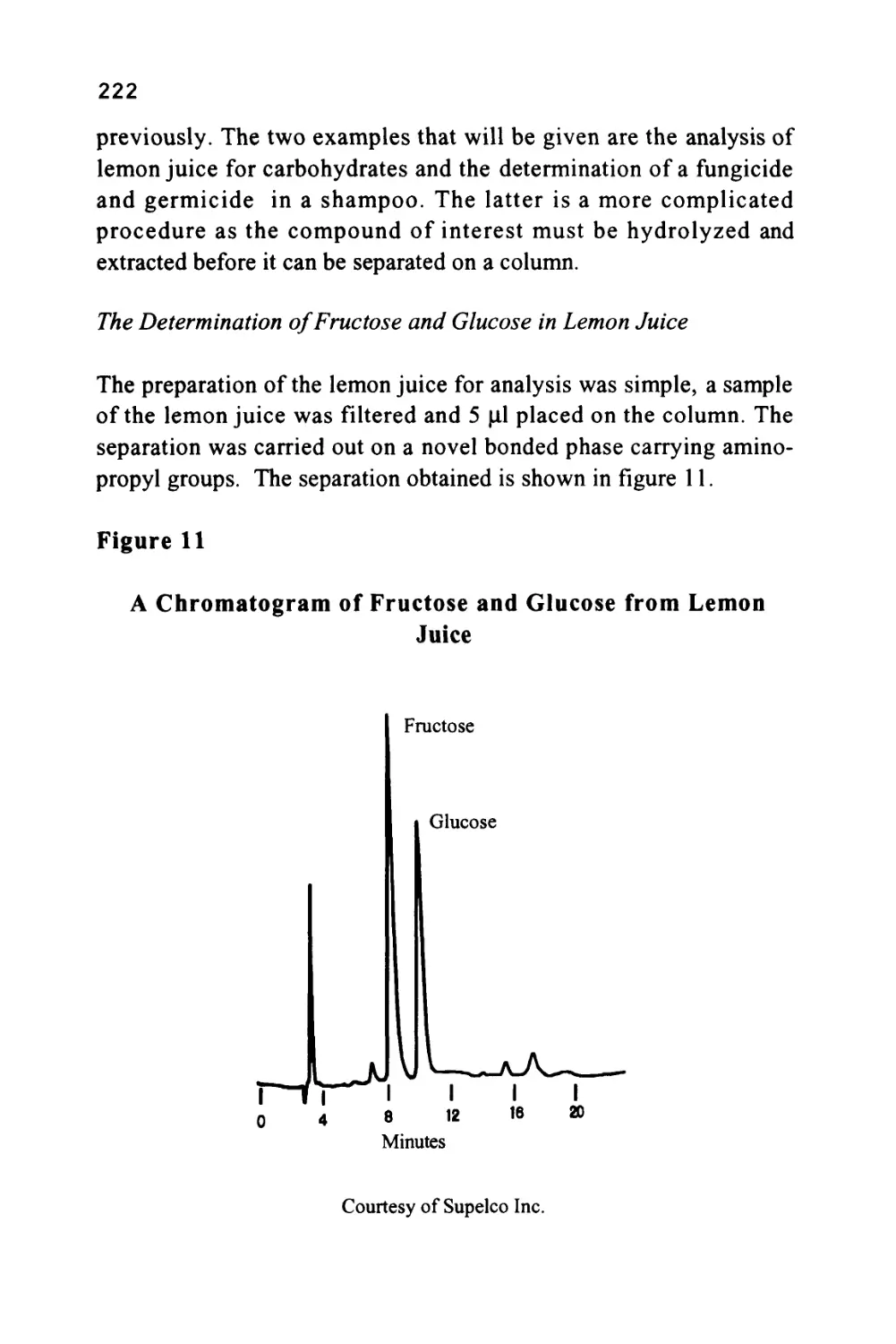
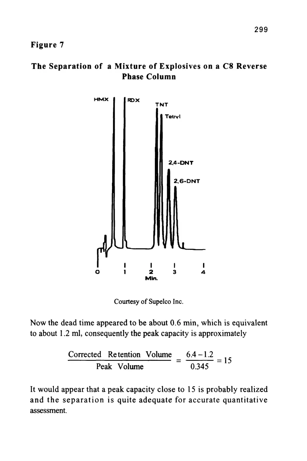
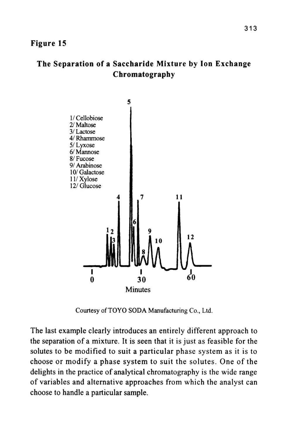
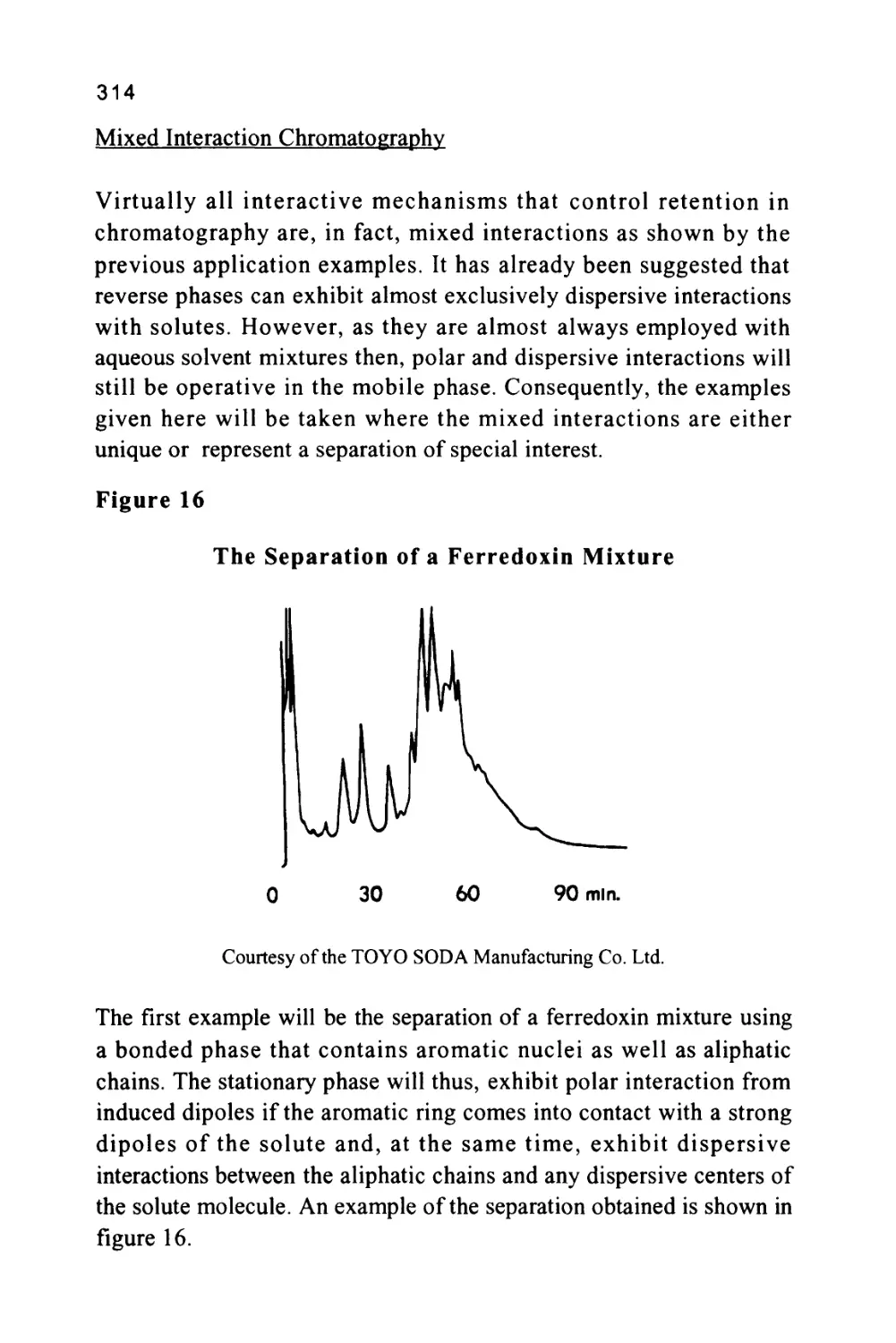
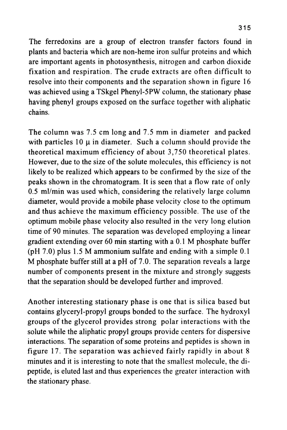
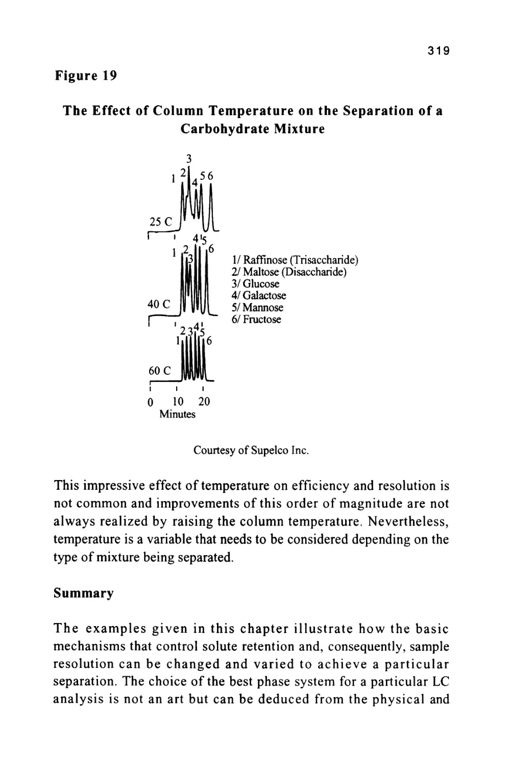
/


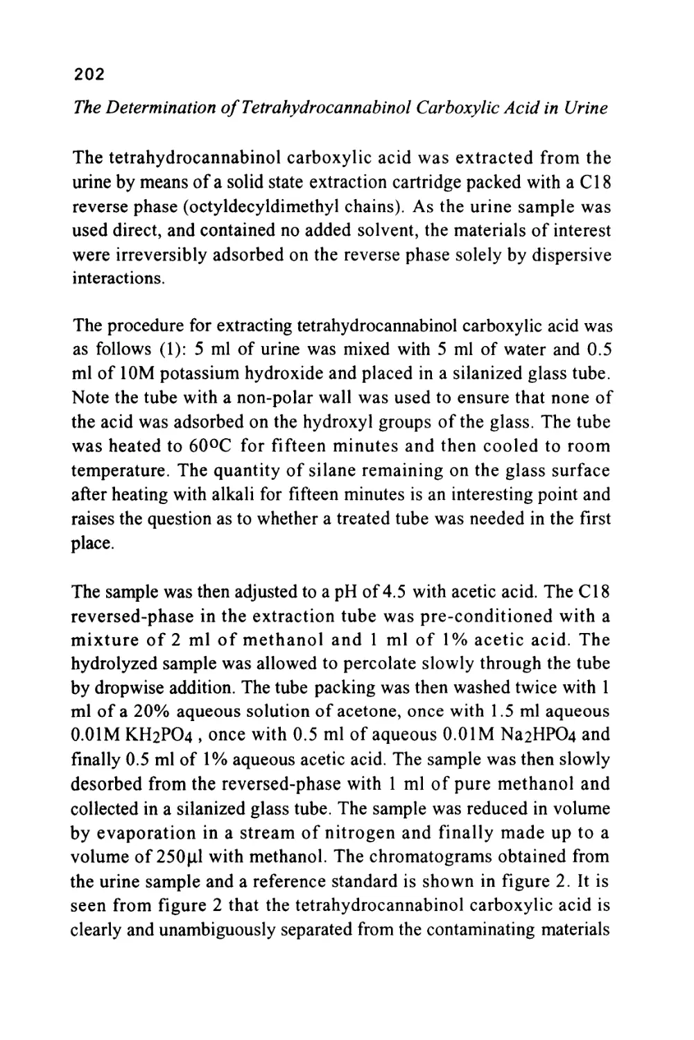
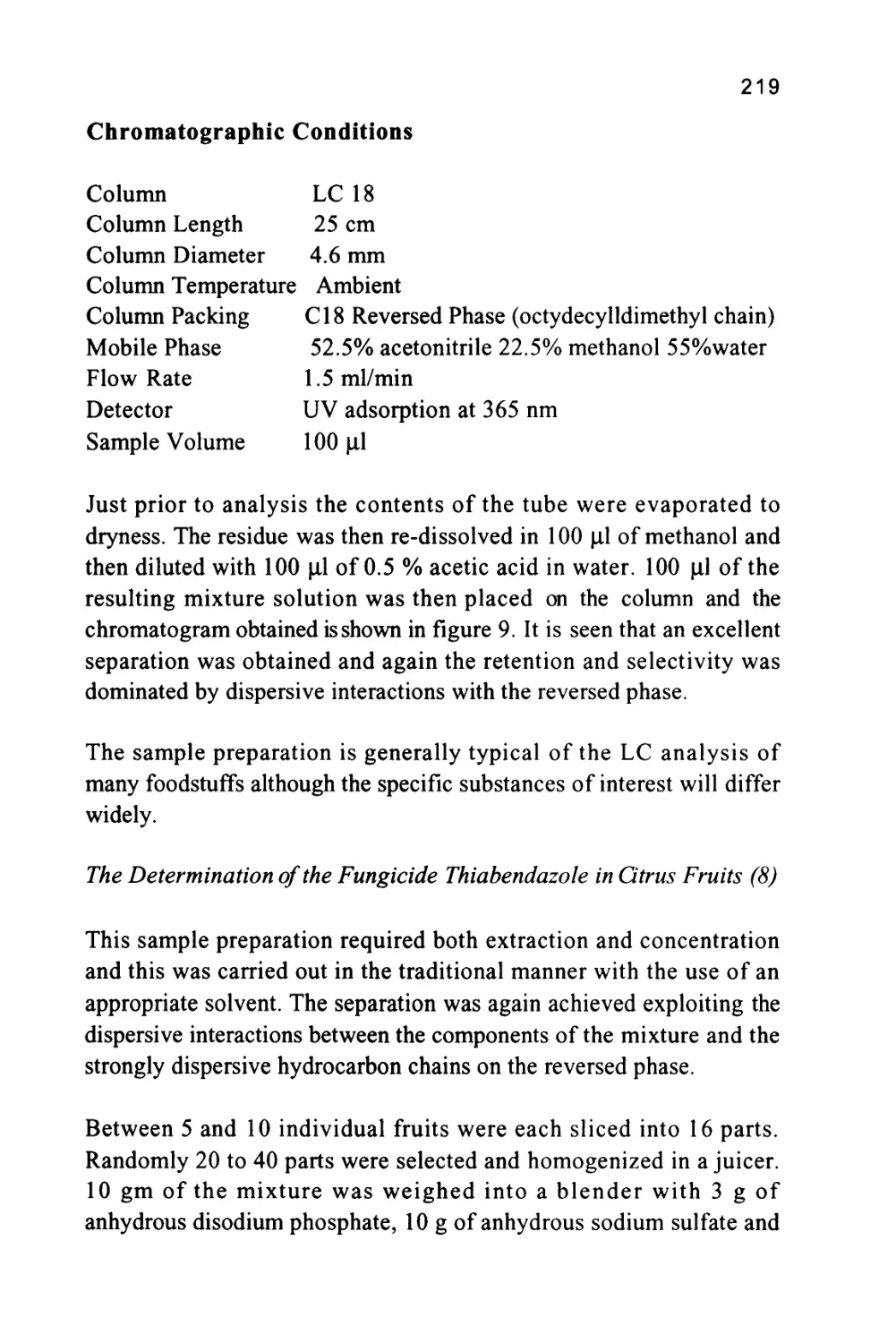
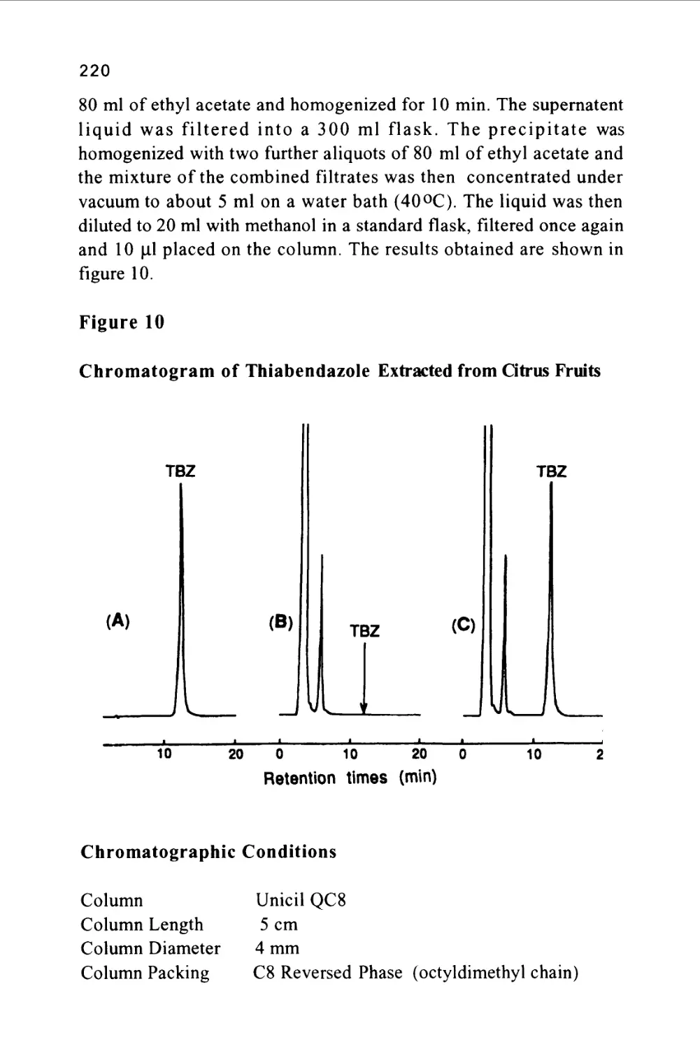


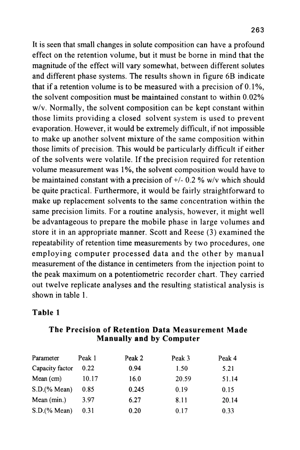


Author: Raymond P.W. Scott
Tags: chemistry chromatography chemical analysis
ISBN: 9780367402112
Year: 1994


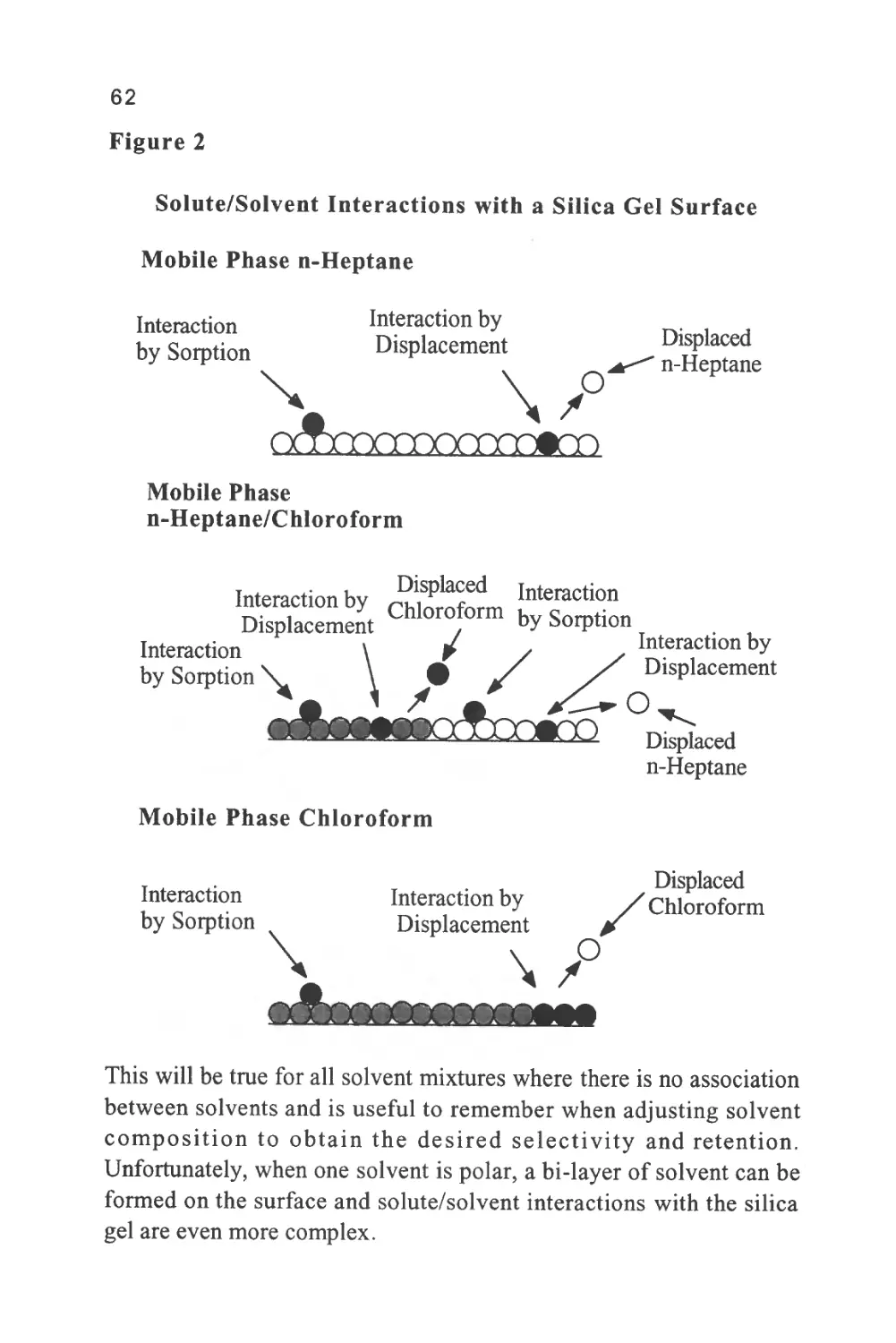
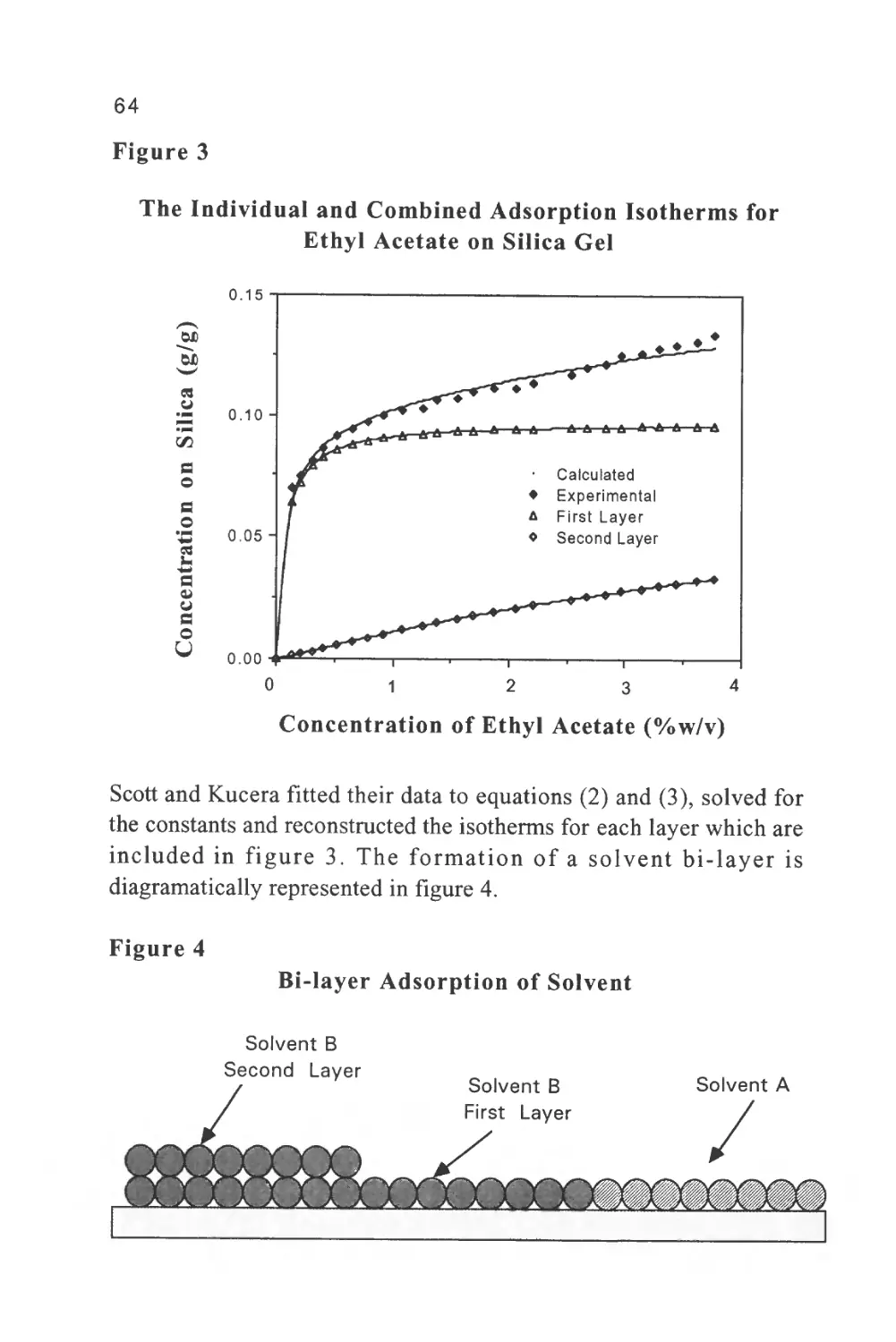
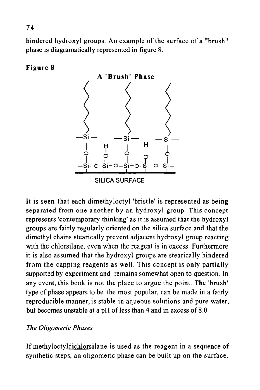
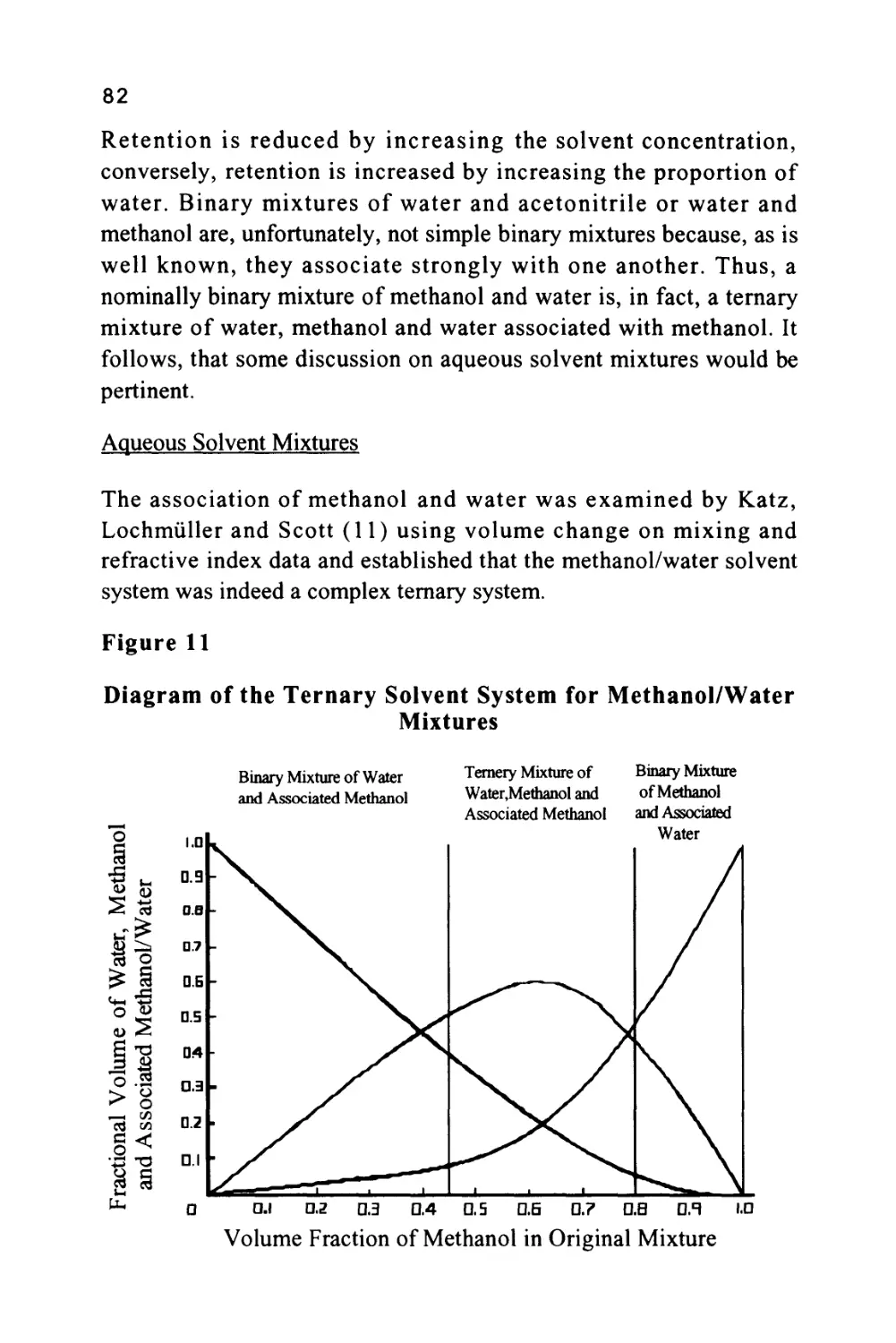
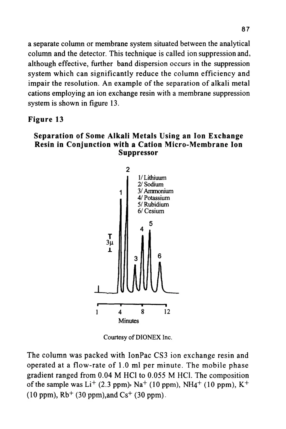
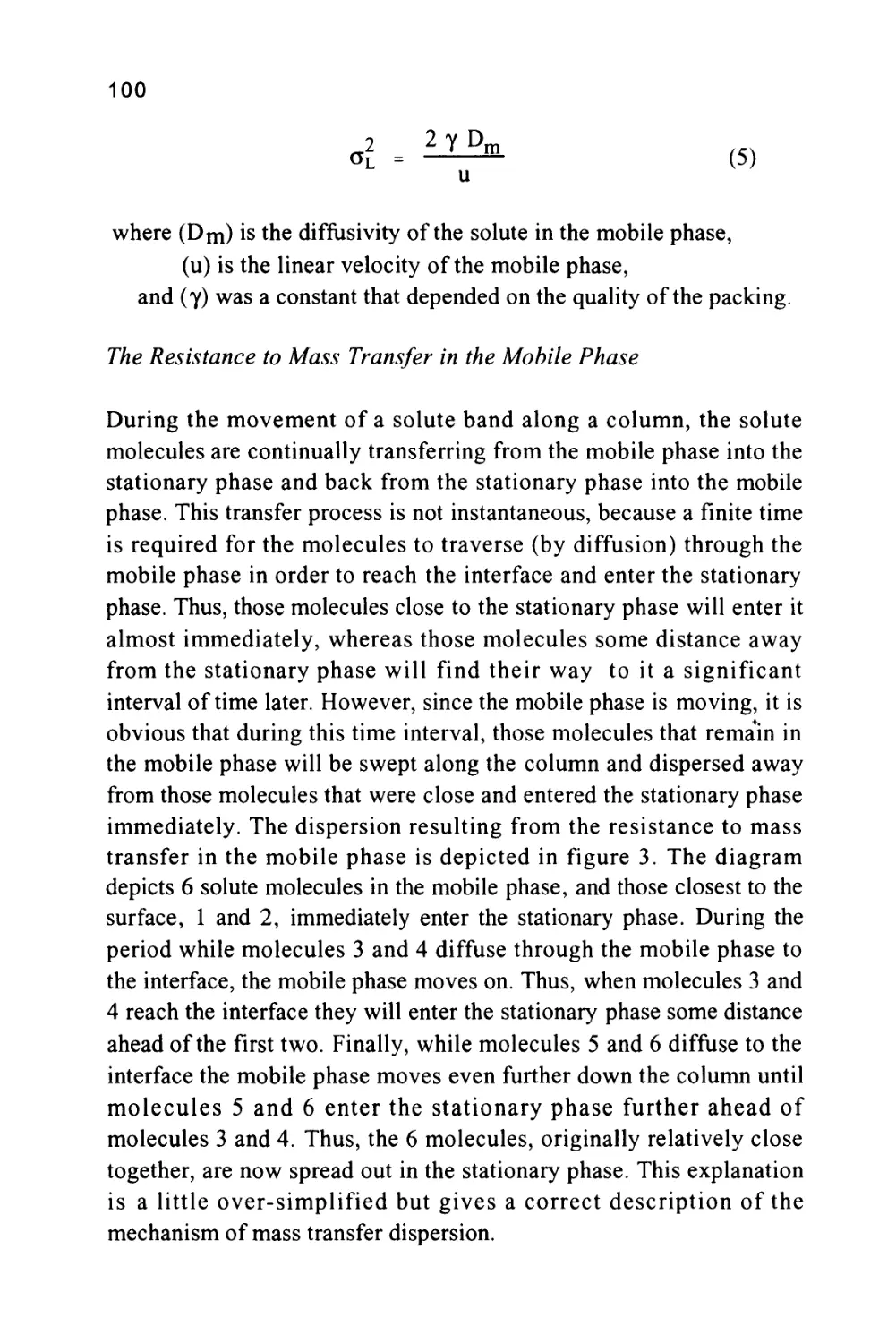
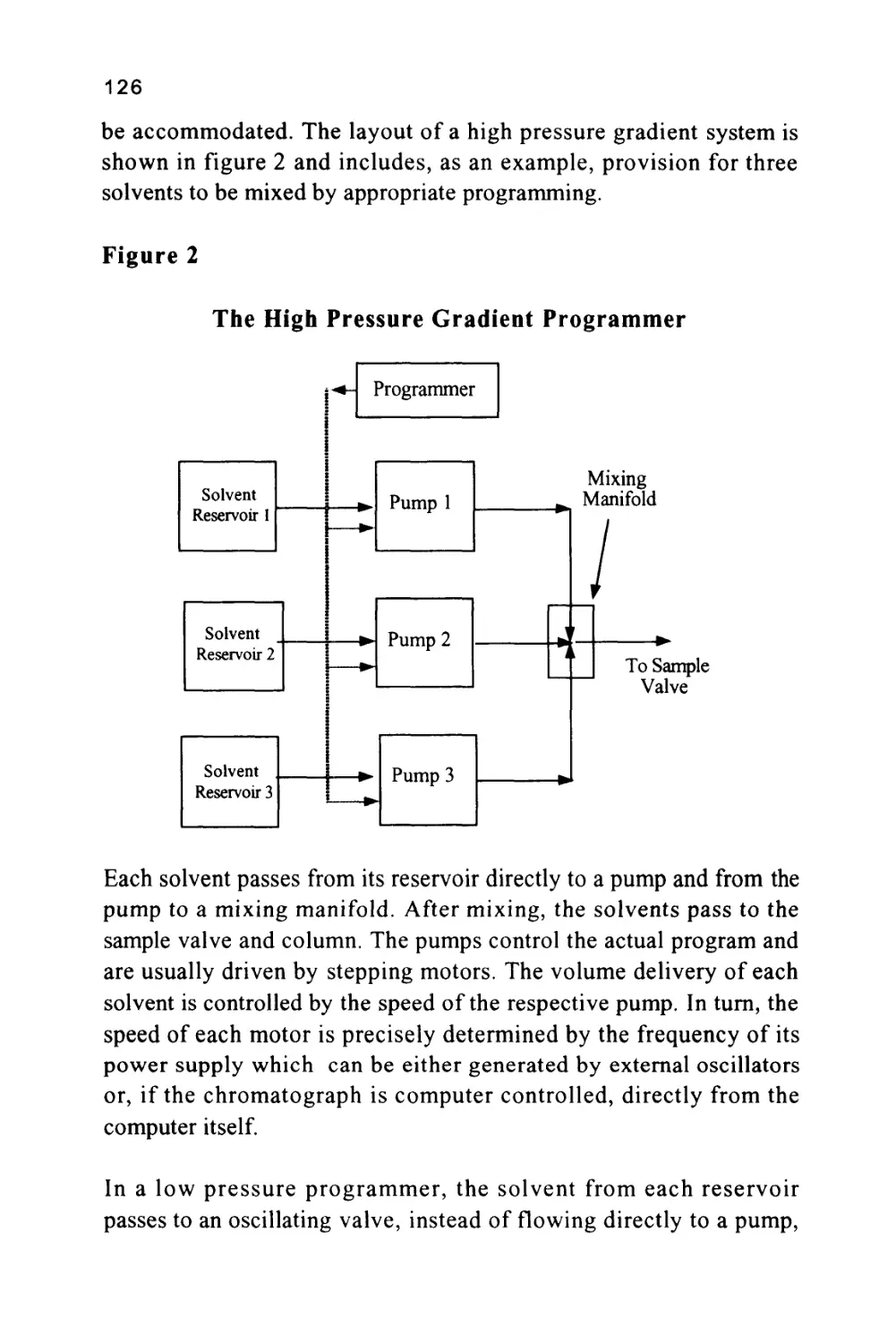
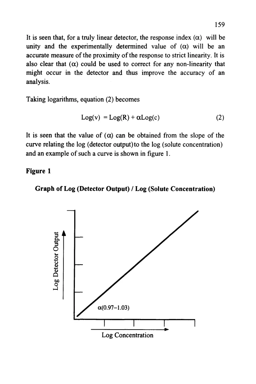
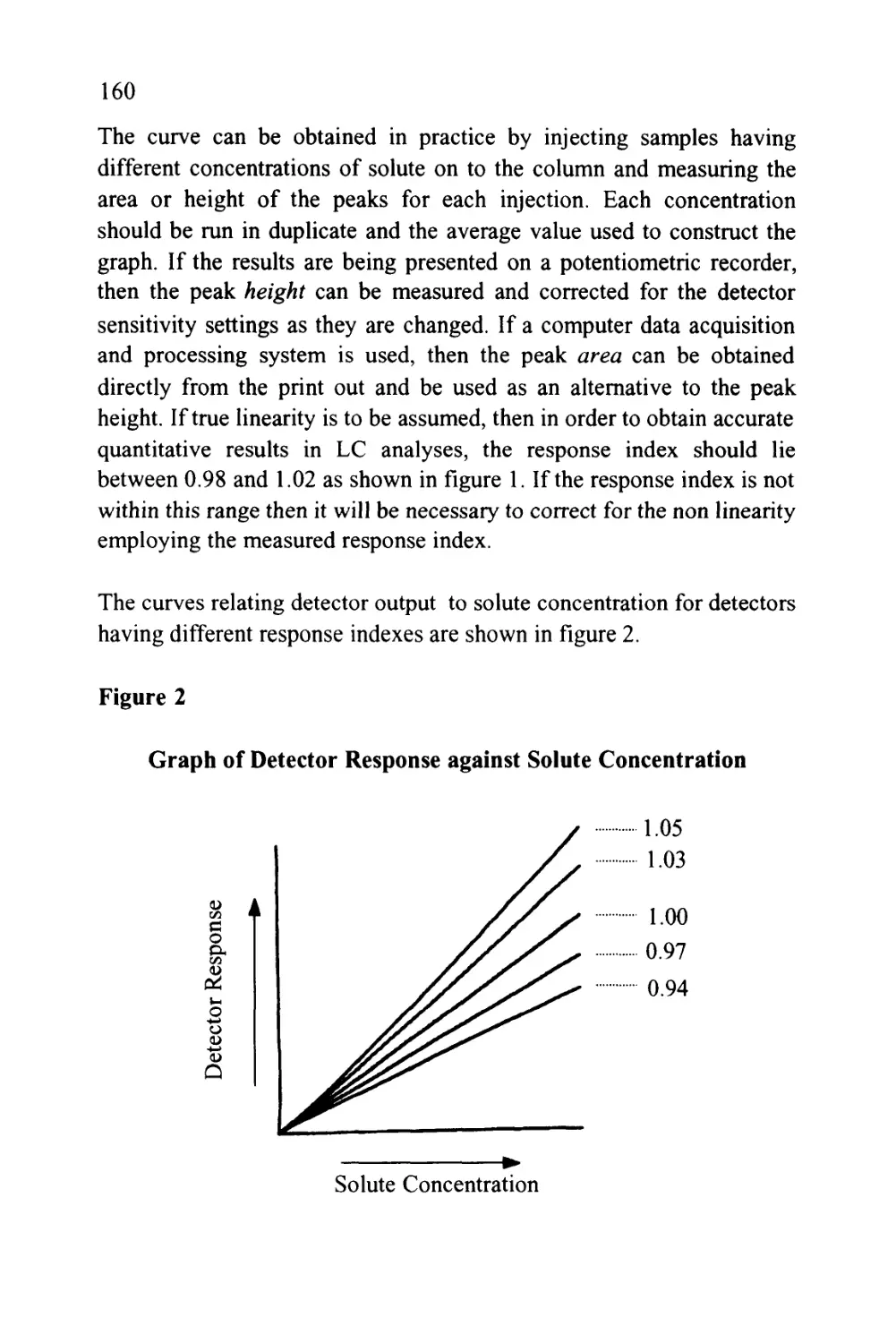
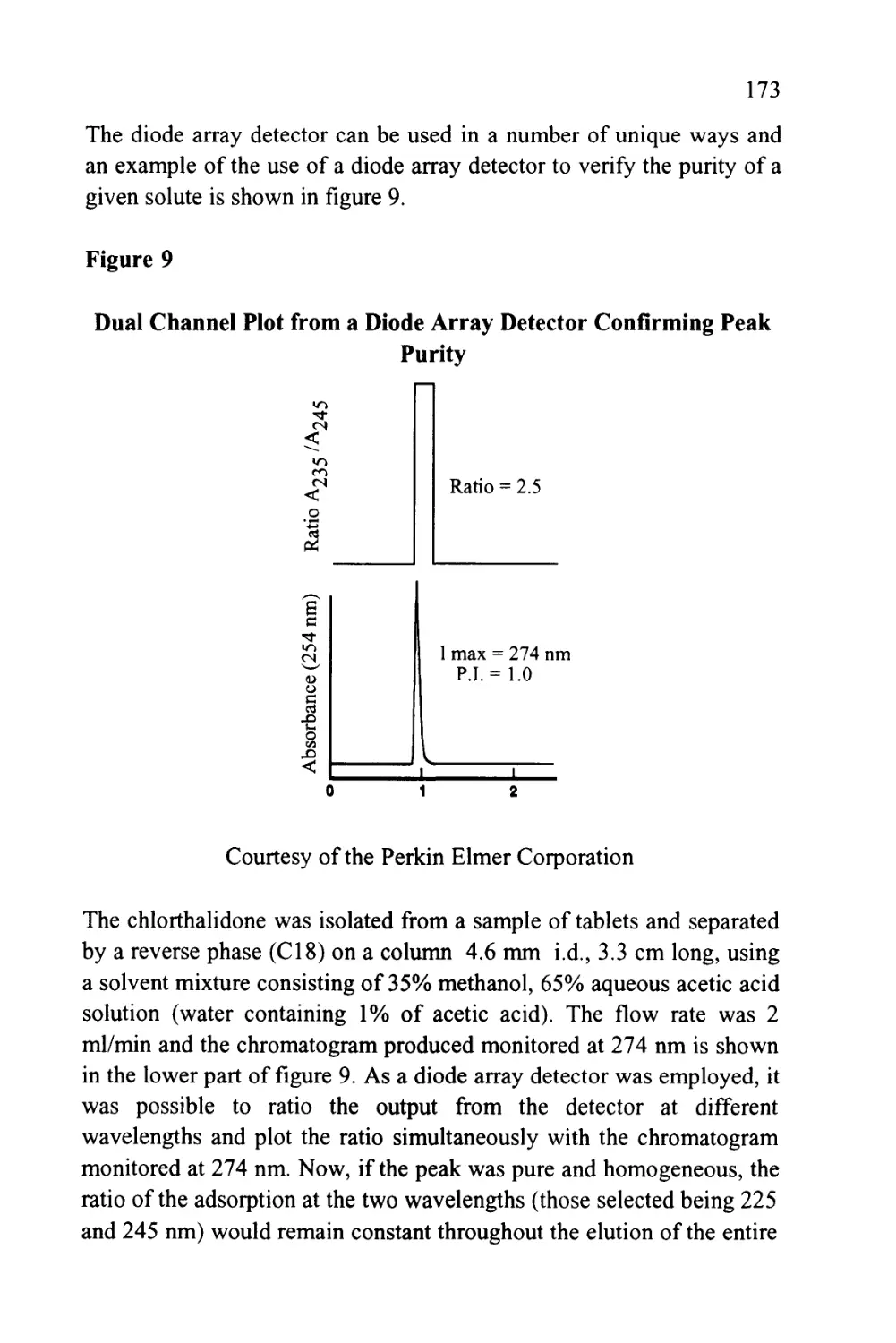
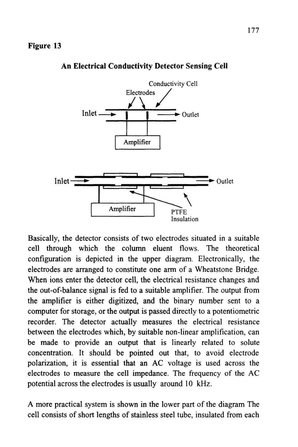
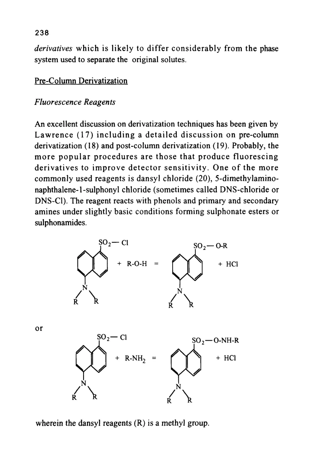
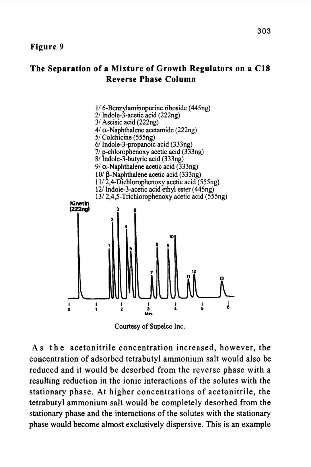
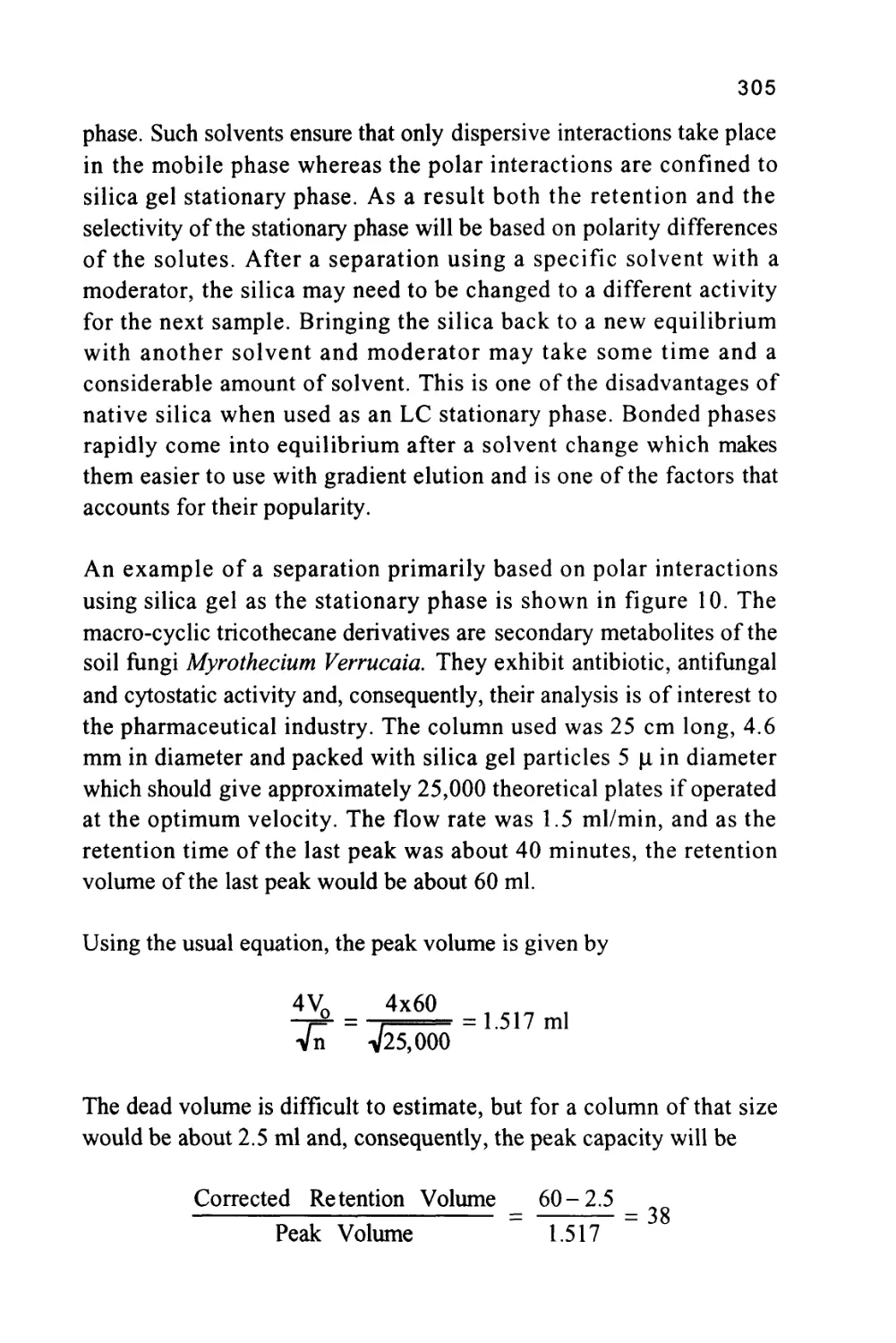
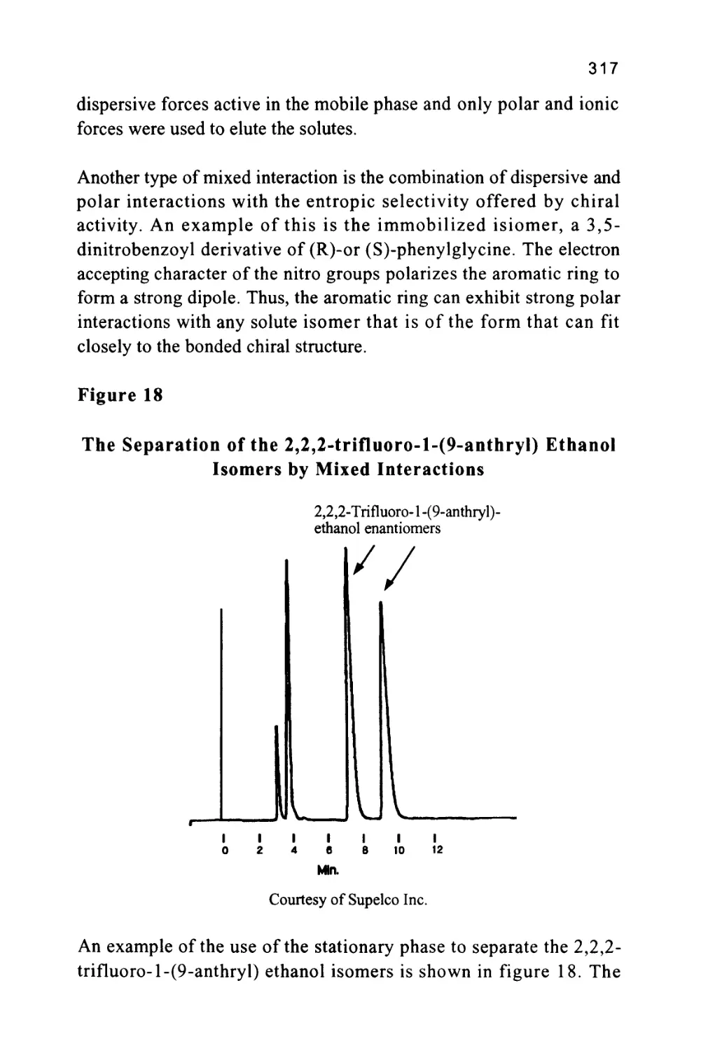
Text
1
An Introduction to Chromatography
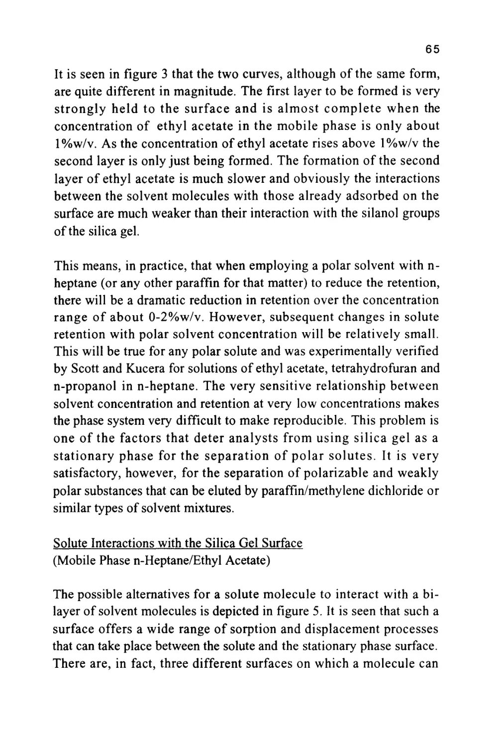
Chromatography is probably the most powerful and versatile
analytical technique available to the modern chemist. Its power arises
from its capacity to determine quantitatively many individual
components present in a mixture in one, single analytical procedure.
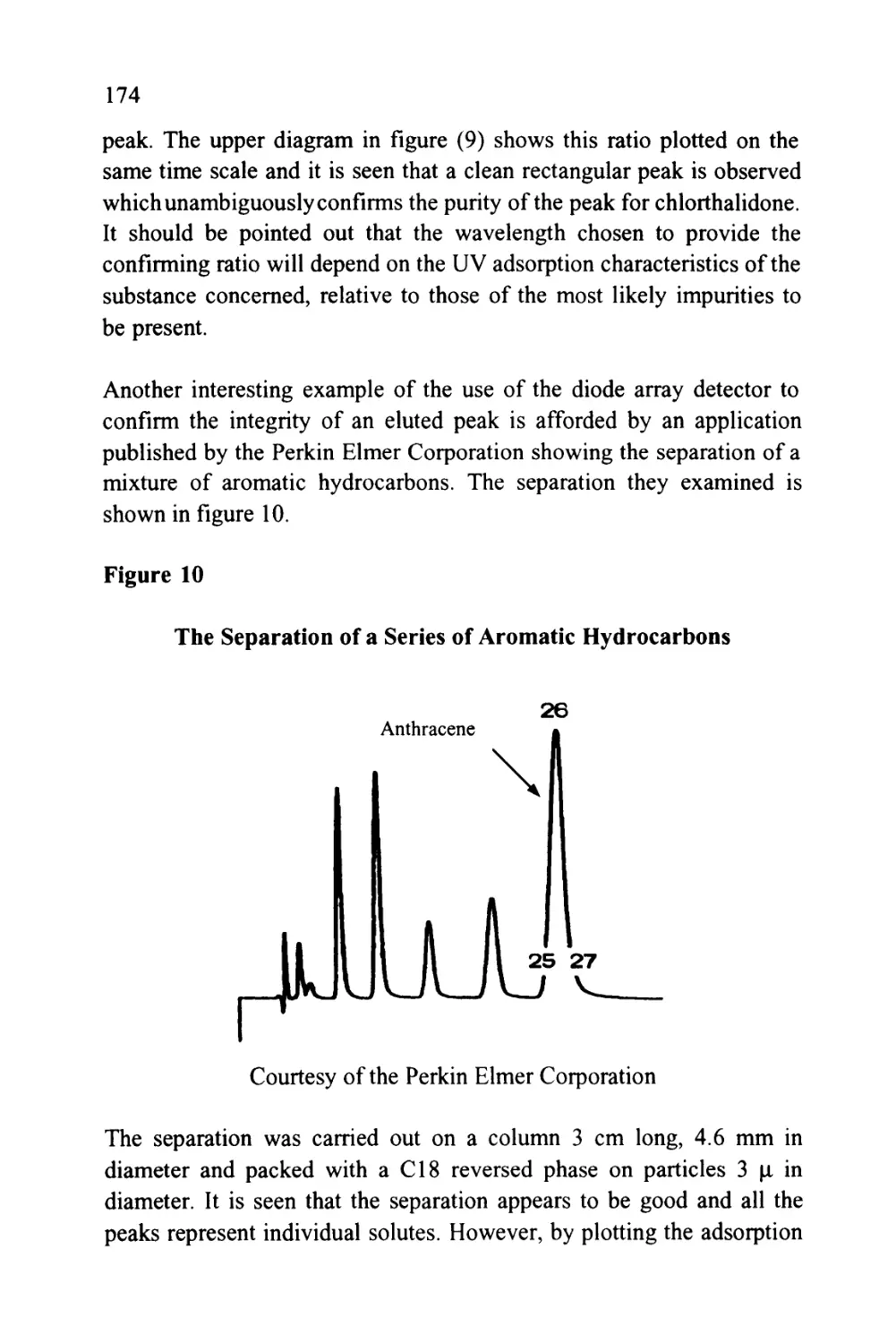
Its versatility comes from its capacity to handle a very wide variety of
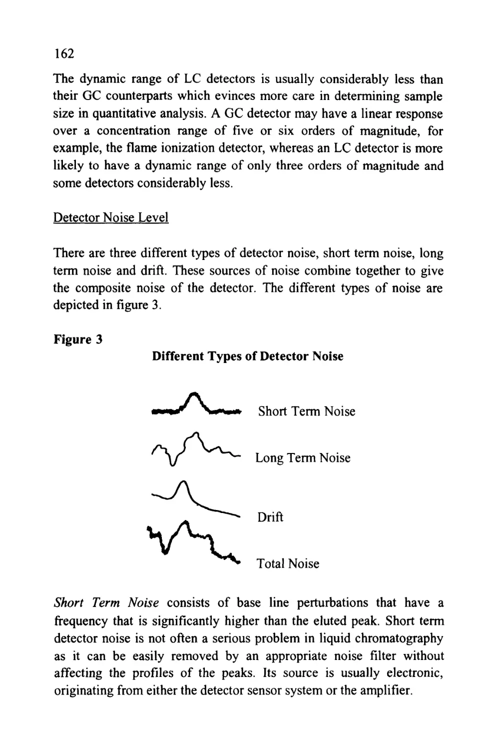
samples, that may be gaseous, liquid or solid in nature. In addition, the
sample can range in complexity from a single substance to a multi-
component mixture containing widely differing chemical species.
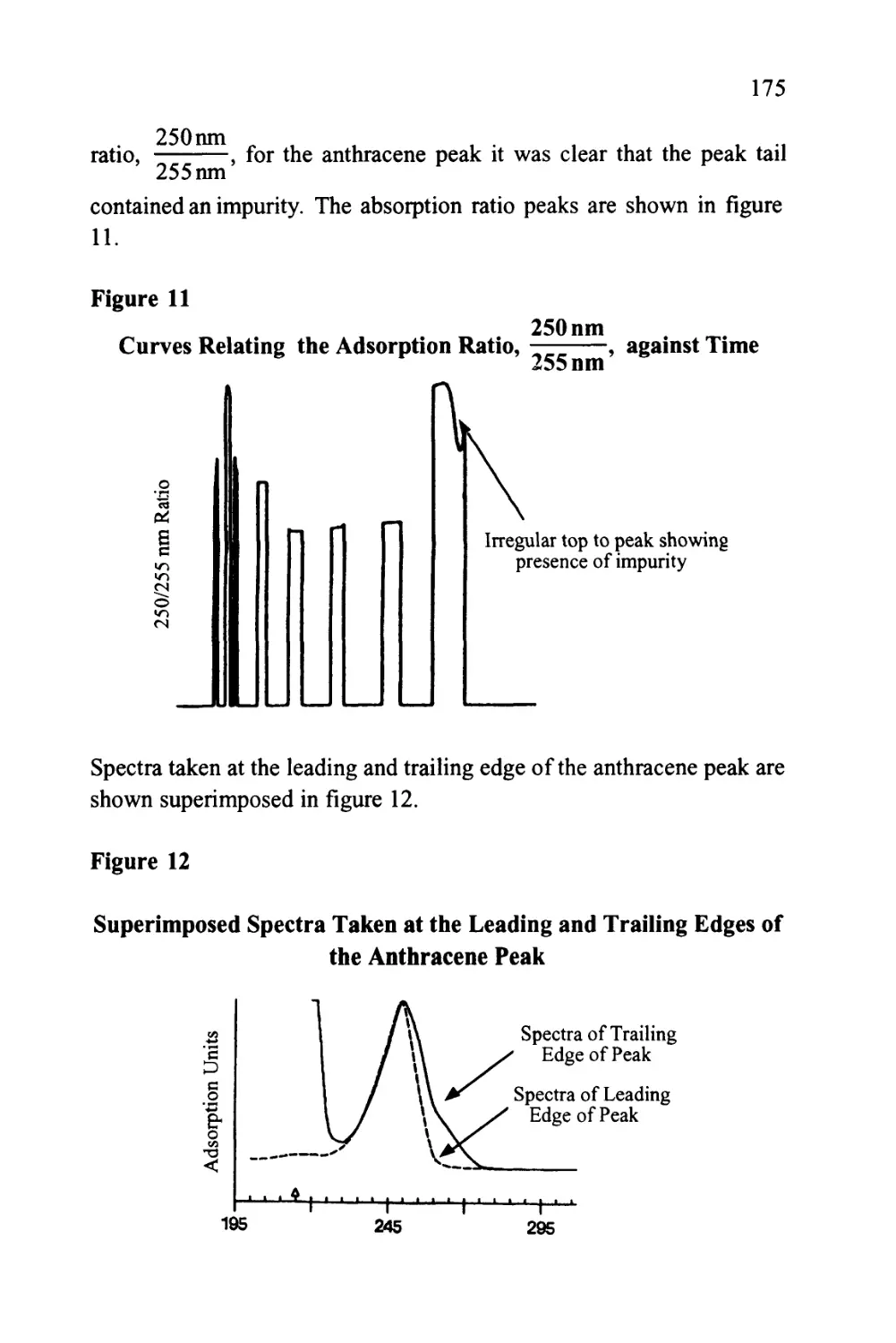
Another aspect of the versatility of the technique is that the analysis
can be carried out, at one extreme, on a very costly and complex
instrument, and at the other, on a simple, inexpensive thin layer plate.
The unique character of the chromatographic method that makes it so
useful arises from the dual nature of its function. Chromatography is,
in fact, a combined separating and measuring system. The sample is
first separated into its individual components and then, by the use of a
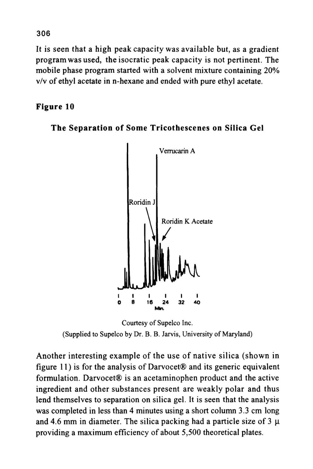
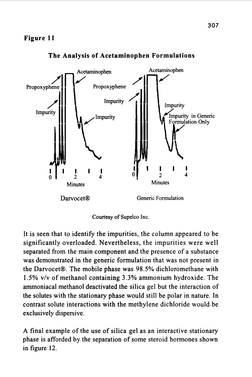
sensor with a quantitative response, the quantity of each component
present can be measured.
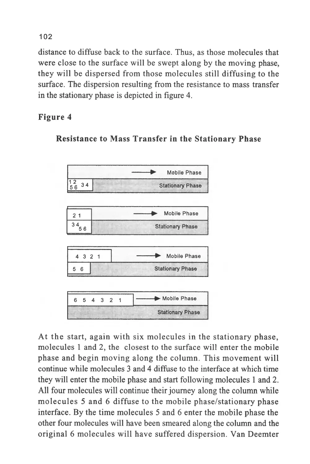
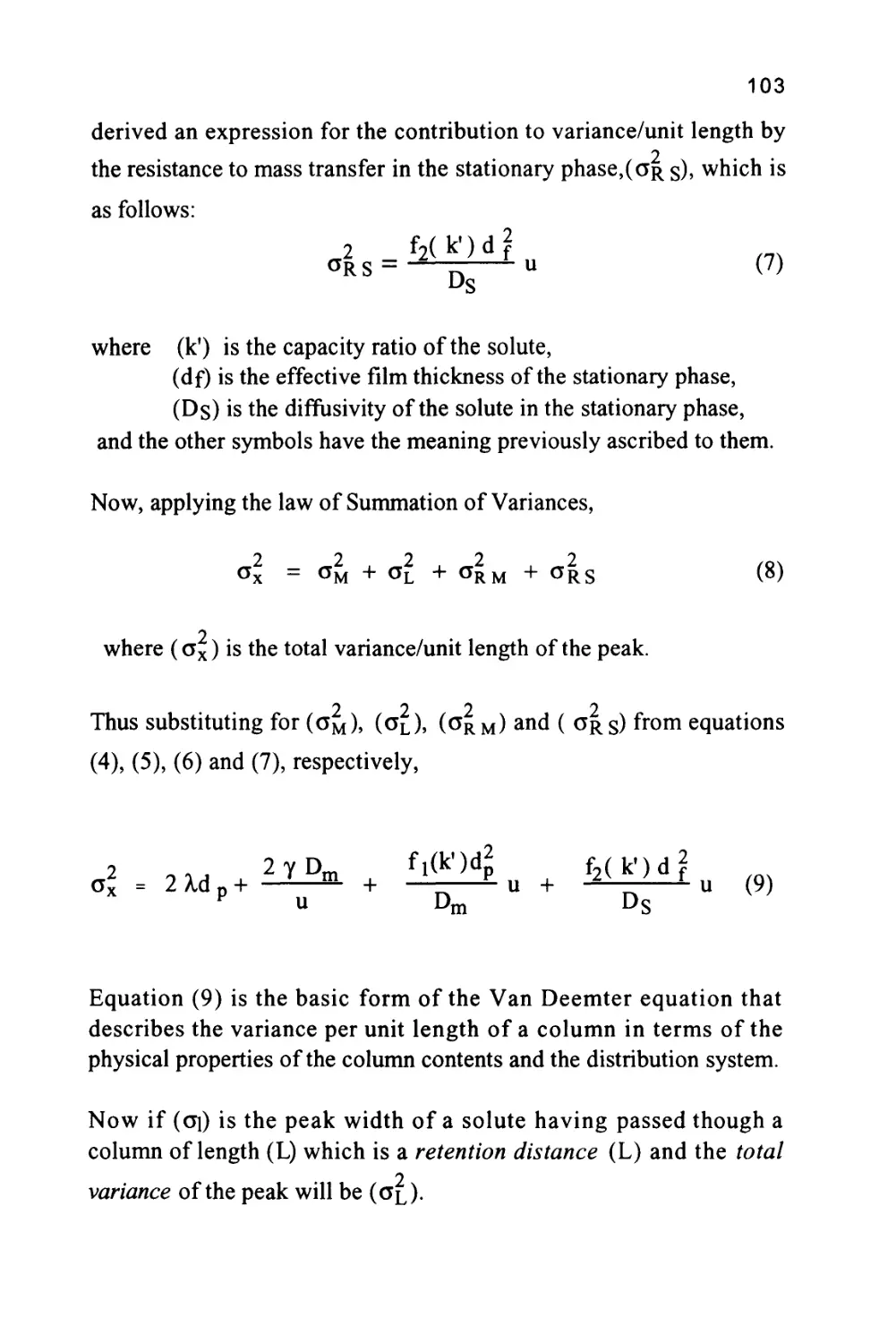
Chromatography was invented nearly 100 years ago, but it is only in
the past few years that the development of the technique and associated
instrumentation has reached a level that might be called the 'steady
state\ The process and methodology is now well established, and
understood, and the practice of the technique is no longer the
exclusive domain of the chromatographer. Chromatography is now
1
2
part of the armory of techniques used by the general analyst and the
chromatograph is now just another instrument among the many that
are present in the analytical laboratory. The technique of
chromatography, however, although well established, is not simple. In
the same way that it is necessary for the analyst to have a basic
understanding of infra-red spectroscopy in order to use an infra-red
spectrometer effectively for analytical purposes, so must the analyst
have a basic understanding of the chromatographic process to use the
chromatograph effectively. It is the purpose of this book to provide
the analyst with a clear, basic understanding of the chromatographic
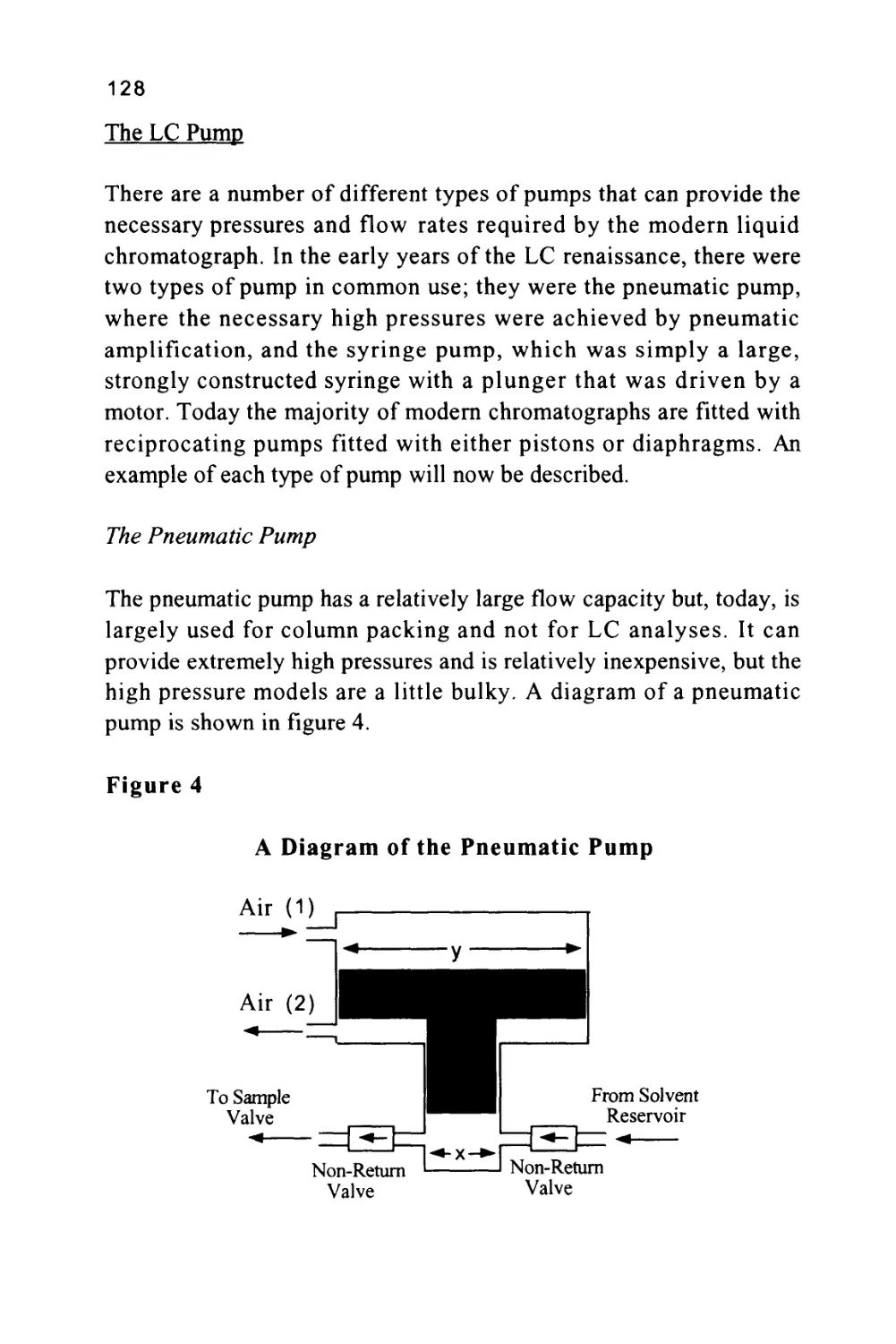
process, the specifications of the equipment necessary to carry out a
chromatographic analysis and the procedures that are essential to
ensure that the technique is used efficiently.
A Short History of LC
Chromatography was invented by a Russian botanist named Tswett
somewhere around the turn of the last century. Tswett, in fact, was
educated in Switzerland but returned to Russia to carry out research
on plant pigments. His technique was to allow a plant extract to
percolate through a bed of powdered calcium carbonate. He reported
his findings at the Biological Section of the Warsaw Naturalist's
Society in 1903 (1). The colored bands produced on the adsorbent
inspired the term chromatography to describe the separation process,
combining the Greek word chromos meaning color with grafe
meaning writing. Although color has little to do with modern
chromatography, the name has persisted and, despite its irrelevance, is
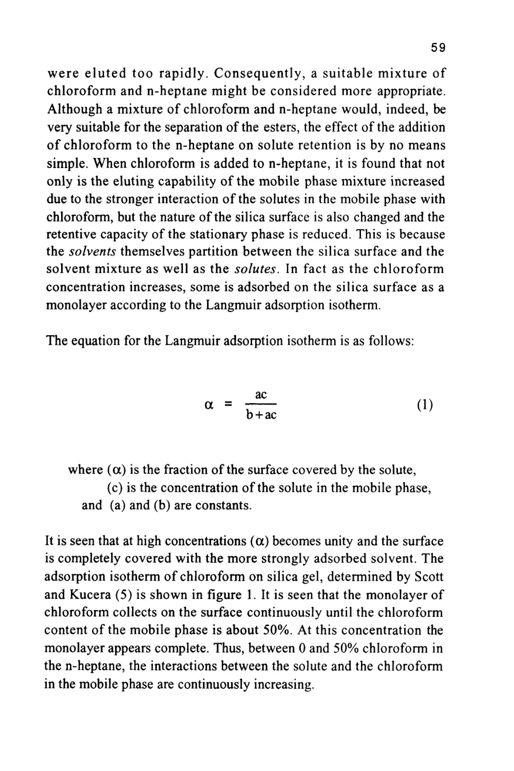
still used to describe all separation techniques that employ a mobile
and stationary phase. Unfortunately, the work of Tswett was not
immediately developed to any significant extent; this was due in part
to the obscurity of the source of the original paper and to the
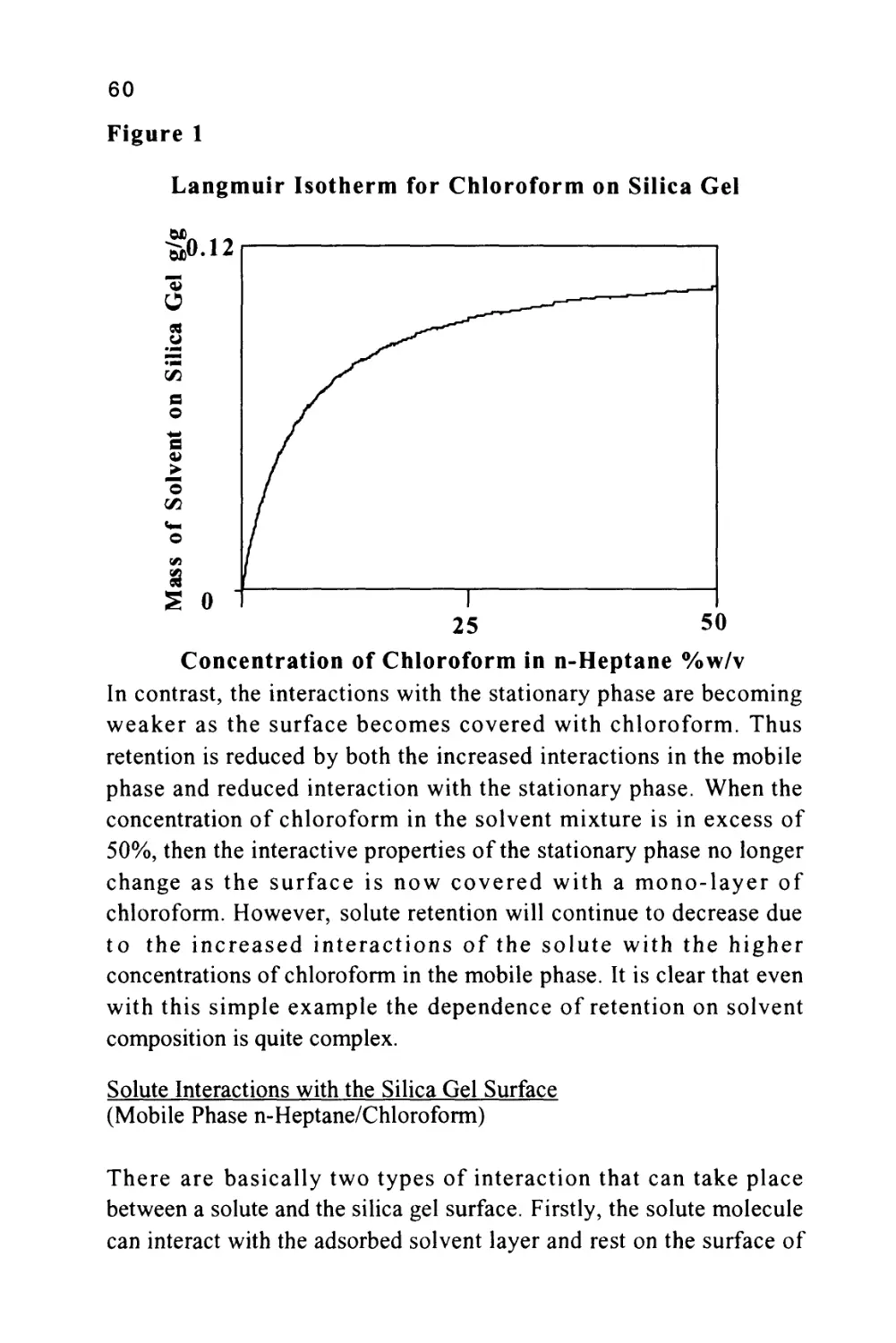
condemnation of the method by Willstatter and Stoll (2). Willstatter
and Stoll tried to repeat the work of Tswett but did not heed the
advice of Tswett to avoid "aggressive" adsorbents and so their
experiments failed. Inaccurate and careless experimental work has
always been a threat to scientific progress and recent years have
3
shown that contemporary science is by no means immune to such
threats. However, the mistake of Willstatter and Stoll was particularly
unfortunate as, not only did it retard the development of a very useful
separation technique, but in doing so, it also inhibited progress in
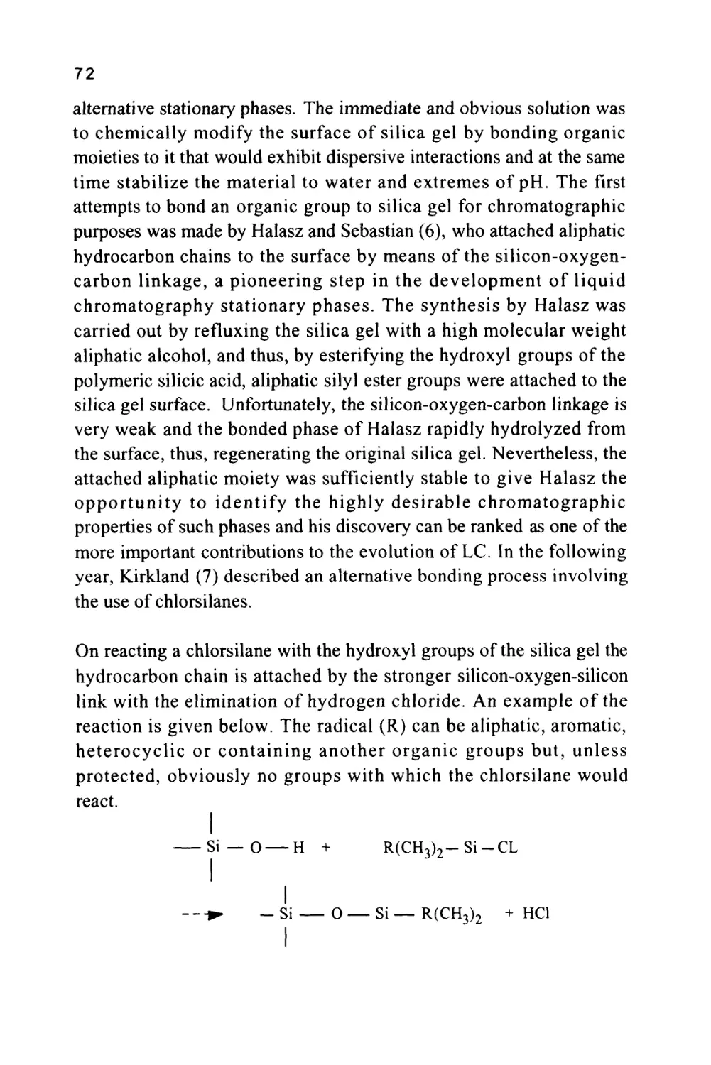
many other fields of chemistry.
A further thirty years were to pass before Kuhn and his co-workers
(3) successfully repeated Tswett's original work and separated lutein
and xanthine from a plant extract. Nevertheless, despite the success of
Kuhn et al and the validation of Tswett's experiments, the new
technique attracted little interest and progress continued to be slow
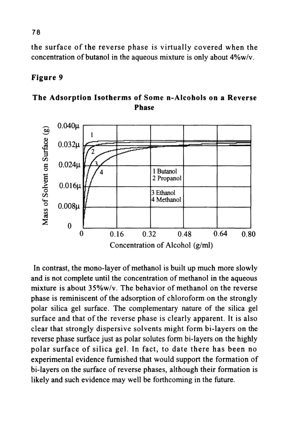
and desultory. In 1941 Martin and Synge (4) introduced liquid-liquid
chromatography by supporting the stationary phase, in this case water,
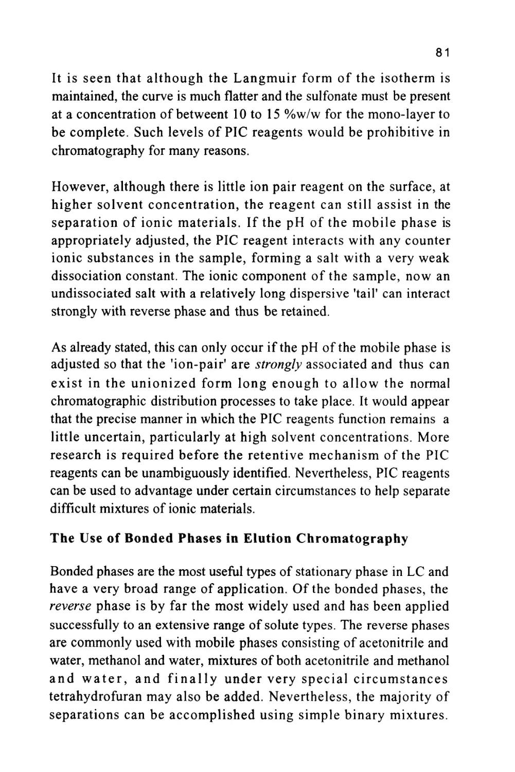
on silica in the form of a packed bed and used it to separate some
acetyl amino acids.
It is interesting to note that although the renaissance of LC began in
1963 and, in fact, has only recently matured to the level where high
resolving power and fast separations are attainable, the essential
requirements for HPLC (High Performance Liquid Chromatography)
were unambiguously stated by Martin in 1941. To quote Martin's
original paper,
"Thus, the smallest H.E.T.P. (the highest efficiency) should be
obtainable by using very small particles and a high pressure
difference across the column".
The statement made by Martin in 1941 contains all the necessary
conditions to realize both the high efficiencies and high resolution
achieved by modern LC columns. Despite his recommendations,
however, it has taken nearly fifty years to bring his concepts to
fruition. In the same paper Martin and Synge suggested that it would
be advantageous to replace the liquid mobile phase by a gas to
improve the rate of transfer between the phases and thus, enhance the
separation. The recommendation was not heeded and it was left to
James and Martin (5) to bring the concept to practical reality in the
4
early fifties. Thus, gas chromatography (GC) was born and a new and
important era of chromatography development began.
Gas chromatography grew from a laboratory novelty into a popular
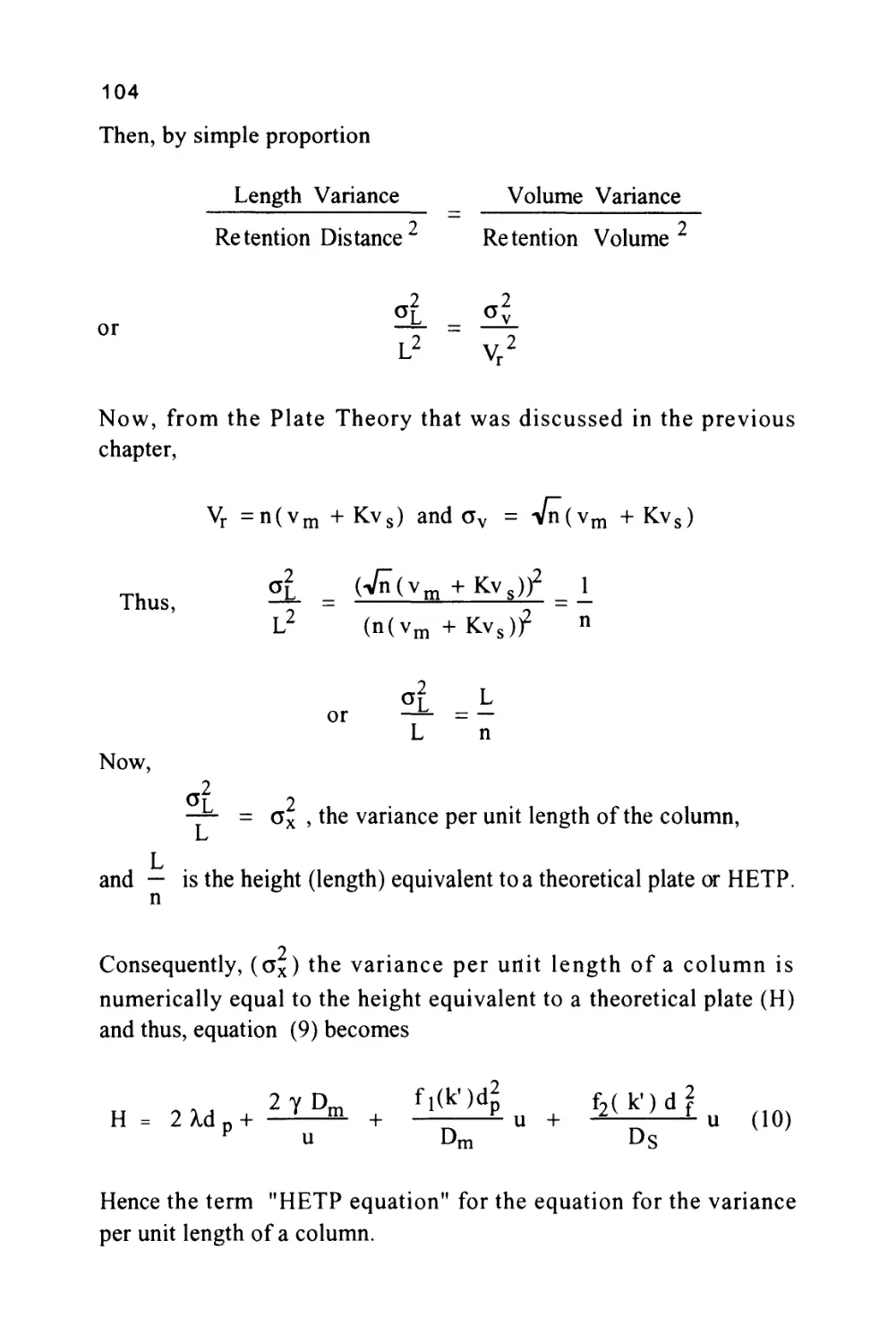
well-established analytical technique in little more than a decade.
During that time, the foundations of chromatography column theory
were laid down which were to guide the development of LC in the
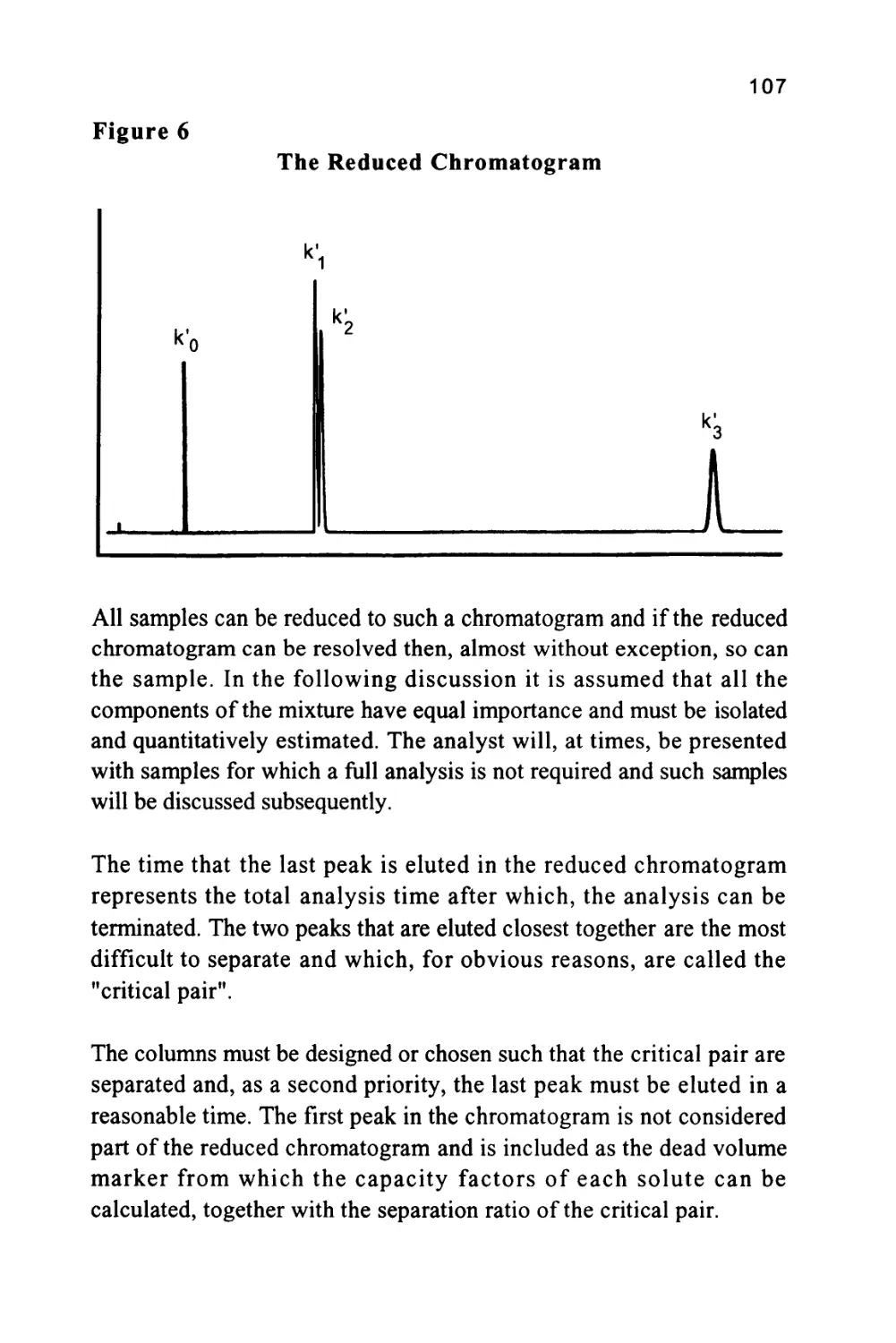
sixties and seventies. As a result of the glamorous success of GC, LC
became the Cinderella of chromatography and it was not until the
major developments of GC were completed that scientists turned their
attention once again to the development of LC. In contrast to GC,
however, the progress of LC has been slow and arduous. The
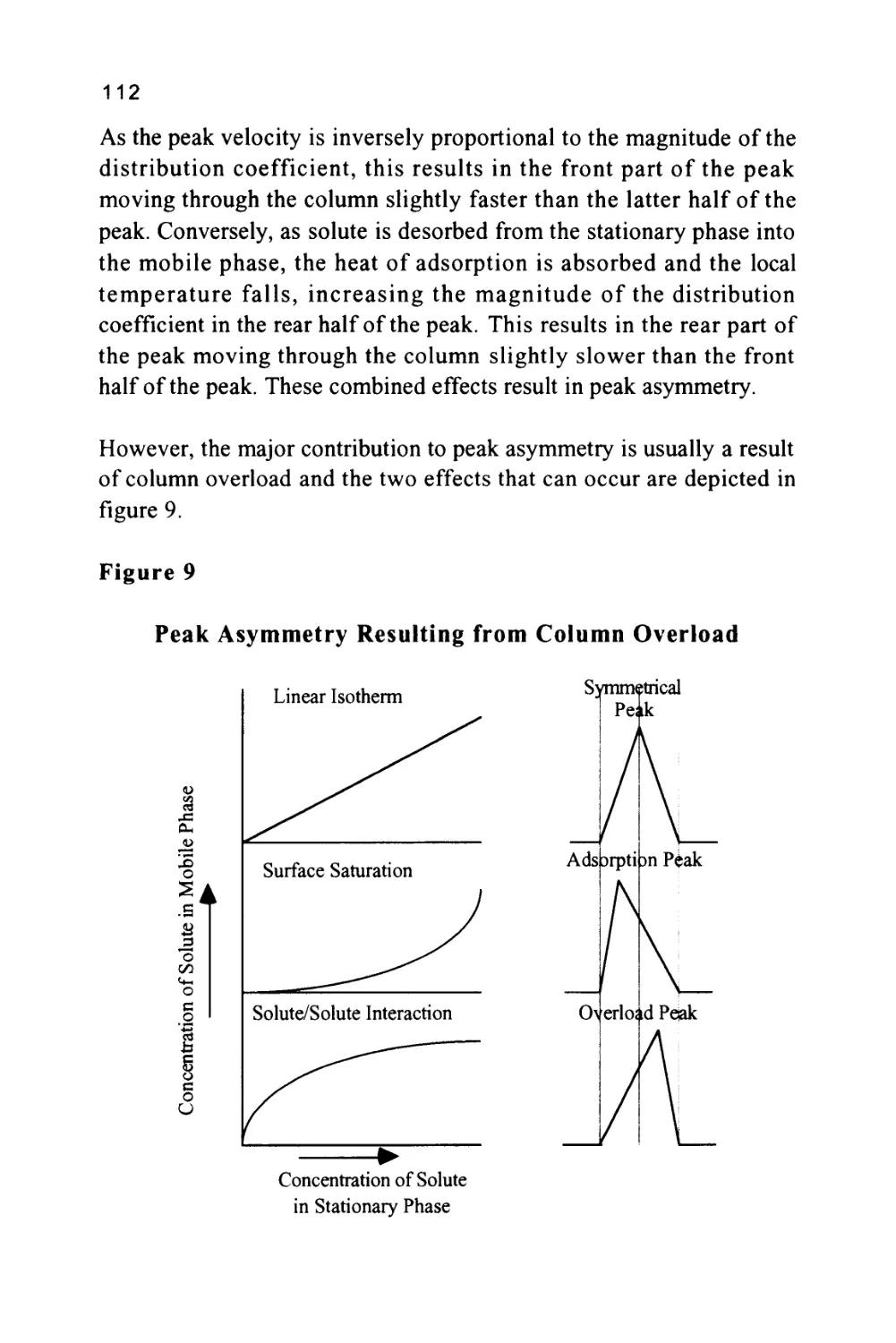
difficulties encountered in the development of LC arose from two
causes. Firstly, substances have a very low diffusivity in liquids
compared with that of a gas and thus, the kinetics of exchange between
the phases are slow and special steps must be taken to achieve efficient
separations. Secondly, very low concentrations of a solute in a liquid
do not modify the properties of the liquid to the same extent that they
do to those of a gas and this has made the development of LC detectors
far more difficult. Today, LC is a well-established separation
technique, a technique which, to the surprise of many, has established
a far wider field of application than GC. It is now a technique with
which no analyst can afford to be unfamiliar.
The Separation Process
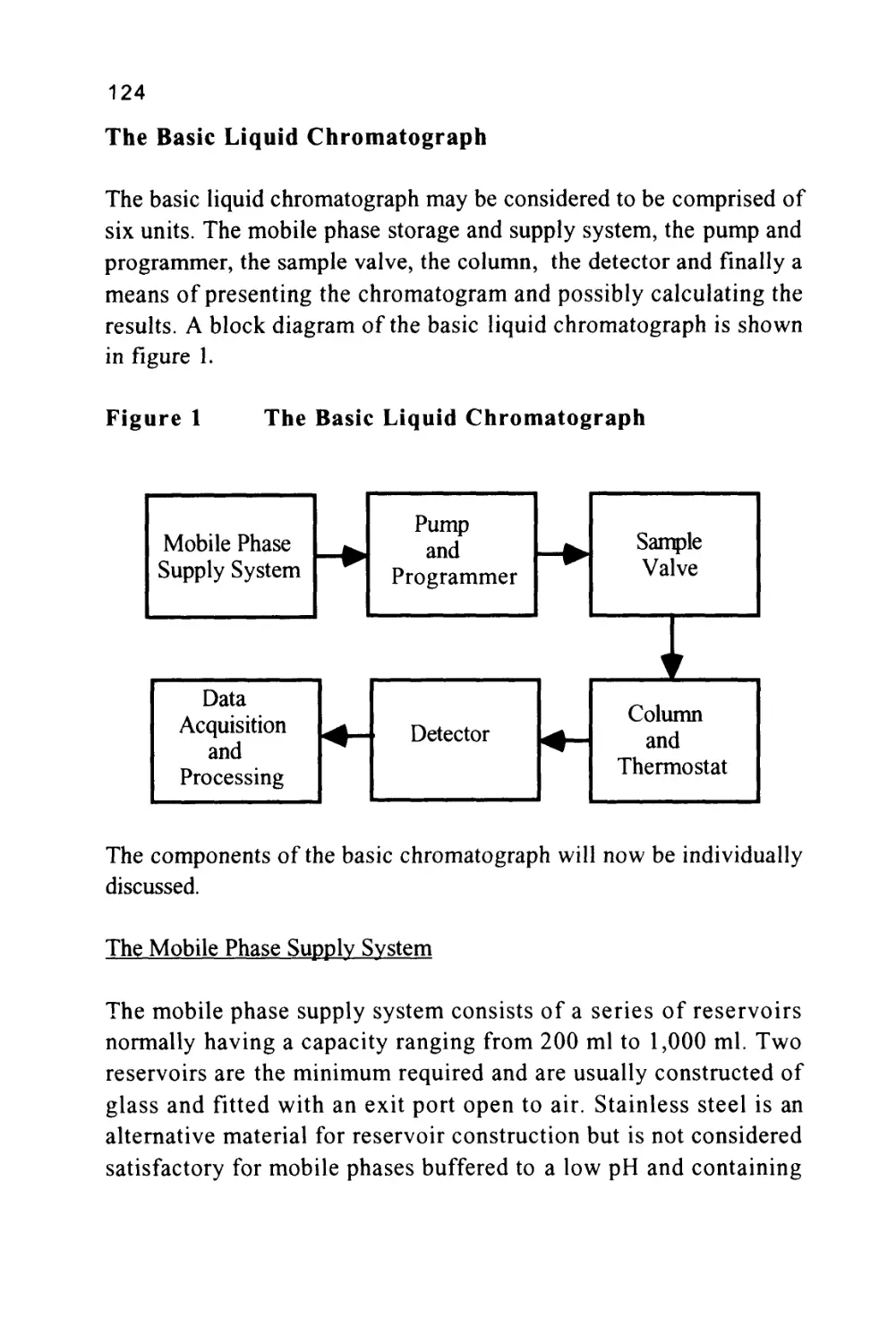
Chromatography has been defined in the classical manner as
"A separation process that is achieved by the distribution of
substances between two phases, a stationary phase and a mobile phase.
Those solutes distributed preferentially in the mobile phase will move
more rapidly through the system than those distributed preferentially
in the stationary phase. Thus, the solutes will elute in order of their
increasing distribution coefficients with respect to the stationary
phase".
5
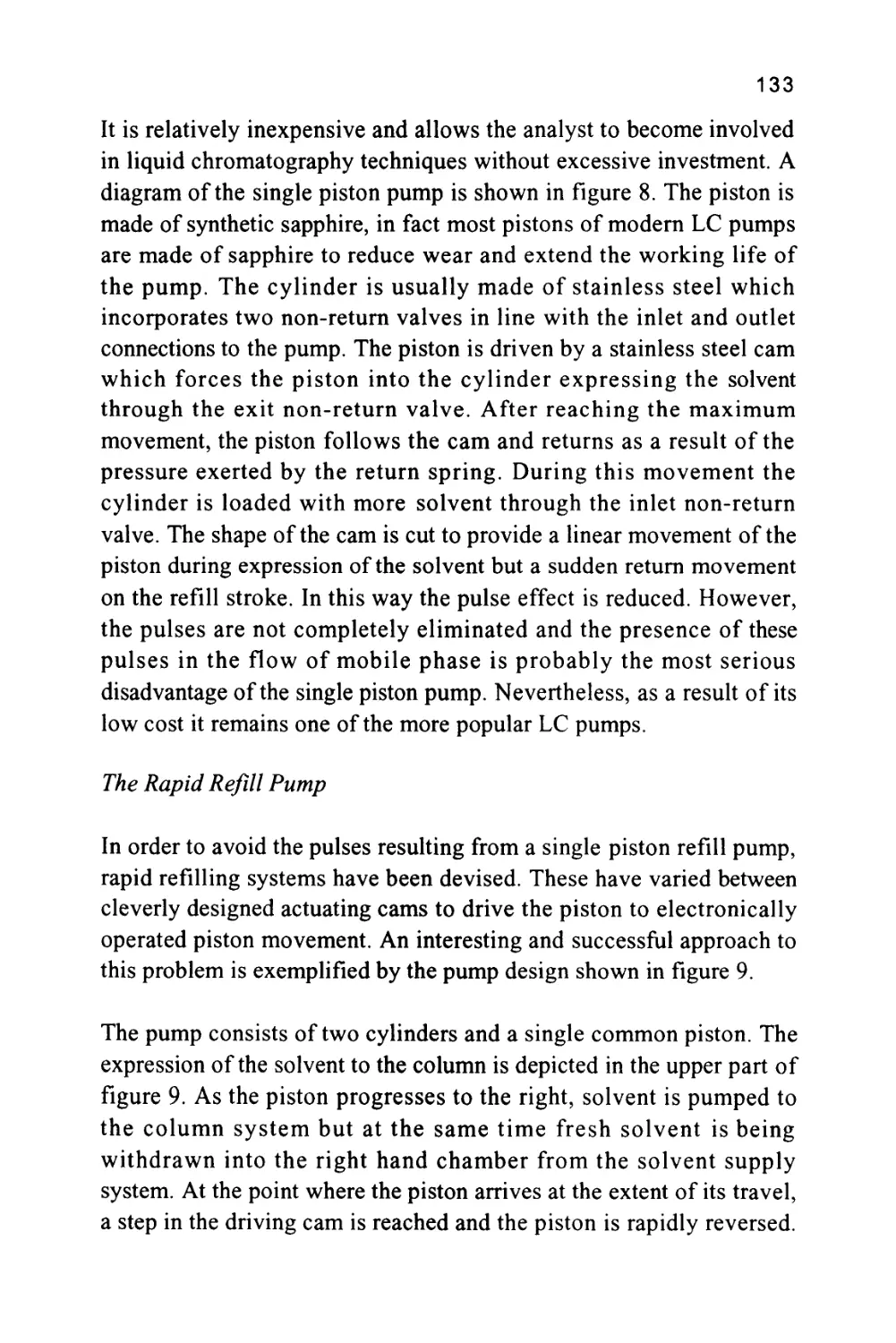
This definition is a little trite and, although it introduces the concept
of a mobile and stationary phase which are essential characteristics of
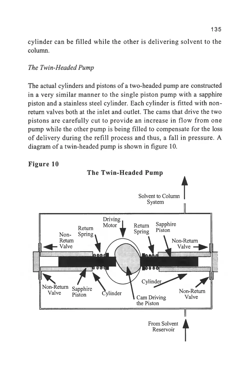
a chromatographic separation, it tends to obscure the basic process of
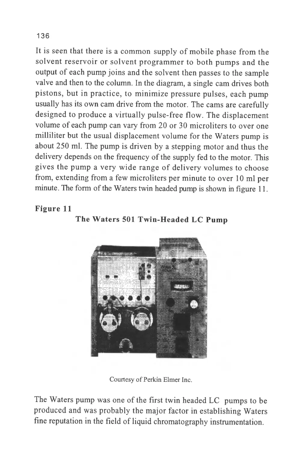
retention in the term distribution. A solute is distributed between two
phases as a result of the molecular forces that exist between the solute
molecules and those of the two phases. The stronger the forces
between the solute molecules and those of the stationary phase, the
greater will be the amount of solute held in the stationary phase under
equilibrium conditions. Conversely, the stronger the interactions
between the solute molecules and those of the mobile phase then the
greater the amount of solute that will be held in the mobile phase.
Now, the solute can only move through the chromatographic system
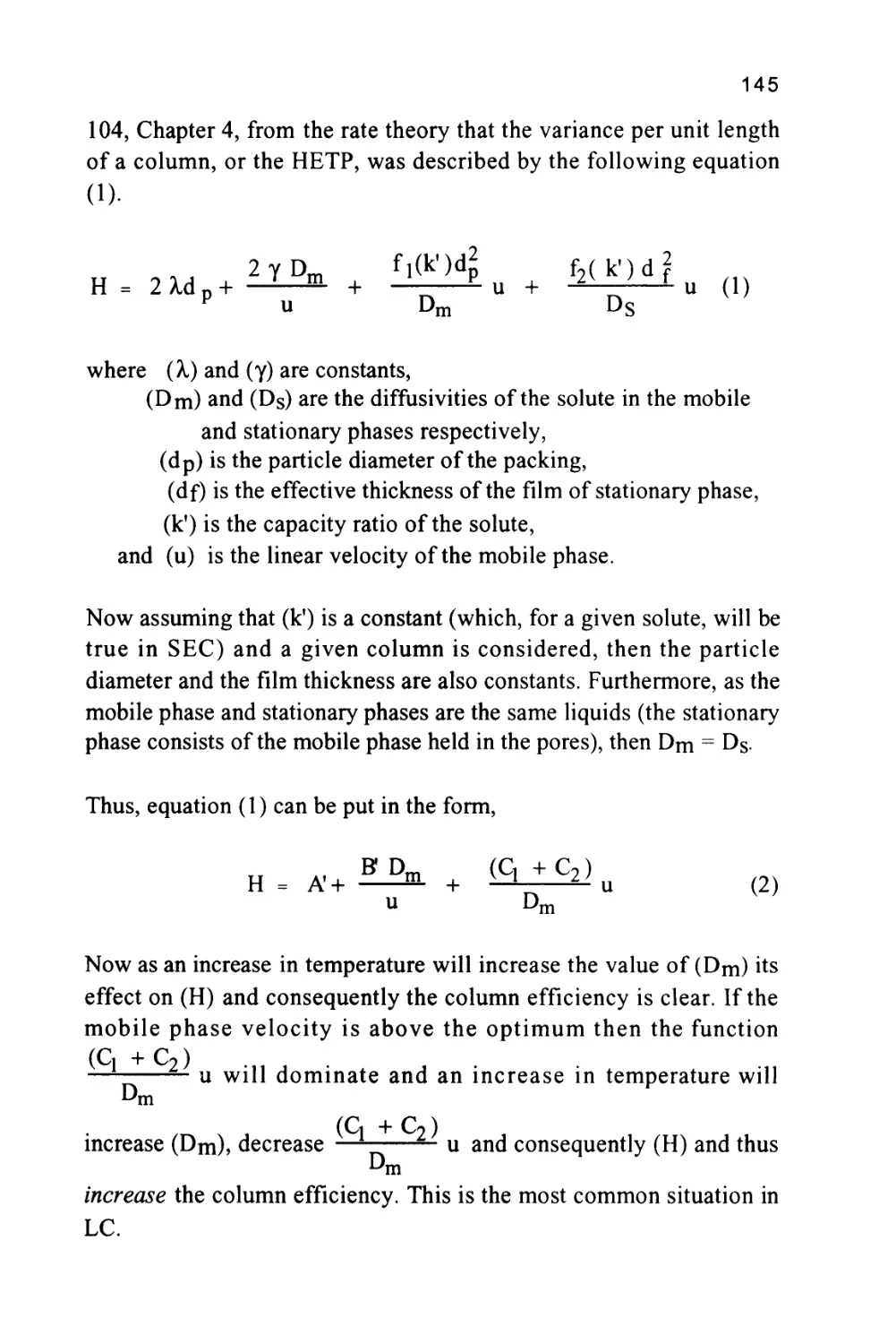
while it is in the mobile phase and thus, the speed at which a particular
solute will pass through the column will be directly proportional to
the concentration of the solute in the mobile phase.
The concentration of the solute in the mobile phase is inversely
proportional to the distribution coefficient of the solute with respect
to the stationary phase.
That is, K = —&- (1)
Xm
where (K.) is the distribution coefficient of the solute between
the two phases,
(Xm) is the concentration of the solute in the mobile
phase,
and (Xs) is the concentration of the solute in the stationary
phase.
Consequently, the solutes will pass through the chromatographic
system at speeds that are inversely proportional to their distribution
coefficients with respect to the stationary phase. The control of solute
retention by the magnitude of the solute distribution coefficient will be
discussed in the next chapter.
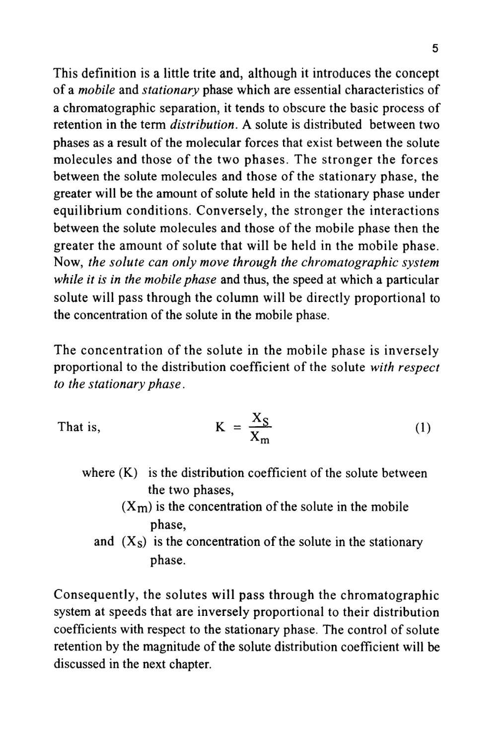
6
To appreciate the nature of a chromatographic separation, the manner
of solute migration through a chromatographic column needs to be
understood. Consider the progress of a solute through a chromatographic
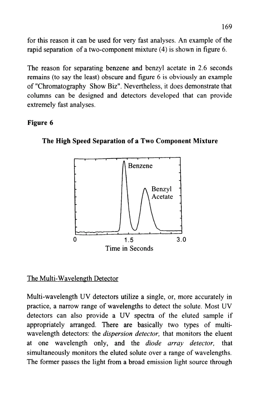
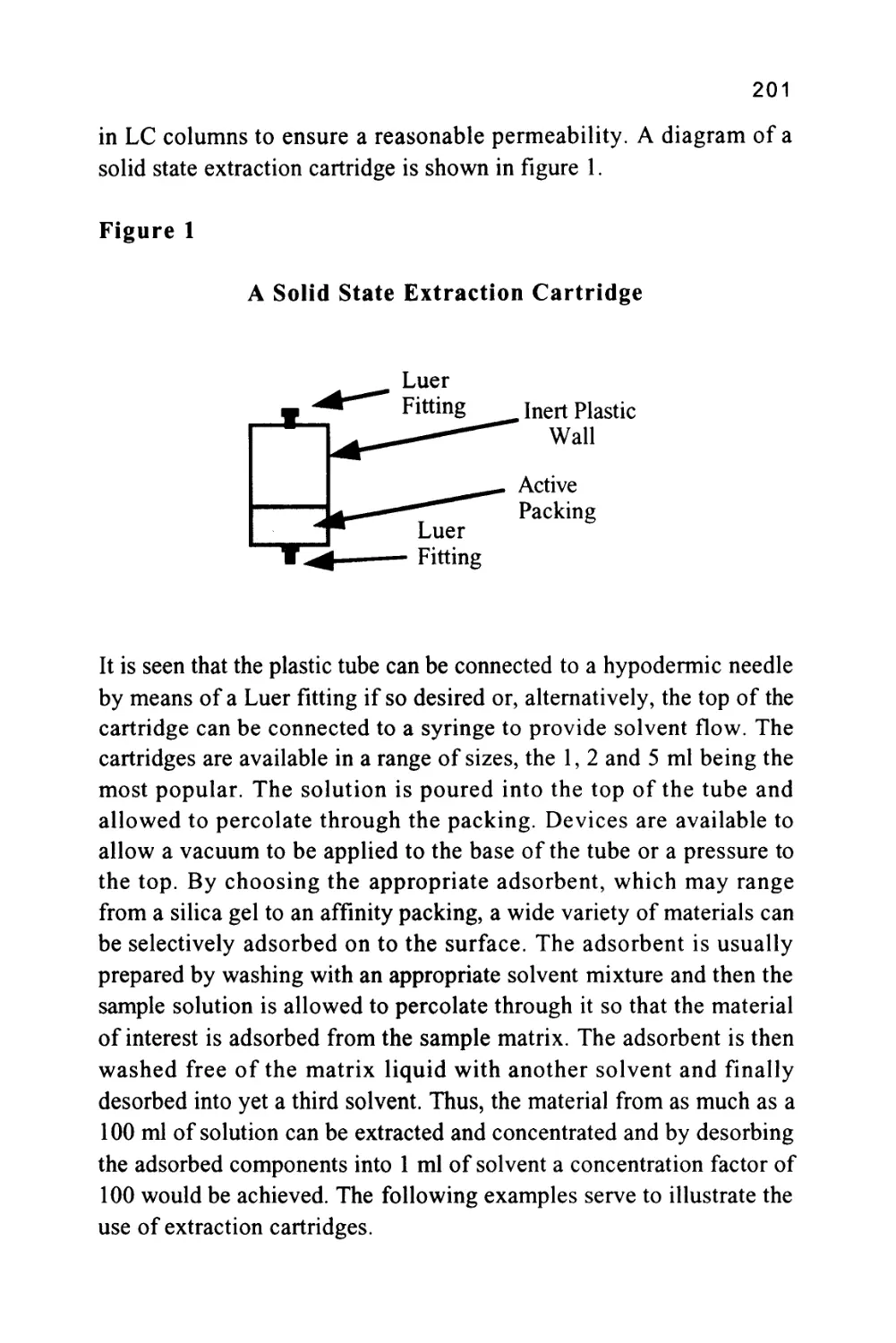
column as depicted in diagrammatic form in figure 1.
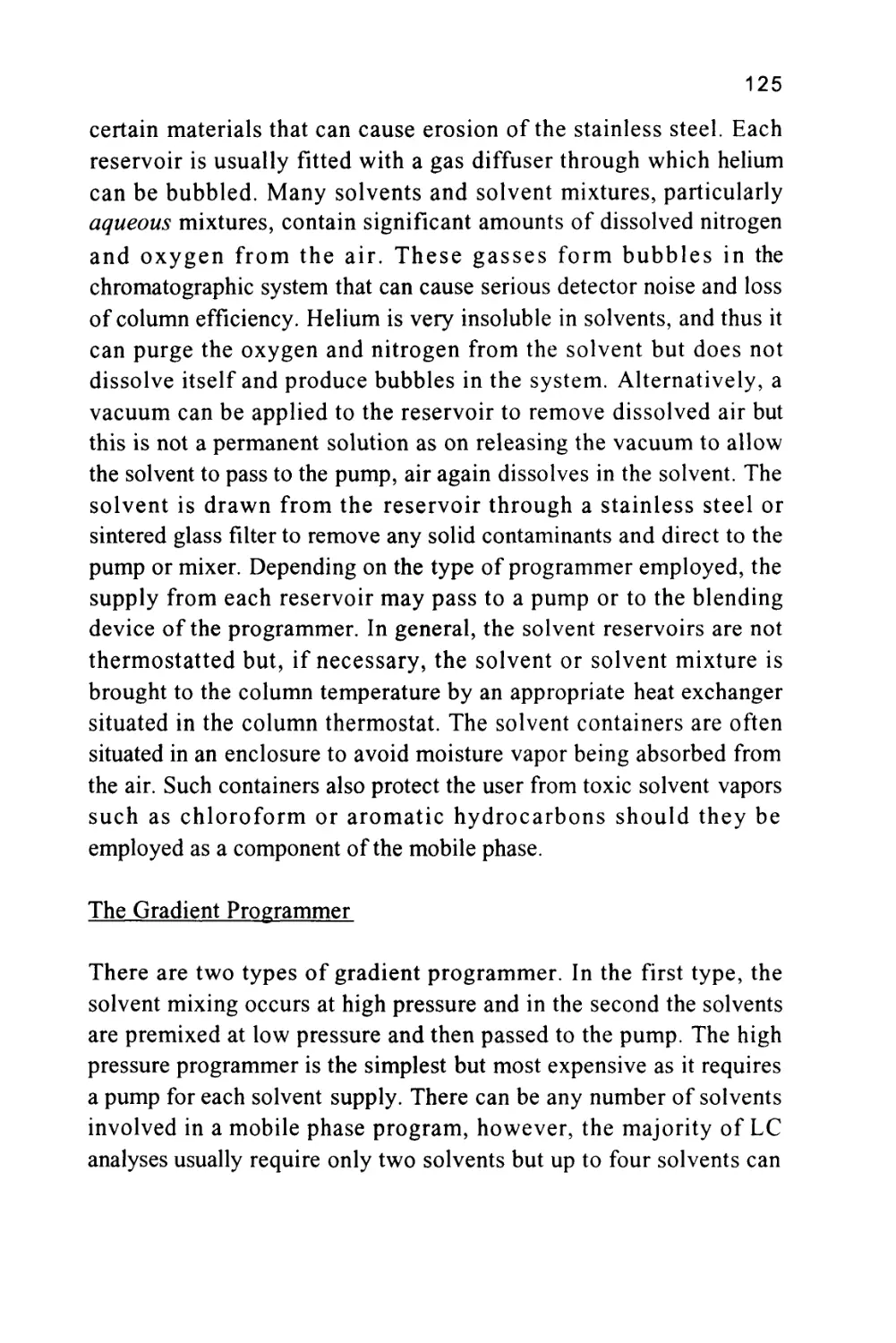
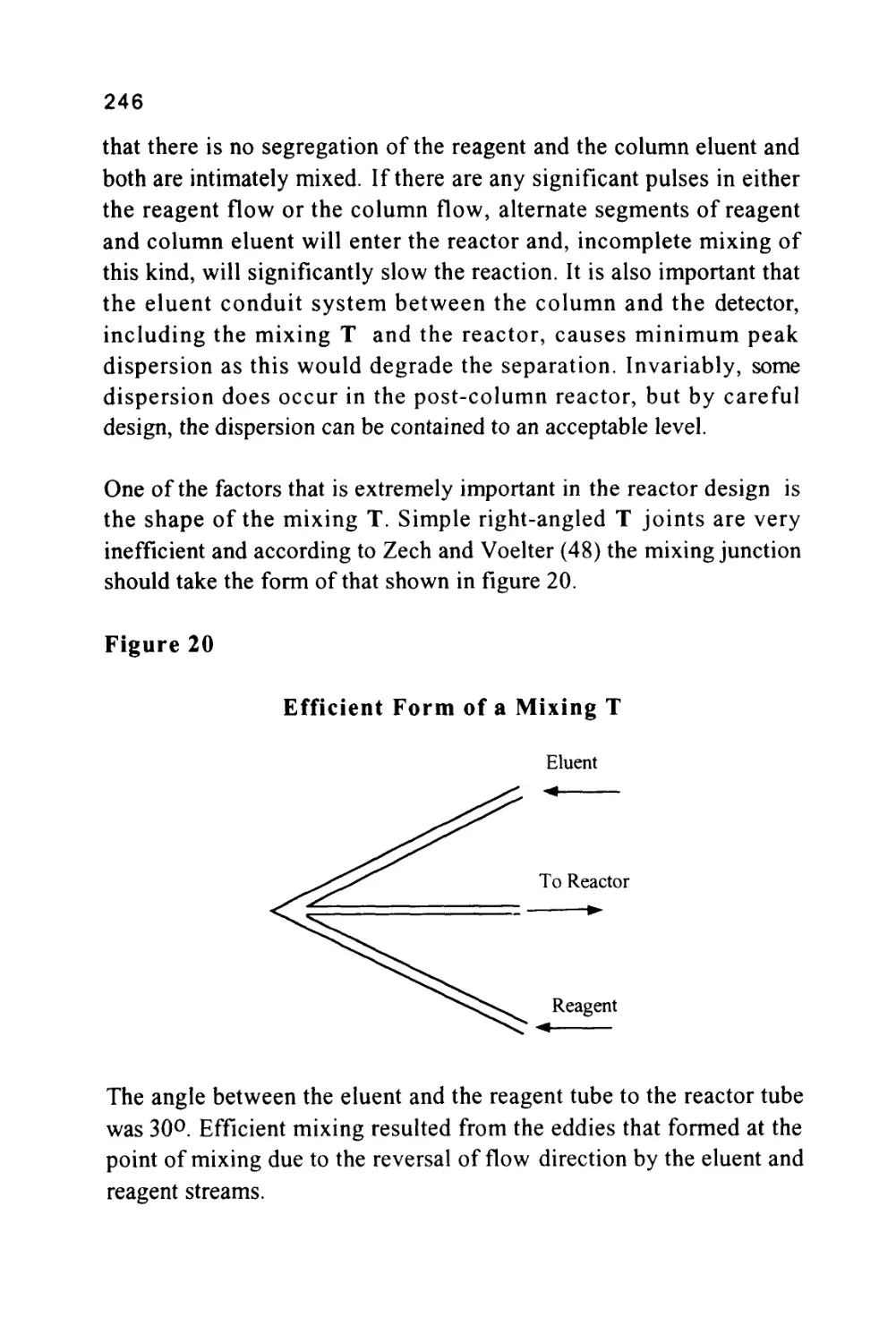
Figure 1
The Passage of a Solute Band Along a Chromatographic
Column
SOLUTE LEAVING
STATIONARY
PHASE AND
ENTERING
MOBILE PHASE
MOBILE PHASE
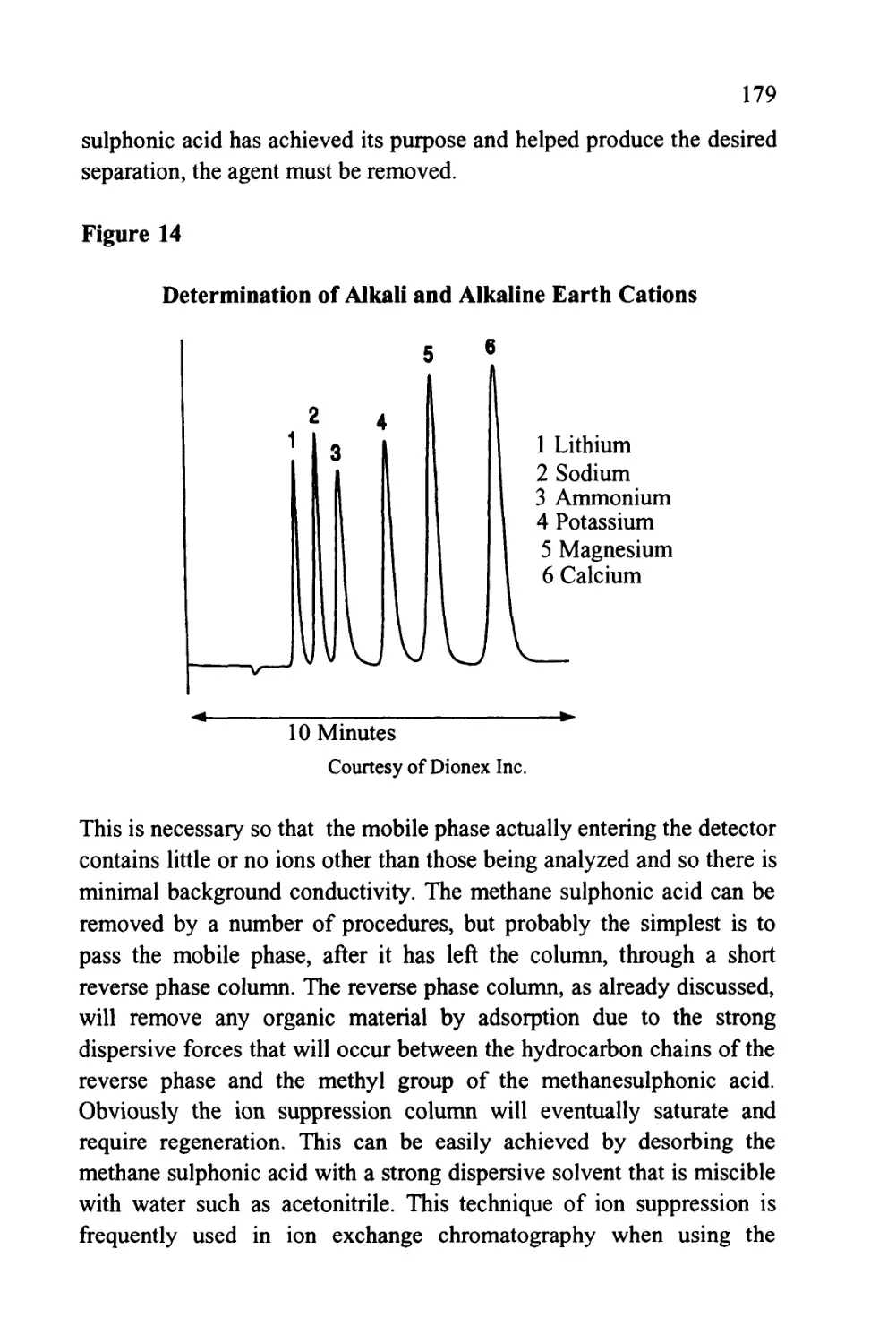
Flow of Mobile Phase
STATIONARY PHASE
SOLUTE LEAVING
MOBILE PHASE
AND ENTERING
STATIONARY
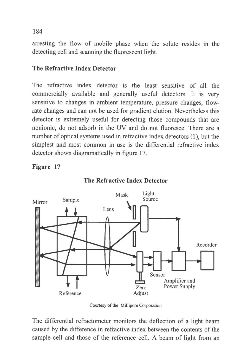
PHASE
The profile of the concentration of a solute in both the mobile and
stationary phases is Gaussian in form and this will be shown to be true
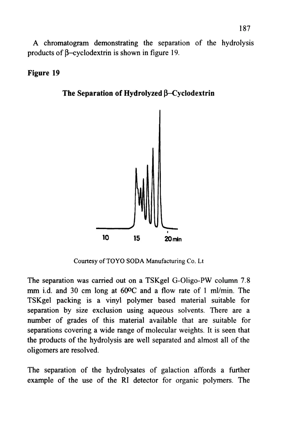
when dealing later with basic chromatography column theory. Thus,
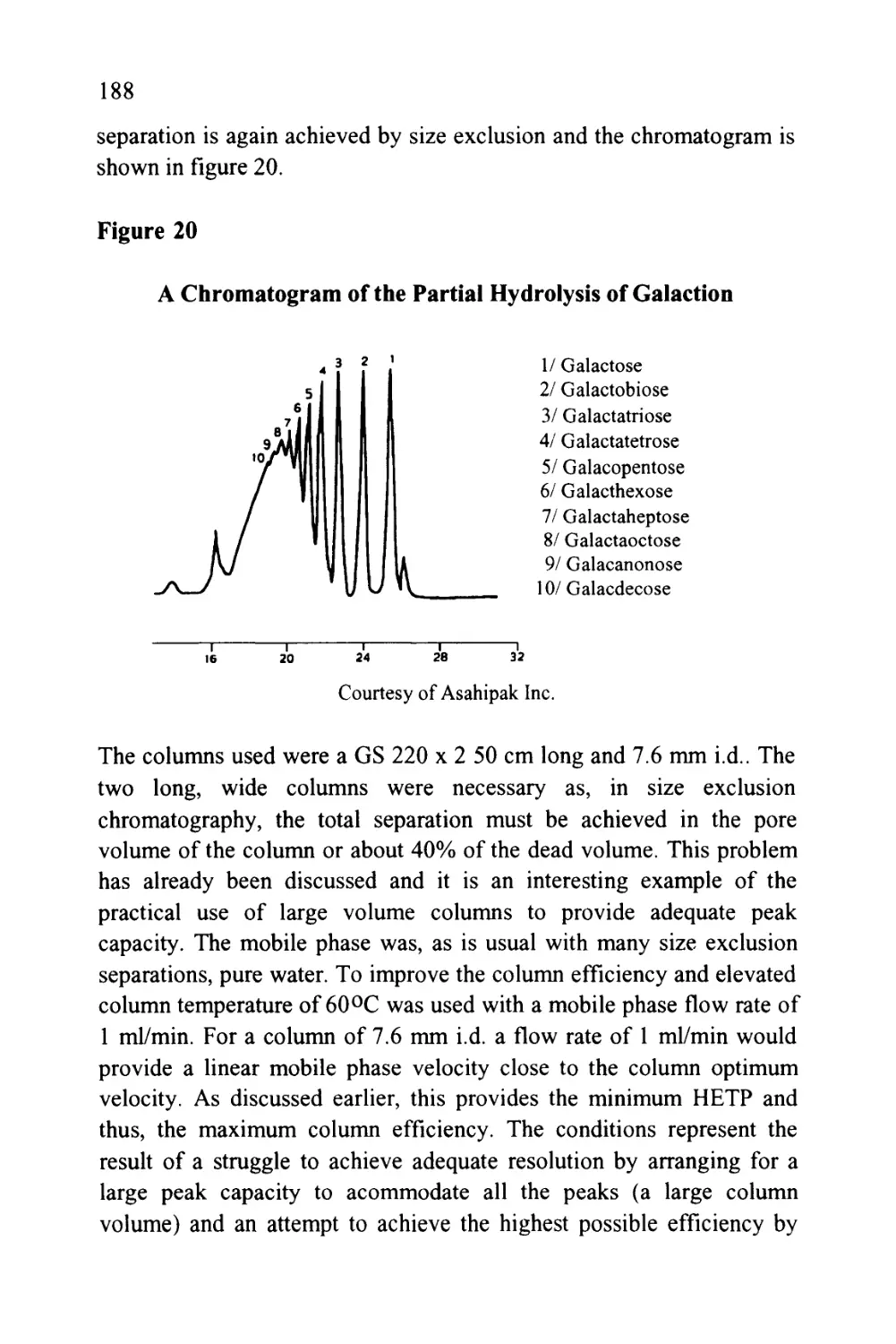
the flow of mobile phase will slightly displace the concentration
profile of the solute in the mobile phase relative to that in the
stationary phase; the displacement depicted in figure 1 is grossly
exaggerated to demonstrate this effect. It is seen that, as a result of this
displacement, the concentration of solute in the mobile phase at the
front of the peak exceeds the equilibrium concentration with respect
to that in the stationary phase. It follows that there is a net transfer of
solute from the mobile phase in the front part of the peak to the
7
stationary phase to re-establish equilibrium as the peak progresses
along the column. At the rear of the peak, the converse occurs. As the
concentration profile moves forward, the concentration of solute in
the stationary phase at the rear of the peak is now in excess of the
equilibrium concentration. Thus, solute leaves the stationary phase
and there is a net transfer of solute to the mobile phase in an attempt
to re-establish equilibrium. The solute band progresses through the
column by a net transfer of solute to the mobile phase at the rear of
the peak and a net transfer of solute to the stationary phase at the front
of the peak.
Solute retention, and consequently chromatographic resolution, is
determined by the magnitude of the distribution coefficients of the
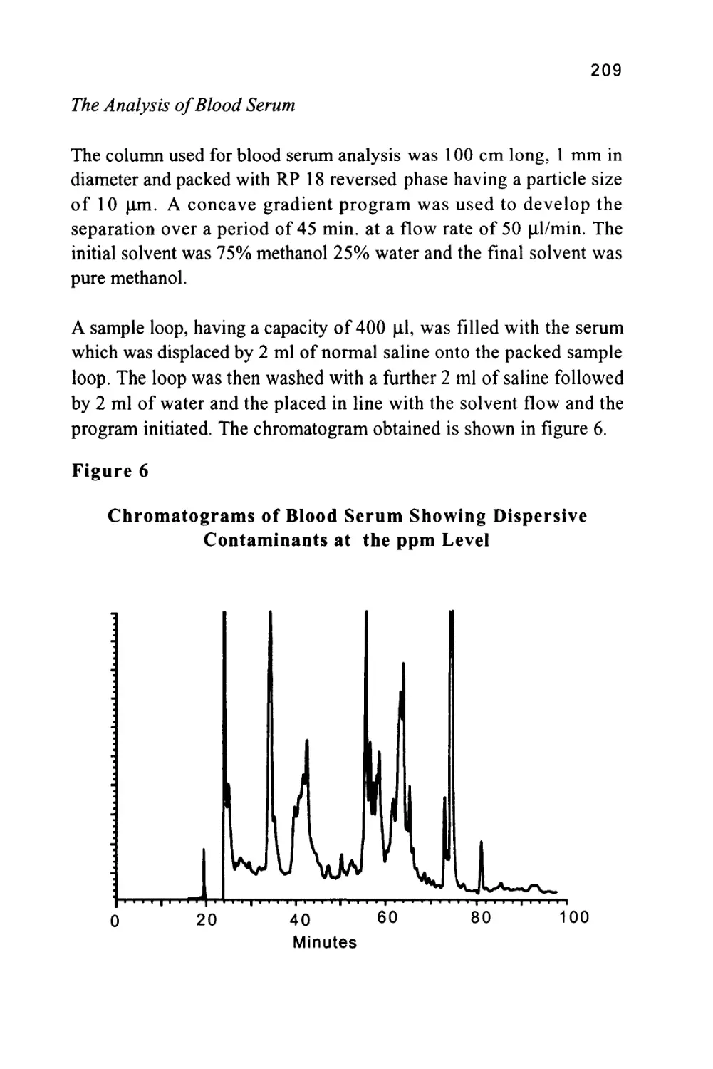
solutes with respect to the stationary phase and relative to each other.
As already suggested, the magnitude of the distribution coefficient is,
in turn, controlled by molecular forces between the solutes and the
two phases. The procedure by which the analyst can manipulate the
solute/phase interactions to effect the desired resolution will also be
discussed in chapter 2.
The Different Forms of Chromatography
The two major classes of chromatography are defined by the nature of
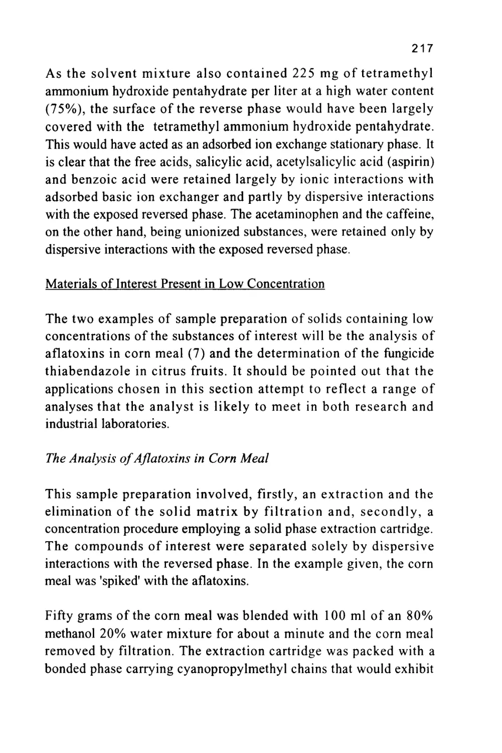
the mobile phase. Gas chromatography (GC) is the term given to all
separations that employ a gas as the mobile phase. Conversely, all
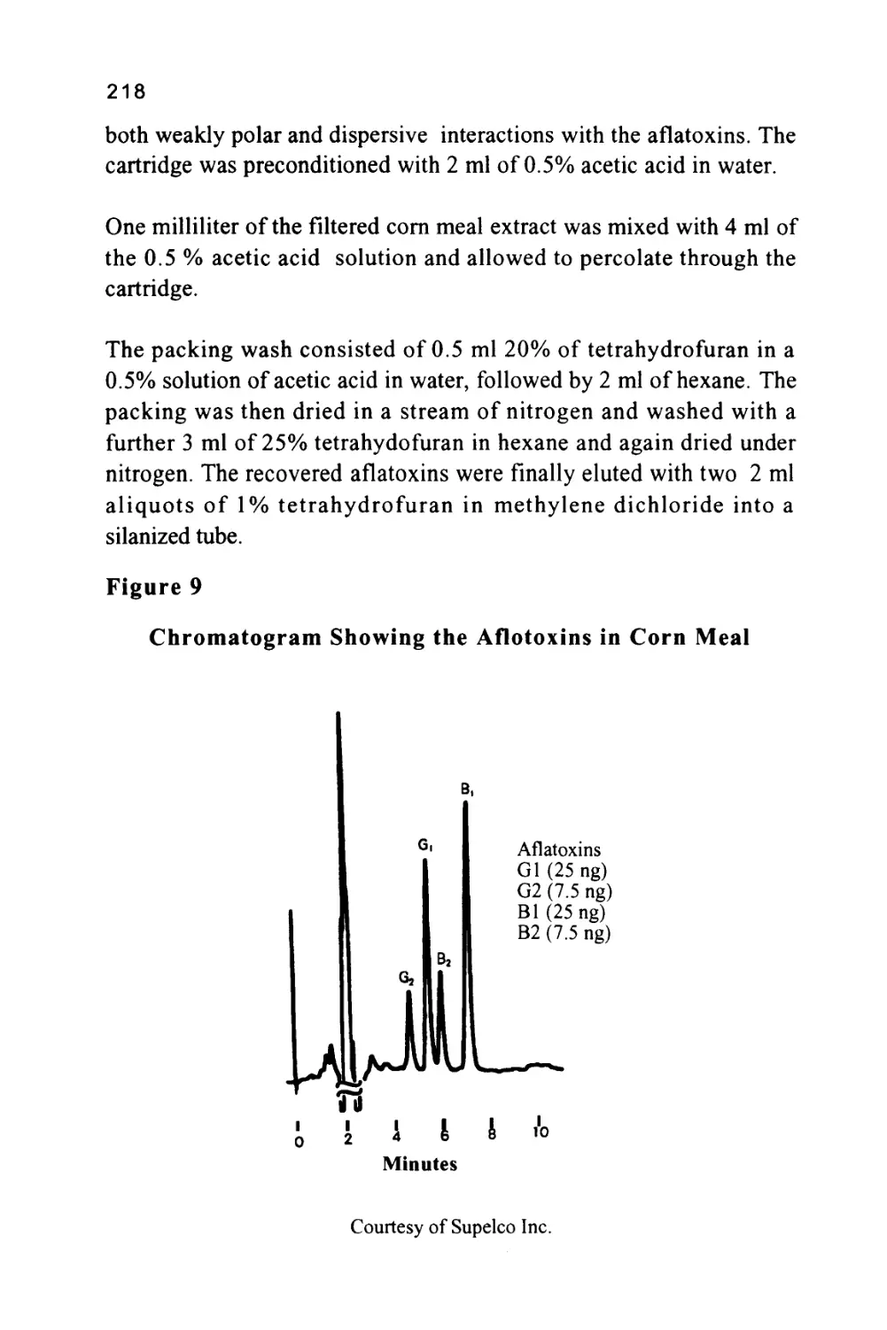
chromatographic systems that employ a liquid as the mobile phase are
classed as liquid chromatography. It has been suggested that
supercritical chromatography, where, during the separation, the
mobile phase can be operated partly above its critical state and partly
below its critical state, represents a third class of chromatography. In
fact, it is a hybrid: when the mobile phase is below its critical
temperature and above its critical pressure, it is a liquid and therefore
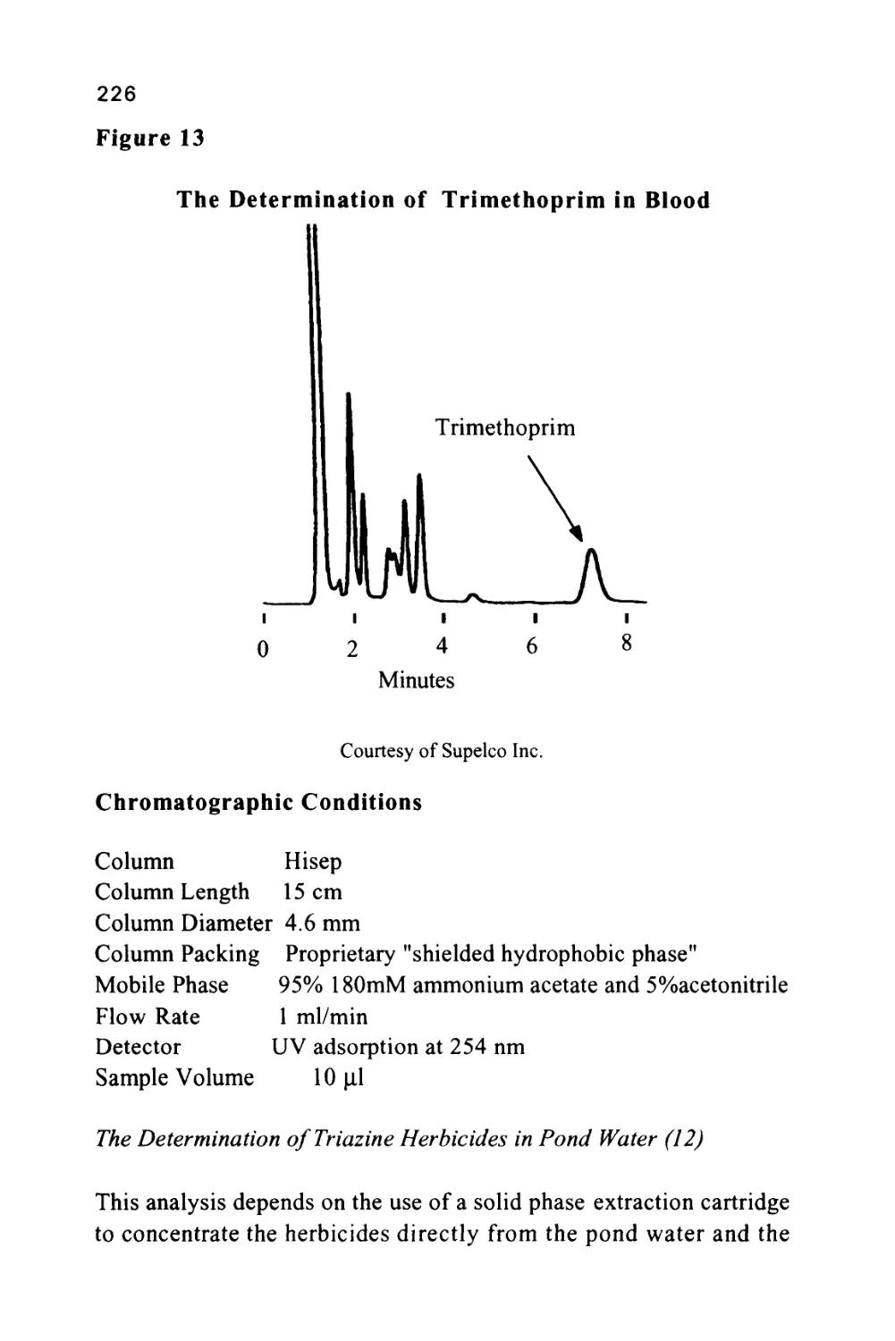
a liquid chromatography system. When the mobile phase is above its
critical temperature and below its critical pressure, it is a gas and
therefore the system can be classed as gas chromatography.
8
It is interesting to note that there have been very few specific
analytical applications reported, which demonstrate that super-critical
chromatography gives results superior to either gas chromatography
or liquid chromatography alone. As a consequence, considering the
added complexity of the super-critical chromatograph, its value in
analytical chemistry must be considered questionable.
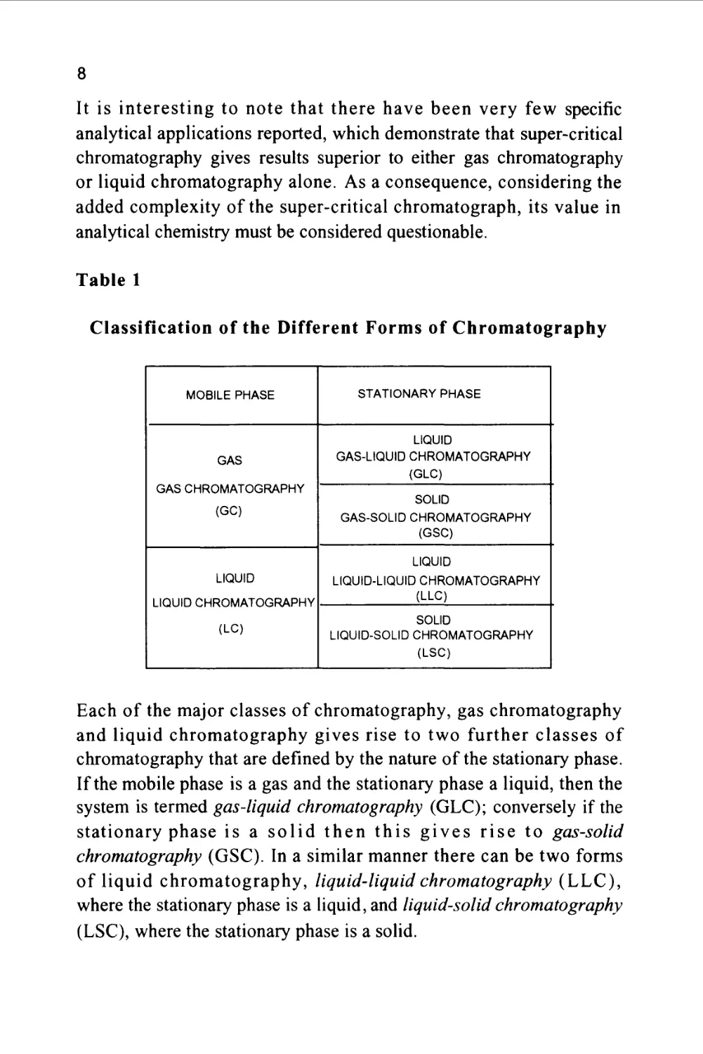
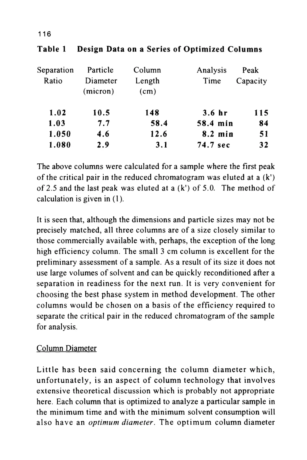
Table 1
Classification of the Different Forms of Chromatography
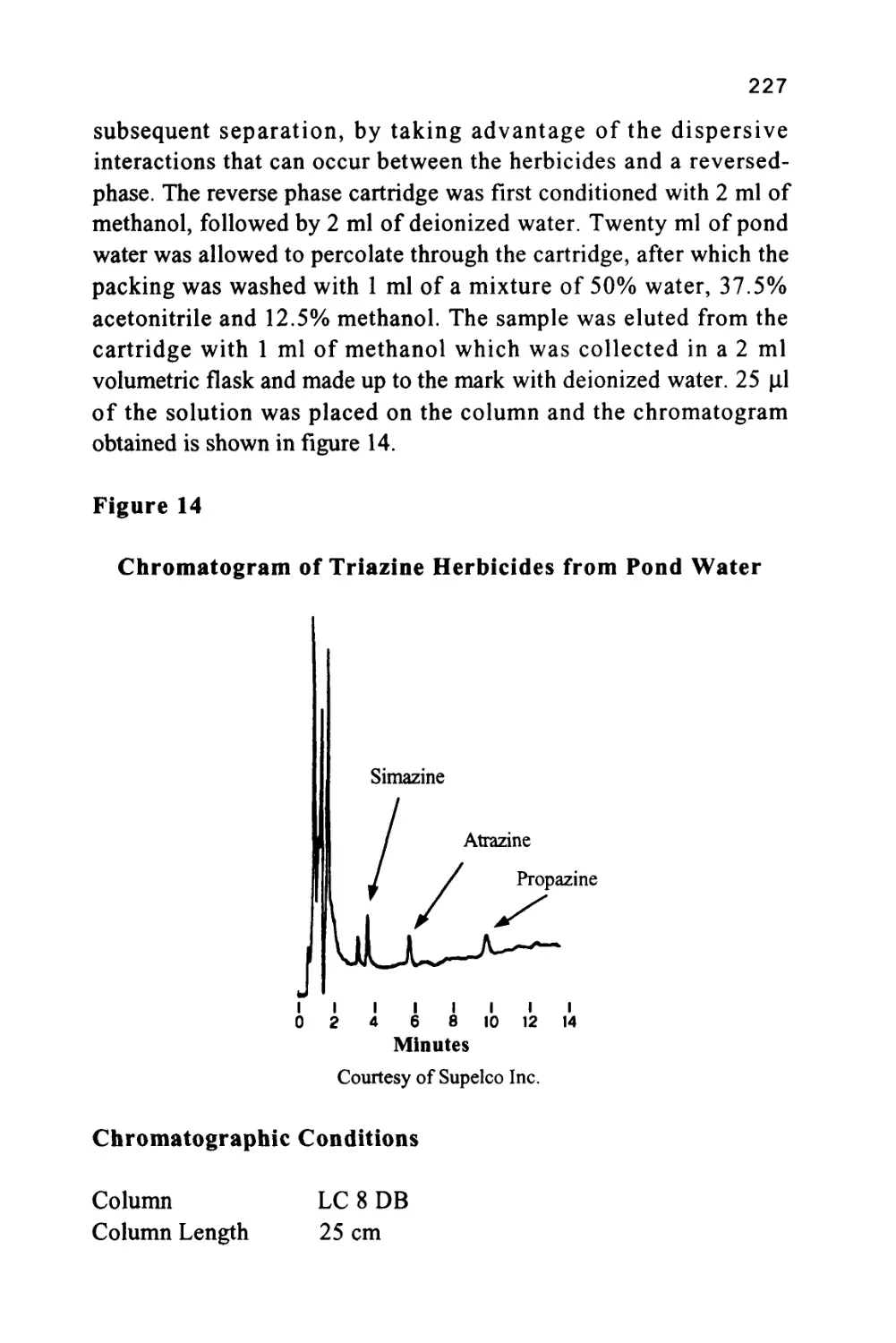
MOBILE PHASE
GAS
GAS CHROMATOGRAPHY
(GC)
LIQUID
LIQUID CHROMATOGRAPHY
(LC)
STATIONARY PHASE
LIQUID
GAS-LIQUID CHROMATOGRAPHY
(GLC)
SOLID
GAS-SOLID CHROMATOGRAPHY
(GSC)
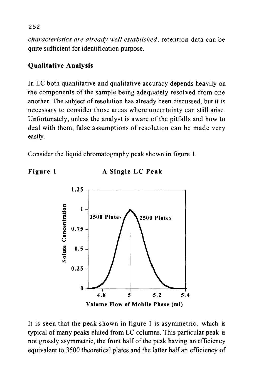
LIQUID
LIQUID-LIQUID CHROMATOGRAPHY
(LLC)
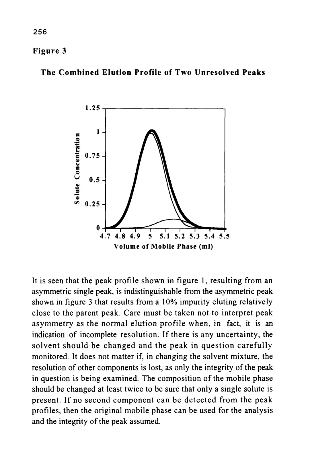
SOLID
LIQUID-SOLID CHROMATOGRAPHY
(LSC)
Each of the major classes of chromatography, gas chromatography
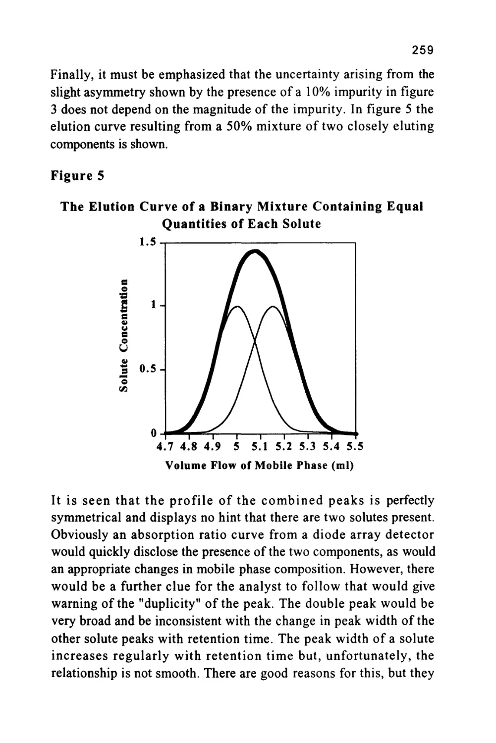
and liquid chromatography gives rise to two further classes of
chromatography that are defined by the nature of the stationary phase.
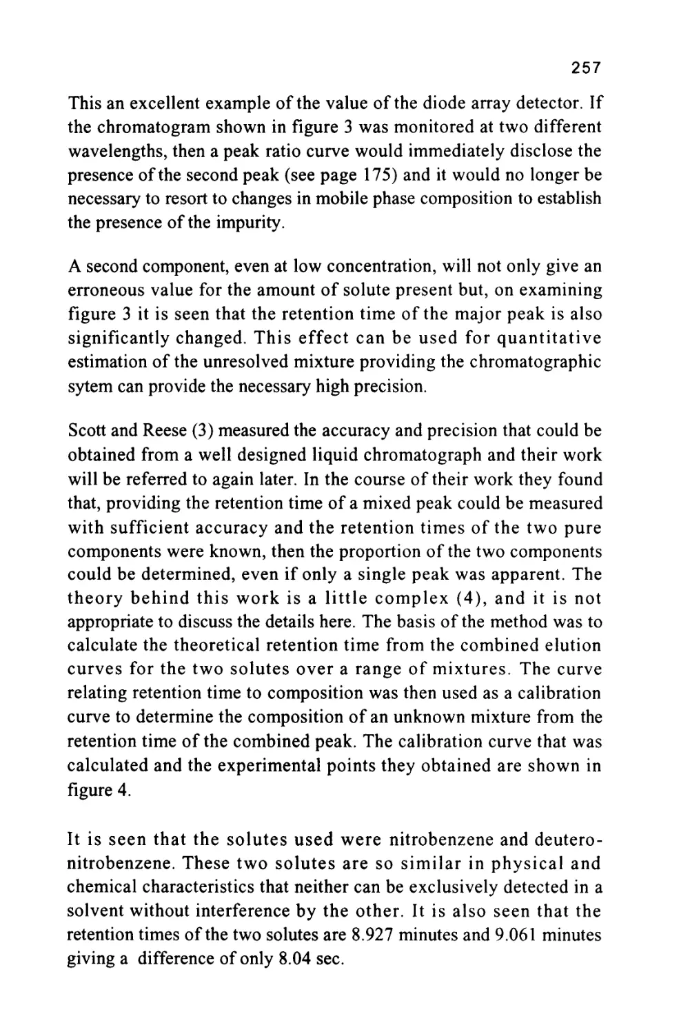
If the mobile phase is a gas and the stationary phase a liquid, then the
system is termed gas-liquid chromatography (GLC); conversely if the
stationary phase is a solid then this gives rise to gas-solid
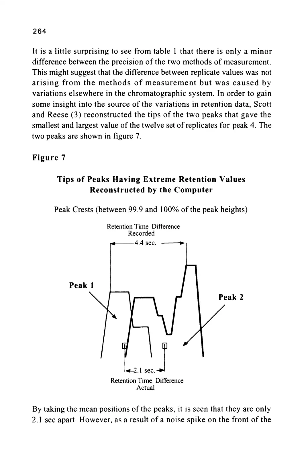
chromatography (GSC). In a similar manner there can be two forms
of liquid chromatography, liquid-liquid chromatography (LLC),
where the stationary phase is a liquid, and liquid-solid chromatography
(LSC), where the stationary phase is a solid.
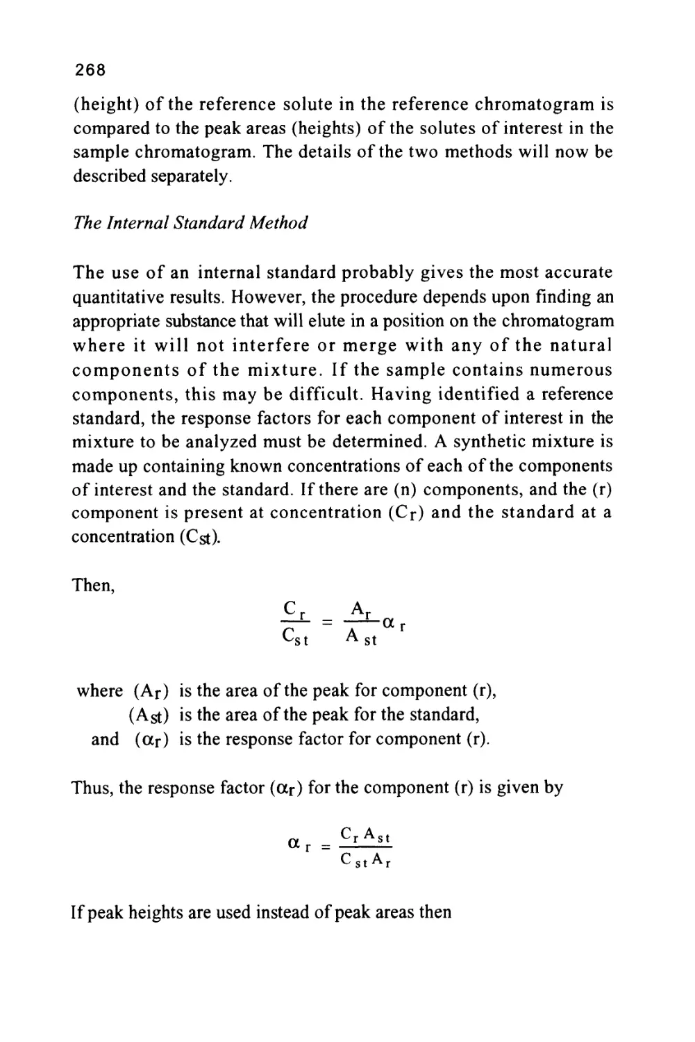
9
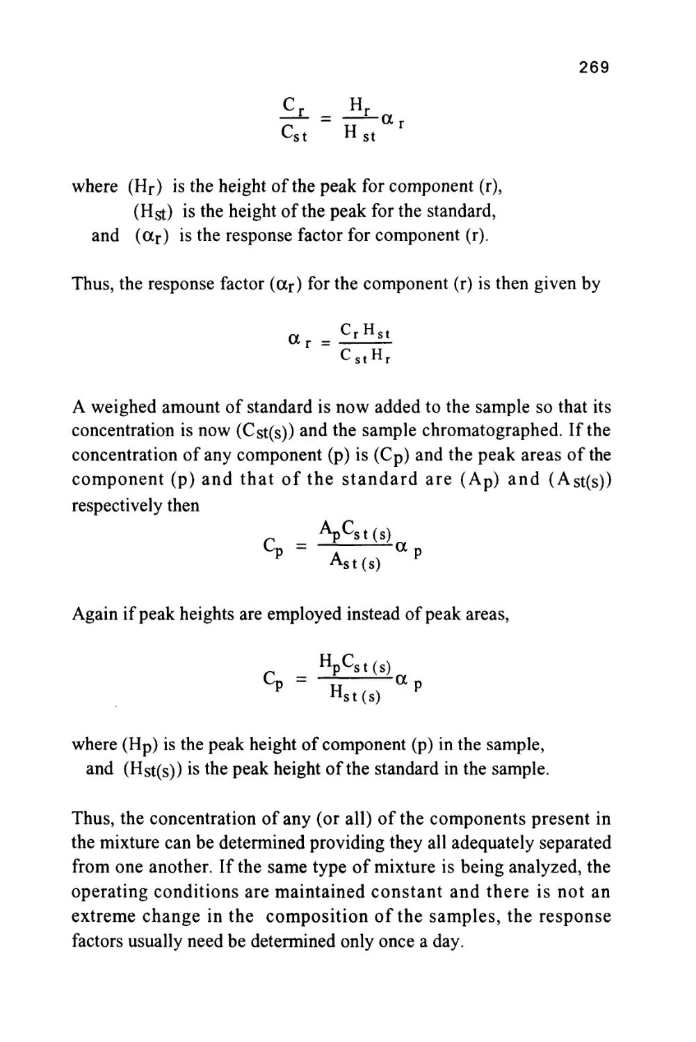
The vast majority of modern liquid chromatography systems involve
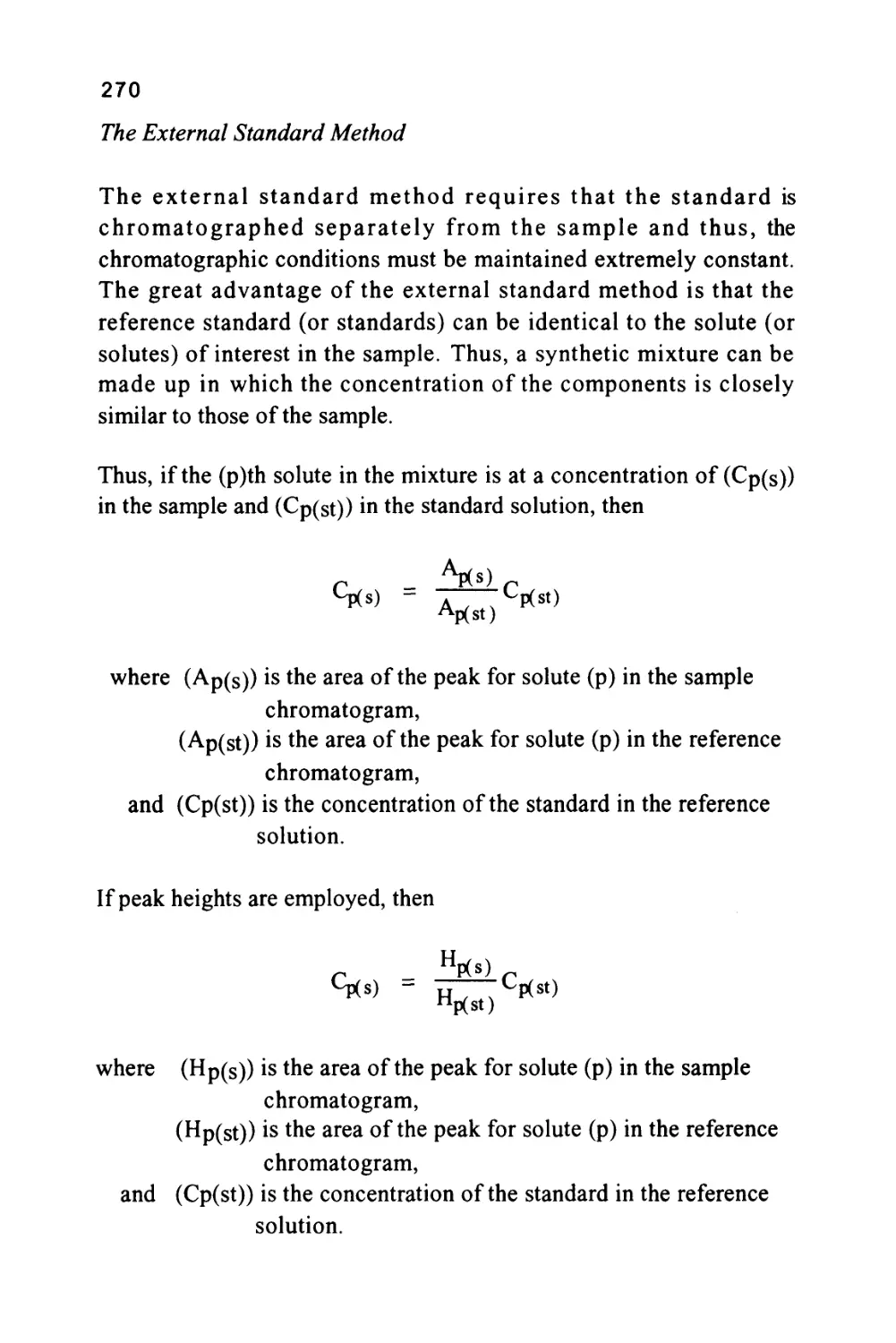
the use of silica gel or a derivative of silica gel, such as a bonded
phase, as a stationary phase. Thus, it would appear that most LC
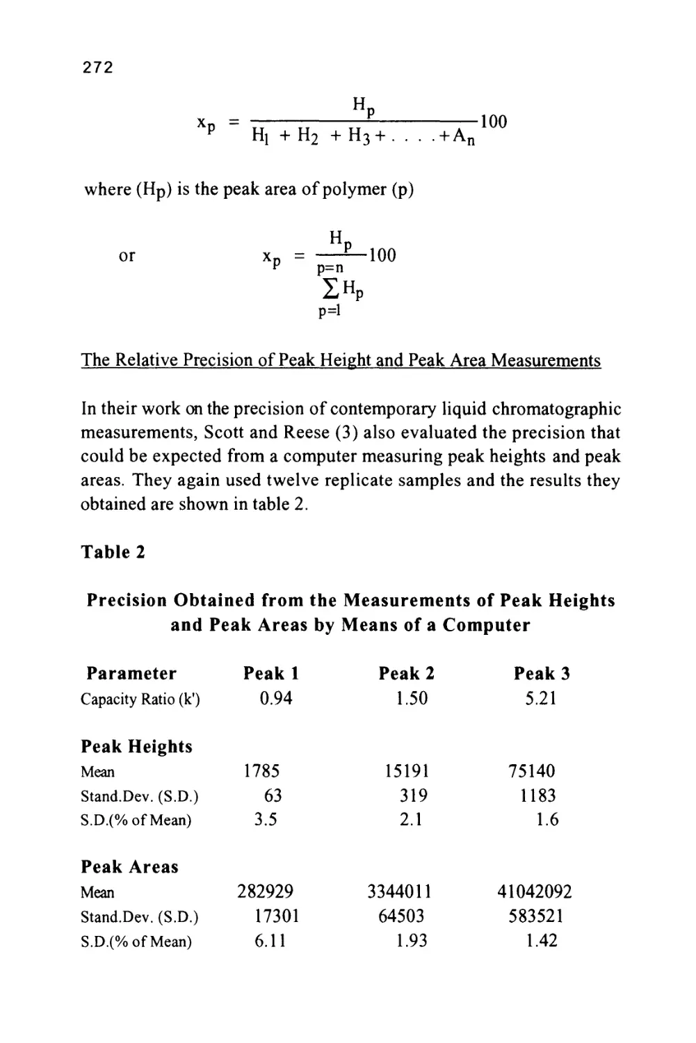
separations are carried out by liquid-solid chromatography. Owing to
the adsorption of solvent on the surface of both silica and bonded
phases, however, the physical chemical characteristics of the separation
are more akin to a liquid-liquid distribution system than that of a
liquid-solid system. As a consequence, although most modern
stationary phases are in fact solids, solute distribution is usually
treated theoretically as a liquid-liquid system.
There are other forms of chromatography classification that have been
proposed based on the geometric form of the distribution system. For
example, the terms column chromatography and lamina
chromatography attempt to differentiate between chromatography
systems that employ a column and those that employ a sheet of paper,
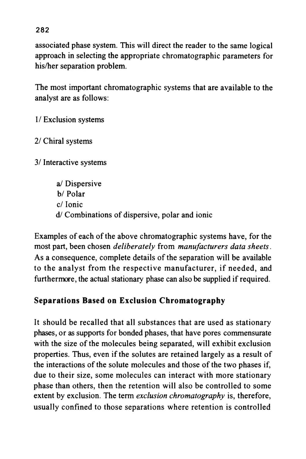
as in paper chromatography, or a sheet of glass coated with silica, as
in thin-layer chromatography. Obviously the distribution system
involved in paper chromatography is the stationary water or solvent
held on the paper and the solvent or solvent mixture that passes over
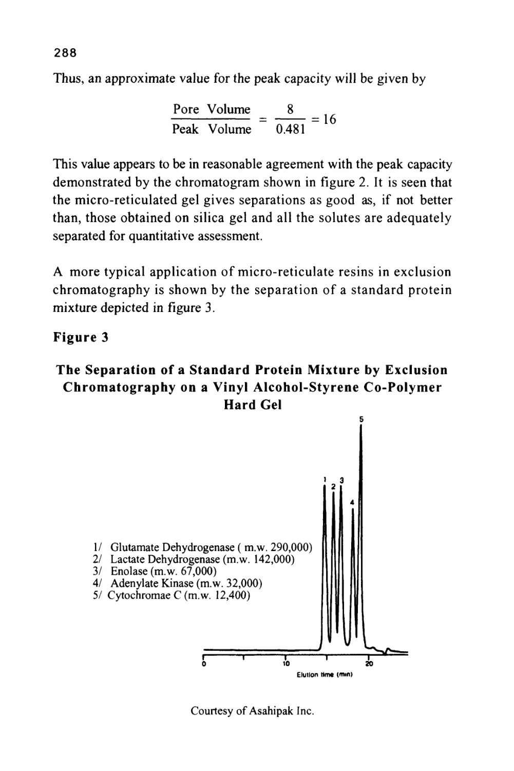
the surface. Such a distribution system is unambiguously liquid-
liquid. The silica gel or bonded phase on the thin layer plate however,
as in a LC column, is covered by an adsorbed layer of solvent and,
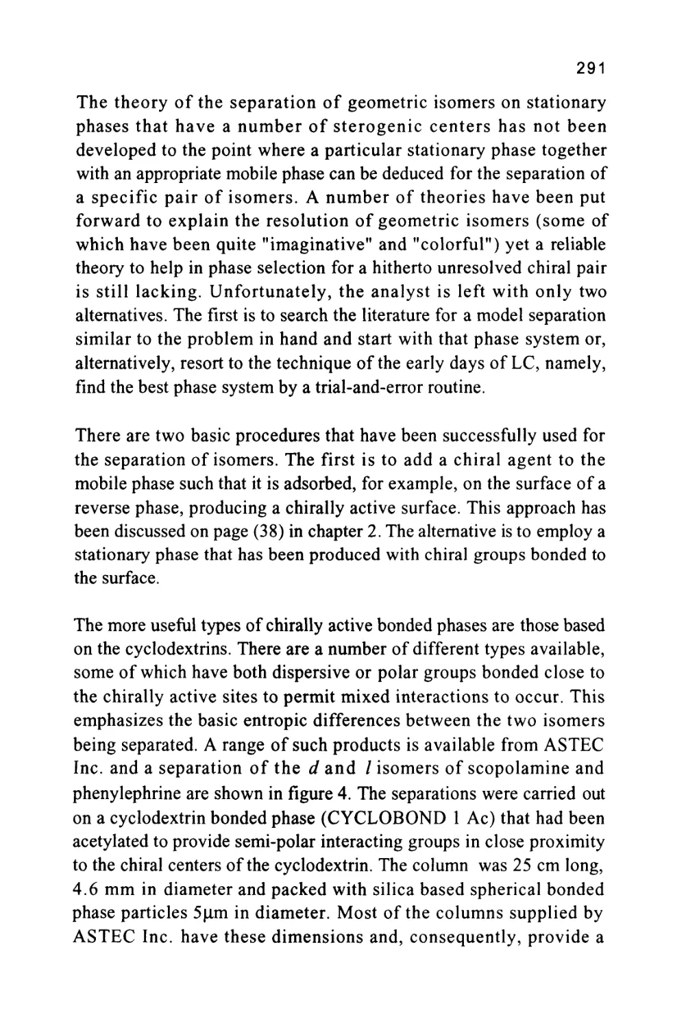
consequently, also behaves as a liquid-liquid system. In general, it is
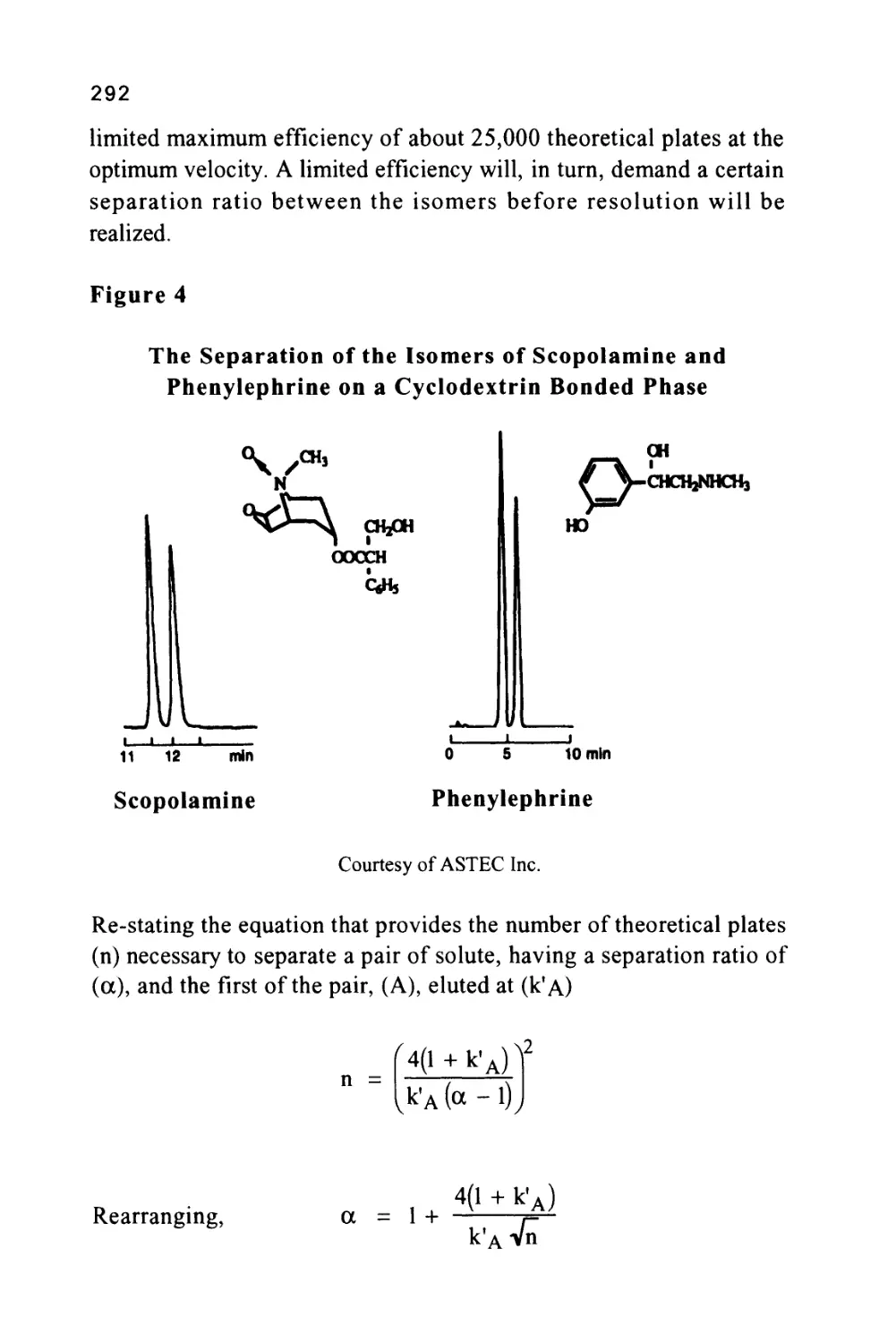
better to classify the type of chromatography on the basic physical
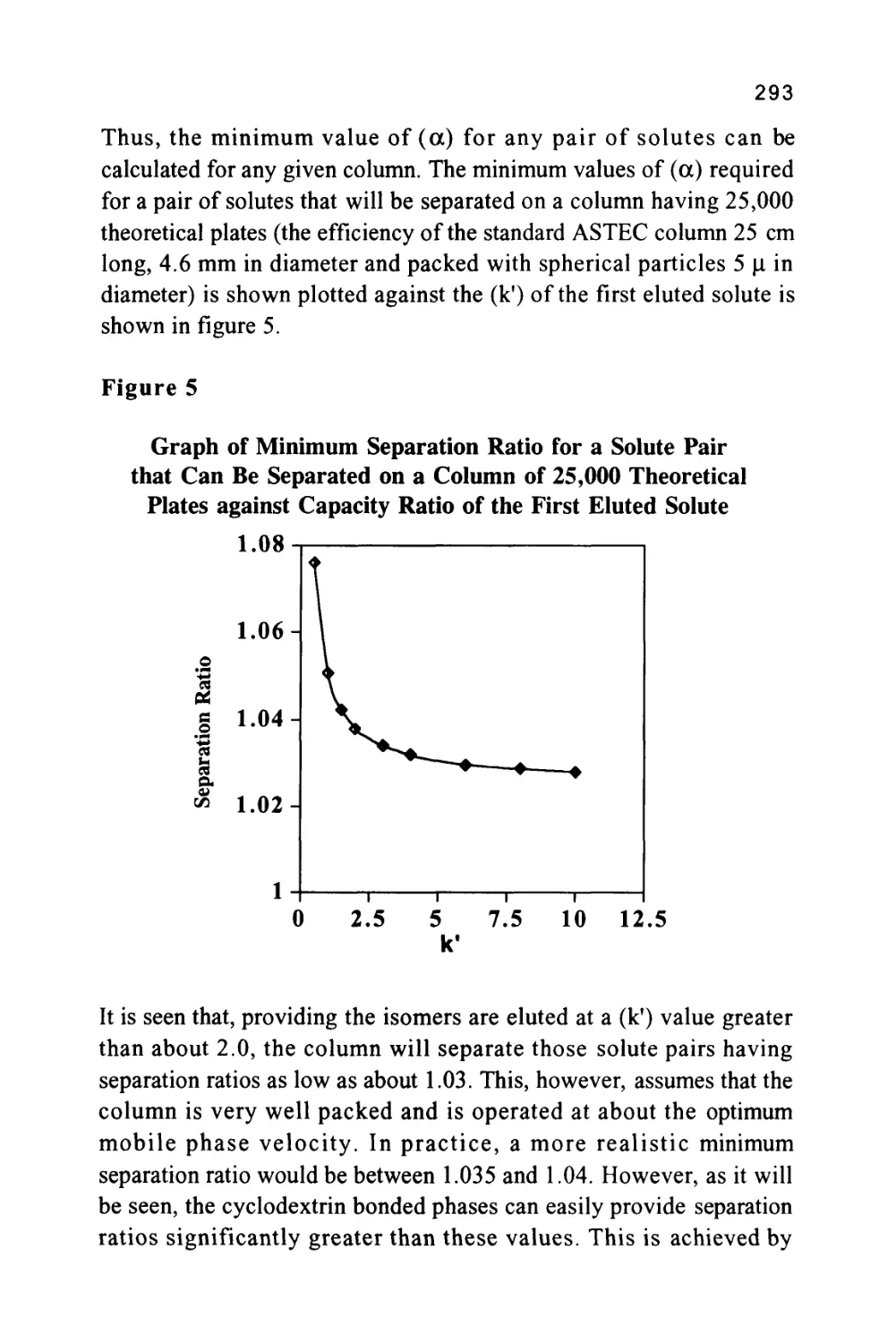
chemistry involved than, somewhat arbitrarily, on the shape of the
apparatus. As a consequence, classification on the basis of the
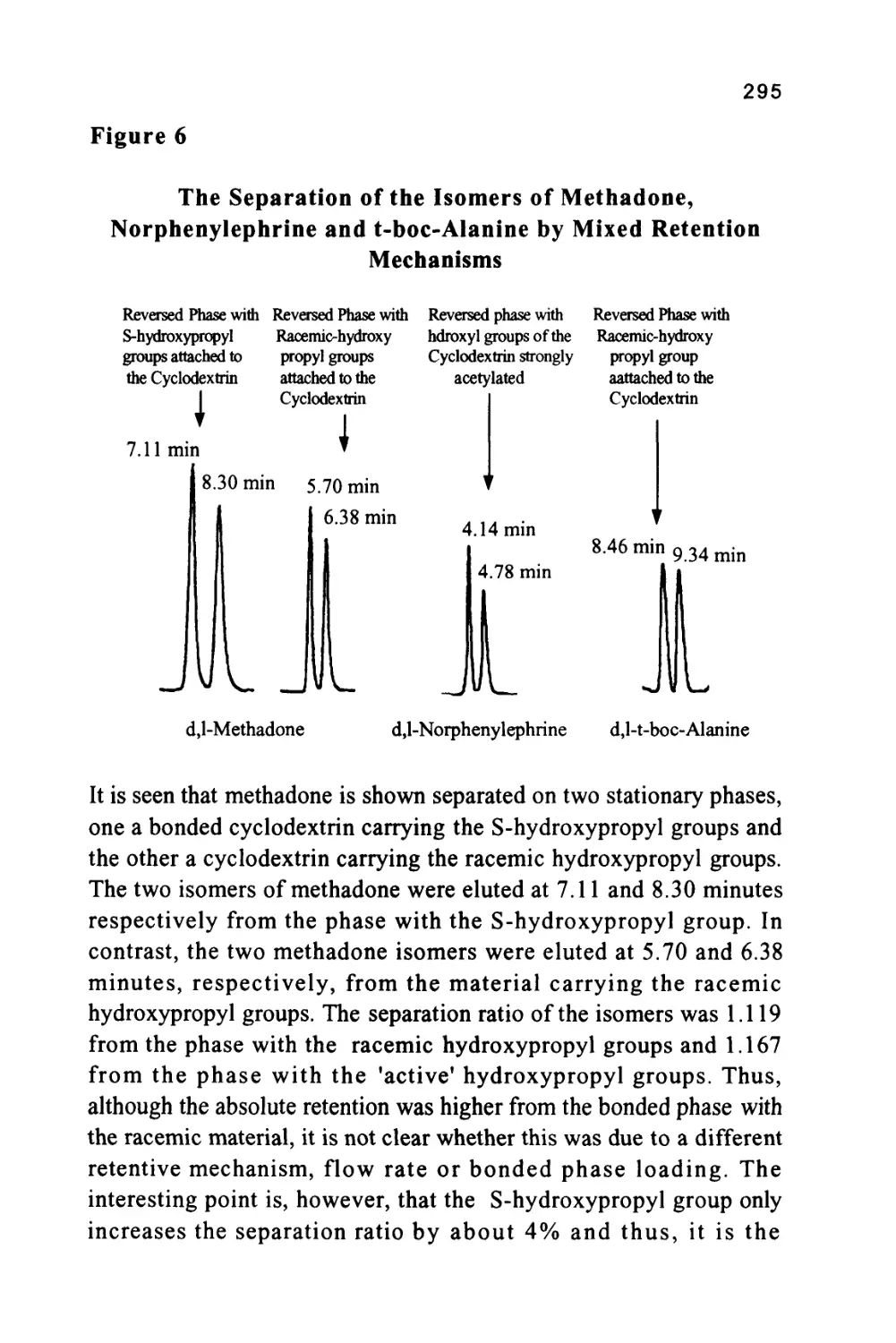
geometry of the distribution system is less commonly employed and,
with alternative well-established terms available, the term lamina
chromatography is hardly justifiable.
Chromatography Nomenclature
Before proceeding to a more detailed discussion of LC apparatus or
separation technology, it is necessary to define some chromatographic
terms and, in particular, the properties of a chromatogram that will be
10
used throughout this book. The terms that will be defined were
introduced many years ago and have been agreed upon by a number of
organizations and are now in common use in all aspects of separation
science.
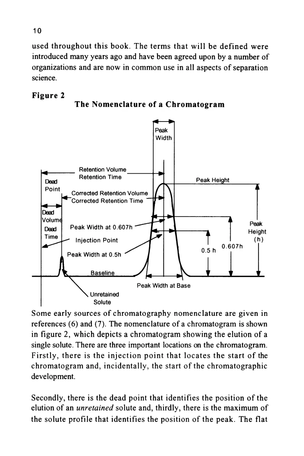
Figure 2
The Nomenclature of a Chromatogram
Peak
Width
Retention Volume
Retention Time
Corrected Retention Volume
Corrected Retention Time
Peak Width at 0.607h
Injection Point
Peak Width at 0.5h
Baseline
Peak Width at Base
Unretained
Solute
Some early sources of chromatography nomenclature are given in
references (6) and (7). The nomenclature of a chromatogram is shown
in figure 2, which depicts a chromatogram showing the elution of a
single solute. There are three important locations on the chromatogram.
Firstly, there is the injection point that locates the start of the
chromatogram and, incidentally, the start of the chromatographic
development.
Secondly, there is the dead point that identifies the position of the
elution of an unretained solute and, thirdly, there is the maximum of
the solute profile that identifies the position of the peak. The flat
11
portion of the chromatogram where there is no solute being eluted is
called the baseline. The baseline should be straight and unperturbed
but at high sensitivities (usually the two highest sensitivity settings on
the detector amplifier) there may be some high frequency excursions
of the trace (about 1-2% full scale deflection (FSD)).
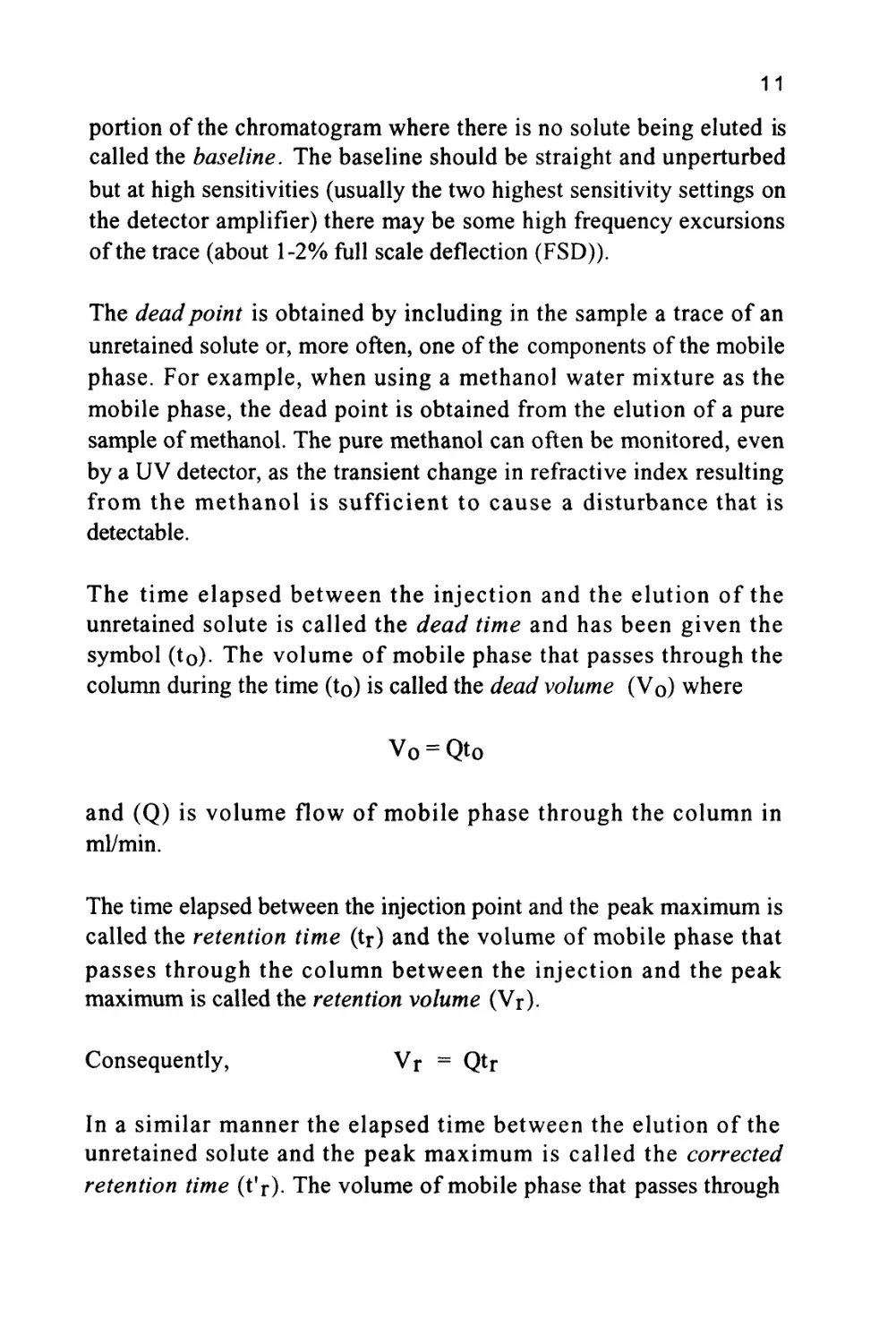
The dead point is obtained by including in the sample a trace of an
unretained solute or, more often, one of the components of the mobile
phase. For example, when using a methanol water mixture as the
mobile phase, the dead point is obtained from the elution of a pure
sample of methanol. The pure methanol can often be monitored, even
by a UV detector, as the transient change in refractive index resulting
from the methanol is sufficient to cause a disturbance that is
detectable.
The time elapsed between the injection and the elution of the
unretained solute is called the dead time and has been given the
symbol (to). The volume of mobile phase that passes through the
column during the time (to) is called the dead volume (Vo) where
V0 = Qt0
and (Q) is volume flow of mobile phase through the column in
ml/min.
The time elapsed between the injection point and the peak maximum is
called the retention time (tr) and the volume of mobile phase that
passes through the column between the injection and the peak
maximum is called the retention volume (Vr).
Consequently, Vr = Qtr
In a similar manner the elapsed time between the elution of the
unretained solute and the peak maximum is called the corrected
retention time (t'r)- The volume of mobile phase that passes through
12
the column between the elution of the unretained peak and the solute
of interest is called the corrected retention volume (V'r).
Thus, V'r = Vr - V0 = Q(tr - t0)
The corrected retention volume and corrected retention time can be
used for solute identification but more appropriate measurements for
this purpose will be discussed later.
The peak height is taken as the distance between the extended base line
beneath the peak and the peak maximum. The peak height, under
certain conditions, will be proportional to the mass of solute present in
the peak and can, thus, be used in quantitative analysis. However, the
most common measurement employed in quantitative analysis is the
peak area.
There are a number of values for the peak width that have evolved
over the years. The first, called the peak width at the base, is obtained
from the distance between the points of intersection of the tangents
drawn to the sides of the peak with the base line produced beneath the
peak. This distance can be shown to be equivalent to four standard
deviations of the peak, i.e. (4o), assuming the peak is not overloaded
and is Gaussian in form. The most useful measurement of peak width
is that taken at the points of inflection of the Gaussian curve and
represents two standard deviations of the peak, i.e. (2 a). This, from a
practical point of view, can be shown to be the peak width at 0.6065
of the peak height but is given the general term of peak width. Unless
otherwise defined, when used throughout this book, the term peak
width will always refer to the peak width at 0.6065 of the peak height.
Another value for the peak width that is sometimes used is the peak
width at half height. The method of measurement is self-explanatory
and is claimed to be a simpler method of measurement. However,
whereas the width at a 0.6065 of the peak height has a theoretical
significance, the width at half height does not and is, therefore, not
recommended for use in column design or column evaluation.
13
In the early days of liquid chromatography the above measurements
were made manually on the chart provided by the potentiometric
recorder. Even today a large number of LC systems are simple in
form and utilize the potentiometric recorder for monitoring the
separation. Accurate results can be obtained from such systems and
they certainly cost considerably less than their more sophisticated
counterparts. However, many modern and more expensive liquid
chromatographs have dispensed with the potentiometric recorder and
have associated computer data acquisition and data processing systems
which in turn pass information to laboratory management computers.
As a consequence, all the measurements described above are calculated
from the raw data by the computer employing appropriate software
and the results presented in the form of a printed report. Nevertheless,
when involved in column design, or procedures where the appropriate
software is not available, then the analyst may need to resort to
manual measurement and calculation to obtain the required
information.
References
1/ M.S.Tswett, Tr. Protok. Varshav. Obshch. Estestvoispyt Otd.
Biol. 14(1905).
2/ R. Willstatter and A.Stoll, Utersuchungenuber Chlorophy,
Springer, Berlin, 1913.
3/ R.Kuhn,A.Winterstein and E.Lederer, Hoppe-Seyler's Z. Physiol.
Ok>w.,197(1931)141.
4/ A.J.P. Martin and R.L.M. Synge,Biochem. J. , 35(1941)1358.
5/ A.T. James and A.J.P. Martin,B iochem. J. , 48(1951)vii.
6/ R.G.Primavesi, J. Inst. P. 527(1967)367.
7/R.G.Primavesi, Pure and Appl. Chem.No. 1(1960)177.
2
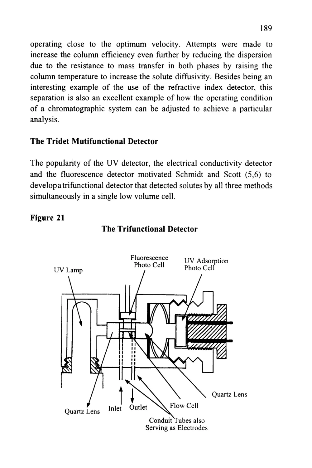
Resolution, Retention and Selectivity
The separation of a mixture into its individual components takes place
in the chromatographic column. The column is a simple tube, a few
centimeters long and a few millimeters in diameter, packed with
particulate material through which the mobile phase permeates.
Despite the apparent complexity of the modern chromatograph, the
separation is completed in this very simple device, the remaining
apparatus providing solvent storage, control of the mobile phase
composition, adequate mobile phase inlet pressure, sampling facilities,
detection and data processing. As a result of modern instrument
design, the essential nature of the column is frequently lost in the
electronic and engineering intricacy of the overall system. Consequently,
the importance of the column and its function may only be
superficially understood, and the technique is not employed in the
most efficient manner.
The chromatographic column has a dichotomy of purpose. During a
separation, two processes ensue in the column, continuously,
progressively and virtually independent of one another. Firstly, the
individual solutes are moved apart as a result of the differing
distribution coefficients of each component with respect to the
stationary phase in the manner previously described. Secondly, having
moved the individual components apart, the column is designed to
constrain the natural dispersion of each solute band (i.e. the band
15
16
spreading) so that, having been separated, the components are eluted
discretely from the column as individual solute bands.
Thus, the column moves the solutes bands apart and simultaneously
contains their dispersion .
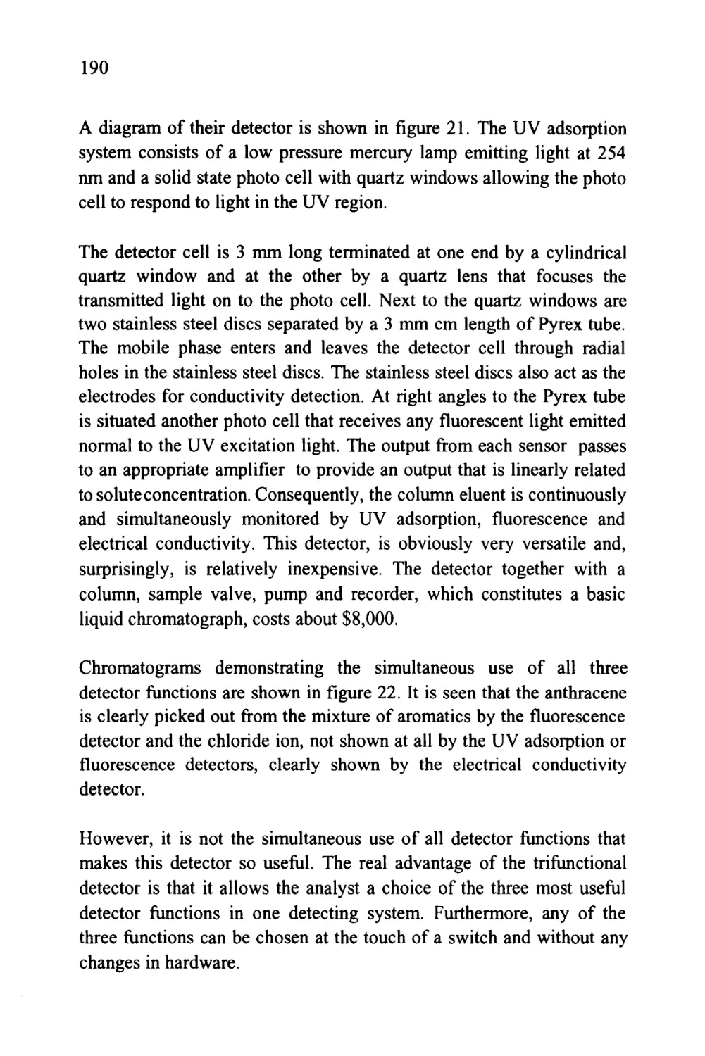
As the individual components of a mixture are moved apart on the
basis of their differing retention, then the separation can be partly
controlled by the choice of the phase system. In contrast, the peak
dispersion that takes place in a column results from kinetic effects and
thus is largely determined by the physical properties of the column
and its contents.
Thus, for optimum performance, each sample will require a specific
phase system to be chosen and a particular column to be selected.
In order to understand the mechanism of retention and selectivity and
thus be in a position to exercise some control over the
chromatographic system, it is necessary to derive an equation for the
retention volume of a solute. Such an equation would enable the
analyst to further understand the process of retention and also identify
the pertinent variables that need to be controlled to carry out a
specific analysis. To employ liquid chromatography in a satisfactory
manner, it is not necessary to have a profound understanding of liquid
chromatography column theory. It is, however, advisable to have a
basic knowledge of the subject to understand the rationale behind
phase selection and column design. In this book, chromatography
theory will only receive minimal treatment but it will include those
aspects essential to the successful operation of the liquid
chromatograph. Those interested in pursuing the subject further are
recommended to read "Liquid Chromatography Column Theory "
published by Wiley (1). Now, in order to obtain an equation for the
retention volume of a solute, a basic measurement by which solute
identification is accomplished, it is necessary to discuss the Plate
Theory.
The Plate Theory
17
Primarily, the Plate Theory provides the equation for the elution
curve (the chromatogram) of a solute in terms of the volume of
mobile phase that has passed through it. From this equation, the
various characteristics of a chromatographic system can be determined
using the data that is provided by the chromatogram. The Plate
Theory was originally derived by Martin and Synge (2) and was
based on the 'plate' concept employed in the theory of distillation
columns. The theory of Martin and Synge was later modified by Said
(3,4) and it is the procedure of Said that will be given here. The Plate
Theory assumes that the solute is, at all times, in equilibrium with
both the mobile and stationary phases. However, due to the continuous
exchange of solute between the two phases as it progresses through the
column, equilibrium between the phases is, in fact, never actually
achieved. As a consequence, the column is considered to be divided
into a number of theoretical plates. Each plate is allotted a finite
length, and thus, the solute is considered to spend a finite time in each
plate. The size of the plate is such that the solute is assumed to have
sufficient time to achieve equilibrium with the two phases. It follows
that if the exchange is fast and efficient, the theoretical plate will be
small in size and there will be a large number of plates in the column.
Conversely, if the column performance is poor, the exchange of solute
between the phases will be slow and the theoretical plates larger and
fewer in number.
Consider the equilibrium existing in each plate, then
XS = KXm (1)
where (Xm) and (Xs) are, respectively, the concentrations of the solute
in the mobile and stationary phases, and (K) is the distribution
coefficient of the solute between the two phases. (It should be
remembered that the distribution coefficient is defined with reference to the
stationary phase, i.e. K = Xs/Xm, and thus the larger the distribution
18
coefficient, the greater the proportion of solute that is distributed in
the stationary phase.)
Equation (1) merely states that the general distribution law applies to
the system and that the adsorption isotherm is linear. At the
concentrations normally employed in liquid chromatographic
separations this will be true.
Differentiating equation (1),
dXs = KdXm
(2)
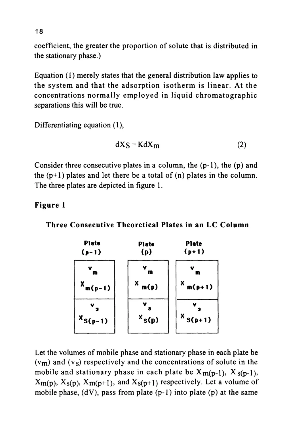
Consider three consecutive plates in a column, the (p-1), the (p) and
the (p+1) plates and let there be a total of (n) plates in the column.
The three plates are depicted in figure 1.
Figure 1
Three Consecutive Theoretical Plates in an LC Column
Plate
(p+1)
V
m
m(p-i
V
3
XS(p+
1)
1)
Let the volumes of mobile phase and stationary phase in each plate be
(vm) and (vs) respectively and the concentrations of solute in the
mobile and stationary phase in each plate be Xm(p-l), Xs(p-l),
Xm(p), Xs(p), Xm(p+i), and Xs(p+1) respectively. Let a volume of
mobile phase, (dV), pass from plate (p-1) into plate (p) at the same
19
time displacing the same volume of mobile phase from plate (p) to
plate (p+1). As a consequence, there will be a change of mass of solute
in plate (p) that will be equal to the difference in the mass entering
plate (p) from plate (p-1) and the mass of solute leaving plate (p) and
entering plate (p+1).
Thus, bearing in mind that mass is the product of concentration and
volume, the change of mass of solute in plate (p) is:
dm=(Xm(p-l)-Xm(p))dV (3)
Now, if equilibrium is to be maintained in the plate (p), the mass (dm)
will distribute itself between the two phases, which will result in a
change of solute concentration in the mobile phase of dXm(p) and in
the stationary phase of dXs(p).
Thus, dm = vsdXs(p) + vmdXm(p) (4)
Substituting for dXs(p) from equation (2),
dm = (vm + Kvs)dXm(p) (5)
Equating equations (3) and (5) and re-arranging,
d Xm (p) _ Xm (p-l)-X (p)
dV vm + K v s
Now, to aid in algebraic manipulation the volume flow of mobile
phase will now be measured in units of (vm + Kvs) instead of
milliliters. Thus the new variable (v) can be defined where
V
( vm + K v s)
(7)
20
The function (vm + Kvs) has been given the name 'plate volume' and
thus, for the present, the flow of mobile phase through the column
will be measured in 'plate volumes' instead of milliliters.
Differentiating equation (7),
dV
dv = (8)
(vm + Kvs)
Substituting for dV from (8) in (6)
dy = Xm(p-l) -X (P) (9)
dXm(p)
Equation (9) is the basic differential equation that describes the rate of
change of concentration of solute in the mobile phase in plate (p) with
the volume flow of mobile phase through it. The integration of
equation (9) will provide the equation for the elution curve of a solute
for any plate in the column. A detailed integration of equation (9) will
not be given here and the interested reader is again directed to
reference (1) for further details.
Integrating equation (9),
X0e"vv n
Xm(„) = °n| (10)
where Xm(n) is the concentration of solute in the mobile phase
leaving the (n)th plate (i.e. the concentration of solute
entering the detector)
and Xo is the initial concentration of solute on the 1st plate
of the column.
Equation (10) describes the elution curve obtained from a
chromatographic column and is the equation of the curve, or
chromatogram, that is traced by the chart recorder or computer
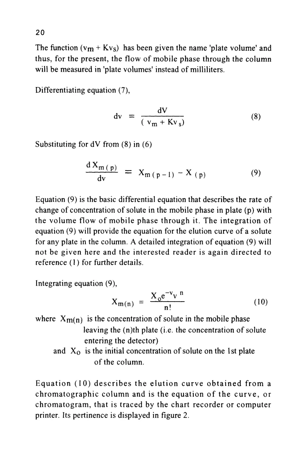
printer. Its pertinence is displayed in figure 2.
21
Figure 2
The Elution of a Single Solute
\e-vv
n!
It can now be seen how an expression for the retention volume of a
solute can be derived. By differentiating equation (10) and equating to
zero, an expression for the volume of mobile phase passed through the
column between the injection point and the peak maximum can be
obtained. This volume has already been defined as the retention
volume (Vr) of the solute.
The Retention Volume of a Solute
Restating equation (10),
X
m(n)
X0
e'vv n
n !
d X
m(n)
dv
= X
-e-vvn+ e~vn v< n~l)
n !
X,
_e-vv(n-l)
n !
(n-v)
Equating to zero,
n-v = 0
or
v = n
22
This means that at the peak maximum, (n) plate volumes of mobile
phase have passed through the column. Remembering that the volume
flow is measured in 'plate volumes' and not milliliters, the volume
passed through the column in ml will be obtained by multiplying by
the 'plate volume' (vm + Kvs).
Thus, the retention volume (Vr) is given by:
Vr = n(vm + Kvs)
= nvm +nKvs
Now the total volume of mobile phase in the column, (Vm), will be
the volume of mobile phase per plate multiplied by the number of
plates, i.e. (nvm). In a similar manner the total volume of stationary
phase in the column (Vs) will be the volume of stationary phase per
plate multiplied by the total number of plates, i.e. (nvs).
Thus, Vr = Vm + KVs (11)
It is now immediately obvious from equation (11) how the separation
of two solutes (A) and (B) must be achieved.
For separation Vr(A) < > Vr(B) and Vr(A) * Vr(B)
Furthermore, as the retention volumes of each substance must be
different then,
either K(a) < > K(B) and K(A) * K(b)
or Vs(a) < > Vs(B) and Vs(a) * Vs(b)
Thus, to achieve the required separation either (1) the distribution
coefficient (K) of all the solutes must be made to differ, or (2) the
amount of stationary phase (Vs) available to each component of the
mixture interacts must be made to differ. A further alternative (3)
23
would be to make appropriate adjustments to both the values of (K)
and the values (Vs).
The analyst is now required to know how to change (K) and (Vs) to
suit the particular sample of interest. Consider first the control of the
distribution coefficient (K).
Factors that Control the Distribution Coefficient of a Solute
Molecular Interactions
The effect of molecular interactions on the distribution coefficient of a
solute has already been mentioned in Chapter 1. Molecular
interactions are the direct effect of intermolecular forces between the
solute and solvent molecules and the nature of these molecular forces
will now be discussed in some detail. There are basically four types of
molecular forces that can control the distribution coefficient of a
solute between two phases. They are chemical forces, ionic forces,
polar forces and dispersive forces. Hydrogen bonding is another type
of molecular force that has been proposed, but for simplicity in this
discussion, hydrogen bonding will be considered as the result of very
strong polar forces. These four types of molecular forces that can
occur between the solute and the two phases are those that the
analyst must modify by choice of the phase system to achieve the
necessary separation. Consequently, each type of molecular force
enjoins some discussion.
Chemical Forces
Chemical forces are normally irreversible in nature (at least in
chromatography) and thus, the distribution coefficient of the solute
with respect to the stationary phase is infinite or close to infinite.
Affinity chromatography is an example of the use of chemical forces
in a separation process. The stationary phase is formed in such a
manner that it will chemically interact with one unique solute present
in the sample and thus, exclusively extract it from the other materials
24
present. The technique of affinity chromatography is, therefore, an
extraction process more than a chromatographic separation, an aspect
of separation science that is not germane to the subject of this book;
ipso facto, the nature of chemical forces need not be discussed
further.
Ionic Forces
Ionic forces are electrical in nature and result from the charges
produced when molecules ionize in solution into positively charged
cations and negatively charged anions. The resulting ionic interactions
are exploited in ion chromatography. For example in the analysis of
organic acids, it is the negatively charged acid anions that require to
be separated. The stationary phase must, therefore, contain positively
charged cations as counter ions to interact with the acid anions, retard
them in the column and effect their resolution. Conversely, to separate
cations, the stationary phase must contain anions as counter ions with
which the cations can interact.
Ion exchange stationary phases are usually available in the form of
cross-linked polymer beads that have been appropriately modified to
contain the desired ion exchange groups. The material is supplied in a
form ready for packing or in pre-packed columns. Alternatively, ion
exchange groups can be chemically bonded to silica by a process
similar to the preparation of ordinary bonded phases. Bonded phases
and their production will be discussed in a later chapter. Ion exchange
materials can also be adsorbed on the surface of a bonded phase which
can then act as an adsorbed ion exchanger. Such materials are usually
called Ion Pair Reagents and are added to the mobile phase in
relatively low concentrations (ca. l%w/v) from which, under
conditions of low solvent concentration, they can be absorbed onto the
surface of the stationary phase. Examples of the use ion pair reagents
will also be discussed in the chapter dealing specifically with
stationary phases. Examples of the separation of a series of inorganic
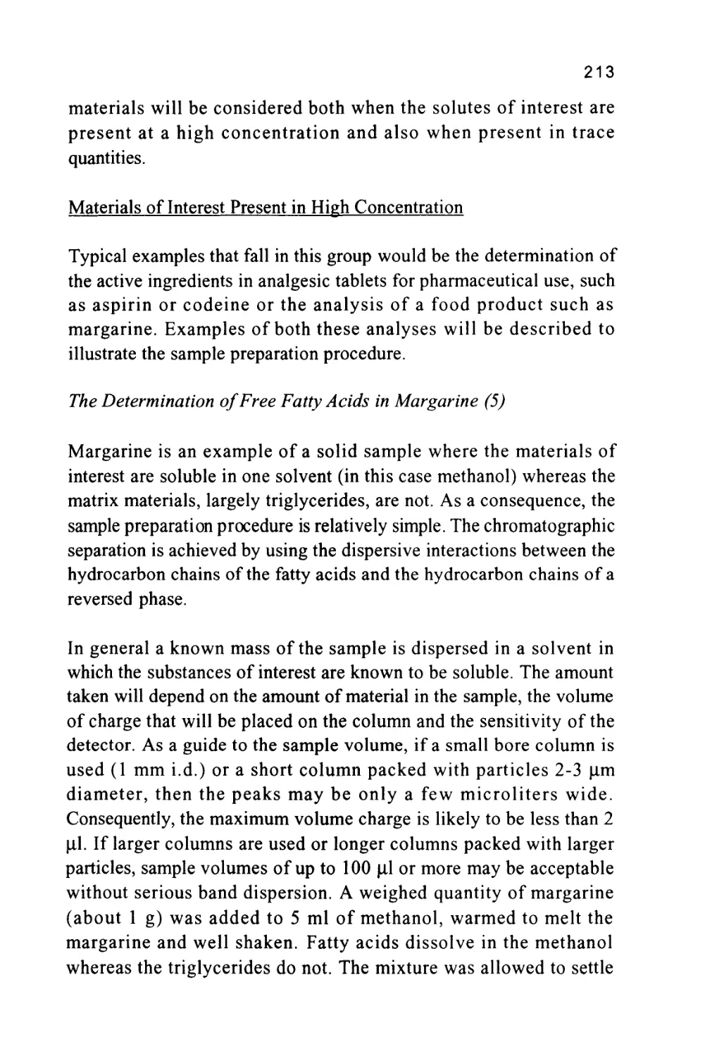
anions on an ion exchange column is shown in figure 3.
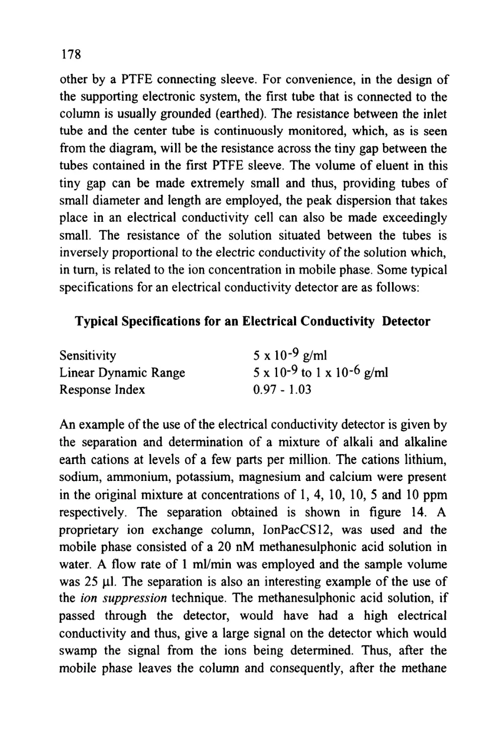
25
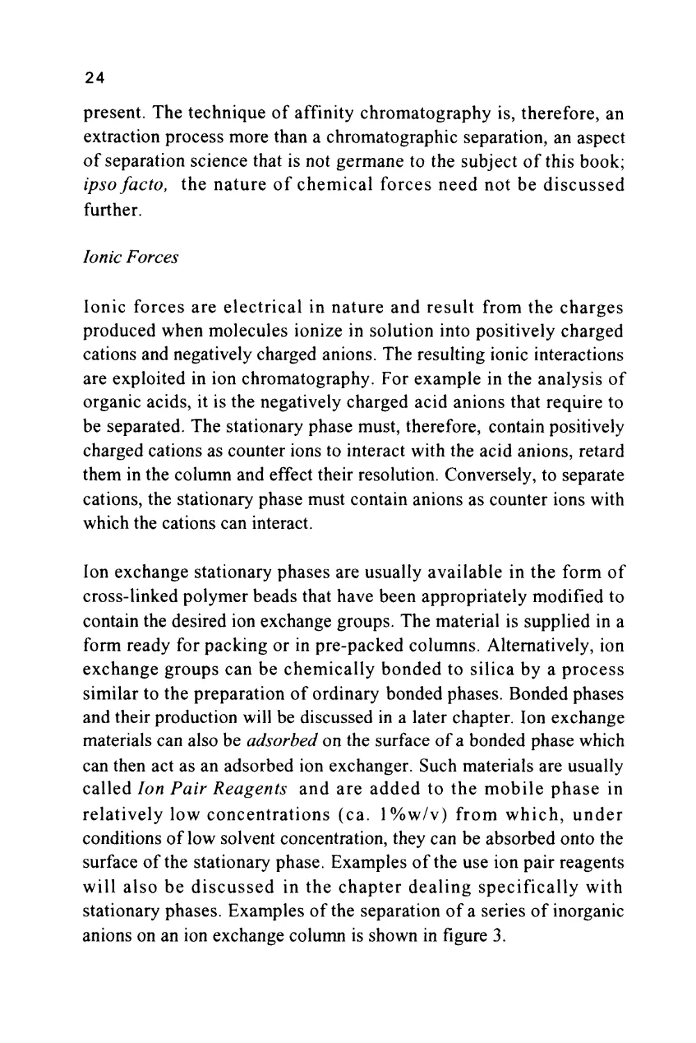
Figure 3
The Separation of a Series of Inorganic Anions
1
0
J
I
0
5
i
4
|
111
7 I
6 I
L_,
T
5
Minu
\J
les
u
1 Fluoride
2 Chloride
5 3 Nitrite
4 Bromide
5 Nitrate
6 Phosphate
7 Sulfate
8 Oxalate
i
to
Courtesy of DIONEX INC.
The column was 15 cm long, 4.6 mm in diameter, and packed with a
proprietary ion exchange material IonPacAS4A. The mobile phase
was an aqueous solution of 1.80 nM sodium carbonate and 1.70 nM
sodium bicarbonate at a flow rate of 2.0 ml/min. The volume of
charge was 50 ul
It should be emphasized that in figure 3, the system was not operated
at its maximum sensitivity and, at higher sensitivity settings, it could
be employed directly for the analysis of drinking water and other
types of water samples. Further practical information can be obtained
from the books by Small (5), Weiss (6) and Smith (7).
Polar Forces
Polar forces also arise from electrical charges on the molecule but in
this case from permanent or induced dipoles. It must be emphasized
26
that there is no net charge on a polar molecule unless it is also ionic.
Examples of substances with permanent dipoles are alcohols, esters,
aldehydes etc. Examples of polarizable molecules are the aromatic
hydrocarbons such as benzene, toluene and xylene. Some molecules
can have permanent dipoles and, at the same time, also be polarizable.
An example of such a substance would be phenyl ethyl alcohol. The
hydroxyl group of the alcohol would form part of a permanent dipole
whereas the phenyl group would be polarizable. To separate polar
materials on a basis of their polarity, a polar stationary phase must be
used. Furthermore, in order to focus the polar forces in the stationary
phase, and consequently the selectivity, a relatively non-polar mobile
phase would be required.
The use of dissimilar molecular interactions in the two phases, to
achieve selectivity, is generally applicable and of fundamental
importance.
The specific interactions that will produce the necessary retention and
selectivitv must dominate in the stationary phase to achieve the
separation. It follows that it is important that they are also as
exclusive as possible to the stationary phase. It is equally important to
ensure that the interactions taking place in the mobile phase differ to
as great extent as possible to that in the stationary phase in order to
maintain the stationary phase selectivity.
To separate some aromatic hydrocarbons, for example, a strongly
polar stationary phase would be appropriate as the solutes do not
contain permanent dipoles. Under such circumstances, when the
polarizable aromatic nucleus approaches the strongly polar group on
the stationary phase, the aromatic nucleus will be polarized and
positive and negative charges generated at different positions on the
aromatic ring. These charges will then interact with the charges from
the dipole of the stationary phase and, as a consequence, the solute
molecules held more strongly and distributed more favorably in the
stationary phase. In practice, silica gel is a strongly polar stationary
phase, its polar character arising from the dipoles of the surface
27
hydroxyl groups. Consequently, silica gel would be an appropriate
stationary phase for the separation of aromatic hydrocarbons. To ensure
that polar selectivity dominates in the stationary phase, and polar
interactions in the mobile phase are minimized, anon-polar or dispersive
solvent, e.g. n-heptane, could be used as the mobile phase. The separation
of some biphenyl derivatives on silica gel is shown in figure 4.
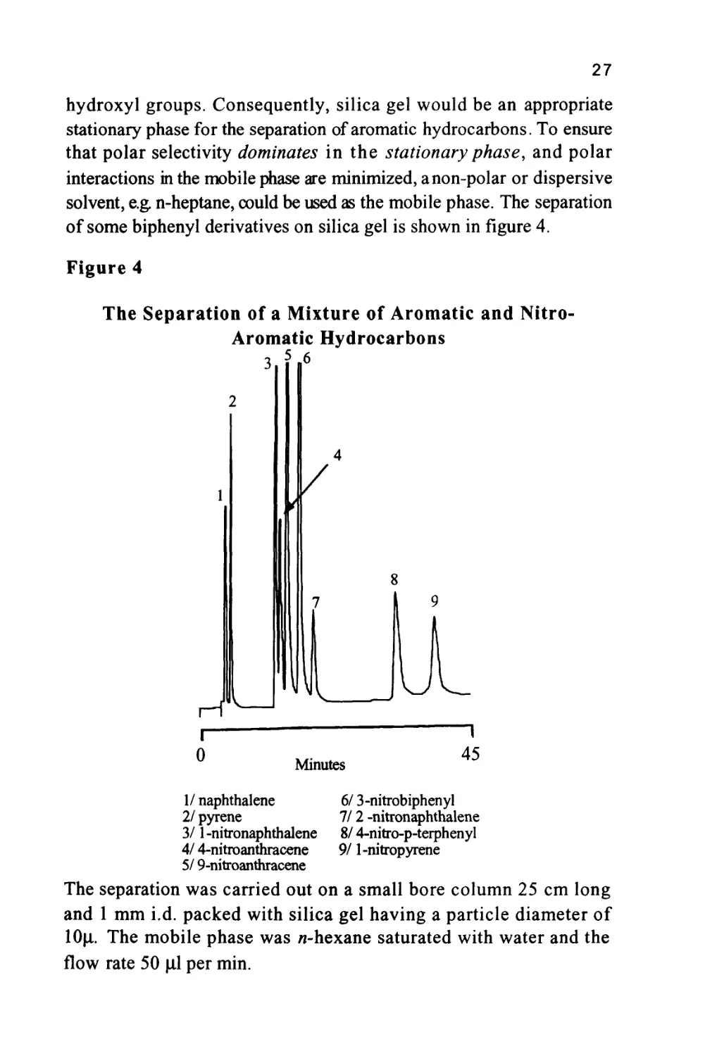
Figure 4
The Separation of a Mixture of Aromatic and Nitro-
Aromatic Hydrocarbons
3
5 6
rA
Minutes
45
1/ naphthalene
2/ pyrene
3/ 1-nitronaphthalene
4/ 4-nitroanthracene
5/ 9-nitroanthracene
6/ 3-nitrobiphenyl
II2 -nitronaphthalene
8/ 4-nitro-p-terphenyl
9/ 1-nitropyrene
The separation was carried out on a small bore column 25 cm long
and 1 mm i.d. packed with silica gel having a particle diameter of
lOu.. The mobile phase was n-hexane saturated with water and the
flow rate 50 (J.1 per min.
28
Dispersive Forces
Dispersive forces are more difficult to describe. Although electric in
nature, they result from charge fluctuations rather than permanent
electrical charges on the molecule. Examples of purely dispersive
interactions are the molecular forces that exist between saturated
aliphatic hydrocarbon molecules. Saturated aliphatic hydrocarbons are
not ionic, have no permanent dipoles and are not polarizable. Yet
molecular forces between hydrocarbons are strong and consequently,
n-heptane is not a gas, but a liquid that boils at 100°C. This is a result
of the collective effect of all the dispersive interactions that hold the
molecules together as a liquid.
To retain solutes selectively by dispersive interactions, the stationary
phase must contain no polar or ionic substances, but only
hydrocarbon-type materials such as the reverse-bonded phases, now so
popular in LC. Reiterating the previous argument, to ensure that
dispersive selectivity dominates in the stationary phase, and dispersive
interactions in the mobile phase are minimized, the mobile phase must
now be strongly polar. Hence the use of methanol-water and
acetonitrile-water mixtures as mobile phases in reverse-phase
chromatography systems. An example of the separation of some
antimicrobial agents on Partisil ODS 3, particle diameter 5\i is shown in
figure 5.
ODS3 is a "bulk type" reverse phase (the meaning of which will be
discussed later) which has a fairly high capacity and is reasonably
stable to small changes in pH. The column was 25 cm long, 4.6 mm in
diameter and the mobile phase a methanol water mixture containing
acetic acid. In this particular separation the solvent mixture was
programmed, a development procedure which will also be discussed in
a later chapter.
The components present in the mixture are as follows:
a/ sulfaguanidine, b/ sulfanilamide, c/ sulfadiazine, d/ sufathiazole,
e/ sulphapyridine, f/ sulfamerazine, g/ sulfamethazine,
29
h/ sulfachloropyridazine, i/ sulfasoxazole, j/ sulfaethoxypyridazine,
k/ sulfadimethoxine, 1/ sulfaquinoxine, m/ sulfabromethazine.
Figure 5
The Separation of a Mixture of Anti-Microbial Agents
wu
Courtesy of Whatman Inc.
The Thermodynamic Explanation of Retention
Solute retention can also be explained on a thermodynamic basis
where the change in free energy is considered when the solute is
moved from the environment of one phase to that of the other.
The classic thermodynamic expression for the distribution coefficient
(K) of a solute between two phases is given by
RTln K = -AG0
where (R) is the Gas Constant,
(T) is the absolute temperature,
and (AGo) is the Excess Free Energy.
30
Now,
where
AG0 = AH0 - TAS0
(AHo) is the Excess Free Enthalpy
and (ASo) is the Excess Free Entropy.
Thus,
or
InK =
K = e
^AH0 _ AS^
RT R
AHQ _ A_So
RT R
It is seen that, if the excess free entropy and excess free enthalpy of
a solute between two phases can be calculated or predicted, then the
magnitude of the distribution coefficient (K) and consequently, the
retention of a solute can also be predicted. Unfortunately, the
thermodynamic properties of a distribution system are bulk
properties, that include the effect of all the different types of
molecular interactions in one measurement. As a result it is difficult,
if not impossible, to isolate the individual contributions so that the
nature of overall distribution can be estimated or controlled. Attempts
have been made to allot specific contributions to the total excess free
energy of a given solute/phase system that represents particular types
of interaction. Although the procedure becomes very complicated, this
empirical approach has proved to be of some use to the analyst. It
must be said that, despite "the sound and fury" surrounding the
subject, thermodynamics has yet to predict a single distribution
coefficient from basic physical chemical data. It is for this reason, that
the thermodynamic control of the magnitude of the distribution
coefficient (K) is only briefly considered in this book. Nevertheless, if
sufficient experimental data is available or can be obtained, then
empirical equations, similar to those given above, can be used to
optimize a particular distribution system once the basic phases have
been identified. A range of computer programs, based on this
rationale, is available, that purport to carry out optimization for up to
31
three component solvent mixtures. Nevertheless, the appropriate
stationary phase is still usually identified from the types of molecular
forces that need to be exploited to effect the required separation.
Equation (12) can also be used to identify the type of retention
mechanism that is taking place in a particular separation by measuring
the retention volume of the solute over a range of temperatures.
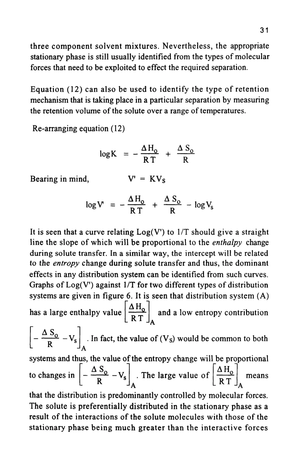
Re-arranging equation (12)
logK = -
AHQ
RT
+
AS(
R
Bearing in mind,
V = KVS
logV =
AH0
RT
+
AS(
R
- logVs
It is seen that a curve relating Log(V') to 1/T should give a straight
line the slope of which will be proportional to the enthalpy change
during solute transfer. In a similar way, the intercept will be related
to the entropy change during solute transfer and thus, the dominant
effects in any distribution system can be identified from such curves.
Graphs of Log(V') against 1/T for two different types of distribution
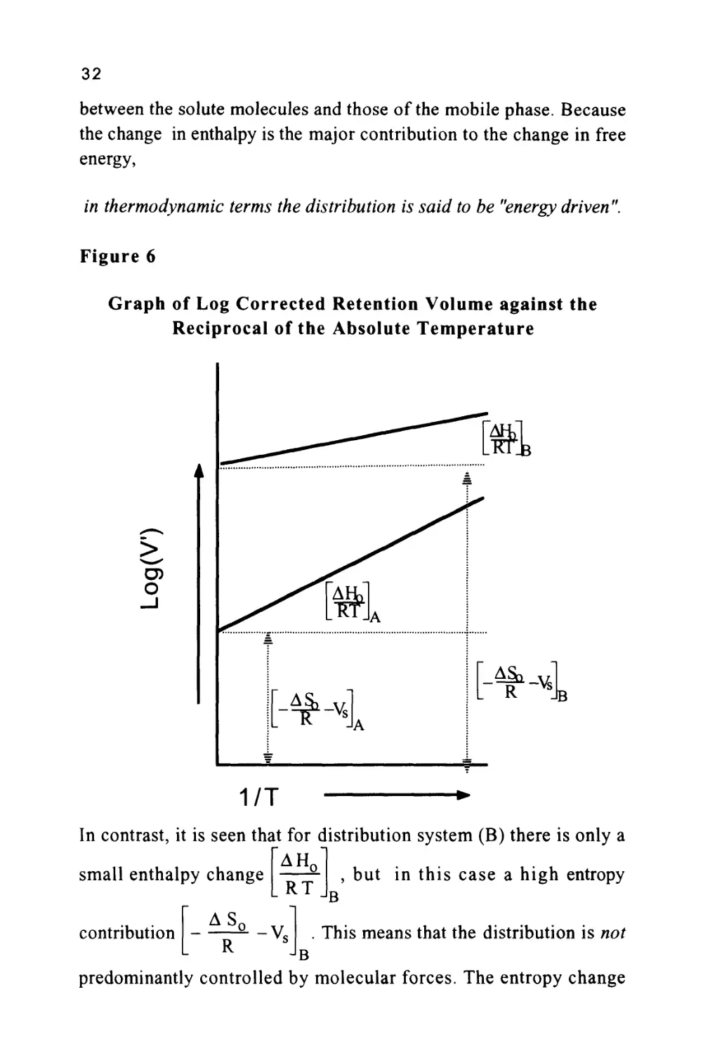
systems are given in figure 6. It is seen that distribution system (A)
^AH,
has a large enthalpy value
RT
and a low entropy contribution
AS(
R
-V«
In fact, the value of (Vs) would be common to both
systems and thus, the value of the entropy change will be proportional
to changes in
AS
R
*-Vfi
. The large value of
JA
AH,
RT
means
that the distribution is predominantly controlled by molecular forces.
The solute is preferentially distributed in the stationary phase as a
result of the interactions of the solute molecules with those of the
stationary phase being much greater than the interactive forces
32
between the solute molecules and those of the mobile phase. Because
the change in enthalpy is the major contribution to the change in free
energy,
in thermodynamic terms the distribution is said to be "energy driven".
Figure 6
Graph of Log Corrected Retention Volume against the
Reciprocal of the Absolute Temperature
O
1/T
In contrast, it is seen that for distribution system (B) there is only a
, but in this case a high entropy
B
small enthalpy change
AS,
RT
contribution
R
Vc
. This means that the distribution is not
B
predominantly controlled by molecular forces. The entropy change
33
reflects the degree of randomness that a solute molecule experiences in
a particular phase. The more random and 'more free' the solute
molecule is to move in a particular phase, the greater the entropy of
the solute. Now as there is a large entropy change, this means that the
solute molecules are more restricted or less random in the stationary
phase in system (B). This loss of freedom is responsible for the
greater distribution of the solute in the stationary phase and thus, its
greater retention. Because the change in entropy in system (B) is the
major contribution to the change in free energy,
in thermodynamic terms the distribution is said to be "entropically
driven".
Examples of entropically driven systems will be those employing
chirally active stationary phases.
Returning to the molecular force concept, in any particular
distribution system it is rare that only one type of interaction is
present and if this occurs, it will certainly be dispersive in nature.
Polar interactions are always accompanied by dispersive interactions
and ionic interactions will, in all probability, be accompanied by both
polar and dispersive interactions. However, as shown by equation
(11), it is not merely the magnitude of the interacting forces between
the solute and the stationary phase that will control the extent of
retention, but also the amount of stationary phase present in the
system and its accessibility to the solutes. This leads to the next
method of retention control, and that is the volume of stationary phase
available to the solute.
Factors that Control the Availability of the Stationary Phase
The volume of stationary phase with which the solutes in a mixture
can interact (Vs in equation (11)) will depend on the physical nature
of the stationary phase or support. If the stationary phase is a porous
solid, and the sizes of the pores are commensurate with the molecular
diameter of the sample components, then the stationary phase becomes
34
size selective. Some solutes (for example those of small molecular
size) can penetrate and interact with more stationary phase than larger
molecules which are partially excluded. Under such circumstances the
retention is at least partly controlled by size exclusion and, as one
might expect, this type of chromatography is called Size Exclusion
Chromatography (SEC). Alternatively, if the stationary phase is chiral
in character, the interaction of a solute molecule with the surface (and
consequently, the amount of stationary phase with which in can
interact) will depend on the chirallity of the solute molecule and how
it fits to the chiral surface. Such separation systems have been
informally termed Chiral Liquid Chromatography (CLC). However, it
must be pointed out that both SEC and CLC fall within the classes of
LLC or LSC depending on the nature of the stationary phase.
Size Exclusion Chromatography
The term size exclusion chromatography implies that the retention of
a solute depends solely on solute molecule size. However, even in
SEC, retention may not be exclusively controlled by the size of the
solute molecule, it will still be controlled by molecular interactions
between the solute and the two phases. Only if the magnitude of the
forces between the solute and both phases is the same will the
retention and selectivity of the chromatographic system depend solely
on the pore size distribution of the stationary phase. Under such
circumstances the larger molecules, being partially or wholly
excluded, will elute first and the smaller molecules elute last. It is
interesting to note that, even if the dominant retention mechanism is
controlled by molecular forces between the solute and the two phases,
if the stationary phase or supporting material has a porosity
commensurate with the molecular size of the solutes, exclusion will
still play a part in retention. The subject of mixed retention
mechanisms will be discussed when considering the physical
characteristics of silica gel. The two most common exclusion media
employed in liquid chromatography are silica gel and macroporous
polystyrene divinylbenzene resins. Exclusion chromatograms obtained
from three different silica gel columns are shown in figure 7 (8). The
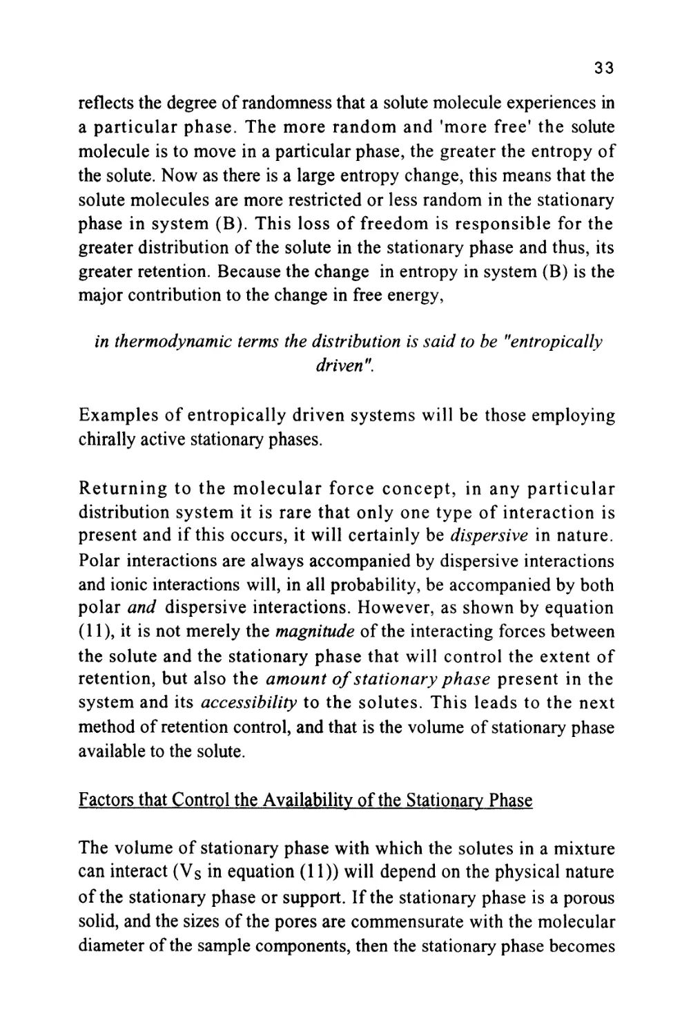
35
three columns, shown in figure 7, were packed with Spherosil 10|X,
Silerex 2 10[i and Partisil lOjx, a series of silicas that exhibit quite
different exclusion properties.
Figure 7
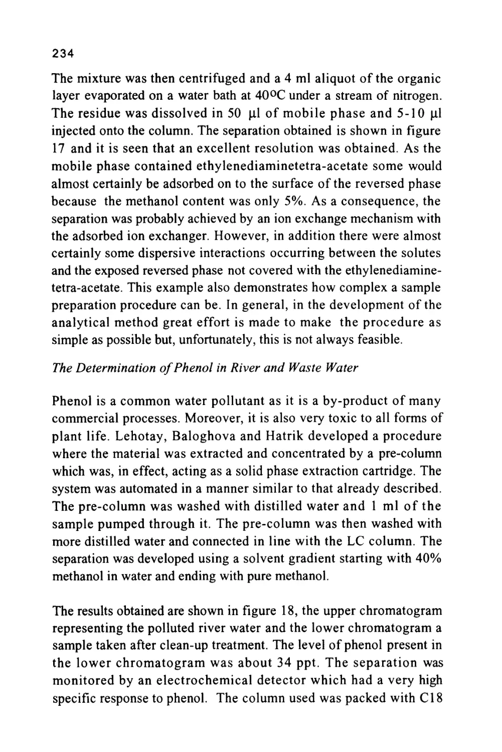
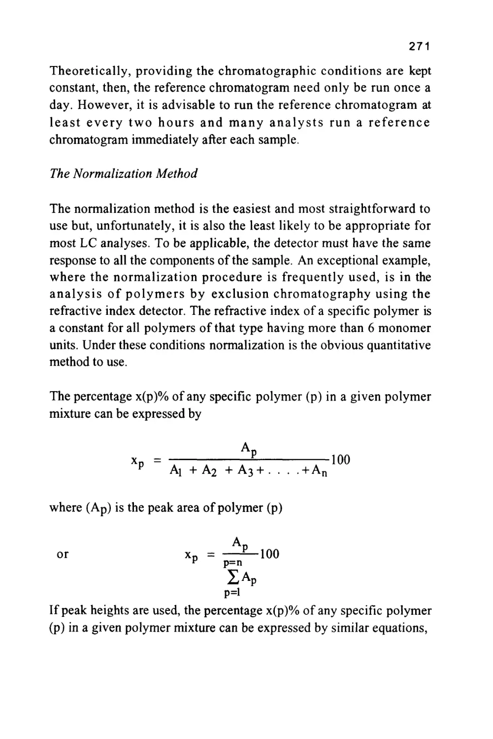
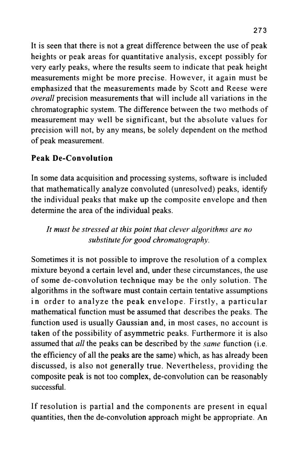
The Separation of a Mixture by Exclusion Chromatography
Chromatograms Demonstrating the Different Exclusion Properties of
Three Silica Gels
3,4,5
UL
Spherosil 10
Silarex 2 10
Partisil 10
Column Length 50 cm, mobile phase tetrahydrofuran, Molecular diameter of solutes,
(1) 11,000A, (2) 240A, (3) 49.5A, (4) 27.1 A and (5) 7.4A.
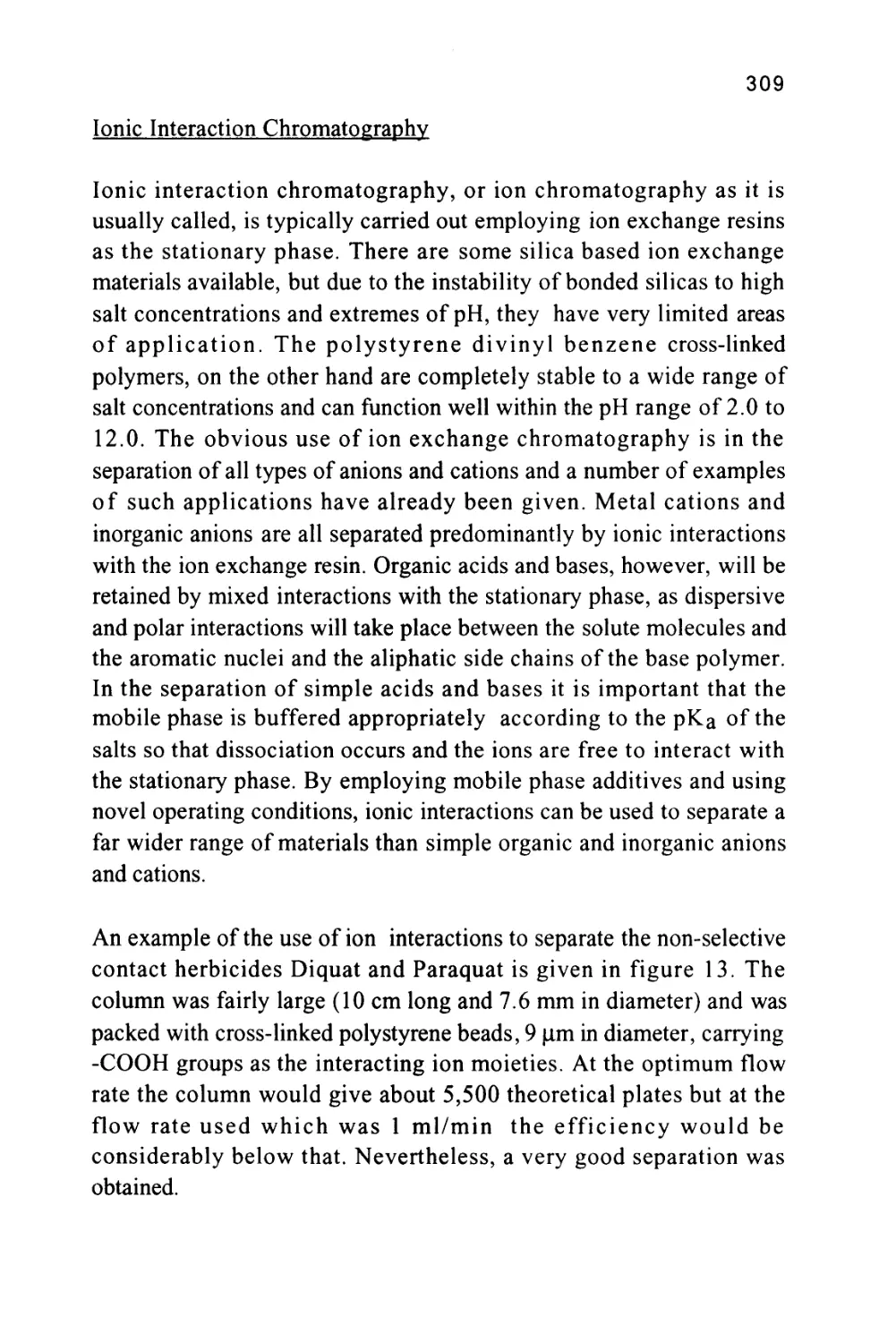
The number 10 refers to the diameter of the silica particles in micron
and not the pore size. The five solutes (1-5) were largely hydrocarbon
in nature having mean molecular diameters of 11,000, 240, 49.5, 27.1
and 7.4 A respectively. The mobile phase employed was
tetrahydrofuran (THF). This solvent is adsorbed as a layer on the
surface of the silica (a phenomenon that will be discussed in more detail
36
in a later chapter) and thus the solutes interact with THF in both
phases. Consequently, the distribution coefficient of each solute with
respect to the mobile phase is unity and there is no interactive
selectivity and the sequence of elution is governed solely by exclusion.
This is supported by the order of elution of the solutes on each
stationary phase shown in figure 7. It is seen that all the smaller
solutes are bunched together in the chromatogram from Spherosil and
thus the material is appropriate for the separation of the larger solutes
having average molecular diameters lying between 50 and 1100A. The
chromatogram from Silerex, however, shows a fairly clean separation
for all solutes and, therefore, could be used to separate solutes
covering the entire molecular diameter range between 7.4A and
1100A. At the other extreme, using Partisil, the solutes having
molecular diameters of 240A and 1100A are eluted first, and close
together, whereas, the solutes having diameters ranging from 7.4A to
49.5 A are well resolved. It follows that Partisil would be appropriate
for the separation of solutes that are relatively small in molecular size.
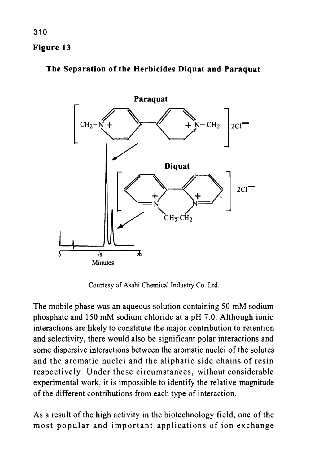
Silica is often used as an exclusion media for the separation of high
molecular weight hydrocarbons and polymers whereas polymeric
materials of biological origin when separated by exclusion, often
employ Sephadex or micro-reticular polystyrene gels as the stationary
phase.
Unfortunately, exclusion chromatography has some inherent
disadvantages that make its selection as the separation method of
choice a little difficult. Although the separation is based on molecular
size, which might be considered an ideal rationale, the total separation
must be contained in the pore volume of the stationary phase. That is
to say all the solutes must be eluted between the excluded volume and
the dead volume, which is approximately half the column dead
volume. In a 25 cm long, 4.6 mm i.d. column packed with silica gel,
this means that all the solutes must be eluted in about 2 ml of mobile
phase. It follows, that to achieve a reasonable separation of a multi-
component mixture, the peaks must be very narrow and each occupy
only a few microliters of mobile phase. Scott and Kucera (9)
constructed a column 14 meters long and 1 mm i.d. packed with 5jx
37
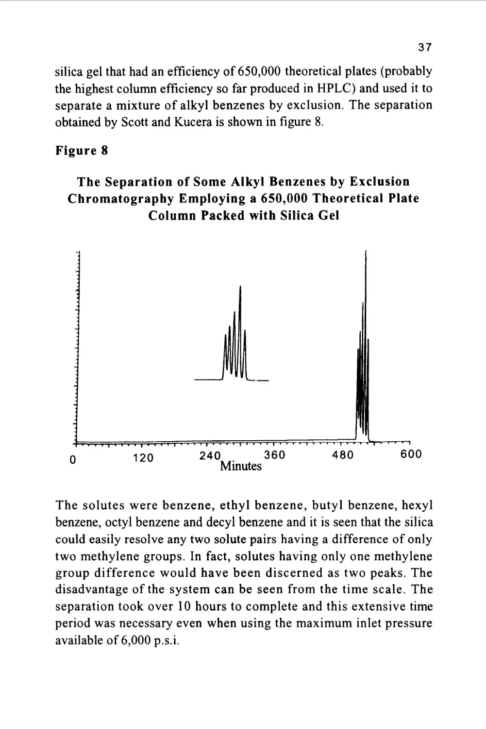
silica gel that had an efficiency of 650,000 theoretical plates (probably
the highest column efficiency so far produced in HPLC) and used it to
separate a mixture of alkyl benzenes by exclusion. The separation
obtained by Scott and Kucera is shown in figure 8.
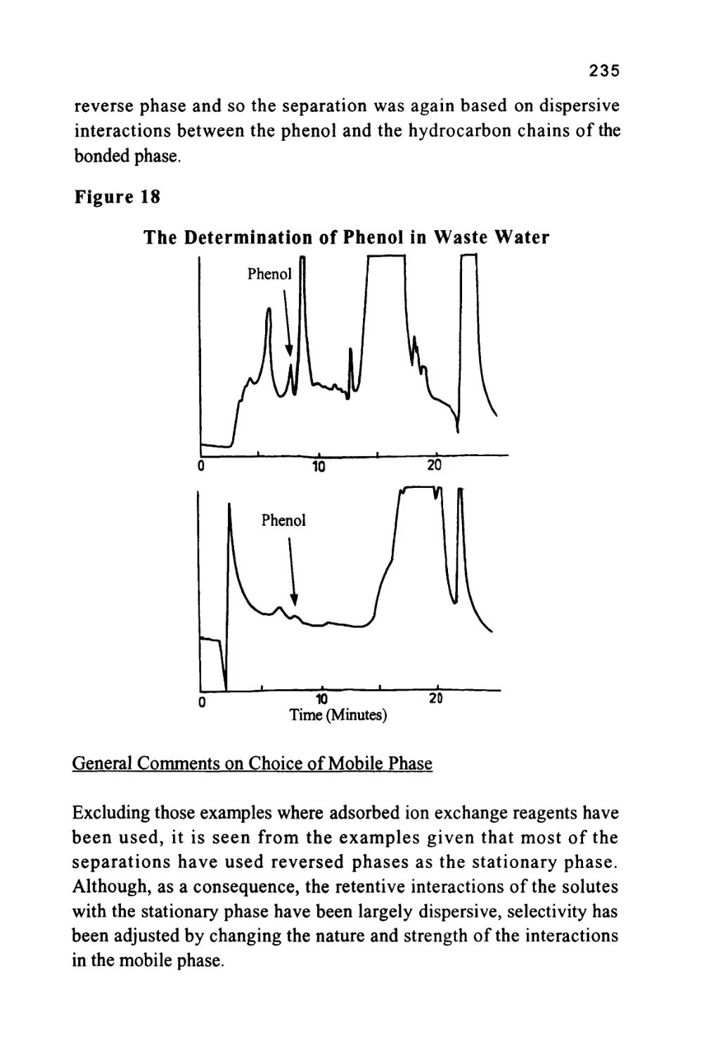
Figure 8
The Separation of Some Alkyl Benzenes by Exclusion
Chromatography Employing a 650,000 Theoretical Plate
Column Packed with Silica Gel
iX—,
120 240 360 480
Minutes
600
The solutes were benzene, ethyl benzene, butyl benzene, hexyl
benzene, octyl benzene and decyl benzene and it is seen that the silica
could easily resolve any two solute pairs having a difference of only
two methylene groups. In fact, solutes having only one methylene
group difference would have been discerned as two peaks. The
disadvantage of the system can be seen from the time scale. The
separation took over 10 hours to complete and this extensive time
period was necessary even when using the maximum inlet pressure
available of 6,000 p.s.i.
38
Nevertheless, despite the inherent disadvantages of exclusion
chromatography, there are instances where it is the only practical
method of choice. The technique is widely used in the separation of
macro-molecules of biological origin, e.g. polypeptides, proteins,
enzymes, etc. In fact, it is in this area of biotechnology where the
major growth in HPLC techniques appears to be taking place.
Chiral Chromatography
Modern organic chemistry is becoming increasingly involved in
methods of asymmetric syntheses. This enthusiasm has been fostered
by the relatively recent appreciation of the differing physiological
activity that has been shown to exist between the geometric isomers of
pharmaceutically active compounds. A sad example lies in the drug,
Thalidomide, which was marketed as a racemic mixture of N-
phthalylglutamic acid imide. The desired pharmaceutical activity
resides in the R-(+)-isomer and it was not found, until too late, that
the corresponding S-enantiomer, was teratogenic and its presence in
the racemate caused serious fetal malformations. It follows that the
separation and identification of isomers can be a very important
analytical problem and liquid chromatography can be very effective in
the resolution of such mixtures.
Many racemic mixtures can be separated by ordinary reverse phase
columns by adding a suitable chiral reagent to the mobile phase. If the
material is adsorbed strongly on the stationary phase then selectivity
will reside in the stationary phase, if the reagent is predominantly in
the mobile phase then the chiral selectivity will remain in the mobile
phase. Examples of some suitable additives are camphor sulphonic
acid (10) and quinine (11). Chiral selectivity can also be achieved by
bonding chirally selective compounds to silica in much the same way
as a reverse phase. A example of this type of chiral stationary phase is
afforded by the cyclodextrins.
The cyclodextrins are produced by the partial degradation of starch
followed by the enzymatic coupling of the glucose units into
39
crystalline, homogeneous toroidal structures of different molecular
sizes. Three of the most widely characterized are alpha, beta and
gamma cyclodextrins which contain 6, 7 and 8 glucose units
respectively. Cyclodextrins are, consequently, chiral structures and the
beta-cyclodextrin has 35 sterogenic centers. CYCLOBOND is a trade
name used to describe a series of chemically bonded cyclodextrins to
spherical silica gel. The process of bonding is proprietary and
patented but a number of CYCLOBOND columns are commercially
available. An example of the separation of the isomers of Warfarin is
shown in figure 9. The column was 25 cm long and 4.6 mm in
diameter packed with 5 micron CYCLOBOND 1. The mobile phase
was approximately 90%v/v acetonitrile, 10%v/v methanol, 0.2 %v/v
glacial acetic acid and 0.2%v/v triethylamine. It is seen that an
excellent separation has been achieved with the two isomers completely
resolved.
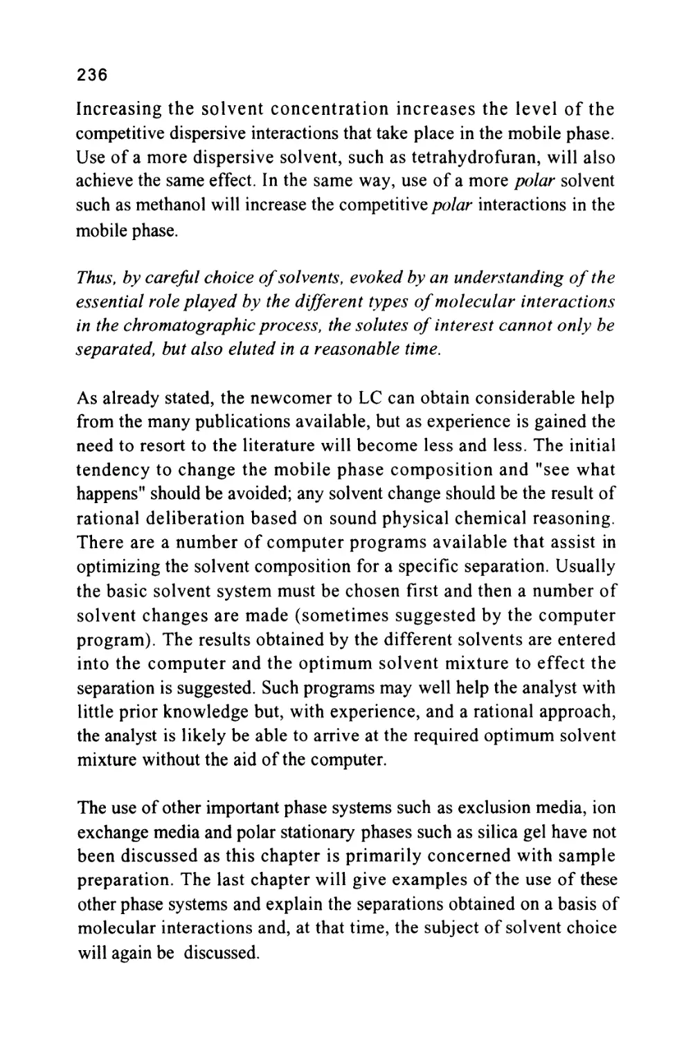
Figure 9
The Separation of Warfarin Isomers on a CYCLOBOND
Column
CHCH2COCH3
I I L
7 9 min
Courtesy of ASTEC Inc.
40
This separation is an impressive example of an entropically driven
distribution system where the normally random movements of the
solute molecules are restricted to different extents depending on the
spatial orientation of the substituent groups. For further information
the reader is directed to an excellent review of chiral separations by
LC (Taylor and Maher (12)) and a monograph on CYCLOBOND
materials from ASTEC Inc. (13).
Chromatographic Methods of Identification
The first chromatographic parameter that was employed for solute
identification was the corrected retention volume (V'r). However, the
measurement of (V'r) is not as straightforward as it might seem.
Consider equation (11), which for convenience will be reiterated.
Vr=Vm + KVs (11)
It must be pointed out that (Vm) refers to the volume of mobile phase
in the column and not the total volume of mobile phase between the
injection valve and the detector (Vo). In practice, the dead volume
(Vo) will include all the extra column volumes (Ve) involved in the
sample valve, connecting tube detector cell etc.
Thus, V0 = Vm+VE (12)
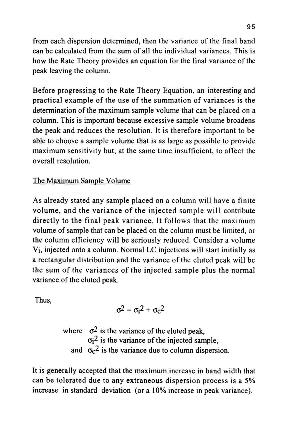
In some cases, (Ve) may be sufficiently small to be ignored, but for
accurate measurements of retention volume, and particularly capacity
ratios, the actual volume measured should always be corrected for the
extra column volume of the system and equation (11) should be put in
the form
Vr = Vm + KVS + Ve
(13)
41
The exact nature of the dead volume is complex and, in fact, will vary
from solute to solute due to the exclusion properties of the stationary
phase, particularly if the stationary phase or support is silica or silica
based. Thus, to measure (Vo) accurately, a non-adsorbed solute of the
same molecular size as the solute should be used and then the correct
retention volume (V'r) can be calculated and employed for
identification purposes.
However, providing
V'r >» V0
then any non-adsorbed solute can be used to measure (Vo), and
V'r =Vr-V0 = KVS (14)
Thus, (V'r) is directly proportional to (K) and as (K) will be a
unique property of a given solute, then (V'r) can be used for solute
identification purposes.
For example for two solutes (A) and (B) their corrected retention
volumes will be will be
V'r(A) = K(A)VS (15)
and V'r(B) = K(B)VS (16)
and both V'r(A) and V'r(B) can be used to identify solutes (A) and (B).
The Capacity Ratio of a Solute
The capacity ratio of a solute (k') was introduced early in the
development of chromatography theory and was defined as the ratio
of the distribution coefficient of the solute to the phase ratio (a) of the
column. In turn the phase ratio of the column was defined as the ratio
of the volume of mobile phase in the column to the volume of
stationary phase in the column.
42
V
Thus, k' = —L
a
and, as a = tt-^, then k =
* m ^ m
Note that (Vm) is the volume of mobile phase in the column and not
Vo the total dead volume of the column.
Consequently, in practice
Equation (17) illustrates the importance of knowing the extra column
volume to obtain accurate values for (k'). Nevertheless it must be
pointed out that, in calculating (k'), the value taken in practice is often
the ratio of the corrected retention distance (the distance in
centimeters on the chart, between the dead point and the peak
maximum) to the dead volume distance (the distance in centimeters on
the chart, between the injection point to the dead point on the
chromatogram). This calculation assumes the extra column dead
volume is not significant and, as stated above, under certain conditions
this may be true. Where computer data processing is used and no chart
is available, the distances defined above would be replaced by the
corresponding times in the software algorithm. The introduction of
the capacity ratio for solute identification is an improvement over
corrected retention volume as it is a dimensionless constant for any
given column. However, the capacity ratio still depends on the phase
ratio which will vary from column to column. As a consequence,
capacity ratio data from one column cannot be used with confidence
to identify a solute chromatographed on a different column.
The Separation Ratio
An alternative measurement, the separation ratio (a), was proposed
to eliminate the effect of different phase ratios and different flow rates
43
that could occur between different columns. The separation ratio is the
ratio of the corrected retention volumes of two solutes that is the ratio
of the respective retention volumes minus the dead volume. The
measurement can be made directly on the chromatogram or, if the
computer data processing is employed, the software will calculate it
from the appropriate retention times.
Thus, for two solutes (A) and (B),
V'r(A) K(A)VS(A)
a = *—- = —^-^
V"r(B) K.(B)VS(B)
where Vs(A) is the volume of stationary phase available to solute (A)
and Vs(B) is the volume of stationary phase available to solute (A)
If exclusion effects are ignored or the solutes (A) and (B) have
approximately the same molecular size then
VS(A) = Vs(B)
and
a =^
K(B)
It is seen that the separation ratio is independent of the phase ratios
of the two columns and the flow rates employed. It follows that the
separation ratio of a solute can be used more reliably as a means of
solute identification. Again, if the data is being processed by a
computer, the corrected retention times will be used to calculate the
separation ratios. In practice, a standard substance is often added to a
mixture and the separation ratio of the substance of interest to the
standard is used for identification.
However, it must be emphasized that retention data, whether they be
corrected retention volumes, capacity ratios or separation ratios, do
not provide unambiguous solute identification. Matching retention
data between a solute and a standard obtained from two columns
employing different phase systems would be more significant. Even
44
so, it is still possible to have co-eluting solutes of different types on
two different phase systems. Unambiguous identification would
require supporting evidence, evinced by mass spectra, IR spectra or
NMR spectra and such support would be essential for forensic
purposes. In many instances the homogeneity of the peak must also be
confirmed by taking appropriate spectra across the whole solute band
during elution, e.g., by using a diode array detector. The use of the
diode array detector for this purpose will be discussed later.
Column Efficiency
It is now necessary to attend to the second important function of the
column. It has already been stated that, in order to achieve the
separation of two substances during their passage through a
chromatographic column, the two solute bands must be moved apart
and, at the same time, must be kept sufficiently narrow so that they
are eluted discretely. It follows, that the extent to which a column can
constrain the peaks from spreading will give a measure of its quality.
It is, therefore, desirable to be able to measure the peak width and
obtain from it, some value that can describe the column performance.
Because the peak will be close to Gaussian in form, the peak width at
the points of inflexion of the curve (which corresponds to twice the
standard deviation of the curve) will be determined. At the points of
inflexion
(
X,
-vyn
A
dv
or
d2
X,
-v n
e v
dv
x0
n!
45
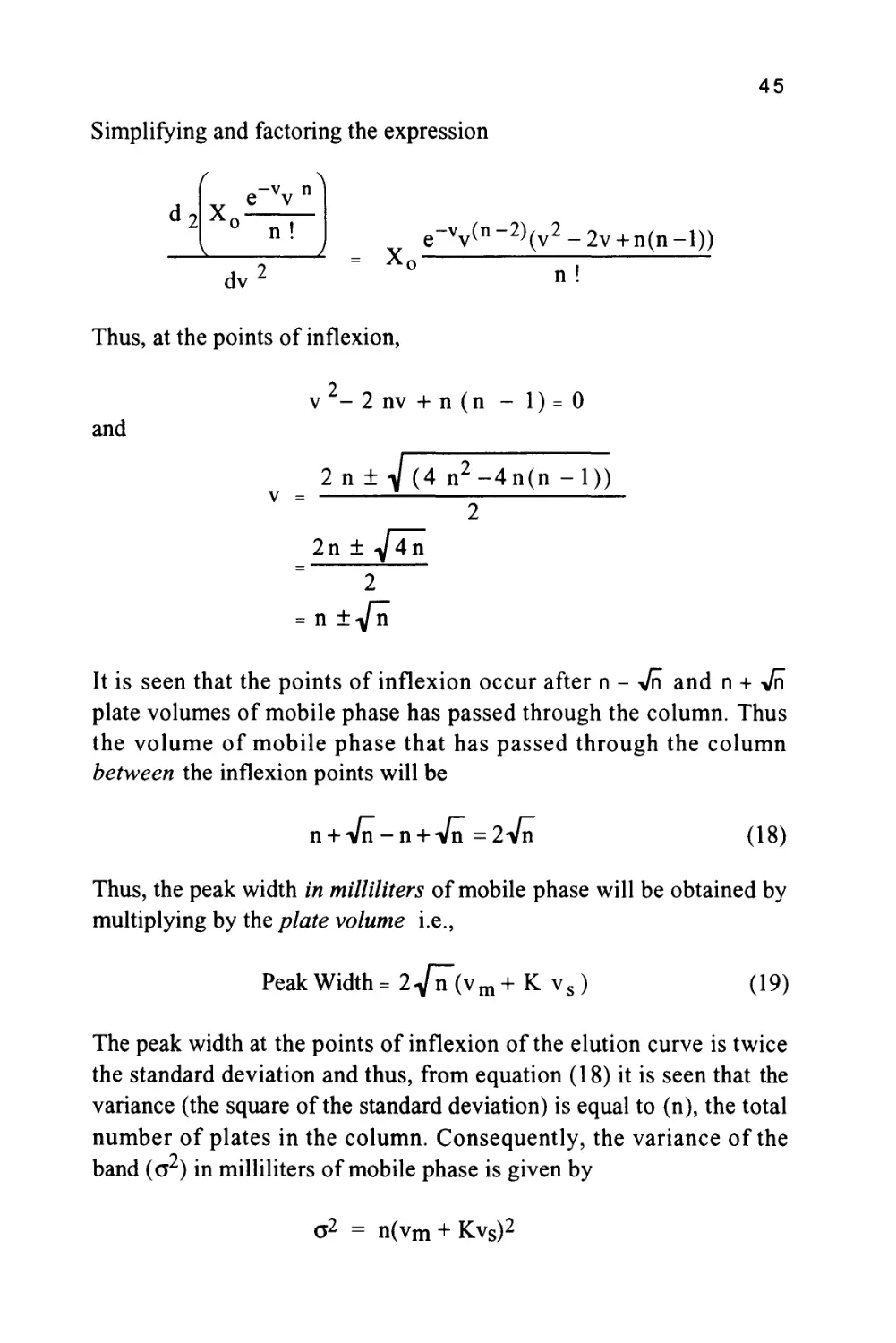
Simplifying and factoring the expression
e~vv(n_2)(v2-2v + n(n-l))
Thus, at the points of inflexion,
v2-2 nv +n (n - 1)= 0
and
2n ± J(4 n2-4n(n -1))
v =
2
2n ± /4~n
2
= n ±<Jn
It is seen that the points of inflexion occur after n - Vn and n + i/n
plate volumes of mobile phase has passed through the column. Thus
the volume of mobile phase that has passed through the column
between the inflexion points will be
n + Vn-n + Vn = 2 Vn (18)
Thus, the peak width in milliliters of mobile phase will be obtained by
multiplying by the plate volume i.e.,
Peak Width = 2</n~(vm+ K vs) (19)
The peak width at the points of inflexion of the elution curve is twice
the standard deviation and thus, from equation (18) it is seen that the
variance (the square of the standard deviation) is equal to (n), the total
number of plates in the column. Consequently, the variance of the
band (a2) in milliliters of mobile phase is given by
( -v n^
e v
X.
n
dv
o2 = n(vm + Kvs)2
46
Now,
Vr =n(vms +Kvs)
Thus,
n
It follows that as the variance of the peak is inversely proportional to
the number of theoretical plates in the column then the larger the
number of theoretical plates, the more narrow the peak and the more
efficiently the column has constrained the band dispersion. As a
consequence the number of theoretical plates in a column has been
given the term Column Efficiency and is used to describe its quality.
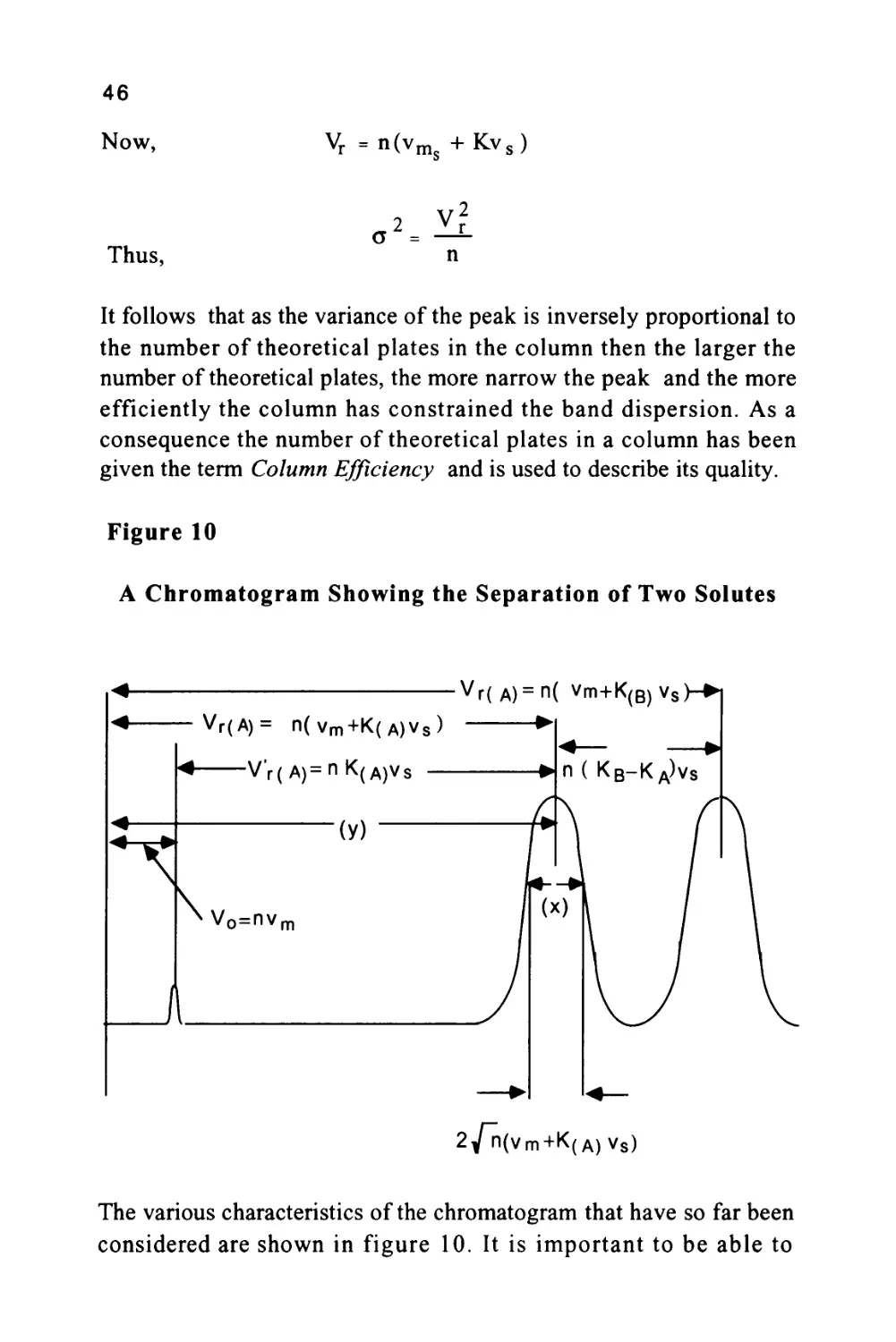
Figure 10
A Chromatogram Showing the Separation of Two Solutes
< vr(A)=n( vm+K(B)vs
< Vr(A)= n(vm+K(A)Vs) ►
2/n(vm+K(A)V8)
The various characteristics of the chromatogram that have so far been
considered are shown in figure 10. It is important to be able to
47
measure the efficiency of any column and, as can be seen from figure
10, this can be carried out in a very simple manner. Let the distance
between the injection point and the peak maximum (the retention
distance on the chromatogram) be (y) cm and the peak width at the
points of inflexion be (x) cm as shown in figure 10.
Then as the retention volume is n(vm + Kvs) and twice the peak
standard deviation at the points of inflexion is 2 Vn (vm + Kvs), then,
by simple proportion,
Ret. Distance
PeakWidth
y
nC
^m+Kvs)
x 2Vn"(vm+Kvs)
n = 4
Vn"
2
(20)
Equation (20) allows the efficiency of any solute peak, from any
column, to be calculated from measurements taken directly from the
chromatogram. Many peaks, if measured manually, will be only a few
millimeters wide and, as the calculation of the column efficiency
requires the width to be squared, the distance (x) must be determined
very accurately. The width should be measured with a comparitor
reading to an accuracy of ± 0.1 mm.
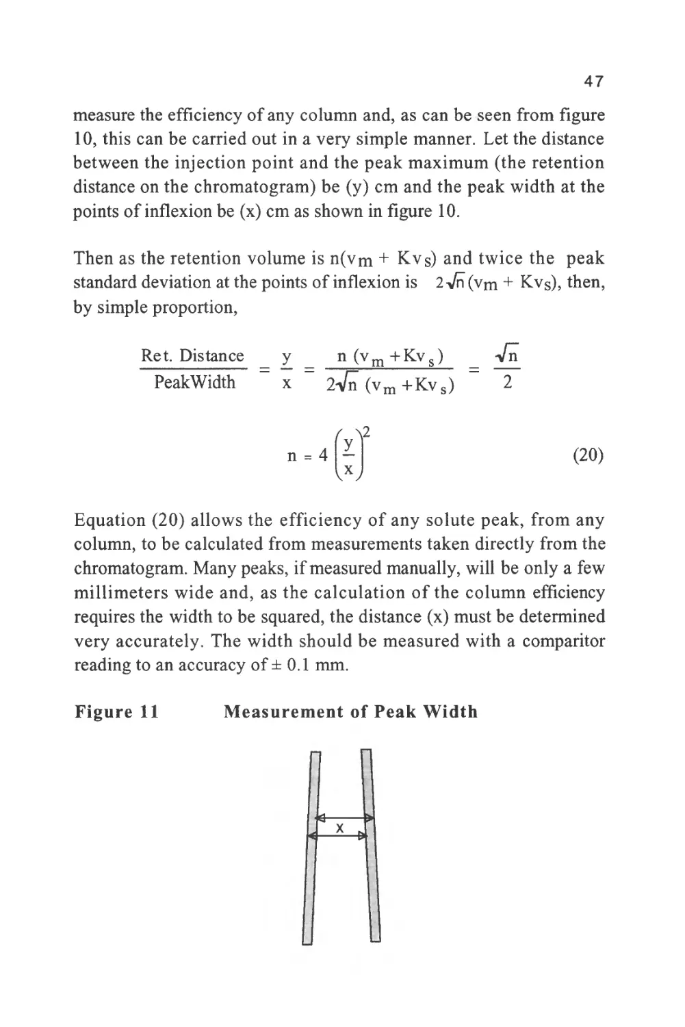
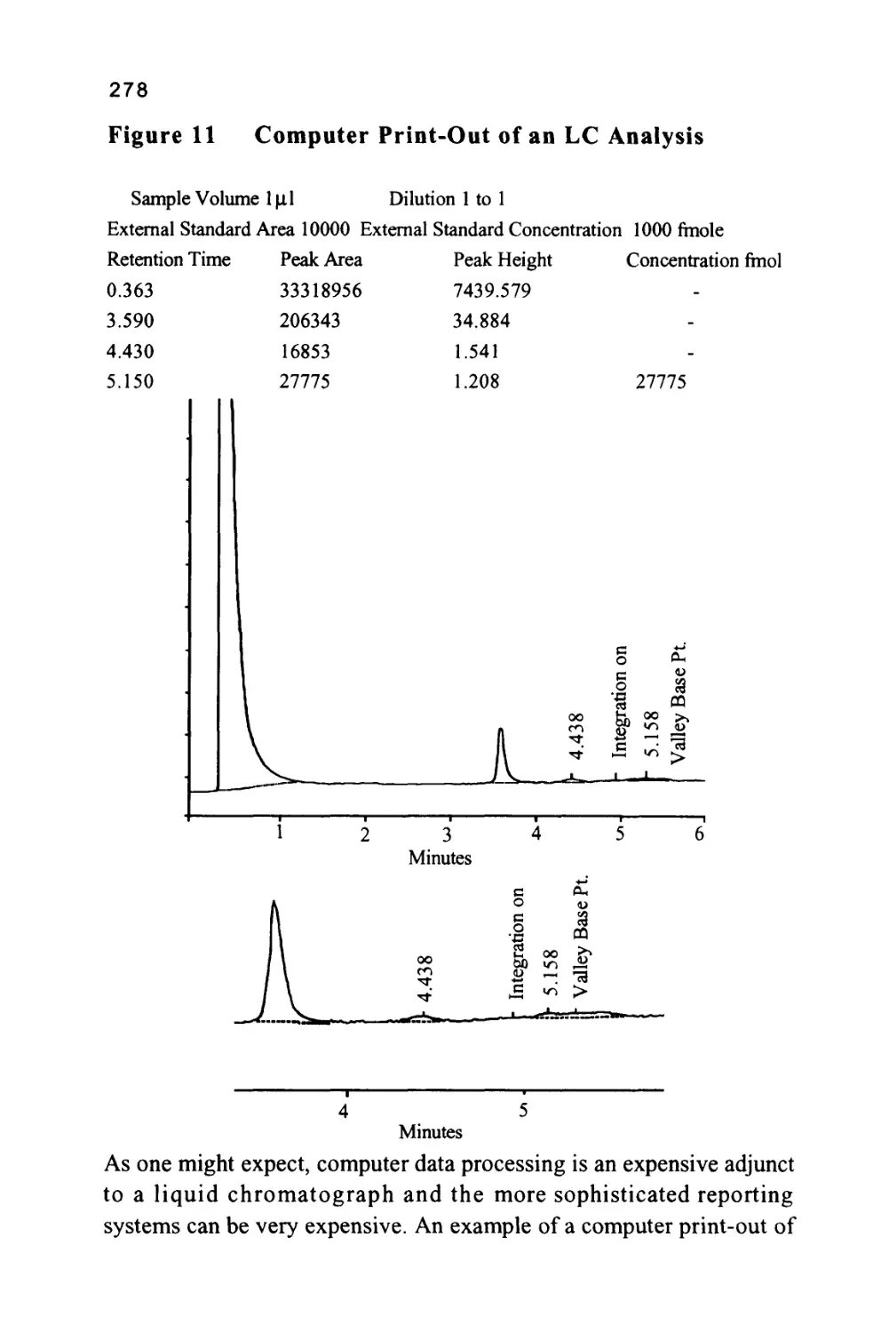
Figure 11
Measurement of Peak Width
o
48
The measurements are taken from the inside of one line to the
outside of the adjacent line, in order to eliminate errors resulting
from the finite width of the ink line drawn on the chart. This
procedure is shown in figure 11. The measurement should be repeated
using the alternate edges of the line and an average taken of the two
readings to avoid errors arising from any variation in line thickness.
At least three replicate runs should be made and the three replicate
values of efficiency should not differ by more than 3%. If the data
acquisition system has software to measure efficiency then this can be
used providing its accuracy is carefully checked manually. Noise on
the detector can often introduce inaccuracies that are less likely to
occur with manual measurement.
It is clear that the first challenge facing the analyst is the choice of the
phase system that is appropriate for the particular sample to be
analyzed. Only after the phase system has been chosen, can the correct
column be selected. It is therefore necessary to know the types and
properties of the different stationary phases that are available and how
to formulate the pertinent mobile phases that must be used with them.
References
\TLiquid Chromatography Column Theory", R.P.W.Scott, John Wiley
and Sons, Chichester-New York-Brisbane-Toronto-Singapore, (1992).
2/ A.J.P.Martin and R.L.Synge, Biochem. J., 35(1941) 1358.
3/" Gas Chromatography " Second Edition, A.I.M. Keulemans (Ed.
C.G.Verver) Reinhold Publishing Corporation, New York,
(1959)106.
4/" Theory and Mathematics of Chromatography", A.S.Said, Dr. Alfred
Huthig Veriag GmbdH Heidelberg (1981)126.
5/ "Ion Chromatography", H. Small, Plenum Press (1989).
49
6/ "Handbook of Ion Chromatography", J.Weiss, Published by Dionex,
(1988).
II"Ion Chromatography Applications", R E. Smith, CRC Press, (1988).
8/ R.P.W. Scott and P.Kucera, /. Chromatogr., 125(1976) 251.
9/ R. P. W. Scott and P. Kucera, J. Chromatogr., 169(1979) 51.
10/C.Peterson and G.Schill, J Chromatogr.,204(1981) 179.
11/C.Peterson, J. Chromatogr.237(1984) 553.
12/ D.R.Taylor, J. Chromatogr. SW.30(1992) 67.
13/ "Cyclobond handBook",T.E.Bcesley, Published by ASTEC (1991).
3
Liquid Chromatography
Phase Systems
It was explained in the previous chapter that solute retention and,
consequently, solute selectivity is accomplished in an LC column by
exploiting three basic and different types of molecular interactions in
the stationary phase; those interactions were described as ionic, polar
and dispersive.
At this point it is necessary to discuss some alternative terms for
molecular forces and molecular interactions that have crept into
chromatography and that are alternatives to the presently accepted
nomenclature. The reason for their introduction is unclear, but they
appear to have become established in the biotechnology field. It is
possible that, in contrast to biotechnology, which has evolved from
organic chemistry and/or biochemistry, chromatography has evolved
from a mixture of physical chemistry and analytical chemistry and, as
a consequence, adopted an entirely different nomenclature. In any
event, the alternative terms do cause confusion to those who are new
to the techniques and are trying to learn more about them. In
particular, they are confusing to those chemists that have had classical
training and have been introduced to the correct and established
physical chemical terms for describing molecular forces and
molecular interactions.
51
52
The four terms that need discussion are (1) "hydrophobic interactions",
(2)"lyophobic interactions", (3)"hydrophilic interactions" and (4)
"lyophilic interactions".
The term "hydrophobic interaction" is a most unfortunate term in that
it implies some form of molecular repulsion which of course, outside
the Van der Waals radii of a molecule, is impossible. The term
"hydrophobic force", literally meaning "fear of water" force, was
coined, for some reason, as an alternative to the well established term,
dispersive force. This may have been provoked by the immiscibility
of a dispersive solvent such as n-heptane, with a very polar solvent
such as water.
The reason that n-heptane and water are immiscible is not because
water molecules repel heptane molecules. They are immiscible because
the forces between two heptane molecules and the forces between two
water molecules are much greater than the forces between a heptane
molecules and a water molecule. Thus, water molecules and heptane
molecules interact very much more strongly with themselves than with
each other. One would have thought that the fact that water has a
small but finite solubility in n-heptane, and n-heptane has a small but
finite solubility in water, would have precluded repulsion as an
interpretation.
Thus,
hydrophobic interactions are dispersive interactions
and hydrophobic solvents and stationary phases are dispersive
solvents and stationary phases.
The term "hydrophilic force", literally meaning "love of water" force,
appears to have been introduced merely as the complement to
"hydrophobic". It is equivalent to the term polar, and polar solvents
are hydrophilic solvents because they interact strongly with water or
other polar solvents.
53
Therefore,
hydrophilic interactions are polar interactions
and hydrophilic solvents and stationary phases are polar solvents and
stationary phases.
The reasons for the introduction of the terms "lyophobic" (meaning
fear of lye) and "lyophilic" (meaning love of lye) are even more
obscure and appear irrelevant as they are virtually alternatives to the
terms hydrophobic and hydrophilic. The terms originated in the early
soap industry during the mid-to-late nineteenth century. In about 1850
soap was prepared by boiling a vegetable oil with an alkaline solution
obtained from leaching 'wood ash' with water.
The alkaline product from the wood ash was a crude solution of
sodium and potassium carbonates called "lye". On boiling the
vegetable oil with the lye, the soap (sodium and potassium salts of long
chained fatty acids) separated from the lye due to the dispersive
interactions between the of the fatty acid alkane chains and were thus,
called "lyophobic". It follows that "lyophobic", from a physical chemical
point of view, would be the same as "hydrophobic", and interactions
between hydrophobic and lyophobic materials are dominantly
dispersive. The other product of the soap making industry was
glycerol which remained in the lye and was consequently, termed
"lyophilic". Thus, glycerol mixes with water because of its many
hydroxyl groups and is very polar and hence a "hydrophilic" or
"lyophilic" substance.
Therefore,
lyophilic interactions are polar interactions
and
lyophobic interactions are dispersive interactions.
Perhaps we should consider it fortunate that, to date, exclusion
chromatography has not yet been dubbed
"claustrophobic interaction chromatography".
54
Finally, before returning to the subject of the chapter, the extravagant
and apparently uncontrollable contemporary use of acronyms must be
mentioned. The reason for their excessive use is not clear but, for
whatever reason, they can be extremely frustrating and annoying
impediments to the student or scientist who is studying a new subject.
Their excessive use is to be deplored and in the following discussion
and, in fact, throughout this book, acronyms will be kept to an
absolute minimum and where used, will be clearly and unambiguously
defined.
Returning now to the subject of the chapter, in addition to appropriate
retentive characteristics, a potential stationary phase must have other
key physical characteristics before it can be considered suitable for use
in LC. It is extremely important that the stationary phase is completely
insoluble (or virtually so) in all solvents that are likely to be used as a
mobile phase. Furthermore, it must be insensitive to changes in pH
and be capable of assuming the range of interactive characteristics that
are necessary for the retention of all types of solutes. In addition, the
material must be available as solid particles a few microns in diameter,
so that it can be packed into a column and at the same time be
mechanically strong enough to sustain bed pressures of 6,000 p.s.i. or
more. It is clear that the need for versatile interactive characteristics,
virtually universal solvent insolubility together with other critical
physical characteristics severely restricts the choice of materials
suitable for LC stationary phases.
To date there have been three possible candidates that will generally
fit the requirements of an LC stationary phase and they are alumina,
silica gel and certain polymeric resins for example, cross-linked
polystyrene. Alumina, despite having an abundance of surface
hydroxyl groups that confer on it strong polar characteristics and
despite it having adequate mechanical strength, is the least useful of
the three materials for LC. Although alumina can be used as a
stationary phase per se, it does not readily form stable bonded phases
though it can be coated with polymeric stationary phases which endow
it with some dispersive character. Furthermore, although it can be
55
ground to particle sizes of a few microns in diameter, a procedure has
not been found that can produce the high column efficiencies that are
consistently attainable from silica gel. As a result alumina stationary
phases are still utilized in only a few per cent of all LC applications.
The polymeric resin beads fill a need that arises from the instability
of silica gel and its products to mobile phases of extreme pH (outside a
pH range of about 4.0-7.0) and, consequently, are employed in most
ion exchange separations. Organic moieties containing ionic groups
can be bonded to silica and produce an effective ion exchange media,
but the restrictions of pH on phase stability still apply. It follows that
ion exchange bonded phases are less popular than the polymer bead
alternatives.
Nevertheless, silica gel is the material of choice for the production of
the vast majority of LC stationary phases. Due to the reactive
character of the hydroxyl groups on the surface of silica gel, various
organic groups can be bonded to the surface using standard silicon
chemistry. Consequently, the silica gel surface can be modified to
encompass the complete range of interactive properties necessary for
LC ranging from the highly polar to almost completely dispersive.
The Production of Silica Gel
As a result of its unique chemical and physical properties, silica gel is
probably the most important single substance involved in liquid
chromatography today. Without silica gel, it is doubtful whether
HPLC could have evolved at all. Silica gel is an amorphous, highly
porous, partially hydrated form of silica which is a substance made
from the two most abundant elements in the earth's crust, silicon and
oxygen. Silica, from which silica gel is manufactured, occurs
naturally, either in conjunction with metal oxides in the form of
silicates, such as clay or shale, or as free silica in the form of quartz,
cristobalite or tridymite crystals. Quartz is sometimes found clear and
colorless, but more often in an opaque form, frequently colored
56
yellow by traces of iron which, when crushed by earth movement and
weathered by air and water, produces sand.
Silica gel is prepared in two stages. Firstly, an intimate mixture of
sand and sodium carbonate are heated together in iron pans forming
sodium silicate with the release of carbon dioxide. The sodium silicate
is leached out of the cooled mixture, unreacted sand removed by
filtration, and the resulting silicate solution treated with hydrochloric
or sulfuric acid.
Initially, silicic acid is released,
Na2Si03 +H2O + 2HC1 = Si(OH)4 + 2NaCl
However, the free acid quickly starts to condense with itself,
accompanied by the elimination of water to form dimers, trimers and
eventually polymeric silicic acid. The polymer continues to grow,
initially forming polymer aggregates and then polymer spheres, a few
Angstroms in diameter. These polymeric spheres are termed the
primary particles of silica gel and must not to be confused with the
macro-particles of silica gel that are packed into the LC column.
The primary particles continue to develop until, at a particular size,
the surface silanol groups (hydroxyl groups attached to the surface
silicon atoms of the primary particles) on adjacent primary polymer
particles, condense with the elimination of water causing the primary
particles to fuse together and the solution begins to gel. During this
process, the primary particles of silica gel that are formed will have a
range of diameters extending from a few Angstroms to many
thousands of Angstroms depending on the conditions of formation. It
is the size of the primary particles that determines the pore size and
pore range of the final gel. The gel formed in the manner described
above is termed the hydrogel and at this stage is very soft with little or
no mechanical strength.
57
The hydrogel is allowed to stand for a few days during which time a
process called sinensis takes place. During sinensis the condensation
of the primary particles, one with another, continues and the gel
shrinks further, accompanied by the elimination of more saline
solution that exudes from the gel. After three or four days, sinensis is
complete and the gel becomes firm and can now be washed free of
residual electrolytes with water. The washed product is finally heated
to 120°C to complete the condensation of the surface silanol groups
between the particles, and a hard xerogel is formed. It is this xerogel
that is used as the LC stationary phase and for bonded phase synthesis.
It is not intended to discuss the production of silica gel in detail and
those interested are referred to "Silica Gel and Bonded Phases",
published by Wiley (1).
However, it should be said in passing that the pore size and surface
area of the silica, which can be critical for certain LC applications, is
controlled by the conditions of gelling, the subsequent washing
conditions and any ensuing thermal treatment.
Silica gel, in the form of the xerogel, is an extremely hard and
abrasive material and thus, must be ground by an appropriate mill.
For effective use as an LC stationary phase the so called "irregular"
particles produced by the mill should be well rounded to simulate
spherical particles. In fact, spherical particles of silica gel can be
produced directly (2-4), but the procedure is tedious and more
expensive. Rounded, irregular silica gel particles, will provide column
efficiencies at least as good, if not better, than those obtained from the
spherical material. The ideal mill for grinding the xerogel for LC
purposes is the "Jet Mill" which can provide narrow cuts of particles
having mean diameters that range from 2 to 20u. The size reduction is
achieved by entraining the particles of grist into three (or if necessary
more) jets of air that are directed to a center point in a cylindrical
mill housing. The particles collide at the center, causing self
fragmentation with minimum wear on the grinding system and very
little product contamination. Due to the nature of the grinding process
it is particularly useful for grinding very hard and abrasive materials.
58
The product from the "Jet Mill" after classification can be used
directly as an LC packing or as the raw material for bonded phase
synthesis.
The silica particles are packed into the LC column by a slurry packing
procedure using either a 'balanced density' solvent or a high viscosity
solvent. The principal of the packing procedure is to complete the
packing before the particles are segregated by sedimentation. Thus, a
solvent mixture (usually a mixture of halogenated paraffins) having
the same density as the silica gel particles can be used so that no
sedimentation takes place at all. Alternatively, a viscous solvent can be
employed to ensure that the sedimentation is so slow that the packing
is complete before any significant size segregation has taken place. In
most cases, analysts will purchase packed columns and thus, details of
packing procedures are not pertinent to this discussion; those
interested in slurry packing methods are again referred to "Silica Gel
and Bonded Phases", published by Wiley (1).
Solute/Solvent Interactions on the Surface of Silica Gel
Mono-Layer Adsorption of Solvents on the Surface of Silica Gel
As a result of the hydroxyl groups that cover its surface, silica gel is
strongly polar and thus, would be useful for separating polarizable or
weakly polar solutes. In a practical separation, to ensure that polar
selectivity dominates in the stationary phase and polar interactions in
the mobile phase are minimized, the mobile phase must be chosen to
be non-polar and strongly dispersive, for example n-heptane.
However, consider the separation of solutes that are more polar than
the aromatic hydrocarbons, for example mixtures of ethers or
aliphatic esters. If it were attempted to separate a series of aliphatic
esters on silica gel employing n-heptane as the mobile phase it would
be found that the retention of the later eluting solutes was inordinately
long. If a slightly stronger solvent, such as chloroform was used as an
alternative to n-heptane, it would be found that the less polar esters
59
were eluted too rapidly. Consequently, a suitable mixture of
chloroform and n-heptane might be considered more appropriate.
Although a mixture of chloroform and n-heptane would, indeed, be
very suitable for the separation of the esters, the effect of the addition
of chloroform to the n-heptane on solute retention is by no means
simple. When chloroform is added to n-heptane, it is found that not
only is the eluting capability of the mobile phase mixture increased
due to the stronger interaction of the solutes in the mobile phase with
chloroform, but the nature of the silica surface is also changed and the
retentive capacity of the stationary phase is reduced. This is because
the solvents themselves partition between the silica surface and the
solvent mixture as well as the solutes. In fact as the chloroform
concentration increases, some is adsorbed on the silica surface as a
monolayer according to the Langmuir adsorption isotherm.
The equation for the Langmuir adsorption isotherm is as follows:
ac
b+ac
where (a) is the fraction of the surface covered by the solute,
(c) is the concentration of the solute in the mobile phase,
and (a) and (b) are constants.
It is seen that at high concentrations (a) becomes unity and the surface
is completely covered with the more strongly adsorbed solvent. The
adsorption isotherm of chloroform on silica gel, determined by Scott
and Kucera (5) is shown in figure 1. It is seen that the monolayer of
chloroform collects on the surface continuously until the chloroform
content of the mobile phase is about 50%. At this concentration the
monolayer appears complete. Thus, between 0 and 50% chloroform in
the n-heptane, the interactions between the solute and the chloroform
in the mobile phase are continuously increasing.
60
Figure 1
Langmuir Isotherm for Chloroform on Silica Gel
OX)
Ob1
%
O
o
C/3
a
©
a
*©
0.12
0
25 50
Concentration of Chloroform in n-Heptane %w/v
In contrast, the interactions with the stationary phase are becoming
weaker as the surface becomes covered with chloroform. Thus
retention is reduced by both the increased interactions in the mobile
phase and reduced interaction with the stationary phase. When the
concentration of chloroform in the solvent mixture is in excess of
50%, then the interactive properties of the stationary phase no longer
change as the surface is now covered with a mono-layer of
chloroform. However, solute retention will continue to decrease due
to the increased interactions of the solute with the higher
concentrations of chloroform in the mobile phase. It is clear that even
with this simple example the dependence of retention on solvent
composition is quite complex.
Solute Interactions with the Silica Gel Surface
(Mobile Phase n-Heptane/Chloroform)
There are basically two types of interaction that can take place
between a solute and the silica gel surface. Firstly, the solute molecule
can interact with the adsorbed solvent layer and rest on the surface of
61
it. This type of interaction is called sorption interaction and occurs
when the molecular forces between the solute and the silica are
relatively weak compared with the forces between the solvent
molecules and the silica. The second type of interaction is where the
solute molecules displace the solvent molecules from the surface and
interact directly with the silica gel itself, for example, the silanol
groups. This type of interaction is called displacement interaction and
occurs when the interactive forces between the solute molecules and
the silica surface are much stronger than those between the solvent
molecules and the silica surface.
The types of interaction that can occur between the solute and the
stationary phase surface when in contact with the pure solvents, n-
heptane, chloroform or a mixture of n-heptane/chloroform are shown
in figure 2.
In pure n-heptane or pure chloroform the solute molecules can either
interact directly with the surface of the adsorbed solvent or displace
the adsorbed solvent and interact directly with the silica surface. In the
case of the solvent mixture the solute molecules may interact with the
surface of either solvent or displace either solvent and interact directly
with the silica surface or any combination of these possibilities. For
example some solute molecules might displace the layer of n-heptane
and interact directly with the surface. At the same time, those solute
molecules striking the layer of chloroform may interact only with the
chloroform and not be capable of displacing it, as the molecular forces
between the chloroform and the silica gel are greater than the
molecular forces between the solute and the silica gel.
From a practical point of view the change in retention with solvent
concentration will be greater at the lower concentrations of
chloroform where interactions in both phases are being changed. At
concentrations above 50%, however, interactions are only changing in
the mobile phase and so the effect of solvent concentration on
retention will be less significant.
62
Figure 2
Solute/Solvent Interactions with a Silica Gel Surface
Mobile Phase n-Heptane
Interaction Interaction by Disnlaced
by Sorption Displacement ^^g£*
nTrrrrrrrrrrmrn
Mobile Phase
n-Heptane/Chloroform
Tntprartinn V>v Displaced Interaction
interaction by Chloroform , s t-
Displacement , e>y sorption
Interaction \ / / Interaction by
by Sorption \ \ • / / Displacement
rrfxx^rooffxrwf?
o
Displaced
n-Heptane
Mobile Phase Chloroform
Displaced
Interaction Interaction by /Chloroform
o
by Sorption Displacement
This will be true for all solvent mixtures where there is no association
between solvents and is useful to remember when adjusting solvent
composition to obtain the desired selectivity and retention.
Unfortunately, when one solvent is polar, a bi-layer of solvent can be
formed on the surface and solute/solvent interactions with the silica
gel are even more complex.
63
Bi-Laver Adsorption of Solvents on the Surface of Silica Gel
The identification of bi-layer adsorption of polar solvents on the
surface of silica gel arose from some work by Scott and Kucera (5)
who measured the adsorption isotherms of the some polar solvents,
ethyl acetate, isopropanol and tetrahydrofuran from n-heptane
solutions onto silica gel. The authors found that the experimental
results for the more polar solvents did not fit the simple mono-layer
adsorption equation and, as a consequence, the possibility of bi-layer
adsorption on the silica gel surface was examined.
Bi-layer adsorption is not uncommon and the development of the bi-
layer adsorption isotherm equation is a simple extension of that used
for the mono-layer equation. The Langmuir equation for bi-layer
adsorption is as follows:
The equation for the first layer,
- bdc + adc
eb+bdc + adc2
where (a) is the surface fraction covered by the first adsorbed layer,
(c) is the concentration of the polar solvent in n-heptane
and (a),(b) and (d) are constants.
The equation for the second layer,
ac
P = 7— (3)
b+ac
where (|3) is the surface fraction covered by the second adsorbed
layer, and the other symbols have the meaning previously ascribed
them.
64
Figure 3
The Individual and Combined Adsorption Isotherms for
Ethyl Acetate on Silica Gel
0.15
OX
;- 0.10-
©
a
o
U.
■*-
a
(J
a
o
U
0.05-
0.00 -it
0 12 3 4
Concentration of Ethyl Acetate (%w/v)
Scott and Kucera fitted their data to equations (2) and (3), solved for
the constants and reconstructed the isotherms for each layer which are
included in figure 3. The formation of a solvent bi-layer is
diagramatically represented in figure 4.
Figure 4
Bi-layer Adsorption of Solvent
Solvent B
Second Layer
Solvent B
First Layer
Solvent A
/
65
It is seen in figure 3 that the two curves, although of the same form,
are quite different in magnitude. The first layer to be formed is very
strongly held to the surface and is almost complete when the
concentration of ethyl acetate in the mobile phase is only about
l%w/v. As the concentration of ethyl acetate rises above l%w/v the
second layer is only just being formed. The formation of the second
layer of ethyl acetate is much slower and obviously the interactions
between the solvent molecules with those already adsorbed on the
surface are much weaker than their interaction with the silanol groups
of the silica gel.
This means, in practice, that when employing a polar solvent with n-
heptane (or any other paraffin for that matter) to reduce the retention,
there will be a dramatic reduction in retention over the concentration
range of about 0-2%w/v. However, subsequent changes in solute
retention with polar solvent concentration will be relatively small.
This will be true for any polar solute and was experimentally verified
by Scott and Kucera for solutions of ethyl acetate, tetrahydrofuran and
n-propanol in n-heptane. The very sensitive relationship between
solvent concentration and retention at very low concentrations makes
the phase system very difficult to make reproducible. This problem is
one of the factors that deter analysts from using silica gel as a
stationary phase for the separation of polar solutes. It is very
satisfactory, however, for the separation of polarizable and weakly
polar substances that can be eluted by paraffin/methylene dichloride or
similar types of solvent mixtures.
Solute Interactions with the Silica Gel Surface
(Mobile Phase n-Heptane/Ethyl Acetate)
The possible alternatives for a solute molecule to interact with a bi-
layer of solvent molecules is depicted in figure 5. It is seen that such a
surface offers a wide range of sorption and displacement processes
that can take place between the solute and the stationary phase surface.
There are, in fact, three different surfaces on which a molecule can
66
interact by sorption and three different surfaces from which molecules
of solvent can be displaced and allow the solute molecule to penetrate.
Figure 5
Different Types of Solute Interaction that Can Occur on
Silica Surfaces Covered with a Solvent Bi-layer
Solute interacting
with second layer of
solvent (B) SORPTION
Solute interacting
with first layer of
solvent (B) by
displacing solvent
from second layer
DISPLACEMENT
0
/Displaced
Solvent (B)
0
/
Displaced
Solvent (B) Djsp|aced
Solvent (A)
Solute interacting
directly with first layer
of solvent (B) SORPTION
Solute interacting
with silica surface by
displacing solvent (B)
from first layer
DISPLACEMENT
Solute interacting
with silica surface by
displacing solvent (A)
from first layer
DISPLACEMENT
Solute interacting
directly with layer of
solvent (A) SORPTION
In any separation all the alternatives are possible, but it is more likely
that for any particular solute, one type of interaction will dominate.
Where there are multi-layers of solvent, the most polar is the solvent
that interacts directly with the silica surface, and consequently
constitutes the first layer. Depending on the concentration of the polar
solvent, the next layer may be a second layer of the same polar solvent
as in the case of ethyl acetate. If, however, the quantity of polar
67
solvent is limited, then the second layer might consist of a less polar
component of the solvent mixture. If a ternary mixture of solvents is
used, the nature of the surface, and the solute interactions with the
surface can become very complex indeed. In general the stronger the
polarity of the solute the more likely it is to interact with the surface
by displacement even to the extent of displacing both layers of solvent
(one of the alternative processes that is not depicted in figure 5). Less
polar solutes a more likely to interact with the surface by sorption.
Silica Gel as an Exclusion Medium
Silica gel can be produced with a wide range of pore sizes and can
thus be used as an exclusion media as discussed in chapter 2. An
example of the different exclusion properties exhibited by silica gel is
shown in figure 6.
Figure 6
Graph of Pore Volume per Gram of Silica Gel against Log
Pore Diameter for Ten Different Silica Gels
w>
s
jg
>
o
0-
Spherosil
Porasil C
Porasil A
Silerex 2
CPG 10
Parti sil 10
LiChrosorb 10
Log Pore Diameter (A)
68
It is seen that the pore diameter of the silica gels cover a range from
about 7 to 250 Angstroms typified by Partisil to that typified by
Porasil C ranging from about 50 to over 1,000 Angstroms. It would
seem that silica would be a valuable media for exclusion
chromatography. Unfortunately, the main application for exclusion
chromatography lies in the biotechnology field in the separation of
macro-molecules, where the mobile phases that can be employed must
be aqueous in nature to permit adequate solubility and solute stability.
Silica gel is soluble in water, albeit very slightly, which renders a
column packed with such material unstable. Furthermore, the silica
gel surface is very active which would be liable to denature large
peptides and proteins during the separation procedure. Nevertheless,
silica gel is used for exclusion chromatography providing the
materials are dispersive or weakly polar in nature and polar or semi-
polar solvents can be employed. For example, silica gel can be used
very elegantly to separate the larger aromatic hydrocarbons by
exclusion using acetonitrile or tetrahydrofuran as the mobile phase or
for the separation of polystyrene polymers using tetrahydrofuran as
the mobile phase.
Figure 7
The Separation of a Mixture of Polyphenyl Siloxanes by
Exclusion Chromatography
An example of the use of silica gel to separate the products from a
phenyl siloxane polymerization employing a high efficiency column
69
(10m long, 1 mm i.d., packed with 20 m Partisil silica gel) is shown in
figure 7. It is seen that the individual polymers are clearly separated
but again a very a high efficiency was necessary and correspondingly
long analysis times had to be tolerated due to the relatively small
molecular weight intervals between each polymer. The chromatogram
shown, covers a time period extending between 4 and 5 hours.
However, it should be pointed out that silica gel can be used for the
separation of dispersive and weakly polar solutes using standard
columns involving separation times of less than an hour.
Application Areas for Silica Gel as a Stationary Phase
It is important for the analyst to be able to select the best stationary
phase to use for a particular chromatographic analysis. Silica gel can
be used in two modes of chromatographic separations: as a stationary
phase in normal elution development or as a stationary phase in
exclusion chromatography.
Silica Gel as a Stationary Phase in Elution Chromatography
As a result of its highly polar character, silica gel is particularly
useful in the separation of polarizable materials such as the aromatic
hydrocarbons and polynuclear aromatics. It is also useful in the
separation of weakly polar solute mixtures such as ethers, esters and in
some cases, ketones. The mobile phases that are commonly employed
with silica gel are the n-paraffins and mixtures of the n-paraffins with
methylene dichloride or chloroform. It should be borne in mind that
chloroform is opaque to UV light at 254 nm and thus, if a fixed
wavelength UV detector is being used, methylene dichloride might be
a better choice. Furthermore, chloroform is considered toxic and
requires special methods of waste disposal. Silica gel is strongly
deactivated with water and thus, to ensure stable retentive
characteristics, the solvent used for the mobile phase should either be
completely dry or have a controlled amount of water present. The
level of water in the solvent that will have significant effect on solute
retention is extremely small. The solubility of water in n-heptane is
70
only a few parts per million but, if present, will, in time, significantly
deactivate silica gel.
If the mixture to be separated contains fairly polar materials, the silica
may need to be deactivated by a more polar solvent such as ethyl
acetate, propanol or even methanol. As already discussed, polar
solutes are avidly adsorbed by silica gel and thus the optimum
concentration is likely to be low, e.g. l-4%v/v and consequently, a
little difficult to control in a reproducible manner. Ethyl acetate is the
most useful moderator as it is significantly less polar than propanol or
methanol and thus, more controllable, but unfortunately adsorbs in the
UV range and can only be used in the mobile phase at concentrations
up to about 5%v/v. Above this concentration the mobile phase may be
opaque to the detector and thus, the solutes will not be discernible
against the background adsorption of the mobile phase. If a detector
such as the refractive index detector is employed then there is no
restriction on the concentration of the moderator. Propanol and
methanol are transparent in the UV so their presence does not effect
the performance of a UV detector. However, their polarity is much
greater than that of ethyl acetate and thus, the adjustment of the
optimum moderator concentration is more difficult and not easy to
reproduce accurately. For more polar mixtures it is better to explore
the possibility of a reverse phase (which will be discussed shortly)
than attempt to utilize silica gel out of the range of solutes for which it
is appropriate.
In summary, examples of the successful use of silica gel as a
conventional stationary phase are in the analysis of mixtures
containing polarizable and relatively low polarity solutes typified by
mixtures of aromatic hydrocarbons, polynuclear aromatics, nitro
compounds, carotenes and vitamin A formulas.
Silica Gel as a Stationary Phase in Exclusion Chromatography
In many respects silica gel is an ideal exclusion media. Due to its
rigidity and mechanical strength, it will sustain high pressures and
71
consequently, can be packed into long columns that provide the
necessary high efficiencies. Furthermore, silica gel is available in a
wide range of pore sizes which would make it suitable for the
separation of substances having a wide range of molecular weights.
Unfortunately it has two major disadvantages. Firstly it is slightly
soluble in water and thus cannot be used for any length of time in
aqueous solvent mixtures. Secondly it is very unstable at extremes of
pH. As a consequence, it is precluded from the major areas of
application for exclusion chromatography, that is the separation of
macro-molecules of biological origin. Such samples require to be
separated in aqueous solvents at pH values outside those to which silica
gel are stable. Nevertheless, there are areas of application where silica
gel is ideally suited as an exclusion media but, unfortunately, these
areas are rather restricted. In order to ensure that the separation is by
exclusion, and there are no differential interactions between the
solutes and the two phases, a fairly polar solvent should be used to
deactivate the silica gel. A typical solvent for use as the mobile phase
when using silica gel as an exclusion medium is tetrahydrofuran.
In summary, silica gel can be an excellent stationary phase for use in
exclusion chromatography in the separation of high molecular weight,
weakly polar or polarizable polymers. It cannot be used for separating
mixtures that require an aqueous mobile phase or operate at a pH
outside the range of 4-8. Examples of the type of materials that can
be separated by exclusion chromatography using silica gel are the
polystyrenes, polynuclear aromatics, polysiloxanes and similar
polymeric mixtures that are soluble and stable in solvents such as
tetrahydrofuran.
Bonded Phases
Although silica gel was the catalyst that partly initiated the renaissance
of liquid chromatography, it was quickly found that separations based
solely on polarity had severe limitations. Furthermore, the labile
nature of silica gel in aqueous environments coupled with its
instability to extremes of pH provoked active research to develop
72
alternative stationary phases. The immediate and obvious solution was
to chemically modify the surface of silica gel by bonding organic
moieties to it that would exhibit dispersive interactions and at the same
time stabilize the material to water and extremes of pH. The first
attempts to bond an organic group to silica gel for chromatographic
purposes was made by Halasz and Sebastian (6), who attached aliphatic
hydrocarbon chains to the surface by means of the silicon-oxygen-
carbon linkage, a pioneering step in the development of liquid
chromatography stationary phases. The synthesis by Halasz was
carried out by refluxing the silica gel with a high molecular weight
aliphatic alcohol, and thus, by esterifying the hydroxyl groups of the
polymeric silicic acid, aliphatic silyl ester groups were attached to the
silica gel surface. Unfortunately, the silicon-oxygen-carbon linkage is
very weak and the bonded phase of Halasz rapidly hydrolyzed from
the surface, thus, regenerating the original silica gel. Nevertheless, the
attached aliphatic moiety was sufficiently stable to give Halasz the
opportunity to identify the highly desirable chromatographic
properties of such phases and his discovery can be ranked as one of the
more important contributions to the evolution of LC. In the following
year, Kirkland (7) described an alternative bonding process involving
the use of chlorsilanes.
On reacting a chlorsilane with the hydroxyl groups of the silica gel the
hydrocarbon chain is attached by the stronger silicon-oxygen-silicon
link with the elimination of hydrogen chloride. An example of the
reaction is given below. The radical (R) can be aliphatic, aromatic,
heterocyclic or containing another organic groups but, unless
protected, obviously no groups with which the chlorsilane would
react.
I
Si — O—H + R(CH3)2-Si-CL
I
---** -Si O — Si—R(CH3)2 + HC1
I
73
In practice (R) is most frequently a straight aliphatic hydrocarbon
chain 8 or 18 carbon atoms long that produces the well known reverse
phases. For example, treating silica, dried at about 150°C, with
dimethyloctylchlorsilane contained in a suitable solvent at elevated
temperatures causes a dimethyloctylsilyl group to be attached to the
surface by silicon-oxygen-silicon bonds and is one of the more
popular reverse phases. This bonding sequence has become the
standard for the production of all classes of bonded phases, although
there are other methods of synthesis and there is now a wide range of
silane reagents from which to choose. A set of reagents of particular
interest are the alkoxyalkylsilanes which react in a similar manner to
the chlorsilanes but, as one might expect, require somewhat different
reaction conditions. The ethoxy- and methoxysilanes are the most
reactive of the alkoxysilanes and, consequently, are the most
commonly used for bonded phase synthesis.
The Different Classes of Bonded Phases
There are three classes of bonded phase, the specific class being
determined by the type of silane reagent that is used in their
preparation. The three types of silane reagents are those with a single
reacting group, those with two reacting groups and those with three,
e.g. the mono-, di- and trichlorsilanes.
The 'Brush'Phases
The 'brush' phases are made from the mono-chlorsilanes or the mono-
alkoxysilanes which attach a single organic moiety to each reacted
hydroxyl group. For example using octyldimethylchlorsilane,
dimethyloctyl chains would be attached to the surface like bristles of a
brush, hence the term 'brush' phase. In all bonding processes, some
hydroxyl groups remain unreacted which would allow the polar
character of the silica play a part in retention and also render the
surface liable to dissolution in water and dilute acids. For this reason
the material is 'capped' by treatment with either trimethylchlorsilane
or hexamethyldisilazane to eliminate any unreacted or stearically
74
hindered hydroxyl groups. An example of the surface of a "brush"
phase is diagramatically represented in figure 8.
Figure 8
A 'Brush' Phase
—Si~ —Si— —Si —
i v i V i
? ? i j ?
—Si-O-Si-O—Si-o-Si-O-Si -
I I I ' ■
SILICA SURFACE
It is seen that each dimethyloctyl 'bristle' is represented as being
separated from one another by an hydroxyl group. This concept
represents 'contemporary thinking' as it is assumed that the hydroxyl
groups are fairly regularly oriented on the silica surface and that the
dimethyl chains stearically prevent adjacent hydroxyl group reacting
with the chlorsilane, even when the reagent is in excess. Furthermore
it is also assumed that the hydroxyl groups are stearically hindered
from the capping reagents as well. This concept is only partially
supported by experiment and remains somewhat open to question. In
any event, this book is not the place to argue the point. The 'brush'
type of phase appears to be the most popular, can be made in a fairly
reproducible manner, is stable in aqueous solutions and pure water,
but becomes unstable at a pH of less than 4 and in excess of 8.0
The Oligomeric Phases
If methvloctvldichlorsilane is used as the reagent in a sequence of
synthetic steps, an oligomeric phase can be built up on the surface.
75
The silica is first reacted with the methyloctyldichlorsilane to link
methyloctylchlorsilyl groups to the surface. The bonded phase is then
treated with water to generate methvloctvlhvdroxvsilvl groups which,
in turn, are then reacted with more methyloctyldichlorsilane attaching
another methyloctylchlorsilyl group to the previous group. This
process can be repeated until eight or ten oligomers are linked to each
other and attached to each stearically available hydroxyl group on the
surface. The product is finally treated with trimethylchlorsilane or
some other capping reagent to eliminate the last hydroxyl groups
formed at the end of the oligomer. The oligomers are layered over the
surface making the product extremely stable exhibiting almost no
polar characteristics whatsoever. However, due to the complexity of
the synthesis, oligomeric phases are expensive to manufacture and,
consequently, are not often used and, at this time, are not
commercially available. They may, however, become more accessible
in the future as demand for bonded phases with good pH stability for
the separation of materials of biological origin becomes more urgent.
The 'Bulk' Phases
If the silica surface is saturated with water and octvltrichlorsilane is
used as the reagent, reaction occurs with both the hydroxyls of the
silica surface and the adsorbed water, causing a cross-linking reaction
and an octylsilyl polymer to be built up on the surface. The same
procedure can be used as that in the synthesis of oligomeric phases and
the material can be alternatively treated with water and the
trichlorsilane reagent. Layers of bonded phase are built up on the
surface but, in this case, due to the trichlor function of the reagent,
cross-linking occurs. As a result of the polymerization process, the
stationary phase has a chemically cross-linked, multi-layer character
and, consequently, is termed a 'bulk' phase.
The "bulk" phases are almost as popular as the 'brush' phases as they
tend to have a higher carbon content (more organic material bonded
to the surface) and thus provide a little greater retention and
76
selectivity. 'Bulk' phases have about the same stability to aqueous
solvents and pH as the 'brush' phases.
Using appropriate organic chlorsilanes, polar or polarizable groups
such as nitriles or aromatic rings can be bonded to the silica to
provide stationary phases covering a wide range of polarities. Bonded
ion exchange materials have also been synthesized, although they are
not as stable to salt solutions and extremes of pH as the ion exchange
resins.
An interesting carbon stationary phase, introduced by Knox (8), is
obtained by filling the pores of appropriately sized silica particles with
an organic polymer and carbonizing the product at elevated
temperatures. The silica is removed from the product by treatment
with strong alkali or hydrofluoric acid forming, perhaps, what might
be termed a true 'reverse phase'. It would be a "reverse phase" in the
sense that the pores are where the primary particles of silica existed
and the solid matrix now replaces the pores. The product is too active
for use in chromatography and so the carbon is graphitized by
exposure to an argon plasma. This is a relatively new material and,
due to the complexity of its manufacture, is expensive. Whether its
performance relative to that of a conventional reverse phase merits the
greater cost, at this time remains to be established.
Reverse Phases
The most popular bonded phases are, without doubt, the reverse
phases which consist solely of aliphatic hydrocarbon chains bonded to
the silica. Reverse phases interact dispersively with solvent and solute
molecules and, as a consequence, are employed with very polar
solvents or aqueous solvent mixtures such as methanol/water and
acetonitrile/water mixtures. The most commonly used reverse phase
appears to be the brush type phase with aliphatic chains having four,
eight or eighteen carbon atom chains attached. These types of reverse
phase have been termed C4, C8 and CI8 phases respectively. The C8
77
and CI8 phases are mainly used for separating solutes having
relatively low molecular weights whereas the C4 phase is used for the
separation of very large molecules.
The C4 reverse phase is also particularly useful in the separation of
materials of biological origin that may be chemically labile or easily
denatured. Due to the strong interactions that can take place between
large polypeptide or protein molecules and the reverse phase, such
compounds are often denatured or de-conformed after interaction
with a reverse phase surface. In many instances, the de-conformation
of the large macro-molecules is accompanied by biological
deactivation and is often irreversible. It is clear that such deactivation
must be avoided. The de-conformation appears to be related to the
chain length of the reverse phase and for this reason, biotechnologists
prefer to use the C4 reverse phases to minimize the possibility of any
biologically active material being deactivated. More recently, C2
bonded phases have also been made available for this reason, which
reduces the possibility of de-conformation still further. Unfortunately,
the retentive capacity of the reversed phase is also reduced.
The Interaction of Reverse Phases with Solvents and Solutes
Solvents interact with reverse phases in very much the same way as
they do with the surface of silica gel. However, in this case it is the
more dispersive component of the mobile phase that is adsorbed on the
surface as opposed to silica gel, which being a polar stationary phase,
adsorbs the more polar solvent onto its surface.
The more dispersive solvent from an aqueous solvent mixture is
adsorbed onto the surface of a reverse phase according to Langmuir
equation and an example of the adsorption isotherms of the lower
series of aliphatic alcohols onto the surface of a reverse phase (9) is
shown in figure 9. It is seen that the alcohol with the longest chain,
and thus the most dispersive in character, is avidly adsorbed onto the
highly dispersive stationary phase, much like the polar ethyl acetate is
adsorbed onto the highly polar surface of silica gel. It is also seen that
78
the surface of the reverse phase is virtually covered when the
concentration of butanol in the aqueous mixture is only about 4%w/v.
Figure 9
The Adsorption Isotherms of Some n-Alcohols on a Reverse
Phase
1
e
o
■»->
g
"o
00
o
0.040^
0.032^
0.024^1
0.016|i
0.008^
0
1
^
1 /a
1 Butanol
2 Propanol
3 Ethanol
4 Methanol
0 0.16 0.32 0.48 0.64
Concentration of Alcohol (g/ml)
0.80
In contrast, the mono-layer of methanol is built up much more slowly
and is not complete until the concentration of methanol in the aqueous
mixture is about 35%w/v. The behavior of methanol on the reverse
phase is reminiscent of the adsorption of chloroform on the strongly
polar silica gel surface. The complementary nature of the silica gel
surface and that of the reverse phase is clearly apparent. It is also
clear that strongly dispersive solvents might form bi-layers on the
reverse phase surface just as polar solutes form bi-layers on the highly
polar surface of silica gel. In fact, to date there has been no
experimental evidence furnished that would support the formation of
bi-layers on the surface of reverse phases, although their formation is
likely and such evidence may well be forthcoming in the future.
79
Solutes will interact with the reverse phase surface in much the same
way as they do with the silica gel surface. There will be basically two
forms of interaction, by sorption and by displacement. Sorption
interaction has been experimentally confirmed by Scott and Kucera
(10) by measuring the adsorption isotherm of acetophenone on the
reverse phase RP18 from a 40%w/v acetonitrile mixture in water. The
authors noted that there was no change in the acetonitrile
concentration, as the solute was adsorbed. Displacement interactions,
although certain to occur, do not appear to have been experimentally
demonstrated to date.
Paired Ion Reagents
Although ion exchange bonded phases have been produced and used
effectively in ion exchange chromatography, they are not very
popular, as they tend to be unstable at a pH below 4.0 and above 8.0.
Even within that pH range, in the presence of significant salt
concentrations, they still have relatively poor long term stability.
Furthermore, as ionic materials can not enter the pores of the bonded
phase due to ion exclusion, it is sometimes difficult to organize a
sufficiently large interactive surface to retain and resolve ionic
solutes. In an attempt to address this problem, the so called Paired Ion
Reagents were introduced. The separation technique using these
reagents was given the title, somewhat vaingloriously, Paired Ion
Chromatography (PIC).
Ion pair reagents may be anion or cation exchangers such as tertiary
butyl ammonium iodide, or hexane sulfonate, that can be added to the
mobile phase in small quantities and which can affect the retention of
ionic materials in two ways. In the first instance, at low solvent
concentrations the aliphatic groups of PIC reagents will interact
strongly with the reverse phase and form a layer of ion exchange
material on the surface. This mono-layer formation of aliphatic ion
exchange material is similar to the layer of butanol depicted by the
first curve in figure 9. It follows that, for a six carbon chain aliphatic
80
sulfonate, the mono-layer will be completed at concentrations of less
than l%w/v of the reagent in the mobile phase
It must be kept in mind, however, that the PIC reagents themselves
will not be able to enter the pores of the reverse phase due to ion
exclusion and will merely coat the external surface of the stationary
phase. Nevertheless, under these circumstances ions will interact with
the surface charges and materials will be retained and separated due to
ionic interactions. However, at higher solvent concentrations, it has
also been suggested that the PIC reagents work in an entirely different
manner.
As the solvent concentration increases, the PIC reagents will interact
more strongly with the mobile phase and will be less strongly
adsorbed on the reverse phase surface. As a consequence, there will be
less ion exchange material on the stationary phase surface. This is
clearly demonstrated by the adsorption isotherm of octane sulfonate
shown in figure 10.
Figure 10
The Adsorption Isotherm for Octane Sulfonate on a Reverse
Phase
5 20 | 1 1 1 1
0 5 10 15 20
Concentration of Octane Sulphonate (5w/v)
Mobile Phase 20%w/v Methanol in Water
81
It is seen that although the Langmuir form of the isotherm is
maintained, the curve is much flatter and the sulfonate must be present
at a concentration of betweent 10 to 15 %w/w for the mono-layer to
be complete. Such levels of PIC reagents would be prohibitive in
chromatography for many reasons.
However, although there is little ion pair reagent on the surface, at
higher solvent concentration, the reagent can still assist in the
separation of ionic materials. If the pH of the mobile phase is
appropriately adjusted, the PIC reagent interacts with any counter
ionic substances in the sample, forming a salt with a very weak
dissociation constant. The ionic component of the sample, now an
undissociated salt with a relatively long dispersive 'tail' can interact
strongly with reverse phase and thus be retained.
As already stated, this can only occur if the pH of the mobile phase is
adjusted so that the 'ion-pair' are strongly associated and thus can
exist in the unionized form long enough to allow the normal
chromatographic distribution processes to take place. It would appear
that the precise manner in which the PIC reagents function remains a
little uncertain, particularly at high solvent concentrations. More
research is required before the retentive mechanism of the PIC
reagents can be unambiguously identified. Nevertheless, PIC reagents
can be used to advantage under certain circumstances to help separate
difficult mixtures of ionic materials.
The Use of Bonded Phases in Elution Chromatography
Bonded phases are the most useful types of stationary phase in LC and
have a very broad range of application. Of the bonded phases, the
reverse phase is by far the most widely used and has been applied
successfully to an extensive range of solute types. The reverse phases
are commonly used with mobile phases consisting of acetonitrile and
water, methanol and water, mixtures of both acetonitrile and methanol
and water, and finally under very special circumstances
tetrahydrofuran may also be added. Nevertheless, the majority of
separations can be accomplished using simple binary mixtures.
82
Retention is reduced by increasing the solvent concentration,
conversely, retention is increased by increasing the proportion of
water. Binary mixtures of water and acetonitrile or water and
methanol are, unfortunately, not simple binary mixtures because, as is
well known, they associate strongly with one another. Thus, a
nominally binary mixture of methanol and water is, in fact, a ternary
mixture of water, methanol and water associated with methanol. It
follows, that some discussion on aqueous solvent mixtures would be
pertinent.
Aqueous Solvent Mixtures
The association of methanol and water was examined by Katz,
Lochmuller and Scott (11) using volume change on mixing and
refractive index data and established that the methanol/water solvent
system was indeed a complex ternary system.
Figure 11
Diagram of the Ternary Solvent System for Methanol/Water
Mixtures
Binary Mixture of Water
and Associated Methanol
Ternery Mixture of Binary Mixture
Water,Methanol and of Methanol
Associated Methanol and Associated
Water
a a.i a.2 Q3 rj.4 d.5 rj.6 a.? d.b d.r i.d
Volume Fraction of Methanol in Original Mixture
83
They identified the association equilibrium constant and from that,
calculated the distribution of the different components of a methanol
water mixture form zero to 100% methanol. The curves they obtained
are shown in figure 11. It is seen that there are three distinct ranges of
methanol concentration over which the effect of the solvent mixture
on retention will be very different. From zero to 40%v/v of methanol
in the original mixture, the solvent will behave as though it were a
binary mixture of water and methanol associated with water. From
40%v/v to 80%v/v of methanol in the original mixture, the solvent
will behave as though it were a ternary mixture of water, methanol
and water associated with methanol. Finally from 80%v/v to
100%v/v of methanol in the original mixture the solvent will again
behave as though it were again a binary mixture, but this time as a
mixture of methanol and water associated with methanol.
It is the solvent, in this case methanol, that is responsible for reducing
the distribution coefficients of the solutes with respect to the stationary
phase (and consequently, their retention) by increasing the solute-
solvent interactions in the mobile phase. Bearing this in mind, then the
curves shown in figure 11 can explain some of the unique
characteristics of methanol water mixtures when used as the mobile
phase in reversed phase LC.
From figure 11 it is seen that when the original methanol mixture
contains 50%v/v of methanol there is little free methanol available in
the mobile phase to elute the solutes as it is mostly associated with
water. Subsequently, however, the proportion of methanol
unassociated with water increases rapidly in the solvent mixture
which quickly reduces solute retention. In practice, when employing
gradient elution, this rapid increase in methanol concentration over
the latter part of the program, is accommodated by the use of a
convex gradient profile. The convex gradient will compensate for the
strongly concave form of the unassociated methanol concentration
profile shown in figure 11. The strong association of methanol with
water can also account for the fact that proteins can tolerate a
significant amount of methanol in the mobile phase without them
84
becoming denatured. This is because there is virtually no methanol
present in the mixture which could cause protein denaturation, since
all the methanol is in a deactivated state associated with water.
Katz, Lochmuller and Scott also examined acetonitrile/water and
tetrahydrofuran (THF)/water mixtures using a similar procedure and
showed that there was significant association between the water and
both solvents but not to the same extent as methanol/water. At the
point of maximum association for methanol, the solvent mixture
contained nearly 60% of the methanol/water associate. In contrast the
maximum amount of THF associate that was formed amounted to only
about 17% and for acetonitrile the maximum amount of associate that
was formed was as little as 8%. It follows that acetonitrile water
mixtures would be expected to behave more nearly as simple binary
mixtures than methanol/water or THF/water mixtures.
The Use of Macro-Porous Polymers as Stationary Phases
The effective use of polymeric ion exchange materials for
chromatographic purposes started to become established with the
introduction of macro-porous polymers in the early sixties (12-14).
The essential technical advance lay in the macro-porous nature of the
resin packing, which consisted of resin particles a few microns in
diameter, which in turn were comprised of a fused mass of polymer
micro-spheres a few Angstroms in diameter. The structure is very
similar to the silica gel particles, which consist of a fused mass of
primary particles of polymeric silicic acid. The resin polymer
microspheres play the same part as the silica gel primary particles, and
confer on the polymer a relatively high surface area as well as high
porosity. The high surface area was the key to the improvement, as it
provided increased solute retention and selectivity together with a
superior loading capacity which in turn provided a larger quantitative
dynamic range of analysis. Chemically, the material consisted of a
highly cross-linked polystyrene resin with about a 50A pore diameter
and for ion exchange chromatography, ionogenic groups of
appropriate charge were chemically attached (for example, by
85
sulfonation). The early materials manufactured by Rohm and Haas
were the Amberlite copolymers that had a pore volume between 0.4
and 0.5 ml, particle sizes of 300 to 1200 microns, a mean pore
diameter of about 235 A and a surface area of about 160 sq m per g.
The first materials manufactured by Rom and Haas were for
production purposes and thus, had the large particle diameters which
were unsuitable for analytical separations. Today there are a number
of manufactures that produce resin type stationary phases with particle
diameters as small as 2.5 or 3.0 microns.
The more popular resin based packings are based on the co-
polymerization of polystyrene and divinylbenzene. The extent of
cross-linking determines its rigidity and the greater the cross-linking
the harder the resin becomes until, at extremely high cross-linking,
the resin becomes brittle. In order to produce an ion exchange resin
the surface of the polystyrene-divinyl benzene copolymer is finally
reacted with appropriate reagents and covered with the required
ionogenic interacting groups.
The pore structure of most cross-linked polystyrene resins are the so
called macro-reticular type which can be produced with almost any
desired pore size, ranging from 20A to 5,000A. They exhibit strong
dispersive type interaction with solvents and solutes with some
polarizability arising from the aromatic nuclei in the polymer.
Consequently the untreated resin is finding use as an alternative to the
C8 and CI8 reverse phase columns based on silica. Their use for the
separation of peptide and proteins at both high and low pH is well
established.
An example of the efficacy of the resin phases used as an alternative to
a conventional silica based reverse phase is shown in figure 12 where
the separation of the three tocopherols are shown separated on the CI 8
Polymer Column and The ODA-A 120A silica gel based columns. The
columns were 15 cm long, 4.6 mm i.d., operated at a flow rate of 0.5
ml/min at 30°C with a mobile phase of 98% methanol/2% water.
86
Figure 12
Comparison of the Separation of Some Tocopherols on a
Polymer C18 Column and a Conventional Silica Based ODS
Column
JUVL_ ._ lUsJl
i i iii
10 20mln 10 20 30 nil
Polymer C18 Column ODS-A 120A Silica Based Reverse Phase Column
(1) d-Tocopherol (2) t-Tocopherol (3) a-Tocopherol
Courtesy of YMC, Incorporated
It is seen that the polymer resin does not have the same retentive
capacity as the conventional reverse phase column and thus, will not
exhibit the same resolution or the equivalent loading capacity.
Nevertheless, the polymer column will function over a wide range of
pH whereas the silica based columns will be restricted to operating
within a pH of 4.0 to 8.0 at the most.
Despite this relatively new use of polymer stationary phases, ion
exchange chromatography is still their major application area. One of
the problems involved with ion exchange chromatography is the
presence of the buffer or salt ions as a background conductivity signal
to the conductivity detector. The performance of conductivity
detectors will be discussed with detectors generally in a later chapter
and in the mean time, it will be sufficient to say that the ions
producing the background conductivity can be selectively removed by
87
a separate column or membrane system situated between the analytical
column and the detector. This technique is called ion suppression and,
although effective, further band dispersion occurs in the suppression
system which can significantly reduce the column efficiency and
impair the resolution. An example of the separation of alkali metal
cations employing an ion exchange resin with a membrane suppression
system is shown in figure 13.
Figure 13
Separation of Some Alkali Metals Using an Ion Exchange
Resin in Conjunction with a Cation Micro-Membrane Ion
Suppressor
T
3u
±
jj
1/Lithiuum
2/Sodium
3/Ammonium
4/ Potassium
5/ Rubidium
6/ Cesium
1 4 8
Minutes
12
Courtesy of DIONEX Inc.
The column was packed with IonPac CS3 ion exchange resin and
operated at a flow-rate of 1.0 ml per minute. The mobile phase
gradient ranged from 0.04 M HCl to 0.055 M HCl. The composition
of the sample was Li+ (2.3 ppm> Na+ (10 ppm), NH4+ (10 ppm), K+
(10 ppm), Rb+ (30 ppm),and Cs+ (30 ppm).
88
Although porous resins can provide higher loading capacity and thus,
greater solute retention and selectivity than their non-porous
counterparts, non-porous ion exchange resins can be very useful in
analytical separations due to their potential for producing higher
column efficiencies. Furthermore, due to the natural phenomena of
'ion exclusion' from stationary phase pores, it is unlikely that any ion
exchange moieties inside the pores can take part in solute retention
anyway. TOSOHAAS has produced a number of non-porous ion
exchange resins that have particle sizes of 2.5u. in diameter. However,
such columns appear to give little more than about 20,000 theoretical
plates per meter. If a 'plate height' of 5 microns was obtained (the
minimum plate height that can be obtained theoretically from a well
packed column is twice the particle diameter), then a well packed
column should provide about 200,000 theoretical plates per meter. It
follows that the efficiencies that are obtainable from silica based
materials have not yet been achieved.
Figure 14
The Separation of a Protein Mixture on a Non-Porous Ion
Exchange Resin
2
1. Conalbumin
2. Transferrin
3. Q-lactoalbumin
4 Ovalbumin
5. Trypsin inhibitor
6 min
Courtesy of TOSOHAAS
89
Nevertheless, as indicated by the separation shown in figure 14, the
efficiencies that have been obtained can be extremely useful. Figure 14
shows the separation of a protein mixture in 6 minutes. The column
was 35 cm long, 4.6 mm i.d. and packed with a non-porous resin
designated as TSKgel DEAE-NPR and operated at 1.5 ml / min with a
gradient from 20 mM tris-HCl buffer (pH 8.0) to the same solvent
containing 0.5 M sodium chloride in 10 minutes. It is seen that a fast,
relatively clean separation is obtained at a pH at which silica based
bonded phases would certainly show some instability. As already
stated, polystyrene cross-linked with divinyl benzene in macro-
reticular form, can be made with a wide rang of pore sizes. The
material being largely dispersive in character, if used with a
sufficiently dispersive solvent, the dispersive interactions in both
phases can be made equal and thus separate solutes solely on the basis
of size exclusion. This type of application of the resin media is
becoming increasingly popular particularly in the biotechnology field.
It has been found particularly valuable in the separation of soluble
organic polymers.
Figure 15
The Separation of a Peptide Mixture on TSK Gel
Octadecyl-NPR
12 3 15 6
Elution Time (Minutes)
Courtesy Toso Corporation
90
The basic polymer appears to be a hydroxylated polyether to which
octadecyl chains have been bonded and so it behaves as a reverse phase
exhibiting dispersive interactions with the solutes. An example of the
separation of a series of peptides is shown in figure 15. The column
was 3.5 cm long, 4.6 mm i.d. The solutes shown were (1) oc-
endorphin, (2) bombesin, (3) y-endorphin, (4) angiotensin, (5)
somatostatin and (6) calcitonon. The separation was carried out with a
10 min linear program from water containing 0.2% trifluoroacetic
acid to 80% acetonitrile.
Polymer Stationary Phases in Elution Chromatography
In addition to the cross-linked polystyrene material, macro-reticular
or porous resin beads have been prepared from
polymethylmethacrylate beads which are claimed to be hydrophilic (polar and
will interact with water) in nature. Polyacrylamide has also been
processed into bead form for use as LC stationary phases. There
appears to be a new type of organic polymeric stationary phase
produced almost every week and newcomers to the field might well
become bemused by the wide choice available. However, if it is
understood that the basis of retention by all stationary phases depends
on ionic, polar or dispersive interactions between it and the solute then
the novelty of the product and its value can be rationally examined.
However recent and exotic a new stationary phase may appear to be,
its chromatographic performance can probably be exactly simulated
by a silica based reverse phase with an appropriately chosen solvent
system. For this reason the precise chemical nature of the stationary
phase needs to be known. Such information should be forthcoming
from all reputable manufacturers. The advantages of the polymer type
phases will be where the mixture needs to be separated at pH values
outside the stability range of silica based phases and where the activity
of the phase can cause deconformation of biologically active materials.
These advantages will apply to the use of polymer stationary phase
both for exclusion and elution chromatography. It is rare that the
chemical nature of a stationary phase makes it uniquely suitable for a
particular analysis.
91
General Advice for the Unknown Sample
The newcomer to chromatography, faced with a hitherto unknown
sample, would do well to start with a C8 silica based reverse phase
and an acetonitrile water mixture as a mobile phase and carry out a
gradient elution from 100% water to 100% acetonitrile. From the
results, the nature and the complexity of the sample can be evaluated
and a more optimum phase system can be inferred.
References
1/ "Silica Gel and Bonded Phases", R. P.W Scott, John Wiley and
Sons, Ltd. Chichester, England (1993).
2/K. K. Unger, Angew. Chem. Int. Engl., 11(1972)267.
3/ M. Le Page, R. Beau, and J. Duchene, Fr. Pat.,
No. 1.473,240 (1967).
4/ M. Le Page and A. de Vries, Fr. Pat, No. 1.475,929 (1967).
5/ R.P.W. Scott and P. Kucera, J. Chromatogr. 149(1978)93.
6/1. Halasz and I. Sebastian, Angew Chem. Interact. Ed., 8(1969)453.
II J. J. Kirkland and J. J. DeStefano, J. Chromatogr. Sci., 8(1970)309.
8/ J.H Knox, KK Unger and H. Mueller, J.Liq.Chromatogr., 6(1983)1.
9/ R. P. W. Scott and C. F. Simpson, Farady Discussions of the Royal
Society of Chemistry, Faraday Symposium, No. 25 (1980) 69.
10/ R. P. W. Scott and P. Kucera, J. Chromatogr, 142(1977)213.
11/ E. D. Katz, C .H. Lochmuller and R. P . W.Scott, Anal. Chem.,
61(1981)344.
12/ R. Kunin, E. F. Meitzner and N. Bostnick, J. Am. Chem.Soc,
84(1962)84.
92
13/ J. R. Millar, D. G. Smith, E. E. Marr and T. R. E. Kressman,
J. Chem. Soc.,21$(\963).
14/ R. Kunin, E. F. Meitzner, J. A. Oline, S. A. Fischer and N.W.
Frisch, Ind. Eng. Chem. Prod. Res. Develop., 1 (1962)140.
15/ YOSHIO KATO, SHIGERU NAKATANI.TAKASHI KITAMURA,
YOSUKE YAMASAKI and TSUT HASHIMOTO, J. Chromatogr.,
502(1990)416.
4
The Liquid Chromatography Column
It has been shown that, in LC, the size of the distribution coefficient of
a solute between the two phases determines the extent of its retention.
As a consequence, the difference between the distribution coefficients
of two solutes establishes the extent of their separation. The
distribution coefficients are controlled by the nature and strength of
the molecular interactions that takes place between the solutes and the
two phases. Thus it is the choice of the phase system that primarily
determines the separation that is achieved by the chromatographic
system.
At this point, it is important to stress the difference between
separation and resolution. Although a pair of solutes may be
separated they will only be resolved if the peaks are kept sufficiently
narrow so that, having been moved apart (that is, separated), they are
eluted discretely. Practically, this means that firstly there must be
sufficient stationary phase in the column to move the peaks apart, and
secondly, the column must be constructed so that the individual bands
do not spread (disperse) to a greater extent than the phase system has
separated them. It follows that the factors that determine peak
dispersion must be identified and this requires an introduction to the
Rate Theory. The Rate Theory will not be considered in detail as this
subject has been treated extensively elsewhere (1), but the basic
processes of band dispersion will be examined in order to understand
93
94
the function of the column, column design and how to choose an
appropriate column for a particular application.
The Rate Theory
The Rate Theory provides an equation that allows the variance of an
eluted peak (the square of half the peak width) to be calculated from
the various physical properties of the two phases, the solute and the
packing. This is called the HETP equation and the reasons for this will
become clear later. A number of HETP equations have been developed
(2-5) but the one that has received the greatest experimental support is
that developed by Van Deemter et al in 1956 (6). Van Deemter et al
proposed that the overall spreading of a peak was the result of a
number of individual, non-interacting, random processes that, taken
together, accounted for the total peak dispersion. The dispersion
processes that takes place in a chromatographic column are, indeed,
random and non-interacting, and do meet this requirement. It is not
possible to sum the band widths resulting from each individual
dispersion process but, due to the random nature of the dispersion
processes, it is possible to sum all the respective variances. This
procedure is called the Summation of Variances.
The Summation of Variances
Assuming there are (p) non-interacting, random dispersive processes
occurring in the chromatographic system, then any process (q) acting
2
alone will produce a Gaussian curve having a variance aq .
Hence, G\+o 2+a 3+...+ Oq+...+o p = a2 (1)
where o is the total variance of the solute band.
Equation (1) is the algebraic expression of the principle of the
summation of variances. If the individual dispersion processes that
take place in a column can be identified, and the variance that results
95
from each dispersion determined, then the variance of the final band
can be calculated from the sum of all the individual variances. This is
how the Rate Theory provides an equation for the final variance of the
peak leaving the column.
Before progressing to the Rate Theory Equation, an interesting and
practical example of the use of the summation of variances is the
determination of the maximum sample volume that can be placed on a
column. This is important because excessive sample volume broadens
the peak and reduces the resolution. It is therefore important to be
able to choose a sample volume that is as large as possible to provide
maximum sensitivity but, at the same time insufficient, to affect the
overall resolution.
The Maximum Sample Volume
As already stated any sample placed on a column will have a finite
volume, and the variance of the injected sample will contribute
directly to the final peak variance. It follows that the maximum
volume of sample that can be placed on the column must be limited, or
the column efficiency will be seriously reduced. Consider a volume
Vi, injected onto a column. Normal LC injections will start initially as
a rectangular distribution and the variance of the eluted peak will be
the sum of the variances of the injected sample plus the normal
variance of the eluted peak.
Thus,
02 = aj2 + ac2
where a^ is the variance of the eluted peak,
<5'fi is the variance of the injected sample,
and <5<p- is the variance due to column dispersion.
It is generally accepted that the maximum increase in band width that
can be tolerated due to any extraneous dispersion process is a 5%
increase in standard deviation (or a 10% increase in peak variance).
96
Let a volume (Vi) be injected onto a column resulting in a rectangular
distribution of sample at the front of the column. According to the
principle of the Summation of Variances, the variance of the final
peak will be the sum of the variances of the sample volume plus the
normal variance of a peak for a small sample.
Now the variance of the rectangular distribution of a sample, volume
(Vi), is
fy2^
12
v j
2
and, from the Plate Theory, ov = ("vn(vm + Kvs)j
Then, assuming a 5% increase in peak width due to the sample volume,
lT+(Vn")(vm + Kvs)2= (l.05Vn~(vm+Kvs))2
12
V
Thus, -^- = n(vm+Kvs)2(l.052-l)
= n(vm+ Kvs)20.102
Consequently, Vj = n (vm + Kvs) 1.23
or Vj =Vn"(vm+Kvs)l.l
Now from the Plate Theory given in chapter 2, Vr = n (vm + Kv s)
Then, i i v
M = -±=± (2)
Vn
It is seen that the that the maximum sample volume that can be
tolerated can be calculated from the retention volume of the solute
concerned and the efficiency of the column. However, a sample does
not consist of a single component, and it is therefore important that
the resolution of any solute, irrespective of where it is eluted, is not
97
excessively dispersed by the sample volume. The solute that will be
most affected will be the solute eluted in the smallest volume, which
will be the solute eluted close to the dead volume. Consequently for
general use the dead volume should be used in equation (2) as opposed
to the retention volume of a specific solute.
1 .1 Vrt
Thus equation (2) becomes Vj =
<J n
Now the total volume (Vc) of a column radius (r) and length (1) will
be 7tr2l. Furthermore, the volume occupied by the mobile phase will
be approximately 0.6Vc (60% of the total column volume is occupied
by mobile phase).Thus as a general rule the maximum sample volume
that can be employed without degrading the resolution of the column
is
■J n
From a practical point of view it is better to use the maximum volume
of sample possible, assuming there is no mass overload. This will
allow the detector to be operated at the lowest possible sensitivity and
in doing so provide the greatest detector stability and, as a
consequence, the highest accuracy.
The analyst can calculate the maximum sample volume (V() in a
simple manner from the efficiency of apeak eluted close to the dead
volume and the dimensions of the column.
The Van Deemter Equation
Van Deemter considered peak dispersion results from four spreading
processes that take place in a column, namely, the Multi-Path Effect,
Longitudinal Diffusion, Resistance to Mass Transfer in the Mobile
Phase and Resistance to Mass Transfer in the Stationary Phase. Each
one of these dispersion processes will now be considered separately
98
and an expression for their contribution to the variance per unit
length of column established. The variance per unit length of the
column for all the dispersion processes will be obtained from a sum of
the individual variance contributions.
The Multi-Path Effect
In a packed column the solute molecules will describe a tortuous path
through the interstices between the particles and it is obvious that
some will travel shorter paths than the average and some longer paths.
The multi-path effect is illustrated in figure 1.
Figure 1
Dispersion by the Multi-Path Effect
Consequently, some molecules, those taking the shorter paths, will
move ahead of the average and some, those that take the longer paths,
will lag behind (dl) thus causing band dispersion.
Van Deemter et al derived the following function for the variance per
unit length contribution of the multi-path effect ( Om) to tne overall
variance of the column,
°M=2;Up (4)
where (dp) was the particle diameter of the packing,
and (X) was a constant that depended on the quality of the packing.
99
Longitudinal Diffusion
If a local concentration of solute is placed at the midpoint of a tube
filled with either a liquid or a gas, the solute will slowly diffuse to
either end of the tube. It will first produce a Gaussian distribution
with a maximum concentration at the center and finally, when the
solute reaches the end of the tube, 'end' effects occur and the solute
will continue to diffuse until there is a constant concentration
throughout the length of the tube. This diffusion effect occurs in the
mobile phase of a packed LC column but the end effects are never
realized. The diffusion process is depicted in figure 2.
Figure 2
Peak Dispersion by Longitudinal Diffusion
I Sample
A
Mobile Phase
The dispersion described in figure 2 shows that the longer the solute
band remains in the column, the greater will be the extent of
longitudinal diffusion. Since the length of time the solute remains in
the column is inversely proportional to the mobile phase velocity, so
will the dispersion be inversely proportional to the mobile phase
velocity. Van Deemter et al derived the following expression for the
variance/unit length contribution due to longitudinal diffusion, (Ol),
to the overall variance/unit length of the column.
100
2 2 Y Dm
<>l = -JL-JIL (5)
u
where (Dm) is the diffusivity of the solute in the mobile phase,
(u) is the linear velocity of the mobile phase,
and (y) was a constant that depended on the quality of the packing.
The Resistance to Mass Transfer in the Mobile Phase
During the movement of a solute band along a column, the solute
molecules are continually transferring from the mobile phase into the
stationary phase and back from the stationary phase into the mobile
phase. This transfer process is not instantaneous, because a finite time
is required for the molecules to traverse (by diffusion) through the
mobile phase in order to reach the interface and enter the stationary
phase. Thus, those molecules close to the stationary phase will enter it
almost immediately, whereas those molecules some distance away
from the stationary phase will find their way to it a significant
interval of time later. However, since the mobile phase is moving, it is
obvious that during this time interval, those molecules that remain in
the mobile phase will be swept along the column and dispersed away
from those molecules that were close and entered the stationary phase
immediately. The dispersion resulting from the resistance to mass
transfer in the mobile phase is depicted in figure 3. The diagram
depicts 6 solute molecules in the mobile phase, and those closest to the
surface, 1 and 2, immediately enter the stationary phase. During the
period while molecules 3 and 4 diffuse through the mobile phase to
the interface, the mobile phase moves on. Thus, when molecules 3 and
4 reach the interface they will enter the stationary phase some distance
ahead of the first two. Finally, while molecules 5 and 6 diffuse to the
interface the mobile phase moves even further down the column until
molecules 5 and 6 enter the stationary phase further ahead of
molecules 3 and 4. Thus, the 6 molecules, originally relatively close
together, are now spread out in the stationary phase. This explanation
is a little over-simplified but gives a correct description of the
mechanism of mass transfer dispersion.
Figure 3
101
Resistance to Mass Transfer in the Mobile Phase
1234
fe.
w
Mobile Phase
Stationary Phase
56
34
Mobile Phase
1 2
Stationary Phase
12 3 4
5 6
^
— w Mobile Pha&e
Stationary Phase
1
2
3 4 5 6
^ «._i_n_ r>i
Stationary Phase
Van Deemter derived an expression for the contribution to
variance/unit length by the resistance to mass transfer in the mobile
2
phase, (cR m), which is given as follows:
°RM ~
fi(k')d;
D
(6)
m
where (k') is the capacity ratio of the solute, and the other symbols
have the meaning previously ascribed to them.
The Resistance to Mass Transfer in the Stationary Phase
The dispersion resulting from the resistance to mass transfer in the
stationary phase is exactly analogous to that in the mobile phase. Those
solute molecules close to the surface of the stationary phase will leave
the surface and enter the mobile phase a significant time before those
that have diffused farther into the stationary phase and have a longer
102
distance to diffuse back to the surface. Thus, as those molecules that
were close to the surface will be swept along by the moving phase,
they will be dispersed from those molecules still diffusing to the
surface. The dispersion resulting from the resistance to mass transfer
in the stationary phase is depicted in figure 4.
Figure 4
Resistance to Mass Transfer in the Stationary Phase
► Mobile Phase
5 g 3 4 Stationary Phase
■► Mobile Phase
Stationary Phase
4 3 2 1 ► Mobile Phase
5 6 Stationary Phase
6 5 4 3 2 1 ►' Mobile Phase
Stationary Phase
At the start, again with six molecules in the stationary phase,
molecules 1 and 2, the closest to the surface will enter the mobile
phase and begin moving along the column. This movement will
continue while molecules 3 and 4 diffuse to the interface at which time
they will enter the mobile phase and start following molecules 1 and 2.
All four molecules will continue their journey along the column while
molecules 5 and 6 diffuse to the mobile phase/stationary phase
interface. By the time molecules 5 and 6 enter the mobile phase the
other four molecules will have been smeared along the column and the
original 6 molecules will have suffered dispersion. Van Deemter
103
derived an expression for the contribution to variance/unit length by
the resistan
as follows:
2
the resistance to mass transfer in the stationary phase,(aR s)> which is
2 f2(k')df m
<5rs = ^—r u (7)
where (k') is the capacity ratio of the solute,
(df) is the effective film thickness of the stationary phase,
(Ds) is the diffusivity of the solute in the stationary phase,
and the other symbols have the meaning previously ascribed to them.
Now, applying the law of Summation of Variances,
<*x = <*M + <TL + 0RM + 0RS (8)
2
where (ax) is the total variance/unit length of the peak.
2 2 2 2
Thus substituting for (oM), (oL), (aRM) and ( Ors) from equations
(4), (5), (6) and (7), respectively,
o2.2Wp+2JrBn. £i£!£!u+ M£2llu (9)
p u Dm DS
Equation (9) is the basic form of the Van Deemter equation that
describes the variance per unit length of a column in terms of the
physical properties of the column contents and the distribution system.
Now if (gi) is the peak width of a solute having passed though a
column of length (L) which is a retention distance (L) and the total
2
variance of the peak will be ((*l).
104
Then, by simple proportion
Length Variance Volume Variance
2 2
Retention Distance Retention Volume
2 2
L2 Vr2
Now, from the Plate Theory that was discussed in the previous
chapter,
Vr = n (v m + Kv s) and av (vm + Kvs)
<>L (Vn"(vm + Kvs))2 1
Thus,
L2 (n(vm+Kvs)f n
o? L
or -i- = —
L n
Now,
_2
^T 2
—— = ax , the variance per unit length of the column,
J—/
L
and — is the height (length) equivalent to a theoretical plate or HETP.
n
2
Consequently, (ax) the variance per unit length of a column is
numerically equal to the height equivalent to a theoretical plate (H)
and thus, equation (9) becomes
I2 r < 1,, x A 2
2yDm , fl(k')dp u + f2(k')d^
Dm U DS
H= 2 Xd p + ' m + -LT;—^u + zv ^ r u (10)
Hence the term "HETP equation" for the equation for the variance
per unit length of a column.
The Significance of the HETP Equation
Equation (10) can be put into a simpler form:
B
H = A + - + (Cm + Cs )u
u
where
105
(11)
A = 2MP B = 2 y Dm Cm =
Dm DS
Equation (11) is that which describes the 'HETP Curve', or the curve
that relates the variance per unit length or HETP of a column to the
mobile phase linear velocity. A typical curve is shown in figure 5.
Figure 5
A Typical HETP Curve
t
HETP
Resistance to
Mass Transfer
Stationary Phase
Resistance to
Mass Transfer
Mobile Phase
Optimum •
Velocity Mobile Phase Velocity
It is seen that the composite curve is hyperbolic, consisting of the sum
of a constant term value (A) that describes the multi-path effect, a
106
reciprocal function — that describes the longitudinal diffusion and a
u
linear function (Cm + Cs )u, which accounts for the dispersion
arising from the two resistance to mass transfer effects.
The curve exhibits a minimum, which means that there is an optimum
mobile phase velocity at which the column will give the minimum
HETP and consequently a maximum efficiency. In practice this usually
means that reducing the flow rate of a column will increase the
efficiency and thus the resolution. In doing so, however, the analysis
time will also be increased. As seen in figure 5, however, there is a
limit to this procedure, as reducing the column flow rate so that the
mobile phase velocity falls below the optimum will result in an
increase in the HETP and thus a decrease in column efficiency.
It is seen that equation (10) is explicit and would permit the design of
a column to have the particular efficiency required for a specified
analysis. Column design, however, is an involved procedure and will
not be described here; those interested will find column design
discussed in detail in reference (1). Nevertheless equation (10) clearly
indicates how high efficiencies can be obtained from LC columns. Not
surprisingly, the major factor affecting the HETP or column
efficiency (as predicted by Martin in 1941) is the particle size. The
smaller the particle, the smaller will be the multi-path term and the
smaller the resistance to mass transfer in mobile phase and thus, the
smaller the overall HETP and the higher the column efficiency. The
HETP equation and the HETP curve can also assist in the general
operation of a chromatograph but firstly, the concept of the Reduced
Chromatogram must be introduced.
The Reduced Chromatogram
The chromatographic challenge associated with a particular sample
can be summarized by the reduced chromatogram. The reduced
chromatogram consists of three peaks and is represented in figure 6.
Figure 6
The Reduced Chromatogram
107
k
i
k
0
1
k'
f
k3
l i
All samples can be reduced to such a chromatogram and if the reduced
chromatogram can be resolved then, almost without exception, so can
the sample. In the following discussion it is assumed that all the
components of the mixture have equal importance and must be isolated
and quantitatively estimated. The analyst will, at times, be presented
with samples for which a full analysis is not required and such samples
will be discussed subsequently.
The time that the last peak is eluted in the reduced chromatogram
represents the total analysis time after which, the analysis can be
terminated. The two peaks that are eluted closest together are the most
difficult to separate and which, for obvious reasons, are called the
"critical pair".
The columns must be designed or chosen such that the critical pair are
separated and, as a second priority, the last peak must be eluted in a
reasonable time. The first peak in the chromatogram is not considered
part of the reduced chromatogram and is included as the dead volume
marker from which the capacity factors of each solute can be
calculated, together with the separation ratio of the critical pair.
108
The above considerations apply to samples where all the components
are of interest and all need to be separated and quantitatively assessed.
In practice, for many samples, only specific components of the
mixture are important and only those need to be separated from the
matrix and be analyzed. The components of the matrix need not be
resolved and they are of no interest. It follows, that under these
circumstances the critical pair will be comprised of the component of
interest that has the closest neighbor and the neighbor itself. Such a
situation usually greatly simplifies the separation problem but it
should be noted that the last peak must still be eluted before the next
analysis can be carried out and so the analysis time may not be
significantly reduced.
Resolution
The column that is required for an analysis must have the efficiency
necessary to resolve the critical pair. However, it is necessary to
decide what constitutes resolution, before the column efficiency can be
calculated. How narrow must the peaks be maintained relative to their
separation to permit an accurate quantitative analysis? In figure 7, five
pairs of peaks are shown, the area of the smaller peak being half that
of the larger peak.
Figure 7
Peaks Showing Different Degrees of Resolution
109
The mixture is identical in each example. The peaks are shown
separated by 2, 3, 4, 5 and 6 (a) and it is clear that a separation of 6a
would appear to be ideal for accurate quantitative results. Such a
resolution, however, will often require very high efficiencies which
will be accompanied by very long analysis times. Furthermore, a
separation of 6c is not necessary for accurate quantitative analysis.
Even with manual measurements made directly on the chromatogram
from a strip chart recorder, accurate quantitative results can be
obtained with a separation of only 4a. That is to say that duplicate
measurements of peak area or peak height should not differ by more
than 2%. (A separation of 4a means that the distance between the
maxima of the two peaks is equal to twice the peak widths). If the
chromatographic data is acquired and processed by a computer, then
with modern software, a separation of 4a is quite adequate.
Calculating the Efficiency Required to Achieve a Specific
Resolution
Having defined that the resolution required to separate the critical pair
in a specific sample is 4a it is now possible to calculate the number of
theoretical plates that are necessary to provide adequate quantitative
accuracy. This can be easily carried out using the information
provided by the Plate Theory in the chapter 2. Restating figure 10
from chapter 2 as figure 8, it is seen that the retention volume
difference between the peaks (Av) is
AV =n(KB -KA)vv
and bearing in mind a = ——, AV = nK^oc - l)vs (12)
Ka
By definition (Av) must be equivalent to (4a) and from figure 8,
AV = 4Vn(vm + KAvs) (13)
110
Equating equations (12) and (13),
Wn(vm + KAvs) = nKA(a - l)vs
Figure 8
A Chromatogram Showing the Separation of Two Solutes
«* Vr(A)=n( vm+K(B)Vs
* Vr(A)= n(vm+K(A)vs) ►
2Vn(vm+K(A) vs)
Dividing throughout by (vm) and remembering k'A =
4Vn(l + k'A) = nk'A(a - 1)
KAvs
m
Solving for (n),
n =
(4(\ + k\f
kA(a-l)
(14)
Equation (14) was first developed by Purnell in 1959 (7) and has
proved to be one of the most important equations in column design
and one that is the greatest use as an aid in column selection for the
111
practicing analyst. Employing the data from the reduced
chromatogram, equation (14) will allow the analyst to calculate the
number of theoretical plates that are necessary to separate the sample
into its constituents in a manner that will provide an accurate
quantitative analysis. In fact, it will also allow the optimum column to
be designed that will provide the analysis in the minimum time, given
the equipment available (1). However, this would only be advisable if
the analysis was to be routine with many samples being analyzed every
day. In general, calculating the required efficiency using equation (14)
allows the analyst to select the most appropriate column available, that
has the required efficiency or perhaps a little in excess.
Peak Asymmetry
Although most concentration profiles of peaks eluted from a liquid
chromatograph are symmetrical in shape and closely approximate to a
Gaussian curve, under some circumstances peak asymmetry will
occur. There are a number of reasons for peak asymmetry. One cause
results from the non equivalence of the resistance to mass transfer
terms in the HETP equation. Because there is always a net transfer of
solute from the mobile phase to the stationary phase in the front of the
peak, the resistance to mass transfer dispersion effect in the mobile
phase will dominate slightly over the dispersion due to the resistance
to mass transfer in the stationary phase in its contribution to the
overall variance of the peak. Now, the mass transfer in the mobile
phase is enhanced by the mixing that results from the eddies caused by
the continual change in direction of the mobile phase as it flows
between the particles of the packing. Consequently, the resistance to
mass transfer in the mobile phase may become significantly less than
that in the stationary phase. As a result, the variance of the front half
of the peak may be less than the variance of the latter half of the peak
and thus, peak asymmetry will result. Another cause of peak
asymmetry is the heat evolved and adsorbed during the distribution
process. As solute is absorbed into the stationary phase, the heat of
adsorption is evolved and the local temperature rises reducing the
magnitude of the distribution coefficient in the front half of the peak.
112
As the peak velocity is inversely proportional to the magnitude of the
distribution coefficient, this results in the front part of the peak
moving through the column slightly faster than the latter half of the
peak. Conversely, as solute is desorbed from the stationary phase into
the mobile phase, the heat of adsorption is absorbed and the local
temperature falls, increasing the magnitude of the distribution
coefficient in the rear half of the peak. This results in the rear part of
the peak moving through the column slightly slower than the front
half of the peak. These combined effects result in peak asymmetry.
However, the major contribution to peak asymmetry is usually a result
of column overload and the two effects that can occur are depicted in
figure 9.
Figure 9
Peak Asymmetry Resulting from Column Overload
Linear Isotherm Symmetrical
Peak
3
o
.!*
c
o
u
Surface Saturation
Solute/Solute Interaction
Concentration of Solute
in Stationary Phase
113
The upper curve shows the adsorption isotherm that normally occurs
in liquid chromatography separations where the concentration of
solute in the system is very low. The isotherm is linear and thus the
distribution coefficient is constant at all concentrations of solute in
either phase. It follows that as the peak velocity is inversely related to
the distribution coefficient, all solute concentrations travel at the same
velocity through the column and the peak is symmetrical.
The second isotherm shown in figure 9 can result from surface
saturation of the stationary phase. If the stationary phase has a limited
surface area and the solute molecules are large, then even at low
concentrations of solute a significant proportion of the surface is
covered. As a result, the probability of a solute molecule interacting
with the surface will be reduced at higher solute concentrations. This
means that the adsorption isotherm takes the form shown in the middle
section of the diagram. It also follows that at the higher
concentrations, the distribution coefficient of the solute with respect to
the stationary phase is reduced. Consequently, the higher concentrations
of the solute move more rapidly through the column than the lower
concentrations resulting in the type of asymmetry termed an
adsorption peak. This term for this type of asymmetry is not ideal and
arises from the fact that this shaped peak commonly occurred in gas-
solid chromatography. For the want of a better term, it has persisted
and is used to describe a peak were the peak maximum is displaced
toward the front of the peak.
The lower isotherm represents the overload condition that can occur
in liquid/liquid or gas/liquid systems under somewhat unique
circumstances. If the interactions between solute molecules with
themselves is stronger than the interactions between the solute
molecules and the stationary phase molecules, then, as the
concentration of solute molecules increases, the distribution coefficient
of the solute with respect to the stationary phase also increases. This is
because the solute molecules interact more strongly with a solution of
themselves in the stationary phase than the stationary phase alone.
Thus, the higher concentrations of solute in the chromatographic
114
system will move more slowly through the system than the lower
concentrations which results in a peak shape shown as an overload
peak. This type of peak, for obvious reasons, is frequently found in
gas-liquid chromatography (from whence it received its name) but
infrequently in liquid-solid chromatography.
Column Selection
Unfortunately, although there are a number of different stationary
phases available, there is only a very limited range of column sizes. If
a column of specific dimensions is needed for a fully optimized
column system, then it will need to be packed by the analyst or a
supporting group. Very few manufacturers will custom-pack a
specific column and if they do, it is likely to be very costly. On the
other hand, packing columns is a tedious procedure and requires some
relatively expensive apparatus. Furthermore, it is necessary to pack
columns at pressures often exceeding 12,000 p.s.i. which demands
special high pressure fittings and appropriate safety precautions.
For the average analytical laboratory it is advisable to avoid packing
columns if at all possible. For a large analytical service group
handling hundreds or even thousands of sample a day, it may be
economical to design and pack optimized columns for specific, high-
throughput LC analyses. Under such circumstances a laboratory fitted
out for column packing might be economically advantageous.
In most cases the analyst must choose a column size that is
commercially available and fortunately most manufactures provide an
appropriate range of sizes. It is interesting to note that, although the
predictions of Martin and Synge were correct and small particles give
the smallest HETP and the highest efficiencies, there is a caveat to this
argument.
The tentative assumption behind this statement is that there is always
sufficient pressure available to provide the necessary flow-rate. In
practice this is not the case. LC pumps have a maximum operating
115
limit which is generally about 6,000 or 10,000 p.s.i. but,
unfortunately, it is not the pump that usually controls the limit of the
operating pressure. It is the sample valve that usually limits the
pressure and although sample valves are rated to operate at pressures
up to 10,000 p.s.i. they cannot do so over long periods of time
particularly if automatically actuated. This is because the spigot and
seating are compressed at high pressure to prevent leaks. When solid
contaminants that are of microscopic size and quantity come in contact
with the valve seat, it rapidly wears and begins to leak. Unfortunately,
such contaminants are almost impossible to eliminate.
In practice, for the long-term satisfactory use of a sample valve
specified for operation at 6,000 or even 10,000 p.s.i., it should not be
subjected to hydraulic pressures in excess of 3,000-3,500 p.s.i. under
continuous operation. It follows that if the pressure is limited to a
maximum, albeit by the operational pressure limit of the pump or by
the limiting pressure for the long term use of the sample valve, there
will be a limit also placed on the particle size that can be used for a
column of given length. This is because the column packing must be
sufficiently permeable so that the mobile phase velocity at the
maximum pressure will be at least as great as the optimum as defined
by the HETP equation. If a higher efficiency is required, the column
must be made longer, then, if the same particle size is employed, the
permeability will be inadequate and the maximum permissible
pressure will not be sufficient to provide the optimum mobile phase
velocity. Under such circumstances the particle size must be made
larger.
If the operating pressure of a column is limited, simple separations
will be achieved very rapidly on short columns packed with very small
particles. In contrast, difficult separations will take longer and will
require long columns packed with larger particles.
The family of columns shown below in table 1 is suggested for
general use which, with the exception of the column 148 cm long, are
mostly commercially available.
116
Table 1 Design Data on a Series of Optimized Columns
Separation Particle Column
Ratio Diameter Length
(micron) (cm)
Analysis Peak
Time Capacity
1.02
1.03
1.050
1.080
10.5
7.7
4.6
2.9
148
58.4
12.6
3.1
3.6 hr
58.4 min
8.2 min
74.7 sec
115
84
51
32
The above columns were calculated for a sample where the first peak
of the critical pair in the reduced chromatogram was eluted at a (k')
of 2.5 and the last peak was eluted at a (k') of 5.0. The method of
calculation is given in (1).
It is seen that, although the dimensions and particle sizes may not be
precisely matched, all three columns are of a size closely similar to
those commercially available with, perhaps, the exception of the long
high efficiency column. The small 3 cm column is excellent for the
preliminary assessment of a sample. As a result of its size it does not
use large volumes of solvent and can be quickly reconditioned after a
separation in readiness for the next run. It is very convenient for
choosing the best phase system in method development. The other
columns would be chosen on a basis of the efficiency required to
separate the critical pair in the reduced chromatogram of the sample
for analysis.
Column Diameter
Little has been said concerning the column diameter which,
unfortunately, is an aspect of column technology that involves
extensive theoretical discussion which is probably not appropriate
here. Each column that is optimized to analyze a particular sample in
the minimum time and with the minimum solvent consumption will
also have an optimum diameter. The optimum column diameter
117
provides the chromatographic system with the maximum mass
sensitivity which is sometimes necessary when there is limited sample
available. In general, short columns packed with small particles should
have a relatively large diameter. Long columns packed with larger
particles will have small diameters. For example the column 3 cm
long in the above table should be about 4 mm in diameter, the column
12.5 cm long about 3 mm in diameter whereas the 150 cm long
column would probably be about 1 mm in diameter. The precise
optimum column diameter will depend on the type of sample and the
specifications of the chromatograph, but the above values will be fair
approximation for most practical purposes.
Preparative Columns
Preparative chromatography, as opposed to analytical chromatography,
involves the collection of a particular component of the sample for
further examination or processing. The scale of the separation can
extend from a few micrograms of pure solute, collected for
subsequent spectroscopic examination, to a kilo or more of the
material separated for production purposes on a column, perhaps a
meter or more in diameter. The analyst, however, is involved very
rarely in large scale preparative separations where the amount of
material collected is much greater than a few milligrams. Preparative
procedures are sometimes required to enable the analyst to obtain
material for structural elucidation, confirm compound identity for
forensic purposes or, in some cases, to assess its physiological activity.
The easiest way for an analyst to obtain small quantities of a
component of a mixture is to overload an analytical column. In order
to exercise this technique, the solute of interest must be well separated
from its closest neighbor. The column can then be overloaded with
sample until the peak dispersion resulting from the overload, causes
the two peaks to touch at their base. There are two types of column
overload, volume overload and mass overload. In practice, it is often
advantageous to employ a combination of both methods and a simple
procedure for doing this will be given overleaf.
118
Volume overload can be treated in a simple way by the plate theory
(8,9). In contrast, the theory of mass overload is complicated (10-12)
and requires a considerable amount of basic physical chemical data,
such as the adsorption isotherms of the solutes, before it can be
applied to a practical problem. Volume overload is useful where the
solutes of interest are relatively insoluble in the mobile phase and thus,
to apply a sample of sufficient size onto the column, a large sample
volume is necessary. If the sample is very soluble in the mobile phase
then mass overload might be appropriate.
Volume Overload
In figure 10 the solute of interest and its closest neighbor are depicted.
Figure 10
Volume Overload
n(Vm+KBVs)
4Vn(vm+KAvs)
4Vn(vm+KBvs)
119
To determine the band dispersion that results from a significant, but
moderate, sample volume overload the summation of variances can be
used. However, when the sample volume becomes excessive, the band
dispersion that results becomes equivalent to the sample volume itself.
In figure 10, two solutes are depicted that are eluted from a column
under conditions of no overload. If the dispersion from the excessive
sample volume just allows the peaks to touch at the base, the peak
separation in milliliters of mobile phase passed through the column
will be equivalent to the sample volume (Vi) plus half the base width
of both peaks. It is assumed in figure 10 that the efficiency of each
peak is the same and in most cases this will be true. If there is some
significant difference, an average value of the efficiencies of the two
peaks can be taken.
It is seen that if (Vi) is the injection volume, then
n(vm + KBVS) - n(vm + KAvs) =
Vi + 2Vn(vm + Kbvs) + 2Vn(vm + KAvs)
Now as Vr = n(vm + Kvs)
2(V'(B) + Vr(A))
Then, Vr(B) - Vr(A) = Vi + v V
Vn
Rearranging,
v nj v ^ 2(Vr(B) + Vr(A)) ,,..
Vi = (Vr(B) - Vr(A)) - r (15)
Vn
Equation (15) allows the analyst to calculate the sample volume that
can be used before loss of resolution from a knowledge of the
retention volume of the solute of interest and its nearest neighbor and
the efficiency of the column.
An even simpler approximation would be
Vi = (Vr(B) - Vr(A))
(16)
120
Volume overload employing a solution of the material in the mobile
phase at a level of about 5% w/v is a recommended method of
sampling for preparative columns if the system is not optimized.
However, a combination of volume overload and mass overload has
also been suggested as an alternative procedure by Knox (13).
Knox and Piper (13) assumed that the majority of the adsorption
isotherms were, indeed, Langmuir in form and then postulated that all
the peaks that were 'mass overloaded' would be approximately
triangular in shape. As a consequence, Knox and Piper proposed that
mass overload could be treated in a similar manner to volume
overload. Whether all solute/stationary phase isotherms are Langmuir
in type is a moot point and the assumption should be taken with some
caution. Knox and Piper then suggested that the best compromise was
to utilize about half the maximum sample volume as defined by
equation (15), which would then reduce the distance between the peaks
by half. They then recommended that the concentration of the solute
should be increased until dispersion due to mass overload just caused
the two peaks to touch.
Knox summarized his recommendations in the following way (14).
1/ Develop an analytical separation which gives the best possible
resolution between the critical solutes.
2/ Determine the difference between the retention volumes of the two
solutes (AV).
3/ Employ sample volumes of about 0.4 DV and increase the
concentration of solute until the gap between the
pair is just filled.
Unfortunately, this procedure can only be successful if the critical pair
can be well resolved and column overload is a practical solution to the
problem. Often, due to the complex nature of practical mixtures,
values for these conditions are not realized and the optimum column
121
may need to be designed (1) which, in the design procedure, will
automatically be given a radius that will accommodate the load that is
required. Column design and construction, however, are not usually
considered part of the responsibilities of the analyst.
References
1/ "Liquid Chromatography Column Theory", R.P.W. Scott, John
Wiley and Sons, Chichester-New York-Singapore, (1992).
2/J. C. Giddings, J. Chromatogr., 5(1961)46.
3/ J. F. K. Huber and J. A. R. J. Hulsman, Anal. Chim ., Acta.,
38(1967)305.
4/ G. J. Kennedy and J. H. Knox, J. Chromatogr. Sci., 10(1972)606.
5/ Cs. Horvath and H.J. Lin, J. Chromatogr., 149(1976)401.
6/ J.J. Van Deemter, F.J. Zuiderwg and A. Klinkenberg, Chem. Eng.
Sci., 5(1956)271.
7/J.H. Purnell, Nature, No. 4704, Dec. 9(1959)2009.
8/ R.P. W. Scott and P. Kucera, J. Chromatogr.,\ 19(1976)467.
9/ J.H. Knox and M. Saleen, J. Chromatogr.Sci.1(1969)614.
10/ S. Golshan-Shirazi, A. Jaulmes and G. Guiochon, Anal. Chem.,
60(1988)1856.
11/ S. Golshan-Shirazi,A. Jaulmes and G. Guiochon, Anal. Chem.,
61(1989)1276.
12/ S. Golshan-Shirazi, A. Jaulmes and G. Guiochon, Anal. Chem.,
61(1989)1368.
122
13/ J.H. Knox and H.P. Piper, J. Chromatogr. 363(1986)1.
14/ J.H.Knox. The Chromatographic Society Bulletin, 29(1988)18.
5
The Liquid Chromatograph
The original LC chromatographic system of Tswett consisted of a
vertical glass tube, a few centimeters in diameter and about 30 cm
high, packed about halfway up with the adsorbent (calcium carbonate).
The extract of plant pigments was placed on the top of the packing and
the mobile phase carefully added to fill the tube. The solvent
percolated through the packing under gravity, developing the
separation which was observed as it proceeded by the different
colored bands at the wall of the tube. The simple apparatus of Tswett
contained all the essentials of a modern chromatograph but, although
he might have recognized the modern LC column for what it is, it is
doubtful if the modern liquid chromatograph would have had any
meaning for him.
The contemporary chromatograph used for analytical purposes is a
very complex instrument that may operate at pressures up to 10,000
p.s.i.and provide flow rates that range from a few microliters per
minute to 10 or 20 ml/minute. Solutes can be detected easily at
concentration levels as low as lxlO-9 g/ml and a complete analysis can
be carried out on a few micrograms of sample in a few minutes. The
range of liquid chromatographs that is available extends from the
relatively simple and inexpensive instrument, suitable for the majority
of routine analyses, to the very elaborate and expensive machines that
are more appropriate for analytical method development.
123
124
The Basic Liquid Chromatograph
The basic liquid chromatograph may be considered to be comprised of
six units. The mobile phase storage and supply system, the pump and
programmer, the sample valve, the column, the detector and finally a
means of presenting the chromatogram and possibly calculating the
results. A block diagram of the basic liquid chromatograph is shown
in figure 1.
Figure 1
The Basic Liquid Chromatograph
Mobile Phase
Supply System
Data
Acquisition
and
Processing
Pump
and
Programmer
Detector
Sample
Valve
1
Column
and
Thermostat
The components of the basic chromatograph will now be individually
discussed.
The Mobile Phase Supply System
The mobile phase supply system consists of a series of reservoirs
normally having a capacity ranging from 200 ml to 1,000 ml. Two
reservoirs are the minimum required and are usually constructed of
glass and fitted with an exit port open to air. Stainless steel is an
alternative material for reservoir construction but is not considered
satisfactory for mobile phases buffered to a low pH and containing
125
certain materials that can cause erosion of the stainless steel. Each
reservoir is usually fitted with a gas diffuser through which helium
can be bubbled. Many solvents and solvent mixtures, particularly
aqueous mixtures, contain significant amounts of dissolved nitrogen
and oxygen from the air. These gasses form bubbles in the
chromatographic system that can cause serious detector noise and loss
of column efficiency. Helium is very insoluble in solvents, and thus it
can purge the oxygen and nitrogen from the solvent but does not
dissolve itself and produce bubbles in the system. Alternatively, a
vacuum can be applied to the reservoir to remove dissolved air but
this is not a permanent solution as on releasing the vacuum to allow
the solvent to pass to the pump, air again dissolves in the solvent. The
solvent is drawn from the reservoir through a stainless steel or
sintered glass filter to remove any solid contaminants and direct to the
pump or mixer. Depending on the type of programmer employed, the
supply from each reservoir may pass to a pump or to the blending
device of the programmer. In general, the solvent reservoirs are not
thermostatted but, if necessary, the solvent or solvent mixture is
brought to the column temperature by an appropriate heat exchanger
situated in the column thermostat. The solvent containers are often
situated in an enclosure to avoid moisture vapor being absorbed from
the air. Such containers also protect the user from toxic solvent vapors
such as chloroform or aromatic hydrocarbons should they be
employed as a component of the mobile phase.
The Gradient Programmer
There are two types of gradient programmer. In the first type, the
solvent mixing occurs at high pressure and in the second the solvents
are premixed at low pressure and then passed to the pump. The high
pressure programmer is the simplest but most expensive as it requires
a pump for each solvent supply. There can be any number of solvents
involved in a mobile phase program, however, the majority of LC
analyses usually require only two solvents but up to four solvents can
126
be accommodated. The layout of a high pressure gradient system is
shown in figure 2 and includes, as an example, provision for three
solvents to be mixed by appropriate programming.
Figure 2
The High Pressure Gradient Programmer
Solvent
Reservoir I
Solvent
Reservoir 2
Solvent
Reservoir 3
Programmer
Mixing
Manifold
To Sample
Valve
Pump 3
Each solvent passes from its reservoir directly to a pump and from the
pump to a mixing manifold. After mixing, the solvents pass to the
sample valve and column. The pumps control the actual program and
are usually driven by stepping motors. The volume delivery of each
solvent is controlled by the speed of the respective pump. In turn, the
speed of each motor is precisely determined by the frequency of its
power supply which can be either generated by external oscillators
or, if the chromatograph is computer controlled, directly from the
computer itself.
In a low pressure programmer, the solvent from each reservoir
passes to an oscillating valve, instead of flowing directly to a pump,
127
the output from which is connected to a mixing manifold. A diagram
of the layout of a typical low pressure solvent programmer is shown
in figure 3.
Figure 3
A Low Pressure Solvent Programmer
-«
Solvent
Reservoir 1
Solvent
Reservoir 2
Solvent
Reservoir 3
*-
Programmer
—►
>
—►
1—►
Valve 1
Valve 2
Valve 3
>
1
Mixing
Manifold
/
/
1
/
Pump
i
'
To Sample
Valve
The manifold also receives and mixes solvents from each of the
programmed valves. The valves are electrically operated and
programmed to open and close for different periods of time by
adjusting the frequency and wave form of the supply. Thus, a
predetermined amount of each solvent is allowed to flow into the
manifold. The valves can be driven by oscillators contained in a
separate electronic programmer or if the chromatograph is computer
controlled, the controlling waveform and frequency can be provided
directly from the computer.
128
The LC Pump
There are a number of different types of pumps that can provide the
necessary pressures and flow rates required by the modern liquid
chromatograph. In the early years of the LC renaissance, there were
two types of pump in common use; they were the pneumatic pump,
where the necessary high pressures were achieved by pneumatic
amplification, and the syringe pump, which was simply a large,
strongly constructed syringe with a plunger that was driven by a
motor. Today the majority of modern chromatographs are fitted with
reciprocating pumps fitted with either pistons or diaphragms. An
example of each type of pump will now be described.
The Pneumatic Pump
The pneumatic pump has a relatively large flow capacity but, today, is
largely used for column packing and not for LC analyses. It can
provide extremely high pressures and is relatively inexpensive, but the
high pressure models are a little bulky. A diagram of a pneumatic
pump is shown in figure 4.
Figure 4
A Diagram of the Pneumatic Pump
Air (1)
To Sample
Valve
From Solvent
Reservoir
Non-Return
Valve
Non-Return
Valve
129
It is seen in figure (4) that the total air pressure on the piston,
diameter (y), is transferred to a piston controlling the liquid pressure
of diameter (x). Because the radii of the pistons differ, there will be a
y2
net pressure amplification of ——. If, for example, the upper piston is
x
10 cm in diameter and the lower piston 1 cm in diameter, then the
102
amplification factor will be —— = 100. It is seen that the system can
l2
provide very high pressures in a relatively simple manner. This type
of pump is usually employed for column packing. The operation of
the pump is as follows. Air enters port (1) and applies a pressure to
the upper piston that is directly transmitted to the lower piston. If
connected to a liquid chromatograph, or column packing manifold,
liquid will flow out of the left hand side non-return valve as shown in
the diagram. This will continue until the maximum movement of the
piston is reached. A micro switch is then activated and the air pressure
transferred to port (2). The piston moves upward drawing mobile
phase through the right hand non-return valve filling the cylinder with
solvent. When the piston reaches the limit of a second micro switch
the air supply is returned to port (1) and the process repeated. The
refilling process is extremely fast and, if an appropriate pulse
dampener is used, the outlet pressure remains reasonably constant
during the refill cycle.
All LC pumps require the use of a non-return valve and so the
function of non-return valves will now be described.
Non-Return Valves
Non-return valves are essential in the operation of pumps. It is
important to ensure that when the pump compresses the solvent, it
leaves at the exit port and is completely arrested at the inlet port.
Conversely when the pump draws fresh solvent into the cylinder, the
non-return valves must allow solvent to flow through the inlet valve,
but flow-back from the other side of the exit valve must be
130
completely arrested. Most non-return valves are of similar design and
the construction of a typical non-return valve is shown in figure 5.
Figure 5
The Design of a Typical Non-Return Valve
Flow Impeded
Sapphire Valve Seat
\f
i4 / Sapphi
Direction of Flow
ire Ball
The critical part of the valve consists of a synthetic sapphire ball
resting on a seat. The seat may be of stainless steel, PTFE or, more
usually, also of sapphire. When the flow is directed against the ball the
ball moves forward allowing the liquid to flow past it. When the
direction of pressure changes resulting in potential flow-back through
the valve, the ball falls back on its seat and arrests the flow.
Figure 6
Twin Non-Return Valve Combination
Flow Path
Flow Impeded
Valve Seats
Courtesy of HITACHI Instruments Inc.
131
With careful design and exacting construction these types of valves can
be extremely efficient. In practice, to ensure absolute minimum back
flow through the valve, a single non-return valve assembly usually
contains two non-return ball valves connected in series as shown in
figure 6.
The Syringe Pump
The syringe pump, as the name implies, is a large, electrically
operated simulation of the hypodermic syringe. Although used in the
early days during the renaissance of LC, it is rarely used today as, due
to its design, it can provide only a limited pressure and the volume of
mobile phase available is restricted to the pump volume. Unless the
separation is stopped while the pump is refilled and the development
subsequently continued, the pump can only develop a separation to the
limit of its own capacity. A diagram of a syringe pump is shown in
figure 7.
Figure 7
The Syringe Pump
To Column
A
Mobile Phase
Reservoir
Piston Drive
Motor
Fast Refill
Motor
Drive Control
Manual Rewind
Courtesy of the Perkin Elmer Corporation
132
The pump consists of a large metal syringe, the piston being propelled
by an electric motor and driven by a worm gear. The speed of the
motor determines the pump delivery. Another motor actuates the
piston by a different system of gearing to refill the syringe rapidly
when required. The solvent is sucked into the cylinder through a hole
in the center of the piston and between the piston and the outlet there
is a coil that acts as a dampener. This type of pump is still occasionally
used for the mobile phase supply to microbore columns that require
small volumes of mobile phase to develop the separation. It is also
sometimes used for reagent delivery in post column derivatization as it
can be made to deliver a very constant reagent supply at very low
flow rates.
The Single Piston Reciprocating Pump
The single piston reciprocating pump was the first of its type to be
used in liquid chromatographs and is still very popular today.
Figure 8
A Single Piston Reciprocating Pump
Sapphire Piston
Cam Driving the Piston
From Solvent
Reservoir
133
It is relatively inexpensive and allows the analyst to become involved
in liquid chromatography techniques without excessive investment. A
diagram of the single piston pump is shown in figure 8. The piston is
made of synthetic sapphire, in fact most pistons of modern LC pumps
are made of sapphire to reduce wear and extend the working life of
the pump. The cylinder is usually made of stainless steel which
incorporates two non-return valves in line with the inlet and outlet
connections to the pump. The piston is driven by a stainless steel cam
which forces the piston into the cylinder expressing the solvent
through the exit non-return valve. After reaching the maximum
movement, the piston follows the cam and returns as a result of the
pressure exerted by the return spring. During this movement the
cylinder is loaded with more solvent through the inlet non-return
valve. The shape of the cam is cut to provide a linear movement of the
piston during expression of the solvent but a sudden return movement
on the refill stroke. In this way the pulse effect is reduced. However,
the pulses are not completely eliminated and the presence of these
pulses in the flow of mobile phase is probably the most serious
disadvantage of the single piston pump. Nevertheless, as a result of its
low cost it remains one of the more popular LC pumps.
The Rapid Refill Pump
In order to avoid the pulses resulting from a single piston refill pump,
rapid refilling systems have been devised. These have varied between
cleverly designed actuating cams to drive the piston to electronically
operated piston movement. An interesting and successful approach to
this problem is exemplified by the pump design shown in figure 9.
The pump consists of two cylinders and a single common piston. The
expression of the solvent to the column is depicted in the upper part of
figure 9. As the piston progresses to the right, solvent is pumped to
the column system but at the same time fresh solvent is being
withdrawn into the right hand chamber from the solvent supply
system. At the point where the piston arrives at the extent of its travel,
a step in the driving cam is reached and the piston is rapidly reversed.
134
As a result the contents of the chamber on the right-hand side are
conveyed to the left-hand chamber. This situation is depicted in the
lower part of figure 9. The transfer rate of the solvent to the left-hand
chamber is 100 times as fast as the delivery rate to the column and
consequently reduces the pulse on refill very significantly.
Furthermore, if a solvent gradient is being used and the right-hand
chamber is being filled with a solvent mixture, excellent mixing is
achieved during the refill of the left-hand chamber.
Figure 9
To Column
1
To Column
I
The Rapid Refill Pump
Delivery
Piston
r±n
From Solvent
Supply System
Solvent Supply 1
Piston '
1 ml per minute
lWW*
^xSSSIft-
Delivery
Piston
jj nst<
Solvent Supply
Piston f
100 ml pa-
minute —•**
From Solvent
Supply System
Courtesy of Perkin Elmer Inc.
An alternative approach to the removal of pump pulses, which is
probably the more successful but, as one might expect, the more
expensive, is the use of twin pump heads. In a two-headed pump, one
135
cylinder can be filled while the other is delivering solvent to the
column.
The Twin-Headed Pump
The actual cylinders and pistons of a two-headed pump are constructed
in a very similar manner to the single piston pump with a sapphire
piston and a stainless steel cylinder. Each cylinder is fitted with
nonreturn valves both at the inlet and outlet. The cams that drive the two
pistons are carefully cut to provide an increase in flow from one
pump while the other pump is being filled to compensate for the loss
of delivery during the refill process and thus, a fall in pressure. A
diagram of a twin-headed pump is shown in figure 10.
Figure 10
The Twin-Headed Pump
Solvent to Column
System
the Piston
From Solvent
Reservoir
136
It is seen that there is a common supply of mobile phase from the
solvent reservoir or solvent programmer to both pumps and the
output of each pump joins and the solvent then passes to the sample
valve and then to the column. In the diagram, a single cam drives both
pistons, but in practice, to minimize pressure pulses, each pump
usually has its own cam drive from the motor. The cams are carefully
designed to produce a virtually pulse-free flow. The displacement
volume of each pump can vary from 20 or 30 microliters to over one
milliliter but the usual displacement volume for the Waters pump is
about 250 ml. The pump is driven by a stepping motor and thus the
delivery depends on the frequency of the supply fed to the motor. This
gives the pump a very wide range of delivery volumes to choose
from, extending from a few microliters per minute to over 10 ml per
minute. The form of the Waters twin headed pump is shown in figure 11.
Figure 11
The Waters 501 Twin-Headed LC Pump
Courtesy of Perkin Elmer Inc.
The Waters pump was one of the first twin headed LC pumps to be
produced and was probably the major factor in establishing Waters
fine reputation in the field of liquid chromatography instrumentation.
The Diaphragm Pump
137
In the reciprocating diaphragm pump the actuating piston does not
come into direct contact with the mobile phase and thus the demands
on the piston-cylinder seal are not so great. Because the diaphragm has
a relatively high surface area, the movement of the diaphragm is
relatively small and thus the pump can be operated at a fairly high
frequency. High frequency pumping results in a reduction in pulse
amplitude. Furthermore, high frequency pulses are more readily
damped by the column system. It must be emphasized, however, that
diaphragm pumps are not pulseless. A diagram of a diaphragm pump,
showing its mode of action, is depicted in figure 12.
Figure 12
The Action of a Diaphragm Pump
138
The wheel driving the crank is rotating anti-clockwise and in position
(1) the diaphragm has been withdrawn and the pumping cavity behind
the diaphragm filled with solvent. In stage (2), the piston advances and
when it passes the pumping fluid inlet, it starts compressing the
diaphragm expressing solvent to the column. In stage (3) the
diaphragm has been compressed to its limit and the piston starts to
return. In stage (4) the piston moves back withdrawing the diaphragm
sucking liquid into the pumping cavity ready for the next thrust. The
inlet from the mobile phase supply and the outlet to the column are
both fitted with non-return valves in the usual manner. Due to the
relatively large volume of the pumping cavity, this type of pump is
not often used in analytical chromatographs but is frequently
employed for preparative chromatography.
The Sample Valve
There are basically two types of LC sample valve, those with an
internal loop and those with an external loop. Valves with an internal
loop are normally designed to deliver sample volumes of less than one
microliters. Valves with external loops can deliver sample volumes
ranging from a few microliters to several milliliters or more. In
general, LC sample valves must be able to sustain pressures up to
10,000 p.s.i., although they are likely to operate on a continuous basis,
at pressures of 3,000 p.s.i. or less.
The effect of fluid pressure on the sample valve, from the point of
view of its impact on its operating lifetime, has already been touched
upon. The higher the operating pressure the tighter the valve seating
surfaces must be forced together to eliminate any leak. It follows that
any abrasive material, however fine, that passes into the valve can
cause the valve seating to become seriously scored each time it is
rotated which will ultimately lead to leaks. This will mean that the
sample size will start to vary between samples and eventually seriously
affect the accuracy of the analysis. It follows that any solid material
must be carefully removed from any sample before filling the valve.
(The subject of solid elimination from the sample will be discussed
139
under sample preparation. However, even with the most stringent
precautions taken, all solid material cannot be completely removed
from a sample. Furthermore, at the column side of the sample valve,
if silica based packings are being employed, highly abrasive material
that has a particle size less than the porosity of the column frit can
swirl back into the valve on injection also scoring the valve seat.
Unfortunately, the only solution to this problem is to avoid, as far as
is possible, operating the valve and column system at excessively high
pressures. It has been suggested in an earlier chapter that a good
compromise between ensuring satisfactory column efficiency and
resolution by the use of adequate pressure and at the same time to
achieve reasonable valve life is to endeavor not to operate the system
at pressures much above 3,000 p.s.i.
As a consequence of the high pressures that must be tolerated, LC
sample valves are usually made from stainless steel. The exception to
the use of stainless steel will arise in biochemical applications where
the materials of construction may need to be bio-compatible. In such
cases the valves may be made from titanium or some other
appropriate bio-compatible material.
Figure 13
A Simple Form of the LC Sample Valve
Pre-load
Assembly
Courtesy of Valco Instruments Inc.
140
It should be stressed that only those surfaces that actually come in
contact with the sample need to be bio-compatible and the major parts
of the valve can still be manufactured from stainless steel. The actual
structure of the valve varies a little from one manufacturer to another
but all are modifications of the basic sample valve shown in figure 13.
The valve usually consists of five parts. Firstly there is the control
knob or handle that allows the valve selector to be rotated and thus
determines the load and sample positions. Secondly, a connecting
device that communicates the rotary movement to the rotor. Thirdly
the valve body that contains the different ports necessary to provide
connections to the mobile phase supply, the column, the sample loop if
one is available, the sample injection port and finally a port to waste.
Then there is the rotor that actually selects the mode of operation of
the valve and contains slots that can connect the alternate ports in the
valve body to provide loading and sampling functions. Finally there is
a pre-load assembly that furnishes an adequate pressure between the
faces of the rotor and the valve body to ensure a leak tight seal.
The Internal Loop Valve
As already stated, the valve system can take two basic forms, the
internal loop sampling valve and the external loop sampling valve. A
diagram of the internal loop valve which utilizes only four ports is
shown in figure 14.
Figure 14 The Internal Loop Valve
Position A Position B
Mobile Mobile
Phase Sample In phase Sample In
To Column v, *Jr To Column
To Waste yf</£ 3Sv>r To Waste
Sample Sample
Slot Slot
Courtesy of Valco Instruments Inc.
141
The sample volume of the internal loop valve is contained in the
connecting slot of the valve rotor and thus is used only for relatively
small sample volumes. Internal sample loop valves usually deliver
samples ranging from 0.1 \i\ to about 0.5 ul. The operation of the
valve is depicted in figure 14 and the diagram on the left-hand side
shows the sample being loaded into the valve. The sample is occupying
the rotor slot on the upper right and has been filled by passing the
sample from an appropriate syringe through the rotor slot to waste.
During this period the mobile phase supply has been passing through
the valve and direct to the column. The valve is then rotated and the
sample position is depicted on the right-hand side of figure 14. The
valve slot containing the sample has now been imposed between the
mobile phase supply and the column and, consequently, the sample is
swept onto the column with the flow of solvent. A few seconds is
allowed to pass to allow the sample to be completely transferred to the
column and the valve can be returned to the load position. This type of
valve is used for placing samples on columns where, due to the
column design, the peak dispersion is constrained to a few microliters
and thus the dispersion resulting from a significant sample volume
would degrade the column performance. A typical example would be
in the use of short columns, perhaps 4.6 mm in diameter and 3 cm
long packed with support particles only 3 (i in diameter. Alternatively,
they might also be used when employing relatively short columns (10
to 50 cm long) only about one millimeter or so in diameter.
The External Loop Valve
Where peak dispersion has not been constrained to very small volumes
the external sample loop injector can be used and the external loop
sample system, which employs six ports, is depicted in figure 15. In
the external loop sample valve, three slots are cut in the rotor so that
any adjacent pair of ports can be connected. In the loading position
shown on the left, the mobile phase supply is connected by a rotor slot
to port (4) and the column to port (5) thus allowing mobile phase to
flow directly through the column. In this position the sample loop is
connected to ports (3) and (6). Sample flows from a syringe into port
(1) through the rotor slot to the sample loop at port (6). At the same
142
time the third slot in the rotor connects the exit of the sample loop to
waste at port (2).
Figure 15 The Externa
Position A
Sample In j,
^*~+-^ To Waste
To Column
<-
Samplt
L* J)
; Loop ^
Mobile
Phase
1 Loop Val
ve
Position B
Sample In y
^--4-^ To Waste
To Column
<-
Sample
(I * D
Loop ^
Mobile
Phase
Courtesy of Valco Instruments Inc.
The sampling position is shown by the diagram on the right. On
rotating the valve to place the sample on the column the sample loop is
interposed between the column and the mobile phase supply by
connecting port (3) and (4) and ports (5) and (6). Thus, the sample is
swept onto the column. In the sampling position, the third rotor slot
connects the syringe port to the waste port. After the sample has been
placed on the column, the rotor can be returned to the loading
position, the system washed with solvent and the sample loop loaded in
readiness for the next injection. As already stated, the sample loop can
take a wide range of volumes, those used for analysis usually falling
within the range of 1 to 20 |il and those for preparative separations up
to a 100 ml or more.
Column Switching
The technique of column switching can increase the versatility of the
liquid chromatograph significantly. Examples of the use of column
switching will be given in the chapter on applications but, as the
technique employs valves similar to those used for sample injection the
143
procedure will be discussed here. An example of a six port valve
arranged for column switching is given in figure 16. The arrangement
shown in figure 16 utilizes the same valve as that used for the external
loop sampling system. It is seen that column (1) is connected between
ports (5) and (6) and column (2) is connected between ports (2) and
(3). Mobile phase from a sample valve, or more usually from another
column, enters port (1) and the detector is connected to port (4). In
the initial position of the rotor shown in the diagram on the left hand
side, the rotor slots connect ports (1) and (6), (2) and (3) and (4) and
(5).
Figure 16
Valve Arrangement for Column Switching
Mobile Mobile
Phase phase
Courtesy of Valco Instruments Inc.
This results in mobile phase passing from port (1) to port (6), through
column (1) to port (5), from port (5) to port (4) and out to the
detector. Thus, the separation is taking place in column (1). The ports
connected to column (2) are themselves connected by the third slot and
thus isolated.
144
When the valve is rotated, the situation is depicted on the right hand
side of figure (7); port (1) is connected to port (2), port (3) connected
to port (4) and port (5) connected to port (6). This results in the
mobile phase from either a sample valve or another column entering
port (1) passing to port (2) through column (2) to port (3), then to
port (4) and then to the detector. The ports (5) and (6) are connected,
this time isolating column (1). This arrangement allows either one of
two columns to be selected for an analysis or part of the eluent from
another column pass to column (1) for separation and the rest passed
to column (2). This system, although increasing the complexity of the
column system renders the chromatographic process far more
versatile. The number of LC applications that require such a complex
chromatographic arrangement is relatively small; however, when
required, column switching can provide a simple solution to difficult
separation problems.
The Column and Column Oven
The use of temperature as a variable to control retention and
selectivity has not been extensively employed in liquid
chromatography. This is because, for most solutes, the change in free
energy of a given solute in one phase with temperature is similar to
that in the other phase. As a result there is little net change in
retention and consequently little or no change in selectivity. Although,
for some solutes, the absolute extent of solute retention can be
affected by adjusting the temperature solute retention is more easily
controlled by a change in mobile phase composition or a change in
column length.
The effect of temperature on column efficiency, however, is
frequently exploited, particularly in size exclusion chromatography
(SEC). As has already been discussed, high efficiencies are essential in
SEC due to the limited peak capacity of the column and consequently,
the very small separation ratios. However the effect of temperature on
column efficiency is not well understood by many analysts and
consequently, will be discussed in some detail. It was shown on page
145
104, Chapter 4, from the rate theory that the variance per unit length
of a column, or the HETP, was described by the following equation
(1).
2yDm , fi(k')dp u + f2(k')d?
Dm U Ds
H= 2 M p + ' m + -^—^u + 2V J * u (1)
where (X) and (y) are constants,
(Dm) and (Ds) are the diffusivities of the solute in the mobile
and stationary phases respectively,
(dp) is the particle diameter of the packing,
(df) is the effective thickness of the film of stationary phase,
(k') is the capacity ratio of the solute,
and (u) is the linear velocity of the mobile phase.
Now assuming that (k') is a constant (which, for a given solute, will be
true in SEC) and a given column is considered, then the particle
diameter and the film thickness are also constants. Furthermore, as the
mobile phase and stationary phases are the same liquids (the stationary
phase consists of the mobile phase held in the pores), then Dm = Ds.
Thus, equation (1) can be put in the form,
B? Dm (G +C2)
H = A'+ s*- + ^ u u (2)
u Dm
Now as an increase in temperature will increase the value of (Dm) its
effect on (H) and consequently the column efficiency is clear. If the
mobile phase velocity is above the optimum then the function
(G +C2)
u will dominate and an increase in temperature will
J-'m
(G +C2)
increase (Dm), decrease —L— u and consequently (H) and thus
Dm
increase the column efficiency. This is the most common situation in
LC.
146
Conversely, if the mobile phase velocity is below the optimum
B Dm
velocity then the function — will dominate and an increase in
u
B Dm
temperature will increase (Dm), increase — and consequently
u
(H) and thus decrease the column efficiency. LC columns are rarely
operated below the optimum velocity and thus this situation is the least
likely scenario.
It is interesting to ascertain the effect of temperature at the optimum
velocity where the value of (H) is a minimum and the column
efficiency a maximum.
Differentiating equation (2) with respect to (u) and equating to zero to
find the optimum velocity,
dH = BDm + (Q + C2)
du u2 Dm
Solving for the optimum velocity (u),
uopt - Dm J-
B
(Q + C2)
(3)
Substituting for u0pt from equation (3) in equation (1) a function for
the minimum value of (H) is obtained.
B Dm (C + C2) B
H = A'+ , m + ^-J-—u Dm J— —
~ B Dm m K(Q + C2)
m fa+c2)
Simplifying,
Hmin - A'+ V^CQ + C2) (4)
147
It is seen that when operating at the optimum velocity that provides
the minimum value of (H) and thus, the maximum efficiency, solute
diffusivity has no effect on solute dispersion and consequently, the
column efficiency is independent of temperature.
However, from equation (3) it is seen that the optimum velocity is
directly related to the solute diffusivity and thus, to the temperature. It
follows that increasing the temperature increases the optimum
velocity and thus provides the same efficiency but a shorter analysis
time.
Figure 17
An LC Column Oven Containing Column and Pre-Column
Courtesy of The Perkin Elmer Corporation
It follows that, at least for SEC, column temperature control can be
important. An example of a commercially available column oven is
shown in figure 17. The available temperature range varies a little
from instrument to instrument but the model shown above has an
operational range from 10°C to 99°C. One of the problems associated
with the temperature control of ovens is the high thermal capacity of
148
the column and that of the mobile phase. In general an air-oven will
not be satisfactory due to the small heat capacity of gases generally.
The use of liquid thermostatting media however, brings its own
problems, including evaporation, spillage and, furthermore, column
replacement and fitting tends to become a little messy. Perkin Elmer
avoided this problem by using high thermal conductivity tubing to
bring the mobile phase to thermal equilibrium with the oven
temperature prior to entering the column. High thermal conductivity
tubing is the same as low dispersion tubing (2) since the conduction of
heat across a tube is mathematically equivalent to the treatment of
solute transfer across a tube. The problem of heat or solute transfer
across an open tube results from the parabolic velocity profile of the
fluid passing through the tube and the relatively low magnitudes of
solute diffusivity and the thermal conductivity of liquids.
Figure 18
Heat Transfer Tube
The diffusivity of a solute is that mass of solute transferred across unit
area per unit time under a unit concentration gradient. Similarly the
thermal conductivity of a liquid is the heat transferred across unit area
of the liquid per unit time by a unit temperature gradient. To improve
both the heat and solute transfer, it is necessary to break up the
parabolic velocity profile in the tube and introduce radial mixing to
enhance diffusion and thermal conductivity. The technique developed
by Katz and Scott (2) employed a serpentine tube, the form of which
is depicted in figure 18. For optimum transfer the ratio of the
serpentine amplitude and the tube diameter should be less than 4. It
functions by the introduction of radial flow as the fluid rapidly
changes direction round the serpentine bends as it passes through the
tube. The tube is clamped flat to the surface of the oven wall and the
heat is transferred from the oven wall to the tube wall and then
rapidly to the liquid passing through it. Without this, or some other
149
type of efficient thermal exchange system, air ovens are not to be
recommended for LC column temperature control.
Detectors
Excluding the column, the detector is the most important component
of the liquid chromatograph. The accuracy and precision of the LC
analysis depends crucially on the quality of the detector. As a result of
its importance, the next chapter will be committed entirely to the
discussion of detectors and so only certain aspects of detection will be
considered here.
It is extremely important that the connection between the column and
the detector be as short as possible and that the diameter of the conduit
should be as small as is practical. Dispersion in open tubes can be
extensive (3). The solute bands will spread in their passage between
the column and detector and the resolution, so painstakingly achieved
in the column itself, will be lost in transit through the connecting tube.
Ideally, the column should be connected directly to the sensing cell of
the detector but this, in most cases, is not mechanically possible.
Nevertheless, the connection between column and detector in many
commercial instruments may be 30 cm or more, which certainly
shows poor instrument design and practice. Unfortunately, it is
sometimes extremely difficult to determine the length of the
connecting tubing due to the lay-out of the instrument. In fact, some
manufacturers use a length of stainless steel tubing between the
column and the detector as a heat exchanger to ensure temperature
equilibrium in the detector cell. To determine the column detector
dispersion, the sample valve should be connected directly to the
detector, replacing the column with a short length (1 cm) of tubing
with an i.d. of about 0.005 in. Using a 0.2 or 0.5 jxl sample volume, a
sample of a single solute (1% solution in the mobile phase) should be
injected through the system at a flow rate of about 0.5 ml/min and the
resulting peak concentration profile monitored. If the detector-column
system is well designed the resulting peak should be symmetrical and
the standard deviation of the peak (half the peak width) should be less
150
than 3 p.1 (ca 0.4 sec at a flow rate of 1 ml/min). One of the most
important specifications of a liquid chromatograph is the extra column
dispersion (4) and this should be an important criteria when
considering the purchase of an instrument. The importance of extra
column dispersion can be seen by the following example.
A column 3 cm long, 4.6 mm in diameter packed with particles 3 um
in diameter will give about 6,000 theoretical plates at the optimum
velocity. This efficiency is typical for a commercially available column.
Now the column volume (Vc) will be
Vc = 7n-2L = 3.14x0.232x3=0.499ml
where (r) is the column radius,
and (L) is the column length.
Now the dead volume (Vo) will be approximately 60% of the column
volume and will be given by
V0 = 0.6VC = 0.6 x 0.499 = 0.299ml
From the Plate Theory already discussed, the standard deviation of the
dead volume peak (Go) will be
Vn 0.299
a = -fL = -_- = 0.00386 ml = 3.86 ul
Vn V6000
It is clearly seen that the connecting tube dispersion of 3 ul will still
be equivalent to 75% of the column dispersion. Ideally, the extra
column dispersion, in terms of standard deviation, should only be
about 1 ul but this is extremely difficult to achieve in practice. Some
151
manufacturers have longer lengths of connecting tube but utilize the
low dispersion tubing (2) already discussed, which can be a
satisfactory alternative. In any event, the importance of knowing the
magnitude of the extra column dispersion is abundantly clear.
Unfortunately, in most cases, data for the extra-column dispersion of
an instrument will not be available from the manufacturer and will
need to be measured by the analyst, preferably before purchase.
The dimensions of the exit tube from the detector are not critical for
analytical separations but they can be for preparative chromatography
if fractions are to be collected for subsequent tests or examination.
The dispersion that occurs in the detector exit tube is more difficult to
measure. Another sample valve can be connected to the detector exit
and the mobile phase passed backwards through the detecting system.
The same experiment is performed, the same measurements made and
the same calculations carried out. The dispersion that occurs in the
exit tube is normally considerably greater than that between the
column and the detector. However, providing the dispersion is known,
the preparative separation can be adjusted to accommodate the exit
tube dispersion and allow an accurate collection of each solute band.
Repetitive routine analysis of a specific sample (e.g., for Quality
Control) will usually require a dedicated instrument. Therefore, the
chromatograph and, in particular, the detector will be chosen for that
specific analysis. Consequently, only one detector will be necessary
and the purchase of an armory of detectors on the basis that they
might be needed in the nebulous future is not advised. An alternative
detector can always be obtained if and when the demand arises. The
same argument applies to multi-solvent reservoirs and multi-solvent
gradient programmers and other accessories that are not immediately
required for the specific analysis in mind.
In contrast, an instrument required for method development must be
as versatile as possible and all the alternative detectors and accessories
should be available to reduce the time spent on the development
152
procedure. Limited equipment can easily delay such research and,
consequently, be very costly.
Data Acquisition and Processing
The analyst does not need to know the details of the electronic
circuitry associated with the data acquisition system of a liquid
chromatograph. In order to use the instrument effectively, however, a
knowledge of the mathematical procedures that take place at each stage
of the data processing will help identify the limits of accuracy and
precision that can be expected from an analysis. The system employed
differs slightly between different manufacturers, but that outlined
below is generally representative of the procedure used. A block
diagram showing the individual steps employed in acquiring and
processing chromatographic data is given in figure 19.
Figure 19
A Typical Data Acquisition and Processing System
Detector Output
1
Scaling Amplifier
1
Analogue to Digital Converter
i
Interface
i
Computer
1
Presentation of Results
153
The output from the detector, which is usually in millivolts, is passed
to a scaling amplifier that converts the voltage range of the detector to
the range that is acceptable to the analog to digital (A/D) converter for
example 0-1 volt. The A/D converter changes the voltage output from
the scaling amplifier to a binary number which is temporarily stored
in a register; this process is continuously repeated at a defined rate,
called the 'sampling rate'. Each binary number, stored in the register
is regularly read by the computer at the same frequency and stored.
On completion of the chromatogram, the computer accesses all the
data from store, calculates the retention report, compares peak heights
or peak areas to provide the quantitative analysis according to the
processing program that is used and finally prints out the results in
tabulated form.
A simplified form of the acquisition procedure is shown
diagramatically in figure 20. The output from most detectors range
from zero to ten millivolts and the input range of many A/D
converters is usually from zero to one volt. Thus, the instantaneous
measurement of 0.2 mv from the detector must be scaled up by a
factor of one hundred to 0.2 volts, which is carried out by the scaling
amplifier. Now the A/D converter changes the analog voltage to a
digital number, the magnitude of which is determined by the number
of "bits" that the computer employs in its calculations. If for example
eight bits are used the largest decimal number will be 255. The digital
data shown in figure 20 can be processed backward to demonstrate
A/D procedure. It is seen that the third and fourth most significant
"bits" (which are counted from the far left) and the two least
significant "bits" (which are counted from the far right) are at the five
volt level, which as shown in figure 20 is equivalent to 51 in decimal
notation (32+16+2+1). It follows that the voltage that was converted
51
must be —- x 1 volt = 0.2 volt. It should also be noted that due to
255
the limitation of 8 "bits", the minimum discrimination that can be
made between any two numbers is -— x 100 ~ 0.4%.
154
Figure 20
Stages of Data Acquisition
10mV
2 mv
1V
Scaling
Amplifier
/\
0.2 volt
I
A/D Converter
w
Counter
128
I
Register
64 32 16 8 4 2 1
Ov Ov
0v Ov
5v 5v
32 + 16
= 51
5v 5v
+ 2+1
Thus the number of bits used for calculation defines the minimum
difference between data values. Although 0.4 % appears a little high,
other factors in the chromatographic procedure produce greater
errors than the 0.4% resulting from the eight "bit" limitation. Many
modern chromatography computer systems utilize more than eight
"bits" in their data processing but, in practice, eight "bits" is often
155
quite adequate due to the magnitude of other instrumental limitations
on precision.
Modern data processing software includes routines that can be used to
obtain accurate quantitative results from chromatograms where the
components of the sample are incompletely resolved. The routines, in
fact, deconvolute the individual peaks from the composite envelope
and calculate the area of the individual de-convoluted peaks. Such
algorithms can be used very effectively on peaks that are entrained in
the tail of a major peak but are not so accurate for composite
envelopes containing many unresolved peaks.
It should be emphasized that clever algorithms or subroutines are no
substitute for good chromatography.
The chromatographic system should, wherever possible, be optimized
to obtain complete resolution of the mixture and not place reliance on
mathematical techniques to aid in the analysis.
References
1/ J.J. Van Deemter, F.J. Zuiderweg and A. Klinkenberg,
Chem. Eng. Set, 5(1956)271.
2/ E.D. Katz and R.P.W. Scott, J.Chromatogr., 268(1983)169.
3/"Small Bore Liquid Chromatography Columns", (Ed. R.P.W.Scott),
John Wiley and Sons, New York-Chichester-Brisbane-Toronto-
Singapore, (1984)23.
4/ R.P.W. Scott,"Liquid Chromatography Column Theory", John
Wiley and Sons, New York-Chichester-Brisbane-Toronto-Singapore
(1984)23.
6
Liquid Chromatography Detectors
The lack of a sensitive, linear detector was probably the greatest single
impediment to the evolution of LC in the years past. The development
of LC detectors has proved to be far more difficult than the
development of GC detectors. This is because the presence of very low
concentrations of solute vapor in a gas modify the physical properties of
the gas to a far greater extent than the same concentration of solute will
modify the physical properties of a liquid. Nevertheless, despite the
sensitivity problems, many LC detectors have been developed over the
past thirty years based on a variety of different sensing principles.
However, only about twelve of them can be used effectively for LC
analyses and, of those twelve, only four are in general use. The four
prevailing detectors are the UV detector (fixed and variable
wavelength), the electrical conductivity detector, the fluorescence
detector and the refractive index detector; they are employed in over
95% of all LC analytical applications. In this chapter only these four
detectors will be described. For those readers requiring more
information on detectors, two books are recommended (1,2). Both
books are dedicated to the subject of LC detectors.
Before describing the individual detectors, the subject of detector
specifications must be discussed as the performance of the detector
strongly influences the accuracy and precision that is realized in the LC
analysis. There are a considerable number of detector specifications,
157
158
many of which are crucial to the design engineer, but only seven are of
prime importance to the analyst.
Detector Specifications
The seven major detector specifications are as follows:
Detector Linearity
Linear Dynamic Range
Detector Noise Level
Detector Sensitivity, or Minimum Detectable Concentration
Pressure Sensitivity
Flow Sensitivity
Temperature Sensitivity
Each of the above specifications will now be considered individually
and those interested in the broader range of detector specifications are
referred to reference (1).
Detector Linearity and Response Index (a)
True detector linearity is, in fact, a theoretical concept, and despite the
claims by many manufacturers, LC detectors can only tend to exhibit
this ideal response. As the linearity of the detector will determine the
accuracy of the analysis, it is important to have some method for
measuring detector linearity that can describe it in numerical terms. A
method for linearity measurement was proposed by Scott and Fowlis
(3), who assumed that for a nearly linear detector the response of the
detector could be expressed by the following equation.
v = Rca (1)
where (v) is the output from the detector,
(R) is a constant,
and (a) is the response index.
159
It is seen that, for a truly linear detector, the response index (a) will be
unity and the experimentally determined value of (a) will be an
accurate measure of the proximity of the response to strict linearity. It is
also clear that (a) could be used to correct for any non-linearity that
might occur in the detector and thus improve the accuracy of an
analysis.
Taking logarithms, equation (2) becomes
Log(v) =Log(R) + aLog(c) (2)
It is seen that the value of (a) can be obtained from the slope of the
curve relating the log (detector output) to the log (solute concentration)
and an example of such a curve is shown in figure 1.
Figure 1
Graph of Log (Detector Output) / Log (Solute Concentration)
f
O
u
O
+j
u
<D
■4-J
<D
Q
o
Log Concentration
160
The curve can be obtained in practice by injecting samples having
different concentrations of solute on to the column and measuring the
area or height of the peaks for each injection. Each concentration
should be run in duplicate and the average value used to construct the
graph. If the results are being presented on a potentiometric recorder,
then the peak height can be measured and corrected for the detector
sensitivity settings as they are changed. If a computer data acquisition
and processing system is used, then the peak area can be obtained
directly from the print out and be used as an alternative to the peak
height. If true linearity is to be assumed, then in order to obtain accurate
quantitative results in LC analyses, the response index should lie
between 0.98 and 1.02 as shown in figure 1. If the response index is not
within this range then it will be necessary to correct for the non linearity
employing the measured response index.
The curves relating detector output to solute concentration for detectors
having different response indexes are shown in figure 2.
Figure 2
Graph of Detector Response against Solute Concentration
• 1.05
o
o
O)
Q
►
Solute Concentration
161
It is seen that, individually, all the curves appear linear and any one of
the five curves might be considered to give accurate quantitative results.
However, the actual results that would be obtained from the analysis of
a binary mixture containing 10% of one component and 90% of the
other, employing detectors with each of the five response factors, is
shown in Table 1.
Table 1
Analysis of a Binary Mixture Employing Detectors with Different
Response Indexes
Solute a=0.94 a=0.97 a=1.00 a=1.03 a=1.05
1 11.25% 10.60% 10.00% 9.42% 9.05%
2 88.75% 89.40% 90.00% 90.58% 90.95%
It is seen that errors in the smaller component can be as great as 12.5%
(1.25% absolute) when the response index is 0.94. Yet on examining
the curve for a response index of 0.94 in figure 2 the non-linearity is
scarcely apparent. When the response index is 1.05 the error is 9.5%
(0.95% absolute) and again the poor linearity is not obvious in figure 2.
As already stated, to obtain accurate results without employing a
correction factor, the response index should lie between 0.98 and 1.02.
Most LC detectors can be designed to meet this linearity criteria.
Linear Dynamic Range
As the linearity of a detector usually deteriorates at high solute
concentration the linear dynamic range is not the same as the dynamic
range. The linear dynamic range of a detector is that range of solute
concentration over which the numerical value of the repose index also
falls within a defined range. For example, the linear dynamic range of a
detector might be specified as
Dl = 3 x 10⁻⁸ to 2 x 10⁻⁵ g/ml (0.98< a < 1.02)
162
The dynamic range of LC detectors is usually considerably less than
their GC counterparts which evinces more care in determining sample
size in quantitative analysis. A GC detector may have a linear response
over a concentration range of five or six orders of magnitude, for
example, the flame ionization detector, whereas an LC detector is more
likely to have a dynamic range of only three orders of magnitude and
some detectors considerably less.
Detector Noise Level
There are three different types of detector noise, short term noise, long
term noise and drift. These sources of noise combine together to give
the composite noise of the detector. The different types of noise are
depicted in figure 3.
Figure 3
Different Types of Detector Noise
Short Term Noise
Long Term Noise
Drift
Total Noise
Short Term Noise consists of base line perturbations that have a
frequency that is significantly higher than the eluted peak. Short term
detector noise is not often a serious problem in liquid chromatography
as it can be easily removed by an appropriate noise filter without
affecting the profiles of the peaks. Its source is usually electronic,
originating from either the detector sensor system or the amplifier.
163
Long Term Noise consists of base line perturbations that have a
frequency that is similar to that of the eluted peak. This type of detector
noise is the most serious as it is indiscernable from the small peaks and
cannot be removed by electronic filtering without affecting the normal
peak profiles. It is seen in figure 3 that the peak profile can easily be
discerned above the high frequency noise but is lost in the long term
noise. The source of long term noise is usually due to changes in either
temperature, pressure or flow rate in the sensing cell. Long term noise
is largely controlled by detector cell design and ultimately limits the
detector sensitivity or the minimum detectable concentration.
Drift consists of base line perturbations that have a frequency that is
significantly larger than that of the eluted peak. Drift is almost always
due to either changes in ambient temperature, changes in solvent
composition, or changes in flow rate. All these factors are easily
constrained by careful control of the operating parameters of the
chromatograph.
All three sources of noise combine to form the type of trace shown at
the bottom of figure 3. In general, the sensitivity of the detector should
never be set above the level where the combined noise exceeds 2% of
the FSD (full scale deflection) of the recorder (if one is used) or
appears as more than 2% FSD of the computer simulation of the
chromatogram.
Measurement of Detector Noise
The detector noise is defined as the maximum amplitude of the
combined short and long term noise, measured in millivolts, over a
period of fifteen minutes. If a column 4.5 mm i.d. is employed, a flow
rate of 1 ml/min is appropriate. The flow rate should be adjusted
appropriately for columns of different diameters. The value for the
detector noise should be obtained by constructing parallel lines
embracing the maximum excursions of the recorder trace over the
defined time period as shown in figure 4. The distance between the
parallel lines measured in millivolts is taken as the noise level.
164
Figure 4
Method for Measuring of Detector Noise
Noise
Level
Detector Sensitivity or the Minimum Detectable Concentration
Detector Sensitivity or the Minimum Detectable Concentration has
been defined as the minimum concentration of an eluted solute that can
be differentiated unambiguously from the noise. The ratio of the signal
to the noise for a peak that is considered decisively identifiable has
been arbitrarily chosen to be two. This ratio originated from electronic
theory and has been transposed to LC. Nevertheless, the ratio is realistic
and any peak having a signal to noise ratio of less than two is seriously
obscured by the noise. Thus, the minimum detectable concentration is
that concentration that provides a signal equivalent to twice the noise
level. Unfortunately, the concentration that will provide a signal
equivalent to twice the noise level will usually depend on the physical
properties of the solute used for measurement. Consequently, the
detector sensitivity, or minimum detectable concentration, must be
quoted in conjunction with the solute that is used for measurement.
Pressure Sensitivity
The pressure sensitivity of a detector will be one of the factors that
determines the long term noise and thus can be very important. It is
usually measured as the change in detector output for unit change in
sensor-cell pressure. Pressure sensitivity and flow sensitivity are to
some extent interdependent, subject to the manner in which the detector
functions. The UV detector, the fluorescence detector and the electrical
165
conductivity detector can be designed to be relatively insensitive to
pressure changes on the sensing cell, but the refractive index detector is
very responsive to fluctuations in cell pressure. It follows that when
selecting a refractive index detector the Pressure Sensitivity will be an
important specification to consider.
Flow Sensitivity
The flow sensitivity of a detector will also be one of the factors that
determines the long term noise and thus will influence the sensitivity or
minimum detectable concentration of the detector.lt is usually measured
as the change in detector output for unit change in flow rate through the
sensor cell. Again, the refractive index detector is the most sensitive to
flow rate changes.
Temperature Sensitivity
Both the sensing device of the LC detector and the associated
electronics can be temperature sensitive and cause the detector output
to drift as the ambient temperature changes. Consequently, the detecting
system should be designed to reduce this drift to a minimum. In practice
the drift should be less than 1% of FSD at the maximum sensitivity for
1°C change in ambient temperature.
The UV Detector
The UV detector is the most popular and useful LC detector that is
available to the analyst at this time. This is particularly true if multi-
wavelength technology is included in the genus of UV detectors.
Although the UV detector has definite limitations, particularly with
respect to the detection of non-polar solutes that do not possess a UV
chromaphore, it has the best combination of sensitivity, versatility and
reliability of all the detectors so far developed for general LC analyses.
The majority of compounds adsorb UV light in the range of 200-3 50A
including all substances having one or more double bonds {k electrons)
166
and all substances that have unshared (non bonded) electrons (e.g., all
olefins, all aromatics and all substances containing >CO, >CS, -N=0
and - N = N - groups). The relationship between the intensity of UV
light transmitted through the cell and solute concentration is given by
Beer's Law,
IT = I0e
where (Io) is the intensity of the light entering the cell,
(IT) is the intensity of the transmitted light,
(L) is the path length of the cell,
(c) is the concentration of the solute,
(k) is the molar extinction coefficient of the solute for the
specific wavelength of the UV light.
or
Ln It = lnlo-kLc
Rearranging,
IT = IolO"
-k'Lc
where (k') is the molar extinction coefficient of the solute.
Differentiating,
( T >
Ln*l
_Jo_
3c
= -kL
(3)
Equation (3) displays the factors that control the detector sensitivity. It
is seen that the sensitivity of the detector is controlled by the magnitude
of the extinction coefficient for the solute being measured, which, in
turn, will depend on the wavelength of the UV light that is used. It
follows that the minimum detectable concentration can be changed by
selecting a light source of different wavelength. The detector sensitivity
167
is seen to depend also on the path length of the cell. Unfortunately, the
cell length cannot be increased indefinitely to provide higher sensitivity
as long cells will provide excessive peak dispersion with consequent
loss of column resolution. It follows that the optimum detector cell
design involves the determination of the cell length that will provide the
maximum sensitivity and at the same time constrain detector dispersion
to a minimum so that there is minimum loss in resolution.
The Fixed Wavelength Detector
There are two types of UV detector: the fixed wavelength detector and
the multi-wavelength detector. A diagram of a fixed wavelength UV
detector is shown in figure 5.
Figure 5
The Fixed Wavelength UV Detector
UV Lamp
3
Quartz
Windows
Sample
Cell
Quartz
Windows
Lens
Reference
Cell
Photo Cells
The detector consists of a small cylindrical cell (2.0 to 10.0 u.1 in volume)
through which flows the eluent from the column. UV light from an
appropriate UV lamp passes through the cell and falls on a UV
photoelectric cell. In a fixed wavelength detector the wavelength of the light
168
depends on the type of lamp that is used. There are a number of lamps
available that provide UV light having wavelengths ranging from about
210 nm to 280 nm. The lamps that are commercially available at the
time of writing this book are as follows:
Lamp Type Emission Wavelengths
Mercury Vapor Lamp 253.7 nm
Zinc Vapor Lamp 212.9 nm and 307.6 nm
Cadmium Vapor Lamp 228.8, 326.1, 340.3, and 346.6 nm
The mercury vapor lamp is by far the most popular, having an emission
wavelength that gives the detector the maximum versatility for
detecting a wide range of solute types. The detector usually contains a
sample and reference cell and the output from the reference cell is
compared to that from the sample cell. The difference is fed to a
nonlinear amplifier that converts the signal to one that is linearly related to
concentration of solute in the sample cell. The fixed wavelength
detector is the least expensive and, as all the light is emitted at a
specific wavelength(s), it has a higher intrinsic sensitivity than the
multi-wavelength UV detectors. However, the multi-wavelength detector
can often compensate for this lack of sensitivity by operating at a
wavelength where the absorption of the solute is a maximum and thus,
provides the greatest response. Average specifications for commercially
available fixed wavelength UV detectors are as follows:
Typical Specifications for a Fixed Wavelength UV Detector
Sensitivity (toluene) 5 x 10⁻⁸ g/ml
Linear Dynamic Range 5 x 10_8 to 5 x 10_4 g/ml
Response Index 0.98 - 1.02
By the use of very small sensing cells and electronic systems with very
small time constants, the fixed wavelength detector can be designed to
give a very fast response at high sensitivity and very low dispersion and
169
for this reason it can be used for very fast analyses. An example of the
rapid separation of a two-component mixture (4) is shown in figure 6.
The reason for separating benzene and benzyl acetate in 2.6 seconds
remains (to say the least) obscure and figure 6 is obviously an example
of "Chromatography Show Biz". Nevertheless, it does demonstrate that
columns can be designed and detectors developed that can provide
extremely fast analyses.
Figure 6
The High Speed Separation of a Two Component Mixture
Benzene
I a Benzyl '
/ \ Acetate "
•** - --1~ ~ ■ ■—i—i—i—'—i—*
0 1.5 3.0
Time in Seconds
The Multi-Wavelength Detector
Multi-wavelength UV detectors utilize a single, or, more accurately in
practice, a narrow range of wavelengths to detect the solute. Most UV
detectors can also provide a UV spectra of the eluted sample if
appropriately arranged. There are basically two types of multi-
wavelength detectors: the dispersion detector, that monitors the eluent
at one wavelength only, and the diode array detector, that
simultaneously monitors the eluted solute over a range of wavelengths.
The former passes the light from a broad emission light source through
170
a monochromator, selects a specific wavelength and allows it to pass
through the detecting cell. The second also uses a broad emission light
source, but all the light is allowed to pass through the sensing cell and
subsequently the light is dispersed by means of a holographic grating
and the dispersed light allowed to fall on an array of diodes. The two
alternative types of detectors will be discussed separately.
The Multi- Wavelength Dispersive Detector
A diagram of the Multi-Wavelength Dispersive Detector is shown in
figure 7.
Figure 7
The Multi-Wave Length Dispersive Detector
Deuterium
Lamp
Curved
Mirror
Curved
Mirror Lens J?™ Len§ Photo Cell
Light from a broad wavelength emission source, such as a deuterium or
xenon discharge lamp, is collimated by two curved mirrors onto a
holographic diffraction grating. The dispersed light is focused by means
of a curved mirror on to a plane mirror and light of specific wavelength
selected by appropriately positioning the angle of the plane mirror.
Light of the selected wavelength is then focused by means of a lens
through the flow cell and, consequently, through the column eluent. The
exit beam from the cell is focused by another lens onto a photo cell
which gives a response that is some function of the intensity of the
171
transmitted light. The detector is usually fitted with a scanning facility
that, by arresting the flow of mobile phase, allows the spectrum of the
solute contained in the cell to be obtained. Due to the limited
information given by most UV spectra and the similarity between many
spectra of widely different types of compound, this procedure is not
very reliable for the identification of most solutes. The technique is
useful, however, for determining the homogeneity of a peak by
obtaining spectra from a sample on both sides of the peak. The
technique is to normalize both spectra, then either subtract one from the
other and show that the difference is close to zero, or take the ratio and
show it is constant throughout the peak.
A more common use of the multi-wavelength detector is to select a
wavelength that is characteristically absorbed by a particular component
or components of a mixture. This can be done to enhance either the
sensitivity of the detector to those particular solutes, or to render the
detector more specific and thus not respond significantly to substances
of little interest in the mixture. The multi-wavelength dispersive
detector is probably the most useful type of UV detector, providing
adequate sensitivity, versatility and a linear response. It is however
somewhat bulky (due to the need for a relatively large internal 'optical
bench'), has mechanically operated wavelength selection and requires a
stop/flow procedure to obtain spectra "on-the-fly". The diode array
detector has the same advantages but none of the disadvantages
athough, as one might expect, it is somewhat more expensive.
The Diode Array Detector
The diode array detector, although offering detection over a range of
UV wavelength, functions in an entirely different way from the
dispersive instrument. A diagram of a diode array detector is shown in
figure 8. Light from the broad emission source such as a deuterium
lamp is collimated by an achromatic lens system so that the total light
passes through the detector cell onto a holographic grating. In this way
the sample is subjected to light of all wavelengths generated by the
lamp.
172
Figure 8
The Diode Array Detector
Deuterium
Lamp
Outlet
Photo Diode
Array
Shutter
Holographic
Grating
The dispersed light from the grating is allowed to fall on to a diode
array. The array may contain many hundreds of diodes and the output
from each diode is regularly sampled by a computer and stored on a
hard disc. At the end of the run, the output from any diode can be
selected and a chromatogram produced employing the UV wavelength
that was falling on that particular diode. Most instruments will permit
the monitoring of at least one diode in real time so that the
chromatogram can be followed as the separation develops. This system
is ideal, in that by noting the time of a particular peak, a spectrum of the
solute can be obtained by recalling from memory the output of all the
diodes at that particular time. This gives directly the spectrum of the
solute i.e. a curve relating adsorption against wavelength.
173
The diode array detector can be used in a number of unique ways and
an example of the use of a diode array detector to verify the purity of a
given solute is shown in figure 9.
Figure 9
Dual Channel Plot from a Diode Array Detector Confirming Peak
Purity
Ratio = 2.5
1 max = 274 nm
P.I. = 1.0
, k
I l_
0 1 2
Courtesy of the Perkin Elmer Corporation
The chlorthalidone was isolated from a sample of tablets and separated
by a reverse phase (CI8) on a column 4.6 mm i.d., 3.3 cm long, using
a solvent mixture consisting of 35% methanol, 65% aqueous acetic acid
solution (water containing 1% of acetic acid). The flow rate was 2
ml/min and the chromatogram produced monitored at 274 nm is shown
in the lower part of figure 9. As a diode array detector was employed, it
was possible to ratio the output from the detector at different
wavelengths and plot the ratio simultaneously with the chromatogram
monitored at 274 nm. Now, if the peak was pure and homogeneous, the
ratio of the adsorption at the two wavelengths (those selected being 225
and 245 nm) would remain constant throughout the elution of the entire
<
O
E
c
o
<
174
peak. The upper diagram in figure (9) shows this ratio plotted on the
same time scale and it is seen that a clean rectangular peak is observed
which unambiguously confirms the purity of the peak for chlorthalidone.
It should be pointed out that the wavelength chosen to provide the
confirming ratio will depend on the UV adsorption characteristics of the
substance concerned, relative to those of the most likely impurities to
be present.
Another interesting example of the use of the diode array detector to
confirm the integrity of an eluted peak is afforded by an application
published by the Perkin Elmer Corporation showing the separation of a
mixture of aromatic hydrocarbons. The separation they examined is
shown in figure 10.
Figure 10
The Separation of a Series of Aromatic Hydrocarbons
Anthracene
Courtesy of the Perkin Elmer Corporation
The separation was carried out on a column 3 cm long, 4.6 mm in
diameter and packed with a CI8 reversed phase on particles 3 [i in
diameter. It is seen that the separation appears to be good and all the
peaks represent individual solutes. However, by plotting the adsorption
175
250nm
ratio, , for the anthracene peak it was clear that the peak tail
255 nm
contained an impurity. The absorption ratio peaks are shown in figure
11.
Figure 11
250 nm
Curves Relating the Adsorption Ratio, — , against Time
255 nm
pi
in
©
Irregular top to peak showing
presence of impurity
Spectra taken at the leading and trailing edge of the anthracene peak are
shown superimposed in figure 12.
Figure 12
Superimposed Spectra Taken at the Leading and Trailing Edges of
the Anthracene Peak
2
o
<
i i i t I l l i
195
245
Spectra of Trailing
Edge of Peak
Spectra of Leading
Edge of Peak
■ ■ * i • ■
295
176
The ratio peaks in figure 11 clearly show the presence of an impurity by
the sloping top of the anthracene peak and again this is confirmed
unambiguously by the difference in the spectra for the leading and
trailing edges of the peak. Further work identified the impurity as t-
butyl benzene at a level of about 5%.
The versatility and advantages of the diode array detector are obvious
but it is basically a research instrument or, from the point of view of the
analyst, would be extremely useful in method development. Its use in
routine analysis, however, might be considered vernacularly as
"overkill". In any routine analysis, its versatility would be hardly used
and its expense might be difficult to justify.
The performance of both types of multi-wavelength detectors are very
similar and typical values for their more important specifications are as
follows:
Typical Specifications for a Multi-Wavelength UV Detector
Sensitivity 1 x 10_7g/ml
Linear Dynamic Range 5 x 10⁻⁷ to 5 x 10⁻⁴ g/ml
Response Index 0.97 - 1.03
The Electrical Conductivity Detector
The electrical conductivity detector is probably the second most
commonly used in LC. By its nature, it can only detect those substances
that ionize and, consequently, is used frequently in the analysis of
inorganic acids, bases and salts. It has also found particular use in the
detection of those ionic materials that are frequently required in
environmental studies and in biotechnology applications. The detection
system is the simplest of all the detectors and consists only of two
electrodes situated in a suitable detector cell. An example of an
electrical conductivity detector sensing cell is shown in figure 13.
177
Figure 13
An Electrical Conductivity Detector Sensing Cell
Conductivity Cell
Electrodes
/\
-► I I ►Outlet
Inlet
Amplifier
Inlet
Outlet
PTFE
Insulation
Basically, the detector consists of two electrodes situated in a suitable
cell through which the column eluent flows. The theoretical
configuration is depicted in the upper diagram. Electronically, the
electrodes are arranged to constitute one arm of a Wheatstone Bridge.
When ions enter the detector cell, the electrical resistance changes and
the out-of-balance signal is fed to a suitable amplifier. The output from
the amplifier is either digitized, and the binary number sent to a
computer for storage, or the output is passed directly to a potentiometric
recorder. The detector actually measures the electrical resistance
between the electrodes which, by suitable non-linear amplification, can
be made to provide an output that is linearly related to solute
concentration. It should be pointed out that, to avoid electrode
polarization, it is essential that an AC voltage is used across the
electrodes to measure the cell impedance. The frequency of the AC
potential across the electrodes is usually around 10 kHz.
A more practical system is shown in the lower part of the diagram The
cell consists of short lengths of stainless steel tube, insulated from each
178
other by a PTFE connecting sleeve. For convenience, in the design of
the supporting electronic system, the first tube that is connected to the
column is usually grounded (earthed). The resistance between the inlet
tube and the center tube is continuously monitored, which, as is seen
from the diagram, will be the resistance across the tiny gap between the
tubes contained in the first PTFE sleeve. The volume of eluent in this
tiny gap can be made extremely small and thus, providing tubes of
small diameter and length are employed, the peak dispersion that takes
place in an electrical conductivity cell can also be made exceedingly
small. The resistance of the solution situated between the tubes is
inversely proportional to the electric conductivity of the solution which,
in turn, is related to the ion concentration in mobile phase. Some typical
specifications for an electrical conductivity detector are as follows:
Typical Specifications for an Electrical Conductivity Detector
Sensitivity 5 x 10 "9 g/ml
Linear Dynamic Range 5 x 10~9 to 1 x 10~6 g/ml
Response Index 0.97 - 1.03
An example of the use of the electrical conductivity detector is given by
the separation and determination of a mixture of alkali and alkaline
earth cations at levels of a few parts per million. The cations lithium,
sodium, ammonium, potassium, magnesium and calcium were present
in the original mixture at concentrations of 1, 4, 10, 10, 5 and 10 ppm
respectively. The separation obtained is shown in figure 14. A
proprietary ion exchange column, IonPacCS12, was used and the
mobile phase consisted of a 20 nM methanesulphonic acid solution in
water. A flow rate of 1 ml/min was employed and the sample volume
was 25 uj. The separation is also an interesting example of the use of
the ion suppression technique. The methanesulphonic acid solution, if
passed through the detector, would have had a high electrical
conductivity and thus, give a large signal on the detector which would
swamp the signal from the ions being determined. Thus, after the
mobile phase leaves the column and consequently, after the methane
179
sulphonic acid has achieved its purpose and helped produce the desired
separation, the agent must be removed.
Figure 14
Determination of Alkali and Alkaline Earth Cations
5 6
1 Lithium
2 Sodium
3 Ammonium
4 Potassium
5 Magnesium
6 Calcium
10 Minutes
Courtesy of Dionex Inc.
This is necessary so that the mobile phase actually entering the detector
contains little or no ions other than those being analyzed and so there is
minimal background conductivity. The methane sulphonic acid can be
removed by a number of procedures, but probably the simplest is to
pass the mobile phase, after it has left the column, through a short
reverse phase column. The reverse phase column, as already discussed,
will remove any organic material by adsorption due to the strong
dispersive forces that will occur between the hydrocarbon chains of the
reverse phase and the methyl group of the methanesulphonic acid.
Obviously the ion suppression column will eventually saturate and
require regeneration. This can be easily achieved by desorbing the
methane sulphonic acid with a strong dispersive solvent that is miscible
with water such as acetonitrile. This technique of ion suppression is
frequently used in ion exchange chromatography when using the
180
electrical conductivity detector. However, depending on the nature of
the separation, a specific type of ion suppression column or membrane
will be required that will be appropriate for the phase system that is
chosen. A wide variety of different types of ion suppression columns
are available for this purpose. It should be pointed out that any
supressor system introduced between the column and the detector that
has a finite volume might cause band spreading. Consequently, the
connecting tubes and suppression column must be very carefully
designed to eliminate or reduce this dispersion to an absolute minimum.
The Fluorescence Detector
The fluorescence detector is probably the most sensitive of all LC
detectors and as a result is often used for trace analysis. When
molecules are excited by electromagnetic radiation and produce
luminescence the effect is called photoluminescence. If the release of
electromagnetic energy is immediate and stops upon the removal of the
exciting radiation, the effect is called fluorescence and it is this
phenomenon that is utilized in the fluorescence detector. Unfortunately,
although the detector is very sensitive, its response is linear over a
relatively limited concentration range. In fact, for accurate work, the
detector cannot be assumed to be linear over a concentration range of
much more than two orders of magnitude. Another disadvantage to the
detector is that the majority of substances do not naturally fluoresce and
thus fluorescent derivatives of the substances must be synthesized to
render them detectable. There are a number of regents that have been
developed specifically for this purpose but the derivatizing procedure
will be considered in detail when methods of sample preparation are
being discussed. A diagram of the fluorescence detector is shown in
figure 15.
In the simplest form, light from a fixed wavelength UV lamp passes
through a cell, through which the column eluent flows, and the
fluorescent light that is emitted by a solute is sensed by a photoelectric
cell positioned normal to the direction of exciting UV light.
181
Figure 15
The Fluorescence Detector
UV Lamp
Inlet ^ZZ
Fluorescent
Cell
Outlet 3^^
▼ Light
UV Light
The photo cell senses light of all wavelengths that is generated by
fluorescence but the wavelength of the excitation light can only be
changed by use of an alternative lamp. This simple type of fluorescence
detector was the first to be developed, is relatively inexpensive, and for
certain compounds can be extremely sensitive. Typical specifications
for a fluorescence detector are as follows:
Typical Specifications for a Fluorescence Detector
Sensitivity (Anthracene) 1 x 10 "9 g/ml
Linear Dynamic Range 1 x 10"^to 5 x 10⁻⁶ g/ml
Response Index 0.96 - 1.04
The ultimate in fluorescence detection is a detector that uses a
monochromator to select the excitation wavelength and a second
monochromator to select the wavelength of the fluorescent light. This
instrument is ideal, giving the maximum versatility and allowing the
Cell
0=
Fluorescent
182
maximum sensitivity to be realized for any solute or solute type. An
excellent example of an application of this type of complex system is
afforded by the separation of the fifteen priority pollutants using
programmed fluorescence detection. A chromatogram of a sample of
this type is shown in figure 16.
Figure 16
Separation of a Series of Priority Pollutants with Programmed
Fluorescence Detection
100
SO
o
=»
E
0 -*—'
300 600 900 1200 1500
Time in Seconds
1800
Courtesy of the Perkin Elmer Corporation
The separation was carried out on a column 25 cm long, 4.6 mm in
diameter and packed with a CI8 reversed phase. The mobile phase was
programmed from a 93% acetonitrile 7% water to 99% acetonitrile 1%
water over a period of 30 minutes. The gradient was linear and the flow
183
rate was 1.3 ml/min. All the solutes are separated and the compounds,
numbering from the left are as follows:
Fifteen Priority Pollutants
1 Naphthalene 9 Chrysene
2 Acenaphthene 10 Benzo(b)fluoranthene
3 Fluorene 11 Benzo(k)fluoranthene
4 Phenanthrene 12 Benzo(a)pyrene
5 Anthracene 13 Dibenz (a,h)anthracene
6 Fluoranthene 14 Benzo(ghi)perylene
7 Pyrene 15 Indeno(123-cd)pyrene
8 Benz(a)anthracene
The program used for the fluorescence detector was complex as, during
the development of the separation, both the wavelength of the excitation
light and the wavelength of the emission light that was monitored was
changed. The program that was used is shown below.
Fluorescence Detector Program
Time
(seconds)
0
220
340
510
720
1050
1620
Wavelength of
Excitation Light
280 nm
290 nm
250 nm
260 nm
265 nm
290 nm
300 nm
Wavelength of
Emitted Light
340 nm
320 nm
385 nm
420 nm
380 nm
430 nm
500 nm
It is seen that the analysis is an elaborate procedure carried out with a
very complex and expensive instrument. Nevertheless, if the analysis is
sufficiently important it may be necessary to resort to this solution. The
system can also provide a fluorescence spectra, should it be required, by
184
arresting the flow of mobile phase when the solute resides in the
detecting cell and scanning the fluorescent light.
The Refractive Index Detector
The refractive index detector is the least sensitive of all the
commercially available and generally useful detectors. It is very
sensitive to changes in ambient temperature, pressure changes, flow-
rate changes and can not be used for gradient elution. Nevertheless this
detector is extremely useful for detecting those compounds that are
nonionic, do not adsorb in the UV and do not fluoresce. There are a
number of optical systems used in refractive index detectors (1), but the
simplest and most common in use is the differential refractive index
detector shown diagramatically in figure 17.
Figure 17
The Refractive Index Detector
Mirror
Sample
Mask
Light
Source
Recorder
Zero
Reference Adjust
Courtesy of the Millipore Corporation
Amplifier and
Power Supply
The differential refractometer monitors the deflection of a light beam
caused by the difference in refractive index between the contents of the
sample cell and those of the reference cell. A beam of light from an
185
incandescent lamp passes through an optical mask that confines the
beam to the region of the cell. The lens collimates the light beam which
passes through both the sample and reference cells to a plane mirror.
The mirror reflects the beam back through the sample and reference
cells to a lens which focuses it onto a photo cell. The location of the
beam, rather than its intensity, is determined by the angular deflection
of the beam caused by the refractive index difference between the
contents of the two cells. As the beam changes its position of focus on
the photoelectric cell, the output changes and the resulting difference
signal is electronically modified to provide a signal proportional to the
concentration of solute in the sample cell.
The refractive index detector, in general, is a 'choice of last resort' and
is used for those applications where, for one reason or another, all other
detectors are inappropriate or impractical. However, the detector has
one particular area of application for which it is unique and that is in the
separation and analysis of polymers. In general, for those polymers that
contain more than six monomer units, the refractive index is directly
proportional to the concentration of the polymer and is practically
independent of the molecular weight. Thus, a quantitative analysis of a
polymer mixture can be obtained by the simple normalization of the
peak areas in the chromatogram, there being no need for the use of
individual response factors. Some typical specifications for the
refractive index detector are as follows:
Typical Specifications for a Refractive Index Detector
Sensitivity (benzene) 1 x 10 "6 g/ml
Linear Dynamic Range 1 x 10⁻⁶ to 1 x 10⁻⁴ g/ml
Response Index 0.97 - 1.03
A typical application of the RI detector is in carbohydrate analysis.
Carbohydrates do not adsorb in the UV, do not ionize and although
fluorescent derivatives can be made, the procedure is tedious.
Consequently, the RI detector can be ideal for detecting such materials
and an example of such an application is shown in figure 18.
186
Figure 18
The Separation of Some Mono- and Di-Saccharides
4)min.
Courtesy of TOYO SODA Manufacturing Co. Ltd.
The separation was carried out on a TSKgel Amide-80 column 4.6 mm
i.d. and 25 cm long with a mobile phase consisting of a 80% acetonitrile
20% water mixture. The flow rate was 1 ml/min and the column was
operated at an elevated temperature of 80°C. The saccharides shown
were 1/ rhamnose, 2/ fucose, 3/ xylose, 4/ fructose, 5/ mannose, 6/
glucose, II sucrose and 8/ maltose. The analysis was completed in less
than 20 minutes. These types of separations including other bio-
monomers, dimers and polymers are frequently carried out employing
refractive index detection.
Two further examples of similar types of analyses using the RI detector
is afforded by the separation of the products of P-cyclodextrin
hydrolysis and of the partial hydrolysis of galaction.
187
A chromatogram demonstrating the separation of the hydrolysis
products of p-cyclodextrin is shown in figure 19.
Figure 19
The Separation of Hydrolyzed (3-Cyclodextrin
20mln
Courtesy of TOYO SODA Manufacturing Co. Lt
The separation was carried out on a TSKgel G-Oligo-PW column 7.8
mm i.d. and 30 cm long at 60°C and a flow rate of 1 ml/min. The
TSKgel packing is a vinyl polymer based material suitable for
separation by size exclusion using aqueous solvents. There are a
number of grades of this material available that are suitable for
separations covering a wide range of molecular weights. It is seen that
the products of the hydrolysis are well separated and almost all of the
oligomers are resolved.
The separation of the hydrolysates of galaction affords a further
example of the use of the RI detector for organic polymers. The
188
separation is again achieved by size exclusion and the chromatogram is
shown in figure 20.
Figure 20
A Chromatogram of the Partial Hydrolysis of Galaction
1/ Galactose
2/ Galactobiose
3/ Galactatriose
4/ Galactatetrose
5/ Galacopentose
6/ Galacthexose
II Galactaheptose
8/ Galactaoctose
9/ Galacanonose
10/ Galacdecose
1 1 1 1 1
16 20 24 28 32
Courtesy of Asahipak Inc.
The columns used were a GS 220 x 2 50 cm long and 7.6 mm i.d.. The
two long, wide columns were necessary as, in size exclusion
chromatography, the total separation must be achieved in the pore
volume of the column or about 40% of the dead volume. This problem
has already been discussed and it is an interesting example of the
practical use of large volume columns to provide adequate peak
capacity. The mobile phase was, as is usual with many size exclusion
separations, pure water. To improve the column efficiency and elevated
column temperature of 60°C was used with a mobile phase flow rate of
1 ml/min. For a column of 7.6 mm i.d. a flow rate of 1 ml/min would
provide a linear mobile phase velocity close to the column optimum
velocity. As discussed earlier, this provides the minimum HETP and
thus, the maximum column efficiency. The conditions represent the
result of a struggle to achieve adequate resolution by arranging for a
large peak capacity to acommodate all the peaks (a large column
volume) and an attempt to achieve the highest possible efficiency by
3 2 '
189
operating close to the optimum velocity. Attempts were made to
increase the column efficiency even further by reducing the dispersion
due to the resistance to mass transfer in both phases by raising the
column temperature to increase the solute diffusivity. Besides being an
interesting example of the use of the refractive index detector, this
separation is also an excellent example of how the operating condition
of a chromatographic system can be adjusted to achieve a particular
analysis.
The Tridet Mutifunctional Detector
The popularity of the UV detector, the electrical conductivity detector
and the fluorescence detector motivated Schmidt and Scott (5,6) to
develop a trifunctional detector that detected solutes by all three methods
simultaneously in a single low volume cell.
Figure 21
The Trifunctional Detector
190
A diagram of their detector is shown in figure 21. The UV adsorption
system consists of a low pressure mercury lamp emitting light at 254
nm and a solid state photo cell with quartz windows allowing the photo
cell to respond to light in the UV region.
The detector cell is 3 mm long terminated at one end by a cylindrical
quartz window and at the other by a quartz lens that focuses the
transmitted light on to the photo cell. Next to the quartz windows are
two stainless steel discs separated by a 3 mm cm length of Pyrex tube.
The mobile phase enters and leaves the detector cell through radial
holes in the stainless steel discs. The stainless steel discs also act as the
electrodes for conductivity detection. At right angles to the Pyrex tube
is situated another photo cell that receives any fluorescent light emitted
normal to the UV excitation light. The output from each sensor passes
to an appropriate amplifier to provide an output that is linearly related
to solute concentration. Consequently, the column eluent is continuously
and simultaneously monitored by UV adsorption, fluorescence and
electrical conductivity. This detector, is obviously very versatile and,
surprisingly, is relatively inexpensive. The detector together with a
column, sample valve, pump and recorder, which constitutes a basic
liquid chromatograph, costs about $8,000.
Chromatograms demonstrating the simultaneous use of all three
detector functions are shown in figure 22. It is seen that the anthracene
is clearly picked out from the mixture of aromatics by the fluorescence
detector and the chloride ion, not shown at all by the UV adsorption or
fluorescence detectors, clearly shown by the electrical conductivity
detector.
However, it is not the simultaneous use of all detector functions that
makes this detector so useful. The real advantage of the trifunctional
detector is that it allows the analyst a choice of the three most useful
detector functions in one detecting system. Furthermore, any of the
three functions can be chosen at the touch of a switch and without any
changes in hardware.
191
Figure 22
Chromatograms Demonstrating the Simultaneous Monitoring of a
Mixture by AH Three Detector Functions
UV Adsorption
Function
Electrical Conductivity
Function
Fluorescence
Function
I
—Mju^
The column used was a Pecosphere™ 3 mm in diameter and 3 cm long carrying a
C18 stationary phase. The mobile phase was a mixture of methanol (75%) and
water (25%) at a flow rate of 2 ml/min. The solutes were 1 benzene, 2 toluene, 3
ethyl benzene, 4 isopropyl benzene, 5 t-butylbenzene, 6 anthracene, and 7 sodium
chloride.
Courtesy of Bacharach Inc.
An example of the use of the three individual detector functions in the
analyses of three quite different types of sample is shown in figure 23
and demonstrates this versatility.
192
Figure 23
Chromatograms Demonstrating the Different Functional Response
oftheTriDet Detector
Column Pecosphere
Size 3 mm x 3 cm C18
17%Methanol/Water
Flow Rate 3.0 ml/min
UV Detector
Column Pecosphere
Size 4.6 mm x 15 cm C18
90% Acetonitrile/Water
Flow Rate 2 ml/min
Column Pecosphere 3
Size 3 mm x 3 cm C18
1 nMtetrabutyl-ammonium
hydroxide and buffer
1.5 ml/min
Fluorescence Detector Conductivity detector
■r
m
^K
1 Theobromine
2 Theophyline
3 Hydroxyethyltheophyline
4 Caffeine
Sample Composition
1 Naphthalene
2 Fluorene
3 Acenaphthene
4 Phenanthrene
5 Anthracene
6 Fluoranthene
7pyrene
8 Benzo(a)anthracene
9 Chrysene
10 Benzo(b) Fluoranthene
11 Benz0(k) Fluoranthene
12 Benzo(k) Fluoranthene
13 Dibenz(a,h)anthracene
14 Idenol(l,2,3-cd))pyrene
15 Benzo(ghi)perylene
1 Solvent peak
2 Chloride ions
3 Nitrite ions
4 Bromide ions
5 Nitrate ions
6 Phosphate ions
7 Phosphite ions
8 Sulfate ions
9 Iodide ions
193
References
1/ "Liquid Chromatography Detectors" second edition, R.P.W.Scott,
Journal of Chromatography Library, vol. 33, Elsevier, Amsterdam-
Oxford-New York-Tokyo, (1986).
2/"Liquid Chromatography Detectors" (Ed. Thomas M. Vickrey)
Chromatography Science Series,vol. 23, Marcel Dekker, Inc. New York
(1983).
3/ I.A. Fowliss and R.P.W. Scott, J. Chromatogr. 11(1963)1.
4/ E. Katz and R. P. W. Scott, J. Chromatogr., 253(1982)159.
5/ G.J. Schmidt and R.P.W. Scoft Analyst, 110(1985)757.
6/ G.J. Schmidt and R.P.W. Scott, U.S. Patent 4,555,936 (1983).
7
Sample Preparation
It is the intent of this chapter to introduce the analyst to some of the
more common procedures that have been established for sample
preparation. It is impossible to cover such a subject comprehensively
in a single chapter and it will still be necessary for the analyst to seek
support from the literature when faced with unusual samples.
Fortunately, analytical LC methods have been reported in the
literature for over two decades and it is highly likely that a publication
exists describing a particular analysis of interest or one very similar to
it. The journals that are recommended for reference are the Journal of
Liquid Chromatography, the Journal of Chromatography, the Journal
of Chromatographic Science, The Analyst and Analytical Chemistry.
The sample preparation in LC analysis is as important as the
chromatographic separation itself. The procedure will often require
considerable skill coupled with a basic understanding of chromatographic
methodology. The analyst will need to have some familiarity with
micro techniques including general micro-manipulation, micro-
filtration, centrifugation and derivatization.
Sample Preparation Techniques
Sample preparation will involve extraction techniques, concentration
procedures and methods for removing solid contaminants that may
damage the sample valve, column or some other part of the
195
196
chromatograph. The column can often be protected by the use of a
pre-column or guard column, but such devices can introduce a
significant extra column volume in the chromatographic system,
causing further peak dispersion, and thus, impair resolution. If the
components of the sample are well separated, then the extra dispersion
resulting from the pre-column will not usually affect the separation
adversely. If, however, the necessary separation is only just achieved
with the phase system selected, then the sample dispersion that would
occur in the guard column could well degrade the resolution to a
point where its use could not be recommended. In the absence of a
guard column, the column proper will only be protected by the
cleaning procedure used in the sample preparation procedure prior to
loading the column.
Filtration Techniques
After the sample has been prepared, any solid material that has carried
through from the untreated sample, or has been introduced during the
preparation procedures, should be removed before the sample can be
safely loaded onto the column. Such precautions are necessary to
protect the seats of the sample valve which are held in contact at very
high pressures to prevent leaking. The most common method for
cleaning the sample is by filtration. Traditional, hardened filter paper
or a sintered glass filter can be used. However, the filter itself should
be washed well with solvent particularly if filter paper is used to
remove any lipid deposits that may have arisen from finger contact. If
the materials of interest are present at a very low concentration, then a
significant proportion of them may be adsorbed onto the solid
material that is being removed from the sample. Alternatively a
portion of the sample could be adsorbed on the surface of the filter
medium itself. As the surface area of the filter is often fairly high, this
loss can be substantial.
If the materials of interest are adsorbed on the surface of the solid
impurities by polar forces, for example, due to contamination by
substances such as silica, aluminum silicate or metal oxide, then they
197
could be desorbed, by water, methanol, or acetonitrile if these solvents
are present in the sample solution. Such solvents would also deactivate
the cellulose of the filter paper so little adsorption would take place on
its surface. However, if the materials of interest are adsorbed on the
surface by dispersive interactions for example if the solid contaminants
are organic or carbonaceous in nature, then the sample solution would
need to contain a solvent that was more dispersive such as
tetrahydrofuran or perhaps an appropriate aliphatic ester. When such
a solvent modification is being considered, then the effect of foreign
solvents on the selectivity of the column must also be borne in mind.
However, if the sample volume is less than 5 u.l, and a small bore
column (i.d. 1 mm or less) is not being used, the column selectivity
should not be significantly affected by the composition of the sample
solvent mixture.
Special solvents that are not components of the mobile phase, but are
included in the sample to improve component solubility, will act as
though they were solutes themselves. Each will produce a spurious
peak somewhere on the chromatogram that must not be misinterpreted
as a solute peak. Irrespective of the sample solvent, the solutes of
interest must always be sufficiently soluble in the mobile phase to
permit effective chromatographic development.
A general method of eliminating the adsorption of trace materials on
solid residues, or container walls, is difficult to predict and each
situation must be evaluated on the basis of its own unique conditions.
It should be emphasized that, assuming there are only small quantities
of contaminating materials present that could adsorb a proportion of
the sample, significant losses would only arise when the solutes of
interest are present in the sample at theppm level. Such problems of
adsorption are reduced considerably if the contaminating solid
material is removed by centrifugation.
Centrifugation Techniques
Removal of solid debris using a micro-centrifuge is an alternative
technique to filtration. Although it requires special apparatus, the
198
process has much to commend it. Firstly there is no filter medium on
which trace components of the sample can be adsorbed, secondly and
more importantly, the sample volume is not changed during solid
removal, and no sample is lost. Micro-centrifuges are particularly
valuable for removing cell debris from biological or environmental
samples. Small glass micro-centrifuge tubes can be used but, if
strongly polar trace-materials are present, they may be adsorbed by
polar forces on to the hydroxyl groups on the wall of the glass tube;
under such circumstances treated tubes should be used.
The tube wall can be deactivated by reacting the surface hydroxyl
groups with an appropriate alkyl silane. This attaches a hydrocarbon
chain to the hydroxyl groups rendering the wall highly dispersive in
character. As a consequence, the polar solutes do not interact strongly
with the glass wall and there is minimal loss by adsorption.
Microcentrifuge tubes, already treated with a silane reagent, are
commercially available. It must be stressed, however, that if the
sample contains trace materials that are significantly dispersive in
character, then the converse applies and they will be rapidly adsorbed
on the surface of the silanized glass wall. Under such circumstances it
is important to use untreated centrifuge tubes for such samples.
It is clear that the nature of the sample and the nature of the materials
with which the sample comes in contact are very important
considerations in trace analysis. Correct choices can be made easily,
on a rational basis, providing the nature of the molecular interactions
that can take place are known and understood.
Concentration and Extraction Techniques
As a result of limited detector sensitivity, there is often a need for
sample concentration when determining trace materials contained in a
bulk matrix. The need for such procedures frequently arises in
forensic work, environmental samples, blood testing etc. A number of
methods have been developed for this purpose and some of those in
common use will be described.
199
Evaporation
In the isolation of trace compounds from bulk material, the substances
of interest are often extracted or recovered in a volatile solvent. The
solutes can be concentrated by direct evaporation, providing the
solutes are sufficiently non-volatile. In fact, all solids have a finite
vapor pressure, some quite large (e. g. naphthalene) and, as the
compounds are present in very low concentration, they need only have
a very low, but significant vapor pressure for substantial quantities to
be lost in the evaporation process. In cases where the substances in
solution do have a sufficiently low vapor pressure, their concentration
can be increased by removing the solvent in a stream of nitrogen or
argon. Air cannot be used as the oxygen present is likely to oxidize
some, or all, of the components. In the evaporation process, the
solution is contained in an appropriate glass tube and care must be
taken to use a slow stream of the gas flowing over the surface of the
solvent to prevent loss by splashing. Sometimes, if the vapor pressure
of the solvent is relatively low it can be increased by raising the
temperature of the sample to 40-50°C, but care must be taken with
thermally labile substances. Evaporation should be continued to reduce
the volume of the solvent below that actually required and then made
up accurately to specific a volume to assure quantitative accuracy.
Lyophilization
Lyophilization is a similar technique and is, in fact, evaporation at
reduced temperature under vacuum. In some cases, an aqueous sample
can be frozen and the vapor pressure of the ice is sufficient to produce
a relatively rapid rate of evaporation. It can also be used effectively
where the substances of interest have vapor pressures that are
sufficiently high at room temperature, to cause substance loss under
normal evaporation procedures. As the vapor pressure of a substance
is exponentially related to the temperature, a relatively small
reduction in temperature can reduce the vapor pressure of the sample
components sufficiently to render any loss during evaporation
relatively insignificant. This technique is gentler than evaporation and,
200
for this reason, is often used for samples of biological origin that are
labile, and for substances such as proteins, which denature easily.
Specific equipment is necessary to lyophilize a solution, but such
apparatus is readily available.
Precipitation
Precipitation is another method of concentration that is used
extensively for biopolymers such as proteins, polypeptides, etc. By
increasing the salt concentration of a protein solution, some proteins
can be precipitated. The sample is then centrifuged and the supernatent
liquid removed. The protein can be reconstituted in an appropriate
solution, usually the one that will subsequently be used as the mobile
phase.
This precipitation process can be carried out rather cleverly on the
surface of a reverse phase. If the protein solution is brought into
contact with a reversed phase, and the protein has dispersive groups
that allow dispersive interactions with the bonded phase, a layer of
protein will be adsorbed onto the surface. This is similar to the
adsorption of a long chain alcohol on the surface of a reverse phase
according to the Langmuir Adsorption Isotherm which has been
discussed in an earlier chapter. Now the surface will be covered by a
relatively small amount of protein. If, however, the salt concentration
is now increased, then the protein already on the surface acts as
deposition or 'seeding' sites for the rest of the protein. Removal of the
reverse phase will separate the protein from the bulk matrix and the
original protein can be recovered from the reverse phase by a separate
procedure.
Solid State Extraction Cartridges
The 'solid phase extraction cartridge' (SPEC) is another somewhat
vainglorious name given to a short inert plastic tube packed with an
adsorbent, usually a reversed phase or an ion exchange resin. The
particle size of the packing is often significantly larger than that used
201
in LC columns to ensure a reasonable permeability. A diagram of a
solid state extraction cartridge is shown in figure 1.
Figure 1
A Solid State Extraction Cartridge
It is seen that the plastic tube can be connected to a hypodermic needle
by means of a Luer fitting if so desired or, alternatively, the top of the
cartridge can be connected to a syringe to provide solvent flow. The
cartridges are available in a range of sizes, the 1, 2 and 5 ml being the
most popular. The solution is poured into the top of the tube and
allowed to percolate through the packing. Devices are available to
allow a vacuum to be applied to the base of the tube or a pressure to
the top. By choosing the appropriate adsorbent, which may range
from a silica gel to an affinity packing, a wide variety of materials can
be selectively adsorbed on to the surface. The adsorbent is usually
prepared by washing with an appropriate solvent mixture and then the
sample solution is allowed to percolate through it so that the material
of interest is adsorbed from the sample matrix. The adsorbent is then
washed free of the matrix liquid with another solvent and finally
desorbed into yet a third solvent. Thus, the material from as much as a
100 ml of solution can be extracted and concentrated and by desorbing
the adsorbed components into 1 ml of solvent a concentration factor of
100 would be achieved. The following examples serve to illustrate the
use of extraction cartridges.
202
The Determination of Tetrahydrocannabinol Carboxylic Acid in Urine
The tetrahydrocannabinol carboxylic acid was extracted from the
urine by means of a solid state extraction cartridge packed with a CI 8
reverse phase (octyldecyldimethyl chains). As the urine sample was
used direct, and contained no added solvent, the materials of interest
were irreversibly adsorbed on the reverse phase solely by dispersive
interactions.
The procedure for extracting tetrahydrocannabinol carboxylic acid was
as follows (1): 5 ml of urine was mixed with 5 ml of water and 0.5
ml of 10M potassium hydroxide and placed in a silanized glass tube.
Note the tube with a non-polar wall was used to ensure that none of
the acid was adsorbed on the hydroxyl groups of the glass. The tube
was heated to 60°C for fifteen minutes and then cooled to room
temperature. The quantity of silane remaining on the glass surface
after heating with alkali for fifteen minutes is an interesting point and
raises the question as to whether a treated tube was needed in the first
place.
The sample was then adjusted to a pH of 4.5 with acetic acid. The CI8
reversed-phase in the extraction tube was pre-conditioned with a
mixture of 2 ml of methanol and 1 ml of 1% acetic acid. The
hydrolyzed sample was allowed to percolate slowly through the tube
by dropwise addition. The tube packing was then washed twice with 1
ml of a 20% aqueous solution of acetone, once with 1.5 ml aqueous
0.01M KH2PO4 , once with 0.5 ml of aqueous 0.01 M Na2HP04 and
finally 0.5 ml of 1% aqueous acetic acid. The sample was then slowly
desorbed from the reversed-phase with 1 ml of pure methanol and
collected in a silanized glass tube. The sample was reduced in volume
by evaporation in a stream of nitrogen and finally made up to a
volume of 250(il with methanol. The chromatograms obtained from
the urine sample and a reference standard is shown in figure 2. It is
seen from figure 2 that the tetrahydrocannabinol carboxylic acid is
clearly and unambiguously separated from the contaminating materials
203
with an extraction efficiency of over 90%. This is a typical application
for solid phase extraction cartridges.
Figure 2
Chromatograms of Tetrahydrocannabinol Carboxylic Acid
from Urine
Urine Extract
(50ng/ml of drug)
Calibration
Standard
\
Tetrahydrocannabinol
HiL.
i i
16
16
Minutes Minutes
Courtesy of Supelco Inc.
Chromatographic Conditions
Column
Column Length
Column Diameter
Column Packing
Mobile Phase
Flow Rate
Detector
LC 18
25 cm
4.6 mm
C18 Reverse Phase (octadecyldimethyl chain)
55% acetonitrile 45% aqueous 1% acetic acid
2.5 ml/min
UV adsorption at 280 nm
Sample Volume lOOjxl containing 500 ng of tetrahydrocannabinol
204
The Determination of the Tricyclic Antidepressant Drugs from Serum
Another interesting example of the use of solid state extraction
cartridges is the determination of the tricyclic antidepressant drugs in
blood serum (2).
The solid phase used in this extraction is a weak ion exchanger and the
material is preconditioned with a wash of 0.5 ml of 0.5M phosphoric
acid followed by 1 ml of deionized water. A volume of 0.5 ml of the
serum containing the tricyclic antidepressant drug standards is mixed
with 0.5 ml of deionized water and allowed to percolate slowly
through the packing.
The drugs are held on the ion exchanger whereas the sample matrix
materials pass through. The packing is then washed with 0.5 ml of
l.OM aqueous ammonium hydroxide and then two, 1 ml aliquots of
5% methanol in water. The sample is then desorbed by two separate
aliquots of 1 ml of 0.22M ammonium hydroxide in pure methanol.
Finally, the sample is collected in a silanized glass tube and the solvent
removed by evaporation under stream of dry nitrogen. The volume of
the sample is then made up to 250 ul and 100 ul placed on the column.
The separation obtained is shown in figure 3.
Chromatographic Conditions
Column LC-PCN
Column Length 25 cm
Column Diameter 4.6 mm
Column Packing CI8 Reverse Phase (cyanopropile chain)
Column Temperature 30°C
Mobile Phase 25%0.01M potassium phosphate (adjusted to
pH 7 with 85% phosphoric acid)
60% acetonitrile and 15% methanol
Flow Rate 2 ml/min
Detector UV adsorption at 215 nm
Sample Volume 100^1
Figure 3
205
Chromatogram of the Tricyclic Antidepressant Drugs from
Blood Serum
1/Trimipidine (int. std.)
2/ Doxepin
3/ Amitriptyline
4/ Imipramine
5/ Desmethyldoxepin
6/ Nortriptyline
II Desipramine
8/ Protriptyline (int. std.)
8
I
10
Minutes
Courtesy of Supelco Inc.
The separation was carried out on a bonded phase LC-PCN column
carrying cyanopropylmethyl moieties on the surface. Thus, in contrast
to the extraction process, which appears to be based on ionic
interactions with the weak ion exchange material, the LC separation
appears to be based on a mixture of interactions. There will be
dispersive interactions of the drugs with the hydrocarbon chains of the
bonded moiety and also weakly polar interactions with the cyano
group. It is seen that the extraction procedures are very efficient and
all the tricyclic antidepressant drugs are eluted discretely.
An Automatic Sample Extraction and Concentration Procedure
An automatic solid phase extraction system was developed by Scott
and Kucera (3) for the determination of drug metabolites in blood.
The system was basically a multi-column switching system utilizing
206
solid phase extraction and the apparatus used is shown in figure 4. The
sampling device was designed for use with small bore columns (4) as
they could provide the high mass sensitivities necessary for measuring
low concentrations of metabolites in blood and blood serum. The
apparatus consisted of two six-port Valco valves that would function
up to pressures of 7000 lbs/sq in. The valves were used in conjunction
with a small single piston Eldex pump. The first valve controls an
open sample loop, the volume of which can be chosen to suit the
sample.
Figure 4
Apparatus for Automatic Sample Extraction and
Concentration
To
Column
From
Gradient
System
Sample
Syringe
Sample
Loop
(Closed)
Sample
Loop
(Open)
3-Way
Tap
nL
Reservoir
(Water)
Reservoir
(Normal
Saline)
207
The second valve controls a sample loop, 5 cm long and 1 mm in
diameter, packed with dimethyloctadecyl reverse phase comprising of
fairly coarse particles 100-120 um in diameter to reduce flow
impedance. The sample pump is supplied via a two-way tap from
either of two reservoirs, one containing pure water and the other,
'normal' saline. The output of the pump can be used to either force the
contents of the open loop sample tube through the packed loop, or to
permit washing with an appropriate solvent. The separate pump is
necessary to overcome the impedance of the packed loop.
The sampling procedure is as follows. The system comprising the two
sample loops is first filled with saline to prevent protein being
precipitated from the serum which can occur if it comes in contact
with pure water. A sample syringe is used to fill the open loop with
the sample of blood serum to be analyzed. The sample pump is then
activated and saline is used to force the serum sample through the
packed tube and sufficient saline is used to displace all the extracted
serum to waste. The drug metabolites and any other materials that
carry dispersive groups will interact strongly with the reversed-phase
and be held tightly to the packing. The saline is now replaced by pure
water and the saline washed from the system. The sample now resides
on the front part of the reversed-phase packing. The second valve is
now rotated and the packed loop placed in line with the mobile phase
supply to the column. The gradient is now commenced and the
separation developed. It should be noted that the mobile phase enters
the loop from the opposite end to that which the sample entered and
thus, the adsorbed material is desorbed by the mobile phase directly
onto the LC column. In this way the sample is not required to traverse
the packed trap before entering the column. After the sample has been
placed on the column, the valves are returned to their primary
position and the system filled with saline in readiness for the next
analysis.
The overall sensitivity of the sampling and concentrating system was
examined using acetophenone as the solute. Purified water (water that
had been passed through a reversed-phase column) was used to make
208
up standard solutions containing 1 ppm, 100 ppb, 10 ppb, and 1 ppb.
For these experiments the saline wash was superfluous. The samples of
acetophenone solutions were drawn into the open loop, the contents
displaced by pure water from the pump through the packed loop and
the sample desorbed on to the column in the manner previously
described. The column was 50 cm long, 1 mm in diameter and packed
with ODS 2 reversed phase having particles 10 [im in diameter. The
mobile phase was a mixture of 75% methanol and 25% water and the
column was operated at a flow rate of 40 |itml/min. The results
obtained are shown in figure 5.
Figure 5
Chromatograms Demonstrating the Concentration Effect of
the Microbore Column Sampling Apparatus
_^-^- 1 ppm 1 ml Sample
>v_ 100 ppb 1ml Sample
-— 10 ppb 1ml Sample
1 ppb 10 ml Sample
Water Blank
It is seen that with 1 ml samples the peak for a concentration of 1 ppm
is well off scale and a clearly defined peak was observed for 10 ppb.
When a 10 ml sample was used, acetophenone at a concentration of 1
ppb could just be detected. Under the conditions used, the ultimate
mass sensitivity of the system was about 10 ng. This level of
sensitivity was achieved, on the one hand, by the sample concentrating
process, and on the other, as a result of the high mass sensitivity of
small bore columns.
209
The Analysis of Blood Serum
The column used for blood serum analysis was 100 cm long, 1 mm in
diameter and packed with RP 18 reversed phase having a particle size
of 10 urn. A concave gradient program was used to develop the
separation over a period of 45 min. at a flow rate of 50 ul/min. The
initial solvent was 75% methanol 25% water and the final solvent was
pure methanol.
A sample loop, having a capacity of 400 (ll, was filled with the serum
which was displaced by 2 ml of normal saline onto the packed sample
loop. The loop was then washed with a further 2 ml of saline followed
by 2 ml of water and the placed in line with the solvent flow and the
program initiated. The chromatogram obtained is shown in figure 6.
Figure 6
Chromatograms of Blood Serum Showing Dispersive
Contaminants at the ppm Level
20
40 60
Minutes
210
It is seen that there are a large number of compounds capable of
dispersive interactions with the reverse phase, contained in the serum
that have been extracted and separated. Again the results have been
obtained, partly as a result of the extraction and concentration
properties of the sampling system, and partly as a result of the high
mass sensitivity of the small bore columns.
Solid phase extraction systems have a wide range of application
whether operated manually or automatically. Wherever materials are
present in solution at very low concentrations they offer a means of
extraction and concentration that is simple, efficient and fast.
A Sample Separation Protocol
The methodology involved in sample preparation must achieve a
number of objectives.
1 / A representative sample must be placed on the column to ensure
accurate quantitative results.
2/ The sample solvent or other constituents must neither affect the
column performance, temporarily or permanently, or the column
resolution.
3/ The sample must not contaminate the sample valve or the column
with materials that may cause damage.
4/ The detector must respond to the samples of interest and if not, then
the necessary derivatization procedures must be carried out.
5/ The concentration of the solutes of interest must be such that an
adequate response is given by the detector.
The sample preparation discussed will not include the addition of
standards for quantitative analysis as this subject will be dealt with in
the chapter on quantitative analysis. Samples can arrive for LC
analyses as solids, liquids or a mixture of both and, therefore, the
three possibilities must be considered separately. Furthermore, the
211
components of interest may be present at high or low concentrations
and consequently, will require either concentration or dilution for
effective LC analysis. Thus, there are six broadly different procedures
that need to be discussed.
Before the actual sample preparation procedure is described some
general observations should first be made. However excellent the
sample preparation and however sophisticated the equipment, the
accuracy of the analysis will only be as good as the quality of the
sample that is taken. If the sample is that of a reaction mixture from
an organic synthesis laboratory, it is likely to be taken from a single
bottle or container, by a professional chemist, and is likely to be truly
representative of the bulk of the material.
At the other extreme, if the sample is of river water and, for example,
is to be analyzed for pesticides, the representative quality of the
sample becomes far more uncertain. However carefully the sample is
extracted and concentrated and prepared for analysis, if the sample
had been taken after it had rained all night, or two days after the
neighboring farmer had sprayed his fields with pesticides, the results
will not be reliably representative of the river contamination. There
are correct ways of taking such samples and as part of the
responsibility of sample preparation, sampling procedures must be
ascertained and evaluated. The sampling method should be reported
with the analytical data to allow the significance of the results to be
estimated. This is particularly important in LC analysis as the
technique is extremely sensitive and is frequently used for the analysis
of trace materials in environmental analysis, drug assays, medical
tests, forensic samples etc., where the results are frequently used for
litigation purposes. Sampling methods are, themselves, complex
procedures but their discussion is outside the scope of this book. Those
interested in pursuing the subject further should refer to the
appropriate publications of the A.S.T.M. (the American Society for
Testing Materials).
In sample preparation, it is assumed that the type of phase system that
will be used for the separation has been established using pure samples
212
of the solutes of interest. Under some circumstances the phase system
for the separation may be developed by using the actual sample for
analysis but this is rare. In any event, whether the correct phase
system has been identified using pure reference substances, or the
sample itself, it will have been established prior to the analysis proper.
Thus, by the time the analysis is to be carried out, the column will
have been chosen and the composition of the mobile phase will be
known. A knowledge of the components of the mobile phase will
provide help in choosing an extraction solvent or dilution solvent
should it be required. Ideally the extraction or dilution solvent should
be the mobile phase itself, or, if the substances are insufficiently
soluble in the mobile phase mixture, then the component of the mobile
phase that has the greatest impact on the elution rate would be the first
choice. For example if the mobile phase was a mixture of acetonitrile
and water, and the materials were not sufficiently soluble, then either
a solvent mixture containing more acetonitrile should be tried or at
the extreme, pure acetonitrile itself.
A number of different sample preparation procedures will now be
described to illustrate how the appropriate method will vary, both
with the physical nature of the sample, and the chemical character of
the components of interest. The examples have been taken from a
variety of sources, including application notes from the manufacturers
of stationary phases and different chromatography journals.
LC Sample Preparation for Solid Materials
Solid samples are generally treated in one of two ways. If completely
soluble, they can be dissolved directly and completely in a suitable
solvent. Alternatively, if the samples contain insoluble materials that
are of no interest, then they can be extracted with a selected solvent to
obtain the relevant compounds in solution. The extract can be
subsequently filtered or centrifuged to remove any unwanted
substances that make up the sample matrix. The procedure will differ,
depending on the amount of the substances present that are germane
to the analysis. The preparation of samples for LC analysis from solid
213
materials will be considered both when the solutes of interest are
present at a high concentration and also when present in trace
quantities.
Materials of Interest Present in High Concentration
Typical examples that fall in this group would be the determination of
the active ingredients in analgesic tablets for pharmaceutical use, such
as aspirin or codeine or the analysis of a food product such as
margarine. Examples of both these analyses will be described to
illustrate the sample preparation procedure.
The Determination of Free Fatty Acids in Margarine (5)
Margarine is an example of a solid sample where the materials of
interest are soluble in one solvent (in this case methanol) whereas the
matrix materials, largely triglycerides, are not. As a consequence, the
sample preparation procedure is relatively simple. The chromatographic
separation is achieved by using the dispersive interactions between the
hydrocarbon chains of the fatty acids and the hydrocarbon chains of a
reversed phase.
In general a known mass of the sample is dispersed in a solvent in
which the substances of interest are known to be soluble. The amount
taken will depend on the amount of material in the sample, the volume
of charge that will be placed on the column and the sensitivity of the
detector. As a guide to the sample volume, if a small bore column is
used (1 mm i.d.) or a short column packed with particles 2-3 um
diameter, then the peaks may be only a few microliters wide.
Consequently, the maximum volume charge is likely to be less than 2
(xl. If larger columns are used or longer columns packed with larger
particles, sample volumes of up to 100 ui or more may be acceptable
without serious band dispersion. A weighed quantity of margarine
(about 1 g) was added to 5 ml of methanol, warmed to melt the
margarine and well shaken. Fatty acids dissolve in the methanol
whereas the triglycerides do not. The mixture was allowed to settle
214
and 1 ml of the methanol layer was taken and diluted in a standard
flask. A portion of the diluted sample was filtered, and 10 \i\ of the
filtered sample which, in the example given, contains about 10 u.g or
free fatty acids, was placed on the column and the separation
developed isocratically. The chromatogram obtained is shown in
figure 7.
Figure 7
Chromatogram of Free Fatty Acids from Margarine
Courtesy of Supelco Inc.
The solutes labeled in the chromatogram are as follows:
Number
1
2
3
4
5
6
7
8
Solute
Linolenic Acid
Myristic Acid
cis-Linoleic Acid
trans-Linoleic Acid
Palmitic Acid
cis-Oleic Acid
trans-Oleic Acid
Stearic Acid
215
Chromatographic Conditions
Column LC 8
Column Length 25 cm
Column Diameter 4.6 mm
Column Packing C8 Reversed Phase (octyldimethyl chain)
Mobile Phase 54% acetonitrile 21.5% tetrahydrofuran 28%
of 0.1 % phosphoric acid in water
Flow Rate 1.6 ml/min
Detector UV adsorption at 215 nm
Sample Volume 10 jil
As reverse phase column ( LC-8) was used (octyldimethyl chains), the
interactions with the stationary phase that controlled retention, and
thus, the separation, were predominantly dispersive. It should be
remembered, however, that although dispersive interactions dominate
in the stationary phase, the separation is controlled by adjusting the
competing dispersive interactions together with the polar interactions
that take place in the mobile phase by the solvent composition.
The Analysis of Acetaminophen and Aspirin Tablets
The analysis of a pharmaceutical tablet (6) requires sample
preparation that is little more complex as most tablets contain
excipients (a solid diluent) that may be starch, chalk, silica gel,
cellulose or some other physiologically inert material. This sample
preparation procedure depends on the insolubility of the excipient in
methanol. As the components of interest are both acidic and neutral,
the separation was achieved by exploiting both the ionic interactions
between the organic acids and the adsorbed ion exchanger and the
dispersive interactions with the remaining exposed reverse phase.
To remove the excipient, the tablet was ground to a powder and a
weighed portion treated with a known volume of a mixture of 5%
glacial acetic acid in methanol. The slurry was well stirred to ensure
all the active ingredients were dissolved and the mixture was filtered.
216
A known volume of the filtrate was taken and quantitatively diluted to
a volume appropriate for the sample volume that was to be used and
the sensitivity of the detector that was to monitor the separation. The
chromatogram obtained is shown in figure 8.
Figure 8
Chromatogram of the Active Ingredients of Acetaminophen
and Aspirin Tablets
Acetaminophen
-0.2
Time (min.)
Courtesy of Whatman Inc.
Chromatographic Conditions
Column
Column Length
Column Diameter
Column Packing
Mobile Phase
Flow Rate
Detector
CI8 (5 |im particle size, pore size 300 A)
25 cm
4.6 mm
C18 Reverse Phase (octyldecyldimethyl chain)
75%water,12%methanol 12%acetonitrile and
l%acetic acid and 225 mg of
tetramethylammonium hydroxide per 1
1.6 ml/min
UV adsorption at 254 nm
217
As the solvent mixture also contained 225 mg of tetramethyl
ammonium hydroxide pentahydrate per liter at a high water content
(75%), the surface of the reverse phase would have been largely
covered with the tetramethyl ammonium hydroxide pentahydrate.
This would have acted as an adsorbed ion exchange stationary phase. It
is clear that the free acids, salicylic acid, acetylsalicylic acid (aspirin)
and benzoic acid were retained largely by ionic interactions with
adsorbed basic ion exchanger and partly by dispersive interactions
with the exposed reversed phase. The acetaminophen and the caffeine,
on the other hand, being unionized substances, were retained only by
dispersive interactions with the exposed reversed phase.
Materials of Interest Present in Low Concentration
The two examples of sample preparation of solids containing low
concentrations of the substances of interest will be the analysis of
aflatoxins in corn meal (7) and the determination of the fungicide
thiabendazole in citrus fruits. It should be pointed out that the
applications chosen in this section attempt to reflect a range of
analyses that the analyst is likely to meet in both research and
industrial laboratories.
The Analysis of Aflatoxins in Corn Meal
This sample preparation involved, firstly, an extraction and the
elimination of the solid matrix by filtration and, secondly, a
concentration procedure employing a solid phase extraction cartridge.
The compounds of interest were separated solely by dispersive
interactions with the reversed phase. In the example given, the corn
meal was 'spiked' with the aflatoxins.
Fifty grams of the corn meal was blended with 100 ml of an 80%
methanol 20% water mixture for about a minute and the corn meal
removed by filtration. The extraction cartridge was packed with a
bonded phase carrying cyanopropylmethyl chains that would exhibit
218
both weakly polar and dispersive interactions with the aflatoxins. The
cartridge was preconditioned with 2 ml of 0.5% acetic acid in water.
One milliliter of the filtered corn meal extract was mixed with 4 ml of
the 0.5 % acetic acid solution and allowed to percolate through the
cartridge.
The packing wash consisted of 0.5 ml 20% of tetrahydrofuran in a
0.5% solution of acetic acid in water, followed by 2 ml of hexane. The
packing was then dried in a stream of nitrogen and washed with a
further 3 ml of 25% tetrahydofuran in hexane and again dried under
nitrogen. The recovered aflatoxins were finally eluted with two 2 ml
aliquots of 1% tetrahydrofuran in methylene dichloride into a
silanized tube.
Figure 9
Chromatogram Showing the Aflotoxins in Corn Meal
B,
Aflatoxins
Gl (25 ng)
G2 (7.5 ng)
Bl(25ng)
B2 (7.5 ng)
rill
2 A I & 1*0
Minutes
•A
Courtesy of Supelco Inc.
219
Chromatographic Conditions
Column LC 18
Column Length 25 cm
Column Diameter 4.6 mm
Column Temperature Ambient
Column Packing CI8 Reversed Phase (octydecylldimethyl chain)
Mobile Phase 52.5% acetonitrile 22.5% methanol 55%water
Flow Rate 1.5 ml/min
Detector UV adsorption at 365 nm
Sample Volume 100 \i\
Just prior to analysis the contents of the tube were evaporated to
dryness. The residue was then re-dissolved in 100 (il of methanol and
then diluted with 100 |il of 0.5 % acetic acid in water. 100 jj.1 of the
resulting mixture solution was then placed on the column and the
chromatogram obtained is shown in figure 9. It is seen that an excellent
separation was obtained and again the retention and selectivity was
dominated by dispersive interactions with the reversed phase.
The sample preparation is generally typical of the LC analysis of
many foodstuffs although the specific substances of interest will differ
widely.
The Determination of the Fungicide Thiabendazole in Gtrus Fruits (8)
This sample preparation required both extraction and concentration
and this was carried out in the traditional manner with the use of an
appropriate solvent. The separation was again achieved exploiting the
dispersive interactions between the components of the mixture and the
strongly dispersive hydrocarbon chains on the reversed phase.
Between 5 and 10 individual fruits were each sliced into 16 parts.
Randomly 20 to 40 parts were selected and homogenized in a juicer.
10 gm of the mixture was weighed into a blender with 3 g of
anhydrous disodium phosphate, 10 g of anhydrous sodium sulfate and
220
80 ml of ethyl acetate and homogenized for 10 min. The supernatent
liquid was filtered into a 300 ml flask. The precipitate was
homogenized with two further aliquots of 80 ml of ethyl acetate and
the mixture of the combined filtrates was then concentrated under
vacuum to about 5 ml on a water bath (40°C). The liquid was then
diluted to 20 ml with methanol in a standard flask, filtered once again
and 10 ul placed on the column. The results obtained are shown in
figure 10.
Figure 10
Chromatogram of Thiabendazole Extracted from Cirrus Fruits
TBZ
(A)
(B)
TBZ
(C)
10 20 0 10 20 0
Retention times (min)
10
Chromatographic Conditions
Column
Column Length
Unicil QC8
5 cm
Column Diameter 4 mm
Column Packing C8 Reversed Phase (octyldimethyl chain)
221
Column Temperature 40°C
Mobile Phase 80% acetonitrile 20%(0.1M phosphoric acid
solution in water)
Flow Rate 1 ml/min
Detector fluorescence, excitation at 301 nm emission
at 350 nm
Sample Volume 10 u.1
It is seen that a very satisfactory separation is obtained; chromatogram
(A) was a reference sample containing 0.5 mg/ml of the fungicide
thiabendazole; chromatogram (B) was a sample of fruit containing no
thiabendazole; chromatogram (C) a sample of fruit that had been
spiked with 0.5 mg/ml of the fungicide. This type of sample
preparation would be typical for fruit and vegetables, although the
specific material that was being analyzed would differ and
consequently, the column used and the operating conditions would also
differ.
The Preparation of Liquid Samples for LC Analysis
Liquid samples might appear to be easier to prepare for LC analysis
than solids, particularly if the compounds of interest are present in
high concentration. In some cases this may be true and the first
example given below requires virtually no sample preparation
whatever. The second example, however, requires more involved
treatment and when analyzing protein mixtures, the procedure can
become very complex indeed involving extraction, centrifugation and
fractional precipitation on reversed phases. In general, however,
liquid samples become more difficult to prepare when the substances
are present at very low concentrations.
Materials of Interest Present in High Concentration
Even if the components of the sample are at concentrations where
direct injection of a suitable volume is possible, all samples should be
filtered before placing on the column for the reasons discussed
222
previously. The two examples that will be given are the analysis of
lemon juice for carbohydrates and the determination of a fungicide
and germicide in a shampoo. The latter is a more complicated
procedure as the compound of interest must be hydrolyzed and
extracted before it can be separated on a column.
The Determination of Fructose and Glucose in Lemon Juice
The preparation of the lemon juice for analysis was simple, a sample
of the lemon juice was filtered and 5 ul placed on the column. The
separation was carried out on a novel bonded phase carrying amino-
propyl groups. The separation obtained is shown in figure 11.
Figure 11
A Chromatogram of Fructose and Glucose from Lemon
Juice
L~w
Fructose
Glucose
4 8 12
Minutes
I
20
Courtesy of Supelco Inc.
223
Chromatographic Conditions
Column L-NH2
Column Length 25 cm
Column Diameter 4.6 mm
Column Packing Amino-propyl chains
Mobile Phase 80% acetonitrile 20% water
Flow Rate 1 ml/min
Detector Refractive index
Sample Volume 5 ul
The dominant interactions that take place with this novel phase are not
clear. There will obviously be dispersive interactions with the propyl
chain and some polar interactions with the amino group. Whether
there are ionic interactions taking place as well is uncertain but,
nevertheless, the material affects an excellent separation of glucose
and fructose and this remains a baseline separation even when the two
sugars are both present at about the 5% level.
The Determination of Suttocide® in Shampoo (10)
This sample preparation involves the decomposition of the fungicide
(sodium hydroxymethylglycinate) into sodium glycinate and
represents the type of sample that requires significant modification
before it can be chromatographed. After decomposition it is then
separated by ion exchange chromatography.
An appropriate volume of the shampoo (adjusted to the fungicide
content of the sample) was passed through a barium2+ cartridge, which
had been pre-conditioned with distilled water to remove excess of
sulfate ions. The cartridge was washed with distilled water and the
sample plus washings were then heated to 60°C for 15 min to convert
the sodium hydroxymethylglycinate to sodium glycinate. The sample
was then cooled and 25 \i\ injected onto the column. The
chromatogram obtained is shown in figure 12. The peak for sodium
glycinate represents 0.18% of the fungicide in the shampoo.
224
Figure 12
Chromatogram of Sodium Glycinate from Suttocide®
Contained in a Shampoo
Sodium
Glycinate
I KL.
2 l» 6
Minutes
10
Chromatographic Conditions
Column
Column Length
Column Diameter
Column Packing
Mobile Phase
Flow Rate
Detector
Sample Volume
Hamilton PRPX100
25 cm
4.6 mm
Proprietary Ion-Exchange
0.15MNaOH
lml/min
Integrated amperometric with gold electrode
25 ul
Detection of the these types of compounds are sometimes difficult as
many components of cosmetic products are aliphatic, do not possess a
UV chromophore and are not easily reacted to give fluorescent
derivatives. Providing the concentration of the component of interest
is sufficiently high, then a refractive index detector is often used. If
225
the materials are present at low concentrations then special detectors
may be necessary, which, in this case, was the integrated
amperometric detector. The separation was achieved by ionic
interactions with the ion exchange material but little more can be said
as the precise nature of the proprietary ion exchange packing was not
reported.
Materials of Interest Present in Low Concentration
The two examples of sample preparation for the analysis of trace
material in liquid matrixes are typical of those met in the analytical
laboratory. They are dealt with in two quite different ways: one uses
the now well established cartridge extraction technique which is the
most common; the other uses a unique type of stationary phase which
separates simultaneously on two different principles. Firstly, due to its
design it can exclude large molecules from the interacting surface;
secondly, small molecules that can penetrate to the retentive surface
can be separated by dispersive interactions. The two examples given
will be the determination of trimethoprim in blood serum and the
determination of herbicides in pond water.
The Determination of Trimethoprim in Blood Serum (11)
The analysis demonstrates the elegant use of a very specific type of
column packing. As a result, there is no sample preparation, so after
the serum has been filtered or centrifuged, which is a precautionary
measure to protect the apparatus, 10 jil of serum is injected directly
on to the column. The separation obtained is shown in figure 13. The
stationary phase, as described by Supelco, was a silica based material
with a polymeric surface containing dispersive areas surrounded by a
polar network. Small molecules can penetrate the polar network and
interact with the dispersive areas and be retained, whereas the larger
molecules, such as proteins, cannot reach the interactive surface and
are thus rapidly eluted from the column. The chemical nature of the
material is not clear, but it can be assumed that the dispersive surface
where interaction with the small molecules can take place probably
contains hydrocarbon chains like a reversed phase.
226
Figure 13
The Determination of Trimethoprim in Blood
Courtesy of Supelco Inc.
Chromatographic Conditions
Column Hisep
Column Length 15 cm
Column Diameter 4.6 mm
Column Packing Proprietary "shielded hydrophobic phase"
Mobile Phase 95% 180mM ammonium acetate and 5%acetonitrile
Flow Rate 1 ml/min
Detector UV adsorption at 254 nm
Sample Volume 10 |il
The Determination ofTriazine Herbicides in Pond Water (12)
This analysis depends on the use of a solid phase extraction cartridge
to concentrate the herbicides directly from the pond water and the
227
subsequent separation, by taking advantage of the dispersive
interactions that can occur between the herbicides and a reversed-
phase. The reverse phase cartridge was first conditioned with 2 ml of
methanol, followed by 2 ml of deionized water. Twenty ml of pond
water was allowed to percolate through the cartridge, after which the
packing was washed with 1 ml of a mixture of 50% water, 37.5%
acetonitrile and 12.5% methanol. The sample was eluted from the
cartridge with 1 ml of methanol which was collected in a 2 ml
volumetric flask and made up to the mark with deionized water. 25 \i\
of the solution was placed on the column and the chromatogram
obtained is shown in figure 14.
Figure 14
Chromatogram of Triazine Herbicides from Pond Water
i i i i
8 10 12 14
Minutes
Courtesy of Supelco Inc.
Chromatographic Conditions
Column
Column Length
LC8DB
25 cm
228
Column Diameter 4.6 mm
Column Packing C8 Reversed Phase (octyldimethyl chain)
Column Temperature Ambient
Mobile Phase 45% acetonitrile and 55% water
Flow Rate 1.5 ml/min
Detector UV adsorption at 254 nm
Sample Volume 25 |il
The solutes were separated by standard reverse phase processes where
differential interactions occur between the dispersive centers of the
solute molecules and the hydrocarbon chains of the reversed phase.
The concentration of the herbicides in the pond water was 10 ppb.
The Preparation of Liquid/Solid Samples for LC Analysis
Samples that contain two phases present a special problem depending
on the site of the materials of interest. If the substances are known to
be associated with one phase only, the sample procedure is simply to
separate the two phases by filtration or centrifugation and treat the
sample as a liquid or solid sample depending on the phase that contains
the materials to be determined. However, if the materials of interest
are distributed between the two phases, some in solution and some
adsorbed on the surface of the solid, then special extraction
procedures will be necessary.
The whole sample can be extracted where this is possible or, again, the
two phases separated and both extracted by different techniques. As
stated before, adsorption of the substances to be determined on the
solid phase can become difficult when they are present at very low
concentrations and the adsorbed material is a significant proportion of
the total sample.
Typical areas where two phase samples commonly occur are
foodstuffs, biological tissue and sludges from environmental tests.
229
Materials of Interest Present in High Concentration
Two-phased samples, where the components of interest are present in
high concentration in the liquid, can often be dealt with by simple
filtration as the amount of material adsorbed on the surface of the
solid phase, relative to that in the liquid phase is likely to be
insignificant. Alternatively if the material is dispersed as a solid
throughout the solid phase, then the sample can be filtered and the
solid extracted exclusively.
The two examples given here will be the determination of flavones in
grapefruit juice and the measurement of histamine in rat brain.
The Determination of Flavones in Grapefruit Juice (13)
The sample preparation was very simple: the sample was centrifuged
to remove plant cell residues and 10 jul of the clear juice was placed
on the column. This type of separation is common with fruits,
vegetables and juices and samples can be obtained by preliminary
homogenizing the total tissues and then centrifuging. If it is suspected
that the residue still contains significant quantities of the substances of
interest, then it can be washed with water or if necessary with solvents
and the washings combined with the separated supernatant liquor. The
results obtained are shown in figure 15.
Chromatographic Conditions
Column LC 18
Column Length 15 cm
Column Diameter 4.6 mm
Column Packing CI8 Reversed Phase (octyldimethyl chain)
Particle size 3 jum
Mobile Phase 20% acetonitrile 80% 0.5 acetic acid in water
Flow Rate lml/min
Detector UV adsorption at 280 nm
Sample Volume 10 jxl
230
Figure 15
Chromatogram of the Flavones in Grapefruit Juice
1/ Narirutin
2/ Naringin
3/ Hesperidin
4/ Neohesperidin
Minutes
Courtesy of Supelco Inc
The Determination of Histamine in Rat Brain(14)
A weighed quantity of rat brain was treated with an appropriate
volume of 0.4 M perchloric acid and homogenized. The homogenate
was then centrifuged for 20 min at 20,000 rpm and 1 ml of the
supematent liquid removed.
To the 1 ml sample 100 jil of concentrated potassium hydroxide was
added and the mixture centrifuged again for 2 min. The supematent
liquid was heated in boiling water for 4 min to precipitate the protein,
cooled and again centrifuged.
231
Figure 16
Chromatogram Showing Histamines from Rat Brain Tissue
Histamine
Methyl Histamine
5 10
Minutes
Chromatographic Conditions
Column
Column Length
Column Diameter
Column Temperature
Column Packing
Mobile Phase
C18
25 cm
4.6 mm
ambient
CI8 Reversed Phase (octadecyldimethyl chain)
79% (0.12 M NaH2P04, 0.1 M NaOH, 19 uM
of lauryl sulfate and 5%methanol in water)
and 21% water
A sample of the supematent liquid was diluted with phosphate buffer
and an appropriate volume placed on the column. The chromatogram
obtained is shown in figure 16.
232
Complete resolution was not achieved due to the carryover of
interfering substances which frequently occurs when separating the
components of biological samples. The column carried a reverse phase,
but as the mobile phase contained low concentrations of lauryl sulfate,
some would have adsorbed on the surface of the stationary phase and
significantly modified its interacting properties. The retention
mechanism is likely to have involved both ionic interactions with the
adsorbed ion exchanger together with dispersive interactions with any
exposed areas of the reverse phase.
Materials Present in Samples at Low Concentration
Samples usually require both an extraction and a concentration
technique, when the solutes of interest are present in the mixture at
low concentrations. Sometimes the two stages are combined in one, as
in the use of solid phase extraction cartridges. In other cases a two
stage procedure is necessary, firstly the materials are extracted and
secondly they are concentrated. The examples given below include
both types of procedure. The sample preparation for the analysis of
metanephrine (15) in urine is a very complex procedure, involving
both solvent extraction of interfering materials and concentration by
an ion exchange column. The determination of phenol in water (16) is
more traditional and uses a short cartridge type column to effect the
extraction and concentration.
The Determination of Metanephrine and Normetanephrine in Urine
Twenty ml of urine was adjusted to a pH of 1.0 in a glass tube and
placed in boiling water bath for 30 min. The urine was then cooled
and 5 ml of a 60% toluene/40% amyl alcohol added. After shaking for
2-3 minutes, the mixture was centrifuged briefly and the upper solvent
layer, containing the urinary pigments, separated and discarded. The
remaining aqueous layer was diluted with 20 ml of boric acid solution
(0.65 mol/liter) and the pH adjusted to 6.5 with 5N NaOH. The
solution was passed through a column filled with Amberlite CG 50.
233
eluted with 5 ml of ammonia solution (4 mol/liter) into a glass tube
containing 2.5 g of sodium chloride. The solution was then extracted
twice with 4 ml of a 2:1 mixture of ethyl acetate and acetone and
shaken for 5 minutes.
Figure 17
Estimation of Metanephrine and Normetanephrine in Urine
Normetanephrine
Metanephrine
Tyramine
3-Methoxytyramine
m* wV-mVWV>v
6 8 10
Time (Minutes)
12
14
Chromatographic Conditions
Column
Column Length
Column Diameter
Column Packing
Mobile Phase
Flow Rate
Detector
Sample Volume
Seperon Six (particle diameter 5 um)
15 cm
3.2 mm
CI 8 Reversed Phase (octadecyldimethyl chain)
5% methanol, 95% aqueous solution of 0.1 m/1
NaH2P04 and 1 mM/1 of sodium ethylene-
diamine tetra-acetate
1.6 ml/min
UV adsorption at 280 nm
10 ul
234
The mixture was then centrifuged and a 4 ml aliquot of the organic
layer evaporated on a water bath at 40°C under a stream of nitrogen.
The residue was dissolved in 50 ul of mobile phase and 5-10 ul
injected onto the column. The separation obtained is shown in figure
17 and it is seen that an excellent resolution was obtained. As the
mobile phase contained ethylenediaminetetra-acetate some would
almost certainly be adsorbed on to the surface of the reversed phase
because the methanol content was only 5%. As a consequence, the
separation was probably achieved by an ion exchange mechanism with
the adsorbed ion exchanger. However, in addition there were almost
certainly some dispersive interactions occurring between the solutes
and the exposed reversed phase not covered with the
ethylenediaminetetra-acetate. This example also demonstrates how complex a sample
preparation procedure can be. In general, in the development of the
analytical method great effort is made to make the procedure as
simple as possible but, unfortunately, this is not always feasible.
The Determination of Phenol in River and Waste Water
Phenol is a common water pollutant as it is a by-product of many
commercial processes. Moreover, it is also very toxic to all forms of
plant life. Lehotay, Baloghova and Hatrik developed a procedure
where the material was extracted and concentrated by a pre-column
which was, in effect, acting as a solid phase extraction cartridge. The
system was automated in a manner similar to that already described.
The pre-column was washed with distilled water and 1 ml of the
sample pumped through it. The pre-column was then washed with
more distilled water and connected in line with the LC column. The
separation was developed using a solvent gradient starting with 40%
methanol in water and ending with pure methanol.
The results obtained are shown in figure 18, the upper chromatogram
representing the polluted river water and the lower chromatogram a
sample taken after clean-up treatment. The level of phenol present in
the lower chromatogram was about 34 ppt. The separation was
monitored by an electrochemical detector which had a very high
specific response to phenol. The column used was packed with CI 8
235
reverse phase and so the separation was again based on dispersive
interactions between the phenol and the hydrocarbon chains of the
bonded phase.
Figure 18
The Determination of Phenol in Waste Water
Time (Minutes)
General Comments on Choice of Mobile Phase
Excluding those examples where adsorbed ion exchange reagents have
been used, it is seen from the examples given that most of the
separations have used reversed phases as the stationary phase.
Although, as a consequence, the retentive interactions of the solutes
with the stationary phase have been largely dispersive, selectivity has
been adjusted by changing the nature and strength of the interactions
in the mobile phase.
236
Increasing the solvent concentration increases the level of the
competitive dispersive interactions that take place in the mobile phase.
Use of a more dispersive solvent, such as tetrahydrofuran, will also
achieve the same effect. In the same way, use of a more polar solvent
such as methanol will increase the competitive polar interactions in the
mobile phase.
Thus, by careful choice of solvents, evoked by an understanding of the
essential role played by the different types of molecular interactions
in the chromatographic process, the solutes of interest cannot only be
separated, but also eluted in a reasonable time.
As already stated, the newcomer to LC can obtain considerable help
from the many publications available, but as experience is gained the
need to resort to the literature will become less and less. The initial
tendency to change the mobile phase composition and "see what
happens" should be avoided; any solvent change should be the result of
rational deliberation based on sound physical chemical reasoning.
There are a number of computer programs available that assist in
optimizing the solvent composition for a specific separation. Usually
the basic solvent system must be chosen first and then a number of
solvent changes are made (sometimes suggested by the computer
program). The results obtained by the different solvents are entered
into the computer and the optimum solvent mixture to effect the
separation is suggested. Such programs may well help the analyst with
little prior knowledge but, with experience, and a rational approach,
the analyst is likely be able to arrive at the required optimum solvent
mixture without the aid of the computer.
The use of other important phase systems such as exclusion media, ion
exchange media and polar stationary phases such as silica gel have not
been discussed as this chapter is primarily concerned with sample
preparation. The last chapter will give examples of the use of these
other phase systems and explain the separations obtained on a basis of
molecular interactions and, at that time, the subject of solvent choice
will again be discussed.
237
Derivatization Techniques
In analytical LC there are two primary reasons why chemical
derivatization of the sample constituents would be necessary, and they
are 1) to enhance the separation and 2) to increase the sensitivity of
detection. Under certain circumstances, derivatization can also be
used to reduce peak asymmetry, i.e. to reduce tailing, or to improve
the stability of labile components so that they do not re-arrange or
decompose during the chromatographic process. However, sensitivity
enhancement is the most common goal of derivatization. For example,
aliphatic alcohols that contain no UV chromaphore can be reacted with
benzoyl chloride to form a benzoic ester.
/^~V-CO-Cl + R-O-H = ^ ^-CO-O-R + HC1
The aromatic nucleus adsorbs in the UV and thus, the derivative can
be detected by a UV detector. This is the most common type of
chemical derivatization but the derivative may be chosen to be
appropriate for different types of detector. For example, the solute
can be reacted with a fluorescing reagent, producing a fluorescent
derivative and thus be detectable by the fluorescence detector.
Alternatively, a derivative can be made that is easily oxidized and,
consequently, would be detectable by an electrochemical detector.
In any derivatization procedure certain criteria must be met. Firstly,
the reaction must be rapid and quantitative, or at the very least
reproducible. Secondly, the reagents must be easily separated from the
final products and they must produce a single product from each
component. Thirdly, the derivatives must have detection properties
that differ from those of the original components and the capability
for their subsequent chromatographic separation must be preserved.
Chemical derivatization can be carried out before the separation (pre-
column derivatization) or after the separation and before detection
(post-column derivatization). If derivatization is carried out prior to
separation, then a phase system must now be selected to separate the
238
derivatives which is likely to differ considerably from the phase
system used to separate the original solutes.
Pre-Column Derivatization
Fluorescence Reagents
An excellent discussion on derivatization techniques has been given by
Lawrence (17) including a detailed discussion on pre-column
derivatization (18) and post-column derivatization (19). Probably, the
more popular procedures are those that produce fluorescing
derivatives to improve detector sensitivity. One of the more
commonly used reagents is dansyl chloride (20), 5-dimethylamino-
naphthalene-1-sulphonyl chloride (sometimes called DNS-chloride or
DNS-C1). The reagent reacts with phenols and primary and secondary
amines under slightly basic conditions forming sulphonate esters or
sulphonamides.
+ R-O-H
or
+ R-NHo =
wherein the dansyl reagents (R) is a methyl group.
239
It should be noted that there are other dansyl reagents available that
have somewhat different attributes. The reagents are designated as
follows,
R= C2H5 ethansyl chloride
R = n-C3H7 propansyl chloride
R = n-C4H9 bansyl chloride
R = n-C5Hl 1 pentansyl chloride
The quantum efficiency of the dansyl derivatives is high (that is the
proportion of incident light falling on the derivative that results in the
emission of light of a longer wavelength is relatively large); the
reagent itself does not fluoresce. However, the hydrolysis product of
the reagent, dansylic acid has strong fluorescence and can cause
interference with water soluble derivatives that require an aqueous
mobile phase to achieve separation. In some cases the interfering
materials are separated from the derivatives of interest by the
chromatographic process. Detection limits are around 10-9 g and the
optimum wavelength of the excitation light is 350-370 nm and that of
the emitted light between 490 and 540 nm. Examples of the use of the
dansyl reagents have been reported for amino acids, (21), alkaloids
(22), barbiturates (23) and pesticides (24).
NBD-chloride (4-chloro-7-nitrobenz-2,l,3-oxadiazole) reacts with
aliphatic primary and secondary amines to form derivatives with
strong fluorescence. Fortunately phenols, thiols and aromatic amines
give derivatives that either do not fluoresce at all or give very weak
fluorescence. As a consequence NBD-chloride is specific for aliphatic
primary and secondary amines. The reaction is carried out under basic
conditions and the products can be extracted into polarizable solvents
such as benzene or polar solvents such as ethyl acetate. The
fluorescence from the derivatives can be quenched with water and it
follows that mobile phases containing water would not be suitable for
their separation. The sensitivity of the detector to such derivatives is
<10-9 g. The wavelength of the excitation light is about 480 nm and
that of the emitted light is about 530 nm. Examples have been given of
240
its use in the analysis of amino acids (25), amphetamines (26),
alkaloids (27) and nitrosamines (28).
Another reagent that readily forms fluorescent derivatives with
primary amines is o-phthalaldehyde (trade name "Fluoropa"). The
reaction proceeds in aqueous solution in the presence of a mercaptan
at a pH of 9-11 producing an isoindole.
+ R*NH2+ RSH
SR
The derivatives have an optimum fluorescence at an excitation
wavelength of 340 nm and an emission wavelength of 455 nm. The
adduct is relatively stable at a pH of 9-11 but it rapidly degrades to a
non-fluorescent residue at low pH values. Consequently, when used as
a pre-column derivatizing reagent the pH of the mobile phase should
be kept fairly high, o-phthalaldehyde has been employed for
derivatization in the analysis of dopamine (29), catecholamines (30)
and histamines (31).
Another commercially available fluorescing reagent, "Fluorescamine",
(4-phenylspiro(furan-2-(3H),r-phthalan)3,3'-dione) reacts directly
with a primary amine in aqueous acetone at a pH 8-9.
R—N
241
Excess of the reagent hydrolyses to a non-fluorescent residue and the
reagent itself does not fluoresce. The optimum wavelength of the
excitation light is 390 nm and that of the emitted light 475 nm. This
regent is, however, less sensitive than Fluoropa and the derivative is
unstable consequently, it must be injected onto the column immediately
after formation if used in pre-column derivatization. It has been used
successfully in the separation and analysis of polyamines (32),
catecholamines (33) and amino acids (34).
UV Adsorption Enhancers
The use of UV adsorption enhancers as reagents that introduce a UV
chromaphore into a molecule that is transparent in the UV wavelength
range has already been briefly discussed. The two most common
reagents are the phenyl and methyl isothiocyanates. These reagents
react with amino acids to form thiodantoins.
R
HCCOOH +
X\yN-°=
NH—C—N — C
1 h |\R
COOH
O
V^
V^
0
R
H
-H
H H
y^^ N NH
ii
s
•V
\y
N
R
H
H S
'\
The mechanism involves the initial formation of a substituted urea
followed by ring closure to form the thiohydantoin. The amino acid is
dissolved in 60% aqueous pyridine containing the phenylisothiocyanate
242
and the mixture heated to 40°C for one hour to complete the reaction.
The derivatives are stable under acid conditions and can, therefore, be
used for amino acid sequencing (35,36) in peptide hydrolysis. The
phenyl derivatives can be detected at much lower concentrations than
the methyl analogs. At 260 nm a UV detector can distinguish
concentrations as low as 10-9 g/ml from background noise.
The use of benzoyl chloride has already been mentioned but, p-
methoxy-benzoylchloride and 3,5-dinitro-benzoyl chloride have much
greater extinction coefficients owing to their ring substitution than p-
nitrobenzoyl chloride, and thus, give much greater detector
sensitivity. These reagents have been employed in the analysis of
hydroxysteroids (37), digitalis glycosides (38), carbohydrates (39) and
amphetamines (40).
Another reagent, 2,4-dinitrofluorobenzene, also known as Sanders
Reagent, has been used in a similar manner in the analysis of amino
acids and amines (41).
R
HCCOOH +
NFL
NO-
I
NO
R
HCCOOH
NH
I
NO
NOn
+ HF
The reagent reacts with primary and secondary amines and phenols
but not aliphatic alcohols and is, thus, particularly useful for
determining phenols in the presence of aliphatic hydroxy compounds.
Reagents that provide UV adsorptive derivatives of carboxylic acids
are fairly numerous. The preparation of the simple benzyl esters by
reacting the carboxylic ion with alkyl halides or diazo compounds has
been unsuccessful due to their having unacceptable toxicity. The
243
triazenes such as l-benzyl-3-p-tolyltriazene react with free fatty acids
to give the corresponding benzyl esters (42).
RCOOH +
In the case of l-benzyl-3-p-tolyltriazene, X=H.
The normal procedure is to dissolve the acid in ether, the triazine is
added and the mixture maintained at 35°C for three hours. The
mixture is then washed with successive amounts of hydrochloric acid
to remove the p-toluidine and excess reagent and the final ether
solution can then be injected onto the LC column. The derivatization
procedure reduces the difference in potential phase interactions
between the different carboxylic acids and thus, the separation of the
acid derivatives may be more difficult than the original acids. There
are some disadvantages to the triazines as derivatizing agents: they are
carcinogenic, the evolution of nitrogen must not be allowed to be too
vigorous and causes sample loss, they are expensive and under some
circumstances the formation of by-products can confuse the analysis.
244
The most popular reagent for the formation of aldehyde and ketone
derivatives is 2,4-dinitrophenylhydrazine which forms hydrazones
containing strong chromophores.
N02
Rv H
\ = NN:N ^ J N02
R
The reaction is carried out by dissolving the aldehyde or ketone in
methanol, acidifying the solution with concentrated hydrochloric acid
and then adding a solution of the reagent in methanol. The reaction is
allowed to proceed for about 2 hours at 50-60°C.
2,4-Dinitrophenyl-hydrazine has been successfully employed in the
analysis of simple aldehydes, substituted aldehydes, glyoxal and
gluteraldehyde (43-45), all the isomers of the C3 to C7 aliphatic
ketones (44,45) and in the determination of formaldehyde in tobacco
smoke (46).
There is a wide range of reagents available for derivatization and the
analyst is again referred to the books by Frei and Lawrence (17) and
Karl Blau and John Halket (47) for further reading. The references
given here have been chosen as those that are most likely to include
the complete details of the derivatizing procedures. They were not
chosen as the most contemporary examples of analyses employing
derivatization techniques.
Post-Column Derivatization
245
In post-column derivatization the chromatographic system is modified
to allow the reagent to mix with the column eluent, give the reaction
mixture sufficient time to complete and finally pass the reaction
mixture to the detector.
Figure 19
A Chromatograph System Including a Post-Column Reactor
Reagent
Supply
Reagent
Pump
Mobile Phase
Supply
Sample
Valve
Column
Mixing
T
Detector
Reaction
Chamber
A separate reagent pump is required for the reagent supply, some
form of blending T that combines the reagent and eluent streams and
ensures an adequate reagent-eluent mixing and finally a delay coil or
tube. A block diagram of the lay-out of a post-column reactor is
shown in figure 19. The essential part of the post-column reaction
system is the mixing T as this device must be designed in such a way
246
that there is no segregation of the reagent and the column eluent and
both are intimately mixed. If there are any significant pulses in either
the reagent flow or the column flow, alternate segments of reagent
and column eluent will enter the reactor and, incomplete mixing of
this kind, will significantly slow the reaction. It is also important that
the eluent conduit system between the column and the detector,
including the mixing T and the reactor, causes minimum peak
dispersion as this would degrade the separation. Invariably, some
dispersion does occur in the post-column reactor, but by careful
design, the dispersion can be contained to an acceptable level.
One of the factors that is extremely important in the reactor design is
the shape of the mixing T. Simple right-angled T joints are very
inefficient and according to Zech and Voelter (48) the mixing junction
should take the form of that shown in figure 20.
Figure 20
Efficient Form of a Mixing T
Eluent
To Reactor
Reagent
The angle between the eluent and the reagent tube to the reactor tube
was 30°. Efficient mixing resulted from the eddies that formed at the
point of mixing due to the reversal of flow direction by the eluent and
reagent streams.
247
The reactor can consist of a short packed tube or a length of coiled
tube. Open tubes can give very serious band dispersion as already
discussed and, if a tube is used for the reactor, it should be constructed
of low-dispersion tubing. Low dispersion tubing will not only reduce
band dispersion but will also produce highly efficient mixing and thus
accelerate the reaction.
To minimize pulses in the reagent flow, for the reasons already
mentioned, a syringe pump is normally used for the reagent supply.
Alternatively, if a piston pump is used, then an efficient pulse
dampener should be inserted between the pump and the mixing T.
Post-column reaction is a common feature of many special types of
analyses, the most well-known being the amino acid analyzer that uses
ninhydrin with a post-column reactor to detect the separated amino
acids. In general, derivatization and post-column reactor systems are
techniques of last resort. In some applications they are unavoidable,
but if possible, every effort should made to find a suitable detector for
the actual sample materials before resorting to derivatization
procedures.
References
1/ Application Sheet No 909100-0181 Supelco Inc.
2/ Application Sheet No 909100-0271 Supelco Inc.
3/ R.P.W.Scott and P.Kucem,J.Chromatogr. 185(1979)27.
4/ R.P.W.Scott and P.Kucera,/.CAromafogr. 169(1979)51.
5/ Application Sheet No 909100-0057 Supelco Inc.
6/ Application Sheet No 103 Whatman Inc.
II Application Sheet No 909100-0019 Supelco Inc.
248
8/ Noboru Motohashi,Hideo Nagashima and Oger Meyer, J.Liquid
Chrom.,U(l9)(\99\)359l.
9/ Application Sheet No 311001-0005 Supelco Inc.
10/ R.M.Ianniello, J.Liquid Chrom., 15(17)(1991)3045.
11/ Application Sheet No 309003-0009 Supelco Inc.
12/ Application Sheet No 909200-0048 Supelco Inc.
13/ Application Sheet No 911100-0007 Supelco Inc.
14/ B.Washington, Kinh Nguyen and R.F. Ochillo,
J.Liquid Chrom., 16(5)(1993)1195.
15/ P.Kaplan, M. Tejral and I.Nentwich, J.Liquid Chrom.,
15(14)(1992)2561.
16/ J.Lehotay,M.Balogova and S.Hatrik, J.Liquid Chrom.,
16(5)(1993)999.
17/ "Chemical Derivatization in Analytical Chemistry" (Eds R.W.Frei
and J.F.Lawrence), Plenum Press,New York (1981).
18/ L.A.Sternson, in "Chemical Derivatization in Analytical
Chemistry" (Eds R.W.Frei and J.F.Lawrence), Plenum Press,
New York (1981)127.
19/ R.W.Frei, in "Chemical Derivatization in Analytical
Chemistry" (Eds R.W.Frei and J.F.Lawrence), Plenum Press,
New York (1981)211.
20/ B.S.Hartly and V.M{iney,Biochem.Biophys. Acta.,21 (1956)21.
249
21/ T.Kinoshita,F.Linuma and K.Atsumi, Chem.Pharm.Bull.,
23(1975)1166.
22/ R.W.Frei,W.Santi and M.Thomas,/Chromatogr.,116(1976)365.
23/W.Dunges,G.NaundorfandN.Seiler,ICArowfltogrit/.,12(1974)655.
24/ J.F.Lawrence, and R.W.Frei, J.Chwmatogr.,66(1972)93.
25/ P.B.Gosh and M.W.Whitehouse, Biochem. 1, 108(1968)155.
26/ J.Monforte,R.J.Bath and I. Sunshine., C/m. Chem., 18(1972)329.
27/ J.Reisch,H.J.Kommert and D.C\dLsmg,Pharm.Zig.,\ 15(1970)754.
28/ H.J.Klimisch and D.K.Anmbrosious, J.Chwmatogr., 121(1976)93.
29/T.P.Davis,G.W.Gehrke,T.D.Cunningham,K.C. Kuo,K.O.Gerhadt,
H.D.Johnson and C.H.Williams,C/m.C^w.,24(1978)261.
30/ L.D.Mell,A.R.Daslar and A.B.Gutafrom,J.Liq.Chromatogr.
1(1978)261.
31/ R.E.Subden,R.G.Brown and k.C.Nobis,J.Chwmatogr.
166(1978)310.
32/ K. Samejima. J.Chwmatogr. 96(1974)250.
33/ G.Schwedt, J. Chromatogr. 118(1976)429.
34/ W.McHigh,R.A.Sandman,W.G.Haney,S.P.Sood and D.P.Wittmer,
J.Chwmatogr., 124(1976)376.
35/ V.M.Spepanov,S.P.Katrukha,L.A.Baratova, L.P.Belyanova and
V.P.Korzhenko, Anal Biochem.,43(l971)209.
250
36/ J.Elion,M.Downing and K.Mann,J.Chromatogr., 155(1978)436.
37/ P.J.Porcaro and P.Shubiak, Anal. Chem. 44 (1972) 1865.
38/ F.Nachtmann,Z Anal.Chem.,282 (1976)209.
39/ C.R.Clark,J.D.Teague,M.M.Wells and J.H.Ellis, Anal. Chem.
49(1977)912.
40/ R.Schwyzer and H.Kapp\er,Helv.Chim.Acta.,46(1974)24.
41/ H.Beyer and U. Schenk, J. Chromatogr.,39 (\969)4%2.
42/L.R.Politzer,G.W.Griffin,B.J.Dowty and J.L.Laseter
Anal.Lett.6(\973)539.
43/ L.J.Papal and L.P.Turner,J.Chromatogr.Sci., 10(1972)747.
44/ S.Semlin, J.Chromatogr., 136(1977)271.
45/ R.W.Frei and J.FLawrence,y.CAromflfogr.,83(1973)321.
46/ C.T.Mansfield,B.T.Hodge,R.B.Hedge and W.C.Hamlin,
J.Chromatogr. Set, 15(1977)301.
47/" Handbook of Derivatives for Chromatography", (Ed. Karl Blau
and John Halket) John Wiley and Sons, New York-Chichester-
Brisbane-Toronto-Singapore (1993).
48/ K.Zech and W.Voelter, Chromatographia, 8(1979)350.
8
Qualitative and Quantitative Analysis
The object of an LC analysis is to establish the probable identity, and
determine the precise amount, of each of the pertinent components
present in the sample. The pertinent components may include all the
substances present in the mixture or only those of specific interest.
The identity of the peak is determined from its position on the
chromatogram, that is, the time required for it to be eluted, whereas,
the quantity of a component present is determined from the peak
height or peak area. It must be emphasized that a single LC analysis on
a hitherto unknown sample can not unambiguously confirm the
presence of a particular compound on the basis of retention data alone.
Retention data, whether it is corrected retention volume, capacity
factor or the separation ratio of the solute to that of a standard, can
only indicate the probability of substance identity. Retention data from
a second analysis, using a different phase system, increases the
confidence level but absolute verification requires confirmation by
another analytical technique. This might include infrared spectrometry,
mass spectrometry or nuclear magnetic resonance spectroscopy. Such
evidence would be essential for litigation purposes.
There are in-line LC/spectroscopic systems available, but in most
cases it is easier to carry out a semi-preparative separation, collect the
material and carry out the spectroscopic examination off-line.
However, for routine quality control analyses, where the sample
251
252
characteristics are already well established, retention data can be
quite sufficient for identification purpose.
Qualitative Analysis
In LC both quantitative and qualitative accuracy depends heavily on
the components of the sample being adequately resolved from one
another. The subject of resolution has already been discussed, but it is
necessary to consider those areas where uncertainty can still arise.
Unfortunately, unless the analyst is aware of the pitfalls and how to
deal with them, false assumptions of resolution can be made very
easily.
Consider the liquid chromatography peak shown in figure 1.
Figure 1
A Single LC Peak
1.25
Z 0.75-
o
U
« 0.5-
o
0.25-
4.8 5 5.2 5.4
Volume Flow of Mobile Phase (ml)
It is seen that the peak shown in figure 1 is asymmetric, which is
typical of many peaks eluted from LC columns. This particular peak is
not grossly asymmetric, the front half of the peak having an efficiency
equivalent to 3500 theoretical plates and the latter half an efficiency of
253
2500 theoretical plates. This situation frequently occurs in LC and can
be caused by a number of different effects. The two major causes of
peak asymmetry have already been touched upon and can arise from a
difference in peak dispersion occurring in the front half of the peak
relative to the rear half or to the solute distribution coefficient being
different for the two halves of the peak.
Re-iterating the HETP equation (10) given on page 104,
H.2Ut+u»* + IiMu + MJQiiu (l)
p u Dm DS
where the symbols have the meanings previously defined.
Now, it was also shown on page 145 that for a given column, solute,
mobile phase and flow rate, equation (l)can be reduced to an alternative
abbreviated form which is given as follows,
cidp c7d ?
H = a+ bDm + -^ + -j-1- (2)
2 y
where a = 2 Xd p, b = , q = f j(k' )u and c2 = f2(k' )u.
On page 6, it was shown that in the front half of the peak, there will
be a net transfer of solute from the mobile phase to the stationary
phase and thus the resistance to mass transfer in the mobile phase will
dominate. At the rear half of the peak there is a net transfer of solute
from the stationary phase to the mobile phase and in this case the
resistance to mass transfer in the stationary phase will dominate. Then
if the resistance to mass transfer in the stationary phase is greater than
that for the mobile phase, the rear part of the peak will be broader
than the front half. In which case,
^ < ail ,3)
Dm DS
254
Consequently, the peak will exhibit the asymmetry shown in figure 1.
It is seen that the relative values of the resistance to mass transfer
2
terms is controlled by the functions,
°idp
Dr
and
C2df
D<
'm ^S
It would seem that, in practice, the inequality defined in (3) can
frequently occur but the converse does not appear to be true. Thus,
peak asymmetry (in part or whole) resulting from inequality in mass
transfer between the two phases manifests itself in the form shown in
figure 1.
Alternatively, peak asymmetry could arise from thermal effects.
During the passage of a solute along the column the heats of
adsorption and desorption that are evolved and adsorbed as the solute
distributes itself between the phases. At the front of the peak, where
the solute is being continually adsorbed, the heat of adsorption will be
evolved and thus the front of the peak will be at a temperature above
its surroundings. Conversely, at the rear of the peak, where there will
be a net desorption of solute, heat will be adsorbed and the
temperature or the rear of the peak will fall below its surroundings.
Figure 2
Temperature Profile of a Peak Passing Through a Heat of
Adsorption Detector
Temperature above that of
the surroundings L i
t
s
£
a
S
Temperature below that of
the surroundings
Time
255
In fact, this phenomenon has been used as the basis of a very sensitive
detecting system. An example of the temperature profile of an
adsorbent as a peak passes over it is shown in figure 2. Unfortunately,
it was found almost impossible to produce a true simulation of the
concentration profile of the peak from the temperature profile and
interest in the detector declined.
Nevertheless, it can be seen from figure 2 that the evolution and
adsorption of heat will cause the front of the peak to travel through
the column at an elevated temperature relative to the rear of the peak.
Furthermore as the heat evolved will be proportional to the mass
adsorbed, the largest temperature changes will occur at the highest
concentrations in the peak. As a result, the distribution coefficient of
the solute with respect to the stationary phase will be slightly smaller
at the front of the peak and at the high concentrations, i.e. the peak
maximum. Now, it has already been established that the velocity of a
solute band through a column is inversely proportional to its
distribution coefficient. Hence, the high concentrations of the peak-
front will move slightly faster through the column than the lower
concentrations of the peak. This will cause the peak maximum to move
towards the front of the peak and thus produce peak asymmetry. The
effect of the heat of adsorption on peak shape has been treated
quantitatively for both LC(1) and GC (2).
In practice, it is probable that both of the effects discussed contribute
to the overall peak asymmetry. Unfortunately, peak asymmetry varies
in extent from the very obvious to the barely noticeable and because
of this, peak asymmetry is often dismissed as the normal shape of a
single solute peak. Such an assumption can cause serious errors in both
qualitative and quantitative analysis.
Under circumstances where two solutes are incompletely resolved and
one of the pair is present at a much lower concentration than the
other, the profile of the pair often resembles a normal peak with slight
asymmetry. Consider the combined elution profile of the two peaks
shown in figure 3.
256
Figure 3
The Combined Elution Profile of Two Unresolved Peaks
1.25
M 0.25
4.7 4.8 4.9 5 5.1 5.2 5.3 5.4 5.5
Volume of Mobile Phase (ml)
It is seen that the peak profile shown in figure 1, resulting from an
asymmetric single peak, is indistinguishable from the asymmetric peak
shown in figure 3 that results from a 10% impurity eluting relatively
close to the parent peak. Care must be taken not to interpret peak
asymmetry as the normal elution profile when, in fact, it is an
indication of incomplete resolution. If there is any uncertainty, the
solvent should be changed and the peak in question carefully
monitored. It does not matter if, in changing the solvent mixture, the
resolution of other components is lost, as only the integrity of the peak
in question is being examined. The composition of the mobile phase
should be changed at least twice to be sure that only a single solute is
present. If no second component can be detected from the peak
profiles, then the original mobile phase can be used for the analysis
and the integrity of the peak assumed.
257
This an excellent example of the value of the diode array detector. If
the chromatogram shown in figure 3 was monitored at two different
wavelengths, then a peak ratio curve would immediately disclose the
presence of the second peak (see page 175) and it would no longer be
necessary to resort to changes in mobile phase composition to establish
the presence of the impurity.
A second component, even at low concentration, will not only give an
erroneous value for the amount of solute present but, on examining
figure 3 it is seen that the retention time of the major peak is also
significantly changed. This effect can be used for quantitative
estimation of the unresolved mixture providing the chromatographic
sytem can provide the necessary high precision.
Scott and Reese (3) measured the accuracy and precision that could be
obtained from a well designed liquid chromatograph and their work
will be referred to again later. In the course of their work they found
that, providing the retention time of a mixed peak could be measured
with sufficient accuracy and the retention times of the two pure
components were known, then the proportion of the two components
could be determined, even if only a single peak was apparent. The
theory behind this work is a little complex (4), and it is not
appropriate to discuss the details here. The basis of the method was to
calculate the theoretical retention time from the combined elution
curves for the two solutes over a range of mixtures. The curve
relating retention time to composition was then used as a calibration
curve to determine the composition of an unknown mixture from the
retention time of the combined peak. The calibration curve that was
calculated and the experimental points they obtained are shown in
figure 4.
It is seen that the solutes used were nitrobenzene and deutero-
nitrobenzene. These two solutes are so similar in physical and
chemical characteristics that neither can be exclusively detected in a
solvent without interference by the other. It is also seen that the
retention times of the two solutes are 8.927 minutes and 9.061 minutes
giving a difference of only 8.04 sec.
258
Figure 4
Graph of Retention Time Difference against Sample
Composition for Mixtures of Nitrobenzene and Deutero-
Nitrobenzene
Deutero-
Nitro-
Benzene
I I I
40 60 80
% w/w Deutero-Nitrobenzene
100
It follows that measurements must be made with a precision of about
0.2 second if quantitative results are to be of any value. It is seen from
figure 4 that the experimental points lie very close to the line and a
fairly accurate measurement of the distribution of the two isotopes can
be obtained from retention time measurements. This method has very
limited areas of application and is given here, more to demonstrate the
effect of unresolved impurities on retention time, than to suggest it as
an alternative to adequate chromatographic resolution. In some cases,
however, particularly in the analysis of isotopes, it may be the only
practical way to obtain a quantitative evaluation of the mixture by a
liquid chromatographic method.
259
Finally, it must be emphasized that the uncertainty arising from the
slight asymmetry shown by the presence of a 10% impurity in figure
3 does not depend on the magnitude of the impurity. In figure 5 the
elution curve resulting from a 50% mixture of two closely eluting
components is shown.
Figure 5
The Elution Curve of a Binary Mixture Containing Equal
Quantities of Each Solute
1.5
a
e
£
a
U
a
o
U
4>
"3
4.7 4.8 4.9 5 5.1 5.2 5.3 5.4 5.5
Volume Flow of Mobile Phase (ml)
It is seen that the profile of the combined peaks is perfectly
symmetrical and displays no hint that there are two solutes present.
Obviously an absorption ratio curve from a diode array detector
would quickly disclose the presence of the two components, as would
an appropriate changes in mobile phase composition. However, there
would be a further clue for the analyst to follow that would give
warning of the "duplicity" of the peak. The double peak would be
very broad and be inconsistent with the change in peak width of the
other solute peaks with retention time. The peak width of a solute
increases regularly with retention time but, unfortunately, the
relationship is not smooth. There are good reasons for this, but they
260
are not pertinent to this discussion. However, a peak such as that
shown in figure 5 would be excessively broad and obviously out of
order with the peak widths of neighboring solutes. This should alert
the analyst to the possibility of an unresolved pair of solutes. The
analyst should always be alert to the width of each peak in relationship
to its position on the chromatogram, as this is the first indication of
the presence of a composite peak.
The Effect of Temperature on Retention Volume Measurement
There are two major factors that influence retention volume
measurement and they are temperature and solvent composition. In
order to measure retention volume with adequate precision it is
necessary to know the relationship between retention time and
temperature so that the control limits of the column temperature can
be specified.
The effect of temperature on retention time was investigated by Scott
and Reese (3), who measured the retention volume of the solutes o-
dinitro-benzene, 2-ethoxy naphthalene and p-chlorophenatole over a
range of temperatures. The chromatographic conditions used are as
follows,
Chromatographic Conditions
Column Silerex 1
Column Length 25 cm
Column Diameter 4.6 mm
Column Packing Silica Gel (particle size lOum)
Mobile Phase 44% butyl chloride and 56% n-heptane
Flow Rate 1 ml/min.
Detector UV adsorption at 254 nm
Sample Volume 1 jllI
Scott and Reese chose to monitor retention volume as opposed to
retention time, as retention volume is always the primary dependent
variable in LC. Retention time is not a primary measurement because
it must also include the reproducibility of the flow-rate delivered by
261
the pump. The retention volume was measured absolutely by means of
a burette connected to the end of the column. The column was situated
in a water bath that was controlled to +/- 0.05°C Precautions were taken
to ensure the mobile phase attained the column temperature before
entering the column. The results obtained are shown in figure 6A.
Figure 6A
Graphs of Retention Volume against Temperature for Three
Solutes
20 ■
15 -
10 -
E
a
"o
>
e
o
•v
s
~ 5
O-Dinitrobenzene Mean Retention Volume 17.19 ml
Slope-0.262 ml/C 1.53%/C v
2-Ethoxy Naphthalene Mean Retention Volume 4.93 ml
Slope-0.070 ml/C 1.44%/C
p-chlorophenatol Mean Retention Volume 3.077 ml
Slope-0.044 ml/C 1.42%/C
-1—
20
T—
22
-1—
24
26
28
Temperature (C)
It is seen that in order to measure retention volumes with a precision
of 0.1%, the temperature control must be +/- 0.04°C. This level of
temperature control on a thermostat bath is not difficult to achieve but
it is extremely difficult, if not impossible, to return to a specific
temperature to within +/- 0.04°C after prior change. To achieve a
precision of retention volume measurement of 1%, the temperature
control must be +/- 0.4°C. This is far more practical as most column
oven temperature can be set to a given temperature to within +/-
0.25°C. Although the data was obtained for three specific solutes, the
results can be taken as reasonably representative for all solutes and
phase systems. In most practical analyses, the precision limits of
retention volume measurement will be about 1% but this will not
include the reproducibility of the flow rate given by the pump. As
262
retention times are usually measured in analytical LC, the precision of
measurement may be significantly greater than +/-1%. It follows that
if the identity of the peak must be confirmed, and retention data is
being used for the purpose, then it is essential that the column is
carefully thermostatted.
The Effect of Solvent Composition on Retention Volume Measurement
Scott and Reese (3) also measured the change in retention volume with
solvent composition using the same LC apparatus as that used for
investigating the effect of temperature. The column was thermostatted
at 24.7°C and the results that were obtained are shown in figure 6B.
Figure 6B
Graphs of Retention Volume against Solvent Composition
for Three Solutes
4>
S
"o
>
a
©
•a
20
15
o-Dinitrobenzene Mean 17.57 ml
Slope 5.27% per unit change in concentration
2-Ethoxy Naphthalene Mean 5.01 ml
Slope 5.02% per unit change in concentration
p-chlorophenatole Mean 2.857 ml
Slope 3.71% per unit change in concentration
43 44 48
Solvent Composition % w/v Butyl Chloride
263
It is seen that small changes in solute composition can have a profound
effect on the retention volume, but it must be borne in mind that the
magnitude of the effect will vary somewhat, between different solutes
and different phase systems. The results shown in figure 6B indicate
that if a retention volume is to be measured with a precision of 0.1%,
the solvent composition must be maintained constant to within 0.02%
w/v. Normally, the solvent composition can be kept constant within
those limits providing a closed solvent system is used to prevent
evaporation. However, it would be extremely difficult, if not impossible
to make up another solvent mixture of the same composition within
those limits of precision. This would be particularly difficult if either
of the solvents were volatile. If the precision required for retention
volume measurement was 1%, the solvent composition would have to
be maintained constant with a precision of+/- 0.2 % w/v which should
be quite practical. Furthermore, it would be fairly straightforward to
make up replacement solvents to the same concentration within the
same precision limits. For a routine analysis, however, it might well
be advantageous to prepare the mobile phase in large volumes and
store it in an appropriate manner. Scott and Reese (3) examined the
repeatability of retention time measurements by two procedures, one
employing computer processed data and the other by manual
measurement of the distance in centimeters from the injection point to
the peak maximum on a potentiometric recorder chart. They carried
out twelve replicate analyses and the resulting statistical analysis is
shown in table 1.
Table 1
The Precision of Retention Data Measurement Made
Manually and by Computer
Parameter
Capacity factor
Mean (cm)
S.D.(% Mean)
Mean (min.)
S.D.(% Mean)
Peak 1
0.22
10.17
0.85
3.97
0.31
Peak 2
0.94
16.0
0.245
6.27
0.20
Peak 3
1.50
20.59
0.19
8.11
0.17
Peak 4
5.21
51.14
0.15
20.14
0.33
264
It is a little surprising to see from table 1 that there is only a minor
difference between the precision of the two methods of measurement.
This might suggest that the difference between replicate values was not
arising from the methods of measurement but was caused by
variations elsewhere in the chromatographic system. In order to gain
some insight into the source of the variations in retention data, Scott
and Reese (3) reconstructed the tips of the two peaks that gave the
smallest and largest value of the twelve set of replicates for peak 4. The
two peaks are shown in figure 7.
Figure 7
Tips of Peaks Having Extreme Retention Values
Reconstructed by the Computer
Peak Crests (between 99.9 and 100% of the peak heights)
Retention Time Difference
Recorded
-4.4 sec.
Peak 1
Peak 2
-2.1 sec.
Retention Time Difference
Actual
By taking the mean positions of the peaks, it is seen that they are only
2.1 sec apart. However, as a result of a noise spike on the front of the
265
first peak and a similar noise spike on the back of the second peak, the
computer interpreted each noise spike as the peak maxima, which
resulted in a retention difference of 4.4 sec. It is clear that a
significant part of the scatter of retention data can be due to detector
noise, either arising from the detector itself or from changes in
operating conditions of the chromatograph. This once more emphasizes
the importance of using a chromatograph that can maintain stable
operating conditions in conjunction with a detector having as little
long term noise as possible. The results also indicate that unless the
maximum sensitivity is essential for the analysis, the sample size
should be adjusted so that the detector can be operated well below its
maximum sensitivity to reduce the consequence of the noise.
Quantitative Analysis
Quantitative estimates of the mass of a particular solute present in a
sample are obtained from either peak height or peak area measurements.
The values obtained are then compared with the peak height or area of
a reference solute present in the sample at a known concentration or
mass. In this chapter quantitative analysis by LC will be discussed but
the procedures described should not be considered as entirely
appropriate for other types of chromatographic analysis. Those
interested in general quantitative chromatographic analysis including
GC and TLC are referred to the book by Katz (4).
Peak Height Measurements
Most detectors are concentration sensitive devices and thus the peak
height will be proportional to the maximum concentration in the peak,
which, in turn, will be proportional to the total area of the peak. The
total area of the peak is proportional to the total mass of solute
contained in the peak providing it is not excessively tailing. As the
peak height is inversely related to the peak width, then, if peak heights
are to be used for analytical purposes, all parameters that can affect the
peak width must be held constant. This means that the capacity factor
of the solute (k') must remain constant and, consequently, the solvent
266
composition is held stable. The temperature must also be held constant
and an highly repeatable method of sample injection must be used. If
computer data acquisition and processing are employed, then a direct
printout of the peak heights is obtained and, with most systems, the
calculated analysis is also presented. If the peak heights are to be
measured manually, which even today is carried out in the majority of
LC analyses, then the base line is produced beneath the peak and the
height between the extended base line and the peak maximum
measured. In general, the measurements should be made estimating to
the nearest 0.1 mm.
Peak Area Measurements
The area of a peak is the integration of the peak height (concentration)
with respect to time (volume flow of mobile phase) and thus is
proportional to the total mass of solute eluted. Measurement of peak
area accommodates peak asymmetry and even peak tailing without
compromising the simple relationship between peak area and mass.
Consequently, peak area measurements give more accurate results
under conditions where the chromatography is not perfect and the
peak profiles not truly Gaussian or Poisson.
Unfortunately, neither the computer nor the potentiometric recorder
measures the primary variable, volume of mobile phase, but does
measure the secondary variable, time. This places stringent demands
on the LC pump as the necessary accurate and proportional
relationship between time and volume flow depends on a constant flow
rate. Thus, peak area measurements should never be made unless a
good quality pump is used to control the mobile phase flow rate.
Furthermore, the pump must be a constant flow pump and not a
constant pressure pump.
Peak areas can be measured manually in a number of ways, the
simplest being the product of the peak height and the peak width at
0.6065 of the peak height. This does not give the true peak area but
providing the peak is Poisson, Gaussian or close to Gaussian it will
267
always give accurately the same proportion of the peak area. Other
methods involve the use of a planimeter (an instrument that provides a
numerical value for the area contained within a perimeter traced out
by a stylus), and the measurement of the product of the peak height
and the peak width at the base. The first method is extremely tedious
and the second somewhat inaccurate. The most accurate manual
method of measuring peak area is to cut the peak out and weigh it. A
copy of the chromatogram should be taken and the peaks cut out of the
copy. This procedure is also a little tedious (not as tedious as the use
of a planimeter) but does provide very accurate values for the peak
area. It is particularly effective for skewed or malformed peaks where
other methods of manual peak area measurement (with the exception
of the planimeter) fail dismally and give very inaccurate results. The
recommended method is to use the product of the peak height and the
peak width at 0.6065 of the peak height but this does require adequate
resolution of the components of the mixture.
Procedures for Quantitative Analysis
There are two basic methods used in quantitative analysis; one uses a
reference standard with which the peak areas (peak heights) of the
other solutes in the sample are compared; the other is a normalization
procedure where the area (height) of any one peak is expressed as a
percentage of the total area (heights) of all the peaks. There are
certain circumstances where each method is advantageous, and
providing they are used carefully and appropriately all give
approximately the same accuracy and precision.
Quantitative Analysis Using Reference Standards
Reference standards can be used in two ways; a weighed amount of the
standard can be added directly to the sample and the area of the peaks
of interest compared with that of the standard; alternatively, a
weighed amount of the standard can be made up in a known volume of
solvent, a sample placed on the column and chromatographed under
exactly the same conditions as the original sample. The peak area
268
(height) of the reference solute in the reference chromatogram is
compared to the peak areas (heights) of the solutes of interest in the
sample chromatogram. The details of the two methods will now be
described separately.
The Internal Standard Method
The use of an internal standard probably gives the most accurate
quantitative results. However, the procedure depends upon finding an
appropriate substance that will elute in a position on the chromatogram
where it will not interfere or merge with any of the natural
components of the mixture. If the sample contains numerous
components, this may be difficult. Having identified a reference
standard, the response factors for each component of interest in the
mixture to be analyzed must be determined. A synthetic mixture is
made up containing known concentrations of each of the components
of interest and the standard. If there are (n) components, and the (r)
component is present at concentration (Cr) and the standard at a
concentration (Cst).
Then,
C r Ar
c^ = 7TaT
<-st A st
where (Ar) is the area of the peak for component (r),
(A st) is the area of the peak for the standard,
and (ar) is the response factor for component (r).
Thus, the response factor (ar) for the component (r) is given by
ar = CrAst
C st Ar
If peak heights are used instead of peak areas then
269
Cr Hr
—- = —— a
Qt H st
where (Hr) is the height of the peak for component (r),
(Hst) is the height of the peak for the standard,
and (otr) is the response factor for component (r).
Thus, the response factor (ar) for the component (r) is then given by
ar =
Cr Hst
CstHr
A weighed amount of standard is now added to the sample so that its
concentration is now (Cst(s)) and the sample chromatographed. If the
concentration of any component (p) is (Cp) and the peak areas of the
component (p) and that of the standard are (Ap) and (Ast(s))
respectively then
_ ApCst(s)
P ~" A W P
P Agt(s) V
Again if peak heights are employed instead of peak areas,
_ HpCst(s)
Hst(s)
where (Hp) is the peak height of component (p) in the sample,
and (Hst(s)) is the peak height of the standard in the sample.
Thus, the concentration of any (or all) of the components present in
the mixture can be determined providing they all adequately separated
from one another. If the same type of mixture is being analyzed, the
operating conditions are maintained constant and there is not an
extreme change in the composition of the samples, the response
factors usually need be determined only once a day.
270
The External Standard Method
The external standard method requires that the standard is
chromatographed separately from the sample and thus, the
chromatographic conditions must be maintained extremely constant.
The great advantage of the external standard method is that the
reference standard (or standards) can be identical to the solute (or
solutes) of interest in the sample. Thus, a synthetic mixture can be
made up in which the concentration of the components is closely
similar to those of the sample.
Thus, if the (p)th solute in the mixture is at a concentration of (Cp(s))
in the sample and (Cp(st)) in the standard solution, then
r - ***) r
Ap(st)
where (Ap(s)) is the area of the peak for solute (p) in the sample
chromatogram,
(Ap(st)) is the area of the peak for solute (p) in the reference
chromatogram,
and (Cp(st)) is the concentration of the standard in the reference
solution.
If peak heights are employed, then
^p(s)
^s) = frr~cp(st)
nP(st)
where (Hp(s)) is the area of the peak for solute (p) in the sample
chromatogram,
(Hp(st)) is the area of the peak for solute (p) in the reference
chromatogram,
and (Cp(st)) is the concentration of the standard in the reference
solution.
271
Theoretically, providing the chromatographic conditions are kept
constant, then, the reference chromatogram need only be run once a
day. However, it is advisable to run the reference chromatogram at
least every two hours and many analysts run a reference
chromatogram immediately after each sample.
The Normalization Method
The normalization method is the easiest and most straightforward to
use but, unfortunately, it is also the least likely to be appropriate for
most LC analyses. To be applicable, the detector must have the same
response to all the components of the sample. An exceptional example,
where the normalization procedure is frequently used, is in the
analysis of polymers by exclusion chromatography using the
refractive index detector. The refractive index of a specific polymer is
a constant for all polymers of that type having more than 6 monomer
units. Under these conditions normalization is the obvious quantitative
method to use.
The percentage x(p)% of any specific polymer (p) in a given polymer
mixture can be expressed by
AP
xD = 2 ioo
p Ai + A2 + A3+. . . .+An
where (Ap) is the peak area of polymer (p)
AP
or x0 = ^-lOO
p p=n
lAp
p=l
If peak heights are used, the percentage x(p)% of any specific polymer
(p) in a given polymer mixture can be expressed by similar equations,
272
Xn =
H,
Hj + H2 + H3+ . . . .+An
100
where (Hp) is the peak area of polymer (p)
H„
or
XP =
p=n
IHP
p=l
100
The Relative Precision of Peak Height and Peak Area Measurements
In their work on the precision of contemporary liquid chromatographic
measurements, Scott and Reese (3) also evaluated the precision that
could be expected from a computer measuring peak heights and peak
areas. They again used twelve replicate samples and the results they
obtained are shown in table 2.
Table 2
Precision Obtained from the Measurements of Peak Heights
and Peak Areas by Means of a Computer
Parameter
Capacity Ratio (k')
Peak Heights
Mean
Stand.Dev. (S.D.)
S.D.(%ofMean)
Peak Areas
Mean
Stand.Dev. (S.D.)
S.D.(%ofMean)
Peak 1
0.94
1785
63
3.5
282929
17301
6.11
Peak 2
1.50
15191
319
2.1
3344011
64503
1.93
Peak 3
5.21
75140
1183
1.6
41042092
583521
1.42
273
It is seen that there is not a great difference between the use of peak
heights or peak areas for quantitative analysis, except possibly for
very early peaks, where the results seem to indicate that peak height
measurements might be more precise. However, it again must be
emphasized that the measurements made by Scott and Reese were
overall precision measurements that will include all variations in the
chromatographic system. The difference between the two methods of
measurement may well be significant, but the absolute values for
precision will not, by any means, be solely dependent on the method
of peak measurement.
Peak De-Convolution
In some data acquisition and processing systems, software is included
that mathematically analyze convoluted (unresolved) peaks, identify
the individual peaks that make up the composite envelope and then
determine the area of the individual peaks.
It must be stressed at this point that clever algorithms are no
substitute for good chromatography.
Sometimes it is not possible to improve the resolution of a complex
mixture beyond a certain level and, under these circumstances, the use
of some de-convolution technique may be the only solution. The
algorithms in the software must contain certain tentative assumptions
in order to analyze the peak envelope. Firstly, a particular
mathematical function must be assumed that describes the peaks. The
function used is usually Gaussian and, in most cases, no account is
taken of the possibility of asymmetric peaks. Furthermore it is also
assumed that all the peaks can be described by the same function (i.e.
the efficiency of all the peaks are the same) which, as has already been
discussed, is also not generally true. Nevertheless, providing the
composite peak is not too complex, de-convolution can be reasonably
successful.
If resolution is partial and the components are present in equal
quantities, then the de-convolution approach might be appropriate. An
274
example of the convolution of two partially resolved peaks of equal
size is shown in figure 8.
Figure 8
The De-Convolution of Two Partially Resolved Peaks
Representing Solutes Present in Equal Quantities
1.25
c
e
U
"o
0.75
0.25-
4.7 4.9 5.1 5.3 5.5 5.7
Volume Flow of Mobile Phase (ml)
It is seen that two Gaussian shaped peaks can be easily extracted from
the composite envelope and the software could also supply values for
either the heights of the de-convoluted peaks or their area. It should
be noted, however, that the two peaks are clearly discernible as
unresolved components in the original chromatogram. As a
consequence, the de-convoluting software can easily identify the
approximate positions of the peak maxima and can also obtain a crude
value for the peak widths. Such information allows the software to
arrive at a valid analysis quickly and with reasonable accuracy.
Nevertheless, it should also be pointed out, that in the example shown
in figure 8 most data processing software would construct a
perpendicular from the valley to the base line, thus bisecting the
combined peak envelope. The area of each half would then be taken as
the respective area of each peak.
275
The software will also function well if the same partial resolution is
obtained but for peaks of unequal size. An example of the analysis of
such a composite peak is shown in figure 9.
Figure 9
The De-Convolution of Two Partially Resolved Peaks
Representing Solutes Present in Unequal Quantities
1.25-| 1
4.7 4.9 5.1 5.3 5.5 5.7
Volume Flow of Mobile Phase (ml)
It seen that the de-convolution is likely to be successful as the position
of the peak maximum, and the peak width, of the major component is
easily identifiable. This would mean that the software could accurately
determine the constants in the Gaussian equation that would describe
the profile of the major component. The profile of the major
component would then be subtracted from the total composite peak
leaving the small peak as difference value. This description
oversimplifies the calculation processes which will include a number
of iteration steps to arrive at the closest fit for the two peaks.
However, in the examples taken the solutes were at least partly
resolved and, unfortunately, as the resolution becomes less and less
c
o
'V
S
c
(J
a
e
U
"o
276
and the need for an accurate de-convolution technique becomes even
greater, the value of the software presently available appears to
become minimal.
A typical example at the other extreme where a de-convolution
technique would be useless is given in figure 10.
Figure 10
The De-Convolution of Three Completely Unresolved
Peaks
4.7 4.9 5.1 5.3 5.5 5.7
Volume Flow of Mobile Phase (ml)
It is seen that however sophisticated the software might be, it would be
virtually impossible to de-convolute the peak into the three
components. The peaks shown in the diagram are discernible because
the peaks themselves were assumed and the composite envelope
calculated. The envelope, however, would provide no basic data; there
is no hint of an approximate position for any peak maximum and
absolutely no indication of the peak width of any of the components.
The use of the diode array detector, monitoring at different
wavelengths, might help by identifying uniquely one or more of the
277
components. If the software could import extra data of this type then
de-convolution might be possible. The use of de-convoluting software
has limited application and must be used with considerable caution.
Every effort should be made to separate all the components of a
mixture by chromatography and only employ peak de-convolution as a
last resort.
Reporting Analytical Results
Modern data processing software varies widely in both the data that is
provided and the manner in which it is presented. Most systems give a
choice of peak height, or peak area measurements, or both, which
provide a routine for determining the response factors for each solute
from the calibrating chromatogram. Retention times are taken as the
time at which the peak maximum is reached and if the dead volume
peak is defined, then the capacity ratios of the components will also be
calculated. From the capacity factors a simple ratio algorithm can
provide the retention ratio of each component to any previously
defined solute peak. Some data systems provide peak-valley
identification and also peak-valley-to-baseline construction. A peak
valley is the minimum between two incompletely resolved peaks. Peak
skimming routines are also common which are used when a small peak
is eluted on a badly tailing major peak. The tail of the peak is
constructed (actually extended) under the small peak and the area of
the small peak taken as that peak area above the extended tail.
The information provided on the print-out also varies considerably
from one manufacturer to another. Some provide all the
chromatographic information, including solvent composition, the
gradient program if one is used, column type, dimensions and
operating temperature together with the mobile phase flow rate. In
some cases the type of detector detector operating conditions and the
sensitivity (or attenuation) setting is reported. In general, all the above
information is normally reported with the analysis and so it is very
convenient to have the information included in the computer print-out.
278
Figure 11 Computer Print-Out of an LC Analysis
Sample Volume lul Dilution 1 to 1
External Standard Area 10000 External Standard Concentration 1000 fmole
Retention Time
0.363
3.590
4.430
5.150
Peak Area
33318956
206343
16853
27775
Peak Height
7439.579
34.884
1.541
1.208
Concentration ftnol
-
-
-
27775
i
-3;
3
Minutes
o
c
o
ati
&
n
c
JL —
OO
J-_
Oh
3
CQ
>>
H
>
oo
en
C
o
\c
F1
fch
<F
JC
«n >
_«iJ^.'..J._..—»
Minutes
As one might expect, computer data processing is an expensive adjunct
to a liquid chromatograph and the more sophisticated reporting
systems can be very expensive. An example of a computer print-out of
279
a trace analysis is shown in figure 11. The example that is taken is not
as neat and explicit as those usually shown in the literature but more
typical of those that the analyst is likely to meet in day-to-day
analyses. The sample is of biological origin and the material of
interest is present in trace quantities. The area of the chromatogram
depicting the separation of the substance being determined is shown
enlarged at the base of the diagram. This facility for enlarging a
chosen portion of the chromatogram, for detailed inspection, is also a
common feature of many data processing systems. It is seen that the
substance of interest, that eluted at a retention time of 5.158 min., is
incompletely resolved from its neighbor which is eluted later. It is
also seen that the software marks where integration is initiated and
where it ends at the valley-base line. The analyst can, therefore, check
the limits of the integration and thus, be assured that only the area of
the peak of interest was being calculated.
Although computer systems have become relatively inexpensive and
the software for processing chromatography data is fairly
straightforward to write, the data acquisition and processing systems
(albeit highly desirable) are still a significant added cost to the overall
chromatograph. As a result, even today, manual measurements made
directly on the chromatogram are still used in a large proportion of
all LC analyses. Results obtained by manual measurements suffer from
little loss, if any, in accuracy and precision but are certainly time
consuming. If LC techniques are being used for quality control
analyses, where a large number of samples are chromatographed
every day, then some form of data acquisition and processing facilities
are essential.
References
1/ R.P.W. Scott, "Liquid Chromatography Theory", John Wiley and
Sons,Chichester-NewYork-Brisbane-Toronto-Singapore, (1992)77.
2/ R.P.W. Scott, Analytical Chemistry, 35(1963)481.
280
3/ R.P.W. Scott and C.E. Reese, J. Chromatogr., 138(1977)283.
4/ "Quantitative Analysis using Chromatographic Techniques" (Ed.
E. Katz), John Wiley and Sons, Chichester-NewYork-Brisbane-
Toronto-Singapore (1987).
9
LC Applications
The purpose of this final chapter is to provide the analyst with a
background of practical examples to aid in the selection of, firstly, the
best chromatographic method and, secondly, the best phase system
when faced with an hitherto unknown sample for analysis. The
literature is rich with LC applications and frequently publications are
available for the separation of closely similar mixtures to that of the
sample. It is unlikely, however, that the chromatographic conditions
for the actual separation required will be available and, even if they
are, the conditions reported may well not be optimum. This is more
likely to be true for those applications that are described in earlier
publications. Nevertheless, conditions that have be successfully
employed for related separations may certainly help to identify those
conditions necessary for the sample supplied for assay.
It is important that chromatographic conditions reported in the
literature should not be imitated "parrot fashion" and that the
separation is examined logically in the light of the retentive
mechanisms that are likely to be involved. Changes should be made on a
rational basis, grounded on an understanding of the chromatographic
system that is employed (e.g., exclusion chromatography, ion
exchange chromatography, etc.), and of the type of interactions that
are likely to be involved (e.g., dispersive, polar, ionic, etc.). A
number of different analyses will be examined and used to illustrate
the rationale behind the choice of the separation method and its
281
282
associated phase system. This will direct the reader to the same logical
approach in selecting the appropriate chromatographic parameters for
his/her separation problem.
The most important chromatographic systems that are available to the
analyst are as follows:
1/ Exclusion systems
2/ Chiral systems
3/ Interactive systems
a/ Dispersive
b/ Polar
c/ Ionic
d/ Combinations of dispersive, polar and ionic
Examples of each of the above chromatographic systems have, for the
most part, been chosen deliberately from manufacturers data sheets.
As a consequence, complete details of the separation will be available
to the analyst from the respective manufacturer, if needed, and
furthermore, the actual stationary phase can also be supplied if required.
Separations Based on Exclusion Chromatography
It should be recalled that all substances that are used as stationary
phases, or as supports for bonded phases, that have pores commensurate
with the size of the molecules being separated, will exhibit exclusion
properties. Thus, even if the solutes are retained largely as a result of
the interactions of the solute molecules and those of the two phases if,
due to their size, some molecules can interact with more stationary
phase than others, then the retention will also be controlled to some
extent by exclusion. The term exclusion chromatography is, therefore,
usually confined to those separations where retention is controlled
283
almost solely by exclusion, molecular interaction of the solute
molecules with the two phases being almost identical.
Exclusion chromatography is usually employed to separate mixtures
of polymers where the interactive properties of each solute are very
similar and the major difference between them is molecular size.
Examples would be mixtures of polystyrenes, or polyethylene glycols.
Another area where exclusion chromatography is useful is where
there is a multitude of interactive sites on the solute molecules that
also results in the interactive capacity of each of the solutes being very
similar. This can occur if the molecules are made up of large numbers
of common fragments, for example high molecular weight proteins
comprised of a large number of amino acids. The dispersive, polar
and ionic interactive sites of each solute resulting from the multitude
of common amino acids can, under certain circumstances, be very
similar. Consequently, there will be little or no differential molecular
interactions between the different solutes, irrespective of the phase
system selected. Under these circumstances, separation on the basis of
molecular size may be the only practical alternative.
There are two types of stationary phases commonly used in exclusion
chromatography; silica gel and micro-reticulated cross-linked
polystyrene gels. A third type of exclusion media is comprised of the
Dextran gels. Dextran gels are produced by the action of certain
bacteria on a sucrose substrate. They consist of framework of glucose
units that can form a gel in aqueous solvents that have size exclusion
properties. Unfortunately the gels are mechanically weak and thus,
cannot tolerate the high pressures necessary for HPLC and, as a
consequence, are of very limited use to the analyst.
Exclusion Chromatography Employing Silica Gel
Silica gel was the first stationary phase to be used effectively at high
pressures for exclusion chromatography. Silica gel is mechanically
strong and, as already discussed, can be made available with a wide
range of pore sizes. It is particularly useful in the separation of
284
polymers that are either weakly polar or dispersive in character.
Consequently, if used with a polar solvent, the silica gel can be
deactivated by an adsorbed layer of solvent on the surface so that there
is no net relative interaction between the solute and the two phases.
Under such circumstances, the separation is entirely due to size
exclusion. An example of the use of silica gel for a separation by size
exclusion is shown in figure 1.
Figure 1
The Separation of Some Polystyrene Standards by Exclusion
Chromatography on Silica Gel
1/ 1,800,000 (3.3ug)
2/ 300,000 (3.3ug)
3/100,000 (3.3ug)
4/ 35,000 (5.0ug)
5/17,500 (6.7ug)
6/ 9,000 (6.7|Llg)
7/2,000(10.0ug)
8/Toluene 92
I
6
Minutes
I
10
I
12
Courtesy of Supelco Inc.
All the solutes in exclusion chromatography are eluted between the
interstitial column volume and the column dead volume (i.e. the pore
volume). Consequently, the column must be large enough to provide
285
adequate pore volume to contain all the peaks and at the same time,
maintain narrow solute bands by achieving high efficiencies in order
to achieve the desired resolution. The simple theory described
previously in this book can be used to examine the separation that is
shown in figure 1.
The column used in the separation depicted in figure 1 was 25 cm long
and 6.2 mm in diameter packed with silica gel having a mean pore
diameter of 100 A and a particle diameter of 5 jum. Thus, the column
would have an HETP of approximately 0.001 cm (twice the particle
diameter). Consequently, a column 25 cm long would have an
25
efficiency of about —— = 25,000 theoretical plates. It is seen from
figure 1 that the dead time is about 12 ml, which at the reported flow-
rate of 1 ml/min gives a dead volume of 12 ml. The peaks were
eluted between about 5 minutes and 12 minutes so it would appear that
the pore volume (the volume containing the peaks ) would be 7x1 = 7
ml. Bearing in mind that the peak volume is given approximately by
= 0.481 ml
4V0
V^
Thus, the peak capacity is
4x12
V25,000
given by
Pore Volume
7 =14
Peak Volume 0.481
Thus, the column should completely resolve about 14 equally spaced
peaks. It is seen from figure 1 that a peak capacity of 14 is not
realized although most of the components are separated. This means
that the column may not have been packed particularly well and/or the
flow rate used was significantly above the optimum velocity that
would provide the maximum efficiency. The mobile phase that was
used was tetrahydrofuran which was sufficiently polar to deactivate
the silica gel with a layer (or perhaps bilayer) of adsorbed solvent
molecules yet was sufficiently dispersive to provide adequate sample
286
solubility. This simple arithmetical exercise demonstrates the need to
have well-packed columns and to operate at the optimum velocity if
the maximum efficiency is required. It also shows that the efficiency
of any column purchased should be measured on delivery to ascertain
the quality of the packing and if it is adequate for the intended
separation.
Unfortunately, silica gel suffers from a severe disadvantage in that it
is slightly soluble in water. This means that the native silica cannot be
used in conjunction with aqueous mobile phases. Consequently, silica
is precluded from use in the separation of those substances that are
strongly polar and require aqueous solvents to render them soluble
and stable. For this reason the relatively new, micro-reticular resins
are now used in the separation of strongly polar substances by
exclusion chromatography.
Exclusion Chromatography Employing Micro-Reticulated Cross-
Linked Polystyrene Gels
Micro-reticulated polystyrene gels, as already discussed, are made
from cross-linked styrene-divinyl benzene polymers and can be
produced with a wide selection of pore sizes. However, they are not
used solely for the separation of large multi-interactive molecules
(such as certain protein mixtures), but can be used in the same manner
and for the same type of mixtures as silica gel. The pore volume of
the gels, however, due to their method of manufacture, may be
significantly lower than that of silica gel. Consequently, some gels
may have neither the peak capacity nor the loading capacity normally
experienced with silica gel but, this is generally not a problem in
analytical LC. An example of the separation of some phthalate esters is
shown in figure 2 and demonstrates the use of a micro-reticulated gel
in separating the type of mixture that could be also resolved on silica
gel. The column was 30 cm long and 7.8 mm diameter. As noted, in
exclusion chromatography a large column is necessary to provide
adequate peak capacity. The particle diameter of the packing was 6 urn
and thus, at the optimum velocity should provide an HETP of .0012 cm
287
and consequently, an efficiency of about
30
.0012
= 25,000 theoretical
plates. It is seen in figure 2 that the dead volume time appears to be
about 19 minutes and at a stated flow rate of 1.0 ml/min would be
equivalent to a dead volume of 19.5 ml.
Figure 2
The Separation of Some Phthalate Esters by Exclusion
Chromatography on Styrene-Divinyl Benzene Based Gel
1 Dioctylphthalate (m.w. 391)
2 Diheptylphthalate (m.w. 362)
3 Dihexylphthalate (m.w. 334)
4 Dibutylphthalate (m.w. 278)
5 Dipropylphthalate (m.w. 250)
6 Diethylphthalate (m. w. 222)
7 Dimethylphthalate (m.w. 194)
8 Propylbenzene (m.w. 120)
9 Ehylbenzene (m.w. 116)
10 Toluene (m.w. 92)
11 Solvent Peak
10
Mm.
Courtesy of Supelco Inc.
It is also seen in figure 2 that the solutes are eluted between about 11
minutes and 19 minutes. Consequently the pore volume will be about
(19-11)1.0 = 8 ml.
Now the average peak volume will be approximately
4V 4x19
4ViL__4xiy_ = a4glml
Vn V25,000
288
Thus, an approximate value for the peak capacity will be given by
Pore Volume
Peak Volume 0.481
= 16
This value appears to be in reasonable agreement with the peak capacity
demonstrated by the chromatogram shown in figure 2. It is seen that
the micro-reticulated gel gives separations as good as, if not better
than, those obtained on silica gel and all the solutes are adequately
separated for quantitative assessment.
A more typical application of micro-reticulate resins in exclusion
chromatography is shown by the separation of a standard protein
mixture depicted in figure 3.
Figure 3
The Separation of a Standard Protein Mixture by Exclusion
Chromatography on a Vinyl Alcohol-Styrene Co-Polymer
Hard Gel
1/ Glutamate Dehydrogenase ( m.w. 290,000)
2/ Lactate Dehydrogenase (m.w. 142,000)
3/ Enolase (m.w. 67,000)
4/ Adenylate Kinase (m.w. 32,000)
5/ Cytochromae C (m.w. 12,400)
Eluilon time (mm)
Courtesy of Asahipak Inc.
289
The column used was 50 cm long and 7.6 mm wide giving a total
column volume of about 22.7 ml. This would seem to be in conflict
with the value for the dead volume which, from the chromatogram,
appears to be about 22 ml (the retention time of 22 min at a flow rate
of 1 ml/min). It would appear that the resin occupied no volume in
the column. This paradox could be explained on the basis that the
separation was not achieved solely by exclusion. The dispersive and
polarizable nature of the resin was contributing dispersive and
possibly slight polar interactions with the solutes increasing their
retention above that expected from exclusion alone. This would be
supported by the fact that the mobile phase contained no solvent and
consisted of a buffer solution containing 0.1 M sodium phosphate and
0.3 M sodium chloride (pH 7.0) which would have minimum
dispersive interactions with the solute. In contrast, the hydrocarbon
matrix of the styrene gel would be capable of exerting strong
dispersive interactions with the dispersive groups present in the
proteins. The use of mixed retention systems to achieve the separation
is perfectly acceptable and occurs in most distribution systems. The
stationary phase was GFA-50, the number 50 referring to the columns
length. The pore size was defined in terms of the minimum molecular
weight of a totally excluded solute which was given as 300,000 and the
material was specifically prepared for exclusion chromatography.
The particle size was 5 Jim and thus the expected efficiency would be
in the region of
50
—— = 50,000 theoretical plates
Now from figure 3 it is seen that the retention volume is about 22 ml
and thus a mean value for the peak volume can be calculated.
4V0 4x22 „_ ,
-2- = 0.393 ml
Vn V50,000
290
The peak capacity can be calculated approximately using the corrected
retention volume of the last peak instead of the pore volume as there is
some interactive retention.
Corrected Retention Volume 22-14
= = 20
Peak Volume 0.393
It is seen that the peak capacity realized is far less than would be
expected from the approximate calculation. This, in fact, is not
surprising due to the size of the solute molecules. The diffusivity of
the large solute molecules in either phase is so low that the resistance
to mass transfer terms become inordinately large. Consequently, when
operating significantly above the optimum velocity, very poor
efficiencies are obtained.
The analyst should be aware that generally, when working with large
molecules (particularly proteins), column efficiencies may, under
some circumstances, be as little as 10% of the expected value and
this must be taken into account when choosing the column and the
phase system.
Chiral Separations
The anxiety that arose from the birth defects that were caused by the
drug thalidomide evoked great concern regarding the relative
physiological activity of the different geomeric isomers in all
pharmaceutical products. As a result, the relative amounts of the
different isomers present in virtually all chiral drugs are now
required to be assayed and their physiological activity identified.
Chiral separations are fundamentally entropically driven. The isomers
that fit closest to the chiral sites on the stationary phase will be most
restricted in freedom of movement and thus will have the largest
retention. Those that fit less closely to the surface will have greater
freedom and, consequently, will be the least retained.
291
The theory of the separation of geometric isomers on stationary
phases that have a number of sterogenic centers has not been
developed to the point where a particular stationary phase together
with an appropriate mobile phase can be deduced for the separation of
a specific pair of isomers. A number of theories have been put
forward to explain the resolution of geometric isomers (some of
which have been quite "imaginative" and "colorful") yet a reliable
theory to help in phase selection for a hitherto unresolved chiral pair
is still lacking. Unfortunately, the analyst is left with only two
alternatives. The first is to search the literature for a model separation
similar to the problem in hand and start with that phase system or,
alternatively, resort to the technique of the early days of LC, namely,
find the best phase system by a trial-and-error routine.
There are two basic procedures that have been successfully used for
the separation of isomers. The first is to add a chiral agent to the
mobile phase such that it is adsorbed, for example, on the surface of a
reverse phase, producing a chirally active surface. This approach has
been discussed on page (38) in chapter 2. The alternative is to employ a
stationary phase that has been produced with chiral groups bonded to
the surface.
The more useful types of chirally active bonded phases are those based
on the cyclodextrins. There are a number of different types available,
some of which have both dispersive or polar groups bonded close to
the chirally active sites to permit mixed interactions to occur. This
emphasizes the basic entropic differences between the two isomers
being separated. A range of such products is available from ASTEC
Inc. and a separation of the d and / isomers of scopolamine and
phenylephrine are shown in figure 4. The separations were carried out
on a cyclodextrin bonded phase (CYCLOBOND 1 Ac) that had been
acetylated to provide semi-polar interacting groups in close proximity
to the chiral centers of the cyclodextrin. The column was 25 cm long,
4.6 mm in diameter and packed with silica based spherical bonded
phase particles 5u,m in diameter. Most of the columns supplied by
ASTEC Inc. have these dimensions and, consequently, provide a
292
limited maximum efficiency of about 25,000 theoretical plates at the
optimum velocity. A limited efficiency will, in turn, demand a certain
separation ratio between the isomers before resolution will be
realized.
Figure 4
The Separation of the Isomers of Scopolamine and
Phenylephrine on a Cyclodextrin Bonded Phase
J I L.
11 12 min
Scopolamine
CHjOH
OOOCH
QHs
^V-CHCH2NHCH3
HO
0 5 10 mln
Phenylephrine
Courtesy of ASTEC Inc.
Re-stating the equation that provides the number of theoretical plates
(n) necessary to separate a pair of solute, having a separation ratio of
(a), and the first of the pair, (A), eluted at (k'A)
(
n =
4(l + k'A)Y
Rearranging,
a = 1 +
4(1 + k'A)
k'AVn"
293
Thus, the minimum value of (a) for any pair of solutes can be
calculated for any given column. The minimum values of (a) required
for a pair of solutes that will be separated on a column having 25,000
theoretical plates (the efficiency of the standard ASTEC column 25 cm
long, 4.6 mm in diameter and packed with spherical particles 5 |i in
diameter) is shown plotted against the (k') of the first eluted solute is
shown in figure 5.
Figure 5
Graph of Minimum Separation Ratio for a Solute Pair
that Can Be Separated on a Column of 25,000 Theoretical
Plates against Capacity Ratio of the First Eluted Solute
1.08
1.06-
a
o
"£
a
a>
V5
1.04-
1.02-
12.5
It is seen that, providing the isomers are eluted at a (k') value greater
than about 2.0, the column will separate those solute pairs having
separation ratios as low as about 1.03. This, however, assumes that the
column is very well packed and is operated at about the optimum
mobile phase velocity. In practice, a more realistic minimum
separation ratio would be between 1.035 and 1.04. However, as it will
be seen, the cyclodextrin bonded phases can easily provide separation
ratios significantly greater than these values. This is achieved by
294
introducing appropriate interacting groups proximate to the chiral
sites to augment the entropic differential retention by additional polar
and dispersive interactions. The scopolamine was separated employing
a mobile phase consisting of a 2% solution of acetonitrile in a 0.5%
aqueous solution of triethylamine buffered to a pH of 4.1 with glacial
acetic acid. The two isomers were eluted at 8.7 and 10.9 minutes
respectively which, assuming the dead time to be relatively small,
gives a separation ratio of about 1.25. The phenylephrine was
separated using a 10% methanol with 90% of a 0.5% aqueous sodium
acetate solution buffered to a pH of 6.0. The two isomers were eluted
at 6.97 min and 7.73 min respectively giving a separation ratio of
approximately 1.109. It is clear the column efficiencies were more
than adequate to achieve complete resolution and, consequently,
accurate quantitative results would be obtainable.
Modern bonded phases of the Cyclobond type can achieve large
separation ratios between the different isomers using mixed retention
mechanisms. By bonding appropriate dispersive or polar groups close
to the sterogenic centers of the cyclodextrin, the retention, entropically
driven by geometric fitting, is augmented by polar and/or dispersive
interactions with neighboring groups. The isomer that is geometrically
isolated from the stereogenic site cannot interact with the neighboring
groups and, consequently, the differential interaction of the isomers is
amplified.
The mixed retention mechanism described above has a parallel in the
effect of exclusion on retention when using porous stationary phases.
The smaller molecules can enter more pores and thus interact with
more stationary phase than the larger molecules that are excluded
from many pores and, consequently, interact with less stationary
phase. Assuming the smaller molecules are more strongly retained, the
exclusion of large molecules augments the difference in retention
between molecules of different size.
A further example of mixed retention mechanisms on the resolution
of geometric isomers is afforded by the separation shown in figure 6.
295
Figure 6
The Separation of the Isomers of Methadone,
Norphenylephrine and t-boc-Alanine by Mixed Retention
Mechanisms
Reversed Phase with Reversed Phase with Reversed phase with Reversed Phase with
S-hydroxypropyl Racemic-hydroxy hdroxyl groups of the Racemic-hydroxy
groups attached to
the Cyclodextrin
I
7.11 min
propyl groups
attached to the
Cyclodextrin
Cyclodextrin strongly propyl group
acetylated aattached to the
Cyclodextrin
8.30 min 5.70 min
6.38 min
Jl
8.46 min
9.34 min
d,l-Methadone
d,l-Norphenylephrine d,l-t-boc-Alanine
It is seen that methadone is shown separated on two stationary phases,
one a bonded cyclodextrin carrying the S-hydroxypropyl groups and
the other a cyclodextrin carrying the racemic hydroxypropyl groups.
The two isomers of methadone were eluted at 7.11 and 8.30 minutes
respectively from the phase with the S-hydroxypropyl group. In
contrast, the two methadone isomers were eluted at 5.70 and 6.38
minutes, respectively, from the material carrying the racemic
hydroxypropyl groups. The separation ratio of the isomers was 1.119
from the phase with the racemic hydroxypropyl groups and 1.167
from the phase with the 'active' hydroxypropyl groups. Thus,
although the absolute retention was higher from the bonded phase with
the racemic material, it is not clear whether this was due to a different
retentive mechanism, flow rate or bonded phase loading. The
interesting point is, however, that the S-hydroxypropyl group only
increases the separation ratio by about 4% and thus, it is the
296
stereogenic centers of the cyclodextrin that are still playing the major
role in the chiral selectivity. It is also seen that very high separation
ratios are obtained for the isomers of d,\ norphenylephrine (1.155)
and d,l t-boc-alanine (1.104). Such high differential retention now
obtainable between the optically active components of complex
mixtures has simplified chiral separations considerably.
The Cyclobond materials are some of the most effective in separating
isiomers generally and their development continues. It is likely that
chiral chromatography will become increasingly important as the
products from biotechnology continue to proliferate into the
pharmaceutical field.
Interactive LC Systems
Interactive LC systems are those where solute retention is
predominantly controlled by the relative strengths of the molecular
interactions between solute molecules with those of the two phases. In
such systems, exclusion and entropically driven interactions will be
minor contributions to retention. The three basically different types of
molecular interaction, dispersive, polar and ionic give rise to three
subgroups, each subgroup representing a separation where one
specific type of interaction dominates in the stationary phase and thus
governs solute retention. The subgroups are as follows:
1/ Dispersive Interaction Chromatography
2/ Polar Interaction Chromatography
3/ Ionic Interaction Chromatography
4/ Composite Interaction Chromatography
The fourth group, Composite Interaction Chromatography, involves
more than one type of interaction and no one type of interaction
dominates.
297
Dispersive Interaction Chromatography
Dispersive interaction chromatography is carried out using the well-
known reverse phases, usually silica gel based, but dispersive phases
based on polystyrene divinyl benzene resins are know becoming
popular. There are three classes of reverse phase generally available
and they are the C4, C8, and the CI8 reverse phases, the numbers
referring to the number of carbon atom in the reverse phase chain.
The intensity of the dispersive interactions between the solutes and the
reverse phase increases with the chain length and thus, the C4 chain
exhibits the weakest interaction. This reverse phase, however, is often
used when separating proteins, as the stronger interaction between the
proteins and the phases with longer chain lengths can be sufficiently
severe to cause denaturation. It should be noted, however, that when
separating proteins for analytical purposes, the peaks are not usually
collected for other work, and so it does not matter if the protein is
denatured.
The CI 8 reverse phase exhibits the maximum dispersive interactions
with the solutes and is thus, chosen when the difference in dispersive
character of the solutes is small or subtle. Employing a CI 8 reverse
phase accentuates the dispersive interactions with the solutes and
consequently improves their relative retention. CI 8 columns also
exhibit a somewhat higher loading capacity and so large charges can
be placed on the column before overload occurs. This can be useful in
trace analysis, where large charges are often necessary to detect the
minor components at a level where they can quantitatively evaluated.
The C8 (octyl reverse phase) is the general "work horse" of reverse
phases and is recommended as the first to be tried when attempting to
exploit dispersive interaction to achieve a separation. Columns packed
with C8 material are available in range of lengths from 3 to 50 cm
long and can be packed with particles 3, 5, 10 and 18 m in diameter.
Consequently, a wide range of column efficiencies is available to the
analyst, which, in the methods development laboratory, should always
be readily accessible.
298
The mobile phases that are most effective for use with reverse phases
are aqueous mixtures of methanol or acetonitrile and for subtle
adjustments, ternary mixtures of water, methanol and acetonitrile or
tetrahydrofuran can be used. The greater the water content the more
the solutes with dispersive groups will be retained and in fact, in pure
water, many substances are irreversibly held on a reverse phase. As
already discussed, this characteristic make reverse phases very useful
for solute extraction and concentration from aqueous solutions prior
to analysis.
Methanol/water is the most polar solvent mixture and the least
dispersive, so methanol/water mixtures will offer largely competing
polar interactions to the solutes against the dispersive interaction
between the solutes and the reverse phase. Acetonitrile, however, is
more dispersive than methanol and less polar, so aqueous solutions of
acetonitrile offer greater competing dispersive interactions than
methanol against those of the stationary phase. Tetrahydrofuran is
even more dispersive than acetonitrile and is rarely used alone with
water but as a small component added to a methanol/water, or to
acetonitrile/water mobile phase. The effect of the tetrahydrofuran to
increase the dispersive character of the mobile phase without changing
the polar characteristics significantly. The solvent system can be
adjusted in a very subtle manner to achieve the desired selectivity, but
the rationale for choosing the mixture must be based on the interactive
character of the solutes and the two phases.
An example of the separation of a mixture of explosives on a C8
column is shown in figure 7. The column was 3.3 cm long, 4.6 mm in
diameter and packed with 3 \im C8 silica based reverse phase. This
short column has a potential efficiency of 5,500 theoretical plates.
The flow rate was 2 ml/min and as the last peak was eluted about 3.2
min the retention volume was 6.4 ml.
Figure 7
299
The Separation of a Mixture of Explosives on a C8 Reverse
Phase Column
HMX
r
U
RDX
TNT
Tetryl
2,4-DNT
2.6-DNT
\ I'vlllj
I I
2 3
Min.
Courtesy of Supelco Inc.
Now the dead time appeared to be about 0.6 min, which is equivalent
to about 1.2 ml, consequently the peak capacity is approximately
Corrected Retention Volume 6.4-1.2
Peak Volume
0.345
= 15
It would appear that a peak capacity close to 15 is probably realized
and the separation is quite adequate for accurate quantitative
assessment.
300
The mobile phase used was 2% tetrahydrofuran (THF) in a mixture of
30% methanol and 70% water . This is an interesting example of the
use of a small quantity of THF to increase the dispersive character of
the mobile phase while maintaining the high polarity of the methanol
water mixture. To achieve the same increase in dispersive interactions
by increasing the methanol content would probably require as much as
40-45% methanol. At this concentration the polarity of the mobile
phase would have drastically changed and the selectivity of the system
for the more polar materials probably lost. It is also seen that the
overall sensitivity of the system is high, components being present at a
level of about 100 ng.
Another example of the use of a C8 column for the separation of some
benzodiazepines is shown in figure 8. The column used was 25 cm
long, 4.6 mm in diameter packed with silica based, C8 reverse phase
packing particle size 5 \i. The mobile phase consisted of 26.5% v/v of
methanol, 16.5%v/v acetonitrile and 57.05v/v of 0.1M ammonium
acetate adjusted to a pH of 6.0 with glacial acetic acid and the flow-
rate was 2 ml/min. The approximate column efficiency available at the
optimum velocity would be about 15,000 theoretical plates. The
retention time of the last peak is about 12 minutes giving a retention
volume of 24 ml.
Thus, the peak volume is thus given by
4Vn 4x24
-A = , = 0.784 ml
Vn VI5,000
The dead time is difficult to estimate but appears to be about 0.75
minutes which is equivalent to a dead volume of about 1.5 ml.
Consequently, the peak capacity will be given by
Corrected Retention Volume 24-1.5
_ 98 7
Peak Volume 0.784
301
It is clear that the chromatogram in figure 8 does not have a peak
capacity of 29 although a perfectly satisfactory resolution is obtained.
Figure 8
The Separation of Eight Diazepines Employing a C8
Reverse Phase Column
Demoxepam
Nitrazapam (Int.Std.)
N-Desmethylchlordiazepoxide
Chlordiazepoxide
N-Desmethyldiazepam
Temazepam
Diazepam
Courtesy of Supelco Inc.
It should be noted that at a flow rate of 2 ml/min., the mobile phase
velocity will be well above that of the optimum and so the maximum
efficiency will not be realized. Generally, when there are more
theoretical plates available than required, the flow rate is increased
until the separation required is just realized. This procedure trades
efficiency for time and allows the separation to be achieved in the
minimum time given the column and phase system that has been
chosen. It must be emphasized that the minimum analysis time can
302
only be achieved using the optimum column which will be unique for
the sample and phase system chosen. The design of optimum columns,
however, is outside the scope of this book.
The mobile phase is interesting in that the water is buffered
appropriately to complement the dissociation constants of the solutes.
A mixture of methanol and acetonitrile is employed, the acetonitrile
being used to increase the dispersive interactions in the mobile phase.
The reason for the particular solvent mixture is not clear and it would
appear that the separation might be achieved equally well by using a
stronger solution of methanol alone or a more dilute solution
acetonitrile alone. There is no particular advantage to one solvent
mixture over another except for the fact that 'waste' acetonitrile
produces greater solvent disposal problems than methanol.
Finally an example is included of the use of a CI 8 reverse phase
column. The packing is also a silica based but is contained in a short
column 3.3 cm long, 4.6 mm in diameter and packed with particles 3
Jim in diameter. The example of its use is in the separation of mixture
of growth regulators which is shown in figure 9.
The peak capacity is not pertinent as the separation was developed by a
solvent program. The expected efficiency of the column when
operated at the optimum velocity would be about 5,500 theoretical
plates. This is not a particularly high efficiency and so the separation
depended heavily on the phases selected and the gradient employed.
The separation was achieved by a complex mixture of ionic and
dispersive interactions between the solutes and the stationary phase and
ionic, polar and dispersive forces between the solutes and the mobile
phase. The initial solvent was a 1% acetic acid and 1 mM tetrabutyl
ammonium phosphate buffered to a pH of 2.8. Initially the tetrabutyl
ammonium salt would be adsorbed strongly on the reverse phase and
thus acted as an adsorbed ion exchanger. During the program,
acetonitrile was added to the solvent and initially this increased the
dispersive interactions between the solute and the mobile phase.
303
Figure 9
The Separation of a Mixture of Growth Regulators on a C18
Reverse Phase Column
1/ 6-Benzylaminopurine riboside (445ng)
2/ Indole-3 -acetic acid (222ng)
3/ Ascisic acid (222ng)
4/ a-Naphthalene acetamide (222ng)
5/ Colchicine (555ng)
6/ Indole-3-propanoic acid (333ng)
II p-chlorophenoxy acetic acid (333ng)
8/ Indole-3-butyric acid (333ng)
9/ a-Naphthalene acetic acid (333ng)
10/ P-Naphthalene acetic acid (333ng)
11/ 2,4-Dichlorophenoxy acetic acid (555ng)
12/ Indole-3-acetic acid ethyl ester (445ng)
13/ 2,4,5-Trichlorophenoxy acetic acid (555ng)
Kinetln
(222ng)
Courtesy of Supelco Inc.
As the acetonitrile concentration increased, however, the
concentration of adsorbed tetrabutyl ammonium salt would also be
reduced and it would be desorbed from the reverse phase with a
resulting reduction in the ionic interactions of the solutes with the
stationary phase. At higher concentrations of acetonitrile, the
tetrabutyl ammonium salt would be completely desorbed from the
stationary phase and the interactions of the solutes with the stationary
phase would become almost exclusively dispersive. This is an example
304
where the phase system is complex and is required to be so, because
limited column efficiency was available. One wonders if a column
with intrinsically more theoretical plates might have achieved the
separation with a simpler solvent system and a more straightforward
solvent program.
Polar Interaction Chromatography
Although, by employing reverse phases, it is possible to have
interactions with the stationary phase that are exclusively dispersive, it
is not possible to have exclusively polar interactions with a stationary
phase. This is because all compounds, or groups, that are polarizable
or have permanent dipoles, also exhibit dispersive characteristics. The
hydroxyl group probably has the minimum capacity for dispersive
interactions and so silica gel, with its interacting surface hydroxyl
groups, will come close to a stationary phase that provides solely polar
interactions. However, it must be stressed that even with silica gel,
some dispersive interactions between the solute molecules and the
surface will occur. In contrast, the so called 'polar' bonded phase,
whether carrying -CN groups or -OH groups or other polar moieties,
will also be associated with some alkyl side chains. Consequently,
there will be strong dispersive interactions between the side chains and
the solute molecules as well as polar interactions with the polar group
or groups.
The silica gel surface is extremely polar and, as a result, must often be
deactivated with a polar solvent such as ethyl acetate, propanol or even
methanol. The bulk solvent is usually an n-alkane such as n-heptane
and the moderators (the name given to the deactivating agents) are
usually added at concentrations ranging from 0.5 to 5% v/v. Silica gel
is very effective for separating polarizable materials such as the
aromatic hydrocarbons, nitro hydrocarbons (aliphatic and aromatic),
aliphatic ethers, aromatic esters, etc. When separating polarizable
substances as opposed to substances with permanent dipoles, mixtures
of an aliphatic hydrocarbon with a chlorinated hydrocarbon such as
chlorobutane or methylene dichloride are often used as the mobile
305
phase. Such solvents ensure that only dispersive interactions take place
in the mobile phase whereas the polar interactions are confined to
silica gel stationary phase. As a result both the retention and the
selectivity of the stationary phase will be based on polarity differences
of the solutes. After a separation using a specific solvent with a
moderator, the silica may need to be changed to a different activity
for the next sample. Bringing the silica back to a new equilibrium
with another solvent and moderator may take some time and a
considerable amount of solvent. This is one of the disadvantages of
native silica when used as an LC stationary phase. Bonded phases
rapidly come into equilibrium after a solvent change which makes
them easier to use with gradient elution and is one of the factors that
accounts for their popularity.
An example of a separation primarily based on polar interactions
using silica gel as the stationary phase is shown in figure 10. The
macro-cyclic tricothecane derivatives are secondary metabolites of the
soil fungi Myrothecium Verrucaia. They exhibit antibiotic, antifungal
and cytostatic activity and, consequently, their analysis is of interest to
the pharmaceutical industry. The column used was 25 cm long, 4.6
mm in diameter and packed with silica gel particles 5 )i in diameter
which should give approximately 25,000 theoretical plates if operated
at the optimum velocity. The flow rate was 1.5 ml/min, and as the
retention time of the last peak was about 40 minutes, the retention
volume of the last peak would be about 60 ml.
Using the usual equation, the peak volume is given by
4V0 4x60
—* = i = 1.517 ml
n V25,000
The dead volume is difficult to estimate, but for a column of that size
would be about 2.5 ml and, consequently, the peak capacity will be
Corrected Retention Volume 60-2.5
_ _ oo
Peak Volume 1.517
306
It is seen that a high peak capacity was available but, as a gradient
program was used, theisocratic peak capacity is not pertinent. The
mobile phase program started with a solvent mixture containing 20%
v/v of ethyl acetate in n-hexane and ended with pure ethyl acetate.
Figure 10
The Separation of Some Tricothescenes on Silica Gel
Verrucarin A
Roridin J
J
Roridin K Acetate
JUl-W^
I I
0 8
Courtesy of Supelco Inc.
(Supplied to Supelco by Dr. B. B. Jarvis, University of Maryland)
Another interesting example of the use of native silica (shown in
figure 11) is for the analysis of Darvocet® and its generic equivalent
formulation. Darvocet® is an acetaminophen product and the active
ingredient and other substances present are weakly polar and thus
lend themselves to separation on silica gel. It is seen that the analysis
was completed in less than 4 minutes using a short column 3.3 cm long
and 4.6 mm in diameter. The silica packing had a particle size of 3 u
providing a maximum efficiency of about 5,500 theoretical plates.
307
Figure 11
The Analysis of Acetaminophen Formulations
/
Propoxyphene
__ Acetaminophen
1 Propoxyphene
V
Acetaminophen
Impurity
i^ Impurity in Generic
\l Formulation Only
; rormuu
Darvocet®
Generic Formulation
Courtesy of Supelco Inc.
It is seen that to identify the impurities, the column appeared to be
significantly overloaded. Nevertheless, the impurities were well
separated from the main component and the presence of a substance
was demonstrated in the generic formulation that was not present in
the Darvocet®. The mobile phase was 98.5% dichloromethane with
1.5% v/v of methanol containing 3.3% ammonium hydroxide. The
ammoniacal methanol deactivated the silica gel but the interaction of
the solutes with the stationary phase would still be polar in nature. In
contrast solute interactions with the methylene dichloride would be
exclusively dispersive.
A final example of the use of silica gel as an interactive stationary
phase is afforded by the separation of some steroid hormones shown
in figure 12.
308
Figure 12
The Separation of Steroid Hormones
triamcinolone, (int. std.)
Deoxycorti costerone
Corticosterone
Dexamethasone
6-P-Hydroxycorttisol
Courtesy of Supelco Inc.
(Supplied to Supelco by Dr. S. N. Rao and Prof. M. Okamato, Cornell University
Medical College, New York)
The column used was 25 cm long, 4.6 mm in diameter, and packed
with silica gel particle (diameter 5 |xm) giving an maximum efficiency
at the optimum velocity of 25,000 theoretical plates. The mobile phase
consisted of 76% v/v n-hexane and 24% v/v 2-propyl alcohol at a
flow-rate of 1.0 ml/min. The steroid hormones are mostly weakly
polar and thus, on silica gel, will be separated primarily on a basis of
polarity. The silica, however, was heavily deactivated by a relatively
high concentration of the moderator 2-propyl alcohol and thus the
interacting surface would be covered with isopropanol molecules.
Whether the interaction is by sorption or displacement is difficult to
predict. It is likely that the early peaks interacted by sorption and the
late peaks by possibly by displacement.
309
Ionic Interaction Chromatography
Ionic interaction chromatography, or ion chromatography as it is
usually called, is typically carried out employing ion exchange resins
as the stationary phase. There are some silica based ion exchange
materials available, but due to the instability of bonded silicas to high
salt concentrations and extremes of pH, they have very limited areas
of application. The polystyrene divinyl benzene cross-linked
polymers, on the other hand are completely stable to a wide range of
salt concentrations and can function well within the pH range of 2.0 to
12.0. The obvious use of ion exchange chromatography is in the
separation of all types of anions and cations and a number of examples
of such applications have already been given. Metal cations and
inorganic anions are all separated predominantly by ionic interactions
with the ion exchange resin. Organic acids and bases, however, will be
retained by mixed interactions with the stationary phase, as dispersive
and polar interactions will take place between the solute molecules and
the aromatic nuclei and the aliphatic side chains of the base polymer.
In the separation of simple acids and bases it is important that the
mobile phase is buffered appropriately according to the pKa of the
salts so that dissociation occurs and the ions are free to interact with
the stationary phase. By employing mobile phase additives and using
novel operating conditions, ionic interactions can be used to separate a
far wider range of materials than simple organic and inorganic anions
and cations.
An example of the use of ion interactions to separate the non-selective
contact herbicides Diquat and Paraquat is given in figure 13. The
column was fairly large (10 cm long and 7.6 mm in diameter) and was
packed with cross-linked polystyrene beads, 9 Jim in diameter, carrying
-COOH groups as the interacting ion moieties. At the optimum flow
rate the column would give about 5,500 theoretical plates but at the
flow rate used which was 1 ml/min the efficiency would be
considerably below that. Nevertheless, a very good separation was
obtained.
310
Figure 13
The Separation of the Herbicides Diquat and Paraquat
2C1
2C1
Courtesy of Asahi Chemical Industry Co. Ltd.
The mobile phase was an aqueous solution containing 50 mM sodium
phosphate and 150 mM sodium chloride at a pH 7.0. Although ionic
interactions are likely to constitute the major contribution to retention
and selectivity, there would also be significant polar interactions and
some dispersive interactions between the aromatic nuclei of the solutes
and the aromatic nuclei and the aliphatic side chains of resin
respectively. Under these circumstances, without considerable
experimental work, it is impossible to identify the relative magnitude
of the different contributions from each type of interaction.
As a result of the high activity in the biotechnology field, one of the
most popular and important applications of ion exchange
311
chromatography is for the separation of proteins. In general, proteins
do not have strong ionic moieties with which ion exchange groups can
interact in fact, the basic separation of proteins by ion exchange
interactions is somewhat of an anomaly. Other types of interaction
between the protein and the resin will, without doubt, play a part but
they do not appear to be dominant in the retentive mechanism.
Proteins can be eluted by increasing salt concentration in the mobile
phase which will have little effect on any polar or dispersive
interactions the proteins may have with the resin. An example of a
protein separation on an ion exchange resin is shown in figure 14.
Figure 14
The Separation of a Protein Mixture by Ion Exchange Resin
1/ Conalbumin
2/ Transfer
3/ a-Lactoalbumin
4/ Ovalbumin
5/ Trypsin Imhibitor
Courtesy of TOYO SODA Manufacturing Co., Ltd.
The column, designated as TSKgel DEAE-NPR a weak anion
exchanger, was 3.5 cm long and 4.6 mm in diameter packed with non-
porous resin beads 2.5 jx in diameter. Thus, the maximum efficiency
available at the optimum mobile phase velocity would be about 7,000
theoretical plates. The sample was a crude hexokinase product and an
312
excellent separation was obtained. It should be noted that the peaks,
despite being for high molecular weight proteins, have been
constrained to reasonable widths. The flow rate was 1.5 ml/min (well
above the optimum flow rate) and a linear salt gradient was used to
develop the separation starting at 0 and ending at 0.5 M sodium
chloride solution in 20 mM tris-HCl buffer (pH 8.0). It is claimed that
non-porous ion exchange resins give better separations than the porous
resins, this improvement is achieved, however, at the expense of a
relatively low loading capacity. Stationary phases with a low loading
capacity are not, generally, a problem in analytical ion exchange
chromatography.
Ion chromatography can be used in unique ways and by appropriate
modification can often be applied to the separation of mixtures where
the components themselves do not ionize or do not normally produce
interactive ions in aqueous solution. A good example of this type of
separation is afforded by the analysis of saccharide mixtures using ion
exchange interactions. An illustration of such a separation is given in
figure 15.
The separation is achieved by reacting the saccharides with a borate
which readily forms complex anions. The complex is simply formed
by including a borate buffer in the mobile phase. The process is, in
fact, reminiscent of'in-line' derivatization. The packing, designated as
a TSKgel Sugar AXG was a strong anion exchange resin, had a
particle diameter of 10 jj. and contained quaternary ammonium ions as
the exchange moiety. The material was packed in a column 15 cm long
and 4.6 mm in diameter and consequently would have a potential
efficiency of 7,500 theoretical plates. The mobile phase consisted of
three borate buffer solutions that were employed in a stepwise
gradient. The first was a0.5 Mborate buffer (pH 7.7), the second a 0.7 M
borate buffer (pH 7.3) and the last a 0.7 M borate buffer (pH 8.7).
The flow rate employed was 4 ml/min so an efficiency fairly close to
the maximum would have been obtained, providing the column was
packed well.
313
Figure 15
The Separation of a Saccharide Mixture by Ion Exchange
Chromatography
l/Cellobiose
2/Maltose
3/ Lactose
4/ Rhammose
5/ Lyxose
6/ Mannose
8/ Fucose
9/ Arabinose
10/Galactose
11/Xylose
12/Glucose
Courtesy of TOYO SODA Manufacturing Co., Ltd.
The last example clearly introduces an entirely different approach to
the separation of a mixture. It is seen that it is just as feasible for the
solutes to be modified to suit a particular phase system as it is to
choose or modify a phase system to suit the solutes. One of the
delights in the practice of analytical chromatography is the wide range
of variables and alternative approaches from which the analyst can
choose to handle a particular sample.
314
Mixed Interaction Chromatography
Virtually all interactive mechanisms that control retention in
chromatography are, in fact, mixed interactions as shown by the
previous application examples. It has already been suggested that
reverse phases can exhibit almost exclusively dispersive interactions
with solutes. However, as they are almost always employed with
aqueous solvent mixtures then, polar and dispersive interactions will
still be operative in the mobile phase. Consequently, the examples
given here will be taken where the mixed interactions are either
unique or represent a separation of special interest.
Figure 16
The Separation of a Ferredoxin Mixture
0 30 60 90 mm.
Courtesy of the TOYO SODA Manufacturing Co. Ltd.
The first example will be the separation of a ferredoxin mixture using
a bonded phase that contains aromatic nuclei as well as aliphatic
chains. The stationary phase will thus, exhibit polar interaction from
induced dipoles if the aromatic ring comes into contact with a strong
dipoles of the solute and, at the same time, exhibit dispersive
interactions between the aliphatic chains and any dispersive centers of
the solute molecule. An example of the separation obtained is shown in
figure 16.
315
The ferredoxins are a group of electron transfer factors found in
plants and bacteria which are non-heme iron sulfur proteins and which
are important agents in photosynthesis, nitrogen and carbon dioxide
fixation and respiration. The crude extracts are often difficult to
resolve into their components and the separation shown in figure 16
was achieved using a TSkgel Phenyl-5PW column, the stationary phase
having phenyl groups exposed on the surface together with aliphatic
chains.
The column was 7.5 cm long and 7.5 mm in diameter and packed
with particles 10 p. in diameter. Such a column should provide the
theoretical maximum efficiency of about 3,750 theoretical plates.
However, due to the size of the solute molecules, this efficiency is not
likely to be realized which appears to be confirmed by the size of the
peaks shown in the chromatogram. It is seen that a flow rate of only
0.5 ml/min was used which, considering the relatively large column
diameter, would provide a mobile phase velocity close to the optimum
and thus achieve the maximum efficiency possible. The use of the
optimum mobile phase velocity also resulted in the very long elution
time of 90 minutes. The separation was developed employing a linear
gradient extending over 60 min starting with a 0.1 M phosphate buffer
(pH 7.0) plus 1.5 M ammonium sulfate and ending with a simple 0.1
M phosphate buffer still at a pH of 7.0. The separation reveals a large
number of components present in the mixture and strongly suggests
that the separation should be developed further and improved.
Another interesting stationary phase is one that is silica based but
contains glyceryl-propyl groups bonded to the surface. The hydroxyl
groups of the glycerol provides strong polar interactions with the
solute while the aliphatic propyl groups provide centers for dispersive
interactions. The separation of some proteins and peptides is shown in
figure 17. The separation was achieved fairly rapidly in about 8
minutes and it is interesting to note that the smallest molecule, the di-
peptide, is eluted last and thus experiences the greater interaction with
the stationary phase.
316
Figure 17
The Separation of Some Proteins and a Peptide on a
Glyceryl-Propyl Bonded Phase
35
1/ Ferritin (Mol.Wt. 445,000)
2/ Ovalbumin (Mol.Wt. 45,000)
3/Myoglobin (Mol.Wt. 17,500)
4/ Insulin (Mol.Wt. 6,000)
5/ Glycyl-Tyrosin (Mol.Wt. 238)
8
Courtesy of Supelco Inc.
The first solute, ferritin, is an iron storage protein found mainly in
the spleen, liver and intestinal mucosa of vertebrates. The column used
was 25 cm long, 6.2 mm in diameter and packed with particles 5 \i in
diameter. As a consequence, the column should provide a theoretical
maximum efficiency of about 25,000 theoretical plates. It is clear that
high efficiencies are indeed necessary to separate the materials and
that, as a result of the high molecular weight of the early eluted
compounds the expected high efficiencies are not realized. This is
despite the use of a flow rate of 0.7 ml/min which for a column
having a diameter of 6.2 mm would be approaching the optimum
value for minimum HETP. Unfortunately, this is inevitable due to the
low diffusion rates of large molecules and is not due to any deficiency
in the column. The mobile phase was a solution of 0.1 M potassium di-
hydrogen phosphate and 0.1 M potassium hydrogen phosphate (pH
6.8). Thus, in the absence of solvent, there were virtually no
317
dispersive forces active in the mobile phase and only polar and ionic
forces were used to elute the solutes.
Another type of mixed interaction is the combination of dispersive and
polar interactions with the entropic selectivity offered by chiral
activity. An example of this is the immobilized isiomer, a 3,5-
dinitrobenzoyl derivative of (R)-or (S)-phenylglycine. The electron
accepting character of the nitro groups polarizes the aromatic ring to
form a strong dipole. Thus, the aromatic ring can exhibit strong polar
interactions with any solute isomer that is of the form that can fit
closely to the bonded chiral structure.
Figure 18
The Separation of the 2,2,2-trifluoro-l-(9-anthryl) Ethanol
Isomers by Mixed Interactions
2,2,2-Trifluoro-1 -(9-anthryl)-
ethanol enantiomers
Mn.
Courtesy of Supelco Inc.
An example of the use of the stationary phase to separate the 2,2,2-
trifluoro-l-(9-anthryl) ethanol isomers is shown in figure 18. The
318
column was 25 cm long, 4.6 mm in diameter packed with a silica
based bonded phase with a pore size of 100 A and a particle diameter
of 5 |i. The maximum available efficiency would be 25,000 theoretical
plates and the mobile phase consisted of a mixture of 5% of isopropyl
alcohol and 95% of n-hexane. It is seen that an excellent separation of
the two isomers was obtained and the mixed interaction technique has
worked very well.
Finally, a somewhat different interpretation of mixed interactions is
given in the example of the effect of temperature on column
resolution. This subject has been touched upon earlier in the book and
it may be recalled that the effect of temperature on the separation
process is twofold. Firstly, changing the temperature will change the
free energy of distribution and thus retention. In gas chromatography
the effect of temperature on retention is profound but the effect is
much less in LC systems. This is because the change in free energy
with temperature is similar in both phases and thus, the differential
change is small. Conversely, the effect of temperature on column
efficiency in GC is much less profound than in LC and temperature
can dramatically change the width of a solute band eluted from an LC
column.
The effect of temperature on the resolution obtained from an LC
column is demonstrated unambiguously in figure 19. The mixture
consists of a series of monosaccharides and includes one disaccharide
and one trisaccharide. The column was a SUPERCOGEL C-611 ion
exchange resin contained in a column 30 cm long and 7.8 mm in
diameter. It is seen that the effect of temperature on the separation is
quite startling. It is seen that raising the temperature reduces the
retention of the solutes and the separation ratios between them. The
change is not great, but is in a direction that would normally reduce
the separation that was obtained. The efficiency, on the other hand,
has increased enormously, so much so, that the reduction in peak
width has not only compensated for the reduced separation ratios, but
improved the separation to the point of base-line resolution.
319
Figure 19
The Effect of Column Temperature on the Separation of a
Carbohydrate Mixture
1/ Raffinose (Trisaccharide)
2/ Maltose (Disaccharide)
3/ Glucose
4/ Galactose
5/ Mannose
6/ Fructose
i i i
0 10 20
Minutes
Courtesy of Supelco Inc.
This impressive effect of temperature on efficiency and resolution is
not common and improvements of this order of magnitude are not
always realized by raising the column temperature. Nevertheless,
temperature is a variable that needs to be considered depending on the
type of mixture being separated.
Summary
The examples given in this chapter illustrate how the basic
mechanisms that control solute retention and, consequently, sample
resolution can be changed and varied to achieve a particular
separation. The choice of the best phase system for a particular LC
analysis is not an art but can be deduced from the physical and
320
chemical characteristics of the solutes that are present in the mixture.
The appropriate mechanism and/or the type of molecular interactions
that needs to be exploited to complete the analysis follows rationally
from the nature and chemistry of the sample components. Experience,
without doubt, helps a great deal in phase selection but by applying a
logical approach the novice can also arrive at the same solution but
perhaps take a little longer.
In general, the majority of separations are achieved by exploiting
dispersive interactions in the stationary phase and modifying and
controlling the absolute and relative retention of the solutes by
adjusting the composition of the mobile phase. It is far easier to adjust
the mobile phase by selecting different mixtures of water and the
solvents methanol, acetonitrile and/or tetrahydrofuran than change
from column to column.
Finally, it is worth emphasizing once again that the C8 reverse phase,
with a 3 |i particle size, packed in a column 3 cm long and 4.6 mm in
diameter is an excellent 'scouting' column. A column of this size can
be made to provide very rapid separations and subsequently can be
quickly reconditioned to another mobile phase. By using such a
column, and employing a gradient from pure water to pure
acetonitrile to develop the separation, the complexity of the sample
will often be revealed, and from the results an improved phase system
can be educed.